1

IIE TRANSACTIONS (2009) 41, 209–222

OPTIMIZATION OF PRODUCTION CONTROL POLICIES IN FAILURE-

PRONE HOMOGENOUS TRANSFER LINES

P. Lavoie*, J.-P. Kenné* and A. Gharbi**

*Mechanical Engineering Department, École de technologie supérieure, Laboratory of Integrated Production Technologies, University of Québec, 1100 Notre Dame Street

West, Montreal, QC, Canada H3C 1K3. **Automated Production Engineering Department, École de technologie supérieure,

Production System Design and Control Laboratory, University of Québec, 1100 Notre Dame Street West, Montreal, QC, Canada H3C 1K3.

ABSTRACT

We examine the production control of homogenous transfer lines with machines that are

prone to failure, and consider inventory and backlog costs. Because problem complexity

grows with line size, we developed a heuristic method based on the profile of the

distribution of buffer capacities in moderate size lines in order to enable the optimization

of long lines. A method consisting of analytical formalism, combined

discrete/continuous simulation modelling, design of experiments (DOE), and response

surface methodology (RSM) was used to optimize a set of transfer lines, with one

parameter per machine, for up to 7 machines. We observed a profile in the parameter

distribution which can be modeled using 4 parameters. Consequently, the optimization

problem was reduced to 4 parameters, in turn greatly reducing the required optimization

effort. An example of a 20-machine line, optimized at 130 runs, versus 5,243,090 runs

that would be necessary to solve the 20-parameter problem, is presented to illustrate the

usefulness of the parameterized profile.

2

1. INTRODUCTION

The problem of optimally controlling the production rates of manufacturing systems has

been widely discussed in scientific literature. That is particularly the case for one class

of systems, which is one product flow lines. This type of system is of special interest

because it is usually used in mass production, and is composed of costly specialized

equipment that is dedicated only to this single product. The owner of such a system

would thus want to reach the profit threshold as rapidly as possible, especially

considering that product life-cycle durations are continuously decreasing. It is a complex

problem that could be solved only for very simple manufacturing systems. The solution

for the two-machine transfer line is presented in this paper in order to define the

structure of the control policy, which is necessary for the approach proposed here, for a

general transfer line. The solution obtained for the two-machine transfer line points to an

extended version of the hedging point policy, which consists in building up a fixed level

of inventory whenever possible, and then attempting to maintain this level. Because of

the complexity of this problem, it is still not possible to solve it for general cases such as

the one we are examining in this paper. Heuristic methods have to be developed in order

to obtain satisfactory performances from the system.

We extend the hedging point policy to the transfer line problem, and obtain a class of

sub-optimal policies similar to the well-known Kanban policy. We are then confronted

with a one-parameter-per-machine optimization problem consisting in finding the

hedging levels, or buffer capacities, of the in-process and finished goods buffers.

Although knowing the structure of the policy is of great value for simplifying the

problem, the complexity of the problem grows with the length of the transfer line. Since

there is no analytical method of finding the optimal solution, we need to use a

combination of a performance estimating tool and an optimization technique. Some very

fast tools that have been developed to estimate certain performance measures, usually

throughput, are decomposition techniques. Dallery et al. (1989) introduced the DDX (for

3

Dallery-David-Xie) algorithm that used a continuous flow of material. Burman (1995)

expanded the algorithm to non-homogenous lines. Dallery & Le Bihan (1999) extended

the algorithm to more general failure and repair distribution with the use of generalized

exponential distributions. Schor (1995) and Gershwin & Schor (2000) developed

algorithms for two problems: (i) the allocation of a fixed buffer space in order to achieve

maximum throughput and (ii) the minimization of buffer space while attaining a fixed

throughput. All the contributions mentioned above used the average throughput of the

line as a main performance measure. They assumed a saturated demand meaning

finished goods are never stocked. Bonvik (1996) observed that most decomposition

techniques tended to overestimate the throughput slightly. This might be a problem

when estimating backlog in a high utilization system, where a small overestimation of

throughput could lead to a large underestimation of backlog. Such an underestimation of

backlog for high utilization ratios was observed in Bonvik et al. (2000). This can be

problematic in some cases.

Discrete event simulation is a very effective way of estimating almost any system

performance given that the input data is accurate. However, it can be very time

consuming, especially for long lines. We have observed that performing an

inventory/backlog cost minimization using design of experiments and response surface

methodology can take weeks for a single experimental design for a 6 machine line on a

1.8 MHz Pentium® IV. This task demands a tremendous effort for a 20 machine line.

We have successfully used a combined discrete event/continuous simulation model that

can be used to reduce the number of events generated during a run and have thus

reduced the computational time. However, even using this faster model, the optimisation

of long lines remains too time-consuming to perform for long lines using one parameter

per machine.

In a study of the optimal buffer space allocation in transfer lines under saturated

demands, Hillier et al. (1993) observed what they called the storage bowl phenomenon.

4

Using an exhaustive simulation of all possible combinations of buffers, they observed

that the buffers in the middle portion of the line should be given more storage than the

extremity buffers when allocating a fixed amount of storage among machines. An

approximate relation for the distribution of buffer space in balanced transfer lines with

variable processing times is given by Hillier (2000). The proposed relation gives the

increase in buffer space for the middle buffers in relation to the end buffers (first and

last). This study was conducted on transfer lines of up to 6 machines. Schor (1995)

presented an optimization algorithm for decomposition methods. Results for some

homogenous lines composed of 10 unreliable machines showed that the decrease in

buffer space should be applied to more than just the extremity buffers (3 buffers) for

longer lines. On a case presented on the MIT website (Gershwin (1996)), the solution of

a 20 machine homogenous line obtained with the algorithm from Schor (1995) and

Gershwin & Goldis (1995) showed a transitional portion of approximately 4 buffers at

both ends. The largest step in capacity, however, is always between the extremity and

their adjacent buffers. All of these studies have been conducted under the saturated

demand assumption, meaning that the system operates at maximum capacity all the time

and does not respond to a fixed demand rate. However, the observed recurring profile

lets us believe that saturated demand may not be the only context in which a distinct

pattern arises in the distribution of buffer space/hedging levels. Based on these

observations, we focus our study on the profile of the optimal stock allocation for the

inventory/backlog cost minimization problem. We believe that finding a recurring

profile in the results would enable us to propose a parameterized profile that would

greatly reduce the number of parameters for reasonable size transfer lines. This

reduction of parameters would result in a significant reduction in the number of runs

necessary for optimization of long lines, limiting the optimization problem to only a few

parameters. The subsequent reduction in complexity would allow the optimization of

large systems that would otherwise be too time-consuming to tackle. Profile-based

heuristics have been proposed in the past for the Kanban allocation problem. The most

well know is the inverted bowl profile from Hillier et al. (1993) and Hillier (2000).

5

However, the inverted bowl profile is applicable only when the objective is to minimize

the storage space while attaining a target system throughput or maximize the throughput

with a maximum allowable storage space. The actual utilization of this storage space is

not considered as an optimization variable and production is not triggered by customer

demand. The backlog level is therefore also excluded from the equation. The current

problem statement considers the average inventory level, the backlog level and the

satisfaction of customer demand from the finished product buffer.

The rest of this paper is organized as follows: the problem statement is presented in

section 2, the experimental approach in section 3, the simulation model is briefly

presented in section 4. Section 5 presents the design of experiments and response surface

methodology, section 6 gives numerical results and analysis for the m-parameter

optimized lines and section 7 presents the proposed profile based distribution of buffer

space and its validation. The concluding remarks are presented in section 8.

2. PROBLEM STATEMENT

The studied system is a tandem line composed of m machines separated by in-process

buffers (Bi: i=1,…,m-1.). The maximum production rate of each machine is umax. Every

part goes through every stage of the production and every buffer before ending-up in

finished goods buffer. The constant rate demand (d) is satisfied through the finished

goods buffer (Bm). The raw material supply for machine M1 is considered infinite and all

transportation times are considered null. This system is illustrated at figure 1 with

machines represented by circles and buffers by triangles.

Figure 1: An m-machine transfer line

6

Demands that are not satisfied directly from the finished goods buffer are backlogged.

Backlog cost is a function of the backlog level.

Let ( )iu t and ( )ix t be the production rate of machine iM and the stock level associated

to machine iM . Denoting the state of the machine iM by ( )i t , we can describe the

model of the system by a hybrid state with continuous (dynamics of the stocks) and

discrete component (states of the machines) as follow:

Stocks dynamics: We denote the number of parts in the WIP as , 1, , 1jx j m and

the difference between cumulative production and demand as mx . The surplus mx can be

positive (finished good inventories) or negative (backlogs). The state constraint is then

0 ( )j jx t B where jB is the size of WIP j . Let 1 -1[0, ] [0, ] mmS B B

denote the state constraint domain. The state equations can be written as follow:

1 0( ( )) ( ) ( ), (0) , 1, , -1i i i i i

dx t u t u t x x i m

dt (1)

0( ( )) ( ) (0)m m m m

dx t u t d x x

dt (2)

where 0 0 and i mx x are given initial WIP and surplus.

Machine states: The operational mode of the machine iM at time t can be described by

the random variable ( )i t with value in 1,2iB where

1 if is working( )

0 if is under repairi

ii

Mt

M

The operational mode of the m-machine system can be described by the random vector

1( ) ( ), , ( )mt t t with value in 1 1, , 2mmM B B . The dynamic of the

machine iM is represented by a continuous time Markov process characterized by the

state transition diagram of figure 2. The transition rate from state ( ) 1i t to ( ) 0i t is

i . Therefore, the time to failure is exponentially distributed with average

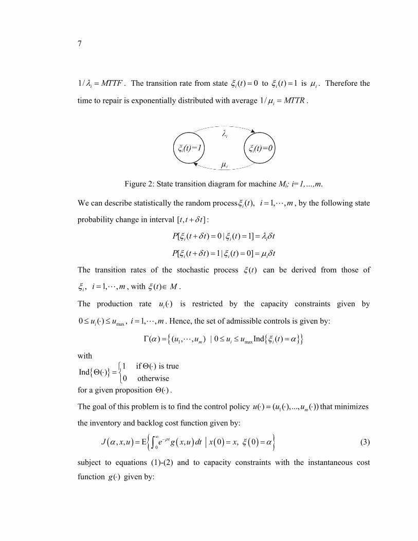
7

1/ i MTTF . The transition rate from state ( ) 0i t to ( ) 1i t is i . Therefore the

time to repair is exponentially distributed with average 1/ i MTTR .

Figure 2: State transition diagram for machine Mi; i=1,…,m.

We can describe statistically the random process ( ), 1, ,i t i m , by the following state

probability change in interval [ , ]t t t :

[ ( ) 0 | ( ) 1]i i iP t t t t

[ ( ) 1| ( ) 0]i i iP t t t t

The transition rates of the stochastic process ( )t can be derived from those of

, 1, ,i i m , with ( )t M .

The production rate ( )iu is restricted by the capacity constraints given by

max0 ( ) , 1, ,iu u i m . Hence, the set of admissible controls is given by:

1 max( ) ( , , ) | 0 Ind ( )m i iu u u u t

with

1 if ( ) is true

Ind ( )0 otherwise

for a given proposition ( ) .

The goal of this problem is to find the control policy 1( ) ( ( ),..., ( ))mu u u that minimizes

the inventory and backlog cost function given by:

0, , , 0 , 0tJ x u e g x u dt x x

(3)

subject to equations (1)-(2) and to capacity constraints with the instantaneous cost

function ( )g given by:

8

( , ) ( ) ( )g x u x t c x t c (4) with

1

1

( ) ( ) max( ( ),0)m

i mi

x t x t x t

(5)

( ) max(0, ( ))mx t x t (6)

The value function of such a problem is defined as follows:

1( , , ) ( )

, inf , ,mu u

v x J x u M

(7)

A necessary and sufficient condition characterizing the optimal control policy is

described by the set of partial differential equations known as the Hamilton Jacobi

Bellman (HJB) equations, as in Presman et al. (1995), by:

m inΓ ( )

ρv(x,α ) = H (x,v (x,α ),u) + q v(x, β) - v(x,α )x αββ α

1( , , )mu u

(8)

where 1

11

( , ( , ), ) ( ) ( - ) ( , ) ( ,.)i m

m

x i i x xi

H x v x u u u v u d v x g x

Note that vx is the partial derivative of v compared to x . The optimal control policy * *1( , , )mu u denotes a minimizer over ( ) of the right hand side of equation (8). This

policy corresponds to the value function described by equation (7). Then, when the value function is available, an optimal control policy can be obtained as in equation (8). However, an analytical solution of equation (8) is almost impossible to obtain. The numerical solution of the HJB equation (8) is a challenge which was considered insurmountable in the past. Using the Kushner approach (see Kushner & Dupuis (1992) and Kenné & Boukas

(1997)), a discrete Markovian decision control problem with finite state space and finite

action characterized by a m -dependent dimension given by:

1

( ) 3 ( )m

m ph j

j

Dim m p N x

where 2mp and ( ) card ( )h j h jN x G x with ( )h jG x describing the numerical grid

for the state variable jx related to the buffer j . Each machine has two states (i.e.,

9

2mp states for a m -machine manufacturing system) and its production rate can take

three values namely maximal production rate, demand rate and zero for each mode (i.e.,

3m p states for a m -machine, p -mode manufacturing system). Such a dimension

significantly grows with the number of machines. Hence, numerical algorithms such as

policy iteration or policy improvement (see Kushner & Dupuis (1992)) can not be

implemented on today’s computers for large transfer lines classified in the control

literature as complex systems.

Due to such a complexity, Samaratunga et al. (1997) determined a near-optimal control

policy of manufacturing system consisting of two unreliable machines in tandem by

using a hierarchical control approach. They compared the performance of their control,

denoted as hierarchical control (HC) to optimal control (when possible) and to stochastic

extension of Kanban control (KC) developed in Sethi et al. (1993) and two boundary

control (TBC) developed in Van Ryzin et al. (1993). It turns out that TBC and KC can

be shown also to be asymptotically optimal under conditions assumed in Samaratunga et

al. (1997); see Sethi and Zhou (1996) for details. For a more general transfer line, the

structure observed in Samaratunga et al. (1997) could be extended to define the control

policy vector 1( , ), 1, , 1,j ju u j m given by the following equation:

1 1

max 1 1 1

max 1 1

max max 1 11

1 1

(0,0), ( ) 0, ( ) ,

(0,min ( , ) ), ( ) , ( )

(0, ), ( ) , ( ) ,

( , ), ( ) , ( ) ,( ( ), ( ))

( , ), ( ) , ( )

j j j

j j j j j

j j j j

j j j jjj

j j j j j

if x t x t Z

u d if x t Z x t Z

u if x t Z x t Z

u u if x t Z x t Zuu

d d if x t Z x t

1

max max 1 1

max 1 1 1

max 1 1 1

,

( , ), 0 ( ) , ( ) ,

( , ), 0 ( ) , ( ) .

( , ), 0 ( ) , ( ) .

j

j j j j

j j j j j

j j j j j

Z

u u if x t Z x t Z

u d if x t Z x t Z

u d if x t Z x t Z

(9)

with ( )ju t being the production rate of machine jM and ( )jd t the demand rate at buffer

jB at time t . Demand ( )md t is constant at rate, jZ is the local hedging level and ( )jd t

10

is the local demand. This type of policy is deemed a good way of obtaining a satisfying

sub-optimal policy. The objective of the control problem is now to find

* * * *1 2[ , ,..., ]mZ Z Z Z which is the vector of decentralized hedging points that minimizes

the cost function. In the next section, we describe the proposed approach to solve the

problem.

3. EXPERIMENTAL APPROACH

The complexity of the problem studied prevents any analytical or numerical solution.

However, practitioners generally fix the input parameters of the Kanban policy in a

relatively instinctive way, which can result in a less desirable performance. A promising

approach proposed in Kenné & Gharbi (1999, 2004) and Gharbi & Kenné (2000, 2003)

consists of using a combination of analytical modelling to obtain a parameterized control

policy structure, simulation, Design of Experiments (DOE) and Response Surface

Methodology (RSM) to optimize the control policy in simpler manufacturing systems.

We adapt and integrate this approach in our methodology. The following paragraphs

describe the different steps to finding a characteristic profile that can be used for policy

optimization in long lines. This methodology is illustrated in Figure 3.

11

Figure 3: Control approach block diagram

1) The transfer line control problem statement, as in section 2, is the mathematical

formulation of the production control problem through a stochastic optimal control

model based on control theory. The objective of the study is specified in the formulation

of the optimal flow control problem described herein. That objective is to find the

control variables , 1,..., .iu i m that minimize the related inventory and backlog costs.

2) The optimality conditions are given by the related HJB. But, due to the complexity of

those equations, the structure of the control policy is adapted from the previous works

such as Samaratunga et al. (1997).

12

3) The control factors ; 1,..., .iZ i m are defined as the parameters of the near-optimal

control policy obtained by adopting the structure of the control policy given by equation

(9) as described in section 2.

4) The combined discrete/continuous transfer line simulation model is developed using

the Visual SLAM language (Pritsker & O'Reilly (1999)) with C language sub-routines.

5) The experimental design approach defines the domain of the factors to be analyzed,

the way in which the factors will vary and the number of replications of the experiments.

The results are used to obtain the effects of the factors and their interactions through the

analysis of variance (ANOVA).

6) The response surface methodology is used to obtain the approximation of the

objective function as a combination of the effects of the factors and their interactions in

the previous step. The residuals are checked for uniformity, serial correlation or other

indications of model weakness.

7) The validation of the solution is done by crosschecking the cost obtained with the

confidence interval obtained with 30 replications of the simulation model with the

obtained solution as input parameter. It is also verified to ensure that the solution lies

within the domain fixed at step 6. It is well known that some choices of Kanban levels

can result in the inability to meet demand. This would result in an infinitely increasing

backlog level. Also, the quadratic approximation of the response surface can only be

accurate if the domain is appropriate. Adjustment of the domain is thus necessary in

order to address these issues. This might require multiple iterations of steps 5 through 7.

The reponse surface is validated using the appropriate analyses Montgomery (2005).

8) The near-optimal control policy is defined with the validated optimal solution. The

cost obtained in this configuration is considered as the minimum.

9) The profile of the parameters for the small lines is observed to find a general

recurring profile. The results from multiple lines are analysed to extrapolate to larger

systems.

13

10) The Profile based distribution is obtained by fitting a parameterized profile well

suited to the shape observed at step 9. The Control Factors are the profile parameters

chosen to determine the distribution of all the buffer capacities.

11) The Comparison of profile with m-parameter policy is done by means of a

hypothesis test. The test is conducted to determine if there is any statistically significant

difference between the two results. The samples that are used for comparison are

validation results.

12) The Profile is accepted if the hypothesis tests conclude that there is no statistically

significant difference between the results from the m-parameter policy and the k-

parameter profile based control policy. We generalize this profile to longer lines.

4. SIMULATION MODEL

The performance estimating tool that was chosen for this study is a combined

discrete/continuous simulation model. It is developed using the Visual SLAM language

(Pritsker & O'Reilly (1999)) with C sub-routines. The Visual SLAM portion is

composed of various networks describing specific tasks (failure and repair events,

threshold crossing of inventory variables, etc...). The model is shown at Figure 4 with

the following descriptions of the different blocks.

1) The INITIALIZATION block sets the values of iZ the demand rate and the machine

parameters such as maxu mean time to failure (MTTF) and mean time to repair (MTTR).

The maximum and minimum time step specifications for integration of the cumulative

variables and allowable errors are also assigned at this step as well as the simulation

time T and the time for the warm up period after which statistics are cleared.

2) The DEMAND RATE is constant and defined in the INITIALIZATION block. It is

shown here as an individual block to facilitate comprehension since it is constantly used

as an input in the state equations.

14

3) The CONTROL POLICY is implemented through the use of observation networks

that raise a flag whenever one of the thresholds is crossed. The production rates of the

machines are then set according to equation (9).

Figure 4: Simulation block diagram

4) The STARVATION of the machines is implemented with the use of observation

networks. Whenever one of the in-process buffers becomes empty, a flag is raised.

Another signal is sent when material becomes available for operation. Starvation is

integrated in the state equations by the means of binary variables multiplying the

production rates .

5) The FAILURES AND REPAIRS block samples the times to failure and times to

repair for the machines from their respective probability distributions. The operational

15

states of the machines are incorporated in the state equations by the means of logical

variables multiplying the production rates.

6) The STATE EQUATIONS are equations defined as a C language insert. They

describe the inventory and backlog variables using the production rates set by the control

policy and the binary variables from the failure and repair and starvation networks.

7) The TIME ADVANCE block uses an algorithm provided by Visual SLAM. It is a

combination of discrete event scheduling (failures and repair), continuous variable

threshold crossing events and time step specifications.

8) The UPDATE INVENTORY LEVELS AND CUMULATIVE VARIABLES block is

used once the time step is chosen. The cumulative variables are integrated using the

Runge-Kutta-Fehlberg (RKF) method as described in Pritsker & O'Reilly (1999).

9) The UPDATE INCURRED COST block calculates the incurred cost according to the

levels of the different variables and the unit costs and c c .

The simulation ends when current simulation time t reaches the defined simulation

period T. To obtain the average backlog and inventory levels, the cumulative variables

are divided by T One understands that the simulation time T cannot be infinite.

Therefore, we ran offline simulations to determine the time necessary for the system to

reach its steady state. We found that for our models, this corresponded approximately to

10 000 times MTTF. This duration is therefore used for all the simulations.

5. DESIGN OF EXPERIMENTS AND RESPONSE SURFACE

METHODOLOGY

The experimental design is obtained and analyzed using a commercial software. From

experience, we know that the response surfaces need to be at least of second degree and

that the interactions between buffer pairs (not necessarily adjacent) often have

statistically significant effects. An efficient design to obtain a response surface with

these characteristics is the central composite type design (CCD, Box-Wilson). It consists

16

of a 2-level factorial design augmented with center and axis points. This type of design

is desirable because of its orthogonality, the ability to measure the effects of the factors

independently from each other, and rotatability, the ability to estimate the response with

equal variance in all directions from the center of the design. The number of runs for

such a design with m parameters and n center points is 2 2m m n . For more details, we

refer the reader to Montgomery (2005). From such a design we will extract 2 responses:

one surface estimating the average surplus and another the average backlog. These

responses are in the form of equation (10).

01 1 1

Y m m m

i i ij i ji i j

j i

Z Z Z

(10)

with Y being the estimated response, ; 1,..., .iZ i m the factors multiplied by their

estimated coefficients. When an acceptable portion of the variance of each response

is explained by the models, the backlog function is multiplied by the unit cost ratio c /

c and both functions are then added together. The resulting function is then minimized

using nonlinear programming.

In order to reduce the variability in the results from one configuration to another, we use

the common random number technique. This technique consists of submitting different

configurations to identical scenarios to estimate the response of the system under similar

failure and repair events. This allows us to remove a portion of the variability in the

response that is attributed to the particular series of events. Once the optimization is

performed, we validate the estimated cost by running 30 replications with optimal

parameters. We compute the 95% confidence interval (CI) using equation (11):

*1.96 / 1.96 /C S n C C S n (11) with S obtained using equation (12):

17

2

1iC C

Sn

(12)

with , 1,..., .iC i n the results from the replications, C the average cost obtained from

these replications, S the sample standard deviation and *C the optimal cost. If the

estimated cost obtained with the cost function *C lies within this confidence interval, we

consider that the response surface estimates the actual cost accurately.

As with most optimization techniques, the number of necessary runs grows with the

number of input parameters. Because simulation can be quite time-consuming, this is

undesirable. In order to eliminate this constraint, we will observe the results from the m

parameter lines to find a recurring profile. We will then use this profile to reduce the

number of parameters of the optimization problem.

6. NUMERICAL EXAMPLES AND RESULTS ANALYSIS

In this section we present the optimization results for various lines. The results are

shown for /c c =20 and /c c =100. The simulations were run for a time period of 106

time units preceded by a warm-up period of 103 time units. The statistical distributions

of the failure times and repair times are exponential. For all cases, MTTF=100,

MTTR=3, umax=1.1 and d=1. Table 1 shows the ANOVA for the inventory response of

the 4 machine line with /c c =100. We notice that the R2 coefficient is almost 100%

which means almost all of the observed variance in the results is explained by the model.

The inventory level is explained almost entirely by the experimental factors. This very

high correlation coefficient is the result of the length of the simulation runs and the

blocking technique used. We notice that the F-Ratios for the individual factors are very

important in comparison with the interactions and the factor squares. This means that the

surface is almost a hyper-plane. The inventory level increases almost linearly with the

18

factor levels. The table shows only the Sources of variance which were considered

significant. The resulting polynomial coefficients are shown in Table 2.

Table 1: ANOVA for inventory response

Source Sum Df Mean Square F-Ratio P-Value A:Z1 535.57 1 535.57 648994.49 0 B:Z2 466.263 1 466.263 565009.09 0 C:Z3 427.654 1 427.654 518223.38 0 D:Z4 399.539 1 399.539 484154.93 0 AA 0.463335 1 0.463335 561.46 0 AB 0.1114 1 0.1114 134.99 0 BB 0.0693565 1 0.0693565 84.05 0 CC 0.0096789 1 0.00967892 11.73 0.0009 blocks 1.89796 9 0.210884 255.55 0 Total error 0.0924258 112 0.00082523 Total (corr.) 1831.8 129 R2 = 99.995 %

Table 2: Polynomial coefficients for the inventory response surface

0 1 2 3 4 11 12 22 33

-11.548 1.5151 1.2988 1.1001 .9897 -2.547E-2 -9.329E-3 -9.856E-3 -3.682E-3

For the backlog results, the variance of the results increases with the mean value of the

backlog. In order to obtain uniformity of the variance and increase the R2 coefficient, a

transformation was used. The transformation that works best in our case is the fractional

exponent transformation. For more details on transformations and their selection, we

refer the reader to Montgomery (2005). Table 3 shows the results of the ANOVA for the

backlog with a ½ exponent transformation. We notice that R2 =98.72%, which is still

very high. Nevertheless, such a high level of explanation is necessary since the penalty

for the average backlog level is much higher than that of the WIP level in the cases

studied. The backlog response exhibits more relative variability than the inventory

response. This is due to the high variability of the exponential distributions used to

19

model the failure and repair processes. The resulting polynomial coefficients are shown

in Table 4.

Table 3: ANOVA for backlog response with ½ exponent transformation

Source Sum of Squares Df Mean Square

F-Ratio P-Value

A:Z1 0.178689 1 0.178689 1619.78 0 B:Z2 0.1502 1 0.1502 1361.53 0 C:Z3 0.137066 1 0.137066 1242.47 0 D:Z4 0.152808 1 0.152808 1385.17 0 AA 0.00570514 1 0.00570514 51.72 0 AB 0.00937076 1 0.00937076 84.94 0 AC 0.00289 1 0.00289 26.2 0 AD 0.000468939 1 0.000468939 4.25 0.0417 BB 0.00182986 1 0.00182986 16.59 0.0001 BC 0.00406175 1 0.00406175 36.82 0 BD 0.000795622 1 0.000795622 7.21 0.0084 CC 0.000872344 1 0.000872344 7.91 0.0059 CD 0.00146932 1 0.00146932 13.32 0.0004 blocks 0.263524 9 0.0292804 265.42 0 Total error 0.0118039 107 0.000110317 Total (corr.) 0.921627 129 R2 = 98.72%

Table 4: Polynomial coefficients for backlog response surface with ½ exponent

transformation.

0 1 2 3 4 11 12 13 14

2.307 1.5151 -0.1052 0.09815 -0.08816 -0.04093 2.827E-3 1.503E-3 6.053E-4

22 23 24 33 34

1.600E-3 1.781E-3 7.884E-4 1.105E-3 1.071E-3

20

Figure 5: Contour plots of the cost function surface

Figures 5 (a), (b), and (c) show different contour plots of the resulting cost function for

the 4 machine line. We notice that the cost function is not very sensitive to the transfer

of a small amount of buffer capacity from one buffer to another. The finished goods

stock seems less sensitive to a slight increase or decrease in capacity around the

optimum. This is because an increase in its capacity will augment inventory costs but

reduce backlog costs, and a decrease in its capacity will have the opposite effect. The

resulting changes in costs seem to balance each other out in a range of Z4.

The values of *iZ and the estimated resulting cost are shown in Table 5 at line /c c

=100 and the distribution of the *iZ along the line are shown in Figure 6. The results for

21

the 4 machine line with /c c =20 are also shown in this table and Figure 6. Table 6 and

Figure 7 show the results for the 5 machine lines, Table 7 and Figure 8 for the 6 machine

lines and Table 8 and Figure 9 for the 7 machine lines. All the obtained cost estimates fit

in the 95% confidence interval (CI) obtained from the validation runs.

Table 5: 4 machine line results

/c c *1Z *

2Z *3Z *

4Z *C Validation CI (95%)

100 5.35 9.17 9.59 20.80 44.13 [43.04:45.22] 20 3.92 8.00 9.00 13.02 32.76 [32.33:33.19]

Table 6: 5 machine line results

/c c *1Z *

2Z *3Z *

4Z *5Z *C Validation

CI (95%) 100 4.2 8.14 9.57 8.72 24.69 51.70 [49.94:52.20]20 3.75 7.07 8.58 9.65 14.70 39.84 [38.86:40.00]

Table 7: 6 machine line results

/c c *1Z *

2Z *3Z *

4Z *5Z *

6Z *C Validation CI (95%)

100 4.52 6.69 9.08 9.69 10.42 24.12 57.53 [56.51:58.41]20 3.06 8.59 8.65 7.50 8.50 17.06 45.46 [45.45:46.63]

Table 8: 7 machine line results

/c c *1Z *

2Z *3Z *

4Z *5Z *

6Z *7Z *C Validation

CI (95%) 100 3.50 7.00 9.00 9.28 9.76 9.93 25.10 64.28 [64.05:66.55]20 2.93 7.13 8.56 8.45 8.90 9.56 15.72 51.84 [51.47:52.67]

22

Figure 0

re

Figure

Fig

ure

6: D

istr

ibut

ion

of b

uffe

r sp

ace

for

the

4 m

achi

ne li

nes

Fig

ure

7: D

istr

ibut

ion

of b

uffe

r sp

ace

for

the

5 m

achi

ne li

nes

Fig

ure

8: D

istr

ibut

ion

of b

uffe

r sp

ace

for

the

6 m

achi

ne li

nes

Fig

ure

9: D

istr

ibut

ion

of b

uffe

r sp

ace

for

the

7 m

achi

ne li

nes

23

We notice a general profile in the distribution of the hedging levels: while the first and

last buffers seem to be more independent, the mid-section of the line seems to vary

linearly. We notice that the optimal values of the parameters increase along the line.

Experiments have shown that for identical buffer capacity, the buffers furthest down the

line build up a lower inventory level. Therefore, as we move down the line, buffers can

have a greater capacity while not generating an inventory level as high as would the

upstream buffers with identical capacities. An explanation for this lies in the propagation

effects of the machine failures. As we know, failures effects propagate to adjacent

machines through blocking for the upstream machine and starvation for the downstream

machine. Roughly, the machines which are furthest upstream have more chances of

being blocked because they can feel the effects of the propagation of failures of more

downstream machines. Even if the upstream machines do not become blocked directly,

the increased buffer levels in front of machines that have become blocked will reduce

the time before the failure propagates when another failure occurs. Results from

experiments with homogenous transfer lines under saturated demand in Chiang et al.

(2001) show that the average blocking probability decreases as we move downstream.

Our experiments confirm this and show that the average buffer level also decreases as

we move down the line. This phenomenon justifies the choice of a linear profile for the

mid portion of the line over a “flat in the center” profile that would be more suited to the

storage bowl phenomenon Hillier et al. (1993). The storage bowl was observed in the

optimal distribution of buffer space in order to obtain a certain line capacity (minimize

buffer space to achieve a desired throughput or maximize throughput with a fixed total

buffer space). Here, we are concerned with the minimization of inventory and backlog

costs. It is then to be expected that the profile that minimizes these costs will be one that

is consequent of buffer space utilization, or the average buffer level, rather than only the

buffer capacity.

We have also noticed that the last buffer is more important than the others. This is due to

the large penalty imposed on backlog. This penalty justifies an important finished goods

24

buffer to prevent backlogging. This effect decreases as the penalty for backlogging

decreases.

We also notice that the first buffer is quite smaller than the other ones. This can be

justified by the fact that the first machine is never starved. Therefore, machine 1M only

needs to build up an inventory to decouple machine 2M from propagation of its failures,

but not starvation. The intermediate buffers have buffer levels that are more similar

while they increase slightly as we move downstream.

Also, the transfer of a small portion of capacity from one buffer to its neighbour will not

have a significant effect on the resulting cost .. This profile will be used to distribute the

hedging levels along the line while reducing the number of parameters of the

optimization problem.

7. OBSERVED PROFILE AND DISTRIBUTION OF BUFFER SPACE

As we have noticed in the preceding section, there is a characteristic profile in the

distribution of the hedging levels along the line. This profile, which is represented in

Figure 10 consists of 2 independent points, 1Z and mZ , and a relatively linear portion

from 2Z to 1mZ . Therefore, we propose to optimize only 4 parameters, buffers 1Z , 2Z ,

1mZ and mZ , while linearly interpolating the values between 2Z and 1mZ . Although

this profile is probably not 100% exact, it will most likely give very desirable results

while considerably reducing the computational effort of optimizing parameters

individually. For example, the 4 parameter CCD with 2 center points replicated 4 times

gives 130 runs. The same CCD for 8 parameters gives 1370 runs and the 3 level factorial

design 6561 runs. Considering that the computational time for simulations increases

with the complexity of the systems (length in our case), we see that this heuristic

approach becomes very useful, even necessary for long lines. We recall that any other

optimization technique would necessitate a large number of simulation runs.

Furthermore, if a flat in the center profile, or even an inverted bowl profile, was to be

25

the best solution for a particular system, the four parameter profile described here can

adapt to these shapes.

Figure 10: Parameterized profile with 4 parameters

7.1. Validation

Tables 9, 10 and 11 show the results obtained with this 4 parameter heuristic approach.

To facilitate comparison of the results from the m parameter optimization problems, both

are presented in the same tables and are noted “full” and 4 parameter profile

optimization problems are noted “prof”. In all cases, the null hypothesis ( 0H ) could not

be rejected (A=accept).

Table 9: Full and profile results for 5 machines

/c c *1Z *

2Z *3Z *

4Z *5Z *C Validation

IC (95%) 0H

100 Full 4.20 8.14 9.57 8.72 24.69 51.70 [49.94:52.20]

A Prof 4.73 7.78 9.64 11.5 20.98 51.25 [49.77:51.85]

20 Full 3.75 7.07 7.85 10.02 14.70 39.84 [38.86:40.00]

A Prof 3.92 7.50 8.58 9.65 13.19 39.53 [38.97:40.03]

Table 10: Full and profile results for 6 machines

/c c *1Z *

2Z *3Z *

4Z *5Z *

6Z *C Validation IC (95%)

0H

100 Full 4.52 6.69 9.08 9.69 10.42 24.12 57.53 [56.51:58.41]

A Prof 4.56 7.50 8.64 9.79 10.93 21.64 56.69 [56.34:57.34]

26

20 Full 3.06 8.59 8.65 7.50 8.50 17.06 45.46 [45.51:46.63]

A Prof 3.50 6.85 7.85 8.85 9.85 15.30 45.60 [45.00:46.30]

Table 11: Full and profile results for 7 machines

/c c *1Z *

2Z *3Z *

4Z *5Z *

6Z *7Z *C Validation

IC (95%) 0H

100 Full 3.50 7.00 9.00 9.28 9.76 9.93 25.10 64.28 [64.05:66.55]

A Prof 4.00 8.00 8.79 9.58 10.36 11.15 22.07 65.19 [63.90:66.46]

20 Full 2.93 7.13 8.56 8.45 8.90 9.56 15.72 52.90 [51.47:52.67]

A Prof 3.05 7.81 8.28 8.74 9.21 9.67 14.60 52.73 [51.64:52.72]

We notice that the results are very close in all cases. Furthermore, the profile does not

systematically give a higher cost than the m parameter optimization. The results show

that the proposed profile gives an excellent approximation of the optimal distribution.

In addition, more experiences have been conducted varying other line parameters such

as MTTF, MTTR, d and maxu . The obtained results are reported in table 12.

27

Table 12: Full and profile results for 6 machines additional cases

/c c MTTF MTTR d umax *1Z *

2Z *3Z *

4Z *5Z *

6Z *C Validation IC (95%)

0H

100 100 11.1 1 1.3 Full 25.52 42.55 47.84 49.77 56.46 96.17 277.42 [276.97,277.92]

A Prof 29.7 41.5 46.22 50.94 55.66 98.08 276.70 [276.55,277.16]

20 100 11.1 1 1.3 Full 22.89 39.02 43.41 47.79 52.18 64.02 224.69 [222.71,225.47]

A Prof 22.98 39.1 44.37 46.83 51.25 64.86 224.79 [222.71,225.47]

100 700 21.0 1 1.1 Full 31.64 46.83 63.56 67.83 72.94 168.84 402.71 [395.57,408.87]

A Prof 31.92 52.5 60.48 68.53 76.51 151.48 396.83 [394.38,401.38]

20 700 21.0 1 1.1 Full 21.48 60.17 60.56 52.59 59.54 119.45 318.26 [318.62,326.5]

A Prof 24.59 48.04 54.97 61.98 68.96 107.18 319.29 [315.08,324.1]

100 25 2.8 3 3.9 Full 19.15 32.00 35.94 37.42 42.39 72.16 208.16 [207.77,208.51]

A Prof 22.35 31.16 34.68 38.28 41.79 73.61 207.58 [207.44,207.9]

20 25 2.8 3 3.9 Full 17.23 29.34 32.65 35.91 39.18 48.07 168.55 [167.09,169.16]

A Prof 17.26 29.38 33.31 35.16 38.47 48.70 168.61 [167.06,169.14]

100 75 2.25

3 3.3 Full 3.39 5.02 6.81 7.27 7.82 18.09 43.15 [42.41:43.85]

A Prof 3.42 5.63 6.48 7.34 8.20 16.23 42.52 [42.26:43.96]

20 75 2.25

3 3.3 Full 2.38 6.47 6.51 5.69 6.39 12.80 34.12 [34.14,34.99]

A Prof 2.72 5.20 5.89 6.70 7.47 11.57 34.23 [33.81,34.75]

100 350

2.8 3 3.9 Full 89.40 148.96 167.48 174.27 197.66 336.60 971.00 [969.49,972.81]

A Prof 103.96 145.33 161.81 178.30 194.84 343.32 968.45 [967.96,970.16]

20 350

2.8 3 3.9 Full 80.20 136.61 152.01 167.28 182.63 224.10 786.42 [779.5,789.18]

A Prof 80.52 136.92 155.39 164.00 179.43 227.02 786.81 [779.51,789.18]

We observe that in all cases, the profile heuristic has given similar results as the full

optimization of the system. Although non exhaustive, these cases confirm that the

heuristic holds for systems with different parameters.

7.2. Application of the heuristic approach to a 20 machine transfer line

To illustrate the use of this heuristic approach, we now give a 20 machine example with

results presented in table 13. This case was optimized using the proposed profile-based

distribution of buffer space.

Table 13: 20 machine example with profile

/c c *1Z *

2Z *; 3,...,18.iZ i *19Z *

20Z *C Validation CI (95%)

100 3.5 7.17 * *2( , , , )mf Z Z m i 10.76 24.2 143.8 [143.61:152.57]

28

With * * * * *2 1 2 1 2( , , , ) ( 1)( ) /( 3); 3,..., 2.m mf Z Z m i Z i Z Z m i m The results cannot

be compared to the m parameter optimization because it could not be obtained with the

proposed technique and is provided as an example. As a comparison, the number of runs

for a 20 parameter CCD with 2 center points replicated 4 times is 5 243 090 runs and 17

433 922 005 runs for the 3-level factorial design compared to 130 runs for the proposed

profile-based policy. The computational effort to perform the full optimization would be

much too important. Exhaustive simulation of all combinations would be simply

impossible with today’s computers.

8. CONCLUSION

Observing the increase in complexity of the production control problem in transfer lines

according to the size of the line, we propose a heuristic method to reduce the number of

parameters in the optimization problem. We have presented a series of hedging points or

Kanban optimization results for homogenous transfer lines subject to failures obtained

using continuous flow simulation, DOE and RSM. The goal of such a problem is to

minimize the average surplus/backlog cost. We have observed that there is a

characteristic profile in the distribution of the hedging points along the line which

consists of independent points at the extremities and a linear distribution for internal

buffers. Based on this observation, we have proposed a heuristic approach, which allows

us to reduce the optimization effort for lines of 4m workstations to a 4 parameter

problem. Such a heuristic approach is highly desirable because it reduces the number of

runs necessary to solve the problem and thus the computational effort. A 20 machine

case, which would have been virtually impossible to tackle as a 20 variable optimization

problem, was solved using this heuristic approach and we provide the results as an

illustration of its usefulness.

Further research would enable the extension of the observed profile to systems with

different performance measures and machine parameter than the ones used in this paper.

29

REFERENCES

Bonvik, A. M. (1996). Performance analysis of manufacturing systems under hybrid control policies. Unpublished Thesis Ph. D. --Massachusetts Institute of Technology Sloan School of Management 1996.

Bonvik, A. M., Dallery, Y., & Gershwin, S. B. (2000). Approximate analysis of production systems operated by a CONWIP/finite buffer hybrid control policy. International Journal of Production Research, 38(13), 2845-2869.

Burman, M. H. (1995). New results in flow line analysis. Unpublished Thesis Ph. D. --Massachusetts Institute of Technology Dept. of Electrical Engineering and Computer Science 1995.

Chiang, S. Y., Kuo, C. T., & Meerkov, S. M. (2001). c-Bottlenecks in Serial Production Lines: Identification and application, Mathematical Problem in Engineering, Vol. 7, 547-578.

Dallery, Y., David, R., & Xie, X. L. (1989). Approximate Analysis of Transfer Lines with Unreliable Machines and Finite Buffers. IEEE Transactions on Automatic Control, 34(9), 943-953.

Dallery, Y., & Le Bihan, H. (1999). An improved decomposition method for the analysis of production lines with unreliable machines and finite buffers. International Journal of Production Research, 37(5), 1093-1117.

Gershwin , S. B. (1996). How to design a production line that has a bottleneck, from http://web.mit.edu/manuf-sys/www/buffer-optimization.html

Gershwin , S. B., & Goldis, Y. (1995). Efficient Algorithms for Transfer Line Design (MIT Laboratory for Manufacturing and Productivity Report No. LMP-95-005): Massachussetts Institute of Technology.

Gershwin, S. B., & Schor, J. E. (2000). Efficient algorithms for buffer space allocation. Annals of Operations Research, Performance Evaluation and Optimization of production Lines. International Workshop, 19-22 May 1997, 93, 117-144.

Gharbi, A., & Kenné, J. P. (2000). Production and preventive maintenance rates control for a manufacturing system: An experimental design approach. International Journal of Production Economics, 65(3), 275-287.

Gharbi, A., & Kenné, J. P. (2003). Optimal production control problem in stochastic multiple-product multiple-machine manufacturing systems. IIE Transactions, 35(10), 941-952.

30

Hillier, F. S., So, K. C., & Boling, R. W. (1993). Toward Characterizing the Optimal Allocation of Storage Space in Production Line Systems with Variable Processing Times. Management Science, 39(1), 126-133.

Hillier, M. S. (2000). Characterizing the optimal allocation of storage space in production line systems with variable processing times. IIE Transactions, 32(1), 1-8.

Kenné, J. P., & Boukas, E. K. (1997, June 1997). Production Rate Control and Corrective Maintenance Planning Problem of a Failure Prone Manufacturing System. Paper presented at the ACC conference, Albuquerque.

Kenné, J. P., & Gharbi, A. (1999). Experimental design in production and maintenance control problem of a single machine, single product manufacturing system. International Journal of Production Research, 37(3), 621-637.

Kenné, J. P., & Gharbi, A. (2004). A simulation optimization based control policy for failure prone one-machine, two-product manufacturing systems. Computers & Industrial Engineering, 46(2), 285-292.

Kushner, H. J., & Dupuis, P. G. (1992). Numerical Methods for Stochastic Control Problems in Continuous Time. New-York: Springer-Verlag.

Montgomery, D. C. (2005). Design and analysis of experiments (6th ed.). New York: Wiley.

Pritsker, A. A. B., & O'Reilly, J. J. (1999). Simulation with Visual SLAM and AweSim (2nd ed.). New York, N.Y., West Lafayette, Ind.: J. Wiley and Sons, Systems Publishing.

Sadr, J., & Malhame, R. P. (2004). Decomposition/aggregation-based dynamic programming optimization of partially homogeneous unreliable transfer lines. IEEE Transactions on Automatic Control, 49(1), 68-81.

Samaratunga, C., Sethi, S.P., & Zhou, X. (1997). Computational Evaluation of Hierarchical Production Control Policies for Stochastic Manufacturing Systems. Operations Research, 45(2), 258-274. Schor, J. E. (1995). Efficient Algorithms for Buffer Space Allocation. MIT. Sethi, S. P. & Zhou, X. Y. (1996). Optimal Feedback Control in Deterministic Dynamic Two-Machine Flowshops, Operations Research Letters, 19, 225-235. Van Ryzin, G., Lou, S. X. C., & Gershwin, S. B. (1993). Production Control for a Tandem Two-Machine System. IIE transactions, 25(5), 5-20.