IEEE TRANSACTIONS ON POWER ELECTRONICS, VOL. 20, NO. 4, JULY 2005 963

Optimization of Perturb and Observe MaximumPower Point Tracking Method

Nicola Femia, Member, IEEE, Giovanni Petrone, Giovanni Spagnuolo, Member, IEEE, and Massimo Vitelli

Abstract—Maximum power point tracking (MPPT) techniquesare used in photovoltaic (PV) systems to maximize the PV arrayoutput power by tracking continuously the maximum power point(MPP) which depends on panels temperature and on irradianceconditions. The issue of MPPT has been addressed in differentways in the literature but, especially for low-cost implementations,the perturb and observe (P&O) maximum power point trackingalgorithm is the most commonly used method due to its ease of im-plementation. A drawback of P&O is that, at steady state, the op-erating point oscillates around the MPP giving rise to the waste ofsome amount of available energy; moreover, it is well known thatthe P&O algorithm can be confused during those time intervalscharacterized by rapidly changing atmospheric conditions. In thispaper it is shown that, in order to limit the negative effects asso-ciated to the above drawbacks, the P&O MPPT parameters mustbe customized to the dynamic behavior of the specific converteradopted. A theoretical analysis allowing the optimal choice of suchparameters is also carried out.

Results of experimental measurements are in agreement with thepredictions of theoretical analysis.

Index Terms—Maximum power point (MPP), maximum powerpoint tracking (MPPT), perturb and observe (P&O), photovoltaic(PV).

I. INTRODUCTION

APHOTOVOLTAIC (PV) array under uniform irradianceexhibits a current-voltage characteristic with a unique

point, called the maximum power point (MPP), where the arrayproduces maximum output power [1].

In Fig. 1, an example of PV module characteristics in terms ofoutput power versus voltage and current versus voltage for threeirradiance levels and two temperature values are shown.The MPP point has been also evidenced in both figures.

As evidenced in Fig. 1, since the I–V characteristic of a PVarray, and hence its MPP, changes as a consequence of the varia-tion of the irradiance level and of the panels’ temperature (whichis in turn function of the irradiance level, of the ambient temper-ature, of the efficiency of the heat exchange mechanism and ofthe operating point of the panels) [1], it is necessary to trackcontinuously the MPP in order to maximize the power outputfrom a PV system, for a given set of operating conditions.

The issue of maximum power point tracking (MPPT) hasbeen addressed in different ways in the literature: examples offuzzy logic, neural networks, pilot cells and DSP based im-

Manuscript received January 16, 2004; revised October 14, 2004. Recom-mended by Associate Editor Z. Chen.

N. Femia, G. Petrone, and G. Spagnuolo are with the Università diSalerno, Fisciano (SA), Italy (e-mail: femia@unisa.it; gpetrone@unisa.it;spanish@ieee.org).

M. Vitelli is with the Seconda Università di Napoli, Aversa (CE), Italy(e-mail: vitelli@unina.it).

Digital Object Identifier 10.1109/TPEL.2005.850975

plementations have been proposed in [2]–[10]. Nevertheless,the perturb and observe (P&O) and INcremental Conductance(INC) [2] techniques are widely used, especially for low-costimplementations.

The P&O MPPT algorithm is mostly used, due to its easeof implementation. It is based on the following criterion: if theoperating voltage of the PV array is perturbed in a given direc-tion and if the power drawn from the PV array increases, thismeans that the operating point has moved toward the MPP and,therefore, the operating voltage must be further perturbed in thesame direction. Otherwise, if the power drawn from the PV arraydecreases, the operating point has moved away from the MPPand, therefore, the direction of the operating voltage perturba-tion must be reversed.

A drawback of P&O MPPT technique is that, at steady state,the operating point oscillates around the MPP giving rise to thewaste of some amount of available energy. Several improve-ments of the P&O algorithm have been proposed in order to re-duce the number of oscillations around the MPP in steady state,but they slow down the speed of response of the algorithm tochanging atmospheric conditions and lower the algorithm effi-ciency during cloudy days [11].

The INC algorithm seeks to overcome such limitations: it isbased on the observation that, at the MPP it is

, where and are the PV array cur-rent and voltage, respectively. When the operating point in theV-P plane is on the right of the MPP, then

, whereas, when the operating point is on theleft of the MPP, then . The signof the quantity indicates the cor-rect direction of perturbation leading to the MPP. By means ofthe INC algorithm it is therefore theoretically possible to knowwhen the MPP has been reached and therefore when the pertur-bation can be stopped, whereas in the P&O implementation theoperating point oscillates around the MPP. Indeed, as discussedin [12], because of noise and measurement and quantization er-rors, the condition is in prac-tice never exactly satisfied, but it is usually required that suchcondition is approximately satisfied within a given accuracy. Asa consequence, the INC operating voltage cannot be exactly co-incident with the MPP and oscillates across it. A disadvantageof the INC algorithm, with respect to P&O, is in the increasedhardware and software complexity; moreover, this latter leadsto increased computation times and to the consequent slowingdown of the possible sampling rate of array voltage and current.

Both P&O and INC methods can be confused during thosetime intervals characterized by changing atmospheric condi-tions, because, during such time intervals, the operating pointcan move away from the MPP instead of keeping close to it [2].This drawback is shown in Fig. 2, where the P&O MPPT oper-ating point path for an irradiance variation from 200 W/m to

0885-8993/$20.00 © 2005 IEEE

964 IEEE TRANSACTIONS ON POWER ELECTRONICS, VOL. 20, NO. 4, JULY 2005

(a) (b)

Fig. 1. PV module characteristics for three irradiance levels S and two different panels’ temperature: (a) output power versus voltage and (b) current versusvoltage.

(a) (b)

Fig. 2. P&O MPPT operating point path. The � represents MPP for different levels of the irradiance: (a) slow change in atmospheric conditions and (b) rapidchange in atmospheric conditions.

800 W/m is reported. The example reports two different behav-iors in the plane output power versus voltage. Fig. 2(a) showsthe operating point path in presence of slowly changing atmo-spheric conditions and Fig. 2(b), instead, shows the failure ofMPPT control to follow the MPP when a rapid change in atmo-spheric conditions occurs. Also the INC MPPT control presentssuch behavior.

There is no general agreement in the literature on which one ofthe two methods is the best one, even if it is often said that the ef-ficiency—expressed as the ratio between the actual array outputenergy and the maximum energy the array could produce underthe same temperature and irradiance level—of the INC algorithmis higher than that one of the P&O algorithm. To this regard, it isworth saying that the comparisons presented in the literature arecarried out without a proper optimization of P&O parameters. In[12] it is shown that the P&O method, when properly optimized,leads to an efficiency which is equal to that obtainable by the INCmethod. These are often merely chosen on the basis of trial anderror tests. Unfortunately, no guidelines or general rules are pro-vided to determine the optimal values of P&O parameters. Thepresent paper is devoted to fill such a hole [13].

A theoretical analysis allowing the optimal choice of the twomain parameters characterizing the P&O algorithm is carried

out. The key idea underlying the proposed optimization ap-proach lies in the customization of the P&O MPPT parametersto the dynamic behavior of the whole system composed bythe specific converter and PV array adopted. Results obtainedby means of such approach clearly show that, in the designof efficient MPPT regulators, the easiness and flexibility ofP&O MPPT control technique can be exploited by optimizingit according to the specific system’s dynamic.

As an example, the boost converter reported in Fig. 3(a) is ex-amined. Results obtained and the considerations that are drawncan be extended to any other converter topology as well.

The system in Fig. 3(a) can be schematically represented asin Fig. 3(b), where d is the duty cycle and p is the power drawnfrom the PV array. In the following, the sampling interval willbe indicated with , and the amplitude of the duty cycle per-turbation with d d A d .

In the P&O algorithm the sign of the duty cycle perturbationat the -th sampling is decided on the basis of the sign ofthe difference between the power and the power

A according to the rules discussed above

d d A d A d

A (1)

FEMIA et al.: OPTIMIZATION OF PERTURB AND OBSERVE MAXIMUM POWER POINT TRACKING METHOD 965

(a) (b)

Fig. 3. Boost converter with MPPT control: (a) simplified circuit and (b) equivalent block diagram.

The amplitude of the duty cycle perturbation is one of thetwo parameters requiring optimization: lowering d reduces thesteady-state losses caused by the oscillation of the array oper-ating point around the MPP; however, it makes the algorithmless efficient in case of rapidly changing atmospheric condi-tions. The optimal choice of d in these situations, when wehave to account for both the source’s and converter’s dynamics,is discussed in detail in Section III. Besides the case of quicklyvarying MPP, which occurs in cloudy days only, there is a moregeneral problem, connected to the choice of the sampling in-terval used by the P&O MPPT algorithm, which arises evenduring sunny days, when the MPP moves very slowly. The sam-pling interval should be set higher than a proper threshold inorder to avoid instability of the MPPT algorithm and to reducethe number of oscillations around the MPP in steady state. Infact, considering a fixed PV array MPP, if the algorithm sam-ples the array voltage and current too quickly, it is subjected topossible mistakes caused by the transient behavior of the wholesystem (PV array+converter), thus missing, even if temporarily,the current MPP of the PV array, which is in steady-state op-eration. As a consequence, the energy efficiency decays as thealgorithm can be confused and the operating point can becomeunstable, entering disordered and/or chaotic behaviors [12]. Toavoid this, it must be ensured that, after each duty-cycle pertur-bation, the system reaches the steady-state before the next mea-surement of array voltage and current is done. In Section II theproblem of choosing is analyzed and an optimized solution,based on the tuning the P&O algorithm according to converter’sdynamics, is proposed. In Section III the optimization proce-dure is illustrated for rapidly varying irradiance conditions. Sec-tion IV introduces experimental verifications and Section V isdevoted to conclusions.

II. STEADY-STATE OPERATION

Let us suppose that the system is working at steady-state,under constant and uniform irradiance level, and that the MPPhas been reached. If the operating point of the PV array lies ina sufficiently narrow interval around the MPP, the power drawnby the PV array can be expressed as

v(2)

where V , with V and the PVarray MPP voltage and current, respectively.

Fig. 4. Equivalent circuit of a PV array.

The PV array power is maximum when the adapted load re-sistance equals the absolute value of the differential re-sistance of the PV array at the MPP. In order to identify the min-imum value to assign to , the behavior of the system forced bya small duty-cycle step perturbation must be analyzed. In fact,in order to allow the MPPT algorithm to make a correct inter-pretation of the effect of a duty-cycle step perturbation on thecorresponding steady-state variation of the array output powerp, it is necessary that the time between two consecutive sam-plings is long enough to allow p to reach its steady state value.

The equivalent circuit of a PV array is shown in Fig. 4.The relation between the array terminal current and voltage

is the following [1]:

sv

V v(3)

where s and are series and shunt resistances, respectively,is the light induced current, is the diode ideality factor, s

is the diode saturation current and V is the thermal voltage.depends on the irradiance level S and on the array temperature

, while s and V depend on only [1]. The PV array cur-rent is a nonlinear function of the PV array voltage v ,of the irradiance level S and of the temperature T. If the oscilla-tions of the operating point v are small compared toV , then the relationship among , v , S and T

can be linearized as

vv

ss (4)

where symbols with hats represent small-signal variationsaround the steady state values of the corresponding quantities.At constant irradiance level, it is s 0. Moreover, at steady-state, due to the relatively high thermal inertia of the PV array

966 IEEE TRANSACTIONS ON POWER ELECTRONICS, VOL. 20, NO. 4, JULY 2005

Fig. 5. Small signal equivalent circuit.

[1], the variations of the PV array temperature, as a conse-quence of small oscillations of the operating point, are certainlynegligible: then . Therefore, (4) can be rewritten as

vv (5)

From (3) we get

v s

sV

V sV

(6)

In the neighborhood of the MPP we have

v V v

V V

v v (7)

From (5)–(7), by using the condition that at MPP V, we get

V

V v v

vV

v

v(8)

This is a general result which is not dependent on the adoptedconverter topology. On the basis of (8), in order to investigatethe performances of an MPPT algorithm it is useful to study thecontrol-to-array voltage transfer function, as explained in thefollowing.

The small signal equivalent circuit of the system under studyis represented in Fig. 5.

As for the technique of circuit averaging from which PWMswitch models can be derived, the interested reader can find acomprehensive treatment in [14] and in references cited therein.

The circuit of Fig. 5, assumed to operate in continuous con-duction mode, can be analyzed to find the small signal control to

Fig. 6. (a) Bode diagrams and (b) step response of ^P and (c) step responsesof v .

array voltage transfer function and the load to array voltagetransfer function

v d V (9)

In the case of an ideal converter model, obtained by ne-glecting parasitic resistances, the transfer functions and

of the power stage assume (10a) and (10b), shown at thebottom of the page, where D is the steady state duty cycle andV is the output voltage.

The transfer function V is useful in order to study thevariations of the array voltage caused by load changes; suchvariations can confuse the MPPT algorithm which is not able to

s (10a)

V s (10b)

FEMIA et al.: OPTIMIZATION OF PERTURB AND OBSERVE MAXIMUM POWER POINT TRACKING METHOD 967

(a) (b)

Fig. 7. Simulations with: " =0.1, T = 0.01 s,�d =0.005, S = 1000 W/m : (a) time domain waveforms and (b) operating points location on PV characteristic.

distinguish between array voltage oscillations caused by the loadchange or by the modulation of the duty. The transfer function

V assumes different relevance depending on the applica-tion. In thecaseofabatterycharger, for example, thebatteryplaysas an ideal voltage source in place of the resistor . In suchconditions, thevariationoftheloadcurrent (representedbymeansof a current source placed in parallel with the battery) has no im-pact on the array voltage and therefore the load to array voltagetransfer function is equal to zero: V . In grid-con-nected applications, instead, the transfer function V mustbe considered in order to analyze the propagation of 100/120 Hzperturbations from grid to PV array. In the following, for sakeof simplicity, the first case is analyzed and the attention will befocused on . Named the equivalent resistance at the con-verter’s input, by assuming the maximum power transfer,

, and remembering that, for a ideal boost converter [14],D , the transfer function assumes

s (11)

where V , and.

Note that has to be considered as the ratio betweenoutput voltage an current; so that (11), where the dependenceof on rather than on has been evidenced, hasgeneral validity.

According to the transfer function (11), the response of vto a small duty-cycle step perturbation of amplitude d is

v d

(12)

On the basis of (8) and (12), the response of to a small dutycycle step perturbation of amplitude d can be approximated asshown in

v

d

(13)

Therefore, will keep in the range, where d , after the time

(14)

where . In the analysis and characterizationof dynamic systems, is commonly assumed as a rea-sonable threshold to consider the transient over. So that, in orderthat the MPPT in not affected by mistakes caused by intrinsictransient oscillations of the PV system, the choicecan be done. For example, let us consider a PV array composedby fourteen panels connected in series with a total surface ofabout 14 m , for which (at s W/m ),

(at s W/m ), and let the values of the cir-cuit parameters be the following: , m(equivalent inductor series resistance) ,

m (equivalent capacitor series resistance), V V,switching frequency s kHz. If the parasitic resistancesare taken into account, the factor assumes the expression:

.Consequently, 0.091 (at s 1000 W/m ), 0.087 (at

s 350 W/m ), and 4082 rad/s. The resistanceintroduces also a high frequency zero in the transfer func-tion but it does not affect the MPPT analysis. The correspondingBode diagrams of are shown in Fig. 6(a). In Fig. 6(b) and

(c) the responses of and v to a small ( d 0.01) dutycycle step perturbation are respectively shown.

In Fig. 7 a detailed view of the PV array voltage and of theduty cycle for the P&O controlled boost battery charger with

0.1, 0.01 s, d 0.005 and 1000 W/m isshown. By using (14) we have 0.007 s. It is evident thata sufficiently low value of ensures that, if , then theP&O MPPT algorithm is not confused by the transient behaviorof the system and the duty cycle oscillates assuming only threedifferent values: d d d d d [Fig. 7(a)].Correspondingly, for the boost battery charger, the operatingpoint assumes only the following three different positions onthe PV array characteristic of Fig. 7(b):

1) position A, on the left of the MPP and characterized by aPV array voltage lower than V ;

2) position B nearly coincident with the MPP;3) position C, on the right of the MPP and characterized by

a PV array voltage higher than V .

968 IEEE TRANSACTIONS ON POWER ELECTRONICS, VOL. 20, NO. 4, JULY 2005

Fig. 8. Time domain simulations: (a)�d = 0.005, T = 0.01 s; (b) �d = 0.001, T = 0.01 s, (c)�d = 0.001, T = 0.0033 s.

It is worth noting that the operating point B is not perfectly co-incident with the MPP because of the discretization of the dutycycle; of course, the lower d the lower either the distance be-tween B and the MPP or the speed of response of the algorithmto changing atmospheric conditions. Before each new perturba-tion of the duty-cycle, the oscillation of the PV array voltage,and hence of the PV array power, vanishes.

The choice of the value of according to the proposedapproach ensures a three-level steady-state duty-cycle swingaround the MPP, whatever duty-cycle step-size d and irradi-ance level S are settled, as shown in the plots of the duty-cyclereported in Fig. 8, obtained with 0.01 s, d 0.005[Fig. 8(a), d 0.001 [Fig. 8(b)] and with an irradiance stepchange from W/m to W/m .

As a consequence of the assumed step change of the irradi-ance level , a correspondent change of the PV power takesplace as evidenced in Fig. 8.

Fig. 8(c) shows, instead, that a lower value ofs leads to a worse behavior of the system, which is

characterized, at both irradiance levels s W/m andW/m , by a wider swing of the operating point around

the MPP and then by a lower efficiency with respect to the cor-responding case s shown in Fig. 8(b). Moreover,in Fig. 8(c) at lower irradiance level, a non repetitive duty cyclebehavior is also evident; this feature is in agreement with theexperimental results reported in [1].

The plots of Fig. 8 also show the PV power transients fromthe steady-state value of 639 W, corresponding to 350 W/m

FEMIA et al.: OPTIMIZATION OF PERTURB AND OBSERVE MAXIMUM POWER POINT TRACKING METHOD 969

(a) (b)

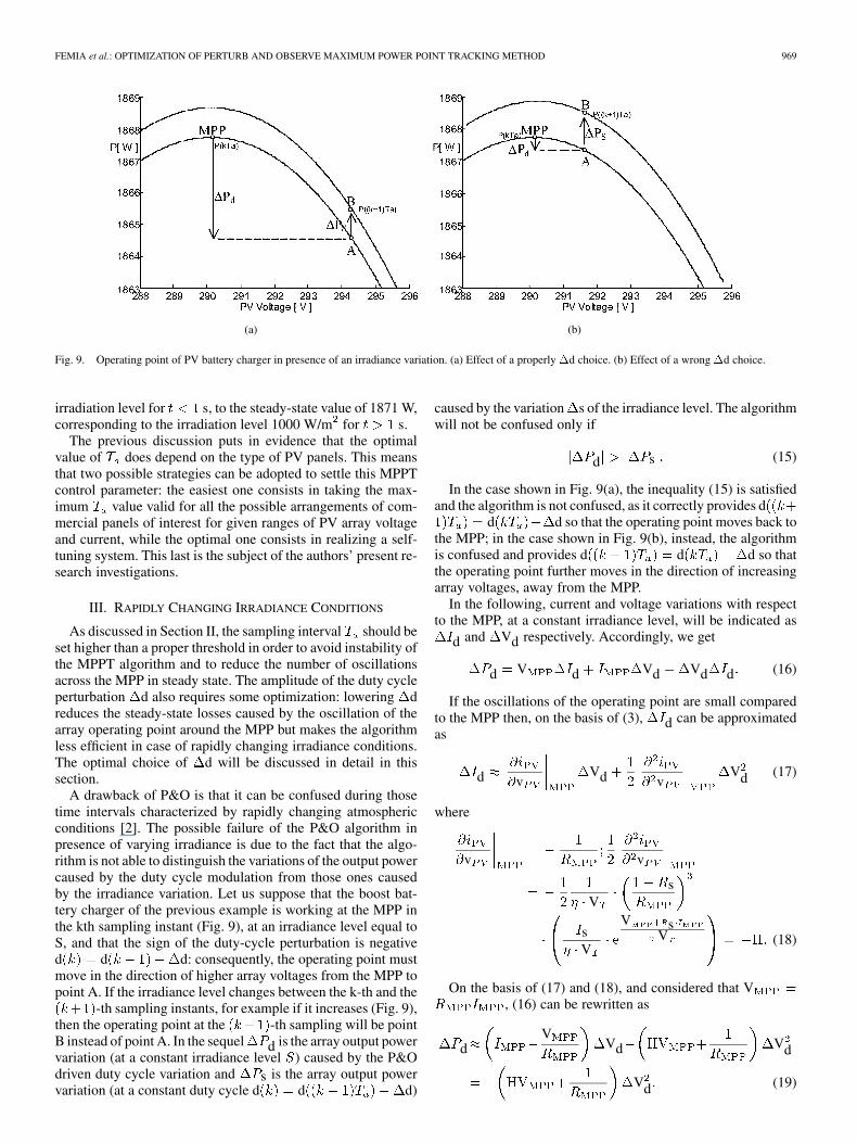
Fig. 9. Operating point of PV battery charger in presence of an irradiance variation. (a) Effect of a properly�d choice. (b) Effect of a wrong�d choice.

irradiation level for s, to the steady-state value of 1871 W,corresponding to the irradiation level 1000 W/m for s.

The previous discussion puts in evidence that the optimalvalue of does depend on the type of PV panels. This meansthat two possible strategies can be adopted to settle this MPPTcontrol parameter: the easiest one consists in taking the max-imum value valid for all the possible arrangements of com-mercial panels of interest for given ranges of PV array voltageand current, while the optimal one consists in realizing a self-tuning system. This last is the subject of the authors’ present re-search investigations.

III. RAPIDLY CHANGING IRRADIANCE CONDITIONS

As discussed in Section II, the sampling interval should beset higher than a proper threshold in order to avoid instability ofthe MPPT algorithm and to reduce the number of oscillationsacross the MPP in steady state. The amplitude of the duty cycleperturbation d also requires some optimization: lowering dreduces the steady-state losses caused by the oscillation of thearray operating point around the MPP but makes the algorithmless efficient in case of rapidly changing irradiance conditions.The optimal choice of d will be discussed in detail in thissection.

A drawback of P&O is that it can be confused during thosetime intervals characterized by rapidly changing atmosphericconditions [2]. The possible failure of the P&O algorithm inpresence of varying irradiance is due to the fact that the algo-rithm is not able to distinguish the variations of the output powercaused by the duty cycle modulation from those ones causedby the irradiance variation. Let us suppose that the boost bat-tery charger of the previous example is working at the MPP inthe kth sampling instant (Fig. 9), at an irradiance level equal toS, and that the sign of the duty-cycle perturbation is negatived d d: consequently, the operating point mustmove in the direction of higher array voltages from the MPP topoint A. If the irradiance level changes between the k-th and the

-th sampling instants, for example if it increases (Fig. 9),then the operating point at the -th sampling will be pointB instead of point A. In the sequel d is the array output powervariation (at a constant irradiance level ) caused by the P&Odriven duty cycle variation and s is the array output powervariation (at a constant duty cycle d d d)

caused by the variation s of the irradiance level. The algorithmwill not be confused only if

d s (15)

In the case shown in Fig. 9(a), the inequality (15) is satisfiedand the algorithm is not confused, as it correctly provides d

d d so that the operating point moves back tothe MPP; in the case shown in Fig. 9(b), instead, the algorithmis confused and provides d d d so thatthe operating point further moves in the direction of increasingarray voltages, away from the MPP.

In the following, current and voltage variations with respectto the MPP, at a constant irradiance level, will be indicated as

d and Vd respectively. Accordingly, we get

d V d Vd Vd d (16)

If the oscillations of the operating point are small comparedto the MPP then, on the basis of (3), d can be approximatedas

d vVd v

Vd (17)

where

v v

Vs

sV

V sV (18)

On the basis of (17) and (18), and considered that V, (16) can be rewritten as

dV

Vd Vd

Vd (19)

970 IEEE TRANSACTIONS ON POWER ELECTRONICS, VOL. 20, NO. 4, JULY 2005

(a) (b)

Fig. 10. Simulation results for: T = 0.01 s; �d =0.01; _s = 50 W=(m s); (b) zoom of (a).

If a first order approximation is used for d, instead of (18),then we get d , if the quantity Vd d is neglected in(16), or d Vd if Vd d is not neglectedin (16). In any case, both expressions are coarse approximationsthat do not allow us to check, with adequate accuracy, whetherinequality (15) is verified or not. The effect of a duty-cycle stepperturbation of amplitude d on the corresponding steady-statevariation Vd of the array voltage can be evaluated by usingthe small signal control to array voltage transfer functionintroduced in Section II

Vd d (20)

where is the dc gain of . As for s, by neglecting Vdwith respect to V , we get

s V s Vd s V s V s(21)

where s is the array current variation (at a constant duty-cycle d(k)) due to the irradiance variation s and K is a materialconstant [1]. In order to avoid the failure of the P&O algorithmin dynamic conditions, on the basis of (15), (19), (20) and (21),the following inequality must be fulfilled

d V s (22)

from which we get

dV

V s

(23)

where is the average rate of change of the irradiance level in-side the time interval of length (sampling period) betweenthe k-th and the -th sampling. The proper value to as-sign to can be found on the basis of the considerations drawn

in Section II; if inequality (23) is fulfilled, then, in the limitof validity of the approximations made, the P&O algorithm isable to track without errors irradiances characterized by averagerates of change (within ) not higher than . The parametersH, V and in (23) depend on the irradiance level: sothat, when using (23), the combination of parameters (H, V ,

) leading to the highest value of the right-hand side mustbe used. In the sequel we will assume the following values forthe parameters of system of Fig. 1: A/V (at

W/m ), A/V (at W/m ),A m W, V V (at W/m ),

V (at W/m ). By assuming a constantrate of change W m s , the minimum value of d al-lowing the tracking of the irradiation without errors is equal to

. In Fig. 10(a) the behavior of the P&O drivenduty-cycle in correspondence of the variation of the irradiancelevel from 350 W/m to 1000 W/m is shown, with a constantrate of change equal to 50 W m s , d and

s. As discussed in Section II, the value adopted forallows the P&O algorithm working efficiently at steady-state.It is evident that, during the transient, the duty-cycle swingsamong more than three values [Fig. 10(b)]; in Section II it hasbeen also shown that, at steady state, when a suitable value of

is chosen, the duty cycle oscillates assuming only three dif-ferent values. Also in transient conditions, if the value of the am-plitude of the duty-cycle perturbation is sufficiently high, thenthe duty-cycle oscillates assuming only three different values.The swing of the duty-cycle among four points in Fig. 10 isdue to the fact that inequality (23) is approximate. Among theother approximations used to get (23), the main one is based onthe assumption that the starting operating point is the MPP. In-deed, as the values assumed by the duty-cycle are quantized, thebest operating point location only neighbors the MPP, as shownin Fig. 11. The degree of approximation involved in (23) dete-riorates when the best operating point is located far from theMPP. Of course, by adopting a value of d much higher thanthe one provided by (23), we would succeed in getting a be-havior characterized by the swinging of the duty-cycle amongonly three values but, at the same time, wider ocillations of theoperating point around the MPP would appear with the conse-quent decrease of the efficiency. In conclusion, the behavior of

FEMIA et al.: OPTIMIZATION OF PERTURB AND OBSERVE MAXIMUM POWER POINT TRACKING METHOD 971

(a) (b)

Fig. 11. Operating point of PV battery charger with T = 0:01 s; �d = 0:01; _S = 50 W=(m s): (a) three points behavior and (b) four points behavior.

Fig. 12. Time domain simulations: (a) T = 0.01 s; _S = 50 W=(m s)and (b) zoom of (a).

the system shown in Fig. 10 is very efficient since no more thanone extra step affects the swing across the MPP, compared withthe best three-step case.

Fig. 13. Experimentally tested grid connected PV system.

In the case of four points behavior, the maximum voltage dis-crepancy between the operating point and the MPP is equal to

Vd: so that, from (19) and (20), the corresponding maximum

d is

(24)

If the theoretical MPPT efficiency is defined as

(25)

then, in the case under study, with d andW m s , it is . Fig. 12 shows

the behaviors of the P&O driven duty-cycle in correspondenceof a sinusoidal time varying irradiance, characterized by amaximum rate of change equal to 50 W m s , in the twocases d d and d d . Fig. 12shows that, when (23) is not fulfilled d d ,then the P&O algorithm fails to track the irradiance and a notnegligible amount of available energy is wasted.

IV. EXPERIMENTAL RESULTS

Fig. 13 shows a grid connected PV system adopted for exper-imental measurements.

972 IEEE TRANSACTIONS ON POWER ELECTRONICS, VOL. 20, NO. 4, JULY 2005

(a) (b)

Fig. 14. Experimental measurements: (a) clear day and (b) cloudy day.

Fig. 15. Experimental PV voltage acquisition.

The boost MPPT converter supplies a 1.5 kW inverter for220 V/50 Hz grid connection. In this case, the dc/ac section in-troduces a 100 Hz disturbance on the photovoltaic array voltage.This represents a worse operating condition for the mppt boostwith respect to the case of the battery charger and allows to testthe robustness of the proposed optimization method. The exper-imental time domain waveforms of v and are shownin Fig. 14.

Data acquisitions during a clear day [Fig. 14(a)] show a threepoints swinging MPPT control, with some occasional correc-tions by means of a further level. Nevertheless, even with avoltage swing of about 40 V, the power swing under its max-imum value does not exceed 40 W. Fig. 14(b) shows the oper-ating point swings during a cloudy day. Fig. 15 shows a moredetailed plot of PV voltage. The high frequency oscillationsare due to the effect of the duty cycle step wise perturbation,weighted by , [first right-hand side term of (9)]. Instead,the slower oscillations, at 100 Hz, represent the effect of thesecond right-hand side term of (9). In this case, the best MPPTparameters are d 0.05 and 20 ms. By using (24) with

Vd 10 V, consistent with the values shown in Fig. 15, aequal to about 90 W is obtained. This prediction, based

on a four point swinging MPPT control, is confirmed by bothplots of PV power of Fig. 14(a) and (b).

V. CONCLUSION

In this paper a theoretical analysis allowing the optimalchoice of the two main parameters characterizing the P&O al-gorithm has been carried out. The idea underlying the proposedoptimization approach lies in the customization of the P&OMPPT parameters to the dynamic behavior of the whole systemcomposed by the specific converter and PV array adopted. Theresults obtained by means of such approach clearly show thatin the design of efficient MPPT regulators the easiness andflexibility of P&O MPPT control technique can be exploitedby optimizing it according to the specific system’s dynamiccharacteristics. As an example a boost converter has beenexamined. The results obtained and the considerations drawncan be extended to any other converter topology as well.

FEMIA et al.: OPTIMIZATION OF PERTURB AND OBSERVE MAXIMUM POWER POINT TRACKING METHOD 973

ACKNOWLEDGMENT

The authors wish to thank Dr. F. De Rosa for his preciouscooperation.

REFERENCES

[1] S. Liu and R. A. Dougal, “Dynamic multiphysics model for solar array,”IEEE Trans. Energy Conv., vol. 17, no. 2, pp. 285–294, Jun. 2002.

[2] K. H. Hussein, I. Muta, T. Hshino, and M. Osakada, “Maximum photo-voltaic power tracking: an algorithm for rapidly changing atmosphericconditions,” Proc. Inst. Elect. Eng., vol. 142, no. 1, pp. 59–64, Jan. 1995.

[3] M. Veerachary, T. Senjyu, and K. Uezato, “Voltage-based maximumpower point tracking control of PV system,” IEEE Trans. Aerosp. Elec-tron. Syst., vol. 38, no. 1, pp. 262–270, Jan. 2002.

[4] K. K. Tse, M. T. Ho, H. S.-H. Chung, and S. Y. Hui, “A novel maximumpower point tracker for PV panels using switching frequency modula-tion,” IEEE Trans. Power Electron., vol. 17, no. 6, pp. 980–989, Nov.2002.

[5] P. Midya, P. Krein, R. Turnbull, R. Reppa, and J. Kimball, “Dynamicmaximum power point tracker for photovoltaic applications,” in Proc.27th Annu. IEEE Power Electronics Specialists Conf., vol. 2, Jun. 1996,pp. 1710–1716.

[6] E. Koutroulis, K. Kalaitzakis, and N. C. Voulgaris, “Development ofa microcontroller-based, photovoltaic maximum power point trackingcontrol system,” IEEE Trans. Power Electron., vol. 16, no. 1, pp. 46–54,Jan. 2001.

[7] T. Noguchi, S. Togashi, and R. Nakamoto, “Short-current pulse-basedmaximum-power-point tracking method for multiple photovoltaic-and-converter module system,” IEEE Trans. Ind. Electron., vol. 49, no. 1, pp.217–223, Feb. 2002.

[8] K. Irisawa, T. Saito, I. Takano, and Y. Sawada, “Maximum power pointtracking control of photovoltaic generation system under nonuniform in-solation by means of monitoring cells,” in Proc. 28th IEEE PhotovoltaicSpecialists Conf., Sep. 2000, pp. 1707–1710.

[9] C. Hua, J. Lin, and C. Shen, “Implementation of a DSP-controlled pho-tovoltaic system with peak power tracking,” IEEE Trans. Ind. Electron.,vol. 45, no. 1, pp. 99–107, Feb. 1998.

[10] T. Wu, C. Chang, and Y. Chen, “A fuzzy-logic-controlled single-stageconverter for PV-powered lighting system applications,” IEEE Trans.Ind. Electron., vol. 47, no. 2, pp. 287–296, Apr. 2000.

[11] I. Batarseh, T. Kasparis, K. Rustom, W. Qiu, N. Pongratananukul, andW. Wu, “DSP-based multiple peak power tracking for expandable powersystem,” in Proc. 18th Annu. IEEE Applied Power Electronics Conf.Expo, vol. 1, Feb. 2003, pp. 525–530.

[12] D. P. Hohm and M. E. Ropp, “Comparative study of maximum powerpoint tracking algorithms,” in Proc. 28th IEEE Photovoltaic SpecialistsConf., Sep. 2000, pp. 1699–1702.

[13] C. A. Desoer and E. S. Kuh, Basic Circuit Theory. New York: Mc-Graw-Hill, 1969.

[14] R. W. Erickson and D. Maksimovic, Fundamental of Power Elec-tronics. Norwell, MA: Kluwer, 2001.

Nicola Femia (M’94) was born in Salerno, Italy, in1963. He received the Ph.D. degree (with honors) inengineering of industrial technologies from the Uni-versity of Salerno, Italy, in 1988.

From 1990 to 1998, he was an Assistant Professor,from 1998 to 2001, he was an Associate Professor,and since 2001 has been a Full Professor of elec-trotechnics at the Faculty of Engineering, Universityof Salerno. He is coauthor of about 80 scientificpapers published in the proceedings of internationalsymposia and in international journals. His main

scientific interests are in the fields of circuit theory and applications and powerelectronics.

Dr. Femia was an Associate Editor of the IEEE TRANSACTIONS ON POWER

ELECTRONICS from 1995 to 2003.

Giovanni Petrone was born in Salerno, Italy, in1975. He received the “Laurea” degree in electronicengineering from the University of Salerno, Italy, in2001 and the Ph.D. degree in electrical engineeringfrom the University of Napoli “Federico II,” Italy, in2004.

Since March 2004, he has collaborated withthe Electrical Engineering Department, Universityof Salerno. His main research interests are in theanalysis and design of switching converters fortelecommunication applications, renewable energy

sources in distributed power systems, and tolerance analysis of electroniccircuits.

Giovanni Spagnuolo (M’98) was born in Salerno,Italy, in 1967. He received the “Laurea” degreein electronic engineering from the University ofSalerno, Italy, in 1993 and the Ph.D. in electricalengineering from the University of Napoli, “FedericoII,” Italy, in 1997.

From November 1993 to October 1994, he was aResearcher on the design, building, and tuning of ahigh voltage test-bed of a cryogenic superconductingcable. In 1993, he joined the Dipartimento di Ingeg-neria dell’Informazione ed Ingegneria Elettrica, Uni-

versity of Salerno, where he was a Post-Doctoral Fellow (1998–1999), an Assis-tant Professor of Electrotechnics (1999–2003) and, since January 2004, an As-sociate Professor. His main research interests are in numerical methods for theanalysis of electromagnetic fields, in the analysis and simulation of switchingconverters and in tolerance analysis and design of electronic circuits.

Massimo Vitelli was born in Caserta, Italy, in 1967.He received the “Laurea” degree (with honors) inelectrical engineering from the University of Naples,“Federico II,” Italy, in 1992.

In 1994, he joined the Department of InformationEngineering, Second University of Naples, as aResearcher. In 2001, he was appointed AssociateProfessor in the Faculty of Engineering, SecondUniversity of Naples, where he teaches Elec-trotechnics. His main research interests concern theelectromagnetic characterization of new insulating

and semi-conducting materials for electrical applications, electromagneticcompatibility and the analysis and simulation of power electronic circuits.

Dr. Vitelli is an Associate Editor of the IEEE TRANSACTIONS ON POWER

ELECTRONICS.