1

Optimization Models and Algorithms for JointUplink/Downlink UMTS Radio Network Planning

with SIR-based Power ControlAmin Abdel Khalek, Lina Al-Kanj, Zaher Dawy, Senior Member, IEEE, and George Turkiyyah

Abstract— UMTS networks should be deployed accordingto cost-effective strategies that optimize a cost objective andsatisfy target quality of service (QoS) requirements. In thispaper, we propose novel algorithms for joint uplink/downlinkUMTS radio planning with the objective of minimizing totalpower consumption in the network. Specifically, we define twocomponents of the radio planning problem: (1) Continuous-based site placement, and (2) Integer-based site selection. Inthe site placement problem, our goal is to find the optimallocations of UMTS base stations in a certain geographic areawith a given user distribution to minimize the total powerexpenditure such that a satisfactory level of downlink and uplinksignal-to-interference ratio (SIR) is maintained with boundedoutage constraints. We model the problem as a constrainedoptimization problem with SIR-based uplink and downlink powercontrol scheme. An algorithm is proposed and implemented usingpattern search techniques for derivative-free optimization withaugmented Lagrange multiplier estimates to support generalconstraints. In the site selection problem, we aim to select theminimum set of base stations from a fixed set of candidatesites that satisfies quality and outage constraints. We developan efficient elimination algorithm by proposing a method forclassifying base stations that are critical for network coverageand quality of service. Finally, the problem is reformulated totake care of location constraints whereby the placement of basestations in a subset of the deployment area is not permitted dueto, e.g., private property limitations or electromagnetic radiationconstraints. Experimental results and optimal tradeoff curves arepresented and analyzed for various scenarios.

Index Terms— Cellular network planning, network optimiza-tion, network deployment, electromagnetic radiation exposure

I. INTRODUCTION

In UMTS networks, the base station (BS) coverage andcapacity are a function of the user distribution, the signal-to-interference ratio (SIR) requirements, and the interferencelevel which is an important coverage-limiting factor. The trans-mit powers of mobile users are power controlled depending

Copyright (c) 2011 IEEE. Personal use of this material is permitted.However, permission to use this material for any other purposes must beobtained from the IEEE by sending a request to pubs-permissions@ieee.org.

This work was supported by a research grant from the National Councilfor Scientific Research (CNRS), Lebanon.

A. Abdel Khalek was with the Department of Electrical and ComputerEngineering, American University of Beirut, Beirut, Lebanon. He is now withthe Department of Electrical and Computer Engineering, The University ofTexas at Austin, TX, USA (email: amin@mail.utexas.edu). L. Al-Kanj andZ. Dawy are with the Department of Electrical and Computer Engineering,American University of Beirut, Beirut, Lebanon (email: lka06@aub.edu.lb,zd03@aub.edu.lb). G. Turkiyyah is with the Department of Computer Science,American University of Beirut, Beirut, Lebanon (email: gt02@aub.edu.lb).

on their distance from the BS to reduce interference, avoidthe near-far problem and ensure coverage for users close tothe cell edge. Given the high cost of network infrastructureinvestments and spectrum licenses, operators should makeinformed decisions on network deployment to satisfy perfor-mance requirements in a cost efficient way. This drives theneed for optimized UMTS-specific planning tools that takeinto account the WCDMA air interface characteristics.

UMTS radio network planning involves configuring thenetwork resources and parameters in a way that guaranteessatisfactory performance for the end-users according to thefollowing three main quality attributes: coverage, capacityand quality of service. Radio network planning is conven-tionally approached as an iterative process which requiressetting target coverage and capacity objectives. The initialnetwork plan is obtained from geographic data, demographicdata, and propagation models, e.g., [1], [2], [3], and is thenoptimized by iterative updates of various network variables.Several modeling techniques are feasible and can be solvedby mathematical and heuristic optimization algorithms suchas simulated annealing, greedy algorithms, genetic algorithms,linear and non-linear programming, etc.

A. Related Work

In [4], [5], [6], the authors propose discrete optimizationalgorithms using randomized greedy procedures and a tabusearch algorithm to plan the process of locating new BSsconsidering quality constraints for the uplink which is arguedto be more stringent than the downlink for symmetric traffic. In[7], the previous work is extended to the downlink for asym-metric traffic by applying SIR-based power control. Modelsspanning both downlink and uplink with power control arealso presented in [8], [9].

In [10], [11], mixed integer linear programming (MILP) isused for planning cost-efficient radio networks under networkquality constraints. Models based on set covering are used toobtain lower bounds on the number of required BSs to serve agiven fixed area and an automatic two phase network planningapproach based on successively solving instances of the modelis presented. In [12] and [13], two graph theory based modelsare proposed: Maximum independent set (MIS) model andminimum dominating set (MDS) model to select a satisfactorysubset out of a user-provided set of BS locations, whileensuring that at least a given percentage of the considered areais served by the selected BSs. A large set of candidate BS sitesis first determined. In [14], a net-revenue maximization model

2

for the selection of BS sites and the calculation of servicecapacity is presented. The integer programming model takesthe candidate BS locations and the traffic demand model asinput, and uses a priority branching scheme to achieve a targetoptimization gap tolerance.

The majority of the contributions on optimized networkplanning focus on locating BSs according to the best trade-off between network infrastructure costs and service coverage,whereas the electromagnetic (EM) field exposure levels arerarely considered. However, raising concerns about seriousconsequences for human health due to exposure to EM fieldshave led to precautionary regulations enforced by publicadministrators [15], [16]. The most widely accepted standardsare those developed by the IEEE [17] and the ICNIRP [18].Due to the increasing concerns about EM pollution in cellularnetworks, it should be considered an important metric fornetwork planning and optimization. The inclusion of EMradiation in the cellular network planning problem has beenaddressed in [19], [20] where two sequential meta-heuristicswere developed to limit the total EM field at selected testpoints and combined in a tabu search (TS) and a genetic algo-rithm (GA). The TS procedure is able to explore the solutionspace deeply enough, but it works on partial configurations,while the GA procedure can manage the complete set ofconsidered parameters, but is computationally expensive.

Current work in the literature focuses on selecting a minimalBS set from a larger candidate fixed BS set. The equally-important continuous version of the problem which involvesfinding the optimal locations of these BSs in the network areawas not considered previously in the literature. By combiningthe two components of the problem, we can target moregeneral application scenarios and further adapt and optimizethe network plan.

B. Contributions of the Paper

In this work, the problem of joint uplink/downlink radionetwork planning is subdivided into two components. In thefirst component, referred to as the site placement problemthroughout the paper, we are interested in finding the optimallocations of a fixed number of UMTS base stations. In thesecond component, referred to as the site selection problem,we are interested in finding the minimal cardinality set froma set of base stations with fixed locations. It can be seen thatthe site placement problem is a continuous problem becausethe problem variables are the physical BS locations, whilethe site selection problem is a combinatorial problem becausethe problem variables are the binary selection variables foreach of the BSs. We solve the continuous problem of findingthe optimal locations of base stations that minimize totalpower expenditure in the network using robust pattern searchalgorithms for derivative-free optimization with non-smoothobjectives. We define QoS targets and maintain boundedoutage levels on a network-wide and per BS basis for bothuplink and downlink channels. Next, we formulate and proposean algorithm to solve the integer problem of selecting thesmallest set of BSs from a fixed set of potential sites suchthat the cost function is minimized and the QoS requirementsare satisfied.

It is important to note that these two problems and theirsolution approaches are distinct, however, we propose that thetwo problems be combined into a hybrid integer/continuousalgorithm involving successive site selection/site placementuntil both components converge, i.e., until no relocation orelimination is feasible. This allows the operator to find theminimal set of BSs needed for satisfactory coverage and theoptimized deployment strategy in the network according to theuser distribution. An additional novel component of our workis the development of a framework for radio network planningwith location constraints. Such constraints arise frequently inpractice due to private property limitations or electromagneticradiation constraints. We formulate the problem of radionetwork planning with location constraints as an optimizationproblem. As part of the problem solution, we use Lagrangianmultiplier estimates and penalty parameters to construct andsolve a sequence of augmented Lagrangian subproblems basedon the Augmented Lagrangian Pattern Search (ALPS) algo-rithm. Finally, we provide optimal tradeoff curves under dif-ferent user distributions and we demonstrate the effectivenessof the proposed schemes compared to conventional clustering.

C. Paper Organization

The rest of the paper is organized as follows: Section IIdescribes the system model. Section III presents the math-ematical formulation for the site selection and site place-ment optimization problems. Section IV presents the strategyand algorithms used to solve the optimization problems. InSection V, we report results for different user distributionsand voice/data traffic combinations and we provide optimaltradeoff curves for the network configuration. In SectionVI, we extend the optimization algorithms to scenarios withlocation constraints and/or EM radiation restrictions. Finally,Section VII provides concluding remarks.

II. SYSTEM MODEL

The user distribution model is assumed to be snapshot-based. A snapshot represents a set of users (or test points)using the physical channel at a given instant of time. For agiven distribution of currently active users or connections, weaim to find a network plan that guarantees minimal powerconsumption in the network, and satisfies coverage and qualityof service requirements in a cost-effective manner.

In UMTS, users rely on channelization and scramblingcodes in order to differentiate their own signal and combatthe effect of multipath and multiuser interference. To guaranteethe required QoS level, a target minimum SIR value should bemaintained for all active connections. The downlink and uplinkSIR expressions for user k can be expressed as follows:

SIRdk = SF

P dreceived,kσ2 + λdIdin,k + Idout,k

(1)

SIRuk = SF

Pureceived,kσ2 + λuIuin,k + Iuout,k

(2)

where P dreceived,k is the downlink received power at mobilestation (MS) k, Pureceived,k is the uplink received power atthe BS from MS k, Idin,k and Idout,k represent the downlink

3

(SF + SIRd

kλd

SIRdk

)gb(k),kP

db(k),k −

λdgb(k),k

∑

j∈Cb(k)

Pb(k),j

−

N∑

i=1,i6=b(k)

(gi,k

∑

l∈Ci

P di,l

)= σ2 (3)

(SF + SIRu

kλu

SIRuk

)gb(k),kP

uk −

λu

∑

j∈Cb(k)

gb(k),jPuj

−

N∑

i=1,i6=b(k)

(∑

l∈Ci

gi,lPdl

)= σ2 (4)

intracell and intercell interference affecting MS k, respectively,Iuin,k and Iuout,k represent the uplink intracell and intercellinterference affecting MS k, respectively, SF is the spreadingfactor, σ2 is the thermal noise power, and λ is the orthogonalityfactor (0.4 ≤ λd ≤ 0.9 in the downlink and λu = 1 inthe uplink [21]). Since we need to satisfy the SIR constraintfor all users, we express the received power and interferencecomponents in (1) and (2) more explicitly for user k asfollows:

P dreceived,k = gb(k),kPdb(k),k; Pureceived,k = gb(k),kP

uk (5)

Idin,k = gb(k),k

(P db(k)−P db(k),k

); Iuin,k =

∑

j∈Cb(k),j 6=k

gb(k),jPuj (6)

Idout,k =N∑

i=1,i6=b(k)

gi,kPdi ; Iuout,k =

N∑

i=1,i6=b(k)

∑

j∈Ci

gi,jPuj (7)

where N is the number of BSs, P di is the total transmit powerof BS i, P di,k is the power allocated by BS i to MS k (subjectto k being covered by BS i), gi,k is an estimate of the pathlossbetween MS k and BS i calculated according to Cost 231-Hatamodel [1], and b(k) is defined as the BS serving MS k andcalculated by constructing the Voronoi tessellations associatedwith the BS locations. Consequently, P db(k),k is the transmitpower allocated to MS k by its serving BS, Pb(k) is the totaltransmit power of the BS serving user k and gb(k),k is anestimate of the pathloss between MS k and its serving BS.The notation j ∈ Ci means all MSs {j} covered by cell i.Consequently, j ∈ Cb(k) means all MSs covered by the sameBS as k. The pathloss coefficients gi,k can be written strictly interms of the BS and MS locations in addition to some constantsas gi,k = 1

keq(di,k)−µ, di,k =

√(xi − uk)2 + (yi − vk)2

where (xi, yi) are the BS locations and (uk, vk) are the fixedMS locations, with keq and µ chosen according to Cost-231Hata Model. In UMTS radio network planning, shadowing andfading are compensated for via link budget margins [1], [21].

Based on the derivation above, (1) can be rewritten in termsof the powers P di,k allocated to MSs which are the downlinkstate variables as shown in (3). Similarly, (2) can be rewrittenin terms of the MS transmit powers Puk which are the uplinkstate variables as shown in (4) where SIRd

k and SIRuk are the

target SIRs to achieve the required QoS for the downlink andthe uplink respectively. Equations (3) and (4) can be expressedin matrix format as follows:[

Gd]U×U ×

[Pd ]

U×1=[σ2]U×1

(8)

[Gu]U×U × [ Pu ]U×1 =[σ2]U×1

(9)

where Gd and Gu are square matrices with size U × U , Pd is acolumn vector with size U × 1 corresponding to the downlinkuser powers P db(k),k, Pu is a column vector with size U × 1

corresponding to the uplink user powers Puk , σ2 is the thermalnoise power column vector with size U × 1, and U is the totalnumber of active users in the network. The kth row of Gd andGu corresponds to user k with each row representing one ofthe U equations, and the columns can be separated into blockscorresponding to the BSs according to the number of users ineach BS. The first term of (3) and (4) appears in the diagonalof Gd and Gu, respectively, the second term represents intracellinterference and appears in the block corresponding to the BSserving user k, the third term represents intercell interferenceand appears in the blocks corresponding to all BSs except theserving BS. Solving the power assignment problem with SIR-based power control reduces to solving this set of equationswhich adjusts the transmit powers in order to to meet the targetSIRs [1], [2].

III. OPTIMIZATION PROBLEM FORMULATION

In this section, we present a formulation for the jointuplink/downlink radio planning problems. The site placementproblem is formulated as a continuous optimization problemand the site selection problem is formulated as an integer opti-mization problem, and the objective, variables, and constraintsfor each of the problems are defined.

A. The Joint Uplink/Downlink Site Placement Problem

The input to the site placement problem is: (1) The areaof interest, (2) the fixed set of MS locations modeling thetypical distribution of active users in the area, (3) the fixednumber of BSs, and (4) the initial locations of the BSs. Thesite placement algorithm optimizes the initial locations of theBSs to minimize the target objective while satisfying the QoSrequirements. The output is the set of optimal locations ofBSs. The objective of joint uplink/downlink site placement isdefined as a weighted linear combination of two objectives:

1) Minimize the downlink power expenditure: The totaldownlink power expenditure is the sum of powers al-located to each user by its serving BS, expressed as∑Uk=1 P

db(k),k. In addition to the inherent benefits of

minimizing power consumption, we will demonstratethat this reduces the variance of BS powers, thus pro-viding a solution that balances the power load accordingto the predicted user distribution.

2) Minimize the uplink outage: The uplink channel islimited by the power capabilities of the MSs, which isby far less than that of the BSs. Thus, it is importantto ensure that uplink transmissions can still reach theBSs at a reasonable power subject to their handset limi-tations while satisfying the minimum SIR threshold foracceptable performance. We formulate this componentas∑Uk=1 (Puk − Pumax)+ where (·)+ = max(·, 0), Puk is

4

the uplink power associated with MS k, and Pumax is themaximum allowed MS power.

Effectively, each MS requiring power in excess of Pumax

will be considered in the second objective. If all MSs do notexceed the threshold, this will be a vector of zeros, essentiallydisregarded from the objective. We do not consider the numberof MSs that are in outage directly in the objective function tomaintain coherence in the units (Watts) and avoid non-smoothstep transitions in the function. However, this approach has thesame potential in minimizing the number of MSs in outagesince the algorithm will attempt to find the BS configurationthat satisfies (Puk − Pumax)+ = 0 ∀k, if such configurationexists.

In the site placement problem, N is fixed, that is, weare not interested in reducing the initial number of BSs butin optimizing their locations. Thus, the decision variablesare the locations of the BSs (xi, yi), i = 1, · · · , N thatminimize the cost function. Since the objective function isexpressed in terms of the downlink powers assigned by theBSs to their MSs, we consider the powers assigned by theBSs (Pi,k), i = 1, · · · , N, k = 1, · · · ,Mi as state variables.Note that

∑Ni=1Mi = U where Mi is the number of MSs

served by BS i. Thus, the total number of variables in theproblem is U + 2N where U � N . The power assignmentvariables relate to the decision variables through the SIR-basedpower control mechanism as shown in (8) and (9). Since thematrices Gd and Gu consist of the pathloss coefficients gi,k,it is worth mentioning that it can be written strictly in termsof the BS and MS locations in addition to some constantsaccording to the equations gi,k = 1

keq(di,k)−µ, di,k =√

(xi − uk)2 + (yi − vk)2. Thus, the power assignments for agiven setting of the location variables can be found by solvingthe U set of equations, an operation that costs O(U3).

Two important observations concerning Gd and Gu areworth pointing out: First, they are strongly diagonally-dominant. For example, the average value of the diagonalterms is at least 103 times the average value of the non-diagonal terms with a spreading factor of 128 since thespreading gain appears only in the diagonal terms and thenon-diagonal terms correspond to interference components.This fact can be exploited by using fast solvers suitable fordiagonally-dominant matrices. Second, if the SIR requirementfor the kth user cannot be satisfied due to high interferenceat its location, the solution of the corresponding equation willyield a negative power, which can be used for spotting outagesin the network.

The outage conditions are defined network-wide and foreach BS. The network-wide outage conditions ensure that thetotal number of users in outage is less than ηnetworkU and theBS outage conditions ensure that the number of users in outagefor every BS i is less than ηBSMi where ηnetwork and ηBS aredesign parameters that satisfy 0 ≤ ηnetwork ≤ ηBS � 1.

The problem of joint uplink/downlink site placement is for-mulated as an optimization problem as in (10)-(20) where (10)represents the weighted objective and α is a constant whichdetermines the relative weight of each of the two components,(11) represents the matrix-form downlink SIR constraint for all

MSs, (12) represents the matrix-form uplink SIR constraint forall MSs, (13) is the downlink network outage condition, (14)is the uplink network outage condition, (15) is the downlinkBS outage condition for every BS, (16) is the uplink BSoutage condition for every BS, (17) is the pathloss according toCost 231-Hata model, (18) is the distance-based assignment ofMSs to BSs obtained by constructing the Voronoi tessellationcorresponding to the BS locations, (19) is the maximum BSpower constraint, and (20) is the area of operation constraint.Note that MS k may be in outage either because it requires atransmission power Puk higher than Pumax to reach the closestBS, or because the transmit power Puk , although lower thanPumax, causes high interference at another MS so that the SIRconstraints cannot be satisfied. Equation (10) eliminates outagedue to the former case while (13)-(16) eliminate outage dueto the latter case.

minx,y

U∑

k=1

P db(k),k + α

U∑

k=1

(Puk − Pumax)+ (10)

s.t.[Gd]

U×U ×[

Pd ]U×1

=[σ2]U×1

(11)

[Gu]U×U × [ Pu ]U×1 =[σ2]U×1

(12)U∑

k=1

(−P dk,b(k)

|P dk,b(k)|

)+

< ηnetwork · U (13)

U∑

k=1

(− Puk|Puk |

)+

< ηnetwork · U (14)

∑

k∈Ci

(−P dk,b(k)

|P dk,b(k)|

)+

< ηBS ·Mi (15)

∑

k∈Ci

(− Puk|Puk |

)+

< ηBS ·Mi (16)

gi,k =1keq

d−µi,k ; di,k=√

(xi − uk)2 + (yi − vk)2(17)

b(k) = argmini di,k (18)∑

j∈Ci

Pi,j ≤ P dmax (19)

xmin ≤ xi ≤ xmax, ymin ≤ yi ≤ ymax (20)i = 1, · · · , N ; k = 1, · · · , U (21)

B. The Joint Uplink/Downlink Site Selection Problem

The input to the site selection problem is: (1) The area ofinterest, (2) the fixed set of MS locations modeling the typicaldistribution of active users in the area, (3) the candidate set ofBSs with fixed locations. The site selection algorithm selectsthe minimal cardinality set of BSs that satisfies the coverageand SIR requirements. The output is the subset of candidatescorresponding to the selected BSs. The main difference fromthe site placement problem is that the decision variables arenot the BS locations, instead, these locations are fixed, andthe decision variables are booleans ci where ci = 1 if BS i isto be used in the optimal network configuration, and ci = 0otherwise. The objective of the problem is to minimize thenumber of selected BSs, that is,

∑N0i=1 ci where N0 is the

5

size of the candidate set of BSs. The problem can thus beformulated as a nested optimization problem as shown in (22)-(24). The inner problem finds the set of BSs that minimizesthe cost function and the outer problem finds the minimalcardinality set of such BSs. We will later show that using theminimization of the total power expenditure as the criterion forBS removal results in better solutions than a removal basedpurely on the feasibility of BS elimination (See Section V-B).Note that the constraints (11)-(20) are only applied to the setof active BSs satisfying ci = 1.

minc

N0∑

i=1

ci (22)

s.t.

minU∑

k=1

cb(k) · P dk,b(k) + α

U∑

k=1

cb(k) · (Puk − Pumax)+(23)

subject to(11), (12), (13), (14), (15), (16), (17), (18), (19), (20)i = 1, · · · , N0; k = 1, · · · , U (24)

IV. OPTIMIZATION STRATEGIES AND ALGORITHMS

Solving the initial site placement optimization probleminvolves nonlinear equality constraints: (11), (12), (17), and(18), nonlinear inequality constraints: (13)-(16) and (19), andlinear bound constraints: (20). Given the current BS locationsx and y, we use (18) to obtain the assignments of MSs totheir closest BS, and (17) to obtain the pathloss between eachMS and its serving BS. Finally, solving the SIR equations(11) and (12), we obtain the power allocated to each MS onthe uplink and downlink to satisfy QoS requirements. Thus,the four sets of equality constraints are implicitly includedin objective function evaluations because they determine thepower allocation scheme throughout the network. The boundconstraint representing the area of operation is a simple linearconstraint that is taken care of by the algorithm by choosingappropriate steps that do not violate that constraint. To solvethe site placement problem, we propose a pattern search algo-rithm based on Mesh Adaptive Direct Search (MADS). Addi-tionally, to ensure satisfying the BS power limit and the outageconstraints, we will describe how to extend the algorithm toinclude any general nonlinear inequality constraints using theAugmented Lagrangian Pattern Search (ALPS) method. Afterpresenting the algorithm for the site placement problem, wewill present the solution for the nested optimization problemof site selection based on successive elimination of BSs.

A. Algorithm for Site Placement with Uplink and DownlinkQoS Guarantees

The MADS class of derivative-free algorithms is effectivefor practical nonlinear optimization problems with nonsmoothobjective functions where the computation of derivatives iseither not possible, or it is not sufficiently representativeof the variability of the function around a point due tothe roughness of the objective function. MADS has a welldeveloped convergence theory based on the Clarke calculusand Rockafeller’s notion of a hypertangent cone [22],[23].

To illustrate why the MADS algorithm is suitable for radioplanning problems, we present a sample pattern of the changeof the objective function value with respect to a change inone of the variables (equivalent to moving one of the BSsalong a coordinate direction). Figure 1 shows that the objectivefunction has a lot of discontinuities and non-smooth changeswhich are explained by the changes in user assignments dueto the shift in the Voronoi diagram. As new users are handed-over to a new BS, they become on the boundary of that BS,requiring higher power to achieve the target SIR, thus causingthe instant rise in power allocations, and correspondingly,in the objective function value. Note that the change inone MS-BS assignment does not affect only that user dueto the changes in intercell and intracell interference effectsexperienced by other users, translated in the change of thestructure and content of the pathloss matrices Gd and Gu andthe solutions to the set of equations in (8) and (9). Althoughthe total power expenditure increases if the BS is moved anydistance larger than 20 meters, a gradient computed using finitedifference method or adjoint method is misleading becauseit will imply that the objective function is decreasing whichis only valid 20 meters away from the BS. These kinds ofpeculiarities make it impractical to follow a line search methodin solving the problem, which is why we advocate the use ofderivative-free optimization algorithms suitable for the non-smooth objectives of the radio network planning problem.

0 100 200 300 400 500180

181

182

183

184

185

186

187

188

Movement Distance (m)

Tota

lPow

erE

xpen

ditu

rein

the

netw

ork

(W)

Fig. 1. Pattern of change of objective function while moving a base stationalong a coordinate direction.

The MADS algorithm operates by performing polling andsearching on a set of mesh points around the current locationof the decision variables. The mesh points are constructed bybuilding a pattern which is a basis set of vectors that thealgorithm uses to determine which points to search at eachiteration. The most common basis set is the 2n basis set wheren is the number of decision variables. In our problem, thenumber of decision variables is n = 2N , thus the basis set willcontain 4N vectors each of size 2N . The vectors are definedas follows: v1 = [1 0 · · · 0], v2 = [0 1 · · · 0], · · · , v2N =[0 0 · · · 1], v2N+1 = [−1 0 · · · 0], v2N+2 = [0 −1 · · · 0], · · · , v4N = [0 0 · · · − 1].

At each iteration, the pattern search polls the points in thecurrent mesh for a point that improves the objective functionby computing the objective function at the mesh points tocheck if there is one whose function value is less than thefunction value at the current point. The mesh points are found

6

Algorithm 1 Proposed solution for the joint uplink/downlinksite placement problem.

Given N ; U ; {xi = xinitial,i}2Ni=1 ; {uk = ufixed,k}2U

k=1 ; ∆ =∆0 ; ∆th ; α ;µ ; keq ; σ2 ; λd ; λu ; SF ; {SIRd

k}Uk=1 ; {SIRuk}Uk=1.

Construct the 2n basis set of vectors v that the algorithm uses to determinewhich points to search at each iteration where n is the number of decisionvariables (2n = 4N )v1 = [1 0 ... 0], v2 = [0 1 ... 0], ... , v2N = [0 0 ... 1]v2N+1 = [−1 0 ... 0], v2N+2 = [0 −1 ... 0], ..., v4N = [0 0 ... −1].while ∆ > ∆th{While the mesh size is higher than the convergencethreshold} do

for m = 1 : 4N{For all possible patterns of movement} doxtemp = x+ ∆m · vp

Step 1. Construct the Voronoi tessellation corresponding to the basestation locations {xm} and find the distance between each (BS ,MS) pairStep 2. Construct the pathloss matrices Gd and Gu based on theestimated pathloss for each (BS , MS) pair in the uplink and downlinkStep 3. Solve the set of equations:

[Gd] ×

[Pd ] =

[σ2]

and[Gu] × [ Pu ] =

[σ2]

to find the downlink power that should beallocated to each MS and the uplink MS power to achieve SIR-basedpower control for all users.Step 4. Calculate the objective function at this mesh point

xm: fm =U∑

k=1

P dk,b(k) + α

U∑

k=1

(Puk − P

umax)+

end forif minm fm < f{Is there a mesh point with smaller objectivefunction} thenx = x+∆·vm{Successful Poll: Advance to the point that minimizesthe objective and expand mesh size}∆ = ∆× (Expansion Factor).

else∆ = ∆× (Contraction Factor){Unsuccessful Poll: reduce meshsize}.

end ifend while.

by multiplying each pattern vector vp by a scalar ∆m to gen-erate a set of direction vectors and adding the direction vectorto the current point found at the previous step. The number ofmesh points 4N is simply due to the four coordinate directionsof polling for each BS. These points can be expressed asxp = x + ∆mvp, p = 1, · · · , 4N where x is a vector ofsize 2N corresponding to the current locations of the N BSs,∆m is the mesh size at iteration m, and xp is the polled meshpoint. Initially, the mesh size is specified based on the scale ofthe problem, and is expanded and contracted during executionof the optimization algorithm. In this way, the algorithm findsa sequence of points, x0, x1, x2, · · · that approach an optimalpoint. The convergence criteria are satisfied when the meshsize is smaller than the mesh tolerance such that minimizingthe objective function further would require moving any BSa distance smaller than this mesh tolerance threshold. Thispolling technique is effectively equivalent to moving the BSsin their neighborhood according to the mesh size at a giveniteration. It is important to note that at each polled point, theobjective function is calculated by reconstructing the Voronoitessellation, building the pathloss matrices Gd and Gu, solvingthe set of equations corresponding to SIR-based power control,and computing the objective function from Pd and Pu. Acomplete algorithmic description is presented in Algorithm 1.

As mentioned previously, the algorithm described abovedoes not account for the nonlinear inequality constraints in theproblem. To include the maximum BS power and the outageconstraints, we use the ALPS algorithm which is a robustextension of pattern search algorithms for general constraints.

Algorithm 2 Proposed solution for the joint uplink/downlinksite selection problem.

Given N = N0 ; U ; F = ∅ ; I = ∅ ; {xi = xinitial,i}N0i=1 ; {yi =

yinitial,i}N0i=1 ; α ;µ ; keq ; σ2 ; λd ; λu ; {uk =

ufixed,k}Uk=1 ; {vk = vfixed,k}Uk=1 ; SF ; {SIRdk}Uk=1 ; {SIRu

k}Uk=1.while true do

for i = 1 : N{Try eliminating base station i} doxtemp = {x1, · · · , xi−1, xi+1, · · · , xN}ytemp = {y1, · · · , yi−1, yi+1, · · · , yN}Step 1. Construct the Voronoi tessellation corresponding to the basestation locations {xtemp, ytemp} and find the distance between each(BS , MS) pairStep 2. Construct the pathloss matrices Gd and Gu based on theestimated pathloss for each (BS , MS) pairStep 3. Solve the set of equations:

[Gd] ×

[Pd ] =

[σ2]

and[Gu]× [ Pu ] =

[σ2]

to find uplink and downlink power allocationachieving SIR-based power control for all users.Step 4.if Pd and Pu do not satisfy (13)-(16) {If eliminating the base stationcauses significant DL or UL coverage loss} theni ∈ I{Place BS i in the infeasible set}

elsei ∈ F{Place BS i in the feasible set}Calculate the objective function at (xtemp,ytemp): fi =∑U

k=1 Pdk,b(k)

+ α∑U

k=1 (Puk − P

umax)+

end ifend forif F 6= ∅{If some base station can be eliminated} thene = argminifi

x = {x1, · · · , xe−1, xe+1, · · · , xN}y = {y1, · · · , ye−1, ye+1, · · · , yN}N = N − 1

elsebreak{Converged: No BS can be eliminated without jeopardizingcoverage}

end ifend while

The algorithm operates by formulating a subproblem obtainedby combining the objective function and nonlinear constraintfunctions using Lagrange multiplier estimates and penaltyparameters. A sequence of such optimization problems areapproximately minimized using a pattern search algorithm andthe convergence to the optimal solution is guaranteed (SeeSection VI-B for more details).B. Algorithm for Site Selection with Uplink and Downlink QoSGuarantees

The site selection problem is a nested optimization problemwith the outer problem minimizing the number of BSs andthe inner problem selecting the set of BSs that minimize theweighted cost function. The approach for solving the problemis based on successive elimination of BSs one at a time. Givena set of fixed BSs S and a user distribution model, at eachelimination step, we can divide the set of BSs S into twodistinct subsets: F and I where F is the feasible set (i.e.,if BS i ∈ F , it can be safely eliminated from the set)and I is the infeasible set (i.e., if BS i ∈ I, it cannotbe eliminated from the set without jeopardizing coverage toa significant fraction of users as defined by ηnetwork andηBS) and F ∪ I = S. Formally, BS i ∈ F if for the set{BS1, · · · , BSi−1, BSi+1, · · · , BSN}, ∃ a solution for the2U equations in (8) and (9) such that (13)-(16) are satisfied.Out of the feasible set, we eliminate the BS that minimizesthe weighted objective after elimination in accordance withour initial cost function. This whole operation is repeated untilat some point, the elimination testing phase yields an empty

7

TABLE I. SIMULATION PARAMETERS

Parameter Value Description Parameter Value DescriptionU 1000 Number of active users xmax 10 Km Area dimensionskeq 2.75× 1015 Pathloss parameters ymax 10 Kmµ 3.52 Eb/I0 (DL) 7 dB QoS parameters

P dmax 30 W Maximum BS power Eb/I0 (UL) 5 dBPumax 1 W Maximum MS power ηnetwork 0.05SF 128 Service characteristics ηBS 0.05Rd

voice 12.2 Kbps λd 0.4 Orthogonality factorsRu

voice 12.2 Kbps λu 1Rd

data 64 Kbps α 0.5 Multiobjective weightRu

data 32 Kbps σ2 2× 10−14 W Noise power

0 2 Km 4 Km 6 Km 8 Km 10 Km0

2 Km

4 Km

6 Km

8 Km

10 Km

0 2 Km 4 Km 6 Km 8 Km 10 Km0

2 Km

4 Km

6 Km

8 Km

10 Km

0 2 Km 4 Km 6 Km 8 Km 10 Km0

2 Km

4 Km

6 Km

8 Km

10 Km

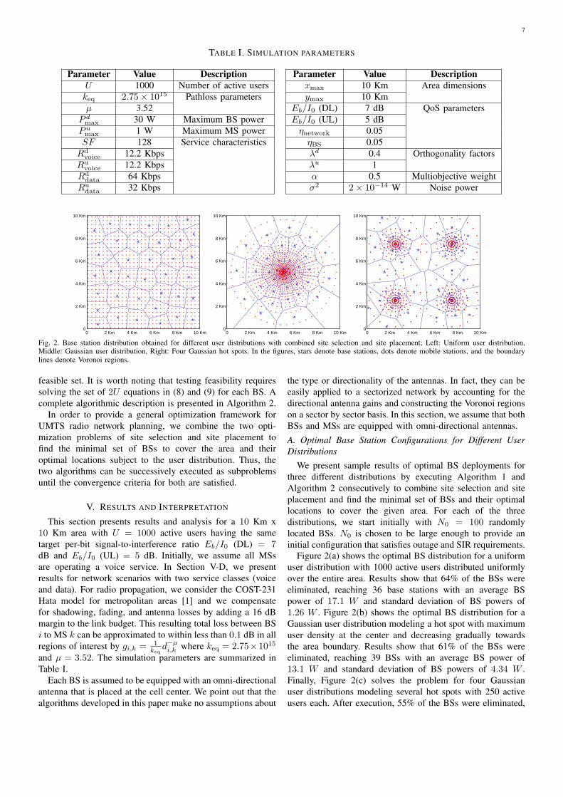
Fig. 2. Base station distribution obtained for different user distributions with combined site selection and site placement; Left: Uniform user distribution,Middle: Gaussian user distribution, Right: Four Gaussian hot spots. In the figures, stars denote base stations, dots denote mobile stations, and the boundarylines denote Voronoi regions.

feasible set. It is worth noting that testing feasibility requiressolving the set of 2U equations in (8) and (9) for each BS. Acomplete algorithmic description is presented in Algorithm 2.

In order to provide a general optimization framework forUMTS radio network planning, we combine the two opti-mization problems of site selection and site placement tofind the minimal set of BSs to cover the area and theiroptimal locations subject to the user distribution. Thus, thetwo algorithms can be successively executed as subproblemsuntil the convergence criteria for both are satisfied.

V. RESULTS AND INTERPRETATION

This section presents results and analysis for a 10 Km x10 Km area with U = 1000 active users having the sametarget per-bit signal-to-interference ratio Eb/I0 (DL) = 7dB and Eb/I0 (UL) = 5 dB. Initially, we assume all MSsare operating a voice service. In Section V-D, we presentresults for network scenarios with two service classes (voiceand data). For radio propagation, we consider the COST-231Hata model for metropolitan areas [1] and we compensatefor shadowing, fading, and antenna losses by adding a 16 dBmargin to the link budget. This resulting total loss between BSi to MS k can be approximated to within less than 0.1 dB in allregions of interest by gi,k = 1

keqd−µi,k where keq = 2.75×1015

and µ = 3.52. The simulation parameters are summarized inTable I.

Each BS is assumed to be equipped with an omni-directionalantenna that is placed at the cell center. We point out that thealgorithms developed in this paper make no assumptions about

the type or directionality of the antennas. In fact, they can beeasily applied to a sectorized network by accounting for thedirectional antenna gains and constructing the Voronoi regionson a sector by sector basis. In this section, we assume that bothBSs and MSs are equipped with omni-directional antennas.A. Optimal Base Station Configurations for Different UserDistributions

We present sample results of optimal BS deployments forthree different distributions by executing Algorithm 1 andAlgorithm 2 consecutively to combine site selection and siteplacement and find the minimal set of BSs and their optimallocations to cover the given area. For each of the threedistributions, we start initially with N0 = 100 randomlylocated BSs. N0 is chosen to be large enough to provide aninitial configuration that satisfies outage and SIR requirements.

Figure 2(a) shows the optimal BS distribution for a uniformuser distribution with 1000 active users distributed uniformlyover the entire area. Results show that 64% of the BSs wereeliminated, reaching 36 base stations with an average BSpower of 17.1 W and standard deviation of BS powers of1.26 W . Figure 2(b) shows the optimal BS distribution for aGaussian user distribution modeling a hot spot with maximumuser density at the center and decreasing gradually towardsthe area boundary. Results show that 61% of the BSs wereeliminated, reaching 39 BSs with an average BS power of13.1 W and standard deviation of BS powers of 4.34 W .Finally, Figure 2(c) solves the problem for four Gaussianuser distributions modeling several hot spots with 250 activeusers each. After execution, 55% of the BSs were eliminated,

8

reaching 45 BSs with an average BS power of 11.6 W and astandard deviation of 3.39 W .

B. Analysis of Site Selection and Site Placement Algorithms

Figure 3 shows the average BS power during executionof the site selection algorithm for different inner objectiveswith a Gaussian user distribution and N0 = 100 BSs. Theouter objective is to minimize the number of BSs and withthe inner objective to either (1) minimize sum of BS powersor (2) eliminate first feasible BS. In the first approach, weeliminate the one that among other BSs minimizes total powerexpenditure as described in Section III-B. This essentiallyprovides a solution that minimizes average BS power. Inthe second approach, while executing the outer problem, wegreedily eliminate the first possible BS that does not causesignificant coverage loss as defined in (13)-(16). Obviously,the average BS power will increase under both approachessince BSs are getting eliminated, however, what the algorithmoptimizes is the rate of this increase. The most noticeabledifference is that 46 BSs were eliminated with the first innerobjective while only 20 BSs were eliminated with the greedyapproach. This demonstrates the impact of the eliminationcriteria on the rate of increase of the average BS power, andthus on the effectiveness of the selection algorithm.

0 5 10 15 20 25 30 35 40 452

3

4

5

6

7

8

Number of Eliminated Base Stations N0 −N

Ave

rage

BS

Pow

er1 N

∑U k=

1P

d k,b

(k)

Inner objective: Min sum of BS powersInner objective: First feasible BS

26 more base stations eliminated

Fig. 3. Improvement in the radio network plan due to the utilization of thenested objective in the site selection algorithm.

Another important observation is that minimizing the totalpower expenditure implicitly reduces the variance of BSpowers by converging to a solution that distributes the powerload nearly equally among BSs. Figure 4(a) shows the averageBS power during the execution of the site placement algorithmwith a Gaussian user distribution for two different objectivefunctions: (1) Minimize sum of BS powers, (2) Minimizevariance of BS powers. The two objectives converge almost tothe same average BS power suggesting that opting for equalBS powers does not greedily increase these powers to achieveequality, instead, the network configuration converges to a lowpower solution due to the SIR-based power control mechanismutilized in the problem. Figure 4(b) shows a similar scenariofor the site selection algorithm with N0 = 100 initial BSs.

We present a case study to analyze the effect of the initialnumber of base stations N0 on the solution. We consider auniform user distribution with U = 200 active users. Initially,the BSs are located randomly in the network. We execute

the site placement and site selection algorithms successivelyas subproblems until the convergence criteria for both aresatisfied. This corresponds to the case where eliminating anyBS causes the quality of service constraints to be violated andmoving any BS a distance larger than the mesh size thresholdwill only increase the objective. The resulting network plansize, average transmit power per BS, global iterations, and totalcomputation time are shown in Table II for N0 = 100, 60, 40,and 25. Global iterations represents the number of times thesite selection and site placement algorithms are sequentiallyexecuted until the aforementioned convergence criteria aresatisfied.

TABLE II. EFFECT OF N0 ON THE SOLUTION QUALITY

N0 Network Average BS Global Total comp.size (BSs) Tx power (W) iterations time (sec)

100 17 21.32 5 471.1560 18 16.29 3 203.6340 20 12.44 2 172.3025 23 9.51 1 99.80

The network plan size is the main metric for judging thequality of the solution. It can be observed from the resultsthat larger N0 generates a finer solution since there are moredegrees of freedom in selecting the candidate sites, thus, morecritical site locations can be picked during the optimization.Consequently, the solution is only slightly dependent on theinitial locations of BSs. On the other hand, a smaller N0 ismore likely to provide a locally optimal solution. Obviously,a solution with lower number of BSs would require higheraverage transmit power per BS that satisfies the BS maximumtransmit power constraint. Additionally, a larger N0 requiresmore global iterations and more computation time.

C. Radio Network Planning Tradeoffs

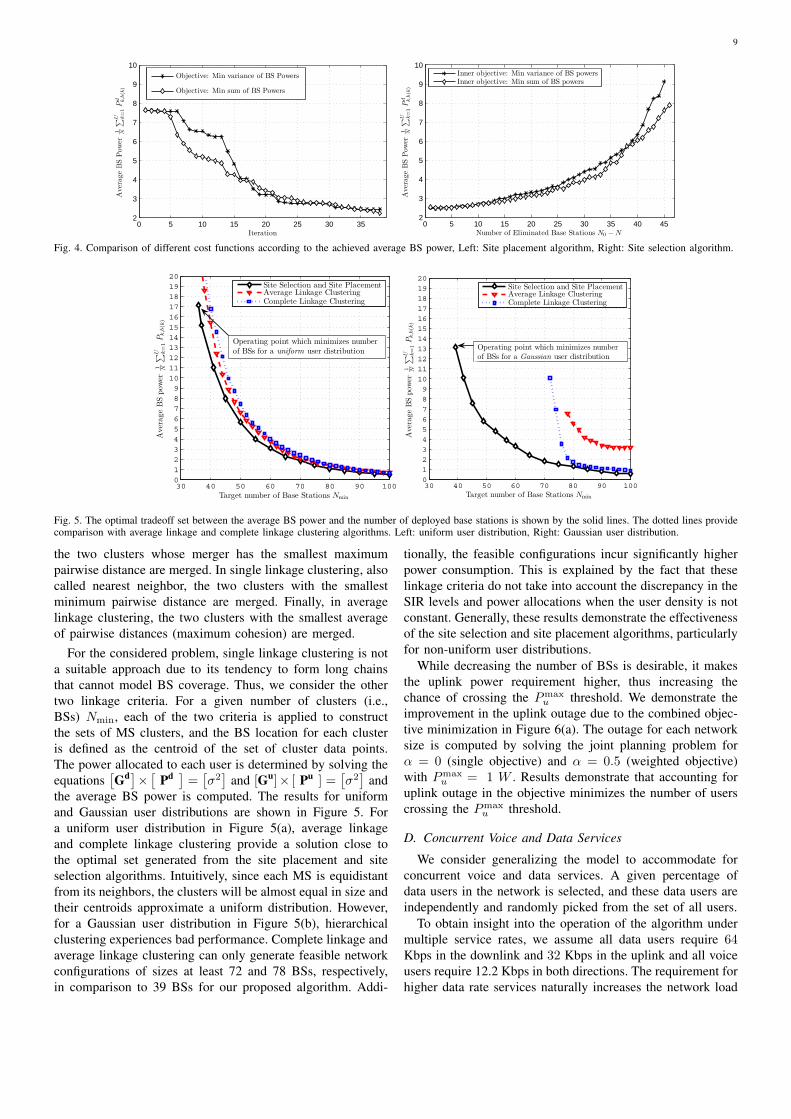
Combining site selection and site placement allows the op-erator to find the minimal set of BSs to cover the network areaand their optimal locations. Since eliminating BSs increasesthe average power per BS, we can think of the problemdifferently by trading-off the number of BSs and the averageBS power. The solid lines of Figure 5 show the set of pareto-optimal points that provide this tradeoff between the minimumaverage BS power achieved and the number of deployed BSs.The pareto sets are generated for a uniform user distribution inFigure 5(a) and for a Gaussian user distribution in Figure 5(b).Generating these sets is performed by running the site selectionalgorithm to select a target number of BSs Nmin from aset of 100 initial BSs. The site placement algorithm is thenexecuted for these Nmin BSs to find their optimal locationsthat minimize total power expenditure.

In an attempt to validate our algorithm and demonstrate itseffectiveness, we compare these results with off-the-shelf hi-erarchical clustering algorithms. Hierarchical clustering treatseach data point initially as a single cluster, and then succes-sively merges clusters according to the linkage criteria. Inthis problem, the data points are the MSs and each clustercorresponds to a single BS serving a set of MSs. In completelinkage hierarchical clustering, also called furthest neighbor,

9

0 5 10 15 20 25 30 352

3

4

5

6

7

8

9

10

Iteration

Ave

rage

BS

Pow

er1 N

∑U k=

1P

d k,b

(k)

Objective: Min variance of BS Powers

Objective: Min sum of BS Powers

0 5 10 15 20 25 30 35 40 452

3

4

5

6

7

8

9

10

Number of Eliminated Base Stations N0 −N

Ave

rage

BS

Pow

er1 N

∑U k=

1P

d k,b

(k)

Inner objective: Min variance of BS powersInner objective: Min sum of BS powers

Fig. 4. Comparison of different cost functions according to the achieved average BS power, Left: Site placement algorithm, Right: Site selection algorithm.

30 40 50 60 70 80 90 10001234567891011121314151617181920

Target number of Base Stations Nmin

Ave

rage

BS

power

1 N

∑U k=

1P

k,b

(k)

Site Selection and Site PlacementAverage Linkage ClusteringComplete Linkage Clustering

Operating point which minimizes numberof BSs for a uniform user distribution

30 40 50 60 70 80 90 1000123456789

1011121314151617181920

Target number of Base Stations Nmin

Ave

rage

BS

power

1 N

∑U k=

1P

k,b

(k)

Site Selection and Site PlacementAverage Linkage ClusteringComplete Linkage Clustering

Operating point which minimizes numberof BSs for a Gaussian user distribution

Fig. 5. The optimal tradeoff set between the average BS power and the number of deployed base stations is shown by the solid lines. The dotted lines providecomparison with average linkage and complete linkage clustering algorithms. Left: uniform user distribution, Right: Gaussian user distribution.

the two clusters whose merger has the smallest maximumpairwise distance are merged. In single linkage clustering, alsocalled nearest neighbor, the two clusters with the smallestminimum pairwise distance are merged. Finally, in averagelinkage clustering, the two clusters with the smallest averageof pairwise distances (maximum cohesion) are merged.

For the considered problem, single linkage clustering is nota suitable approach due to its tendency to form long chainsthat cannot model BS coverage. Thus, we consider the othertwo linkage criteria. For a given number of clusters (i.e.,BSs) Nmin, each of the two criteria is applied to constructthe sets of MS clusters, and the BS location for each clusteris defined as the centroid of the set of cluster data points.The power allocated to each user is determined by solving theequations

[Gd]×

[Pd ] =

[σ2]

and [Gu]× [ Pu ] =[σ2]

andthe average BS power is computed. The results for uniformand Gaussian user distributions are shown in Figure 5. Fora uniform user distribution in Figure 5(a), average linkageand complete linkage clustering provide a solution close tothe optimal set generated from the site placement and siteselection algorithms. Intuitively, since each MS is equidistantfrom its neighbors, the clusters will be almost equal in size andtheir centroids approximate a uniform distribution. However,for a Gaussian user distribution in Figure 5(b), hierarchicalclustering experiences bad performance. Complete linkage andaverage linkage clustering can only generate feasible networkconfigurations of sizes at least 72 and 78 BSs, respectively,in comparison to 39 BSs for our proposed algorithm. Addi-

tionally, the feasible configurations incur significantly higherpower consumption. This is explained by the fact that theselinkage criteria do not take into account the discrepancy in theSIR levels and power allocations when the user density is notconstant. Generally, these results demonstrate the effectivenessof the site selection and site placement algorithms, particularlyfor non-uniform user distributions.

While decreasing the number of BSs is desirable, it makesthe uplink power requirement higher, thus increasing thechance of crossing the Pmax

u threshold. We demonstrate theimprovement in the uplink outage due to the combined objec-tive minimization in Figure 6(a). The outage for each networksize is computed by solving the joint planning problem forα = 0 (single objective) and α = 0.5 (weighted objective)with Pmax

u = 1 W . Results demonstrate that accounting foruplink outage in the objective minimizes the number of userscrossing the Pmax

u threshold.

D. Concurrent Voice and Data Services

We consider generalizing the model to accommodate forconcurrent voice and data services. A given percentage ofdata users in the network is selected, and these data users areindependently and randomly picked from the set of all users.

To obtain insight into the operation of the algorithm undermultiple service rates, we assume all data users require 64Kbps in the downlink and 32 Kbps in the uplink and all voiceusers require 12.2 Kbps in both directions. The requirement forhigher data rate services naturally increases the network load

10

30 40 50 60 70 80 90 1000

1

2

3

4

5

6

7

8

9

10

Number of Base Stations N

Per

cent

age

ofO

utag

eU

sers

With Uplink Outage Minimization (α=0.5)Without Uplink Outage Minimization (α=0)

5 10 20 30 40 50 60 70 80 90 950

10

20

30

40

50

60

Percentage of data users in the network

Per

cent

age

ofou

tage

for

voic

e/da

taus

ers

Voice users - 36 BS plan

Data users - 36 BS plan

Voice users - 50 BS plan

Data users - 50 BS plan

Data users

Voice users

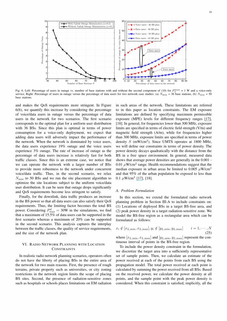
Fig. 6. Left: Percentage of users in outage vs. number of base stations with and without the second component of (10) for Pmaxu = 1 W and a voice-only

service, Right: Percentage of users in outage versus the percentage of data users for two network case studies: (a) Nmin = 36 base stations, (b) Nmin = 50base stations.

and makes the QoS requirements more stringent. In Figure6(b), we quantify this increase by considering the percentageof voice/data users in outage versus the percentage of datausers in the network for two scenarios. The first scenariocorresponds to the optimal plan for a uniform user distributionwith 36 BSs. Since this plan is optimal in terms of powerconsumption for a voice-only deployment, we expect thatadding data users will adversely impact the performance ofthe network. When the network is dominated by voice users,the data users experience 19% outage and the voice usersexperience 3% outage. The rate of increase of outage as thepercentage of data users increase is relatively fast for bothtraffic classes. Since this is an extreme case, we notice thatwe can operate the network with a larger number of BSsto provide more robustness to the network under concurrentvoice/data traffic. Thus, in the second scenario, we relaxNmin to 50 BSs and we run the site placement algorithm tooptimize the site locations subject to the uniform voice/datauser distribution. It can be seen that outage drops significantlyand QoS requirements become less stringent to satisfy.

Finally, for the downlink, data traffic produces an increasein the BS power so that all data users can also satisfy their QoSrequirements. Thus, the limiting factor becomes the total BSpower. Considering P dmax = 30W in the simulations, we findthat a maximum of 15.5% of data users can be supported in thefirst scenario whereas a maximum of 20% can be supportedin the second scenario. This analysis captures the interplaybetween the traffic classes, the quality of service requirements,and the size of the network plan.

VI. RADIO NETWORK PLANNING WITH LOCATIONCONSTRAINTS

In realistic radio network planning scenarios, operators oftendo not have the liberty of placing BSs in the entire area ofthe network for two main reasons. First, the presence of roughterrains, private property such as universities, or city zoningrestrictions in the network region limits the scope of placingBS sites. Second, the presence of radiation-sensitive zonessuch as hospitals or schools places limitations on EM radiation

in such areas of the network. These limitations are referredto in this paper as location constraints. The EM exposurelimitations are defined by specifying maximum permissibleexposure (MPE) levels for different frequency ranges [17],[18]. In general, for frequencies lower than 300 MHz, exposurelimits are specified in terms of electric field strength (V/m) andmagnetic field strength (A/m), while for frequencies higherthan 300 MHz, exposure limits are specified in terms of powerdensity S (mW/cm2). Since UMTS operates at 1800 MHz,we will define our constraints in terms of power density. Thepower density decays quadratically with the distance from theBS in a free space environment. In general, measured datashows that average power densities are generally in the 0.001 -0.01 µW/cm2 range. Health recommendations suggest that themedian exposure in urban areas be limited to 0.005 µW/cm2

and that 95% of the urban population be exposed to less than0.1 µW/cm2 [17], [18].

A. Problem Formulation

In this section, we extend the formulated radio networkplanning problem in Section III-A to include constraints on:(1) Locations of deployed BSs in a target BS-free area, and(2) peak power density in a target radiation-sensitive zone. Wemodel the BS-free region as a rectangular area which can beformulated as follows:

xi /∈ [xL,min, xL,max], yi /∈ [yL,min, yL,max] i = 1, · · · , N(25)

where [xL,min, xL,max] and [yL,min, yL,max] represent the con-tinuous interval of points in the BS-free region.

To include the power density constraint in the formulation,we discretize the target area into a sufficiently representativeset of sample points. Then, we calculate an estimate of thepower received at each of the points from each BS using thepropagation model. The total power received at each point iscalculated by summing the power received from all BSs. Basedon the received power, we calculate the power density at allpoints, and the sample point with the peak power density isconsidered. When this constraint is satisfied, implicitly, all the

11

area will satisfy the constraint. The constraint is formulatedas follows:

maxsj

(N∑

i=1

((∑

k∈Ci

P dk,i

)· 1keq

(di,sj

)−µ)· 4πf2

c2G

)≤ Sth

j = 1, · · · , p (26)

where sj is the sample point j in the target area with j between1 and p and p is the number of sample points taken in thetarget area, f is the carrier frequency (assumed 1800 MHz forUMTS), c is the speed of light, G is the gain of the transmittingantenna of the BS in the direction of the radiation, Sth isthe recommended power density threshold, and keq and µ areparameters depending on the pathloss model.

The site placement problem with location constraints canthen be formulated as follows:

minx,y

U∑

k=1

P dk,b(k) + α

U∑

k=1

(Puk − Pumax)+ (27)

subject to (25), (26),(11), (12), (13), (14), (15), (16), (17), (18), (19), (20)

Similarly, the site selection problem with location con-straints can also be formulated as an extension to the initialsite selection problem as follows:

minc

N0∑

i=1

ci (28)

s.t.

minU∑

k=1

cb(k) · P dk,b(k) + α

U∑

k=1

cb(k)(Puk − Pumax)+ (29)

subject to (25), (26),(11), (12), (13), (14), (15), (16), (17), (18), (19), (20)i = 1, · · · , N0; k = 1, · · · , U (30)

In both problems, (25) and (26) represent the locationconstraints. Note that the constraints (11)-(20) from the initialproblems are also included in the formulation. The next sectiondescribes how to extend the algorithms developed in SectionIV to solve the radio network planning problem with locationconstraints.

B. Algorithm for the Radio Network Planning Problem withLocation Constraints

The location constraints as defined in (25) and (26) arenonlinear inequality constraints. To satisfy such constraints,we modify the algorithms presented in Section IV. A robustextension of pattern search algorithms for general constraintsis the globally convergent ALPS which solves general prob-lems.

Initially, the problem is modified to convert the inequalityconstraints into equality constraints by introducing nonneg-ative slack variables. Next, we attempt to find Lagrangemultiplier estimates for the equality constraints updated at eachiteration, such that the estimates do not involve information

about derivatives of the objective or constraints to be consistentwith the derivative-free nature of pattern search algorithms.

The algorithm begins with an initial value for the penaltyparameter and the Lagrange multiplier estimates. The mathe-matical significance of these parameters is explained in [24]. Asubproblem is formulated by combining the objective functionand the nonlinear constraint function using the Lagrangianmultiplier estimates and the penalty parameters. A sequenceof such optimization problems are approximately minimizedusing a pattern search algorithm such that the linear constraintsand bounds are satisfied. When the subproblem is minimizedto a required accuracy and satisfies feasibility conditions, theLagrangian multiplier estimates are updated. Otherwise, thepenalty parameter is increased. These steps are repeated untilthe stopping criteria are met. A frequently used Lagrangianupdate is the first order Hestenes-Powell multiplier update forthe augmented Lagrangian which assumes no knowledge ofderivative information [24].

Convergence analysis for the ALPS algorithm can be foundin [25], [24]. It is shown that despite the absence of anyexplicit estimation of any derivatives, the pattern searchaugmented Lagrangian approach exhibits first-order globalconvergence properties. Although the subproblems are solvedapproximately, and the stopping criterion of the subproblem isbased on the magnitude of a measure of first-order stationarity,the algorithm converges to Karush-Kuhn-Tucker points of theoriginal problem. This important result establishes that pro-ceeding by successive, inexact minimization of the augmentedLagrangian via pattern search methods ensures convergence[25], [24].

Since our nonlinear constraints are written in terms ofthe powers allocated to users, we need to solve the set ofequations

[Gd] ×

[Pd ] =

[σ2]

and [Gu] × [ Pu ] =[σ2]

for a given x (BS locations) to find the uplink and downlinkpowers, compute the value of the constraints, and solve theinner augmented Lagrangian subproblem. Algorithm 1 andAlgorithm 2 can be extended to ALPS by constructing thesubproblem at each iteration, minimizing this subproblem overthe mesh points instead of minimizing the objective fm(x),updating the Lagrange multipliers at each successful iterationusing the Hestenes-Powell multiplier update, and adjusting thepenalty factor based on the success or failure of the polls.

C. Analysis of Network Topologies with Location Constraints

In order to demonstrate the performance of the proposedalgorithm to solve the network planning problem with loca-tion constraints, we run the modified site selection and siteplacement algorithms presented in Section VI-B consecutivelyto select the smallest set of BSs that cover the network areasuch that the location constraints and the QoS constraints aresatisfied. To ensure limited EM radiation within the area ofinterest, we set the target peak power density in the area toSth=0.005 µW/cm2. For computing the power density, weassume G = 1 and f =1800 MHz. All other parameters are thesame as those listed in Table I. Figure 7 shows a particular casewith a uniform user distribution where the radiation-limitedarea is a square with 4 Km x 4 Km dimensions defined as

12

0 2 Km 4 Km 6 Km 8 Km 10 Km0

2 Km

4 Km

6 Km

8 Km

10 Km Power Density (log10(W/m2))

−11.5

−11

−10.5

−10

−9.5

−9

−8.5

−8

−7.5

−7

3 Km 4 Km 5 Km 6 Km 7 Km3 Km

4 Km

5 Km

6 Km

7 Km Power Density (log10(W/m2))

−11

−10.5

−10

−9.5

−9

Fig. 7. A uniform user distribution with location constraints in a 4 Km x 4 Km area; Left: total area, Right: radiation-limited area. The color scale denotesthe base-10 logarithm of the power density, e.g., -9 corresponds to S = 10−9 W/m2.

0 500 1000 1500 2000 2500 3000 3500 400017

18

19

20

21

22

23

24

25

26

Radiation-limited area dimensions (m)

Ave

rage

BS

power

1 N

∑U k=

1P

d k,b

(k)

Without Maximum Power Constraint

With Maximum Power Constraint

0 500 1000 1500 2000 2500 3000

14

16

18

20

22

24

26

Radiation-limited area dimensions (m)

Ave

rage

BS

power

1 N

∑U k=

1P

d k,b

(k)

Without Maximum Power Constraint

With Maximum Power Constraint

Fig. 8. Pareto-Optimal set that provides the tradeoff between average BS power and the dimensions of the radiation-limited area; Left: Uniform user distribution,Right: Gaussian user distribution.

follows: 3000 m ≤ x ≤ 7000 m, 3000 m ≤ y ≤ 7000 m.The figure shows that the peak power density in the area isS = 10−8.5W/m2 = 3.16×10−9W/m2 = 0.003 µW/m2

which is below the predefined threshold Sth. Additionally, itis clear that all BSs satisfy as well the location constraints.

Finally, we generate pareto-optimal sets to show the tradeoffbetween the dimensions of the radiation-limited area and theachieved average BS power in the whole network. The largerthe area, the more power is required to achieve coverage tousers in the area and satisfy their SIR requirements, whicheventually increases the average BS power. Because the mod-ified site selection and site placement algorithms are bothexecuted, the case with zero area dimensions is equivalent tothe point of operation on Figures 5(a) and 5(b) with the lowestnumber of BSs and highest average BS power. Figure 8 showsthe achievable average BS powers for sample uniform andGaussian user distributions. For the uniform case, the squareis characterized by its center at [5000, 5000]. For the Gaussiancase, the square is characterized by: 1) yL,max touches theupper boundary, 2) The centroids of xL,min and xL,max lie atx = 5000.

We can see that with a Gaussian user distribution the slopeof increase is faster, which is why we cannot reach the 4 Kmdimension as in the uniform case; otherwise, the increase in BS

powers would prohibit satisfying the SIR requirements. Thealgorithm is executed with and without a maximum BS powerconstraint. The maximum BS power constraint correspondsto (19) with P dmax = 30 W. Such constraint will furtherlimit the area dimensions, because even though the averageBS power is lower than the constraint, some BSs (specificallythose covering the radiation-limited area) will require a veryhigh power to achieve the required SIR for most users. Thearea dimensions in the unconstrained power case are limitedby interference whereby further increasing BS power forsome user makes the SIR requirement for other users non-achievable. On the other hand, the area dimensions in theconstrained power case are limited by the physical maximumBS power limit which turns out to be a more stringentlimitation. Obviously, these two sets represent specific casestudies for the area locations we considered. In fact, the slopeof the curve depends greatly on the location of the square,especially in the Gaussian distribution case.

Another important observation is that placing a maximumBS power constraint decreases the average BS power for somefixed area dimensions. This is explained by the fact that whenBSs are not allowed to exceed a certain peak transmit power,the site selection algorithm will be forced to select a largernumber of BSs to cover the entire network, specifically to

13

cover users inside the constrained area. Looking back at Figure5, we recall that the average BS power decreases as the numberof BSs increases for a given user distribution which explainsthe gap between the two curves in each of Figure 8(a) andFigure 8(b).

VII. CONCLUSION

We presented optimization-based formulations for the prob-lems of joint uplink/downlink site placement and site selectionin cellular networks. The formulations use an SIR-based powercontrol mechanism with outage conditions to provide qualityguarantees. We proposed algorithms to solve the continuouscomponent of the problem using derivative-free optimizationtechniques with general constraints. We also developed anoptimization algorithm for solving the integer componentof the problem based on a nested approach with an outerproblem that minimizes the number of base stations and aninner problem that minimizes a cost function of the networkdeployment. Case studies were presented and analyzed foruniform and non-uniform user distributions and pareto-optimalsets were generated to tradeoff network configuration param-eters. Finally, the formulation and solution were extendedto provide a framework for solving general radio networkplanning problems with location constraints.

REFERENCES

[1] Blaustein Matha, Radio propagation in cellular networks. Artech House,Boston-London, November 1999.

[2] J. Laiho, A. Wacker, and T. Novosad, Radio network planning andoptimisation for UMTS. John Wiley & Sons, 2006.

[3] A. Mishra, Fundamentals of cellular network planning and optimisation:2G / 2.5G / 3G... Evolution to 4G. Wiley-Interscience, 2004.

[4] E. Amaldi, A. Capone, and F. Malucelli, “Improved models and algo-rithms for UMTS radio planning,” In Proceedings of IEEE VehicularTechnology Conference, October 2001.

[5] E. Amaldi, A. Capone, and F. Malucelli, “Optimizing base station sitingin UMTS networks,” In Proceedings of IEEE Vehicular TechnologyConference, October 2001.

[6] Amaldi, E. and Capone, A. and Malucelli, F. and Signori, F., “Opti-mization models and algorithms for downlink UMTS radio planning,”In Proceedings of IEEE Wireless Communications and NetworkingConference (WCNC), March 2003.

[7] E. Amaldi, A. Capone, and Malucelli, “Planning UMTS base stationlocation: Optimization models with power control and algorithms,” IEEETransactions on Wireless Communications, vol. 2, no. 5, pp. 939–952,September 2003.

[8] A. Eisenblatter, A. Fugenschuh, T. Koch, A. M. C. A. Koster, A. Martin,T. Pfender, O. Wegel, and R. Wessaly, “Modelling feasible networkconfigurations for UMTS,” Technical Report ZR-02-16, Konrad-Zuse-Zentrum fur Informationstechnik Berlin (ZIB), Germany, March 2002.

[9] E. Amaldi, A. Capone, and F. Malucelli, “Radio planning and coverageoptimization of 3G cellular networks,” Journal of Wireless Networks,vol. 14, no. 4, pp. 435–447, August 2008.

[10] A. Eisenblatter, A. Fugenschuh, H. Geerdes, D. Junglas, T. Koch, andA. Martin, “Integer programming methods for UMTS radio networkplanning,” In Proceedings of WiOpt, March 2004.

[11] A. Eisenblatter and H. Geerd, “Wireless network design: solution-oriented modeling and mathematical optimization,” IEEE Wireless Com-munications Magazine, vol. 13, no. 6, pp. 8–14, December 2006.

[12] P. Calegari, F. Guidec, P. Kuonen, B. Chamaret, S. Ubeda, S. Josselin,D. Wagner, and M. Pizarosso, “Radio network planning with combi-natorial optimization algorithms,” In Proceedings of the ACTS MobileTelecommunications Summit, September 1996.

[13] P. Calegari, F. Guidec, P. Kuonen, and D. Wagner, “Genetic approachto radio network optimization for mobile systems,” In Proceedings ofIEEE 47th Vehicular Technology Conference, May 1997.

[14] J. K. J. Kalvanes and E. Olinick, “Base station location and serviceassignments in WCDMA networks,” INFORMS Journal on Computing,vol. 18, no. 3, pp. 366–376, March 2006.

[15] J. Osepchuk and R. Petersen, “Safety standards for exposure to RFelectromagnetic fields,” IEEE Microwave Magazine, vol. 2, no. 2,pp. 57–69, June 2001.

[16] L. Catarinucci, P. Palazzari, and L. Tarricone, “Human exposure tothe near field of radiobase antennas-a full-wave solution using parallelFDTD,” IEEE Transactions on Microwave Theory, vol. 51, no. 3,pp. 935–940, March 2003.

[17] IEEE Standard C95. 1, “IEEE standard for safety levels with respect tohuman exposure to radio frequency electromagnetic fields, 3 kHz to 300GHz,” 1999.

[18] International Commission on Non-Ionizing Radiation Protection (IC-NIRP), “Guidelines for limiting exposure to time-varying electric, mag-netic, and electromagnetic fields,” Health Physics, vol. 74, pp. 494–522,April 1998.

[19] B. Di Chiara, M. Nonato, M. Strappini, L. Tarricone, and M. Zappatore,“Hybrid metaheuristic methods in parallel environments for 3G networkplanning,” In Proceedings of EMC Europe Workshop, September 2005.

[20] T. Crainic, B. Di Chiara, M. Nonato, and L. Tarricone, “Tackling elec-trosmog in completely configured 3G networks by parallel cooperativemeta-heuristics,” IEEE Wireless Communications Magazine, vol. 13,no. 6, pp. 34–41, December 2006.

[21] H. Holma and A. Toskala, WCDMA for UMTS. England: Wiley, 2000.[22] E. Dolan, R. Lewis, and V. Torczon, “On the local convergence of pattern

search,” SIAM Journal on Optimization, vol. 14, no. 2, pp. 567–583,February 2003.

[23] R. Lewis, V. Torczon, and M. Trosset, “Why pattern search works,”Optima, vol. 59, pp. 1–7, December 1998.

[24] R. Lewis and V. Torczon, “A globally convergent augmented Lagrangianpattern search algorithm for optimization with general constraints andsimple bounds,” SIAM Journal on Optimization, vol. 12, no. 4, pp. 1075–1089, July 2002.

[25] A. Conn, N. Gould, and P. Toint, “Globally convergent augmentedlagrangian algorithm for optimization with general constraints andsimple bounds,” SIAM Journal on Numerical Analysis, vol. 28, no. 2,pp. 545 – 572, April 1991.