Optimal management of a size-distributed forest with respect to timber

and carbon sequestration

Renan Ulrich Goetz a

Natali Hritonenko b

Angels Xabadia a

Yuri Yatsenko c

Preliminary version: please do not cite

a University of Girona, Campus Montilivi, s/n, 17071 Girona, Spain; renan.goetz@udg.es (corresponding

author), Phone: +34 972-418719, Fax: +34 972-418032

b Prairie View A&M University, Box 519, Prairie View, Texas, USA; nahritonenko@pvamu.edu

c Houston Baptist University, 7502 Fondren Road, Houston, Texas, USA; yyatsenko@hbu.edu

Abstract

The Kyoto protocol and subsequent agreements allow Annex I countries to deduct carbon sequestered by land use,

land-use change and forestry from their national carbon emissions. From this point of view the determination of the

optimal logging regime in the presence of timber and carbon sequestration benefits is of utmost importance. Thornley

and Cannell (2000) demonstrated that the objectives of maximizing timber and carbon sequestration are not

complementary. They show that management regimes that maintain a continuous canopy cover and mimic, to some

extent, regular natural forest disturbance are likely to achieve the best combination of wood yield and carbon storage

expressed in biophysical units. Based on this finding, this paper determines the optimal selective cutting regime taking

into account the underlying biophysical and economic processes. By varying the price for sequestered carbon, this

paper establishes the corresponding optimal management regime with respect to the number of young trees to be

planted, the size and number of trees to be cut, and the amount of CO2 sequestered in the long run. The results show

that the net benefits of carbon storage only compensate the decrease in net benefits of timber production once the

carbon price has exceeded a certain threshold value which in turn depends on the permanence rate of the sequestered

carbon in the wood products.

Key words: Kyoto protocol, forest management, selective logging, carbon sequestration, dynamic

optimization.

1

Optimal management of a size-distributed forest with respect to timber

and carbon sequestration

1. Introduction

Many signatory countries of the Kyoto Protocol are currently analyzing the policy options available to them

to comply with their country-specific CO2 protocol targets. In order to make rational choices between the

various options, the countries need to have precise information about the costs of each measure. According

to Articles 3.3 and 3.4 of the protocol, Annex 1 countries can deduct carbon sequestrated by land use, land-

use change and forestry from their national carbon emissions. The protocol and later agreements

(Marrakech and Bonn, 2001) explicitly mention changes in forest management, afforestation and

reforestation within certain limits either in the Annex I country itself or in Non-Annex I countries in the

form of clean development mechanisms.

The economic literature determines the cost of forest carbon sequestration in two different ways. One strand

of the literature estimates the cost of forest carbon sequestration at the regional or national level (Sohngen

and Mendelsohn; 2003, van’t Veld and Plantinga 2005; Lubowski, Plantinga and Stavins, 2006). These

studies focus on the cost of land-use changes given a predetermined tree harvesting regime. Hence, they do

not determine an optimal forest management that maximizes timber and carbon sequestration benefits.

Precisely this fact was considered in a second strand of the literature (van Kooten, Binkley and Delcourt,

1995; Creedy and Wurzbacher, 2001; Huang and Konrad, 2001; Tassone, Wessler and Nesci, 2004). These

studies determined the optimal logging regime in the presence of timber and carbon sequestration benefits.

However, the optimal logging regime was determined based either on purely biological indicators, such as

the mean annual increment of the biomass, or on the Faustman Formula, and did not take into account the

interdependencies between the formulated objectives. Forest management with respect to the maximization

of the net benefits of timber calls for growing a reduced number of high value trees while the maximization

of the net benefits of sequestered carbon requires maximizing the standing biomass. Consequently, the

compatibility of these two maximization objectives is limited (van Kooten and Bulte, 1999; Healey, Price

and Tay, 2000). Thornley and Cannell (2000) demonstrated that there is no simple inverse relationship

between the amount of timber harvested from a forest and the amount of carbon stored. They show that

management regimes that maintain a continuous canopy cover and mimic, to some extent, regular natural

forest disturbance are likely to achieve the best combination of high wood yield and carbon storage.1 Since

1 Thornley and Cannell (2000) report that more carbon was stored in an undisturbed forest (35.2 kg C m–2) than in any regime in which wood was harvested. Plantation management gave moderate carbon storage (14.3 kg C m–2) and

2

these findings are based completely on physical units, the determination of the optimal forest management

regime that considers the net benefits from timber production and carbon sequestration remains an open

question. To achieve this objective, the correct modeling of the forest dynamics that allows for different

management regimes is crucial. In particular, it should allow for modeling disturbances that range from

management regimes without harvesting to clear cutting. At the midpoint between these two extremes we

have the selective logging regime.

1.1 Distinguishing features of this study

The existing literature about the economics of carbon sequestration does not describe the growth of

individual trees but rather the growth of the biomass of the entire forest. Hence, it assumes that the forest is

not structured, i.e., all trees have the same size, and the number of trees is not relevant for the correct

description of the biological growth process. However, as demonstrated in the literature of biological

mathematics, the growth of each tree depends on its own size and on the density of the trees within the

stand (Keyfitz, 1968). Moreover, as the density of the forest affects the biological growth of the individual

trees, the number of planted trees should be determined endogenously by the model if the young trees are

planted. If the forest reproduces naturally, the density of the forest can be regulated by thinning, i.e., by the

selective logging of younger trees. Xabadia and Goetz (2007) and Goetz, Xabadia and Calvo (2007)

determined the optimal selective logging regime for timber production of a size-structured forest without,

however, considering the net benefits from carbon sequestration.

The modeling of a size-structured forest is able to include the fact that the price of timber increases with the

size of the trees because the timber of larger trees can be used for higher-value products, such as furniture.

Consequently, the price of timber can be considered as a function of the size of the tree. This aspect is not

only important for the correct determination of the net benefits of timber production but also for the

accurate measure of the sequestered carbon. The size of the tree and the density of the stand are therefore

essential for an accurate description of the biological growth process of the trees and the carbon cycle and

for the correct modeling of economic factors.

Another important part of the carbon cycle is the carbon sequestered in the soil. The potential of forest soils

to sequester carbon is well known (Rasse et al., 2001) and, according to Brown (1998) and to a study by the

UNDP (2000), the capacity of forest soil to sequester carbon is superior to that of above-ground vegetation.

timber yield (15.6 m3 ha–1 year–1). Notably, the annual removal of 10 or 20% of woody biomass per year gave both a high timber yield (25 m3 ha–1 year–1) and high carbon storage (20 to 24 kg C m-2). The efficiency of the latter regimes could be attributed (in the model) to high light interception and net primary productivity, but less evapotranspiration and summer water stress than in the undisturbed forest, high litter input to the soil giving high soil carbon and N2 fixation, low maintenance respiration and low N leaching owing to soil mineral pool depletion.

3

Matthews (1993), for instance, reports that the change from agricultural land to forest land led, after 200

years, to an increase in soil carbon from 30 t C/ha initially to 70 t C/ha. The previous literature, with the

exceptions of some studies (Sohngen and Sedjo, 2000; Lubowski, Plantinga and Stavins, 2006; and

McCarney, Armstrong and Adamowicz, 2006), did not consider the dynamics of soil carbon. However, the

consideration of selective logging requires the dynamics of soil carbon not to be modeled as a pure

accumulation process, as was done in the previous studies, but as an accumulation and extraction process

resulting from the continuous growth and harvest of the trees.

The paper is organized as follows. The next section describes the dynamics of a forest, and presents the

economic decision problem. In Section 3 an empirical analysis is conducted to determine the optimal

selective-logging regime of a privately owned forest with respect to timber and carbon sequestration, and

the effects of carbon prices on the optimal management regime are analyzed. The conclusions are presented

in Section 4.

2. The bioeconomic model

The dynamics of the bioeconomic model reflects, on one hand, the change in the density of the size-

structured trees x(t,l) over calendar time t and size l and, on the other hand, the change in the soil carbon s(t)

over time. Before we can specify the precise mathematical presentation of these two equations we need to

introduce some notation.

The size of the tree is measured by the diameter at breast height (130 cm above the ground) and is denoted

by l. The set of the admissible values of the variable l consists of the interval [l0, lm], where l0 corresponds to

the minimum vital diameter of the tree and lm is the maximum diameter that the trees can reach. However,

as we are considering the case of a completely managed forest, no natural reproduction takes place, and all

young trees have to be planted. Therefore, the parameter l0 corresponds to the diameter of the trees when

they are planted. The flux of logged trees is denoted u(t,l), and the flux of planted young trees at time t with

diameter l0 by p(t;l0). We assume that a diameter-distributed forest can be fully characterized by the number

of trees and by the distribution of the diameter of the trees. In other words, space and the local

environmental conditions of the trees are not taken into account.

As the density function x(t,l) indicates the population density with respect to the structuring variable l at

time t, the number of trees in the forest at time t is given by

0

( ) ( , ) .ml

l

X t x t l dl= ∫ (1)

4

The term E(t,l0) presents environmental characteristics that affect the growth rate of the diameter of

individual trees. In the absence of pests these environmental characteristics are given by the local conditions

where the tree is growing, and by the neighboring trees. Since our model does not consider space, the term

E(t,l0) exclusively presents the competition between individuals, i.e., the competition between individuals

for space, light and nutrients. Environmental pressure can be expressed, for example, by the total number of

trees, or the basal area of all trees of the stand.2 Hence, a large (small) basal area of the stand signifies a

high (low) intraspecific competition of the trees. This feature of the model is supported by Álvarez et al.

(2003), who analyzed various indices to evaluate the effect of intraspecific competition on the individual

growth rate of the trees and found that the basal area is the statistic that best explains the differences in

diameter growth. Thus, the change in diameter of the tree over time is described by the function g(E(t,l0),l),

i.e.,

0( ( , ), ).dldt

g E t l l= (2)

where the basal E(t, l0) is determined based upon the functional relationship between diameter and basal

area, that is 0

20( , ) ( , )

4

ml

lE t l l x t l dl

π= ∫ .

The instantaneous mortality rate, δ(E(t,l0),l), describes the rate at which the probability of survival of an l-

sized tree in the presence of intraspecific competition E(t,l0) decreases with time. Based on the well known

McKendrick equation for age-structured populations (McKendrick, 1926) the dynamics of a diameter-

distributed forest can be described by the following partial integrodifferential equation as discussed by de

Roos (1997) or by Metz and Diekmann (1986)

00

( , ) [ ( ( , ), ) ( , )]( ( , ), ) ( , ) ( , ),

x t l g E t l l x t lE t l l x t l u t l

t lδ

∂ ∂+ = − −

∂ ∂ t∈[0, T), l∈[l0, lm] (3)

subject to the boundary conditions x(0,l) = x0(l), l∈[l0, lm], and x(t,l0) = p(t,l0), t∈[0, T). The first two terms

of equation (3) present the change of the tree density over time and diameter. The term ( () ())g x l∂ ⋅ ⋅ ∂ =

x gg xl l

∂ ∂+

∂ ∂ takes account of the interdependence between diameter and time, i.e., it presents the

temporal change in diameter multiplied by the change in tree density over diameter plus the temporal

change in diameter over diameter multiplied by the tree density.3 Thus, the forest dynamics are described by

2 The basal area is the area of the cross section of a tree measured at a height of 1.30 m above the ground. It is often used to indicate the tree density of the stand, where the sum of the basal area of all trees is normally expressed as square meters per hectare. 3 If we had chosen age as the structuring variable the function g would be constant and equal to 1 since (age) 1d dt g= = and therefore the aging of the tree by one year corresponds to one year of calendar time.

5

the flux of tree density with respect to diameter and time being equal to the terms of the right hand side of

equation (3), given by tree mortality and logging.

To consider, in addition, the net benefits of carbon sequestration in the economic model, one needs to

analyze how the carbon content of the forest ecosystem changes over time.

The change in the carbon content is given by ,dz db ds

dt dt dt= + and depends on the change in carbon

sequestered in timber and the final use of the timber, both captured by db

dt, and the change in the carbon

content in the soil ds

dt.

With respect to the dynamics of soil carbon, we denote the above-ground volume of the biomass of the

forest by dlltxltVml

l

),()(0

0βγ ∫= , where the strictly positive parameters β and γ0 have to be chosen

according to the species of the tree and the empirical data at hand. After the definition of the function V we

are now in the position to specify the dynamics of soil carbon, which are given by

( ) ( )

, ( ) ,ds t dV t

h s tdt dt

=

t∈[0, T), s(0) = s0. (4)

The function h reflects to what extent the growth or harvest of trees and the current amount of soil carbon

affect the change in the soil carbon over time.

Before stating the complete bioeconomic model we need to define two functions. The first one presents the

amount of sequestered carbon in the long run and is given by

0

0( ) ( ) ( , )ml

l

b t v l l x t l dlβγ= ∫ . The calculation of

b(t) is based upon the calculation of the above-ground biomass of the forest, lβx, weighted by the function

υ(l). Although the carbon content is more or less constant throughout the growth process of the tree, this

function reflects the fact that the value of the timber increases with the size of the tree and, therefore, also

the probability that it will be employed for the production of durable, not disposable, goods. Consequently,

we assume that the amount of carbon sequestered in the long run increases with the size of the tree, i.e.,

v’(l)>0. The function ( ( , ), ( , ))B x t l u t l presents the net benefits of timber production as a function of the

standing and the harvested trees, with Bu > 0 and Bx < 0, where a subscript of a variable with respect to a

function indicates the partial derivative of the function with respect to this variable. Finally, we denote the

price of carbon by ρ2 and the cost of planting young trees by ρ3.

The decision problem (DP) of the manager or forest owner is to find the optimal trajectories of the control

variables u(t,l) and p(t,l0). The determination of the optimal trajectories can determine, in turn, the optimal

6

trajectories of the state variables x(t,l) and s(t), and of the variables b(t), E(t,l0) and V(t). We assume that the

owner or manager of the forest maximizes the joint net benefits of timber production and carbon

sequestration denoted by J. Currently, the literature distinguishes between two principal accounting

methods for carbon. In the first one payments are based on the flux of carbon in the ecosystem within a

period of time. That is, if there is a net storage of carbon ( ) ( )

0db t ds t

dt dt

+ >

within this time period,

forest owners receive compensation. However, if the carbon released as a consequence of logging activities

is greater than the carbon sequestered within this time period, forest owners have to pay. The second

accounting method is based on “carbon equivalent units”, where forest owners are paid per period of time

according to the amount of carbon they maintain sequestered during this period. This approach is suitable if

information about the stock of carbon is available but not about the flux. As our model accounts for the

flow of carbon sequestered in the forest, we opted for the first approach. Collecting the previously

introduced elements, the decision problem takes the form of:

( , ), ( )maxu t l p t

0

2 3

0

( ) ( )( ( , ), ( , )) ( ) ( ) ( )

mlT

rt

l

db t ds tJ e B x t l u t l dl t t p t dt

dt dtρ ρ−

= + + − ∫ ∫ (DP)

under the restrictions

( , ) [ ( ( ), ) ( , )]( ( ), ) ( , ) ( , ),

x t l g E t l x t lE t l x t l u t l

t lδ

∂ ∂+ = − −

∂ ∂ t∈[0, T), l∈[l0, lm],

0

2( ) ( , )4

ml

l

E t l x t l dlπ

= ∫

( ) ( )

, ( ) ,ds t dV t

h s tdt dt

=

t∈[0, T), s(0) = s0 ,

dlltxltVml

l

),()(0

0βγ ∫= ,

,),()()(0

0 dlltxllvtbml

l

βγ ∫= v’(l) > 0,

x(0,l) = x0(l), l∈[l0, lm], x(t,l0) = p(t), t∈[0, T),

0≤ u(t,l) ≤ umax(t,l), 0 ≤ p(t) ≤ pmax(t),

where the parameter l0 has been dropped from the presentation of the functions E and p to simplify the

notation.

7

As the decision problem (DP) is based on one partial integrodifferential equation, Eq. (3), and one ordinary

integrodifferential equation, Eq. (4), previously presented necessary conditions for the maximization of the

function J cannot be applied. In a separate paper Hritonenko, Yatsenko, Goetz and Xabadia (2007) establish

the necessary extremum conditions in the form of a maximum principle for this type of decision problem

and discuss its characteristics.

The necessary conditions for a maximum yield

∂J/∂u(t,l)≤0 at u*(t,l)=0, ∂J/∂u(t,l)≥0 at u*(t,l)=umax(t,l),

∂J/∂u(t,l)=0 at 0<u*(t,l)<umax(t,l) for almost all (a.a.) t∈[0, T), l∈[l0, lm]; (5)

∂J/∂p(t)≤0 at p*(t)=0, ∂J/∂p(t)≥0 at p*(t)=pmax(t), ∂J/∂p(t)=0 at 0<p*(t)<pmax(t), a.a. t∈[0, T). (6)

( , ) [ ( ( ), ) ( , )]( ( ), ) ( , ) ( , ),

x t l g E t l x t lE t l x t l u t l

t lδ

∂ ∂+ = − −

∂ ∂ (7)

x(0,l) = x0(l), l∈[l0, lm], x(t,l0) = p(t), t∈[0, T) (8)

2( , ) ( , )( ( ), ) [ ( ( ), )] ( , ) ( ( , ), ( , )) ( ) ( , ) ( , ),

4x t

t l t lg E t l r E t l t l B x t l u t l l t F t l rF t l

t l

λ λ πδ λ γ

∂ ∂+ = + − + + −

∂ ∂ (9)

λ(T,l) = 0, l∈[l0, lm], λ(t,lm) = 0, t∈[0, T), (10)

( )2 0

0

( ) ( )( ) ( ) , ( )

T

r t

t

dV dst t e h s d d

s d d

τ

τ τ ξς ρ ξ ς τ τ

τ ξ

− − ∂ = + + ∂

∫ ∫ , (11)

where λ(t,l) and ( )tς are unknown dual variables, and

0 2 0

0

( ) ( )( , ) ( ) ( ) ( ) ,

tdV t ds

F t l l t v l t h s ddV dt d

dt

β ξγ ρ ς ξ

ξ

∂ = + + ∂

∫ , (12)

0

[ ( ( ), ) ( , )]( ) { ( ( ), ) ( , )} ( , )

ml

EE

l

g E t l x t lt E t l x t l t l dl

lγ δ λ

∂= − −

∂∫ . (13)

The variables λ(t,l) and ( )tς present the in-situ value of trees and sequestered carbon in the soil,

respectively.

Equations (5) and (6) provide for an interior solution the following necessary conditions.

( , )( ( , ), ( , ))rt

u t le B x t l u t l λ− = , (a.a.) t∈[0, T), l∈[l0, lm]; and (14)

8

3 0( ) ( , )rte t t lρ λ−− = , t∈[0,T). (15)

According to equation (14) the discounted net benefits of logging have to be equal to the in-situ value of the

trees for almost all t and l along the optimal path. Likewise, equation (15) states that the discounted cost of

planting a young tree has to be identical to the in-situ value of a young tree along the optimal trajectory.

Equation (7) describes the dynamics of the forest as discussed above. However, for the brevity of the

exposition, the discussion is not repeated here. The subsequent line presents the boundary conditions of the

state variable x., i.e., the initial diameter distribution of the trees and the inflow of newly planted trees.

Equation (9) indicates that the changes of the value of a standing tree (in situ value) over time and diameter

have to correspond to the changes of the value if the tree were cut. The change in the in-situ value over

diameter in equation (9) is a composite expression given by ( , )

( ( ), )t l

g E t ll

λ∂

∂ and reflects the physical

growth in diameter over time evaluated by the change in the in-situ value over diameter. The right-hand

side of equation (9) indicates that if we had cut trees, the earned interest of the invested money from the sale

of these trees should have been rλ and the value of the trees that had not died naturally should be δλ .

Likewise, cutting trees has diminished the maintenance cost of the remaining trees, -Bx, which would be a

positive contribution if we had cut trees. In addition, if we had cut trees, the expression 2 ( )4l tπγ would

reflect the monetary value of the improved conditions for the growth of the remaining trees due to the

decrease in intraspecific competition. The term ( , )tF t l reflects the change in benefits or costs of the carbon

flow in the biomass and the soil over time if we had cut trees. Consequently, ( , )rF t l presents the renounced

earned interest on an income for a positive carbon flow if we had cut trees. If the carbon flow is negative,

( , )rF t l presents the interest on the payment for the decrease in carbon. The transversality conditions of the

decision problem are stated in equation (10). Equation (11) provides the in-situ value of soil carbon which

is given by the price of sequestered carbon plus the discounted value of future changes in soil carbon as the

level of soil carbon increases or decreases.

As the decision problem (DP) is based on one partial integrodifferential equation, Eq. (3), and one ordinary

integrodifferential equation, Eq. (4), the first order conditions include a system of partial integrodifferential

equations. Given the complexity of the resulting equations, an analytical solution of the first order

conditions cannot be obtained, and one has to resort to numerical techniques to obtain a solution to the

forest manager’s decision problem. Nevertheless, the first order conditions allow the partial

integrodifferential equation associated with the costate variable, i.e., the in-situ value of the trees, to be

interpreted as a modified Faustmann formula.

To solve a distributed optimal control problem numerically, available techniques such as the gradient

projection method (Veliov 2003) or the method of finite elements may be appropriate choices (Calvo and

Goetz, 2001). However, all of these methods require the programming of complex algorithms that are not

9

widely known. Therefore, we propose a different method called the Escalator Boxcar Train, EBT, used by

de Roos (1988) to describe the evolution of physiologically-structured populations. He has shown that this

technique is an efficient integration technique for structured population models. In contrast to the other

available methods, the EBT can be implemented with standard computer software such as GAMS (General

Algebraic Modeling System), used for solving mathematical programming problems.

The application of the EBT allows the partial integrodifferential equations of problem (DP) to be

transformed into a set of ordinary differential equations which are subsequently approximated by difference

equations. Beside the presentation of a short introduction, Goetz, Xabadia and Calvo (2007) show how this

approach can be extended to account for optimization problems by incorporating decision variables. For the

transformation of the decision problem (DP), we first divide the range of diameter into n equal parts, and

define ( )iX t as the number of trees in the cohort i, being i = 0, 2, 3,…, n, that is, the trees whose diameter

falls within the limits li and li+1 are grouped in the cohort i. Likewise, we define ( )iL t as the average

diameter, ( )iU t as the number of cut trees within cohort i, and ( )P t as the number of planted trees in cohort

0.

However, before the decision problem can be solved, all functions have to be specified. While the

specification of the benefit and cost functions are straightforward, the growth and mortality functions have

to be estimated, based on data generated by a biophysical forest growth simulator. For this purpose we

employed the bio-physical simulation model GOTILWA (Growth Of Trees Is Limited by Water). It not

only simulates the development of the trees, it also simulates the amount of sequestered carbon in the

biomass and in the soil. The next section describes the simulation of forest growth by GOTILWA in detail,

and presents the solution to the forest manager’s decision problem, i.e., the optimal short- and long-run

trajectories of the logging and planting decisions and the evolution of the standing trees in the forest.

3. Empirical analysis

The purpose of the empirical analysis is to determine initially the selective-logging regime that maximizes

the discounted private net benefits from timber production and carbon sequestration of a stand of Pinus

sylvestris over a time horizon of 200 years. Thereafter, the analysis concentrates on the principal aspect of

the empirical study by establishing to what extent a change in the price of carbon affects the optimal

logging regime. For this end we specify the parameters and the functions in Section 3.1, and we analyze the

optimal management regime in Section 3.2.

3.1. Data and specification of functions

10

The net benefit function of the economic model, ( ( , ), ( , ))B x t l u t l , consists of the net revenue from the sale

of timber at time t, minus the costs of maintenance comprising clearing, pruning and grinding the residues.

The net revenue is given by the sum of the revenue of the timber sale minus logging costs defined as:

( )( )( ) ( )( ) ( )( ) ( ) ( )( )0

n

i i i i

i

L t vc tv L t mv L t U t mc X tρ=

− −

∑ where ( ) ( )

0

n

i

i

X t X t=

=∑ . The first term in square

brackets denotes the sum of the revenue of the timber sale minus the cutting costs of each cohort i, and the

second term, ( )( )mc X t , accounts for the maintenance costs. The parameter ( )iLρ denotes the timber price

per cubic meter of wood as a function of the diameter, ( )itv L is the total volume of a tree as a function of its

diameter, ( )imv L is the part of the total volume of the tree that is marketable, vc is variable cutting cost, and

fc is fixed cutting cost. Timber price per cubic meter was taken from a study by Palahí and Pukkala (2003),

who analyzed the optimal management of a Pinus sylvestris forest in a clear-cutting regime. They estimated

a polynomial function given by ( ) 23.24 13.63 , 86.65L Min Lρ = − + , which is an increasing and strictly

convex function, for a diameter lower than 65cm. At L = 65 the price reaches its maximum value, and for L

> 65 it is considered constant. Data about costs was provided by the consulting firm Tecnosylva, which

elaborates forest management plans throughout Spain. The logging cost comprises logging, pruning,

cleaning the underbrush, and collecting and removing residues, and it is given by 15 € per cubic meter of

logged timber. According to the data supplied by Tecnosylva, the maintenance cost function is

approximated by ( ( ))mc X t , and is given by 2( ( )) 44.33 0.0159 0.0000186mc X t X X= + + . The

planting cost is linear in the amount of planted trees and is given by C(P) = 0.73P. The thinning and

planting period, ∆t, is set equal to 10 years, which is a common practice for a Pinus sylvestris forest

(Cañellas et al., 2000).

To proceed with the empirical study, various initial diameter distributions of a forest were chosen. These

distributions were specified as a transformed beta density function ( )lθ since it is defined over a closed

interval and allows a great variety of distinct shapes of the initial diameter distributions of the trees to be

defined (Mendenhall, Wackerly and Scheaffer, 1990). The initial forest consists of a population of trees

with diameters within the interval 0 cm ≤ l ≤ 50 cm. The density function of the diameter of trees,

( ); ;lθ γ ϕ , is defined over a closed interval, and thus the integral

( )1 1

1

1

; ,l

l dlθ γ ϕ+

∫ (9)

gives the proportion of trees lying within the range [ , 1)i il l + . We defined l0 = 0 and lm = 80 as minimum and

maximum commercial diameters of the tree, respectively. For the simulation of the forest dynamics, we

concentrate on the diameter interval [0, 50], because thereafter the growth rate of the trees is close to zero.

11

This interval was divided into 10 subintervals of identical length. In this way, the diameters of the trees of

each cohort differ at most by 5 cm, and the size of the trees of each cohort can be considered as

homogeneous.

To determine the forest dynamics, the growth of a diameter-distributed stand of Pinus sylvestris without

thinning was simulated with the bio-physical simulation model GOTILWA. This model simulates growth

and mortality and explores how the life cycle of an individual tree is influenced by the climate,

characteristics of the tree itself and environmental conditions. The model is defined by 11 input files

specifying more than 90 parameters related to the site, soil composition, tree species, photosynthesis,

stomatal conductance, forest composition, canopy hydrology and climate. Based on the previously specified

initial diameter distributions, we simulated the growth of the forest for over 150 years. After that, the

growth process practically comes to a halt so the time period of 150 years is sufficient to determine the

factors affecting the growth process of the trees.

The data generated from the series of simulations allows the function ( ), ig E L , which describes the change

in diameter over time, to be estimated. The type of the function was specified as a von Bertalanffy growth

curve (von Bertalanffy, 1957), generalized by Millar and Myers (1990), which allows the rate of growth of

the diameter to vary with environmental conditions specified as the total basal area of all trees whose

diameter is greater than that of the individual tree. The precise specification of the function is given by

( ) ( ) ( )0 1, ·i m i ig E L l L BAβ β= − − . The exogenous variables of this function are diameter at breast height

(DBHi) and basal area (BAi) provided by GOTILWA. The parameters β0 and β1 are proportionality

constants and were estimated by OLS. The estimation yielded the growth function

( , ) (80 - )(0.0070177 -0.000043079 )g E l l E= . Other functional forms of ( ), ig E L were evaluated as well,

but they explained the observed variables to a lesser degree. As GOTILWA only allows simulating the

survival or death of an entire cohort but not the survival or death of an individual tree, it was not possible to

obtain an adequate estimation of the function ( ), iE Lδ describing the mortality of the forest. Nevertheless,

information provided by the company Tecnosylva suggests that the mortality rate in a managed forest can

be considered almost constant over time and independent of the diameter. Thus, according to the data

supplied by Tecnosylva, ( ), iE Lδ was chosen to be constant over time and equal to 0.01 for each cohort.

The value of the parameters of tree volume, ( )itv L , are also estimated using the data generated with

GOTILWA. The tree volume is based on the allometric relation ( ) 1.7450870.00157387tv L L= . A study by

Cañellas et al. (2000) provides information that allows the marketable part of the tree volume, ( ( ))imv L t ,

to be estimated as a function of the diameter. The marketable part of the timber volume of each tree is an

increasing function of the diameter and is given by ( ) 0.699 0.0004311mv L L= + .

12

Finally, the data obtained allowed us to estimate the change in soil carbon over time as a function of the

forest tree volume and the amount of soil carbon. The estimation yielded the

function (263.89 ( ))( 0.002316 0.0000669 ( ))h s t V t= − − + . The parameter v (l)= v is set equal to 0.55,

implying that when timber is logged, the carbon is released to the atmosphere as a constant proportion

during 80 years, which is within the range used in the literature (van Kooten and Bulte, 1999).

For a given initial diameter distribution of the trees, and given specifications of the economic and

biophysical functions of the model, a numerical solution of the decision problem (DP) can be obtained. To

proceed with the empirical study, three different initial diameter distributions of a forest were chosen. They

were obtained by varying the parameters γ and ϕ of the beta density function, and are depicted in Figure 1.

They stand for a young forest, a mature forest, and a forest in which trees are distributed uniformly over the

diameter-range.

Figure 1. Initial distributions used in the study

0 10 20 30 40diameter at breast height HcmL

50

100

150

200

250

300

numberoftrees

matureforest

youngforest

uniform

distribution

The initial basal area of all three distributions is identical to allow for a comparison of the resulting optimal

management regimes.

3.2. Analysis of the optimal selective-logging regime

In this part of the empirical study we determine the optimal management regime of a size-distributed forest

and examine how the optimal regime is affected by the carbon price in the market. The optimizations were

carried out with the CONOPT3 solver available in the optimization package of GAMS. For a given initial

13

distribution, the numerical solution of the problem determines the optimal values of the decision variables

logging, iU , and planting, P, and of the state variables number of trees, iX , and diameter, iL .

Consequently, it also determines the value of the economic variables, such as the net revenue from timber

sales, logging costs, planting costs, maintenance costs and revenues from carbon storage. All optimizations

were carried out on a per-hectare basis.

The empirical analysis started out by calculating the optimal selective-logging regime for the young forest

distribution, given an initial basal area of 25 m2/ha, and a discount rate of 2%.4 Figure 2 depicts the

evolution of the main biological variables over time for different levels of the price of carbon. It shows that

the price of sequestered carbon has a significant influence on the optimal selective-logging regime. When

the price increases from zero (base case) to 20 €/Mg (1Mg = 1 metric ton), it is optimal to increase the

investment in the forest. Therefore, the number of planted trees increases from 251 to 683 in the first period,

and the number of logged trees decreases from 115 to 0. As a result, the number of trees in the forest

increases, especially in the initial periods of the time horizon, and the amount of carbon sequestered

increases in the long run. For a CO2 price of 0 €/Mg, the amount of soil carbon at the end of the planning

horizon is 43.4 Mg/ha but it increases to 76.9 Mg/ha when the carbon price is 20 €/Mg. In a parallel way,

the carbon stored in the biomass, including the above-ground and below-ground biomass (roots), increases

from 37.4 to 109.2 Mg/ha. The carbon stored in the ecosystem in the long run is more than doubled (from

80.8 Mg/ha to 186.1 Mg/ha).

Figure 2: Variation in the evolution of the main variables over time for different levels of the carbon price

0 50 100 150 200year

500

1000

1500

2000

number

of

trees

CO2 price of 20 euro

CO2 price of 10 euro

CO2 price of 0 euro

4 The choice of a discount rate of only 2% has been justified by several authors who analyzed optimal forest management (Palahí and Pukkala, 2003; Trasobares and Pukkala, 2004).

14

0 50 100 150 200year

5

10

15

20

25

30

proportion

of

logged

trees

H%L

CO2 price of 20 euro

CO2 price of 10 euro

CO2 price of 0 euro

0 50 100 150 200year

20

40

60

80

100

Carbon

in

soil

HMg�haL

CO2 price of 20 euro

CO2 price of 10 euro

CO2 price of 0 euro

0 50 100 150 200year

25

50

75

100

125

150

175

Carbon

in

the

biomass

HMg�haL

CO2 price of 20 euro

CO2 price of 10 euro

CO2 price of 0 euro

15

Table 1 presents a more detailed analysis of the numerical results given a CO2 price of 0 €/Mg, that is, when

carbon is not taken into account, and a CO2 price of 15 €/Mg. In particular, it is important to analyze the

discounted net benefits obtained from the forest management. One can observe that when carbon

sequestration does not form part of the management objectives, the net present value (NPV) of the benefits

over 200 years is about 6000 €/ha. However, when the benefits and costs of carbon sequestration are

incorporated in the formulation of the decision problem, the NPV of the benefits decreases to 4548 €/ha.

This result can be explained by the fact that the forest owner needs to pay when the net carbon flux is

negative. Hence, the discounted sum of benefits obtained from the carbon revenues, given a CO2 price of 15

€/Mg, does not compensate the lower benefits obtained from timber sale and the higher maintaining costs

resulting from a change in the forest management regime. This is a very significant result, since it implies

that forest owners are not likely to enter the carbon market, i.e., they will most likely not adapt their logging

regime to sequester more carbon.

Table 1 here

To study if this is an atypical result or if it can be generalized, we conducted a sensitivity analysis for the

three initial distributions considered for the forest and for different levels of the CO2 price of 0 – 25 €/ha.

Figure 3 depicts the NPV of the different optimization scenarios. The figure corroborates the previously

obtained result by showing that the NPV of the net benefits of forest management decreases with an

increase in the CO2 price from 0 to 15 €/Mg. A further increase of the CO2 price produces an increase in the

NPV of benefits. However, even with a CO2 price of 25 €/ha, the forest owner does not have sufficient

incentive to adapt a logging regime that favors carbon sequestration.

Figure 3: Net present value of the forest management over 200 years as a function of the CO2 price for

different initial distributions of the forest

0 5 10 15 20 25Price of CO2 Heuros�MgL

3500

4000

4500

5000

5500

6000

NPV

of

benefits

HeurosL

mature

forest

uniform

distribution

young

forest

16

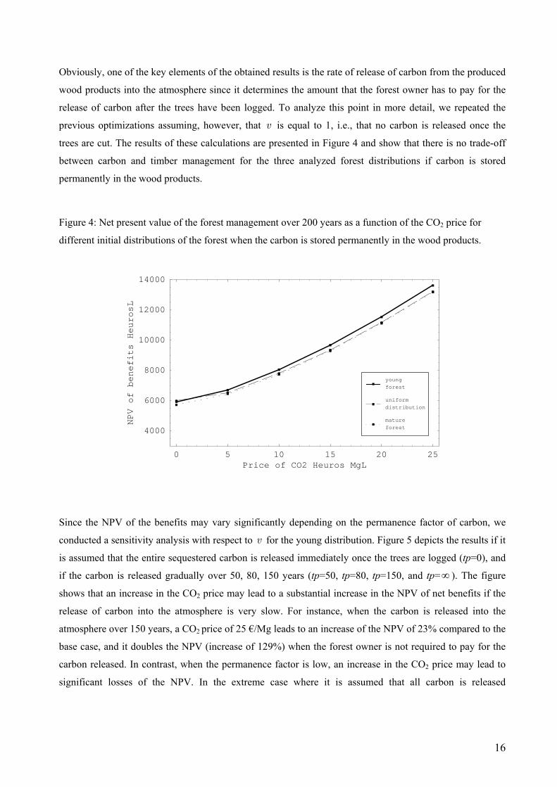
Obviously, one of the key elements of the obtained results is the rate of release of carbon from the produced

wood products into the atmosphere since it determines the amount that the forest owner has to pay for the

release of carbon after the trees have been logged. To analyze this point in more detail, we repeated the

previous optimizations assuming, however, that v is equal to 1, i.e., that no carbon is released once the

trees are cut. The results of these calculations are presented in Figure 4 and show that there is no trade-off

between carbon and timber management for the three analyzed forest distributions if carbon is stored

permanently in the wood products.

Figure 4: Net present value of the forest management over 200 years as a function of the CO2 price for

different initial distributions of the forest when the carbon is stored permanently in the wood products.

0 5 10 15 20 25Price of CO2 Heuros�MgL

4000

6000

8000

10000

12000

14000

NPV

of

benefits

HeurosL

mature

forest

uniform

distribution

young

forest

Since the NPV of the benefits may vary significantly depending on the permanence factor of carbon, we

conducted a sensitivity analysis with respect to v for the young distribution. Figure 5 depicts the results if it

is assumed that the entire sequestered carbon is released immediately once the trees are logged (tp=0), and

if the carbon is released gradually over 50, 80, 150 years (tp=50, tp=80, tp=150, and tp=∞ ). The figure

shows that an increase in the CO2 price may lead to a substantial increase in the NPV of net benefits if the

release of carbon into the atmosphere is very slow. For instance, when the carbon is released into the

atmosphere over 150 years, a CO2 price of 25 €/Mg leads to an increase of the NPV of 23% compared to the

base case, and it doubles the NPV (increase of 129%) when the forest owner is not required to pay for the

carbon released. In contrast, when the permanence factor is low, an increase in the CO2 price may lead to

significant losses of the NPV. In the extreme case where it is assumed that all carbon is released

17

immediately after logging, given a CO2 price of 15 €/Mg, the forest owners achieve only 34% of the NPV

they would obtain when carbon sequestration is not accounted for.

Figure 5: Net present value of the forest management over 200 years as a function of the CO2 price for

different levels of the permanence factor.

5 10 15 20 25

Price of CO2 Heuros�MgL

2000

4000

6000

8000

10000

12000

14000

NPV

of

benefits

HeurosL

tp=¥

tp=150

tp=80

tp=50tp=0

In the figure, “tp=n” indicates that the carbon is released in a proportional manner over n years.

4. Conclusions

In this paper we present a theoretical model that allows us to determine the optimal management of a

diameter-distributed forest. The theoretical model can be formulated as a distributed optimal control

problem where the control variables and the state variable depend on two arguments: time and diameter of

the tree. As the resulting necessary conditions of this problem include a system of partial integro-

differential equations, the problem cannot be solved analytically. For this reason, a numerical method is

employed. The Escalator Boxcar Train technique can be used to solve a distributed optimal control problem

by transforming the independent argument, diameter, into a state variable of the system that evolves over

time. In this way, the partial integro-differential equation is decoupled into a system of ordinary differential

equations, converting the distributed optimal control problem into a classic optimization problem that can

be solved by utilizing standard mathematical programming techniques.

An empirical analysis is conducted to determine the optimal selective-logging regime, that is, the selective

logging scheme that maximizes the present value of net benefits from timber production and carbon

18

sequestration of a privately owned Pinus sylvestris forest, and to evaluate how the optimal management of

the forest is affected by a variation in the market prices for carbon sequestration. The study is characterized

by the account taken of the complex growth process of the trees and the storage of carbon in the soil and in

the biomass.

The results of our calculations show that an increase in the carbon price leads to an increase in the number

of trees in the forest and to an increase in the carbon sequestered in the forest ecosystem. However, the

results demonstrate that the net benefits from carbon storage only compensate the decrease in net benefits

from wood production once the carbon price has exceeded a certain threshold value. This threshold can be

high depending on the assumption of the length of time the carbon is sequestered in the wood products. In

the extreme case where the forest owner does not have to pay for the release of carbon, it is worthwhile to

sequester additional carbon for any given positive price of CO2. However, when it is assumed that the

carbon is released into the atmosphere in a proportional manner over 80 years, even a CO2 price of 25 €/ha

is not able to make the carbon storage profitable, and the forest manager will therefore not change the

selective logging scheme. Hence, the results demonstrate that a correct assessment of the carbon accounting

is crucial for the correct determination of the optimal forest and carbon management regime.

19

Table 1: Optimal Selective-Logging Regime of Young Stand

Considering only timber

Year Number Of trees

Planted trees

Logged trees

Logged Volume (m3/ha)

Net revenue from timber sale

(€/ha)(b)

Maintenance cost (€/ha)

Planting cost (€/ha)

Carbon in soil (Mg/ha)

C in the biomass (Mg/ha)

Carbon revenue (€/ha)

Net benefit (€/ha)

Discounted net benefit (€/ha)

0 820 251 115 98.78 3211.29 -699.04 -150.43 25.00 62.76 - 2361.82 2361.82

10 996 109 67 42.26 1130.72 -786.42 -65.19 25.34 52.90 - 279.11 228.97

20 1009 122 85 49.92 1281.70 -793.68 -72.87 25.85 62.91 - 415.16 279.39

30 1016 136 105 58.12 1443.98 -797.32 -81.34 26.57 72.57 - 565.32 312.10

40 1013 152 129 68.60 1663.05 -795.68 -91.08 27.47 80.57 - 776.29 351.57

50 995 146 160 82.96 1978.95 -786.19 -87.25 28.49 85.45 - 1105.52 410.73

60 984 140 147 75.50 1788.35 -780.20 -83.86 29.53 85.44 - 924.29 281.71

70 986 177 128 75.31 1946.35 -781.43 -106.15 30.62 87.03 - 1058.78 264.72

80 955 124 199 121.75 3211.54 -765.12 -74.09 31.75 88.73 - 2372.32 486.59

90 968 132 101 61.78 1623.86 -771.70 -79.17 32.57 76.14 - 772.99 130.06

100 977 143 113 68.72 1800.68 -776.46 -85.70 33.51 81.51 - 938.52 129.55

Discounted sum over 200 years 10653.41 4220.96 511.31 - 5921.15

Considering timber and carbon sequestration ( carbon price =15 €/ha)

0 935 504 0 0.00 0.00 -754.94 -301.62 25.00 62.76 0.00 -1056.56 -1056.56

10 1366 0 63 69.91 2566.10 -1008.26 0.00 26.09 83.56 -189.80 1368.04 1122.27

20 1326 0 26 23.47 770.40 -982.05 0.00 27.18 90.15 917.27 705.62 474.86

30 1289 41 24 23.87 829.53 -958.13 -24.80 28.79 112.46 1067.41 914.02 504.60

40 1252 68 65 60.70 2023.70 -934.84 -40.94 30.96 134.79 368.93 1416.84 641.67

50 1226 87 83 71.57 2295.67 -918.15 -51.83 33.41 145.74 129.85 1455.54 540.77

60 1198 142 102 82.49 2554.47 -901.43 -85.26 36.03 152.46 -136.68 1431.10 436.17

70 1204 20 125 95.82 2876.84 -904.76 -12.12 38.71 154.95 -453.27 1506.68 376.71

80 1155 102 57 41.76 1221.71 -875.57 -61.08 41.32 152.49 570.54 855.60 175.49

90 1148 378 97 79.50 2474.74 -871.68 -226.16 44.23 164.33 -211.58 1165.33 196.08

100 1284 0 231 181.73 5537.96 -954.67 0.00 47.11 165.04 -2258.11 2325.18 320.95

Discounted Sum over 200 years 9376.18 5002.61 480.90 655.59 4548.26

20

References

Álvarez, M., Barrio, M., Gorgoso, J., and Álvarez, J., 2003. Influencia de la competencia en el crecimiento

en sección en Pinus radiata (D. Don). Investigación Agraria: Sistemas y Recursos Forestales. 12, 25-35.

Brown, P. (1998). Climate, Biodiversity and Forests: Issues and Opportunities Emerging from the Kyoto

Protocol, World Resources Institute, Washington, D.C.

Calvo, E. and Goetz, R. (2001). Using distributed optimal control in economics: A numerical approach

based on the finite element method, Optimal Control Applications and Methods 22(5/6): 231–249.

Cañellas, I., Martinez García, F. and Montero, G. (2000). Silviculture and dynamics of Pinus Sylvestris L.

stands in Spain, Investigación Agraria: Sistemas y Recursos Forestales Fuera de Serie N. 1.

Creedy, J., Wurzbacher, A.D., 2001. The economic value of a forested catchment with timber, water and

carbon sequestration benefits. Ecological Economics 38, 71–83.

de Roos, A. (1988). Numerical methods for structured population models: The Escalator Boxcar Train,

Numerical Methods for Partial Differential Equations 4: 173–195.

Goetz, R., Xabadia, A. and Calvo, E. (2007). A numerical approach to determine the optimal forest

management regime under varying pressure of intra-specific competition, manuscript, University of

Girona.

Healey, J., Price, C. and Tay, J. (2000). The cost of carbon retention by reduced impact logging, Forest

Ecology and Management 139: 237-255.

Hritonenko, N., Yatsenko, Y., Goetz, R.U. and Xabadia, A. (2007) Maximum principle for a size-structured

model of forest and carbon sequestration management, manuscript, Prairie View A&M University.

Huang, C. and Kronrad, G. (2001). The cost of sequestering carbon on private forest land, Forest Policy and

Economics 2: 133-142.

Keyfitz, N. (1968). Introduction to the mathematics of population, New York: Addison-Wesley.

Lubowski, R., Plantinga, A. and Stavins, R. (2006). Land-use change and carbon sinks: Econometric

estimation of the carbon sequestration supply function, Journal of Environmental Economics and

Management 51: 35-52.

Matthews, R. (1993). Towards a methodology for the evaluation of the carbon budget of forests, mimeo,

Mensuration Branch, Forestry Commission, Alice Holt Lodge, Farnham.

McKendrick, A., 1926. Application of mathematics to medical problems, Proceeding Edinburgh

Mathematical Society 44, 98–130.

21

McCarney, G., Armstrong, G. and Adamowicz, W. (2006). Implications for carbon on timber and non-

timber values in an uncertain world, manuscript presented at the Third World Congress of Environmental

and Resource Economists, Kyoto, Japan, July 3-7.

Mendenhall, W., Wackerly, D. and Scheaffer, R. (1990). Mathematical Statistics with Applications, 4 edn,

PWSKent, Boston.

Metz, J. and Diekmann, O., (1986). The dynamics of physiologically structured populations, Springer

Lecture Notes in Biomathematics, Springer-Verlag, Heidelberg.

Millar, R. and Myers, R. (1990). Modelling environmentally induced change in growth for Atlantic Canada

cod stocks, ICES C.M./G24 .

Palahí, M. and Pukkala, T. (2003). Optimising the management of Scots Pine (Pinus sylvestris L.) stands in

Spain based on individual-tree models, Annals of Forest Science 60: 105–114.

Rasse, D., Longdoz, B. and Ceulemans, R. (2001). TRAP: a modelling approach to below-ground carbon

allocation in temperate forests, Plant and Soil 229: 281-293.

Sohngen, B. and Mendelsohn, R. (2003). An Optimal Control Model of Forest Carbon Sequestration,

American Journal of Agricultural Economics 85 (2): 448-457.

Sohngen, B. and Sedjo, R. (2000). Potential carbon flux from timber harvests and management in the

context of a global timber market., Climatic Change 44: 151-172.

Tassone, V., Wessler, J. and Nesci, F. (2004). Diverging incentives for afforestation from carbon

sequestration: an economic analysis of the EU afforestation program in the south of Italy, Forest Policy

and Economics 6: 567-578.

Thornley, J. and Cannell, M. (2000). Managing forests for wood yield and carbon storage: a theoretical

study, Tree Physiology 20: 477-484.

Trasobares, A. and Pukkala, T. (2004). Optimising the management of uneven-aged Pinus sylvestris L. and

Pinus nigra Arn. mixed stands in Catalonia, north-east Spain, Annals of Forest Science 61: 747–758.

United Nations Development Programme (UNDP), United Nations Environment Programme (UNEP),

World Bank and the World Resources Institute. (2000). World Resources 2000-2001: People and

ecosystems, the fraying web of life, Technical report, Elsevier Science, Amsterdam.

van Kooten, G.C., Binkley, C.S., and Delcourt, G., 1995. Effect of carbon taxes and subsidies on optimal

forest rotation age and supply of carbon services. American Journal of Agricultural Economics

77(2):365-374.

22

van Kooten, G. and Bulte, E. (1999). How much primary coastal temperate rain forest should society retain?

Carbon uptake, recreation and other values, Canadian Journal of Forest Research 29: 1879-89.

van’t Veld, K. and Plantinga, A. (2005). Carbon sequestration or abatement? The effect of rising carbon

prices on the optimal portfolio of greenhouse-gas mitigation strategies, Journal of Environmental

Economics and Management 50: 59-81.

von Bertalanffy, L. (1957). Quantitative laws in metabolism and growth, Quarterly Review of Biology 32:

217–231.

Veliov, V.M. (2003). Newton’s method for problems of optimal control of heterogeneous systems.

Optimization Methods and Software 18: 387-411.

Xabadia, A and Goetz, R. (2007). The economics of competition between individuals in biological

populations, manuscript, University of Girona.