Optimal cruise control with dual

electric motors

Thomas Miller

Supervised by Peter Pudney & Peng Zhou

University of South Australia

Vacation Research Scholarships are funded jointly by the Department of Education and

Training and the Australian Mathematical Sciences Institute.

Abstract

The ATN group of universities is building a solar car to participate in the 2019 World Solar

Challenge. The car will have two identical electric motors—one on each of the rear wheels. Each

motor has a associated motor controller that controls the current applied to the motor windings,

and hence the torque of the motor. The motors and motor controllers have efficiencies that depend

on parameters including speed, current, torque and temperature.

When the car is cruising at a constant speed, the torque required to maintain the required

speed will depend on external forces including aerodynamic drag, wind forces and the gradient of

the road. Usually, the total torque required will be less than the capability of a single motor. The

aim of the research is to determine how much total torque is required to maintain a constant speed,

and how much of this total torque should be generated from each motor to minimise the sum of

the power losses in the motors and controllers. For some conditions, the optimal control might be

to generate the same torque from both motors, whereas for different conditions it might be more

efficient to generate all of the torque from one motor.

The motor manufacturer provides information that can be used to model the efficiency of the

motor, which depends on torque and angular velocity. The controller manufacturer provides an

efficiency map for the controller; controller efficiency also depends on torque and angular velocity.

We show that the power losses are minimised if the same torque is applied to both motors.

1 Introduction

In the World Solar Challenge, when a car leaves Darwin on the 3,000 km journey to Adelaide it starts

with only about one tenth of the energy required to make it to the end. The rest of the energy is

provided by the sun [World Solar Challenge, 2019]. Solar cars make this journey with far less energy

than a commercial automobile requires [Thacher, 2015]. To make this possible, solar cars must be as

efficient as possible by minimising the energy losses that occur during the journey.

The Australian Technology Network (ATN) group of universities are building a solar car (Figure 1) to

compete in the 2019 World Solar Challenge. This solar car will be powered by two in-wheel motors,

each controlled by an associated motor controller. The roads from Darwin to Adelaide are mostly

long and straight allowing the car to spend most of the journey cruising at a constant speed.

Figure 1: The ATN Solar Car

1

The aim of this project is to analyse the losses that occur in the motors and controllers at cruising

speed and propose a simple real-time control strategy that minimises the energy lost at this speed.

2 Modelling

The factors that influence losses in the motor and controller at cruising speed are:

• the rotational speed of the motors

• the torque required to maintain cruising speed

• the DC bus voltage that the battery provides to the system

• the ambient temperature around the motors.

The cruising speed v of the car will be 75 km/h. As the motors are in the wheels, the rotational speed

of the motors at cruising speed (measured in radians per second) is determined by the cruising speed

and the radius of the tyres, which is 0.2792 meters. To convert from km/h to radians per second

(rad/s) we first convert to m/s by dividing by 3.6 so 75 km/h = 75/3.6 m/s, then to get to rad/s we

divide this value by the tyre radius giving us ω = (75/3.6)/0.2792 ≈ 74.62 rad/s.

The torque τ required to maintain cruising speed depends on the tractive force F required to main-

tain cruising speed and the radius r of the wheels, and is given by τ = Fr. The tractive force is

approximately

F ≈ crrmg +1

2cdAρv

2 +mg sin θ.

The term crrmg is the rolling resistance caused by forces between the wheels and the road, and depends

on the rolling resistance coefficient of the tyres crr, and the load on the wheels mg which depends on

the mass of the car m and the experienced gravitational force g. The term 12cdρv

2A is the aerodynamic

drag experienced by the car and depends on the air density ρ, the drag coefficient of the car cd the

reference area of the car A and the square of the car’s velocity. The final term is mg sin θ and represents

the force on the car due to the gradient of the road.

In our case we have:

• m = 410 kg (with two occupants)

• g = 9.8 m s−2

• crr = 0.005

• ρ = 1.16 kg m−3

• cdA = 0.16 m3

• v = 75 km/h ≈ 21 m/s

• sin θ as high as 0.06.

2

For a flat road this means we will need a force of approximately 61 N to maintain a speed of 75 km/h,

and for a steep uphill section a force of 302 N is required. These forces correspond to torques of 17 Nm

and 84 Nm respectively.

The input voltage to the controller, Vbus, will vary from 114 V when the battery is empty to 160 V

when the battery is full. Nominally we expect the voltage will be 141 V. We will model the problem

firstly with the nominal voltage but also examine how the loses change as this voltage changes.

Finally for the ambient temperature we will assume an average of 35°C (308 K), and we will also

examine how the loses change as the ambient temperature changes.

The above parameters are the inputs of our problem. We wish to find how to distribute the required

torque between the two motors in order to minimise the total power losses in the motors and motor

controllers. The outputs we will produce are:

• the torque provided by motor one

• the torque provided by motor two

• the total power lost by the system.

To solve the problem we must consider losses in three different components of the drive system:

• the motors

• the motor controllers

• the three inductors used between each controller and the corresponding motor.

3 The Motors

The motors to be used in the ATN solar car are two identical Axial Flux Stub Axle Wheel Motors,

built by Marand. The motors were designed by the CSIRO for use by the Aurora solar car team for

the 1996 World Solar Challenge from Darwin to Adelaide [Lovatt et al., 1998]. Appendix A shows the

specifications for the motors.

They are permanent magnet synchronous motors, which is a type of motor that gives the benefits of

both a high torque density and high efficiency. The losses that arise from the motors are [Thacher,

2015]:

• copper losses, which are the dominant loss in this motor and are caused by resistance to the flow

of current in the motor

• eddy current losses, because the rotation of the motor induces small circulating currents in the

motor that impede the motors rotation

• windage losses due to aerodynamic drag resistance to the rotation to the motor caused by air

contained in the motor.

3

Figure 2 shows how these losses vary with torque. Copper loss is the main source of loss in this motor

and increases at an increasing rate as torque increases, while eddy and windage losses are almost

negligible and are practically independent of torque.

Figure 2: How the Motor Loses Change with Torque

The copper loss and eddy loss are calculated in an iterative process. This process depends on the

ambient temperature Ta in K, the motor torque τ in Nm, the motor speed ω in rad/s and requires an

estimate of the steady state winding temperature Tw in K [Mar, 2013].

1. The magnet temperature Tm is calculated as approximately halfway between the ambient and

winding temperatures: Tm = (Ta + Tw)/2.

2. The magnet remanence B is given by: B = 1.32− 1.2× 10−3(Tm − 293).

3. The RMS per phase motor current i is given by: i = 0.561Bτ.

4. The per phase motor winding resistance R is given by: R = 0.0575 (1 + 0.0039 (Tw − 293)) .

5. The copper loss Pc is given by: Pc = 3i2R.

6. The motor eddy current loss Pe is given by: Pe =(9.602× 10−6(Bω)2

)/R.

7. The winding temperature Tw is then given by: Tw = 0.455(Pc + Pe) + Ta.

8. The calculations (1)–(7) are repeated the process until the difference between the previous and

next winding temperature is less than 0.05 K.

Testing showed that these calculations are accurate to within 5% when the torque is in the range

[0, 40] Nm [Mar, 2013].

The other loss associated with the motor is the internal windage loss Pw which is given by [Mar, 2013]:

Pw = 170.4× 10−6ω2.

The total motor loss Pml is the summation of the three individual losses:

Pml = Pc + Pe + Pw.

4

4 The Controllers

Each motor has an associated motor controller that takes high voltage DC power from the car’s

batteries and converts it to a lower voltage 3-phase AC power to drive the motor [Tri, 2015]. In our

solar car we are using Tritium WaveSculptor 22 motor controllers.

There are two types of losses associated with the motor controller [Tri, 2015]:

• conduction losses, like copper losses, are incurred due to the resistance of current flowing through

the motor controller

• switching losses, associated with the switching of the battery voltage that controls the current

flowing through the motor phase windings Thacher [2015].

The controller losses are dependent on current which, as shown in Section 3, is proportional to the

torque produced by the motor. Figure 3 shows the controller losses. Controller losses are generally

lower then the motor losses shown in Figure 2. Both the switching losses and the conduction loss

provide a significant contribution to the total controller loss, although the conduction loss is the only

loss that is increasing at an increasing rate.

Figure 3: Controller Losses

Simple equations exist for estimating the controller losses [Tri, 2015]:

• conduction loss: ReqI20

• switching loss: (αI0 + β)Vbus + CfeqV2bus.

The total controller loss is

Pcl = ReqI20 + (αI0 + β)Vbus + CfeqV

2bus

5

where

• I0 is the output current of the controller in Arms

• Vbus is the bus voltage (battery voltage) of the controller

• Req is the equivalent resistance of the entire controller

• α is the linear component of the switching loss (per unit of bus voltage)

• β is the constant component of the switching loss (per unit of bus voltage)

• Cfeq is the equivalent capacitance and frequency product of the entire controller

• Req = 1.0800× 10−2

• α = 3.3450× 10−3

• β = 1.8153× 10−2

• Cfeq = 1.5625× 10−4.

5 The Inductors

The Wave Sculptor 22 requires a minimum amount of inductance for each motor phase in order

to operate properly [Tri, 2015]. In order to achieve this minimum amount of inductance a set of

three inductors are provided with the motors to connect to the three phases of the motor in a series

connection [Mar, 2013].

When used with a Wave Sculptor 22, the loss of one inductor can be approximated by [Mar, 2013]:

Pil = 12× 10−3(i

2

)2

+ 2.7× 10−6(i

2

)3

× 3.183ω.

As with the controller, the dependence on torque τ comes from the currents i dependence on torque.

And as we need three inductors per motor, the total loss will be three times this value. Figure 4 shows

the inductor losses versus torque. Like the motor loss, the inductor losses increase at an increasing

rate as torque increases.

Figure 4: Inductor Losses

6

6 Total Losses

The total losses are the sum of the motor losses, the controller losses and the three inductor losses,

and are a function of required torque τ :

f(τ) = Pml + Pcl + 3Pil.

Figure 5 shows how the total losses change with torque. Losses from the motor make up the majority

of total losses. We also see from this graph that the losses appear to be increasing at an increasing

rate, which suggests that the derivative of the losses is always increasing and the second derivative is

always positive. Due to how the motor losses are calculated we don’t have a simple formula for the

total loss function or it’s derivatives (although if we fix the number of iterations we could obtain a

formula). However, using numerical approximation we can still calculate and graph the derivatives.

Figure 6a shows the derivative of the total loss function and as expected it is always increasing.

Likewise Figure 6b shows the second derivative of the total loss function which is always positive.

Figure 5: Total Losses

(a) Total Loss Derivative (b) Total Loss Second Derivative

Figure 6: Numerical Approximations of the Total Loss Function’s Derivatives

7

At cruising speed, beside the required torque there are two other variables that may vary—the ambient

temperature around the motors and the voltage of the battery. Figure 7a shows how total losses are

related to the ambient temperature around the motor and Figure 7b shows how the total losses are

related to the voltage of the battery.

Table 1 shows that losses increase with temperature, and as torque increases the percentage loss

increases with torque. Table 2 shows that losses increase with bus voltage, but the percentage loss

decreases with torque.

(a) How Loss Varies With Ambient Temperature (b) How Loss Varies With Battery Voltage

Figure 7: How Loss Varies With Non-Torque Factors

Torque Total Loss at 273 K Total Loss at 408 K Difference Percent Increase

10 Nm 22.20 W 23.98 W 1.78 W 8.02 %

20 Nm 59.03 W 65.64 W 6.61 W 11.20 %

30 Nm 123.60 W 139.83 W 16.23 W 13.13 %

40 Nm 224.38 W 257.98 W 33.60 W 14.97 %

Table 1: Total Loss Values as Ambient Temperature Vary

Torque Total Loss at 114 V Total Loss at 160 V Difference Percent Increase

10 Nm 20.42 W 24.37 W 3.95 W 19.34 %

20 Nm 57.80 W 62.88 W 5.08 W 8.79 %

30 Nm 124.12 W 130.30 W 6.18 W 4.98 %

40 Nm 228.58 W 235.79 W 7.21 W 3.15 %

Table 2: Total Loss Values As Battery Voltages Vary

8

7 Optimal Power Split

7.1 Identical Motor and Controller Systems

Suppose the two motor and controller systems are identical. For a given battery voltage, speed and

required torque, we want to determine the proportion of the required torque that should be supplied

from each motor so that the total loss is minimised. The power loss from a single motor and controller

is f(τ) for required torque τ . To find the optimal way to split the torque production we define the

torque split function as:

g(α) = f(ατ) + f ((1− α)τ) , (1)

which describes the total loss from both motors and controllers for a required torque τ in terms of

the proportion α of torque produced by one of the motor and controller systems, as ατ will give the

torque to be provided by one motor and controller system and (1−α)τ will give the remainder of the

required torque which is to be produced by the other motor and controller system. Figure 8 shows the

optimal split function graphed for a variety of torques. From this graph it appears that the optimal

solution is always α = 0.5. We will show that not only is this the case for our motor and controller

systems, it is also the case for many motor and controller systems. Figure 9 shows the differences

in the losses from using one motor for all the torque versus splitting the torque equally between the

motors, we see that in low torques this difference is relatively minor, but that the difference increases

quickly at the higher torque values.

Figure 8: The Optimal Power Split Curves

What causes the equal split solution is that, as seen in Section 6, losses increase at an increasing rate

as torque increases. This means that the first derivative of the total loss function is an increasing

function, so that a < b =⇒ f ′(a) < f ′(b), and that the second derivative of the loss function is

always positive: ∀x, f ′′(x) > 0.

9

Figure 9: Losses From Using One Motor Versus Both Motors

To show that the equal split solution is optimal we take the derivative of the torque split function

(Equation (1)):

g(α) = f(ατ) + f ((1− α)τ) ,

g′(α) = τf ′(ατ)− τf ′ ((1− α)τ) .

The torque split function has a stationary point when g′(α) = 0:

0 = τf ′(ατ)− τf ′ ((1− α)τ)

=⇒ τf ′(ατ) = τf ′ ((1− α)τ)

=⇒ f ′(ατ) = f ′ ((1− α)τ) ,

which shows that the value of the derivative of one motor loss function has to equal the value of the

derivative of the other’s loss derivative. However, from before we know that this derivative is always

increasing, a < b =⇒ f ′(a) < f ′(b), which means this equality is only possible when the arguments

are equal, giving us:

ατ = (1− α)τ

=⇒ α =1

2.

This means that the torque split function has only one stationary point at α = 12 . We can classify this

is a minimum using the second derivative test. The second derivative of the torque split function is:

g′′(α) = τ2f ′′(ατ) + τ2f ′′ ((1− α)τ) .

When the required torque τ > 0 we also have that the second derivative of the motor loss functions is

always positive, ∀x, f ′′(x) > 0. Therefore g′′(α) is clearly always positive including for α = 12 , which

by the second derivative test for stationary points means that g(0.5) is a minimum point.

Furthermore, as g′′(α) > 0 for all τ > 0 and all 0 ≤ α ≤ 1, then g(α) is strictly convex meaning any

local minimum is also the unique global minimum, meaning that the minimum point found at α = 12

is the only possible minimum point.

10

So we have found that the strategy that minimises losses in our dual in-wheel motor controller system

is equally splitting torque production between the motors. However, this solution applies only if the

two motor and controller systems have the exact same loss curves, which may not apply in general.

In the next section we examine what happens if the two systems have different losses.

7.2 Non-identical Motors

We now consider the case where the second motor’s loss function is some multiple of the losses of

the first motor, so the first motor’s losses will remain f(τ), but the second motor’s losses will be

h(τ) = βf(τ). The torque split function becomes:

g(α) = f(ατ) + h ((1− α)τ)

=⇒ g(α) = f(ατ) + βf ((1− α)τ) . (2)

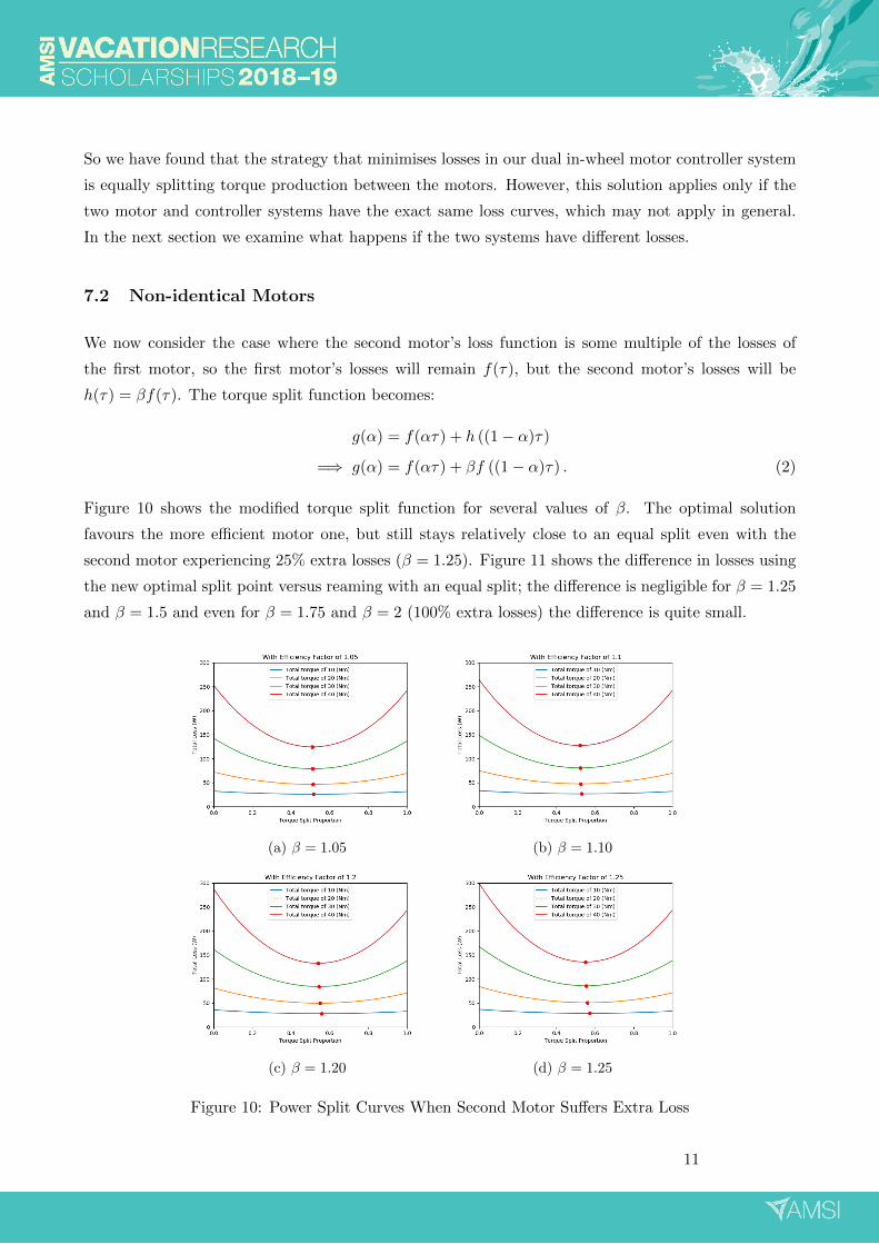
Figure 10 shows the modified torque split function for several values of β. The optimal solution

favours the more efficient motor one, but still stays relatively close to an equal split even with the

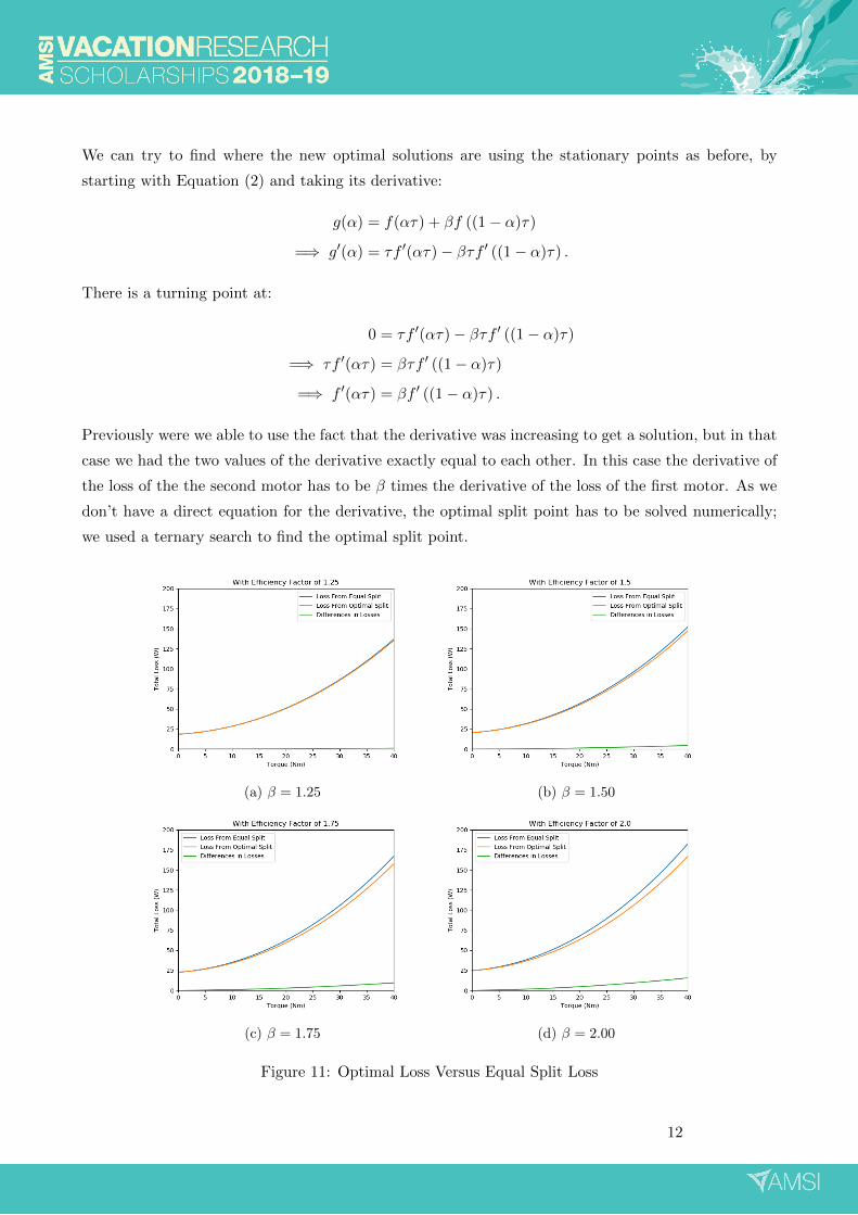
second motor experiencing 25% extra losses (β = 1.25). Figure 11 shows the difference in losses using

the new optimal split point versus reaming with an equal split; the difference is negligible for β = 1.25

and β = 1.5 and even for β = 1.75 and β = 2 (100% extra losses) the difference is quite small.

(a) β = 1.05 (b) β = 1.10

(c) β = 1.20 (d) β = 1.25

Figure 10: Power Split Curves When Second Motor Suffers Extra Loss

11

We can try to find where the new optimal solutions are using the stationary points as before, by

starting with Equation (2) and taking its derivative:

g(α) = f(ατ) + βf ((1− α)τ)

=⇒ g′(α) = τf ′(ατ)− βτf ′ ((1− α)τ) .

There is a turning point at:

0 = τf ′(ατ)− βτf ′ ((1− α)τ)

=⇒ τf ′(ατ) = βτf ′ ((1− α)τ)

=⇒ f ′(ατ) = βf ′ ((1− α)τ) .

Previously were we able to use the fact that the derivative was increasing to get a solution, but in that

case we had the two values of the derivative exactly equal to each other. In this case the derivative of

the loss of the the second motor has to be β times the derivative of the loss of the first motor. As we

don’t have a direct equation for the derivative, the optimal split point has to be solved numerically;

we used a ternary search to find the optimal split point.

(a) β = 1.25 (b) β = 1.50

(c) β = 1.75 (d) β = 2.00

Figure 11: Optimal Loss Versus Equal Split Loss

12

Using the second derivative of the modified torque split function:

g′(α) = τf ′(ατ)− βτf ′ ((1− α)τ)

=⇒ g′′(α) = τ2f ′′(ατ) + βτ2f ′ ((1− α)τ) ,

we find that like the original torque split function, it is always positive making this a strictly convex

function when the required torque and β are both positive, meaning we always have one minimum

point which is also the global minimum point. Therefore a ternary search will find the optimal split

point.

So we have found that if the motors differ slightly the optimal torque split will be to favour the more

efficient motor. However, we have also seen that the extra loss incurred when using an equal split

solution is relatively small for our motors.

7.3 Final Strategy

We saw that if the motor and controller loss functions are exactly the same for both motors and

loss increases with torque with increasing derivative that the optimal strategy is to distribute torque

production equally among both motors. We also saw that the extra losses incurred from using equal

torque distribution when there is a slight difference in the performance of our motors is not expected

to be significant. So considering all these factors, the torque distribution strategy at cruising speed

that makes sense is to always equally split torque production across both motors, which has the benefit

of being simple to implement on a microcontroller as a real time strategy.

8 Related work

The literature contains some articles on the control of dual motors, but mostly concerns systems more

complicated that the system that will be used by the solar car.

Jian et al. [2009] discuss optimal system efficiency for a multi-motor drive system for a bus. They note

that while permanent magnet synchronous motors already have high efficiency, this efficiency depends

on the methods used to control the motors. They suggest that an appropriate torque distribution

strategy can improve the multi-motor drive system efficiency, and show that it is more efficient to use

one motor under light load conditions, and to use both motors under heavy load conditions. They

also show that dividing the torque evenly between motors is not necessarily the most efficient strategy,

but they do not discuss the structure of the optimal solution.

Hu et al. [2015] propose a system using two motors with different powers, connected using gears and

clutches. They use a sequential quadratic programming method to find the optimal power split for

13

different conditions, and store the results in a look-up table that can be used while driving. The

optimisation of the efficiency gives the optimal torque motor 1 should be driven at, the optimal torque

motor 2 should be driven at, the optimal speed motor 1 should be driven at and the optimal speed

motor 2 should be driven at as function of the vehicle speed, the vehicle acceleration and the state of

charge of the battery.

Tseng et al. [2015] describe online maximum efficiency tracking control for a dual-motor drive system.

They do not model losses in the system. Instead, they measure the input power at the DC bus,

measure the output power, and then vary the motor input torques to find the torque distribution that

maximises efficiency. Two algorithms are proposed and compared: a steepest ascent algorithm and

a fuzzy logic algorithm. They found that their fuzzy logic algorithm performed better, reaching a

slightly better maximum efficiency and reaching the most efficient point quicker. Their control system

operates on very small time scales of less then 0.1 seconds.

Zhang et al. [2015] use Pontryagin’s principle to find necessary conditions for an optimal control

strategy for a dual-motor-driven electric bus. Their drive system includes gears and clutches that

introduce mechanical losses that we do not have.

Hu et al. [2018] propose a dual-motor powertrain system to improve the dynamic and economic

performance of a pure electric vehicles. They consider a powertrain with a 22 kW motor and a 10 kW

motor connected using a gear and clutch system that can operate in four modes: driving from motor

1, driving from motor 2, a torque combining mode, and a speed combining mode for high-speed

operation. Overall efficiency is a function of transmission mode and the torque and speed of each

motor. They use sequential quadratic programming to find the optimal mode and motor controls

for various required vehicle speeds and torques, from which they develop a mode selection strategy

that depends on the vehicle speed and required torque. Our system is simpler—we do not have a

complicated transmission, and the speeds of the two motors are given.

Zhao et al. [2018] established a energy saving strategy for a dual motor system for an urban bus. They

find an optimal torque ratio using the state of charge of the battery, the target torque and the target

velocity using a dynamic programming solution, but the calculation is too slow for solving in real

time. For on-road solutions, they pre-calculate solutions for different scenarios using their dynamic

programming algorithm, then use a clustering algorithm to split these solutions in to separate clusters.

The boundaries of the clusters are determined using a classification algorithm such as a support

vector machine. Then, within each cluster, the actual points (torque split ratio, velocity, accelerator

pedal position) were approximated by piecewise polynomials, and these polynomials used for on-road

selection of strategy. The result was that the efficiency of the on-road strategy achieved is usually only

10% worse but can reach up to 95% of the dynamic programming strategy efficiency over a start-stop

traffic cycle.

14

Da and Bo [2015] focused on optimising when a dual-motor system should switch from using one motor

to using two motors. To do this they found the optimal driving force split between the two motors as

a function of the vehicle speed and target driving force. They focused on identifying situations when

all the driving force is supplied by one motor, compared to when the driving force is split between the

two motors. Their problem differs from ours, as they used two different motors, one connected to the

front axle and one connected to the rear axle with different gear ratios.

9 Conclusion and Discussion

This project was concerned with finding out how a solar car powered by two in-wheel motors should

be controlled in order to minimise power losses in the motors and motor controllers.

Most of the previous research concerned much more complex systems than our in-wheel motors, and

often used practical experiments to get exact measurements for the performance of the motors in order

to create their control strategies. However the papers Zhao et al. [2018] and Da and Bo [2015] did

provide the idea for solving the problem using the torque split ratio, representing the proportion of

torque provided by motor one.

To solve the problem we investigated the power losses that occur in the ATN Solar Car’s motor and

controller systems. While there is not a simple formula for these losses, we were still able to analyse

losses using algebraic, graphical and numeric methods. When cruising at a constant speed, motor and

controller losses were minimised by splitting torque production equally among both motors.

15

A Motor Specifications

Table 3 contains the technical specifications of the motors. Table 4 contains the performance of the

motors at its nominally rated speed and torque which is 111 rad/s and 16.2 Nm respectively. Table 5

contains the absolute maximum ratings for the motors. All these tables come from the manual for the

motors [Mar, 2013].

Table 3: Motor Specifications

Property Value

Number of poles 40

Number of phases 3

Mass of wheel motor 18.8 kg

Nominal speed 111 rad/s ≈ 1060 rpm

Nominal torque 16.2 Nm

Phase resistance 0.0575 Ω

EMF constant – L-N RMS EMF/speed 0.45 Vs/rad

Torque constant per phase 0.44 Nm/A

Table 4: Motor Performance at Nominal Rating

Property Value

L-N RMS EMF 50 V

RMS phase current 12.3 A

Copper loss 25.9 W

Eddy Current Loss 2.6 W

Internal Motor Windage 2.1 W

Wheel Losses 25.1 W

Total loss 55.7 W

Output Power 1800 W

Efficiency 97.0 %

Nominal winding temperature rise 14 K

Overload winding temperature rise 70 K

Table 5: Motor Absolute Maximum Ratings

Property Value

Maximum winding temperature 135 °CMaximum speed 157 rad/s ≈ 1500 rpm

Maximum rated torque 80 Nm

Maximum continuous torque 42 Nm

16

References

W. Da and W. Bo. Research on driving force optimal distribution and fuzzy decision control system

for a dual-motor electric vehicle. In 2015 34th Chinese Control Conference (CCC), pages 8146–8153,

July 2015. doi: 10.1109/ChiCC.2015.7260936.

Jianjun Hu, Lingling Zheng, Meixia Jia, Yi Zhang, and Tao Pang. Optimization and model validation

of operation control strategies for a novel dual-motor coupling-propulsion pure electric vehicle.

Energies, 11(4), 2018. ISSN 1996-1073. doi: 10.3390/en11040754. URL http://www.mdpi.com/

1996-1073/11/4/754.

M. Hu, J. Zeng, S. Xu, C. Fu, and D. Qin. Efficiency study of a dual-motor coupling EV powertrain.

IEEE Transactions on Vehicular Technology, 64(6):2252–2260, June 2015. ISSN 0018-9545. doi:

10.1109/TVT.2014.2347349.

Zhang Jian, Wen Xuhui, and Zeng Lili. Optimal system efficiency operation of dual PMSM motor

drive for fuel cell vehicles propulsion. In 2009 IEEE 6th International Power Electronics and Motion

Control Conference, pages 1889–1892, May 2009. doi: 10.1109/IPEMC.2009.5157704.

H. C. Lovatt, V. S. Ramsden, and B. C. Mecrow. Design of an in-wheel motor for a solar-powered

electric vehicle. IEE Proceedings - Electric Power Applications, 145(5):402–408, Sept 1998. ISSN

1350-2352. doi: 10.1049/ip-epa:19982167.

Axial Flux Stub Axle Wheel Motor For Solar Vehicle Applications. Marand, April 2013.

Eric Forsta Thacher. A Solar Car Primer: A Guide to the Design and Construction of Solar-Powered

Racing Vehicles. Springer, 2015.

WaveSculptor 22 Motor Drive User’s Manual. Tritium, August 2015.

S. Tseng, T. Liu, J. Hsu, L. R. Ramelan, and E. Firmansyah. Implementation of online maximum

efficiency tracking control for a dual-motor drive system. IET Electric Power Applications, 9(7):

449–458, 2015. ISSN 1751-8660. doi: 10.1049/iet-epa.2014.0415.

World Solar Challenge. 2019 world solar challenge: Overview, 2019. URL https://www.

worldsolarchallenge.org/about_wsc/overview. [Online; accessed 22-January-2019].

Shuo Zhang, Rui Xiong, and Chengning Zhang. Pontryagin’s minimum principle-based power man-

agement of a dual-motor-driven electric bus. Applied Energy, 159:370–380, 2015. ISSN 0306-2619.

doi: 10.1016/j.apenergy.2015.08.129. URL http://www.sciencedirect.com/science/article/

pii/S030626191501065X.

Mingjie Zhao, Junhui Shi, and Cheng Lin. Energy management strategy design for dual-motor coax-

ial coupling propulsion electric city-buses. Energy Procedia, 152:568–573, 2018. ISSN 1876-6102.

17

doi: 10.1016/j.egypro.2018.09.212. URL http://www.sciencedirect.com/science/article/

pii/S1876610218307574. Cleaner Energy for Cleaner Cities.

18