Optimal control of a flywheel energy storage system with a radial flux hybrid magnetic bearing

Journal of the Franklin Institute 339 (2002) 189–210

Optimal control of a flywheel energy storagesystem with a radial flux hybrid magnetic bearing

Jr-Yi Shen, Brian C. Fabien*

Department of Mechanical Engineering, University of Washington, Box 352600, Seattle, WA 98195, USA

Received 3 March 2000; received in revised form 30 October 2001; accepted 9 January 2002

Abstract

This paper describes the design and implementation of digital controllers for a flywheel

energy storage device that incorporates a radial flux hybrid permanent magnetic bearing.

Although the uncontrolled device is asymptotically stable, active control is required to: (i)

ensure that a finite radial air gap is maintained at all times, and (ii) attenuate the oscillations of

the flywheel which reduce the efficiency of the motor generator. The paper presents the design

of gain scheduled discrete time linear quadratic regulator (LQR) and linear quadratic

Gaussian (LQG) controllers for this rotordynamic system. Real time experiments are

conducted to investigate the performance of the controllers. The result indicates that the LQR

controller with approximate system velocities is easier to implement than the LQG controller,

and also provides superior performance.r 2002 The Franklin Institute. Published by Elsevier

Science Ltd. All rights reserved.

1. Introduction

Stienmier et al. [1] presented the design and dynamic modeling of a flywheel energystorage (FES) device that uses radial flux permanent magnetic bearings. A schematicof this device is shown in Fig. 1. The device contains a motor that converts inputelectrical energy into mechanical (kinetic) energy by causing the flywheel to rotate.Alternatively, the motor acts as a generator in converting the mechanical energystored in the flywheel into electrical energy. In this device the motor coils areattached to the stator (i.e., the center post in Fig. 1), and the motor permanentmagnets are attached to the flywheel.

*Corresponding author.

E-mail address: [email protected] (B.C. Fabien).

0016-0032/02/$22.00 r 2002 The Franklin Institute. Published by Elsevier Science Ltd. All rights reserved.

PII: S 0 0 1 6 - 0 0 3 2 ( 0 2 ) 0 0 0 2 1 - 2

The hybrid magnetic bearing consists of a stationary disk magnet in the stator anda ring magnet that is embedded in the flywheel. The disk and ring magnets arearranged such that they generate a repulsive radial force. The prototype FES deviceconsidered in this study has ring/disk magnet pairs near the top and bottom of theflywheel. The flywheel is supported in the axial direction via a thrust bearingconsisting of a synthetic ruby ball embedded in the flywheel and a synthetic sapphireplate embedded in the stator.Unlike electromagnetic bearings [2,3], no active control is required to stabilize the

equilibrium position of this hybrid magnetic bearing device. This is due to the factthat the disk/ring permanent magnet pairs act as passive radial springs, and frictionat the thrust bearing contact point provides the damping necessary to dissipateoscillations of the flywheel. Hence, if the FES device is free of external disturbancesand the flywheel is well balanced, no active control will be required to regulate theposition of the flywheel.In practical applications however, the FES device will be subject to external

disturbances and active control will be required to limit the radial displacement ofthe flywheel. Regulation of the flywheel’s radial motion is necessary since anycontact between the flywheel and the stator can result in a catastrophic failure whenthe system is operating at high speeds of rotation. It should also be noted thatoscillations of the flywheel will cause misalignment of the magnetic flux between thestator (motor) coils and the disk magnets. This flux misalignment will result inreduced efficiency of the motor/generator.The prototype FES device considered here uses four pairs of electromagnets to

control the position and orientation of the flywheel. As illustrated in Fig. 1 theseelectromagnets attract steel rings that are located near the top and bottom of theflywheel outer surface. By activating the different combinations of electromagnets itis possible to apply forces and torques to the flywheel and thus manipulate itsposition and orientation. This configuration is selected to demonstrate the feasibilityof active control of this hybrid magnetic bearing system. A detailed description ofthe device and its components can be found in [4,5].

Jewel Bearing

Vacuum Chamber

Motor / Generator

Active control coils

Repulsive Force Permanent Magnet Bearings

Fig. 1. Cross section of the FES system.

J.-Y. Shen, B.C. Fabien / Journal of the Franklin Institute 339 (2002) 189–210190

This paper considers the design and implementation of two LQ optimal controlschemes for the prototype FES device. Section 2 presents the equations of motion forthe device. Section 3 presents the design of gain scheduled LQR and LQG controllersfor the system. Section 4 presents experimental results comparing the performance ofthe LQR and LQG controllers when applied to the FES device. The paper concludesin Section 5 with a discussion of the results obtained.

2. Dynamic equations

This section presents the dynamic equations of motion for the flywheel. FromFig. 1 it can be seen that the flywheel can be treated as a top that is supported bysprings in the radial direction. The dynamic equations of motion for a top are wellknown [6,7]. Typically, these equations are written using Euler angles to describe theorientation of the top. Unfortunately, Euler angles are difficult to measure directlyand their use would complicate the design of feedback control systems [8]. Hence, weconsider here a set of dynamic equations that are based on coordinates that arerelated to the output of the sensors used to measure the position and orientation ofthe flywheel.First, let the X–Y–Z rectangular coordinate system represent the fixed reference

frame. Next, attach to the flywheel the 1–2–3 rectangular coordinate system, withthe origin of the 1–2–3 frame coincident with the center of mass of the flywheel, andthe 3-axis being the axis of symmetry. Then using Fig. 2 define the coordinate a

as the tangent of the angle between the Y–3 plane and Y–Z plane. Similarly, define b

as the tangent of the angle between the X–3 plane and the X–Z plane.The coordinates a and b are used to describe the orientation of the flywheel instead

of the traditional Euler angles. The advantage of using a and b over Euler angles is

Z

X

Y

1

2

3

ab

Fig. 2. Flywheel coordinate system.

J.-Y. Shen, B.C. Fabien / Journal of the Franklin Institute 339 (2002) 189–210 191

that a and b can be determined from direct measurements. In particular, infraredsensors are used to measure the X and Y displacements of the top and bottom of theflywheel, as illustrated in Fig. 3.The two top sensor determine the displacements Xt; Yt in the X and Y directions,

respectively. Similarly, the two bottom sensors determine the displacements Xb; Yb inthe X and Y directions, respectively. If the sensors are placed equidistant from thecenter of mass then a and b can be computed using

a ¼Xt � Xb

lzs

; b ¼Yt � Yb

lzs

;

where lzs is the vertical distance between the sensors.If x and y are used to denote the location of the center of mass of the flywheel in

the X–Y plane, then the dynamic equations of motion for small displacements a andb are given by Shen [4]

.a

.b

.x

.y

’a

’b

’x

’y

2666666666666664

3777777777777775

¼A11 A12

I 0

" #’a

’b

’x

’y

a

b

x

y

2666666666666664

3777777777777775

þ

B11

0

264

375

Fxct

Fxcb

Fyct

Fycb

26664

37775; ð1Þ

Flywheel edge

IR Photodetector

IR Emitters

IR PhotodetectorX displacement

Y displacement

X

Y

Fig. 3. Side view of sensors.


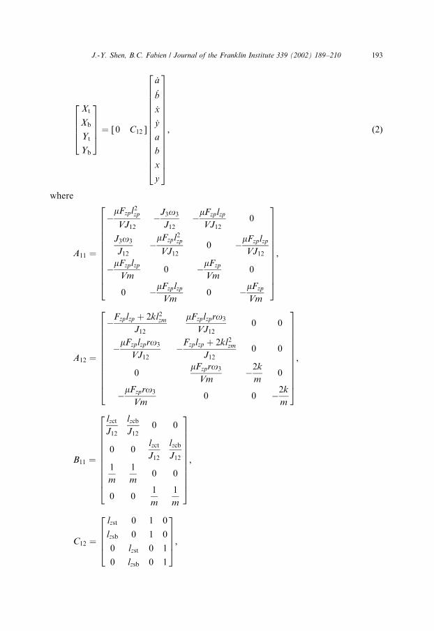
Xt

Xb

Yt

Yb

26664

37775 ¼ ½ 0 C12 �

’a

’b

’x

’y

a

b

x

y

2666666666666664

3777777777777775

; ð2Þ

where

A11 ¼

�mFzpl2zp

VJ12�

J3o3J12

�mFzplzp

VJ120

J3o3J12

�mFzpl2zp

VJ120 �

mFzplzp

VJ12

�mFzplzp

Vm0 �

mFzp

Vm0

0 �mFzplzp

Vm0 �

mFzp

Vm

2666666666664

3777777777775;

A12 ¼

�Fzplzp þ 2kl2zm

J12

mFzplzpro3VJ12

0 0

�mFzplzpro3

VJ12�

Fzplzp þ 2kl2zm

J120 0

0mFzpro3

Vm�2k

m0

�mFzpro3

Vm0 0 �

2k

m

2666666666664

3777777777775;

B11 ¼

lzct

J12

lzcb

J120 0

0 0lzct

J12

lzcb

J121

m

1

m0 0

0 01

m

1

m

266666666664

377777777775;

C12 ¼

lzst 0 1 0

lzsb 0 1 0

0 lzst 0 1

0 lzsb 0 1

26664

37775;


V ¼ffiffiffiffiffiffiffiffiffiffiffiffiffiffiffiffiffiffiV 2

x þ V2y

q;

Vx ¼ ’x þ lzp ’a � ro3b;

Vy ¼ ’y þ lzp’b � ro3a:

Here, V denotes the magnitude of the sliding velocity at the thrust bearing point ofcontact. The physical parameters of the prototype FES system are presented inTable 1. The electromagnets at the top of the flywheel exert control forces Fxct andFyct in the X and Y directions, respectively. Similarly, the electromagnets at thebottom of the flywheel exert control forces Fxcb and Fycb in the X and Y directions,respectively.Eqs. (1) and (2) can be written in more compact form as

’%x ¼ Aðo3Þ %x þ Bu; ð3Þ

%y ¼ C %x; ð4Þ

%xT ¼ ½ ’a ’b ’x ’y a b x y�;

%yT ¼ ½Xt Xb Yt Yb�;

uT ¼ ½Fxct Fxcb Fyct Fycb�;

Aðo3Þ ¼A11 A12

I 0

" #; B ¼

B11

0

" #; C ¼ ½0 C12�:

It is important to note that the coefficient matrices (A11;A12) depend on the speed ofrotation of the flywheel, i.e., o3:

Table 1

Physical properties

The coefficient of friction, m 0.11

Mass of the flywheel, m 1:47 kgAcceleration due to gravity, g 9:81 m=s2

Normal force at the contact point, Fzp 14:42 NDistance between center of mass and contact point, lzp �0:0445 mDistance between center of mass and permanent magnets, lzm 0:0508 mDistance between center of mass and the top sensor, lzst 0:0352 mDistance between center of mass and the bottom sensor, lzsb �0:0378 mDistance between center of mass and the top actuator, lzct 0:0508 mDistance between center of mass and the bottom actuator, lzcb �0:0508 mRadius of the contact ball, r 0:003175 mMoment of inertia about the X ; and Y axis, J12 0:0039 kgm2

Moment of inertia in Z axis, J3 0:00395 kgm2

Effective spring constant for modeling the permanent magnetic force, k 600 N=m


3. Controller design

As stated previously the controller for this FES device must ensure that there is afinite radial air gap between the flywheel and the stator at all times. For thisprototype device the air gap between the flywheel and the stator is 2 mm: Thecontroller design task is made difficult due to the fact that (i) the dynamic equationsof motion for the system are nonlinear, (ii) the controller must ensure stability of theclosed-loop system for all operating speeds in the interval, 0po3p6000 rpm; and(iii) only the position variables (a; b;x; y) are available from direct measurement.It can be shown that the system is controllable and observable at all speeds.

However, it should be noted that using the rank of the matrix ½B AB y A7B� todetermine the controllability of the system is unreliable in this case. Instead, it can beshown that at all speeds the system can be transformed into a staircase form wherethere are no uncontrollable states [9].A number of control schemes for unstable electromagnetic bearings have appeared

in the literature [10–12]. This paper considers the development of discrete LQcontrollers for the FES device with a hybrid magnetic bearing. The controllers aredesigned using linearized versions of Eqs. (3) and (4). Specifically, the analysisconsiders Eqs. (3) and (4) at specific speeds, and assumes that the friction at thecontact point is negligible, i.e., m=V ¼ 0: This last assumption is conservative sincefriction at the contact point adds damping to the system which is stabilizing.To ensure stable operation over the range of operating speeds the controllers used

in this study employs the gain scheduling technique. Here, gain scheduling is feasiblesince the rotational speed, o3 changes slowly. Different linear controllers aredesigned for various speeds in the range of operating speeds. During operation therotational speed, o3; is used to select the appropriate controller. Although it ispossible to implement a single (constant) controller over the range of operatingspeeds, gain scheduled controllers will allow near optimal performance at discretespeeds.Two approaches are used to estimate the system velocities, in the first technique

the velocities are computed using approximate digital differentiation, the secondapproach uses a Kalman filter to estimate the entire state vector.

3.1. Linear quadratic regulator (LQR)

Since digital control is used to regulate the position and orientation of theflywheel, a discrete zero-order-hold equivalent model for systems (3) and (4) are

%xkþ1 ¼ F %xk þ Guk; ð5Þ

%yk ¼ C %xk; ð6Þ

where F ¼ eAðo3ÞT ; G ¼R T

0 eAðo3Þt dt B; T is the sampling period, %xk ¼ %xðkTÞ is the

discrete state vector, and %uk is the discrete control input. It should be noted that thematrices F and G are computed at a specific operating speed o3:


The discrete LQR design problem is to find the state feedback control gain Kðo3Þthat minimize cost function

J ¼1

2

XN0

ð %xTi Q %xi þ %uTi R %uiÞ

subject to Eq. (5) and %uk ¼ �Kðo3Þ %x: It is well known that the solution to thisproblem is given by [13,14],

Kðo3Þ ¼ ðR þ GTPGÞ�1GTPF; ð7Þ

where P is the solution of the Riccati equation FTPF� P þ Q � FTPðR þGTPGÞ�1GTPF ¼ 0:The controller gains used in the experiment below are determined by solving

Eq. (7) at 101 logarithmically spaced speeds in the interval 0po3p6000 rpm:Hence,we obtain P and K at 101 discrete speeds o3 ¼ 0; 0:1; 0:112;y; 4:815� 103; 5:375�103; 6:0� 103 rpm:When implementing the controller in the experiments the measured rotational

speed o3 is used to select the appropriate controller gain from a lookup table. Forexample, if o3o0:1 rpm; the controller computed at o3 ¼ 0 rpm is used, ifo3o0:112 rpm; the controller computed at o3 ¼ 0:1 rpm is used, and so on.The weights used in the cost function are Q ¼ diag½1; 1; lc; lc; 100; 100; 100lc; 100lc�

and R ¼ diag½0:1; 0:1; 0:1; 0:1�: The coefficient lc ¼ 0:0508 m is the vertical distancebetween the top and bottom electromagnets. The weights in Q penalize thedisplacements of the flywheel to a much greater extent than the velocities. Theseweights are selected based on the impulse response of the closed-loop system ato3 ¼ 0: Here, Q is selected such that for a unit impulse from any electromagnet theflywheel does not touch the stator, i.e., the maximum radial displacement of theflywheel due to an impulsive input is less than 2 mm:Fig. 4 shows the components of controller gain matrix Kðo3Þ as a function of the

operating speed o3: As can be seen most of these gains approach a ‘‘steady-state’’value as o3 increases. One may be tempted to use the controller designed at o3 ¼6000 rpm for all operating speeds. However, it can be shown that this leads to anunstable closed-loop system for some operating speeds.To implement this state feedback control scheme %uk ¼ �Kðo3Þ %xk; we require the

derivatives of the displacement variables, i.e., ’a; ’b; ’x and ’y: In the experimentsbelow the gain scheduled LQR control is implemented using digital differentiation toapproximate the velocities. For example, the velocity in the center of mass in the X

direction at time step k is approximated using ’xk ¼ ðxk � xk�1Þ=T ; where xk is theposition at the current time step, xk�1 is the position at the previous time step, and T

is the sampling period. Similar expressions are used to compute the velocities of theother state variables.

3.2. Linear quadratic Gaussian (LQG)

The LQR implementation discussed above uses digital differentiation toestimate the system velocities. It is well known that in the presence of noisy


position measurements, the use of digital differentiation can lead to poorperformance (or even instability) of the closed-loop system. To account fornoise in the position measurements, as well external disturbances, consider

Fig. 4. LQR gains vs. o3:


the augmented system

%xkþ1 ¼ F %xk þ Guk þ Gwk; ð8Þ

%yk ¼ C %xk þ %vk: ð9Þ

Fig. 4. (Continued ).


In Eq. (9) %vk represents the measurement noise, which is assumed to be a stationarywhite noise process with zero mean and covariance V : In Eq. (8) %wk represents astationary white noise disturbance with zero mean and covariance W :For the system defined by Eqs. (8) and (9) it is well known that an estimate of the

state vector can be obtained form the steady-state Kalman filter given by

#xkþ1 ¼ F #xk þ G %uk þ Eðyk � C #xkÞ: ð10Þ

The filter gain E is determined from

Eðo3Þ ¼ FLCTðCLCT þ V Þ�1 ð11Þ

and L is the solution to the Riccati equation L ¼ FðL� CTðCLCT þ V Þ�1CLÞFT þGWGT: The LQG controller uses the state estimate (10) and gain (7) to form thecontrol input uk ¼ �Kðo3Þ #xk:

3.2.1. Noise covariance

For the LQG design, sensor noise and process noise information are required forthe computation of the filter gains Eðo3Þ: To determine the measurement noisecovariance, 50,000 points of data are collected at o3 ¼ 0 for each of the positionsensors used to measure Xt; Xb; Yt and Yb: Fig. 5 shows the first 5000 samples forthe sensors at Xt and Xb: Fig. 6 shows the history diagram of four sensormeasurements. A normal distribution curve based on its corresponding mean and

0 500 1000 1500 2000 2500 3000 3500 4000 4500 5000 _2

_1

0

1

2x 10

_4

Xto

p [m

]

number of samples

0 500 1000 1500 2000 2500 3000 3500 4000 4500 5000_4

_2

0

2

4x 10

_4

Xbo

t [m

]

number of samples

Fig. 5. Sensors data.


standard deviation value is added for comparison. In each case the readings are inunits of 1:0� 10�6 m:Using this data the sensor noise covariance matrix is estimatedas V ¼ diagð1:383� 10�10; 2:214� 10�11; 3:145� 10�10; 4:547� 10�10Þ:To determine an estimate of the process noise covariance matrix the electro-

magnetic force is measured for a constant actuation current. Fig. 7 shows the first5000 samples of the measured force. Using this data an estimate of the process noisecovariance matrix as W ¼ diagð1� 10�4; 1� 10�4; 1� 10�4; 1� 10�4Þ:

3.2.2. Kalman filter gains

Using the covariance determined above the filter gain Eðo3Þ is computed at 101logarithmically spaced speeds in the interval 0po3p6000 rpm: The plant matrices Fand G are evaluated at each speed o3: These plant matrices are the used to computethe filter gains via Eq. (11). Fig. 8 shows the components of the filter gains as afunction of the operating speed. During operation of the measured rotational speedo3 is used to select the appropriate filter gains via a lookup table.

4. Experiments

This section describes two experiments used to evaluate the performance of thegain scheduled LQR and LQG controllers. In the first experiment, the flywheel isspun at a constant angular acceleration to evaluate the performance of the

_200 _100 0 100 2000

1000

2000

3000

4000

5000

6000

Xtop Readings

times

_500 0 5000

5000

10000

15000

Xbot Readings

times

_200 0 200 4000

1000

2000

3000

4000

Ytop Readings

times

_200 _100 0 100 2000

2000

4000

6000

8000

10000

12000

Ybot Readings

times

Fig. 6. History diagram of sensors.


controllers over a range of speeds. The second experiment evaluates the disturbanceattenuation capabilities of the controllers.The digital control is implemented on a Macintosh Quadra 800 with a National

Instrument’s NB-DIO-24 A/D D/A interface. The controller code is written in C,and by disabling the mouse trap on the MacOS 7 a sampling period of 5� 10�4 s isachieved.

4.1. Steady-state response

Fig. 9 shows a typical Bode diagrams for the system with and without control. Thefigure shows the response of the output Xt due to a sinusoidal input for control Fxct

(all other control inputs are zero). The characteristics discussed below are also foundfor the other output and input variables. The frequency response is given for o3 ¼ 0;3000, and 6000 rpm:First consider the system with no control. Here, we see that the system exhibits

behavior typical of rotordynamic systems [15]. For o3 ¼ 0 rpm (the solid line) thesystem has resonance peaks near 25.9 and 28:6 rad=s: For the disk (i.e., the rotor)these peaks correspond to the rigid body torsional natural frequency and the rigidbody radial natural frequency, respectively.For o3 ¼ 3000 rpm (the dashed line) the system has resonance peaks near

2:1 rad=s; which corresponds to the backward precession of the rotor; near28:6 rad=s; which corresponds to the rigid body radial natural frequency of therotor; and near 320 rad=s; which corresponds to the forward precession of the rotor.

Fig. 7. Actuator data.


Similarly, for o3 ¼ 6000 rpm (the dash-dot line) the system has resonance peaksnear 1:05 rad=s; which corresponds to the backward precession of the rotor; near28:6 rad=s; which corresponds to the rigid body radial natural frequency of the rotor;and near 637 rad=s; which corresponds to the forward precession of the rotor.

Fig. 8. Kalman filter gains vs. o3 (rpm).


Fig. 8. (Continued ).


Fig. 9 also shows the frequency response of the system with the gain scheduledLQR (and LQG) control. As can be seen the controllers have attenuated the systembackward and forward precession modes. The only significant response peak is thatdue to the rigid body radial natural frequency at 28:6 rad=s: It is possible to designcontrollers that will attenuate this fundamental mode [16]. However, this comes atthe expense of larger controller gains which cause saturation of the actuators duringthe experiments.

4.2. Transient response

This experiment evaluates the behavior of the system as the speed of flywheelrotation changes. Here the flywheel rotates from rest at a constant angularacceleration of ’o3 ¼ 10 rad=s2:The radial displacement at the top of the flywheel Rtop ¼

ffiffiffiffiffiffiffiffiffiffiffiffiffiffiffiffiffiffiX 2t þ Y 2

t

pis shown in

Fig. 10, and the radial displacement at the bottom of the flywheel Rbot ¼ffiffiffiffiffiffiffiffiffiffiffiffiffiffiffiffiffiffiX 2b þ Y 2

b

qis shown in Fig. 11. These figures present the transient response of the flywheel withno feedback control, gain scheduled LQR control and gain scheduled LQG control.As is typical with rotordynamic systems [15] small imbalances in the flywheel act

as a harmonic disturbance with frequency equal to the speed of rotation. Thus, for alightly damped device, the system response is amplified when the frequency of thedisturbance (rotational speed) coincides with a natural frequency of the system.This behavior can be observed in Figs. 10 and 11 where a peak in the system

response corresponds to the ‘‘radial’’ natural frequency of the rotor. For theuncontrolled device the peak radial response at the top of the flywheel exceeds1:2 mm: Both the LQR and LQG controllers attenuate the response of the systemnear the critical speed. The peak radial response for the LQR controller is 0:5 mmand the peak radial response for the LQG controller is 0:9 mm: It can also be seenthat the LQR and LQG controllers are effective at attenuating the system responseas the rotational speed of the flywheel increases.It is possible to improve the transient performance of the LQG controller by

increasing the weights on the states Q (or decreasing the weights on the control

100

102

10

10

10 _2

_4

_610

10

10 _2

_4

_6

100

No control

Frequency (rad/sec)

|Xto

p| dB

0 RPM 3000 RPM6000 RPM

100

102

100

LQR/LQG control

Frequency (rad/sec)

|Xto

p| dB

0 RPM 3000 RPM6000 RPM

Fig. 9. Frequency response.


input R). Although the resultant systems perform well in simulations, in practicethe these controllers do not perform well. Again, this is primarily due to the fact thatthe controller gains tend to be large, and the actuators become saturated during theexperiments.It should be noted that the controllers considered here are not designed to

specifically reject disturbances due to flywheel imbalance. Such controller designscan be found in [16,10]. Although active controllers can be designed to mitigate theeffects of flywheel imbalance we believe that designers of energy storage devicesshould first consider careful dynamic balancing of the flywheel. This is becausesuppressing the vibration due to imbalance via active control will require perpetualenergy loss through the actuators, and thus result in lower overall efficiency of theFES device.

4.3. Disturbance attenuation

4.3.1. Non-spinning case

In this experiment there is no rotation of the flywheel about the axis of symmetry,i.e., o3 ¼ 0: An impulse disturbance torque is applied about the Y -axis. This torqueis generated by applying a þ1 N impulse force at Xt and a �1 N impulse force at Xb:This impulse torque is applied to the FES device under the following conditions: (i)

300 10 20 300

0.5

1

1.5

2x 10

_3 No control

time (sec)

Rto

p (m

)

0 10 200

0.5

1

1.5

2x 10

_3 LQR control

time (sec)

Rto

p (m

)

0 10 20 300

0.5

1

1.5

2x 10

_3 LQG control

time (sec)

Rto

p (m

)

Fig. 10. Transient response Rtop:


no feedback control, (ii) LQR feedback control, and (iii) LQG control. Thisimpulsive torque is used to mimic possible external disturbances to the system, e.g.,base excitation of the stator due to shock and vibration.Fig. 12 shows the system response when no feedback control is used. The response

of the system using the LQR controller is shown in Fig. 13, and the behavior of thesystem with the LQG controller is shown in Fig. 14.It can be seen that in this non-spinning case the X - and Y -axis displacements of

the flywheel are uncoupled. For the uncontrolled system, the motion of the top of theflywheel (Xt; Yt) is similar to that of the lightly damped oscillator.From Fig. 13, it can be seen that the settling time for the LQR controller is

approximately 0:4 s; whereas the settling time for the LQG controller isapproximately 4 s: It should be noted that in all cases the friction forces at thecontact point is sufficient to prevent significant motion at the bottom of the flywheel.

4.3.2. Spinning case

In this experiment the flywheel is spun at a constant angular acceleration ’o3 ¼2:6 rad=s2: Once the flywheel reaches o3 ¼ 2000 rpm (209:44 rad=s), an impulsivetorque is then applied about the Y -axis. This experiment is performed on the FESdevice with no control, with LQR feedback control and with LQG control.

0 10 20 300

0.5

1

1.5

2

time (sec)

Rbo

t (m

)

0 10 20 300

0.5

1

1.5

2

time (sec)

Rbo

t (m

)

0 10 20 300

0.5

1

1.5

2x 10

_3

x 10 _3

x 10 _3

LQG control

LQR controlNo control

time (sec)

Rbo

t (m

)

Fig. 11. Transient response Rbot:


Fig. 15 shows the trajectory of the top and bottom of the flywheel for the FESdevice with no control. This plot represents 1 s of sensor data that is recorded afterthe impulsive torque is applied. These X–Y plots show the path traced by the

0 1 2 3_2

_1

_2

_1

0

1

2x 10

_3

time (sec)

posi

tion

(m)

XtopXbot

0 1 2 3

0

1

2x 10

_3

time (sec)

posi

tion

(m)

YtopYbot

Fig. 12. No control, 0 rpm:

0 0.2 0.4 0.6 0.8 1_2

_1

0

1

2x 10

_3

time (sec)

posi

tion

(m)

XtopXbot

0 0.2 0.4 0.6 0.8 1_2

_1

0

1

2x 10

_3

time (sec)

posi

tion

(m)

YtopYbot

Fig. 13. LQR, 0 rpm:

0 1 2 3_2

_1

0

1

2x 10

_3

time (sec)

posi

tion

(m)

XtopXbot

0 1 2 3_2

_1

0

1

2x 10

time (sec)

posi

tion

(m)

YtopYbot

_3

Fig. 14. LQG, 0 rpm:


geometric center of the top and bottom of the flywheel. Again the motion at the topof the flywheel is much larger than the motion at the bottom of the flywheel.The behavior of the system using the LQR controller is shown in Fig. 16, and

Fig. 17 shows the response for the system that uses the LQG controller. In both casesthe range of motion of the flywheel is less than that of the uncontrolled FES device.It should be noted that both LQR and LQG designs meet the stated objective of

maintaining a finite air gap at all times. (Recall that the air gap between the flywheeland the stator is 2 mm:) However, it is clear that the amplitude of motion is smallerfor the LQR design than it is for the LQG design. This result indicates that the use ofdigital differentiation to estimate the velocities of does not adversely affect theperformance of the system. The performance on the LQG controller can be made toapproach the behavior of the LQR controller by increasing the estimator gains.However, the LQR controller with digital differentiation is much simpler toimplement than the LQG controller.These experiments have shown that the friction at the contact point plays a

significant role in the dynamic behavior of the FES device. It has been observed thatthe sliding friction force depends on the rotational speed of the flywheel. At low

_2 _1 0 1 2

x 10 _3

_2

_1

0

1

2x 10

_3

Xtop (m)

Yto

p (m

)

_2 _1 0 1 2

x 10 _3

_2

_1

0

1

2x 10

_3

Xbot (m)

Ybo

t (m

)

Fig. 15. No control, 2000 rpm; X–Y Plot.

0 1 2

x 10

0

1

2x 10

Xtop (m)

Yto

p (m

)

0 1 2

x 10

0

1

2x 10

Xbot (m)

Ybo

t (m

)

_2_2

_1

_2_2

_1

_1_1

_3

_3 _3

_3

Fig. 16. LQR, 2000 rpm; X–Y Plot.


rotational speeds the friction force is sufficient to prevent the motion of the contactpoint, and thus the flywheel behaves similar to top rotating about a fixed point. Asthe rotational speed increases the friction force is reduced and the contact point is nolonger stationary.Issues related to wear and energy loss due to friction at the contact point are

studied in [4,5]. Using the results in [5] an estimate the energy loss due to friction atthe contact point can be obtained as follows. Consider a practical FES device withcoefficient of friction, m ¼ 0:1; normal contact force, F ¼ 10 N; and radius ofcurvature at the contact point, r ¼ 3:2 mm: In this case the torque due to friction willbe T ¼ 2:9� 10�5 Nm corresponding to an energy dissipation of 0:3 W at100; 000 rpm: For a flywheel with moment of inertia, J ¼ 0:04 kgm2 and rotationalspeed of 100; 000 rpm this frictional torque results in an energy dissipation rate of0.04%/h or a rundown time of 210 days, which would be reasonable for backuppower system [17]. Furthermore, FES devices are being consider for use in space-based application [18], in these cases the effect of the friction force due to gravity issignificantly reduced.

5. Summary

This paper considered the application of gain scheduled LQR and LQGcontrollers for a flywheel energy storage device that is supported by a hybrid radialflux permanent magnetic bearing. Unlike pure electromagnetic bearings, theuncontrolled device considered here is stable due to the presence of friction forcesat the flywheel thrust bearing. Active control is used to suppress the effects ofexternal disturbances, and to ensure that there is a finite air gap between the flywheeland the stator.The device sensors measure only the system displacements, hence approximations

to the system velocities are required to implement the controllers. The LQRcontroller is implemented using digital differentiation to approximate the velocities,

_2_2

_1

_1_2

_2

_1

_10 1 2

x 10

0

1

2x 10

Xtop (m)

Yto

p (m

)

0 1 2

x 10

0

1

2x 10

Xbot (m)

Ybo

t (m

)

_3 _3

_3 _3

Fig. 17. LQG, 2000 rpm; X–Y Plot.


and the LQG controller uses a Kalman filter to estimate the entire state vector.Experimental results show that velocity estimation via digital differentiation doesnot have an adverse effect on system performance. Experiments also demonstratethat both controller designs are capable of regulating the position of the flywheel toensure that the flywheel does not collide with the stator. Impulse response tests showthat the LQR controller provides a smaller settling time as well as smaller flywheelamplitudes when compared to the LQG controller.Future studies will consider the design of a single controller that will guarantee

stability over all operating speeds instead of gain scheduled linear controllers.

References

[1] J.D. Stienmier, S. Thielman, B.C. Fabien, Analysis and control of a flywheel energy storage system

with a hybrid magnetic bearing, Trans. ASME 119 (1997) 650–656.

[2] M. Ahrens, L. Kucera, R. Larsonneur, Performance of a magnetically suspended flywheel energy

storage device, IEEE Trans. Control Syst. Technol. 4 (1996) 494–502.

[3] S. Thielman, B.C. Fabien, Experimental control of a nonlinear electromagnetic suspension via

feedback linearization, 1995 American Control Conference, Vol. 5, 1995, pp. 3818–3819.

[4] J.Y. Shen, Linear controllers for rejecting disturbances in a flywheel energy storage device, M.S.

Thesis, The University of Washington, 1997.

[5] J. Stienmier, David, Issues in the design of a flywheel energy storage system, Ph.D. Dissertation,

Department of Mechanical Engineering, University of Washington, 1997.

[6] E.G. Gallop, On the rise of a spinning top, Trans. Cambridge Philos. Soc. (1903) 356–373.

[7] C. Wan, V. Coppola, D. Bernstein, Global asymptotic stabilization of the spinning top, Optim.

Control Appl. Meth. 16 (1995) 189–215.

[8] J.L. Junkins, J.D. Turner, in: Optimal Spacecraft Rotational Maneuvers, Series on Astronautics, Vol.

3, Elsevier Science Publishers, Amsterdam, 1986.

[9] M. Rosenbrock, State-Space and Multivariable Theory, Wiley, New York, 1970.

[10] K-y. Lum, V. Coppola, S. Bernstein, Adaptive autocentering control for an active magnetic bearing

supporting a rotor with unknown mass imbalance, IEEE Trans. Control Syst. Technol. 4 (1996)

587–597.

[11] F. Matsumura, T. Namerikawa, K. Hagiwara, M. Fujita, Application of gain scheduled HN robust

controllers to magnetic bearings, IEEE Trans. Control Syst. Technol. 4 (1996) 484–493.

[12] K. Nonami, T. Ito, m Synthesis of flexible rotor-magnetic bearing systems, IEEE Trans. Control Syst.Technol. 4 (1996) 503–512.

[13] G.F. Franklin, J.D. Powell, A. Emami-Naeini, Digital Control of Dynamic Systems, Addison-Wesley

Publishing Company, New York, 1990.

[14] R.G. Jacquot, Modern Digital Control System, Marcel Dekker, New York, 1995.

[15] M. Lalanne, G. Ferraris, Rotordynamics Prediction in Engineering, Wiley, New York, 1998.

[16] B.C. Fabien, Output feedback stabilizing control with a bounds on disturbance attenuation, ASME J.

Dyn. Syst. Meas. Control 115 (1993) 531–535.

[17] I. Andoh, A. Moriyama, I. Takahashi, Development of a new uninterruptible power supply using

flywheel energy storage techniques, Trans. Inst. Electrical Engrs. Jpn. Part D 116-D (11) (1996)

1153–1158.

[18] C. Roithmayr, International space station attiude control and energy storage experiment: effects of

flywheel torque, NASA/TN-1999-209100.


Optimal control of a flywheel energy storage system with a radial flux hybrid magnetic bearing

Documents

Transcript of Optimal control of a flywheel energy storage system with a radial flux hybrid magnetic bearing