�����������������

Citation: Tan, X.; Liu, D.; Xiong, H.

Optimal Control Method of Path

Tracking for Four-Wheel Steering

Vehicles. Actuators 2022, 11, 61.

https://doi.org/10.3390/

act11020061

Academic Editors: Peng Hang,

Xin Xia and Xinbo Chen

Received: 18 January 2022

Accepted: 16 February 2022

Published: 18 February 2022

Publisher’s Note: MDPI stays neutral

with regard to jurisdictional claims in

published maps and institutional affil-

iations.

Copyright: © 2022 by the authors.

Licensee MDPI, Basel, Switzerland.

This article is an open access article

distributed under the terms and

conditions of the Creative Commons

Attribution (CC BY) license (https://

creativecommons.org/licenses/by/

4.0/).

actuators

Communication

Optimal Control Method of Path Tracking for Four-WheelSteering VehiclesXiaojun Tan 1,2, Deliang Liu 1 and Huiyuan Xiong 1,*

1 School of Intelligent Systems Engineering, Sun Yat-sen University, Guangzhou 510006, China;tanxj@mail.sysu.edu.cn (X.T.); liudliang5@mail2.sysu.edu.cn (D.L.)

2 Southern Marine Science and Engineering Guangdong Laboratory (Zhuhai), Zhuhai 519082, China* Correspondence: xionghy@mail.sysu.edu.cn

Abstract: Path tracking is a key technique for intelligent electric vehicles, while four-wheel steering(4WS) technology is of great significance to improve its accuracy and flexibility. However, thecontrol methods commonly used in path tracking for a 4WS vehicle cannot take full advantage ofthe additional steering freedom of the 4WS vehicle, because of restricting the relationship betweenthe front and rear wheels steering angle. To address this issue, we derive a kinematic model withoutthe restriction based on the small-angle assumption. Then, the objective function and constraintsof system control quantity optimization are designed based on the tracking error model. After theoptimization problem is solved in the form of quadratic programming with constraints, the controlsequence with the smallest performance index is obtained through rolling optimization. The proposedmethod is tested on a high-fidelity Carsim/Simulink co-simulation platform and an experimentalvehicle. The results show that the standard deviation of the lateral error and the yaw angle error ofthe algorithm is less than 0.1 m and 3.0◦, respectively. Compared with the other two algorithms, thecontrol of the front and rear wheels angle of this method is more flexible and the tracking accuracyis higher.

Keywords: four-wheel steering; model predictive control; path tracking

1. Introduction

In recent years, unmanned vehicles have become a research hotspot due to the increaseof various traffic problems such as traffic congestion and traffic accidents [1]. The keytechnologies mainly include environmental perception, precise localization, planning anddecision-making, and motion control. Path tracking is one of the key problems of motioncontrol for autonomous vehicles, which is denoted as tracking a predetermined path bycontrolling the lateral and yaw movement of the vehicle [2]. Thus, it can be defined asminimizing the lateral offset and heading errors [3].

Path tracking control methods can be mainly divided into two categories. One isgeometry-based, which mainly includes pure pursuit (PP) [4] and Stanley [5], etc. Theother is model-based, represented by synovial membrane control [6], linear quadraticregulator (LQR) [7,8] and model predictive control (MPC) [9,10], etc. Geometry-basedcontrol methods are often used in low-speed scenarios, with good interpretability and fastcalculation speed. Model-based methods mainly based on dynamic models are often usedfor stability control of high-speed vehicles [11], whose disadvantages include poor real-timeperformance and the difficulty to obtain kinetic parameters accurately [12]. However, theabove studies are mostly based on front-wheel steering (FWS) vehicles. The only controlinput for lateral tracking control is the front-wheel steering angle, which limits the abilityof path tracking control.

To improve the flexibility and stability of vehicles, the concept of the 4WS vehicle wasproposed in the late 1980s [13]. At low speed, the steering modes of a 4WS vehicle are more

Actuators 2022, 11, 61. https://doi.org/10.3390/act11020061 https://www.mdpi.com/journal/actuators

Actuators 2022, 11, 61 2 of 16

diverse than FWS vehicles [14,15]. The front and rear wheels can be turned in reverse phaseto reduce the turning radius and improve maneuverability. At high speed, a 4WS vehiclecan improve handling stability by steering the front and rear wheels in phase to ensure zeroslip angle and ideal yaw rate [16]. Making full use of the additional degrees of freedom ofthe 4WS vehicle can independently control the path and attitude of the vehicle, reduce theyaw motion required by the body, and improve the responsiveness of the vehicle headingchange [2]. At the same time, the vehicle has better path tracking performance due to theimprovement of flexibility [17].

Aiming at the path tracking problem of the 4WS vehicle, Ye et al. [18] designed astrategy to switch steering modes include active front and rear steering (AFRS), Acker-mann steering, and crab steering for achieving accurate path-following of the vehicle.Hiraoka et al. [6] proposed a 4WS vehicle path tracking controller based on the slidingmode control theory, which uses front and rear control points for tracking. However,the above methods restrict the steering freedom of the 4WS vehicle and reduce flexibility.Wu et al. [19] developed a novel rear-steering-based decentralized control (RDC) algorithmfor the 4WS vehicle. Yin et al. [20] carried out a new distribution controller to allocatedriving torques to four-wheel motors, which can use each tire to generate yaw moment andachieve a quicker yaw response. Fnadi et al. [21] synthesized a new controller for dynamicpath tracking by using constrained model predictive control (MPC) for double steeringoff-road vehicles, which takes into account steering and sliding constraints to ensure safetyand lateral stability. However, these methods only use rear-wheel steering within a smallturning angle range and are not suitable for flexible control of 4WS vehicle at low speed.

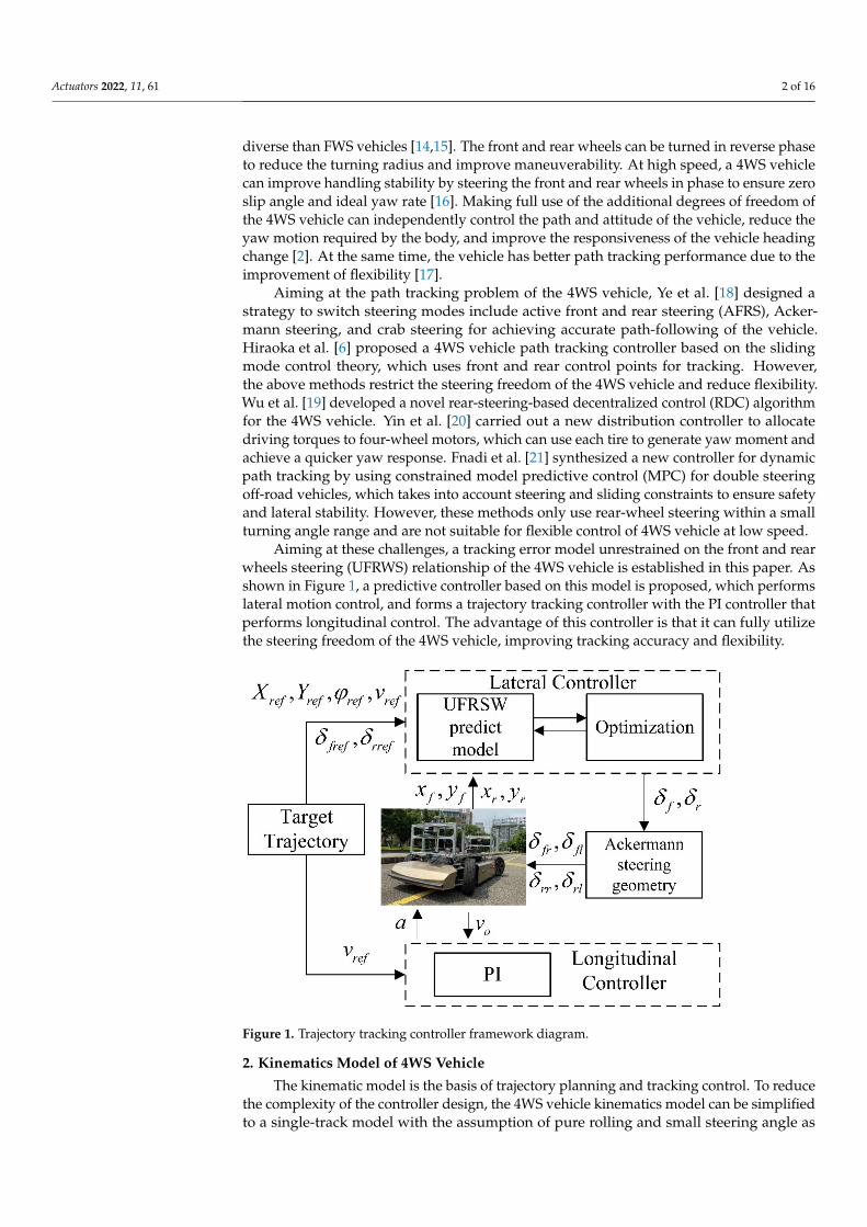
Aiming at these challenges, a tracking error model unrestrained on the front and rearwheels steering (UFRWS) relationship of the 4WS vehicle is established in this paper. Asshown in Figure 1, a predictive controller based on this model is proposed, which performslateral motion control, and forms a trajectory tracking controller with the PI controller thatperforms longitudinal control. The advantage of this controller is that it can fully utilizethe steering freedom of the 4WS vehicle, improving tracking accuracy and flexibility.

Figure 1. Trajectory tracking controller framework diagram.

2. Kinematics Model of 4WS Vehicle

The kinematic model is the basis of trajectory planning and tracking control. To reducethe complexity of the controller design, the 4WS vehicle kinematics model can be simplifiedto a single-track model with the assumption of pure rolling and small steering angle as

Actuators 2022, 11, 61 3 of 16

shown in Figure 2. The points F(x f , y f ) and B(xr, yr) are the center of the front and the rearaxle of the vehicle, respectively. The point M(x, y) is the geometric center of the vehicle,and the point C is the center of rotation of the vehicle.R denotes the radius of rotation ofthe vehicle. The wheelbase L is the distance between the front and rear axles, and the wheeltrack W refers to the distance between the left and right wheels. The heading angle ϕ refersto the angle between the body direction and the X axis in the global coordinate systemXOY. The center of mass slip angle β is the angle between the speed vm at the point M andthe direction of the body.

Figure 2. Schematic diagram of relevant variables of 4WS vehicle kinematics model.

The 4WS vehicle bicycle model is gray as shown in Figure 2. Its front steering angle δ fand rear steering angle δr should satisfy the Ackerman steering geometric relationship. So,the steering angle of each wheel δi(i = f r, f l, rr, rl) satisfies the Equation (1).

tan δ f l =tan δ f

1−W2L (tan δ f−tan δr)

tan δ f r =tan δ f

1+ W2L (tan δ f−tan δr)

tan δrl =tan δr

1−W2L (tan δ f−tan δr)

tan δrr =tan δr

1+ W2L (tan δ f−tan δr)

(1)

We take M as the control point. Then, the nonlinear kinematics equations of the 4WSvehicle bicycle model in the global coordinate system can be expressed as

.X = vm cos(ϕ + β).

Y = vm sin(ϕ + β).ϕ = vm cos(β)

L

(tan(

δ f

)− tan(δr)

)β = arctan

( tan δr+tan δ f2

) (2)

Most of the existing path tracking lateral control methods are designed for the ap-plication of front-wheel steering vehicles. Therefore, to apply PP and MPC methods tofour-wheel steered vehicles, this article regards 4WS as FWS vehicles with the wheelbasehalved by restricting the steering angles of the front and the rear to be equal and out ofphase as shown in Figure 3. Then, Equation (2) can be simplified to Equation (3), which isthe symmetrical front and the rear wheels steering (SFRWS) model of the 4WS vehicle. The

Actuators 2022, 11, 61 4 of 16

PP and MPC methods based on the SFRWS model can be used as the comparison algorithmin this article for the method based UFRWS model.

.X = vm cos ϕ.

Y = vm sin ϕ.ϕ = 2vm tan δ f /L

(3)

Figure 3. Schematic diagram of the SFRWS kinematics model of the 4WS vehicle.

Obviously, due to the constraint between the front and rear wheel angle relationship,the SFRWS model limits the steering freedom of 4WS vehicle, which reduces flexibility. Forthis reason, this paper proposes a predictive control method based on the unconstrainedsteering model of 4WS.

From the trigonometric function operation, we can get the Equation (4).

tan δr + tan δ f = tan(δ f + δr)(1− tan δr tan δ f ) (4)

We can further simplify the kinematics model because the vehicle turning angle is lessthan 30◦.

tan δr + tan δ f ≈ (δ f + δr) (5)

Combining Equations (1) and (5), we can get a simplified non-linear 4WS kinematicsmodel unrestrained on the front and the rear wheel steering relationship (UFRWS). Themodel is as follows: .

X = V cos(ψ +(

δr+δ f2

))

.Y = V sin(ψ +

(δr+δ f

2

))

.ψ =

V cos(

δr+δ f2

)` f +`r

(δ f − δr

) (6)

3. Optimal Predictive Control Based Different Model

In this section, the objective functions and constraints of system control quantityoptimization are designed based on the UFRWS model and SFRWS model. The optimiza-tion problem is solved in the form of a constrained quadratic programming and rollingoptimization is performed.

3.1. Linear Discrete Tracking Error Model Based UFRWS Model

We define the state vector χ = [ ex ey eϕ ]T , the control input u = [ δ f δr ]

T ,where the error ex is the difference between the actual position of the vehicle and thereference position in the X direction, the error ey is in the Y direction, and the heading error

Actuators 2022, 11, 61 5 of 16

eϕ is the difference between the vehicle heading angle and the reference heading angle.Then, the tracking error model based on UFRWS model can be obtained.

.χ =

.ex.ey.eϕ

=

.

X−.

Xre f.Y−

.Yre f.

ϕ− .ϕre f

= f (χ, u) (7)

Since the reference points are all on the reference trajectory, Equation (7) can be ex-panded by the first-order Taylor expansion at the reference state quantity χre f = [ 0 0 0 ]

T ,and we can get:

.χ =

∂ f (χ, u)∂χ

∣∣∣∣ χ = χre f ,u = ure f

(χ− χre f

)+

∂ f (χ, u)∂u

∣∣∣∣ χ = χre f ,u = ure f

(u− ure f

)(8)

Based on the Jacobi matrix, the state space form of the linear tracking error model canbe developed as follows: { .

χ = Aχ + Bu + Wη = Cχ

, (9)

where η is the state transition matrix, C is the 3× 3 identity matrix.Discretizing the continuous system Equation (9) by using the forward Euler method

can obtain a linear discrete tracking error model Equation (10).

χ(k + 1) = Adχ(k) + Bdu(k) + Wd, (10)

Where Ad = I + AT =

1 0 −Tvre f sin

(ϕre f + βre f

)0 1 Tvre f cos

(ϕre f + βre f

)0 0 1

,

Bd = BT =

− 1

2 Tvre f sin(

ϕre f + βre f

)− 1

2 Tvre f sin(

ϕre f + βre f

)12 Tvre f cos

(ϕre f + βre f

)12 Tvre f cos

(ϕre f + βre f

)−Tvre f

sinβre f (δ f−δr)−cosβre f2L −Tvre f

sinβre f (δ f−δr)+cosβre f2L

,

Wd = WT =

12 vre f sin

(ϕre f + βre f

)(δ f + δr)T

− 12 vre f cos

(ϕre f + βre f

)(δ f + δr)T

12 δ f vre f (sin βre f (δ f − δr)− cosβre f )T/L + 1

2 δrvre f (sin βre f (δ f − δr) + cosβre f )T/L

.

3.2. Linear Discrete Tracking Error Model Based SFRWS Model

Different from the UFRWS-based model, the control input of the SFRWS-based systemis only the front wheel angle, that is u = δ f . In the same way, the discretization modelbased SFRWS model can be obtained as follows:

χ(k + 1) = Adχ(k) + Bdu(k) + Wd, (11)

where Ad =

1 0 −Tvre f sin

(ϕre f

)0 1 Tvre f cos

(ϕre f

)0 0 1

,Bd =

00

Tvre fL cos2 δ f

,Wd = WT =

00

− Tvre f δ fL cos2 δ f

.

Actuators 2022, 11, 61 6 of 16

3.3. State Prediction Model

According to Equation (11), the state quantity at each moment can be predicted.

χ(k + 1|k ) = Adχ(k) + Bdu(k) + Wdχ(k + 2|k ) = Ad

2χ(k) + AdBdu(k) + Bdu(k + 1) + AdWd + Wdχ(k + 3|k ) = Ad

3χ(k) + A2dBdu(k) + AdBdu(k + 1) + Bdu(k + 2) + A2

dWd + AdWd + Wd...

χ(k + Np|k ) = AdNp χ(k) + A

Np−1d Bdu(k) + . . . + A

Np−Nc−1d Bdu(k + Nc) + ANP−1

d Wd + . . . + ANp−Npd Wd

(12)

Then, the state prediction equation is:

Y(k) = Ψχ(k) + ΘU(k) + We, (13)

where Y(k) =

η(k + 1|k )η(k + 2|k )η(k + 3|k )· · ·

η(k + Np|k )

, U(k) =

u(k|k )

u(k + 1|k )u(k + 2|k )· · ·

u(k + Nc|k )

, Ψ =

CAdCAd

2

CAd3

· · ·CAd

Np

,

Θ =

CBd

CAdBd CBdCAd

2Bd CAdBd CBd· · ·

CAdNp−1Bd CAd

Np−2Bd · · · CAdNp−Nc−1Bd

We =

CWd

CAdWd + CWdCA2

dWd + CAdWd + CWd...

CAk−1d Wd + CAk−2

d Wd + · · ·+ CWd

.

3.4. Scrolling Optimization

The control goal of the system is to make the 4WS vehicle track the target trajectoryquickly and stably. Therefore, it is necessary to optimize the state quantity of the system,the control quantity, and the amount of change in the control quantity.

At the k moment, the amount of change in the control quantity is defined as:

∆u(k) = u(k)− u(k− 1). (14)

Then:

∆U(k) =

∆u(k)

∆u(k + 1)· · ·

∆u(k + Nc)

=

1 −1−1 1

. . .−1 1

U = DU. (15)

The design objective function is as follows:

J(k) =Np

∑i=1‖χ(k + i)‖2

Q +Nc−1

∑i=1

∥∥∥U(k + i)−Ure f (k + i)∥∥∥2

R1+

Nc−1

∑i=1‖∆U(k + i)‖2

∆R, (16)

where the first part is to make the current state error that is the lateral error and headingerror close to 0. The importance of each state quantity can be adjusted by changing theweight value in the matrix R. The second part is to minimize the error between thecontrol quantity and the reference value. The weight of each control variable can be setby adjusting the weight value in the matrix R1. The third part is to make the change of

Actuators 2022, 11, 61 7 of 16

the control variable as small as possible to reduce the output angular velocity value. Theparameters and weights can be set by adjusting the matrix ∆R.

This paper mainly considers the control quantity limit constraint and control incrementconstraint in the control process. The expression form of the control quantity is as follows:

umin(k) 6 u(k) 6 umin(k), k = 0, 1, · · · , Nc − 1, (17)

The expression for the control increment is as follows:

∆umin(k) 6 ∆u(k) 6 ∆umin(k), k = 0, 1, · · · , Nc − 1, (18)

Define E = ΦX0 + W,R2 = DT∆RD. After simplifying, the cost function is trans-formed into a standard format for quadratic objective functions with linear constraints.

minJ = 12 UT HU + f TU

st.[Umin

∆Umin

]<

[ID

]U <

[Umax

∆Umax

] (19)

where H =(ΘTQΘ + R1 + R2

), f =

(ETQΘ−UT

r R1)T , Umin is the lower limit sequence

of the angle value umin, Umax is the upper limit sequence of the angle value umax, ∆Uminis the lower limit sequence of the angle rate value ∆umin, and ∆Umax is the upper limitsequence of the angle rate value ∆umax.

In each control cycle, the effective set method is used to solve the Equation (16), thenthe optimal control sequence in the control time domain is obtained.

U∗ =[

u∗k u∗k+1 · · · u∗k+Nc−1

](20)

The first element in the control sequence is used as the actual control input to act onthe system. After entering the next cycle, the optimal control sequence is recalculated andthe first control increment acts on the control system. So, scrolling realizes the optimalcontrol of vehicle trajectory tracking.

4. Experimental Results and Discussion

This article establishes a high-fidelity dynamic model in Carsim based on four-wheelsteer-by-wire vehicle, which forms a joint platform with Simulink for simulation exper-iments. After that, real vehicle trajectory tracking experiments were carried out. ThePure Pursuit based on the SFRWS (PP-SFRWS) model tracking method, the Model PredictControl based on the SFRWS (MPC-SFRWS) model, and the Model Predict Control basedon the model unconstrained the front and the rear wheels steering (MPC-UFRWS) arecompared and verified.

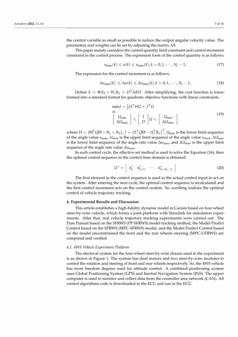
4.1. 4WS Vehicle Experiment Platform

The electrical system for the four-wheel steer-by-wire chassis used in the experimentis as shown in Figure 4. The system has dual motors and two steer-by-wire modules tocontrol the rotation and steering of front and rear wheels respectively. So, the 4WS vehiclehas more freedom degrees used for attitude control. A combined positioning systemuses Global Positioning System (GPS) and Inertial Navigation System (INS). The uppercomputer is used to monitor and collect data from the controller area network (CAN). Allcontrol algorithms code is downloaded to the ECU and run in the ECU.

Actuators 2022, 11, 61 8 of 16

Figure 4. Steer-by-wire electrical system for Chassis of 4WS vehicle.

The main structural parameters of 4WS AGV are shown in Table 1.

Table 1. Vehicle parameters.

Parameters Symbol Value Unit

The quality of the whole vehicle m 700 kgWheelbase L 1.9 m

Wheel track W 1.2 mMaximum steering angle δmax 30 ◦/s

Maximum steering angle rate ∆δmax 20 ◦/s

The vehicle drive control topology can be divided into the chassis domain and theautonomous driving domain as shown in Figure 5. The vehicle control unit (VCU) com-municate with the motor control unit (MCU), the steering by wire (SBW), the electricalhydraulic brake (EHB), the electric park brake (EPB), the battery management system(BMS), and instrument electronic control unit (I-ECU) through the CAN bus to obtain theinformation of the remote control, the automatic driving domain computer (IndustrialPersonal Computer, IPC), and the parallel driving controller.

Figure 5. The software architecture of the chassis platform.

In the trajectory tracking control system established in this paper, lidar is mainly usedto establish point cloud map and positioning. As shown in Figure 6, the acquisition ofvehicle pose in this paper mainly relies on the fusion positioning system composed of lidarand GNSS-RTK.

Actuators 2022, 11, 61 9 of 16

Figure 6. The location system framework.

When the vehicle starts outdoors, the navigation system is initialized with the GNSS-RTK information at the starting point. When the IMU data are received, the state variablesof navigation system (position, speed, attitude, etc.) are updated recursively, and therecursive prediction is calculated to represent the uncertainty of the error state. Whenthe LIDAR point cloud is received, the local map is used for registration, and the poseinformation of the vehicle relative to the local map is obtained. Taking the pose informationas the observation, the new error state quantity and the filter gain are calculated. Theparameters of the navigation module are modified according to the filter gain to realize thedata fusion between IMU and LIDAR. As a result, vehicle pose is generated accurately andoutput to the control module.

4.2. Simulation Platform Construction

Based on the vehicle parameters of the experimental platform, a vehicle dynamicssimulation model is established in Carsim, where the road adhesion coefficient is set to 0.8,and the rolling resistance coefficient is set to 0.8. The trajectory tracking controller is builtby the S-function module in Simulink. A co-simulation platform is established with Carsimas shown in Figure 7.

Figure 7. Carsim/Simulink co-simulation platform.

Actuators 2022, 11, 61 10 of 16

In the vehicle trajectory tracking simulation, the double lane change maneuver isa commonly used reference trajectory in the trajectory tracking test. In this paper, thefunction equation of the double lane change trajectory used in the simulation is as follows Yre f (X) =

dy12 (1 + tanh(z1))−

dy22 (1 + tanh(z2))

ϕre f (X) = tan−1(dy1

(1

cosh(z1)

)2( 1.2dx1

)− dy2

(1

cosh(z2)

)2( 1.2dx2

))

(21)

where z1 = 2.425 (X − 27.19) − 1.2, z2 = 2.4

21.95 (X − 56.46) − 1.2, dx1= 25, dx2= 21.95,dy1= 4.05, dy2= 5.7.

4.3. Analysis of Simulation Results

The simulation and real vehicle verification results are represented based on thetrajectory of the vehicle’s geometric center point. As shown in Figure 8a,b, the MPC-UFRSSmethod has better tracking performance for double lane change maneuver. At a speed of5 m/s, the maximum lateral tracking error of the MPC-UFRWS method does not exceed0.01 m, with 0.03 m for the SFRSW method and 0.1 m for the PP-SFRSW method.

Figure 8. Cont.

Actuators 2022, 11, 61 11 of 16

Figure 8. Simulation results of different algorithms. (a) Trajectory tracking; (b) Lateral error; (c) Steer-ing angle.

As shown in Figure 8c, the PP-SFRSW method has the hard constraint between thefront and rear wheels that the equal steering angles and opposite phase, while the MPC-UFRWS does not have this limitation. Therefore, the latter steering control changes aremore flexible in corners, and the front and rear wheels steering forms are more diverse.As shown in Figure 8, when the vehicle enters the curve, the MPC-UFRWS method isrelatively gentle, while the lateral tracking error of the PP-SFRSW increases sharply. Thefront and rear wheels angle adjustment of the MPC-UFRWS is larger, which can respond tothe change of tracking error faster and track reference trajectory more flexibly.

4.4. Simulation Comparison at Different Speeds

The trajectory tracking of the MPC-UFRWS method comparison at different speeds isas shown in Figure 9. The greater speed, the greater the control error and the greater theovershoot. Similar to other methods based on the kinematics model, the proposed methodis suitable for low-speed conditions. When the speed is less than 5 m/s, the lateral trackingerror is less than 0.01 m. When the speed is 10 m/s, the lateral tracking error is greaterthan 0.06 m. However, when the speed is 15 m/s, the vehicle path deviates far from thereference path.

Figure 9. Cont.

Actuators 2022, 11, 61 12 of 16

Figure 9. Tracking comparison at a different speed. (a) Trajectory tracking; (b) Lateral error.

4.5. Analysis of Real Vehicle Verification Results

To ensure the safety of personnel and vehicles, the vehicle experiment was carriedout in an open space of Sun Yat-sen University. To verify the performance of the vehicletracking straight and curved lines at the same time, we choose a recorded B-like trajectoryas the reference trajectory considering the site constraints. The test site and vehicle are asshown in Figure 10.

Figure 10. Experimental site and vehicle.

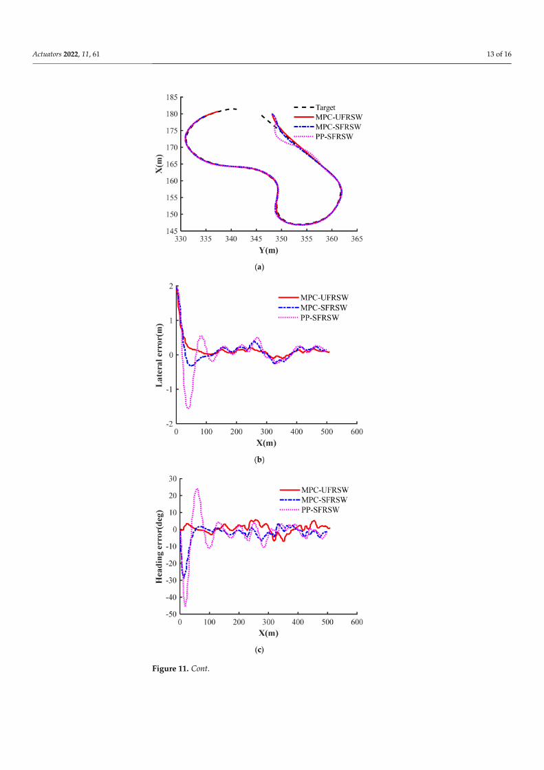
The real vehicle verification results of MPC-UFRWS, PP-SFRWS, and MPC-SFRWS areas shown in Figure 11 and Table 2, and analysis are as follows:

Actuators 2022, 11, 61 13 of 16

Figure 11. Cont.

Actuators 2022, 11, 61 14 of 16

Figure 11. Results of different methods in vehicle experiments. (a) Trajectory tracking; (b) Lateralerror; (c) Heading error; (d) Steering angle.

Table 2. Result data of vehicle verification.

Method Max LatErr MaxYawErr stdPLatErr stdPYawErr

PP-SFRWS 0.7663 12.2829 0.3168 3.4911MPC-SFRWS 0.3488 7.2850 0.1202 1.7169MPC-UFRWS 0.1998 6.7354 0.0678 2.6064

1. Compared with the PP-SFRWS method, the trajectory tracking accuracy of the MPC-UFRSW is higher. At the speed of 2 m/s, the maximum lateral error and yaw angleerror are reduced by 0.567 m and 5.55◦, respectively. This is because the Pure Pursuitmethod only determines the control input based on the deviation of the currentmeasured values from the reference value, while the MPC method uses the predictionmodel to estimate the future deviation value and determine the current values in arolling optimization manner.

2. The MPC-UFRWS method has higher tracking accuracy than the MPC-SRFRS. Ata speed of 2 m/s, the maximum lateral error and yaw angle error are reduced by0.15 m and 0.5◦, respectively. This is because MPC-UFRWS does not constrain therelationship between the front and rear wheels angle, which can give full play to themore flexible characteristics of 4WS vehicle and avoid oversteering or understeering.

3. The proposed method enables better steering flexibility of 4WS vehicle. At the startingpoint, the lateral error between the vehicle and the reference trajectory is about 2.5 m.When the vehicle starts to drive, the MPC-URFSW method makes the vehicle mergeinto the trajectory in an approximate crab-walking manner, while the front and rearwheels turn in phase or out of phase in the corners. Therefore, the proposed methodcan realize the switching of various steering modes such as out-of-phase steering andcrab steering without adding additional judgment.

4. Compared with the simulation results, the real vehicle tracking error increases severaltimes. The reason may be that the curvature change rate of the B-like rail is largerthan the double lane change maneuver. At the same time, external factors such asactuators, sensors, and road surfaces may also cause large tracking errors duringvehicle verification.

5. Conclusions

In this paper, a path tracking controller with unconstrained front and rear wheelssteering is established for the trajectory tracking control of 4WS vehicle. The controller

Actuators 2022, 11, 61 15 of 16

relies on the proposed optimization function considering the tracking accuracy and controlflexibility. Then, the simulation and vehicle verification are carried out to prove theeffectiveness of the controller. In the Carsim/Simulink platform, MPC-UFRSW has highertracking accuracy than PP-SFRSW and MPC-SFRSW when tracking double lane changetrajectory at a speed not exceeding 10 m/s. In the real vehicle experiment with B-likecurve, the steering angle of the front and rear wheels of the proposed controller changesmore flexibly. The maximum lateral error and yaw angle error are reduced by 60% and 9%,respectively. The simulation and real vehicle verification results show that the proposedmethod has more flexible steering modes and higher tracking accuracy. The next work willfurther analyze the stability of the trajectory tracking of the 4WS vehicle at high speed fromthe dynamic point of view.

Author Contributions: Conceptualization, X.T. and D.L.; methodology, H.X.; validation, D.L., X.T.and H.X.; investigation, D.L.; data curation, D.L.; writing—original draft preparation, X.T. and D.L.;writing—review and editing, H.X.; visualization, D.L.; project administration, H.X. All authors haveread and agreed to the published version of the manuscript.

Funding: This research was funded by the Natural Science and Technology Special Projects underGrant 2019-1496, Southern Marine Science and Engineering Guangdong Laboratory (Zhuhai) underGrant SML2020SP011, and the Key-Area Research and Development Program of Guangdong Provinceunder Grant 2020B090921003.

Institutional Review Board Statement: Not applicable.

Informed Consent Statement: Not applicable.

Data Availability Statement: Detailed data are contained within the article. More data that supportthe findings of this study are available from the author D.L. upon reasonable request.

Acknowledgments: The authors are thankful for the support of the School of Intelligent SystemsEngineering, Sun Yat-sen University, China Nuclear Power Engineering Co., Ltd., and SouthernMarine Science and Engineering Guangdong Laboratory. At the same time, we thank Guohui Wuand Yuelong Pan for their help in the experiment and writing.

Conflicts of Interest: The authors declare no conflict of interest.

References1. Paden, B.; Cap, M.; Yong, S.Z.; Yershov, D.; Frazzoli, E. A Survey of Motion Planning and Control Techniques for Self-Driving

Urban Vehicles. IEEE Trans. Intell. Veh. 2016, 1, 33–55. [CrossRef]2. Hang, P.; Chen, X. Path tracking control of 4-wheel-steering autonomous ground vehicles based on linear parameter-varying

system with experimental verification. Proc. Inst. Mech. Eng. Part I J. Syst. Control. Eng. 2021, 235, 411–423. [CrossRef]3. Cui, Q.; Ding, R.; Wei, C.; Zhou, B. Path-tracking and lateral stabilisation for autonomous vehicles by using the steering angle

envelope. Veh. Syst. Dyn. 2020, 59, 1672–1696. [CrossRef]4. Coulter, R. Implementation of the Pure Pursuit Path Tracking Algorithm. Carnegie-Mellon UNIV Pittsburgh PA Robotics INST,

1992; p. CM U-RI-TR-92-01.5. Thrun, S.; Montemerlo, M.; Dahlkamp, H.; Stavens, D.; Aron, A.; Diebel, J.; Fong, P.; Gale, J.; Halpenny, M.; Hoffmann, G.; et al.

Stanley: The robot that won the DARPA Grand Challenge. J. Field Robot. 2006, 23, 661–692. [CrossRef]6. Hiraoka, T.; Nishihara, O.; Kumamoto, H. Automatic path-tracking controller of a four-wheel steering vehicle. Veh. Syst. Dyn.

2009, 47, 1205–1227. [CrossRef]7. Jiang, Z.; Xiao, B. LQR optimal control research for four-wheel steering forklift based-on state feedback. J. Mech. Sci. Technol. 2018,

32, 2789–2801. [CrossRef]8. Park, M.; Kang, Y. Experimental Verification of a Drift Controller for Autonomous Vehicle Tracking: A Circular Trajectory Using

LQR Method. Int. J. Control Autom. Syst. 2021, 19, 404–416. [CrossRef]9. Falcone, P.; Borrelli, F.; Asgari, J.; Tseng, H.E.; Hrovat, D. Predictive Active Steering Control for Autonomous Vehicle Systems.

IEEE Trans. Contr. Syst. Technol. 2007, 15, 566–580. [CrossRef]10. Kabzan, J.; Hewing, L.; Liniger, A.; Zeilinger, M.N. Learning-based Model Predictive Control for Autonomous Racing. IEEE

Robot. Autom. Lett. 2019, 4, 3363–3370. [CrossRef]11. Geng, K.; Chulin, N.A.; Wang, Z. Fault-Tolerant Model Predictive Control Algorithm for Path Tracking of Autonomous Vehicle.

Sensors 2020, 20, 4245. [CrossRef] [PubMed]12. Jiang, J.; Astolfi, A. Lateral Control of an Autonomous Vehicle. IEEE Trans. Intell. Veh. 2018, 3, 228–237. [CrossRef]

Actuators 2022, 11, 61 16 of 16

13. Furukawa, Y.; Yuhara, N.; Sano, S.; Takeda, H.; Matsushita, Y. A Review of Four-Wheel Steering Studies from the Viewpoint ofVehicle Dynamics and Control. Veh. Syst. Dyn. 1989, 18, 151–186. [CrossRef]

14. Oksanen, T.; Backman, J. Guidance system for agricultural tractor with four wheel steering. IFAC Proc. Vol. 2013, 46, 124–129.[CrossRef]

15. Yan, Y.; Geng, K.; Liu, S.; Ren, Y. A New Path Tracking Algorithm for Four-Wheel Differential Steering Vehicle. In Proceedings ofthe 2019 Chinese Control and Decision Conference (CCDC), Nanchang, China, 3–5 June 2019; pp. 1527–1532.

16. Liang, Y.; Li, Y.; Zheng, L.; Yu, Y.; Ren, Y. Yaw rate tracking-based path-following control for four-wheel independent driving andfour-wheel independent steering autonomous vehicles considering the coordination with dynamics stability. Proc. Inst. Mech.Eng. Part D J. Automob. Eng. 2021, 235, 260–272. [CrossRef]

17. Hang, P.; Chen, X. Towards Autonomous Driving: Review and Perspectives on Configuration and Control of Four-WheelIndependent Drive/Steering Electric Vehicles. Actuators 2021, 10, 184. [CrossRef]

18. Ye, Y.; He, L.; Zhang, Q. Steering Control Strategies for a Four-Wheel-Independent-Steering Bin Managing Robot. IFAC-PapersOnLine 2016, 49, 39–44. [CrossRef]

19. Wu, Y.; Li, B.; Zhang, N.; Du, H.; Zhang, B. Rear-Steering Based Decentralized Control of Four-Wheel Steering Vehicle. IEEETrans. Veh. Technol. 2020, 69, 10899–10913. [CrossRef]

20. Yin, D.; Wang, J.; Du, J.; Chen, G.; Hu, J.-S. A New Torque Distribution Control for Four-Wheel Independent-Drive ElectricVehicles. Actuators 2021, 10, 122. [CrossRef]

21. Fnadi, M.; Plumet, F.; Benamar, F. Model Predictive Control based Dynamic Path Tracking of a Four-Wheel Steering MobileRobot. In Proceedings of the IEEE/RSJ International Conference on Intelligent Robots and Systems (IROS), Macau, China,3–8 November 2019.