ARTICLE IN PRESS

0952-1976/$ - se

doi:10.1016/j.en

�CorrespondE-mail addr

Engineering Applications of Artificial Intelligence 20 (2007) 11–24

www.elsevier.com/locate/engappai

Optimal combination of document binarization techniques using aself-organizing map neural network

E. Badekas, N. Papamarkos�

Image Processing and Multimedia Laboratory, Department of Electrical & Computer Engineering, Democritus University of Thrace, 67100 Xanthi, Greece

Received 22 July 2005; received in revised form 6 April 2006; accepted 11 April 2006

Available online 11 July 2006

Abstract

This paper proposes an integrated system for the binarization of normal and degraded printed documents for the purpose of

visualization and recognition of text characters. In degraded documents, where considerable background noise or variation in contrast

and illumination exists, there are many pixels that cannot be easily classified as foreground or background pixels. For this reason, it is

necessary to perform document binarization by combining and taking into account the results of a set of binarization techniques,

especially for document pixels that have high vagueness. The proposed binarization technique takes advantage of the benefits of a set of

selected binarization algorithms by combining their results using a Kohonen self-organizing map neural network. Specifically, in the first

stage the best parameter values for each independent binarization technique are estimated. In the second stage and in order to take

advantage of the binarization information given by the independent techniques, the neural network is fed by the binarization results

obtained by those techniques using their estimated best parameter values. This procedure is adaptive because the estimation of the best

parameter values depends on the content of images. The proposed binarization technique is extensively tested with a variety of degraded

document images. Several experimental and comparative results, exhibiting the performance of the proposed technique, are presented.

r 2006 Elsevier Ltd. All rights reserved.

Keywords: Binarization; Thresholding; Document processing

1. Introduction

In general, digital documents include text, line-drawingsand graphics regions and can be considered as mixed typedocuments. In many practical applications there is need torecognize or improve mainly the text content of thedocuments. In order to achieve this, a powerful documentbinarization technique is usually applied. Documents in thebinary form can be recognized, stored, retrieved andtransmitted more efficiently than the original gray-scaleones. For many years, the binarization of gray-scaledocuments was based on the standard bilevel techniquesthat are also called global thresholding algorithms (Otsu,1979; Kittler and Illingworth, 1986; Reddi et al., 1984;Kapur et al., 1985; Papamarkos and Gatos, 1994; Chiet al., 1996). These techniques, which can be considered as

e front matter r 2006 Elsevier Ltd. All rights reserved.

gappai.2006.04.003

ing author. Tel.: +3025410 79585; fax: +30 25410 79569.

ess: papamark@ee.duth.gr (N. Papamarkos).

clustering approaches, are suitable for converting any gray-scale image into a binary form but are inappropriate forcomplex documents, and even more, for degraded docu-ments. However, the binarization of degraded documentimages is not an easy procedure because these documentscontain noise, shadows and other types of degradations. Inthese special cases, it is important to take into account thenatural form and the spatial structure of the documentimages. For these reasons, specialized binarization techni-ques have been developed for degraded document images.In one category, local thresholding techniques have been

proposed for document binarization. These techniquesestimate a different threshold for each pixel according tothe gray-scale information of the neighboring pixels. In thiscategory belong the techniques of Bernsen (1986), Chowand Kaneko (1972), Eikvil (1991), Mardia and Hainsworth(1988), Niblack (1986), Taxt et al. (1989), Yanowitz andBruckstein (1989), Sauvola et al. (1997), and Sauvola andPietikainen (2000). In another category belong the hybrid

ARTICLE IN PRESSE. Badekas, N. Papamarkos / Engineering Applications of Artificial Intelligence 20 (2007) 11–2412

techniques, which combine information of global andlocal thresholds. The best known techniques in thiscategory are the methods of Gorman (1994), and Liu andSrihari (1997).

For document binarization, probably, the most powerfultechniques are those that take into account not only theimage gray-scale values, but also the structural character-istics of the characters. In this category belong binarizationtechniques that are based on stroke analysis, such as thestroke width (SW) and characters geometry properties. Themost powerful techniques in this category are the logicallevel technique (LLT) (Kamel and Zhao, 1993) and itsimproved adaptive logical level technique (ALLT) (Yangand Yan, 2000), and the integrated function algorithmtechnique (IFA) (White and Rohrer, 1983) and itsadvanced ‘‘improvement of integrated function algorithm’’(IIFA) (Trier and Taxt, 1995b). For those two techniquesfurther improvements were proposed by Badekas andPapamarkos (2003). Recently, Papamarkos (2003) pro-posed a new neuro-fuzzy technique for binarization andgray-level (or color) reduction of mixed-type documents.According to this technique a neuro-fuzzy classifier is fedby not only the image pixels’ values but also withadditional spatial information extracted in the neighbor-hood of the pixels.

Despite the existence of all these binarization techniques,it is proved, by evaluations that have been carried out(Trier and Taxt, 1995a; Trier and Jain, 1995; Leedhamet al., 2003; Sezgin and Sankur, 2004), that there is not anytechnique that can be applied effectively to all types ofdigital documents. Each one of them has its ownadvantages and disadvantages.

The proposed binarization system, takes advantages ofbinarization results obtained by a set of the most powerfulbinarization techniques from all categories. These techni-ques are incorporated into one system and considered as itscomponents. We have included document binarizationtechniques that gave the highest scores in evaluation teststhat have been made so far. Trier and Taxt (1995a) foundthat Niblack’s and Bernsen’s techniques are the fastest ofthe best performing binarization techniques. Furthermore,Trier and Jain’s evaluation tests (1995) identify Niblack’stechnique, with a post-processing step, as the best. Kameland Zhao (1993) use six evaluation aspects (subjectiveevaluation, memory, speed, stroke-width restriction, num-ber of parameters of each technique) to evaluate andanalyze seven character/graphics extraction based binar-ization techniques. The best method, in this test, is theLLT. Recently, Sezgin and Sankur (2004), compare 40binarization techniques and they conclude that the localbased technique of Sauvola and Pietikainen (2000) as wellas the technique of White and Rohrer (IIFA) (Trier andTaxt, 1995b) are the best performing document binariza-tion techniques. Apart from the above techniques, weinclude in the proposed system the powerful globalthresholding technique of Otsu (1979) and the fuzzyC-mean (FCM) technique (Chi et al., 1996).

The main subject of the proposed document binarizationtechnique is to build a system that takes advantages of thebenefits of a set of selected binarization techniques bycombining their results, using the Kohonen self-organizingmap (KSOM) neural network. This is important, especiallyfor the fuzzy pixels of the documents, i.e. for the pixels thatcannot be easily classified. The techniques that areincorporated in the proposed system are the following:Otsu (1979), FCM (Chi et al., 1996), Bernsen (1986),Niblack (1986), Sauvola and Pietikainen (2000), andimprovement versions of ALLT (Yang and Yan, 2000;Badekas and Papamarkos, 2003), and IIFA (Trier andTaxt, 1995b; Badekas and Papamarkos, 2003). Most ofthese techniques, especially those coming from the categoryof local thresholding algorithms, have parameter valuesthat must be defined before their application to a documentimage. It is obvious that different values of the parameterset (PS) of a technique lead to different binarization resultswhich means that there is not a set of best PS values for alltypes of document images. Therefore, for every technique,in order to achieve the best binarization results the best PSvalues must be initially estimated.Specifically, in the first stage of the proposed binariza-

tion technique, a parameter estimation algorithm (PEA), isused to detect the best PS values of every documentbinarization technique. The estimation is based on theanalysis of the correspondence between the differentdocument binarization results obtained by the applicationof a specific binarization technique to a document image,using different PS values. The proposed method is based onthe work of Yitzhaky and Peli (2003) which has beenproposed for edge detection evaluation. In their approach,a specific range and a specific step for each one of theparameters is initially defined. The best values for the PSare then estimated by comparing the results obtained by allpossible combinations of the PS values. The best PS valuesare estimated using a receiver operating characteristics(ROC) analysis and a Chi-square test. In order to improvethis algorithm, a wide initial range for every parameter isused and in order to estimate the best parameter value anadaptive convergence procedure is applied. Specifically, ineach iteration of the adaptive procedure, the parameters’ranges are redefined according to the estimation of the bestbinarization result obtained. The adaptive procedureterminates when the ranges of the parameters valuescannot be further reduced and the best PS values are thoseobtained from the last iteration.In order to combine the best binarization results

obtained by the independent binarization techniques(IBT) using their best PS values, the KSOM neuralnetwork (Strouthopoulos et al., 2002; Haykin, 1994) isused as the final stage of the proposed method. Specifically,the neural network classifier is fed using the binarizationresults obtained from the application of the IBT and acorresponding weighting value that is calculated for eachone of them. After the training stage, the output neuronsspecify the classes obtained, and using a mapping

ARTICLE IN PRESS

Fig. 1. The structure of the Kohonen self-organizing map neural network.

E. Badekas, N. Papamarkos / Engineering Applications of Artificial Intelligence 20 (2007) 11–24 13

procedure, these classes are categorized as classes of theforeground and background pixels.

The proposed binarization technique was extensivelytested by using a variety of document images most of whichcome from the old Greek Parliamentary Proceedings andfrom the Mediateam Oulu Document Database (Sauvolaand Kauniskangas, 1999). Characteristic examples andcomparative results are presented to confirm the effective-ness of the proposed method. The entire system has beenimplemented in a visual environment.

The main stages of the proposed binarization system areanalyzed in Section 2. Section 3, describes analytically themethod that is used to detect the best binarization resultobtained by the application of the IBT. Also, the samesection illustrates the algorithm used for the estimation ofthe weighting values for each one of the IBT. Section 4,analyses the method used for the detection of the properparameter values. Section 5, gives a recent description ofthe IBT included in the proposed binarization system.Finally, Section 6 presents the experimental results andSection 7 the conclusions.

2. Description of the proposed binarization system

The proposed binarization system performs documentbinarization by combining the best results of a set of IBT,most of which are developed for document binarization.That is, a number of powerful IBT are included in theproposed binarization system. Specifically, the IBT thatwere implemented and included in the proposed evaluationsystem are:

�

Otsu (1979), � FCM (Chi et al., 1996), � Bernsen (1986), � Niblack (1986), � Sauvola and Pietikainen (2000), � An improved version of ALLT (Yang and Yan, 2000;

Badekas and Papamarkos, 2003) and

� An improved version of IIFA (Trier and Taxt, 1995b;

Badekas and Papamarkos, 2003).

The structure of the KSOM used in the proposedtechnique is depicted in Fig. 1. The number of the inputneurons is equal to the number of the IBT included in thebinarization system. The number of the output neurons isusually taken equal to four. Usually, the KSOM for itsconvergence needs 300 epochs. The initial neighboringparameter d is taken equal to the number of the outputneurons and the initial learning rate a is equal to 0.05. TheKSOM is competitively trained according to the followingweight update function:

Dwij ¼aðyi � wijÞ; if c� j

�� ��od;

0; otherwise

((1)

where yi are the input values, c the winner neuron and i,j

are the numbers of input and output neurons. The valuesof parameters a and d are reduced during the learningprocess.A step by step description of the proposed document

binarization technique follows:Stage 1: Initially choose the N IBT that will participate

in the binarization system.Stage 2: For those of the selected IBT that have

parameters, estimate the best PS values of them for thespecific image. Section 4, analyzes the Parameter Estima-tion Algorithm which is a converge procedure used toestimate the best PS values for each one of the selected IBT.

Stage 3: Apply the IBT, using their best PS values, toobtain In(x,y), n ¼ 1y,N binary images.

Stage 4: Compare the binarization results obtained bythe IBT and calculate a weighting value wn, n ¼ 1y,N foreach binary image according to the comparison resultsobtained using the chi-square test. Analytical descriptionof how the weighting values are calculated is given inSection 3.

Stage 5: Define the Sp set of pixels, the binary values ofwhich will be used to feed the KSOM. If Np is the numberof pixels obtained, and N IBT are included in the system,then we have NT ¼ N �Np training samples. The Sp set ofpixels must include mainly the ‘‘fuzzy’’ pixels, i.e. the pixelsthat cannot be easily classified as background or fore-ground pixels. For this reason, the Sp set of pixels is usuallyobtained by using the FCM classifier (Chi et al., 1996).Thus, these pixels can be defined as the pixels with highvagueness, as they come up from the application of theFCM method. To achieve this, the image is firstly binarizedusing the FCM method and then the fuzzy pixels aredefined as those pixels having membership function (MF)values close to 0.5. That is, the pixels with MF values close

ARTICLE IN PRESSE. Badekas, N. Papamarkos / Engineering Applications of Artificial Intelligence 20 (2007) 11–2414

to 0.5 are the vague ones and their degree of vaguenessdepend on how close to 0.5 are these values.

According to above analysis, the proper Sp set isobtained by the following procedure:

(a)

Apply the FCM globally to the original image and fortwo classes only. After this, each pixel has two MF

values: MF1 and MF2.

(b) Scale the MF values of each pixel (x,y) to the range

[0,255] and produce a new gray-scale image Iv, usingthe relation

IV ðx; yÞ ¼ round 255ðmaxðMF 1;MF 2Þ �minðMF 1;MF 2Þ

1�minðMF1;MF 2Þ

� �.

(2)

(c)

Apply the global binarization technique of Otsu toimage Iv and obtain a new binary image Ip. The set ofpixels Sp is now defined as the pixels of Ip that havevalue equal to zero.Instead of using the FCM the Sp set of pixels can bealternatively obtained as� Edge pixels extracted from the original image by the

application of an edge extraction mask. This is agood choice because the majority of fuzzy pixels areclose to the edge pixels.� Random pixels sampled from the entire image. This

option is used in order to adjust the number oftraining pixels as a percentage of the total number ofimage pixels.

Stage 6: The training set ST is defined as the set ofthe binary values of the N binary images that correspondto the positions of the Sp set pixels. In this stage theweighting values wn, n ¼ 1,y,N, can be used to adjust theinfluence of each binary image to the final binarizationresult via the KSOM. Using the weighting values thetraining set ST is composed of the binary values of the N

binary images multiplied by the corresponding weightingvalues.

Stage 7: Define the number of the output neurons of theKSOM and feed the neural network with the values of theST set. From our experiments, it has been found that aproper number for the output neurons is K ¼ 4. After thetraining, the centers of the output classes obtainedcorrespond to Ok, k ¼ 1,y,K vectors.

Stage 8: Classify each output class (neuron) as back-ground or foreground by examining the Euclideandistances of their centers from the [0,y,0]T and [1,y,1]T

vectors, which represent the background and foregroundpositions in the feature space, respectively. That is

Ok ¼backgound class; if

ffiffiffiffiffiffiffiffiffiffiffiffiffiffiffiffiffiPNi¼1

O2kðiÞ

so

ffiffiffiffiffiffiffiffiffiffiffiffiffiffiffiffiffiffiffiffiffiffiffiffiffiffiffiffiffiffiffiPNi¼1

OkðiÞ � 1½ �2;

s

foreground class; otherwise:

8><>:

(3)

Stage 9: This stage is the mapping stage. Each pixelcorresponds to a vector of N elements with values thebinary results obtained by the N IBT multiplied by theirweighting values. During the mapping process, each pixel isclassified by the KSOM to one of the obtained classes, andconsequently to background or foreground pixel.

Stage 10: A post-processing step can be applied toimprove and emphasize the final binarization results. Thisstep usually includes a size filtering or the application of theMDMF filters (Ping and Lihui, 2001).

3. Obtaining the best Binarization Result

It is obvious that when a document is binarized, it is notknown initially the optimum result that must be obtained.This is a major problem in comparative evaluation tests. Inorder to have comparative results, it is important toestimate a ground truth image. By estimating the groundtruth image we can compare the different binarizationresults obtained, and therefore, we can choose the best.This ground truth image, known as estimated ground truth(EGT) image, can be selected from a list of potentialground truth (PGT) images, as it is proposed by Yitzhakyand Peli (2003) for edge detection evaluation.Consider N document binary images Dj(k,l), j ¼ 1,y,N

of size K�L, obtained by the application of a documentbinarization technique using N different PS values or by N

IBT. In order to estimate the best binary image it isnecessary to obtain the EGT image. Then, the independentbinarization results are compared with the EGT imageusing the ROC analysis or a Chi-square test.Let pgti(k,l), i ¼ 1,y,N be the N PGT images and

egt(k,l) the EGT image. In the entire procedure is describedbelow ‘‘0’’ and ‘‘1’’ are considered the background andforeground pixels, respectively.

Stage 1: For every pixel, it is calculated how many binaryimages consider this as foreground pixel. The results are storedin a matrix C(k,l), k ¼ 0,y, K�1 and l ¼ 0,y,L�1. It isobvious that the values of this matrix will be between 0 and N.

Stage 2: N pgti(k,l), i ¼ 1,y,N binary images areproduced using the matrix C(k,l). Every pgt(k,l) image isconsidered as the image that has as foreground pixels allthe pixels with C(k,l)Zi.

Stage 3: For each pgti(k,l) image, four cases are defined:

�

A pixel is a foreground pixel in both pgti(k,l) and Dj(k,l),images:

TPpgti ;Dj¼

1

K � L

XK

k¼1

XL

l¼1

pgti1 ðk; lÞ \Dj1 ðk; lÞ. (4)

�

A pixel is a foreground pixel in pgti(k,l) image andbackground pixel in Dj(k,l) image:

FPpgti ;Dj¼

1

K � L

XK

k¼1

XL

l¼1

pgti1 ðk; lÞ \Dj0 ðk; lÞ. (5)

ARTICLE IN PRESSE. Badekas, N. Papamarkos / Engineering Applications of Artificial Intelligence 20 (2007) 11–24 15

�

A pixel is a background pixel in both pgti(k,l) and Dj(k,l)images:

TNpgti ;Dj¼

1

K � L

XK

k¼1

XL

l¼1

pgti0ðk; lÞ \Dj0 ðk; lÞ. (6)

�

Fig. 2. An example of a CT-ROC diagram. The 5th level is the CT level.

Fig. 3. An example of a CT chi-square histogram. The 5th level is the CT

level.

A pixel is a background pixel in pgti(k,l) image andforeground pixel in Dj(k,l) image:

FNpgti ;Dj¼

1

K � L

XK

k¼1

XL

l¼1

pgti0ðk; lÞ \Dj1 ðk; lÞ, (7)

pgti0ðk; lÞ and pgti1ðk; lÞ represent the background andforeground pixels in pgti(k,l) image, while Djo(k,l) andDj1(k,l) represent the background and foreground pixels inDj(k,l) image. According to the above definitions, for eachpgti(k,l) the average value of the four cases resulting fromits match with each of the individual binarization resultsDj(k,l), is calculated:

TPpgti¼

1

N

XN

j¼1

TPpgti ;Dj, (8)

FPpgti¼

1

N

XN

j¼1

FPpgti ;Dj, (9)

TNpgti¼

1

N

XN

j¼1

TNpgti ;Dj, (10)

FNpgti¼

1

N

XN

j¼1

FNpgti ;Dj. (11)

Stage 4: In this stage, the sensitivity TPRPgti andspecificity (1�FPRPgti) values are calculated according tothe relations:

TPRpgti¼

TPpgti

P, (12)

FPRpgti¼

FPpgti

1� P, (13)

where P ¼ TPPgti+FNPgti, 8i.Stage 5: This stage is used to obtain the egt(k,l) image,

which is selected to be one of the Pgti(k,l) images. There aretwo methods that can be used:

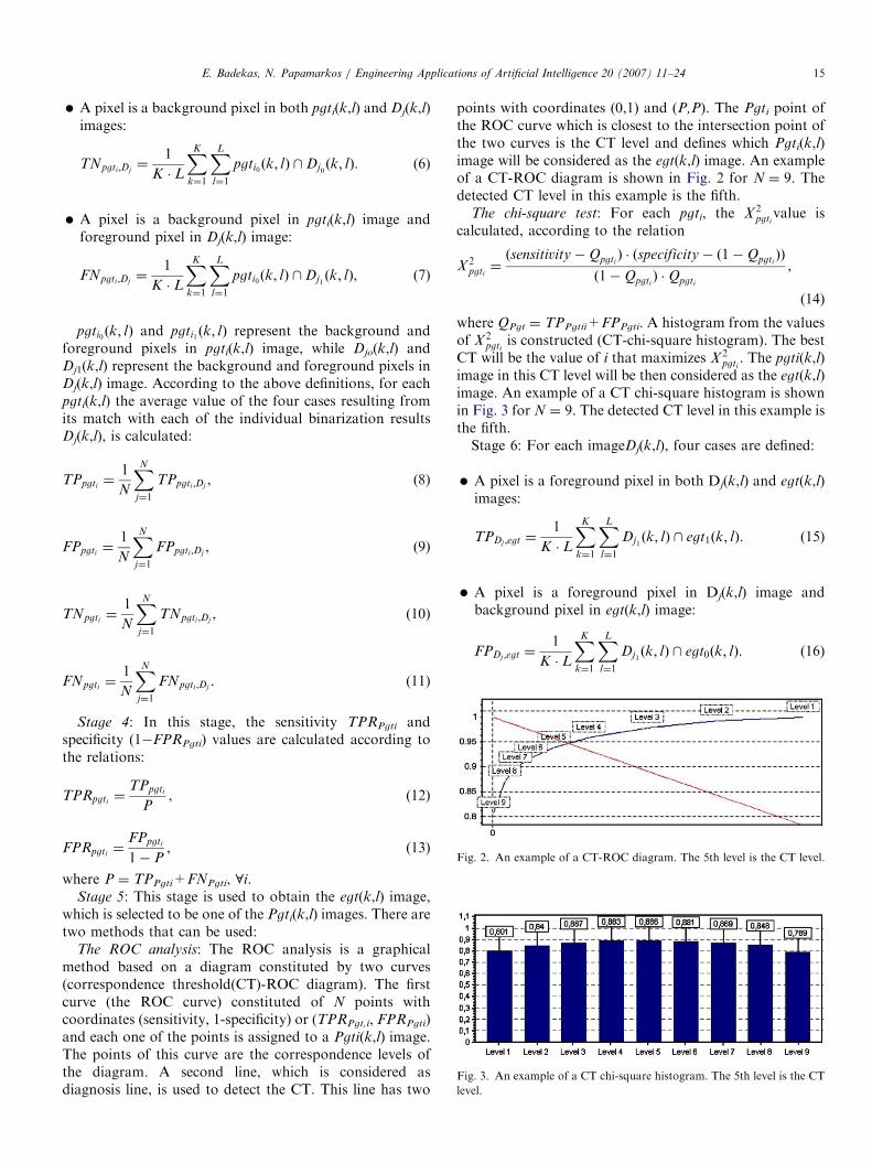
The ROC analysis: The ROC analysis is a graphicalmethod based on a diagram constituted by two curves(correspondence threshold(CT)-ROC diagram). The firstcurve (the ROC curve) constituted of N points withcoordinates (sensitivity, 1-specificity) or (TPRPgt,i, FPRPgti)and each one of the points is assigned to a Pgti(k,l) image.The points of this curve are the correspondence levels ofthe diagram. A second line, which is considered asdiagnosis line, is used to detect the CT. This line has two

points with coordinates (0,1) and (P,P). The Pgti point ofthe ROC curve which is closest to the intersection point ofthe two curves is the CT level and defines which Pgti(k,l)image will be considered as the egt(k,l) image. An exampleof a CT-ROC diagram is shown in Fig. 2 for N ¼ 9. Thedetected CT level in this example is the fifth.

The chi-square test: For each pgti, the X 2pgti

value iscalculated, according to the relation

X 2pgti¼ðsensitivity�Qpgti

Þ � ðspecificity� ð1�QpgtiÞÞ

ð1�QpgtiÞ �Qpgti

,

(14)

where QPgt ¼ TPPgtii+FPPgti. A histogram from the valuesof X 2

pgtiis constructed (CT-chi-square histogram). The best

CT will be the value of i that maximizes X 2pgti

. The pgti(k,l)image in this CT level will be then considered as the egt(k,l)image. An example of a CT chi-square histogram is shownin Fig. 3 for N ¼ 9. The detected CT level in this example isthe fifth.Stage 6: For each imageDj(k,l), four cases are defined:

�

A pixel is a foreground pixel in both Dj(k,l) and egt(k,l)images:

TPDj ;egt ¼1

K � L

XK

k¼1

XL

l¼1

Dj1 ðk; lÞ \ egt1ðk; lÞ. (15)

�

A pixel is a foreground pixel in Dj(k,l) image andbackground pixel in egt(k,l) image:

FPDj ;egt ¼1

K � L

XK

k¼1

XL

l¼1

Dj1 ðk; lÞ \ egt0ðk; lÞ. (16)

ARTICLE IN PRESS

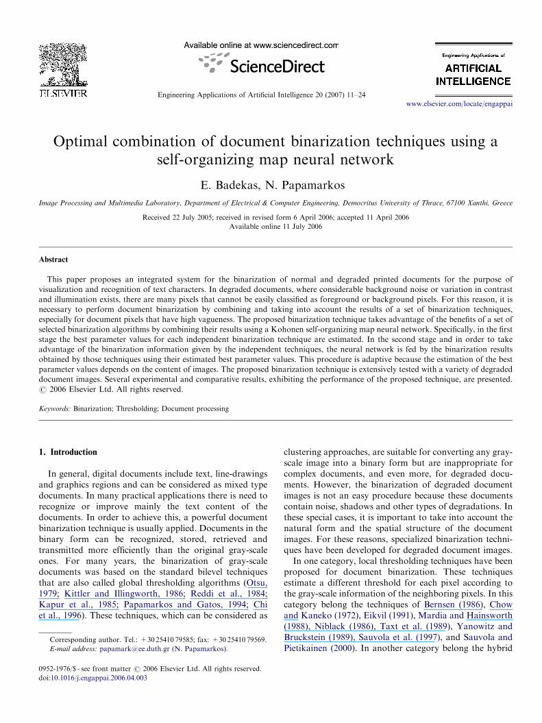
Fig. 4. A 9-level chi-square histogram. The detected best values are W ¼ 5, k ¼ 0.25 in the fifth level.

E. Badekas, N. Papamarkos / Engineering Applications of Artificial Intelligence 20 (2007) 11–2416

�

Fig. 5. Initial gray-scale document image for Experiment 1.

A pixel is a background pixel in both Dj(k,l) and egt(k,l)images:

TNDj ;egt ¼1

K � L

XK

k¼1

XL

l¼1

Dj0 ðk; lÞ \ egt0ðk; lÞ. (17)

�

Table 1

Initial ranges and the estimated best PS values for Experiment 1

Technique Initial ranges Best PS values

1. Niblack WA[1,9], kA[0.1,1] W ¼ 5 and k ¼ 0.32

2. Sauvola WA[1,9], kA[0.1,0.4] W ¼ 5 and k ¼ 0.17

3. Bernsen WA[1,9], LA[10,100] W ¼ 5 and L ¼ 89

4. ALLT aA[0.1,0.25] a ¼ 0.10

5. IIFA TpA[10,40] Tp ¼ 24

A pixel is a background pixel in Dj(k,l) image andforeground pixel in egt(k,l) image:

FNDj ;egt ¼1

K � L

XK

k¼1

XL

l¼1

Dj0 ðk; lÞ \ egt1ðk; lÞ. (18)

Stage 7: Stages 4 and 5 are repeated to compare eachbinary image Dj(k,l) with the egt(k,l) image, using relations(15)–(18) rather than relations (8)–(11) which are used inStage 3. According to the chi-square test, the maximumvalue of X 2

Dj ;egt indicates the Dj(k,l) image which is theestimated best document binarization result. Sorting thevalues of the chi-square histogram, the binarization resultsare sorted according to their quality.

The values of the chi-square test obtained in Stage 7 areconsidered as the weighting values that are used in Stage 6of the proposed binarization technique, described inSection 2. The relation that gives the weighting value foreach one of the IBT is

wj ¼ X 2Dj ;egt. (19)

4. Parameter estimation algorithm

In the first stage of the proposed binarization techniqueit is necessary to estimate the best PS values for each one ofthe IBT. This estimation is based on the method ofYitzhaky and Peli (2003) proposed for edge detectionevaluation. However, in order to increase the accuracy ofthe estimated best PS values we improve this algorithm by

using a wide initial range for every parameter and anadaptive convergence procedure. That is, the ranges of theparameters are redefined according to the estimation ofthe best binarization result obtained in each iteration of theadaptive procedure. This procedure terminates when theranges of the parameters values cannot be further reducedand the best PS values are those obtained from the lastiteration. It is important to notice that this is an adaptiveprocedure because it is applied to every processingdocument image.The main stages of the proposed PEA, for two

parameters (P1,P2), are as follows:Stage 1: Define the initial range of the PS values.

Consider as [S1,e1] the range for the first parameter and[S2,e2] the range for the second one.

Stage 2: Define the number of steps that will be used ineach iteration. For the two parameters case, let St1 and St2be the numbers of steps for the ranges [S1,e1] and [S2,e2],respectively. In most cases St1 ¼ St2 ¼ 3.

ARTICLE IN PRESS

Table 2

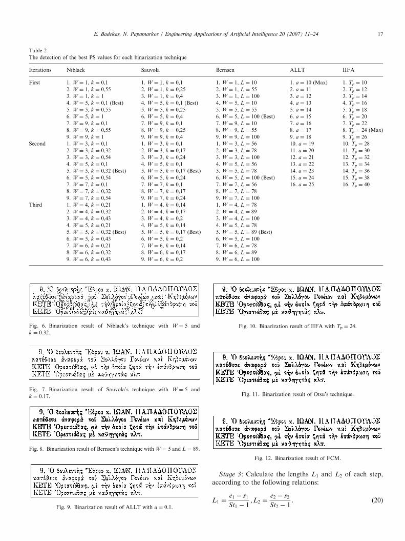
The detection of the best PS values for each binarization technique

Iterations Niblack Sauvola Bernsen ALLT IIFA

First 1. W ¼ 1, k ¼ 0,1 1. W ¼ 1, k ¼ 0,1 1. W ¼ 1, L ¼ 10 1. a ¼ 10 (Max) 1. Tp ¼ 10

2. W ¼ 1, k ¼ 0,55 2. W ¼ 1, k ¼ 0,25 2. W ¼ 1, L ¼ 55 2. a ¼ 11 2. Tp ¼ 12

3. W ¼ 1, k ¼ 1 3. W ¼ 1, k ¼ 0,4 3. W ¼ 1, L ¼ 100 3. a ¼ 12 3. Tp ¼ 14

4. W ¼ 5, k ¼ 0,1 (Best) 4. W ¼ 5, k ¼ 0,1 (Best) 4. W ¼ 5, L ¼ 10 4. a ¼ 13 4. Tp ¼ 16

5. W ¼ 5, k ¼ 0,55 5. W ¼ 5, k ¼ 0,25 5. W ¼ 5, L ¼ 55 5. a ¼ 14 5. Tp ¼ 18

6. W ¼ 5, k ¼ 1 6. W ¼ 5, k ¼ 0,4 6. W ¼ 5, L ¼ 100 (Best) 6. a ¼ 15 6. Tp ¼ 20

7. W ¼ 9, k ¼ 0,1 7. W ¼ 9, k ¼ 0,1 7. W ¼ 9, L ¼ 10 7. a ¼ 16 7. Tp ¼ 22

8. W ¼ 9, k ¼ 0,55 8. W ¼ 9, k ¼ 0,25 8. W ¼ 9, L ¼ 55 8. a ¼ 17 8. Tp ¼ 24 (Max)

9. W ¼ 9, k ¼ 1 9. W ¼ 9, k ¼ 0,4 9. W ¼ 9, L ¼ 100 9. a ¼ 18 9. Tp ¼ 26

Second 1. W ¼ 3, k ¼ 0,1 1. W ¼ 3, k ¼ 0,1 1. W ¼ 3, L ¼ 56 10. a ¼ 19 10. Tp ¼ 28

2. W ¼ 3, k ¼ 0,32 2. W ¼ 3, k ¼ 0,17 2. W ¼ 3, L ¼ 78 11. a ¼ 20 11. Tp ¼ 30

3. W ¼ 3, k ¼ 0,54 3. W ¼ 3, k ¼ 0,24 3. W ¼ 3, L ¼ 100 12. a ¼ 21 12. Tp ¼ 32

4. W ¼ 5, k ¼ 0,1 4. W ¼ 5, k ¼ 0,1 4. W ¼ 5, L ¼ 56 13. a ¼ 22 13. Tp ¼ 34

5. W ¼ 5, k ¼ 0,32 (Best) 5. W ¼ 5, k ¼ 0,17 (Best) 5. W ¼ 5, L ¼ 78 14. a ¼ 23 14. Tp ¼ 36

6. W ¼ 5, k ¼ 0,54 6. W ¼ 5, k ¼ 0,24 6. W ¼ 5, L ¼ 100 (Best) 15. a ¼ 24 15. Tp ¼ 38

7. W ¼ 7, k ¼ 0,1 7. W ¼ 7, k ¼ 0,1 7. W ¼ 7, L ¼ 56 16. a ¼ 25 16. Tp ¼ 40

8. W ¼ 7, k ¼ 0,32 8. W ¼ 7, k ¼ 0,17 8. W ¼ 7, L ¼ 78

9. W ¼ 7, k ¼ 0,54 9. W ¼ 7, k ¼ 0,24 9. W ¼ 7, L ¼ 100

Third 1. W ¼ 4, k ¼ 0,21 1. W ¼ 4, k ¼ 0,14 1. W ¼ 4, L ¼ 78

2. W ¼ 4, k ¼ 0,32 2. W ¼ 4, k ¼ 0,17 2. W ¼ 4, L ¼ 89

3. W ¼ 4, k ¼ 0,43 3. W ¼ 4, k ¼ 0,2 3. W ¼ 4, L ¼ 100

4. W ¼ 5, k ¼ 0,21 4. W ¼ 5, k ¼ 0,14 4. W ¼ 5, L ¼ 78

5. W ¼ 5, k ¼ 0,32 (Best) 5. W ¼ 5, k ¼ 0,17 (Best) 5. W ¼ 5, L ¼ 89 (Best)

6. W ¼ 5, k ¼ 0,43 6. W ¼ 5, k ¼ 0,2 6. W ¼ 5, L ¼ 100

7. W ¼ 6, k ¼ 0,21 7. W ¼ 6, k ¼ 0,14 7. W ¼ 6, L ¼ 78

8. W ¼ 6, k ¼ 0,32 8. W ¼ 6, k ¼ 0,17 8. W ¼ 6, L ¼ 89

9. W ¼ 6, k ¼ 0,43 9. W ¼ 6, k ¼ 0,2 9. W ¼ 6, L ¼ 100

Fig. 9. Binarization result of ALLT with a ¼ 0.1.

Fig. 6. Binarization result of Niblack’s technique with W ¼ 5 and

k ¼ 0.32.

Fig. 7. Binarization result of Sauvola’s technique with W ¼ 5 and

k ¼ 0.17.

Fig. 8. Binarization result of Bernsen’s technique with W ¼ 5 and L ¼ 89.

Fig. 10. Binarization result of IIFA with Tp ¼ 24.

Fig. 11. Binarization result of Otsu’s technique.

Fig. 12. Binarization result of FCM.

E. Badekas, N. Papamarkos / Engineering Applications of Artificial Intelligence 20 (2007) 11–24 17

Stage 3: Calculate the lengths L1 and L2 of each step,according to the following relations:

L1 ¼e1 � s1

St1 � 1;L2 ¼

e2 � s2

St2 � 1. (20)

ARTICLE IN PRESS

Fig. 13. Comparison of the binarization results obtained by the IBT.

Fig. 15. The final binarization result using the KSOM and the weight

values obtained by the comparison of the IBT.

Fig. 14. The binarization result obtained feeding the KSOM by the IBT.

E. Badekas, N. Papamarkos / Engineering Applications of Artificial Intelligence 20 (2007) 11–2418

Stage 4: In each step, the values of parameters P1,P2 areupdated according to the relations:

P1ðiÞ ¼ s1 þ i � L1; i ¼ 0; :::;St1 � 1, (21)

P2ðiÞ ¼ s2 þ i � L2; i ¼ 0; :::;St2 � 1. (22)

Stage 5: Apply the binarization technique to theprocessing document image using all the possible combina-tions of (P1,P2). Thus, N binary images Dj, j ¼ 1,y,N areproduced, where N is equal to N ¼ St1 �St2.

Stage 6: Examine the N binary document results, usingthe algorithm described in Section 3 and the chi-squarehistogram. The best value of a parameter, for exampleparameter P1, is equal to the value (from the set of allpossible values) that give the maximum sum of level valuescorresponding to this specific parameter value. Forexample, in the chi-square histogram of Fig. 4, we havenine levels produced by the combination of two parametershaving each one three values. As it can be observed, eachparameter value appears in three levels. In order todetermine the best value of a parameter, we calculate thesums of all level values that correspond to each parametervalue and the maximum sum indicates the best value of thespecific parameter. In our example, the levels (1, 2, 3) aresummed and they compared with the sum of the levels (4, 5,6) and levels (7, 8, 9). The maximum value defines that thebest value of the W parameter is equal to five. In order to

estimate the best value of the second parameter k, wecompare the sums of the levels (1, 4, 7), (2, 5, 8) and (3, 6,9) and conclude that the best value is equal to 0.1. Let(P1B,P2B)

T¼ (5,0.1)T be the best parameters’ values and

(StNO1B,StNO2B)T¼ (2,1)T the specific steps of the

parameters that give these best values. The values ofStNO1B and StNO2B must be between [1,St1] and [1,St2],respectively.

Stage 7: Redefine the lengths (L01,L02) of the steps for the

two parameters that will be used during the next iterationof the method:

L0

1 ¼L1

2and L

0

2 ¼L2

2. (23)

Stage 8: Redefine the ranges for the two parameters as½s0

1; e0

1� and ½s0

2; e0

2� that will be used during the nextiteration of the method, according to the relations:

s01 ¼ P1B � ðStNo1B � 1Þ � L01 and

e01 ¼ P1B þ ðSt1 � StNo1BÞ � L01, ð24Þ

s02 ¼ P2B � ðStNo2B � 1Þ � L02 and

e02 ¼ P2B þ ðSt2 � StNo2BÞ � L02. ð25Þ

Stage 9: Redefine the steps St0

1;St0

2 for the ranges thatwill be used in the next iteration according to the relations:

St0

1 ¼if St14e01 � s01 þ 1 then St01 ¼ e01 � s01 þ 1;

else St01 ¼ St1;

(

(26)

St02 ¼if St24e02 � s02 þ 1 then St02 ¼ e02 � s02 þ 1;

else St02 ¼ St2:

(

(27)

Stage 10: If St01 � St0243 go to Stage 4 and repeat all thestages. The iterations are terminated when the calculatednumbers of the new steps have a product less or equal to 3(St01 � St02p3). The best PS values are those estimatedduring the Stage 6 of the last iteration.

ARTICLE IN PRESSE. Badekas, N. Papamarkos / Engineering Applications of Artificial Intelligence 20 (2007) 11–24 19

5. The binarization techniques included in the proposed

system

The seven binarization techniques, which are implemen-ted and included in the proposed binarization system, arealready referred in Section 2. The Otsu’s technique (1979) isa global binarization method while FCM (Chi et al., 1996)performs global binarization by using fuzzy logic. We useFCM with a value of fuzzyfier m equal to 1.5.

In the category of local binarization techniques belongthe techniques of Bernsen (1986), Niblack (1986) andSauvola and Pietikainen (2000). Each one of thesetechniques uses two parameters to calculate a localthreshold value for each pixel. Then, this threshold valueis used locally in order to decide if a pixel is considered asforeground or background pixel. The relations that give thelocal threshold values T(x,y) for each one of thesetechniques are:

1.

Bernsen’s technique

Tðx; yÞ ¼

PlowþPhigh

2if Phigh � Plow � L;

GT if Phigh � PlowoL:

((28)

where Plow and Phigh are the lowest and the highest gray-level value in a N�N window centered in the pixel (x,y),respectively and GT a global threshold value (forexample a threshold value that is calculated from theapplication of the method of Otsu to the entire image).The window size N and the parameter L are the twoindependent parameters of this technique.

2.

Niblack’s technique

Tðx; yÞ ¼ mðx; yÞ þ k � sðx; yÞ, (29)

where m(x,y) and s(x,y) are the local mean and standarddeviation values in a N�N window centered on thepixel (x,y), respectively. The window size N and theconstant k are the two independent parameters of thistechnique.

3.

Sauvola and Pietikainen’s technique

Tðx; yÞ ¼ mðx; yÞ 1þ k 1�sðx; yÞ

R

� �� �, (30)

Fig. 16. Comparison of the binarization results ob

where m(x,y) and s(x,y) are the same as in the previoustechnique and R is equal to 128 in most cases. Thewindow size N and the constant k are the twoindependent parameters of this technique.

The ALLT (Kamel and Zhao, 1993; Yang and Yan,2000) and the IIFA (White and Rohrer, 1983, Trier andTaxt, 1995b) belong to the category of document binariza-tion techniques that are based on structural text character-istics such as the characters’ stroke width. In order toimprove further the document binarization results, ob-tained by these techniques, significant improvements areproposed by Badekas and Papamarkos (2003) and theseversions of techniques are included in the proposedevaluations system. Our experiments show that thesetechniques are very stable when they are applied todifferent types of document images. However, ALLT ismore sensitive in the definition of its parameter a comparedto the definition of the IIFA’s parameter Tp.

6. Experimental results

The proposed system was tested with a variety ofdocument images most of which come from the old GreekParliamentary Proceedings and from the Mediateam OuluDocument Database (Sauvola and Kauniskangas, 1999).In this section, four characteristic experiments that includecomparative results are presented.

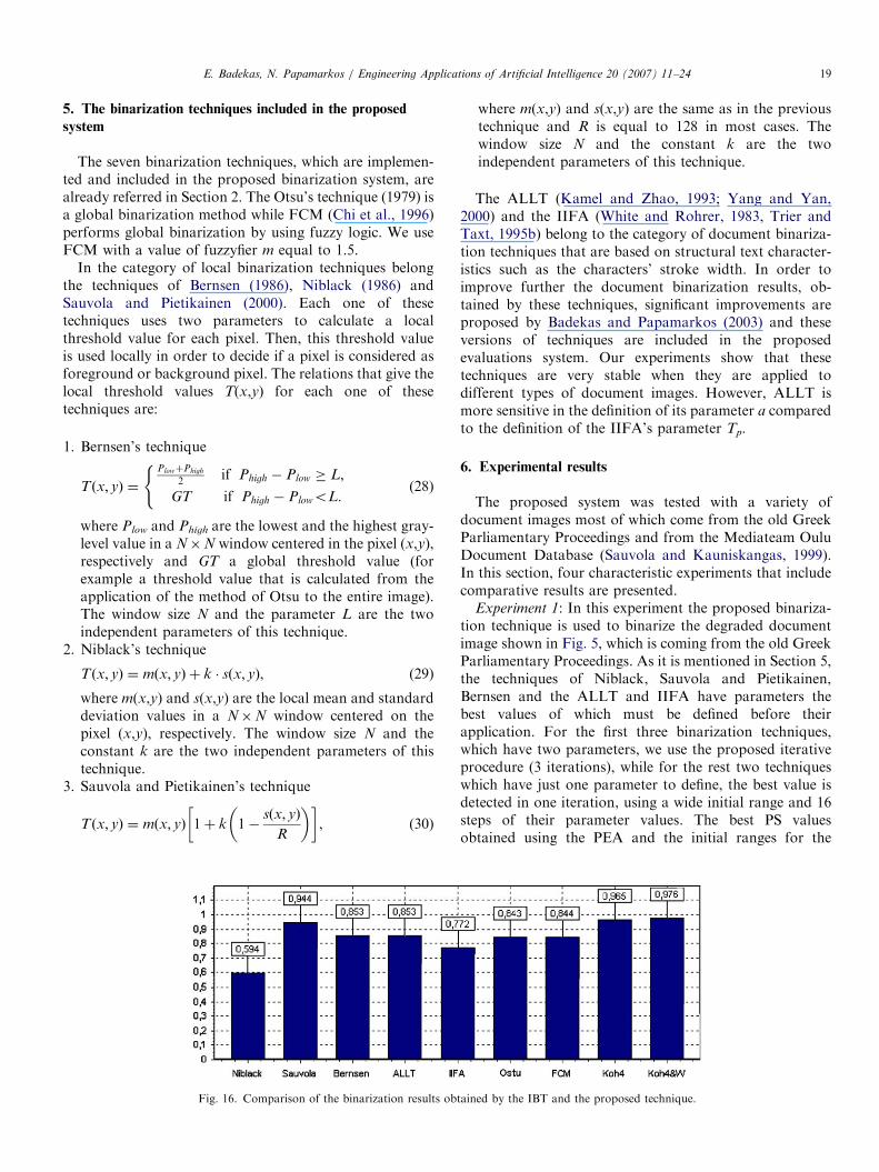
Experiment 1: In this experiment the proposed binariza-tion technique is used to binarize the degraded documentimage shown in Fig. 5, which is coming from the old GreekParliamentary Proceedings. As it is mentioned in Section 5,the techniques of Niblack, Sauvola and Pietikainen,Bernsen and the ALLT and IIFA have parameters thebest values of which must be defined before theirapplication. For the first three binarization techniques,which have two parameters, we use the proposed iterativeprocedure (3 iterations), while for the rest two techniqueswhich have just one parameter to define, the best value isdetected in one iteration, using a wide initial range and 16steps of their parameter values. The best PS valuesobtained using the PEA and the initial ranges for the

tained by the IBT and the proposed technique.

ARTICLE IN PRESS

Fig. 17. (a) The initial gray-scale advertisement image. (b) The binariza-

tion result obtained by the proposed technique.

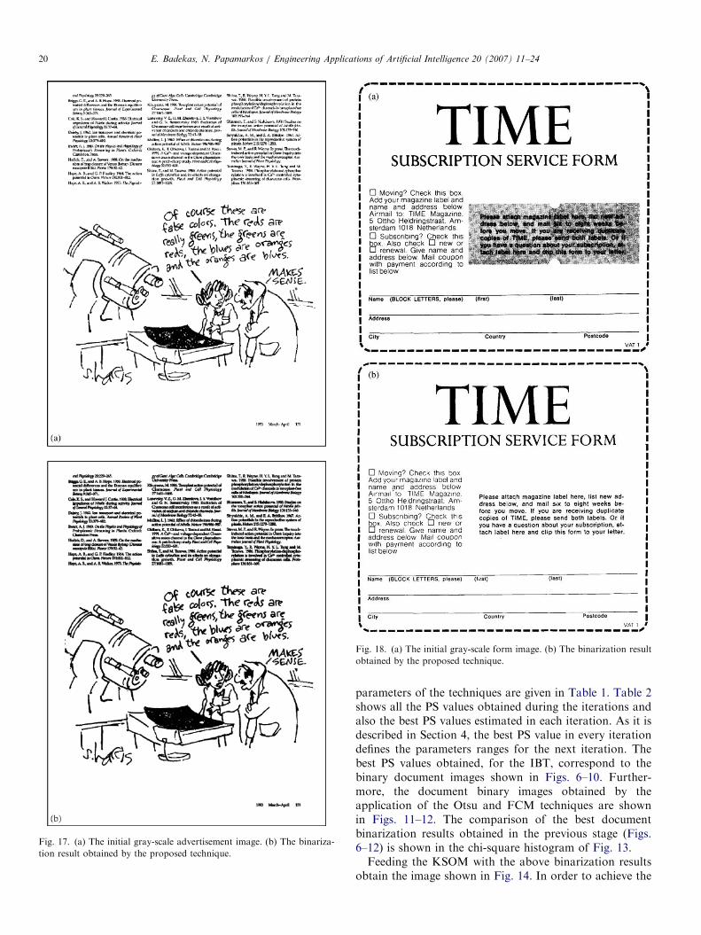
Fig. 18. (a) The initial gray-scale form image. (b) The binarization result

obtained by the proposed technique.

E. Badekas, N. Papamarkos / Engineering Applications of Artificial Intelligence 20 (2007) 11–2420

parameters of the techniques are given in Table 1. Table 2shows all the PS values obtained during the iterations andalso the best PS values estimated in each iteration. As it isdescribed in Section 4, the best PS value in every iterationdefines the parameters ranges for the next iteration. Thebest PS values obtained, for the IBT, correspond to thebinary document images shown in Figs. 6–10. Further-more, the document binary images obtained by theapplication of the Otsu and FCM techniques are shownin Figs. 11–12. The comparison of the best documentbinarization results obtained in the previous stage (Figs.6–12) is shown in the chi-square histogram of Fig. 13.Feeding the KSOM with the above binarization results

obtain the image shown in Fig. 14. In order to achieve the

ARTICLE IN PRESS

Fig. 19. (a) The initial gray-scale article image. (b) The binarization result

obtained by the proposed technique.

E. Badekas, N. Papamarkos / Engineering Applications of Artificial Intelligence 20 (2007) 11–24 21

best possible binarization result, the values of the chi-square histogram of Fig. 13 are used as weighting valuesduring the feeding of the KSOM. In this way, the finalbinarization result is obtained and it is shown in Fig. 15.

The number of the output neurons of the KSOM is takenequal to four and the number of samples in the training istaken equal to 2000. There is not any post-processingtechnique applied in this experiment.The binarization results obtained by the proposed

technique can be evaluated, comparing them with thebinarization results obtained by the seven IBT. The ninebinary images (Figs. 6-12 and 14–15) can be comparedusing the method described in Section 3. As it is shown inthe Chi-square histogram of Fig. 16, the binarization resultproduced by the KSOM (Fig. 14) is better than any of theresults of the IBT and the binarization result obtained bythe KSOM using the weighting values (Fig. 15) is the bestone.

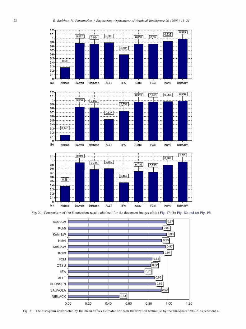
Experiment 2: The proposed technique has been exten-sively tested with document images from the MediateamOulu Document Database (Sauvola and Kauniskangas,1999). Specific examples of the application of the proposedtechnique to grayscale images obtained from the abovedatabase are discussed in this experiment. We use the sameprocedure, as in the previous experiment, in order tobinarize three document images, each one belonging to adifferent category: advertisement (Fig. 17(a)), form image(Fig. 18(a)) and article (Fig. 19(a)). It should be noticedthat for the binarization of the Form image presented inFig. 18(a), is used as a post-processing step, a size filter thatremoves from the final binary image objects consisting ofless than five pixels. The binarization results obtained areshown in Figs. 17(b), 18(b) and 19(b), respectively. Thehistograms of Fig. 20 show the comparative resultsobtained by the chi-square test for the three images usedin this experiment. From these histograms it is proved thatthe proposed binarization technique, using the weightingvalues, gives the best binarization result.It is important to notice that due to the combination of

the binarization results obtained by the IBT, the proposedtechnique leads to appropriate binarization of the imagesincluded in the processing documents. This is obvious fromthe binarization results of this experiment, where it can beobserved that the proposed binarization technique leads tosatisfactory results not only in the text regions but also inthe image regions included in the documents.

Experiment 3: This is a psycho-visual experiment that isperformed asking a group of people to compare the resultsof the proposed binarization technique with the resultsobtained by IBT. This test is based on 10 document imagescoming from the Mediateam Oulu Document Database.For these documents we obtain and print the binary imagesproduced by the proposed technique and the seven IBT.The printed documents were given to 50 persons askingthem to detect visually the best binary image of eachdocument. All persons conclude that the binary documentsobtained by the application of the proposed technique toall testing images are always between the best threebinarization results. A percentage of 91.8% (459/500) ofthe answers, state that the proposed technique, using theweighting values, result to the best binary document.

ARTICLE IN PRESS

Fig. 20. Comparison of the binarization results obtained for the document images of: (a) Fig. 17; (b) Fig. 18; and (c) Fig. 19.

0,51

0,92

0,86

0,86

0,75

0,82

0,83

0,94

0,97

0,93

0,98

0,93

0,97

NIBLACK

SAUVOLA

BERNSEN

ALLT

IIFA

OTSU

FCM

Koh3

Koh3&W

Koh4

Koh4&W

Koh5

Koh5&W

0,00 0,20 0,40 0,60 0,80 1,00 1,20

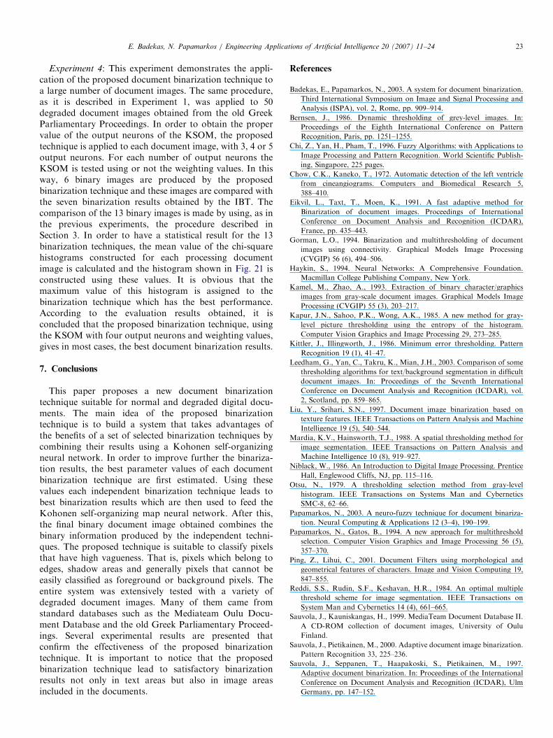
Fig. 21. The histogram constructed by the mean values estimated for each binarization technique by the chi-square tests in Experiment 4.

E. Badekas, N. Papamarkos / Engineering Applications of Artificial Intelligence 20 (2007) 11–2422

ARTICLE IN PRESSE. Badekas, N. Papamarkos / Engineering Applications of Artificial Intelligence 20 (2007) 11–24 23

Experiment 4: This experiment demonstrates the appli-cation of the proposed document binarization technique toa large number of document images. The same procedure,as it is described in Experiment 1, was applied to 50degraded document images obtained from the old GreekParliamentary Proceedings. In order to obtain the propervalue of the output neurons of the KSOM, the proposedtechnique is applied to each document image, with 3, 4 or 5output neurons. For each number of output neurons theKSOM is tested using or not the weighting values. In thisway, 6 binary images are produced by the proposedbinarization technique and these images are compared withthe seven binarization results obtained by the IBT. Thecomparison of the 13 binary images is made by using, as inthe previous experiments, the procedure described inSection 3. In order to have a statistical result for the 13binarization techniques, the mean value of the chi-squarehistograms constructed for each processing documentimage is calculated and the histogram shown in Fig. 21 isconstructed using these values. It is obvious that themaximum value of this histogram is assigned to thebinarization technique which has the best performance.According to the evaluation results obtained, it isconcluded that the proposed binarization technique, usingthe KSOM with four output neurons and weighting values,gives in most cases, the best document binarization results.

7. Conclusions

This paper proposes a new document binarizationtechnique suitable for normal and degraded digital docu-ments. The main idea of the proposed binarizationtechnique is to build a system that takes advantages ofthe benefits of a set of selected binarization techniques bycombining their results using a Kohonen self-organizingneural network. In order to improve further the binariza-tion results, the best parameter values of each documentbinarization technique are first estimated. Using thesevalues each independent binarization technique leads tobest binarization results which are then used to feed theKohonen self-organizing map neural network. After this,the final binary document image obtained combines thebinary information produced by the independent techni-ques. The proposed technique is suitable to classify pixelsthat have high vagueness. That is, pixels which belong toedges, shadow areas and generally pixels that cannot beeasily classified as foreground or background pixels. Theentire system was extensively tested with a variety ofdegraded document images. Many of them came fromstandard databases such as the Mediateam Oulu Docu-ment Database and the old Greek Parliamentary Proceed-ings. Several experimental results are presented thatconfirm the effectiveness of the proposed binarizationtechnique. It is important to notice that the proposedbinarization technique lead to satisfactory binarizationresults not only in text areas but also in image areasincluded in the documents.

References

Badekas, E., Papamarkos, N., 2003. A system for document binarization.

Third International Symposium on Image and Signal Processing and

Analysis (ISPA), vol. 2, Rome, pp. 909–914.

Bernsen, J., 1986. Dynamic thresholding of grey-level images. In:

Proceedings of the Eighth International Conference on Pattern

Recognition, Paris, pp. 1251–1255.

Chi, Z., Yan, H., Pham, T., 1996. Fuzzy Algorithms: with Applications to

Image Processing and Pattern Recognition. World Scientific Publish-

ing, Singapore, 225 pages.

Chow, C.K., Kaneko, T., 1972. Automatic detection of the left ventricle

from cineangiograms. Computers and Biomedical Research 5,

388–410.

Eikvil, L., Taxt, T., Moen, K., 1991. A fast adaptive method for

Binarization of document images. Proceedings of International

Conference on Document Analysis and Recognition (ICDAR),

France, pp. 435–443.

Gorman, L.O., 1994. Binarization and multithresholding of document

images using connectivity. Graphical Models Image Processing

(CVGIP) 56 (6), 494–506.

Haykin, S., 1994. Neural Networks: A Comprehensive Foundation.

Macmillan College Publishing Company, New York.

Kamel, M., Zhao, A., 1993. Extraction of binary character/graphics

images from gray-scale document images. Graphical Models Image

Processing (CVGIP) 55 (3), 203–217.

Kapur, J.N., Sahoo, P.K., Wong, A.K., 1985. A new method for gray-

level picture thresholding using the entropy of the histogram.

Computer Vision Graphics and Image Processing 29, 273–285.

Kittler, J., Illingworth, J., 1986. Minimum error thresholding. Pattern

Recognition 19 (1), 41–47.

Leedham, G., Yan, C., Takru, K., Mian, J.H., 2003. Comparison of some

thresholding algorithms for text/background segmentation in difficult

document images. In: Proceedings of the Seventh International

Conference on Document Analysis and Recognition (ICDAR), vol.

2, Scotland, pp. 859–865.

Liu, Y., Srihari, S.N., 1997. Document image binarization based on

texture features. IEEE Transactions on Pattern Analysis and Machine

Intelligence 19 (5), 540–544.

Mardia, K.V., Hainsworth, T.J., 1988. A spatial thresholding method for

image segmentation. IEEE Transactions on Pattern Analysis and

Machine Intelligence 10 (8), 919–927.

Niblack, W., 1986. An Introduction to Digital Image Processing. Prentice

Hall, Englewood Cliffs, NJ, pp. 115–116.

Otsu, N., 1979. A thresholding selection method from gray-level

histogram. IEEE Transactions on Systems Man and Cybernetics

SMC-8, 62–66.

Papamarkos, N., 2003. A neuro-fuzzy technique for document binariza-

tion. Neural Computing & Applications 12 (3–4), 190–199.

Papamarkos, N., Gatos, B., 1994. A new approach for multithreshold

selection. Computer Vision Graphics and Image Processing 56 (5),

357–370.

Ping, Z., Lihui, C., 2001. Document Filters using morphological and

geometrical features of characters. Image and Vision Computing 19,

847–855.

Reddi, S.S., Rudin, S.F., Keshavan, H.R., 1984. An optimal multiple

threshold scheme for image segmentation. IEEE Transactions on

System Man and Cybernetics 14 (4), 661–665.

Sauvola, J., Kauniskangas, H., 1999. MediaTeam Document Database II.

A CD-ROM collection of document images, University of Oulu

Finland.

Sauvola, J., Pietikainen, M., 2000. Adaptive document image binarization.

Pattern Recognition 33, 225–236.

Sauvola, J., Seppanen, T., Haapakoski, S., Pietikainen, M., 1997.

Adaptive document binarization. In: Proceedings of the International

Conference on Document Analysis and Recognition (ICDAR), Ulm

Germany, pp. 147–152.

ARTICLE IN PRESSE. Badekas, N. Papamarkos / Engineering Applications of Artificial Intelligence 20 (2007) 11–2424

Sezgin, M., Sankur, B., 2004. Survey over image thresholding techniques

and quantitative performance evaluation. Journal of Electronic

Imaging 13 (1), 146–165.

Strouthopoulos, C., Papamarkos, N., Atsalakis, A., 2002. Text extraction

in complex color documents. Pattern Recognition 35 (8), 1743–1758.

Taxt, T., Flynn, P.J., Jain, A.K., 1989. Segmentation of document images.

IEEE Transactions on Pattern Analysis and Machine Intelligence 11

(12), 1322–1329.

Trier, O.D., Jain, A.K., 1995. Goal-Directed Evaluation of binarization

methods. IEEE Transactions on Pattern Analysis and Machine

Intelligence 17 (12), 1191–1201.

Trier, O.D., Taxt, T., 1995a. Evaluation of binarization methods for

document images. IEEE Transactions on Pattern Analysis and

Machine Intelligence 17 (3), 312–315.

Trier, O.D., Taxt, T., 1995b. Improvement of ‘Integrated Function

Algorithm’ for binarization of document images. Pattern Recognition

Letters 16, 277–283.

White, J.M., Rohrer, G.D., 1983. Image segmentation for optical

character recognition and other applications requiring character image

extraction. IBM Journal Research Development 27 (4), 400–411.

Yang, Y., Yan, H., 2000. An adaptive logical method for binarization of

degraded document images. Pattern Recognition 33, 787–807.

Yanowitz, S.D., Bruckstein, A.M., 1989. A new method for image

segmentation. Computer Vision, Graphics and Image Processing 46

(1), 82–95.

Yitzhaky, Y., Peli, E., 2003. A Method for Objective Edge Detection

Evaluation and Detector Parameter Selection. IEEE Transactions on

Pattern Analysis and Machine Intelligence 25 (8), 1027–1033.