Operational Two-Stage Stratified Topographic Correction of Spaceborne Multispectral Imagery...
35
112 IEEE TRANSACTIONS ON GEOSCIENCE AND REMOTE SENSING, VOL. 48, NO. 1,JANUARY 2010 Operational Two-Stage Stratified Topographic Correction of Spaceborne Multispectral Imagery Employing an Automatic Spectral-Rule-Based Decision-Tree Preliminary Classifier Andrea Baraldi, Matteo Gironda, and Dario Simonetti Abstract—The increasing amount of remote sensing (RS) im- agery acquired from multiple platforms and the recent announce- ments that scientists and decision makers around the world will soon have unrestricted access at no charge to large-scale space- borne multispectral (MS) image databases make urgent the need to develop easy-to-use, effective, efficient, robust, and scalable satellite-based measurement systems. In these scientific and in- dustrial contexts, it is well known that, to date, the operational performance of existing stratified non-Lambertian (anisotropic) topographic correction (SNLTOC) algorithms has been limited by the need for a priori knowledge of structural landscape character- istics, such as surface roughness which is land cover class specific. In practice, to overcome the circular nature of the SNLTOC problem, a mutually exclusive and totally exhaustive land cover classification map of a spaceborne MS image is required before SNLTOC takes place. This system requirement is fulfilled by the original operational automatic two-stage SNLTOC approach presented in this paper which comprises, in cascade, 1) an auto- matic stratification first stage and 2) a second-stage ordinary SNLTOC method selected from the literature. The former com- bines 1) four subsymbolic digital-elevation-model-derived strata, namely, horizontal areas, self-shadows, and sunlit slopes either facing the sun or facing away from the sun, and 2) symbolic (semantic) strata generated from the input MS image by an oper- ational fully automated spectral-rule-based decision-tree prelimi- nary classifier recently presented in RS literature. In this paper, first, previous works related to the TOC subject are surveyed, and next, the novel operational two-stage SNLTOC system is pre- sented. Finally, the original two-stage SNLTOC system is validated in up to 19 experiments where the system’s capability of reduc- ing within-stratum spectral variance while preserving pixel-based spectral patterns (shapes) is assessed quantitatively. Index Terms—Decision-tree classification, digital elevation model (DEM), fuzzy rule, image-understanding system, inductive data learning, prior knowledge, topographic correction. Manuscript received May 27, 2008; revised July 24, 2008, November 14, 2008, March 16, 2009, and June 3, 2009. First published October 6, 2009; current version published December 23, 2009. A. Baraldi was with the European Commission Joint Research Centre, 21020 Ispra, Italy. He is now with Baraldi Consultancy in Remote Sensing, 40129 Bologna, Italy (e-mail: [email protected]). M. Gironda was with the University Institute of Architecture of Venice, 30135 Venezia, Italy (e-mail: [email protected]). D. Simonetti is with the European Commission Joint Research Centre, 21020 Ispra, Italy (e-mail: [email protected]). Color versions of one or more of the figures in this paper are available online at http://ieeexplore.ieee.org. Digital Object Identifier 10.1109/TGRS.2009.2028017 I. I NTRODUCTION T HE POTENTIAL of remote sensing (RS) for the mon- itoring of the Earth’s environment and the detection of its temporal variations at geographic extents ranging from local (areas up to 100 000 km 2 ) to regional (roughly between 100 000 and 1 000 000 km 2 [1]), continental, and global scales is well known by user communities involved with urban growth assessment and planning, intelligence/surveillance applications for national security and defense purposes, ecosystem man- agement, watershed protection, water balance calculations, risk management, and global change [1]–[3]. The increasing number of Earth observation (EO) space- borne platforms featuring enhanced combinations of radiomet- ric, spatial, spectral, and temporal resolution and the recent announcements that scientists and decision makers around the world will soon have unrestricted access at no charge to large- scale RS image databases [4] make urgent the need to develop operational satellite-based measurement systems suitable for automating the quantitative analysis of RS imagery, which is one of the traditional goals of the RS community involved with global land cover and land cover change assessment [1]. Unfortunately, to date, the transformation of huge amounts of multisource spaceborne imagery into information still remains far below reasonable expectations and mostly confined to sci- entific applications [5]. In common practice, an insufficient RS image mapping capability may be due to two main factors. 1) Existing scientific and commercial RS image- understanding systems (RS-IUSs), such as [6] and [7] which have recently gained a noteworthy popularity, score low in operational performance which encompasses [8], [9] the following: a) ease of use (degree of automation); b) effectiveness (e.g., classification accuracy); c) efficiency (e.g., computation time and memory occupation); d) economy (costs increase monotonically with man- power, e.g., the manpower required to collect scene- specific training samples); e) robustness to changes in input parameters; f) robustness to changes in the input data set; g) maintainability/scalability/reusability to keep up with users’ changing needs; 0196-2892/$26.00 © 2009 IEEE Authorized licensed use limited to: CNR ISSIA. Downloaded on January 21, 2010 at 05:56 from IEEE Xplore. Restrictions apply.
-
Upload
independent -
Category
Documents
-
view
1 -
download
0
Transcript of Operational Two-Stage Stratified Topographic Correction of Spaceborne Multispectral Imagery...

112 IEEE TRANSACTIONS ON GEOSCIENCE AND REMOTE SENSING, VOL. 48, NO. 1, JANUARY 2010
Operational Two-Stage Stratified TopographicCorrection of Spaceborne Multispectral ImageryEmploying an Automatic Spectral-Rule-Based
Decision-Tree Preliminary ClassifierAndrea Baraldi, Matteo Gironda, and Dario Simonetti
Abstract—The increasing amount of remote sensing (RS) im-agery acquired from multiple platforms and the recent announce-ments that scientists and decision makers around the world willsoon have unrestricted access at no charge to large-scale space-borne multispectral (MS) image databases make urgent the needto develop easy-to-use, effective, efficient, robust, and scalablesatellite-based measurement systems. In these scientific and in-dustrial contexts, it is well known that, to date, the operationalperformance of existing stratified non-Lambertian (anisotropic)topographic correction (SNLTOC) algorithms has been limited bythe need for a priori knowledge of structural landscape character-istics, such as surface roughness which is land cover class specific.In practice, to overcome the circular nature of the SNLTOCproblem, a mutually exclusive and totally exhaustive land coverclassification map of a spaceborne MS image is required beforeSNLTOC takes place. This system requirement is fulfilled bythe original operational automatic two-stage SNLTOC approachpresented in this paper which comprises, in cascade, 1) an auto-matic stratification first stage and 2) a second-stage ordinarySNLTOC method selected from the literature. The former com-bines 1) four subsymbolic digital-elevation-model-derived strata,namely, horizontal areas, self-shadows, and sunlit slopes eitherfacing the sun or facing away from the sun, and 2) symbolic(semantic) strata generated from the input MS image by an oper-ational fully automated spectral-rule-based decision-tree prelimi-nary classifier recently presented in RS literature. In this paper,first, previous works related to the TOC subject are surveyed,and next, the novel operational two-stage SNLTOC system is pre-sented. Finally, the original two-stage SNLTOC system is validatedin up to 19 experiments where the system’s capability of reduc-ing within-stratum spectral variance while preserving pixel-basedspectral patterns (shapes) is assessed quantitatively.
Index Terms—Decision-tree classification, digital elevationmodel (DEM), fuzzy rule, image-understanding system, inductivedata learning, prior knowledge, topographic correction.
Manuscript received May 27, 2008; revised July 24, 2008, November 14,2008, March 16, 2009, and June 3, 2009. First published October 6, 2009;current version published December 23, 2009.
A. Baraldi was with the European Commission Joint Research Centre, 21020Ispra, Italy. He is now with Baraldi Consultancy in Remote Sensing, 40129Bologna, Italy (e-mail: [email protected]).
M. Gironda was with the University Institute of Architecture of Venice,30135 Venezia, Italy (e-mail: [email protected]).
D. Simonetti is with the European Commission Joint Research Centre, 21020Ispra, Italy (e-mail: [email protected]).
Color versions of one or more of the figures in this paper are available onlineat http://ieeexplore.ieee.org.
Digital Object Identifier 10.1109/TGRS.2009.2028017
I. INTRODUCTION
THE POTENTIAL of remote sensing (RS) for the mon-itoring of the Earth’s environment and the detection of
its temporal variations at geographic extents ranging fromlocal (areas up to 100 000 km2) to regional (roughly between100 000 and 1 000 000 km2 [1]), continental, and global scalesis well known by user communities involved with urban growthassessment and planning, intelligence/surveillance applicationsfor national security and defense purposes, ecosystem man-agement, watershed protection, water balance calculations, riskmanagement, and global change [1]–[3].
The increasing number of Earth observation (EO) space-borne platforms featuring enhanced combinations of radiomet-ric, spatial, spectral, and temporal resolution and the recentannouncements that scientists and decision makers around theworld will soon have unrestricted access at no charge to large-scale RS image databases [4] make urgent the need to developoperational satellite-based measurement systems suitable forautomating the quantitative analysis of RS imagery, which isone of the traditional goals of the RS community involved withglobal land cover and land cover change assessment [1].
Unfortunately, to date, the transformation of huge amounts ofmultisource spaceborne imagery into information still remainsfar below reasonable expectations and mostly confined to sci-entific applications [5]. In common practice, an insufficient RSimage mapping capability may be due to two main factors.
1) Existing scientific and commercial RS image-understanding systems (RS-IUSs), such as [6] and[7] which have recently gained a noteworthy popularity,score low in operational performance which encompasses[8], [9] the following:a) ease of use (degree of automation);b) effectiveness (e.g., classification accuracy);c) efficiency (e.g., computation time and memory
occupation);d) economy (costs increase monotonically with man-
power, e.g., the manpower required to collect scene-specific training samples);
e) robustness to changes in input parameters;f) robustness to changes in the input data set;g) maintainability/scalability/reusability to keep up with
users’ changing needs;
0196-2892/$26.00 © 2009 IEEE
Authorized licensed use limited to: CNR ISSIA. Downloaded on January 21, 2010 at 05:56 from IEEE Xplore. Restrictions apply.

BARALDI et al.: OPERATIONAL TWO-STAGE STRATIFIED TOPOGRAPHIC CORRECTION OF SPACEBORNE MS IMAGERY 113
h) timeliness (defined as the time span between dataacquisition and product delivery to the end user; itincreases monotonically with manpower).
For example, a low operational performance measure-ment may explain why the impact upon commercialRS image-processing software toolboxes of the literallyhundreds of so-called novel low (subsymbolic)- and high(symbolic)-level image-processing algorithms presentedeach year in scientific literature remains negligible [5].
2) The increasing rate of collection of RS data of enhancedquality outpaces the capabilities of both manual inspec-tion and inductive machine learning from supervised(labeled) EO data [2]. The cost, timeliness, quality, andavailability of adequate reference (training/testing) datasets derived from field sites, existing maps, and tabulardata as a source of prior knowledge are considered themost limiting factors on RS data product generation andvalidation [1].
From a technical viewpoint, a data processing system istermed fully automated when it requires neither user-definedparameters nor reference data samples to run; therefore, itsease of use is unsurpassed [10]. To automate a data processingsystem, necessary, although not sufficient, conditions are forinput data to be [11] 1) well behaved (well conditioned), i.e.,not violating any assumptions needed to successfully applywhatever analysis the system performs, e.g., every input datasource is expressed in a physical unit of measure and belongsto a known domain of variation, and 2) well understood by thesystem developer, namely, every input data source is providedwith a clear physical meaning and with a community-agreeddata format.
In particular, EO sensor-derived data are well behaved whenthey are as follows.
1) Radiometrically calibrated, i.e., dimensionless digitalnumbers (DNs) are transformed into a community-agreedradiometric unit of measure. For example, in the con-text of the Global Monitoring for the Environment andSecurity (GMES) program, led by the European Union(EU) in partnership with the European Space Agency(ESA), and of the Global Earth Observation System ofSystems (GEOSS), conceived by the Group on EarthObservations (GEO) [12]–[14], calibration and valida-tion (Cal/Val)-related activities are considered crucialin accomplishing harmonization and interoperability ofEO data and derived products generated from multiplesources. In particular, the Quality Assurance Frameworkfor Earth Observation data (QA4EO) [15] initiative ledby the Committee of Earth Observations (CEOS) [16]Working Group on Calibration and Validation [17] aimsat establishing an appropriate coordinated program ofCal/Val initiatives throughout all stages of a spacebornemission, from sensor build to end of life.
2) Geometrically corrected, i.e., projected onto acommunity-agreed terrestrial reference system.
3) Validated, i.e., provided with quantitative, unequivocal,and traceable measures of geometric and radiometric EOdata quality. For example, in the words of the QA4EO
initiative, in an EO data product generation and deliverychain, every operation or data flow must be providedwith a quality indicator (QI) based on an unequivo-cal quantifiable metrological/statistically based measure[15, p. 7], i.e., a QI is based on a documented quantitativeassessment of its traceability to a community-agreed ref-erence standard ideally tied to a physical unit of measurebelonging to an international system of units. Accurateoperation performance/data quality tracking (traceability)provides knowledge on what is not performing up to areference standard, so that alternative quality assurancestrategies can be enforced at that stage.
In multisensor data fusion, image mosaicking for visualiza-tion and classification purposes, multitemporal image analysis,and quantitative biophysical [e.g., leaf area index (LAI)] andbiochemical [e.g., fraction of absorbed photosynthetically ac-tive radiation (FAPAR)] parameter extraction [11], [18]–[26],well-known undesired RS inter- and intra-image radiometricchanges are due to the following:
1) changes in instrumental conditions;2) changes in solar illumination due to changes in the sun’s
position and in the Earth–sun distance;3) atmospheric effects;4) changes in solar illumination due to topographic
influences.
To normalize the aforementioned sources 1)–4) of radiomet-ric change, a standard Cal/Val-related protocol for RS imagepreprocessing should comprise steps 1) and 2), which aredescribed next.
1) Radiometric calibration and atmospheric correction. Itcomprises a sequence of three steps.a) Absolute radiometric calibration [27], namely, the
linear transformation of DNs into nonnegative top-of-atmosphere (TOA) radiance (TOARDT ) values ≥0, where the subscript T means terrain, i.e.,TOARDT values are affected by topographic ef-fects. This first calibration step depends on offset andgain calibration parameters retrieved from calibrationmetadata files accounting for instrumental conditions.
b) Nonlinear transformation of TOARDT values intoTOA reflectance (TOARFT ) values belonging torange [0, 1], where influences of the sun zenith angle(as a function of the time of RS data acquisitionand position of the RS image footprint) and of theEarth–sun distance (as a function of the time of RSdata acquisition) are normalized [24]. In the rest ofthis paper, this step is considered mandatory and pre-liminary to topographic normalization.
c) When atmospheric effects are taken into account,the transformation of either TOARDT or TOARFT
values into terrain radiance LT values ≥ 0 orterrain reflectance ρT values belonging to range [0, 1][28]. In existing literature, some authors recommendthe concurrent application of topographic and at-mospheric correction [29] while other authors andcommercial RS image-processing software toolboxes,
Authorized licensed use limited to: CNR ISSIA. Downloaded on January 21, 2010 at 05:56 from IEEE Xplore. Restrictions apply.

114 IEEE TRANSACTIONS ON GEOSCIENCE AND REMOTE SENSING, VOL. 48, NO. 1, JANUARY 2010
such as [6], recommend applying RS image at-mospheric correction prior to topographic normal-ization. Atmospheric correction is a typical ill- orpoorly posed problem requiring ancillary data (sum-mary statistics) to be collected at several locationswithin the RS image footprint at the time of RSimage acquisition, which are rarely available in prac-tice. Consequently, atmospheric correction is verydifficult to solve and requires the user’s supervisionto make it better posed [6]. In this paper, ill-posedatmospheric correction is considered optional (there-fore, it is ignored in practice) by an RS image spectral-rule-based decision-tree preliminary classifier (SRC)requiring as input a multispectral (MS) image radio-metrically calibrated into TOARFT values, whichare considered a parent class of surface reflectanceρT values, i.e., TOARFT ⊇ ρT (see Sections III-Aand IV-A2).
2) RS image topographic correction (TOC), also calledtopographic normalization, whose aim is to compen-sate for changes in terrain exposure to direct sun-light, i.e., to transform TOARFT /LT /ρT values intoTOARFH/LH/ρH values where the index H identifiesa horizontal-like surface. Although it has been investi-gated for at least 20 years, the TOC problem has notyet been solved satisfactorily due to its circular nature[6], [18], [29]–[44]. While an automatic classificationof an RS MS image must rely upon well-behaved in-put data, realistic TOC approaches must account fornon-Lambertian (anisotropic) surface reflectance as afunction of structural landscape characteristics such assurface roughness, which is land cover class specific.In other words, realistic non-Lambertian TOC (NLTOC)systems must incorporate the “stratified” or “layered”approach. In RS common practice, the exploitation ofstratified NLTOC (SNLTOC) approaches is limited bythe need for a priori knowledge of land-cover-class-specific surface roughness. To overcome this limitation,“more research regarding the use of better stratifica-tion methods” is strongly encouraged [37, p. 2130],[38, p. 294].
To summarize, an original operational automatic solution tothe aforementioned circular SNLTOC problem 2) stems fromthe a priori availability of a classification map automaticallygenerated from an RS image well behaved in agreement withthe aforementioned resolution 1). On the contrary, several land-cover-class- or unsupervised data-cluster-specific SNLTOCapplications found in existing literature ignore or neglect thenecessary, although not sufficient, radiometric calibration re-quirement for automating data processing. As a consequence,these SNLTOC applications adopt a manual or semiautomaticscene-by-scene data understanding approach. For example, in[43], an extended pixel-based k-means clustering algorithm, ca-pable of detecting automatically the number k of unlabeled dataclusters, is employed for preliminary stratification (slicing).One-class (vegetation) [31], [42], two-class (vegetation/nonvegetation and forest/nonforest) [34]–[36], or three-class(snow/vegetation/nonvegetation) [37], [38] image strata are
generated by preliminary image photointerpretation [36], imagefeature [e.g., normalized difference vegetation index (NDVI)]thresholding [34], [35], or semiautomated two-stage hybriddata-learning image-classification approaches [37], [38]. Inaddition, in [34] and [35], a dichotomous digital elevationmodel (DEM)-driven terrain slope thresholding is adoptedwhere slopes below 10◦, which include horizontal surfaces, areexcluded from SNLTOC. In [44], ten strata based on DEM-driven slope ranges are generated irrespective of land covertypes. Next, ten stratum-specific Minnaert coefficients (referto Section III-B2b) are estimated image-wide and interpolated.Finally, pixel-based Minnaert coefficients are estimated fromthe interpolation curve to be employed in a pixel-basedSNLTOC approach. Unfortunately, the correlation of surfaceroughness, relevant to the TOC problem, with empirical DEM-derived stratification (slicing) criteria independent of land covertypes is expected to be moderate or low.
The original contribution of this paper to existing knowl-edge on the TOC subject is fourfold. First, Lambertian TOC(LTOC), NLTOC, and SNLTOC approaches found in existingliterature are critically revised, which provides this paper witha significant survey value. Second, an original combination ofautomatic subsymbolic and symbolic (semantic) stratificationmethods suitable for developing an operational SNLTOC sys-tem are proposed in line with recommendations found in [37]and [38]. The novel stratification strategy combines: 1) foursubsymbolic (asemantic) solar illumination layers, namely,self-shadows, horizontal surfaces, slopes facing the sun, andslopes facing away from the sun, generated from a DEMand the sun zenith and azimuth angles at the time of RSdata acquisition and 2) symbolic (semantic) strata generatedfrom a spaceborne MS image radiometrically calibrated intoTOARFT ⊇ ρT values by a fully automated SRC system ofsystems presented and discussed in related papers [21]–[23],[45]. Third, this paper presents a novel operational automatictwo-stage SNLTOC approach capable of satisfying the systemrequirements a)–h) listed previously to be considered eligiblefor use in an operational satellite-based measurement system.To the best of our knowledge, no alternative operational so-lution to the circular MS image TOC problem can be foundin existing literature. Fourth, a novel set of SNLTOC qualityindexes is proposed.
Due to its degree of novelty in agreement with the newQA4EO guidelines, this paper is of potential interest to thesegment of the RS community involved with automating thequantitative analysis of RS data, e.g., in the framework ofthe ongoing GEOSS and GMES international programs.
This paper is structured as follows. Section II introducesthe terms and symbols adopted in the rest of this paper. InSection III, previous works related to the TOC problem aresurveyed. The novel operational two-stage SNLTOC systemis presented in Section IV. Study areas, testing images, andancillary data employed in the experimental session are de-scribed in Section V. Methods for the quantitative assessmentof alternative SNLTOC algorithms are discussed in Section VI.Quantitative and qualitative SNLTOC results are collected anddiscussed in Section VII. Final conclusions are proposed inSection VIII.
Authorized licensed use limited to: CNR ISSIA. Downloaded on January 21, 2010 at 05:56 from IEEE Xplore. Restrictions apply.
BARALDI et al.: OPERATIONAL TWO-STAGE STRATIFIED TOPOGRAPHIC CORRECTION OF SPACEBORNE MS IMAGERY 115
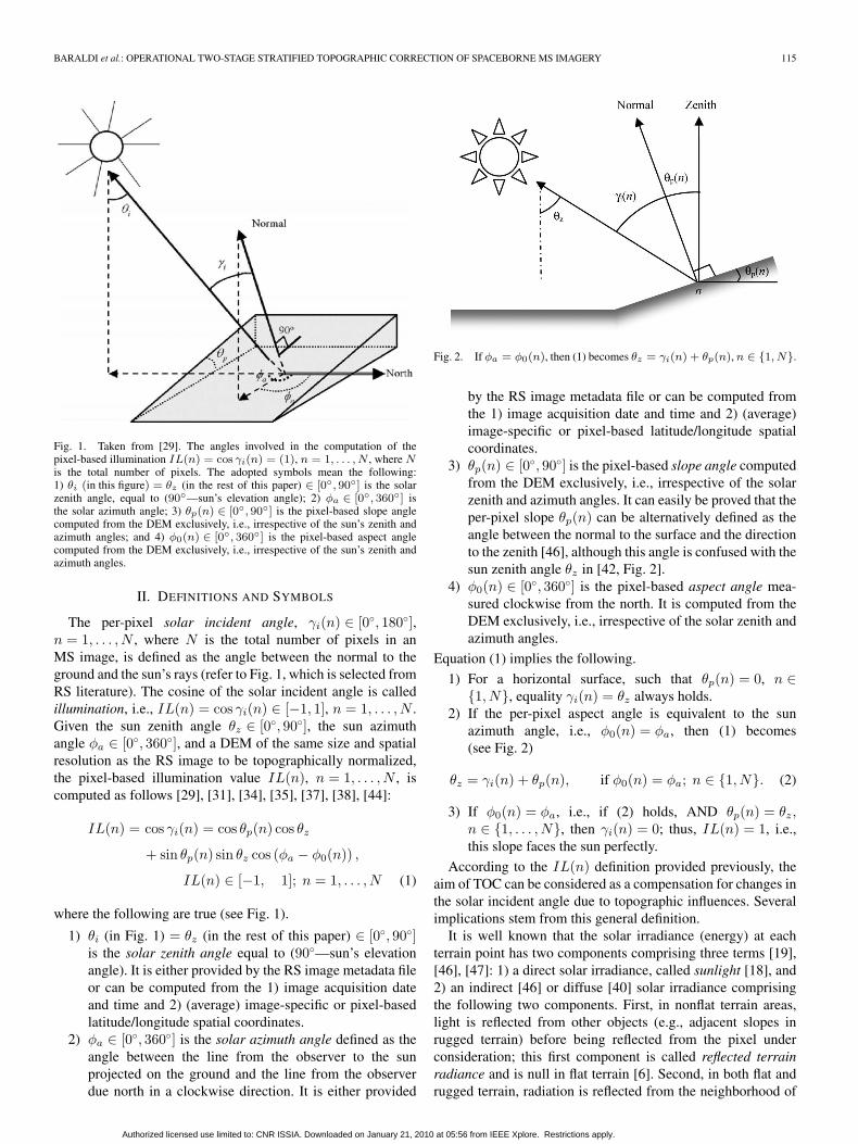
Fig. 1. Taken from [29]. The angles involved in the computation of thepixel-based illumination IL(n) = cos γi(n) = (1), n = 1, . . . , N , where Nis the total number of pixels. The adopted symbols mean the following:1) θi (in this figure) = θz (in the rest of this paper) ∈ [0◦, 90◦] is the solarzenith angle, equal to (90◦—sun’s elevation angle); 2) φa ∈ [0◦, 360◦] isthe solar azimuth angle; 3) θp(n) ∈ [0◦, 90◦] is the pixel-based slope anglecomputed from the DEM exclusively, i.e., irrespective of the sun’s zenith andazimuth angles; and 4) φ0(n) ∈ [0◦, 360◦] is the pixel-based aspect anglecomputed from the DEM exclusively, i.e., irrespective of the sun’s zenith andazimuth angles.
II. DEFINITIONS AND SYMBOLS
The per-pixel solar incident angle, γi(n) ∈ [0◦, 180◦],n = 1, . . . , N , where N is the total number of pixels in anMS image, is defined as the angle between the normal to theground and the sun’s rays (refer to Fig. 1, which is selected fromRS literature). The cosine of the solar incident angle is calledillumination, i.e., IL(n) = cos γi(n) ∈ [−1, 1], n = 1, . . . , N .Given the sun zenith angle θz ∈ [0◦, 90◦], the sun azimuthangle φa ∈ [0◦, 360◦], and a DEM of the same size and spatialresolution as the RS image to be topographically normalized,the pixel-based illumination value IL(n), n = 1, . . . , N , iscomputed as follows [29], [31], [34], [35], [37], [38], [44]:
IL(n) = cos γi(n) = cos θp(n) cos θz
+ sin θp(n) sin θz cos (φa − φ0(n)) ,
IL(n) ∈ [−1, 1]; n = 1, . . . , N (1)
where the following are true (see Fig. 1).
1) θi (in Fig. 1) = θz (in the rest of this paper) ∈ [0◦, 90◦]is the solar zenith angle equal to (90◦—sun’s elevationangle). It is either provided by the RS image metadata fileor can be computed from the 1) image acquisition dateand time and 2) (average) image-specific or pixel-basedlatitude/longitude spatial coordinates.
2) φa ∈ [0◦, 360◦] is the solar azimuth angle defined as theangle between the line from the observer to the sunprojected on the ground and the line from the observerdue north in a clockwise direction. It is either provided
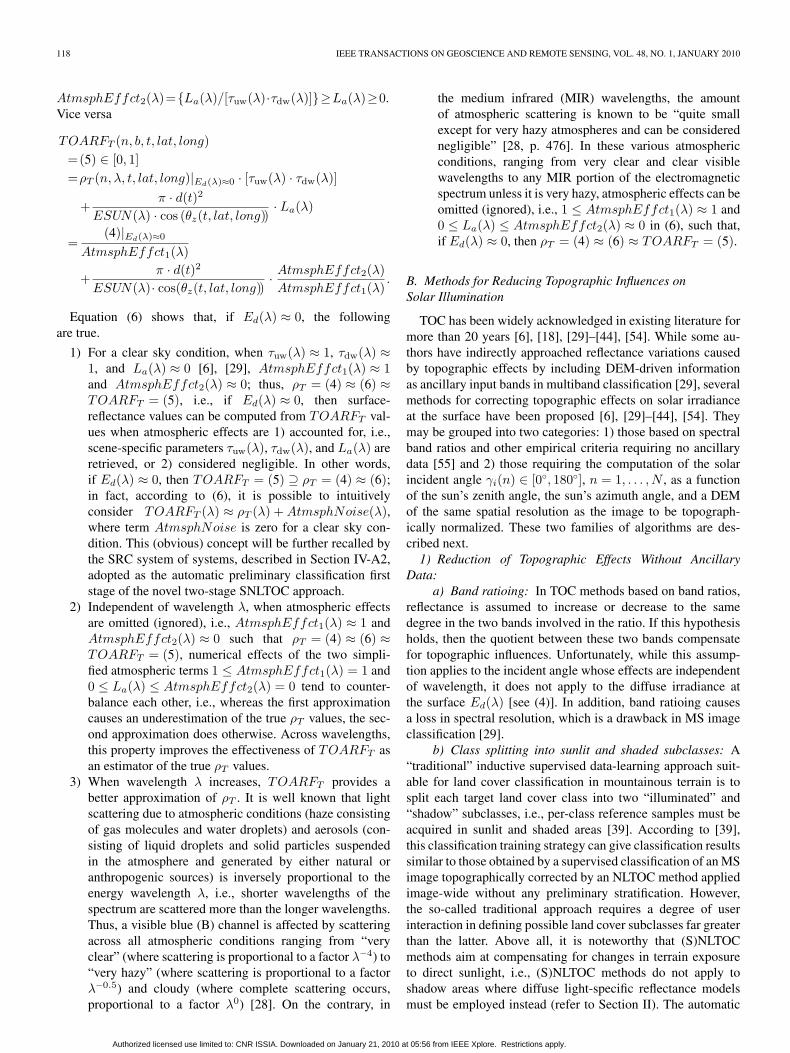
Fig. 2. If φa = φ0(n), then (1) becomes θz = γi(n) + θp(n), n ∈ {1, N}.
by the RS image metadata file or can be computed fromthe 1) image acquisition date and time and 2) (average)image-specific or pixel-based latitude/longitude spatialcoordinates.
3) θp(n) ∈ [0◦, 90◦] is the pixel-based slope angle computedfrom the DEM exclusively, i.e., irrespective of the solarzenith and azimuth angles. It can easily be proved that theper-pixel slope θp(n) can be alternatively defined as theangle between the normal to the surface and the directionto the zenith [46], although this angle is confused with thesun zenith angle θz in [42, Fig. 2].
4) φ0(n) ∈ [0◦, 360◦] is the pixel-based aspect angle mea-sured clockwise from the north. It is computed from theDEM exclusively, i.e., irrespective of the solar zenith andazimuth angles.
Equation (1) implies the following.
1) For a horizontal surface, such that θp(n) = 0, n ∈{1, N}, equality γi(n) = θz always holds.
2) If the per-pixel aspect angle is equivalent to the sunazimuth angle, i.e., φ0(n) = φa, then (1) becomes(see Fig. 2)
θz = γi(n) + θp(n), if φ0(n) = φa; n ∈ {1, N}. (2)
3) If φ0(n) = φa, i.e., if (2) holds, AND θp(n) = θz,n ∈ {1, . . . , N}, then γi(n) = 0; thus, IL(n) = 1, i.e.,this slope faces the sun perfectly.
According to the IL(n) definition provided previously, theaim of TOC can be considered as a compensation for changes inthe solar incident angle due to topographic influences. Severalimplications stem from this general definition.
It is well known that the solar irradiance (energy) at eachterrain point has two components comprising three terms [19],[46], [47]: 1) a direct solar irradiance, called sunlight [18], and2) an indirect [46] or diffuse [40] solar irradiance comprisingthe following two components. First, in nonflat terrain areas,light is reflected from other objects (e.g., adjacent slopes inrugged terrain) before being reflected from the pixel underconsideration; this first component is called reflected terrainradiance and is null in flat terrain [6]. Second, in both flat andrugged terrain, radiation is reflected from the neighborhood of
Authorized licensed use limited to: CNR ISSIA. Downloaded on January 21, 2010 at 05:56 from IEEE Xplore. Restrictions apply.

116 IEEE TRANSACTIONS ON GEOSCIENCE AND REMOTE SENSING, VOL. 48, NO. 1, JANUARY 2010
the pixel under consideration, and next, it is scattered by theatmosphere into the viewing direction; this second componentis called skylight [18] or adjacency radiance [6]. The contri-bution of indirect illumination to the radiance reflected by thetarget terrain area subject to direct illumination is relatively low,particularly in a flat terrain [48]. On sunlit (sunny) slopes, bothdirect and indirect light sources provide their contribution tothe energy at the sensor, whereas on sun-shaded (shady) slopesdirect sunlight at the surface is occluded.
In spite of their common use, the two terms sunlit slopes andsun-shaded slopes, which are totally exhaustive and mutuallyexclusive, suffer from vague or ambiguous definitions in RS lit-erature. For example, in [29, p. 1056], shaded areas are definedas “slopes showing less than expected reflectance, whereasin sunny areas, the effect is the opposite.” In [31], the termsun-shaded or shady slope is considered a synonym of slopefacing away from the sun while the term sunny slope is usedinterchangeably with slope facing the sun. A formal definitionof sun-shaded slopes and sunlit slopes either facing the sun orfacing away from the sun as a function of the pixel-based solarincident angle γi(n) ∈ [0◦, 180◦], n = 1, . . . , N , and the solarzenith angle θz ∈ [0◦, 90◦] is provided in Section IV-A1.
To summarize, despite some confusion in the definitions ofsun-shaded slopes and sunlit slopes either facing the sun orfacing away from the sun found in RS literature, an alter-native definition of traditional LTOC (isotropic) and NLTOC(anisotropic) methods (see Section I) refers to compensation forchanges in terrain exposure to the direct (sunlight) componentof solar energy at the surface. This is tantamount to saying thatLTOC and NLTOC methods transform radiance (respectively,reflectance) values of sunlit slopes either facing the sun or fac-ing away from the sun into radiance (respectively, reflectance)values of sunlit horizontal-like surfaces.
This latter definition of LTOC and NLTOC methods is nottrivial. It means that, in slopes occluded from the sun, illumi-nated by no sunlight, LTOC and NLTOC methods cannot beapplied. Rather, shaded slopes require a physically basedsurface-reflectance model (whose aim is to link surface prop-erties with sensor-measured radiance) specific for skylight andreflected terrain irradiance [19], [42], [46]–[48]. If the afore-mentioned definition holds, i.e., if LTOC and NLTOC methodshave nothing to do with shaded slopes, then the assessmentof NLTOC methods across sunlit and shadow areas, such asthat proposed in [39] and, perhaps [31], makes no theoreticalsense.
III. PREVIOUS WORKS
This section provides a summary of related works on thefollowing subjects:
1) radiometric calibration of DNs into TOARFT ⊇ ρT val-ues, which are required as input by the SRC first stageof the original two-stage SNLTOC method proposed inSection IV;
2) traditional methods for reducing topographic effects re-quiring no ancillary data;
3) LTOC, NLTOC, and SNLTOC methods requiring ancil-lary data (e.g., a DEM).
A. Radiometric Calibration and Atmospheric Correction
Although it is often ignored in common practice by RSscientists and practitioners in disagreement with the QA4EOguidelines, radiometric calibration, which is the transformationof dimensionless DNs into a unit of measure related to acommunity-agreed radiometric scale, achieves the followingobjectives well known by a significant portion of existing liter-ature and clearly acknowledged by international EO programssuch as GEOSS and GMES (see Section I).
1) It ensures the harmonization and interoperability of mul-tisource observational data and derived products suchas those required by the ongoing GEOSS and GMESprojects [12]–[14].
2) It makes RS data well behaved and well understood[11], which paves the way to automating the quantitativeanalysis of EO data [19], [24].
The first step in radiometric calibration, which is the so-called absolute radiometric calibration [27], is the linear trans-formation of a pixel value DN(n, b) ≥ 0, with n = 1, . . . , Nand b = 1, . . . , Bnd, where N is the total number of pixelsand Bnd is the number of spectral channels (bands), into aTOARDT value TOARDT (n, b) ≥ 0, expressed in a radio-metric unit of measure, either W/(m2 × sr × μm) (e.g., in thespaceborne Landsat, Satellite Pour l’Observation de la Terre(SPOT), Advanced Spaceborne Thermal Emission and Reflec-tion (ASTER), and QuickBird optical sensors) or mW/(cm2 ×sr × μm) (e.g., in the spaceborne IKONOS and Indian RSSatellite (IRS) optical sensors) [6], as a function of the gainG(b) ≥ 0 and offset O(b) ≥ 0 calibration parameters for bandb = 1, . . . , Bnd, to be retrieved from the RS metadata file. Forexample, in the case of SPOT-1/-5 imagery [49]
0 ≤ TOARDT (n, b) = [DN(n, b)/G(b)] + O(b),
n = 1, . . . , N ; b = 1, . . . , Bnd (3)
where gain and offset parameters are identified, respectively,as “〈PHYSICAL_GAIN〉” and “〈PHYSICAL_BIAS〉” in theSPOT metadata digital image map (DIMAP) file format.
The model for obtaining dimensionless true terrain re-flectance ρT (n, λ, t, lat, long) ∈ [0, 1] from the spectral ra-diance at the sensor’s aperture TOARDT (n, λ) may beexpressed as follows [29]:
ρT (n, λ, t, lat, long)
=π · d(t)2 ·
(TOARDT (n,λ)−La(λ)
τuw(λ)
)ESUN(λ) · cos (θz(t, lat, long)) · τdw(λ) + Ed(n, λ)
∈ [0, 1],
n = 1, . . . , N (4)
where λ is the electromagnetic wavelength, (lat, long) isthe pixel position in geographic coordinates, and d(t) is theEarth–sun distance in astronomical units to be interpolatedfrom values found in literature as a function of the view-ing day and time t, transformed into a Julian day value in
Authorized licensed use limited to: CNR ISSIA. Downloaded on January 21, 2010 at 05:56 from IEEE Xplore. Restrictions apply.

BARALDI et al.: OPERATIONAL TWO-STAGE STRATIFIED TOPOGRAPHIC CORRECTION OF SPACEBORNE MS IMAGERY 117
the range {1, 365}, such that d(t) approximately belongs torange 1 ± 3.5% [50]. La(λ) ≥ 0 is the atmospheric upwellingradiance scattered at the sensor by the atmosphere (calledairlight [18], equivalent to an additive term to be assessed bydark-object subtraction techniques: If, by definition of a darkobject, ρT = (4) = 0, then the unknown variable La is equalto the measured TOARDT value [28]), and Ed(n, λ) ≥ 0 iscalled diffuse irradiance at the surface [29], ambient light,or indirect illumination [46], contains no information on thesurface properties of the pixel, and comprises two compo-nents: 1) in nonflat terrain areas, reflected terrain radiance[6] or 2) in both flat and rugged terrain, skylight [18] oradjacency radiance [6] (also refer to Section II). Overall,Ed(λ) changes with wavelength; it can provide a relevantcontribution to incident radiance in rugged terrains [28], [29],but is relatively low in flat terrains [48]. Furthermore, τuw(λ) ∈[0, 1] and τdw(λ) ∈ [0, 1] are the path atmospheric transmit-tances of the upwelling (ground surface–sensor path) anddownwelling (sun–ground surface path) flows, respectively, andESUN(λ) is the mean solar exoatmospheric (TOA, plane-tary) irradiance found in literature [29] (e.g., in the SPOTmetadata DIMAP file format, parameter ESUN(λ) is iden-tified as “〈SOLAR_IRRADIANCE_VALUE〉”). θz ∈ [0◦, 90◦]is the sun’s zenith angle in degrees (also refer to Section II),typically provided in the image metadata file or computedfrom the data acquisition time t and per-scene or pixel-basedlatitude–longitude coordinates. The term [ESUN(λ) · cos(θz)]is called sunlight [18] or direct illumination [29] and representsthe only radiation component reflected from the pixel underconsideration that contains “pure” information on the surfaceproperties of the pixel (also refer to Section II).
In (4), atmospheric effects are modeled by atmospheric pa-rameters τuw(λ) ∈ [0, 1], τdw(λ) ∈ [0, 1], and La(λ) ≥ 0. Toretrieve these atmospheric parameters, ancillary data (summarystatistics), which are rarely available in practice, should becollected at several locations within the RS image footprintat the time of RS image acquisition. This means that theproblem of atmospheric correction is typically ill or poorlyposed. Consequently, it is very difficult to solve and requiresuser’s supervision to make it better posed [6] (also refer toSection I). In common practice, Baraldi has observed that RSimages radiometrically calibrated into ρT values by several EUinstitutions mentioned later in this paper are unreliable, namely,they are affected by spectral distortion causing scene-derivedsurface-reflectance spectra to disagree with reference surface-reflectance signatures found in existing literature (e.g., refer to[81, p. 273]) or in public domain spectral libraries such as theU.S. Geological Survey (USGS) mineral and vegetation spec-tral libraries, the Johns Hopkins University spectral library, andthe Jet Propulsion Laboratory mineral spectral library [6], [56].
A reduction in interscene variability across time, space,and sensors can be achieved by a simplification of (4) intodimensionless TOARFT values belonging to the range [0, 1].Starting from (4), TOARFT values are computed as a func-tion of the electromagnetic wavelength for spectral band b =1, . . . , Bnd, by considering the following: 1) atmosphericeffects negligible, such as for relatively “clear” sceneswhere τuw(λ) ≈ 1, τdw(λ) ≈ 1, and La(λ) ≈ 0 [6], [29], and
2) flat and/or nonflat neighboring terrain effects negligible, i.e.,Ed(λ) ≈ 0 [29]. Thus, (4) becomes
TOARFT (n, b, t, lat, long)
=π · d(t)2 · TOARDT (n, b)
ESUN(b) · cos (θz(t, lat, long))∈ [0, 1],
n = 1, . . . ; N, b = 1, . . . , Bnd. (5)
Although often overlooked by RS scientists and practi-tioners, it is well known in existing literature that the ra-diometric calibration of DNs into TOARFT = (5) valuesfeatures several advantages over the radiometric calibration intoTOARDT = (3) values.
1) The former is recommended before calculating variousvegetation indices (VIs) [19]. In fact, while the relation-ships between the LAI and a great variety of well-knownVIs calculated from TOARDT values are nonlinear, therelationships between LAI and the same VIs calculatedfrom TOARFT are, in several cases, reasonably linear.
2) By accounting for seasonal and latitudinal differences insolar illumination, the former guarantees better interim-age comparability/interpretation (classification, mapping)across time, space, and sensors [24], [25], which is in linewith the goals of EO data harmonization and interoper-ability required by the GEOSS and GMES programs.
3) The former is more consistent with the scenario oflow- and high-level image-processing capabilities to bedeveloped onboard future intelligent fourth-generationEO satellites (FIEOSs) [52], [53]. The developmentof FIEOS, where onboard integration of sensors, dataprocessors, and communication systems is pursued,should become a major scientific challenge to the RScommunity within the next ten years [52].
It is noteworthy that, when neighboring terrain effects areomitted, i.e., Ed(λ) ≈ 0, then ρT |Ed(λ)≈0 = (4)|Ed(λ)≈0 =f1(TOARDT )|Ed(λ)≈0 can be expressed as ρT = |Ed(λ)≈0 =f2(TOARFT ) as follows:
ρT (n, λ, t, lat, long)|Ed(λ)≈0
= (4)|Ed(λ)≈0 ∈ [0, 1]
= TOARFT (n, b, t, lat, long)
× 1τuw(λ) · τdw(λ)
− π · d(t)2
ESUN(λ) · cos (θz(t, lat, long))
× La(λ)τuw(λ) · τdw(λ)
= (5) · AtmsphEffct1(λ)
− π · d(t)2
ESUN(λ) · cos (θz(t, lat, long))× AtmsphEffct2(λ),
n = 1, . . . , N ; b = 1, . . . , Bnd (6)
where TOARFT (n, b, t, lat, long) = (5) ∈ [0, 1],AtmsphEffct1(λ) = {1/[τuw(λ) · τdw(λ)]} ≥ 1, and
Authorized licensed use limited to: CNR ISSIA. Downloaded on January 21, 2010 at 05:56 from IEEE Xplore. Restrictions apply.
118 IEEE TRANSACTIONS ON GEOSCIENCE AND REMOTE SENSING, VOL. 48, NO. 1, JANUARY 2010
AtmsphEffct2(λ)={La(λ)/[τuw(λ)·τdw(λ)]}≥La(λ)≥0.Vice versa
TOARFT (n, b, t, lat, long)=(5) ∈ [0, 1]=ρT (n, λ, t, lat, long)|Ed(λ)≈0 · [τuw(λ) · τdw(λ)]
+π · d(t)2
ESUN(λ) · cos (θz(t, lat, long))· La(λ)
=(4)|Ed(λ)≈0
AtmsphEffct1(λ)
+π · d(t)2
ESUN(λ)· cos(θz(t, lat, long))· AtmsphEffct2(λ)AtmsphEffct1(λ)
.
Equation (6) shows that, if Ed(λ) ≈ 0, the followingare true.
1) For a clear sky condition, when τuw(λ) ≈ 1, τdw(λ) ≈1, and La(λ) ≈ 0 [6], [29], AtmsphEffct1(λ) ≈ 1and AtmsphEffct2(λ) ≈ 0; thus, ρT = (4) ≈ (6) ≈TOARFT = (5), i.e., if Ed(λ) ≈ 0, then surface-reflectance values can be computed from TOARFT val-ues when atmospheric effects are 1) accounted for, i.e.,scene-specific parameters τuw(λ), τdw(λ), and La(λ) areretrieved, or 2) considered negligible. In other words,if Ed(λ) ≈ 0, then TOARFT = (5) ⊇ ρT = (4) ≈ (6);in fact, according to (6), it is possible to intuitivelyconsider TOARFT (λ) ≈ ρT (λ) + AtmsphNoise(λ),where term AtmsphNoise is zero for a clear sky con-dition. This (obvious) concept will be further recalled bythe SRC system of systems, described in Section IV-A2,adopted as the automatic preliminary classification firststage of the novel two-stage SNLTOC approach.
2) Independent of wavelength λ, when atmospheric effectsare omitted (ignored), i.e., AtmsphEffct1(λ) ≈ 1 andAtmsphEffct2(λ) ≈ 0 such that ρT = (4) ≈ (6) ≈TOARFT = (5), numerical effects of the two simpli-fied atmospheric terms 1 ≤ AtmsphEffct1(λ) = 1 and0 ≤ La(λ) ≤ AtmsphEffct2(λ) = 0 tend to counter-balance each other, i.e., whereas the first approximationcauses an underestimation of the true ρT values, the sec-ond approximation does otherwise. Across wavelengths,this property improves the effectiveness of TOARFT asan estimator of the true ρT values.
3) When wavelength λ increases, TOARFT provides abetter approximation of ρT . It is well known that lightscattering due to atmospheric conditions (haze consistingof gas molecules and water droplets) and aerosols (con-sisting of liquid droplets and solid particles suspendedin the atmosphere and generated by either natural oranthropogenic sources) is inversely proportional to theenergy wavelength λ, i.e., shorter wavelengths of thespectrum are scattered more than the longer wavelengths.Thus, a visible blue (B) channel is affected by scatteringacross all atmospheric conditions ranging from “veryclear” (where scattering is proportional to a factor λ−4) to“very hazy” (where scattering is proportional to a factorλ−0.5) and cloudy (where complete scattering occurs,proportional to a factor λ0) [28]. On the contrary, in
the medium infrared (MIR) wavelengths, the amountof atmospheric scattering is known to be “quite smallexcept for very hazy atmospheres and can be considerednegligible” [28, p. 476]. In these various atmosphericconditions, ranging from very clear and clear visiblewavelengths to any MIR portion of the electromagneticspectrum unless it is very hazy, atmospheric effects can beomitted (ignored), i.e., 1 ≤ AtmsphEffct1(λ) ≈ 1 and0 ≤ La(λ) ≤ AtmsphEffct2(λ) ≈ 0 in (6), such that,if Ed(λ) ≈ 0, then ρT = (4) ≈ (6) ≈ TOARFT = (5).
B. Methods for Reducing Topographic Influences onSolar Illumination
TOC has been widely acknowledged in existing literature formore than 20 years [6], [18], [29]–[44], [54]. While some au-thors have indirectly approached reflectance variations causedby topographic effects by including DEM-driven informationas ancillary input bands in multiband classification [29], severalmethods for correcting topographic effects on solar irradianceat the surface have been proposed [6], [29]–[44], [54]. Theymay be grouped into two categories: 1) those based on spectralband ratios and other empirical criteria requiring no ancillarydata [55] and 2) those requiring the computation of the solarincident angle γi(n) ∈ [0◦, 180◦], n = 1, . . . , N , as a functionof the sun’s zenith angle, the sun’s azimuth angle, and a DEMof the same spatial resolution as the image to be topograph-ically normalized. These two families of algorithms are des-cribed next.
1) Reduction of Topographic Effects Without AncillaryData:
a) Band ratioing: In TOC methods based on band ratios,reflectance is assumed to increase or decrease to the samedegree in the two bands involved in the ratio. If this hypothesisholds, then the quotient between these two bands compensatefor topographic influences. Unfortunately, while this assump-tion applies to the incident angle whose effects are independentof wavelength, it does not apply to the diffuse irradiance atthe surface Ed(λ) [see (4)]. In addition, band ratioing causesa loss in spectral resolution, which is a drawback in MS imageclassification [29].
b) Class splitting into sunlit and shaded subclasses: A“traditional” inductive supervised data-learning approach suit-able for land cover classification in mountainous terrain is tosplit each target land cover class into two “illuminated” and“shadow” subclasses, i.e., per-class reference samples must beacquired in sunlit and shaded areas [39]. According to [39],this classification training strategy can give classification resultssimilar to those obtained by a supervised classification of an MSimage topographically corrected by an NLTOC method appliedimage-wide without any preliminary stratification. However,the so-called traditional approach requires a degree of userinteraction in defining possible land cover subclasses far greaterthan the latter. Above all, it is noteworthy that (S)NLTOCmethods aim at compensating for changes in terrain exposureto direct sunlight, i.e., (S)NLTOC methods do not apply toshadow areas where diffuse light-specific reflectance modelsmust be employed instead (refer to Section II). The automatic
Authorized licensed use limited to: CNR ISSIA. Downloaded on January 21, 2010 at 05:56 from IEEE Xplore. Restrictions apply.

BARALDI et al.: OPERATIONAL TWO-STAGE STRATIFIED TOPOGRAPHIC CORRECTION OF SPACEBORNE MS IMAGERY 119
detection of occluded areas in spaceborne imagery requiresancillary data, namely, a DEM, the sun’s zenith angle, andthe sun’s azimuth angle. If this ancillary data are missing,then a manual photointerpretation of occluded areas is typicallyaffected by commission errors with slopes facing away from thesun (refer to Section II). To conclude, (S)NLTOC approachesand supervised class splitting into sunlit and shaded subclassesare complementary rather than alternative approaches.
c) Standard SAM: Due to its relative insensitiveness totopographic and atmospheric effects, the spectral angle map-per (SAM) is considered a standard classifier implemented inseveral commercial image-processing software toolboxes suchas the Environment for Visualizing Images (ENVI), licensedby ITT Industries, Inc. [56]. In a D-dimensional measurement(feature) space, SAM computes the spectral angle α formedbetween a reference vector from the origin r̄, representing areference spectrum (signature) belonging to a collection of so-called endmember spectra [56], and the vector from the originrepresenting an unclassified pixel v̄. The unclassified pixel isassigned to the reference class forming the smallest angle withthe pixel vector.
The vector pair in between angles is computed as [57], [58]
SAM(v, r) = arccos(α) = arccos(
< v,r >
‖v‖ · ‖r‖)
∈ [0, π] (7)
where 〈v, r〉 =∑D
d=1 vdrd is the dot product between vectors v̄
and r̄, ‖v‖ =√∑D
d=1(vd)2 is the magnitude (intensity) opera-tor, and cos α = (〈v, r〉/‖v‖ · ‖r‖) ∈ [−1, 1] is the normalizeddot product. It is to be noted that the so-called Cosine of theAngle Concept (CAC) classifier employs the normalized dotproduct in place of (7) [57]. Both SAM and CAC are invariantto linearly scaled variations of vectors v̄ and r̄ when they areboth multiplied by a coefficient belonging to the domain of realnumbers R.
The fuzzy prior knowledge exploited by SAM is the fol-lowing: “spectra of the same type of surface objects are ap-proximately linearly scaled versions of one another due to theatmospheric and topographic variations” [57]–[59]. Accordingto existing literature (e.g., [60]), this statement is known to beextremely fuzzy (vague, qualitative), as shown in Fig. 3, wherea set of reflectance patterns, extracted from Landsat imagesradiometrically calibrated into TOARFT values and belongingto the endmember collection spectra employed to develop SRC[45] (refer to Section IV-A2), can be compared.
An additional theoretical drawback of both SAM and CACis that, by ignoring a comparison between magnitudes ‖v‖ and‖r‖, they employ no intensity (brightness, panchromatic [61])information criteria in their decision rule. This information lossis well known in existing literature where, starting from SAM,alternative transformed distance concepts were proposed, e.g.,refer to [62].
2) TOC Methods Exploiting Ancillary Data: To estimatethe flat-normalized (horizontal) reflectance TOARFH(n, b),where n = 1, . . . , N and b = 1, . . . , Bnd, from an input MSimage radiometrically calibrated into TOARFT (n, b) values,with n = 1, . . . , N and b = 1, . . . , Bnd, several TOC meth-
Fig. 3. Endmember collection spectra employed to design the decision ruleset in SRC [45]. Spectral signatures in TOARFT values, belonging to thecontinuous range [0, 1] linearly scaled onto the discrete range {0, 255} (witha discretization error equaling 0.4%), are extracted from Landsat-7 ETM+images.
ods require the precomputation of the pixel-based illumina-tion, IL(n) = cos(γi(n)) = (1) ∈ [−1, 1], n = 1, . . . , N , as afunction of the sun’s zenith angle θz ∈ [0◦, 90◦], the sun’sazimuth angle φa ∈ [0◦, 360◦], and a DEM of the same spatialresolution as the MS image to be topographically normalized(see Section II). These TOC approaches can be grouped into
Authorized licensed use limited to: CNR ISSIA. Downloaded on January 21, 2010 at 05:56 from IEEE Xplore. Restrictions apply.

120 IEEE TRANSACTIONS ON GEOSCIENCE AND REMOTE SENSING, VOL. 48, NO. 1, JANUARY 2010
the following two subcategories, depending on whether theyassume the surface reflectance as being independent of theobservation and incident angles (see Section I).
1) LTOC (isotropic) approaches. The Lambertian assump-tion is very simple but unrealistic because most land covertypes are rugged and feature non-Lambertian behavior.
2) NLTOC (anisotropic) approaches comprising eithernonstratified or stratified (SNLTOC) methods. On a the-oretical basis, the bidirectional reflectance distributionfunction (BRDF) describes how reflectance varies in eachland cover type by considering all possible angles ofincidence and observation. In practice, the determinationof BRDF is extremely complex. To provide a simpli-fied estimation of a non-Lambertian spectral reflectancemodel, NLTOC and SNLTOC methods have been devel-oped starting from different assumptions about the real(3-D) scene depicted in an (2-D) MS image.
Ordinary LTOC and NLTOC methods are surveyed anddiscussed next to highlight several inconsistencies found inexisting literature.
a) LTOC (isotropic) methods: The simplest and bestknown LTOC method is the cosine LTOC equation. Widelyadopted in most image-processing software toolboxes [56], itis computed as follows [29], [31], [34], [35]:
TOARFH(n, b) = TOARFT (n, b)(
cos θz
cos γi(n)
),
n = 1, . . . , N ; b = 1, . . . , Bnd (8)
where incident angle γi(n) ∈ [0◦, 180◦], and thus, cos γi(n) =IL(n) ∈ [−1,+1] (see Section II), and where the sun’s zenithangle θz ∈ [0◦, 90◦] is used to take into account the nonvertical-ity of direct sun rays. Several considerations stem from (8).
1) In (8), the larger the incident angle γi(n) in range[0◦, 90◦], i.e., the lower the per-pixel illumination IL(n)in range [0, +1], the higher the corrected reflectanceTOARFH(n, b).
2) When γi(n) ∈ (90◦, 180◦], i.e, IL(n) ∈ [−1, 0), then (8)< 0, which has no physical meaning. To the best of ourknowledge, the sole explicit strategy on employing (8)when γi(n) ∈ (90◦, 180◦] is found in [36], where it iswritten that, if γi(n) ≥ 85◦, then the pixel informationvalue is low and topographic normalization does nothelp. This is tantamount to saying that, when γi(n) ∈[85◦, 180◦], (8) is not applied.
3) For a horizontal surface, where γi(n) = θz ∈ [0◦, 90◦](see Section II), (8) becomes TOARFH(n, b) =TOARFT (n, b), i.e., the measured terrain surfaceTOARFT (n, b) is left unchanged after topographicnormalization. This means that, when (8) is adopted,horizontal surfaces can be skipped in topographicnormalization to save computation time.
In contrast with the RS image preprocessing protocol recom-mended in Section I, if (8) is meant to be applied to TOARDT
rather than to TOARFT values, i.e., when topographic normal-ization is applied in series with absolute radiometric calibration
[see (3)] but before the transformation of TOARDT intoTOARFT values [refer to (5)], (8) becomes [34], [35]
TOARDH(n, b) =TOARDT (n, b)
cos γi(n),
with n = 1, . . . , N ; b = 1, . . . , Bnd (9)
where incident angle γi(n) ∈ [0◦, 180◦]; thus, cos γi(n) =IL(n) ∈ [−1,+1] (see Section II). The following are worthnoting.
1) According to [36], when γi(n) ∈ [85◦, 180◦], (9) shouldnot be applied (see aforementioned comments).
2) If γi(n) ∈ [0◦, 90◦], i.e., IL(n) ∈ [0,+1], then (9) showsthat TOARDH(n, b) ≥ TOARDT (n, b) n ∈ {1, N}and b = 1, . . . , Bnd. Condition γi(n) ∈ [0◦, 90◦]includes horizontal surfaces, where γi(n) = θz ∈[0◦, 90◦] (refer to Section II), such that (9) be-comes TOARDH(n, b) = (TOARDT (n, b)/ cos θz) ≥TOARDT (n, b). This means that, unlike (8), whoseeffect on TOARFT values belonging to horizontalsurfaces is null, (9) must be applied to the wholeTOARDT image, including horizontal surfaces. Thereason for this difference between (8) and (9) is that,in line with the RS image preprocessing protocolrecommended in Section I, (8) is applied in series with(5), such that the denominator cos(θz) employed in (5) iselicited by the numerator cos(θz) adopted by (8).
Unfortunately, differences between (8) and (9) appear tobe not always understood in literature. For example, in [31],(8) is wrongly referred to as radiance rather than reflectancewhile (9) is incorrectly identified as topographically normalizedreflectance rather than radiance in [44]. More dangerous thanthat, in [39, p. 3839], (9) is not applied to horizontal surfaces.
Limitations:
1) Several authors have shown that (8) and (9) overcor-rect the image in areas of “low” IL(n) values [29],[34], [35]. The empirical (fuzzy) nature of this state-ment can be better formalized as follows. In (8) and(9), low IL(n) values should be identified as valueswhere IL(n) = cos γi(n) < cos θz with θz ∈ [0◦, 90◦],i.e., γi(n) ∈ (θz, 180◦]. This condition corresponds to1) nonhorizontal nonoccluded surfaces facing away fromthe sun if γi(n) ∈ (θz, 90◦] and 2) occluded surfacesbelonging to shadow casters (self-shadows) if γi(n) ∈(90◦, 180◦] (see Section IV-A1).
2) Topographic normalization introduced by (8) and (9) iswavelength independent. This assumption is unrealisticbecause diffuse irradiance at the surface [refer to termEd(λ) in (4)] is highly wavelength dependent [28], [29].
3) Most land cover types are rugged and feature non-Lambertian behavior.
b) NLTOC (anisotropic) methods: NLTOC and SNLTOCmethods employ different hypotheses to constrain the problemof surface-roughness estimation. In particular, NLTOC methodsadopt the following hypothesis [29].
Hypothesis 1: The pixel-based corrected horizontal (flat-normalized) reflectance TOARFH(n, b), where n = 1, . . . , N
Authorized licensed use limited to: CNR ISSIA. Downloaded on January 21, 2010 at 05:56 from IEEE Xplore. Restrictions apply.
BARALDI et al.: OPERATIONAL TWO-STAGE STRATIFIED TOPOGRAPHIC CORRECTION OF SPACEBORNE MS IMAGERY 121
and b = 1, . . . , Bnd, is assumed to be per-band image-wideconstant (homogeneous), i.e., TOARFH(n, b) = Constant(b),where n = 1, . . . , N and b = 1, . . . , Bnd. This is tantamountto saying that the whole image belongs to a single land coverclass.
Some authors consider Hypothesis 1 so poorly constrainedthat unrealistic but simpler LTOC methods are preferred toNLTOC approaches [29]. To replace Hypothesis 1 with amore realistic constraint, SNLTOC approaches assume thefollowing.
Hypothesis 2: Before topographic normalization takes place,the input MS image radiometrically calibrated intoTOARFT (n, b) values, where n = 1, . . . , N and b = 1, . . . ,Bnd, must be provided with an exhaustive and mutuallyexclusive partition (map) equivalent to a land-cover-class-specific surface-roughness stratification Strtm(n) ∈ {1, S},n = 1, . . . , N , where S is the total number of strata, such thatS ≥ C ≥ 1, where C is the total number of land cover classes(excluding class “unknown”) predetected in the input imageTOARFT (n, b), where n = 1, . . . , N and b = 1, . . . , Bnd. Inother words, an SNLTOC approach assumes that, first, eachpredefined stratum s ∈ {1, S} features a typical or “average”surface roughness. Second, the map-conditional topographical-ly corrected (horizontal) reflectance TOARFH [n, b|Strtm(n);n = 1, . . . , N , b = 1, . . . , Bnd, Strtm(n) ∈ {1, S}] isassumed to be per-band per-stratum piecewise constant, i.e.,TOARFH [n, b|Strtm(n) = s;n ∈ {1, N}, s = 1, . . . , S, b =1, . . . , Bnd] = Constant[b, s; s = 1, . . . , S, b = 1, . . . , Bnd].
In practice, SNLTOC approaches are limited by the need fora priori knowledge of the spatial structure (namely, roughness)of the landscape (refer to Section I) [37]. For example, severalpapers in literature employ SNLTOC approaches capable ofsatisfying Hypothesis 2, where the number of target classes C isas coarse as one to three [31], [34]–[39], [43]. It is noteworthythat the stratification strategy adopted in [44], which is DEMdriven but land cover class independent, does not satisfy theaforementioned Hypothesis 2.
3) Minnaert Equation: In existing literature, the best knownNLTOC and SNLTOC approaches are based on the ideas ofMinnaert, who first proposed a semiempirical equation to as-sess the roughness of the moon’s surface [29]. According toMinnaert’s ideas, the LTOC equation (8) is revised as followsin the so-called Minnaert NLTOC equation [29]:
TOARFH(n, b) = TOARFT (n, b)[
cos θz
cos γi(n)
]K(b)
,
n = 1, . . . , N ; b = 1, . . . , Bnd (10)
where incident angle γi(n) ∈ [0◦, 180◦], and thus, cos γi(n) =IL(n) ∈ [−1,+1] (see Section II), and where coefficientK(b) ∈ [0, 1] is a dimensionless real number, called theMinnaert constant for spectral band b = 1, . . . , Bnd, capableof modeling the non-Lambertian behavior of the surface dueto surface roughness. If K(b) = 1, the surface behaves as aperfect Lambertian reflector. If K(b) → 0, the surface is porousand exhibits asymmetrical diffuse scattering (which explainsthe low values of K(b) for class forest) [36].
To estimate the value of K(b) for each spectral band b =1, . . . , Bnd, (10) can be linearized as follows:
Y (n, b) = log10 [TOARFT (n, b)]
= log10 [TOARFH(b)] + K(b) log10
[cos γi(n)cos θz
]
= D(b) + A(b) · X(n) (11)
where n = 1, . . . , N , b = 1, . . . , Bnd, and D(b) =log10[TOARFH(b)] and A(b) = K(b) are the tworegression coefficients of the observed reflectance valuesY (n, b) = log10[TOARFT (n, b)], where n = 1, . . . , N andb = 1, . . . , Bnd, versus incident angle-dependent termsX(n) = log10[cos γi(n)/ cos θz], n = 1, . . . , N .
In practice, estimated Minnaert constant values K(b) > 1and K(b) < 0 indicate that the adopted regression methodand its Y (n, b) and X(n) data sets are poor, e.g., when datasets Y (n, b) and X(n) feature large and unstable variationsdue to the presence of “outliers,” namely, pixels belongingto different strata of surface roughness within the image-widedata set of observed reflectance values TOARFT (n, b), wheren = 1, . . . , N and b = 1, . . . , Bnd [36]. Thus, the estimatedMinnaert constant values K(b) > 1 and K(b) < 0 should berounded to values 1 and 0, respectively, in line with [36],although this is rarely done in practice, e.g., refer to [44].
When (9) is employed in place of (8), (10) becomes
TOARDH(n, b) =TOARDT (n, b)
[cos γi(n)]K(b)=
TOARDT (n, b)IL(n)K(b)
,
n = 1, . . . , N ; b = 1, . . . , Bnd. (12)
For the sake of completeness, the SNLTOC version of theMinnaert NLTOC equation (10) incorporates Hypothesis 2,defined previously, to become
TOARFH (n, b|Strtm(n) = s)
= TOARFT (n, b|Strtm(n) = s)[
cos θz
cos γi(n)
]K(b,s)
(13)
where n ∈ {1, N}, b = 1, . . . , Bnd, s = 1, . . . , S, andk(b, s) ∈ [0, 1].
Limitations:
1) In their original formulation, the NLTOC equations (10)and (11) adopt the unrealistic Hypothesis 1. In [34], anSNLTOC version of (10) adapted to incorporate a strati-fied or layered approach [see (13)] performs better thanthe NLTOC equation (10) by improving classificationaccuracies of land cover types after SNLTOC.
2) In [29], (10) is found to overcorrect the TOARFT
image in areas of low IL(n) values, like (8) (refer toSection III-B2a).
4) Enhanced Minnaert Equation: In [54], the MinnaertNLTOC equation (10) was further modified to include the slope
Authorized licensed use limited to: CNR ISSIA. Downloaded on January 21, 2010 at 05:56 from IEEE Xplore. Restrictions apply.
122 IEEE TRANSACTIONS ON GEOSCIENCE AND REMOTE SENSING, VOL. 48, NO. 1, JANUARY 2010
of the terrain, which is θp(n) ∈ [0◦, 90◦], n = 1, . . . , N , asfollows [29], [34], [35]:
TOARFH(n, b) =TOARFT (n, b) cos θp(n)
×[
cos θz
cos γi(n) cos θp(n)
]K(b)
,
n = 1, . . . , N ; b = 1, . . . , Bnd (14)
where incident angle γi(n) ∈ [0◦, 180◦], and thus, cos γi(n) =IL(n) ∈ [−1,+1] (see Section II), K(b) ∈ [0, 1] (as discussedpreviously), and θz ∈ [0◦, 90◦].
The NLTOC-enhanced Minnaert equation (14) forTOARDT values becomes [31], [36]–[38], [44]
TOARDH(n, b) =TOARDT (n, b) cos θp(n)
[cos γi(n) cos θp(n)]K(b),
n = 1, . . . , N ; b = 1, . . . , Bnd. (15)
For the sake of completeness, the SNLTOC version ofthe enhanced Minnaert NLTOC equation (14) incorporatesHypothesis 2, defined previously, to become
TOARFH (n, b, |Strtm(n) = s)
= TOARFT (n, b, |Strtm(n) = s)
× cos θp(n) ·[
cos θz
cos γi(n) cos θp(n)
]K(b,s)
,
n ∈ {1, N}; b = 1, . . . , Bnd;
s = 1, . . . , S; k(b, s) ∈ [0, 1]. (16)
Limitations: According to [29] where an NLTOC ap-proach is adopted, (14) suffers from the same limitations asthe Minnaert equation (10). This conclusion is in contrast with[35], where (14) employed in an NLTOC approach performsbetter than the ordinary Minnaert equation (10) by reducingovercorrection when IL(n) is low and by increasing image-wide homogeneity. In [35], in line with theoretical expectations,the SNLTOC equation (16) performs better than the NLTOCequation (14).
5) C Correction Method: In an NLTOC framework, the Ccorrection method assumes a linear correlation between the ob-served terrain reflectance of each spectral band TOARFT (n, b)and illumination IL(n) = cos γi(n) ∈ [0◦, 180◦] as follows[29], [34], [35]:
Y (n, b) = TOARFT (n, b) = TOARFH(b) + C(b)IL(n)
= E(b) + C(b) · X(n) (17)
where n = 1, . . . , N , b = 1, . . . , Bnd, and the terms E(b) =TOARFH(b), which is assumed to be constant for the entireimage band b in line with Hypothesis 1, and C(b) are the re-gression coefficients, namely, the former is the intercept and thelatter is the gradient of the regression equation TOARFT (n, b)
versus IL(n). Next, starting from the equations proposed in[29], the C correction method is defined as
TOARFH(n, b) =TOARFT (n, b)·(
C(b) cos θz+E(b)C(b) cos γi(n)+E(b)
)
=TOARFT (n, b)·(
C(b) cos θz+E(b)C(b)IL(n)+E(b)
),
n = 1, . . . , N ; b = 1, . . . , Bnd. (18)
The SNLTOC version of the C correction equation (18)incorporates Hypothesis 2, defined previously, to become
TOARFH(n, b|Strtm(n)=s)= TOARFT (n, b|Strtm(n)=s)
×(
C(b, s) cos θz+E(b, s)C(b, s) cos γi(n)+E(b, s)
),
n∈{1, N}; b=1, . . . , Bnd; s=1, . . . , S. (19)
Limitations: According to [29], in an NLTOC framework,the limitations of (18) are the same as for the Minnaert equation(10) (refer to the earlier part of this paper). This conclusion isin line with [34], [35], and [41], where only small differenceswere observed between (10) and (18) in an NLTOC framework,although (18) is considered simpler to use.
6) Smoothed C Correction Method: In [29], it was ob-served that, in an NLTOC framework, (10), (14), and(18) cause an overcorrection of the horizontal reflectanceTOARFH(n, b) where IL(n) is low. Thus, in (10), (14),and (18), a reduction of the slope angle θp(n) ∈ [0◦, 90◦]is forced. To justify this strategy, consider that, in (10), ifθp(n) ⇒ 0, then γi(n) ⇒ θz; thus, cos(θz)/ cos γi(n) ⇒ 1 andTOARFH(n, b) ⇒ TOARFT (n, b) ∀K(b) ∈ [0, 1] and ∀n ∈{1, N}. In practice, in (1), the slope angle θp ∈ [0◦, 90◦] isreplaced by the smoothed slope angle θ̄p ∈ [0, θp] where, ac-cording to [29]
θ̄p(n) =θp(n)Smt
, Smt = 3, 5, 7; n = 1, . . . , N (20)
where the smoothing factor Smt ≥ 1.In [29], the Minnaert NLTOC equation (10), the enhanced
Minnaert NLTOC equation (14), the C NLTOC equation (18),and the smoothed C NLTOC equations (18) and (20) arecompared on the basis of their capability of decreasing within-class variance (i.e., increasing intraclass homogeneity). On theaverage, the smoothed C correction method with a correctionfactor Smt = 5 gave the best performance.
Limitations:
1) The unrealistic Hypothesis 1 is implicitly adopted.2) The smoothed C NLTOC method is provided with
one free parameter Smt to be user defined based onheuristics.
IV. NOVEL OPERATIONAL TWO-STAGE SNLTOC SYSTEM
This section is the core of the present work, where thenovel two-stage operational SLTOC system is proposed. Thedata flow diagram (DFD) of the original operational automatic
Authorized licensed use limited to: CNR ISSIA. Downloaded on January 21, 2010 at 05:56 from IEEE Xplore. Restrictions apply.

BARALDI et al.: OPERATIONAL TWO-STAGE STRATIFIED TOPOGRAPHIC CORRECTION OF SPACEBORNE MS IMAGERY 123
Fig. 4. DFD of the proposed operational two-stage SNLTOC system. According to [8], in a DFD, a process is shown as a bubble, a data flow is shown as anarrow, and a data store is shown as a rectangle with rounded corners.
two-stage SNLTOC approach is shown in Fig. 4 [8]. This sys-tem comprises, in cascade (also refer to Section I), the following.
1) A first-stage automatic MS image stratification. This par-tition maps each input pixel into a discrete and finite set oftotally exhaustive and mutually exclusive strata (layers)provided with a well-understood physical and seman-tic meaning relevant to the provision of an operationalSNLTOC solution. This stratification strategy combinesthe following.a) Four slices generated from the continuous domain of
change of the subsymbolic (asemantic) pixel-basedsolar incident angle γi(n) ∈ [0◦, 180◦], n = 1, . . . , N ,computed from a DEM and the sun’s position. Referto Processes 1–3 in Fig. 4.
b) Symbolic (semantic) strata generated from the MS im-age by a fully automated SRC presented and discussedin related papers [21]–[23], [45]. Refer to Processes 6and 7 in Fig. 4.
2) An ordinary second-stage SNLTOC method selectedfrom among alternative approaches surveyed inSection III-B2b. Refer to Processes 4, 5, and 8 inFig. 4.
A. First-Stage Automatic MS Image Stratification
The concept of stratification is well known in statistics andsystem design. In statistics, stratified sampling means that“a sampling frame is divided into nonoverlapping groups orstrata, e.g., equivalent to geographical areas. A sample is takenfrom each stratum, and when this sample is a simple randomsample, it is referred to as stratified random sampling.” Oneadvantage is that “stratification will always achieve greaterprecision provided that the strata have been chosen so thatmembers of the same stratum are as similar as possible withrespect to the characteristic of interest.” For example, in [34],an SNLTOC equation (13) performs better than the NLTOCequation (10). A possible disadvantage is that the identificationof appropriate strata may be difficult [63]. Hereafter, this poten-tial disadvantage does not hold because stratification is pursuedautomatically.
It is worthy to note that, in system design, the concept ofstratification is adopted as a synonym of modularization, whichenforces the well-known divide-and-conquer problem-solvingprinciple. It works by recursively breaking down a problem intotwo or more subproblems of the same (or related) type, untilthese become simple enough to be solved directly [64].
Authorized licensed use limited to: CNR ISSIA. Downloaded on January 21, 2010 at 05:56 from IEEE Xplore. Restrictions apply.

124 IEEE TRANSACTIONS ON GEOSCIENCE AND REMOTE SENSING, VOL. 48, NO. 1, JANUARY 2010
Finally, it is worth mentioning that the stratified or layeredapproach works analogously to the focus of visual attention,which is selectively shifted in both biological vision (duringso-called attentive vision [65], [66]) and artificial IUSs to detectsubtle image features (namely, points and regions or, vice versa,region boundaries, i.e., edges) within a localized image area[51], [67], [68].
1) Continuous Incident Angle Domain Slicing: Stratifica-tion criteria employing per-pixel terrain properties, such asthe pixel-based slope angle θp(n) ∈ [0◦, 90◦], n = 1, . . . , N ,computed from a DEM irrespective of the sun’s position are nota novelty in SNLTOC applications. For example, in [34] and[35], a dichotomous slope-thresholding approach is adopted,where slope values below 10◦ are omitted from SNLTOC.In [39], where (15) is employed in an NLTOC framework,horizontal surfaces are masked [which is inappropriate (referto Section III-B2a)]. In [44], ten strata based on slope ranges,but irrespective of land cover types that affect the target surfaceroughness (refer to Section I), are employed as input to anSNLTOC method.
In place of the pixel-based slope angle θp(n) ∈ [0◦, 90◦],n = 1, . . . , N , stratification irrespective of the sun’s position[34], [35], [39], [44], the per-pixel solar incident angle γi(n) ∈[0◦, 180◦], computed via (1) from a DEM and the sun’s zenithand azimuth angles θz ∈ [0◦, 90◦] and φa ∈ [0◦, 360◦], can bemapped onto four slices, provided with a well-understood phys-ical meaning, as a discrete function of the sun’s zenith angle.These four strata Strtm(n, γi(n) = (1), θz) ∈ {1, S = 4} aredescribed next.
1) Self-shadows [82], i.e., (shaded) pixels occluded fromthe sun and belonging to shadow-casting objects, whereγi(n) ∈ [90◦, 180◦], i.e., IL(n) ∈ [−1, 0], n ∈ {1, N},illuminated by indirect light exclusively (refer toSection II). This condition is acknowledged in[39, p. 3833] where it is stated that pixels featuringnegative illumination (indicated erroneously as negativeincident angle values, which do not exist) “will beilluminated solely by the diffuse skylight effect.” Thesepixels must be masked in the stratum-specific selectionof training samples for a two-stage SNLTOC secondstage [42], which makes SNLTOC approaches moreeffective and more efficient (in terms of computationtime). This is in line with [42], where “bad pixels aremasked if their incident angles are bigger than a certainvalue (for example, 90◦).” Two important observationsfollow.a) Context-sensitive determination of cast shadows, i.e.,
shadows cast on the ground by objects occludingthe direct sunlight, in series with the pixel-basedself-shadow detection [where γi(n) ∈ [90◦, 180◦] (seeearlier part of this paper)]. For example, theprestratification approach proposed in [42] em-ploys a context-sensitive so-called sun-ray-tracingalgorithm suitable for shadow casting. Inputs of thesun-ray-tracing algorithm are a DEM and the sun’sazimuth angle φa ∈ [0◦, 360◦]. As output, it generatesa so-called line of sight (LOS) image. Each pixel in a
LOS image stores the minimum required solar eleva-tion angle for that pixel to be unshadowed (sunlit) asa function of the given solar azimuth angle φa and theavailable DEM. Alternative real-time shadow-castingalgorithms using shadow volumes extracted from anirregular mesh of vertices have been developed incomputer graphics and virtual reality, e.g., refer to[69]. In general, when the sun’s elevation angle de-creases, shadows cast on the ground increase theirlength dramatically and proportional to the cotangentof the sun’s elevation angle. It is worthy to note that,if a sun-ray-tracing algorithm were incorporated inour operational two-stage SNLTOC system to detectcast shadows, this sun-ray-tracing algorithm could bemade more efficient (“intelligent”) by providing itwith an input mask consisting of pixels where γi(n) ∈[90◦, 180◦], n ∈ {1, N}, i.e., occluded pixels belong-ing to shadow-casting objects (self shadows [82]).
b) Physically based surface-reflectance model forshaded (occluded) pixels. Shaded pixels, belongingto self-shadows, such that γi(n) ∈ [90◦, 180◦], n ∈{1, N}, or cast shadows (as discussed previously),should employ a physically based surface-reflectancemodel specific for indirect illumination. For exam-ple, in computational geometry and terrain modeling[46], the so-called ambient occlusion is commonlyused as a lighting technique to simulate a subtleindirect illumination effect accounting for multiplescattering due to nearby surfaces. In [46], ambientocclusion is computed by the OpenGL extensionARB_OCCLUSION_QUERY [70] for every pointin an irregular mesh of vertices, which is the datastructure commonly used in terrain modeling. Thisquery employs, as input parameter, the resolution ofthe local window for the context-sensitive occlusioncalculation. Since it is computationally expensive, theambient occlusion can be precalculated once and forall for a given DEM.
2) Sunlit (sunny) pixels, unless occluded from the sunby one or more shadow-casting objects, where γi(n) ∈[0◦, 90◦), i.e., IL(n) ∈ (0, 1], n ∈ {1, N}. Every pixelbelonging to this layer is exposed to direct sunlight inaddition to indirect light (see Section II) unless it isoccluded from the sun by a shadow-casting object lo-cated in the surroundings of the pixel depending on thetopography of the terrain and the sun’s position. Basedon per-pixel (context-insensitive) terrain properties, it isimpossible to state whether an nth pixel featuring γi(n) ∈[0◦, 90◦) falls in a shadow cast by an object located nearthe pixel (see earlier discussion). If shaded, this pixelshould be masked in an SNLTOC second stage (refer toearlier discussion). Otherwise, if a pixel featuring γi(n) ∈[0◦, 90◦) is not occluded from the sun by a shadow caster,then it is exposed to both direct sunlight and indirect light.Therefore, its reflectance value tends to be superior tothose of pixels belonging to the same land cover typelocalized on slopes occluded from the sun and illuminatedby indirect light exclusively where γi(n) ∈ [90◦, 180◦].
Authorized licensed use limited to: CNR ISSIA. Downloaded on January 21, 2010 at 05:56 from IEEE Xplore. Restrictions apply.

BARALDI et al.: OPERATIONAL TWO-STAGE STRATIFIED TOPOGRAPHIC CORRECTION OF SPACEBORNE MS IMAGERY 125
When γi(n) ∈ [0◦, 90◦), n ∈ {1, N}, this range of valuescan be further split into three layers featuring a physicalmeaning relevant to the SNLTOC problem solution asdescribed next.a) Sunlit horizontal pixels, unless occluded from
the sun by one or more shadow-casting objects,where slope angle θp(n) ≈ 0, n ∈ {1, N},and thus, according to (1), γi(n) ≈ θz
(see Fig. 2). For example, in this case, (13)becomes TOARFH(n, b|Strtm(n)) ≈TOARFT (n, b|Strtm(n)) ∀K(b, s) ∈ [0, 1], n ∈{1, N}, b = 1, . . . , Bnd, and Strtm(n) ∈ {1, S},i.e., reflectance values in horizontal surfaces areleft unchanged. Thus, sunlit pixels belonging tohorizontal surfaces should be excluded from (13) tosave computation time (see Section III-B2a).
b) Sunlit nonhorizontal pixels facing the sun, unlessoccluded from the sun by one or more shadow-casting objects, where incident angleγi(n) ∈ [0◦, θz), n ∈ {1, N}. Thus, in (13),the term cos θz/ cos γi(n) < cos θz ≤ 1 and(13) becomes TOARFH(n, b|Strtm(n)) <TOARFT (n, b/Strtm(n)). It is noteworthy that,when γi(n) = 0, i.e., the slope is perfectly facing thesun because conditions [φ0(n) = φa] AND [θp(n) =θz] hold [see (2)] cos θz/ cos γi(n) = cos θz ≤ 1.This means that, based on (13), per-stratum meanreflectance values on sunlit slopes facing the sun areexpected to decrease.
c) Sunlit nonhorizontal pixels facing away fromthe sun, unless occluded from the sun by one ormore shadow-casting objects, where incidentangle γi(n) ∈ (θz, 90◦), n ∈ {1, N}. Thus,in (13), the term cos θz/ cos γi(n) > 1 and(13) becomes TOARFH(n, b|Strtm(n)) >TOARFT (n, b/Strtm(n)). This means that,based on (13), per-stratum mean reflectance values onsunlit slopes facing away from the sun are expected toincrease. In combination with the opposite behaviorof (13) upon sunlit slopes facing the sun (refer toearlier comments in this paper), it means that thespectral variability (standard deviation) of a landcover class-specific stratum, computed across sunlitslopes facing the sun and facing away from thesun, where γi(n) ∈ [0◦, θz) OR γi(n) ∈ (θz, 90◦),n ∈ {1, N}, is expected to decrease.
To the best of our knowledge, the proposed stratification ofthe incident angle domain of change, i.e., γi(n) ∈ [0◦, 180◦],n = 1, . . . , N , into the four aforementioned slices is original. Ifso, this would be surprising if we consider the amount of workon the subject of TOC found in the literature. For example,in [31], the TOC method proposed by Civco [32] was testedon vegetation class-specific large samples falling on the slopeeither facing the sun or away from the sun. Unfortunately,in [31], slopes either facing the sun or away from the sunare also called sunny slopes and either shady or sun-shadedslopes, respectively, which is quite misleading according to
the terminology introduced earlier in this paper (also refer toSections II and III-B2). The same misunderstanding appearsto hold in [39] where an ordinary NLTOC method is comparedagainst a standard plug-in maximum likelihood classifier whoseGaussian basis functions are generated independently from landcover class (e.g., grass) samples belonging to sunlit and shadowareas to be merged into one output class.
To summarize, the main contribution of this section to exist-ing knowledge on the TOC subject is to point out that, whena two-stage SNLTOC system is input with a stratified MS im-age radiometrically calibrated into TOARFT (n, b/Strtm(n))values, with n = 1, . . . , N , b = 1, . . . , Bnd, and Strtm(n) ∈{1, S}, the SNLTOC linear regression second stage, comprising(13), (16), or (19) discussed in Section III-B2b, must mask out(omit) horizontal pixels together with shaded pixels belongingto self-shadows or cast shadows. This is tantamount to sayingthat such a two-stage SNLTOC method applies exclusively tosunlit slopes either facing the sun or facing away from the sun,in agreement with the preliminary masking strategy adopted in[42] (although that work selected occluded pixels belongingto shadow casters on the basis of DEM-driven considerationsthat are more empirical than those reported previously in thispaper).
2) Automatic Preliminary MS Image Classification: It isobviously true that, in general, surface roughness changeswith land cover class (as a special case, two different landcover types observed from space, for example, (calm) waterand (smooth) snow, may feature the same surface roughness),although surface roughness may vary locally within class (e.g.,within a deciduous forest). In addition, changes in roughnessdo not necessarily imply changes in spectral signature (spectralcategory), but changes in symbolic (semantic) spectral cate-gories [for example, vegetation versus bare soil or built-up(refer to the latter part of this paper)] imply, in general, a changein surface roughness (as a special case, two different spectralcategories observed from space, for example, strong vegetation(SV) and average vegetation (AV), may feature a difference insurface roughness equal to zero).
To conclude, it is unquestionable that, in primis, land coverclasses [(3-D) concepts] and, in addition, semantic spectralcategories [(2-D) spectral-based semiconcepts] provide can-didate areas for homogeneous surface-roughness estimation.While land cover classes are provided with a superior semanticmeaning, but are difficult to be detected automatically, spectral-based semiconcepts are provided with an inferior semanticmeaning, but can be detected automatically as shown in recentworks [21]–[23], [45].
To the best of our knowledge, the integrated SRC system ofsystems constitutes the sole example found in existing literatureof an operational fully automated classifier requiring neitheruser-defined parameters nor reference data samples to maponto a discrete and finite set of spectral categories an MSimage, acquired across time, space, and sensors, radiometri-cally calibrated into TOARFT = (5) or ρT = (4) values, thelatter being an ideal case of the former when atmosphericeffects are accounted for or are considered negligible (referto Section III-A) [21]–[23], [45]. As a consequence, SRCmay benefit from, but does not require, inherently ill-posed
Authorized licensed use limited to: CNR ISSIA. Downloaded on January 21, 2010 at 05:56 from IEEE Xplore. Restrictions apply.

126 IEEE TRANSACTIONS ON GEOSCIENCE AND REMOTE SENSING, VOL. 48, NO. 1, JANUARY 2010
atmospheric correction preprocessing stage. In other words,SRC considers ill-posed atmospheric correction an optionalMS image preprocessing stage unlike competing classificationapproaches employing surface-reflectance spectra, such as theAtmospheric/Topographic correction (ATCOR3) [6], for whichthe solution of the ill-posed atmospheric correction problembecomes mandatory. Due to its operational properties, SRC iseligible for use as the automatic preliminary classification firststage in a two-stage stratified hierarchical RS-IUS architectureoriginally proposed by Shackelford and Davis [51], [68].
Starting from concepts (terms) of the terminology definedin the (3-D) world, namely, land cover classes belonging totaxonomies such as the USGS land cover taxonomy [18], theCoordination of Information on the Environment (CORINE)[71], and the International Geosphere–Biosphere ProgrammeDiscover (IGBP-DIS) [11], the rationale of SRC is to map apixel-based vector of MS TOARFT values (see Section III-A)into a discrete and finite set of (2-D) color-based semiconcepts.Each spectral-based semiconcept is 1) a semantic conjecturebased solely on the per-pixel (noncontextual) color (spectral,i.e., chromatic and achromatic) properties and 2) equivalent toa class (concept) set comprising either one (land cover) class ormore (land cover) classes affected by spectral overlap. Thus, bydefinition, spectral categories are mutually exclusive in termsof spectral overlap. In particular, the SRC set of (mutuallyexclusive) spectral-based semiconcepts is finite and totally ex-haustive, in line with the Congalton requirements [88]. This setof spectral-based semiconcepts comprises six parent spectralcategories (supercategories, eventually split into a hierarchicaltree of subcategories [45]) listed as follows according to theirorder of detection: 1) cloud; 2) either snow or ice; 3) eitherwater or shadow; 4) vegetation; 5) either bare soil or built-up;and 6) outliers.
It has been proven that the original seven-band Landsat-likeSRC system (LSRC), together with its downscaled versionssuitable for mapping MS imagery whose spectral resolutionoverlaps with, but is inferior to, the Landsat-5 Thematic Mapper(TM) and Landsat-7 Enhanced TM (ETM)+ spectral resolution,such as the four-band SPOT-like SRC (SSRC) system, areeffective, efficient, and robust to changes in the input dataset acquired across time, space, and sensors [21]–[23], [45].LSRC together with its downscaled versions, such as SSRC, areidentified as the integrated SRC system of systems [21], [22].
Starting from [45], where enough information is providedto the reader for the LSRC implementation to be reproduced,the SSRC system is generated by removing the excess spectralchannels from the LSRC rule set, namely [21], [22]
1) (E)TM1 (B);2) (E)TM62 [thermal IR (TIR)];3) (E)TM7 [medium IR (MIR2)].
For the remaining spectral bands, the following equalities areenforced, where bands CH1 to CH4 identify the four SPOT-likebands monotonically increasing with wavelength:
1) (E)TM2 [Visible Green (G)] → Channel 1 (CH1);2) (E)TM3 [Visible Red (R)] → CH2;3) (E)TM4 [near IR (NIR)] → CH3;4) (E)TM5 (MIR1) → CH4.
From a theoretical standpoint, the following are the expectedconsequences of the loss in spectral resolution affecting SSRCin comparison with LSRC.
1) Due to the loss of the TIR channel, an increase in spec-tral confusion (decrease in spectral separability) betweenlight-toned (highly reflective) soil types, particularly inmountainous (and cold) areas, with classes cloud, snow,and ice, is expected.
2) It is well known that light scattering due to atmosphericconditions (haze) and aerosols is inversely proportionalto the energy wavelength λ (refer to Section III-A).Thus, the B channel is affected by scattering across allatmospheric conditions ranging from very clear to veryhazy and cloudy [28]. As a consequence, due to theloss of the B channel, a decrease in the capability ofdetecting haze, smoke plumes, and water types is ex-pected in SSRC. The other spectral categories detectedby LSRC and, as a consequence, by its downscaledversion SSRC, were designed to be scarcely affected byatmospheric scattering by taking visible bands into scantconsideration [45], in line with the well-known Landsat-7automatic cloud cover assessment (ACCA) algorithm[24]. In practice, weights of visible channels are lowin the LSRC decision rules based on a convergence-of-evidence mechanism.
3) Due to the loss of the MIR2 channel, a decrease in thecapability of discriminating bare soil types is expected inSSRC. For example, several burned area indexes employMIR2 in comparison with the NIR channel [49]. How-ever, in general, weights of the MIR2 channel are low inthe LSRC decision rule set based on a convergence-of-evidence approach [45], i.e., the importance of the MIR2channel is not relevant in LSRC.
4) An overall decrease in the number of detected spec-tral categories is expected due to the fact that, whenadapted to the four-band SPOT-like spectral resolution,the following occur: 1) Several LSRC’s spectral indexesand their fuzzy sets cannot be computed (refer to [45,Table 3]); 2) different LSRC spectral rules may coincide(refer to [45, Table 4]); 3) several LSRC spectral cate-gories cannot be computed (refer to [45, Table 5]); and4) different LSRC spectral categories may coincide.Overall, the number of spectral types detected by thedownscaled LSRC version reduces from 46 in LSRC to32 in SSRC, which is approximately equal to a 30% lossin comparison with LSRC [21], [22].
As will be recalled in Section VII, it is noteworthy that,starting from the “standard fine” classification map wherespectral categories are equivalent to leaves in the hierarchicalrule-based decision tree (respectively, 46 leaves in LSRC (referto [45, Table 7]) and 32 leaves in SSRC, as aforementioned),LSRC (respectively, SSRC) derives two additional “standard”classification maps, featuring a medium and a coarse semanticgranularity, potentially useful for different end users. The “in-termediate set of spectral categories,” equal to 24 (respectively,20 for SSRC), is generated by grouping leaves of the decisiontree up to their mother category, if any (for LSRC, refer to
Authorized licensed use limited to: CNR ISSIA. Downloaded on January 21, 2010 at 05:56 from IEEE Xplore. Restrictions apply.

BARALDI et al.: OPERATIONAL TWO-STAGE STRATIFIED TOPOGRAPHIC CORRECTION OF SPACEBORNE MS IMAGERY 127
[45, Table 7]). The “small (coarse) set of spectral categories,”equal to 17 (respectively, 14 for SSRC), is obtained by an arbi-trary (user-specific) semantic-driven grouping of spectral cate-gories belonging to the “intermediate set of spectral categories.”For example, as will be employed in Section VII, the SSRC“standard coarse” semantic granularity comprises the following14 spectral categories (also refer to [45, Table 7]): 1) vegetation;2) shadow area with vegetation; 3) rangeland; 4) weak range-land; 5) pit bog (also typical of forests and vegetated agri-cultural fields); 6) greenhouse (also typical of forests andvegetated agricultural fields); 7) barren land and built-up;8) shadow area with barren land (also typical of built-up areas,particularly asphalt roads, lava rock, etc.); 9) water or shadow;10) cloud; 11) thin cloud; 12) smoke plume; 13) snow; and14) outliers.
To conclude, when compared to alternative symbolic(semantic) stratification techniques adopted as the first stage ina two-stage SNLTOC approach found in literature [31], [34]–[38], [42], SRC features several advantages. Compared to oneto three land cover types predetected manually or semiautomat-ically (refer to Section I) [31], [34]–[36], [42], SRC provides astandard fine information granularity which is 1) automaticallydetected and 2) much finer than the former’s.
When compared to traditional parametric or nonparametricsupervised classifiers such as the supervised SAM classifierrevised in Section III-B1c, the spectral prior knowledge-basedSRC is complementary and not at all alternative in operationalterms as described in Appendix I.
When compared to well-known unsupervised (unlabeled)data-learning (e.g., clustering) algorithms adopted as the firststage of a traditional two-stage hybrid (unsupervised and su-pervised) data-learning classifier (such as in [37] and [38],where an ISODATA clustering algorithm is applied to aunivariate NDVI image, and in [43] where an extendedk-means unsupervised data-learning algorithm capable of au-tomatically defining the number of clusters is applied to anMS image), SRC features several advantages highlighted inAppendix II.
B. Second-Stage Automatic SNLTOC Method
In cascade to the two-stage SNLTOC stratification firststage (refer to Section IV-A), a second-stage SNLTOC methodcomprising the stratified Minnaert equation (13), the stratifiedenhanced Minnaert equation (16), or the stratified smoothed Cequations (19) and (20), does the following: 1) Free param-eter(s) of the selected SNLTOC method are estimated perinput stratum s = 1, . . . , S, by means of a robust linear re-gression technique, e.g., implemented in the Interactive DataLanguage (IDL), licensed by ITT Industries, Inc. [56], and2) the trained SNLTOC method is applied per input stratums = 1, . . . , S.
To benefit from the degree of novelty of the stratificationcriteria proposed in Section IV-A, a stratified version of (20)is presented next, together with the pseudocode of the second-stage SNLTOC module.
1) Stratified Smoothing Slope Criterion: To exploit thenovel stratification strategy proposed in Section IV-A, a
stratified version of (20) was conceived as follows:{θ̄p(n|Strtm = s1) = θp(n|Strtm=s1)
Smtfs
θ̄p(n|Strtm = s2) = θp(n|Strtm=s2)Smtnfs
, n ∈ {1, N}(21)
where the stratum instantiation s1 ∈ {1, S} identifies aper-class layer c1 ∈ {1, C ≤ S, refer to Hypothesis 2 inSection III-B2b} generated by SRC (refer to Section IV-A2)and overlapping with the DEM-driven stratum of nonhorizontalpixels facing the sun (refer to Section IV-A1) while stratums2 ∈ {1, S}, s2 �= s1, belongs to the same per-class layer c1 ∈{1, C} and overlaps with nonhorizontal pixels facing awayfrom the sun (refer to Section IV-A1). In (21), smoothingfactors Smtnfs ≥ Smtfs ≥ 1 are user defined, e.g., based ona trial-and-error strategy. Standard values are Smtnfs = 3 andSmtfs = 1.
The advantage of (21) compared to (20) is that the formerallows 1) the reduction of undesired overcorrection effects of,for example, the Minnaert SNLTOC equation (13) for lowIL(n) values by increasing the system parameter Smtnfs ≥ 1when incident angle γi(n) ∈ (θz, 90◦), i.e., in nonhorizontalslopes facing away from the sun, and, simultaneously, 2) theconservation of (not a decrease in) the desired capability of,for example, the Minnaert SNLTOC equation (13) in reducingterrain reflectance values in slopes facing the sun, i.e., whenincident angle γi(n) ∈ [0◦, θz), by letting Smtfs = 1.
The drawback of (21) in comparison with (20) is that the for-mer requires two system parameters to be user defined based onheuristics, whereas the latter requires only one free parameter.Moreover, the exploitation of (21) increases the computationtime of the two-stage SNLTOC system (refer to Fig. 4).
2) Pseudocode: The two-stage SNLTOC second stage,equivalent to Process 8 in Fig. 4, is described in the pseudocodein Table I. Its advantages are as follows.
1) SNLTOC computation time is optimized by masking hor-izontal surfaces and occluded slopes belonging to shadowcasters.
2) The preliminary classification map generated bySRC enforces the better constrained and realisticHypothesis 2 in place of the traditional Hypothesis 1(refer to Section III-B2b).
3) It combines (21) with the following: 1) the stratified Min-naert equation (13); 2) the stratified enhanced Minnaertequation (16); and 3) the stratified C correction equation(19). If Smtnfs = Smtfs = 1, then (21) becomes ineffec-tive. Otherwise, Smtnfs = 3 and Smtfs = 1 by default.
V. STUDY AREAS, TESTING IMAGES,AND ANCILLARY DATA
The Forestry Department of Regione Veneto (FDRV), Italy,is the institution in charge of the management and protectionof forests across the Veneto region in Northern Italy. Areasof activity of the FDRV are forestry planning, hydrogeologicalsurveys, and control of forest fires.
A forest cartography of the Veneto region at scale 1 : 10 000,generated by manual photointerpretation of airborne 1-m
Authorized licensed use limited to: CNR ISSIA. Downloaded on January 21, 2010 at 05:56 from IEEE Xplore. Restrictions apply.

128 IEEE TRANSACTIONS ON GEOSCIENCE AND REMOTE SENSING, VOL. 48, NO. 1, JANUARY 2010
TABLE IPROCESS 8 IN FIG. 4: SECOND STAGE OF THE TWO-STAGE
SNLTOC SYSTEM IN PSEUDOCODE
resolution orthophotos in true colors acquired in August–September 2000, was delivered by FDRV to end users in 2005.
In collaboration with the European Commission Joint Re-search Centre (EC-JRC), a comparison between airborne andspaceborne data mapping techniques and derived output prod-ucts was planned and carried out in 2008.
A. Study Area and Observation Period
A rugged and mountainous area in the vicinity of thecity of Vicenza (Italy) was selected as the testing site whereaccurate ground surveys of forest types were conducted byFRDV from the year 2006 to the present. The geographiccoordinates of the area of interest are as follows: upper left
corner latitude–longitude coordinates (45.61, 11.32) and lowerright corner latitude–longitude coordinates (45.14, 11.92).
To overlap with the acquisition time of available airborneimagery (see the following section), the summer season of theyear 2006 was set as the target observation period.
B. Airborne Imagery
Uncalibrated 0.5-m-resolution three-band true-color pho-togrammetric images of the study area were acquired by anairborne camera in September 2006.
C. Spaceborne Imagery
According to [83], a set of RS images suitable for comparingthe performance of alternative algorithms should be as follows:1) as small as possible; 2) consistent with the aim of testing; and3) as realistic as possible, i.e., each member of the set reflects agiven type of images encountered in practice.
In the frame of the ESA Category 1 policy of free access todata in the ESA IMAGE2006 online archive at the Europeanscale for scientific users [84], two satellite MS images of thesurface area of interest acquired in the target observation periodwere selected for testing.
The first selected RS image is a four-band SPOT-4 high-resolution visible and infrared (HRVIR) image comprising a G,an R, a NIR, and a MIR channel and featuring 20-m spatialresolution, with an acquisition date and time equal to July 21,2006 at 10:34:42, path 060, row 258, orthorectified by theDeutsches Zentrum für Luft- und Raumfahrt (DLR) and de-livered to ESA in the framework of the GMES IMAGE2006component and development of the European mosaic [84].
The second selected RS image is a SPOT-like four-bandIRS-P6 Linear Imaging Self-Scanner (LISS)-III image com-prising a G, R, NIR, and MIR channel and featuring a 23.5-mspatial resolution, with an acquisition date and time equal toJune 13, 2006 at 10:15:05, orbit 13786, frame 37, orthorecti-fied by the DLR and delivered to ESA in the framework ofthe GMES IMAGE2006 component and development of theEuropean mosaic [84].
Unfortunately, in disagreement with the QA4EO guidelinesdelivered by the CEOS to which the aforementioned Europeaninstitutions ESA, DLR, and EC belong [23], the two selectedimages retrieved from the ESA IMAGE2006 online archivewere not provided with their original calibration metadatafiles. These two metafiles were incidentally recovered from theEC-JRC IMAGE2006 repository by P. Soille of the EC-JRCwho radiometrically calibrated the two orthorectified imagesinto TOARFT values (refer to Section III-A).
D. DEM
The standard requirements of a DEM for rugged terrains arelisted next.
1) A root mean square (rms) coregistration error withthe MS image to be draped over the DEM should be≤ 0.5 pixels according to [85] and < 1/5 of a pixel basedon change detection application requirements [86].
Authorized licensed use limited to: CNR ISSIA. Downloaded on January 21, 2010 at 05:56 from IEEE Xplore. Restrictions apply.

BARALDI et al.: OPERATIONAL TWO-STAGE STRATIFIED TOPOGRAPHIC CORRECTION OF SPACEBORNE MS IMAGERY 129
2) DEM spatial resolution should be ≤ (1/4) ÷ 1 times thespatial resolution of the MS sensor [6].
To assess the robustness of alternative SNLTOC approachesto changes in the input data set, two DEMs were selected.
1) The well-known 90-m spatial resolution Shuttle RadarTopography Mission (SRTM). It is noteworthy that, giventhe two testing images described in Section VI-C, theSRTM does not satisfy the second recommendation listedpreviously.
2) A 25-m spatial resolution digital terrain model (DTM),georeferenced to the Italian national grid Gauss-Boaga-1,with Hayford-1924 datum. Provided by Regione Veneto, itwas generated from contour lines and known altitudepoints acquired from cartographic maps provided by theIstituto Geografico Militare Italiano (Florence, Italy).
It is worthy to note that, in the target study area (referto Section VI-A), the maximum height value varies around900–1000 m, namely, 894-m height in the 25-m resolutionDTM and 1061-m height in the 90-m resolution SRTM. Themaximum slope is estimated at about 48◦, namely, 47.76◦ inthe DTM and 48.14◦ in the SRTM.
VI. METHODS
A. Reference Data Set
This section computes the reference sample size as a func-tion of the classification project requirements. Although well-known in the existing literature [87], [88], this issue is typicallyneglected by RS scientists and practitioners.
In this paper, the forest classification problem inherited fromFRDV is dealt with as a one-class classification problem. In thisclassification case, it is well known that a classification overallaccuracy (OA) probability estimate pOA ∈ [0, 1] is a randomvariable (sample statistic) with a confidence interval ±δ (alsoknown as error tolerance, such that 0 < δ < pOA ∈ [0, 1]) as-sociated with it, i.e., pOA is a function of the specific referencesample set being used for its assessment. As a consequence,the reference sample size can be estimated from a given targetclassification accuracy and confidence interval pOA ± δ [87],[88]. For example, based on the assumption that reference sam-ples are independent and identically distributed (i.i.d.; whichdoes not strictly hold in the case of image mapping due tospatial autocorrelation between neighboring pixels), the testingsample set size Mtest needed to estimate a target pOA ± δ at adesired confidence level (e.g., if confidence level = 95% thenthe critical value is 1.96) becomes [88]
Mtest =(1.96)2 · pOA · (1 − pOA)
δ2. (22)
For example, if in a dichotomous (e.g., one-forest class) classi-fication problem, where the target pOA ± δ is equal to 0.85 ±0.05 at a confidence level of 95%, then Mtest = (22) ≈ 196i.i.d. (e.g., forest) samples. Typically, ground-truth samplesbelong to connected regions of interest (ROIs) located across anRS image footprint. Thus, ROIs are inherently affected by au-tocorrelation, i.e., they violate the i.i.d. assumption; therefore,
the size of these ROIs should be largely superior to the Mtest
value provided by (22).In the present one-forest class project, forest ROIs were ex-
tracted from two different sources of prior semantic knowledge.As a consequence, two independent forest ground-truth sampledata sets were collected, featuring different combinations ofreference sample cardinality and reliability as described next.
1) ROIs extracted from a first ground-truth knowledge baseof certified quality, but smaller in size, namely, 1) 0.5-morthophotos in true colors acquired in September 2006(refer to Section V-B) and 2) ground surveys conductedfrom the year 2006 to the present. This reference data setwas overlapped with the two testing satellite images asfollows.a) SPOT-4 image draped over the SRTM or DTM (refer
to Section V-D). The forest-class reference data setconsists of 9770 pixels, hereafter referred to as ref-erence data set 1(a).
b) IRS-P6 LISS-III image draped over the SRTM orDTM (refer to Section V-D). The forest-class ref-erence data set consists of 21 999 pixels, hereafterreferred to as reference data set 1(b).
2) ROIs extracted from a second ground-truth knowledgebase of uncertified quality, but larger in size than the for-mer, namely (refer to Sections I–V), forest cartography atscale 1 : 10 000 generated by FDRV from 1-m resolutionorthophotos acquired in August–September 2000. Thisreference data set was overlapped with the available RSimagery as follows.a) SPOT-4 image draped over the SRTM or DTM (refer
to Section VI-D). The forest-class reference data setconsists of 163 393 pixels, hereafter referred to asreference data set 2(a).
b) IRS-P6 LISS-III image draped upon the SRTM orDTM (refer to Section VI-D). The forest-class ref-erence data set consists of 305 244 pixels, hereafterreferred to as reference data set 2(b).
It is noteworthy that, to compensate for their autocorrelationsuperior to zero, the four aforementioned reference data setsfeature a size far larger than the 200 i.i.d. samples requiredby (22).
B. Image Preprocessing
As discussed in Section I, RS image preprocessing steps 1.a(linear transformation of DNs into TOARDT values) [referto (3)] and 1.b (nonlinear transformation of TOARDT intoTOARFT values) [refer to (5)] were applied to the SPOT-4and IRS-P6 testing images described in Section V-C. Next, thetwo radiometrically calibrated MS input images were projectedonto the European Terrestrial Reference System 1989, usuallyreferred to as ETRS89, which is the EU-recommended frame ofreference for European geodata, while the SRTM data portionof interest was projected onto a geographic (latitude/longitude)projection with the WGS84 horizontal datum and the EGM96vertical datum. Finally, the two selected DEMs (refer toSection V-D) were resampled at the spatial resolution of the MSimage at hand by cubic convolution and reprojected onto the
Authorized licensed use limited to: CNR ISSIA. Downloaded on January 21, 2010 at 05:56 from IEEE Xplore. Restrictions apply.

130 IEEE TRANSACTIONS ON GEOSCIENCE AND REMOTE SENSING, VOL. 48, NO. 1, JANUARY 2010
ETRS89 system. The four estimated rms coregistration errorswere below one pixel, which was considered satisfactory basedon project requirements (refer to Section V-D).
C. Software Solutions
Several commercial RS image-processing software tool-boxes can be employed for image preprocessing tasks suchas image resampling, orthorectification, geographic projection,3-D surface viewing, etc. Unfortunately, in most cases, thesesoftware toolboxes do not support RS image radiometric cal-ibration into TOARFT values (refer to Section III-A). Thisobservation supports the opinion that, although the problemof RS image radiometric calibration is well known in theexisting literature, it is often underestimated in RS commonpractice (also refer to Section III-A). In our experiments, allimage preprocessing operations (see Section VI-B), except theradiometric calibration of DNs into TOARFT values, wereperformed with the ENVI commercial software, licensed byITT Industries, Inc. [56]. The software for the radiometriccalibration of DNs into TOARFT values for the testingSPOT-4 and IRS-P6 image pair was implemented by theEC-JRC in the IDL, licensed by ITT Industries, Inc. [56].
The SSRC module, downscaled from the LSRC systemdescribed in [45], and the two-stage SNLTOC system (referto Fig. 4), including the second-stage algorithm sketched inTable I, were implemented by the EC-JRC in the IDL program-ming language.
D. SNLTOC Quality Indexes
Inherently, no evaluation measure can be injective. For ex-ample, different classification maps may produce the sameconfusion matrix, and different confusion matrices may gener-ate the same confusion matrix accuracy measure (e.g., Kappacoefficient). These observations suggest that no single uni-versally acceptable measure of accuracy should be employedin practice. Instead, a variety of uncorrelated quality indexesare required. Although in agreement with a part of existingliterature [88], [89], this statement is in contrast with the highscientific impact of universal image quality indexes widely and“profitably used” by the scientific community of image andsignal processing [90].
In [29], [31], and [39], several quality indexes suitablefor assessing results of an NLTOC procedure are reviewedand selected. In [38], quality indexes are adopted in anSNLTOC framework. These two sets of quality criteria arediscussed next.
1) Image-wide changes in pixel-based spectral patterns(spectral shapes [57], reflectance patterns [58]) beforeand after NLTOC should be small [29]. This statement,although vague, appears reasonable. However, in prac-tice, it is enforced by requiring that image-wide summarystatistics, namely, mean and standard deviation, shouldbe maintained before and after NLTOC. In [31], image-wide per-class mean values must be maintained beforeand after NLTOC because the mean values of each landcover type on sunlit slopes facing away from the sun(identified erroneously as the shady side) should increase
while those on sunlit slopes facing the sun (identifiederroneously as the sunny side) should decrease.
2) For each land-cover-class-specific reference data set, theimage-wide spectral standard deviation after NLTOCshould decrease irrespective of the pixel-based solarincident angle [29], [31].
3) In [38], the per-class local spectral variance computed bymeans of a semivariogram analysis must decrease afterSNLTOC.
4) A spectrally homogenous class (namely, snow) is ex-pected to feature a radiance value constant across incidentangles after SNLTOC [38].
5) In [38], the quality assessment of a land-cover-specificstratified linear regression enforced by a two-stageSNLTOC approach is twofold. First, the estimated slopeof the linear regression, equivalent to the Minnaert con-stant, must belong to range [0, 1] and monotonicallydecrease with surface roughness, i.e., if the Minnaertconstant equals 1, then an isotropic surface model holds(see Section III-B2b). Second, the square of the cor-relation between terms in the linear regression r2 ∈[0, 1] monotonically increases with the capacity of theestimated Minnaert constant (slope) to characterize theclass-specific relationship between topography and solarenergy at the surface [37]–[39]. For example, in [38],when the enhanced Minnaert SNLTOC equation (16) isapplied to the NIR band of a SPOT-3 image for classesnonvegetation, vegetation, and snow, respectively, then r2
equals 0.40, 0.51, and 0.57, and the Minnaert constantequals 0.40, 0.44, and 0.48. In [39], when the enhancedMinnaert NLTOC equation (14) is applied image-wide tothe three bands of a SPOT-2 image, r2 ranges from 0.17to 0.57.
6) In [39], supervised classification accuracy on a testingsample must increase after (S)NLTOC.
The quality criterion 1) listed previously (mean and standarddeviation to be maintained before and after NLTOC) is max-imized when image-wide spectral statistics after NLTOC areleft unchanged, i.e., when no NLTOC takes place. Therefore,it does not guarantee consistency with the (S)NLTOC objectiveand is ignored hereafter.
The NLTOC quality assessment criterion 2) listed previously(image-wide spectral standard deviation after NLTOC shoulddecrease) contradicts the first criterion and is consistent with thetarget of an (S)NLTOC procedure. Therefore, the first SNLTOCquality index adopted hereafter requires per-stratum spectralstandard deviation to decrease after SNLTOC, where each stra-tum consists of slopes facing the sun and facing away from thesun within the same spectral category (refer to Section IV-A).
The quality criterion 3) listed previously (per-class radianceconstant across incident angles) is difficult to apply because ofthe lack of per-class (e.g., snow) spectrally homogeneous slopesin spaceborne MS imagery. It is ignored hereafter.
The physical meaning of the estimated Minnaert constantwithin range [0, 1], if any, and the maximization of the squarecorrelation r2 in stratified linear regression, refer to the afore-mentioned points 4) and 5), provide the second and thirdSNLTOC quality criteria adopted hereafter.
Authorized licensed use limited to: CNR ISSIA. Downloaded on January 21, 2010 at 05:56 from IEEE Xplore. Restrictions apply.

BARALDI et al.: OPERATIONAL TWO-STAGE STRATIFIED TOPOGRAPHIC CORRECTION OF SPACEBORNE MS IMAGERY 131
In addition to the three aforementioned quality factors takenfrom existing literature, a fourth original (S)NLTOC qualityindex is conceived to assess how well the pixel-based spectral(reflectance) pattern (shape) is maintained after SNLTOC. Thismeans that, for example, a pixel that looks like snow before(S)NLTOC must look like snow after (S)NLTOC. In practice,the within-stratum spectral mean is required to change by asimilar amount (in terms of absolute or percentage quantity?This aspect remains vague to the authors of this paper.) after(S)NLTOC irrespective of band. Although stemming from thesame rationale somehow expressed in point 1) previously, thisimplementation differs from those proposed in [29], [31], [38],and [39].
Finally, related to point 6), a fifth original (S)NLTOC qualityindex using semantics is adopted. It requires spectral-basedsemiconcepts [e.g., vegetation (refer to Section IV-A2)] pro-vided as output by (S)SRC both before and after SLNTOCto be semantically consistent with land cover concepts (e.g.,forest) provided by an independent reference data set (seeSection VI-A). If this semantic consistency is proven beforeSNLTOC occurs, its merit is due to (S)SRC alone. If thissemantic consistency holds after SNLTOC, its merit ought tobe assigned to the two-stage SNLTOC system as a whole. Thelatter semantic consistency implicitly requires the two-stageSNLTOC system to maintain the overall shape of the pixel-based spectral signature for every pixel in the image, which isthe same SNLTOC system requirement assessed by the fourth(S)NLTOC quality index selected previously.
VII. EXPERIMENTAL RESULTS
In [91] and [92], the following algorithm benchmarkingcriteria are proposed.
1) At least two real and standard/ appropriate data sets mustbe adopted to demonstrate the potential utility of analgorithm.
2) The proposed algorithm must be compared against atleast one existing technique.
3) At least one-fifth of the total paper length should bedevoted to evaluation.
To fulfil the aforementioned requirements, this experimentalsession is organized as follows.
1) The selected testing data set is two source and two reso-lution. It comprises a four-band 20-m-resolution SPOT-4HRVIR image and a four-band 23.5-m resolution IRS-P6LISS-III image (refer to Section V-C).
2) Two different DEMs, namely, a 90-m resolution SRTMand a 25-m resolution DTM are selected (refer toSection V-D). The latter is expected to guarantee en-hanced SNLTOC performance.
3) To the best of our knowledge, no automatic SNLTOCsystem alternative to the operational automatic two-stageSNLTOC algorithm proposed in Section IV exists inRS literature. As a consequence, the latter is comparedto no alternative approach. Rather, three different in-stantiations (A)–(C) of the proposed two-stage SNLTOCarchitecture are implemented and quantitatively com-
pared by means of two different reference data sets asdescribed next.
a) First-stage stratification implemented according toSection IV-A. To maintain the size (cardinality)of output strata statistically significant, the selectedgranularity of the SSRC output map is standardcoarse, featuring 14 spectral categories, i.e., C =14 (refer to Section IV-A2). Thus, the total numberof input image strata is (refer to Hypothesis 2 inSection III-B2b) S = 2 (horizontal areas + occludedareas, to be ignored) + 14 (spectral categories) ∗ 2(slopes facing the sun + slopes facing away from thesun) = 30. As a consequence (refer to Table I above),the total number of linear regressions to be performed,NLR, is equal to C = 14.
b) Competing second-stage SNLTOC methods wherethe stratified smoothing slope (21) (refer toSection IV-B1) is combined with (refer toSection III-B2b) the following: (A) the stratifiedMinnaert equation (13); (B) the stratified enhancedMinnaert equation (16); and (C) the stratified Ccorrection equation (19). If Smtnfs = Smtfs = 1,then the stratified smoothing slope (21) is ineffective.Otherwise, Smtnfs = 3 and Smtfs = 1 by default(refer to Section III-B2b).
c) Two independent sets of ground-truth ROIs are em-ployed for result validation [e.g., within-stratum vari-ance is expected to decrease after SNLTOC (refer toSection VI-D)]. The first reference data set featuresinferior cardinality but superior reliability than thesecond data set (refer to Section V-A).
A. Second-Stage SNLTOC Method Selection
In [29], the smoothed C NLTOC equations (18) and(20) outperform alternative NLTOC methods described inSection III-B2b. In disagreement with [29], in [35], the en-hanced Minnaert NLTOC equation (14) performs better thanthe C NLTOC equation (18), and in line with theoreticalexpectations, the enhanced Minnaert SNLTOC equation (16)performs better than its nonstratified counterpart (14), whenthe number of predefined input strata S = C = 2 (forest andnonforest).
These conclusions are expected to be of scant utility in theselection of the best second-stage SNLTOC method amongthose surveyed in Section III-B2b in the framework of theproposed two-stage SNLTOC system whose number of inputstrata S = 30 > C = 14 = NLR (see this earlier discussion).
Table II compares quantitative results collected whenthe three aforementioned competing implementations (A)–(C)of the proposed two-stage SNLTOC system employ, as input,the NIR band (CH3) of the testing IRS-P6 image draped overthe DTM. Table II shows that, if Smtnfs =3 and Smtfs =1,then implementation (C) maximizes the spectral category-specific linear regression variables r2
c , c = 1, . . . , C = 14 (alsorefer to Table I), which is somehow in line with the conclusionsin [29]. However, absolute values of these square correlations
Authorized licensed use limited to: CNR ISSIA. Downloaded on January 21, 2010 at 05:56 from IEEE Xplore. Restrictions apply.

132 IEEE TRANSACTIONS ON GEOSCIENCE AND REMOTE SENSING, VOL. 48, NO. 1, JANUARY 2010
TABLE IILAND COVER STRATIFIED REGRESSION ANALYSIS. SEMANTIC MEANING OF SPECTRAL CATEGORIES: (1) VEGETATION. (2) SHADOW AREA WITH
VEGETATION. (3) RANGELAND. (4) WEAK RANGELAND. (5) PIT BOG (ALSO TYPICAL OF FORESTS AND VEGETATED AGRICULTURAL FIELDS).(6) GREENHOUSE (ALSO TYPICAL OF FORESTS AND VEGETATED AGRICULTURAL FIELDS). (7) BARREN LAND AND BUILT-UP. (8) SHADOW AREA WITH
BARREN LAND (ALSO TYPICAL OF BUILT-UP AREAS, PARTICULARLY ASPHALT ROADS, LAVA ROCK, ETC.). (9) WATER OR SHADOW.(10) CLOUD. (11) THIN CLOUD. (12) SMOKE PLUME. (13) SNOW. (14) OUTLIERS (EMPTY, IN THIS CIRCUMSTANCE). (IN GRAY HIGHLIGHT) RELEVANT
VALUES. (IN DARK GRAY HIGHLIGHT) MINNAERT CONSTANT VALUES WITHOUT A CLEAR PHYSICAL MEANING
are extremely low, i.e., below those (≈0.5) found in [38]where S = 2 (refer to Section VI-D). High values (> 0.8) ofthe spectral category-specific linear regression variables r2
c ,c = 1, . . . , C = 14, are obtained with implementation (B) ifand only if the enhanced Minnaert SNLTOC equation (16) isadopted in combination with no smoothing effect, i.e., Smtfs =Smtnfs = 1, which is fairly in line with the conclusions foundin [35]. Additional advantages of (16) versus (19) and (21) arethat the former is automatic (i.e., it requires no system param-eter to be user defined) and computationally more efficient(see Fig. 4).
These conclusions were found invariant to changes in theinput MS image and DEM. Thus, (16) is the only one adopted inthe further testing of the proposed two-stage SNLTOC system.
B. Two-Stage SNLTOC System Results
Three preliminary classification maps, featuring a standardfine semantic granularity comprising 32 spectral categories (seeSection IV-A2), are automatically generated by SSRC from thetesting SPOT (respectively, IRS) image 1) without SNLTOC,2) with SNLTOC based on the SRTM, and 3) with SNLTOCbased on the DTM [see Figs. 5–8 (respectively, Figs. 9–12for IRS)].
Table III (respectively, Table IV for IRS) is generated fromthe SPOT (respectively, IRS) image to investigate the firstand fourth quality indexes selected in Section VI-D, namely:1) the within-forest class variance, measured in ground-truthROIs, expected to decrease after SNLTOC and 2) the within-forest class mean, measured in ground-truth ROIs, whose rateof change after SNLTOC should be homogeneous (constant)across spectral bands.
Table V (respectively, Table VI) is generated from the SPOT(respectively, IRS) image to investigate the fifth quality indexproposed in Section VI-D, namely, ground-truth forest ROIsshould overlap with vegetation spectral categories automati-cally detected by SSRC.
In the following discussion of Tables III–VI, wherever nec-essary, land cover classes are defined according to the USGS[18], the CORINE [71], and the IGBP-DIS [11] land covertaxonomies.
1) Spot-4 Image Data Set: To make Tables III and V moremeaningful, their quantitative results are commented in thefollowing.
a) Reference data set 1(a): ROIs of forest areas fromorthophotos and ground surveys
Case 1—No TOC: Table III provides statistics generatedfrom the input radiometrically calibrated SPOT-4 image before
Authorized licensed use limited to: CNR ISSIA. Downloaded on January 21, 2010 at 05:56 from IEEE Xplore. Restrictions apply.

BARALDI et al.: OPERATIONAL TWO-STAGE STRATIFIED TOPOGRAPHIC CORRECTION OF SPACEBORNE MS IMAGERY 133
Fig. 5. (a) SPOT-4 HRVIR image. Spatial resolution: 20 m. Acquisition time: July 21, 2006 at 10:34:42. Path: 060. Row: 258. Orthorectified and radiometricallycalibrated into TOARFT values, shown in false colors (R: band 4, G: band 3, and B: band 1). (b) Preliminary spectral classification map, shown in pseudocolors,generated by SSRC from the SPOT-4 image shown in (a). Water and shadow areas are in blue, clouds are in white, snow and ice are in light blue, vegetation typesare in different shades of green, rangeland types are in different shades of light green, and barren land types are in different shades of brown and gray.
Fig. 6. (a) SPOT-4 SRTM-based SNLTOC image generated from Fig. 5(a) and (b). (b) Preliminary spectral classification map, shown in pseudocolors [same asin Fig. 5(b)], generated by SSRC from the SPOT-4 image shown in (a).
Fig. 7. (a) Zoomed area extracted from Fig. 5(a), shown in grayscale fromfalse colors (R: band 4, G: band 3, and B: band 1). (b) Zoomed area extractedfrom Fig. 6(a), shown in grayscale from false colors (R: band 4, G: band 3, andB: band 1). (c) Three-dimensional surface view of (a) draped over the SRTM.
SNLTOC takes place to be used as a reference by the SNL-TOC approach with SRTM and by the SNLTOC approachwith DTM.
Table V, in line with theoretical expectations, shows thefollowing.
1) Six vegetation spectral categories feature a degree ofoverlap with the reference forest data set 1(a) superiorto 0.5% and, overall, cover 99.62% of the forest ground
truth. The acronyms of these six vegetation spectral cat-egories [sorted according to their decreasing LAI values(see the following discussion)] are SVVHNIR, SVHNIR,SVMNIR, AVHNIR, AVMNIR, and AVLNIR.
2) Aside from few reference samples belonging to mixedpixels, no semantic inconsistency between SSRC and thereference forest data set 1(a) is found. This confirms theSSRC reliability and robustness to changes in the inputdata set acknowledged in related works [21]–[23], [45].
These quantitative results were validated by visual (qual-itative) photointerpretation of year 2006 orthophotos (seeSection V-B) where relationships between land cover classesand the six aforementioned vegetation spectral categories wereidentified as follows.
1) Strong Vegetation (SV) featuring Very High NIR Leaf(in the SSRC decision tree) Spectral Category (LSC)(SVVHNIR). It overlaps with very high density decidu-ous forests and agricultural fields.
Authorized licensed use limited to: CNR ISSIA. Downloaded on January 21, 2010 at 05:56 from IEEE Xplore. Restrictions apply.

134 IEEE TRANSACTIONS ON GEOSCIENCE AND REMOTE SENSING, VOL. 48, NO. 1, JANUARY 2010
Fig. 8. (a) SPOT-4 DTM-based SNLTOC image generated from Fig. 5(a) and (b). (b) Preliminary spectral classification map, shown in pseudocolors [same asin Fig. 5(b)], generated by SSRC from the SPOT-4 image shown in (a).
Fig. 9. (a) IRS-P6 LISS-III image. Spatial resolution: 23.5 m. Acquisition time: June 13, 2006 at 10:15:05.83. Orbit: 13 786. Frame: 37. Orthorectified andradiometrically calibrated into TOARFT values, shown in false colors (R: band 4, G: band 3, and B: band 1). (b) Preliminary spectral classification map, shownin pseudocolors [same as in Fig. 5(b)], generated by SSRC from the IRS-P6 image shown in (a).
Fig. 10. (a) IRS-P6 SRTM-based SNLTOC image generated from Fig. 9(a) and (b). (b) Preliminary spectral classification map, shown in pseudocolors [same asin Fig. 5(b)], generated by SSRC from the IRS-P6 image shown in (a).
2) SV with High-NIR LSC (SVHNIR). It overlaps withhigh-density deciduous forests, agricultural fields, andpastures (grasslands).
3) SV with Medium-NIR LSC (SVMNIR). It overlaps withhigh-density evergreen forests, mainly broad leaved, andhigh-density deciduous forests.
Authorized licensed use limited to: CNR ISSIA. Downloaded on January 21, 2010 at 05:56 from IEEE Xplore. Restrictions apply.
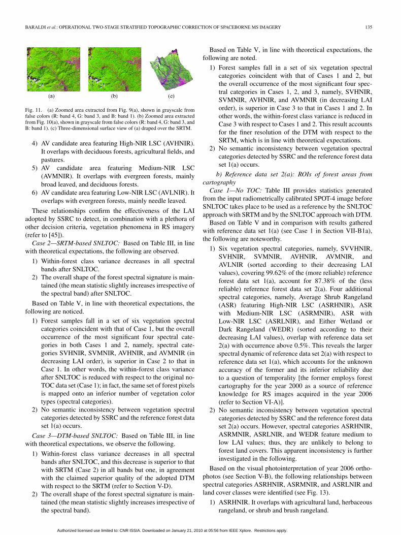
BARALDI et al.: OPERATIONAL TWO-STAGE STRATIFIED TOPOGRAPHIC CORRECTION OF SPACEBORNE MS IMAGERY 135
Fig. 11. (a) Zoomed area extracted from Fig. 9(a), shown in grayscale fromfalse colors (R: band 4, G: band 3, and B: band 1). (b) Zoomed area extractedfrom Fig. 10(a), shown in grayscale from false colors (R: band 4, G: band 3, andB: band 1). (c) Three-dimensional surface view of (a) draped over the SRTM.
4) AV candidate area featuring High-NIR LSC (AVHNIR).It overlaps with deciduous forests, agricultural fields, andpastures.
5) AV candidate area featuring Medium-NIR LSC(AVMNIR). It overlaps with evergreen forests, mainlybroad leaved, and deciduous forests.
6) AV candidate area featuring Low-NIR LSC (AVLNIR). Itoverlaps with evergreen forests, mainly needle leaved.
These relationships confirm the effectiveness of the LAIadopted by SSRC to detect, in combination with a plethora ofother decision criteria, vegetation phenomena in RS imagery(refer to [45]).
Case 2—SRTM-based SNLTOC: Based on Table III, in linewith theoretical expectations, the following are observed.
1) Within-forest class variance decreases in all spectralbands after SNLTOC.
2) The overall shape of the forest spectral signature is main-tained (the mean statistic slightly increases irrespective ofthe spectral band) after SNLTOC.
Based on Table V, in line with theoretical expectations, thefollowing are noticed.
1) Forest samples fall in a set of six vegetation spectralcategories coincident with that of Case 1, but the overalloccurrence of the most significant four spectral cate-gories in both Cases 1 and 2, namely, spectral cate-gories SVHNIR, SVMNIR, AVHNIR, and AVMNIR (indecreasing LAI order), is superior in Case 2 to that inCase 1. In other words, the within-forest class varianceafter SNLTOC is reduced with respect to the original no-TOC data set (Case 1); in fact, the same set of forest pixelsis mapped onto an inferior number of vegetation colortypes (spectral categories).
2) No semantic inconsistency between vegetation spectralcategories detected by SSRC and the reference forest dataset 1(a) occurs.
Case 3—DTM-based SNLTOC: Based on Table III, in linewith theoretical expectations, we observe the following.
1) Within-forest class variance decreases in all spectralbands after SNLTOC, and this decrease is superior to thatwith SRTM (Case 2) in all bands but one, in agreementwith the claimed superior quality of the adopted DTMwith respect to the SRTM (refer to Section V-D).
2) The overall shape of the forest spectral signature is main-tained (the mean statistic slightly increases irrespective ofthe spectral band).
Based on Table V, in line with theoretical expectations, thefollowing are noted.
1) Forest samples fall in a set of six vegetation spectralcategories coincident with that of Cases 1 and 2, butthe overall occurrence of the most significant four spec-tral categories in Cases 1, 2, and 3, namely, SVHNIR,SVMNIR, AVHNIR, and AVMNIR (in decreasing LAIorder), is superior in Case 3 to that in Cases 1 and 2. Inother words, the within-forest class variance is reduced inCase 3 with respect to Cases 1 and 2. This result accountsfor the finer resolution of the DTM with respect to theSRTM, which is in line with theoretical expectations.
2) No semantic inconsistency between vegetation spectralcategories detected by SSRC and the reference forest dataset 1(a) occurs.
b) Reference data set 2(a): ROIs of forest areas fromcartography
Case 1—No TOC: Table III provides statistics generatedfrom the input radiometrically calibrated SPOT-4 image beforeSNLTOC takes place to be used as a reference by the SNLTOCapproach with SRTM and by the SNLTOC approach with DTM.
Based on Table V and in comparison with results gatheredwith reference data set 1(a) (see Case 1 in Section VII-B1a),the following are noteworthy.
1) Six vegetation spectral categories, namely, SVVHNIR,SVHNIR, SVMNIR, AVHNIR, AVMNIR, andAVLNIR (sorted according to their decreasing LAIvalues), covering 99.62% of the (more reliable) referenceforest data set 1(a), account for 87.38% of the (lessreliable) reference forest data set 2(a). Four additionalspectral categories, namely, Average Shrub Rangeland(ASR) featuring High-NIR LSC (ASRHNIR), ASRwith Medium-NIR LSC (ASRMNIR), ASR withLow-NIR LSC (ASRLNIR), and Either Wetland orDark Rangeland (WEDR) (sorted according to theirdecreasing LAI values), overlap with reference data set2(a) with occurrence above 0.5%. This reveals the largerspectral dynamic of reference data set 2(a) with respect toreference data set 1(a), which accounts for the unknownaccuracy of the former and its inferior reliability dueto a question of temporality [the former employs forestcartography for the year 2000 as a source of referenceknowledge for RS images acquired in the year 2006(refer to Section VI-A)].
2) No semantic inconsistency between vegetation spectralcategories detected by SSRC and the reference forest dataset 2(a) occurs. However, spectral categories ASRHNIR,ASRMNIR, ASRLNIR, and WEDR feature medium tolow LAI values; thus, they are unlikely to belong toforest land covers. This apparent inconsistency is furtherinvestigated in the following.
Based on the visual photointerpretation of year 2006 ortho-photos (see Section V-B), the following relationships betweenspectral categories ASRHNIR, ASRMNIR, and ASRLNIR andland cover classes were identified (see Fig. 13).
1) ASRHNIR. It overlaps with agricultural land, herbaceousrangeland, or shrub and brush rangeland.
Authorized licensed use limited to: CNR ISSIA. Downloaded on January 21, 2010 at 05:56 from IEEE Xplore. Restrictions apply.

136 IEEE TRANSACTIONS ON GEOSCIENCE AND REMOTE SENSING, VOL. 48, NO. 1, JANUARY 2010
Fig. 12. (a) IRS-P6 DTM-based SNLTOC image generated from Fig. 9(a) and (b). (b) Preliminary spectral classification map, shown in pseudocolors [same asin Fig. 5(b)], generated by SSRC from the IRS-P6 image shown in (a).
TABLE IIISPOT-4 INPUT IMAGE. REFLECTANCE MEAN AND STANDARD DEVIATION OF REFERENCE FOREST SAMPLES IN THE 1) RAW (NON-TOC) SPOT-4 IMAGE,
2) SRTM-BASED SNLTOC SPOT-4 IMAGE, AND 3) DTM-BASED SNLTOC SPOT-4 IMAGE. (IN GRAY HIGHLIGHT) RELEVANT VALUES
TABLE IVIRS-P6 LISS-III DATA SET. REFLECTANCE MEAN AND STANDARD DEVIATION OF REFERENCE FOREST SAMPLES IN THE 1) RAW (NON-TOC) IRS-P6
LISS-III IMAGE, 2) SRTM-BASED SNLTOC IRS-P6 LISS-III IMAGE, AND 3) DTM-BASED SNLTOC IRS-P6 LISS-III IMAGE.(IN GRAY HIGHLIGHT) RELEVANT VALUES
2) ASRMNIR. It overlaps with open deciduous and mixedforests (called woody savannas in the IGBP-DIS classifi-cation scheme [11]).
3) ASRLNIR. It overlaps with permanent crops (particularlyolive groves) or shrub and brush rangeland.
These relationships confirm the effectiveness of the LAIadopted by SSRC, but appear inconsistent with the existingoverlap between spectral categories ASRHNIR, ASRMNIR,and ASRLNIR and the reference forest data set 2(a), as shownin Fig. 13. Since these pixels do not satisfy the forest-class
Authorized licensed use limited to: CNR ISSIA. Downloaded on January 21, 2010 at 05:56 from IEEE Xplore. Restrictions apply.

BARALDI et al.: OPERATIONAL TWO-STAGE STRATIFIED TOPOGRAPHIC CORRECTION OF SPACEBORNE MS IMAGERY 137
TABLE VSPOT-4 INPUT IMAGE. SEMANTIC CONSISTENCY OF REFERENCE FOREST SAMPLES WITH PRELIMINARY SPECTRAL MAP INDEXES GENERATED BY
SSRC FROM 1) RAW (NON-TOC) SPOT-4 IMAGE, 2) SRTM-BASED SNLTOC SPOT-4 IMAGE, AND 3) DTM-BASED SNLTOC SPOT-4 IMAGE.(IN GRAY HIGHLIGHT) RELEVANT VALUES
definition adopted by, for example, the IGBP-DIS classificationscheme, which considers, as forest lands, those dominated bywoody vegetation with a percent cover > 60% and heightexceeding 2 m, they were rejected by the reference forest dataset 2(a).
To summarize, as already outlined in [21], [22], and [45],due to its effectiveness and reliability, (S)SRC can be adoptedas a source of semantic information, which is automaticallygenerated from RS imagery and capable of improving the (oftenunknown) quality of any available ground-truth data set (e.g.,CORINE).
Case 2—SRTM-based SNLTOC: Based on Table III, in linewith theoretical expectations, we note the following.
1) Within-forest class variance decreases in all spectralbands after SNLTOC, and this decrease is inferior to thatwith the more reliable reference data set 1(a).
2) The overall shape of the forest spectral signature is main-tained (the mean statistic slightly increases irrespective ofthe spectral band).
Based on Table V, in line with theoretical expectations, thefollowing observations are noted.
1) Forest samples fall in a set of ten spectral categoriescoincident with that of Case 1, but the overall occurrence
of the most significant four spectral categories in bothCases 1 and 2, namely, spectral categories SVHNIR,AVHNIR, AVMNIR, and ASRMNIR (sorted according totheir decreasing LAI value), is superior in Case 2 to thatin Case 1. In other words, the within-forest class varianceis reduced with respect to the original no-TOC data set(Case 1).
2) As in Case 1, based on the photointerpretation of year2006 orthophotos, the reference forest samples overlap-ping with spectral categories ASRHNIR, ASRMNIR, andASRLNIR were considered incorrect and rejected fromthe forest ground truth 2(a).
3) No semantic inconsistency between the vegetation spec-tral categories detected by SSRC and the (revised) refer-ence forest data set 2(a) occurs.
Case 3—DTM-based SNLTOC: Based on Table III, in linewith theoretical expectations, the following are noteworthy.
1) Within-forest class variance decreases in all spectralbands after SNLTOC. This decrease is superior to thatwith SRTM (Case 2) and inferior to that assessed withthe more reliable reference data set 1(a).
2) The overall shape of the forest spectral signature is main-tained (although the mean statistic slightly decreases in
Authorized licensed use limited to: CNR ISSIA. Downloaded on January 21, 2010 at 05:56 from IEEE Xplore. Restrictions apply.
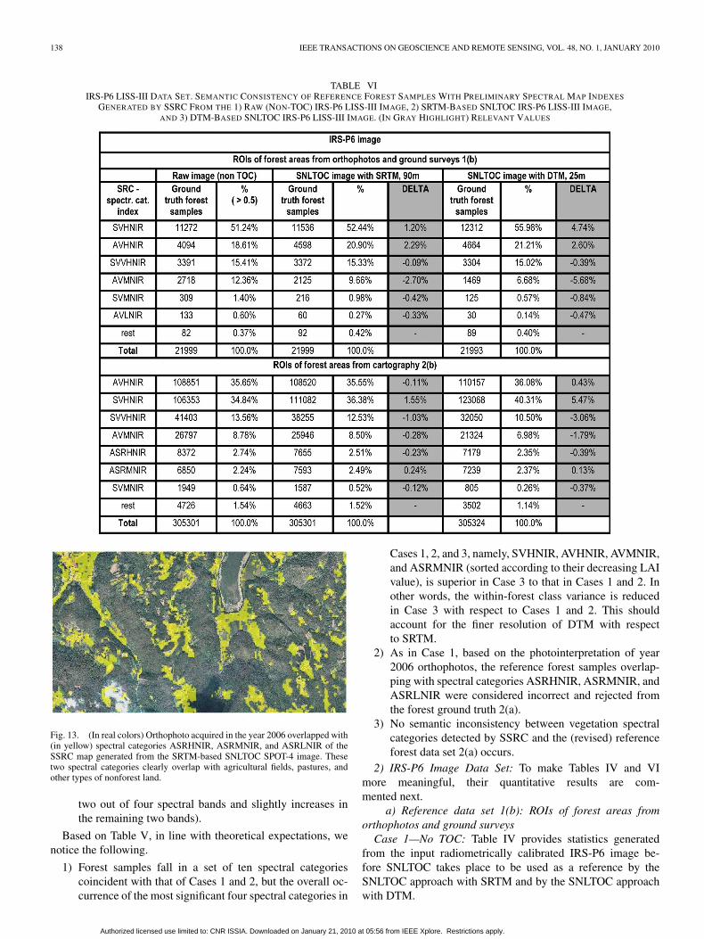
138 IEEE TRANSACTIONS ON GEOSCIENCE AND REMOTE SENSING, VOL. 48, NO. 1, JANUARY 2010
TABLE VIIRS-P6 LISS-III DATA SET. SEMANTIC CONSISTENCY OF REFERENCE FOREST SAMPLES WITH PRELIMINARY SPECTRAL MAP INDEXES
GENERATED BY SSRC FROM THE 1) RAW (NON-TOC) IRS-P6 LISS-III IMAGE, 2) SRTM-BASED SNLTOC IRS-P6 LISS-III IMAGE,AND 3) DTM-BASED SNLTOC IRS-P6 LISS-III IMAGE. (IN GRAY HIGHLIGHT) RELEVANT VALUES
Fig. 13. (In real colors) Orthophoto acquired in the year 2006 overlapped with(in yellow) spectral categories ASRHNIR, ASRMNIR, and ASRLNIR of theSSRC map generated from the SRTM-based SNLTOC SPOT-4 image. Thesetwo spectral categories clearly overlap with agricultural fields, pastures, andother types of nonforest land.
two out of four spectral bands and slightly increases inthe remaining two bands).
Based on Table V, in line with theoretical expectations, wenotice the following.
1) Forest samples fall in a set of ten spectral categoriescoincident with that of Cases 1 and 2, but the overall oc-currence of the most significant four spectral categories in
Cases 1, 2, and 3, namely, SVHNIR, AVHNIR, AVMNIR,and ASRMNIR (sorted according to their decreasing LAIvalue), is superior in Case 3 to that in Cases 1 and 2. Inother words, the within-forest class variance is reducedin Case 3 with respect to Cases 1 and 2. This shouldaccount for the finer resolution of DTM with respectto SRTM.
2) As in Case 1, based on the photointerpretation of year2006 orthophotos, the reference forest samples overlap-ping with spectral categories ASRHNIR, ASRMNIR, andASRLNIR were considered incorrect and rejected fromthe forest ground truth 2(a).
3) No semantic inconsistency between vegetation spectralcategories detected by SSRC and the (revised) referenceforest data set 2(a) occurs.
2) IRS-P6 Image Data Set: To make Tables IV and VImore meaningful, their quantitative results are com-mented next.
a) Reference data set 1(b): ROIs of forest areas fromorthophotos and ground surveys
Case 1—No TOC: Table IV provides statistics generatedfrom the input radiometrically calibrated IRS-P6 image be-fore SNLTOC takes place to be used as a reference by theSNLTOC approach with SRTM and by the SNLTOC approachwith DTM.
Authorized licensed use limited to: CNR ISSIA. Downloaded on January 21, 2010 at 05:56 from IEEE Xplore. Restrictions apply.

BARALDI et al.: OPERATIONAL TWO-STAGE STRATIFIED TOPOGRAPHIC CORRECTION OF SPACEBORNE MS IMAGERY 139
Based on Table VI, in line with theoretical expectations, thefollowing are observed.
1) Six vegetation spectral categories, namely, SVVHNIR,SVHNIR, SVMNIR, AVHNIR, AVMNIR, and AVLNIR(sorted according to their decreasing LAI values), featurea degree of overlap with the reference forest data set 1(b)superior to 0.5% and, overall, cover 99.63% of the forestground truth. These spectral types are in common withthe SPOT-4 image Case 1 (refer to Section VII-B1a).
2) No semantic inconsistency between vegetation spectralcategories detected by SSRC and the reference forestdata set occurs, which confirms the SSRC reliabilityand robustness to changes in the input data set, in linewith [45].
Case 2—SRTM-based SNLTOC: Based on Table IV, in par-tial agreement with theoretical expectations, the following arenoticed.
1) Within-forest class variance decreases in only two of fourspectral bands after SNLTOC.
2) The overall shape of the forest spectral signature is main-tained (the mean statistic slightly increases irrespective ofthe spectral band).
Based on Table VI, observations analogous to those drivenfrom reference data set 1(a) in the SRTM-based SNLTOCSPOT-4 image Case 2 reported in Section VII-B1a hold here.
Case 3—DTM-based SNLTOC: Based on Table IV, inpartial agreement with theoretical expectations, we note thefollowing.
1) Within-forest class variance decreases in only three outof four spectral bands after SNLTOC, and this decrease issuperior to that with SRTM.
2) The overall shape of the forest spectral signature is main-tained after SNLTOC (although the mean statistic slightlyincreases in three out of four spectral bands and slightlydecreases in the fourth spectral band).
Based on Table VI, observations analogous to those drivenby reference data set 1(a) in the DTM-based SNLTOC SPOT-4image Case 3 reported in Section VII-B1a hold here.
b) Reference data set 2(b): ROIs of forest areas fromcartography
Case 1—No TOC: Table IV provides statistics generatedfrom the input radiometrically calibrated IRS-P6 image beforeSNLTOC takes place to be used as a reference by the SNLTOCapproach with SRTM and by the SNLTOC approach with DTM.
Based on Table VI, observations analogous to those drivenby reference data set 2(a) in the no-TOC SPOT-4 image Case 1reported in Section VII-B1b hold here.
Case 2—SRTM-based SNLTOC: Based on Table IV, in par-tial agreement with theoretical expectations, we notice thefollowing.
1) Within-forest class variance decreases in two out of fourspectral bands, and this decrease is inferior to that withthe more reliable reference data set 1(b).
2) The overall shape of the forest spectral signature is main-tained (the mean statistic slightly decreases irrespectiveof the spectral band).
Based on Table VI, we observe the following, in agreementwith theoretical expectations.
1) Forest samples fall in a set of spectral categories coin-cident with that of Case 1. After SNLTOC, the spectralcategory SVHNIR gains occurrence although the overalloccurrence of the most significant four spectral categoriesin both Cases 1 and 2, namely, SVVHNIR, SVHNIR,AVHNIR, and AVMNIR (sorted according to their de-creasing LAI value), remains unchanged. This meansthat the spectral spread of class forest is reduced afterSNLTOC.
2) No semantic inconsistency between vegetation spectralcategories detected by SSRC and the reference forest dataset 2(b) occurs.
Case 3—DTM-based SNLTOC: Based on Table IV, in par-tial agreement with theoretical expectations, the following arenoted.
1) Within-forest class variance decreases in all spectralbands after SNLTOC. This decrease is superior to thatwith SRTM (Case 2), but it is not always inferior to thatwith the more reliable reference data set 1(b).
2) The overall shape of the forest spectral signature is main-tained (the mean statistic slightly decreases irrespectiveof the spectral band).
Based on Table VI, we observe the following, in agreementwith theoretical expectations.
1) After SNLTOC, the spectral category SVHNIR gainsoccurrence although the overall occurrence of the mostsignificant four spectral categories in Cases 1, 2, and 3,namely, SVVHNIR, SVHNIR, AVHNIR, and AVMNIR(sorted according to their decreasing LAI value), remainsunchanged. This means that the spectral spread of classforest is reduced in Case 3 with respect to Cases 1 and 2.
2) No semantic inconsistency between vegetation spectralcategories detected by SSRC and the reference forest dataset 2(b) occurs.
3) Discussion of Results: The quantitative SNLTOC resultsshown in Tables III–VI require the availability of an indepen-dent reference (ground truth, e.g., forest) data set. Absolutevalues of quality indexes generated from Tables III–VI are notsignificant. Rather, their relative values are important for com-paring alternative SNLTOC solutions. Overall, the agreement ofthese relative values with theoretical expectations is impressive.Tables III–VI prove the following. First, the proposed auto-matic two-stage SNLTOC system is effective in reducing thewithin-(forest) class variance while no significant distortion inpixel-based spectral signatures is introduced. This effectivenessdecreases monotonically with the spatial resolution of the DEM(i.e., effectiveness increases as the spatial resolution of theDEM becomes finer). Second, the first-stage automatic SSRCmodule is effective and robust to changes in the input data set;thus, it can be adopted as the core of an automatic two-stageSNLTOC system.
Authorized licensed use limited to: CNR ISSIA. Downloaded on January 21, 2010 at 05:56 from IEEE Xplore. Restrictions apply.

140 IEEE TRANSACTIONS ON GEOSCIENCE AND REMOTE SENSING, VOL. 48, NO. 1, JANUARY 2010
Fig. 14. (a) Landsat 7 ETM+ image of Siberia (path: 033, row: 033, acquisi-tion date: September 14, 2000), shown in false colors (R: band ETM5, G: bandETM4, and B: band ETM1), with 30-m resolution and calibrated into TOAreflectance. (b) Two-stage SNLTOC of (a), based on the SRTM. (Top right inthe image) Maximum mountain height: 2230 m. (Bottom right in the image)Flat height: 460 m.
C. Qualitative SNLTOC Results in a High Mountainous Site
The capability of the proposed automatic two-stageSNLTOC system to deal with RS images of high-altituderegions (featuring elevation, for example, > 1500 m), withsparse vegetation and bare soil, where rock and snow coverdominate the landscape, is investigated qualitatively (since noindependent ground-truth data set is available, which is oftenthe case in RS image mapping problems) in a Landsat 7 ETM+image of Siberia (path: 033, row: 033, acquisition date: 2000-14-09) calibrated into TOARFT values (see Section III-A). Inthis test site, according to the available 90-m-resolution SRTM,the maximum mountainous height is 2230 m with a flat terrainheight of 460 m.
To deal with Landsat imagery, the proposed two-stageSNLTOC system adopts, as its preliminary classification firststage, the automatic LSRC module (refer to Section IV-A2) inplace of the SSRC system adopted in Section VII-B. The LSRCstandard coarse output map features 17 spectral categories, i.e.,C = 17 (refer to Section IV-A2); thus, the total number of inputimage strata is S = 2 (horizontal areas + occluded areas) +17 (spectral categories) ∗ 2 (slopes facing the sun + slopesfacing away from the sun) = 36, thus NLR = C = 17 (alsorefer to Section VII).
The radiometrically calibrated input image and the SNLTOCoutput image can be visually compared in Fig. 14(a) and (b). Avisual assessment of these two images shows that the SNLTOCtransformation provides an effective compensation for changesin the solar incident angle. This qualitative conclusion is con-firmed by experimental evidence. Several ROIs belonging toclasses bare soil, rangeland, woodland, and snow are identifiedacross Fig. 14(a) by an expert photointerpreter. These ROIsoverlap with slopes facing the sun and facing away from the sunaccording to the given DEM (refer to Section IV-A1). Spectralvariance is diminished after SNLTOC in all selected ROIs. Theoverall shape of spectral signatures generated from the selectedROIs is well preserved after SNLTOC, which means that, inpractice, a pixel belonging to a given class, for example, snow,looks like snow after SNLTOC [refer to Fig. 14(a) and (b)].Finally, small but genuine image details appear well preservedafter SNLTOC (although some artifacts are introduced due tothe presence of spurious pits in the DEM). This merit is due toLSRC whose semantic partition of the Landsat image is pixel
Fig. 15. (a) Forest/nonforest binary classification map generated fromthe IRS-P6 LISS-III image shown in Fig. 9(a) by SAM implemented inENVI. Maximum angle threshold (in radians) = 0.1. Forest sample data setcardinality = 21 999. Overall accuracy (OA) = 20 820/21 999 = 94.64%.(b) Example of combination of the forest map generated by SAM, shownin (a), with the mutually exclusive and totally exhaustive classification map,automatically generated by SSRC, shown in Fig. 9(b). The land cover classforest shown in (a) is shown in a bright green pseudocolor. (c) Continuousintelligent SVI: Second-derivative greenness index computed by SSRC fromFig. 9(a) masked by a binary vegetation mask extracted from the SSRC mapshown in Fig. 9(b).
based (therefore intrinsically able to detect small but genuineimage details), but effective and reliable, namely, unaffectedby the typical salt-and-pepper classification noise effect char-acterizing ordinary pixel-based classifiers (such as maximumlikelihood, neural networks, etc.) [72].
To conclude, this experiment shows that, in a high-altitude re-gion (featuring maximum mountainous height equal to 2230 mwith a flat terrain height of 460 m), the following are true:1) The proposed automatic two-stage SNLTOC system iseffective in reducing within-class variance while no signifi-cant distortion in pixel-based spectral signatures is introduced,and 2) the automatic LSRC module is effective and eligiblefor adoption as the core of an automatic two-stage SNLTOCsystem.
D. Supervised Classification in Series With SNLTOC
In [21]–[23], and [45], it was clearly stated that an oper-ational automatic SRC system is preliminary and not at allalternative to traditional algorithms capable of learning fromeither unlabeled (unsupervised) or labeled (supervised) data.
To highlight this fundamental concept in an operationalframework, this section compares output products generatedfrom the testing IRS-P6 satellite image draped over the DTM(refer to Section VII-B8) by the following: 1) SSRC (referto Section IV-A2); 2) a two-stage SNLTOC system incor-porating SSRC (refer to Section IV); and 3) a standard su-pervised data-learning classifier, for example, SAM (refer toSection III-B1c), which is well known for its relative insen-sitiveness to illumination and albedo effects [57], [58] (fora theoretical comparison between SAM and SRC, refer toAppendix I).
The reliable ground-truth knowledge base represented by thereference data set 1(b), consisting of 21 999 ground-truth forestsamples distributed across the IRS-P6 satellite image (refer toSection VI-A), was selected for quantitative SNLTOC qualityassessment (refer to Section VI-D).
In RS common practice, the forest-class reference data set1(b) can be employed by SAM to solve a dichotomous (one-class) forest–nonforest classification problem. For example,Fig. 15(a) shows the binary forest map generated by SAM,
Authorized licensed use limited to: CNR ISSIA. Downloaded on January 21, 2010 at 05:56 from IEEE Xplore. Restrictions apply.

BARALDI et al.: OPERATIONAL TWO-STAGE STRATIFIED TOPOGRAPHIC CORRECTION OF SPACEBORNE MS IMAGERY 141
implemented in the ENVI software toolbox with a maximumangle threshold in radians equal to 0.1 (for outlier detection),from the IRS-P6 image shown in Fig. 9(a). In this one-classclassification problem, computation time is equivalent to a fewseconds with an OA probability pOA ± δ = (20 820/21 999 =94.64%)± (22) = 0.0%.
Let us consider an alternative RS application scenario where,in addition (and not as an alternative) to SAM, an operationalautomatic two-stage SNLTOC system incorporating SSRC inits first stage (refer to Section IV) is made available to endusers together with the DTM of the input IRS-P6 image. In thisinnovative operational frame, the same (identical) ground-truthforest data set 1(b) employed previously to generate Fig. 15(a)can be profitably exploited as follows.
1) A preliminary spectral map can be automatically gener-ated by SSRC from Fig. 9(a) in a few minutes of compu-tation time (< 5 min when SSRC is implemented in theC programming language) on a desktop computer pro-vided with a Dual Core Pentium processor [21]–[23].As shown in Fig. 9(b), this output product, per se,can be employed to refine the semantic quality of theavailable ground-truth forest data set 1(b) (analogouslyto the ground-truth sample refinement conducted inSection VII-B8).
2) An automatic two-stage SNLTOC system can gener-ate a topographically normalized MS image, shown inFig. 12(a), from the input DTM, the preliminary SSRCmap shown in Fig. 9(b), and the IRS-P6 image shown inFig. 9(a) in a few minutes of computation time (< 10 minwhen SNLTOC is implemented in the IDL programminglanguage).
3) If useful, the SNLTOC image shown in Fig. 12(a) can beautomatically reclassified by SSRC, e.g., see Fig. 12(b).
4) At this stage, the supervised information representedby the ground-truth forest data set 1(b) can come intoplay. The same (identical) SAM implementation ex-ploiting the same (identical) ground-truth forest dataset 1(b) previously adopted to generate Fig. 15(a) cannow be employed to map the SNLTOC image shownin Fig. 12(a). The binary classification map generatedby SAM from the SNLTOC image shown in Fig. 12(a)features pOA ± δ = (21 011/21 999 = 95.51%)± (22) =0.0%. This value is (slightly) superior to the pOA ±δ value = (20 820/21 999 = 94.64%) ± 0.0% estimatedin Fig. 15(a), as mentioned earlier in this paper. Thisis one more evidence of the expected benefits of MSimage topographic normalization before classificationacknowledged in existing literature, e.g., classificationpOA values improved around 4%, namely, from 79%to 83%, in [34] and around 6%, namely, from 82% to88%, in [36] after NLTOC and SNLTOC (also refer toSection VI-D).
5) Aside from improving the classification map generated bySAM in series with SNLTOC, the mutually exclusive andtotally exhaustive classification map generated by SSRCat no cost (in terms of user supervision for parameterselection and collection of ground-truth samples), shown
in Fig. 9(b), can be employed to replace pixels unclas-sified by SAM in Fig. 15(a), as shown in Fig. 15(b).In other words, Fig. 15(b) can replace Fig. 15(a) at noadditional cost.
In operational terms, another important difference betweenSAM and (S)SRC is that, unlike the former, the latter generatesseveral value-added products suitable for RS applications dif-ferent from classification, including estimation of either canopybiophysical structure variables (e.g., LAI) or canopy biochem-ical properties (e.g., FAPAR) from a continuous spectral VI(SVI) [60]. Any traditional SVI, such as the well-known NDVI[19], is computed as an algebraic combination of pixel com-ponents from different wavelength bands to produce a scalarvalue. An SVI should be very sensitive to target vegetationfactors (such as vegetation structure and the state of vege-tation cover in terms of leaf water content, leaf chlorophyllcontent, age, mineral deficiencies, etc.) while being insensi-tive to other factors affecting spectral reflectance such as soil(background) properties in addition to solar/viewing geometryand atmospheric conditions [19]. In the case of (S)SRC, anintelligent SVI generated from Fig. 9(a) is shown in Fig. 15(c).It consists of a novel second-derivative greenness index, whichis proposed in [21], [22] masked by a binary vegetationmask extracted from the preliminary (S)SRC map shown inFig. 9(b). As a result, the intelligent SVI responds zero tononvegetation surface types, which is not the case of any tradi-tional SVI.
VIII. SUMMARY AND CONCLUSION
The near-real-time availability of a preliminary spectralclassification map automatically generated from MS imageryby SRC paves the way to the design and implementation ofoperational automatic RS-IUSs as potential components ofoperational GEOSS and GMES instantiations.
In this paper, the degree of novelty of SRC is exploited toprovide an operational solution to the well-known RS imageTOC problem traditionally considered an unsolvable circulardilemma: While image classification benefits from prelimi-nary TOC, the latter requires a priori knowledge of surfaceroughness which is land cover class specific. The proposedTOC solution consists of an operational automatic two-stageSNLTOC system comprising, in cascade, a novel automaticRS image stratification first stage and a second-stage ordinarySNLTOC equation (16) selected from existing literature andincorporating the stratified or layered approach.
The innovative automatic MS image stratification first stageis twofold. First, given a DEM of the input MS imageand the sun’s azimuth and zenith angles, the pixel-based in-cident angle γi(n) ∈ [0◦, 180◦], n = 1, . . . , N , is computed.Next, the incident angle domain is partitioned into four strataas a pixel-based (context-insensitive) function of the solarzenith angle. These four DEM-driven slices are identified asfollows:
1) self-shadows, i.e., occluded areas belonging to shadowcasters (to be masked out in the second-stage SNLTOCmethod);
Authorized licensed use limited to: CNR ISSIA. Downloaded on January 21, 2010 at 05:56 from IEEE Xplore. Restrictions apply.

142 IEEE TRANSACTIONS ON GEOSCIENCE AND REMOTE SENSING, VOL. 48, NO. 1, JANUARY 2010
2) horizontal surfaces (to be masked out in the second-stageSNLTOC method);
3) slopes facing the sun;4) slopes facing away from the sun.
Second, symbolic (semantic) strata are automatically generatedby SRC from the MS image radiometrically calibrated intoTOARFT ⊇ ρT values.
The advantages of the operational automated two-stageSNLTOC system applied to nonhorizontal nonoccluded sur-faces, either facing the sun or facing away from the sun,and belonging to the same symbolic layer (spectral category)provided by SRC are expected to be the following: 1) Com-putation time is optimized by ignoring pixels belonging tothe aforementioned surface types 1) or 2), and 2) within-stratum variance should be reduced while pixel-based spec-tral patterns (shapes) are expected to be well preserved, i.e.,no spectral distortion should be introduced by topographicnormalization.
Up to 19 experiments were conducted in collaboration withan independent institutional partner to validate the novel oper-ational automated two-stage SNLTOC system. Collected quan-titative results are quite consistent with theoretical expectationsand allow to reach the following conclusions.
1) In terms of operational performance measurement, theautomatic SRC first stage is considered effective, com-putationally efficient, and robust to changes in the inputdata set acquired across time, space, and optical imagingsensors. Collected quantitative results are quite consistentwith theoretical expectations, i.e., the theoretical frame-work of SRC appears sound, and in line with resultscollected in previous works [21]–[23], [45]. Therefore,SRC is, per se, considered eligible for use in oper-ational satellite-based measurement systems providingpotential components to the GEOSS and GMES systeminstantiations.
2) Applied to nonhorizontal nonoccluded surfaces, eitherfacing the sun or away from the sun, and belonging tothe same symbolic layer provided by the first-stage SRC,the automatic two-stage SNLTOC system features thefollowing advantages: 1) Its ease of use is unsurpassed;2) computation time is optimized (by ignoring pixelsin horizontal surfaces or occluded surfaces belonging toshadow casters); 3) within-stratum variance is reducedwhile pixel-based spectral patterns (shapes) are wellpreserved, i.e., no spectral distortion is introduced bytopographic normalization; and 4) it is robust to changesin the input data set acquired across time, space, andsensors. To summarize, the proposed two-stage SNLTOCsystem satisfies, as a whole, the set of system qualityrequirements, reviewed in Section I, to be consideredeligible for use in an operational flow of RS data and landcover information.
As a secondary result, the RS image recovery from the ESAIMAGE2006 online archive experienced in this work provesthat, to date, in spite of their 10- to 20-year membership inthe CEOS, European institutions such as the ESA, DLR, and
EC-JRC, involved with ongoing international projects focusedon spaceborne multisource multitemporal image mosaickingand mapping at continental scale, either underestimate or ig-nore in practice 1) the problem of transforming DNs intoa community-agreed radiometric scale to enhance interimagecomparability across time, space, and sensors as required bythe QA4EO initiative in the framework of the GEOSS andGMES programs and 2) the well-known principle that datamanagement, including data sharing and redundancy (duplica-tion), is often more critical than data collection in guaranteeingthe integrity (i.e., accuracy and completeness) of a database[39, p. 16].
Future developments of this paper will be the following.
1) Integration of a shadow-casting algorithm into the DEM-driven stratification phase (refer to Section IV-A1).
2) Implementation of an ambient occlusion algorithm formodeling indirect illumination in shadow (occluded)areas (refer to Section IV-A1).
3) Integration of spatial relationships into the two-stageSNLTOC system to detect slopes facing the sun andfacing away from the sun that are adjacent to one anotherand belong to the same semantic layer (e.g., vegetation).Thus, local area estimation of SNLTOC regression pa-rameters can be based on convergence of topographic(e.g., slopes facing the sun and facing away from the sun),semantic (e.g., vegetation), and spatial (e.g., adjacency)evidence.
APPENDIX ISRC COMPARED TO SAM
It is noteworthy that there are at least four structural differ-ences between SAM and SRC which make these two pixel-based vector data mapping approaches not at all alternative, butcomplementary in operational terms.
1) SRC maps each pixel onto a discrete and finite setof indexes based on both the pixel-based reflectancepattern (shape) and the data vector magnitude, whileSAM pursues spectral pattern matching exclusively.This allows SRC to discriminate between, for example,a spectral category [color-based semiconcept (refer toSection IV-A2)] named vegetation in shadow areas[which can be spectrally indistinguishable from conif-erous forest (see Fig. 3)] from spectral categories suchas strong/average/weak vegetation in sun-exposed areas(where fuzzy sets strong/average/weak vegetations de-pend on both the LAI and the intensity of sunlight).In particular, in Fig. 3, the spectral category shadowedvegetation is not linearly scaled from the spectral cate-gories strong/average/weak vegetation. Rather, the latterspectral types mainly differ in brightness (magnitude),i.e., they are approximately linearly scaled versions ofone another analogously to dark- and light-toned soils(see [81, p. 276]). In this example, the discriminationcapability of SAM is inferior to SRC’s since the formerwould consider spectral categories strong/average/weakvegetation as indistinguishable.
Authorized licensed use limited to: CNR ISSIA. Downloaded on January 21, 2010 at 05:56 from IEEE Xplore. Restrictions apply.

BARALDI et al.: OPERATIONAL TWO-STAGE STRATIFIED TOPOGRAPHIC CORRECTION OF SPACEBORNE MS IMAGERY 143
2) SRC is prior knowledge based, i.e., it is nonadaptiveto data, and is capable of providing a totally exhaus-tive and mutually exclusive classification of the inputRS image without requiring any user supervision (seeSection IV-A2). On the contrary, SAM is supervised(labeled) data driven, i.e., it requires the acquisi-tion of ground-truth data across the study area fortraining.
3) SRC requires no user-defined parameter while SAM re-quires one user-defined parameter, namely, the maximumangle threshold (in radians) to consider pixels furtheraway than the specified maximum angle threshold notclassified (outliers).
4) SRC provides a classification map consisting of spec-tral semiconcepts [e.g., vegetation (see Section IV-A2)]less informative than land cover concepts (e.g., forest)provided by SAM, which counterbalances the superiordegree of automation of the former.
APPENDIX IISRC COMPARED TO UNSUPERVISED
DATA-CLUSTERING ALGORITHMS
In classical philosophy, the general notion of inference(learning) comprises two types of learning mechanisms knownas “induction [i.e., progressing from particular cases (e.g., train-ing data) to general (e.g., estimated dependence or model)],”therefore called bottom–up, fine to coarse, data driven, orlearning by example, and “deduction [i.e., progressing fromgeneral (e.g., model) to particular cases (e.g., output values)],”therefore called top–down, coarse to fine, model driven, orlearning by rule [72]. In particular, “induction amounts toforming generalizations from particular true facts. This is aninherently difficult (ill-posed) problem and its solution requiresa priori knowledge in addition to data” [72, p. 39].
When compared to well-known inductive unsupervised (un-labeled) data-learning algorithms, such as ISODATA andk-means typically employed in unlabeled data-clustering prob-lems, the fully automated prior knowledge-based SRC map-ping system is more successful in providing a preliminaryunderstanding (mapping) of an MS image. This is due tothe fact that the latter accounts for a dictionary of referencespectra in TOARFT values (see Fig. 3) representing its priorknowledge of the (3-D) world depicted in a spaceborne MS(2-D) image. The drawbacks of the former approach are asfollows.
1) Since the goal of clustering is to group the data at handrather than to provide an accurate characterization ofunobserved (future) samples generated from the sameprobability distribution, the task of clustering may falloutside the framework of predictive (inductive) learning.In spite of this, clustering analysis often employs un-supervised data-learning techniques originally developedfor vector quantization (such as the k-means unsuper-vised data-learning algorithm which belongs to the fam-ily of the crisp competitive minimum-distance-to-meansalgorithms [73], [74]) which is a predictive learningproblem [72].
2) Unlabeled data clustering is an inherently ill-posed datamapping problem, whereas the spectral pattern matchingperformed by SRC is well posed. In fact, the goal ofclustering is to separate a finite unlabeled data set athand into a finite and discrete set of “natural” hiddendata structures on the basis of an often subjectivelychosen measure of similarity, i.e., chosen subjectivelybased on its ability to create “interesting” clusters [72],[75]–[78]. Thus, the subjective (ill-posed) nature of thenonpredictive clustering problem precludes an absolutejudgement as to the relative effectiveness of all clusteringtechniques [78]. In spite of this, the inherent ill-posednessof unlabeled data-clustering problems is not clearly statedin existing literature where, as a consequence, dozensof papers proposing alternative clustering algorithms arepublished every year (perhaps in search of a “final” bestclustering algorithm which cannot exist) [79].
3) Crisp (hard) competitive minimum-distance-to-means al-gorithms, such as k-means data clustering, try to min-imize a sum-of-squares error function. To reduce therisk of being trapped in a local minimum of the er-ror function, soft-to-hard rather than hard competitiveclustering algorithms have been conceived [73], [74].In addition, it is well known that either crisp or fuzzyk-means data-clustering algorithms cannot perform wellwith nonconvex types of data, i.e., they are effective ifand only if data clusters are hyperspherical [80]. To over-come this problem, a k-means unsupervised data-learningalgorithm capable of defining automatically the numberof clusters splits a nonconvex data cluster, for example,a data cluster shaped like a banana, into several hyper-spheres. Thus, these hyperspheres should be linked tomap the banana-like data cluster. To perform nonconvexunlabeled data mapping, topologically preserving data-clustering algorithms have been developed [75]–[78].
4) Any clustering algorithm provides unlabeled data witha subsymbolic (asemantic) label (e.g., cluster 1, clus-ter 2, etc.), whereas SRC, which is prior knowledgebased, provides unknown pixels with a label equivalentto a color-based semiconcept featuring a semantic mean-ing (e.g., vegetation, either water or shadow, etc.) (seeSection IV-A2).
5) In terms of ease of use, every data-clustering algorithmrequires at least one free parameter, to be either userdefined or fixed by the application developer based onheuristics, to make the inherently ill-posed unlabeleddata-clustering problem better posed. For example, it isparadoxical that the well-known k-means vector quan-tizer typically employed for unlabeled data clusteringrequires the user to predefine the number of clustershidden in the data.
6) In terms of computation time, unlabeled data clustering isiterative while SRC is a one-pass mapping algorithm.
7) In terms of effectiveness and robustness to changes inthe input data set, a qualitative (visual) assessment ofthe SRC maps shown in [45] should be sufficient tosupport the superiority of SRC versus k-means unlabeleddata clustering among RS scientists and practitioners at
Authorized licensed use limited to: CNR ISSIA. Downloaded on January 21, 2010 at 05:56 from IEEE Xplore. Restrictions apply.
144 IEEE TRANSACTIONS ON GEOSCIENCE AND REMOTE SENSING, VOL. 48, NO. 1, JANUARY 2010
first glance. Typically, RS images mapped by pixel-basedclustering algorithms are affected by a well-known salt-and-pepper classification noise effect which is absent inthe SRC maps. This is due to the fact that SRC, whichis also pixel-based, is successful in modeling the within-class spectral variance from prior spectral knowledgeconsisting of endmember collection spectra.
ACKNOWLEDGMENT
A. Baraldi would like to thank P. Soille of EC-JRC forradiometrically calibrating the two testing images. The authorswould also like to thank the Editor-in-Chief, the Associate Ed-itor, and the anonymous reviewers for their helpful commentsand their patience in reviewing this paper, as well as for theircompetence and willingness to help.
REFERENCES
[1] G. Gutman, A. C. Janetos, C. O. Justice, E. F. Moran, J. F. Mustard,R. R. Rindfuss, D. Skole, B. L. Turner, II, and M. A. Cochrane, Eds.Land Change Science. Dordrecht, The Netherlands: Kluwer, 2004.
[2] O. Sjahputera, C. H. Davis, B. Claywell, N. J. Hudson, J. M. Keller,M. G. Vincent, Y. Li, M. Klaric, and C. R. Shyu, “GeoCDX: Anautomated change detection and exploitation system for high reso-lution satellite imagery,” in Proc. IGARSS, Boston, MA, Jul. 6–11, 2008,pp. V-467–V-470.
[3] F. Sart, J. Inglada, R. Landry, and T. Pultz, “Risk management using re-mote sensing data: Moving from scientific to operational applications,” inProc. SBSR Workshop, Florianopolis, Brasil, Apr. 23–27, 2001. [Online].Available: www.treemail.nl/download/sarti01.pdf
[4] [Online]. Available: www.fabricadebani.ro/userfiles/GEO_press_release.doc
[5] P. Zamperoni, “Plus ça va, moins ça va,” Pattern Recognit. Lett., vol. 17,no. 7, pp. 671–677, Jun. 1996.
[6] R. Richterin “Atmospheric/topographic correction (ATCOR) for satel-lite imagery,” DLR, Wessling, Germany, Rep. DLR-IB 565-01/06, 2006.[Online]. Available: http://www.geosystems.de/atcor/index.html
[7] eCognition User Guide 4, Definiens Imaging GmbH, Munich, Germany,2004.
[8] M. Page-Jones, The Practical Guide to Structured Systems Design.Englewood Cliffs, NJ: Prentice-Hall, 1988.
[9] Z. G. Wei, A. P. Macwan, and P. A. Wieringa, “A quantitative measure fordegree of automation and its relation to system performance and mentalload,” Hum. Factors, vol. 40, no. 2, pp. 277–295, Jun. 1998.
[10] Q. Yu and D. A. Clausi, “SAR sea–ice image analysis based on iterativeregion growing using semantics,” IEEE Trans. Geosci. Remote Sens.,vol. 45, no. 12, pp. 3919–3931, Dec. 2007.
[11] A. Strahler, D. Muchoney, J. Borak, M. Friedl, S. Gopal, E. Lambin,and A. Moody, Modis Land Cover Product Algorithm Theoretical BasisDocument (ATBD). ver. 5.0, MODIS Science Team. [Online]. Available:http://modis.gsfc.nasa.gov/data/atbd/atbd_mod12.pdf
[12] GEO, GEO 2007–2009 Work Plan: Toward Convergence, 2008. [Online].Available: http://earthobservations.org
[13] GEO, The Global Earth Observation System of Systems (GEOSS)10-Year Implementation Plan. adopted Feb. 16, 2005. [Online].Available: http://www.earthobservations.org/docs/10-Year%20Implementation%20Plan.pdf
[14] [Online]. Available: http://www.gmes.info[15] GEO/CEOSS, A Quality Assurance Framework for Earth Observation,
Sep. 2008. ver. 2.0. [Online]. Available: http://calvalportal.ceos.org/CalValPortal/showQA4EO.do?section=qa4eoIntro
[16] [Online]. Available: http://www.ceos.org[17] I. Dowman, “Foreword,” in International Society for Photogramme-
try and Remote Sensing (ISPRS) Book Series—Post-Launch Calibrationof Satellite Sensors, S. A. Morain and A. M. Buedge, Eds. Leiden,The Netherlands: Balkema, 2004, p. IX.
[18] T. Lillesand and R. Kiefer, Remote Sensing and Image Interpretation.New York: Wiley, 1979.
[19] S. Liang, Quantitative Remote Sensing of Land Surfaces. Hoboken, NJ:Wiley, 2004.
[20] P. Mather, Computer Processing of Remotely-Sensed Images—AnIntroduction. Chichester, U.K.: Wiley, 1994.
[21] A. Baraldi, V. Puzzolo, L. Durieux, D. Simonetti, G. Conchedda,F. Holecz, and P. Blonda, “Automatic spectral rule-based preliminary clas-sification of radiometrically calibrated SPOT-4/-5/IRS, AVHRR/MSG,AATSR, IKONOS/QuickBird/OrbView/GeoEye and DMC/SPOT-1/-2imagery—Part I: System design and implementation,” IEEE Trans.Geosci. Remote Sens., to be published.
[22] A. Baraldi, V. Puzzolo, L. Durieux, D. Simonetti, G. Conchedda,F. Holecz, and P. Blonda, “Automatic spectral rule-based preliminary clas-sification of radiometrically calibrated SPOT-4/-5/IRS, AVHRR/MSG,AATSR, IKONOS/QuickBird/OrbView/GeoEye and DMC/SPOT-1/-2imagery—Part II: Classification accuracy assessment,” IEEE Trans.Geosci. Remote Sens., to be published.
[23] A. Baraldi, T. Wassenaar, and S. Kay, “Automatic preliminary spectralrule-based decision-tree classification of spaceborne very high resolutionoptical imagery—Mapping vegetation and bare soil types across the Euro-pean Union’s agricultural landscapes,” IEEE Trans. Geosci. Remote Sens.,submitted for publication.
[24] R. R. Irish “Landsat 7 automatic cloud cover assessment (ACCA),” inProc. SPIE—Algorithms Multispectral, Hyperspectral, and UltraspectralImagery VI, S. S. Shen and M. R. Descour, Eds., 2000, vol. 4049,pp. 348–355. [Online]. Available: http://landsathandbook.gsfc.nasa.gov/handbook/pdfs/ACCA_SPIE_paper.pdf
[25] C. Small, “The Landsat ETM+ spectral mixing space,” Remote Sens.Environ., vol. 93, no. 1/2, pp. 1–17, Oct. 2004.
[26] A. Baraldi, “Impact of radiometric calibration and specifications ofspaceborne optical imaging sensors on the development of operationalautomatic remote sensing image understanding systems,” IEEE J. Sel.Topics Appl. Earth Obs. Remote Sens., vol. 2, no. 2, pp. 104–134,Jun. 2009.
[27] P. Henry and A. Meygret, “Calibration of VEGETATION cameraon-board SPOT4,” Adv. Space Res., vol. 28, no. 1, pp. 49–58,2001.
[28] P. S. Chavez, “An improved dark-object subtraction technique foratmospheric scattering correction of multispectral data,” Remote Sens.Environ., vol. 24, no. 3, pp. 459–479, Apr. 1988.
[29] D. Riaño, E. Chuvieco, J. Salas, and I. Aguado, “Assessment of differ-ent topographic corrections in Landsat TM data for mapping vegetationtypes,” IEEE Trans. Geosci. Remote Sens., vol. 41, no. 5, pp. 1056–1061,May 2003.
[30] A. Thomson and C. Jones, “Effects of topography on radiance fromupland vegetation in North Wales,” Int. J. Remote Sens., vol. 11, no. 5,pp. 829–840, May 1990.
[31] K. H. Law and J. Nichol, “Topographic correction for differential illu-mination effects on IKONOS satellite imagery,” Int. Arch. Photogramm.Remote Sens. Spat. Inf. Sci., vol. 35, no. 3, pp. 641–646, 2004.
[32] D. L. Civco, “Topographic normalization of Landsat Thematic Map-per digital imagery,” Photogramm. Eng. Remote Sens., vol. 55, no. 9,pp. 1303–1309, 1989.
[33] P. M. Teillet, B. Guindon, and D. G. Goodenough, “On the slope-aspectcorrection of multispectral scanner data,” Can. J. Remote Sens., vol. 8,no. 2, pp. 84–106, 1982.
[34] A. Twele, M. Kappas, J. Lauer, and S. Erasmi, “The effect of strat-ified topographic correction on land cover classification in tropicalmountainous regions,” in Proc. ISPRS Comm. VII Symp., Enschede,The Netherlands, May 8–11, 2006, pp. 432–437.
[35] A. Twele and S. Erasmi, “Evaluating topographic correction algo-rithms for improved land cover discrimination in mountainous areasof Central Sulawesi,” in Remote Sensing and GIS for EnvironmentalStudies, vol. 113, S. Erasmi, B. Cyffka, and M. Kappas, Eds. Göttingen,Germany: Verlag Erich Goltze, 2005, pp. 287–295.
[36] T. Tokola, J. Sarkeala, and M. Van der Linden, “Use of topographiccorrection in Landsat TM-based forest interpretation in Nepal,” Int. J.Remote Sens., vol. 22, no. 4, pp. 551–563, Mar. 2001.
[37] M. P. Bishop and J. D. Colby, “Anisotropic reflectance correctionof SPOT-3 HRV imagery,” Int. J. Remote Sens., vol. 23, no. 10, pp. 2125–2131, May 2002.
[38] M. P. Bishop, J. F. Shroder, and J. D. Colby, “Remote sensing andgeomorphometry for studying relief production in high mountains,” Geo-morphology, vol. 55, no. 1–4, pp. 345–361, Sep. 2003.
[39] L. Blesius and F. Weirich, “The use of the Minnaert correction for landcover classification in mountainous terrain,” Int. J. Remote Sens., vol. 26,no. 17, pp. 3831–3851, Sep. 2005.
[40] J. D. Shepherd and J. R. Dymond, “Correcting satellite imagery for thevariance of reflectance and illumination with topography,” Int. J. RemoteSens., vol. 24, no. 17, pp. 3831–3851, Sep. 2005.
Authorized licensed use limited to: CNR ISSIA. Downloaded on January 21, 2010 at 05:56 from IEEE Xplore. Restrictions apply.

BARALDI et al.: OPERATIONAL TWO-STAGE STRATIFIED TOPOGRAPHIC CORRECTION OF SPACEBORNE MS IMAGERY 145
[41] E. R. McDonald, X. Wu, P. Caccetta, and N. Campbell, “Illuminationcorrection of Landsat TM data in South East NSW,” in Proc. 10thARSPC, Adelaide, Australia, Aug. 21–25, 2000. [Online]. Available:http://www.environment.gov.au/land/publications/pubs/illumination.pdf
[42] X. Wu, S. Furby, and J. Wallace, “An approach for terrain il-lumination correction,” in Proc. 12th ARSPC, Fremantle, Australia,Oct. 2004. [Online]. Available: http://www.cmis.csiro.au/rsm/research/pdf/wu_x_12ARSPC_TerrainIllumination.pdf
[43] G. Palubinskas, R. Muller, and P. Reinartz, “Radiometric normalizationof optical remote sensing imagery,” in Proc. IGARSS, Jul. 21–25, 2003,vol. 2, pp. 720–722.
[44] D. Lu, H. Ge, S. He, A. Xu, G. Zhou, and H. Du, “Pixel-based Minnaertcorrection method for reducing topographic effects on a Landsat 7 ETM+image,” Photogramm. Eng. Remote Sens., vol. 74, no. 11, pp. 1343–1350,Nov. 2008.
[45] A. Baraldi, V. Puzzolo, P. Blonda, L. Bruzzone, and C. Tarantino, “Auto-matic spectral rule-based preliminary mapping of calibrated Landsat TMand ETM+ images,” IEEE Trans. Geosci. Remote Sens., vol. 44, no. 9,pp. 2563–2586, Sep. 2006.
[46] D. Foldes and B. Benes, “Occlusion-based snow accumulation simula-tion,” in Proc. 4th Workshop VRIPHYS, 2007, pp. 35–41.[Online]. Available: http://www.envision.purdue.edu/pdfs/papers/Foldes07Vriphys.pdf
[47] S. Sandmeier and K. Itten, “A physical-based model to correct at-mospheric and illumination effects in optical satellite data of ruggedterrain,” IEEE Trans. Geosci. Remote Sens., vol. 35, no. 3, pp. 708–717,May 1997.
[48] N. Hoffman and K. Mitchell, Real-Time Photorealistic TerrainLighting. [Online]. Available: www.gamasutra.com/features/gdcarchive/2001/hoffman.doc
[49] [Online]. Available: http://www.SPOTimage.fr/html/_167_224_584_php[50] [Online]. Available: http://eo1.usgs.gov[51] A. K. Shackelford and C. H. Davis, “A hierarchical fuzzy classifica-
tion approach for high-resolution multispectral data over urban areas,”IEEE Trans. Geosci. Remote Sens., vol. 41, no. 9, pp. 1920–1932,Sep. 2003.
[52] G. Zhou and M. Kafatos, “Future intelligent earth observing satel-lites (FIEOS),” in Proc. ISPRS/FIEOS Conf., 2002. [Online]. Available:http://www.isprs.org/commission1/proceedings02/paper/00031.pdf
[53] [Online]. Available: http://directory.eoportal.org/info_3rdInternationalSymposiumonFutureIntelligentEarthObservingSatellitesFIEOS.html
[54] J. D. Colby, “Topographic normalization in rugged terrain,” Photogramm.Eng. Remote Sens., vol. 57, no. 5, pp. 531–537, May 1991.
[55] T. Svoray and Y. Carmel, “Empirical method for topographic correctionin aerial photographs,” IEEE Geosci. Remote Sens. Lett., vol. 2, no. 2,pp. 211–214, Apr. 2005.
[56] ENVI 4.3 User Manual, ITT Industries Inc., Boulder, CO, 2006.[57] Y. Sohn, E. Motan, and F. Gurri, “Deforestation in North-Central Yu-
catan (1985–1995): Mapping secondary succession of forest and agri-cultural land use in Sotuta using the Cosine of the angle concept,”Photogramm. Eng. Remote Sens., vol. 65, no. 8, pp. 947–958,Aug. 1999.
[58] S. South, J. Qi, and D. P. Lusch, “Optimal classification methods formapping agricultural tillage practices,” Remote Sens. Environ., vol. 91,no. 1, pp. 90–97, May 2004.
[59] L. J. Guo and J. M. Moore, “Cloud-shadow suppression technique forenhancement of airborne Thematic Mapper imagery,” Photogramm. Eng.Remote Sens., vol. 59, no. 8, pp. 1287–1291, Aug. 1993.
[60] K. F. Huemmrich, “Effects of shadows on vegetation indices,” in Proc.IGARSS, 1996, vol. 4, pp. 2372–2374.
[61] A. Baraldi and F. Parmiggiani, “Combined detection of intensityand chromatic contours in color images,” Opt. Eng., vol. 35, no. 5,pp. 1413–1439, May 1996.
[62] A. Baraldi and F. Parmiggiani, “A neural network for unsupervisedcategorization of multivalued input patterns: An application to satelliteimage clustering,” IEEE Trans. Geosci. Remote Sens., vol. 33, no. 2,pp. 305–316, Mar. 1995.
[63] [Online]. Available: http://www.coventry.ac.uk/ec/~nhunt/meths/strati.html
[64] C. M. Bishop, Neural Networks for Pattern Recognition. Oxford, U.K.:Clarendon, 1995.
[65] C. Mason and E. R. Kandel, “Central visual pathways,” in Principles ofNeural Science, E. Kandel and J. Schwartz, Eds. Norwalk, CT: AppletonLange, 1991, pp. 420–439.
[66] P. Gouras, “Color vision,” in Principles of Neural Science,E. Kandel and J. Schwartz, Eds. Norwalk, CT: Appleton Lange,1991, pp. 467–479.
[67] T. Matsuyama and V. Shang-Shouq Hwang, SIGMA—A Knowledge-Based Aerial Image Understanding System. New York: Plenum,1990.
[68] K. Shackelford and C. H. Davis, “A combined fuzzy pixel-based andobject-based approach for classification of high-resolution multispectraldata over urban areas,” IEEE Trans. Geosci. Remote Sens., vol. 41, no. 10,pp. 2354–2363, Oct. 2003.
[69] J. Bestimt and B. Freitag, Real-Time Shadow Casting Using ShadowVolumes. [Online]. Available: http://www.gamasutra.com/features/19991115/bestimt_freitag_01.htm
[70] M. Woo Davis and M. B. Sheridan, OpenGL Programming Guide: The Of-ficial Guide to Learning OpenGL. Boston, MA: Addison-Wesley, 2006.ver. 2.0.
[71] V. Perdigao and A. Annoni, “Technical and methodological guide forupdating CORINE land cover data base,” Eur. Comm. Joint Res. Center,Ispra, Italy, Tech. Rep. EUR 17288, 1997.
[72] V. Cherkassky and F. Mulier, Learning From Data: Concepts, Theory, andMethods. New York: Wiley, 1998.
[73] A. Baraldi and P. Blonda, “A survey of fuzzy clustering algorithms forpattern recognition: Part I,” IEEE Trans. Syst., Man, Cybern. B, Cybern.,vol. 29, no. 6, pp. 778–785, Dec. 1999.
[74] A. Baraldi and P. Blonda, “A survey of fuzzy clustering algorithms forpattern recognition: Part II,” IEEE Trans. Syst., Man, Cybern. B, Cybern.,vol. 29, no. 6, pp. 786–801, Dec. 1999.
[75] A. Baraldi and E. Alpaydin, “Constructive feedforward ART clusteringnetworks—Part I,” IEEE Trans. Neural Netw., vol. 13, no. 3, pp. 645–661,May 2002.
[76] A. Baraldi and E. Alpaydin, “Constructive feedforward ART clusteringnetworks—Part II,” IEEE Trans. Neural Netw., vol. 13, no. 3, pp. 662–677, May 2002.
[77] B. Fritzkein “Some competitive learning methods,” Ruhr-UniversitätBochum, Bochum, Germany, 1997. [Online]. Available: http://www.ki.inf.tu-dresden.de/~fritzke/JavaPaper
[78] E. Backer and A. K. Jain, “A clustering performance measure basedon fuzzy set decomposition,” IEEE Trans. Pattern Anal. Mach. Intell.,vol. PAMI-3, no. 1, pp. 66–75, Jan. 1981.
[79] R. Xu and D. Wunsch, II, “Survey of clustering algorithms,” IEEE Trans.Neural Netw., vol. 16, no. 3, pp. 645–678, May 2005.
[80] R. Duda, P. Hart, and D. Stork, Pattern Classification. New York: Wiley,2001.
[81] P. H. Swain and S. M. Davis, Remote Sensing: The Quantitative Approach.New York: McGraw-Hill, 1978.
[82] W. Zhou, G. Huang, A. Troy, and M. L. Cadenasso, “Object-based landcover classification of shaded areas in high spatial resolution imagery ofurban areas: A comparison study,” Remote Sens. Environ., vol. 113, no. 8,pp. 1769–1777, Aug. 2009.
[83] L. Delves, R. Wilkinson, C. Oliver, and R. White, “Comparing the per-formance of SAR image segmentation algorithms,” Int. J. Remote Sens.,vol. 13, no. 11, pp. 2121–2149, 1992.
[84] GMES IMAGE2006 Mosaic. [Online]. Available: http://www.gmes-gseland.info/com/news/GMES-Land_NewsLetter_I1.00.pdf
[85] R. Lunetta and D. Elvidge, Remote Sensing Change Detection: Environ-mental Monitoring Methods and Applications. London, U.K.: Taylor &Francis, 1999.
[86] X. Dai and S. Khorram, “The effects of image misregistration on the accu-racy of remotely sensed change detection,” IEEE Trans. Geosci. RemoteSens., vol. 36, no. 5, pp. 1566–1577, Sep. 1998.
[87] A. Baraldi, L. Bruzzone, and P. Blonda, “Quality assessment ofclassification and cluster maps without ground truth knowledge,”IEEE Trans. Geosci. Remote Sens., vol. 43, no. 4, pp. 857–873,Apr. 2005.
[88] R. G. Congalton and K. Green, Assessing the Accuracy of RemotelySensed Data. Boca Raton, FL: Lewis, 1999.
[89] G. M. Foody, “Status of land cover classification accuracy assessment,”Remote Sens. Environ., vol. 80, no. 1, pp. 185–201, Apr. 2002.
[90] Z. Wang and A. C. Bovik, “A universal image quality index,” IEEE SignalProcess. Lett., vol. 9, no. 3, pp. 81–84, Mar. 2002.
[91] P. Lukowicz, E. Heinz, L. Prechelt, and W. Tichy, “Experimental eval-uation in computer science: A quantitative study,” Univ. Karlsruhe,Karlsruhe, Germany, Tech. Rep. 17/94, 1994.
[92] L. Prechelt, “A quantitative study of experimental evaluations of neuralnetwork learning algorithms: Current research practice,” Neural Netw.,vol. 9, no. 3, pp. 457–462, Apr. 1996.
[93] Proceedings and Recommendations of the Workshop on European Ref-erence Grids, European Commission Joint Research Center—Institutefor Environment and Sustainability, Ispra, Italy, Oct. 27–29, 2003.EUR 21494 EN.
Authorized licensed use limited to: CNR ISSIA. Downloaded on January 21, 2010 at 05:56 from IEEE Xplore. Restrictions apply.
146 IEEE TRANSACTIONS ON GEOSCIENCE AND REMOTE SENSING, VOL. 48, NO. 1, JANUARY 2010
Andrea Baraldi was born in Modena, Italy, in1963. He received the Laurea (M.S.) degree in elec-tronic engineering from the University of Bologna,Bologna, Italy, in 1989. His M.S. thesis focused onthe development of segmentation and classificationalgorithms for remotely sensed optical imagery.
From 1989 to 1990, he was a Research Asso-ciate with the Centro di Studio per l’InterazioneOperatore–Calcolatore, National Research Council(CNR), Bologna, and served in the army with theIstituto Geografico Militare, Florence, Italy, working
on satellite image classifiers and geographic information systems (GISs). Asa Consultant with the European Space Agency European Space ResearchInstitute, Frascati, Italy, he worked on object-oriented applications for GISsfrom 1991 to 1993. From December 1997 to June 1999, he was assignedwith a Postdoctoral Fellowship in Artificial Intelligence with the InternationalComputer Science Institute, Berkeley, CA. From 2000 to 2002, as a Postdoc-toral Researcher, he joined the Global Vegetation Monitoring Unit, Institute forEnvironment and Sustainability (IES), European Commission Joint ResearchCentre (JRC), Ispra, Italy, in the development and validation of algorithmsfor forest classification of radar mosaics at continental scale. From 2005 to2009, with the IES–Spatial Data Infrastructure Unit, JRC, he was involved withsatellite optical image calibration, classification, and mosaicking at continentalscale. Since his master’s thesis, he has continued his collaboration with Istitutodi Scienze dell’Atmosfera e del Clima, CNR, Bologna, and Istituto di Studi suiSistemi Intelligenti per l’Automazione, CNR, Bari, Italy. He is currently withBaraldi Consultancy in Remote Sensing, Bologna. His main research interestscenter on image understanding, with special emphasis on the developmentof operational automatic hierarchical multisource multiresolution spaceborneimage-understanding systems consistent with biological vision.
Mr. Baraldi was an Associate Editor of the IEEE TRANSACTIONS ON
NEURAL NETWORKS from 2001 to 2006.
Matteo Gironda was born in Noventa Vicentina,Italy, in 1979. He received the B.S. degree in forestryfrom Padua University, Padua, Italy, in 2003 andthe M.S. degree in geographic information systemsand remote sensing from the University Institute ofArchitecture of Venice, Venezia, Italy, in 2008.
He was with the University Institute of Architec-ture of Venice. He is currently a Private Officer in theenvironmental field.
Dario Simonetti was born in Varese, Italy, in 1981.He received the Laurea (M.S.) degree in informaticsfrom the Facoltà di Scienze Matematiche, Fisiche eNaturali, Università dell’Insubria, Varese, in 2004.His thesis focused on the development of improvedclassification algorithms for near-real-time fire de-tection at global scale from satellite optical imagery.
Since 2004, he has been an Analyst–ProgrammerConsultant with the Global Environment MonitoringUnit, Institute for Environment and Sustainability,European Commission Joint Research Centre, Ispra,
Italy. His main activities are focused on automatic near-real-time analysis offire occurrences in African protected areas, development and assessment ofprocessing chain for calibration, coregistration, topographic correction, andclassification of satellite imagery, and development of user-friendly geographicinformation system applications for validation of satellite imagery classificationacross different epochs. He is contributing in delivering products and servicesderived from the analysis of satellite remote sensing data, with special emphasison biodiversity and land cover change detection.
Authorized licensed use limited to: CNR ISSIA. Downloaded on January 21, 2010 at 05:56 from IEEE Xplore. Restrictions apply.