www.usn.no

FMH606 Master’s Thesis 2019Electrical Power Engineering

Online monitoring and visualizing of a

generator’s capability with Simulink

Visualization tool

Prabesh Khadka

Faculty of Technology, Natural Sciences and Maritime Sciences

Campus Porsgrunn

2

www.usn.no

Course: FMH606 Master’s Thesis 2019Title: Online monitoring and visualizing of a generator’s capability with Sim-

ulinkPages: 93

Keywords: Voltage stability, Voltage collapse, Long-term dynamics, Generators cap-ability curve

Student: Prabesh KhadkaSupervisor: Thomas Øyvang, Dietmar Winkler

External partner: StatkraftAvailability: Open

Summary:The power systems today are becoming more larger, complex and are operating closer to theirsecurity and stability limits particularly due to an increase in load demands and numberof environmental concerns. Voltage stability has been a major subject of discussion andconcern in electric power system operation and planning worldwide. Firstly, this thesis aimsto do the survey on voltage stability and collapse phenomena in order to get insights intothe mechanisms, causes, and prevention techniques to avoid such.

The dynamic long-term voltage stability analysis is carried out using a free and open source,MATLAB based-PSAT software taking a test power system. The influence of load models,overexcitation limiter and transformer load tap changers on voltage collapse are investigatedas a part of the thesis. It is observed that the constant power load has a greater impacton the voltage instability as it tries to restore the load unlike constant impedance and theconstant current loads.

Furthermore, a mathematical model for drawing the generator PQ capability diagram ispresented and implemented in MATLAB software environment. For improved visualizationand user interactions, a visualization tool is developed using the Graphical User Interface.In addition, the temperature development in the rotor and stator of the 103 MVA hydro-generator at ‘Åbjøra’ in Norway, is investigated in the same visualization tool utilizing thealready developed thermal model.

For increased accuracy of the results from dynamic voltage analysis, development and useof more accurate power system component models is recommended. Moreover, the effectof changing armature voltage and the direct axis synchronous reactance on PQ capabilitydiagram can be investigated under further study.

The University of South-Eastern Norway accepts no responsibility for the results andconclusions presented in this report.

Preface

This thesis is submitted to the University of South-Eastern Norway (USN) as the partialrequirement for the fulfillment of the master’s degree program in Electrical Power Engin-eering. The thesis was undertaken as a part of the course FMH606 starting January 2019with Statkraft as the external partner. The eagerness to study about the role of reactivepower in maintaining voltage stability in an AC electrical network and the generator’srole in handling such is what motivated me to take this topic as my thesis work.

I would like to thank my supervisor Thomas Øyvang and co-supervisor Dietmar Winklerfor their excellent guidance and valuable support throughout the work. Special thanksto Mr. Om Prakash Chapagain for giving valuable insights into mathematical computa-tions and programming. Thanks to my friend Madhusudhan Pandey for his co-operationand support throughout this journey. Finally, sincere gratitude to my family for theircontinuous encouragement and support throughout the work.

Porsgrunn, 13th May 2019

Prabesh Khadka

5

6

Contents

Preface

Contents

List of Figures . . . . . . . . . . . . . . . . . . . . . . . . . . . . . . . . . . . . .List of Tables . . . . . . . . . . . . . . . . . . . . . . . . . . . . . . . . . . . . . .

Introduction

. Background and objective . . . . . . . . . . . . . . . . . . . . . . . . . . . .

. Scope of work . . . . . . . . . . . . . . . . . . . . . . . . . . . . . . . . . .

. Outline of the thesis . . . . . . . . . . . . . . . . . . . . . . . . . . . . . . .

Theory

. Voltage stability . . . . . . . . . . . . . . . . . . . . . . . . . . . . . . . . .. . Study of voltage collapse phenomenon in time domain . . . . . . . . .. . Mechanism of voltage collapse . . . . . . . . . . . . . . . . . . . . .. . Approaches to voltage stability analysis . . . . . . . . . . . . . . . . .

. Generator power capability . . . . . . . . . . . . . . . . . . . . . . . . . . .

Modelling of power system components

. Load models . . . . . . . . . . . . . . . . . . . . . . . . . . . . . . . . . . .

. Under load tap changer . . . . . . . . . . . . . . . . . . . . . . . . . . . . .

. Thermal model of a hydrogenerator . . . . . . . . . . . . . . . . . . . . . . .. . Copper losses . . . . . . . . . . . . . . . . . . . . . . . . . . . . . .. . Iron losses . . . . . . . . . . . . . . . . . . . . . . . . . . . . . . . .. . Stray losses . . . . . . . . . . . . . . . . . . . . . . . . . . . . . . .. . Mechanical losses . . . . . . . . . . . . . . . . . . . . . . . . . . . .

Simulation

. Power System Analysis Toolbox (PSAT) . . . . . . . . . . . . . . . . . . . . . .

. Case Study: Kundur -bus test system . . . . . . . . . . . . . . . . . . . . .. . Description of a test system . . . . . . . . . . . . . . . . . . . . . . .. . System modelling . . . . . . . . . . . . . . . . . . . . . . . . . . . .

. On-line PQ diagram . . . . . . . . . . . . . . . . . . . . . . . . . . . . . . .. . Implementation of PQ diagram . . . . . . . . . . . . . . . . . . . . .. . Automatic visualization tool for generator’s capability . . . . . . . . .

7

Contents

. . Temperature visualization . . . . . . . . . . . . . . . . . . . . . . . .

Results and discussions

. -bus test system . . . . . . . . . . . . . . . . . . . . . . . . . . . . . . . .. . Effect of load models . . . . . . . . . . . . . . . . . . . . . . . . . .. . Effect of ULTC and OXL . . . . . . . . . . . . . . . . . . . . . . . . . .. . Countermeasures against voltage collapse . . . . . . . . . . . . . . .

. Visualization tool for generator’s capability . . . . . . . . . . . . . . . . . . .

Conclusion

Further work

Bibliography

A Task Description

B Parameters

B. System diagram . . . . . . . . . . . . . . . . . . . . . . . . . . . . . . . . .B. Load flow data . . . . . . . . . . . . . . . . . . . . . . . . . . . . . . . . . .B. Dynamic data . . . . . . . . . . . . . . . . . . . . . . . . . . . . . . . . . .B. Thermal model parameters . . . . . . . . . . . . . . . . . . . . . . . . . . .B. Machine data of Åbjøra . . . . . . . . . . . . . . . . . . . . . . . . . . . . .

C Codes and programs

D Scientific paper

8

List of Figures

2.1 Classification of power system stability [5]. . . . . . . . . . . . . . . . . . . 192.2 Equivalent circuit of a simple two bus system [4]. . . . . . . . . . . . . . . 202.3 Power voltage characteristics of the system [4]. . . . . . . . . . . . . . . . . 212.4 Voltage stability phenomena and time frames [6]. . . . . . . . . . . . . . . 222.5 Equivalent steady state circuit diagram for round rotor generators with a

step-up transformer [14]. . . . . . . . . . . . . . . . . . . . . . . . . . . . . 262.6 Capability diagram of synchronous generator [9], [15]. . . . . . . . . . . . . 27

3.1 Schematic diagram of online low order thermal model [3]. . . . . . . . . . . 34

4.1 Graphical User Interface of PSAT [20]. . . . . . . . . . . . . . . . . . . . . 384.2 Single line diagram of test system [21]. . . . . . . . . . . . . . . . . . . . . 394.3 Single line diagram implementation of test system in PSAT. . . . . . . . . 404.4 Equivalent π circuit of Under Load Tap Changer [20] . . . . . . . . . . . . 414.5 Secondary voltage control scheme of LTC [20]. . . . . . . . . . . . . . . . . 414.6 Over excitation limiter [20]. . . . . . . . . . . . . . . . . . . . . . . . . . . 424.7 Derivation of a P-Q capability diagram from the phasor diagram (cyl-

indrical rotor) [23]. . . . . . . . . . . . . . . . . . . . . . . . . . . . . . . . 434.8 On-line PQ diagram with different operational condition from (1) -(4) [22]. 444.9 Rated stator current limit and maximum turbine limit plot. . . . . . . . . 464.10 Rated field current limit plot. . . . . . . . . . . . . . . . . . . . . . . . . . 474.11 Theoretical and practical stability limit plot. . . . . . . . . . . . . . . . . . 474.12 Work flow diagram for PQ curve implementation in visualization tool. . . . 484.13 Graphical User Interface for Generator Capability Diagram. . . . . . . . . 494.14 Graphical User Interface for Generator Capability Diagram showing ‘NOR-

MAL’ condition. . . . . . . . . . . . . . . . . . . . . . . . . . . . . . . . . 504.15 Work flow diagram for temperature visualization. . . . . . . . . . . . . . . 514.16 Simulink circuit for the thermal model proposed in [3]. . . . . . . . . . . . 524.17 Schematic setup for the temperature measurement in Simulink [3]. . . . . . 52

5.1 Steady state voltage at various buses. . . . . . . . . . . . . . . . . . . . . . 535.2 Steady state reactive power at various buses. . . . . . . . . . . . . . . . . . 545.3 Voltage profile at bus 11 for different load types. . . . . . . . . . . . . . . . 555.4 Bus 11 voltage without and with OXL. . . . . . . . . . . . . . . . . . . . . 575.5 Bus 10 voltage without and with OXL. . . . . . . . . . . . . . . . . . . . . 57

9

List of Figures

5.6 Bus 3 voltage without and with OXL. . . . . . . . . . . . . . . . . . . . . . 585.7 Reactive power output of generator G3 without and with OXL. . . . . . . 585.8 Field voltage at generator 3 without and with OXL. . . . . . . . . . . . . . 595.9 Visualization of generator operating point in over excited regime indicated

by black asterisk. . . . . . . . . . . . . . . . . . . . . . . . . . . . . . . . . 605.10 Visualization of generator operating point in under excited regime indic-

ated by black asterisk. . . . . . . . . . . . . . . . . . . . . . . . . . . . . . 615.11 Temperature observation in the visualization tool. . . . . . . . . . . . . . . 615.12 Rotor and Stator temperature plots from machine data ‘Åbjøra’. . . . . . . 62

B.1 Single line diagram of test system [21]. . . . . . . . . . . . . . . . . . . . . 76

10

List of Tables

5.1 Case studies . . . . . . . . . . . . . . . . . . . . . . . . . . . . . . . . . . . 54

B.1 Bus data of test system . . . . . . . . . . . . . . . . . . . . . . . . . . . . 76B.2 Generators load flow data . . . . . . . . . . . . . . . . . . . . . . . . . . . 77B.3 Transmission lines data . . . . . . . . . . . . . . . . . . . . . . . . . . . . 77B.4 Transformers data . . . . . . . . . . . . . . . . . . . . . . . . . . . . . . . 77B.5 Thermal model data [3] . . . . . . . . . . . . . . . . . . . . . . . . . . . . 79B.6 Machine data of Åbjøra [30] . . . . . . . . . . . . . . . . . . . . . . . . . . 79

11

12

List of Abbreviations

AVR Automatic Voltage RegulatorCPF Continuation Power FlowEHV Extra-high-voltageFACTS flexible Alternating Current Transmission SystemGUI Graphical User InterfaceLTC Load Tap ChangingOC Open-circuitOPF Optimal Power FlowOXL Overexcitation LimiterPMU Phasor Measurement UnitPSAT Power System Analysis ToolboxPSS Power System StabilizerTCSC Thyristor Controlled Series CapacitorsZIP Constant impedance, Constant current and Constant power load

13

14

List of Symbols

Symbol Explanation Unit

I Armature current [A]I f d Rated field current [A]It Rated armature current [A]P Active power [W ]Q Reactive power [var]Rs Stator winding resistance per phase [Ω]Tr Temperature of rotor [C]Ts Temperature of stator [C]V Terminal voltage (or U) [V ]V Terminal voltage [V ]xd Synchronous reactance d-axis (or Xd) [p.u.]xq Synchronous reactance q-axis [p.u.]Z Impedance [Ω]θ Load angle (or δ) [degrees]φ Power factor angle [degrees]

The phasors are indicated by a tilde symbol, e.g. I

15

16

Introduction

. Background and objective

Voltage instability is becoming one of the major issues in power system operation andplanning worldwide due to the increased power demand. Several voltage collapse incidentshave been reported at different corners of the world and few examples can be found inCIGRE report [1]. The inability of the power system to meet the reactive power demandin an electrical network is one of the cause of voltage instability. Generators are normallythe sources of reactive power support during voltage insecurities. So monitoring thevoltage profiles, voltage regulation and the reactive power output of generators is one ofthe important countermeasures for voltage collapse.

In a recent Ph.D. study [2], utilization of the thermal capacity of a hydrogenerator toenhance the voltage stability of the power system was studied. The available voltage con-trol capability depends upon the temperature rise of the machine during contingencies [2].Furthermore, the normal limits of operation of generators without exceeding their thermallimitations is defined by the reactive capability curve. This thesis work will primarily ad-dress the implementation of PQ capability diagram for online monitoring of generator’scapability. In addition, long term voltage stability or the collapse phenomenon whichincludes the dynamics of slow acting components such as load tap changers, generatorexcitation limiters and thermostat controlled loads will be studied.

. Scope of work

In this thesis work, a survey on the voltage stability including power voltage charac-teristics of the network and the mechanisms of the voltage collapse phenomenon has tobe carried out including its time domain characteristics. The large disturbance voltagestability shall be analyzed taking a standard 10-bus test system using time-domain sim-ulations. Furthermore, an automatic visualization tool needs to be developed to monitorthe capability of the generator present in the same test system.

17

1 Introduction

The dynamic simulation of the test system will be carried out in MATLAB based powersystem toolbox PSAT, a Free and Open Source Software (FOSS) which includes differ-ent static and dynamic power system component models. Moreover, the PQ capabilitydiagram will be implemented in the MATLAB programming language.

. Outline of the thesis

The overall thesis work is presented in mainly seven chapters. Chapter 1 includes theintroduction to the project. In Chapter 2, the background theories regarding the voltagestability and collapse phenomenon are reviewed followed by the description of some of thepower system component models in Chapter 3.

Chapter 4 describes the simulation setup and description of the 10-bus test system, theused PSAT models, MATLAB setup for capability diagram and the Simulink setup forthe thermal model of hydrogenerator described in Ph.D. thesis [3].

In Chapter 5, the results and discussions regarding the simulation are presented.

Chapter 6 gives the concluding remarks on the overall thesis work while in Chapter 7, thepossible future works are recommended.

18

Theory

In this section, the basic theory and concepts related to voltage stability, collapse phe-nomenon and the synchronous generator PQ capability diagram has been described.

. Voltage stability

The ability of a power system to maintain the steady acceptable voltage at all the busesduring normal operating conditions and after being subjected to the disturbance can betermed as voltage stability [4]. Disturbances such as system faults, loss of generation orlines, an increase in load demand or change in system condition cause an uncontrollabledrop in voltage and system enters into a state of voltage instability. The inability of thepower system to meet the reactive power demand is the main reason for instability [4].

Figure 2.1 shows the classification of power system stability according to IEEE/CIGREjoint Task Force report [5]. This thesis work focuses on Long term voltage stability.

Power System Stability

Rotor Angle Stabiliy

Frequency Stability

Voltage Stability

Small-Disturbance

Angle Stability

Transient Stability

Short term Long term

Large -Disturbance

Voltage Stability

Small -Disturbance

Voltage Stability

Short term Short term Long term

Figure 2.1: Classification of power system stability [5].

19

2 Theory

According to CIGRE definition [1], “Voltage instability is the absence of voltage stability,and causes a progressive decrease (or increase).”

The voltage stability limit or the margin of the system can be defined by determiningthe maximum amount of power that a system can supply to a load. The maximumpower transfer level can be described by considering the following two terminal networkof Figure 2.2.

LNZ

sE~

I~

RV~

RR jQP +

LDZ

Figure 2.2: Equivalent circuit of a simple two bus system [4].

The expression for the current I for Figure 2.2 is given by

I =Es

ZLN + ZLD(2.1)

19

where I and Es are phasors, and

ZLN = ZLN 6 θ , ZLD = ZLD 6 φ

The magnitude of current is given by

I =Es√

(ZLN cosθ +ZLD cosφ)2 +(ZLN sinθ +ZLD sinφ)2

This can be expressed in the following form

I =1√F

Es

ZLN(2.2)

20

2.1 Voltage stability

where

F = 1+(

ZLD

ZLN

)2

+2(

ZLD

ZLN

)cos(θ −φ)

The magnitude of the receiving end voltage is given by

VR = ZLDI =1√F

ZLD

ZLNEs (2.3)

The power supplied to the load is

PR =VRI cosφ =ZLD

F

(Es

ZLN

)2

cosφ (2.4)

From basic circuit theory, it is evident that the power transfer to the load is maximumwhen the value of source impedance equals to the value of load impedance, that is whenZLN = ZLD. From equations 2.2 and 2.3, it can also be seen that the power-voltage charac-teristics of the system (PR and VR) depends upon the load power factor cosφ . Figure 2.3shows the power-voltage characteristics for different values of load power factor [4]. Thetip of this characteristic curve represents the maximum power transfer limit for a givenload power factor.

Figure 2.3: Power voltage characteristics of the system [4].

. . Study of voltage collapse phenomenon in time domain

The dynamics of voltage collapse could range from a few seconds to tens of minutes. So,depending upon the duration of dynamics, there are mainly two-time frames for voltage

21

2 Theory

stability namely transient and the long term [1]. Figure 2.4 shows a time response chartwhich includes different system components and their time responses that characterizethe difference between transient and the long-term phenomena.

1 10 100 10000.1 10000Time-seconds

Transient Voltage Stability Longer-Term Voltage Stability

Generator/Excitation Dynamics LTCs

Prime Mover Control Load Diversity/ Thermostat

Induction Motor Dynamics Maximum Excitation Limiter Gas Turbines

Mechanically Switched Capacitors Powerplant Operator Intervention

SVC Generation Change/AGC

Inertial Dynamics Boiler Dynamics Line/Transf. Overload

DC DC Converter LTCs System Operator Intervention

Protective Relaying including Overload Protection

1 Minute 10 Minutes 1 Hour

Figure 2.4: Voltage stability phenomena and time frames [6].

The two important definitions are as follows:

• Transient voltage collapse includes the dynamics of fast acting loads such as induc-tion motor or HVDC converters and the time period is one to several seconds.

• Long term voltage collapse involves slow acting load components such as LTC1

transformers, thermostat-controlled loads and generator excitation limiters. Thetime frame ranges from 0.5 to 30 minutes [1].

.

1The Load tap changing (LTC) is also sometimes referred by other names such as On-load tap changing(OLTC) and Under-load tap changing (ULTC).

22

2.1 Voltage stability

. . Mechanism of voltage collapse

Different network components are responsible for the long-term voltage collapse phe-nomenon. Following are some components which play an important role in the reactivepower balance process in the network.

Generators

During normal operating conditions, the generator’s AVRs maintains the terminal voltageconstant. Following the disturbances in the network, the system voltages falls and duringsuch conditions, the reactive power demand on generators might exceed field currentlimits. The overexcitation limiters (OXL) limits the generator’s field current automaticallyaccording to its characteristics [4]. The generator terminal voltage decreases when itreaches its reactive power output limit. Now the other generators in the network try tomeet the increased reactive power demand and this might lead to cascading overloadingof generators. Only a few generators remain which can help in controlling the voltageand are situated far away from the load center. The effectiveness of the shunt capacitorsis also reduced at reduced transmission voltage. In such situation, the system is likely toundergo voltage instability and is prone to voltage collapse [7].

Transformer On-load tap changers

The automatic load tap changers normally keep the distribution voltage at a constantvalue by adjusting its taps. The loads are restored to a pre-fault level following a disturb-ance and after some time delay [1]. This resulting increment in load causes increases inMWs, Mvar’s, losses in the EHV lines which would ultimately cause high voltage dropsin the line. Therefore, the reactive power output from all the generators would increasewith each tap-changing operation and when the generators reache their reactive powercapability limits, the system is on the verge of voltage instability [8].

Loads

Normally the voltage dependency of loads helps to stabilize the system after an event ofdisturbance or a fault in a system [1]. With the drop-in voltage, residential active andreactive loads decreases and this will helps to reduce line loading and reactive power losses.But the industrial loads with a large share of induction motors causes a net increase inthe reactive load as the reactive output of capacitors decreases with a decrease in voltage[4].

23

2 Theory

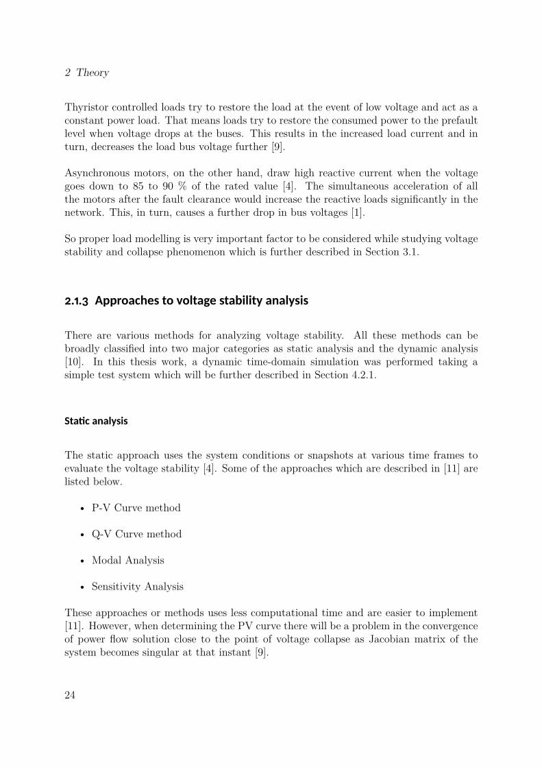
Thyristor controlled loads try to restore the load at the event of low voltage and act as aconstant power load. That means loads try to restore the consumed power to the prefaultlevel when voltage drops at the buses. This results in the increased load current and inturn, decreases the load bus voltage further [9].

Asynchronous motors, on the other hand, draw high reactive current when the voltagegoes down to 85 to 90 % of the rated value [4]. The simultaneous acceleration of allthe motors after the fault clearance would increase the reactive loads significantly in thenetwork. This, in turn, causes a further drop in bus voltages [1].

So proper load modelling is very important factor to be considered while studying voltagestability and collapse phenomenon which is further described in Section 3.1.

. . Approaches to voltage stability analysis

There are various methods for analyzing voltage stability. All these methods can bebroadly classified into two major categories as static analysis and the dynamic analysis[10]. In this thesis work, a dynamic time-domain simulation was performed taking asimple test system which will be further described in Section 4.2.1.

Static analysis

The static approach uses the system conditions or snapshots at various time frames toevaluate the voltage stability [4]. Some of the approaches which are described in [11] arelisted below.

• P-V Curve method

• Q-V Curve method

• Modal Analysis

• Sensitivity Analysis

These approaches or methods uses less computational time and are easier to implement[11]. However, when determining the PV curve there will be a problem in the convergenceof power flow solution close to the point of voltage collapse as Jacobian matrix of thesystem becomes singular at that instant [9].

24

2.2 Generator power capability

Dynamic analysis

In contrast to the static analysis, dynamic approaches give the detail events and theirchronology which leads to the voltage instability and the collapse [4]. However, the timedomain simulations are time-consuming as larger time constants are involved and thedetail dynamics of various power system component models such as ULTC, excitationsystem limiters, dynamic loads, are considered during simulation [9].

A new approach of using combined static and dynamic approach for voltage stabilityanalysis has been presented in paper [11].

. Generator power capability

Synchronous generator is a primary source of reactive power in the network and plays animportant role in maintaining the voltage stability in the network. The boundaries forsupplying the reactive power at a given active power output is defined by the generatorcapability curve provided by the manufacturers [12]. The generator capability diagramprovides a boundary within which the generator can operate safely without exceedingthe thermal limitations. Moreover, another important role of the capability curves is theproper settings of the relays used in the protection of synchronous generator such as AVR,under-excited controllers, overexcitation limiter, loss of field relay [13].

Synchronous generator is a source of active as well as reactive power which can be con-trolled over a wide range of values. The active power P and reactive output power Q forround-rotor generators (xd = xq) when neglecting the resistance (r=0 ) for the generator-transformer unit as shown in Figure 2.5 can be expressed as the following equations [14].

P =Eq Vxd

sinδ (2.5)

Q =Eq Vxd

cosδ − V 2

xd(2.6)

where,xd = Xd +XT = direct axis synchronous reactance.xq = quadrature axis synchronous reactance.r = R+RT = generator resistance when added to the transformer resistance.Eq = air-gap electromotive force (emf).V = voltage on the terminal of step-up transformer.δ = power angle of generator.

Figure 2.6 shows the synchronous generator capability diagram where the area boundedby the curve ABCDEFG indicates the safe region of operation for salient-pole machine.

25

2 Theory

Figure 2.5: Equivalent steady state circuit diagram for round rotor generators with a step-up transformer[14].

Following operational constraints are the reasons for the limits in active and reactivepower of the synchronous generator [14].

1. Armature current limit.

2. Field current limit.

3. Steady-state stability limit.

4. Stator end region heating limit.

5. Generator active power limit.

Armature current limit

The armature current I causes I2R power loss in the armature winding which then in-creases the temperature in the windings. So, this current should be smaller than a certainmaximum value Imax in order to limit the temperature rise.

The active and reactive power is given by P = V I cosφ and Q = V Isinφ respectively.Squaring and adding these two equations yields, P2 +Q2 = (V I)2 which represents theequation of a circle in the P−Q plane with centre at origin and radius V I [14].

For a given voltage V and loading I = Imax,

P2 +Q2 = (V Imax)2 (2.7)

which is as shown by curve-1 in Figure 2.6.

26

2.2 Generator power capability

Q

Practical stability Limit (4)

Theoretical stability Limit

Reluctance circle Minimum rotor

field current limit

Cylindrical rotorCylindrical rotorSalient-poleSalient-pole

P

Q

Maximum turbine power rating (5)

Armature heating limit(1)

Maxmimum field current

limit (2)

QLeading Lagging

A B

C

DE

F

G(3)

5 % excitation margin

0

qx

V 2−

dx

V 2−

d

q

x

VE max

maxVI

Figure 2.6: Capability diagram of synchronous generator [9], [15].

Field current limit

The field winding gets heated because of I2f power loss. So, to keep the temperature

within the certain limit in field windings, the field current I f should be less than certainmaximum value say I f max. By manipulating the equations 2.5 and 2.6, following relationscan be obtained [14],

P =Eq Vxd

sinδ (2.8)

Q+V 2

xd=

Eq Vxd

cosδ (2.9)

Squaring and adding above two equations yields:

P2 +

(Q+

V 2

xd

)2

=

(Eq Vxd

)2

(2.10)

For Eq = Eqmax,

27

2 Theory

P2 +

(Q+

V 2

xd

)2

=

(Eqmax V

xd

)2

(2.11)

Equation 2.11 represents a circle with center (0,-V 2

xd) and radius Eqmax V

xdin P−Q plane as

shown by curve-2 in Figure 2.6.

Steady-state stability limit

For the stable operation of generators, the power angle δ should be within the limit andthe theoretical stability limit occurs when δ = 90°. Dividing equation 2.8 by 2.9 followingequation can be obtained:

P =

(Q+

V 2

xd

)tanδ (2.12)

Putting δ = δmax gives,

P = mQ+ c where slope m = tanδ and intercept c= V 2

xdtanδ.

So, theoretical stability limit can be represented by a straight line which intersects thereactive power axis at a point P = 0 or Q =− c

m =−V 2

xdas shown in Figure 2.6 (line-3).

But in practice, in order to allow the load increase of either 10 or 20 % before instability,a safety margin is always introduced [16]. So, practical stability limit can be obtained byreducing the active power output by 10% of the rated power at constant field current [9]as shown by curve-4 in Figure 2.6.

Stator end region heating limit

This constraint is due to the localized heating at the end region of the armature duringunder-excited operation of the synchronous generator. During under-excitation operation,the field current is low so the retaining ring is not saturated as well as the flux produced bythe armature current gets added up to the flux produced by the field current during thiscondition. Hence, armature end-turn leakage flux gets enhanced and results in the heatingeffects at the end regions due to the eddy current produced in the stator core laminationsbecause of these fluxes entering and leaving in a perpendicular direction especially in theround rotor machine [4].

The end-region heating limit is determined experimentally by the manufacturer [14].

28

2.2 Generator power capability

Generator active power limit

The generator active power limit is limited by the turbine power and depends upon thetype of turbine. The two turbine limits; upper Pmax and the lower limit Pmin can berepresented by two lines parallel to Q-axis in the P−Q plane. Line-6 in the Figure 2.6represents the upper constrain due to maximum turbine power rating [14].

The area bounded by the bold lines in Figure 2.6 represents the safe region of operation.It can also be noted that the first three limitations described above depend upon theterminal voltage V . That means the change in terminal voltage affects the center andradius of the circle as well as the position of the straight lines and ultimately the area ofsafe operation [14].

29

30

Modelling of power system components

In this chapter, two of the important power system component models; load models andthe under-load tap changer has been discussed. These components have a significantrole in long-term voltage stability analysis of a power system. In addition, an alreadydeveloped online low order thermal model of a hydrogenerator based on [2] has also beendescribed.

. Load models

There are generally two types of load models: static and dynamic load models which arefurther described in this section [4]. Out of two types, only the effect of static load modelson voltage stability has been taken as a part of the study in this research work.

Static load modelling

In this modelling technique, loads are modelled as algebraic functions of the bus voltagemagnitude and frequency at some instant of time [4]. Exponential load model, polynomialor ZIP model, frequency-dependent load model, piecewise approximation are some typesof mathematical models which reflects various load behaviours [14].

The polynomial or the ZIP model is represented by the following equation [4]:

P = P0[p1V 2 + p2V + p3]

Q = Q0[q1V 2 +q2V +q3](3.1)

where,V = V

V0; subscript 0 represents variables at initial operating condition.

P and Q represents the active and reactive power consumption by the load at particularbus when bus voltage is V .p1, p2, p3 and q1,q2,q3 are the proportion of active and the reactive power representingconstant impedance, constant current and constant power respectively.

31

3 Modelling of power system components

The frequency dependent load is characterized by multiplying the exponential model orZIP model by some factor as shown below [4]:

P = P0[p1V 2 + p2V + p3][1+Kp f ∆ f ]

Q = Q0[q1V 2 +q2V +q3][1+Kq f ∆ f ](3.2)

where,∆ f is the frequency deviation ( f − f0).Kp f and Kq f ranges from 0 to 3.0 and -2.0 to 0 respectively [4].

Following equation depicts the exponential load model:

P = P0

(VV0

)a

Q = Q0

(VV0

)b (3.3)

where, a and b are the parameters of the model which represents constant impedance,constant current and constant power characteristics of load for the values 0,1 and 2 re-spectively [4].

Dynamic load models

The areas like studies of inter-area oscillations, voltage stability, and long-term stabilitydemands the dynamics of load components to be studied. The dynamic characteristics ofthe motor load is an important aspect of voltage stability studies as it occupies a largepercentage of total power consumption in the power system.

Other dynamics aspects includes the extinction of discharge lamps, operation of protectiverelays, thermostatically controlled load and the response of LTCs [4].

. Under load tap changer

in Section 2.1.2, influence of LTC transformer on voltage collapse has been described. Thefactors governing a tap changing operation are step size, time constant, reference voltage,and deadband. The load side voltage is monitored by a voltage relay and if voltage goesoutside of the deadband, a timer relay is energized. The tap changing mechanism startswhen the relay’s time delay exceeds (after tens of seconds) and process of tap changinggoes on until minimum or maximum tap is reached or until the voltage goes within the

32

3.3 Thermal model of a hydrogenerator

band limit. After the voltage comes within the bandwidth, the timer mechanism andvoltage relay are reset [17].

Usually the LTC transformers possess tap range of ±10% consisting of thirty-two stepseach of 5/8%. A certain time delay in the range of 10-120 seconds before the tapping isallowed out of which the typical time delay is 30 to 60 seconds [17].

The detail model of LTC used for the simulation test case shall be discussed in theSection 4.2.2.

. Thermal model of a hydrogenerator

In this section, typical power losses in the synchronous generator and the online thermalmodel based on [3] is described. The operational losses associated with the synchronousgenerator are the main inputs to the thermal model. The scope of this thesis work coversthe visualization of the generator temperature variations in the visualization tool.

. . Copper losses

Copper losses comprise resistive heating losses in the stator and rotor windings of the ma-chine. The three-phase stator DC-copper losses Ps can be obtained by using the followingequation [2].

Ps = 3 ·Rs(DC)· I2

t (3.4)

where, Rs(DC)represents the resistance of the stator winding per phase. The total rotor

copper losses Pr can be obtained by using the following relation [2]:

Pr = 1.1 ·Rr · I2f d (3.5)

where, Rr and Rs(DC)are the corrected resistances of the rotor winding and stator winding

according to the reference temperature for different class of insulation system [18].

. . Iron losses

Iron losses PFe comprises of hysteresis losses and eddy current losses. Hysteresis lossdepends upon the frequency and the value of maximum flux density per pole whereas theeddy current loss depends upon the square of the frequency and maximum flux density[19].

33

3 Modelling of power system components

. . Stray losses

Stray losses are caused by non-sinusoidal, non-fundamental flux density variations. Itconsists of the losses related to eddy current losses in the stator windings, stator endregion losses and the losses related to damper bars in the rotor laminations [19].

. . Mechanical losses

The mechanical losses Pv includes the losses related to friction in bearings and windage.Windage losses are present in the cooling fans and the rotor blades [19].

Figure 3.1 shows the schematic diagram of the proposed online monitoring algorithmbased on [3]. It clearly shows how the model inputs- field current of the machine I f d,terminal current It , the speed of the machine ω and machine terminal voltage Vt , relatesto the corresponding temperatures via the machine losses.

)(tV t

)(t

)(tTFe

)(tTs

)(tTr

)( ts IP

)( fdr IP

)( tFe VP

)(vP

)(tI fd

)(tI t

Online low order modelInputs Outputs

Figure 3.1: Schematic diagram of online low order thermal model [3].

The three governing differential equations defined in [3] for online monitoring of temper-atures are as follows:

34

3.3 Thermal model of a hydrogenerator

dTr

dt=

1τT,r

[∆PrRr − (Tr −T1,o)] (3.6)

dTs

dt=

1τT,s

[∆PsRs − (Ts −TFe)] (3.7)

dTFe

dt=

1τT,Fe

[∆PFeRFe +RFe

Rs(Ts −TFe)− (TFe −Tδ )] (3.8)

where, Tr, Ts and TFe represents the temperature of rotor winding, stator winding and thestator iron respectively.

35

36

Simulation

In this chapter, simulation setup for the Kundur 10-bus test system which has been usedfor long-term voltage stability study, and the visualization of generator’s capability curvehas been discussed.

The simulation for the study of long-term voltage stability phenomenon has been carriedout using the Power System Analysis Toolbox (PSAT). In addition, the mathematicalapproach of drawing generator capability diagram in MATLAB software environment hasbeen presented. The section also describes the methodology applied for the developmentof automatic visualization tool in MATLAB using Graphical User Interface.

. Power System Analysis Toolbox (PSAT)

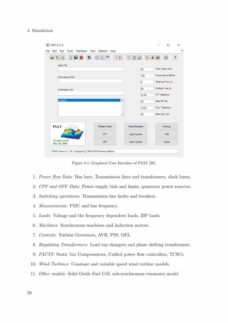
PSAT is a MATLAB based toolbox for the analysis and control of electric power system.It includes power flow, continuation power flow, optimal power flow, small signal stabilityanalysis, and time domain simulation. It provides Graphical user interfaces (GUIs) toaccess all its functions as shown in Figure 4.1 and a Simulink-based library that allowseasy access of tools required for the network design. The single line diagram drawn usingSimulink library is loaded first through data file field of GUI and required analysis aslisted below is carried out as simulation. Power flow Analysis is the core of the PSATwhich allows to initialize the algebraic variables and the states after which further staticor dynamic analysis can be performed. Some of the features are as follows [20].

1. Continuation power flow.

2. Optimal power flow.

3. Small signal stability analysis.

4. Time domain simulations.

5. Phasor measurement unit (PMU) placement.

Furthermore, PSAT contains various static and dynamic component models for powersystem analysis, out of which some component models has been used for this particularcase study of long term voltage stability phenomenon. The models are as follows:

37

4 Simulation

Figure 4.1: Graphical User Interface of PSAT [20].

1. Power flow Data: Bus bars, Transmission lines and transformers, slack buses.

2. CPF and OPF Data: Power supply bids and limits, generator power reserves.

3. Switching operations: Transmission line faults and breakers.

4. Measurements: PMU and bus frequency.

5. Loads: Voltage and the frequency dependent loads, ZIP loads.

6. Machines: Synchronous machines and induction motors.

7. Controls: Turbine Governors, AVR, PSS, OEL

8. Regulating Transformers: Load tap changers and phase shifting transformers.

9. FACTS : Static Var Compensators, Unified power flow controllers, TCSCs.

10. Wind Turbines: Constant and variable speed wind turbine models.

11. Other models: Solid Oxide Fuel Cell, sub-synchronous resonance model

38

4.2 Case Study: Kundur 10-bus test system

. Case Study: Kundur -bus test system

In this section the overall layout of the test system and the different power system com-ponent models used in same system has been presented. The models described are basedon the PSAT models.

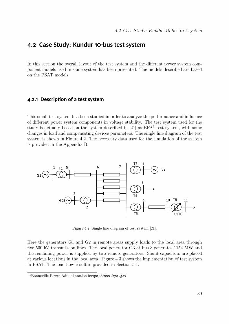
. . Description of a test system

This small test system has been studied in order to analyze the performance and influenceof different power system components in voltage stability. The test system used for thestudy is actually based on the system described in [21] as BPA1 test system, with somechanges in load and compensating devices parameters. The single line diagram of the testsystem is shown in Figure 4.2. The necessary data used for the simulation of the systemis provided in the Appendix B.

~ ~

~

~ G1

G2

G3

ULTC

T1

T2

T3

T4

T5

T6

1

2

5 6 73

8

9 10 11

Figure 4.2: Single line diagram of test system [21].

Here the generators G1 and G2 in remote areas supply loads to the local area throughfive 500 kV transmission lines. The local generator G3 at bus 3 generates 1154 MW andthe remaining power is supplied by two remote generators. Shunt capacitors are placedat various locations in the local area. Figure 4.3 shows the implementation of test systemin PSAT. The load flow result is provided in Section 5.1.

1Bonneville Power Administration https://www.bpa.gov

39

4 Simulation

Bus1

G1

PQ1

Bus2

Bus3Bus5 Bus6 Bus7

Bus8

Bus9 Bus10

T1T3

G2

T2T4

T5T6

Bus11

G3

PQ2

PQ3

Breaker

PQ4

Figure 4.3: Single line diagram implementation of test system in PSAT.

. . System modelling

For the test system, the loss of one of the transmission lines between bus 6 and bus 7 isconsidered as a disturbance during the simulation.

Generators G2 and G3 are modelled using 6th order model of PSAT whereas the gener-ator G1 is modelled as an infinite bus.

Load at bus 8 is modelled as constant power for both active and reactive power whereasthe load at bus 11 is modelled as constant impedance load for both active and reactivepower as represented by PQ2 and PQ1 load respectively in Figure 4.3. The shunt capa-citors at buses 7, 8 & 9 are modeled as PQ load (PQ4, PQ2, PQ3) respectively with thevalues presented in Table B.4.

Transformer LTC performance is characterized by deadband and step size. The dead-band is taken as ±1% p.u. of bus voltage to which LTC is controlling and the tap rangeis ±16 steps with a step size of 5/8%. The integral deviation H and inverse time constantK for the system is taken as 0.001 p.u. and 0.10 per second respectively.

Figure 4.4 and Figure 4.5 shows the equivalent π circuit model and secondary voltagecontrol scheme of LTC transformer respectively. If the tap ratio step ∆m is set as zero(∆m = 0), then

m = m, (4.1)

40

4.2 Case Study: Kundur 10-bus test system

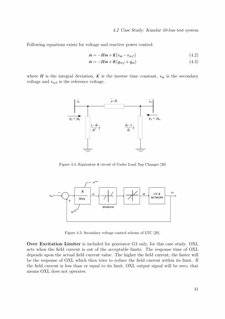
Following equations exists for voltage and reactive power control:

m =−Hm+K(vm − vre f ) (4.2)m =−Hm+K(qre f +qm) (4.3)

where H is the integral deviation, K is the inverse time constant, vm is the secondaryvoltage and vre f is the reference voltage.

mm jqp +

mvmy ~/

ym

m2~

~1−y

m

m~

1~ −

kv

kk jqp +

Figure 4.4: Equivalent π circuit of Under Load Tap Changer [20]

mK

H+s

LTC & NETWORK

deadzone

mmax

vref

mmin

mvm

Figure 4.5: Secondary voltage control scheme of LTC [20].

Over Excitation Limiter is included for generator G3 only, for this case study. OXLacts when the field current is out of the acceptable limits. The response time of OXLdepends upon the actual field current value. The higher the field current, the faster willbe the response of OXL which then tries to reduce the field current within its limit. Ifthe field current is less than or equal to its limit, OXL output signal will be zero; thatmeans OXL does not operates.

41

4 Simulation

OXL provides an additional signal vOXL to the reference value of AVR. The AVR Type Iof PSAT model is used for both the generators. The detailed model can be found in PSATmanual [20]. The OXL has been modeled as a pure integrator with anti-windup limits.When the field current is greater than its thermal limit (i f > ilimf ) , OXL outputs somesignal vOXL to the summing block of AVR as shown in Figure 4.6 [20]. The integratortime constant To for the limiter is taken as 60 seconds whereas the maximum field currentlimit is chosen as 11.7 p.u. for the test system.

Figure 4.6: Over excitation limiter [20].

The equations that characterizes the operation of overexcitation limiter as shown in Fig-ure 4.6 are as follows:

vOXL = (i f − ilimf )/T0 if i f > ilimf

vOXL = 0 if i f ≤ ilimf(4.4)

Each overexcitation limiter model has following algebraic equations:

0 =√

(v+ γq)2 + p2 +(xd

xq+1)

γq(v+ γq)+ γp√(vg + γq)2 + p2

− i f (4.5)

0 = v0re f − vref + vOXL (4.6)

where,

γp = xp/vγq = xq/v

v, p, and q are voltage, active and the reactive power of the generator respectively whereasxd and xq are direct axis and quadrature axis reactances of the generator to which OXLis connected respectively.

42

4.3 On-line PQ diagram

. On-line PQ diagram

The theoretical PQ diagram is developed from the phasor diagrams of operation for boththe salient pole rotor and the cylindrical rotor machines [22]. Active power, field current,stator current, frequency, terminal voltage, rated power of the turbine, heating-up ofstator core end region and stability limits are the parameters which defines the operationof these machines.

The theoretical PQ diagram can be derived by dividing every phasor in the vector diagramby direct-axis synchronous reactance Xd and multiplying them with the armature voltageas shown in Figure 4.7. The figure so obtained, contains P and Q as the x-axis and y-axisrespectively which then can be upgraded by implementing different constraints to obtainthe Figure 2.6 [22].

0E

U

dIX dX

UE0

dX

U 2

UI

Q

0E

U

dIX dX

UE0

dX

U 2

UI

Q

P

Figure 4.7: Derivation of a P-Q capability diagram from the phasor diagram (cylindrical rotor) [23].

In the On-line PQ diagram, all the defining parameters as mentioned before are achieveddirectly from the process and the point of operation is continuously updated in real time[22]. The parameters like active and reactive powers, terminal voltage, field current, fre-quency of grid, temperature and pressure of the cooling agent, varies during the operationso that the PQ diagram changes its configuration in real time. But the P, Q coordinateaxes, and some curves like maximum and minimum turbine power and minimum fieldcurrent do not changes. Temperature control system or the temperature of cooling agent(hydrogen, water) has a significant effect on the position of some operational limits likeoverheating limit of stator core end region, rated field current and the stator current limit[22].

Figure 4.8 shows the On-line PQ diagram with different operating conditions as follows:

• (1)- rated operation condition: voltage (Un), frequency ( fn), hydrogen cooling gastemperature (tn H2).

• (2)- reduced terminal voltage 0.95Un.

43

4 Simulation

• (3)-increased cooling gas temperature 1.1 tn H2.

• (4)- increased stator cooling water temperature 1.1 tn water due to congested hollowcopper strands.

nS

P

nS

Q0.2 0.4 0.6 0.8

0.2

0.4

0.6

0.8

1.0

0.20.40.6

4

1

2

3F

1

2

3

1.0

Figure 4.8: On-line PQ diagram with different operational condition from (1) -(4) [22].

. . Implementation of PQ diagram

The generator’s capability diagram with different constraints as stated in Section 2.2was implemented in MATLAB software environment. The MATLAB code used duringthe implementation of PQ diagram using visualization tool is provided in Appendix C.This software environment provides a sophisticated visualization for the implementedmathematical model of capability diagram. This thesis work presents the methodologyfor obtaining the PQ diagram for a cylindrical rotor synchronous generator with thefollowing simplification during its modelling:

• The synchronous generator has been assumed to be connected to the infinite busi.e. with constant voltage.

• The machine saturation effect on the direct axis synchronous reactance has not beenconsidered, i.e. Xd = constant.

• The effect of armature resistance has been neglected.

The limits of the capability diagram which are implemented during its construction areas follows:

44

4.3 On-line PQ diagram

1. Rated turbine power limit

2. Rated stator Current limit

3. Rated field current limit

4. Practical stability limit

The rated parameters of generator G3 in local area in the 10-bus system is taken asreference for determining capability diagram which are as follows:

1. Rated terminal voltage, V : 13.8 kV

2. Rated MVA, Sn: 1600 MVA

3. Rated power factor, cosφn: 0.72 p.u.

4. Direct axis synchronous reactance, xd: 2.07 p.u.

5. Stability margin: 10 %

Rated turbine power limit

The maximum and the minimum turbine power limits are drawn according to the followingtwo conditions [24]:

• If the power of the turbine (PT ) exceeds the rated power of the generator (Pn), i.e.if PT > Pn, then Pmax = Pn.

• If the power of the turbine is equal to or less than the rated power of the generator(PT ≤ Pn), then Pmax = PT .ηG.

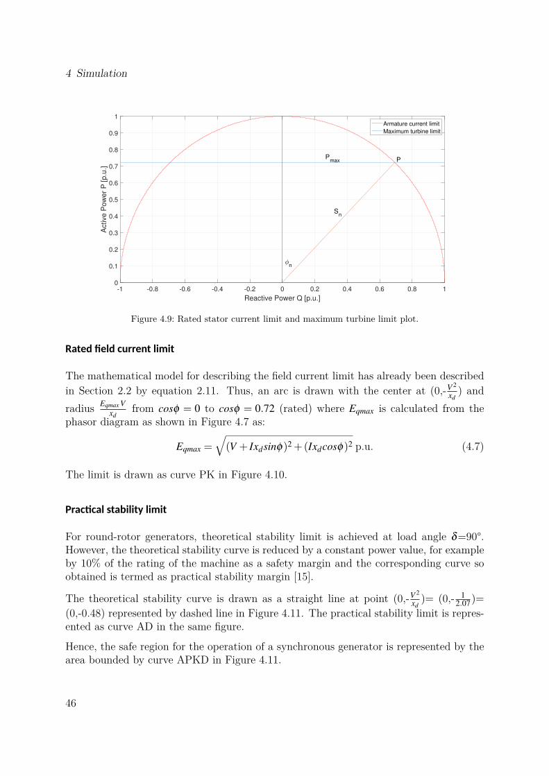
This limit is shown in Figure 4.9 labelled as Pmax. The minimum power depends uponthe turbine requirements. For example, in Kaplan and Francis turbine minimum poweroutput is 5 % to 30% of rated output whereas in some turbines like Pelton turbine thislimitation does not exists [24].

Rated stator current limit

The rated stator current limit is plotted as a constant semi-circle with center at origin‘0’ and radius as the rated apparent power, Sn as shown in Figure 4.9. Point ‘P’ denotesthe rated operating condition of the generator which is defined at its rated power factorcosφn = 0.72. So,Prated = Sncosφ = 1∗0.72 = 0.72 p.u.Qrated = Snsinφ = 1∗

√1− (cosφ)2 = 0.69 p.u.

45

4 Simulation

-1 -0.8 -0.6 -0.4 -0.2 0 0.2 0.4 0.6 0.8 1

Reactive Power Q [p.u.]

0

0.1

0.2

0.3

0.4

0.5

0.6

0.7

0.8

0.9

1

Active

Po

we

r P

[p.u

.]

P

Sn

Pmax

n

Armature current limit

Maximum turbine limit

Figure 4.9: Rated stator current limit and maximum turbine limit plot.

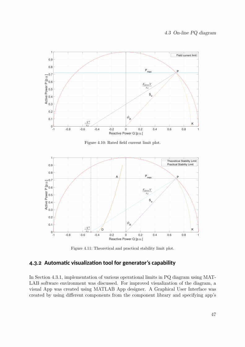
Rated field current limit

The mathematical model for describing the field current limit has already been describedin Section 2.2 by equation 2.11. Thus, an arc is drawn with the center at (0,-V 2

xd) and

radius Eqmax Vxd

from cosφ = 0 to cosφ = 0.72 (rated) where Eqmax is calculated from thephasor diagram as shown in Figure 4.7 as:

Eqmax =√

(V + Ixdsinφ)2 +(Ixdcosφ)2 p.u. (4.7)

The limit is drawn as curve PK in Figure 4.10.

Practical stability limit

For round-rotor generators, theoretical stability limit is achieved at load angle δ=90°.However, the theoretical stability curve is reduced by a constant power value, for exampleby 10% of the rating of the machine as a safety margin and the corresponding curve soobtained is termed as practical stability margin [15].

The theoretical stability curve is drawn as a straight line at point (0,-V 2

xd)= (0,- 1

2.07)=(0,-0.48) represented by dashed line in Figure 4.11. The practical stability limit is repres-ented as curve AD in the same figure.

Hence, the safe region for the operation of a synchronous generator is represented by thearea bounded by curve APKD in Figure 4.11.

46

4.3 On-line PQ diagram

-1 -0.8 -0.6 -0.4 -0.2 0 0.2 0.4 0.6 0.8 1

Reactive Power Q [p.u.]

0

0.1

0.2

0.3

0.4

0.5

0.6

0.7

0.8

0.9

1

Active

Po

we

r P

[p.u

.]

P

Sn

Pmax

n

K

Field current limit

Figure 4.10: Rated field current limit plot.

-1 -0.8 -0.6 -0.4 -0.2 0 0.2 0.4 0.6 0.8 1

Reactive Power Q [p.u.]

0

0.1

0.2

0.3

0.4

0.5

0.6

0.7

0.8

0.9

1

Active

Po

we

r P

[p

.u.]

P

Sn

Pmax

n

K

A

D

Theoretical Stability Limit

Practical Stability Limit

Figure 4.11: Theoretical and practical stability limit plot.

. . Automatic visualization tool for generator’s capability

In Section 4.3.1, implementation of various operational limits in PQ diagram using MAT-LAB software environment was discussed. For improved visualization of the diagram, avisual App was created using MATLAB App designer. A Graphical User Interface wascreated by using different components from the component library and specifying app’s

47

4 Simulation

design and layout. For defining the App behavior, App designer allows an integratedversion of the MATLAB Editor [25]. All the parameter values implemented, and the dy-namics observed in the visualization tool is based upon the case study of Kundur 10-bustest system described in Section 4.2. Figure 4.12 shows a simple workflow diagram ad-opted during the implementation of generator’s capability diagram in the visualizationtool.

Kundur 10 - bus test system

MATLABWorkspace

Simulation

P, Q, V

Graphical User Interface

(App Designer)Limits

implementation

Result

Figure 4.12: Work flow diagram for PQ curve implementation in visualization tool.

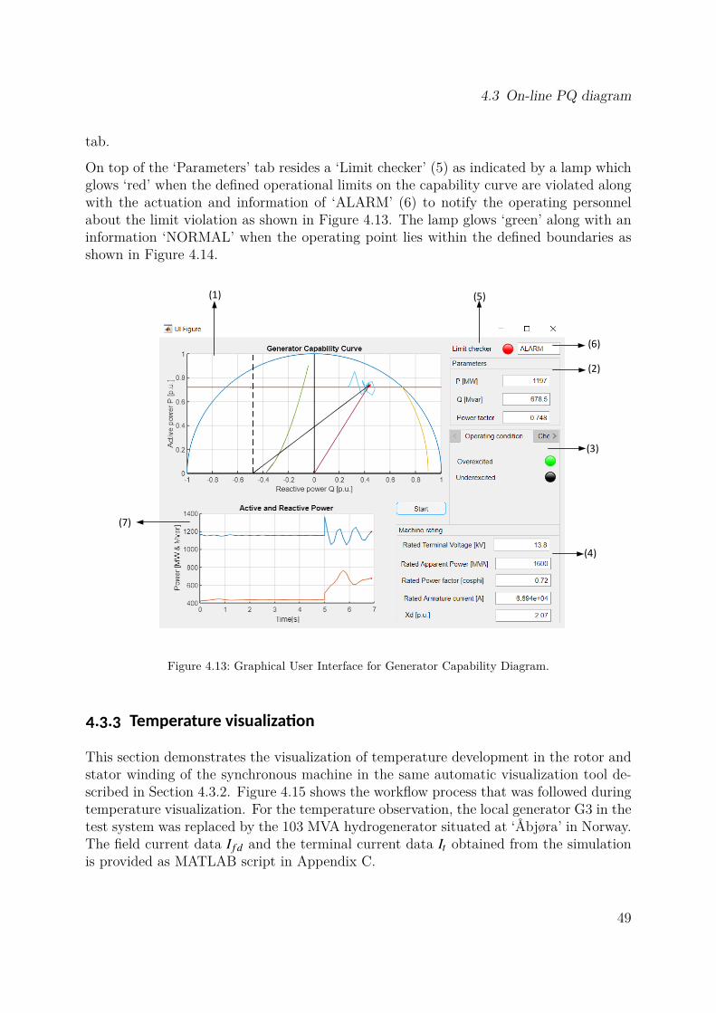
Figure 4.13 shows a GUI environment for the designed App in order to visualize the gener-ator capability. The GUI consists of two figure windows and three tabs. The upper figurewindow (1) in the user interface shows the capability curve with the real-time operatingpoint as indicated by ‘red’ asterisk symbol. The ‘Parameters’ tab (2) shows the operatingpoint (P and Q) values in real time along with the operational power factor. Moreover,the dynamics of P and Q can be observed in the lower figure window (7). The ‘Operatingconditions’ tab (3) shows the actual operating condition i.e. whether the generator isoperating in over excitation mode or under excitation mode with current operation modeindicated by lamp glowing ‘green’. The ‘Machine rating’ tab (4) indicates the generatorrated conditions which can be changed by changing the values in the respective fields. Forexample, the effect of change of direct axis synchronous reactance on the generator limitscan be visualized in the figure section (1) by changing its value in the ‘Machine rating’

48

4.3 On-line PQ diagram

tab.

On top of the ‘Parameters’ tab resides a ‘Limit checker’ (5) as indicated by a lamp whichglows ‘red’ when the defined operational limits on the capability curve are violated alongwith the actuation and information of ‘ALARM’ (6) to notify the operating personnelabout the limit violation as shown in Figure 4.13. The lamp glows ‘green’ along with aninformation ‘NORMAL’ when the operating point lies within the defined boundaries asshown in Figure 4.14.

(1)

(7)

(4)

(3)

(2)

(5)

(6)

Figure 4.13: Graphical User Interface for Generator Capability Diagram.

. . Temperature visualization

This section demonstrates the visualization of temperature development in the rotor andstator winding of the synchronous machine in the same automatic visualization tool de-scribed in Section 4.3.2. Figure 4.15 shows the workflow process that was followed duringtemperature visualization. For the temperature observation, the local generator G3 in thetest system was replaced by the 103 MVA hydrogenerator situated at ‘Åbjøra’ in Norway.The field current data I f d and the terminal current data It obtained from the simulationis provided as MATLAB script in Appendix C.

49

4 Simulation

Figure 4.14: Graphical User Interface for Generator Capability Diagram showing ‘NORMAL’ condition.

Figure 4.16 shows the thermal model of a hydrogenerator developed in Simulink softwareenvironment as proposed in paper [3]. The circuit parameters used in the simulation areprovided in Table B.5. Figure 4.17 shows the schematic setup which takes field currentI f d and the terminal current It from the local generator G3 as inputs and calculates thewinding losses as I2

f dR and I2t R respectively. The outputs rotor temperature Tr and the

stator temperature Ts was extracted into the MATLAB workspace and then plotted. Theinputs to the thermal model were continuously updated in real time from the workspace.The gain block in the output converts the measured voltage signal into the equivalenttemperature signal. This gain factor (1/2236) was calculated by comparing the value ofoutput measured signal from the ‘Simulink model’ as implemented in this thesis work andfrom ‘DAE-ODE model’ of the same low order thermal model described in [26].

50

4.3 On-line PQ diagram

Kundur 10 - bus test system with Åbjøra as local

generator

MATLABWorkspace

Simulation Thermal model

in Simulink

tfd II ,

tfd II ,

sr TT ,

Temperature visualization

Figure 4.15: Work flow diagram for temperature visualization.

51

4 Simulation

Figure 4.16: Simulink circuit for the thermal model proposed in [3].

Figure 4.17: Schematic setup for the temperature measurement in Simulink [3].

52

Results and discussions

In this section, results and discussion regarding the simulation of 10-bus system and thePQ capability diagram has been presented.

Section 5.1 provides the results of load flow analysis of the test system. The effect ofstatic load models and the influence of ULTC and OXL on long-term voltage stabilityis shown in this section. Furthermore, the outcome of the development of an automaticvisualization tool is described in Section 5.2.

. -bus test system

Under the long-term voltage stability study, the impact of ULTC and OXL on voltagecollapse was investigated. The voltage at various buses and the reactive power outputs ofthe generator was compared for the test system including and excluding the over excitationlimiter with ULTC in action for both cases which are as presented in the Figures from 5.4to 5.8. The steady state voltage profile and reactive power at different buses are shownin Figure 5.1 and 5.2 respectively.

1 10 11 2 3 5 6 7 8 9

Bus #

0

0.2

0.4

0.6

0.8

1

1.2

V [p.u

.]

Voltage Magnitude Profile

Figure 5.1: Steady state voltage at various buses.

53

5 Results and discussions

1 10 11 2 3 5 6 7 8 9

Bus #

-400

-200

0

200

400

600

800

1000

1200

QG

- Q

L [M

Var]

Reactive Power Profile

Figure 5.2: Steady state reactive power at various buses.

Four different cases were considered for the test system which is presented in Table 5.1.These cases are taken from the cases considered in dissertation [10] where the dynamicphenomenon was observed using PSS/E software taking the standard BPA power sys-tem.

Table 5.1: Case studies

Case Load OEL ULTCBus 8 Bus 11 G2 G3A Constant impedance Constant impedance Inactive Inactive InactiveB Constant current Constant impedance Inactive Inactive InactiveC Constant power Constant impedance Inactive Inactive InactiveD Constant power Constant impedance Inactive Active Active

Scenario Loss of transmission line between Bus 6 & Bus 7

. . Effect of load models

As mentioned earlier in Chapter 3.1 about the types of load models, the effect of static loadmodels on long term voltage stability was studied for the test case considered. Figure 5.3shows the voltage profile at bus 11 under three cases namely A, B and C as presentedin Table 5.1. For all these three cases, transformer T6 is equipped with a fixed tap ratio(instead of ULTC) of value equal to that of T5. Hence, the steady voltage at bus 11before contingency in this case (0.814 p.u.) is different to the voltage magnitude (0.791p.u.) as shown in Figure 5.4 where T6 is equipped with a ULTC.

54

5.1 10-bus test system

From the voltage profiles in all three cases, it can also be seen that after the fault,the system stabilizes at lower voltages. The reason behind this is the inadequacy ofreactive power in the system due to the disturbance considered. Due to tripping ofone of the transmission line, the equivalent impedance of the line increases and hencethe losses increases. In addition, the constant power load stabilizes at a lower value ascompared to constant impedance and constant power load because of its load restoringcharacteristics [10]. That means constant power load tries to consume the same power ata pre-disturbance level as consumed power is independent of voltage variations and hencethe voltage drops even further. The dynamics of voltage profile obtained is comparableto the similar case study performed in [10] using PSS/E software.

0 10 20 30 40 50 60

Time [sec]

0.78

0.785

0.79

0.795

0.8

0.805

0.81

0.815

Voltage m

agnitude [p.u

.]

constant impedence

constant current

constant power

Figure 5.3: Voltage profile at bus 11 for different load types.

. . Effect of ULTC and OXL

In order to study the dynamics of ULTC and OXL in long term voltage stability scenario,Case D as mentioned in Table 5.1 was considered. The sequence of events triggered duringthe simulation in different time frames can be explained as follows.

• One of the transmission lines is disconnected at time t=5 seconds. When the linehas been disconnected, the apparent impedance and consequently the line lossesand voltage drop of the transmission system is increased.

55

5 Results and discussions

• The second time frame starts at around 10 seconds where the ULTC is activated asthe voltage at the bus 11 is lower than the preset value. The ULTC tries to keepthe voltage at the secondary bus (bus-11) at its original value by adjusting its tapratio which demands more reactive power support from the generators present inthe network. Thus, to meet the increased reactive power demand the excitationcurrent is continuously increased until the maximum tap of transformer is reachedor voltages at the buses are recovered. This time frame can be observed in figuresfrom 5.4a-5.8a. The voltage at bus 11 is restored to nearly its reference value inabout 90 seconds as shown in Figure 5.4.

• The third time frame begins with the actuation of overexcitation limiter as shownin Figure 5.4b at around t=150 seconds by ramping down the field current. Thefollowing chains of events occurs after the actuation of OXL:

– As the field current of G3 is reduced, its terminal voltage drops.

– Voltages at bus 11, 10 and 7 drops.

– ULTC on T6 tries to restore the voltage at bus 11 back to its original value.

– The reactive power demand on generators increases. Field current of machine3 increases and continues to remain at its limit and the terminal voltage of G3further decreases.

– Voltage at bus 7 drops and causes a further reduction in terminal voltage ofbus 10 and bus 11.

– The ULTC operates again, repeating above mentioned chains of events.

Hence in response to each tap movement of ULTC, the voltage at bus 11 reducesrather than increased. This indicates that the system has entered into the voltageinstability phase. The bus 11 voltage falls progressively as shown in Figure 5.4buntil the ULTC reaches its maximum tap position at around 260 seconds. Thevoltage at bus 11 settles at around 0.77162 p.u.

. . Countermeasures against voltage collapse

There are different methods of mitigating voltage instability and preventing the powersystem from voltage collapse situation. Some of the preventive and corrective control forvoltage stability based on paper [27] are as follows:

• Rescheduling of active power generation

• Implementation of generator secondary voltage control

• Additional shunt capacitance inclusion

56

5.1 10-bus test system

0 20 40 60 80 100 120

Time [s]

0.755

0.76

0.765

0.77

0.775

0.78

0.785

0.79

0.795

Vo

lta

ge

ma

gn

itu

de

[p

.u.]

(a) With only ULTC

0 50 100 150 200 250 300

Time [s]

0.75

0.755

0.76

0.765

0.77

0.775

0.78

0.785

0.79

0.795

Vo

lta

ge

ma

gn

itu

de

[p

.u.]

(b) With ULTC and OXL

Figure 5.4: Bus 11 voltage without and with OXL.

0 20 40 60 80 100 120

Time [s]

0.82

0.83

0.84

0.85

0.86

0.87

0.88

Vo

lta

ge

ma

gn

itu

de

[p

.u.]

(a) With only ULTC

0 50 100 150 200 250 300

Time [s]

0.68

0.7

0.72

0.74

0.76

0.78

0.8

0.82

0.84

0.86

0.88

Vo

lta

ge

ma

gn

itu

de

[p

.u.]

(b) With ULTC and OXL

Figure 5.5: Bus 10 voltage without and with OXL.

57

5 Results and discussions

0 20 40 60 80 100 120

Time [s]

1.01

1.015

1.02

1.025

1.03

1.035

1.04

1.045

1.05

1.055

1.06

Vo

lta

ge

ma

gn

itu

de

[p

.u.]

(a) With only ULTC

0 50 100 150 200 250 300

Time [s]

0.94

0.96

0.98

1

1.02

1.04

1.06

1.08

Vo

lta

ge

ma

gn

itu

de

[p

.u.]

(b) With ULTC and OXL

Figure 5.6: Bus 3 voltage without and with OXL.

0 20 40 60 80 100 120

Time [s]

400

450

500

550

600

650

700

750

800

Re

active

po

we

r o

utp

ut[

Mva

r]

(a) With only ULTC

0 50 100 150 200 250 300

Time [s]

400

500

600

700

800

900

1000

Re

active

po

we

r o

utp

ut[

Mva

r]

(b) With ULTC and OXL

Figure 5.7: Reactive power output of generator G3 without and with OXL.

58

5.2 Visualization tool for generator’s capability

0 20 40 60 80 100 120

Time [s]

1.8

2

2.2

2.4

2.6

2.8

3

3.2

3.4

Fie

ld v

olta

ge

ma

gn

itu

de

[p

.u.]

(a) With only ULTCL

0 50 100 150 200 250 300

Time [s]

1.6

1.8

2

2.2

2.4

2.6

2.8

3

3.2

3.4

3.6

Fie

ld v

olta

ge

ma

gn

itu

de

[p

.u.]

(b) With ULTC and OXL

Figure 5.8: Field voltage at generator 3 without and with OXL.

• Adjustment of ULTC transformer taps; tap locking, tap blocking or tap reversing[10]

• Shedding of loads

The preventive and corrective control is an optimization problem where the objectivefunction could be either minimizing the number of control equipment, load sheddingminimization or the control cost minimization [27]. The issues and concepts regardingunder-voltage load shedding which has been described as an economical solution to dealwith voltage stability problem has been described in paper [6].

There was a combined influence of ULTC and current limiter of Generator G3 in voltagecollapse of Kundur test system. Any of the above-mentioned control measures can beused as a mitigating measure for instability. The effect of load shedding and tap changerlocking on the stabilization of voltages in the BPA test system is described by Larsson in[28].

. Visualization tool for generator’s capability

As mentioned in Section 4.3.2, an automatic visualization tool was developed in MATLABsoftware environment with GUI which provides real-time power factor, active and thereactive power. The generator reactive power capability can be visualized in a real-timealong with an alarm signal in the case of limit violation.

In addition to the features described in Section 4.3.2, a ‘Check condition’ tab was im-plemented in the tool in order to confirm the indication of generators operation in both

59

5 Results and discussions

over and under excited regimes. This operation is indicated by a black ‘asterisk’ as shownin Figure 5.9. User can give the active and the reactive power values as inputs in the‘Check condition’ tab fields and the corresponding operation can be observed in both thecapability chart and the lamp in the same tab which glows ‘green’ depending on whetherthe generator is over-excited or under-excited. For example, when the user gives a valueof 0.5 and -0.7 in the P and Q fields, the operation will be observed as under excitedindicated by ‘under excited lamp’ glowing ‘green’ as shown in Figure 5.10.

Figure 5.9: Visualization of generator operating point in over excited regime indicated by black asterisk.

The temperature development in the stator and rotor windings in the synchronous gener-ator was also observed in the same tool which is as shown in Figure 5.11 and 5.12 using thethermal model as described in Section 3.3. The output temperatures as seen in the figureis the result of input field current and armature current taken from the local generatorG3 in Kundur 10-bus system when replaced by 103 MVA hydrogenerator at ‘Åbjøra’ inNorway. The machine data of hydrogenerator is provided in Table B.6. The field andthe stator currents in real time are observable in the tool. The initial temperature in thestator and rotor was taken as 28°C during the simulation. From Figure 5.12, it can beobserved that the dynamics of temperature development is similar to the dynamics of thereactive power as seen in Figure 5.7b.

60

5.2 Visualization tool for generator’s capability

Figure 5.10: Visualization of generator operating point in under excited regime indicated by black asterisk.

Figure 5.11: Temperature observation in the visualization tool.

61

5 Results and discussions

0 50 100 150 200 250 300

Time [min]

20

40

60

80

100

120

140

Te

mp

era

ture

[°C

]

Rotor

Stator

Figure 5.12: Rotor and Stator temperature plots from machine data ‘Åbjøra’.

62

Conclusion

The dynamic analysis of voltage stability using time-domain simulation has been presentedin this thesis work using a test power system containing 10 buses as a case study. Fromthe simulation, it can be concluded that dynamic analysis is very useful in understandingthe detail dynamics involved during the larger disturbances such as a loss of transmissionline or loss of generation in the system and to study the coordination between the controland the protection as well. This type of analysis gives accurate results though it requiresdetail accurate models of the components and is time-consuming. A MATLAB basedtool, PSAT was chosen as a long-term time domain simulation program where dynamicvoltage stability was carried out and experienced to be little time consuming.

The influence of static load models on the voltage collapse scenario was presented. Theseverity of the effect depends upon the type of load. Constant power load has the mostsevere effect on the voltage collapse as compared to constant impedance and the constantcurrent load. It is because the constant power loads are independent of the voltage andwhen the voltage drops in the network due to disturbances in the network, they try toconsume the same power as pre-fault power so that the voltage drops even further. But theconstant impedance loads decreases proportionally to the square of the voltage magnitudeso has least effect on the voltage collapse.

Through long-term dynamic simulation, the dynamic behaviour of these two importantpower system components: ULTC and OXL is found to have huge influence on the voltagecollapse phenomena. Accurate and detail modelling of these devices is necessary for detailand proper analysis of voltage stability.

The development and implementation of PQ capability diagram for the cylindrical rotormachine was done in MATLAB. The use of Graphical User Interface provides the userinteraction with the visualization tool through graphical displays, inputs and visual in-dicators. During implementation, the infinite bus-bar assumption was made which is notpractical in real case as the terminal voltage can significantly vary from the rated value.As the terminal voltage varies, the field and the armature limits also vary. Furthermore,the assumption of constant direct-axis synchronous reactance is also not valid as the syn-chronous machine are designed with certain amount of saturation level and depends uponmachine operating point such as armature voltage and current [23].

While implementing the Åbjøra hydrogenerator as a local generator (G3) in the testpower system considered, it was found that the OXL does not came into the operation

63

6 Conclusion

as expected. The reason could be the inappropriate parameters for the load flow analysisas every parameter values for the models were scaled down for this comparatively lowerrating hydrogenerator during implementation. An already developed thermal model in[2] was used to visualize the temperature of hydrogenerator in the visualization tool.

64

Further work

Some of the recommendations which can be undertaken as a further work are presentedbelow.

• This thesis work presented the effect of generator overexcitation limiter, transformertap changer and the static loads on the voltage stability. The effect of dynamicload characteristics which has a significant influence on voltage stability can beanalyzed further. Moreover, other simulation tools like PSS/E, DIgSILENT Power-Factory, EUROSTAG, SimPowerSystems, EPRI Extended Transient Mid-Term Sta-bility Program (ETMSP) can be used to test and compare results from the sametest system for voltage instability and collapse phenomena.

• The generator PQ capability diagram was implemented in this thesis assumingcylindrical rotor machine. Salient pole generators on the other hand exhibit differentcharacteristics in the under-excited regime. The theoretical and practical stabilitylimit curve for salient pole machine is different to that of cylindrical rotor machineas it contains both the direct and quadrature axis reactances as seen in Figure 2.6.Furthermore the minimum rotor field current limit is present only in salient polemachines due to additional reluctance power in such machines [9]. Hence, both typesof aforementioned limits could be executed in PQ diagram for salient pole machine.Moreover, the stator end region heating limit which imposes an additional limit inunder-excited region of generator capability diagram can also be analyzed under thefurther work.

• Change of generator terminal voltage changes the boundaries defined in capabilitydiagram. In this thesis work, the limits are defined taking the generator terminalvoltage as 1 p.u. So, the effect of change of terminal voltage on the PQ capabilitylimits can be analyzed further. Moreover, the dependency of apparent power onother factors such as inlet air temperature of a cooling system, maximum tension ofthe coupled rotor on fault conditions, capacity of a cooling system could be studiedwhile defining the armature current limit [29].

65

66

Bibliography

[1] CIGRE Task Force 38.02.10, ‘Modelling of Voltage Collapse Including DynamicPhenomena’, Tech. Rep., 1993.

[2] T. Øyvang, ‘Enhanced power capability of generator units for increased operationalsecurity’, PhD thesis, 2018.

[3] T. Øyvang, J. K. Noland, G. J. Hegglid and B. Lie, ‘Online model-based thermalprediction for flexible control of an air-cooled hydrogenerator’, IEEE Transactionson Industrial Electronics, pp. 1–1, 2018. doi: 10.1109/tie.2018.2875637.

[4] P. Kundur, Power System Stability and Control. McGraw-Hill, Inc., 1994.[5] ‘Definition and classification of power system stability IEEE/CIGRE joint task force

on stability terms and definitions’, IEEE Transactions on Power Systems, vol. 19,no. 3, pp. 1387–1401, Aug. 2004. doi: 10.1109/tpwrs.2004.825981.

[6] C.W.Taylor, ‘Concepts of undervoltage load shedding for voltage stability’, IEEETransactions on Power Delivery, vol. 7, no. 2, pp. 480–488, Apr. 1992. doi: 10.1109/61.127040.

[7] (2019). Voltage stability, [Online]. Available: http://shodhganga.inflibnet.ac.in/bitstream/10603/40792/7/07_chapter2.pdf (visited on 02/02/2019).

[8] D. Thukaram, L. Jenkins, H. Khincha, G. Yesuratnam and B. Kumar, ‘Monitoringthe effects of on-load tap changing transformers on voltage stability’, in 2004 Inter-national Conference on Power System Technology, 2004. PowerCon 2004., IEEE.doi: 10.1109/icpst.2004.1460031.

[9] V. Storvann, ‘Maintaining voltage stability : An analysis of voltage stability indic-ators and mitigating actions’, Master’s thesis, Norwegian University of Science andTechnology, 2012.

[10] D. T. Nguyen, ‘Contributions to analysis and prevention of power system blackouts’,Theses, Institut National Polytechnique de Grenoble - INPG, Nov. 2008. [Online].Available: https://tel.archives-ouvertes.fr/tel-00352414.

[11] M. Hasani and M. Parniani, ‘Method of combined static and dynamic analysis ofvoltage collapse in voltage stability assessment’, in 2005 IEEE/PES Transmission& Distribution Conference & Exposition: Asia and Pacific, IEEE. doi: 10.1109/tdc.2005.1547182.

67

Bibliography

[12] J. Dragosavac, D. Arnautovic, Z. Janda, J. Milanovic and B. Radojicic, ‘On-line es-timation of available generator reactive power for network voltage support’, in 8thMediterranean Conference on Power Generation, Transmission, Distribution andEnergy Conversion (MEDPOWER 2012), Institution of Engineering and Techno-logy, 2012. doi: 10.1049/cp.2012.2014.

[13] D. E. Moghadam, A. Shiri, S. Sadr and D. A. Khaburi, ‘A practical method forcalculation of over-excited region in the synchronous generator capability curves’,in 2014 IEEE 23rd International Symposium on Industrial Electronics (ISIE), IEEE,Jun. 2014. doi: 10.1109/isie.2014.6864702.

[14] J. Machowski, J. W. Bialek and J. R. Bumby, Power System Dynamics : Stabilityand Control, 2nd ed. John Wiley & Sons, Ltd, 2008.

[15] J. Walker, ‘Operating characteristics of salient-pole machines’, Proceedings of theIEE - Part II: Power Engineering, vol. 100, no. 73, pp. 13–24, Feb. 1953. doi:10.1049/pi-2.1953.0004.

[16] B. M. Weedy, B. J. Cory, N. Jenkins, J. B. Ekanayake and G. Strbac, Electric PowerSystems, 5th ed. Wiley, 2012.

[17] C. W. Taylor, Power System Voltage Stability. McGraw-Hill, 1993.[18] IEEE standard for salient-pole 50 hz and 60 hz synchronous generators and gen-

erator/motors for hydraulic turbine applications rated 5 MVA and above. doi: 10.1109/ieeestd.2006.99082.

[19] C. Mejuto, ‘Improved lumped parameter thermal modelling of synchronous gener-ators’, PhD thesis, 2010. [Online]. Available: https://www.era.lib.ed.ac.uk/handle/1842/4612.

[20] F. Milano, Power System Analysis Toolbox Documentation for PSAT, version 2.1.8,2013.

[21] CIGRE Task Force 38.02.08, ‘Long Term Dynamics Phase II’, CIGRE, Tech. Rep.,1995.

[22] Working Group A1.38, ‘Generator On-Line Over and Under Excitation Issues’,Technical Brochure CIGRE, Jun. 2015.

[23] M. Vrazic, A. Viskovic and Z. Hanic, ‘User P-Q Diagram as a Part of a SynchronousGenerator Monitoring System’, Electronics and Electrical Engineering, vol. 20, no. 4,Apr. 2014. doi: 10.5755/j01.eee.20.4.5333.

[24] I.Ilić, Z. Maljković, I. Gašparac, M. Pavlica, D. Ilić-Zubović, V. Jarić, A. Viškovićand R. Belobrajić, ‘Methodology for Determining the Actual PQ Diagram of aHydrogenerator’, Journal of Energy, vol. 56, no. 2, pp. 144–181, 2007. [Online].Available: https://hrcak.srce.hr/13153.

[25] (2019). Matlab app designer, [Online]. Available: https://se.mathworks.com/products/matlab/app-designer.html (visited on 22/03/2019).

68

Bibliography

[26] M. Pandey, ‘Model fitting and state estimation for thermal model of synchronousgenerator’, unpublished thesis, 2019.

[27] V. A. Qin Wang, ‘A critical review on preventive and corrective control againstvoltage collapse’, Electric Power Components and Systems, vol. 29, no. 12, pp. 1133–1144, Dec. 2001. doi: 10.1080/153250001753246862.

[28] M. Larsson, ‘Coordinated voltage control in electric power systems’, PhD thesis,2000. [Online]. Available: http://www.iea.lth.se.

[29] D. E. Moghadam, A. Shiri, S. Sadr and D. A. Khaburi, ‘A practical method forcalculation of over-excited region in the synchronous generator capability curves’,in 2014 IEEE 23rd International Symposium on Industrial Electronics (ISIE), IEEE,Jun. 2014. doi: 10.1109/isie.2014.6864702.

[30] T. Øyvang, G. J. Hegglid and B. Lie, ‘Models of synchronous generators with ex-citation system, for transient power system studies’, IFAC-PapersOnLine, vol. 51,no. 2, pp. 91–96, 2018. doi: 10.1016/j.ifacol.2018.03.016.

69

70

Appendix A

Signed version of task description

71

Appendix B

Parameters used in the Kundur test system

and the thermal model

75

Appendix B Parameters

B. System diagram

~ ~

~

~ G1

G2

G3

ULTC

T1

T2

T3

T4

T5

T6

1

2

5 6 73

8

9 10 11

Figure B.1: Single line diagram of test system [21].

B. Load flow data

Sbase = 100 MVA

Table B.1: Bus data of test systemBus Base Vscheduled Phase Shunt P load Q load

[kV] [p.u.] [rad] [Mvar] [MW] [Mvar]Bus1 13.8 0.98 0 0 0 0Bus2 13.8 0.96 0 0 0 0Bus3 13.8 1.04 0 0 0 0Bus5 500 1.00 0 0 0 0Bus6 500 1.00 0 0 0 0Bus7 500 1.00 0 750 0 0Bus8 13.8 0.94 0 1500 3000 1800Bus9 115 0.95 0 300 0 0Bus10 115 0.89 0 0 30 0Bus11 13.8 0.91 0 0 3100 90

76

B.3 Dynamic data

Table B.2: Generators load flow dataBus No. Gen Base P gen Q gen Sbase Qmax Qmin

Name [kV] [MW] [Mvar] [MVA] [Mvar] [Mvar]1 G1 13.8 3471.9 1129.03 5000 1600 -10002 G2 13.8 1736 712.53 2200 725 2003 G3 13.8 1154 414.58 1600 700 -100

Table B.3: Transmission lines dataFrom To bus R X BBus [p.u.] [p.u.] [p.u.]5 6 0.0000 0.0040 0.00006 7 0.0015 0.0288 1.17309 10 0.0010 0.0030 0.0000

Table B.4: Transformers dataTransformer R X Tap ratio

[p.u.] [p.u.]T1 0.0000 0.0020 0.8857T2 0.0000 0.0045 0.8857T3 0.0000 0.0125 0.9024T4 0.0000 0.0030 1.0664T5 0.0000 0.0026 1.0800T6 0.0000 0.0010 0.9750

B. Dynamic data

Machine parameters:

Machine 1: Infinite busMachine 2: H = 2.09, MVA rating = 2200 MVAMachine 3: H= 2.33, MVA rating = 1400 MVA

Following are the parameters for machine 2 and machine 3 on their respective MVA

77

Appendix B Parameters

ratings:

Ra = 0.0046 Xd = 2.07 Xq = 1.99Xl = 0.155 X ′

d = 0.28 X ′q = 0.49

X ′′d = 0.215 X ′′

q = 0.215

T ′do = 4.10 T ′

qo = 0.56

T ′′do = 0.033 T ′′

qo = 0.062

Exciters:

Both machine 2 and machine 3 uses thyristor exciters with a gain of 100 and the timedelay of the measurement system as 0.02 seconds.

Overexcitation limiter for machine :

The OXL model used in the simulation is as described in the Section 4.2.2 with integratortime constant (T0)= 60 seconds, maximum field current ilimf d = 11.7 p.u. and maximumoutput signal vmax

OXL= 5.02 p.u.

ULTC data for transformer T between bus and :

Deadband: ±1% p.u. bus voltageTap range: ±16 stepsStep size: 5/8 % (=0.00625 p.u.)

78

B.4 Thermal model parameters

B. Thermal model parameters

Table B.5: Thermal model data [3]Parameters Symbol Value UnitThermal resistance, TFe −Tδ RFe 0.07 K/kWThermal resistance, Ts −TFe Rs 0.05 K/kWThermal resistance, air R1 0.018 K/kWGain coefficient, T2,i K1 0.59 -Gain coefficient rotor(Cu) K2 0.5 -Gain coefficient stator(Fe) K3 0.36 -Heat exchanger effieicency (epsi) ε 0.595 -

B. Machine data of Åbjøra

Table B.6: Machine data of Åbjøra [30]Description Parameters Value UnitRated power Sn 103 MVARated voltage Vtn 11 kVRated current Itn 5406 ARated field current I f dn 1064 AInertia constant H 2.66 sNumber of polepairs p 6 -Synchronous reactance d-axis xd 1.09 [p.u.]Synchronous reactance q-axis xq 0.67 [p.u.]Transient reactance d-axis x′d 0.24 [p.u.]Subtransient reactance d-axis x′′d 0.15 [p.u.]Subtransient reactance q-axis x′′q 0.19 [p.u.]Transient OC Time constant d-axis T ′

do 10 sTransient OC Time constant q-axis T ′

qo 0.23 sSubtransient OC Time constant d-axis T ′′

do 0.086 sSubransient OC Time constant q-axis T ′′

qo 0.23 sStator leakage inductance Xl 0.08 [p.u.]Stator resistance Ra 0.00182 [p.u.]

79

80

Appendix C

Codes and programs used in the thesis work

81

Appendix C Codes and programs

The MATLAB code used for the development of visualization tool and the models de-veloped can be access through the following GitHub link.

https://github.com/prabesh213922/Thesis.git

The suggestions for using those files is included in the ‘README’ file provided in thesame folder.

82

Appendix D

Paper for SIMS conference

The preliminary version of the paper regarding the thesis work is provided in this sec-tion.

83

Online Monitoring and Visualizing of a Generator’s Capabilitywith Simulink

Prabesh Khadka Dietmar Winkler Thomas Øyvang

Department of Electrical Engineering, Information Technology and Cybernetics, University of South-EasternNorway, Porsgrunn, Norway versatile.prabesh@gmail.com

AbstractThe power systems today are becoming more larger, com-plex and are operating closer to its security and stabilitylimits particularly due to an increase in load demands andnumber of environmental concerns. Voltage stability hasbeen a major subject of discussion and concern in electricpower system operation and planning worldwide. This re-search paper presents the long-term voltage stability anal-ysis of a power system using time-domain simulation withPSAT software. Furthermore, a mathematical approach ofplotting PQ capability diagram of a generator is suggestedin MATLAB software environment. It is shown that theload models, load tap changing transformer and genera-tor over-excitation limiter have a significant influence onvoltage stability and collapse phenomena.Keywords: long-term voltage stability, dynamic voltagestability, generator capability diagram, PSAT (Power Sys-tem Analysis Toolbox)

1 IntroductionVoltage instability is becoming one of the major issuesin power system operation and planning worldwide dueto the increased power demand. Many incidents of volt-age collapse have been reported at different corners of theworld and few examples can be found in CIGRE report(CIGRE Task Force 38.02.10 1993). The inability of thepower system to meet the reactive power demand in anelectrical network is one of the cause of voltage instabil-ity. Generators are normally the sources of reactive powersupport during voltage insecurities. So, monitoring thevoltage profiles, voltage regulation and the reactive poweroutput of generators is one of the important countermea-sures for voltage collapse.

In a recent Ph.D. study (Øyvang 2018), utilization ofthe thermal capacity of a hydrogenerator to enhance thevoltage stability of the power system was studied. Theavailable voltage control capability depends upon the tem-perature rise of the machine during contingencies (Øy-vang 2018). Furthermore, the normal limits of operationof generators without exceeding their thermal limitationsis defined by the reactive capability curve. This paperwill primarily address the implementation of PQ capabil-ity diagram for online monitoring of generators capabil-ity. In addition, long term voltage stability or the collapse

phenomenon which includes the dynamics of slow actingcomponents such as load tap changers, generator excita-tion limiters and thermostat controlled loads, has been in-vestigated in this research work.

The dynamic simulation is carried out on Kundur 10-bus test system (Kundur 1994), in MATLAB based powersystem toolbox PSAT; a Free and Open Source Software(FOSS) which includes different static and dynamic powersystem component models. Moreover, the PQ capabilitydiagram is implemented in the MATLAB programminglanguage with the help of Graphical User Interface.

This paper is organized as follows. Section 2 gives abrief introduction to voltage stability and its types depend-ing upon the time frame. Section 3 provides the descrip-tion of the test system and the models of components usedin the test system. The simulation results and the discus-sions regarding long-term voltage analysis are included inthe same section. Section 4 presents the generator capa-bility diagram whereas the description about the visual-ization tool is included in Section 5. Finally, Section 6presents the conclusion and further work.

2 Voltage StabilityThe ability of a power system to maintain the steady ac-ceptable voltage at all the buses during normal operatingconditions and after being subjected to the disturbance canbe termed as voltage stability (Kundur 1994). The dynam-ics of voltage collapse could range from a few secondsto tens of minutes. So, depending upon the duration ofdynamics, there are mainly two-time frames for voltagestability namely transient and the long term (CIGRE TaskForce 38.02.10 1993).

• Transient voltage collapse includes the dynamics offast acting loads such as induction motor or HVDCconverters and the time period is one to several sec-onds.

• Long term voltage collapse involves slow acting loadcomponents such as LTC1 transformers, thermostat-controlled loads and generator excitation limiters.The time frame ranges from 0.5 to 30 minutes (CI-GRE Task Force 38.02.10 1993).

1The Load tap changing (LTC) is also sometimes referred by othernames such as On-load tap changing (OLTC) and Under-load tap chang-ing (ULTC).

.

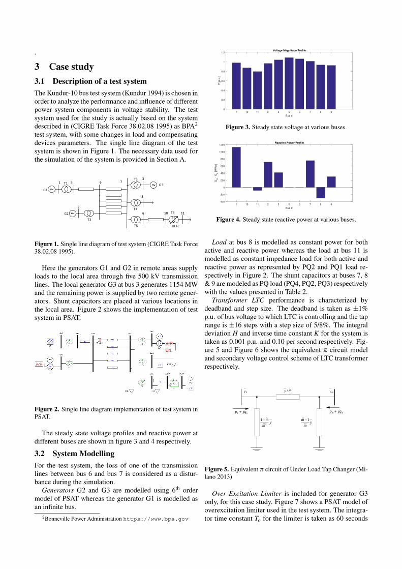
3 Case study3.1 Description of a test systemThe Kundur-10 bus test system (Kundur 1994) is chosen inorder to analyze the performance and influence of differentpower system components in voltage stability. The testsystem used for the study is actually based on the systemdescribed in (CIGRE Task Force 38.02.08 1995) as BPA2

test system, with some changes in load and compensatingdevices parameters. The single line diagram of the testsystem is shown in Figure 1. The necessary data used forthe simulation of the system is provided in Section A.

~ ~

~

~ G1

G2

G3

ULTC

T1

T2

T3

T4

T5

T6

1

2

5 6 73

8

9 10 11

Figure 1. Single line diagram of test system (CIGRE Task Force38.02.08 1995).

Here the generators G1 and G2 in remote areas supplyloads to the local area through five 500 kV transmissionlines. The local generator G3 at bus 3 generates 1154 MWand the remaining power is supplied by two remote gener-ators. Shunt capacitors are placed at various locations inthe local area. Figure 2 shows the implementation of testsystem in PSAT.

Figure 2. Single line diagram implementation of test system inPSAT.

The steady state voltage profiles and reactive power atdifferent buses are shown in figure 3 and 4 respectively.

3.2 System ModellingFor the test system, the loss of one of the transmissionlines between bus 6 and bus 7 is considered as a distur-bance during the simulation.

Generators G2 and G3 are modelled using 6th ordermodel of PSAT whereas the generator G1 is modelled asan infinite bus.

2Bonneville Power Administration https://www.bpa.gov

1 10 11 2 3 5 6 7 8 9

Bus #

0

0.2

0.4

0.6

0.8

1

1.2

V [p.u

.]

Voltage Magnitude Profile

Figure 3. Steady state voltage at various buses.

1 10 11 2 3 5 6 7 8 9

Bus #

-400

-200

0

200

400

600

800

1000

1200

QG

- Q

L [M

Var]

Reactive Power Profile

Figure 4. Steady state reactive power at various buses.

Load at bus 8 is modelled as constant power for bothactive and reactive power whereas the load at bus 11 ismodelled as constant impedance load for both active andreactive power as represented by PQ2 and PQ1 load re-spectively in Figure 2. The shunt capacitors at buses 7, 8& 9 are modeled as PQ load (PQ4, PQ2, PQ3) respectivelywith the values presented in Table 2.

Transformer LTC performance is characterized bydeadband and step size. The deadband is taken as ±1%p.u. of bus voltage to which LTC is controlling and the taprange is ±16 steps with a step size of 5/8%. The integraldeviation H and inverse time constant K for the system istaken as 0.001 p.u. and 0.10 per second respectively. Fig-ure 5 and Figure 6 shows the equivalent π circuit modeland secondary voltage control scheme of LTC transformerrespectively.

mm jqp +

mvmy ~/

ym

m2~

~1−y

m

m~

1~ −

kv

kk jqp +

Figure 5. Equivalent π circuit of Under Load Tap Changer (Mi-lano 2013)

Over Excitation Limiter is included for generator G3only, for this case study. Figure 7 shows a PSAT model ofoverexcitation limiter used in the test system. The integra-tor time constant To for the limiter is taken as 60 seconds

mK

H+s

LTC & NETWORK

deadzone

mmax

vref

mmin

mvm

Figure 6. Secondary voltage control scheme of LTC (Milano2013).

whereas the maximum field current limit is chosen as 11.7p.u. for the test system.

Figure 7. Over excitation limiter (Milano 2013).

3.3 Simulation ResultsThe voltage at various buses and the reactive power out-puts of the generator is compared for the test system in-cluding and excluding the over excitation limiter withULTC in action for both cases which are as presented inthe Figures from 8 to 12.

The sequence of events triggered during the simulationin different time frames can be explained as follows.

• One of the transmission lines is disconnected at timet=5 seconds. When the line has been disconnected,the apparent impedance and consequently the linelosses and voltage drop of the transmission systemis increased.

• The second time frame starts at around 10 secondswhere the ULTC is activated as the voltage at the bus11 is lower than the preset value. The ULTC triesto keep the voltage at the secondary bus (bus-11) atits original value by adjusting its tap ratio which de-mands more reactive power support from the gener-ators present in the network. Thus, to meet the in-creased reactive power demand the excitation currentis continuously increased until the maximum tap oftransformer is reached or voltages at the buses arerecovered. This time frame can be observed in sub-figures from 8a-12a. The voltage at bus 11 is restoredto nearly its reference value in about 90 seconds asshown in Figure 8.

• The third time frame begins with the actuation ofoverexcitation limiter as shown in sub-figure 8b at

around t=150 seconds by ramping down the field cur-rent. The following chains of events occurs after theactuation of OXL:

– As the field current of G3 is reduced, its termi-nal voltage drops.

– Voltages at bus 11, 10 and 7 drops.

– ULTC on T6 tries to restore the voltage at bus11 back to its original value.

– The reactive power demand on generators in-creases. Field current of machine 3 increasesand continues to remain at its limit and the ter-minal voltage of G3 further decreases.

– Voltage at bus 7 drops and causes a further re-duction in terminal voltage of bus 10 and bus11.

– The ULTC operates again, repeating abovementioned chains of events.

Hence in response to each tap movement of ULTC,the voltage at bus 11 reduces rather than increased.This indicates that the system has entered into thevoltage instability phase. The bus 11 voltage fallsprogressively as shown in Figure 8b until the ULTCreaches its maximum tap position at around 260 sec-onds. The voltage at bus 11 settles at around 0.77162p.u.

Furthermore, the effect of static load models on longterm voltage stability was studied for the test case consid-ered. Figure 13 shows the voltage profile at bus 11 whenthe load at bus 8 is modelled as constant impedeance, con-stant current and constant power load keeping the load atbus 11 as constant impedeance. The ULTC and OXL werekept inactive during this condition and transformer T6 isimplemented as a fixed tap transformer with tap ratio sameas that of transformer T5.

It is observed that the constant power load stabilizes at alower value as compared to constant impedance and con-stant power load because of its load restoring character-istics (Nguyen 2008). That means constant power loadtries to consume the same power at a pre-disturbance levelas consumed power is independent of voltage variationsand hence the voltage drops even further. The dynamicsof voltage profile obtained is comparable to the similarcase study performed in Ph.D. thesis (Nguyen 2008) us-ing PSS/E software.

4 Generator PQ capability curveSynchronous generator is a primary source of reactivepower in the network and plays an important role in main-taining the voltage stability in the network. The bound-aries for supplying the reactive power at a given activepower output is defined by the generator capability curveprovided by the manufacturers (Dragosavac et al. 2012).The generator capability diagram provides a boundary

0 20 40 60 80 100 120

Time [s]

0.755

0.76

0.765

0.77

0.775

0.78

0.785

0.79

0.795V

oltage m

agnitude [p.u

.]

(a) With only ULTC

0 50 100 150 200 250 300

Time [s]

0.75

0.755

0.76

0.765

0.77

0.775

0.78

0.785

0.79

0.795

Voltage m

agnitude [p.u

.]

(b) With ULTC and OXL

Figure 8. Bus 11 voltage without and with OXL.

0 20 40 60 80 100 120

Time [s]

0.82

0.83

0.84

0.85

0.86

0.87

0.88

Voltage m

agnitude [p.u

.]

(a) With only ULTC

0 50 100 150 200 250 300

Time [s]

0.68

0.7

0.72

0.74

0.76

0.78

0.8

0.82

0.84

0.86

0.88

Voltage m

agnitude [p.u

.]

(b) With ULTC and OXL

Figure 9. Bus 10 voltage without and with OXL.

0 20 40 60 80 100 120

Time [s]

1.01

1.015

1.02

1.025

1.03

1.035

1.04

1.045

1.05

1.055

1.06

Voltage m

agnitude [p.u

.]

(a) With only ULTC

0 50 100 150 200 250 300

Time [s]

0.94

0.96

0.98

1

1.02

1.04

1.06

1.08

Voltage m

agnitude [p.u

.]

(b) With ULTC and OXL

Figure 10. Bus 3 voltage without and with OXL.

0 20 40 60 80 100 120

Time [s]

400

450

500

550

600

650

700

750

800

Reactive p

ow

er

outp

ut[M

var]

(a) With only ULTC

0 50 100 150 200 250 300

Time [s]

400

500

600

700

800

900

1000

Reactive p

ow

er

outp

ut[M

var]

(b) With ULTC and OXL

Figure 11. Reactive power output of generator G3 without andwith OXL.

0 20 40 60 80 100 120

Time [s]

1.8

2

2.2

2.4

2.6

2.8

3

3.2

3.4

Fie

ld v

oltage m

agnitude [p.u

.]

(a) With only ULTC

0 50 100 150 200 250 300

Time [s]

1.6

1.8

2

2.2

2.4

2.6

2.8

3

3.2

3.4

3.6

Fie

ld v

oltage m

agnitude [p.u

.]

(b) With ULTC and OXL

Figure 12. Field voltage at generator 3 without and with OXL.

0 10 20 30 40 50 60

Time [sec]

0.78

0.785

0.79

0.795

0.8

0.805

0.81

0.815

Voltage m

agnitude [p.u

.]

constant impedence

constant current

constant power

Figure 13. Voltage profile at bus 11 for different load types.

within which the generator can operate safely without ex-ceeding the thermal limitations. Following operationalconstraints are the reasons for the limits in active and re-active power of the synchronous generator (Machowski,Bialek, and Bumby 2008).

1. Armature current limit.

2. Field current limit.

3. Steady-state stability limit.

4. Stator end region heating limit.

5. Generator active power limit.

This paper presents the methodology for obtaining thePQ diagram for a cylindrical rotor synchronous generatorwith the following simplification during its modelling:

• The synchronous generator has been assumed to beconnected to the infinite bus i.e. with constant volt-age.

• The machine saturation effect on the direct axis syn-chronous reactance has not been considered, i.e.Xd = constant.

• The effect of armature resistance has also been ne-glected.

The rated parameters of generator G3 in local area inthe 10-bus system is taken as reference for determiningcapability diagram with 10% stability margin.

The theoretical PQ diagram can be derived by divid-ing every phasor in the vector diagram by direct-axis syn-chronous reactance Xd and multiplying them with the ar-mature voltage as shown in figure 14. The figure so ob-tained, contains P and Q as the x-axis and y-axis respec-tively.

0E

U

dIX dX

UE0

dX

U 2

UI

Q

0E

U

dIX dX

UE0

dX

U 2

UI

Q

P

Figure 14. Derivation of a P-Q capability diagram from thephasor diagram (cylindrical rotor) (Vrazic, Viskovic, and Hanic2014).

4.1 Rated turbine power limitThe maximum and the minimum turbine power limits aredrawn according to the following two conditions (I.Ilic etal. 2007):

• If the power of the turbine (PT ) exceeds the ratedpower of the generator (Pn), i.e. if PT > Pn, thenPmax = Pn.

• If the power of the turbine is equal to or less than therated power of the generator (PT ≤ Pn), then Pmax =PT .ηG.

This limit is shown in Figure 15 labelled as Pmax. Theminimum power depends upon the turbine requirements.For example, in Kaplan and Francis turbine minimumpower output is 5 % to 30% of rated output whereas insome turbines like Pelton turbine this limitation does notexists (I.Ilic et al. 2007).

4.2 Rated stator current limitThe rated stator current limit is plotted as a constant semi-circle with center at origin ‘0’ and radius as the rated ap-parent power, Sn as shown in Figure 15. Point ‘P’ denotesthe rated operating condition of the generator which is de-fined at its rated power factor cosφn = 0.72. So,Prated = Sncosφ = 1∗0.72 = 0.72 p.u.Qrated = Snsinφ = 1∗

√1− (cosφ)2 = 0.69 p.u.

-1 -0.8 -0.6 -0.4 -0.2 0 0.2 0.4 0.6 0.8 1

Reactive Power Q [p.u.]

0

0.1

0.2

0.3

0.4

0.5

0.6

0.7

0.8

0.9

1

Active

Po

we

r P

[p

.u.]

P

Sn

Pmax

n

Armature current limit

Maximum turbine limit

Figure 15. Rated stator current limit and maximum turbine limitplot.

4.3 Rated field current limitFor implementing the rated field current limit, an arc isdrawn with the center at (0,-V 2

xd) and radius Eqmax V

xdfrom

cosφ = 0 to cosφ = 0.72 (rated) where Eqmax is calculatedfrom the phasor diagram as shown in Figure 14 as:

Eqmax =√(V + Ixdsinφ)2 +(Ixdcosφ)2 pu (1)

The limit is drawn as curve PK in Figure 16.

-1 -0.8 -0.6 -0.4 -0.2 0 0.2 0.4 0.6 0.8 1

Reactive Power Q [p.u.]

0

0.1

0.2

0.3

0.4

0.5

0.6

0.7

0.8

0.9

1

Active

Po

we

r P

[p

.u.]

P

Sn

Pmax

n

K

Field current limit

Figure 16. Rated field current limit plot.

4.4 Practical Stability limitFor round-rotor generators, theoretical stability limit isachieved at load angle δ=90°. However, the theoreticalstability curve is reduced by a constant power value, forexample by 10% of the rating of the machine as a safetymargin and the corresponding curve so obtained is termedas practical stability margin (Walker 1953).

The theoretical stability curve is drawn as a straightline at point (0,-V 2

xd)= (0,- 1

2.07 )= (0,-0.48) represented by

-1 -0.8 -0.6 -0.4 -0.2 0 0.2 0.4 0.6 0.8 1

Reactive Power Q [p.u.]

0

0.1

0.2

0.3

0.4

0.5

0.6

0.7

0.8

0.9

1

Active

Po

we

r P

[p

.u.]

P

Sn

Pmax

n

K

A

D

Theoretical Stability Limit

Practical Stability Limit

Figure 17. Theoretical and practical stability limit plot.

dashed line in Figure 17. The practical stability limit isrepresented as curve AD in the same figure.

Hence, the safe region for the operation of a syn-chronous generator is represented by the area bounded bycurve APKD in Figure 17.

5 Visualization toolAs discussed in Section 4, various operational limits in PQdiagram was implemented in MATLAB software environ-ment. For improved visualization of the diagram, a visualApp was created using MATLAB App designer. A Graph-ical User Interface was created by using different com-ponents from the component library and specifying app’sdesign and layout. For defining the App behavior, App de-signer allows an integrated version of the MATLAB Editor(MATLAB App Designer 2019). All the parameter valuesimplemented, and the dynamics observed in the visualiza-tion tool is based upon the case study of Kundur 10-bustest system described in Section 3.1.

(1)

(7)

(4)

(3)

(2)

(5)

(6)

Figure 18. Graphical User Interface for generator capability di-agram.

Figure 18 shows a GUI environment for the designedApp in order to visualize the generator capability. TheGUI consists of two figure windows and three tabs. Theupper figure (1) in the user interface shows the capabilitycurve with the real-time operating point as indicated by‘red’ asterisk symbol. The ‘Parameters’ tab (2) shows theoperating point (P and Q) values in real time along with

the operational power factor. The ‘Operating conditions’tab (3) shows the actual operating condition i.e. whetherthe generator is operating in over excitation mode or underexcitation mode with current operation mode indicated bylamp glowing ‘green’. The ‘Machine rating’ tab (4) indi-cates the generator rated conditions which can be changedby changing the values in the respective fields. For exam-ple, the effect of change of direct axis synchronous reac-tance on the generator limits can be visualized in the figuresection (1) by changing its value in the ‘Machine rating’tab.

On top of the ‘Parameters’ tab resides a ‘Limit checker’(5) as indicated by a lamp which glows ‘red’ whenthe defined operational limits on the capability curveare violated along with the actuation and information of‘ALARM’ (6) to notify the operating personnel about thelimit violation as shown in Figure 18. The lamp glows‘green’ along with an information ‘NORMAL’ when theoperating point lies within the defined boundaries asshown in Figure 19.

Figure 19. Graphical User Interface for Generator CapabilityDiagram showing ‘NORMAL’ condition.

5.1 Temperature visualization

The temperature development in the stator and rotor wind-ings in the synchronous generator was also observed in thesame tool which is as shown in Figure 21 using the thermalmodel as described in Ph.D. thesis (Øyvang, Noland, et al.2018). Figure 20 shows the thermal model implementedin Simulink software environment. The output tempera-tures as seen in the figure is the result of input field cur-rent and armature current taken from the local generatorG3 in Kundur 10-bus system when replaced by 103 MVAhydrogenerator at ‘Åbjøra’ in Norway. The machine dataof hydrogenerator is provided in Table 6. The field andthe stator currents in real time are observable in the tool.The initial temperature in the stator and rotor was taken as28°C during the simulation.

Figure 20. Simulink circuit for the thermal model proposed in(Øyvang, Noland, et al. 2018).

Figure 21. Temperature observation in the visualization tool.

6 Conclusion and further workThe dynamic analysis of voltage stability using time-domain simulation has been presented in this paper usinga test power system containing 10 buses as a case study.From the simulation, it can be concluded that dynamicanalysis is very useful in understanding the detail dynam-ics involved during the larger disturbances such as a loss oftransmission line or loss of generation in the system and tostudy the coordination between the control and the protec-tion as well. This type of analysis gives accurate resultsthough it requires detail accurate models of the compo-nents and is time-consuming. The influence of static loadmodels on the voltage collapse scenario is well-presentedin this paper. The severity of the effect depends upon thetype of load.

The development and implementation of PQ capabil-

ity diagram for the cylindrical rotor machine was done inMATLAB. The use of Graphical User Interface providesthe user interaction with the visualization tool throughgraphical displays, inputs and visual indicators. Duringimplementation, the infinite bus-bar assumption was madewhich is not practical in real case as the terminal voltagecan significantly vary from the rated value. As the termi-nal voltage varies, the field and the armature limits alsovary. Furthermore, the assumption of constant direct-axissynchronous reactance is also not valid as the synchronousmachine are designed with certain amount of saturationlevel and depends upon machine operating point such asarmature voltage and current (Vrazic, Viskovic, and Hanic2014).

The effect of dynamic load characteristics which has asignificant influence on voltage stability can be analyzedunder further work. Moreover, other simulation tools likePSS/E, DIgSILENT PowerFactory, EUROSTAG, Sim-PowerSystems, EPRI Extended Transient Mid-Term Sta-bility Program (ETMSP) can be used to test and compareresults from the same test system for voltage instabilityand collapse phenomena.

A Data for Test SystemSbase = 100 MVA

Table 1. Bus Data

Bus Base Vscheduled Phase Shunt P load Q load[kV] [p.u.] [rad] [Mvar] [MW] [Mvar]

Bus1 13.8 0.98 0 0 0 0Bus2 13.8 0.96 0 0 0 0Bus3 13.8 1.04 0 0 0 0Bus5 500 1.00 0 0 0 0Bus6 500 1.00 0 0 0 0Bus7 500 1.00 0 750 0 0Bus8 13.8 0.94 0 1500 3000 1800Bus9 115 0.95 0 300 0 0Bus10 115 0.89 0 0 30 0Bus11 13.8 0.91 0 0 3100 90

Table 2. Generators load flow data

Bus No. Gen Base P gen Q gen Sbase Qmax QminName [kV] [MW] [Mvar] [MVA] [Mvar] [Mvar]

1 G1 13.8 3471.9 1129.03 5000 1600 -10002 G2 13.8 1736 712.53 2200 725 2003 G3 13.8 1154 414.58 1600 700 -100

Machine parameters:Machine 1: Infinite busMachine 2: H = 2.09, MVA rating = 2200 MVAMachine 3: H = 2.33, MVA rating = 1400 MVA

Following are the parameters for machine 2 and ma-

Table 3. Transmission lines data

From To bus R X BBus [p.u.] [p.u.] [p.u.]

5 6 0.0000 0.0040 0.00006 7 0.0015 0.0288 1.17309 10 0.0010 0.0030 0.0000

Table 4. Transformers data

Transformer R X Tap ratio[p.u.] [p.u.]

T1 0.0000 0.0020 0.8857T2 0.0000 0.0045 0.8857T3 0.0000 0.0125 0.9024T4 0.0000 0.0030 1.0664T5 0.0000 0.0026 1.0800T6 0.0000 0.0010 0.9750

Table 5. Thermal model data

Parameters Symbol Value Unit

Thermal resistance, TFe−Tδ RFe 0.07 K/kWThermal resistance, Ts−TFe Rs 0.05 K/kWThermal resistance, air R1 0.018 K/kWGain coefficient, T2,i K1 0.59 -Gain coefficient rotor(Cu) K2 0.5 -Gain coefficient stator(Fe) K3 0.36 -Heat exchanger effieicency (epsi) ε 0.595 -

Table 6. Machine data of Åbjøra (Øyvang, Hegglid, and Lie2018).

Description Parameters Value Unit

Rated power Sn 103 MVARated voltage Vtn 11 kVRated current Itn 5406 ARated field current I f dn 1064 AInertia constant H 2.66 sNumber of polepairs p 6 -Synchronous reactance d-axis xd 1.09 [p.u.]Synchronous reactance q-axis xq 0.67 [p.u.]Transient reactance d-axis x′d 0.24 [p.u.]Subtransient reactance d-axis x′′d 0.15 [p.u.]Subtransient reactance q-axis x′′q 0.19 [p.u.]Transient OC Time constant d-axis T ′do 10 sTransient OC Time constant q-axis T ′qo 0.23 sSubtransient OC Time constant d-axis T ′′do 0.086 sSubransient OC Time constant q-axis T ′′qo 0.23 sStator leakage inductance Xl 0.08 [p.u.]Stator resistance Ra 0.00182 [p.u.]

chine 3 on their respective MVA ratings:

Ra = 0.0046 Xd = 2.07 Xq = 1.99Xl = 0.155 X ′d = 0.28 X ′q = 0.49

X ′′d = 0.215 X ′′q = 0.215

T ′do = 4.10 T ′qo = 0.56

T ′′do = 0.033 T ′′qo = 0.062

Exciters: Both machine 2 and machine 3 uses thyris-tor exciters with a gain of 100 and the time delay of themeasurement system as 0.02 seconds.

Overexcitation limiter for machine 3: The OXLmodel used in the simulation is as described in the sec-tion...with integrator time constant (T0)= 60 seconds, max-imum field current ilimf d = 11.7 p.u. and maximum outputsignal vmax

OXL= 5.02 p.u.ULTC data for transformer T6 between bus 10 and

11:Deadband: ±1 % p.u. bus voltageTap range: ±16 stepsStep size: 5/8 % (=0.00625 p.u.)

ReferencesCIGRE Task Force 38.02.08 (1995). Long Term Dynamics

Phase II. Tech. rep. CIGRE.CIGRE Task Force 38.02.10 (1993). Modelling of Voltage

Collapse Including Dynamic Phenomena. Tech. rep.Dragosavac, J. et al. (2012). “On-line Estimation of

Available Generator Reactive Power for Network Volt-age Support”. In: 8th Mediterranean Conference onPower Generation, Transmission, Distribution and En-ergy Conversion (MEDPOWER 2012). Institution ofEngineering and Technology. DOI: 10.1049/cp.2012.2014.

I.Ilic et al. (2007). “Methodology for Determining the Ac-tual PQ Diagram of a Hydrogenerator”. In: Journal ofEnergy 56.2, pp. 144–181. URL: https://hrcak.srce.hr/13153.

Kundur, Prabha (1994). Power System Stability and Con-trol. McGraw-Hill, Inc.

Machowski, Jan, Janusz W. Bialek, and James R. Bumby(2008). Power System Dynamics : Stability and Control.2nd ed. John Wiley & Sons, Ltd.

MATLAB App Designer (2019). URL: https://se.mathworks.com/products/matlab/app-designer.html (visited on 03/22/2019).

Milano, Federico (2013). Power System Analysis ToolboxDocumentation for PSAT. Version 2.1.8.

Nguyen, Dang Toan (2008). “Contributions to analysisand prevention of power system blackouts”. Theses.Institut National Polytechnique de Grenoble - INPG.URL: https://tel.archives- ouvertes.fr/tel-00352414.

Øyvang, Thomas (2018). “Enhanced power capability ofgenerator units for increased operational security”. PhDthesis.

Øyvang, Thomas, Gunne J. Hegglid, and Bernt Lie (2018).“Models of synchronous generators with excitation sys-tem, for transient power system studies”. In: IFAC-PapersOnLine 51.2, pp. 91–96. DOI: 10.1016/j.ifacol.2018.03.016.

Øyvang, Thomas, Jonas Kristiansen Noland, et al. (2018).“Online Model-Based Thermal Prediction for FlexibleControl of an Air-Cooled Hydrogenerator”. In: IEEE

Transactions on Industrial Electronics, pp. 1–1. DOI:10.1109/tie.2018.2875637.

Vrazic, M., A. Viskovic, and Z. Hanic (2014). “User P-QDiagram as a Part of a Synchronous Generator Monitor-ing System”. In: Electronics and Electrical Engineer-ing 20.4. DOI: 10.5755/j01.eee.20.4.5333.

Walker, J.H. (1953). “Operating characteristics of salient-pole machines”. In: Proceedings of the IEE - PartII: Power Engineering 100.73, pp. 13–24. DOI: 10.1049/pi-2.1953.0004.