Online learning in estimation of distributionalgorithms for dynamic environments

Andre R. Goncalves∗, Fernando J. Von Zuben†School of Electrical and Computer Engineering

University of Campinas (Unicamp)Campinas, SP, Brazil

{∗andreric, †vonzuben}@dca.fee.unicamp.br

Abstract—In this paper, we propose an estimation of distri-bution algorithm based on an inexpensive Gaussian mixturemodel with online learning, which will be employed in dynamicoptimization. Here, the mixture model stores a vector of sufficientstatistics of the best solutions, which is subsequently used to ob-tain the parameters of the Gaussian components. This approachis able to incorporate into the current mixture model potentiallyrelevant information of the previous and current iterations. Theonline nature of the proposal is desirable in the context ofdynamic optimization, where prompt reaction to new scenariosshould be promoted. To analyze the performance of our proposal,a set of dynamic optimization problems in continuous domainswas considered with distinct levels of complexity, and the obtainedresults were compared to the results produced by other existingalgorithms in the dynamic optimization literature.

Index Terms—Online learning; mixture model; estimation ofdistribution algorithms; optimization in dynamic environments.

I. INTRODUCTION

Evolutionary algorithms (EAs) have been applied success-fully to a variety of optimization problems. Such problemsare generally considered to be stationary, i.e., the objectivefunction and other aspects of the formulation does not changeover time. However, it is common to face scenarios in whichsome aspects of the optimization problem varies with time,such as the presence of a nonstationary objective functionand/or a time-varying constraint set. Under these circum-stances, the location of the optimal solution in the searchspace might change with time as well. As practical examples,we may cite a scheduling problem in which new jobs arriveover time, and vehicle routing problems where the cost totravel from one location to another is nonstationary. Thus,standard evolutionary algorithms, which are basically builtto deal with stationary problems, tends to produce a poorperformance in dynamic environments, due to the absence ofreaction mechanisms when facing new conditions.

To be adapted to dynamic environments, EAs should beendowed with specific (implicit or explicit) operators devotedto the maintenance of diversity in the population, and mainlyto avoid stagnation. Some of these additional operators, aspointed out by [1], should promote: (i) generation of diversityafter a change; (ii) maintenance of diversity throughout theexecution; (iii) employment of memory to store and recalluseful information from the recent past; and (iv) execution of

a multipopulation search to track multiple local optima in thefitness landscape.

Trying to implement at least part of the aforementionedfunctionalities, several evolutionary approaches have beendeveloped and extended to deal with dynamic environments.Among them, we can cite genetic algorithms [2], [3], particleswarm optimization [4], [5], artificial immune systems [6], [7]and estimation of distribution algorithms (EDAs) [8]–[10].

In this paper, we introduce an inexpensive EDA to theoptimization of dynamic environments in continuous domains.This approach employs an online learning version of a mixturemodel, augmented by an automatic control of the number ofcomponents and by an operator to promote population diver-sity. The purpose is to make the search mechanism effectiveeven in multimodal and time-varying fitness landscapes, byproperly applying a concise model of the information from theprevious iterations. This paper is organized as follows: SectionII presents a brief introduction to estimation of distributionalgorithms. In Section III, mixture models, the Expectation-Maximization (EM) algorithm and an online version of EMare described. The details of the proposed algorithm are pre-sented in Section IV. A generator of dynamic environments incontinuous search spaces, to be considered in the experiments,is depicted in Section V. Section VI discusses the obtainedresults on a number of dynamic optimization problems. Con-cluding remarks and further steps of the research are outlinedin Section VII.

II. ESTIMATION OF DISTRIBUTION ALGORITHM

Estimation of distribution algorithms (EDAs) are evolution-ary methods that use estimation of distribution techniques,instead of genetic operators, to guide the search for bettersolutions. These algorithms were motivated by some short-comings of genetic algorithms, more specifically the absenceof a proper mechanism for detecting and preserving buildingblocks [11].

The key aspect in EDAs is how to estimate the truedistribution of promising solutions. In fact, the estimation ofthe joint probability distribution associated with the variablesthat form the search space is the main distinctive componentof EDAs. Once estimated the joint probability distribution,new candidate solutions are generated obeying the obtaineddistribution. Though essential to characterize an EDA, this

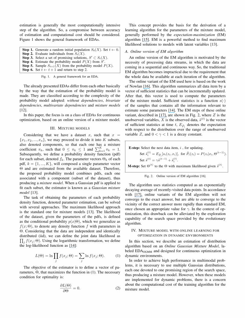
estimation is generally the most computationally intensivestep of the algorithm. So, a compromise between accuracyof estimation and computational cost should be considered.Figure 1 shows the general framework of EDAs.

Step 1. Generate a random initial population S0(X). Set t← 0.Step 2. Evaluate individuals from St(X).Step 3. Select a set of promising solutions, S′ ⊂ St(X).Step 4. Estimate the probability model P (X) from S′.Step 5. Sample St+1(X) from the probability model P (X).Step 6. Set t← t+ 1 and return to step 2.

Fig. 1. A general framework for an EDA.

The already presented EDAs differ from each other basicallyby the way that the estimation of the probability model ismade. They are classified according to the complexity of theprobability model adopted: without dependencies, bivariatedependencies, multivariate dependencies and mixture models[12].

In this paper, the focus is on a class of EDAs for continuousoptimization, based on an online version of a mixture model.

III. MIXTURE MODELS

Considering that we have a dataset x, such that x ={x1, x2, ..., xn}, we may proceed to divide it into K subsets,also denoted components, so that each one has a mixturecoefficient πk, such that 0 ≤ πk ≤ 1 and

∑Kk=1 πk = 1.

Subsequently, we define a probability density function (pdf)for each subset, denoted fk. The parameter vectors Θk of eachpdf, k = {1, ...,K}, will composed a single parameter vectorΘ and are estimated from the available dataset. Therefore,the proposed probability model combines pdfs, each oneassociated with a component (subset of the dataset), thusproducing a mixture model. When a Gaussian pdf is applied tofit each subset, the estimator is known as a Gaussian mixturemodel [13].

The task of obtaining the parameters of each probabilitydensity function, denoted parameter estimation, can be solvedwith several approaches. The maximum likelihood approachis the standard one for mixture models [13]. The likelihoodof the dataset, given the parameters of the pdfs, is definedas the conditional probability p(x|Θ), which we generalize asf(x; Θ), to denote any density function f with parameters inΘ. Considering that the data are independent and identicallydistributed (iid), we can define the joint data likelihood as∏

j f(xj ; Θ). Using the logarithmic transformation, we definethe log-likelihood function as [14]:

L(Θ) = ln∏j

f(xj ; Θ) =∑j

ln f(xj ; Θ). (1)

The objective of the estimator is to define a vector of pa-rameters, Θ, that maximizes the function in (1). The necessarycondition for optimality is:

∂L(Θ)

∂Θ= 0. (2)

This concept provides the basis for the derivation of alearning algorithm for the parameters of the mixture model,generally performed by the expectation-maximization (EM)algorithm [15]. EM is a powerful method to find maximumlikelihood solutions to models with latent variables [13].

A. Online version of EM algorithm

An online version of the EM algorithm is motivated by thenecessity of processing data streams, in which the data arecoming in a sequential and continuous way. So, the traditionalEM algorithm becomes impractical due to the requirement thatthe whole data be available at each iteration of the algorithm.

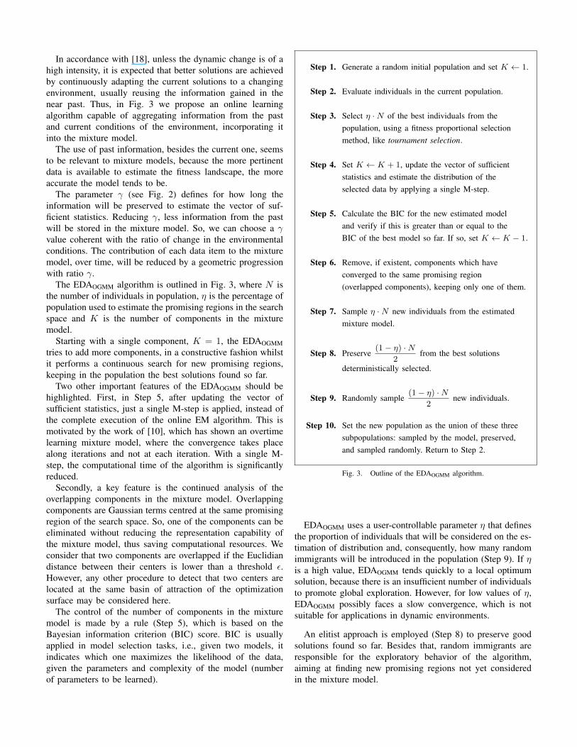
The online variant of the EM used here is based on the workof Nowlan [16]. This algorithm summarizes all data item by avector of sufficient statistics that can be incrementally updated.After that, this vector is used to compute the parametersof the mixture model. Sufficient statistics is a function s(·)of the samples that contains all the information relevant toestimate some parameters [14]. The EM steps of these onlinevariant, described in [17], are shown in Fig. 2, where Z is theunobserved variables, X is the observed data, s(t) is the vectorof sufficient statistics at time t, EPi

denotes the expectationwith respect to the distribution over the range of unobservedvariable Z, and 0 < γ < 1 is a decay constant.

E-step: Select the next data item, i , for updating.

Set s(t)i = EPi[si(zi, xi)], for Pi(zi) = P (zi|xi,Θ(t−1)).

Set s(t) = γs(t−1) + s(t)i .

M-step: Set Θ(t) to the Θ with maximum likelihood given s(t).

Fig. 2. Online version of EM algorithm [16].

The algorithm uses statistics computed as an exponentiallydecaying average of recently-visited data points. In accordancewith [17], online variants of the EM algorithm will notconverge to the exact answer, but are able to converge to thevicinity of the correct answer more rapidly than standard EM,once chosen an appropriate value for γ. In the context of op-timization, this drawback can be alleviated by the explorationcapability of the search space provided by the evolutionaryalgorithm.

IV. MIXTURE MODEL WITH ONLINE LEARNING FOROPTIMIZATION IN DYNAMIC ENVIRONMENTS

In this section, we describe an estimation of distributionalgorithm based on an Online Gaussian Mixture Model, la-beled EDAOGMM and designed for continuous optimization indynamic environments.

In order to achieve high performance in multimodal prob-lems, it is necessary to use multiple Gaussian distributions,each one devoted to one promising region of the search space,thus producing a mixture model. However, when these modelsare implemented for dynamic problems, there is a concernabout the computational cost of the training algorithm for themixture model.

In accordance with [18], unless the dynamic change is of ahigh intensity, it is expected that better solutions are achievedby continuously adapting the current solutions to a changingenvironment, usually reusing the information gained in thenear past. Thus, in Fig. 3 we propose an online learningalgorithm capable of aggregating information from the pastand current conditions of the environment, incorporating itinto the mixture model.

The use of past information, besides the current one, seemsto be relevant to mixture models, because the more pertinentdata is available to estimate the fitness landscape, the moreaccurate the model tends to be.

The parameter γ (see Fig. 2) defines for how long theinformation will be preserved to estimate the vector of suf-ficient statistics. Reducing γ, less information from the pastwill be stored in the mixture model. So, we can choose a γvalue coherent with the ratio of change in the environmentalconditions. The contribution of each data item to the mixturemodel, over time, will be reduced by a geometric progressionwith ratio γ.

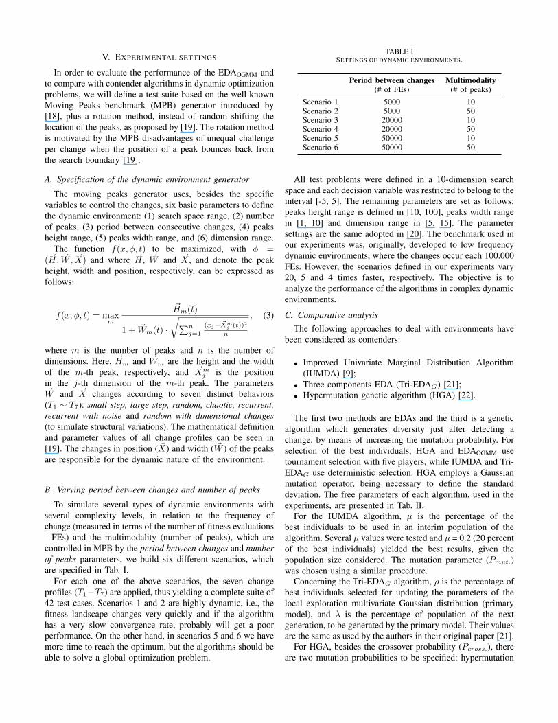
The EDAOGMM algorithm is outlined in Fig. 3, where N isthe number of individuals in population, η is the percentage ofpopulation used to estimate the promising regions in the searchspace and K is the number of components in the mixturemodel.

Starting with a single component, K = 1, the EDAOGMMtries to add more components, in a constructive fashion whilstit performs a continuous search for new promising regions,keeping in the population the best solutions found so far.

Two other important features of the EDAOGMM should behighlighted. First, in Step 5, after updating the vector ofsufficient statistics, just a single M-step is applied, instead ofthe complete execution of the online EM algorithm. This ismotivated by the work of [10], which has shown an overtimelearning mixture model, where the convergence takes placealong iterations and not at each iteration. With a single M-step, the computational time of the algorithm is significantlyreduced.

Secondly, a key feature is the continued analysis of theoverlapping components in the mixture model. Overlappingcomponents are Gaussian terms centred at the same promisingregion of the search space. So, one of the components can beeliminated without reducing the representation capability ofthe mixture model, thus saving computational resources. Weconsider that two components are overlapped if the Euclidiandistance between their centers is lower than a threshold ε.However, any other procedure to detect that two centers arelocated at the same basin of attraction of the optimizationsurface may be considered here.

The control of the number of components in the mixturemodel is made by a rule (Step 5), which is based on theBayesian information criterion (BIC) score. BIC is usuallyapplied in model selection tasks, i.e., given two models, itindicates which one maximizes the likelihood of the data,given the parameters and complexity of the model (numberof parameters to be learned).

Step 1. Generate a random initial population and set K ← 1.

Step 2. Evaluate individuals in the current population.

Step 3. Select η ·N of the best individuals from thepopulation, using a fitness proportional selectionmethod, like tournament selection.

Step 4. Set K ← K + 1, update the vector of sufficientstatistics and estimate the distribution of theselected data by applying a single M-step.

Step 5. Calculate the BIC for the new estimated modeland verify if this is greater than or equal to theBIC of the best model so far. If so, set K ← K − 1.

Step 6. Remove, if existent, components which haveconverged to the same promising region(overlapped components), keeping only one of them.

Step 7. Sample η ·N new individuals from the estimatedmixture model.

Step 8. Preserve(1− η) ·N

2from the best solutions

deterministically selected.

Step 9. Randomly sample(1− η) ·N

2new individuals.

Step 10. Set the new population as the union of these threesubpopulations: sampled by the model, preserved,and sampled randomly. Return to Step 2.

Fig. 3. Outline of the EDAOGMM algorithm.

EDAOGMM uses a user-controllable parameter η that definesthe proportion of individuals that will be considered on the es-timation of distribution and, consequently, how many randomimmigrants will be introduced in the population (Step 9). If ηis a high value, EDAOGMM tends quickly to a local optimumsolution, because there is an insufficient number of individualsto promote global exploration. However, for low values of η,EDAOGMM possibly faces a slow convergence, which is notsuitable for applications in dynamic environments.

An elitist approach is employed (Step 8) to preserve goodsolutions found so far. Besides that, random immigrants areresponsible for the exploratory behavior of the algorithm,aiming at finding new promising regions not yet consideredin the mixture model.

V. EXPERIMENTAL SETTINGS

In order to evaluate the performance of the EDAOGMM andto compare with contender algorithms in dynamic optimizationproblems, we will define a test suite based on the well knownMoving Peaks benchmark (MPB) generator introduced by[18], plus a rotation method, instead of random shifting thelocation of the peaks, as proposed by [19]. The rotation methodis motivated by the MPB disadvantages of unequal challengeper change when the position of a peak bounces back fromthe search boundary [19].

A. Specification of the dynamic environment generator

The moving peaks generator uses, besides the specificvariables to control the changes, six basic parameters to definethe dynamic environment: (1) search space range, (2) numberof peaks, (3) period between consecutive changes, (4) peaksheight range, (5) peaks width range, and (6) dimension range.

The function f(x, φ, t) to be maximized, with φ =( ~H, ~W, ~X) and where ~H , ~W and ~X , and denote the peakheight, width and position, respectively, can be expressed asfollows:

f(x, φ, t) = maxm

~Hm(t)

1 + ~Wm(t) ·√∑n

j=1

(xj− ~Xmj (t))2

n

, (3)

where m is the number of peaks and n is the number ofdimensions. Here, ~Hm and ~Wm are the height and the widthof the m-th peak, respectively, and ~Xm

j is the positionin the j-th dimension of the m-th peak. The parameters~W and ~X changes according to seven distinct behaviors(T1 ∼ T7): small step, large step, random, chaotic, recurrent,recurrent with noise and random with dimensional changes(to simulate structural variations). The mathematical definitionand parameter values of all change profiles can be seen in[19]. The changes in position ( ~X) and width ( ~W ) of the peaksare responsible for the dynamic nature of the environment.

B. Varying period between changes and number of peaks

To simulate several types of dynamic environments withseveral complexity levels, in relation to the frequency ofchange (measured in terms of the number of fitness evaluations- FEs) and the multimodality (number of peaks), which arecontrolled in MPB by the period between changes and numberof peaks parameters, we build six different scenarios, whichare specified in Tab. I.

For each one of the above scenarios, the seven changeprofiles (T1−T7) are applied, thus yielding a complete suite of42 test cases. Scenarios 1 and 2 are highly dynamic, i.e., thefitness landscape changes very quickly and if the algorithmhas a very slow convergence rate, probably will get a poorperformance. On the other hand, in scenarios 5 and 6 we havemore time to reach the optimum, but the algorithms should beable to solve a global optimization problem.

TABLE ISETTINGS OF DYNAMIC ENVIRONMENTS.

Period between changes Multimodality(# of FEs) (# of peaks)

Scenario 1 5000 10Scenario 2 5000 50Scenario 3 20000 10Scenario 4 20000 50Scenario 5 50000 10Scenario 6 50000 50

All test problems were defined in a 10-dimension searchspace and each decision variable was restricted to belong to theinterval [-5, 5]. The remaining parameters are set as follows:peaks height range is defined in [10, 100], peaks width rangein [1, 10] and dimension range in [5, 15]. The parametersettings are the same adopted in [20]. The benchmark used inour experiments was, originally, developed to low frequencydynamic environments, where the changes occur each 100.000FEs. However, the scenarios defined in our experiments vary20, 5 and 4 times faster, respectively. The objective is toanalyze the performance of the algorithms in complex dynamicenvironments.

C. Comparative analysisThe following approaches to deal with environments have

been considered as contenders:

• Improved Univariate Marginal Distribution Algorithm(IUMDA) [9];

• Three components EDA (Tri-EDAG) [21];• Hypermutation genetic algorithm (HGA) [22].

The first two methods are EDAs and the third is a geneticalgorithm which generates diversity just after detecting achange, by means of increasing the mutation probability. Forselection of the best individuals, HGA and EDAOGMM usetournament selection with five players, while IUMDA and Tri-EDAG use deterministic selection. HGA employs a Gaussianmutation operator, being necessary to define the standarddeviation. The free parameters of each algorithm, used in theexperiments, are presented in Tab. II.

For the IUMDA algorithm, µ is the percentage of thebest individuals to be used in an interim population of thealgorithm. Several µ values were tested and µ = 0.2 (20 percentof the best individuals) yielded the best results, given thepopulation size considered. The mutation parameter (Pmut.)was chosen using a similar procedure.

Concerning the Tri-EDAG algorithm, ρ is the percentage ofbest individuals selected for updating the parameters of thelocal exploration multivariate Gaussian distribution (primarymodel), and λ is the percentage of population of the nextgeneration, to be generated by the primary model. Their valuesare the same as used by the authors in their original paper [21].

For HGA, besides the crossover probability (Pcross.), thereare two mutation probabilities to be specified: hypermutation

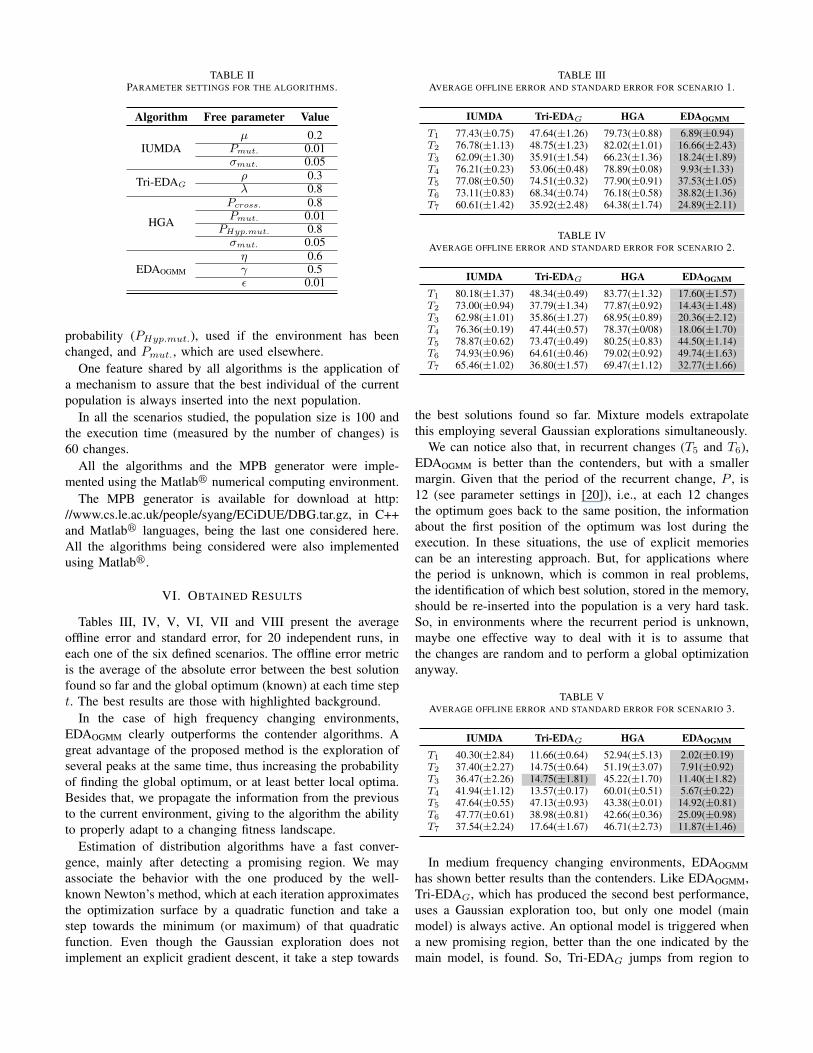
TABLE IIPARAMETER SETTINGS FOR THE ALGORITHMS.

Algorithm Free parameter Value

IUMDAµ 0.2

Pmut. 0.01σmut. 0.05

Tri-EDAGρ 0.3λ 0.8

HGA

Pcross. 0.8Pmut. 0.01

PHyp.mut. 0.8σmut. 0.05

EDAOGMM

η 0.6γ 0.5ε 0.01

probability (PHyp.mut.), used if the environment has beenchanged, and Pmut., which are used elsewhere.

One feature shared by all algorithms is the application ofa mechanism to assure that the best individual of the currentpopulation is always inserted into the next population.

In all the scenarios studied, the population size is 100 andthe execution time (measured by the number of changes) is60 changes.

All the algorithms and the MPB generator were imple-mented using the Matlabr numerical computing environment.

The MPB generator is available for download at http://www.cs.le.ac.uk/people/syang/ECiDUE/DBG.tar.gz, in C++and Matlabr languages, being the last one considered here.All the algorithms being considered were also implementedusing Matlabr.

VI. OBTAINED RESULTS

Tables III, IV, V, VI, VII and VIII present the averageoffline error and standard error, for 20 independent runs, ineach one of the six defined scenarios. The offline error metricis the average of the absolute error between the best solutionfound so far and the global optimum (known) at each time stept. The best results are those with highlighted background.

In the case of high frequency changing environments,EDAOGMM clearly outperforms the contender algorithms. Agreat advantage of the proposed method is the exploration ofseveral peaks at the same time, thus increasing the probabilityof finding the global optimum, or at least better local optima.Besides that, we propagate the information from the previousto the current environment, giving to the algorithm the abilityto properly adapt to a changing fitness landscape.

Estimation of distribution algorithms have a fast conver-gence, mainly after detecting a promising region. We mayassociate the behavior with the one produced by the well-known Newton’s method, which at each iteration approximatesthe optimization surface by a quadratic function and take astep towards the minimum (or maximum) of that quadraticfunction. Even though the Gaussian exploration does notimplement an explicit gradient descent, it take a step towards

TABLE IIIAVERAGE OFFLINE ERROR AND STANDARD ERROR FOR SCENARIO 1.

IUMDA Tri-EDAG HGA EDAOGMM

T1 77.43(±0.75) 47.64(±1.26) 79.73(±0.88) 6.89(±0.94)T2 76.78(±1.13) 48.75(±1.23) 82.02(±1.01) 16.66(±2.43)T3 62.09(±1.30) 35.91(±1.54) 66.23(±1.36) 18.24(±1.89)T4 76.21(±0.23) 53.06(±0.48) 78.89(±0.08) 9.93(±1.33)T5 77.08(±0.50) 74.51(±0.32) 77.90(±0.91) 37.53(±1.05)T6 73.11(±0.83) 68.34(±0.74) 76.18(±0.58) 38.82(±1.36)T7 60.61(±1.42) 35.92(±2.48) 64.38(±1.74) 24.89(±2.11)

TABLE IVAVERAGE OFFLINE ERROR AND STANDARD ERROR FOR SCENARIO 2.

IUMDA Tri-EDAG HGA EDAOGMM

T1 80.18(±1.37) 48.34(±0.49) 83.77(±1.32) 17.60(±1.57)T2 73.00(±0.94) 37.79(±1.34) 77.87(±0.92) 14.43(±1.48)T3 62.98(±1.01) 35.86(±1.27) 68.95(±0.89) 20.36(±2.12)T4 76.36(±0.19) 47.44(±0.57) 78.37(±0/08) 18.06(±1.70)T5 78.87(±0.62) 73.47(±0.49) 80.25(±0.83) 44.50(±1.14)T6 74.93(±0.96) 64.61(±0.46) 79.02(±0.92) 49.74(±1.63)T7 65.46(±1.02) 36.80(±1.57) 69.47(±1.12) 32.77(±1.66)

the best solutions found so far. Mixture models extrapolatethis employing several Gaussian explorations simultaneously.

We can notice also that, in recurrent changes (T5 and T6),EDAOGMM is better than the contenders, but with a smallermargin. Given that the period of the recurrent change, P , is12 (see parameter settings in [20]), i.e., at each 12 changesthe optimum goes back to the same position, the informationabout the first position of the optimum was lost during theexecution. In these situations, the use of explicit memoriescan be an interesting approach. But, for applications wherethe period is unknown, which is common in real problems,the identification of which best solution, stored in the memory,should be re-inserted into the population is a very hard task.So, in environments where the recurrent period is unknown,maybe one effective way to deal with it is to assume thatthe changes are random and to perform a global optimizationanyway.

TABLE VAVERAGE OFFLINE ERROR AND STANDARD ERROR FOR SCENARIO 3.

IUMDA Tri-EDAG HGA EDAOGMM

T1 40.30(±2.84) 11.66(±0.64) 52.94(±5.13) 2.02(±0.19)T2 37.40(±2.27) 14.75(±0.64) 51.19(±3.07) 7.91(±0.92)T3 36.47(±2.26) 14.75(±1.81) 45.22(±1.70) 11.40(±1.82)T4 41.94(±1.12) 13.57(±0.17) 60.01(±0.51) 5.67(±0.22)T5 47.64(±0.55) 47.13(±0.93) 43.38(±0.01) 14.92(±0.81)T6 47.77(±0.61) 38.98(±0.81) 42.66(±0.36) 25.09(±0.98)T7 37.54(±2.24) 17.64(±1.67) 46.71(±2.73) 11.87(±1.46)

In medium frequency changing environments, EDAOGMMhas shown better results than the contenders. Like EDAOGMM,Tri-EDAG, which has produced the second best performance,uses a Gaussian exploration too, but only one model (mainmodel) is always active. An optional model is triggered whena new promising region, better than the one indicated by themain model, is found. So, Tri-EDAG jumps from region to

TABLE VIAVERAGE OFFLINE ERROR AND STANDARD ERROR FOR SCENARIO 4.

IUMDA Tri-EDAG HGA EDAOGMM

T1 37.57(±1.39) 12.55(±0.70) 51.04(±4.08) 3.57(±0.36)T2 34.68(±1.35) 10.05(±0.49) 47.74(±2.32) 5.54(±0.62)T3 34.85(±1.23) 17.07(±1.45) 43.10(±1.19) 13.95(±1.28)T4 33.23(±0.93) 11.12(±0.23) 53.10(±0.60) 4.84(±0.14)T5 50.21(±0.64) 40.36(±1.46) 45.63(±0.27) 13.40(±0.77)T6 46.55(±1.57) 40.53(±1.11) 44.54(±1.36) 35.10(±1.32)T7 35.73(±1.35) 20.00(±1.45) 43.80(±1.26) 15.10(±1.26)

region, looking for the best one. Based on results obtained byEDAOGMM, Tri-EDAG would possibly get better performanceif it could manipulate many active models at the same time.

TABLE VIIAVERAGE OFFLINE ERROR AND STANDARD ERROR FOR SCENARIO 5.

IUMDA Tri-EDAG HGA EDAOGMM

T1 10.47(±0.85) 6.48(±0.57) 12.51(±1.15) 1.93(±0.24)T2 14.29(±0.97) 11.64(±0.86) 16.86(±1.22) 8.89(±0.85)T3 18.16(±2.09) 15.65(±2.00) 19.68(±1.94) 14.00(±1.95)T4 8.13(±0.11) 7.01(±0.16) 8.86(±0.08) 5.07(±0.07)T5 43.32(±0.01) 40.36(±1.10) 43.25(±0.01) 10.00(±0.41)T6 41.91(±0.65) 36.25(±0.93) 41.44(±0.56) 21.85(±0.90)T7 16.63(±2.37) 15.49(±2.31) 21.76(±2.79) 12.77(±2.28)

TABLE VIIIAVERAGE OFFLINE ERROR AND STANDARD ERROR FOR SCENARIO 6.

IUMDA Tri-EDAG HGA EDAOGMM

T1 14.17(±2.30) 8.62(±1.16) 13.45(±2.04) 2.61(±0.43)T2 12.96(±1.53) 8.93(±1.00) 13.50(±1.44) 5.93(±0.60)T3 16.19(±1.18) 14.10(±1.81) 16.57(±1.44) 12.33(±1.65)T4 7.34(±0.30) 6.11(±0.12) 6.55(±0.12) 3.37(±0.1)T5 45.03(±0.01) 32.54(±0.86) 45.04(±0.05) 9.39(±0.51)T6 39.72(±1.63) 35.79(±0.83) 39.41(±1.81) 32.85(±0.87)T7 17.42(±0.81) 15.58(±0.60) 18.94(±0.84) 12.97(±0.53)

For scenarios 5 and 6, the algorithm has more time to findthe global optimum. If the algorithm has a fast convergence,but get stuck in a local optimum, probably it will reachpoor performance in highly multimodal environments. So, thealgorithm should execute a global optimization in a restrictedtime. Like in the other four scenarios, EDAOGMM has achievedthe best results, followed by Tri-EDAG.

In global optimization problems, the mixture model, ini-tially, can cover several peaks and, by means of the selectionoperator and sampling, the mixture model finds better regions,and focuses on those promising regions. Subsequently, itapplies a Gaussian exploration at each region (local optimiza-tion), to reach the local optimum.

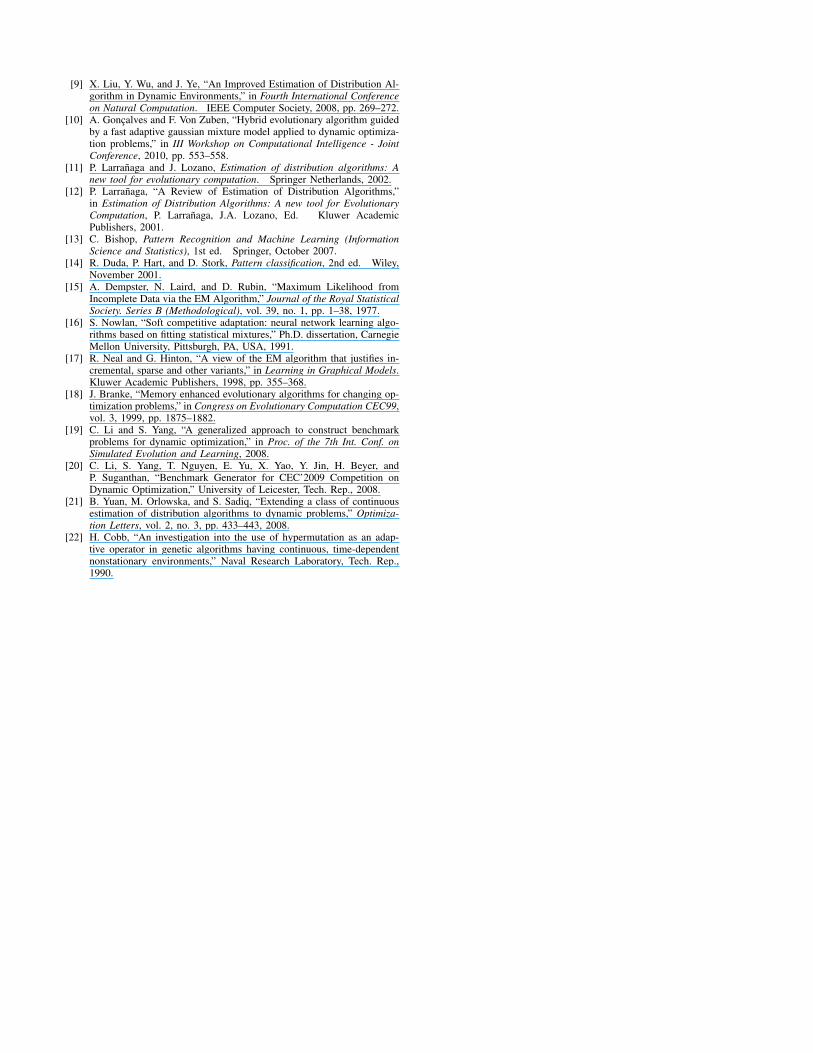
Figures 4, 5, 6 and 7 present the median convergencebehavior, over the 20 independent runs executed, of IUMDA,Tri-EDAG, HGA and EDAOGMM, respectively, when appliedin scenario 2 with random change with dimensional changes(T7). The performance is measure by means of the ratiobetween the best solution found and the global optimum. So,the ideal performance would be to stay as close as possible tothe value 1.

Fig. 4. Relative performance of the IUMDA algorithm.

In the first environment (t = 1), IUMDA finds a good localoptimum (the performance achieved a value close to 0.9), but itis not able to adapt to the subsequent scenarios, reaching poorsolutions in these fitness landscapes. These results showed theimpact of the loss in population diversity. In t = 1, wherethe algorithm has obtained better results, the population wasrandomly generated, and for t > 1, the algorithm cannot insertsufficient diversity in the population. A possible solution is toemploy the random immigrants approach at every generationor when an environment change is detected.

Fig. 5. Relative performance of the Tri-EDAG algorithm.

Figure 5 shows, clearly, an oscillatory performance of theTri-EDAG algorithm. This is due to the variation in the numberof dimensions of the search space. Decreasing the numberof dimensions, the search space is significantly reduced and,given the same population size, the algorithm can achieve abetter exploration of the search space, getting better results.

The hypermutation genetic algorithm has a slow conver-gence rate, which in dynamic environments is extremelyundesirable. When the new position of the global optimum isvery close to the old position, this approach seems interesting.

The loss of population diversity can be a bottleneck in

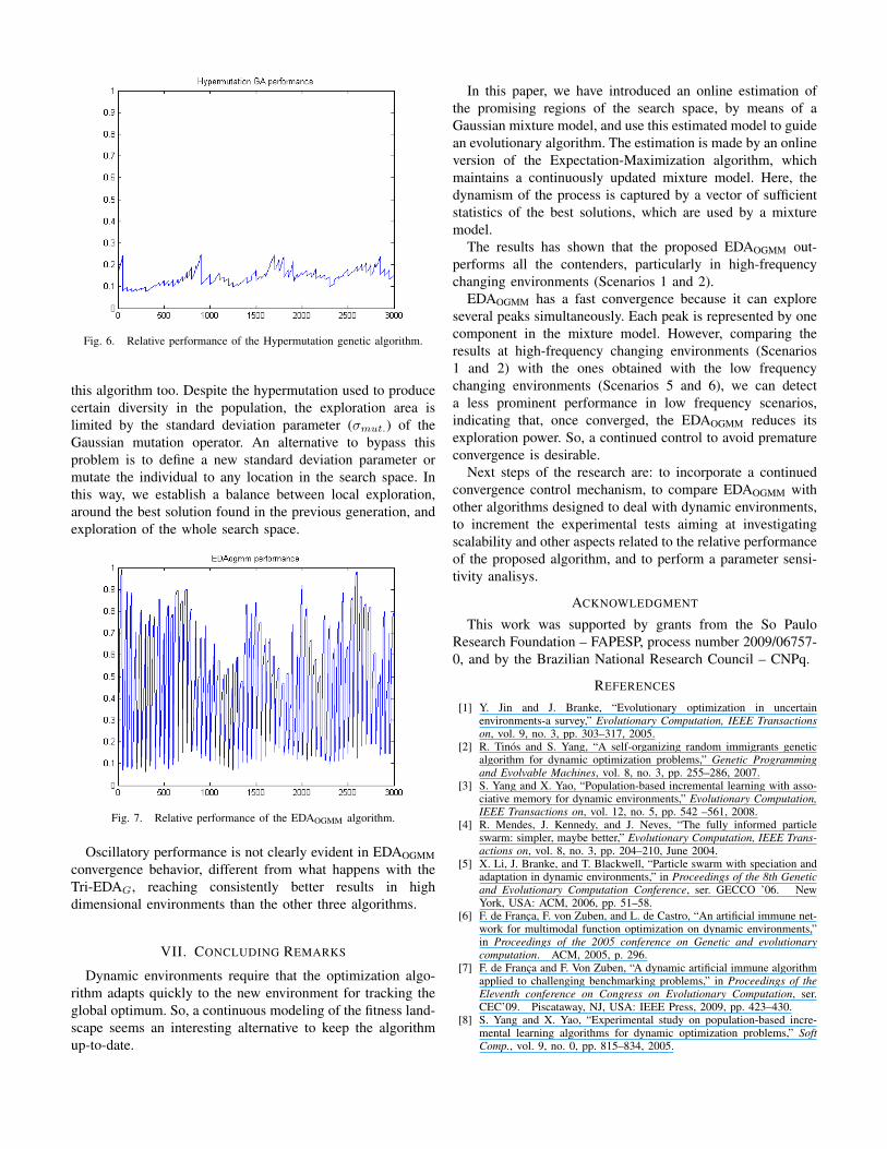
Fig. 6. Relative performance of the Hypermutation genetic algorithm.

this algorithm too. Despite the hypermutation used to producecertain diversity in the population, the exploration area islimited by the standard deviation parameter (σmut.) of theGaussian mutation operator. An alternative to bypass thisproblem is to define a new standard deviation parameter ormutate the individual to any location in the search space. Inthis way, we establish a balance between local exploration,around the best solution found in the previous generation, andexploration of the whole search space.

Fig. 7. Relative performance of the EDAOGMM algorithm.

Oscillatory performance is not clearly evident in EDAOGMMconvergence behavior, different from what happens with theTri-EDAG, reaching consistently better results in highdimensional environments than the other three algorithms.

VII. CONCLUDING REMARKS

Dynamic environments require that the optimization algo-rithm adapts quickly to the new environment for tracking theglobal optimum. So, a continuous modeling of the fitness land-scape seems an interesting alternative to keep the algorithmup-to-date.

In this paper, we have introduced an online estimation ofthe promising regions of the search space, by means of aGaussian mixture model, and use this estimated model to guidean evolutionary algorithm. The estimation is made by an onlineversion of the Expectation-Maximization algorithm, whichmaintains a continuously updated mixture model. Here, thedynamism of the process is captured by a vector of sufficientstatistics of the best solutions, which are used by a mixturemodel.

The results has shown that the proposed EDAOGMM out-performs all the contenders, particularly in high-frequencychanging environments (Scenarios 1 and 2).

EDAOGMM has a fast convergence because it can exploreseveral peaks simultaneously. Each peak is represented by onecomponent in the mixture model. However, comparing theresults at high-frequency changing environments (Scenarios1 and 2) with the ones obtained with the low frequencychanging environments (Scenarios 5 and 6), we can detecta less prominent performance in low frequency scenarios,indicating that, once converged, the EDAOGMM reduces itsexploration power. So, a continued control to avoid prematureconvergence is desirable.

Next steps of the research are: to incorporate a continuedconvergence control mechanism, to compare EDAOGMM withother algorithms designed to deal with dynamic environments,to increment the experimental tests aiming at investigatingscalability and other aspects related to the relative performanceof the proposed algorithm, and to perform a parameter sensi-tivity analisys.

ACKNOWLEDGMENT

This work was supported by grants from the So PauloResearch Foundation – FAPESP, process number 2009/06757-0, and by the Brazilian National Research Council – CNPq.

REFERENCES

[1] Y. Jin and J. Branke, “Evolutionary optimization in uncertainenvironments-a survey,” Evolutionary Computation, IEEE Transactionson, vol. 9, no. 3, pp. 303–317, 2005.

[2] R. Tinos and S. Yang, “A self-organizing random immigrants geneticalgorithm for dynamic optimization problems,” Genetic Programmingand Evolvable Machines, vol. 8, no. 3, pp. 255–286, 2007.

[3] S. Yang and X. Yao, “Population-based incremental learning with asso-ciative memory for dynamic environments,” Evolutionary Computation,IEEE Transactions on, vol. 12, no. 5, pp. 542 –561, 2008.

[4] R. Mendes, J. Kennedy, and J. Neves, “The fully informed particleswarm: simpler, maybe better,” Evolutionary Computation, IEEE Trans-actions on, vol. 8, no. 3, pp. 204–210, June 2004.

[5] X. Li, J. Branke, and T. Blackwell, “Particle swarm with speciation andadaptation in dynamic environments,” in Proceedings of the 8th Geneticand Evolutionary Computation Conference, ser. GECCO ’06. NewYork, USA: ACM, 2006, pp. 51–58.

[6] F. de Franca, F. von Zuben, and L. de Castro, “An artificial immune net-work for multimodal function optimization on dynamic environments,”in Proceedings of the 2005 conference on Genetic and evolutionarycomputation. ACM, 2005, p. 296.

[7] F. de Franca and F. Von Zuben, “A dynamic artificial immune algorithmapplied to challenging benchmarking problems,” in Proceedings of theEleventh conference on Congress on Evolutionary Computation, ser.CEC’09. Piscataway, NJ, USA: IEEE Press, 2009, pp. 423–430.

[8] S. Yang and X. Yao, “Experimental study on population-based incre-mental learning algorithms for dynamic optimization problems,” SoftComp., vol. 9, no. 0, pp. 815–834, 2005.

[9] X. Liu, Y. Wu, and J. Ye, “An Improved Estimation of Distribution Al-gorithm in Dynamic Environments,” in Fourth International Conferenceon Natural Computation. IEEE Computer Society, 2008, pp. 269–272.

[10] A. Goncalves and F. Von Zuben, “Hybrid evolutionary algorithm guidedby a fast adaptive gaussian mixture model applied to dynamic optimiza-tion problems,” in III Workshop on Computational Intelligence - JointConference, 2010, pp. 553–558.

[11] P. Larranaga and J. Lozano, Estimation of distribution algorithms: Anew tool for evolutionary computation. Springer Netherlands, 2002.

[12] P. Larranaga, “A Review of Estimation of Distribution Algorithms,”in Estimation of Distribution Algorithms: A new tool for EvolutionaryComputation, P. Larranaga, J.A. Lozano, Ed. Kluwer AcademicPublishers, 2001.

[13] C. Bishop, Pattern Recognition and Machine Learning (InformationScience and Statistics), 1st ed. Springer, October 2007.

[14] R. Duda, P. Hart, and D. Stork, Pattern classification, 2nd ed. Wiley,November 2001.

[15] A. Dempster, N. Laird, and D. Rubin, “Maximum Likelihood fromIncomplete Data via the EM Algorithm,” Journal of the Royal StatisticalSociety. Series B (Methodological), vol. 39, no. 1, pp. 1–38, 1977.

[16] S. Nowlan, “Soft competitive adaptation: neural network learning algo-rithms based on fitting statistical mixtures,” Ph.D. dissertation, CarnegieMellon University, Pittsburgh, PA, USA, 1991.

[17] R. Neal and G. Hinton, “A view of the EM algorithm that justifies in-cremental, sparse and other variants,” in Learning in Graphical Models.Kluwer Academic Publishers, 1998, pp. 355–368.

[18] J. Branke, “Memory enhanced evolutionary algorithms for changing op-timization problems,” in Congress on Evolutionary Computation CEC99,vol. 3, 1999, pp. 1875–1882.

[19] C. Li and S. Yang, “A generalized approach to construct benchmarkproblems for dynamic optimization,” in Proc. of the 7th Int. Conf. onSimulated Evolution and Learning, 2008.

[20] C. Li, S. Yang, T. Nguyen, E. Yu, X. Yao, Y. Jin, H. Beyer, andP. Suganthan, “Benchmark Generator for CEC’2009 Competition onDynamic Optimization,” University of Leicester, Tech. Rep., 2008.

[21] B. Yuan, M. Orlowska, and S. Sadiq, “Extending a class of continuousestimation of distribution algorithms to dynamic problems,” Optimiza-tion Letters, vol. 2, no. 3, pp. 433–443, 2008.

[22] H. Cobb, “An investigation into the use of hypermutation as an adap-tive operator in genetic algorithms having continuous, time-dependentnonstationary environments,” Naval Research Laboratory, Tech. Rep.,1990.