On the use of Synchronous and Asynchronous Single-Objective Deterministic Particle Swarm...

OPTI 2014An International Conference on

Engineering and Applied Sciences OptimizationM. Papadrakakis, M.G. Karlaftis, N.D. Lagaros (eds.)

Kos Island, Greece, 4-6, June 2014

ON THE USE OF SYNCHRONOUS AND ASYNCHRONOUSSINGLE-OBJECTIVE DETERMINISTIC PARTICLE SWARM

OPTIMIZATION IN SHIP DESIGN PROBLEMS

A. Serani1,2, M. Diez1, C. Leotardi1, D. Peri3, G. Fasano4, U. Iemma2, E.F. Campana1

1National Research Council–Marine Technology Research Institute (CNR-INSEAN)Via di Vallerano 139, 00128 Rome, Italy

e-mail: {matteo.diez, emiliofortunato.campana}@cnr.it; [email protected]

2Department of Engineering, Roma Tre UniversityVia Vito Volterra 62, 00146 Rome, Italy

e-mail: {andrea.serani, umberto.iemma}@uniroma3.it

3National Research Council–Institute for Applied Mathematics “Mauro Picone” (CNR-IAC)Via dei Taurini 19, 00185 Rome, Italy

e-mail: [email protected]

4Department of Management, Ca’ Foscari University of VeniceSan Giobbe, Cannaregio 873, 30121 Venice, Italy

e-mail: [email protected]

Keywords: Simulation-based design, derivative-free optimization, global optimization, PSO.

Abstract. A guideline for an effective and efficient use of a deterministic variant of the ParticleSwarm Optimization (PSO) algorithm is presented and discussed, assuming limited computa-tional resources. PSO was introduced in Kennedy and Eberhart (1995) and successfully appliedin many fields of engineering optimization for its ease of use. Its performance depends on threemain characteristics: the number of swarm particles used, their initialization in terms of initiallocation and speed, and the set of coefficients defining the behavior of the swarm. Original PSOmakes use of random coefficients to sustain the variety of the swarm dynamics, and requires ex-tensive numerical campaigns to achieve statistically convergent results. Such an approach canbe too expensive in industrial applications, especially when CFD simulations are used, and forthis reason, efficient deterministic approaches have been developed (Campana et al. 2009).Additionally, the availability of parallel architectures has offered the opportunity to developand compare synchronous and asynchronous implementation of PSO. The objective of presentwork is the identification of the most promising implementation for deterministic PSO. A para-metric analysis is conducted using 60 analytical test functions and three different performancecriteria, varying the number of particles, the initialization of the swarm, and the set of coeffi-cients. The most promising PSO setup is applied to a ship design optimization problem, namelythe high-speed Delft catamaran advancing in calm water at fixed speed, using a potential-flowcode.

A. Serani, M. Diez, C. Leotardi, D. Peri, G. Fasano, U. Iemma, E.F. Campana

1 INTRODUCTION

Particle Swarm Optimization (PSO) was originally introduced by Kennedy and Eberhart[1, 2], based on the social-behavior metaphor of a flock of birds or a swarm of bees in searchfor food, and belongs to the class of heuristic algorithms for single-objective evolutionaryderivative-free global optimization. Derivative-free global optimization approaches are usu-ally preferred to derivative-based local approaches, when objectives are noisy, derivatives areunknown and the existence of multiple local optima cannot be excluded, as often encountered insimulation-based design (SBD) optimization. Original PSO makes use of random coefficientsto sustain the variety of the swarm dynamics, and therefore requires extensive numerical cam-paigns to provide statistically convergent results. Such an approach can be too expensive inSBD optimization for industrial applications, when CPU-time expensive computer simulationsare used directly as analysis tools. For these reason, efficient deterministic approaches (D-PSO)have been developed and their use in ship hydrodynamics applications has been proven to beeffective and efficient, compared to local methods [3] and random PSO [4]. Moreover, the avail-ability of parallel architectures and high performance computing (HPC) systems has offered theopportunity to extend original synchronous PSO (S-PSO) to CPU-time efficient asynchronousapproaches (A-PSO) [5, 6]. Recent applications of PSO to ship SBD include medium- to high-fidelity hull-form and waterjet design optimization of fast catamaran, by morphing techniques[7, 8] and geometry modifications based on Karhunen-Loeve expansion (KLE) [4], and low-to medium-fidelity optimization of unconventional multi-hull configurations [9]. When globaltechniques are used with CPU-time expensive solvers, the optimization process is computation-ally very expensive and its effectiveness and efficiency remain an algorithmic and technologicalchallenge.

Effectiveness and efficiency of PSO are significantly influenced by the choice of three mainparameters: (a) the number of swarm particles interacting during the evolutionary optimization,(b) the initialization of the particles in terms of initial location and speed, and (c) the set of coef-ficients defining the personal or social tendency of the swarm dynamics. These parameters andtheir effects on PSO have been studied by a number of authors (see, e.g., [10]). Nevertheless,a specific indication of the optimal number of particles to be used with PSO is not present, theparticles initialization has been little discussed (although significantly affects the PSO algorithmperformance), and the coefficient set has been rarely investigated in a systematic way, includingexhaustive combination of all parameters.

The objective of the present work is the identification of the most effective and efficientparameters for S/A D-PSO, for use in SBD optimization. The focus is on industrial problemsdirectly using CPU-time expensive analyses, with a number of design variables ranging fromtwo to twenty and simulations budget up to 1024 times the number of variables.

The approach includes a parametric analysis using 60 analytical test functions [11, 12] char-acterized by different degrees of non-linearities and number of local minima, with full-factorialcombination of: (a) number of particles, using power of two per number of design variables; (b)initialization of the swarm, in terms of initial position and velocity, by Hammersley distributions[13]; (c) five set of coefficients, chosen from literature [14, 15, 16, 17, 18, 19]. Box constraintsare treated by an inelastic-wall-type approach (IW) [20]. Three absolute metrics are defined andapplied for the evaluation of the algorithm performances, based on the distance between PSO-found and analytical optima. The most significant parameter among (a), (b) and (c) is identified,based on the associated relative variability of the results. The most promising parameters forS/A D-PSO are defined and applied to an industrial problem, namely a fast catamaran hull-form


optimization in calm water at fixed speed. The objective function is the total resistance over dis-placement ratio. The hull geometry modification is performed using the KLE-based morphingapproach presented in [4], using respectively four- and six-dimensional design spaces. Inelasticand semi-elastic wall-type (IW/SEW) approaches are used for box constraints. Computer sim-ulations are performed using a potential flow (PF) model with the INSEAN-WARP code [21].Finally, present optimization results are compared with those obtained in earlier research, basedon a high-fidelity URANS solver [4].

2 PSO FORMULATIONS

Consider an objective function:

f(x) : Rn −→ R (1)

The global optimization problem reads as follows

minx∈L

f(x), L ⊂Rn (2)

where L is a closed and bounded set belonging to Rn. To minimize the objective function f isnecessary to find a ∈ L so that:

∀ b ∈ L : f(a) ≤ f(b) (3)

Then a is a global minimum for the function f(x). Usually, the identification of the globalminimum is not possible or very hard, therefore solutions with sufficient good fitness are con-sidered acceptable for practical purposes. In PSO, candidate solutions are the particles, denotedby x ∈ L with associated fitness f(x).

2.1 Original formulation

The original formulation of the PSO algorithm, as presented by Shi and Eberhart [14], is{vk+1

i = wvki + c1r1(xi,pb − xk

i ) + c2r2(xgb − xki )

xk+1i = xk

i + vk+1i

(4)

The above equations represent speed and position of the i-th particle at the k-th iteration respec-tively: w is the inertia weight; c1 and c2 are the social and cognitive learning rate; r1 and r2 aretwo random numbers in the range [0, 1]; xi,pb is the personal best position ever found by the i-thparticle and xgb is global best position ever found among all particles.

From the work of Clerc, Kennedy, Eberhart and Shi [22, 23, 24, 25, 15] appears that use of aconstriction factor χ may be necessary to ensure convergence of PSO. Accordingly, the systemin Eq. 4 is amended as follows{

vk+1i = χ

[vk

i + c1r1(xi,pb − xki ) + c2r2(xgb − xk

i )]

xk+1i = xk

i + vk+1i

(5)

χ = 2˛q2−ϕ−

√ϕ2−4ϕ

˛ , where ϕ = c1 + c2, ϕ > 4(6)

Typically, when Clerc’s constriction method is used [23], ϕ value is set to 4.1, with χ = 0.729,c1 = c2 = 1.494.


2.2 Deterministic formulation (D-PSO)

In order to make the overall PSO more efficient for use in SBD with CPU-time expensiveanalyses, a deterministic algorithm was formulated in [3] by suppressing the random coeffi-cients in Eq. 5, which becomes{

vk+1i = χ

[vk

i + c1(xi,pb − xki ) + c2(xgb − xk

i )]

xk+1i = xk

i + vk+1i

(7)

The above formulation was compared to the original random PSO in, e.g., [4].

2.3 Synchronous and asynchronous implementations (S/A-PSO)

The synchronous implementation of PSO updates personal and global bests, particles speedand position at the end of each iteration. If the evaluation time of the objective function issignificantly not uniform (e.g., due to iterative process/convergence of analysis tools), this leadsto an increase of wall-clock time and CPU-time reservation. S-PSO is presented as a pseudo-code in the following and as a block diagram in Fig. 1a.

Algorithm 1 S-PSOFor k = 1, number of iterations

For i = 1, number of particlesEvaluate objective function f(xi)

EndUpdate xi,pb, xgb, and particle positions and velocities xk+1

i , vk+1i

End

In contrast to S-PSO, the asynchronous implementation updates personal and global bests,particles speed and position as soon as the information is available and the individual particleaccomplished its analysis and is ready for a new one. A-PSO is presented as a pseudo-code inthe following and as a block diagram in Fig. 1b.

Algorithm 2 A-PSOFor k = 1, number of iterations

For i = 1, number of particlesEvaluate objective function f(xi)Update xi,pb, xgb, and particle positions and velocities xk+1

i , vk+1i

EndEnd

Initialize

Check & Update

f(x)

No

. o

f P

SO

ite

rati

on

s

No. of swarm particles . . . f(x) f(x)

(a) Synchronous PSO

Initialize

Check

&

Update

No. of swarm particles

. . . f(x)

f(x) f(x)

f(x)

f(x) f(x)

(b) Asynchronous PSO

Figure 1: Block diagram for parallel PSO algorithm. The green boxes represent the first set of particles evaluatedby the algorithm


2.4 Box constraints

The original PSO provides a free update of position and velocity of particles, regardless ofthe domain of interest and its bounds. This implies that, during the evolution of the swarm,the particles are allowed to go outside the domain bounds. This can be a critical issue in SBDproblems, when the domain bounds cannot be violated due to physical/geometrical/grids con-straints. Accordingly, a barrier (wall) is used on the bounds of the research space in order toconfine the particles [26, 27]. Herein, the approach presented in [20] is used.

𝒙𝒌

𝑣𝑘+1

𝑥𝑘+1 𝒙𝒌+𝟏

𝑣𝑗𝑘+1

𝑣𝑖𝑘+1

𝒗𝒌+𝟏

𝑖

𝑗 𝑗 − 𝑏𝑜𝑢𝑛𝑑

𝑢𝑛𝑓𝑒𝑎𝑠𝑖𝑏𝑙𝑒 𝑓𝑒𝑎𝑠𝑖𝑏𝑙𝑒

(a) Inelastic Wall

𝒙𝒌

𝑣𝑘+1

𝑥𝑘+1 𝒙𝒌+𝟏

𝑣𝑗𝑘+1

𝑣𝑖𝑘+1

𝒗𝒌+𝟏 𝑖

𝑗 𝑗 − 𝑏𝑜𝑢𝑛𝑑

−𝒗𝒊𝒌+𝟏

c(𝒄𝟏 + 𝒄𝟐)

𝒗𝒋𝒌+𝟏

𝑢𝑛𝑓𝑒𝑎𝑠𝑖𝑏𝑙𝑒 𝑓𝑒𝑎𝑠𝑖𝑏𝑙𝑒

(b) Semi-Elastic Wall

Figure 2: Inelastic (a) and semi-elastic (b) wall type approaches applied in the transition from k-th to (k + 1)-thPSO iteration

The particles are confined with an inelastic wall (IW) type approach. Specifically, if a parti-cle is found to exceed one of the bounds in the transition from k-th to (k + 1)-th PSO iteration,it is placed on the bound setting to zero the associated velocity component (see Fig.2a). Thisapproach helps the algorithm to explore the domain bounds. The IW approach is implementedherein as follows.

Algorithm 3 Inelastic-wall-type approach (IW)For i = 1, number of particles

For j = 1, number of variablesif xj

i > xj,maxi then xj

i = xj,maxi , vj

i = 0if xj

i < xj,mini then xj

i = xj,mini , vj

i = 0End

End

The use of IW has some limitation: in the unlikely event that all the particles tend to leave thedomain from the same hyper-corner, the IW sets all speeds to zero and the PSO algorithm maystop. For this reason, a semi-elastic wall (SEW) type approach is also used. Accordingly, theparticle is placed on the bound, while the associated velocity component is defined as follows(see also Fig. 2b):

Algorithm 4 Semi-elastic-wall-type approach (SEW)For i = 1, number of particles

For j = 1, number of variablesif xj

i > xj,maxi then xj

i = xj,maxi , vj

i = − vji

χ(c1+c2)

if xji < xj,min

i then xji = xj,min

i , vji = − vj

i

χ(c1+c2)

EndEnd


The damping factor [χ(c1 + c2)]−1 is used to ensure that the particle falls within the feasible

domain.

3 PSO PARAMETERS AND EVALUATION METRIC

PSO parameters used are defined in the following. Their full-factorial combination is takeninto account, resulting in 210 PSO setups.

3.1 Number of particles

The number of particles used is defined as

Np = 2m ·Ndv , with m ∈ N [1, 7] (8)

therefore ranging from 2 ·Ndv to 128 ·Ndv.

3.2 Particles initialization

The initialization of particles location and speed is performed using a deterministic and ho-mogeneous distribution, following the Hammersley sequence sampling [13]. Specifically, letp = {p1, . . . , pNdv−1} be a vector of prime numbers with pi 6= pj , ∀i 6= j. Any positive integeri can be expressed using any pj by

i =r∑

k=0

akpkj (9)

where r is a suitable integer and ak is an integer in [0, pj − 1]. Finally, define φpj(i) =∑r

k=0 ak/pk+1j and the i-th particle location as

ζi =

{i

Np

, φp1(i), · · · , φpNdv−1(i)

}for i = 0, 1, 2, ..., Np − 1 (10)

The above equation is applied to three different regions, defined as:

1. entire optimization domain (red dots in Fig. 3a)

2. domain bounds (blu triangles in Fig. 3b)

3. domain and bounds (red dots and blue triangles in Fig. 3c)

-1

-0.5

0

0.5

1

-1 -0.5 0 0.5 1

(a) Domain

-1

-0.5

0

0.5

1

-1 -0.5 0 0.5 1

(b) Bounds

-1

-0.5

0

0.5

1

-1 -0.5 0 0.5 1

(c) Domain and bounds

Figure 3: Examples of initializations in L = [−1, 1]× [−1, 1] with 32 particles

The initial velocity is defined by the following positions:


• null velocity:vi = 0, ∀ i ∈ [1, Np] (11)

• non-null velocity, based on initial particle position:

vi =2√Ndv

(xi −

l + u

2

)(12)

where l and u represent the lower and upper bound for x, respectively [4].

Combining initial position and velocity approaches results in six different initializations,summarized in Tab. 1.

Table 1: Swarm initialization

Hammersley, over v = 0 v 6= 0

Domain A.0 A.1Bounds B.0 B.1

Domain and bounds C.0 C.1

3.3 Coefficient set

Table 2 summarizes the coefficient sets used herein. The first set is the original proposed byEberhart and Clerc [14, 15]; the second was suggested by Carlisle and Dozier in [16]; the thirdis that proposed by Trela in [17]; the fourth is a further suggestion by Clerc in [18]; the fifthwas suggested by Peri and Tinti in [19].

Table 2: Coefficient set

ID Set Name χ c1 c2 β

1 Eberhart and Clerc (2000) 0.729 2.050 2.050 0.8692 Carlisle and Dozier (2001) 0.729 2.300 1.800 0.8693 Trelea (2003) 0.600 1.700 1.700 0.6424 Clerc (2006) 0.721 1.655 1.655 0.6975 Peri and Tinti (2012) 0.754 2.837 1.597 0.953

As shown in [12], the particles free dynamics is oscillatory and stable if the following con-dition holds: {

0 < a < 1

(1−√

a)2

< ω < (1 +√

a)2 (13)

where a = χ and ω = χ (c1 + c2). Introducing

β =ω − (1−

√a)

2

(1 +√

a)2 − (1−

√a)

2 (14)

the condition of Eq. 13 reduces to {0 < χ < 1

0 < β < 1(15)

which is satisfied by all coefficient sets in Tab. 2.


3.4 Number of function evaluations and PSO iterations

The number of function evaluations Nfeval (evaluations budget) is defined as

Nfeval = 2n ·Ndv, where n ∈ N [7, 10] (16)

and therefore ranges from 128 ·Ndv to 1024 ·Ndv. As per Eq. 8, the number of PSO iterationsNiter is

Niter =Nfeval

Np

=2n ·Ndv

2m ·Ndv

= 2n−m (17)

3.5 Evaluation metric

Three absolute performance criteria are introduced as evaluation metric, and defined as fol-lows:

∆x =

√√√√ 1

Ndv

Ndv∑i=1

(xi − x?

i

Ri

)2

∆f =fmin − f ?

min

f ?max − f ?

min

∆ =

√∆2

x + ∆2f

2(18)

∆x is the root mean square of the normalized Euclidean distance (in the domain space) betweenPSO-found (x) and analytical minimum (x?); Ri is the range of the i-th variable; ∆f is theassociated normalized distance in the image space, where fmin is the PSO-found minimum andf ?

min is the analytical one, and f ?max is the analytical maximum in the research space.

4 OPTIMIZATION PROBLEMS

4.1 Test functions

Sixty analytical test functions are used, as summarized in appendix A, Tab. 9. They includesimple unimodal, highly complex multimodal and not differentiable problems (see e.g., [11, 12,28]), with dimensionality ranging from two to twenty.

4.2 Hull-form SBD optimization of a high-speed catamaran

The high-speed Delft catamaran [7] is used as SBD test problem. The objective function isthe total resistance over displacement ratio (obj = Rt/δ) in calm water, advancing at Froudenumber (Fr) equal to 0.5 [4]. Geometry modifications have to fit in a box, defined by maxi-mum overall length, beam and draught. Two feasible design spaces are considered. The firstincludes overall dimension bounds, whereas the second includes overall dimension bounds and,in addition, constant length between perpendiculars (Lpp). Modifications of the parent hullare performed using high-dimensional free-form deformation (FFD) and 95%-confidence di-mensionality reduction based on KLE. Accordingly, four variables are used for the first designspace and six for the second, referred to in the following as 4D and 6D space, respectively.New designs g are produced as

g(x) =

(1−

Ndv∑j=1

xj

)g0 +

Ndv∑j=1

xj gj (19)

where−1 ≤ xj ≤ 1,∀j ∈ [1, Ndv] are the design variables; Ndv = 4 for the first feasible designspace whereas equals 6 for the second; g0 is the original geometry and gj are the geometries


associated to the design space principal directions, as provided by KLE for dimensionalityreduction. For details, the reader is referred to [4].

Simulations are conducted using the WARP (WAve Resistance Program) code, developedat CNR-INSEAN. Wave resistance computations are based on linear potential flow theory anddetails of equations, numerical implementation and validation of the numerical solver are givenin [21]. The frictional resistance is estimated using a flat-plate approximation, based on localReynolds number [29]. Simulations are performed for the right demi-hull, since the problem issymmetrical with respect to the xz plane. The problem is discretized as follows: 20× 1 panelsin the inner-upstream sub-domain, 20 × 40 in the outer-upstream, 20 × 1 on the inner-hull,20 × 40 on the outer-hull, 80 × 1 in the inner-dowstream, 80 × 2 in the transom-downstream,80 × 40 in the outer-downstream and 125 × 50 on the body surface (Fig. 4). Domain boundsare defined by 1 Lpp in the upstream, 4 Lpp in the downstream and 2 Lpp in the side.

XY

Z

hull body

XY

Z

outer hull

outer upstream

outer downstream

inner downstream

inner hull

inner upstream

Figure 4: Panel-grid for INSEAN-WARP

5 NUMERICAL RESULTS

5.1 Test functions and guideline identification

Test-function results are presented in the following and used to define guidelines for S/AD-PSO.

5.1.1 SD-PSO

Figures 5 and 6, show the performances of SD-PSO versus the budget of function evalua-tions, in terms of ∆x, ∆f , ∆, for Ndv < 10 and≥ 10 respectively. Average values are presented,conditional to number of particles, particles initialization and coefficient set, respectively. Fig-ures 7 and 8 show the relative variance σ2

r of ∆x, ∆f , ∆ for Ndv < 10 and ≥ 10 respectively,retained by each of the PSO parameters. The particles initialization is found the most signifi-cant parameters, especially for Ndv ≥ 10, whereas the coefficient set is shown to be the leastimportant. Tables 3 and 4 summarizes the five best performing setups based on ∆x, ∆f , ∆, forNdv < 10 and ≥ 10 respectively, varying the budget of function evaluations available. Averagevalues and standard deviations among all PSO setups are also provided.


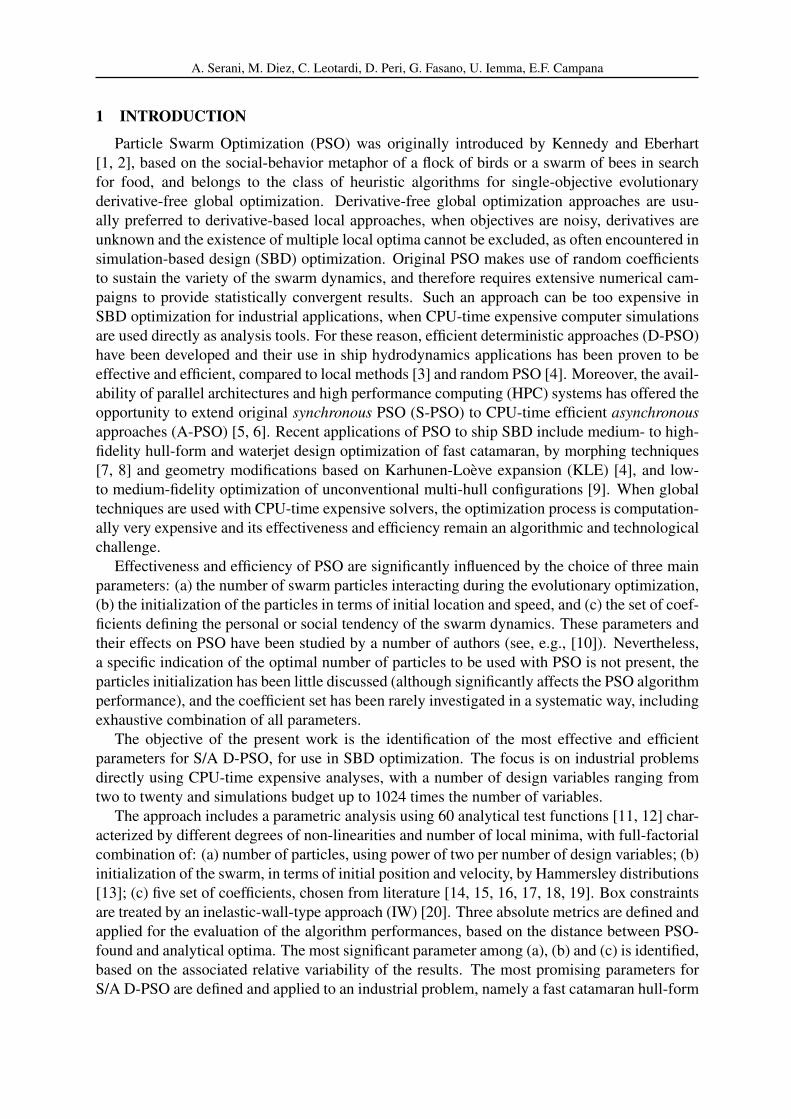
5.1.2 AD-PSO

Generally, AD-PSO results are found similar to SD-PSO. Specifically, Figs. 9 and 10, showthe performances of AD-PSO versus the budget of function evaluations, in terms of ∆x, ∆f ,∆, for Ndv < 10 and ≥ 10 respectively. Average values are presented, conditional to numberof particles, particles initialization and coefficient set, respectively. Figures 11 and 12 show therelative variance σ2

r of ∆x, ∆f , ∆ for Ndv < 10 and ≥ 10 respectively, retained by each ofthe PSO parameters. The particles initialization is the most significant parameters, especiallyfor low budgets and Ndv ≥ 10. The coefficient set is shown to have a small effect on theperformance, compared to other PSO parameters. Tables 5 and 6 summarizes the five bestperforming setups based on ∆x, ∆f , ∆, for Ndv < 10 and ≥ 10, respectively, varying thebudget of function evaluations. Overall averages and standard deviations among all PSO setupsare also included.

0.05

0.1

0.15

0.2

0.25

0.3

0.35

100 1000

∆x [-

]

No. of feval per Ndv [-]

2Ndv4Ndv8Ndv

16Ndv32Ndv64Ndv

128Ndv

0.05

0.1

0.15

0.2

0.25

0.3

0.35

100 1000

∆f

[-]


2Ndv4Ndv8Ndv

16Ndv32Ndv64Ndv

128Ndv

0.05

0.1

0.15

0.2

0.25

0.3

0.35

100 1000

∆ [-

]


2Ndv4Ndv8Ndv

16Ndv32Ndv64Ndv

128Ndv

(a) Average performance, conditional to number of particles

0.05

0.1

0.15

0.2

0.25

0.3

0.35

0.4

100 1000

∆x [-

]


A.0B.0C.0A.1B.1C.1

0.05

0.1

0.15

0.2

0.25

0.3

0.35

0.4

100 1000

∆f

[-]


A.0B.0C.0A.1B.1C.1

0.05

0.1

0.15

0.2

0.25

0.3

0.35

0.4

100 1000

∆ [-

]


A.0B.0C.0A.1B.1C.1

(b) Average performance, conditional to particle initialization

0.05

0.1

0.15

0.2

0.25

100 1000

∆x [-

]


Set 1Set 2Set 3Set 4Set 5

0.05

0.1

0.15

0.2

0.25

100 1000

∆f

[-]



0.05

0.1

0.15

0.2

0.25

100 1000

∆ [-

]



(c) Average performance, conditional to coefficient set

Figure 5: SD-PSO average performance for Ndv < 10


Table 3: Best performing setups for SD-PSO, Ndv < 10

Nfeval/Ndv

Average Best SD-PSO(STD)

∆x ∆f ∆Np

NdvInit Coef ∆x

NpNdv

Init Coef ∆fNp

NdvInit Coef ∆

128

16 A.1 3 0.072 4 C.1 4 0.015 4 C.1 4 0.0640.180 0.168 0.203 64 A.1 5 0.075 2 A.1 4 0.030 2 A.1 4 0.073

32 A.1 3 0.076 8 A.1 3 0.048 4 C.1 3 0.083(0.098) (0.114) (0.109) 16 A.0 3 0.080 4 A.1 3 0.053 16 A.1 3 0.083

4 C.1 3 0.080 4 C.1 3 0.053 8 A.1 3 0.087

256

64 A.1 4 0.063 4 C.1 4 0.014 16 A.0 3 0.0530.166 0.145 0.183 16 A.1 3 0.064 16 A.0 3 0.017 16 A.1 3 0.055

32 A.1 5 0.065 16 A.1 3 0.026 4 C.1 4 0.060(0.097) (0.118) (0.112) 16 A.0 3 0.066 2 A.1 4 0.030 2 A.1 4 0.072

32 C.0 3 0.067 8 C.1 4 0.038 16 A.0 4 0.053

512

64 A.1 4 0.049 16 A.0 3 0.012 16 C.0 3 0.0490.156 0.129 0.167 64 A.0 4 0.056 4 C.1 4 0.013 32 A.1 3 0.049

64 A.1 2 0.056 32 C.0 3 0.017 32 C.0 3 0.049(0.098) (0.120) (0.114) 32 A.1 5 0.058 16 A.0 1 0.018 16 A.1 3 0.053

32 C.0 3 0.059 32 A.1 3 0.019 16 A.0 1 0.053

1024

64 A.1 4 0.038 64 A.0 4 0.004 64 A.1 4 0.0300.149 0.118 0.156 64 A.1 2 0.039 32 C.1 4 0.005 64 A.0 4 0.031

64 A.0 4 0.043 64 A.1 3 0.005 64 A.1 3 0.039(0.099) (0.123) (0.117) 128 C.1 4 0.049 64 A.0 3 0.007 64 A.1 2 0.039

32 A.1 1 0.049 64 A.1 4 0.007 32 C.1 4 0.041

Av.

64 A.1 4 0.047 4 C.1 4 0.014 16 A.0 3 0.0600.163 0.140 0.177 64 A.0 4 0.062 16 A.0 3 0.025 4 C.1 4 0.061

32 A.1 5 0.064 2 A.1 4 0.030 16 A.1 3 0.061(0.097) (0.118) (0.111) 16 A.1 3 0.064 16 A.1 3 0.034 32 A.1 3 0.066

32 A.1 3 0.065 32 A.1 3 0.039 32 C.0 3 0.071

0.05

0.1

0.15

0.2

0.25

0.3

0.35

100 1000

∆x [-

]


2Ndv4Ndv8Ndv

16Ndv32Ndv64Ndv

128Ndv

0.05

0.1

0.15

0.2

0.25

0.3

0.35

100 1000

∆f

[-]


2Ndv4Ndv8Ndv

16Ndv32Ndv64Ndv

128Ndv

0.05

0.1

0.15

0.2

0.25

0.3

0.35

100 1000

∆ [-

]


2Ndv4Ndv8Ndv

16Ndv32Ndv64Ndv

128Ndv


0

0.1

0.2

0.3

0.4

0.5

100 1000

∆x [-

]


A.0B.0C.0A.1B.1C.1

0

0.1

0.2

0.3

0.4

0.5

100 1000

∆f

[-]


A.0B.0C.0A.1B.1C.1

0

0.1

0.2

0.3

0.4

0.5

100 1000

∆ [-

]


A.0B.0C.0A.1B.1C.1


0.16

0.18

0.2

0.22

0.24

0.26

0.28

0.3

0.32

0.34

100 1000

∆x [-

]



0.16

0.18

0.2

0.22

0.24

0.26

0.28

0.3

0.32

0.34

100 1000

∆f

[-]



0.16

0.18

0.2

0.22

0.24

0.26

0.28

0.3

0.32

0.34

100 1000

∆ [-

]




Figure 6: SD-PSO average performance for Ndv ≥ 10


Table 4: Best performing setups for SD-PSO, Ndv ≥ 10

Nfeval/Ndv

Average Best SD-PSO(STD)

∆x ∆f ∆Np

NdvInit Coef ∆x

NpNdv

Init Coef ∆fNp

NdvInit Coef ∆

128

2 A.1 2 0.155 2 C.1 2 0.023 2 A.1 2 0.1180.323 0.217 0.301 4 A.1 4 0.155 2 A.1 4 0.025 2 C.1 2 0.119

2 C.1 1 0.156 4 C.1 2 0.027 2 A.1 4 0.121(0.136) (0.195) (0.162) 4 C.1 4 0.158 4 A.1 3 0.030 4 C.1 4 0.122

2 A.1 4 0.159 4 C.1 4 0.031 4 C.1 2 0.122

256

4 C.1 2 0.149 4 C.1 2 0.019 4 C.1 2 0.1080.311 0.199 0.286 4 A.1 4 0.152 8 A.1 4 0.019 8 A.1 4 0.115

2 A.1 2 0.153 4 C.1 4 0.021 4 C.1 4 0.116(0.139) (0.196) (0.163) 2 C.1 1 0.154 8 C.1 4 0.022 8 C.1 4 0.116

4 C.1 4 0.156 2 C.1 2 0.022 2 A.1 2 0.117

512

4 C.1 2 0.147 16 A.1 3 0.011 4 C.1 2 0.1060.298 0.183 0.272 32 A.1 4 0.149 8 A.1 4 0.013 8 C.1 4 0.110

4 A.1 4 0.151 8 C.1 2 0.014 8 A.1 4 0.111(0.140) (0.197) (0.165) 64 A.1 3 0.153 8 A.0 4 0.017 4 C.1 4 0.114

8 C.1 4 0.153 4 C.1 2 0.018 8 C.1 2 0.115

1024

32 A.1 4 0.136 16 A.1 3 0.009 32 A.1 4 0.0980.291 0.172 0.263 64 A.1 3 0.144 16 A.1 4 0.011 64 A.1 3 0.105

64 C.1 4 0.145 32 A.1 4 0.011 4 C.1 2 0.106(0.142) (0.199) (0.168) 4 C.1 2 0.147 8 A.1 4 0.012 16 A.1 4 0.109

128 A.1 4 0.148 32 C.1 3 0.013 8 C.1 4 0.109

Av.

4 A.1 4 0.152 4 C.1 2 0.020 4 C.1 2 0.1110.306 0.193 0.280 4 C.1 2 0.152 8 C.1 2 0.022 4 C.1 4 0.117

2 A.1 2 0.153 2 C.1 2 0.022 2 A.1 2 0.117(0.139) (0.196) (0.164) 2 C.1 1 0.154 8 A.1 4 0.023 8 C.1 4 0.117

4 C.1 4 0.156 4 C.1 4 0.039 2 C.1 4 0.118

0

20

40

60

80

100

100 1000

σ2

r [%

]


N. PartInit

Coef

(a) ∆x

0

20

40

60

80

100

100 1000

σ2

r [%

]


N. PartInit

Coef

(b) ∆f

0

20

40

60

80

100

100 1000

σ2

r [%

]


N. PartInit

Coef

(c) ∆

Figure 7: σ2r(%) of SD-PSO for Ndv < 10

0

20

40

60

80

100

100 1000

σ2

r [%

]


N. PartInit

Coef

(a) ∆x

0

20

40

60

80

100

100 1000

σ2

r [%

]


N. PartInit

Coef

(b) ∆f

0

20

40

60

80

100

100 1000

σ2

r [%

]


N. PartInit

Coef

(c) ∆

Figure 8: σ2r(%) of SD-PSO for Ndv ≥ 10


0.05

0.1

0.15

0.2

0.25

0.3

0.35

100 1000

∆x [-

]


2Ndv4Ndv8Ndv

16Ndv32Ndv64Ndv

128Ndv

0.05

0.1

0.15

0.2

0.25

0.3

0.35

100 1000

∆f

[-]


2Ndv4Ndv8Ndv

16Ndv32Ndv64Ndv

128Ndv

0.05

0.1

0.15

0.2

0.25

0.3

0.35

100 1000

∆ [-

]


2Ndv4Ndv8Ndv

16Ndv32Ndv64Ndv

128Ndv


0.05

0.1

0.15

0.2

0.25

0.3

0.35

0.4

100 1000

∆x [-

]


A.0B.0C.0A.1B.1C.1

0.05

0.1

0.15

0.2

0.25

0.3

0.35

0.4

100 1000

∆f

[-]


A.0B.0C.0A.1B.1C.1

0.05

0.1

0.15

0.2

0.25

0.3

0.35

0.4

100 1000

∆ [-

]


A.0B.0C.0A.1B.1C.1


0.05

0.1

0.15

0.2

0.25

100 1000

∆x [-

]



0.05

0.1

0.15

0.2

0.25

100 1000

∆f

[-]



0.05

0.1

0.15

0.2

0.25

100 1000

∆ [-

]




Figure 9: AD-PSO average performance for Ndv < 10

Table 5: Best performing setups for AD-PSO, Ndv < 10

Nfeval/Ndv

Average Best AD-PSO(STD)

∆x ∆f ∆Np

NdvInit Coef ∆x

NpNdv

Init Coef ∆fNp

NdvInit Coef ∆

128

16 A.1 1 0.069 4 C.1 3 0.004 4 C.1 4 0.0530.175 0.164 0.199 16 A.1 3 0.069 4 C.1 4 0.007 4 C.1 3 0.061

16 A.0 3 0.071 4 C.0 3 0.021 4 C.0 4 0.076(0.096) (0.113) (0.107) 4 C.1 4 0.073 4 C.0 4 0.022 8 A.1 3 0.080

16 A.1 4 0.076 2 A.1 4 0.037 2 A.1 4 0.082

256

16 A.1 2 0.057 4 C.1 4 0.003 4 C.1 4 0.0460.160 0.142 0.178 16 A.1 3 0.057 4 C.1 3 0.004 4 C.1 3 0.059

16 A.1 1 0.059 4 C.0 4 0.014 16 A.0 3 0.066(0.093) (0.118) (0.107) 16 A.0 3 0.060 4 C.0 3 0.020 4 C.0 4 0.067

16 A.0 4 0.060 2 A.1 4 0.037 16 A.1 3 0.074

512

32 C.1 4 0.046 4 C.1 4 0.003 16 A.0 4 0.0360.146 0.124 0.159 16 A.0 4 0.049 4 C.1 3 0.004 4 C.1 4 0.040

16 A.1 2 0.050 16 A.0 4 0.005 16 A.1 2 0.053(0.092) (0.117) (0.109) 32 A.1 4 0.051 4 C.0 4 0.014 16 A.1 3 0.056

16 A.1 1 0.053 4 C.0 3 0.019 16 A.1 4 0.057

1024

32 C.1 4 0.040 16 A.0 4 0.002 16 A.0 4 0.0340.138 0.110 0.147 32 A.1 2 0.043 4 C.1 4 0.003 64 A.0 4 0.036

64 A.0 4 0.046 4 C.1 3 0.004 32 A.1 4 0.038(0.093) (0.120) (0.111) 32 A.1 4 0.047 64 A.0 3 0.006 64 A.0 3 0.038

16 A.1 2 0.047 64 A.0 4 0.008 32 C.1 4 0.039

Av.

16 A.1 4 0.058 4 C.1 4 0.004 4 C.1 4 0.0450.154 0.135 0.170 16 A.1 1 0.058 4 C.1 3 0.004 4 C.1 3 0.060

16 A.1 3 0.059 4 C.0 4 0.016 16 A.0 4 0.065(0.092) (0.114) (0.106) 32 C.1 4 0.060 4 C.0 3 0.020 16 A.0 3 0.068

16 A.0 3 0.061 2 A.1 4 0.037 4 C.0 4 0.069


0.05

0.1

0.15

0.2

0.25

0.3

0.35

100 1000

∆x [-

]


2Ndv4Ndv8Ndv

16Ndv32Ndv64Ndv

128Ndv

0.05

0.1

0.15

0.2

0.25

0.3

0.35

100 1000

∆f

[-]


2Ndv4Ndv8Ndv

16Ndv32Ndv64Ndv

128Ndv

0.05

0.1

0.15

0.2

0.25

0.3

0.35

100 1000

∆ [-

]


2Ndv4Ndv8Ndv

16Ndv32Ndv64Ndv

128Ndv


0

0.1

0.2

0.3

0.4

0.5

100 1000

∆x [-

]


A.0B.0C.0A.1B.1C.1

0

0.1

0.2

0.3

0.4

0.5

100 1000

∆f

[-]


A.0B.0C.0A.1B.1C.1

0

0.1

0.2

0.3

0.4

0.5

100 1000

∆ [-

]


A.0B.0C.0A.1B.1C.1

(b) Average performance, conditional to particles initialization

0.1

0.15

0.2

0.25

0.3

0.35

100 1000

∆x [-

]



0.1

0.15

0.2

0.25

0.3

0.35

100 1000

∆f

[-]



0.1

0.15

0.2

0.25

0.3

0.35

100 1000

∆ [-

]




Figure 10: AD-PSO average performance for Ndv ≥ 10

Table 6: Best performing setups for AD-PSO, Ndv ≥ 10

Nfeval/Ndv

Average Best AD-PSO(STD)

∆x ∆f ∆Np

NdvInit Coef ∆x

NpNdv

Init Coef ∆fNp

NdvInit Coef ∆

128

4 A.1 4 0.147 2 C.1 4 0.013 4 A.1 4 0.1070.320 0.214 0.297 2 C.1 4 0.152 4 A.1 4 0.015 2 C.1 4 0.109

8 C.1 4 0.152 2 A.1 4 0.019 4 C.1 4 0.116(0.136) (0.191) (0.159) 2 A.1 2 0.158 4 C.1 4 0.022 2 A.1 4 0.116

4 C.1 4 0.159 4 C.1 3 0.027 8 C.1 4 0.117

256

4 A.1 4 0.145 4 A.1 4 0.010 4 A.1 4 0.1040.307 0.194 0.282 8 C.1 4 0.149 2 C.1 4 0.012 8 C.1 4 0.108

4 C.1 2 0.150 8 A.1 3 0.016 2 C.1 4 0.108(0.137) (0.190) (0.160) 2 C.1 4 0.151 2 A.1 4 0.016 4 C.1 2 0.111

32 A.1 3 0.154 8 C.1 4 0.017 4 C.1 4 0.114

512

32 A.1 3 0.141 16 A.0 3 0.010 4 A.1 4 0.1030.292 0.176 0.265 4 A.1 4 0.144 4 A.1 4 0.010 8 C.1 4 0.105

16 A.1 4 0.145 8 A.1 4 0.011 16 A.1 4 0.105(0.139) (0.191) (0.162) 8 C.1 4 0.147 2 C.1 4 0.012 2 C.1 4 0.108

4 C.1 2 0.147 16 A.1 4 0.013 32 A.1 3 0.108

1024

32 A.1 3 0.136 16 A.1 4 0.008 32 A.1 3 0.1000.283 0.165 0.255 64 C.1 3 0.140 16 A.0 3 0.008 16 A.1 4 0.101

128 A.1 2 0.141 16 A.0 4 0.009 4 A.1 4 0.102(0.140) (0.194) (0.164) 32 C.1 4 0.142 8 A.1 4 0.010 32 C.1 4 0.104

16 A.1 4 0.142 4 A.1 4 0.010 8 C.1 4 0.104

Av.

4 A.1 4 0.145 4 A.1 4 0.011 4 A.1 4 0.1040.300 0.187 0.275 8 C.1 4 0.148 2 C.1 4 0.012 2 C.1 4 0.108

2 C.1 4 0.151 2 A.1 4 0.016 8 C.1 4 0.108(0.136) (0.190) (0.160) 4 C.1 2 0.151 4 C.1 4 0.018 4 C.1 2 0.112

32 A.1 3 0.152 8 A.1 3 0.018 4 C.1 4 0.114


0

20

40

60

80

100

100 1000

σ2

r [%

]


N. PartInit

Coef

(a) ∆x

0

20

40

60

80

100

100 1000

σ2

r [%

]


N. PartInit

Coef

(b) ∆f

0

20

40

60

80

100

100 1000

σ2

r [%

]


N. PartInit

Coef

(c) ∆

Figure 11: σ2r(%) of AD-PSO for Ndv < 10

0

20

40

60

80

100

100 1000

σ2

r [%

]


N. PartInit

Coef

(a) ∆x

0

20

40

60

80

100

100 1000

σ2

r [%

]


N. PartInit

Coef

(b) ∆f

0

20

40

60

80

100

100 1000

σ2

r [%

]


N. PartInit

Coef

(c) ∆

Figure 12: σ2r(%) of AD-PSO for Ndv ≥ 10

5.1.3 Suggested guideline for S/A D-PSO

The most frequent setup is selected in Tabs. 3, 4, 5 and 6, in order to define a guidelinefor the use of S/A D-PSO as simple and general as possible. This corresponds to a numberof particles Np equal to 4 times the number of design variables Ndv, a particles initializationincluding distribution on domain and bounds with non-null velocity, and the set of coefficientsby Clerc (2006) [18], χ = 0.721, c1 = c2 = 1.655. The guideline is summarized in Tab. 7.

Table 7: Suggested guideline for S/A D-PSO

Np/Ndv Init Coef

4 C.1 (including domain and bounds) 4 (Clerc, 2006)

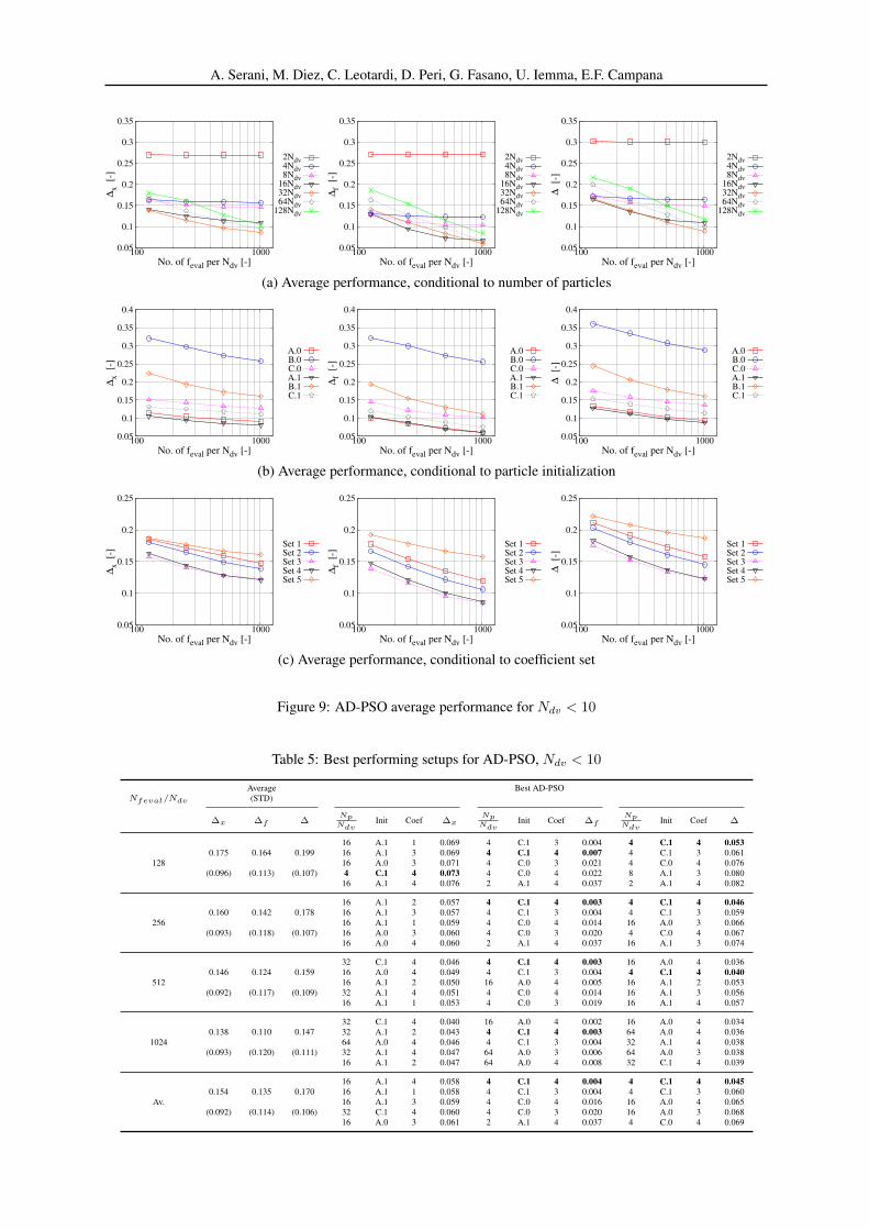
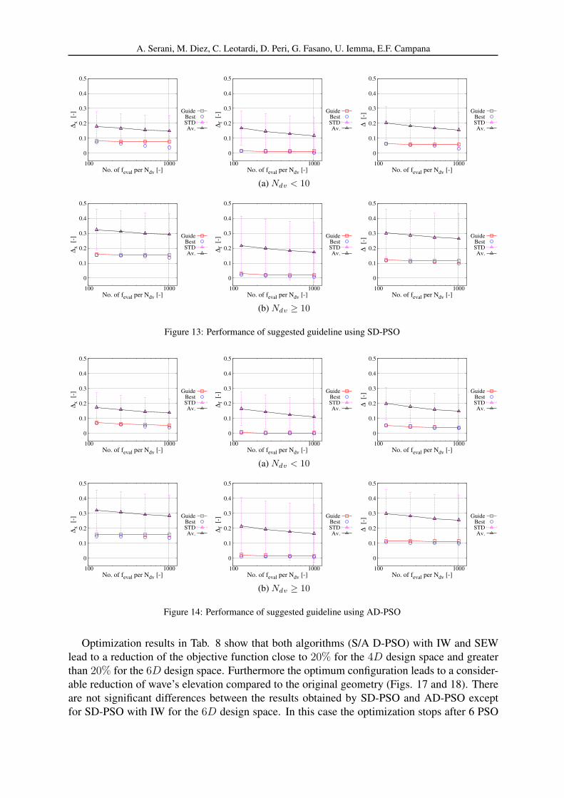
Figures 13 and 14 show the performance of the suggested PSO setup, for SD-PSO and AD-PSO and Ndv < 10 and ≥ 10, respectively. Average performance, standard deviation and bestperforming setup among all combinations is shown for each budget. The guideline setup isfound always very close or coincident to the best. In addition, it may be noted how AD-PSO isalways equivalent or slightly better than SD-PSO.

5.2 High-speed catamaran SBD optimization

A preliminary sensitivity analysis for each design variable is shown in Fig. 15, showing ∆obj

compared to the parent hull. Changes in ∆obj are found significant in each direction, revealinga reduction of the objective function close to 9% for the 4D design space, and close to 10% forthe 6D.


0

0.1

0.2

0.3

0.4

0.5

100 1000

∆x [-

]


GuideBestSTDAv.

0

0.1

0.2

0.3

0.4

0.5

100 1000

∆f

[-]


GuideBestSTDAv.

0

0.1

0.2

0.3

0.4

0.5

100 1000

∆ [-

]


GuideBestSTDAv.

(a) Ndv < 10

0

0.1

0.2

0.3

0.4

0.5

100 1000

∆x [-

]


GuideBestSTDAv.

0

0.1

0.2

0.3

0.4

0.5

100 1000

∆f

[-]


GuideBestSTDAv.

0

0.1

0.2

0.3

0.4

0.5

100 1000

∆ [-

]


GuideBestSTDAv.

(b) Ndv ≥ 10

Figure 13: Performance of suggested guideline using SD-PSO

0

0.1

0.2

0.3

0.4

0.5

100 1000

∆x [-

]


GuideBestSTDAv.

0

0.1

0.2

0.3

0.4

0.5

100 1000

∆f

[-]


GuideBestSTDAv.

0

0.1

0.2

0.3

0.4

0.5

100 1000

∆ [-

]


GuideBestSTDAv.

(a) Ndv < 10

0

0.1

0.2

0.3

0.4

0.5

100 1000

∆x [-

]


GuideBestSTDAv.

0

0.1

0.2

0.3

0.4

0.5

100 1000

∆f

[-]


GuideBestSTDAv.

0

0.1

0.2

0.3

0.4

0.5

100 1000

∆ [-

]


GuideBestSTDAv.

(b) Ndv ≥ 10

Figure 14: Performance of suggested guideline using AD-PSO

Optimization results in Tab. 8 show that both algorithms (S/A D-PSO) with IW and SEWlead to a reduction of the objective function close to 20% for the 4D design space and greaterthan 20% for the 6D design space. Furthermore the optimum configuration leads to a consider-able reduction of wave’s elevation compared to the original geometry (Figs. 17 and 18). Thereare not significant differences between the results obtained by SD-PSO and AD-PSO exceptfor SD-PSO with IW for the 6D design space. In this case the optimization stops after 6 PSO


-10

-5

0

5

10

15

-1 -0.5 0 0.5 1

∆ξ

[%]

variable space [-]

x1

x2

x3

x4

(a) 4D design space

-10

-5

0

5

10

15

-1 -0.5 0 0.5 1

∆ξ

[%]

variable space [-]

x1

x2

x3

x4

x5

x6

(b) 6D design space

Figure 15: Sensitivity analysis

iterations, due to IW approach. As shown in Fig. 16, differences in optimal design variablesare due to the use of IW or SEW for box constraints. The final configuration for the first designspace (4D) is fairly close (except for the second variable) to that obtained using metamodelswith a URANS solver [4] (Fig. 16a), while for the second design space (6D) the differencesare more significant (Fig. 16b). Finally, S/A D-PSO iterations are shown in Fig. 19, revealing aquite sudden convergence.

Table 8: SBD results

Design space wall approach Rt [N] δ [N] obj ∆obj(%)

Original 50.15 852.5 5.88e-2

4DSD-PSO IW 39.92 850.9 4.69e-2 -20.24

SEW 40.36 850.6 4.67e-2 -20.57

AD-PSO IW 39.85 851.1 4.68e-2 -20.41SEW 40.68 851.7 4.71e-2 -19.90

6DSD-PSO IW 39.41 849.1 4.64e-2 -21.10

SEW 34.29 835.4 4.10e-2 -30.27

AD-PSO IW 34.31 835.5 4.11e-2 -30.10SEW 34.08 830.8 4.09e-2 -30.30

-1

-0.5

0

0.5

1

1 2 3 4

Des

ign v

aria

ble

val

ue

[-]

Design variable id [-]

SDPSO (IW)

SDPSO (SEW)

ADPSO (IW)

ADPSO (SEW)

reference

(a) 4D design space

-1

-0.5

0

0.5

1

1 2 3 4 5 6

Des

ign v

aria

ble

val

ue

[-]

Design variable id [-]

SDPSO (IW)

SDPSO (SEW)

ADPSO (IW)

ADPSO (SEW)

reference

(b) 6D design space

Figure 16: Comparison between optimal design variables of SD-PSO, AD-PSO with IW and SEW by PF and thoseobtained by metamodels with URANS in [4]


(a) Original Delft catamaran

(b) SD-PSO with IW

(c) SD-PSO with SEW

(d) AD-PSO with IW

(e) AD-PSO with SEW

Figure 17: 4D SBD results


(a) Original Delft catamaran

(b) SD-PSO with IW

(c) SD-PSO with SEW

(d) AD-PSO with IW

(e) AD-PSO with SEW

Figure 18: 6D SBD results


-21

-20

-19

-18

-17

-16

-15

-14

-13

50 100 150 200 250

∆obj [

%]

D-PSO iteration [-]

SDPSO (IW)

SDPSO (SEW)

ADPSO (IW)

ADPSO (SEW)

(a) 4D design space

-31

-30

-29

-28

-27

-26

-25

-24

-23

-22

-21

50 100 150 200 250

∆obj [

%]

D-PSO iteration [-]

SDPSO (IW)

SDPSO (SEW)

ADPSO (IW)

ADPSO (SEW)

(b) 6D design space

Figure 19: Convergence of S/A D-PSO

6 CONCLUSIONS AND FUTURE WORK

A guideline for an effective and efficient use of S/A D-PSO has been suggested and dis-cussed, assuming limited computational resources. A parametric analysis has been conductedusing 60 analytical test functions from literature and three different absolute performance crite-ria, varying the number of particles, the initialization of the swarm, and the set of coefficients.All possible combinations of PSO parameters led to 210 optimizations for each function. Themost promising PSO setup has been identified and successfully applied to a ship SBD optimiza-tion problem, namely the high-speed Delft catamaran advancing in calm water at fixed speedusing a potential-flow code. The optimization pertained to the hull form and aimed at the totalresistance over displacement ratio reduction, using four- and six-dimensional design spaces.

The outcomes of the current analysis may be summarized as follows:

• The particles initialization has been found the most significant PSO parameter, especiallyfor Ndv ≥ 10 and low budgets of function evaluations. Conversely, the coefficient set hasbeen found with a little influence on the PSO performance, compared to other parameters.

• The suggested guideline setup corresponds to: a number of particles Np equal to 4 timesthe number of design variables Ndv; particles initialization including (Hammersley) dis-tribution on domain and bounds with non-null velocity; set of coefficient by Clerc (2006)[18], i.e., χ = 0.721, c1 = c2 = 1.655.

• The guideline setup has been found always very close or coincident to the best setupamong all 210 available, for each budget. In addition, it has been proven to perform wellfor a 4D and a 6D ship SBD problems.

• AD-PSO has been found with equivalent performance to SD-PSO.

• SEW approach for box constraints should be preferred to IW, in order to avoid an earlyarrest of the swarm particles.

Future work includes developments for new particles initialization methodologies, with ap-plication to test functions and ship SBD problems, using S/A D-PSO. Future research also in-cludes the extension of present studies to multi-objective D-PSO with application to reliability-based robust design optimization [30].


ACKNOWLEDGEMENTS

The present research is supported by the US Office of Naval Research, NICOP Grant N62909-11-1-7011, under the administration of Dr. Ki-Han Kim and Dr. Woei-Min Lin, and by theItalian Flagship Project RITMARE, coordinated by the Italian National Research Council andfunded by the Italian Ministry of Education, within the National Research Program 2011-2013.

REFERENCES

[1] J. Kennedy, R.C. Eberhart, Particle swarm optimization, in: Proc. IEEE Conf. on NeuralNetworks, IV, Piscataway, NJ, 1995, pp. 1942-1948.

[2] R.C. Eberhart, J. Kennedy, A new optimizer using particle swarm theory, Proc. Sixth Intl.Symp. on Micro Machine and Human Science (Nagoja, Japan), IEEE Service Center,Piscantaway, NJ, 1995, pp. 39-43.

[3] E.F. Campana, G. Liuzzi, S. Lucidi, D. Peri, V. Piccialli, A. Pinto, New global optimiza-tion methods for ship design problems, Optimization and Engineering, December 2009,Volume 10, Issue 4, pp. 533-555.

[4] X. Chen, M. Diez, M. Kandasamy, Z. Zhang, E.F. Campana, F. Stern, High-fidelity globaloptimization for shape design by dimensionality reduction, metamodels and deterministicparticle swarm, Engineering Optimization, 2014.

[5] G. Venter, J. Sobieszczanski-Sobieski, A parallel particle swarm optimization algorithmaccelerated by asynchronous evaluations, 6th World Congresses of Structural and Multi-disciplinary Optimization, Rio de Janeiro, 30 May–03 June 2005, Brazil.

[6] B.-I. Koh, A.D. George, R.T. Haftka, B.J. Fregly, Parallel asynchronous particle swarmoptimization, Int. J. Numer. Meth. Engng 2006; 67:578–595, DOI: 10.1002/nme.1646.

[7] M. Kandasamy, D. Peri, Y. Tahara, W. Wilson, M. Miozzi, S. Georgiev, E. Milanov,E.F. Campana, F. Stern, Simulation based design optimization of waterjet propelled Delftcatamaran, International Shipbuilding Progress, Volume 60, 2013, pp. 277-308, DOI10.3233/ISP-130098.

[8] X. Chen, M. Diez, M. Kandasamy, E.F. Campana, F. Stern, Design optimization of thewaterjet-propelled Delft Catamaran in calm water using URANS, design of experiments,metamodels and swarm intelligence, 12th International Conference on Fast Sea Trans-portation, FAST2013, Amsterdam, The Netherlands, 2013.

[9] B. Rosenthal, D.C. Kring, Optimal design of a lifting body SWATH, 12th InternationalConference on Fast Sea Transportation, FAST2013, Amsterdam, The Netherlands, 2013.

[10] R. Poli, J. Kennedy, T. Blackwell, Particle Swarm Optimization - An overview, SwarmIntell, 2007, Volume 1, pp. 33-57.

[11] S. Lucidi, M. Piccioni, Random Tunneling by Means of Acceptance-Rejection Samplingfor Global Optimization, Journal of optimization theory and applications, Vol. 62, N. 2,August 1989, pp. 255-277.


[12] E.F. Campana, G. Fasano, A. Pinto, Dynamic analysis for the selection of parametersand initial population, in particle swarm optimization, Journal of Global Optimization,November 2010, Volume 48, Issue 3, pp. 347-397.

[13] T.T. Wong, W.S. Luk, P.A. Heng, Sampling with Hammersley and Halton Points, Journalof Graphics Tools, 1997, pp. 9-24.

[14] Y. Shi, R.C. Eberhart, Parameter selection in particle swarm optimization, Proceedings ofEvolutionary Programming VII (EP98), 1998, pp. 591-600.

[15] M. Clerc, J. Kennedy, The particle swarm: explosion, stability and convergence in a multi-dimensional complex space, IEEE Trans Evolution. Comput. 6(1), 2002, pp. 58-73.

[16] A. Carlisle, G. Dozier, An Off-the-shelf PSO, Proceding of the Workshop on ParticleSwarm Optimization, 2001, pp. 1-6.

[17] I.C. Trelea, The particle swarm optimization algorithm: convergence analysis and param-eter selection, Information Processing Letters, 85, 2003, pp. 317-325.

[18] M. Clerc, Stagnation analysis in particle swarm optimization or what happens when noth-ing happens, http://hal.archives-ouvertes.fr/hal-00122031, Tech. Rep. 2006.

[19] D. Peri, F. Tinti, A multistart gradient-based algorithm with surrogate model for globaloptimization, Communications in Applied and Industrial Mathematics, 2012.

[20] S. Helwig, J. Branke, S. Mostaghim, Experimental Analysis of Bound Handling Tech-niques in Particle Swarm Optimization, IEEE Transactions on Evolutionary computation,Vol. 17, No. 2, April 2013.

[21] P. Bassanini, U. Bulgarelli, E.F. Campana, F. Lalli, The wave resistance problem in aboundary integral formulation, Surv. Math. Ind. (1994) 4:151-194.

[22] Y. Shi, R.C. Eberhart, A modified Particle Swarm Optimizer, IEEE International Confer-ence on Evolutionary Computation, Anchorage, Alaska, 1998.

[23] M. Clerc, The swarm and the queen: towards a deterministic and adaptive particle swarmoptimization, in: Proc. ICEC, Washington, DC, 1999, pp. 1951-1957.

[24] R.C Eberhart, Y. Shi, Comparing inertia weights and constriction factor in particle swarmoptimization, in Congress on Evolutionary Computing, vol. 1, pp. 84–88, 2000.

[25] R.C. Eberhart, Y. Shi, Particle Swarm Optimization: Developments, Applications andResources, Evolutionary computation, 2001.

[26] M. Clerc, Confinements and Biases in Particle Swarm Optimization,http://clerc.maurice.free.fr/pso, 2006.

[27] D. Bratton, J. Kennedy, Defining a standard for particle swarm optimization, in Proc. IEEESwarm Intell. Symp, Apr. 2007, pp. 120-127.

[28] A. Levy, A. Montalvo, S. Gomez, and A. Galderon, Topics in Global Optimization, Lec-ture Notes in Mathematics No. 909, Springer-Verlag, 1981.


[29] H. Schlichting, K. Gersten, Boundary-Layer Theory, Springer-Verlag, Berlin, 2000.

[30] M. Diez, X. Chen, E.F. Campana, F. Stern, Reliability-based robust design optimization forships in real ocean evironment, 12th International Conference on Fast Sea TransportationFAST2013, Amsterdam, December 2013.

A LIST OF TEST FUNCTIONS

Table 9 summarizes the test functions used in the current work.

Table 9: Test functions

fk(x) Name Dimension Bounds OptimumNdv [xmin, xmax]i,...,Ndv min f(x)

f1(x) Sphere 2 [−5, 5]Ndv 0.000f2(x) Freudenstein-Roth 2 [−5, 5]Ndv 0.000f3(x) Ackley 2 [−5, 5]Ndv 0.000f4(x) Three-Hump Camel Back 2 [−5, 5]Ndv 0.000f5(x) Six-Hump Camel Back 2 [−2.5, 2.5]i, [−1.5, 1.5]j -1.032f6(x) Quartic 2 [−10, 10]Ndv -0.352f7(x) Beale 2 [−4.5, 4.5]Ndv 0.000f8(x) Schubert penalty 1 2 [−10, 10]Ndv -186.731f9(x) Schubert penalty 2 2 [−10, 10]Ndv -186.731f10(x) Booth 2 [−10, 10]Ndv 0.000f11(x) Matyas 2 [−10, 10]Ndv 0.000f12(x) Goldstein-Price 2 [−2, 2]Ndv 3.000f13(x) Bukin n.6 2 [−15,−5]i, [−3, 3]j 0.000f14(x) Rosenbrock 2 [−100, 100]Ndv 0.000f15(x) Schaffer n.2 2 [−100, 100]Ndv 0.000f16(x) Schaffer n.6 2 [−100, 100]Ndv 0.000f17(x) Easom 2 [−100, 100]Ndv -1.000f18(x) Test Tube Holder 2 [−10, 10]Ndv -10.872f19(x) Treccani 2 [−5, 5]Ndv 0.000f20(x) Tripod 2 [−100, 100]Ndv 0.000

f21,22(x) Exponential 2, 4 [−10, 10]Ndv -1.000f23,24(x) Styblinski-Tang 2, 4 [−5, 5]Ndv −39.166 ·Ndv

f25,26(x) Cosine Mixture 2, 4 [−1, 1]Ndv −0.100 ·Ndv

f27,28(x) Hartman n.3, n.6 3, 6 [0, 1]Ndv -3.860, -3.320f29,30,31,32(x) 5n loc. minima (Levy) 2, 5, 10, 20 [−10, 10]Ndv 0.000f33,34,35,36(x) 10n loc. minima (Levy) 2, 5, 10, 20 [−10, 10]Ndv 0.000f37,38,39,40(x) 15n loc. minima (Levy) 2, 5, 10, 20 [−5, 5]Ndv 0.000f41,42,43,44(x) Griewank 2, 5, 10, 20 [−10, 10]Ndv 0.000f45,46,47,48(x) Alpine 2, 5, 10, 20 [−10, 10]Ndv 0.000f49,50,51,52(x) Multi Modal 2, 5, 10, 20 [−10, 10]Ndv 0.000f53,54,55,56(x) Dixon-Price 2, 5, 10, 20 [−10, 10]Ndv 0.000

f57(x) Colville 4 [−10, 10]Ndv 0.000f58(x) Shekel n.5 4 [0, 10]Ndv -10.153f59(x) Shekel n.7 4 [0, 10]Ndv -10.403f60(x) Shekel n.10 4 [0, 10]Ndv -10.536

On the use of Synchronous and Asynchronous Single-Objective Deterministic Particle Swarm...

Documents

Transcript of On the use of Synchronous and Asynchronous Single-Objective Deterministic Particle Swarm...