On the Urban Connectivity ofVehicular Sensor Networks

Hugo Conceicao1,2,3, Michel Ferreira1,2, and Joao Barros1,3,4

1 DCC2 LIACC

3 Instituto de TelecomunicacoesFaculdade de Ciencias da Universidade do Porto, Portugal

4 LIDS, MIT, Cambridge, MA, USA{hc,michel,barros}@dcc.fc.up.pt

Abstract. Aiming at a realistic mobile connectivity model for vehicu-lar sensor networks in urban environments, we propose the combinationof large-scale traffic simulation and computational tools to character-ize fundamental graph-theoretic parameters. To illustrate the proposedapproach, we use the DIVERT simulation framework to illuminate thetemporal evolution of the average node degree in this class of networksand provide an algorithm for computing the transitive connectivity pro-file that ultimately determines the flow of information in a vehicularsensor network.

1 Introduction

Mobile sensor networks are arguably substantially different from their staticcounterparts. First and foremost, the fact that the network topology can varydramatically in time depending on the particular application and deploymentscenario, offers richer connectivity profiles and proven opportunities e.g. to in-crease the system capacity [1] or to enhance the level of security [2]. Althoughsome of the typical problems faced by static sensor networks, in particular un-fair load balancing and fast energy depletion of nodes close to the sink [3], mayoften disappear in the presence of dynamically changing topologies, other taskssuch as routing, topology control or data aggregation require non-trivial solu-tions capable of exploiting the existing mobility patterns and providing highereffectiveness and efficiency.

Our goal here is to develop a methodology for characterizing the aforemen-tioned mobility patterns for vehicular sensor networks in urban environments —a task we deem crucial towards developing adequate protocols for this class ofdistributed systems. In sharp contrast with state-of-the-art stochastic mobilitymodels, which frequently rely on somewhat simplistic decision models either foreach sensor vehicle (e.g. the random walk or the random way point model) orwith respect to the urban road network (e.g. the Manhattan grid or hexago-nal lattices), we propose to use a realistic traffic simulator capable of capturingthe complexity of trajectories followed by sensor nodes placed in vehicles and

S. Nikoletseas et al. (Eds.): DCOSS 2008, LNCS 5067, pp. 112–125, 2008.c© Springer-Verlag Berlin Heidelberg 2008

On the Urban Connectivity of Vehicular Sensor Networks 113

the dynamics of the resulting connectivity profiles when using tractable wirelesscommunication models.

Our main contributions are as follows:

– Modeling Methodology: We combine large-scale traffic simulation with a basicwireless communication model in order to make inferences about the dynamicbehavior of mobile sensor networks with thousands of nodes.

– Analysis of the Average Node Degree in an Urban Environments: Based onour large-scale vehicular network simulator, in which micro-simulated vehi-cles circulate in a real-life urban network, we characterize the average nodedegree for various traffic flow conditions, transmission radii and time inter-vals;

– Connectivity Dynamics: We present an algorithm capable of computing thetransitive connectivity, which is key towards understanding information flowin a vehicular sensor network.

The remainder of the paper is organized as follows. Section 2 provides anoverview of related work on modeling vehicular sensor networks. In Section 3 wedescribe our general methodology based on the DIVERT simulation frameworkand show our results for the average degree of the evolutionary connectivitygraph. Section 4 then describes our algorithm and its results for the transientconnectivity of the vehicular sensor network, and Section 5 concludes the paper.

2 Related Work

Vehicular sensor networks, which in the context of vehicle-to-vehicle (V2V) wire-less communication are sometimes called Vehicular Ad-Hoc Networks (VANETs),consist in a distributed network of vehicles equipped with sensors that gather in-formation related to the road. The main variables monitored are related to trafficefficiency and safety. An example of the later is the detection of hazardous loca-tions such as ice or oil detected through the traction control devices of the vehi-cle. In the context of this paper traffic sensing is more relevant, because it canbe exploited in the distributed computation performed by the vehicles’ traffic-congestion-aware route planners. Traffic sensing is essentially done by measuringmobility (average speed) in a road segment.

Both types of information have to be propagated through the network andthus the topology of the communications network is naturally affected by themobility of the nodes (mobility plays a dual-role in this context, as a sensingmeasure and as a sensor property). Realistic models to study the topology ofthese networks are very important, in particular for large-scale scenarios wherethousands of nodes can interact in a geographically confined space, such as acity. If unrealistic models are used, invalid conclusions may be drawn [4]. Modelsfor VANETs have two main components: modeling of mobility, which is veryrelated to traffic modeling; and modeling of inter-vehicle communication.

According to the concept map for mobility models presented in [5], these mod-els can be primarily categorized in analytical and simulation based. Analytical

114 H. Conceicao, M. Ferreira, and J. Barros

models are in general based on very simple assumptions regarding movementpatterns. Typically, nodes are considered to be uniformly distributed over agiven area. The direction of movement of each node is also considered to beuniformly distributed in an interval of [0...2π[, as well as speed ([0...vmax[). Insome models these parameters of direction and speed remain constant until thenode crosses the boundary of the given area [6], while other models allow themto change [7]. The main advantage of analytical models is the fact that theyallow the derivation of mathematical expressions describing mobility metrics.

Simulation based models are much more detailed regarding movement pat-terns. In the context of vehicular movement these models originated from thearea of transportation theory and have been an object of intense study over thepast sixty years. Depending on the level of detail in which traffic entities aretreated, current models can be divided into three main categories: microscopic,macroscopic and mesoscopic.

The microscopic model requires a highly detailed description where each ve-hicle/entity is distinguished. Each vehicle is simulated independently with itsown autonomous variables, e.g. position and velocity. Microscopic models arevery useful to describe the interaction between the traffic entities, braking andacceleration patterns, or navigation related parameters. There are two instanceswith great relevance, namely the Car-Following model (CF-model) [8] and theCellular-Automaton model (CA-model)[9]. The former follows the principle thatthe variables of one vehicle depend on the vehicle (or vehicles) in front, whichcan be described using ordinary differential equations.

More recent than the CF-model, the CA-model divides the roads in cells withboolean states: either the cell is empty or it contains one vehicle. The simulationis done in time steps and each vehicle may move only if the next cell is free. Insome CA-models the vehicles can advance more than one cell in each step. Thevelocity is calculated considering the number of cells one vehicle advances perstep and associating values to the size of each cell (typically 7.5m) and to theduration of each step (typically 1s).

The model with the lowest-detail description is the macroscopic model, whichtries to describe the traffic flow as if it was a fluid or a gas[10], thus analyzingthe traffic in terms of density, flow and velocity.

As a more recent approach, the mesoscopic model can be viewed as standingbetween the aforementioned models in terms of detail. It combines some of theadvantages of the microscopic model, such as the possibility to define individ-ual routes for each vehicle, with the easiness to calibrate the model parametersof the macroscopic model. In the mesoscopic model the speed of the vehicle isdefined by the cell in which it is, contrary to what happens in the microscopicmodel. This speed is the result of a speed-density function that relates the speedwith the current density in each cell. Ongoing research efforts in transportationtheory are targeting a hybrid model [11]. Here, the main idea is to use a mi-croscopic approach in road segments where a high level of detail is necessary,using a mesoscopic model for the remaining parts. This approach facilitates thecalibration of the simulators and saves on computational complexity.

On the Urban Connectivity of Vehicular Sensor Networks 115

All these models have an associated degree of randomness in parameters suchas routes, direction and speed. A highly used simulation model for the study ofwireless systems is the random walk model [12], where nodes can move freelyanywhere in the simulation area. In vehicular simulators the randomness of thedirection of movements is usually much more limited, as it is bounded by thespatial configuration of the road network. Randomness in vehicular simulatorsusually lies in the choice of speed and direction at road intersections. The ran-domness of speed is minimized in sophisticated simulators by relating it to thedensity of road segments or defining it by monitoring distance to the vehiclesahead. However, the randomness associated to direction decision in these sim-ulators is quite unrealistic and does not reflect the actual mobility behaviourof vehicles in real scenarios. A more deterministic approach, where pre-definedroutes are set up and their frequency is calibrated to mimic a realistic scenariois very likely to provide more coherent results.

Capturing the fundamental properties of wireless communications is also achallenging task towards realistic modeling of mobile sensor networks. Beyondthe simple random geometric graph, where each node is connected to any othernode within a prescribed radius, it is possible to incorporate more sophisticatedelements such as shadowing and fading [13,14]. Reference [15] gives a criticaloverview of the most common modeling assumptions.

3 Connectivity of Vehicular Adhoc Networks

In this section we describe the study of mobile nodes connectivity in the contextof a large-scale vehicular sensor network, simulated over an urban scenario usingthe DIVERT framework [16], which will be briefly described. We present ourstudy abstracting the details of the spatial configuration of the road networkand of vehicles and communication location into concepts from graph theory,such as node degree and transitive connectivity.

3.1 The DIVERT Simulation Environment

The DIVERT simulation environment (Development of Inter-VEhicular Reli-able Telematics) has been developed in order to provide a state-of-the-art toolto study the behaviour of realistic and large-scale vehicular sensor networks,providing a testbed for the development and evaluation of distributed protocols,such as collaborative route-planning [17]. It is out-of-the-scope of this paperto describe the DIVERT framework.Other examples of traffic simulators in thespirit of DIVERT include TraNS [18], NCTUns [19] and GrooveNet [20]. Wejust outline the realistic features present in DIVERT, pointing out how suchfeatures can substantially affect the connectivity profile of the network. A videoof a simulation is available at http://myddas.dcc.fc.up.pt/divert.

DIVERT works over real maps of cities (that can be setup by the user). Thecity used for the simulations presented in this paper was Porto, second largestin Portugal. It has several types of roads, from highways to residential streets,

116 H. Conceicao, M. Ferreira, and J. Barros

totaling 965kms. Each road has a speed limit, that is used in the simulation,and mimics the traffic signs enforcements. Each road has a different number oftraffic lanes, ranging from 4 to 1, and the connectivity of each lane is discrimi-nated in road intersections. In most roads, traffic circulates two-ways, which hasclearly a crucial impact on the pattern of short-range communications. DIVERTincludes a detailed traffic signs layer, in particular of priorities at intersectionsand traffic lights location and parametrization. This is also crucial, has our sim-ulations show that the updating of traffic information happens primarily at roadintersections, being the stop time of each vehicle a vital parameter. DIVERT in-cludes parking location. Vehicles appear and disappear in the simulation, eitherbecause they enter/leave the city area, or because they start/stop in a parkingplace. This also affects connectivity. DIVERT allows defining the aimed num-ber of vehicles in the city, dividing in sensor vehicles (vehicles that are part ofthe VANET), and non-communicating vehicles, which just affect the mobility ofthe former. This allows the realistic simulation of scenarios with different pen-etration rates of V2V technology. In the simulations presented in this paper, a10% penetration rate was considered, for an aimed total of 5000 vehicles in si-multaneous simulation. Regarding vehicle routes, DIVERT uses a hybrid modelof pre-defined routes and randomly generated routes. For randomly generatedroutes, DIVERT arbitrarily selects an origin and a destination and calculates theroute based on a shortest-path algorithm, either parameterized by distance or bytime. Shortest-path based on time uses not only the speed limits of segments, butmainly the dynamic calibration of average mobility derived from previous sim-ulation results. Pre-defined routes are setup by the user and have an associatedfrequency. In the simulations presented in this paper they have been carefullydesigned to approximate the simulation to our perception of traffic distributionin Porto. DIVERT allows parameterizing the transmission range of sensor vehi-cles, which obviously affects the network connectivity. In this paper we presentresults for simulations with varying transmission ranges and show its impact onthe network connectivity. The DIVERT model for communication is based onthe purely geometric link model.

3.2 Graphs with Mobile Nodes

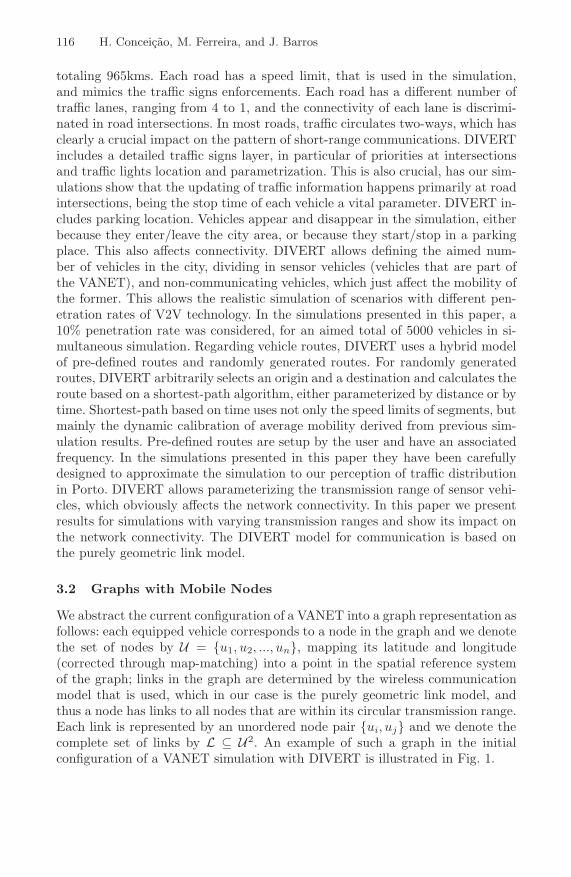
We abstract the current configuration of a VANET into a graph representation asfollows: each equipped vehicle corresponds to a node in the graph and we denotethe set of nodes by U = {u1, u2, ..., un}, mapping its latitude and longitude(corrected through map-matching) into a point in the spatial reference systemof the graph; links in the graph are determined by the wireless communicationmodel that is used, which in our case is the purely geometric link model, andthus a node has links to all nodes that are within its circular transmission range.Each link is represented by an unordered node pair {ui, uj} and we denote thecomplete set of links by L ⊆ U2. An example of such a graph in the initialconfiguration of a VANET simulation with DIVERT is illustrated in Fig. 1.

On the Urban Connectivity of Vehicular Sensor Networks 117

An important measure of the connectivity of a graph is its average node degree,which is given by:

davg =1n

n∑

i=1

|N (ui)|

where |N (ui)| is the cardinality of the set of nodes to which node i is connected,the neighbors of node ui, denoted by N (ui).

Fig. 1. Graph of the initial configuration of a VANET

As it can be seen from Fig. 1, the average node degree of the initial configu-ration of our VANET is very low (≈ 1.6 in Fig. 1, where a transmission range of150 meters was used), resulting in an extremely disconnected network. From thespatial configuration of the nodes, which reflects the actual geographic distribu-tion of vehicles, we can see that even a significant increase in the transmissionrange would still result in a very low average node degree. However, the mobilityof the nodes can significantly improve the network connectivity. If we considerthe mobility of a node ui in a time interval [0...t], we can define the degree of ui

in that interval as follows:

d(ui)[0...t] =

∣∣∣∣∣∣

t⋃

j=0

N (ui)j

∣∣∣∣∣∣(1)

where N (ui)j is the set of neighbors of ui at instant j. In DIVERT simulations,one j step corresponds to one second.

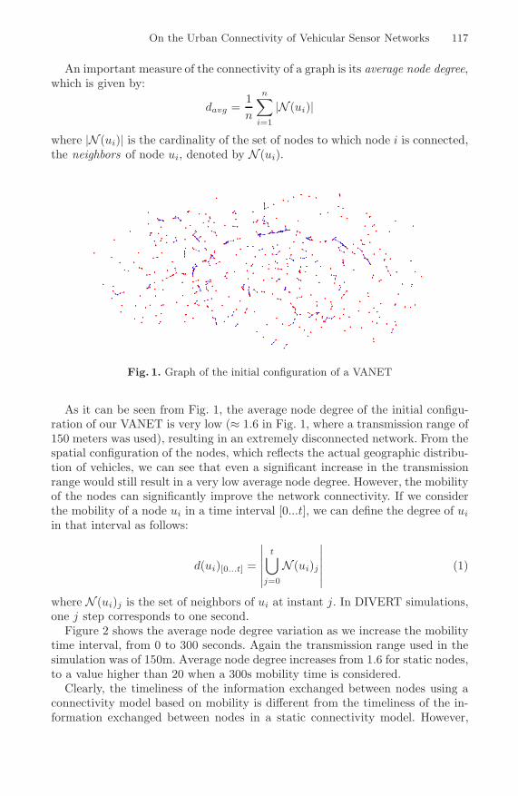
Figure 2 shows the average node degree variation as we increase the mobilitytime interval, from 0 to 300 seconds. Again the transmission range used in thesimulation was of 150m. Average node degree increases from 1.6 for static nodes,to a value higher than 20 when a 300s mobility time is considered.

Clearly, the timeliness of the information exchanged between nodes using aconnectivity model based on mobility is different from the timeliness of the in-formation exchanged between nodes in a static connectivity model. However,

118 H. Conceicao, M. Ferreira, and J. Barros

0 50 100 150 200 250 300time (s)

0

5

10

15

20

25

ave

rag

e d

eg

ree

150m

Fig. 2. Average node connectivity with varying mobility time

some of the information circulating a VANET is tolerant to a certain levelof obsoleteness, such as traffic speed in road segments, where a 300-seconds-old report can still be validly used by dynamic navigation engines to avoid atraffic jam.

Information exchange in a VANET graph happens not only between nodesdirectly connected but also through transitive links. An example is the dissem-ination of traffic information, where communicating vehicles exchange informa-tion about the average speed of road segments they traveled, but also about theaverage speed of road segments they received from other vehicles. This tran-sitivity of node connection is conveyed in the graph representation in Fig. 1,where node mobility has not been considered, as nodes can be reached throughmulti-link transitive paths. However, when mobility is considered in the connec-tivity of a node, simple transitive paths cannot be assumed to allow a node toreach another node. Consider for instance that N (u1)0 = {u2}, N (u2)0 = {u1},N (u2)1 = {u3} and N (u3)1 = {u2}. At t = 0, u1 and u2 are connected and canexchange information. At t = 1, u2 and u3 connect, and u3 will receive informa-tion from u2 that includes the data u1 sent at t = 0, but u1 will not received anyinformation from u3. In this case, we consider that u3[0...1] is transitively con-nected to u1[0...1] but not vice-versa. Links in the mobile graph become directed,while in the static model they were undirected.

We generalize the set of links for a mobile graph in an interval [0...t] to a setof triples of the form (ui, uj, t

′), for t′ in [0...t] (e.g. (u1, u2, 0)). The set of linksis denoted by L′ ⊆ U2×[0...t] and we consider the following rule to compute thetransitive closure L′∗ of L′:

On the Urban Connectivity of Vehicular Sensor Networks 119

∀ui, uj ∈ U , t′ ∈ [0...t],

(ui, uj, t′) ∈ L′∗ ⇐⇒

{uj ∈ N (ui)t′

∃uk ∈ U , (ui, uk, t′) ∈ L′ ∧ (uk, uj, t′′) ∈ L′∗ ∧ t′ ≥ t′′

(2)By 2, L′∗ = {(u1, u2, 0), (u2, u1, 0), (u2, u3, 1), (u3, u2, 1), (u3, u1, 1)}. Note

that u3 is linked to u1 but not vice-versa.After computing the transitive closure of L′ we perform the following pro-

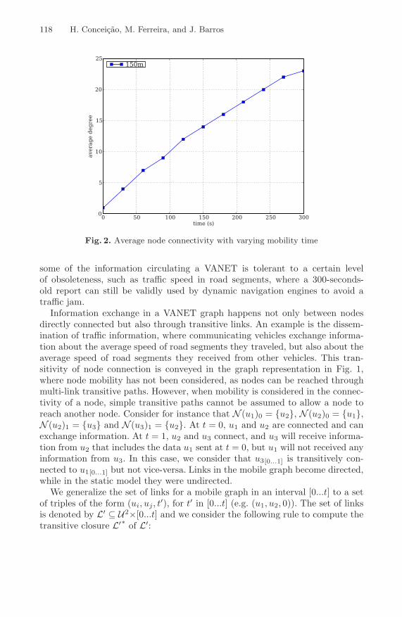
jection on its triples, Π1,2(L′∗), obtaining the set of pairs of the graph thatrepresents the transitive connectivity in the mobility interval [0...t]. Nodes arerepresented in their position at instant t. Figure 3 represents such as graph wherean interval of 30s of node mobility was considered, maintaining the 150m trans-mission range. This graph is based on the simulation that generated graph inFig. 1 at instant 0. Nodes in this graph can only exchange information throughdirect links. The mobility-based average node degree is thus a very good measureto quantify the graph connectivity.

Fig. 3. Transitive closure graph considering a node mobility of 30s

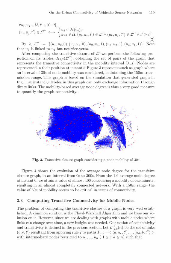
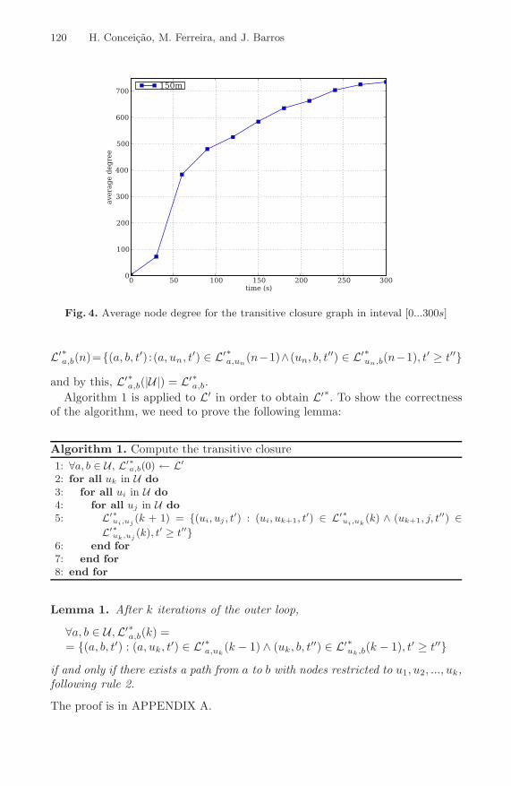
Figure 4 shows the evolution of the average node degree for the transitiveclosure graph, in an interval from 0s to 300s. From the 1.6 average node degreeat instant 0, we attain a value of almost 400 considering a mobility of one minute,resulting in an almost completely connected network. With a 150m range, thevalue of 60s of mobility seems to be critical in terms of connectivity.

3.3 Computing Transitive Connectivity for Mobile Nodes

The problem of computing the transitive closure of a graph is very well estab-lished. A common solution is the Floyd-Warshall Algorithm and we base our so-lution on it. However, since we are dealing with graphs with mobile nodes wherelinks can change over time, a new insight was needed. Our notion of connectivityand transitivity is defined in the previous section. Let L′∗

a,b(n) be the set of links(a, b, t′) resultant from applying rule 2 to paths Pa,b =< (a, uc, t

′), ..., (ud, b, t′′) >

with intermediary nodes restricted to u1, ..., un ( 1 ≤ c, d ≤ n) such that

120 H. Conceicao, M. Ferreira, and J. Barros

0 50 100 150 200 250 300time (s)

0

100

200

300

400

500

600

700

ave

rag

e d

eg

ree

150m

Fig. 4. Average node degree for the transitive closure graph in inteval [0...300s]

L′∗a,b(n)={(a, b, t′) :(a, un, t′) ∈ L′∗

a,un(n−1)∧(un, b, t′′) ∈ L′∗

un,b(n−1), t′ ≥ t′′}

and by this, L′∗a,b(|U|) = L′∗

a,b.Algorithm 1 is applied to L′ in order to obtain L′∗. To show the correctness

of the algorithm, we need to prove the following lemma:

Algorithm 1. Compute the transitive closure1: ∀a, b ∈ U , L′∗

a,b(0) ← L′

2: for all uk in U do3: for all ui in U do4: for all uj in U do5: L′∗

ui,uj(k + 1) = {(ui, uj , t

′) : (ui, uk+1, t′) ∈ L′∗

ui,uk(k) ∧ (uk+1, j, t

′′) ∈L′∗

uk,uj(k), t′ ≥ t′′}

6: end for7: end for8: end for

Lemma 1. After k iterations of the outer loop,

∀a, b ∈ U , L′∗a,b(k) =

= {(a, b, t′) : (a, uk, t′) ∈ L′∗a,uk

(k − 1) ∧ (uk, b, t′′) ∈ L′∗uk,b(k − 1), t′ ≥ t′′}

if and only if there exists a path from a to b with nodes restricted to u1, u2, ..., uk,following rule 2.

The proof is in APPENDIX A.

On the Urban Connectivity of Vehicular Sensor Networks 121

4 Varying Mobility Time/Transmission Range

So far in this paper we have used a transmission range of 150m in our DIVERTsimulations. However, connectivity is clearly affected by different transmissionranges. Figure 5 shows the variation of the average node degree with varyingmobility time ([0..300s]) and transmission range ([50..300m]). The graphic plotsexpression 1 in Section 3.2 for the 6 different transmission ranges considered. Asit can be seen from Fig. 5, an average node degree of 10 is obtained after 30sof mobility for a 300m transmission range, after 60s for a range of 200m andafter 120s for a range of 100m. If the latency of the information is not critical,higher mobility times can achieve the same connectivity with lower transmissionranges.

0 50 100 150 200 250 300time (s)

0

5

10

15

20

25

30

35

40

45

ave

rag

e d

eg

ree

50m100m150m200m250m300m

Fig. 5. Average node degree with varying mobility time and transmission range

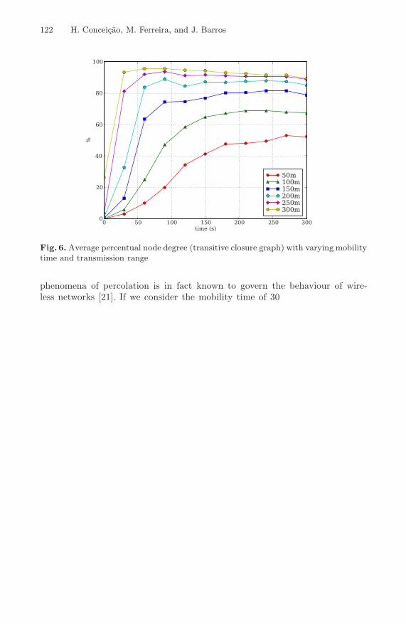
Results for the transitive closure graph are presented in Fig. 6, considering thedifferent transmission ranges. We now use the average percentual node degree,meaning that we divide the degree of the nodes by the total number of nodessimulated. It should be noted that in a realistic environment sensors can leavethe city area, or end their trip within the city, during the mobility time beingconsidered. On the other hand, some sensors enter or appear in the city nearthe end of the mobility time being considered. It is thus almost impossible toachieve a 100% connected network. Our approach is to measure connectivity inthe presence of such realistic behaviour, rather than defining unrealistic bordermodels (such as reflection) or forcing all trips to last more than the mobilitytime.

It is clear from Fig. 6 that the connectivity profile of the network percolatesover the two dimensions considered, transmission radii and mobility time. The

122 H. Conceicao, M. Ferreira, and J. Barros

0 50 100 150 200 250 300time (s)

0

20

40

60

80

100

%

50m100m150m200m250m300m

Fig. 6. Average percentual node degree (transitive closure graph) with varying mobilitytime and transmission range

phenomena of percolation is in fact known to govern the behaviour of wire-less networks [21]. If we consider the mobility time of 30s, percolation on thetransmission radius happens around the critical threshold of 200m. Only for thetransmission ranges higher than 200m we achieve an average node degree higherthan 50% of the total of nodes. Percolation on the mobility time seems to happenaround thresholds of 60s or 90s. At 90s, average node degrees of around 50%or higher of the total of nodes are already found for all the transmission rangesexcept for the conservative 50m radius.

5 Conclusions and Further Work

Vehicular sensor networks are undoubtedly poised to become a very relevantexample of distributed computation, featuring large numbers of vehicles thatcooperate in a self-organized fashion to find optimal ways of exploring the roadnetwork. The deployment of such networks and the development of their pro-tocols require a fundamental understanding of the dominant mobility and con-nectivity patterns — a task that in our belief must rely heavily on trustworthycomputer simulations.

Focusing on one instance of this problem, we provided a preliminary charac-terization of the connectivity of a vehicular sensor network operating in an urbanenvironment. Seeking a realistic model for sensor mobility, we opted for a sce-nario in which vehicular trajectories and velocities are bounded by the geographyof the road network (in our case, a real city) and determined by detailed traf-fic entities, such as traffic lights, speed limits and number of lanes of a given road.

On the Urban Connectivity of Vehicular Sensor Networks 123

Vehicle movement in our model is also very much determined by the interactionwith other vehicles and the ensuing decisions of each driver.

As part of our contribution, we were able to extract some of the most sig-nificant graph-theoretic parameters that capture the dynamics of this complexnetwork. For this purpose, we extended concepts such as average node degreeto account for mobility intervals, and developed an algorithm for computingthe transitive closure of such graphs based on mobile links. Our results illumi-nate the relationship between transmission radius and mobility time, showingan attenuation of percolation effects when these two dimensions are viewed ascomplementary.

In future work, we plan to compare our results with simpler mobility models,such as the random way point or the Manhattan grid, using the same graph-basedevaluation, highlighting the role of realistic mobility models towards understand-ing the dynamics of urban connectivity for vehicular sensor networks.

Acknowledgments

The authors gratefully acknowledge useful discussions with Prof. Luıs Damas(LIACC/UP and DCC-FCUP), who contributed decisively towards the develop-ment of the DIVERT simulation framework. The first author is also grateful toClaudio Amaral for useful discussions.

This work has been partially supported by the Portuguese Foundation for Sci-ence and Tecnology (FCT) under projects MYDDAS (POSC/EIA/59154/2004),JEDI (PTDC/EIA/66924/2006) and also STAMPA (PTDC/EIA/67738/2006),and by funds granted to LIACC and IT through the Programa de FinanciamentoPlurianual and POSC.

References

1. Grossglauser, M., Tse, D.: Mobility increases the capacity of ad hoc wireless net-works. IEEE/ACM Transactions on Networking (TON) 10(4), 477–486 (2002)

2. Capkun, S., Hubaux, J., Buttyan, L.: Mobility helps security in ad hoc networks. In:Proceedings of the 4th ACM international symposium on Mobile ad hoc networking& computing, pp. 46–56 (2003)

3. Intanagonwiwat, C., Govindan, R., Estrin, D.: Directed diffusion: A scalableand robust communication paradigm for sensor networks. In: Proceedings of theACM/IEEE International Conference on Mobile Computing and Networking, pp.56–67 (2000)

4. Kurkowski, S., Camp, T., Colagrosso, M.: MANET simulation studies: the incred-ibles. Mobile Computing and Communications Review 9(4), 50–61 (2005)

5. Bettstetter, C.: Smooth is better than sharp: a random mobility model for sim-ulation of wireless networks. In: Meo, M., Dahlberg, T.A., Donatiello, L. (eds.)MSWiM, pp. 19–27. ACM, New York (2001)

6. Hong, D., Rappaport, S.S.: Traffic model and performance analysis for cellularmobile radio telephone systems with prioritized and non-prioritized handoff proce-dures. In: ICC, pp. 1146–1150 (1986)

124 H. Conceicao, M. Ferreira, and J. Barros

7. Zonoozi, M.M., Dassanayake, P.: User mobility modeling and characterization ofmobility patterns. IEEE Journal on Selected Areas in Communications 15(7), 1239–1252 (1997)

8. Wilhelm, W.E., Schmidt, J.W.: Review of car following theory. TransportationEnginnering Journal 99, 923–933 (1973)

9. Hoogendoorn, S., Bovy, P.: State-of-the-art of vehicular traffic flow modelling. Pro-ceedings of the Institution of Mechanical Engineers, Part I: Journal of Systems andControl Engineering 215(4), 283–303 (2001)

10. Hoogendoorn, S., Bovy, P.: Gas-Kinetic Model for Multilane Heterogeneous TrafficFlow. Transportation Research Record 1678(-1), 150–159 (1999)

11. Burghout, W., Koutsopoulos, H., Andreasson, I.: Hybrid Mesoscopic-MicroscopicTraffic Simulation. Transportation Research Record 1934(-1), 218–255 (2005)

12. Bar-Noy, A., Kessler, I., Sidi, M.: Mobile users: To update or not to update? Wire-less Networks 1(2), 175–185 (1995)

13. Bettstetter, C., Hartmann, C.: Connectivity of Wireless Multihop Networks in aShadow Fading Environment. Wireless Networks 11(5), 571–579 (2005)

14. Chiang, C., Wu, H., Liu, W., Gerla, M.: Routing in clustered multihop, mobilewireless networks with fading channel. Proceedings of IEEE SICON 97, 197–211(1997)

15. Kotz, D., Newport, C., Gray, R.S., Liu, J., Yuan, Y., Elliott, C.: Experimentalevaluation of wireless simulation assumptions. In: MSWiM 2004: Proceedings ofthe 7th ACM international symposium on Modeling, analysis and simulation ofwireless and mobile systems, pp. 78–82. ACM, New York (2004)

16. Conceicao, H., Damas, L., Ferreira, M., Barros, J.: Large-Scale Simulation of V2VEnvironments. In: Proceedings of the 23rd Annual ACM Symposium on AppliedComputing, SAC 2008, Fortaleza, Ceara, Brazil, March 2008. ACM Press, NewYork (2008)

17. Yamashita, T., Izumi, K., Kurumatani, K., Nakashima, H.: Smooth traffic flow witha cooperative car navigation system. In: AAMAS 2005: Proceedings of the fourthinternational joint conference on Autonomous agents and multiagent systems, pp.478–485. ACM, New York (2005)

18. Piorkowski, M., Raya, M., Lugo, A., Papadimitratos, P., Grossglauser, M., Hubaux,J.P.: TraNS: Realistic Joint Traffic and Network Simulator for VANETs. ACMSIGMOBILE Mobile Computing and Communications Review

19. Wang, S., Chou, C., Huang, C., Hwang, C., Yang, Z., Chiou, C., Lin, C.: Thedesign and implementation of the NCTUns 1.0 network simulator. Computer Net-works 42(2), 175–197 (2003)

20. Mangharam, R., Weller, D., Rajkumar, R., Mudalige, P., Bai, F.: GrooveNet: AHybrid Simulator for Vehicle-to-Vehicle Networks. In: Second International Work-shop on Vehicle-to-Vehicle Communications (IEEE V2VCOM), San Jose, USA(July 2006)

21. Booth, L., Bruck, J., Franceschetti, M., Meester, R.: Covering Algorithms, Contin-uum Percolation and the Geometry of Wireless Networks. The Annals of AppliedProbability 13(2), 722–741 (2003)

On the Urban Connectivity of Vehicular Sensor Networks 125

APPENDIX A

The following proves lemma 1:

Proof. By induction on k.Let A(x)=L′∗

i,j(x). When k = 0 the statement is obviously true as the pathsPi,j =< i, j >, that is, the paths from i to j without intermediary nodes, arethe links from i to j and L′∗

i,j(0) is initialized with L′.Assume lemma 1 to be true for the first k iterations. In the (k+1)th iteration,

A(k+1)={(i, j, t′) :{i, uk+1, t′} ∈ L′∗

i,uk+1(k)∧(uk+1, j, t

′′) ∈ L′∗uk+1,j(k), t′ ≥ t′′}

and so uk+1 is added to the set of allowed intermediary nodes. The paths consid-ered are of the form < (i, ua, tt), ..., (ub, uk+1, t

′), (uk+1, uc, t′′), ..., (ud, j, tt

′) >.By induction assumption the subpaths considered < (i, ua, tt), ..., (ub, uk+1, t

′) >and < (uk+1, uc, t

′′), ..., (ud, j, tt′) > are valid since they are paths considered in

L′∗i,uk+1

(k) and L′∗uk+1,j(k), respectively. Also the intermediary nodes of these

subpaths are restricted to nodes u1...uk. To see that the complete path is validit is only necessary to verify that < (ub, uk+1, t

′), (uk+1, uc, t′′) > respects rule 2.

Since it is ensured that t′ ≥ t′′ the path is valid. Thus we get that in the (k+1)th

iteration

A(k+1)={(i, j, t′) :{i, uk+1, t′} ∈ L′∗

i,uk+1(k)∧(uk+1, j, t

′′) ∈ L′∗uk+1,j(k), t′ ≥ t′′}

if and only if there exists a path from i to j with nodes restricted to u1, ..., uk+1,following rule 2. Therefore, lemma 1 holds for the (k+1)th iteration of the outerloop and by the principle of mathematical induction, the lemma holds for allvalues of k.

By considering k = |U| we prove that L′∗a,b(|U|) = L′∗

a,b.