Large-scale Urban Vehicular Mobilityfor Networking Research

Sandesh Uppoor, Marco FioreUniversite de Lyon, INRIA

INSA-Lyon, CITI, F-69621, Villeurbanne, France{sandesh.uppoor,marco.fiore}@insa-lyon.fr

Abstract—Simulation is the tool of choice for the large-scale performance evaluation of upcoming telecommunicationnetworking paradigms that involve users aboard vehicles, suchas next-generation cellular networks for vehicular access, purevehicular ad hoc networks, and opportunistic disruption-tolerantnetworks. The single most distinguishing feature of vehicularnetworks simulation lies in the mobility of users, which is theresult of the interaction of complex macroscopic and microscopicdynamics. Notwithstanding the improvements that vehicular mo-bility modeling has undergone during the past few years, no cartraffic trace is available today that captures both macroscopic andmicroscopic behaviors of drivers over a large urban region,anddoes so with the level of detail required for networking research.In this paper, we present a realistic synthetic dataset of the cartraffic over a typical 24 hours in a 400-km2 region around the cityof Koln, in Germany. We outline how our mobility descriptionimproves today’s existing traces and show the potential impactthat a comprehensive representation of vehicular mobilitycanhave one the evaluation of networking technologies.

I. I NTRODUCTION

Vehicular environments have become increasingly attractiveto the telecommunication networking research communityover the last years. The reason is that cars are envisioned tobecome real communication hubs in the near future, thanks tothe proliferation of smartphones and tablets, whose Internet-connection capabilities appear especially appealing to passen-gers aboard cars, as well as to the growing presence of radiointerfaces on the vehicles themselves.

Enhanced infrastructure-based systems, involving, e.g.,theWiMAX and LTE-A technologies, and novel communicationparadigms, such as, e.g., ad hoc and opportunistic networking,are being studied in order to accommodate the traffic generatedand requested by forthcoming communicating vehicles. Mostof these solution require large-scale performance evaluationsthat are not feasible through experimentation directly, due tocosts and complexity. Simulation becomes thus the tool ofchoice to assess the quality such solutions.

When simulating a vehicular network, particular attentionmust be paid to faithfully represent the unique dynamics of carmobility, characterized at a time by high-peak high-variancespeeds, road topology-and road rules-constrained movements,and strong movement correlations over time and space. Theseproperties are the result of macroscopic and microscopic cartraffic dynamics, that need to be properly modeled in order toperform a simulative campaign whose results are credible.

The relevance of mobility modeling in the simulation of ve-hicular networks is widely acknowledged, a factor that has ledto a substantial progress in the quality of car movement tracesfor vehicular networking research. The simplistic stochasticmodels employed in early works [1], [2] have been replaced by

random mobility overrealistic road topologies[3] at first, andby microscopic vehicular modelsborrowed from transportationresearch [4] later on. These features were then included indedicated simulation environments, and integrated with roadsignalization [5], [6]. Since then, vehicular mobility simulatorshave been growing their complexity and features [7], allowingto accurately simulate the individual movement of vehiclesover realistic road topologies.

Today’s challenge lies in generating traffic traces that (i)compass very large urban areas, i.e., whole cities includingtheir surroundings, and (ii) are realistic also from a macro-scopic point of view, i.e., that faithfully mimic large trafficflows across a metropolitan area. To that end, one mustcorrectly identify thetraffic demand, i.e., the start time, theorigin and the destination of each car trip in the simulatedregion, which are stored in a so-called Origin/Destination(O/D) matrix. Then, an appropriatetraffic assignmentmodelneeds to be run on the O/D matrix, so to identify the realisticroute followed by each driver to reach his/her destination.Indeed, the current common practice is to employ a randomtraffic demand and shortest path-based assignment, which canlead to unrealistic flows and thus biased simulation results.

The few large-scale vehicular mobility traces accountingfor macroscopic mobility and publicly available have beenextensively used in the literature, but are either representativeof a subset of the whole traffic, as in the case of real-worldtaxi traces [8], or only model major arterial roads and neglectmost of the streets present in urban areas [9]. Additionally,both these kinds of dataset lack detail, since they report carpositions with low granularity, in the order of tens of seconds,or employ fast but approximate microscopic mobility models.Recently, the iTetris initiative [10] generated very detailedurban mobility traces based on realistic macroscopic datacollected in the city of Bologna, Italy. However, such tracesonly cover a short timespan of one hour and are limited torelatively small areas of around 10 km2; moreover, the tracesare not publicly available at the moment.

In this paper, we combine the four key aspects mentionedabove, i.e., a real-world road topology, an accurate microscopicmobility modeling, a realistic traffic demand, and a state-of-art traffic assignment technique, and generate a large-scalesynthetic trace of the car traffic in a the city of Koln, Germany.The dataset covers a region of 400 km2 for a period of 24hours. We detail the generation process, and then outline howour mobility dataset compares with some reference tracescommonly employed in the recent literature. Our analysissuggest that employing incomplete representations of vehicularmobility in the evaluation of networking protocols may indeedresult in over-optimistic performance.Accepted for publication at IEEE VNC 2011 –c© 2011 IEEE

II. T HE TAPASCOLOGNE DATASET

The vehicular mobility dataset we introduce in this paperis mainly based on the data made available by the TAPAS-Cologne project [11]. TAPASCologne, an initiative by theInstitute of Transportation Systems at the German AerospaceCenter (ITS-DLR), aims at reproducing, with the highest levelof realism possible, car traffic in the greater urban area of thecity of Koln, in Germany.

To that end, different state-of-art data sources and simula-tion tools are brought together, so to cover all of the specificaspects required for a proper characterization of vehiculartraffic. In the remainder of this section, we detail the featuresof the different components, as well as the process throughwhich they are combined to generate the mobility dataset.

A. Road topology

The street layout of the Koln urban area is obtained fromthe OpenStreetMap (OSM) database [12]. The OSM projectprovides freely exportable maps of cities worldwide, whichare contributed and updated by a vast user community. Mapsinclude information on roads, railways, buildings, and Pointsof Interests (PoI) such as parks, commercial centers, leisurecenters and commercial activities.

In particular, the OSM road information is generated andvalidated by means of satellite imagery and GPS traces, andis commonly regarded as the highest-quality road data publiclyavailable today. Indeed, the accuracy of OSM street layouts,comprising highways, major urban arteries and minor roads,often matches that of proprietary ones such as, e.g., GoogleMaps or Mappy, especially for large cities.

We employed the osmosis tool [13] to filter the OSMdata and extract the road topology information for an areaof approximately 400 km2 around the urban agglomerationof Koln, thus including almost 4500 km of roads. We thenresorted to the Java OpenStreetMap Editor (JOSM) [14] torepair the OSM data file and make it compatible with themicroscopic mobility simulator, as detailed in Sec. III.

B. Microscopic vehicular mobility

The microscopic mobility of vehicles is simulated with theSimulation of Urban Mobility (SUMO) software [15]. SUMOis an open-source, space-continuous, discrete-time traffic simu-lator developed by the German Aerospace Center (DLR), capa-ble of accurately modeling the behavior of individual drivers,accounting for car-to-car and car-to-road signalization interac-tions. More precisely, SUMO can import road maps in multipleformats, including OSM, and faithfully reproduce traffic lights,roundabouts, stop and yield signs. The microscopic modelsimplemented by SUMO are Krauss’ car-following model [16]and Krajzewicz’s lane-changing model [17], that respectivelyregulate a driver’s acceleration and overtaking decisions, bytaking into account a number of factors, including the distanceto the leading vehicle, the traveling speed, and the accelerationand deceleration profiles. These models have been long val-idated by the transportation research community, a fact that,jointly with the high scalability of the simulator, makes ofSUMO the most complete and reliable among today’s open-source microscopic vehicular mobility generators. The versionwe employed for the dataset generation is 12.3.

SUMO simulation

Gawron’s algorithm

TAPASCologne O/D matrix

OSM map

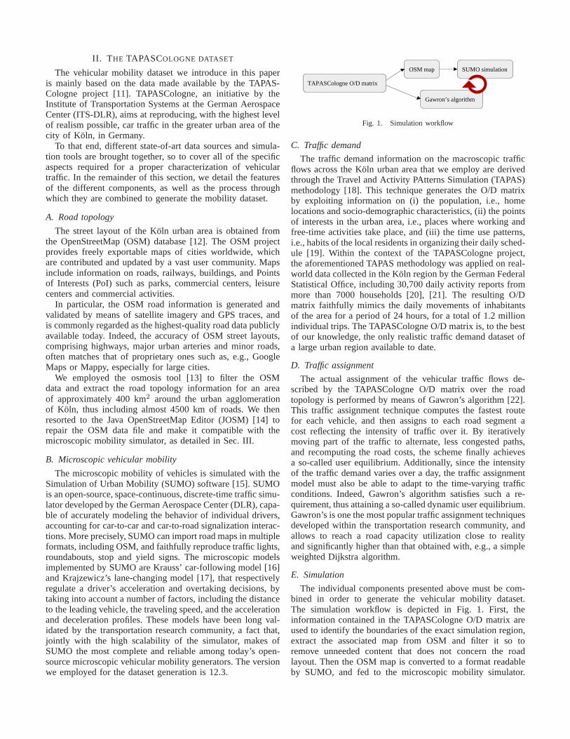
Fig. 1. Simulation workflow

C. Traffic demand

The traffic demand information on the macroscopic trafficflows across the Koln urban area that we employ are derivedthrough the Travel and Activity PAtterns Simulation (TAPAS)methodology [18]. This technique generates the O/D matrixby exploiting information on (i) the population, i.e., homelocations and socio-demographic characteristics, (ii) the pointsof interests in the urban area, i.e., places where working andfree-time activities take place, and (iii) the time use patterns,i.e., habits of the local residents in organizing their daily sched-ule [19]. Within the context of the TAPASCologne project,the aforementioned TAPAS methodology was applied on real-world data collected in the Koln region by the German FederalStatistical Office, including 30,700 daily activity reports frommore than 7000 households [20], [21]. The resulting O/Dmatrix faithfully mimics the daily movements of inhabitantsof the area for a period of 24 hours, for a total of 1.2 millionindividual trips. The TAPASCologne O/D matrix is, to the bestof our knowledge, the only realistic traffic demand dataset ofa large urban region available to date.

D. Traffic assignment

The actual assignment of the vehicular traffic flows de-scribed by the TAPASCologne O/D matrix over the roadtopology is performed by means of Gawron’s algorithm [22].This traffic assignment technique computes the fastest routefor each vehicle, and then assigns to each road segment acost reflecting the intensity of traffic over it. By iterativelymoving part of the traffic to alternate, less congested paths,and recomputing the road costs, the scheme finally achievesa so-called user equilibrium. Additionally, since the intensityof the traffic demand varies over a day, the traffic assignmentmodel must also be able to adapt to the time-varying trafficconditions. Indeed, Gawron’s algorithm satisfies such a re-quirement, thus attaining a so-called dynamic user equilibrium.Gawron’s is one the most popular traffic assignment techniquesdeveloped within the transportation research community, andallows to reach a road capacity utilization close to realityand significantly higher than that obtained with, e.g., a simpleweighted Dijkstra algorithm.

E. Simulation

The individual components presented above must be com-bined in order to generate the vehicular mobility dataset.The simulation workflow is depicted in Fig. 1. First, theinformation contained in the TAPASCologne O/D matrix areused to identify the boundaries of the exact simulation region,extract the associated map from OSM and filter it so toremove unneeded content that does not concern the roadlayout. Then the OSM map is converted to a format readableby SUMO, and fed to the microscopic mobility simulator.

0

50

100

150

200

250

6am 7am 8am 9am 10am

Veh

icle

s (x

100

0)

Time (h)

TravelingEndedWaiting

(a) Simulated vehicles status

0

10

20

30

40

50

60

6am 7am 8am 9am 10am 0

10

20

30

40

50

60

Tim

e (m

)

Spe

ed (

km/h

)

Time (h)

Travel timeSpeed

(b) Mean travel time and speed

Fig. 2. Original TAPASCologne dataset. Traffic features over time

3 km

Speed (km/h)0

30

60

90+

Fig. 3. Original TAPASCologne dataset. Snapshot of the traffic status at7:00 am, in a 400 km2 region centered on the city of Koln. Blue vehicles aremoving, whereas bright red ones are still (this figure is bestviewed in colors)

The TAPASCologne O/D matrix is also used as an inputto Gawron’s algorithm, which, in turn, determines an initialtraffic assignment and provides it to SUMO. Then, a firstvehicular mobility simulation can be run with SUMO, and,once finished, a feedback on the resulting traffic densityover the road topology is sent back to Gawron’s algorithm.Based on such new information, a new traffic assignment iscomputed, and a second SUMO simulation is run. The processis repeated until a traffic assignment is generated that allowsto sustain the whole volume of the traffic demand.

III. R EPAIRING THE DATASET

The result obtained by running the vehicular mobility sim-ulation with the data sources made available by OSM andTAPASCologne is plain unusable. In Fig. 2(a), we plot theevolution over time of the number of vehicles that (i) aretraveling on the road topology, (ii) have successfully endedtheir trip by reaching the their destination, (iii) are waiting toenter the road topology, which they cannot presently do due toan excessive congestion of the road segment they are supposedto start their trip from. This third condition is a simulationartifact, identifying situations where the road topology cannotaccommodate all the traffic demand in the O/D matrix, and, assuch, is an undesirable effect. Clearly, the three sets of vehiclesabove are disjoint.

From the plot, we can note how the number of travelingvehicles present in the simulation rapidly grows up to exceed

0

20

40

60

80

100

6am 8am 10am 12am

Inje

cted

veh

icle

s (v

eh/s

)

Time (h)

(a) Original

0

20

40

60

80

100

6am 8am 10am 12am

Inje

cted

veh

icle

s (v

eh/s

)

Time (h)

(b) Fixed

Fig. 4. Volume of traffic injected in the road network between6:00 am and12:00 am, according to the TAPASCologne O/D matrix

a hundred thousands units, a figure completely unrealistic fora city the size of Koln. Additionally, such a number does nottend to decrease as one could expect once the morning trafficpeak is exhausted; instead, it keeps growing indefinitely. Itis also possible to observe that the number of vehicles thatend their trip grows very slowly over time: in fact, from thevalues portrayed in the figure, only a very small fraction ofthe cars that are present on the road topology can reach theirdestination. Finally, the number of vehicles that are waiting toenter the road topology, which we would like to stay as closeas possible to zero, consistently grows over time instead.

The mean travel time, in Fig. 2(b), also shows a quiteunrealistic behavior, as more than half an hour is required,on average, for a driver to reach its destination at 10:00 am,when the traffic should be sparse. Similarly, the average speedof vehicles, in the same plot, tends to zero as the time elapses.

These results are clear symptoms of how the road topologycannot sustain the volume of cars injected according to thetraffic demand model. Indeed, when looking at a snapshot ofthe car traffic in the region, it is clear that the simulationquickly reduces to a huge traffic jam. As an example, Fig. 3depicts the map of the road topology at 7:00 am, a daytimetypically characterized by rather fluid traffic conditions.How-ever, the road topology is mostly covered by bright red dots,representing cars stuck in heavily congested traffic.

In the following we discuss the reasons for such a simulationresult, and present solutions to them.

A. Over-comprehensive and bursty traffic demand

The original TAPASCologne O/D matrix results in the trafficdemand volume depicted in Fig. 4(a), which shows the numberof vehicles injected in the whole road network every second.By analyzing the O/D matrix, its source data, and its effect onthe microscopic mobility simulation, we identified and fixedthe following two problems.

First, the demand in the O/D matrix is not limited to thevehicular traffic; rather, it includes information on the dailytrips of all Koln inhabitants, independently from whethertheirwalk to their destination, or employ public transports, or takea car as either passengers or drivers. Clearly, we are onlyinterested in the latter kind of mobility, since the volume ofvehicular traffic directly maps to that of car drivers. Accordingto [19, Fig. 4], car drivers account for approximately 50% ofthe overall trips in the TAPASCologne O/D matrix: thus, weadjusted the O/D matrix by only considering that one trip everytwo concerns the movement of a vehicle.

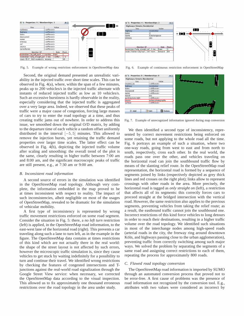
Fig. 5. Example of wrong restriction enforcement in OpenStreetMap data

Second, the original demand presented an unrealistic vari-ability in the injected traffic over short time scales. This can beobserved in Fig. 4(a), where, within the span of a few minutes,peaks up to 200 vehicles/s in the injected traffic alternate withinstants of reduced injected traffic as low as 10 vehicles/s.Such an excessive burstiness is hardly observable in the reality,especially considering that the injected traffic is aggregatedover a very large area. Indeed, we observed that these peaks oftraffic were a major cause of congestion, forcing large massesof cars to try to enter the road topology at a time, and thuscreating traffic jams out of nowhere. In order to address thisissue, we smoothed down the original O/D matrix, by addingto the departure time of each vehicle a random offset uniformlydistributed in the interval[−5, 5] minutes. This allowed toremove the injection bursts, yet retaining the traffic demandproperties over larger time scales. The latter effect can beobserved in Fig. 4(b), depicting the injected traffic volumeafter scaling and smoothing: the overall trend of the plot isthe same, clearly resulting in higher traffic between 7:00 amand 8:00 am, and the significant macroscopic peaks of trafficare still present, e.g., at 7:30 am or 9:00 am.

B. Inconsistent road information

A second source of errors in the simulation was identifiedin the OpenStreetMap road topology. Although very com-plete, the information embedded in the map proved to beat times inconsistent with respect to reality. The impact ofsuch inconsistencies, albeit negligible on most of the usagesof OpenStreetMap, revealed to be dramatic for the simulationof vehicular mobility.

A first type of inconsistency is represented by wrongtraffic movement restrictions enforced on some road segment.Consider the situation in Fig. 5: there, ano left turnrestriction(left) is applied, in the OpenStreetMap road information, to theeast-west lane of the horizontal road (right). This prevents a cartraveling along such a lane to turn left, as in the example in thefigure. The OpenStreetMap data contains at times restrictionsof this kind which are not actually there in the real world:the shape of the street layout is not affected by such errors,however the microscopic traffic simulation is, since they causevehicles to get stuck by waiting indefinitely for a possibility toturn and continue their travel. We identified wrong restrictionsby checking the features of congested intersections and T-junctions against the real-world road signalization through theGoogle Street View service: when necessary, we correctedthe OpenStreetMap data according to the visual inspection.This allowed us to fix approximately one thousand erroneousrestrictions over the road topology in the area under study.

Fig. 6. Example of continuous restriction enforcement in OpenStreetMap

Fig. 7. Example of unrecognized information ignored duringmap conversion

We then identified a second type of inconsistency, repre-sented by correct movement restrictions being enforced onsome roads, but not applying to the whole road all the time.Fig. 6 portrays an example of such a situation, where twoone-way roads, going from west to east and from north tosouth, respectively, cross each other. In the real world, theroads pass one over the other, and vehicles traveling onthe horizontal road can join the southbound traffic flow bymeans of the slanting relief route. In the OpenStreetMap roadrepresentation, the horizontal road is formed by a sequenceofsegments joined by links (respectively depicted as grey thicklines and red crosses on the right plot); links allow to representcrossings with other roads in the area. More precisely, thehorizontal road is tagged asonly straight on(left), a restrictionthat affects all of its segments: this correctly forces carstoproceed straight at the bridged intersection with the verticalroad. However, the same restriction also applies to the previoussegments, preventing vehicles from taking the relief route; asa result, the eastbound traffic cannot join the southbound one.Incorrect restrictions of this kind force vehicles to long detoursin order to reach their destinations, resulting in a higher trafficvolume over the road topology. We identified such situationsin most of the interchange nodes among high-speed roads(arterial roads in the city, the freeway ring around downtownKoln, and highways passing close to the urban agglomeration),preventing traffic from correctly switching among such majorways. We solved the problem by separating the segments of asame road and assigning correct restrictions to each of them,repeating the process for approximately 800 roads.

C. Flawed road topology conversion

The OpenStreetMap road information is imported by SUMOthrough an automated conversion process that proved not tobe error-free. A first cause of problems was the presence ofroad information not recognized by the conversion tool. E.g.,attributes with two values were considered as incorrect by

Fig. 8. Example of topological information unfitness duringmap conversion

the converter, and the associated roads were not included inthe topology used for the simulation. An example is shownin Fig. 7: the double value of thesourcefield (left) causesSUMO not to account for the associated road in simulation(right, a road should connect the north and south branches).We corrected the OpenStreetMap data so to make all attributescompatible with the SUMO converter.

A second critical aspect we had to address was the factthat the topological information in OpenStreetMap is, attimes, simply unfit to be directly converted to the SUMOstreet layout. An example is depicted in Fig. 8. There, thereal world aerial photography of one intersection (top right),the associated Google map information (top left), and theOpenStreetMap road topology (bottom left) match. However,the conversion of the latter in SUMO results in an exceedinglycomplex intersection, where vehicles get stuck and rapidlyform a permanent traffic jam (bottom right). The reason forsuch a simulation result is that, since two segment links (whitedots in the bottom left plot) are present, SUMO interprets theOpenStreetMap topology as if two road junctions co-existed,one placed right after the other. As a consequence, the numberof traffic lights that regulate the car flows to the crossroad isdoubled, and yield signs are placed right at the middle ofthe intersection: the result is the impossibility for vehicularin-flows to correctly merge at the intersection. In order tofix such a problem, we acted directly on the OpenStreetMaproad information, by joining road segment links that referto the same physical intersection. Such an operation allowedthen a correct conversion by SUMO, so that no traffic jamswere observed anymore at the road junctions. Additionally,wecorrected in several cases the number of road lanes enteringand leaving an intersection, so to match the aerial photographydata.

The third problem we remarked in the OpenStreetMap-to-Sumo conversion lies in the traffic light deployment. Open-StreetMap road information already includes data on thepresence or absence of traffic lights at road junctions, andSUMO automatically sets the periodicity of the green and red

0

5

10

15

20

25

30

6am 7am 8am 9am 10am

Veh

icle

s (x

100

0)

Time (h)

iteration 0iteration 10iteration 20iteration 30iteration 35

(a) Traveling vehicles

0

50

100

150

200

6am 7am 8am 9am 10am

Veh

icle

s (x

100

0)

Time (h)

iteration 0iteration 10iteration 20iteration 30iteration 35

(b) Ended trips

Fig. 9. Traffic evolution over multiple iterations of the assignment algorithm

according to the priority of the roads entering each junction.However, the SUMO converter also employs by default atechnique to place additional traffic lights over the streetlayout. After having verified the negative impact of such atraffic light guessing, we disabled it. In addition, we identifieda number of situations where the presence of traffic lights wasnot beneficial, and indeed did not correspond to reality: inparticular, this was often the case for intersections formed byperipheral roads with identical priority but very unbalancedtraffic. Indeed, the similar periodicity assigned to each road insuch a context led to long queues on the trafficked roads. Wethus removed such traffic lights from the OpenStreetMap datain order to be consistent with the real-world observations.

D. Simplistic default traffic assignment

Running the microscopic mobility simulation with the trafficdemanded corrected as from Sec. III-A and the road topologyfixed as from Sec. III-B and Sec. III-C still results in largecongestion and continuous traffic jams all over the streetlayout. The reason lies in the traffic assignment, i.e., the waydrivers choose the route to reach their intended destination.Indeed, SUMO employs a simple Dijkstra’s algorithm on theroad topology graph, by weighting edges, i.e., road segments,on their length, as well as on the maximum speed theyallow: clearly, shorter faster roads are preferable, and thusare associated with smaller weights. Unfortunately, this meansthat drivers having similar origin and destination points willall choose the same routes for their trips: as a result, they willconcentrate on major roadways, which will be rapidly filledto their maximum capacity, whereas slower or minor roadswill remain unused. Obviously, high-speed roads alone cannothandle the whole demand in the region, and thus the trafficassignment needs to be improved.

To that end, we resorted to the traffic assignment techniqueproposed by Gawron and presented in Sec. II-D. Such atechnique needs to iterate over multiple simulations in orderto achieve a dynamic user equilibrium, however the numberof iterations cannot be known a priori. Thus, we run the trafficassignment until no significant difference could be observedbetween subsequent iterations.

Fig. 9 shows the evolution of traffic while iterating theassignment algorithm. The number of vehicles traveling atthe same time over the road topology, in Fig. 9(a), tendsto explode during the first iterations, as it happened beforepatching the demand and road topology. However, as Gawron’s

0

5

10

15

20

25

30

3am 6am 9am 12am

Veh

icle

s (x

100

0)

Time (h)

TravelingEndedWaiting

(a) Simulated vehicles status

0

10

20

30

40

50

60

3am 6am 9am 12am 0

10

20

30

40

50

60

Tim

e (m

)

Spe

ed (

km/h

)

Time (h)

Travel timeSpeed

(b) Mean travel time and speed

Fig. 10. Final TAPASCologne dataset. Traffic features over time

algorithm iterates, the car traffic is progressively reduced,since drivers tend to employ the different available routesand thus better exploit the capacity of the road network.Fig. 9(b) confirms that iterations significantly improve thetraffic conditions, as they increase the number of vehicles thatreach their destination, successfully ending their trip. Similartrends were observed for the other traffic metrics, and in allcases iterations after the 35th did not produce any noticeableimprovement. Therefore, in the following, we will considerthe traffic assignment obtained at the 35th iterations.

IV. L ARGE-SCALE URBAN MOBILITY TRACE

The resulting dataset comprises seven hundred thousandtrips of vehicles in the Koln larger metropolitan area, overa period of 24 hours. The simulated traffic now mimics thenormal daily road activity in the region, as the fixed roadtopology can accommodate the updated traffic demand andassignment.

Evidences of the correct behavior of the simulated mobilityare given in Fig. 10(a). By comparing it to the equivalentplot before repair, in Fig. 2(a), it is clear that the number oftraveling cars now follows the traffic demand, being thus verylow at night, growing during the peak morning hours, between7:00 am and 9:00 am, and then remaining steady at a lowervalues for the rest of the morning. We can remark that thedataset includes approximately 15000 vehicles concurrentlytraveling over the road topology around 8:00 am. Also, thenumber of ended trips now grows over time, as more and moredrivers reach their destinations over time, and the number ofvehicles waiting to enter the simulation is reduced to valuesclose to zero. The average travel time and speed recordedduring the morning, in Fig. 10(b) confirm the previous results,as we observe quite constant behaviors, only modified duringthe peak hours.

As a result, the road traffic at 7:00 am, in Fig. 11, lookssignificantly better than the original one, in Fig. 3. Indeed,large portions of the roads are in blue, especially in thesuburbs, indicating fluid traffic and high traveling speeds.Thetraffic appears more congested in the city center, as one wouldexpect: however, red areas are dark, and no bright red isvisible, meaning that vehicles move at slower speeds, from30 to 50 km/h, but are not stuck as it was previously the case.

Interestingly, we found the macroscopic traffic simulated inthe final TAPASCologne dataset to nicely match that observedin the real world, through real-time traffic information services.In Fig. 12, we compare the traffic information retrieved on

3 km

Speed (km/h)0

30

60

90+

Fig. 11. Final TAPASCologne dataset. Snapshot of the trafficstatus at 7:00am, in a 400 km2 region centered on the city of Koln. Blue vehicles aremoving, whereas bright red ones are still (this figure is bestviewed in colors)

(a) Real-world

Fluid

Moderate

Heavy

(b) Dataset

Fig. 12. Final TAPASCologne dataset. Traffic at 5:00 pm, versus real world

ViaMichelin live traffic website with the simulation output,at 5:00 pm. This represent a critical period of the day, inthe middle of the afternoon traffic peak, and key features ofreal-world mobility patterns are faithfully reproduced inthedataset: e.g., the congestion on the highways around the city,where commuters merge with long-distance travelers passingthrough the region, or the heavy traffic on the bridges thatconnect the two parts of the city. Although we acknowledgethat more rigorous tests are needed to fully prove the realismof the dataset, we regard the result as a very encouragingstart, especially considering that more complex assessment areunfeasible at this moment due to the unavailability of sensibledata (e.g., traffic counter records in the urban area).

V. V EHICULAR NETWORK CONNECTIVITY ANALYSIS

In order to provide a preliminary study of the potential im-pact that a large-scale realistic vehicular mobility tracecouldhave on the performance evaluation of networking protocols,we analyze the connectivity properties of the TAPASColognedataset, and compare them with those of other vehicular tracesemployed in the literature. The rationale for this choice isthat such an approach is protocol-independent and thus allowsus to draw results of general validity. In the following, wewill employ a 100 m unit disc model in order to determinethe vehicular network connectivity. We reckon that this is avery simplistic approach, however it allows us to evaluate theimpact of mobility, which is the focus of this paper, without

3 km

500 m

500 m

Fig. 13. Road topology and instantaneous speed in the reference scenarios:Zurich region (left), Zurich downtown (middle) and Turin downtown (right)

0

5

10

15

20

25

6am 7am 8am 9am 10am 11am 12am

Veh

icle

s (x

100

0)

Time (h)

KolnZurich

0

1

2

3

4

5

6am 7am 8am 9am 10am 11am 12am

Veh

icle

s (x

100

0)

Time (h)

KolnZurichTurin

Fig. 14. Number of vehicles over time concurrently traveling in the largerregion scenarios (left) and smallerdowntownscenarios (right)

biases due to the highly irregular signal propagation of urbanenvironments. Including a realistic signal propagation ispartof our future objectives, as discussed in Sec. VI.

Reference scenarios. We consider three reference scenarios,portrayed in Fig. 13. The first, referred to asZurich region,covers 400 km2 around Zurich, Switzerland, for a periodof 24 hours. Traffic in the area was simulated using theMulti-agent Microscopic Traffic Simulator (MMTS) [9] forthe microscopic mobility, and an estimation on the dailytraffic demand for the macroscopic mobility. This is the onlylarge-scale vehicular movement trace of a metropolitan areaavailable to date; however, the level of detail it provides isrelatively low, since (i) the road map is coarse, only accountingfor highways and main traffic arteries in Zurich, (ii) the MMTSis based on a queuing approach, faster but less accurate thanthe car-following we adopt, and (ii) the traffic demand is notas accurate as the one we dispose of, as we will later observe.

The second reference scenario is namedZurich downtown,and covers around 12 km2 of the same city above, for aperiod of 20 minutes. The car traffic was simulated using theGeneric Mobility Simulation Framework (GMSF) [23], whichincludes road topology information from the Swiss GeographicInformation System, and car-following microscopic mobilityvia the Intelligent Driver Model (IDM). However, the tracedoes not account for a realistic traffic demand.

Also the third scenario, referred to asTurin downtown, isrepresentative of a city center, covering 20 km2 of Turin,Italy, for around 1 hour. The trace was generated usingOpenStreetMap road information, as well as SUMO for themicroscopic mobility. The traffic demand was built based ondirect observations by the authors [24].

Traffic volumes. We first comment on the traffic present ineach scenario. In the left plot of Fig. 14 we compare the trafficvolume recorded in our dataset with that obtained from theZurich region scenario. We can note that the general trendis the same, with traffic peaks between 7:00 am and 8:00

0.0

0.5

1.0

1.5

2.0

Koln Zurich Koln Zurich Turin 0

10

20

30

40

50

60

70

Num

ber

of c

lust

ers

(x 1

000)

Clu

ster

siz

e

region downtown

ClustersSingletonsSize

Fig. 15. Average number of clusters, with singletons, and mean cluster size

am and a reduced intensity otherwise. However, the trafficdemand in the Zurich region scenario unrealistically dropstozero at around 10:00 am: we observed a similar behavior inthe afternoon part of the trace, not shown here for the sake ofclarity, with complete absence of traffic but in the peak hours.

The right plot of Fig. 14 shows similar information for theZurich downtown and Turin downtown scenarios. In this case,we portray the curves with that recorded in the inner 20 km2

of the whole Koln region only, so to perform a meaningfulcomparison. We refer to such a trace subset asKoln downtownscenario, to distinguish it from the whole dataset, termedKolnregion from now on. From the plot, the limitations of theZurich and Turin downtown scenarios are evident, as they canonly marginally capture the demand evolution over time.

By simply looking at the traffic volumes, it is clear thatlarge-scale mobility traces available today lack of detail, anda higher precision is paid in terms of limited road topologysize and short trace timespan. Our dataset captures the bestof the two worlds, providing high accuracy over a wide roadtopology for a whole day.

Network clustering. Fig. 15 shows the average number ofclusters, i.e., groups of disconnected components in the net-work, as observed in each scenario. The plot also reports themean cluster size, as well as standard deviations. By lookingat the largerregion scenarios, on the left of the plot, a cleardifference emerges between our dataset and that of Zurich:the latter results in a much more connected network thanthe former, with vehicles grouping in less than one thirdof the clusters we record in our dataset. One could wonderwhether that is the effect of a much higher percentage ofsingletons, i.e., clusters composed of one isolated node, inthe TAPASCologne-based trace: from the figure, however, asimilar fraction of singletons is present in both scenarios,accounting for approximately 50% of the overall clusters.The reason for such a difference is instead explained by theextremely high average and standard deviation of the clustersize in Zurich scenario: these are evidences of the existence ofa few giant connected components that gather a large portionof the vehicles. Such giant components cannot instead befound in the Koln scenario, where clusters tend to be muchsmaller and more uniform in size.

When looking at thedowntownscenarios, on the right sideof the figure, we can note a much lower cluster number, whichis consistent with the smaller size of the areas. Results aremore similar throughout the different scenarios in this case,although the connectivity of the vehicular network in the K¨olntrace presents a significantly higher variability. The latter isclearly an effect of the fact that our dataset captures the evo-

0.0

0.2

0.4

0.6

0.8

1.0

0 30 60 90 120 150

CD

F

Node degree

Koln regionZurich regionKoln downtownZurich downtownTurin downtown

0.0

0.5

1.0

0 5 10

Fig. 16. Distribution of the node degree in the different scenarios

lution of the traffic over the day, whereas the other scenariosare only representative of a short time span characterized byquasi-static network clustering properties.

We can conclude that the topology of a vehicular networkbuilt on the car traffic described by our dataset is sensiblydifferent from those obtained with currently available mobilitytraces. As the latter result in more connected and stablenetworks, one could conjecture that evaluating a networkprotocol or architecture with the former could lead to over-optimistic results.

Degree distribution. Fig. 16 shows the Cumulative Dis-tribution Function (CDF) of the node degree, as recordedin the different scenarios. The inset plot provides a moredetailed view of the distributions for lower values of the nodedegree. A significant difference can be observed between thedistributions obtained from our dataset and those derived fromthe Zurich and Turin traces, the first been much steeper thanthe second. Therefore, vehicles in the Koln scenarios tendtohave a smaller 1-hop neighborhoods, with only 5% of the themhaving more than 30 neighbors, while 60% have less than fivenodes within communication range. On the contrary, in thethree scenarios we take as a reference, the fraction of vehicleswith large neighborhoods of more than 30 nodes grows to25%, and only 20 to 30% of the nodes have five or lessneighbors.

These results confirm those on the network clustering, andreinforce our speculation that tests conducted on mobilitytraces characterized by simplistic macroscopic or microscopicmodeling may result in exceedingly positive performance.

VI. CONCLUSIONS AND FUTURE WORK

In this paper, we described the generation of a large-scaleurban vehicular mobility trace. The dataset is obtained byconsidering realistic road topology, microscopic mobility andmacroscopic flows. A comparison with traces employed inthe literature showed that incomplete mobility representationscan lead to significantly different network topologies, possiblybiasing the performance evaluation of protocols and architec-tures. Our dataset represents, to the best of our knowledge,the most complete vehicular mobility trace to date, and willbe made available via [11]. However, we remark that we arestill far from full realism: in particular, in the future we willfocus on finding rigorous means to validate the dataset, onthe integration of the dataset with realistic signal propagationinformation, as well as on a more comprehensive networkconnectivity analysis.

ACKNOWLEDGMENTS

This work was supported by the joint lab between INRIAand Alcatel-Lucent Bell Labs on Self Organizing Networks.We also thank Claudia Barberis and Giovanni Malnati forproviding the Turin mobility traces, and Nguyen Tien Thanfor helping us with the connectivity analysis.

REFERENCES

[1] V. Davies, “Evaluating Mobility Models within an Ad Hoc Network”,MS thesis, Colorado School of Mines, 2000.

[2] F. Bai, N. Sadagopan, A. Helmy, “The IMPORTANT frameworkforanalyzing the Impact of Mobility on Performance Of RouTing protocolsfor Adhoc NeTworks”,Elsevier Ad Hoc Networks, vol.1, pp.383–403,2003.

[3] A. K. Saha, D. B. Johnson, “Modeling Mobility for Vehicular Ad HocNetworks”, ACM VANET, Philadelphia, PA, USA, Oct. 2004.

[4] S. Jaap, M. Bechler, L. Wolf, “Evaluation of Routing Protocols forVehicular Ad Hoc Networks in City Traffic Scenarios”,IEEE ITSC,Vienna, Austria, Sep. 2005.

[5] D. Krajzewicz, G. Hertkorn, C. Rossel, P. Wagner, “SUMO (Simulationof Urban MObility): An open-source traffic simulation”,SCS MESM,Sharjah, United Arab Emirates, Sep. 2002.

[6] M. Fiore, J. Harri, F. Filali, C. Bonnet, “Vehicular Mobility Simulationfor VANETs”, SCS/IEEE ANSS, Norfolk, VA, USA, Mar. 2007.

[7] J. Harri, F. Filali, C. Bonnet, “Mobility models for vehicular ad hocnetworks: a survey and taxonomy”,IEEE Communications Surveys andTutorials, vol.11, no.4, pp. 19–41, Dec. 2009.

[8] H. Zhu, M. Li, Y. Zhu, L.M. Ni, “Hero: Online real-time vehicletracking”, IEEE Transactions on Parallel and Distributed Systems,vol.20, no.5, pp. 740-752, May 2009.

[9] N. Cetin, A. Burri, K. Nagel, “A large-scale multi-agenttraffic microsim-ulation based on queue model,”STRC, Ascona, Switzerland, Mar. 2003.

[10] iTetris - An Integrated Wireless and Traffic Platform for Real-Time RoadTraffic Management Solutions, http://ict-itetris.eu.

[11] TAPASCologne project,http://sourceforge.net/apps/mediawiki/sumo/index.php?title=TAPASCologne.

[12] OpenStreetMap, http://www.openstreetmap.org.[13] Osmosis, http://wiki.openstreetmap.org/wiki/Osmosis.[14] Java OpenStreetMap Editor, http://josm.openstreetmap.de/.[15] Simulation of Urban Mobility, http://sumo.sourceforge.net.[16] S. Krauß, P. Wagner, C. Gawron, “Metastable States in a Microscopic

Model of Traffic Flow”, Physical Review E, vol.55, no.304, pp.55–97,May 1997.

[17] D. Krajzewicz, “Kombination von taktischen und strategischen Einflssenin einer mikroskopischen Verkehrsflusssimulation”, in T. Jurgensohn, H.Kolrep (editors),Fahrermodellierung in Wissenschaft und Wirtschaft,VDI-Verlag, pp.104–115, Berlin-Adlershof, Germany, 2009.

[18] C. Varschen, P. Wagner, “Mikroskopische Modellierungder Personen-verkehrsnachfrage auf Basis von Zeitverwendungstagebuchern”, StadtRegion Land, vol.81, pp.63–69, 2006.

[19] G. Hertkorn, P. Wagner, “The application of microscopic activity basedtravel demand modelling in large scale simulations”,World Conferenceon Transport Research, Istanbul, Turkey, Jul. 2004.

[20] G. Rindsfuser, J. Ansorge, H. Muhlhans, “Aktivitatenvorhaben”, in K.J.Beckmann (editor),SimVV Mobilitat verstehen und lenken – zu einerintegrierten quantitativen Gesamtsicht und Mikrosimulation von Verkehr,Final report, Ministry of School, Science and Research of Nordrhein-Westfalen, Dusseldorf, Germany, 2002.

[21] M. Ehling, W. Bihler, “Zeit im Blickfeld. Ergebnisse einerreprasentativen Zeitbudgeterhebung”, in K. Blanke, M. Ehling, N.Schwarz (editors),Schriftenreihe des Bundesministeriums fur Fami-lie, Senioren, Frauen und Jugend, vol.121, pp.237–274, Kohlhammer,Stuttgart, Germany, 1996.

[22] C. Gawron, “An Iterative Algorithm to Determine the Dynamic UserEquilibrium in a Traffic Simulation Model”,International Journal ofModern Physics C, vol.9, no.3, pp.393–407, 1998.

[23] R. Baumann, F. Legendre, P. Sommer, “Generic mobility simula-tion framework (GMSF)”,ACM MobilityModels, Hong Kong, China,Apr. 2008.

[24] C. Barberis, G. Malnati, “Epidemic information diffusion in realisticvehicular network mobility scenarios,”IEEE ICUMT, St. Petersburg,Russia, Oct. 2009.