
Cooperative Communications and Networking
643
-
Upload
khangminh22 -
Category
Documents
-
view
3 -
download
0
Transcript of Cooperative Communications and Networking

This page intentionally left blank

Cooperative Communications and Networking
Presenting the fundamental principles of cooperative communications and networking,this book treats the concepts of space, time, frequency diversity, and MIMO, with aholistic approach to principal topics where significant improvements can be obtained.
Beginning with background and MIMO systems, Part I includes a review of basicprinciples of wireless communications, space–time diversity and coding, and broad-band space–time–frequency diversity and coding. Part II then goes on to present topicson physical layer cooperative communications, such as relay channels and proto-cols, performance bounds, optimum power control, multi-node cooperation, distributedspace–time and space–frequency coding, relay selection, differential cooperative trans-mission, and energy efficiency. Finally, Part III focuses on cooperative networkingincluding cooperative and content–aware multiple access, distributed routing, source–channel coding, source–channel diversity, coverage expansion, broadband cooperativecommunications, and network lifetime maximization.
With end-of-chapter review questions included, this text will appeal to graduatestudents of electrical engineering and is an ideal textbook for advanced courses onwireless communications. It will also be of great interest to practitioners in the wirelesscommunications industry.
Presentation slides for each chapter and instructor-only solutions are available atwww.cambridge.org/9780521895132
K. J. Ray Liu is Professor in the Electrical and Computer Engineering Department, andDistinguished Scholar-Teacher, at the University of Maryland, College Park. Dr. Liu hasreceived numerous honours and awards including best paper awards from IEEE SignalProcessing Society, IEEE Vehicular Technology Society, and EURASIP, the IEEE Sig-nal Processing Society Distinguished Lecturer, and National Science Foundation YoungInvestigator Award.
Ahmed K. Sadek is Senior Systems Engineer with Corporate Research and Develop-ment, Qualcomm Incorporated. He received his Ph.D. in Electrical Engineering from theUniversity of Maryland, College Park, in 2007. His research interests include commu-nication theory and networking, information theory and signal processing, with currentfocus on cognitive radios, spectrum sharing, cooperative communications, and interfacemanagement.
Weifeng Su is Assistant Professor at the Department of Electrical Engineering, StateUniversity of New York (SUNY) at Buffalo. He received his Ph.D. in Applied Math-ematics from Nankai University, China in 1999, followed by his Ph.D. in ElectricalEngineering from the University of Delaware, Newark in 2002. His research interestsspan a broad range of areas from signal processing to wireless communications and net-working, and he won the Invention of the Year Award from the University of Marylandin 2005.

Andres Kwasinski is with Texas Instruments Inc., Communication Infrastructure Group.After receiving his Ph.D. in Electrical and Computer Engineering from the Universityof Maryland, College Park in 2004, he became Faculty Research Associate in the Uni-versity’s Department of Electrical and Computer Engineering. His research interests arein the areas of multimedia wireless communications, cross layer designs, digital signalprocessing, and speech and video processing.
Cooperative Communicationsand Networking
K. J. R A Y L I UUniversity of Maryland, College Park
A H M E D K. S A D E KQualcomm, San Diego, California
W E I F E N G S UState University of New York (SUNY) at Buffalo
A N D R E S K W A S I N S K ITexas Instruments, Germantown, Maryland

CAMBRIDGE UNIVERSITY PRESS
Cambridge, New York, Melbourne, Madrid, Cape Town, Singapore, São Paulo
Cambridge University Press
The Edinburgh Building, Cambridge CB2 8RU, UK
First published in print format
ISBN-13 978-0-521-89513-2
ISBN-13 978-0-511-46548-2
© Cambridge University Press 2009
2008
Information on this title: www.cambridge.org/9780521895132
This publication is in copyright. Subject to statutory exception and to the
provision of relevant collective licensing agreements, no reproduction of any part
may take place without the written permission of Cambridge University Press.
Cambridge University Press has no responsibility for the persistence or accuracy
of urls for external or third-party internet websites referred to in this publication,
and does not guarantee that any content on such websites is, or will remain,
accurate or appropriate.
Published in the United States of America by Cambridge University Press, New York
www.cambridge.org
eBook (NetLibrary)
hardback

To my parents Dr. Chau-Han Liu and Tama Liu – KJRLTo my parents Dr. Kamel and Faten and my wife Dina – AKSTo my wife Ming Yu and my son David – WSTo my wife Mariela and my daughters Victoria and Emma – AK


Contents
Preface page xi
Part I Background and MIMO systems 1
1 Introduction 3
1.1 Wireless channels 41.2 Characterizing performance through channel capacity 221.3 Orthogonal frequency division multiplexing (OFDM) 251.4 Diversity in wireless channels 291.5 Cooperation diversity 401.6 Bibliographical notes 42
2 Space–time diversity and coding 43
2.1 System model and performance criteria 432.2 Space–time coding 472.3 Chapter summary and bibliographical notes 60Exercises 61
3 Space–time–frequency diversity and coding 64
3.1 Space–frequency diversity and coding 643.2 Space–time–frequency diversity and coding 983.3 Chapter summary and bibliographical notes 113Exercises 114
Part II Cooperative communications 117
4 Relay channels and protocols 119
4.1 Cooperative communications 1194.2 Cooperation protocols 121
viii Contents
4.3 Hierarchical cooperation 1384.4 Chapter summary and bibliographical notes 148Exercises 150
5 Cooperative communications with single relay 152
5.1 System model 1525.2 SER analysis for DF protocol 1555.3 SER analysis for AF protocol 1705.4 Comparison of DF and AF cooperation gains 1815.5 Trans-modulation in relay communications 1865.6 Chapter summary and bibliographical notes 190Exercises 192
6 Multi-node cooperative communications 194
6.1 Multi-node decode-and-forward protocol 1946.2 Multi-node amplify-and-forward protocol 2176.3 Chapter summary and bibliographical notes 234Exercises 235
7 Distributed space–time and space–frequency coding 238
7.1 Distributed space–time coding (DSTC) 2387.2 Distributed space–frequency coding (DSFC) 2567.3 Chapter summary and bibliographical notes 273Appendix 274Exercises 275
8 Relay selection: when to cooperate and with whom 278
8.1 Motivation and relay-selection protocol 2788.2 Performance analysis 2828.3 Multi-node scenario 2898.4 Optimum power allocation 2958.5 Chapter summary and bibliographical notes 301Exercises 302
9 Differential modulation for cooperative communications 306
9.1 Differential modulation 3069.2 Differential modulations for DF cooperative communications 3089.3 Differential modulation for AF cooperative communications 3479.4 Chapter summary and bibliographical notes 370Exercises 372
Contents ix
10 Energy efficiency in cooperative sensor networks 374
10.1 System model 37410.2 Performance analysis and optimum power allocation 37710.3 Multi-relay scenario 38110.4 Experimental results 38310.5 Chapter summary and bibliographical notes 390Exercises 391
Part III Cooperative networking 393
11 Cognitive multiple access via cooperation 395
11.1 System model 39611.2 Cooperative cognitive multiple access (CCMA) protocols 39911.3 Stability analysis 40111.4 Throughput region 42311.5 Delay analysis 42411.6 Chapter summary and bibliographical notes 429Exercises 429
12 Content-aware cooperative multiple access 432
12.1 System model 43312.2 Content-aware cooperative multiple access protocol 43712.3 Dynamic state model 43812.4 Performance analysis 44212.5 Access contention–cooperation tradeoff 45212.6 Chapter summary and bibliographical notes 455Exercises 456
13 Distributed cooperative routing 457
13.1 Network model and transmission modes 45813.2 Link analysis 46113.3 Cooperation-based routing algorithms 46313.4 Simulation examples 46913.5 Chapter summary and bibliographical notes 474Exercises 475
14 Source–channel coding with cooperation 478
14.1 Joint source–channel coding bit rate allocation 47814.2 Joint source–channel coding with user cooperation 48014.3 The Source–channel–cooperation tradeoff problem 48214.4 Source codec 48414.5 Channel codec 488
x Contents
14.6 Analysis of source–channel–cooperation performance 49014.7 Validation of D-SNR characterization 50414.8 Effects of source–channel–cooperation tradeoffs 50514.9 Chapter summary and bibliographical notes 510Exercises 512
15 Asymptotic performance of distortion exponents 514
15.1 Systems setup for source–channel diversity 51515.2 Multi-hop channels 51915.3 Relay channels 53215.4 Discussion 54515.5 Chapter summary and bibliographical notes 547Exercises 548
16 Coverage expansion with cooperation 550
16.1 System model 55016.2 Relay assignment: protocols and analysis 55316.3 Relay assignment algorithms 55716.4 Numerical results 56316.5 Chapter summary and bibliographical notes 566Exercises 566
17 Broadband cooperative communications 569
17.1 System model 56917.2 Cooperative protocol and relay-assignment scheme 57117.3 Performance analysis 57317.4 Performance lower bound 57717.5 Optimum relay location 57817.6 Chapter summary and bibliographical notes 580Exercises 581
18 Network lifetime maximization via cooperation 583
18.1 Introduction 58318.2 System models 58418.3 Lifetime maximization by employing a cooperative node 58818.4 Deploying relays to improve device lifetime 59718.5 Simulation examples 60118.6 Chapter summary and bibliographical notes 605Exercises 607
References 609Index 623
Preface
Wireless communications technologies have seen a remarkably fast evolution in the pasttwo decades. Each new generation of wireless devices has brought notable improve-ments in terms of communication reliability, data rates, device sizes, battery life, andnetwork connectivity. In addition, the increase homogenization of traffic transportsusing Internet Protocols is translating into network topologies that are less and lesscentralized. In recent years, ad-hoc and sensor networks have emerged with many newapplications, where a source has to rely on the assistance from other nodes to forwardor relay information to a desired destination.
Such a need of cooperation among nodes or users has inspired new thinking andideas for the design of communications and networking systems by asking whethercooperation can be used to improve system performance. Certainly it means we haveto answer what and how performance can be improved by cooperative communicationsand networking. As a result, a new communication paradigm arose, which had an impactfar beyond its original applications to ad-hoc and sensor networks.
First of all, why are cooperative communications in wireless networks possible?Note that the wireless channel is broadcast by nature. Even directional transmissionis in fact a kind of broadcast with fewer recipients limited to a certain region. Thisimplies that many nodes or users can “hear” and receive transmissions from a sourceand can help relay information if needed. The broadcast nature, long considered as asignificant waste of energy causing interference to others, is now regarded as a poten-tial resource for possible assistance. For instance, it is well known that the wirelesschannel is quite bursty, i.e., when a channel is in a severe fading state, it is likely tostay in the state for a while. Therefore, when a source cannot reach its destination dueto severe fading, it will not be of much help to keep trying by leveraging repeating-transmission protocols such as ARQ. If a third party that receives the information fromthe source could help via a channel that is independent from the source–destination link,the chances for a successful transmission would be better, thus improving the overallperformance.
Then how to develop cooperative schemes to improve performance? The key liesin the recent advances in MIMO (multiple-input multiple-output) communication tech-nologies. In the soon-to-be-deployed fourth-generation (4G) wireless networks, veryhigh data rates can only be expected for full-rank MIMO users. More specifically, full-rank MIMO users must be equipped multiple transceiver antennas. In practice, most
xii Preface
users either do not have multiple antennas installed on small-size devices, or the propa-gation environment cannot support MIMO requirements. To overcome the limitations ofachieving MIMO gains in future wireless networks, one must think of new techniquesbeyond traditional point-to-point communications.
A wireless network system is traditionally viewed as a set of nodes trying to commu-nicate with each other. However, from another point of view, because of the broadcastnature of wireless channels, one may think of those nodes as a set of antennas distributedin the wireless system. Adopting this point of view, nodes in the network may cooper-ate together for distributed transmission and processing of information. A cooperatingnode can act as a relay node for a source node. As such, cooperative communicationscan generate independent MIMO-like channel links between a source and a destinationvia the introduction of relay channels.
Indeed, cooperative communications can be thought of as a generalized MIMO con-cept with different reliabilities in antenna array elements. It is a new paradigm thatdraws from the ideas of using the broadcast nature of the wireless channels to makecommunicating nodes help each other, of implementing the communication process ina distribution fashion, and of gaining the same advantages as those found in MIMO sys-tems. Such a new viewpoint has brought various new communication techniques thatimprove communication capacity, speed, and performance; reduce battery consumptionand extend network lifetime; increase the throughput and stability region for multi-ple access schemes; expand the transmission coverage area; and provide cooperationtradeoff beyond source–channel coding for multimedia communications.
The main goals of this textbook are to introduce the concepts of space, time,frequency diversity, and MIMO techniques that form the foundation of coopera-tive communications, to present the basic principles of cooperative communicationsand networking, and to cover a broad range of fundamental topics where signifi-cant improvements can be obtained by use of cooperative communications. The bookincludes three main parts:
• Part I: Background and MIMO systems In this part, the focus is on buildingthe foundation of MIMO concepts that will be used extensively in cooperative com-munications and networking. Chapter 1 reviews of fundamental material on wirelesscommunications to be used in the rest of the book. Chapter 2 introduces the con-cept of space–time diversity and the development of space–time coding, includingcyclic codes, orthogonal codes, unitary codes, and diagonal codes. The last chapter inthis part, Chapter 3, concerns the maximum achievable space–time–frequency diver-sity available in broadband wireless communications and the design of broadbandspace–frequency and space–time–frequency codes.
• Part II: Cooperative communications This part considers mostly the physicallayer issues of cooperative communications to illustrate the differences and improve-ments under the cooperative paradigm. Chapter 4 introduces the concepts of relaychannels and various relay protocols and schemes. A hierarchical scheme that canachieve linear capacity scaling is also considered to give the fundamental reason
Preface xiii
for the adoption of cooperation. Chapter 5 studies the basic issues of cooperationin the physical layer with a single relay, including symbol error rate analysis fordecode-and-forward and amply-and-forward protocols, performance upper bounds,and optimum power control. Chapter 6 analyses multi-node scenarios. Chapter 7presents distributed space–time and space–frequency coding, a concept similar tothe conventional space–time and space–frequency coding but different in that it isnow in a distributed setting where assumptions and conditions vary significantly.Chapter 8 concerns the issue of minimizing the inherent bandwidth loss of coop-erative communications by considering when to cooperate and whom to cooperatewith. The main issue is on devising a scheme for relay selection and maximizing thecode rate for cooperative communications while maintaining significant performanceimprovement. Chapter 9 develops differential schemes for cooperative communi-cations to reduce transceiver complexity. Finally, Chapter 10 studies the issues ofenergy efficiency in cooperative communications by taking into account the practicaltransmission, processing, and receiving power consumption and illustrates the trade-off between the gains in the transmit power and the losses due to the receive andprocessing powers when applying cooperation.
• Part III: Cooperative networking This part presents impacts of cooperative com-munications beyond physical layer, including MAC, networking, and applicationlayers. Chapter 11 considers the effect of cooperation on the capacity and stabilityregion improvement for multiple access. Chapter 12 studies how special properties inspeech content can be leveraged to efficiently assign resources for cooperation andfurther improve the network performance. Chapter 13 discusses cooperative routingwith cooperation as an option. Chapter 14 develops the concept of source–channel–cooperation to consider the tradeoff of source coding, channel coding, and diversityfor multimedia content. Chapter 15 focuses on studying how source coding diver-sity and channel coding diversity interact with cooperative diversity, and the systembehavior is characterized and compared in terms of the asymptotic performance of thedistortion exponent. Chapter 16 presents the coverage area expansion with the helpof cooperation. Chapter 17 considers the various effects of cooperation on OFDMbroadband wireless communications. Finally, Chapter 18 discusses network lifetimemaximization via the leverage of cooperation.
This textbook primarily targets courses in the general field of cooperative communi-cations and networking where readers have a basic background in digital communica-tions and wireless networking. An instructor could select Chapters 1, 2, 4, 5, 6, 7.1, 8,10, 11, 13, 14, and 16 to form the core of the material, making use of the other chaptersdepending on the focus of the course.
It can also be used for courses on wireless communications that partially cover thebasic concepts of MIMO and/or cooperative communications which can be consideredas generalized MIMO scenarios. A possible syllabus may include selective chaptersfrom Parts I and II. If it is a course on wireless networking, then material can be drawnfrom Chapter 4 and the chapters in Part III.

xiv Preface
This book comes with presentation slides for each chapter to aid instructors with thepreparation of classes. A solution manual is also available to instructors upon request.Both can be obtained from the publisher via the proper channels.
This book could not have been made possible without the contributions of the fol-lowing people: Amr El-Sherif, T. Kee Himsoon, Ahmed Ibrahim, Zoltan Safar, KarimSeddik, and W. Pam Siriwongpairat. We also would like to thank them for their technicalassistance during the preparation of this book.

Part I
Background and MIMO systems

1 Introduction
Wireless communications have seen a remarkably fast technological evolution.Although separated by only a few years, each new generation of wireless devices hasbrought significant improvements in terms of link communication speed, device size,battery life, applications, etc. In recent years the technological evolution has reacheda point where researchers have begun to develop wireless network architectures thatdepart from the traditional idea of communicating on an individual point-to-point basiswith a central controlling base station. Such is the case with ad-hoc and wireless sen-sor networks, where the traditional hierarchy of a network has been relaxed to allowany node to help forward information from other nodes, thus establishing communica-tion paths that involve multiple wireless hops. One of the most appealing ideas withinthese new research paths is the implicit recognition that, contrary to being a point-to-point link, the wireless channel is broadcast by nature. This implies that any wirelesstransmission from an end-user, rather than being considered as interference, can bereceived and processed at other nodes for a performance gain. This recognition facili-tates the development of new concepts on distributed communications and networkingvia cooperation.
The technological progress seen with wireless communications follows that of manyunderlying technologies such as integrated circuits, energy storage, antennas, etc. Digi-tal signal processing is one of these underlying technologies contributing to the progressof wireless communications. Perhaps one of the most important contributions to theprogress in recent years has been the advent of MIMO (multiple-input multiple-output)technologies. In a very general way, MIMO technologies improve the received signalquality and increase the data communication speed by using digital signal processingtechniques to shape and combine the transmitted signals from multiple wireless pathscreated by the use of multiple receive and transmit antennas.
Cooperative communications is a new paradigm that draws from the ideas of usingthe broadcast nature of the wireless channel to make communicating nodes help eachother, of implementing the communication process in a distribution fashion and ofgaining the same advantages as those found in MIMO systems. The end result isa set of new tools that improve communication capacity, speed, and performance;reduce battery consumption and extend network lifetime; increase the throughputand stability region for multiple access schemes; expand the transmission coveragearea; and provide cooperation tradeoff beyond source–channel coding for multimediacommunications.

4 Introduction
In this chapter we begin with the study of basic communication systems and conceptsthat are highly related to user cooperation, by reviewing a number of concepts that willbe useful throughout this book. The chapter starts with a brief description of the relevantcharacteristics of wireless channels. It then follows by discussing orthogonal frequencydivision multiplexing followed by the different concepts of channel capacity. After this,we describe the basic ideas and concepts of MIMO systems. The chapter concludes bydescribing the new paradigm of user cooperative communications.
1.1 Wireless channels
Communication through a wireless channel is a challenging task because the mediumintroduces much impairment to the signal. Wireless transmitted signals are affected byeffects such as noise, attenuation, distortion and interference. It is then useful to brieflysummarize the main impairments that affect the signals.
1.1.1 Additive white Gaussian noise
Some impairments are additive in nature, meaning that they affect the transmitted signalby adding noise. Additive white Gaussian noise (AWGN) and interference of differentnature and origin are good examples of additive impairments. The additive white Gaus-sian channel is perhaps the simplest of all channels to model. The relation between theoutput y(t) and the input x(t) signal is given by
y(t) = x(t)/√� + n(t), (1.1)
where � is the loss in power of the transmitted signal x(t) and n(t) is noise. The additivenoise n(t) is a random process with each realization modeled as a random variablewith a Gaussian distribution. This noise term is generally used to model backgroundnoise in the channel as well as noise introduced at the receiver front end. Also, theadditive Gaussian term is frequently used to model some types of inter-user interferencealthough, in general, these processes do not strictly follow a Gaussian distribution.
1.1.2 Large-scale propagation effects
The path loss is an important effect that contributes to signal impairment by reducingits power. The path loss is the attenuation suffered by a signal as it propagates from thetransmitter to the receiver. The path loss is measured as the value in decibels (dB) ofthe ratio between the transmitted and received signal power. The value of the path lossis highly dependent on many factors related to the entire transmission setup. In general,the path loss is characterized by a function of the form
�dB = 10ν log(d/d0)+ c, (1.2)
where �dB is the path loss � measured in dB, d is the distance between transmitterand receiver, ν is the path exponent, c is a constant, and d0 is the distance to a power
1.1 Wireless channels 5
measurement reference point (sometimes embedded within the constant c). In manypractical scenarios this expression is not an exact characterization of the path loss, butis still used as a sufficiently good and simple approximation. The path loss exponent νcharacterizes the rate of decay of the signal power with the distance, taking values in therange of 2 (corresponding to signal propagation in free space) to 6. Typical values forthe path loss exponent are 4 for an urban macro cell environment and 3 for urban microcell. The constant c includes parameter related to the physical setup of the transmissionsuch as signal wavelength, antennas height, etc.
Equation (1.2) shows the relation between the path loss and the distance between thetransmit and the receive antenna. In practice, the path losses of two receive antennassituated at the same distance from the transmit antenna are not the same. This is, inpart, because the transmitted signal is obstructed by different objects as it travels to thereceive antennas. Consequently, this type of impairment has been named shadow lossor shadow fading. Since the nature and location of the obstructions causing shadow losscannot be known in advance, the path loss introduced by this effect is a random variable.Denoting by S the value of the shadow loss, this effect can be added to (1.2) by writing
�dB = 10ν log(d/d0)+ S + c. (1.3)
It has been found through experimental measurements that S when measured in dB canbe characterized as a zero-mean Gaussian distributed random variable with standarddeviation σ (also measured in dB). Because of this, the shadow loss value is a randomvalue that follows a log-normal distribution and its effect is frequently referred as log-normal fading.
1.1.3 Small-scale propagation effects
From the explanation of path loss and shadow fading it should be clear that the reasonwhy they are classified as large-scale propagation effects is because their effects arenoticeable over relatively long distances. There are other effects that are noticeable atdistances in the order of the signal wavelength; thus being classified as small-scale prop-agation effects. We now review the main concepts associated with these propagationeffects.
In wireless communications, a single transmitted signal encounters random reflec-tors, scatterers, and attenuators during propagation, resulting in multiple copies of thesignal arriving at the receiver after each has traveled through different paths. Such achannel where a transmitted signal arrives at the receiver with multiple copies is knownas a multipath channel. Several factors influence the behavior of a multipath channel.One is the already mentioned random presence of reflectors, scatterers and attenuators.In addition, the speed of the mobile terminal, the speed of surrounding objects and thetransmission bandwidth of the signal are other factors determining the behavior of thechannel. Furthermore, due to the presence of motion at the transmitter, receiver, or sur-rounding objects, the multipath channel changes over time. The multiple copies of thetransmitted signal, each having a different amplitude, phase, and delay, are added atthe receiver creating either constructive or destructive interference with each other. This
6 Introduction
results in a received signal whose shape changes over time. Therefore, if we denote thetransmitted signal by x(t) and the received signal by y(t), we can write their relation as
y(t) =L∑
i=1
hi (t)x(t − τi (t)), (1.4)
where hi (t) is the attenuation of the i-th path at time t , τi (t) is the corresponding pathdelay, and L is the number of resolvable paths at the receiver. This relation implicitlyassumes that the channel is linear, for which y(t) is equal to the convolution of x(t)and the channel response at time t to an impulse sent at time τ , h(t, τ ). From (1.4), thisimpulse response can be written as
h(t, τ ) =L∑
i=1
hi (t)δ(t − τi (t)), (1.5)
Furthermore, if it is safe to assume that the channel does not change over time, thereceived signal can be simplified as
y(t) =L∑
i=1
hi x(t − τi ),
and the channel impulse response as
h(t) =L∑
i=1
hiδ(t − τi ). (1.6)
In many situations it is convenient to consider the discrete-time baseband-equivalentmodel of the channel, for which the input–output relation derived from (1.4) for samplem can be written as
y[m] =L∑
k=l
hk[m]x[m − k], (1.7)
where hk[m] represents the channel coefficients. In this relation it is implicit that there isa sampling operation at the receiver and that all signals are considered as in the basebandequivalent model. The conversion to a discrete-time model combines all the paths witharrival time within one sampling period into a single channel response coefficient hl [m].Also, note that the model in (1.7) is nothing more than a time-varying FIR digital filter.In fact, it is quite common to call the channel model based on the impulse responseas the tapped-delay model. Since the nature of each path, its length, and the presenceof reflectors, scatterers, and attenuators are all random, the channel coefficients hk ofa time-invariant channel are random variables (and note that the redundant time indexneeds not be specified). If, in addition, the channel changes randomly over time, then thechannel coefficients hk[m] are random processes. Such an effect needs to be taken intoconsideration with functions that depend on the coefficients, since now they becomerandom functions.
1.1 Wireless channels 7
1.1.4 Power delay profile
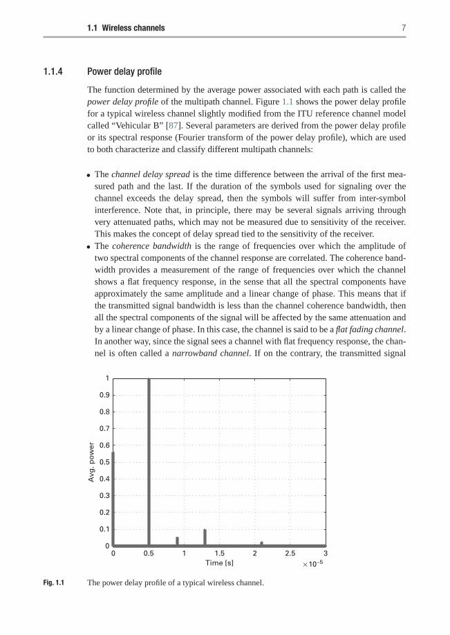
The function determined by the average power associated with each path is called thepower delay profile of the multipath channel. Figure 1.1 shows the power delay profilefor a typical wireless channel slightly modified from the ITU reference channel modelcalled “Vehicular B” [87]. Several parameters are derived from the power delay profileor its spectral response (Fourier transform of the power delay profile), which are usedto both characterize and classify different multipath channels:
• The channel delay spread is the time difference between the arrival of the first mea-sured path and the last. If the duration of the symbols used for signaling over thechannel exceeds the delay spread, then the symbols will suffer from inter-symbolinterference. Note that, in principle, there may be several signals arriving throughvery attenuated paths, which may not be measured due to sensitivity of the receiver.This makes the concept of delay spread tied to the sensitivity of the receiver.
• The coherence bandwidth is the range of frequencies over which the amplitude oftwo spectral components of the channel response are correlated. The coherence band-width provides a measurement of the range of frequencies over which the channelshows a flat frequency response, in the sense that all the spectral components haveapproximately the same amplitude and a linear change of phase. This means that ifthe transmitted signal bandwidth is less than the channel coherence bandwidth, thenall the spectral components of the signal will be affected by the same attenuation andby a linear change of phase. In this case, the channel is said to be a flat fading channel.In another way, since the signal sees a channel with flat frequency response, the chan-nel is often called a narrowband channel. If on the contrary, the transmitted signal
0 0.5 1 1.5 2 2.5 3× 10⁻⁵Time [s]
0
0.1
0.2
0.3
0.4
0.5
0.6
0.7
0.8
0.9
1
Avg
. po
wer
Fig. 1.1 The power delay profile of a typical wireless channel.
8 Introduction
bandwidth is more than the channel coherence bandwidth, then the spectral compo-nents of the signal will be affected by different attenuations. In this case, the channelis said to be a frequency selective channel or a broadband channel.
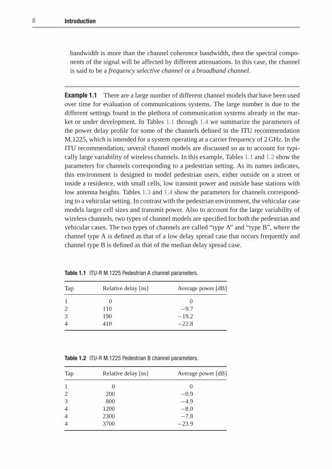
Example 1.1 There are a large number of different channel models that have been usedover time for evaluation of communications systems. The large number is due to thedifferent settings found in the plethora of communication systems already in the mar-ket or under development. In Tables 1.1 through 1.4 we summarize the parameters ofthe power delay profile for some of the channels defined in the ITU recommendationM.1225, which is intended for a system operating at a carrier frequency of 2 GHz. In theITU recommendation, several channel models are discussed so as to account for typi-cally large variability of wireless channels. In this example, Tables 1.1 and 1.2 show theparameters for channels corresponding to a pedestrian setting. As its names indicates,this environment is designed to model pedestrian users, either outside on a street orinside a residence, with small cells, low transmit power and outside base stations withlow antenna heights. Tables 1.3 and 1.4 show the parameters for channels correspond-ing to a vehicular setting. In contrast with the pedestrian environment, the vehicular casemodels larger cell sizes and transmit power. Also to account for the large variability ofwireless channels, two types of channel models are specified for both the pedestrian andvehicular cases. The two types of channels are called “type A” and “type B”, where thechannel type A is defined as that of a low delay spread case that occurs frequently andchannel type B is defined as that of the median delay spread case.
Table 1.1 ITU-R M.1225 Pedestrian A channel parameters.
Tap Relative delay [ns] Average power [dB]
1 0 02 110 −9.73 190 −19.24 410 −22.8
Table 1.2 ITU-R M.1225 Pedestrian B channel parameters.
Tap Relative delay [ns] Average power [dB]
1 0 02 200 −0.93 800 −4.94 1200 −8.04 2300 −7.84 3700 −23.9
1.1 Wireless channels 9
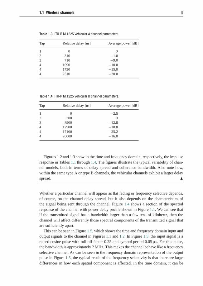
Table 1.3 ITU-R M.1225 Vehicular A channel parameters.
Tap Relative delay [ns] Average power [dB]
1 0 02 310 −1.03 710 −9.04 1090 −10.04 1730 −15.04 2510 −20.0
Table 1.4 ITU-R M.1225 Vehicular B channel parameters.
Tap Relative delay [ns] Average power [dB]
1 0 −2.52 300 03 8900 −12.84 12900 −10.04 17100 −25.24 20000 −16.0
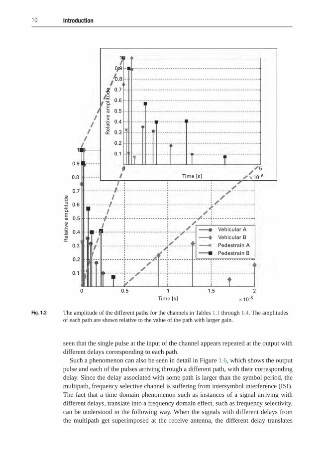
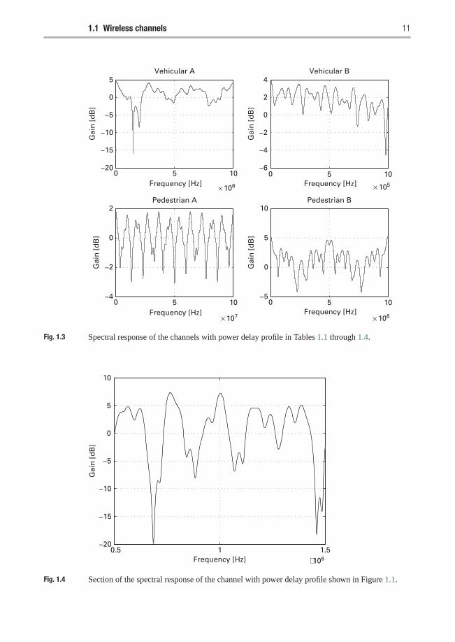
Figures 1.2 and 1.3 show in the time and frequency domain, respectively, the impulseresponse in Tables 1.1 through 1.4. The figures illustrate the typical variability of chan-nel models, both in terms of delay spread and coherence bandwidth. Also note how,within the same type A or type B channels, the vehicular channels exhibit a larger delayspread. �
Whether a particular channel will appear as flat fading or frequency selective depends,of course, on the channel delay spread, but it also depends on the characteristics ofthe signal being sent through the channel. Figure 1.4 shows a section of the spectralresponse of the channel with power delay profile shown in Figure 1.1. We can see thatif the transmitted signal has a bandwidth larger than a few tens of kilohertz, then thechannel will affect differently those spectral components of the transmitted signal thatare sufficiently apart.
This can be seen in Figure 1.5, which shows the time and frequency domain input andoutput signals to the channel in Figures 1.1 and 1.2. In Figure 1.5, the input signal is araised cosine pulse with roll off factor 0.25 and symbol period 0.05 μs. For this pulse,the bandwidth is approximately 2 MHz. This makes the channel behave like a frequencyselective channel. As can be seen in the frequency domain representation of the outputpulse in Figure 1.5, the typical result of the frequency selectivity is that there are largedifferences in how each spatial component is affected. In the time domain, it can be
10 Introduction
Rel
ativ
e am
plit
ud
e
Rel
ativ
e am
plit
ud
e0.9
1
0.8
0.7
0.6
0.5
0.4
0.3
0.2
0.1
0.9
1
0.8
0.7
0.6
0.5
0.4
0.3
0.2
0.1
Time [s]
Time [s]
× 10–6
× 10–5
50
Vehicular A
Vehicular B
Pedestrain B
Pedestrain A
0 0.5 1 1.5 2
Fig. 1.2 The amplitude of the different paths for the channels in Tables 1.1 through 1.4. The amplitudesof each path are shown relative to the value of the path with larger gain.
seen that the single pulse at the input of the channel appears repeated at the output withdifferent delays corresponding to each path.
Such a phenomenon can also be seen in detail in Figure 1.6, which shows the outputpulse and each of the pulses arriving through a different path, with their correspondingdelay. Since the delay associated with some path is larger than the symbol period, themultipath, frequency selective channel is suffering from intersymbol interference (ISI).The fact that a time domain phenomenon such as instances of a signal arriving withdifferent delays, translate into a frequency domain effect, such as frequency selectivity,can be understood in the following way. When the signals with different delays fromthe multipath get superimposed at the receive antenna, the different delay translates
1.1 Wireless channels 11
0 5 10
× 106
−20
−15
−10
−5
0
5Vehicular A
Frequency [Hz]
0 5 10
× 107Frequency [Hz]
0 5 10
× 105Frequency [Hz]
0 5 10
× 106Frequency [Hz]
Gai
n [
dB
]
−6
−4
−2
0
2
4Vehicular B
Gai
n [
dB
]
−4
−2
0
2Pedestrian A
Gai
n [
dB
]
−5
0
5
10Pedestrian B
Gai
n [
dB
]
Fig. 1.3 Spectral response of the channels with power delay profile in Tables 1.1 through 1.4.
0.5 1 1.5−20
−15
−10
−5
0
5
10
Frequency [Hz]
Gai
n [
dB
]
× 106
Fig. 1.4 Section of the spectral response of the channel with power delay profile shown in Figure 1.1.
12 Introduction
−2 −1 0 1 2−0.5
0
0.5
1Input pulse − time domain
Time [s]
Am
plit
ud
e
−0.5
0
0.5
1
Am
plit
ud
e
−4 −2 0 2 40
0.2
0.4
0.6
0.8
1Input pulse − frequency domain
Frequency [Hz]
Gai
n [
dB
]
0 1 2 3 4
Output pulse − time domain Output pulse − frequency domain
× 10–6
Time [s] × 10–5
× 106
−4 −2 0 2 40
0.2
0.4
0.6
0.8
1
Frequency [Hz]
Gai
n [
dB
]
× 106
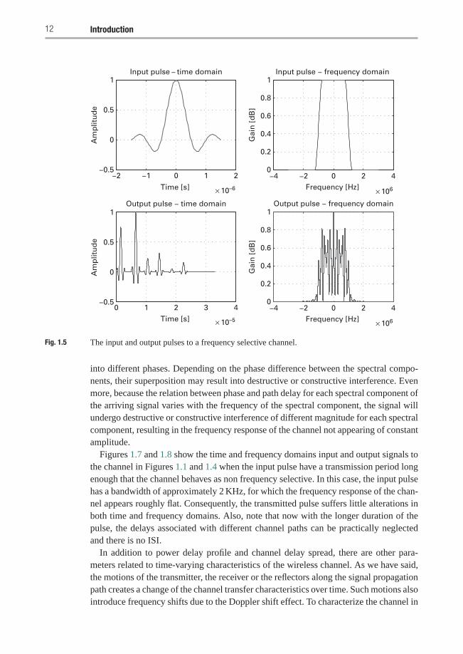
Fig. 1.5 The input and output pulses to a frequency selective channel.
into different phases. Depending on the phase difference between the spectral compo-nents, their superposition may result into destructive or constructive interference. Evenmore, because the relation between phase and path delay for each spectral component ofthe arriving signal varies with the frequency of the spectral component, the signal willundergo destructive or constructive interference of different magnitude for each spectralcomponent, resulting in the frequency response of the channel not appearing of constantamplitude.
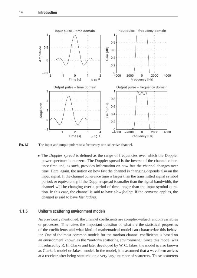
Figures 1.7 and 1.8 show the time and frequency domains input and output signals tothe channel in Figures 1.1 and 1.4 when the input pulse have a transmission period longenough that the channel behaves as non frequency selective. In this case, the input pulsehas a bandwidth of approximately 2 KHz, for which the frequency response of the chan-nel appears roughly flat. Consequently, the transmitted pulse suffers little alterations inboth time and frequency domains. Also, note that now with the longer duration of thepulse, the delays associated with different channel paths can be practically neglectedand there is no ISI.
In addition to power delay profile and channel delay spread, there are other para-meters related to time-varying characteristics of the wireless channel. As we have said,the motions of the transmitter, the receiver or the reflectors along the signal propagationpath creates a change of the channel transfer characteristics over time. Such motions alsointroduce frequency shifts due to the Doppler shift effect. To characterize the channel in
1.1 Wireless channels 13
Am
plit
ud
e
0
0
0
0 0.5 1 1.5 2 2.5 3 3.5
0
−0.5
0
0.5
1
−101
−101
−0.5
0.5
−0.5
0.5
−0.1
0.1
−0.2
0.2
Time [s] × 10–5
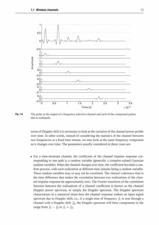
Fig. 1.6 The pulse at the output of a frequency selective channel and each of the component pulsesdue to multipath.
terms of Doppler shift it is necessary to look at the variation of the channel power profileover time. In other words, instead of considering the statistics of the channel betweentwo frequencies at a fixed time instant, we now look at the same frequency componentas it changes over time. The parameters usually considered in these cases are:
• For a time-invariant channel, the coefficient of the channel impulse response cor-responding to one path is a random variable (generally a complex-valued Gaussianrandom variable). When the channel changes over time, the coefficient becomes a ran-dom process, with each realization at different time instants being a random variable.These random variables may or may not be correlated. The channel coherence time isthe time difference that makes the correlation between two realizations of the chan-nel impulse response be approximately zero. The Fourier transform of the correlationfunction between the realizations of a channel coefficient is known as the channelDoppler power spectrum, or simply the Doppler spectrum. The Doppler spectrumcharacterizes in a statistical sense how the channel response widens an input signalspectrum due to Doppler shift, i.e., if a single tone of frequency fc is sent through achannel with a Doppler shift fd, the Doppler spectrum will have components in therange from fc − fd to fc + fd.
14 Introduction
−2 −1 0 1 2−0.5
0
0.5
1Input pulse − time domain
Time [s]
Am
plit
ud
e
−4000 −2000 0 2000 40000
0.2
0.4
0.6
0.8
1Input pulse − frequency domain
Frequency [Hz]
Gai
n [
dB
]
−4000 −2000 0 2000 40000
0.2
0.4
0.6
0.8
1Output pulse − frequency domain
Frequency [Hz]
Gai
n [
dB
]
0 1 2 3 4−1
0
1
2
3Output pulse − time domain
Time [s]
Am
plit
ud
e
× 10–3
× 10–3
Fig. 1.7 The input and output pulses to a frequency non-selective channel.
• The Doppler spread is defined as the range of frequencies over which the Dopplerpower spectrum is nonzero. The Doppler spread is the inverse of the channel coher-ence time and, as such, provides information on how fast the channel changes overtime. Here, again, the notion on how fast the channel is changing depends also on theinput signal. If the channel coherence time is larger than the transmitted signal symbolperiod; or equivalently, if the Doppler spread is smaller than the signal bandwidth, thechannel will be changing over a period of time longer than the input symbol dura-tion. In this case, the channel is said to have slow fading. If the converse applies, thechannel is said to have fast fading.
1.1.5 Uniform scattering environment models
As previously mentioned, the channel coefficients are complex-valued random variablesor processes. This raises the important question of what are the statistical propertiesof the coefficients and what kind of mathematical model can characterize this behav-ior. One of the most common models for the random channel coefficients is based onan environment known as the “uniform scattering environment.” Since this model wasintroduced by R. H. Clarke and later developed by W. C. Jakes, the model is also knownas Clarke’s model or Jakes’ model. In the model, it is assumed that a waveform arrivesat a receiver after being scattered on a very large number of scatterers. These scatterers
1.1 Wireless channels 15
Am
plitu
de
Time [s]
0
0
0
0
01
01
−1
1
0
2
3
−1
−1
−0.5
0.5
−0.5
0.5
−0.1
0.1
−0.2
0.2
0 0.5 1 1.5 2 2.5 3 3.5
× 10–3
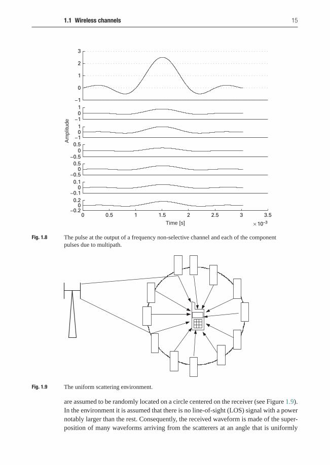
Fig. 1.8 The pulse at the output of a frequency non-selective channel and each of the componentpulses due to multipath.
Fig. 1.9 The uniform scattering environment.
are assumed to be randomly located on a circle centered on the receiver (see Figure 1.9).In the environment it is assumed that there is no line-of-sight (LOS) signal with a powernotably larger than the rest. Consequently, the received waveform is made of the super-position of many waveforms arriving from the scatterers at an angle that is uniformly
16 Introduction
distributed between 0 and 2π . For the purpose of this study, let us first introduce thecomplex baseband representation of the transmitted bandpass signals s(t),
s(t) = �{
x(t)ej2π fct},
where fc is the carrier frequency. Expanding this expression, we get
s(t) = �{x(t)} cos (2π fct)+ �{x(t)} sin (2π fct)
= sI(t) cos (2π fct)+ sQ(t) sin (2π fct),
where sI(t) and sQ(t) are the in-phase and quadrature components of s(t), respectively.When this signal is transmitted through a channel with baseband impulse response h(t),the resulting received signal is
y(t) = �{(
x(t) ∗ h(t))ej2π fct
}.
If the channel has L paths, with path n having amplitude hn(t), an associated delayτn(t), and a Doppler phase shift ϕn (which accounts for the Doppler shift due to themotion of the receiver of each received wave), the received signal can be written as
y(t) = �{ L∑
n=1
hn(t)x(t − τn(t)
)ej [2π fc(t−τn(t))+ϕn]
}.
If, for the purpose of this characterization, we assume that the transmitted signal isa single tone with the same frequency as the carrier frequency, the received signalbecomes
y(t) = �{ L∑
n=1
[hn(t)e
−j(2π fcτn(t)−ϕn)]ej2π fct
}= yI(t) cos (2π fct)+ yQ(t) sin (2π fct), (1.8)
where
yI(t) =L∑
n=1
hn(t) cos (2π fcτn(t)− ϕn), (1.9)
yQ(t) =L∑
n=1
hn(t) sin (2π fcτn(t)− ϕn). (1.10)
This result shows that both the in-phase and the quadrature components of the receivedsignal are actually composed of the superposition of multiple copies of the signal arriv-ing with a change of amplitude and phase as determined by the characteristics of eachof the channel paths.
Next, as part of the settings associated with the uniform scattering environment, weassume that all the received signals arrive with the same amplitude. This is a reasonableassumption because, given the geometry of the uniform scattering environment, in theabsence of a direct LOS path, each signal arriving at the receiver would experience sim-ilar attenuations. Furthermore, in the uniform scattering environment, it is reasonable
1.1 Wireless channels 17
to assume that the number of paths L is very large. Therefore, resorting to the CentralLimit Theorem, it follows that each coefficient can be modeled as a circularly symmetriccomplex Gaussian random variable with zero mean (i.e., as a random variable made oftwo quadrature components, with each component being a zero mean Gaussian randomvariable with the same variance as the other component σ 2). We denote this observationas yI ∼ N (0, σ 2), yQ ∼ N (0, σ 2).
To better understand the channel behavior, it is important to find the statistics (interms of probability density function (pdf)) of the envelope and phase of the channelcoefficients. To get this, it is necessary to consider the transformation of those randomvariables representing a channel coefficient in Cartesian coordinates into those repre-senting the coefficient in polar coordinates. This means that, if we write the coefficientas h = hI+jhQ (hI and hQ represent the in-phase and the quadrature phase components,respectively), we want to find the pdf of the random variables r and θ , obtained throughthe transformations
r =√
h2I + h2
Q,
θ = arctan(hQ/hI), (1.11)
which represent a channel coefficient as h = r ejθ . Equivalently, we may consider theinverse transform
hI = r cos θ,
hQ = r sin θ. (1.12)
For the general case of transforming random variables V = t1(X, Y ) and W =t2(X, Y ), the transformation of the joint pdf fX,Y of the random variables X and Yinto the joint pdf fV,W of the random variables V and W , is given by the expression[112]
fV,W (v,w) = fX,Y(s1(v,w), s2(v,w)
)|J (x, y)| ,
J (x, y) = det
[∂v∂x
∂v∂y
∂w∂x
∂w∂y
],
where J (x, y) is the Jacobian of the transformation and where x = s1(v,w) and y =s2(v,w) are the inverse transformations of t1 and t2, respectively. Applying this relationto the transformation (1.12) results in the Jacobian J (r, θ) = r/σ 2, which leads to thejoint pdf
f (r, θ) = r
2πσ 2e−r2/(2σ 2), r ≥ 0, 0 ≤ θ ≤ 2π,
18 Introduction
where we have used for easier readability a slightly modified notation for the pdf. Fromthe joint pdf it is possible to find the marginal pdfs
f (r) =∫ 2π
0f (r, θ)dθ = r
σ 2e−r2/(2σ 2), r ≥ 0,
f (θ) =∫ ∞
0f (r, θ)dr = 1
2π, 0 ≤ θ ≤ 2π.
This result shows that the magnitude of the channel coefficients is a random variablewith a Rayleigh distribution and the phase is also a random variable with a uniformdistribution in the range [0, 2π ]. Because the magnitude of the channel coefficientsfollow a Rayleigh distribution, this model is frequently called a Rayleigh fading model.
Also, for the case of two nonnegative random variables related by the transformationY = X2, using similar random variables transformation techniques yields the relationbetween pdfs
fY (y) = fX (x)
dy/dx.
With this relation it can be shown that a random variable X that is defined as thesquared magnitude of a Rayleigh-distributed channel coefficient (X = |h|2) followsan exponential distribution, with pdf
fX (x) = 1
σ 2e−x/σ 2
, x ≥ 0. (1.13)
In addition, the sum of the squared magnitude of channel coefficient,∑
i |hi |2, whereeach is the sum of two real i.i.d. Gaussian random variables representing the in-phaseand quadrature components (i.e., hi = hIi + jhQi ), results in a Chi-square randomvariable with 2L (L being the number of channel coefficients in the sum) degrees offreedom. The pdf of this distribution is
f (x) = x L−1
(L − 1)!e−x , x ≥ 0. (1.14)
To consider the statistics of the received signal and the channel as they change overtime, the two most important results are the time correlation and its Fourier transform,the power spectral density (PSD). Using as a starting point (1.8), (1.9), and (1.10), thetime correlation of the received signal is
Cy(τ ) = E[y(t)y(t + τ)]= CyI(τ ) cos(2π fcτ)+ CyI,yQ(τ ) sin(2π fcτ), (1.15)
where E[·] is the expectation operator. The autocorrelation of yI , CyI(τ ) equals
CyI(τ ) = E[yI(t)yI(t + τ)].Considering the expression for yI(t) in (1.9), the magnitude of the Doppler phase shift,ϕn , depends on the velocity of the receiver relative to the scatterer from where the wavecomes from. This relative velocity is equal to v cosαk , where v is the absolute velocity
1.1 Wireless channels 19
of the receiver. If we denote the angle associated with the k-th wave as αk , the Dopplershift for waveform k equals
ϕk = 2πv
λt cosαk = 2π fDt cosαk,
where λ is the wavelength and fD = v/λ is the Doppler frequency. Now we can write(1.9) as
yI(t) =L∑
n=1
hn(t) cos (2π fcτn(t)− 2πv
λt cosαn). (1.16)
In the uniform scattering environment the phase 2π fcτn(t) changes more rapidly thanthe Doppler phase shift. In addition, since the distance from the scatterers to the mobileis much larger than the signal wavelength, it is possible to assume that the angle asso-ciated with the k-th wave, αk , is a random variable uniformly distributed in [0, 2π ]and independent of the angle associated with other paths. Under these conditions, theautocorrelation of yI, CyI(τ ) equals
CyI(τ ) =Pr
2π
∫ 2π
0cos(πvτ cosα/λ)dα
= Pr J0(2π fcvτ/c),
where c is the speed of light, Pr is the received power, and J0(·) is the Bessel functionof the first kind and zeroth order, defined as
J0(x) = 1
π
∫ π
0e−jx cos θdθ.
Using similar reasoning, the cross-correlation between the in-phase and quadraturecomponents of the received signal, CyI,yQ(τ ), can be found to equal zero. Therefore,using (1.15), the time correlation of the received signal is
Cy(τ ) = Pr J0(2π fcvτ/c) cos(2π fcτ). (1.17)
In this result, the cos(2π fcτ) component indicates the correlation of the received signalto a complete period shift due to being a single tone of frequency fc. Taking the Fouriertransform of (1.17) yields the power spectral density of the received signal
Sy( f ) =⎧⎨⎩
Pr4π fD
1√1−( | f− fc |
fD
)2if | f − fc| ≤ fD
0 else.(1.18)
Note here that the frequency shift f − fc is a consequence of the cos(2π fcτ) componentin (1.17) and the frequency shift property of Fourier transforms. Since the input signalis a single tone, ignoring the frequency shift in the power spectral density of the channeleffects, which consequently has a time correlation equal to
Ch(τ ) = Pr J0(2π fcvτ/c). (1.19)
20 Introduction
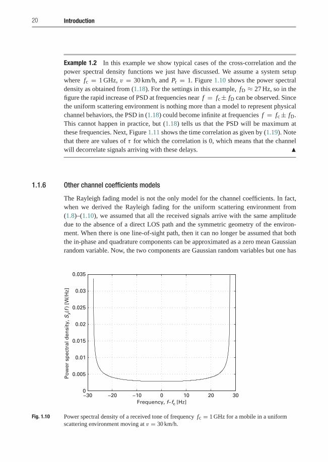
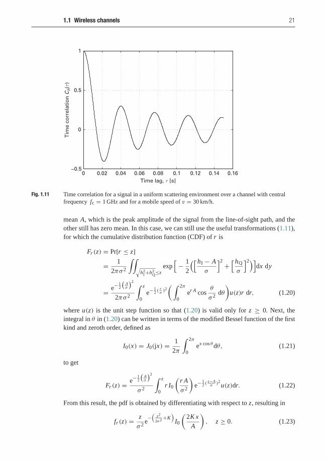
Example 1.2 In this example we show typical cases of the cross-correlation and thepower spectral density functions we just have discussed. We assume a system setupwhere fc = 1 GHz, v = 30 km/h, and Pr = 1. Figure 1.10 shows the power spectraldensity as obtained from (1.18). For the settings in this example, fD ≈ 27 Hz, so in thefigure the rapid increase of PSD at frequencies near f = fc± fD can be observed. Sincethe uniform scattering environment is nothing more than a model to represent physicalchannel behaviors, the PSD in (1.18) could become infinite at frequencies f = fc± fD.This cannot happen in practice, but (1.18) tells us that the PSD will be maximum atthese frequencies. Next, Figure 1.11 shows the time correlation as given by (1.19). Notethat there are values of τ for which the correlation is 0, which means that the channelwill decorrelate signals arriving with these delays. �
1.1.6 Other channel coefficients models
The Rayleigh fading model is not the only model for the channel coefficients. In fact,when we derived the Rayleigh fading for the uniform scattering environment from(1.8)–(1.10), we assumed that all the received signals arrive with the same amplitudedue to the absence of a direct LOS path and the symmetric geometry of the environ-ment. When there is one line-of-sight path, then it can no longer be assumed that boththe in-phase and quadrature components can be approximated as a zero mean Gaussianrandom variable. Now, the two components are Gaussian random variables but one has
−30 −20 −10 0 10 20 300
0.005
0.01
0.015
0.02
0.025
0.03
0.035
Frequency, f−fc [Hz]
Po
wer
sp
ectr
al d
ensi
ty, S
y(f )
[W
/Hz]
Fig. 1.10 Power spectral density of a received tone of frequency fc = 1 GHz for a mobile in a uniformscattering environment moving at v = 30 km/h.
1.1 Wireless channels 21
0 0.02 0.04 0.06 0.08 0.1 0.12 0.14 0.16−0.5
0
0.5
1
Time lag, τ [s]
Tim
e co
rrel
atio
n C
h(τ
)
Fig. 1.11 Time correlation for a signal in a uniform scattering environment over a channel with centralfrequency fc = 1 GHz and for a mobile speed of v = 30 km/h.
mean A, which is the peak amplitude of the signal from the line-of-sight path, and theother still has zero mean. In this case, we can still use the useful transformations (1.11),for which the cumulative distribution function (CDF) of r is
Fr (z) = Pr[r ≤ z]= 1
2πσ 2
∫∫√
h2I+h2
Q≤zexp[− 1
2
([hI − A
σ
]2 + [hQ
σ
]2)]dx dy
= e−12
(Aσ
)22πσ 2
∫ z
0e−
12 (
rσ)2(∫ 2π
0er A cos
θ
σ 2dθ
)u(z)r dr, (1.20)
where u(z) is the unit step function so that (1.20) is valid only for z ≥ 0. Next, theintegral in θ in (1.20) can be written in terms of the modified Bessel function of the firstkind and zeroth order, defined as
I0(x) = J0(jx) = 1
2π
∫ 2π
0ex cos θdθ, (1.21)
to get
Fr (z) = e−12
(Aσ
)2σ 2
∫ z
0r I0
(r A
σ 2
)e−
12 (
z−Aσ)2u(z)dr. (1.22)
From this result, the pdf is obtained by differentiating with respect to z, resulting in
fr (z) = z
σ 2e−(
z2
2σ2+K)I0
(2K x
A
), z ≥ 0. (1.23)
22 Introduction
0 0.5 1 1.5 2 2.5 3 3.5 40
0.2
0.4
0.6
0.8
1
1.2
1.4RayleighExponentialRice, K = 1.5Rice, K = 0.5Nakagami, m = 2Nakagami, m = 0.75Chi-square, L = 2
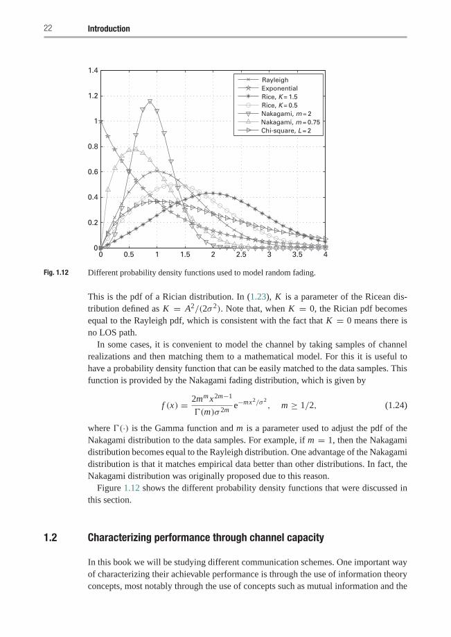
Fig. 1.12 Different probability density functions used to model random fading.
This is the pdf of a Rician distribution. In (1.23), K is a parameter of the Ricean dis-tribution defined as K = A2/(2σ 2). Note that, when K = 0, the Rician pdf becomesequal to the Rayleigh pdf, which is consistent with the fact that K = 0 means there isno LOS path.
In some cases, it is convenient to model the channel by taking samples of channelrealizations and then matching them to a mathematical model. For this it is useful tohave a probability density function that can be easily matched to the data samples. Thisfunction is provided by the Nakagami fading distribution, which is given by
f (x) = 2mm x2m−1
�(m)σ 2me−mx2/σ 2
, m ≥ 1/2, (1.24)
where �(·) is the Gamma function and m is a parameter used to adjust the pdf of theNakagami distribution to the data samples. For example, if m = 1, then the Nakagamidistribution becomes equal to the Rayleigh distribution. One advantage of the Nakagamidistribution is that it matches empirical data better than other distributions. In fact, theNakagami distribution was originally proposed due to this reason.
Figure 1.12 shows the different probability density functions that were discussed inthis section.
1.2 Characterizing performance through channel capacity
In this book we will be studying different communication schemes. One important wayof characterizing their achievable performance is through the use of information theoryconcepts, most notably through the use of concepts such as mutual information and the
1.2 Characterizing performance through channel capacity 23
characterization of performance limits through system capacity. At its core, informationtheory deals with the information provided by the outcome of a random variable. Theinformation provided by the outcome x of a discrete random variable X is defined as
IX (x) = log1
Pr[X = x] = − log Pr[X = x], (1.25)
where Pr[X = x] is the probability of the outcome X = x and the logarithm can be,in principle, of any base but is most frequently taken with base 2, followed by base ein some fewer cases. Intuitively, the rarer an event is, the more information it provides.Since the communication process is inherently a process relating more than one randomvariable (e.g. the input and output of a channel, an uncompressed and a compressedrepresentation of a signal, etc.), it is also important to define a magnitude relating theinformation shared by two random variables. This magnitude is the mutual information,which for two discrete random variables X and Y is defined as
I (X; Y ) =∑x∈X
∑y∈Y
Pr[X = x, Y = y] logPr[X = x, Y = y]
Pr[X = x]Pr[Y = y] ,
where Pr[X = x, Y = y] is the joint probability mass function and Pr[X = x] andPr[Y = y] are marginal probability mass functions. Following Bayes theorem (Pr[X =x, Y = y] = Pr[X = x |Y = y]Pr[Y = y], with Pr[X = x |Y = y] being the conditionalprobability mass function of X given that Y = y), the mutual information can also bewritten as
I (X; Y ) =∑x∈X
∑y∈Y
Pr[X = x, Y = y] logPr[X = x |Y = y]
Pr[X = x] .
Furthermore, we can write
I (X; Y ) = −∑x∈X
log Pr[X = x]∑y∈Y
Pr[X = x, Y = y]
+∑x∈X
∑y∈Y
Pr[X = x, Y = y] log Pr[X = x |Y = y]
= −∑x∈X
Pr[X = x] log Pr[X = x]
+∑x∈X
∑y∈Y
Pr[X = x, Y = y] log Pr[X = x |Y = y]. (1.26)
The first term in this result is called the entropy of the random variable X ,
H(X) = −∑x∈X
Pr[X = x] log Pr[X = x],
and the second term can be written in terms of the conditional entropy of X ,
H(X |Y ) = −∑x∈X
Pr[X = x, Y = y] log Pr[X = x |Y = y].
Considering (1.25), the entropy of the random variable can also be read as the meanvalue of the information provided by all its outcomes. Likewise, the conditional entropy
24 Introduction
can be regarded as the mean value of the information provided by all the outcomesof a random variable (X ) given than the outcome of a second random variable (Y ) isknown, or how much uncertainty about a random variable (X ) remains after knowingthe outcome of a second random variable (Y ). Therefore, the mutual information as in(1.26) can now be written as
I (X; Y ) = H(X)− H(X |Y ),
and intuitively be interpreted as the mean amount of uncertainty about one randomvariable (X ) that is resolved after learning about the outcome of another random variable(Y ), or the average amount of information shared by the two random variables. Finally,we note here that although the concepts we have been introducing were tailored todiscrete random variables, the same concepts apply to continuous random variableswith the only differences that the sums are replaced by integrals and the probabilitymass functions by probability density functions.
In information theory, one of the main measures of performance is system capacity.Nevertheless, due to the fact that the calculation of capacity always involves a numberof assumptions and simplifications, the measurement of capacity does not come in a“one size fits all” solution. In particular, the notion of capacity is influenced by howmuch the channel changes over the duration of a coding interval and the properties ofthe random process associated with the channel fluctuations.
When the random variations of the channel are a stationary and ergodic process it ispossible to consider the traditional notion of capacity as introduced by Claude Shan-non [181]. In this case, coding is assumed to be done using arbitrary long blocks. Also,the random process driving the channel changes needs to be stationary and ergodic.Because of this, this notion of capacity is known as ergodic capacity or Shannon capac-ity. The capacity of an AWGN channel with fast flat fading, when only the receiver hasknowledge of the channel state,
C = E[
log(1+ |h|
2 P
N0
)], (1.27)
where E[·] is the expectation operator (operating on the random channel attenuation), Pis the power of the transmitted signal (assumed i.i.d. Gaussian, with zero mean so as toachieve capacity), N0 is the variance of the background noise, and |h|2 is the envelopeof the channel attenuation.
Although the notion of Shannon capacity is quite useful, there are also many designsettings where the assumptions of using arbitrary long codes or that the channel is a sta-tionary and ergodic random process do not hold. In these cases, Shannon capacity maynot yield useful results. For example, in the case of a non-ergodic slowly fading channelfollowing a Rayleigh distribution, the Shannon capacity is arbitrary small or zero. Thisis because the result is affected by those realizations of the channel corresponding todeep fades. Nevertheless, an arbitrary small capacity is not the true depiction of manyrealizations of the fading process (which is confirmed by the many communicationstaking place every day under these conditions!). Therefore, for these cases it is more
1.3 Orthogonal frequency division multiplexing (OFDM) 25
appropriate to consider the notion of outage capacity. This notion is tied to the conceptof an outage event.
There are many ways of defining an outage event but, from an information theorypoint of view, an outage event is defined as the set of channel realizations that cannotsupport reliable transmission at a rate R. In other words, the outage event is the set ofchannel realizations with an associated capacity less than a transmit rate R. Consideringnow that the setup that led to (1.27) corresponds to a non-ergodic channel, the outagecondition for a realization of the fading can be written as
log(1+ |h|
2 P
N0
)< R. (1.28)
From here, the outage probability is calculated as the one associated with the outageevent,
Pout = Pr[
log(1+ |h|
2 P
N0
)< R
], (1.29)
where Pr[·] is the probability operator (once again on the random channel attenuation).Once we have introduced the concepts of outage event and outage probability,
the Prout outage capacity, Cout, is defied as the information rate that can be reliablycommunicated with a probability 1− Prout, that is
Pr[C ≤ Cout
]= Prout, (1.30)
where C is the Shannon capacity associated with the channel.We finally note here that, as mentioned above, the outage probability may be defined
differently from (1.29). Another way of defining the outage probability is by consideringthe event that the received signal to noise ratio is below a threshold. This definition canbe related to (1.29) by simple algebraic operations that expose the received signal-to-noise ratio as the random variable, i.e., for the signal-to-noise ratio (SNR) γ and SNRthreshold γT,
Pout = Pr[γ < 2R − 1
]= Pr[γ < γT].
1.3 Orthogonal frequency division multiplexing (OFDM)
In Section 1.1.3 we discussed that when the signal bandwidth is much larger than thechannel coherence bandwidth, the channel is frequency selective. We also explained thatthese channels present such impairments as intersymbol interference, which deform theshape of the transmitted pulse, risking the introduction of detection errors at the receiver.This impairment can be addressed with different techniques. One of these techniques ismulticarrier modulation. In multicarrier modulation, the high bandwidth signal to betransmitted is divided over multiple mutually orthogonal signals of a bandwidth smallenough such that the channel appears to be non-frequency selective. Different multicar-rier modulation techniques may differ based on the choice of orthogonal signals. Among
26 Introduction
the many possible multicarrier modulation techniques, orthogonal frequency divisionmultiplexing (OFDM) is the one that has gained more acceptance as the modulationtechnique for high-speed wireless networks and 4G mobile broadband standards. InOFDM, the orthogonal signals used for multicarrier modulation are truncated complexexponentials. Assume an OFDM transmitter where the high rate serial input stream issplit into N parallel substreams. Assume also that, at some instant of time, the sequence{dk}N−1
k=0 represents the N complex symbols that are input to the OFDM modulator fortransmission as a single OFDM symbol of duration Ts. This translates in practice into anoperation where the input stream to the OFDM modulator is divided and organized intoblocks of N symbols, which are modulated into a single OFDM symbol. The resultingOFDM modulated symbol is, for 0 ≤ t ≤ Ts,
s(t) =N−1∑k=0
dkφk(t) =N−1∑k=0
dkej2π fk t , (1.31)
where fk = f0 + k� f and � f = 1/Ts. In (1.31) the signals φk(t), which are definedas
φk(t) ={
ej2π fk t if 0 ≤ t ≤ Ts
0 else,(1.32)
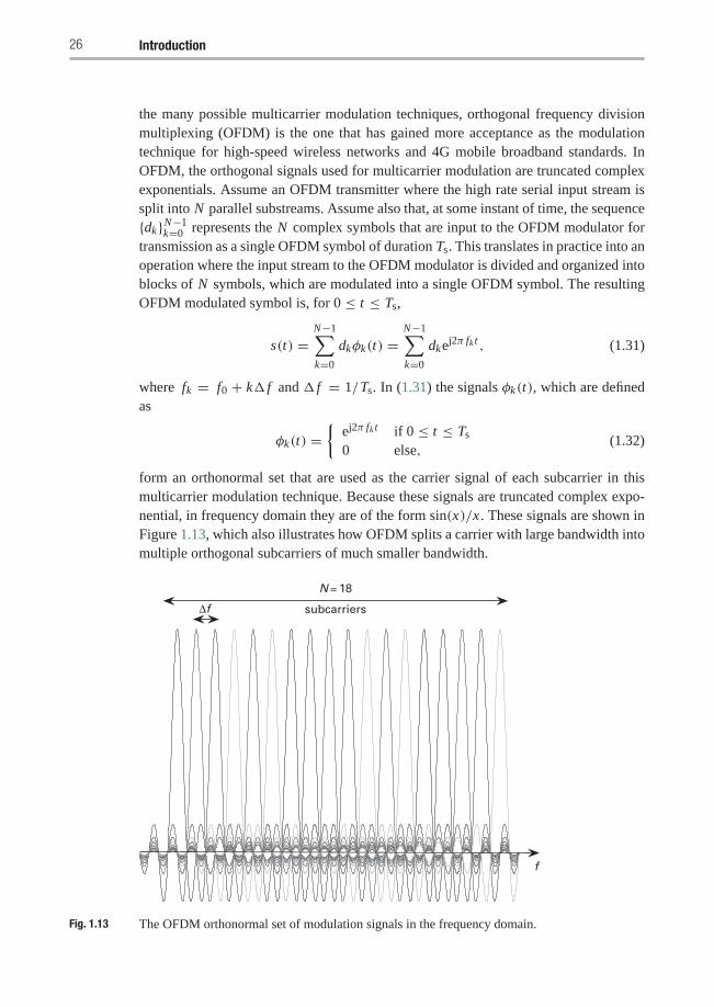
form an orthonormal set that are used as the carrier signal of each subcarrier in thismulticarrier modulation technique. Because these signals are truncated complex expo-nential, in frequency domain they are of the form sin(x)/x . These signals are shown inFigure 1.13, which also illustrates how OFDM splits a carrier with large bandwidth intomultiple orthogonal subcarriers of much smaller bandwidth.
N = 18
subcarriersΔf
f
Fig. 1.13 The OFDM orthonormal set of modulation signals in the frequency domain.
1.3 Orthogonal frequency division multiplexing (OFDM) 27
Assume, next, that the OFDM symbol in (1.31) is sampled with a period Tsa = Ts/N .Then, we can write the resulting sampled signal s[n] as
s[n] = s(nTsa) =N−1∑k=0
dkej2π fknTs/N , 0 ≤ n ≤ N − 1.
If we assume, without loss of generality, that f0 = 0 we get fk = k� f = k/Ts,leading to
s[n] =N−1∑k=0
dkej2πnk/N . (1.33)
This result can be read as s[n] being the inverse Fourier transform of dk , which is asimple way of generating an OFDM symbol and one of its main advantages.
In practice, the OFDM symbol as defined in (1.33) is extended with the addition of acyclic prefix. To understand the construction of the prefix, assume a multipath channelwith L taps defined through the coefficients h[0], h[1], . . . , h[L−1]. With this in mind,the original channel input sequence s[0], s[1], . . . , s[N−L], s[N−L+1], . . . , s[N−1],becomes s[N−L+1], . . . , s[N−1], s[0], s[1], . . . s[N−L], s[N−L+1], . . . , s[N−1]after adding the cyclic prefix. Note that the prefix is built by just copying the last L − 1elements of the original channel input sequence at the beginning of it. This operationdoes not affect the OFDM signal or its properties, such as the orthogonality betweenthe multicarrier modulated signals, because it is simply a reaffirmation of the periodic-ity of the OFDM symbol (period equal to N ), as follows from (1.33). Also note that,following the assumption of a multipath channel with delay spread L , the samples cor-responding to the cyclic prefix will be affected by intersymbol interference from theprevious OFDM symbol. To combat this interference, the prefix can be eliminated atthe receiver without any loss of information in the original sequence and without inter-symbol interference affecting the original sequence. Next, let us illustrate the effect ofadding the cyclic prefix on transforming a frequency selective fading channel into a setof parallel flat fading channels.
Let us call the channel input sequence, after adding the cyclic prefix, as x where
x = [s[N − L + 1], . . . , s[N − 1], s[0], s[1], . . . , s[N − L] ,s[N − L + 1], . . . , s[N − 1]] . (1.34)
The output of the channel can be written as
y[n] =L−1∑l=0
h[l]x[n − l] + v[n], n = 1, 2, . . . , N + L − 1, (1.35)
where v[n] is additive white Gaussian noise.The multipath channel affects the first L − 1 symbols and therefore the receiver
ignores these symbol. The received sequence is then given by
y = [y[L], y[L + 1], . . . , y[N + L − 1]] . (1.36)
28 Introduction
Equivalently, one can write the received signal in terms of the original channel input as
y[n] =L−1∑l=0
h[l]s [(n − l − L)modN ]+ v[n]. (1.37)
This can be also written in terms of cyclic convolution as follows:
y = h⊗ s+ v, (1.38)
where ⊗ denotes cyclic convolution. At the receiver, after taking the discrete Fouriertransform (DFT) of the received signal and after removing the cyclic prefix, we get
Yn = Hn Sn + Vn, (1.39)
where Yn , Hn , Sn , and Vn are the n-th point of the N -point DFT of the received signal,channel response, channel input, and noise vector, respectively.
From (1.39), at the receiver side the frequency selective fading channel has beentransformed to a set of parallel flat fading channels. Therefore, one can see the benefitof OFDM and how it reduces the complexities associated with time equalization.
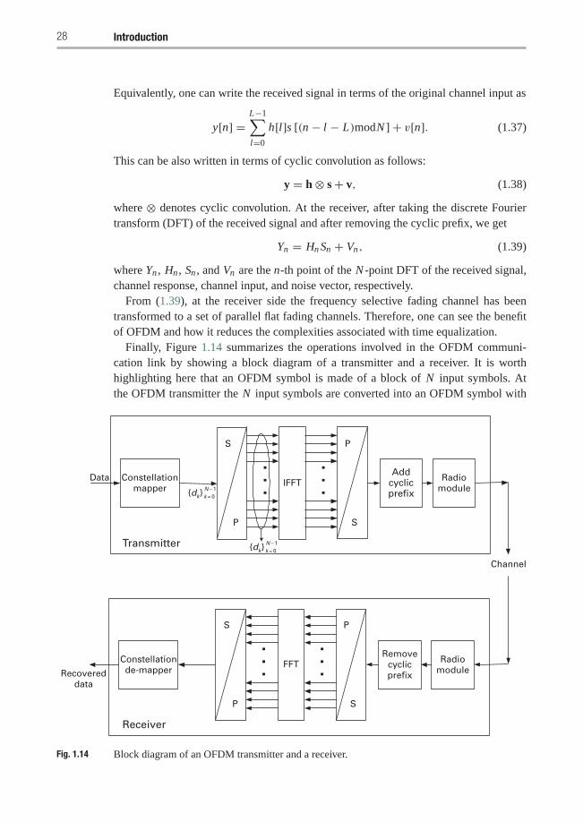
Finally, Figure 1.14 summarizes the operations involved in the OFDM communi-cation link by showing a block diagram of a transmitter and a receiver. It is worthhighlighting here that an OFDM symbol is made of a block of N input symbols. Atthe OFDM transmitter the N input symbols are converted into an OFDM symbol with
Constellationmapper {dk
} k = 0N – 1
{dk } k = 0
N – 1
S
P
Data
. . . IFFT
. . .
S
P
Addcyclicprefix
Radiomodule
Channel
Transmitter
Constellationde-mapper
S
P
. . . FFT
. . .
S
P
Removecyclicprefix
Radiomodule
Receiver
Recovereddata
Fig. 1.14 Block diagram of an OFDM transmitter and a receiver.
1.4 Diversity in wireless channels 29
N subcarriers. If we now consider the successive transmission of several OFDM sym-bols, the data organization on the channel can be conceptually pictured as a grid in afrequency × time plane with a width of N subcarriers (in the frequency dimension) anda depth equal to the number of transmitted OFDM symbols (in the time dimension).
1.4 Diversity in wireless channels
As we have explained, fading wireless channels present the challenge of being chang-ing over time. In communication systems designed around a single signal path betweensource and destination, a crippling fade on this path is a likely event that needs to beaddressed with such techniques as increasing the error correcting capability of the chan-nel coding block, reducing the transmission rate, using more elaborate detectors, etc.Nevertheless, these solutions may still fall short for many practical channel realizations.
Viewing the problem of communication through a fading channel with a differentperspective, the overall reliability of the link can be significantly improved by provid-ing more than one signal path between source and destination, each exhibiting a fadingprocess as much independent from the others as possible. In this way, the chance thatthere is at least one sufficiently strong path is improved. Those techniques that aim atproviding multiple, ideally independent, signal paths are collectively known as diver-sity techniques. In its simplest form, akin to repetition coding (where signal redundancyis achieved by simply repeating the signal symbols multiple times), the multiple pathsmay carry multiple distorted copies of the original message. Nevertheless, better perfor-mance may be achieved by applying some kind of coding across the signals sent overthe multiple paths and by combining in a constructive way the signals received throughthe multiple paths.
Also important is the processing performed at the receiver, where the signals arrivingthrough the multiple paths are constructively combined. The goal in combining is toprocess the multiple received signals so as to obtain a resulting signal of better qualityor with better probability of successful reception than each of the received ones. Thenature of the processing that is applied to each signal during combining is a functionof the particular design goals. If the goal is to linearly combine the signals so thatthe signal-to-noise ratio (SNR) is maximized at the resulting signal, then the resultingmechanism is called a maximal ratio combiner (MRC). Suppose that at the input ofthe MRC there are L signal samples, y0, y1, . . . , yL−1, that are to be combined into asignal sample yM . Each of the received signals correspond to a unit-energy transmitedsignal that have been received through the corresponding L different paths characterizedas h0ejφ0 , h1ejφ1 , . . . , hL−1ejφL−1 . Since the MRC is a linear combiner, the input andoutput are related through the relation
yM =L−1∑k=0
cke−jφk yk, (1.40)
30 Introduction
where ck are the coefficients of the MRC combiner and the complex exponential is usedfor equalizing the phases of each term (cophasing). Assuming that the signals to becombined are equally affected by noise at the receiver with power density N0, the SNRat the output of the MRC, γM is
γM =
(L−1∑k=0
ckhk
)2
N0
L−1∑k=0
c2k
, (1.41)
because the noise is also processed as part of the received signal samples. The MRCcoefficients that maximize (1.41) also maximize its numerator. Then, the maximizingcoefficients can be found by using the Cauchy–Schwarz inequality,(
L−1∑k=0
ckhk
)2
≤(
L−1∑k=0
c2k
)(L−1∑k=0
h2k
). (1.42)
The SNR in (1.41) is maximized when (1.42) is an equality. This is achieved by letting
ck = hk√N0.
The resulting maximized SNR at the output of the MRC is
γM =
(L−1∑k=0
h2k
)N0
. (1.43)
Intuitively, the MRC combines multiple signals by first cophasing them, followed byweighting each sample proportionally to the corresponding path SNR and finally addingthem. The resulting signal at the output of the MRC will have an SNR equal to the sumof the SNRs corresponding to each path.
As mentioned earlier, the MRC is not the only known combiner. Other cases arethe selection combiner, where the output is the input with best SNR, and the thresholdcombiner, which sequentially scans the received signals and outputs the first one withSNR exceeding a threshold.
For any diversity technique, the performance improvement is manifested by thecommunication error probability decreasing at a much larger rate at a high channelsignal-to-noise ratio (SNR) than systems with less or no diversity. When using log–logscales, this rate of decrease in the communication error probability becomes the slopeof the line representing the communication error probability at high SNR and is knownas the diversity gain. Strictly speaking, the diversity gain is defined as [239]
m = − limγ→∞
log PSER
log γ, (1.44)
where γ is the SNR and PSER is the probability of symbol error (a function of theSNR). This definition establishes an implicit behavior at high SNR for the probability
1.4 Diversity in wireless channels 31
of symbol error as being a linear function of the SNR when seen in a plot with log–logscales. Then it can be seen that, as previously stated, in these conditions the diversitygain is the slope of the linear relation. It is better to have as large a diversity gain aspossible, since it means that the probability of symbol error is reduced at a faster rate.
For MIMO systems, as will be shown in Chapters 2 and 3, it is possible to achieve adiversity gain equal to the product between the number of transmit and receive antennas.Also, it is important to note that, depending on the particular diversity scheme andthe system setup, other measures of probability of error can be used. For example, theoutage probability is used in some cases, instead of the probability of symbol error.
There are many different forms of diversity in addition to the spatial diversity men-tioned above. For example, in time diversity, multiple (possibly coded) copies of asymbol are sent at different time instants, and in frequency diversity, multiple (pos-sibly coded) copies of a symbol are sent through channels of different carrier frequency.Furthermore, multiple diversity techniques can be combined to provide even greater per-formance improvement. Next, a succinct introduction to time, frequency, and antennadiversity systems is provided. Some of the following chapters will consider techniquesthat are derived from or that combine these forms of diversity.
1.4.1 Time diversity
It is quite common to find communication scenarios where the channel coherence timeequals or exceeds several symbol transmission periods. This implies that two symbolstransmitted with a separation in time longer than the coherence time will experiencechannel realizations that are highly uncorrelated and can be used to obtain diversity.The simplest way to achieve this is to form the two symbols by using a repetition codingscheme. Also, to guarantee that the repeated symbols will be transmitted over uncorre-lated channel realization, an appropriate interleaver is applied to the stream of symbolsto be transmitted.
At the receiver, the copies of the symbol will have to be combined together.As explained above, if the transmission of each symbol can be represented by aninput–output expression of the form
yi = hi x + ni , (1.45)
where x is the unit-energy transmitted symbol, yi is the symbol received over path i , ni
is the background noise modeled as a circularly symmetric Gaussian random variablewith zero mean and variance N0, and hi is the channel realization over path i , assumedto be following a Rayleigh fading, optimal combining that maximizes the received SNRis achieved with a maximal ratio combiner. Recall that the SNR at the output of anMRC equals the sum of the SNRs of the branches at the input of the MRC. From theexplanation above on Rayleigh fading, the MRC output SNR will have a Chi-squareddistribution as in (1.14).
If, for example, we assume BPSK modulation, and M copies of the transmitted sym-bol being combined with path channel gains, h1, h2, . . . , hM , the error probability thatcan be obtained using MRC combiner is
32 Introduction
Q
⎛⎝√√√√ 2
N0
M∑n=1
|hn|2⎞⎠ .
From here, the average probability of symbol error is [45]
PSER =∫ ∞
0Q(√
2γ ) f (γ )dγ (1.46)
=
⎛⎜⎜⎜⎜⎝1−
√γ
1+ γ2
⎞⎟⎟⎟⎟⎠M
M−1∑m=0
(M + m − 1
m
)⎛⎜⎜⎜⎜⎝1+
√γ
1+ γ2
⎞⎟⎟⎟⎟⎠m
, (1.47)
where γ = (1/N0)∑M
n=1 |hn|2 is the SNR at the output of the MRC, f (γ ) is theprobability density function of the Chi-squared distribution, as in (1.14), and γ is themean SNR at the output of the MRC.
Example 1.3 Although it is possible to derive useful results from (1.47), in the studyof systems with some form of diversity (and, in fact, in many other communication sys-tems also), it is sometimes better to work with upper bounds derived from the Chernoffbound. The Chernoff bound is a useful inequality in applications of probability and ran-dom processes to signal processing problems that establishes an upper bound on the tailprobability of a random variable X ,
Pr[X ≥ a] ≤ mint{e−atE[et X ]}, (1.48)
where a is a constant. When X is a standard Gaussian random variable N (0, 1) (zeromean, unit variance), the Chernoff bound becomes
Pr[X ≥ a] ≤ mint{e(−at+t2/2)} = e−a2/2, (1.49)
where the minimization is done by simply equating the derivative of e(−at+t2/2) to zero.When applying the Chernoff bound to the Q function in (1.46), we obtain the upperbound on average probability [45]
PSER ≤M∏
m=1
1
1+ γi2
. (1.50)
At large SNR, this upper bound becomes tighter, leading to the approximation
PSER ≈(γ
2
)−M
. (1.51)
�
The result (1.51) is revealing in presenting the physical meaning of diversity gain. Ifnow, we look at this expression using log–log scales we get
log(PSER) ≈ −M log(γ ), (1.52)
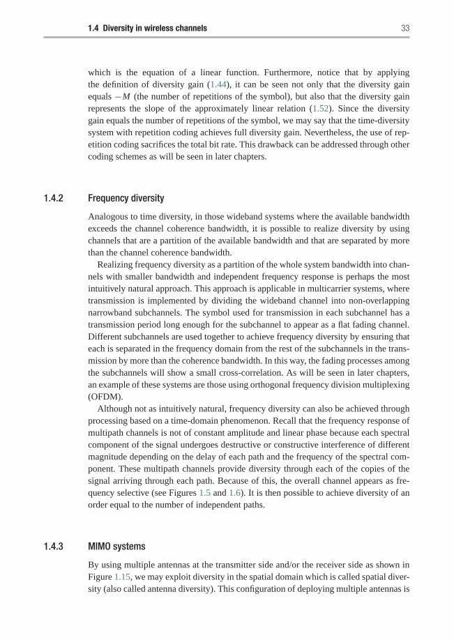
1.4 Diversity in wireless channels 33
which is the equation of a linear function. Furthermore, notice that by applyingthe definition of diversity gain (1.44), it can be seen not only that the diversity gainequals −M (the number of repetitions of the symbol), but also that the diversity gainrepresents the slope of the approximately linear relation (1.52). Since the diversitygain equals the number of repetitions of the symbol, we may say that the time-diversitysystem with repetition coding achieves full diversity gain. Nevertheless, the use of rep-etition coding sacrifices the total bit rate. This drawback can be addressed through othercoding schemes as will be seen in later chapters.
1.4.2 Frequency diversity
Analogous to time diversity, in those wideband systems where the available bandwidthexceeds the channel coherence bandwidth, it is possible to realize diversity by usingchannels that are a partition of the available bandwidth and that are separated by morethan the channel coherence bandwidth.
Realizing frequency diversity as a partition of the whole system bandwidth into chan-nels with smaller bandwidth and independent frequency response is perhaps the mostintuitively natural approach. This approach is applicable in multicarrier systems, wheretransmission is implemented by dividing the wideband channel into non-overlappingnarrowband subchannels. The symbol used for transmission in each subchannel has atransmission period long enough for the subchannel to appear as a flat fading channel.Different subchannels are used together to achieve frequency diversity by ensuring thateach is separated in the frequency domain from the rest of the subchannels in the trans-mission by more than the coherence bandwidth. In this way, the fading processes amongthe subchannels will show a small cross-correlation. As will be seen in later chapters,an example of these systems are those using orthogonal frequency division multiplexing(OFDM).
Although not as intuitively natural, frequency diversity can also be achieved throughprocessing based on a time-domain phenomenon. Recall that the frequency response ofmultipath channels is not of constant amplitude and linear phase because each spectralcomponent of the signal undergoes destructive or constructive interference of differentmagnitude depending on the delay of each path and the frequency of the spectral com-ponent. These multipath channels provide diversity through each of the copies of thesignal arriving through each path. Because of this, the overall channel appears as fre-quency selective (see Figures 1.5 and 1.6). It is then possible to achieve diversity of anorder equal to the number of independent paths.
1.4.3 MIMO systems
By using multiple antennas at the transmitter side and/or the receiver side as shown inFigure 1.15, we may exploit diversity in the spatial domain which is called spatial diver-sity (also called antenna diversity). This configuration of deploying multiple antennas is
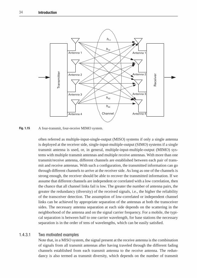
34 Introduction
Tran
smit
ter
Rec
eive
r
Antenna 1 Antenna 1
Antenna 2 Antenna 2
Antenna 3 Antenna 3
Antenna 4 Antenna 4
h11
h12
h44
h43
Channel
Fig. 1.15 A four-transmit, four-receive MIMO system.
often referred as multiple-input-single-output (MISO) systems if only a single antennais deployed at the receiver side, single-input-multiple-output (SIMO) systems if a singletransmit antenna is used, or, in general, multiple-input-multiple-output (MIMO) sys-tems with multiple transmit antennas and multiple receive antennas. With more than onetransmit/receive antenna, different channels are established between each pair of trans-mit and receive antennas. With such a configuration, the transmitted information can gothrough different channels to arrive at the receiver side. As long as one of the channels isstrong enough, the receiver should be able to recover the transmitted information. If weassume that different channels are independent or correlated with a low correlation, thenthe chance that all channel links fail is low. The greater the number of antenna pairs, thegreater the redundancy (diversity) of the received signals, i.e., the higher the reliabilityof the transceiver detection. The assumption of low-correlated or independent channellinks can be achieved by appropriate separation of the antennas at both the transceiversides. The necessary antenna separation at each side depends on the scattering in theneighborhood of the antenna and on the signal carrier frequency. For a mobile, the typi-cal separation is between half to one carrier wavelength, for base stations the necessaryseparation is in the order of tens of wavelengths, which can be easily satisfied.
1.4.3.1 Two motivated examplesNote that, in a MISO system, the signal present at the receive antenna is the combinationof signals from all transmit antennas after having traveled through the different fadingchannels established from each transmit antenna to the receive antenna. The redun-dancy is also termed as transmit diversity, which depends on the number of transmit
1.4 Diversity in wireless channels 35
antennas. While in a SIMO system, a transmitted signal goes through different channelsand is received at each receive antenna. Signals from each receive antenna are com-bined and jointly detected at the receiver side. The corresponding redundancy is oftencalled receive diversity, which is related to the number of receive antennas. In general,in a MIMO system, both transmit and receive diversities are realized. As we will dis-cuss in Chapter 2, the overall signal redundancy, or diversity order, is in this case theproduct of the numbers of transmit and receive antennas. The MIMO configuration canbe exploited through different designs that differ, among other factors, in the antennaconfiguration at the receiver and the transmitter, as well as the particular form of per-formance improvement that it is intended to obtain. For better understanding the spatialdiversity, we consider the following two motivated examples.
Example 1.4 Consider a system that implements receive diversity by using one antennaat the transmitter and Mr antennas at the receiver (i.e., a SIMO system). There areMr paths between transmitter and receiver. The signal arriving from all paths needto be combined at the receiver. If the additive background noise is complex-valued,zero-mean circularly symmetric Gaussian, and independent from each path, then theoptimal combiner is the maximal ratio combiner (MRC) (a fact that can be acceptedafter realizing the similarity of the combining problem here and the one in diversityfrom repetition coding over time, with the diversity branches now over space instead ofover time). Assuming BPSK modulation, and conditioning on the Mr channel gains ofthe paths, h1, h2, . . . , hMr , the error probability that can be obtained using MRC com-
biner is Q(√
2γ∑Mr
j=1 |h j |2). This error probability can be written in the following
form, which provides more insight into the achievable gains,
Pe = Q
⎛⎜⎝√√√√2(Mrγ )
(∑Mrj=1 |h j |2
Mr
)⎞⎟⎠ .In this expression, the factor Mrγ shows that the use of the MRC results in a linearincrease of SNR with the number of paths. This gain is called the array gain. Also,the factor (1/Mr)
∑Mrj=1 |h j |2 shows an averaging effect on the paths gain where the
paths in deeper fade are compensated by those in a good condition, thus resulting in alower probability that the overall link attenuation will be too large. This effect is thematerialization of the diversity gain in this scheme. To see this more clearly, considerthat each h j is the sum of two i.i.d. real Gaussian random variables, and recall fromSection 1.1.3 that
∑Mrj=1 |h j |2 follows a Chi-square distribution with 2Mr degrees of
freedom (see (1.14)). Integrating over this distribution to obtain the average probabilityof symbol error results in
PSER =
⎛⎜⎜⎝1−√
γ
1+ γ2
⎞⎟⎟⎠Mr
Mr−1∑m=0
(Mr + m − 1
m
)⎛⎜⎜⎝1+√
γ
1+ γ2
⎞⎟⎟⎠m
. (1.53)
36 Introduction
Unsurprisingly, this expression is very similar to (1.47). This is due to the analogybetween achieving diversity by transmitting at different time instants and by transmit-ting through different paths. The essence of this similarity resides in the common useof an MRC combiner, which results in a similar expression for the probability of error.Furthermore, we can now draw on this similarly and apply the Chernoff bound to deriveexpressions similar to (1.50) and (1.51) to get
PSER ≈ αMr
(βMrγ
2
)−Mr
,
which shows the diversity order Mr, since the SNR decays as γ−Mr . �
Example 1.5 (Alamouti scheme) Consider now a system that implements transmitdiversity, with two antennas at the transmitter and one antenna at the receiver. Trans-mission is done by sending two symbols, s1 and s2, over the duration of two symbolsperiods. We assume a flat fading channel, i.e., the channel does not change during thetwo symbol periods. Instead of sending the symbol s1 during the first symbol period andthe symbol s2 during the second period, the Alamouti scheme treats the two symbolsas a block and applies a form of precoding to the symbols. Specifically, during the firsttransmission period, s1 is sent from antenna 1 and s2 is sent from antenna 2; and duringthe second transmission period,−s∗2 is sent from antenna 1 and s∗1 from antenna 2 (heres∗1 denotes the complex conjugate of s1).
At the receiver, we denote by y1 and y2 the signals received during the first and secondsymbol periods, respectively. The two received signals are processed as a vector givenby [
y1
y2
]=[
s1 s2
−s∗2 s∗1
] [h1
h2
]+[
z1
z2
]The above transceiver signals can be rearranged as[
y1
y∗2
]=[
h1 h2
h∗2 −h∗1
] [s1
s2
]+[
z1
z∗2
].
Denote y = [y1 y∗2 ]T and
H =[
h1 h2
h∗2 −h∗1
].
Then the receiver processes the received vector y by taking y = HHy, resulting in
y =[ |h1|2 + |h2|2 0
0 |h21| + |h2
2|] [
s1
s2
]+HH
[z1
z∗2
].
Since the processed noise vector is still complex Gaussian with zero mean, but now witha covariance matrix equal to the diagonal matrix diag(|h2
1| + |h22|, |h2
1| + |h22|) times the
received noise power, the received SNR for a symbol detected with z is
1.4 Diversity in wireless channels 37
γ = |h21| + |h2
2|2
γS,
where γS is the SNR of a symbol transmitted without the Alamouti scheme and thefactor 2 is due to the fact that each si is transmitted at half γS. We finally note herethat this result shows in a fashion similar to Example 1.4 that the Alamouti scheme canachieve a diversity order 2. �
1.4.3.2 MIMO capacityIn this subsection, we address advantages of MIMO systems from an information the-ory aspect by reviewing a fundamental capacity result indicating that the capacity ofa MIMO system increases at least linearly with the minimum number of transmit orreceive antennas.
We consider a MIMO system with Mt transmit antennas and Mr receive antennas.The channel coefficient between transmit antenna i, 1 ≤ i ≤ Mt, and receive antennaj, 1 ≤ j ≤ Mr, is denoted by hi, j . These coefficients are modeled as independentcircularly symmetric complex Gaussian random variables with zero mean and varianceone. The MIMO transceiver can be modeled as
Y =√ρ
MtX H + Z , (1.54)
where X = [x1 x2 . . . xMt ] is a signal vector transmitted by the Mt antennas, Y =[y1 y2 . . . yMr ] is a signal vector received by the Mr receive antennas, and Z =[z1 z2 . . . zMr ] is a noise vector whose elements are modeled as independent circu-larly symmetric complex Gaussian random variables with zero mean and variance one.The channel coefficient matrix H = {hi, j : 1 ≤ i ≤ Mt, 1 ≤ j ≤ Mr} is assumed tobe known at the receiver side, but unknown at the transmitter side. The signal vector isassumed to satisfy the energy constraint E ||X ||2F = Mt, where ||X ||F is the Frobeniusnorm of X , defined as
||X ||2F =Mt∑
i=1
|xi |2.
In (1.54), the factor√ρ/Mt ensures that ρ is the average signal to noise ratio (SNR) at
each receive antenna, and it is independent of the number of transmit antennas.If the input signal X is a circularly symmetric complex Gaussian random vector
with zero mean and variance E{XH X} = Q, then the output signal is also a circularlysymmetric complex Gaussian random vector with zero mean and variance
E{Y HY } = ρ
MtHHQH + IMr ,
in which IMr is an identity matrix of size Mr by Mr. So, for any given channel H , themutual information between the input X and the output Y is
I (X; Y |H) = log2 det
(IMr +
ρ
MtHHQH
). (1.55)
38 Introduction
Since E ||X ||2F = Mt, trace(Q) = trace(E{XH X}) = Mt. Next, we would like to
maximize the mutual information I (X; Y |H) as in (1.55) over the choice of nonnegativeQ with the constraint trace(Q) = Mt. Since we can write Q as Q = UHQ0U , whereU is unitary and Q0 is diagonal, so
log2 det
(IMr +
ρ
MtHHQH
)= log2 det
(IMr +
ρ
MtHHQ0 H
), (1.56)
in which H = U H . Note that H has the same distribution as that of H since U isunitary. So we just need to maximize
log2 det
(IMr +
ρ
MtHHQ0 H
)over the nonnegative diagonal matrix Q0 with the constraint trace(Q0) = Mt. It hasbeen shown in [215] that
log2 det
(IMr +
ρ
MtHHQ0 H
)is maximized when Q0 has equal diagonal elements, i.e., Q0 = IMt . Intuitively, it iseasy to understand that if the transmitter has no prior information about the channel,each transmit antenna should be treated equally and allocated the same weight, i.e.,the variance of the input signal vector over Mt transmit antennas should be an identitymatrix. Therefore, the maximal mutual information is
log2 det
(IMr +
ρ
MtHH H
).
Finally, we assume that the channel is memoryless, i.e., the channel H changes inde-pendently from each use of the channel to another. Thus the average capacity of theMIMO system is given by
C = EH
{log2 det
(IMr +
ρ
MtHH H
)}, (1.57)
in which the expectation is taken over the fading channel H . We can see that whenMt = Mr = 1, the above result reduces to the capacity in (1.27) for a conventionalsingle-input-single-output (SISO) system.
In the following, we further interpret the capacity result in (1.57) for SIMO, MISO,and MIMO systems, respectively. For a SIMO system, i.e., Mt = 1 and Mr > 1, thechannel H is a vector as H = [h1,1 h1,2 . . . h1,Mr]. Since
det(
IMr + ρHH H)= det
(IMt + ρH HH
)= 1+ ρ
Mr∑j=1
|h1, j |2,
in which the first equality follows from the determinant identity det(Im + AB) =det(In+B A) for any matrices A and B of sizes m×n and n×m respectively. Therefore,the capacity of the SIMO system is
1.4 Diversity in wireless channels 39
C = EH
⎧⎨⎩log2
⎛⎝1+ ρMr∑j=1
|h1, j |2⎞⎠⎫⎬⎭ , (1.58)
in which∑Mr
j=1 |h1, j |2 is a Chi-square random variable with 2Mr degrees of freedom,
compared with the SISO case where C = Eh{log2
(1+ ρ|h|2)} and |h|2 is a Chi-
square random variable with two degrees of freedom.For a MISO system, i.e., Mr = 1 and Mt > 1, the channel H is a column vector as
H = [h1,1 h1,2 . . . hMt,1]T. In this case,
det
(IMr +
ρ
MtHH H
)= 1+ ρ
Mt
Mt∑i=1
|hi,1|2.
So the corresponding capacity can be specified as
C = EH
{log2
(1+ ρ
∑Mti=1 |hi,1|2
Mt
)}. (1.59)
We can see that when Mt is large,(∑Mt
i=1 |hi,1|2)/Mt ≈ E{|h|2}, in which |h|2 is a
Chi-square random variable with two degrees of freedom. Thus, the capacity in (1.59)is almost the same as that of the SISO system.
For a MIMO system, without loss of generality, we assume Mt = Mr > 1. Note that
HH H =
⎡⎢⎢⎢⎢⎣∑Mt
i=1 |hi,1|2 ∑Mti=1 h∗i,1hi,2 · · · ∑Mt
i=1 h∗i,1hi,Mr
h∗i,2hi,1∑Mt
i=1 |hi,2|2 · · · ∑Mti=1 h∗i,2hi,Mr
......
. . ....
h∗i,Mrhi,1
∑Mti=1 h∗i,Mr
hi,2 · · · ∑Mti=1 |hi,Mr |2
⎤⎥⎥⎥⎥⎦ .Since hi, j are i.i.d. complex Gaussian random variables with zero mean and vari-
ance one, so for large Mt,(∑Mt
i=1 |hi, j |2)/Mt → 1 for each 1 ≤ j ≤ Mr and(∑Mt
i=1 h∗i, j1hi, j2
)/Mt → 0 for any 1 ≤ j1 �= j2 ≤ Mr. Thus, for large Mt,
(1/Mt) HH H → IMr . Therefore, for large Mt , the capacity in (1.57) is
C → log2 det(IMr + ρ IMr
)= Mr log2(1+ ρ), (1.60)
which increases linearly with the number of receive antennas. Note that the above dis-cussion is also true for any Mt ≥ Mr. Based on the above discussion for SIMO, MISO,and MIMO systems, we can see that the capacity of a multiple-antenna system increasesat least linearly with the minimum number of transmit or receive antennas.
1.4.3.3 Diversity–multiplexing tradeoffIn MIMO systems, the multiple paths created between any pair of transmit-receiveantennas can be used to obtain diversity gain. On the other hand, these paths can alsobe used to transmit independent messages from each transmit antenna, in which caseit is possible to achieve an increase in transmit bit rate given by a multiplexing gain.
40 Introduction
At the receiver, the MIMO configuration allows for separation of each data stream. Itis readily apparent that there should be a tradeoff between diversity and multiplexinggains because the later is achieved at the expense of signal paths that otherwise couldbe used to increase the former.
The diversity–multiplexing tradeoff is specified through the choice of an achiev-able combination of diversity and multiplexing gains, or, in other words, by specifyingthe achievable diversity gain as a function of the multiplexing gain. Let d∗(r) be thediversity–multiplexing tradeoff curve for the slow fading channel. A point on this curve,a diversity gain d∗(r), is achieved at multiplexing gain r if
d∗(r) = − limγ→∞
log Pout(r log γ )
log γ. (1.61)
This definition means that when communicating at a rate R = r log γ , the achievablediversity gain is that for which the outage probability decays as Pout(r log γ ) ≈ γ−d∗(r)
at arbitrary large SNR. Also, this formulation can be extended to any type of fadingchannel, beyond the slow fading channel, by replacing the outage probability with theprobability of error, i.e.,
d∗(r) = − limγ→∞
log Pe(r log γ )
log γ. (1.62)
Example 1.6 Consider a system that transmits a single symbol using QAM modulationat SNR γ over a channel with unit-average power Rayleigh fading and complex-valued,circularly symmetric additive Gaussian background noise with zero mean and unitpower. At the receiver, the detection performance is driven by the minimum distancebetween constellation points dmin, which at high SNR is approximately given by [219]
dmin ≈√γ
2R/2.
This leads to an error probability at high SNR approximately equal to
Pe ≈ 1
d2min
= 2R
γ,
which results in the diversity–multiplexing tradeoff
d(r) = 1− r,
for r between 0 and 1. �
1.5 Cooperation diversity
The proliferation of wireless communication applications in the last few years isunprecedented. Voice communication is no longer the only application people need.
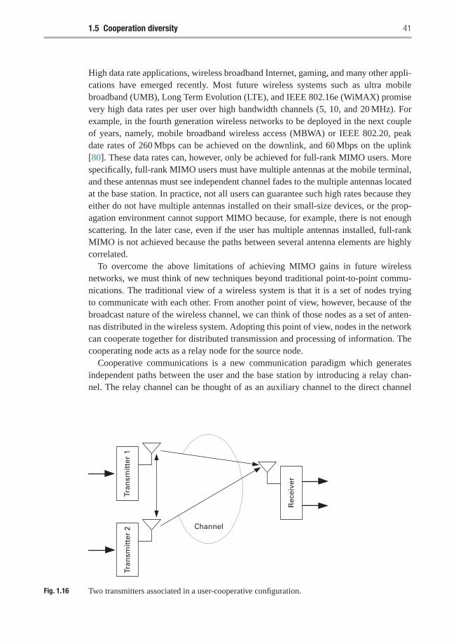
1.5 Cooperation diversity 41
High data rate applications, wireless broadband Internet, gaming, and many other appli-cations have emerged recently. Most future wireless systems such as ultra mobilebroadband (UMB), Long Term Evolution (LTE), and IEEE 802.16e (WiMAX) promisevery high data rates per user over high bandwidth channels (5, 10, and 20 MHz). Forexample, in the fourth generation wireless networks to be deployed in the next coupleof years, namely, mobile broadband wireless access (MBWA) or IEEE 802.20, peakdate rates of 260 Mbps can be achieved on the downlink, and 60 Mbps on the uplink[80]. These data rates can, however, only be achieved for full-rank MIMO users. Morespecifically, full-rank MIMO users must have multiple antennas at the mobile terminal,and these antennas must see independent channel fades to the multiple antennas locatedat the base station. In practice, not all users can guarantee such high rates because theyeither do not have multiple antennas installed on their small-size devices, or the prop-agation environment cannot support MIMO because, for example, there is not enoughscattering. In the later case, even if the user has multiple antennas installed, full-rankMIMO is not achieved because the paths between several antenna elements are highlycorrelated.
To overcome the above limitations of achieving MIMO gains in future wirelessnetworks, we must think of new techniques beyond traditional point-to-point commu-nications. The traditional view of a wireless system is that it is a set of nodes tryingto communicate with each other. From another point of view, however, because of thebroadcast nature of the wireless channel, we can think of those nodes as a set of anten-nas distributed in the wireless system. Adopting this point of view, nodes in the networkcan cooperate together for distributed transmission and processing of information. Thecooperating node acts as a relay node for the source node.
Cooperative communications is a new communication paradigm which generatesindependent paths between the user and the base station by introducing a relay chan-nel. The relay channel can be thought of as an auxiliary channel to the direct channel
Tran
smit
ter
2Tr
ansm
itte
r 1
Rec
eive
r
Channel
Fig. 1.16 Two transmitters associated in a user-cooperative configuration.
42 Introduction
between the source and destination. Since the relay node is usually several wavelengthsdistant from the source, the relay channel is guaranteed to fade independently from thedirect channel, which introduces a full-rank MIMO channel between the source and thedestination. In the cooperative communications setup, there are a-priori few constraintsto different nodes receiving useful energy that has been emitted by another transmittingnode. The new paradigm in user cooperation is that, by implementing the appropriatesignal processing algorithms at the nodes, multiple terminals can process the transmis-sions overheard from other nodes and be made to collaborate by relaying informationfor each other (Figure 1.16). The relayed information is subsequently combined at adestination node so as to create spatial diversity. This creates a network that can beregarded as a system implementing a distributed multiple antenna where collaboratingnodes create diverse signal paths for each other.
Hence, cooperative communications is a new paradigm shift for the fourth generationwireless system that will guarantee high data rates to all users in the network, and weanticipate that it will be the key technology aspect in fifth generation wireless networks.
In terms of research “ascendance,” cooperative communications can be seen asrelated to research in relay channel and MIMO systems. The concept of user coop-eration itself was introduced in two-part series of papers [179, 180]. In these works,Sendonaris et al. proposed a two user cooperation system, in which pairs of terminals inthe wireless network are coupled to help each other forming a distributed two-antennasystem. Parts II and III of this book will study in detail the design and analysis ofcooperative communications, so we defer further explanation until then.
1.6 Bibliographical notes
Because this is an introductory chapter, we have not covered in detail any of the topicsstudied here. Nevertheless, there are plenty of excellent textbooks and research papersthat complement our presentation. On the topic of wireless channels, the reader can findmore information in the books by Proakis [146], Rappaport [150], Tse and Viswanath[219], and Goldsmith [45]. For a practical presentation, the description of channel mod-els used in different standards such as [87] are always a good reference. The books byTse and Viswanath [219] and by Goldsmith [45] were the main sources for most of thetopics covered in this introduction and are where further explanations can be found. Thebook by Cover and Thomas [26] presents very good in-depth study of many topics ininformation theory. Also, in-depth study of the concept of outage capacity can be foundin [141]. Extra coverage on the topic of diversity can be found in books such as [91],tutorial papers such as [144], or books covering communications over fading channels[189]. Finally, the topic of diversity–multiplexing tradeoff has been studied in [239] andrelated papers.
2 Space–time diversity and coding
The idea of using multiple transmit and receive antennas in wireless communicationsystems has attracted considerable attention with the aim of increasing data transmissionrate and system capacity. A key issue is how to develop proper transmission techniquesto exploit all of the diversities available in the space, time, and frequency domains.In the case of narrow-band wireless communications, the channel fading is frequencynon-selective (flat) and diversities are available only in the space and time domains. Themodulation and coding approach that is developed for this scenario is termed space–time(ST) coding, exploiting available spatial and temporal diversity.
In this chapter, we first describe the MIMO communication system architecture withfrequency-non-selective fading channels, which are often termed as narrow-band wire-less channels, and discuss design criteria in achieving the full space–time diversity.Then, we introduce several well-known ST coding techniques that can be guaranteed toachieve full space–time diversity.
2.1 System model and performance criteria
Assume that the MIMO systems have Mt transmit and Mr receive antennas. Channelstate information (CSI) is assumed to be known at the receiver, but not at the transmit-ter. In narrowband transmission scenario, the fading channel is frequency-non-selectiveor flat, and is assumed to be quasi-static, i.e., the channel stays constant during one code-word transmission and it may change independently from one codeword transmissionto another. In this case, diversity is available only in the space and time domains.
An ST-coded MIMO system is shown in Figure 2.1. The ST encoder divides inputdata stream into b bit long blocks and, for each block, selects one ST codeword fromthe codeword set of size L = 2b. The selected codeword is then transmitted throughthe channel over the Mt transmit antennas and T time slots. Each codeword can berepresented as a T × Mt matrix
C =
⎡⎢⎢⎢⎢⎣c1
1 c21 · · · cMt
1c1
2 c22 · · · cMt
2...
.... . .
...
c1T c2
T · · · cMtT
⎤⎥⎥⎥⎥⎦ �= {cit : i = 1, 2, . . . ,Mt}, (2.1)
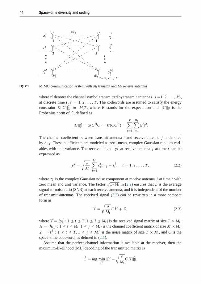
44 Space–time diversity and coding
1
2
1
2
ct
hi, j
Mr t = 1, 2,..., TMt
1
ct2
ctMt yt
Mr
yt2
yt1
Fig. 2.1 MIMO communication system with Mt transmit and Mr receive antennas
where cit denotes the channel symbol transmitted by transmit antenna i, i =1, 2, . . . ,Mt,
at discrete time t, t = 1, 2, . . . , T . The codewords are assumed to satisfy the energyconstraint E ||C ||2F = MtT , where E stands for the expectation and ||C ||F is theFrobenius norm of C , defined as
||C ||2F = tr(CHC) = tr(CCH) =T∑
t=1
Mt∑i=1
|cit |2.
The channel coefficient between transmit antenna i and receive antenna j is denotedby hi, j . These coefficients are modeled as zero-mean, complex Gaussian random vari-
ables with unit variance. The received signal y jt at receive antenna j at time t can be
expressed as
y jt =
√ρ
Mt
Mt∑i=1
cit hi, j + z j
t , t = 1, 2, . . . , T, (2.2)
where z jt is the complex Gaussian noise component at receive antenna j at time t with
zero mean and unit variance. The factor√ρ/Mt in (2.2) ensures that ρ is the average
signal-to-noise ratio (SNR) at each receive antenna, and it is independent of the numberof transmit antennas. The received signal (2.2) can be rewritten in a more compactform as
Y =√ρ
MtC H + Z , (2.3)
where Y = {y jt : 1 ≤ t ≤ T, 1 ≤ j ≤ Mr} is the received signal matrix of size T × Mr,
H = {hi, j : 1 ≤ i ≤ Mt, 1 ≤ j ≤ Mr} is the channel coefficient matrix of size Mt×Mr,
Z = {z jt : 1 ≤ t ≤ T, 1 ≤ j ≤ Mr} is the noise matrix of size T × Mr, and C is the
space–time codeword, as defined in (2.1).Assume that the perfect channel information is available at the receiver, then the
maximum-likelihood (ML) decoding of the transmitted matrix is
C = arg minC||Y −
√ρ
MtC H ||2F.

2.1 System model and performance criteria 45
Suppose that codeword C is transmitted and the receiver erroneously in favor of code-word C . Since the noise term is a zero-mean Gaussian random variable, the pairwiseerror probability (PEP) for a fixed channel realization can be determined as (leave theproof as an exercise)
P(C → C |H) = Q
(√ρ
2Mt||(C − C)H ||F
)= 1
π
∫ π/2
0exp
(− ρ
4Mt sin2 θ||(C − C)H ||2F
)dθ, (2.4)
where Q(x) = 1/√
2π∫∞
x exp(−t2/2
)dt is the Gaussian error function, and the
second equality comes from the Craig expression
Q(x) = 1
π
∫ π/2
0exp
(− x2
2 sin2 θ
)dθ.
Averaging over the Rayleigh fading channel H , the PEP can be determined as follows(leave the proof as an exercise):
P(C → C) = 1
π
∫ π/2
0
γ∏i=1
(1+ ρλi
4Mt sin2 θ
)−Mr
dθ, (2.5)
where γ = rank(C − C), and λ1, λ2, . . . , λγ are the non-zero eigenvalues of(C − C)(C − C)H. The superscript H stands for the complex conjugate and transposeof a matrix. By taking θ = π/2 in (2.5), we have the well known upper bound
P(C → C) ≤ 1
2
γ∏i=1
(1+ ρλi
4Mt
)−Mr
(2.6)
≤ 1
2
(ρ
4Mt
)−γMr(γ∏
i=1
λi
)−Mr
. (2.7)
On the other hand, for high enough SNR, it is easy to see that the exact PEP in (2.5) canbe upper bounded as
P(C → C) ≤ 1
π
∫ π/2
0
γ∏i=1
(ρλi
4Mt sin2 θ
)−Mr
dθ
=(
2γMr − 1γMr − 1
)(ρ
Mt
)−γMr(γ∏
i=1
λi
)−Mr
, (2.8)
where the equality comes from
1
π
∫ π/2
0(sin θ)2γMrdθ = 22γMr
(2γMr − 1γMr − 1
).
Let us compare the three upper bounds in (2.6–2.8) with the exact PEP (2.5) inFigure 2.2. We can see that, at high SNR, the upper bound (2.8) is much tighter than
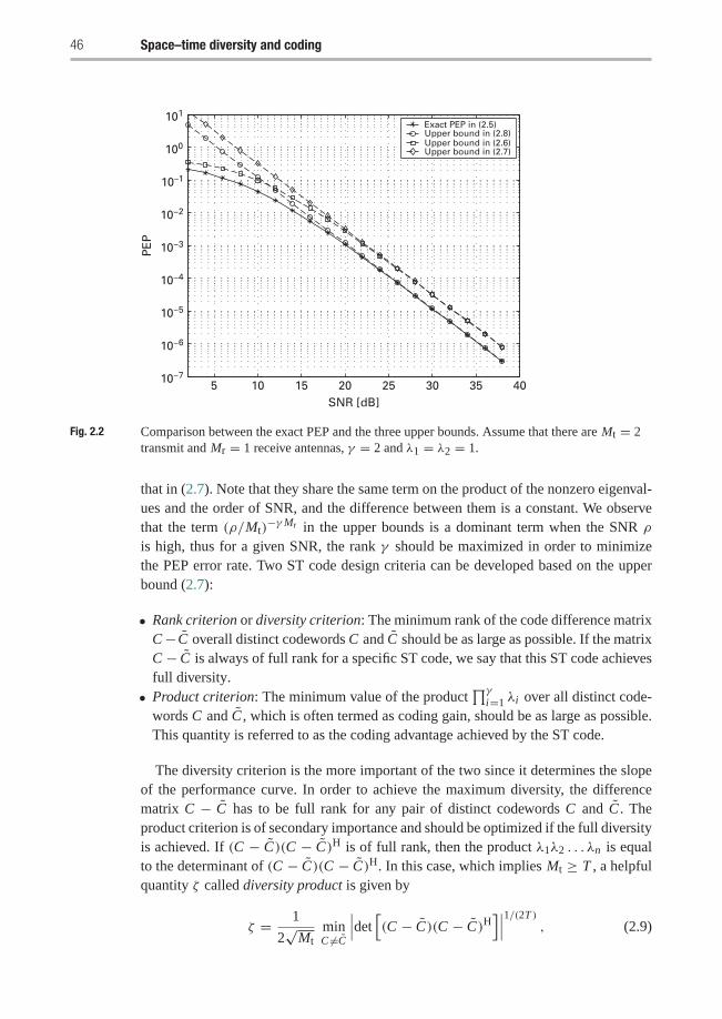
46 Space–time diversity and coding
5 10 15 20 25 30 35 4010−7
10−6
10−5
10−4
10−3
10−2
10–1
100
101
SNR [dB]
PE
P
Exact PEP in (2.5)Upper bound in (2.8)Upper bound in (2.6)Upper bound in (2.7)
Fig. 2.2 Comparison between the exact PEP and the three upper bounds. Assume that there are Mt = 2transmit and Mr = 1 receive antennas, γ = 2 and λ1 = λ2 = 1.
that in (2.7). Note that they share the same term on the product of the nonzero eigenval-ues and the order of SNR, and the difference between them is a constant. We observethat the term (ρ/Mt)
−γMr in the upper bounds is a dominant term when the SNR ρ
is high, thus for a given SNR, the rank γ should be maximized in order to minimizethe PEP error rate. Two ST code design criteria can be developed based on the upperbound (2.7):
• Rank criterion or diversity criterion: The minimum rank of the code difference matrixC− C overall distinct codewords C and C should be as large as possible. If the matrixC − C is always of full rank for a specific ST code, we say that this ST code achievesfull diversity.
• Product criterion: The minimum value of the product∏γ
i=1 λi over all distinct code-words C and C , which is often termed as coding gain, should be as large as possible.This quantity is referred to as the coding advantage achieved by the ST code.
The diversity criterion is the more important of the two since it determines the slopeof the performance curve. In order to achieve the maximum diversity, the differencematrix C − C has to be full rank for any pair of distinct codewords C and C . Theproduct criterion is of secondary importance and should be optimized if the full diversityis achieved. If (C − C)(C − C)H is of full rank, then the product λ1λ2 . . . λn is equalto the determinant of (C − C)(C − C)H. In this case, which implies Mt ≥ T , a helpfulquantity ζ called diversity product is given by
ζ = 1
2√
MtminC �=C
∣∣∣det[(C − C)(C − C)H
]∣∣∣1/(2T ), (2.9)
2.2 Space–time coding 47
which is a normalized coding gain. The factor 1/(2√
Mt) guarantees that 0 ≤ ζ ≤ 1.When all codewords are square matrices, i.e., T = Mt, the diversity product can besimplified as
ζ = 1
2√
MtminC �=C
∣∣∣det(C − C)∣∣∣1/Mt
, (2.10)
which is often used as a benchmark in designing ST codes.
2.2 Space–time coding
In the previous section, we analyzed the performance of the ST-coded MIMO systemsand obtained ST code design criteria in achieving the spatial and temporal diversity. Inthis section, we introduce several well-known ST coding techniques that can guaranteeto achieve the full space–time diversity.
2.2.1 Cyclic and unitary ST codes
A simple and effective coding scheme achieving full space–time diversity is the cyclicST coding approach which follows the following code structure:
Cl =√
Mt diag{eju1θl , eju2θl , . . . , ejuMt θl }, l = 0, 1, . . . , L − 1, (2.11)
where diag{eju1θl , eju2θl , . . . , ejuMt θl } is a diagonal matrix with diagonal entrieseju1θl , eju2θl , . . . , and ejuMt θl , in which θl = (l/L)2π and u1, u2, . . . , uMt
∈{0, 1, . . . , L − 1} are some integers to be optimized. We observe that if we denote
V1 = diag{eju12πL , eju2
2πL , . . . , ejuMt
2πL }, (2.12)
then Cl = √Mt V l1 for l = 0, 1, . . . , L − 1, and V L
1 = V 01 , which has a cyclic structure,
hence the term cyclic ST codes.In the following, we discuss how the cyclic structure can guarantee the full diver-
sity and we will also optimize the parameters u1, u2, . . . , uMt . For any two distinctcodewords Cl and Cl ′ , l �= l ′, we have
Cl − Cl ′ =√
Mt diag{eju1θl − eju1θl′ , eju2θl − eju2θl′ , . . . , ejuMt θl − ejuMt θl′ }= √
Mt diag{eju1θl′ , eju2θl′ , . . . , ejuMt θl′ }× diag{eju1θl−l′ − 1, eju2θl−l′ − 1, . . . , ejuMt θl−l′ − 1}
= Cl ′ diag{eju1θl−l′ − 1, eju2θl−l′ − 1, . . . , ejuMt θl−l′ − 1},
48 Space–time diversity and coding
in which θl−l ′ = l−l ′L 2π . So the determinant of the difference matrix is
|det(Cl − Cl ′)| = |det(Cl ′)| ·∣∣∣det(diag{eju1θl−l′ − 1,
eju2θl−l′ − 1, . . . , ejuMt θl−l′ − 1})∣∣∣
= MMt2
t
Mt∏i=1
∣∣∣ejui θl−l′ − 1∣∣∣
= MMt2
t
Mt∏i=1
∣∣∣∣2 sinui (l − l ′)π
L
∣∣∣∣ . (2.13)
From (2.13), we can see that if sin ui (l−l ′)L �= 0 for u1, u2, . . . , uMt and for any l �= l ′,
then the cyclic code achieves the full diversity according to the rank criterion discussedin the previous section.
From (2.13), we can calculate the diversity product of the cyclic code as follows:
ζ = 1
2√
Mtminl �=l ′
|det(Cl − Cl ′)|1/Mt
= minl �=l ′
∣∣∣∣∣Mt∏
i=1
sinui (l − l ′)π
L
∣∣∣∣∣1/Mt
= min1≤l≤L−1
∣∣∣∣∣Mt∏
i=1
sinui lπ
L
∣∣∣∣∣1/Mt
. (2.14)
Thus, the parameters ui ∈ {0, 1, . . . , L − 1} should be chosen such that the diver-sity product ζ is maximized. For small L and Mt, exhaustive computer search can beperformed to find the optimum parameters u1, u2, . . . , uMt ∈ {0, 1, . . . , L − 1}.
Example 2.1 For Mt = 2 and L = 4 (i.e., R = 1 bit/s/Hz), by exhaustive computersearch, the optimum parameters in this case are [u1 u2] = [1 1]. The correspondingcyclic ST codes are given by:
C0 =√
2
[1 00 1
], C1 =
√2
[j 00 j
],
C2 =√
2
[ −1 00 −1
], C3 =
√2
[ −j 00 −j
].
The diversity product ζ = min1≤l≤3
∣∣∣∏2i=1 sin ui lπ
4
∣∣∣1/2 = √2
2 . �
Example 2.2 For Mt = 2 and L = 16 (i.e., R = 2 bits/s/Hz), by exhaustive computersearch, the optimum parameters in this case are [u1 u2] = [1 7]. The correspondingcyclic ST codes are given by:
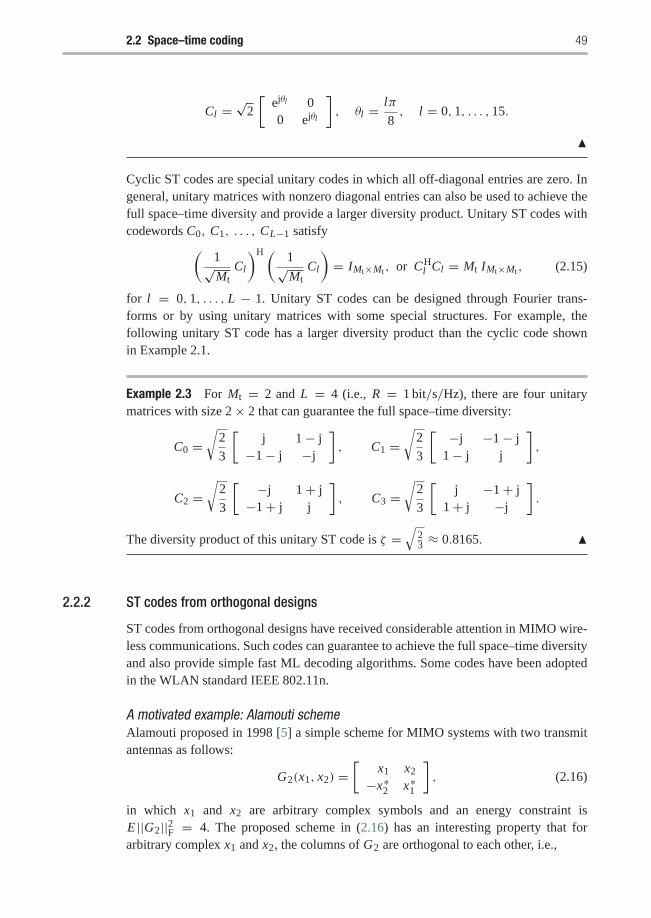
2.2 Space–time coding 49
Cl =√
2
[ejθl 00 ejθl
], θl = lπ
8, l = 0, 1, . . . , 15.
�
Cyclic ST codes are special unitary codes in which all off-diagonal entries are zero. Ingeneral, unitary matrices with nonzero diagonal entries can also be used to achieve thefull space–time diversity and provide a larger diversity product. Unitary ST codes withcodewords C0, C1, . . . , CL−1 satisfy(
1√Mt
Cl
)H ( 1√Mt
Cl
)= IMt×Mt , or CH
l Cl = Mt IMt×Mt , (2.15)
for l = 0, 1, . . . , L − 1. Unitary ST codes can be designed through Fourier trans-forms or by using unitary matrices with some special structures. For example, thefollowing unitary ST code has a larger diversity product than the cyclic code shownin Example 2.1.
Example 2.3 For Mt = 2 and L = 4 (i.e., R = 1 bit/s/Hz), there are four unitarymatrices with size 2× 2 that can guarantee the full space–time diversity:
C0 =√
2
3
[j 1− j
−1− j −j
], C1 =
√2
3
[ −j −1− j1− j j
],
C2 =√
2
3
[ −j 1+ j−1+ j j
], C3 =
√2
3
[j −1+ j
1+ j −j
].
The diversity product of this unitary ST code is ζ =√
23 ≈ 0.8165. �
2.2.2 ST codes from orthogonal designs
ST codes from orthogonal designs have received considerable attention in MIMO wire-less communications. Such codes can guarantee to achieve the full space–time diversityand also provide simple fast ML decoding algorithms. Some codes have been adoptedin the WLAN standard IEEE 802.11n.
A motivated example: Alamouti schemeAlamouti proposed in 1998 [5] a simple scheme for MIMO systems with two transmitantennas as follows:
G2(x1, x2) =[
x1 x2
−x∗2 x∗1
], (2.16)
in which x1 and x2 are arbitrary complex symbols and an energy constraint isE ||G2||2F = 4. The proposed scheme in (2.16) has an interesting property that forarbitrary complex x1 and x2, the columns of G2 are orthogonal to each other, i.e.,
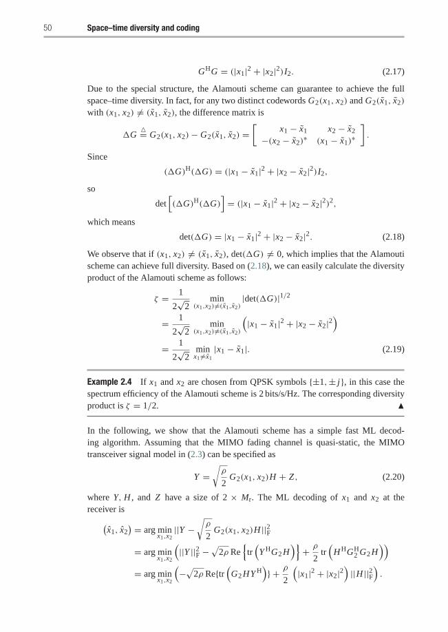
50 Space–time diversity and coding
GHG = (|x1|2 + |x2|2)I2. (2.17)
Due to the special structure, the Alamouti scheme can guarantee to achieve the fullspace–time diversity. In fact, for any two distinct codewords G2(x1, x2) and G2(x1, x2)
with (x1, x2) �= (x1, x2), the difference matrix is
�G�= G2(x1, x2)− G2(x1, x2) =
[x1 − x1 x2 − x2
−(x2 − x2)∗ (x1 − x1)
∗].
Since
(�G)H(�G) = (|x1 − x1|2 + |x2 − x2|2)I2,
so
det[(�G)H(�G)
]= (|x1 − x1|2 + |x2 − x2|2)2,
which means
det(�G) = |x1 − x1|2 + |x2 − x2|2. (2.18)
We observe that if (x1, x2) �= (x1, x2), det(�G) �= 0, which implies that the Alamoutischeme can achieve full diversity. Based on (2.18), we can easily calculate the diversityproduct of the Alamouti scheme as follows:
ζ = 1
2√
2min
(x1,x2)�=(x1,x2)|det(�G)|1/2
= 1
2√
2min
(x1,x2)�=(x1,x2)
(|x1 − x1|2 + |x2 − x2|2
)= 1
2√
2min
x1 �=x1
|x1 − x1|. (2.19)
Example 2.4 If x1 and x2 are chosen from QPSK symbols {±1,± j}, in this case thespectrum efficiency of the Alamouti scheme is 2 bits/s/Hz. The corresponding diversityproduct is ζ = 1/2. �
In the following, we show that the Alamouti scheme has a simple fast ML decod-ing algorithm. Assuming that the MIMO fading channel is quasi-static, the MIMOtransceiver signal model in (2.3) can be specified as
Y =√ρ
2G2(x1, x2)H + Z , (2.20)
where Y, H , and Z have a size of 2 × Mr. The ML decoding of x1 and x2 at thereceiver is(
x1, x2) = arg min
x1,x2||Y −
√ρ
2G2(x1, x2)H ||2F
= arg minx1,x2
(||Y ||2F −
√2ρ Re
{tr(Y HG2 H
)}+ ρ
2tr(
HHGH2 G2 H
))= arg min
x1,x2
(−√2ρ Re{tr
(G2 HY H
)} + ρ
2
(|x1|2 + |x2|2
)||H ||2F
).
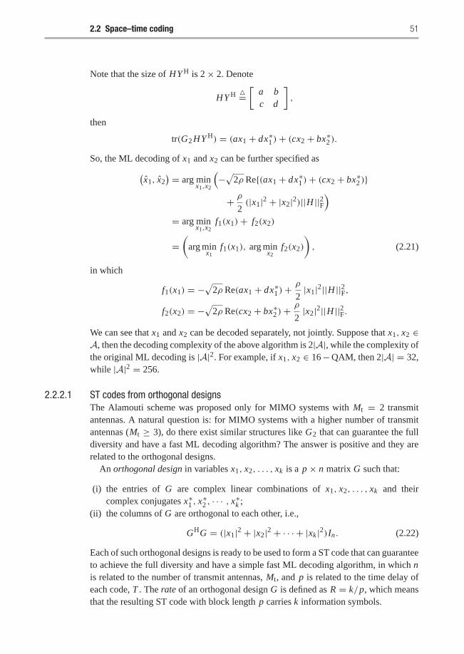
2.2 Space–time coding 51
Note that the size of HY H is 2× 2. Denote
HY H �=[
a bc d
],
then
tr(G2 HY H) = (ax1 + dx∗1 )+ (cx2 + bx∗2 ).
So, the ML decoding of x1 and x2 can be further specified as(x1, x2
) = arg minx1,x2
(−√2ρ Re{(ax1 + dx∗1 )+ (cx2 + bx∗2 )}
+ ρ2(|x1|2 + |x2|2)||H ||2F
)= arg min
x1,x2f1(x1)+ f2(x2)
=(
arg minx1
f1(x1), arg minx2
f2(x2)
), (2.21)
in which
f1(x1) = −√
2ρ Re(ax1 + dx∗1 )+ρ
2|x1|2||H ||2F,
f2(x2) = −√
2ρ Re(cx2 + bx∗2 )+ρ
2|x2|2||H ||2F.
We can see that x1 and x2 can be decoded separately, not jointly. Suppose that x1, x2 ∈A, then the decoding complexity of the above algorithm is 2|A|, while the complexity ofthe original ML decoding is |A|2. For example, if x1, x2 ∈ 16−QAM, then 2|A| = 32,while |A|2 = 256.
2.2.2.1 ST codes from orthogonal designsThe Alamouti scheme was proposed only for MIMO systems with Mt = 2 transmitantennas. A natural question is: for MIMO systems with a higher number of transmitantennas (Mt ≥ 3), do there exist similar structures like G2 that can guarantee the fulldiversity and have a fast ML decoding algorithm? The answer is positive and they arerelated to the orthogonal designs.
An orthogonal design in variables x1, x2, . . . , xk is a p × n matrix G such that:
(i) the entries of G are complex linear combinations of x1, x2, . . . , xk and theircomplex conjugates x∗1 , x∗2 , · · · , x∗k ;
(ii) the columns of G are orthogonal to each other, i.e.,
GHG = (|x1|2 + |x2|2 + · · · + |xk |2)In . (2.22)
Each of such orthogonal designs is ready to be used to form a ST code that can guaranteeto achieve the full diversity and have a simple fast ML decoding algorithm, in which nis related to the number of transmit antennas, Mt, and p is related to the time delay ofeach code, T . The rate of an orthogonal design G is defined as R = k/p, which meansthat the resulting ST code with block length p carries k information symbols.

52 Space–time diversity and coding
The first ST code from orthogonal design was proposed by Alamouti for systems withMt = 2 transmit antennas, which is specified in (2.16). Clearly, the rate of G2(x1, x2)
is 1. For three and four transmit antennas, ST codes from orthogonal designs with rateR = 3/4 are given by
G3(x1, x2, x3) =
⎡⎢⎢⎣x1 x2 x3
−x∗2 x∗1 0−x∗3 0 x∗1
0 −x∗3 x∗2
⎤⎥⎥⎦ , (2.23)
G4(x1, x2, x3) =
⎡⎢⎢⎣x1 x2 x3 0
−x∗2 x∗1 0 x3
−x∗3 0 x∗1 −x2
0 −x∗3 x∗2 x1
⎤⎥⎥⎦ . (2.24)
In fact, G3 is obtained by taking the first three columns of G4.For Mt = 2k (k = 1, 2, 3, . . .), a recursive expression for orthogonal designs can be
given as follows. Let
G1(x1) = x1 I1,
and
G2k (x1, . . . , xk+1) =[
G2k−1(x1, . . . , xk) xk+1 I2k−1
−x∗k+1 I2k−1 GH2k−1(x1, . . . , xk)
], (2.25)
for k = 1, 2, 3, . . .. Then, G2k (x1, x2, . . . , xk+1) is an orthogonal design of size 2k ×2k
with complex variables x1, x2, . . . , xk+1. The rate of G2k is (k + 1)/2k , which is themaximum rate for orthogonal designs of square size. If the number of transmit antennasis not a power of two, a ST code can be obtained by deleting some columns from alarger ST code with a number of transmit antennas that is a power of two.
Example 2.5 According to the recursive method, ST codes from orthogonal designsare illustrated for Mt = 2, 4, 8 as follows:
G2(x1, x2) =[
G1(x1) x2
−x∗2 GH1 (x1)
]=[
x1 x2
−x∗2 x∗1
];
G4(x1, x2, x3) =[
G2(x1, x2) x3 I2
−x∗3 I2 GH2 (x1, x2)
]=
⎡⎢⎢⎣x1 x2 x3 0
−x∗2 x∗1 0 x3
−x∗3 0 x∗1 −x2
0 −x∗3 x∗2 x1
⎤⎥⎥⎦ ;
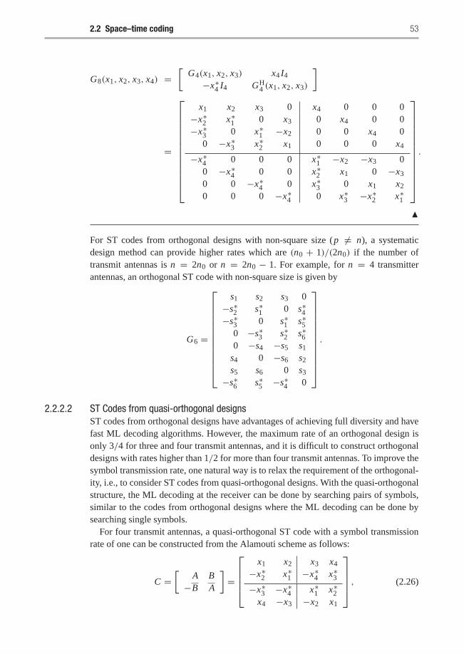
2.2 Space–time coding 53
G8(x1, x2, x3, x4) =[
G4(x1, x2, x3) x4 I4
−x∗4 I4 GH4 (x1, x2, x3)
]
=
⎡⎢⎢⎢⎢⎢⎢⎢⎢⎢⎢⎢⎢⎣
x1 x2 x3 0 x4 0 0 0−x∗2 x∗1 0 x3 0 x4 0 0−x∗3 0 x∗1 −x2 0 0 x4 0
0 −x∗3 x∗2 x1 0 0 0 x4
−x∗4 0 0 0 x∗1 −x2 −x3 00 −x∗4 0 0 x∗2 x1 0 −x3
0 0 −x∗4 0 x∗3 0 x1 x2
0 0 0 −x∗4 0 x∗3 −x∗2 x∗1
⎤⎥⎥⎥⎥⎥⎥⎥⎥⎥⎥⎥⎥⎦.
�
For ST codes from orthogonal designs with non-square size (p �= n), a systematicdesign method can provide higher rates which are (n0 + 1)/(2n0) if the number oftransmit antennas is n = 2n0 or n = 2n0 − 1. For example, for n = 4 transmitterantennas, an orthogonal ST code with non-square size is given by
G6 =
⎡⎢⎢⎢⎢⎢⎢⎢⎢⎢⎢⎢⎣
s1 s2 s3 0−s∗2 s∗1 0 s∗4−s∗3 0 s∗1 s∗5
0 −s∗3 s∗2 s∗60 −s4 −s5 s1
s4 0 −s6 s2
s5 s6 0 s3
−s∗6 s∗5 −s∗4 0
⎤⎥⎥⎥⎥⎥⎥⎥⎥⎥⎥⎥⎦.
2.2.2.2 ST Codes from quasi-orthogonal designsST codes from orthogonal designs have advantages of achieving full diversity and havefast ML decoding algorithms. However, the maximum rate of an orthogonal design isonly 3/4 for three and four transmit antennas, and it is difficult to construct orthogonaldesigns with rates higher than 1/2 for more than four transmit antennas. To improve thesymbol transmission rate, one natural way is to relax the requirement of the orthogonal-ity, i.e., to consider ST codes from quasi-orthogonal designs. With the quasi-orthogonalstructure, the ML decoding at the receiver can be done by searching pairs of symbols,similar to the codes from orthogonal designs where the ML decoding can be done bysearching single symbols.
For four transmit antennas, a quasi-orthogonal ST code with a symbol transmissionrate of one can be constructed from the Alamouti scheme as follows:
C =[
A B−B A
]=
⎡⎢⎢⎢⎣x1 x2 x3 x4
−x∗2 x∗1 −x∗4 x∗3−x∗3 −x∗4 x∗1 x∗2
x4 −x3 −x2 x1
⎤⎥⎥⎥⎦ , (2.26)
54 Space–time diversity and coding
where
A =[
x1 x2
−x∗2 x∗1
], B =
[x3 x4
−x∗4 x∗3
], (2.27)
and A and B are the complex conjugates of A and B, respectively. One can check that
CHC =
⎡⎢⎢⎣a 0 0 b0 a −b 00 −b a 0b 0 0 a
⎤⎥⎥⎦ , (2.28)
where a = |x1|2 + |x2|2 + |x3|2 + |x4|2, and b = x1x∗4 + x4x∗1 − x2x∗3 − x3x∗2 . Wecan see that the ML decision metric of this code can be written as the sum of two termsf1(s1, s4)+ f2(s2, s3), where f1 depends only on s1 and s4, and f2 depends only on s2
and s3. Thus, the minimization can be done separately on these two terms, i.e., symbolpairs (s1, s4) and (s2, s3) can be decoded separately, which leads to a fast ML decoding.However, according to (2.28), the minimum rank of the difference matrix between twodistinct codewords is 2, which means that the code (2.26) does not have the full diversity.
A similar quasi-orthogonal STBC for four transmit antennas has the followingstructure:
C =[
A BB A
]=
⎡⎢⎢⎣x1 x2 x3 x4
−x∗2 x∗1 −x∗4 x∗3x3 x4 x1 x2
−x∗4 x∗3 −x∗2 x∗1
⎤⎥⎥⎦ , (2.29)
where A and B are the same as those in (2.27). Similarly,
CHC =
⎡⎢⎢⎣a 0 b 00 a 0 bb 0 a 00 b 0 a
⎤⎥⎥⎦ ,where a = |x1|2 + |x2|2 + |x3|2 + |x4|2, and b = x1x∗3 + x3x∗1 − x2x∗4 − x4x∗2 . Thebehaviors of (2.29) are similar to those of (2.26).
The performance of the quasi-orthogonal ST codes in (2.26) and (2.29) is better thanthat of the codes from orthogonal designs at low SNR due to the higher rate, but worseat high SNR since it does not guarantee full diversity. In fact, in both (2.26) and (2.29),the symbols are chosen from the same signal constellation arbitrarily and the resultingST codes cannot guarantee the full diversity. A method of optimum signal rotation canbe developed for the quasi-orthogonal ST codes to achieve full diversity.
The main idea of the optimum signal rotation is to choose the signal constellationsproperly to ensure that the resulting codes achieve the full diversity. In the following, wefocus on the code structure in (2.29). The discussion with the code structure in (2.26)is similar. Assume that G p(x1, x2, . . . , xk) is a p × p orthogonal design in complexvariables x1, x2, . . . , xk . A quasi-orthogonal design Q2p(x1, x2, . . . , x2k) of size 2p ×2p in complex variables x1, x2, . . . , x2k is defined as
2.2 Space–time coding 55
Q2p =[
A BB A
], (2.30)
where A = G p(x1, x2, . . . , xk) and B = G p(xk+1, xk+2, . . . , x2k). Since both A and Bare orthogonal designs, we have
QH2p Q2p =
[AH A + BH B AH B + BH ABH A + AH B BH B + AH A
]=[
aIp bIp
bIp a Ip
], (2.31)
where a =∑2ki=1 |xi |2, and b =∑k
i=1(xi x∗k+i + xk+i x∗i ).For each i, 1 ≤ i ≤ k, let Ai denote a signal constellation with average energy
1, and Ak+i denote the signal constellation generated by rotating Ai with an angle ofφi , i.e., Ak+i = {ejφi s : s ∈ Ai }, denoted as ejφiAi . Furthermore, let |Ai | denotethe number of elements in Ai . For any information sequence of log2(
∏2ki=1 |Ai |) bits,
it chooses 2k symbols s1 ∈ A1, s2 ∈ A2, . . . , s2k ∈ A2k . In Q2p(x1, x2, . . . , x2k),if we replace x1, x2, . . . , x2k by s1, s2, . . . , s2k , respectively, we have a new matrixQ2p(s1, s2, . . . , s2k). Consequently, an ST code from a quasi-orthogonal design canbe formed as
C = √γ Q2p(s1, s2, . . . , s2k). (2.32)
The factor√γ ensures that the transmitted signal in (2.32) obeys the energy constraint.
According to (2.31), the ML decoding of (2.32) can be done separately on each pair ofsymbols si and sk+i .
For any pair of distinct transmitted signals C = √γ Q2p(s1, s2, . . . , s2k) and C =√
γ Q2p(s1, s2, . . . , s2k), the difference matrix is√γ Q2p(s1−s1, s2−s2, . . . , s2k−s2k),
denoted as �C for simplicity. Then, from (2.31), we have
(�C)H(�C) = γ[(�a)Ip (�b)Ip
(�b)Ip (�a)Ip
], (2.33)
where �a =2k∑
i=1
|si − si |2, and
�b =k∑
i=1
[(si − si )(sk+i − sk+i )
∗ + (sk+i − sk+i )(si − si )∗] .
The determinant of (2.33) can be calculated as
det[(�C)H(�C)
]= γ 2p
[(�a)2 − (�b)2
]p. (2.34)
Note that for both codes in (2.26) and (2.29), φi = 0 for all i , therefore the determinantin (2.34) can be zero, for example when si − si = sk+i − sk+i , which means thatthe space–time signals do not have the full diversity. Now we can properly choose therotation angle φi to ensure that the determinant in (2.34) is nonzero.
Example 2.6 If all of Ai , 1 ≤ i ≤ k, are BPSK, i.e., Ai = {1,−1}, then we choosethe rotation angle as π/2, i.e., φi = π/2. The resulting signal constellation Ak+i =ejπ/2Ai = {j,−j}. Therefore, for any two symbols si and si in Ai , the difference si − si
56 Space–time diversity and coding
belongs to set {0, 2,−2}; and for any two symbols sk+i and sk+i in Ak+i , the differencesk+i − sk+i belongs to the set {0, 2j,−2j}. It is easy to check that �b in (2.33) is zero.Thus, the determinant of (�C)H(�C) is nonzero, which means that the space–timesignals achieve the full diversity. �
According to (2.34), the diversity product of the quasi-orthogonal ST codes with signalrotation can be calculated as
ζ = 1
2√
2pmin�C �=0
∣∣∣det[(�C)H(�C)
]∣∣∣1/(4p)
= 1
2
√γ
2pmin
1≤i≤kmin
u, u ∈ Ai ; v, v ∈ Ak+i
(u, v) �= (u, v)
∣∣∣(u − u)2 − (v − v)2∣∣∣1/2 .
(2.35)
For convenience, let us define the minimum ζ -distance between two signal constella-tions A and B as follows:
dmin,ζ (A,B)�= min(s1,s2)�=(s1,s2)
∣∣∣(s1 − s1)2 − (s2 − s2)
2∣∣∣1/2 , (2.36)
where s1, s1 and s2, s2 are understood as s1, s1 ∈ A, and s2, s2 ∈ B. Obviously, we have
dmin,ζ (A,B) ≤ min {dmin(A), dmin(B)} , (2.37)
where dmin(A) and dmin(B) are the minimum Euclidean distances of the signalconstellations A and B, respectively. Thus, we have
dmin,ζ (A, e jφA) ≤ dmin(A). (2.38)
We now go back to (2.35). The diversity product can be rewritten as
ζ = 1
2
√γ
2pmin
1≤i≤kdmin,ζ (Ai ,Ak+i )
≤ 1
2
√γ
2pmin
1≤i≤kdmin(Ai ). (2.39)
We observe that the diversity product is determined by the minimumζ -distance of eachpair of signal constellationsAi andAk+i , and the minimum ζ -distance is upper boundedby the minimum Euclidean distance of each signal constellation.
In the example we discussed before, where the signal constellations Ai are BPSK andthe rotation angle is chosen as π/2, the minimum ζ -distance between Ai and ejπ/2Ai
is equal to the minimum Euclidean distance of Ai . However, for a general signal con-stellation, dmin(A) is not always achieved by dmin,ζ (A, ejφA). We will show later thatif A is 8-PSK, then the minimum ζ -distance dmin,ζ (A, e jφA) cannot be greater than(2 sinπ/8)1/2dmin(A), which is strictly less than dmin(A).
In the following, we determine an optimum rotation angle φ for a given signal con-stellation A such that the minimum ζ -distance between A and ejφA is maximized. First,let us derive a necessary condition for the minimum ζ -distance to reach the minimum
2.2 Space–time coding 57
Euclidean distance. Specifically, for a fixed signal constellation A, assume sb and se aretwo signals in A such that the Euclidean distance between sb and se is the minimumEuclidean distance of A, i.e., |sb − se| = dmin. From (2.36), we have
dmin,ζ (A, ejφA) ≤∣∣∣(sb − se)
2 − (ejφsb − ejφse)2∣∣∣1/2
= |1− ej2φ |1/2 · |sb − se|= |2 sinφ|1/2dmin.
Thus, we can conclude that the minimum ζ -distance between A and ejφA cannot begreater than |2 sinφ|1/2dmin, i.e.,
dmin,ζ (A, ejφA) ≤ |2 sinφ|1/2dmin. (2.40)
A necessary condition for the minimum ζ -distance to reach the minimum Euclideandistance is |2 sinφ|1/2 ≥ 1, i.e., | sinφ| ≥ 1/2 or π/6 ≤ |φ| ≤ 5π/6. If thesignal constellation A is r -PSK, then the effective rotation angle is in the interval[−π/r, π/r ] from the symmetry of signals in r -PSK. According to (2.40), we havedmin,ζ (A, ejφA) ≤ |2 sin(π/r)|1/2dmin. Thus, for r -PSK with r > 6, the minimumζ -distance is strictly less than dmin. Note that for different signal constellations, thecorresponding optimum rotation angles may be different.
Example 2.7 Assume that A is a signal constellation drawn from a square lattice (grid),where the side length of the squares is equal to dmin(A). Then, the minimum ζ -distancebetween A and ejπ/4A is dmin(A), i.e.,
dmin,ζ (A, ejπ/4A) = dmin(A).
The signal constellation A can be of any arbitrary subset of the square lattice. The onlyrequirement is that the side length of the squares in the lattice is equal to dmin(A). Thus,for the commonly used QAM1 constellations, the optimum rotation angle is φ = π/4.
�
Example 2.8 Assume that A is a signal constellation drawn from an equilaterally trian-gular lattice, where the side length of the equilateral triangles is equal to dmin(A). Then,the minimum ζ -distance between A and ejπ/6A is dmin(A), i.e.,
dmin,ζ (A, ejπ/6A) = dmin(A).
The signal constellation A could be of any subset of the lattice of equilateral triangleswith the requirement that the side length of the equilateral triangles is equal to dmin(A).For such a signal constellation A, φ = π/6 is an optimum rotation angle. �
1 Strictly, QAM stands for a constellation drawn from a square lattice, where the side length of the squares inthe lattice is equal to the minimum Euclidean distance of the constellation.
58 Space–time diversity and coding
2.2.3 Diagonal algebraic ST codes
Another approach to design full-diversity ST codes is to apply transforms (such asHadamard transforms and Vandermonde transforms) over input data symbols and feedthe output to different transmit antennas at different times [28, 122]. Specifically, forK information symbols, s1 s2 · · · sK (from arbitrary signal constellations such as PSK,QAM, and so on), let
[x1 x2 · · · xK ] = [s1 s2 · · · sK ] · V (θ1, θ2, . . . , θK ), (2.41)
where V (θ1, θ2, . . . , θK ) is a Vandermonde matrix with variables θ1, θ2, . . . , θK , whichis a K × K matrix:
V (θ1, θ2, . . . , θK )�=
⎡⎢⎢⎢⎣1 1 · · · 1θ1 θ2 · · · θK...
.... . .
...
θK−11 θK−1
2 · · · θK−1K
⎤⎥⎥⎥⎦ . (2.42)
The variables θ1, θ2, . . . , θK should be optimized for different signal constellations.With [x1 x2 · · · xK ], a diagonal ST codeword can be formed as follows:
C = diag{x1, x2, . . . , xK }, (2.43)
which can be sent out by K transmit antennas.The ST code in (2.43) satisfies the energy constraint of E ||C ||2F = K 2, which can be
verified as follows:
E ||C ||2F =K∑
i=1
E |xi |2 =K∑
i=1
E
∣∣∣∣∣∣∣∣∣[s1 s2 · · · sK ] ·
⎡⎢⎢⎢⎣1θi...
θK−1i
⎤⎥⎥⎥⎦∣∣∣∣∣∣∣∣∣
2
=K∑
i=1
E
∣∣∣∣∣K∑
k=1
skθk−1i
∣∣∣∣∣2
=K∑
i=1
K∑k=1
E |sk |2 = K 2,
in which we use the assumptions that sk are independent of each other, Esk = 0,E |sk |2 = 1, and |θi | = 1.
The full diversity of the diagonal code in (2.43) can be guaranteed by the Vander-monde matrix with algebraic numbers θ1, θ2, . . . , θK . For any two distinct codewordsC = diag{x1, x2, . . . , xK } (with input information symbols s1 s2 · · · sK ) and C =diag{x1, x2, . . . , xK } (with input information symbols s1 s2 · · · sK ), the determinantof the difference matrix can be calculated as follows:
2.2 Space–time coding 59
det(C − C) =K∏
i=1
|xi − xi |
=K∏
i=1
∣∣∣∣∣K∑
k=1
(sk − sk)θk−1i
∣∣∣∣∣ .For a given signal constellation, the minimum value of the determinant can be maxi-mized by properly selecting the variables θ1, θ2, . . . , θK . We summarize in the followingsome of the best-known results from [44, 14]:
(i) If K = 2s (s ≥ 1), the optimum transform MK for a signal constellation � from
Z[j] �= {a + b j : both a and b are integers, j = √−1} is given by
MK = 1√K
V (θ1, θ2, . . . , θK ), (2.44)
where θ1, θ2, . . . , θK are the roots of the polynomial θK − j over field Q[j] �={c + d j : both c and d are rational numbers}, and they can be determined as
θk = ej 4k−32K π , k = 1, 2, . . . , K . (2.45)
(ii) If K = 3 ·2s (s ≥ 0), the optimum transform MK for a signal constellation� from
Z[ω] �= {a + bω : both a and b are integers, ω = (−1+ j√
3)/2} is given by
MK = 1√K
V (θ1, θ2, . . . , θK ), (2.46)
where θ1, θ2, . . . , θK are the roots of the polynomial θK + ω over field Q[ω] �={c + d ω : both c and d are rational numbers}, and they can be specified as
θk = ej 6k−13K π , k = 1, 2, . . . , K . (2.47)
The signal constellations � from Z[j] such as QAM and PAM constellations are ofpractical interest.
Example 2.9 When K = 2, for two 4-QAM symbols s1 and s2, let [x1 x2] =[s1 s2] · V (θ1, θ2), where the optimum variables θ1 = ej π4 and θ2 = ej 5π
4 . Thus, thecorresponding 2× 2 diagonal algebraic ST code is formed as:
C =[
s1 + s2ej π4 00 s1 − s2ej π4
].
�
60 Space–time diversity and coding
2.3 Chapter summary and bibliographical notes
In this chapter, we reviewed ST code design criteria for MIMO communications systemsfor narrowband wireless communications. We derived ST code pair-wise error proba-bility and developed several error bounds. ST code design criteria were then developedbased on a tight error probability bound. We reviewed several well-known ST blockcodes that can achieve full spatial and temporal diversity, including ST cyclic codes, STunitary codes, ST codes from orthogonal and quasi-orthogonal designs, and diagonalalgebraic codes.
We provide some bibliographical notes as follows. Both [214] and [40] discoveredin the late 1990s that MIMO communication systems deploying multiple transmit andreceive antennas have a huge capacity gain compared to that of conventional singleantenna communication systems. Since then, a large number of works have been carriedout to exploit MIMO capacity and performance diversity. The fundamental performancecriteria of ST codes were derived in [52, 212]. Two ST code design criteria based onthe upper bound (2.7) were developed in [52, 212]. The quantity of diversity productwas given in [70, 184]. To achieve the maximum diversity (or the maximum degreesof freedom available in the multiple antenna systems), the difference matrix betweenany two distinct codewords should be of full rank. Some popular ST codes achievingfull space–time diversity include cyclic ST codes in [70, 77], orthogonal ST codes in[5, 213], quasi-orthogonal ST codes in [90, 216, 202], and diagonal algebraic ST codesin [28]. In addition, diversity analysis of space–time modulation for time-correlatedRayleigh fading channels can be found in [201].
The cyclic ST coding approach was developed specifically in [70, 77] in 2000, inde-pendently. Unitary ST codes have been designed through Fourier transforms [71, 72]or by using unitary matrices with some special structures [71, 72, 184, 63]. The firstST code from orthogonal design was proposed by Alamouti in [5] for systems withMt = 2 transmit antennas. For three and four transmit antennas, ST codes from orthog-onal designs with rate R = 3/4 were presented in [213, 43, 217]. For Mt = 2k
(k = 1, 2, 3, . . .), a recursive expression for orthogonal designs was given in [200].Designs for space–time trellis codes were presented in [164, 165]. For ST code fromorthogonal designs with non-square size (p �= n), a general design with rate 1/2 for anynumber of transmit antennas was shown in [213]. Later, a systematic design methodwas presented in [203] that provide higher rates.
For 4 transmit antennas, the quasi-orthogonal ST code with symbol transmission rate1 was proposed in [90, 216] but without achieving full diversity. Later, a method ofrotating signal constellations was proposed in [202] for the quasi-orthogonal ST codesto achieve full diversity, in which optimum rotation angles were also developed. Diag-onal algebraic ST codes were proposed in [28] and related code transforms were alsodeveloped in [44, 14, 122].
Exercises 61
Exercises
2.1 Show the derivation in (2.4), i.e., to show that the instantaneous PEP betweentwo distinct codewords C and C can be determined as
P(C → C |H) = Q
(√ρ
2Mt||(C − C)H ||F
)= 1
π
∫ π/2
0exp
(− ρ
4Mt sin2 θ||(C − C)H ||2F
)dθ,
where Q(x) = (1/√
2π)∫∞
x exp(−t2/2
)dt is the Gaussian error function.
Moreover, show that by averaging over the Rayleigh fading channel H , theaverage PEP can be determined as
P(C → C) = 1
π
∫ π/2
0
γ∏i=1
(1+ ρλi
4Mt sin2 θ
)−Mr
dθ,
where γ = rank(C − C), and λ1, λ2, . . . , λγ are the nonzero eigenvalues of(C − C)(C − C)H.
2.2 A MIMO system with Mt = 2 transmit antennas uses the following set of STsignals:
C0 =√
2
3
[j 1− j
−1− j −j
], C1 =
√2
3
[ −j −1− j1− j j
],
C2 =√
2
3
[ −j 1+ j−1+ j j
], C3 =
√2
3
[j −1+ j
1+ j −j
].
Show that this set of ST signals can guarantee the full diversity, and determinethe diversity product of the ST signals.
2.3 An orthogonal ST code for MIMO systems with Mt = 4 transmit antennas isgiven by
G4 =
⎡⎢⎢⎣x1 x2 x3 0
−x∗2 x∗1 0 x3
−x∗3 0 x∗1 −x2
0 −x∗3 x∗2 x1
⎤⎥⎥⎦ ,where x1, x2, and x3 can be chosen from arbitrary signal constellations.(a) Show that
GH4 G4 = (|x1|2 + |x2|2 + |x3|2)I4.
(b) If x1, x2 and x3 are chosen independently from QPSK signals {1,−1, j,−j},what is the spectral efficiency (bits per time slot) of the ST code?
(c) Determine the normalized coding gain of the orthogonal ST code when x1,x2, and x3 are chosen independently from QPSK signals {1,−1, j,− j}.
(d) Show that the orthogonal ST code has fast maximum-likelihood (ML) decod-ing at the receiver, i.e., x1, x2, and x3 can be decoded separately, notjointly.
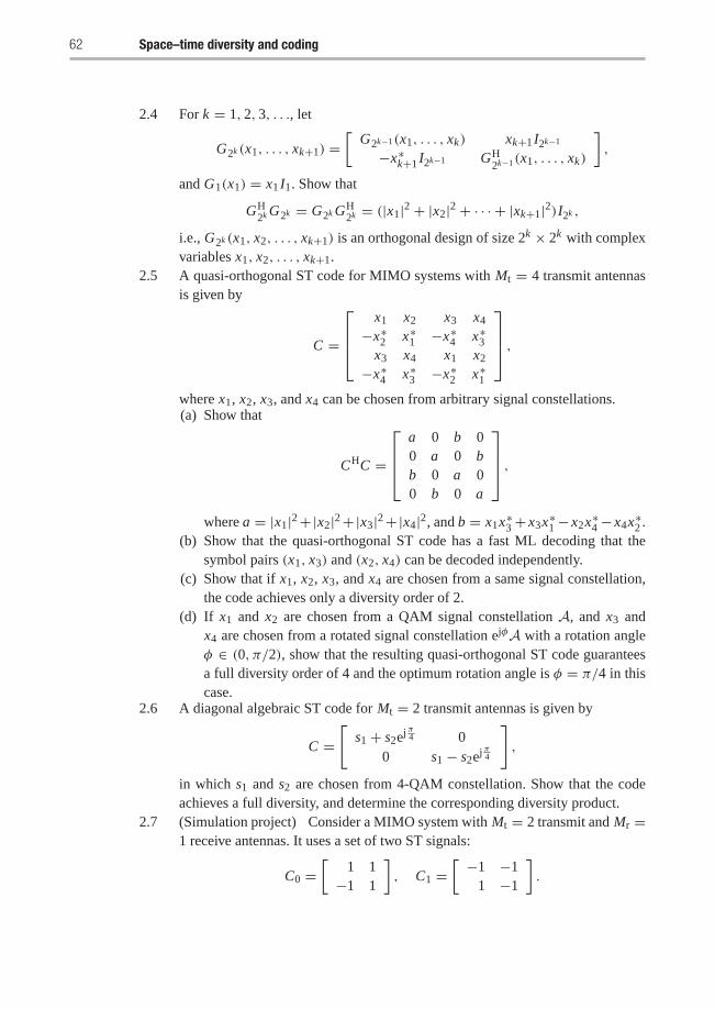
62 Space–time diversity and coding
2.4 For k = 1, 2, 3, . . ., let
G2k (x1, . . . , xk+1) =[
G2k−1(x1, . . . , xk) xk+1 I2k−1
−x∗k+1 I2k−1 GH2k−1(x1, . . . , xk)
],
and G1(x1) = x1 I1. Show that
GH2k G2k = G2k GH
2k = (|x1|2 + |x2|2 + · · · + |xk+1|2)I2k ,
i.e., G2k (x1, x2, . . . , xk+1) is an orthogonal design of size 2k × 2k with complexvariables x1, x2, . . . , xk+1.
2.5 A quasi-orthogonal ST code for MIMO systems with Mt = 4 transmit antennasis given by
C =
⎡⎢⎢⎣x1 x2 x3 x4
−x∗2 x∗1 −x∗4 x∗3x3 x4 x1 x2
−x∗4 x∗3 −x∗2 x∗1
⎤⎥⎥⎦ ,where x1, x2, x3, and x4 can be chosen from arbitrary signal constellations.(a) Show that
CHC =
⎡⎢⎢⎣a 0 b 00 a 0 bb 0 a 00 b 0 a
⎤⎥⎥⎦ ,where a = |x1|2+|x2|2+|x3|2+|x4|2, and b = x1x∗3 + x3x∗1 − x2x∗4 − x4x∗2 .
(b) Show that the quasi-orthogonal ST code has a fast ML decoding that thesymbol pairs (x1, x3) and (x2, x4) can be decoded independently.
(c) Show that if x1, x2, x3, and x4 are chosen from a same signal constellation,the code achieves only a diversity order of 2.
(d) If x1 and x2 are chosen from a QAM signal constellation A, and x3 andx4 are chosen from a rotated signal constellation ejφA with a rotation angleφ ∈ (0, π/2), show that the resulting quasi-orthogonal ST code guaranteesa full diversity order of 4 and the optimum rotation angle is φ = π/4 in thiscase.
2.6 A diagonal algebraic ST code for Mt = 2 transmit antennas is given by
C =[
s1 + s2ej π4 00 s1 − s2ej π4
],
in which s1 and s2 are chosen from 4-QAM constellation. Show that the codeachieves a full diversity, and determine the corresponding diversity product.
2.7 (Simulation project) Consider a MIMO system with Mt = 2 transmit and Mr =1 receive antennas. It uses a set of two ST signals:
C0 =[
1 1−1 1
], C1 =
[ −1 −11 −1
].
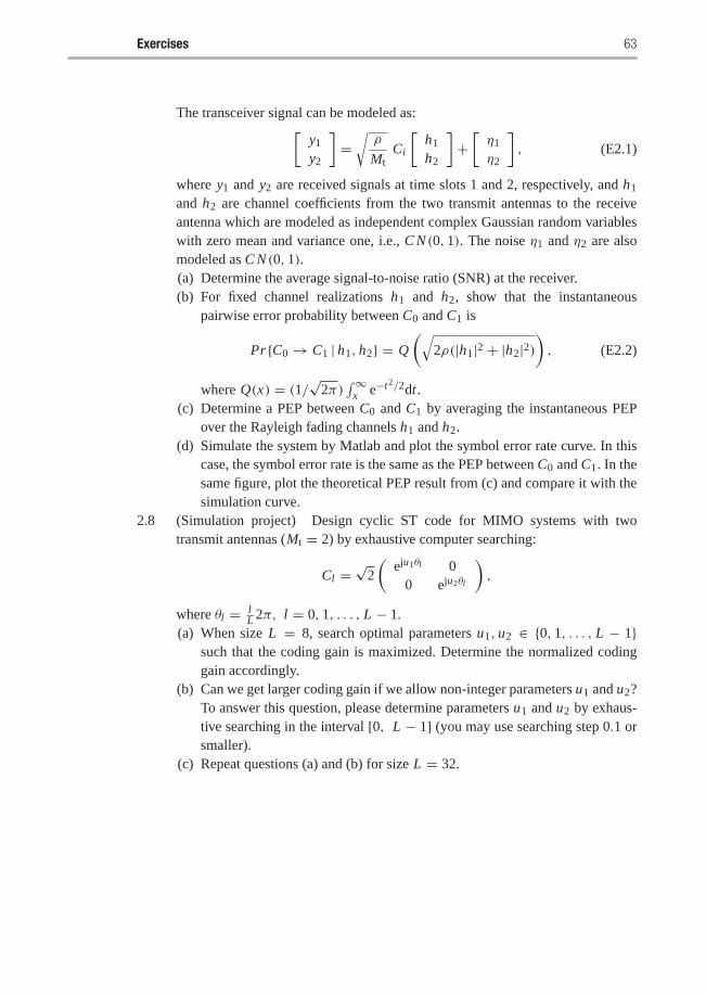
Exercises 63
The transceiver signal can be modeled as:[y1
y2
]=√ρ
MtCi
[h1
h2
]+[η1
η2
], (E2.1)
where y1 and y2 are received signals at time slots 1 and 2, respectively, and h1
and h2 are channel coefficients from the two transmit antennas to the receiveantenna which are modeled as independent complex Gaussian random variableswith zero mean and variance one, i.e., C N (0, 1). The noise η1 and η2 are alsomodeled as C N (0, 1).(a) Determine the average signal-to-noise ratio (SNR) at the receiver.(b) For fixed channel realizations h1 and h2, show that the instantaneous
pairwise error probability between C0 and C1 is
Pr{C0 → C1 | h1, h2} = Q
(√2ρ(|h1|2 + |h2|2)
), (E2.2)
where Q(x) = (1/√2π)∫∞
x e−t2/2dt .(c) Determine a PEP between C0 and C1 by averaging the instantaneous PEP
over the Rayleigh fading channels h1 and h2.(d) Simulate the system by Matlab and plot the symbol error rate curve. In this
case, the symbol error rate is the same as the PEP between C0 and C1. In thesame figure, plot the theoretical PEP result from (c) and compare it with thesimulation curve.
2.8 (Simulation project) Design cyclic ST code for MIMO systems with twotransmit antennas (Mt = 2) by exhaustive computer searching:
Cl =√
2
(eju1θl 0
0 eju2θl
),
where θl = lL 2π, l = 0, 1, . . . , L − 1.
(a) When size L = 8, search optimal parameters u1, u2 ∈ {0, 1, . . . , L − 1}such that the coding gain is maximized. Determine the normalized codinggain accordingly.
(b) Can we get larger coding gain if we allow non-integer parameters u1 and u2?To answer this question, please determine parameters u1 and u2 by exhaus-tive searching in the interval [0, L − 1] (you may use searching step 0.1 orsmaller).
(c) Repeat questions (a) and (b) for size L = 32.
3 Space–time–frequency diversityand coding
In broadband wireless communications, the channel exhibits frequency selectivity(delay spread), resulting in inter-symbol interference (ISI) that can cause serious per-formance degradation. A mature technique to mitigate the frequency selectivity is touse orthogonal frequency division multiplexing (OFDM), which eliminates the need forhigh complexity equalization and offers high spectral efficiency. In order to combine theadvantages of both the MIMO systems and the OFDM, space–frequency (SF)-codedMIMO-OFDM systems, where two-dimensional coding is applied to distribute chan-nel symbols across space (transmit antennas) and frequency (OFDM tones) within oneOFDM block, can be developed to exploit the available spatial and frequency diversity.
If longer decoding delay and higher decoding complexity are allowable, one mayconsider coding over several OFDM block periods, resulting in space–time–frequencycodes to exploit all of the spatial, temporal, and frequency diversity.
The chapter is organized as follows. First, we focus on SF-coded MIMO-OFDMsystems in broadband scenario and introduce two systematic approaches to designSF codes to achieve full spatial and frequency diversity within each OFDM block.Then, we consider STF coding for MIMO-OFDM systems, where the coding is appliedacross multiple OFDM blocks to exploit the spatial, temporal, and frequency diversityavailable in broadband MIMO wireless communications.
3.1 Space–frequency diversity and coding
In this section, we focus on SF-coded MIMO-OFDM systems to achieve the spatial andfrequency diversity in broadband wireless communications. First, we specify an SF-coded MIMO-OFDM system model and discuss design criteria for achieving the fullspatial and frequency diversity. Then, we review two systematic approaches to designSF codes to achieve the full spatial and frequency diversity within each OFDM block.
3.1.1 MIMO-OFDM system model
An SF-coded MIMO-OFDM system with Mt transmit antennas, Mr receive antennas,and N subcarriers is shown in Figure 3.1. Suppose that the frequency selective fadingchannels between each pair of transmit and receive antennas have L independent delaypaths and the same power delay profile. The MIMO channel is assumed to be constant
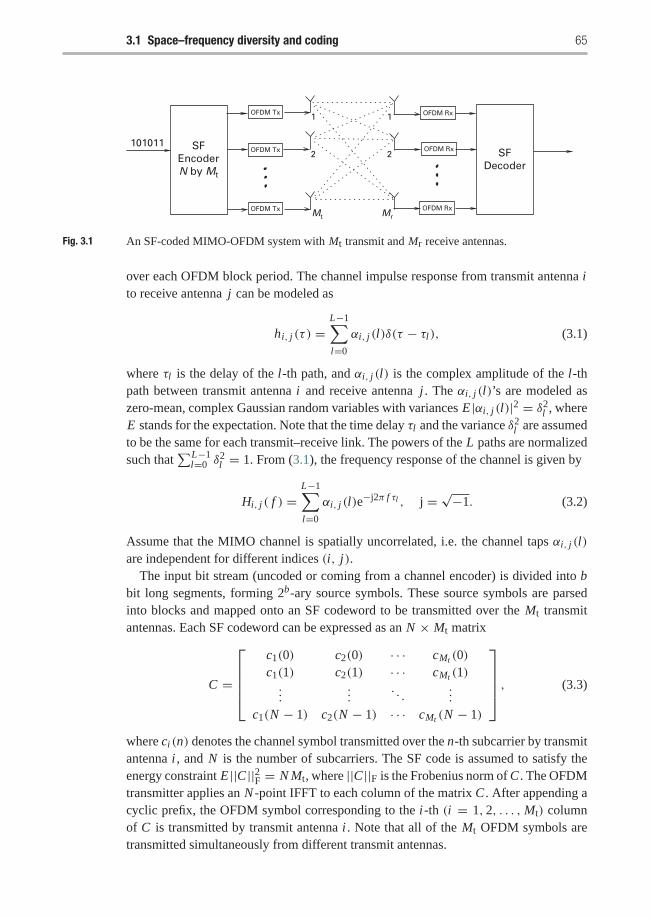
3.1 Space–frequency diversity and coding 65
SFEncoderN by Mt
SFDecoder
1
2
1
2
Mt Mr
101011OFDM Tx
OFDM Tx
OFDM Tx OFDM Rx
OFDM Rx
OFDM Rx
Fig. 3.1 An SF-coded MIMO-OFDM system with Mt transmit and Mr receive antennas.
over each OFDM block period. The channel impulse response from transmit antenna ito receive antenna j can be modeled as
hi, j (τ ) =L−1∑l=0
αi, j (l)δ(τ − τl), (3.1)
where τl is the delay of the l-th path, and αi, j (l) is the complex amplitude of the l-thpath between transmit antenna i and receive antenna j . The αi, j (l)’s are modeled aszero-mean, complex Gaussian random variables with variances E |αi, j (l)|2 = δ2
l , whereE stands for the expectation. Note that the time delay τl and the variance δ2
l are assumedto be the same for each transmit–receive link. The powers of the L paths are normalizedsuch that
∑L−1l=0 δ
2l = 1. From (3.1), the frequency response of the channel is given by
Hi, j ( f ) =L−1∑l=0
αi, j (l)e−j2π f τl , j = √−1. (3.2)
Assume that the MIMO channel is spatially uncorrelated, i.e. the channel taps αi, j (l)are independent for different indices (i, j).
The input bit stream (uncoded or coming from a channel encoder) is divided into bbit long segments, forming 2b-ary source symbols. These source symbols are parsedinto blocks and mapped onto an SF codeword to be transmitted over the Mt transmitantennas. Each SF codeword can be expressed as an N × Mt matrix
C =
⎡⎢⎢⎢⎣c1(0) c2(0) · · · cMt (0)c1(1) c2(1) · · · cMt (1)...
.... . .
...
c1(N − 1) c2(N − 1) · · · cMt (N − 1)
⎤⎥⎥⎥⎦ , (3.3)
where ci (n) denotes the channel symbol transmitted over the n-th subcarrier by transmitantenna i , and N is the number of subcarriers. The SF code is assumed to satisfy theenergy constraint E ||C ||2F = N Mt, where ||C ||F is the Frobenius norm of C . The OFDMtransmitter applies an N -point IFFT to each column of the matrix C . After appending acyclic prefix, the OFDM symbol corresponding to the i-th (i = 1, 2, . . . ,Mt) columnof C is transmitted by transmit antenna i . Note that all of the Mt OFDM symbols aretransmitted simultaneously from different transmit antennas.
66 Space–time–frequency diversity and coding
At the receiver, after matched filtering, removing the cyclic prefix, and applying FFT,the received signal at the n-th subcarrier at receive antenna j is given by
y j (n) =√ρ
Mt
Mt∑i=1
ci (n)Hi, j (n)+ z j (n), (3.4)
where
Hi, j (n) =L−1∑l=0
αi, j (l)e−j2πn� f τl (3.5)
is the channel frequency response at the n-th subcarrier between transmit antenna i andreceive antenna j ,� f = 1/T is the subcarrier separation in the frequency domain, andT is the OFDM symbol period. We assume that the channel state information Hi, j (n) isknown at the receiver, but not at the transmitter. In (3.4), z j (n) denotes the additive com-plex Gaussian noise with zero mean and unit variance at the n-th subcarrier at receiveantenna j . The noise samples z j (n) are assumed to be uncorrelated for different j’s andn’s. The factor
√ρ/Mt in (3.4) ensures that ρ is the average signal to noise ratio (SNR)
at each receive antenna, independently of the number of transmit antennas.
3.1.1.1 General performance criteriaThe received signal (3.4) can be rewritten in vector form as
Y =√ρ
MtDH+ Z, (3.6)
where D is an N Mr × N MtMr matrix constructed from the SF codeword C in (3.3) asfollows:
D =
⎡⎢⎢⎢⎣D1 D2 · · · DM 0 0 · · · 0 · · · 0 0 · · · 00 0 · · · 0 D1 D2 · · · DM · · · 0 0 · · · 0
......
. . ....
0 0 · · · 0 0 0 · · · 0 · · · D1 D2 · · · DM
⎤⎥⎥⎥⎦ ,(3.7)
in which
Di = diag{ci (0), ci (1), . . . , ci (N − 1)}, i = 1, 2, . . . ,Mt. (3.8)
Each Di in (3.8) is related to the i-th column of the SF codeword C . The channel vectorH of size N MtMr × 1 is formatted as
H = [HT1,1 · · · HT
Mt ,1 HT1,2 · · · HT
Mt,2 · · · HT1,Mr
· · · HTMt,Mr
]T, (3.9)
where
Hi, j = [Hi, j (0) Hi, j (1) · · · Hi, j (N − 1)]T. (3.10)
The received signal vector Y of size N Mr × 1 is given by
Y = [y1(0) · · · y1(N − 1) y2(0) · · · y2(N − 1) · · · yMr(0) · · · yMr(N − 1)]T,
(3.11)

3.1 Space–frequency diversity and coding 67
and the noise vector Z has the same form as Y, i.e.,
Z = [z1(0) · · · z1(N − 1) z2(0) · · · z2(N − 1) · · · zMr(0) · · · zMr(N − 1)]T.
(3.12)Suppose that D and D are two different matrices related to two different SF codewords
C and C , respectively. Then, the pairwise error probability between D and D can beupper bounded as (leave proof as an exercise)
P(D → D) ≤(
2r − 1r
) ( r∏i=1
γi
)−1 (ρ
Mt
)−r
, (3.13)
where r is the rank of (D− D)R(D− D)H, γ1, γ2, . . . , γr are the nonzero eigenvaluesof (D−D)R(D−D)H, and R = E{HHH} is the correlation matrix of H. The superscriptH stands for the complex conjugate and transpose of a matrix.
Based on the upper bound on the pairwise error probability in (3.13), two general SFcode performance criteria can be proposed as follows:
• Diversity (rank) criterion: The minimum rank of (D− D)R(D− D)H over all pairs ofdifferent codewords C and C should be as large as possible.
• Product criterion: The minimum value of the product∏r
i=1 γi over all pairs ofdifferent codewords C and C should be maximized.
However, it is hard to design SF codes directly based on the discussion on (D − D)R(D− D)H, which is related to an N MtMr × N MtMr correlation matrix R.
3.1.1.2 Performance criteriaIn case of spatially uncorrelated MIMO channels, i.e., the channel taps αi, j (l) are inde-pendent for different transmit antenna i and receive antenna j , the correlation matrix Rof size N MtMr × N MtMr becomes
R = E{HHH}= diag
(R1,1, . . . , RMt,1, R1,2, . . . , RMt,2,
. . . , R1,Mr , . . . , RMt,Mr
), (3.14)
where
Ri, j = E{
Hi, j HHi, j
}(3.15)
is the correlation matrix of the channel frequency response from transmit antenna i toreceive antenna j . Using the notation w = e−j2π� f , from (3.5) and (3.10), we have
Hi, j =[
L−1∑l=0
αi, j (l)L−1∑l=0
αi, j (l)wτl · · ·
L−1∑l=0
αi, j (l)w(N−1)τl
]T
= W · Ai, j , (3.16)
68 Space–time–frequency diversity and coding
where
W =
⎡⎢⎢⎢⎣1 1 · · · 1wτ0 wτ1 · · · wτL−1
......
. . ....
w(N−1)τ0 w(N−1)τ1 · · · w(N−1)τL−1
⎤⎥⎥⎥⎦N×L
,
and
Ai, j =[αi, j (0) αi, j (1) · · · αi, j (L − 1)
]T.
Note that, in general, W is not a unitary matrix. If all of the L delay paths fall at thesampling instances of the receiver, then W is part of the DFT-matrix, which is unitary.Substituting (3.16) into (3.15), Ri, j in (3.15) can be expressed as
Ri, j = E{
W Ai, j AHi, j W
H}
= W E{
Ai, j AHi, j
}W H
= Wdiag(δ20, δ
21, . . . , δ
2L−1)W
H �= R. (3.17)
The third equality follows from the assumption that the path gains αi, j (l) are indepen-dent for different paths and different pairs of transmit and receive antennas. Note thatthe correlation matrix R is independent of the transmit and receive antenna indices iand j . From (3.14) and (3.17), we obtain
R = IMt Mr ⊗ R, (3.18)
where IMt Mr is the identity matrix of size MtMr × MtMr, and ⊗ denotes the tensorproduct which is defined as follows: for any two matrices A = {ai, j } and B = {bi, j } ofsize m × n,
A ⊗ B�=⎡⎣ a1,1 B · · · a1,n B
· · · · · · · · ·am,1 B · · · am,n B
⎤⎦ . (3.19)
Therefore, combining (3.3), (3.7), (3.8), and (3.18), the expression for (D − D)R(D− D)H in (3.13) can be rewritten as
(D− D)R(D− D)H = IMr ⊗[ Mt∑
i=1
(Di − Di )R(Di − Di )H
]= IMr ⊗
{[(C − C)(C − C)H
]◦ R}, (3.20)
where ◦ denotes the Hadamard product, which is defined as follows: for any twomatrices A = {ai, j } and B = {bi, j } of size m × n,
A ◦ B�=⎡⎣ a1,1b1,1 · · · a1,nb1,n
· · · · · · · · ·am,1bm,1 · · · am,nbm,n
⎤⎦ . (3.21)
3.1 Space–frequency diversity and coding 69
Denoting a matrix � as
� = (C − C)(C − C)H, (3.22)
and substituting (3.20) into (3.13), the pairwise error probability between C and C canbe upper bounded as
P(C → C) ≤(
2K Mr − 1K Mr
) ( K∏i=1
λi
)−Mr (ρ
Mt
)−K Mr
, (3.23)
where K is the rank of�◦ R, and λ1, λ2, . . . , λK are the nonzero eigenvalues of�◦ R.As a consequence, we can formulate the performance criteria as follows:
• Diversity (rank) criterion: The minimum rank of�◦R over all pairs of distinct signalsC and C should be as large as possible.
• Product criterion: The minimum value of the product∏K
i=1 λi over all pairs of distinctsignals C and C should also be maximized.
According to a rank inequality on Hadamard products ([74], p.307), we have therelationship
rank(� ◦ R) ≤ rank(�)rank(R). (3.24)
Since the rank of � is at most Mt, the rank of R is at most L , and the rank of � ◦ R isat most N , so
rank(� ◦ R) ≤ min{L Mt , N }. (3.25)
Thus, the maximum achievable diversity is at most min{L MtMr, N Mr}. When N islarge, the full diversity is L MtMr, which is the product of the number of multiple delaysand the number of transmit and receive antennas.
3.1.2 Full-diversity SF code design via mapping
In this subsection, we present an interesting approach to systematically design full-diversity SF codes from ST codes. It shows that using a simple repetition mapping,full-diversity SF codes can be constructed from any ST (block or trellis) code designedfor quasi-static flat Rayleigh fading channels.
3.1.2.1 SF code design via mappingIn the sequel, the SF encoder will consist of an ST encoder and a mapping Ml , as shownin Figure 3.2. For each 1 × Mt output vector [g1 g2 · · · gMt] from the ST encoder anda fixed number l (1 ≤ l ≤ L), the mapping Ml is defined as
Ml : [g1 g2 · · · gMt] → 1l×1[g1 g2 · · · gMt], (3.26)
where 1l×1 is an all one matrix of size l × 1. The resulting l × Mt matrix is actuallya repetition of the vector [g1 g2 · · · gMt] l times. Suppose that lMt is not greater thanthe number of OFDM subcarriers, N , and k is the largest integer such that klMt ≤ N .
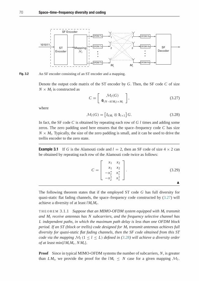
70 Space–time–frequency diversity and coding
SFDecoder
1
2
1
2
Mt Mr
STEncoder
SF Encoder
101011Mapping
�l
OFDM Tx
OFDM Tx
OFDM Tx
OFDM Rx
OFDM Rx
OFDM Rx
Fig. 3.2 An SF encoder consisting of an ST encoder and a mapping.
Denote the output code matrix of the ST encoder by G. Then, the SF code C of sizeN × Mt is constructed as
C =[
Ml(G)0(N−klMt)×Mt
], (3.27)
where
Ml(G) =[IkMt ⊗ 1l×1
]G. (3.28)
In fact, the SF code C is obtained by repeating each row of G l times and adding somezeros. The zero padding used here ensures that the space–frequency code C has sizeN × Mt. Typically, the size of the zero padding is small, and it can be used to drive thetrellis encoder to the zero state.
Example 3.1 If G is the Alamouti code and l = 2, then an SF code of size 4 × 2 canbe obtained by repeating each row of the Alamouti code twice as follows:
C =
⎡⎢⎢⎣x1 x2
x1 x2
−x∗2 x∗1−x∗2 x∗1
⎤⎥⎥⎦ . (3.29)
�
The following theorem states that if the employed ST code G has full diversity forquasi-static flat fading channels, the space–frequency code constructed by (3.27) willachieve a diversity of at least lMtMr.
T H E O R E M 3.1.1 Suppose that an MIMO-OFDM system equipped with Mt transmitand Mr receive antennas has N subcarriers, and the frequency selective channel hasL independent paths, in which the maximum path delay is less than one OFDM blockperiod. If an ST (block or trellis) code designed for Mt transmit antennas achieves fulldiversity for quasi-static flat fading channels, then the SF code obtained from this STcode via the mapping Ml (1 ≤ l ≤ L) defined in (3.28) will achieve a diversity orderof at least min{lMtMr, N Mr}.
Proof Since in typical MIMO-OFDM systems the number of subcarriers, N , is greaterthan L Mt, we provide the proof for the lMt ≤ N case for a given mapping Ml ,
3.1 Space–frequency diversity and coding 71
1 ≤ l ≤ L . If lMt > N , the proof is similar to the one described below and is omittedfor brevity. Assume that k is the largest integer such that klMt ≤ N .
For two distinct SF codewords C and C of size N × Mt, there are two correspondingdistinct ST codewords G and G of size kMt × Mt such that
C − C =[
Ml(G − G)0(N−klMt)×Mt
], (3.30)
in which
Ml(G − G) = [IkMt ⊗ 1l×1](G − G). (3.31)
Since the ST code achieves full diversity for quasi-static flat fading channels, G − G isof full rank for two distinct G and G, i.e., the rank of G − G is Mt.
Based on the SF code performance criteria, the objective of the proof is to show thatthe matrix � ◦ R has a rank of at least lMt. From (3.22) and (3.30), we have
� =[
Ml(G − G)[Ml(G − G)]H 0klMt×(N−klMt)
0(N−klMt)×klMt 0(N−klMt)×(N−klMt)
]. (3.32)
Thus, in�◦ R, all entries are zero except a klMt× klMt submatrix. Denote this klMt×klMt submatrix as (� ◦ R)klMt×klMt .
On the other hand, from (3.17), it can be verified that the entries of the correlation
matrix R�= {ri, j }1≤i, j≤N can be expressed as
ri, j =L−1∑s=0
δ2sw
(i− j)τs , 1 ≤ i, j ≤ N .
Therefore, from (3.30), (3.31), and (3.32), we obtain
(� ◦ R)klMt×klMt ={Ml(G − G)[Ml(G − G)]H
}◦ P
={[IkMt ⊗ 1l×1](G − G)(G − G)H[IkMt ⊗ 1l×1]H
}◦ P
={[(G − G)(G − G)H
]⊗ 1l×l
}◦ P, (3.33)
where P = {pi, j }1≤i, j≤klMt is a klMt × klMt matrix with entries
pi, j =L−1∑s=0
δ2sw
(i− j)τs , 1 ≤ i, j ≤ klMt. (3.34)
The last equality in (3.33) follows from the identities [IkMt ⊗1l×1]H = IkMt ⊗11×l and(A1 ⊗ B1)(A2 ⊗ B2)(A3 ⊗ B3) = (A1 A2 A3)⊗ (B1 B2 B3) ([74], p.251).
We further partition the klMt × klMt matrix P into l × l submatrices as follows:
P =
⎡⎢⎢⎢⎣P1,1 P1,2 · · · P1,kMt
P2,1 P2,2 · · · P2,kMt...
.... . .
...
PkMt,1 PkMt,2 · · · PkMt,kMt
⎤⎥⎥⎥⎦ , (3.35)
72 Space–time–frequency diversity and coding
where each submatrix Pm,n, 1 ≤ m, n ≤ kMt, is of size l × l. Denoting the entries ofPm,n as pm,n(i, j), 1 ≤ i, j ≤ l, we obtain
pm,n(i, j) =L−1∑s=0
δ2sw
[(m−n)l+(i− j)]τs , 1 ≤ i, j ≤ l. (3.36)
As a consequence, each submatrix Pm,n, 1 ≤ m, n ≤ kMt, can be expressed as
Pm,n = Wmdiag{δ20, δ
21, . . . , δ
2L−1}W H
n , (3.37)
where
Wm =
⎡⎢⎢⎢⎣w(m−1)lτ0 w(m−1)lτ1 · · · w(m−1)lτL−1
w[(m−1)l+1]τ0 w[(m−1)l+1]τ1 · · · w[(m−1)l+1]τL−1
......
. . ....
w[(m−1)l+(l−1)]τ0 w[(m−1)l+(l−1)]τ1 · · · w[(m−1)l+(l−1)]τL−1
⎤⎥⎥⎥⎦ , (3.38)
for m = 1, 2, . . . , kMt. In (3.38), Wm can be further decomposed as
Wm = W1diag{w(m−1)lτ0, w(m−1)lτ1 , . . . , w(m−1)lτL−1} (3.39)
for 1 ≤ m ≤ kMt, where
W1 =
⎡⎢⎢⎢⎣1 1 · · · 1wτ0 wτ1 · · · wτL−1
......
. . ....
w(l−1)τ0 w(l−1)τ1 · · · w(l−1)τL−1
⎤⎥⎥⎥⎦ . (3.40)
Let us denote the matrix consisting of the first l columns of W1 by W0. We observe thatW0 is an l× l Vandermonde matrix in l variables wτ0 , wτ1 , . . . , wτl−1 ([74], p.400). Thedeterminant of W0 can be calculated as follows:
det(W0) =∏
0≤i< j≤l−1
(wτ j − wτi )
=∏
0≤i< j≤l−1
[e−j2π� f (τ j−τi ) − 1
]e−j2π� f τi .
Since � f is the inverse of the OFDM block period T and the maximum path delay isless than T , we have � f (τ j − τi ) < 1 for any 0 ≤ i < j ≤ l − 1. Thus, W0 is of fullrank, and so is W1. It follows that for any m = 1, 2, . . . , kMt, the rank of Wm is l.
We now go back to (3.33) to investigate the rank of � ◦ R. For convenience, we usethe notation
(G − G)(G − G)H�=
⎡⎢⎢⎢⎣a1,1 a1,2 · · · a1,kMt
a2,1 a2,2 · · · a2,kMt...
.... . .
...
akMt,1 akMt,2 · · · akMt,kMt
⎤⎥⎥⎥⎦ ,
3.1 Space–frequency diversity and coding 73
and � = diag{δ20, δ
21, . . . , δ
2L−1}. Then, substituting (3.35) and (3.37) into (3.33), we
obtain
(� ◦ R)klMt×klMt
=
⎡⎢⎢⎢⎣a1,1 P1,1 a1,2 P1,2 · · · a1,kMt P1,kMt
a2,1 P2,1 a2,2 P2,2 · · · a2,kMt P2,kMt...
.... . .
...
akMt,1 PkMt,1 akMt,2 PkMt,2 · · · akMt,kMt PkMt,kMt
⎤⎥⎥⎥⎦
=
⎡⎢⎢⎢⎢⎣W1a1,1�W H
1 W1a1,2�W H2 · · · W1a1,kMt�W H
kMt
W2a2,1�W H1 W2a2,2�W H
2 · · · W2a2,kMt�W HkMt
......
. . ....
WkMtakMt,1�W H1 WkMtakMt,2�W H
2 · · · WkMtakMt,kMt�W HkMt
⎤⎥⎥⎥⎥⎦= Q
{[(G − G)(G − G)H
]⊗�
}QH, (3.41)
where
Q = diag{W1, W2, . . . , WkMt
}.
Since the rank of G − G is Mt, there are Mt linearly independent rows in G − G.Suppose that the fi -th, 1 ≤ f1 < f2 < · · · < fMt ≤ kMt, rows of G − G are linearlyindependent of each other. Then, the matrix
A�=
⎡⎢⎢⎢⎣a f1, f1 a f1, f2 · · · a f1, fMt
a f2, f1 a f2, f2 · · · a f2, fMt...
.... . .
...
a fMt , f1 a fMt , f2 · · · a fMt , fMt
⎤⎥⎥⎥⎦is a submatrix of (G − G)(G − G)H, and the rank of A is Mt. Using the notation
Q0 = diag{W f1, W f2 , . . . , W fMt},
from (3.41), we can see that Q0 {A ⊗�} QH0 is an lMt × lMt submatrix of (� ◦
R)klMt×klMt . Therefore, to show that the rank of � ◦ R is at least lMt, it is sufficient toshow that the submatrix Q0 {A ⊗�} QH
0 has rank lMt.Since the rank of A is Mt and the rank of � is L , according to a rank equality on
tensor products ([74], p.246), we have
rank(A ⊗�) = rank(A)rank(�) = MtL ,
so the matrix A ⊗� is of full rank. Recall that for any m = 1, 2, . . . , kMt, the rank ofWm is l, so the rank of Q0 is lMt. Therefore, the rank of Q0 {A ⊗�} QH
0 is lMt. Thisproves the theorem. �
In addition, from the proof of Theorem 3.1.1, we can see that the SF code obtained froma space–time block code of square size via the mapping Ml (1 ≤ l ≤ L) will achieve adiversity of lMtMr exactly. Since the maximum achievable diversity is upper boundedby min{L MtMr, N Mr}, we arrive at the following result.
74 Space–time–frequency diversity and coding
Corollary 3.1.1 Under the assumptions of Theorem 3.1.1, the SF code obtained froma full diversity ST code via the mapping ML defined in (3.28) achieves the maximumachievable diversity min{L MtMr, N Mr}.
The symbol rate of the resulting SF codes obtained via the mapping Ml (3.28) is 1/ ltimes that of the corresponding ST codes. For example, for a system with two trans-mit antennas, eight subcarriers and a two-ray delay profile, the symbol rate of thefull-diversity SF codes discussed here is 1/2. In certain practical situations, this effectcan be compensated by expanding the constellation size, maintaining the same spectralefficiency. Furthermore, from a system performance point of view, there is a tradeoffbetween the diversity order and the coding rate. Theorem 3.1.1 offers a flexible choiceon the diversity order.
3.1.2.2 Coding advantageIn the following, we characterize the coding advantage of the resulting SF codes interms of the coding advantage of the underlying ST codes by defining and evaluatingthe diversity product for SF codes.
We recall from (2.9) that the diversity product or the normalized coding advantage ofa full-diversity ST code for quasi-static flat fading channels is
ζST = 1
2√
MtminG �=G
∣∣∣∣∣Mt∏
i=1
βi
∣∣∣∣∣1
2Mt
, (3.42)
where β1, β2, . . . , βMt are the nonzero eigenvalues of (G− G)(G− G)H for any pair ofdistinct ST codewords G and G. Similarly, the diversity product of a full-diversity SFcode can be defined as
ζSF, R = 1
2√
MtminC �=C
∣∣∣∣∣L Mt∏i=1
λi
∣∣∣∣∣1
2L Mt
, (3.43)
where λ1, λ2, . . . , λL Mt are the nonzero eigenvalues of � ◦ R for any pair of dis-tinct space–frequency codewords C and C . In the rest of this section, without loss ofgenerality, we assume that the number of subcarriers, N , is not less than L Mt, i.e.,L Mt ≤ N .
The relationship between the diversity products of the full-diversity SF codesobtained via the repetition mapping and the underlying ST codes is characterized bythe following theorem.
T H E O R E M 3.1.2 The diversity product of the full-diversity SF code in Corollary3.1.1 is bounded by that of the corresponding ST code as follows:
√ηL �ζST ≤ ζSF, R ≤ √η1�ζST, (3.44)
3.1 Space–frequency diversity and coding 75
where � =(∏L−1
l=0 δl
)1/L, and η1 and ηL are the largest and smallest eigenvalues,
respectively, of the matrix H defined as
H =
⎡⎢⎢⎢⎣H(0) H(1)∗ · · · H(L − 1)∗H(1) H(0) · · · H(L − 2)∗...
.... . .
...
H(L − 1) H(L − 2) · · · H(0)
⎤⎥⎥⎥⎦L×L
, (3.45)
and the entries of H are given by
H(n) =L−1∑l=0
e−j2πn� f τl , n = 0, 1, . . . , L − 1.
Proof In the following, we use the notation developed in the proof of Theorem 3.1.1by replacing the repetition factor l with L , since the full diversity is achieved in Corol-lary 3.1.1 by using the mapping ML . For any n × n nonnegative definite matrix A,we denote its eigenvalues in a non-increasing order as: eig1(A) ≥ eig2(A) ≥ · · · ≥eign(A).
For two distinct SF codewords C and C , there are two corresponding ST codewordsG and G such that the relationship of C − C and G − G in (3.30) and (3.31) holds.According to (3.25) and Corollary 3.1.1, the rank of � ◦ R is exactly L Mt. It meansthat � ◦ R has totally L Mt nonzero eigenvalues, which are the same as the nonzeroeigenvalues of (� ◦ R)kL Mt×kL Mt . Thus,
ζSF, R = 1
2√
MtminC �=C
∣∣∣∣∣L Mt∏i=1
eigi
((� ◦ R)kL Mt×kL Mt
)∣∣∣∣∣1
2L Mt
= 1
2√
MtminG �=G
∣∣∣∣∣L Mt∏i=1
eigi
(Q{[(G − G)(G − G)H
]⊗�
}QH)∣∣∣∣∣
12L Mt
= 1
2√
MtminG �=G
∣∣∣∣∣L Mt∏i=1
θi eigi
([(G − G)(G − G)H
]⊗�
)∣∣∣∣∣1
2L Mt
, (3.46)
where eigkL Mt(QQH) ≤ θi ≤ eig1(QQH) for i = 1, 2, . . . , L Mt. In (3.46), the second
equality follows from (3.41), and the last equality follows by Ostrowski’s theorem ([73],p.224). Since Q = diag
{W1, W2, . . . , WkMt
}, we have
QQH = diag{
W1W H1 , W2W H
2 , . . . , WkMt WHkMt
}.
As a requirement of Ostrowski’s theorem, the matrix Q should be nonsingular, which isguaranteed by the fact that each matrix Wm is of full rank for any m = 1, 2, . . . , kMt.Furthermore, from (3.39), we know that for any 1 ≤ m ≤ kMt,
WmW Hm = W1 DDHW H
1 = W1W H1 ,
76 Space–time–frequency diversity and coding
where D = diag{w(m−1)Lτ0 , w(m−1)Lτ1 , . . . , w(m−1)LτL−1}. From (3.40), it is easy toverify that W1W H
1 is the matrix H defined in (3.45). Thus, QQH = IkMt⊗H . Therefore,we can conclude that eigL(H) ≤ θi ≤ eig1(H) for any i = 1, 2, . . . , L Mt.
Since the set of L Mt nonzero eigenvalues of[(G − G)(G − G)H
]⊗ � can be
expressed as ([73], p.246){eigi
((G − G)(G − G)H
)· eig j (�) : 1 ≤ i ≤ Mt, 1 ≤ j ≤ L
}, (3.47)
substituting (3.47) into (3.46), we arrive at
ζSF, R = 1
2√
MtminG �=G
(L Mt∏i=1
θi
) 12L Mt
∣∣∣∣∣Mt∏i=1
eigi
((G − G)(G − G)H
)∣∣∣∣∣1
2Mt⎛⎝ L∏
j=1
eig j (�)
⎞⎠1
2L
=(L Mt∏
i=1
θi
) 12L Mt
⎛⎝ L∏j=1
δ2j
⎞⎠1
2L
ζST. (3.48)
Since ηL ≤ θi ≤ η1 for any i = 1, 2, . . . , L Mt, we have the inequalities in (3.44). �
From Theorem 3.1.2, we can see that the larger the coding advantage of the ST code,the larger the coding advantage of the resulting SF code, suggesting that to maximizethe performance of the SF codes, we should look for the best-known ST codes existingin the literature. Moreover, the coding advantage of the SF code depends on the powerdelay profile:
• First, it depends on the power distribution through the square root of the geometric
average of path powers, i.e., � =(∏L−1
l=0 δl
)1/L. Since the sum of the powers of the
paths is unity, this implies that the best performance is expected in the case of uniformpower distribution (i.e., δ2
l = 1/L).• Second, the entries of the matrix H defined in (3.45) are functions of the path delays,
so the coding advantage also depends on the delay distribution of the paths.
For example, in case of a two-ray delay profile (i.e., L = 2), the matrix H in (3.45) hastwo eigenvalues:
η1 = 2+ 2| cosπ(τ1 − τ0)/T |,η2 = 2− 2| cosπ(τ1 − τ0)/T |.
Typically, the ratio of (τ1− τ0)/T is less than 1/2, so cosπ(τ1− τ0)/T is nonnegative.Thus, the smaller the separation of the two rays, the smaller the eigenvalue η2. If thetwo rays are very close compared to the duration of one OFDM symbol, T , the lowerbound in (3.44) approaches zero. Simulation results seem to suggest that the behaviorof the coding advantage is close to the lower bound.
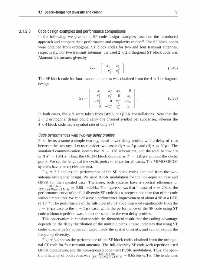
3.1 Space–frequency diversity and coding 77
3.1.2.3 Code design examples and performance comparisonsIn the following, we give some SF code design examples based on the introducedapproach and compare their performance and complexity tradeoff. The SF block codeswere obtained from orthogonal ST block codes for two and four transmit antennas,respectively. For two transmit antennas, the used 2 × 2 orthogonal ST block code wasAlamouti’s structure, given by
G2 =[
x1 x2
−x∗2 x∗1
]. (3.49)
The SF block code for four transmit antennas was obtained from the 4 × 4 orthogonaldesign
G4 =
⎡⎢⎢⎣x1 x2 x3 0
−x∗2 x∗1 0 x3
−x∗3 0 x∗1 −x2
0 −x∗3 x∗2 x1
⎤⎥⎥⎦ . (3.50)
In both cases, the xi ’s were taken from BPSK or QPSK constellations. Note that the2 × 2 orthogonal design could carry one channel symbol per subcarrier, whereas the4× 4 block code had a symbol rate of only 3/4.
Code performances with two-ray delay profilesFirst, let us assume a simple two-ray, equal-power delay profile, with a delay of τ μsbetween the two rays. Let us consider two cases: (i) τ = 5 μs and (ii) τ = 20 μs. Thesimulated communication system has N = 128 subcarriers, and the total bandwidthis BW = 1 MHz. Thus, the OFDM block duration is T = 128 μs without the cyclicprefix. We set the length of the cyclic prefix to 20 μs for all cases. The MIMO-OFDMsystems have one receive antenna.
Figure 3.3 depicts the performance of the SF block codes obtained from the two-antenna orthogonal design. We used BPSK modulation for the non-repeated case andQPSK for the repeated case. Therefore, both systems have a spectral efficiency of
128×1 bits(128 μs+20 μs)×1 MHz = 0.86 bits/s/Hz. The figure shows that in case of τ = 20 μs, theperformance curve of the full-diversity SF code has a steeper slope than that of the codewithout repetition. We can observe a performance improvement of about 4 dB at a BERof 10−4. The performance of the full-diversity SF code degraded significantly from theτ = 20 μs case to the τ = 5 μs case, while the performance of the SF code using STcode without repetition was almost the same for the two delay profiles.
This observation is consistent with the theoretical result that the coding advantagedepends on the delay distribution of the multiple paths. It also indicates that using STcodes directly as SF codes can exploit only the spatial diversity, and cannot exploit thefrequency diversity.
Figure 3.4 shows the performance of the SF block codes obtained from the orthogo-nal ST code for four transmit antennas. The full-diversity SF code with repetition usedQPSK modulation, and the non-repeated code used BPSK modulation. Thus, the spec-tral efficiency of both codes was 128×3/4 bits
(128 μs+20 μs)×1 MHz = 0.65 bits/s/Hz. The tendencies
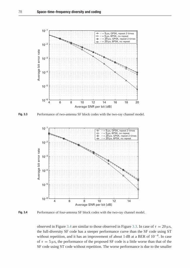
78 Space–time–frequency diversity and coding
4 6 8 10 12 14 16 18 2010−6
10−5
10–4
10−3
10−2
10−1
Average SNR per bit [dB]
Ave
rag
e b
it e
rro
r ra
teτ = 5 μs, QPSK, repeat 2 timesτ = 5 μs, BPSK, no repeatτ = 20 μs, QPSK, repeat 2 timesτ = 20 μs, BPSK, no repeat
Fig. 3.3 Performance of two-antenna SF block codes with the two-ray channel model.
4 6 8 10 12 1410−6
10−5
10–4
10−3
10−2
10−1
Average SNR per bit [dB]
Ave
rag
e b
it e
rro
r ra
te
τ = 5 μs, QPSK, repeat 2 timesτ = 5 μs, BPSK, no repeatτ = 20 μs, QPSK, repeat 2 timesτ = 20 μs, BPSK, no repeat
Fig. 3.4 Performance of four-antenna SF block codes with the two-ray channel model.
observed in Figure 3.4 are similar to those observed in Figure 3.3. In case of τ = 20 μs,the full-diversity SF code has a steeper performance curve than the SF code using STwithout repetition, and it has an improvement of about 1 dB at a BER of 10−4. In caseof τ = 5 μs, the performance of the proposed SF code is a little worse than that of theSF code using ST code without repetition. The worse performance is due to the smaller
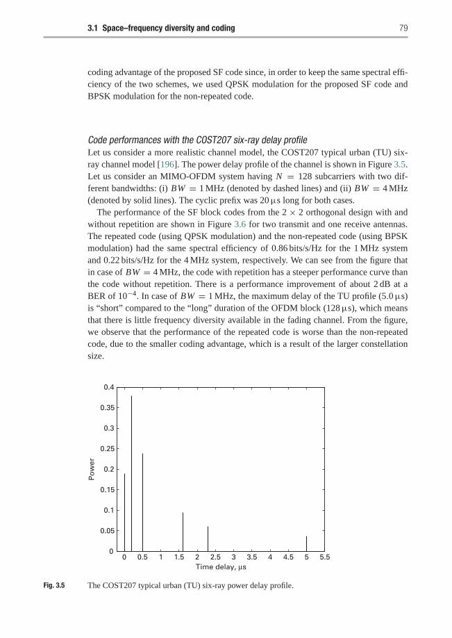
3.1 Space–frequency diversity and coding 79
coding advantage of the proposed SF code since, in order to keep the same spectral effi-ciency of the two schemes, we used QPSK modulation for the proposed SF code andBPSK modulation for the non-repeated code.
Code performances with the COST207 six-ray delay profileLet us consider a more realistic channel model, the COST207 typical urban (TU) six-ray channel model [196]. The power delay profile of the channel is shown in Figure 3.5.Let us consider an MIMO-OFDM system having N = 128 subcarriers with two dif-ferent bandwidths: (i) BW = 1 MHz (denoted by dashed lines) and (ii) BW = 4 MHz(denoted by solid lines). The cyclic prefix was 20 μs long for both cases.
The performance of the SF block codes from the 2 × 2 orthogonal design with andwithout repetition are shown in Figure 3.6 for two transmit and one receive antennas.The repeated code (using QPSK modulation) and the non-repeated code (using BPSKmodulation) had the same spectral efficiency of 0.86 bits/s/Hz for the 1 MHz systemand 0.22 bits/s/Hz for the 4 MHz system, respectively. We can see from the figure thatin case of BW = 4 MHz, the code with repetition has a steeper performance curve thanthe code without repetition. There is a performance improvement of about 2 dB at aBER of 10−4. In case of BW = 1 MHz, the maximum delay of the TU profile (5.0 μs)is “short” compared to the “long” duration of the OFDM block (128 μs), which meansthat there is little frequency diversity available in the fading channel. From the figure,we observe that the performance of the repeated code is worse than the non-repeatedcode, due to the smaller coding advantage, which is a result of the larger constellationsize.
0 0.5 1 1.5 2 2.5 3 3.5 4 4.5 5 5.50
0.05
0.1
0.15
0.2
0.25
0.3
0.35
0.4
Time delay, μs
Po
wer
Fig. 3.5 The COST207 typical urban (TU) six-ray power delay profile.
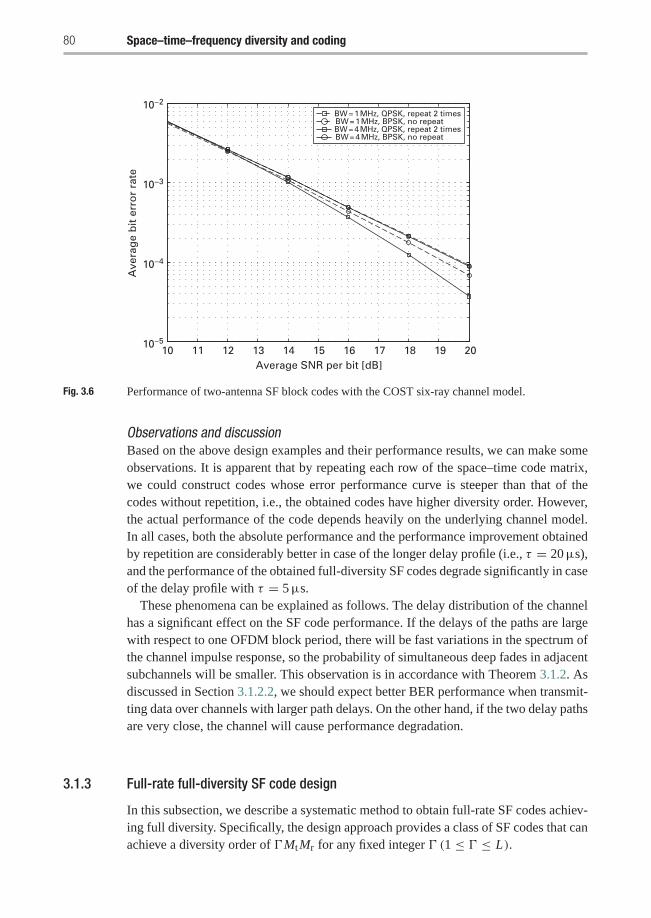
80 Space–time–frequency diversity and coding
10 11 12 13 14 15 16 17 18 19 2010−5
10−4
10−3
10−2
Average SNR per bit [dB]
Ave
rag
e b
it e
rro
r ra
te
BW = 1 MHz, QPSK, repeat 2 timesBW = 1 MHz, BPSK, no repeatBW = 4 MHz, QPSK, repeat 2 timesBW = 4 MHz, BPSK, no repeat
Fig. 3.6 Performance of two-antenna SF block codes with the COST six-ray channel model.
Observations and discussionBased on the above design examples and their performance results, we can make someobservations. It is apparent that by repeating each row of the space–time code matrix,we could construct codes whose error performance curve is steeper than that of thecodes without repetition, i.e., the obtained codes have higher diversity order. However,the actual performance of the code depends heavily on the underlying channel model.In all cases, both the absolute performance and the performance improvement obtainedby repetition are considerably better in case of the longer delay profile (i.e., τ = 20 μs),and the performance of the obtained full-diversity SF codes degrade significantly in caseof the delay profile with τ = 5 μs.
These phenomena can be explained as follows. The delay distribution of the channelhas a significant effect on the SF code performance. If the delays of the paths are largewith respect to one OFDM block period, there will be fast variations in the spectrum ofthe channel impulse response, so the probability of simultaneous deep fades in adjacentsubchannels will be smaller. This observation is in accordance with Theorem 3.1.2. Asdiscussed in Section 3.1.2.2, we should expect better BER performance when transmit-ting data over channels with larger path delays. On the other hand, if the two delay pathsare very close, the channel will cause performance degradation.
3.1.3 Full-rate full-diversity SF code design
In this subsection, we describe a systematic method to obtain full-rate SF codes achiev-ing full diversity. Specifically, the design approach provides a class of SF codes that canachieve a diversity order of �MtMr for any fixed integer � (1 ≤ � ≤ L).
3.1 Space–frequency diversity and coding 81
3.1.3.1 Code structureThe basic idea of the full-rate full-diversity SF codes is similar to the diagonal algebraiccode design. Specifically, let us consider a coding strategy where each SF codeword Cis a concatenation of some matrices G p:
C =[GT
1 GT2 · · · GT
P 0TN−P�Mt
]T, (3.51)
where P = �N/(�Mt )�, and each matrix G p, p = 1, 2, . . . , P , is of size �Mt × Mt.The zero padding in (3.51) is used if the number of subcarriers N is not an integermultiple of �Mt . Each matrix G p (1 ≤ p ≤ P) has the same structure given by
G = √Mt diag(X1, X2, . . . , XMt
), (3.52)
where diag(X1, X2, . . . , X Mt) is a block diagonal matrix, Xi =[x(i−1)�+1x(i−1)
�+2 · · · xi�]T, i = 1, 2, . . . ,Mt, and xk, k = 1, 2, . . . , �Mt, are complex symbolsand will be specified later. The energy constraint is
E
(�Mt∑k=1
|xk |2)= �Mt.
For a fixed p, the symbols in G p are designed jointly, but the design of G p1 and G p2 ,p1 �= p2, is independent of each other. The symbol rate of the code is P�Mt/N , ignor-ing the cyclic prefix. If N is a multiple of �Mt, the symbol rate is 1. If not, the rate is lessthan 1, but since usually N is much greater than �Mt, the symbol rate is very close to 1.
Now we derive sufficient conditions for the SF codes described above to achieve adiversity order of �MtMr. Suppose that C and C are two distinct SF codewords whichare constructed from G1,G2, . . . ,G P and G1, G2, . . . , G P , respectively. We wouldlike to determine the rank of�◦ R, where� is defined in (3.22) and R is the correlationmatrix defined in (3.17). For two distinct codewords C and C , there exists at least oneindex p0 (1 ≤ p0 ≤ P) such that G p0 �= G p0 . We may further assume that G p = G p
for any p �= p0 since the rank of�◦ R does not decrease if G p = G p for some p �= p0
([74], Corollary 3.1.3, p.149).
From (3.17), we know that the correlation matrix R�= {ri, j }1≤i, j≤N is a Toeplitz
matrix. The entries of R are given by
ri, j =L−1∑l=0
δ2l w
(i− j)τl , 1 ≤ i, j ≤ N . (3.53)
Under the assumption that G p = G p for any p �= p0, we observe that the nonzeroeigenvalues of� ◦ R are the same as those of [(G p0 − G p0)(G p0 − G p0)
H] ◦ Q, whereQ = {qi, j }1≤i, j≤�Mt is also a Toeplitz matrix whose entries are
82 Space–time–frequency diversity and coding
qi, j =L−1∑l=0
δ2l w
(i− j)τl , 1 ≤ i, j ≤ �Mt. (3.54)
Note that Q is independent of the index p0, i.e., it is independent of the position ofG p0 − G p0 in C − C . Suppose that G p0 and G p0 have symbols X = [x1 x2 · · · x�Mt ]and X = [x1 x2 · · · x�Mt ], respectively. Then, the difference matrix between G p0 andG p0 is
G p0 − G p0 =√
Mt diag(X1 − X1, X2 − X2, . . . , XMt − X Mt)
= √Mt diag(X− X)(IMt ⊗ 1�×1
), (3.55)
where diag(X − X)�= diag(x1 − x1, x2 − x2, . . . , x�Mt − x�Mt), IMt is the identity
matrix of size Mt × Mt, 1�×1 is an all one matrix of size � × 1, and ⊗ stands for thetensor product. Thus, we have[
(G p0 − G p0)(G p0 − G p0)H]◦ Q
= Mt
[diag(X− X)
(IMt ⊗ 1�×1
) (IMt ⊗ 1�×1
)H diag(X− X)H]◦ Q
= Mt
[diag(X− X)
(IMt ⊗ 1�×�
)diag(X− X)H
]◦ Q
= Mt diag(X− X)[(
IMt ⊗ 1�×�) ◦ Q
]diag(X− X)H. (3.56)
In the above derivation, the second equality follows from the identities
[IMt ⊗ 1�×1]H = IMt ⊗ 11×�
and
(A1 ⊗ B1)(A2 ⊗ B2)(A3 ⊗ B3) = (A1 A2 A3)⊗ (B1 B2 B3),
and the last equality follows from a property of the Hadamard product ([74], p.304). Ifall of the eigenvalues of [(G p0 − G p0)(G p0 − G p0)
H] ◦ Q are nonzero, the product ofthe eigenvalues is
det([(G p0 − G p0)(G p0 − G p0)
H]◦ Q)
= M�Mtt
�Mt∏k=1
|xk − xk |2 · det((
IMt ⊗ 1�×�) ◦ Q
)= M�Mt
t
�Mt∏k=1
|xk − xk |2 · (det(Q0))Mt , (3.57)
where Q0 = {qi, j }1≤i, j≤� and qi, j is specified in (3.54). Q0 can also be expressed as
Q0 = W0diag(δ20, δ
21, . . . , δ
2L−1)W
H0 , (3.58)
3.1 Space–frequency diversity and coding 83
where
W0 =
⎡⎢⎢⎢⎣1 1 · · · 1wτ0 wτ1 · · · wτL−1
......
. . ....
w(�−1)τ0 w(�−1)τ1 · · · w(�−1)τL−1
⎤⎥⎥⎥⎦�×L
.
Clearly, with τ0 < τ1 < · · · < τL−1, Q0 is non-singular. Therefore, from (3.57) weobserve that if
∏�Mtk=1 |xk− xk | �= 0, the determinant of [(G p0− G p0)(G p0− G p0)
H]◦Qis nonzero. This implies that the SF code achieves a diversity order of �MtMr.
The assumption that G p = G p for any p �= p0 is also sufficient to calculate thediversity product. If the rank of � ◦ R is �Mt and G p �= G p for some p �= p0, theproduct of the nonzero eigenvalues of�◦R cannot be less than that with the assumptionthat G p = G p for any p �= p0 ([74], Corollary 3.1.3, p.149). Specifically, the diversityproduct can be calculated as
ζ = 1
2√
MtminG p0 �=G p0
∣∣∣det([(G p0 − G p0)(G p0 − G p0)
H]◦ Q)∣∣∣ 1
2�Mt
= 1
2minX�=X
(�Mt∏k=1
|xk − xk |) 1�Mt
|det(Q0)| 12�
= ζin · |det(Q0)| 12� , (3.59)
and
ζin = 1
2minX�=X
(�Mt∏k=1
|xk − xk |) 1�Mt
(3.60)
is termed as the “intrinsic” diversity product of the SF code. The “intrinsic” diversityproduct ζin does not depend on the power delay profile of the channel. Thus, we havethe following theorem.
T H E O R E M 3.1.3 For any SF code constructed by (3.51) and (3.52), if∏�Mt
k=1 |xk −xk | �= 0 for any pair of distinct sets of symbols X = [x1 x2 · · · x�Mt ] and X =[x1 x2 · · · x�Mt ], the SF code achieves a diversity order of �MtMr, and the diversityproduct is
ζ = ζin |det(Q0)| 12� , (3.61)
where Q0 is defined in (3.58), and ζin is the “intrinsic” diversity product defined in(3.60).
From Theorem 3.1.4, we observe that |det(Q0)| depends only on the power delayprofile of the channel, and the “intrinsic” diversity product ζin depends only onminX�=X(
∏�Mtk=1 |xk − xk |)1/(�Mt), which is called the minimum product distance of the
set of symbols X = [x1 x2 · · · x�Mt ]. Therefore, given the code structure (3.52), it isdesirable to design the set of symbols X such that the minimum product distance is aslarge as possible.
84 Space–time–frequency diversity and coding
3.1.3.2 Maximizing the “intrinsic” diversity productThe problem of maximizing the minimum product distance of a set of signal pointshas arisen previously as the problem of constructing signal constellations for Rayleighfading channels. In this subsection, we will discuss two approaches to design the set ofvariables X = [x1 x2 · · · x�Mt ]. For simplicity, we will use the notation K = �Mt.
One approach to designing the signal points X = [x1 x2 · · · xK ] is to apply atransform over a K -dimensional signal set. Specifically, assume that � is a set ofsignal points (a constellation such as QAM, PAM, and so on). For any signal vectorS = [s1 s2 · · · sK ] ∈ �K , let
X = SMK , (3.62)
where MK is a K × K matrix. For a given signal constellation �, the transform MK
should be optimized such that the minimum product distance of the set of X vectorsis as large as possible. Both Hadamard transforms and Vandermonde matrices havebeen proposed for constructing MK [44, 14]. The results have been used recently todesign space–time block codes with full diversity. Note that the transforms MK basedon Vandermonde matrices result in larger minimum product distance than those basedon Hadamard transforms. Some best-known transforms MK based on Vandermondematrices can be found in the previous section for diagonal algebraic ST codes.
The other approach to designing the signal set X is to exploit the structure of thediagonal space–time block codes. Suppose that the spectral efficiency of the SF codeis r bits/s/Hz. We may consider designing the set of L0 = 2r K variables directly underthe energy constraint E ||X||2F = K . We can take advantage of the diagonal space–timeblock codes which are given by:
Cl = diag(eju1θl , eju2θl , . . . , ejuK θl ), l = 0, 1, . . . , L0 − 1, (3.63)
where θl = (l/L0)2π, 0 ≤ l ≤ L0 − 1, and u1, u2, . . . , uK ∈ {0, 1, . . . , L0 − 1}. Theparameters u1, u2, . . . , uK need to be optimized such that the metric
minl �=l ′
K∏k=1
∣∣∣ejukθl − ejukθl′∣∣∣ = min
1≤l≤L0−1
K∏k=1
∣∣∣∣2 sin
(ukl
L0π
)∣∣∣∣ (3.64)
is maximized. Then, we can design a set of variables X = [x1 x2 · · · xK ] as follows.For any l = 0, 1, . . . , L0 − 1, let
xk = ejukθl , k = 1, 2, . . . , K . (3.65)
As a consequence, the minimum product distance of the set of the resulting sig-nal vectors X is determined by the metric in (3.64). The optimum parameters u =[u1 u2 · · · uK ] can be obtained via computer search. With exhaustive search [70], onecan find
K = 4, L0 = 16, u = [1 3 5 7];K = 4, L0 = 256, u = [1 25 97 107];K = 6, L0 = 64, u = [1 9 15 17 23 25];K = 6, L0 = 1024, u = [1 55 149 327 395 417]; . . . .
3.1 Space–frequency diversity and coding 85
3.1.3.3 Maximizing the coding advantage by permutationsIn the previous subsection, we obtained a class of SF codes with full rate and full diver-sity assuming that the transmitter has no a priori knowledge about the channel. In thiscase, the performance of the SF codes can be improved by random interleaving, as itcan reduce the correlation between adjacent subcarriers. However, if the power delayprofile of the channel is available at the transmitter side, further improvement can beachieved by developing a permutation (or interleaving) method that explicitly takes thepower delay profile into account. This possibility will be explored in this subsection.
Suppose that the path delays τ0, τ1, . . . , τL−1 and powers δ20, δ
21, . . . , δ
2L−1 are
available at the transmitter. Our objective is to develop an optimum permutation (orinterleaving) method for the SF codes defined by (3.51) and (3.52) such that the result-ing coding advantage is maximized. By permuting the rows of an SF codeword C , weobtain an interleaved codeword σ(C). We know that for two distinct SF codewordsC and C constructed from G1,G2, . . . ,G P and G1, G2, . . . , G P , respectively, thereexists at least one index p0 (1 ≤ p0 ≤ P) such that G p0 �= G p0 . In order to determinethe minimum rank of [σ(C− C)σ (C− C)H]◦ R, we may further assume that G p = G p
for any p �= p0 for the same reason as stated in the previous section.Suppose that G p0 and G p0 consist of symbols X = [x1 x2 · · · x�Mt ] and X =
[x1 x2 · · · x�Mt ], respectively, with xk �= xk for all 1 ≤ k ≤ �Mt. For simplicity,we use the notation �xk = xk − xk for k = 1, 2, . . . , �Mt. After row permutation,we assume that the k-th (1 ≤ k ≤ �Mt) row of G p0 − G p0 is located at the nk-th(0 ≤ nk ≤ N−1) row of σ(C−C), i.e., the k-th row of G p0 will be transmitted at the nk-th subcarrier. Then, all the (n(m−1)�+i , n(m−1)�+ j )-th, 1 ≤ i, j ≤ � and 1 ≤ m ≤ Mt,entries of σ(C − C)σ (C − C)H are nonzero, and the other entries are zero. Thus, allthe entries of [σ(C−C)σ (C−C)H]◦R are zeros except the (n(m−1)�+i , n(m−1)�+ j )-thentries for 1 ≤ i, j ≤ � and 1 ≤ m ≤ Mt . For convenience, we define the matricesAm , m = 1, 2, . . . ,Mt , such that the (i, j)-th (1 ≤ i, j ≤ �) entry of Am is the(n(m−1)�+i , n(m−1)�+ j )-th entry of [σ(C − C)σ (C − C)H] ◦ R. Since the correlationmatrix R is a Toeplitz matrix (see (3.53)), the (i, j)-th, 1 ≤ i, j ≤ �, entry of Am canbe expressed as
Am(i, j) = Mt�xq�x∗rL−1∑l=0
δ2l ω
(nq−nr )τl , (3.66)
where q = (m − 1)� + i and r = (m − 1)� + j . Note that the nonzero eigenvalues of[σ(C − C)σ (C − C)H] ◦ R are determined by the matrices Am,m = 1, 2, . . . ,Mt . Itcan be shown that the product of the nonzero eigenvalues of [σ(C− C)σ (C− C)H] ◦ R,λ1, λ2, . . . , λ�Mt , can be calculated as (leave proof as an exercise)
�Mt∏k=1
λk =Mt∏
m=1
|det(Am)| . (3.67)
From (3.66), for each m = 1, 2, . . . ,Mt, the �� matrix Am can be decomposed asfollows:
Am = DmWm�W Hm DH
m, (3.68)
86 Space–time–frequency diversity and coding
where
� = diag(δ20, δ
21, . . . , δ
2L−1),
Dm =√
Mt diag(�x(m−1)�+1, �x(m−1)�+2, . . . ,�xm�),
Wm =
⎡⎢⎢⎢⎣wn(m−1)�+1τ0 wn(m−1)�+1τ1 · · · wn(m−1)�+1τL−1
wn(m−1)�+2τ0 wn(m−1)�+2τ1 · · · wn(m−1)�+2τL−1
......
. . ....
wnm�τ0 wnm�τ1 · · · wnm�τL−1
⎤⎥⎥⎥⎦ . (3.69)
As a consequence, the determinant of Am is given by
det(Am) = M�t
�∏i=1
∣∣�x(m−1)�+i∣∣2 det(Wm�W H
m ). (3.70)
Substituting (3.70) into (3.67), the expression for the product of the nonzero eigenvaluesof [σ(C − C)σ (C − C)H] ◦ R takes the form
�Mt∏k=1
λk = M�Mtt
�Mt∏k=1
|�xk |2Mt∏
m=1
∣∣∣det(Wm�W Hm )
∣∣∣ . (3.71)
Therefore, the diversity product of the permuted SF code can be calculated as
ζ = 1
2minX�=X
(�Mt∏k=1
|�xk |) 1�Mt( Mt∏
m=1
∣∣∣det(Wm�W Hm )
∣∣∣)1
2�Mt
= ζin · ζex, (3.72)
where ζin is the “intrinsic” diversity product defined in (3.60), and ζex, the “extrinsic”diversity product, is defined by
ζex =( Mt∏
m=1
∣∣∣det(Wm�W Hm )
∣∣∣)1
2�Mt
. (3.73)
The “extrinsic” diversity product ζex depends only on the permutation and the powerdelay profile of the channel. The permutation does not effect the “intrinsic” diversityproduct ζin.
From (3.69), for each m = 1, 2, . . . ,Mt, Wm can be written as
Wm = Vm · diag(wn(m−1)�+1τ0 , wn(m−1)�+1τ1 , . . . , wn(m−1)�+1τL−1), (3.74)
where
Vm =
⎡⎢⎢⎢⎣1 · · · 1
w[n(m−1)�+2−n(m−1)�+1]τ0 · · · w[n(m−1)�+2−n(m−1)�+1]τL−1
.... . .
...
w[nm�−n(m−1)�+1]τ0 · · · w[nm�−n(m−1)�+1]τL−1
⎤⎥⎥⎥⎦ . (3.75)
Thus, det(Wm�W Hm ) = det(Vm�V H
m ). We observe that the determinant of Wm�W Hm
depends only on the relative positions of the permuted rows with respect to the positionn(m−1)�+1, not on their absolute positions.
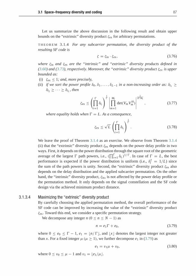
3.1 Space–frequency diversity and coding 87
Let us summarize the above discussion in the following result and obtain upperbounds on the “extrinsic” diversity product ζex for arbitrary permutations.
T H E O R E M 3.1.4 For any subcarrier permutation, the diversity product of theresulting SF code is
ζ = ζin · ζex, (3.76)
where ζin and ζex are the “intrinsic” and “extrinsic” diversity products defined in(3.60) and (3.73), respectively. Moreover, the “extrinsic” diversity product ζex is upperbounded as:(i) ζex ≤ 1; and, more precisely,
(ii) if we sort the power profile δ0, δ1, . . . , δL−1 in a non-increasing order as: δl1 ≥δl2 ≥ · · · ≥ δlL , then
ζex ≤(�∏
i=1
δli
) 1�∣∣∣∣∣
Mt∏m=1
det(Vm V Hm )
∣∣∣∣∣1
2�Mt
, (3.77)
where equality holds when � = L. As a consequence,
ζex ≤√
L
(�∏
i=1
δli
) 1�
. (3.78)
We leave the proof of Theorem 3.1.4 as an exercise. We observe from Theorem 3.1.4(ii) that the “extrinsic” diversity product ζex depends on the power delay profile in twoways. First, it depends on the power distribution through the square root of the geometricaverage of the largest � path powers, i.e., (
∏�i=1 δli )
1/� . In case of � = L , the bestperformance is expected if the power distribution is uniform (i.e., δ2
l = 1/L) sincethe sum of the path powers is unity. Second, the “extrinsic” diversity product ζex alsodepends on the delay distribution and the applied subcarrier permutation. On the otherhand, the “intrinsic” diversity product, ζin, is not affected by the power delay profile orthe permutation method. It only depends on the signal constellation and the SF codedesign via the achieved minimum product distance.
3.1.3.4 Maximizing the “extrinsic” diversity productBy carefully choosing the applied permutation method, the overall performance of theSF code can be improved by increasing the value of the “extrinsic” diversity productζex. Toward this end, we consider a specific permutation strategy.
We decompose any integer n (0 ≤ n ≤ N − 1) as
n = e1� + e0, (3.79)
where 0 ≤ e0 ≤ � − 1, e1 = �n/��, and �x� denotes the largest integer not greaterthan x . For a fixed integer μ (μ ≥ 1), we further decompose e1 in (3.79) as
e1 = v1μ+ v0, (3.80)
where 0 ≤ v0 ≤ μ− 1 and v1 = �e1/μ�.
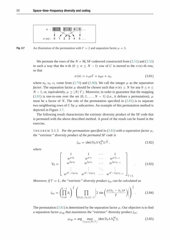
88 Space–time–frequency diversity and coding
σ (n) : 0 1 2 3 4 5 . . .
0 1 2 3 4 5 . . .n :
Fig. 3.7 An illustration of the permutation with � = 2 and separation factor μ = 3.
We permute the rows of the N ×Mt SF codeword constructed from (3.51) and (3.52)in such a way that the n-th (0 ≤ n ≤ N − 1) row of C is moved to the σ(n)-th row,so that
σ(n) = v1μ� + e0μ+ v0, (3.81)
where e0, v0, v1 come from (3.79) and (3.80). We call the integer μ as the separationfactor. The separation factor μ should be chosen such that σ(n) ≤ N for any 0 ≤ n ≤N − 1, or, equivalently, μ ≤ �N/��. Moreover, in order to guarantee that the mapping(3.81) is one-to-one over the set {0, 1, . . . , N − 1} (i.e., it defines a permutation), μmust be a factor of N . The role of the permutation specified in (3.81) is to separatetwo neighboring rows of C by μ subcarriers. An example of this permutation method isdepicted in Figure 3.7.
The following result characterizes the extrinsic diversity product of the SF code thatis permuted with the above described method. A proof of the result can be found in theexercise.
T H E O R E M 3.1.5 For the permutation specified in (3.81) with a separation factor μ,the “extrinsic” diversity product of the permuted SF code is
ζex = |det(V0�V H0 )|
12� , (3.82)
where
V0 =
⎡⎢⎢⎢⎢⎢⎣1 1 · · · 1wμτ0 wμτ1 · · · wμτL−1
w2μτ0 w2μτ1 · · · w2μτL−1
......
. . ....
w(�−1)μτ0 w(�−1)μτ1 · · · w(�−1)μτL−1
⎤⎥⎥⎥⎥⎥⎦�×L
. (3.83)
Moreover, if � = L, the “extrinsic” diversity product ζex can be calculated as
ζex =(
L−1∏l=0
δl
) 1L⎛⎝ ∏
0≤l1<l2≤L−1
∣∣∣∣2 sin
(μ(τl2 − τl1)π
T
)∣∣∣∣⎞⎠
1L
. (3.84)
The permutation (3.81) is determined by the separation factor μ. Our objective is to finda separation factor μop that maximizes the “extrinsic” diversity product ζex:
μop = arg max1≤μ≤�N/��
|det(V0�V H0 )|. (3.85)
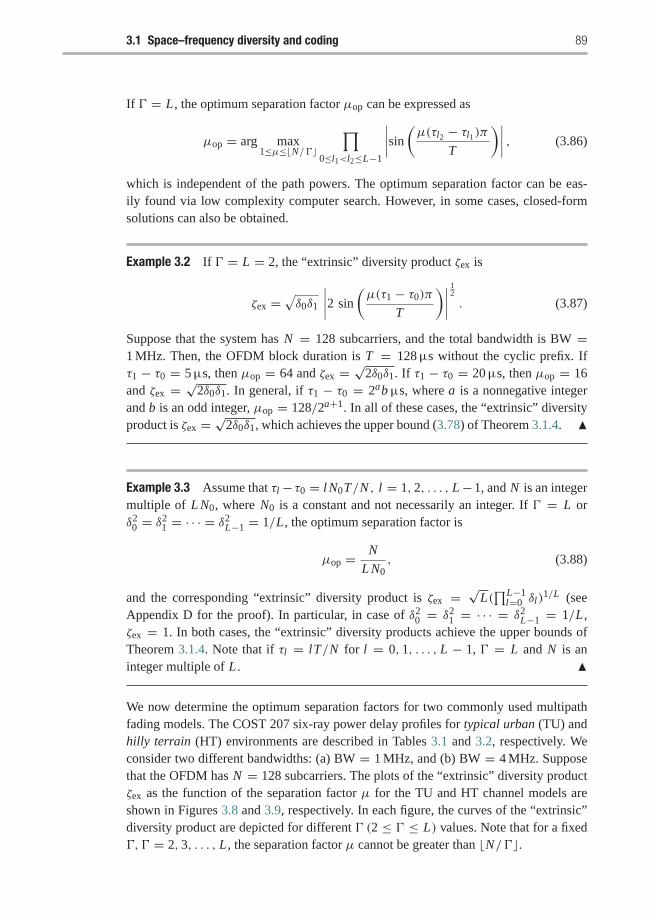
3.1 Space–frequency diversity and coding 89
If � = L , the optimum separation factor μop can be expressed as
μop = arg max1≤μ≤�N/��
∏0≤l1<l2≤L−1
∣∣∣∣sin(μ(τl2 − τl1)πT
)∣∣∣∣ , (3.86)
which is independent of the path powers. The optimum separation factor can be eas-ily found via low complexity computer search. However, in some cases, closed-formsolutions can also be obtained.
Example 3.2 If � = L = 2, the “extrinsic” diversity product ζex is
ζex =√δ0δ1
∣∣∣∣2 sin
(μ(τ1 − τ0)π
T
)∣∣∣∣ 12
. (3.87)
Suppose that the system has N = 128 subcarriers, and the total bandwidth is BW =1 MHz. Then, the OFDM block duration is T = 128 μs without the cyclic prefix. Ifτ1 − τ0 = 5 μs, then μop = 64 and ζex = √2δ0δ1. If τ1 − τ0 = 20 μs, then μop = 16and ζex = √2δ0δ1. In general, if τ1 − τ0 = 2ab μs, where a is a nonnegative integerand b is an odd integer, μop = 128/2a+1. In all of these cases, the “extrinsic” diversityproduct is ζex = √2δ0δ1, which achieves the upper bound (3.78) of Theorem 3.1.4. �
Example 3.3 Assume that τl−τ0 = lN0T/N , l = 1, 2, . . . , L−1, and N is an integermultiple of L N0, where N0 is a constant and not necessarily an integer. If � = L orδ2
0 = δ21 = · · · = δ2
L−1 = 1/L , the optimum separation factor is
μop = N
L N0, (3.88)
and the corresponding “extrinsic” diversity product is ζex =√
L(∏L−1
l=0 δl)1/L (see
Appendix D for the proof). In particular, in case of δ20 = δ2
1 = · · · = δ2L−1 = 1/L ,
ζex = 1. In both cases, the “extrinsic” diversity products achieve the upper bounds ofTheorem 3.1.4. Note that if τl = lT/N for l = 0, 1, . . . , L − 1, � = L and N is aninteger multiple of L . �
We now determine the optimum separation factors for two commonly used multipathfading models. The COST 207 six-ray power delay profiles for typical urban (TU) andhilly terrain (HT) environments are described in Tables 3.1 and 3.2, respectively. Weconsider two different bandwidths: (a) BW = 1 MHz, and (b) BW = 4 MHz. Supposethat the OFDM has N = 128 subcarriers. The plots of the “extrinsic” diversity productζex as the function of the separation factor μ for the TU and HT channel models areshown in Figures 3.8 and 3.9, respectively. In each figure, the curves of the “extrinsic”diversity product are depicted for different � (2 ≤ � ≤ L) values. Note that for a fixed�,� = 2, 3, . . . , L , the separation factor μ cannot be greater than �N/��.
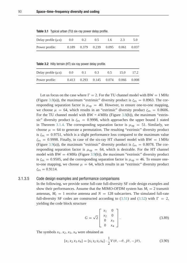
90 Space–time–frequency diversity and coding
Table 3.1 Typical urban (TU) six-ray power delay profile.
Delay profile (μs): 0.0 0.2 0.5 1.6 2.3 5.0
Power profile: 0.189 0.379 0.239 0.095 0.061 0.037
Table 3.2 Hilly terrain (HT) six-ray power delay profile.
Delay profile (μs): 0.0 0.1 0.3 0.5 15.0 17.2
Power profile: 0.413 0.293 0.145 0.074 0.066 0.008
Let us focus on the case where � = 2. For the TU channel model with BW = 1 MHz(Figure 3.8(a)), the maximum “extrinsic” diversity product is ζex = 0.8963. The cor-responding separation factor is μop = 40. However, to ensure one-to-one mapping,we choose μ = 64, which results in an “extrinsic” diversity product ζex = 0.8606.For the TU channel model with BW = 4 MHz (Figure 3.8(b)), the maximum “extrin-sic” diversity product is ζex = 0.9998, which approaches the upper bound 1 statedin Theorem 3.1.4. The corresponding separation factor is μop = 51. Similarly, wechoose μ = 64 to generate a permutation. The resulting “extrinsic” diversity productis ζex = 0.9751, which is a slight performance loss compared to the maximum valueζex = 0.9998. Finally, in case of the six-ray HT channel model with BW = 1 MHz(Figure 3.9(a)), the maximum “extrinsic” diversity product is ζex = 0.8078. The cor-responding separation factor is μop = 64, which is desirable. For the HT channelmodel with BW = 4 MHz (Figure 3.9(b)), the maximum “extrinsic” diversity productis ζex = 0.9505, and the corresponding separation factor is μop = 46. To ensure one-to-one mapping, we choose μ = 64, which results in an “extrinsic” diversity productζex = 0.9114.
3.1.3.5 Code design examples and performance comparisonsIn the following, we provide some full-rate full-diversity SF code design examples andshow their performances. Assume that the MIMO-OFDM system has Mt = 2 transmitantennas, Mr = 1 receive antenna and N = 128 subcarriers. The simulated full-ratefull-diversity SF codes are constructed according to (3.51) and (3.52) with � = 2,yielding the code block structure
G = √2
⎡⎢⎢⎣x1 0x2 00 x3
0 x4
⎤⎥⎥⎦ . (3.89)
The symbols x1, x2, x3, x4 were obtained as
[x1 x2 x3 x4] = [s1 s2 s3 s4] · 1
2V (θ,−θ, jθ,− jθ), (3.90)
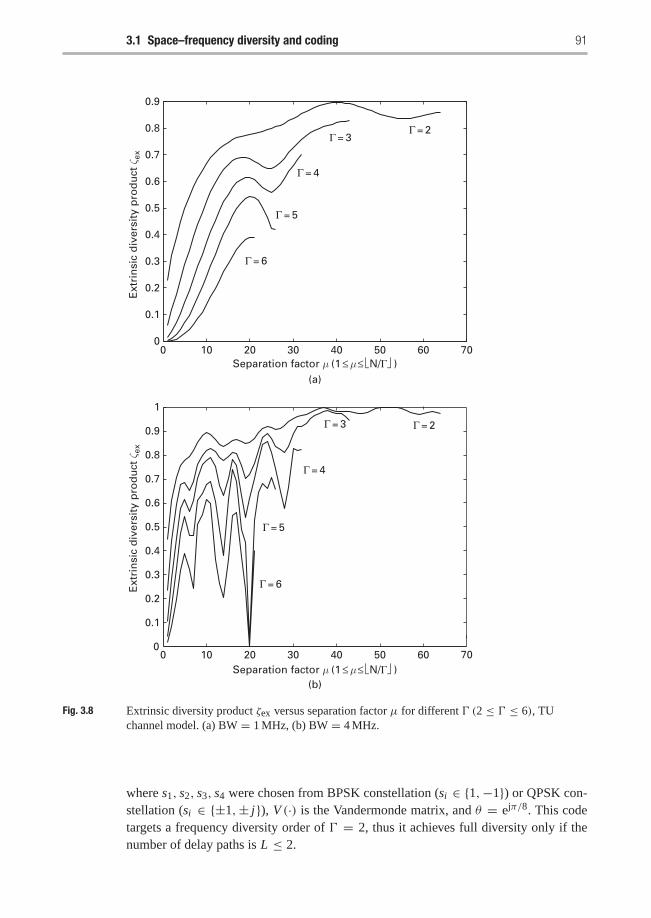
3.1 Space–frequency diversity and coding 91
0 10 20 30 40 50 60 700
0.1
0.2
0.3
0.4
0.5
0.6
0.7
0.8
0.9
Separation factor μ (1 ≤ μ ≤ ⎣N/Γ⎦ )(a)
0 10 20 30 40 50 60 70Separation factor μ (1 ≤ μ ≤ ⎣N/Γ⎦ )
(b)
Ext
rin
sic
div
ersi
ty p
rod
uct
ζ ex
Ext
rin
sic
div
ersi
ty p
rod
uct
ζ ex
Γ = 2Γ = 3
Γ = 4
Γ = 5
Γ = 6
0
0.1
0.2
0.3
0.4
0.5
0.6
0.7
0.8
0.9
1
Γ = 2 Γ = 3
Γ = 4
Γ = 5
Γ = 6
Fig. 3.8 Extrinsic diversity product ζex versus separation factor μ for different � (2 ≤ � ≤ 6), TUchannel model. (a) BW = 1 MHz, (b) BW = 4 MHz.
where s1, s2, s3, s4 were chosen from BPSK constellation (si ∈ {1,−1}) or QPSK con-stellation (si ∈ {±1,± j}), V (·) is the Vandermonde matrix, and θ = ejπ/8. This codetargets a frequency diversity order of � = 2, thus it achieves full diversity only if thenumber of delay paths is L ≤ 2.
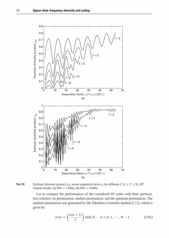
92 Space–time–frequency diversity and coding
0 10 20 30 40 50 60 70Separation factor μ (1 ≤ μ ≤ ⎣N/Γ⎦ )
(b)
Ext
rin
sic
div
ersi
ty p
rod
uct
ζ ex
0
0.1
0.2
0.3
0.4
0.5
0.6
0.7
0.8
0.9
1
Γ = 2
Γ = 3
Γ = 4
Γ = 5
Γ = 6
Γ = 2Γ = 3
Γ = 4
Γ = 5
Γ = 6
0 10 20 30 40 50 60 700
0.1
0.2
0.3
0.4
0.5
0.6
0.7
0.8
0.9
Separation factor μ (1 ≤ μ ≤ ⎣N/Γ⎦ )(a)
Ext
rin
sic
div
ersi
ty p
rod
uct
ζ ex
Fig. 3.9 Extrinsic diversity product ζex versus separation factor μ for different � (2 ≤ � ≤ 6), HTchannel model. (a) BW = 1 MHz, (b) BW = 4 MHz.
Let us compare the performances of the considered SF codes with three permuta-tion schemes: no permutation, random permutation, and the optimum permutation. Therandom permutation was generated by the Takeshita–Constello method [210], which isgiven by
σ(n) =(
n(n + 1)
2
)mod N , n = 0, 1, · · · , N − 1. (3.91)
3.1 Space–frequency diversity and coding 93
Code performances with different permutation schemesLet us compare the performance of the full-rate full-diversity SF codes using differentpermutation schemes. For example, let us focus on the code (3.89) with the channelsymbols s1, s2, s3, s4 chosen from BPSK constellation. The symbol rate of this code is1, and its spectral efficiency is 1 bit/s/Hz, ignoring the cyclic prefix.
First, we consider a simple two-ray, equal-power delay profile, with a delay τ μsbetween the two rays. We consider two cases: (a) τ = 5 μs, and (b) τ = 20 μs withOFDM bandwidth BW = 1 MHz. From the BER curves, shown in Figures 3.10(a) and(b), we observe that the performance of the proposed SF code with the random per-mutation is better than that without permutation. In case of τ = 5μs, the performanceimprovement is more significant. With the optimum permutation, the performance isfurther improved. In case of τ = 5μs, there is a 3 dB gain between the optimum permu-tation (μop = 64) and the random permutation at a BER of 10−5. In case of τ = 20μs,the performance improvement of the optimum permutation (μop = 16) over the randompermutation is about 2 dB at a BER of 10−5. If no permutation is used, the performanceof the code in the τ = 5 μs case (ζex = 0.3499) is worse than that in the τ = 20 μscase (ζex = 0.6866). However, if we apply the optimum permutation, the performanceof the SF code in both the τ = 5 μs case (μop = 64, ζex = 1) and the τ = 20 μscase (μop = 16, ζex = 1) is approximately the same. This confirms that by care-ful interleaver design, the performance of the SF codes can be significantly improved.Moreover, the consistency between the theoretical diversity product values and the sim-ulation results suggests that the “extrinsic” diversity product ζex is a good indicator ofthe code performance.
Let us simulate the code (3.89) with a more practical TU channel model. We con-sider two situations: (a) BW = 1 MHz, and (b) BW = 4 MHz. Figure 3.11 providesthe performance results of the code with different permutations for the TU channelmodel. From Figures 3.11(a) and (b), we observe that in both cases, the code with ran-dom permutation has a significant improvement over the non-permuted code. Usingthe proposed permutation with a separation factor μ = 64, there is an additional gainof 1.5 dB and 1 dB at a BER of 10−5 in case of BW = 1 MHz and BW = 4 MHz,respectively.
Comparisons of the full-rate full-diversity SF codes with other SF codesLet us compare the performance of the full-rate full-diversity SF codes with that of thefull-diversity SF codes obtained via mapping. We consider the full-rate full-diversitySF code (3.89) with symbols s1, s2, s3, s4 chosen from QPSK constellation. The sym-bol rate of the code is 1, and the spectral efficiency is 2 bits/s/Hz, ignoring the cyclicprefix. The full-diversity SF code is a repetition of the Alamouti scheme two times asfollows:
G =
⎡⎢⎢⎣x1 x2
x1 x2
−x∗2 x∗1−x∗2 x∗1
⎤⎥⎥⎦ , (3.92)
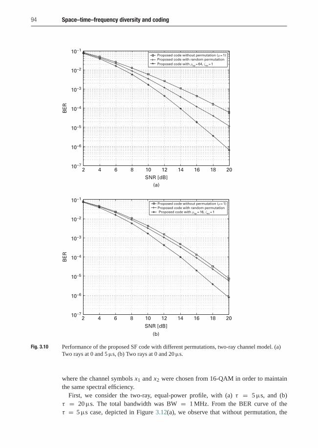
94 Space–time–frequency diversity and coding
2 4 6 8 10 12 14 16 18 2010−7
10−6
10−5
10−4
10−3
10−2
10−1
BE
R
SNR [dB](a)
(b)
Proposed code without permutation (μ = 1)Proposed code with random permutationProposed code with μop = 64, ζex = 1
2 4 6 8 10 12 14 16 18 2010−7
10−6
10−5
10−4
10−3
10−2
10−1
BE
R
SNR [dB]
Proposed code without permutation (μ = 1)Proposed code with random permutationProposed code with μop = 16, ζex = 1
Fig. 3.10 Performance of the proposed SF code with different permutations, two-ray channel model. (a)Two rays at 0 and 5 μs, (b) Two rays at 0 and 20 μs.
where the channel symbols x1 and x2 were chosen from 16-QAM in order to maintainthe same spectral efficiency.
First, we consider the two-ray, equal-power profile, with (a) τ = 5 μs, and (b)τ = 20 μs. The total bandwidth was BW = 1 MHz. From the BER curve of theτ = 5 μs case, depicted in Figure 3.12(a), we observe that without permutation, the
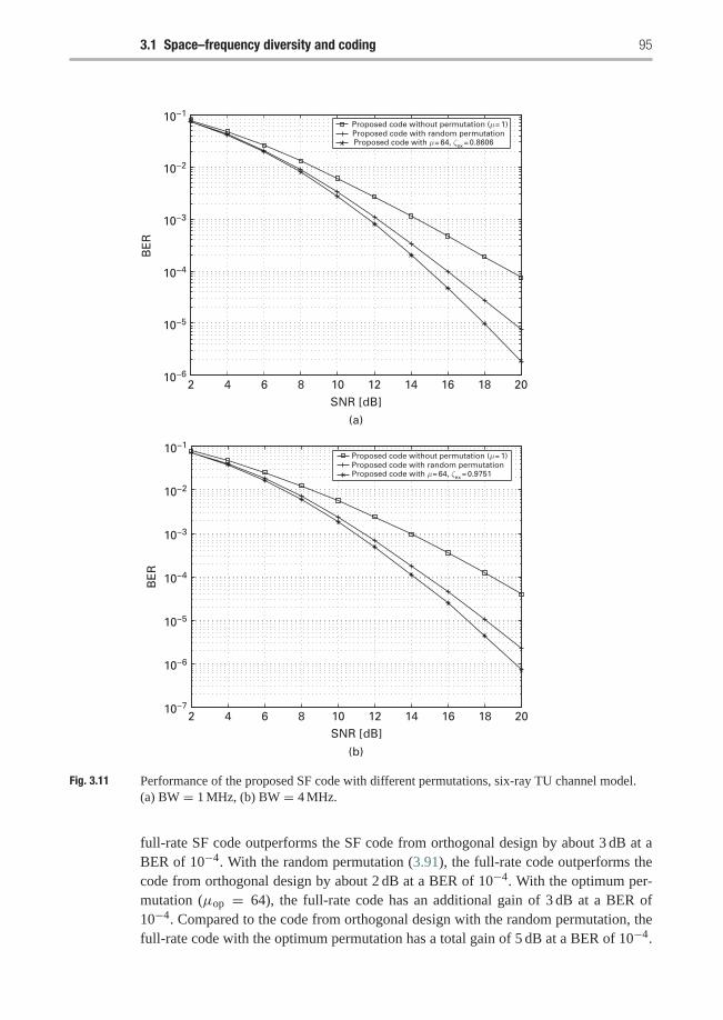
3.1 Space–frequency diversity and coding 95
2 4 6 8 10 12 14 16 18 2010−6
10−5
10−4
10−3
10−2
10−1
BE
R
SNR [dB]
2 4 6 8 10 12 14 16 18 2010−7
10−6
10−5
10−4
10−3
10−2
10−1
BE
R
SNR [dB]
Proposed code without permutation (μ = 1)Proposed code with random permutationProposed code with μ = 64, ζex = 0.8606
Proposed code without permutation (μ = 1)Proposed code with random permutationProposed code with μ = 64, ζex = 0.9751
(a)
(b)
Fig. 3.11 Performance of the proposed SF code with different permutations, six-ray TU channel model.(a) BW = 1 MHz, (b) BW = 4 MHz.
full-rate SF code outperforms the SF code from orthogonal design by about 3 dB at aBER of 10−4. With the random permutation (3.91), the full-rate code outperforms thecode from orthogonal design by about 2 dB at a BER of 10−4. With the optimum per-mutation (μop = 64), the full-rate code has an additional gain of 3 dB at a BER of10−4. Compared to the code from orthogonal design with the random permutation, thefull-rate code with the optimum permutation has a total gain of 5 dB at a BER of 10−4.
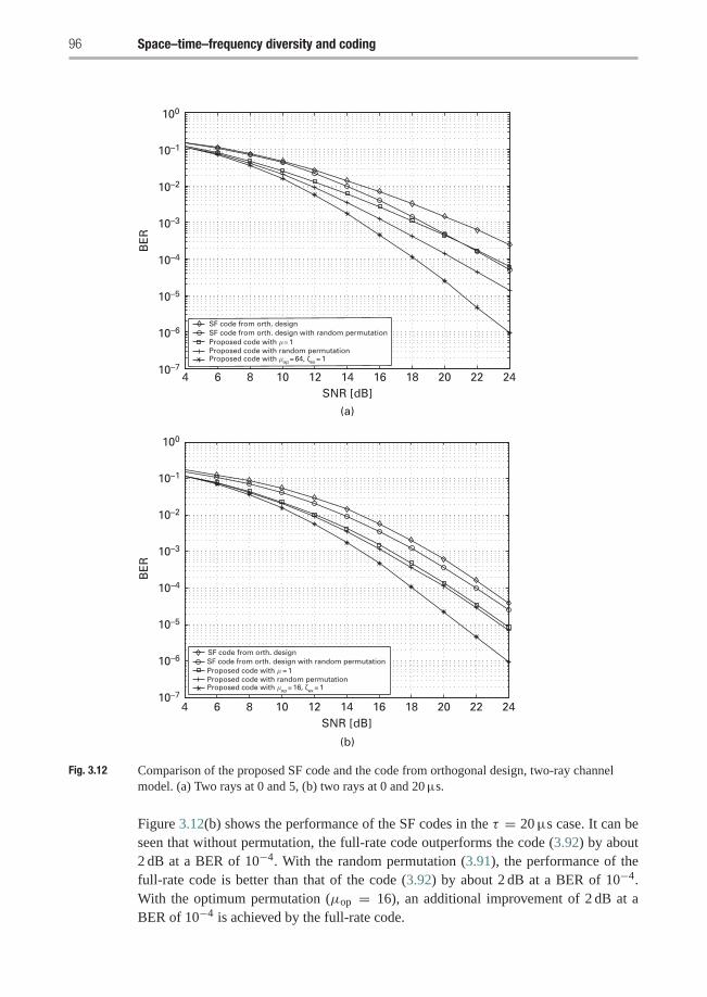
96 Space–time–frequency diversity and coding
4 6 8 10 12 14 16 18 20 22 2410–7
10–6
10–5
10–4
10–3
10–2
10–1
100
BE
R
SNR [dB]
(a)
(b)
4 6 8 10 12 14 16 18 20 22 2410–7
10–6
10–5
10–4
10–3
10–2
10–1
100
BE
R
SNR [dB]
SF code from orth. designSF code from orth. design with random permutationProposed code with μ = 1Proposed code with random permutationProposed code with μop = 64, ζex = 1
SF code from orth. designSF code from orth. design with random permutationProposed code with μ = 1Proposed code with random permutationProposed code with μop = 16, ζex = 1
Fig. 3.12 Comparison of the proposed SF code and the code from orthogonal design, two-ray channelmodel. (a) Two rays at 0 and 5, (b) two rays at 0 and 20 μs.
Figure 3.12(b) shows the performance of the SF codes in the τ = 20 μs case. It can beseen that without permutation, the full-rate code outperforms the code (3.92) by about2 dB at a BER of 10−4. With the random permutation (3.91), the performance of thefull-rate code is better than that of the code (3.92) by about 2 dB at a BER of 10−4.With the optimum permutation (μop = 16), an additional improvement of 2 dB at aBER of 10−4 is achieved by the full-rate code.
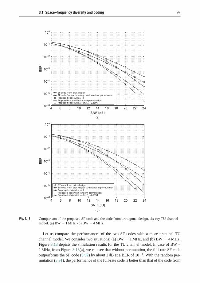
3.1 Space–frequency diversity and coding 97
4 6 8 10 12 14 16 18 20 22 24
BE
R
SNR [dB](a)
(b)
10–6
10–5
10–4
10–3
10–2
10–1
100
4 6 8 10 12 14 16 18 20 22 24
BE
R
SNR [dB]
10–6
10–5
10–4
10–3
10–2
10–1
100
SF code from orth. designSF code from orth. design with random permutationProposed code with μ = 1Proposed code with random permutationProposed code with μ = 64, ζex = 0.8606
SF code from orth. designSF code from orth. design with random permutationProposed code with μ = 1Proposed code with random permutationProposed code with μ = 64, ζex = 0.9751
Fig. 3.13 Comparison of the proposed SF code and the code from orthogonal design, six-ray TU channelmodel. (a) BW = 1 MHz, (b) BW = 4 MHz.
Let us compare the performances of the two SF codes with a more practical TUchannel model. We consider two situations: (a) BW = 1 MHz, and (b) BW = 4 MHz.Figure 3.13 depicts the simulation results for the TU channel model. In case of BW =1 MHz, from Figure 3.13(a), we can see that without permutation, the full-rate SF codeoutperforms the SF code (3.92) by about 2 dB at a BER of 10−4. With the random per-mutation (3.91), the performance of the full-rate code is better than that of the code from
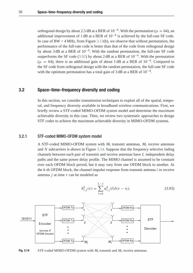
98 Space–time–frequency diversity and coding
orthogonal design by about 2.5 dB at a BER of 10−4. With the permutation (μ = 64), anadditional improvement of 1 dB at a BER of 10−4 is achieved by the full-rate SF code.In case of BW = 4 MHz, from Figure 3.13(b), we observe that without permutation, theperformance of the full-rate code is better than that of the code from orthogonal designby about 3 dB at a BER of 10−4. With the random permutation, the full-rate SF codeoutperforms the SF code (3.92) by about 2 dB at a BER of 10−4. With the permutation(μ = 64), there is an additional gain of about 1 dB at a BER of 10−4. Compared tothe SF code from orthogonal design with the random permutation, the full-rate SF codewith the optimum permutation has a total gain of 3 dB at a BER of 10−4.
3.2 Space–time–frequency diversity and coding
In this section, we consider transmission techniques to exploit all of the spatial, tempo-ral, and frequency diversity available in broadband wireless communications. First, webriefly review a STF-coded MIMO-OFDM system model and determine the maximumachievable diversity in this case. Then, we review two systematic approaches to designSTF codes to achieve the maximum achievable diversity in MIMO-OFDM systems.
3.2.1 STF-coded MIMO-OFDM system model
A STF-coded MIMO-OFDM system with Mt transmit antennas, Mr receive antennasand N subcarriers is shown in Figure 3.14. Suppose that the frequency selective fadingchannels between each pair of transmit and receive antennas have L independent delaypaths and the same power delay profile. The MIMO channel is assumed to be constantover each OFDM block period, but it may vary from one OFDM block to another. Atthe k-th OFDM block, the channel impulse response from transmit antenna i to receiveantenna j at time τ can be modeled as
hki, j (τ ) =
L−1∑l=0
αki, j (l)δ(τ − τl), (3.93)
1
2
1
2
Mt Mr
101011OFDM Tx
OFDM Tx
OFDM Tx OFDM Rx
OFDM Rx
OFDM Rx
Decoder
STFSTF
Encoder
(across KOFDM blocks)
Fig. 3.14 STF-coded MIMO-OFDM system with Mt transmit and Mr receive antennas.
3.2 Space–time–frequency diversity and coding 99
where τl is the delay and αki, j (l) is the complex amplitude of the l-th path between
transmit antenna i and receive antenna j . The αki, j (l)’s are modeled as zero-mean, com-
plex Gaussian random variables with variances E |αki, j (l)|2 = δ2
l , where E stands for
the expectation. The powers of the L paths are normalized such that∑L−1
l=0 δ2l = 1.
Assume that the MIMO channel is spatially uncorrelated, so the channel coefficientsαk
i, j (l) are independent for different indices (i, j). From (3.93), the frequency responseof the channel is given by
Hki, j ( f ) =
L−1∑l=0
αki, j (l)e
−j2π f τl , (3.94)
where j = √−1.Let us consider STF coding across Mt transmit antennas, N OFDM subcarriers’ and
K consecutive OFDM blocks. Each STF codeword can be expressed as a K N × Mt
matrix
C = [CT1 CT
2 · · · CTK ]T, (3.95)
where the channel symbol matrix Ck is given by
Ck =
⎡⎢⎢⎢⎢⎣ck
1(0) ck2(0) · · · ck
Mt(0)
ck1(1) ck
2(1) · · · ckMt(1)
......
. . ....
ck1(N − 1) ck
2(N − 1) · · · ckMt(N − 1)
⎤⎥⎥⎥⎥⎦ , (3.96)
and cki (n) is the channel symbol transmitted over the n-th subcarrier by transmit antenna
i in the k-th OFDM block. The STF code is assumed to satisfy the energy constraintE ||C ||2F = K N Mt , where ||C ||F is the Frobenius norm of C . During the k-th OFDMblock period, the transmitter applies an N -point IFFT to each column of the matrixCk . After appending a cyclic prefix, the OFDM symbol corresponding to the i-th (i =1, 2, . . . ,Mt) column of Ck is transmitted by transmit antenna i .
At the receiver, after matched filtering, removing the cyclic prefix, and applying FFT,the received signal at the n-th subcarrier at receive antenna j in the k-th OFDM blockis given by
ykj (n) =
√ρ
Mt
Mt∑i=1
cki (n)H
ki, j (n)+ zk
j (n), (3.97)
where
Hki, j (n) =
L−1∑l=0
αki, j (l)e
−j2πn� f τl (3.98)
is the channel frequency response at the n-th subcarrier between transmit antenna i andreceive antenna j ,� f = 1/T is the subcarrier separation in the frequency domain, andT is the OFDM symbol period. Assume that the channel state information Hk
i, j (n) is
known at the receiver, but not at the transmitter. In (3.97), zkj (n) denotes the additive
100 Space–time–frequency diversity and coding
white complex Gaussian noise with zero mean and unit variance at the n-th subcarrierat receive antenna j in the k-th OFDM block. The factor
√ρ/Mt in (3.97) ensures that
ρ is the average signal to noise ratio (SNR) at each receive antenna.
3.2.2 Performance criteria and maximum achievable diversity
In this subsection, we discuss the performance criteria for STF-coded MIMO-OFDMsystems and determine the maximum achievable diversity order for such systems.
Using the notation
ci ((k − 1)N + n)�= ck
i (n),
Hi, j ((k − 1)N + n)�= Hk
i, j (n),
y j ((k − 1)N + n)�= yk
j (n),
z j ((k − 1)N + n)�= zk
j (n)
for 1 ≤ k ≤ K , 0 ≤ n ≤ N − 1, 1 ≤ i ≤ Mt and 1 ≤ j ≤ Mr, the received signal in(3.97) can be expressed as
y j (m) =√ρ
Mt
Mt∑i=1
ci (m)Hi, j (m)+ z j (m) (3.99)
for m = 0, 1, . . . , K N − 1. We further rewrite the received signal in vector form as
Y =√ρ
MtDH+ Z, (3.100)
where D is a K N Mr×K N MtMr matrix constructed from the STF codeword C in (3.95)as follows:
D = IMr ⊗[D1 D2 · · · DMt
], (3.101)
where ⊗ denotes the tensor product, IMr is the identity matrix of size Mr × Mr, and
Di = diag{ci (0), ci (1), . . . , ci (K N − 1)} (3.102)
for any i = 1, 2, . . . ,Mt. The channel vector H of size K N MtMr × 1 is formatted as
H = [HT1,1 · · · HT
Mt,1 HT1,2 · · · HT
Mt,2 · · · HT1,Mr
· · · HTMt,Mr
]T, (3.103)
where
Hi, j = [Hi, j (0) Hi, j (1) · · · Hi, j (K N − 1)]T. (3.104)
The received signal vector Y of size K N Mr × 1 is given by
Y = [y1(0) · · · y1(K N − 1) y2(0) · · · y2(K N − 1) · · · yMr(0) · · · yMr(K N − 1)]T,(3.105)
and the noise vector Z has the same form as Y, i.e.,
Z = [z1(0) · · · z1(K N − 1) z2(0) · · · z2(K N − 1) · · · zMr (0) · · · zMr (K N − 1)]T.(3.106)
3.2 Space–time–frequency diversity and coding 101
Suppose that D and D are two matrices constructed from two different codewords Cand C , respectively. Then, the pairwise error probability between D and D can be upperbounded as
Pr(D → D) ≤(
2r − 1r
) ( r∏i=1
γi
)−1 (ρ
Mt
)−r
, (3.107)
where r is the rank of (D−D)R(D−D)H, γ1, γ2, . . . , γr are the nonzero eigenvalues of(D− D)R(D− D)H, and R = E{HHH} is the correlation matrix of H. The superscript Hstands for the complex conjugate and transpose of a matrix. Based on the upper boundon the pairwise error probability in (3.107), two general STF code performance criteriacan be proposed as follows:
• Diversity (rank) criterion: The minimum rank of (D− D)R(D− D)H over all pairs ofdifferent codewords C and C should be as large as possible.
• Product criterion: The minimum value of the product∏r
i=1 γi over all pairs ofdifferent codewords C and C should be maximized.
In the case of spatially uncorrelated MIMO channels, i.e., the channel taps αki, j (l) are
independent for different transmit antenna index i and receive antenna index j , thecorrelation matrix R of size K N MtMr × K N MtMr becomes
R = diag
(R1,1, . . . , RMt,1, R1,2, . . . , RMt,2, . . . , R1,Mr , . . . , RMt,Mr
), (3.108)
where
Ri, j = E{
Hi, j HHi, j
}(3.109)
is the correlation matrix of the channel frequency response from transmit antenna i toreceive antenna j . Using the notation w = e−j2π� f , from (3.98), we have
Hi, j = (IK ⊗W )Ai, j , (3.110)
where
W =
⎡⎢⎢⎢⎣1 1 · · · 1wτ0 wτ1 · · · wτL−1
......
. . ....
w(N−1)τ0 w(N−1)τ1 · · · w(N−1)τL−1
⎤⎥⎥⎥⎦ ,and
Ai, j = [α1i, j (0) α
1i, j (1) · · · α1
i, j (L − 1) · · · αKi, j (0) α
Ki, j (1) · · · αK
i, j (L − 1)]T.Substituting (3.110) into (3.109), Ri, j can be calculated as follows:
Ri, j = E{(IK ⊗W )Ai, j AH
i, j (IK ⊗W )H}
= (IK ⊗W )E{
Ai, j AHi, j
}(IK ⊗W H).
102 Space–time–frequency diversity and coding
With the assumptions that the path gains αki, j (l) are independent for different paths
and different pairs of transmit and receive antennas, and that the second order statisticsof the time correlation is the same for all transmit and receive antenna pairs and all paths(i.e. the correlation values do not depend on i , j and l), we can define the time correla-
tion at lag m as rT(m) = E{αki, j (l)α
k+mi, j
∗(l)}. Thus, the correlation matrix E
{Ai, j AH
i, j
}can be expressed as
E{
Ai, j AHi, j
}= RT ⊗�, (3.111)
where � = diag{δ20, δ
21, · · · , δ2
L−1}, and RT is the temporal correlation matrix of sizeK × K , whose entry in the p-th row and the q-th column is given by rT (q − p) for1 ≤ p, q ≤ K . We can also define the frequency correlation matrix, RF, as RF =E{Hk
i, j Hki, j
H}, where
Hki, j = [ Hk
i, j (0), . . . , Hki, j (N − 1) ]T.
Then, RF = W�W H. As a result, we arrive at
Ri, j = (IK ⊗W )(RT ⊗�)(IK ⊗W H)
= RT ⊗ (W�W H) = RT ⊗ RF, (3.112)
yielding
R = IMt Mr ⊗ (RT ⊗ RF). (3.113)
Finally, combining (3.96), (3.101), (3.102), and (3.113), the expression for(D− D)R(D− D)H in (3.107) can be rewritten as
(D− D)R(D− D)H
= IMr ⊗[ Mt∑
i=1
(Di − Di )(RT ⊗ RF)(Di − Di )H
]= IMr ⊗
{[(C − C)(C − C)H
]◦ (RT ⊗ RF)
}, (3.114)
where ◦ denotes the Hadamard product. Let
��= (C − C)(C − C)H, (3.115)
and R�= RT⊗RF. Then, substituting (3.114) into (3.107), the pairwise error probability
between C and C can be upper bounded as
Pr(C → C) ≤(
2νMr − 1νMr
) ( ν∏i=1
λi
)−Mr (ρ
Mt
)−νMr
, (3.116)
where ν is the rank of � ◦ R, and λ1, λ2, . . . , λν are the nonzero eigenvalues of � ◦ R.The minimum value of the product
∏νi=1 λi over all pairs of distinct signals C and C is
termed as coding advantage, denoted by
ζSTF = minC �=C
ν∏i=1
λi . (3.117)
3.2 Space–time–frequency diversity and coding 103
As a consequence, we can formulate the performance criteria for STF codes as follows:
• Diversity (rank) criterion: The minimum rank of � ◦ R over all pairs of distinctcodewords C and C should be as large as possible.
• Product criterion: The coding advantage or the minimum value of the product∏νi=1 λi over all pairs of distinct signals C and C should also be maximized.
If the minimum rank of � ◦ R is ν for any pair of distinct STF codewords C andC , we say that the STF code achieves a diversity order of νMr. For a fixed number ofOFDM blocks K , number of transmit antennas Mt, and correlation matrices RT and RF,the maximum achievable diversity or full diversity is defined as the maximum diversityorder that can be achieved by STF codes of size K N × Mt.
According to the rank inequalities on Hadamard products and tensor products, wehave
rank(� ◦ R) ≤ rank(�)rank(RT)rank(RF).
Since the rank of � is at most Mt and the rank of RF is at most L , we obtain
rank(� ◦ R) ≤ min{L Mtrank(RT), K N }. (3.118)
Thus, the maximum achievable diversity is at most min{L MtMrrank(RT), K N Mr}. Wecan see from the following discussion that this upper bound can indeed be achieved. Wealso observe that if the channel stays constant over multiple OFDM blocks (rank(RT) =1), the maximum achievable diversity is min{L MtMr, K N Mr}. In this case, STF cod-ing basically reduces to SF coding and cannot provide additional diversity advantagecompared to the SF coding approach.
Note that the above analytical framework includes ST and SF codes as special cases.If we consider only one subcarrier (N = 1), and one delay path (L = 1), the channelbecomes a single-carrier, time-correlated, flat fading MIMO channel. The correlationmatrix R simplifies to R = RT, and the code design problem reduces to that of ST codedesign. In the case of coding over a single OFDM block (K = 1), the correlation matrixR becomes R = RF, and the code design problem simplifies to that of SF codes.
3.2.3 Full-diversity STF code design methods
In this subsection, we review two STF code design methods to achieve the maximumachievable diversity order min{L MtMrrank(RT), K N Mr}. Without loss of generality,let us assume that the number of subcarriers, N , is not less than L Mt, so the maximumachievable diversity order is L MtMrrank(RT).
3.2.3.1 Repetition-based STF code designIn the previous section, a systematic approach was proposed to design full-diversity SFcodes. Suppose that CSF is a full-diversity SF code of size N ×Mt. A full-diversity STFcode, CSTF, can be constructed by repeating CSF K times (over K OFDM blocks) asfollows:
CSTF = 1k×1 ⊗ CSF, (3.119)
104 Space–time–frequency diversity and coding
where 1k×1 is an all one matrix of size k × 1. Let
�STF = (CSTF − CSTF)(CSTF − CSTF)H
and
�SF = (CSF − CSF)(CSF − CSF)H.
Then we have
�STF =[1k×1 ⊗ (CSF − CSF)
] [11×k ⊗ (CSF − CSF)
H]= 1k×k ⊗�SF.
Thus,
�STF ◦ R = (1k×k ⊗�SF) ◦ (RT ⊗ RF)
= RT ⊗ (�SF ◦ RF).
Since the SF code CSF achieves full diversity in each OFDM block, the rank of �SF ◦RF is L Mt. Therefore, the rank of �STF ◦ R is L Mtrank(RT), so CSTF in (3.119) isguaranteed to achieve a diversity order of L MtMrrank(RT).
We can see that the maximum achievable diversity depends on the rank of the tempo-ral correlation matrix RT. If the fading channels are constant during K OFDM blocks,i.e., rank(RT) = 1, the maximum achievable diversity order for STF codes (codingacross several OFDM blocks) is the same as that for SF codes (coding within one OFDMblock). Moreover, if the channel changes independently in time, i.e., RT = IK , the rep-etition structure of STF code CSTF in (3.119) is sufficient, but not necessary to achievethe full diversity. In this case,
� ◦ R = diag(�1 ◦ RF, �2 ◦ RF, . . . , �K ◦ RF),
where �k = (Ck − Ck)(Ck − Ck)H for 1 ≤ k ≤ K . Thus, in this case, the necessary
and sufficient condition to achieve full diversity K L MtMr is that each matrix �k ◦ RF
be of rank L Mt over all pairs of distinct codewords simultaneously for all 1 ≤ k ≤ K .The above repetition-based STF code design ensures full diversity at the price of
the symbol rate decreasing by a factor of 1/K (over K OFDM blocks) compared tothe symbol rate of the underlying SF code. The advantage of this approach is that anyfull-diversity SF code (block or trellis) can be used to design full-diversity STF codes.
3.2.3.2 Full-rate STF code designLet us consider a STF code structure consisting of STF codewords C of size K N by Mt:
C = [CT1 CT
2 · · · CTK ]T, (3.120)
where
Ck =[GT
k,1 GTk,2 · · · GT
k,P 0TN−P�Mt
]T(3.121)
for k = 1, 2, . . . , K . In (3.121), P = �N/(�Mt)�, and each matrix Gk,p (1 ≤ k ≤K , 1 ≤ p ≤ P) is of size �Mt by Mt. The zero padding in (3.121) is used if the numberof subcarriers N is not an integer multiple of �Mt. For each p (1 ≤ p ≤ P), we design
3.2 Space–time–frequency diversity and coding 105
the code matrices G1,p,G2,p, . . . ,GK ,p jointly, but the design of Gk1,p1 and Gk2,p2 ,p1 �= p2, is independent of each other. For a fixed p (1 ≤ p ≤ P), let
Gk,p =√
Mt diag(Xk,1, Xk,2, . . . , Xk,Mt
), k = 1, 2, . . . , K (3.122)
where diag(Xk,1, Xk,2, . . . , Xk,Mt) is a block diagonal matrix, in which Xk,i =[xk,(i−1)�+1 xk,(i−1)�+2 . . . xk,i�]T, i = 1, 2, . . . ,Mt, and xk, j , j = 1, 2, . . . , �Mt,are complex symbols and will be specified later. The energy normalization condition is
E
⎛⎝ K∑k=1
�Mt∑j=1
|xk, j |2⎞⎠ = K�Mt.
The symbol rate of the proposed scheme is P�Mt/N , ignoring the cyclic prefix. If N isa multiple of �Mt, the symbol rate is 1. If not, the rate is less than 1, but since usuallyN is much greater than �Mt, the symbol rate is very close to 1. We term full rate asone channel symbol per subcarrier per OFDM block period, so the proposed methodcan either achieve the full symbol rate, or it can perform very close to it. Note thatthis scheme includes the code design method proposed in [205] as a special case whenK = 1.
The following theorem provides a sufficient condition for the STF codesdescribed above to achieve a diversity order of �Mt Mr rank(RT). For simplicity,let us use the notation X = [x1,1 · · · x1,�Mt · · · xK ,1 · · · xK ,�Mt ] and X =[x1,1 · · · x1,�Mt · · · xK ,1 · · · xK ,�Mt ]. Moreover, for any n × n nonnegative definitematrix A, let us denote its eigenvalues in a non-increasing order as: eig1(A) ≥eig2(A) ≥ · · · ≥ eign(A).
T H E O R E M 3.2.1 For any STF code specified in (3.120)–(3.122), if∏K
k=1∏�Mt
j=1
|xk, j − xk, j | �= 0 for any pair of distinct symbols X and X, the STF code achievesa diversity order of �MtMrrank(RT), and the coding advantage is bounded by
(Mtδmin)�Mtrank(RT) � ≤ ζSTF ≤ (Mtδmax)
�Mtrank(RT) �, (3.123)
where
δmin = minX�=X
min1≤k≤K ,1≤ j≤�Mt
|xk, j − xk, j |2, (3.124)
δmax = maxX�=X
max1≤k≤K ,1≤ j≤�Mt
|xk, j − xk, j |2, (3.125)
� = |det(Q0)|Mt rank(RT)
rank(RT)∏i=1
(eigi (RT)
)�Mt , (3.126)
and
Q0 = W0diag(δ20, δ
21, . . . , δ
2L−1)W
H0 , (3.127)
106 Space–time–frequency diversity and coding
W0 =
⎡⎢⎢⎢⎣1 1 · · · 1wτ0 wτ1 · · · wτL−1
......
. . ....
w(�−1)τ0 w(�−1)τ1 · · · w(�−1)τL−1
⎤⎥⎥⎥⎦�×L
. (3.128)
Furthermore, if the temporal correlation matrix RT is of full rank, i.e., rank(RT) = K,the coding advantage is
ζSTF = δ M K�Mtt |det(RT)|�Mt |det(Q0)|K Mt , (3.129)
where
δ = minX�=X
K∏k=1
�Mt∏j=1
|xk, j − xk, j |2. (3.130)
Proof Suppose that C and C are two distinct STF codewords which are constructedfrom Gk,p and Gk,p (1 ≤ k ≤ K , 1 ≤ p ≤ P), respectively. We would like to determinethe rank of�◦R, where� = (C−C)(C−C)H and R = RT⊗RF. For convenience, let
Gp =[GT
1,p GT2,p · · · GT
K ,p
]Tfor each p = 1, 2, . . . , P . For two distinct codewords C and C , there exists at least oneindex p0 (1 ≤ p0 ≤ P) such that Gp0 �= Gp0 . We may further assume that Gp = Gp
for any p �= p0 since the rank of�◦ R does not decrease if Gp �= Gp for some p �= p0
([74], Corollary 3.1.3, p.149).Note that the frequency correlation matrix RF is a Toeplitz matrix. With the assump-
tion that Gp = Gp for any p �= p0, we observe that the nonzero eigenvalues of�◦R arethe same as those of [(Gp0−Gp0)(Gp0−Gp0)
H]◦(RT⊗Q), where Q = {qi, j }1≤i, j≤�Mt
is also a Toeplitz matrix whose entries are
qi, j =L−1∑l=0
δ2l w
(i− j)τl , 1 ≤ i, j ≤ �Mt. (3.131)
Note that Q is independent of the index p0, i.e., it is independent of the position ofGp0 − Gp0 in C − C . For any 1 ≤ k ≤ K , we have
Gk,p0 − Gk,p0
= √Mt diag(Xk,1 − Xk,1, Xk,2 − Xk,2, . . . , Xk,Mt − Xk,Mt)
= √Mt diag(xk,1 − xk,1, . . . , xk,�Mt − xk,�Mt)(IMt ⊗ 1�×1
),
so the difference matrix between Gp0 and Gp0 is
Gp0 − Gp0 =√
Mt
⎡⎢⎢⎣diag(x1,1 − x1,1, . . . , x1,�Mt − x1,�Mt)
(IMt ⊗ 1�×1
)diag(x2,1 − x2,1, . . . , x2,�Mt − x2,�Mt)
(IMt ⊗ 1�×1
)· · ·
diag(xK ,1 − xK ,1, . . . , xK ,�Mt − xK ,�Mt)(IMt ⊗ 1�×1
)⎤⎥⎥⎦
= √Mt diag(X− X)[1K×1 ⊗
(IMt ⊗ 1�×1
)],
3.2 Space–time–frequency diversity and coding 107
where
diag(X− X)�= diag(x1,1 − x1,1, . . . , x1,�Mt − x1,�Mt , . . . ,
xK ,1 − xK ,1, . . . , xK ,�Mt − xK ,�Mt).
Thus, we have[(Gp0 − Gp0)(Gp0 − Gp0)
H]◦ (RT ⊗ Q)
= Mt
{diag(X− X)
[1K×1 ⊗
(IMt ⊗ 1�×1
)] [1K×1 ⊗
(IMt ⊗ 1�×1
)]H×diag(X− X)H
}◦ (RT ⊗ Q)
= Mt
[diag(X− X)
(1K×K ⊗ IMt ⊗ 1�×�
)diag(X− X)H
]◦ (RT ⊗ Q)
= Mt diag(X− X){
RT ⊗[(
IMt ⊗ 1�×�) ◦ Q
]}diag(X− X)H
= Mt diag(X− X)(RT ⊗ IMt ⊗ Q0
)diag(X− X)H, (3.132)
where Q0 = {qi, j }1≤i, j≤� and qi, j is given by (3.131). In the above derivation, thesecond equality follows from the identities [1K×1⊗(IMt⊗1�×1)]H = 11×K⊗IMt⊗11×�and (A1⊗B1)(A2⊗B2)(A3⊗B3) = (A1 A2 A3)⊗(B1 B2 B3) ([74], p.251), and the thirdequality follows from a property of the Hadamard product ([74], p.304). From (3.132),we observe that if diag(X− X) is of full rank, i.e., xk, j − xk, j �= 0 for any 1 ≤ k ≤ K
and 1 ≤ j ≤ �Mt, then the rank of[(Gp0 − Gp0) (Gp0 − Gp0)
H]◦ (RT ⊗ Q) can be
determined as rank(RT ⊗ IMt ⊗ Q0), which is equal to Mtrank(RT)rank(Q0). Similarto the correlation matrix RF in (3.112), Q0 can be expressed as
Q0 = W0diag(δ20, δ
21, . . . , δ
2L−1)W
H0 ,
where W0 is defined in (3.128). Note that W0 is a � by L matrix consisting of � rows ofa Vandermonde matrix [74], so with τ0 < τ1 < · · · < τL−1, W0 is nonsingular. Thus,Q0 is of full rank (rank �). Therefore, if
∏Kk=1∏�Mt
j=1 |xk, j − xk, j | �= 0, the rank of� ◦ R is �Mtrank(RT).
The assumption that Gp = Gp for any p �= p0 is also sufficient to calculate thecoding advantage since the nonzero eigenvalues of � ◦ R do not decrease if Gp �= Gp
for some p �= p0 ([74], Corollary 3.1.3, p.149). Using the notation ν0 = �Mtrank(RT),the coding advantage can be calculated as
ζSTF = minX�=X
ν0∏i=1
eigi
([(Gp0 − Gp0)(Gp0 − Gp0)
H]◦ (RT ⊗ Q)
)= min
X�=X
ν0∏i=1
eigi
(Mt diag(X− X)
(RT ⊗ IMt ⊗ Q0
)diag(X− X)H
)(3.133)
= minX�=X
ν0∏i=1
θi Mteigi
(RT ⊗ IMt ⊗ Q0
), (3.134)
108 Space–time–frequency diversity and coding
where the constants θi satisfy eigK�Mt(diag(X − X)diag(X − X)H) ≤ θi ≤
eig1(diag(X−X)diag(X−X)H) for i = 1, 2, . . . , ν0. In the above derivation, the secondequality follows by (3.132), and the last equality follows by Ostrowski’s theorem ([73],p.224). Since
ν0∏i=1
eigi
(RT ⊗ IMt ⊗ Q0
) = �rank(RT)∏i=1
(eigi (RT ⊗ Q0)
)Mt
= |det(Q0)|Mt rank(RT)
rank(RT)∏i=1
(eigi (RT)
)�Mt ,
and
eig1
(diag(X− X)diag(X− X)H
)= max
X�=Xmax
1≤k≤K ,1≤ j≤�Mt|xk, j − xk, j |2,
eigK�Mt
(diag(X− X)diag(X− X)H
)= min
X�=Xmin
1≤k≤K ,1≤ j≤�Mt|xk, j − xk, j |2,
we have the lower and upper bounds in (3.123).
Finally, if RT is of full rank, ν0 = K�Mt. From (3.133), the coding advantage is
ζSTF = minX�=X
det(
Mt diag(X− X)(RT ⊗ IMt ⊗ Q0
)diag(X− X)H
)= M K�Mt
t det(RT ⊗ IMt ⊗ Q0
)minX�=X
K∏k=1
�Mt∏j=1
|xk, j − xk, j |2
= δ M K�Mtt |det(RT)|�Mt |det(Q0)|K Mt ,
where δ is given by (3.130). Thus, we have proved Theorem 3.2.1 completely. �
From Theorem 3.2.1, we observe that with the code structure specified in (3.120)–(3.122), it is not difficult to achieve the maximum diversity order of �MtMrrank(RT).The remaining problem is to design a set of complex symbol vectors, X =[x1,1 · · · x1,�Mt · · · xK ,1 · · · xK ,�Mt ], such that the coding advantage ζSTF is as largeas possible. One approach is to maximize δmin and δmax in (3.123) according to thelower and upper bounds of the coding advantage. Another approach is to maximize δin (3.130). We follow the latter for two reasons. First, the coding advantage ζSTF in(3.129) is determined by δ in closed form although this closed form only holds with theassumption that the temporal correlation matrix RT is of full rank. Second, the problemof designing X to maximize δ is related to the problem of constructing signal constel-lations for Rayleigh fading channels. In the literature, δ is called the minimum productdistance of the set of symbols X.
We summarize some existing results on designing X in order to maximize the mini-mum product distance δ as follows. For simplicity, denote L = K�Mt, and assume that� is a constellation such as QAM, PAM, and so on. The set of complex symbol vectors
3.2 Space–time–frequency diversity and coding 109
is obtained by applying a transform over a L-dimensional signal set �L. Specifically,
X = S · 1√L
V (θ1, θ2, . . . , θL), (3.135)
where S = [s1 s2 · · · sL] ∈ �K is a vector of arbitrary channel symbols to be transmit-ted, and V (θ1, θ2, . . . , θL) is a Vandermonde matrix with variables θ1, θ2, . . . , θL
V (θ1, θ2, . . . , θL) =
⎡⎢⎢⎢⎣1 1 · · · 1θ1 θ2 · · · θL...
.... . .
...
θL−11 θL−1
2 · · · θL−1L
⎤⎥⎥⎥⎦ . (3.136)
The optimum θl , 1 ≤ l ≤ L, have been specified for different L and �.
Example 3.4 If � is a QAM constellation, and L = 2s (s ≥ 1), the optimum θl ’s weregiven by
θl = ej 4l−32L π , l = 1, 2, . . . ,L. (3.137)
In case of L = 2s · 3t (s ≥ 1, t ≥ 1), a class of θl ’s were given as
θl = ej 6l−53L π , l = 1, 2, . . . ,L. (3.138)
�
For more details and other cases of � and L, readers can refer to [44, 14].The STF code design discussed in this subsection achieves full symbol rate, which
is much larger than that of the repetition coding approach. However, the maximum-likelihood decoding complexity of this approach is high. Its complexity increasesexponentially with the number of OFDM blocks, K , while the decoding complexityof the repetition-coded STF codes increases only linearly with K . Fortunately, somesphere decoding methods [166] can be used to reduce the complexity.
3.2.3.3 STF code design examples and performance comparisonsIn the following, we provide some full-diversity STF code design examples and showtheir performances. The OFDM modulation has N = 128 subcarriers, and the totalbandwidth is 1 MHz. Thus, the OFDM block duration is 128 μs. Let us set the length ofthe cyclic prefix to 20 μs for all cases.
Performances of the repetition-coded STF codesLet us consider a block code and a trellis code example. Assume that the communicationsystem has Mr = 1 receive antenna. We consider a two-ray, equal power delay profile(L = 2), with a delay of 20 μs between the two rays. Each ray was modeled as azero-mean, complex Gaussian random variable with variance 0.5.
The full-diversity STF block codes were obtained by repeating a full-diversity SFblock code via (3.119) across K = 1, 2, 3, 4 OFDM blocks. The used full-diversity SF
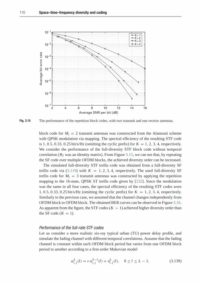
110 Space–time–frequency diversity and coding
2 4 6 8 10 12 14 16Average SNR per bit [dB]
Ave
rag
e b
it e
rro
r ra
te
10−7
10−6
10−5
10−4
10−3
10−2
10−1
K = 1K = 2K = 3K = 4
Fig. 3.15 The performance of the repetition block codes, with two transmit and one receive antennas.
block code for Mt = 2 transmit antennas was constructed from the Alamouti schemewith QPSK modulation via mapping. The spectral efficiency of the resulting STF codeis 1, 0.5, 0.33, 0.25 bit/s/Hz (omitting the cyclic prefix) for K = 1, 2, 3, 4, respectively.We consider the performance of the full-diversity STF block code without temporalcorrelation (RT was an identity matrix). From Figure 3.15, we can see that, by repeatingthe SF code over multiple OFDM blocks, the achieved diversity order can be increased.
The simulated full-diversity STF trellis code was obtained from a full-diversity SFtrellis code via (3.119) with K = 1, 2, 3, 4, respectively. The used full-diversity SFtrellis code for Mt = 3 transmit antennas was constructed by applying the repetitionmapping to the 16-state, QPSK ST trellis code given by [232]. Since the modulationwas the same in all four cases, the spectral efficiency of the resulting STF codes were1, 0.5, 0.33, 0.25 bit/s/Hz (omitting the cyclic prefix) for K = 1, 2, 3, 4, respectively.Similarly to the previous case, we assumed that the channel changes independently fromOFDM block to OFDM block. The obtained BER curves can be observed in Figure 3.16.As apparent from the figure, the STF codes (K > 1) achieved higher diversity order thanthe SF code (K = 1).
Performance of the full-rate STF codesLet us consider a more realistic six-ray typical urban (TU) power delay profile, andsimulate the fading channel with different temporal correlations. Assume that the fadingchannel is constant within each OFDM block period but varies from one OFDM blockperiod to another according to a first-order Makovian model
αki, j (l) = ε αk−1
i, j (l)+ ηki, j (l), 0 ≤ l ≤ L − 1, (3.139)
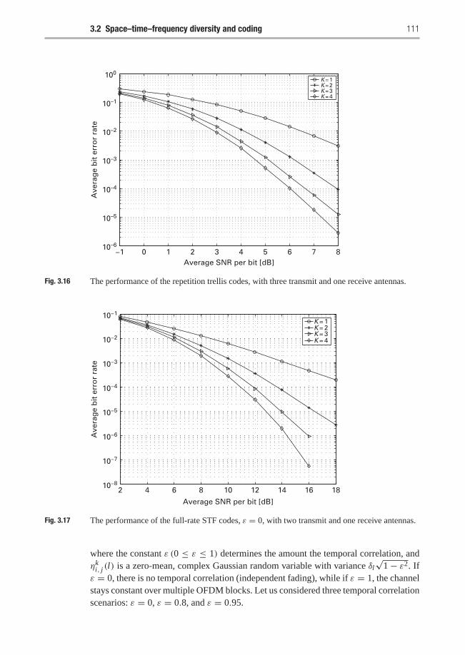
3.2 Space–time–frequency diversity and coding 111
−1 0 1 2 3 4 5 6 7 8
Ave
rag
e b
it e
rro
r ra
te
Average SNR per bit [dB]
10–6
10–5
10–4
10–3
10–2
10–1
100K = 1K = 2K = 3K = 4
Fig. 3.16 The performance of the repetition trellis codes, with three transmit and one receive antennas.
2 4 6 8 10 12 14 16 1810−8
10−7
10−6
10−5
10−4
10−3
10−2
10−1
Average SNR per bit [dB]
Ave
rag
e b
it e
rro
r ra
te
K = 1K = 2K = 3K = 4
Fig. 3.17 The performance of the full-rate STF codes, ε = 0, with two transmit and one receive antennas.
where the constant ε (0 ≤ ε ≤ 1) determines the amount the temporal correlation, andηk
i, j (l) is a zero-mean, complex Gaussian random variable with variance δl√
1− ε2. Ifε = 0, there is no temporal correlation (independent fading), while if ε = 1, the channelstays constant over multiple OFDM blocks. Let us considered three temporal correlationscenarios: ε = 0, ε = 0.8, and ε = 0.95.
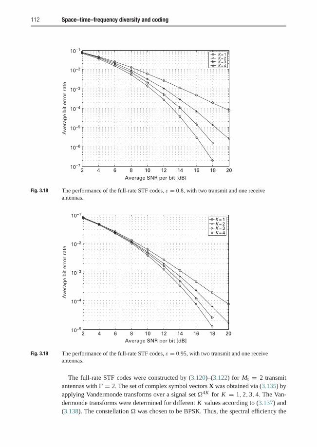
112 Space–time–frequency diversity and coding
2 4 6 8 10 12 14 16 18 2010−7
10−6
10−5
10−4
10−3
10−2
10−1
Average SNR per bit [dB]
Ave
rag
e b
it e
rro
r ra
te
K = 1K = 2K = 3K = 4
Fig. 3.18 The performance of the full-rate STF codes, ε = 0.8, with two transmit and one receiveantennas.
2 4 6 8 10 12 14 16 18 2010−5
10−4
10−3
10−2
10−1
Average SNR per bit [dB]
Ave
rag
e b
it e
rro
r ra
te
K = 1K = 2K = 3K = 4
Fig. 3.19 The performance of the full-rate STF codes, ε = 0.95, with two transmit and one receiveantennas.
The full-rate STF codes were constructed by (3.120)–(3.122) for Mt = 2 transmitantennas with � = 2. The set of complex symbol vectors X was obtained via (3.135) byapplying Vandermonde transforms over a signal set �4K for K = 1, 2, 3, 4. The Van-dermonde transforms were determined for different K values according to (3.137) and(3.138). The constellation � was chosen to be BPSK. Thus, the spectral efficiency the
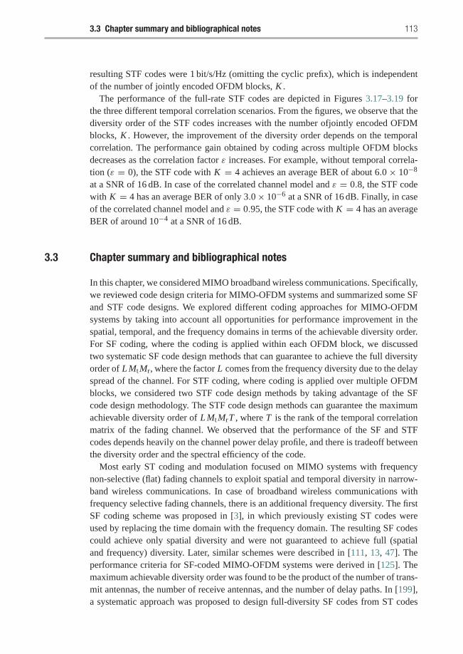
3.3 Chapter summary and bibliographical notes 113
resulting STF codes were 1 bit/s/Hz (omitting the cyclic prefix), which is independentof the number of jointly encoded OFDM blocks, K .
The performance of the full-rate STF codes are depicted in Figures 3.17–3.19 forthe three different temporal correlation scenarios. From the figures, we observe that thediversity order of the STF codes increases with the number ofjointly encoded OFDMblocks, K . However, the improvement of the diversity order depends on the temporalcorrelation. The performance gain obtained by coding across multiple OFDM blocksdecreases as the correlation factor ε increases. For example, without temporal correla-tion (ε = 0), the STF code with K = 4 achieves an average BER of about 6.0 × 10⁻⁸
at a SNR of 16 dB. In case of the correlated channel model and ε = 0.8, the STF codewith K = 4 has an average BER of only 3.0× 10⁻⁶ at a SNR of 16 dB. Finally, in caseof the correlated channel model and ε = 0.95, the STF code with K = 4 has an averageBER of around 10−4 at a SNR of 16 dB.
3.3 Chapter summary and bibliographical notes
In this chapter, we considered MIMO broadband wireless communications. Specifically,we reviewed code design criteria for MIMO-OFDM systems and summarized some SFand STF code designs. We explored different coding approaches for MIMO-OFDMsystems by taking into account all opportunities for performance improvement in thespatial, temporal, and the frequency domains in terms of the achievable diversity order.For SF coding, where the coding is applied within each OFDM block, we discussedtwo systematic SF code design methods that can guarantee to achieve the full diversityorder of L MtMr, where the factor L comes from the frequency diversity due to the delayspread of the channel. For STF coding, where coding is applied over multiple OFDMblocks, we considered two STF code design methods by taking advantage of the SFcode design methodology. The STF code design methods can guarantee the maximumachievable diversity order of L MtMrT , where T is the rank of the temporal correlationmatrix of the fading channel. We observed that the performance of the SF and STFcodes depends heavily on the channel power delay profile, and there is tradeoff betweenthe diversity order and the spectral efficiency of the code.
Most early ST coding and modulation focused on MIMO systems with frequencynon-selective (flat) fading channels to exploit spatial and temporal diversity in narrow-band wireless communications. In case of broadband wireless communications withfrequency selective fading channels, there is an additional frequency diversity. The firstSF coding scheme was proposed in [3], in which previously existing ST codes wereused by replacing the time domain with the frequency domain. The resulting SF codescould achieve only spatial diversity and were not guaranteed to achieve full (spatialand frequency) diversity. Later, similar schemes were described in [111, 13, 47]. Theperformance criteria for SF-coded MIMO-OFDM systems were derived in [125]. Themaximum achievable diversity order was found to be the product of the number of trans-mit antennas, the number of receive antennas, and the number of delay paths. In [199],a systematic approach was proposed to design full-diversity SF codes from ST codes
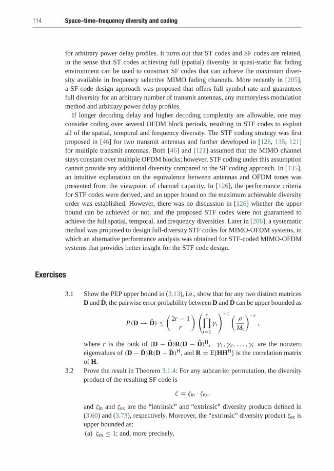
114 Space–time–frequency diversity and coding
for arbitrary power delay profiles. It turns out that ST codes and SF codes are related,in the sense that ST codes achieving full (spatial) diversity in quasi-static flat fadingenvironment can be used to construct SF codes that can achieve the maximum diver-sity available in frequency selective MIMO fading channels. More recently in [205],a SF code design approach was proposed that offers full symbol rate and guaranteesfull diversity for an arbitrary number of transmit antennas, any memoryless modulationmethod and arbitrary power delay profiles.
If longer decoding delay and higher decoding complexity are allowable, one mayconsider coding over several OFDM block periods, resulting in STF codes to exploitall of the spatial, temporal and frequency diversity. The STF coding strategy was firstproposed in [46] for two transmit antennas and further developed in [126, 135, 121]for multiple transmit antennas. Both [46] and [121] assumed that the MIMO channelstays constant over multiple OFDM blocks; however, STF coding under this assumptioncannot provide any additional diversity compared to the SF coding approach. In [135],an intuitive explanation on the equivalence between antennas and OFDM tones waspresented from the viewpoint of channel capacity. In [126], the performance criteriafor STF codes were derived, and an upper bound on the maximum achievable diversityorder was established. However, there was no discussion in [126] whether the upperbound can be achieved or not, and the proposed STF codes were not guaranteed toachieve the full spatial, temporal, and frequency diversities. Later in [206], a systematicmethod was proposed to design full-diversity STF codes for MIMO-OFDM systems, inwhich an alternative performance analysis was obtained for STF-coded MIMO-OFDMsystems that provides better insight for the STF code design.
Exercises
3.1 Show the PEP upper bound in (3.13), i.e., show that for any two distinct matricesD and D, the pairwise error probability between D and D can be upper bounded as
P(D → D) ≤(
2r − 1r
) ( r∏i=1
γi
)−1 (ρ
Mt
)−r
,
where r is the rank of (D − D)R(D − D)H, γ1, γ2, . . . , γr are the nonzeroeigenvalues of (D − D)R(D − D)H, and R = E{HHH} is the correlation matrixof H.
3.2 Prove the result in Theorem 3.1.4: For any subcarrier permutation, the diversityproduct of the resulting SF code is
ζ = ζin · ζex,
and ζin and ζex are the “intrinsic” and “extrinsic” diversity products defined in(3.60) and (3.73), respectively. Moreover, the “extrinsic” diversity product ζex isupper bounded as:(a) ζex ≤ 1; and, more precisely,
Exercises 115
(b) if we sort the power profile δ0, δ1, . . . , δL−1 in a non-increasing order as:δl1 ≥ δl2 ≥ · · · ≥ δlL , then
ζex ≤(�∏
i=1
δli
) 1�∣∣∣∣∣
Mt∏m=1
det(Vm V Hm )
∣∣∣∣∣1
2�Mt
,
where equality holds when � = L . In this case, ζex ≤√
L(∏�
i=1 δli
) 1�.
3.3 Prove the equation in (3.67), i.e., show that the product of the nonzero eigen-values of [σ(C − C)σ (C − C)H] ◦ R, λ1, λ2, . . . , λ�Mt , can be calculatedas
�Mt∏k=1
λk =Mt∏
m=1
|det(Am)| .
3.4 Prove the result in Theorem 3.1.5: For the permutation specified in (3.81) with aseparation factor μ, the “extrinsic” diversity product of the permuted SF code is
ζex = |det(V0�V H0 )|
12� ,
where V0 is specified in (3.83). Moreover, if � = L , the “extrinsic” diversityproduct ζex can be calculated as
ζex =(
L−1∏l=0
δl
) 1L⎛⎝ ∏
0≤l1<l2≤L−1
∣∣∣∣2 sin
(μ(τl2 − τl1)π
T
)∣∣∣∣⎞⎠
1L
.
3.5 Prove the result in (3.86): If � = L , the optimum separation factor μop definedin (3.85) can be determined as follows:
μop = arg max1≤μ≤�N/��
∏0≤l1<l2≤L−1
∣∣∣∣sin(μ(τl2 − τl1)πT
)∣∣∣∣ ,which is independent to the power profile of the multipath channel.
3.6 (Simulation project) Consider a MIMO-OFDM system with Mt = 2 transmitand Mr = 1 receive antennas. It uses an SF code that is obtained by repeatingeach row of the Alamouti code twice as follows:
C =
⎡⎢⎢⎣x1 x2
x1 x2
−x∗2 x∗1−x∗2 x∗1
⎤⎥⎥⎦ , (E3.1)
in which x1 and x2 are QPSK symbols. Assume that the system bandwidth isBW = 1 MHz and the OFDM has N = 128 subcarriers. The SF code is appliedover subcarriers within each OFDM block.(a) Determine the duration of each OFDM block and spectral efficiency of the
code without considering the cyclic prefix.
116 Space–time–frequency diversity and coding
(b) Consider a two-ray, equal-power delay profile, with a delay of τ μs betweenthe two rays. If the delay of the two rays is τ = 5 μs, simulate the systemby Matlab and plot the bit error rate curve versus the signal-to-noise ratio.Repeat the simulation if τ = 20 μs. Compare the simulation results andexplain your observations.
(c) Simulate the system by considering the TU six-ray channel model shown inFigure 3.5. Repeat the simulation if the system bandwidth is BW = 4 MHz.Compare the simulation results and explain your observations.
3.7 (Simulation project) Consider a MIMO-OFDM system with Mt = 2 transmitand Mr = 1 receive antennas. In this simulation, we compare performances ofthe SF code as shown in (E3.1) and the full-rate full-diversity SF code shown in(3.51).(a) Design a proper full-rate full-diversity SF code based on (3.51) with the
same spectral efficiency as the one shown in (E3.1).(b) Assume that the system bandwidth is BW = 1 MHz and the OFDM has
N = 128 subcarriers. Consider a two-ray, equal-power delay profile, with adelay of τ = 20 μs between the two rays. Simulate both the SF codes andcompare their bit error rate performances
(c) With the same channel assumption as in (b), compare performances of thetwo SF codes if rows of each code are randomly permuted among the N =128 subcarriers.
(d) With the same channel assumption as in (b), determine the optimum per-mutation factor, i.e., the separation factor defined in (3.81), for the full-ratefull-diversity SF code. Compare the performances of the full-rate code underthree scenarios: without permutation, random permutation, and the optimumpermutation.
(e) Repeat (b), (c), and (d) with the TU six-ray channel model shown inFigure 3.5 and a system bandwidth of BW = 4 MHz.

Part II
Cooperative communications

4 Relay channels and protocols
In this chapter, we will discuss shortcomings of conventional point-to-point communi-cations that led to the introduction of the new paradigm shift for wireless communica-tions, i.e., cooperative communications. We will define what the relay channel is, and inwhat aspects it is different from the direct point-to-point channel. We will also describeseveral protocols that can be implemented at the relay channel, and discuss the perfor-mance of these protocols which will be assessed based on their outage probability anddiversity gains.
4.1 Cooperative communications
In cooperative communications, independent paths between the user and the base sta-tion are generated via the introduction of a relay channel as illustrated in Figure 4.1.The relay channel can be thought of as an auxiliary channel to the direct channelbetween the source and destination. A key aspect of the cooperative communicationprocess is the processing of the signal received from the source node done by therelay. These different processing schemes result in different cooperative communica-tions protocol. Cooperative communications protocols can be generally categorizedinto fixed relaying schemes and adaptive relaying schemes. In fixed relaying, the chan-nel resources are divided between the source and the relay in a fixed (deterministic)manner. The processing at the relay differs according to the employed protocol. In afixed amplify-and-forward (AF) relaying protocol, the relay simply scales the receivedversion and transmits an amplified version of it to the destination. Another possi-bility of processing at the relay node is for the relay to decode the received signal,re-encode it and then retransmit it to the receiver. This kind of relaying is termed a fixeddecode-and-forward (DF) relaying protocol.
Fixed relaying has the advantage of easy implementation, but the disadvantage oflow bandwidth efficiency. This is because half of the channel resources are allocatedto the relay for transmission, which reduces the overall rate. This is true especiallywhen the source–destination channel is not very bad, because in such a scenario a highpercentage of the packets transmitted by the source to the destination could be receivedcorrectly by the destination and the relay’s transmissions would be wasted. Adaptiverelaying techniques, comprising selective and incremental relaying, try to overcomethis problem.
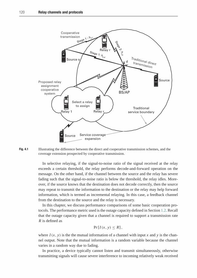
120 Relay channels and protocols
Source
Traditional directtransmission
Select a relay
to assign
Relay r
Source s
Source
BS/AP
Stage 1 : hs,r
Stage 1: h
s,d
Traditionalservice boundaryRelay rRelay 1
Stage 2: hr,d
Cooperativetransmission
Proposed relayassignmentcooperative
system
Service coverageexpansion
d
Fig. 4.1 Illustrating the difference between the direct and cooperative transmission schemes, and thecoverage extension prospected by cooperative transmission.
In selective relaying, if the signal-to-noise ratio of the signal received at the relayexceeds a certain threshold, the relay performs decode-and-forward operation on themessage. On the other hand, if the channel between the source and the relay has severefading such that the signal-to-noise ratio is below the threshold, the relay idles. More-over, if the source knows that the destination does not decode correctly, then the sourcemay repeat to transmit the information to the destination or the relay may help forwardinformation, which is termed as incremental relaying. In this case, a feedback channelfrom the destination to the source and the relay is necessary.
In this chapter, we discuss performance comparisons of some basic cooperation pro-tocols. The performance metric used is the outage capacity defined in Section 1.2. Recallthat the outage capacity given that a channel is required to support a transmission rateR is defined as
Pr [I (x, y) ≤ R] ,
where I (x, y) is the the mutual information of a channel with input x and y is the chan-nel output. Note that the mutual information is a random variable because the channelvaries in a random way due to fading.
In practice, a device typically cannot listen and transmit simultaneously, otherwisetransmitting signals will cause severe interference to incoming relatively weak received
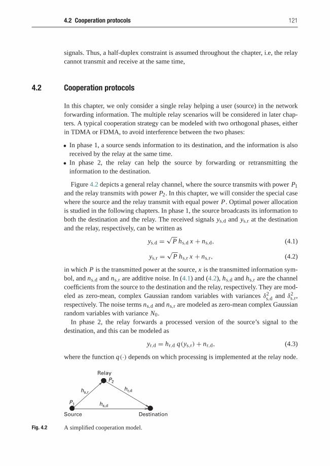
4.2 Cooperation protocols 121
signals. Thus, a half-duplex constraint is assumed throughout the chapter, i.e, the relaycannot transmit and receive at the same time,
4.2 Cooperation protocols
In this chapter, we only consider a single relay helping a user (source) in the networkforwarding information. The multiple relay scenarios will be considered in later chap-ters. A typical cooperation strategy can be modeled with two orthogonal phases, eitherin TDMA or FDMA, to avoid interference between the two phases:
• In phase 1, a source sends information to its destination, and the information is alsoreceived by the relay at the same time.
• In phase 2, the relay can help the source by forwarding or retransmitting theinformation to the destination.
Figure 4.2 depicts a general relay channel, where the source transmits with power P1
and the relay transmits with power P2. In this chapter, we will consider the special casewhere the source and the relay transmit with equal power P . Optimal power allocationis studied in the following chapters. In phase 1, the source broadcasts its information toboth the destination and the relay. The received signals ys,d and ys,r at the destinationand the relay, respectively, can be written as
ys,d =√
P hs,d x + ns,d, (4.1)
ys,r =√
P hs,r x + ns,r, (4.2)
in which P is the transmitted power at the source, x is the transmitted information sym-bol, and ns,d and ns,r are additive noise. In (4.1) and (4.2), hs,d and hs,r are the channelcoefficients from the source to the destination and the relay, respectively. They are mod-eled as zero-mean, complex Gaussian random variables with variances δ2
s,d and δ2s,r,
respectively. The noise terms ns,d and ns,r are modeled as zero-mean complex Gaussianrandom variables with variance N0.
In phase 2, the relay forwards a processed version of the source’s signal to thedestination, and this can be modeled as
yr,d = hr,d q(ys,r)+ nr,d, (4.3)
where the function q(·) depends on which processing is implemented at the relay node.
Relay
hs,rhr,d
P2
DestinationSource
hs,dP1
Fig. 4.2 A simplified cooperation model.
122 Relay channels and protocols
4.2.1 Fixed cooperation strategies
In fixed relaying, the channel resources are divided between the source and the relayin a fixed (deterministic) manner. The processing at the relay differs according to theemployed protocols. The most common techniques are the fixed AF relaying protocoland the fixed relaying DF protocol.
4.2.1.1 Fixed amplify-and-forward relaying protocolIn a fixed AF relaying protocol, which is often simply called an AF protocol, the relayscales the received version and transmits an amplified version of it to the destina-tion. The amplify-and-forward relay channel can be modeled as follows. The signaltransmitted from the source x is received at both the relay and destination as
ys,r =√
Phs,rx + ns,r, and ys,d =√
Phs,dx + ns,d, (4.4)
where hs,r and hs,d are the channel fades between the source and the relay and destina-tion, respectively, and are modeled as Rayleigh flat fading channels. The terms ns,r andns,d denote the additive white Gaussian noise with zero-mean and variance N0. In thisprotocol, the relay amplifies the signal from the source and forwards it to the destina-tion ideally to equalize the effect of the channel fade between the source and the relay.The relay does that by simply scaling the received signal by a factor that is inverselyproportional to the received power, which is denoted by
βr =√
P√P|hs,r|2 + N0
. (4.5)
The signal transmitted from the relay is thus given by βrys,r and has power P equal tothe power of the signal transmitted from the source. To calculate the mutual informationbetween the source and the destination, we need to calculate the total instantaneoussignal-to-noise ratio at the destination. The SNR received at the destination is the sumof the SNRs from the source and relay links. The SNR from the source link is given by
SNRs,d = �|hs,d|2, (4.6)
where � = P/N0.In the following we calculate the received SNR from the relay link. In phase 2 the
relay amplifies the received signal and forwards it to the destination with transmittedpower P . The received signal at the destination in phase 2 according to (4.5) is given by
yr,d =√
P√P|hs,r|2 + N0
hr,d ys,r + nr,d, (4.7)
where hr,d is the channel coefficient from the relay to the destination and nr,d is anadditive noise. More specifically, the received signal yr,d in this case is
yr,d =√
P√P|hs,r|2 + N0
√P hr,d hs,r x + n′r,d, (4.8)
4.2 Cooperation protocols 123
where
n′r,d =√
P√P|hs,r|2 + N0
hr,d ns,r + nr,d (4.9)
Assume that the noise terms ns,r and nr,d are independent, then the equivalent noise n′r,dis a zero-mean, complex Gaussian random variable with variance
N ′0 =(
P|hr,d|2P|hs,r|2 + N0
+ 1
)N0. (4.10)
The destination receives two copies from the signal x through the source link and relaylink. As discussed in Section 1.4, there are different techniques to combine the twosignals. The optimal technique that maximize the overall signal-to-noise ratio is themaximal ratio combiner (MRC). Note that MRC combining requires a coherent detectorthat has knowledge of all channel coefficients. Also, as shown in (1.43), the signal-to-noise ratio at the output of the MRC is equal to the sum of the received signal-to-noiseratios from both branches.
With knowledge of the channel coefficients hs,d, hs,r, and hr,d, the output of the MRCdetector at the destination can be written as
y = a1ys,d + a2yr,d, (4.11)
The combining factors a1 and a2 should be designed to maximize the combined SNR.As discussed in Section 1.4, this can be solved by formulating an optimization problemand selecting these factors correspondingly. An easier way to design them is be resort-ing to signal space and detection theory principles. Since, the AWGN noise terms spanthe whole space, to minimize the noise effects the detector should project the receivedsignals ys,d and ys,r to the desired signal spaces. Hence, ys,d and yr,d should be pro-jected along the directions of hs,d and hr,dhs,r, respectively, after normalizing the noisevariance terms in both received signals. Therefore, a1 and a2 are given by
a1 =√
Ph∗s,dN0
and a2 =√
PP|hs,r|2+N0
√P h∗s,rh∗r,d(
P|hr,d|2P|hs,r|2+N0
+ 1)
N0
. (4.12)
By assuming that the transmitted symbol x in (4.1) has average energy 1, theinstantaneous SNR of the MRC output is
γ = γ1 + γ2, (4.13)
where
γ1 = |a1√(P)hs,d|2|a1|2N0
= P|hs,d|2/N0, (4.14)
124 Relay channels and protocols
and
γ2 =|a2
√P√
P|hs,r|2+N0
√P hr,d hs,r |2
N ′0|a2|2
=P2
P|hs,r|2+N0|hs,r|2|hr,d|2(
P|hr,d|2P1|hs,r|2+N0
+ 1)
N0
= 1
N0
P2|hs,r|2|hr,d|2P|hs,r|2 + P|hr,d|2 + N0
. (4.15)
From the above, the instantaneous mutual information as a function of the fadingcoefficients for amplify-and-forward is given by
IAF = 1
2log(1+ γ1 + γ2). (4.16)
Substituting for the values of the SNR of both links, we can write the mutual infor-mation as
IAF = 1
2log(1+ �|hs,d|2 + f (�|hs,r|2, �|hr,d|2)
)(4.17)
where
f (x, y) � xy
x + y + 1. (4.18)
The outage probability can be obtained by averaging over the exponential channelgain distribution, as follows:
Pr[IAF < R] = Ehs,d,hs,r,hr,d
[1
2log(1+ �|hs,d|2 + f (�|hs,r|2, �|hr,d|2)
)< R
](4.19)
Calculating the above integration, the outage probability at high SNR is given by
Pr[IAF < R] �⎛⎝ σ 2
s,r + σ 2r,d
2σ 2s,d
(σ 2
s,rσ2r,d
)⎞⎠(22R − 1
�
)2
, (4.20)
where the multiplicative factor of 2 in 2R is because half of the bandwidth is lost incooperation by allocating them to the relay. The outage expression decays as �−2, whichmeans that the AF protocol achieves diversity 2.
Example 4.1 In this example, we study the outage probability of amplify-and-forwardprotocol and compare it to the performance of direct transmission. The channel variancebetween the source and destination σs,d is taken to be 1, while the channel variancesfor the source–relay or relay–destination channels are equal to 0.5. The noise varianceis one.
In Figure 4.3, the outage probability is depicted versus SNR in dB for a fixed rate of2 bps/Hz. As shown from the figure, diversity order two is achieved by AF as clear fromthe curve slope.
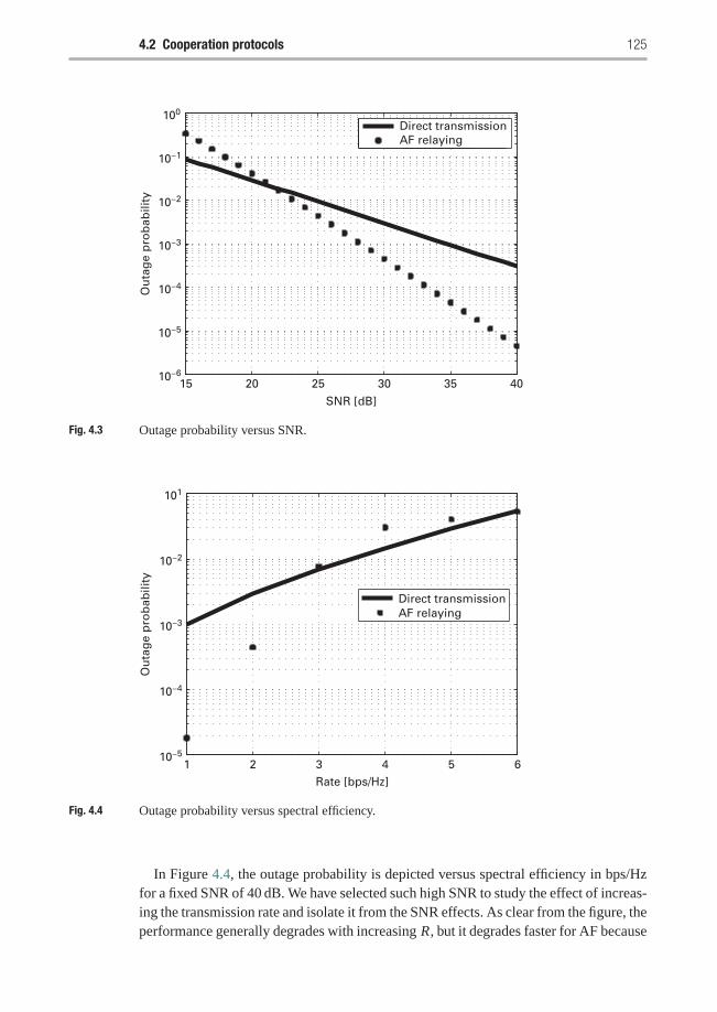
4.2 Cooperation protocols 125
15 20 25 30 35 4010−6
10−5
10−4
10−3
10−2
10−1
100
SNR [dB]
Ou
tag
e p
rob
abili
tyDirect transmissionAF relaying
Fig. 4.3 Outage probability versus SNR.
1 2 3 4 5 6Rate [bps/Hz]
10−5
10−4
10−3
10−2
101
Ou
tag
e p
rob
abili
ty
Direct transmissionAF relaying
Fig. 4.4 Outage probability versus spectral efficiency.
In Figure 4.4, the outage probability is depicted versus spectral efficiency in bps/Hzfor a fixed SNR of 40 dB. We have selected such high SNR to study the effect of increas-ing the transmission rate and isolate it from the SNR effects. As clear from the figure, theperformance generally degrades with increasing R, but it degrades faster for AF because
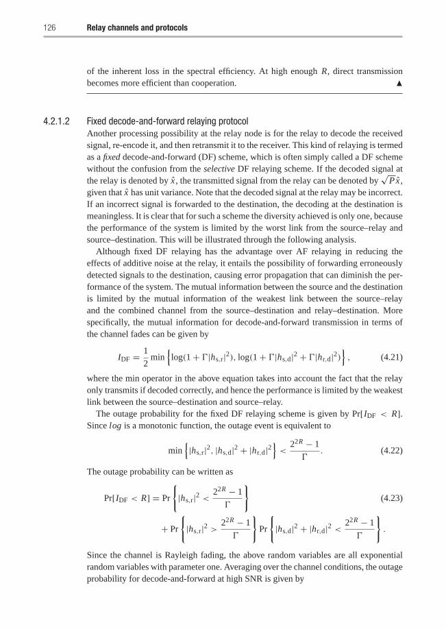
126 Relay channels and protocols
of the inherent loss in the spectral efficiency. At high enough R, direct transmissionbecomes more efficient than cooperation. �
4.2.1.2 Fixed decode-and-forward relaying protocolAnother processing possibility at the relay node is for the relay to decode the receivedsignal, re-encode it, and then retransmit it to the receiver. This kind of relaying is termedas a fixed decode-and-forward (DF) scheme, which is often simply called a DF schemewithout the confusion from the selective DF relaying scheme. If the decoded signal atthe relay is denoted by x , the transmitted signal from the relay can be denoted by
√Px ,
given that x has unit variance. Note that the decoded signal at the relay may be incorrect.If an incorrect signal is forwarded to the destination, the decoding at the destination ismeaningless. It is clear that for such a scheme the diversity achieved is only one, becausethe performance of the system is limited by the worst link from the source–relay andsource–destination. This will be illustrated through the following analysis.
Although fixed DF relaying has the advantage over AF relaying in reducing theeffects of additive noise at the relay, it entails the possibility of forwarding erroneouslydetected signals to the destination, causing error propagation that can diminish the per-formance of the system. The mutual information between the source and the destinationis limited by the mutual information of the weakest link between the source–relayand the combined channel from the source–destination and relay–destination. Morespecifically, the mutual information for decode-and-forward transmission in terms ofthe channel fades can be given by
IDF = 1
2min
{log(1+ �|hs,r|2), log(1+ �|hs,d|2 + �|hr,d|2)
}, (4.21)
where the min operator in the above equation takes into account the fact that the relayonly transmits if decoded correctly, and hence the performance is limited by the weakestlink between the source–destination and source–relay.
The outage probability for the fixed DF relaying scheme is given by Pr[IDF < R].Since log is a monotonic function, the outage event is equivalent to
min{|hs,r|2, |hs,d|2 + |hr,d|2
}<
22R − 1
�. (4.22)
The outage probability can be written as
Pr[IDF < R] = Pr
{|hs,r|2 < 22R − 1
�
}(4.23)
+ Pr
{|hs,r|2 > 22R − 1
�
}Pr
{|hs,d|2 + |hr,d|2 < 22R − 1
�
}.
Since the channel is Rayleigh fading, the above random variables are all exponentialrandom variables with parameter one. Averaging over the channel conditions, the outageprobability for decode-and-forward at high SNR is given by
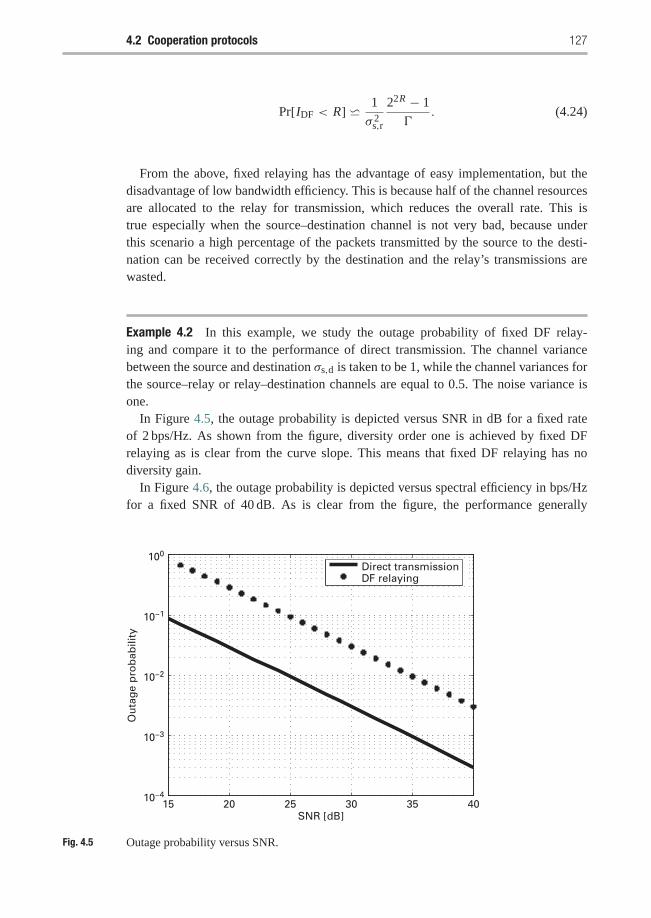
4.2 Cooperation protocols 127
Pr[IDF < R] � 1
σ 2s,r
22R − 1
�. (4.24)
From the above, fixed relaying has the advantage of easy implementation, but thedisadvantage of low bandwidth efficiency. This is because half of the channel resourcesare allocated to the relay for transmission, which reduces the overall rate. This istrue especially when the source–destination channel is not very bad, because underthis scenario a high percentage of the packets transmitted by the source to the desti-nation can be received correctly by the destination and the relay’s transmissions arewasted.
Example 4.2 In this example, we study the outage probability of fixed DF relay-ing and compare it to the performance of direct transmission. The channel variancebetween the source and destination σs,d is taken to be 1, while the channel variances forthe source–relay or relay–destination channels are equal to 0.5. The noise variance isone.
In Figure 4.5, the outage probability is depicted versus SNR in dB for a fixed rateof 2 bps/Hz. As shown from the figure, diversity order one is achieved by fixed DFrelaying as is clear from the curve slope. This means that fixed DF relaying has nodiversity gain.
In Figure 4.6, the outage probability is depicted versus spectral efficiency in bps/Hzfor a fixed SNR of 40 dB. As is clear from the figure, the performance generally
15 20 25 30 35 4010−4
10−3
10−2
10−1
100
SNR [dB]
Ou
tag
e p
rob
abili
ty
Direct transmissionDF relaying
Fig. 4.5 Outage probability versus SNR.
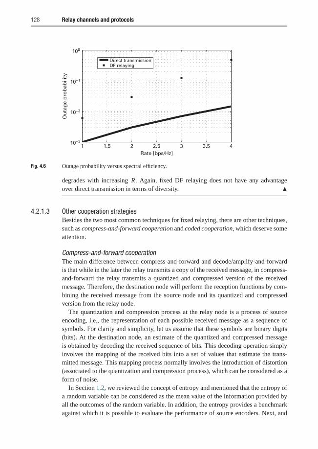
128 Relay channels and protocols
1 1.5 2 2.5 3 3.5 410−3
10−2
10−1
100
Rate [bps/Hz]
Ou
tag
e p
rob
abili
tyDirect transmissionDF relaying
Fig. 4.6 Outage probability versus spectral efficiency.
degrades with increasing R. Again, fixed DF relaying does not have any advantageover direct transmission in terms of diversity. �
4.2.1.3 Other cooperation strategiesBesides the two most common techniques for fixed relaying, there are other techniques,such as compress-and-forward cooperation and coded cooperation, which deserve someattention.
Compress-and-forward cooperationThe main difference between compress-and-forward and decode/amplify-and-forwardis that while in the later the relay transmits a copy of the received message, in compress-and-forward the relay transmits a quantized and compressed version of the receivedmessage. Therefore, the destination node will perform the reception functions by com-bining the received message from the source node and its quantized and compressedversion from the relay node.
The quantization and compression process at the relay node is a process of sourceencoding, i.e., the representation of each possible received message as a sequence ofsymbols. For clarity and simplicity, let us assume that these symbols are binary digits(bits). At the destination node, an estimate of the quantized and compressed messageis obtained by decoding the received sequence of bits. This decoding operation simplyinvolves the mapping of the received bits into a set of values that estimate the trans-mitted message. This mapping process normally involves the introduction of distortion(associated to the quantization and compression process), which can be considered as aform of noise.
In Section 1.2, we reviewed the concept of entropy and mentioned that the entropy ofa random variable can be considered as the mean value of the information provided byall the outcomes of the random variable. In addition, the entropy provides a benchmarkagainst which it is possible to evaluate the performance of source encoders. Next, and
4.2 Cooperation protocols 129
for the purpose of simplifying the presentation, let us consider that the source data isgenerated from a discrete memoryless source. For this setting, the entropy of the randomvariable being encoded at the source provides a lower bound on the average numberof bits per source symbol (the source encoding rate) needed to encode the source. Inthis sense, the entropy provides a lower bound on the source encoding rate used at therelay node if in a peer-to-peer communication setup. The use of cooperation and thepossibility of combining at the destination the messages from the source and the relaynode, changes this point. Effectively, the information received at the destination fromthe source can be used, as side information, while decoding the message from the relay.This will allow for encoding at a lower source encoding rate. The following examplefurther illustrates the operation of compress-and-forward.
Example 4.3 In this example we discuss a simplified model of a compress-and-forwardscheme so as to highlight its main characteristics. Consider a source node that trans-mits a signal with four possible values: −1.5, 0.5, 0.5, and 1.5. With no cooperation,the signal is sent over an AWGN channel with standard deviation σ = 0.5. Whenusing cooperation the source–relay and relay–destination channels are also assumedalso AWGN with standard deviation σ = 0.25 and σ = 0.6, respectively.
Assume now that the signal equal to 1.5 is transmitted without cooperation. The setupis illustrated in Figure 4.7, which shows the figures associated with the channel. At thedestination node, the value of 1.5 is decoded whenever the received signal exceeds avalue of 1. Then, the probability of a successful reception equals
pnc = 1− Q(1− 1.5
0.5
) = 0.84,
where
Q(x) =∫ ∞
x
exp(− x2
2
)√
2πdx .
When using compress-and-forward, the relay transmits a quantized and compressedversion of the received message. In this case, the message is the signal equal to 1.5.Since the destination node receives information from both the source and the relay,compression is not done in isolation from the information sent from the source to thedestination node. As shown in Figure 4.7, the relay will encode the received signal as abinary 0 whenever the received signal is larger than 1 or in the interval [−1, 0) and willencode the received signal as a binary 1 whenever the received signal is smaller than−1 or in the interval [0, 1]. Note that only one bit is necessary to encode the receivedsignal, as opposed to two bits when the four possible inputs are equiprobable and thereis no extra information at the receiver. The binary 0 or 1 resulting from the encodingprocess are transmitted as a signal with value +1 and −1, respectively. The thresholdused to receive the message from the relay is equal to 0 (meaning that when the receivedsignal is positive, a binary 0 is estimated as the encoded digit sent by the relay). Atthe destination node, the encoded message from the relay is decoded using the signalreceived from the source as side information. The decoding uses the following rules:
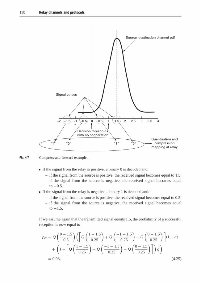
130 Relay channels and protocols
Source–destination channel pdf
Signal values
Decision thresholdswith no cooperation
–2 –1.5 –1 –0.5 0 0.5 1.5 2 2.5 3 3.5 41
“0”“0” “1”“1”Quantization and
compressionmapping at relay
Fig. 4.7 Compress-and-forward example.
• If the signal from the relay is positive, a binary 0 is decoded and:
– if the signal from the source is positive, the received signal becomes equal to 1.5;– if the signal from the source is negative, the received signal becomes equal
to −0.5.• If the signal from the relay is negative, a binary 1 is decoded and:
– if the signal from the source is positive, the received signal becomes equal to 0.5;– if the signal from the source is negative, the received signal becomes equal
to −1.5.
If we assume again that the transmitted signal equals 1.5, the probability of a successfulreception is now equal to
pcf = Q
(0− 1.5
0.5
)([Q
(1− 1.5
0.25
)+ Q
(−1− 1.5
0.25
)− Q
(0− 1.5
0.25
)](1− q)
+(
1−[
Q
(1− 1.5
0.25
)+ Q
(−1− 1.5
0.25
)− Q
(0− 1.5
0.25
)])q
)= 0.93, (4.25)
4.2 Cooperation protocols 131
where
q = Q
(0− 1
0.6
),
is the probability of successfully receiving the encoded message, a binary 0, from therelay. In 4.25, the first factor is the probability that the signal from the source is positive.This factor then multiplies two terms: the first being that the relay encodes a 0, which isreceived as such, and the second being the lucky coincidence that the relay incorrectlyencodes a 1, but is received as a 0.
Although this example shows a simplified implementation of compress-and-forward,the numerical comparison of pnc and pcf shows in simple terms how cooperationimproves the link quality. �
As a final note to compress-and-forward cooperation, we note that much of the sourceencoding operation done at the relay falls into the realm of the set of coding techniquesknown as distributed source coding, Sleppian–Wolf coding, or Wyner–Ziv coding.
Coded cooperationCoded cooperation differs from the previous schemes in that the cooperation isimplemented at the level of the channel coding subsystem. Note that both the amplify-and-forward and the decode-and-forward schemes presented earlier in this chapter werebased on schemes where the relay repeats the bits sent by the source. In coded coopera-tion the relay sends incremental redundancy, which when combined at the receiver withthe codeword sent by the source, results in a codeword with larger redundancy.
To understand coded cooperation, consider first the operation of a typical error cor-recting code. The encoder for an error correcting code takes a sequence of information-bearing symbols and applies mathematical operations in such a way that it generates asequence of symbols containing not only the information present at the input sequence,but also redundant information. The redundancy in the codeword is used at the receiverto increase the chances of recovering the original information if errors have been intro-duced during the transmission process. While in some codewords the information andredundancy are encoded in such a way that they can only be separated through com-plete decoding, in many other codes the encoding and decoding operation can be donein such a way that it is possible to add redundancy to, or remove redundancy from, thecodeword in a simple manner (such as through concatenation of new redundancy sym-bols or deletion of selected symbols). It is this second type of code that is used in codedcooperation.
In coded cooperation a codeword is transmitted in two parts, each using a differ-ent path or channel. Figure 4.8 summarizes one cycle of information transmission incoded cooperation. The main steps in the process are sequentially labeled with the cir-cled numbers. One cycle of information transmission in coded cooperation is as follows.The cycle starts with a block of NI information symbols being entered to a cyclic redun-dancy check (CRC) encoder at the source node (step 1). The result of the CRC encoderis then entered to a forward error correcting (FEC) code encoder (step 2), resulting
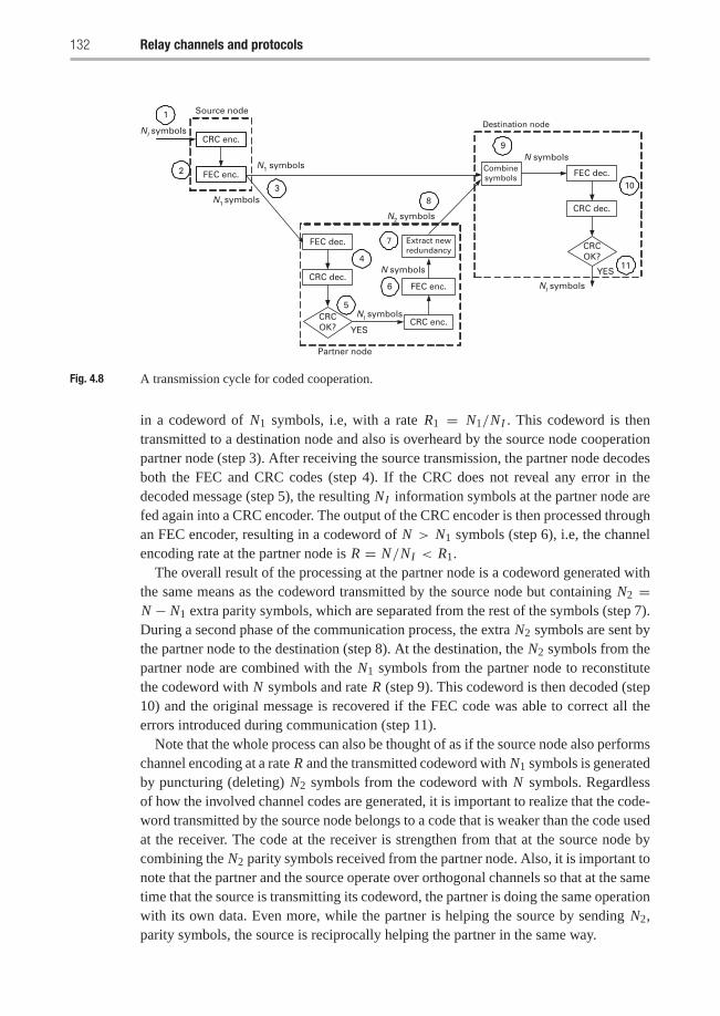
132 Relay channels and protocols
CRC enc.
FEC enc.
NI symbols
1
FEC dec.
CRC dec.
CRCOK?
FEC enc.
CRC enc.NI symbols
YES
N symbols
Extract newredundancy
N1 symbols
N1 symbols Combinesymbols
N2 symbols
N symbols
FEC dec.
CRC dec.
CRCOK?
YES
NI symbols
2
3
4
5
6
7
8
9
10
11
Source node
Partner node
Destination node
Fig. 4.8 A transmission cycle for coded cooperation.
in a codeword of N1 symbols, i.e, with a rate R1 = N1/NI . This codeword is thentransmitted to a destination node and also is overheard by the source node cooperationpartner node (step 3). After receiving the source transmission, the partner node decodesboth the FEC and CRC codes (step 4). If the CRC does not reveal any error in thedecoded message (step 5), the resulting NI information symbols at the partner node arefed again into a CRC encoder. The output of the CRC encoder is then processed throughan FEC encoder, resulting in a codeword of N > N1 symbols (step 6), i.e, the channelencoding rate at the partner node is R = N/NI < R1.
The overall result of the processing at the partner node is a codeword generated withthe same means as the codeword transmitted by the source node but containing N2 =N − N1 extra parity symbols, which are separated from the rest of the symbols (step 7).During a second phase of the communication process, the extra N2 symbols are sent bythe partner node to the destination (step 8). At the destination, the N2 symbols from thepartner node are combined with the N1 symbols from the partner node to reconstitutethe codeword with N symbols and rate R (step 9). This codeword is then decoded (step10) and the original message is recovered if the FEC code was able to correct all theerrors introduced during communication (step 11).
Note that the whole process can also be thought of as if the source node also performschannel encoding at a rate R and the transmitted codeword with N1 symbols is generatedby puncturing (deleting) N2 symbols from the codeword with N symbols. Regardlessof how the involved channel codes are generated, it is important to realize that the code-word transmitted by the source node belongs to a code that is weaker than the code usedat the receiver. The code at the receiver is strengthen from that at the source node bycombining the N2 parity symbols received from the partner node. Also, it is important tonote that the partner and the source operate over orthogonal channels so that at the sametime that the source is transmitting its codeword, the partner is doing the same operationwith its own data. Even more, while the partner is helping the source by sending N2,parity symbols, the source is reciprocally helping the partner in the same way.
4.2 Cooperation protocols 133
The operation of coded cooperation as described so far assumes that the partner isable to successfully decode the source message (which it knows after checking theCRC). If this is not the case, the partner is unable to generate N2 extra parity sym-bols for the source and, instead, it generates and transmits N2 parity symbols from itsown data. Because of this, the weaker codeword transmitted by the source has to be avalid codeword that can be decoded when the partner is not sending the extra N2 paritysymbols.
Since in coded cooperation the operation of the source node and its partner is com-pletely symmetric, let us denote in what follows the two cooperating nodes as node oneand node two. The performance of coded cooperation is driven by the likelihood of fourpossible events:
(i) Both node one and node two succeed in decoding each other (weaker) channelcode.
(ii) Both node one and node two fail in decoding each other (weaker) channel code.(iii) Node one succeeds in decoding the channel code from node two but node two fails
in decoding the channel code from node one. In this case, both nodes send theextra parity for node two, which can be combined together at the receiver using,for example, a maximum ratio combiner.
(iv) Node one succeeds in decoding the channel code from node two but node two failsin decoding the channel code from node one. In this case, both nodes send theextra parity for node two, which can be combined together at the receiver using,for example, a maximum ratio combiner.
As a consequence of this four-event dynamics, the outage probability in codedcorporation is given by the mean outage probability among the four events.
4.2.2 Adaptive cooperation strategies
Fixed relaying suffers from deterministic loss in the transmission rate, for example,there is 50% loss in the spectral efficiency with transmissions in two phases. Moreover,fixed DF relaying suffers from the fact that the performance is limited by the weakestsource–relay and relay–destination channels which reduces the diversity gains to one.To overcome this problem, adaptive relaying protocols can be developed to improve theinefficiency. We consider two strategies: selective DF relaying and incremental relaying.
4.2.2.1 Selective DF relayingIn a selective DF relaying scheme, if the signal-to-noise ratio of a signal received at therelay exceeds a certain threshold, the relay decodes the received signal and forwardsthe decoded information to the destination. On the other hand, if the channel betweenthe source and the relay suffers a severe fading such that the signal-to-noise ratio fallsbelow the threshold, the relay idles. Selective relaying improves upon the performanceof fixed DF relaying, as the threshold at the relay can be determined to overcome theinherent problem in fixed DF relaying in which the relay forwards all decoded signalsto the destination although some decoded signals are incorrect. For simplicity, selective
134 Relay channels and protocols
DF relaying is sometime simply called DF relaying without the confusion from fixedDF relaying, which is the case when we discuss selective DF relaying in later chaptersin this book.
If the SNR in the source–relay link exceeds the threshold, the relay is likely able todecode the source’s signal correctly. In this case, the SNR of the combined MRC signalat the destination is the sum of the received SNR from the source and the relay. Thus,the mutual information for selective DF relaying is given by
ISDF ={
12 log(1+ 2�|hs,d|2), |hs,r|2 < g(�)12 log(1+ �|hs,d|2 + �|hr,d|2), |hs,r|2 ≥ g(�)
(4.26)
where g(�) = (22R − 1)/�.The outage probability for selective relaying can be derived as follows. Using the law
of total probability, conditioning on whether the relay forwards the source signal or not,we have
P[ISDF < R] = P[ISDF < R||hs,r|2 < g(�)]Pr[|hs,r|2 < g(�)]+ P[ISDF < R||hs,r|2 > g(�)]Pr[|hs,r|2 > g(�)].
From (4.26), the outage probability for selective DF relaying is given by
P[ISDF < R] = P[12
log(1+ 2�|hs,d|2) < R||hs,r|2 < g(�)]Pr[|hs,r|2 < g(�)]
+ P[12
log(1+ �|hs,d|2 + �|hr,d|2)||hs,r|2 > g(�)]Pr[|hs,r|2 > g(�)].From the above, the source can achieve diversity order two because the first term inthe summation above is the product of two probabilities each account to diversity orderone, and the second term in the summation is also a product of two terms the firstof which has diversity order two. In other words, the selective relaying scheme canachieve diversity order two because in order for an outage event to happen, either boththe source–destination and source–relay channels should be in outage, or the com-bined source–destination and relay–destination channel should be in outage. All therandom variables in the above expression are independent exponential random vari-ables, which makes the calculation of the outage probability straightforward, and theoutage expression at high SNR is given by
Pr[ISDF < R] �⎛⎝ σ 2
s,r + σ 2r,d
2σ 2s,d
(σ 2
s,rσ2r,d
)⎞⎠(22R − 1
�
)2
, (4.27)
which has the same diversity gain as the AF case. This means that at high SNR, bothselective DF relaying and AF relaying have the same diversity gain.
4.2.2.2 Incremental relayingFor incremental relaying, it is assumed that there is a feedback channel from the des-tination to the relay. The destination sends an acknowledgement to the relay if it wasable to receive the source’s message correctly in the first transmission phase, so the
4.2 Cooperation protocols 135
relay does not need to transmit. This protocol has the best spectral efficiency amongthe previously described protocols because the relay does not always need to trans-mit, and hence the second transmission phase becomes opportunistic depending on thechannel state condition of the direct channel between the source and the destination.Nevertheless, incremental relaying achieves a diversity order of two as shown below.
In incremental relaying, if the source transmission in the first phase was successful,then there is no second phase and the source transmits new information in the next timeslot. On the other hand, if the source transmission was not successful in the first phase,the relay can use any of the fixed relaying protocols to transmit the source signal fromthe first phase. We will focus here on the relay that utilizes the AF protocol, and in thefollowing chapters the selective DF relaying protocol will be explored.
Note that the transmission rate is random in incremental relaying. If the first phasewas successful, the transmission rate is R, while if the first transmission was in outagethe transmission rate becomes R/2 as in fixed relaying. The outage probability can becalculated as follows:
Pr[IIR < R] = Pr[ID < R]Pr[IAF <R
2|ID < R]. (4.28)
The outage expressions for both direct transmission and AF relaying were computedbefore. As a function of the SNR and the rate R, the outage probability is
Pr[IIR < R] = Pr
[|hs,d|2 + 1
�f (�|hs,r|2, �|hr,d|2) ≤ g(�)
], (4.29)
where g(�) = (2R−1)/�. The spectral efficiency is R if the source–destination channelis not in outage, and R/2 if the channel is not in outage. The average spectral efficiencyis given by
R = RPr[|hs,r|2 ≥ g(�)] + R
2Pr[|hs,r|2 < g(�)]
= R
2
[1+ exp
(−2R − 1
�
)]. (4.30)
For large SNR, we have
Pr[IIAF < R] �(
1
σ 2s,d
σ 2s,r + σ 2
r,d
σ 2s,rσ
2r,d
)(2R − 1
�
)2
. (4.31)
Example 4.4 In this example, we study the outage probability of incremental relayingand compare it to the performance of direct transmission. The channel variance betweenthe source and destination σs,d is taken to be 1, while the channel variances for thesource–relay or relay–destination channels are equal to 0.5. The noise variance is one.
In Figure 4.9, the outage probability is depicted versus SNR in dB for a fixed rate of2 bps/Hz. As shown in the figure, a diversity order of two is achieved by incrementalrelaying, as is clear from the curve slope.
In Figure 4.10, the outage probability is depicted versus spectral efficiency in bps/Hzfor a fixed SNR of 40 dB. Is is clear from the figure that the performance degrades with
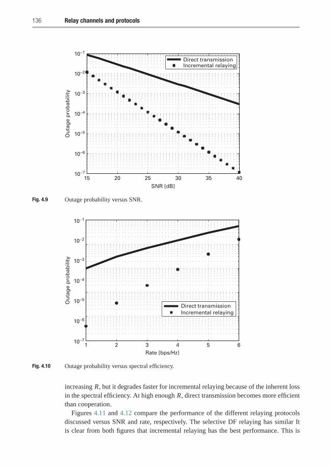
136 Relay channels and protocols
15 20 25 30 35 4010−7
10−6
10−5
10−4
10−3
10−2
10−1
SNR [dB]
Ou
tag
e p
rob
abili
tyDirect transmissionIncremental relaying
Fig. 4.9 Outage probability versus SNR.
10−7
10−6
10−5
10−4
10−3
10−2
10−1
Ou
tag
e p
rob
abili
ty
1 2 3 4 5 6Rate [bps/Hz]
Direct transmissionIncremental relaying
Fig. 4.10 Outage probability versus spectral efficiency.
increasing R, but it degrades faster for incremental relaying because of the inherent lossin the spectral efficiency. At high enough R, direct transmission becomes more efficientthan cooperation.
Figures 4.11 and 4.12 compare the performance of the different relaying protocolsdiscussed versus SNR and rate, respectively. The selective DF relaying has similar Itis clear from both figures that incremental relaying has the best performance. This is
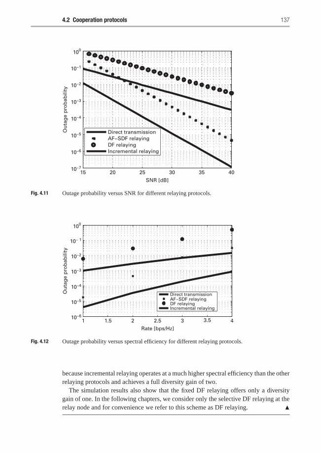
4.2 Cooperation protocols 137
15 20 25 30 35 4010−7
10−6
10−5
10−4
10−3
10−2
10−1
100
SNR [dB]
Ou
tag
e p
rob
abili
ty
Direct transmissionAF−SDF relayingDF relayingIncremental relaying
Fig. 4.11 Outage probability versus SNR for different relaying protocols.
1 1.5 2 2.5 3 3.5 4Rate [bps/Hz]
Direct transmissionAF−SDF relayingDF relayingIncremental relaying
10−6
10−5
10−4
10−3
10−2
10− 1
100
Ou
tag
e p
rob
abili
ty
Fig. 4.12 Outage probability versus spectral efficiency for different relaying protocols.
because incremental relaying operates at a much higher spectral efficiency than the otherrelaying protocols and achieves a full diversity gain of two.
The simulation results also show that the fixed DF relaying offers only a diversitygain of one. In the following chapters, we consider only the selective DF relaying at therelay node and for convenience we refer to this scheme as DF relaying. �
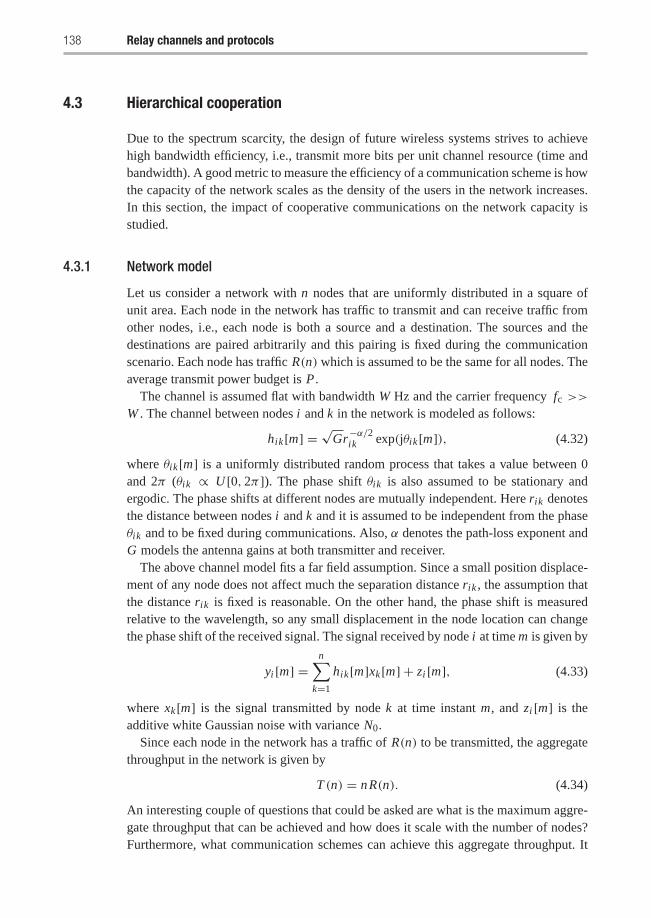
138 Relay channels and protocols
4.3 Hierarchical cooperation
Due to the spectrum scarcity, the design of future wireless systems strives to achievehigh bandwidth efficiency, i.e., transmit more bits per unit channel resource (time andbandwidth). A good metric to measure the efficiency of a communication scheme is howthe capacity of the network scales as the density of the users in the network increases.In this section, the impact of cooperative communications on the network capacity isstudied.
4.3.1 Network model
Let us consider a network with n nodes that are uniformly distributed in a square ofunit area. Each node in the network has traffic to transmit and can receive traffic fromother nodes, i.e., each node is both a source and a destination. The sources and thedestinations are paired arbitrarily and this pairing is fixed during the communicationscenario. Each node has traffic R(n) which is assumed to be the same for all nodes. Theaverage transmit power budget is P .
The channel is assumed flat with bandwidth W Hz and the carrier frequency fc >>W . The channel between nodes i and k in the network is modeled as follows:
hik[m] =√
Gr−α/2ik exp(jθik[m]), (4.32)
where θik[m] is a uniformly distributed random process that takes a value between 0and 2π (θik ∝ U [0, 2π ]). The phase shift θik is also assumed to be stationary andergodic. The phase shifts at different nodes are mutually independent. Here rik denotesthe distance between nodes i and k and it is assumed to be independent from the phaseθik and to be fixed during communications. Also, α denotes the path-loss exponent andG models the antenna gains at both transmitter and receiver.
The above channel model fits a far field assumption. Since a small position displace-ment of any node does not affect much the separation distance rik , the assumption thatthe distance rik is fixed is reasonable. On the other hand, the phase shift is measuredrelative to the wavelength, so any small displacement in the node location can changethe phase shift of the received signal. The signal received by node i at time m is given by
yi [m] =n∑
k=1
hik[m]xk[m] + zi [m], (4.33)
where xk[m] is the signal transmitted by node k at time instant m, and zi [m] is theadditive white Gaussian noise with variance N0.
Since each node in the network has a traffic of R(n) to be transmitted, the aggregatethroughput in the network is given by
T (n) = nR(n). (4.34)
An interesting couple of questions that could be asked are what is the maximum aggre-gate throughput that can be achieved and how does it scale with the number of nodes?Furthermore, what communication schemes can achieve this aggregate throughput. It
4.3 Hierarchical cooperation 139
has been shown that the nearest neighbor multihop transmission has a network capacitythat is upper bounded as follows [54]:
T (n) ≤ O(√
n). (4.35)
This means that the traffic rate per link scales as
R(n) ≤ O
(1√n
), (4.36)
hence the throughput per node drops as the density of the nodes increases. One can askthe question whether this network scaling is the best that we could get or it is a limitationof the nearest neighbor multihop transmission. It turns out that the network scaling in(4.35) is indeed a result of assuming nearest neighbor multihop transmission becausethis results in an interference limited scenario.
In the following section, a hierarchical cooperation protocol proposed in [142] thatachieves linear capacity scaling is described.
4.3.2 Hierarchical cooperation protocol description
First, we consider an upper bound for the best network scaling that can be achieved fora unit area network with n nodes uniformly distributed.
T H E O R E M 4.3.1 For a network with n nodes, the aggregate network throughput isupper bounded by
T (n) ≤ Kn log n, (4.37)
with probability approaching 1 as the number of nodes n goes to infinity, where K is aconstant independent of n.
Proof To prove this upper bound, let us consider a single input multiple output(SIMO) system in which a source node s is transmitting to a destination node d andthe rest of the nodes in the network are collocated with node d. The capacity of thischannel is upper bounded by
R(n) ≤ log
⎛⎝1+ P
N0
n∑i=1,i =s
|his |2⎞⎠
= log
⎛⎝1+ P
N0
∑i=1,i =s
G
rαis
⎞⎠ . (4.38)
The right-hand side in the above inequality can be further upper bounded if the destina-tion node is assumed to be the nearest neighbor for the source. The minimum distancebetween two nodes in a unit area where n nodes are uniformly distributed is larger than1/n1+δ for δ > 0. In the following this claim is verified.
Consider a node in the network, where the event that the nearest neighbor is at dis-tance 1/n1+δ is equivalent to the event that an area equal to π/n2+2δ is free of nodes.Denote this event by �, where the probability of � is given by
140 Relay channels and protocols
Pr (�) =(1− π
n2+2δ
)n−1. (4.39)
The above event is true for all nodes in the network with probability
Pr
(minimum distance in the network is smaller than
1
n1+δ
)≤ n
(1− π
n2+2δ
)n−1,
(4.40)
where the above is true by the union bound. Therefore, the minimum distance betweenany two nodes in the network is given by
rmin = 1
n1+δ , (4.41)
for δ > 0 with high probability. Substituting the minimum distance in (4.38), we get
R(n) ≤ log
(1+ PG
N0n(1+δ)α+1
), (4.42)
which concludes the theorem. �
This means that the upper bound on the capacity scaling of a network with n nodeslinearly scales with the number of nodes up to a logarithmic term. In other words, ifthere is a scheme that can achieve linear capacity scaling, this scheme is optimal.
Let us now describe the hierarchical cooperation protocol that is the focus of this sec-tion. The hierarchical scheme is based on clustering and long-range MIMO transmissionacross clusters. This can achieve two main goals:
• Using clustering one can achieve spatial reuse. This is because clusters that are wellseparated can work in parallel. The nodes operating in each cluster can lower theirpower accordingly to limit the interference to other clusters working in parallel.
• Using long-range MIMO we can achieve high spatial multiplexing gain.
The network is divided into clusters each with M nodes. Consider a specific node swithin some cluster. Node s will first disseminate its bits to the other M − 1 nodesinside its cluster. The M nodes within the cluster can then form a distributed MIMOtransmission and transmit the bits from source s to its destination, which might bein a different cluster. The nodes in destination’s cluster form a MIMO receiver. Eachnode in the receiving cluster will then quantize the received observation and relay theinformation to the destination. In the following we describe these three phases in moredetail.
4.3.2.1 Phase I: Setting up transmit cooperationIn this phase, each node distributes its data to the rest of the node inside its cluster. Thisis shown in Figure 4.13 in which source node s1 distributes its bits to its neighbors withinthe cluster. There are nodes in all of the square areas in Figure 4.13, but only few ofthem are shown for clarity. Clusters work in parallel according to the 9-TDMA schemedepicted in Figure 4.14, which works as follows: between any two active clusters there
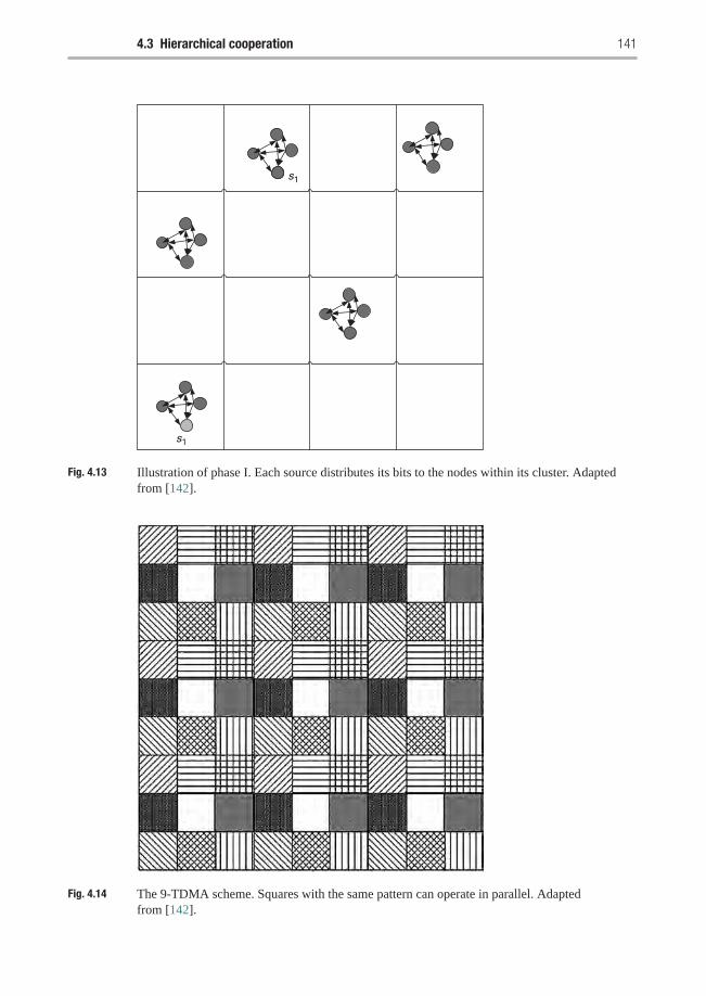
4.3 Hierarchical cooperation 141
s1
s1
Fig. 4.13 Illustration of phase I. Each source distributes its bits to the nodes within its cluster. Adaptedfrom [142].
Fig. 4.14 The 9-TDMA scheme. Squares with the same pattern can operate in parallel. Adaptedfrom [142].
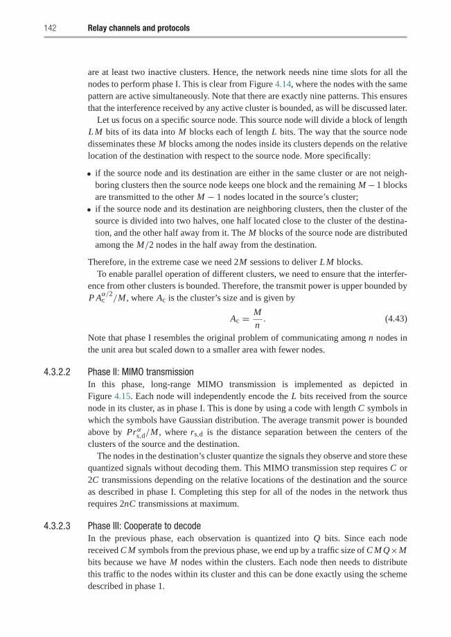
142 Relay channels and protocols
are at least two inactive clusters. Hence, the network needs nine time slots for all thenodes to perform phase I. This is clear from Figure 4.14, where the nodes with the samepattern are active simultaneously. Note that there are exactly nine patterns. This ensuresthat the interference received by any active cluster is bounded, as will be discussed later.
Let us focus on a specific source node. This source node will divide a block of lengthL M bits of its data into M blocks each of length L bits. The way that the source nodedisseminates these M blocks among the nodes inside its clusters depends on the relativelocation of the destination with respect to the source node. More specifically:
• if the source node and its destination are either in the same cluster or are not neigh-boring clusters then the source node keeps one block and the remaining M − 1 blocksare transmitted to the other M − 1 nodes located in the source’s cluster;
• if the source node and its destination are neighboring clusters, then the cluster of thesource is divided into two halves, one half located close to the cluster of the destina-tion, and the other half away from it. The M blocks of the source node are distributedamong the M/2 nodes in the half away from the destination.
Therefore, in the extreme case we need 2M sessions to deliver L M blocks.To enable parallel operation of different clusters, we need to ensure that the interfer-
ence from other clusters is bounded. Therefore, the transmit power is upper bounded byP Aα/2c /M , where Ac is the cluster’s size and is given by
Ac = M
n. (4.43)
Note that phase I resembles the original problem of communicating among n nodes inthe unit area but scaled down to a smaller area with fewer nodes.
4.3.2.2 Phase II: MIMO transmissionIn this phase, long-range MIMO transmission is implemented as depicted inFigure 4.15. Each node will independently encode the L bits received from the sourcenode in its cluster, as in phase I. This is done by using a code with length C symbols inwhich the symbols have Gaussian distribution. The average transmit power is boundedabove by Prαs,d/M , where rs,d is the distance separation between the centers of theclusters of the source and the destination.
The nodes in the destination’s cluster quantize the signals they observe and store thesequantized signals without decoding them. This MIMO transmission step requires C or2C transmissions depending on the relative locations of the destination and the sourceas described in phase I. Completing this step for all of the nodes in the network thusrequires 2nC transmissions at maximum.
4.3.2.3 Phase III: Cooperate to decodeIn the previous phase, each observation is quantized into Q bits. Since each nodereceived C M symbols from the previous phase, we end up by a traffic size of C M Q×Mbits because we have M nodes within the clusters. Each node then needs to distributethis traffic to the nodes within its cluster and this can be done exactly using the schemedescribed in phase 1.

4.3 Hierarchical cooperation 143
Fig. 4.15 Illustration of phase II showing Long-range MIMO transmission from the source’s cluster to thedestination’s cluster.
Note that, depending on whether the source and the destination are in neighboringclusters or not, we will have M/2 nodes with 2C observations each, or M nodes withC observations each. An exception is when the destination node belongs to the samecluster as the source node. In this case, each node in the cluster has L bits of the originaldata and no MIMO observations because there is no phase II in this case. By assumingL ≤ C Q these exceptions can be ignored and all nodes can be assumed to have MIMOobservations for simplicity.
4.3.3 Protocol analysis
In the following, the proof that a hierarchical protocol that consists of the previous threephases can achieve arbitrarily close to linear scaling is described. We first present alemma that plays a fundamental rule in the proof.
Consider a path-loss exponent α > 2 and a network with n nodes subject tointerference from external sources. The received signal by node i is modeled as
yi =n∑
k=1
hik xk + zi + Ii . (4.44)
Assume that {Ii , 1 ≤ i ≤ n} is a collection of uncorrelated zero-mean stationary andergodic random process with power PIi upper bounded by
PIi ≤ KI , 1 ≤ i ≤ n, (4.45)
for some constant KI > 0 independent of n. We have the following result.
Lemma 4.3.2 If there exists a scheme that can achieve an aggregate throughput of
T (n) ≥ K1nb, 0 ≤ b < 1, (4.46)
144 Relay channels and protocols
with probability at least 1 − exp (−nc1) for some constant c1 which is independent ofn, and the per node average power budget required to achieve this scheme is upper-bounded by P/n, then one can construct another scheme for this network that achievea higher aggregate throughput of
T (n) ≥ K2n1
2−b , (4.47)
and the failure rate of this second scheme is upper bounded by exp(−nC2
). Moreover,
the per node average power required to achieve this scheme is also upper boundedby P/n.
Proof Let us divide the unit square into areas of Ac, each equal to
Ac = M
n. (4.48)
Hence, each area has on average M nodes inside it. The proof of the lemma depends ona claim that the number of nodes inside each square equals M with high probability. Toshow this, let us calculate the probability that the number of nodes inside each square ofarea Ac is between ((1− δ)Acn, (1+ δ)Acn) for some δ > 0. The proof is a standardapplication of Chebyshev’s inequality as follows.
The number of nodes in any area of size Ac is a sum of n i.i.d. Bernoulli randomvariables Bi such that P(Bi = 1) = Ac. We have
P(
n∑i=1
Bi ≥ (1+ δ)Acn
)= P
(es∑n
i=1 Bi ≥ es(1+δ)Acn)
≤(E[esB1
])ne−s(1+δ)Acn
= (es Ac + (1− Ac))n e−s(1+δ)Acn
≤ e−Acn(s(1+δ)−es+1),
where the last inequality used the following lower bound
(1− x) ≤ exp(−x). (4.49)
Finally we have
P(
n∑i=1
Bi ≥ (1+ δ)Acn
)≤ e−Acn�+(δ) (4.50)
where�+(δ) = (1+δ) log(1+δ)−δ, and this is achieved through choosing s to tightenthe bound as follows:
s = log(1+ δ). (4.51)
One can get a lower bound by following similar steps as above for negative Bi . Thisproves that the probability that the number of nodes inside the square Ac deviates fromM decays exponentially with n. Hence, with high probability the number of nodeswithin a square Ac is equal to its mean M . In the following, it is always assumed thatthere exists M bits in each cluster.
4.3 Hierarchical cooperation 145
Analysis of phase IAs described before, each node in a cluster divides its data into L M bits, and hencewe have in total L M × M bits traffic for each cluster. For the special case where thesource and the destination lie in neighbor clusters, the source will need to organize 2Msessions to transfer the information. Each node will scale its power proportional to thesize of the cluster as P(Ac)
α/2/M . The main reason for this is to allow parallel operationof the clusters. This leads to a bounded interference at each node (this is proven later inthe exercises), then according to Lemma 4.3.2 all the conditions is satisfied to achievean aggregate throughput of K1Mb in each session for some K1 > 0. This throughputalso can be achieved with probability larger than 1− exp(−Mc1). By the union bound,and since we have at maximum 2M sessions in each cluster and n/M clusters, thethroughput can be achieved with probability 1− 2n exp(−Mc1).
With this aggregate throughput, each session requires at most
Tsession = L M
K1Mb= L
K1M1−b (4.52)
channel uses. Since, we have at most 2M sessions, and taking into account the 9-TDMA scheme, the total number of channels uses required to complete phase I isgiven by
TI = 9× 2M × L
K1M1−b = 18L
K1M2−b (4.53)
channel uses to finish all the transmission required by the n nodes in the network withintheir clusters.
Analysis of phase IIIn this phase, long-range MIMO transmission takes place. It is this step essentiallythat allows the protocol to achieve high capacity scaling. This is because with MIMOtransmission, as discussed in earlier chapters, the throughput scales linearly with theminimum of the number of transmit and receive antennas.
In phase II, each source’s information is transmitted to its destination while the othersources are silent. Hence, this resembles a TDMA scheme where all the sources inthe network transmit in a serial way, but the major difference between this and plainTDMA is that while the source transmits all the nodes within its cluster cooperate bytransmitting the bits they received from the source in the previous phase. This forms anM virtual antenna array at the source’s cluster.
At the same time, all of the M nodes at the destination cluster cooperate to receivethe transmitted information. This is done through each node storing a quantized versionof the received information to forward later to the destination node, hence forming adistributed receive antenna array.
As described before, each node in the source’s cluster encode the L bits receivedfrom the source in phase I into C symbols. This code is generated according to anaverage power constraint of Prαs,d/M , where rs,d is the distance between the center ofthe source’s cluster to the center of the destination’s cluster.
146 Relay channels and protocols
In the special case in which the source and the destination belong to neighboringclusters, only half of the nodes in the source’s cluster have the information. In thiscase, each node encodes the information into 2C symbols. Therefore, each node in thenetwork requires either C or 2C channel uses to transmit its information. Since thereare n nodes in the network, the maximum number of channel uses required to achievephase II is given by
TII = 2nC. (4.54)
Analysis of phase IIIIn this phase, each node delivers the observation it received from phase II to the intendeddestination. Either the M nodes in the clusters have C symbols or M/2 nodes have 2Csymbols depending on whether the source and the destination belong to neighboringclusters or not. A node quantizes each symbol into Q bits. Therefore, at most we endup having a traffic of 2M × QC M bits.
Similar to phase I, clusters work in parallel using the 9-TDMA scheme. This meansthat there are at least two idle clusters between any two active clusters. Since nodeswithin a cluster scale down their power proportionally to the cluster size, the inter-ference from other active clusters can be shown to be bounded above by a constantindependent of n.
Therefore, similar to phase I, the conditions to apply Lemma 4.3.2 are all satis-fied. Hence, the number of channel uses required to complete this phase is givenby (2C Q/K1)M2−b. Taking into account the 9-TDMA scheme, the total number ofchannel uses required for the n nodes in the network to complete phase III is given by
TIII = 18C Q
K1M2−b. (4.55)
This is achieved with probability larger than 1− 2ne−Mc1 .The above depends on the quantization done at the nodes inside the clusters not intro-
ducing any distortion, although the nodes use a fixed quantizer of size Q bits. This isindeed possible and the observations can be encoded using a fixed number of bits, therationale being that the observations have a bounded power that does not scale with M .
Combining all the resultsSummarizing the results above, we have three phases and the total number of channeluses required to complete these phases has been computed. The total number of channeluses is given by
Tt = TI + TII + TIII
= 18L
K1M2−b + 2Cn + 18C Q
K1M2−b.
(4.56)
Therefore, with high probability and bounded average power per node, the aggregatethroughput is given by
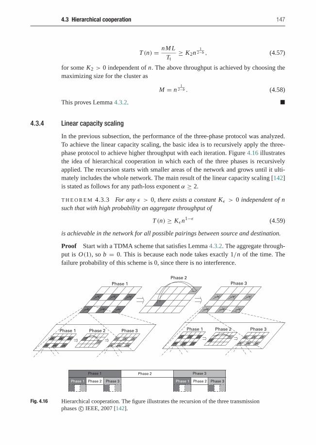
4.3 Hierarchical cooperation 147
T (n) = nM L
Tt≥ K2n
12−b , (4.57)
for some K2 > 0 independent of n. The above throughput is achieved by choosing themaximizing size for the cluster as
M = n1
2−b . (4.58)
This proves Lemma 4.3.2. �
4.3.4 Linear capacity scaling
In the previous subsection, the performance of the three-phase protocol was analyzed.To achieve the linear capacity scaling, the basic idea is to recursively apply the three-phase protocol to achieve higher throughput with each iteration. Figure 4.16 illustratesthe idea of hierarchical cooperation in which each of the three phases is recursivelyapplied. The recursion starts with smaller areas of the network and grows until it ulti-mately includes the whole network. The main result of the linear capacity scaling [142]is stated as follows for any path-loss exponent α ≥ 2.
T H E O R E M 4.3.3 For any ε > 0, there exists a constant Kε > 0 independent of nsuch that with high probability an aggregate throughput of
T (n) ≥ Kεn1−ε (4.59)
is achievable in the network for all possible pairings between source and destination.
Proof Start with a TDMA scheme that satisfies Lemma 4.3.2. The aggregate through-put is O(1), so b = 0. This is because each node takes exactly 1/n of the time. Thefailure probability of this scheme is 0, since there is no interference.
Phase 1 Phase 1Phase 2 Phase 2Phase 3 Phase 3
Phase 3Phase 2
Phase 2 Phase 3Phase 1
Phase 2Phase 2 Phase 3 Phase 3Phase 1 Phase 1
Phase 1
Fig. 4.16 Hierarchical cooperation. The figure illustrates the recursion of the three transmissionphases c© IEEE, 2007 [142].
148 Relay channels and protocols
Applying Lemma 4.3.2 recursively yields schemes that achieve higher throughputwith each recursion. More precisely, starting with a TDMA scheme with b = 0 andapplying Lemma 4.3.2 recursively h times, one gets a scheme achieving �
(nh/(1+h)
)aggregate throughput.
Given any ε > 0, we can now choose h such that
h
1+ h≥ 1− ε, (4.60)
and we get a scheme that achieves �(n1−ε) with high probability. �
4.4 Chapter summary and bibliographical notes
In this chapter, we introduced the new notion of cooperative communications. Coop-erative communications is a new communication paradigm that generalizes MIMOcommunications to much broader applications. In this new paradigm, the terminals dis-persed in a wireless network cell can be thought of as distributed antennas. Throughcooperation among these nodes, MIMO-like gains can be achieved by increasing thediversity gains of the system. Different protocols have been described to implementcooperation. We described the performance of these algorithms through calculatingoutage capacity and characterizing diversity gains. The performance of adaptive relay-ing techniques in general outperforms that of fixed relaying techniques because of theextra information utilized in implementing the protocols, for example, knowledge ofthe received SNR in selective relaying and the feedback from the destination in incre-mental relaying. On the other hand, fixed relaying techniques are simpler to implementcompared to fixed relaying techniques due to the extra overhead needed to implementthe former protocols. Therefore, it is ultimately a tradeoff between performance andcomplexity that the system designer must decide on.
In addition, in this chapter we have studied the capacity scaling in wireless ad hocnetworks when cooperation is applied. It was shown that the hierarchical coopera-tion scheme proposed in [142] can achieve linear scaling in ad hoc networks. Thismeans that as the number of nodes per unit area increases the throughput per nodedoes not drop. This is an interesting result which shows that cooperation can over-come the interference limitation in wireless networks. The scheme that achieves thelinear scaling is a recursive scheme that consists of three steps. The network is dividedinto clusters. In the first step, nodes within a cluster distribute their bits to the othernodes within the cluster. In the second phase, long-range MIMO transmission betweenclusters is implemented, and finally in the third phase local signal quantization anddistribution within each cluster similar to phase 1 is implemented. Hence, the schememakes use of two very important concepts: spatial reuse by allowing different clus-ters to operate in parallel, and long-range MIMO transmission that achieves linearthroughput.
4.4 Chapter summary and bibliographical notes 149
We provide some bibliographical notes as follows. The classical relay channel intro-duced by Van der Meulen [224] models a three-terminal communication channel. Therelay channel, in general, is a channel with one transmitter, one receiver, and a num-ber of intermediate nodes that act as relays to improve the system performance. Thesimplest relay channel contains one terminal, the relay, that listens to the signal trans-mitted by the source, processes it, and then transmits it to the destination. Cover andEl Gamal [25] developed lower and upper bounds on the channel capacity for specificnon-faded relay channel models. The lower and upper bound do not coincide in gen-eral except for some special cases, such as in the degraded relay channel. Later, severalworks have studied the capacity of the relay channels and developed coding strategiesthat can achieve the ergodic capacity of the channel under certain scenarios, see [99]and the references there in.
In [109] and [108], Laneman et al. proposed different cooperative diversity protocolsand analyzed their performance in terms of outage behavior. The terms decode-and-forward and amplify-and-forward have been introduced in these two works. Indecode-and-forward, each relay receives and decodes the signal transmitted by thesource, and then forwards the decoded signal to the destination, which combines all thecopies in a proper way. Amplify-and-forward is a simpler technique, in which the relayamplifies the received signal and then forwards it to the destination. Although the noiseis amplified along with the signal in this technique, we still gain spatial diversity bytransmitting the signal over two spatially independent channels. Compress-and-forwardwas studied in [25] and [99]. More information about the related distributed sourcecoding technique can be found in [230]. Terminologies other than cooperative diversityare also used in the research community to refer to the same concept of achieving spa-tial diversity via forming virtual antennas. User cooperation diversity was introducedby Sendonaris et al. in [179] in which the authors implemented a two-user CDMAcooperative system, where both users are active and use orthogonal codes to avoidmultiple access interference. Another technique to achieve diversity that incorporateserror-control-coding into cooperation is coded cooperation, introduced by Hunter et al.in [78].
Capacity scaling in wireless networks has been studied by several researchersrecently. The seminal work of Gupta and Kumar [54] has stimulated a lot of think-ing in this problem. Gupta and Kumar showed that an aggregate throughput scaling of�(√
n) is an upper bound for what can be achievable by multihop transmission. Thelimitation in their model is that no cooperation is allowed between networks, and henceif a signal is not intended to be transmitted to a node it is treated as interference. Coop-eration, on the other hand, benefits from the broadcast nature of the channel, and tries totake advantage of this aspect instead of treating the overheard signals as interference. Inanother recent work by Aeron and Saligrama [2], distributed collaborative schemes areproposed that lead to an increase in throughput over the traditional multihop schemes.The scheme proposed in this work achieves an aggregate throughput of �
(n2/3
). The
scheme that achieves the linear capacity scaling in wireless ad hoc networks when coop-eration is applied, and the associated analysis studied in this chapter, was presented in[142].
150 Relay channels and protocols
Exercises
4.1 In (4.12), the MRC parameters were derived from a detection theory and signalspace perspective. Another approach to solve for the MRC parameters is viasolving an optimization problem with the cost function being the SNR at theoutput of the detector and the optimization variables being the MRC parameters.
Assume that signal x is received at the destination via two independent pathsas follows:
y1 = h1x + n1
y2 = h2x + n2
where h1, h2, n1, and n2 are all mutually independent complex normal Gaussianrandom variables with zero mean and variances σ 2
1 , σ 22 , N01, and N02. Find the
optimal combining ratios a1 and a2 that maximize the output SNR of the detector.4.2 In describing the different relaying protocols in this chapter, it was assumed that
the relay already exists in some position and is helping the source node. In areal scenario, there might exist multiple relays that can help the source and thesource needs to decide which relay to select. Therefore, studying the effect ofrelay position on the performance of various cooperation protocols is important.(a) In AF relaying, assume the relay is located on the straight line joining
the source and destination. Assume that the channel variance between twonodes depends on the distance d separating the two nodes according to anexponential path loss model as follows:
σ 2 = d−α. (E4.1)
Find the outage probability of AF relaying as a function of the relay distancefrom the source ds,r assuming a unit distance between the source and desti-nation, and that ds,r takes values between 0.1 and 0.9. Use a Matlab code todraw this outage probability as a function of the relay position.
(b) Repeat the previous calculations to DF, selective, and incremental relaying.4.3 In proving that the schemes in phases I and III work, it was assumed that the
9-TDMA scheme and scaling the transmission power relative to the cluster sizeresult in uncorrelated and bounded interference. Consider clusters of size M andarea Ac. The clusters operate according to the 9-TDMA scheme shown in Fig-ure 4.14 in a network of size n. The average power of each node is assumed to beconstrained to P Aα/2c /M . For α > 2, show that the interference power receivedby a node from the clusters operating in parallel is upper bounded by a constantKI independent of n.
4.4 In phase III, each node in the destination cluster quantizes the MIMO receivedinformation into Q bits. The number of bits Q is assumed to be a fixed num-ber independent of M . The argument is that this is sufficient to achieve linearthroughput from MIMO transmission without introducing distortion because thereceived power in phase II by each node in the destination cluster is bounded
Exercises 151
below and above by constants P1 and P2, respectively, which are independent ofM . Show that this claim is correct.
4.5 In this chapter, equal transmit power at both the source and the relay wasassumed. Consider the case where the transmit power at the source and the relayare given by Ps and Pr.(a) Find the outage probability for amplify-and-forward relaying as a function
of Ps and Pr.(b) Assuming an equal average power constraint as follows:
Ps + Pr = 2P, (E4.2)
where P is the transmit power used for direct transmission. Find the optimalpower allocation Ps and Pr to minimize the outage probability expression.
(c) Repeat the previous problem for selective decode-and-forward and incre-mental relaying.
(d) Find the outage probability for selective decode-and-forward relaying whentwo relays are available to help the source. What is the diversity gainachieved?
5 Cooperative communicationswith single relay
In this chapter, we consider single relay cooperative communications in wireless net-works. We focus on the discussion of symbol error rate (SER) performance analysisand optimum power allocation for uncoded cooperative communications with either anamplify-and-forward (AF) or a selective decode-and-forward (DF)1 cooperation proto-col. In this chapter and the rest of this book, we simply call the selective DF cooperationprotocol a DF protocol without confusing it with the fixed DF relaying protocol.
The chapter is organized as follows. First, we briefly describe a system model forcooperative communications with either DF or AF cooperation protocols. Second, weanalyze the SER performance for DF cooperation systems, in which a closed-form SERformulation is obtained explicitly for systems with M-PSK and M-QAM modulations.An SER upper bound as well as an approximation are provided to reveal the asymp-totic performance of the cooperative system. Based on the tight SER approximation,we can determine an asymptotic optimum power allocation for DF cooperation sys-tems. Third, we consider the SER performance for AF cooperation systems, in whichwe first derive a simple closed-form moment-generating function (MGF) expression forthe harmonic mean of two independent exponential random variables. Then, based onthe simple MGF expression, closed-form SER formulations are given for AF cooper-ation systems with M-PSK and M-QAM modulations. We also provide a tight SERapproximation to show the asymptotic performance of AF cooperation systems and todetermine an optimum power allocation. Fourth, we discuss performance comparisonsbetween the cooperation systems with DF and AF protocols and show some simulationexamples. Finally, we consider a method of re-mapping signal constellation points atthe relay to improve the SER performance of the DF protocol.
5.1 System model
A cooperative communication strategy with two phases is considered for wireless net-works such as mobile ad hoc networks, sensor networks, or cellular networks. In bothphases, users transmit signals through orthogonal channels by using TDMA, FDMA, or
1 In this chapter, we consider that an ideal selective DF cooperation protocol is one in which a relay is able todetect whether the decoding at the relay is correct or not. If the decoding is correct, the relay forwards thedecoded symbol to a destination, otherwise the relay does not send or remains idle.
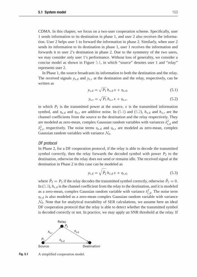
5.1 System model 153
CDMA. In this chapter, we focus on a two-user cooperation scheme. Specifically, user1 sends information to its destination in phase 1, and user 2 also receives the informa-tion. User 2 helps user 1 to forward the information in phase 2. Similarly, when user 2sends its information to its destination in phase 1, user 1 receives the information andforwards it to user 2’s destination in phase 2. Due to the symmetry of the two users,we may consider only user 1’s performance. Without loss of generality, we consider aconcise model as shown in Figure 5.1, in which “source” denotes user 1 and “relay”represents user 2.
In Phase 1, the source broadcasts its information to both the destination and the relay.The received signals ys,d and ys,r at the destination and the relay, respectively, can bewritten as
ys,d =√
P1 hs,d x + ηs,d, (5.1)
ys,r =√
P1 hs,r x + ηs,r, (5.2)
in which P1 is the transmitted power at the source, x is the transmitted informationsymbol, and ηs,d and ηs,r are additive noise. In (5.1) and (5.2), hs,d and hs,r are thechannel coefficients from the source to the destination and the relay respectively. Theyare modeled as zero-mean, complex Gaussian random variables with variances δ2
s,d and
δ2s,r, respectively. The noise terms ηs,d and ηs,r are modeled as zero-mean, complex
Gaussian random variables with variance N0.
DF protocolIn Phase 2, for a DF cooperation protocol, if the relay is able to decode the transmittedsymbol correctly, then the relay forwards the decoded symbol with power P2 to thedestination, otherwise the relay does not send or remains idle. The received signal at thedestination in Phase 2 in this case can be modeled as
yr,d =√
P2 hr,d x + ηr,d, (5.3)
where P2 = P2 if the relay decodes the transmitted symbol correctly, otherwise P2 = 0.In (5.3), hr,d is the channel coefficient from the relay to the destination, and it is modeledas a zero-mean, complex Gaussian random variable with variance δ2
r,d. The noise termηr,d is also modeled as a zero-mean complex Gaussian random variable with varianceN0. Note that for analytical tractability of SER calculations, we assume here an idealDF cooperation protocol that the relay is able to detect whether the transmitted symbolis decoded correctly or not. In practice, we may apply an SNR threshold at the relay. If
Relay
hs,rhr,d
P2
DestinationSource
hs,dP1
Fig. 5.1 A simplified cooperation model.
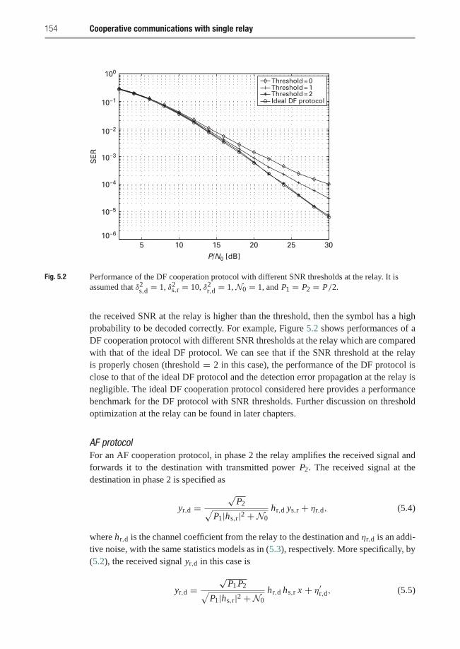
154 Cooperative communications with single relay
5 10 15 20 25 30
P/N0 [dB]
SE
RThreshold = 0Threshold = 1 Threshold = 2 Ideal DF protocol
10−6
10−4
10−5
10−3
10−2
10−1
100
Fig. 5.2 Performance of the DF cooperation protocol with different SNR thresholds at the relay. It isassumed that δ2s,d = 1, δ2s,r = 10, δ2r,d = 1, N0 = 1, and P1 = P2 = P/2.
the received SNR at the relay is higher than the threshold, then the symbol has a highprobability to be decoded correctly. For example, Figure 5.2 shows performances of aDF cooperation protocol with different SNR thresholds at the relay which are comparedwith that of the ideal DF protocol. We can see that if the SNR threshold at the relayis properly chosen (threshold = 2 in this case), the performance of the DF protocol isclose to that of the ideal DF protocol and the detection error propagation at the relay isnegligible. The ideal DF cooperation protocol considered here provides a performancebenchmark for the DF protocol with SNR thresholds. Further discussion on thresholdoptimization at the relay can be found in later chapters.
AF protocolFor an AF cooperation protocol, in phase 2 the relay amplifies the received signal andforwards it to the destination with transmitted power P2. The received signal at thedestination in phase 2 is specified as
yr,d =√
P2√P1|hs,r|2 +N0
hr,d ys,r + ηr,d, (5.4)
where hr,d is the channel coefficient from the relay to the destination and ηr,d is an addi-tive noise, with the same statistics models as in (5.3), respectively. More specifically, by(5.2), the received signal yr,d in this case is
yr,d =√
P1 P2√P1|hs,r|2 +N0
hr,d hs,r x + η′r,d, (5.5)
5.2 SER analysis for DF protocol 155
where
η′r,d =√
P2√P1|hs,r|2 +N0
hr,d ηs,r + ηr,d (5.6)
Assume that the noise terms ηs,r and ηr,d are independent, then the equivalent noise η′r,dis a zero-mean, complex Gaussian random variable with variance(
P2|hr,d|2P1|hs,r|2 +N0
+ 1
)N0.
In both the DF and AF cooperation protocols, the channel coefficients hs,d, hs,r, andhr,d are assumed to be known at the receiver, but not at the transmitter. The destinationjointly combines the received signal from the source in Phase 1 and that from the relayin phase 2, and detects the transmitted symbols by using maximum-ratio combining(MRC). In both protocols, we consider a total transmitted power P such as
P1 + P2 = P. (5.7)
Note that in the DF cooperation protocol, the power saving in the case of P2 = 0 isnegligible, since at high SNR, the chance that the relay incorrectly decodes the symbolis rare as we will see later in the performance analysis.
5.2 SER analysis for DF protocol
In this section, we consider the SER performance analysis for the DF cooperative com-munication systems. First, we introduce closed-form SER formulations for the systemswith M-PSK and M-QAM2 modulations, respectively. Then, we provide an SER upperbound as well as an approximation to reveal the asymptotic performance of the sys-tems, in which the approximation is asymptotically tight at high SNR. Finally, based onthe tight SER approximation, we are able to determine an asymptotic optimum powerallocation for DF cooperation systems.
5.2.1 Closed-form SER analysis
With knowledge of the channel coefficients hs,d (between the source and the destination)and hr,d (between the relay and the destination), the destination detects the transmittedsymbols by jointly combining the received signal ys,d (5.1) from the source and yr,d
(5.3) from the relay. The combined signal at the MRC detector can be written as
y = a1ys,d + a2yr,d, (5.8)
in which the factors a1 and a2 are determined such that the SNR of the MRC output ismaximized, and, from Section 1.4, they can be specified as
a1 =√
P1h∗s,d/N0, a2 =√
P2h∗r,d/N0.
2 In this chapter, QAM represents a square QAM constellation whose size is given by M = 2k with k even.
156 Cooperative communications with single relay
Assume that the transmitted symbol x in (5.1) and (5.3) has average energy 1, then theSNR of the MRC output is
γ = P1|hs,d|2 + P2|hr,d|2N0
. (5.9)
First, let us review SER formulations for an uncoded system with M-PSK or M-QAM(M = 2k with k even) modulation [187], which are given by
�PSK(ρ)�= 1
π
∫ (M−1)π/M
0exp
(−bPSKρ
sin2 θ
)dθ, (5.10)
�QAM(ρ)�= 4K Q(
√bQAMρ)− 4K 2Q2(
√bQAMρ), (5.11)
in which ρ is SNR, bPSK = sin2(π/M), K = 1 − (1/√M), bQAM = 3/(M − 1), andQ(u) = (1/√2π)
∫∞u exp(−t2/2)dt is the Gaussian Q-function. Therefore, if M-PSK
modulation is used in the DF cooperation system, with the instantaneous SNR γ in(5.9), the conditional SER of the system with the channel coefficients hs,d, hs,r and hr,d
can be written as
Phs,d,hs,r,hr,dPSK = �PSK(γ ). (5.12)
If M-QAM (M = 2k with k even) signals are used in the system, the conditional SERof the system can also be expressed as
Phs,d,hs,r,hr,dQAM = �QAM(γ ). (5.13)
It is easy to see that, in the case of QPSK or 4-QAM modulation, the conditional SERsin (5.12) and (5.13) are the same.
Note that in phase 2 we assume that if the relay decodes the transmitted symbol xfrom the source correctly, then the relay forwards the decoded symbol with power P2 tothe destination, i.e., P2 = P2; otherwise the relay does not send, i.e., P2 = 0. If an M-PSK symbol is sent from the source, then at the relay, the chance of incorrect decodingis �PSK(P1|hs,r|2/N0), and the chance of correct decoding is 1−�PSK(P1|hs,r|2/N0).Similarly, if an M-QAM symbol is sent out at the source, then the chance of incorrectdecoding at the relay is �QAM(P1|hs,r|2/N0), and the chance of correct decoding is1−�QAM(P1|hs,r|2/N0).
Let us first focus on the SER performance analysis in the case of M-PSK modulation.Taking into account the two scenarios P2 = P2 and P2 = 0, we further calculate theconditional SER in (5.12) as follows:
Phs,d,hs,r,hr,dPSK
= �PSK(γ )|P2=0�PSK
(P1|hs,r|2
N0
)+�PSK(γ )|P2=P2
[1−�PSK
(P1|hs,r|2
N0
)]
= 1
π2
∫ (M−1)π/M
0exp
(−bPSK P1|hs,d|2
N0 sin2 θ
)dθ∫ (M−1)π/M
0exp
(−bPSK P1|hs,r|2
N0 sin2 θ
)dθ
5.2 SER analysis for DF protocol 157
+ 1
π
∫ (M−1)π/M
0exp
(−bPSK(P1|hs,d|2 + P2|hr,d|2)
N0 sin2 θ
)dθ
×[
1− 1
π
∫ (M−1)π/M
0exp
(−bPSK P1|hs,r|2
N0 sin2 θ
)dθ
]. (5.14)
In the following, we average the conditional SER (5.14) over the Rayleigh fading chan-nels hs,d, hs,r, and hr,d with variances δ2
s,d, δ2s,r, and δ2
r,d, respectively. Since the fadingchannels hs,d, hs,r, and hr,d are independent of each other, and
∫ ∞
0exp
(− bPSK P1z
N0 sin2 θ
)p|h|2(z)dz = 1
1+ bPSK P1δ2h
N0 sin2 θ
,
we are able to obtain the SER of the DF cooperation system with M-PSK modulationas follows:
PPSK = F1
(1+ bPSK P1δ
2s,d
N0 sin2 θ
)F1
(1+ bPSK P1δ
2s,r
N0 sin2 θ
)
+ F1
((1+ bPSK P1δ
2s,d
N0 sin2 θ
)(1+ bPSK P2δ
2r,d
N0 sin2 θ
))
×[
1− F1
(1+ bPSK P1δ
2s,r
N0 sin2 θ
)], (5.15)
where
F1(x(θ)) = 1
π
∫ (M−1)π/M
0
1
x(θ)dθ. (5.16)
For DF cooperation systems with M-QAM modulation, the conditional SER in (5.13)with the channel coefficients hs,d, hs,r, and hr,d can be similarly determined as
Phs,d,hs,r,hr,dQAM = �QAM(γ )|P2=0�QAM
(P1|hs,r|2
N0
)
+ �QAM(γ )|P2=P2
[1−�QAM
(P1|hs,r|2
N0
)]. (5.17)
By substituting (5.11) into the above formulation and averaging it over the fadingchannels hs,d, hs,r, and hr,d, as in the case of M-PSK modulation, the SER of the DFcooperation system with M-QAM modulation can be given by
158 Cooperative communications with single relay
PQAM = F2
(1+ bQAM P1δ
2s,d
2N0 sin2 θ
)F2
(1+ bQAM P1δ
2s,r
2N0 sin2 θ
)
+ F2
((1+ bQAM P1δ
2s,d
2N0 sin2 θ
)(1+ bQAM P2δ
2r,d
2N0 sin2 θ
))
×[
1− F2
(1+ bQAM P1δ
2s,r
2N0 sin2 θ
)], (5.18)
where
F2(x(θ)) = 4K
π
∫ π/2
0
1
x(θ)dθ − 4K 2
π
∫ π/4
0
1
x(θ)dθ. (5.19)
In order to get the SER formulation in (5.18), two special properties of the GaussianQ-function are needed as follows:
Q(u) = 1
π
∫ π/2
0exp
(− u2
2 sin2 θ
)dθ,
Q2(u) = 1
π
∫ π/4
0exp
(− u2
2 sin2 θ
)dθ
for any u ≥ 0. Note that for 4-QAM modulation,
F2(x(sin2(θ))) = 2
π
∫ π/2
0
1
x(sin2(θ))dθ − 1
π
∫ π/4
0
1
x(sin2(θ))dθ
= 1
π
∫ π/2
0
1
x(sin2(θ))dθ + 1
π
∫ π/2
π/4
1
x(sin2(θ))dθ
= 1
π
∫ 3π/4
0
1
x(sin2(θ))dθ,
which shows that the SER formulation in (5.18) for 4-QAM modulation is consistentwith that in (5.15) for QPSK modulation.
5.2.2 SER upper bound and asymptotic approximation
Even though the closed-form SER formulations in (5.15) and (5.18) can be efficientlycalculated numerically, they are very complex and it is hard to gain an insight into thesystem performance from these. In the following, we introduce a SER upper bound andSER approximation which are useful in demonstrating the asymptotic performance ofthe DF cooperation scheme.
T H E O R E M 5.2.1 The SER of DF cooperation systems with M-PSK or M-QAMmodulation can be upper bounded as
Ps ≤ (M − 1)N 20
M2· MbP1δ
2s,r + (M − 1)bP2δ
2r,d + (2M − 1)N0
(N0 + bP1δ2s,d)(N0 + bP1δ2
s,r)(N0 + bP2δ2r,d), (5.20)
where b = bPSK for M-PSK signals and b = bQAM/2 for M-QAM signals.
5.2 SER analysis for DF protocol 159
Proof In the case of M-PSK modulation, the closed-form SER expression is given in(5.15). By removing the negative term in (5.15), we have
PPSK ≤ F1
(1+ bPSK P1δ
2s,d
N0 sin2 θ
)F1
(1+ bPSK P1δ
2s,r
N0 sin2 θ
)
+ F1
((1+ bPSK P1δ
2s,d
N0 sin2 θ
)(1+ bPSK P2δ
2r,d
N0 sin2 θ
)), (5.21)
where
F1(x(θ)) = 1
π
∫ (M−1)π/M
0
1
x(θ)dθ.
We observe that, in the right-hand side of the above inequality, all integrands have theirmaximum value when sin2 θ = 1. Therefore, by substituting sin2 θ = 1 into (5.21),we have
PPSK ≤ (M − 1)2
M2· N 2
0
(N0 + bPSK P1δ2s,d)(N0 + bPSK P1δ2
s,r)
+ M − 1
M· N 2
0
(N0 + bPSK P1δ2s,d)(N0 + bPSK P2δ
2r,d)
= (M − 1)N 20
M2· MbPSK P1δ
2s,r + (M − 1)bPSK P2δ
2r,d + (2M − 1)N0
(N0 + bPSK P1δ2s,d)(N0 + bPSK P1δ2
s,r)(N0 + bPSK P2δ2r,d),
which validates the upper bound in (5.20) for M-PSK modulation. Similarly, in the caseof M-QAM modulation, the SER in (5.18) can be upper bounded as
PQAM ≤ F2
(1+ bQAM P1δ
2s,d
2N0 sin2 θ
)F2
(1+ bQAM P1δ
2s,r
2N0 sin2 θ
)
+ F2
((1+ bQAM P1δ
2s,d
2N0 sin2 θ
)(1+ bQAM P2δ
2r,d
2N0 sin2 θ
)), (5.22)
where
F2(x(θ)) = 4K
π
∫ π/2
0
1
x(θ)dθ − 4K 2
π
∫ π/4
0
1
x(θ)dθ.
Note that the function F2(x(θ)) can be rewritten as
F2(x(θ)) = 4K
π√
M
∫ π/2
0
1
x(θ)dθ + 4K 2
π
∫ π/2
π/4
1
x(θ)dθ, (5.23)
which does not contain negative term. It turns out that the integrands in (5.22) havetheir maximum value when sin2 θ = 1. Thus, by substituting (5.23) and sin2 θ = 1 into(5.22), we have
160 Cooperative communications with single relay
PQAM ≤(
2K√M+ K 2
)2 N 20
(N0 + bQAM2 P1δ
2s,d)(N0 + bQAM
2 P1δ2s,r)
+(
2K√M+ K 2
) N 20
(N0 + bQAM2 P1δ
2s,d)(N0 + bQAM
2 P2δ2r,d)
= (M − 1)N 20
M2· M
bQAM2 P1δ
2s,r + (M − 1) bQAM
2 P2δ2r,d + (2M − 1)N0
(N0 + bQAM2 P1δ
2s,d)(N0 + bQAM
2 P1δ2s,r)(N0 + bQAM
2 P2δ2r,d),
in which K = 1− 1/√
M . Therefore, the upper bound in (5.20) holds for both M-PSKand M-QAM modulation. �
In the sequel, we provide an asymptotically tight SER approximation if all of the chan-nel links hs,d, hs,r, and hr,d are available, i.e., δ2
s,d �= 0, δ2s,r �= 0, and δ2
r,d �= 0. Accordingto (5.15) and (5.18), let us denote the SER of DF cooperation systems with M-PSK orM-QAM modulation as
Ps = I1(P1/N0)+ I2(P1/N0, P2/N0), (5.24)
where
I1(x) = Fi
(1+ xbδ2
s,d
sin2 θ
)Fi
(1+ xbδ2
s,r
sin2 θ
), (5.25)
I2(x, y) = Fi
((1+ xbδ2
s,d
sin2 θ
)(1+ ybδ2
r,d
sin2 θ
))[1− Fi
(1+ xbδ2
s,r
sin2 θ
)], (5.26)
in which i = 1 and b = bPSK for M-PSK modulation, and i = 2 and b = bQAM/2 forM-QAM modulation. Then, we have the following results (leave proof as an exercise):
limx→∞ x2 I1(x) = A2
b2δ2s,dδ
2s,r
, (5.27)
limx, y→∞ xy I2(x, y) = B
b2δ2s,dδ
2r,d
, (5.28)
where, for M-PSK signals, b = bPSK and
A = M − 1
2M+ sin 2π
M
4π, (5.29)
B = 3(M − 1)
8M+ sin 2π
M
4π− sin 4π
M
32π; (5.30)
while for M-QAM signals, b = bQAM/2 and
A = M − 1
2M+ K 2
π, (5.31)
B = 3(M − 1)
8M+ K 2
π. (5.32)
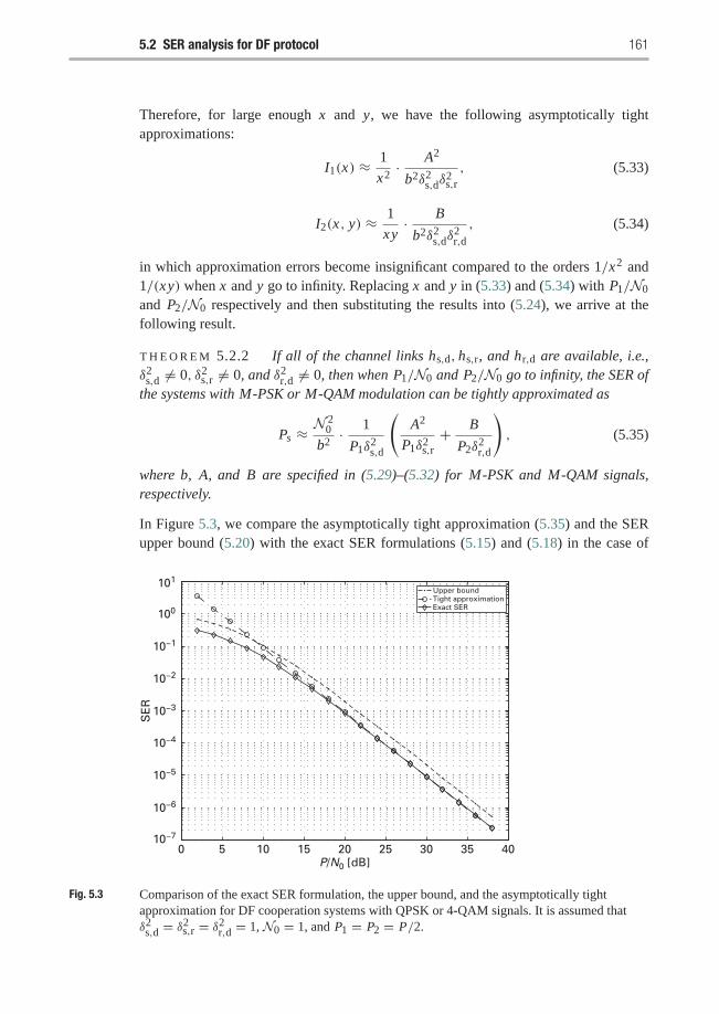
5.2 SER analysis for DF protocol 161
Therefore, for large enough x and y, we have the following asymptotically tightapproximations:
I1(x) ≈ 1
x2· A2
b2δ2s,dδ
2s,r
, (5.33)
I2(x, y) ≈ 1
xy· B
b2δ2s,dδ
2r,d
, (5.34)
in which approximation errors become insignificant compared to the orders 1/x2 and1/(xy) when x and y go to infinity. Replacing x and y in (5.33) and (5.34) with P1/N0
and P2/N0 respectively and then substituting the results into (5.24), we arrive at thefollowing result.
T H E O R E M 5.2.2 If all of the channel links hs,d, hs,r, and hr,d are available, i.e.,δ2
s,d �= 0, δ2s,r �= 0, and δ2
r,d �= 0, then when P1/N0 and P2/N0 go to infinity, the SER ofthe systems with M-PSK or M-QAM modulation can be tightly approximated as
Ps ≈ N 20
b2· 1
P1δ2s,d
(A2
P1δ2s,r+ B
P2δ2r,d
), (5.35)
where b, A, and B are specified in (5.29)–(5.32) for M-PSK and M-QAM signals,respectively.
In Figure 5.3, we compare the asymptotically tight approximation (5.35) and the SERupper bound (5.20) with the exact SER formulations (5.15) and (5.18) in the case of
SE
R
10−6
10−7
10−4
10−5
10−3
10−2
10−1
101
100
0 5 10 15 20 25 30 35 40
Upper boundTight approximationExact SER
P/N0 [dB]
Fig. 5.3 Comparison of the exact SER formulation, the upper bound, and the asymptotically tightapproximation for DF cooperation systems with QPSK or 4-QAM signals. It is assumed thatδ2s,d = δ2s,r = δ2r,d = 1, N0 = 1, and P1 = P2 = P/2.
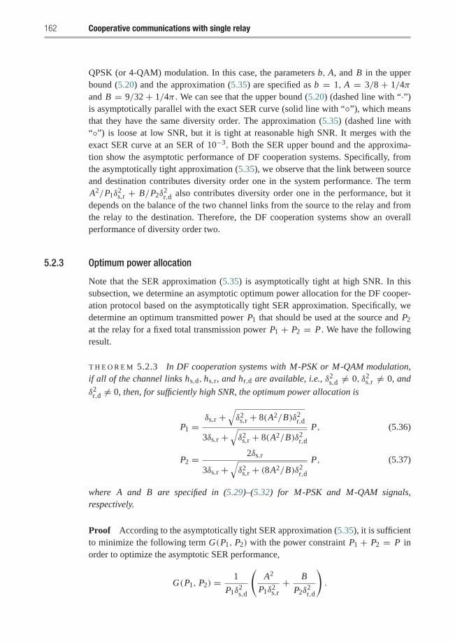
162 Cooperative communications with single relay
QPSK (or 4-QAM) modulation. In this case, the parameters b, A, and B in the upperbound (5.20) and the approximation (5.35) are specified as b = 1, A = 3/8 + 1/4πand B = 9/32 + 1/4π . We can see that the upper bound (5.20) (dashed line with “·”)is asymptotically parallel with the exact SER curve (solid line with “�”), which meansthat they have the same diversity order. The approximation (5.35) (dashed line with“◦”) is loose at low SNR, but it is tight at reasonable high SNR. It merges with theexact SER curve at an SER of 10−3. Both the SER upper bound and the approxima-tion show the asymptotic performance of DF cooperation systems. Specifically, fromthe asymptotically tight approximation (5.35), we observe that the link between sourceand destination contributes diversity order one in the system performance. The termA2/P1δ
2s,r + B/P2δ
2r,d also contributes diversity order one in the performance, but it
depends on the balance of the two channel links from the source to the relay and fromthe relay to the destination. Therefore, the DF cooperation systems show an overallperformance of diversity order two.
5.2.3 Optimum power allocation
Note that the SER approximation (5.35) is asymptotically tight at high SNR. In thissubsection, we determine an asymptotic optimum power allocation for the DF cooper-ation protocol based on the asymptotically tight SER approximation. Specifically, wedetermine an optimum transmitted power P1 that should be used at the source and P2
at the relay for a fixed total transmission power P1 + P2 = P . We have the followingresult.
T H E O R E M 5.2.3 In DF cooperation systems with M-PSK or M-QAM modulation,if all of the channel links hs,d, hs,r, and hr,d are available, i.e., δ2
s,d �= 0, δ2s,r �= 0, and
δ2r,d �= 0, then, for sufficiently high SNR, the optimum power allocation is
P1 =δs,r +
√δ2
s,r + 8(A2/B)δ2r,d
3δs,r +√δ2
s,r + 8(A2/B)δ2r,d
P, (5.36)
P2 = 2δs,r
3δs,r +√δ2
s,r + (8A2/B)δ2r,d
P, (5.37)
where A and B are specified in (5.29)–(5.32) for M-PSK and M-QAM signals,respectively.
Proof According to the asymptotically tight SER approximation (5.35), it is sufficientto minimize the following term G(P1, P2) with the power constraint P1 + P2 = P inorder to optimize the asymptotic SER performance,
G(P1, P2) = 1
P1δ2s,d
(A2
P1δ2s,r+ B
P2δ2r,d
).
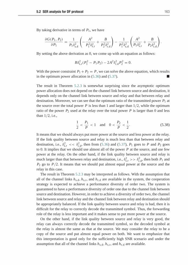
5.2 SER analysis for DF protocol 163
By taking derivative in terms of P1, we have
∂G(P1, P2)
∂P1= 1
P1δ2s,d
(− A2
P21 δ
2s,r
+ B
P22 δ
2r,d
)− 1
P21 δ
2s,d
(A2
P1δ2s,r+ B
P2δ2r,d
).
By setting the above derivation as 0, we come up with an equation as follows:
Bδ2s,r(P
21 − P1 P2)− 2A2δ2
r,d P22 = 0.
With the power constraint P1+ P2 = P , we can solve the above equation, which resultsin the optimum power allocation in (5.36) and (5.37). �
The result in Theorem 5.2.3 is somewhat surprising since the asymptotic optimumpower allocation does not depend on the channel link between source and destination, itdepends only on the channel link between source and relay and that between relay anddestination. Moreover, we can see that the optimum ratio of the transmitted power P1 atthe source over the total power P is less than 1 and larger than 1/2, while the optimumratio of the power P2 used at the relay over the total power P is larger than 0 and lessthan 1/2, i.e.,
1
2<
P1
P< 1 and 0 <
P2
P<
1
2. (5.38)
It means that we should always put more power at the source and less power at the relay.If the link quality between source and relay is much less than that between relay anddestination, i.e., δ2
s,r << δ2r,d, then from (5.36) and (5.37), P1 goes to P and P2 goes
to 0. It implies that we should use almost all of the power P at the source, and use fewpower at the relay. On the other hand, if the link quality between source and relay ismuch larger than that between relay and destination, i.e., δ2
s,r >> δ2r,d, then both P1 and
P2 go to P/2. It means that we should put almost equal power at the source and therelay in this case.
The result in Theorem 5.2.3 may be interpreted as follows. With the assumption thatall of the channel links hs,d, hs,r, and hr,d are available in the system, the cooperationstrategy is expected to achieve a performance diversity of order two. The system isguaranteed to have a performance diversity of order one due to the channel link betweensource and destination. However, in order to achieve a diversity of order two, the channellink between source and relay and the channel link between relay and destination shouldbe appropriately balanced. If the link quality between source and relay is bad, then it isdifficult for the relay to correctly decode the transmitted symbol. Thus, the forwardingrole of the relay is less important and it makes sense to put more power at the source.
On the other hand, if the link quality between source and relay is very good, therelay can always correctly decode the transmitted symbol, so the decoded symbol atthe relay is almost the same as that at the source. We may consider the relay to be acopy of the source and put almost equal power on both. We want to emphasize thatthis interpretation is good only for the sufficiently high SNR scenario and under theassumption that all of the channel links hs,d, hs,r, and hr,d are available.
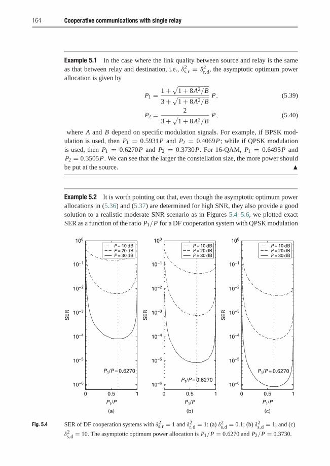
164 Cooperative communications with single relay
Example 5.1 In the case where the link quality between source and relay is the sameas that between relay and destination, i.e., δ2
s,r = δ2r,d, the asymptotic optimum power
allocation is given by
P1 = 1+√1+ 8A2/B
3+√1+ 8A2/BP, (5.39)
P2 = 2
3+√1+ 8A2/BP, (5.40)
where A and B depend on specific modulation signals. For example, if BPSK mod-ulation is used, then P1 = 0.5931P and P2 = 0.4069P; while if QPSK modulationis used, then P1 = 0.6270P and P2 = 0.3730P . For 16-QAM, P1 = 0.6495P andP2 = 0.3505P . We can see that the larger the constellation size, the more power shouldbe put at the source. �
Example 5.2 It is worth pointing out that, even though the asymptotic optimum powerallocations in (5.36) and (5.37) are determined for high SNR, they also provide a goodsolution to a realistic moderate SNR scenario as in Figures 5.4–5.6, we plotted exactSER as a function of the ratio P1/P for a DF cooperation system with QPSK modulation
0 0.5
(a) (b) (c)
1
10−6
10−5
10−4
10−3
10−2
10−1
100
P1/P
0 0.5 1
P1/P
0 0.5 1
P1/P
SE
R
10−6
10−5
10−4
10−3
10−2
10−1
100
SE
R
10−6
10−5
10−4
10−3
10−2
10−1
100
SE
R
P1/P = 0.6270
P = 10 dBP = 20 dBP = 30 dB
P = 10 dBP = 20 dBP = 30 dB
P = 10 dBP = 20 dBP = 30 dB
P1/P = 0.6270
P1/P = 0.6270
Fig. 5.4 SER of DF cooperation systems with δ2s,r = 1 and δ2r,d = 1: (a) δ2s,d = 0.1; (b) δ2s,d = 1; and (c)
δ2s,d = 10. The asymptotic optimum power allocation is P1/P = 0.6270 and P2/P = 0.3730.
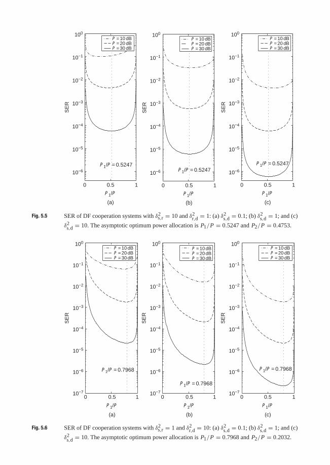
0 0.5
(a)
1
10−6
10−5
10−4
10−3
10−2
10−1
100
P1/P
0 0.5
(b)
1
P1/P
0 0.5
(c)
1
P1/P
SE
R
10−6
10−5
10−4
10−3
10−2
10−1
100
SE
R
10−6
10−5
10−4
10−3
10−2
10−1
100
SE
R
P1/P = 0.5247P1/P = 0.5247
P1/P = 0.5247
P = 10 dBP = 20 dBP = 30 dB
P = 10 dBP = 20 dBP = 30 dB
P = 10 dBP = 20 dBP = 30 dB
Fig. 5.5 SER of DF cooperation systems with δ2s,r = 10 and δ2r,d = 1: (a) δ2s,d = 0.1; (b) δ2s,d = 1; and (c)
δ2s,d = 10. The asymptotic optimum power allocation is P1/P = 0.5247 and P2/P = 0.4753.
0 0.5
(a)
1
10−6
10−7
10−5
10−4
10−3
10−2
10−1
100
P1/P
0 0.5
(b)
1
P1/P
0 0.5
(c)
1
P1/P
SE
R
10−6
10−7
10−5
10−4
10−3
10−2
10−1
100
SE
R
10−6
10−7
10−5
10−4
10−3
10−2
10−1
100
SE
R
P1/P = 0.7968
P1/P = 0.7968
P1/P = 0.7968
P = 10 dBP = 20 dBP = 30 dB
P = 10 dBP = 20 dBP = 30 dB
P = 10 dBP = 20 dBP = 30 dB
Fig. 5.6 SER of DF cooperation systems with δ2s,r = 1 and δ2r,d = 10: (a) δ2s,d = 0.1; (b) δ2s,d = 1; and (c)
δ2s,d = 10. The asymptotic optimum power allocation is P1/P = 0.7968 and P2/P = 0.2032.
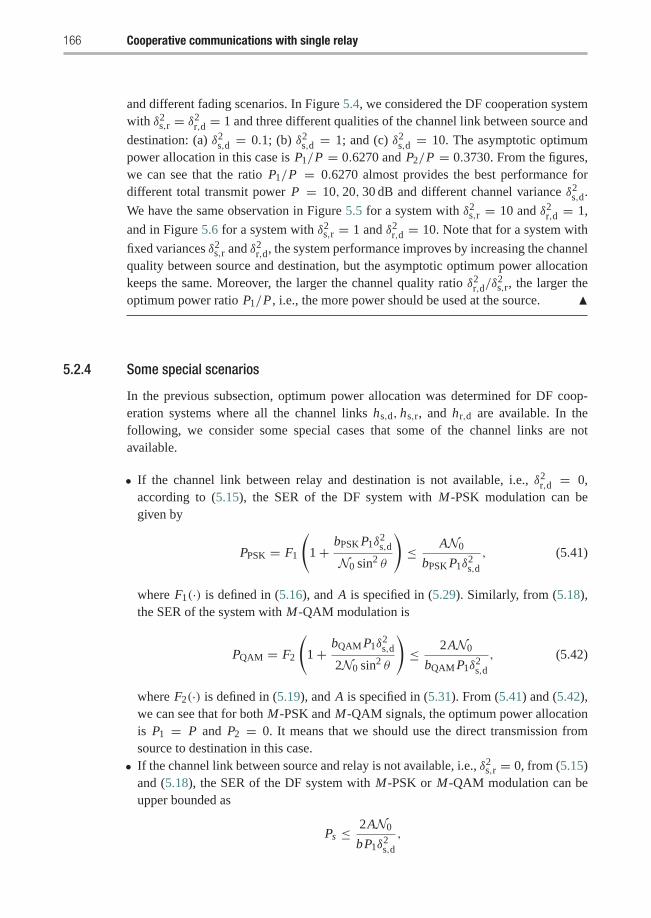
166 Cooperative communications with single relay
and different fading scenarios. In Figure 5.4, we considered the DF cooperation systemwith δ2
s,r = δ2r,d = 1 and three different qualities of the channel link between source and
destination: (a) δ2s,d = 0.1; (b) δ2
s,d = 1; and (c) δ2s,d = 10. The asymptotic optimum
power allocation in this case is P1/P = 0.6270 and P2/P = 0.3730. From the figures,we can see that the ratio P1/P = 0.6270 almost provides the best performance fordifferent total transmit power P = 10, 20, 30 dB and different channel variance δ2
s,d.
We have the same observation in Figure 5.5 for a system with δ2s,r = 10 and δ2
r,d = 1,
and in Figure 5.6 for a system with δ2s,r = 1 and δ2
r,d = 10. Note that for a system with
fixed variances δ2s,r and δ2
r,d, the system performance improves by increasing the channelquality between source and destination, but the asymptotic optimum power allocationkeeps the same. Moreover, the larger the channel quality ratio δ2
r,d/δ2s,r, the larger the
optimum power ratio P1/P , i.e., the more power should be used at the source. �
5.2.4 Some special scenarios
In the previous subsection, optimum power allocation was determined for DF coop-eration systems where all the channel links hs,d, hs,r, and hr,d are available. In thefollowing, we consider some special cases that some of the channel links are notavailable.
• If the channel link between relay and destination is not available, i.e., δ2r,d = 0,
according to (5.15), the SER of the DF system with M-PSK modulation can begiven by
PPSK = F1
(1+ bPSK P1δ
2s,d
N0 sin2 θ
)≤ AN0
bPSK P1δ2s,d
, (5.41)
where F1(·) is defined in (5.16), and A is specified in (5.29). Similarly, from (5.18),the SER of the system with M-QAM modulation is
PQAM = F2
(1+ bQAM P1δ
2s,d
2N0 sin2 θ
)≤ 2AN0
bQAM P1δ2s,d
, (5.42)
where F2(·) is defined in (5.19), and A is specified in (5.31). From (5.41) and (5.42),we can see that for both M-PSK and M-QAM signals, the optimum power allocationis P1 = P and P2 = 0. It means that we should use the direct transmission fromsource to destination in this case.
• If the channel link between source and relay is not available, i.e., δ2s,r = 0, from (5.15)
and (5.18), the SER of the DF system with M-PSK or M-QAM modulation can beupper bounded as
Ps ≤ 2AN0
bP1δ2s,d
,
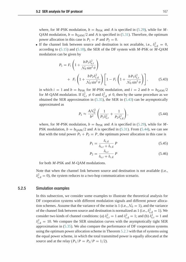
5.2 SER analysis for DF protocol 167
where, for M-PSK modulation, b = bPSK and A is specified in (5.29), while for M-QAM modulation, b = bQAM/2 and A is specified in (5.31). Therefore, the optimumpower allocation in this case is P1 = P and P2 = 0.
• If the channel link between source and destination is not available, i.e., δ2s,d = 0,
according to (5.15) and (5.18), the SER of the DF system with M-PSK or M-QAMmodulation can be given by
Ps = Fi
(1+ bP1δ
2s,r
N0 sin2 θ
)
+ Fi
(1+ bP2δ
2r,d
N0 sin2 θ
)[1− Fi
(1+ bP1δ
2s,r
N0 sin2 θ
)], (5.43)
in which i = 1 and b = bPSK for M-PSK modulation, and i = 2 and b = bQAM/2for M-QAM modulation. If δ2
s,r �= 0 and δ2r,d �= 0, then by the same procedure as we
obtained the SER approximation in (5.35), the SER in (5.43) can be asymptoticallyapproximated as
Ps ≈ AN 20
b2
(1
P1δ2s,r+ 1
P2δ2r,d
), (5.44)
where, for M-PSK modulation, b = bPSK and A is specified in (5.29), while for M-PSK modulation, b = bQAM/2 and A is specified in (5.31). From (5.44), we can seethat with the total power P1 + P2 = P , the optimum power allocation in this case is
P1 = δr,d
δs,r + δr,d P (5.45)
P2 = δs,r
δs,r + δr,d P (5.46)
for both M-PSK and M-QAM modulations.
Note that when the channel link between source and destination is not available (i.e.,δ2
s,d = 0), the system reduces to a two-hop communication scenario.
5.2.5 Simulation examples
In this subsection, we consider some examples to illustrate the theoretical analysis forDF cooperation systems with different modulation signals and different power alloca-tion schemes. Assume that the variance of the noise is 1 (i.e., N0 = 1), and the varianceof the channel link between source and destination is normalized as 1 (i.e., δ2
s,d = 1). We
consider two kinds of channel conditions: (a) δ2s,r = 1 and δ2
r,d = 1; and (b) δ2s,r = 1 and
δ2r,d = 10. We compare the SER simulation curves with the asymptotically tight SER
approximation in (5.35). We also compare the performance of DF cooperation systemsusing the optimum power allocation scheme in Theorem 5.2.3 with that of systems usingthe equal power scheme, in which the total transmitted power is equally allocated at thesource and at the relay (P1/P = P2/P = 1/2).
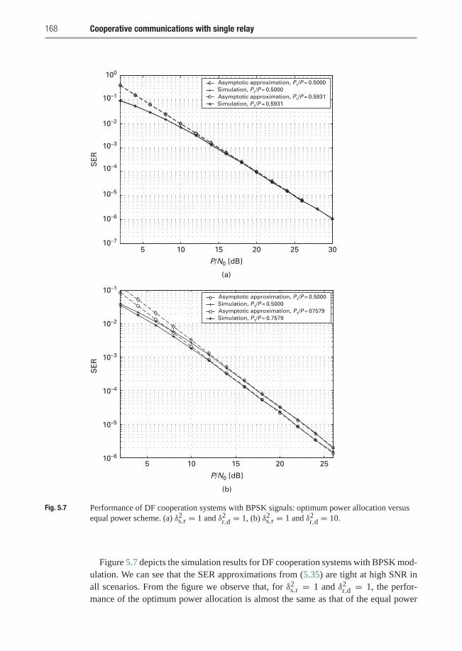
168 Cooperative communications with single relay
5 10 15 20 25
10–1
10–2
10–3
10–4
10–5
10–6
10–7
100
SE
R
10–2
10–3
10–4
10–5
10–6
10–1
SE
RAsymptotic approximation, P1/P = 0.5000Simulation, P1/P = 0.5000Asymptotic approximation, P1/P = 0.5931Simulation, P1/P = 0.5931
P/N0 [dB]
5 10 15 20 25 30
P/N0 [dB]
Asymptotic approximation, P1/P = 0.5000Simulation, P1/P = 0.5000Asymptotic approximation, P1/P = 07579Simulation, P1/P = 0.7579
(a)
(b)
Fig. 5.7 Performance of DF cooperation systems with BPSK signals: optimum power allocation versusequal power scheme. (a) δ2s,r = 1 and δ2r,d = 1, (b) δ2s,r = 1 and δ2r,d = 10.
Figure 5.7 depicts the simulation results for DF cooperation systems with BPSK mod-ulation. We can see that the SER approximations from (5.35) are tight at high SNR inall scenarios. From the figure we observe that, for δ2
s,r = 1 and δ2r,d = 1, the perfor-
mance of the optimum power allocation is almost the same as that of the equal power
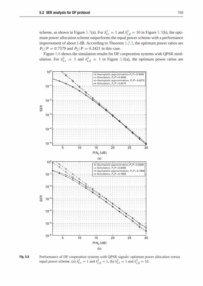
5.2 SER analysis for DF protocol 169
scheme, as shown in Figure 5.7(a). For δ2s,r = 1 and δ2
r,d = 10 in Figure 5.7(b), the opti-mum power allocation scheme outperforms the equal power scheme with a performanceimprovement of about 1 dB. According to Theorem 5.2.3, the optimum power ratios areP1/P = 0.7579 and P2/P = 0.2421 in this case.
Figure 5.8 shows the simulation results for DF cooperation systems with QPSK mod-ulation. For δ2
s,r = 1 and δ2r,d = 1 in Figure 5.8(a), the optimum power ratios are
10–1
10–2
10–3
10–4
10–5
100
SE
R
10–1
10–2
10–3
10–4
10–5
10–6
100
SE
R
5 10 15 20 25 30
P/N0 [dB]
(a)
5 10 15 20 25 30
P/N0 [dB]
(b)
Asymptotic approximation,P1/P = 0.5000Simulation, P1/P = 0.5000Asymptotic approximation, P1/P = 0.6270Simulation, P1/P = 0.6270
Asymptotic approximation,P1/P = 0.5000Simulation, P1/P = 0.5000Asymptotic approximation, P1/P = 0.7968Simulation, P1/P = 0.7968
Fig. 5.8 Performance of DF cooperation systems with QPSK signals: optimum power allocation versusequal power scheme. (a) δ2s,r = 1 and δ2r,d = 1, (b) δ2s,r = 1 and δ2r,d = 10.
170 Cooperative communications with single relay
P1/P = 0.6270 and P2/P = 0.3730 by Theorem 5.2.3. From the figure we observethat the performance of the optimum power allocation is a little bit better than that ofthe equal power case, and the two SER approximations are consistent with the simu-lation curves at high SNR. For δ2
s,r = 1 and δ2r,d = 10, the optimum power ratios are
P1/P = 0.7968 and P2/P = 0.2032 according to Theorem 5.2.3. From Figure 5.8(b),we can see that the optimum power allocation scheme outperforms the equal powerscheme with a performance improvement of about 1 dB. Note that if the ratio of the linkquality δ2
r,d/δ2s,r becomes larger, we will observe a greater performance improvement of
the optimum power allocation over the equal power case. In all of the above simulations,we can see that the SER approximation in (5.35) is asymptotically tight at high SNR.
5.3 SER analysis for AF protocol
In this section, we consider the SER performance of AF cooperative communicationsystems. First, we derive a simple closed-form MGF expression for the harmonic meanof two independent exponential random variables. Second, based on the simple MGFexpression, closed-form SER formulations are given for AF cooperation systems withM-PSK and M-QAM modulations. Third, we provide an SER approximation, which isis tight at high SNR, to show the asymptotic performance of the systems. Finally, basedon the tight approximation, we are able to determine an optimum power allocation forAF cooperation systems.
5.3.1 SER analysis by MGF approach
In the AF cooperation systems, the relay amplifies not only the received signal, but alsothe noise as shown in (5.4)–(5.6). The equivalent noise η′r,d at the destination in phase 2is a zero-mean complex Gaussian random variable with variance(
P2|hr,d|2P1|hs,r|2 +N0
+ 1
)N0.
Therefore, with knowledge of the channel coefficients hs,d, hs,r and hr,d, the output ofthe MRC detector at the destination can be written as
y = a1ys,d + a2yr,d, (5.47)
where a1 and a2 are specified as
a1 =√
P1h∗s,dN0
and a2 =√
P1 P2P1|hs,r|2+N0
h∗s,rh∗r,d(P2|hr,d|2
P1|hs,r|2+N0+ 1)N0
. (5.48)
Note that to determine the factor a2 in (5.48), we considered the equivalent receivedsignal model in (5.5). By assuming that the transmitted symbol x in (5.1) has averageenergy 1, we know that the instantaneous SNR of the MRC output is
5.3 SER analysis for AF protocol 171
γ = γ1 + γ2, (5.49)
where γ1 = P1|hs,d|2/N0, and
γ2 =P1 P2
P1|hs,r|2+N0|hs,r|2|hr,d|2(
P2|hr,d|2P1|hs,r|2+N0
+ 1)N0
= 1
N0
P1 P2|hs,r|2|hr,d|2P1|hs,r|2 + P2|hr,d|2 +N0
. (5.50)
The instantaneous SNR γ2 in (5.50) can be tightly upper bounded as
γ2 ≤ γ2�= 1
N0
P1 P2|hs,r|2|hr,d|2P1|hs,r|2 + P2|hr,d|2 , (5.51)
which is the harmonic mean of two exponential random variables P1|hs,r|2/N0 andP2|hr,d|2/N0. If we approximate the SNR as γ ≈ γ1 + γ2, then, according to (5.12)and (5.13), the conditional SER of AF cooperation systems with M-PSK and M-QAMmodulations can be given as follows:
Phs,d,hs,r,hr,dPSK ≈ 1
π
∫ (M−1)π/M
0exp
(−bPSK(γ1 + γ2)
sin2 θ
)dθ, (5.52)
Phs,d,hs,r,hr,dQAM ≈ 4K Q
(√bQAM(γ1 + γ2)
)− 4K 2Q2
(√bQAM(γ1 + γ2)
), (5.53)
where bPSK = sin2(π/M), bQAM = 3/(M − 1), and K = 1− 1/√
M .Let us denote the moment-generating function (MGF) of a random variable Z as
MZ (s) =∫ ∞
−∞exp(−sz)pZ (z)dz, (5.54)
for any real number s. By averaging over the Rayleigh fading channels hs,d, hs,r, andhr,d in (5.52) and (5.53), we obtain the SER of AF cooperation systems in terms of MGFMγ1(s) and Mγ2(s) as follows:
PPSK ≈ 1
π
∫ (M−1)π/M
0Mγ1
(bPSK
sin2 θ
)Mγ2
(bPSK
sin2 θ
)dθ, (5.55)
PQAM ≈[
4K
π
∫ π/2
0− 4K 2
π
∫ π/4
0
]Mγ1
(bQAM
2 sin2 θ
)Mγ2
(bQAM
2 sin2 θ
)dθ, (5.56)
in which, for simplicity, we use the following notation[4K
π
∫ π/2
0− 4K 2
π
∫ π/4
0
]x(θ)dθ
�= 4K
π
∫ π/2
0x(θ)dθ − 4K 2
π
∫ π/4
0x(θ)dθ.
172 Cooperative communications with single relay
From (5.55) and (5.56), we can see that the remaining problem is to obtain the MGFMγ1(s) and Mγ2(s). Since γ1 = P1|hs,d|2/N0 has an exponential distribution withparameter N0/(P1δ
2s,d), the MGF of γ1 can be simply given by
Mγ1(s) =1
1+ s P1δ2s,d
N0
. (5.57)
However, it is not easy to get the MGF of γ2, which is the harmonic mean of two expo-nential random variables P1|hs,r|2/N0 and P2|hr,d|2/N0. The MGF can be obtainedby applying a Laplace transform and a solution was presented in [58] in terms of thehypergeometric function as follows:
Mγ2(s) =16β1β2
3(β1 + β2 + 2√β1β2 + s)2
[4(β1 + β2)
β1 + β2 + 2√β1β2 + s
× 2F1
(3,
3
2; 5
2; β1 + β2 − 2
√β1β2 + s
β1 + β2 + 2√β1β2 + s
)
+ 2F1
(2,
1
2; 5
2; β1 + β2 − 2
√β1β2 + s
β1 + β2 + 2√β1β2 + s
)], (5.58)
in which β1 = N0/(P1δ2s,r), β2 = N0/(P2δ
2r,d), and 2F1(·, ·; ·; ·) is the hypergeometric
function.3 Because the hypergeometric function 2F1(·, ·; ·; ·) is defined as an integral itis hard to use in an SER analysis aimed at revealing the asymptotic performance andoptimizing the power allocation. Using an alternative approach, we introduce a simpleclosed-form solution for the MGF of γ2 as shown in the next subsection.
5.3.2 Simple MGF expression for the harmonic mean
In this subsection, first we obtain a general result on the probability density function(pdf) for the harmonic mean of two independent random variables. Then, we are ableto determine a simple closed-form MGF expression for the harmonic mean of twoindependent exponential random variables.
T H E O R E M 5.3.1 Suppose that X1 and X2 are two independent random variableswith pdf pX1(x) and pX2(x) defined for all x ≥ 0, and pX1(x) = 0 and pX2(x) = 0 forx < 0. Then the pdf of Z = X1 X2
X1+X2, the harmonic mean of X1 and X2, is
pZ (z) = z∫ 1
0
1
t2(1− t)2pX1(
z
1− t) pX2(
z
t)dt ·U (z), (5.59)
in which U (z) = 1 for z ≥ 0 and U (z) = 0 for z < 0.
3 A hypergeometric function with variables α, β, γ , and z is defined as [50]
2F1(α, β; γ ; z) = �(γ )
�(β)�(γ − β)∫ 1
0tβ−1(1− t)γ−β−1(1− t z)−αdt,
where �(·) is the Gamma function.
5.3 SER analysis for AF protocol 173
The proof of Theorem 5.3.1 is omitted (as an exercise). Note that there is no spec-ification for the distributions of the two independent random variables in Theorem5.3.1. Suppose that X1 and X2 are two independent exponential random variables withparameters β1 and β2, respectively, i.e.,
pX1(x) = β1 e−β1x ·U (x),pX2(x) = β2 e−β2x ·U (x).
Then, according to Theorem 5.3.1, the pdf of the harmonic mean Z = X1 X2X1+X2
can besimply given as
pZ (z) = z∫ 1
0
β1β2
t2(1− t)2e−(β11−t+ β2
t
)zdt ·U (z). (5.60)
The pdf expression in (5.60) is critical in the following to obtain a simple closed-formMGF result for the harmonic mean Z .
Let us start calculating the MGF of the harmonic mean of two independent exponen-tial random variables by substituting the pdf of Z (5.60) into the definition (5.54) asfollows:
MZ (s) =∫ ∞
0e−sz z
∫ 1
0
β1β2
t2(1− t)2e−(β11−t+ β2
t
)zdtdz
=∫ 1
0
β1β2
t2(1− t)2
(∫ ∞
0z e−(β11−t+ β2
t +s)
zdz
)dt, (5.61)
in which we switch the integration order. Since∫ ∞
0z e−(β11−t+ β2
t +s)
zdz =
(β1
1− t+ β2
t+ s
)−2
,
the MGF in (5.61) can be determined as
MZ (s) =∫ 1
0
β1β2[β2 + (β1 − β2 + s)t − st2
]2 dt, (5.62)
which is an integration of a quadratic trinomial and has a closed-form solution [50]. Fornotation simplicity, denote α = (β1 − β2 + s)/2, then, for any s > 0, we have∫ 1
0
1
(β2 + 2αt − st2)2dt
= st − α2(β2s + α2)(β2 + 2αt − st2)
∣∣∣∣10
+ s
4(β2s + α2)32
ln
∣∣∣∣∣−st + α −√β2s + α2
−st + α +√β2s + α2
∣∣∣∣∣∣∣∣∣∣1
0
= β2s + α(β1 − β2)
2β1β2(β2s + α2)+ s
4(β2s + α2)32
ln
(β2 + α +
√β2s + α2
)2
β1β2. (5.63)
174 Cooperative communications with single relay
By substituting α = (β1 − β2 + s)/2 into (5.63) and denoting � = 2√β2s + α2, we
obtain a simple closed-form MGF for the harmonic mean Z as follows:
MZ (s) = (β1 − β2)2 + (β1 + β2)s
�2+ 2β1β2s
�3ln(β1 + β2 + s +�)2
4β1β2, s > 0,
(5.64)
where � = √(β1 − β2)2 + 2(β1 + β2)s + s2. We can see that if β1 and β2 go to zero,then � can be approximated as s. In this case, the MGF in (5.64) can be simplified as
MZ (s) ≈ β1 + β2
s+ 2β1β2
s2ln
s2
β1β2. (5.65)
Note that in (5.65), the second term goes to zero faster than the first term. As a result,the MGF in (5.65) can be further simplified as
MZ (s) ≈ β1 + β2
s. (5.66)
We summarize the above discussion in the following theorem.
T H E O R E M 5.3.2 Let X1 and X2 be two independent exponential random variableswith parameters β1 and β2 respectively. Then, the MGF of Z = X1 X2
X1+X2is
MZ (s) = (β1 − β2)2 + (β1 + β2)s
�2+ 2β1β2s
�3ln(β1 + β2 + s +�)2
4β1β2(5.67)
for any s > 0, in which
� =√(β1 − β2)2 + 2(β1 + β2)s + s2. (5.68)
Furthermore, if β1 and β2 go to zero, then the MGF of Z can be approximated as
MZ (s) ≈ β1 + β2
s. (5.69)
We can see that the closed-form solution in (5.67) does not involve any integration. IfX1 and X2 are i.i.d. exponential random variables with parameter β, then according tothe result in Theorem 5.3.2, the MGF of Z = X1 X2
X1+X2can be simply given as
MZ (s) = 2β
4β + s+ 4β2s
�30
ln2β + s +�0
2β, (5.70)
where s > 0 and �0 =√
4βs + s2. The approximation in (5.69) will provide a verysimple solution for the SER calculations in (5.55) and (5.56), as shown in the nextsubsection.
5.3.3 Asymptotically tight approximation
Now let us apply the result of Theorem 5.3.2 to the harmonic mean of two random vari-ables X1 = P1|hs,r|2/N0 and X2 = P2|hr,d|2/N0 as we considered in Section 4.1. Theyare two independent exponential random variables with parameters β1 = N0/(P1δ
2s,r)
and β2 = N0/(P2δ2r,d), respectively. With the closed-form MGF expression in Theorem
5.3 SER analysis for AF protocol 175
5.3.2, the SER formulations in (5.55) and (5.56) for AF systems with M-PSK andM-QAM modulations can be determined respectively as
PPSK ≈ 1
π
∫ (M−1)π/M
0
1
1+ bPSK
β0 sin2 θ
{(β1 − β2)
2 + (β1 + β2)bPSK
sin2 θ
�2
+ 2β1β2bPSK
�3 sin2 θln(β1 + β2 + bPSK
sin2 θ+�)2
4β1β2
}dθ, (5.71)
PQAM ≈[
4K
π
∫ π/2
0−4K 2
π
∫ π/4
0
]1
1+ bQAM
2β0 sin2 θ
⎧⎨⎩ (β1 − β2)2 + (β1 + β2)
bQAM
2 sin2 θ
�2
+ β1β2bQAM
�3 sin2 θln(β1 + β2 + bQAM
2 sin2 θ+�)2
4β1β2
⎫⎬⎭ dθ, (5.72)
in which β0 = N0/(P1δ2s,d), β1 = N0/(P1δ
2s,r), β2 = N0/(P2δ
2r,d), and �2 =
(β1 − β2)2 + 2(β1 + β2)s +s2 with s = bPSK/ sin2 θ for M-PSK modulation and
s = bQAM/(2 sin2 θ) for M-QAM modulation.We observe that it is hard to understand AF system performance based on the SER
formulations in (5.71) and (5.72), even though they can be numerically calculated. In thefollowing, we provide an asymptotically tight approximation for the SER formulationswhen all of the channel links hs,d, hs,r, and hr,d are available, i.e., δ2
s,d �= 0, δ2s,r �= 0,
and δ2r,d �= 0. For simplicity of discussion, we denote∫
�1
x(θ) dθ�= 1
π
∫ (M−1)π/M
0x(θ) dθ, (5.73)
∫�2
x(θ) dθ�=[
4K
π
∫ π/2
0− 4K 2
π
∫ π/4
0
]x(θ) dθ, (5.74)
for any function x(θ). Then, the SER formulations in (5.71) and (5.72) can beexpressed as
Ps ≈∫�i
1
1+ bP1δ2s,d
N0 sin2 θ
⎧⎪⎪⎪⎨⎪⎪⎪⎩(
N0P1δ
2s,r− N0
P2δ2r,d
)2
+(
N0P1δ
2s,r+ N0
P2δ2r,d
)b
sin2 θ
�2
+2bN 2
0 ln
[P1 P2δ
2s,rδ
2r,d
(N0
P1δ2s,r+ N0
P2δ2r,d+ b
sin2 θ+�
)2/(4N 2
0
)]P1 P2δ2
s,rδ2r,d�
3 sin2 θ
⎫⎪⎪⎪⎪⎬⎪⎪⎪⎪⎭ dθ,
(5.75)
where i = 1 and b = bPSK, for M-PSK modulation, and i = 2 and b = bQAM/2 forM-QAM modulation, and
176 Cooperative communications with single relay
�2 =(
N0
P1δ2s,r− N0
P2δ2r,d
)2
+ 2
(N0
P1δ2s,r+ N0
P2δ2r,d
)b
sin2 θ+ b2
sin4 θ.
Let us separate the right-hand side of the above equation (5.75) as two parts as follows:
Ps ≈ J1(P1/N0, P2/N0)+ J2(P1/N0, P2/N0), (5.76)
in which
J1(x, y) =∫�i
1
1+ xbδ2s,d
sin2 θ
⎧⎪⎪⎨⎪⎪⎩1
xδ2s,r
(1
xδ2s,r− 1
yδ2r,d
)+ b
xδ2s,r sin2 θ
�2
+ 2b ln y
xyδ2s,rδ
2r,d�
3 sin2 θ
}dθ, (5.77)
J2(x, y) =∫�i
1
1+ xbδ2s,d
sin2 θ
⎧⎪⎪⎨⎪⎪⎩− 1
yδ2r,d
(1
xδ2s,r− 1
yδ2r,d
)+ b
yδ2r,d sin2 θ
�2
+2b ln
[xδ2
s,rδ2r,d
(1
xδ2s,r+ 1
yδ2r,d+ b
sin2 θ+�
)2/4
]xyδ2
s,rδ2r,d�
3 sin2 θ
⎫⎪⎪⎪⎪⎬⎪⎪⎪⎪⎭ dθ,
(5.78)
in which i = 1 and b = bPSK for M-PSK modulation, and i = 2 and b = bQAM/2for M-QAM modulation. Then, we have the following results (leave the proof as anexercise)
limx, y→∞ x2 J1(x, y) = B
b2δ2s,dδ
2s,r
, (5.79)
limx, y→∞ xy J2(x, y) = B
b2δ2s,dδ
2r,d
, (5.80)
where for M-PSK signals, b = bPSK and
B = 3(M − 1)
8M+ sin 2π
M
4π− sin 4π
M
32π; (5.81)
while for M-QAM signals, b = bQAM/2 and
B = 3(M − 1)
8M+ K 2
π. (5.82)
Therefore, for large enough x and y, we have the following asymptotically tightapproximations:
J1(x, y) ≈ 1
x2· B
b2δ2s,dδ
2s,r
, (5.83)
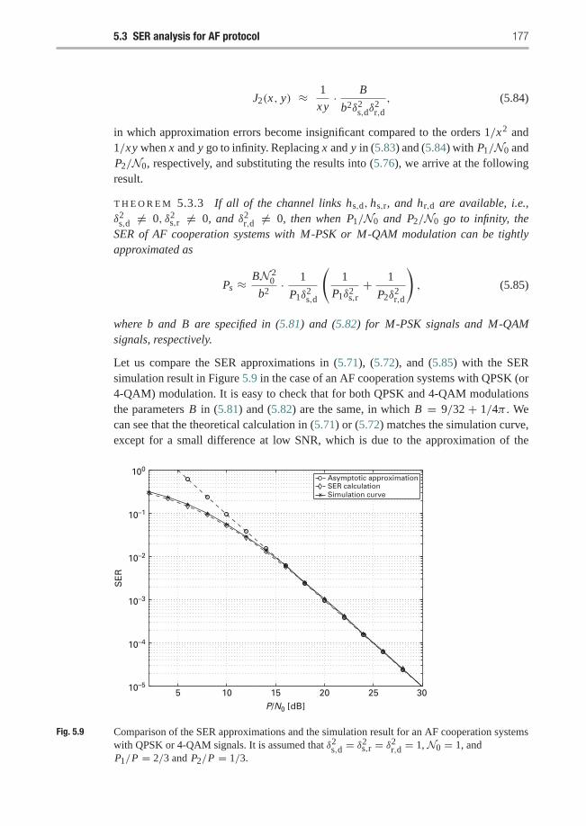
5.3 SER analysis for AF protocol 177
J2(x, y) ≈ 1
xy· B
b2δ2s,dδ
2r,d
, (5.84)
in which approximation errors become insignificant compared to the orders 1/x2 and1/xy when x and y go to infinity. Replacing x and y in (5.83) and (5.84) with P1/N0 andP2/N0, respectively, and substituting the results into (5.76), we arrive at the followingresult.
T H E O R E M 5.3.3 If all of the channel links hs,d, hs,r, and hr,d are available, i.e.,δ2
s,d �= 0, δ2s,r �= 0, and δ2
r,d �= 0, then when P1/N0 and P2/N0 go to infinity, theSER of AF cooperation systems with M-PSK or M-QAM modulation can be tightlyapproximated as
Ps ≈ BN 20
b2· 1
P1δ2s,d
(1
P1δ2s,r+ 1
P2δ2r,d
), (5.85)
where b and B are specified in (5.81) and (5.82) for M-PSK signals and M-QAMsignals, respectively.
Let us compare the SER approximations in (5.71), (5.72), and (5.85) with the SERsimulation result in Figure 5.9 in the case of an AF cooperation systems with QPSK (or4-QAM) modulation. It is easy to check that for both QPSK and 4-QAM modulationsthe parameters B in (5.81) and (5.82) are the same, in which B = 9/32 + 1/4π . Wecan see that the theoretical calculation in (5.71) or (5.72) matches the simulation curve,except for a small difference at low SNR, which is due to the approximation of the
5 10 15 20 25 30
100
10–1
10–2
10–3
10–4
10–5
SE
R
Asymptotic approximationSER calculationSimulation curve
P/N0 [dB]
Fig. 5.9 Comparison of the SER approximations and the simulation result for an AF cooperation systemswith QPSK or 4-QAM signals. It is assumed that δ2s,d = δ2s,r = δ2r,d = 1, N0 = 1, andP1/P = 2/3 and P2/P = 1/3.
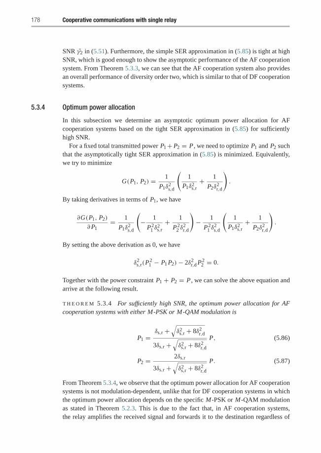
178 Cooperative communications with single relay
SNR γ2 in (5.51). Furthermore, the simple SER approximation in (5.85) is tight at highSNR, which is good enough to show the asymptotic performance of the AF cooperationsystem. From Theorem 5.3.3, we can see that the AF cooperation system also providesan overall performance of diversity order two, which is similar to that of DF cooperationsystems.
5.3.4 Optimum power allocation
In this subsection we determine an asymptotic optimum power allocation for AFcooperation systems based on the tight SER approximation in (5.85) for sufficientlyhigh SNR.
For a fixed total transmitted power P1+ P2 = P , we need to optimize P1 and P2 suchthat the asymptotically tight SER approximation in (5.85) is minimized. Equivalently,we try to minimize
G(P1, P2) = 1
P1δ2s,d
(1
P1δ2s,r+ 1
P2δ2r,d
).
By taking derivatives in terms of P1, we have
∂G(P1, P2)
∂P1= 1
P1δ2s,d
(− 1
P21 δ
2s,r
+ 1
P22 δ
2r,d
)− 1
P21 δ
2s,d
(1
P1δ2s,r+ 1
P2δ2r,d
).
By setting the above derivation as 0, we have
δ2s,r(P
21 − P1 P2)− 2δ2
r,d P22 = 0.
Together with the power constraint P1 + P2 = P , we can solve the above equation andarrive at the following result.
T H E O R E M 5.3.4 For sufficiently high SNR, the optimum power allocation for AFcooperation systems with either M-PSK or M-QAM modulation is
P1 =δs,r +
√δ2
s,r + 8δ2r,d
3δs,r +√δ2
s,r + 8δ2r,d
P, (5.86)
P2 = 2δs,r
3δs,r +√δ2
s,r + 8δ2r,d
P. (5.87)
From Theorem 5.3.4, we observe that the optimum power allocation for AF cooperationsystems is not modulation-dependent, unlike that for DF cooperation systems in whichthe optimum power allocation depends on the specific M-PSK or M-QAM modulationas stated in Theorem 5.2.3. This is due to the fact that, in AF cooperation systems,the relay amplifies the received signal and forwards it to the destination regardless of
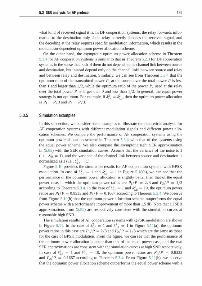
5.3 SER analysis for AF protocol 179
what kind of received signal it is. In DF cooperation systems, the relay forwards infor-mation to the destination only if the relay correctly decodes the received signal, andthe decoding at the relay requires specific modulation information, which results in themodulation-dependent optimum power allocation scheme.
On the other hand, the asymptotic optimum power allocation scheme in Theorem5.3.4 for AF cooperation systems is similar to that in Theorem 5.2.3 for DF cooperationsystems, in the sense that both of them do not depend on the channel link between sourceand destination, but instead depend only on the channel links between source and relayand between relay and destination. Similarly, we can see from Theorem 5.3.4 that theoptimum ratio of the transmitted power P1 at the source over the total power P is lessthan 1 and larger than 1/2, while the optimum ratio of the power P2 used at the relayover the total power P is larger than 0 and less than 1/2. In general, the equal powerstrategy is not optimum. For example, if δ2
s,r = δ2r,d, then the optimum power allocation
is P1 = P/3 and P2 = P/3.
5.3.5 Simulation examples
In this subsection, we consider some examples to illustrate the theoretical analysis forAF cooperation systems with different modulation signals and different power allo-cation schemes. We compare the performance of AF cooperation systems using theoptimum power allocation scheme in Theorem 5.3.4 with that of the systems usingthe equal power scheme. We also compare the asymptotic tight SER approximationin (5.85) with the SER simulation curves. Assume that the variance of the noise is 1(i.e., N0 = 1), and the variance of the channel link between source and destination isnormalized as 1 (i.e., δ2
s,d = 1).Figure 5.10 provides the simulation results for AF cooperation systems with BPSK
modulation. In case of δ2s,r = 1 and δ2
r,d = 1 in Figure 5.10(a), we can see that theperformance of the optimum power allocation is slightly better than that of the equalpower case, in which the optimum power ratios are P1/P = 2/3 and P2/P = 1/3according to Theorem 5.3.4. In the case of δ2
s,r = 1 and δ2r,d = 10, the optimum power
ratios are P1/P = 0.8333 and P2/P = 0.1667 according to Theorem 5.3.4. We observefrom Figure 5.10(b) that the optimum power allocation scheme outperforms the equalpower scheme with a performance improvement of more than 1.5 dB. Note that all SERapproximations from (5.85) are respectively consistent with the simulation curves atreasonable high SNR.
The simulation results of AF cooperation systems with QPSK modulation are shownin Figure 5.11. In the case of δ2
s,r = 1 and δ2r,d = 1 in Figure 5.11(a), the optimum
power ratios in this case are P1/P = 2/3 and P2/P = 1/3 which are the same as thosefor the case of BPSK modulation. From the figure, we can see that the performance ofthe optimum power allocation is better than that of the equal power case, and the twoSER approximations are consistent with the simulation curves at high SNR respectively.In case of δ2
s,r = 1 and δ2r,d = 10, the optimum power ratios are P1/P = 0.8333
and P2/P = 0.1667 according to Theorem 5.3.4. From Figure 5.11(b), we observethat the optimum power allocation scheme outperforms the equal power scheme with a
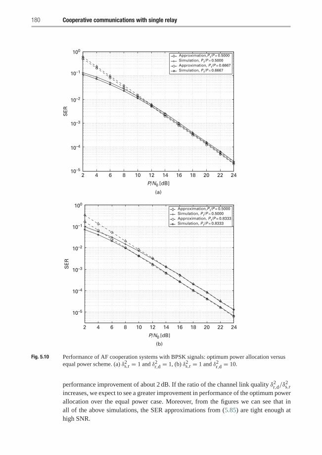
180 Cooperative communications with single relay
2 4
(a)
6 8 10 12 14 16 18 20 22 24
100
10–1
10–2
10–3
10–4
10–5
SE
R
P/N0 [dB]
Approximation,P1/P = 0.5000Simulation, P1/P = 0.5000Approximation, P1/P = 0.6667Simulation, P1/P = 0.6667
2 4
(b)
6 8 10 12 14 16 18 20 22 24
P/N0 [dB]
10–5
100
10–1
10–2
10–3
10–4
SE
R
Approximation,P1/P = 0.5000Simulation, P1/P = 0.5000Approximation, P1/P = 0.8333Simulation, P1/P = 0.8333
Fig. 5.10 Performance of AF cooperation systems with BPSK signals: optimum power allocation versusequal power scheme. (a) δ2s,r = 1 and δ2r,d = 1, (b) δ2s,r = 1 and δ2r,d = 10.
performance improvement of about 2 dB. If the ratio of the channel link quality δ2r,d/δ
2s,r
increases, we expect to see a greater improvement in performance of the optimum powerallocation over the equal power case. Moreover, from the figures we can see that inall of the above simulations, the SER approximations from (5.85) are tight enough athigh SNR.
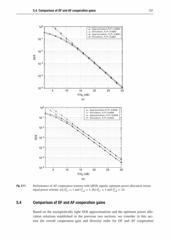
5.4 Comparison of DF and AF cooperation gains 181
10–1
10–2
10–3
10–4
10–5
10–6
100
SE
R
5 10 15 20 25 30
P/N0 [dB]
(b)
Approximation,P1/P = 0.5000Simulation, P1/P = 0.5000Approximation, P1/P = 0.8333Simulation, P1/P = 0.8333
5 10
(a)
15 20 25 30
SE
R
P/N0 [dB]
10–1
10–2
10–3
10–4
10–5
100Approximation,P1/P = 0.5000Simulation, P1/P = 0.5000Approximation, P1/P = 0.6667Simulation, P1/P = 0.6667
Fig. 5.11 Performance of AF cooperation systems with QPSK signals: optimum power allocation versusequal power scheme. (a) δ2s,r = 1 and δ2r,d = 1, (b) δ2s,r = 1 and δ2r,d = 10.
5.4 Comparison of DF and AF cooperation gains
Based on the asymptotically tight SER approximations and the optimum power allo-cation solutions established in the previous two sections, we consider in this sec-tion the overall cooperation gain and diversity order for DF and AF cooperation
182 Cooperative communications with single relay
systems, respectively. Then, we compare the cooperation gain between the DF and AFcooperation protocols.
Let us first focus on the DF cooperation protocol. According to the asymptoticallytight SER approximation (5.35) in Theorem 5.2.2, we know that for sufficiently highSNR, the SER performance of DF cooperation systems can be approximated as
Ps ≈ N 20
b2· 1
P1δ2s,d
(A2
P1δ2s,r+ B
P2δ2r,d
), (5.88)
where A and B are specified in (5.29)–(5.32) for M-PSK and M-QAM signals, respec-tively. By substituting the asymptotic optimum power allocation (5.36) and (5.37) into(5.88), we have
Ps ≈ �−2DF
(P
N0
)−2
, (5.89)
where
�DF = 2√
2 bδs,dδs,rδr,d√B
(δs,r +
√δ2
s,r + 8(A2/B)δ2r,d
)1/2
(3δs,r +
√δ2
s,r + 8(A2/B)δ2r,d
)3/2, (5.90)
in which b = bPSK for M-PSK signals and b = bQAM/2 for M-QAM signals. From(5.89), we can see that the DF cooperation systems can guarantee a performance diver-sity of order two. Note that the term �DF in (5.90) depends only on the statistics ofthe channel links. We call it the cooperation gain of the DF cooperation systems, and itindicates the best performance gain that we are able to achieve through the DF cooper-ation protocol with any kind of power allocation. If the link quality between source andrelay is much less than that between relay and destination, i.e., δ2
s,r << δ2r,d, then the
cooperation gain is approximated as
�DF = bδs,dδs,rA
, (5.91)
in which A = (M−1)/2M+(sin 2πM )/4π → 1/2 (for large M) for M-PSK modulation,
or A = (M−1)/2M+ K 2/π → 1/2+1/π when M is large for M-QAM modulation.For example, in case of QPSK modulation, A = 3/8+ 1/4π = 0.4546.
On the other hand, if the link quality between source and relay is much larger thanthat between relay and destination, i.e., δ2
s,r >> δ2r,d, then the cooperation gain can be
approximated as
�DF = bδs,dδr,d
2√
B, (5.92)
in which B = 3(M−1)/8M+(sin 2π
M
)/4π−
(sin 4π
M
)/32π → 3/8 (for large M) for
M-PSK modulation, or B = 3(M−1)/8M+ K 2/π → 3/8+1/π when M is large forM-QAM modulation. For example, in case of QPSK modulation, B = 9/32+ 1/4π =0.3608.
5.4 Comparison of DF and AF cooperation gains 183
Similarly, for the AF cooperation protocol, from the the asymptotically tight SERapproximation (5.85) in Theorem 5.3.3, we can see that for sufficiently high SNR, theSER performance of AF cooperation systems can be approximated as
Ps ≈ BN 20
b2· 1
P1δ2s,d
(1
P1δ2s,r+ 1
P2δ2r,d
), (5.93)
where b = bPSK for M-PSK signals and b = bQAM/2 for M-QAM signals, and Bis specified in (5.81) and (5.82) for M-PSK and M-QAM signals respectively. Bysubstituting the asymptotic optimum power allocation (5.86) and (5.87) into (5.93),we have
Ps ≈ �−2AF
(P
N0
)−2
, (5.94)
�AF = 2√
2 bδs,dδs,rδr,d√B
(δs,r +
√δ2
s,r + 8δ2r,d
)1/2
(3δs,r +
√δ2
s,r + 8δ2r,d
)3/2, (5.95)
which is called the cooperation gain of the AF cooperation systems, and indicates thebest asymptotic performance gain of the AF cooperation protocol with the optimumpower allocation scheme. From (5.94), we can see that AF cooperation systems canalso guarantee a performance diversity of order two, which is similar to that of DFcooperation systems.
Note that both AF and DF cooperation systems are able to achieve a performancediversity of order two. In the following, we compare the cooperation gains of the twocooperation systems. Let us define a ratio λ = �DF/�AF to indicate the performancegain of the DF cooperation protocol compared with the AF protocol. According to (5.90)and (5.95), we have
λ =⎛⎝δs,r +
√δ2
s,r + 8(A2/B)δ2r,d
δs,r +√δ2
s,r + 8δ2r,d
⎞⎠1/2⎛⎝ 3δs,r +√δ2
s,r + 8δ2r,d
δs,r +√
3δ2s,r + 8(A2/B)δ2
r,d
⎞⎠3/2
, (5.96)
where A and B are specified in (5.29)–(5.32) for M-PSK and M-QAM signals,respectively.
• If the channel link quality between source and relay is much less than that betweenrelay and destination, i.e., δ2
s,r << δ2r,d, then
λ = �DF
�AF→√
B
A. (5.97)
In the case of BPSK modulation, A = 1/4 and B = 3/16, so λ = √3 > 1. In the caseof QPSK modulation, A = 3/8+1/4π and B = 9/32+1/4π , so λ = 1.3214 > 1. Inthe case of 8-PSK modulation, A = 7/16+√2/8π and B = 21/64+√2/8π−1/32π ,so λ = 1.2393 > 1. In the case of 16-QAM modulation, A = 15/32 + 9/16π and
184 Cooperative communications with single relay
B = 45/128 + 9/16π , so λ = 1.1245 > 1. In general, for M-PSK modulation
(M large), A = (M − 1)/2M +(sin 2π
M
)/4π → 1/2 and B = 3(M − 1)/8M +(
sin 2πM
)/4π −
(sin 4π
M
)/32π → 3/8, so
λ→√
6
2≈ 1.2247 > 1.
For M-QAM modulation (M large), A = (M − 1)/2M + K 2/π → 1/2 + 1/π andB = 3(M − 1)/8M + K 2/π → 3/8+ 1/π ,
λ→√
38 + 1
π
12 + 1
π
≈ 1.0175 > 1.
We can see that if δ2s,r << δ
2r,d, the cooperation gain of DF systems is always larger
than that of AF systems for both M-PSK and M-QAM modulations. The advantageof the DF cooperation systems is more significant if M-PSK modulation is used.
• If the channel link quality between source and relay is much better than that betweenrelay and destination, i.e., δ2
s,r >> δ2r,d, from (5.96) we have
λ = �DF
�AF→ 1.
This implies that if δ2s,r >> δ
2r,d, the performance of DF cooperation systems is almost
the same as that of AF cooperation systems for both M-PSK and M-QAM modula-tions. Since the DF cooperation protocol requires decoding process at the relay, wemay suggest the use of the AF cooperation protocol in this case to reduce the systemcomplexity.
• If the channel link quality between source and relay is the same as that between relayand destination, i.e., δ2
s,r = δ2r,d, we have
λ =(
1+√1+ 8(A2/B)
4
)1/2 (6
3+√1+ 8(A2/B)
)3/2
.
In the case of BPSK modulation, A = 1/4 and B = 3/16, so λ ≈ 1.1514 > 1. In thecase of QPSK modulation, A = 3/8+1/4π and B = 9/32+1/4π , so λ ≈ 1.0851 >1. In the case of 8-PSK modulation, A = 0.4938 and B = 0.3744, so λ = 1.0670 > 1.In the case of 16-QAM modulation, A = 0.6478 and B = 0.5306, so λ = 1.0378. In
general, for M-PSK modulation (M large), A = (M−1)/2M+(sin 2π
M
)/4π → 1/2
and B = 3(M − 1)/8M +(sin 2π
M
)/4π −
(sin 4π
M
)/32π → 3/8, so
λ→(
1+√1+ 16/3
4
)1/2 ( 6
3+√1+ 16/3
)3/2
≈ 1.0635 > 1.
5.4 Comparison of DF and AF cooperation gains 185
For M-QAM modulation (M large), A = (M − 1)/2M + K 2/π → 1/2 + 1/π andB = 3(M − 1)/8M + K 2/π → 3/8+ 1/π , λ goes to
⎛⎝1+√
1+ 8( 12 + 1
π)2/( 3
8 + 1π)
4
⎞⎠1/2⎛⎝ 6
3+√
1+ 8( 12 + 1
π)2/( 3
8 + 1π)
⎞⎠3/2
which is approximately 1.0058. We can see that if the modulation size is large,the performance advantage of the DF cooperation protocol is negligible comparedwith the AF cooperation protocol. Actually, with QPSK modulation, the ratio of thecooperation gain is λ ≈ 1.0851 which is already small.
From the above discussion, we can see that the performance of the DF coopera-tion protocol is always not less than that of the AF cooperation protocol. However, theperformance advantage of the DF cooperation protocol is not significant unless (i) thechannel link quality between the relay and the destination is much stronger than thatbetween the source and the relay, and (ii) the constellation size of the signaling is small.These represent a tradeoff between the two cooperation protocols.
The complexity of the AF cooperation protocol is less than that of the DFcooperation protocol in which decoding process at the relay is required. For high-data-rate cooperative communications (with large modulation size), we may use theAF cooperation protocol to reduce the system complexity while the performance iscomparable.
Example 5.3 In this example, we compare the performances of DF and AF coopera-tion systems with BPSK modulation, as shown in Figure 5.12. In the case of δ2
s,r = 1and δ2
r,d = 1, the performance of the DF cooperation protocol is better than that ofthe AF protocol by about 1dB, as shown in Figure 5.12(a). In this case, the optimumpower ratios for the DF cooperation protocol are P1/P = 0.5931 and P2/P = 0.4069according to Theorem 5.2.3, while the optimum ratios for the AF protocol are P1/P =2/3 and P2/P = 1/3 according to Theorem 5.3.4.
In the case of δ2s,r = 1 and δ2
r,d = 10, from Figure 5.12(b) we can see that theDF cooperation protocol outperforms the AF protocol with an SER performance ofabout 2 dB. In this case, the optimum power ratios for the DF cooperation proto-col are P1/P = 0.7579 and P2/P = 0.2421, while the optimum ratios for theAF protocol are P1/P = 0.8333 and P2/P = 0.1667. It seems that the larger theratio of the channel link quality δ2
r,d/δ2s,r, the greater the performance gain of the DF
cooperation protocol compared with the AF protocol. However, the performance gaincannot be larger than λ = √
3 ≈ 2.4 dB as shown in (5.97) in the case of BPSKmodulation. �
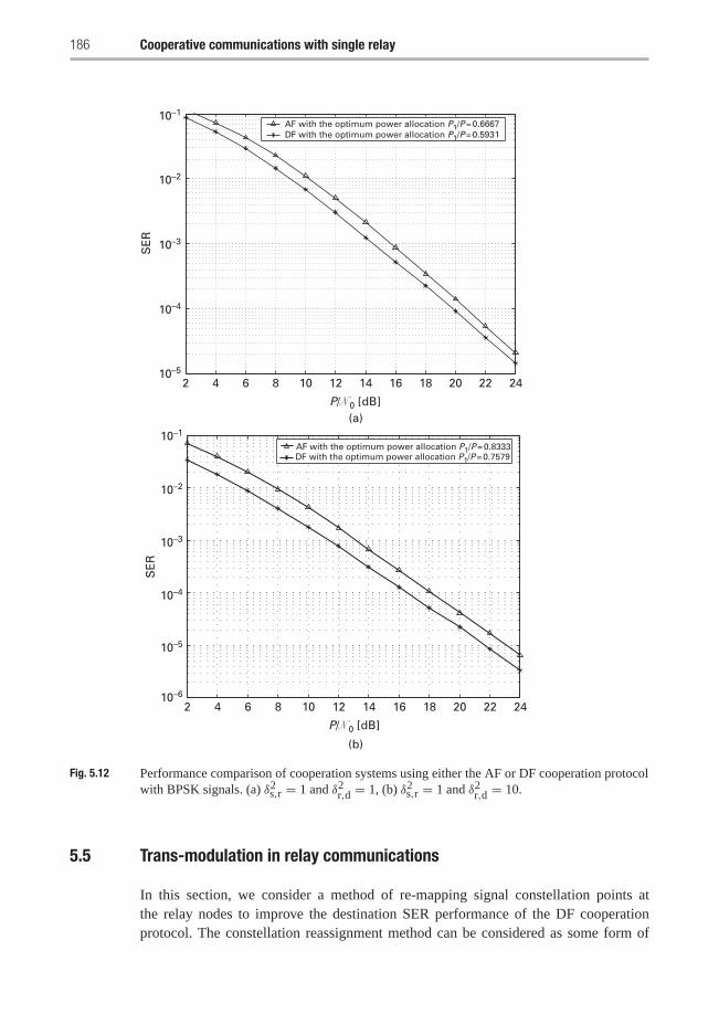
186 Cooperative communications with single relay
2 4 6 8 10 12 14 16 18 20 22 24
AF with the optimum power allocation P1/P = 0.8333DF with the optimum power allocation P1/P = 0.7579
10–1
10–2
10–3
10–4
10–5
10–6
SE
R
P/N0 [dB]
(b)
SE
R
10–1
10–2
10–3
10–4
10–5
2 4 6 8 10 12 14 16 18 20 22 24
P/N0 [dB](a)
AF with the optimum power allocation P1/P = 0.6667DF with the optimum power allocation P1/P = 0.5931
Fig. 5.12 Performance comparison of cooperation systems using either the AF or DF cooperation protocolwith BPSK signals. (a) δ2s,r = 1 and δ2r,d = 1, (b) δ2s,r = 1 and δ2r,d = 10.
5.5 Trans-modulation in relay communications
In this section, we consider a method of re-mapping signal constellation points atthe relay nodes to improve the destination SER performance of the DF cooperationprotocol. The constellation reassignment method can be considered as some form of
5.5 Trans-modulation in relay communications 187
complex field coding by trying to increase the Euclidean distance between differenttransmitted symbols.
The transceiver model of the DF cooperation protocol was specified at the beginningof this chapter. We recall that if the relay node is able to decode correctly, it will helpthe source in phase 2; otherwise, it will remain idle. Specifically, the received signal atthe destination in phase 2, due to the relay node transmission, is given by
yr,d =√
Prhr,dxr + ηr,d, (5.98)
where Pr is the relay transmitted power, ηr,d denotes the additive white Gaussian noise atthe destination, and hr,d is the channel coefficient from the relay node to the destination.Here xr denotes the new constellation point transmitted from the relay node and isnormalized such that E{|xr|2} = 1. For the repetition-based approach, the symbol xr isthe same as the transmitted symbol xs from the source.
We derive in the following an expression of the pairwise symbol error rate (PSER)between two possible transmitted source symbols. This analysis gives a guideline onhow to design the constellation points at the relay node to improve the system SERperformance. The PSER at the destination node is defined as
Pr {x1 → x2} = Pr {x1 → x2|x1, relay decodes erroneously}× Pr {relay decodes erroneously}+ Pr {x1 → x2|x1, relay decodes correctly}× Pr {relay decodes correctly} , (5.99)
where x1 and x2 are two possible transmitted source symbols. The vector x1 =[√Ps xs1
√Prxr1 ]T, where xs1 is the source transmitted constellation point and xr1 is
the relay transmitted constellation point, similarly, x2 = [√Ps xs2
√Prxr2 ]T. The PSER
expression in (5.99) has two terms depending on the state of the relay node (whetheror not it has decoded correctly). The first term corresponds to the case when the relaydecodes erroneously. This term only depends on the constellation used at the sourcenode while the second term clearly depends on the constellations used at the source andrelay nodes. We consider the design of the constellation points at the relay node in orderto minimize the PSER.
The use of a maximum likelihood (ML) detector at the receiver is assumed. Weconsider minimizing the term
PSERr = Pr {x1 → x2|x1, relay decodes correctly} ,which corresponds to the case when the relay correctly decodes the source symbol.Under our system model assumptions, the PSERr of the ML detector can be expressed as
PSERr = E {Pr {q < 0|x1, relay decodes correctly}} , (5.100)
where
q =[zH
1 zH2
] [ I2 00 −I2
] [z1
z2
]
188 Cooperative communications with single relay
in which z1 = (diag(x1)− diag(x2))h+ n, z2 = n, h = [hs,d hr,d]T , n = [ηs,d ηr,d]T ,and I2 is the 2 × 2 identity matrix. It can be shown that the conditional pdf of q in(5.100), given the channel coefficients and given that x1 was transmitted and the relaydecoded correctly, is Gaussian. The PSERr can be proved to be given by
PSERr = E
{Q
(√1
2N0
(Ps |hs,d|2|xs1 − xs2 |2 + Pr|hr,d|2|xr1 − xr2 |2
))}, (5.101)
where Q(u) = (1/√
2π)∫∞
u exp(−t2/2)dt is the Gaussian Q-function. The expecta-tion in (5.101) is with respect to the channel state information (CSI). Using the specialproperty of the Gaussian Q-function as Q(u) = 1/π
∫ π/20 exp(−u2/2 sin2 θ)dθ and
averaging over the exponential distribution of the squared magnitude of the channelgains, it can proved that the PSERr is given by
PSERr = 1
π
∫ π/2
0
1(1+ Psδ
2s,d|xs1−xs2 |24N0 sin2 θ
) · 1(1+ Prδ
2r,d|xr1−xr2 |24N0 sin2 θ
)dθ. (5.102)
An upper bound on PSERr can be obtained by neglecting the one term in the denom-inator of the terms inside the integration of (5.102). The PSERr can now be upperbounded as
PSERr ≤ 3N 20
δ2s,dδ
2r,d Ps Pr|xs1 − xs2 |2|xr1 − xr2 |2
. (5.103)
In order to minimize the PSER, symbols that have adjacent constellation points inthe source constellation are assigned nonadjacent constellation points in the relay con-stellation assignment and vice versa. So instead of using repetition at the relay node(i.e., using the same constellation as the source node) we can do constellation reas-signment at the relay node to better separate the symbols to maximize the product|xs1 − xs2 |2|xr1 − xr2 |2. The constellation reassignment scheme can improve the systemPSER performance, and hence the SER performance, without increasing the complexityof the system.
The most common constellations used in communication systems are BPSK, QPSK,16-QAM, and 64-QAM. For BPSK, constellation reassignment at the relay nodes ismeaningless since the BPSK constellation has only two points. For QPSK, the perfor-mance gains of using constellation reassignment are not significant and we do not showthe results for that case. For 16-QAM and 64-QAM constellations, one possible way todo the constellation reassignment at the relay nodes is to perform an exhaustive searchover all possible relay constellation assignments and select the one that maximizes theminimum value of the product |xs1− xs2 |2|xr1− xr2 |2 over all possible pairs of transmit-ted symbols. However, the exhaustive search is extremely complex–for example, for thesingle-relay case, the number of possible constellation assignments at the relay node is16! = 2.0923 × 10¹³ for the 16-QAM constellation and 64! = 1.2689 × 1089 for the64-QAM constellation. This renders the exhaustive search impractical for constellationreassignment at the relay node. Therefore, we resort to the use of heuristic approaches
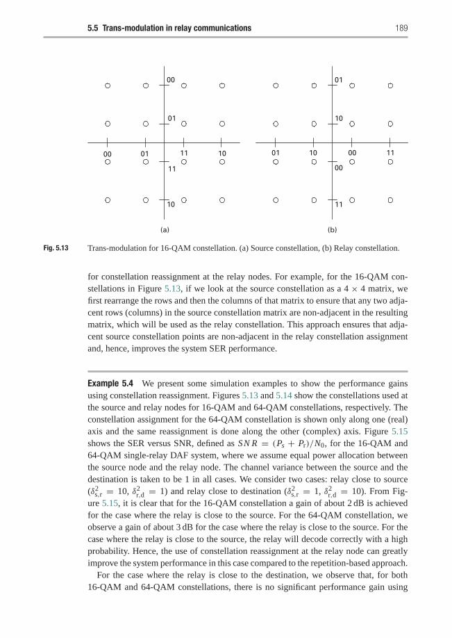
5.5 Trans-modulation in relay communications 189
00 01
11
01
00
1011
10
(a)
01 10
00
10
01
00
11
(b)
11
Fig. 5.13 Trans-modulation for 16-QAM constellation. (a) Source constellation, (b) Relay constellation.
for constellation reassignment at the relay nodes. For example, for the 16-QAM con-stellations in Figure 5.13, if we look at the source constellation as a 4 × 4 matrix, wefirst rearrange the rows and then the columns of that matrix to ensure that any two adja-cent rows (columns) in the source constellation matrix are non-adjacent in the resultingmatrix, which will be used as the relay constellation. This approach ensures that adja-cent source constellation points are non-adjacent in the relay constellation assignmentand, hence, improves the system SER performance.
Example 5.4 We present some simulation examples to show the performance gainsusing constellation reassignment. Figures 5.13 and 5.14 show the constellations used atthe source and relay nodes for 16-QAM and 64-QAM constellations, respectively. Theconstellation assignment for the 64-QAM constellation is shown only along one (real)axis and the same reassignment is done along the other (complex) axis. Figure 5.15shows the SER versus SNR, defined as SN R = (Ps + Pr)/N0, for the 16-QAM and64-QAM single-relay DAF system, where we assume equal power allocation betweenthe source node and the relay node. The channel variance between the source and thedestination is taken to be 1 in all cases. We consider two cases: relay close to source(δ2
s,r = 10, δ2r,d = 1) and relay close to destination (δ2
s,r = 1, δ2r,d = 10). From Fig-
ure 5.15, it is clear that for the 16-QAM constellation a gain of about 2 dB is achievedfor the case where the relay is close to the source. For the 64-QAM constellation, weobserve a gain of about 3 dB for the case where the relay is close to the source. For thecase where the relay is close to the source, the relay will decode correctly with a highprobability. Hence, the use of constellation reassignment at the relay node can greatlyimprove the system performance in this case compared to the repetition-based approach.
For the case where the relay is close to the destination, we observe that, for both16-QAM and 64-QAM constellations, there is no significant performance gain using
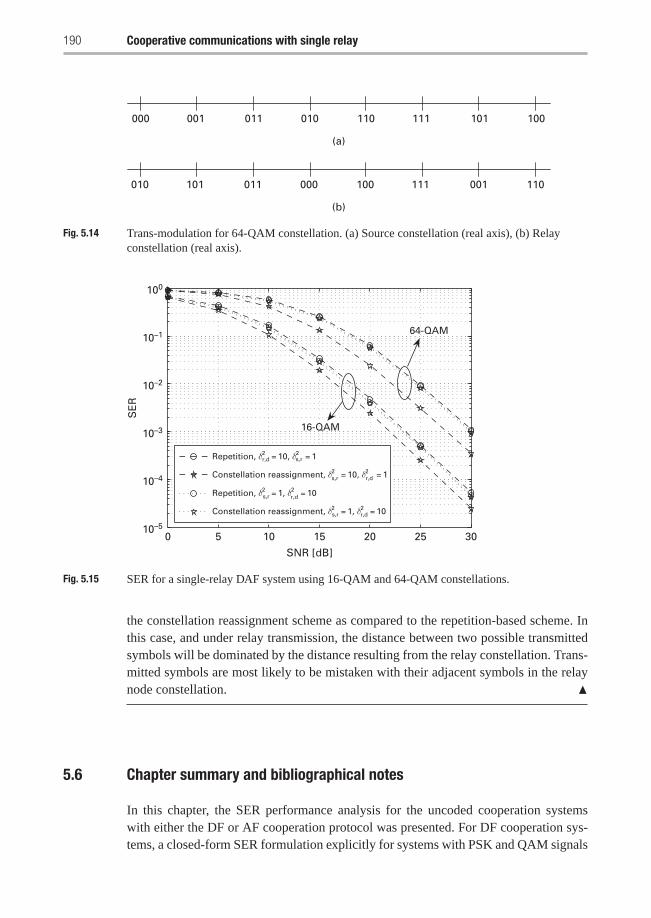
190 Cooperative communications with single relay
000 001 010011 110
(a)
111 100101
010 101 000
(b)
011 100 111 110001
Fig. 5.14 Trans-modulation for 64-QAM constellation. (a) Source constellation (real axis), (b) Relayconstellation (real axis).
0 5 10 15 20 25 30
SNR [dB]
r,d
Constellation reassignment, δ2 = 1, δ2
= 10
Repetition, δ2 = 1, δ2 = 10
Repetition, δ2 = 10, δ2
= 1
64-QAM
16-QAM
10–1
10–2
10–3
10–4
10–5
100
SE
R
s,r
s,r
s,r
s,rConstellation reassignment, δ2 = 10, δ2 = 1r,d
r,d
r,d
Fig. 5.15 SER for a single-relay DAF system using 16-QAM and 64-QAM constellations.
the constellation reassignment scheme as compared to the repetition-based scheme. Inthis case, and under relay transmission, the distance between two possible transmittedsymbols will be dominated by the distance resulting from the relay constellation. Trans-mitted symbols are most likely to be mistaken with their adjacent symbols in the relaynode constellation. �
5.6 Chapter summary and bibliographical notes
In this chapter, the SER performance analysis for the uncoded cooperation systemswith either the DF or AF cooperation protocol was presented. For DF cooperation sys-tems, a closed-form SER formulation explicitly for systems with PSK and QAM signals
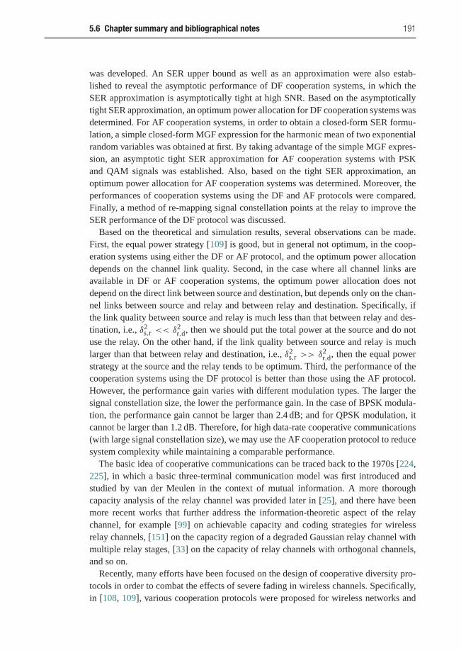
5.6 Chapter summary and bibliographical notes 191
was developed. An SER upper bound as well as an approximation were also estab-lished to reveal the asymptotic performance of DF cooperation systems, in which theSER approximation is asymptotically tight at high SNR. Based on the asymptoticallytight SER approximation, an optimum power allocation for DF cooperation systems wasdetermined. For AF cooperation systems, in order to obtain a closed-form SER formu-lation, a simple closed-form MGF expression for the harmonic mean of two exponentialrandom variables was obtained at first. By taking advantage of the simple MGF expres-sion, an asymptotic tight SER approximation for AF cooperation systems with PSKand QAM signals was established. Also, based on the tight SER approximation, anoptimum power allocation for AF cooperation systems was determined. Moreover, theperformances of cooperation systems using the DF and AF protocols were compared.Finally, a method of re-mapping signal constellation points at the relay to improve theSER performance of the DF protocol was discussed.
Based on the theoretical and simulation results, several observations can be made.First, the equal power strategy [109] is good, but in general not optimum, in the coop-eration systems using either the DF or AF protocol, and the optimum power allocationdepends on the channel link quality. Second, in the case where all channel links areavailable in DF or AF cooperation systems, the optimum power allocation does notdepend on the direct link between source and destination, but depends only on the chan-nel links between source and relay and between relay and destination. Specifically, ifthe link quality between source and relay is much less than that between relay and des-tination, i.e., δ2
s,r << δ2r,d, then we should put the total power at the source and do not
use the relay. On the other hand, if the link quality between source and relay is muchlarger than that between relay and destination, i.e., δ2
s,r >> δ2r,d, then the equal power
strategy at the source and the relay tends to be optimum. Third, the performance of thecooperation systems using the DF protocol is better than those using the AF protocol.However, the performance gain varies with different modulation types. The larger thesignal constellation size, the lower the performance gain. In the case of BPSK modula-tion, the performance gain cannot be larger than 2.4 dB; and for QPSK modulation, itcannot be larger than 1.2 dB. Therefore, for high data-rate cooperative communications(with large signal constellation size), we may use the AF cooperation protocol to reducesystem complexity while maintaining a comparable performance.
The basic idea of cooperative communications can be traced back to the 1970s [224,225], in which a basic three-terminal communication model was first introduced andstudied by van der Meulen in the context of mutual information. A more thoroughcapacity analysis of the relay channel was provided later in [25], and there have beenmore recent works that further address the information-theoretic aspect of the relaychannel, for example [99] on achievable capacity and coding strategies for wirelessrelay channels, [151] on the capacity region of a degraded Gaussian relay channel withmultiple relay stages, [33] on the capacity of relay channels with orthogonal channels,and so on.
Recently, many efforts have been focused on the design of cooperative diversity pro-tocols in order to combat the effects of severe fading in wireless channels. Specifically,in [108, 109], various cooperation protocols were proposed for wireless networks and
192 Cooperative communications with single relay
extensive outage probability performance analysis has been presented for such coopera-tion systems. The concept of user cooperation diversity was also proposed in [179, 180],where a specific two-user cooperation scheme was investigated for CDMA systems anda substantial performance gain was demonstrated over the non-cooperative approach.In [92], a coded two-user cooperation scheme was proposed by taking advantage of theexisting channel codes, in which the coded information of each user is divided into twoparts: one part is transmitted by the user itself and the other sent by its cooperator.
Note that in order to analyze the SER performance of AF cooperation systems, wehave to investigate the statistics of the harmonic mean of two random variables, whichare related to the instantaneous SNR at the destination [58]. A moment-generatingfunction of the harmonic mean of two independent exponential random variables wasderived in [58] by applying the Laplace transform and the hypergeometric functions[50]. However, the result involves an integration of the hypergeometric functions andit is hard to use for analyzing AF cooperation systems. The simple closed-form MGFexpression for the harmonic mean derived in this chapter is useful beyond the SERanalysis. The analysis of AF and DF cooperation systems discussed in this chapter waspublished in [207] and [204]. Interested readers may refer to [168] for more details ontrans-modulation.
Exercises
5.1 Prove the claims in (5.27) and (5.28), i.e., show the following results
limx→∞ x2 I1(x) = A2
b2δ2s,dδ
2s,r
,
limx, y→∞ xy I2(x, y) = B
b2δ2s,dδ
2r,d
,
where I1(x) and I2(x, y) are defined in (5.25) and (5.26), respectively, and theconstants b, A, and B are specified in (5.29)–(5.32) for M-PSK and M-QAMmodulation, respectively. Moreover, based on the above results, prove the claimin Theorem 5.2.2.
5.2 Let X be a random variable with pdf pX (x) for all x ≥ 0 and pX (x) = 0 forx < 0. Then, the pdf of Y = 1/X is
pY (y) = 1
y2pX
(1
y
)·U (y).
5.3 Let X1 and X2 be two independent random variables with pdf pX1(x) and pX2(x)defined for all x . Then, the pdf of the sum Y = X1 + X2 is
pY (y) =∫ ∞
−∞pX1(y − x) pX2(x)dx,
which is the convolution of pX1(x) and pX2(x).
Exercises 193
5.4 Prove the result in Theorem 5.3.1. Suppose that X1 and X2 are two indepen-dent random variables with pdf pX1(x) and pX2(x) defined for all x ≥ 0, andpX1(x) = 0 and pX2(x) = 0 for x < 0. Then the pdf of Z = X1 X2
X1+X2, the
harmonic mean of X1 and X2, is
pZ (z) = z∫ 1
0
1
t2(1− t)2pX1(
z
1− t) pX2(
z
t)dt ·U (z),
in which U (z) = 1 for z ≥ 0 and U (z) = 0 for z < 0.5.5 By applying the closed-form MGF expression in Theorem 5.3.2, show the SER
formulations in (5.71) and (5.72) for AF systems with M-PSK andM-QAMmodulations, respectively.
5.6 Prove the claims in (5.79) and (5.80), i.e., show the following results
limx, y→∞ x2 J1(x, y) = B
b2δ2s,dδ
2s,r
,
limx, y→∞ xy J2(x, y) = B
b2δ2s,dδ
2r,d
,
where J1(x, y) and J2(x, y) are defined in (5.77) and (5.78), respectively, andthe constants b and B are specified in (5.81) and (5.82) for M-PSK and M-QAMmodulation, respectively.
5.7 Prove the results in Theorem 5.3.4, i.e., show that for sufficiently high SNR, theoptimum power allocation for AF cooperation systems with either M-PSK orM-QAM modulation is
P1 =δs,r +
√δ2
s,r + 8δ2r,d
3δs,r +√δ2
s,r + 8δ2r,d
P,
P2 = 2δs,r
3δs,r +√δ2
s,r + 8δ2r,d
P.
5.8 (Simulation project) Consider a simplified network with a source node, arelay node and a destination node. The source–destination channel hs,d, thesource–relay channel hs,r, and the relay–destination channel hr,d are modeledas independent zero-mean, complex Gaussian random variables with variancesδ2
s,d, δ2s,r and δ2
r,d, respectively. Assume that δ2s,r = 1 and δ2
r,d = 1. We compareperformances of the AF and DF cooperation protocols with QPSK modulation.(a) Determine the optimum power allocation at the source and the relay for the
DF cooperation protocol.(b) Determine the optimum power allocation at the source and the relay for the
AF cooperation protocol.(c) Simulate both the DF and AF protocols with corresponding optimum power
allocations, and compare their performances.(d) Repeat (a), (b), and (c) for the case of δ2
s,r = 1 and δ2r,d = 10.
6 Multi-node cooperativecommunications
In the previous chapter, the symbol error rate performance of single-relay cooperativecommunications was analyzed for both the decode-and-forward and amplify-and-forward relaying strategies. This chapter builds upon the results in the previous chapterand generalizes the symbol error rate performance analysis to the multi-relay scenario.
Decode-and-forward relaying will be considered first, followed by the amplify-and-forward case. In both scenarios, exact and approximate expressions for the symbol errorrate will be derived. The symbol error rate expressions are then used to characterize anoptimal power allocation strategy among the relays and the source node.
6.1 Multi-node decode-and-forward protocol
We begin by presenting a class of cooperative decode-and-forward protocols for arbi-trary N -relay wireless networks, in which each relay can combine the signal receivedfrom the source along with one or more of the signals transmitted by previous relays.Then, we focus on the performance of a general cooperation scenario and present anexact symbol error rate (SER) expressions for both M-ary phase shift keying (PSK) andquadrature amplitude modulation (QAM) signalling. We also consider an approximateexpression for the SER of a general cooperation scenario that is shown to be tight athigh enough SNR. Finally, we study optimal power allocation for the class of cooper-ative diversity schemes, where the optimality is determined in terms of minimizing theSER of the system.
6.1.1 System model and protocol description
We consider an arbitrary N -relay wireless network, where information is to be transmit-ted from a source to a destination. Due to the broadcast nature of the wireless channel,some relays can overhear the transmitted information and thus can cooperate with thesource to send its data. The wireless link between any two nodes in the network ismodeled as a Rayleigh fading narrowband channel with additive white Gaussian noise(AWGN). The channel fades for different links are assumed to be statistically indepen-dent. This is a reasonable assumption as the relays are usually spatially well separated.The additive noise at all receiving terminals is modeled as zero-mean, complex Gaus-sian random variables with variance N0. For medium access, the relays are assumed to
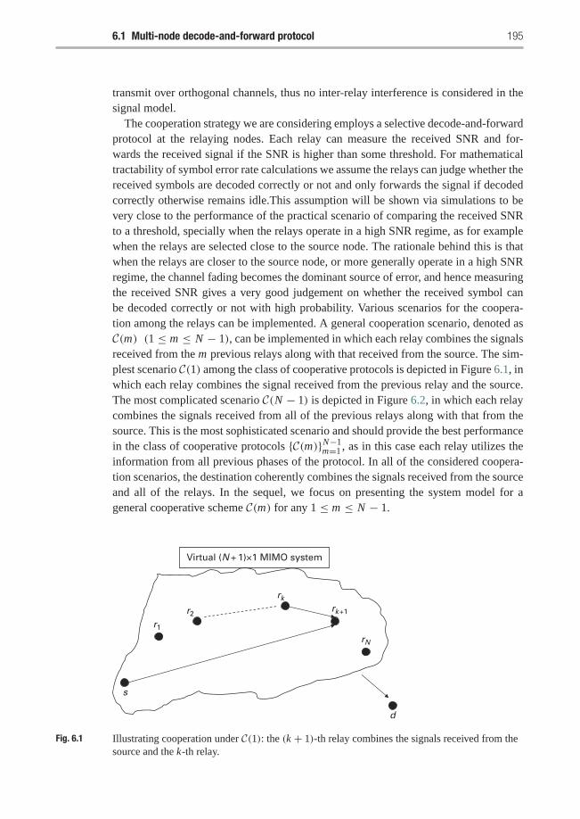
6.1 Multi-node decode-and-forward protocol 195
transmit over orthogonal channels, thus no inter-relay interference is considered in thesignal model.
The cooperation strategy we are considering employs a selective decode-and-forwardprotocol at the relaying nodes. Each relay can measure the received SNR and for-wards the received signal if the SNR is higher than some threshold. For mathematicaltractability of symbol error rate calculations we assume the relays can judge whether thereceived symbols are decoded correctly or not and only forwards the signal if decodedcorrectly otherwise remains idle.This assumption will be shown via simulations to bevery close to the performance of the practical scenario of comparing the received SNRto a threshold, specially when the relays operate in a high SNR regime, as for examplewhen the relays are selected close to the source node. The rationale behind this is thatwhen the relays are closer to the source node, or more generally operate in a high SNRregime, the channel fading becomes the dominant source of error, and hence measuringthe received SNR gives a very good judgement on whether the received symbol canbe decoded correctly or not with high probability. Various scenarios for the coopera-tion among the relays can be implemented. A general cooperation scenario, denoted asC(m) (1 ≤ m ≤ N − 1), can be implemented in which each relay combines the signalsreceived from the m previous relays along with that received from the source. The sim-plest scenario C(1) among the class of cooperative protocols is depicted in Figure 6.1, inwhich each relay combines the signal received from the previous relay and the source.The most complicated scenario C(N − 1) is depicted in Figure 6.2, in which each relaycombines the signals received from all of the previous relays along with that from thesource. This is the most sophisticated scenario and should provide the best performancein the class of cooperative protocols {C(m)}N−1
m=1 , as in this case each relay utilizes theinformation from all previous phases of the protocol. In all of the considered coopera-tion scenarios, the destination coherently combines the signals received from the sourceand all of the relays. In the sequel, we focus on presenting the system model for ageneral cooperative scheme C(m) for any 1 ≤ m ≤ N − 1.
s
r1
r2
rk
Virtual (N + 1)×1 MIMO system
rk +1
rN
d
Fig. 6.1 Illustrating cooperation under C(1): the (k + 1)-th relay combines the signals received from thesource and the k-th relay.
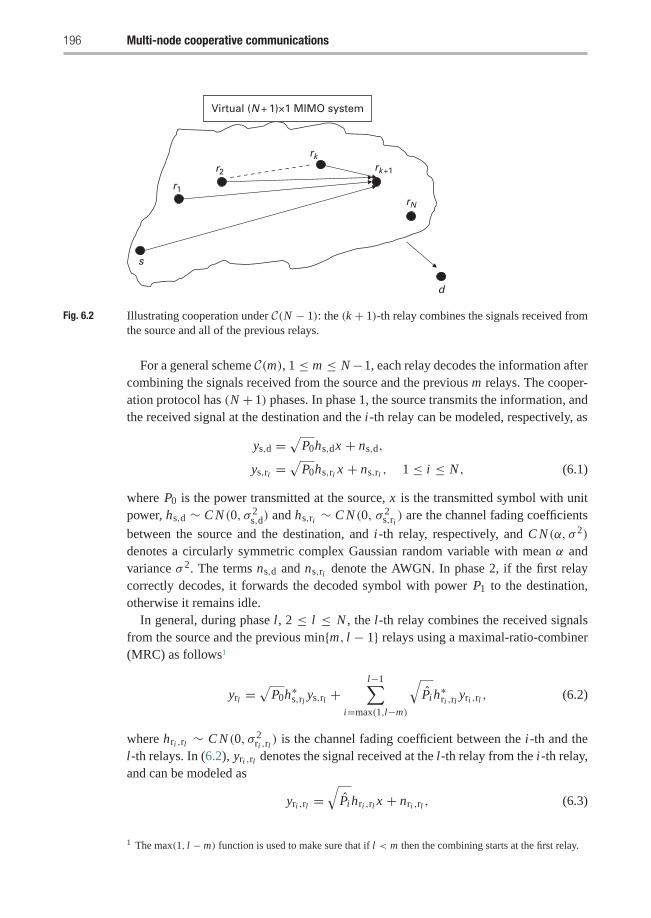
196 Multi-node cooperative communications
s
r1
r2
rk
Virtual (N + 1)×1 MIMO system
rk +1
rN
d
Fig. 6.2 Illustrating cooperation under C(N − 1): the (k + 1)-th relay combines the signals received fromthe source and all of the previous relays.
For a general scheme C(m), 1 ≤ m ≤ N−1, each relay decodes the information aftercombining the signals received from the source and the previous m relays. The cooper-ation protocol has (N + 1) phases. In phase 1, the source transmits the information, andthe received signal at the destination and the i-th relay can be modeled, respectively, as
ys,d =√
P0hs,dx + ns,d,
ys,ri =√
P0hs,ri x + ns,ri , 1 ≤ i ≤ N , (6.1)
where P0 is the power transmitted at the source, x is the transmitted symbol with unitpower, hs,d ∼ C N (0, σ 2
s,d) and hs,ri ∼ C N (0, σ 2s,ri ) are the channel fading coefficients
between the source and the destination, and i-th relay, respectively, and C N (α, σ 2)
denotes a circularly symmetric complex Gaussian random variable with mean α andvariance σ 2. The terms ns,d and ns,ri denote the AWGN. In phase 2, if the first relaycorrectly decodes, it forwards the decoded symbol with power P1 to the destination,otherwise it remains idle.
In general, during phase l, 2 ≤ l ≤ N , the l-th relay combines the received signalsfrom the source and the previous min{m, l − 1} relays using a maximal-ratio-combiner(MRC) as follows1
yrl =√
P0h∗s,rl ys,rl +l−1∑
i=max(1,l−m)
√Pi h
∗ri ,rl yri ,rl , (6.2)
where hri ,rl ∼ C N (0, σ 2ri ,rl ) is the channel fading coefficient between the i-th and the
l-th relays. In (6.2), yri ,rl denotes the signal received at the l-th relay from the i-th relay,and can be modeled as
yri ,rl =√
Pi hri ,rl x + nri ,rl , (6.3)
1 The max(1, l − m) function is used to make sure that if l < m then the combining starts at the first relay.
6.1 Multi-node decode-and-forward protocol 197
where Pi is the power transmitted at relay i in phase (i + 1), and Pi = Pi if relayi correctly decodes the transmitted symbol, otherwise Pi = 0. The l-th relay usesyrl in (6.2) as the detection statistics. If relay l decodes correctly it transmits withpower Pl = Pl in Phase (l + 1), otherwise it remains idle. Finally, in phase (N + 1),the destination coherently combines all of the received signals using an MRC asfollows
yd =√
P0h∗s,dys,d +N∑
i=1
√Pi h
∗ri ,dyri ,d. (6.4)
For fair comparison purpose, the total transmitted power is fixed as P0 + ∑Ni=1
Pi = P .
6.1.2 Exact SER performance analysis
In this subsection, we present the SER performance analysis for a general cooperativescheme C(m) for any 1 ≤ m ≤ N − 1. Exact SER expressions of this general schemeare presented for systems with both M-PSK and M-QAM modulation. Some simulationexamples are also discussed at the end of this subsection.
First, we introduce some terminologies that will be used throughout the analysis. Fora given transmission, each relay can be in one of two states: either it decoded correctlyor not. Let us define a 1× n, 1 ≤ n ≤ N , vector Sn to represent the states of the first nrelays for a given transmission. The k-th entry of the vector Sn denotes the state of thek-th relay as follows:
Sn[k] ={
1 if relay k correctly decodes,
0 otherwise,1 ≤ k ≤ n. (6.5)
Since the decimal value of the binary vector Sn can take on values from 0 to 2n − 1, forconvenience we denote the state of the network by an integer decimal number. Let
Bx,n =(Bx,n[1], Bx,n[2], . . . , Bx,n[n]
)(6.6)
be the 1× n binary representation of a decimal number x , with Bx,n[1] being the mostsignificant bit. So, SN = Bx,N indicates that the k-th relay, 1 ≤ k ≤ N , is in stateSN [k] = Bx,N [k].
We consider a general cooperation scheme C(m), 1 ≤ m ≤ N − 1, in which the k-th(1 ≤ k ≤ N ) relay coherently combines the signals received from the source along withthe signals received from the previous min{m, k − 1} relays. The state of each relay inthis scheme depends on the states of the previous m relays, i.e., whether these relaysdecoded correctly or not. This is due to the fact that the number of signals received ateach relay depends on the number of relays that decoded correctly from the previous mrelays. Hence, the joint probability of the states is given by
P(SN ) = P(SN [1])P(SN [2] | SN [1]) · · · P(SN [N ] | SN [N − 1], . . . , SN [N − m]).(6.7)
198 Multi-node cooperative communications
Conditioning on the network state, which can take 2N values, the probability of errorat the destination given the channel state information (CSI) can be calculated using thelaw of total probability as follows:
Pe|CSI =2N−1∑i=0
Pr(e | SN = Bi,N )Pr(SN = Bi,N ), (6.8)
where e denotes the event that the destination decoded in error. The summation in theabove equation is over all possible states of the network.
Now, let us compute the terms in (6.8). The destination collects the copies of thesignal transmitted in the previous phases using an MRC (6.4). The resulting SNR atthedestination can be computed as
SNRd =P0 | hs,d |2 +∑N
j=1 Pj Bi,N [ j] | hr j ,d |2No
, (6.9)
where Bi,N [ j] takes value 1 or 0 and determines whether the j-th relay has decodedcorrectly or not. The k-th relay coherently combines the signals received from the sourceand the previous m relays. The resulting SNR can be calculated as
SNRmrk= P0 | hs,rk |2 +
∑k−1j=max(1,k−m) Pj Bi,N [ j] | hr j ,rk |2
No. (6.10)
If M-PSK modulation is used in the system, with instantaneous SNR γ , the SER withthe channel state information is given by
PPSKCSI = �PSK(γ ) � 1
π
∫ (M−1)π/M
0exp
(− bPSKγ
sin2(θ)
)dθ, (6.11)
where bPSK = sin2(π/M). If M-QAM (M = 2k with k even) modulation is used in thesystem, the corresponding conditional SER can be expressed as
PQAMCSI = �QAM(γ ) � 4C Q(
√bQAMγ )− 4C2 Q2(
√bQAMγ ), (6.12)
in which C = 1 − 1/√
M , bQAM = 3/(M − 1), and Q(x) is the complementarydistribution function (CDF) of the Gaussian distribution.
Let us focus on computing the SER in the case of M-PSK modulation, and the sameprocedure is applicable for the case of M-QAM modulation. From (6.9), and for a givennetwork state SN = Bi,N , the conditional SER at the destination can be computed as
Pr(e|SN = Bi,N ) = �PSK (SNRd) . (6.13)
Denote the conditional probability that the k-th relay is in state Bi,N [k] given the states ofthe previous m relays by Pm
k,i . From (6.10), this probability can be computed as follows:
Pmk,i � Pr(SN [k] = Bi,N [k] | SN [k − 1] = Bi,N [k − 1], . . . , SN [k − m]= Bi,N [k − m])
={�PSK(SNRm
rk ), if Bi,N [k] = 0,
1−�PSK(SNRmrk ), if Bi,N [k] = 1.
(6.14)
6.1 Multi-node decode-and-forward protocol 199
To compute the average SER, we need to average the probability in (6.8) over all channelrealizations, i.e., PSER(m) = ECSI
[Pe|CSI
]. Using (6.7), (6.13), and (6.14), PSER(m)
can be expanded as follows
PSER(m) =2N−1∑i=0
ECSI
[�PSK (SNRd)
N∏k=1
Pmk,i
]. (6.15)
Since the channel fades between different pairs of nodes in the network are statisticallyindependent by the virtue that different nodes are not co-located, the quantities insidethe expectation operator in the above equation are functions of independent randomvariables, and thus can be further decomposed as
PSER(m) =2N−1∑i=0
{ECSI [�PSK (SNRd)]
N∏k=1
ECSI[Pm
k,i
]}. (6.16)
The above analysis is applicable to the M-QAM case by replacing the function �PSK(·)by �QAM(·).
Since the channels between the nodes are modeled as Rayleigh fading channels, theabsolute norm square of any channel realization hi, j between any two nodes i and j inthe network has an exponential distribution with mean σ 2
i, j . Hence, ECSI[�q(γ )] can beexpressed as
ECSI[�q(γ )] =∫γ
�q(γ ) f (γ )dγ (6.17)
where f (γ ) is the probability density function of the random variable γ , and q = 1 (q =2) correspond to M-PSK (M-QAM), respectively. If γ is an exponentially distributedrandom variable with mean γ , then it can be shown [187] that ECSI[�q(γ )] is given by
ECSI[�q (γ )
] = Fq
(1+ bqγ
sin2(θ)
), (6.18)
where Fq(·) and the constant bq are defined as
F1(x(θ)) = 1
π
∫ (M−1)π/M
0
1
x(θ)dθ, b1 = bpsk
F2(x(θ)) = 4C
π
∫ π/2
0
1
x(θ)dθ − 4C2
π
∫ π/4
0
1
x(θ)dθ, b2 = bQAM
2. (6.19)
In order to get the above expressions, we use two special properties of the Q(·) function,specifically,
Q(x) = 1
π
∫ π/2
0exp
(− x2
2 sin2(θ)
)dθ (6.20)
Q2(x) = 1
π
∫ π/4
0exp
(− x2
2 sin2(θ)
)dθ (6.21)
for x ≥ 0.
200 Multi-node cooperative communications
Averaging over all the Rayleigh fading channel realizations, the SER at the destina-tion for a given network state Bi,N is given by
ECSI(�q(SNRd)) = Fq
⎡⎣(1+ bq P0σ2s,d
No sin2(θ)
)N∏
j=1
(1+
bq Bi,N [ j]Pjσ2r j ,d
No sin2(θ)
)⎤⎦ . (6.22)
Similarly, the probability that the k-th relay is in state Bi,N [k] given the states of theprevious m relays is given by
ECSI[Pm
k,i
] = Gmk (Bi,N [k]), (6.23)
where Gmk (·) is defined as
Gmk (x) =
⎧⎪⎪⎪⎪⎪⎪⎪⎨⎪⎪⎪⎪⎪⎪⎪⎩
Fq
[(1+ bq P0σ
2s,rk
No sin2(θ)
)∏k−1j=max(1,k−m)
(1+ bq Bi,N [ j]Pjσ
2r j ,rk
No sin2(θ)
)],
if x = 0,
1− Fq
[(1+ bq P0σ
2s,rk
No sin2(θ)
)∏k−1j=max(1,k−m)
(1+ bq Bi,N [ j]Pjσ
2r j ,rk
No sin2(θ)
)],
if x = 1.(6.24)
in which Fq(·) and the constant bq are specified in (6.19). As a summary, the SER in(6.16) of the cooperative multi-node system employing scenario C(m) with M-PSK orM-QAM modulation can be determined from (6.22), (6.23), and (6.24) in the followingtheorem.
T H E O R E M 6.1.1 The SER of an N-relay decode-and-forward cooperative diversitynetwork utilizing protocol C(m), 1 ≤ m ≤ N − 1, and M-PSK or M-QAM modulationis given by
PSER(m) =2N−1∑i=0
Fq
⎡⎣(1+ bq P0σ2s,d
No sin2(θ)
)N∏
j=1
(1+
bq Bi,N [ j]Pjσ2r j ,d
N0 sin2(θ)
)⎤⎦N∏
k=1
Gmk (Bi,N [k]), (6.25)
where the functions Fq(·) and Gmk (·) are defined in (6.19) and (6.24), respectively.
Example 6.1 We illustrate the validity of the theoretical results by some simulationexamples. Let us focus on the cooperative protocol C(1). The number of relays is takento be N = 1, 2, 3, in addition to the source and the destination nodes. We consideredtwo simulation setups:
• In the first setup we simulate the SER performance under the assumption that the relaycorrectly judges whether the received signal is decoded correctly or not, i.e., no errorpropagation, which is the model analyzed in the chapter.
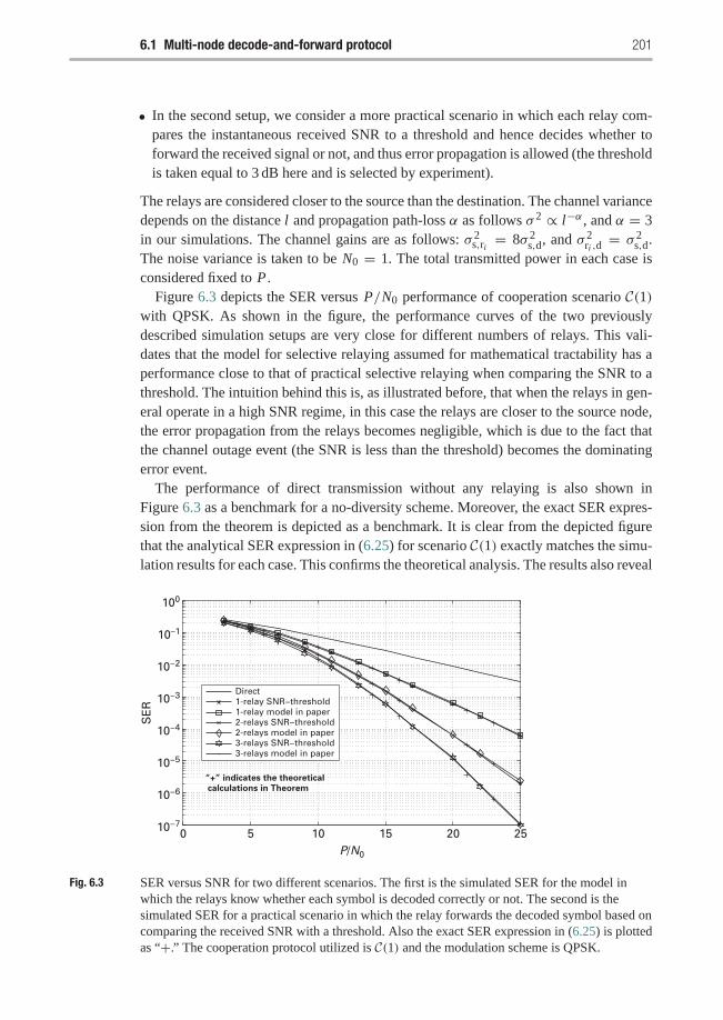
6.1 Multi-node decode-and-forward protocol 201
• In the second setup, we consider a more practical scenario in which each relay com-pares the instantaneous received SNR to a threshold and hence decides whether toforward the received signal or not, and thus error propagation is allowed (the thresholdis taken equal to 3 dB here and is selected by experiment).
The relays are considered closer to the source than the destination. The channel variancedepends on the distance l and propagation path-loss α as follows σ 2 ∝ l−α , and α = 3in our simulations. The channel gains are as follows: σ 2
s,ri = 8σ 2s,d, and σ 2
ri ,d= σ 2
s,d.The noise variance is taken to be N0 = 1. The total transmitted power in each case isconsidered fixed to P .
Figure 6.3 depicts the SER versus P/N0 performance of cooperation scenario C(1)with QPSK. As shown in the figure, the performance curves of the two previouslydescribed simulation setups are very close for different numbers of relays. This vali-dates that the model for selective relaying assumed for mathematical tractability has aperformance close to that of practical selective relaying when comparing the SNR to athreshold. The intuition behind this is, as illustrated before, that when the relays in gen-eral operate in a high SNR regime, in this case the relays are closer to the source node,the error propagation from the relays becomes negligible, which is due to the fact thatthe channel outage event (the SNR is less than the threshold) becomes the dominatingerror event.
The performance of direct transmission without any relaying is also shown inFigure 6.3 as a benchmark for a no-diversity scheme. Moreover, the exact SER expres-sion from the theorem is depicted as a benchmark. It is clear from the depicted figurethat the analytical SER expression in (6.25) for scenario C(1) exactly matches the simu-lation results for each case. This confirms the theoretical analysis. The results also reveal
0 5 10 15 20 25P/N0
SE
R
Direct1-relay SNR−threshold1-relay model in paper2-relays SNR−threshold2-relays model in paper3-relays SNR−threshold3-relays model in paper
“+” indicates the theoretical
calculations in Theorem
10−7
10−6
10−5
10−4
10−3
10−2
10–1
100
Fig. 6.3 SER versus SNR for two different scenarios. The first is the simulated SER for the model inwhich the relays know whether each symbol is decoded correctly or not. The second is thesimulated SER for a practical scenario in which the relay forwards the decoded symbol based oncomparing the received SNR with a threshold. Also the exact SER expression in (6.25) is plottedas “+.” The cooperation protocol utilized is C(1) and the modulation scheme is QPSK.
202 Multi-node cooperative communications
that the cooperative diversity protocols can achieve full diversity gain in the number ofcooperating terminals, which can be seen from the slopes of the performance curves,which become steeper with an increasing number of relays. �
6.1.3 SER approximation
In the previous subsection, we provided exact expressions for the SER of a generalcooperative scheme C(m), 1 ≤ m ≤ N − 1, for arbitrary N -relay networks with eitherM-PSK or M-QAM modulation. The derived SER expressions, however, involve 2N
terms and integral functions. In this subsection, we provide approximate expressionsfor the SER performance of the class of cooperative diversity schemes. The approxi-mation is derived at high SNR and yields simple expressions that can provide insightsto help understand the factors that affect system performance, which helps in designingdifferent network functions as power allocation, scheduling, routing, and node selection.
6.1.3.1 SER approximation for general cooperative protocolOne can see that any term in the exact SER formulation (6.25) in Theorem 6.1.1 consistsof the product of two quantities:
• The first is
Fq
⎡⎣(1+ bq P0σ2s,d
No sin2(θ)
)N∏
j=1
(1+
bq Bi,N [ j]Pjσ2r j ,d
No sin2(θ)
)⎤⎦ , (6.26)
which corresponds to the conditional SER at the destination for a given networkstate Bi,N .
• The second is the probability of the network being in that state, and is given by∏Nk=1 Gm
k (Bi,N [k]).At high enough SNR, the probability of error Fq(·) is sufficiently small compared to 1,thus we can assume that 1 − Fq(·) � 1. Hence, the only terms in the second quantity∏N
k=1 Gmk (Bi,N [k]) that will count are those corresponding to relays that have decoded
in error. For convenience, we make the following definition: let �i (n,m) denote thesubset of nodes that decode correctly from node max(1, n−m) to node n− 1, when thenetwork was in state Bi,N . More specifically,
�i (n,m) � {relay j : s.t.Bi,N [ j] = 1,max(1, n − m) ≤ j ≤ n − 1.} (6.27)
Then, the SER formulation (6.25) in Theorem 6.1.1 can be approximated as
PSER(m) �2N−1∑i=0
Fq
⎡⎣(1+ bq P0σ2s,d
No sin2(θ)
)N∏
j=1
(1+
bq Bi,N [ j]Pjσ2r j ,d
No sin2(θ)
)⎤⎦·
∏k∈�c(N+1,N )
Gmk (Bi,N [k]), (6.28)
where�c is the complementary set of�, i.e., the set of nodes that decoded erroneously.
6.1 Multi-node decode-and-forward protocol 203
First, we simplify the first term corresponding to the SER at the destination. Usingthe definition of Fq in (6.19), and ignoring all the 1’s in Fq(·) in (6.28), the conditionalSER at the destination for a given network state Bi,N can be approximated as
Fq
⎡⎣(1+ bq P0σ2s,d
No sin2(θ)
)N∏
j=1
(1+
bq Bi,N [ j]Pjσ2r j ,d
No sin2(θ)
)⎤⎦� N 1+|�i (N+1,N )|
o gq(1+ | �i (N + 1, N ) |)b1+|�i (N+1,N )|
q P0σ2s,d
∏j∈�i (N+1,N ) Pjσ
2r j ,d
, (6.29)
where | �i (N+1, N ) | denotes the cardinality of the set�i (N+1, N ), i.e., the numberof nodes that decode correctly, which also denotes the number of signal copies trans-mitted from the N relays to the destination at network state Bi,N . The function gq(·) in(6.29) is specified as
gq(x) =⎧⎨⎩
1π
∫ (M−1)π/M0 sin2x (θ)dθ, for M-PSK, q = 1
4Cπ
[∫ π/20 sin2x (θ)dθ − C
∫ π/40 sin2x (θ)dθ
], for M-QAM, q = 2.
(6.30)Let us write the transmitter powers allocated at the source and different relays as a
ratio of the total available power P as follows: P0 = a0 P , and Pi = ai P, 1 ≤ i ≤ N ,in which the power ratios are normalized as a0 +∑N
i=1 ai = 1. One can then rewrite(6.29) in terms of the power allocation ratios as follows:
Fq
⎡⎣(1+ bq P0σ2s,d
No sin2(θ)
)N∏
j=1
(1+
bq Bi,N [ j]Pjσ2r j ,d
No sin2(θ)
)⎤⎦� (No/P)1+|�i (N+1,N )| gq(1+ | �i (N + 1, N ) |)
b1+|�i (N+1,N )|q a0σ
2s,d
∏j∈�i (N+1,N ) a jσ
2r j ,d
. (6.31)
Note that the SNR term (No/P) in (6.31) is of order (1+ | �i (N + 1, N ) |). This isintuitively meaningful since the destination receives (1+ | �i (N + 1, N ) |) copies ofthe signal, in which the term 1 is due to the copy from the source. Thus (6.31) decaysas SNR−(1+|�i (N+1,N )|) at high SNR.
At the k-th relay, 1 ≤ k ≤ N , the conditional SER for a given network state Bi,N canbe similarly approximated as
Fq
⎡⎣(1+ bq P0σ2s,rk
No sin2(θ)
)k−1∏
j=max(1,k−m)
(1+ bq Bi,N [ j]Pjσ
2r j ,rk
No sin2(θ)
)⎤⎦� (No/P)1+|�i (k,m)|gq(1+ | �i (k,m) |)
b1+|�i (k,m)|q a0σ 2
s,rk
∏j∈�i (k,m) a jσ 2
r j ,rk
, (6.32)
where | �i (k,m) |) is the number of relays that decodes correctly from the previousmin(k − 1,m) relays.
204 Multi-node cooperative communications
The SNR in the above expression is of order 1+ | �i (k,m) |. From (6.32), theproduct
∏k∈�c
i (N+1,N ) Gmk (Bi,N [k]) in (6.28) is given by
∏k∈�c
i (N+1,N )
Gmk (Bi,N [k]) =
∏k∈�c
i (N+1,N )
(No/P)1+|�i (k,m)|gq(1+ | �i (k,m) |)b1+|�i (k,m)|
q a0σ 2s,rk
∏j∈�i (k,m) a jσ 2
r j ,rk
,
(6.33)
in which the SNR is of order∑
k∈�ci (N+1,N )(1+ | �i (k,m) |) =| �c
i (N + 1, N ) | +∑k∈�c
i (N+1,N ) | �i (k,m) |. Substituting (6.31) and (6.33) into (6.28), we get
PSER(m) �∑2N−1i=0
(N0/P)di gq (1+|�i (N+1,N )|)b
diq a
1+|�ci (N+1,N )|
0 σ 2s,d
∏j∈�i (N+1,N ) a jσ
2r j ,d
·∏
k∈�ci (N+1,N ) gq (1+|�i (k,m)|)∏
k∈�ci (N+1,N ) σ
2s,rk
∏l∈�i (k,m)
alσ2rl ,rk, (6.34)
where
di = 1+ | �i (N + 1, N ) | + | �ci (N + 1, N ) | +
∑k∈�c
i (N+1,N )
| �i (k,m) | . (6.35)
From (6.34), we can see that the SNR is of order di . Since | �i (N + 1, N ) | +| �c
i (N + 1, N ) |= N , the order di can be lower bounded as follows:
di = 1+ N +∑
k∈�ci (N+1,N )
| �i (k,m) |≥ N + 1, (6.36)
in which the equality holds if and only if∑k∈�c
i (N+1,N )
| �i (k,m) |= 0. (6.37)
Thus the smallest order of the SNR is N + 1.The equality in (6.36) holds if and only if | �i (k,m) |= 0, for any k ∈ �c
i (N +1, N ), and 0 ≤ i ≤ 2N −1. Essentially, this means that the equality in (6.36) is satisfiedif and only if for each relay k that decodes erroneously, the m preceding relays mustalso have decoded erroneously. One can think of this condition as a chain rule, and thisleads to the conclusion that the equality holds if and only if for each relay k that decodesin error all the previous relays must have decoded in error. As a result, the only networkstates that will contribute in the SER expression with terms of order N + 1 in the SNRare those of the form
SN = B2n−1,N , 0 ≤ n ≤ N . (6.38)
For example, a network state of the form SN = [0, . . . , 0, 1, . . . , 1] will contribute toa term in the SER with SNR raised to the order N + 1, and a network state SN =[0, . . . , 0, 1, 1, 0, 1, . . . , 1] will contribute to a term in the SER with SNR raised to anexponent larger than (N + 1) depending on m. Therefore, only N + 1 states of thenetwork have SER terms that decay as 1/SNRN+1 and the rest of the network states
6.1 Multi-node decode-and-forward protocol 205
decay with faster rates, hence these N + 1 terms will dominant the SER expression athigh enough SNR.
In order to write the approximate expression for the SER corresponding to theseN + 1 terms, we need to note the following points that can be deduced from the aboveanalysis. As described above, in order for the equality in (6.36) to hold, the followingset of conditions must be satisfied:
• First, since for any relay that decodes erroneously all the previous m relays must havedecoded in error, we have
�i (k,m) = �, (6.39)
for all k ∈ �ci (N + 1, N ), where � is the empty set.
• Second, for these N + 1 states that satisfy the equality in (6.36) the set �ci (N + 1, N )
takes one of the following forms:
�ci (N + 1, N ) ∈ {�, {1}, {1, 2}, . . . , {1, 2, . . . , N }} . (6.40)
For example, �ci (N + 1, N ) = {1, 2, . . . , k} denotes the state in which only the first k
relays decoded erroneously. Accordingly, its cardinality, denoted by | �ci (N + 1, N ) |,
takes one of the following values:
| �ci (N + 1, N ) |∈ {0, 1, 2, . . . , N } . (6.41)
Thus, only the N + 1 states determined from the above conditions will contribute to theSER expression at high SNR because they decay as 1/SNRN+1, which is the slowestdecaying rate as seen from (6.36). From (6.34), (6.39), (6.40), and (6.41), the conditionalSER for any of these states, e.g., �c
i (N + 1, N ) = {1, 2, . . . , k}, can be determined asfollows:
SERk(m) =(No/P)N+1gq(N − k + 1)gk
q(1)
bN+1q σ 2
s,da1+ko∏
j∈�i (N+1,N ) a jσ2r j ,d
∏kl=1 σ
2s,rl
. (6.42)
Summing the above expression over the N+1 states in (6.40), we can further determinethe approximate expression for the SER in the following theorem.
T H E O R E M 6.1.2 At high enough SNR, the SER of an N relay decode-and-forwardcooperative diversity network employing cooperation scheme C(m) and utilizingM-PSK or M-QAM modulation can be approximated by
PSER(m) � (No/P)N+1
bN+1q σ 2
s,d
N+1∑j=1
gq(N − j + 2)g j−1q (1)
a j0
∏Ni= j aiσ
2ri ,d
∏ j−1l=1 σ
2s,rl
. (6.43)
A very important point to be noticed from the above theorem is that the approximatedSER expression in (6.43) does not depend on m, the class parameter. Hence, the wholeclass of cooperative diversity protocols {C(m)}N−1
m=1 shares the same asymptotic perfor-mance at high enough SNR. The results obtained illustrate that utilizing the simplestscheme, namely, scenario C(1), results in the same asymptotic SER performance as themost sophisticated scheme, namely, C(N − 1). This motivates us to utilize scenario
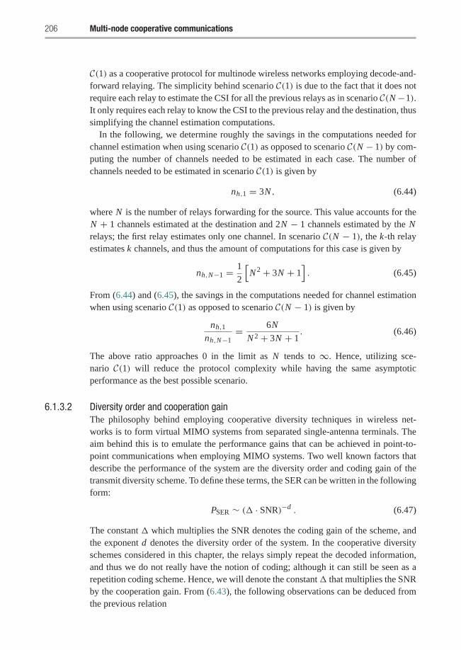
206 Multi-node cooperative communications
C(1) as a cooperative protocol for multinode wireless networks employing decode-and-forward relaying. The simplicity behind scenario C(1) is due to the fact that it does notrequire each relay to estimate the CSI for all the previous relays as in scenario C(N−1).It only requires each relay to know the CSI to the previous relay and the destination, thussimplifying the channel estimation computations.
In the following, we determine roughly the savings in the computations needed forchannel estimation when using scenario C(1) as opposed to scenario C(N − 1) by com-puting the number of channels needed to be estimated in each case. The number ofchannels needed to be estimated in scenario C(1) is given by
nh,1 = 3N , (6.44)
where N is the number of relays forwarding for the source. This value accounts for theN + 1 channels estimated at the destination and 2N − 1 channels estimated by the Nrelays; the first relay estimates only one channel. In scenario C(N − 1), the k-th relayestimates k channels, and thus the amount of computations for this case is given by
nh,N−1 = 1
2
[N 2 + 3N + 1
]. (6.45)
From (6.44) and (6.45), the savings in the computations needed for channel estimationwhen using scenario C(1) as opposed to scenario C(N − 1) is given by
nh,1
nh,N−1= 6N
N 2 + 3N + 1. (6.46)
The above ratio approaches 0 in the limit as N tends to ∞. Hence, utilizing sce-nario C(1) will reduce the protocol complexity while having the same asymptoticperformance as the best possible scenario.
6.1.3.2 Diversity order and cooperation gainThe philosophy behind employing cooperative diversity techniques in wireless net-works is to form virtual MIMO systems from separated single-antenna terminals. Theaim behind this is to emulate the performance gains that can be achieved in point-to-point communications when employing MIMO systems. Two well known factors thatdescribe the performance of the system are the diversity order and coding gain of thetransmit diversity scheme. To define these terms, the SER can be written in the followingform:
PSER ∼ (� · SNR)−d . (6.47)
The constant � which multiplies the SNR denotes the coding gain of the scheme, andthe exponent d denotes the diversity order of the system. In the cooperative diversityschemes considered in this chapter, the relays simply repeat the decoded information,and thus we do not really have the notion of coding; although it can still be seen as arepetition coding scheme. Hence, we will denote the constant� that multiplies the SNRby the cooperation gain. From (6.43), the following observations can be deduced fromthe previous relation
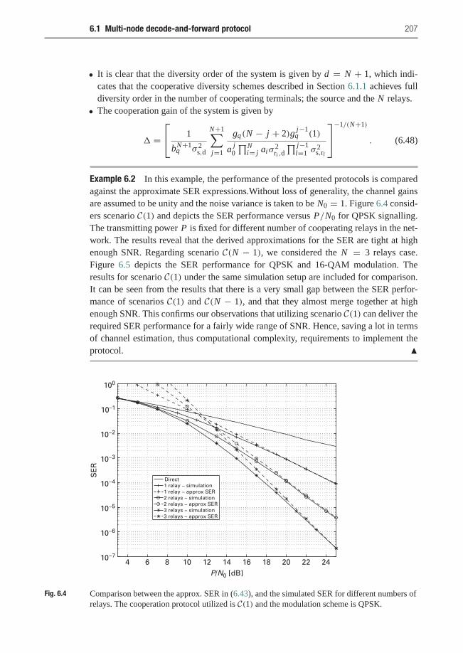
6.1 Multi-node decode-and-forward protocol 207
• It is clear that the diversity order of the system is given by d = N + 1, which indi-cates that the cooperative diversity schemes described in Section 6.1.1 achieves fulldiversity order in the number of cooperating terminals; the source and the N relays.
• The cooperation gain of the system is given by
� =⎡⎣ 1
bN+1q σ 2
s,d
N+1∑j=1
gq(N − j + 2)g j−1q (1)
a j0
∏Ni= j aiσ
2ri ,d
∏ j−1l=1 σ
2s,rl
⎤⎦−1/(N+1)
. (6.48)
Example 6.2 In this example, the performance of the presented protocols is comparedagainst the approximate SER expressions.Without loss of generality, the channel gainsare assumed to be unity and the noise variance is taken to be N0 = 1. Figure 6.4 consid-ers scenario C(1) and depicts the SER performance versus P/N0 for QPSK signalling.The transmitting power P is fixed for different number of cooperating relays in the net-work. The results reveal that the derived approximations for the SER are tight at highenough SNR. Regarding scenario C(N − 1), we considered the N = 3 relays case.Figure 6.5 depicts the SER performance for QPSK and 16-QAM modulation. Theresults for scenario C(1) under the same simulation setup are included for comparison.It can be seen from the results that there is a very small gap between the SER perfor-mance of scenarios C(1) and C(N − 1), and that they almost merge together at highenough SNR. This confirms our observations that utilizing scenario C(1) can deliver therequired SER performance for a fairly wide range of SNR. Hence, saving a lot in termsof channel estimation, thus computational complexity, requirements to implement theprotocol. �
4 6 8 10 12 14 16 18 20 22 24
Direct1 relay − simulation1 relay − approx SER2 relays − simulation2 relays − approx SER3 relays − simulation3 relays − approx SER
P/N0 [dB]
SE
R
10−7
10−6
10−5
10−4
10−3
10−2
10–1
100
Fig. 6.4 Comparison between the approx. SER in (6.43), and the simulated SER for different numbers ofrelays. The cooperation protocol utilized is C(1) and the modulation scheme is QPSK.
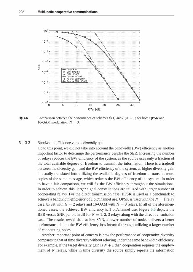
208 Multi-node cooperative communications
C(1) QPSKC(N−1) QPSKC(1) 16QAMC(N−1) 16QAMApprox SER QPSKApprox SER 16QAM
0 5 10 15 20 25 30P/N0 [dB]
SE
R
10−7
10−6
10−5
10−4
10−3
10−2
10–1
100
Fig. 6.5 Comparison between the performance of schemes C(1) and C(N − 1) for both QPSK and16-QAM modulation, N = 3.
6.1.3.3 Bandwidth efficiency versus diversity gainUp to this point, we did not take into account the bandwidth (BW) efficiency as anotherimportant factor to determine the performance besides the SER. Increasing the numberof relays reduces the BW efficiency of the system, as the source uses only a fraction ofthe total available degrees of freedom to transmit the information. There is a tradeoffbetween the diversity gain and the BW efficiency of the system, as higher diversity gainis usually translated into utilizing the available degrees of freedom to transmit morecopies of the same message, which reduces the BW efficiency of the system. In orderto have a fair comparison, we will fix the BW efficiency throughout the simulations.In order to achieve this, larger signal constellations are utilized with larger number ofcooperating relays. For the direct transmission case, BPSK is used as a benchmark toachieve a bandwidth efficiency of 1 bit/channel use. QPSK is used with the N = 1 relaycase, 8PSK with N = 2 relays and 16-QAM with N = 3 relays. In all of the aforemen-tioned cases, the achieved BW efficiency is 1 bit/channel use. Figure 6.6 depicts theBER versus SNR per bit in dB for N = 1, 2, 3 relays along with the direct transmissioncase. The results reveal that, at low SNR, a lower number of nodes delivers a betterperformance due to the BW efficiency loss incurred through utilizing a larger numberof cooperating nodes.
Another important point of concern is how the performance of cooperative diversitycompares to that of time diversity without relaying under the same bandwidth efficiency.For example, if the target diversity gain is N + 1 then cooperation requires the employ-ment of N relays, while in time diversity the source simply repeats the information
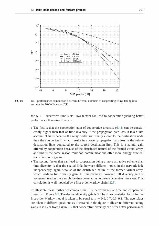
6.1 Multi-node decode-and-forward protocol 209
SNR per bit [dB]
Direct (BPSK)1 relay (QPSK)2 relays (8PSK)3 relays (16QAM)
0 5 10 15 20 25–5
SE
R
10−7
10−6
10−5
10−4
10−3
10−2
10–1
100
Fig. 6.6 BER performance comparison between different numbers of cooperating relays taking intoaccount the BW efficiency, C(1).
for N + 1 successive time slots. Two factors can lead to cooperation yielding betterperformance than time diversity:
• The first is that the cooperation gain of cooperative diversity (6.48) can be consid-erably higher than that of time diversity if the propagation path loss is taken intoaccount. This is because the relay nodes are usually closer to the destination nodethan the source itself, which results in a lower propagation path loss in the relay–destination links compared to the source–destination link. This is a natural gainoffered by cooperation because of the distributed natural of the formed virtual array,and this is the same reason multihop communications offer more energy efficienttransmission in general.
• The second factor that can lead to cooperation being a more attractive scheme thantime diversity is that the spatial links between different nodes in the network fadeindependently, again because of the distributed nature of the formed virtual array,which leads to full diversity gain. In time diversity, however, full diversity gain isnot guaranteed as there might be time correlation between successive time slots. Thiscorrelation is well modeled by a first-order Markov chain [226].
To illustrate these further we compare the SER performance of time and cooperativediversity in Figure 6.7. The desired diversity gain is 3. The time correlation factor for thefirst-order Markov model is taken to be equal to ρ = 0.9, 0.7, 0.3, 0.1. The two relaysare taken in different positions as illustrated in the figure to illustrate different codinggains. It is clear from Figure 6.7 that cooperative diversity can offer better performance
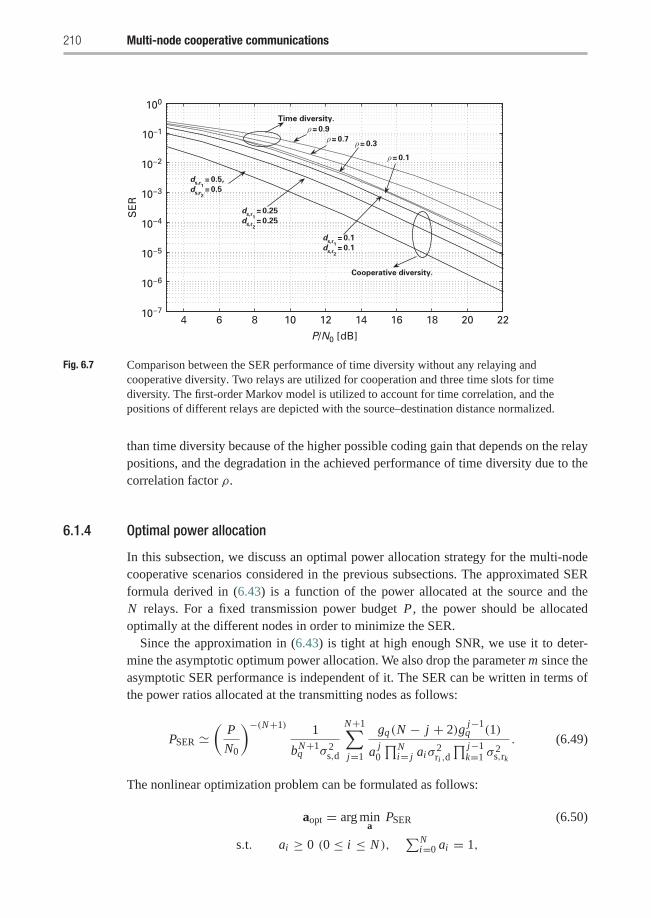
210 Multi-node cooperative communications
4 6 8 10 12 14 16 18 20 22
Time diversity.
ds,r
2 = 0.1
ds,r
1 = 0.1
ds,r
2 = 0.25
ds,r
1 = 0.25
ds,r
2 = 0.5
ds,r
1 = 0.5,
Cooperative diversity.
P/N0 [dB]
SE
R
10−7
10−6
10−5
10−4
10−3
10−2
10–1
100
ρ = 0.9
ρ = 0.7 ρ = 0.3
ρ = 0.1
Fig. 6.7 Comparison between the SER performance of time diversity without any relaying andcooperative diversity. Two relays are utilized for cooperation and three time slots for timediversity. The first-order Markov model is utilized to account for time correlation, and thepositions of different relays are depicted with the source–destination distance normalized.
than time diversity because of the higher possible coding gain that depends on the relaypositions, and the degradation in the achieved performance of time diversity due to thecorrelation factor ρ.
6.1.4 Optimal power allocation
In this subsection, we discuss an optimal power allocation strategy for the multi-nodecooperative scenarios considered in the previous subsections. The approximated SERformula derived in (6.43) is a function of the power allocated at the source and theN relays. For a fixed transmission power budget P , the power should be allocatedoptimally at the different nodes in order to minimize the SER.
Since the approximation in (6.43) is tight at high enough SNR, we use it to deter-mine the asymptotic optimum power allocation. We also drop the parameter m since theasymptotic SER performance is independent of it. The SER can be written in terms ofthe power ratios allocated at the transmitting nodes as follows:
PSER �(
P
N0
)−(N+1) 1
bN+1q σ 2
s,d
N+1∑j=1
gq(N − j + 2)g j−1q (1)
a j0
∏Ni= j aiσ
2ri ,d
∏ j−1k=1 σ
2s,rk
. (6.49)
The nonlinear optimization problem can be formulated as follows:
aopt = arg mina
PSER (6.50)
s.t. ai ≥ 0 (0 ≤ i ≤ N ),∑N
i=0 ai = 1,
6.1 Multi-node decode-and-forward protocol 211
where a = [a0, a1, . . . , aN ] is the power allocating vector. The Lagrangian of thisproblem can be written as
L = PSER + ν(
N∑i=0
ai − 1
)−
N∑j=0
β j a j (6.51)
where the β’s act as slack variables.Although this nonlinear optimization problem should, in general, be solved numer-
ically, there are some insights which can be drawn out of it. Applying first-orderoptimality conditions, we can show that the optimum power allocation vector aopt mustsatisfy the following necessary conditions:
∂PSER
∂ai= ∂PSER
∂a j, i, j ∈ {0, 1, 2, . . . , N }. (6.52)
Next, we solve these equations simultaneously to get the relations between the opti-mal power allocations at different nodes. To simplify the notations, let μ j denote theconstant quantity inside the summation in (6.49), i.e.,
μ j =(
P
N0
)−(N+1) gq(N − j + 2)g j−1q (1)
bN+1q σ 2
s,d
∏Ni= j σ
2ri ,d
∏ j−1k=1 σ
2s,rk
. (6.53)
The derivative of the SER with respect to a0 is given by
∂PSER
∂a0=
N+1∑j=1
− jμ j
a j+10
∏Ni= j ai
, (6.54)
while the derivative with respect to ak , 1 ≤ k ≤ N , is given by
∂PSER
∂ak=
k∑j=1
−μ j
a j0 ak∏N
i= j ai
, (6.55)
where the summation is to the k-th term only as ak does not appear in the terms fromk + 1 to N . Using (6.52), we equate the derivatives of the SER with respect to any twoconsecutive variables ak and ak+1, 1 ≤ k ≤ N − 1, as follows:
k∑j=1
−μ j
a j0 ak∏N
i= j ai
=k+1∑j=1
−μ j
a j0 ak+1
∏Ni= j ai
. (6.56)
Rearranging the terms in the above equation we get
ak+1 − ak
akak+1
k∑j=1
μ j
a j0
∏Ni= j ai
= μk+1
a j0 ak+1
∏Ni=k+1 ai
. (6.57)
Since both sides of the above equation are positive, we conclude that ak+1 ≥ ak for anyk = 1, 2, . . . , N . Similarly, we can show that ao ≥ ak for all 1 ≤ k ≤ N . Hence, solvingthe optimality conditions simultaneously we get the following relationships between thepowers allocated at different nodes:
P0 ≥ PN ≥ PN−1 ≥ · · · ≥ P1. (6.58)
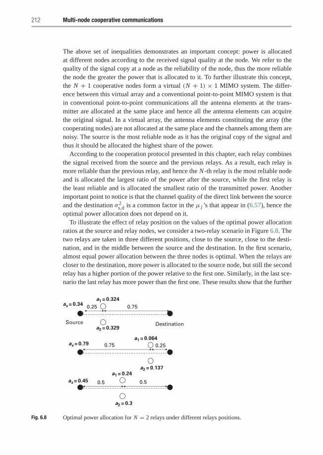
212 Multi-node cooperative communications
The above set of inequalities demonstrates an important concept: power is allocatedat different nodes according to the received signal quality at the node. We refer to thequality of the signal copy at a node as the reliability of the node, thus the more reliablethe node the greater the power that is allocated to it. To further illustrate this concept,the N + 1 cooperative nodes form a virtual (N + 1) × 1 MIMO system. The differ-ence between this virtual array and a conventional point-to-point MIMO system is thatin conventional point-to-point communications all the antenna elements at the trans-mitter are allocated at the same place and hence all the antenna elements can acquirethe original signal. In a virtual array, the antenna elements constituting the array (thecooperating nodes) are not allocated at the same place and the channels among them arenoisy. The source is the most reliable node as it has the original copy of the signal andthus it should be allocated the highest share of the power.
According to the cooperation protocol presented in this chapter, each relay combinesthe signal received from the source and the previous relays. As a result, each relay ismore reliable than the previous relay, and hence the N -th relay is the most reliable nodeand is allocated the largest ratio of the power after the source, while the first relay isthe least reliable and is allocated the smallest ratio of the transmitted power. Anotherimportant point to notice is that the channel quality of the direct link between the sourceand the destination σ 2
s,d is a common factor in the μ j ’s that appear in (6.57), hence theoptimal power allocation does not depend on it.
To illustrate the effect of relay position on the values of the optimal power allocationratios at the source and relay nodes, we consider a two-relay scenario in Figure 6.8. Thetwo relays are taken in three different positions, close to the source, close to the desti-nation, and in the middle between the source and the destination. In the first scenario,almost equal power allocation between the three nodes is optimal. When the relays arecloser to the destination, more power is allocated to the source node, but still the secondrelay has a higher portion of the power relative to the first one. Similarly, in the last sce-nario the last relay has more power than the first one. These results show that the further
0.25 0.75
0.25
0.50.5
0.75
Source Destination
a1 = 0.324
a2 = 0.329
a1 = 0.064
a2 = 0.137a1 = 0.24
a2 = 0.3
as = 0.34
as = 0.79
as = 0.45
Fig. 6.8 Optimal power allocation for N = 2 relays under different relays positions.
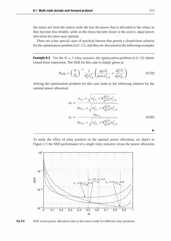
6.1 Multi-node decode-and-forward protocol 213
the relays are from the source node the less the power that is allocated to the relays asthey become less reliable, while as the relays become closer to the source, equal powerallocation becomes near optimal.
There are a few special cases of practical interest that permit a closed-form solutionfor the optimization problem in (6.50), and they are discussed in the following examples
Example 6.3 For the N = 1 relay scenario, the optimization problem in (6.50) admitsclosed-form expression. The SER for this case is simply given as
PSER =(
P
N0
)−2 1
b2qσ
2s,d
(gq(2)
a0a1σ2r1,d
+ g2q(1)
a20σ
2s,r1
). (6.59)
Solving the optimization problem for this case leads to the following solution for theoptimal power allocation:
a0 =σs,r1 +
√σ 2
s,r1 + 8g2
q (1)gq (2)
σ 2r1,d
3σs,r1 +√σ 2
s,r1 + 8g2
q (1)gq (2)
σ 2r1,d
,
a1 = 2σs,r1
3σs,r1 +√σ 2
s,r1 + 8g2
q (1)gq (2)
σ 2r1,d
. (6.60)
�
To study the effect of relay position on the optimal power allocation, we depict inFigure 6.9 the SER performance of a single relay scenario versus the power allocation
0 0.1 0.2 0.3 0.4 0.5 0.6 0.7 0.8 0.9 1a0
ds,r = 0.25, dr,d = 0.75
ds,r = 0.5, dr,d = 0.5ds,r = 0.75, dr,d = 0.25S
ER
10−3
10−2
10–1
100
Fig. 6.9 SER versus power allocation ratio at the source node for different relay positions.
214 Multi-node cooperative communications
at the source node a0 for different relay positions. The first observation that the fig-ure reveals is that the SER performance is relatively flat around equal power allocationwhen the relay is not very close to the destination. Another observation to notice here isthat as the relay becomes closer to the destination, the value of the optimal power allo-cation at the source node a0 approaches 1, which means that as the relay node becomesless reliable more power should be allocated to the source node.
Example 6.4 The propagation path-loss and networks with linear topologies will betaken into account here. The channel attenuation between any two nodes σ 2
i, j depends
on the distance between these two nodes di, j as follows: σ 2i, j ∝ d−α , where α is the
propagation constant. For a linear network topology, the most significant channel gainsare for the channels between the source and the first relay σ 2
s,r1 , and between the lastrelay and the destination σ 2
rN ,d, the other channel gains are considerably smaller than
these two channels. In the SER expression in (6.43), these two terms appear as a productin all the terms except the first and the last. Hence these two terms dominate the SERexpression, and we can further approximate the SER in this case as follows:
PSER � (No/P)N+1
bN+1q σ 2
s,d
[gq(N + 1)
a0∏N
i=1 aiσ2ri ,d
+ gN+1q (1)
aN+10
∏Ni=1 σ
2s,ri
]. (6.61)
Taking the power constraint into consideration, the Lagrangian of the above problemcan be written as
L(a) = μ1
ao∏N
i=1 ai+ μN+1
aN+1o
+ λ(
N∑i=0
ai − 1
). (6.62)
Taking the partial derivatives of the Lagrangian with respect to a j , 1 ≤ j ≤ N , andequating with 0, we get
a j = μ1
λao∏N
i=1 ai. (6.63)
Thus, we deduce that the power allocated to all of the relays is the same. Let the constantκ be defined as follows:
κ = P0 − Pj
Pj. (6.64)
From the above definition, along with the power constraint, we get
Pj = 1
1+ κ + NP,
P0 = 1+ κ1+ κ + N
P. (6.65)
To find the optimum value for κ , substitute (6.65) into the expression for the SER in(6.61) to get
PSER � μ1(1+ κ)N (1+ κ + N )N+1 + μN+1(1+ κ + N )N+1
(1+ κ)N+1. (6.66)
6.1 Multi-node decode-and-forward protocol 215
Differentiating (6.66) and equating to 0, we can find that the optimum κ satisfies theequation κ(1+ κ)N = A, in which A is a constant given by
A = (N + 1)gN+1
q (1)∏N
i=1 σ2ri ,d
gq(N + 1)∏N
i=1 σ2s,ri
. (6.67)
�
From the above analysis, the optimal power allocation for a linear network can be foundin the following theorem.
T H E O R E M 6.1.3 The optimal power allocation for a linear network that minimizesthe SER expression in (6.61) is as follows:
P0 = 1+ κ1+ κ + N
P, Pi = 1
1+ κ + NP, 1 ≤ i ≤ N , (6.68)
where κ is found through solving the equation κ(1+ κ)N = A, in which A is a constant
given by (N + 1)gN+1(1)
∏Ni=1 σ
2ri ,d
g(N+1)∏N
i=1 σ2s,ri
.
The above theorem agrees with the optimality conditions we found for the general prob-lem in (6.58). Also, it shows an interesting property that in linear network topologiesequal power allocation at the relays is asymptotically optimal.
Example 6.5 The cooperating relays can be chosen to be closer to the source than tothe destination, in order for the N + 1 cooperating nodes to mimic a multi-input-single-output (MISO) transmit antenna diversity system. This case is of special interest becausedecode-and-forward relaying can be a capacity achieving scheme when the relays aretaken to be closer to the source and it has the best performance compared to amplify-and-forward and compress-and-forward relaying in this case. In order to model thisscenario in our SER formulation, we will consider the channel gains from the sourceto the relays to have higher gains than those from the relays to the destination, i.e.,σ 2
s,ri � σ 2ri ,d
for 1 ≤ i ≤ N . Taking this into account, the approximate SER expressionin (6.43) can be further approximated as
PSER � N N+10 gq(N + 1)
bN+1q σ 2
s,d P N+1a0∏N
i=1 aiσ2ri ,d
. (6.69)
It is clear from the above equation that the SER depends equally on the power allocatedto all nodes including the source, and thus the optimal power allocation strategy for thiscase is simply given by
P0 = Pi = P
N + 1, 1 ≤ i ≤ N . (6.70)
216 Multi-node cooperative communications
This result is intuitively meaningful as all the relays are located near to the sourceand thus they all have high reliability and are allocated equal power as if they forma conventional antenna array. �
Example 6.6 Now we consider the opposite scenario in which all the relays are locatednear the destination. In this case the channels between the relays and the destinationare of a higher quality, higher gain, than those between the source and the relays, i.e.,σ 2
ri ,d� σ 2
s,ri for 1 ≤ i ≤ N . In this case the SER can be approximated as
PSER � N N+10 g(1)N+1
bN+1q σ 2
s,d P N+10
∏Nk=1 σ
2s,rk
. (6.71)
The SER in the above equation is not a function of the power allocated at the coop-erating relays, and thus the optimal power allocation in this case is simply P0 = P ,i.e., allocating all the available power at the source. This result is very interesting as itreveals a very important concepts: If the relays are located closer to the destination thanto the transmitter then direct transmission can lead better performance than decode-and-forward relaying. This is also consistent with the results in [99] in which it was shownthat the performance of the decode-and-forward strategy degrades significantly whenthe relays get closer to the destination. This result can be intuitively interpreted as fol-lows: the further the relays are from the source the more noisy the channels betweenthem and the less reliable the signals received by those relays, to the extent that we cannot rely on them on forwarding copies of the signal to the destination. �
6.1.4.1 Numerical examplesIn this subsection, we present some numerical results to verify the analytical results forthe optimal power allocation problem for the considered network topologies. The effectof the geometry on the channel links qualities is taken into consideration. We assumethat the channel variance between any two nodes is proportional to the distance betweenthem, more specifically σ 2
i, j ∝ d−αi, j , where α is determined by the propagation environ-ment is taken equal to 4 throughout our simulations. We provide comparisons betweenthe optimal power allocation via exhaustive search to minimize the SER expression in(6.43), and optimal power allocation provided by the closed-form expressions providedin this section.
First, for the linear network topology, we consider a uniform linear network, i.e.,ds,r1 = dr1,r2 = · · · = drN ,d. The variance of the direct link between the source andthe destination is taken to be σ 2
s,d = 1. Table 6.1 demonstrates the results for N = 3relays. Second, for the case when all the relays are near the source, the channel linksare taken to be: σ 2
s,ri = σ 2ri ,r j
= 10, while σ 2s,d = σ 2
ri ,d= 0.1. Finally, for the case
when all of the relays are near the destination, the channel link qualities are taken tobe: σ 2
s,d = σ 2s,ri = 0.1, while σ 2
ri ,r j= σ 2
ri ,d= 10. Table 6.2 illustrates the results for
N = 3 relays for the two previous cases. In all of the provided numerical examples it is

6.2 Multi-node amplify-and-forward protocol 217
Table 6.1 Comparison between optimal power allocation via exhaustivesearch and analytical results. N= 3 relays, uniform network topology.
Exhaustive search Analytical results
P0 = 0.31P P0 = 0.31PP1 = 0.23P P1 = 0.23PP2 = 0.23P P2 = 0.23PP3 = 0.23P P3 = 0.23P
Table 6.2 Comparison between optimal power allocation via exhaustive search and analytical results.N= 3 relays: (a) all relays near the source; (b) all relays near the destination.
(a) Exhaustive search Analytical results (b) Exhaustive search Analytical results
P0 = 0.25P P0 = 0.25P P0 = 0.875P P0 = PP1 = 0.25P P1 = 0.25P P1 = 0.015P P1 = 0P2 = 0.25P P2 = 0.25P P2 = 0.035P P2 = 0P3 = 0.25P P3 = 0.25P P3 = 0.075P P3 = 0
clear that the optimal power allocations obtained via exhaustive search agree with thatvia analytical results for all the considered scenarios. In addition, the numerical resultsshow that the optimal power allocation obtained via exhaustive search has the sameordering as the one we got in (6.58).
6.2 Multi-node amplify-and-forward protocol
In the second part of this chapter, we focus on a multi-node amplify-and-forward strat-egy. Different from the decode-and-forward protocol, an amplify-and-forward protocoldoes not suffer from the error propagation problem because the relays do not performany hard-decision operation on the received signal. We first describe the multi-nodeamplify-and-forward protocol in detail and then analyze its SER performance. Finally,we consider the outage probability of the multi-node amplify-and-forward protocol, aswell as the mutual information of the system.
The multi-node amplify-and-forward system model is shown in Figure 6.10. In thefollowing, we will consider two relaying strategies. In the first scenario, each relayforwards only the source’s signal to the the destination, while in the second scenarioeach relay forwards a combined signal from the source and previous relays.
6.2.1 Source-only amplify-and-forward relaying
6.2.1.1 System model and protocol descriptionWe first consider a source-only multi-node amplify-and-forward relaying strategy, i.e.,each relay forwards only the source’s signal to the the destination, in which cooperation
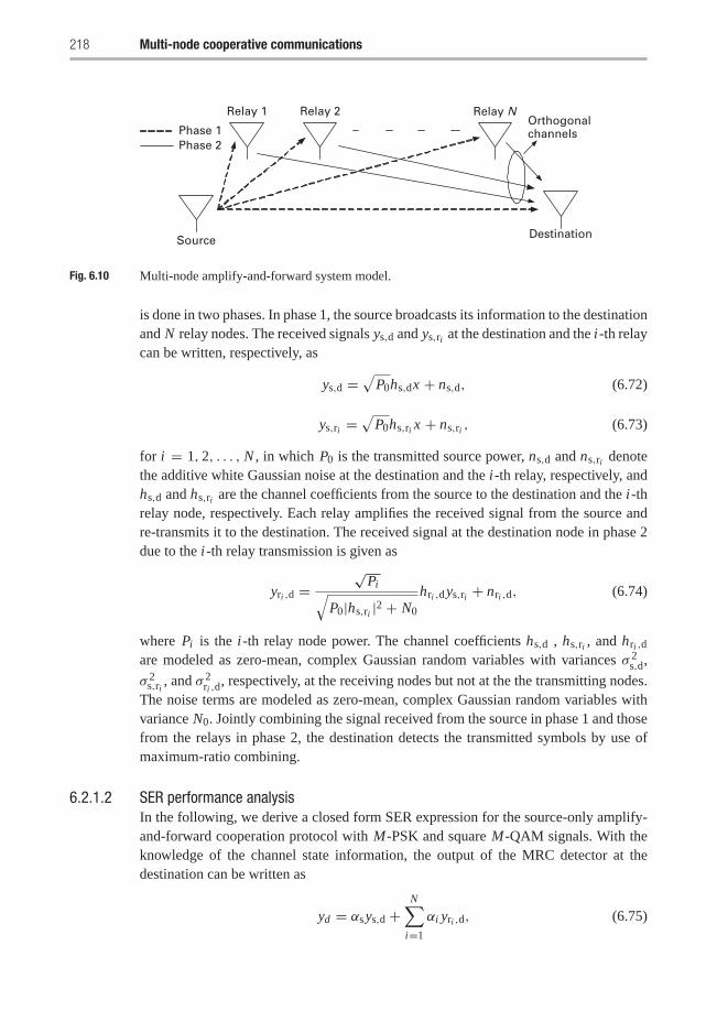
218 Multi-node cooperative communications
Source Destination
Relay 1 Relay 2 Relay NOrthogonalchannelsPhase 1
Phase 2
Fig. 6.10 Multi-node amplify-and-forward system model.
is done in two phases. In phase 1, the source broadcasts its information to the destinationand N relay nodes. The received signals ys,d and ys,ri at the destination and the i-th relaycan be written, respectively, as
ys,d =√
P0hs,dx + ns,d, (6.72)
ys,ri =√
P0hs,ri x + ns,ri , (6.73)
for i = 1, 2, . . . , N , in which P0 is the transmitted source power, ns,d and ns,ri denotethe additive white Gaussian noise at the destination and the i-th relay, respectively, andhs,d and hs,ri are the channel coefficients from the source to the destination and the i-threlay node, respectively. Each relay amplifies the received signal from the source andre-transmits it to the destination. The received signal at the destination node in phase 2due to the i-th relay transmission is given as
yri ,d =√
Pi√P0|hs,ri |2 + N0
hri ,dys,ri + nri ,d, (6.74)
where Pi is the i-th relay node power. The channel coefficients hs,d , hs,ri , and hri ,d
are modeled as zero-mean, complex Gaussian random variables with variances σ 2s,d,
σ 2s,ri , and σ 2
ri ,d, respectively, at the receiving nodes but not at the the transmitting nodes.
The noise terms are modeled as zero-mean, complex Gaussian random variables withvariance N0. Jointly combining the signal received from the source in phase 1 and thosefrom the relays in phase 2, the destination detects the transmitted symbols by use ofmaximum-ratio combining.
6.2.1.2 SER performance analysisIn the following, we derive a closed form SER expression for the source-only amplify-and-forward cooperation protocol with M-PSK and square M-QAM signals. With theknowledge of the channel state information, the output of the MRC detector at thedestination can be written as
yd = αsys,d +N∑
i=1
αi yri ,d, (6.75)
6.2 Multi-node amplify-and-forward protocol 219
where αs = √P0h∗s,d/N0 and
αi =
√P0 Pi
P0|hs,ri |2+N0h∗s,ri h
∗ri ,d(
Pi |hri ,d|2P0|hs,ri |2+N0
+ 1
)N0
.
If we assume that the transmitted symbol x has an average energy of 1, then the SNRat the MRC detector output is
SNRd = γs +N∑
i=1
γi (6.76)
where γs = P0|hs,d|2/N0, and
γi = 1
N0
P0 Pi |hs,ri |2|hri ,d|2P0|hs,ri |2 + Pi |hri ,d|2 + N0
. (6.77)
The instantaneous SNR γi can be tightly upper bounded as
γi = 1
N0
P0 Pi |hs,ri |2|hri ,d|2P0|hs,ri |2 + Pi |hri ,d|2
, (6.78)
which is the harmonic mean of P0|hs,ri |2/N0 and Pi |hri ,d|2/N0. The SER of M-PSKand M-QAM conditional on the channel state information are defined before in (6.11)and (6.12), respectively.
Let us denote the MGF of a random variable Z as
MZ (s) =∫ ∞
−∞exp(−sz)PZ (z)dZ . (6.79)
Averaging the conditional SER over the Rayleigh fading channels, the SER of the M-PSK signals and M-QAM signals can be given, respectively, as
PSER ≈ 1
π
∫ (M−1)π/M
0Mγs
(bPSK
sin2 θ
) N∏i=1
Mγi
(bPSK
sin2 θ
)dθ, (6.80)
PSER ≈ 4C
π
∫ π/2
0Mγs
(bQAM
2 sin2 θ
) N∏i=1
Mγi
(bQAM
2 sin2 θ
)dθ
− 4C2
π
∫ π/4
0Mγs
(bQAM
2 sin2 θ
) N∏i=1
Mγi
(bQAM
2 sin2 θ
)dθ, (6.81)
in which we use the SNR approximation γi (6.78) instead of γi .The MGF of γs, which is an exponential random variable, can be simply given by
Mγs =1
1+ s P0σ2s,d
N0
. (6.82)
The challenge is how to get the MGF of γi . We follow the same approach of analyzingthe SER performance of the single-relay amplify-and-forward protocol as presented in
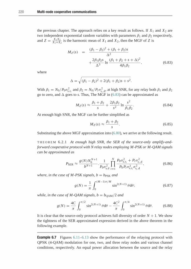
220 Multi-node cooperative communications
the previous chapter. The approach relies on a key result as follows. If X1 and X2 aretwo independent exponential random variables with parameters β1 and β2 respectively,and Z = X1 X2
X1+X2is the harmonic mean of X1 and X2, then the MGF of Z is
MZ (s) = (β1 − β2)2 + (β1 + β2)s
�2
+2β1β2s
�3ln(β1 + β2 + s +�)2
4β1β2, (6.83)
where
� =√(β1 − β2)2 + 2(β1 + β2)s + s2.
With β1 = N0/P0σ2s,ri and β2 = N0/Piσ
2ri ,d
, at high SNR, for any relay both β1 and β2
go to zero, and � goes to s. Thus, The MGF in (6.83) can be approximated as
MZ (s) ≈ β1 + β2
s+ 2β1β2
s2ln
s2
β1β2. (6.84)
At enough high SNR, the MGF can be further simplified as
MZ (s) ≈ β1 + β2
s. (6.85)
Substituting the above MGF approximation into (6.80), we arrive at the following result.
T H E O R E M 6.2.1 At enough high SNR, the SER of the source-only amplify-and-forward cooperative protocol with N relay nodes employing M-PSK or M-QAM signalscan be approximated as
PSER ≈ g(N )N N+10
bN+1.
1
P0σ2s,d
N∏i=1
P0σ2s,ri + Piσ
2ri ,d
P0 Piσ 2s,riσ
2ri ,d
, (6.86)
where, in the case of M-PSK signals, b = bPSK and
g(N ) = 1
π
∫ (M−1)π/M
0sin2(N+1) θdθ; (6.87)
while, in the case of M-QAM signals, b = bQAM/2 and
g(N ) = 4C
π
∫ π/2
0sin2(N+1) θdθ − 4C2
π
∫ π/4
0sin2(N+1) θdθ. (6.88)
It is clear that the source-only protocol achieves full diversity of order N + 1. We showthe tightness of the SER approximated expression derived in the above theorem in thefollowing example.
Example 6.7 Figures 6.11–6.13 show the performance of the relaying protocol withQPSK (4-QAM) modulation for one, two, and three relay nodes and various channelconditions, respectively. An equal power allocation between the source and the relay
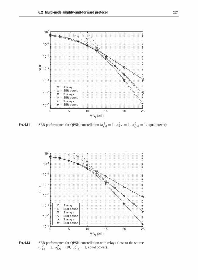
6.2 Multi-node amplify-and-forward protocol 221
0 5 10 15 20 25
1 relaySER bound2 relaysSER bound3 relaysSER bound
P/N0 [dB]
SE
R
10−6
10−5
10−4
10−3
10−2
10–1
100
Fig. 6.11 SER performance for QPSK constellation (σ 2s,d = 1, σ 2
s,ri = 1, σ 2ri ,d
= 1, equal power).
0 5 10 15 20 25
SE
R
10−7
10−6
10−5
10−4
10−3
10−2
10–1
100
1 relaySER bound2 relaysSER bound3 relaysSER bound
P/N0 [dB]
Fig. 6.12 SER performance for QPSK constellation with relays close to the source(σ 2
s,d = 1, σ 2s,ri = 10, σ 2
ri ,d= 1, equal power).
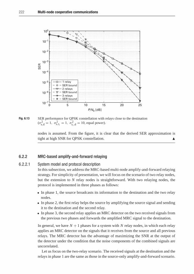
222 Multi-node cooperative communications
0 5 10 15 20 25
1 relaySER bound2 relaysSER bound3 relaysSER bound
P/N0 [dB]
SE
R
10−7
10−6
10−5
10−4
10−3
10−2
10–1
100
Fig. 6.13 SER performance for QPSK constellation with relays close to the destination(σ 2
s,d = 1, σ 2s,ri = 1, σ 2
ri ,d= 10, equal power).
nodes is assumed. From the figure, it is clear that the derived SER approximation istight at high SNR for QPSK constellation. �
6.2.2 MRC-based amplify-and-forward relaying
6.2.2.1 System model and protocol descriptionIn this subsection, we address the MRC-based multi-node amplify-and-forward relayingstrategy. For simplicity of presentation, we will focus on the scenario of two relay nodes,but the extension to N relay nodes is straightforward. With two relaying nodes, theprotocol is implemented in three phases as follows:
• In phase 1, the source broadcasts its information to the destination and the two relaynodes.
• In phase 2, the first relay helps the source by amplifying the source signal and sendingit to the destination and the second relay.
• In phase 3, the second relay applies an MRC detector on the two received signals fromthe previous two phases and forwards the amplified MRC signal to the destination.
In general, we have N + 1 phases for a system with N relay nodes, in which each relayapplies an MRC detector on the signals that it receives from the source and all previousrelays. The MRC detector has the advantage of maximizing the SNR at the output ofthe detector under the condition that the noise components of the combined signals areuncorrelated.
Let us focus on the two-relay scenario. The received signals at the destination and therelays in phase 1 are the same as those in the source-only amplify-and-forward scenario.
6.2 Multi-node amplify-and-forward protocol 223
In phase 2, the received signal at the destination due to the first relay transmission is alsothe same as in the source-only scenario. However, the received signal at the second relaydue to the first relay transmission is given as
yr1,r2 =√
P1√P0|hs,r1 |2 + N0
hr1,r2 ys,r1 + nr1,r2 , (6.89)
where the inter-relay channel, hr1,r2 , is modeled as a zero-mean, complex Gaussian ran-dom variable with variance σ 2
r1,r2 . In phase 3, the second relay applies an MRC detectoron the signals received in phases 1 and 2, and the output of the MRC detector can bewritten as
y = αsys,r2 + α1yr1,r2 , (6.90)
where αs = √P0h∗s,r2/N0 and
α1 =
√P0 P1
P0|hs,r1 |2+N0h∗s,r1h∗r1,r2(
P1|hr1,r2 |2P0|hs,r1 |2+N0
+ 1
)N0
.
The received signal at the destination in phase 3 is given by
yr2,d =√
P2hr2,dy√
K 2 + K+ nr2,d, (6.91)
where
K =P0 P1
P0|hs,r1 |2+N0|hs,r1 |2|hr1,r2 |2(
P1|hr1,r2 |2P0|hs,r1 |2+N0
+ 1
)N0
+ P0|hs,r2 |2N0
. (6.92)
Finally, the destination applies an MRC detector on the signals that it receives from allphases and jointly detects the information from the source.
6.2.2.2 Performance analysisIn this subsection, we try to gain some insight into the performance of the MRC-basedamplify-and-forward protocol. We again focus on the two-relay scenario. The analysiscan be similarly extended to the case of more relay nodes. With the knowledge of thechannel state information, the output of the MRC detector in the two-relay case can bewritten as
yd = αsys,d + α1yr1,d + α2yr2,d, (6.93)
where αs, α1 are the same as the source-only amplify-and-forward protocol and α2 isgiven by
α2 =√
P2h∗r2,dK√
K 2+K
P2|hr2,d|2 KK 2+K
+ N0.
The SER analysis of the protocol is very complicated and a close-form analysis is nottractable.
224 Multi-node cooperative communications
We may think the performance of the MRC-based protocol would be better than thatof the source-only protocol since the relays put more efforts in forwarding signals. How-ever, simulations show that this is not the case. The reason behind this is that the systemsuffers from the noise propagation problem. For the simple example of two relays net-work, the noise terms at the destination in phases 2 and 3 contain a contribution fromthe noise generated at the first relay, ns,r1 in phase 1. So the noise components in thereceived signals during the several phases are no more uncorrelated and the MRC detec-tor is no more optimal. This noise propagation problem causes a degradation in the SERperformance of the protocol. The problem is more severe for increased number of relaysbecause we will have more noise components that will propagate to the destination. Theoptimum receiver in this case is to apply a pre-whitening on the received signals andthen apply the MRC detector. Although the source-only amplify-and-forward protocolis less complex than the MRC-based amplify-and-forward protocol, we will show that itcan give approximately the same, if not better in some cases, SER performance. This isbecause the benefit we get from applying an MRC detector at each relay node is dimin-ished by the noise propagation problem. To see the effect of the noise propagation onthe MRC-based protocol, we consider two extreme scenarios for the two-relay networkand compare the performance of the two protocols under these two scenarios:
(i) |hr1,d| = 0: In this case, we do not have the noise propagation problem because thenoise term ns,r1 will be received only once in phase 3. In this case the SNR at thedestination of the MRC-based protocol can be written as
SNRMRC � P0|hs,d|2N0
+ KP2|hr2,d|2
N0
K + P2|hr2,d|2N0
. (6.94)
Similarly, the SNR at the destination of the source-only protocol can be written as
SNRsource-only �P0|hs,d|2
N0+
P0|hs,r2 |2N0
.P2|hr2,d|2
N0
P0|hs,r2 |2N0
+ P2|hr2,d|2N0
. (6.95)
Clearly, SNRMRC > SNRsource-only because K >P0|hs,r2 |2
N0. Intuitively, because
we do not have noise propagation in this case, it is better for relay 2 to combinethe signals it receives from both the source and relay 1 using the MRC detector tomaximize the SNR at its output instead of using the source signal only. Under thisscenario the MRC-based protocol is better than the source-only protocol because itresults in a higher SNR at the destination.
(ii) |hr1,d| >>, |hr2,d| >>, |hr1,r2 | >> and |hs,r2 | = 0: In this case, the relay–destination links can be approximated to be noise free. The output of the destinationdetector in the MRC-based protocol can be written as
yMRC �(
P0|hs,d|2N0
+ 2P0|hs,r1 |2
N0
)x +
√P0h∗s,dN0
ns,d (6.96)
+2√
P0h∗s,r1N0
ns,r1 , (6.97)
6.2 Multi-node amplify-and-forward protocol 225
because the signal at the first relay in phase 1 is transmitted twice in phases 2 and 3.The output of the destination detector in the source-only protocol can be written as
ysource-only �(
P0|hs,d|2N0
+ P0|hs,r1 |2N0
)x (6.98)
+√
P0h∗s,dN0
ns,d +√
P0h∗s,r1N0
ns,r1 . (6.99)
Clearly, we have
SNRsource-only �P0|hs,d|2
N0+ P0|hs,r1 |2
N0(6.100)
> SNRMRC �
(P0|hs,d|2
N0+ 2
P0|hs,r1 |2N0
)2
P0|hs,d|2N0
+ 4P0|hs,r1 |2
N0
. (6.101)
In this case, the source-only protocol achieves better performance than the MRC-based protocol. This is because the MRC-based protocol combines the same signaltwice (the signals received in phases 2 and 3). Thus, in this case, the noise propa-gation problem is highly severe and causes a high degradation in the system SERperformance.
Although the above two scenarios occur with zero probability, they can give someinsights about how the system performance is affected by the different channels mag-nitudes. From the above two scenarios, intuition suggests that the source-only protocolwill give better performance than the MRC-based protocol if the relays become closer tothe destination. Moreover, the MRC-based protocol requires more channels to estimateat each relay node, which increases the overhead in the network required for channelestimation. Finally, the MRC-based protocol may have a higher delay because eachrelay node must wait for the transmission of all of the previous relay nodes, while in thesource-only amplify-and-forward protocol, all the relays can forward the source data atthe same time using FDM, for example.
6.2.3 Outage analysis and optimum power allocation
In this subsection, we investigate the outage performance of the source-only multi-nodeamplify-and-forward relaying protocol and determine its optimum power allocation.
We recall that in the source-only relaying protocol, the received signal at thedestination in phase 2 due to the i-th relay transmission is given by
yri ,d = hri ,dβi ys,ri + nri ,d, (6.102)
and βi is a scaling factor that satisfies the power constraint
βi ≤√
Pi
P0|hs,ri |2 + N0. (6.103)
226 Multi-node cooperative communications
The output of the MRC detector is given by
yd = αsys,d +N∑
i=1
αi yri ,d, (6.104)
where αs = √P0h∗s,d/N0 and αi =
√P0βi h∗ri ,dh∗s,ri
(β2i |hri ,d|2+1)N0
. We can write yd in terms of the
source signal x as
yd =(
P0|hs,d|2N0
+N∑
i=1
P0β2i |hri ,d|2|hs,ri |2
(β2i |hri ,d|2 + 1)N0
)x +
√P0h∗s,dN0
ns,d
+N∑
i=1
√P0βi h∗ri ,dh∗s,ri
(β2i |hri ,d|2 + 1)N0
(nri ,d + hri ,dβi ns,ri ). (6.105)
The SNR at the MRC detector output is
SNRd = γs +N∑
i=1
γi (6.106)
where γs = P0|hs,d|2/N0, and
γi = P0β2i |hri ,d|2|hs,ri |2
(β2i |hri ,d|2 + 1)N0
. (6.107)
For simplicity, let us denote an (N + 1)× 1 vector
y = [ys,d, yr1,d, . . . , yrN ,d]T. (6.108)
Then, for given x and channel state information, the probability density function (pdf)of y follows an exponential distribution. Moreover, yd is a sufficient statistic for x , i.e.,
py/x,yd (y/x, yd) = py/yd (y/yd), (6.109)
where py/x,yd (y/x, yd) is pdf of y given x and yd , and py/yd (y/yd) is the pdf of y givenyd . Since yd is a sufficient statistics for x , then the mutual information between x and yequals the mutual information between x and yd , that is
I (x; yd) = I (x; y). (6.110)
Then the average mutual information for amplify-and-forward IAF satisfies
IAF ≤ I (x; yd) ≤ log
(1+ P0|hs,d|2
N0+
N∑i=1
P0β2i |hri ,d|2|hs,ri |2
(β2i |hri ,d|2 + 1)N0
), (6.111)
with equality for x being a zero-mean, circularly symmetric complex Gaussian ran-dom variable. It is clear that (6.111) is increasing in βi ’s, so to maximize the mutualinformation the constraint in (6.103) should be satisfied with equality, yielding
IAF = log
(1+ |hs,d|2SNRs,d +
N∑i=1
f(|hs,ri |2SNRs,ri , |hri ,d|2SNRri ,d
)),
6.2 Multi-node amplify-and-forward protocol 227
where SNRs,d = SNRs,ri = P0/N0 and SNRri ,d = Pi/N0 for all i = 1, 2, . . . , N , and
f (v, u) = uv
u + v + 1.
6.2.3.1 Outage analysisThe outage probability for spectral efficiency R is defined as
PoutAF (R) = Pr
{1
N + 1IAF < R
}, (6.112)
and the 1/(N + 1) factor comes from the fact that the relays help the source through Nuses of orthogonal channels. Using the notation
p = [P0, P1, P2, . . . , PN ]T, (6.113)
equation (6.112) can be rewritten as
PoutAF (p, R) = Pr
{(P0
N0|hs,d|2 +
N∑i=1
f
(P0
N0|hs,ri |2,
Pi
N0|hri ,d|2
))<(2(N+1)R − 1
)}.
At high SNR, we can neglect the 1 in the denominator of the function f (u, v), and itfollows that the outage probability is given by
PoutAF (p, R) � Pr
{(P0
N0|hs,d|2 +
N∑i=1
P0N0|hs,ri |2 Pi
N0|hri ,d|2
P0N0|hs,ri |2 + Pi
N0|hri ,d|2
)<(2(N+1)R − 1
)}.
Denote some random variables
w1 = P0
N0|hs,d|2
wi+1 =P0N0|hs,ri |2 Pi
N0|hri ,d|2
P0N0|hs,ri |2 + Pi
N0|hri ,d|2
, ∀i ∈ [1, N ]. (6.114)
The outage probability is now given as
PoutAF (p, R) � Pr
⎧⎨⎩N+1∑j=1
w j < (2(N+1)R − 1)
⎫⎬⎭ . (6.115)
The random variable w1 has an exponential distribution with rate
λ1 = N0
P0σ2s,d
. (6.116)
To calculate the outage probability in (6.115), we consider an approach based onapproximating the harmonic mean of two exponential random variables by an expo-nential random variable.
Note that each w j for j ∈ [2, N + 1] is a harmonic mean of two exponential randomvariables. The CDF of w j , j = 2, . . . , N + 1 can be given as
Pw j (w) = Pr{w j < w
} = 1− 2w√ζ j1ζ j2e−w(ζ j1+ζ j2)K1(2w
√ζ j1ζ j2), (6.117)
228 Multi-node cooperative communications
where
ζ j1 = N0
P0σ 2s,r j−1
ζ j2 = N0
Pj−1σ 2s,r j−1
(6.118)
and K1(·) is the first-order modified Bessel function of the second kind. The func-tion K1(·) can be approximated as K1(x) � 1/x for small x , from which we canapproximate the CDF of w j at high SNR as
Pw j (w) = Pr{w j < w
} � 1− e−w(ζ j1+ζ j2), (6.119)
which is the CDF of an exponential random variable of rate
λ j = N0
P0σ 2s,r j−1
+ N0
Pj−1σ2r j−1,d
. (6.120)
Define a random variable W as
W =N+1∑j=1
w j , (6.121)
the CDF of W , assuming the λi ’s to be distinct, can be obtained as
Pr {W ≤ w} �N+1∑k=1
⎛⎝ N+1∏m=1,m �=k
λm
λm − λk
⎞⎠ (1− e−λkw). (6.122)
The outage probability can be expressed in terms of the CDF of W as
PoutAF (p, R) � Pr
{W ≤ (2(N+1)R − 1)
}. (6.123)
The CDF of W can now be written as
Pr {W ≤ w} =N+1∑k=1
⎛⎝ N+1∏m=1,m �=k
λm
λm − λk
⎞⎠(N+1∑n=1
(−1)n+1λnkwn
n!
)+ H.O.T., (6.124)
where H.O.T. stands for the higher order terms. Rearranging the terms in (6.124) we get
Pr {W ≤ w} =N+1∑n=1
⎛⎝N+1∑k=1
⎛⎝ N+1∏m=1,m �=k
λm
λm − λk
⎞⎠ λnk
⎞⎠ (−1)n+1wn
n!+ H.O.T. (6.125)
In order for the system to achieve a diversity of order (N + 1), the coefficients of wn
have to be zero for all n ∈ [1, N ]. This requirement can be reformulated in a matrixform as
6.2 Multi-node amplify-and-forward protocol 229
⎡⎢⎢⎢⎣λ1 . . . λN+1
λ21 . . . λ2
N+1...
......
λN+11 . . . λN+1
N+1
⎤⎥⎥⎥⎦︸ ︷︷ ︸
V
⎡⎢⎢⎢⎢⎣∏N+1
m=2λm
λm−λ1∏N+1m=1,m �=2
λmλm−λ2
...∏Nm=1
λmλm−λN+1
⎤⎥⎥⎥⎥⎦︸ ︷︷ ︸
q
=
⎡⎢⎢⎢⎣00...
c1
⎤⎥⎥⎥⎦ . (6.126)
To prove (6.126), let us consider the following equations:
Va = [0, 0, . . . , 1]T︸ ︷︷ ︸c
, (6.127)
where c1 is some non-zero constant, and q = c1a. Note that as the columns ofthe V matrix are scaled versions of the columns of a Vandermonde matrix, i.e., itis a nonsingular matrix, the solution for the system of equations in (6.127) can befound as
a = V−1c = 1
det(V)adj(V)c. (6.128)
where adj(V) is the adjoint matrix of V. The determinant of a Vandermonde matrix isgiven by
det
⎡⎢⎢⎢⎣1 1 . . . 1λ1 λ2 . . . λN+1...
......
...
λN1 λN
2 . . . λNN+1
⎤⎥⎥⎥⎦ =N+1∏k=1
N+1∏m>k
(λm − λk), (6.129)
from which we can express the determinant of the V matrix as
det(V) =⎛⎝N+1∏
j=1
λ j
⎞⎠ N+1∏k=1
N+1∏m>k
(λm − λk). (6.130)
Due to the structure of the c vector, we are only interested in the last column of theadj(V) matrix. The i-th element of the a vector can be obtained as
ai =(−1)N+i−1
(∏N+1j=1, j �=i λ j
)∏N+1k=1,k �=i
∏N+1m>k,m �=i (λm − λk)(∏N+1
j=1 λ j
)∏N+1k=1
∏N+1m>k (λm − λk)
= (−1)N
λi
N+1∏j=1, j �=i
1
(λ j − λi ). (6.131)
From (6.131), it is clear that q = c1a where
c1 = (−1)NN+1∏i=1
λi . (6.132)
230 Multi-node cooperative communications
Using the CDF of W defined in (6.125), The outage probability can now beexpressed as
PoutAF (p, R) � Pr
{W < (2(N+1)R − 1)
}= 1
(N + 1)!
(N+1∏i=1
λi
)(2(N+1)R − 1
)N+1 + H.O.T.
(6.133)
Based on the λi ’s from (6.116), we get
PoutAF (p, R) ∼ 1
(N + 1)! .1
P0σ2s,d
.
N∏i=1
P0σ2s,ri + Piσ
2ri ,d
P0 Piσ 2s,riσ
2ri ,d
(2(N+1)R − 1
)N+1N N+1
0 .
(6.134)
From the expression in (6.134), let P be the total power and let P0 = a0 P andPi = ai P where a0 +∑N
i=1 ai = 1, a0 > 0, ai > 0, i = 1, . . . , N . Denote the SNRas SNR = P/N0, the diversity order of the system, based on the outage probability, isdefined as
doutAF = lim
SNR→∞−log Pout
AF (SNR, R)
log SNR= N + 1. (6.135)
So the system achieves a diversity of order N + 1, in terms of outage probability, for Nrelay nodes helping the source. For the special case of single relay node (N = 1) andlet SNR = P0/N0 = P1/N0, we get
PoutAF (SNR, R) ∼ 1
2.
1
σ 2s,d
.σ 2
s,r1 + σ 2r1,d
σ 2s,r1σ
2r1,d
(22R − 1
SNR
)2
. (6.136)
6.2.3.2 Optimal power allocationThe optimal power allocation is based on minimizing the outage probability expressionin (6.134) under a total power constraint. Ignoring the constant factor from the outageprobability, the optimization problem can be formulated as
popt = arg minp
1
P N+10
N∏i=1
P0σ2s,ri + Piσ
2ri ,d
Pi,
s.t. P0 +N∑
i=1
Pi ≤ P, Pi ≥ 0 ∀i, (6.137)
where P is the maximum allowable total power for one symbol transmission.
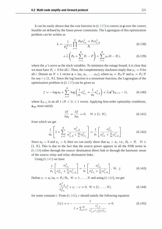
6.2 Multi-node amplify-and-forward protocol 231
It can be easily shown that the cost function in (6.137) is convex in p over the convexfeasible set defined by the linear power constraints. The Lagrangian of this optimizationproblem can be written as
L = 1
P N+10
N∏i=1
P0σ2s,ri + Piσ
2ri ,d
Pi(6.138)
+ λ(
P0 +N∑
i=1
Pi − P
)+
N∑i=1
μi (0− Pi ), (6.139)
where the μ’s serve as the slack variables. To minimize the outage bound, it is clear thatwe must have Pi > 0 for all i . Then, the complementary slackness imply that μi = 0 forall i . Denote an N × 1 vector a = [a0, a1, . . . , aN ], where a0 = P0/P and ai = Pi/Pfor any i ∈ [1, N ]. Since the log function is a monotone function, the Lagrangian of theoptimization problem in (6.137) can be given as
f = − log a0 +N∑
i=1
log
(1
aiσ 2
s,ri +1
a0σ 2
ri ,d
)+ λ(aT1N+1 − 1), (6.140)
where 1N+1 is an all 1 (N + 1) × 1 vector. Applying first-order optimality conditions,aopt must satisfy
∂ f
∂a0= ∂ f
∂ai= 0, ∀i ∈ [1, N ] , (6.141)
from which we get
1
a0
⎡⎣1+N∑
j=1
σ 2r j ,d
σ 2r j ,d+ a0
a jσ 2
s,r j
⎤⎦ = 1
ai
[σ 2
s,ri
σ 2s,ri + ai
a0σ 2
ri ,d
]. (6.142)
Since a0 > 0 and a j > 0, then we can easily show that a0 > ai , i.e., P0 > Pi ∀i ∈[1, N ]. This is due to the fact that the source power appears in all the SNR terms in(6.134) either through the source–destination direct link or through the harmonic meanof the source–relay and relay–destination links.
Using (6.141) we have
1
a j
[σ 2
s,r j
σ 2s,r j+ a j
a0σ 2
r j ,d
]= 1
ai
[σ 2
s,ri
σ 2s,ri + ai
a0σ 2
ri ,d
], ∀i, j. (6.143)
Define ci = ai/a0 = Pi/P0, ∀i = 1, . . . , N and using (6.142), we get
σ 2ri ,d
σ 2s,ri
c2i + ci − c = 0, ∀i ∈ [1, . . . , N ] , (6.144)
for some constant c. From (6.142), c should satisfy the following equation
f (c) = c − 1
1+∑Nj=1
σ 2r j ,d
σ 2r j ,d+ 1
c j (c)σ 2
s,r j
= 0. (6.145)
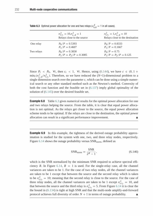
232 Multi-node cooperative communications
Table 6.3 Optimal power allocation for one and two relays (σ 2s,d = 1 in all cases).
σ 2s,ri = 10,σ 2
ri ,d= 1 σ 2
s,ri = 1,σ 2ri ,d
= 10Relays close to the source Relays close to the destination
One relay P0/P = 0.5393 P0/P = 0.8333P1/P = 0.4607 P1/P = 0.1667
Two relays P0/P = 0.3830 P0/P = 0.75P1/P = P2/P = 0.3085 P1/P = P2/P = 0.125
Since Pi < P0, ∀i , then ci < 1, ∀i . Hence, using (6.144), we have c ∈ (0, 1 +mini (σ
2ri ,d/σ 2
s,ri ). Therefore, so we have reduced the (N+1)-dimensional problem to asingle dimension search over the parameter c, which can be done using a simple numer-ical search or any other standard method such as the Newton’s method. Convexity ofboth the cost function and the feasible set in (6.137) imply global optimality of thesolution of (6.145) over the desired feasible set.
Example 6.8 Table 6.3 gives numerical results for the optimal power allocation for oneand two relays helping the source. From the table, it is clear that equal power alloca-tion is not optimal. As the relays get closer to the source, the equal power allocationscheme tends to be optimal. If the relays are close to the destination, the optimal powerallocation can result in a significant performance improvement. �
Example 6.9 In this example, the tightness of the derived outage probability approx-imation is studied for the system with one, two, and three relay nodes, respectively.Figure 6.14 shows the outage probability versus SNRnorm, defined as
SNRnorm = SNR
2R − 1, (6.146)
which is the SNR normalized by the minimum SNR required to achieve spectral effi-ciency R. In Figure 6.14, R = 1 is used. For the single-relay case, all the channelvariances are taken to be 1. For the case of two relay nodes, all the channel variancesare taken to be 1 except that between the source and the second relay which is takento be σ 2
s,r2 = 10; meaning that the second relay is close to the source. For the case ofthree relay nodes, all the channel variances are taken to be 1 except σ 2
s,r2 = 10, andthat between the source and the third relay is σ 2
s,r3 = 5. From Figure 6.14 it is clear thethe bound in (6.134) is tight at high SNR and that the multi-node amplify-and-forwardprotocol achieves full diversity of order N + 1 in terms of outage probability. �
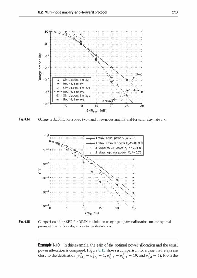
6.2 Multi-node amplify-and-forward protocol 233
0 5 10 15 20 25 30SNRnorm [dB]
Ou
tag
e p
rob
abili
ty
Simulation, 1 relayBound, 1 relaySimulation, 2 relaysBound, 2 relaysSimulation, 3 relaysBound, 3 relays
1 relay
2 relays
3 relays10−6
10−5
10−4
10−3
10−2
10–1
100
Fig. 6.14 Outage probability for a one-, two-, and three-nodes amplify-and-forward relay network.
0 5 10 15 20 25
1 relay, equal power Ps /P = 0.5.
1 relay, optimal power Ps /P = 0.8333
2 relays, equal power Ps /P = 0.3333
2 relays, optimal power Ps /P = 0.75
P/N0 [dB]
SE
R
10−5
10−4
10−3
10−2
10–1
100
Fig. 6.15 Comparison of the SER for QPSK modulation using equal power allocation and the optimalpower allocation for relays close to the destination.
Example 6.10 In this example, the gain of the optimal power allocation and the equalpower allocation is compared. Figure 6.15 shows a comparison for a case that relays areclose to the destination (σ 2
s,r1 = σ 2s,r2 = 1, σ 2
r1,d= σ 2
r2,d= 10, and σ 2
s,d = 1). From the
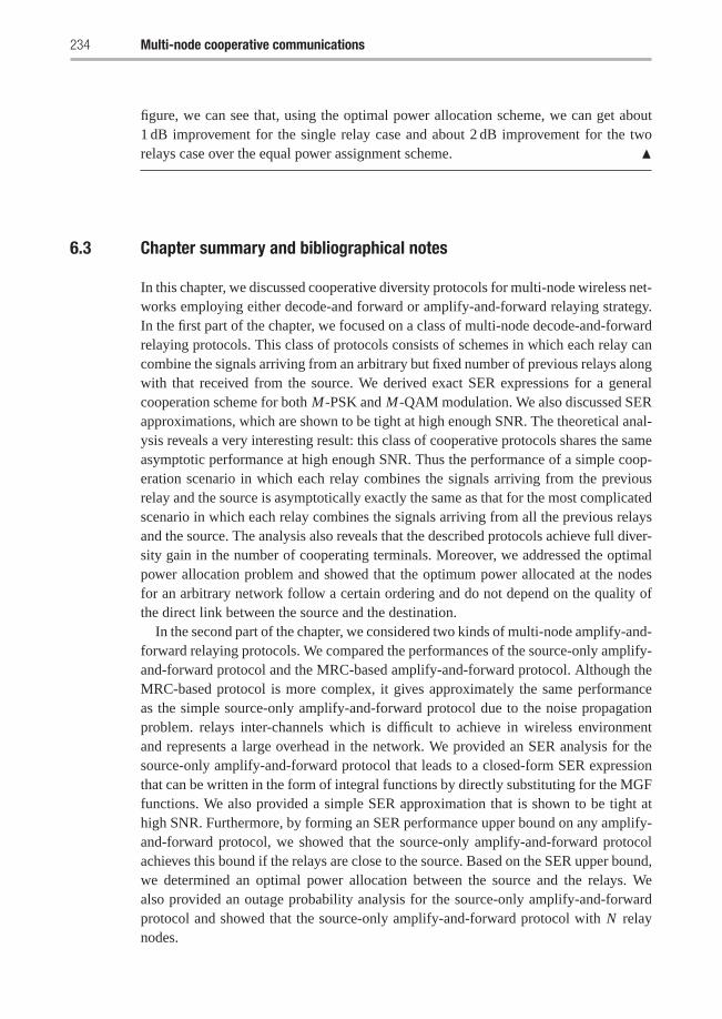
234 Multi-node cooperative communications
figure, we can see that, using the optimal power allocation scheme, we can get about1 dB improvement for the single relay case and about 2 dB improvement for the tworelays case over the equal power assignment scheme. �
6.3 Chapter summary and bibliographical notes
In this chapter, we discussed cooperative diversity protocols for multi-node wireless net-works employing either decode-and forward or amplify-and-forward relaying strategy.In the first part of the chapter, we focused on a class of multi-node decode-and-forwardrelaying protocols. This class of protocols consists of schemes in which each relay cancombine the signals arriving from an arbitrary but fixed number of previous relays alongwith that received from the source. We derived exact SER expressions for a generalcooperation scheme for both M-PSK and M-QAM modulation. We also discussed SERapproximations, which are shown to be tight at high enough SNR. The theoretical anal-ysis reveals a very interesting result: this class of cooperative protocols shares the sameasymptotic performance at high enough SNR. Thus the performance of a simple coop-eration scenario in which each relay combines the signals arriving from the previousrelay and the source is asymptotically exactly the same as that for the most complicatedscenario in which each relay combines the signals arriving from all the previous relaysand the source. The analysis also reveals that the described protocols achieve full diver-sity gain in the number of cooperating terminals. Moreover, we addressed the optimalpower allocation problem and showed that the optimum power allocated at the nodesfor an arbitrary network follow a certain ordering and do not depend on the quality ofthe direct link between the source and the destination.
In the second part of the chapter, we considered two kinds of multi-node amplify-and-forward relaying protocols. We compared the performances of the source-only amplify-and-forward protocol and the MRC-based amplify-and-forward protocol. Although theMRC-based protocol is more complex, it gives approximately the same performanceas the simple source-only amplify-and-forward protocol due to the noise propagationproblem. relays inter-channels which is difficult to achieve in wireless environmentand represents a large overhead in the network. We provided an SER analysis for thesource-only amplify-and-forward protocol that leads to a closed-form SER expressionthat can be written in the form of integral functions by directly substituting for the MGFfunctions. We also provided a simple SER approximation that is shown to be tight athigh SNR. Furthermore, by forming an SER performance upper bound on any amplify-and-forward protocol, we showed that the source-only amplify-and-forward protocolachieves this bound if the relays are close to the source. Based on the SER upper bound,we determined an optimal power allocation between the source and the relays. Wealso provided an outage probability analysis for the source-only amplify-and-forwardprotocol and showed that the source-only amplify-and-forward protocol with N relaynodes.
Exercises 235
The problem of SER performance analysis for multi-node amplify-and-forwardrelaying was studied in [152], in which the authors presented an approximate analy-sis and they considered the first term of the McLaurin series expansion of the SERaround SNR = 0. The approach presented in this chapter has some similarities withthe approach in [6] but differs in the way that the signal is normalized at each relay.In [6], the authors normalized the signal at the relays by a factor that can cause exces-sive increase in the signal peak in the case of deep fades. The approximations presentedin this chapter are also tighter than the bound in [6]. Some protocols for multi nodecooperative communications were presented in [156].
In [109], the outage probability of the single-relay amplify-and-forward network wasobtained by considering the high SNR behavior of the outage probability based on thelimiting behavior of the cumulative distribution function (CDF) of certain combinationsof exponential random variables. We also considered the high SNR behavior of theoutage probability of the multi-node source-only amplify-and-forward protocol. Thecase considered in [109] can be considered as a special case of the analysis presentedin this chapter with N = 1. The study of multi-node cooperative communication can befound in [163, 176].
Exercises
6.1 The symbol error rate for a general decode-and-forward scenario C(m) in whicheach relay combines the signals from the previous m relays and the source wasanalyzed for 1 ≤ m ≤ N .(a) Find the symbol error rate for the scenario C(0) in whicheach relay only
decodes the signal from the source.(b) Find the asymptotic symbol error rate performance of C(0) at high SNR.
Does this scheme also achieve full diversity gains.(c) Find the optimal power allocation in case of C(0).
6.2 Find the symbol error rate performance for a time diversity scheme, in whichthe source transmits the same message in three consecutive time slots. Assume afirst-order Markov model for the time correlation as follows
hs,d(t + 1) = ρhs,d(t)+√(1− ρ2)n
where hs,d(t) is the channel gain at time t , and ρ is the correlation coefficient.The channel is modeled as a Rayleigh flat-fading channel with unit variance.
Plot the symbol error rate expression versus the SNR for different values of ρ.6.3 Consider a symmetric network scenario in which all channels have identical
statistics. Find the optimal power allocation among the relays and the source.Find the optimal power allocation for the following two scenarios:
(a) A three-relay decode-and-forward network in which a C(1) scheme is used;(b) a three-relay source-only amplify-and-forward network.
236 Multi-node cooperative communications
6.4 Write a Matlab code to compare the BPSK bit error rate performance of N = 2-relay C(1) decode-and-forward protocol and N = 2-relay source-only amplify-and-forward protocols. Assume the source–destination channel variance to beequal to 1. Take N = 2, 3, 4. Consider the following three cases:(a) All relays close to the source.(b) All relays close to the destination.(c) All relays are at mid-distance between the source and the destination.For all of the previous cases assume the channel variance between any two relaysto be equal to 1. What is the effects of increasing N to 3 on the performance gapbetween the two schemes?
6.5 Consider a multi-relay decode-and-forward protocol. For an average SNR of20 dB per symbol and a spectral efficiency of 1 bps/Hz. Find the minimum num-ber of relays to achieve a bit error rate of 10−4. Assume a unit variance betweenthe source and the destination and that all relays are close to the source with allinter-relay channel variance being equal to 1.(a) What is the corresponding number of relays for amplify-and-forward
relaying?(b) Repeat for a bit error rate requirement of 10−6.(c) Find the minimum number of relays in all of the previous cases when the
relays are closer to the destination.6.6 Compare the bit error rate performance of a 2 × 1 Alamouti scheme and a
one-relay decode-and-forward system under the following scenarios assumingan exponential propagation path-loss with exponent 3 and BPSK modulation.Assume the channel variance for a unit distance is normalized to 1.(a) The relay is at the mid-point of the source–destination link with the source–
destination separation equal to 1 and 2.(b) The source–destination channel variance is 2 and the relay is located 0.25
from the source node.(c) The source–destination separation distance is 2 and the relay is located 0.25
from the destination.6.7 As shown in this chapter, cooperation provides both spatial diversity gains and
power gains due to its multi-hop nature. Time diversity schemes on the other handcan only provide diversity gains. Consider a source–destination pair separatedwith distance d . Calculate the bit error rate (BER) of binary phase shift keying(BPSK) for the following two transmission schemes.(a) A direct transmission scheme in which the source uses a two-repetition code
under an average power constraint P per bit. In this repetition coding, a bitis transmitted twice in two consecutive time slots. Assume flat fading i.i.d.channel.
(b) A cooperative diversity scheme in which the source transmits in the first slotand the relay uses amplify-and-forward to forward the bit in the second timeslot.
Exercises 237
6.8 The relay state vector SN , which represents whether each relay has decodedcorrectly or not, was defined as
Sn[k] ={
1 if relay k correctly decodes,
0 otherwise,1 ≤ k ≤ n.
Find the probability mass function of the vector SN .6.9 The outage probability for the amplify-and-forward scenario was specified as
PoutAF (p, R) � Pr
{W < (2(N+1)R − 1)
}= 1
(N + 1)!
(N+1∏i=1
λi
)(2(N+1)R − 1
)N+1 + H.O.T.
in (6.133). Prove this expression.
7 Distributed space–time andspace–frequency coding
The main drawback of the multi-node decode-and-forward (DF) protocol and the multi-node amplify-and-forward (AF) protocol, presented in Chapter 5, is the loss in the datarate as the number of relay nodes increases. The use of orthogonal subchannels for therelay node transmissions, either through TDMA or FDMA, results in a high loss ofthe system spectral efficiency. This leads to the use of what is known as distributedspace–time coding (DSTC) and distributed space–frequency coding (DSFC), whererelay nodes are allowed to simultaneously transmit over the same channel by emu-lating a space–time or a space–frequency code. The term distributed comes from thefact that the virtual multi-antenna transmitter is distributed between randomly locatedrelay nodes. Employing DSTCs or DSFCs reduces the data rate loss due to relay nodestransmissions without sacrificing the system diversity order, as will be seen in thischapter.
7.1 Distributed space–time coding (DSTC)
In this section, the design of distributed space–time codes for wireless relay networksis considered. The two-hop relay network model depicted in Figure 7.1, where the sys-tem lacks a direct link from the source to destination node, is considered. Distributedspace–time (space–frequency) coding can be achieved through node cooperation toemulate multiple antennas transmitter. First, the decode-and-forward protocol, in whicheach relay node decodes the symbols received from the source node before retrans-mission, is considered. A space–time code designed to achieve full diversity andmaximum coding gain over MIMO channels is shown to achieve full diversity butdoes not necessarily maximize the coding gain if used with the decode-and-forwardprotocol. Next, the amplify-and-forward protocol is considered; each relay node canonly perform simple operations such as linear transformation of the received signaland then amplify the signal before retransmission. A space–time code designed toachieve full diversity and maximum coding gain over MIMO channels is shown toachieve full diversity and maximum coding gain if used with the amplify-and-forwardprotocol.
Next, the design of DSTC that can mitigate the relay nodes synchronization errors isconsidered. Most of the work on cooperative transmission assume perfect synchroniza-tion between the relay nodes, which means that the relays’ timings, carrier frequencies,
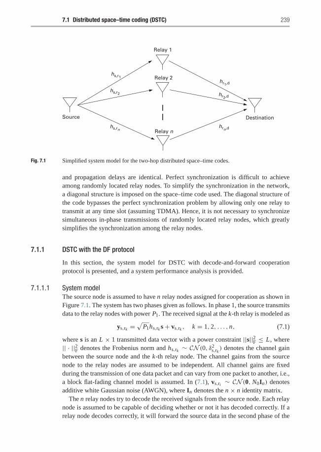
7.1 Distributed space–time coding (DSTC) 239
Source Destination
hs,r1 Relay 2
Relay 1
Relay n
hs,r2
hs,rn
hr1,d
hr2,d
hrn,d
Fig. 7.1 Simplified system model for the two-hop distributed space–time codes.
and propagation delays are identical. Perfect synchronization is difficult to achieveamong randomly located relay nodes. To simplify the synchronization in the network,a diagonal structure is imposed on the space–time code used. The diagonal structure ofthe code bypasses the perfect synchronization problem by allowing only one relay totransmit at any time slot (assuming TDMA). Hence, it is not necessary to synchronizesimultaneous in-phase transmissions of randomly located relay nodes, which greatlysimplifies the synchronization among the relay nodes.
7.1.1 DSTC with the DF protocol
In this section, the system model for DSTC with decode-and-forward cooperationprotocol is presented, and a system performance analysis is provided.
7.1.1.1 System modelThe source node is assumed to have n relay nodes assigned for cooperation as shown inFigure 7.1. The system has two phases given as follows. In phase 1, the source transmitsdata to the relay nodes with power P1. The received signal at the k-th relay is modeled as
ys,rk =√
P1hs,rk s+ vs,rk , k = 1, 2, . . . , n, (7.1)
where s is an L × 1 transmitted data vector with a power constraint ||s||2F ≤ L , where|| · ||2F denotes the Frobenius norm and hs,rk ∼ CN (0, δ2
s,rk ) denotes the channel gainbetween the source node and the k-th relay node. The channel gains from the sourcenode to the relay nodes are assumed to be independent. All channel gains are fixedduring the transmission of one data packet and can vary from one packet to another, i.e.,a block flat-fading channel model is assumed. In (7.1), vs,ri ∼ CN (0, N0In) denotesadditive white Gaussian noise (AWGN), where In denotes the n × n identity matrix.
The n relay nodes try to decode the received signals from the source node. Each relaynode is assumed to be capable of deciding whether or not it has decoded correctly. If arelay node decodes correctly, it will forward the source data in the second phase of the
240 Distributed space–time and space–frequency coding
cooperation protocol; otherwise, it remains idle. This can be achieved through the useof cyclic redundancy check (CRC) codes. This performance can also be approached bysetting a SNR threshold at the relay nodes, and the relay will only forward the sourcedata if the received SNR is larger than that threshold. For the analysis in this section,the relay nodes are assumed to be synchronized either by a centralized or a distributedalgorithm.
In phase 2, the relay nodes that have decoded correctly re-encode the data vector swith a pre-assigned code structure. In the subsequent development, no specific codedesign will be assumed, instead a generic space–time (ST) code structure is considered.The ST code is distributed among the relays such that each relay will emulate a singleantenna in a multiple-antenna transmitter. Hence, each relay will generate a column inthe corresponding ST code matrix. Let Xr denote the K × n space–time code matrixwith K ≥ n. Column k of Xr represents the code transmitted from the k-th relay node.The signal received at the destination is given by
yd =√
P2Xr DIhd + vd , (7.2)
where
hd =[hr1,d, hr2,d, . . . , hrn ,d
]T (7.3)
is an n×1 channel gains vector from the n relays to the destination, hrk ,d ∼ CN (0, δ2rk ,d),
and P2 is the relay node power. Without loss of generality, equal power allocation amongthe relay nodes is assumed. The channel gains from the relay nodes to the destinationnode are assumed to be statistically independent as the relays are spatially separated.The K × 1 vector vd ∼ CN (0, N0IK ) denotes AWGN at the destination node.
The state of the k-th relay, i.e., whether it has decoded correctly or not, is denotedby the random variable Ik (1 ≤ k ≤ n), which takes values 1 or 0 if the relay decodescorrectly or erroneously, respectively. Let
I = [I1, I2, . . . , In]T (7.4)
denote the state vector of the relay nodes and nI denote the number of relay nodes thathave decoded correctly corresponding to a certain realization I. The random variablesIk’s are statistically independent as the state of each relay depends only on its channelconditions to the source node, which are independent from other relays. The matrix
DI = diag(I1, I2, . . . , In) (7.5)
in (7.2) is defined as the state matrix of the relay nodes. An energy constraint is imposedon the generated ST code such that ||Xr ||2F ≤ L , and this guarantees that the transmittedpower per source symbol is less than or equal to P1 + P2.
7.1.1.2 Performance analysisIn this section, the pairwise error probability (PEP) performance analysis for the coop-eration scheme described in Section 7.1.1.1 is provided. The diversity and coding gainachieved by the protocol are then analyzed.
7.1 Distributed space–time coding (DSTC) 241
One can see that the random variable Ik is a Bernoulli random variable. Therefore,the probability distribution of Ik is given by
Ik ={
0 with probability = 1− (1− SERk)L
1 with probability = (1− SERk)L ,
where SERk is the un-coded SER at the k-th relay node and is modulation dependent.For M-ary quadrature amplitude modulation (M-QAM, M = 2p with p even), the exactexpression for SERk can be shown to be upper-bounded by
SERk ≤ 2N0g
bP1δ2s,rk
, (7.6)
where b = 3/(M − 1) and
g = 4R
π
∫ π/2
0sin2 θdθ − 4R2
π
∫ π/4
0sin2 θdθ, (7.7)
in which
R = 1− 1√M. (7.8)
The destination is assumed to have perfect channel state information as well as therelay nodes state vector. The destination applies a maximum likelihood (ML) receiver,which is based on a minimum distance rule. The conditional pairwise error probability(PEP) is given by
Pr (X1 → X2|I, hd)
= Pr(‖yd −
√P2X1DIhd‖2
F > ‖yd −√
P2X2DIhd‖2F |I, hd , X1 was transmitted
),
(7.9)
where X1 and X2 are two possible transmitted codewords. The conditional PEP can beexpressed as quadratic form of a complex Gaussian random vector as
Pr (X1 → X2|I, hd) = Pr (q < 0|I, hd) , (7.10)
where
q = [ zH1 zH
2
] [ In 00 −In
] [z1
z2
],
z1 =√
P2 (X1 − X2)DIhd + vd , (7.11)
and
z2 = vd . (7.12)
The random vectors hd and I are mutually independent as they arise from independentprocesses. First, the conditional PEP was averaged over the channel realizations hd . Bydefining the signal matrix
CI = (X1 − X2)DIdiag(δ2r1,d, δ
2r2,d, . . . , δ
2rn ,d)DI (X1 − X2)
H , (7.13)
242 Distributed space–time and space–frequency coding
the conditional PEP in (7.10) can be tightly upper-bounded, using equation (2.13), by
Pr (X1 → X2|I) ≤
(2�(I)− 1�(I)− 1
)N�(I)0
P�(I)2
∏�(I)i=1 λ
Ii
, (7.14)
where �(I) is the number of nonzero eigenvalues of the signal matrix and λIi ’s are the
nonzero eigenvalues of the signal matrix corresponding to the state vector I. Thenonzero eigenvalues of the signal matrix are the same as the nonzero eigenvalues ofthe matrix
� (X1,X2) = diag(δr1,d, δr2,d, . . . , δrn ,d)DI�(X1,X2)DIdiag(δr1,d, δr2,d, . . . , δrn ,d),
where
�(X1,X2) = (X1 − X2)H (X1 − X2) . (7.15)
The employed space–time scheme is assumed to achieve full diversity and maximumcoding gain over MIMO channels, which means that the matrix �(X1,X2) is fullrank of order n for any pair of distinct codewords X1 and X2. Achieving maximumcoding gain means that the minimum of the products
∏ni=1 λi , where the λi ’s are
the eigenvalues of the matrix �(X1,X2), is maximized over all the pairs of distinctcodewords.
Clearly, if the matrix �(X1,X2) has a rank of order n then the matrix � (X1,X2)
will have a rank of order nI, which is the number of relays that have decoded correctly.Equation (7.14) can now be rewritten as
Pr (X1 → X2|I) ≤
(2nI − 1nI − 1
)NnI
0
PnI2
∏nIi=1 λ
Ii
. (7.16)
Next, the conditional PEP is averaged over the relays’ state vector I. The dependenceof the expression in (7.16) on I appears through the set of nonzero eigenvalues
{λI
i
}nIi=1,
which depends on the number of relays that have decoded correctly and their realiza-tions. The state vector I of the relay nodes determines which columns from the ST codematrix are replaced with zeros and thus affect the resulting eigenvalues.
The probability of having a certain realization of I is given by
Pr(I) =⎛⎝ ∏
k∈C R(I)
(1− SERk)L
⎞⎠⎛⎝ ∏k∈E R(I)
(1− (1− SERk)
L)⎞⎠ , (7.17)
where C R(I) is the set of relays that have decoded correctly and E R(I) is the set ofrelays that have decoded erroneously corresponding to the I realization. For simplicityof presentation symmetry is assumed between all relays, i.e., is δ2
s,rk = δ2s,r and δ2
rk ,d=
δ2r,d for all k. Averaging over all realizations of the states of the relays, gives the PEP at
high SNR as
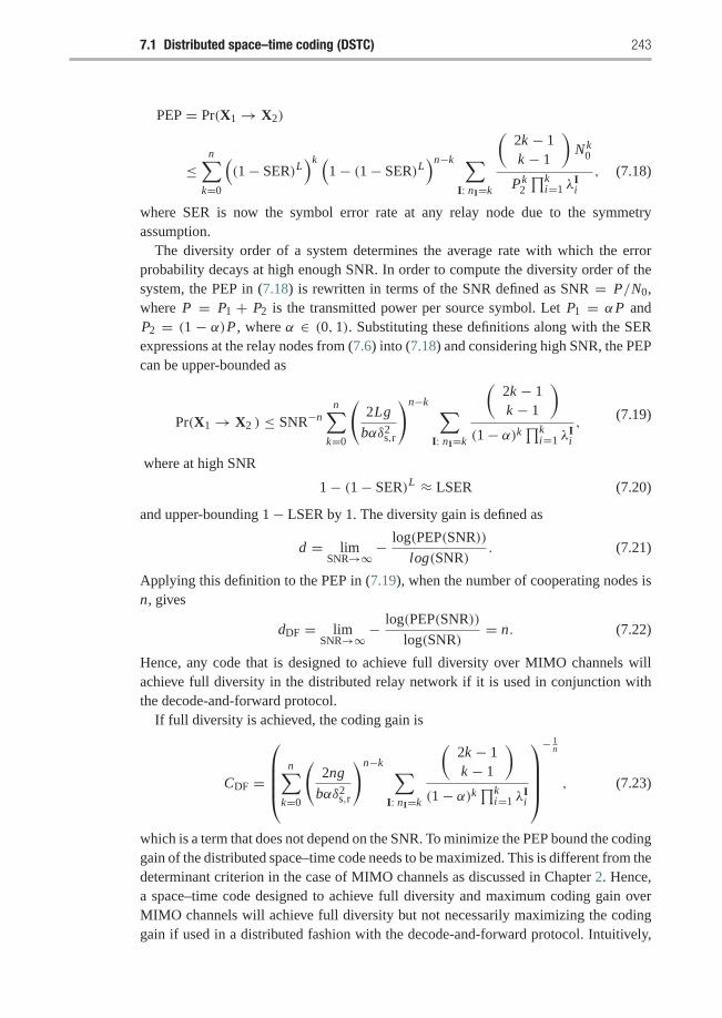
7.1 Distributed space–time coding (DSTC) 243
PEP = Pr(X1 → X2)
≤n∑
k=0
((1− SER)L
)k (1− (1− SER)L
)n−k ∑I: nI=k
(2k − 1k − 1
)Nk
0
Pk2
∏ki=1 λ
Ii
, (7.18)
where SER is now the symbol error rate at any relay node due to the symmetryassumption.
The diversity order of a system determines the average rate with which the errorprobability decays at high enough SNR. In order to compute the diversity order of thesystem, the PEP in (7.18) is rewritten in terms of the SNR defined as SNR = P/N0,where P = P1 + P2 is the transmitted power per source symbol. Let P1 = αP andP2 = (1 − α)P , where α ∈ (0, 1). Substituting these definitions along with the SERexpressions at the relay nodes from (7.6) into (7.18) and considering high SNR, the PEPcan be upper-bounded as
Pr(X1 → X2 ) ≤ SNR−nn∑
k=0
(2Lg
bαδ2s,r
)n−k ∑I: nI=k
(2k − 1k − 1
)(1− α)k ∏k
i=1 λIi
,(7.19)
where at high SNR
1− (1− SER)L ≈ LSER (7.20)
and upper-bounding 1− LSER by 1. The diversity gain is defined as
d = limSNR→∞−
log(PEP(SNR))
log(SNR). (7.21)
Applying this definition to the PEP in (7.19), when the number of cooperating nodes isn, gives
dDF = limSNR→∞−
log(PEP(SNR))
log(SNR)= n. (7.22)
Hence, any code that is designed to achieve full diversity over MIMO channels willachieve full diversity in the distributed relay network if it is used in conjunction withthe decode-and-forward protocol.
If full diversity is achieved, the coding gain is
CDF =
⎛⎜⎜⎜⎝n∑
k=0
(2ng
bαδ2s,r
)n−k ∑I: nI=k
(2k − 1k − 1
)(1− α)k ∏k
i=1 λIi
⎞⎟⎟⎟⎠− 1
n
, (7.23)
which is a term that does not depend on the SNR. To minimize the PEP bound the codinggain of the distributed space–time code needs to be maximized. This is different from thedeterminant criterion in the case of MIMO channels as discussed in Chapter 2. Hence,a space–time code designed to achieve full diversity and maximum coding gain overMIMO channels will achieve full diversity but not necessarily maximizing the codinggain if used in a distributed fashion with the decode-and-forward protocol. Intuitively,
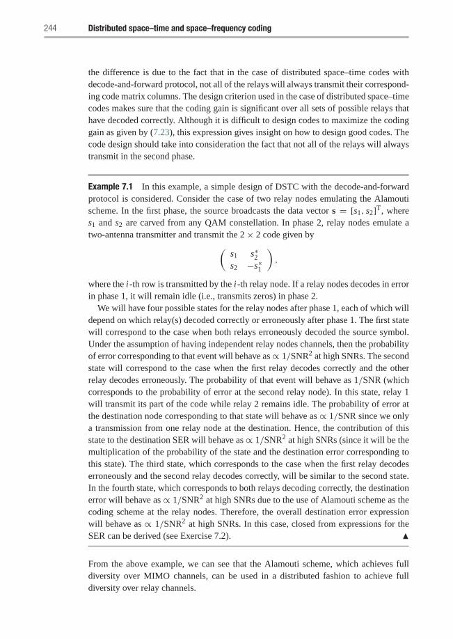
244 Distributed space–time and space–frequency coding
the difference is due to the fact that in the case of distributed space–time codes withdecode-and-forward protocol, not all of the relays will always transmit their correspond-ing code matrix columns. The design criterion used in the case of distributed space–timecodes makes sure that the coding gain is significant over all sets of possible relays thathave decoded correctly. Although it is difficult to design codes to maximize the codinggain as given by (7.23), this expression gives insight on how to design good codes. Thecode design should take into consideration the fact that not all of the relays will alwaystransmit in the second phase.
Example 7.1 In this example, a simple design of DSTC with the decode-and-forwardprotocol is considered. Consider the case of two relay nodes emulating the Alamoutischeme. In the first phase, the source broadcasts the data vector s = [s1, s2]T, wheres1 and s2 are carved from any QAM constellation. In phase 2, relay nodes emulate atwo-antenna transmitter and transmit the 2× 2 code given by(
s1 s∗2s2 −s∗1
),
where the i-th row is transmitted by the i-th relay node. If a relay nodes decodes in errorin phase 1, it will remain idle (i.e., transmits zeros) in phase 2.
We will have four possible states for the relay nodes after phase 1, each of which willdepend on which relay(s) decoded correctly or erroneously after phase 1. The first statewill correspond to the case when both relays erroneously decoded the source symbol.Under the assumption of having independent relay nodes channels, then the probabilityof error corresponding to that event will behave as∝ 1/SNR2 at high SNRs. The secondstate will correspond to the case when the first relay decodes correctly and the otherrelay decodes erroneously. The probability of that event will behave as 1/SNR (whichcorresponds to the probability of error at the second relay node). In this state, relay 1will transmit its part of the code while relay 2 remains idle. The probability of error atthe destination node corresponding to that state will behave as ∝ 1/SNR since we onlya transmission from one relay node at the destination. Hence, the contribution of thisstate to the destination SER will behave as ∝ 1/SNR2 at high SNRs (since it will be themultiplication of the probability of the state and the destination error corresponding tothis state). The third state, which corresponds to the case when the first relay decodeserroneously and the second relay decodes correctly, will be similar to the second state.In the fourth state, which corresponds to both relays decoding correctly, the destinationerror will behave as ∝ 1/SNR2 at high SNRs due to the use of Alamouti scheme as thecoding scheme at the relay nodes. Therefore, the overall destination error expressionwill behave as ∝ 1/SNR2 at high SNRs. In this case, closed from expressions for theSER can be derived (see Exercise 7.2). �
From the above example, we can see that the Alamouti scheme, which achieves fulldiversity over MIMO channels, can be used in a distributed fashion to achieve fulldiversity over relay channels.
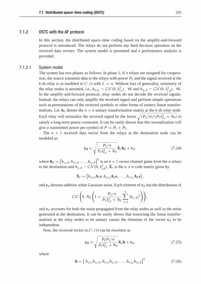
7.1 Distributed space–time coding (DSTC) 245
7.1.2 DSTC with the AF protocol
In this section, the distributed space–time coding based on the amplify-and-forwardprotocol is introduced. The relays do not perform any hard decision operation on thereceived data vectors. The system model is presented and a performance analysis isprovided.
7.1.2.1 System modelThe system has two phases as follows. In phase 1, if n relays are assigned for coopera-tion, the source transmits data to the relays with power P1 and the signal received at thek-th relay is as modeled in (7.1) with L = n. Without loss of generality, symmetry ofthe relay nodes is assumed, i.e., hs,rk ∼ CN (0, δ2
s,r), ∀k and hrk ,d ∼ CN (0, δ2r,d), ∀k.
In the amplify-and-forward protocol, relay nodes do not decode the received signals.Instead, the relays can only amplify the received signal and perform simple operationssuch as permutations of the received symbols or other forms of unitary linear transfor-mations. Let Ak denote the n × n unitary transformation matrix at the k-th relay node.
Each relay will normalize the received signal by the factor√(P2/n)/(P1δ2
s,r + N0) to
satisfy a long-term power constraint. It can be easily shown that this normalization willgive a transmitted power per symbol of P = P1 + P2.
The n × 1 received data vector from the relays at the destination node can bemodeled as
yd =√
P2/n
P1δ2s,r + N0
Xr hd + vd , (7.24)
where hd =[hr1,d, hr2,d, . . . , hrn ,d
]T is an n × 1 vector channel gains from the n relaysto the destination and hri ,d ∼ CN (0, δ2
r,d), Xr is the n × n code matrix given by
Xr =[hs,r1A1s, hs,r2A2s, . . . , hs,rn Ans
],
and vd denotes additive white Gaussian noise. Each element of vd has the distribution of
CN(
0, N0
(1+ P2/n
P1δ2s,r + N0
n∑i=1
|hri ,d|2))
,
and vd accounts for both the noise propagated from the relay nodes as well as the noisegenerated at the destination. It can be easily shown that restricting the linear transfor-mations at the relay nodes to be unitary causes the elements of the vector vd to beindependent.
Now, the received vector in (7.24) can be rewritten as
yd =√
P2 P1/n
P1δ2s,r + N0
Xr h+ vd , (7.25)
where
h = [ hs,r1hr1,d, hs,r2hr2,d, . . . , hs,rn hrn ,d]T (7.26)
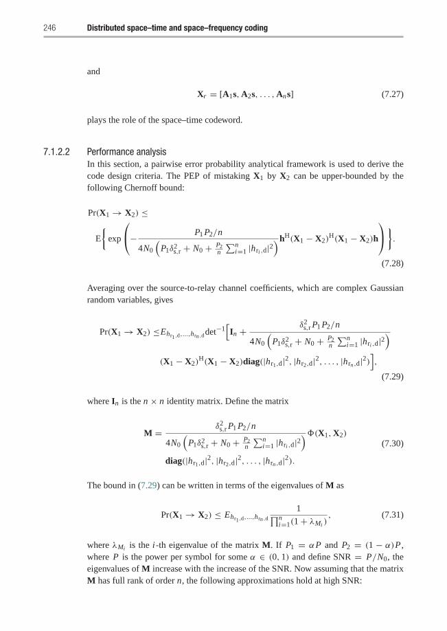
246 Distributed space–time and space–frequency coding
and
Xr = [A1s,A2s, . . . ,Ans] (7.27)
plays the role of the space–time codeword.
7.1.2.2 Performance analysisIn this section, a pairwise error probability analytical framework is used to derive thecode design criteria. The PEP of mistaking X1 by X2 can be upper-bounded by thefollowing Chernoff bound:
Pr(X1 → X2) ≤
E
{exp
⎛⎝− P1 P2/n
4N0
(P1δ2
s,r + N0 + P2n
∑ni=1 |hri ,d|2
)hH(X1 − X2)H(X1 − X2)h
⎞⎠}.(7.28)
Averaging over the source-to-relay channel coefficients, which are complex Gaussianrandom variables, gives
Pr(X1 → X2) ≤Ehr1,d,...,hrn ,ddet−1
[In +
δ2s,r P1 P2/n
4N0
(P1δ2
s,r + N0 + P2n
∑ni=1 |hri ,d|2
)(X1 − X2)
H(X1 − X2)diag(|hr1,d|2, |hr2,d|2, . . . , |hrn ,d|2)],
(7.29)
where In is the n × n identity matrix. Define the matrix
M = δ2s,r P1 P2/n
4N0
(P1δ2
s,r + N0 + P2n
∑ni=1 |hri ,d|2
)�(X1,X2)
diag(|hr1,d|2, |hr2,d|2, . . . , |hrn ,d|2).(7.30)
The bound in (7.29) can be written in terms of the eigenvalues of M as
Pr(X1 → X2) ≤ Ehr1,d,...,hrn ,d
1∏ni=1(1+ λMi )
, (7.31)
where λMi is the i-th eigenvalue of the matrix M. If P1 = αP and P2 = (1 − α)P ,where P is the power per symbol for some α ∈ (0, 1) and define SNR = P/N0, theeigenvalues of M increase with the increase of the SNR. Now assuming that the matrixM has full rank of order n, the following approximations hold at high SNR:
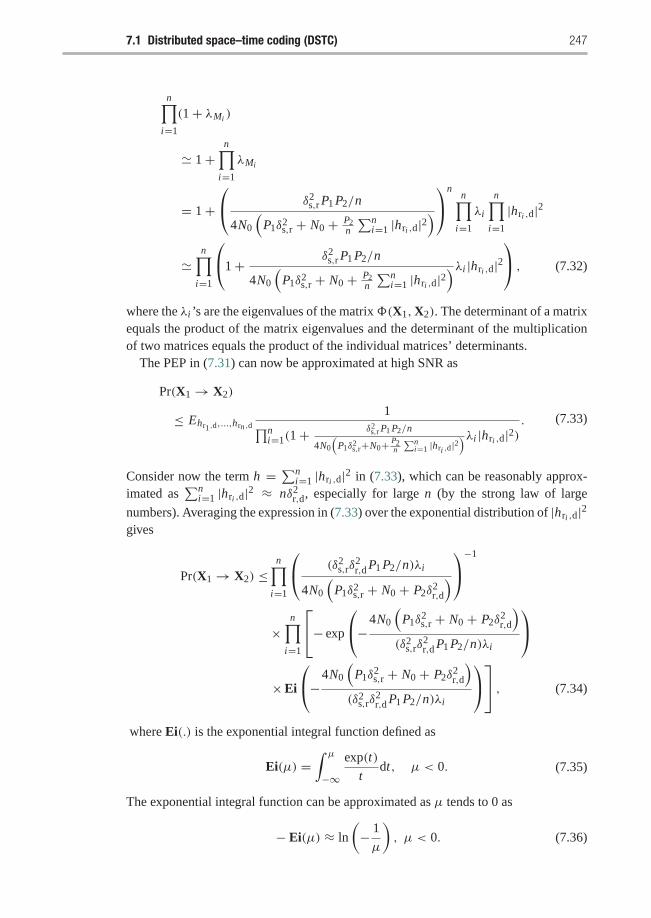
7.1 Distributed space–time coding (DSTC) 247
n∏i=1
(1+ λMi )
� 1+n∏
i=1
λMi
= 1+⎛⎝ δ2
s,r P1 P2/n
4N0
(P1δ2
s,r + N0 + P2n
∑ni=1 |hri ,d|2
)⎞⎠n
n∏i=1
λi
n∏i=1
|hri ,d|2
�n∏
i=1
⎛⎝1+ δ2s,r P1 P2/n
4N0
(P1δ2
s,r + N0 + P2n
∑ni=1 |hri ,d|2
)λi |hri ,d|2⎞⎠ , (7.32)
where the λi ’s are the eigenvalues of the matrix�(X1,X2). The determinant of a matrixequals the product of the matrix eigenvalues and the determinant of the multiplicationof two matrices equals the product of the individual matrices’ determinants.
The PEP in (7.31) can now be approximated at high SNR as
Pr(X1 → X2)
≤ Ehr1,d,...,hrn ,d
1∏ni=1(1+ δ2
s,r P1 P2/n
4N0
(P1δ
2s,r+N0+ P2
n
∑ni=1 |hri ,d|2
)λi |hri ,d|2). (7.33)
Consider now the term h = ∑ni=1 |hri ,d|2 in (7.33), which can be reasonably approx-
imated as∑n
i=1 |hri ,d|2 ≈ nδ2r,d, especially for large n (by the strong law of large
numbers). Averaging the expression in (7.33) over the exponential distribution of |hri ,d|2gives
Pr(X1 → X2) ≤n∏
i=1
⎛⎝ (δ2s,rδ
2r,d P1 P2/n)λi
4N0
(P1δ2
s,r + N0 + P2δ2r,d
)⎞⎠−1
×n∏
i=1
⎡⎣− exp
⎛⎝−4N0
(P1δ
2s,r + N0 + P2δ
2r,d
)(δ2
s,rδ2r,d P1 P2/n)λi
⎞⎠×Ei
⎛⎝−4N0
(P1δ
2s,r + N0 + P2δ
2r,d
)(δ2
s,rδ2r,d P1 P2/n)λi
⎞⎠⎤⎦ , (7.34)
where Ei(.) is the exponential integral function defined as
Ei(μ) =∫ μ
−∞exp(t)
tdt, μ < 0. (7.35)
The exponential integral function can be approximated as μ tends to 0 as
− Ei(μ) ≈ ln
(− 1
μ
), μ < 0. (7.36)
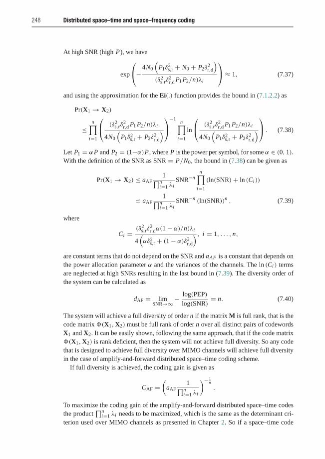
248 Distributed space–time and space–frequency coding
At high SNR (high P), we have
exp
⎛⎝−4N0
(P1δ
2s,r + N0 + P2δ
2r,d
)(δ2
s,rδ2r,d P1 P2/n)λi
⎞⎠ ≈ 1, (7.37)
and using the approximation for the Ei(.) function provides the bound in (7.1.2.2) as
Pr(X1 → X2)
≤n∏
i=1
⎛⎝ (δ2s,rδ
2r,d P1 P2/n)λi
4N0
(P1δ2
s,r + P2δ2r,d
)⎞⎠−1
n∏i=1
ln
⎛⎝ (δ2s,rδ
2r,d P1 P2/n)λi
4N0
(P1δ2
s,r + P2δ2r,d
)⎞⎠ . (7.38)
Let P1 = αP and P2 = (1−α)P , where P is the power per symbol, for some α ∈ (0, 1).With the definition of the SNR as SNR = P/N0, the bound in (7.38) can be given as
Pr(X1 → X2) ≤ aAF1∏n
i=1 λiSNR−n
n∏i=1
(ln(SNR)+ ln (Ci ))
� aAF1∏n
i=1 λiSNR−n (ln(SNR))n , (7.39)
where
Ci =(δ2
s,rδ2r,dα(1− α)/n)λi
4(αδ2
s,r + (1− α)δ2r,d
) , i = 1, . . . , n,
are constant terms that do not depend on the SNR and aAF is a constant that depends onthe power allocation parameter α and the variances of the channels. The ln (Ci ) termsare neglected at high SNRs resulting in the last bound in (7.39). The diversity order ofthe system can be calculated as
dAF = limSNR→∞−
log(PEP)
log(SNR)= n. (7.40)
The system will achieve a full diversity of order n if the matrix M is full rank, that is thecode matrix �(X1,X2) must be full rank of order n over all distinct pairs of codewordsX1 and X2. It can be easily shown, following the same approach, that if the code matrix�(X1,X2) is rank deficient, then the system will not achieve full diversity. So any codethat is designed to achieve full diversity over MIMO channels will achieve full diversityin the case of amplify-and-forward distributed space–time coding scheme.
If full diversity is achieved, the coding gain is given as
CAF =(
aAF1∏n
i=1 λi
)− 1n
.
To maximize the coding gain of the amplify-and-forward distributed space–time codesthe product
∏ni=1 λi needs to be maximized, which is the same as the determinant cri-
terion used over MIMO channels as presented in Chapter 2. So if a space–time code
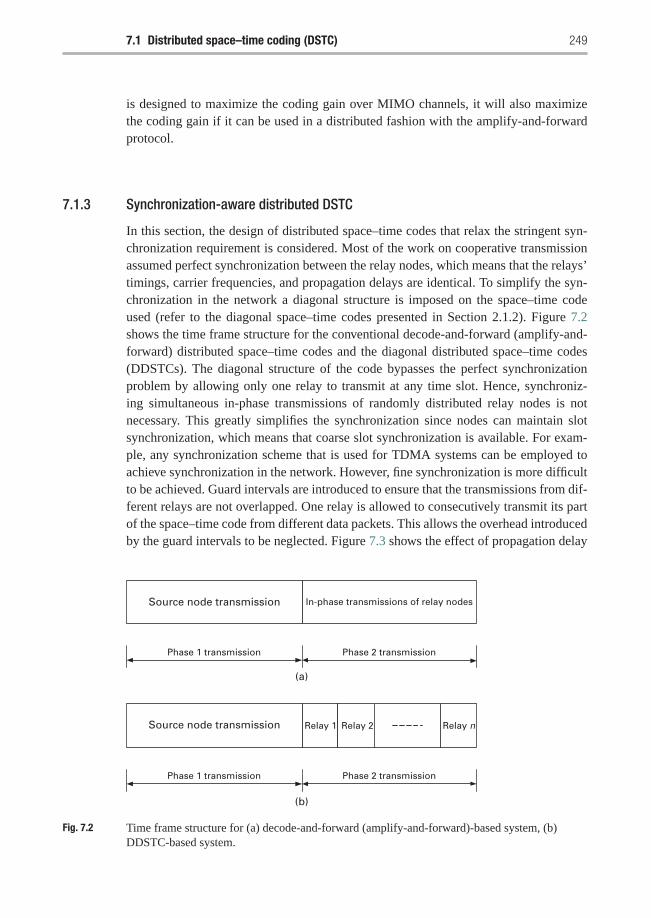
7.1 Distributed space–time coding (DSTC) 249
is designed to maximize the coding gain over MIMO channels, it will also maximizethe coding gain if it can be used in a distributed fashion with the amplify-and-forwardprotocol.
7.1.3 Synchronization-aware distributed DSTC
In this section, the design of distributed space–time codes that relax the stringent syn-chronization requirement is considered. Most of the work on cooperative transmissionassumed perfect synchronization between the relay nodes, which means that the relays’timings, carrier frequencies, and propagation delays are identical. To simplify the syn-chronization in the network a diagonal structure is imposed on the space–time codeused (refer to the diagonal space–time codes presented in Section 2.1.2). Figure 7.2shows the time frame structure for the conventional decode-and-forward (amplify-and-forward) distributed space–time codes and the diagonal distributed space–time codes(DDSTCs). The diagonal structure of the code bypasses the perfect synchronizationproblem by allowing only one relay to transmit at any time slot. Hence, synchroniz-ing simultaneous in-phase transmissions of randomly distributed relay nodes is notnecessary. This greatly simplifies the synchronization since nodes can maintain slotsynchronization, which means that coarse slot synchronization is available. For exam-ple, any synchronization scheme that is used for TDMA systems can be employed toachieve synchronization in the network. However, fine synchronization is more difficultto be achieved. Guard intervals are introduced to ensure that the transmissions from dif-ferent relays are not overlapped. One relay is allowed to consecutively transmit its partof the space–time code from different data packets. This allows the overhead introducedby the guard intervals to be neglected. Figure 7.3 shows the effect of propagation delay
Relay 1 Relay 2 Relay nSource node transmission
(b)
In-phase transmissions of relay nodesSource node transmission
Phase 1 transmission
(a)
Phase 2 transmission
Phase 1 transmission Phase 2 transmission
Fig. 7.2 Time frame structure for (a) decode-and-forward (amplify-and-forward)-based system, (b)DDSTC-based system.
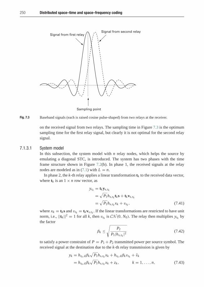
250 Distributed space–time and space–frequency coding
Sampling point
Signal from first relaySignal from second relay
Fig. 7.3 Baseband signals (each is raised cosine pulse-shaped) from two relays at the receiver.
on the received signal from two relays. The sampling time in Figure 7.3 is the optimumsampling time for the first relay signal, but clearly it is not optimal for the second relaysignal.
7.1.3.1 System modelIn this subsection, the system model with n relay nodes, which helps the source byemulating a diagonal STC, is introduced. The system has two phases with the timeframe structure shown in Figure 7.2(b). In phase 1, the received signals at the relaynodes are modeled as in (7.1) with L = n.
In phase 2, the k-th relay applies a linear transformation tk to the received data vector,where tk is an 1× n row vector, as
yrk = tkys,rk
= √P1hs,rk tks+ tkvs,rk
= √P1hs,rk xk + vrk , (7.41)
where xk = tks and vrk = tkvs,rk . If the linear transformations are restricted to have unitnorm, i.e., ||tk ||2 = 1 for all k, then vrk is CN (0, N0). The relay then multiplies yrk bythe factor
βk ≤√
P2
P1|hs,rk |2(7.42)
to satisfy a power constraint of P = P1+ P2 transmitted power per source symbol. Thereceived signal at the destination due to the k-th relay transmission is given by
yk = hrk ,dβk
√P1hs,rk xk + hrk ,dβkvrk + vk
= hrk ,dβk
√P1hs,rk xk + zk, k = 1, . . . , n, (7.43)
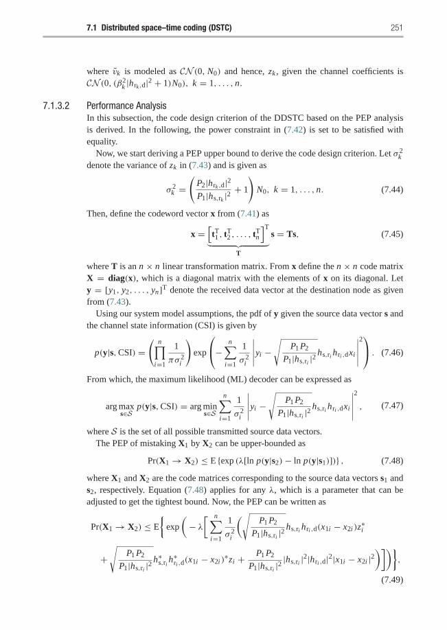
7.1 Distributed space–time coding (DSTC) 251
where vk is modeled as CN (0, N0) and hence, zk , given the channel coefficients isCN (0, (β2
k |hrk ,d|2 + 1)N0), k = 1, . . . , n.
7.1.3.2 Performance AnalysisIn this subsection, the code design criterion of the DDSTC based on the PEP analysisis derived. In the following, the power constraint in (7.42) is set to be satisfied withequality.
Now, we start deriving a PEP upper bound to derive the code design criterion. Let σ 2k
denote the variance of zk in (7.43) and is given as
σ 2k =
(P2|hrk ,d|2P1|hs,rk |2
+ 1
)N0, k = 1, . . . , n. (7.44)
Then, define the codeword vector x from (7.41) as
x =[tT1 , t
T2 , . . . , t
Tn
]T︸ ︷︷ ︸
T
s = Ts, (7.45)
where T is an n × n linear transformation matrix. From x define the n × n code matrixX = diag(x), which is a diagonal matrix with the elements of x on its diagonal. Lety = [y1, y2, . . . , yn]T denote the received data vector at the destination node as givenfrom (7.43).
Using our system model assumptions, the pdf of y given the source data vector s andthe channel state information (CSI) is given by
p(y|s,CSI) =(
n∏i=1
1
πσ 2i
)exp
⎛⎝− n∑i=1
1
σ 2i
∣∣∣∣∣yi −√
P1 P2
P1|hs,ri |2hs,ri hri ,dxi
∣∣∣∣∣2⎞⎠ . (7.46)
From which, the maximum likelihood (ML) decoder can be expressed as
arg maxs∈S
p(y|s,CSI) = arg mins∈S
n∑i=1
1
σ 2i
∣∣∣∣∣yi −√
P1 P2
P1|hs,ri |2hs,ri hri ,dxi
∣∣∣∣∣2
, (7.47)
where S is the set of all possible transmitted source data vectors.The PEP of mistaking X1 by X2 can be upper-bounded as
Pr(X1 → X2) ≤ E {exp (λ[ln p(y|s2)− ln p(y|s1)])} , (7.48)
where X1 and X2 are the code matrices corresponding to the source data vectors s1 ands2, respectively. Equation (7.48) applies for any λ, which is a parameter that can beadjusted to get the tightest bound. Now, the PEP can be written as
Pr(X1 → X2) ≤ E
{exp
(− λ[ n∑
i=1
1
σ 2i
(√P1 P2
P1|hs,ri |2hs,ri hri ,d(x1i − x2i )z
∗i
+√
P1 P2
P1|hs,ri |2h∗s,ri h
∗ri ,d(x1i − x2i )
∗zi + P1 P2
P1|hs,ri |2|hs,ri |2|hri ,d|2|x1i − x2i |2
)])},
(7.49)
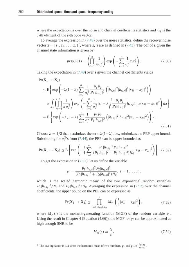
252 Distributed space–time and space–frequency coding
where the expectation is over the noise and channel coefficients statistics and xi j is thej-th element of the i-th code vector.
To average the expression in (7.49) over the noise statistics, define the receiver noisevector z = [z1, z2, . . . , zn]T, where zi ’s are as defined in (7.43). The pdf of z given thechannel state information is given by
p(z|CSI ) =(
n∏i=1
1
πσ 2i
)exp
(−
n∑i=1
1
σ 2i
zi z∗i
). (7.50)
Taking the expectation in (7.49) over z given the channel coefficients yields
Pr(X1 → X2)
≤ E
{exp
(−λ(1− λ)
n∑i=1
1
σ 2i
P1 P2
P1|hs,ri |2(|hs,ri |2|hri ,d|2|x1i − x2i |2
))
×∫
z
(n∏
i=1
1
πσ 2i
)exp
(−
n∑i=1
1
σ 2i
|zi + λ√
P1 P2
P1|hs,ri |2hs,ri hri ,d(x1i − x2i )|2
)dz}
= E
{exp
(−λ(1− λ)
n∑i=1
1
σ 2i
P1 P2
P1|hs,ri |2(|hs,ri |2|hri ,d|2|x1i − x2i |2
))}.
(7.51)
Choose λ = 1/2 that maximizes the term λ(1−λ), i.e., minimizes the PEP upper bound.Substituting for σ 2
i ’s from (7.44), the PEP can be upper-bounded as
Pr(X1 → X2) ≤ E
{exp
(−1
4
n∑i=1
P1|hs,ri |2 P2|hri ,d|2(P1|hs,ri |2 + P2|hri ,d|2)N0
|x1i − x2i |2)}
. (7.52)
To get the expression in (7.52), let us define the variable
γi = P1|hs,ri |2 P2|hri ,d|2(P1|hs,ri |2 + P2|hri ,d|2)N0
, i = 1, . . . , n,
which is the scaled harmonic mean1 of the two exponential random variablesP1|hs,ri |2/N0 and P2|hri ,d|2/N0. Averaging the expression in (7.52) over the channelcoefficients, the upper bound on the PEP can be expressed as
Pr(X1 → X2) ≤n∏
i=1,x1i �=x2i
Mγi
(1
4|x1i − x2i |2
), (7.53)
where Mγi (.) is the moment-generating function (MGF) of the random variable γi .Using the result in Chapter 4 (Equation (4.66)), the MGF for γi can be approximated athigh enough SNR to be
Mγi (s) �ζi
s, (7.54)
1 The scaling factor is 1/2 since the harmonic mean of two numbers, g1 and g2, is 2g1g2g1+g2
.
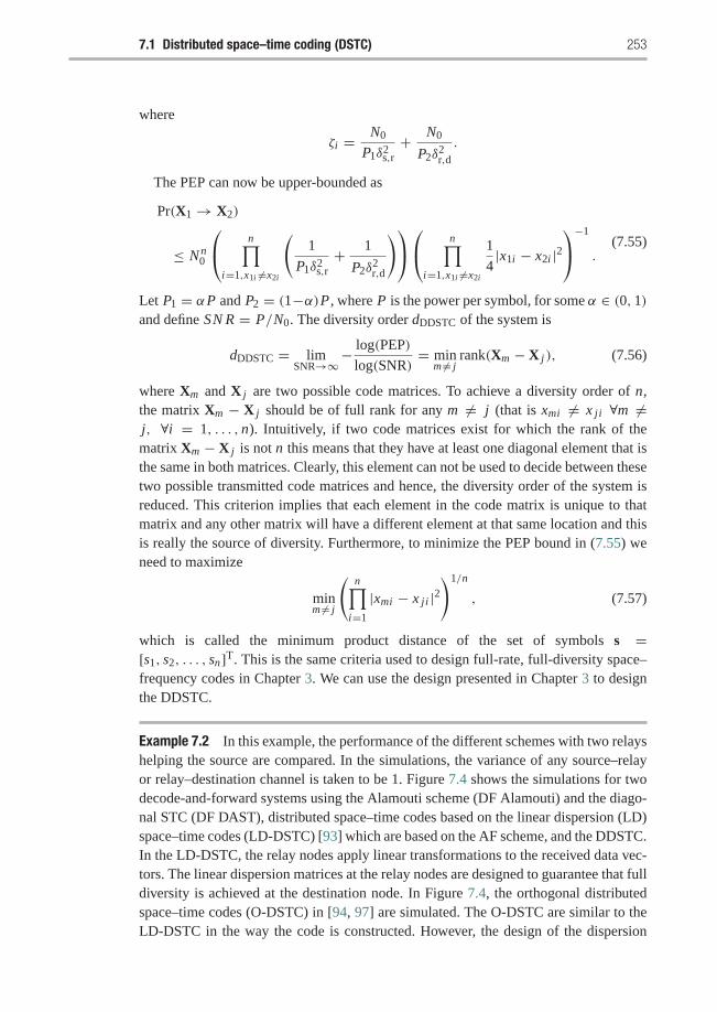
7.1 Distributed space–time coding (DSTC) 253
where
ζi = N0
P1δ2s,r+ N0
P2δ2r,d
.
The PEP can now be upper-bounded as
Pr(X1 → X2)
≤ Nn0
⎛⎝ n∏i=1,x1i �=x2i
(1
P1δ2s,r+ 1
P2δ2r,d
)⎞⎠⎛⎝ n∏i=1,x1i �=x2i
1
4|x1i − x2i |2
⎞⎠−1
.(7.55)
Let P1 = αP and P2 = (1−α)P , where P is the power per symbol, for some α ∈ (0, 1)and define SN R = P/N0. The diversity order dDDSTC of the system is
dDDSTC = limSNR→∞−
log(PEP)
log(SNR)= min
m �= jrank(Xm − X j ), (7.56)
where Xm and X j are two possible code matrices. To achieve a diversity order of n,the matrix Xm − X j should be of full rank for any m �= j (that is xmi �= x ji ∀m �=j, ∀i = 1, . . . , n). Intuitively, if two code matrices exist for which the rank of thematrix Xm − X j is not n this means that they have at least one diagonal element that isthe same in both matrices. Clearly, this element can not be used to decide between thesetwo possible transmitted code matrices and hence, the diversity order of the system isreduced. This criterion implies that each element in the code matrix is unique to thatmatrix and any other matrix will have a different element at that same location and thisis really the source of diversity. Furthermore, to minimize the PEP bound in (7.55) weneed to maximize
minm �= j
(n∏
i=1
|xmi − x ji |2)1/n
, (7.57)
which is called the minimum product distance of the set of symbols s =[s1, s2, . . . , sn]T. This is the same criteria used to design full-rate, full-diversity space–frequency codes in Chapter 3. We can use the design presented in Chapter 3 to designthe DDSTC.
Example 7.2 In this example, the performance of the different schemes with two relayshelping the source are compared. In the simulations, the variance of any source–relayor relay–destination channel is taken to be 1. Figure 7.4 shows the simulations for twodecode-and-forward systems using the Alamouti scheme (DF Alamouti) and the diago-nal STC (DF DAST), distributed space–time codes based on the linear dispersion (LD)space–time codes (LD-DSTC) [93] which are based on the AF scheme, and the DDSTC.In the LD-DSTC, the relay nodes apply linear transformations to the received data vec-tors. The linear dispersion matrices at the relay nodes are designed to guarantee that fulldiversity is achieved at the destination node. In Figure 7.4, the orthogonal distributedspace–time codes (O-DSTC) in [94, 97] are simulated. The O-DSTC are similar to theLD-DSTC in the way the code is constructed. However, the design of the dispersion
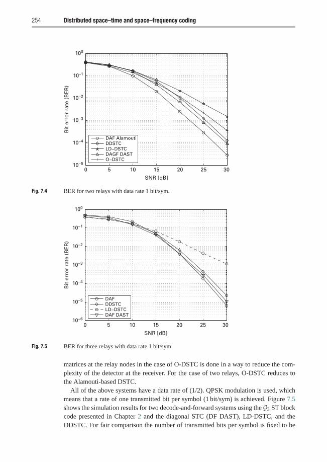
254 Distributed space–time and space–frequency coding
0 5 10 15 20 25 3010−5
10−4
10−3
10−2
10–1
100
SNR [dB]
Bit
err
or
rate
(B
ER
)
DAF AlamoutiDDSTCLD−DSTCDAGF DASTO−DSTC
Fig. 7.4 BER for two relays with data rate 1 bit/sym.
0 5 10 15 20 25 3010−6
10−5
10−4
10−3
10−2
10−1
100
SNR [dB]
Bit
err
or
rate
(B
ER
)
DAFDDSTCLD−DSTCDAF DAST
Fig. 7.5 BER for three relays with data rate 1 bit/sym.
matrices at the relay nodes in the case of O-DSTC is done in a way to reduce the com-plexity of the detector at the receiver. For the case of two relays, O-DSTC reduces tothe Alamouti-based DSTC.
All of the above systems have a data rate of (1/2). QPSK modulation is used, whichmeans that a rate of one transmitted bit per symbol (1 bit/sym) is achieved. Figure 7.5shows the simulation results for two decode-and-forward systems using the G3 ST blockcode presented in Chapter 2 and the diagonal STC (DF DAST), LD-DSTC, and theDDSTC. For fair comparison the number of transmitted bits per symbol is fixed to be
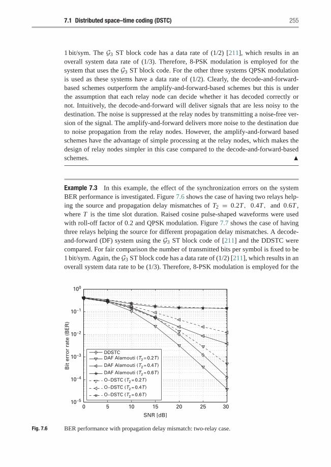
7.1 Distributed space–time coding (DSTC) 255
1 bit/sym. The G3 ST block code has a data rate of (1/2) [211], which results in anoverall system data rate of (1/3). Therefore, 8-PSK modulation is employed for thesystem that uses the G3 ST block code. For the other three systems QPSK modulationis used as these systems have a data rate of (1/2). Clearly, the decode-and-forward-based schemes outperform the amplify-and-forward-based schemes but this is underthe assumption that each relay node can decide whether it has decoded correctly ornot. Intuitively, the decode-and-forward will deliver signals that are less noisy to thedestination. The noise is suppressed at the relay nodes by transmitting a noise-free ver-sion of the signal. The amplify-and-forward delivers more noise to the destination dueto noise propagation from the relay nodes. However, the amplify-and-forward basedschemes have the advantage of simple processing at the relay nodes, which makes thedesign of relay nodes simpler in this case compared to the decode-and-forward-basedschemes. �
Example 7.3 In this example, the effect of the synchronization errors on the systemBER performance is investigated. Figure 7.6 shows the case of having two relays help-ing the source and propagation delay mismatches of T2 = 0.2T, 0.4T, and 0.6T ,where T is the time slot duration. Raised cosine pulse-shaped waveforms were usedwith roll-off factor of 0.2 and QPSK modulation. Figure 7.7 shows the case of havingthree relays helping the source for different propagation delay mismatches. A decode-and-forward (DF) system using the G3 ST block code of [211] and the DDSTC werecompared. For fair comparison the number of transmitted bits per symbol is fixed to be1 bit/sym. Again, the G3 ST block code has a data rate of (1/2) [211], which results in anoverall system data rate to be (1/3). Therefore, 8-PSK modulation is employed for the
0 5 10 15 20 25 3010−5
10−4
10−3
10−2
10−1
100
SNR [dB]
Bit
err
or
rate
(B
ER
)
DDSTCDAF Alamouti (T2 = 0.2T )
DAF Alamouti (T2 = 0.4T )
DAF Alamouti (T2 = 0.6T )
O−DSTC (T2 = 0.2T )
O−DSTC (T2 = 0.4T )
O−DSTC (T2 = 0.6T )
Fig. 7.6 BER performance with propagation delay mismatch: two-relay case.
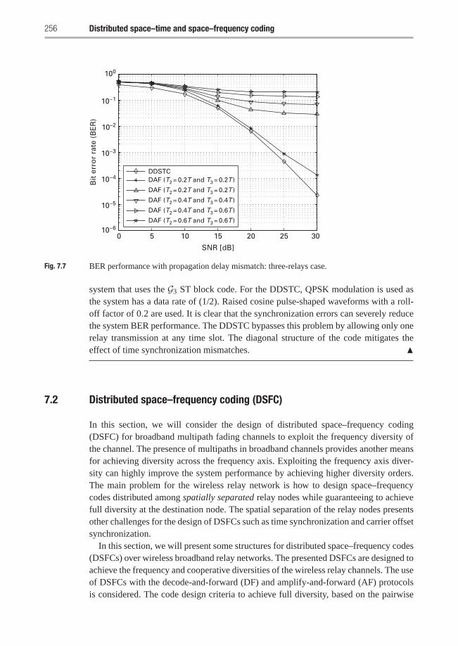
256 Distributed space–time and space–frequency coding
0 5 10 15 20 25 3010−6
10−5
10−4
10−3
10–2
10−1
100
SNR [dB]
Bit
err
or
rate
(B
ER
)
DDSTCDAF (T2 = 0.2T and T3 = 0.2T )
DAF (T2 = 0.2T and T3 = 0.2T )
DAF (T2 = 0.4T and T3 = 0.4T )
DAF (T2 = 0.4T and T3 = 0.6T )
DAF (T2 = 0.6T and T3 = 0.6T )
Fig. 7.7 BER performance with propagation delay mismatch: three-relays case.
system that uses the G3 ST block code. For the DDSTC, QPSK modulation is used asthe system has a data rate of (1/2). Raised cosine pulse-shaped waveforms with a roll-off factor of 0.2 are used. It is clear that the synchronization errors can severely reducethe system BER performance. The DDSTC bypasses this problem by allowing only onerelay transmission at any time slot. The diagonal structure of the code mitigates theeffect of time synchronization mismatches. �
7.2 Distributed space–frequency coding (DSFC)
In this section, we will consider the design of distributed space–frequency coding(DSFC) for broadband multipath fading channels to exploit the frequency diversity ofthe channel. The presence of multipaths in broadband channels provides another meansfor achieving diversity across the frequency axis. Exploiting the frequency axis diver-sity can highly improve the system performance by achieving higher diversity orders.The main problem for the wireless relay network is how to design space–frequencycodes distributed among spatially separated relay nodes while guaranteeing to achievefull diversity at the destination node. The spatial separation of the relay nodes presentsother challenges for the design of DSFCs such as time synchronization and carrier offsetsynchronization.
In this section, we will present some structures for distributed space–frequency codes(DSFCs) over wireless broadband relay networks. The presented DSFCs are designed toachieve the frequency and cooperative diversities of the wireless relay channels. The useof DSFCs with the decode-and-forward (DF) and amplify-and-forward (AF) protocolsis considered. The code design criteria to achieve full diversity, based on the pairwise
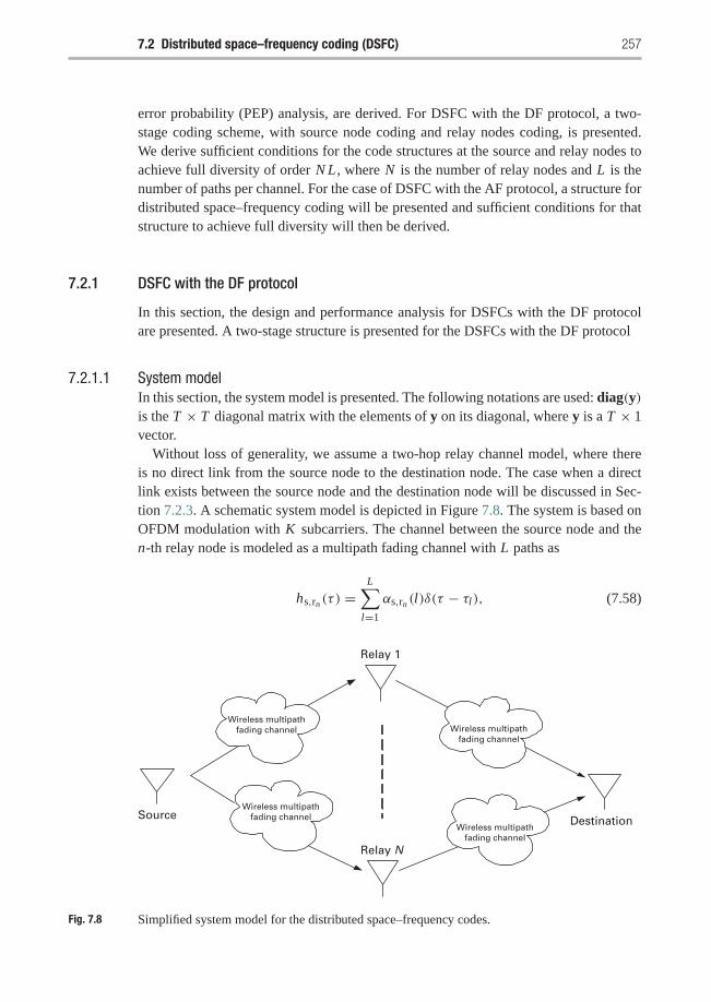
7.2 Distributed space–frequency coding (DSFC) 257
error probability (PEP) analysis, are derived. For DSFC with the DF protocol, a two-stage coding scheme, with source node coding and relay nodes coding, is presented.We derive sufficient conditions for the code structures at the source and relay nodes toachieve full diversity of order N L , where N is the number of relay nodes and L is thenumber of paths per channel. For the case of DSFC with the AF protocol, a structure fordistributed space–frequency coding will be presented and sufficient conditions for thatstructure to achieve full diversity will then be derived.
7.2.1 DSFC with the DF protocol
In this section, the design and performance analysis for DSFCs with the DF protocolare presented. A two-stage structure is presented for the DSFCs with the DF protocol
7.2.1.1 System modelIn this section, the system model is presented. The following notations are used: diag(y)is the T × T diagonal matrix with the elements of y on its diagonal, where y is a T × 1vector.
Without loss of generality, we assume a two-hop relay channel model, where thereis no direct link from the source node to the destination node. The case when a directlink exists between the source node and the destination node will be discussed in Sec-tion 7.2.3. A schematic system model is depicted in Figure 7.8. The system is based onOFDM modulation with K subcarriers. The channel between the source node and then-th relay node is modeled as a multipath fading channel with L paths as
hs,rn (τ ) =L∑
l=1
αs,rn (l)δ(τ − τl), (7.58)
Source Destination
Relay 1
Relay N
Wireless multipathfading channel
Wireless multipathfading channel
Wireless multipathfading channel
Wireless multipathfading channel
Fig. 7.8 Simplified system model for the distributed space–frequency codes.
258 Distributed space–time and space–frequency coding
where τl is the delay of the l-th path, δ(·) is the Dirac delta function, and αs,rn (l) is thecomplex amplitude of the l-th path. The αs,rn (l)’s are modeled as zero-mean, complexGaussian random variables with variance E
[|αs,rn (l)|2] = σ 2(l). We assume symme-
try between the relay nodes for simplicity of presentation; the analysis can be easilyextended to the asymmetric case. The channels are normalized such that the chan-nel variance
∑Ll=1 σ
2(l) = 1. A cyclic prefix is introduced to convert the multipathfrequency-selective fading channels to flat fading subchannels.
The system has two phases as follows. In phase 1, the source node broadcasts theinformation to the N relays. The received signal in the frequency domain on the k-thsubcarrier at the n-th relay node is given by
ys,rn (k) =√
P1 Hs,rn (k)s(k)+ vs,rn (k), k = 1, . . . , K ; n = 1, . . . , N , (7.59)
where P1 is the transmitted source node power, Hs,rn (k) is the channel attenuation of thesource node to the n-th relay node channel on the k-th subcarrier, s(k) is the transmittedsource node symbol on the k-th subcarrier with E
{|s(k)|2} = 1, and vs,rn (k) is the n-threlay node additive white Gaussian noise on the k-th subcarrier that is modeled as zero-mean circularly symmetric complex Gaussian random variable with variance N0/2 perdimension. The subcarrier noise terms are statistically independent assuming that thetime-domain noise samples are statistically independent and identically distributed.2 In(7.59), Hs,rn (k) is given by
Hs,rn (k) =L∑
l=1
αs,rn (l)e−j2π(k−1)� f τl , k = 1, . . . , K , (7.60)
where � f = 1/T is the subcarrier frequency separation and T is the OFDM symbolduration. We assume perfect channel state information at any receiving node but nochannel information at transmitting nodes.
In phase 2, relays that have decoded correctly in phase 1 will forward the source nodeinformation. Each relay is assumed to be able to decide whether it has decoded correctlyor not. This can be achieved through the use of error detecting codes such as the cyclicredundancy codes (CRC).
The transmitted K × N space–frequency (SF) codeword from the relay nodes isgiven by
Cr =
⎛⎜⎜⎜⎝Cr(1, 1) Cr(1, 2) · · · Cr(1, N )Cr(2, 1) Cr(2, 2) · · · Cr(2, N )...
.... . .
...
Cr(K , 1) Cr(K , 2) · · · Cr(K , N )
⎞⎟⎟⎟⎠ , (7.61)
2 FFT, which is used to transform the received data from the time-domain to the frequency-domain, can berepresented by a unitary matrix multiplication. Unitary transformation of a Gaussian random vector, whosecomponents are statistically independent and identically distributed, results in a Gaussian random vectorwith statistically independent and identically distributed components.
7.2 Distributed space–frequency coding (DSFC) 259
where Cr(k, n) is the symbol transmitted by the n-th relay node on the k-th subcarrier.Note that Cr will be SF code transmitted by the relay nodes if all of them have decodedcorrectly in phase 1. The SF is assumed to satisfy the power constraint ||Cr||2F ≤ K .
The received signal at the destination node on the k-th subcarrier is given by
yd(k) =√
P2
N∑n=1
Hrn ,d(k)Cr(k, n)In + vrn ,d(k), (7.62)
where P2 is the relay node power, Hrn ,d(k) is the attenuation of the channel between then-th relay node and the destination node on the k-th subcarrier, vrn ,d(k) is the destinationadditive white Gaussian noise on the k-th subcarrier, and In is the state of the n-th relay.In will equal 1 if the n-th relay has decoded correctly in phase 1, otherwise, In willequal 0.
7.2.1.2 Performance analysisIt is now necessary to develop sufficient code design criteria for the DSFC to achievefull diversity of order N × L . Unlike the case of MIMO space–frequency coding, wewill need a two-stage coding to achieve full diversity at the destination node. Therefore,the presented DSFCs will have two stages of coding: the first stage is coding at thesource node and the second stage is coding at the relay nodes. The transmitted sourcenode code will be designed to guarantee a diversity of order L at any relay node, andthis will in turn cause the presented DSFC to achieve full diversity of order N × L , aswill be shown later.
7.2.1.3 Source node codingDue to the symmetry assumption, the pairwise error probability (PEP) is the same atany relay node. For two distinct transmitted source node symbols, s and s, the PEP canbe tightly upper-bounded as (refer to Chapter 3)
P E P(s → s) ≤(
2ν − 1ν
)( ν∏i=1
λi
)−1 (P1
N0
)−ν(7.63)
and ν is the rank of the matrix C ◦ R where
C = (s− s)(s− s)H,
R = E{Hs,rn HH
s,rn
},
and
Hs,rn = [Hs,rn (1), . . . , Hs,rn (K )]T.
Here the λi ’s are the nonzero eigenvalues of the matrix C ◦ R, where ◦ denotes theHadamard product.
260 Distributed space–time and space–frequency coding
The correlation matrix, R, of the channel impulse response can be found as
R = E{Hs,rn HH
s,rn
}= WE
{αs,rnα
Hs,rn
}WH
= Wdiag{σ 2(1), σ 2(2), . . . , σ 2(L)}WH, (7.64)
where
αs,rn = [αs,rn (1), αs,rn (2), . . . , αs,rn (L)]T,
W =
⎛⎜⎜⎜⎝1 1 · · · 1wτ1 wτ2 · · · wτL
......
. . ....
w(K−1)τ1 w(K−1)τ2 · · · w(K−1)τL
⎞⎟⎟⎟⎠ ,
and w = e−j2π� f .The coding at the source node is implemented to guarantee a diversity of order L ,
which is the maximum achievable diversity order at any relay node. The transmittedK × 1 source node code is partitioned into subblocks of length L and each subblockwill be designed to guarantee a diversity of order L at any relay node as will be seenlater. Let M = �K/L� denote the number of subblocks in the source node transmittedOFDM block. The transmitted K × 1 source node code is given as
s = [s(1), s(2), . . . , s(K )]T= [FT
1 ,FT2 , . . . ,F
TM , 0
TK−M L ]T, (7.65)
where
Fi = [Fi (1), . . . , Fi (L)]T
is the i-th subblock of dimension L×1. Zeros are padded if K is not an integer multipleof L . For any two distinct source codewords, s and s = [FT
1 , FT2 , . . . , F
TM , 0
TK−M L ]T, at
least one index p0 exists for which Fp0 is not equal to Fp0 .Based on the presented structure of the transmitted code from the source node, suf-
ficient conditions for the code to achieve a diversity of order L at the relay nodes arederived. We assume for s and s that Fp = Fp for all p �= p0, which corresponds to theworst-case PEP. This does not decrease the rank of the matrix C ◦ R.
Define the L × L matrix Q = {qi, j } as
qi, j =L∑
l=1
σ 2(l)w(i− j)τ (l), 1 ≤ i, j ≤ L .
7.2 Distributed space–frequency coding (DSFC) 261
Note that the nonzero eigenvalues of the matrix C◦R are the same as those of the matrix(Fp0 − Fp0
) (Fp0 − Fp0
)H ◦Q. Hence, we have(Fp0 − Fp0
) (Fp0 − Fp0
)H ◦Q
=[diag
(Fp0 − Fp0
)1L×Ldiag
(Fp0 − Fp0
)H]◦Q
= diag(Fp0 − Fp0
)Q diag
(Fp0 − Fp0
)H(7.66)
where 1L×L is the L × L matrix whose all elements are ones. The last equality followsfrom a property of the Hadamard product.
If all of the eignenvalues of the matrix(Fp0 − Fp0
) (Fp0 − Fp0
)H ◦Q are nonzero,
then their product can be calculated as
det
((Fp0 − Fp0
) (Fp0 − Fp0
)H ◦Q)
= det(diag
(Fp0 − Fp0
))det (Q) det
(diag
(Fp0 − Fp0
)H)
=L∏
l=1
∣∣∣Fp0(l)− Fp0(l)∣∣∣2 (det(Q)) . (7.67)
The matrix Q is nonsingular. Hence, if the product∏L
l=1
∣∣∣Fp0(l)− Fp0(l)∣∣∣2 is nonzero
over all possible pairs of distinct transmitted source codewords, s and s, then a diversityof order L will be achieved at each relay node.
In phase 2, relays that have decoded correctly in phase 1 will forward the sourcenode information. The received signal at the destination node on the k-th subcarrier isas given in (7.62). The state of the n-th relay node In is a Bernoulli random variablewith a probability mass function (pmf) given by
In ={
0 with probability = SER
1 with probability = 1− SER,
where SER is the symbol error rate at the n-th relay node. Note that SER is the same forany relay node due to the symmetry assumption. If the transmitted code from the source
node is designed such that the product∏L
l=1
∣∣∣Fp0(l)− Fp0(l)∣∣∣2 is nonzero, for at least
one index p0, over all the possible pairs of distinct transmitted source codewords, s ands, then the SER at the n-th relay node can be upper-bounded as
SER =∑s∈S
Pr{s} Pr{error given that s was transmitted}
≤∑s∈S
Pr{s}∑
s∈S,s �=s
PEP(s → s)
≤ c × SNR−L , (7.68)
262 Distributed space–time and space–frequency coding
where S is the set of all possible transmitted source codewords and c is a constant thatdoes not depend on the SNR. The first inequality follows from the union upper boundand the second inequality follows from (7.63), where SNR is defined as SNR = P1/N0.
7.2.1.4 Relay Nodes CodingNext, the design of the SF code at the relay nodes to achieve a diversity of order N Lis considered. We will present SF codes constructed from the concatenation of blockdiagonal matrices, which is similar to the structure used in Chapter 3 to design full-rate,full-diversity space–frequency codes over MIMO channels. We will derive sufficientconditions for that code structure to achieve full diversity at the destination node.
Let P = �K/N L� denote the number of subblocks in the transmitted OFDM blockfrom the relay nodes. The transmitted K × N SF codeword from the relay nodes, if allrelays decoded correctly, is given by
Cr = [GT1 ,G
T2 , . . . ,G
TP , 0
TK−PLN]T, (7.69)
where Gi is the i-th subblock of dimension N L × N . Zeros are padded if K is not aninteger multiple of N L . Each Gi is a block diagonal matrix that has the structure
Gi =
⎛⎜⎜⎜⎝X1L×1 0L×1 · · · 0L×1
0L×1 X2L×1 · · · 0L×1...
.... . .
...
0L×1 0L×1 · · · XNL×1
⎞⎟⎟⎟⎠ (7.70)
and let
X = [XT1 ,X
T2 , · · · ,XT
N ] = [x(1), x(2), · · · , x(N L)].For two distinct transmitted source codewords, s and s, and a given realization of the
relays states I = [I1, I2, . . . , In]T, the conditional PEP can be tightly upper-bounded as
PEP(s → s/I) ≤(
2κ − 1κ
)( κ∏i=1
λi
)−1 (P2
N0
)−κ, (7.71)
and κ is the rank of the matrix C(I) ◦ R where
C(I) = (Cr − Cr )diag(I)(C− Cr )H.
For two source codewords, s and s, at least one index p0 exists for which Gp0 �= Gp0 .We assume for s and s that Gp = Gp for all p �= p0. As for the source node codingcase, this does not decrease the rank of the matrix C(I) ◦ R that corresponds to anyrealization I of the relays states.
Define the N L × N L matrix S = {si, j } as
si, j =L∑
l=1
σ 2(l)w(i− j)τ (l), 1 ≤ i, j ≤ N L .
Note that the nonzero eigenvalues of the matrix C(I) ◦ R are the same as the nonzero
eigenvalues of the matrix(Gp0(I)− Gp0(I)
) (Gp0(I)− Gp0(I)
)H ◦S, where Gp0(I) is
7.2 Distributed space–frequency coding (DSFC) 263
formed from Gp0 by setting the columns corresponding to the relays that have decodederroneously to zeros. Hence,(
Gp0(I)− Gp0(I)) (
Gp0(I)− Gp0(I))H ◦ S
=(
diag(X− X) (diag(I)⊗ 1L×1) (diag(I)⊗ 1L×1)H diag(X− X)H
)◦ S
=(diag(X− X) (diag(I)⊗ 1L×L)diag(X− X)H
)◦ S
= diag(X− X)[(diag(I)⊗ 1L×L) ◦ S
]diag(X− X)H, (7.72)
where the second and the third equalities follow from the properties of the tensor andHadamard products.
Let
nI =N∑
n=1
In
denote the number of relays that have decoded correctly corresponding to a realizationI of the relays states. Using (7.72), the product of the nonzero eigenvalues of the matrixC(I) ◦ R can be found as
κ∏i=1
λi =⎛⎝ N L∏
i=1, i∈I|x(i)− x(i)|2
⎞⎠ · (det(S0))nI (7.73)
where I is the index set of symbols that are transmitted from the relays that havedecoded correctly corresponding to the realization I and
S0 = {si, j }, 1 ≤ i, j ≤ L .
The result in (7.73) is based on the assumption that the product∏N L
i=1, i∈I} |x(i)− x(i)|2is nonzero. The first product in (7.73) is over nIL terms. The matrix S0 is always fullrank of order L . Hence, designing the product
∏N Li=1, i∈I |x(i) − x(i)|2 to be nonzero
will guarantee a rate of decay, at high SNR, of the conditional PEP as SNR−nIL , whereSNR is now defined as SNR = P2/N0. To guarantee that this rate of decay, SNR−nIL , isalways achieved irrespective of the state realization I of the relay nodes then the product∏N L
i=1 |x(i)−x(i)|2 should be nonzero. Hence, designing the product∏N L
i=1 |x(i)−x(i)|2to be nonzero for any pair of distinct source codewords is a sufficient condition for theconditional PEP to decay as SNR−nIL for any realization I, where nI is the number ofrelays that have decoded correctly corresponding to I.
Now, we calculate the PEP at the destination node for our DSFC structure. Let cr
denote the number of relays that have decoded correctly. Then cr follows a Binomialdistribution as
Pr{cr = k} =(
Nk
)(1− SER)kSERN−k, (7.74)
264 Distributed space–time and space–frequency coding
where SER is the symbol error rate at the relay nodes. The destination PEP is given by
PEP(s → s) =∑
I
Pr{I}PEP(s → s/I)
=N∑
k=0
Pr{cr = k}∑
{I:nI=k}PEP(s → s/I)
=N∑
k=0
(Nk
)(1− SER)kSERN−k
∑{I:nI=k}
PEP(s → s/I), (7.75)
Using the upper bound on the SER at the relay nodes given in (7.68) and the expressionfor the conditional PEP at the destination node in (7.71), and upper-bounding (1−SER)by 1, it can be shown that
PEP(s → s) ≤ constant× SNR−N L . (7.76)
Hence, our structure for DSFCs with two-stage coding at the source node and the relaynodes achieves a diversity of order N L , which is the rate of decay of the PEP at highSNR.
7.2.2 DSFC with the AF protocol
In this section, the design and performance analysis for DSFCs with the AF protocol arepresented. A structure is presented and sufficient conditions for that structure to achievefull diversity are then derived for some special cases.
7.2.2.1 System modelIn this section, we describe the system model for DSFC with the AF protocol. Thereceived signal model at the relay nodes and the channel gains are modeled as in Sec-tion 7.2.1. The transmitted data from the source node is parsed into subblocks of sizeN L × 1. Let P = �K/N L� denote the number of subblocks in the transmitted OFDMblock. The transmitted K × 1 source codeword is given by
s = [s(1), s(2), . . . , s(K )]T = [BT1 ,B
T2 , . . . ,B
TP , 0
TK−PLN]T, (7.77)
where Bi is the i-th subblock of dimension N L × 1. Zeros are padded if K is not aninteger multiple of N L . For each subblock, Bi , the n-th relay only forwards the dataon L subcarriers. For example, relay 1 will only forward [Bi (1), . . . ,Bi (L)] for all i’sand send zeros on the remaining set of subcarriers. In general, the n-th relay will onlyforward [Bi ((n − 1)L + 1), . . . ,Bi ((n − 1)L + L)] for all i’s.
At the relay nodes, each node will normalize the received signal on the subcarriersthat it will forward before retransmission and send zeros on the remaining set of subcar-riers. If the k-th subcarrier is to be forwarded by the n-th relay, the relay will normalizethe received signal on that subcarrier by the factor
β(k) =√
1
P1|Hs,rn (k)|2 + N0.
7.2 Distributed space–frequency coding (DSFC) 265
The relay nodes will use OFDM modulation for transmission to the destination node.At the destination node, the received signal on the k-th subcarrier, assuming it wasforwarded by the n-th relay, is given by
y(k) = Hrn ,d(k)√
P2
(√1
P1|Hs,rn (k)|2 + N0
(√P1 Hs,rn (k)s(k)+ vs,rn (k)
))+ vrn ,d(k), (7.78)
where P2 is the relay node power, Hrn ,d(k) is the attenuation of the channel between then-th relay node and the destination node on the k-th subcarrier, and vs,rn (k) is the desti-nation noise on the k-th subcarrier. The vrn ,d(k)’s are modeled as zero mean, circularlysymmetric complex Gaussian random variables with a variance of N0/2 per dimension.
7.2.2.2 Performance analysisIn this section, the PEP of the DSFC with the AF protocol is presented. Based on thePEP analysis, code design criteria are derived.
The received signal at destination on the k-th subcarrier given by (7.78) can berewritten as
y(k) = Hrn ,d(k)√
P2
(√1
P1|Hs,rn (k)|2 + N0
√P1 Hs,rn (k)s(k)
)+ zrn ,d(k), (7.79)
where zrn ,d(k) accounts for the noise propagating from the relay node as well as thedestination noise. zrn ,d(k) follows a circularly symmetric complex Gaussian randomvariable with a variance
δ2z (k) =
(P2|Hrn ,d(k)|2
P1|Hs,rn (k)|2 + N0+ 1
)N0.
The probability density function of zrn ,d(k) given the channel state information (CSI) isgiven by
p(zrn ,d(k)/CSI) = 1
πδ2z (k)
exp
(− 1
δ2z (k)
|zrn ,d(k)|2). (7.80)
The receiver applies a maximum likelihood (ML) detector to the received signal, whichis given as
s = arg mins
K∑k=1
1
δ2z (k)
∣∣∣∣∣∣y(k)−√
P1 P2 Hs,rn (k)Hrn ,d(k)√P1|Hs,rn (k)|2 + N0
s(k)
∣∣∣∣∣∣2
, (7.81)
where the n index (which is the index of the relay node) is adjusted according to the kindex (which is the index of the subcarrier).
Now, sufficient conditions for the presented code structure to achieve full diversityare derived. The pdf of a received vector
y = [y(1), y(2), . . . , y(K )]T
266 Distributed space–time and space–frequency coding
given that the codeword s was transmitted is given by
p(y/s,CSI)
=(
K∏k=1
1
πδ2z (k)
)exp
( K∑k=1
− 1
δ2z (k)
∣∣∣∣∣∣y(k)−√
P1 P2 Hs,rn (k)Hrn ,d(k)√P1|Hs,rn (k)|2 + N0
s(k)
∣∣∣∣∣∣2 ).
(7.82)
The PEP of mistaking s by s can be upper-bounded as
PEP(s → s) ≤ E{exp(λ[ln p(y/s)− ln p(y/s)])} , (7.83)
and the relation applies for any λ, which can selected to get the tightest bound. Any twodistinct codewords s and
s = [B1, B2, . . . , Bp]T
will have at least one index p0 such that Bp0 �= Bp0 . We will assume that s and s willhave only one index p0 such that Bp0 �= Bp0 , which corresponds to the worst case PEP.
Averaging the PEP expression in (7.83) over the noise distribution given in (7.80)we get
PEP(s → s) ≤ E
{exp
(− λ(1− λ)
N∑n=1
L∑l=1(
P1|Hs,rn (J + (n − 1)L + l)|2 P2|Hrn ,d(J + (n − 1)L + l)|2(P1|Hs,rn (J + (n − 1)L + l)|2 + P2|Hrn ,d(J + (n − 1)L + l)|2 + N0
)N0
)×∣∣∣Bp0((n − 1)L + l)− Bp0((n − 1)L + l)
∣∣∣2 )}, (7.84)
where J = (p0 − 1)N L . Take λ = 1/2 to minimize the upper bound in (7.84), hence,we get
PEP(s → s) ≤ E
{exp
(− 1
4
N∑n=1
L∑l=1(
P1|Hs,rn (J + (n − 1)L + l)|2 P2|Hrn ,d(J + (n − 1)L + l)|2(P1|Hs,rn (J + (n − 1)L + l)|2 + P2|Hrn ,d(J + (n − 1)L + l)|2 + N0
)N0
)×∣∣∣Bp0((n − 1)L + l)− Bp0((n − 1)L + l)
∣∣∣2 )}, (7.85)
At high SNR, we have
P1|Hs,rn (k)|2 P2|Hrn ,d(k)|2(P1|Hs,rn (k)|2 + P2|Hrn ,d(k)|2 + N0
)N0≈ P1|Hs,rn (k)|2 P2|Hrn ,d(k)|2(
P1|Hs,rn (k)|2 + P2|Hrn ,d(k)|2)
N0,
7.2 Distributed space–frequency coding (DSFC) 267
which is the scaled harmonic mean of the source–relay and relay–destination SNRs onthe k-th subcarrier.
The scaled harmonic mean of two non-negative numbers, a1 and a2, can be upper-and lower-bounded as
1
2min (a1, a2) ≤ a1a2
a1 + a2≤ min (a1, a2) . (7.86)
Using the lower-bound in (7.86) the PEP in (7.85) can be further upper-bounded as
PEP(s → s) ≤ E
{exp
(− 1
8
N∑n=1
L∑l=1
min
(P1
N0|Hs,rn ((p0 − 1)N L
+ (n − 1)L + l)|2, P2
N0|Hrn ,d((p0 − 1)N L + (n − 1)L + l)|2
)∣∣∣Bp0((n − 1)L + l)− Bp0((n − 1)L + l)
∣∣∣2 )}. (7.87)
If P2 = P1 and SNR is defined as P1/N0, then the PEP is now upper-bounded as
PEP(s → s) ≤ E
{exp
(− 1
8
N∑n=1
L∑l=1
min
(SNR|Hs,rn ((p0 − 1)N L
+ (n − 1)L + l)|2,SNR|Hrn ,d((p0 − 1)N L + (n − 1)L + l)|2)
∣∣∣Bp0((n − 1)L + l)− Bp0((n − 1)L + l)∣∣∣2 )}. (7.88)
7.2.2.3 PEP Analysis for L= 1The case of L equal to 1 corresponds to a flat, frequency nonselective fading channel.The PEP in (7.88) is now given by
PEP(s → s) ≤ E
{exp
(− 1
8
N∑n=1
min
(SNR|Hs,rn ((p0 − 1)N L
+ (n − 1)L + 1)|2,SNR|Hrn ,d((p0 − 1)N L + (n − 1)L + 1)|2)
∣∣∣Bp0((n − 1)L + 1)− Bp0((n − 1)L + 1)∣∣∣2 )}. (7.89)
The random variables SNR|Hs,rn (k)|2 and SNR|Hrn ,d(k)|2 follow an exponential distri-bution with rate 1/SNR for all k. The minimum of two exponential random variablesis an exponential random variable with rate that is the sum of the two randomvariables rates. Hence, min
(SNR|Hs,rn (k)|2 , SNR|Hrn ,d(k)|2
)follows an exponential
distribution with rate 2/SNR.
268 Distributed space–time and space–frequency coding
The PEP upper bound is now given by
PEP(s → s) ≤N∏
n=1
1
1+ 116SNR
∣∣∣Bp0((n − 1)L + 1)− Bp0((n − 1)L + 1)∣∣∣2 . (7.90)
At high SNR, we can neglect 1 besides the SN R dependent term in the denominator of(7.90). Hence, the PEP can now be upper-bounded as
PEP(s → s)
�(
1
16SNR
)−N(
N∏n=1
∣∣∣Bp0((n − 1)L + 1)− Bp0((n − 1)L + 1)∣∣∣2)−1
. (7.91)
The result in (7.91) is under the assumption that the product
N∏n=1
∣∣∣Bp0((n − 1)L + 1)− Bp0((n − 1)L + 1)∣∣∣2
is nonzero. Clearly, if that product is nonzero, then the system will achieve a diversity oforder N L , where L is equal to 1 in this case. From the expression in (7.91) the codinggain of the space–frequency code is maximized when the product
mins�=s
N∏n=1
∣∣∣Bp0((n − 1)L + 1)− Bp0((n − 1)L + 1)∣∣∣2
is maximized, which is the minimum product distance.
7.2.2.4 PEP analysis for L= 2The PEP in (7.88) can now be given as
PEP(s → s) ≤ E
{exp
(− 1
8
N∑n=1
2∑l=1
min
(SNR|Hs,rn ((p0 − 1)N L
+ (n − 1)L + l)|2,SNR|Hrn ,d((p0 − 1)N L + (n − 1)L + l)|2)
∣∣∣Bp0((n − 1)L + l)− Bp0((n − 1)L + l)∣∣∣2 )}, (7.92)
where L = 2. The analysis in this case is more involved since the random variablesappearing in (7.92) are correlated. Signals transmitted from the same relay node ondifferent subcarriers will experience correlated channel attenuations.
As a first step in deriving the code design criterion, we prove that the channel attenua-tions, |Hs,rn (k1)|2 and|Hs,rn (k2)|2 for any k1 �= k2, have a bivariate Gamma distributionas their joint pdf. The same applies for |Hrn ,d(k1)|2 and |Hrn ,d(k2)|2 for any k1 �= k2.The proof of this result is given in the Appendix to this chapter.
To evaluate the expectation in (7.92) we need the expression for the joint pdf of thetwo random variables
M1 = min(SNR|Hs,rn (k1)|2,SNR|Hrn ,d(k1)|2
)
7.2 Distributed space–frequency coding (DSFC) 269
and
M2 = min(SNR|Hs,rn (k2)|2,SNR|Hrn ,d(k2)|2
)for some k1 �= k2. Although M1 and M2 can be easily seen to be marginally expo-nential random variables, they are not jointly Gamma distributed. Define the randomvariables X1 = SNR|Hs,rn (k1)|2, X2 = SNR|Hs,rn (k2)|2, Y1 = SNR|Hrn ,d(k1)|2, andY2 = SNR|Hrn ,d(k2)|2. All of these random variables are marginally exponential withrate 1/SN R. Under the assumptions of our channel model, the pairs (X1, X2) and(Y1, Y2) are independent. Hence, the joint pdf of (X1, X2, Y1, Y2), using the result inthe Appendix, is given by
f X1,X2,Y1,Y2(x1, x2, y1, y2)
= fX1,X2(x1, x2) fY1,Y2(y1, y2)
= 1
SNR2(1− ρx1x2)(1− ρy1 y2)exp
(− x1 + x2
SNR(1− ρx1x2)
)· I0
(2√ρx1x2
SNR(1− ρx1x2)
√x1x2
)exp
(− y1 + y2
SNR(1− ρy1 y2)
)· I0
(2√ρy1 y2
SNR(1− ρy1 y2)
√y1y2
)U (x1)U (x2)U (y1)U (y2), (7.93)
where I0(·) is the modified Bessel function of the first kind of order zero and U (·) is theHeaviside unit step function. ρx1x2 is the correlation coefficient between X1 and X2 andsimilarly, ρy1 y2 is the correlation coefficient between Y1 and Y2.
The joint cumulative distribution function (cdf) of the pair (M1,M2) can becomputed as
F M1,M2(m1,m2)
� Pr [M1 ≤ m1,M2 ≤ m2]
= Pr [min (X1, Y1) ≤ m1,min (X2, Y2) ≤ m2]
= 2∫ m1
y1=0
∫ ∞
x1=y1
∫ m2
y2=0
∫ ∞
x2=y2
fX1,X2(x1, x2) fY1,Y2(y1, y2)dy1dx1dy2dx2
+ 2∫ m1
y1=0
∫ ∞
x1=y1
∫ m2
x2=0
∫ ∞
y2=x2
fX1,X2(x1, x2) fY1,Y2(y1, y2)dy1dx1dx2dy2, (7.94)
where we have used the symmetry assumption of the source–relay and relay–destinationchannels.
The joint pdf of (M1,M2) can now be given as
fM1,M2(m1,m2) = ∂2
∂m1∂m2FM1,M2(m1,m2)
= 2 fY1,Y2(m1,m2)
∫ ∞
x1=m1
∫ ∞
x2=m2
fX1,X2(x1, x2)dx1dx2
+ 2∫ ∞
x1=m1
∫ ∞
y2=m2
fX1,X2(x1,m2) fY1,Y2(m1, y2)dx1dx2. (7.95)
270 Distributed space–time and space–frequency coding
To get the PEP upper bound in (7.92) we need to calculate the expectation
E
{exp
(− 1
8
(M1
∣∣∣B(k1)− B(k1)
∣∣∣2 + M2
∣∣∣B(k2)− B(k2)
∣∣∣2 ))}=∫ ∞
m1=0
∫ ∞
m2=0exp
(− 1
8
(m1
∣∣∣B(k1)− B(k1)
∣∣∣2 + m2
∣∣∣B(k2)− B(k2)
∣∣∣2 ))fM1,M2(m1,m2)dm1dm2.
(7.96)
At high enough SNR, we have
I0
( 2√ρx1x2
SNR(1− ρx1x2)
√x1x2
)≈ 1.
Using this approximation, the PEP upper bound can be approximated at high SNR as
PEP(s → s) �(
2N∏m=1
∣∣∣Bp0(m)− Bp0(m)∣∣∣2)−1 (
1
16(1− ρ)SNR
)−2N
, (7.97)
where ρ = ρx1x2 = ρy1 y2 . Again, full diversity is achieved when the product
2N∏m=1
∣∣∣Bp0(m)− Bp0(m)∣∣∣2
is nonzero. The coding gain of the space–frequency code is maximized when theproduct
mins�=s
2N∏m=1
∣∣∣Bp0(m)− Bp0(m)∣∣∣2
is maximized.The analysis becomes highly involved for any L ≥ 3. It is very difficult to get closed
form expressions in this case due to the correlation among the summed terms in (7.88)for which there is no closed form pdf expressions, similar to (7.93).
Example 7.4 In this example, we investigate the performance of the presented SDFCs.Figure 7.9 shows the case of a simple two-ray, L = 2, channel model with a delay ofτ = 5μs between the two rays. The two rays have equal powers, i.e., σ 2(1) = σ 2(2).The number of subcarriers is K = 128 with a system bandwidth of 1 MHz. We useBPSK modulation and Vandermonde-based linear transformations. Figure 7.9 showsthe SER of the presented DSFCs versus the SNR defined as SNR = (P1 + P2)/N0,and we use P1 = P2, i.e., equal power allocation between the source and relay nodes.We simulated three cases: all channel variances are ones, relays close to source, andrelays close to destination. For the case of relays close to source, the variance of anysource–relay channel is taken to be 10 and the variance of any relay–destination channelis taken to be 1. For the case of relays close to destination, the variance of any source–relay channel is taken to be 1 and the variance of any relay–destination channel is takento be 10. From Figure 7.9, it is clear that DSFCs with the DF protocol have a better
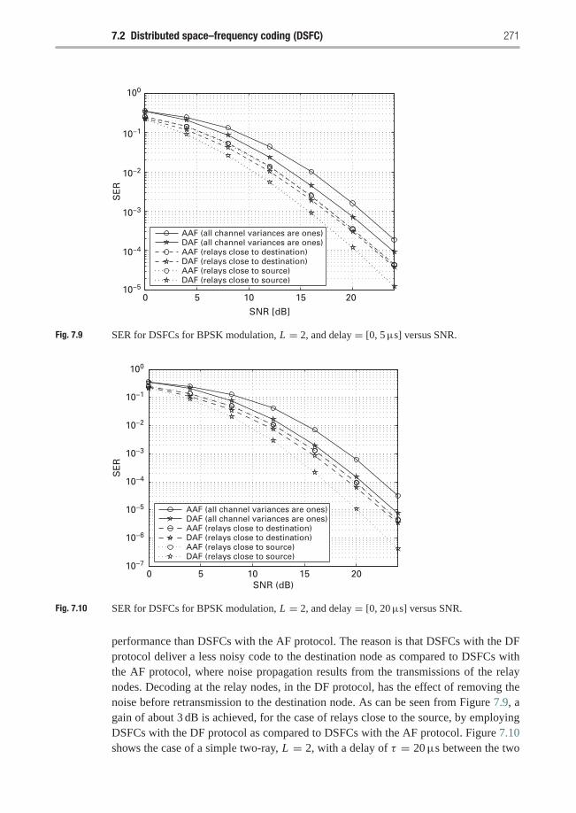
7.2 Distributed space–frequency coding (DSFC) 271
0 5 10 15 2010−5
10−4
10−3
10−2
10−1
100
SNR [dB]
SE
R
AAF (all channel variances are ones)DAF (all channel variances are ones)AAF (relays close to destination)DAF (relays close to destination)AAF (relays close to source)DAF (relays close to source)
Fig. 7.9 SER for DSFCs for BPSK modulation, L = 2, and delay = [0, 5 μs] versus SNR.
0 5 10 15 2010−7
10−6
10−5
10−4
10−3
10−2
10−1
100
SNR (dB)
SE
R
AAF (all channel variances are ones)DAF (all channel variances are ones)AAF (relays close to destination)DAF (relays close to destination)AAF (relays close to source)DAF (relays close to source)
Fig. 7.10 SER for DSFCs for BPSK modulation, L = 2, and delay = [0, 20 μs] versus SNR.
performance than DSFCs with the AF protocol. The reason is that DSFCs with the DFprotocol deliver a less noisy code to the destination node as compared to DSFCs withthe AF protocol, where noise propagation results from the transmissions of the relaynodes. Decoding at the relay nodes, in the DF protocol, has the effect of removing thenoise before retransmission to the destination node. As can be seen from Figure 7.9, again of about 3 dB is achieved, for the case of relays close to the source, by employingDSFCs with the DF protocol as compared to DSFCs with the AF protocol. Figure 7.10shows the case of a simple two-ray, L = 2, with a delay of τ = 20 μs between the two
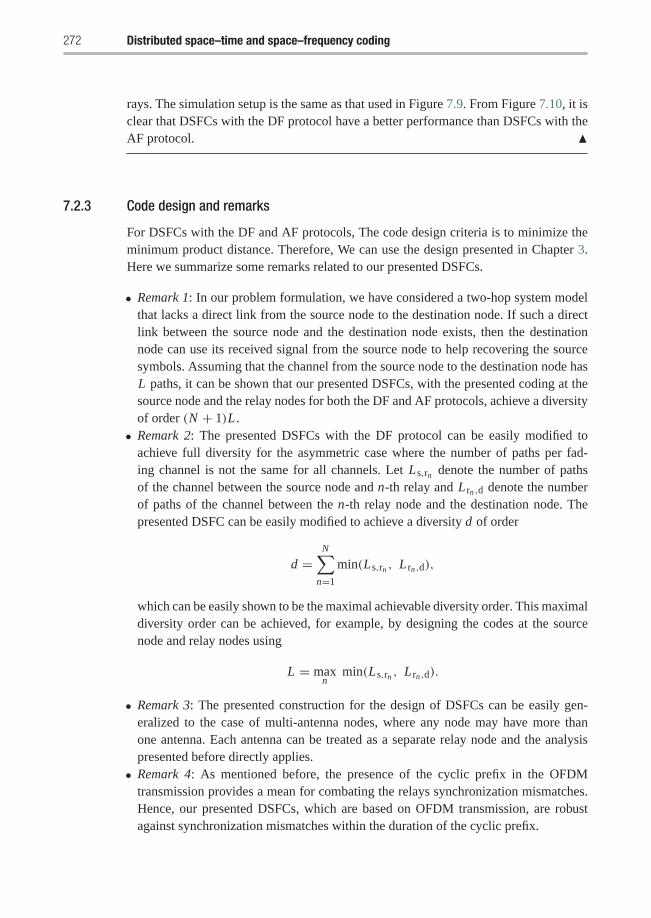
272 Distributed space–time and space–frequency coding
rays. The simulation setup is the same as that used in Figure 7.9. From Figure 7.10, it isclear that DSFCs with the DF protocol have a better performance than DSFCs with theAF protocol. �
7.2.3 Code design and remarks
For DSFCs with the DF and AF protocols, The code design criteria is to minimize theminimum product distance. Therefore, We can use the design presented in Chapter 3.Here we summarize some remarks related to our presented DSFCs.
• Remark 1: In our problem formulation, we have considered a two-hop system modelthat lacks a direct link from the source node to the destination node. If such a directlink between the source node and the destination node exists, then the destinationnode can use its received signal from the source node to help recovering the sourcesymbols. Assuming that the channel from the source node to the destination node hasL paths, it can be shown that our presented DSFCs, with the presented coding at thesource node and the relay nodes for both the DF and AF protocols, achieve a diversityof order (N + 1)L .
• Remark 2: The presented DSFCs with the DF protocol can be easily modified toachieve full diversity for the asymmetric case where the number of paths per fad-ing channel is not the same for all channels. Let Ls,rn denote the number of pathsof the channel between the source node and n-th relay and L rn ,d denote the numberof paths of the channel between the n-th relay node and the destination node. Thepresented DSFC can be easily modified to achieve a diversity d of order
d =N∑
n=1
min(Ls,rn , L rn ,d),
which can be easily shown to be the maximal achievable diversity order. This maximaldiversity order can be achieved, for example, by designing the codes at the sourcenode and relay nodes using
L = maxn
min(Ls,rn , L rn ,d).
• Remark 3: The presented construction for the design of DSFCs can be easily gen-eralized to the case of multi-antenna nodes, where any node may have more thanone antenna. Each antenna can be treated as a separate relay node and the analysispresented before directly applies.
• Remark 4: As mentioned before, the presence of the cyclic prefix in the OFDMtransmission provides a mean for combating the relays synchronization mismatches.Hence, our presented DSFCs, which are based on OFDM transmission, are robustagainst synchronization mismatches within the duration of the cyclic prefix.
7.3 Chapter summary and bibliographical notes 273
7.3 Chapter summary and bibliographical notes
The design of distributed space–time codes in wireless relay networks is considered fordifferent schemes, which vary in the processing performed at the relay nodes. For thedecode-and-forward distributed space–time codes, any space–time code that is designedto achieve full diversity over MIMO channels can achieve full diversity under theassumption that the relay nodes can decide whether they have decoded correctly ornot. A code that maximizes the coding gain over MIMO channels is not guaranteedto maximize the coding gain in the decode-and-forward distributed space–time coding.This is due to the fact that not all of the relays will always transmit their code columnsin the second phase. The code design criteria for the amplify-and-forward distributedspace–time codes were also considered. In this case, a code designed to achieve fulldiversity over MIMO channels will also achieve full diversity. Furthermore, a code thatmaximizes the coding gain over MIMO channels will also maximize the coding gain inthe amplify-and-forward distributed space–time scheme.
Then, the design of DDSTC for wireless relay networks was studied. In DDSTC, thediagonal structure of the code was imposed to simplify the synchronization betweenrandomly located relay nodes. Synchronization mismatches between the relay nodescauses inter-symbol interference, which can highly degrade the system performance.DDSTC relaxes the stringent synchronization requirement by allowing only one relay totransmit at any time slot. The code design criterion for the DDSTC based on minimizingthe PEP was derived and the design criterion is found to be maximizing the minimumproduct distance. This is the same criterion used for designing DAST codes and full-rate, full-diversity space frequency codes.
Next, the design of distributed space–frequency codes (DSFCs) was considered forthe wireless multipath relay channels. The use of DSFCs can greatly improve systemperformance by achieving higher diversity orders by exploiting the multipath diversityof the channel as well as the cooperative diversity. We have considered the design ofDSFCs with the DF and AF cooperation protocols. For the case of DSFCs with the DFprotocol, we have presented a two-stage coding scheme: source node coding and relaynodes coding. We have derived sufficient conditions for the presented code structure toachieve full diversity of order N L where N is the number of relay nodes and L is thenumber of multipaths per channel. For the case of DSFCs with the AF protocol, we havederived sufficient conditions for the presented code structure to achieve full diversity oforder N L for the special cases of L = 1 and L = 2.
The presented DSFCs are robust against the synchronization errors caused by therelays timing mismatches and propagation delays due to the presence of the cyclic prefixin the OFDM transmission.
Several works have considered the design of distributed space–time codes. It was pro-posed in [108] to use relay nodes to form a virtual multi-antenna transmitter to achievediversity. In addition, an outage analysis was presented for the system.
Some works have considered the application of the existing space–time codes in adistributed fashion for the wireless relay network [193, 7, 8, 93]. In [193], space–time
274 Distributed space–time and space–frequency coding
block codes were used in a completely distributed fashion. Each relay node transmitsa randomly selected column from the space–time code matrix. This system achievesa diversity of order one, as the signal-to-noise (SNR) tends to infinity, limited by theprobability of having all of the relay nodes selecting to transmit the same column of thespace–time code matrix. In [7], distributed space–time coding based on the Alamoutischeme and amplify-and-forward cooperation protocol was analyzed. An expressionfor the average symbol error rate (SER) was derived. In [8], a performance analysis ofthe gain of using cooperation among nodes was considered assuming that the number ofrelays available for cooperation is a Poisson random variable. The authors compared theperformance of different distributed space–time codes designed for the MIMO channelsunder this assumption. In [93], the performance of the linear dispersion (LD) space–timecodes of [59] was analyzed when used for distributed space–time coding in wirelessrelay networks.
For the case of DSFCs, a design of DSFCs was considered in [116], where a sys-tem that employs the DF protocol was used. It was assumed that all of the relay nodeswill always decode correctly, which is not always true, especially over wireless fadingchannels. Such proposed DSFCs mitigate synchronization errors due to the timing mis-matchs of relay nodes and propagation delays by employing OFDM transmission. Thepresence of the cyclic prefix in OFDM modulation can mitigate synchronization errorsof relay nodes. This follows directly due to the use of OFDM transmission and the sameapplies for our proposed DSFCs.
Further information and details can be found in [169, 170, 171, 172, 174, 175, 178].
Appendix
Consider the two random variables Hs,rn (k1) and Hs,rn (k2), we will assume without lossof generality that τ1 = 0, i.e., the delay of the first path is zero. Hs,rn (k1) is given by
Hs,rn (k1) = αs,rn (1)+ αs,rn (2)e−j2π(k1−1)� f τ2 = � (Hs,rn (k1)
)+ j� (Hs,rn (k1)),
(7.98)
where �(x), and �(x) are the real, and imaginary parts of x , respectively. From (7.98)we have
� (Hs,rn (k1)) = �(αs,rn (1))+�(αs,rn (2)) cos(2π(k1 − 1)� f τ2)
+ �(αs,rn (2)) sin(2π(k1 − 1)� f τ2)
� (Hs,rn (k1)) = �(αs,rn (1))+ �(αs,rn (2)) cos(2π(k1 − 1)� f τ2)
−�(αs,rn (2)) sin(2π(k1 − 1)� f τ2). (7.99)
Based on the channel model presented in Section 7.2.1.1 both � (Hs,rn (k1))
and� (Hs,rn (k1)
)are zero-mean Gaussian random variables with variance 1/2. The cor-
relation coefficient, ρri , between � (Hs,rn (k1))
and � (Hs,rn (k1))
can be calculated as
ρri = E{� (Hs,rn (k1)
)� (Hs,rn (k1))} = 0. (7.100)
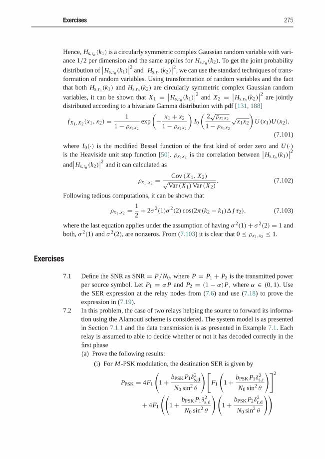
Exercises 275
Hence, Hs,rn (k1) is a circularly symmetric complex Gaussian random variable with vari-ance 1/2 per dimension and the same applies for Hs,rn (k2). To get the joint probability
distribution of∣∣Hs,rn (k1)
∣∣2 and∣∣Hs,rn (k2)
∣∣2, we can use the standard techniques of trans-formation of random variables. Using transformation of random variables and the factthat both Hs,rn (k1) and Hs,rn (k2) are circularly symmetric complex Gaussian random
variables, it can be shown that X1 =∣∣Hs,rn (k1)
∣∣2 and X2 =∣∣Hs,rn (k2)
∣∣2 are jointlydistributed according to a bivariate Gamma distribution with pdf [131, 188]
fX1,X2(x1, x2) = 1
1− ρx1x2
exp
(− x1 + x2
1− ρx1x2
)I0
(2√ρx1x2
1− ρx1x2
√x1x2
)U (x1)U (x2),
(7.101)
where I0(·) is the modified Bessel function of the first kind of order zero and U (·)is the Heaviside unit step function [50]. ρx1x2 is the correlation between
∣∣Hs,rn (k1)∣∣2
and∣∣Hs,rn (k2)
∣∣2 and it can calculated as
ρx1,x2 =Cov (X1, X2)√
Var (X1)Var (X2). (7.102)
Following tedious computations, it can be shown that
ρx1,x2 =1
2+ 2σ 2(1)σ 2(2) cos(2π(k2 − k1)� f τ2), (7.103)
where the last equation applies under the assumption of having σ 2(1)+ σ 2(2) = 1 andboth, σ 2(1) and σ 2(2), are nonzeros. From (7.103) it is clear that 0 ≤ ρx1,x2 ≤ 1.
Exercises
7.1 Define the SNR as SNR = P/N0, where P = P1 + P2 is the transmitted powerper source symbol. Let P1 = αP and P2 = (1 − α)P , where α ∈ (0, 1). Usethe SER expression at the relay nodes from (7.6) and use (7.18) to prove theexpression in (7.19).
7.2 In this problem, the case of two relays helping the source to forward its informa-tion using the Alamouti scheme is considered. The system model is as presentedin Section 7.1.1 and the data transmission is as presented in Example 7.1. Eachrelay is assumed to able to decide whether or not it has decoded correctly in thefirst phase(a) Prove the following results:
(i) For M-PSK modulation, the destination SER is given by
PPSK = 4F1
(1+ bPSK P1δ
2s,d
N0 sin2 θ
)[F1
(1+ bPSK P1δ
2s,r
N0 sin2 θ
)]2
+ 4F1
((1+ bPSK P1δ
2s,d
N0 sin2 θ
)(1+ bPSK P2δ
2r,d
N0 sin2 θ
))
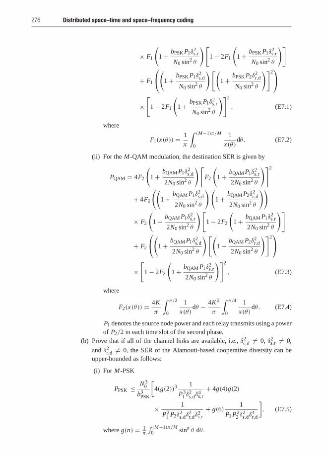
276 Distributed space–time and space–frequency coding
× F1
(1+ bPSK P1δ
2s,r
N0 sin2 θ
)[1− 2F1
(1+ bPSK P1δ
2s,r
N0 sin2 θ
)]
+ F1
⎛⎝(1+ bPSK P1δ2s,d
N0 sin2 θ
)[(1+ bPSK P2δ
2r,d
N0 sin2 θ
)]2⎞⎠
×[
1− 2F1
(1+ bPSK P1δ
2s,r
N0 sin2 θ
)]2
, (E7.1)
where
F1(x(θ)) = 1
π
∫ (M−1)π/M
0
1
x(θ)dθ. (E7.2)
(ii) For the M-QAM modulation, the destination SER is given by
PQAM = 4F2
(1+ bQAM P1δ
2s,d
2N0 sin2 θ
)[F2
(1+ bQAM P1δ
2s,r
2N0 sin2 θ
)]2
+ 4F2
((1+ bQAM P1δ
2s,d
2N0 sin2 θ
)(1+ bQAM P2δ
2r,d
2N0 sin2 θ
))
× F2
(1+ bQAM P1δ
2s,r
2N0 sin2 θ
)[1− 2F2
(1+ bQAM P1δ
2s,r
2N0 sin2 θ
)]
+ F2
⎛⎝(1+ bQAM P1δ2s,d
2N0 sin2 θ
)[(1+ bQAM P2δ
2r,d
2N0 sin2 θ
)]2⎞⎠
×[
1− 2F2
(1+ bQAM P1δ
2s,r
2N0 sin2 θ
)]2
, (E7.3)
where
F2(x(θ)) = 4K
π
∫ π/2
0
1
x(θ)dθ − 4K 2
π
∫ π/4
0
1
x(θ)dθ. (E7.4)
P1 denotes the source node power and each relay transmits using a powerof P2/2 in each time slot of the second phase.
(b) Prove that if all of the channel links are available, i.e., δ2s,d �= 0, δ2
s,r �= 0,
and δ2r,d �= 0, the SER of the Alamouti-based cooperative diversity can be
upper-bounded as follows:
(i) For M-PSK
PPSK ≤ N 30
b3PSK
[4(g(2))3
1
P31 δ
2s,dδ
4s,r
+ 4g(4)g(2)
× 1
P21 P2δ
2s,dδ
2r,dδ
2s,r
+ g(6)1
P1 P22 δ
2s,dδ
4r,d
], (E7.5)
where g(n) = 1π
∫ (M−1)π/M0 sinn θ dθ .
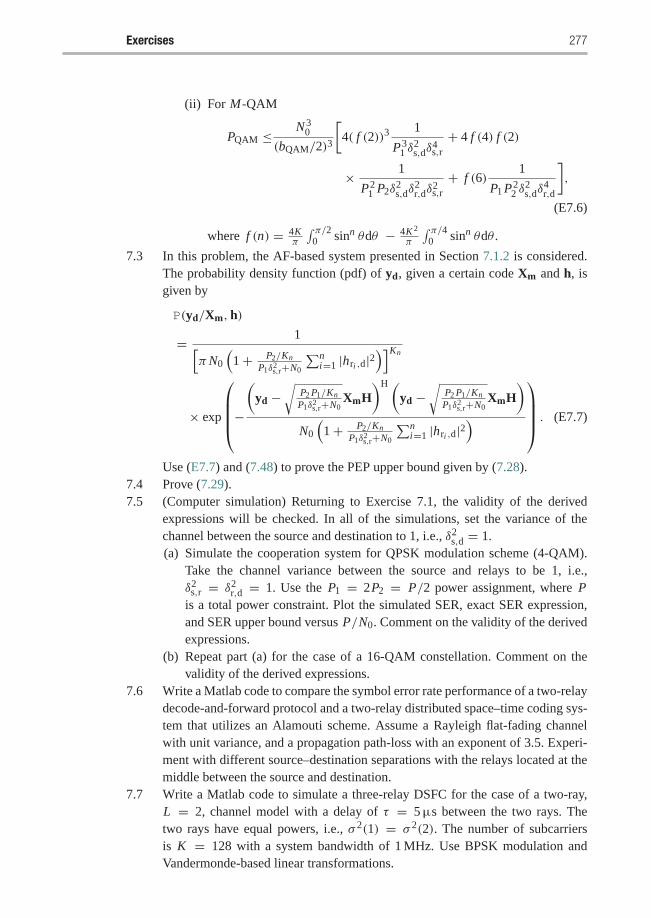
Exercises 277
(ii) For M-QAM
PQAM ≤ N 30
(bQAM/2)3
[4( f (2))3
1
P31 δ
2s,dδ
4s,r
+ 4 f (4) f (2)
× 1
P21 P2δ
2s,dδ
2r,dδ
2s,r
+ f (6)1
P1 P22 δ
2s,dδ
4r,d
],
(E7.6)
where f (n) = 4Kπ
∫ π/20 sinn θdθ − 4K 2
π
∫ π/40 sinn θdθ .
7.3 In this problem, the AF-based system presented in Section 7.1.2 is considered.The probability density function (pdf) of yd, given a certain code Xm and h, isgiven by
P(yd/Xm,h)
= 1[πN0
(1+ P2/Kn
P1δ2s,r+N0
∑ni=1 |hri ,d|2
)]Kn
× exp
⎛⎜⎜⎜⎝−(
yd −√
P2 P1/KnP1δ
2s,r+N0
XmH)H (
yd −√
P2 P1/KnP1δ
2s,r+N0
XmH)
N0
(1+ P2/Kn
P1δ2s,r+N0
∑ni=1 |hri ,d|2
)⎞⎟⎟⎟⎠ . (E7.7)
Use (E7.7) and (7.48) to prove the PEP upper bound given by (7.28).7.4 Prove (7.29).7.5 (Computer simulation) Returning to Exercise 7.1, the validity of the derived
expressions will be checked. In all of the simulations, set the variance of thechannel between the source and destination to 1, i.e., δ2
s,d = 1.(a) Simulate the cooperation system for QPSK modulation scheme (4-QAM).
Take the channel variance between the source and relays to be 1, i.e.,δ2
s,r = δ2r,d = 1. Use the P1 = 2P2 = P/2 power assignment, where P
is a total power constraint. Plot the simulated SER, exact SER expression,and SER upper bound versus P/N0. Comment on the validity of the derivedexpressions.
(b) Repeat part (a) for the case of a 16-QAM constellation. Comment on thevalidity of the derived expressions.
7.6 Write a Matlab code to compare the symbol error rate performance of a two-relaydecode-and-forward protocol and a two-relay distributed space–time coding sys-tem that utilizes an Alamouti scheme. Assume a Rayleigh flat-fading channelwith unit variance, and a propagation path-loss with an exponent of 3.5. Experi-ment with different source–destination separations with the relays located at themiddle between the source and destination.
7.7 Write a Matlab code to simulate a three-relay DSFC for the case of a two-ray,L = 2, channel model with a delay of τ = 5 μs between the two rays. Thetwo rays have equal powers, i.e., σ 2(1) = σ 2(2). The number of subcarriersis K = 128 with a system bandwidth of 1 MHz. Use BPSK modulation andVandermonde-based linear transformations.
8 Relay selection: when to cooperateand with whom
In this chapter, we present a cooperative protocol based on the relay-selection tech-nique using the availability of the partial channel state information (CSI) at the sourceand the relays. The main objective of this scheme is to achieve higher bandwidth effi-ciency while guaranteeing the same diversity order as in a conventional cooperativescheme. Two cooperation scenarios are addressed: a single-relay scenario and a multi-relay scenario. In the single-relay scenario, the focus is to answer the question: “Whento cooperate?” The rationale behind this protocol is that there is no need for the relay toforward the source’s information if the direct link, between the source and destination,is of high quality. It turns out that an appropriate metric to represent the relay’s abilityto help is a modified version of the harmonic mean function of its source–relay andrelay–destination instantaneous channel gains. The source decides when to cooperateby taking the ratio between the source–destination channel gain and the relay’s metricand comparing it with a threshold, which is referred to as the cooperation threshold .If this ratio is greater than or equal to the cooperation threshold, then the source sendsits information to the destination directly without the need for the relay. Otherwise,the source employs the relay in forwarding its information to the destination as in theconventional cooperative scheme.
An extension to the multi-node cooperative scenario with arbitrary N relays is con-sidered as well. In the multi-node scenario, the focus is to answer two questions: “Whento cooperate?” and “Who to cooperate with?” The user picks only one relay to coop-erate with, in case it needs help. This optimal relay is the one which has the maximuminstantaneous value of the relay’s metric among the N relays. By determining thatinstantaneous optimal relay, the user can determine whether to utilize it or not, in a sim-ilar fashion to the single-relay scenario. For the symmetric scenario, it is shown that fulldiversity order is guaranteed and obtain the optimum power allocation which minimizesthe SER performance. Finally, we discuss tradeoff curves between the bandwidth effi-ciency and the SER, which are utilized to determine the optimum cooperation threshold.
8.1 Motivation and relay-selection protocol
In this section, we review the system model of the conventional single-relay decode-and-forward cooperative scenario along with the SER results. This is to help illustratethe motivation behind choosing a modified harmonic mean function of the source–relay
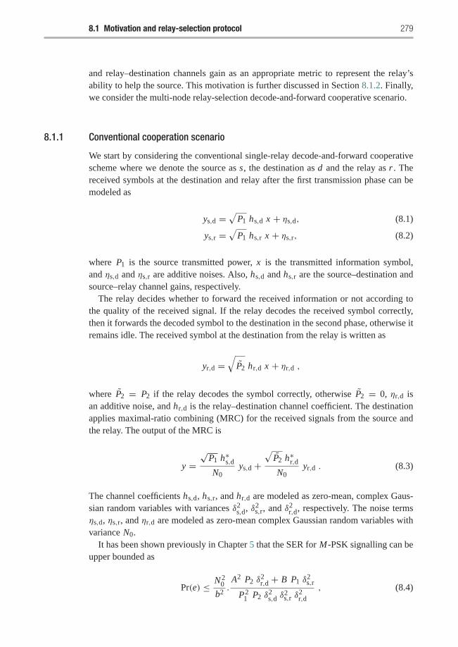
8.1 Motivation and relay-selection protocol 279
and relay–destination channels gain as an appropriate metric to represent the relay’sability to help the source. This motivation is further discussed in Section 8.1.2. Finally,we consider the multi-node relay-selection decode-and-forward cooperative scenario.
8.1.1 Conventional cooperation scenario
We start by considering the conventional single-relay decode-and-forward cooperativescheme where we denote the source as s, the destination as d and the relay as r . Thereceived symbols at the destination and relay after the first transmission phase can bemodeled as
ys,d =√
P1 hs,d x + ηs,d, (8.1)
ys,r =√
P1 hs,r x + ηs,r, (8.2)
where P1 is the source transmitted power, x is the transmitted information symbol,and ηs,d and ηs,r are additive noises. Also, hs,d and hs,r are the source–destination andsource–relay channel gains, respectively.
The relay decides whether to forward the received information or not according tothe quality of the received signal. If the relay decodes the received symbol correctly,then it forwards the decoded symbol to the destination in the second phase, otherwise itremains idle. The received symbol at the destination from the relay is written as
yr,d =√
P2 hr,d x + ηr,d ,
where P2 = P2 if the relay decodes the symbol correctly, otherwise P2 = 0, ηr,d isan additive noise, and hr,d is the relay–destination channel coefficient. The destinationapplies maximal-ratio combining (MRC) for the received signals from the source andthe relay. The output of the MRC is
y =√
P1 h∗s,dN0
ys,d +√
P2 h∗r,dN0
yr,d . (8.3)
The channel coefficients hs,d, hs,r, and hr,d are modeled as zero-mean, complex Gaus-sian random variables with variances δ2
s,d, δ2s,r, and δ2
r,d, respectively. The noise termsηs,d, ηs,r, and ηr,d are modeled as zero-mean complex Gaussian random variables withvariance N0.
It has been shown previously in Chapter 5 that the SER for M-PSK signalling can beupper bounded as
Pr(e) ≤ N 20
b2.A2 P2 δ
2r,d + B P1 δ
2s,r
P21 P2 δ
2s,d δ
2s,r δ
2r,d
, (8.4)
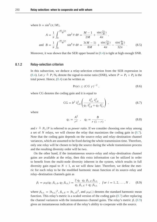
280 Relay selection: when to cooperate and with whom
where b = sin2(π/M),
A = 1
π
∫ (M−1)πM
0sin2 θ dθ = M − 1
2M+ sin( 2π
M )
4π,
and B = 1
π
∫ (M−1)πM
0sin4 θ dθ = 3(M − 1)
8M+ sin( 2π
M )
4π− sin( 4π
M )
32π. (8.5)
Moreover, it was shown that the SER upper bound in (8.4) is tight at high enough SNR.
8.1.2 Relay-selection criterion
In this subsection, we deduce a relay-selection criterion from the SER expression in(8.4). Let γ � P/N0 denote the signal-to-noise ratio (SNR), where P = P1 + P2 is thetotal power. Hence, (8.4) can be written as
Pr(e) ≤ (CG γ )−2 , (8.6)
where CG denotes the coding gain and it is equal to
CG = b2 δ2s,d
(δ2
s,r δ2r,d
q1 δ2r,d + q2 δ2
s,r
), (8.7)
where
q1 = A2
r2, q2 = B
r (1− r), (8.8)
and r � P1/P is referred to as power ratio. If we consider choosing one relay amonga set of N relays, we will choose the relay that maximizes the coding gain in (8.7).Note that the coding gain depends on the source–relay and relay–destination channelvariances, which are assumed to be fixed during the whole transmission time. Therefore,only one relay will be chosen to help the source during the whole transmission processand the resulting diversity order will be two.
On the other hand, if the instantaneous source–relay and relay–destination channelgains are available at the relay, then this extra information can be utilized in orderto benefit from the multi-node diversity inherent in the system, which results in fulldiversity gain equal to N + 1, as we will show later. Therefore, we define the met-ric for each relay to be the modified harmonic mean function of its source–relay andrelay–destination channels gain as
βi = μH(q1 βri ,d, q2 βs,ri ) =2 q1 q2 βri ,d βs,ri
q1 βri ,d + q2 βs,ri, f or i = 1, 2, . . . , N . (8.9)
where βs,ri = |hs,ri |2, βri ,d = |hri ,d|2, and μH(.) denotes the standard harmonic meanfunction. This relay’s metric is a scaled version of the coding gain (8.7) after replacingthe channel variances with the instantaneous channel gains. The relay’s metric βi (8.9)gives an instantaneous indication of the relay’s ability to cooperate with the source.
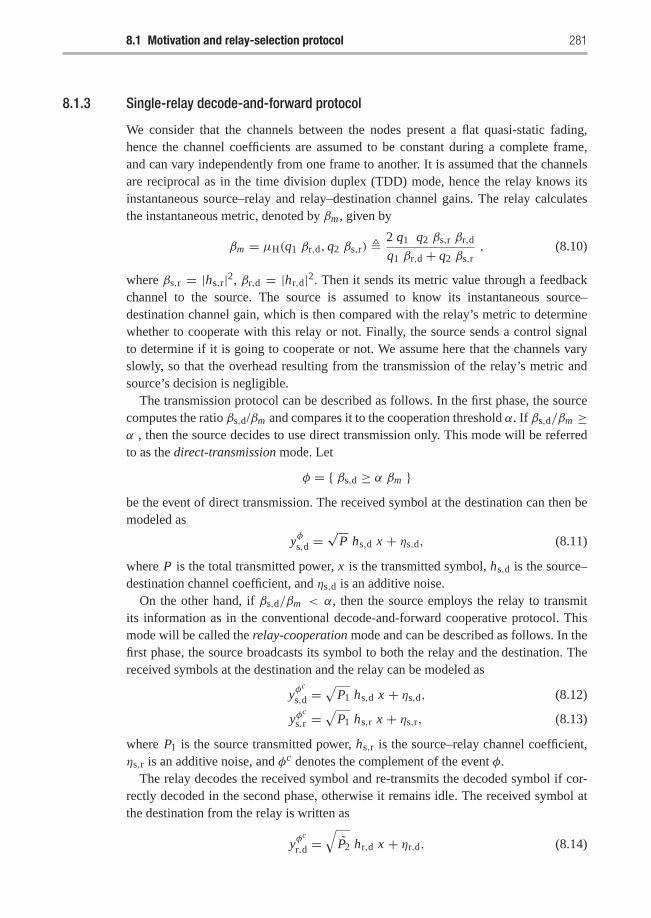
8.1 Motivation and relay-selection protocol 281
8.1.3 Single-relay decode-and-forward protocol
We consider that the channels between the nodes present a flat quasi-static fading,hence the channel coefficients are assumed to be constant during a complete frame,and can vary independently from one frame to another. It is assumed that the channelsare reciprocal as in the time division duplex (TDD) mode, hence the relay knows itsinstantaneous source–relay and relay–destination channel gains. The relay calculatesthe instantaneous metric, denoted by βm , given by
βm = μH(q1 βr,d, q2 βs,r) � 2 q1 q2 βs,r βr,d
q1 βr,d + q2 βs,r, (8.10)
where βs,r = |hs,r|2, βr,d = |hr,d|2. Then it sends its metric value through a feedbackchannel to the source. The source is assumed to know its instantaneous source–destination channel gain, which is then compared with the relay’s metric to determinewhether to cooperate with this relay or not. Finally, the source sends a control signalto determine if it is going to cooperate or not. We assume here that the channels varyslowly, so that the overhead resulting from the transmission of the relay’s metric andsource’s decision is negligible.
The transmission protocol can be described as follows. In the first phase, the sourcecomputes the ratio βs,d/βm and compares it to the cooperation threshold α. If βs,d/βm ≥α , then the source decides to use direct transmission only. This mode will be referredto as the direct-transmission mode. Let
φ = { βs,d ≥ α βm }be the event of direct transmission. The received symbol at the destination can then bemodeled as
yφs,d =√
P hs,d x + ηs,d, (8.11)
where P is the total transmitted power, x is the transmitted symbol, hs,d is the source–destination channel coefficient, and ηs,d is an additive noise.
On the other hand, if βs,d/βm < α, then the source employs the relay to transmitits information as in the conventional decode-and-forward cooperative protocol. Thismode will be called the relay-cooperation mode and can be described as follows. In thefirst phase, the source broadcasts its symbol to both the relay and the destination. Thereceived symbols at the destination and the relay can be modeled as
yφc
s,d =√
P1 hs,d x + ηs,d, (8.12)
yφc
s,r =√
P1 hs,r x + ηs,r, (8.13)
where P1 is the source transmitted power, hs,r is the source–relay channel coefficient,ηs,r is an additive noise, and φc denotes the complement of the event φ.
The relay decodes the received symbol and re-transmits the decoded symbol if cor-rectly decoded in the second phase, otherwise it remains idle. The received symbol atthe destination from the relay is written as
yφc
r,d =√
P2 hr,d x + ηr,d, (8.14)
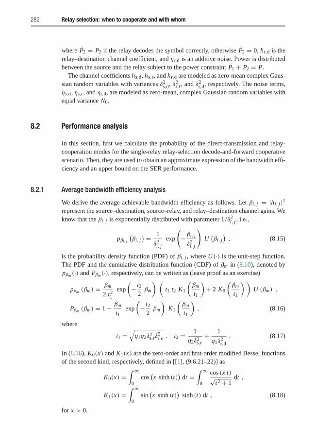
282 Relay selection: when to cooperate and with whom
where P2 = P2 if the relay decodes the symbol correctly, otherwise P2 = 0, hr,d is therelay–destination channel coefficient, and ηr,d is an additive noise. Power is distributedbetween the source and the relay subject to the power constraint P1 + P2 = P .
The channel coefficients hs,d, hs,r, and hr,d are modeled as zero-mean complex Gaus-sian random variables with variances δ2
s,d, δ2s,r, and δ2
r,d, respectively. The noise terms,ηs,d, ηs,r, and ηr,d, are modeled as zero-mean, complex Gaussian random variables withequal variance N0.
8.2 Performance analysis
In this section, first we calculate the probability of the direct-transmission and relay-cooperation modes for the single-relay relay-selection decode-and-forward cooperativescenario. Then, they are used to obtain an approximate expression of the bandwidth effi-ciency and an upper bound on the SER performance.
8.2.1 Average bandwidth efficiency analysis
We derive the average achievable bandwidth efficiency as follows. Let βi, j = |hi, j |2represent the source–destination, source–relay, and relay–destination channel gains. Weknow that the βi, j is exponentially distributed with parameter 1/δ2
i, j , i.e.,
pβi, j
(βi, j) = 1
δ2i, j
exp
(−βi, j
δ2i, j
)U(βi, j), (8.15)
is the probability density function (PDF) of βi, j , where U (·) is the unit-step function.The PDF and the cumulative distribution function (CDF) of βm in (8.10), denoted bypβm (·) and Pβm (·), respectively, can be written as (leave proof as an exercise)
pβm (βm) = βm
2 t21
exp
(− t2
2βm
) (t1 t2 K1
(βm
t1
)+ 2 K0
(βm
t1
) )U (βm) ,
Pβm (βm) = 1− βm
t1exp
(− t2
2βm
)K1
(βm
t1
), (8.16)
where
t1 =√
q1q2δ2s,rδ
2r,d , t2 = 1
q2δ2s,r+ 1
q1δ2r,d
. (8.17)
In (8.16), K0(x) and K1(x) are the zero-order and first-order modified Bessel functionsof the second kind, respectively, defined in [[1], (9.6.21–22)] as
K0(x) =∫ ∞
0cos(x sinh (t)
)dt =
∫ ∞
0
cos (x t)√t2 + 1
dt ,
K1(x) =∫ ∞
0sin(x sinh (t)
)sinh (t) dt , (8.18)
for x > 0.
8.2 Performance analysis 283
The probability of direct-transmission mode can be obtained as follows:
Pr(φ) = Pr(βs,d ≥ α βm
) = ∫ ∞
0Pβm
(βs,d
α
)pβs,d
(βs,d)
dβs,d
= 1− 1
αt1δ2s,d
∫ ∞
0βs,d exp
(−(
1
δ2s,d
+ t22α
)βs,d
)K1
(βs,d
αt1
)dβs,d,
(8.19)
where we used (8.15) and (8.16). K1(.) can be approximated as
K1(x) ≈ 1
x. (8.20)
Substituting (8.20) into (8.19), the probability of the direct transmission is approxi-mated as
Pr(φ) ≈ 1− 1
δ2s,d
∫ ∞
0exp
(−(
1
δ2s,d
+ t22α
)βs,d
)dβs,d
≈ t2 δ2s,d
2α + t2 δ2s,d
, (8.21)
and the probability of the relay-cooperation mode is
Pr(φc) = 1− Pr(φ) ≈ 2α
2α + t2 δ2s,d
. (8.22)
Since the bandwidth efficiency of the direct-transmission mode is 1 symbols per chan-nel use (SPCU), and that of the relay-cooperation mode is 1/2 SPCU, the averagebandwidth efficiency can be written as
R = Pr(φ)+ 1
2Pr(φc) . (8.23)
Substituting (8.21) and (8.22) into (8.23) and substituting t2 as in (8.17), we get thefollowing theorem.
T H E O R E M 8.2.1 The bandwidth efficiency of the relay-selection decode-and-forward cooperative scenario, utilizing a single relay, can be approximated as
R ≈α + ( 1−r
B δ2s,r+ r
A2 δ2r,d) r δ2
s,d
2α + ( 1−rB δ2
s,r+ r
A2 δ2r,d) r δ2
s,d
SPCU, (8.24)
where SPCU stands for symbols per channel use.
8.2.2 SER analysis and upper bound
We obtain the SER of the single-relay decode-and-forward scheme for M-PSK sig-nalling. The probability of symbol error, or SER, is defined as
Pr(e) = Pr(e|φ) · Pr(φ)+ Pr(e|φc) · Pr(φc) , (8.25)
284 Relay selection: when to cooperate and with whom
where Pr(e|φ) ·Pr(φ) represents the SER of the direct-transmission mode and Pr(e|φc) ·Pr(φc) represents the relay-cooperation mode SER. The SER of the direct-transmissionmode can be calculated as follows. First, the instantaneous direct-transmission SNR is
γ φ = P βs,d
N0. (8.26)
The conditional direct-transmission SER can be written as
Pr(e|phi, βs,d) = �(γ φ) � 1
π
∫ (M−1)πM
0exp
(− b γ φ
sin2 θ
)dθ . (8.27)
where b = sin2(π/M). Since
Pr(e|φ) Pr(φ) =∫ ∞
0Pr(e|φ, βs,d) Pr(φ|βs,d) pβs,d(βs,d) dβs,d
=∫ (M−1)π
M
0
1
π
∫ ∞
0
1
δ2s,d
exp
(−(
b P
N0 sin2 θ+ 1
δ2s,d
)βs,d
)
×(
1− βs,d
αt1exp
(− t2
2αβs,d
)K1
(βs,d
α t1
))dβs,d dθ,
(8.28)
where we used (8.15), (8.16), and (8.27). Substituting (8.20) into (8.28), we get
Pr(e|φ) Pr(φ) ≈ F1
(1+ b P δ2
s,d
N0 sin2 θ
)− F1
(1+ t2δ2
s,d
2α+ b P δ2
s,d
N0 sin2 θ
)
≈ t2 δ2s,d
2αF1
( (1+ b P δ2
s,d
N0 sin2 θ
) (1+ t2 δ2
s,d
2α+ b P δ2
s,d
N0 sin2 θ
) ),
(8.29)
where
F1(x(θ)
) = 1
π
∫ (M−1)πM
0
1
x(θ)dθ.
We obtain the SER of the relay-cooperation mode as follows. For the relay-cooperation mode, maximal-ratio combining (MRC) is applied at the destination. Theoutput of the MRC can be written as
yφc =
√P0 h∗s,dN0
yφc
s,d +√
P1 h∗r,dN0
yφc
r,d . (8.30)
The instantaneous SNR of the MRC output can be written as
γ φc = P0βs,d + P1βr,d
N0. (8.31)
8.2 Performance analysis 285
We can easily see that the conditional SER of the relay-cooperation mode can bewritten as
Pr(e|φc, βs,d, βs,r, βr,d) = �(γ φc)|P1=0 �
(P0βs,r
N0
)+ �(γ φ
c)|P1=P1
(1−�
(P0βs,r
N0
)). (8.32)
Let us denote Pr(A|φc, βs,d, βs,r, βr,d) � �(γ φc)�(
P0βs,rN0) and Pr(B|φc, β) � �(γ φ
c),
in which β � [βs,d, βs,r, βr,d]. Then
Pr(A|φc, βs,d, βs,r, βr,d)
= 1
π
∫ (M−1)πM
θ1=0exp(− b P0
N0 sin2 θ1βs,d)
exp(− b P1
N0 sin2 θ1βr,d)
dθ1
× 1
π
∫ (M−1)πM
θ2=0exp(− b P0
N0 sin2 θ2βs,r)
dθ2 , (8.33)
so we have
Pr(A|φc) Pr(φc) =∫β
Pr(A/φc, β) Pr(φc/β) pβ(β) dβ . (8.34)
Moreover, since βm is a function of βs,r and βr,d as given by (8.10), so
Pr(φc|β) = Pr(βs,d < αβm/βs,d, βs,r, βr,d) = U (αβm − βs,d) . (8.35)
Substituting (8.33) and (8.35) into (8.34), we get
Pr(A|φc) Pr(φc)
=∫β
1
π2
∫ (M−1)πM
θ1=0
∫ (M−1)πM
θ2=0exp(− P0 C(θ1) βs,d
)exp(− P1 C(θ1) βr,d
)× exp
(− P0 C(θ2) βs,r)
U (αβm − βs,d) pβ(β) dθ2 dθ1 dβ , (8.36)
where C(θ) = b/(N0 sin2 θ
). Since βs,d, βs,r, and βr,d are statistically independent, thus
pβ(β) = pβs,d(βs,d) pβs,r(βs,r) pβr,d(βr,d) = pβs,d(βs,d) pβ (β) , (8.37)
Pr(A|φc) Pr(φc)
=∫β
1
π2
∫ (M−1)πM
θ1=0
∫ (M−1)πM
θ2=0
1− exp(− (P0 C(θ1)+ 1
δ2s,d
)αβm
)1+ P0 C(θ1)δ2
s,d
× exp(− P1 C(θ1)βr,d
)exp(− P0 C(θ2)βs,r
)pβ (β) dθ2 dθ1 dβ . (8.38)
It is difficult to get an exact expression of (8.38) for βm defined in (8.10). Thus, weobtain an upper bound via the worst-case scenario. We replace βs,r and βr,d in (8.38) by
286 Relay selection: when to cooperate and with whom
their worst-case values in terms of βm . Then, we average (8.38) over βm only. It followsfrom (8.10) that
1
βm= 1
2 q2 βs,r+ 1
2 q1 βr,d, (8.39)
thus, βm ≤ 2 q2 βs,r and βm ≤ 2 q1 βr,d. If we replace βs,r and βr,d by their worst-casevalues in terms of βm as
βs,r −→ βm
2 q2, βr,d −→ βm
2 q1. (8.40)
Then, the probability in (8.38) can be upper bounded as
Pr(A|φc) Pr(φc)
≤ 1
π2
∫ (M−1)πM
θ1=0
1
1+ P0 C(θ1)δ2s,d
∫ (M−1)πM
θ2=0Mβm
( P1 C(θ1)
2 q1+ P0 C(θ2)
2 q2
)−Mβm
((P0 C(θ1)+ 1
δ2s,d
)α + P1 C(θ1)
2 q1+ P0 C(θ2)
2 q2
)dθ2dθ1, (8.41)
where Mβm (.) is the moment-generation function (MGF) of βm . It can be shown thatfor two independent exponential random variables with parameters λ1 and λ2, the MGFof their harmonic mean function can be written as (leave proof as an exercise)
Mβm (γ ) = Eβm
(exp(−γ βm)
)= 16 λ1 λ2
3 (λ1 + λ2 + 2√λ1 λ2 + γ )2
⎛⎝4 (λ1 + λ2) 2F1
(3, 3
2 ; 52 ; λ1+λ2−2
√λ1 λ2+γ
λ1+λ2+2√λ1 λ2+γ
)(λ1 + λ2 + 2
√λ1 λ2 + γ )
+ 2F1
(2,
1
2; 5
2; λ1 + λ2 − 2
√λ1 λ2 + γ
λ1 + λ2 + 2√λ1 λ2 + γ
))(8.42)
where Eβm (.) represents the statistical average with respect to βm and 2F1(., .; .; .) isthe Gauss’ hypergeometric function as defined on page 172. Following similar steps asdone in (8.33)–(8.41), we have (leave proof as an exercise)
Pr(B|φc) Pr(φc)
≤ 1
π
∫ (M−1)πM
θ=0
Mβm
(P1 C(θ)
2 q1
)− Mβm
((P0 C(θ)+ 1
δ2s,d
)α + P1 C(θ)
2 q1
)dθ
1+ P0 C(θ)δ2s,d
.
(8.43)
Note that the unconditional SER of the relay-cooperation mode in (8.32) can berewritten as
Pr(e|φc) Pr(φc)
=(Pr(A|φc)|P1=0 − Pr(A|φc)|P1=P1
+ Pr(B|φc)|P1=P1
)Pr(φc),
≤(Pr(A|φc)|P1=0 + Pr(B|φc)|P1=P1
)Pr(φc). (8.44)
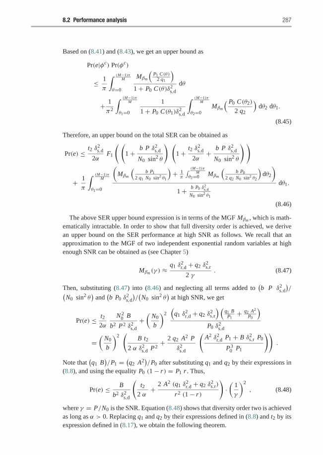
8.2 Performance analysis 287
Based on (8.41) and (8.43), we get an upper bound as
Pr(e|φc) Pr(φc)
≤ 1
π
∫ (M−1)πM
θ=0
Mβm
(P1 C(θ)
2 q1
)1+ P0 C(θ)δ2
s,d
dθ
+ 1
π2
∫ (M−1)πM
θ1=0
1
1+ P0 C(θ1)δ2s,d
∫ (M−1)πM
θ2=0Mβm
( P0 C(θ2)
2 q2
)dθ2 dθ1.
(8.45)
Therefore, an upper bound on the total SER can be obtained as
Pr(e) ≤ t2 δ2s,d
2αF1
( (1+ b P δ2
s,d
N0 sin2 θ
) (1+ t2 δ2
s,d
2α+ b P δ2
s,d
N0 sin2 θ
) )
+ 1
π
∫ (M−1)πM
θ1=0
(Mβm
(b P1
2 q1 N0 sin2 θ1
)+ 1π
∫ (M−1)πM
θ2=0 Mβm
(b P0
2 q2 N0 sin2 θ2
)dθ2
)1+ b P0 δ
2s,d
N0 sin2 θ1
dθ1.
(8.46)
The above SER upper bound expression is in terms of the MGF Mβm , which is math-ematically intractable. In order to show that full diversity order is achieved, we derivean upper bound on the SER performance at high SNR as follows. We recall that anapproximation to the MGF of two independent exponential random variables at highenough SNR can be obtained as (see Chapter 5)
Mβm (γ ) ≈q1 δ
2r,d + q2 δ
2s,r
2 γ. (8.47)
Then, substituting (8.47) into (8.46) and neglecting all terms added to(b P δ2
s,d
)/(
N0 sin2 θ)
and(b P0 δ
2s,d
)/(N0 sin2 θ
)at high SNR, we get
Pr(e) ≤ t22α
N 20 B
b2 P2 δ2s,d
+(
N0
b
)2(q1 δ
2r,d + q2 δ
2s,r
) (q1 BP1+ q2 A2
P0
)P0 δ
2s,d
=(
N0
b
)2(
B t22 α δ2
s,d P2+ 2 q2 A2 P
δ2s,d
(A2 δ2
r,d P1 + B δ2s,r P0
P30 P1
)).
Note that(q1 B
)/P1 =
(q2 A2
)/P0 after substituting q1 and q2 by their expressions in
(8.8), and using the equality P0 (1− r) = P1 r . Thus,
Pr(e) ≤ B
b2 δ2s,d
(t2
2 α+ 2 A2 (q1 δ
2r,d + q2 δ
2s,r)
r2 (1− r)
)·(
1
γ
)2
, (8.48)
where γ = P/N0 is the SNR. Equation (8.48) shows that diversity order two is achievedas long as α > 0. Replacing q1 and q2 by their expressions defined in (8.8) and t2 by itsexpression defined in (8.17), we obtain the following theorem.
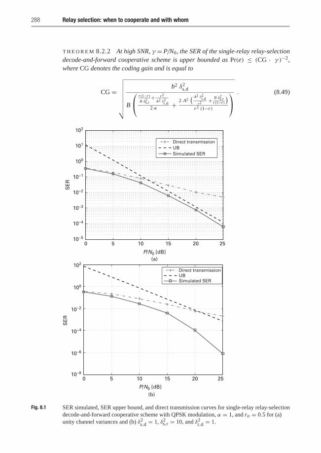
288 Relay selection: when to cooperate and with whom
T H E O R E M 8.2.2 At high SNR, γ = P/N0, the SER of the single-relay relay-selectiondecode-and-forward cooperative scheme is upper bounded as Pr(e) ≤ (CG · γ )−2,where CG denotes the coding gain and is equal to
CG =√√√√√√√√
b2 δ2s,d
B
⎛⎝ r(1−r)
B δ2s,r+ r2
A2 δ2r,d2 α + 2 A2
( A2 δ2r,dr2 + B δ2s,r
r(1−r)
)r2 (1−r)
⎞⎠ . (8.49)
0 5 10 15 20 2510−5
10−4
10−3
10−2
10−1
100
101
102
P/N0 [dB](a)
SE
R
Direct transmissionUBSimulated SER
Direct transmissionUBSimulated SER
0 5 10 15 20 25
P/N0 [dB](b)
10−4
10−6
10−8
10−2
100
102
SE
R
Fig. 8.1 SER simulated, SER upper bound, and direct transmission curves for single-relay relay-selectiondecode-and-forward cooperative scheme with QPSK modulation, α = 1, and ro = 0.5 for (a)unity channel variances and (b) δ2s,d = 1, δ2s,r = 10, and δ2r,d = 1.
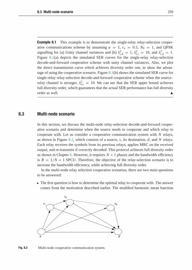
8.3 Multi-node scenario 289
Example 8.1 This example is to demonstrate the single-relay relay-selection cooper-ative communications scheme by assuming α = 1, ro = 0.5, N0 = 1, and QPSKsignalling for (a) Unity channel variances and (b) δ2
s,d = 1, δ2s,r = 10, and δ2
r,d = 1.Figure 8.1(a) depicts the simulated SER curves for the single-relay relay-selectiondecode-and-forward cooperative scheme with unity channel variances. Also, we plotthe direct transmission curve which achieves diversity order one, to show the advan-tage of using the cooperative scenario. Figure 8.1(b) shows the simulated SER curve forsingle-relay relay-selection decode-and-forward cooperative scheme when the source–relay channel is stronger, δ2
s,r = 10. We can see that the SER upper bound achievesfull diversity order, which guarantees that the actual SER performance has full diversityorder as well. �
8.3 Multi-node scenario
In this section, we discuss the multi-node relay-selection decode-and-forward cooper-ative scenario and determine when the source needs to cooperate and which relay tocooperate with. Let us consider a cooperative communication system with N relays,as shown in Figure 8.2, which consists of a source, s, its destination, d, and N relays.Each relay receives the symbols from its previous relays, applies MRC on the receivedoutput, and re-transmits if correctly decoded. This protocol achieves full diversity orderas shown in Chapter 6. However, it requires N + 1 phases and the bandwidth efficiencyis R = 1/N + 1 SPCU. Therefore, the objective of the relay-selection scenario is toincrease the bandwidth efficiency, while achieving full diversity order.
In the multi-node relay selection cooperative scenarios, there are two main questionsto be answered:
• The first question is how to determine the optimal relay to cooperate with. The answercomes from the motivation described earlier. The modified harmonic mean function
s d
r1
r2
rN
Fig. 8.2 Multi-node cooperative communication system.
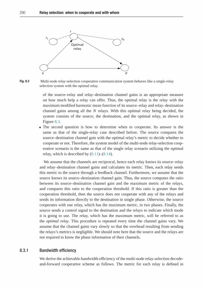
290 Relay selection: when to cooperate and with whom
s d
r
r1
Optimalrelay
rN
Fig. 8.3 Multi-node relay-selection cooperative communication system behaves like a single-relayselection system with the optimal relay.
of the source–relay and relay–destination channel gains is an appropriate measureon how much help a relay can offer. Thus, the optimal relay is the relay with themaximum modified harmonic mean function of its source–relay and relay–destinationchannel gains among all the N relays. With this optimal relay being decided, thesystem consists of the source, the destination, and the optimal relay, as shown inFigure 8.3.
• The second question is how to determine when to cooperate. Its answer is thesame as that of the single-relay case described before. The source compares thesource–destination channel gain with the optimal relay’s metric to decide whether tocooperate or not. Therefore, the system model of the multi-node relay-selection coop-erative scenario is the same as that of the single relay scenario utilizing the optimalrelay, which is described by (8.11)–(8.14).
We assume that the channels are reciprocal, hence each relay knows its source–relayand relay–destination channel gains and calculates its metric. Then, each relay sendsthis metric to the source through a feedback channel. Furthermore, we assume that thesource knows its source–destination channel gain. Thus, the source computes the ratiobetween its source–destination channel gain and the maximum metric of the relays,and compares this ratio to the cooperation threshold. If this ratio is greater than thecooperation threshold, then the source does not cooperate with any of the relays andsends its information directly to the destination in single phase. Otherwise, the sourcecooperates with one relay, which has the maximum metric, in two phases. Finally, thesource sends a control signal to the destination and the relays to indicate which modeit is going to use. The relay, which has the maximum metric, will be referred to asthe optimal relay. This procedure is repeated every time the channel gains vary. Weassume that the channel gains vary slowly so that the overhead resulting from sendingthe relays’s metrics is negligible. We should note here that the source and the relays arenot required to know the phase information of their channels.
8.3.1 Bandwidth efficiency
We derive the achievable bandwidth efficiency of the multi-node relay-selection decode-and-forward cooperative scheme as follows. The metric for each relay is defined in
8.3 Multi-node scenario 291
(8.9). We denote the PDF and CDF of βi for i = 1, 2, . . . , N as pβi (.) and Pβi (.),respectively. They are as defined in (8.16) with t1 and t2 being replaced by
t1,i =√
q1 q2 δ2s,ri δ
2ri ,d
and t2,i = 1
q2 δ2s,ri
+ 1
q1 δ2ri ,d
,
respectively. The optimum relay will have a metric which is equal to
βmax = max{ β1, β2, . . . , βN } . (8.50)
The CDF of βmax can be written as
Pβmax(β) = Pr( β1 ≤ β , β2 ≤ β , . . . , βN ≤ β ) =N∏
i=1
Pβi (β)
=N∏
i=1
(1− βi
t1,iexp(− t2,i
2β) K1(
β
t1,i)
), (8.51)
and the PDF of βmax is written as
pβmax(β) =∂Pβmax(β)
∂β=
N∑j=1
pβ j (β)
⎛⎝ N∏i=1,i �= j
Pβi (β)
⎞⎠≈
N∑j=1
pβ j (β)
⎛⎝ N∏i=1,i �= j
(1− exp(− t2,i
2β)
) ⎞⎠ , (8.52)
where we have used the approximation in (8.20). The expression in (8.52) is complexand will lead to more complex and intractable expressions. Without loss of generality,we consider the symmetric scenario where all the relays have the same source–relayand relay–destination channel variances, i.e.,
δ2s,ri = δ2
s,r , δ2ri ,d= δ2
r,d , for i = 1, 2, . . . , N . (8.53)
According to (8.51) and (8.52), the CDF and PDF of βmax can be written as
Pβmax(β) =(
1− β
t1exp
(− t2
2β
)K1
(β
t1
) )N
pβmax(β) = N
(1− β
t1exp
(− t2
2β
)K1
(β
t1
) )N−1
pβm (β) , (8.54)
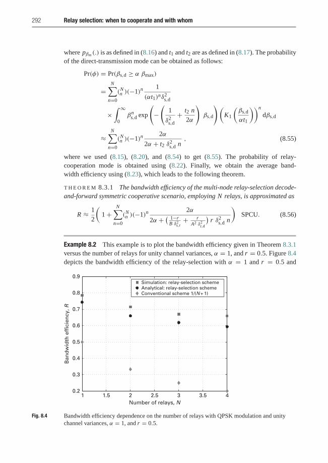
292 Relay selection: when to cooperate and with whom
where pβm (.) is as defined in (8.16) and t1 and t2 are as defined in (8.17). The probabilityof the direct-transmission mode can be obtained as follows:
Pr(φ) = Pr(βs,d ≥ α βmax)
=N∑
n=0
(Nn )(−1)n1
(αt1)nδ2s,d
×∫ ∞
0βn
s,d exp
(−(
1
δ2s,d
+ t2 n
2α
)βs,d
)(K1
(βs,d
αt1
))n
dβs,d
≈N∑
n=0
(Nn )(−1)n2α
2α + t2 δ2s,d n
, (8.55)
where we used (8.15), (8.20), and (8.54) to get (8.55). The probability of relay-cooperation mode is obtained using (8.22). Finally, we obtain the average band-width efficiency using (8.23), which leads to the following theorem.
T H E O R E M 8.3.1 The bandwidth efficiency of the multi-node relay-selection decode-and-forward symmetric cooperative scenario, employing N relays, is approximated as
R ≈ 1
2
(1+
N∑n=0
(Nn )(−1)n2α
2α + ( 1−rB δ2
s,r+ r
A2 δ2r,d
)r δ2
s,d n
)SPCU. (8.56)
Example 8.2 This example is to plot the bandwidth efficiency given in Theorem 8.3.1versus the number of relays for unity channel variances, α = 1, and r = 0.5. Figure 8.4depicts the bandwidth efficiency of the relay-selection with α = 1 and r = 0.5 and
1 1.5 2 2.5 3 3.5 40.2
0.3
0.4
0.5
0.6
0.7
0.8
0.9
Number of relays, N
Ban
dw
idth
eff
icie
ncy
, R
Simulation: relay-selection schemeAnalytical: relay-selection schemeConventional scheme 1/(N + 1)
Fig. 8.4 Bandwidth efficiency dependence on the number of relays with QPSK modulation and unitychannel variances, α = 1, and r = 0.5.
8.3 Multi-node scenario 293
the conventional cooperative schemes for different number of relays and unity chan-nel variances. It is clear that the bandwidth efficiency decreases down to 0.5 as Nincreases, because the probability of the direct-transmission mode decreases down to0 as N goes to ∞. Furthermore, we plot the bandwidth efficiency of the conventionalcooperative scheme, Rconv = 1/N + 1 SPCU, to show the significant increasing in thebandwidth efficiency of the relay-selection cooperative scenario over the conventionalcooperative scheme. �
8.3.2 SER analysis and upper bound
Before determining the SER of the multi-node relay-selection decode-and-forward sym-metric cooperative scenario, we mention the following lemma, which is used to provefull diversity later.
Lemma 8.3.1 For any x, y, and N
N∑n=0
(N
n
)(−1)n
1
x + n y= (N )! yN∏N
n=0(x + n y), (8.57)
Proof First, we prove that
N∑n=0
(Nn
)(−1)n
1+ n z= N ! zN∏N
n=0(1+ n z). (8.58)
Let A(z) =∑Nn=0
(Nn ) (−1)N
1+n z , B(z) =∏Nn=0(1+n z), and G(z) = A(z)·B(z). The order
of G(z) is N , thus it can be written as G(z) = ∑Ni=0 gi zi where gi = 1
i !∂ i G(z)∂zi |z=0. It
can be easily shown that
∂ i A(z)
∂zi= (−1)i i !
N∑n=0
(Nn ) (−1)n ni
(1+ n z)i+1. (8.59)
Using the identity obtained in [[50], (0.154, 3–4)] As
N∑n=0
(N
n
)(−1)n ni =
⎧⎨⎩0, 0 ≤ i < N
(−1)N N !, i = N(8.60)
we get
∂ i A(z)
∂zi
∣∣∣∣z=0
= (−1)i i !(
N∑n=0
(Nn ) (−1)n ni
)=⎧⎨⎩
0, 0 ≤ i < N
(N !)2, i = N(8.61)
294 Relay selection: when to cooperate and with whom
Since, A(z)|z=0 = 0 and B(z)|z=0 = 1, thus
gi = 1
i !∂ i ( A(z) · B(z) )
∂zi
∣∣∣∣z=0
= 1
i !∂ i A(z)
∂zi
∣∣∣∣z=0
· B(z)∣∣∣z=0
=⎧⎨⎩
0, 0 ≤ i < N .
N !, i = N .(8.62)
Thus,
A(z) = G(z)
B(z)= N ! zN∏N
n=0(1+ n z), (8.63)
which proves (8.58). Replacing z = y/x in (8.58), we obtain Lemma 8.3.1.The SER derivation in the multi-node system is similar to those in the single-relay
system. The major difference is the usage of the PDF and CDF of βmax defined in (8.54)instead of the PDF and CDF of βm defined in (8.16). The total SER can be obtained asa summation of the SER of both the direct-transmission and relay-cooperation modesas in (8.25). First, we obtain the SER of the direct-transmission mode similar to thesingle-relay case (8.28) as follows:
Pr(e|φ) Pr(φ) ≈N∑
n=0
(Nn )(−1)n F1
(1+ t2 δ2
s,d n
2α+ b P
N0 sin2 θδ2
s,d
)
= N !(
t2 δ2s,d
2α
)N
F1
(N∏
n=0
(1+ t2 δ2s,d n
2α+ b P
N0 sin2 θδ2
s,d)
),
(8.64)
where we have applied (8.15), (8.20), (8.54), and Lemma 8.3.1. As for the relay-cooperation mode, its SER is similar to that of the single-relay system, but using theMGF of βmax. The MGF of βmax can be written as
Mβmax(γ ) = Eβmax ( exp(−γ βmax) )
= NN−1∑n=0
(N−1n
)(−1)n Mβm
(γ + n t2
2
), (8.65)
where we have applied (8.20).Similar to the single-relay scenario, we can obtain an upper bound on the total SER
as (leave proof as an exercise)
Pr(e) ≤ N !(
N0
b P
)N+1 ( t22α
)N I (2N + 2)
δ2s,d
+ N !(
N0
b
)N+1
t N−12
(q1 δ
2r,d + q2 δ
2s,r
)P0 δ
2s,d
×( (
q1
P1
)N
I (2 N + 2)+(
q2
P0
)N
A I (2 N )
), (8.66)
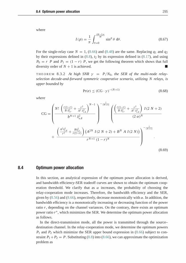
8.4 Optimum power allocation 295
where
I (p) = 1
π
∫ (M−1)πM
θ=0sinp θ dθ. (8.67)
For the single-relay case N = 1, (8.66) and (8.48) are the same. Replacing q1 and q2
by their expressions defined in (8.8), t2 by its expression defined in (8.17), and usingP0 = r P and P1 = (1 − r) P , we get the following theorem which shows that fulldiversity order of N + 1 is achieved. �
T H E O R E M 8.3.2 At high SNR γ = P/N0, the SER of the multi-node relay-selection decode-and-forward symmetric cooperative scenario, utilizing N relays, isupper bounded by
Pr(e) ≤ (CG · γ )−(N+1) (8.68)
where
CG =
⎛⎜⎜⎜⎝N !(
r(1−r)B δ2
s,r+ r2
A2 δ2r,d
)N−1
bN+1 δ2s,d
⎞⎟⎟⎟⎠− 1(N+1) ⎛⎜⎜⎝
(r(1−r)B δ2
s,r+ r2
A2 δ2r,d
)I (2 N + 2)
(2 α)N
+
(A2δ2
r,d
r2 + Bδ2s,r
r(1−r)
) (A2N I (2 N + 2)+ BN A I (2 N )
)r N+1 (1− r)N
⎞⎟⎟⎠− 1(N+1)
.
(8.69)
8.4 Optimum power allocation
In this section, an analytical expression of the optimum power allocation is derived,and bandwidth efficiency-SER tradeoff curves are shown to obtain the optimum coop-eration threshold. We clarify that as α increases, the probability of choosing therelay-cooperation mode increases. Therefore, the bandwidth efficiency and the SER,given by (8.56) and (8.66), respectively, decrease monotonically with α. In addition, thebandwidth efficiency is a monotonically increasing or decreasing function of the powerratio r , depending on the channel variances. On the contrary, there exists an optimumpower ratio r∗, which minimizes the SER. We determine the optimum power allocationas follows.
In the direct-transmission mode, all the power is transmitted through the source–destination channel. In the relay-cooperation mode, we determine the optimum powersP1 and P2 which minimize the SER upper bound expression in (8.66) subject to con-straint P1+P2 = P . Substituting (8.8) into (8.66), we can approximate the optimizationproblem as
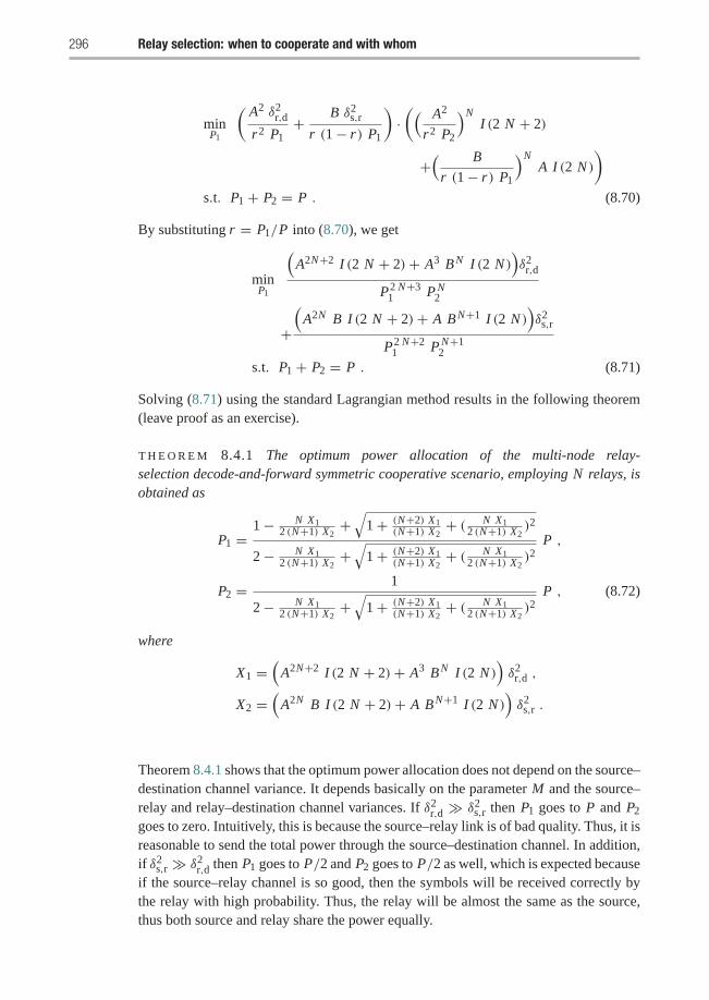
296 Relay selection: when to cooperate and with whom
minP1
(A2 δ2
r,d
r2 P1+ B δ2
s,r
r (1− r) P1
)·(( A2
r2 P2
)NI (2 N + 2)
+( B
r (1− r) P1
)NA I (2 N )
)s.t. P1 + P2 = P . (8.70)
By substituting r = P1/P into (8.70), we get
minP1
(A2N+2 I (2 N + 2)+ A3 BN I (2 N )
)δ2
r,d
P2 N+31 P N
2
+(
A2N B I (2 N + 2)+ A BN+1 I (2 N ))δ2
s,r
P2 N+21 P N+1
2
s.t. P1 + P2 = P . (8.71)
Solving (8.71) using the standard Lagrangian method results in the following theorem(leave proof as an exercise).
T H E O R E M 8.4.1 The optimum power allocation of the multi-node relay-selection decode-and-forward symmetric cooperative scenario, employing N relays, isobtained as
P1 =1− N X1
2 (N+1) X2+√
1+ (N+2) X1(N+1) X2
+ ( N X12 (N+1) X2
)2
2− N X12 (N+1) X2
+√
1+ (N+2) X1(N+1) X2
+ ( N X12 (N+1) X2
)2P ,
P2 = 1
2− N X12 (N+1) X2
+√
1+ (N+2) X1(N+1) X2
+ ( N X12 (N+1) X2
)2P , (8.72)
where
X1 =(
A2N+2 I (2 N + 2)+ A3 BN I (2 N ))δ2
r,d ,
X2 =(
A2N B I (2 N + 2)+ A BN+1 I (2 N ))δ2
s,r .
Theorem 8.4.1 shows that the optimum power allocation does not depend on the source–destination channel variance. It depends basically on the parameter M and the source–relay and relay–destination channel variances. If δ2
r,d � δ2s,r then P1 goes to P and P2
goes to zero. Intuitively, this is because the source–relay link is of bad quality. Thus, it isreasonable to send the total power through the source–destination channel. In addition,if δ2
s,r � δ2r,d then P1 goes to P/2 and P2 goes to P/2 as well, which is expected because
if the source–relay channel is so good, then the symbols will be received correctly bythe relay with high probability. Thus, the relay will be almost the same as the source,thus both source and relay share the power equally.
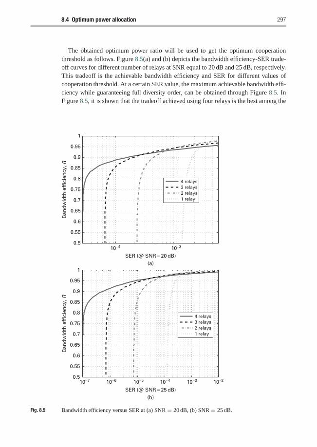
8.4 Optimum power allocation 297
The obtained optimum power ratio will be used to get the optimum cooperationthreshold as follows. Figure 8.5(a) and (b) depicts the bandwidth efficiency-SER trade-off curves for different number of relays at SNR equal to 20 dB and 25 dB, respectively.This tradeoff is the achievable bandwidth efficiency and SER for different values ofcooperation threshold. At a certain SER value, the maximum achievable bandwidth effi-ciency while guaranteeing full diversity order, can be obtained through Figure 8.5. InFigure 8.5, it is shown that the tradeoff achieved using four relays is the best among the
10−4 10−30.5
0.55
0.6
0.65
0.7
0.75
0.8
0.85
0.9
0.95
1
SER (@ SNR = 20 dB)(a)
(b)
Ban
dw
idth
eff
icie
ncy
, R
4 relays3 relays2 relays1 relay
0.5
0.55
0.6
0.65
0.7
0.75
0.8
0.85
0.9
0.95
1
SER (@ SNR = 25 dB)
Ban
dw
idth
eff
icie
ncy
, R
4 relays3 relays2 relays1 relay
10−7 10−6 10−5 10−4 10−3 10−2
Fig. 8.5 Bandwidth efficiency versus SER at (a) SNR = 20 dB, (b) SNR = 25 dB.
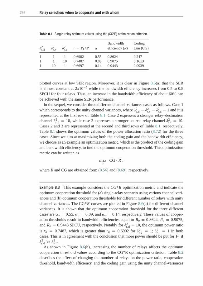
298 Relay selection: when to cooperate and with whom
Table 8.1 Single-relay optimum values using the (CG*R) optimization criterion.
Bandwidth Codingδ2s,d δ2s,r δ2r,d r = P1/P α efficiency (R) gain (CG)
1 1 1 0.6902 0.55 0.8624 0.2471 1 10 0.7487 0.09 0.9075 0.16131 10 1 0.6697 0.14 0.9443 0.0939
plotted curves at low SER region. Moreover, it is clear in Figure 8.5(a) that the SERis almost constant at 2x10⁻⁵ while the bandwidth efficiency increases from 0.5 to 0.8SPCU for four relays. Thus, an increase in the bandwidth efficiency of about 60% canbe achieved with the same SER performance.
In the sequel, we consider three different channel-variances cases as follows. Case 1which corresponds to the unity channel variances, where δ2
s,d = δ2s,r = δ2
r,d = 1 and it isrepresented at the first row of Table 8.1. Case 2 expresses a stronger relay–destinationchannel δ2
r,d = 10, while case 3 expresses a stronger source–relay channel δ2s,r = 10.
Cases 2 and 3 are represented at the second and third rows of Table 8.1, respectively.Table 8.1 shows the optimum values of the power allocation ratio (8.72) for the threecases. Since we aim at maximizing both the coding gain and the bandwidth efficiency,we choose as an example an optimization metric, which is the product of the coding gainand bandwidth efficiency, to find the optimum cooperation threshold. This optimizationmetric can be written as
maxα
CG · R ,
where R and CG are obtained from (8.56) and (8.69), respectively.
Example 8.3 This example considers the CG*R optimization metric and indicate theoptimum cooperation threshold for (a) single-relay scenario using various channel vari-ances and (b) optimum cooperation thresholds for different number of relays with unitychannel variances. The CG*R curves are plotted in Figure 8.6(a) for different channelvariances. It is shown that the optimum cooperation threshold for the three differentcases are αo = 0.55, αo = 0.09, and αo = 0.14, respectively. These values of cooper-ation thresholds result in bandwidth efficiencies equal to Ro = 0.8624, Ro = 0.9075,and Ro = 0.9443 SPCU, respectively. Notably for δ2
r,d = 10, the optimum power ratio
is ro = 0.7487, which is greater than ro = 0.6902 for δ2r,d = 1; δ2
s,r = 1 in bothcases. This is in agreement with the conclusion that more power should be put for P1 ifδ2
r,d � δ2s,r.
As shown in Figure 8.6(b), increasing the number of relays affects the optimumcooperation threshold values according to the CG*R optimization criterion. Table 8.2describes the effect of changing the number of relays on the power ratio, cooperationthreshold, bandwidth efficiency, and the coding gain using the unity channel-variances
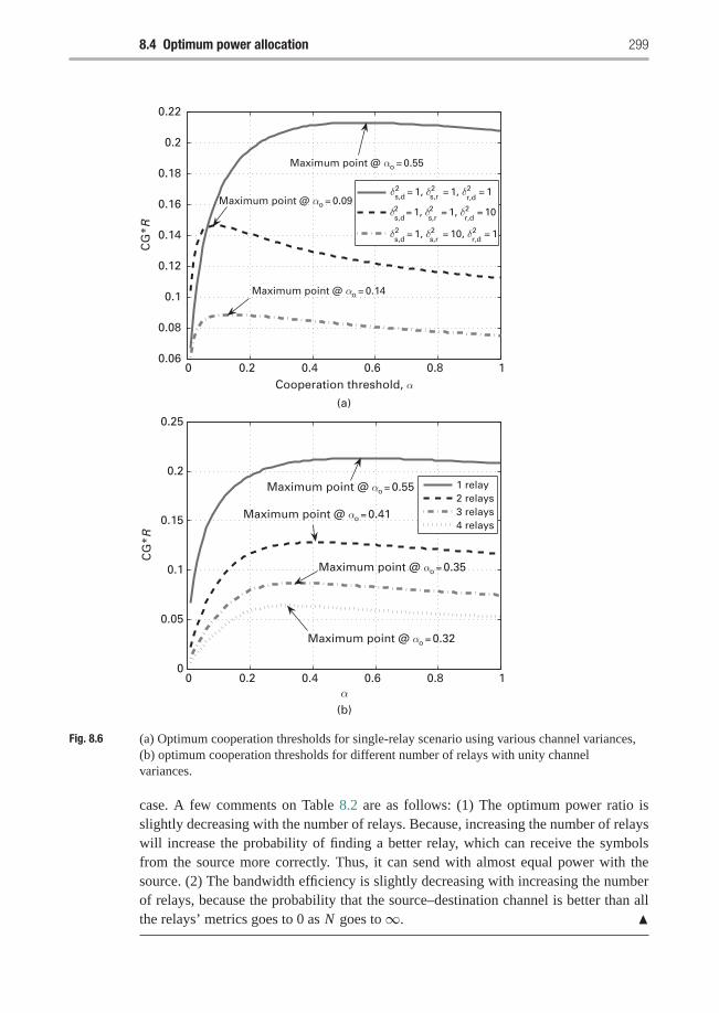
8.4 Optimum power allocation 299
0 0.2 0.4 0.6 0.8 10.06
0.08
0.1
0.12
0.14
0.16
0.18
0.2
0.22
Cooperation threshold, α(a)
(b)
CG
*R
Maximum point @ αo = 0.55
Maximum point @ αo = 0.09
Maximum point @ αo = 0.14
0 0.2 0.4 0.6 0.8 10
0.05
0.1
0.15
0.2
0.25
α
CG
*R
1 relay2 relays3 relays4 relays
Maximum point @ αo = 0.55
Maximum point @ αo = 0.41
Maximum point @ αo = 0.35
Maximum point @ αo = 0.32
δ 2 = 1, δ
2 = 1, δ 2 = 1
δ2 = 1, δ2 = 1, δ 2 = 10
s,d
s,d
s,r
s,r
r,d
r,d
δ 2 = 1, δ
2 = 10, δ 2 = 1
s,d s,r r,d
Fig. 8.6 (a) Optimum cooperation thresholds for single-relay scenario using various channel variances,(b) optimum cooperation thresholds for different number of relays with unity channelvariances.
case. A few comments on Table 8.2 are as follows: (1) The optimum power ratio isslightly decreasing with the number of relays. Because, increasing the number of relayswill increase the probability of finding a better relay, which can receive the symbolsfrom the source more correctly. Thus, it can send with almost equal power with thesource. (2) The bandwidth efficiency is slightly decreasing with increasing the numberof relays, because the probability that the source–destination channel is better than allthe relays’ metrics goes to 0 as N goes to∞. �
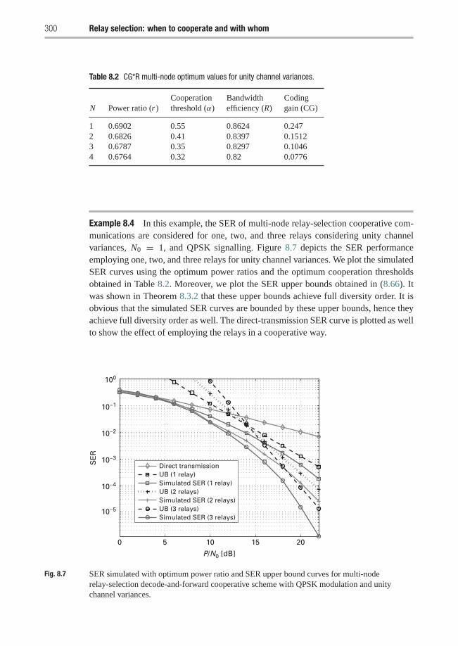
300 Relay selection: when to cooperate and with whom
Table 8.2 CG*R multi-node optimum values for unity channel variances.
Cooperation Bandwidth CodingN Power ratio (r ) threshold (α) efficiency (R) gain (CG)
1 0.6902 0.55 0.8624 0.2472 0.6826 0.41 0.8397 0.15123 0.6787 0.35 0.8297 0.10464 0.6764 0.32 0.82 0.0776
Example 8.4 In this example, the SER of multi-node relay-selection cooperative com-munications are considered for one, two, and three relays considering unity channelvariances, N0 = 1, and QPSK signalling. Figure 8.7 depicts the SER performanceemploying one, two, and three relays for unity channel variances. We plot the simulatedSER curves using the optimum power ratios and the optimum cooperation thresholdsobtained in Table 8.2. Moreover, we plot the SER upper bounds obtained in (8.66). Itwas shown in Theorem 8.3.2 that these upper bounds achieve full diversity order. It isobvious that the simulated SER curves are bounded by these upper bounds, hence theyachieve full diversity order as well. The direct-transmission SER curve is plotted as wellto show the effect of employing the relays in a cooperative way.
0 5 10 15 20
10−5
10−4
10−3
10−2
10−1
100
P/N0 [dB]
SE
R
Direct transmissionUB (1 relay)Simulated SER (1 relay)UB (2 relays)Simulated SER (2 relays)UB (3 relays)Simulated SER (3 relays)
Fig. 8.7 SER simulated with optimum power ratio and SER upper bound curves for multi-noderelay-selection decode-and-forward cooperative scheme with QPSK modulation and unitychannel variances.
8.5 Chapter summary and bibliographical notes 301
Moreover, the simulated bandwidth efficiencies are 0.8973, 0.8805, and 0.8738employing one, two, and three relays, respectively. These results are slightly higherthan the analytical results shown in Table 8.2. �
8.5 Chapter summary and bibliographical notes
In this chapter, we have discussed single-relay and multi-node relay-selection decode-and-forward cooperative scenarios, which utilize the partial CSI available at the sourceand the relays to achieve higher bandwidth efficiency and guarantee full diversity order.In the single-relay system, it was shown that the modified harmonic mean function of thesource–relay and relay–destination channels gain gives a proper measure on how muchhelp a relay can offer. An approximate expression of the achievable bandwidth effi-ciency and an upper bound on the SER performance were derived. It turns out that thebandwidth efficiency is increased to 0.9 SPCU when the source–relay channel is rela-tively strong. Moreover, it was also shown that full diversity order is guaranteed as longas there is a positive probability of having the relay-cooperation mode.
In the multi-node system using arbitrary N relays, we considered the optimal relayas the one which has the maximum instantaneous modified harmonic mean functionof its source–relay and relay–destination channels gain among the N relays. For thesymmetric scenario, we have presented the approximate expression of the achiev-able bandwidth efficiency, which decreases with increasing the number of employedrelays. Furthermore, we have also derived the SER upper bound, which proves thatfull diversity order is guaranteed as long as there is a positive probability of havingthe relay-cooperation mode. It was shown that the bandwidth efficiency is boosted upfrom 0.2 to 0.77 SPCU for N = 4 relays and unity channel variances case. More-over, we determined the optimum power allocation for the multi-node relay-selectionscheme, which minimizes the SER. As for the optimum cooperation threshold, thebandwidth efficiency-SER tradeoff curves was also shown to determine the optimalcooperation threshold.
There are various protocols proposed to choose the best relay among a collectionof available relays in the literature. In [237], the authors proposed to choose the bestrelay depending on its geographic position, based on the geographic random forward-ing (GeRaF) protocol proposed in [240]. In GeRaF, the source broadcasts its data toa collection of nodes and the node that is closest to the destination is chosen in a dis-tributed manner to forward the source’s data to the destination. In [128], the authorsconsidered a best-select relay scheme in which only the relay, which has received thetransmitted data from the source correctly and has the highest mean signal-to-noiseratio (SNR) to the destination node, is chosen to forward the source’s data. In [83], arelay-selection scheme for single-relay decode-and-forward cooperative systems wasproposed. In this scheme, the source decides whether to employ the relay in forwardingits information or not, depending on the instantaneous values of the source–destination
302 Relay selection: when to cooperate and with whom
and source–relay channel gains. While [83] considered a single relay scenario, themulti-node case was considered in [84]. More information on the topics studied in thischapter can be found in [82].
Exercises
8.1 Prove that the PDF and CDF of the variable βm specified in (8.10) can bedetermined as
pβm (βm) = βm
2 t21
exp
(− t2
2βm
)(t1 t2 K1
(βm
t1
)+ 2 K0
(βm
t1
) )U (βm) ,
Pβm (βm) = 1− βm
t1exp
(− t2
2βm
)K1
(βm
t1
),
where t1 =√
q1q2δ2s,rδ
2r,d, t2 = 1/q2δ
2s,r + 1/q1δ
2r,d, and K0(x) and K1(x)
are the zero-order and first-order modified Bessel functions of the second kind,respectively, defined as
K0(x) =∫ ∞
0cos(x sinh (t)
)dt =
∫ ∞
0
cos (x t)√t2 + 1
dt ,
K1(x) =∫ ∞
0sin(x sinh (t)
)sinh (t) dt ,
for x > 0.
8.2 Show that the MGF of the variable βm specified in (8.10) can be written as
Mβm (γ ) = Eβm
(exp(−γ βm)
)= 16 λ1 λ2
3 (λ1 + λ2 + 2√λ1 λ2 + γ )2
×⎛⎝4 (λ1 + λ2) 2F1
(3, 3
2 ; 52 ; λ1+λ2−2
√λ1 λ2+γ
λ1+λ2+2√λ1 λ2+γ
)(λ1 + λ2 + 2
√λ1 λ2 + γ )
+ 2F1
(2,
1
2; 5
2; λ1 + λ2 − 2
√λ1 λ2 + γ
λ1 + λ2 + 2√λ1 λ2 + γ
))where Eβm (.) represents the statistical average with respect to βm and
2F1(., .; .; .) is the Gauss’ hypergeometric function.
8.3 Show the probability upper bound in (8.43), i.e.,
Pr(B|φc) Pr(φc)
≤ 1
π
∫ (M−1)πM
θ=0
Mβm
(P1 C(θ)
2 q1
)− Mβm
((P0 C(θ)+ 1
δ2s,d
)α + P1 C(θ)
2 q1
)dθ
1+ P0 C(θ)δ2s,d
.
Exercises 303
8.4 Prove the result in Theorem 8.4.1, i.e., the optimum power allocation of themulti-node relay-selection decode-and-forward symmetric cooperative scenariowith N relays is given by
P1 =1− N X1
2 (N+1) X2+√
1+ (N+2) X1(N+1) X2
+ ( N X12 (N+1) X2
)2
2− N X12 (N+1) X2
+√
1+ (N+2) X1(N+1) X2
+ ( N X12 (N+1) X2
)2P ,
P2 = 1
2− N X12 (N+1) X2
+√
1+ (N+2) X1(N+1) X2
+ ( N X12 (N+1) X2
)2P ,
where
X1 =(
A2N+2 I (2 N + 2)+ A3 BN I (2 N ))δ2
r,d ,
X2 =(
A2N B I (2 N + 2)+ A BN+1 I (2 N ))δ2
s,r .
8.5 In this exercise, we will consider an alternative relay selection metric and shownits effect on the single-relay relay-selection decode-and-forward scheme. Therelay’s metric is represented by its source–relay channel gain. Based on thismetric, the source determines whether to cooperate with the relay or not. Letφ = { βs,d ≥ α βs,r } be the event of direct transmission. The transmis-sion protocol can be modelled as in (8.11)–(8.14). The channel coefficientshs,d, hs,r, and hr,d are modeled as zero-mean complex Gaussian random vari-ables with variances δ2
s,d, δ2s,r, and δ2
r,d, respectively. The noise terms ηs,d, ηs,r,and ηr,d are modeled as zero-mean, complex Gaussian random variables withequal variance N0.(a) Show that the probability of direct transmission is given by
Pr(φ) = Pr(βs,d ≥ αβs,r) =δ2
s,d
δ2s,d + α δ2
s,r
. (E8.1)
(b) Based on (8.23), show that the bandwidth efficiency is given by
R = 2 δ2s,d + α δ2
s,r
2 δ2s,d + 2 α δ2
s,r
. (E8.2)
(c) For the direct-transmission mode and using M-PSK modulation, the condi-tional direct-transmission SER is given by (8.27). By averaging (8.27) overβs,d, show that the direct-transmission SER is given by
Pr(e|φ)Pr(φ)
= F1
(1+ bPδ2
s,d
N0 sin2 θ
)− F1
(1+ δ2
s,d
αδ2s,r+ bPδ2
s,d
N0 sin2 θ
), (E8.3)
where
F1 (x(θ)) = 1
π
∫ (M−1)πM
0
1
x(θ)dθ. (E8.4)
304 Relay selection: when to cooperate and with whom
(d) For the relay-cooperation mode, maximum ratio combining (MRC) [17] isapplied at the destination. The output of the MRC can be written as in (8.30).The conditional SER of the relay-cooperation mode is given by (8.32).By averaging (8.32) over the exponentially distributed random variablesβs,d, βs,r, and βr,d, show that
Pr(e/φc)Pr(φc) = F2
(1
π2, P1, 0,
(M − 1)π
M,(M − 1)π
M
)+ F1
((1+ δ2
s,d
αδ2s,r+ bP1δ
2s,d
N0 sin2 θ
)(1+ bP2δ
2r,d
N0 sin2 θ
))
− F2
(1
π2, P1, P2,
(M − 1)π
M,(M − 1)π
M
), (E8.5)
where
F2 (C, P1, P2, θ1, θ2) = C∫ θ1
0
∫ θ2
0
1(1+ b P1δ
2s,r
N0 sin2 θ2
)dθ2 dθ1(
1+ δ2s,d
αδ2s,r+ b P1δ
2s,d
N0
(1
sin2 θ1+ 1α sin2 θ2
))(1+ b P2δ
2r,d
N0 sin2 θ1
) . (E8.6)
(e) Obtain a complete SER expression for the M-PSK signalling based on (c)and (d).
8.6 For the communication system described in Exercise 8.5, consider the ratiobetween the SER and the bandwidth efficiency (SER/R) as an optimizationmetric to determine the optimum cooperation threshold and power ratio.
(a) At SNR=10 dB and using a unity channel-variances case δ2s,d = δ2
s,r = δ2r,d =
1 with QPSK modulation, plot a 3-dimensional curve for the SER/R, and ver-ify that the optimum values, which minimize the SER/R optimization metric,are αo = 0.35 and ro = 0.52. Moreover, plot the SER of the relay-selectionscheme and compare the simulated SER with the analytical SER, given bythe summation of (E8.3) and (E8.5). Verify that the bandwidth efficiencyresulting from the simulations is 0.870 37 SPCU.
(b) Consider the multi-node case where arbitrary N relays are available. Eachrelay’s metric is represented by its source–relay channel gain. Plot the SERof this system assuming two and three relays. From the simulation results,does this relay’s metric guarantees full diversity order? Explain.
8.7 Consider a relay metric, which is given by the minimum of the relay’ssource–relay and relay–destination channel gains, i.e., the relay’s metric can begiven by
βi = min(|hs,ri |2, |hri ,d|2) , f or i = 1, 2, . . . , N . (E8.7)

Exercises 305
For simplicity, consider that the cooperation threshold is 1 and the power ratiois 0.5. Hence, the direct transmission event is denoted by φ = { βs,d ≥ αβi }.Plot the SER for system with one, two, and three relays assuming unity chan-nel variances for all the channels, r = 0.5, α = 1, and QPSK signalling.Based on the simulation results, does this relay’s metric guarantee full diversityorder? Explain.
9 Differential modulation forcooperative communications
In wireless communication systems with a single antenna, the channel capacity canbe very low and the bit error rate high when fading occurs. Various techniques canbe utilized to mitigate fading, e.g., robust modulation, coding and interleaving, error-correcting coding, equalization, and diversity. Different kinds of diversities such asspace, time, frequency, or any combination of them are possible. Among these diver-sity techniques, space diversity is of special interest because of its ability to improveperformance without sacrificing delay and bandwidth efficiency. Recently, space diver-sity has been intensively investigated in point-to-point wireless communication systemsby the deployment of a MIMO concept together with efficient coding and modulationschemes. In recent years, cooperative communication [109] has been proposed as analternative communication system that explores MIMO-like diversity to improve linkperformance without the requirement of additional antennas. However, most of exist-ing works on MIMO systems and cooperative communications are designed based onan assumption that the receivers have full knowledge of the channel state information(CSI). In this case, the schemes must incorporate reliable multi-channel estimation,which inevitably increases the cost of frequent retraining and the number of estimatedparameters to the receivers. Although the channel estimates may be available whenthe channel changes slowly comparing with the symbol rate, they may not be possi-bly acquired in a fast-fading environment. To develop practical schemes that omit suchCSI requirements, we consider in this chapter differential modulations for cooperativecommunications.
We first briefly review differential modulation for non-cooperative or direct wire-less communication systems. Then, we consider differential modulation for cooperativecommunication systems employing the decode-and-forward (DF) protocol. We dis-cuss system design, performance analysis, and performance optimization. Finally,we consider differential modulation for the amplify-and-forward (AF) cooperativecommunication protocol.
9.1 Differential modulation
In conventional single-antenna systems, non-coherent modulation is useful when theknowledge of CSI is not available. The non-coherent modulation simplifies the receiverstructure by omitting channel estimation and carrier or phase tracking. In this chapter,
9.1 Differential modulation 307
although we focus on the differential M-ary phase-shift-keying (DMPSK) scheme, theconcept of differential modulation schemes covered in subsequent sections can also beapplied to differential M-ary quadrature amplitude modulation (DMQAM).
In the DMPSK scheme, information is modulated through the phase differenceamong two consecutive symbols. Specifically, for a data rate of R bits per chan-nel use, the DPMSK signal constellation comprises M = 2R symbols. Each symbolm ∈ 0 ≤ M − 1 is generated by the m-th root of unity: vm = ej2πm/M . Define sτ asthe differentially encoded symbol to be transmitted at time τ . The differential modula-tor transmits sτ = 1 at the first symbol period, i.e., at τ = 0. For subsequent symbolperiods, the differential transmission follows a recursive multiplication rule:
sτ = vmsτ−1. (9.1)
If we let hτ denote the fading coefficient and nτ represent additive noise, then thereceived signal for DMPSK modulation can be written as
yτ = √ρhτ sτ + wτ . (9.2)
The detection rule for differential demodulation can be obtained by the followingderivations. We first rewrite (9.2) as
yτ = √ρhτ sτ + wτ = √ρhτ vmsτ−1 + wτ .We also knew from (9.2) that
√ρhτ−1sτ−1 = yτ−1 − wτ−1. (9.3)
By assuming that fading channel keeps constant over two symbol periods, i.e., hτ−1 ≈hτ , and substitute (9.3) into (9.2), we have
yτ = yτ−1vm − vmwτ−1 + wτ .
= yτ−1vm +√
2wτ , (9.4)
where wτ � (1/√
2)(wτ − vmwτ−1) is a complex Gaussian random variable with zero
mean and unit variance. From (9.4), by treating yτ−1 as a known channel informationand vm as a transmitted symbol, the expression in (9.4) can be considered as a receivedsignal for coherent detection. In this way, the optimum detector is simply the minimumdistance detector. Therefore, the differential decoder estimates the transmit informationusing the following decoding rule:
m = arg minm∈0,1,...M−1
|yτ − vm yτ−1|2. (9.5)
We can see from (9.5) that the efficient differential demodulation for an informa-tion symbol relies on two consecutive received symbols, and the decoding error doesnot propagate to subsequent decoded information symbols. In terms of performance,since the noise power has twice the variance of its coherent counterpart, the differentialscheme looses 3 dB performance in comparison to its coherent counterpart. For con-venience in subsequence derivations of optimum differential detector, (9.5) is furthersimplified to
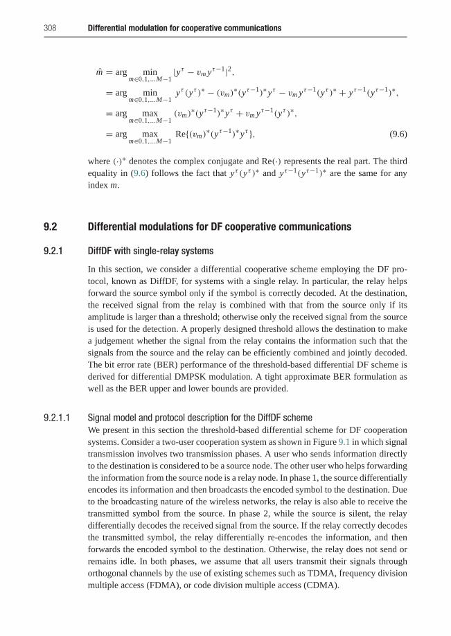
308 Differential modulation for cooperative communications
m = arg minm∈0,1,...M−1
|yτ − vm yτ−1|2,= arg min
m∈0,1,...M−1yτ (yτ )∗ − (vm)
∗(yτ−1)∗yτ − vm yτ−1(yτ )∗ + yτ−1(yτ−1)∗,
= arg maxm∈0,1,...M−1
(vm)∗(yτ−1)∗yτ + vm yτ−1(yτ )∗,
= arg maxm∈0,1,...M−1
Re{(vm)∗(yτ−1)∗yτ }, (9.6)
where (·)∗ denotes the complex conjugate and Re(·) represents the real part. The thirdequality in (9.6) follows the fact that yτ (yτ )∗ and yτ−1(yτ−1)∗ are the same for anyindex m.
9.2 Differential modulations for DF cooperative communications
9.2.1 DiffDF with single-relay systems
In this section, we consider a differential cooperative scheme employing the DF pro-tocol, known as DiffDF, for systems with a single relay. In particular, the relay helpsforward the source symbol only if the symbol is correctly decoded. At the destination,the received signal from the relay is combined with that from the source only if itsamplitude is larger than a threshold; otherwise only the received signal from the sourceis used for the detection. A properly designed threshold allows the destination to makea judgement whether the signal from the relay contains the information such that thesignals from the source and the relay can be efficiently combined and jointly decoded.The bit error rate (BER) performance of the threshold-based differential DF scheme isderived for differential DMPSK modulation. A tight approximate BER formulation aswell as the BER upper and lower bounds are provided.
9.2.1.1 Signal model and protocol description for the DiffDF schemeWe present in this section the threshold-based differential scheme for DF cooperationsystems. Consider a two-user cooperation system as shown in Figure 9.1 in which signaltransmission involves two transmission phases. A user who sends information directlyto the destination is considered to be a source node. The other user who helps forwardingthe information from the source node is a relay node. In phase 1, the source differentiallyencodes its information and then broadcasts the encoded symbol to the destination. Dueto the broadcasting nature of the wireless networks, the relay is also able to receive thetransmitted symbol from the source. In phase 2, while the source is silent, the relaydifferentially decodes the received signal from the source. If the relay correctly decodesthe transmitted symbol, the relay differentially re-encodes the information, and thenforwards the encoded symbol to the destination. Otherwise, the relay does not send orremains idle. In both phases, we assume that all users transmit their signals throughorthogonal channels by the use of existing schemes such as TDMA, frequency divisionmultiple access (FDMA), or code division multiple access (CDMA).
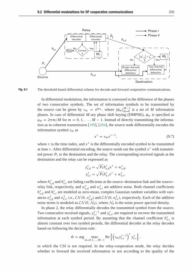
9.2 Differential modulations for DF cooperative communications 309
Source
Relay
Destination
P2
P1
hr,d
hs,d
hs,r
M2M1
Differentialdecoder
Differentialencoder
Single channeldifferentialdetection
~
Correct
?
Phase IPhase II
Yes
No
Stop
,r dyτ ζ>Yes
Two channeldifferentialdetection
?
No
Fig. 9.1 The threshold-based differential scheme for decode-and-forward cooperative communications.
In differential modulation, the information is conveyed in the difference of the phasesof two consecutive symbols. The set of information symbols to be transmitted bythe source can be given by vm = ejϕm , where {φm}M−1
m=0 is a set of M informationphases. In case of differential M-ary phase shift keying (DMPSK), φm is specified asϕm = 2πm/M for m = 0, 1, . . . ,M − 1. Instead of directly transmitting the informa-tion as in coherent transmission [109], [204], the source node differentially encodes theinformation symbol vm as
xτ = vmxτ−1, (9.7)
where τ is the time index, and xτ is the differentially encoded symbol to be transmittedat time τ . After differential encoding, the source sends out the symbol xτ with transmit-ted power P1 to the destination and the relay. The corresponding received signals at thedestination and the relay can be expressed as
yτs,d =√
P1hτs,dxτ + wτs,d,yτs,r =
√P1hτs,rx
τ + wτs,r,where hτs,d and hτs,r are fading coefficients at the source–destination link and the source–relay link, respectively, and wτs,d and wτs,r are additive noise. Both channel coefficientshτs,d and hτs,r are modeled as zero-mean, complex Gaussian random variables with vari-
ances σ 2s,d and σ 2
s,r, i.e., CN (0, σ 2s,d) and CN (0, σ 2
s,r), respectively. Each of the additivenoise terms is modeled as CN (0,N0), where N0 is the noise power spectral density.
In phase 2, the relay differentially decodes the transmitted symbol from the source.Two consecutive received signals, yτ−1
s,r and yτs,r, are required to recover the transmittedinformation at each symbol period. By assuming that the channel coefficient hτs,r isalmost constant over two symbol periods, the differential decoder at the relay decodesbased on following the decision rule:
m = arg maxm=0,1,...,M−1
Re{(vm yτ−1
s,r
)∗yτs,r},
in which the CSI is not required. In the relay-cooperation mode, the relay decideswhether to forward the received information or not according to the quality of the
310 Differential modulation for cooperative communications
received signal. For mathematical tractability, we assume that the relay can judgewhether the decoded information is correct or not.1 If the relay incorrectly decodesthe received signal, such incorrectly decoded symbol is discarded, and the relay doesnot send any information. Otherwise, the relay differentially re-encodes the correctlydecoded information symbol and forwards it to the destination.
In general, successful differential decoding requires that the encoder differentiallyencodes each information symbol with the previously transmitted symbol. For example,if the information symbols are sent every time slot, then the information symbol to betransmitted at time τ is differentially encoded with the transmitted symbol at time τ−1.In this differential DF scheme, since the information symbols at the relay are transmittedonly if they are correctly decoded, the transmission time of the previously transmittedsymbol can be any time before the current time τ . We denote such previous transmissiontime as τ − k, k ≥ 1, i.e., τ − k is the latest time that the relay correctly decodes thesymbol before time τ . In order to perform successful differential en/decoding, we leta memory M1 at the relay (see Figure 9.1) store the transmitted symbol at time τ − k.Note that having a memory M1 does not increase the system complexity compared tothe conventional differential system. The difference is that the memory in this DiffDFscheme stores the transmitted symbol at time τ − k instead of time τ − 1 as does theconventional differential scheme.
The differentially re-encoded signal at the relay in phase 2 can be expressed as
xτ = vm xτ−k, (9.8)
where xτ is the differentially encoded symbol at the relay at time τ . We can see from(9.7) and (9.8) that the differentially encoded symbols xτ at the relay and xτ at thesource convey the same information symbol vm . However, the two encoded symbolscan be different since the relay differentially encodes the information symbol vm withthe symbol in the memory, which may not be xτ−1 as used at the source. After differ-ential re-encoding, the relay sends the symbol xτ to the destination with transmittedpower P2, and then stores the transmitted symbol xτ in the memory M1 for subsequentdifferential encoding. The received signal at the destination from the relay in phase 2can be expressed as
yτr,d ={ √
P2hτr,d xτ + wτr,d : if relay correctly decodes (Pτ2 = P2);wτr,d : if relay incorrectly decodes (Pτ2 = 0),
(9.9)
where hτr,d is the channel coefficient from the relay to the destination and wτr,d is an
additive noise. We assume that hτr,d is CN (0, σ 2r,d) distributed, and wτr,d is CN (0,N0)
distributed.The received signals at the destination comprise the received signal from the source in
phase 1 and that from the relay in phase 2. As discussed previously, in phase 2, therelay may forward the information or remain idle. Without knowledge of the CSI, the
1 Practically, this can be done at the relay by applying a simple SNR threshold test on the received data,although it can lead to some error propagation. Nevertheless, for practical ranges of operating SNR, theevent of error propagation can be assumed negligible.
9.2 Differential modulations for DF cooperative communications 311
destination is unable to know whether the received signal from the relay contains theinformation or not. In order for the destination to judge whether to combine the signalsfrom the source–destination and relay–destination links, we use a decision threshold ζat the destination node (see Figure 9.1). We consider the received signal with amplitude|yτr,d| greater than the threshold ζ as a high-potential information bearing signal to beused for further differential detection.
Particularly, if the amplitude of the received signal from the relay is not greaterthan the decision threshold, i.e., |yτr,d| ≤ ζ , the destination estimates the transmittedsymbol based only on the received signal from the direct link. On the other hand, if|yτr,d| > ζ , the received signal from the source and that from the relay are combinedtogether, and then the combined output is jointly differentially decoded. Note that, inorder to successfully decode, the differential detector requires the previously receivedsignal, which serves as a CSI estimate. Since the received signal from the relay maycontain the transmitted symbol or only noise, we use a memory M2 at the destinationas shown in Figure 9.1 to store the previously received signal at the relay–destinationlink that tends to contain the information. An ideal situation is to let the memory storethe received signal yτr,d only when the signal contains the transmitted symbol; however,such information is not available since the destination does not have the knowledge ofthe CSI. So, to efficiently decode the received signal from the relay, the memory M2
is used to store the received signal yτr,d whose amplitude is greater than the decisionthreshold. If the threshold is properly designed, then the signal in the memory M2 cor-responds to the received signal from the relay that carries the encoded symbol stored inthe memory M1.
With an assumption that the channel coefficients stay almost constant for severalsymbol periods, the signal in the memory M2 serves as a channel estimate of therelay–destination link, which can then be used for efficient differential decoding at thedestination. When we combine all received signals for joint detection, the combinedsignal prior to the differential decoding is
y ={
a1(yτ−1s,d )
∗yτs,d + a2(yτ−lr,d )
∗yτr,d if |yτr,d| > ζ ;(yτ−1
s,d )∗yτs,d if |yτr,d| ≤ ζ,
(9.10)
where a1 and a2 are combining weight coefficients, and τ−l (l ≥ 1) represents the timeindex of the latest signal in memory M2, i.e., yτ−l
r,d is the most recent received signalfrom the relay whose amplitude is larger than the threshold. Note that different com-bining weights, a1 and a2, result in different system performances. In Section 9.2.1.2,the BER performance is derived in case of a1 = 1/2N0 and a2 = 1/2N0. The useof these combining weights maximizes the signal-to-noise ratio (SNR) of the com-biner output when the destination is able to differentially decode the signals from bothsource and relay. Based on the combined signal in (9.10), the decoder at the destinationjointly differentially decodes the transmitted information symbol by using the followingdecision rule:
m = arg maxm=0,1,...,M−1
Re{v∗m y
}.
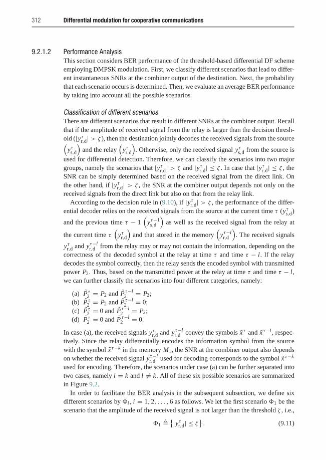
312 Differential modulation for cooperative communications
9.2.1.2 Performance AnalysisThis section considers BER performance of the threshold-based differential DF schemeemploying DMPSK modulation. First, we classify different scenarios that lead to differ-ent instantaneous SNRs at the combiner output of the destination. Next, the probabilitythat each scenario occurs is determined. Then, we evaluate an average BER performanceby taking into account all the possible scenarios.
Classification of different scenariosThere are different scenarios that result in different SNRs at the combiner output. Recallthat if the amplitude of received signal from the relay is larger than the decision thresh-old (|yτr,d| > ζ ), then the destination jointly decodes the received signals from the source(
yτs,d
)and the relay
(yτr,d
). Otherwise, only the received signal yτs,d from the source is
used for differential detection. Therefore, we can classify the scenarios into two majorgroups, namely the scenarios that |yτr,d| > ζ and |yτr,d| ≤ ζ . In case that |yτr,d| ≤ ζ , theSNR can be simply determined based on the received signal from the direct link. Onthe other hand, if |yτr,d| > ζ , the SNR at the combiner output depends not only on thereceived signals from the direct link but also on that from the relay link.
According to the decision rule in (9.10), if |yτr,d| > ζ , the performance of the differ-ential decoder relies on the received signals from the source at the current time τ (yτs,d)
and the previous time τ − 1(
yτ−1s,d
)as well as the received signal from the relay at
the current time τ(
yτr,d
)and that stored in the memory
(yτ−l
r,d
). The received signals
yτr,d and yτ−lr,d from the relay may or may not contain the information, depending on the
correctness of the decoded symbol at the relay at time τ and time τ − l. If the relaydecodes the symbol correctly, then the relay sends the encoded symbol with transmittedpower P2. Thus, based on the transmitted power at the relay at time τ and time τ − l,we can further classify the scenarios into four different categories, namely:
(a) Pτ2 = P2 and Pτ−l2 = P2;
(b) Pτ2 = P2 and Pτ−l2 = 0;
(c) Pτ2 = 0 and Pτ−l2 = P2;
(d) Pτ2 = 0 and Pτ−l2 = 0.
In case (a), the received signals yτr,d and yτ−lr,d convey the symbols xτ and xτ−l , respec-
tively. Since the relay differentially encodes the information symbol from the sourcewith the symbol xτ−k in the memory M1, the SNR at the combiner output also dependson whether the received signal yτ−l
r,d used for decoding corresponds to the symbol xτ−k
used for encoding. Therefore, the scenarios under case (a) can be further separated intotwo cases, namely l = k and l �= k. All of these six possible scenarios are summarizedin Figure 9.2.
In order to facilitate the BER analysis in the subsequent subsection, we define sixdifferent scenarios by �i , i = 1, 2, . . . , 6 as follows. We let the first scenario �1 be thescenario that the amplitude of the received signal is not larger than the threshold ζ , i.e.,
�1 �{|yτr,d| ≤ ζ} . (9.11)
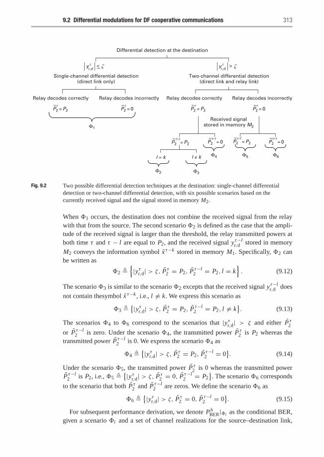
9.2 Differential modulations for DF cooperative communications 313
Differential detection at the destination
Two-channel differential detection(direct link and relay link)
Relay decodes correctly Relay decodes incorrectly
Received signalstored in memory M2
Single-channel differential detection(direct link only)
Relay decodes correctly Relay decodes incorrectly
r,dyτ ζ< r,dyτ ζ>
= P2P2~τ
= 0P2~τ
= 0P2~τ–l
= P2P2~τ
= P2P2~τ–l
= 0P2~τ–l
= P2P2~τ–l
= 0P2~τ
l = k l ≠ k
Φ1
Φ4
Φ2 Φ3
Φ5 Φ6
Fig. 9.2 Two possible differential detection techniques at the destination: single-channel differentialdetection or two-channel differential detection, with six possible scenarios based on thecurrently received signal and the signal stored in memory M2.
When �1 occurs, the destination does not combine the received signal from the relaywith that from the source. The second scenario �2 is defined as the case that the ampli-tude of the received signal is larger than the threshold, the relay transmitted powers atboth time τ and τ − l are equal to P2, and the received signal yτ−l
r,d stored in memory
M2 conveys the information symbol xτ−k stored in memory M1. Specifically, �2 canbe written as
�2 �{|yτr,d| > ζ, Pτ2 = P2, Pτ−l
2 = P2, l = k}. (9.12)
The scenario�3 is similar to the scenario�2 excepts that the received signal yτ−lr,d does
not contain thesymbol xτ−k , i.e., l �= k. We express this scenario as
�3 �{|yτr,d| > ζ, Pτ2 = P2, Pτ−l
2 = P2, l �= k}. (9.13)
The scenarios �4 to �6 correspond to the scenarios that |yτr,d| > ζ and either Pτ2or Pτ−l
2 is zero. Under the scenario �4, the transmitted power Pτ2 is P2 whereas thetransmitted power Pτ−l
2 is 0. We express the scenario �4 as
�4 �{|yτr,d| > ζ, Pτ2 = P2, Pτ−l
2 = 0}. (9.14)
Under the scenario �5, the transmitted power Pτ2 is 0 whereas the transmitted powerPτ−l
2 is P2, i.e., �5 �{|yτr,d| > ζ, Pτ2 = 0, Pτ−l
2 = P2}. The scenario �6 corresponds
to the scenario that both Pτ2 and Pτ−l2 are zeros. We define the scenario �6 as
�6 �{|yτr,d| > ζ, Pτ2 = 0, Pτ−l
2 = 0}. (9.15)
For subsequent performance derivation, we denote PhBER|�i as the conditional BER,
given a scenario �i and a set of channel realizations for the source–destination link,
314 Differential modulation for cooperative communications
the source–relay link, and the relay–destination link. We also denote Phr (�i ) as the
chance that the scenario �i occurs given a set of channel realizations. Accordingly, theconditional BER of the differential DF scheme can be expressed as
PhBER =
6∑i=1
PhBER|�i Ph
r (�i ). (9.16)
By averaging (9.16) over all channel realizations, the average BER of the DiffDFscheme is given by
PBER =6∑
i=1
E[
PhBER|�i Ph
r (�i )]=
6∑i=1
P(i)BER, (9.17)
where E[·] represents the expectation operation.In the following subsections, we determine the chance that each scenario occurs
(Phr (�i )), the conditional BER (Ph
BER|�i ), and finally obtain the average BER (PBER)for the differential DF scheme.
Probability of occurrenceWe first note that for a specific channel realization, the amplitude of the received signalyτr,d depends on the relay transmitted power Pτ2 , which in turn relies on the correctnessof the decoded symbol at the relay. With DMPSK signals, the chance of incorrect decod-ing at the relay, and hence the chance of Pτ2 = 0, can be obtained from the conditionalsymbol error rate (SER) of the transmission from the source to the relay. The SER ofDMPSK signals is [145]:
Phr
(Pτ2 = 0
)= �(γ τs,r) � 1
π
∫ (M−1)π/M
0exp[−g(φ)γ τs,r
]dφ, (9.18)
where
γ τs,r =P1|hτs,r|2
N0(9.19)
is the instantaneous SNR per symbol at the relay due to the transmitted symbol fromthe source, and
g(φ) = sin2(π/M)
1 + cos(π/M) cos(φ). (9.20)
The chance that the relay forwards the symbol with transmitted power Pτ2 = P2 isdetermined by the chance of correct decoding at the relay, hence
Phr
(Pτ2 = P2
)= 1−�(γ τs,r), (9.21)
where �(γ τs,r) is specified in (9.18).Consider the scenario �1 in which the amplitude of the received signal yτr,d is not
greater than the decision threshold. The chance that �1 occurs can be written as
9.2 Differential modulations for DF cooperative communications 315
Phr (�1) = Ph
r
(|yτr,d| ≤ ζ
∣∣ Pτ2 = 0)�(γ τs,r)
+ Phr
(|yτr,d| ≤ ζ
∣∣ Pτ2 = P2
) [1−�(γ τs,r)
]. (9.22)
The conditional probabilities, Phr (|yτr,d| ≤ ζ
∣∣∣ Pτ2 = 0) and Phr (|yτr,d| ≤ ζ
∣∣∣ Pτ2 = P2)
can be obtained from the cumulative distribution function (CDF) of the random vari-able |yτr,d|. The received signal yτr,d is a complex Gaussian random variable with mean√
P2hτr,d xτ and variance N0, i.e., yτr,d ∼ CN(√
P2hτr,d xτ ,N0
). If Pτ2 = 0, which
results from incorrect decoding at the relay, the received signal yτr,d is simply a zero-mean, complex Gaussian random variable with variance N0, i.e., yτr,d ∼ CN (0,N0),and its amplitude is Rayleigh distributed. Hence, the conditional probability that |yτr,d|is not greater than the decision threshold given that the relay does not send informationcan be expressed as
Phr
(|yτr,d| ≤ ζ
∣∣∣ Pτ2 = 0)= 1− exp(−ζ 2/N0). (9.23)
If Pτ2 = P2, which corresponds to the case of correct decoding at the relay, then thereceived signal yτr,d is Gaussian distributed with mean
√P2hτr,d xτ and variance N0.
In this case, |yτr,d|2 can be viewed as a summation of two squared Gaussian randomvariables with means
m1 = Re{√
P2hτr,d xτ}, m2 = Im
{√P2hτr,d xτ
},
and a common variance σ 2 = N0/2. We observe that |yτr,d|2 is non-central chi-square
distributed with parameter s2 = m21 + m2
2 [146]. In case of DMPSK signals, theparameter s can be determined as
s =√
P2|hτr,d xτ |2 =√
P2|hτr,d|2, (9.24)
where the second equality results from the fact that each DMPSK symbol has unitenergy. From (9.24), the conditional probability that |yτr,d| is not greater than the deci-sion threshold given that the relay sends the information with transmitted power P2 canbe written as
Phr
(|yτr,d| ≤ ζ
∣∣∣ Pτ2 = P2
)= 1−M
(P2|hτr,d|2, ζ
), (9.25)
where
M(
P2|hτr,d|2, ζ)
� Q1
⎛⎝√ P2|hτr,d|2N0/2
,ζ√N0/2
⎞⎠ , (9.26)
in which Q1 (α, β) is the Marcum Q-function [188]:
Q1 (α, β) =∫ ∞
β
λ exp
[−(λ2 + α2
2
)]I0(αλ)dλ, (9.27)
316 Differential modulation for cooperative communications
and I0(·) is the zeroth-order modified Bessel function of the first kind. By substituting(9.23) and (9.25) into (9.22), we can express the chance that �1 occurs as
Phr (�1) =
(1− e(−ζ 2/N0)
)�(γ τs,r)+
(1−M
(P2|hτr,d|2, ζ
)) [1−�(γ τs,r)
]. (9.28)
The rest of the scenarios, �2 to �6, are related to the situation when the amplitudeof the received signal from the relay, |yτr,d|, is greater than the decision threshold ζ . Inthese scenarios, both the currently received signal (yτr,d) and that stored in the memory
M2 (yτ−lr,d ) are used for differential detection at the destination. In the DiffDF scheme,
the memory M2 stores only the received signal from the relay whose amplitude is largerthan the threshold. This implies that the amplitude |yτ−l
r,d | is larger than the threshold.Therefore, the chance that each of the scenarios�2 to�6 happens is conditioned on theevent that |yτ−l
r,d | > ζ . From (9.12), the chance that the scenario �2 occurs is given by
Phr (�2) = Ph
r
(|yτr,d| > ζ, Pτ2 = P2, Pτ−l
2 = P2, l = k∣∣∣|yτ−l
r,d | > ζ). (9.29)
Since the events at time τ − l are independent of the events at time τ , Phr (�2) can be
written as a product of the probabilities:
Phr (�2) = Ph
r
(|yτr,d| > ζ, Pτ2 = P2
)Ph
r
(Pτ−l
2 = P2, l = k∣∣∣ |yτ−l
r,d | > ζ). (9.30)
The first term on the right-hand side of (9.30) represents the probability that the relaytransmits the decoded symbol with power P2 and that the received signal from the relayis larger than the threshold. This term can be expressed as
Phr
(|yτr,d| > ζ, Pτ2 = P2
)= Ph
r
(|yτr,d| > ζ
∣∣∣ Pτ2 = P2
)Ph
r
(Pτ2 = P2
). (9.31)
In (9.31), the chance that the amplitude of the received signal from the relay is largerthan the threshold given that the relay sends the information can be obtained from(9.25) as
Phr
(|yτr,d| > ζ
∣∣∣ Pτ2 = P2
)=M
(P2|hτr,d|2, ζ
). (9.32)
Therefore, using the results in (9.21) and (9.32), (9.31) can be rewritten as
Phr
(|yτr,d| > ζ, Pτ2 = P2
)=M
(P2|hτr,d|2, ζ
) (1−�(γ τs,r)
). (9.33)
The second term on the right-hand side of (9.30) represents the chance that the relaytransmits with power Pτ−l
2 = P2, and the received signal yτ−lr,d stored in the memory
M2 conveys the information symbol xτ−k stored in the memory M1. We can calculateit as
Phr
(Pτ−l
2 = P2, l = k∣∣∣|yτ−l
r,d | > ζ)
=∑k≥1
Phr
(Pτ−k
2 = P2
∣∣∣|yτ−kr,d | > ζ
)Ph
r
(|yτ−k
r,d | > ζ)
×k−1∏i=1
Phr
(|yτ−i
r,d | ≤ ζ)
Phr
(Pτ−i
2 = 0∣∣∣|yτ−i
r,d | ≤ ζ). (9.34)
9.2 Differential modulations for DF cooperative communications 317
Based on (9.33), the term Phr
(Pτ−k
2 = P2∣∣|yτ−k
r,d | > ζ)Ph
r
(|yτ−kr,d | > ζ
)in (9.34)
can be evaluated as M(P2|hτ−k
r,d |2, ζ)(
1 − �(γ τ−ks,r )
), which can be approximated
byM(P2|hτr,d|2, ζ
)(1 − �(γ τs,r)
)if the channels stay almost constant for several time
slots. By applying Bayes’ rule and using the results in (9.18) and (9.23), we can expressthe product term in (9.34) as
k−1∏i=1
Phr
(|yτ−i
r,d | ≤ ζ)
Phr
(Pτ−i
2 = 0∣∣∣|yτ−i
r,d | ≤ ζ)
=k−1∏i=1
Phr
(|yτ−i
r,d | ≤ ζ∣∣∣Pτ−i
2 = 0)
Phr
(Pτ−i
2 = 0)
≈[(1− e−ζ 2/N0)�(γ τs,r)
]k−1, (9.35)
where the resulting approximation comes from approximating Phr (P
τ−i2 = 0) = �(γ τ−i
s,r )
by �(γ τs,r) for all i . Accordingly, we can approximate (9.34) as
Phr
(Pτ−l
2 = P2, l = k∣∣∣|yτ−l
r,d | > ζ)
≈M(P2|hτr,d|2, ζ
)(1−�(γ τs,r)
)∑k≥1
[(1− e−ζ 2/N0)�(γ τs,r)
]k−1
=M(
P2|hτr,d|2, ζ) (
1−�(γ τs,r))
(1− e−ζ 2/N0)�(γ τs,r). (9.36)
Hence, by substituting (9.33) and (9.36) into (9.30), the chance that the scenario �2
happens can be approximated by
Phr (�2) ≈
M2(
P2|hτr,d|2, ζ) (
1−�(γ τs,r))2
(1− e−ζ 2/N0)�(γ τs,r). (9.37)
Next, we consider the scenario �3, which is similar to the scenario �2 except thatthe received signal yτ−l
r,d stored in the memory M2 at the destination does not convey
the symbol xτ−k stored in the memory M2 at the relay. The chance that the scenario�3
happens can be given by
Phr (�3) = Ph
r
(|yτr,d| > ζ, Pτ2 = P2, Pτ−l
2 = P2, l �= k∣∣∣|yτ−l
r,d | > ζ). (9.38)
Observe that the scenarios �2 and �3 are disjoint. Thus, the chance that the scenario�3 happens can be obtained from Ph
r (�2) as
Phr (�3) = Ph
r (�2 ∪�3)− Phr (�2), (9.39)
where
Phr (�2 ∪�3) = Ph
r
(|yτr,d| > ζ, Pτ2 = P2, Pτ−l
2 = P2,∣∣|yτ−l
r,d | > ζ).
318 Differential modulation for cooperative communications
Since the signals at time τ and time τ − l are independent, we can expressPh
r (�2 ∪�3) as
Phr (�2 ∪�3) = Ph
r
(|yτr,d| > ζ, Pτ2 = P2
)Ph
r
(Pτ−l
2 = P2∣∣|yτ−l
r,d | > ζ). (9.40)
By applying Bayes’ rule, the second term on the right-hand side of (9.40) is given by
Phr
(Pτ−l
2 = P2∣∣|yτ−l
r,d | > ζ)= Ph
r
(|yτ−lr,d | > ζ, Pτ−l
2 = P2)
Phr
(|yτ−l
r,d | > ζ) . (9.41)
The numerator on the right-hand side of (9.41) is in the same form as (9.33) with τreplaced by τ − l, whereas the denominator can be calculated by using the concept oftotal probability:
P(|yτ−l
r,d | > ζ) = P
(|yτ−lr,d | > ζ
∣∣Pτ−l2 = P2
)P(Pτ−l
2 = P2)
+ P(|yτ−l
r,d | > ζ∣∣Pτ−l
2 = 0)P(Pτ−l
2 = 0). (9.42)
In (9.42), the chance that the received signal |yτ−lr,d | is greater than the decision threshold
given that the relay does not send information can be obtained from (9.23) as
Phr
(|yτ−l
r,d | > ζ∣∣∣ Pτ2 = 0
)= exp(−ζ 2/N0). (9.43)
Substitute (9.18), (9.33), and (9.43) into (9.42) resulting in
P(|yτ−l
r,d | > ζ)=M
(P2|hτ−l
r,d |2, ζ) (
1−�(γ τ−ls,r )
)+ exp(−ζ 2/N0)�(γ
τ−ls,r )
� �(P1|hτ−ls,r |2, P2|hτ−l
r,d |2). (9.44)
By assuming that the channel coefficients hτ−li, j ≈ hτi, j for any (i, j) link, then from
(9.33), (9.42), and (9.44), we can determine the chance Phr (�2 ∪�3) in (9.40) as
Phr (�2 ∪�3) =
M2(
P2|hτr,d|2, ζ) (
1−�(γ τs,r))2
�(P1|hτs,r|2, P2|hτr,d|2). (9.45)
Similarly, we can obtain the following results (proofs left as exercises):
Phr (�3) =M2
(P2|hτr,d|2, ζ
) (1−�(γ τs,r)
)2×(
1
�(P1|hτs,r|2, P2|hτr,d|2)− 1
(1− e−ζ 2/N0)�(γ τs,r)
), (9.46)
Phr (�4) = Ph
r (�5) =M(
P2|hτr,d|2, ζ)
exp(−ζ 2/N0)�(γτs,r)(1−�(γ τs,r)
)�(P1|hτs,r|2, P2|hτr,d|2)
, (9.47)
Phr (�6) =
exp(−2ζ 2/N0)�(γτs,r)
�(P1|hτs,r|2, P2|hτr,d|2). (9.48)
9.2 Differential modulations for DF cooperative communications 319
Average BER analysisIn this subsection, we provide the conditional BER given that each scenario �i fori = 1, 2, . . . , 6 happens. From the resulting conditional BER together with the chancethat each scenario occurs as derived in the previous subsection, we then provide theaverage BER formulation for the differential DF scheme.
Conditional BER of each scenario When the scenario �1 occurs, the destination estimatesthe transmitted symbol vm from the source by using only the received signal yτs,d fromthe source. The conditional BER for the scenario �1 is
PhBER|�1 = �1(γ1) � 1
4π
∫ π
−πf1 (θ) exp [−α(θ)γ1]dθ, (9.49)
where γi represents the instantaneous SNR given that the scenario �i occurs, and
f1(θ) = 1− β2
1+ 2β sin θ + β2, (9.50)
α(θ) = b2
2 log2 M(1+ 2β sin θ + β2), (9.51)
in which M is the constellation size [188]. For the scenario �1, the instantaneous SNRγ1 is specified as γ1 = P1|hτs,d|2/N0. In (9.50) and (9.51), the parameter β = a/b
is a constant whose value depends on constellation size. For example, a = 10−3 and
b = √2 for DBPSK modulation, and a =
√2−√2 and b =
√2+√2 for DQPSK
modulation [188]. The values of a and b for larger constellation sizes can be obtainedby using the result in [146].
The scenarios �2 to �6 correspond to the case that the destination combines thereceived signal yτs,d from the source and yτr,d from the relay. The conditional BER forthese scenarios depends on the combining weight coefficients a1 and a2 (see (9.10)).Under the scenario �2, the received signals from the source and the relay can beexpressed as
yτs,d = vm yτ−1s,d + wτs,d, (9.52)
yτr,d = vm yτ−lr,d + wτr,d, (9.53)
where wτs,d and wτr,d are the additive noise terms, and each of them is zero-mean Gaus-sian distributed with variance 2N0. Since the noise terms of the received signals fromboth direct link and relay link have the same mean and variance, the SNR of thecombiner output under the scenario �2 can be maximized by choosing the weightingcoefficients a1 = a2 = 1/2N0. Such weighting coefficients lead to an optimum two-branch differential detection with equal gain combining. With weighting coefficientsa1 = a2 = 1/2N0, the conditional BER can be determined as follows [188]:
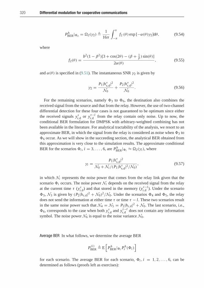
320 Differential modulation for cooperative communications
PhBER|�2 = �2(γ2) � 1
16π
∫ π
−πf2 (θ) exp [−α(θ)γ2]dθ, (9.54)
where
f2(θ) =b2(1− β2)[3+ cos(2θ)− (β + 1
β) sin(θ)]
2α(θ), (9.55)
and α(θ) is specified in (9.51). The instantaneous SNR γ2 is given by
γ2 =P1|hτs,d|2
N0+ P2|hτr,d|2
N0. (9.56)
For the remaining scenarios, namely �3 to �6, the destination also combines thereceived signal from the source and that from the relay. However, the use of two-channeldifferential detection for these four cases is not guaranteed to be optimum since eitherthe received signals yτr,d or yτ−l
r,d from the relay contain only noise. Up to now, theconditional BER formulation for DMPSK with arbitrary-weighted combining has notbeen available in the literature. For analytical tractability of the analysis, we resort to anapproximate BER, in which the signal from the relay is considered as noise when�3 to�6 occur. As we will show in the succeeding section, the analytical BER obtained fromthis approximation is very close to the simulation results. The approximate conditionalBER for the scenarios �i , i = 3, . . . , 6, are Ph
BER|�i ≈ �2(γi ), where
γi =P1|hτs,d|2
N0 +Ni/(P1|hτs,d|2/N0), (9.57)
in which Ni represents the noise power that comes from the relay link given that thescenario �i occurs. The noise power Ni depends on the received signal from the relayat the current time τ (yτr,d) and that stored in the memory (yτ−l
r,d ). Under the scenario
�3, N3 is given by (P2|hr,d|2 + N0)2/N0. Under the scenarios �4 and �5, the relay
does not send the information at either time τ or time τ − l. These two scenarios resultin the same noise power such that N4 = N5 = P2|hr,d|2 +N0. The last scenario, i.e.,�6, corresponds to the case when both yτr,d and yτ−l
r,d does not contain any informationsymbol. The noise power N6 is equal to the noise variance N0.
Average BER In what follows, we determine the average BER
P(i)BER � E[
PhBER|�i Ph
r (�i )]
for each scenario. The average BER for each scenario, �i , i = 1, 2, . . . , 6, can bedetermined as follows (proofs left as exercises):
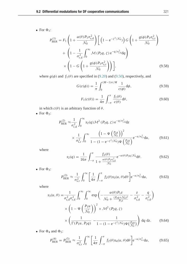
9.2 Differential modulations for DF cooperative communications 321
• For �1:
P(1)BER = F1
(1+ α(θ)P1σ
2s,d
N0
)[(1− e−ζ 2/N0)
)G
(1+ g(φ)P1σ
2s,r
N0
)
+(
1− 1
σ 2r,d
∫ ∞
0M (P2q, ζ ) e−q/σ 2
r,ddq
)
×(
1− G
(1+ g(φ)P1σ
2s,r
N0
))], (9.58)
where g(φ) and f1(θ) are specified in (9.20) and (9.50), respectively, and
G(c(φ)) = 1
π
∫ (M−1)π/M
0
1
c(φ)dφ, (9.59)
F1(c(θ)) = 1
4π
∫ π
−πf1(θ)
c(θ)dθ, (9.60)
in which c(θ) is an arbitrary function of θ .• For �2:
P(2)BER ≈1
σ 2r,d
∫ ∞
0s2(q)M2 (P2q, ζ ) e−q/σ 2
r,ddz
× 1
σ 2s,r
∫ ∞
0
(1−�
(P1uN0
))2
1− (1− e−ζ 2/N0)�(
P1uN0
)e−u/σ 2s,rdu, (9.61)
where
s2(q) = 1
16π
∫ π
−πf2(θ)
1+ α(θ)P1σ2s,d
N0
e−α(θ)P2q/N0dθ. (9.62)
• For �3:
P(3)BER ≈1
σ 2s,r
∫ ∞
0
[1
4π
∫ π
−πf2(θ)s3(u, θ)dθ
]e−u/σ 2
s,rdu, (9.63)
where
s3(u, θ) = 1
σ 2s,dσ
2r,d
∫ ∞
0
∫ ∞
0exp
(− α(θ)P1z
N0 + (P2q+N0)2
P1z
− z
σ 2s,d
− q
σ 2r,d
)
×(
1−�(
P1u
N0
))2
×M2 (P2q, ζ )
×(
1
�(P1u, P2q)− 1
1− (1− e−ζ 2/N0)�( P1uN0
)) dq dz. (9.64)
• For �4 and �5:
P(4)BER = P(5)BER ≈1
σ 2s,r
∫ ∞
0
[1
4π
∫ π
−πf2(θ)s4(u, θ)dθ
]e−u/σ 2
s,rdu, (9.65)
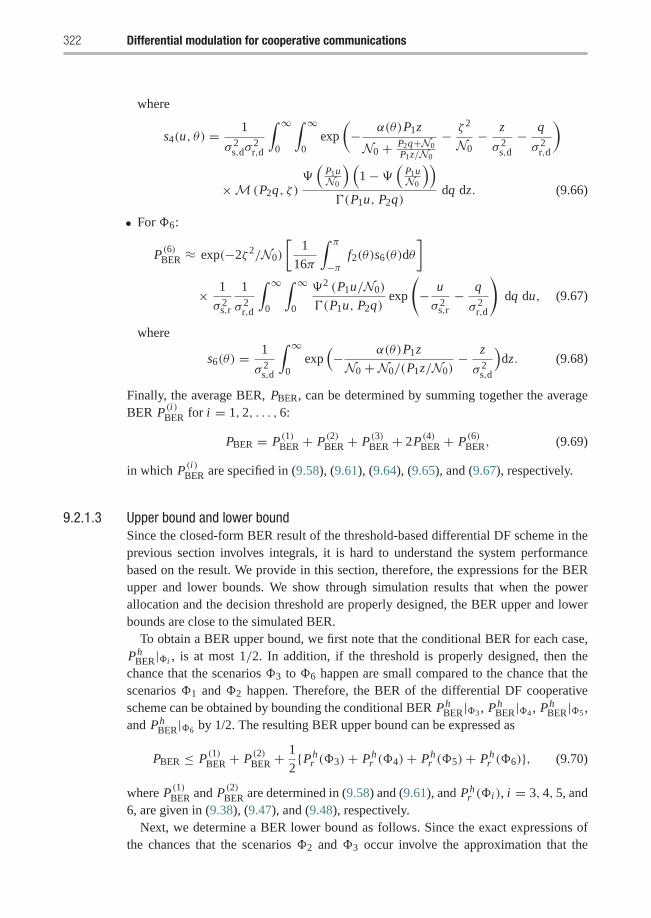
322 Differential modulation for cooperative communications
where
s4(u, θ) = 1
σ 2s,dσ
2r,d
∫ ∞
0
∫ ∞
0exp
(− α(θ)P1z
N0 + P2q+N0P1z/N0
− ζ 2
N0− z
σ 2s,d
− q
σ 2r,d
)
×M (P2q, ζ )�(
P1uN0
) (1−�
(P1uN0
))�(P1u, P2q)
dq dz. (9.66)
• For �6:
P(6)BER ≈ exp(−2ζ 2/N0)
[1
16π
∫ π
−πf2(θ)s6(θ)dθ
]× 1
σ 2s,r
1
σ 2r,d
∫ ∞
0
∫ ∞
0
�2 (P1u/N0)
�(P1u, P2q)exp
(− u
σ 2s,r− q
σ 2r,d
)dq du, (9.67)
where
s6(θ) = 1
σ 2s,d
∫ ∞
0exp(− α(θ)P1z
N0 +N0/(P1z/N0)− z
σ 2s,d
)dz. (9.68)
Finally, the average BER, PBER, can be determined by summing together the averageBER P(i)BER for i = 1, 2, . . . , 6:
PBER = P(1)BER + P(2)BER + P(3)BER + 2P(4)BER + P(6)BER, (9.69)
in which P(i)BER are specified in (9.58), (9.61), (9.64), (9.65), and (9.67), respectively.
9.2.1.3 Upper bound and lower boundSince the closed-form BER result of the threshold-based differential DF scheme in theprevious section involves integrals, it is hard to understand the system performancebased on the result. We provide in this section, therefore, the expressions for the BERupper and lower bounds. We show through simulation results that when the powerallocation and the decision threshold are properly designed, the BER upper and lowerbounds are close to the simulated BER.
To obtain a BER upper bound, we first note that the conditional BER for each case,Ph
BER|�i , is at most 1/2. In addition, if the threshold is properly designed, then thechance that the scenarios �3 to �6 happen are small compared to the chance that thescenarios �1 and �2 happen. Therefore, the BER of the differential DF cooperativescheme can be obtained by bounding the conditional BER Ph
BER|�3 , PhBER|�4 , Ph
BER|�5 ,and Ph
BER|�6 by 1/2. The resulting BER upper bound can be expressed as
PBER ≤ P(1)BER + P(2)BER +1
2{Ph
r (�3)+ Phr (�4)+ Ph
r (�5)+ Phr (�6)}, (9.70)
where P(1)BER and P(2)BER are determined in (9.58) and (9.61), and Phr (�i ), i = 3, 4, 5, and
6, are given in (9.38), (9.47), and (9.48), respectively.Next, we determine a BER lower bound as follows. Since the exact expressions of
the chances that the scenarios �2 and �3 occur involve the approximation that the
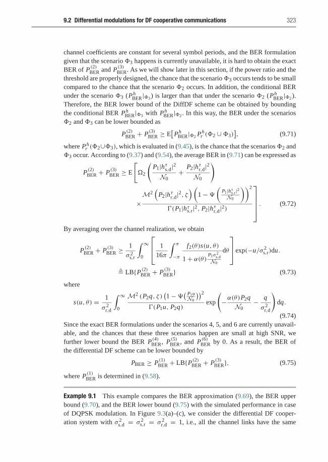
9.2 Differential modulations for DF cooperative communications 323
channel coefficients are constant for several symbol periods, and the BER formulationgiven that the scenario�3 happens is currently unavailable, it is hard to obtain the exactBER of P(2)BER and P(3)BER. As we will show later in this section, if the power ratio and thethreshold are properly designed, the chance that the scenario�3 occurs tends to be smallcompared to the chance that the scenario �2 occurs. In addition, the conditional BERunder the scenario �3 (Ph
BER|�3 ) is larger than that under the scenario �2 (PhBER|�2 ).
Therefore, the BER lower bound of the DiffDF scheme can be obtained by boundingthe conditional BER Ph
BER|�3 with PhBER|�2 . In this way, the BER under the scenarios
�2 and �3 can be lower bounded as
P(2)BER + P(3)BER ≥ E[Ph
BER|�2 Phr (�2 ∪�3)
], (9.71)
where Phr (�2∪�3), which is evaluated in (9.45), is the chance that the scenarios�2 and
�3 occur. According to (9.37) and (9.54), the average BER in (9.71) can be expressed as
P(2)BER + P(3)BER ≥ E
[�2
(P1|hτs,d|2
N0+ P2|hτr,d|2
N0
)
×M2
(P2|hτr,d|2, ζ
)(1−�
(P1|hτs,r|2N0
))2
�(P1|hτs,r|2, P2|hτr,d|2)
⎤⎥⎥⎥⎦ . (9.72)
By averaging over the channel realization, we obtain
P(2)BER + P(3)BER ≥1
σ 2s,r
∫ ∞
0
⎡⎢⎣ 1
16π
∫ π
−πf2(θ)s(u, θ)
1+ α(θ) P1σ2s,d
N0
dθ
⎤⎥⎦ exp(−u/σ 2s,r)du.
� LB{P(2)BER + P(3)BER} (9.73)
where
s(u, θ) = 1
σ 2r,d
∫ ∞
0
M2 (P2q, ζ )(1−�( P1u
N0
))2�(P1u, P2q)
exp
(−α(θ)P2q
N0− q
σ 2r,d
)dq.
(9.74)Since the exact BER formulations under the scenarios 4, 5, and 6 are currently unavail-able, and the chances that these three scenarios happen are small at high SNR, wefurther lower bound the BER P(4)BER, P(5)BER, and P(6)BER by 0. As a result, the BER ofthe differential DF scheme can be lower bounded by
PBER ≥ P(1)BER + LB{P(2)BER + P(3)BER}, (9.75)
where P(1)BER is determined in (9.58).
Example 9.1 This example compares the BER approximation (9.69), the BER upperbound (9.70), and the BER lower bound (9.75) with the simulated performance in caseof DQPSK modulation. In Figure 9.3(a)–(c), we consider the differential DF cooper-ation system with σ 2
s,d = σ 2s,r = σ 2
r,d = 1, i.e., all the channel links have the same
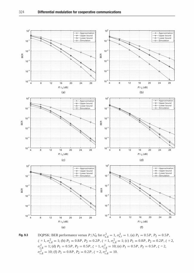
324 Differential modulation for cooperative communications
4 8 12 16 20 24 2810–5
10–4
10–3
10–2
10–1
100
(a)
(c)
(e)
(b)
(d)
(f)
BE
R
4 8 12 16 20 24 2810–5
10–4
10–3
10–2
10–1
100
BE
R
4 8 12 16 20 24 2810–5
10–4
10–3
10–2
10–1
100
BE
R
4 8 12 16 20 24 2810–5
10–4
10–3
10–2
10–1
100
BE
R
4 8 12 16 20 24 2810–5
10–4
10–3
10–2
10–1
100
BE
R
4 8 12 16 20 24 2810–5
10–4
10–3
10–2
10–1
100
BE
R
ApproximationUpper boundLower boundSimulation
ApproximationUpper boundLower boundSimulation
ApproximationUpper boundLower boundSimulation
ApproximationUpper boundLower boundSimulation
ApproximationUpper boundLower boundSimulation
ApproximationUpper boundLower boundSimulation
P/�0 [dB]P/�0 [dB]
P/�0 [dB]P/�0 [dB]
P/�0 [dB]P/�0 [dB]
Fig. 9.3 DQPSK: BER performance versus P/N0 for σ 2s,d = 1, σ 2
s,r = 1. (a) P1 = 0.5P , P2 = 0.5P ,
ζ = 1, σ 2r,d = 1; (b) P1 = 0.8P , P2 = 0.2P , ζ = 1, σ 2
r,d = 1; (c) P1 = 0.8P , P2 = 0.2P , ζ = 2,
σ 2r,d = 1; (d) P1 = 0.5P , P2 = 0.5P , ζ = 1, σ 2
r,d = 10; (e) P1 = 0.5P , P2 = 0.5P , ζ = 2,
σ 2r,d = 10; (f) P1 = 0.8P , P2 = 0.2P , ζ = 2, σ 2
r,d = 10.
9.2 Differential modulations for DF cooperative communications 325
qualities. From the figures, we can see that the approximated BER closely matches thesimulated BER, and both the approximated and simulated BER lie between the BERupper and lower bounds. Moreover, the system performance depends on the power allo-cation and the threshold. By choosing proper power allocation and threshold, not onlythe BER performance improves, but also the lower bound is closer to the simulatedperformance.
For example, considering a system with threshold of ζ = 1 and total transmit powerP1+ P2= P where P1 and P2 are transmitted power of the source and the relay, respec-tively. By changing the power allocation from P1/P = 0.5 to P1/P = 0.8 the BERperformance is improved by 1 dB at a BER of 10−4, while the performance gap betweenthe simulated BER and the BER lower bound is reduced by 2 dB at the same BER.
This result follows the fact that when the threshold ζ is appropriately chosen, thescenarios �3 to �6 occur with much smaller probability than the scenarios �1 and �2.Even though the BER under each of the scenarios �3 to �6 is larger than that underthe scenarios �1 or �2, the average BER P(i)BER, i = 3, . . . , 6 are smaller. The BERPBER is dominated by the BER under scenarios�1 and�2. Therefore, the performancegaps between the bounds and the approximate BER is small if the threshold is properlydesigned.
For a system with σ 2s,d = 1, σ 2
s,r = 1, and σ 2r,d = 10, the same observation can
be obtained in Figure 9.3(d)–(f). At a threshold of ζ = 1, the performance can beimproved by allocating more power at the source and less power at the relay. It illustratesthat the channel link between source and relay and the channel link between relay anddestination should be balanced in order to achieve a performance diversity of two.
Interestingly, by choosing a proper threshold, the performance can be significantlyimproved, regardless of the power allocation. For instance, increasing the threshold from1 to 2, the performance of the DiffDF scheme with equal power allocation improves4 dB at a BER of 10−4. At the threshold of ζ = 2, by changing the power allocationfrom P1/P = 0.5 to P1/P = 0.8, the system performance is further improved by only0.5 dB at the same BER. This implies that the effect of the threshold dominates; theperformance does not severely depend on the power allocation after the threshold isproperly designed.
Another observation obtained from Figure 9.3 is that the threshold depends on thechannel link qualities. To be specific, the threshold should be increased as the link qual-ity between the relay and the destination increases. For example, under the scenarioσ 2
s,d = σ 2s,r = 1, the threshold ζ = 1 results in superior performance in case of σ 2
r,d = 1,
while the threshold ζ = 2 leads to better performance in case of σ 2r,d = 10. This obser-
vation can be explained as follows. When the link quality between the relay and thedestination is good, i.e., the channel variance is high, the received signal from the relaytends to have large energy if it carries the information. As a result, by increasing thethreshold from 1 to 2, we reduce the chance that the received signal whose amplitudeis larger than the threshold contains no information. Thus, with a threshold of 2, thereceived signals from the relay and the destination are efficiently combined, and henceresult in better performance. �
326 Differential modulation for cooperative communications
9.2.1.4 Optimum decision threshold and power allocationAs we observe in the above examples in the previous section, the choice of powerallocation and threshold ζ affect the performance a lot; we determine in this sectionthe optimum decision threshold and the optimum power allocation for the differentialDF cooperation system based on the tight BER approximation in (9.69). To sim-plify the notation, let us denote r = P1/P as the power ratio of the transmittedpower at the source (P1) over the total power (P). For a fixed total transmitted powerP1 + P2 = P , we will jointly optimize the threshold ζ and the power ratio r such thatthe tight BER approximation in (9.69) is minimized. The optimization problem can beformulated as
minζ,r
PBER(ζ, r), (9.76)
where PBER(ζ, r) represents the BER approximation with P1 = r P and P2 = (1−r)P .Figure 9.4 shows the BER performance of the DiffDF scheme with DQPSK signals
as a function of power allocation and threshold. In Figure 9.4(a)–(c), we consider thecase when the channel variances of all communication links are equal, i.e., σ 2
s,d = σ 2s,r =
σ 2r,d = 1. The BER approximation is plotted in Figure 9.4(a) and its cross sections are
shown in Figure 9.4(b) and (c) together with the simulated BER curves. Based on theapproximated BER in Figure 9.4(a), the jointly optimum power allocation and decisionthreshold are r = 0.7 and ζ = 1. Figure 9.4(b) compares the cross sectional curveof the approximated BER with r = 0.7 with the simulated BER. We can see that theapproximate BER is close to the simulated BER.
Furthermore, the DiffDF scheme with any threshold less than 1.5 yields almost thesame BER performance, and the performance significantly degrades as the thresh-old increases above 1.5. This is because as the threshold increases, the chances thatthe scenarios �4 to �6 occur increases, and hence the average BER is dominatedby the BER under these scenarios. Figure 9.4(c) depicts the approximated and simu-lated BER curves as functions of power allocation in case of the decision thresholdζ = 1. We can obviously see that the power ratio of r = 0.7 results in the optimumperformance.
In Figure 9.4(d)–(f), we consider the case of channel variances σ 2s,d = 1, σ 2
s,r = 1,
σ 2r,d = 10. Figure 9.4(d) depicts the BER of the DiffDF scheme as a function of the
power allocation r and the decision threshold ζ . In this scenario, we can see that thejointly optimum power allocation and decision threshold are r = 0.8 and ζ = 1.7.Figure 9.4(e) shows a cross-sectional curve of the approximate BER in Figure 9.4(d)at r = 0.8 together with the simulated BER performance of the cooperation sys-tem with the same power allocation. We can see that the approximated BER closelymatches to the simulated BER for every threshold value. According to both the simu-lated and approximated BER, the optimum threshold for this case is about 1.7. We showin Figure 9.4(f) a comparison of the approximated and simulated BER with a decisionthreshold ζ = 1.7 under different power allocations. Clearly, the approximated BERfollows the same trend as the simulated BER, and the optimum power allocation isr = 0.8 for the differential DF system with a decision threshold ζ = 1.7.
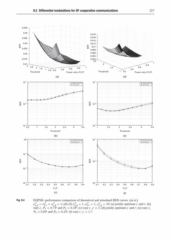
9.2 Differential modulations for DF cooperative communications 327
0.2 0.4 0.6 0.8 10.511.522.53
0.01
0.015
0.02
0.025
0.03
0.035
0.04
0.045
Power ratio (P1/P)
(a)
(b)
(c)
(d)
(e)
(f)
Threshold Power ratio (P1/P)Threshold
BE
R
0.5 1 1.5 2 2.5 3 3.510−3
10−2
10−1
10−3
10−2
100
10−1
Threshold
BE
RB
ER
1 1.5 2 2.5 3 3.510−3
10−2
10−1
Threshold
BE
R
10−3
10−2
10−1
BE
R
ApproximationSimulation
0.1 0.2 0.3 0.4 0.5 0.6 0.7 0.8 0.9
P1/P
0.1 0.2 0.3 0.4 0.5 0.6 0.7 0.8 0.9
P1/P
ApproximationSimulation
0.20.4
0.60.8
1
1
1.5
22.5
0.0020.0040.0060.008
0.010.0120.0140.0160.018
BE
R
ApproximationSimulation
ApproximationSimulation
Fig. 9.4 DQPSK: performance comparison of theoretical and simulated BER curves. (a)–(c)σ 2
s,d = σ 2s,r = σ 2
r,d = 1; (d)–(f) σ 2s,d = 1, σ 2
s,r = 1, σ 2r,d = 10: (a) jointly optimum ζ and r ; (b)
vary ζ , P1 = 0.7P and P2 = 0.3P; (c) vary r , ζ = 1; (d) jointly optimum ζ and r ; (e) vary ζ ,P1 = 0.8P and P2 = 0.2P; (f) vary r , ζ = 1.7.
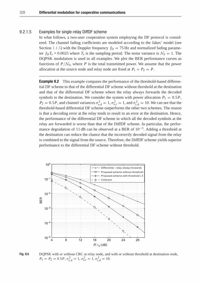
328 Differential modulation for cooperative communications
9.2.1.5 Examples for single-relay DiffDF schemeIn what follows, a two-user cooperation system employing the DF protocol is consid-ered. The channel fading coefficients are modeled according to the Jakes’ model (seeSection 1.1.5) with the Doppler frequency fD = 75 Hz and normalized fading parame-ter fDTs = 0.0025 where Ts is the sampling period. The noise variance is N0 = 1. TheDQPSK modulation is used in all examples. We plot the BER performance curves asfunctions of P/N0, where P is the total transmitted power. We assume that the powerallocation at the source node and relay node are fixed at P1 + P2 = P .
Example 9.2 This example compares the performance of the threshold-based differen-tial DF scheme to that of the differential DF scheme without threshold at the destinationand that of the differential DF scheme where the relay always forwards the decodedsymbols to the destination. We consider the system with power allocation P1 = 0.5P ,P2 = 0.5P , and channel variances σ 2
s,d = 1, σ 2s,r = 1, and σ 2
r,d = 10. We can see that thethreshold-based differential DF scheme outperforms the other two schemes. The reasonis that a decoding error at the relay tends to result in an error at the destination. Hence,the performance of the differential DF scheme in which all the decoded symbols at therelay are forwarded is worse than that of the DiffDF scheme. In particular, the perfor-mance degradation of 11 dB can be observed at a BER of 10−3. Adding a threshold atthe destination can reduce the chance that the incorrectly decoded signal from the relayis combined to the signal from the source. Therefore, the DiffDF scheme yields superiorperformance to the differential DF scheme without threshold.
4 8 12 16 20 24 2810–5
10–4
10–3
10–2
10–1
100
BE
R
Differential : relay always forwards
Proposed scheme without threshold
Proposed scheme with threshold = 2
Coherent
P/�0 [dB]
Fig. 9.5 DQPSK with or without CRC at relay node, and with or without threshold at destination node,P1 = P2 = 0.5P , σ 2
s,d = 1, σ 2s,r = 1, σ 2
r,d = 10.
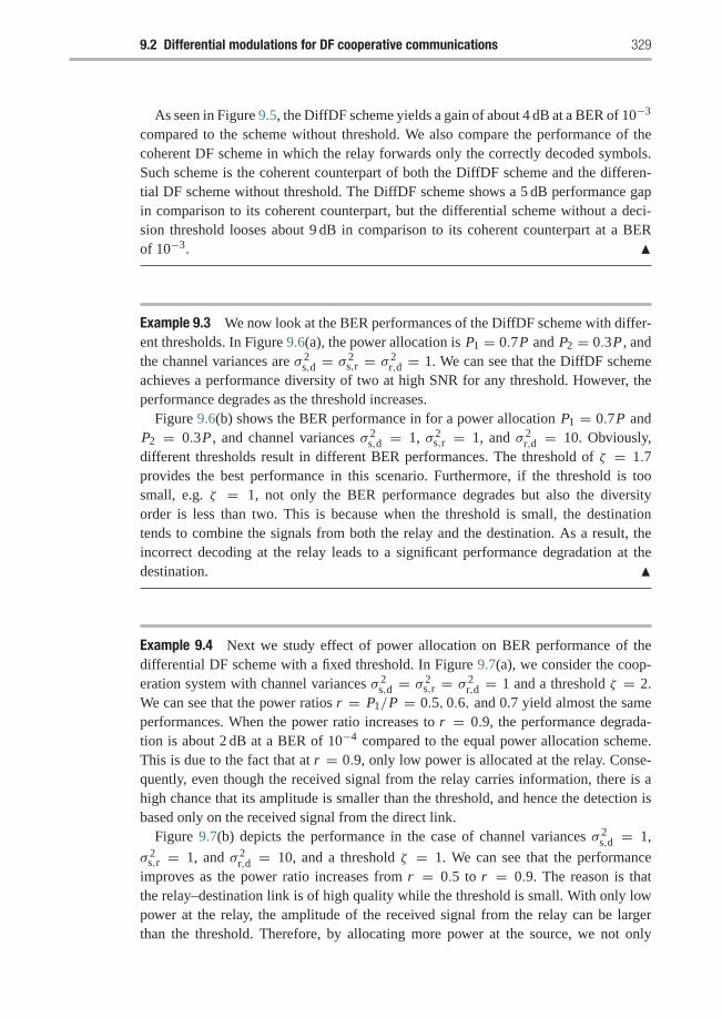
9.2 Differential modulations for DF cooperative communications 329
As seen in Figure 9.5, the DiffDF scheme yields a gain of about 4 dB at a BER of 10−3
compared to the scheme without threshold. We also compare the performance of thecoherent DF scheme in which the relay forwards only the correctly decoded symbols.Such scheme is the coherent counterpart of both the DiffDF scheme and the differen-tial DF scheme without threshold. The DiffDF scheme shows a 5 dB performance gapin comparison to its coherent counterpart, but the differential scheme without a deci-sion threshold looses about 9 dB in comparison to its coherent counterpart at a BERof 10−3. �
Example 9.3 We now look at the BER performances of the DiffDF scheme with differ-ent thresholds. In Figure 9.6(a), the power allocation is P1 = 0.7P and P2 = 0.3P , andthe channel variances are σ 2
s,d = σ 2s,r = σ 2
r,d = 1. We can see that the DiffDF schemeachieves a performance diversity of two at high SNR for any threshold. However, theperformance degrades as the threshold increases.
Figure 9.6(b) shows the BER performance in for a power allocation P1 = 0.7P andP2 = 0.3P , and channel variances σ 2
s,d = 1, σ 2s,r = 1, and σ 2
r,d = 10. Obviously,different thresholds result in different BER performances. The threshold of ζ = 1.7provides the best performance in this scenario. Furthermore, if the threshold is toosmall, e.g. ζ = 1, not only the BER performance degrades but also the diversityorder is less than two. This is because when the threshold is small, the destinationtends to combine the signals from both the relay and the destination. As a result, theincorrect decoding at the relay leads to a significant performance degradation at thedestination. �
Example 9.4 Next we study effect of power allocation on BER performance of thedifferential DF scheme with a fixed threshold. In Figure 9.7(a), we consider the coop-eration system with channel variances σ 2
s,d = σ 2s,r = σ 2
r,d = 1 and a threshold ζ = 2.We can see that the power ratios r = P1/P = 0.5, 0.6, and 0.7 yield almost the sameperformances. When the power ratio increases to r = 0.9, the performance degrada-tion is about 2 dB at a BER of 10−4 compared to the equal power allocation scheme.This is due to the fact that at r = 0.9, only low power is allocated at the relay. Conse-quently, even though the received signal from the relay carries information, there is ahigh chance that its amplitude is smaller than the threshold, and hence the detection isbased only on the received signal from the direct link.
Figure 9.7(b) depicts the performance in the case of channel variances σ 2s,d = 1,
σ 2s,r = 1, and σ 2
r,d = 10, and a threshold ζ = 1. We can see that the performanceimproves as the power ratio increases from r = 0.5 to r = 0.9. The reason is thatthe relay–destination link is of high quality while the threshold is small. With only lowpower at the relay, the amplitude of the received signal from the relay can be largerthan the threshold. Therefore, by allocating more power at the source, we not only
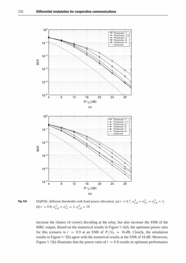
330 Differential modulation for cooperative communications
BE
RTheshold = 1Theshold = 1.5Theshold = 2Theshold = 3Theshold = 5Coherent
10–5
10–4
10–3
10–2
10–1
100
(a)
4 8 12 16 20 24 28
(b)
BE
R
10–5
10–4
10–3
10–2
10–1
100
4 8 12 16 20 24 28
Theshold = 1Theshold = 1.7Theshold = 3Theshold = 5
Theshold = 9Theshold = 7
Coherent
P/�0 [dB]
P/�0 [dB]
Fig. 9.6 DQPSK: different thresholds with fixed power allocation. (a) r = 0.7, σ 2s,d = σ 2
s,r = σ 2r,d = 1;
(b) r = 0.8, σ 2s,d = σ 2
s,r = 1, σ 2r,d = 10.
increase the chance of correct decoding at the relay, but also increase the SNR of theMRC output. Based on the numerical results in Figure 9.4(d), the optimum power ratiofor this scenario is r = 0.9 at an SNR of P/N0 = 16 dB. Clearly, the simulationresults in Figure 9.7(b) agree with the numerical results at the SNR of 16 dB. Moreover,Figure 9.7(b) illustrates that the power ratio of r = 0.9 results in optimum performance
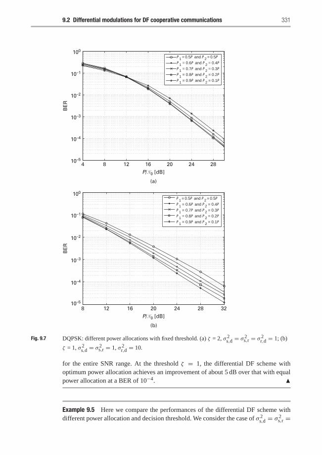
9.2 Differential modulations for DF cooperative communications 331
P1 = 0.5P and P2 = 0.5P
P1 = 0.6P and P2 = 0.4P
P1 = 0.7P and P2 = 0.3P
P1 = 0.8P and P2 = 0.2P
P1 = 0.9P and P2 = 0.1P
BE
R
10–5
10–4
10–3
10–2
10–1
100
(a)
4 8 12 16 20 24 28
P1 = 0.5P and P2 = 0.5P
P1 = 0.6P and P2 = 0.4P
P1 = 0.7P and P2 = 0.3P
P1 = 0.8P and P2 = 0.2P
P1 = 0.9P and P2 = 0.1P
BE
R
10–5
10–4
10–3
10–2
10–1
100
(b)
8 12 16 20 24 28 32
P/�0 [dB]
P/�0 [dB]
Fig. 9.7 DQPSK: different power allocations with fixed threshold. (a) ζ = 2, σ 2s,d = σ 2
s,r = σ 2r,d = 1; (b)
ζ = 1, σ 2s,d = σ 2
s,r = 1, σ 2r,d = 10.
for the entire SNR range. At the threshold ζ = 1, the differential DF scheme withoptimum power allocation achieves an improvement of about 5 dB over that with equalpower allocation at a BER of 10−4. �
Example 9.5 Here we compare the performances of the differential DF scheme withdifferent power allocation and decision threshold. We consider the case of σ 2
s,d = σ 2s,r =
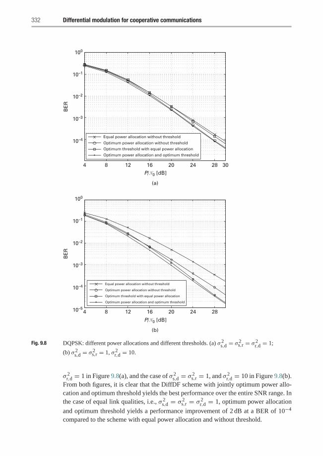
332 Differential modulation for cooperative communications
4 8 12 16 20 24 28 30
Equal power allocation without threshold
Optimum power allocation without threshold
Optimum threshold with equal power allocation
Optimum power allocation and optimum threshold
Equal power allocation without threshold
Optimum power allocation without threshold
Optimum threshold with equal power allocation
Optimum power allocation and optimum threshold
BE
R
10–4
10–3
10–2
10–1
100
(a)
BE
R
10–5
10–4
10–3
10–2
10–1
100
4 8 12 16 20 24 28
P/�0 [dB]
(b)
P/�0 [dB]
Fig. 9.8 DQPSK: different power allocations and different thresholds. (a) σ 2s,d = σ 2
s,r = σ 2r,d = 1;
(b) σ 2s,d = σ 2
s,r = 1, σ 2r,d = 10.
σ 2r,d = 1 in Figure 9.8(a), and the case of σ 2
s,d = σ 2s,r = 1, and σ 2
r,d = 10 in Figure 9.8(b).From both figures, it is clear that the DiffDF scheme with jointly optimum power allo-cation and optimum threshold yields the best performance over the entire SNR range. Inthe case of equal link qualities, i.e., σ 2
s,d = σ 2s,r = σ 2
r,d = 1, optimum power allocation
and optimum threshold yields a performance improvement of 2 dB at a BER of 10−4
compared to the scheme with equal power allocation and without threshold.
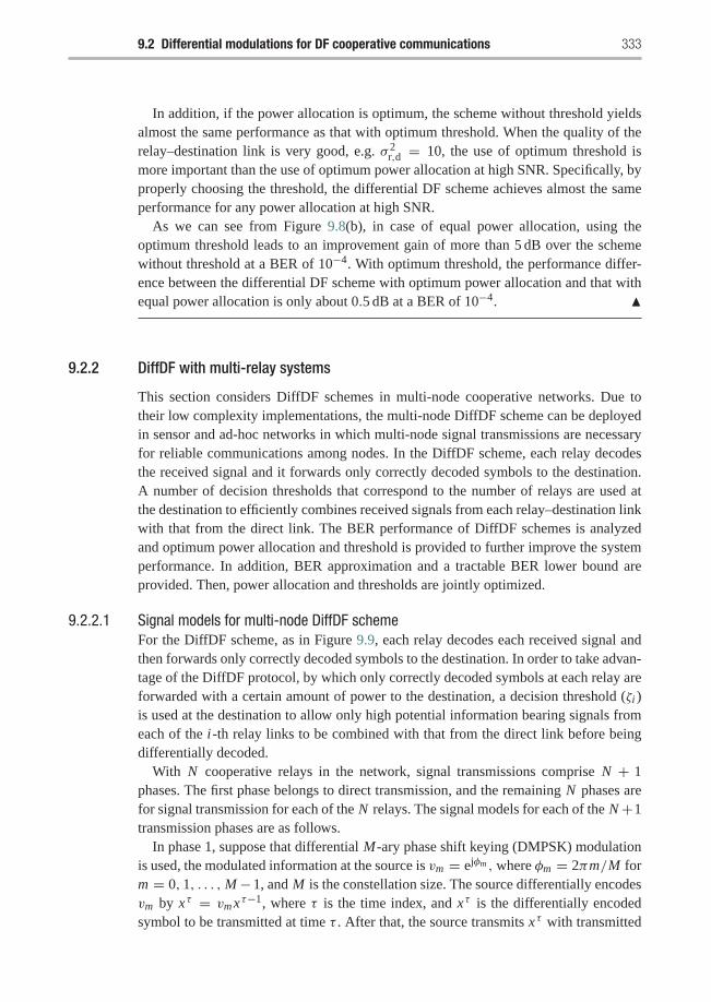
9.2 Differential modulations for DF cooperative communications 333
In addition, if the power allocation is optimum, the scheme without threshold yieldsalmost the same performance as that with optimum threshold. When the quality of therelay–destination link is very good, e.g. σ 2
r,d = 10, the use of optimum threshold ismore important than the use of optimum power allocation at high SNR. Specifically, byproperly choosing the threshold, the differential DF scheme achieves almost the sameperformance for any power allocation at high SNR.
As we can see from Figure 9.8(b), in case of equal power allocation, using theoptimum threshold leads to an improvement gain of more than 5 dB over the schemewithout threshold at a BER of 10−4. With optimum threshold, the performance differ-ence between the differential DF scheme with optimum power allocation and that withequal power allocation is only about 0.5 dB at a BER of 10−4. �
9.2.2 DiffDF with multi-relay systems
This section considers DiffDF schemes in multi-node cooperative networks. Due totheir low complexity implementations, the multi-node DiffDF scheme can be deployedin sensor and ad-hoc networks in which multi-node signal transmissions are necessaryfor reliable communications among nodes. In the DiffDF scheme, each relay decodesthe received signal and it forwards only correctly decoded symbols to the destination.A number of decision thresholds that correspond to the number of relays are used atthe destination to efficiently combines received signals from each relay–destination linkwith that from the direct link. The BER performance of DiffDF schemes is analyzedand optimum power allocation and threshold is provided to further improve the systemperformance. In addition, BER approximation and a tractable BER lower bound areprovided. Then, power allocation and thresholds are jointly optimized.
9.2.2.1 Signal models for multi-node DiffDF schemeFor the DiffDF scheme, as in Figure 9.9, each relay decodes each received signal andthen forwards only correctly decoded symbols to the destination. In order to take advan-tage of the DiffDF protocol, by which only correctly decoded symbols at each relay areforwarded with a certain amount of power to the destination, a decision threshold (ζi )is used at the destination to allow only high potential information bearing signals fromeach of the i-th relay links to be combined with that from the direct link before beingdifferentially decoded.
With N cooperative relays in the network, signal transmissions comprise N + 1phases. The first phase belongs to direct transmission, and the remaining N phases arefor signal transmission for each of the N relays. The signal models for each of the N+1transmission phases are as follows.
In phase 1, suppose that differential M-ary phase shift keying (DMPSK) modulationis used, the modulated information at the source is vm = ejφm , where φm = 2πm/M form = 0, 1, . . . ,M−1, and M is the constellation size. The source differentially encodesvm by xτ = vmxτ−1, where τ is the time index, and xτ is the differentially encodedsymbol to be transmitted at time τ . After that, the source transmits xτ with transmitted
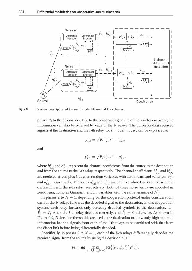
334 Differential modulation for cooperative communications
Discard
Discard
Source
Relay N
Ps
DifferentialDecoder
DifferentialEncoder
Correct ?
YesNoSTOP
1NM
?
Yes
No 2NM
L-channeldifferentialdetectionRelay 1
P1Differential
DecoderDifferential
Encoder
~
Correct ?
YesNoSTOP
11M
Yes
No12M
.
.
.
.
.
.
.
.
.
.
.
.
hs,dτ
r1,dh
τ
P1~
hrN,dτ
hs,r1
τ
hs,rN
τ
Destination
yr1,dτ
yrN,dτ
> ζ1
> ζN
?
Fig. 9.9 System description of the multi-node differential DF scheme.
power Ps to the destination. Due to the broadcasting nature of the wireless network, theinformation can also be received by each of the N relays. The corresponding receivedsignals at the destination and the i-th relay, for i = 1, 2, . . . , N , can be expressed as
yτs,d =√
Pshτs,dxτ + ητs,d,
and
yτs,ri =√
Pshτs,ri x
τ + ητs,ri .
where hτs,d and hτs,ri represent the channel coefficients from the source to the destinationand from the source to the i-th relay, respectively. The channel coefficients hτs,d and hτs,riare modeled as complex Gaussian random variables with zero means and variances σ 2
s,d
and σ 2s,ri , respectively. The terms ητs,d and ητs,ri are additive white Gaussian noise at the
destination and the i-th relay, respectively. Both of these noise terms are modeled aszero-mean, complex Gaussian random variables with the same variance of N0.
In phases 2 to N + 1, depending on the cooperation protocol under consideration,each of the N relays forwards the decoded signal to the destination. In this cooperationsystem, each relay forwards only correctly decoded symbols to the destination, i.e.,Pi = Pi when the i-th relay decodes correctly, and Pi = 0 otherwise. As shown inFigure 9.9, N decision thresholds are used at the destination to allow only high potentialinformation bearing signals from each of the i-th relays to be combined with that fromthe direct link before being differentially decoded.
Specifically, in phases 2 to N + 1, each of the i-th relays differentially decodes thereceived signal from the source by using the decision rule:
m = arg maxm=0,1,...,M−1
Re{(vm yτ−1
s,ri
)∗yτs,ri}.
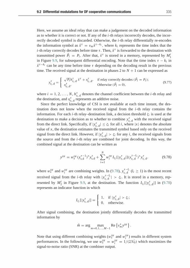
9.2 Differential modulations for DF cooperative communications 335
Here, we assume an ideal relay that can make a judgement on the decoded informationas to whether it is correct or not. If any of the i-th relays incorrectly decodes, the incor-rectly decoded symbol is discarded. Otherwise, the i-th relay differentially re-encodesthe information symbol as xτ = vm xτ−ki , where ki represents the time index that thei-th relay correctly decodes before time τ . Then, xτ is forwarded to the destination withtransmitted power Pi = Pi . After that, xτ is stored in a memory, represented by Mi
1in Figure 9.9, for subsequent differential encoding. Note that the time index τ − ki inxτ−ki can be any time before time τ depending on the decoding result in the previoustime. The received signal at the destination in phases 2 to N + 1 can be expressed as
yτri ,d ={ √
Pi hτri ,d
xτ + ητri ,d, if relay correctly decodes (Pi = Pi );ητri ,d
, Otherwise (Pi = 0),(9.77)
where i = 1, 2, . . . , N , hτri ,d denotes the channel coefficient between the i-th relay andthe destination, and ητri ,d represents an additive noise.
Since the perfect knowledge of CSI is not available at each time instant, the des-tination does not know when the received signal from the i-th relay contains theinformation. For each i-th relay–destination link, a decision threshold ζi is used at thedestination to make a decision as to whether to combine yτri ,d with the received signalfrom the direct link. Specifically, if |yτri ,d| ≤ ζi for all i , where |x | denotes the absolutevalue of x , the destination estimates the transmitted symbol based only on the receivedsignal from the direct link. However, if |yτri ,d| > ζi for any i , the received signals fromthe source and from the i-th relay are combined for joint decoding. In this way, thecombined signal at the destination can be written as
yDF = wDFs (y
τ−1s,d )
∗yτs,d +N∑
i=1
wDFi Iζi [|yτri ,d|](yτ−li
ri ,d)∗yτri ,d. (9.78)
where wDFs and wDF
i are combining weights. In (9.78), yτ−liri ,d
(li ≥ 1) is the most recent
received signal from the i-th relay with |yτ−liri ,d
| > ζi . It is stored in a memory, rep-
resented by Mi2 in Figure 9.9, at the destination. The function Iζi [|yτri ,d|] in (9.78)
represents an indicator function in which
Iζi [|yτri ,d|] ={
1, if |yτri ,d| > ζi ;0, otherwise.
After signal combining, the destination jointly differentially decodes the transmittedinformation by
m = arg maxm=0,1,...,M−1
Re{v∗m yDF
}.
Note that using different combining weights (wDFs and wDF
i ) results in different systemperformances. In the following, we use wDF
s = wDFi = 1/(2N0) which maximizes the
signal-to-noise ratio (SNR) at the combiner output.
336 Differential modulation for cooperative communications
9.2.2.2 BER AnalysisBER analysis of the multi-node DiffDF scheme is considered in this subsection. First,different SNR scenarios are characterized according to the received signal yτri ,d, thresh-
old ζi , and memories Mi1 and Mi
2. Then, the probability of occurrence is provided foreach of these SNR scenarios. After that, the average BER is derived based on the prob-ability of occurrence and the combined SNR for each scenario. Finally, a tractable BERlower bound is provided.
Characterization of different SNR scenariosAt the destination, different combined SNRs may occur based on the received signal(yτri ,d), the threshold (ζi ), and the signals stored in memory Mi
1 and Mi2. In this way, the
destination encounters six possible SNR scenarios at each relay–destination link, andwe characterize each of them as follows. For a given network state j , we denote si
j asan integer number that represents an SNR scenario at the i-th relay–destination link,i.e., si
j ∈ {1, 2, 3, 4, 5, 6}. A set of joint events �isi
jfor i = 1, 2, . . . , N will be related
to each of the scenarios sij . Specifically, when si
j = 1,
�i1 �
{|yτri ,d| ≤ ζi
}represents a joint event that received signals from the i-th relay link are not greater thanthe thresholds. We characterize
�i2 �
{|yτri ,d| > ζi , Pτi = Pi , Pτ−lii = Pi , li = ki
}as a joint event including |yτri ,d| > ζi , the relay correctly decodes at time τ and τ − li ,
and the information symbols at time ki and li in memories Mi1 and Mi
2 are the same.The remaining scenarios are
�i3 �
{|yτri ,d| > ζi , Pτi = Pi , Pτ−lii = Pi , li �= ki
},
�i4 �
{|yτri ,d| > ζi , Pτi = Pi , Pτ−lii = 0
},
�i5 �
{|yτri ,d| > ζi , Pτi = 0, Pτ−lii = Pi
},
�i6 �
{|yτri ,d| > ζi , Pτi = 0, Pτ−lii = 0
}.
They are interpreted in a similar way to �i2.
Probability of occurrence for each SNR scenarioTo determine the probability of occurrence for each scenario, we first find that the prob-ability that the i-th relay forwards information with transmitted power Pi = 0 due toincorrect decoding is related to the symbol error rate of DMPSK modulation as
�(γ DFs,ri ) =
1
π
∫ (M−1)π/M
0exp [−g(φ)γ DF
s,ri ]dφ, (9.79)
where γ DFs,ri = Ps |hτs,ri |2/N0 represents an instantaneous SNR at the i-th relay, and g(φ)
is given by (9.20). Accordingly, the probability of correct decoding at the i-th relay (orprobability of forwarding with transmitted power Pi = Pi ) is 1−�(γ DF
s,ri ). Therefore, the
9.2 Differential modulations for DF cooperative communications 337
chance that �i1 occurs is determined by the weighted sum of conditional probabilities
given that Pi = Pi or 0, so that
Ph,DFr (�i
1) = Ph,DFr
(|yτri ,d| ≤ ζi
∣∣ Pτi = 0)�(γ τs,ri )
+ Ph,DFr
(|yτri ,d| ≤ ζi
∣∣ Pτi = Pi
) [1−�(γ τs,ri )
]=(1− exp(−ζ 2
i /N0))�(γ τs,ri )+
(1−M
(Pi |hτri ,d|2, ζi
)) [1−�(γ τs,ri )
],
(9.80)
where
M(
Pi |hτri ,d|2, ζi)
� Q1(√
Pi |hτri ,d|2/(N0/2), ζi/√N0/2
), (9.81)
in which Q1 (α, β) is the Marcum Q-function [188](proof left as an exercise).According to the definition of each SNR scenario in Section 9.2.2.2, the chance that
each of the scenarios �2 to �6 happens is conditioned on an event that |yτ−liri ,d
| > ζi .
Since the events at time τ − li and time τ are independent, then the probability that �i2
occurs is given by
Ph,DFr (�i
2) = Ph,DFr
(|yτri ,d| > ζi , Pτi = Pi
)Ph,DF
r
(Pτ−li
i = Pi , li = ki
∣∣∣ |yτ−liri ,d
| > ζi).
≈M2
(Pi |hτri ,d|2, ζi
) (1−�(γ τs,ri )
)21− (1− e−ζ 2
i /N0)�(γ τs,ri ). (9.82)
Next, the chance that the scenario �i3 happens can be written as
Ph,DFr (�i
3) = Ph,DFr (�i
2 ∪�i3)− Ph,DF
r (�i2), (9.83)
where
Ph,DFr (�i
2 ∪�i3) � Ph,DF
r (|yτri ,d| > ζi , Pτi = Pi , Pτ−lii = Pi ,
∣∣|yτ−liri ,d
| > ζi )= Ph,DF
r(|yτri ,d| > ζi , Pτi = Pi
)× Ph,DF
r(|yτ−li
ri ,d| > ζi , Pτ−li
i = Pi)
Ph,DFr(|yτ−li
ri ,d| > ζi
) , (9.84)
Substituting (9.82) and (9.84) into (9.83), after some manipulations, we have
Ph,DFr (�i
3) =M2(Pi |hτri ,d|2, ζi)(
1−�(γ τs,ri ))2
×⎛⎝ 1
�(Ps |hτs,ri |2, Pi |hτri ,d|2)− 1(
1− (1− e−ζ 2i /N0)�(γ τs,ri )
)⎞⎠ ,(9.85)
in which �(Ps |hτ−lis,ri |2, Pi |hτ−li
ri ,d|2) is defined as an expression that results from applying
the concept of total probability[195] to Ph,DFr
(|yτ−li
ri ,d| > ζi
):
Ph,DFr(|yτ−li
ri ,d| > ζi
) =M(Pi |hτ−li
ri ,d|2, ζi
)(1−�(γ τ−li
s,ri ))+ e−ζ 2
i /N0�(γ τ−lis,ri )
� �(Ps |hτ−lis,ri |2, Pi |hτ−li
ri ,d|2). (9.86)
338 Differential modulation for cooperative communications
With the assumption of almost constant channels at time τ and τ − li , we havePh,DF
r (�i4) = Ph,DF
r (�i5), i.e., scenarios �i
4 and �i5 occur with the same probability.
Following the calculation steps used in (9.84), we have
Ph,DFr (�i
4) = Ph,DFr (�i
5) =M(Pi |hτri ,d|2, ζi
)e−ζ 2
i /N0�(γ τs,ri )(1−�(γ τs,ri )
)�(Ps |hτs,ri |2, Pi |hτri ,d|2)
. (9.87)
Finally, the chance that scenario �i6 occurs can be determined as
Ph,DFr (�i
6) =Ph,DF
r(|yτri ,d| > ζi , Pτi = 0
)Ph,DF
r(|yτ−li
ri ,d| > ζi , Pτ−li
i = 0)
Ph,DFr(|yτ−li
ri ,d| > ζi
)= e−2ζ 2
i /N0�(γ τs,ri )
(1
�(Ps |hτs,ri |2, Pi |hτri ,d|2)
). (9.88)
Approximated BER expression for the DiffDF schemeWe know from Section 9.2.2.2 that each relay contributes six possible SNR scenarios atthe destination. For a network with N relays, there are a total of 6N numbers of networkstates. We denote S j � [s1
j s2j · · · sN
j ] as an 1 × N matrix of a network state j , where
sij ∈ {1, 2, . . . , 6}. Accordingly, the average BER can be expressed as
PDFb = E
[Ph,DF
b
]=
6N∑j=1
E
[(Ph,DF
b |S j
) N∏i=1
Ph,DFr (�i
sij)
], (9.89)
where Ph,DFr (�i
sij) for each si
j is specified in (9.80)–(9.88), Ph,DFb |S j represents a
conditional BER for a given S j , and E[·] denotes the expectation operator.Since it is difficult to find a closed-form solution for the BER in (9.89), we further
simplify (9.89) by separating a set of all possible network states, denoted by S, into twodisjoint subsets as S = S1,2 ∪ (S1,2)c, where S1,2 denotes all possible network statesthat every element in the network state S j is either one or two, and (S1,2)c denotesthe remaining possible network states. Note that the cardinality of S1,2 and (S1,2)c are|S1,2| = 2N and |(S1,2)c| = 6N − 2N , respectively. In this way, we can express theaverage BER (9.89) as
PDFb =
2N∑j=1
E
[(Ph,DF
b |S j∈S1,2
) N∏i=1
Ph,DFr (si
j )
]
+6N−2N∑
j=1
E
[(Ph,DF
b |S j∈(S1,2)c
) N∏i=1
Ph,DFr (si
j )
],
� PDFb,1 + PDF
b,2 . (9.90)
The first term in the right-hand side of (9.90), PDFb,1 , results from the cases where every
element in the network state S j is either one or two; the second term, PDFb,2 , results from
the remaining cases. These two terms can be determined as follows.
9.2 Differential modulations for DF cooperative communications 339
First, for notational convenience, let us denote L(S j ) as the number of combiningbranches. By definition, we can express L(S j ) as
L(S j ) =N∑
i=1
L(sij )+ 1, (9.91)
where L(sij ) = 0 when si
j = 1, and L(sij ) = 1 otherwise. Note that the addition of 1 in
(9.91) corresponds to the contribution of the signal from the direct link.Next, consider the case that every element in the network state S j is either one or two.
Therefore, the conditional BER Ph,DFb |S j∈S1,2 can be obtained from the multi-branch
differential detection of DMPSK signals as
Ph,DFb |S j∈S1,2 = 1
22L(S j )π
∫ π
−πf(θ, β, L(S j )
)exp
[−α(θ)γ DF
S j∈S1,2
]dθ
� �(γ DF
S j∈S1,2), (9.92)
in which α(θ) and f (θ, β, L(S j )) are specified in (9.51) and (9.140), respectively. Theterm γ DF
S j∈S1,2is the SNR at the combined output, which is given by
γ DF
S j∈S1,2= Ps |hτs,d|2
N0+
N∑i=1
(sij − 1)Pi |hτri ,d|2
N0, si
j ∈ {1, 2}, ∀i. (9.93)
Then, the conditional BER Ph,DFb |S j∈(S1,2)c for the remaining cases can be found as
follows. Since up to now the conditional BER formulation for DMPSK with arbitrary-weighted combining has not been available in the literature, Ph,DF
b |S j∈(S1,2)c cannot beexactly determined. For analytical tractability of the analysis, we resort to an approx-imated BER, in which the signal from the relay i is considered as noise when anyscenario from�i
3 to�i6 occurs. As we will show in the following section, the analytical
BER obtained from this approximation is close to the simulation results. The conditionalBER for these cases can be approximated as
Ph,DFb |S j∈(S1,2)c ≈ �
(γ DF
S j∈(S1,2)c
),
where
γ DFS j∈(S1,2)c
=Ps |hτs,d|2 +
∑Ni=1 I2[si
j ]Pi |hτri ,d|2N0 + N0
, sij ∈ {1, 2, . . . , 6}, ∀i, (9.94)
in which
N0 �(
N∑i=1
(1− I2[sij ])Nsi
j
)/(Ps |hτs,d|2/N0 +
N∑i=1
I [sij ]Pi |hτri ,d|2N0
),
and Nsij
depends on sij as follows:
Nsij=
⎧⎪⎨⎪⎩(Pi |hτri ,d|2 +N0)
2/N0, when sij = 2;
Pi |hτri ,d|2 +N0, when sij = 3, 4, 5;
N0, when sij = 6.
340 Differential modulation for cooperative communications
In (9.94), I2[sij ] is defined as an indicator function based on the occurrence of si
j such
that I2[sij ] = 1 when si
j = 2, and I2[sij ] = 0 when si
j = 1, 3, 4, 5, 6.
From the above results, PDFb,2 in (9.90) can be approximated as (proof left as an
exercise)
PDFb,2
≈6N−2N∑
j=1
1
4L(S j )π
∫ π
−πf(θ, β, L(S j )
)E[e
(−α(θ)γDF
S j∈(S1,2)c
) N∏i=1
Ph,DFr (si
j )]dθ,
(9.95)
where
E[e
(−α(θ)γDF
S j∈(S1,2)c
) N∏i=1
Ph,DFr (si
j )]
=∫· · ·∫
︸ ︷︷ ︸2N+1 folds
exp
(−α(θ)γ DF
S j∈(S1,2)c
)
×N∏
i=1
Ph,DFr (si
j ) f (ε1) f (ε2) · · · f (ε2N+1)dε1dε2 · · · dε2N+1, (9.96)
in which γ DFS j∈(S1,2)c
is given in (9.94), and∏N
i=1 Ph,DFr (si
j ) is calculated using (9.80)–
(9.88). We can see from (9.95) that the evaluation of PDFb,2 involves at most (2N + 2)-fold
integration. Although PDFb,2 can be numerically determined, the calculation time is
prohibitively long even for a cooperation system with a small number of relays.Now we determine PDF
b,1 in (9.90) as follows. The term∏N
i=1 Ph,DFr (si
j ) is a productof the probabilities of occurrence of scenarios 1 and 2, and can be expressed as
N∏i=1
Ph,DFr (si
j ) =N∏
i=1
[(2− si
j )Ph,DFr (�i
1)+ (sij − 1)Ph,DF
r (�i2)]. (9.97)
Substitute (9.92), (9.93), and (9.97) into the expression of PDFb,1 in (9.90), and then
average over all CSIs, resulting in
PDFb,1 ≈
2N∑j=1
( 1
22L(S j )π
) ∫ π
−π
(f (θ, β, L(S j ))
1+ α(θ)Psσ2s,d/N0
)N∏
i=1
[(2− si
j )X + (sij − 1)Y
]dθ,
(9.98)
where we denote X � E[
Ph,DFr (�i
1)], which can be determined as
X = (1− e−ζ 2i /N0)G
(1+ g(φ)Psσ
2s,ri
N0
)
+(
1−∫ ∞
0
M(Piq, ζi )
σ 2ri ,d
e−q/σ 2
ri ,ddq
)(1− G(1+ g(φ)Psσ
2s,ri
N0)
), (9.99)
9.2 Differential modulations for DF cooperative communications 341
in which
G(c(φ)) � 1
π
∫ (M−1)π/M
0[c(φ)]−1dφ, (9.100)
and
Y � E[exp(−α(θ)Pi |hτri ,d|2/N0) · Ph,DF
r (�i2)] 1
π
∫ (M−1)π/M
0[c(φ)]−1dφ, (9.101)
which can be further approximated as
Y ≈ 1
σ 2s,riσ
2ri ,d
∫ ∞
0
∫ ∞
0
M2(Piq, ζi )(1−�(Psu/N0))2
1− (1− e−ζ 2i /N0)�(Psu/N0)
× e−(α(θ) Pi
N0+ 1σ2ri ,d)q
e−u/σ 2s,ri dq du. (9.102)
Substituting (9.95) and (9.98) into (9.90), we finally obtain the average BER of themulti-node DiffDF scheme.
To gain a more insightful understanding, we further determine a BER lower boundof the multi-node DiffDF scheme as follows. Since the exact BER formulations underthe scenarios�i
4,�i5, and�i
6 are currently unavailable, and the chances that these threescenarios happen are small at high SNR, we lower bound the BER from these scenariosby zero. Also, we lower bound the BER under the scenario �i
3 by that under �i2; this
allows us to express the lower bound in terms of Phr (�
i2 ∪ �i
3) (instead of Phr (�
i3) or
Phr (�
i2)) which can be obtained without any approximation. In this way, the BER of the
multi-node DiffDF scheme can be lower bounded by
Plb,DFb
≈2N∑j=1
(1
22L(S j )π
)∫ π
−π
(f (θ, β, L(S j ))
1+ α(θ)Psσ2s,d/N0
)N∏
i=1
[(2− si
j )X + (sij − 1)Y
]dθ,
(9.103)
where X is given in (9.99) and
Y � E[exp(−α(θ)Pi |hτri ,d|2/N0) · Ph,DF
r (�i2 ∪�i
3)]
= 1
σ 2s,ri
∫ ∞
0s(u, θ)e−u/σ 2
s,ri du,
342 Differential modulation for cooperative communications
in which
s(u, θ) �∫ ∞
0
M2(Pi q, ζi )(1−�(Psu/N0))2
σ 2ri ,d�(Psu, Pi q)
e−(α(θ)
PiN0+ 1σ2ri ,d
)q
dq. (9.104)
We will show through numerical evaluation that the BER lower bound (9.103) is veryclose to the simulated performance.
9.2.2.3 Optimizing power allocation and thresholdsThis subsection considers the performance improvement of the DiffDF scheme throughthe joint optimization of power allocation and thresholds based on the BER lower bound(9.103). Specifically, for a fixed total power P = Ps +∑N
i=1 Pi , we jointly optimizethe threshold ζi , the power allocation at the source as = Ps/P , and the power alloca-tion at each of the i-th relays ai = Pi/P with an objective to minimize the BER lowerbound (9.103):
({ζi }Ni=1, as, {ai }Ni=1) = arg min{ζi }Ni=1,as ,{ai }Ni=1
Plb,DFb ({ζi }Ni=1, as, {ai }Ni=1), (9.105)
where Plb,DFb ({ζi }Ni=1, as, {ai }Ni=1) results from substituting Ps = as P and Pi = ai P
into (9.103). However, joint optimization in (9.105) involves 2N + 1 dimensionalsearching, which includes N + 1 power allocation ratios and N decision thresholds.To make the optimization problem tractable and to gain some insights into the optimumpower allocation and the optimum thresholds, each relay is assumed to be allocated withthe same transmitted power, and the decision thresholds are assumed to be the same atthe destination for each relay–destination link. Accordingly, the source is allocated withpower as = Ps/P and every relay is allocated with power ai = (1− as)/N . Hence, thesearch space for this optimization problem reduces to two-dimensional searching overas and ζ :
(ζ ∗, a∗s ) = arg minζ,as
Plb,DFb (ζ, as, {ai }Ni=1), (9.106)
where Plb,DFb (ζ, as, {ai }Ni=1) results from substituting ζi = ζ , Ps = as P , and Pi =
(1− as)P/N into (9.103).Table 9.1 summarizes theobtained power allocation and thresholds based on the opti-
mization problem (9.106). The DBPSK and DQPSK cooperation systems with tworelays are considered, and different channel variances are used to investigate powerallocation and thresholds for different cooperation network setups. From the results inTable 9.1, even though the obtained power allocation is sub-optimum, it provides someinsights into how much power should be allocated to improve system performance. Inparticular, as the channel quality of the relay–destination links increases, the thresholdshould be increased and more power should be allocated at the source to maintain linkreliability.
For example, if all the channel links are of the same quality, about half of the trans-mitted power should be allocated at the source and the optimum threshold is 0.4. On theother hand, if the channel link between each relay and the destination is very good, thenthe optimum power allocation at the source increases to about 70% of the transmitted
9.2 Differential modulations for DF cooperative communications 343
Table 9.1 DiffDF: optimum power allocation and thresholds for a cooperation system with two relays.
DBPSK DQPSK[σ 2
s,d, σ2s,ri , σ
2ri ,d
] [as , a1, a2, ζ
] [as , a1, a2, ζ
][1, 1, 1
] [0.50, 0.25, 0.25, 0.4
] [0.52, 0.24, 0.24, 0.4
][1, 10, 1
] [0.44, 0.28, 0.28, 0.4
] [0.40, 0.30, 0.30, 0.4
][1, 1, 10
] [0.68, 0.16, 0.16, 1.6
] [0.70, 0.15, 0.15, 1.8
]
power, and the optimum threshold increases to 1.6 and 1.8 for DBPSK and DQPSKmodulations, respectively.
9.2.2.4 Examples for the multi-node DiffDF schemeLet us see some simulation performances of the multi-node DiffDF scheme withDBPSK and DQPSK modulations. Let us consider the scenarios where two or threerelays (N = 2 or 3) are in the networks. The channel coefficients follow the Jakes’model (see Section 1.1.5) with Doppler frequency fD = 75 Hz and normalized fad-ing parameter fDTs = 0.0025, where Ts is the sampling period. The noise variance isassumed to be one (N0 = 1). The average BER curves are plotted as functions ofP/N0.
Example 9.6 We first compare the BER lower bound with the simulated performance.Let us consider a DQPSK cooperation system with two relays. All nodes are allocatedwith equal power. The decision threshold is set at ζ = 1 and the channel variancesare σ 2
s,d = σ 2s,ri = σ 2
ri ,d= 1 for all i . We can see from Figure 9.10(a) that the BER
lower bound yields the same diversity order as that from the simulated performanceeven though there is a performance gap of 2 dB between these two curves. Also inthe figure, the performance of the multi-node DiffDF scheme is 5 dB away from theperformance with coherent detection at a BER of 10−3. An interesting observation isthat when the transmitted powers are optimally allocated (Ps = 0.6P, Pi = 0.2P) ata fixed threshold of ζ = 1, as shown in Figure 9.10(b), the performance gap betweenthe simulated performance and the BER lower bound is reduced to about 1 dB at aBER of 10−3.
In addition, the performance of the DiffDF scheme is closer to the performance ofcoherent detection scheme. From the two figures, we can see that the performance gapbetween the differential detection and coherent detection is larger than 3 dB. The reasonis that the power allocation and the combining weights used in the proposedmulti-nodeDiffDF scheme is not optimum, hence the maximum SNR of the combined signal can-not be achieved. However, when we discard the scenarios that the signals from the relaysdo not contain any information, the resulting BER lower bound is about 3 dB away fromthe performance with coherent detection. �
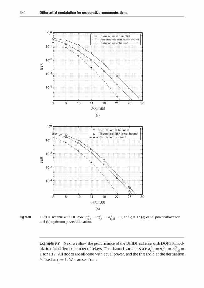
344 Differential modulation for cooperative communications
2 6 10 14 18 22 26 30
Simulation: differentialTheoretical: BER lower boundSimulation: coherent
BE
R
10–4
10–3
10–2
10–1
100
(a)
Simulation: differentialTheoretical: BER lower boundSimulation: coherent
P/�0 [dB]
2 6 10 14 18 22 26 30
BE
R
10–4
10–3
10–2
10–1
100
(b)
P/�0 [dB]
Fig. 9.10 DiffDF scheme with DQPSK: σ 2s,d = σ 2
s,ri = σ 2ri ,d
= 1, and ζ = 1 : (a) equal power allocationand (b) optimum power allocation.
Example 9.7 Next we show the performance of the DiffDF scheme with DQPSK mod-ulation for different number of relays. The channel variances are σ 2
s,d = σ 2s,ri = σ 2
ri ,d=
1 for all i . All nodes are allocate with equal power, and the threshold at the destinationis fixed at ζ = 1. We can see from
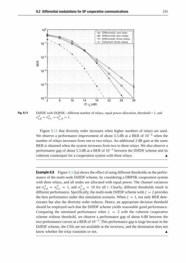
9.2 Differential modulations for DF cooperative communications 345
2 6 10 14 18 22 26 30
Differential: one relayDifferential: two relaysDifferential: three relaysCoherent: three relays
10–5
10–4
10–3
10–2
10–1
100
BE
R
P/�0 [dB]
Fig. 9.11 DiffDF with DQPSK : different number of relays, equal power allocation, threshold = 1, andσ 2
s,d = σ 2s,ri = σ 2
ri ,d= 1.
Figure 9.11 that diversity order increases when higher numbers of relays are used.We observe a performance improvement of about 3.5 dB at a BER of 10−4 when thenumber of relays increases from one to two relays. An additional 2 dB gain at the sameBER is obtained when the system increases from two to three relays. We also observe aperformance gap of about 5.5 dB at a BER of 10−3 between the DiffDF scheme and itscoherent counterpart for a cooperation system with three relays. �
Example 9.8 Figure 9.12(a) shows the effect of using different thresholds on the perfor-mance of the multi-node DiffDF scheme, by considering a DBPSK cooperation systemwith three relays, and all nodes are allocated with equal power. The channel variancesare σ 2
s,d = σ 2s,ri = 1, and σ 2
ri ,d= 10 for all i . Clearly, different thresholds result in
different performance. Specifically, the multi-node DiffDF scheme with ζ = 2 providesthe best performance under this simulation scenario. When ζ = 1, not only BER dete-riorates but also the diversity order reduces. Hence, an appropriate decision thresholdshould be employed such that the DiffDF scheme yields reasonable good performance.Comparing the simulated performance when ζ = 2 with the coherent cooperativescheme without threshold, we observe a performance gap of about 6 dB between thetwo performance curves at a BER of 10−3. This performance gap is large because in theDiffDF scheme, the CSIs are not available at the receivers, and the destination does notknow whether the relay transmits or not. �
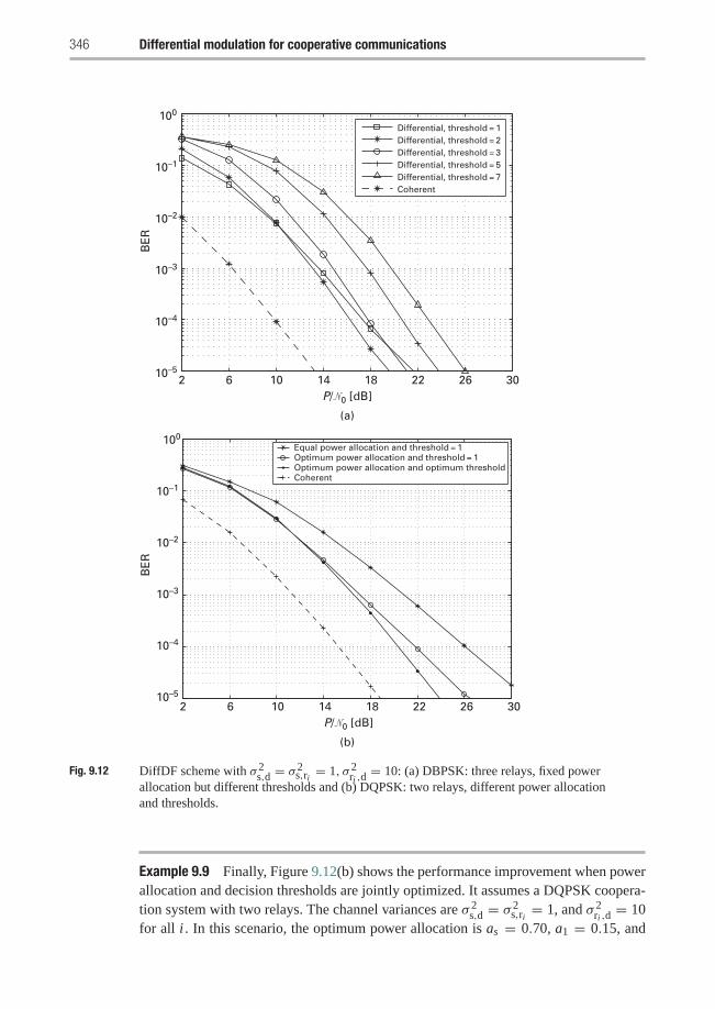
346 Differential modulation for cooperative communications
Differential, threshold = 1Differential, threshold = 2Differential, threshold = 3Differential, threshold = 5Differential, threshold = 7Coherent
Equal power allocation and threshold = 1Optimum power allocation and threshold = 1Optimum power allocation and optimum thresholdCoherent
2 6 10 14 18 22 26 3010–5
10–4
10–3
10–2
10–1
100
BE
R
P/�0 [dB]
(a)
(b)
2 6 10 14 18 22 26 3010–5
10–4
10–3
10–2
10–1
100
BE
R
P/�0 [dB]
Fig. 9.12 DiffDF scheme with σ 2s,d = σ 2
s,ri = 1, σ 2ri ,d
= 10: (a) DBPSK: three relays, fixed powerallocation but different thresholds and (b) DQPSK: two relays, different power allocationand thresholds.
Example 9.9 Finally, Figure 9.12(b) shows the performance improvement when powerallocation and decision thresholds are jointly optimized. It assumes a DQPSK coopera-tion system with two relays. The channel variances are σ 2
s,d = σ 2s,ri = 1, and σ 2
ri ,d= 10
for all i . In this scenario, the optimum power allocation is as = 0.70, a1 = 0.15, and
9.3 Differential modulation for AF cooperative communications 347
a2 = 0.15, and the optimum threshold is ζ = 1.8. We can see that the performancecurve with optimum power allocation and threshold significantly improves from thatwith equal power allocation and an arbitrary decision threshold (ζ = 1 in this case). Aperformance gain of 4–5 dB is observed at a BER of 10−3–10−4.
Also in the figure, we compare the performance of optimum power allocation andthreshold with that of optimum power allocation (as = 0.8, a1 = 0.1, and a2 = 0.1)but an arbitrary threshold (ζ = 1). We can see that jointly optimizing power allocationand threshold leads to a gain of about 1–2.5 dB over the scheme with optimum powerallocation but arbitrary threshold at BER range between 10−3 and 10−5. Note that theperformance of the DiffDF scheme with optimum power allocation and threshold is5 dB away from that of coherent detection. �
9.3 Differential modulation for AF cooperative communications
We now consider differential modulation schemes for amplify-and-forward cooperativecommunications, DiffAF schemes in short, and we start from a single relay scheme.
9.3.1 DiffAF with single-relay systems
This section considers a DiffAF protocol in a two-user cooperative communications sys-tem. The scheme efficiently combines signals from all branches, in which only long termaverage of the received signals is required. As a performance benchmark, we provide anexact BER formulation and its simple bounds for the optimum-combining cooperationsystem with DMPSK signals. Based on the theoretical BER benchmark, the optimumpower allocation can be obtained, and it is used to further improve the performance ofthe DiffAF scheme.
9.3.1.1 Signal model and protocol description for the DiffAF schemeWe consider a two-user cooperative communications system employing the AF proto-col. Each user can be a source node that sends its information to the destination, or itcan be a relay node that helps transmit the other user’s information. Basically, signaltransmission can be separated into two phases. In phase 1, the source node transmitsthe information to its destination. Due to the broadcasting nature of wireless networks,this information is also received by the relay node. In phase 2, while the source nodeis silent, the relay node amplifies the received signal and forwards it to the destination.In both phases, the signals of all users are transmitted through orthogonal channels byusing existing schemes such as TDMA, FDMA, or CDMA.
In differential transmission, the information is conveyed in the difference of thephases of two consecutive symbols. Specifically, information symbols to be broadcastedby the source are given by vm = ejφm ,where {φm}M−1
m=0 is a set of M information phases.In the case of DMPSK, φm can be specified as φm = 2πm/M for m = 0, 1, . . . ,M−1.
348 Differential modulation for cooperative communications
Instead of directly transmitting the information as in coherent transmission, the sourcenode differentially encodes the information symbol vm as
xτ = vm xτ−1, (9.107)
where τ is the time index, and xτ is the differentially encoded symbol to be transmittedat time τ .
In phase 1, the source sends out the symbol xτ with transmit power P1. Thecorresponding received signals at the destination and the relay nodes can be expressed as
yτs,d =√
P1hτs,dxτ + wτs,d,and
yτs,r =√
P1hτs,rxτ + wτs,r,
respectively. Here, hτs,d and hτs,r represent the channel coefficients from the source tothe destination and from the source to the relay, respectively, whereas wτs,d and wτs,r areadditive noise.
In phase 2, the relay amplifies the received signal and forwards it to the destinationwith transmit power P2. The received signal at the destination can be modeled as
yτr,d =√
P2hτr,dyτs,r + wτr,d, (9.108)
where hτr,d is the channel coefficient from the relay to the destination, and wτr,d is addi-tive noise. In a Rayleigh fading environment, the channel coefficients hτs,d, hτs,r, and hτr,dcan be modeled as independent zero-mean complex Gaussian random variables withvariances σ 2
s,d, σ 2s,r, and σ 2
r,d, respectively. All of the fading coefficients are unknownto either the transmitter or the receiver, and they are assumed to be constant overtwo symbol periods. The noise wτs,d, wτs,r, and wτr,d are modeled as independent com-plex Gaussian random variables with zero means and variances N0. To ensure that theaverage transmit power of the relay node is P2, the normalized power P2 is specified as
P2 = P2
P1σ 2s,r +N0
, (9.109)
where the variance σ 2s,r can be obtained from the long-term average of the received
signals. The normalized power in (9.109) differs from its coherent counterpart in thatthe latter uses instantaneous fading amplitude, i.e.,
∣∣hs,r∣∣2, instead of σ 2
s,r.At the destination, the received signal from the source through direct transmission in
phase 1 (yτs,d) and that from the relay in phase 2 (yτr,d) are combined together, and thenthe combined output is differentially decoded. The combined signal prior to differentialdecoding is
y = a1(yτ−1
s,d
)∗yτs,d + a2
(yτ−1
r,d
)∗yτr,d, (9.110)
where the coefficients a1 and a2 are given by
a1 = 1
N0, a2 =
P1σ2s,r +N0
N0(P1σ 2s,r + P2σ
2r,d +N0)
, (9.111)
9.3 Differential modulation for AF cooperative communications 349
which are determined to maximized the SNR of the combined signal. Without acquiringCSI, the decoder use the sufficient statistics given in (9.110), and its decision rule fordecoding information symbol follows:
m = arg maxm = 0,1,...,M−1
Re{v∗m y
}.
9.3.1.2 Performance analysis and discussionsWhile the exact BER formulation that is applicable for multi-channel differentialscheme with arbitrary-weight combining as in (9.111) is currently not available, in thissection we discuss a BER formulation for the case of optimum combining weights,which are specified in the following:
a1 = 1
N0, a2 =
P1σ2s,r +N0
N0(P1σ 2s,r + P2|hr,d|2 +N0)
. (9.112)
Even though these optimum weights are not practical for the DiffAD scheme becausethe instantaneous channel amplitude at the relay–destination link, i.e.,
∣∣hr,d∣∣2, is
assumed unknown to the receiver, the performance evaluation based on optimumweights (9.112) can be used as a performance benchmark for the DiffAF scheme.
With the optimum weight a1 and a2, the instantaneous SNR per bit of the optimumcombiner output can be calculated as
γ = γ1 + γ2, (9.113)
where
γ1 = P1∣∣hs,d
∣∣2N0
, (9.114)
and
γ2 = P1 P2∣∣hs,r
∣∣2 ∣∣hr,d∣∣2
N0
(P1σ 2
s,r + P2∣∣hr,d
∣∣2 +N0
) . (9.115)
To simplify the notation, we omit the time index τ in this section for convenience in thederivation.
Similar to the DiffDF scheme, the conditional BER of the DiffAF is given by
Pb|γ = 1
16π
∫ π
−πf (θ) exp [−α(θ)γ ]dθ, (9.116)
where
f (θ) = b2(1− β2) [3+ cos(2θ)− (β + 1/β) sin θ ]
2α(θ), (9.117)
and
α(θ) = b2(1+ 2β sin θ + β2)
2, (9.118)
in which β = a/b denotes a constant parameter in which a and b depend on the mod-ulation size [188]. Specifically, a = 10−3 and b = √
2 for DBPSK modulation, and
350 Differential modulation for cooperative communications
a =√
2−√2 and b =√
2+√2 for DQPSK modulation [188]. The values of a and bfor larger modulation sizes can be obtained by using the result in [146].
By averaging the conditional BER over the Rayleigh fading channels, hs,d, hs,r, andhr,d, we have an average BER formulation in terms of MGF functions as follows:
Pb = 1
16π
∫ π
−πf (θ)Mγ1 (θ)Mγ2 (θ) dθ, (9.119)
where
Mγi (θ) =∫ +∞
−∞e−α(θ)λ pγi (λ)dλ, (9.120)
denotes the MGF of the SNR γi for i = 1, 2, evaluating at α(θ), and f (θ) and α(θ) arespecified in (9.117) and (9.118), respectively. Observe that the exact evaluation of theBER in (9.141) involves triple integration, which is hard to obtain. In what follows, weprovide a simplified exact BER formulation that involve only double integration. TheBER formulation in (9.119) can be further calculated as follows.
The simplified BER formulation can be obtained by calculating Mγ1 (θ) and Mγ2
separately as follows. For Rayleigh fading channels,∣∣hs,d
∣∣2,∣∣hs,r
∣∣2, and∣∣hr,d
∣∣2 areindependent exponential random variables with parameters 1/σ 2
s,d, 1/σ 2s,r, and 1/σ 2
r,d,respectively. Based on (9.120), Mγ1(θ) can be expressed as (proof left as an exercise)
Mγ1(θ) =1
1+ ks,d(θ), (9.121)
where
ks,d(θ) � α(θ)P1σ2s,d/N0. (9.122)
Observe that Mγ2(θ) depends on both∣∣hs,r
∣∣2 and∣∣hr,d
∣∣2. By averaging over∣∣hs,r
∣∣2, andafter some manipulations, we can express Mγ2(θ) as (proof left as an exercise)
Mγ2(θ)
= 1
1+ ks,r(θ)
(1+ ks,r(θ)
1+ ks,r(θ)
P1σ2s,r +No
P2
1
σ 2r,d
∫ ∞
0
exp(−u/σ 2
r,d
)u + R(θ)
du
),
(9.123)
where
R(θ) �P1σ
2s,r +No
P2(1+ ks,r(θ)
) , (9.124)
in which ks,r(θ) is given by
ks,r(θ) � α(θ)P1σ2s,r/N0, (9.125)
Finally, by substituting (9.121) and (9.123) into (9.119), we obtain a BER expressionthat involves only double integration. In what follows, we can further obtain single-integral BER lower bound, single-integral BER upper bound, and their correspondingsimple BER approximations that involve no integration.
9.3 Differential modulation for AF cooperative communications 351
The BER expression in (9.119) can be upper bounded by using the upper boundof Mγ2(θ) in (9.123). We will bound the integration term in (9.123) with a constantZmax that is not a function of θ . The value of Zmax can be found by replacing R(θ)in the integrand with its minimum value. We can see from (9.125) and (9.124) thatR(θ) reaches its minimum value when B(θ) attains its maximum at θ = π/2, i.e.,B(θ) ≤ −b2(1+ β)2/2. Accordingly, the minimum value of R(θ) is given by
R(θ) ≥ P1σ2s,r +No
P2
[1− P1σ
2s,rb
2(1+ β)22N0
]−1
� Rmin. (9.126)
Substituting R(θ) in (9.123) with Rmin, the BER upper bound is given by
Pb ≤ 1
16π
∫ π
−πF (θ)
1
[1+ ks,d(θ)][1+ ks,r(θ)]
×(
1+ P1σ2s,r + 1
P2σ2r,d
ks,r(θ)
1+ ks,r(θ)Zmax
)dθ, (9.127)
in which
Zmax =∫ ∞
0exp(−u/σ 2
r,d)[u + Rmin
]−1du (9.128)
is a constant that can be easily obtained for any given values of σ 2r,d and Rmin. The upper
bound in (9.127) involves only single integration, and it is simpler than the exact BERprovided in (9.119).
To gain further insight, we further simplify the BER upper bound in (9.127) as fol-lows. For high enough SNR, we can ignore all 1’s in the denominator of (9.127). Thisresults in
Pb ≤(
1+ P1σ2s,r + 1
P2σ2r,d
Zmax
)1
16π
∫ π
−πf (θ)
ks,d(θ)ks,r(θ)dθ
=(P1σ
2s,r + 1
)Zmax + P2σ
2r,d
P21 P2σ
2s,dσ
2s,rσ
2r,d
N 20 C (β, θ) , (9.129)
where
C (β, θ) = 1
8πb4
∫ π−π
(1− β2)[3+ cos(2θ)− (β + 1/β) sin θ ](1+ 2β sin θ + β2)3
dθ (9.130)
is a constant that depends on the modulation size.The BER lower bound can be obtained in a similar way to the BER upper bound. We
will briefly provide details of the derivations. In this case, R(θ) reaches its maximumvalue when B(θ) attains its minimum at θ = −π/2, i.e., B(θ) ≥ −b2(1 − β)2/2.Accordingly, the maximum value of R(θ) is given by
R(θ) ≤ P1σ2s,r +No
P2
[1+ P1σ
2s,rb
2(1− β)22N0
]−1
� Rmax. (9.131)
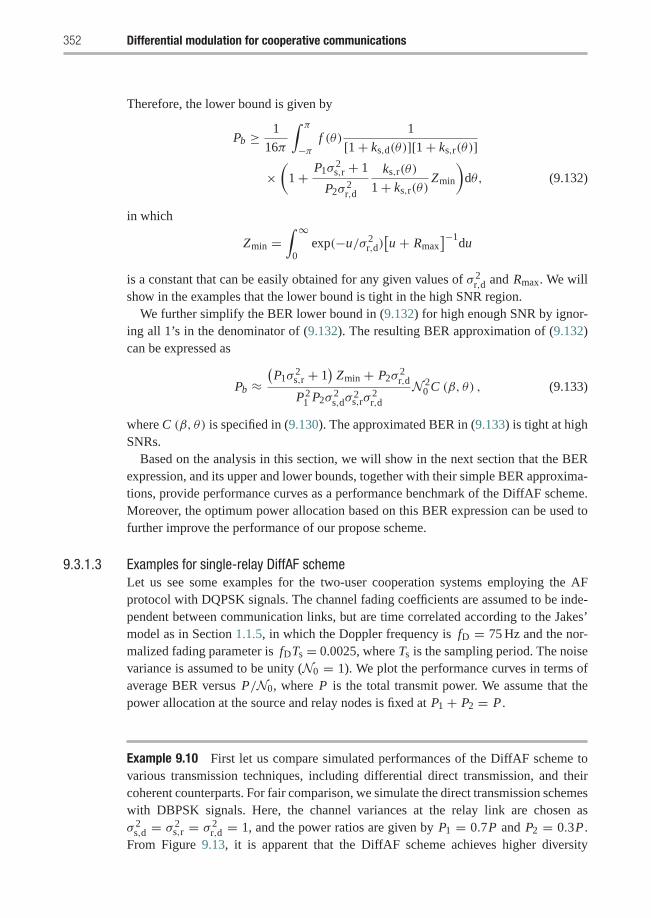
352 Differential modulation for cooperative communications
Therefore, the lower bound is given by
Pb ≥ 1
16π
∫ π
−πf (θ)
1
[1+ ks,d(θ)][1+ ks,r(θ)]
×(
1+ P1σ2s,r + 1
P2σ2r,d
ks,r(θ)
1+ ks,r(θ)Zmin
)dθ, (9.132)
in which
Zmin =∫ ∞
0exp(−u/σ 2
r,d)[u + Rmax
]−1du
is a constant that can be easily obtained for any given values of σ 2r,d and Rmax. We will
show in the examples that the lower bound is tight in the high SNR region.We further simplify the BER lower bound in (9.132) for high enough SNR by ignor-
ing all 1’s in the denominator of (9.132). The resulting BER approximation of (9.132)can be expressed as
Pb ≈(P1σ
2s,r + 1
)Zmin + P2σ
2r,d
P21 P2σ
2s,dσ
2s,rσ
2r,d
N 20 C (β, θ) , (9.133)
where C (β, θ) is specified in (9.130). The approximated BER in (9.133) is tight at highSNRs.
Based on the analysis in this section, we will show in the next section that the BERexpression, and its upper and lower bounds, together with their simple BER approxima-tions, provide performance curves as a performance benchmark of the DiffAF scheme.Moreover, the optimum power allocation based on this BER expression can be used tofurther improve the performance of our propose scheme.
9.3.1.3 Examples for single-relay DiffAF schemeLet us see some examples for the two-user cooperation systems employing the AFprotocol with DQPSK signals. The channel fading coefficients are assumed to be inde-pendent between communication links, but are time correlated according to the Jakes’model as in Section 1.1.5, in which the Doppler frequency is fD = 75 Hz and the nor-malized fading parameter is fDTs = 0.0025, where Ts is the sampling period. The noisevariance is assumed to be unity (N0 = 1). We plot the performance curves in terms ofaverage BER versus P/N0, where P is the total transmit power. We assume that thepower allocation at the source and relay nodes is fixed at P1 + P2 = P .
Example 9.10 First let us compare simulated performances of the DiffAF scheme tovarious transmission techniques, including differential direct transmission, and theircoherent counterparts. For fair comparison, we simulate the direct transmission schemeswith DBPSK signals. Here, the channel variances at the relay link are chosen asσ 2
s,d = σ 2s,r = σ 2
r,d = 1, and the power ratios are given by P1 = 0.7P and P2 = 0.3P .From Figure 9.13, it is apparent that the DiffAF scheme achieves higher diversity
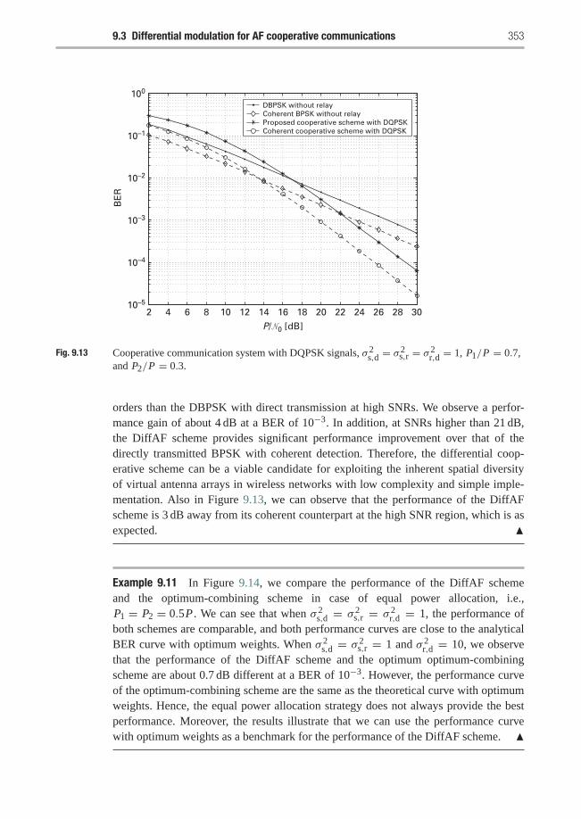
9.3 Differential modulation for AF cooperative communications 353
2 4 6 8 10 12 14 16 18 20 22 24 26 28 30
DBPSK without relayCoherent BPSK without relayProposed cooperative scheme with DQPSKCoherent cooperative scheme with DQPSK
10–5
10–4
10–3
10–2
10–1
100
BE
R
P/�0 [dB]
Fig. 9.13 Cooperative communication system with DQPSK signals, σ 2s,d = σ 2
s,r = σ 2r,d = 1, P1/P = 0.7,
and P2/P = 0.3.
orders than the DBPSK with direct transmission at high SNRs. We observe a perfor-mance gain of about 4 dB at a BER of 10−3. In addition, at SNRs higher than 21 dB,the DiffAF scheme provides significant performance improvement over that of thedirectly transmitted BPSK with coherent detection. Therefore, the differential coop-erative scheme can be a viable candidate for exploiting the inherent spatial diversityof virtual antenna arrays in wireless networks with low complexity and simple imple-mentation. Also in Figure 9.13, we can observe that the performance of the DiffAFscheme is 3 dB away from its coherent counterpart at the high SNR region, which is asexpected. �
Example 9.11 In Figure 9.14, we compare the performance of the DiffAF schemeand the optimum-combining scheme in case of equal power allocation, i.e.,P1 = P2 = 0.5P . We can see that when σ 2
s,d = σ 2s,r = σ 2
r,d = 1, the performance ofboth schemes are comparable, and both performance curves are close to the analyticalBER curve with optimum weights. When σ 2
s,d = σ 2s,r = 1 and σ 2
r,d = 10, we observethat the performance of the DiffAF scheme and the optimum optimum-combiningscheme are about 0.7 dB different at a BER of 10−3. However, the performance curveof the optimum-combining scheme are the same as the theoretical curve with optimumweights. Hence, the equal power allocation strategy does not always provide the bestperformance. Moreover, the results illustrate that we can use the performance curvewith optimum weights as a benchmark for the performance of the DiffAF scheme. �
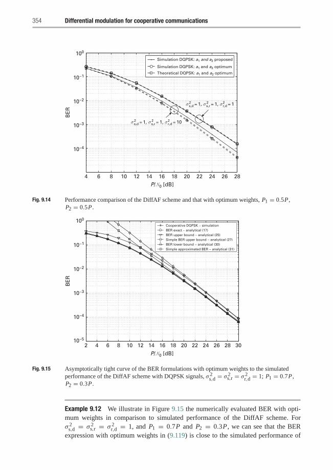
354 Differential modulation for cooperative communications
4 6 8 10 12 14 16 18 20 22 24 26 28
10−4
10−3
10−2
10−1
100
BE
RTheoretical DQPSK: a1 and a2 optimum
Simulation DQPSK: a1 and a2 optimum
Simulation DQPSK: a1 and a2 proposed
σ s,d = 1, σ s,r = 1, σ r,d = 102 2 2
σ s,d = 1, σ s,r = 1, σ r,d = 12 2 2
P/�0 [dB]
Fig. 9.14 Performance comparison of the DiffAF scheme and that with optimum weights, P1 = 0.5P ,P2 = 0.5P .
2 4 6 8 10 12 14 16 18 20 22 24 26 28 3010−5
10−4
10−3
10−2
10−1
100
BE
R
Cooperative DQPSK − simulationBER exact − analytical (17)BER upper bound − analytical (25)Simple BER upper bound − analytical (27)BER lower bound − analytical (30)Simple approximated BER − analytical (31)
P/�0 [dB]
Fig. 9.15 Asymptotically tight curve of the BER formulations with optimum weights to the simulatedperformance of the DiffAF scheme with DQPSK signals, σ 2
s,d = σ 2s,r = σ 2
r,d = 1; P1 = 0.7P ,P2 = 0.3P .
Example 9.12 We illustrate in Figure 9.15 the numerically evaluated BER with opti-mum weights in comparison to simulated performance of the DiffAF scheme. Forσ 2
s,d = σ 2s,r = σ 2
r,d = 1, and P1 = 0.7P and P2 = 0.3P , we can see that the BERexpression with optimum weights in (9.119) is close to the simulated performance of
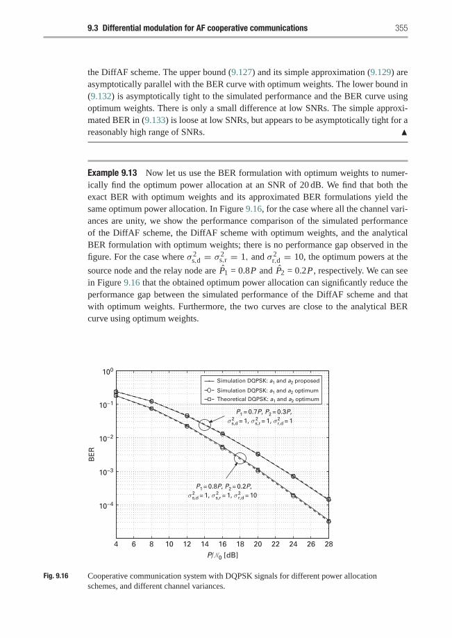
9.3 Differential modulation for AF cooperative communications 355
the DiffAF scheme. The upper bound (9.127) and its simple approximation (9.129) areasymptotically parallel with the BER curve with optimum weights. The lower bound in(9.132) is asymptotically tight to the simulated performance and the BER curve usingoptimum weights. There is only a small difference at low SNRs. The simple approxi-mated BER in (9.133) is loose at low SNRs, but appears to be asymptotically tight for areasonably high range of SNRs. �
Example 9.13 Now let us use the BER formulation with optimum weights to numer-ically find the optimum power allocation at an SNR of 20 dB. We find that both theexact BER with optimum weights and its approximated BER formulations yield thesame optimum power allocation. In Figure 9.16, for the case where all the channel vari-ances are unity, we show the performance comparison of the simulated performanceof the DiffAF scheme, the DiffAF scheme with optimum weights, and the analyticalBER formulation with optimum weights; there is no performance gap observed in thefigure. For the case where σ 2
s,d = σ 2s,r = 1, and σ 2
r,d = 10, the optimum powers at the
source node and the relay node are P1 = 0.8P and P2 = 0.2P , respectively. We can seein Figure 9.16 that the obtained optimum power allocation can significantly reduce theperformance gap between the simulated performance of the DiffAF scheme and thatwith optimum weights. Furthermore, the two curves are close to the analytical BERcurve using optimum weights.
P1 = 0.8P, P2 = 0.2P,
P1 = 0.7P, P2 = 0.3P,
4 6 8 10 12 14 16 18 20 22 24 26 28
10−4
10−3
10−2
10−1
100
BE
R
Theoretical DQPSK: a1 and a2 optimum
Simulation DQPSK: a1 and a2 optimum
Simulation DQPSK: a1 and a2 proposed
σ s,d = 1, σ s,r = 1, σ r,d = 102 2 2
σ s,d = 1, σ s,r = 1, σ r,d = 12 2 2
P/�0 [dB]
Fig. 9.16 Cooperative communication system with DQPSK signals for different power allocationschemes, and different channel variances.
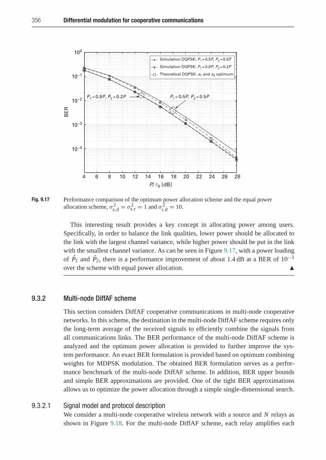
356 Differential modulation for cooperative communications
P1 = 0.8P, P2 = 0.2P P1 = 0.5P, P2 = 0.5P
4 6 8 10 12 14 16 18 20 22 24 26 28
10−4
10−3
10−2
10−1
100
BE
R
Theoretical DQPSK: a1 and a2 optimum
Simulation DQPSK: P1 = 0.8P, P2 = 0.2P
Simulation DQPSK: P1 = 0.5P, P2 = 0.5P
P/�0 [dB]
Fig. 9.17 Performance comparison of the optimum power allocation scheme and the equal powerallocation scheme, σ 2
s,d = σ 2s,r = 1 and σ 2
r,d = 10.
This interesting result provides a key concept in allocating power among users.Specifically, in order to balance the link qualities, lower power should be allocated tothe link with the largest channel variance, while higher power should be put in the linkwith the smallest channel variance. As can be seen in Figure 9.17, with a power loadingof P1 and P2, there is a performance improvement of about 1.4 dB at a BER of 10−3
over the scheme with equal power allocation. �
9.3.2 Multi-node DiffAF scheme
This section considers DiffAF cooperative communications in multi-node cooperativenetworks. In this scheme, the destination in the multi-node DiffAF scheme requires onlythe long-term average of the received signals to efficiently combine the signals fromall communications links. The BER performance of the multi-node DiffAF scheme isanalyzed and the optimum power allocation is provided to further improve the sys-tem performance. An exact BER formulation is provided based on optimum combiningweights for MDPSK modulation. The obtained BER formulation serves as a perfor-mance benchmark of the multi-node DiffAF scheme. In addition, BER upper boundsand simple BER approximations are provided. One of the tight BER approximationsallows us to optimize the power allocation through a simple single-dimensional search.
9.3.2.1 Signal model and protocol descriptionWe consider a multi-node cooperative wireless network with a source and N relays asshown in Figure 9.18. For the multi-node DiffAF scheme, each relay amplifies each
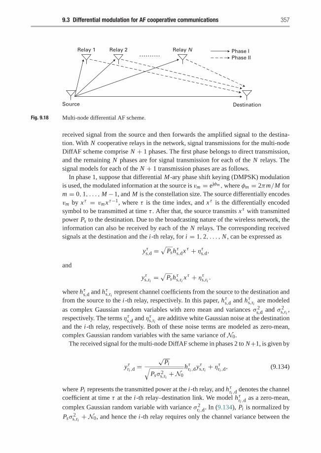
9.3 Differential modulation for AF cooperative communications 357
Source
Relay 1 Relay 2 Relay N Phase IPhase II
Destination
Fig. 9.18 Multi-node differential AF scheme.
received signal from the source and then forwards the amplified signal to the destina-tion. With N cooperative relays in the network, signal transmissions for the multi-nodeDiffAF scheme comprise N + 1 phases. The first phase belongs to direct transmission,and the remaining N phases are for signal transmission for each of the N relays. Thesignal models for each of the N + 1 transmission phases are as follows.
In phase 1, suppose that differential M-ary phase shift keying (DMPSK) modulationis used, the modulated information at the source is vm = ejφm , where φm = 2πm/M form = 0, 1, . . . ,M−1, and M is the constellation size. The source differentially encodesvm by xτ = vmxτ−1, where τ is the time index, and xτ is the differentially encodedsymbol to be transmitted at time τ . After that, the source transmits xτ with transmittedpower Ps to the destination. Due to the broadcasting nature of the wireless network, theinformation can also be received by each of the N relays. The corresponding receivedsignals at the destination and the i-th relay, for i = 1, 2, . . . , N , can be expressed as
yτs,d =√
Pshτs,dxτ + ητs,d,
and
yτs,ri =√
Pshτs,ri x
τ + ητs,ri .where hτs,d and hτs,ri represent channel coefficients from the source to the destination andfrom the source to the i-th relay, respectively. In this paper, hτs,d and hτs,ri are modeled
as complex Gaussian random variables with zero mean and variances σ 2s,d and σ 2
s,ri ,respectively. The terms ητs,d and ητs,ri are additive white Gaussian noise at the destinationand the i-th relay, respectively. Both of these noise terms are modeled as zero-mean,complex Gaussian random variables with the same variance of N0.
The received signal for the multi-node DiffAF scheme in phases 2 to N+1, is given by
yτri ,d =√
Pi√Psσ 2
s,ri +N0
hτri ,dyτs,ri + ητri ,d, (9.134)
where Pi represents the transmitted power at the i-th relay, and hτri ,d denotes the channelcoefficient at time τ at the i-th relay–destination link. We model hτri ,d as a zero-mean,
complex Gaussian random variable with variance σ 2ri ,d
. In (9.134), Pi is normalized by
Psσ2s,ri + N0, and hence the i-th relay requires only the channel variance between the
358 Differential modulation for cooperative communications
source and the i-th relay (σ 2s,ri ) rather than its instantaneous value. In practice, σ 2
s,ri canbe obtained through long-term averaging of the received signals at the i-th relay.
Finally, the received signals from the source and all of the relays are combined at thedestination, giving
yAF = wAFs
(yτ−1
s,d
)∗yτs,d +
N∑i=1
wAFi
(yτ−1
ri ,d
)∗yτri ,d, (9.135)
where
wAFs = 1
N0, wAF
i = Psσ2s,ri +N0
N0(Psσ 2s,ri + Piσ
2ri ,d+N0)
are combining weights that maximize the combiner output. Here, the channel σ 2ri ,d
and
σ 2s,ri are assumed to be available at the destination. Note that σ 2
s,ri and σ 2ri ,d
can beobtained through long-term averaging of the received signals at the i-th relay and thedestination, respectively. In practice, σ 2
s,ri can be forwarded from each of the i-th relaysto the destination over a reliable channel link. Accordingly, without acquiring perfectCSI, the combined signal (9.135) is differentially decoded using the detection rule
m = arg maxm = 0,1,...,M−1
Re{v∗m yAF
}.
9.3.2.2 BER analysisThe BER formulation based on arbitrary combining weights, . i.e., wAF
s and wAFi
in (9.135), is currently not available in the literature. For mathematical tractability,we provide an alternative BER analysis based on the following optimum combiningweights:
wAFs = 1
N0, wAF
i = Psσ2s,ri +N0
N0(Psσ 2s,ri + Pi |hτri ,d|2 +N0)
,
which are determined to maximized the SNR of the combined signal. Note that wAFi
requires instantaneous channel information which is not available in the differentialmodulation; however, the BER analysis based on these optimum combining weightsserves as the BER performance benchmark of the multi-node DiffAF scheme. As will beshown in Section 9.3.2.4, the multi-node DiffAF scheme with optimum power allocationyields very close performance to the BER benchmark. Using the optimum combiningweights wAF
s and wAFi , an instantaneous SNR at the combiner output can be written as
γ AF = γ AFs +
N∑i=1
γ AFi , (9.136)
where
γ AFs �
Ps |hτs,d|2N0
, (9.137)
9.3 Differential modulation for AF cooperative communications 359
and
γ AFi �
Ps Pi |hτs,ri |2|hτri ,d|2N0(Psσ 2
s,ri + Pi |hτri ,d|2 +N0). (9.138)
Accordingly, the conditional BER expression for the multi-node DiffAF scheme can begiven by
PAFb|γ AF =
1
22Lπ
∫ π
−πf (θ, β, L) exp [−α(θ)γ AF ]dθ, (9.139)
where α(θ) is specified in (9.118) and
f (θ, β, L) = b2
2α(θ)
L∑l=1
(2L − 1L − 1
)�(β, θ, l), (9.140)
in which
�(β, θ, l) = [(β−l+1 − βl+1) cos((l − 1)(θ + π2))− (β−l+2 − βl) cos(l(θ + π
2))].
Here, L = N+1, and β = a/b in which a = 10−3 and b = √2 for DBPSK modulation,
and a =√
2−√2 and b =√
2+√2 for DQPSK modulation [188]. The value ofβ for higher constellation sizes can be found in [146]. Averaging the conditional BER(9.139) over the Rayleigh distributed random variables by the use of the MGF functions,we have
PAFb = 1
22(N+1)π
∫ π
−πf (θ, β, N + 1)Mγ AF
s(θ)
N∏i=1
Mγ AFi(θ) dθ, (9.141)
where
MγAFμ(θ) �
∫ +∞
−∞e−α(θ)λ pγAF
μ(λ)dλ,
denotes the MGF of γ AFμ in which μ ∈ {s, 1, . . . , N }. In (9.141), MγAF
s(θ) is obtained
by an integration over an exponential random variable∣∣hs,d
∣∣2 such that
MγAFs(θ) = 1
1+ ks,d(θ), (9.142)
in which ks,d(θ) � α(θ)Psσ2s,d/N0. The MGF MγAF
i(θ), however, is obtained through
double integration of each γ AFi over two exponential random variables
∣∣hs,ri
∣∣2 and∣∣hri ,d∣∣2. After some manipulation, we have
MγAFi(θ) = 1
σ 2ri ,d
∫ ∞
0�i (θ) exp
(− u
σ 2ri ,d
)du, (9.143)
where
�i (θ) =N0(Pi u + Psσ
2s,ri +N0
)N0(Pi u + Psσ 2
s,ri +N0)+ α(θ)Ps Piσ 2
s,ri u.
360 Differential modulation for cooperative communications
Denoting ks,ri (θ) � α(θ)Psσ2s,ri /N0 and ks,ri (θ) � Pi (1 + ks,ri (θ)), we can further
simplify it as
�i (θ) = 1
1+ ks,ri (θ)+ 1− 1/
[1+ ks,ri (θ)
]1+ ks,ri (θ)u/
(Psσ 2
s,ri +N0) , (9.144)
such that (9.143) can be expressed as
MγAFi(θ) = 1
1+ ks,ri (θ)
(1+ ks,ri (θ)
1+ ks,ri (θ)
Psσ2s,ri +N0
Pi
1
σ 2ri ,d
Zi (θ)
), (9.145)
where
Zi (θ) =∫ ∞
0
exp(−u/σ 2
ri ,d
)u + Ri (θ)
du
= −eRi (θ)
[E + ln Ri (θ)+
∫ Ri (θ)
0
exp(−t)− 1
tdt
], (9.146)
in which
Ri (θ) �(
Psσ2s,ri +N0
)/(Pi[1+ ks,ri (θ)
])and Ri (θ) � Ri (θ)/σ
2ri ,d
. Note that the last expression in (9.146) is obtained by
applying results from [50] (p.358: Eq. (3.352.4) and p.934: Eq. (8.212.1)), and E �0.577 215 664 90... represents the Euler’s constant (proof left as an exercise). Hence, bysubstituting (9.142) and (9.145) into (9.141), the average BER formulation is
PAFb = 1
22(N+1)π
∫ π
−πf (θ, β, N + 1)
1+ ks,d(θ)
×N∏
i=1
1
1+ ks,ri (θ)
(1+ ks,ri (θ)Zi (θ)
1+ ks,ri (θ)
Psσ2s,ri +N0
Piσ2ri ,d
)dθ.
(9.147)
Although PAFb can be calculated numerically, it is difficult to get some insights because
it involves double integration. In the following we provide a single-integral BERupper bound, a simple BER upper bound without integration, and two tight BERapproximations.
We first determine the BER upper bound and its simple expression as follows. From(9.145)–(9.147), we can see that the BER upper bound can be obtained by lower bound-ing Ri (θ) in the denominator of the integrand of Zi (θ) in (9.146). By substituting
9.3 Differential modulation for AF cooperative communications 361
θ = π/2 in (9.118), α(θ) is upper bounded by α(θ) ≤ (b2(1 + β)2)/2. Therefore,Ri (θ) is lower bounded by
Ri (θ) ≥Psσ
2s,ri +N0
Pi
[1+ Psσ
2s,ri b
2(1+ β)22N0
]−1
� Ri,min. (9.148)
Substituting Ri (θ) = Ri,min into (9.146) results in an upper bound on Zi (θ), i.e.,Zi (θ) ≤ Zi,max where
Zi,max = −eRi,min
[E + ln Ri,min +
∫ Ri,min
0
exp(−t)− 1
tdt
], (9.149)
in which Ri,min � Ri,min/σ2ri ,d
. Note that for any given channel variances σ 2s,ri and σ 2
ri ,d,
and power allocation, Zi,max can be determined numerically. Therefore, the BER upperbound can be obtained by replacing Zi (θ) in (9.147) by Zi,max, giving
PAFb ≤ 1
22(N+1)π
∫ π
−πf (θ, β, N + 1)
1+ ks,d(θ)
×N∏
i=1
1
1+ ks,ri (θ)
(1+ ks,ri (θ)Zi,max
1+ ks,ri (θ)
Psσ2s,ri +N0
Piσ2ri ,d
)dθ. (9.150)
We further simplify the right-hand side of (9.150) to obtain a simple BER upper boundand to get some insights into the achievable diversity order. We focus on the highSNR region so that all 1’s in the denominator of (9.150) can be discarded. After somemanipulation, the simple BER upper bound can be expressed as
PAFb ≤ C (β, N + 1)N N+1
0
Psσ2s,d
N∏i=1
Piσ2ri ,d+ (Psσ
2s,ri +N0
)Zi,max
Ps Piσ 2s,riσ
2ri ,d
, (9.151)
where
C (β, N + 1) = 1
22(N+1)π
∫ π
−πf (θ, β, N + 1)
αN+1(θ)dθ (9.152)
is a constant that depends on modulation size and number of relays, and α(θ) andf (θ, β, N +1) are specified in (9.118) and (9.140), respectively. The BER upper bound(9.151) reveals that when N relays are available in the network, the multi-node DiffAFscheme achieves a diversity order of N + 1, as specified in the exponent of the noisevariance.
In the following derivations, we determine two BER approximations in which one ofthem is an asymptotically tight simple BER approximation. We first note that α(θ) in(9.118) can be lower bounded by α(θ) ≥ α(−π/2) = (b2(1 − β)2)/2 such that theupper bound on Ri (θ) can be written as
Ri (θ) ≤Psσ
2s,ri +N0
Pi
[1+ Psσ
2s,ri b
2(1− β)22N0
]−1
� Ri,max. (9.153)
362 Differential modulation for cooperative communications
By substituting Ri (θ) = Ri,max into (9.146), we obtain a lower bound on Zi (θ), denotedby Zi,min:
Zi,min = −eRi,max
[E + ln Ri,max +
∫ Ri,max
0
exp(−t)− 1
tdt
], (9.154)
in which Ri,max � Ri,max/σ2ri ,d
and E is the Euler’s constant. Then, replacing Zi (θ) in(9.147) by Zi,min, we obtain a BER approximation
PAFb � 1
22(N+1)π
∫ π
−πf (θ, β, N + 1)
1+ ks,d(θ)
×N∏
i=1
1
1+ ks,ri (θ)
(1+ ks,ri (θ)Zi,min
1+ ks,ri (θ)
Psσ2s,ri +N0
Piσ2ri ,d
)dθ. (9.155)
Furthermore, by ignoring all 1’s in the denominator of (9.155), we obtain a simple BERapproximation
PAFb ≈ C (β, N + 1)N N+1
0
Psσ2s,d
N∏i=1
Piσ2ri ,d+ (Psσ
2s,ri +N0
)Zi,min
Ps Piσ 2s,riσ
2ri ,d
, (9.156)
where C (β, N + 1) and Zi,min are specified in (9.152) and (9.154), respectively. We cansee from the exponent of the noise variance in (9.156) that the achievable diversity orderis N + 1. As will be shown in the simulation results, these two BER approximations aretight in the high SNR region.
9.3.2.3 Optimum power allocationNext, we formulate an optimization problem to minimize the BER under a fixed totaltransmitted power, P = Ps + ∑N
i=1 Pi . Based on the simple BER approximation(9.156), the optimization problem can be formulated as
arg minPs ,{Pi }Ni=1
{C (β, N + 1)N N+1
0
Psσ2s,d
N∏i=1
Piσ2ri ,d+ (Psσ
2s,ri +N0)Zi,min
Ps Piσ 2s,riσ
2ri ,d
},
s.t. Ps +N∑
i=1
Pi ≤ P, Pi ≥ 0,∀i, (9.157)
Although (9.157) can be solved numerically, it is difficult to gain insights from numeri-cal solutions. To further simplify the problem, we consider the high SNR region whereRi,max in (9.153) can be approximated as
Ri,max ≈ (2N0)/(b2(1− β)2 Pi ).
Then we can rewrite Zi,min in (9.154) as
Zi,min ≈∫ ∞
0
exp(−u/σ 2ri ,d)
u + 2N0/(b2(1− β)2 Psci )du
= −eBci
[E + ln Bci +
∫ Bci
0
exp(−t)− 1
tdt
], (9.158)
9.3 Differential modulation for AF cooperative communications 363
where ci = Pi/Ps and Bci � Bci /σ2ri ,d
in which Bci = 2N0/(b2(1 − β)2 Psci ). Sincethe integration term in the last expression of (9.158) is small compared to E + ln Bci , itcan be neglected without significant effect on the power allocation. Hence Zi,min can befurther approximated by
Zi,min ≈ −eBci(E + ln Bci
). (9.159)
As will be shown later, the obtained optimum power allocation based on the approxi-mated Zi,min in (9.159) yields almost the same performance as that with exact Zi,min asspecified in (9.154).
Substituting (9.159) into (9.157), the optimization problem can be simplified to
arg minPs ,{Pi }Ni=1
{1
P N+1s
N∏i=1
Piσ2ri ,d− Psσ
2s,ri e
Bci(E + ln Bci
)Pi
},
s.t. Ps +N∑
i=1
Pi ≤ P, Pi ≥ 0, ∀i. (9.160)
By taking the logarithm of the Lagrangian of (9.160) and letting ci = Pi/Ps , we obtain
G = −(N + 1) ln Ps + λ(cT1− P/Ps)
−N∑
i=1
ln ci +N∑
i=1
ln(ciσ
2ri ,d − σ 2
s,ri eBci(E + ln Bci
)), (9.161)
in which c = [1, c1, . . . , cN ]T is an N × 1 vector, and 1 denotes an N × 1 vector withall ones. By differentiating (9.161) with respect to ci and Ps and equating the results tozero, we have
∂G∂ci
= λ− 1
ci+σ 2
ri ,d+ σ 2
s,ri
[Bci eBci
ci
(E + ln Bci
)+ eBci
ci
]ciσ
2ri ,d− σ 2
s,ri eBci(E + ln Bci
) = 0, (9.162)
and
∂G∂Ps
= − (N + 1)
Ps+ λ P
P2s+
N∑i=1
σ 2s,ri
eBci
Ps
[BciPs
(E + ln Bci
)+ 1]
ciσ2ri ,d− σ 2
s,ri eBci(E + ln Bci
) = 0, (9.163)
respectively. From (9.163), we can find that
λ = (N + 1)Ps
P− 1
P
N∑i=1
σ 2s,riϒeBci
(E + ln Bci + 1
Bci
)ci[ciσ
2ri ,d− σ 2
s,ri eBci(E + ln Bci
)] , (9.164)
in which we denote
ϒ � (2N0)/(b2(1− β2)σ 2
ri ,d).
Observe from (9.158) that Bci can be re-expressed as
Bci = (2N0)/(b2(1− β)2σ 2
ri ,d Pqci ),
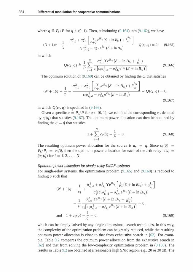
364 Differential modulation for cooperative communications
where q � Ps/P for q ∈ (0, 1). Then, substituting (9.164) into (9.162), we have
(N + 1)q − 1
ci+σ 2
ri ,d+ σ 2
s,ri
[ϒ
Pqc2ieBci
(E + ln Bci
)+ eBcici
]ciσ
2ri ,d
− σ 2s,ri e
Bci(E + ln Bci
) − Q(ci , q) = 0, (9.165)
in which
Q(ci , q) � 1
P
N∑i=1
σ 2s,riϒeBci
(E + ln Bci + 1
Bci
)ci[ciσ
2ri ,d− σ 2
s,ri eBci(E + ln Bci
)] . (9.166)
The optimum solution of (9.160) can be obtained by finding the ci that satisfies
(N + 1)q − 1
ci+σ 2
ri ,d+ σ 2
s,ri
[ϒ
Pqc2ieBci(E + ln Bci
)+ eBci
ci
]ciσ
2ri ,d− σ 2
s,ri eBci(E + ln Bci
) − Q(ci , q) = 0,
(9.167)
in which Q(ci , q) is specified in (9.166).Given a specific q � Ps/P for q ∈ (0, 1), we can find the corresponding ci , denoted
by ci (q) that satisfies (9.167). The optimum power allocation can then be obtained byfinding the q = q that satisfies
1+N∑
i=1
ci (q)− 1
q= 0. (9.168)
The resulting optimum power allocation for the source is as = q. Since ci (q) =Pi/Ps = ai/q , then the optimum power allocation for each of the i-th relay is ai =qci (q) for i = 1, 2, . . . , N .
Optimum power allocation for single-relay DiffAF systemsFor single-relay systems, the optimization problem (9.165) and (9.168) is reduced tofinding q such that
(N + 1)q − 1
c1+σ 2
r1,d+ σ 2
s,r1ϒeBc1
[1
Pq
(E + ln Bc1
)+ 1Bc1
]c2
1[c1σ2r1,d− σ 2
s,r1eBc1(E + ln Bc1
)]− 1
P
σ 2s,r1ϒeBc1
(E + ln Bc1 + 1
Bc1
)c1[c1σ
2r1,d− σ 2
s,r1eBc1(E + ln Bc1
)] = 0,
and 1+ c1(q)− 1
q= 0, (9.169)
which can be simply solved by any single-dimensional search techniques. In this way,the complexity of the optimization problem can be greatly reduced, while the resultingoptimum power allocation is close to that from exhaustive search in [62]. For exam-ple, Table 9.2 compares the optimum power allocation from the exhaustive search in[62] and that from solving the low-complexity optimization problem in (9.169). Theresults in Table 9.2 are obtained at a reasonable high SNR region, e.g., 20 or 30 dB. The
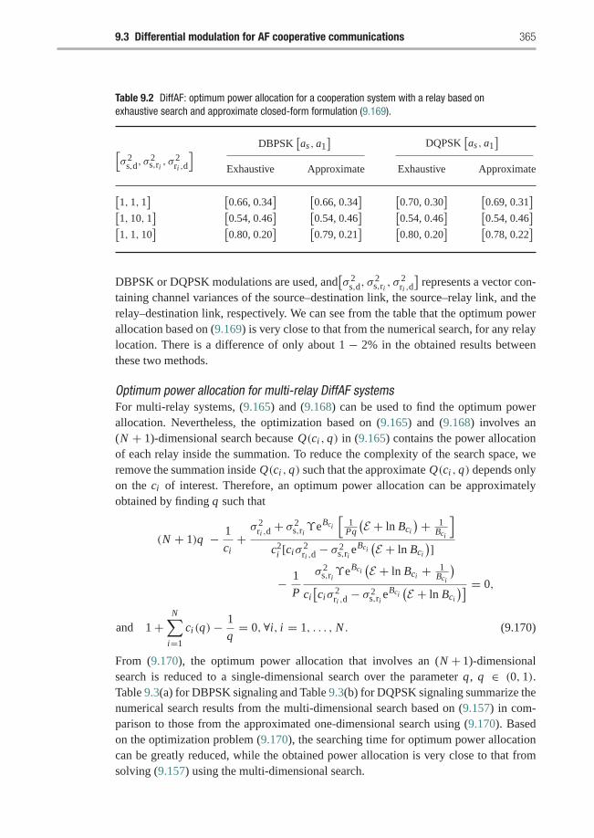
9.3 Differential modulation for AF cooperative communications 365
Table 9.2 DiffAF: optimum power allocation for a cooperation system with a relay based onexhaustive search and approximate closed-form formulation (9.169).
DBPSK[as , a1
]DQPSK
[as , a1
][σ 2
s,d, σ2s,ri , σ
2ri ,d
]Exhaustive Approximate Exhaustive Approximate
[1, 1, 1
] [0.66, 0.34
] [0.66, 0.34
] [0.70, 0.30
] [0.69, 0.31
][1, 10, 1
] [0.54, 0.46
] [0.54, 0.46
] [0.54, 0.46
] [0.54, 0.46
][1, 1, 10
] [0.80, 0.20
] [0.79, 0.21
] [0.80, 0.20
] [0.78, 0.22
]
DBPSK or DQPSK modulations are used, and[σ 2
s,d, σ2s,ri , σ
2ri ,d
]represents a vector con-
taining channel variances of the source–destination link, the source–relay link, and therelay–destination link, respectively. We can see from the table that the optimum powerallocation based on (9.169) is very close to that from the numerical search, for any relaylocation. There is a difference of only about 1 − 2% in the obtained results betweenthese two methods.
Optimum power allocation for multi-relay DiffAF systemsFor multi-relay systems, (9.165) and (9.168) can be used to find the optimum powerallocation. Nevertheless, the optimization based on (9.165) and (9.168) involves an(N + 1)-dimensional search because Q(ci , q) in (9.165) contains the power allocationof each relay inside the summation. To reduce the complexity of the search space, weremove the summation inside Q(ci , q) such that the approximate Q(ci , q) depends onlyon the ci of interest. Therefore, an optimum power allocation can be approximatelyobtained by finding q such that
(N + 1)q − 1
ci+σ 2
ri ,d+ σ 2
s,riϒeBci
[1
Pq
(E + ln Bci
)+ 1Bci
]c2
i [ciσ2ri ,d− σ 2
s,ri eBci(E + ln Bci
)]− 1
P
σ 2s,riϒeBci
(E + ln Bci + 1
Bci
)ci[ciσ
2ri ,d− σ 2
s,ri eBci(E + ln Bci
)] = 0,
and 1+N∑
i=1
ci (q)− 1
q= 0,∀i, i = 1, . . . , N . (9.170)
From (9.170), the optimum power allocation that involves an (N + 1)-dimensionalsearch is reduced to a single-dimensional search over the parameter q, q ∈ (0, 1).Table 9.3(a) for DBPSK signaling and Table 9.3(b) for DQPSK signaling summarize thenumerical search results from the multi-dimensional search based on (9.157) in com-parison to those from the approximated one-dimensional search using (9.170). Basedon the optimization problem (9.170), the searching time for optimum power allocationcan be greatly reduced, while the obtained power allocation is very close to that fromsolving (9.157) using the multi-dimensional search.
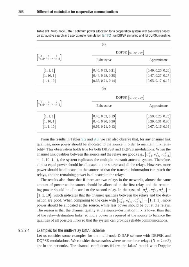
366 Differential modulation for cooperative communications
Table 9.3 Multi-node DiffAF: optimum power allocation for a cooperation system with two relays basedon exhaustive search and approximate formulation (9.170) : (a) DBPSK signaling and (b) DQPSK signaling.
(a)
DBPSK[as , a1, a2
][σ 2
s,d, σ2s,ri , σ
2ri ,d
]Exhaustive Approximate
[1, 1, 1
] [0.46, 0.33, 0.21
] [0.49, 0.26, 0.26
][1, 10, 1
] [0.44, 0.28, 0.28
] [0.47, 0.27, 0.27
][1, 1, 10
] [0.65, 0.21, 0.14
] [0.65, 0.17, 0.17
](b)
DQPSK[as , a1, a2
][σ 2
s,d, σ2s,ri , σ
2ri ,d
]Exhaustive Approximate
[1, 1, 1
] [0.48, 0.33, 0.19
] [0.50, 0.25, 0.25
][1, 10, 1
] [0.40, 0.30, 0.30
] [0.39, 0.31, 0.30
][1, 1, 10
] [0.66, 0.21, 0.13
] [0.67, 0.16, 0.16
]From the results in Tables 9.2 and 9.3, we can also observe that, for any channel link
qualities, more power should be allocated to the source in order to maintain link relia-bility. This observation holds true for both DBPSK and DQPSK modulations. When thechannel link qualities between the source and the relays are good (e.g.,
[σ 2
s,d, σ2s,ri , σ
2ri ,d
]=[1, 10, 1,
]), the system replicates the multiple transmit antenna system. Therefore,
almost equal power should be allocated to the source and all the relays. However, morepower should be allocated to the source so that the transmit information can reach therelays, and the remaining power is allocated to the relays.
The results also show that if there are two relays in the networks, almost the sameamount of power as the source should be allocated to the first relay, and the remain-ing power should be allocated to the second relay. In the case of
[σ 2
s,d, σ2s,ri , σ
2ri ,d
]=[
1, 1, 10], which indicates that the channel qualities between the relays and the desti-
nation are good. When comparing to the case with[σ 2
s,d, σ2s,ri , σ
2ri ,d
] = [1, 1, 1], morepower should be allocated at the source, while less power should be put at the relays.The reason is that the channel quality at the source–destination link is lower than thatof the relay–destination links, so more power is required at the source to balance thequalities of all possible links so that the system can provide reliable communications.
9.3.2.4 Examples for the multi-relay DiffAF schemeLet us consider some examples for the multi-node DiffAF scheme with DBPSK andDQPSK modulations. We consider the scenarios where two or three relays (N = 2 or 3)are in the networks. The channel coefficients follow the Jakes’ model with Doppler
9.3 Differential modulation for AF cooperative communications 367
frequency fD = 75 Hz and normalized fading parameter fDTs = 0.0025, where Ts isthe sampling period. The noise variance is assumed to be one (N0 = 1). The averageBER curves are plotted as functions of P/N0.
Example 9.14 Let us see the performance of the multi-node DiffAF scheme withDBPSK modulation for a network with two relays. Figure 9.19(a) is observed underequal channel variances, i.e., σ 2
s,d = σ 2s,ri = σ 2
ri ,d= 1, and equal power allocation strat-
egy (Ps = P1 = P2 = P/3). We can see that the exact theoretical BER benchmarkwell matches the simulated BER curve. In addition, the BER upper bound, the simpleBER upper bound, and the two simple BER approximations are tight to the simulatedcurve at high SNR. The BER curve for coherent detection is also shown in the figure;we observe a performance gap of about 4 dB between the multi-node DiffAF schemeand its coherent counterpart at a BER of 10−3.
We also illustrate in Figure 9.19(b) the BER performance of the multi-node DiffAFscheme with DQPSK modulation when using a different number of relays (N ). Thesimulation scenario is the same as that of Figure 9.19(a), and we consider two possiblenumbers of relays, namely N = 2 and N = 3. It is apparent that the multi-node DiffAFscheme achieves higher diversity orders as N increases. Specifically, as N increasesfrom 2 to 3, we observe a gain of about 1.7–2 dB at a BER of 10−3. This observationconfirms our theoretical analysis in Section 9.3.2.2. Also in the figure, the exact theoret-ical BER curves for N = 2 and N = 3 are tight to the corresponding simulated curves.In addition, the performance curves of the multi-node DiffAF scheme are about 4 dBaway from their coherent counterparts. �
Example 9.15 This example shows the BER performance of the multi-node DiffAFscheme with optimum power allocation in comparison to that with equal power alloca-tion. We consider the multi-node DiffAF scheme with DQPSK modulation for a networkwith two relays. The channel variances are σ 2
s,d = σ 2ri ,d= 1 and σ 2
s,ri = 10, and the opti-mum power allocation is [0.39, 0.31, 0.30] (from Table 9.3). Figure 9.20(a) shows thatwhen all relays are close to the source, i.e., σ 2
s,ri = 10, the multi-node DiffAF schemewith optimum power allocation yields again of about 0.6 dB a gain of over the schemewith equal power allocation at a BER of 10−3. We observe a small performance gainin this scenario because the signals at the relays are as good as the signal at the source.Therefore, the scheme with equal power allocation yields almost as good a performanceunder optimal power allocation, so that there is a small room for improvement. Alsoin the figure, the exact theoretical BER curves are provided for both power allocationschemes, and they closely match to their corresponding simulated curves.
Figure 9.20(b) shows the BER performance of the optimum power allocation schemefor a DQPSK cooperation system with two relays. The channel variances are σ 2
s,d =σ 2
s,ri = 1 and σ 2ri ,d
= 10, which corresponds to a scenario where all relays are closeto the destination. The optimum power allocation for this scenario is [0.67, 0.16, 0.16](from Table 9.3). We observe that the performance with optimum power allocation is
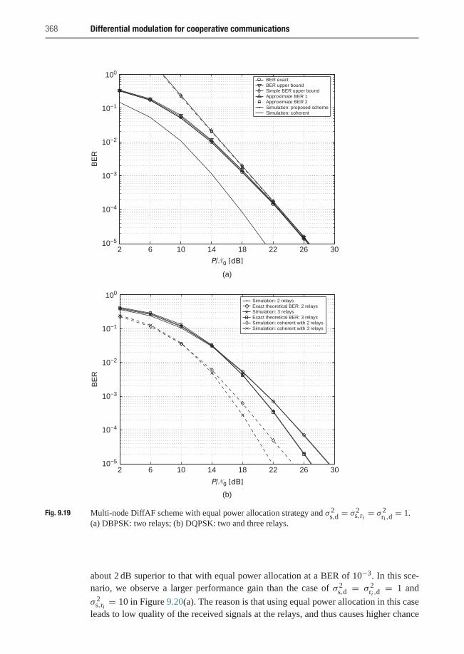
368 Differential modulation for cooperative communications
2 6 10 14 18 22 26 3010−5
10−4
10−3
10−2
10−1
100
BE
R
2 6 10 14 18 22 26 3010−5
10−4
10−3
10−2
10−1
100
(b)
(a)
BE
R
BER exactBER upper boundSimple BER upper boundApproximate BER 1Approximate BER 2Simulation: proposed schemeSimulation: coherent
Simulation: 2 relaysExact theoretical BER: 2 relaysSImulation: 3 relaysExact theoretical BER: 3 relaysSimulation: coherent with 2 relaysSimulation: coherent with 3 relays
P/�0 [dB]
P/�0 [dB]
Fig. 9.19 Multi-node DiffAF scheme with equal power allocation strategy and σ 2s,d = σ 2
s,ri = σ 2ri ,d
= 1.(a) DBPSK: two relays; (b) DQPSK: two and three relays.
about 2 dB superior to that with equal power allocation at a BER of 10−3. In this sce-nario, we observe a larger performance gain than the case of σ 2
s,d = σ 2ri ,d
= 1 and
σ 2s,ri = 10 in Figure 9.20(a). The reason is that using equal power allocation in this case
leads to low quality of the received signals at the relays, and thus causes higher chance
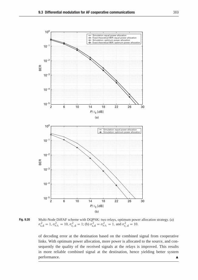
9.3 Differential modulation for AF cooperative communications 369
Simulation: equal power allocationSimulation: optimum power allocation
Simulation: equal power allocationExact theoretical BER: equal power allocationSimulation: optimum power allocationExact theoretical BER: optimum power allocation
2 6 10 14 18 22 26 3010−5
10−4
10−3
10−2
10−1
100
BE
R
2 6 10 14 18 22 26 3010−5
10−4
10−3
10−2
10−1
100
(b)
(a)
BE
R
P/�0 [dB]
P/�0 [dB]
Fig. 9.20 Multi-Node DiffAF scheme with DQPSK: two relays, optimum power allocation strategy. (a)σ 2
s,d = 1, σ 2s,ri = 10, σ 2
ri ,d= 1; (b) σ 2
s,d = σ 2s,ri = 1, and σ 2
ri ,d= 10.
of decoding error at the destination based on the combined signal from cooperativelinks. With optimum power allocation, more power is allocated to the source, and con-sequently the quality of the received signals at the relays is improved. This resultsin more reliable combined signal at the destination, hence yielding better systemperformance. �
370 Differential modulation for cooperative communications
9.4 Chapter summary and bibliographical notes
In the first part of this chapter, differential decode-and-forward schemes (DiffDF) forcooperative communications are presented. Both single-relay and multi-relay cooper-ation systems are given. By allowing the relay to forward only the correctly decodedsymbols and introducing a decision threshold at the destination node, the DiffDFscheme efficiently combines the signals from the direct and the relay links.
In case of the single-relay DiffDF scheme, BER analysis for DMPSK modulation iscategorized into six different scenarios that lead to different instantaneous SNRs at thecombiner output of the destination. A tight BER approximation is also provided. Basedon the tight BER approximation, the optimum decision threshold and power allocationare jointly determined. Both theoretical and simulation examples reveal that the opti-mum threshold and optimum power allocation rely on the qualities of the channel links.When the quality of the relay–destination link is much larger than the other links, i.e.,σ 2
s,d = σ 2s,r = 1 and σ 2
r,d = 10, then the decision threshold is more important than thepower allocation at high SNR. For instance, in case of DQPSK signals with equal powerallocation, using the optimum threshold resulted in an improvement gain of more than5 dB over the scheme without threshold at a BER of 10−4. By further using the optimumpower allocation, the performance improvement is about 0.5 dB at the same BER. Sim-ulation examples also showed that the DiffDF scheme with DQPSK signals provides aperformance improvement of 11 dB at a BER of 10−3 over the differential DF schemewhere the relay always forwards the decoded symbols.
In the case of the multi-node DiffDF scheme, a multi-node scenario follows theassumption that each of N cooperative relays forwards only correctly decoded sym-bols to the destination. Decision thresholds are used at the destination to efficientlycombine the signals from each relay–destination link with that from the direct link. Anapproximated BER analysis for DMPSK is provided, and a low-complexity BER lowerbound is derived. The BER lower bound is very close to the simulated performanceunder some scenarios. While jointly optimizing power allocation and thresholds basedon the BER lower bound introduces (2N + 1)-dimensional searching, the search spaceis reduced by assuming that the same power is used at each relay and the same thresholdis used at the destination. Numerical results reveal that more power should be allocatedat the source, with the rest allocated to the relays. In addition, a larger threshold shouldbe used when the relays are close to the destination. Simulation examples show that thediversity gain of the multi-node DiffDF scheme increases with the number of relays. Fora DBPSK cooperation system, the multi-node DiffDF scheme with different thresholdsleads to a performance improvement of up to 6 dB at a BER of 10−4. In the case of theDQPSK cooperation system, the multi-node DiffDF scheme with joint optimum powerallocation and optimum threshold achieves a gain of about 4–5 dB over the scheme withequal power allocation and a unit threshold at a BER of 10−3−10−4.
The second part of the chapter presents differential modulation for the amplify-and-forward cooperation protocol (DiffAF) for single-relay and multi-relay systems. Forthe single-relay DiffAF scheme, the DiffAF scheme with DQPSK signals yielded aperformance improvement of 4 dB at a BER of 10−3 over that of the DBPSK direct
9.4 Chapter summary and bibliographical notes 371
transmission scheme. In comparison to the coherent detection without relay, the DiffAFscheme provided a practical alternative with lower complexity and simpler implemen-tation. In addition, simulation examples showed that the performance of the DiffAFscheme was superior to that of direct transmission with coherent detection at SNRshigher than 21 dB. This is due to the fact that the cooperative communications providemore diversity gain than the direct transmission schemes. While the BER analysis of theDiffAF scheme is not available currently, we provided the exact BER expression basedon optimum combining weights, and it is considered to be a performance benchmark forthe DiffAF scheme. By using the obtained optimum power allocation based on the pro-vided BER expression, the DiffAF scheme is able to achieve comparable performanceto the scheme with optimum weights in any channel variances of all links. Moreover, theperformance of the scheme with optimum power strategy outperforms the equal powerscheme by about 1.4 dB at a BER of 10−3.
In the case of the multi-node DiffAF scheme, the BER expression for DMPSK modu-lation based on optimum combining weights is given; it is considered as a performancebenchmark of the multi-node DiffAF scheme. BER upper bounds and BER approxi-mations are provided; they are tight to the simulated performance, especially at highSNR. The theoretical BER reveals that the diversity order of the multi-node DiffAFscheme is N + 1, where N is the number of relays, and this is confirmed by the sim-ulation results. There is a gain of about 1.7–2 dB at a BER of 10−3 when N increasesfrom 2 to 3. The BER approximation is further simplified; based on the approximateBER, power allocation can be optimized by using a low-complexity single-dimensionalsearch. Simulation examples show that when all relays are close to the source, the multi-node DiffAF scheme obtains a gain of about 0.6 dB over the scheme with equal powerallocation at a BER of 10−3. When all relays are close to the destination, the perfor-mance with optimum power allocation achieves an improvement of about 2 dB overthat with equal power allocation.
The study of MIMO channel capacity was presented in [215] and many works onMIMO systems assuming full CSI available at the transmitter have been given, forexample in [212, 215, 109, 5, 213, 213, 198, 3, 111, 199, 46, 135, 206]. In conventionalsingle-antenna systems, noncoherent modulation is useful when the knowledge of CSI isnot available. The noncoherent modulation simplifies the receiver structure by omittingchannel estimation and carrier or phase trackings. Some examples of the noncoherentmodulation techniques are noncoherent frequency shift keying (NFSK) and differen-tial modulation [146]. Among these modulation techniques, the differential schemeis preferred to NFSK because it provides a better performance at the same operatingSNR. Two classes of differential modulation schemes are available: differential M-aryquadrature amplitude modulation (DMQAM) and differential M-ary phase shift keying(DMPSK). In the DMQAM scheme, information is modulated through the amplitudedifference between two consecutive symbols. The DMPSK, however, modulates infor-mation through the phase difference among two consecutive symbols. For a data rate ofR bits per channel use, DPMSK signal constellation contains M = 2R symbols. Eachof the symbol m ∈ 0 ≤ M − 1 is generated by the m-th root of unity: vm = ej2πm/M .
To learn more about this topic, interested readers should also refer to [66, 67].
372 Differential modulation for cooperative communications
Exercises
9.1 Assume that the Rayleigh fading channels hτs,d, hτs,r, and hτr,d are independent of
each other. Prove the average BER P(i)BER, i = 1, 2, . . . , 6, which are specified in(9.58), (9.61), (9.64), (9.65), and (9.67), respectively.
9.2 Prove the probabilities for different scenarios specified in (9.46)–(9.88), respec-tively, i.e.,
Phr (�3) =M2
(P2|hτr,d|2, ζ
) (1−�(γ τs,r)
)2×(
1
�(P1|hτs,r|2, P2|hτr,d|2)− 1
(1− e−ζ 2/N0)�(γ τs,r)
),
Phr (�4) = Ph
r (�5)
=M(
P2|hτr,d|2, ζ)
exp(−ζ 2/N0)�(γτs,r)(1−�(γ τs,r)
)�(P1|hτs,r|2, P2|hτr,d|2)
,
Phr (�6) =
exp(−2ζ 2/N0)�(γτs,r)
�(P1|hτs,r|2, P2|hτr,d|2).
9.3 Prove the probability approximations in (9.95) and (9.98) for the differential DFcooperative scheme.
9.4 For the differential AF cooperative scheme, prove the moment generationfunctions Mγ1(θ) and Mγ2(θ), specified in (9.121) and (9.123), respectively.
9.5 Prove the moment generation function MγAFi(θ), specified in (9.145).
9.6 (Simulation project) Consider a simplified model with a source node, a relaynode, and a destination node. The source–destination channel hs,d, the source–relay channel hs,r, and the relay–destination channel hr,d are modeled as indepen-dent zero-mean, complex Gaussian random variables with variances δ2
s,d, δ2s,r, and
δ2r,d, respectively. Assume that δ2
s,d = δ2s,r = δ2
r,d = 1, and DQPSK modulationis used. In this project, we compare performances of the threshold-based differ-ential DF cooperation scheme with choices of power allocations and decisionthreshold at the destination.(a) Simulate the threshold-based differential DF scheme with an equal power
allocation scheme (P1 = P2) and a decision threshold of ζ = 1. Comparesthe simulated BER performance with the BER approximation (9.69), theBER upper bound (9.70), and the BER lower bound (9.75).
(b) With the equal power allocation (P1 = P2), simulate the differential DFscheme without threshold at the destination and the differential DF schemethat the relay always forwards the decoded symbols to the destination. Com-pare their BER performances with that of the threshold-based differentialDF scheme simulated in (a).
(c) Simulate the threshold-based differential DF scheme with different thresh-olds (for example, ζ = 0.5, 1 or 2). Compare the BER performances anddetermine a best threshold.
Exercises 373
(d) Repeat (a), (b), and (c) for an unequal power allocation (P1/P2 = 9).9.7 (Simulation project) We consider a differential AF cooperative scheme with a
single-relay node. The source–destination channel hs,d, the source–relay channelhs,r, and the relay–destination channel hr,d are modeled as independent zero-mean, complex Gaussian random variables with variances δ2
s,d, δ2s,r, and δ2
r,d,
respectively. Assume that δ2s,d = δ2
s,r = δ2r,d = 1, and DQPSK modulation and an
equal power allocation scheme (P1 = P2) are used.(a) Simulate the differential AF cooperative scheme, the direct differential
scheme, and their coherent counterparts, respectively. Compare their per-formances and explain.
(b) Simulate the differential AF scheme with an equal weight combining,the weight combining proposed in (9.111), and the ideal maximum ratiocombining (9.112), respectively, and compare their performances.
(c) Repeat (a) and (b) for an unequal power allocation (P1/P2 = 4).
10 Energy efficiency in cooperativesensor networks
In the previous chapters, the gains of cooperative diversity were established underthe ideal model of negligible listening and computing power. In sensor networks, anddepending on the type of motes used, the power consumed in receiving and processingmay constitute a significant portion of the total consumed power. Cooperative diversitycan provide gains in terms of savings in the required transmit power in order to achievea certain performance requirement because of the spatial diversity it adds to the system.However, if one takes into account the extra processing and receiving power consump-tion at the relay and destination nodes required for cooperation, then there is obviouslya tradeoff between the gains in the transmit power and the losses due to the receive andprocessing powers when applying cooperation. Hence, there is a tradeoff between thegains promised by cooperation, and this extra overhead in terms of the energy efficiencyof the system should be taken into consideration in the design of the network.
In this chapter the gains of cooperation under this extra overhead are studied. More-over, some practical system parameters, such as the power amplifier loss, the quality ofservice (QoS) required, the relay location, and the optimal number of relays, are consid-ered. Two communications architectures are considered, direct transmission and coop-erative transmission. The performance metric for comparison between the two archi-tectures is the energy efficiency of the communication scheme. More specifically, forboth architectures the optimal total power consumption to achieve certain QoS require-ments is computed, and the cooperation gain is defined as the ratio between the powerrequired for direct transmission and cooperation. When this ratio is smaller than one,this indicates that direct transmission is more energy efficient, and that the extra over-head induced by cooperation overweighs its gains in the transmit power. Comparisonsbetween optimal power allocation at the source and relay nodes and equal power alloca-tion are demonstrated. The results reveal that, under some scenarios, equal power allo-cation is almost equivalent to optimal power allocation. The effect of relay location onthe performance is investigated to provide guidelines for relay assignment algorithms.
10.1 System model
Consider a single source–destination pair separated by a distance rs,d. The number ofpotential relays available to help the source is N . This is illustrated in Figure 10.1, wherethe distances between source and relay i , and relay i and destination are rs,i and ri,d,
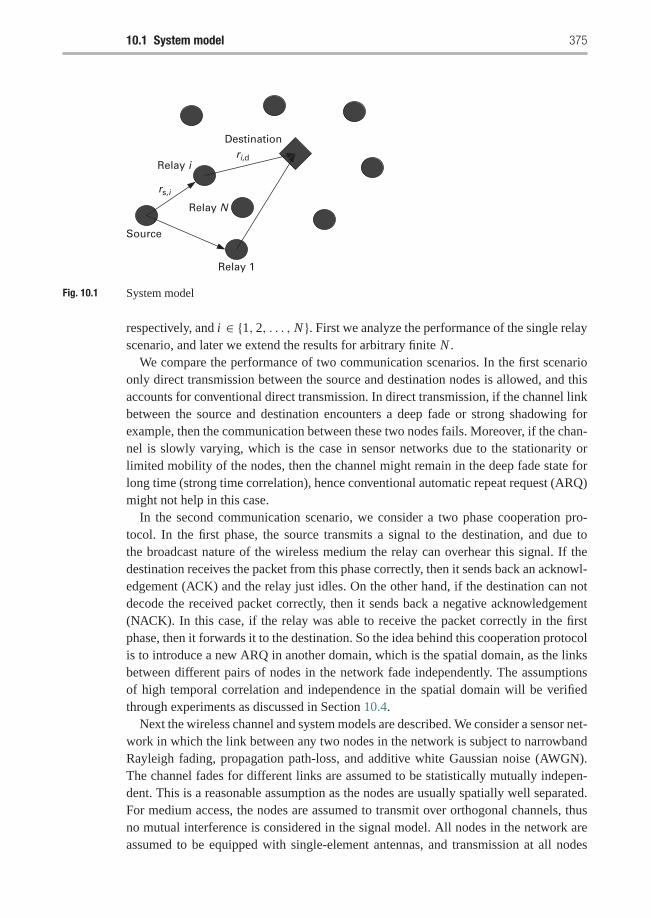
10.1 System model 375
Source
Relay 1
Relay N
Relay i
Destinationri,d
rs,i
Fig. 10.1 System model
respectively, and i ∈ {1, 2, . . . , N }. First we analyze the performance of the single relayscenario, and later we extend the results for arbitrary finite N .
We compare the performance of two communication scenarios. In the first scenarioonly direct transmission between the source and destination nodes is allowed, and thisaccounts for conventional direct transmission. In direct transmission, if the channel linkbetween the source and destination encounters a deep fade or strong shadowing forexample, then the communication between these two nodes fails. Moreover, if the chan-nel is slowly varying, which is the case in sensor networks due to the stationarity orlimited mobility of the nodes, then the channel might remain in the deep fade state forlong time (strong time correlation), hence conventional automatic repeat request (ARQ)might not help in this case.
In the second communication scenario, we consider a two phase cooperation pro-tocol. In the first phase, the source transmits a signal to the destination, and due tothe broadcast nature of the wireless medium the relay can overhear this signal. If thedestination receives the packet from this phase correctly, then it sends back an acknowl-edgement (ACK) and the relay just idles. On the other hand, if the destination can notdecode the received packet correctly, then it sends back a negative acknowledgement(NACK). In this case, if the relay was able to receive the packet correctly in the firstphase, then it forwards it to the destination. So the idea behind this cooperation protocolis to introduce a new ARQ in another domain, which is the spatial domain, as the linksbetween different pairs of nodes in the network fade independently. The assumptionsof high temporal correlation and independence in the spatial domain will be verifiedthrough experiments as discussed in Section 10.4.
Next the wireless channel and system models are described. We consider a sensor net-work in which the link between any two nodes in the network is subject to narrowbandRayleigh fading, propagation path-loss, and additive white Gaussian noise (AWGN).The channel fades for different links are assumed to be statistically mutually indepen-dent. This is a reasonable assumption as the nodes are usually spatially well separated.For medium access, the nodes are assumed to transmit over orthogonal channels, thusno mutual interference is considered in the signal model. All nodes in the network areassumed to be equipped with single-element antennas, and transmission at all nodes
376 Energy efficiency in cooperative sensor networks
is constrained to the half-duplex mode, i.e., any terminal cannot transmit and receivesimultaneously.
The power consumed in a transmitting or receiving stage is described as follows. Ifa node transmits with power P , only P(1− α) is actually utilized for RF transmission,where (1 − α) accounts for the efficiency of the RF power amplifier which generallyhas a non-linear gain function. The processing power consumed by a transmitting nodeis denoted by Pc. Any receiving node consumes Pr power units to receive the data. Thevalues of the parameters α, Pr, Pc are assumed the same for all nodes in the network andare specified by the manufacturer. Following, we describe the received signal model forboth direct and cooperative transmissions.
First, we describe the received signal model for the direct transmission mode. In thedirect transmission scheme, which is employed in current wireless networks, each usertransmits their signal directly to the next node in the route which we denote as thedestination d here. The signal received at the destination d from source user s, can bemodeled as
ys,d =√
PDs (1− α)r−γs,d hs,dx + ns,d, (10.1)
where PDs is the transmission power from the source in the direct communication sce-
nario, x is the transmitted data with unit power, hs,d is the channel fading gain betweenthe two terminals s and d. The channel fade of any link is modeled as a zero mean cir-cularly symmetric complex Gaussian random variable with unit variance. In (10.1), γis the path loss exponent, and rs,d is the distance between the two terminals. The termns,d in (10.1) denotes additive noise; the noise components throughout the paper aremodeled as white Gaussian noise (AWGN) with variance N0.
Second, we describe the signal model for cooperative transmission. The cooperativetransmission scenario comprises two phases as illustrated before. The signals receivedfrom the source at the destination d and relay 1 in the first stage can be modeledrespectively as,
ys,d =√
PCs (1− α)r−γs,d hs,dx + ns,d, (10.2)
ys1 =√
PCs (1− α)r−γs,1 hs,1x + ns,1, (10.3)
where PCs is the transmission power from the source in the cooperative scenario. The
channel gains hs,d and hs,1 between the source–destination and source–relay are mod-eled as zero-mean circular symmetric complex Gaussian random variables with zeromean. If the SNR of the signal received at the destination from the source falls belowthe threshold β, the destination broadcasts a NACK. In this case, if the relay was ableto receive the packet from the source correctly in the first phase, it forwards the packetto the destination with power P1
y1,d =√
P1(1− α)r−γ1,d h1,dx + n1,d. (10.4)
Cooperation results in additional spatial diversity by introducing this artificial mul-tipath through the relay link. This can enhance the transmission reliability against
10.2 Performance analysis and optimum power allocation 377
wireless channel impairmens as fading, but will also result in extra receiving andprocessing power. In the next section, we discuss this in more detail.
10.2 Performance analysis and optimum power allocation
We characterize the system performance in terms of outage probability. Outage isdefined as the event that the received SNR falls below a certain threshold β, hence,the probability of outage PO is defined as
PO = P(SNR ≤ β). (10.5)
If the received SNR is higher than the threshold β, the receiver is assumed to be able todecode the received message with negligible probability of error. If an outage occurs,the packet is considered lost. The SNR threshold β is determined according to the appli-cation and the transmitter/receiver structure. For example, larger values of β is requiredfor applications with higher QoS requirements. Also increasing the complexity of trans-mitter and/or receiver structure, for example applying strong error coding schemes, canreduce the value of β for the same QoS requirements.
Based on the derived outage probability expressions, we can formulate a constrainedoptimization problem to minimize the total consumed power subject to a given outageperformance. We then compare the total consumed power for the direct and coopera-tive scenarios to quantify the energy savings, if any, gained by applying cooperativetransmission.
10.2.1 Direct transmission
As discussed before, the outage is defined as the event that the received SNR falls belowa predefined threshold which we denoted by β. From the received signal model in (10.1),the received SNR from a user at a distance rs,d from the destination is given by
SNR(rs,d) =| hs,d |2 r−γs,d PD
s (1− α)N0
, (10.6)
where | hs,d |2 is the magnitude square of the channel fade and follows an exponentialdistribution with unit mean; this follows because of the Gaussian zero mean distributionof hs,d. Hence, the outage probability for the direct transmission mode POD can becalculated as
POD = P(SNR(rs,d) ≤ β
) = 1− exp
(− N0γ rγs,d(1− α)PD
s
). (10.7)
The total transmitted power PDtot for the direct transmission mode is given by
PDtot = PD
s + Pc + Pr, (10.8)
where PDs is the power consumed at the RF stage of the source node, Pc is the pro-
cessing power at the source node, and Pr is the receiving power at the destination. The
378 Energy efficiency in cooperative sensor networks
requirement is to minimize this total transmitted power subject to the constraint that wemeet a certain QoS requirement that the outage probability is less than a given outagerequirement, which we denote by P∗out. Since both the processing and receiving powersare fixed, the only variable of interest is the transmitting power PD
s .The optimization problem can be formulated as follows:
minPD
s
PDtot, (10.9)
s.t. POD ≤ P∗out. (10.10)
The outage probability POD is a decreasing function in the power PDs . Substituting P∗out
in the outage expression in (10.7), we get after some simple arithmetics that the optimaltransmitting power is given by
PD∗s = − βN0rγs,d
(1− α) ln(1− P∗out). (10.11)
The minimum total power required for direct transmission in order to achieve therequired QoS requirement is therefore given by
P∗tot = Pc + Pr −βN0rγs,d
(1− α) ln(1− P∗out). (10.12)
In the next subsection we formulate the optimal power allocation problem for thecooperative communication scenario.
10.2.2 Cooperative transmission
For the optimal power allocation problem in cooperative transmission, we consider twopossible scenarios.
• In the first scenario, the relay is allowed to transmit with different power than thesource and hence the optimization space is two-dimensional: source and relay powerallocations. The solution for this setting provides the minimum possible total con-sumed power. However, the drawback of this setting is that the solution for theoptimization problem is complex and might not be feasible to implement in sensornodes.
• The second setting that we consider is constraining the source and relay nodes to trans-mit with equal power. This is much easier to implement as the optimization space isone dimensional in this case, moreover, a relaxed version of the optimization problemcan render a closed form solution.
Clearly the solution of the equal power allocation problem provides a suboptimal solu-tion to the general case in which we allow different power allocations at the source andthe relay. It is interesting then to investigate the conditions under which these two powerallocation strategies have close performance.
First, we characterize the optimal power allocations at the source and relay nodes.Consider a source–destination pair that are rs,d units distance. Let us compute the con-ditional outage probability for given locations of the source and the helping relay. As
10.2 Performance analysis and optimum power allocation 379
discussed before, cooperative transmission encompasses two phases. Using (10.2), theSNR received at the destination d and relay 1 from the source s in the first phase aregiven by
SNRs,d =| hs,d |2 r−γs,d PC
s (1− α)N0
, (10.13)
SNRs,1 =| hs,1 |2 r−γs,1 PC
s (1− α)N0
. (10.14)
While from (10.4), the SNR received at the destination from the relay in the secondphase is given by
SNR1,d =| h1,d |2 r−γ1,d P1(1− α)
N0. (10.15)
Note that the second phase of transmission is only initiated if the packet received atthe destination from the first transmission phase is not correctly received. The terms| hs,d |2, | hs,1 |2, and | h1,d |2 are mutually independent exponential random variableswith unit mean.
The outage probability of the cooperative transmission POC can be calculated asfollows
POC = P((
SNRs,d ≤ β) ∩ (SNRs,l ≤ β
))+ P
((SNRs,d ≤ β
) ∩ (SNRl,d ≤ β) ∩ (SNRs,l > β
))=(1− f (rs,d, PC
s )) (
1− f (rs,l, PCs ))
+(1− f (rs,d, PC
s )) (
1− f (rl,d, Pl))
f (rs,l, PCs ), (10.16)
where
(x, y) = exp
(− N0βxγ
y(1− α)). (10.17)
The first term in the above expression corresponds to the event that both the source–destination and the source–relay channels are in outage, and the second term cor-responds to the event that both the the source–destination and the relay–destinationchannels are in outage while the source–relay channel is not. The above expression canbe simplified as follows
POC =(1− f (rs,d, PC
s )) (
1− f (rl,d, Pl) f (rs,l, PCs )). (10.18)
The total average consumed power for cooperative transmission to transmit a packetis given by
E[PCtot] = (PC
s + Pc + 2Pr)P(SNRs,d ≥ β)+ (PC
s + Pc + 2Pr)P(SNRs,d < β)P(SNRs,1 < β)
+ (PCs + P1 + 2Pc + 3Pr)P(SNRs,d < β)P(SNRs,1 > β),
380 Energy efficiency in cooperative sensor networks
where the first term in the right-hand side corresponds to the event that the direct linkin the first phase is not in outage, therefore, the total consumed power is only given bythat of the source node, and the 2 in front of the received power term Pr is to account forthe relay receiving power. The second term in the summation corresponds to the eventthat both the direct and the source–relay links are in outage, hence the total consumedpower is still given as in the first term. The last term in the total summation accounts forthe event that the source–destination link is in outage while the source–relay link is not,and hence we need to account for the relay transmitting and processing powers, and theextra receiving power at the destination. Using the Rayleigh fading channel model, theaverage total consumed power can be given as follows
PCtot = (PC
s + Pc + 2Pr) f (rs,d, PCs )
+ (PCs + Pc + 2Pr)
(1− f (rs,d, PC
s )) (
1− f (rs,l, PCs ))
+ (PCs + P1 + 2Pc + 3Pr)
(1− f (rs,d, PC
s ))× f (rs,l, PC
s ).
(10.19)
We can formulate the power minimization problem in a similar way to (10.10) withthe difference that there are two optimization variables in the cooperative transmissionmode, namely, the transmit powers PC
s and P1 at the source and relay nodes respectively.The optimization problem can be stated as follows
minPC
s ,P1
PCtot(P
Cs , P1), (10.20)
s.t. POC(PCs , P1) ≤ P∗out. (10.21)
This optimization problem is nonlinear and does not admit a closed form solution.Therefore we resort to numerical optimization techniques in order to solve for thispower allocation problem at the relay and source nodes, and the results are shown inthe simulations section.
In the above formulation we considered optimal power allocation at the sourceand relay node in order to meet the outage probability requirement. The performanceattained by such an optimization problem provides a benchmark for the cooperativetransmission scheme. However, in a practical setting, it might be difficult to implementsuch a complex optimization problem at the sensor nodes. A more practical scenariowould be that all the nodes in the network utilize the same power for transmission.Denote the equal transmission power in this case by PCE; the optimization problem canthen be formulated as
minPCE
PCtot(PCE),
s.t. POC(PCE) ≤ P∗out.
Beside being a one-dimensional optimization problem that can be easily solved, theproblem can be relaxed to render a closed form solution. Note that at enough high SNRthe following approximation holds exp(−x) � (1 − x); where x here is proportionalto 1/SN R.
10.3 Multi-relay scenario 381
Using the above approximation in (10.19), and after some mathematical manipula-tion, the total consumed power can be approximated as follows
PCtot � PCE + Pc + 2Pr + (PCE + Pc + Pr)
k1
PCE− (PCE + Pc + Pr)
k1k2
P2CE
.
Similarly, the outage probability can be written as follows
POC � k1k2
P2CE
+ k1k3
P2CE
− k1k2k3
P3CE
, (10.22)
where k1 = βN0rγs,d/(1 − α), k2 = βN0rγs,l/(1 − α), and k3 = βN0rγl,d/(1 − α). Thisis a constrained optimization problem in one variable and its Lagrangian is given by
∂PCtot
∂PCE+ λ∂POC
∂PCE= 0, (10.23)
where the derivatives of the total power consumption PCtot and the outage probability
POC with respect to the transmit power PCE are given by
∂PCtot
∂PCE= 1+ k1k2 − (Pc + Pr)k1
P2CE
+ 2k1k2(Pc + Pr)
P3CE
; (10.24)
∂POC
∂PCE= −2(k1k2 + k1k3)
P3CE
+ 3k1k2k3
P4CE
, (10.25)
respectively. Substituting the derivatives in (10.25) into the Lagrangian in (10.23), anddoing simple change of variables 1/PCE = x , the Lagrangian can be written in thefollowing simple polynomial form
1+ (k1k2 − (Pc + Pr)k1)x2 + 2(k1k2(Pc + Pr)
− λ(k1k2 + k1k3))x3 + 3λk1k2k3x4 = 0,
under the outage constraint
(k1k2 + k1k3) x2 − k1k2k3x3 = P∗out. (10.26)
The constraint equation above is only a polynomial of order three, so it can be easilysolved and we can find the root that minimizes the cost function.
10.3 Multi-relay scenario
In this section, we extend the study to the case when there is more than one potentialrelay. Let N be the number of relays assigned to help a given source. The cooperationprotocol then works as an N -stage ARQ protocol as follows. The source node transmitsits packets to the destination and the relays try to decode this packet. If the destinationdoes not decode the packet correctly, it sends a NACK that can be heard by the relays.If the first relay is able to decode the packet correctly, it forwards the packet with powerP1 to the destination. If the destination does not receive correctly again, then it sends aNACK and the second candidate relay, if it received the packet correctly, forwards the
382 Energy efficiency in cooperative sensor networks
source’s packet to the destination with power P2. This is repeated until the destinationgets the packet correctly or the N trials corresponding to the N relays are exhausted.
We model the status of any relay by 1 or 0, corresponding to whether the relayreceived the source’s packet correctly or not, respectively. Writing the status of all therelays in a column vector results in a N×1 vector whose entries are either 0 or 1. Hence,the decimal number representing this N × 1 vector can take any integer value between0 and 2N − 1. Denote this vector by Sk , where k ∈ {0, 1, 2, . . . , 2N − 1}.
For a given status of the N relays, an outage occurs if and only if the links betweenthe relays that decoded correctly and the destination are all in outage. Denote the set ofthe relays that received correctly by χ(Sk) = {i : Sk(i) = 1, 1 ≤ i ≤ N }, and χC(Sk)
as the set of relays that have not received correctly, i.e., χC(Sk) = {i : Sk(i) = 0, 1 ≤i ≤ N }. The conditional probability of outage given the relays status Sk is thus given by
POC|Sk = P
⎛⎝SNRs,d ≤ βN⋂
j∈χ(Sk)
(SNR jd ≤ β
)⎞⎠ , (10.27)
The total outage probability is thus given by
POC =2N−1∑k=0
P(Sk)POC|Sk . (10.28)
We then need to calculate the probability of the set Sk , which can then be written as
P(Sk) = P
⎛⎝ ⋂i∈χ(Sk )
(SNRsi ≥ β)⋂
j∈χc(Sk )
(SNRs j ≤ β
)⎞⎠ . (10.29)
The average outage probability expression can thus be given by
POC =2N−1∑k=0
(1− f (rs,d, PC
s ))∏
j∈χ(Sk )
(1− f (r jd , Pj )
)f (rs j , PC
s ) (10.30)
·∏
j∈χC(Sk )
(1− f (rs j , PC
s )). (10.31)
where Pj , j ∈ {1, 2, . . . , N }, is the power allocated to the j-th relay.Next we compute the average total consumed power for the N -relays scenario. First,
we condition on some relays’ status vector χ(Sk):
E[
PCtot
]= E
[E[
PCtot|χ (Sk)
]]=
2N−1∑k=0
P (χ(Sk))E[
PCtot|χ(Sk)
]. (10.32)
For a given χ (Sk), we can further condition on whether the source get the packetthrough from the first trial or not. This event happens with probability f (rs,d, PC
s ),and the consumed power in this case is given by
PC,1tot = PC
s + (N + 1)Pr + Pc; (10.33)
10.4 Experimental results 383
The complementary event that the source failed to transmit its packet from the directtransmission phase happens with probability 1− f (rs,d, PC
s ), and this event can be fur-ther divided into two mutually exclusive events. The first is when the first | χ(Sk) | −1relays from the set χ(Sk) fails to forward the packet and this happens with probability∏|χ(Sk)|−1
i=1
(1− f (ri,d, Pi )
)and the corresponding consumed power is given by
PC,2tot = PC
s + (N + 1+ | χ(Sk) |) Pr + (| χ(Sk) | +1) Pc +|χ(Sk)|∑
n=1
Pχ(Sk )(n); (10.34)
The second is when one of the intermediate relays in the set χ(Sk) successfully forwardsthe packet and this happens with probability
∏ j−1m=1
(1− f (rm,d , Pm)
)f (r j,d , Pj ) if this
intermediate relay was relay number j , and the corresponding power is given by
PC,3, jtot = PC
s + (N + 1+ j)Pr + (1+ j)Pc +j∑
i=1
Pχ(Sk )(i). (10.35)
From (10.32), (10.33), (10.34), and (10.35), the average total consumed power can begiven by
E[
PCtot
]=
2N−1∑k=0
P (χ(Sk)){
f (rs,d, PCs )P
C,1tot
+(1− f (rs,d, PC
s ))⎡⎣|χ(Sk)|−1∏
i=1
(1− f (ri,d,Pi )
)PC,2
tot
+|χ(Sk )|−1∑
j=1
j−1∏m=1
(1− f (rm,d, Pm)
)f (r j,d, Pj )P
C,3, jtot
⎤⎦⎫⎬⎭ .The optimization problem can then be written as
minP
PCtot(P),
s.t. POC(P) ≤ P∗out.
where P = [PCs , P1, P2, . . . , PN
]T.
10.4 Experimental results
In the system model, it is assumed that the channel independence between the followinglinks: the source–relay link, the source–destination link, and the relay–destination link.Moreover, a strong motivation for applying cooperative transmission instead of ARQ inthe time domain, is the assumption of high temporal correlation which results in delayand requires performing interleaving at the transmitter side. In this section, we show theresults for a set of experiments to justify these two fundamental assumptions.
The experiments are set up as follows. We have three wireless nodes in the experi-ments, one of them acts as the sender and the other two act as receivers. Each wireless
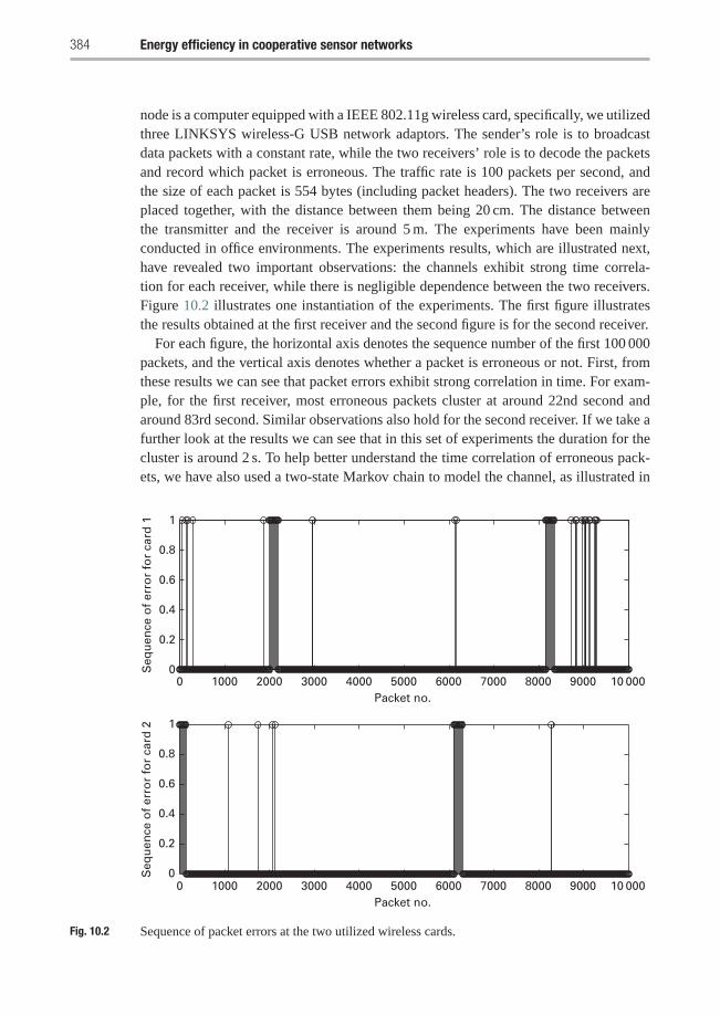
384 Energy efficiency in cooperative sensor networks
node is a computer equipped with a IEEE 802.11g wireless card, specifically, we utilizedthree LINKSYS wireless-G USB network adaptors. The sender’s role is to broadcastdata packets with a constant rate, while the two receivers’ role is to decode the packetsand record which packet is erroneous. The traffic rate is 100 packets per second, andthe size of each packet is 554 bytes (including packet headers). The two receivers areplaced together, with the distance between them being 20 cm. The distance betweenthe transmitter and the receiver is around 5 m. The experiments have been mainlyconducted in office environments. The experiments results, which are illustrated next,have revealed two important observations: the channels exhibit strong time correla-tion for each receiver, while there is negligible dependence between the two receivers.Figure 10.2 illustrates one instantiation of the experiments. The first figure illustratesthe results obtained at the first receiver and the second figure is for the second receiver.
For each figure, the horizontal axis denotes the sequence number of the first 100 000packets, and the vertical axis denotes whether a packet is erroneous or not. First, fromthese results we can see that packet errors exhibit strong correlation in time. For exam-ple, for the first receiver, most erroneous packets cluster at around 22nd second andaround 83rd second. Similar observations also hold for the second receiver. If we take afurther look at the results we can see that in this set of experiments the duration for thecluster is around 2 s. To help better understand the time correlation of erroneous pack-ets, we have also used a two-state Markov chain to model the channel, as illustrated in
0 1000 2000 3000 4000 5000 6000 7000 8000 9000 10 0000
0.2
0.4
0.6
0.8
1
Packet no.
0 1000 2000 3000 4000 5000 6000 7000 8000 9000 10 000Packet no.
Seq
uen
ce o
f er
ror
for
card
1
0
0.2
0.4
0.6
0.8
1
Seq
uen
ce o
f er
ror
for
card
2
Fig. 10.2 Sequence of packet errors at the two utilized wireless cards.
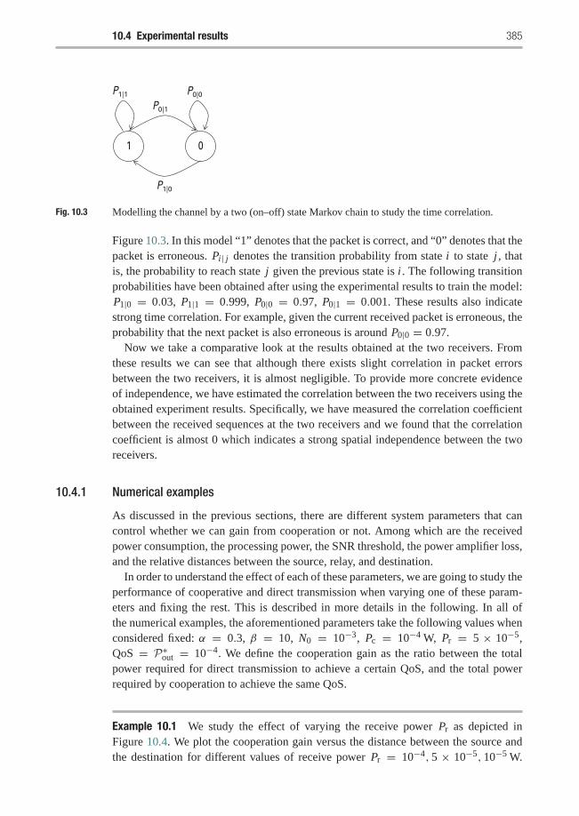
10.4 Experimental results 385
P0|1
P1|0
P0|0P1|1
1 0
Fig. 10.3 Modelling the channel by a two (on–off) state Markov chain to study the time correlation.
Figure 10.3. In this model “1” denotes that the packet is correct, and “0” denotes that thepacket is erroneous. Pi | j denotes the transition probability from state i to state j , thatis, the probability to reach state j given the previous state is i . The following transitionprobabilities have been obtained after using the experimental results to train the model:P1|0 = 0.03, P1|1 = 0.999, P0|0 = 0.97, P0|1 = 0.001. These results also indicatestrong time correlation. For example, given the current received packet is erroneous, theprobability that the next packet is also erroneous is around P0|0 = 0.97.
Now we take a comparative look at the results obtained at the two receivers. Fromthese results we can see that although there exists slight correlation in packet errorsbetween the two receivers, it is almost negligible. To provide more concrete evidenceof independence, we have estimated the correlation between the two receivers using theobtained experiment results. Specifically, we have measured the correlation coefficientbetween the received sequences at the two receivers and we found that the correlationcoefficient is almost 0 which indicates a strong spatial independence between the tworeceivers.
10.4.1 Numerical examples
As discussed in the previous sections, there are different system parameters that cancontrol whether we can gain from cooperation or not. Among which are the receivedpower consumption, the processing power, the SNR threshold, the power amplifier loss,and the relative distances between the source, relay, and destination.
In order to understand the effect of each of these parameters, we are going to study theperformance of cooperative and direct transmission when varying one of these param-eters and fixing the rest. This is described in more details in the following. In all ofthe numerical examples, the aforementioned parameters take the following values whenconsidered fixed: α = 0.3, β = 10, N0 = 10−3, Pc = 10−4 W, Pr = 5 × 10⁻⁵,QoS = P∗out = 10−4. We define the cooperation gain as the ratio between the totalpower required for direct transmission to achieve a certain QoS, and the total powerrequired by cooperation to achieve the same QoS.
Example 10.1 We study the effect of varying the receive power Pr as depicted inFigure 10.4. We plot the cooperation gain versus the distance between the source andthe destination for different values of receive power Pr = 10−4, 5 × 10⁻⁵, 10−5 W.
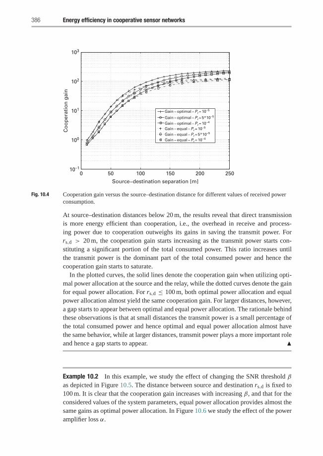
386 Energy efficiency in cooperative sensor networks
0 50 100 150 200 25010–1
100
101
102
103
Source−destination separation [m]
Co
op
erat
ion
gai
n
Gain − optimal − Pr = 5*10−5
Gain − equal − Pr = 5*10−5
Gain − equal − Pr = 10−4
Gain − optimal − Pr = 10−4
Gain − optimal − Pr = 10−5
Gain − equal − Pr = 10−5
Fig. 10.4 Cooperation gain versus the source–destination distance for different values of received powerconsumption.
At source–destination distances below 20 m, the results reveal that direct transmissionis more energy efficient than cooperation, i.e., the overhead in receive and process-ing power due to cooperation outweighs its gains in saving the transmit power. Forrs,d > 20 m, the cooperation gain starts increasing as the transmit power starts con-stituting a significant portion of the total consumed power. This ratio increases untilthe transmit power is the dominant part of the total consumed power and hence thecooperation gain starts to saturate.
In the plotted curves, the solid lines denote the cooperation gain when utilizing opti-mal power allocation at the source and the relay, while the dotted curves denote the gainfor equal power allocation. For rs,d ≤ 100 m, both optimal power allocation and equalpower allocation almost yield the same cooperation gain. For larger distances, however,a gap starts to appear between optimal and equal power allocation. The rationale behindthese observations is that at small distances the transmit power is a small percentage ofthe total consumed power and hence optimal and equal power allocation almost havethe same behavior, while at larger distances, transmit power plays a more important roleand hence a gap starts to appear. �
Example 10.2 In this example, we study the effect of changing the SNR threshold βas depicted in Figure 10.5. The distance between source and destination rs,d is fixed to100 m. It is clear that the cooperation gain increases with increasing β, and that for theconsidered values of the system parameters, equal power allocation provides almost thesame gains as optimal power allocation. In Figure 10.6 we study the effect of the poweramplifier loss α.
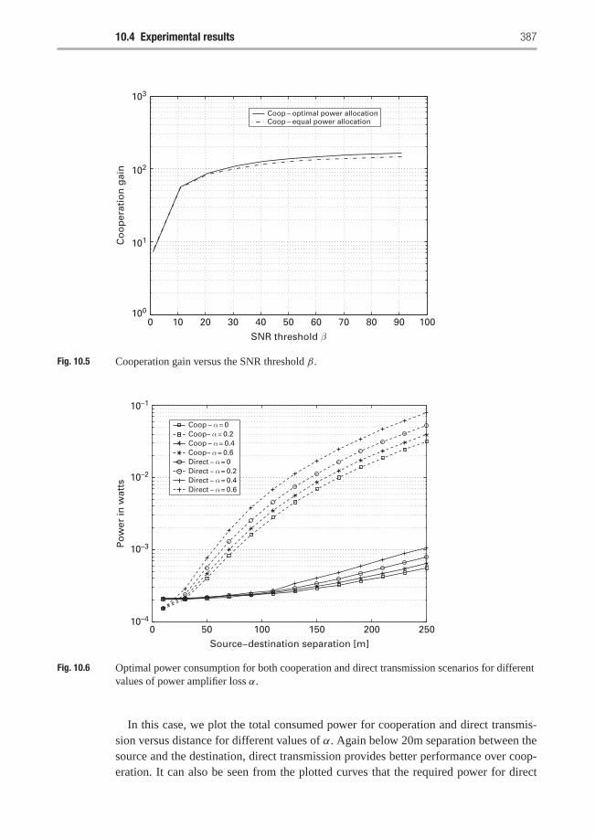
10.4 Experimental results 387
0 10 20 30 40 50 60 70 80 90 100
103
102
101
100
SNR threshold β
Co
op
erat
ion
gai
nCoop − optimal power allocationCoop − equal power allocation
Fig. 10.5 Cooperation gain versus the SNR threshold β.
0 50 100 150 200 250Source−destination separation [m]
Po
wer
in w
atts
Coop − α = 0Coop− α = 0.2Coop − α = 0.4Coop− α = 0.6Direct − α = 0Direct − α = 0.2Direct − α = 0.4Direct − α = 0.6
10–1
10–2
10–3
10–4
Fig. 10.6 Optimal power consumption for both cooperation and direct transmission scenarios for differentvalues of power amplifier loss α.
In this case, we plot the total consumed power for cooperation and direct transmis-sion versus distance for different values of α. Again below 20m separation between thesource and the destination, direct transmission provides better performance over coop-eration. It can also be seen from the plotted curves that the required power for direct
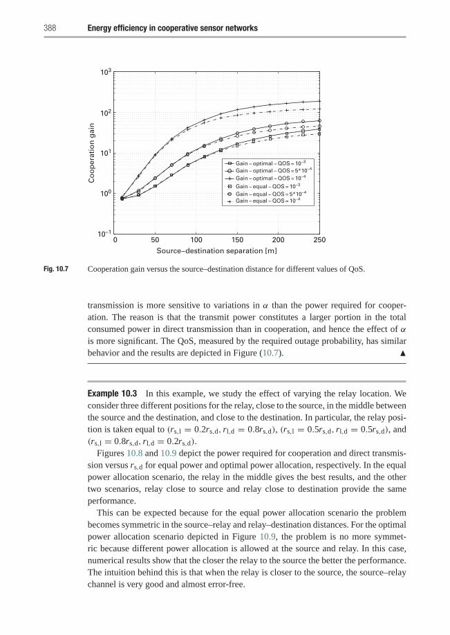
388 Energy efficiency in cooperative sensor networks
0 50 100 150 200 250
103
102
100
10–1
101
Source−destination separation [m]
Co
op
erat
ion
gai
n
Gain − optimal − QOS = 10−3
Gain − equal − QOS = 10−3
Gain − optimal − QOS = 5*10−4
Gain − equal − QOS = 5*10−4
Gain − optimal − QOS = 10−4
Gain − equal − QOS = 10−4
Fig. 10.7 Cooperation gain versus the source–destination distance for different values of QoS.
transmission is more sensitive to variations in α than the power required for cooper-ation. The reason is that the transmit power constitutes a larger portion in the totalconsumed power in direct transmission than in cooperation, and hence the effect of αis more significant. The QoS, measured by the required outage probability, has similarbehavior and the results are depicted in Figure (10.7). �
Example 10.3 In this example, we study the effect of varying the relay location. Weconsider three different positions for the relay, close to the source, in the middle betweenthe source and the destination, and close to the destination. In particular, the relay posi-tion is taken equal to (rs,l = 0.2rs,d, rl,d = 0.8rs,d), (rs,l = 0.5rs,d, rl,d = 0.5rs,d), and(rs,l = 0.8rs,d, rl,d = 0.2rs,d).
Figures 10.8 and 10.9 depict the power required for cooperation and direct transmis-sion versus rs,d for equal power and optimal power allocation, respectively. In the equalpower allocation scenario, the relay in the middle gives the best results, and the othertwo scenarios, relay close to source and relay close to destination provide the sameperformance.
This can be expected because for the equal power allocation scenario the problembecomes symmetric in the source–relay and relay–destination distances. For the optimalpower allocation scenario depicted in Figure 10.9, the problem is no more symmet-ric because different power allocation is allowed at the source and relay. In this case,numerical results show that the closer the relay to the source the better the performance.The intuition behind this is that when the relay is closer to the source, the source–relaychannel is very good and almost error-free.
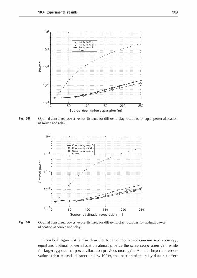
10.4 Experimental results 389
0 50 100 150 200 250
100
10–1
10–2
10–3
10–4
Source−destination separation [m]
Po
wer
Relay near DRelay in middleRelay near SDirect
Fig. 10.8 Optimal consumed power versus distance for different relay locations for equal power allocationat source and relay.
0 50 100 150 200 25010−4
10−3
10−2
10−1
100
Source−destination separation [m]
Op
tim
al p
ow
er
Coop−relay near DCoop−relay middleCoop−relay near SDirect
Fig. 10.9 Optimal consumed power versus distance for different relay locations for optimal powerallocation at source and relay.
From both figures, it is also clear that for small source–destination separation rs,d,equal and optimal power allocation almost provide the same cooperation gain whilefor larger rs,d optimal power allocation provides more gain. Another important obser-vation is that at small distances below 100 m, the location of the relay does not affect
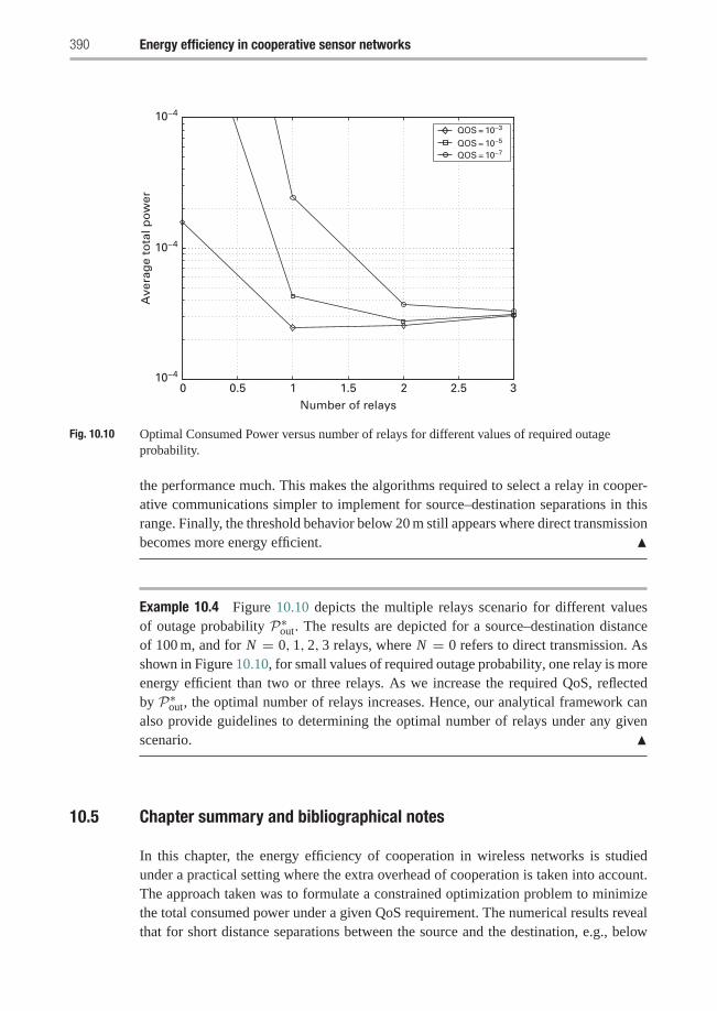
390 Energy efficiency in cooperative sensor networks
0 0.5 1 1.5 2 2.5 3
10−4
10−4
10−4
Number of relays
Ave
rag
e to
tal p
ow
erQOS = 10−3
QOS = 10−5
QOS = 10−7
Fig. 10.10 Optimal Consumed Power versus number of relays for different values of required outageprobability.
the performance much. This makes the algorithms required to select a relay in cooper-ative communications simpler to implement for source–destination separations in thisrange. Finally, the threshold behavior below 20 m still appears where direct transmissionbecomes more energy efficient. �
Example 10.4 Figure 10.10 depicts the multiple relays scenario for different valuesof outage probability P∗out. The results are depicted for a source–destination distanceof 100 m, and for N = 0, 1, 2, 3 relays, where N = 0 refers to direct transmission. Asshown in Figure 10.10, for small values of required outage probability, one relay is moreenergy efficient than two or three relays. As we increase the required QoS, reflectedby P∗out, the optimal number of relays increases. Hence, our analytical framework canalso provide guidelines to determining the optimal number of relays under any givenscenario. �
10.5 Chapter summary and bibliographical notes
In this chapter, the energy efficiency of cooperation in wireless networks is studiedunder a practical setting where the extra overhead of cooperation is taken into account.The approach taken was to formulate a constrained optimization problem to minimizethe total consumed power under a given QoS requirement. The numerical results revealthat for short distance separations between the source and the destination, e.g., below
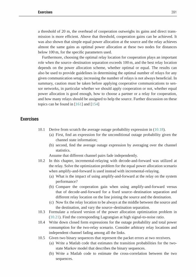
Exercises 391
a threshold of 20 m, the overhead of cooperation outweighs its gains and direct trans-mission is more efficient. Above that threshold, cooperation gains can be achieved. Itwas also shown that simple equal power allocation at the source and the relay achievesalmost the same gains as optimal power allocation at these two nodes for distancesbelow 100 m, for the specific parameters used.
Furthermore, choosing the optimal relay location for cooperation plays an importantrole when the source–destination separation exceeds 100 m, and the best relay locationdepends on the power allocation scheme, whether optimal or equal. The results canalso be used to provide guidelines in determining the optimal number of relays for anygiven communication setup; increasing the number of relays is not always beneficial. Insummary, caution must be taken before applying cooperative communications to sen-sor networks, in particular whether we should apply cooperation or not, whether equalpower allocation is good enough, how to choose a partner or a relay for cooperation,and how many relays should be assigned to help the source. Further discussion on thesetopics can be found in [161] and [154]
Exercises
10.1 Derive from scratch the average outage probability expression in (10.18).(a) First, find an expression for the unconditional outage probability given the
channel state information;(b) second, find the average outage expression by averaging over the channel
statistics.Assume that different channel pairs fade independently.
10.2 In this chapter, incremental-relaying with decode-and-forward was utilized atthe relay. Solve the optimization problem for the equal power allocation scenariowhen amplify-and-forward is used instead with incremental-relaying.(a) What is the impact of using amplify-and-forward at the relay on the system
performance?(b) Compare the cooperation gain when using amplify-and-forward versus
that of decode-and-forward for a fixed source–destination separation anddifferent relay location on the line joining the source and the destination.
(c) Now fix the relay location to be always at the middle between the source andthe destination, and vary the source–destination separation.
10.3 Formulate a relaxed version of the power allocation optimization problem in(10.21). Find the corresponding Lagrangian at high signal-to-noise ratio.
10.4 Write down closed form expressions for the outage probability and total powerconsumption for the two-relay scenario. Consider arbitrary relay locations andindependent channel fading among all the links.
10.5 Given two binary sequences that represent the packet errors at two receivers.(a) Write a Matlab code that estimates the transition probabilities for the two-
state Markov model that describes the binary sequences.(b) Write a Matlab code to estimate the cross-correlation between the two
sequences.
392 Energy efficiency in cooperative sensor networks
10.6 As shown in the results in this chapter, direct transmission might be more energyefficient than cooperation depending on the relay location and source–destinationseparation. Let us define the cooperation region to be the set of relay locationsthat results in cooperation being more energy efficient than direct transmission.(a) For a source–destination separation of 100 m. Write Matlab code to specify
the cooperation region and draw it. Consider optimal power allocation inyour calculation.
(b) Find the cooperation region for the above scenario for a source–destinationseparation of 500 m and 1000 m.
(c) Repeat the above assuming equal power allocation at the source and therelay.
10.7 A cooperative communication system is a generalization of a MIMO systemwhen the antennas are distributed in a geographic area. Compare the performanceof a 2×1 MIMO system that utilizes an Alamouti scheme and a single-relaycooperative communication system considering the overhead of cooperation.Can cooperation be more energy efficient than a MIMO system? If yes, determineunder what conditions. In your calculations consider a propagation path-lossexponent of 2.5, 3, 3.5, and 4. What is the effect of increasing the propagationpath-loss on the performance of the two systems?
10.8 Repeat the previous problem for a 1×2 MIMO system that utilizes a maximalratio combiner at the receiver. Is there a difference, and why?

Part III
Cooperative networking

11 Cognitive multiple access viacooperation
Despite the promised gains of cooperative communication demonstrated in many pre-vious works, the impact of cooperation at higher network levels is not yet completelyunderstood. In the previous chapters, it was assumed that the user always has a packet totransmit, which is not generally true in a wireless network. For example, in a network,most of the sources are bursty in nature, which leads to periods of silence in which theusers may have no data to transmit. Such a phenomenon may affect important systemparameters that are relevant to higher network layers, for example, buffer stability andpacket delivery delay. We focus on the multiple access layer in this chapter. One canask many important questions now. Can we design cooperation protocols that take thesehigher layer network features into account? Can the gains promised by cooperation atthe physical layer be applied to the multiple access layer? More specifically, what is theimpact of cooperation on important multiple access performance metrics such as stablethroughput region and packet delivery delay?
In this chapter, we try to address all of these important questions to demonstratethe possible gains of cooperation at the multiple access layer. A slotted time divisionmultiple access (TDMA) framework in which each time slot is assigned only to one ter-minal, i.e., orthogonal multiple access is considered. If a user does not have a packet totransmit in his time slot, then this time slot is not utilized. These unutilized time slots arewasted channel resources that could be used to enhance the system performance. In fact,the concept of cognitive radio has been introduced recently to allow the utilization ofunused channel resources by enabling the operation of a secondary system overlappingwith the original system.
This chapter presents a cognitive multiple access strategy with the concept of coop-eration. The relay is cognitive in that it tries to “smartly” utilize the periods of sourcesilence to cooperate with other terminals in the network, i.e., to increase the reliability ofcommunications against random channel fades. In particular, when the relay senses thechannel for empty time slots, the slots are then used to help other users in the network byforwarding any of their packets that were lost in previous transmissions. Thus the pro-tocol has cooperative cognitive aspects in the sense that the unused channel resourcesare being utilized by the relay to cooperate with other users in the network. It should bepointed out that the cooperative protocol does not result in any bandwidth loss becausethere are no channel resources reserved for the relay to cooperate. We demonstrate laterthat this important feature of the protocol can lead to significant gains, particularly inhigh spectral efficiency regimes.
396 Cognitive multiple access via cooperation
Two protocols to implement this new cooperative cognitive multiple access (CCMA)strategy are developed. The first protocol is CCMA within a single frame (CCMA-S),where the relay keeps a lost packet for no more than one time frame and then drops thepacket if unable to deliver it successfully to the destination. The dropped packet then hasto be retransmitted by the originating user. It turns out that in this protocol the relay’squeue is always bounded, and that the terminals queues are interacting. To analyzethe stability of the system’s queues we resort to a stochastic dominance approach. Theinteraction between the queues arise due to the role of the relay in enabling cooperation.To analyze the stability of CCMA-S, we present a dominant system to resolve thisinteraction.
The second protocol, named CCMA-multiple-enhanced (CCMA-Me), differs in theway the relay handles the lost packets. In CCMA-Me, if a packet is captured by therelay and not by the destination, then this packet is removed from the correspondinguser’s queue and it becomes the relay’s responsibility to deliver it to the destination.The term enhanced refers to the design of the protocol, as the relay only helps the userswith inferior channel gains, which are reflected in the distances from the terminals to thedestination. Unlike CCMA-S, the size of the relay’s queue can possibly be unboundedand so its stability must be taken into consideration.
In addition to characterizing the stable throughput region, an analysis for the queu-ing delay performance is presented. Delay is an important performance measure andnetwork parameter that may affect the tradeoff between the rate and reliability of com-munication. We consider a symmetric two-user scenario when analyzing the delayperformance of the protocols.
11.1 System model
Let us consider the uplink of a TDMA system. The network consists of a finite numberM < ∞ of source terminals numbered 1, 2, . . . ,M , a relay node l,1 and a destinationnode d, see Figure 11.1. Let T = {M, l} denote the set of transmitting nodes, whereM = {1, 2, . . . ,M} is the set of source terminals, and D = {l, d} denotes the set ofreceiving nodes or possible destinations. For simplicity of presentation, in the followingwe use terminal to refer to a source terminal.
First, we describe the queuing model for the multiple access channel. Each of the Mterminals and the relay l have an infinite buffer for storing fixed length packets. Thechannel is slotted, and a slot duration is equal to a packet duration. The arrival processat any terminal’s queue is independent identically distributed (i.i.d.) from one slot toanother, and the arrival processes are independent from one terminal to another. Thearrival process at the i-th queue (i ∈ {1, 2, . . . ,M}) is assumed stationary with mean λi .Terminals access the channel by dividing the channel resources, time in this case, amongthem, hence, each terminal is allocated a fraction of the time. Let� = [ω1, ω2, . . . , ωM ]
1 We use l here to denote the relay in order not to confuse with r , which denotes distance.
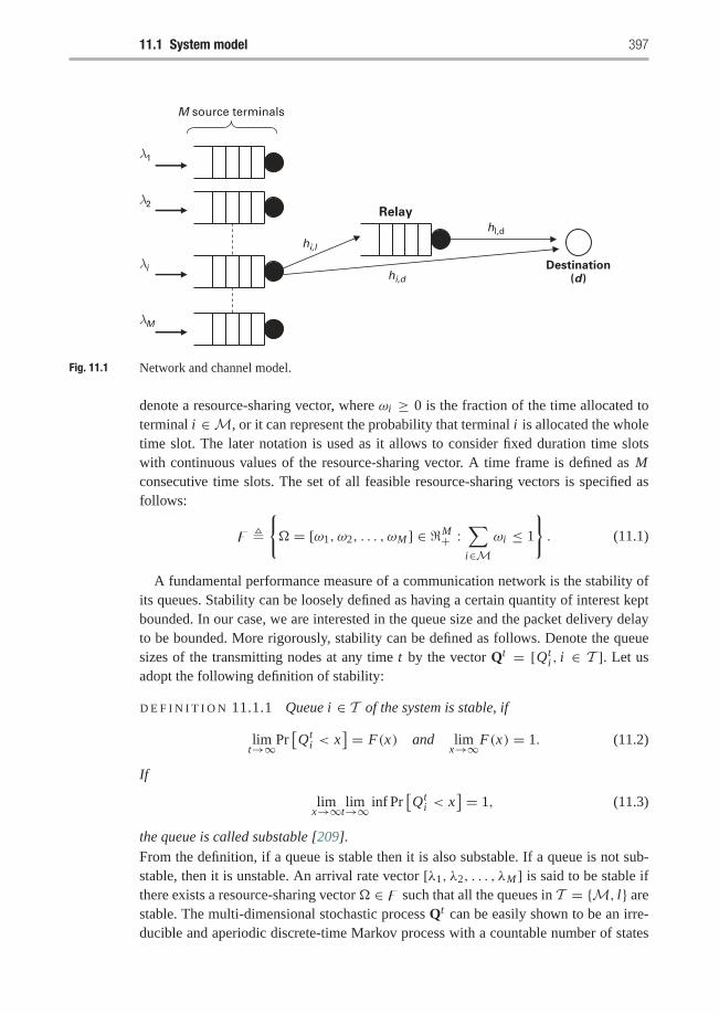
11.1 System model 397
λ1
λ2
λi
λM
Relay
Destination(d )
M source terminals
hi,l
hi,d
hl,d
Fig. 11.1 Network and channel model.
denote a resource-sharing vector, where ωi ≥ 0 is the fraction of the time allocated toterminal i ∈M, or it can represent the probability that terminal i is allocated the wholetime slot. The later notation is used as it allows to consider fixed duration time slotswith continuous values of the resource-sharing vector. A time frame is defined as Mconsecutive time slots. The set of all feasible resource-sharing vectors is specified asfollows:
� �{� = [ω1, ω2, . . . , ωM ] ∈ �M+ :
∑i∈M
ωi ≤ 1
}. (11.1)
A fundamental performance measure of a communication network is the stability ofits queues. Stability can be loosely defined as having a certain quantity of interest keptbounded. In our case, we are interested in the queue size and the packet delivery delayto be bounded. More rigorously, stability can be defined as follows. Denote the queuesizes of the transmitting nodes at any time t by the vector Qt = [Qt
i , i ∈ T ]. Let usadopt the following definition of stability:
D E F I N I T I O N 11.1.1 Queue i ∈ T of the system is stable, if
limt→∞Pr
[Qt
i < x] = F(x) and lim
x→∞F(x) = 1. (11.2)
If
limx→∞ lim
t→∞ inf Pr[Qt
i < x] = 1, (11.3)
the queue is called substable [209].From the definition, if a queue is stable then it is also substable. If a queue is not sub-stable, then it is unstable. An arrival rate vector [λ1, λ2, . . . , λM ] is said to be stable ifthere exists a resource-sharing vector� ∈ � such that all the queues in T = {M, l} arestable. The multi-dimensional stochastic process Qt can be easily shown to be an irre-ducible and aperiodic discrete-time Markov process with a countable number of states
398 Cognitive multiple access via cooperation
and state space ∈ ZM+1+ . For such a Markov chain, the process is stable if and only if apositive probability exists for every queue being empty [127], i.e.,
limt→∞Pr [Qi (t) = 0] > 0, i ∈ T . (11.4)
If the arrival and service processes of a queuing system are strictly stationary, thenone can apply Loynes’ theorem to check for stability conditions [124]. This theoremstates that if the arrival process and the service process of a queuing system are strictlystationary, and the average arrival rate is less than the average service rate, then thequeue is stable; if the average arrival rate is greater than the average service rate thenthe queue is unstable.
Next, we describe the physical channel model. The wireless channel between anytwo nodes in the network is modeled as a Rayleigh narrowband flat-fading channel withadditive Gaussian noise. The transmitted signal also suffers from propagation path lossthat causes the signal power to attenuate with distance. The signal received at a receivingnode j ∈ D from a transmitting node i ∈ T at time t can be modeled as
yti, j =
√Gr−γi, j ht
i, j xti + nt
i, j , i ∈ T , j ∈ D, i �= j, (11.5)
where G is the transmitting power, assumed to be the same for all transmitting terminals,ri, j denotes the distance between the two nodes i, j , γ is the path loss exponent, and ht
i, jcaptures the channel fading coefficient at time t and is modeled as an i.i.d. zero-mean,circularly symmetric complex Gaussian random process with unit variance. The termxt
i denotes the transmitted packet with average unit power at time t , and nti, j denotes
i.i.d. additive white Gaussian noise with zero mean and variance N0. Since the arrival,channel gains, and additive noise processes are assumed to be stationary, we can dropthe index t without loss of generality. We consider the scenario in which the fadingcoefficients are known to the appropriate receivers, but are not known at the transmitters.
In this chapter, we characterize the success and failure of packet reception by outageevents and outage probability, which is defined as follows. For a target signal-to-noise(SNR) ratio β, if the received SNR as a function of the fading realization h is given bySNR(h), then the outage event O is the event that SNR(h) < β, and Pr [SNR(h) < β]denotes the outage probability,also defined in previous chapters. The SNR threshold βis a function of different parameters in the communication system; it is a function ofthe application, data rate, signal-processing applied at the encoder/decoder sides, error-correction codes, and other factors. For example, varying the data rate and fixing allother parameters, the required SNR threshold β to achieve certain system performanceis a monotonically increasing function of the data rate. Also, increasing the signal-processing and encode/decoder complexity in the physical layer reduces the requiredSNR threshold β for a required system performance.
For the channel model in (11.5), the received SNR of a signal transmitted betweentwo terminals i and j can be specified as follows:
SNRi, j =| hi, j |2 r−γi, j G
N0, (11.6)
11.2 Cooperative cognitive multiple access (CCMA) protocols 399
where | hi, j |2 is the magnitude channel gain square and has an exponential distributionwith unit mean. The outage event for a SNR threshold β is equivalent to
Oi, j = {hi, j : SNRi, j < β} ={
hi, j :| hi, j |2<βN0rγi, j
G
}(11.7)
Accordingly, the probability of outage is given by
Pr[Oi, j
] = Pr
[| hi, j |2<
βN0rγi, jG
]= 1− exp
(−βN0rγi, j
G
), (11.8)
where the above follows from the exponential distribution of the received SNR. Sincewe will use the above expression frequently in our subsequent analysis, and for com-pactness of representation, we will use the following notation to denote the successprobability (no outage) at SNR threshold β:
fi, j = exp
(−βN0rγi, j
G
). (11.9)
11.2 Cooperative cognitive multiple access (CCMA) protocols
In a TDMA system without relays, if a terminal does not have a packet to transmit,its time slot remains idle, i.e., the slot becomes a wasted channel resource. We con-sider the possibility of utilizing these wasted channel resources by employing a relay.In this section, we introduce the cognitive multiple access strategy based on employingrelays in the wireless network. Furthermore, we develop two protocols to implementthis new approach. We assume that the relay can sense the communication channelto detect empty time slots and we assume that the errors and delay in the packetacknowledgement feedback are negligible.
First, let us describe the multiple access strategy:• Due to the broadcast nature of the wireless medium, the relay can listen to the
packets transmitted by the terminals to the destination.• If the packet is not received correctly by the destination, the relay stores this packet
in its queue, given that it was able to decode this packet correctly. Thus, the relay’squeue contains packets that have not been transmitted successfully by the terminals.
• At the beginning of each time slot, the relay listens to the channel to check whetherthe time slot is empty (not utilized for packet transmission) or not.
• If the time slot is empty the relay will retransmit the packet at the head of its queue,hence utilizing a channel resource that was previously wasted in a TDMA systemwithout a relay.
Moreover, this introduces spatial diversity in the network as the channel fades betweendifferent nodes in the network are independent. In the following we present two differentprotocols to implement the proposed cognitive multiple access approach. The protocolsare cognitive in the sense that the system introduces a relay in the network that tries to
400 Cognitive multiple access via cooperation
detect unused channel resources and uses them to help other terminals by forwardingpackets lost in previous transmissions.
11.2.1 CCMA-single frame
The first protocol that wepresent is cooperative cognitive multiple access within a singleframe duration or (CCMA-S). The characteristic feature of CCMA-S is that any terminalkeeps its lost packet in its queue until it is captured successfully at the destination.CCMA-S operates according to the following rules:• Each terminal transmits the packet at the head of its queue in its assigned slot, if
the terminal’s queue is empty the slot is free.• If destination receives a packet successfully, it sends an ACK which can be heard
by both the terminal and the relay. If the destination does not succeed in receivingthe packet correctly but the relay does, then the relay stores this packet at the endof its queue. The corresponding terminal still keeps the lost packet at the head ofits queue
• The relay senses the channel, and at each empty time slot the relay transmits thepacket at the head of its queue, if its queue is nonempty. If the transmitted packetis received correctly by the destination it sends an ACK and the correspondingterminal removes this packet from its queue.
• If the relay does not succeed in delivering a packet to the destination during a timeframe starting from the time it received this packet, then the relay drops the packetfrom its queue. In this case the corresponding terminal becomes responsible fordelivering the packet to the destination.
Following are some important remarks on the above protocol. According to the abovedescription of CCMA-S, the relay’s queue has always a finite number of packets (at mostit has M backlogged packets). This follows because, according to the protocol, the relaycan have at most one packet from each terminal. Thus the stability of the system is onlydetermined by the stability of the terminals’ queues. Secondly, successful service of apacket in a frame depends on whether the other terminals have idle time slots or not.Therefore individual terminals’ queues are interacting.
11.2.2 CCMA-multiple frames
In this section, we describe the implementation of protocol CCMA-M. The maindifference between protocols CCMA-S and CCMA-M is in the role of the relayand the behavior of the terminals’ regarding their backlogged packets. More specif-ically, a terminal removes a packet from its queue if it is received successfully byeither the destination or the relay. CCMA-M operates according to the followingrules:• Each terminal transmits the packet at the head of its queue in its assigned time slot.
If the queue is empty the time slot is free.
11.3 Stability analysis 401
• If a packet is received successfully by either the destination or the relay, the packetis removed from the terminal’s queue (the relay needs to send an ACK if one is notheard by the destination in this case).
• If a packet is not received successfully by both the relay and the destination, thecorresponding terminal retransmits this packet in its next assigned time slot.
• At each sensed empty time slot, the relay retransmits the packet at the head of itsqueue.
One can now point out the differences between the queues in CCMA-S and CCMA-M:
• The size of the relay’s queue can possibly grow in CCMA-M as it can have morethan one packet from each terminal; however, it can not exceed size M in CCMA-S.
• The terminal’s queues in CCMA-M are not interacting as in CCMA-S. This isbecause the terminal removes the packets which were received correctly by therelay or the destination. In other words, servicing the queue of any terminal dependsonly on the channel conditions from that terminal to the destination and relay, anddoes not depend on the status of the other terminals’ queues.
• The stable throughput region of CCMA-M requires studying the stability of boththe terminals’ and the relay’s queues.
11.3 Stability analysis
The aim of this section is to characterize the stable throughput region of the presentedcooperation protocols. Furthermore, we show comparison for the stable through-put regions of TDMA without relaying, ALOHA, selection decode-and-forward, andincremental decode-and-forward.
11.3.1 Stability analysis of CCMA-S
11.3.1.1 The two-terminals caseIn CCMA-S, we observed in the previous section that the relay’s queue size is alwaysfinite, hence it is always stable. For the two-terminals case, the queues evolve as a two-dimensional Markov-chain in the first quadrant. From the protocol description in theprevious section, one can observe that the queues in CCMA-S are interacting. In otherwords, the transition probabilities differ according to whether the size of the queuesare empty or not. For example, if one of the two terminals’ queues was empty for along time, then the relay serves the lost packets from the other terminal more often.On the other hand, if one of the two terminals queues never empties, then the otherterminal will never get served by the relay. Studying stability conditions for interactingqueues is a difficult problem that has been addressed for ALOHA systems [149, 127].The concept of dominant systems can be adopted to help finding bounds on the stabilityregion.
To analyze the stability of CCMA-S, we develop a dominant system to decouplethe interaction of the originating terminals from the role of the relay in cooperation.
402 Cognitive multiple access via cooperation
Using our developed dominant system we are able to characterize the stability regionof CCMA-S for a fixed resource-sharing vector, and hence the whole stability region.The following lemma states the stability region of CCMA-S for a fixed resource sharingvector [ω1, ω2].Lemma 11.3.1 The stability region of CCMA-S for a fixed resource-sharing vector[ω1, ω2] is given by R(S1)
⋃R(S2) where
R(S1) ={[λ1, λ2] ∈ R2+ : λ2 < h(λ1;w1, w2, f1,d , f2,d , f2,l , fl,d), for λ1 < ω1 f1,d .
}(11.10)
and
R(S2) ={[λ1, λ2] ∈ R2+ : λ1 < h(λ2;w2, w1, f2,d , f1,d , f1,l , fl,d), for λ2 < ω2 f2,d .
}(11.11)
where
h(x;α1, α2, α3, α4, α5, α6) = α2α4 + α1α2
(1− x
α1α3
)(1− α3)α5α6. (11.12)
Proof The proof of Lemma 11.3.1 depends on constructing a dominant system thatdecouples the interaction between the queues and thus renders the analysis tractable. Bydominance, we mean that the queues in the dominant system stochastically dominate thequeues in the original CCMA-S system, i.e., with the same initial conditions for queuesizes in both the original and dominant systems, the queue sizes in the dominant systemare not smaller than those in the original system.We define the dominant system for CCMA-S as follows. For j ∈ {1, 2}, define S j asfollows:
• arrivals at queue i ∈M in S j are the same as in CCMA-S;• the channel realizations hk,l , where k ∈ T and l ∈ D, are identical for both S j and
CCMA-S;• time slots assigned to user i ∈M are identical for both S j and CCMA-S;• the noise generated at the receiving ends of both systems is identical;• the packets successfully transmitted by the relay for user j are not removed from user j’s
queue in S j .
The above definition of the dominant system implies that queue j evolves exactly as ina TDMA system without a relay. If both the dominant system and the original CCMA-Sstarted with the same initial queue sizes, then the queues in system S j are always notshorter than those in CCMA-S. This follows because a packet successfully transmittedfor queue j in S j is always successfully transmitted from the corresponding queue inCCMA-S. However, the relay can succeed in forwarding some packets from queue jin CCMA-S in the empty time slots of the other terminal. This implies that queue jempties more frequently in CCMA-S and therefore the other terminal is better served inCCMA-S compared to S j . Consequently, stability conditions for the dominant systemS j ( j ∈ {1, 2}) are sufficient for the stability of the original CCMA-S system. In thefollowing, we first derive the sufficient conditions for stability of CCMA-S.
11.3 Stability analysis 403
Consider system S1 in which the relay only helps terminal 2, and terminal 1 acts exactlyas in a TDMA system. In order to apply Loynes’ theorem, we require the arrival andservice processes for each queue to be stationary. The queue size for terminal i ∈ {1, 2}in system S1 at time t , denoted by Qt
i (S1), evolves as follows:
Qt+1i (S1) =
(Qt
i (S1)− Y ti (S1)
)+ + Xti (S1), (11.13)
where Xti (S1) represents the number of arrivals in slot t and is a stationary process by
assumption with finite mean E[Xt
i (S1)] = λi . The function ()+ is defined as (x)+ =
max(x, 0). Y ti (S1) denotes the possible (virtual) departures from queue i at time t ; by
virtual we mean that Y ti (S1) can be equal to 1 even if Qt
i (S1 = 0). We assume thatdepartures occur before arrivals, and the queue size is measured at the beginning of theslot. For terminal i = 1, the service process can be modeled as
Y t1(S1) = 1
[At
1 ∩ Ot1,d
], (11.14)
where 1[·] is the indicator function, At1 denotes the event that slot t is assigned to ter-
minal 1, and Ot1,d denotes the complement of the outage event between terminal 1 and
the destination d at time t .2 Due to the stationarity assumption of the channel gain pro-cess {ht
i,d}, and using the outage expression in (11.8), the probability of this event is
given by Pr[Ot
1,d
]= f1,d . From the above, it is clear that the service process Y t
1(S1) is
stationary and has a finite mean given by
E[Y t
1(S1)] = ω1 f1,d , (11.15)
where E[·] denotes statistical expectation. According to Loynes theorem, stability ofqueue 1 in the dominant system S1 is achieved if the following condition holds:
λ1 < ω1 f1,d . (11.16)
Consider now queue 2 in system S1. The difference between the evolution of this queueand queue 1 is in the definition of the service process Y t
2(S1). A packet from queue 2can be served in a time slot in either one of the two following events:
• if the time slot belongs to queue 2 and the associated channel ht2,d is not in outage; or
• the time slot belongs to queue 1, queue 1 is empty, in the previous time slot there wasa successful “maybe virtual” reception of a packet at the relay from terminal 2, and therelay–destination channel is not in outage.
This can be modeled as
Y t2(S1) = 1
[At
2
⋂Ot
2,d
]+ 1
[At
1
⋂{Qt
1(S1)} = 0}⋂At−1
2
⋂Ot−1
2,l
⋂Ot−1
2,d
⋂Ot
l,d
](11.17)
2 (·) denotes the complement of the event.
404 Cognitive multiple access via cooperation
where {Qt1(S1) = 0} denotes the event that terminal’s 1 queue is empty in time slot
t . The two indicator functions in the right-hand side of equation (11.17) are mutuallyexclusive, hence, the average rate of the service process is given by
E[Y t
2(S11)]
= ω2 f2,d + ω1Pr[{Qt
1(S11) = 0}
]ω2 (1− Pr[O2l ])Pr[O2,d ]
(1− Pr[Ol,d]
),
(11.18)
where Pr[Oi, j ] is the probability of outage between nodes i and j .Using (11.16) and the fact that, at steady state, the fraction of time a queue is occupiedequals the ratio of the arrival rate and service rate, the probability that queue 1 is emptyis given by
Pr[{Qt
1(S11) = 0}
]= 1− λ1
ω1 f1,d. (11.19)
Using the expression of the outage probability in (11.8) and Loynes conditions forstability [124], the stability condition for queue 2 in the dominant system S1 isgiven by
λ2 < ω2 f2,d + ω1ω2
(1− λ1
ω1 f1,d
) (1− f2,d
)f2,l fl,d. (11.20)
Both conditions (11.16) and (11.20) represent the stability region for system S1 for aspecific resource-sharing vector (ω1, ω2) pair. Call this region R(S1). Using parallelarguments for the dominant system S2, we can characterize the stability region R(S2)
for this system by the following pair of inequalities:
λ2 < ω2 f2,d ,
λ1 < ω1 f1,d + ω2ω1
(1− λ2
ω2 f2,d
) (1− f1,d
)f1,l fl,d. (11.21)
Since the stability conditions for a dominant system are sufficient for the stability ofCCMA-S, any point inside the regions R(S1) and R(S2) can be achieved by the originalsystem CCMA-S, hence R(S1)
⋃R(S2) is a subset from the stability region of CCMA-
S for a fixed resource sharing pair (ω1, ω2). This region is depicted in Figure 11.2.Up to this point have we only proved the sufficient conditions for the stability ofCCMA-S in Lemma 11.3.1. To prove the necessary conditions, we have to prove theindistinguishability of the dominant and original systems at saturation. The argumentis as follows. Consider the dominant system S1 whose stability region is charac-terized by the pair of inequalities (11.16), (11.20). Note that if queue 2 does notempty, packets of user 1 are always dropped by the relay in both S1 and CCMA-S, and both systems become identical. In S1, for λ1 < ω1 f1,d , if λ2 > ω2 f2,d +ω1ω2
(1− λ1/ω1 f1,d
) (1− f2,d
)f2,l fl,d then using same argument as before Qt
1 isstable and Qt
2 is unstable by Loynes, i.e., limt→∞Qt
2 → ∞ almost surely. If Qt2 tends
to infinity almost surely, i.e., does not empty, then S1 and CCMA-S are identical, andif both systems are started from the same initial conditions, then on a set of samplepaths of positive probability Qt
2 in CCMA-S never returns to zero for t ≥ 0. Hence Qt2
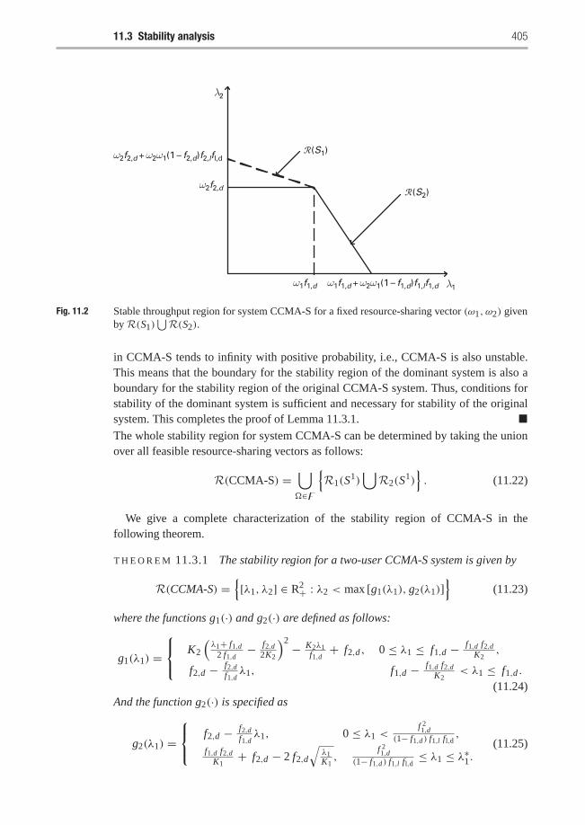
11.3 Stability analysis 405
ω1f1,d + ω2ω1(1 – f1,d)f1,lf1,d
ω2f2,d + ω2ω1(1 – f2,d)f2,lfl,d
ω2f2,d
λ1
λ2
�(S1)
�(S2)
ω1f1,d
Fig. 11.2 Stable throughput region for system CCMA-S for a fixed resource-sharing vector (ω1, ω2) givenby R(S1)
⋃R(S2).
in CCMA-S tends to infinity with positive probability, i.e., CCMA-S is also unstable.This means that the boundary for the stability region of the dominant system is also aboundary for the stability region of the original CCMA-S system. Thus, conditions forstability of the dominant system is sufficient and necessary for stability of the originalsystem. This completes the proof of Lemma 11.3.1. �The whole stability region for system CCMA-S can be determined by taking the unionover all feasible resource-sharing vectors as follows:
R(CCMA-S) =⋃�∈�
{R1(S
1)⋃
R2(S1)}. (11.22)
We give a complete characterization of the stability region of CCMA-S in thefollowing theorem.
T H E O R E M 11.3.1 The stability region for a two-user CCMA-S system is given by
R(CCMA-S) ={[λ1, λ2] ∈ R2+ : λ2 < max [g1(λ1), g2(λ1)]
}(11.23)
where the functions g1(·) and g2(·) are defined as follows:
g1(λ1) =⎧⎨⎩ K2
(λ1+ f1,d
2 f1,d− f2,d
2K2
)2 − K2λ1f1,d
+ f2,d , 0 ≤ λ1 ≤ f1,d − f1,d f2,dK2
,
f2,d − f2,df1,dλ1, f1,d − f1,d f2,d
K2< λ1 ≤ f1,d .
(11.24)And the function g2(·) is specified as
g2(λ1) =⎧⎨⎩ f2,d − f2,d
f1,dλ1, 0 ≤ λ1 <
f 21,d
(1− f1,d ) f1,l fl,d,
f1,d f2,dK1
+ f2,d − 2 f2,d√λ1K1,
f 21,d
(1− f1,d ) f1,l fl,d≤ λ1 ≤ λ∗1.
(11.25)
406 Cognitive multiple access via cooperation
where
λ∗1 ={
f1,d , (1− f1,d) f1,l fl,d < f1,d ,1
4K1( f1,d + K1)
2, f1,d ≤ (1− f1,d) f1,l fl,d.(11.26)
and Ki = (1− fi,d) fi,l fl,d, i ∈ {1, 2}.
Proof The stable throughput region of CCMA-S for a fixed resource-sharing vector(ω1, ω2) is specified in Lemma 11.3.1. In order to find the whole stability region ofthe protocol, we need to take the union over all possible values of (ω1, ω2) in �. Onemethod to characterize this union is to solve a constrained optimization problem tofind the maximum feasible λ2 corresponding to each feasible λ1. For a fixed λ1, themaximum stable arrival rate for queue 2 is given by solving the following optimizationproblem:
maxw1,w2
λ2 = w2 f2,d + w1w2K2 − λ1w2 K2f1,d
, (11.27)
s.t. w1 + w2 ≤ 1, λ1 ≤ w1 f1,d , (11.28)
where Ki = (1 − f2,d) f2,l fl,d, and i ∈ {1, 2}. To put this problem in a standardform, we can equivalently write it as the minimization of −λ2. The Lagrangian of thisoptimization problem is given by[
−w2K2
−w1K2 + λ1 K2f1,d
− f2,d
]+ u1
[11
]+ u2
[ − f1,d0
]= 0, (11.29)
where u1, u2 are the complementary slackness variables that are nonnegative. Solvingfor the complementary slacknessvariables we get the following relation between u1
and u2:
u1 = w2K2 + u2 f1,d . (11.30)
This shows that u1 > 0, i.e., the first constraint (w1 + w2 = 1) in (11.28) is met withequality.Substituting w2 = 1− w1 in the cost function in (11.28), we get
λ2 = (1− w1) f2,d + w1(1− w1)K2 − (1− w1)λ1K2
f1,d. (11.31)
Taking the first derivative of the above equation with respect to w1, we get
∂λ2
∂w1= − f2,d + K2 − 2w1K2 + λ1K2
f1,d. (11.32)
Since K2 is non-negative, the second derivative is negative, hence, the cost function in(11.31) is concave in w1 and the necessary conditions for optimality KKT [15] are alsosufficient. Equating the first derivative in (11.32) to zero, the solution w∗1 is given by
w∗1 =1
2K2
(K2 − f2,d + λ1K2
f1,d
). (11.33)
From the first constraint in (11.28), the minimum value for w1 that guarantees the sta-bility of queue 1 in system S1 is given by w1,min = λ1/ f1,d . Hence, if w∗1 > w1,min,
11.3 Stability analysis 407
and given concavity of the cost function, the optimal solution is just w∗1 , otherwise itis given by w1,min. Characterizing this in terms of the channel parameters, the optimalsolution for the optimization problem in (11.28) is given by
w∗1 =⎧⎨⎩
12K2
(K2 − f2,d + λ1 K2
f1,d
), λ1 ≤ f1,d − f1,d f2,d
K2
λ1f1,d, f1,d − f1,d f2,d
K2< λ1 < f1,d .
(11.34)
If λ1 > f1,d , then the first queue can never be stable by construction of S1.Now we solve for the other branch in the stability region given by the dominant systemS2. The equations for this branch are given by (11.20). Similar to the first stabilityregion branch, solving for the Lagrangian of this branch gives the necessary conditionw1 + w2 = 1. First, we find the maximum achievable stable rate for the first queue,which is achieved when λ2 = 0. Substituting in (11.20), the arrival rate λ1 can bewritten as
λ1 = w1 f1,d + w1(1− w1)K1. (11.35)
The above equation is obviously concave. Taking the first derivative and equating tozero we get
w∗1 |λ2=0 = 1
2K1( f1,d + K1). (11.36)
Since w1 ≤ 1, then if w∗1 |λ2=0 > 1, i.e., f1,d > K1, and given the concavity of the costfunction, we letw∗1 |λ2=0 = 1. Substitutingw∗1 |λ2=0 in (11.35), the maximum achievablerate λ1 can be given by
λ∗1 ={
f1,d , f1,d > K1,
14K1( f1,d + K1)
2, 0 ≤ f1,d ≤ K1.(11.37)
Next for a fixed λ1, we solve for the optimal λ2 that can be achieved from the secondbranch. We can write (11.20) in terms of λ2 as follows:
λ2 = f1,d f2,dK1
+ (1− w1) f2,d − λ1f2,dw1K1
. (11.38)
Taking the first derivative with respect to w1 we get
∂λ2
∂w1= − f2,d + λ1
f2,dK1w
21
. (11.39)
The second derivative is negative, which renders the whole function concave. Equatingthe first derivative to zero we get
w∗1 =√
λ1
(1− f1,d) f1,l fl,d. (11.40)
From (11.20), we have the following constraint for the stability of the second queue,λ2 ≤ w2 f2,d , which can be written in terms of w1 as follows:
w1 ≤ 1− λ2
f2,d. (11.41)
408 Cognitive multiple access via cooperation
Substituting λ2 from (11.41) into (11.38), we find that the maximum value for w1 interms of λ1 is given by w1 ≤ λ1/ f1,d . Therefore, the optimal value for w1 can bewritten as
w∗1 = min
(√λ1
(1− f1,d) f1,l fl,d,λ1
f1,d
). (11.42)
The value of the expression in (11.42) can be shown to never exceed 1 by substituting themaximum value of λ1 given by (11.37) in the above equation. After some manipulations,the optimum w∗1 in (11.42) can be further simplified as follows:
w1∗ =⎧⎨⎩
λ1f1,d, if λ1 ≤ f 2
1,d(1− f1,d ) f1,l fl,d
,√λ1
(1− f1,d ) f1,l fl,d, otherwise.
(11.43)
We summarize equations (11.31), (11.34), (11.38), and (11.43) describing the envelopesof the first and second branches as follows. For the first branch given by equations(11.31) and (11.34), substituting (11.34) in (11.31) we get
g1(λ1) =⎧⎨⎩ K2
(λ1
2 f1,d+ 0.5− f2,d
2K2
)2 − K2λ1f1,d
+ f2,d , 0 ≤ λ1 ≤ f1,d − f1,d f2,dK2
,
f2,d − f2,df1,dλ1, f1,d − f1,d f2,d
K2< λ1 ≤ f1,d .
(11.44)Similarly, by substituting (11.43) in (11.38), we get for the second branch
g2(λ1) =⎧⎨⎩ f2,d − f2,d
f1,d, λ1 <
f 21,d
(1− f1,d ) f1,l fl,d,
f1,d f2,dK1
+ f2,d − 2 f2,d√λ1K1,
f 21,d
(1− f1,d ) f1,l fl,d≤ λ1 ≤ λ∗1.
(11.45)
The value for λ∗1 is given by (11.37). Since g1(λ1) and g2(λ2) are achieved by thedominant systems S1 and S2 respectively, then they are both achieved by CCMA-S.This proves the theorem. �An interesting observation that we make from the above theorem is that both functionsg1(λ1) and g2(λ1) are linear over some part of their domain and strictly convex over theother part. It is not obvious, however, whether both functions are strictly convex overtheir domain of definition, and hence, whether the boundary of the stability region ofCCMA-S given by max{g1, g2} is convex or not. In the following lemma, we prove thisproperty.
Lemma 11.3.2 The boundary of the stability region of system CCMA-S given bymax{g1, g2} is convex.
Proof We prove the convexity of the envelope of region R(CCMA-S). First we con-sider the envelope g1(λ1) for the first branch. As shown in Figure 11.3, g1(λ1) isdefined over two regions: for λ1 ∈ [0, f1,d − f1,d f2,d/K2], g1(λ1) � g11(λ1) =K2(λ1/2 f1,d + 0.5− f2,d/2K2
)2 − K2λ1/ f1,d + f2,d ; while for λ1 ∈ ( f1,d −f1,d f2,d/K2, f1,d ], g1(λ1) � g12(λ1) is a straight line given by f2,d − f2,d/ f1,d . It canbe readily seen that g1(λ1) is convex over both regions because its second derivative
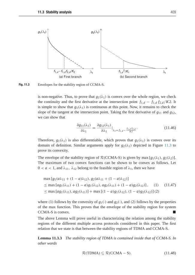
11.3 Stability analysis 409
f1,d – f1,d f2,d
/K2
(a) First branch (b) Second branch
f1,d 2
/K1λ1 λ1
g1(λ1) g2(λ1)
Fig. 11.3 Envelopes for the stability region of CCMA-S.
is non-negative. Thus, to prove that g1(λ1) is convex over the whole region, we checkthe continuity and the first derivative at the intersection point f1,d − f1,d f2,d/K2. Itis simple to show that g1(λ1) is continuous at this point. Now, it remains to check theslope of the tangent at the intersection point. Taking the first derivative of g11 and g12,we can show that
∂g11(λ1)
∂λ1= ∂g12(λ1)
∂λ1|λ1= f1,d− f1,d f2,d
K2. (11.46)
Therefore, g1(λ1) is also differentiable, which proves that g1(λ1) is convex over itsdomain of definition. Similar arguments apply for g2(λ1) depicted in Figure 11.3 toprove its convexity.
The envelope of the stability region of R(CCMA-S) is given by max [g1(λ1), g2(λ2)].The maximum of two convex functions can be shown to be convex as follows. Let0 < a < 1, and λ11, λ12 belong to the feasible region of λ1, then we have
max [g1(aλ11 + (1− a)λ12), g2(aλ11 + (1− a)λ12)]
≤ max [ag1(λ11)+ (1− a)g1(λ12), ag2(λ11)+ (1− a)g2(λ12)] , (1)
≤ max [ag1(λ11), ag2(λ11)]+max [(1− a)g1(λ12), (1− a)g2(λ12)] (2)
(11.47)
where (1) follows by the convexity of g1(·) and g2(·), and (2) follows by the propertiesof the max function. This proves that the envelope of the stability region for systemCCMA-S is convex. �The above Lemma will prove useful in characterizing the relation among the stabilityregions of the different multiple access protocols considered in this paper. The firstrelation that we state is that between the stability regions of TDMA and CCMA-S.
Lemma 11.3.3 The stability region of TDMA is contained inside that of CCMA-S. Inother words
R(TDMA) ⊆ R(CCMA− S). (11.48)
410 Cognitive multiple access via cooperation
The two regions are identical if the following two conditions are satisfiedsimultaneously
(1− f2,d) f2,l fl,d < f2,d , (11.49)
(1− f1,d) f1,l fl,d < f1,d . (11.50)
Proof We use Theorem 11.3.1 and Lemma 11.3.2 in the proof of the this lemma.The stability region of TDMA is determined according to the following parametricinequalities:
λ1 ≤ ω1 f1,d , λ2 ≤ ω2 f2,d (11.51)
or, equivalently,
λ1
f1,d+ λ2
f2,d≤ 1. (11.52)
From Lemma 11.3.2, both functions g1 and g2 that determine the boundary of the sta-bility region of CCMA-S are convex. From the proof of the convexity, we note that thestraight line λ2 = f2,d − f2,d/ f1,dλ1 is a tangent for both functions, hence, it lies belowboth functions. Since this straight line is itself the boundary for the TDMA stabilityregion, then the stability region of TDMA is a subset of that of CCMA-S. To prove thesecond part of the Lemma we use the definitions of the functions g1, g2 in Theorem11.3.1. From (11.37), observe that if (1− f1,d) f1,l fl,d < f1,d then the maximum λ1 isdetermined by f1,d . If simultaneously (1 − f2,d) f2,l f2,d < f2,d , then by substitutingboth conditions in the domain definitions of the functions g1, g2, it can be seen that bothfunctions reduce to
g1(λ1) = g2(λ1) = f2,d − f2,df1,d
λ1, 0 ≤ λ1 ≤ f1,d , (11.53)
which is the boundary for the stability region of TDMA. Hence if both conditions in(11.50) are satisfied, CCMA-S and TDMA have the same stable throughput regions.This completes the proof of the lemma. �
11.3.1.2 The symmetric M-terminals caseStability analysis for the general M-terminals case is very complicated. For the ALOHAcase, only bounds on the stability region have been derived before. In this section, weonly focus on the symmetric scenario. We define the dominant system for M-terminalsCCMA-S as follows. For 1 ≤ j ≤ N , define SM
j as follows:
• arrivals at queue i in SMj are the same as in CCMA;
• the channel realizations hkl , where k ∈ T and l ∈ R, are identical for both SMj and
CCMA;• user i ∈M is assigned the same time slots in both systems;• the noise generated at the receiving ends of both systems is identical;• the packets served by the relay for the first j terminals are not removed from these
terminals’ queues.
11.3 Stability analysis 411
The last rule implies that the first j queues act as in a TDMA system without a relay.The relay, however, can help the other users j + 1 ≤ k ≤ N in the empty slots of theTDMA frame.
Now consider system SMM in which the relay does not help any of the users. It is
clear that the queue sizes in this system are never smaller than those in the originalsystem CCMA-S. For SM
M , the success probability of transmitting a packet is equal forall terminals and is given by
Ps(SMM ) = Pr [SNR ≥ β] = f1,d . (11.54)
The service rate per terminal is thus given by μ(SMM ) = f1,d/M , due to the symmetry
of the problem. Since system SMM acts as a TDMA system without a relay, the queues
are decoupled and hence the arrival process and departure process of each of them isstrictly stationary. Applying Loynes’ theorem, the stability condition for SM
M is given by
λ < f1,d , (11.55)
where λ is the aggregate arrival rate for the M terminals.Next, let us consider the stability of symmetric CCMA-S. Since SM
M as describedbefore dominates CCMA-S, if SM
M is stable then CCMA-S is also stable. Therefore,for λ < f1,d , system CCMA-S is stable. On the other hand, if all the queues inSM
M are unstable, then none of these queues ever empty, hence, the relay loses itsrole and both systems CCMA-S and SM
M are indistinguishable if both started withthe same initial conditions. Therefore, if we have λ > f1,d then all the queues inSM
M are unstable and accordingly system CCMA-S is unstable as well. Therefore, themaximum stable throughput for system CCMA-S can be summarized in the followingtheorem.
T H E O R E M 11.3.2 The maximum stable throughput λMST(CCMA− S) for systemCCMA-S is equal to that of a TDMA system without a relay and is given by
λMST(CCMA-S) = f1,d . (11.56)
However, we conjecture that for the general asymmetric M-terminals scenario, thewhole stability region of TDMA will be contained inside that of CCMA-S. Anotherimportant issue to point out is that although CCMA-S and TDMA have the same maxi-mum stable throughput for the symmetrical case, the two systems do not have the samedelay performance as will be discussed later.
11.3.2 Stability analysis of CCMA-M
In CCMA-M the relay’s queue can possibly grow and hence should be taken intoaccount when studying the system stability. This means that for stability we requireboth the M terminals’ queues and the relay’s queue to be stable. The stability region ofthe whole system is the intersection of the stability regions of the M terminals and thatof the relay. First, we consider the M = 2-terminals case. According to the operation
412 Cognitive multiple access via cooperation
of system CCMA-M, a terminal succeeds in transmitting a packet if either the destina-tion or the relay receives this packet correctly. The success probability of terminal i inCCMA-M can thus be calculated as
Pr[Success of terminal i] = Pr[Oi,l ∪ Oi,d
], (11.57)
where Oi,l denotes the event that the relay received the packet successfully, and Oi,d
denotes the event that the destination received the packet successfully. The successprobability of terminal i ∈ {1, 2} in CCMA-M can thus be specified as follows
Pi = fi,d + fi,l − fi,d fi,l . (11.58)
We first consider the stability region for the system determined just by the terminals’queues. Since for each queue i ∈M, the queue behaves exactly as in a TDMA systemwith the success probability determined by (11.58), the stability region RM(CCMA-M)for the set of queues in M is given by
RM(CCMA-M) ={[λ1, λ2, . . . , λM ] ∈ RM+ : λi < ωi Pi ,∀i ∈M,
and [ω1, ω2, . . . , ωM ] ∈ �} .(11.59)
Next we study the stability of the relay’s queue l. The evolution of the relay’s queue canbe modeled as
Qtl =
(Qt
l − Y tl
)+ + Xtl , (11.60)
where Xtl denotes the number of arrivals at time slot t and Y t
l denotes the possibility ofserving a packet at this time slot from the relay’s queue (Y t
l (G) takes values in {0, 1}).Now we establish the stationarity of the arrival and service processes of the relay. Ifthe terminals’ queues are stable, then by definition the departure processes from bothterminals are stationary. A packet departing from a terminal queue is stored in the relay’squeue (i.e., counted as an arrival) if simultaneously the following two events happen:the terminal–destination channel is in outage and the terminal–relay channel is not inoutage. Hence, the arrival process to the queue can be modeled as follows:
Xtl =
∑i∈M
1[
Ati
⋂{Qt
i �= 0}⋂
Oti,d
⋂Ot
i,l
]. (11.61)
In (11.61), {Qti �= 0} denotes the event that terminal i’s queue is not empty, i.e., the
terminal has a packet to transmit, and according to Little’s theorem it has probabil-ity λi/(ωi Pi ), where Pi is terminal i’s success probability and is defined in (11.58).The random processes involved in the above expressions are all stationary, hence thearrival process to the relay is stationary. The expected value of the arrival process canbe computed as follows:
λl =∑i∈M
λi(1− fi,d) fi,l
Pi. (11.62)
Similarly, we establish the stationarity of the service process from the relay’s queue.The service process of the relay’s queue depends by definition on the empty slots avail-able from the terminals, and on the channel from the relay to the destination not being
11.3 Stability analysis 413
in outage. By assuming the terminals’ queues to be stable, they offer stationary emptyslots (stationary service process) to the relay. Also the channel statistics is stationary,hence, the relay’s service process is stationary. The service process of the relay’s queuecan be modeled as
Y tl =
∑i∈M
1[
Ati
⋂{Qt
i = 0}⋂
Otl,d
], (11.63)
and the average service rate of the relay can be determined from the following equation:
E[Y tl ] =
∑i∈M
ωi
(1− λi
ωi Pi
)fl,d. (11.64)
Using Loynes’ theorem and (11.62) and (11.64), the stability region forthe relay Rl(CCMA-M) is determined by the condition E[Xt
l ]<E[Y tl ]. The
total stability region for system CCMA-M is given by the intersection of tworegions RM(CCMA-M)
⋂Rl(CCMA-M) which is easily shown to be equal to
Rl(CCMA-M). The stability region for CCMA-M with two terminals is thus character-ized as follows:
R(S2)
={[λ1, λ2] ∈ R+2 : λ1
P1
((1− f1,d) f1,l + fl,d
)+ λ2
P2
((1− f2,d) f2,l + fl,d
)< fl,d
}(11.65)
For M = 2, this reveals that the stability region of CCMA-M is bounded by a straightline. Since the stability region for TDMA is also determined by a straight line, whencomparing both stability regions it is enough to compare the intersection of these lineswith the axes. These intersections for CCMA-M are equal to
λ∗1(CCMA-M) = fl,d P1fl,d+(1− f1,d ) f1,l
,
λ∗2(CCMA-M) = fl,d P2fl,d+(1− f2,d ) f2,l
, (11.66)
while the corresponding values for TDMA are given by
λ∗1(TDMA) = f1,d ,
λ∗2(TDMA) = f2,d . (11.67)
It is clear that the stability region for TDMA is completely contained inside the sta-bility region of CCMA-M if λ∗1(CCMA-M) > λ∗1(TDMA) and λ∗2(CCMA-M) >λ∗2(TDMA). Using (11.66) and (11.67), these two conditions are equivalent to
fl,d > f1,d , fl,d > f2,d . (11.68)
These conditions have the following intuitive explanation. If the channel between therelay and destination has higher success probability than the channel between the ter-minal and destination, then it is better to have the relay help the terminal transmit itspackets. Note that (11.68) implies that TDMA can offer better performance for the ter-minal whose success probability does not satisfy (11.68). This possible degradation in
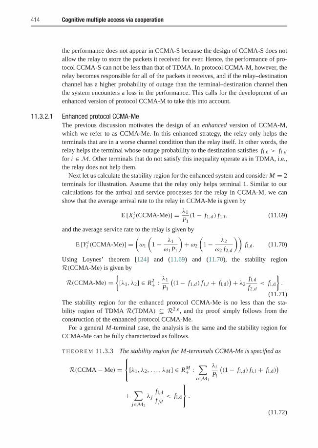
414 Cognitive multiple access via cooperation
the performance does not appear in CCMA-S because the design of CCMA-S does notallow the relay to store the packets it received for ever. Hence, the performance of pro-tocol CCMA-S can not be less than that of TDMA. In protocol CCMA-M, however, therelay becomes responsible for all of the packets it receives, and if the relay–destinationchannel has a higher probability of outage than the terminal–destination channel thenthe system encounters a loss in the performance. This calls for the development of anenhanced version of protocol CCMA-M to take this into account.
11.3.2.1 Enhanced protocol CCMA-MeThe previous discussion motivates the design of an enhanced version of CCMA-M,which we refer to as CCMA-Me. In this enhanced strategy, the relay only helps theterminals that are in a worse channel condition than the relay itself. In other words, therelay helps the terminal whose outage probability to the destination satisfies fl,d > fi,dfor i ∈M. Other terminals that do not satisfy this inequality operate as in TDMA, i.e.,the relay does not help them.
Next let us calculate the stability region for the enhanced system and consider M = 2terminals for illustration. Assume that the relay only helps terminal 1. Similar to ourcalculations for the arrival and service processes for the relay in CCMA-M, we canshow that the average arrival rate to the relay in CCMA-Me is given by
E [Xtl (CCMA-Me)] = λ1
P1(1− f1,d) f1,l , (11.69)
and the average service rate to the relay is given by
E [Y tl (CCMA-Me)] =
(ω1
(1− λ1
ω1 P1
)+ ω2
(1− λ2
ω2 f2,d
))fl,d. (11.70)
Using Loynes’ theorem [124] and (11.69) and (11.70), the stability regionR(CCMA-Me) is given by
R(CCMA-Me) ={[λ1, λ2] ∈ R2+ :
λ1
P1
((1− f1,d) f1,l + fl,d)
)+ λ2fl,df2,d
< fl,d
}.
(11.71)The stability region for the enhanced protocol CCMA-Me is no less than the sta-bility region of TDMA R(TDMA) ⊆ R2,e, and the proof simply follows from theconstruction of the enhanced protocol CCMA-Me.
For a general M-terminal case, the analysis is the same and the stability region forCCMA-Me can be fully characterized as follows.
T H E O R E M 11.3.3 The stability region for M-terminals CCMA-Me is specified as
R(CCMA−Me) =⎧⎨⎩[λ1, λ2, . . . , λM ] ∈ RM+ :
∑i∈M1
λi
Pi
((1− fi,d) fi,l + fl,d)
)
+∑
j∈M2
λ jfl,df jd
< fl,d
⎫⎬⎭ .(11.72)
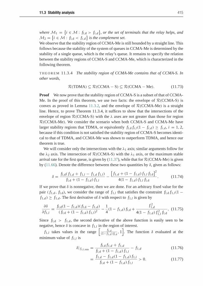
11.3 Stability analysis 415
where M1 ={i ∈M : fl,d > fi,d
}, or the set of terminals that the relay helps, and
M2 ={i ∈M : fl,d < fi,d
}is the complement set.
We observe that the stability region of CCMA-Me is still bounded by a straight line. Thisfollows because the stability of the system of queues in CCMA-Me is determined by thestability of a single queue, which is the relay’s queue. It remains to specify the relationbetween the stability regions of CCMA-S and CCMA-Me, which is characterized in thefollowing theorem.
T H E O R E M 11.3.4 The stability region of CCMA-Me contains that of CCMA-S. Inother words,
R(TDMA) ⊆ R(CCMA− S) ⊆ R(CCMA−Me). (11.73)
Proof We now prove that the stability region of CCMA-S is a subset of that of CCMA-Me. In the proof of this theorem, we use two facts: the envelope of R(CCMA-S) isconvex as proved in Lemma 11.3.2, and the envelope of R(CCMA-Me) is a straightline. Hence, to prove Theorem 11.3.4, it suffices to show that the intersections of theenvelope of region R(CCMA-S) with the λ axes are not greater than those for regionR(CCMA-Me). We consider the scenario when both CCMA-S and CCMA-Me havelarger stability regions that TDMA, or equivalently fl,d fi,l(1 − fi,d) ≥ fi,d , i = 1, 2,because if this condition is not satisfied the stability region of CCMA-S becomes identi-cal to that of TDMA, and CCMA-Me was shown to outperform TDMA, and hence ourtheorem is true.
We will consider only the intersections with the λ1 axis; similar arguments follow forthe λ2 axis. The intersection of R(CCMA-S) with the λ1 axis, or the maximum stablearrival rate for the first queue, is given by (11.37), while that for R(CCMA-Me) is givenby (11.66). Denote the difference between these two quantities by δ, given as follows:
δ = fl,d( f1,d + f1,l − f1,d f1,l)
fl,d + (1− f1,d) f1,l−[
f1,d + (1− f1,d) f1,l fl,d]2
4(1− f1,d) f1,l fl,d. (11.74)
If we prove that δ is nonnegative, then we are done. For an arbitrary fixed value for thepair ( f1,d , fl,d), we consider the range of f1,l that satisfies the constraint fl,d f1,l(1 −f1,d) ≥ f1,d . The first derivative of δ with respect to f1,l is given by
∂δ
∂ f1,l= fl,d(1− f1,d)( fl,d − f1,d)
( fl,d + (1− f1,d) f1,l)2− 1
4(1− f1,d) fl,d+
f 21,d
4(1− f1,d) f 21,l fl,d
, (11.75)
Since fl,d > f1,d , the second derivative of the above function is easily seen to benegative, hence δ is concave in f1,l in the region of interest.
f1,l takes values in the range[
f1,d(1− f1,d ) fl,d
, 1]. The function δ evaluated at the
minimum value of f1,l is
δ| f1,l,min =fl,d f1,d + f1,d
fl,d + (1− f1,d) f1,l− f1,d (11.76)
= f1,d − f1,d(1− f1,d) f1,lfl,d + (1− f1,d) f1,l
> 0. (11.77)
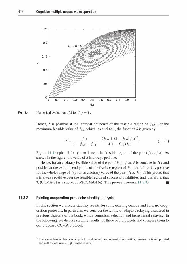
416 Cognitive multiple access via cooperation
0 0.1 0.2 0.3 0.4 0.5 0.6 0.7 0.8 0.9 10
0.05
0.1
0.15
0.2
0.25
fl,d
δ
f1,d = 0:0.5
Fig. 11.4 Numerical evaluation of δ for f1,l = 1 .
Hence, δ is positive at the leftmost boundary of the feasible region of f1,l . For themaximum feasible value of f1,l , which is equal to 1, the function δ is given by
δ = fl,d1− f1,d + fl,d
− ( f1,d + (1− f1,d) fl,d)2
4(1− f1,d) fl,d. (11.78)
Figure 11.4 depicts δ for f1,l = 1 over the feasible region of the pair ( f1,d , fl,d). Asshown in the figure, the value of δ is always positive.
Hence, for an arbitrary feasible value of the pair ( f1,d , fl,d), δ is concave in f1,l andpositive at the extreme end points of the feasible region of f1,l ; therefore, δ is positivefor the whole range of f1,l for an arbitrary value of the pair ( f1,d , fl,d). This proves thatδ is always positive over the feasible region of success probabilities, and, therefore, thatR(CCMA-S) is a subset of R(CCMA-Me). This proves Theorem 11.3.3.3 �
11.3.3 Existing cooperation protocols: stability analysis
In this section we discuss stability results for some existing decode-and-forward coop-eration protocols. In particular, we consider the family of adaptive relaying discussed inprevious chapters of the book, which comprises selection and incremental relaying. Inthe following, we discuss stability results for these two protocols and compare them toour proposed CCMA protocol.
3 The above theorem has another proof that does not need numerical evaluation; however, it is complicatedand will not add new insights to the results.
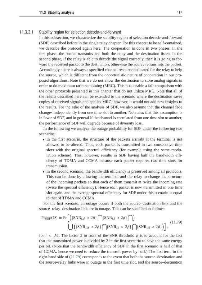
11.3 Stability analysis 417
11.3.3.1 Stability region for selection decode-and-forwardIn this subsection, we characterize the stability region of selection decode-and-forward(SDF) described before in the single relay chapter. For this chapter to be self-contained,we describe the protocol again here. The cooperation is done in two phases. In thefirst phase, the source transmits and both the relay and the destination listen. In thesecond phase, if the relay is able to decode the signal correctly, then it is going to for-ward the received packet to the destination, otherwise the source retransmits the packet.Accordingly, there is always a specified channel resource dedicated for the relay to helpthe source, which is different from the opportunistic nature of cooperation in our pro-posed algorithms. Note that we do not allow the destination to store analog signals inorder to do maximum ratio combining (MRC). This is to enable a fair comparison withthe other protocols presented in this chapter that do not utilize MRC. Note that all ofthe results described here can be extended to the scenario where the destination savescopies of received signals and applies MRC; however, it would not add new insights tothe results. For the sake of the analysis of SDF, we also assume that the channel fadechanges independently from one time slot to another. Note also that this assumption isin favor of SDF, and in general if the channel is correlated from one time slot to another,the performance of SDF will degrade because of diversity loss.
In the following we analyze the outage probability for SDF under the following twoscenarios:• In the first scenario, the structure of the packets arrivals at the terminal is not
allowed to be altered. Thus, each packet is transmitted in two consecutive timeslots with the original spectral efficiency (for example using the same modu-lation scheme). This, however, results in SDF having half the bandwidth effi-ciency of TDMA and CCMA because each packet requires two time slots fortransmission.
• In the second scenario, the bandwidth efficiency is preserved among all protocols.This can be done by allowing the terminal and the relay to change the structureof the incoming packets so that each of them transmit at twice the incoming rate(twice the spectral efficiency). Hence each packet is now transmitted in one timeslot again, and the average spectral efficiency for SDF under this scenario is equalto that of TDMA and CCMA.
For the first scenario, an outage occurs if both the source–destination link and thesource–relay–destination link are in outage. This can be specified as follows:
PrSDF(O) = Pr[({SNRi,d < 2β}
⋂{SNRi,l < 2β}
⋂)⋃(
{SNRi,d < 2β}⋂{SNRi,l > 2β}
⋂{SNRl,d < 2β}
)],
(11.79)
for i ∈ M. The factor 2 in front of the SNR threshold β is to account for the factthat the transmitted power is divided by 2 in the first scenario to have the same energyper bit. (Note that the bandwidth efficiency of SDF in the first scenario is half of thatof CCMA, hence we need to reduce the transmit power by half.) The first term in theright-hand side of (11.79) corresponds to the event that both the source–destination andthe source–relay links were in outage in the first time slot, and the source–destination
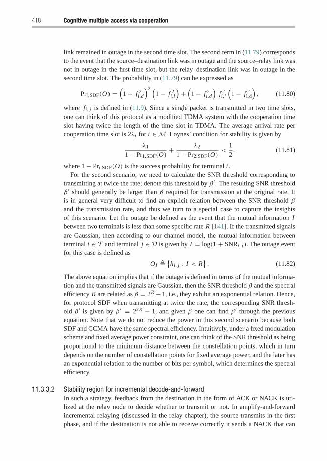
418 Cognitive multiple access via cooperation
link remained in outage in the second time slot. The second term in (11.79) correspondsto the event that the source–destination link was in outage and the source–relay link wasnot in outage in the first time slot, but the relay–destination link was in outage in thesecond time slot. The probability in (11.79) can be expressed as
Pri,SDF(O) =(1− f 2
i,d
)2 (1− f 2
i,l
)+(1− f 2
i,d
)f 2i,l
(1− f 2
l,d
), (11.80)
where fi, j is defined in (11.9). Since a single packet is transmitted in two time slots,one can think of this protocol as a modified TDMA system with the cooperation timeslot having twice the length of the time slot in TDMA. The average arrival rate percooperation time slot is 2λi for i ∈M. Loynes’ condition for stability is given by
λ1
1− Pr1,SDF(O)+ λ2
1− Pr2,SDF(O)<
1
2, (11.81)
where 1− Pri,SDF(O) is the success probability for terminal i .For the second scenario, we need to calculate the SNR threshold corresponding to
transmitting at twice the rate; denote this threshold by β ′. The resulting SNR thresholdβ ′ should generally be larger than β required for transmission at the original rate. Itis in general very difficult to find an explicit relation between the SNR threshold βand the transmission rate, and thus we turn to a special case to capture the insightsof this scenario. Let the outage be defined as the event that the mutual information Ibetween two terminals is less than some specific rate R [141]. If the transmitted signalsare Gaussian, then according to our channel model, the mutual information betweenterminal i ∈ T and terminal j ∈ D is given by I = log(1+ SNRi, j ). The outage eventfor this case is defined as
OI �{hi, j : I < R
}. (11.82)
The above equation implies that if the outage is defined in terms of the mutual informa-tion and the transmitted signals are Gaussian, then the SNR threshold β and the spectralefficiency R are related as β = 2R − 1, i.e., they exhibit an exponential relation. Hence,for protocol SDF when transmitting at twice the rate, the corresponding SNR thresh-old β ′ is given by β ′ = 22R − 1, and given β one can find β ′ through the previousequation. Note that we do not reduce the power in this second scenario because bothSDF and CCMA have the same spectral efficiency. Intuitively, under a fixed modulationscheme and fixed average power constraint, one can think of the SNR threshold as beingproportional to the minimum distance between the constellation points, which in turndepends on the number of constellation points for fixed average power, and the later hasan exponential relation to the number of bits per symbol, which determines the spectralefficiency.
11.3.3.2 Stability region for incremental decode-and-forwardIn such a strategy, feedback from the destination in the form of ACK or NACK is uti-lized at the relay node to decide whether to transmit or not. In amplify-and-forwardincremental relaying (discussed in the relay chapter), the source transmits in the firstphase, and if the destination is not able to receive correctly it sends a NACK that can
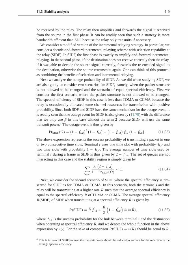
11.3 Stability analysis 419
be received by the relay. The relay then amplifies and forwards the signal it receivedfrom the source in the first phase. It can be readily seen that such a strategy is morebandwidth efficient than SDF because the relay only transmits if necessary.
We consider a modified version of the incremental relaying strategy. In particular, weconsider a decode-and-forward incremental relaying scheme with selection capability atthe relay (SIDF). In SIDF, the first phase is exactly as amplify-and-forward incrementalrelaying. In the second phase, if the destination does not receive correctly then the relay,if it was able to decode the source signal correctly, forwards the re-encoded signal tothe destination, otherwise the source retransmits again. One can think of this protocolas combining the benefits of selection and incremental relaying.
Next we analyze the outage probability of SIDF. As we did when studying SDF, weare also going to consider two scenarios for SIDF, namely, when the packet structureis not allowed to be changed and the scenario of equal spectral efficiency. First weconsider the first scenario where the packet structure is not allowed to be changed.The spectral efficiency of SIDF in this case is less than TDMA or CCMA because therelay is occasionally allocated some channel resources for transmission with positiveprobability. Since both SDF and SIDF have the same mechanism for the outage event, itis readily seen that the outage event for SIDF is also given by (11.79) with the differencethat we only use β in this case without the term 2 because SIDF will use the sametransmit power.4 The outage event is thus given by
PrSIDF(O) =(1− fi,d
)2 (1− fi,l)+ (1− fi,d
)fi,l(1− fl,d
). (11.83)
The above expression represents the success probability of transmitting a packet in oneor two consecutive time slots. Terminal i uses one time slot with probability fi,d andtwo time slots with probability 1 − fi,d . The average number of time slots used byterminal i during a frame in SIDF is thus given by 2 − fi,d . The set of queues are notinteracting in this case and the stability region is simply given by∑
i∈M
λi(2− fi,d
)1− PrSIDF(O)
< 1. (11.84)
Next, we consider the second scenario of SIDF where the spectral efficiency is pre-served for SIDF as for TDMA or CCMA. In this scenario, both the terminals and therelay will be transmitting at a higher rate R such that the average spectral efficiency isequal to the spectral efficiency R of TDMA or CCMA. The average spectral efficiencyR(SIDF) of SIDF when transmitting at a spectral efficiency R is given by
R(SIDF) = R ˜fi,d + R
2
(1− ˜fi,d
)� v(R), (11.85)
where ˜fi,d is the success probability for the link between terminal i and the destinationwhen operating at spectral efficiency R, and we denote the whole function in the aboveexpression by v(·). For the sake of comparison R(SIDF) = v(R) should be equal to R.
4 This is in favor of SIDF because the transmit power should be reduced to account for the reduction in theaverage spectral efficiency.
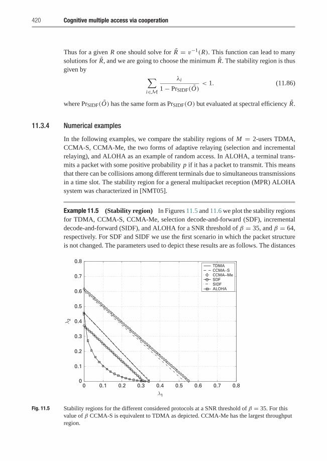
420 Cognitive multiple access via cooperation
Thus for a given R one should solve for R = v−1(R). This function can lead to manysolutions for R, and we are going to choose the minimum R. The stability region is thusgiven by ∑
i∈M
λi
1− PrSIDF(O)< 1. (11.86)
where PrSIDF(O) has the same form as PrSIDF(O) but evaluated at spectral efficiency R.
11.3.4 Numerical examples
In the following examples, we compare the stability regions of M = 2-users TDMA,CCMA-S, CCMA-Me, the two forms of adaptive relaying (selection and incrementalrelaying), and ALOHA as an example of random access. In ALOHA, a terminal trans-mits a packet with some positive probability p if it has a packet to transmit. This meansthat there can be collisions among different terminals due to simultaneous transmissionsin a time slot. The stability region for a general multipacket reception (MPR) ALOHAsystem was characterized in [NMT05].
Example 11.5 (Stability region) In Figures 11.5 and 11.6 we plot the stability regionsfor TDMA, CCMA-S, CCMA-Me, selection decode-and-forward (SDF), incrementaldecode-and-forward (SIDF), and ALOHA for a SNR threshold of β = 35, and β = 64,respectively. For SDF and SIDF we use the first scenario in which the packet structureis not changed. The parameters used to depict these results are as follows. The distances
0 0.1 0.2 0.3 0.4 0.5 0.6 0.7 0.80
0.1
0.2
0.3
0.4
0.5
0.6
0.7
0.8
λ 1
λ 2
TDMACCMA−SCCMA−MeSDFSIDFALOHA
Fig. 11.5 Stability regions for the different considered protocols at a SNR threshold of β = 35. For thisvalue of β CCMA-S is equivalent to TDMA as depicted. CCMA-Me has the largest throughputregion.
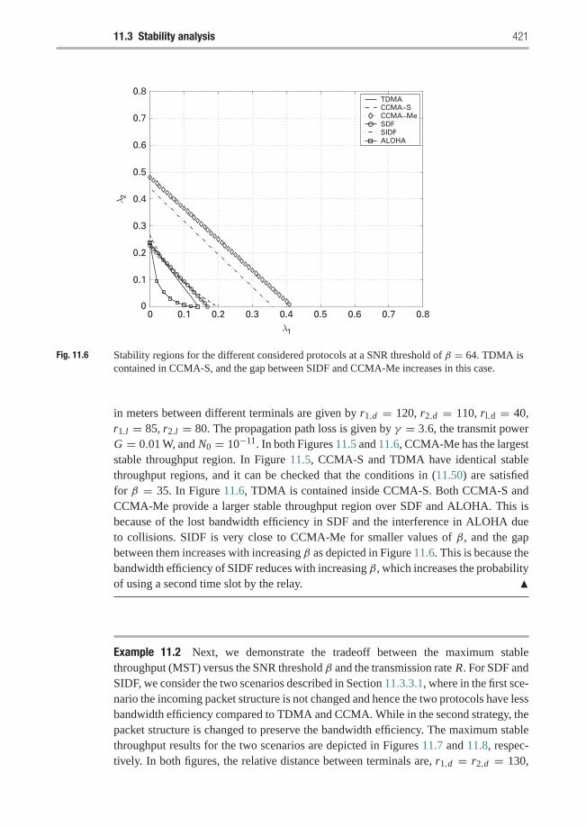
11.3 Stability analysis 421
0 0.1 0.2 0.3 0.4 0.5 0.6 0.7 0.80
0.1
0.2
0.3
0.4
0.5
0.6
0.7
0.8
λ1
λ 2
TDMACCMA−SCCMA−MeSDFSIDFALOHA
Fig. 11.6 Stability regions for the different considered protocols at a SNR threshold of β = 64. TDMA iscontained in CCMA-S, and the gap between SIDF and CCMA-Me increases in this case.
in meters between different terminals are given by r1,d = 120, r2,d = 110, rl,d = 40,r1,l = 85, r2,l = 80. The propagation path loss is given by γ = 3.6, the transmit powerG = 0.01 W, and N0 = 10−11. In both Figures 11.5 and 11.6, CCMA-Me has the largeststable throughput region. In Figure 11.5, CCMA-S and TDMA have identical stablethroughput regions, and it can be checked that the conditions in (11.50) are satisfiedfor β = 35. In Figure 11.6, TDMA is contained inside CCMA-S. Both CCMA-S andCCMA-Me provide a larger stable throughput region over SDF and ALOHA. This isbecause of the lost bandwidth efficiency in SDF and the interference in ALOHA dueto collisions. SIDF is very close to CCMA-Me for smaller values of β, and the gapbetween them increases with increasing β as depicted in Figure 11.6. This is because thebandwidth efficiency of SIDF reduces with increasing β, which increases the probabilityof using a second time slot by the relay. �
Example 11.2 Next, we demonstrate the tradeoff between the maximum stablethroughput (MST) versus the SNR threshold β and the transmission rate R. For SDF andSIDF, we consider the two scenarios described in Section 11.3.3.1, where in the first sce-nario the incoming packet structure is not changed and hence the two protocols have lessbandwidth efficiency compared to TDMA and CCMA. While in the second strategy, thepacket structure is changed to preserve the bandwidth efficiency. The maximum stablethroughput results for the two scenarios are depicted in Figures 11.7 and 11.8, respec-tively. In both figures, the relative distance between terminals are, r1,d = r2,d = 130,
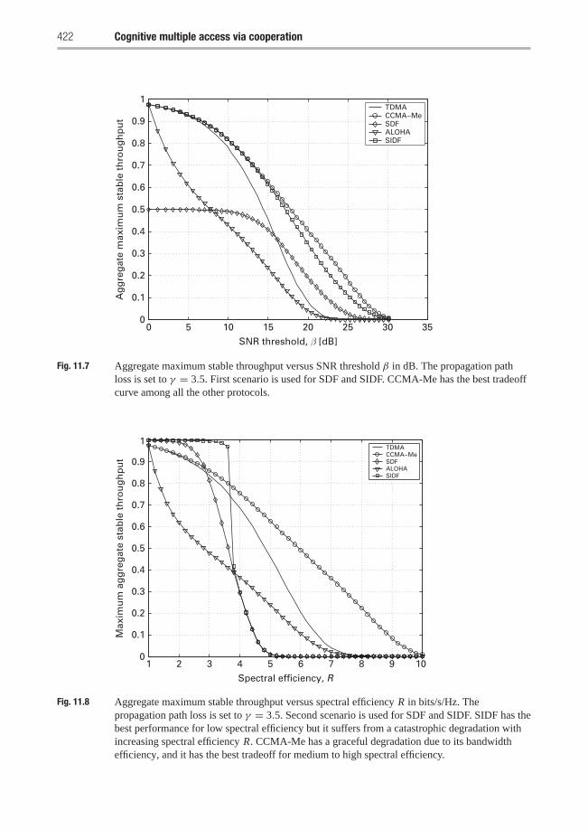
422 Cognitive multiple access via cooperation
0 5 10 15 20 25 30 350
0.1
0.2
0.3
0.4
0.5
0.6
0.7
0.8
0.9
1
SNR threshold, β [dB]
Ag
gre
gat
e m
axim
um
sta
ble
th
rou
gh
pu
tTDMACCMA−MeSDFALOHASIDF
Fig. 11.7 Aggregate maximum stable throughput versus SNR threshold β in dB. The propagation pathloss is set to γ = 3.5. First scenario is used for SDF and SIDF. CCMA-Me has the best tradeoffcurve among all the other protocols.
1 2 3 4 5 6 7 8 9 100
0.1
0.2
0.3
0.4
0.5
0.6
0.7
0.8
0.9
1
Spectral efficiency, R
Max
imu
m a
gg
reg
ate
stab
le t
hro
ug
hp
ut
TDMACCMA−MeSDFALOHASIDF
Fig. 11.8 Aggregate maximum stable throughput versus spectral efficiency R in bits/s/Hz. Thepropagation path loss is set to γ = 3.5. Second scenario is used for SDF and SIDF. SIDF has thebest performance for low spectral efficiency but it suffers from a catastrophic degradation withincreasing spectral efficiency R. CCMA-Me has a graceful degradation due to its bandwidthefficiency, and it has the best tradeoff for medium to high spectral efficiency.
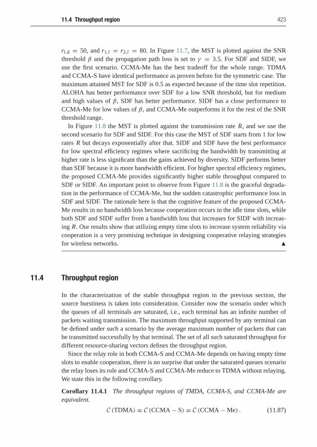
11.4 Throughput region 423
rl,d = 50, and r1,l = r2,l = 80. In Figure 11.7, the MST is plotted against the SNRthreshold β and the propagation path loss is set to γ = 3.5. For SDF and SIDF, weuse the first scenario. CCMA-Me has the best tradeoff for the whole range. TDMAand CCMA-S have identical performance as proven before for the symmetric case. Themaximum attained MST for SDF is 0.5 as expected because of the time slot repetition.ALOHA has better performance over SDF for a low SNR threshold, but for mediumand high values of β, SDF has better performance. SIDF has a close performance toCCMA-Me for low values of β, and CCMA-Me outperforms it for the rest of the SNRthreshold range.
In Figure 11.8 the MST is plotted against the transmission rate R, and we use thesecond scenario for SDF and SIDF. For this case the MST of SDF starts from 1 for lowrates R but decays exponentially after that. SIDF and SDF have the best performancefor low spectral efficiency regimes where sacrificing the bandwidth by transmitting athigher rate is less significant than the gains achieved by diversity. SIDF performs betterthan SDF because it is more bandwidth efficient. For higher spectral efficiency regimes,the proposed CCMA-Me provides significantly higher stable throughput compared toSDF or SIDF. An important point to observe from Figure 11.8 is the graceful degrada-tion in the performance of CCMA-Me, but the sudden catastrophic performance loss inSDF and SIDF. The rationale here is that the cognitive feature of the proposed CCMA-Me results in no bandwidth loss because cooperation occurs in the idle time slots, whileboth SDF and SIDF suffer from a bandwidth loss that increases for SIDF with increas-ing R. Our results show that utilizing empty time slots to increase system reliability viacooperation is a very promising technique in designing cooperative relaying strategiesfor wireless networks. �
11.4 Throughput region
In the characterization of the stable throughput region in the previous section, thesource burstiness is taken into consideration. Consider now the scenario under whichthe queues of all terminals are saturated, i.e., each terminal has an infinite number ofpackets waiting transmission. The maximum throughput supported by any terminal canbe defined under such a scenario by the average maximum number of packets that canbe transmitted successfully by that terminal. The set of all such saturated throughput fordifferent resource-sharing vectors defines the throughput region.
Since the relay role in both CCMA-S and CCMA-Me depends on having empty timeslots to enable cooperation, there is no surprise that under the saturated queues scenariothe relay loses its role and CCMA-S and CCMA-Me reduce to TDMA without relaying.We state this in the following corollary.
Corollary 11.4.1 The throughput regions of TMDA, CCMA-S, and CCMA-Me areequivalent.
C (TDMA) ≡ C (CCMA− S) ≡ C (CCMA−Me) . (11.87)
424 Cognitive multiple access via cooperation
From the above corollary, we conclude that the saturated throughput region is a subsetof the stability region for both CCMA-S and CCMA-Me. This is an important observa-tion, because for ALOHA systems it is conjectured in [129] that the maximum stablethroughput region is identical to the throughput region. It is of interest then to pointout that CCMA-S and CCMA-Me are examples of multiple access protocols where thestable throughput region is different from the throughput region.
11.5 Delay analysis
In this section we characterize the delay performance of the cognitive cooperativemultiple access protocols, CCMA-S and CCMA-Me.
11.5.1 Delay performance for CCMA-S
In CCMA-S, a packet does not depart a terminal’s queue until it is successfully trans-mitted to the destination. Therefore, the delay encountered by a a packet is the oneencountered in the terminal’s queue. Delay analysis for interacting queues in ALOHAhas been studied before, and it turns out to be a notoriously hard problem. Most of theknown results are only for the two-user ALOHA case. In this section we consider asymmetric two-user CCMA-S scenario and characterize its delay performance.
Define the moment-generating function of the joint queues’ sizes processes (Qt1, Qt
2)
as follows:
G(u, v) = limt→∞E
[uQt
1vQt2
]. (11.88)
From the queue evolution equations in (11.13), we have
E[uQt+1
1 vQt+12
]= E
[uXt
1vXt2
]E[u(Q
t1−Y t
1)+v(Q
t2−Y t
2)+], (11.89)
where the above equation follows from the independence assumption of the futurearrival processes from the past departure and arrival processes. Since the arrival pro-cesses are assumed to follow a Bernoulli random process, the moment-generatingfunction of the joint arrival process is given by
A(u, v) � limt→∞E
[uXt
1vXt2
]= (uλ+ 1− λ) (vλ+ 1− λ) , (11.90)
where, due to the symmetry of the two terminals, each has an arrival rate λ. From thedefinition of the service process of CCMA-S (11.17), it follows that
E[u(Q
t1−Y t
1)+v(Q
t2−Y t
2)+]= E
[1(Qt
1= 0, Qt2= 0)
]+ B(u)E[1(Qt
1>0, Qt2 = 0)uQt
1
]+ B(v)E
[1(Qt
1 = 0, Qt2 > 0)vQt
2
]+ D(u, v)E
[1(Qt
1 > 0, Qt2 > 0)uQt
1vQt2
],
where
B(z) = w f1,d+w2 f1,l fl,d(1− f1,d )z + 1− (w f1,d + w2 f1,l fl,d(1− f1,d)
), (11.91)
D(u, v) = w f1,d(1u + 1
v)+ 2w(1− f1,d), (11.92)
11.5 Delay analysis 425
in which we use w to denote the symmetric resource-sharing portion of eachterminal.
Substituting (11.90) and (11.91) into (11.89) and taking the limits we get
G(u, v) = A(u, v) (G(0, 0)+ B(u) [G(u, 0)− G(0, 0)]+ B(v) [G(0, v)
−G(0, 0)] +D(u, v) [G(u, v)+ G(0, 0)− G(u, 0)− G(0, v)]) .
(11.93)
We can rewrite the above equation as G(u, v) = H(u, v)/F(u, v), where
H(u, v) = G(0, 0)+ B(u) [G(u, 0)− G(0, 0)]+ B(v)× [G(0, v)− G(0, 0)]
+ D(u, v)(G(0, 0)− G(u, 0)− G(0, v)),
and F(u, v) = 1− A(u, v)D(u, v).Define
G1(u, v) � ∂G(u, v)
∂u. (11.94)
Due to symmetry, the average queue size is given by G1(1, 1). Hence, to find the averagequeuing delay, we need to compute G1(1, 1).
First we find a relation between G(0, 0) and G(1, 0) using the following two prop-erties which follow from the symmetry of the problem: G(1, 1) = 1 and G(1, 0) =G(0, 1). Applying these two properties to (11.93) along with a simple application of theL’Hopital limit theorem we get(w2 f1,l fl,d(1− f1,d)
)G(0, 0)+
(w f1,d − w2 f1,l fl,d(1− f1,d)
)G(1, 0) = w f1,d−λ.
(11.95)Taking the derivative of (11.93) with respect to u, applying L’Hopital twice, and usingthe relation in (11.95) we get
G1(1, 1) = λ(1− λ)w f1,d − λ −
w2 f1,l fl,d(1− f1,d)
w f1,d − λ G1(1, 0). (11.96)
To find another equation relating G1(1, 1) and G1(1, 0), we compute ∂G(u, u)/∂u atu = 1. After some tedious but straightforward calculations, we get
G(u, u)
u|u=1 = 2λ− 1+ w f1,d − w2 f1,l fl,d(1− f1,d)
w f1,d − λG1(1, 0)− 4w f1,dλ− 2w f1,d − λ2
2(w f1,d − λ) . (11.97)
Due to the symmetry of the problem, we have the following property:
∂G(u, u)
∂u|u=1 = 2G1(1, 1). (11.98)
Using the above equation, and solving (11.96) and (11.97), we get
G1(1, 1) = − (2w f1,d + w2 f1,l fl,d(1− f1,d))λ2 + 2w f1,dλ
2(w f1,d + w2 f1,l fl,d(1− f1,d))(w f1,d − λ) . (11.99)
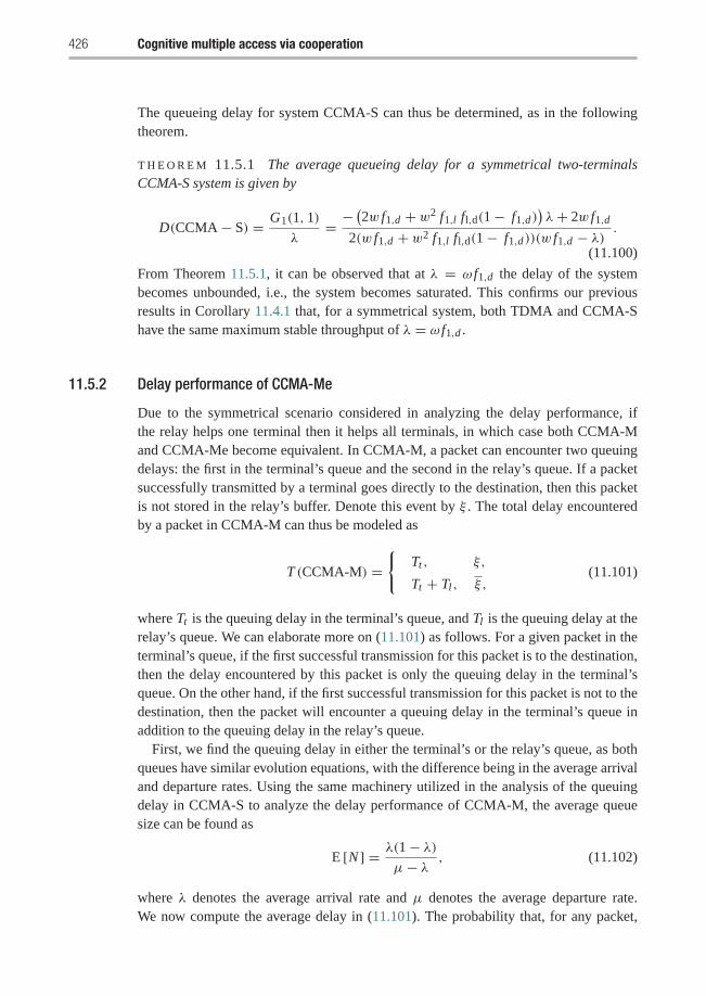
426 Cognitive multiple access via cooperation
The queueing delay for system CCMA-S can thus be determined, as in the followingtheorem.
T H E O R E M 11.5.1 The average queueing delay for a symmetrical two-terminalsCCMA-S system is given by
D(CCMA− S) = G1(1, 1)
λ= − (2w f1,d + w2 f1,l fl,d(1− f1,d)
)λ+ 2w f1,d
2(w f1,d + w2 f1,l fl,d(1− f1,d))(w f1,d − λ) .(11.100)
From Theorem 11.5.1, it can be observed that at λ = ω f1,d the delay of the systembecomes unbounded, i.e., the system becomes saturated. This confirms our previousresults in Corollary 11.4.1 that, for a symmetrical system, both TDMA and CCMA-Shave the same maximum stable throughput of λ = ω f1,d .
11.5.2 Delay performance of CCMA-Me
Due to the symmetrical scenario considered in analyzing the delay performance, ifthe relay helps one terminal then it helps all terminals, in which case both CCMA-Mand CCMA-Me become equivalent. In CCMA-M, a packet can encounter two queuingdelays: the first in the terminal’s queue and the second in the relay’s queue. If a packetsuccessfully transmitted by a terminal goes directly to the destination, then this packetis not stored in the relay’s buffer. Denote this event by ξ . The total delay encounteredby a packet in CCMA-M can thus be modeled as
T (CCMA-M) ={
Tt , ξ,
Tt + Tl , ξ ,(11.101)
where Tt is the queuing delay in the terminal’s queue, and Tl is the queuing delay at therelay’s queue. We can elaborate more on (11.101) as follows. For a given packet in theterminal’s queue, if the first successful transmission for this packet is to the destination,then the delay encountered by this packet is only the queuing delay in the terminal’squeue. On the other hand, if the first successful transmission for this packet is not to thedestination, then the packet will encounter a queuing delay in the terminal’s queue inaddition to the queuing delay in the relay’s queue.
First, we find the queuing delay in either the terminal’s or the relay’s queue, as bothqueues have similar evolution equations, with the difference being in the average arrivaland departure rates. Using the same machinery utilized in the analysis of the queuingdelay in CCMA-S to analyze the delay performance of CCMA-M, the average queuesize can be found as
E [N ] = λ(1− λ)μ− λ , (11.102)
where λ denotes the average arrival rate and μ denotes the average departure rate.We now compute the average delay in (11.101). The probability that, for any packet,
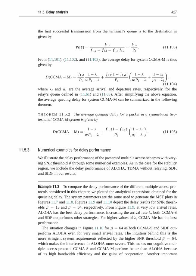
11.5 Delay analysis 427
the first successful transmission from the terminal’s queue is to the destination isgiven by
Pr[ξ ] = f1,df1,d + f1,l − f1,d f1,l
= f1,dP1. (11.103)
From (11.101), (11.102), and (11.103), the average delay for system CCMA-M is thusgiven by
D(CCMA−M) = f1,dP1
1− λwP1 − λ +
f1,l(1− f1,d)
P1
(1− λwP1 − λ +
1− λl
μl − λl
),
(11.104)where λl and μl are the average arrival and departure rates, respectively, for therelay’s queue defined in (11.61) and (11.63). After simplifying the above equation,the average queuing delay for system CCMA-M can be summarized in the followingtheorem.
T H E O R E M 11.5.2 The average queuing delay for a packet in a symmetrical two-terminal CCMA-M system is given by
D(CCMA−M) = 1− λwP1 − λ +
f1,l(1− f1,d)
P1
(1− λl
μl − λl
). (11.105)
11.5.3 Numerical examples for delay performance
We illustrate the delay performance of the presented multiple access schemes with vary-ing SNR threshold β through some numerical examples. As in the case for the stabilityregion, we include the delay performance of ALOHA, TDMA without relaying, SDF,and SIDF in our results.
Example 11.3 To compare the delay performance of the different multiple access pro-tocols considered in this chapter, we plotted the analytical expressions obtained for thequeueing delay. The system parameters are the same used to generate the MST plots inFigures 11.7 and 11.8. Figures 11.9 and 11.10 depict the delay results for SNR thresh-olds β = 15 and β = 64, respectively. From Figure 11.9, at very low arrival rates,ALOHA has the best delay performance. Increasing the arrival rate λ, both CCMA-Sand SDF outperforms other strategies. For higher values of λ, CCMA-Me has the bestperformance
The situation changes in Figure 11.10 for β = 64 as both CCMA-S and SIDF out-perform ALOHA even for very small arrival rates. The intuition behind this is themore stringent system requirements reflected by the higher SNR threshold β = 64,which makes the interference in ALOHA more severe. This makes our cognitive mul-tiple access protocol CCMA-S and CCMA-M perform better than ALOHA becauseof its high bandwidth efficiency and the gains of cooperation. Another important
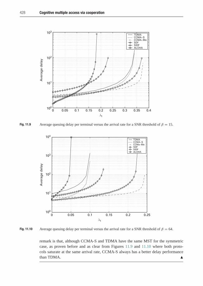
428 Cognitive multiple access via cooperation
0 0.05 0.1 0.15 0.2 0.25 0.3 0.35 0.4100
101
102
103
λ1
Ave
rag
e d
elay
TDMACCMA−SCCMA−MeSDfSIDFALOHA
Fig. 11.9 Average queuing delay per terminal versus the arrival rate for a SNR threshold of β = 15.
0 0.05 0.1 0.15 0.2 0.25100
101
102
103
104
λ1
Ave
rag
e d
elay
TDMACCMA−SCCMa−MeSDFSIDFALOHA
Fig. 11.10 Average queuing delay per terminal versus the arrival rate for a SNR threshold of β = 64.
remark is that, although CCMA-S and TDMA have the same MST for the symmetriccase, as proven before and as clear from Figures 11.9 and 11.10 where both proto-cols saturate at the same arrival rate, CCMA-S always has a better delay performancethan TDMA. �
Exercises 429
11.6 Chapter summary and bibliographical notes
In this chapter, we have studied the impact of cooperative communications at the mul-tiple access layer. We described a cognitive multiple access protocol in the presenceof a relay in the network. The relay senses the channel for idle channel resources andexploits them to cooperate with the terminals in forwarding their packets. Two protocolsto implement the proposed multiple access strategy, namely, CCMA-S and CCMA-Me, were described. We characterized the maximum stable throughput region of theproposed protocols and compared them to some existing adaptive relaying strategies:non-cooperative TDMA and random-access ALOHA.
We studied the delay performance of the described protocols. The analysis revealssignificant performance gains of the cognitive protocols over their non-cognitive coun-terparts. This is because the described cognitive multiple access strategies do notresult in any bandwidth loss, as cooperation is enabled only in idle “unused” channelresources, which results in a graceful degradation of the maximum stable through-put when increasing the communication rate. On the other hand, the maximum stablethroughput of non-cognitive relaying strategies as selection and incremental relayingsuffer from catastrophic degradation with increasing communication rate, because oftheir inherent bandwidth inefficiency.
Analyzing the stability of interacting queues is a difficult problem that has beenaddressed for ALOHA systems initially in [220]. Later in [149], the dominant systemapproach was explicitly introduced and employed to find bounds on the stable through-put region of ALOHA with collision channel model. Many other works followed that tostudy the stability of ALOHA. In [209], necessary and sufficient conditions for the sta-bility of a finite number of queues were provided; however, the stable throughput regionwas only explicitly characterized for a three-terminals system. In [127], the authors pro-vided tighter bounds on the stable throughput region for the ALOHA system using theconcept of stability ranks, which was also introduced in the same paper. The stabil-ity of ALOHA systems under a multi-packet reception model (MPR) was consideredin [138, 129]. Characterizing the stable throughput region for interacting queues withM > 3 terminals is still an open problem.
Delay analysis for interacting queues is a notoriously hard problem that has beeninvestigated in [136, 185] for ALOHA. Studies on the design and stability analysis ofthe cognitive collaborative multiple access protocol can be found in [159, 160, 162].
Exercises
11.1 In Section 11.3.3, the stability regions for selective and incremental relaying werederived.
(a) Derive the outage probability for both decode-and-forward relaying andamplify-and-forward relaying and use the results to characterize the stablethroughput regions for both relaying techniques using Loynes’ theorem.
(b) Find the maximum stable throughput for these two protocols and plot theresults against the SNR threshold for a fixed spectral efficiency, and against

430 Cognitive multiple access via cooperation
the spectral efficiency when fixing the SNR. Compare the performance toCCMA-S and CCMA-Me.
11.2 The stability results for CCMA-S and CCMA-Me were derived under theRayleigh flat fading channel model.
(a) Derive the stability regions for the two protocols under an AWGN channelmodel including the propagation path loss.
(b) Characterize the relation between the stability regions of the proposedprotocols and TDMA under the AWGN channel.
11.3 Use the moment-generating function approach to analyze the delay performanceof decode-and-forward and amplify-and-forward relaying under a Rayleigh flatfading channel model for a two-user system. Plot the delay performance versusthe arrival rate for a symmetric case. Find the arrival rate at which the systemsaturates. Perform the previous calculations for the following three scenarios:
(a) Relay close to the source.(b) Relay close to the destination.(c) Relay in the middle.
Compare the delay performance results of decode-and-forward and amplify-and-forward to the CCMA-S and CCMA-Me protocols presented in this chapter.
11.4 Find another approach to prove the results of Theorem 11.3.3 without usingnumerical techniques.[Hint: Find an auxiliary system whose stability region contains that of CCMA-Sand at the same time is a subset from the stability region of CCMA-Me.]
11.5 Characterize the maximum sum stable throughput that can be achieved by oftwo-user TDMA, CCMA-S, and CCMA-Me for a general asymmetric case.What is the impact of a scheme that maximizes the sum stable throughput on thesystem fairness? In other words, do both users transmit at the same rate?
11.6 In Exercise 11.5 the goal was to maximize the system sum-stable throughput.Consider now that the objective is to achieve an equal grade of service, i.e., allusers in the system achieve the same throughput.Find the maximum common throughput that all users in the system can achieve.[An equal grade of service corresponds to absolute fairness because all users getto transmit at the same throughput.][Hint: An equal grade of service corresponds to the point on the stable throughputregion that intersects with a line that makes a 45◦ with the x-axis.]
11.7 Write down a Matlab code that draws the stability region of CCMA-S usingthe expression in (11.22), and without resorting to the closed-form expressionin Theorem 11.3.1. Next compare your numerical results to this closed-formexpression.
11.8 In (11.42), the optimal amount of resources allocated for the first user wasspecified as
w1∗ =⎧⎨⎩
λ1f1,d, if λ1 ≤ f 2
1,d(1− f1,d ) f1,l fl,d
,√λ1
(1− f1,d ) f1,l fl,d, otherwise.
(E11.1)
Prove that this expression never exceeds one.
Exercises 431
11.9 A moment-generating function approach was used to analyze the delay ofCCMA-S. The moment-generating function expression was given as (11.93)
G(u, v) = A(u, v) (G(0, 0)+ B(u) [G(u, 0)− G(0, 0)]+ B(v) [G(0, v)(E11.2)
−G(0, 0)] +D(u, v) [G(u, v)+ G(0, 0)− G(u, 0)− G(0, v)]) .(E11.3)
Prove this expression.11.10 Applying the L’ Hopital theorem twice prove the expression in (11.99), i.e.,
prove
G1(1, 1) = − (2w f1,d + w2 f1,l fl,d(1− f1,d))λ2 + 2w f1,dλ
2(w f1,d + w2 f1,l fl,d(1− f1,d))(w f1,d − λ) . (E11.4)
12 Content-aware cooperative multipleaccess
The previous chapter studied the effects and use of cooperation on the multiple accesschannel. In this chapter we look further into using the properties of the source trafficto improve the efficiency of cooperative multiple access. Because the presentation inthis chapter is highly dependent on the characteristics of the source, we will focus onthe communication of packet speech. Nevertheless, the main underlying ideas can beextended to other types of sources.
Speech communication has a distinctive characteristic that differentiates it from datacommunication, which was the main focus of the previous chapter. Speech sourcesare characterized by periods of silence in between talk spurts. The speech talk–silencepatterns could be exploited in statistical multiplexing-like schemes where silent usersrelease their reserved channel resources, which can then be utilized to admit more usersto the network. This comes at the cost of requiring a more sophisticated multiple accessprotocol. One well-known protocol that uses this approach for performance improve-ment is the packet reservation multiple access (PRMA) protocol [49], which can beviewed as a combination of TDMA and slotted ALOHA protocols. In PRMA, terminalsin talk spurts contend for the channel in empty time slots. If a user contends succesfully,then the slot used for contention is reserved for the user. Users with reservations trans-mit their voice packets in their reserved slots. If a user fails to transmit its packet dueto channel errors, the user looses the reservation and the reserved slot becomes free forcontention again. Although the effects of this operation is practically unnoticeable inchannels where errors are very infrequent, in channels with frequent errors (such as thewireless channel) the loss of renovation due to an error has the potential to adverselyaffect the efficiency of the protocol. This is because channel errors not only force thediscarding of the damaged packets, but also increase the network traffic and accessdelay, as users with lost packets have to repeat the contention process again.
This chapter will focus on a cooperative multiple access protocol that uses the prop-erties of speech to increase the network capacity and the user cooperation efficiency. Asis the case with established multiple access protocols, the network capacity is increasedby reserving the network resources only to the users in a call spurt. Those users fin-ishing a silence period need to contend for channel access over a shared resource. Atthe same time, the use of cooperation increases the system performance by helpingusers in talk spurts to reduce the probability of dropping packets and having to contendagain. Cooperation is achieved through the deployment of a relay node. This relay nodeexploits the silence periods typical of speech communications in a new way, since it
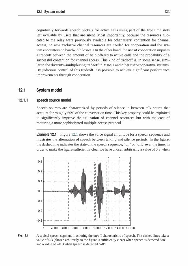
12.1 System model 433
cognitively forwards speech packets for active calls using part of the free time slotsleft available by users that are silent. Most importantly, because the resources allo-cated to the relay were previously available for other users’ contention for channelaccess, no new exclusive channel resources are needed for cooperation and the sys-tem encounters no bandwidth losses. On the other hand, the use of cooperation imposesa tradeoff between the amount of help offered to active calls and the probability of asuccessful contention for channel access. This kind of tradeoff is, in some sense, simi-lar to the diversity–multiplexing tradeoff in MIMO and other user-cooperative systems.By judicious control of this tradeoff it is possible to achieve significant performanceimprovements through cooperation.
12.1 System model
12.1.1 speech source model
Speech sources are characterized by periods of silence in between talk spurts thataccount for roughly 60% of the conversation time. This key property could be exploitedto significantly improve the utilization of channel resources but with the cost ofrequiring a more sophisticated multiple access protocol.
Example 12.1 Figure 12.1 shows the voice signal amplitude for a speech sequence andillustrates the alternation of speech between talking and silence periods. In the figure,the dashed line indicates the state of the speech sequence, “on” or “off,” over the time. Inorder to make the figure sufficiently clear we have chosen arbitrarily a value of 0.3 when
0 2000 4000 6000 8000 10 000 12 000 14 000 16 000
0.3
0.2
0.1
0.0
–0.1
–0.2
–0.3
Fig. 12.1 A typical speech segment illustrating the on/off characteristic of speech. The dashed lines take avalue of 0.3 (chosen arbitrarily so the figure is sufficiently clear) when speech is detected “on”and a value of −0.3 when speech is detected “off”.
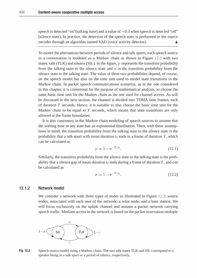
434 Content-aware cooperative multiple access
speech is detected “on”(talking state) and a value of−0.3 when speech is detected “off”(silence state). In practice, the detection of the speech state is performed in the sourceencoder through an algorithm named VAD (voice activity detector). �
To model the alternations between periods of silence and talk spurts, each speech sourcein a conversation is modeled as a Markov chain as shown in Figure 12.2 with twostates: talk (TLK) and silence (SIL). In the figure, γ represents the transition probabilityfrom the talking state to the silence state and σ is the transition probability from thesilence state to the talking state. The value of these two probabilities depend, of course,on the speech model but also on the time unit used to model state transitions in theMarkov chain. In packet speech communications scenarios, as in the one consideredin this chapter, it is convenient for the purpose of mathematical analysis, to choose thesame basic time unit for the Markov chain as the one used for channel access. As willbe discussed in the next section, the channel is divided into TDMA time frames, eachof duration T seconds. Hence, it is suitable to also choose the basic time unit for theMarkov chain to be equal to T seconds, which means that state transitions are onlyallowed at the frame boundaries.
It is also customary in the Markov chain modeling of speech sources to assume thatthe waiting time in any state has an exponential distribution. Then, with these assump-tions in mind, the transition probability from the talking state to the silence state is theprobability that a talk spurt with mean duration t1 ends in a frame of duration T , whichcan be calculated as
γ = 1− e−T/t1 . (12.1)
Similarly, the transition probability from the silence state to the talking state is the prob-ability that a silence gap of mean duration t2 ends during a frame of duration T , and canbe calculated as
σ = 1− e−T/t2 . (12.2)
12.1.2 Network model
We consider a network with three types of nodes as illustrated in Figure 12.3: sourcenodes, associated with each user of the network; a relay node; and a base station. Wewill focus exclusively on the uplink channel and assume a packet network carryingspeech traffic. Medium access in the network is based on the packet reservation multiple
SIL1 – σ
σ
γ
1 – γTLK
Fig. 12.2 Speech source model using a Markov chain. The two talk states TLK and SIL correspond to aspeaker being in a talk spurt or a period of silence, respectively.
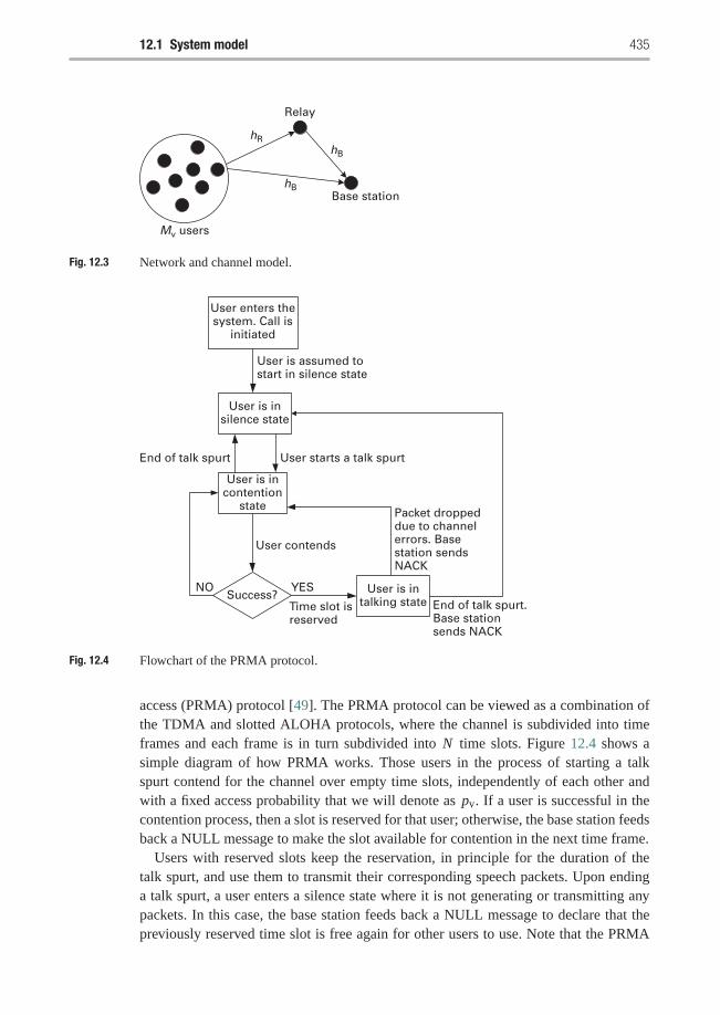
12.1 System model 435
hR
hB
hB
Relay
Base station
Mv users
Fig. 12.3 Network and channel model.
User enters thesystem. Call is
initiated
User is insilence state
User is assumed tostart in silence state
User is incontention
state
User starts a talk spurt
Success? User is intalking state
Packet droppeddue to channelerrors. Basestation sendsNACK
User contends
Time slot isreserved
End of talk spurt.Base stationsends NACK
YESNO
End of talk spurt
Fig. 12.4 Flowchart of the PRMA protocol.
access (PRMA) protocol [49]. The PRMA protocol can be viewed as a combination ofthe TDMA and slotted ALOHA protocols, where the channel is subdivided into timeframes and each frame is in turn subdivided into N time slots. Figure 12.4 shows asimple diagram of how PRMA works. Those users in the process of starting a talkspurt contend for the channel over empty time slots, independently of each other andwith a fixed access probability that we will denote as pv. If a user is successful in thecontention process, then a slot is reserved for that user; otherwise, the base station feedsback a NULL message to make the slot available for contention in the next time frame.
Users with reserved slots keep the reservation, in principle for the duration of thetalk spurt, and use them to transmit their corresponding speech packets. Upon endinga talk spurt, a user enters a silence state where it is not generating or transmitting anypackets. In this case, the base station feeds back a NULL message to declare that thepreviously reserved time slot is free again for other users to use. Note that the PRMA
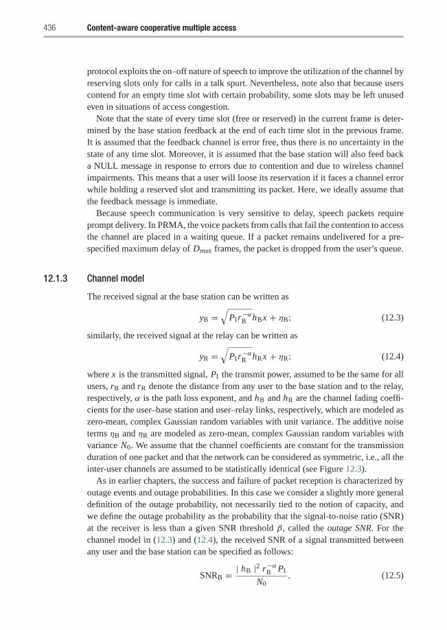
436 Content-aware cooperative multiple access
protocol exploits the on–off nature of speech to improve the utilization of the channel byreserving slots only for calls in a talk spurt. Nevertheless, note also that because userscontend for an empty time slot with certain probability, some slots may be left unusedeven in situations of access congestion.
Note that the state of every time slot (free or reserved) in the current frame is deter-mined by the base station feedback at the end of each time slot in the previous frame.It is assumed that the feedback channel is error free, thus there is no uncertainty in thestate of any time slot. Moreover, it is assumed that the base station will also feed backa NULL message in response to errors due to contention and due to wireless channelimpairments. This means that a user will loose its reservation if it faces a channel errorwhile holding a reserved slot and transmitting its packet. Here, we ideally assume thatthe feedback message is immediate.
Because speech communication is very sensitive to delay, speech packets requireprompt delivery. In PRMA, the voice packets from calls that fail the contention to accessthe channel are placed in a waiting queue. If a packet remains undelivered for a pre-specified maximum delay of Dmax frames, the packet is dropped from the user’s queue.
12.1.3 Channel model
The received signal at the base station can be written as
yB =√
P1r−αB hBx + ηB; (12.3)
similarly, the received signal at the relay can be written as
yR =√
P1r−αR hRx + ηR; (12.4)
where x is the transmitted signal, P1 the transmit power, assumed to be the same for allusers, rB and rR denote the distance from any user to the base station and to the relay,respectively, α is the path loss exponent, and hB and hR are the channel fading coeffi-cients for the user–base station and user–relay links, respectively, which are modeled aszero-mean, complex Gaussian random variables with unit variance. The additive noiseterms ηB and ηR are modeled as zero-mean, complex Gaussian random variables withvariance N0. We assume that the channel coefficients are constant for the transmissionduration of one packet and that the network can be considered as symmetric, i.e., all theinter-user channels are assumed to be statistically identical (see Figure 12.3).
As in earlier chapters, the success and failure of packet reception is characterized byoutage events and outage probabilities. In this case we consider a slightly more generaldefinition of the outage probability, not necessarily tied to the notion of capacity, andwe define the outage probability as the probability that the signal-to-noise ratio (SNR)at the receiver is less than a given SNR threshold β, called the outage SNR. For thechannel model in (12.3) and (12.4), the received SNR of a signal transmitted betweenany user and the base station can be specified as follows:
SNRB = | hB |2 r−αB P1
N0, (12.5)
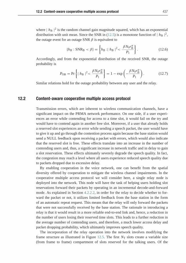
12.2 Content-aware cooperative multiple access protocol 437
where | hB |2 is the random channel gain magnitude squared, which has an exponentialdistribution with unit mean. Since the SNR in (12.5) is a monotone function of | hB |2,the outage event for an outage SNR β is equivalent to
{hB : SNRB < β} ={
hB :| hB |2< βN0rαBP1
}. (12.6)
Accordingly, and from the exponential distribution of the received SNR, the outageprobability is
POB = Pr
{| hB |2< βN0rαB
P1
}= 1− exp
(−βN0rαB
P1
). (12.7)
Similar relations hold for the outage probability between any user and the relay.
12.2 Content-aware cooperative multiple access protocol
Transmission errors, which are inherent to wireless communication channels, have asignificant impact on the PRMA network performance. On one side, if a user experi-ences an error while contending for access to a time slot, it would fail on the try andwould have to contend again in another free slot. Moreover, if a user that already holdsa reserved slot experiences an error while sending a speech packet, the user would haveto give it up and go through the contention process again because the base station wouldsend a NULL feedback upon receiving a packet with errors, which would also indicatethat the reserved slot is free. These effects translate into an increase in the number ofcontending users and, thus, a significant increase in network traffic and in delay to gaina slot reservation. These effects ultimately severely degrade the speech quality. In fact,the congestion may reach a level where all users experience reduced speech quality dueto packets dropped due to excessive delay.
By enabling cooperation in the voice network, one can benefit from the spatialdiversity offered by cooperation to mitigate the wireless channel impairments. In thecooperative multiple access protocol we will consider here, a single relay node isdeployed into the network. This node will have the task of helping users holding slotreservations forward their packets by operating in an incremental decode-and-forwardmode. As explained in Section 4.2.2.2, in order for the relay to decide whether to for-ward the packet or not, it utilizes limited feedback from the base station in the formof an automatic repeat request. This means that the relay will only forward the packetsthat were not successfully received by the base station. The rationale in introducing arelay is that it would result in a more reliable end-to-end link and, hence, a reduction inthe number of users losing their reserved time slots. This leads to a further reduction inthe average number of contending users, and therefore, a much lower access delay andpacket dropping probability, which ultimately improves speech quality.
The incorporation of the relay operation into the network involves modifying theframe structure as illustrated in Figure 12.5. The first NT slots create a variable size(from frame to frame) compartment of slots reserved for the talking users. Of the
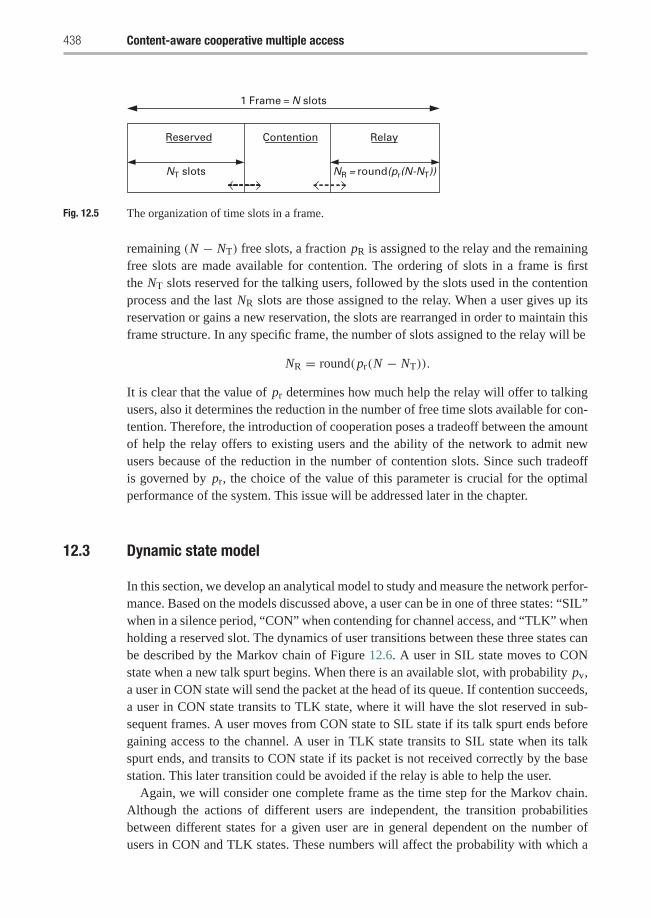
438 Content-aware cooperative multiple access
Reserved Contention Relay
1 Frame = N slots
NT slots NR = round(pr(N-NT))
Fig. 12.5 The organization of time slots in a frame.
remaining (N − NT) free slots, a fraction pR is assigned to the relay and the remainingfree slots are made available for contention. The ordering of slots in a frame is firstthe NT slots reserved for the talking users, followed by the slots used in the contentionprocess and the last NR slots are those assigned to the relay. When a user gives up itsreservation or gains a new reservation, the slots are rearranged in order to maintain thisframe structure. In any specific frame, the number of slots assigned to the relay will be
NR = round(pr(N − NT)).
It is clear that the value of pr determines how much help the relay will offer to talkingusers, also it determines the reduction in the number of free time slots available for con-tention. Therefore, the introduction of cooperation poses a tradeoff between the amountof help the relay offers to existing users and the ability of the network to admit newusers because of the reduction in the number of contention slots. Since such tradeoffis governed by pr, the choice of the value of this parameter is crucial for the optimalperformance of the system. This issue will be addressed later in the chapter.
12.3 Dynamic state model
In this section, we develop an analytical model to study and measure the network perfor-mance. Based on the models discussed above, a user can be in one of three states: “SIL”when in a silence period, “CON” when contending for channel access, and “TLK” whenholding a reserved slot. The dynamics of user transitions between these three states canbe described by the Markov chain of Figure 12.6. A user in SIL state moves to CONstate when a new talk spurt begins. When there is an available slot, with probability pv,a user in CON state will send the packet at the head of its queue. If contention succeeds,a user in CON state transits to TLK state, where it will have the slot reserved in sub-sequent frames. A user moves from CON state to SIL state if its talk spurt ends beforegaining access to the channel. A user in TLK state transits to SIL state when its talkspurt ends, and transits to CON state if its packet is not received correctly by the basestation. This later transition could be avoided if the relay is able to help the user.
Again, we will consider one complete frame as the time step for the Markov chain.Although the actions of different users are independent, the transition probabilitiesbetween different states for a given user are in general dependent on the number ofusers in CON and TLK states. These numbers will affect the probability with which a
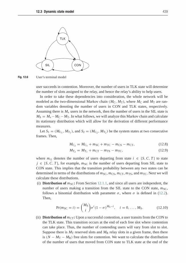
12.3 Dynamic state model 439
SIL CON
TLK
Fig. 12.6 User’s terminal model
user succeeds in contention. Moreover, the number of users in TLK state will determinethe number of slots assigned to the relay, and hence the relay’s ability to help users.
In order to take these dependencies into consideration, the whole network will bemodeled as the two-dimensional Markov chain (MC,MT), where MC and MT are ran-dom variables denoting the number of users in CON and TLK states, respectively.Assuming there is Mv users in the network, then the number of users in the SIL state isMS = Mv−MC−MT. In what follows, we will analyze this Markov chain and calculateits stationary distribution which will allow for the derivation of different performancemeasures.
Let S1 = (MC1 ,MT1), and S2 = (MC2 ,MT2) be the system states at two consecutiveframes. Then,
MC2 = MC1 + mSC + mTC − mCS − mCT, (12.8)
MT2 = MT1 + mCT − mTS − mTC, (12.9)
where mi j denotes the number of users departing from state i ∈ {S,C, T } to statej ∈ {S,C, T }, for example, mSC is the number of users departing from SIL state toCON state. This implies that the transition probability between any two states can bedetermined in terms of the distributions of mSC, mCS, mCT, mTS, and mTC. Next we willcalculate these distributions.(i) Distribution of mSC: From Section 12.1.1, and since all users are independent, the
number of users making a transition from the SIL state to the CON state, mSC,follows a binomial distribution with parameter σ , where σ is defined in (12.2).Then,
Pr(mSC = i) =(
MS
i
)σ i (1− σ)MS−i , i = 0, . . . ,MS. (12.10)
(ii) Distribution of mCT: Upon a successful contention, a user transits from the CON tothe TLK state. This transition occurs at the end of each free slot where contentioncan take place. Thus, the number of contending users will vary from slot to slot.Suppose there is MT reserved slots and MR relay slots in a given frame, then thereis (N − MT − MR) free slots for contention. We want to calculate the distributionof the number of users that moved from CON state to TLK state at the end of the
440 Content-aware cooperative multiple access
last free slot. This distribution could be calculated using the following recurrencemodel. Let q(M ′
C) be the probability that a user succeeds in contention when thereis M ′
C contending users, then
q(M ′C) = M ′
C pv(1− pv)M ′
C−1(1− POB),
which is the probability that only one user has permission to transmit and thechannel was not in outage during packet transmission.Define Rk(M ′
C) as the probability that M ′C terminals remain in the CON state at the
end of the k-th available slot, (k = 0, 1, 2, . . . , N − MT − MR). Conditioning onthe outcome of the (k − 1)st time slot, it follows that
Rk(M′C) = Rk−1(M
′C)[1− q(M ′
C)]++ Rk−1(M
′C + 1)q(M ′
C + 1), (12.11)
for M ′C = 0, 1, . . . ,MC and where MC is the number of users in the CON state at
the beginning of the frame. The initial condition for this recursion is
R0(M′C) =
{1 M ′
C = MC
0 M ′C �= MC
(12.12)
and the boundary condition q(MC + 1) = 0, which follows from the fact that thetotal number of contending users is MC. Finally, the distribution of mCT is
Pr (mCT = i) = RN −MT−MR(MC − i), i = 0, . . . ,MC.
(iii) Distribution of mTS: It follows from Section 12.1.1, and from users independence,that the number of users making a transition from the TLK state to the SIL state,mTS, is binomially distributed with parameter γ , where γ is defined in (12.1). Then,
Pr (mTS = i) =(
MT
i
)γ i (1− γ )MT−i , i = 0, . . . ,MT.
(iv) Distribution of mCS: A user makes a transition from the CON state to the SILstate if its talk spurt ends before gaining access to the channel. Conditioning on thenumber of users that successfully accessed the channel, mCT, and through the sameargument as in (iii) above, we have
Pr (mCS = i |mCT) =(
MC − mCT
i
)γ i (1− γ )MC−mCT−i , (12.13)
for i = 0, . . . ,MC − mCT. In what follows, we will not seek to remove the condi-tioning on mCT from this distribution because this is the form we will be interestedin when calculating the state transition matrix later in this chapter.
(v) Distribution of mTC: A user leaves the TLK state to the CON state if its transmittedpacket fails to reach the base station successfully, and if the relay did not help thatuser. Also, a user in the TLK state will leave to SIL state if its talk spurt ends in thecurrent frame irrespective of the reception state of its last transmitted packet. Thismeans that this user will not attempt to retransmit its last packet in the talk spurtand the relay will not try to help this user.
12.3 Dynamic state model 441
Given the number of users making transitions from TLK state to SIL state, mTS,the number of transmission errors from the remaining users in the TLK state, ε,follows a binomial distribution with parameter POB, the outage probability of thelink between any user and the base station as defined in (12.7). Therefore,
Pr (ε = i |mTS) =(
M ′T
i
)POi B, (1− POB)
M ′T−i , (12.14)
for i = 0, . . . ,M ′T and where M ′
T = MT − mTS, the number of remaining usersin the TLK state. Assume that the relay can successfully receive εR packets of theε erroneous packets. Then, conditioned on ε, the number of successfully receivedpackets by the relay, εR, is also binomially distributed but with parameter POR, theoutage probability of the link from any user to the relay,
Pr (εR = i |ε) =(ε
i
)(1− POR)
i POε−i R, i = 0, . . . , ε.
For each of the slots assigned to the relay, a packet among the εR packets in therelay’s queue is selected at random and forwarded. It follows that the number ofsuccessfully forwarded packets εF is binomially distributed with parameter POB,
Pr (εF = i |εR) =(
min(MR, εR)
i
)(1− POB)
i POBmin(MR,εR)−i ,
for i = 0, . . . ,min(MR, εR) and where MR is the number of time slots assignedfor the relay. The minimum of MR and εR is taken, since the number of forwardedpackets cannot exceed the number of slots assigned to the relay or the number ofpackets in the relay’s queue. Now, the probability that i users make the transitionfrom TLK state to CON state is the probability that from the ε erroneous packets,the relay successfully forwards (εF = εR− i) packets. Then the distribution of mTC
is given by
Pr (mTC = i |mTS) =MT−mTS∑
k=0
k∑l=0
Pr (εF = εR − i |εR = l)
× Pr (εR = l|ε = k)Pr (ε = k|mTS).
(12.15)
At this point, it is important to remark that all the distributions calculated above are statedependent because they generally depend on MC and MT. This means that it is necessaryto calculate a different set of distributions for each possible state of the system.
12.3.1 State transition probabilities
Having derived the probability distributions for the state transitions, the next step inmathematically characterizing a Markov chain is to write the state transition matrix P.For the present case, this matrix is square, and it can be shown that its dimension M is
442 Content-aware cooperative multiple access
M =⎧⎨⎩
(N+1)(N+2)2 if Mv ≤ N
(N + 1)(Mv − N2 + 1) if Mv > N
An element P(S1, S2) of this matrix is the transition probability from state S1 =(MC1 ,MT1) to state S2 = (MC2,MT2). We also have P(S1, S2) = 0 when
MT2 > min(MT1 + MC1, N ),
because the number of terminals in TLK state in the next frame cannot exceed the totalnumber of time slots in a frame or the number of terminals in TLK and CON states inthe current frame. From (12.8) and (12.9), and the distributions developed above, thetransition probability P(S1, S2) is given by
P(S1, S2) =MC1∑x=0
M ′∑y=0
MT1∑z=0
Pr (mCS = x |mCT = y, S1)Pr (mCT = y|S1)
× Pr(mTC = MT1 − MT2 + y − z|mTS = z, S1)
× Pr(mTS = z|S1)
× Pr(mSC = MC2 − MC1 + x + y − z|S1), (12.16)
where
M ′ = min(MC1 − x, N − MT1 − MR1).
It should be noted that
Pr (mTC = MT1 − MT2 + y − z|S1) = 0
if MT1 − MT2 + y − z > MT1 − z, because the number of users transiting from TLKstate to CON state cannot exceed the difference between the number of users initially inthe TLK state and the number of users leaving the TLK state to the SIL state. Also,
Pr (mSC = MC2 − MC1 + x + y − z|S1) = 0
if MC2 − MC1 + x + y − z > MS1 , because the number of users leaving the SIL statecannot be larger than the number of users initially in this state.
Finally, the stationary distribution vector π (indicating the probability of each state)can be calculated as the left eigenvector of the minimum eigenvalue of the matrix P or,in other words, can be obtained by solving π = πP.
12.4 Performance analysis
To assess the performance of the voice network under the content-aware cooperativeMAC protocol, four measures will be considered: network throughput, multiple accessdelay, packet dropping probability, and subjective speech quality.
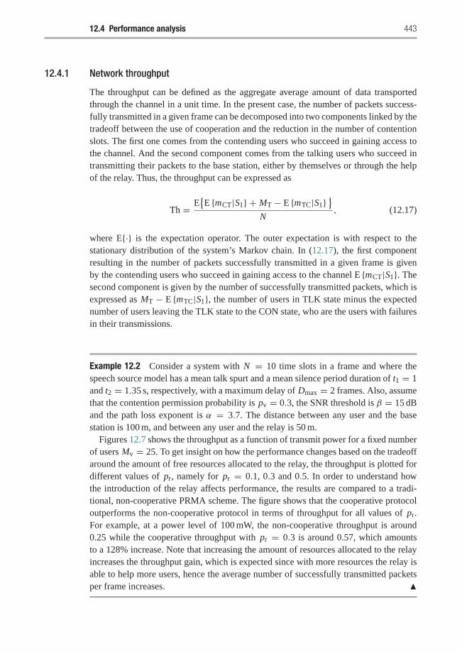
12.4 Performance analysis 443
12.4.1 Network throughput
The throughput can be defined as the aggregate average amount of data transportedthrough the channel in a unit time. In the present case, the number of packets success-fully transmitted in a given frame can be decomposed into two components linked by thetradeoff between the use of cooperation and the reduction in the number of contentionslots. The first one comes from the contending users who succeed in gaining access tothe channel. And the second component comes from the talking users who succeed intransmitting their packets to the base station, either by themselves or through the helpof the relay. Thus, the throughput can be expressed as
Th = E{E {mCT|S1} + MT − E {mTC|S1}
}N
, (12.17)
where E{·} is the expectation operator. The outer expectation is with respect to thestationary distribution of the system’s Markov chain. In (12.17), the first componentresulting in the number of packets successfully transmitted in a given frame is givenby the contending users who succeed in gaining access to the channel E {mCT|S1}. Thesecond component is given by the number of successfully transmitted packets, which isexpressed as MT − E {mTC|S1}, the number of users in TLK state minus the expectednumber of users leaving the TLK state to the CON state, who are the users with failuresin their transmissions.
Example 12.2 Consider a system with N = 10 time slots in a frame and where thespeech source model has a mean talk spurt and a mean silence period duration of t1 = 1and t2 = 1.35 s, respectively, with a maximum delay of Dmax = 2 frames. Also, assumethat the contention permission probability is pv = 0.3, the SNR threshold is β = 15 dBand the path loss exponent is α = 3.7. The distance between any user and the basestation is 100 m, and between any user and the relay is 50 m.
Figures 12.7 shows the throughput as a function of transmit power for a fixed numberof users Mv = 25. To get insight on how the performance changes based on the tradeoffaround the amount of free resources allocated to the relay, the throughput is plotted fordifferent values of pr, namely for pr = 0.1, 0.3 and 0.5. In order to understand howthe introduction of the relay affects performance, the results are compared to a tradi-tional, non-cooperative PRMA scheme. The figure shows that the cooperative protocoloutperforms the non-cooperative protocol in terms of throughput for all values of pr.For example, at a power level of 100 mW, the non-cooperative throughput is around0.25 while the cooperative throughput with pr = 0.3 is around 0.57, which amountsto a 128% increase. Note that increasing the amount of resources allocated to the relayincreases the throughput gain, which is expected since with more resources the relay isable to help more users, hence the average number of successfully transmitted packetsper frame increases. �
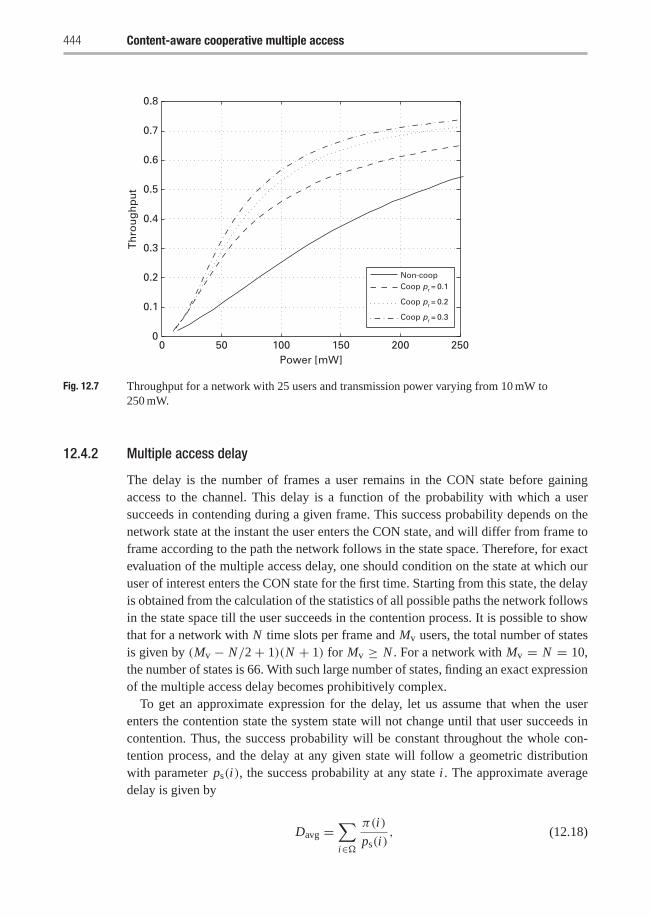
444 Content-aware cooperative multiple access
0 50 100 150 200 250
0.8
0.7
0.6
0.5
0.4
0.3
0.2
0.1
0
Power [mW]
Th
rou
gh
pu
t
Non-coopCoop pr = 0.1
Coop pr = 0.2
Coop pr = 0.3
Fig. 12.7 Throughput for a network with 25 users and transmission power varying from 10 mW to250 mW.
12.4.2 Multiple access delay
The delay is the number of frames a user remains in the CON state before gainingaccess to the channel. This delay is a function of the probability with which a usersucceeds in contending during a given frame. This success probability depends on thenetwork state at the instant the user enters the CON state, and will differ from frame toframe according to the path the network follows in the state space. Therefore, for exactevaluation of the multiple access delay, one should condition on the state at which ouruser of interest enters the CON state for the first time. Starting from this state, the delayis obtained from the calculation of the statistics of all possible paths the network followsin the state space till the user succeeds in the contention process. It is possible to showthat for a network with N time slots per frame and Mv users, the total number of statesis given by (Mv − N/2+ 1)(N + 1) for Mv ≥ N . For a network with Mv = N = 10,the number of states is 66. With such large number of states, finding an exact expressionof the multiple access delay becomes prohibitively complex.
To get an approximate expression for the delay, let us assume that when the userenters the contention state the system state will not change until that user succeeds incontention. Thus, the success probability will be constant throughout the whole con-tention process, and the delay at any given state will follow a geometric distributionwith parameter ps(i), the success probability at any state i . The approximate averagedelay is given by
Davg =∑i∈�
π(i)
ps(i), (12.18)
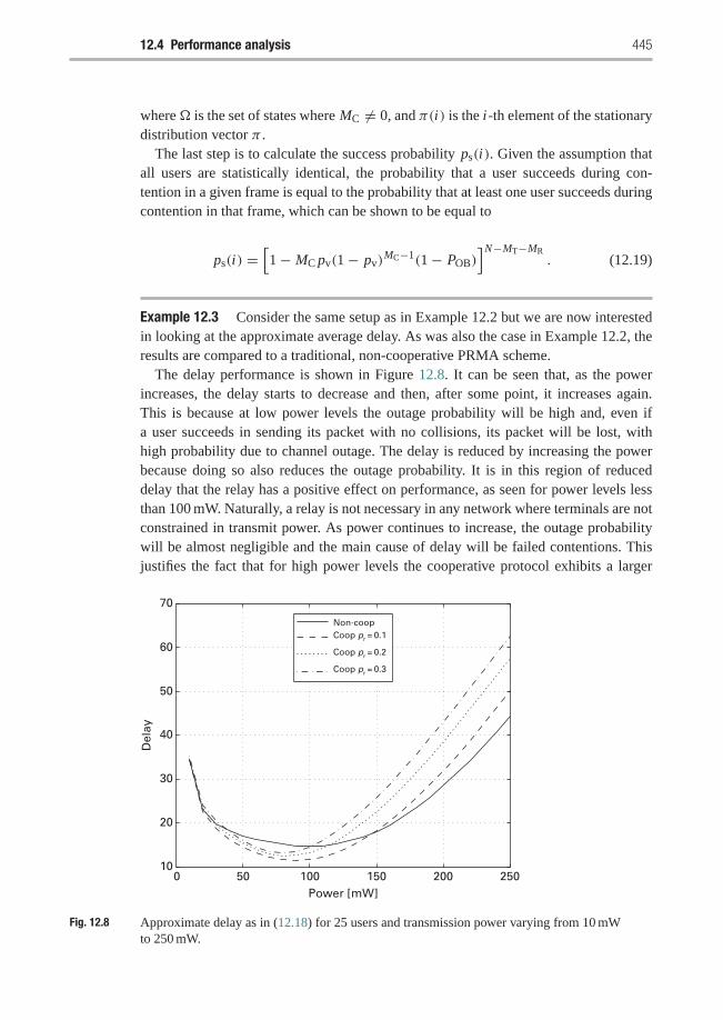
12.4 Performance analysis 445
where� is the set of states where MC �= 0, and π(i) is the i-th element of the stationarydistribution vector π .
The last step is to calculate the success probability ps(i). Given the assumption thatall users are statistically identical, the probability that a user succeeds during con-tention in a given frame is equal to the probability that at least one user succeeds duringcontention in that frame, which can be shown to be equal to
ps(i) =[1− MC pv(1− pv)
MC−1(1− POB)]N−MT−MR
. (12.19)
Example 12.3 Consider the same setup as in Example 12.2 but we are now interestedin looking at the approximate average delay. As was also the case in Example 12.2, theresults are compared to a traditional, non-cooperative PRMA scheme.
The delay performance is shown in Figure 12.8. It can be seen that, as the powerincreases, the delay starts to decrease and then, after some point, it increases again.This is because at low power levels the outage probability will be high and, even ifa user succeeds in sending its packet with no collisions, its packet will be lost, withhigh probability due to channel outage. The delay is reduced by increasing the powerbecause doing so also reduces the outage probability. It is in this region of reduceddelay that the relay has a positive effect on performance, as seen for power levels lessthan 100 mW. Naturally, a relay is not necessary in any network where terminals are notconstrained in transmit power. As power continues to increase, the outage probabilitywill be almost negligible and the main cause of delay will be failed contentions. Thisjustifies the fact that for high power levels the cooperative protocol exhibits a larger
0 50 100 150 200 25010
20
30
40
50
60
70
Power [mW]
Del
ay
Non-coopCoop pr = 0.1
Coop pr = 0.2
Coop pr = 0.3
Fig. 12.8 Approximate delay as in (12.18) for 25 users and transmission power varying from 10 mWto 250 mW.
446 Content-aware cooperative multiple access
delay, as the presence of the relay decreases the number of slots available for contentionand, hence, increases the probability of packet collisions. This is also why the delayperformance is better for lower values of pr. �
12.4.3 Packet dropping probability
Speech communication is delay sensitive and requires prompt delivery of speech pack-ets. In the PRMA protocol, packets start to be dropped if they are delayed in the networkfor more than a maximum allowable delay of Dmax frames. Based on the assumptionthat the speech coder generates exactly one speech packet per frame, every user willmaintain a buffer of length Dmax. Whenever the buffer is full at the start of a frame, theoldest packet is dropped until the user succeeds in reserving a time slot. After gaininga reservation, in each frame the oldest packet in the queue will be transmitted and thenew incoming packet is added at the end of the queue. If the talk spurt ends beforegetting a slot reservation, all the packets in the buffer are dropped. Because of channelerrors, a user with a reserved time slot may lose its reservation and return to the groupof contending users, thus risking further packet dropping.
First, we focus on the case when a user is trying to access the channel for the firsttime. Given that the system is at state i with NC contending user and NT users hold-ing slot reservations, consider a contending user whose talk spurt started at the currentframe. The talk spurt consists of L packets, where L is a random variable. The userwill start to contend for a time slot in the current frame and continue in subsequentframes until it succeeds or the talk spurt ends. The user waits in the CON state for Dframes to obtain a reservation. Using the assumption developed above that delay D isgeometrically distributed, the probability that a user waits for d frames is
PD(d) = (1− ps(i))(ps(i))d , d = 0, 1, . . . . (12.20)
We need to distinguish between two different cases relating the length of the talkspurt L and the maximum allowable delay Dmax:(i) L ≤ Dmax: In this case, the buffer is long enough to store the whole talk spurt. If
reservation is obtained before the talk spurt ends, no packets are lost. Otherwise, allthe talk spurt packets are discarded. As a function of the waiting time d, the numberof dropped packets is
nd(d) ={
0, 0 ≤ d < LL , d ≥ L
and the distribution of the number of dropped packets is given by
Pr {nd|L ≤ Dmax, i} ={ ∑L
d=0 PD(d), nd = 0∑∞d=L+1 PD(d), nd = L
(ii) L > Dmax: In this case, after waiting Dmax frames, one packet is dropped per frameuntil being able to reserve a slot. The dropped packet is the oldest in the queue with
12.4 Performance analysis 447
an associated delay of Dmax. The number of dropped packets as a function of thedelay is given by
nd(d) =⎧⎨⎩
0, 0 ≤ d ≤ Dmax − 1k, d = Dmax + k − 1, k = 1, 2, . . . , (L − Dmax)
L , d ≥ L
and its distribution
Pr {nd|L > Dmax, i} =
⎧⎪⎨⎪⎩∑Dmax−1
d=0 PD(d), nd = 0(1− ps(i))(Ps(i))nd, nd = 1, 2, . . . , (L − Dmax)∑∞
d=L PD(d), nd = L
We note here that although all the summations mentioned above have closed-formexpressions, they tend to become complex and lengthy. Therefore, we avoid writingthem here, so as to keep the presentation compact. This will also apply to the nextsection.
The expected number of dropped packets for the above two cases, namely E {nd|L ≤Dmax, i} and E {nd|L > Dmax, i}, can be easily calculated using the correspondingdistributions and, then, combined to get the total expected number of dropped packets as
E {nd|i} =Dmax∑l=1
E {nd|L ≤ Dmax, i}PL(l)
+∞∑
l=Dmax+1
E{nd|L > Dmax, i}PL(l), (12.21)
where PL(l) is the probability mass function of the length of the talk spurt. Fromthe speech source model of Figure 12.2, the talk spurt duration, L , is geometricallydistributed with parameter γ , i.e.,
Pr {L} = γ (1− γ )l−1, l = 1, 2, . . . . (12.22)
Finally, the packet dropping probability is the ratio between the average number ofdropped packets per talk spurt to the average number of packets generated per talkspurt, i.e,
Pd0 =1
γ
∑i∈�
E{nd|i}π(i), (12.23)
where the sum is over �, the set of states with NC �= 0 (because packets are droppedonly when the user is in the CON state).
Next we consider the packet dropping probability due to the first transition fromthe TLK state to the CON state caused by channel errors. First, we need to make thefollowing assumptions:• Any user in a TLK state has obtained its reservation with the first packet in the talk
spurt. This means no packets were dropped in the first contention process. Further-more, this packet is delayed by D0 = Davg frames, i.e., this packet is delayed bythe average multiple access delay calculated in the last section.
448 Content-aware cooperative multiple access
• The first channel error occurs while transmitting the j-th packet of the talk spurt.Since the first packet was delayed by D0 frames, the remaining maximum delay forthe subsequent packets in the talk spurt is D1 = Dmax − D0 frames.
• There are L packets in the talk spurt, and L1 packets following and including thej-th packet which encountered a channel error.
Based on the time instant when the user left TLK state to CON state, we need to analyzethree cases:• Case 1: Transmission instant of the j-th packet is after the end of the talk spurt.
This means, D0 + ( j − 1) ≥ L , or L1 ≤ D0. In this case all the remaining L1
packets are discarded without any contentions and
E {nd|L1 ≤ D0, i} = L1.
• Case 2: Transmission instant of the j-th packet is before the end of the talk spurtand the remaining time till the end of the talk spurt is less than the maximumremaining delay D1. That is, 0 < L − D0 − ( j − 1) ≤ D1, or D0 < L1 ≤ Dmax.In this case, no packets are dropped if the user gets a reserved slot before the endof the talk spurt. Otherwise, all L1 are discarded. The number of dropped packetsas a function of the waiting time is
nd(d) ={
0, 0 ≤ d ≤ L1 − D0
L1, d > L1 − D0(12.24)
The waiting time is distributed according to (12.20), and
Pr {nd|D0 < L1 ≤ Dmax, i} =
⎧⎪⎪⎪⎪⎪⎨⎪⎪⎪⎪⎪⎩
L1−D0∑d=0
PD(d), nd = 0
∞∑d=L1−D0+1
PD(d), nd = L1
(12.25)
• Case 3: Here L − D0 − ( j − 1) > D1, or L1 > Dmax. In this case, the j-th packetis dropped after waiting for D1 frames and a packet will be dropped every frametill the user gets access to the channel. If the talk spurt ends before accessing thechannel, all the packets in the buffer are discarded. We have
nd(d) =⎧⎨⎩
0, 0 ≤ d ≤ D1 − 1k, d = D1 + k − 1, k = 1, 2, . . . , (L1 − Dmax)
L1, d > L − D0
(12.26)
and
Pr {nd|L1 > Dmax, i} =
⎧⎪⎪⎪⎪⎪⎪⎪⎪⎨⎪⎪⎪⎪⎪⎪⎪⎪⎩
D1−1∑d=0
PD(d), nd = 0
(1− Ps(i))(Ps(i))nd , nd = 1, . . . , (L1 − Dmax)
∞∑d=L1−D0
PD(d), nd = L1.
12.4 Performance analysis 449
Having the distributions of the number of dropped packets for each case, one cancalculate the corresponding expected number of dropped packets, E{nd|L1 ≤ D0, i},E{nd|D0 < L1 ≤ Dmax, i}, and E{nd|L1 > Dmax, i}.
The next step is to average with respect to L1, the number of remaining packets inthe talk spurt after the first error. From the earlier assumptions, we have
Pr {L1 = l1|L = l} = u(1− u)(l−l1−1), l1 = 1, 2, . . . , l − 1,
where u is the user’s transition probability from the TLK state to the CON state. A userleaves the TLK state to the CON state if: (i) the packet transmission failed, (ii) a relaydid not help that user, and (iii) the talk spurt did not end during current frame (hadthe talk spurt ended, the transition would have been to the SIL state). Now, we need toconsider the talk spurt length L . If (L − 1) ≤ Dmax, cases one and two above wouldoccur, otherwise all three cases would occur. Therefore,
E {nd|L , i} = E {nd|L − 1 ≤ Dmax, i} + E {nd|L − 1 > Dmax, i},where
E {nd|L − 1 ≤ Dmax, i} =D0∑
L1=1
E {nd|L1 ≤ D0, i}Pr {L1|L}
+Dmax∑
L1=D0+1
E {nd|D0 < L1 ≤ Dmax, i}Pr {L1|L},
E{nd|L − 1 > Dmax, i} =D0∑
L1=1
E {nd|L1 ≤ D0, i}Pr {L1|L}
+Dmax∑
L1=D0+1
E {nd|D0 < L1 ≤ Dmax, i}Pr {L1|L}
+L−1∑
L1=Dmax+1
E {nd|L1 > Dmax, i}Pr {L1|L}.
Finally,
E {nd|i} =Dmax+1∑
L=2
E {nd|L − 1 ≤ Dmax, i}Pr {L}
+∞∑
L=Dmax+2
E {nd|L − 1 > Dmax, i}Pr {L},
where Pr {L} is defined in (12.22). As in (12.23), the packet dropping probability dueto the first error in the talk spurt is
Pd1 =1
γ
∑i∈�
E {nd|i}π(i). (12.27)
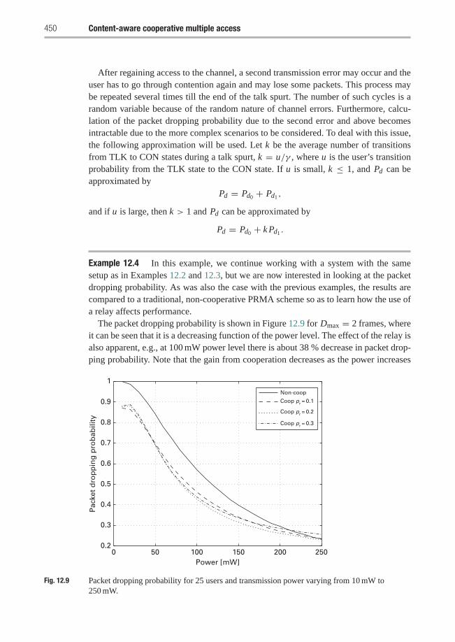
450 Content-aware cooperative multiple access
After regaining access to the channel, a second transmission error may occur and theuser has to go through contention again and may lose some packets. This process maybe repeated several times till the end of the talk spurt. The number of such cycles is arandom variable because of the random nature of channel errors. Furthermore, calcu-lation of the packet dropping probability due to the second error and above becomesintractable due to the more complex scenarios to be considered. To deal with this issue,the following approximation will be used. Let k be the average number of transitionsfrom TLK to CON states during a talk spurt, k = u/γ , where u is the user’s transitionprobability from the TLK state to the CON state. If u is small, k ≤ 1, and Pd can beapproximated by
Pd = Pd0 + Pd1 ,
and if u is large, then k > 1 and Pd can be approximated by
Pd = Pd0 + k Pd1 .
Example 12.4 In this example, we continue working with a system with the samesetup as in Examples 12.2 and 12.3, but we are now interested in looking at the packetdropping probability. As was also the case with the previous examples, the results arecompared to a traditional, non-cooperative PRMA scheme so as to learn how the use ofa relay affects performance.
The packet dropping probability is shown in Figure 12.9 for Dmax = 2 frames, whereit can be seen that it is a decreasing function of the power level. The effect of the relay isalso apparent, e.g., at 100 mW power level there is about 38 % decrease in packet drop-ping probability. Note that the gain from cooperation decreases as the power increases
0 50 100 150 200 250
1
0.9
0.8
0.7
0.6
0.5
0.4
0.3
0.2
Power [mW]
Pac
ket
dro
pp
ing
pro
bab
ility
Non-coop
Coop pr = 0.1
Coop pr = 0.2
Coop pr = 0.3
Fig. 12.9 Packet dropping probability for 25 users and transmission power varying from 10 mW to250 mW.
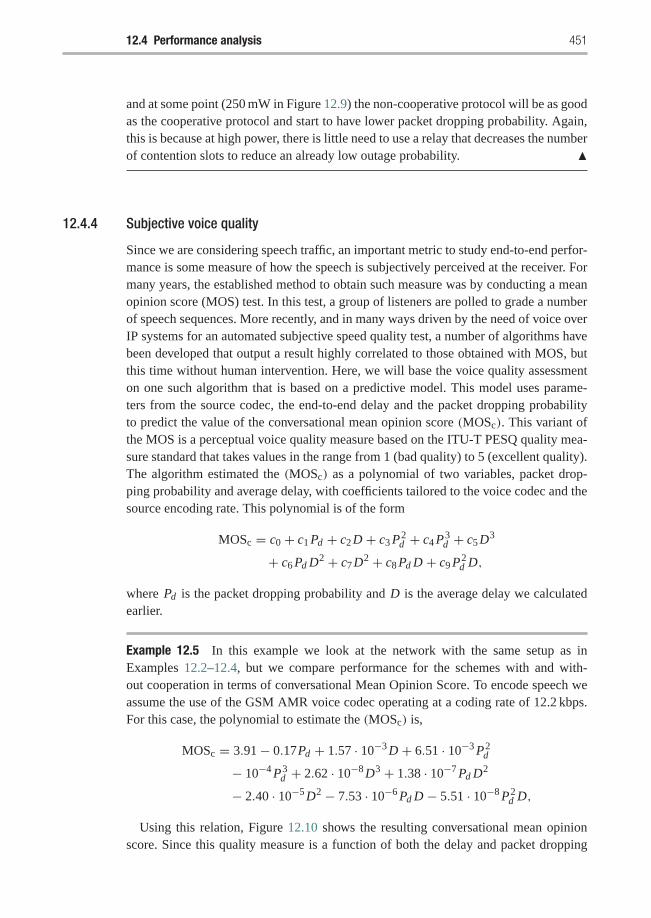
12.4 Performance analysis 451
and at some point (250 mW in Figure 12.9) the non-cooperative protocol will be as goodas the cooperative protocol and start to have lower packet dropping probability. Again,this is because at high power, there is little need to use a relay that decreases the numberof contention slots to reduce an already low outage probability. �
12.4.4 Subjective voice quality
Since we are considering speech traffic, an important metric to study end-to-end perfor-mance is some measure of how the speech is subjectively perceived at the receiver. Formany years, the established method to obtain such measure was by conducting a meanopinion score (MOS) test. In this test, a group of listeners are polled to grade a numberof speech sequences. More recently, and in many ways driven by the need of voice overIP systems for an automated subjective speed quality test, a number of algorithms havebeen developed that output a result highly correlated to those obtained with MOS, butthis time without human intervention. Here, we will base the voice quality assessmenton one such algorithm that is based on a predictive model. This model uses parame-ters from the source codec, the end-to-end delay and the packet dropping probabilityto predict the value of the conversational mean opinion score (MOSc). This variant ofthe MOS is a perceptual voice quality measure based on the ITU-T PESQ quality mea-sure standard that takes values in the range from 1 (bad quality) to 5 (excellent quality).The algorithm estimated the (MOSc) as a polynomial of two variables, packet drop-ping probability and average delay, with coefficients tailored to the voice codec and thesource encoding rate. This polynomial is of the form
MOSc = c0 + c1 Pd + c2 D + c3 P2d + c4 P3
d + c5 D3
+ c6 Pd D2 + c7 D2 + c8 Pd D + c9 P2d D,
where Pd is the packet dropping probability and D is the average delay we calculatedearlier.
Example 12.5 In this example we look at the network with the same setup as inExamples 12.2–12.4, but we compare performance for the schemes with and with-out cooperation in terms of conversational Mean Opinion Score. To encode speech weassume the use of the GSM AMR voice codec operating at a coding rate of 12.2 kbps.For this case, the polynomial to estimate the (MOSc) is,
MOSc = 3.91− 0.17Pd + 1.57 · 10−3 D + 6.51 · 10−3 P2d
− 10−4 P3d + 2.62 · 10−8 D3 + 1.38 · 10−7 Pd D2
− 2.40 · 10−5 D2 − 7.53 · 10−6 Pd D − 5.51 · 10−8 P2d D,
Using this relation, Figure 12.10 shows the resulting conversational mean opinionscore. Since this quality measure is a function of both the delay and packet dropping
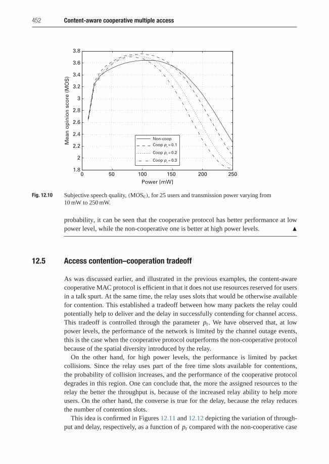
452 Content-aware cooperative multiple access
0 50 100 150 200 250
3.8
3.6
3.4
3.2
3
2.8
2.6
2.4
2.2
2
1.8
Power [mW]
Mea
n o
pin
ion
sco
re (
MO
S)
Non-coop
Coop pr = 0.1
Coop pr = 0.2
Coop pr = 0.3
Fig. 12.10 Subjective speech quality, (MOSc), for 25 users and transmission power varying from10 mW to 250 mW.
probability, it can be seen that the cooperative protocol has better performance at lowpower level, while the non-cooperative one is better at high power levels. �
12.5 Access contention–cooperation tradeoff
As was discussed earlier, and illustrated in the previous examples, the content-awarecooperative MAC protocol is efficient in that it does not use resources reserved for usersin a talk spurt. At the same time, the relay uses slots that would be otherwise availablefor contention. This established a tradeoff between how many packets the relay couldpotentially help to deliver and the delay in successfully contending for channel access.This tradeoff is controlled through the parameter pr. We have observed that, at lowpower levels, the performance of the network is limited by the channel outage events,this is the case when the cooperative protocol outperforms the non-cooperative protocolbecause of the spatial diversity introduced by the relay.
On the other hand, for high power levels, the performance is limited by packetcollisions. Since the relay uses part of the free time slots available for contentions,the probability of collision increases, and the performance of the cooperative protocoldegrades in this region. One can conclude that, the more the assigned resources to therelay the better the throughput is, because of the increased relay ability to help moreusers. On the other hand, the converse is true for the delay, because the relay reducesthe number of contention slots.
This idea is confirmed in Figures 12.11 and 12.12 depicting the variation of through-put and delay, respectively, as a function of pr compared with the non-cooperative case
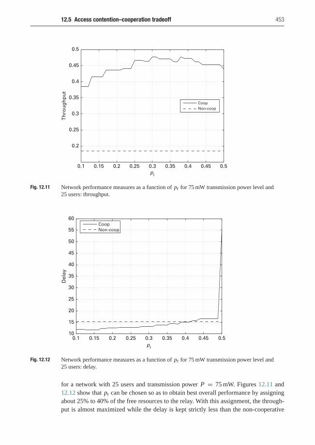
12.5 Access contention–cooperation tradeoff 453
0.5
0.45
0.4
0.35
0.3
0.25
0.2
0.1 0.15 0.2 0.25 0.3 0.35 0.4 0.45 0.5pr
Th
rou
gh
pu
t
CoopNon-coop
Fig. 12.11 Network performance measures as a function of pr for 75 mW transmission power level and25 users: throughput.
100.1 0.15 0.2 0.25 0.3 0.35 0.4 0.45 0.5
15
20
25
30
35
40
45
50
55
60
pr
Del
ay
CoopNon-coop
Fig. 12.12 Network performance measures as a function of pr for 75 mW transmission power level and25 users: delay.
for a network with 25 users and transmission power P = 75 mW. Figures 12.11 and12.12 show that pr can be chosen so as to obtain best overall performance by assigningabout 25% to 40% of the free resources to the relay. With this assignment, the through-put is almost maximized while the delay is kept strictly less than the non-cooperative
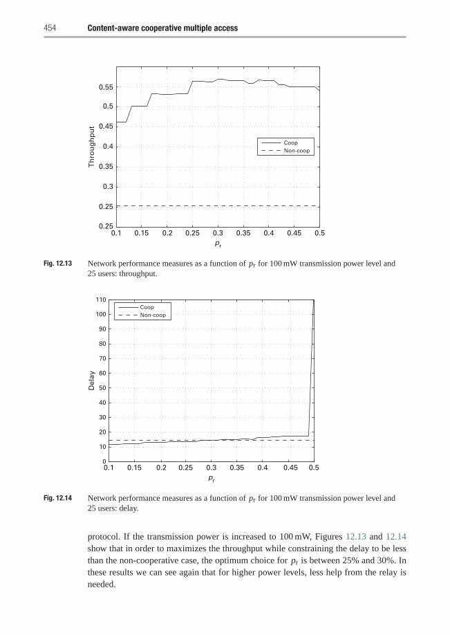
454 Content-aware cooperative multiple access
0.55
0.5
0.45
0.4
0.35
0.3
0.25
0.25
Th
rou
gh
pu
t
CoopNon-coop
0.1 0.15 0.2 0.25 0.3 0.35 0.4 0.45 0.5pr
Fig. 12.13 Network performance measures as a function of pr for 100 mW transmission power level and25 users: throughput.
0
10
20
30
40
50
60
70
80
90
100
110
Del
ay
CoopNon-coop
0.1 0.15 0.2 0.25 0.3 0.35 0.4 0.45 0.5pr
Fig. 12.14 Network performance measures as a function of pr for 100 mW transmission power level and25 users: delay.
protocol. If the transmission power is increased to 100 mW, Figures 12.13 and 12.14show that in order to maximizes the throughput while constraining the delay to be lessthan the non-cooperative case, the optimum choice for pr is between 25% and 30%. Inthese results we can see again that for higher power levels, less help from the relay isneeded.
12.6 Chapter summary and bibliographical notes 455
12.6 Chapter summary and bibliographical notes
In this chapter we have shown how user cooperation can be used to improve theperformance of multiple access protocols. In particular, we considered protocols thattake advantage of the statistical properties of the traffic, which in this chapter is real-time speech. From the point of view of traditional approaches that do not considercooperation, perhaps the best known multiple access protocols that take advantage ofthe traffic characteristics of packet speech is the packet reservation multiple access(PRMA) protocol, which was studied in [49] and other derived literature [229, 95].More specifically, the impact of channel losses on performance is studied in [95].Indeed, much of the packet dropping probability analysis in this chapter is based onthe work in [137] and [147] for the PRMA protocol. The talk spurt–silence speechmodel that is used by this protocol have been studied in different contexts but oneof the most frequently cited references for the Markov chain modeling of speechsources and the exponential distribution model for the waiting time in any state is [16].Also, we note here that the subjective speech quality measure used in Section 12.4.4is based on the algorithm developed in [208], which is in turn based on the ITU-TPESQ quality measure standard [88]. More information on the MOS test can be foundin [86].
In this chapter we showed that the use of cooperation reduces, for those users hold-ing a time slot, the number of packets that are lost due to channel errors. Since time slotreservations are lost by those users experiencing dropped packets, the use of cooperationreduces the traffic load from users contending for channel access. Also, in this chapterwe have shown how cooperation can be implemented efficiently by taking advantageof idle times in the sources and using resources that are not exclusively reserved foractive calls. The approach explained in this chapter entails the implementation of coop-eration through the use of time slots left unused by those users that are in a periodof silence during the conversation. These free time slots can also be used for randomaccess contention by those users transitioning from a silence period into a talk spurt.The dual use establishes a tradeoff between how many packets the relay could poten-tially help to deliver and the delay in successfully contending for channel access. Wenamed this tradeoff the access contention–cooperation tradeoff. This tradeoff is con-trolled through the parameter pr. By judiciously choosing this parameter, the protocolthat uses cooperation shows a clear performance advantage compared with a protocolwith no cooperation.
As we have noted at different places in this book, previously published literatureon cooperative communications has focused for a large part on the physical layer. Thestudy in this chapter is a clear example of the impact and implementation of cooperationat higher network layers, for which there are, nevertheless, some previous publishedworks. Such is the case in [120], where the authors proposed a distributed version of thenetwork diversity multiple access (NDMA) protocol [218]. Also, in [167], the notion ofutilizing the spatial separation between users to assign cooperating pairs was presented.Further study of the content-aware multiple access protocol studied in this chapter canbe found in [35, 34].
456 Content-aware cooperative multiple access
Exercises
12.1 Consider the derivation of the dynamic state model:
(a) Derive (12.10) and discuss, also, the conditions under which the derivation isvalid.
(b) Derive (12.13) and discuss, also, the conditions under which the derivation isvalid
12.2 Consider the derivation of the multiple access delay and derive (12.19).12.3 In packet wireless communications there are two causes for packet dropping:
packets that are dropped due to channel errors and packets that are dropped dueto excessive delay. As we have discussed in this chapter, these two causes notonly interact in the usual way, but also through the access contention–cooperationtradeoff. Assume a system with N = 10 time slots in a frame, where the speechsource model has a mean talk spurt and a mean silence period duration of t1 = 1and t2 = 1.35 s, respectively, with a maximum delay of Dmax = 2 frames, thecontention permission probability pv = 0.3, SNR threshold β = 15 dB, and pathloss exponent α = 3.7. Also assume that the transmit power level is 100 mW andthat distance between any user and the base station is 100 m, and between anyuser and the relay is 50 m. Plot the packet dropping probability due to excessivedelay and the probability of a call transitioning to a contention state from the talkstate (the probability of a packet loss due to channel errors) assuming Mv = 25and pr = 0.1, 0.3, and 0.5. Comment on the results observed on both curvesfrom the point of view of the involved tradeoffs.
12.4 (Simulation project)
(a) Build and run a Monte Carlo simulation to find the throughput and delayperformance of the content-aware cooperative multiple access protocol.Compare the results with the analytical results presented in this chapter.
(b) In this chapter, the results were focused on a network setup where all channelstatistics for the sources were assumed identical. For a more general case,modify your Monte Carlo simulator so this condition on the network setupis relaxed. Within the new setup, examine the tradeoff between relaying andcontention.
(c) Note that in this chapter the focus was on evaluating performance throughthe use of average magnitudes, such as average throughput or average delay.In this problem we take a look at other statistics, which are also helpful instudying the overall performance.
(d) Use Monte Carlo simulation to find the complete CDF curves of throughputand delay. Use these results to calculate the tenth percentile of the throughput(which is important to ensure fairness for users with bad channel conditions).Also calculate the 90th percentile of the delay (which is important whenevaluating quality-of-service). Comment on the results.
(e) Study the effects of changing pr on the results.
13 Distributed cooperative routing
Routing is the process of transferring data packets from one terminal to another. Routingaims to find the optimal path according to some criterion. Shortest-path routing is acommon scheme used for routing in data networks. It depends on assigning a length toeach link in the network. A path made up of a series of links will have a path lengthequal to the sum of the lengths of the links in the route. Then, it chooses the pathbetween source and destination that has the shortest route. The shortest-path route canbe implemented using one of two well-known techniques, namely, the Bellman–Fordalgorithm or the Dijkstra’s algorithm [11].
In mobile ad hoc networks (MANETs), data packet transmissions between source anddestination nodes are done through relaying the data packets by intermediate nodes.Hence, the source needs to locate the destination and set up a path to reach it. Thereare two types of routing algorithms in MANETs, namely, table-based and on-demandalgorithms. In table-based routing algorithms, each node in the network stores a routingtable, which indicates the geographic locations of each node in the network. These rout-ing tables are updated periodically, through a special HELLO message sent by everynode. Table-based routing protocols for MANETs include the destination sequencedistance vector routing protocol (DSDV), wireless routing protocol (WRP), and cluster-head gateway switch routing (CGSR). The periodical updating of the routing tablesmakes table-based routing algorithms inefficient.
On the other hand, in on-demand routing protocols, only when a terminal needs tosend data packets to a destination does it discover and maintain a route to that des-tination. A source initiates a route discovery request which goes from one node toanother until it reaches the destination or a node which has a route to the destina-tion. Hence, each node does not have to store information about the other nodes in thewhole network or to store a route to every node. On-demand protocols in use includeAd-hoc on-demand distance vector routing (AODV), dynamic source routing (DSR),and temporary ordered routing algorithm (TORA).
In Part II, the merits of cooperative communications in the physical layerwere explored; however, the impact of the cooperative communications on thedesign of the higher layers was not covered. Routing algorithms, which are basedon cooperative communications, are known in the literature as cooperative rout-ing algorithms. Designing cooperative routing algorithms can lead to significantpower savings. Cooperative routing can make use of two facts: the wireless broad-cast advantage in the broadcast mode and the wireless cooperative advantage in
458 Distributed cooperative routing
the cooperative mode. In the broadcast mode each node sends its data to more thanone node, while in the cooperative mode many nodes send the same data to the samedestination.
A straightforward approach for cooperation-based routing algorithms is implementedby finding a shortest-path route first and then building the cooperative route based onthe shortest-path one. But such routing algorithms do not fully exploit the merits ofcooperative communications at the physical layer, since the optimal cooperative routemight be completely different from the shortest-path route. In addition, most of thesecooperation-based routing algorithms require a central node, which has global informa-tion about all the nodes in the network, in order to calculate the best route given a certainsource–destination pair. Having such a central node may not be possible in some wire-less networks. Particularly, in infrastructureless networks (e.g., mobile ad hoc networks)routes should be constructed in a distributed manner, i.e., each node is responsible forchoosing the next node towards the destination. Thus, the main goal of this chapter is toconsider a distributed cooperation-based routing algorithm that takes into considerationthe effect of the cooperative communications while constructing the minimum-powerroute.
In this chapter, we consider the minimum-power routing problem with cooperation inwireless networks. The optimum route is defined as the route that requires the minimumtransmitted power while guaranteeing a certain end-to-end throughput. First, we derive acooperation-based link cost formula, which represents the minimum transmitted powerover a particular link, required to guarantee the desired QoS: a cooperation-based rout-ing algorithm, namely the minimum-power cooperative routing (MPCR) algorithm,which can choose the minimum-power route while guaranteeing the desired QoS willbe presented in this chapter.
13.1 Network model and transmission modes
In this section, we describe the network model and formulate the minimum-power rout-ing problem. Then, we present the direct transmission and cooperative transmissionmodes.
13.1.1 Network model
We consider a graph G(N , E)with N nodes and E edges. Given any source–destinationpair (S, D), the goal is to find the route S−D that minimizes the total transmitted power,while satisfying a specific throughput. For a given source–destination pair, denote � asthe set of all possible routes, where each route is defined as a set consisting of its hops.For a route ω ∈ �, denote ωi as the i-th hop of this route. Thus, the problem can beformulated as
minω∈�
∑ωi∈ω
Pωi s.t. ηω ≥ ηo , (13.1)
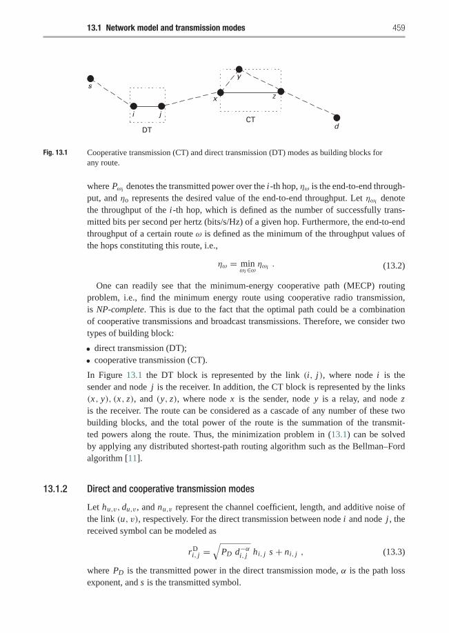
13.1 Network model and transmission modes 459
d
z
y
x
i j
DTCT
s
Fig. 13.1 Cooperative transmission (CT) and direct transmission (DT) modes as building blocks forany route.
where Pωi denotes the transmitted power over the i-th hop, ηω is the end-to-end through-put, and ηo represents the desired value of the end-to-end throughput. Let ηωi denotethe throughput of the i-th hop, which is defined as the number of successfully trans-mitted bits per second per hertz (bits/s/Hz) of a given hop. Furthermore, the end-to-endthroughput of a certain route ω is defined as the minimum of the throughput values ofthe hops constituting this route, i.e.,
ηω = minωi∈ω
ηωi . (13.2)
One can readily see that the minimum-energy cooperative path (MECP) routingproblem, i.e., find the minimum energy route using cooperative radio transmission,is NP-complete. This is due to the fact that the optimal path could be a combinationof cooperative transmissions and broadcast transmissions. Therefore, we consider twotypes of building block:
• direct transmission (DT);• cooperative transmission (CT).
In Figure 13.1 the DT block is represented by the link (i, j), where node i is thesender and node j is the receiver. In addition, the CT block is represented by the links(x, y), (x, z), and (y, z), where node x is the sender, node y is a relay, and node zis the receiver. The route can be considered as a cascade of any number of these twobuilding blocks, and the total power of the route is the summation of the transmit-ted powers along the route. Thus, the minimization problem in (13.1) can be solvedby applying any distributed shortest-path routing algorithm such as the Bellman–Fordalgorithm [11].
13.1.2 Direct and cooperative transmission modes
Let hu,v, du,v , and nu,v represent the channel coefficient, length, and additive noise ofthe link (u, v), respectively. For the direct transmission between node i and node j , thereceived symbol can be modeled as
rDi, j =
√PD d−αi, j hi, j s + ni, j , (13.3)
where PD is the transmitted power in the direct transmission mode, α is the path lossexponent, and s is the transmitted symbol.
460 Distributed cooperative routing
For the cooperative transmission, we consider a modified version of thedecode-and-forward incremental relaying cooperative scheme previously described inSection 4.2.2.1. The transmission scheme for a sender x , a relay y, and a receiver z, canbe described as follows. The sender sends its symbol in the current time slot. Due to thebroadcast nature of the wireless medium, both the receiver and the relay receive noisyversions of the transmitted symbol. The received symbols at the receiver and the relaycan be modeled as
rCx,z =
√PC d−αx,z hx,z s + nx,z (13.4)
and
rCx,y =
√PC d−αx,y hx,y s + nx,y , (13.5)
respectively, where PC is the source transmitted power in the cooperative transmissionmode.
Once the symbol is received, the receiver and the relay decode it. We assume thatthe relay and the receiver decide that the received symbol is correctly received if thereceived signal-to-noise ratio (SNR) is greater than a certain threshold, which dependson the transmitter and the receiver structures. Such system suffers from error propaga-tion but its effect can be neglectable. The rationale behind this is that when the relaysoperate in a high SNR regime, the dominant source of error is the channel being in out-age, i.e., deep fade, which corresponds to the SNR falling below some threshold. Thisissue had been illustrated at length in Example 6.1.
If the receiver decodes the symbol correctly, then it sends an acknowledgment (ACK)to the sender and the relay to confirm a correct reception. Otherwise, it sends a negativeacknowledgment (NACK) that allows the relay, if it received the symbol correctly, totransmit this symbol to the receiver in the next time slot. This model represents a mod-ified form of the automatic repeat request (ARQ), where the relay retransmits the datainstead of the sender, if necessary. The received symbol at the receiver can be written as
rCy,z =
√PC d−αy,z hy,z s + ny,z . (13.6)
In general, the relay can transmit with a power that is different from the sender powerPC . However, this complicates the problem of finding the minimum-power formula, aswill be derived later. For simplicity, we consider that both the sender and the relay sendtheir data using the same power PC .
Flat quasi-static fading channels are considered, hence, the channel coefficients areassumed to be constant during a complete frame, and may vary from a frame toanother. We assume that all the channel terms are independent complex Gaussian ran-dom variables with zero mean and unit variance. Finally, the noise terms are modeled aszero-mean, complex Gaussian random variables with equal variance N0. In this section,we have formulated the minimum-power routing problem and we have defined the twomain transmission modes. In the next section, we derive the closed-form expressionsfor the transmitted power in both direct and cooperative transmission modes required toachieve the desired throughput.
13.2 Link analysis 461
13.2 Link analysis
Since the throughput is a continuous monotonously increasing function of thetransmission power, the optimization problem in (13.1) has the minimum whenηω = ηo,∀ω ∈ �. Since the end-to-end throughput ηω = minωi∈ω ηωi , then the opti-mum power allocation, which achieves a desired throughput ηo along the route ω, forcesthe throughput at all the hops ηωi to be equal to the desired one, i.e.,
ηωi = ηo , ∀ ωi ∈ ω. (13.7)
This result can be explained as follows. Let P∗ω1, P∗ω2
, . . . , P∗ωnrepresent the required
powers on a route consisting of n hops, where P∗i results in ηωi = ηo for i = 1, . . . , n.If we increase the power of the i-th block to Pωi > P∗ωi
then the resulting throughputof the i-th block increases, i.e., ηωi > ηo, while the end-to-end throughput does notchange as minωi∈ω ηωi = ηo. Therefore, there is no need to increase the throughput ofany hop over ηo, which is indicated in (13.7).
Since the throughput of a given link ωi is defined as the number of successfullytransmitted bits per second per hertz, it can thus be calculated as
ηωi = pSωi× Rωi , (13.8)
where pSωi
and Rωi denote the per-link probability of success and transmission rate,respectively. We assume that the desired throughput can be factorized as
ηo = pSo × Ro , (13.9)
where pSo and Ro denote the desired per-link probability of success and transmission
rate, respectively. Next, we calculate the required transmitted power in order to achievethe desired per-link probability of success and transmission rate for both the direct andcooperative transmission modes. As previously noted (see (1.13) in Section 1.1.5), thechannel gain |hu,v|2 between any two nodes u and v, is exponentially distributed withparameter one [146].
For the direct transmission mode in (13.3), the mutual information between sender iand receiver j is
Ii, j = log
(1+ PD d−αi, j |hi, j |2
N0
). (13.10)
Without loss of generality, we have assumed unit bandwidth in (13.10). The out-age probability is defined as the probability that the mutual information is less thanthe required transmission rate Ro. Thus, the outage probability of the link (i, j) iscalculated as
pOi, j = Pr (Ii, j ≤ Ro) = 1− exp
(− (2
Ro − 1) N0 dαi, jPD
). (13.11)
If an outage occurs, the data is considered lost. The probability of success is calculatedas pS
i, j = 1− pOi, j . Thus, to achieve the desired pS
o and Ro for direct transmission mode,the required transmitted power is
462 Distributed cooperative routing
PD(di, j ) =(2Ro − 1) N0 dαi, j− log(pS
o ). (13.12)
For the cooperative transmission mode, the total outage probability is given by
pOx,y,z = Pr (Ix,z ≤ RC ) ·
(1− Pr (Ix,y ≤ RC )
) · Pr (Iy,z ≤ RC )
+ Pr (Ix,z ≤ RC ) · Pr (Ix,y ≤ RC ) , (13.13)
where RC denotes the transmission rate for each time slot. In (13.13), the first termcorresponds to the event when both the sender–receiver and relay–receiver channels arein outage but the sender–relay is not, and the second term corresponds to the event whenboth the sender–receiver and the sender–relay channels are in outage. Consequently, theprobability of success of the cooperative transmission mode can be calculated as
ps = exp(− g dαx,z
)+ exp(− g (dαx,y + dαy,z)
)− exp(− g (dαx,y + dαy,z + dαx,z)
),
(13.14)
where
g = (2RC − 1) N0
PC. (13.15)
In (13.13) and (13.14), we assume that the receiver decodes the signals received fromthe relay either at the first time slot or at the second time slot, instead of combining thereceived signals together. In general, maximum ratio combining (MRC) at the receivergives a better result. However, it requires the receiver to store an analog version of thereceived data from the sender, which requires huge storage capacity. The probabilitythat the source transmits only, denoted by Pr(φ), is calculated as
Pr(φ) = 1− Pr(Ix,z ≤ RC )+ Pr(Ix,z ≤ RC )Pr(Ix,y ≤ RC )
= 1− exp(− g dαx,y
)+ exp(− g (dαx,y + dαx,z)
),
(13.16)
where the term(1−Pr(Ix,z ≤ RC )
)corresponds to the event when the sender–receiver
channel is not in outage, while the other term corresponds to the event when both thesender–receiver and sender–relay channels are in outage. The probability that the relaycooperates with the source is calculated as
Pr(φ) = 1− Pr(φ). (13.17)
Thus, the average transmission rate of the cooperative transmission mode can becalculated as
R = RC · Pr(φ)+ RC
2· Pr(φ) = RC
2
(1+ Pr(φ)
), (13.18)
where RC corresponds to the transmission rate if the sender is sending alone in onetime slot and RC/2 corresponds to the transmission rate if the relay cooperates with thesender in the consecutive time slot.
We set the probability of success in (13.14) as pS = pSo and the average transmission
rate in (13.18) as R = Ro. By approximating the exponential functions in (13.14) asexp(−x) ≈ 1− x + x2/2, we obtain
13.3 Cooperation-based routing algorithms 463
g ≈√
1− pSo
deq, (13.19)
where deq � dαx,z(dαx,y + dαy,z). Thus, RC can be obtained using (13.18) as
RC = 2 Ro
1+ Pr(φ)
≈ 2 Ro
2− exp
(−√
1−pSo
deqdαx,y
)+ exp
(−√
1−pSo
deq(dαx,y + dαx,z)
) , (13.20)
where we substituted (13.19) in (13.16). In addition, the required power per link can becalculated using (13.15) and (13.19) as
PC ≈ (2RC − 1) N0
√deq
1− pSo. (13.21)
Finally, the total transmitted power of the cooperative transmission mode can becalculated as
PCtot(dx,z, dx,y, dy,z) = PC · Pr(φ)+ 2 PC · Pr(φ) = PC
(2− Pr(φ)
), (13.22)
where Pr(φ) and PC are given in (13.16) and (13.21), respectively.
13.3 Cooperation-based routing algorithms
In this section, we present two cooperation-based routing algorithms, which requirepolynomial complexity to find the minimum-power route. Then, we discuss the impactof cooperation on the routing in specific regular wireless networks, which are the regularlinear and grid networks. We assume that each node periodically broadcasts a HELLOpacket to its neighbors to update the topology information. In addition, we consider asimple medium access control (MAC) protocol, which is the conventional time divisionmultiple access (TDMA) scheme with equal time slots.
First, let us describe a cooperation-based routing algorithm, namely, the minimum-power cooperative routing (MPCR) algorithm. The MPCR algorithm takes into consid-eration the cooperative communications while constructing the minimum-power route.The derived power formulas for direct transmission and cooperative transmission areutilized to construct the minimum-power route. It can be distributively implementedby the Bellman–Ford shortest path algorithm [11]. In the conventional Bellman–Fordshortest path algorithm, each node i ∈ {1, . . . , N } executes the iteration
Di = minj∈N (i)
(dαi, j + D j ) , (13.23)
where N (i) denotes the set of neighboring nodes of node i , dαi, j denotes the effectivedistance between node i and j , and D j represents the latest estimate of the shortest pathfrom node j to the destination that is included in the HELLO packet.
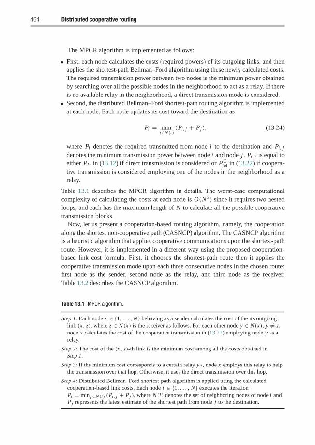
464 Distributed cooperative routing
The MPCR algorithm is implemented as follows:
• First, each node calculates the costs (required powers) of its outgoing links, and thenapplies the shortest-path Bellman–Ford algorithm using these newly calculated costs.The required transmission power between two nodes is the minimum power obtainedby searching over all the possible nodes in the neighborhood to act as a relay. If thereis no available relay in the neighborhood, a direct transmission mode is considered.
• Second, the distributed Bellman–Ford shortest-path routing algorithm is implementedat each node. Each node updates its cost toward the destination as
Pi = minj∈N (i)
(Pi, j + Pj ), (13.24)
where Pi denotes the required transmitted from node i to the destination and Pi, j
denotes the minimum transmission power between node i and node j . Pi, j is equal toeither PD in (13.12) if direct transmission is considered or PC
tot in (13.22) if coopera-tive transmission is considered employing one of the nodes in the neighborhood as arelay.
Table 13.1 describes the MPCR algorithm in details. The worst-case computationalcomplexity of calculating the costs at each node is O(N 2) since it requires two nestedloops, and each has the maximum length of N to calculate all the possible cooperativetransmission blocks.
Now, let us present a cooperation-based routing algorithm, namely, the cooperationalong the shortest non-cooperative path (CASNCP) algorithm. The CASNCP algorithmis a heuristic algorithm that applies cooperative communications upon the shortest-pathroute. However, it is implemented in a different way using the proposed cooperation-based link cost formula. First, it chooses the shortest-path route then it applies thecooperative transmission mode upon each three consecutive nodes in the chosen route;first node as the sender, second node as the relay, and third node as the receiver.Table 13.2 describes the CASNCP algorithm.
Table 13.1 MPCR algorithm.
Step 1: Each node x ∈ {1, . . . , N } behaving as a sender calculates the cost of the its outgoinglink (x, z), where z ∈ N (x) is the receiver as follows. For each other node y ∈ N (x), y �= z,node x calculates the cost of the cooperative transmission in (13.22) employing node y as arelay.
Step 2: The cost of the (x, z)-th link is the minimum cost among all the costs obtained inStep 1.
Step 3: If the minimum cost corresponds to a certain relay y∗, node x employs this relay to helpthe transmission over that hop. Otherwise, it uses the direct transmission over this hop.
Step 4: Distributed Bellman–Ford shortest-path algorithm is applied using the calculatedcooperation-based link costs. Each node i ∈ {1, . . . , N } executes the iterationPi = min j∈N (i) (Pi, j + Pj ), where N (i) denotes the set of neighboring nodes of node i andPj represents the latest estimate of the shortest path from node j to the destination.
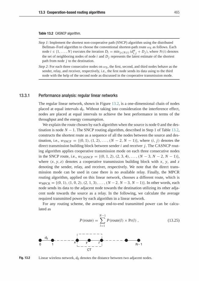
13.3 Cooperation-based routing algorithms 465
Table 13.2 CASNCP algorithm.
Step 1: Implement the shortest non-cooperative path (SNCP) algorithm using the distributedBellman–Ford algorithm to choose the conventional shortest-path route ωS as follows. Eachnode i ∈ {1, . . . , N } executes the iteration Di = min j∈N (i) (d
αi, j + D j ), where N (i) denotes
the set of neighboring nodes of node i and D j represents the latest estimate of the shortestpath from node j to the destination.
Step 2: For each three consecutive nodes on ωS , the first, second, and third nodes behave as thesender, relay, and receiver, respectively, i.e., the first node sends its data using to the thirdnode with the help of the second node as discussed in the cooperative transmission mode.
13.3.1 Performance analysis: regular linear networks
The regular linear network, shown in Figure 13.2, is a one-dimensional chain of nodesplaced at equal intervals d0. Without taking into consideration the interference effect,nodes are placed at equal intervals to achieve the best performance in terms of thethroughput and the energy consumption.
We explain the route chosen by each algorithm when the source is node 0 and the des-tination is node N − 1. The SNCP routing algorithm, described in Step 1 of Table 13.2,constructs the shortest route as a sequence of all the nodes between the source and des-tination, i.e., wSNCP = {(0, 1), (1, 2), . . . , (N − 2, N − 1)}, where (i, j) denotes thedirect transmission building block between sender i and receiver j . The CASNCP rout-ing algorithm applies cooperative transmission mode on each three consecutive nodesin the SNCP route, i.e., wCASNCP = {(0, 1, 2), (2, 3, 4), . . . , (N − 3, N − 2, N − 1)},where (x, y, z) denotes a cooperative transmission building block with x , y, and zdenoting the sender, relay, and receiver, respectively. We note that the direct trans-mission mode can be used in case there is no available relay. Finally, the MPCRrouting algorithm, applied on this linear network, chooses a different route, which iswMPCR = {(0, 1), (1, 0, 2), (2, 1, 3), . . . , (N − 2, N − 3, N − 1)}. In other words, eachnode sends its data to the adjacent node towards the destination utilizing its other adja-cent node towards the source as a relay. In the following, we calculate the averagerequired transmitted power by each algorithm in a linear network.
For any routing scheme, the average end-to-end transmitted power can be calcu-lated as
P(route) =N−1∑l=1
P(route|l)× Pr(l) , (13.25)
0 N – 1
CT
d0
zyx1
Fig. 13.2 Linear wireless network, d0 denotes the distance between two adjacent nodes.
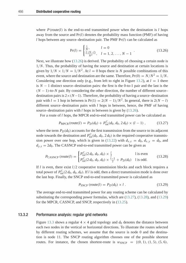
466 Distributed cooperative routing
where P(route|l) is the end-to-end transmitted power when the destination is l hopsaway from the source and Pr(l) denotes the probability mass function (PMF) of havingl hops between any source–destination pair. The PMF Pr(l) can be calculated as
Pr(l) ={
1N , l = 02 (N−l)
N2 , l = 1, 2, . . . , N − 1. (13.26)
Next, we illustrate how (13.26) is derived. The probability of choosing a certain node is1/N . Thus, the probability of having the source and destination at certain locations isgiven by 1/N × 1/N = 1/N 2. At l = 0 hops there is N possible combinations of thisevent, where the source and destination are the same. Therefore, Pr(0) = N/N 2 = 1/N .Considering one direction only (e.g., from left to right in Figure 13.2), at l = 1 thereis N − 1 distinct source–destination pairs: the first is the 0-to-1 pair and the last is the(N − 1)-to-N pair. By considering the other direction, the number of different source–destination pairs is 2×(N−1). Therefore, the probability of having a source–destinationpair with l = 1 hop in between is Pr(1) = 2(N − 1)/N 2. In general, there is 2(N − l)different source–destination pairs with l hops in between, hence, the PMF of havingsource–destination pairs with l hops in between is given by (13.26).
For a route of l hops, the MPCR end-to-end transmitted power can be calculated as
PMPCR(route|l) = PD(d0)+ PCtot(d0, d0, 2 d0)× (l − 1) , (13.27)
where the term PD(d0) accounts for the first transmission from the source to its adjacentnode towards the destination and PC
tot(d0, d0, 2 d0) is the required cooperative transmis-sion power over one hop, which is given in (13.22) with dx,z = d0, dx,y = d0, anddy,z = 2d0. The CASNCP end-to-end transmitted power can be given as
PCASNCP (route|l) ={
PCtot(2 d0, d0, d0)× l
2 l is even
PCtot(2 d0, d0, d0)× l−1
2 + PD(d0) l is odd.(13.28)
If l is even, there exist l/2 cooperative transmission blocks and each block requires atotal power of PC
tot(2 d0, d0, d0). If l is odd, then a direct transmission mode is done overthe last hop. Finally, the SNCP end-to-end transmitted power is calculated as
PSNCP (route|l) = PD(d0)× l . (13.29)
The average end-to-end transmitted power for any routing scheme can be calculated bysubstituting the corresponding power formulas, which are (13.27), (13.28), and (13.29)for the MPCR, CASNCP, and SNCP, respectively in (13.25).
13.3.2 Performance analysis: regular grid networks
Figure 13.3 shows a regular 4 × 4 grid topology and d0 denotes the distance betweeneach two nodes in the vertical or horizontal directions. To illustrate the routes selectedby different routing schemes, we assume that the source is node 0 and the destina-tion is node 11. The SNCP routing algorithm chooses one of the possible shortestroutes. For instance, the chosen shortest-route is wSNCP = {(0, 1), (1, 5), (5, 6),
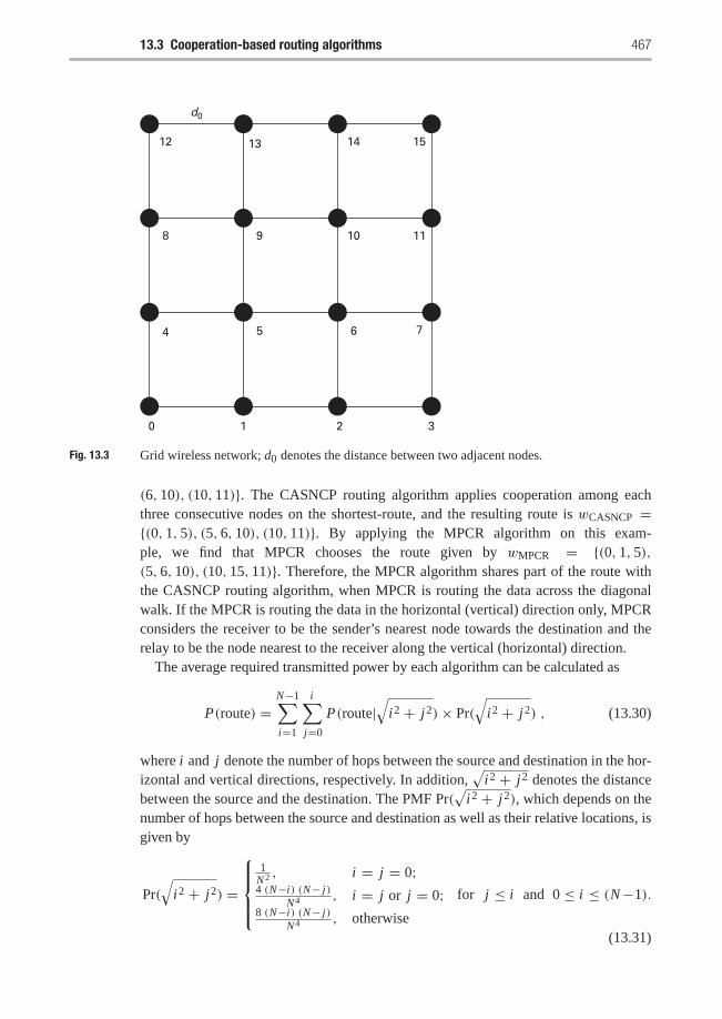
13.3 Cooperation-based routing algorithms 467
d0
0
12
1110
13
8
7654
321
1514
9
Fig. 13.3 Grid wireless network; d0 denotes the distance between two adjacent nodes.
(6, 10), (10, 11)}. The CASNCP routing algorithm applies cooperation among eachthree consecutive nodes on the shortest-route, and the resulting route is wCASNCP ={(0, 1, 5), (5, 6, 10), (10, 11)}. By applying the MPCR algorithm on this exam-ple, we find that MPCR chooses the route given by wMPCR = {(0, 1, 5),(5, 6, 10), (10, 15, 11)}. Therefore, the MPCR algorithm shares part of the route withthe CASNCP routing algorithm, when MPCR is routing the data across the diagonalwalk. If the MPCR is routing the data in the horizontal (vertical) direction only, MPCRconsiders the receiver to be the sender’s nearest node towards the destination and therelay to be the node nearest to the receiver along the vertical (horizontal) direction.
The average required transmitted power by each algorithm can be calculated as
P(route) =N−1∑i=1
i∑j=0
P(route|√
i2 + j2)× Pr(√
i2 + j2) , (13.30)
where i and j denote the number of hops between the source and destination in the hor-izontal and vertical directions, respectively. In addition,
√i2 + j2 denotes the distance
between the source and the destination. The PMF Pr(√
i2 + j2), which depends on thenumber of hops between the source and destination as well as their relative locations, isgiven by
Pr(√
i2 + j2) =
⎧⎪⎪⎨⎪⎪⎩1
N2 , i = j = 0;4 (N−i) (N− j)
N4 , i = j or j = 0;8 (N−i) (N− j)
N4 , otherwise
for j ≤ i and 0 ≤ i ≤ (N−1).
(13.31)
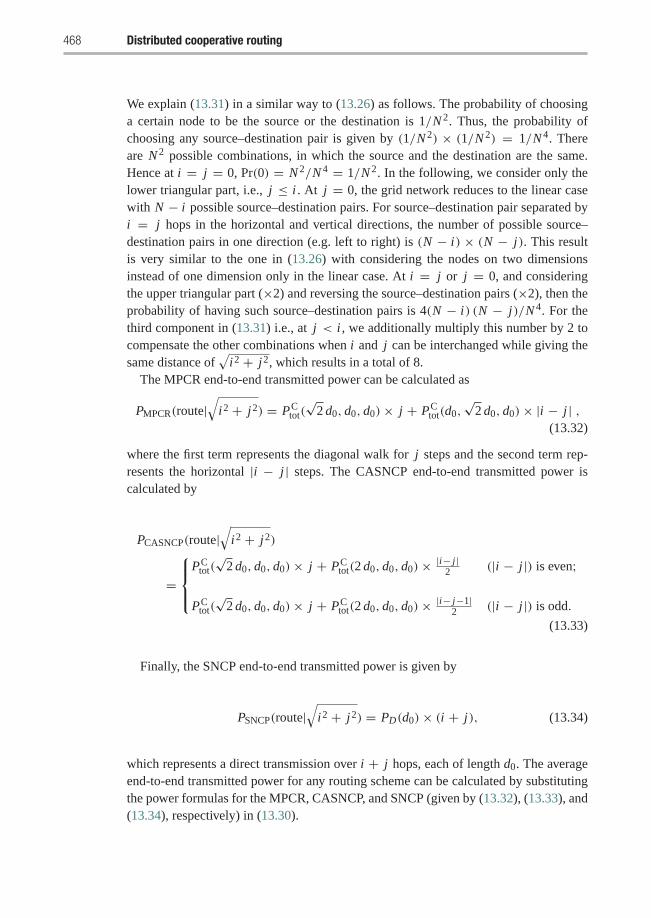
468 Distributed cooperative routing
We explain (13.31) in a similar way to (13.26) as follows. The probability of choosinga certain node to be the source or the destination is 1/N 2. Thus, the probability ofchoosing any source–destination pair is given by (1/N 2) × (1/N 2) = 1/N 4. Thereare N 2 possible combinations, in which the source and the destination are the same.Hence at i = j = 0, Pr(0) = N 2/N 4 = 1/N 2. In the following, we consider only thelower triangular part, i.e., j ≤ i . At j = 0, the grid network reduces to the linear casewith N − i possible source–destination pairs. For source–destination pair separated byi = j hops in the horizontal and vertical directions, the number of possible source–destination pairs in one direction (e.g. left to right) is (N − i) × (N − j). This resultis very similar to the one in (13.26) with considering the nodes on two dimensionsinstead of one dimension only in the linear case. At i = j or j = 0, and consideringthe upper triangular part (×2) and reversing the source–destination pairs (×2), then theprobability of having such source–destination pairs is 4(N − i) (N − j)/N 4. For thethird component in (13.31) i.e., at j < i , we additionally multiply this number by 2 tocompensate the other combinations when i and j can be interchanged while giving thesame distance of
√i2 + j2, which results in a total of 8.
The MPCR end-to-end transmitted power can be calculated as
PMPCR(route|√
i2 + j2) = PCtot(√
2 d0, d0, d0)× j + PCtot(d0,
√2 d0, d0)× |i − j | ,
(13.32)
where the first term represents the diagonal walk for j steps and the second term rep-resents the horizontal |i − j | steps. The CASNCP end-to-end transmitted power iscalculated by
PCASNCP(route|√
i2 + j2)
=
⎧⎪⎨⎪⎩PC
tot(√
2 d0, d0, d0)× j + PCtot(2 d0, d0, d0)× |i− j |
2 (|i − j |) is even;
PCtot(√
2 d0, d0, d0)× j + PCtot(2 d0, d0, d0)× |i− j−1|
2 (|i − j |) is odd.
(13.33)
Finally, the SNCP end-to-end transmitted power is given by
PSNCP(route|√
i2 + j2) = PD(d0)× (i + j), (13.34)
which represents a direct transmission over i + j hops, each of length d0. The averageend-to-end transmitted power for any routing scheme can be calculated by substitutingthe power formulas for the MPCR, CASNCP, and SNCP (given by (13.32), (13.33), and(13.34), respectively) in (13.30).
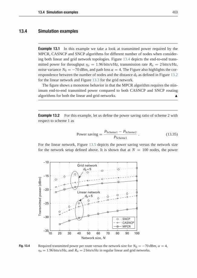
13.4 Simulation examples 469
13.4 Simulation examples
Example 13.1 In this example we take a look at transmitted power required by theMPCR, CASNCP and SNCP algorithms for different number of nodes when consider-ing both linear and grid network topologies. Figure 13.4 depicts the end-to-end trans-mitted power for throughput ηo = 1.96 bits/s/Hz, transmission rate Ro = 2 bits/s/Hz,noise variance N0 = −70 dBm, and path loss α = 4. The Figure also highlights the cor-respondence between the number of nodes and the distance d0 as defined in Figure 13.2for the linear network and Figure 13.3 for the grid network.
The figure shows a monotone behavior in that the MPCR algorithm requires the min-imum end-to-end transmitted power compared to both CASNCP and SNCP routingalgorithms for both the linear and grid networks. �
Example 13.2 For this example, let us define the power saving ratio of scheme 2 withrespect to scheme 1 as
Power saving = PScheme1 − PScheme2
PScheme1. (13.35)
For the linear network, Figure 13.5 depicts the power saving versus the network sizefor the network setup defined above. It is shown that at N = 100 nodes, the power
10 20 30 40 50 60 70 80 90 100−35
−30
−25
−20
−15
−10
Network size, N
Tra
nsm
itte
d p
ow
er [
dB
m]
Grid networkd0 = 5
Linear networkd0 = 5
SNCPCASNCPMPCR
Fig. 13.4 Required transmitted power per route versus the network size for N0 = −70 dBm, α = 4,ηo = 1.96 bits/s/Hz, and Ro = 2 bits/s/Hz in regular linear and grid networks.
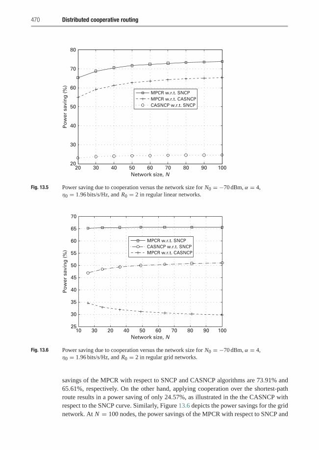
470 Distributed cooperative routing
20 30 40 50 60 70 80 90 10020
30
40
50
60
70
80
Network size, N
Po
wer
sav
ing
(%
)
MPCR w.r.t. SNCPMPCR w.r.t. CASNCPCASNCP w.r.t. SNCP
Fig. 13.5 Power saving due to cooperation versus the network size for N0 = −70 dBm, α = 4,η0 = 1.96 bits/s/Hz, and R0 = 2 in regular linear networks.
10 2030 40 50 60 70 80 90 10025
30
35
40
45
50
55
60
65
70
Network size, N
Po
wer
sav
ing
(%
)
MPCR w.r.t. SNCPCASNCP w.r.t. SNCPMPCR w.r.t. CASNCP
Fig. 13.6 Power saving due to cooperation versus the network size for N0 = −70 dBm, α = 4,η0 = 1.96 bits/s/Hz, and R0 = 2 in regular grid networks.
savings of the MPCR with respect to SNCP and CASNCP algorithms are 73.91% and65.61%, respectively. On the other hand, applying cooperation over the shortest-pathroute results in a power saving of only 24.57%, as illustrated in the the CASNCP withrespect to the SNCP curve. Similarly, Figure 13.6 depicts the power savings for the gridnetwork. At N = 100 nodes, the power savings of the MPCR with respect to SNCP and
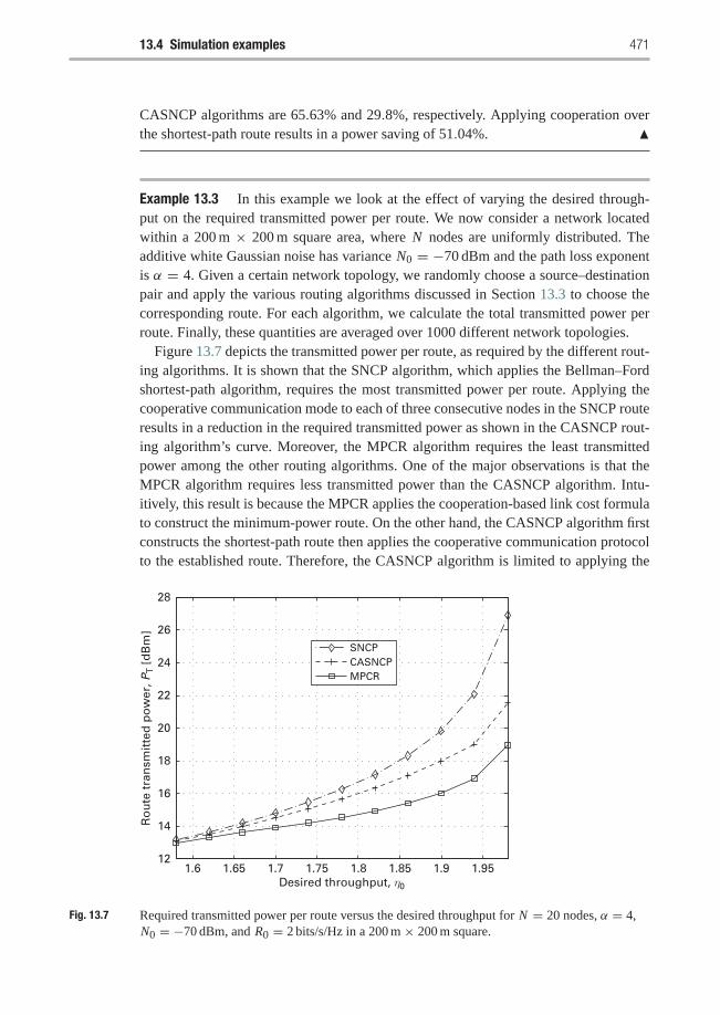
13.4 Simulation examples 471
CASNCP algorithms are 65.63% and 29.8%, respectively. Applying cooperation overthe shortest-path route results in a power saving of 51.04%. �
Example 13.3 In this example we look at the effect of varying the desired through-put on the required transmitted power per route. We now consider a network locatedwithin a 200 m × 200 m square area, where N nodes are uniformly distributed. Theadditive white Gaussian noise has variance N0 = −70 dBm and the path loss exponentis α = 4. Given a certain network topology, we randomly choose a source–destinationpair and apply the various routing algorithms discussed in Section 13.3 to choose thecorresponding route. For each algorithm, we calculate the total transmitted power perroute. Finally, these quantities are averaged over 1000 different network topologies.
Figure 13.7 depicts the transmitted power per route, as required by the different rout-ing algorithms. It is shown that the SNCP algorithm, which applies the Bellman–Fordshortest-path algorithm, requires the most transmitted power per route. Applying thecooperative communication mode to each of three consecutive nodes in the SNCP routeresults in a reduction in the required transmitted power as shown in the CASNCP rout-ing algorithm’s curve. Moreover, the MPCR algorithm requires the least transmittedpower among the other routing algorithms. One of the major observations is that theMPCR algorithm requires less transmitted power than the CASNCP algorithm. Intu-itively, this result is because the MPCR applies the cooperation-based link cost formulato construct the minimum-power route. On the other hand, the CASNCP algorithm firstconstructs the shortest-path route then applies the cooperative communication protocolto the established route. Therefore, the CASNCP algorithm is limited to applying the
1.6 1.65 1.7 1.75 1.8 1.85 1.9 1.9512
14
16
18
20
22
24
26
28
Desired throughput, η0
Ro
ute
tra
nsm
itte
d p
ow
er, P
T [
dB
m]
SNCPCASNCPMPCR
Fig. 13.7 Required transmitted power per route versus the desired throughput for N = 20 nodes, α = 4,N0 = −70 dBm, and R0 = 2 bits/s/Hz in a 200 m × 200 m square.
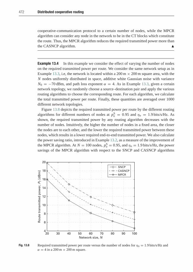
472 Distributed cooperative routing
cooperative-communication protocol to a certain number of nodes, while the MPCRalgorithm can consider any node in the network to be in the CT blocks which constitutethe route. Thus, the MPCR algorithm reduces the required transmitted power more thanthe CASNCP algorithm. �
Example 13.4 In this example we consider the effect of varying the number of nodeson the required transmitted power per route. We consider the same network setup as inExample 13.3, i.e, the network is located within a 200 m × 200 m square area, with theN nodes uniformly distributed in space, additive white Gaussian noise with varianceN0 = −70 dBm, and path loss exponent α = 4. As in Example 13.3, given a certainnetwork topology, we randomly choose a source–destination pair and apply the variousrouting algorithms to choose the corresponding route. For each algorithm, we calculatethe total transmitted power per route. Finally, these quantities are averaged over 1000different network topologies.
Figure 13.8 depicts the required transmitted power per route by the different routingalgorithms for different numbers of nodes at pS
o = 0.95 and ηo = 1.9 bits/s/Hz. Asshown, the required transmitted power by any routing algorithm decreases with thenumber of nodes. Intuitively, the higher the number of nodes in a fixed area, the closerthe nodes are to each other, and the lower the required transmitted power between thesenodes, which results in a lower required end-to-end transmitted power. We also calculatethe power saving ratio, introduced in Example 13.2, as a measure of the improvement ofthe MPCR algorithm. At N = 100 nodes, pS
o = 0.95, and ηo = 1.9 bits/s/Hz, the powersavings of the MPCR algorithm with respect to the SNCP and CASNCP algorithms
20 30 40 50 60 70 80 90 1004
6
8
10
12
14
16
18
20
Ro
ute
tra
nsm
itte
d p
ow
er, P
T [
dB
m]
Network size, N
SNCPCASNCPMPCR
Fig. 13.8 Required transmitted power per route versus the number of nodes for ηo = 1.9 bits/s/Hz andα = 4 in a 200 m × 200 m square.
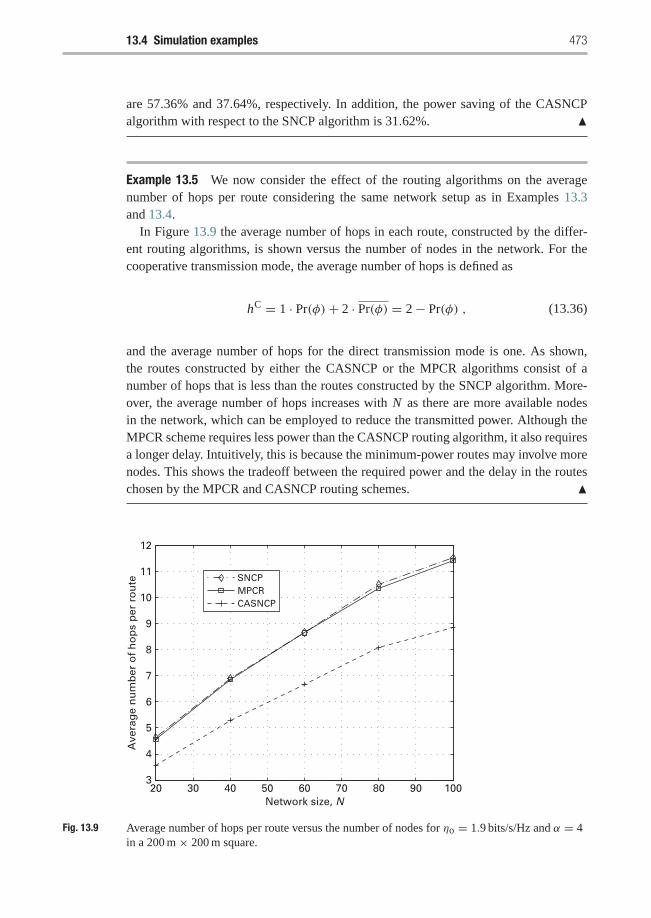
13.4 Simulation examples 473
are 57.36% and 37.64%, respectively. In addition, the power saving of the CASNCPalgorithm with respect to the SNCP algorithm is 31.62%. �
Example 13.5 We now consider the effect of the routing algorithms on the averagenumber of hops per route considering the same network setup as in Examples 13.3and 13.4.
In Figure 13.9 the average number of hops in each route, constructed by the differ-ent routing algorithms, is shown versus the number of nodes in the network. For thecooperative transmission mode, the average number of hops is defined as
hC = 1 · Pr(φ)+ 2 · Pr(φ) = 2− Pr(φ) , (13.36)
and the average number of hops for the direct transmission mode is one. As shown,the routes constructed by either the CASNCP or the MPCR algorithms consist of anumber of hops that is less than the routes constructed by the SNCP algorithm. More-over, the average number of hops increases with N as there are more available nodesin the network, which can be employed to reduce the transmitted power. Although theMPCR scheme requires less power than the CASNCP routing algorithm, it also requiresa longer delay. Intuitively, this is because the minimum-power routes may involve morenodes. This shows the tradeoff between the required power and the delay in the routeschosen by the MPCR and CASNCP routing schemes. �
20 30 40 50 60 70 80 90 1003
4
5
6
7
8
9
10
11
12
Ave
rag
e n
um
ber
of
ho
ps
per
ro
ute
Network size, N
SNCPMPCRCASNCP
Fig. 13.9 Average number of hops per route versus the number of nodes for ηo = 1.9 bits/s/Hz and α = 4in a 200 m × 200 m square.
474 Distributed cooperative routing
13.5 Chapter summary and bibliographical notes
In this chapter, we have considered the impact of cooperative communication on theminimum-power routing problem in wireless networks. For a given source–destinationpair, the optimum route requires the minimum end-to-end transmitted power whileguaranteeing certain throughput. This chapter first focused on the MPCR algorithm,which applies the cooperative communication while constructing the route. The MPCRalgorithm constructs the minimum-power route using any number of the proposedcooperation-based building blocks, which require the least possible transmitted power.This chapter also presented the CASNCP algorithm, which is similar to most of theexisting cooperative routing algorithms. The CASNCP algorithm first constructs theconventional shortest-path route then applies a cooperative-communication protocol tothe established route. As we have seen, for random networks of N = 100 nodes, thepower savings of the MPCR algorithm with respect to the conventional shortest-path andCASNCP routing algorithms are 57.36% and 37.64%, respectively. In addition to ran-dom networks, we have considered regular linear and grid networks, and have derivedthe analytical results for the power savings due to cooperation in these cases. In the caseof a regular linear network with N = 100 nodes, the power savings of the MPCR algo-rithm with respect to the shortest-path and CASNCP routing algorithms are 73.91% and65.61%, respectively. Similarly, the power savings of the MPCR algorithm with respectto the shortest-path and CASNCP routing algorithms in a grid network of 100 nodes are65.63% and 29.8%, respectively.
The topic of routing in MANETs has resulted in a number of publications address-ing different problems. A useful reference to learn about different routing protocolsis [119]. One of the main concerns when designing routing algorithms for differentwireless networks, such as mobile ad hoc networks, is to ensure that the result pro-vides energy savings to extend the device’s battery life. The goal of energy savings isone of the main objectives in [234] (for sensor networks). Also, it was shown in [38]that in some wireless networks, such as ad hoc networks, nodes spend most of theirpower in communication, either sending their own data or relaying other nodes’ data.An analysis of the complexity associated with finding the solution of the minimum-energy cooperative path routing problem can be found in [115], where it was shownthat finding the minimum-energy route using cooperative radio transmission requiressolving a NP-complete problem. In addition to saving more energy, the routes selectedby the routing protocol may be required to guarantee a certain quality of Service (qoS),as it is of great importance for some wireless applications (e.g., multimedia applica-tions) [236]. The use of cross-layer techniques in routing protocols, such as providingthe physical information about the wireless medium to upper layers, is a relative newapproach aimed at achieving efficient scheduling, routing, resource allocation, and flowcontrol algorithms. One work following this approach is [55], where it was shown thatfor high end-to-end delivery probabilities and given a certain delay constraint, long-hop schemes save more energy than that of the traditional nearest-neighbor routingalgorithm.
Exercises 475
As in other areas of cooperative communications, the cooperative routing problemhas received recent attention from the research community, resulting in some notewor-thy published research. In [96], two centralized heuristic algorithms (cooperation alongthe minimum energy non-cooperative path (CAN-L) and progressive cooperation (PC-L)) are proposed. In these algorithms, the optimum route is found through a dynamicprogramming mechanism which is N P hard. Also, [115] proposed the cooperativeshortest path (CSP) algorithm, which chooses the next node in the route that minimizesthe power transmitted by the last L nodes added to the route, while [186] presented aninformation-theoretic viewpoint of the cooperative routing in linear wireless network forboth the power-limited and bandwidth-limited regimes. In addition, this paper presentsan analysis of the transmission power required to achieve a desired end-to-end rate. Forthe case of a wireless sensor network, [143] studied the impact of cooperative com-munication on maximizing the lifetime of the network. Finally, [128] considered threecooperative routing algorithms, namely, relay-by-flooding, relay-assisted routing, andrelay-enhanced routing. In the relay-by-flooding, the message is propagated by flood-ing and multiple hops. The relay-assisted routing uses cooperative nodes of an existingroute and the relay-enhanced routing adds cooperative nodes to an existing route. Bothof these routing schemes start with a route determined without cooperation. The authorsalso assume that more than one relay can send the data in the same time period, while notconsidering the synchronization problem. More discussion on the topic of distributedenergy-efficient cooperative routing can be found in [81] and [85].
Exercises
13.1 In this exercise, we consider minimum-power cooperative routing problems withQoS, which are determined by the end-to-end probability of success and band-width efficiency. We aim at designing centralized cooperation-based routingalgorithms. For a route ω ∈ �, denote ωi as the i-th block of this route. Thus,the problem can be formulated as
minω∈�
∑ωi∈ω
Pωi s.t. pS ≥ pSd and R ≥ Rd ,
where Pωi denotes the transmitted power over the i-th block and pS and R are theend-to-end probability of success and bandwidth efficiency, respectively. Sim-ilarly, pS
d and Rd represent the minimum desired values of the probability ofsuccess and the bandwidth efficiency, respectively.
(a) Given that the bandwidth efficiency R = minωi∈ω Rωi , what is the desiredbandwidth efficiency at all the hops Rωi that require minimum transmittedpower and achieve the desired bandwidth efficiency?
(b) The pS of the route ω can be calculated as
pS =∏ωi∈ω
pSωi, R = min
ωi∈ωRωi ,
476 Distributed cooperative routing
where pSωi
and Rωi denote the probability of success and the bandwidth effi-ciency of the i-th block, respectively. In order to get the per-link probability ofsuccess, consider a solution for a route of n hops that assumes that the proba-bilities of success over all the links constituting this route are equal to the n-throot of the desired probability of success. i.e.,
pSωi= pS
h = n√
pSd , for i = 1, . . . , n,
where pSh is the probability of success per hop. Compare the results obtained
by this solution with the optimal results obtained numerically for a two-stageroute. The central node approximates the number of hops in a given route asthe one given by the shortest-path routing algorithm.
(c) Based on the obtained probability of success and bandwidth efficiency perlink, calculate the link costs for both the direct transmission and cooperativetransmission building blocks.
(d) Implement the centralized MPCR and CASNCP routing algorithms based onthe obtained link-level QoS.
(e) (Computer simulations) Consider a 200 m × 200 m grid, where N nodesare uniformly distributed. The additive white Gaussian noise has varianceN0 = −70 dBm.
(i) Assume that the desired bandwidth efficiency is Rd = 2 bits/s/Hz.Show the transmitted power per route, required by the different routingalgorithms for α = 2 and α = 4.
(ii) Show the resulting probability of success for the three routing algorithmsat N = 20, Rd = 2 bits/s/Hz, and α = 4.
(iii) Show the average number of hops per route versus the number of nodesfor pS
d = 0.95, Rd = 2 bits/s/Hz, and α = 4.(iv) Plot the transmitted power per route versus the desired transmission rate
for pSd = 0.95 bits/s/Hz and α = 4.
(v) Finally, plot the transmitted power per route and the power saving versusthe number of nodes for pS
d = 0.95, Rd = 2 bits/s/Hz, and α = 4.
13.2 Consider the three consecutive nodes x , y, and z in Figure 13.2, where node xneeds to transmit its data to node z. Illustrate the route chosen by each of therouting algorithms in this case.
(a) The SNCP routing algorithm transmits the data directly from node x to nodey then from node y to node z. Calculate the required power for the SNCProuting algorithm.
(b) The CASNCP routing algorithm applies cooperative communication trans-mission to the shortest-path route. Calculate the transmitted power for theCASNCP routing algorithm.
(c) By applying the MPCR algorithm, we find that the route is chosen in twoconsecutive phases as follows. First, node x transmits its data directly tonode y utilizing direct transmission mode. Second, node y transmits its data

Exercises 477
to node z in a cooperative transmission mode utilizing node x as a relay. Inother words, if node z does not receive the data correctly from node y, thennode x will retransmit the data to node z. Calculate the transmitted powerrequired by the MPCR algorithm.
(d) Plot the required transmitted power per block (x, y, z) as a function ofthe distance d0 at throughput η0 = 1.96 bits/s/Hz, transmission rate R0 =2 bits/s/Hz, noise variance N0 = −70 dBm, and path loss exponent α = 4.
13.3 In a 5 m× 5 m grid network, consider the lower left corner node to be the sourceand the upper right corner to be the destination. Apply the MPCR and CASNCProuting algorithms and show the route chosen by each algorithm. Calculate theenergy saving due to cooperation in this case?
13.4 (Computer simulations) Verify by numerical results that the probability densityfunction (PDF) of the distance between any two nodes in linear or grid networks,are given by (13.26) and (13.31), respectively.
13.5 Consider a linear network of N = 5 nodes. Let the source be the first node 0 andthe destination be node 9. Apply the MPCR and CASNCP routing algorithmsand show the route chosen by each algorithm. Calculate the energy saving due tocooperation in this case.
14 Source–channel codingwith cooperation
The design of wireless devices and networks present unique design challenges due tothe combined effects of physical constraints, such as bandwidth and power, and com-munication errors introduced through channel fading and noise. The limited bandwidthhas to be addressed through a compression operation that removes redundant informa-tion from the source. Unfortunately, the removal of redundancy makes the transmitteddata not only more important but also more sensitive to channel errors. Therefore, it isnecessary to complement the source compression operation with the application of anerror control code to do channel coding. The goal of the channel coding operation isto add redundancy back to the source coded data that has been designed to efficientlydetect and correct errors introduced in the channel. In this chapter we will study theuse of cooperation to transmit multimedia traffic (such as voice or video conferencing).This involves studying the performance of schemes with strict delay constraint whereuser cooperation is combined with source and channel coding.
Although the source and channel codecs complement each other, historically theirdesign had been approached independently of each other. The basic assumptions in thisdesign method are that the source encoder will present to the channel encoder a bitstream where all source redundancy have been removed and that the channel decoderwill be able to present to the source decoder a bit stream where all channel errors havebeen corrected. This approach is justified in Shannon’s separation theorem [181, 182],which states that for certain systems there is no loss of optimality in designing sourceand channel coding each independently of the other. Unfortunately, this theorem doesnot apply in many practical systems where its assumptions of arbitrary large complexityand infinite delay do not hold. Networks carrying delay sensitive traffic, such as multi-media, are one example of systems for which the assumptions in Shannon’s separationtheorem are not practical. For these systems, it is better to jointly design the source andchannel units, an approach that is named joint source-channel coding (JSCC).
14.1 Joint source–channel coding bit rate allocation
In this chapter we will study the use of cooperation as part of a network where perfor-mance is best studied from an end-to-end viewpoint. Specifically, we will now study theapplication of user cooperation to transmit an interactive media. We will assume that thetransmitted source may be speech, video, or some other synthetic source that is useful
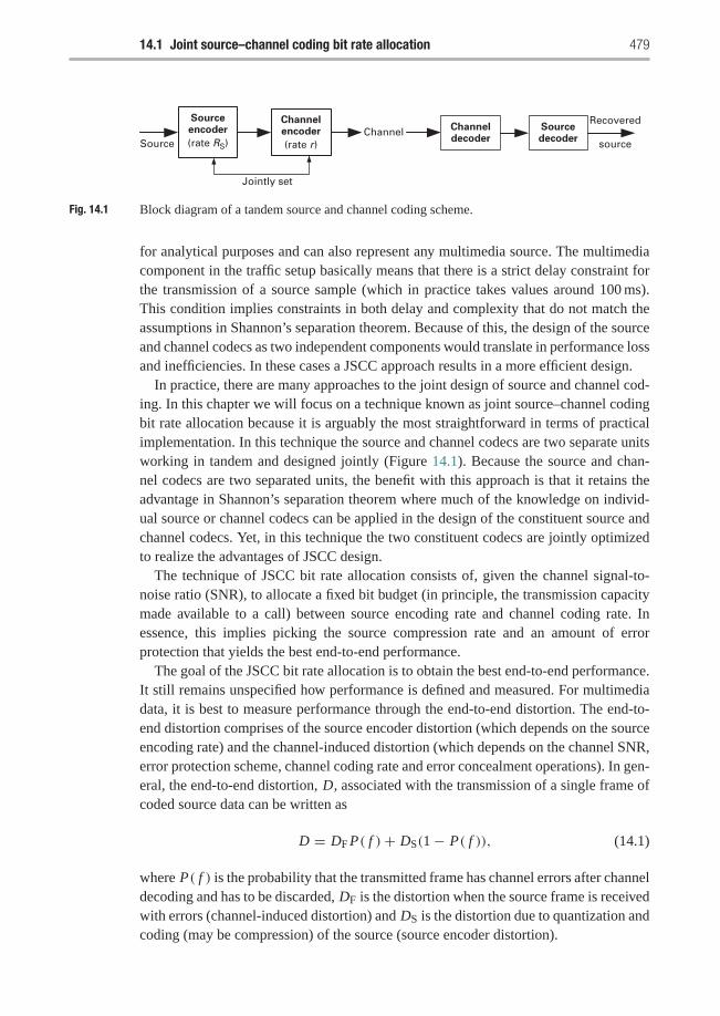
14.1 Joint source–channel coding bit rate allocation 479
Sourceencoder
(rate RS)
Channelencoder
(rate r )Channel Source
decoderChanneldecoderSource
Recovered
source
Jointly set
Fig. 14.1 Block diagram of a tandem source and channel coding scheme.
for analytical purposes and can also represent any multimedia source. The multimediacomponent in the traffic setup basically means that there is a strict delay constraint forthe transmission of a source sample (which in practice takes values around 100 ms).This condition implies constraints in both delay and complexity that do not match theassumptions in Shannon’s separation theorem. Because of this, the design of the sourceand channel codecs as two independent components would translate in performance lossand inefficiencies. In these cases a JSCC approach results in a more efficient design.
In practice, there are many approaches to the joint design of source and channel cod-ing. In this chapter we will focus on a technique known as joint source–channel codingbit rate allocation because it is arguably the most straightforward in terms of practicalimplementation. In this technique the source and channel codecs are two separate unitsworking in tandem and designed jointly (Figure 14.1). Because the source and chan-nel codecs are two separated units, the benefit with this approach is that it retains theadvantage in Shannon’s separation theorem where much of the knowledge on individ-ual source or channel codecs can be applied in the design of the constituent source andchannel codecs. Yet, in this technique the two constituent codecs are jointly optimizedto realize the advantages of JSCC design.
The technique of JSCC bit rate allocation consists of, given the channel signal-to-noise ratio (SNR), to allocate a fixed bit budget (in principle, the transmission capacitymade available to a call) between source encoding rate and channel coding rate. Inessence, this implies picking the source compression rate and an amount of errorprotection that yields the best end-to-end performance.
The goal of the JSCC bit rate allocation is to obtain the best end-to-end performance.It still remains unspecified how performance is defined and measured. For multimediadata, it is best to measure performance through the end-to-end distortion. The end-to-end distortion comprises of the source encoder distortion (which depends on the sourceencoding rate) and the channel-induced distortion (which depends on the channel SNR,error protection scheme, channel coding rate and error concealment operations). In gen-eral, the end-to-end distortion, D, associated with the transmission of a single frame ofcoded source data can be written as
D = DF P( f )+ DS(1− P( f )), (14.1)
where P( f ) is the probability that the transmitted frame has channel errors after channeldecoding and has to be discarded, DF is the distortion when the source frame is receivedwith errors (channel-induced distortion) and DS is the distortion due to quantization andcoding (may be compression) of the source (source encoder distortion).
480 Source–channel coding with cooperation
Furthermore, when including the channel state, the performance is measured in termsof the end-to-end distortion as a function of the channel SNR, a function we name the D-SNR curve. One of the problems when studying JSCC bit rate allocation is that it is notpossible to obtain closed form solutions for the D-SNR curves, especially for real mul-timedia data. This is because generally the design has to be based on iterative methodsor on an exhaustive search over reduced spaces. A simple solution to obtain a boundon the D-SNR curve is to ignore delay and complexity constraints and assume thatthe source is encoded optimally and transmitted at a rate equal to the channel capacity.This results in the OPTA (optimum performance theoretically attainable) curve. Anotherapproach aimed at obtaining performance bounds is based on resorting to high and lowSNR approximations, error exponents, asymptotically large source code dimension, andinfinite complexity and delay. This approach presents a valuable step forward in under-standing the D-SNR curve for jointly source–channel coded sources because it suggeststhe D-SNR relation of the type that will be discussed later in this chapter. Nevertheless,by the own nature of this approach, it cannot answer questions arising in more practicaldesigns for multimedia communications, such as if performance can still be character-ized in the same way, and how it will change depending on the source and channel codesbeing used.
The discussion so far points to the need for a new approach to studying the D-SNRcurve that is suitable for system with strict delay constraints and featuring practical(non-capacity achieving) source and channel codes. In an effort to model the D-SNRcurve of video signals with practical channel codes, a model can be selected from sev-eral candidates by choosing the best fit to measured data. As it turns out, it is possibleto exploit the properties of how the D-SNR curve is obtained from solving the JSCC bitrate allocation problem and arrive at a good closed-form characterization of the D-SNRcurve without the need for proposing a model beforehand. This close-form approxima-tion will be derived later in this chapter as our main tool to study the interaction betweencooperation and JSCC.
14.2 Joint source–channel coding with user cooperation
Another limitation associated with the delay constraint we will be dealing with in thischapter is the type of error correcting techniques that can be used. This is because afteraccounting for the many sources of delay (such as encoding, decoding, propagation,routing, transcoding, etc.), there is little time left for error correcting techniques thatintroduce significant delay, such as ARQ. Because of this, techniques that improve thelink quality, such as user cooperation, become a necessity.
Nevertheless, the application of user cooperation to multimedia traffic brings up theimportant design consideration that for user cooperation there is a tradeoff betweenreceived signal quality and bandwidth efficiency. As we have studied in previous chap-ters, typical implementations of user cooperation improve signal quality through thecombination of signals received from multiple paths, but at the same time, it can reducethe bandwidth efficiency. This is important for schemes that adapt source and channel
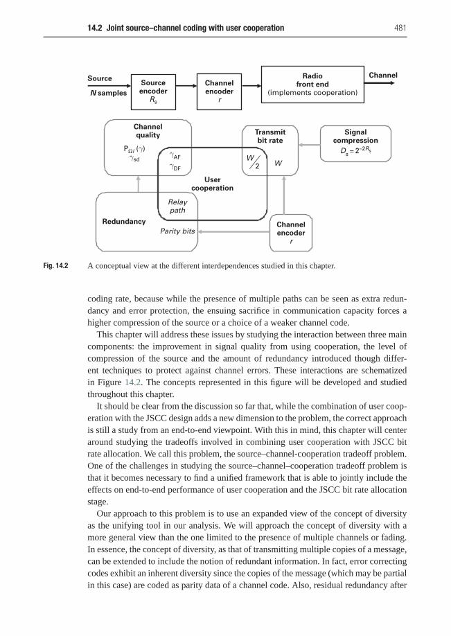
14.2 Joint source–channel coding with user cooperation 481
Sourceencoder
Rs
SourceChannelencoder
r
Channelencoder
r
Radiofront end
(implements cooperation)
Channel
Transmitbit rate
Signalcompression
Redundancy
Channelquality
Usercooperation
Relaypath
Parity bits
W2W
N samples
PΩi (γ)γsd
γAF
γDF
Ds =
2–2Rs
Fig. 14.2 A conceptual view at the different interdependences studied in this chapter.
coding rate, because while the presence of multiple paths can be seen as extra redun-dancy and error protection, the ensuing sacrifice in communication capacity forces ahigher compression of the source or a choice of a weaker channel code.
This chapter will address these issues by studying the interaction between three maincomponents: the improvement in signal quality from using cooperation, the level ofcompression of the source and the amount of redundancy introduced though differ-ent techniques to protect against channel errors. These interactions are schematizedin Figure 14.2. The concepts represented in this figure will be developed and studiedthroughout this chapter.
It should be clear from the discussion so far that, while the combination of user coop-eration with the JSCC design adds a new dimension to the problem, the correct approachis still a study from an end-to-end viewpoint. With this in mind, this chapter will centeraround studying the tradeoffs involved in combining user cooperation with JSCC bitrate allocation. We call this problem, the source–channel-cooperation tradeoff problem.One of the challenges in studying the source–channel–cooperation tradeoff problem isthat it becomes necessary to find a unified framework that is able to jointly include theeffects on end-to-end performance of user cooperation and the JSCC bit rate allocationstage.
Our approach to this problem is to use an expanded view of the concept of diversityas the unifying tool in our analysis. We will approach the concept of diversity with amore general view than the one limited to the presence of multiple channels or fading.In essence, the concept of diversity, as that of transmitting multiple copies of a message,can be extended to include the notion of redundant information. In fact, error correctingcodes exhibit an inherent diversity since the copies of the message (which may be partialin this case) are coded as parity data of a channel code. Also, residual redundancy after
482 Source–channel coding with cooperation
source encoding can be seen as diversity in the form of partial information that can beused to improve the received message quality. Then, since redundancy can be seen asa form of diversity, we explore both in a unified way and we apply the concept to thestudy and characterization of end-to-end performance resulting from source–channel–cooperation tradeoffs. We will do so by using a unified framework for the modeling,analysis and performance measurement of multimedia systems that use two magnitudes:the coding gain and the diversity gain.
In conjunction with the need to study the source–channel–cooperation tradeoffs in aunified way, it is also important not to loose track of considerations typical of multime-dia systems, such as delay constraints precluding the use of capacity achieving codesor typical operational envelopes that are not necessarily restricted to high SNR chan-nels. Even when including the extra dimension of user cooperation, these are qualitiesof the approach to characterize the D-SNR curve that will be developed in this chapter.Because of this, the characterization of the D-SNR curves will be suitable not only tostudy the combination of cooperation with practical source and channel codes, but alsoto analyze from an end-to-end viewpoint the practical design issues associated with thissetup such as how performance is affected by the use of a stronger channel code or aless efficient source encoder.
14.3 The Source–channel–cooperation tradeoff problem
We now formalize the description of the source–channel–cooperation tradeoff problem.Let us consider a wireless network carrying conversational multimedia traffic between asource node and a destination node, i.e., each ongoing call carries the information from asource, which has been coded for transmission over noisy and bandwidth-limited chan-nels, while also being subject to strict delay and jitter constraints. Bandwidth is sharedbetween users by allocating to each call an orthogonal channel that delivers a constantnumber of bits, W , per transmission period. Without loss of generality, we will assumethat these bits are transmitted using BPSK modulation with coherent detection andmaximum-likelihood decoding in the receiver. As shown in Figures 14.1 and 14.2, foreach transmission period, the transmission of a message is divided in three main stages:a source encoder, which compresses a source, a channel encoder, which adds protec-tion against channel errors, and a radio link. In order to minimize end-to-end distortion,both the source coding and channel coding rates can be adapted to channel conditionsthrough jointly allocating the W available bits. Also, cooperative communication mayor may not be used in the radio link
We assume a low mobility scenario, where the communication is carried over a quasi-static fading channel; i.e., fading may be considered constant during the transmissionof a frame. Furthermore, we will consider the source–channel–cooperation tradeoffswithin each transmission period so as to obtain best performance when having perfectknowledge of the channels. For this, let us implicitly assume that the network offers amechanism that allows the transmitters to estimate the channel states (similarly to thatof MIMO communications). This can be achieved in a time division duplexed network
14.3 The Source–channel–cooperation tradeoff problem 483
by using techniques such as channel sounding. In this case, after assuming reciprocity ofthe channels, the source can estimate the source–relay channel from the signal emittedby the relay (likely containing pilots) and the source–destination and relay–destinationchannels from estimates fed back from the destination. As long as the quasi-static fadingassumption holds, the difference between the actual channels states and their estimate(due to actual errors in channel estimation and due to the time evolution of the channel)should have little effect on the final result. This is because, under these conditions, therewould be no difference in the parameters chosen for source and channel coding as therange of possible choices is discrete and the selection of parameters remains the sameover a range of channel SNRs.
In general terms, in most scenarios involving node movement at speeds consistentwith pedestrian setups, the channel is expected to stay constant over the duration ofseveral transmit frames (for example, at a carrier frequency of 2.5 GHz and a nodevelocity of 5 mph the channel coherence time is approximately 50 ms). As the channelstarts to change more rapidly, there may be differences between the actual channelsstates and their estimates that would translate into a mismatched choice of source andchannel coding parameters, which would result in performance loss. The magnitude ofthis loss depends on several variables, such as the rate at which the channel is changingin relation with the duration of a transmission period, the coarseness in the range ofchoices for source and channel coding, the performance of both the source and thechannel codecs, etc. Nevertheless, the effect of a rapidly changing channel affects theconsidered scheme whether user cooperation is used or not.
Since the main goal of this chapter is to study the interaction between the receivedsignal quality-bandwidth efficiency tradeoff (stemming from user cooperation) and thesource compression-error protection tradeoff, the effects of channel mismatch can bedecouple from the results by assuming that channel states are ideally estimated at thetransmitter. This will lead to results that reveal the pure source–channel–cooperationtradeoffs and that reflect the best performance that can be achieved in each of theconsidered schemes. Finally, to follow these assumptions, we will consider that per-formance measurement and setting design for the three transmission stages is done on aframe-by-frame basis.
Note that the source–channel–cooperation tradeoff problem encompasses many lay-ers of the communication stack. This affects the way in which we measure performance.Measuring performance using relations between some measure involving channelerrors, such as bit error rate (BER), and channel SNR is applicable for studies focusedon lower layers of the communication stack, such as modulation schemes, user cooper-ation or channel coding, but is not useful to represent all the effect of the higher layers.At the application layer and for the case of source codecs, performance is best measuredthrough the distortion-rate (D-R) function; which characterizes the distortion observedin a reconstructed source after it had been compressed at a given rate.
However, for the source–channel–cooperation tradeoff problem, it is best to use aperformance measure that reflects tradeoff effects at all layers of the source–channel–cooperation problem and that is consistent with multimedia traffic. Thus, it is best tomeasure performance through the relation between end-to-end distortion and channel
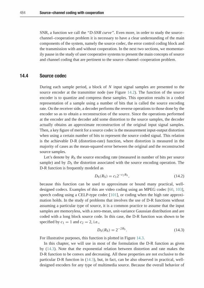
484 Source–channel coding with cooperation
SNR, a function we call the “D-SNR curve”. Even more, in order to study the source–channel–cooperation problem it is necessary to have a clear understanding of the maincomponents of the system, namely the source codec, the error control coding block andthe transmission with and without cooperation. In the next two sections, we momentar-ily pause in the study of user cooperative systems to present the main concepts of sourceand channel coding that are pertinent to the source–channel–cooperation problem.
14.4 Source codec
During each sample period, a block of N input signal samples are presented to thesource encoder at the transmitter node (see Figure 14.2). The function of the sourceencoder is to quantize and compress these samples. This operation results in a codedrepresentation of a sample using a number of bits that is called the source encodingrate. On the receiver side, a decoder performs the reverse operations to those done by theencoder so as to obtain a reconstruction of the source. Since the operations performedat the encoder and the decoder add some distortion to the source samples, the decoderactually obtains an approximate reconstruction of the original input signal samples.Then, a key figure of merit for a source codec is the measurement input-output distortionwhen using a certain number of bits to represent the source coded signal. This relationis the achievable D-R (distortion-rate) function, where distortion is measured in themajority of cases as the mean-squared error between the original and the reconstructedsource samples.
Let’s denote by RS the source encoding rate (measured in number of bits per sourcesample) and by DS the distortion associated with the source encoding operation. TheD-R function is frequently modeled as
DS(RS) = c12−c2 RS , (14.2)
because this function can be used to approximate or bound many practical, well-designed codecs. Examples of this are video coding using an MPEG codec [60, 103],speech coding using a CELP-type codec [101], or coding when the high rate approxi-mation holds. In the study of problems that involves the use of D-R functions withoutassuming a particular type of source, it is a common practice to assume that the inputsamples are memoryless, with a zero-mean, unit-variance Gaussian distribution and arecoded with a long block source code. In this case, the D-R function was shown to bespecified by c1 = 1 and c2 = 2, i.e.,
DS(RS) = 2−2RS . (14.3)
For illustrative purposes, this function is plotted in Figure 14.3.In this chapter, we will use in most of the formulation the D-R function as given
by (14.3). Note that the exponential relation between distortion and rate makes theD-R function to be convex and decreasing. All these properties are not exclusive to theparticular D-R function in (14.3), but, in fact, can be also observed in practical, well-designed encoders for any type of multimedia source. Because the overall behavior of
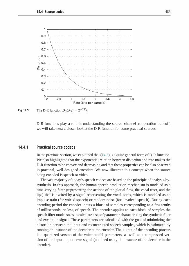
14.4 Source codec 485
0 0.5 1 1.5 2 2.5 3 3.50
0.1
0.2
0.3
0.4
0.5
0.6
0.7
0.8
0.9
1
Rate (bits per sample)
Dis
tort
ion
Fig. 14.3 The D-R function DS(RS) = 2−2RS .
D-R functions play a role in understanding the source–channel–cooperation tradeoff,we will take next a closer look at the D-R function for some practical sources.
14.4.1 Practical source codecs
In the previous section, we explained that (14.3) is a quite general form of D-R function.We also highlighted that the exponential relation between distortion and rate makes theD-R function to be convex and decreasing and that these properties can be also observedin practical, well-designed encoders. We now illustrate this concept when the sourcebeing encoded is speech or video.
The vast majority of today’s speech codecs are based on the principle of analysis-by-synthesis. In this approach, the human speech production mechanism is modeled as atime-varying filter (representing the actions of the glottal flow, the vocal tract, and thelips) that is excited by a signal representing the vocal cords, which is modeled as animpulse train (for voiced speech) or random noise (for unvoiced speech). During eachencoding period the encoder inputs a block of samples corresponding to a few tenthsof milliseconds, or less, of speech. The encoder applies to each block of samples thespeech filter model so as to calculate a set of parameter characterizing the synthetic filterand excitation signal. These parameters are calculated with the goal of minimizing thedistortion between the input and reconstructed speech samples, which is estimated byrunning an instance of the decoder at the encoder. The output of the encoding processis a quantized version of the voice model parameters, as well as a compressed ver-sion of the input-output error signal (obtained using the instance of the decoder in theencoder).
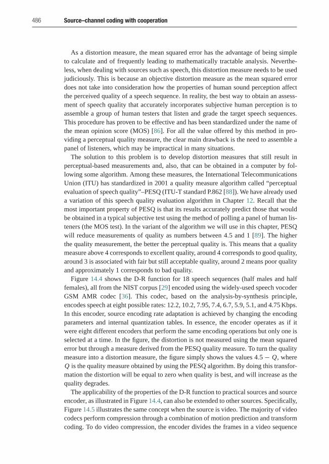
486 Source–channel coding with cooperation
As a distortion measure, the mean squared error has the advantage of being simpleto calculate and of frequently leading to mathematically tractable analysis. Neverthe-less, when dealing with sources such as speech, this distortion measure needs to be usedjudiciously. This is because an objective distortion measure as the mean squared errordoes not take into consideration how the properties of human sound perception affectthe perceived quality of a speech sequence. In reality, the best way to obtain an assess-ment of speech quality that accurately incorporates subjective human perception is toassemble a group of human testers that listen and grade the target speech sequences.This procedure has proven to be effective and has been standardized under the name ofthe mean opinion score (MOS) [86]. For all the value offered by this method in pro-viding a perceptual quality measure, the clear main drawback is the need to assemble apanel of listeners, which may be impractical in many situations.
The solution to this problem is to develop distortion measures that still result inperceptual-based measurements and, also, that can be obtained in a computer by fol-lowing some algorithm. Among these measures, the International TelecommunicationsUnion (ITU) has standardized in 2001 a quality measure algorithm called “perceptualevaluation of speech quality”–PESQ (ITU-T standard P.862 [88]). We have already useda variation of this speech quality evaluation algorithm in Chapter 12. Recall that themost important property of PESQ is that its results accurately predict those that wouldbe obtained in a typical subjective test using the method of polling a panel of human lis-teners (the MOS test). In the variant of the algorithm we will use in this chapter, PESQwill reduce measurements of quality as numbers between 4.5 and 1 [89]. The higherthe quality measurement, the better the perceptual quality is. This means that a qualitymeasure above 4 corresponds to excellent quality, around 4 corresponds to good quality,around 3 is associated with fair but still acceptable quality, around 2 means poor qualityand approximately 1 corresponds to bad quality.
Figure 14.4 shows the D-R function for 18 speech sequences (half males and halffemales), all from the NIST corpus [29] encoded using the widely-used speech vocoderGSM AMR codec [36]. This codec, based on the analysis-by-synthesis principle,encodes speech at eight possible rates: 12.2, 10.2, 7.95, 7.4, 6.7, 5.9, 5.1, and 4.75 Kbps.In this encoder, source encoding rate adaptation is achieved by changing the encodingparameters and internal quantization tables. In essence, the encoder operates as if itwere eight different encoders that perform the same encoding operations but only one isselected at a time. In the figure, the distortion is not measured using the mean squarederror but through a measure derived from the PESQ quality measure. To turn the qualitymeasure into a distortion measure, the figure simply shows the values 4.5 − Q, whereQ is the quality measure obtained by using the PESQ algorithm. By doing this transfor-mation the distortion will be equal to zero when quality is best, and will increase as thequality degrades.
The applicability of the properties of the D-R function to practical sources and sourceencoder, as illustrated in Figure 14.4, can also be extended to other sources. Specifically,Figure 14.5 illustrates the same concept when the source is video. The majority of videocodecs perform compression through a combination of motion prediction and transformcoding. To do video compression, the encoder divides the frames in a video sequence
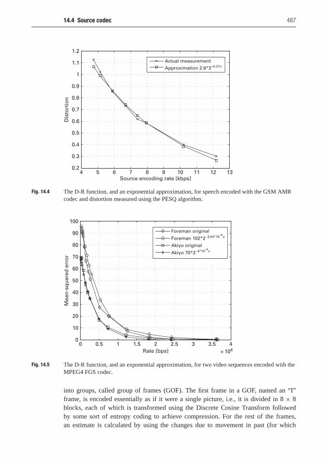
14.4 Source codec 487
4 5 6 7 8 9 10 11 12 130.2
0.3
0.4
0.5
0.6
0.7
0.8
0.9
1
1.1
1.2
Source encoding rate [kbps]
Dis
tort
ion
Actual measurement
Approximation 2.6*2−0.27x
Fig. 14.4 The D-R function, and an exponential approximation, for speech encoded with the GSM AMRcodec and distortion measured using the PESQ algorithm.
0 0.5 1 1.5 2 2.5 3 3.5 4× 10⁶
0
10
20
30
40
50
60
70
80
90
100
Rate [bps]
Mea
n-s
qu
ared
err
or
Foreman original
Foreman 102*2−3.04*10−6
x
Akiyo original
Akiyo 70*2−4*10−6
x
Fig. 14.5 The D-R function, and an exponential approximation, for two video sequences encoded with theMPEG4 FGS codec.
into groups, called group of frames (GOF). The first frame in a GOF, named an “I”frame, is encoded essentially as if it were a single picture, i.e., it is divided in 8 × 8blocks, each of which is transformed using the Discrete Cosine Transform followedby some sort of entropy coding to achieve compression. For the rest of the frames,an estimate is calculated by using the changes due to movement in past (for which
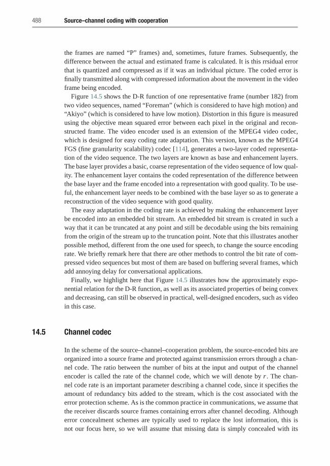
488 Source–channel coding with cooperation
the frames are named “P” frames) and, sometimes, future frames. Subsequently, thedifference between the actual and estimated frame is calculated. It is this rrsidual errorthat is quantized and compressed as if it was an individual picture. The coded error isfinally transmitted along with compressed information about the movement in the videoframe being encoded.
Figure 14.5 shows the D-R function of one representative frame (number 182) fromtwo video sequences, named “Foreman” (which is considered to have high motion) and“Akiyo” (which is considered to have low motion). Distortion in this figure is measuredusing the objective mean squared error between each pixel in the original and recon-structed frame. The video encoder used is an extension of the MPEG4 video codec,which is designed for easy coding rate adaptation. This version, known as the MPEG4FGS (fine granularity scalability) codec [114], generates a two-layer coded representa-tion of the video sequence. The two layers are known as base and enhancement layers.The base layer provides a basic, coarse representation of the video sequence of low qual-ity. The enhancement layer contains the coded representation of the difference betweenthe base layer and the frame encoded into a representation with good quality. To be use-ful, the enhancement layer needs to be combined with the base layer so as to generate areconstruction of the video sequence with good quality.
The easy adaptation in the coding rate is achieved by making the enhancement layerbe encoded into an embedded bit stream. An embedded bit stream is created in such away that it can be truncated at any point and still be decodable using the bits remainingfrom the origin of the stream up to the truncation point. Note that this illustrates anotherpossible method, different from the one used for speech, to change the source encodingrate. We briefly remark here that there are other methods to control the bit rate of com-pressed video sequences but most of them are based on buffering several frames, whichadd annoying delay for conversational applications.
Finally, we highlight here that Figure 14.5 illustrates how the approximately expo-nential relation for the D-R function, as well as its associated properties of being convexand decreasing, can still be observed in practical, well-designed encoders, such as videoin this case.
14.5 Channel codec
In the scheme of the source–channel–cooperation problem, the source-encoded bits areorganized into a source frame and protected against transmission errors through a chan-nel code. The ratio between the number of bits at the input and output of the channelencoder is called the rate of the channel code, which we will denote by r . The chan-nel code rate is an important parameter describing a channel code, since it specifies theamount of redundancy bits added to the stream, which is the cost associated with theerror protection scheme. As is the common practice in communications, we assume thatthe receiver discards source frames containing errors after channel decoding. Althougherror concealment schemes are typically used to replace the lost information, this isnot our focus here, so we will assume that missing data is simply concealed with its
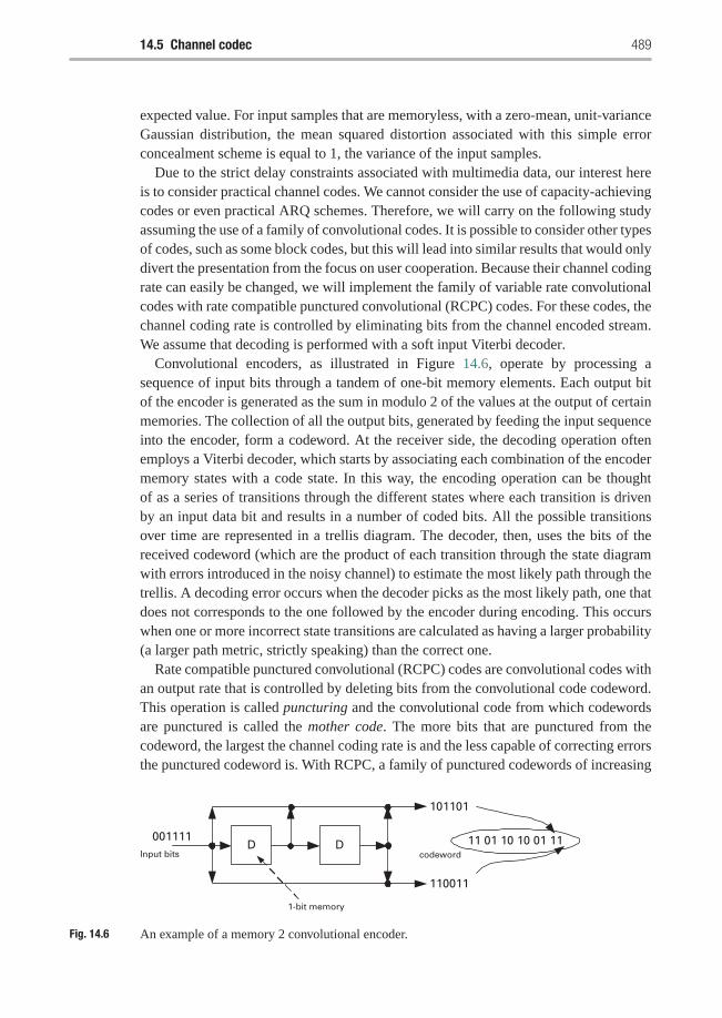
14.5 Channel codec 489
expected value. For input samples that are memoryless, with a zero-mean, unit-varianceGaussian distribution, the mean squared distortion associated with this simple errorconcealment scheme is equal to 1, the variance of the input samples.
Due to the strict delay constraints associated with multimedia data, our interest hereis to consider practical channel codes. We cannot consider the use of capacity-achievingcodes or even practical ARQ schemes. Therefore, we will carry on the following studyassuming the use of a family of convolutional codes. It is possible to consider other typesof codes, such as some block codes, but this will lead into similar results that would onlydivert the presentation from the focus on user cooperation. Because their channel codingrate can easily be changed, we will implement the family of variable rate convolutionalcodes with rate compatible punctured convolutional (RCPC) codes. For these codes, thechannel coding rate is controlled by eliminating bits from the channel encoded stream.We assume that decoding is performed with a soft input Viterbi decoder.
Convolutional encoders, as illustrated in Figure 14.6, operate by processing asequence of input bits through a tandem of one-bit memory elements. Each output bitof the encoder is generated as the sum in modulo 2 of the values at the output of certainmemories. The collection of all the output bits, generated by feeding the input sequenceinto the encoder, form a codeword. At the receiver side, the decoding operation oftenemploys a Viterbi decoder, which starts by associating each combination of the encodermemory states with a code state. In this way, the encoding operation can be thoughtof as a series of transitions through the different states where each transition is drivenby an input data bit and results in a number of coded bits. All the possible transitionsover time are represented in a trellis diagram. The decoder, then, uses the bits of thereceived codeword (which are the product of each transition through the state diagramwith errors introduced in the noisy channel) to estimate the most likely path through thetrellis. A decoding error occurs when the decoder picks as the most likely path, one thatdoes not corresponds to the one followed by the encoder during encoding. This occurswhen one or more incorrect state transitions are calculated as having a larger probability(a larger path metric, strictly speaking) than the correct one.
Rate compatible punctured convolutional (RCPC) codes are convolutional codes withan output rate that is controlled by deleting bits from the convolutional code codeword.This operation is called puncturing and the convolutional code from which codewordsare punctured is called the mother code. The more bits that are punctured from thecodeword, the largest the channel coding rate is and the less capable of correcting errorsthe punctured codeword is. With RCPC, a family of punctured codewords of increasing
D D001111
101101
110011
11 01 10 10 01 11codewordInput bits
1-bit memory
Fig. 14.6 An example of a memory 2 convolutional encoder.
490 Source–channel coding with cooperation
channel coding rate is built by incrementally removing bits from the lower coding ratecodewords in such a way that once a bit has been removed, it remains punctured fromall the codewords of higher coding rate.
To consider in the analysis the contribution of channel errors to end-to-end distortion,we are interested in finding the probability of having a source frame with errors afterchannel decoding. Since RCPC codes are convolutional codes, which in turn are linearcodes, the probability that the decoder will be unable to correct channel errors can beobtained by assuming that a sequence with all its bits equal to zero is transmitted, anddetermining the probability that the decoder decides in error for a different sequence, i.echooses a different path in the decoding trellis. This is essentially the probability that theall-zero sequence is sent, but a different sequence is decoded. With this assumption, theprobability of a decoding error can be obtained by first calculating the probability thata path with d input bits has a larger probability (a larger path metric, strictly speaking)than the correct one, and thus is chosen. Given the channel SNR γ , this can be shownto equal
Pe(d|γ ) = 0.5 erfc√
dγ , (14.4)
for BPSK modulation [56], with erfc(γ ) being the complementary error functiondefined as erfc(γ ) = 2/π
∫∞γ
e−u2du. Since we are assuming that the all-zero sequence
is sent, considering sequences that differ in d bits is equivalent to consider that thesequences in error have Hamming weight d.
Next, to obtain the probability of a decoding error, it is necessary to compute theprobability of decoding error associated with all paths with Hamming weight d. Thiscan be upper-bounded as a(d)Pe(d|γ ), where a(d) is the number of valid codewordswith Hamming weight d (i.e., d bits differing from the all-zero codeword). Finally, theprobability of having a source frame with errors after channel decoding results fromcombining the effects of all possible paths with nonzero Hamming weight and can beupper-bounded using the union bound as [130]
P(γ ) ≤ 1−⎡⎣1−
W∑d=df
a(d)Pe(d|γ )⎤⎦N Rs
, (14.5)
where df is the free distance of the code, which is the minimum number of bits equal to1 in a valid codeword.
14.6 Analysis of source–channel–cooperation performance
We approach the study of the source–channel–cooperation tradeoff by first characteriz-ing the end-to-end distortion as a function of SNR, and then using this characterizationto compare the performance of different schemes. Recall that we call this function theD-SNR curve. The end-to-end distortion is formed by the source encoder distortion(which depends on the source encoding rate) and the channel-induced distortion (which
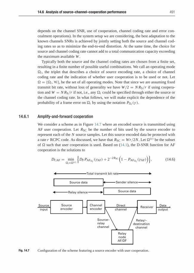
14.6 Analysis of source–channel–cooperation performance 491
depends on the channel SNR, use of cooperation, channel coding rate and error con-cealment operations). In the system setup we are considering, the best adaptation to theknown channels SNRs is achieved by jointly setting both the source and channel cod-ing rates so as to minimize the end-to-end distortion. At the same time, the choice forsource and channel coding rate cannot add to a total communication capacity exceedingthe maximum available W .
Typically both the source and the channel coding rates are chosen from a finite set,resulting in a finite number of possible useful combinations. We call an operating mode�i , the triplet that describes a choice of source encoding rate, a choice of channelcoding rate and the indication of whether user cooperation is to be used or not. Let� = {�i ,∀i}, be the set of all operating modes. Note that since we are assuming fixedtransmit bit rate, without loss of generality we have W/2 = N RS/r if using coopera-tion and W = N RS/r if not, i.e., any �i could be specified through either the source orthe channel coding rate. In what follows, we will make explicit the dependence of theprobability of a frame error on �i by using the notation P�i (γ ).
14.6.1 Amplify-and-forward cooperation
We consider a scheme as in Figure 14.7 where an encoded source is transmitted usingAF user cooperation. Let RSC be the number of bits used by the source encoder torepresent each of the N source samples. Let this source encoded data be protected witha rate r RCPC code. As discussed, we have that RSC = Wr/2N . Let �(c) be the subsetof � such that user cooperation is used. Based on (14.1), the D-SNR function for AFcooperation is the solutions to
DCAF = min�i∈�(c)
{DF PAF�i
(γAF)+ 2−2RSC(1− PAF�i
(γAF))}, (14.6)
Source–relaychannel
RelaynodeAF/DF
Relay/–destination
channel
Total transmit bit rate
Source data
Source dataRelay silence
Sender silence
Sourceencoder
Channelencoder ReceiverDirect
channelSourceinput
Dataoutput
Fig. 14.7 Configuration of the scheme featuring a source encoder with user cooperation.
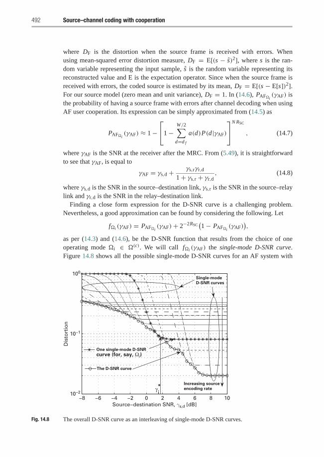
492 Source–channel coding with cooperation
where DF is the distortion when the source frame is received with errors. Whenusing mean-squared error distortion measure, DF = E[(s − s)2], where s is the ran-dom variable representing the input sample, s is the random variable representing itsreconstructed value and E is the expectation operator. Since when the source frame isreceived with errors, the coded source is estimated by its mean, DF = E[(s − E[s])2].For our source model (zero mean and unit variance), DF = 1. In (14.6), PAF�i
(γAF) isthe probability of having a source frame with errors after channel decoding when usingAF user cooperation. Its expression can be simply approximated from (14.5) as
PAF�i(γAF) ≈ 1−
⎡⎣1−W/2∑
d=d f
a(d)P(d|γAF)
⎤⎦N RSC
, (14.7)
where γAF is the SNR at the receiver after the MRC. From (5.49), it is straightforwardto see that γAF, is equal to
γAF = γs,d + γs,rγr,d
1+ γs,r + γr,d, (14.8)
where γs,d is the SNR in the source–destination link, γs,r is the SNR in the source–relaylink and γr,d is the SNR in the relay–destination link.
Finding a close form expression for the D-SNR curve is a challenging problem.Nevertheless, a good approximation can be found by considering the following. Let
f�i (γAF) = PAF�i(γAF)+ 2−2RSC
(1− PAF�i
(γAF)),
as per (14.3) and (14.6), be the D-SNR function that results from the choice of oneoperating mode �i ∈ �(c). We will call f�i (γAF) the single-mode D-SNR curve.Figure 14.8 shows all the possible single-mode D-SNR curves for an AF system with
−8 −6 −4 −2 0 2 4 6 8 1010−2
10−1
100
Source−destination SNR, γs,d [dB]
Dis
tort
ion
γ*
i
Single-mode
D-SNR curves
Increasing source
encoding rate
One single-mode D-SNR
curve (for, say, Ωi)
The D-SNR curve
Fig. 14.8 The overall D-SNR curve as an interleaving of single-mode D-SNR curves.
14.6 Analysis of source–channel–cooperation performance 493
γs,r = γr,d = 1 dB and using a memory 4, mother code rate 1/4, RCPC code familyfrom [56]. In addition, the Figure shows that the envelope formed by the single-modeD-SNR curves is the solution to (14.6), i.e, the D-SNR curve. As implied in (14.6)and seen in Figure 14.8, the D-SNR curve is made from the interleaving of sections ofD-SNR curves.
The comparison of two single-mode D-SNR curves shows the basic tradeoff asso-ciated with bit rate allocation process in (14.6). Let’s consider that the indexes of theoperating modes are sorted in increasing source encoding rate order; i.e., i> j (from �i
and � j ) if RSCi > RSC j . Note that, due to the relation W = 2N RSC/r , i> j meansthat ri > r j also. For each single-mode D-SNR curve the distortion only increases dueto channel errors because source and channel coding are fixed. Figure 14.8 illustratesthe behavior of single-mode D-SNR curves. By examining any of the of single-modeD-SNR curves it is possible to identify three distinct parts:
• At high SNR the channel errors are few and of negligible impact. This is becausethe channel code is strong enough to correct most of channel errors, making the end-to-end distortion be practically constant and equal to the source encoder distortionDS(�i ) for operating mode �i .
• At low SNR, the distortion increases rapidly because the channel code of the cor-responding operating mode is too weak to correct the errors introduced by thechannel.
• Between the section where the single-mode D-SNR curve is practically constant andthe section where distortion increases rapidly, there is a section that acts as a transitionsince it corresponds to the range of channel SNR for which the distortion starts toincrease due to channel errors. Let γ ∗i be the SNR value at which the distortion of themode-�i single-mode D-SNR curve starts to increase.
Next, we have that for i > j , DS(�i ) < DS(� j ). This implies that, over the sectionwhere the single-mode D-SNR curve is approximately constant, a single-mode D-SNRcurve associated with a larger source encoding rate will present a lower distortion. Also,we have that for i > j , γ ∗i > γ ∗j because ri > r j , i.e., channel errors start to becomesignificant for weaker channel codes at higher SNR values. The overall effect is thatfor two single-mode D-SNR curves, f�i (γ ) and f�i+1(γ ), we have f�i+1(γ ) < f�i (γ )
for γ > γ ∗i+1 and f�i+1(γ ) > f�i (γ ) for γ < γ ∗i Operating modes for which theseconditions do not hold are not useful because either one or both are not active in thesolution to (14.6) (they are a degenerate mode for which, at any SNR, there is alwaysanother operating mode with lower distortion) or they are over a negligible range ofSNRs. As Figure 14.8 illustrates, this means that the D-SNR performance resulting fromsolving (14.6) is the sequential interlacing of sections of single-mode D-SNR curves.These sections are the portion of single-mode D-SNR curves where channel-induceddistortion is such that DS(�i+1) ≤ f�i+1(γ ) ≤ DS(�i ), approximately.
Note that these observations follow from the mechanics associated with problem(14.6), they can be found as well in applications of this problem with setups very differ-ent from the one we are considering. Also note in Figure 14.8, that at very low SNR (andlarge distortion) there is an operating region where the smallest of the channel codes had
494 Source–channel coding with cooperation
already been chosen and there is no more use of JSCC bit rate allocation. Performancein this region follows that of a system with fixed channel coding, thus it is of no interestto us.
The challenge in characterizing the D-SNR curve is that, even when there is no use ofcooperation, the expressions that can be derived do not lead to a closed-form solution to(14.6). Because of this, we study the D-SNR curve by approximating its representationthrough a curve determined by a subset of its points. Each of these points is selectedfrom a different single-mode D-SNR curve. The criterion used to select each point isbased on the observation that the segment of a single-mode D-SNR curve that belongsto the solution of (14.6) follows DS(�i+1)≤ f�i+1(γ )≤DS(�i ), approximately; whichmeans that a point where the relative contribution of channel errors to the end-to-enddistortion is small is likely to belong to the overall D-SNR curve. Points with a rel-ative contribution that is practically negligible or is large may or may not belong tothe D-SNR curve and, thus, are not good choices to form the approximation. Then, foreach single-mode D-SNR curve, the point chosen to represent the D-SNR curve is suchthat D = (1 + �)DS(�i ), �i ∈ �(c), where � is a small number. Formally, we areconsidering those points where
D = (1+�)DS(�i )
= DF PAF�i(γAF)+ DS(�i )
(1− PAF�i
(γAF)), (14.9)
Equivalently, from (14.9), the D-SNR curve is formed by those points where
PAF�i(γAF) = �
DFDS(�i )
− 1. (14.10)
This expression offers the advantage that it simplifies the D-SNR curve characterizationproblem by translating it into a problem essentially in error control coding. By examin-ing Figure 14.8 it is possible to see that a choice of � as a small number means that thepoints used in the characterization of the D-SNR function falls into the “elbow” regionof typical single-mode D-SNR curves. Therefore, the choice of � as a small number,besides being justified by the above discussion, have the advantage that the results willshow little changes to different values of �. This is because in the “elbow” region oftypical single-mode D-SNR curves, relatively large changes in distortion translate inrelatively small changes in SNR. This idea will be further explored in the problemsat the end of this chapter. Even more, to solve the characterization problem, it wouldbe possible to use the related fact that channel-induced errors are relatively few andapply approximations that are accurate at low BER regime. Following these ideas andcombining (14.7) and (14.10), it follows that
�
DFDS(�i )
− 1≈ 1−
(1− a(df)
2erfc√
d f γAF
)N RSC, (14.11)
where we have used (14.4).Equation (14.11) shows an implicit dependence, through d f and a(d f ), between
PAF�i(γAF) and the rate of the particular code chosen from the RCPC family, i.e. the
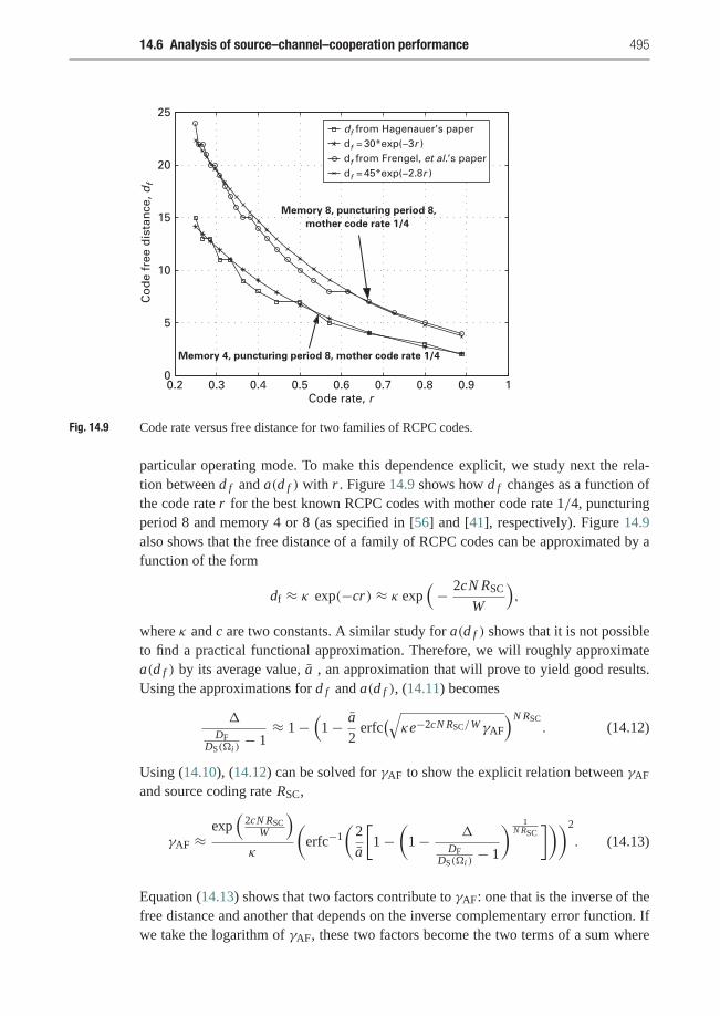
14.6 Analysis of source–channel–cooperation performance 495
0.2 0.3 0.4 0.5 0.6 0.7 0.8 0.9 10
5
10
15
20
25
Code rate, r
Co
de
free
dis
tan
ce, d
f
Memory 4, puncturing period 8, mother code rate 1/4
Memory 8, puncturing period 8,
mother code rate 1/4
df from Hagenauer’s paperdf = 30*exp(−3r )df from Frengel, et al.’s paperdf = 45*exp(−2.8r )
Fig. 14.9 Code rate versus free distance for two families of RCPC codes.
particular operating mode. To make this dependence explicit, we study next the rela-tion between d f and a(d f ) with r . Figure 14.9 shows how d f changes as a function ofthe code rate r for the best known RCPC codes with mother code rate 1/4, puncturingperiod 8 and memory 4 or 8 (as specified in [56] and [41], respectively). Figure 14.9also shows that the free distance of a family of RCPC codes can be approximated by afunction of the form
df ≈ κ exp(−cr) ≈ κ exp(− 2cN RSC
W
),
where κ and c are two constants. A similar study for a(d f ) shows that it is not possibleto find a practical functional approximation. Therefore, we will roughly approximatea(d f ) by its average value, a , an approximation that will prove to yield good results.Using the approximations for d f and a(d f ), (14.11) becomes
�
DFDS(�i )
− 1≈ 1−
(1− a
2erfc(√κe−2cN RSC/WγAF
)N RSC. (14.12)
Using (14.10), (14.12) can be solved for γAF to show the explicit relation between γAF
and source coding rate RSC,
γAF ≈exp(
2cN RSCW
)κ
(erfc−1
(2
a
[1−
(1− �
DFDS(�i )
− 1
) 1N RSC
]))2
. (14.13)
Equation (14.13) shows that two factors contribute to γAF: one that is the inverse of thefree distance and another that depends on the inverse complementary error function. Ifwe take the logarithm of γAF, these two factors become the two terms of a sum where
496 Source–channel coding with cooperation
the first term is linear in RSC. Let us work next with this second term, which we denoteas log
(g(RSC)
), where
g(RSC) =(
erfc−1(
2
a
[1−
(1− �
DFDS(�i )
− 1
)1/(N RSC)]))2
.
Using the approximation erfc−1(y) ≈ √− ln(y), [24], we can write
g(RSC) ≈ ln( a2
)− ln
(1−
(1− �
DFDS(RSC)
− 1
)1/(N RSC)). (14.14)
Before continuing, we note that the approximation erfc−1(y) ≈ √− ln(y) is not tight,yet it is still useful for us here because it is very good in representing the functionalbehavior of the inverse error function. In essence, this means that the probability oferror associated with the modulation scheme approximately behaves as exp(−x2) withrespect to SNR. Working with the second term of the right-hand side of (14.14),
θ = − ln
(1−
(1− �
DFDS(RSC)
− 1
)1/(N x))(14.15)
⇒ ln(1− e−θ
) = 1
N RSCln
(1− �
DFDS(RSC)
− 1
)(14.16)
⇒ − e−θ ≈ 1
N RSC
(− �
DFDS(RSC)
− 1
)(14.17)
⇒ θ ≈ ln
(N
�RSC
( DF
DS(RSC)− 1))
(14.18)
≈ ln
(N
�RSC
)+ ln
(DF
DS(RSC)
), (14.19)
where (14.17) follows from the fact that both logarithms in (14.16) are of the formln(1 − y) with y# 1 and the approximation in (14.19) follows from recognizing thatin general DF/DS(x) − 1 ≈ DF/DS(x), i.e., the reconstructed source error in the caseof transmission errors is typically much larger than the quantization distortion. Fol-lowing (14.3), θ in (14.18) is the sum of the logarithm of N RSC/� and a term that isapproximately linear in RSC, where generally N/�� RSC. Then, we can approximate
ln(N RSC
�
)≈ ln
(N RSC
�
),
with RSC being the average value of RSC, and consider that the approximately linearterm would determine the overall behavior of θ(RSC). Using (14.3), it follows that
g(RSC) ≈ ln( aN DF RSC
2�
)+ 2RSC ln(2).
Recall that we are interested in finding a more useful expression for log(g(RSC)).Through algebraic operations it can be shown that the coefficients of Taylor’s expansionof log(g(RSC)) around RSC are of the form t i/ i !, with
14.6 Analysis of source–channel–cooperation performance 497
t = ln(4)
(ln
(aN DF RSC
2�DS(RSC)
))−1
being much smaller than 1 for typical system parameters. This means that the weight ofcoefficients in Taylor’s expansion fall quite rapidly and log(g(RSC)) can be accuratelyapproximated through the first order expansion
log(g(RSC)) ≈ log(� + 2RSC ln(2))+ (RSC − RSC) log(4)
� + 2RSC ln(2)(14.20)
where
� = ln
(aN DF RSC
2�
).
Recall that we noticed that the logarithm of γAF can be decomposed into two terms:one that is linear in RSC and the other being log(g(RSC)), which we have just shown isapproximately linear also. Therefore, we can see that, when measured in decibels, γAF
is approximately a linear function of RSC. Specifically, using (14.13) and (14.20), wecan write γAF in decibels as
γAFdB ≈20cN RSC log(e)
W− 10 log(κ)+ 10 log(� + 2RSC ln(2))
+ 10log(4)
� + 2RSC ln(2)(RSC − RSC). (14.21)
Then, we have γAFdB(RSC) ≈ A1x + B1, or, equivalently, RSC ≈ A2γAFdB + B2. SinceD = (1+�)DS = (1+�)2−2RSC , we have
D = (1+�)10−(log 4)RSC
≈ (1+�)10−(log 4)(
A2γAFdB+B2
)= (1+�)10−B2(log 4)γ
−10A2 log 4AF . (14.22)
This is a relation of the form D ≈ (Gcγ )−10m with, from (14.21) ,
DCAF ≈ (GcγAF)−10mc , (14.23)
mc = log(4)
A1=[20
(cN
W ln(4)+ 1
2� + 2RSC ln(4)
)]−1
, (14.24)
Gc =[(1+�)] −1
10m 10−B110
= κ(1+�) −110m
� + RSC ln(4)10
log(4)RSC�+RSC ln(4) . (14.25)
Equation (14.23) has the appeal of being of the same form as the error rate-SNRfunction found in the study of communication systems, as is illustrated in Section 1.4.The main differences are that we are considering distortion instead of average errorprobability, there is no assumption of asymptotically large SNR, and that (14.23) modelsperformance of systems with practical components instead of being a bound at high
498 Source–channel coding with cooperation
SNR. Following this similarity, we can derive the analogy that Gc is the coding gainand mc is the diversity gain.
The coding gain Gc represents the SNR for a reference distortion value of 1. Thediversity gain mc determines the slope (i.e., rate of change) of the logarithm of thedistortion when SNR is measured in decibels (the factor of 10 multiplying mc in (14.23)is to set these units). Here, we are using the concept of diversity beyond its natural realmof transmitting multiple copies of a message over fading channels. This expanded useof the concept of diversity beyond its natural realm of systems with fading is basedon considering that there is a significant overlap between the concept of diversity andredundancy.
The general concept of diversity, as that of transmitting multiple copies of a message,can be extended to other forms of redundancy. Such is the case for error correctingcodes when considering that they exhibit an inherent diversity because the (maybe par-tial) copies of the message are coded in the form of parity data. In this sense, such anexpanded view of diversity aims at measuring more general forms of redundant infor-mation in cross-layer designs, which allows us to consider in a unified way the useof cooperation to deliver multiple copies of the message and the tradeoffs in redun-dancy at the source–channel bit rate allocation stages. Also, it is worth highlightingthat the basic premise on which we base the D-SNR characterization, i.e (14.9), followsfrom the problem setup and the general dynamics of the interaction of source encodingand channel-induced distortion. This is not exclusive to a particular choice of source,channel code family, or even a particular distortion measure. This implies that theanalysis could be extended to other types of channel code, yielding similar qualitativeresults.
14.6.2 Decode-and-forward cooperation
We now consider the case when transmission is carried on using DF user cooperation.In this case, the system setup can still be schematized as in Figure 14.7 and we stillassume a source coding rate RSC and channel coding rate r . For DF cooperation therelation RSC = Wr/2N still holds. Thus, following (14.30), the D-SNR performancefunction for DF cooperation is the solutions to
DCDF = min�i∈�(c)
{DF PDF�i
(γDF)+ 2−2RSC(1− PDF�i
(γDF))}.
Here, PDF�i(γDF) is the probability of having a source frame with errors after chan-
nel decoding when using DF user cooperation. If we denote by � the event “correctdecoding at relay” and by � the event “incorrect decoding at relay,” this probability is
PDF�i(γDF) = P�i (γDF|�)P�i (�)+ P�i (γDF|�)P�i (�)
= P�i (γs,d + γr,d)(1− P�i (γs,r)
)+ P�i (γs,d)P�i (γs,r).
(14.26)
Note that this relation is derived by considering that the first term in the right-hand sideof (14.26) represents the probability of successful transmission from the source to the
14.6 Analysis of source–channel–cooperation performance 499
relay and then to the destination. The second term represents the case when the relayfails decoding. Here, γDF represents the received SNR at the output of the MRC whenusing DF cooperation.
Therefore, to derive a close form approximation to the D-SNR curve, it is necessaryto appropriately consider the structure of PDF�i
(γDF) as in (14.26). Consequently, weconsider three cases: the source–relay channel is “good”, the source–relay channel is“bad”, and the channel states are such that there is no solution to (14.10) when con-sidering DF cooperation. One element introduced by the adaptability of channel codingrate is that the classification of “good” or ‘bad” source–relay channel does not dependonly on γs,r, but also on the operating mode and the strength of its associated channelcode. This is because for a given channel state the strongest channel codes may be oper-ating at the low BER regime but the weakest codes may be operating in the high BERregime. This is why the source–relay channel needs to be qualified in terms of the frameerror probability P�i (γs,r).
In the case of a “good” source–relay channel the source frame error probability(14.26) can be approximated as PDF�i
(γDF) ≈ P�i (γs,d + γr,d) for most operatingmodes. In this case (14.9) becomes
D = (1+�)DS(�i ) = DF P�i (γs,d + γr,d)+ DS(�i )(1− P�i (γs,d + γr,d)
),
and we have
DCDF ≈(Gc(γs,d + γr,d)
)−10mc . (14.27)
In the case of a “bad” source–relay channel, (14.26) can be approximated asPDF�i
(γDF) ≈ P�i (γs,d) for most operating modes. In this case we have
DCDF ≈(Gcγs,d
)−10mc . (14.28)
The differentiation between “good” and “bad” source–relay channels is done by set-ting a threshold on P�i (γs,r) such that the operating modes are separated into tworegimes. These regimes are those where PDF(γDF) in (14.26) can approximate eitherPDF�i
(γDF) ≈ P�i (γs,d+γr,d) (applicable to operating modes with strong error protec-tion such that P�i (γs,r) is less than the threshold) or PDF�i
(γDF)≈ P�i (γs,d) (applicableto operating modes with weak error protection such that P�i (γs,r) is more than thethreshold). Although there may be one or two operating modes in borderline cases withP�i (γs,r) near the threshold, the rest of the modes will be clearly in a good or bad chan-nel regime. Because of this, the composition of the two sets of modes in good or badchannel regime show little sensitivity to the value chosen as a threshold. Following this,we considered the threshold to be P�i (γs,r) ≈ 0.1. Also, we note that because the band-width efficiency of DF cooperation is the same as in AF cooperation, and because bothschemes share the same value for the variables that affect mc and Gc, the value of thesetwo magnitudes in (14.27) and (14.28) are given by (14.24) and (14.25).
The third modeling case corresponds to situations where the channel states are suchthat there is no solution to (14.10). This may occur when γs,d is very low, both γs,r andγr,d are such that
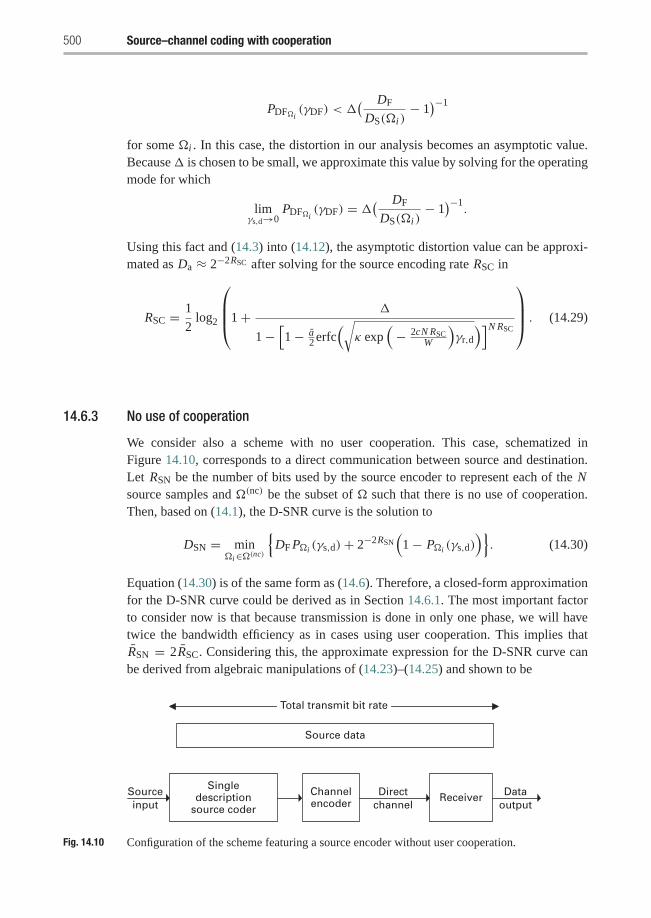
500 Source–channel coding with cooperation
PDF�i(γDF) < �
( DF
DS(�i )− 1)−1
for some �i . In this case, the distortion in our analysis becomes an asymptotic value.Because� is chosen to be small, we approximate this value by solving for the operatingmode for which
limγs,d→0
PDF�i(γDF) = �
( DF
DS(�i )− 1)−1.
Using this fact and (14.3) into (14.12), the asymptotic distortion value can be approxi-mated as Da ≈ 2−2RSC after solving for the source encoding rate RSC in
RSC = 1
2log2
⎛⎜⎜⎝1+ �
1−[1− a
2 erfc(√κ exp
(− 2cN RSC
W
)γr,d
)]N RSC
⎞⎟⎟⎠ . (14.29)
14.6.3 No use of cooperation
We consider also a scheme with no user cooperation. This case, schematized inFigure 14.10, corresponds to a direct communication between source and destination.Let RSN be the number of bits used by the source encoder to represent each of the Nsource samples and �(nc) be the subset of � such that there is no use of cooperation.Then, based on (14.1), the D-SNR curve is the solution to
DSN = min�i∈�(nc)
{DF P�i (γs,d)+ 2−2RSN
(1− P�i (γs,d)
)}. (14.30)
Equation (14.30) is of the same form as (14.6). Therefore, a closed-form approximationfor the D-SNR curve could be derived as in Section 14.6.1. The most important factorto consider now is that because transmission is done in only one phase, we will havetwice the bandwidth efficiency as in cases using user cooperation. This implies thatRSN = 2RSC. Considering this, the approximate expression for the D-SNR curve canbe derived from algebraic manipulations of (14.23)–(14.25) and shown to be
Singledescription
source coder
Channelencoder ReceiverDirect
channelSourceinput
Dataoutput
Total transmit bit rate
Source data
Fig. 14.10 Configuration of the scheme featuring a source encoder without user cooperation.
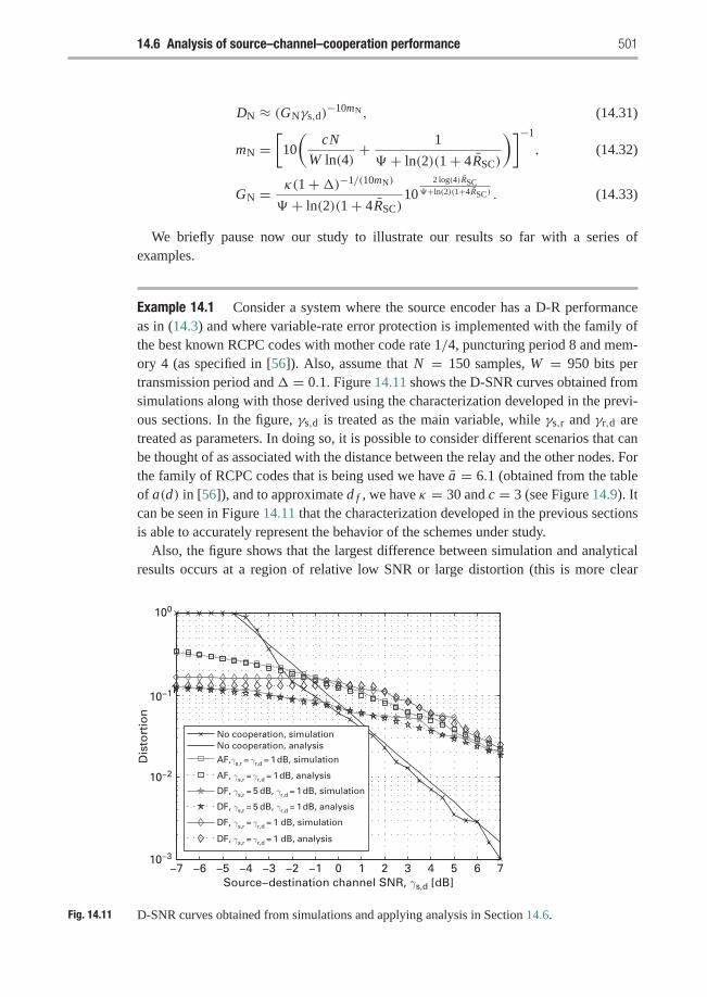
14.6 Analysis of source–channel–cooperation performance 501
DN ≈ (GNγs,d)−10mN, (14.31)
mN =[10
(cN
W ln(4)+ 1
� + ln(2)(1+ 4RSC)
)]−1
, (14.32)
GN = κ(1+�)−1/(10mN)
� + ln(2)(1+ 4RSC)10
2 log(4)RSC�+ln(2)(1+4RSC) . (14.33)
We briefly pause now our study to illustrate our results so far with a series ofexamples.
Example 14.1 Consider a system where the source encoder has a D-R performanceas in (14.3) and where variable-rate error protection is implemented with the family ofthe best known RCPC codes with mother code rate 1/4, puncturing period 8 and mem-ory 4 (as specified in [56]). Also, assume that N = 150 samples, W = 950 bits pertransmission period and� = 0.1. Figure 14.11 shows the D-SNR curves obtained fromsimulations along with those derived using the characterization developed in the previ-ous sections. In the figure, γs,d is treated as the main variable, while γs,r and γr,d aretreated as parameters. In doing so, it is possible to consider different scenarios that canbe thought of as associated with the distance between the relay and the other nodes. Forthe family of RCPC codes that is being used we have a = 6.1 (obtained from the tableof a(d) in [56]), and to approximate d f , we have κ = 30 and c = 3 (see Figure 14.9). Itcan be seen in Figure 14.11 that the characterization developed in the previous sectionsis able to accurately represent the behavior of the schemes under study.
Also, the figure shows that the largest difference between simulation and analyticalresults occurs at a region of relative low SNR or large distortion (this is more clear
−7 −6 −5 −4 −3 −2 −1 0 1 2 3 4 5 6 7
10−2
10−3
10−11
100
Source−destination channel SNR, γs,d [dB]
Dis
tort
ion
No cooperation, simulationNo cooperation, analysis
AF,γs,r = γr,d = 1 dB, simulation
AF, γs,r = γr,d = 1 dB, analysis
DF, γs,r = 5 dB, γr,d = 1 dB, simulation
DF, γs,r = 5 dB, γr,d = 1 dB, analysis
DF, γs,r = γr,d = 1 dB, simulation
DF, γs,r = γr,d = 1 dB, analysis
Fig. 14.11 D-SNR curves obtained from simulations and applying analysis in Section 14.6.
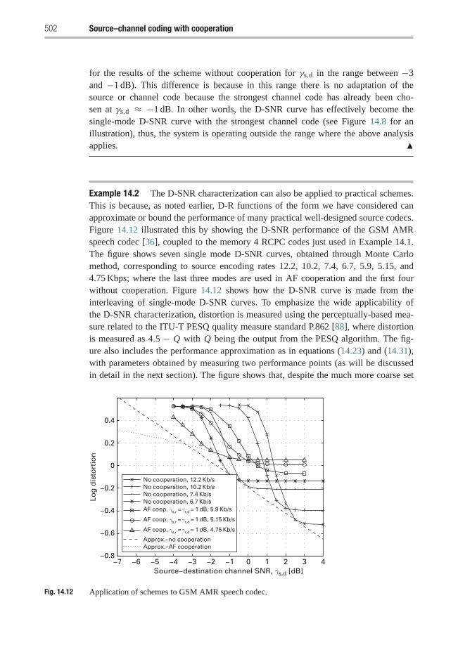
502 Source–channel coding with cooperation
for the results of the scheme without cooperation for γs,d in the range between −3and −1 dB). This difference is because in this range there is no adaptation of thesource or channel code because the strongest channel code has already been cho-sen at γs,d ≈ −1 dB. In other words, the D-SNR curve has effectively become thesingle-mode D-SNR curve with the strongest channel code (see Figure 14.8 for anillustration), thus, the system is operating outside the range where the above analysisapplies. �
Example 14.2 The D-SNR characterization can also be applied to practical schemes.This is because, as noted earlier, D-R functions of the form we have considered canapproximate or bound the performance of many practical well-designed source codecs.Figure 14.12 illustrated this by showing the D-SNR performance of the GSM AMRspeech codec [36], coupled to the memory 4 RCPC codes just used in Example 14.1.The figure shows seven single mode D-SNR curves, obtained through Monte Carlomethod, corresponding to source encoding rates 12.2, 10.2, 7.4, 6.7, 5.9, 5.15, and4.75 Kbps; where the last three modes are used in AF cooperation and the first fourwithout cooperation. Figure 14.12 shows how the D-SNR curve is made from theinterleaving of single-mode D-SNR curves. To emphasize the wide applicability ofthe D-SNR characterization, distortion is measured using the perceptually-based mea-sure related to the ITU-T PESQ quality measure standard P.862 [88], where distortionis measured as 4.5 − Q with Q being the output from the PESQ algorithm. The fig-ure also includes the performance approximation as in equations (14.23) and (14.31),with parameters obtained by measuring two performance points (as will be discussedin detail in the next section). The figure shows that, despite the much more coarse set
−0.8
−0.6
−0.4
−0.2
0
0.2
0.4
Log
dis
tort
ion
−7 −6 −5 −4 −3 −2 −1 0 1 2 3 4Source−destination channel SNR, γs,d [dB]
No cooperation, 12.2 Kb/sNo cooperation, 10.2 Kb/sNo cooperation, 7.4 Kb/sNo cooperation, 6.7 Kb/sAF coop. γs,r = γr,d = 1 dB, 5.9 Kb/s
AF coop. γs,r = γr,d = 1 dB, 5.15 Kb/s
AF coop. γs,r = γr,d = 1 dB, 4.75 Kb/s
Approx.–no cooperationApprox.–AF cooperation
Fig. 14.12 Application of schemes to GSM AMR speech codec.
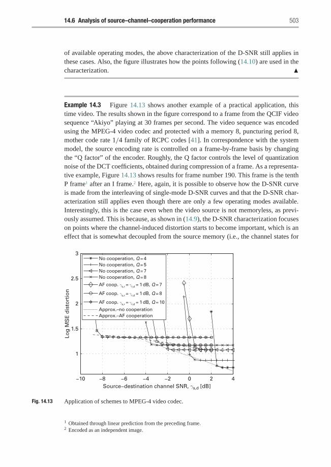
14.6 Analysis of source–channel–cooperation performance 503
of available operating modes, the above characterization of the D-SNR still applies inthese cases. Also, the figure illustrates how the points following (14.10) are used in thecharacterization. �
Example 14.3 Figure 14.13 shows another example of a practical application, thistime video. The results shown in the figure correspond to a frame from the QCIF videosequence “Akiyo” playing at 30 frames per second. The video sequence was encodedusing the MPEG-4 video codec and protected with a memory 8, puncturing period 8,mother code rate 1/4 family of RCPC codes [41]. In correspondence with the systemmodel, the source encoding rate is controlled on a frame-by-frame basis by changingthe “Q factor” of the encoder. Roughly, the Q factor controls the level of quantizationnoise of the DCT coefficients, obtained during compression of a frame. As a representa-tive example, Figure 14.13 shows results for frame number 190. This frame is the tenthP frame1 after an I frame.2 Here, again, it is possible to observe how the D-SNR curveis made from the interleaving of single-mode D-SNR curves and that the D-SNR char-acterization still applies even though there are only a few operating modes available.Interestingly, this is the case even when the video source is not memoryless, as previ-ously assumed. This is because, as shown in (14.9), the D-SNR characterization focuseson points where the channel-induced distortion starts to become important, which is aneffect that is somewhat decoupled from the source memory (i.e., the channel states for
−10 −8 −6 −4 −2 0 2 4
1
1.5
2
2.5
3
Log
MS
E d
isto
rtio
n
Source−destination channel SNR, γs,d [dB]
No cooperation, Q = 4No cooperation, Q = 5No cooperation, Q = 7No cooperation, Q = 8
AF coop. γs,r = γr,d = 1 dB, Q = 7
AF coop. γs,r = γr,d = 1 dB, Q = 8
AF coop. γs,r = γr,d = 1 dB, Q = 10
Approx.–no cooperationApprox.–AF cooperation
Fig. 14.13 Application of schemes to MPEG-4 video codec.
1 Obtained through linear prediction from the preceding frame.2 Encoded as an independent image.
504 Source–channel coding with cooperation
which the channel-induced distortion becomes important is such that it significantlyaffects all memory interdependent frames). �
14.7 Validation of D-SNR characterization
Through the series of steps shown in (14.9)–(14.22) it was possible to find an accuratecharacterization for the D-SNR function. Nevertheless, the series of steps involved anumber of approximations that are likely to accumulate error into the final distortionapproximation. Therefore, it is important, as a way to evaluate the approximation, tolook at the error between the distortion and its approximation. Due to the approachfollowed to characterize the D-SNR curve, the error should be measured as the relativeerror between the logarithm of the actual and the approximated distortion values at thosespecific points used to approximate the D-SNR curve.
Recall from the discussion that led to (14.10), that the actual distortion value at thesepoints is, by definition, (1 + �)DS(�i ), where �i may or may not involve the use ofcooperation. For each point used to approximate the D-SNR curve (one per operatingmode) it is possible to find the actual SNR value by solving for γ in
P�i (γ ) =�
DFDS(�i )
− 1. (14.34)
When the operating modes �i in (14.34) are those with no cooperation, the resulting γwill correspond to the γs,d of the points used to approximate the D-SNR curve. Because(14.34) does not depend on the specific type of cooperation and we are solving for γas the unknown variable, when the operating modes are those with cooperation, theresulting γ at the points used to approximate the D-SNR curve, will correspond to γAF
if using AF cooperation or either γs,d + γr,d or γs,d if using DF cooperation. From theknowledge of γ for each scenario, it is possible to find the approximate values of thedistortion at the points used to approximate the D-SNR curve through (14.24), (14.27),(14.28), or (14.31).
Figure 14.14 shows, for the memory 4 RCPC code already used before, the relativeerror between the logarithm of the actual and the approximated distortion values at thepoints used to approximate the D-SNR curve for schemes with and without cooperation.Only one curve is needed for all the schemes with cooperation because the abscissa rep-resents γAF, γs,d + γr,d or γs,d, depending on the case and because Gc and mc are thesame for all schemes with cooperation. In the figure, it can be seen that the approxima-tion is sufficiently good with most points having relative errors of less than 5% (many,in fact, less than 2.5%) and only one slightly exceeding 10%. The source for most ofthe error can be traced to the tightness of the approximation df ≈ κ exp(−cr) and theapproximation of a(df) by its average value.
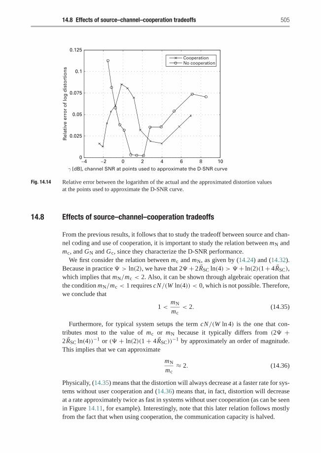
14.8 Effects of source–channel–cooperation tradeoffs 505
−4 −2 0 2 4 6 8 100
0.025
0.05
0.075
0.1
0.125
γ [dB], channel SNR at points used to approximate the D-SNR curve
Rel
ativ
e er
ror
of
log
dis
tort
ion
sCooperationNo cooperation
Fig. 14.14 Relative error between the logarithm of the actual and the approximated distortion valuesat the points used to approximate the D-SNR curve.
14.8 Effects of source–channel–cooperation tradeoffs
From the previous results, it follows that to study the tradeoff between source and chan-nel coding and use of cooperation, it is important to study the relation between mN andmc, and GN and Gc, since they characterize the D-SNR performance.
We first consider the relation between mc and mN, as given by (14.24) and (14.32).Because in practice � > ln(2), we have that 2� + 2RSC ln(4) > � + ln(2)(1+ 4RSC),which implies that mN/mc < 2. Also, it can be shown through algebraic operation thatthe condition mN/mc < 1 requires cN/(W ln(4)) < 0, which is not possible. Therefore,we conclude that
1 <mN
mc< 2. (14.35)
Furthermore, for typical system setups the term cN/(W ln 4) is the one that con-tributes most to the value of mc or mN because it typically differs from (2� +2RSC ln(4))−1 or (� + ln(2)(1 + 4RSC))
−1 by approximately an order of magnitude.This implies that we can approximate
mN
mc≈ 2. (14.36)
Physically, (14.35) means that the distortion will always decrease at a faster rate for sys-tems without user cooperation and (14.36) means that, in fact, distortion will decreaseat a rate approximately twice as fast in systems without user cooperation (as can be seenin Figure 14.11, for example). Interestingly, note that this later relation follows mostlyfrom the fact that when using cooperation, the communication capacity is halved.
506 Source–channel coding with cooperation
Secondly, to study the relation between GN and Gc, we recall that (14.23), (14.27),(14.28), and (14.31) show that the functional relation between end-to-end distortion andreceived SNR (be it γs,d, γAF, or γDF) is linear in log-log scales. Therefore, mN, GN, mc
and Gc can be calculated from the knowledge of only two points of the D-SNR curve.Let (DN1, γN1) and (DN2, γN2) be the coordinates of these points for schemes withoutcooperation and (DC1, γC1) and (DC2, γC2) be those for schemes using cooperation.The coordinates of these points could be approximated using again the observation thateach single-mode D-SNR curve contributes to the overall D-SNR curve over a sectionwhere the contribution of channel-induced error is relatively small. Then, from (14.9)and (14.10), and for i equalt to 1 and 2,
Di =(1+�
)2−2Ri , γdBi = 10 log
[P−1�i
(�
22Ri − 1
)], (14.37)
where the subscript dB denotes a magnitude expressed in decibels. Knowing the pointscoordinates, it is then possible to find
mN = log(DN1/DN2
)γN2,dB − γN1,dB
, GNdB = −(γN1,dB + log DN1
mN
),
mc = log(DC1/DC2
)γC2,dB − γC1,dB
, GcdB = −(γC1,dB + log DC1
mc
).
Focusing on GN and Gc, note that log DC1 = log(1+�)− 2RSC1 log 2. Since � issmall, log DC1 ≈ −2RSC1 log 2 = −RSN1 log 2 ≈ (log DN1)/2. Then, since mN/mc ≈2, we have log DC1/mc ≈ log DN1/mN, which implies that the relation between GN
and Gc, approximately only depends on the relation between γN1,dB and γC1,dB. Fur-thermore, when the channel-induced errors are few, (14.5) can be approximated using afirst-order Taylor approximation as
P(γ ) � N Rs
⎛⎝ W∑d=df
a(d)P(d|γ )⎞⎠ .
Differentiating explicitly between the use or not of cooperation by using the subscriptsC and N, respectively, it follows that PC(γ ) ≈ PN(γ )/2 for a given operating mode�i .Considering these observations along with (14.9) and (14.10), leads to (14.37) beingre-written as
γCi,dB = 10 log
[P−1
N�i
(2�
2RSNi − 1
)], i = 1, 2, (14.38)
which implies that γC1,dB < γNi,dB. Therefore, we conclude that
GCdB > GNdB . (14.39)
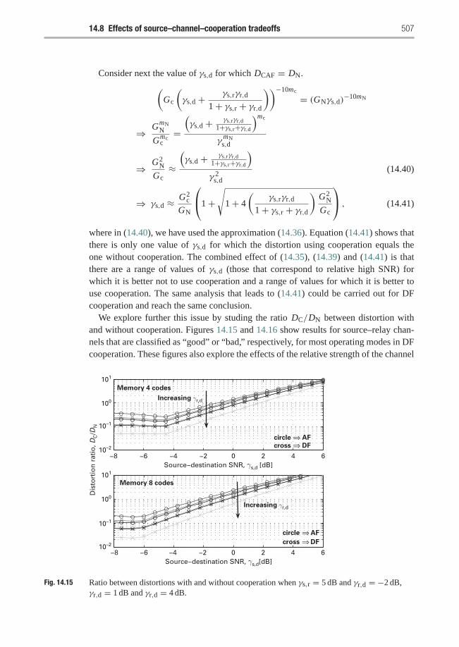
14.8 Effects of source–channel–cooperation tradeoffs 507
Consider next the value of γs,d for which DCAF = DN.(Gc
(γs,d + γs,rγr,d
1+ γs,r + γr,d
))−10mc
= (GNγs,d)−10mN
⇒ GmNN
Gmcc=(γs,d + γs,rγr,d
1+γs,r+γr,d
)mc
γmNs,d
⇒ G2N
Gc≈(γs,d + γs,rγr,d
1+γs,r+γr,d
)γ 2
s,d
(14.40)
⇒ γs,d ≈ G2c
GN
⎛⎝1+√
1+ 4
(γs,rγr,d
1+ γs,r + γr,d
)G2
N
Gc
⎞⎠ , (14.41)
where in (14.40), we have used the approximation (14.36). Equation (14.41) shows thatthere is only one value of γs,d for which the distortion using cooperation equals theone without cooperation. The combined effect of (14.35), (14.39) and (14.41) is thatthere are a range of values of γs,d (those that correspond to relative high SNR) forwhich it is better not to use cooperation and a range of values for which it is better touse cooperation. The same analysis that leads to (14.41) could be carried out for DFcooperation and reach the same conclusion.
We explore further this issue by studing the ratio DC/DN between distortion withand without cooperation. Figures 14.15 and 14.16 show results for source–relay chan-nels that are classified as “good” or “bad,” respectively, for most operating modes in DFcooperation. These figures also explore the effects of the relative strength of the channel
Dis
tort
ion
rat
io, D
C/D
N
−8 −6 −4 −2 0 2 4 610–2
10–1
100
101
101
100
10–2
10–1
Source−destination SNR, γs,d[dB]
−8 −6 −4 −2 0 2 4 6Source−destination SNR, γs,d [dB]
circle AF
cross DF
circle
cross
AF
DF
Increasing γr,d
Increasing γr,d
Memory 4 codes
Memory 8 codes
⇒⇒
⇒⇒
Fig. 14.15 Ratio between distortions with and without cooperation when γs,r = 5 dB and γr,d = −2 dB,γr,d = 1 dB and γr,d = 4 dB.
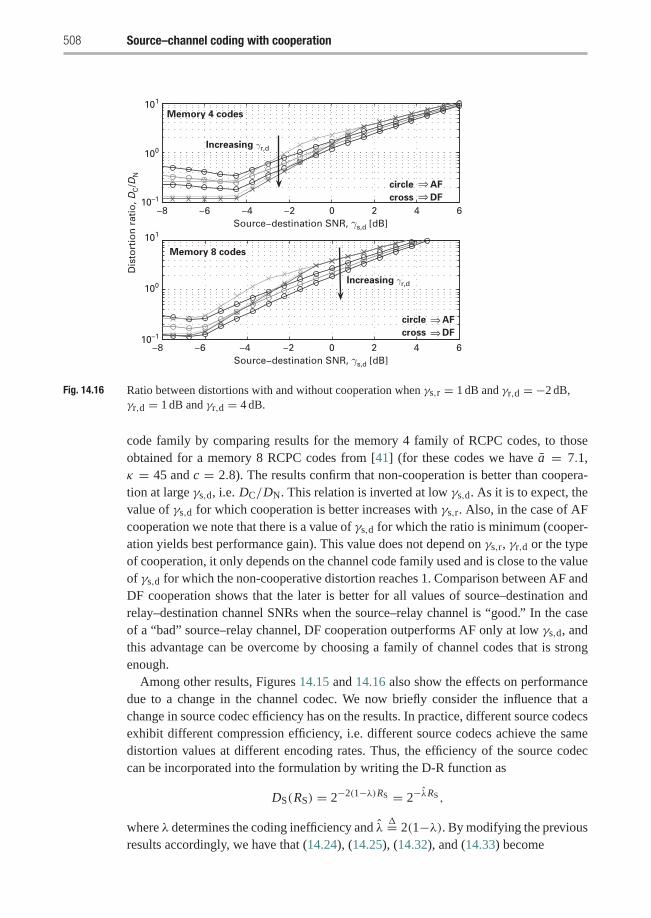
508 Source–channel coding with cooperation
Dis
tort
ion
rat
io, D
C/D
N
−8 −6 −4 −2 0 2 4 610–1
100
101
101
100
10–1
Source−destination SNR, γs,d [dB]
−8 −6 −4 −2 0 2 4 6Source−destination SNR, γs,d [dB]
circle AF
cross DF
circle
DFcross
AF
Increasing γr,d
Increasing γr,d
Memory 4 codes
Memory 8 codes
⇒⇒
⇒⇒
Fig. 14.16 Ratio between distortions with and without cooperation when γs,r = 1 dB and γr,d = −2 dB,γr,d = 1 dB and γr,d = 4 dB.
code family by comparing results for the memory 4 family of RCPC codes, to thoseobtained for a memory 8 RCPC codes from [41] (for these codes we have a = 7.1,κ = 45 and c = 2.8). The results confirm that non-cooperation is better than coopera-tion at large γs,d, i.e. DC/DN. This relation is inverted at low γs,d. As it is to expect, thevalue of γs,d for which cooperation is better increases with γs,r. Also, in the case of AFcooperation we note that there is a value of γs,d for which the ratio is minimum (cooper-ation yields best performance gain). This value does not depend on γs,r, γr,d or the typeof cooperation, it only depends on the channel code family used and is close to the valueof γs,d for which the non-cooperative distortion reaches 1. Comparison between AF andDF cooperation shows that the later is better for all values of source–destination andrelay–destination channel SNRs when the source–relay channel is “good.” In the caseof a “bad” source–relay channel, DF cooperation outperforms AF only at low γs,d, andthis advantage can be overcome by choosing a family of channel codes that is strongenough.
Among other results, Figures 14.15 and 14.16 also show the effects on performancedue to a change in the channel codec. We now briefly consider the influence that achange in source codec efficiency has on the results. In practice, different source codecsexhibit different compression efficiency, i.e. different source codecs achieve the samedistortion values at different encoding rates. Thus, the efficiency of the source codeccan be incorporated into the formulation by writing the D-R function as
DS(RS) = 2−2(1−λ)RS = 2−λRS ,
where λ determines the coding inefficiency and λ�= 2(1−λ). By modifying the previous
results accordingly, we have that (14.24), (14.25), (14.32), and (14.33) become
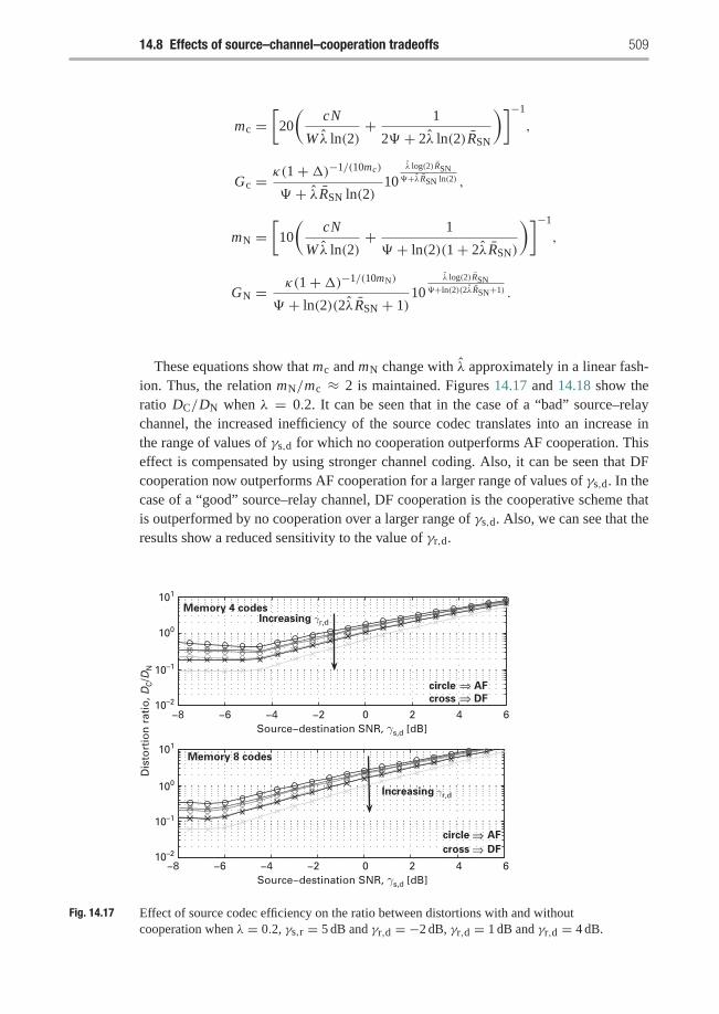
14.8 Effects of source–channel–cooperation tradeoffs 509
mc =[20
(cN
W λ ln(2)+ 1
2� + 2λ ln(2)RSN
)]−1
,
Gc = κ(1+�)−1/(10mc)
� + λRSN ln(2)10
λ log(2)RSN�+λRSN ln(2) ,
mN =[10
(cN
W λ ln(2)+ 1
� + ln(2)(1+ 2λRSN)
)]−1
,
GN = κ(1+�)−1/(10mN)
� + ln(2)(2λRSN + 1)10
λ log(2)RSN�+ln(2)(2λRSN+1) .
These equations show that mc and mN change with λ approximately in a linear fash-ion. Thus, the relation mN/mc ≈ 2 is maintained. Figures 14.17 and 14.18 show theratio DC/DN when λ = 0.2. It can be seen that in the case of a “bad” source–relaychannel, the increased inefficiency of the source codec translates into an increase inthe range of values of γs,d for which no cooperation outperforms AF cooperation. Thiseffect is compensated by using stronger channel coding. Also, it can be seen that DFcooperation now outperforms AF cooperation for a larger range of values of γs,d. In thecase of a “good” source–relay channel, DF cooperation is the cooperative scheme thatis outperformed by no cooperation over a larger range of γs,d. Also, we can see that theresults show a reduced sensitivity to the value of γr,d.
Dis
tort
ion
rat
io, D
C/D
N
−8 −6 −4 −2 0 2 4 610–2
10–1
100
101
101
100
10–2
10–1
Source−destination SNR, γs,d [dB]
−8 −6 −4 −2 0 2 4 6Source−destination SNR, γs,d [dB]
circle AF
cross DF
circle AF
cross DF
Increasing γr,d
Increasing γr,d
Memory 4 codes
Memory 8 codes
⇒⇒
⇒⇒
Fig. 14.17 Effect of source codec efficiency on the ratio between distortions with and withoutcooperation when λ = 0.2, γs,r = 5 dB and γr,d = −2 dB, γr,d = 1 dB and γr,d = 4 dB.
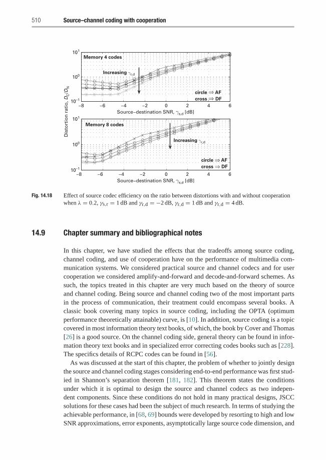
510 Source–channel coding with cooperation
Dis
tort
ion
rat
io, D
C/D
N
−8 −6 −4 −2 0 2 4 610–1
100
101
101
100
10–1
Source−destination SNR, γs,d [dB]
−8 −6 −4 −2 0 2 4 6Source−destination SNR, γs,d [dB]
circle AF
cross DF
circle AF
cross DF
Increasing γr,d
Increasing γr,d
Memory 4 codes
Memory 8 codes
⇒⇒
⇒⇒
Fig. 14.18 Effect of source codec efficiency on the ratio between distortions with and without cooperationwhen λ = 0.2, γs,r = 1 dB and γr,d = −2 dB, γr,d = 1 dB and γr,d = 4 dB.
14.9 Chapter summary and bibliographical notes
In this chapter, we have studied the effects that the tradeoffs among source coding,channel coding, and use of cooperation have on the performance of multimedia com-munication systems. We considered practical source and channel codecs and for usercooperation we considered amplify-and-forward and decode-and-forward schemes. Assuch, the topics treated in this chapter are very much based on the theory of sourceand channel coding. Being source and channel coding two of the most important partsin the process of communication, their treatment could encompass several books. Aclassic book covering many topics in source coding, including the OPTA (optimumperformance theoretically attainable) curve, is [10]. In addition, source coding is a topiccovered in most information theory text books, of which, the book by Cover and Thomas[26] is a good source. On the channel coding side, general theory can be found in infor-mation theory text books and in specialized error correcting codes books such as [228].The specifics details of RCPC codes can be found in [56].
As was discussed at the start of this chapter, the problem of whether to jointly designthe source and channel coding stages considering end-to-end performance was first stud-ied in Shannon’s separation theorem [181, 182]. This theorem states the conditionsunder which it is optimal to design the source and channel codecs as two indepen-dent components. Since these conditions do not hold in many practical designs, JSCCsolutions for these cases had been the subject of much research. In terms of studying theachievable performance, in [68, 69] bounds were developed by resorting to high and lowSNR approximations, error exponents, asymptotically large source code dimension, and
14.9 Chapter summary and bibliographical notes 511
infinite complexity and delay. In practice, there are many approaches to the joint designof source and channel coding. Hence, there are many JSCC techniques, encompassingdigital, analog and hybrid digital-analog (HDA) implementations. Among the not all-digital techniques, many are built on the idea of designing mappings from the sourcespace into the channel space. While for the analog JSCC techniques the mapping isdirect [61], in HDA techniques there is a quantization step that is applied to the sourcesamples [42, 148, 113, 27].
With respect to all the digital techniques, many are reviewed in [51, 30]. Integratedsource–channel coders (those where the source and channel codecs are two separateunits working in tandem and designed jointly) are studied in [31], and specific variationsof this technique are studied in [37] for channel optimized quantization, [238] for indexassignment, [194] for unequal error protection and [139] for joint bit rate allocation.In this chapter we have focused on the joint source–channel coding bit rate allocationtechnique because is one of the most practical and straightforward to implement. Thereare many examples in the research literature where JSCC bit rate allocation has beenapplied to transmission of multimedia sources. For illustrative purposes, we highlighthere only the representative works [48, 221] for speech transmission in mobile channels,[134] for image transmission and [19, 197, 98] for video communication. Also, thereare many works presenting different design methods for different problem setups, as isthe case in [227, 183, 118, 102], which deals with iterative solutions, or [20], whichpresents a design based on exhaustive search over reduced spaces.
The study in this chapter is based on measuring performance using the D-SNR curve.This curve represents the relation between end-to-end distortion and channel SNR. Wesaw that the D-SNR curve can be accurately approximated as a linear function in a log–log scale. To show this, we used an approach that considers practical source and channelcodes and their settings, while it avoids resorting to high SNR asymptotic analysis.While further study of the D-SNR curve can be found in [106] and [100], the extensionof the theory to consider cooperation can be found in [107].
We have also seen that the schemes using cooperation have better coding gain (dueto the better error performance when using cooperation) but they show a decrease ofdistortion at approximately half the rate of schemes not using cooperation (due to thesacrifice in bandwidth efficiency). The overall effect is that non-cooperative schemeshave better performance at high source–destination SNR, while AF or DF coopera-tive schemes have better performance in the rest of cases. Further analysis showedthat the best performance among cooperative schemes is achieved with DF coopera-tion in most of the cases but, when the source–relay channel is bad the performanceadvantage of DF cooperation is reduced by choosing a channel code family sufficientlystrong.
In addition, in this chapter we have studied the effects that the efficiency of the sourcecodec has on system performance and we showed that it reduces the diversity gainproportionally to the codec loss of efficiency. Also, we saw that for a “bad” source–relay channel, AF cooperation is outperformed by DF cooperation and no cooperationover a larger range of channel SNRs but this effect could be compensated by choosinga stronger family of channel codes. Similar observations apply to DF cooperation in
512 Source–channel coding with cooperation
the case of a “good” source–relay channel. Further study of the interaction betweenpractical source and channel coding with cooperation for multimedia communicationscan be found in [104] and [105].
Exercises
14.1 In this problem we explore the dependence of the diversity and coding gain onthe choice of the parameter �. We do so in two steps.
(a) We first study how a small charge in� affects the calculation of mc and GcdB .Formally, this is measured by calculating the sensitivity of mc and GcdB withrespect to �, which is respectively defined as
Smc� = dmc/mc
d�/�
SGcdB� = dGcdB/GcdB
d�/�
Find the expression for the sensitivity of mc and GcdB with respect to �and plot these results for � between 0.05 and 0.2. What conclusions canbe derived? To plot the results use the same setup as in Example 14.1 onpage 501, i.e., the source encoder has a D-R performance as in (14.3), thevariable-rate error protection is implemented with the family of memory 4,puncturing period 8, mother code rate 1/4, RCPC codes from [56] (a = 6.1,κ = 30, and c = 3), N = 150 samples, and W = 950 bits per transmissionperiod.
(b) We now study how relatively large charges in � (while still remaining asmall number) affects the calculation of mc and GcdB . Taking the setup fromexample 14.1, in page 501, plot the characterization of the D-SNR curve forAF cooperation, as in 14.23, for � = 0.05, � = 0.1, and � = 0.2. Whatconclusions can be derived?
14.2 Derive the expressions for mN and GN in (14.32) and (14.33).14.3 Derive the expression for the source encoding rate associated with the asymptotic
distortion in decode-and-forward given by (14.29).14.4 In this problem we study how channel encoding affects the performance of a vari-
ation of a decode-and-forward scheme. Consider a decode-and-forward wheretwo transmitting nodes are paired-up. Phase 1 of the scheme remains unchargedfrom the scheme used in this chapter. In phase 2 a node will forward the messagefrom the partner only if its reception was correct, otherwise it will send a copy ofits own transmitted message. Both paired nodes will symmetrically operate withthe same protocol. Consider that variable source and channel coding is still usedbut now the performance measure of interest is the block error rate after channeldecoding.
(a) What would be the advantage of this DF scheme instead of the oneconsidered in this chapter?
Exercises 513
(b) Derive the expression for the probability of having a source frame with errorsafter channel decoding.
(c) Assume that the variable-rate error protection is implemented with the familyof memory 4, puncturing period 8, mother code rate 1/4, RCPC codes from[56] (a = 6.1, κ = 30, and c = 3), N = 150 samples, and W = 950bits per transmission period. Applying the modeling equations used duringthe analysis in this chapter, plot the probability of having a source framewith errors after channel decoding as a function of the channel SNR for−4 dB ≤ γs,d ≤ 4 dB and
(i) γs,r = 6 dB, γr,d = 0 dB.(ii) γs,r = 3 dB, γr,d = 0 dB.
(iii) γs,r = 0 dB, γr,d = 0 dB.
Explain the differences in the results and draw conclusions.
15 Asymptotic performance of distortionexponents
In Chapter 13 we argued that cooperation can benefit the layers of the communicationstack that are above the physical layer, where the idea was approached through the studyof distributed cooperative routing. In Chapter 14 cooperation was studied as combinedwith source and channel coding, which extends the use of cooperation with the higherapplication layer. In fact, when considering that the benefits of cooperation come fromthe degree of diversity it provides, it is important to also recognize that diversity is notexclusive to implementations at the physical layer. Diversity can also be formed whenmultiple channels are provided to the application layer, where they are exploited throughthe use of multiple description source encoders. In multiple description coding differentdescriptions of the source are generated with the property that they can each be individ-ually decoded or, if possible, be jointly decoded to obtain a reconstruction of the sourcewith lower distortion. More importantly, a multiple description stream provides diver-sity that can be exploited by sending each description through an independent channel.This form of diversity has been called source coding diversity. Similarly, if we considerchannel coding instead of source coding as the originator of diversity, we would be gen-erating channel coding diversity. This chapter focuses on studying systems that exhibitthree forms of diversity: source coding diversity, channel coding diversity, and cooper-ation. More specifically, in this chapter we consider how cooperative diversity interactswith source and channel coding diversity in its traditional form (when compared withChapter 14)
We will be considering source coding diversity through the particular form of multi-ple description coding where the number of descriptions is two. This form of multipledescription coding is known as dual description coding and, because it is the simplestform of multiple description coding, it is by far the best understood. On the side of user-cooperation diversity, we will consider both relay channels and multi-hop channels, witha single or M relays helping the source by repeating its information either using theamplify-and-forward or the decode-and-forward protocols. As understood in this chap-ter, the differentiation between relay channels and multi-hop channels means whetherthere is or not a direct communication path between the source and the destination, asystem design variable that is worth considering in this study.
Given the presence of fading channels, we will study the system behavior atlarge SNR where system performances can be compared in terms of the dis-tortion exponent, which measures the rate of decay of the end-to-end distortion
15.1 Systems setup for source–channel diversity 515
at high SNR. Based on this, the goal will be to study the tradeoff between the diver-sity gain (which will be directly related to the number of relays) and the quality of thesource encoder.
15.1 Systems setup for source–channel diversity
Let us focus on systems that communicate a source signal over a wireless multi-hopor relay channel. Let the input to the system be a memoryless sourcer. Let us alsoassume that communication is performed over a complex, additive white Gaussian noise(AWGN) fading channel. Denoting by I the maximum average mutual informationbetween the channel input and output for a given channel realization, from Section 1.2
I = log(1+ |h|2SNR), (15.1)
where h is the fading value. Because of the random nature of the fading, I and the abilityof the channel to support transmission at some rate are themselves random. Recall thatthe probability of the channel not being able to support a rate R is called the outageprobability and was given in (1.29), or in short form by P0 = Pr[I < R].
It will be convenient for us to work with the random function eI . At large SNR, eI
from (15.1) can be simplified to
eI ≈ |h|2SNR. (15.2)
This implies that the random function eI will have at high SNR approximately the samestatistics as |h|2 (although the SNR scaling will trivially affect them). The study in thischapter will frequently make use of the cumulative distribution function (cdf) for eI .In particular, at high SNR eI will have approximately the same cumulative distribu-tion function (cdf) as |h|2, e.g., if the channel is Rayleigh, eI will have the cdf of anexponential random variable. Furthermore, with the goal of using a sufficiently generalmodel for the cdf of eI (or |h|2) beyond the Rayleigh case, we will assume that the cdfof |h|2 is smooth enough that it can be approximated through the first term of its Taylorseries around the origin. In other words, we will assume that the cdf, FeI , of eI can beapproximated at high SNR as
FeI (t) ≈ c
(t
SNR
)p
. (15.3)
Both c and p are model-dependent parameters. The parameter c can be seen as a nor-malizing constant, which will play a rather minor role in the study in this chapter. Theparameter p is the order of the first nonzero derivative in the Taylor series. For the caseof Rayleigh fading we have p = 1. Other values of p may be used to consider otherdistributions suitable for modeling |h|2, such as the Nakagami distribution.
Let us consider a communication system, as shown in Figure 15.1, consisting of asource, a source encoder and a channel encoder. Let the input to the system be a memo-ryless sourcer. The source samples are fed into the source encoder for quantization andcompression. The output of the source encoder are fed into a channel encoder which
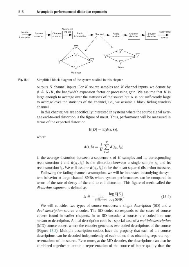
516 Asymptotic performance of distortion exponents
Sourceencoder
Channelencoder
Channel Sourcedecoder
Channeldecoder
Recovered
source
Source
K samples
N channelinputs
Radiotransmitter
Radioreceiver
Multihop
Relay
Fig. 15.1 Simplified block diagram of the system studied in this chapter.
outputs N channel inputs. For K source samples and N channel inputs, we denote byβ � N/K , the bandwidth expansion factor or processing gain. We assume that K islarge enough to average over the statistics of the source but N is not sufficiently largeto average over the statistics of the channel, i.e., we assume a block fading wirelesschannel.
In this chapter, we are specifically interested in systems where the source signal aver-age end-to-end distortion is the figure of merit. Thus, performance will be measured interms of the expected distortion
E[D] = E[d(s, s)],where
d(s, s) = 1
K
K∑k=1
d(sk, sk)
is the average distortion between a sequence s of K samples and its correspondingreconstruction s and d(sk, sk) is the distortion between a single sample sk and itsreconstruction sk . We will assume d(sk, sk) to be the mean-squared distortion measure.
Following the fading channels assumption, we will be interested in studying the sys-tem behavior at large channel SNRs where system performances can be compared interms of the rate of decay of the end-to-end distortion. This figure of merit called thedistortion exponent is defined as
� � − limSNR→∞
log E[D]log SNR
. (15.4)
We will consider two types of source encoders: a single description (SD) and adual description source encoder. The SD codec corresponds to the cases of sourcecodecs found in earlier chapters. In an SD encoder, a source is encoded into onestream or description. A dual description code is a special case of a multiple description(MD) source codec, where the encoder generates two coded descriptions of the source(Figure 15.2). Multiple description codecs have the property that each of the sourcedescriptions can be decoded independently of each other, thus obtaining separate rep-resentations of the source. Even more, at the MD decoder, the descriptions can also becombined together to obtain a representation of the source of better quality than the
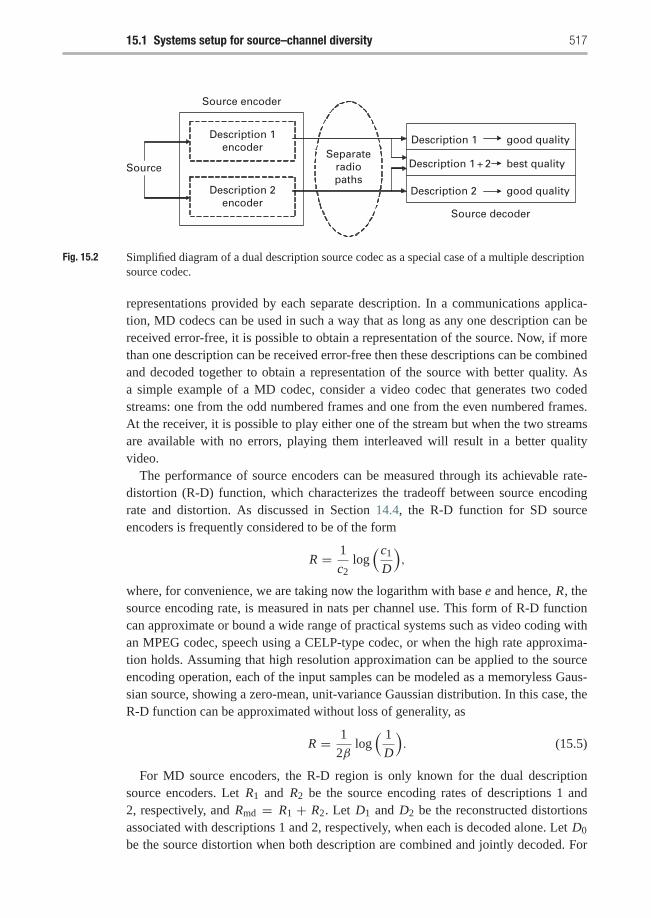
15.1 Systems setup for source–channel diversity 517
Description 1encoder
Description 2encoder
SourceSeparate
radiopaths
Description 1 good quality
Description 1 + 2 best quality
Description 2 good quality
Source decoder
Source encoder
Fig. 15.2 Simplified diagram of a dual description source codec as a special case of a multiple descriptionsource codec.
representations provided by each separate description. In a communications applica-tion, MD codecs can be used in such a way that as long as any one description can bereceived error-free, it is possible to obtain a representation of the source. Now, if morethan one description can be received error-free then these descriptions can be combinedand decoded together to obtain a representation of the source with better quality. Asa simple example of a MD codec, consider a video codec that generates two codedstreams: one from the odd numbered frames and one from the even numbered frames.At the receiver, it is possible to play either one of the stream but when the two streamsare available with no errors, playing them interleaved will result in a better qualityvideo.
The performance of source encoders can be measured through its achievable rate-distortion (R-D) function, which characterizes the tradeoff between source encodingrate and distortion. As discussed in Section 14.4, the R-D function for SD sourceencoders is frequently considered to be of the form
R = 1
c2log(c1
D
),
where, for convenience, we are taking now the logarithm with base e and hence, R, thesource encoding rate, is measured in nats per channel use. This form of R-D functioncan approximate or bound a wide range of practical systems such as video coding withan MPEG codec, speech using a CELP-type codec, or when the high rate approxima-tion holds. Assuming that high resolution approximation can be applied to the sourceencoding operation, each of the input samples can be modeled as a memoryless Gaus-sian source, showing a zero-mean, unit-variance Gaussian distribution. In this case, theR-D function can be approximated without loss of generality, as
R = 1
2βlog( 1
D
). (15.5)
For MD source encoders, the R-D region is only known for the dual descriptionsource encoders. Let R1 and R2 be the source encoding rates of descriptions 1 and2, respectively, and Rmd = R1 + R2. Let D1 and D2 be the reconstructed distortionsassociated with descriptions 1 and 2, respectively, when each is decoded alone. Let D0
be the source distortion when both description are combined and jointly decoded. For
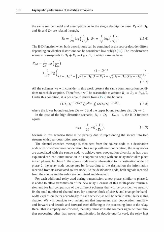
518 Asymptotic performance of distortion exponents
the same source model and assumptions as in the single description case, R1 and D1,and R2 and D2 are related through,
R1 = 1
2βlog( 1
D1
), R2 = 1
2βlog( 1
D2
). (15.6)
The R-D function when both descriptions can be combined at the source decoder differsdepending on whether distortions can be considered low or high [32]. The low distortionscenario corresponds to D1 + D2 − D0 < 1, in which case we have,
Rmd = 1
2βlog( 1
D0
)+ 1
2βlog
((1− D0)
2
(1− D0)2 −[√(1− D1)(1− D2)−√(D1 − D0)(D2 − D0)
]2).(15.7)
All the schemes we will consider in this work present the same communication condi-tions to each description. Therefore, it will be reasonable to assume R1 = R2 = Rmd/2.Under this condition, it is possible to derive from (15.7) the bounds
(4D0 D1)−1/(2β) � eRmd � (2D0 D1)
−1/(2β), (15.8)
where the lower bound requires D0 → 0 and the upper bound requires also D1 → 0.In the case of the high distortion scenario, D1 + D2 − D0 > 1, the R-D function
equals
Rmd = 1
2βlog( 1
D0
), (15.9)
because in this scenario there is no penalty due to representing the source into twostreams with dual-description properties.
The channel-encoded message is then sent from the source node to a destinationnode with or without user cooperation. In a setup with user cooperation, the relay nodesare associated with the source node to achieve user-cooperation diversity as has beenexplained earlier. Communication in a cooperative setup with one relay node takes placein two phases. In phase 1, the source node sends information to its destination node. Inphase 2, the relay node cooperates by forwarding to the destination the informationreceived from its associated source node. At the destination node, both signals receivedfrom the source and the relay are combined and detected.
For each additional relay used during transmission, a new phase, similar to phase 2,is added to allow transmission of the new relay. Because of this multi-phase transmis-sion and for fair comparison of the different schemes that will be consider, we need tofix the total number of channel uses for a source block of size K and change the band-width expansion factor accordingly to each scheme, as will be seen in detail later in thischapter. We will consider two techniques that implement user cooperation, amplify-and-forward and decode-and-forward, each differing in the processing done at the relay.Recall that in amplify-and-forward, the relay retransmits the source’s signal without fur-ther processing other than power amplification. In decode-and-forward, the relay first
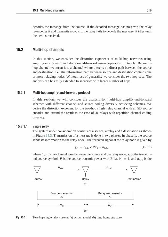
15.2 Multi-hop channels 519
decodes the message from the source. If the decoded message has no error, the relayre-encodes it and transmits a copy. If the relay fails to decode the message, it idles untilthe next is received.
15.2 Multi-hop channels
In this section, we consider the distortion exponents of multi-hop networks usingamplify-and-forward and decode-and-forward user-cooperation protocols. By multi-hop channel we mean it is a channel where there is no direct path between the sourceand destination; i.e., the information path between source and destination contains oneor more relaying nodes. Without loss of generality we consider the two-hop case. Theanalysis can be easily extended to scenarios with larger number of hops.
15.2.1 Multi-hop amplify-and-forward protocol
In this section, we will consider the analysis for multi-hop amplify-and-forwardschemes with different channel and source coding diversity achieving schemes. Wederive the distortion exponent for the two-hop single relay channel with an SD sourceencoder and extend the result to the case of M relays with repetition channel codingdiversity.
15.2.1.1 Single relayThe system under consideration consists of a source, a relay and a destination as shownin Figure 15.3. Transmission of a message is done in two phases. In phase 1, the sourcesends its information to the relay node. The received signal at the relay node is given by
yr1 = hs,r1
√Pxs + ns,r1 , (15.10)
where hs,r1 is the channel gain between the source and the relay node, xs is the transmit-ted source symbol, P is the source transmit power with E[‖xs‖2] = 1, and ns,r1 is the
(a)
(b)
Source transmitsxs
Relay re-transmitsxs
Source Relay Destination
Nm Nm
hs,r1hr1,d
Fig. 15.3 Two-hop single relay system: (a) system model, (b) time frame structure.
520 Asymptotic performance of distortion exponents
noise at the relay node modeled, as zero-mean, circularly symmetric complex Gaussiannoise with variance N0/2 per dimension. In phase 2, the relay normalizes the receivedsignal by the factor
α1 ≤√
P
P|hs,r1 |2 + N0,
as discussed in previous chapters, and retransmits to the destination. The received signalat the destination is given by
yd = hr1,dα1yr1 + nr1,d
= hr1,dα1hs,r1
√Pxs + hr1,dα1ns,r1 + nr1,d, (15.11)
where nr1,d is the noise at the destination node and is modeled as zero-mean, circu-larly symmetric complex Gaussian noise with variance N0/2 per dimension. Following(4.17), the mutual information in this case is given by
I (xs, yd) = log
(1+ |hs,r1 |2SNR|hr1,d|2SNR
|hs,r1 |2SNR+ |hr1,d|2SNR+ 1
), (15.12)
where SNR = P/N0. At high SNR, we have
I (xs, yd) ≈ log
(1+ |hs,r1 |2SNR|hr1,d|2SNR
|hs,r1 |2SNR+ |hr1,d|2SNR
)
≈ log
(|hs,r1 |2SNR|hr1,d|2SNR
|hs,r1 |2SNR+ |hr1,d|2SNR
). (15.13)
Equation (15.13) indicates that the two-hop amplify-and-forward channel appears asa link with signal-to-noise ratio that is the harmonic mean of the source–relay andrelay–destination channels signal-to-noise ratios. To calculate the distortion exponent,consider the source–relay and relay–destination channels for which the maximumaverage mutual information is, respectively,
I1 = log(1+ |hs,r1 |2SNR),
I2 = log(1+ |hr1,d|2SNR).
At high SNR we can write
exp(I1) ≈ |hs,r1 |2SNR,
exp(I2) ≈ |hr1,d|2SNR.
Denoting
Z1 = |hs,r1 |2SNR,
Z2 = |hr1,d|2SNR,
15.2 Multi-hop channels 521
and assuming statistical symmetry between the source–relay and relay–destinationchannels, we have
FZ1(t) ≈ c
(t
SNR
)p
FZ2(t) ≈ c
(t
SNR
)p
,
(15.14)
where FZ1(.) and FZ2(.) are the cdf of Z1 and Z2, respectively.The harmonic mean of two nonnegative random variables can be upper and lower
bounded as1
2min(Z1, Z2) ≤ Z1 Z2
Z1 + Z2≤ min(Z1, Z2), (15.15)
where the lower bound is achieved if and only if Z1 = Z2, Z1 = 0 or Z2 = 0, and theupper bound is achieved if and only if Z1 = 0 or Z2 = 0.
Define the random variable
Z = Z1 Z2
Z1 + Z2,
from (15.15) we have
Pr [min(Z1, Z2) < t] < Pr [Z < t] ≤ Pr [min(Z1, Z2) < 2t] . (15.16)
Then we have
Pr [min(Z1, Z2) < t] = 2FZ1(t)−(FZ1(t)
)2≈ 2c
(t
SNR
)p
− c2(
t
SNR
)2p
≈ c1
(t
SNR
)p
,
(15.17)
where c1 = 2c. Similarly, we have
Pr [min(Z1, Z2) < 2t] ≈ c2
(t
SNR
)p
, (15.18)
where c2 = 2p+1c. From (15.17) and (15.18) we get
c1
(t
SNR
)p
� FZ (t) � c2
(t
SNR
)p
, (15.19)
where FZ (t) is the cdf of the random variable Z . The minimum expected end-to-enddistortion can now be computed as
E[D] = minD
{Pr [I (xs, yd) < R(D)]+ D Pr [I (xs, yd) ≥ R(D)]
}, (15.20)
where D is the source encoder distortion and R is the source encoding rate. Note that(15.20) implicitly assumes that in case of an outage the missing source data is concealed
522 Asymptotic performance of distortion exponents
by replacing the missing source samples with their expected value (equal to zero).Using the bounds in (15.19) the minimum expected distortion can be upper and lowerbounded as
minD
{c1
(exp(R(D))
SNR
)p
+[1− c2
(exp(R(D))
SNR
)p]D
}� E[D] � min
D
{c2
(exp(R(D))
SNR
)p
+[1− c1
(exp(R(D))
SNR
)p]D
}.
(15.21)
For sufficiently large SNRs, we have
minD
{c1
(exp(R(D))
SNR
)p
+ D
}� E[D] � min
D
{c2
(exp(R(D))
SNR
)p
+ D
}. (15.22)
From (15.5), exp(R(D)) = D−1/2βm , where βm = Nm/K as illustrated in Figure 15.3,which leads to
minD
c1D
−p2βm
SNRp + D � E[D] � minD
c2D
−p2βm
SNRp + D. (15.23)
Differentiating the lower bound and setting equal to zero we get the optimizingdistortion
D∗ =(
2βm
c1 p
) −2βm2βm+p
SNR−2βm p2βm+p . (15.24)
Substituting from (15.24) into (15.23) we get
CLB SNR−2βm p2βm+p � E[D] � CUB SNR
−2βm p2βm+p , (15.25)
where CLB and CUB are terms that are independent of the SN R.The distortion exponent is now given by the following theorem.
T H E O R E M 15.2.1 The distortion exponent of the two-hop single-relay amplify-and-forward protocol is
�SH−1R−AMP = 2pβm
p + 2βm, (15.26)
where βm = Nm/K, and Nm is the number of the source channel uses and K is thenumber of source samples.
Before continuing, we note here that in the sequel, for simplicity of presentation wewill use
FZ (t) ≈ c
(t
SNR
)p
, (15.27)
where Z is the harmonic mean of the source–relay and relay–destination signal-to-noiseratios and c is a constant. The basis for the simplification is that the analysis will notbe affected by this substitution as we can always apply the analysis presented here byforming upper and lower bounds on the expected distortion and this will yield the samedistortion exponent.
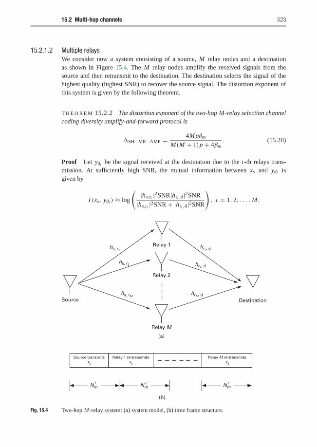
15.2 Multi-hop channels 523
15.2.1.2 Multiple relaysWe consider now a system consisting of a source, M relay nodes and a destinationas shown in Figure 15.4. The M relay nodes amplify the received signals from thesource and then retransmit to the destination. The destination selects the signal of thehighest quality (highest SNR) to recover the source signal. The distortion exponent ofthis system is given by the following theorem.
T H E O R E M 15.2.2 The distortion exponent of the two-hop M-relay selection channelcoding diversity amplify-and-forward protocol is
�SH−MR−AMP = 4Mpβm
M(M + 1)p + 4βm. (15.28)
Proof Let ydi be the signal received at the destination due to the i-th relays trans-mission. At sufficiently high SNR, the mutual information between xs and ydi isgiven by
I (xs, ydi ) ≈ log
(|hs,ri |2SNR|hri ,d|2SNR
|hs,ri |2SNR+ |hri ,d|2SNR
), i = 1, 2, . . . ,M.
(a)
(b)
Source transmitsxs
Relay 1 re-transmitsxs
Relay M re-transmitsxs
Source
Relay 1
Destination
Relay 2
Relay M
hs, r1
hs, r2
hs, rM
hr1, d
hr2, d
hrM, d
Nm′ Nm′ Nm′
Fig. 15.4 Two-hop M-relay system: (a) system model, (b) time frame structure.
524 Asymptotic performance of distortion exponents
Define the random variable
Wi = |hs,ri |2SNR|hri ,d|2SNR
|hs,ri |2SNR+ |hri ,d|2SNR, i = 1, 2, . . . ,M.
The cdf of Wi can be approximated at high SNR as
FWi (t) ≈ c
(t
SNR
)p
. (15.29)
The minimum end-to-end expected distortion can be computed as
E [D] =minD
{Pr[max(I (xs, yd1), I (xs, yd2), . . . , I (xs, ydM )) < R(D)
]+ Pr
[max(I (xs, yd1), I (xs, yd2), . . . , I (xs, ydM )) ≥ R(D)
]D
}
=minD
{M∏
i=1
FWi (exp(R(D)))+[
1−M∏
i=1
FWi (exp(R(D)))
]D
}
≈minD
⎧⎨⎩cM D−Mp2β′m
SNRMp+⎡⎣1− cM D
−Mp2β′m
SNRMp
⎤⎦ D
⎫⎬⎭≈min
D
⎧⎨⎩cM D−Mp2β′m
SNRMp+ D
⎫⎬⎭ , (15.30)
where D is the source encoding distortion, β ′m = N ′m/K , and N ′m is the number of thesource channel uses, as illustrated in Figure 15.4. Differentiating and setting equal tozero we get the optimizing distortion
D∗ =(
cM Mp
2β ′m
) 2β′mMp+2β′m
SNR−2Mβ′m p2β′m+Mp . (15.31)
Substituting we get
E [D] ≈ CMR SNR−2Mβ′m p2β′m+Mp , (15.32)
where CMR is a term that does not depend on the SNR. Hence, the distortion exponentis given as
�SH−MR−AMP = 2Mβ ′m p
2β ′m + Mp. (15.33)
For fair comparison with the single relay case, we should compare the different systemsunder the same number of channel uses. So that we have 2Nm = (M + 1)N ′m , fromwhich we have β ′m = (2/M + 1)βm . Substituting in (15.33) we get
�SH−MR−AMP = 4Mpβm
M(M + 1)p + 4βm. (15.34)
�
15.2 Multi-hop channels 525
The distortion exponent shows a tradeoff between the diversity and the source encoderperformance. Increasing the number of relay nodes increases the diversity of the sys-tem at the expense of using lower rate source encoder, e.g., higher distortion under nooutage.
Now let us calculate the optimal number of relays nodes to maximize the distortionexponent in (15.28). To get the optimal number of relays, Mopt , note that the distortionexponent in (15.28) can be easily shown to be concave in the number of relays (if wethink of M as a continuous variable). Differentiating and setting equal to zero, we get
∂
∂M�SH−MR−AMP = 0 −→ Mopt = 2
√βm
p. (15.35)
If Mopt in (15.35) is an integer number then it is the optimal number of relays. If Mopt
in (15.35) is not an integer, substitute in (15.28) with the largest integer that is less thanMopt and the smallest integer that is greater than Mopt and choose the one that yieldsthe higher distortion exponent as the optimum number of relay nodes. From the resultin (15.35) it is clear that the number of relays decreases, for a fixed βm , as p increases.
For higher channel quality (higher p) the system performance is limited by the dis-tortion introduced by the source encoder in the absence of outage. Then, as p increases,the optimum number of relays decreases to allow for the use of a better source encoderwith lower source encoding distortion. In this scenario, the system is said to be a qualitylimited system because the dominant phenomena in the end-to-end distortion is sourceencoding distortion and not outage.
Similarly as βm increases (higher bandwidth), for a fixed p, the performance will belimited by the outage event rather than the source encoding distortion. As βm increases,the optimum number of relays increases to achieve better outage performance. In thiscase, the system is said to be an outage limited system.
15.2.1.3 Optimal channel coding diversity with two relaysWe now expand the study of performance in terms of distortion exponent by exploitingthe cooperative diversity at higher layers of the communication stack. In this section,this idea translates into splitting the output of the channel coding stage into parts thatare transmitted through a different relay node, i.e., a separate path. Let us consider nowa system as shown in Figure 15.5 comprising a source, two relays and a destination.After channel encoding, the resulting block is split into two blocks: xs1 and xs2 , whichare transmitted to the relay nodes. The first relay will only forward the block xs1 andthe second relay will only forward xs2 as shown in Figure 15.5. From (15.13), it can beshown that the mutual information is
I ≈ log
(1+ |hs,r1 |2SNR|hr1,d|2SNR
|hs,r1 |2SNR+ |hr1,d|2SNR
)
+ log
(1+ |hs,r2 |2SNR|hr2,d|2SNR
|hs,r2 |2SNR+ |hr2,d|2SNR
), (15.36)
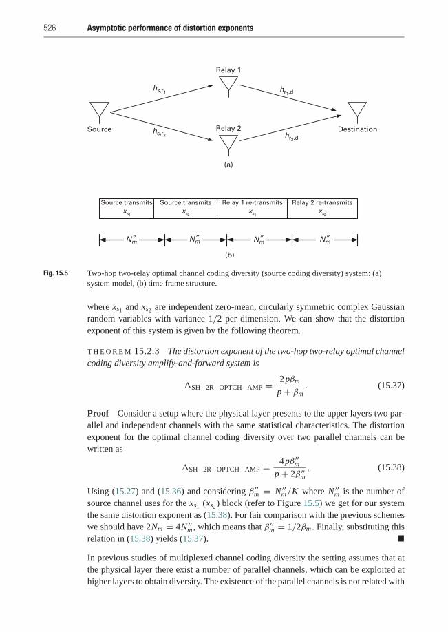
526 Asymptotic performance of distortion exponents
(a)
(b)
Source transmitsxs1
Source transmitsxs2
Relay 1 re-transmitsxs1
Relay 2 re-transmitsxs2
Source
Relay 1
DestinationRelay 2
hs,r1
hs,r2
hr1,d
hr2,d
Nm′′Nm′′Nm′′Nm′′
Fig. 15.5 Two-hop two-relay optimal channel coding diversity (source coding diversity) system: (a)system model, (b) time frame structure.
where xs1 and xs2 are independent zero-mean, circularly symmetric complex Gaussianrandom variables with variance 1/2 per dimension. We can show that the distortionexponent of this system is given by the following theorem.
T H E O R E M 15.2.3 The distortion exponent of the two-hop two-relay optimal channelcoding diversity amplify-and-forward system is
�SH−2R−OPTCH−AMP = 2pβm
p + βm. (15.37)
Proof Consider a setup where the physical layer presents to the upper layers two par-allel and independent channels with the same statistical characteristics. The distortionexponent for the optimal channel coding diversity over two parallel channels can bewritten as
�SH−2R−OPTCH−AMP = 4pβ ′′mp + 2β ′′m
, (15.38)
Using (15.27) and (15.36) and considering β ′′m = N ′′m/K where N ′′m is the number ofsource channel uses for the xs1 (xs2 ) block (refer to Figure 15.5) we get for our systemthe same distortion exponent as (15.38). For fair comparison with the previous schemeswe should have 2Nm = 4N ′′m , which means that β ′′m = 1/2βm . Finally, substituting thisrelation in (15.38) yields (15.37). �
In previous studies of multiplexed channel coding diversity the setting assumes that atthe physical layer there exist a number of parallel channels, which can be exploited athigher layers to obtain diversity. The existence of the parallel channels is not related with
15.2 Multi-hop channels 527
the use of cooperation; which translates into the observation of a gain in the distortionexponent for the multiplexed channel coding diversity scheme (compared to the directtransmission) due to the increase in the bandwidth obtained from the simultaneous useof the parallel channels. When introducing cooperative diversity into the system setup,there is no gain in using multiplexed channel coding diversity because the overall band-width of the channel is kept fixed and needs to be distributed among the transmissionsin the different cooperative phases, i.e., using either one relay or two relays does notincrease the bandwidth of the channel. This is because only one node, either the sourceor a relay, is transmitting at a given time slot. The multiplexed channel coding diversityin this case is equivalent to allowing one relay helping the source to forward an SDsource-coded message during one block and using the other relay for the next block.Hence, when using cooperative diversity, the multiplexed channel coding diversity isequivalent to the two-hop single-relay system with the same distortion exponent.
15.2.1.4 Source coding diversity with two relaysIn the previous section we exploited cooperative diversity to transmit different parts ofthe output of the channel coding stage through different relay nodes. The same gen-eral idea can be extended to the source encoder, with the difference that now the sourceencoder is a dual description encoder, which implies that its output will have some prop-erties that are not present in SD codecs and that can be used at the decoder to providesource coding diversity. Let us consider again a system with one source, two relays, andone destination nodes as shown in Figure 15.5. The source transmits two blocks xs1 andxs2 to the relay nodes. Each block represents one of the two descriptions generated bythe dual descriptions source encoder. In this case, the two blocks are broken up beforethe channel encoder, that is, each description is fed to a different channel encoder. Thefirst relay will only forward the block xs1 and the second relay will only forward xs2 asshown in Figure 15.5. The distortion exponent of this system is given by the followingtheorem.
T H E O R E M 15.2.4 The distortion exponent of the two-hop two-relay source codingdiversity amplify-and-forward protocol is
�SH−2R−SRC−AMP = max
[4pβm
3p + 2βm,
2pβm
p + 2βm
]. (15.39)
Proof The distortion exponent for the source coding diversity over two parallelchannels can be written as
�SH−2R−SRC−AMP = max
[8pβ ′′m
3p + 4β ′′m,
4pβ ′′mp + 4β ′′m
], (15.40)
Using (15.27) and (15.36) and considering β ′′m = N ′′m/K (refer to Figure 15.5) we getfor our system the same distortion exponent as (15.40). For fair comparison with theprevious schemes, 2Nm = 4N ′′m ; which leads to β ′′m = 1/2βm . Substituting this equalityin (15.40) completes the proof. �
528 Asymptotic performance of distortion exponents
15.2.2 Multi-hop decode-and-forward protocol
In this section, we will analyze schemes using multi-hop decode-and-forward user coop-eration under different channel and source coding diversity schemes. In these cases, therelay nodes decode the received source symbols. Only those relay nodes that had cor-rectly decoded the source symbols will proceed to retransmit them to the destinationnode. When a relay fails in decoding the source symbols we say that an outage hasoccurred. Furthermore, an outage occurs when either the source–relay or the relay–destination channel are in outage, as discussed in Sections 4.2.1.2 and 15.1. Thatis, the quality of the source–relay–destination link is limited by the minimum of thesource–relay and relay–destination channels. Therefore, for the single–relay case wecan formulate the outage as
Poutage = Pr[min(I (xs, yr1), I (xr1 , yd)) < R(D)
], (15.41)
where xr1 is the transmitted signal from the relay node.Note that in those schemes using decode-and-forward the mutual information of any
source–relay–destination link is limited by the minimum of the source–relay and relay–destination links SNRs. On the other hand, for two-hop amplify-and-forward schemes,the performance is limited by the harmonic mean of the source–relay and the relay–destination links SNRs which is strictly less than the minimum of the two links SNRs.Hence, the multi-hop amplify-and-forward protocol has a higher outage probability(lower quality) than the multi-hop decode-and-forward protocol. That is, in terms of out-age probability, the multi-hop decode-and-forward protocol outperforms the multi-hopamplify-and-forward protocol.
The above argument is also applicable under different performance measures (forexample, if the performance measure was symbol error rate). From our presentation sofar it is clear that the distortion exponents for multi-hop decode-and-forward schemesare the same as their corresponding multi-hop amplify-and-forward schemes for therepetition channel coding diversity and source coding diversity cases. For example, forthe two-hop single–relay decode-and-forward scheme, the minimum expected distortionis given by the lower bound in (15.25), which has the same distortion exponent as thetwo-hop single–relay amplify-and-forward scheme. The following theorem summarizesthe results (see Exercise 15.5).
T H E O R E M 15.2.5 The distortion exponent of the multi-hop decode-and-forwardschemes are:
• for the two-hop single relay
�SH−1R−DEC = 2pβm
p + 2βm, (15.42)
• for the two-hop M-relay selection channel coding diversity
�SH−MR−DEC = 4Mpβm
M(M + 1)p + 4βm, (15.43)
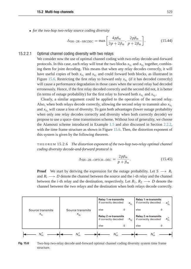
15.2 Multi-hop channels 529
• for the two-hop two-relay source coding diversity
�SH−2R−SRCDEC = max
[4pβm
3p + 2βm,
2pβm
p + 2βm
]. (15.44)
15.2.2.1 Optimal channel coding diversity with two relaysWe consider now the use of optimal channel coding with two-relay decode-and-forwardprotocols. In this case, each relay will treat the two blocks xs1 and xs2 together, combin-ing them for joint decoding. This means that when any relay decodes correctly, it willhave useful copies of both xs1 and xs2 and could forward both blocks, as illustrated inFigure 15.6. Restricting the first relay to forward only xs1 (if it has decoded correctly)will cause a performance degradation in those cases when the second relay had decodederroneously. Hence, if the first relay decoded correctly and the second did not, it is better(in terms of outage probability) for the first relay to forward both xs1 and xs2 .
Clearly, a similar argument could be applied to the operation of the second relay.Also, when both relays decode correctly, allowing the second relay to transmit also xs1
and xs2 will cause a loss of diversity. To gain both advantages (lower outage probabilitywhen only one relay decodes correctly and diversity when both correctly decode) wepropose to use a space–time transmission scheme. Without loss of generality, we choosethe Alamouti scheme introduced in Example 1.5 and also discussed in Section 2.2.2,with the time frame structure as shown in Figure 15.6. Then, the distortion exponent ofthis system is given by the following theorem.
T H E O R E M 15.2.6 The distortion exponent of the two-hop two-relay optimal channelcoding diversity decode-and-forward protocol is
�SH−2R−OPTCH−DEC = 2pβm
p + βm. (15.45)
Proof We start by deriving the expression for the outage probability. Let S −→ Ri
and Ri −→ D denote the channel between the source and the i-th relay and the channelbetween the i-th relay and the destination, respectively. Let R1, R2 −→ D denote thechannel between the two relays and the destination when both relays decode correctly.
Relay 1 re-transmitsif correctly decoded
Relay 2 re-transmitsif correctly decoded
else 0
else 0
Source transmitsxs1
Source transmitsxs2
∗
∗
xs1
xs2
Relay 1 re-transmitsif correctly decoded
Relay 2 re-transmitsif correctly decoded
else 0
-
else 0
xs2
xs1
Nm′′Nm′′Nm′′ Nm′′
Fig. 15.6 Two-hop two-relay decode-and-forward optimal channel coding diversity system time framestructure.
530 Asymptotic performance of distortion exponents
Also, we denote by Rio−→D as the event that a channel is in outage and by Ri
o−→D theevent that it is not in outage. We calculate the outage probability by splitting the outageevent into disjoint events, i.e., Poutage = Po1 + Po2 + Po3 + Po4 , where
Po1 = Pr[S
o−→R1, So−→R2
]= Pr
[S
o−→R1
].Pr[S
o−→R2
]= Pr
[2 log(1+ |hs,r1 |2SNR) < R(D)
]Pr[2 log(1+ |hs,r2 |2SNR) < R(D)
]≈ co1
(exp(pR(D))
SNR2p
). (15.46)
Po2 = Pr[S
o−→R1, So−→R2, R2
o−→D]
= Pr[S
o−→R1
].Pr[S
o−→R2
].Pr[R2
o−→D]
≈ co2
(exp(pR(D))
SNR2p
). (15.47)
Po3 = Pr[S
o−→R2, So−→R1, R1
o−→D]
≈ co3
(exp(pR(D))
SNR2p
). (15.48)
Po4 = Pr[S
o−→R1, So−→R2, R1, R2
o−→D]
= Pr[S
o−→R1
].Pr[S
o−→R2
].Pr[R1, R2
o−→D]
≈ Pr[2 log(1+ 1
2(|hr1,d|2SNR+ |hr2,d|2SNR)) < R(D)
],
(15.49)
where the factor 1/2 in (15.49) is due to the loss in SNR because of the use of transmitdiversity. To calculate Po4 in (15.49) we need to calculate the cdf of the random variable|hr1,d|2SNR + |hr2,d|2SNR. Let W1 = |hr1,d|2SNR and W2 = |hr2,d|2SNR. The pdf ofW1 +W2 can be computed as
fW1+W2(w) =∫ w
0fW1(τ ) fW2(w − τ)dτ
≈ c11c22 p2
SNR2p
∫ w
0τ p−1(w − τ)p−1dτ
= c11c22 p2 w2p−1
SNR2pB(p, p), (15.50)
15.2 Multi-hop channels 531
where B(., .) is the Beta function [50]. The cdf of W1 +W2 can be computed as
FW1+W2(w) =∫ w
0fW1+W2(τ )dτ = c33
( w
SNR
)2p, (15.51)
from which we have
Po4 ≈ co4
(exp(pR(D))
SNR2p
). (15.52)
Then, the outage probability is
Poutage = Po1 + Po2 + Po3 + Po4
= co
(exp(pR(D))
SNR2p
).
In the proof, we have assumed that xs1 and xs2 are independent zero-mean, complexGaussian with variance 1/2 per dimension. We can easily show that this choice of xs1
and xs2 is the optimal choice for maximizing the mutual information (minimizing theoutage probability) by inspection of the individual outage events in (15.53).Following this result, the minimum expected distortion can now be computed as
E[D] = minD
{Poutage + D
(1− Poutage
)}≈ min
D
{co
(exp(pR(D))
SNR2p
)+ D
[1− co
(exp(pR(D))
SNR2p
)]}≈ min
D
{co
(exp(pR(D))
SNR2p
)+ D
}(15.53)
≈ minD
{co
D− p
2β′′m
SNR2p+ D
}, (15.54)
where D is the source encoder distortion, (15.53) follows from high SNR approximationand (15.54) follows from (15.5). Differentiating and setting equal to zero we get theoptimizing distortion
D∗ =(
2β ′′mco p
) −2β′′m2β′′m+p
SNR−4β′′m p2β′′m+p . (15.55)
Hence, the distortion exponent is given as
�RC−1R−AMP = 4β ′′m p
2β ′′m + p. (15.56)
For fair comparison, the total number of channel uses should be kept fixed for allschemes. Thus, we have Nm = 2N ′′m , from which we have β ′′m = (1/2)βm . Substitutingin (15.56) we get
�SH−2R−OPTCH−DEC = 2pβm
p + βm. (15.57)
�
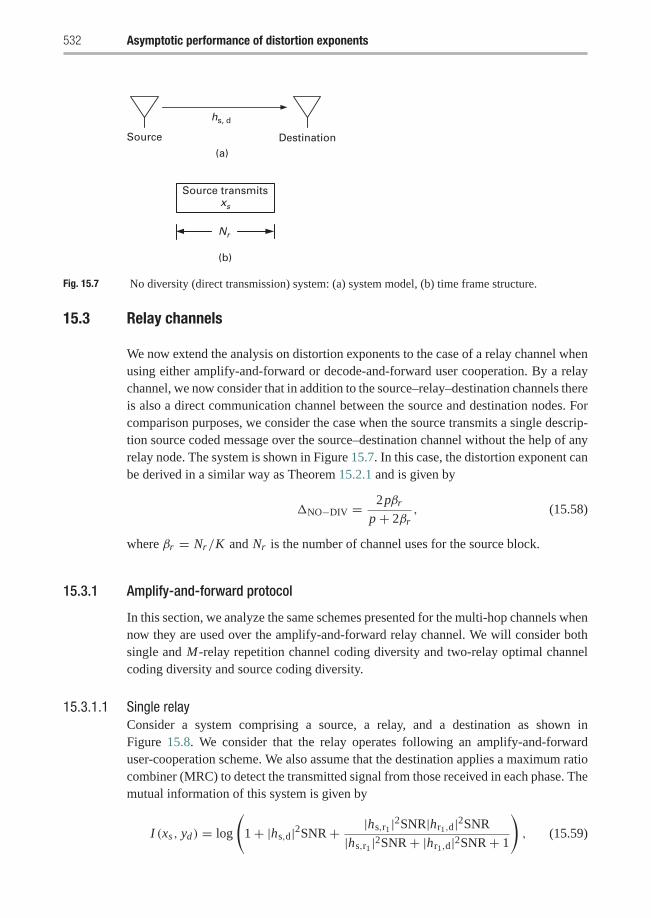
532 Asymptotic performance of distortion exponents
(a)
(b)
Source Destination
hs, d
Nr
Source transmitsxs
Fig. 15.7 No diversity (direct transmission) system: (a) system model, (b) time frame structure.
15.3 Relay channels
We now extend the analysis on distortion exponents to the case of a relay channel whenusing either amplify-and-forward or decode-and-forward user cooperation. By a relaychannel, we now consider that in addition to the source–relay–destination channels thereis also a direct communication channel between the source and destination nodes. Forcomparison purposes, we consider the case when the source transmits a single descrip-tion source coded message over the source–destination channel without the help of anyrelay node. The system is shown in Figure 15.7. In this case, the distortion exponent canbe derived in a similar way as Theorem 15.2.1 and is given by
�NO−DIV = 2pβr
p + 2βr, (15.58)
where βr = Nr/K and Nr is the number of channel uses for the source block.
15.3.1 Amplify-and-forward protocol
In this section, we analyze the same schemes presented for the multi-hop channels whennow they are used over the amplify-and-forward relay channel. We will consider bothsingle and M-relay repetition channel coding diversity and two-relay optimal channelcoding diversity and source coding diversity.
15.3.1.1 Single relayConsider a system comprising a source, a relay, and a destination as shown inFigure 15.8. We consider that the relay operates following an amplify-and-forwarduser-cooperation scheme. We also assume that the destination applies a maximum ratiocombiner (MRC) to detect the transmitted signal from those received in each phase. Themutual information of this system is given by
I (xs, yd) = log
(1+ |hs,d|2SNR+ |hs,r1 |2SNR|hr1,d|2SNR
|hs,r1 |2SNR+ |hr1,d|2SNR+ 1
), (15.59)
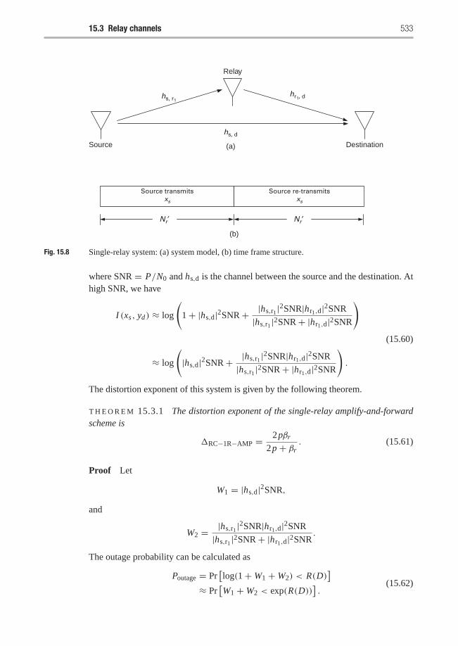
15.3 Relay channels 533
(a)Source
Relay
Destination
hs, r1
hs, d
hr1, d
(b)
Nr′Nr′
Source transmitsxs
Source re-transmitsxs
Fig. 15.8 Single-relay system: (a) system model, (b) time frame structure.
where SNR = P/N0 and hs,d is the channel between the source and the destination. Athigh SNR, we have
I (xs, yd) ≈ log
(1+ |hs,d|2SNR+ |hs,r1 |2SNR|hr1,d|2SNR
|hs,r1 |2SNR+ |hr1,d|2SNR
)
≈ log
(|hs,d|2SNR+ |hs,r1 |2SNR|hr1,d|2SNR
|hs,r1 |2SNR+ |hr1,d|2SNR
).
(15.60)
The distortion exponent of this system is given by the following theorem.
T H E O R E M 15.3.1 The distortion exponent of the single-relay amplify-and-forwardscheme is
�RC−1R−AMP = 2pβr
2p + βr. (15.61)
Proof Let
W1 = |hs,d|2SNR,
and
W2 = |hs,r1 |2SNR|hr1,d|2SNR
|hs,r1 |2SNR+ |hr1,d|2SNR.
The outage probability can be calculated as
Poutage = Pr[log(1+W1 +W2) < R(D)
]≈ Pr
[W1 +W2 < exp(R(D))
].
(15.62)
534 Asymptotic performance of distortion exponents
From the proof of Theorem 15.2.6, the cdf of W1 +W2 is given by
FW1+W2(w) ≈ c33
( w
SNR
)2p. (15.63)
The minimum expected distortion can now be computed as
E[D] ≈ minD
{Pr[W1 +W2 < exp(R(D))
]+ Pr[W1 +W2 ≥ exp(R(D))
]D}
= minD
{FW1+W2(exp(R(D)))+ Pr[1− FW1+W2(exp(R(D)))] D
}≈ min
D
{c33
(exp(2pR(D))
SNR2p
)+[1− c33
(exp(2pR(D))
SNR2p
)]D
}
≈ minD
{c33
⎛⎝ D−pβ′r
SNR2p
⎞⎠+ D
}, (15.64)
where β ′r = N ′r/K and N ′r is the number of source channel uses (refer to Figure 15.8).Differentiating and setting equal to zero we get the optimizing distortion
D∗ =(βr
c33 p
) −β′rβ′r+p
SNR−2β′r pβ′r+p . (15.65)
Hence, the distortion exponent is given as
�RC−1R−AMP = 2β ′r p
β ′r + p. (15.66)
For fair comparison we should have Nr = 2N ′r from which we have β ′r = (1/2)βr .Substituting into (15.66) we get
�RC−1R−AMP = 2βr p
βr + 2p. (15.67)
�
If we asymptotically compare the distortion exponents for the cases of no diversity anda single relay we have
limβr /p→∞
�RC−1R−AMP
�NO−DIV= 2,
limβr /p→0
�RC−1R−AMP
�NO−DIV= 1
2.
(15.68)
Note that as βr/p increases (bandwidth increases) the system becomes outage limitedbecause the performance is limited by the outage event. In this case, the single-relay amplify-and-forward system will achieve a higher distortion exponent since itachieves diversity. Conversely, as βr/p tends to zero (higher channel quality) the per-formance is not limited by the outage event, but is limited by the source encoder qualityperformance.
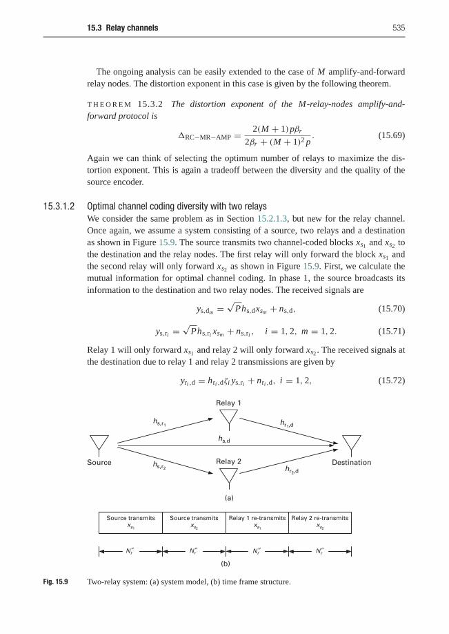
15.3 Relay channels 535
The ongoing analysis can be easily extended to the case of M amplify-and-forwardrelay nodes. The distortion exponent in this case is given by the following theorem.
T H E O R E M 15.3.2 The distortion exponent of the M-relay-nodes amplify-and-forward protocol is
�RC−MR−AMP = 2(M + 1)pβr
2βr + (M + 1)2 p. (15.69)
Again we can think of selecting the optimum number of relays to maximize the dis-tortion exponent. This is again a tradeoff between the diversity and the quality of thesource encoder.
15.3.1.2 Optimal channel coding diversity with two relaysWe consider the same problem as in Section 15.2.1.3, but new for the relay channel.Once again, we assume a system consisting of a source, two relays and a destinationas shown in Figure 15.9. The source transmits two channel-coded blocks xs1 and xs2 tothe destination and the relay nodes. The first relay will only forward the block xs1 andthe second relay will only forward xs2 as shown in Figure 15.9. First, we calculate themutual information for optimal channel coding. In phase 1, the source broadcasts itsinformation to the destination and two relay nodes. The received signals are
ys,dm =√
Phs,dxsm + ns,d, (15.70)
ys,ri =√
Phs,ri xsm + ns,ri , i = 1, 2, m = 1, 2. (15.71)
Relay 1 will only forward xs1 and relay 2 will only forward xs2 . The received signals atthe destination due to relay 1 and relay 2 transmissions are given by
yri ,d = hri ,dζi ys,ri + nri ,d, i = 1, 2, (15.72)
(a)
(b)
Source transmitsxs1
Source transmitsxs2
Relay 1 re-transmitsxs1
Relay 2 re-transmitsxs2
Source
Relay 1
DestinationRelay 2
hs,r1
hs,d
hs,r2
hr1,d
hr2,d
Nr″ Nr″ Nr″ Nr″
Fig. 15.9 Two-relay system: (a) system model, (b) time frame structure.
536 Asymptotic performance of distortion exponents
where ζi is the signal amplification performed at the relay which satisfies the powerconstraint with equality, that is,
ζi =√
P
P|hs,ri |2 + N0, (15.73)
and where all the noise components are modeled as independent zero-mean, complexGaussian random variables with variance N0/2 per dimension.
Define the 4×1 vector, y = [ys,d1 , ys,d2 , yr1,d, yr2,d]T. To get the mutual informationbetween x = [xs1 , xs2 ] and y, we consider that the receiver has to detect the twoblocks xs1 and xs2 by operating separately on the two amplify-and-forward channelsthat are established through each of the relays. In this way, an MRC detector is appliedon ys,d1 , yr1,d and another MRC detector is applied on ys,d2, yr2,d. The output of the firstMRC detector is given by
r1 = αs ys,d1 + α1yr1,d, (15.74)
where αs =√
Ph∗s,d/N0 and
α1 =√
Pζ1h∗r1,dh∗s,r1(ζ 2
1 |hr1,d|2 + 1)N0.
We can write r1 in terms of xs1 as
r1 =(|hs,d|2SNR+ |hr1,d|2SNR|hs,r1 |2SNR
|hs,r1 |2SNR+ |hr1,d|2SNR+ 1
)xs1 + n1, (15.75)
where n1 is a zero-mean, complex Gaussian noise of variance
|hs,d|2SNR+ |hr1,d|2SNR|hs,r1 |2SNR
|hs,r1 |2SNR+ |hr1,d|2SNR+ 1.
Similarly we can have r2, representing the output of the second MRC detector, given by
r2 =(|hs,d|2SNR+ |hr2,d|2SNR|hs,r2 |2SNR
|hs,r2 |2SNR+ |hr2,d|2SNR+ 1
)xs2 + n2, (15.76)
where n2 is a zero-mean, complex Gaussian noise of variance
|hs,d|2SNR+ |hr2,d|2SNR|hs,r2 |2SNR
|hs,r2 |2SNR+ |hr2,d|2SNR+ 1.
This means that, given the channel coefficients, r1 and r2 act as the received xs1 and xs2
when transmitted over an additive white Gaussian channel. Because of this, it followsthe well known fact that r1 and r2, given the channel coefficients, are sufficient statisticsfor x [223]. This implies that the mutual information between x and y equals the mutualinformation between x and r = [r1, r2], that is
I (x; r) = I (x; y). (15.77)
15.3 Relay channels 537
As was discussed in the proof of Theorem 15.2.6, for any covariance matrix of x themutual information is maximized when x is a zero-mean, complex Gaussian randomvector. Define
γ1 = |hs,d|2SNR+ |hr1,d|2SNR|hs,r1 |2SNR
|hs,r1 |2SNR+ |hr1,d|2SNR+ 1
γ2 = |hs,d|2SNR+ |hr2,d|2SNR|hs,r2 |2SNR
|hs,r2 |2SNR+ |hr2,d|2SNR+ 1.
The mutual information can be computed as
I (x, y) = I (x, r) = log
(det
[I2 +
[γ1 αγ ′α∗γ ′′ γ2
]]), (15.78)
where I2 is the 2× 2 identity matrix, γ ′ and γ ′′ are functions of the channel coefficientsand the noise variance and α = E
[xs1 x∗s2
]. It is next necessary to maximize (15.78)
in order to find the maximum mutual information. From (15.78) it is clear that both αand −α will give the same mutual information. From the concavity of the log-functionwe can see that the mutual information maximizing α is α = 0, that is xs1 and xs2 areindependent (since both xs1 and xs2 are Gaussian). The maximum mutual informationcan now be given as
I ≈ log
(1+ |hs,d|2SNR+ |hs,r1 |2SNR|hr1,d|2SNR
|hs,r1 |2SNR+ |hr1,d|2SNR
)
+ log
(1+ |hs,d|2SNR+ |hs,r2 |2SNR|hr2,d|2SNR
|hs,r2 |2SNR+ |hr2,d|2SNR
). (15.79)
The distortion exponent of this system is given by the following theorem.
T H E O R E M 15.3.3 The distortion exponent of the two-relay optimal channel codingdiversity amplify-and-forward protocol is
�RC−2R−OPTCH−AMP = 3pβr
3p + βr. (15.80)
Proof To compute the distortion exponent we start with the analysis of a subopti-mal system at the destination node. In the suboptimal system, the detector (suboptimaldetector) selects the paths with the highest SNR and does not apply an MRC detector(the optimal detector is the one that applies MRC on the received signals). For example,for xs1 , it either selects the source–destination link or the source–relay–destination linkbased on which one has higher SNR. The mutual information for the suboptimal systemcan be easily proved to be
Isub ≈ log
(1+max
(|hs,d|2SNR,
|hs,r1 |2SNR|hr1,d|2SNR
|hs,r1 |2SNR+ |hr1,d|2SNR
))
+ log
(1+max
(|hs,d|2SNR,
|hs,r2 |2SNR|hr2,d|2SNR
|hs,r2 |2SNR+ |hr2,d|2SNR
)). (15.81)
538 Asymptotic performance of distortion exponents
Let
W1 = |hs,d|2SNR,
W2 = |hs,r1 |2SNR|hr1,d|2SNR
|hs,r1 |2SNR+ |hr1,d|2SNR,
W3 = |hs,r2 |2SNR|hr2,d|2SNR
|hs,r2 |2SNR+ |hr2,d|2SNR.
The outage probability of the suboptimal system is given by
Poutage = Pr[Isub < R]= Pr
[log(1+max(W1,W2))+ log(1+max(W1,W3)) < R
]= Pr
[{2 log(1+W1) < R,W1 > W2,W1 > W3}⋃{log(1+W1)+ log(1+W3) < R,W1 > W2,W3 > W1}⋃{log(1+W2)+ log(1+W1) < R,W2 > W1,W1 > W3}⋃{log(1+W2)+ log(1+W3) < R,W2 > W1,W3 > W1}
]= Pr[2 log(1+W1) < R,W1 > W2,W1 > W3]+ Pr[log(1+W1)+ log(1+W3) < R,W1 > W2,W3 > W1]+ Pr[log(1+W2)+ log(1+W1) < R,W2 > W1,W1 > W3]+ Pr[log(1+W2)+ log(1+W3) < R,W2 > W1,W3 > W1],
(15.82)
where the last equality follows from the events being disjoint. In the last equation weused R instead of R(D) for simplicity of presentation. The joint pdf of W1, W2, andW3, which are independent random variables, is given by
f (w1, w2, w3) ≈ c j p3
(w
p−11 w
p−12 w
p−13
SNR3p
), (15.83)
where c j is a constant. To find the outage probability, we calculate the probability of theindividual outage events in (15.82),
P1 = Pr[2 log(1+W1) < R,W1 > W2,W1 > W3]
=∫ exp(R/2)
w1=0
∫ w1
w3=0
∫ w1
w2=0f (w1, w2, w3)dw2dw3dw1
≈∫ exp(R/2)
w1=0
∫ w1
w3=0
∫ w1
w2=0c j p3
(w
p−11 w
p−12 w
p−13
SNR3p
)dw2dw3dw1
=c j exp
(3pR
2
)3SNR3p
.
15.3 Relay channels 539
P2 = Pr[log(1+W1)+ log(1+W3) < R,W1 > W2,W3 > W1]≈ Pr[log(W1)+ log(W3) < R,W1 > W2,W3 > W1]
=∫ exp(R/2)
w1=0
∫ exp(R)w1
w3=w1
∫ w1
w2=0f (w1, w2, w3)dw2dw3dw1
≈∫ exp(R/2)
w1=0
∫ exp(R)w1
w3=w1
∫ w1
w2=0c j p3
(w
p−11 w
p−12 w
p−13
SNR3p
)dw2dw3dw1
= c j p2
SNR3p
∫ exp(R/2)
w1=0
∫ exp(R)w1
w3=w1
w2p−11 w
p−13 dw3dw1
=2c j exp
(3pR
2
)3SNR3p
.
P3 = Pr[log(1+W2)+ log(1+W1) < R,W2 > W1,W1 > W3]≈ Pr[log(W1)+ log(W3) < R,W1 > W2,W3 > W1]
≈2c j exp
(3pR
2
)3SNR3p
.
P4 = Pr[log(1+W2)+ log(1+W3) < R,W2 > W1,W3 > W1]≈ Pr[log(W2)+ log(W3) < R,W2 > W1,W3 > W1]
=∫ exp(R/2)
w1=0
∫ exp(R)w1
w2=w1
∫ exp(R)w2
w3=w1
f (w1, w2, w3)dw3dw2dw1
≈∫ exp(R/2)
w1=0
∫ exp(R)w1
w2=w1
∫ exp(R)w2
w3=w1
c j p3
(w
p−11 w
p−12 w
p13
SNR3p
)dw3dw2dw1
=4c j exp
(3pR
2
)3SNR3p
,
where we have limw1→0wp1 logw1 = 0 for p ≥ 1. The outage probability for the
suboptimal system is
Poutage = P1 + P2 + P3 + P4 ≈cm exp
(3pR
2
)SNR3p
, (15.84)
where cm is a constant. The minimum expected end-to-end distortion can now becomputed as
E[D] = minD
{Poutage +
(1− Poutage
)D}
≈ minD
⎧⎨⎩cm exp(
3pR2
)SNR3p
+⎛⎝1−
cm exp(
3pR2
)SNR3p
⎞⎠ D
⎫⎬⎭
540 Asymptotic performance of distortion exponents
≈ minD
⎧⎨⎩cm D−3p4β′′r
SNR3p+⎛⎝1− cm D
−3p4β′′r
SNR3p
⎞⎠ D
⎫⎬⎭≈ min
D
⎧⎨⎩cm D−3p4β′′r
SNR3p+ D
⎫⎬⎭ , (15.85)
where β ′′r = N ′′r /K (refer to Figure 15.9), D is the source encoder distortion and wehave used both high SNR approximations and (15.5). Differentiating and setting equalto zero, we get the optimizing distortion
D∗ =(
4β ′′r3cm p
) −4β′′r4β′′r +3p
SNR−12β′′r p4β′′r +3p .
Substituting we get the distortion exponent for this suboptimal system as
�SUBOPTIMAL = 12β ′′r p
4β ′′r + 3p.
For fair comparison the total number of channel uses is fixed and, thus, β ′′r = (1/4)βr ,which leads to the distortion exponent of the suboptimal system be given by
�SUBOPTIMAL = 3βr p
βr + 3p.
For the optimal detector (the one using an MRC detector), the distortion exponentsatisfies
�RC−2R−OPTCH−AMP ≥ �SUBOPTIMAL = 3βr p
βr + 3p. (15.86)
Next, we find an upper bound on the distortion exponent for the optimal system. In thiscase, the mutual information in (15.79) can be upper and lower bounded as
log(1+ 2W1 +W2 +W3) ≤ log (1+W1 +W2)+ log (1+W1 +W3)
≤ 2 log(1+W1 + 1
2W2 + 1
2W3),
where W1, W2, and W3 are non-negative numbers. The upper bound follows fromthe concavity of the log-function. Therefore, the outage probability Po of the optimalsystem can be upper and lower bounded as
Pr[2 log(1+W1 + 1
2W2 + 1
2W3) < R] ≤ Po ≤ Pr[log(1+ 2W1 +W2 +W3) < R].
(15.87)
From (15.87) we can easily show that
CL
exp(
3pR2
)SNR3p
� Po � CUexp(3pR)
SNR3p, (15.88)
15.3 Relay channels 541
where CL and CU are two constants that do not depend on the SNR. Similar to thesuboptimal system, and using (15.88), the minimum expected end-to-end distortion forthe optimal system can be lower bounded as
E[D] � minD
⎧⎨⎩CL
exp(
3pR2
)SNR3p
+(
1− CUexp(3pR)
SNR3p
)D
⎫⎬⎭≈min
D
⎧⎨⎩CL D−3p4β′′r
SNR3p+⎛⎝1− CU D
−3p2β′′r
SNR3p
⎞⎠ D
⎫⎬⎭≈min
D
⎧⎨⎩CL D−3p4β′′r
SNR3p+ D
⎫⎬⎭ .(15.89)
Differentiating the lower bound and setting equal to zero we get the optimizingdistortion as
D∗ =(
4β ′′r3pCL
) −4β′′r4β′′r +3p
SNR−12β′′r p4β′′r +3p . (15.90)
Substituting, we get
E[D] � CLOSNR−12β′′r p4β′′r +3p , (15.91)
from which we can upper bound the distortion exponent of the optimal system as
�RC−2R−OPTCH−AMP ≤ 12β ′′r p
4β ′′r + 3p= 3βr p
βr + 3p. (15.92)
Finally, from (15.86) and (15.92) we get
�RC−2R−OPTCH−AMP = 3βr p
βr + 3p. (15.93)
�
15.3.1.3 Source coding diversity with two relaysWe continue analyzing a system as in Figure 15.9 but now we assume that each of thetwo blocks sent from the source, xs1 and xs2 , represents one description generated froma dual descriptions source encoder. The first relay will only forward the block xs1 andthe second relay will only forward xs2 as shown in Figure 15.9. The distortion exponentof this system is given by the following theorem.
T H E O R E M 15.3.4 The distortion exponent of the two-relay source coding diversityamplify-and-forward protocol is
�RC−2R−SRC−AMP = max
[2pβr
2p + βr,
3pβr
4p + βr
], (15.94)
542 Asymptotic performance of distortion exponents
Proof The receiver applies an MRC detector on the received data to detect xs1 and xs2 .Let
W1 = |hs,d|2SNR,
W2 = |hs,r1 |2SNR|hr1,d|2SNR
|hs,r1 |2SNR+ |hr1,d|2SNR,
W3 = |hs,r2 |2SNR|hr2,d|2SNR
|hs,r2 |2SNR+ |hr2,d|2SNR.
The minimum expected end-to-end distortion is given by
E[D] ≈ minD0,D1
Pr[
log(1+W1 +W2) < Rmd(D0, D1)/2,
log(1+W1 +W3) < Rmd(D0, D1)/2]
+ Pr[
log(1+W1 +W2) < Rmd(D0, D1)/2,
log(1+W1 +W3) > Rmd(D0, D1)/2]
+ Pr[
log(1+W1 +W2) > Rmd(D0, D1)/2,
log(1+W1 +W3) < Rmd(D0, D1)/2]D1
+ Pr[
log(1+W1 +W2) > Rmd(D0, D1)/2,
log(1+W1 +W3) > Rmd(D0, D1)/2]D0, (15.95)
where Rmd, D0, and D1 are as introduced in Section 15.1. To calculate the minimumexpected distortion we need to calculate the following probabilities in (15.95):
P ′1 = Pr[
log(1+W1 +W2) < Rmd(D0, D1)/2,
log(1+W1 +W3) < Rmd(D0, D1)/2]
= Pr[
log(1+W1 +max(W2,W3)) < Rmd(D0, D1)/2]
≈ cs11
SNR3pexp
(3p
2Rmd(D0, D1)
).
P ′2 = Pr[
log(1+W1 +W2) > Rmd(D0, D1)/2,
log(1+W1 +W3) > Rmd(D0, D1)/2]
= Pr[
log(1+W1 +min(W2,W3)) > Rmd(D0, D1)/2]
= 1− Pr[
log(1+W1 +min(W2,W3)) < Rmd(D0, D1)/2]
≈ 1− cs21
SNR2pexp(
pRmd(D0, D1)).
15.3 Relay channels 543
P ′3 = Pr[
log(1+W1 +W2) < Rmd(D0, D1)/2,
log(1+W1 +W3) > Rmd(D0, D1)/2]
+ Pr[
log(1+W1 +W2) > Rmd(D0, D1)/2,
log(1+W1 +W3) < Rmd(D0, D1)/2]
= 1− P ′1 − P ′2
≈ cs21
SNR2pexp (pRmd(D0, D1))− cs1
1
SNR3pexp
(3p
2Rmd(D0, D1)
)≈ cs2
1
SNR2pexp (pRmd(D0, D1)) .
The minimum expected distortion in (15.95) can now be calculated as
E[D] ≈ minD0,D1
{cs1
1
SNR3pexp
(3p
2Rmd(D0, D1)
)+ cs2
1
SNR2pexp (pRmd(D0, D1)) D1
+(
1− cs21
SNR2pexp (pRmd(D0, D1))
)D0
}≈ min
D0,D1
{cs1
1
SNR3pexp
(3p
2Rmd(D0, D1)
)+ cs2
1
SNR2pexp (pRmd(D0, D1)) D1 + D0
}.
Substituting from (15.8) yields upper and lower bound for the minimum expected end-to-end distortion as
E[D] � minD0,D1
cs1
SNR3p
(1
4D0 D1
) 3p4β′′r + cs2
SNR2p
(1
4D0 D1
) p2β′′r.D1 + D0
E[D] � minD0,D1
cs1
SNR3p
(1
2D0 D1
) 3p4β′′r + cs2
SNR2p
(1
2D0 D1
) p2β′′r.D1 + D0.
(15.96)
Note that for p ≥ 2β ′′r the minimum expected distortion increases as D1 decreases.Hence, the optimal choice of D1 approaches a constant that is bounded away from zero.For D1 ≥ 1/2 the source coding rate is given by (15.9) and not (15.8). The optimalsystem in this case degenerates to the single relay system (the argument is the same asfor the multi-hop channel). Thus, the distortion exponent is given by
�RC−2R−SRC−AMP = 2pβr
2p + βr, p ≥ 1
2βr = 2β ′′r . (15.97)
544 Asymptotic performance of distortion exponents
For p < 2β ′′r , we can find the optimal value of D1 by differentiating the lower bound in(15.96) and setting it equal to zero. We get
D∗1 =(
cs1
cs2
(3p
(βr − 2p)
)) βrp+βr
SNR−pβr
p+βr (4D0)− p
p+βr , p <1
2βr , (15.98)
where, for fair comparison, we fix the total number of channel uses and get β ′′r =(1/4)βr . For the case when p < (1/2)βr , substituting (15.98) in the lower bound in(15.96) we get
E[D] � minD0
C.D− 3p
p+βr0 .SNR−
3pβrp+βr + D0, p <
1
2βr , (15.99)
where C is a constant that does not depend on D0 and the SNR. Differentiating andsetting equal to zero we can get the expression for the optimizing D0 as
D∗0 = C ′.SNR−3pβr
4p+βr , p <1
2βr . (15.100)
Hence, from (15.100) we have
C ′LBSNR−3pβr
4p+βr � E[D] � C ′UBSNR−3pβr
4p+βr , p <1
2βr . (15.101)
From (15.97) and (15.101) we conclude that the distortion exponent for the sourcediversity system is given by
�RC−2R−SRC−AMP = max
[2pβr
2p + βr,
3pβr
4p + βr
], (15.102)
where the second term in (15.102) is the maximum for the case p < (1/2)βr . �
15.3.2 Decode-and-forward relay channel
We now analyze the decode-and-forward relay channel. The distortion exponents forthe different schemes can be easily derived from the analysis presented in the previoussections. We collect the corresponding results in the following theorem.
T H E O R E M 15.3.5 The distortion exponents of the decode-and-forward relaychannel are:
• For the single-relay channel
�RC−1R−DEC = 2pβr
2p + βr. (15.103)
• For the M-relay selection channel coding diversity
�RC−MR−DEC = 2(M + 1)pβr
2βr + (M + 1)2 p. (15.104)
• For the optimal channel coding with two relays, with the same time frame structure as inFigure 15.6,
�RC−2R−OPTCH−AMP = 3pβr
3p + βr. (15.105)
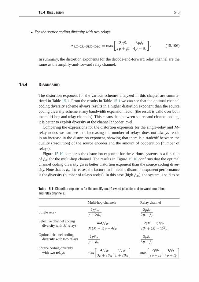
15.4 Discussion 545
• For the source coding diversity with two relays
�RC−2R−SRC−DEC = max
[2pβr
2p + βr,
3pβr
4p + βr
]. (15.106)
In summary, the distortion exponents for the decode-and-forward relay channel are thesame as the amplify-and-forward relay channel.
15.4 Discussion
The distortion exponent for the various schemes analyzed in this chapter are summa-rized in Table 15.1. From the results in Table 15.1 we can see that the optimal channelcoding diversity scheme always results in a higher distortion exponent than the sourcecoding diversity scheme at any bandwidth expansion factor (the result is valid over boththe multi-hop and relay channels). This means that, between source and channel coding,it is better to exploit diversity at the channel encoder level.
Comparing the expressions for the distortion exponents for the single-relay and M-relay nodes we can see that increasing the number of relays does not always resultin an increase in the distortion exponent, showing that there is a tradeoff between thequality (resolution) of the source encoder and the amount of cooperation (number ofrelays).
Figure 15.10 compares the distortion exponent for the various systems as a functionof βm for the multi-hop channel. The results in Figure 15.10 confirms that the optimalchannel coding diversity gives better distortion exponent than the source coding diver-sity. Note that as βm increases, the factor that limits the distortion exponent performanceis the diversity (number of relays nodes). In this case (high βm), the system is said to be
Table 15.1 Distortion exponents for the amplify-and-forward (decode-and-forward) multi-hopand relay channels.
Multi-hop channels Relay channel
Single relay2pβm
p + 2βm
2pβr
2p + βr
Selective channel codingdiversity with M relays
4Mpβm
M(M + 1)p + 4βm
2(M + 1)pβr
2βr + (M + 1)2 p
Optimal channel codingdiversity with two relays
2pβm
p + βm
3pβr
3p + βr
Source coding diversitywith two relays max
[4pβm
3p + 2βm,
2pβm
p + 2βm
]max
[2pβr
2p + βr,
3pβr
4p + βr
]
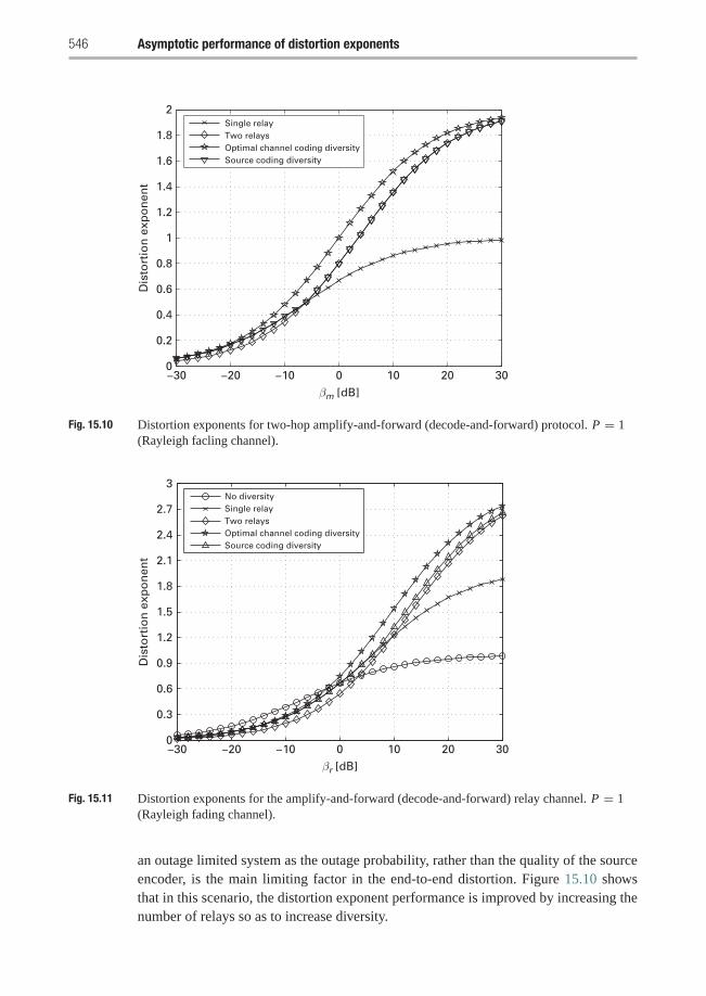
546 Asymptotic performance of distortion exponents
−30 −20 −10 0 10 20 300
0.2
0.4
0.6
0.8
1
1.2
1.4
1.6
1.8
2
βm [dB]
Dis
tort
ion
exp
on
ent
Single relayTwo relaysOptimal channel coding diversitySource coding diversity
Fig. 15.10 Distortion exponents for two-hop amplify-and-forward (decode-and-forward) protocol. P = 1(Rayleigh facling channel).
−30 −20 −10 0 10 20 300
0.3
0.6
0.9
1.2
1.5
1.8
2.1
2.4
2.7
3
βr [dB]
Dis
tort
ion
exp
on
ent
No diversitySingle relayTwo relaysOptimal channel coding diversitySource coding diversity
Fig. 15.11 Distortion exponents for the amplify-and-forward (decode-and-forward) relay channel. P = 1(Rayleigh fading channel).
an outage limited system as the outage probability, rather than the quality of the sourceencoder, is the main limiting factor in the end-to-end distortion. Figure 15.10 showsthat in this scenario, the distortion exponent performance is improved by increasing thenumber of relays so as to increase diversity.
15.5 Chapter summary and bibliographical notes 547
At low βm the system is said to be quality limited as the quality of the source encoder(distortion under no outage), rather than the outage probability, is the main limiting fac-tor in the end-to-end distortion. In this case, the gain from using a better source encoder,that has a higher resolution, is more significant than the gain from increasing the num-ber of relay nodes. Figure 15.10 shows that in this scenario, the distortion exponentperformance is improved by using only a single relay node, which allows for the use ofa higher resolution source encoder.
Figure 15.11 shows the distortion exponent versus βr for the various relay channelschemes. Figure 15.11 confirms that the scheme with optimal channel coding diver-sity yields a better distortion exponent than the one with source coding diversity. Aswas the case for multi-hop schemes, as βm increases, diversity becomes the limitingfactor for the distortion exponent, in which case, Figure 15.11 also shows that increas-ing the number of relays improves the distortion exponent results. Again, at low βm ,direct transmission (no-diversity) results in a lower end-to-end distortion which can beinterpreted in the same way as for the multi-hop channel.
15.5 Chapter summary and bibliographical notes
In this chapter, we have studied the performance of systems that combine user coopera-tion diversity with diversity generated at higher layers of the communication stack in theform of source coding and channel coding diversity. In the case of source coding, diver-sity is introduced through the use of dual-description source encoders. Channel codingdiversity is obtained from joint decoding of channel coded blocks sent through differentchannels. From the viewpoint of user cooperation, diversity is provided to upper layersthrough configurations with a direct path between the source and the destination node(a relay channel), and without such direct path (a multi-hop channel). We have consid-ered user cooperation using either the amplify-and-forward or the decode-and-forwardtechniques to study the achievable performance limits, which was measured in terms ofthe distortion exponent.
The study in this chapter shows that channel coding diversity provides better perfor-mance, followed by source coding diversity. For the case of having multiple relays thatcan help the source node to forward its information, and depending on the operatingbandwidth expansion factor, we have determined the optimal number of relay nodes tocooperate with the source node to maximize the distortion exponent. The study shows atradeoff between the source coding resolution and the number of relay nodes assignedfor helping the source node. We note that at low bandwidth it is not the channel out-age event, but the distortion introduced at the source coding stage the dominant factorlimiting the distortion exponent performance. Therefore, in these cases it is better notto cooperate and use a lower distortion source encoder. Similarly, we showed that asthe bandwidth expansion factor increases, the distortion exponent improves by allow-ing user cooperation. In these cases, the system is said to be an outage limited systemand it is better to cooperate so as to minimize the outage probability and, consequently,minimize the end-to-end distortion.
548 Asymptotic performance of distortion exponents
The presentation in this chapter can be framed first within the idea that diversity canalso be formed when multiple channels are provided to the application layer. A goodstudy of this idea, from the perspective of the achievable performance of source–channeldiversity over general parallel channels, can be found in [110]. The study in this paper isalso focused on distortion exponent but without considering cooperation. An example ofa work that uses distortion exponent to study single description source coded schemeswith cooperation is [53]. In terms of multiple description coding, the work in [140]presents an early and useful study of the most important topics, such as rate-distortionperformance. A further study on the achievable rates of multiple description coding canbe found in [32] and further information on source–channel diversity in cooperativenetworks can be found in [173, 177, 169]
Exercises
15.1 For the dual description description source encoder operating in the region of lowdistortion (D1+D2−D0 < 1), use (15.7) and the fact that for any well-designedMD codec D0 ≤ D1/2, to derive the inequalities (15.8),
(4D0 D1)−1/(2β) � eRmd � (2D0 D1)
−1/(2β).
[Hint: Recall that the lower bound requires D0 → 0 and the upper bound requiresalso D1 → 0.]
15.2 Using the techniques presented in this chapter prove that for the case when thesource transmits a single description source coded message without the help ofany relay node the distortion exponent is given by
�NO−DIV = 2pβr
p + 2βr,
where βr = Nr/K and Nr is the number of channel uses for the source block(refer to Figure 15.7).
15.3 Using the techniques presented in this chapter prove that Theorem 15.2.3 istrue, i.e., show that for the two-hop two-relay optimal channel coding diversityamplify-and-forward system the distortion exponent is
�SH−2R−OPTCH−AMP = 2pβm
p + βm.
15.4 Following the techniques used in this chapter show that the distortion exponentfor the source coding diversity over two parallel channels can be written as
�SH−2R−SRC−AMP = max
[8pβ ′′m
3p + 4β ′′m,
4pβ ′′mp + 4β ′′m
].
15.5 For the multi-hop channels with the decode-and-forward protocol, we have thefollowing expressions for the distortion exponents, as stated in Theorem 15.2.5:
Exercises 549
• for the two-hop single relay
�SH−1R−DEC = 2pβm
p + 2βm,
• for the two-hop M-relay selection channel coding diversity
�SH−MR−DEC = 4Mpβm
M(M + 1)p + 4βm,
• for the two-hop two relay source coding diversity
�SH−2R−SRC−DEC = max
[4pβm
3p + 2βm,
2pβm
p + 2βm
].
Prove Theorem 15.2.5 using the techniques presented in this chapter.15.6 For the relay channels with the decode-and-forward protocol, we have the
following expressions for the distortion exponents, as stated in Theorem 15.3.5:
• For the single-relay channel
�RC−1R−DEC = 2pβr
2p + βr.
• For the M-relay selection channel coding diversity
�RC−MR−DEC = 2(M + 1)pβr
2βr + (M + 1)2 p.
• For the optimal channel coding with two relays, with the same time framestructure as in Figure 15.6
�RC−2R−OPTCH−AMP = 3pβr
3p + βr.
• For the source coding diversity with two relays
�RC−2R−SRC−DEC = max
[2pβr
2p + βr,
3pβr
4p + βr
].
Prove Theorem 15.3.5 using the techniques presented in this chapter.15.7 In Section 15.1 we highlighted the fact that a high SNR approximation of the
CDF of eI as
FeI (t) ≈ c
(t
SNR
)p
,
allows considering other distributions suitable for modeling |h|2 besides theRayleigh distribution. Assume now that the channel can be modeled with a Ricedistribution and derive the value of the parameter p for this case. Use this resultto redo Figures 15.10 and 15.11, and analyze the differences.
16 Coverage expansion with cooperation
For practical implementation of cooperative communications in wireless networks, weneed to develop protocols by which nodes are assigned to cooperate with each other.In most of the previous chapters on cooperation, the cooperating relays are assumedto exist and are already paired with the source nodes in the network. A deterministicnetwork topology, i.e., deterministic channel gain variances between different nodesin the network, was also assumed. If the random users’ spatial distribution, and theassociated propagation path losses between different nodes in the network, are takeninto consideration, then these assumptions, in general, are no longer valid.
Moreover, it is of great importance for service providers to improve the coverage areain wireless networks without the cost of more infrastructure and under the same qualityof service requirements. This poses challenges for deployment of wireless networksbecause of the difficult and unpredictable nature of wireless channels.
In this chapter, we address the relay assignment problem for implementing coopera-tive diversity protocols to extend the coverage area in wireless networks. We study theproblem under the knowledge of the users’ spatial distribution which determines thechannel statistics, as the variance of the channel gain between any two nodes is a func-tion of the distance between these two nodes. We consider an uplink scenario where aset of users are trying to communicate to a base station (BS) or access point (AP) anddescribe practical algorithms for relay assignment.
Another way to look at employing cooperation for coverage extension is to think ofthe relays as additional cheap access points that the service provider can deploy in thenetwork. These relays communicate to the base station through the wireless channels,and can help those users away from the base station. Next, we elaborate more on thisconcept.
16.1 System model
We consider a wireless network with a circular cell of radius ρ. The BS/AP is locatedat the center of the cell, and N users are uniformly distributed within the cell. Theprobability density function of the user’s distance r from the BS/AP is thus given by
q(r) = 2r
ρ2, 0 ≤ r ≤ ρ, (16.1)
16.1 System model 551
and the user’s angle is uniformly distributed between [0, 2π). Two communicationsschemes are going to be examined in the sequel. Non-cooperative transmission, ordirect transmission, where users transmit their information directly to the BS/AP, andcooperative communications where users can employ a relay to forward their data.
In the direct transmission scheme, which is employed in current wireless networks,the signal received at the destination d (BS/AP) from source user s, can be modeled as
ys,d =√
P Kr−αs,d hs,dx + ns,d; (16.2)
where P is the transmitted signal power, x is the transmitted data with unit power, hs,d
is the channel fading gain between the two terminals. The channel fade of any link ismodeled as a zero-mean, circularly symmetric complex Gaussian random variable withunit variance. In (16.2), K is a constant that depends on the antennas design, α is thepath loss exponent, and rs,d is the distance between the two terminals. K , α, and P areassumed to be the same for all users. The term ns,d in (16.2) denotes additive noise. Allthe noise components are modeled as white Gaussian noise (AWGN) with variance N0.From (16.2), the received signal-to-noise ratio is
SNR(rs,d) =| hs,d |2 Kr−αs,d P
N0. (16.3)
We characterize the system performance in terms of outage probability. Outage isdefined as the event that the received SNR falls below a certain threshold γnc, wherethe subscript nc denotes non-cooperative transmission. The probability of outage Pnc
for non-cooperative transmission is defined as,
Pnc = P(SNR(r) ≤ γnc). (16.4)
The SNR threshold γnc is determined according to the application and the transmit-ter/receiver structure. If the received SNR is higher than the threshold γnc, the receiveris assumed to be able to decode the received message with negligible probability oferror. If an outage occurs, the packet is considered lost.
For the cooperation protocol, a hybrid version of the incremental and selection relay-ing is employed. In this hybrid protocol, if a user’s packet is lost, the BS/AP broadcastsnegative acknowledgement (NACK) so that the relay assigned to this user can re-transmit this packet again. This introduces spatial diversity because the source messagecan be transmitted via two independent channels as depicted in Figure 16.1. The relaywill only transmit the packet if it is capable of capturing the packet, i.e., if the receivedSNR at the relay is above the threshold. In practice, this can be implemented by utilizinga cyclic redundancy check (CRC) code in the transmitted packet. The signal receivedfrom the source to the destination d and the relay l in the first stage can be modeled as
ys,d =√
P Kr−αs,d hs,dx + ns,d,
ys,l =√
P Kr−αs,l hs,lx + ns,l. (16.5)
If the SNR of the signal received at the destination from the source falls below thecooperation SNR threshold γc, the destination requests a second copy from the relay.
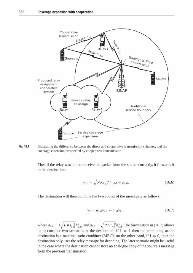
552 Coverage expansion with cooperation
Source
Traditional directtransmission
Select a relay
to assign
Relay l
Source s
Source
BS/AP
Stage 1 : rs,l
Stage 1: rs,d
Traditionalservice boundaryRelay lRelay 1
Stage 2: rl,d
Cooperativetransmission
Proposed relayassignmentcooperative
system
Service coverageexpansion
d
Fig. 16.1 Illustrating the difference between the direct and cooperative transmission schemes, and thecoverage extension prospected by cooperative transmission.
Then if the relay was able to receive the packet from the source correctly, it forwards itto the destination:
yl,d =√
P Kr−αl,d hl,dx + nl,d. (16.6)
The destination will then combine the two copies of the message x as follows:
yd = as,dys,d + al,dyl,d; (16.7)
where as,d = I√
P Kl−αs,d h∗s,d, and ar,d =√
P Kl−αr,d h∗r,d. The formulation in (16.7) allows
us to consider two scenarios at the destination: if I = 1 then the combining at thedestination is a maximal ratio combiner (MRC); on the other hand, if I = 0, then thedestination only uses the relay message for decoding. The later scenario might be usefulin the case where the destination cannot store an analogue copy of the source’s messagefrom the previous transmission.
16.2 Relay assignment: protocols and analysis 553
16.2 Relay assignment: protocols and analysis
In this section, we start with driving the average outage for direct transmission. Thenwe calculate the conditional outage probability for cooperative transmission and try touse the formulas to deduce the best relay location.
16.2.1 Direct transmission
As discussed before, the outage is defined as the event that the received SNR is lowerthan a predefined threshold which we denote by γnc. The outage probability for thedirect transmission mode POD conditioned on the user’s distance can be calculated as
POD(rs,d) = P(SNR(rs,d) ≤ γnc
)= 1− exp
(−N0γncrαs,d
K P
)� N0γncrαs,d
K P, (16.8)
where the above follows because | hs,d |2, the magnitude of the channel fade squared,has an exponential distribution with unit mean. The approximation in (16.8) is at highSNR.
To find the average outage probability over the cell, we need to average over the userdistribution in (16.1). The average outage probability is thus given by
POD =∫ ρ
0POD(rs,d)q(rs,d)drs,d
=∫ ρ
0
2rs,d
ρ2
(1− exp
(−N0γncrαs,d
K P
))drs,d
= 1− 2
αρ2
(K P
N0γnc
) 2α
�
(2
α,
N0γncρα
K P
)� 2γncρ
αN0
K P(α + 2), (16.9)
where �(., .) is the incomplete Gamma function, and it is defined as
�(a, x) =∫ x
0exp−t ta−1dt. (16.10)
16.2.2 Cooperative transmission: conditional outage probability
Consider a source–destination pair that are rs,d units distance apart. Let us computethe conditional outage probability for given locations of the user and the helping relay.Using (16.5), the SNR received at the BS/AP d and the relay l from the source s isgiven by
554 Coverage expansion with cooperation
SNR(rs,d) =| hs,d |2 Kr−αs,d P
N0,
SNR(rs,l) =| hs,l |2 Kr−αs,l P
N0. (16.11)
While from (16.7), the SNR of the combined signal received at the BS/AP is given by
SNRd = I| hs,d |2 Kr−αs,d P
N0+ | hl,d |2 Kr−αl,d P
N0. (16.12)
The terms | hs,d |2, | hs,l |2, and | hl,d |2 are mutually independent exponential ran-dom variables with unit mean. The outage probability of the cooperative transmissionPOC conditioned on the fixed topology of the user s and the relay l can be calculated asfollows. Using the law of total probability we have
POC = Pr(Outage|SNRs,d ≤ γc)Pr(SNRs,d ≤ SNRs,d) (16.13)
where the probability of outage is zero if SNRs,d > γc. The outage probabilityconditioned on the event that the source–destination link is in outage is given by
Pr(Outage|SNRs,d ≤ γc) = Pr(SNRs,l ≤ γc)+ Pr(SNRs,l > γc)
× Pr(SNRd ≤ γc|SNRs,d ≤ γc), (16.14)
where the addition of the above probabilities is because they are disjoint events, and themultiplication is because the source–relay link is assumed to fade independently fromthe other links. The conditioning was removed for the same reason.
For the case where MRC is allowed at the destination, then the conditional outageprobability at the destination is given by
Pr(SNRd ≤ γc|SNRs,d ≤ γc) = Pr(SNRd ≤ γc)
Pr(SNRs,d ≤ γc. (16.15)
Using (16.15) and (16.14) in (16.13), the conditional outage probability for cooperativecommunications with MRC can be calculated as
POC(rs,d, rs,l, rl,d) =(1− f (γc, rs,d)
) (1− f (γc, rs,l)
)+ f (γc, rs,l)
×[
1− r−αs,d
r−αs,d − r−αl,d
f (γc, rs,d)−r−αl,d
r−αl,d − r−αs,d
f (γc, rl,d)
]where f (x, y) = exp(−N0xyα/K P). The above expression can be simplified asfollows:
POC(rs,d, rs,l, rl,d) =(1− f (γc, rs,d)
)− r−αl,d
r−αl,d − r−αs,d
× f (γc, rs,l)(
f (γc, rl,d)− f (γc, rs,d)).
For the I = 1 case, or when MRC is used at the destination, then using the approx-imation exp(−x) � 1 − x + x2/2 for small x , the above outage expression can beapproximated at high SNR to
16.2 Relay assignment: protocols and analysis 555
POC(rs,d, rs,l, rl,d) � N0
K Prαs,d −
N 20
2K 2 P2r2αs,d −
rαs,drαs,d − rαl,d
×[
N0
K P(rαs,d − rαl,d)+
N 20
2K 2 P2
((rαl,d − rαs,d)(2rαs,l + rαl,d + rαs,d)
)]
Simplifying the above expression, we get
POC(rs,d, rs,l, rl,d) � N 20
2K 2 P2r2αs,d
[2
rαs,lrαs,d
+ rαl,drαs,d
](16.16)
For the I = 0 case, or when no MRC is used at the destination, then the conditionaloutage expression in (16.15) simplifies to
Pr(SNRd ≤ γc|SNRs,d ≤ γc) = Pr(SNRd ≤ γc). (16.17)
This is because the SNR received at the destination in this case is just due to the signalreceived from the relay–destination path. The conditional outage expression in this casecan be shown to be given by
POC(rs,d, rs,l, rl,d) =(1− f (γc, rs,d)
) [1− f (γc, rl,d) f (γc, rs,l)
]. (16.18)
16.2.3 Optimal relay position
To find the optimal relay position, we need to find the pair (rs,l, rl,d) that minimizesthe conditional outage probability expression in (16.16). First we consider the I = 1scenario, where MRC is utilized at the receiver.
16.2.3.1 MRC caseIn the following, we will prove that the optimal relay position, under fairly generalconditions, is towards the source and on the line connecting the source and destination.Examining the conditional outage expression in (16.16), it is clear that, for any valueof rl,d, the optimal value for rs,l that minimizes the outage expression is the minimumvalue for rs,l. And since for any value of rl,d the minimum rs,l lies on the straight lineconnecting the source and destination, we get the first intuitive result that the optimalrelay position is on this straight line.
Now, we prove that the optimal relay position is towards the source. Normalizingwith respect to rs,d by substituting x = rl,d/rs,d in (16.16) and 1 − x = rs,l/rs,d, wehave
POC(x) = N 20
2K 2 P2r2αs,d
[2(1− x)α + xα
]. (16.19)
Taking the derivative with respect to x we get
∂POC(x)
∂x= N 2
0
2K 2 P2r2αs,d
[−2α(1− x)α−1 + αxα−1
]. (16.20)
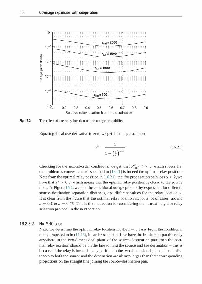
556 Coverage expansion with cooperation
0.1 0.2 0.3 0.4 0.5 0.6 0.7 0.8 0.910−5
10−4
10−3
10−2
10−1
100
Relative relay location from the destination
Ou
tag
e p
rob
abili
ty
rs,d = 500
rs,d = 1000
rs,d = 1500
rs,d = 2000
Fig. 16.2 The effect of the relay location on the outage probability.
Equating the above derivative to zero we get the unique solution
x∗ = 1
1+(
12
) 1α−1
. (16.21)
Checking for the second-order conditions, we get, that P ′′OC(x) ≥ 0, which shows thatthe problem is convex, and x∗ specified in (16.21) is indeed the optimal relay position.Note from the optimal relay position in (16.21), that for propagation path loss α ≥ 2, wehave that x∗ > 0.5, which means that the optimal relay position is closer to the sourcenode. In Figure 16.2, we plot the conditional outage probability expression for differentsource–destination separation distances, and different values for the relay location x .It is clear from the figure that the optimal relay position is, for a lot of cases, aroundx = 0.6 to x = 0.75. This is the motivation for considering the nearest-neighbor relayselection protocol in the next section.
16.2.3.2 No-MRC caseNext, we determine the optimal relay location for the I = 0 case. From the conditionaloutage expression in (16.18), it can be seen that if we have the freedom to put the relayanywhere in the two-dimensional plane of the source–destination pair, then the opti-mal relay position should be on the line joining the source and the destination – this isbecause if the relay is located at any position in the two-dimensional plane, then its dis-tances to both the source and the destination are always larger than their correspondingprojections on the straight line joining the source–destination pair.
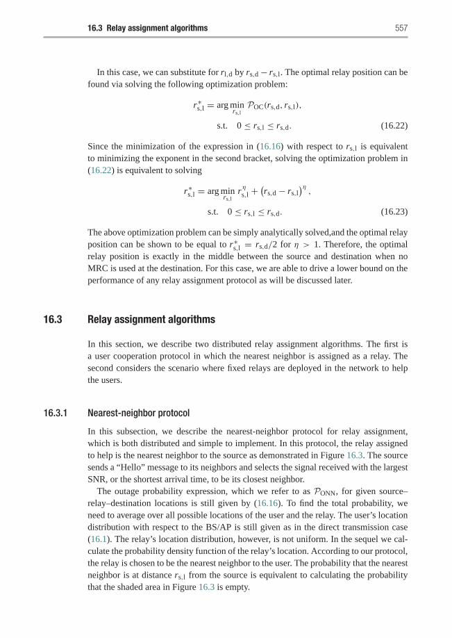
16.3 Relay assignment algorithms 557
In this case, we can substitute for rl,d by rs,d− rs,l. The optimal relay position can befound via solving the following optimization problem:
r∗s,l = arg minrs,l
POC(rs,d, rs,l),
s.t. 0 ≤ rs,l ≤ rs,d. (16.22)
Since the minimization of the expression in (16.16) with respect to rs,l is equivalentto minimizing the exponent in the second bracket, solving the optimization problem in(16.22) is equivalent to solving
r∗s,l = arg minrs,l
rηs,l +(rs,d − rs,l
)η,
s.t. 0 ≤ rs,l ≤ rs,d. (16.23)
The above optimization problem can be simply analytically solved,and the optimal relayposition can be shown to be equal to r∗s,l = rs,d/2 for η > 1. Therefore, the optimalrelay position is exactly in the middle between the source and destination when noMRC is used at the destination. For this case, we are able to drive a lower bound on theperformance of any relay assignment protocol as will be discussed later.
16.3 Relay assignment algorithms
In this section, we describe two distributed relay assignment algorithms. The first isa user cooperation protocol in which the nearest neighbor is assigned as a relay. Thesecond considers the scenario where fixed relays are deployed in the network to helpthe users.
16.3.1 Nearest-neighbor protocol
In this subsection, we describe the nearest-neighbor protocol for relay assignment,which is both distributed and simple to implement. In this protocol, the relay assignedto help is the nearest neighbor to the source as demonstrated in Figure 16.3. The sourcesends a “Hello” message to its neighbors and selects the signal received with the largestSNR, or the shortest arrival time, to be its closest neighbor.
The outage probability expression, which we refer to as PONN, for given source–relay–destination locations is still given by (16.16). To find the total probability, weneed to average over all possible locations of the user and the relay. The user’s locationdistribution with respect to the BS/AP is still given as in the direct transmission case(16.1). The relay’s location distribution, however, is not uniform. In the sequel we cal-culate the probability density function of the relay’s location. According to our protocol,the relay is chosen to be the nearest neighbor to the user. The probability that the nearestneighbor is at distance rs,l from the source is equivalent to calculating the probabilitythat the shaded area in Figure 16.3 is empty.
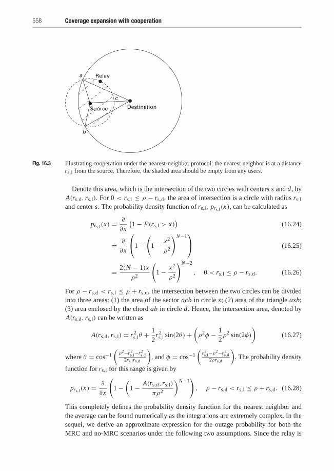
558 Coverage expansion with cooperation
a Relay
DestinationSource
c
b
Fig. 16.3 Illustrating cooperation under the nearest-neighbor protocol: the nearest neighbor is at a distancers,l from the source. Therefore, the shaded area should be empty from any users.
Denote this area, which is the intersection of the two circles with centers s and d, byA(rs,d, rs,l). For 0 < rs,l ≤ ρ − rs,d, the area of intersection is a circle with radius rs,l
and center s. The probability density function of rs,l, prs,l(x), can be calculated as
prs,l(x) =∂
∂x
(1− P(rs,l > x)
)(16.24)
= ∂
∂x
⎛⎝1−(
1− x2
ρ2
)N−1⎞⎠ (16.25)
= 2(N − 1)x
ρ2
(1− x2
ρ2
)N−2
, 0 < rs,l ≤ ρ − rs,d. (16.26)
For ρ − rs,d < rs,l ≤ ρ + rs,d, the intersection between the two circles can be dividedinto three areas: (1) the area of the sector acb in circle s; (2) area of the triangle asb;(3) area enclosed by the chord ab in circle d. Hence, the intersection area, denoted byA(rs,d, rs,l) can be written as
A(rs,d, rs,l) = r2s,lθ +
1
2r2s,l sin(2θ)+
(ρ2φ − 1
2ρ2 sin(2φ)
)(16.27)
where θ = cos−1(ρ2−r2
s,l−r2s,d
2rs,lrs,d
), and φ = cos−1
(r2s,l−ρ2−r2
s,d2ρrs,d
). The probability density
function for rs,l for this range is given by
prs,l(x) =∂
∂x
(1−
(1− A(rs,d, rs,l)
πρ2
)N−1), ρ − rs,d < rs,l ≤ ρ + rs,d. (16.28)
This completely defines the probability density function for the nearest neighbor andthe average can be found numerically as the integrations are extremely complex. In thesequel, we derive an approximate expression for the outage probability for both theMRC and no-MRC scenarios under the following two assumptions. Since the relay is
16.3 Relay assignment algorithms 559
chosen to be the nearest neighbor to the source, the SNR received at the relay fromthe source is rarely below the threshold γc, hence, we assume that the event of the relaybeing in outage is negligible. The second assumption is that the nearest neighbor alwayslies on the intersection of the two circles, as points a or b in Figure 16.3. This secondassumption is a kind of worst-case scenario, because a relay at distance rs,l from thesource can be anywhere on the arc acb, and a worst-case scenario is to be at points aor b. This simplifies the outage calculation as the conditional outage probability (16.16)for the MRC case is now only a function of the source distance rs,l as follows:
PONN(rs,d) � 1− f (γc, rs,d)− N0γc
K Prγs,d f (γc, rs,d). (16.29)
Averaging (16.29) over the user distribution (16.1) and using the definition of theincomplete Gamma function in (16.10), we get
PONN � 1− 2
αρ2
(K P
N0γc
) 2α
�
(2
α,
N0γcρα
K P
)− 2
αρ2
(K P
N0γc
) 2α
�
(2
α+ 1,
N0γcρα
K P
).
Using the same approximation as above, the conditional outage probability for theno-MRC case is given by
PONN(rs,d) =(1− f (γc, rs,d)
)2. (16.30)
Averaging the above expression over rs,d we have
PONN � 1− 4
αρ2
(K P
N0γc
) 2α
�
(2
α,
N0γcρα
K P
)+ 2
αρ2
(K P
2N0γc
) 2α
�
(2
α,
2N0γcρα
K P
).
16.3.2 Fixed relays strategy
In some networks, it might be easier to deploy fixed nodes in the cell to act as relays.This will reduce the overhead of communications between users to pair for cooperation.Furthermore, in wireless networks users who belong to different authorities might actselfishly to maximize their own gains, i.e., selfish nodes. For such scenarios protocolsfor enforcing cooperation or to introduce incentives for the users to cooperate need tobe implemented. In this subsection, we consider deploying nodes in the network that actas relays and do not have their own information. Each user will be associated with onerelay to help in forwarding the dropped packets. The user can select the closets relay,which can be implemented using the exchange of “Hello” messages and selecting thesignal with shortest arrival time, for example.
Continuing with our circular model for the cell, with uniform users distribution, therelays are deployed uniformly by dividing the cell into a finite number m of equal sec-tors, equal to the number of fixed relays to be deployed. Figure 16.4 depicts a network
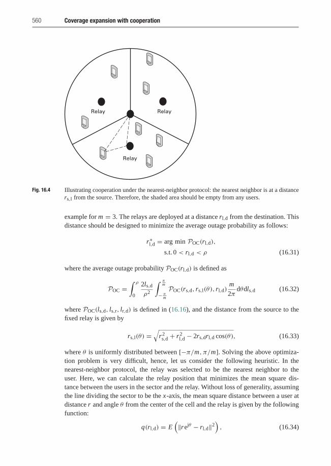
560 Coverage expansion with cooperation
Relay Relay
Relay
Fig. 16.4 Illustrating cooperation under the nearest-neighbor protocol: the nearest neighbor is at a distancers,l from the source. Therefore, the shaded area should be empty from any users.
example for m = 3. The relays are deployed at a distance rl,d from the destination. Thisdistance should be designed to minimize the average outage probability as follows:
r∗l,d = arg min POC(rl,d),
s.t. 0 < rl,d < ρ (16.31)
where the average outage probability POC(rl,d) is defined as
POC =∫ ρ
0
2ls,dρ2
∫ πm
− πm
POC(rs,d, rs,l(θ), rl,d)m
2πdθdls,d (16.32)
where POC(ls,d, ls,r, lr,d) is defined in (16.16), and the distance from the source to thefixed relay is given by
rs,l(θ) =√
r2s,d + r2
l,d − 2rs,drl,d cos(θ), (16.33)
where θ is uniformly distributed between [−π/m, π/m]. Solving the above optimiza-tion problem is very difficult, hence, let us consider the following heuristic. In thenearest-neighbor protocol, the relay was selected to be the nearest neighbor to theuser. Here, we can calculate the relay position that minimizes the mean square dis-tance between the users in the sector and the relay. Without loss of generality, assumingthe line dividing the sector to be the x-axis, the mean square distance between a user atdistance r and angle θ from the center of the cell and the relay is given by the followingfunction:
q(rl,d) = E(‖rejθ − rl,d‖2
), (16.34)
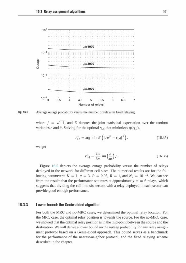
16.3 Relay assignment algorithms 561
3 3.5 4 4.5 5 5.5 6 6.5 710−3
10−2
10−1
100
Number of relays
Ou
tag
e
ρ = 2000
ρ = 3000
ρ = 4000
Fig. 16.5 Average outage probability versus the number of relays in fixed relaying.
where j = √−1, and E denotes the joint statistical expectation over the randomvariables r and θ . Solving for the optimal rl,d that minimizes q(rl,d),
r∗l,d = arg min E(‖rejθ − rl,d‖2
), (16.35)
we get
r∗l,d =2m
3πsin(π
m
)ρ. (16.36)
Figure 16.5 depicts the average outage probability versus the number of relaysdeployed in the network for different cell sizes. The numerical results are for the fol-lowing parameters: K = 1, α = 3, P = 0.05, R = 1, and N0 = 10−12. We can seefrom the results that the performance saturates at approximately m = 6 relays, whichsuggests that dividing the cell into six sectors with a relay deployed in each sector canprovide good enough performance.
16.3.3 Lower bound: the Genie-aided algorithm
For both the MRC and no-MRC cases, we determined the optimal relay location. Forthe MRC case, the optimal relay position is towards the source. For the no-MRC case,we showed that the optimal relay position is in the mid-point between the source and thedestination. We will derive a lower bound on the outage probability for any relay assign-ment protocol based on a Genie-aided approach. This bound serves as a benchmarkfor the performance of the nearest-neighbor protocol, and the fixed relaying schemedescribed in the chapter.
562 Coverage expansion with cooperation
The Genie-aided protocol works as follows. For any source node in the network, aGenie is going to put a relay at the optimal position on the line joining this source nodeand the destination (BS/AP).
Next we analyze the average outage performance of the Genie-aided protocol. For theMRC case, substituting the optimal relay position in (16.21) in the conditional outageexpression in (16.16) we get
POC(rs,d) = 1− f (γc, rs,d)− 1
1− x∗f (γc, (1− x∗)rs,d)
(f (γc, x
∗rs,d)− f (γc, rs,d)).
(16.37)
Averaging the above expression over the user distribution, the average outage probabil-ity for the Genie-aided lower bound for the MRC case I = 1 is given by
POG,1 = 1− 2
αρ2
(K P
N0γc
) 2α
�
(2
α,
N0γcρα
K P
)− 1
1− (x∗)α2
αρ2
(K P
N0γc ((1− x∗)α + (x∗)α)) 2α
�
(2
α,((1− x∗)α + (x∗)α) N0γcρ
α
K P
)+ 1
1− (x∗)α2
αρ2
(K P
N0γc ((1− x∗)α + 1)
) 2α
�
(2
α,((1− x∗)α + 1) N0γcρ
α
K P
)(16.38)
We will denote the average probability of outage for the no-MRC case by POG,2.Substituting the optimal relay position r∗s,l in the conditional outage expression (16.16),we get
POG(rs,d) =(
1− exp
(−N0γcrαs,d
K P
))(1− exp
(−2N0γc
( rs,d2
)αK P
)). (16.39)
Averaging the above expression over all possible users’ locations,
POG,2 = 1+ 2
αρ2
(k P
N0γc(1+ 21−α)
) 2α
�
(2
α,
N0γc(1+ 21−α) ρα
k P
)
− 2
αρ2
(k P
N0γc
) 2α
�
(2
α,
N0γcρα
k P
)− 2
αρ2
(k P
N0γc21−α
) 2α
�
(2
α,
N0γc21−αρα
k P
). (16.40)
16.4 Numerical results 563
16.4 Numerical results
We performed some computer simulations to compare the performance of the abovediscussed relay assignment protocols and validate the theoretical results we derived inthis chapter. In all of our simulations, we compared the outage performance of three dif-ferent transmission schemes: direct transmission, nearest-neighbor protocol, and fixedrelaying. In all of the simulations, the channel fading between any two nodes (either auser and the BS/AP or two users) is modeled as a random Rayleigh fading channel withunit variance.
For fairness in comparison between the described cooperative schemes and the directtransmission scheme, the spectral efficiency is kept fixed in both cases and this is doneas follows. Since a packet is either transmitted once or twice in the cooperative protocol,the average rate in the cooperative case can be calculated as
E(Rc) = RcPOD,γc(rs,d)+ Rc
2POD,γc(rsd). (16.41)
where Rc is the spectral efficiency in bits/s/Hz for cooperative transmission, andPOD,γc(rs,d) denotes the outage probability for the direct link at rate Rc. In (16.41),note that one time slot is utilized if the direct link is not in outage, and two time slotsare utilized if it is in outage. Note that the later scenario is true even if the relay does nottransmit because the time slot is wasted anyway. Averaging over the source–destinationseparation, the average rate is given by
Rc = Rc
2
(1+ 2
αρ2
(K P
γcN0
) 2α
�
(2
α,
N0γcρα
K P
))(16.42)
We need to calculate the SNR threshold γc corresponding to transmitting at rate Rc.The resulting SNR threshold γc should generally be larger than γnc required for non-cooperative transmission. It is in general very difficult to find an explicit relationbetween the SNR threshold γc and the transmission rate Rc, and thus we render to aspecial case to capture the insights of this scenario. Let the outage be defined as theevent that the mutual information I between two terminals is less than some specificrate R. If the transmitted signals are Gaussian, then according to our channel model, themutual information is given by I = log(1 + SNRs,d). The outage event for this case isdefined as
OI �{hs,d : I < R
} = {hs,d : SNRs,d < 2R − 1}. (16.43)
The above equation implies that if the outage is defined in terms of the mutual informa-tion and the transmitted signals are Gaussian, then the SNR threshold γc and the spectralefficiency R are related as γc = 2R
c − 1, i.e., they exhibit an exponential relation. Intu-itively, under a fixed modulation scheme and fixed average power constraint, one canthink of the SNR threshold as being proportional to the minimum distance between theconstellation points, which in turn depends on the number of constellation points forfixed average power, and the later has an exponential relation to the number of bits persymbol that determines the spectral efficiency R. For the sake of comparison Rc should
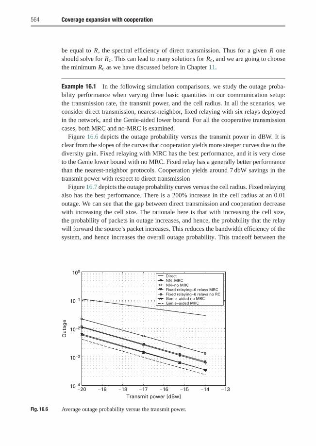
564 Coverage expansion with cooperation
be equal to R, the spectral efficiency of direct transmission. Thus for a given R oneshould solve for Rc. This can lead to many solutions for Rc, and we are going to choosethe minimum Rc as we have discussed before in Chapter 11.
Example 16.1 In the following simulation comparisons, we study the outage proba-bility performance when varying three basic quantities in our communication setup:the transmission rate, the transmit power, and the cell radius. In all the scenarios, weconsider direct transmission, nearest-neighbor, fixed relaying with six relays deployedin the network, and the Genie-aided lower bound. For all the cooperative transmissioncases, both MRC and no-MRC is examined.
Figure 16.6 depicts the outage probability versus the transmit power in dBW. It isclear from the slopes of the curves that cooperation yields more steeper curves due to thediversity gain. Fixed relaying with MRC has the best performance, and it is very closeto the Genie lower bound with no MRC. Fixed relay has a generally better performancethan the nearest-neighbor protocols. Cooperation yields around 7 dbW savings in thetransmit power with respect to direct transmission
Figure 16.7 depicts the outage probability curves versus the cell radius. Fixed relayingalso has the best performance. There is a 200% increase in the cell radius at an 0.01outage. We can see that the gap between direct transmission and cooperation decreasewith increasing the cell size. The rationale here is that with increasing the cell size,the probability of packets in outage increases, and hence, the probability that the relaywill forward the source’s packet increases. This reduces the bandwidth efficiency of thesystem, and hence increases the overall outage probability. This tradeoff between the
−20 −19 −18 −17 −16 −15 −14 −1310−4
10−3
10−2
10−1
100
Transmit power [dBw]
Ou
tag
e
DirectNN−MRCNN−no MRCFixed relaying−6 relays MRCFixed relaying−6 relays no RC
Genie−aided MRCGenie−aided no MRC
Fig. 16.6 Average outage probability versus the transmit power.
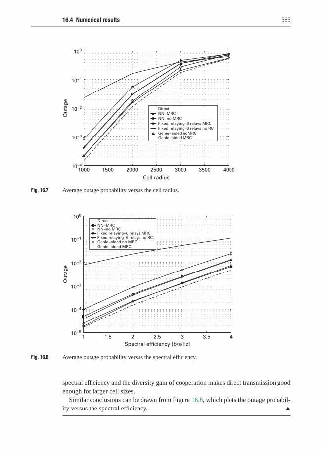
16.4 Numerical results 565
1000 1500 2000 2500 3000 3500 400010−4
10−3
10−2
10−1
100
Cell radius
Ou
tag
e
DirectNN−MRCNN−no MRCFixed relaying−6 relays MRCFixed relaying−6 relays no RC
Genie−aided MRCGenie−aided noMRC
Fig. 16.7 Average outage probability versus the cell radius.
1 1.5 2 2.5 3 3.5 410−5
10−4
10−3
10−2
10−1
100
Spectral efficiency [b/s/Hz]
Ou
tag
e
DirectNN−MRCNN−no MRCFixed relaying−6 relays MRCFixed relaying−6 relays no RC
Genie−aided MRCGenie−aided no MRC
Fig. 16.8 Average outage probability versus the spectral efficiency.
spectral efficiency and the diversity gain of cooperation makes direct transmission goodenough for larger cell sizes.
Similar conclusions can be drawn from Figure 16.8, which plots the outage probabil-ity versus the spectral efficiency. �
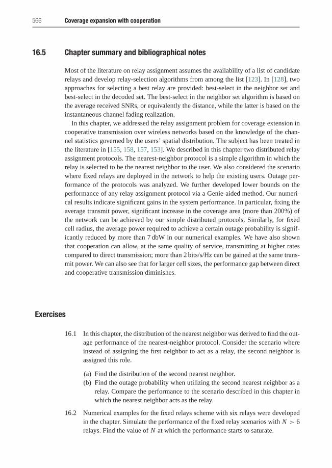
566 Coverage expansion with cooperation
16.5 Chapter summary and bibliographical notes
Most of the literature on relay assignment assumes the availability of a list of candidaterelays and develop relay-selection algorithms from among the list [123]. In [128], twoapproaches for selecting a best relay are provided: best-select in the neighbor set andbest-select in the decoded set. The best-select in the neighbor set algorithm is based onthe average received SNRs, or equivalently the distance, while the latter is based on theinstantaneous channel fading realization.
In this chapter, we addressed the relay assignment problem for coverage extension incooperative transmission over wireless networks based on the knowledge of the chan-nel statistics governed by the users’ spatial distribution. The subject has been treated inthe literature in [155, 158, 157, 153]. We described in this chapter two distributed relayassignment protocols. The nearest-neighbor protocol is a simple algorithm in which therelay is selected to be the nearest neighbor to the user. We also considered the scenariowhere fixed relays are deployed in the network to help the existing users. Outage per-formance of the protocols was analyzed. We further developed lower bounds on theperformance of any relay assignment protocol via a Genie-aided method. Our numeri-cal results indicate significant gains in the system performance. In particular, fixing theaverage transmit power, significant increase in the coverage area (more than 200%) ofthe network can be achieved by our simple distributed protocols. Similarly, for fixedcell radius, the average power required to achieve a certain outage probability is signif-icantly reduced by more than 7 dbW in our numerical examples. We have also shownthat cooperation can allow, at the same quality of service, transmitting at higher ratescompared to direct transmission; more than 2 bits/s/Hz can be gained at the same trans-mit power. We can also see that for larger cell sizes, the performance gap between directand cooperative transmission diminishes.
Exercises
16.1 In this chapter, the distribution of the nearest neighbor was derived to find the out-age performance of the nearest-neighbor protocol. Consider the scenario whereinstead of assigning the first neighbor to act as a relay, the second neighbor isassigned this role.
(a) Find the distribution of the second nearest neighbor.(b) Find the outage probability when utilizing the second nearest neighbor as a
relay. Compare the performance to the scenario described in this chapter inwhich the nearest neighbor acts as the relay.
16.2 Numerical examples for the fixed relays scheme with six relays were developedin the chapter. Simulate the performance of the fixed relay scenarios with N > 6relays. Find the value of N at which the performance starts to saturate.
Exercises 567
16.3 Assume a cell with a fixed user density of 20 users/km2.
(a) Write a Matlab code to simulate the outage probability performanceof the nearest neighbor protocol with increasing cell radius from 1 kmto 5 km.
(b) Assuming six relays are deployed in the cell, simulate the outage perfor-mance as a function of the cell radius.
16.4 Consider the scenario when you can at most deploy three relays in the cell inthe fixed-relaying technique. Compare the performance to the nearest-neighborprotocol assuming a fixed user density as in the previous problem.
16.5 Prove that the optimal relay location in the fixed relays strategy is given by(16.36), i.e., prove that
r∗l,d =2m
3πsin(π
m
)ρ. (E16.1)
16.6 Prove the outage probability expression when maximal ratio combiner (MRC)is used at the destination. Prove the following simplified form of the outageexpression:
POC(rs,d, rs,l, rl,d) =(1− f (γc, rs,d)
)− r−αl,d
r−αl,d − r−αs,d
× f (γc, rs,l)(
f (γc, rl,d)− f (γc, rs,d)).
16.7 Prove that the average outage probability for the Genie-aided lower bound forthe MRC case I = 1 is given by (16.38):
POG,1 = 1− 2
αρ2
(K P
N0γc
) 2α
�
(2
α,
N0γcρα
K P
)− 1
1− (x∗)α2
αρ2
(K P
N0γc ((1− x∗)α + (x∗)α)) 2α
× �(
2
α,((1− x∗)α + (x∗)α) N0γcρ
α
K P
)+ 1
1− (x∗)α2
αρ2
(K P
N0γc ((1− x∗)α + 1)
) 2α
× �(
2
α,((1− x∗)α + 1) N0γcρ
α
K P
).

568 Coverage expansion with cooperation
16.8 Prove that the average outage probability for the Genie-aided lower bound forthe no-MRC case is given by (16.40):
POG,2 = 1+ 2
αρ2
(k P
N0γc(1+ 21−α)
) 2α
�
(2
α,
N0γc(1+ 21−α) ρα
k P
)
− 2
αρ2
(k P
N0γc
) 2α
�
(2
α,
N0γcρα
k P
)− 2
αρ2
(k P
N0γc21−α
) 2α
× �(
2
α,
N0γc21−αρα
k P
).
17 Broadband cooperativecommunications
In broadband communications, OFDM is an effective means to capture multipathenergy, mitigate the intersymbol interference, and offer high spectral efficiency. OFDMis used in many communications systems, e.g., wireless local area networks (WLANs)and wireless personal area networks (WPANs). Recently, OFDM together with time–frequency interleaving across subbands, the so-called multiband OFDM [9], has beenadopted in the ultra-wideband (UWB) standard for wireless personal area networks(WPANs).
To improve the performance of OFDM systems, the fundamental concept of cooper-ative diversity can be applied. Nevertheless, special modulations/cooperation strategiesare needed to efficiently exploit the available multiple carriers.
In this chapter, we study an OFDM cooperative protocol that improves spectralefficiency over those based on fixed relaying protocols while achieving the same perfor-mance of full diversity. By exploiting limited feedback from the destination node, thedescribed protocol allows each relay to help forward information of multiple sourcesin one OFDM symbol. We also describe a practical relay assignment scheme forimplementing this cooperative protocol in OFDM networks.
17.1 System model
In this section, we describe the system model of a wireless network, in which we takeinto consideration the random users’ spatial distribution. The channel model, the signalmodel, and the performance measure in term of outage probability are discussed.
We consider an OFDM wireless network such as a WLAN or a WPAN with a circularcell of radius ρ. The cell contains one central node and multiple users, each communi-cating with the central node. The central node can be a base station or an access point incase of the WLAN, and it can be a piconet coordinator in case of the WPAN. Supposethe central node is located at the center of the cell, and K users are uniformly locatedwithin the cell. Then, the user’s distance Ds,d from the central node has the followingprobability density function (pdf):
pDs,d(D) = 2D/ρ2, 0 ≤ D ≤ ρ, (17.1)
and the user’s angle is uniformly distributed over [0, 2π). We assume that each node isequipped with single antenna, and its transmission is constrained to half-duplex mode.
570 Broadband cooperative communications
We consider an uplink scenario where all users transmit their information to the centralnode. Channel access within the cell is based on orthogonal multiple access mechanismas used in many current OFDM wireless networks.
The channel fades for different propagation links are assumed to be statisticallyindependent. This assumption is reasonable since nodes in the network are usually spa-tially well separated. The data packet of each user consists of preamble, header, andframe payload which carries several OFDM data symbols. The header includes the pilotsymbols which allow channel estimation to be performed at the central node.
For subsequent analysis, we consider a stochastic tapped-delay-line channel modelas in (1.6), which allows to take into consideration the frequency selectivity of wirelesschannels. If the channel between each pair of transmit-receive nodes have L inde-pendent delay paths, the channel impulse response from node i to node j can bemodeled as
hi, j (t) =L−1∑l=0
αi, j (l)δ(t − τi, j (l)), (17.2)
where the subscript {i, j} indicates the channel link from node i to node j , τi, j (l) is thedelay of the l-th path, and αi, j (l) is the complex amplitude of the l-th path. The pathamplitude |αi, j (l)| is Rayleigh distributed, whereas the phase � αi, j (l) is uniformly dis-tributed over [0, 2π). Specifically, The fade αi, j (l) is modeled as zero-mean, complexGaussian random variables with variances E
[|αi, j (l)|2] = �i, j (l),
The received signal at subcarrier n of destination d from source user s can bemodeled as
ys,d(n) =√
PncκD−νs,d Hs,d(n)xs(n)+ zs,d(n), (17.3)
where Pnc is the transmitted power in each subcarrier at the source in non-cooperativemode, xs(n) denotes an information symbol to be transmitted from the source s atsubcarrier n, zs,d(n) is an additive white Gaussian noise with zero mean and varianceN0, and Hs,d(n) is the frequency response of the channel at the n-th subcarrier. If weconsider OFDM with N subcarriers and assume that the length of cyclic prefix in theOFDM symbol is longer than the channel delay spread, then we can express the channelfrequency response as
Hs,d(n) =L−1∑l=0
αs,d(l) exp (−j2πnτs,d(l)/N ). (17.4)
In (17.3), κ is a constant whose value depends on the propagation environment andantenna design, ν is the propagation loss factor, and Ds,d represents the distancebetween source node s and destination node d. The parameters Pnc, κ , and ν areassumed to be the same for all users.
Let each information symbol have unit energy. For a given distance Ds,d betweenthe source and the destination, the received signal-to-noise ratio (SNR) for the n-thsubcarrier can be given by
ζ(n)s,d = PncκD−νs,d |Hs,d(n)|2/N0. (17.5)
17.2 Cooperative protocol and relay-assignment scheme 571
In case of direct transmission between two nodes that are Ds,d apart, the maximumaverage mutual information in a subcarrier n, which is achieved for the independentand identically distributed zero-mean, circularly symmetric complex Gaussian inputs,is given by
I (n)(Ds,d) = log(1+ ζ (n)s,d ). (17.6)
Let R denote a target rate for each subcarrier, then the probability that a subcarrier is inoutage can be given by
PDout(Ds,d) = Pr
(I (n)(Ds,d) ≤ R
)= Pr
(ζ(n)s,d ≤ 2R − 1
). (17.7)
If an outage occurs in a subcarrier, then the transmitted information in that subcarrieris considered loss. Otherwise, the receiver is assumed to be able to decode the receivedinformation with negligible probability of error.
17.2 Cooperative protocol and relay-assignment scheme
In this section, we first describe the cooperative protocol for OFDM wireless networks,and then present the relay assignment scheme. Consider a cooperation scenario whereeach source can employ a relay to forward its information to the destination.
In phase 1, each user transmits its packet to the destination (central node) and thepackets are also received at the relay. After receiving the user’s packet, the destinationperforms channel estimation using the OFDM pilot symbols in the packet header. Basedon the estimated channel coefficients, the destination is able to specify which subcarriersymbols are not received successfully (i.e., those in the subcarriers of which the com-bined SNRs fall below the required SNR threshold), and then broadcasts the indicesof the subcarriers carrying those symbols. Such feedback enables the assigned relay tohelp forward the source information only when necessary.
In phase 2, the relay decodes the source symbols that are unsuccessfully receivedat the destination via direct transmission, and then forwards the decoded information tothe destination. The relay will only decode the source symbol that the relay is capable ofcapturing, i.e., when the received SNR at the relay is above the target threshold. Since itis unlikely that all subcarrier symbols are sent unsuccessfully by the source, the protocolmakes efficient use of the available bandwidth by allowing the relay to help forward theinformation of multiple source users in one OFDM block.
Specifically, suppose a relay is assigned to help k users, then after all k users transmittheir packets in phase 1, the relay sends in phase 2 an additional packet containingthese users’ symbols that are not captured at the destination in phase 1. In order for thedestination to know which relay subcarriers carry information of which users, the relaycan send an additional overhead together with the source symbols. Or the relay can usea fixed subcarrier assignment scheme such that that the destination can specify the relaysubcarrier assignment without the use of additional overhead.
For instance, if ni subcarriers of user i are in outage, then in phase 2, the relay canuse the first n1 subcarriers to transmit the data of user 1, the next n2 subcarriers to
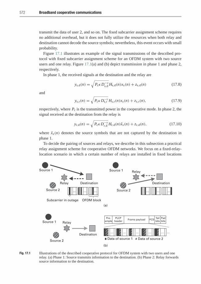
572 Broadband cooperative communications
transmit the data of user 2, and so on. The fixed subcarrier assignment scheme requiresno additional overhead, but it does not fully utilize the resources when both relay anddestination cannot decode the source symbols; nevertheless, this event occurs with smallprobability.
Figure 17.1 illustrates as example of the signal transmissions of the described pro-tocol with fixed subcarrier assignment scheme for an OFDM system with two sourceusers and one relay. Figure 17.1(a) and (b) depict transmission in phase 1 and phase 2,respectively.
In phase 1, the received signals at the destination and the relay are
ys,d(n) =√
PcκD−νs,d Hs,d(n)xs(n)+ zs,d(n) (17.8)
and
ys,r(n) =√
PcκD−νs,r Hs,r(n)xs(n)+ zs,r(n), (17.9)
respectively, where Pc is the transmitted power in the cooperative mode. In phase 2, thesignal received at the destination from the relay is
yr,d(n) =√
PcκD−νr,d Hr,d(n)xs(n)+ zr,d(n), (17.10)
where xs(n) denotes the source symbols that are not captured by the destination inphase 1.
To decide the pairing of sources and relays, we describe in this subsection a practicalrelay assignment scheme for cooperative OFDM networks. We focus on a fixed-relay-location scenario in which a certain number of relays are installed in fixed locations
Source 1
Source 1
Source 1
Relay
Relay
Relay
Destination
DestinationData of source 1 Data of source 2
Frame payload FCSTailbits
Padbits
Pre-ample
PLCPheader
Destination
Subcarrier in outage
Source 2
Source 2
Source 2
OFDM block
(a)
(b)
Fig. 17.1 Illustrations of the described cooperative protocol for OFDM system with two users and onerelay. (a) Phase 1: Source transmits information to the destination. (b) Phase 2: Relay forwardssource information to the destination.
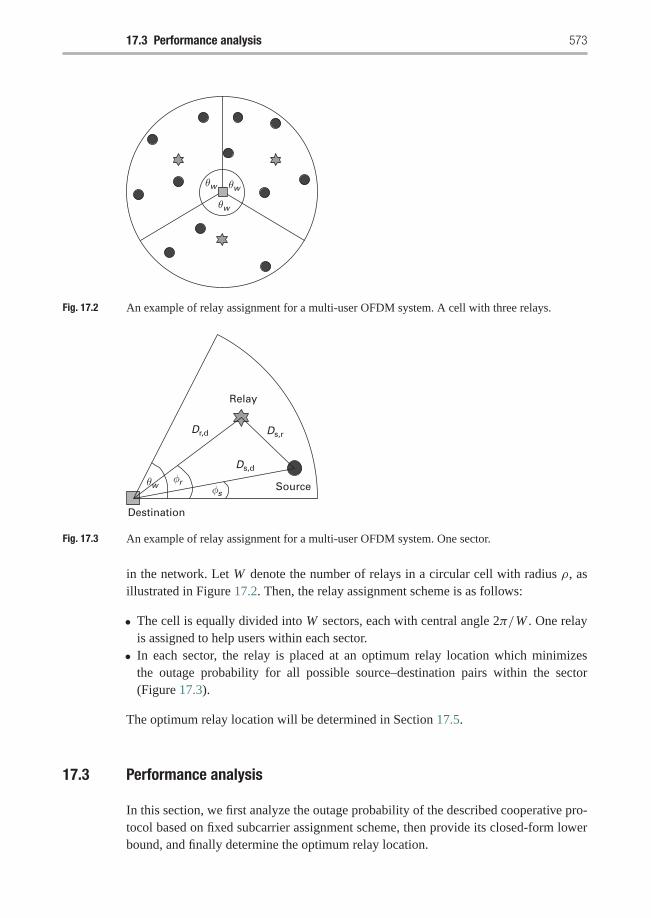
17.3 Performance analysis 573
θw θw
θw
Fig. 17.2 An example of relay assignment for a multi-user OFDM system. A cell with three relays.
Source
Relay
Destination
Dr,d
Ds,d
φs
φrθw
Ds,r
Fig. 17.3 An example of relay assignment for a multi-user OFDM system. One sector.
in the network. Let W denote the number of relays in a circular cell with radius ρ, asillustrated in Figure 17.2. Then, the relay assignment scheme is as follows:
• The cell is equally divided into W sectors, each with central angle 2π/W . One relayis assigned to help users within each sector.
• In each sector, the relay is placed at an optimum relay location which minimizesthe outage probability for all possible source–destination pairs within the sector(Figure 17.3).
The optimum relay location will be determined in Section 17.5.
17.3 Performance analysis
In this section, we first analyze the outage probability of the described cooperative pro-tocol based on fixed subcarrier assignment scheme, then provide its closed-form lowerbound, and finally determine the optimum relay location.
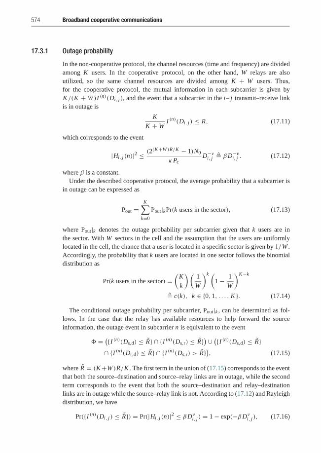
574 Broadband cooperative communications
17.3.1 Outage probability
In the non-cooperative protocol, the channel resources (time and frequency) are dividedamong K users. In the cooperative protocol, on the other hand, W relays are alsoutilized, so the same channel resources are divided among K + W users. Thus,for the cooperative protocol, the mutual information in each subcarrier is given byK/(K + W )I (n)(Di, j ), and the event that a subcarrier in the i– j transmit–receive linkis in outage is
K
K +WI (n)(Di, j ) ≤ R, (17.11)
which corresponds to the event
|Hi, j (n)|2 ≤ (2(K+W )R/K − 1)N0
κPcD−νi, j � βD−νi, j . (17.12)
where β is a constant.Under the described cooperative protocol, the average probability that a subcarrier is
in outage can be expressed as
Pout =K∑
k=0
Pout|kPr(k users in the sector), (17.13)
where Pout|k denotes the outage probability per subcarrier given that k users are inthe sector. With W sectors in the cell and the assumption that the users are uniformlylocated in the cell, the chance that a user is located in a specific sector is given by 1/W .Accordingly, the probability that k users are located in one sector follows the binomialdistribution as
Pr(k users in the sector) =(
K
k
)(1
W
)k (1− 1
W
)K−k
� c(k), k ∈ {0, 1, . . . , K }. (17.14)
The conditional outage probability per subcarrier, Pout|k , can be determined as fol-lows. In the case that the relay has available resources to help forward the sourceinformation, the outage event in subcarrier n is equivalent to the event
� = ({I (n)(Ds,d) ≤ R} ∩ {I (n)(Ds,r) ≤ R}) ∪ ({I (n)(Ds,d) ≤ R}∩ {I (n)(Dr,d) ≤ R} ∩ {I (n)(Ds,r) > R}), (17.15)
where R = (K+W )R/K . The first term in the union of (17.15) corresponds to the eventthat both the source–destination and source–relay links are in outage, while the secondterm corresponds to the event that both the source–destination and relay–destinationlinks are in outage while the source–relay link is not. According to (17.12) and Rayleighdistribution, we have
Pr({I (n)(Di, j ) ≤ R}) = Pr(|Hi, j (n)|2 ≤ βDνi, j ) = 1− exp(−βDνi, j ), (17.16)
17.3 Performance analysis 575
where β is defined in (17.12). Note that the events in the union in (17.15) are mutuallyexclusive. Hence, the conditional outage probability under the cooperative mode can bedetermined as
PCout =
⎡⎣1− exp
⎛⎝− (2R − 1)N0 Dνs,dκPc
⎞⎠⎤⎦[1− exp
(− (2
R − 1)N0
κPc(Dνs,r + Dνr,d)
)].
(17.17)In case that the relay does not have resources to help forward the source information,the outage event in subcarrier n is equivalent to that of direct transmission between thesource and destination, which is given by
PDout = Pr
(I (n)(Ds,d) ≤ R
) = 1− exp
(− (2
(K+W )R/K − 1)N0 Dνs,dκPc
). (17.18)
Given k users in the sector, the conditional outage probability per subcarrier can beobtained from (17.17) and (17.18) as
Pout|k = PCout(1− Q|k)+ PD
outQ|k . (17.19)
In (17.19), Q|k is defined as the probability that a source subcarrier that is in outage isnot helped by the relay, under the condition that there are k users in the sector. In otherwords, the relay uses all of its resources to help forward the k users’ information carriedin other subcarriers. The physical meaning of (17.19) is that a diversity gain of two isachieved when the relay has available resource to help forward the source information,which occurs with probability Q|k , whereas the diversity gain reduces to one when allthe resources (allocated subcarriers) at the relay are fully used.
The probability Q|k can be determined as follows. Consider a sector with k users,each transmitting information in N subcarriers during one OFDM symbol period.Equivalently, the total number of kN subcarriers (in k OFDM symbol periods) are usedto transmit the information from all k users in the sector. Assume that the subcarriersin outage are helped by the relay with equal probability. Then, given that x out of kNsubcarriers are in outage, the probability that a subcarrier in outage is not helped by therelay is (x − N )/x for N + 1 ≤ x ≤ kN . Thus, the probability Q|k can be obtained as
Q|k =kN∑
x=N+1
x − N
xPr(x out of kN subcarriers in outage). (17.20)
Since each subcarrier is in outage with probability PDout, the probability that x out of
kN subcarriers are in outage can be approximated by
Pr(x out of kN subcarriers in outage) =(
kN
x
)(PD
out
)x (1− PD
out
)kN−x. (17.21)
In (17.21), it is difficult, if not impossible, to derive a closed form formulation thatincludes all possible combinations of the users’ locations. For analytical tractability ofthe analysis, we resort to an approximate probability which is based on an assumptionthat all the x subcarriers are in outage with the same probability PD
out. This approx-imation would be effective for small cell sizes where path loss is not the dominant
576 Broadband cooperative communications
fading effect. As we will show later, the analytical outage probability obtained fromthis approximation is very close to the simulation results.
Substituting (17.18) and (17.21) into (17.20), we obtain the probability Q|k as
Q|k =kN∑
x=N+1
x − N
x
(kN
x
)[1− exp(−βDνs,d)
]x[ exp(−βDνs,d)]kN−x
. (17.22)
From (17.22) and (17.19), we can determine the conditional outage probability of thedescribed scheme as
Pout|k =(1− exp(−βDνs,d)
)(1− exp(−β(Dνs,r + Dνr,d))
)(1− Q|k)
+ (1− exp(−βDνs,d))Q|k . (17.23)
Substituting (17.14) and (17.23) into (17.13), the outage probability of the describedscheme can be obtained as
Pout =(1− exp(−βDνs,d)
)[1− exp(−β(Dνs,r + Dνr,d))(1− g(Ds,d))
]; (17.24)
where
g(Ds,d) =K∑
k=1
c(k)kN∑
x=N+1
x − N
x
(kN
x
)[1− exp(−βDνs,d)
]x[ exp(−βDνs,d)]kN−x
.
(17.25)It is worth noting that when spectral efficiency goes to infinity, direct transmission out-performs cooperative communications. As the number of users increases, for a fixednumber of relays, the performance of the cooperative scheme approaches that of directtransmission.
Finally, we determine the average outage probability by averaging (17.24) over thedistribution of the user’s distance as follows. Without loss of generality, we consider asector as shown in Figure 17.2 where the relay is located at Dr,dejφr and a source useris located at Ds,dejφs (0 ≤ φr , φs ≤ θw). The distance between the source and the relaycan be expressed as
Ds,r =[D2
s,d + D2r,d − 2Ds,d Dr,d cos(φr − φs)
] 12 � f (Ds,d, φs). (17.26)
Assuming that users are uniformly distributed within the cell, the pdf of the user’s dis-tance D from the destination conditioned that the user is located in the sector can begiven by
pD(D | 0 ≤ φs ≤ θW ) = 2D
Wρ2, 0 ≤ D ≤ ρ. (17.27)
Therefore, given specific relay locations, the average outage probability of the coopera-tive protocol can be obtained as
Pout = 1
πρ2
∫ ρ
0
∫ 2πW
0
[1− e−β( f ν (Ds,d,φs )+Dνr,d)(1− g(Ds,d))
]× Ds,d
(1− e−βDνs,d
)dφsdDs,d. (17.28)
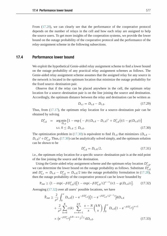
17.4 Performance lower bound 577
From (17.28), we can clearly see that the performance of the cooperative protocoldepends on the number of relays in the cell and how each relay are assigned to helpthe source users. To get more insights of the cooperation systems, we provide the lowerbound on the outage probability of the cooperative protocol and the performance of therelay-assignment scheme in the following subsections.
17.4 Performance lower bound
We exploit the hypothetical Genie-aided relay assignment scheme to find a lower boundon the outage probability of any practical relay assignment schemes as follows. TheGenie-aided relay assignment scheme assumes that the assigned relay for any source inthe network is located in the optimum location that minimize the outage probability forthe fixed source–destination pair.
Observe that if the relay can be placed anywhere in the cell, the optimum relaylocation for a source–destination pair is on the line joining the source and destination.Accordingly, the optimum distance between the relay and destination can be written as
Ds,r = Ds,d − Dr,d. (17.29)
Thus, from (17.17), the optimum relay location for a source–destination pair can beobtained by solving
D∗r,d = arg minDr,d
{1− exp
(− β((Ds,d − Dr,d)ν + Dνr,d)
)(1− g(Ds,d))
}s.t. 0 ≤ Dr,d ≤ Ds,d. (17.30)
The optimization problem in (17.30) is equivalent to find Dr,d that minimizes (Ds,d −Dr,d)
ν+Dνr,d. Thus, (17.30) can be analytically solved simply, and the optimum solutioncan be shown to be
D∗r,d = Ds,d/2, (17.31)
i.e., the optimum relay location for a specific source–destination pair is at the mid pointof the line joining the source and the destination.
Using the Genie-aided relay assignment scheme and the optimum relay location D∗r,d,we can determine the lower bound on the outage probability as follows. Substitute D∗r,dand D∗s,r = Ds,d − D∗r,d = Ds,d/2 into the outage probability formulation in (17.28),then the outage probability of the cooperative protocol can be lower bounded by
Pout ≥(1− exp(−βDνs,d)
)[1− exp(−βDνs,d/(2
ν−1))(1− g(Ds,d))]. (17.32)
Averaging (17.32) over all users’ possible locations, we have
Pout ≥ 2
ρ2
∫ ρ
0Ds,d
(1− e−βDνs,d
)[1− e−βDνs,d/(2
ν−1)]dDs,d
+ 2
ρ2
K∑k=0
c(k)kN∑
x=N+1
x − N
x
(kN
x
)∫ ρ
0Ds,d
(1− e−βDνs,d
)x+1
× (e−βDνs,d)kN−x+ 1
2ν−1 dDs,d. (17.33)
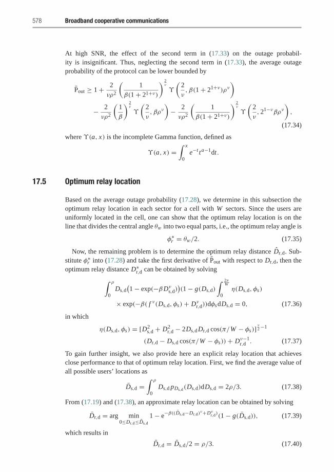
578 Broadband cooperative communications
At high SNR, the effect of the second term in (17.33) on the outage probabil-ity is insignificant. Thus, neglecting the second term in (17.33), the average outageprobability of the protocol can be lower bounded by
Pout ≥ 1+ 2
νρ2
(1
β(1+ 21+ν)
) 2ν
ϒ
(2
ν, β(1+ 21+ν)ρν
)− 2
νρ2
(1
β
) 2ν
ϒ
(2
ν, βρν
)− 2
νρ2
(1
β(1+ 21+ν)
) 2ν
ϒ
(2
ν, 21−νβρν
),
(17.34)
where ϒ(a, x) is the incomplete Gamma function, defined as
ϒ(a, x) =∫ x
0e−t ta−1dt.
17.5 Optimum relay location
Based on the average outage probability (17.28), we determine in this subsection theoptimum relay location in each sector for a cell with W sectors. Since the users areuniformly located in the cell, one can show that the optimum relay location is on theline that divides the central angle θw into two equal parts, i.e., the optimum relay angle is
φ∗r = θw/2. (17.35)
Now, the remaining problem is to determine the optimum relay distance Dr,d. Sub-stitute φ∗r into (17.28) and take the first derivative of Pout with respect to Dr,d, then theoptimum relay distance D∗r,d can be obtained by solving∫ ρ
0Ds,d
(1− exp(−βDνs,d)
)(1− g(Ds,d)
∫ 2πW
0η(Ds,d, φs)
× exp(−β( f ν(Ds,d, φs)+ Dνr,d))dφsdDs,d = 0, (17.36)
in which
η(Ds,d, φs) = [D2s,d + D2
r,d − 2Ds,d Dr,d cos(π/W − φs)] ν2−1
(Dr,d − Ds,d cos(π/W − φs))+ Dν−1r,d . (17.37)
To gain further insight, we also provide here an explicit relay location that achievesclose performance to that of optimum relay location. First, we find the average value ofall possible users’ locations as
Ds,d =∫ ρ
0Ds,d pDs,d(Ds,d)dDs,d = 2ρ/3. (17.38)
From (17.19) and (17.38), an approximate relay location can be obtained by solving
Dr,d = arg min0≤Dr,d≤Ds,d
1− e−β((Ds,d−Dr,d)ν+Dνr,d)(1− g(Ds,d)), (17.39)
which results in
Dr,d = Ds,d/2 = ρ/3. (17.40)
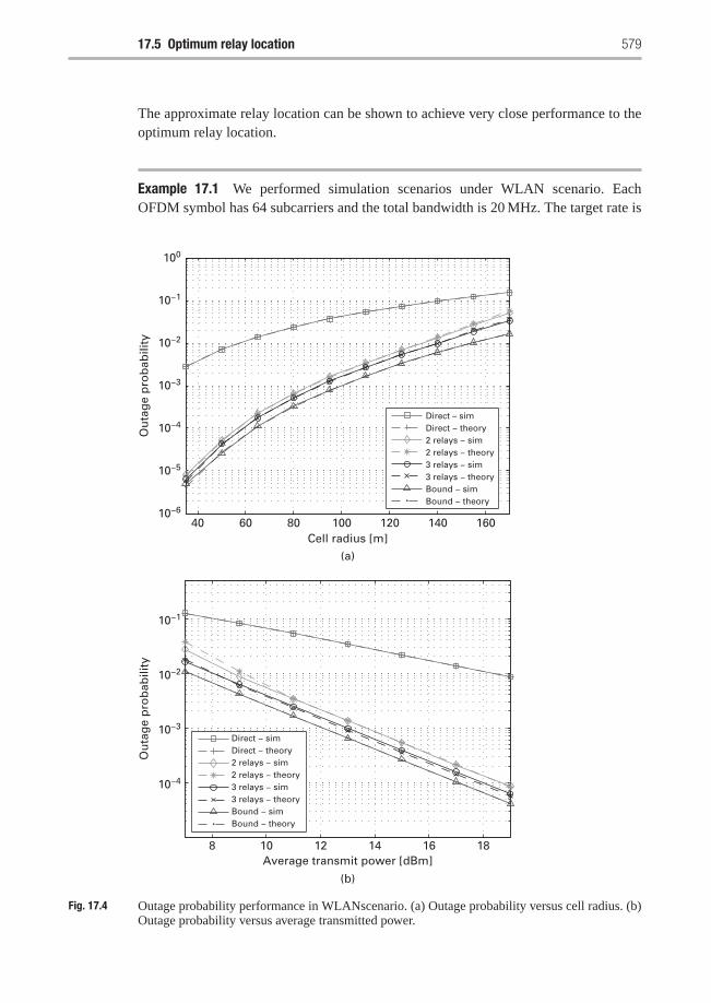
17.5 Optimum relay location 579
The approximate relay location can be shown to achieve very close performance to theoptimum relay location.
Example 17.1 We performed simulation scenarios under WLAN scenario. EachOFDM symbol has 64 subcarriers and the total bandwidth is 20 MHz. The target rate is
40 60 80 100 120 140 16010−6
10−5
10−4
10−3
10−2
10−1
10−4
10−3
10−2
10−1
100
Ou
tag
e p
rob
abili
ty
Cell radius [m]
(a)
(b)
Direct – simDirect − theory2 relays − sim2 relays − theory3 relays − sim3 relays − theoryBound − simBound − theory
8 10 12 14 16 18
Ou
tag
e p
rob
abili
ty
Average transmit power [dBm]
Direct − simDirect − theory2 relays − sim2 relays − theory3 relays − sim3 relays − theoryBound − simBound − theory
Fig. 17.4 Outage probability performance in WLANscenario. (a) Outage probability versus cell radius. (b)Outage probability versus average transmitted power.
580 Broadband cooperative communications
fixed at R = 1 bit/s/Hz per user per subcarrier. The propagation loss factor is ν = 2.6,and the number of users in the cell is set at 10 users.
Figure 17.4(a) and (b) compare the performance of the cooperative protocol withthat of direct transmission scheme and the lower bound. The theoretical performance isplotted along with the simulation curves.
Figure 17.4(a) depicts the outage probability versus the cell radius. The average trans-mitted power is fixed at 12 dBm. If the outage performance is required to be at most0.01, then the maximum cell size achieved by the direct transmission scheme is about60 m. With the cooperative protocol, the maximum cell size of 132 m and 140 m canbe achieved when 2 and 3 relays are deployed, respectively. The cooperative protocolcan increase the cell size by about 130% in this case. Moreover, the described schemeachieves close performance to the lower bound, especially when the cell size is small.
In Figure 17.4(b), we study the performance gain that can be achieved by the coop-eration protocol in terms of energy efficiency. The cell radius is fixed at 100 m, andthe average transmitted power varies from 7 dBm to 19 dBm. If the outage is requiredto be at most 0.01, then the direct transmission scheme requires the transmitted powerof 18 dBm, whereas the cooperation scheme requires only about 8 dBm; in other words,10 dB power saving is achieved. It is worth pointing out that diversity is a high SNR con-cept and the cooperative scheme is able to achieve the diversity gain of two at practicaltransmit powers.
In both figures, the theoretical curves closely match to the simulation results, whichvalidates the analysis. Note that the simulation and theoretical results completely matchin the direct transmission case. �
17.6 Chapter summary and bibliographical notes
For broadband networks, we described a bandwidth-efficient cooperative protocol formultiuser OFDM systems. The destination broadcasts subcarrier indices of which thereceived SNR falls below a specific SNR threshold, and the relay forwards only thesource symbols carried in those subcarriers. In this way, the relay can help forwardthe data of multiple sources in one OFDM symbol, and the described protocol greatlyimproves the spectral efficiency, while still achieving full diversity at high SNR. Relayassignment algorithms have been described. On the topic of cooperative communi-cations protocol for multiuser OFDM networks, more information can be found in[192, 191].
An application of space–time cooperation in OFDM systems was investigated in[233]. In [57], pairing of users and level of cooperation are jointly determined to mini-mize overall transmitted power of OFDM system. Most of the existing works are basedon fixed relaying protocols, in which the relays always repeat the source information.Moreover, these works rely on an assumption of fixed channel variances which impliesa fixed network topology and fixed source–relay pairs.
Exercises 581
Exercises
17.1 Prove the conditional outage probability expression under the cooperative modein 17.17, i.e., prove
PCout =
[1− exp
(− (2
R − 1)N0 Dνs,dκPc
)]×[1− exp
(− (2
R − 1)N0
κPc(Dνs,r + Dνr,d)
)].
17.2 Prove the expression in (17.23):
Pout|k =(1− exp(−βDνs,d)
)(1− exp(−β(Dνs,r + Dνr,d))
)(1− Q|k)
+ (1− exp(−βDνs,d))Q|k .
17.3 Conditioned on the user’s location, prove that the outage probability of thecooperative broadband scheme described in this chapter is given by
Pout =(1− exp(−βDνs,d)
)[1− exp(−β(Dνs,r + Dνr,d))(1− g(Ds,d))
];where
g(Ds,d) =K∑
k=1
c(k)kN∑
x=N+1
x − N
x
(kN
x
)× [1− exp(−βDνs,d)
]x[ exp(−βDνs,d)]kN−x
.
17.4 Consider a WLAN system. Each OFDM symbol has 128 subcarriers and thetotal bandwidth is 20 MHz. The target rate is fixed at R=1 bit/s/Hz per user persubcarrier. The propagation loss factor is ν = 2.6, and the number of users in thecell is set at 10 users.
(a) Write Matlab code to simulate the outage performance of the broadbandcooperative protocol with direct transmission versus cell radius when thepower is fixed at 12 dBm.
(b) Repeat part (a) by fixing the cell radius at 100 m and varying the transmitpower.
(c) Consider now an OFDM system that uses 512 subcarriers. Repeat parts (a)and (b). What is the effect of increasing the number of subcarriers on theperformance of the cooperation protocol.
17.5 In this chapter, the relay is assumed to use an incremental relaying scheme withdecode-and-forward. Assume instead that the relay uses only selective decode-and-forward. In such scenario the relay will only forward the packets from usersthat where decoded correctly irrespective of whether the destination was able todecode the packet correctly or not.
(a) Find the outage probability for a single user.(b) Find the outage probability assuming N users in each sector.

582 Broadband cooperative communications
(c) Compare the performance of such relaying scheme with that described in thechapter.
17.6 The uplink case is studied in this chapter. Consider now the downlink where thebase station transmits data to different users. Assume there are N users in eachsector, and that the base station schedules the users in N consecutive time slots.In each time slot the base station transmits an OFDM symbol to a user. A singlerelay is deployed in each sector to help the users using a similar approach asdescribed in the chapter.
(a) Find the probability that a user has n subcarriers in outage.(b) Find the outage probability of m subcarriers at the relay node for a given
base station transmission.(c) Find the total average outage probability taking into account the finite
resources at the relay.
18 Network lifetime maximizationvia cooperation
Extending the lifetime of battery-operated devices is a key design issue that allowsuninterrupted information exchange among distributed nodes in wireless networks.Cooperative communications enables and leverages effective resource sharing amongcooperative nodes. This chapter provides a general framework for lifetime extension ofbattery-operated devices by exploiting cooperative diversity. The framework efficientlytakes advantage of different locations and energy levels among distributed nodes. First,a lifetime maximization problem via cooperative nodes is considered and performanceanalysis for M-ary PSK modulation is provided. With an objective to maximize theminimum device lifetime under a constraint on bit error rate performance, the optimiza-tion problem determines which nodes should cooperate and how much power should beallocated for cooperation. Moreover, the device lifetime is further improved by a deploy-ment of cooperative relays in order to help forward information of the distributed nodesin the network. Optimum location and power allocation for each cooperative relay aredetermined with an aim to maximize the minimum device lifetime. A suboptimal algo-rithm is presented to solve the problem with multiple cooperative relays and cooperativenodes.
18.1 Introduction
In many applications of wireless networks, extending the lifetime of battery-operateddevices is a key design issue that ensures uninterrupted information exchange and alle-viates burden of replenishing batteries. Lifetime extension of battery-limited deviceshas become an important issue due to the need in sensor and ad-hoc networks. However,there is not a broadly accepted definition of the concept of network lifetime because itoften depends on the application of the networks under consideration. For example, anetwork lifetime can be defined as the time until the first node in the network dies or asthe time until a certain percentage of nodes die. Alternatively, concerning the quality ofcommunication, network lifetime can be defined in terms of the packet delivery rate orin terms of the number of alive flows.
Consider contemporary wireless networks which comprise heterogeneous devicessuch as mobile phones, laptop computers, personal digital assistants (PDAs), etc. Thesedevices have limited lifetime; nevertheless, some of them may have longer lifetimes dueto their location or energy advantages. For instance, a devices in some ideal location
584 Network lifetime maximization via cooperation
may have location advantage, while another devices may have energy advantage if theyare equipped with high initial energy. By introducing a cooperation protocol among dis-tributed nodes, a portion of energy from these devices can be allocated to help forwardinformation of other energy depleting devices in the network. In this way, the lifetime ofthe energy depleting devices can be greatly improved, and hence, the minimum devicelifetime of the network is increased.
In this chapter, we show a framework to increase the device lifetime by exploitingcooperative diversity and leveraging both location and energy advantages in wirelessnetworks. The framework is based on the decode-and-forward (DF) cooperation pro-tocol, which is well-suited for wireless LAN or cellular settings; nevertheless, othercooperation protocols such as amplify-and-forward can be used as well. We firstdescribe a signal model for a non-cooperative network. Then, we present a signal modelfor a cooperative networks employing the DF protocol. After that, we consider an opti-mization problem with the goal of maximizing the minimum device lifetime under a biterror rate (BER) constraint. Following this, we analyze the problem based on the useof an M-ary phase shift keying (M-PSK) modulation scheme. From this, it becomespossible to derive an analytical solution for a two-node cooperative network, whichprovides some insights into the optimization problem. The challenge in this stage isthat the problem is N P hard. Based on the two-node solution, we consider a fast sub-optimal algorithm to reduce the complexity of the formulated problem. Furthermore,we consider device lifetime improvement by deploying additional relays over a net-work with energy depleting nodes. This will lead into determining where to place therelays and how much power should these relays use for cooperation in order to maxi-mize the device lifetime. In addition, to reduce complexity of the optimization problem,we restrict the number of relays per nodes to at most one, in which case we study anefficient suboptimal algorithm.
18.2 System models
Consider a wireless network with N randomly deployed nodes as shown in Figure 18.1.Each node knows its next node in a predetermined route that connects to the destina-tion to deliver information. The destination node can be a base station or an accesspoint in wireless local area networks, a piconet coordinator in wireless personal areanetwork, or a data-gathering unit in wireless sensor networks. Next, we describe the sys-tem model for a non-cooperative network and for a cooperative network in two separatesubsections, starting with the non-cooperative scenario.
18.2.1 Non-cooperative wireless networks
In a non-cooperative wireless network, each source node transmits only its own infor-mation to the destination node through a predetermined route. Figure 18.1 shows anexample of a wireless network with several randomly deployed nodes. Suppose thereare N nodes in the network, and let x j denotes a symbol to be transmitted from node j to
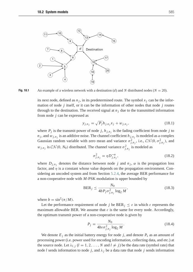
18.2 System models 585
Destinationd
14
15
17
2018
19
16
6
5
4
3
2
1
7 8
9
101112
13
Fig. 18.1 An example of a wireless network with a destination (d) and N distributed nodes (N = 20).
its next node, defined as n j , in its predetermined route. The symbol x j can be the infor-mation of node j itself, or it can be the information of other nodes that node j routesthrough to the destination. The received signal at n j due to the transmitted informationfrom node j can be expressed as
y j,n j =√
Pj h j,n j x j + w j,n j , (18.1)
where Pj is the transmit power of node j , h j,n j is the fading coefficient from node j ton j , andw j,n j is an additive noise. The channel coefficient h j,n j is modeled as a complexGaussian random variable with zero mean and variance σ 2
j,n j, i.e., CN (0, σ 2
j,n j), and
w j,n j is CN (0, N0) distributed. The channel variance σ 2j,n j
is modeled as
σ 2j,n j
= ηD−αj,n j, (18.2)
where D j,n j denotes the distance between node j and n j , α is the propagation lossfactor, and η is a constant whose value depends on the propagation environment. Con-sidering an uncoded system and from Section 5.2.4, the average BER performance fora non-cooperative node with M-PSK modulation is upper bounded by
BER j ≤ N0
4bPjσ2j,n j
log2 M, (18.3)
where b = sin2(π/M).Let the performance requirement of node j be BER j ≤ ε in which ε represents the
maximum allowable BER. We assume that ε is the same for every node. Accordingly,the optimum transmit power of a non-cooperative node is given by
Pj = N0
4bεσ 2j,n j
log2 M. (18.4)
We denote E j as the initial battery energy for node j , and denote Ps as an amount ofprocessing power (i.e. power used for encoding information, collecting data, and etc.) atthe source node. Let λl, j (l = 1, 2, . . . , N and l �= j) be the data rate (symbol rate) thatnode l sends information to node j , and λ j be a data rate that node j sends information
586 Network lifetime maximization via cooperation
to its next node n j . Assume that the symbol length is fixed and equal for all nodes inthe network and that the symbol length is normalized such that the energy required totransmit a symbol is given by the transmit power. Furthermore assume that the symbolrate generated at any node is low which is typical for most sensor networks applications.Also assume in the analysis that the cumulative data rate that need to be transmitted atany node (node’s own generated data plus the data being routed for other nodes) is lowerthan the node’s service rate. This guarantees that any node’s buffer in the network doesnot overflow.
The average power that node j uses to send information to n j is λ j Ps+∑Nl=1 λl, j Pj ,
where λ j Ps is the average processing power at node j , λ j Pj represents the averagepower that node j sends its own formation, and
∑Nl=1,l �= j λl, j Pj corresponds to the
average power that node j routes information of other nodes. Accordingly, the lifetimeof node j can be determined as
Tj = E j
λ j Ps + Pj∑N
l=1 λl, j=
4bεσ 2j,n j
E j log2 M
4bεσ 2j,n jλ j Ps log2 M + N0
∑Nl=1 λl, j
.
From this equation, we can see that the lifetime of each node relies on both the initialenergy and the geographical location of the node. Clearly, the node whose energy issmall and location is far away from its next node tends to have small lifetime. Suchnode can result in small network lifetime. In the following subsection, we introduce theuse of cooperative communications to prolong the network lifetime.
18.2.2 Cooperative DF protocol
We consider a cooperative wireless network where all nodes can transmit informationcooperatively. Each node can be a source node that transmits its information or it canbe a relay node that helps forward information of other nodes. The cooperation strategyis based on the DF protocol. We assume that each signal transmission is constrained tohalf-duplex mode, the system is uncoded, and the source and the relay transmit signalsthrough orthogonal channels by using existing TDMA, FDMA, or CDMA schemes. Forsubsequent derivations, we define a power allocation matrix P as an N × N matrix withthe following properties:
(i) Each element Pi, j ≥ 0, for i, j = 1, 2, . . . , N .(ii) Pj represents a power that node j uses to transmit its own information to its next
node n j and the relays.(iii) Pi, j represents a power that node i helps forward information of node j (informa-
tion of other nodes) to the next node n j .
Let us assume that all nodes have their information to be transmitted, then Pj > 0for all j . Figure 18.2(a) illustrates a cooperative network with N = 4 nodes. Eachsolid line represents a transmission link from a source node to its next node, and eachdash line represents a link from a source to a relay. In addition, Figure 18.2(b) showsa power allocation matrix P which corresponds to the cooperative network in Figure
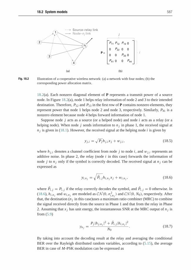
18.2 System models 587
P =
P11 0
0 P22 0 0
0 0 P33 0
0 0 P44
i
P12 P13
P41
j
(a) (b)
Source–relay linkNode–nj link
3
1
2
4
nj
Fig. 18.2 Illustration of a cooperative wireless network: (a) a network with four nodes; (b) thecorresponding power allocation matrix.
18.2(a). Each nonzero diagonal element of P represents a transmit power of a sourcenode. In Figure 18.2(a), node 1 helps relay information of node 2 and 3 to their intendeddestination. Therefore, P12 and P13 in the first row of P contains nonzero elements, theyrepresent power that node 1 helps node 2 and node 3, respectively. Similarly, P41 is anonzero element because node 4 helps forward information of node 1.
Suppose node j acts as a source (or a helped node) and node i acts as a relay (or ahelping node). When node j sends information to n j in phase 1, the received signal atn j is given in (18.1). However, the received signal at the helping node i is given by
y j,i =√
Pj h j,i x j + w j,i , (18.5)
where h j,i denotes a channel coefficient from node j to node i , and w j,i represents anadditive noise. In phase 2, the relay (node i in this case) forwards the information ofnode j to n j only if the symbol is correctly decoded. The received signal at n j can beexpressed as
yi,n j =√
Pi, j hi,n j x j + wi,n j , (18.6)
where Pi, j = Pi, j if the relay correctly decodes the symbol, and Pi, j = 0 otherwise. In(18.6), hi,n j and wi,n j are modeled as CN (0, σ 2
i,n j) and CN (0, N0), respectively. After
that, the destination (n j in this case)uses a maximum ratio combiner (MRC) to combinethe signal received directly from the source in Phase 1 and that from the relay in Phase2. Assuming that x j has unit energy, the instantaneous SNR at the MRC output of n j isfrom (5.9)
γn j =Pj |h j,n j |2 + Pi, j |hi,n j |2
N0. (18.7)
By taking into account the decoding result at the relay and averaging the conditionalBER over the Rayleigh distributed random variables, according to (5.15), the averageBER in case of M-PSK modulation can be expressed as
588 Network lifetime maximization via cooperation
BER j = 1
log2 MF
(1+
bPjσ2j,n j
N0 sin2 θ
)· F
(1+ bPjσ
2j,i
N0 sin2 θ
)
+ 1
log2 MF
((1+
bPjσ2j,n j
N0 sin2 θ
)(1+
bPi, jσ2i,n j
N0 sin2 θ
))
×[
1− F
(1+ bPjσ
2j,i
N0 sin2 θ
)], (18.8)
where
F(x(θ)) = 1
π
∫ (M−1)π/M
0[x(θ)]−1dθ (18.9)
and b is defined in (18.3). The first term on the right-hand-side of (18.8) correspondsto an incorrect decoding at the relay whereas the second term corresponds to a correctdecoding at the relay. By assuming that all channel links are available, i.e., σ 2
j,n j�= 0
and σ 2j,i �= 0, the BER upper bound of (18.8) can be obtained by removing the negative
term and all one’s in (18.8), from Theorem 5.2.2, we have
BER j ≤ N 20
b2 log2 M·
A2 Pi, jσ2i,n j+ B Pjσ
2j,i
P2j Pi, jσ
2j,n jσ 2
j,iσ2i,n j
, (18.10)
where
A � M − 1
2M+ sin(2π/M)
4π, (18.11)
and
B � 3M − 1
8M+ sin(2π/M)
4π− sin(4π/M)
32π. (18.12)
We can see from (18.10) that cooperative transmission obtains a diversity order of two asindicated in the power of N0. Hence, with cooperative diversity, the total power requiredat the source and the relay is less than that required for non-cooperative transmissionin order to obtain the same BER performance. Therefore, by properly allocating thetransmit power at the source (Pj ) and the transmit power at the relay (Pi, j ), the lifetimeof the source can be significantly increased whereas the lifetime of the relay is slightlydecreased.
18.3 Lifetime maximization by employing a cooperative node
In this section, we aim to maximize the minimum device lifetime among all cooperativenodes in the network. First, we formulate the lifetime maximization problem. Then,an analytical solution is provided for a network with two cooperative nodes. Afterthat, based on the solution for the two-node network, a fast suboptimal algorithm isdeveloped to solve a problem for a network with multiple cooperative nodes.
18.3 Lifetime maximization by employing a cooperative node 589
18.3.1 Problem formulation
As shown in the previous section, the cooperative scheme requires less power to achievethe same performance as the non-cooperative scheme, thus it can be used to improvethe minimum device lifetime. Note that different nodes may have different remainingenergy, and they may contribute to different performance improvement due to theirdifferent locations. So the nodes with energy or location advantages can help forwardinformation of other energy depleting nodes. In what follows, we formulate an opti-mization problem to determine which node should be a helping node and how muchpower should be allocated in order to efficiently increase the minimum device lifetime.
Let us first determine the device lifetime in a non-cooperative network. From Section18.2.1, the non-cooperative device lifetime of node j is given by
Tj =κεσ 2
j,n jE j
(κεσ 2j,n jλ j Ps + N0
∑Nl=1 λl, j )
, (18.13)
where κ � 4b log2 M , and Ps represents the processing power. From (18.13), we cansee that the lifetime of each node depends on its initial energy and its geographicallocation. Intuitively, the node whose energy is small and location is far away from itsnext node tends to have small device lifetime.
In the case of a cooperative network, the overall transmit power of each node is asummation of the power used by the node to transmit its own information and the powerused by the node to cooperatively help forward information of other nodes. Let Pr bethe processing power at each relay node, i.e., the power that the relay uses for decodingand forwarding information. From the power allocation matrix P in Section 18.2.2, theoverall average transmit power of the cooperating node i is
Pi
N∑l=1
λli +N∑
j=1j �=i
Pi, j
( N∑l=1
λl, j
), (18.14)
and the overall average processing power of node i is
λi Ps +N∑
j=1j �=i
Pr sgn(Pi, j )( N∑
l=1
λl, j
)(18.15)
where sgn(Pi, j ) represents the sign function that returns 1 if Pi, j > 0, and 0 otherwise.Therefore, the lifetime of the cooperative node i can be written as
Ti (P) = Ei
λi Ps + Pi∑N
l=1 λli +�(Pr , Pi, j , λl, j ), (18.16)
where
�(Pr , Pi, j , λl, j ) �N∑
j=1j �=i
(Pr sgn(Pi, j )+ Pi, j
)( N∑l=1
λl, j
), (18.17)
590 Network lifetime maximization via cooperation
and Ei is an initial energy of node i . Obviously, the lifetime of node i reduces if node ihelps transmit information of other nodes. However, the more the power Pi, j that nodei uses in helping forward the information of node j , the longer the lifetime of node j .Therefore, it is crucial to properly design the power allocation matrix P such that theminimum device lifetime is maximized.
With an objective to maximize the minimum device lifetime under the BER constrainton each node, the optimization problem can be formulated as
maxP
mini
Ti (P) (18.18)
s.t.
⎧⎨⎩Performance: BERi ≤ ε, ∀i;Power: 0 < Pi ≤ Pmax, ∀i;Power: 0 ≤ Pi, j ≤ Pmax, ∀ j �= i,
where ε denotes a BER requirement. In (18.18), the first constraint is to satisfy theBER requirement as specified in (18.8), the second constraint guarantees that each nodehas information to be transmitted and the transmit power is no greater than Pmax andthe third constraint ensures that all the allocated power is nonnegative and no greaterthan Pmax. Due to its assignment and combinatorial nature, the formulated problemis N P hard. Even though each source–destination route is already known, this frame-work needs to optimize the pairing between each source and its relay. This problem ofchoosing relay is an assignment problem.
18.3.2 Analytical solution for a two-node wireless network
To get some insightful understanding on the formulated problem, we provide in thissection a closed-form analytical solution at high SNR scenario for a network with twocooperative nodes (N = 2). Each node transmits its information directly to the des-tination d . In this two-node network, there are three possible transmission strategies,namely:
(i) each node transmits non-cooperatively;(ii) one node helps forward information of the other;
(iii) both nodes help forward information of each other.
In the sequel, we will maximize the minimum device lifetime for each strategy. Withoutloss of generality, we assume that the transmit power required for a non-cooperativetransmission is less than Pmax.
18.3.2.1 Non-cooperative transmission among nodes
Based on the discussion in Section 18.2.1, the optimum power allocation for non-cooperative case is Pj = N0/(κεσ
2jd) for j = 1, 2, and Pi, j = 0 for i �= j . Using
(18.13), the optimum device lifetime for this transmission strategy is given by
T ∗non-coop = min
[κεσ 2
1d E1
λ11(κεσ21d Ps + N0)
,κεσ 2
2d E2
λ22(κεσ22d Ps + N0)
]. (18.19)
18.3 Lifetime maximization by employing a cooperative node 591
18.3.2.2 Cooperative transmission when one node helps the other nodeWithout loss of generality, we will provide a solution for a case that node i helps relayinformation of node j to the destination. In this case, the lifetimes of node i and node jare given by
Ti = Ei
λi (Ps + Pi )+ λ j (Pr + Pi, j )(18.20)
and
Tj = E j
λ j (Ps + Pj ), (18.21)
respectively. Hence, appropriately choosing Pi , Pi, j , and Pj can improve the minimumdevice lifetime while maintaining a specified BER requirement.
In order for node i to satisfy the BER requirement ε, the optimum transmit power ofnode i is
Pi = N0
κεσ 2id
.
To determine Pj and Pi, j , we first note that, according to the BER upper bound in(18.10), Pj and Pi, j must satisfy
N 20 A2 Pi, jσ
2id + N 2
0 B Pjσ2j,i
b2 log2(M)P2j Pi, jσ
2jdσ
2j,iσ
2i
= ε. (18.22)
Then, we can express Pi, j in term of Pj as
Pi, j = Pj
Ci, j P2j − Di, j
� f (Pj ), (18.23)
where
Ci, j =εσ 2
idσ2jdb2 log2 M
BN 20
,
and
Di, j = A2σ 2id
Bσ 2j,i
.
From the expressions for Pi and Pi, j , we have
Ti = Ei
λi (Ps + N0κεσ 2
id)+ λ j (Pr + f (Pj ))
, (18.24)
which is a function of Pj . Therefore, the optimization problem (18.18) is simplified to
T ∗i-helps- j = maxPj
⎡⎣min
⎛⎝ Ei
λi (Ps + N0κεσ 2
id)+ λ j (Pr + f (Pj ))
,
E j
λ j (Ps + Pj )
)]. (18.25)
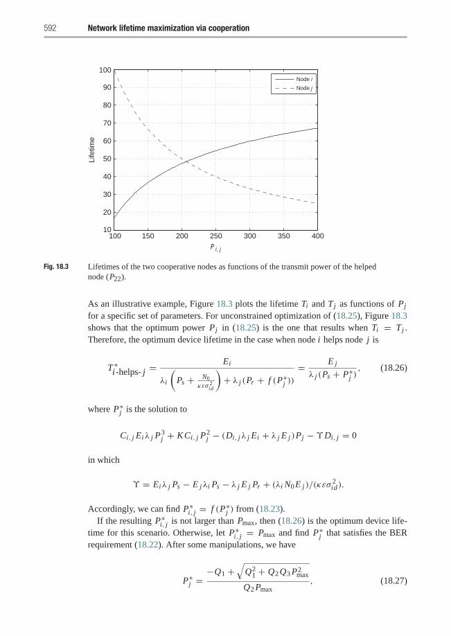
592 Network lifetime maximization via cooperation
100 150 200 250 300 350 40010
20
30
40
50
60
70
80
90
100
Pi, j
Life
time
Node i
Node j
Fig. 18.3 Lifetimes of the two cooperative nodes as functions of the transmit power of the helpednode (P22).
As an illustrative example, Figure 18.3 plots the lifetime Ti and Tj as functions of Pj
for a specific set of parameters. For unconstrained optimization of (18.25), Figure 18.3shows that the optimum power Pj in (18.25) is the one that results when Ti = Tj .Therefore, the optimum device lifetime in the case when node i helps node j is
T ∗i-helps- j =Ei
λi
(Ps + N0
κεσ 2id
)+ λ j (Pr + f (P∗j ))
= E j
λ j (Ps + P∗j ), (18.26)
where P∗j is the solution to
Ci, j Eiλ j P3j + KCi, j P2
j − (Di, jλ j Ei + λ j E j )Pj −ϒDi, j = 0
in which
ϒ = Eiλ j Ps − E jλi Ps − λ j E j Pr + (λi N0E j )/(κεσ2id).
Accordingly, we can find P∗i, j = f (P∗j ) from (18.23).If the resulting P∗i, j is not larger than Pmax, then (18.26) is the optimum device life-
time for this scenario. Otherwise, let P∗i, j = Pmax and find P∗j that satisfies the BERrequirement (18.22). After some manipulations, we have
P∗j =−Q1 +
√Q2
1 + Q2Q3 P2max
Q2 Pmax, (18.27)
18.3 Lifetime maximization by employing a cooperative node 593
where
Q1 = Bσ 2j,i N 2
0
b2 log2 M,
Q2 = 2εσ 2idσ
2j,iσ
2jd ,
and
Q3 = 2A2σ 2id N 2
0
b2 log2 M.
Therefore, the lifetimes of nodes i and node j are T ∗i = Ei/(λi (Ps + Pi ) + λ j (Pr +Pmax)) and T ∗j = E j/(λ j (Ps + P∗j )), respectively. Hence, the optimum device lifetimewhen P∗i, j > Pmax is the minimum among T ∗i and T ∗j . As a result, the optimum devicelifetime when node i helps node j can be summarized as follows:
T ∗i-helps- j =⎧⎨⎩
E jλ j (Ps+P∗j )
, P∗i, j ≤ Pmax;min{T ∗i , T ∗j }, T ∗i, j > Pmax.
(18.28)
18.3.2.3 Cooperative transmission when both nodes help each otherWhen both nodes help each other, Pi, j and Ti are given in (18.23) and (18.24), respec-tively. The optimum device lifetime in this case can be obtained by finding P∗i and P∗jthat maximizes Ti (or Tj ) under the condition Ti = Tj , we have
T ∗both-help =Ei
λi (Ps + P∗i )+ λ j
(Pr + P∗j
Ci, j (P∗j )2−Di, j
)= E j
λ j (Ps + P∗j )+ λi
(Pr + P∗i
C j,i (P∗i )2−D j,i
) , (18.29)
where P∗i and P∗j are the solutions to:
arg maxPi ,Pj
Ei
λid(Ps + Pi )+ λ j,i
(Pr + Pj
Ci, j P2j −Di, j
) (18.30)
s.t.
⎧⎪⎪⎨⎪⎪⎩[(λi Ps+λ j Pr+λi Pi )(Ci, j P2
j −Di, j )+λ j Pj
](C j,i P2
i −D j,i )[(λ j Ps+λi Pr+λ j Pj )(C j,i P2
i −D j,i )+λi Pi](Ci, j P2
j −Di, j )= Ei
E j;
Pj >
√Di, jCi, j, ∀ j �= i,
in which, the first constraint ensures that Ti = Tj , and the second constraint guaranteesthat Pi, j = Pj/(Ci, j P2
j − Di, j ) > 0.If P∗i, j ≤ Pmax and P∗j,i ≤ Pmax, then the solution to (18.29) is the optimum device
lifetime for this transmission strategy. Otherwise, the optimization problem is separatedinto two subproblems:
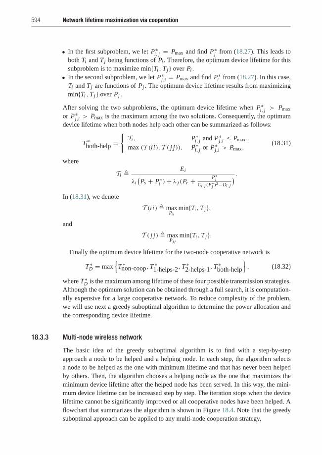
594 Network lifetime maximization via cooperation
• In the first subproblem, we let P∗i, j = Pmax and find P∗j from (18.27). This leads toboth Ti and Tj being functions of Pi . Therefore, the optimum device lifetime for thissubproblem is to maximize min{Ti , Tj } over Pi .
• In the second subproblem, we let P∗j,i = Pmax and find P∗i from (18.27). In this case,Ti and Tj are functions of Pj . The optimum device lifetime results from maximizingmin{Ti , Tj } over Pj .
After solving the two subproblems, the optimum device lifetime when P∗i, j > Pmax
or P∗j,i > Pmax is the maximum among the two solutions. Consequently, the optimumdevice lifetime when both nodes help each other can be summarized as follows:
T ∗both-help ={
Ti , P∗i, j and P∗j,i ≤ Pmax,
max (T (i i), T ( j j)), P∗i, j or P∗j,i > Pmax,(18.31)
where
Ti � Ei
λi(Ps + P∗i )+ λ j (Pr + P∗j
Ci, j (P∗j )2−Di, j
) .In (18.31), we denote
T (i i) � maxPii
min{Ti , Tj },
and
T ( j j) � maxPj j
min{Ti , Tj }.
Finally the optimum device lifetime for the two-node cooperative network is
T ∗D = max{
T ∗non-coop, T∗1-helps-2, T
∗2-helps-1, T
∗both-help
}, (18.32)
where T ∗D is the maximum among lifetime of these four possible transmission strategies.Although the optimum solution can be obtained through a full search, it is computation-ally expensive for a large cooperative network. To reduce complexity of the problem,we will use next a greedy suboptimal algorithm to determine the power allocation andthe corresponding device lifetime.
18.3.3 Multi-node wireless network
The basic idea of the greedy suboptimal algorithm is to find with a step-by-stepapproach a node to be helped and a helping node. In each step, the algorithm selectsa node to be helped as the one with minimum lifetime and that has never been helpedby others. Then, the algorithm chooses a helping node as the one that maximizes theminimum device lifetime after the helped node has been served. In this way, the mini-mum device lifetime can be increased step by step. The iteration stops when the devicelifetime cannot be significantly improved or all cooperative nodes have been helped. Aflowchart that summarizes the algorithm is shown in Figure 18.4. Note that the greedysuboptimal approach can be applied to any multi-node cooperation strategy.
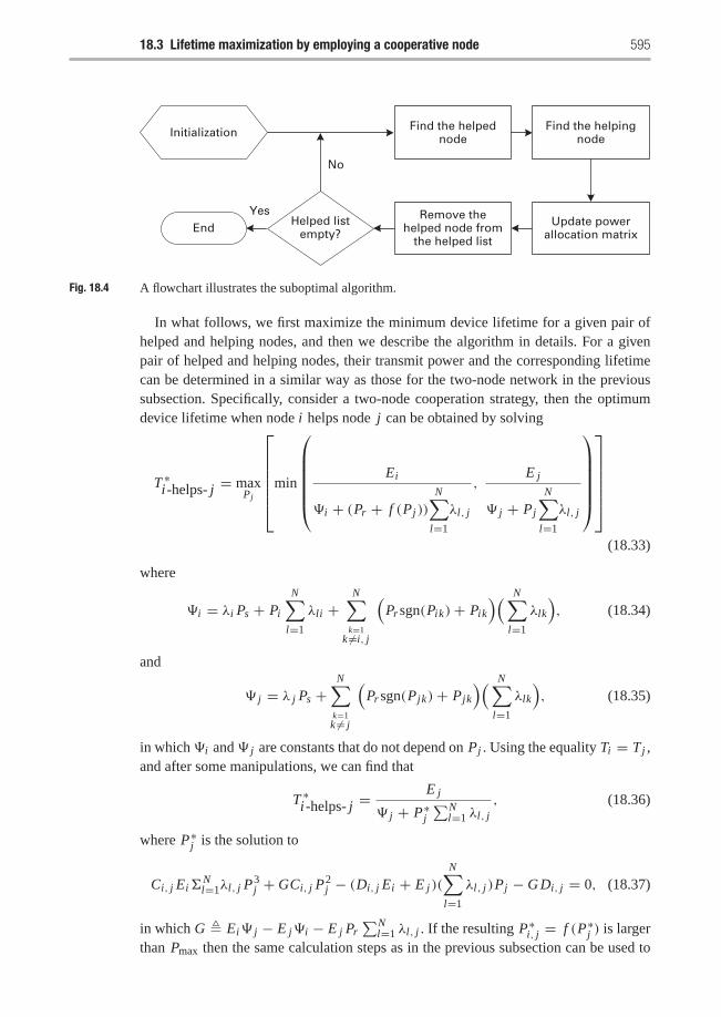
18.3 Lifetime maximization by employing a cooperative node 595
Find the helpednode
Find the helpingnode
Update powerallocation matrix
Remove thehelped node from
the helped list
Helped listempty?End
No
Yes
Initialization
Fig. 18.4 A flowchart illustrates the suboptimal algorithm.
In what follows, we first maximize the minimum device lifetime for a given pair ofhelped and helping nodes, and then we describe the algorithm in details. For a givenpair of helped and helping nodes, their transmit power and the corresponding lifetimecan be determined in a similar way as those for the two-node network in the previoussubsection. Specifically, consider a two-node cooperation strategy, then the optimumdevice lifetime when node i helps node j can be obtained by solving
T ∗i-helps- j = maxPj
⎡⎢⎢⎢⎢⎢⎣min
⎛⎜⎜⎜⎜⎜⎝Ei
�i + (Pr + f (Pj ))
N∑l=1
λl, j
,E j
� j + Pj
N∑l=1
λl, j
⎞⎟⎟⎟⎟⎟⎠
⎤⎥⎥⎥⎥⎥⎦(18.33)
where
�i = λi Ps + Pi
N∑l=1
λli +N∑
k=1k �=i, j
(Pr sgn(Pik)+ Pik
)( N∑l=1
λlk
), (18.34)
and
� j = λ j Ps +N∑
k=1k �= j
(Pr sgn(Pjk)+ Pjk
)( N∑l=1
λlk
), (18.35)
in which�i and� j are constants that do not depend on Pj . Using the equality Ti = Tj ,and after some manipulations, we can find that
T ∗i-helps- j =E j
� j + P∗j∑N
l=1 λl, j, (18.36)
where P∗j is the solution to
Ci, j Ei Nl=1λl, j P3
j + GCi, j P2j − (Di, j Ei + E j )(
N∑l=1
λl, j )Pj − G Di, j = 0, (18.37)
in which G � Ei� j − E j�i − E j Pr∑N
l=1 λl, j . If the resulting P∗i, j = f (P∗j ) is largerthan Pmax then the same calculation steps as in the previous subsection can be used to
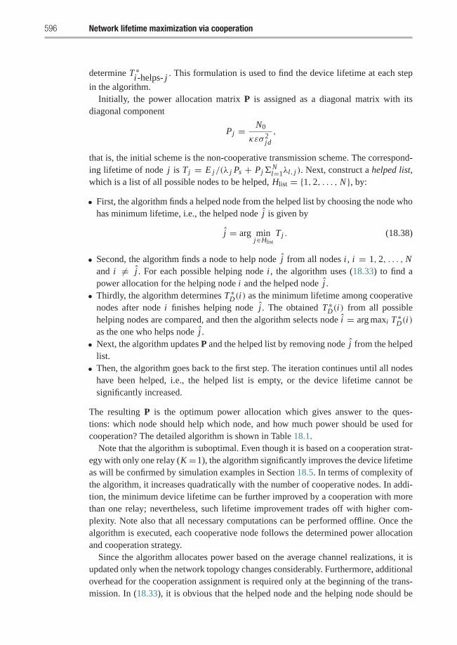
596 Network lifetime maximization via cooperation
determine T ∗i-helps- j . This formulation is used to find the device lifetime at each step
in the algorithm.Initially, the power allocation matrix P is assigned as a diagonal matrix with its
diagonal component
Pj = N0
κεσ 2jd
,
that is, the initial scheme is the non-cooperative transmission scheme. The correspond-ing lifetime of node j is Tj = E j/(λ j Ps + Pj
Nl=1λl, j ). Next, construct a helped list,
which is a list of all possible nodes to be helped, Hlist = {1, 2, . . . , N }, by:
• First, the algorithm finds a helped node from the helped list by choosing the node whohas minimum lifetime, i.e., the helped node j is given by
j = arg minj∈Hlist
Tj . (18.38)
• Second, the algorithm finds a node to help node j from all nodes i , i = 1, 2, . . . , Nand i �= j . For each possible helping node i , the algorithm uses (18.33) to find apower allocation for the helping node i and the helped node j .
• Thirdly, the algorithm determines T ∗D(i) as the minimum lifetime among cooperativenodes after node i finishes helping node j . The obtained T ∗D(i) from all possiblehelping nodes are compared, and then the algorithm selects node i = arg maxi T ∗D(i)as the one who helps node j .
• Next, the algorithm updates P and the helped list by removing node j from the helpedlist.
• Then, the algorithm goes back to the first step. The iteration continues until all nodeshave been helped, i.e., the helped list is empty, or the device lifetime cannot besignificantly increased.
The resulting P is the optimum power allocation which gives answer to the ques-tions: which node should help which node, and how much power should be used forcooperation? The detailed algorithm is shown in Table 18.1.
Note that the algorithm is suboptimal. Even though it is based on a cooperation strat-egy with only one relay (K =1), the algorithm significantly improves the device lifetimeas will be confirmed by simulation examples in Section 18.5. In terms of complexity ofthe algorithm, it increases quadratically with the number of cooperative nodes. In addi-tion, the minimum device lifetime can be further improved by a cooperation with morethan one relay; nevertheless, such lifetime improvement trades off with higher com-plexity. Note also that all necessary computations can be performed offline. Once thealgorithm is executed, each cooperative node follows the determined power allocationand cooperation strategy.
Since the algorithm allocates power based on the average channel realizations, it isupdated only when the network topology changes considerably. Furthermore, additionaloverhead for the cooperation assignment is required only at the beginning of the trans-mission. In (18.33), it is obvious that the helped node and the helping node should be
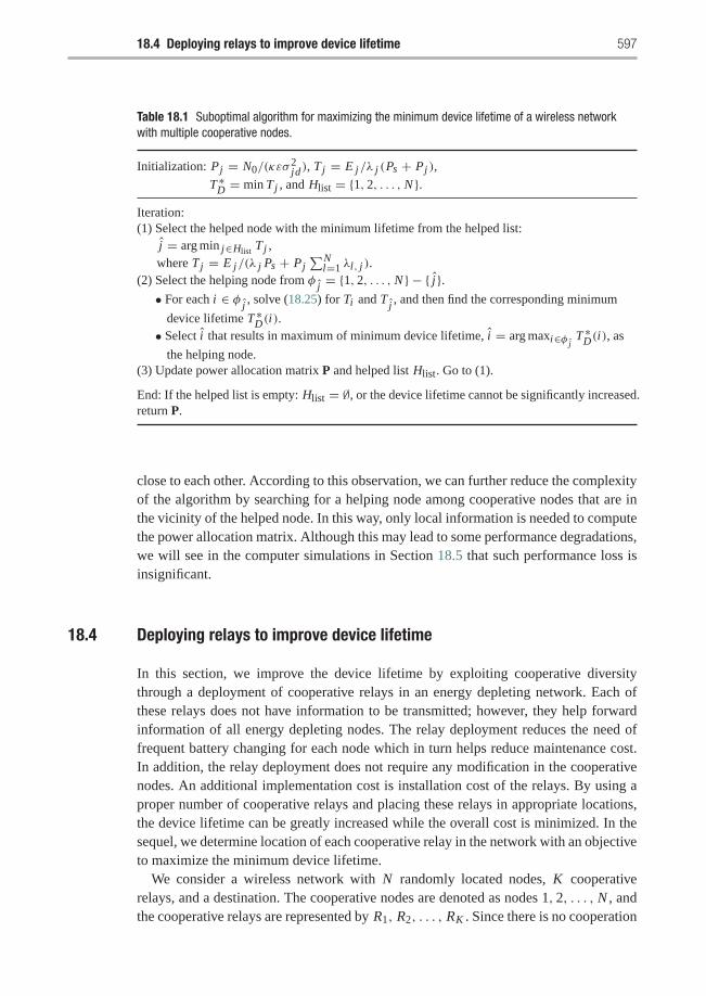
18.4 Deploying relays to improve device lifetime 597
Table 18.1 Suboptimal algorithm for maximizing the minimum device lifetime of a wireless networkwith multiple cooperative nodes.
Initialization: Pj = N0/(κεσ2jd ), Tj = E j/λ j (Ps + Pj ),
T ∗D = min Tj , and Hlist = {1, 2, . . . , N }.Iteration:(1) Select the helped node with the minimum lifetime from the helped list:
j = arg min j∈Hlist Tj ,where Tj = E j/(λ j Ps + Pj
∑Nl=1 λl, j ).
(2) Select the helping node from φ j = {1, 2, . . . , N } − { j}.• For each i ∈ φ j , solve (18.25) for Ti and Tj , and then find the corresponding minimum
device lifetime T ∗D(i).• Select i that results in maximum of minimum device lifetime, i = arg maxi∈φ j
T ∗D(i), as
the helping node.(3) Update power allocation matrix P and helped list Hlist. Go to (1).
End: If the helped list is empty: Hlist = ∅, or the device lifetime cannot be significantly increased.return P.
close to each other. According to this observation, we can further reduce the complexityof the algorithm by searching for a helping node among cooperative nodes that are inthe vicinity of the helped node. In this way, only local information is needed to computethe power allocation matrix. Although this may lead to some performance degradations,we will see in the computer simulations in Section 18.5 that such performance loss isinsignificant.
18.4 Deploying relays to improve device lifetime
In this section, we improve the device lifetime by exploiting cooperative diversitythrough a deployment of cooperative relays in an energy depleting network. Each ofthese relays does not have information to be transmitted; however, they help forwardinformation of all energy depleting nodes. The relay deployment reduces the need offrequent battery changing for each node which in turn helps reduce maintenance cost.In addition, the relay deployment does not require any modification in the cooperativenodes. An additional implementation cost is installation cost of the relays. By using aproper number of cooperative relays and placing these relays in appropriate locations,the device lifetime can be greatly increased while the overall cost is minimized. In thesequel, we determine location of each cooperative relay in the network with an objectiveto maximize the minimum device lifetime.
We consider a wireless network with N randomly located nodes, K cooperativerelays, and a destination. The cooperative nodes are denoted as nodes 1, 2, . . . , N , andthe cooperative relays are represented by R1, R2, . . . , RK . Since there is no cooperation
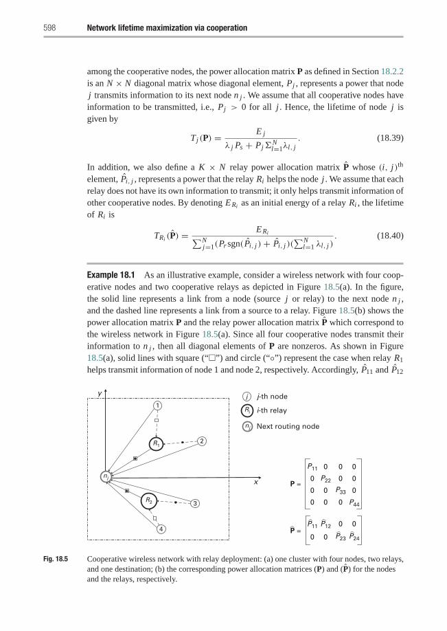
598 Network lifetime maximization via cooperation
among the cooperative nodes, the power allocation matrix P as defined in Section 18.2.2is an N × N diagonal matrix whose diagonal element, Pj , represents a power that nodej transmits information to its next node n j . We assume that all cooperative nodes haveinformation to be transmitted, i.e., Pj > 0 for all j . Hence, the lifetime of node j isgiven by
Tj (P) = E j
λ j Ps + Pj Nl=1λl, j
. (18.39)
In addition, we also define a K × N relay power allocation matrix P whose (i, j)th
element, Pi, j , represents a power that the relay Ri helps the node j . We assume that eachrelay does not have its own information to transmit; it only helps transmit information ofother cooperative nodes. By denoting ERi as an initial energy of a relay Ri , the lifetimeof Ri is
TRi (P) =ERi∑N
j=1(Pr sgn(Pi, j )+ Pi, j )(∑N
l=1 λl, j ). (18.40)
Example 18.1 As an illustrative example, consider a wireless network with four coop-erative nodes and two cooperative relays as depicted in Figure 18.5(a). In the figure,the solid line represents a link from a node (source j or relay) to the next node n j ,and the dashed line represents a link from a source to a relay. Figure 18.5(b) shows thepower allocation matrix P and the relay power allocation matrix P which correspond tothe wireless network in Figure 18.5(a). Since all four cooperative nodes transmit theirinformation to n j , then all diagonal elements of P are nonzeros. As shown in Figure18.5(a), solid lines with square (“”) and circle (“◦”) represent the case when relay R1
helps transmit information of node 1 and node 2, respectively. Accordingly, P11 and P12
y
R1
R2
2
1
4
3
x
j-th node
i-th relay
Next routing node
j
Ri
P11 0 0 0
0 P22 0 0
0 0 P33 0
0 0 0 P44
0
0
0
P11P =
P =
P12
P23
0
P24
nj
nj
Fig. 18.5 Cooperative wireless network with relay deployment: (a) one cluster with four nodes, two relays,and one destination; (b) the corresponding power allocation matrices (P) and (P) for the nodesand the relays, respectively.
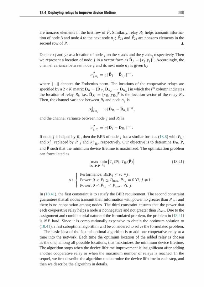
18.4 Deploying relays to improve device lifetime 599
are nonzero elements in the first row of P . Similarly, relay R2 helps transmit informa-tion of node 3 and node 4 to the next node n j ; P23 and P24 are nonzero elements in thesecond row of P . �
Denote x j and y j as a location of node j on the x-axis and the y-axis, respectively. Thenwe represent a location of node j in a vector form as D j = [x j y j ]T. Accordingly, thechannel variance between node j and its next node n j is given by
σ 2j,n j
= η‖D j − Dn j ‖−α,where ‖ · ‖ denotes the Frobenius norm. The locations of the cooperative relays arespecified by a 2×K matrix DR = [DR1 DR2 · · · DRK ] in which the i th column indicatesthe location of relay Ri , i.e., DRi = [xRi yRi ]T is the location vector of the relay Ri .Then, the channel variance between Ri and node n j is
σ 2Ri ,n j
= η‖DRi − Dn j ‖−α,and the channel variance between node j and Ri is
σ 2j,Ri
= η‖D j − DRi ‖−α.If node j is helped by Ri , then the BER of node j has a similar form as (18.8) with Pi, j
and σ 2j,i replaced by Pi, j and σ 2
j,Ri, respectively. Our objective is to determine DR , P,
and P such that the minimum device lifetime is maximized. The optimization problemcan formulated as
maxDR ,P,P
mini, j
{Tj (P), TRi (P)
}(18.41)
s.t.
⎧⎨⎩Performance: BER j ≤ ε, ∀ j;Power: 0 < Pi ≤ Pmax, Pi, j = 0 ∀i, j �= i;Power: 0 ≤ Pi, j ≤ Pmax, ∀i, j.
In (18.41), the first constraint is to satisfy the BER requirement. The second constraintguarantees that all nodes transmit their information with power no greater than Pmax andthere is no cooperation among nodes. The third constraint ensures that the power thateach cooperative relay helps a node is nonnegative and not greater than Pmax. Due to theassignment and combinatorial nature of the formulated problem, the problem in (18.41)is N P hard. Since it is computationally expensive to obtain the optimum solution to(18.41), a fast suboptimal algorithm will be considered to solve the formulated problem.
The basic idea of the fast suboptimal algorithm is to add one cooperative relay at atime into the network. Each time the optimum location of the added relay is chosenas the one, among all possible locations, that maximizes the minimum device lifetime.The algorithm stops when the device lifetime improvement is insignificant after addinganother cooperative relay or when the maximum number of relays is reached. In thesequel, we first describe the algorithm to determine the device lifetime in each step, andthen we describe the algorithm in details.

600 Network lifetime maximization via cooperation
To maximize the minimum device lifetime when the number of relays and their loca-tions are given, a step algorithm, similar to the one described in Figure 18.4 in Section18.3.3, can be used:
• Initially, all nodes are sorted in ascending order according to their non-cooperativelifetimes, as specified in (18.13), and then register them in a helped list Hlist.
• In each iteration, first, select the first node in the helped list as the one to be helped.• Second, determine the minimum device lifetime after all of the cooperative relay Ri ’s
(i = 1, 2, . . . , K ) finish helping the selected node,• Choose the relay Ri where i is the relay that maximizes the minimum device lifetime
to help the selected node.• Update the power allocation matrices P and P, and remove the selected node in the
first step from the helped list.• Continue the iteration until all nodes have been helped and the helped list is empty or
until the device lifetime improvement is insignificant.
The algorithm to find an optimum location of each cooperative relay is described asfollows:
• Denote Kmax as the maximum number of cooperative relays and denote �D as a setof all possible relay locations.
• Initially, the number of relays is set to zero.• In each iteration, the number of relay is increased by one, and the optimum relay
location D is determined using one of the heuristic search methods (e.g., local searchor simulated annealing) together with the algorithm in Table 18.2.
• The location D that results in the maximum of the minimum device lifetime is selectedas the optimum relay location and, then, the device lifetime is updated.
Table 18.2 Suboptimal algorithm to determine device lifetime when relay locations are fixed.
Initialization: Pj = N0κεσ 2
jd, Tj = E j
λ j (Ps+Pj ), T ∗D = min Tj ,
Sort N nodes by their lifetimes in ascending orderand list in Hlist.
Iteration:(1) Select the first node in the Hlist as the helped node.(2) Select the helping relay Ri from the set of K relays.• For each i , use the heuristic algorithm to maximize the minimum device lifetime, T ∗D(i).• Select Ri that results in maximum of minimum device lifetime to help the node j .
(3) Update Pj j in P and update Pi j in P.
Set Pi j = 0 for all i �= i and set T ∗D = TD(i).
Remove node j from the helped list Hlist. Go to (1).
End: If the helped list is empty: Hlist = ∅, or the device lifetime cannot be significantlyincreased. Return P, P, T ∗D .
18.5 Simulation examples 601
Table 18.3 Algorithm to determine relay locations.
Initialization: q = 0
Iteration:(1) Increase number of relays: q = q + 1(2) For each location Dl ∈ �D . Set DRq = Dl .
Find T ∗D , P and P using the algorithm in Table 18.2Denote the obtained results by T ∗D(l), P(l) and P(l)
(3) Find the relay location Rq : DRq = Dl∗ , where l∗ = arg maxl T ∗D(l)(4) Update P, P, and T ∗D . Go to (1).
End: If the device lifetime improvement is insignificant, or q = Kmax. Return P, P, T ∗D .
• Finally, the algorithm goes back to the first step.• The algorithm stops if the device lifetime improvement is insignificant or the number
of relays reaches Kmax.
The detailed algorithm is presented in Table 18.3.Note that the fast suboptimal algorithm allows at most one relay to help each node.
Although the algorithm is suboptimal, simulation example in Section 18.5 shows thatthe algorithm significantly improves the device lifetime. In addition, all of the requiredcomputations can be performed offline. In addition, the problems and algorithms in Sec-tion 18.3 and Section 18.4 are closely related. Specifically, both sections aim to extendthe device lifetime by exploiting cooperative diversity. In Section 18.3, the cooperativediversity is exploited by cooperation among devices. In Section 18.4, however, coop-erative relays are deployed, and the cooperative diversity is exploited by cooperationbetween each device and one of these additional cooperative relays. Therefore, the basicalgorithm of finding P and P in Section 18.4 is similar to that in Section 18.3. The searchprocess of P and P is done under the given locations of relays (i.e., for a fixed D); theprocess is not affected by the method of finding D.
18.5 Simulation examples
In all examples, BPSK modulation is used in the system, the propagation loss factor isα = 3, η = 1, and ε = 10−3 (unless stated otherwise). The processing power of eachnode (Ps) is set at 25% of transmit power of the node whose location is at (10m, 0). Theprocessing power of each relay (Pr ) is set at 50% of Ps . All nodes are equipped withequal initial energy of E j = 105. The noise variance is set at N0 = 10−2. The nodesare randomly distributed based on uniform distribution and the destination is located inthe center of the area. Each node sends information to the destination via a route that isdetermined by the Dijkstra’s algorithm.

602 Network lifetime maximization via cooperation
1 5 10 15 20 25 300
500
1000
1500
2000
2500
Location of node 2
Life
time
Minimum device lifetime (cooperative) – optimalMinimum device lifetime (cooperative) – suboptimal ( Table 18.1)
Non-cooperative lifetime of node 1 – T1
Non-cooperative lifetime of node 2 – T2
Minimum device lifetime (non-cooperative) – min(T1,T2)
Fig. 18.6 Device lifetime in a two-node wireless network.
Example 18.2 Figure 18.6 considers a two-node wireless network where the destina-tion is located at coordinate (0, 0). Node 1 is fixed at coordinate (0, 8m). The locationof node 2 varies from (0, 1) to (0, 30 m). We can see that the minimum device life-time of the non-cooperative scheme is determined by the lifetime of the node who islocated farther from the destination as shown by the curve marked with circles (“◦”).Under cooperative transmission, the minimum device lifetime is significantly increased,especially when node 2 is located close to the destination.
The reason is that node 2 requires small transmit power to reach the destination,after node 2 helps node 1, the transmit power of node 2 slightly increases, while thetransmit power of node 1 greatly reduces due to the cooperative diversity. With thesuboptimal algorithm (Table 18.1), the minimum device lifetime is improved to almostthe same as the lifetime of the node who is closer to the destination (see the curvewith rectangular “” markers). By using the optimum power allocation obtained fromSection 18.3.2, the minimum device lifetime can be further increased (see the curvewith diamond “♦” markers) since both nodes take advantage of the cooperative diversitywhile using smaller amount of their transmit power. �
Example 18.3 Figure 18.7 depicts the minimum device lifetime according to the den-sity of cooperative nodes in a square area. The number of randomly located nodes varyfrom 20 to 50 over an area of size 100 m × 100 m. In the simulation, we normalizethe transmission rate to be the same for all network sizes. For local search, the helpingnode is chosen among the nodes whose distances from the source node are less than20 m. From the figure, we can see that the minimum device lifetime of the cooperativenetwork is higher than that of the non-cooperative network for all network sizes. For
18.5 Simulation examples 603
2 2.5 3 3.5 4 4.5 5 × 10–320
40
60
80
100
120
140
160
180
200
Node density (per square meter)
Min
imu
m d
evic
e lif
etim
e
Cooperative – global searchCooperative – local searchNon-cooperative
Fig. 18.7 Minimum device lifetime with different numbers of randomly located nodes.
example, in the cooperative network the minimum device lifetime is twice that of thenon-cooperative network when there are 50 nodes in the network. Note that the perfor-mance gain is calculated as Tcoop/Tnon−coop, where Tcoop and Tnon−coop represent thelifetime of cooperative and non-cooperative networks, respectively.
From Figure 18.7, the cooperative scheme with local search yields similar perfor-mance to the one with global search, especially when the node density is high. Thisconfirms our expectation that the helping node is chosen as the one that is located closeto the helped node. Note that the minimum device lifetimes for non-cooperative andcooperative networks increase with the number of nodes because the chance of beinghelped by a node with good location and high energy increases. �
Example 18.4 Figure 18.8 illustrates an improvement of minimum device lifetimeaccording to different BER requirements. We assume in the simulation that there are30 randomly located cooperative nodes in an area of size 100 m × 100 m. We can seefrom the figure that the minimum device lifetime is small at a BER requirement of10−6 under both non-cooperative and cooperative networks. This is because each noderequires large transmit power to satisfy such small BER requirement. As the BER con-straint increases, the minimum device lifetime also increases since the transmit powerrequired to satisfy the BER constraint decreases.
Note that the cooperative network achieves longer device lifetime than that for thenon-cooperative network over the entire range of BER requirement. For example,the cooperative network achieves 125/49 = 2.6 times longer lifetime than the non-cooperative network at a BER requirement of 10−3. However, both cooperative and
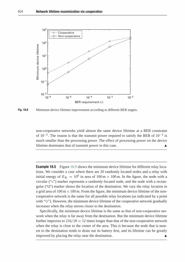
604 Network lifetime maximization via cooperation
10−610−2
10−1
100
101
102
103
10−5 10−4 10−3 10−2
BER requirement (ε)
Min
imu
m d
evic
e lif
etim
e
CooperativeNon-cooperative
Fig. 18.8 Minimum device lifetime improvement according to different BER targets.
non-cooperative networks yield almost the same device lifetime at a BER constraintof 10−2. The reason is that the transmit power required to satisfy the BER of 10−2 ismuch smaller than the processing power. The effect of processing power on the devicelifetime dominates that of transmit power in this case. �
Example 18.5 Figure 18.9 shows the minimum device lifetime for different relay loca-tions. We consider a case where there are 20 randomly located nodes and a relay withinitial energy of ERi = 106 in area of 100 m × 100 m. In the figure, the node with acircular (“◦”) marker represents a randomly-located node, and the node with a rectan-gular (“%&”) marker shows the location of the destination. We vary the relay location ina grid area of 100 m× 100 m. From the figure, the minimum device lifetime of the non-cooperative network is the same for all possible relay locations (as indicated by a pointwith “♦”). However, the minimum device lifetime of the cooperative network graduallyincreases when the relay moves closer to the destination.
Specifically, the minimum device lifetime is the same as that of non-cooperative net-work when the relay is far away from the destination. But the minimum device lifetimefurther improves to 216/18 = 12 times longer than that of the non-cooperative networkwhen the relay is close to the center of the area. This is because the node that is near-est to the destination tends to drain out its battery first, and its lifetime can be greatlyimproved by placing the relay near the destination. �
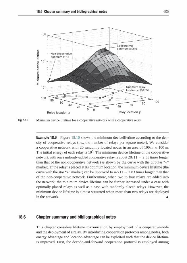
18.6 Chapter summary and bibliographical notes 605
10080
6040
200 0 20 40 60 80 100
101
102
103
Relay location yRelay location x
Min
imu
m d
evic
e lif
etim
e
Non-cooperative:optimum at 18
Optimum relaylocation at [50,55]
Cooperative:optimum at 216
Fig. 18.9 Minimum device lifetime for a cooperative network with a cooperative relay.
Example 18.6 Figure 18.10 shows the minimum devicelifetime according to the den-sity of cooperative relays (i.e., the number of relays per square meter). We considera cooperative network with 20 randomly located nodes in an area of 100 m × 100 m.The initial energy of each relay is 105. The minimum device lifetime of the cooperativenetwork with one randomly-added cooperative relay is about 28/11 = 2.55 times longerthan that of the non-cooperative network (as shown by the curve with the circular “◦”marker). If the relay is placed at its optimum location, the minimum device lifetime (thecurve with the star “∗” marker) can be improved to 42/11 = 3.83 times longer than thatof the non-cooperative network. Furthermore, when two to four relays are added intothe network, the minimum device lifetime can be further increased under a case withoptimally-placed relays as well as a case with randomly-placed relays. However, theminimum device lifetime is almost saturated when more than two relays are deployedin the network. �
18.6 Chapter summary and bibliographical notes
This chapter considers lifetime maximization by employment of a cooperative-nodeand the deployment of a relay. By introducing cooperation protocols among nodes, bothenergy advantage and location advantage can be exploited such that the device lifetimeis improved. First, the decode-and-forward cooperation protocol is employed among
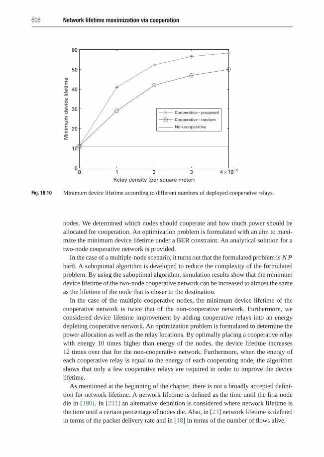
606 Network lifetime maximization via cooperation
0 1 2 3 4 × 10–40
10
20
30
40
50
60
Relay density (per square meter)
Min
imu
m d
evic
e lif
etim
e
Cooperative – proposed
Cooperative – random
Non-cooperative
Fig. 18.10 Minimum device lifetime according to different numbers of deployed cooperative relays.
nodes. We determined which nodes should cooperate and how much power should beallocated for cooperation. An optimization problem is formulated with an aim to maxi-mize the minimum device lifetime under a BER constraint. An analytical solution for atwo-node cooperative network is provided.
In the case of a multiple-node scenario, it turns out that the formulated problem is N Phard. A suboptimal algorithm is developed to reduce the complexity of the formulatedproblem. By using the suboptimal algorithm, simulation results show that the minimumdevice lifetime of the two-node cooperative network can be increased to almost the sameas the lifetime of the node that is closer to the destination.
In the case of the multiple cooperative nodes, the minimum device lifetime of thecooperative network is twice that of the non-cooperative network. Furthermore, weconsidered device lifetime improvement by adding cooperative relays into an energydepleting cooperative network. An optimization problem is formulated to determine thepower allocation as well as the relay locations. By optimally placing a cooperative relaywith energy 10 times higher than energy of the nodes, the device lifetime increases12 times over that for the non-cooperative network. Furthermore, when the energy ofeach cooperative relay is equal to the energy of each cooperating node, the algorithmshows that only a few cooperative relays are required in order to improve the devicelifetime.
As mentioned at the beginning of the chapter, there is not a broadly accepted defini-tion for network lifetime. A network lifetime is defined as the time until the first nodedie in [190]. In [231] an alternative definition is considered where network lifetime isthe time until a certain percentage of nodes die. Also, in [23] network lifetime is definedin terms of the packet delivery rate and in [18] in terms of the number of flows alive.
Exercises 607
The problem of network algorithm designs that are aware of network lifetime havebeen the subject of some research interest. A data routing algorithm that aims at max-imizing the minimum lifetime among nodes in wireless sensor networks was proposedin [22]. Later, considerable research efforts have been devoted to maximize such min-imum lifetime. For example, upper bounds on lifetime of various wireless networkswith energy-constrained nodes are derived in [12, 235, 76] and references therein. Theproblem of finding an energy-efficient tree for network lifetime maximization has beenconsidered in [12, 132] for a broadcasting scenario, and in [39] for a multicastingscenario. The works in [4, 21, 117] considered the problem of minimum-energy broad-casting, which is proved to be N P-complete. In [133], a technique for network lifetimemaximization by employing a ccumulative broadcast strategy was considered. The pro-posed work relies on the assumption that nodes cooperatively accumulate energy ofunreliable receptions over the relay channels. The work in [75] considered provisioningadditional energy on existing nodes and deploying relays to extend the network lifetime.
In terms of previous approaches to the problem tackled in this chapter, it is worthnoticing that the works in [109, 179, 180, 222, 79, 204, 57, 128] have proved the sig-nificant potential of using cooperative diversity in wireless networks, but most focus onimproving physical layer performance or minimizing energy consumption. On the otherhand, note that there are many works on extending lifetime [22, 12, 235, 76, 132, 39,4, 21, 117, 133, 75] but they all concentrate on settings with non-cooperative transmis-sions. Cases of works that focus on lifetime maximization via cooperative nodes andrelay deployment are [64, 65].
Exercises
18.1 The device lifetime was derived in this chapter assuming MPSK modulation.Assume that the nodes in the network use MQAM instead.
(a) Find the bit error rate performance for non-cooperative and cooperativetransmission for MQAM.
(b) Find the optimal power allocation for the two-node network scenario for thethree cases discussed in the chapter: no-cooperation; one node only helps;both node help each other.
(c) Derive device lifetime in case of MQAM modulation and find optimumlifetime for two-node wireless networks. Compare and discuss lifetimeimprovement for cooperative nodes with MPSK or MQAM.
18.2 Show that T ∗i-helps- j can be expressed as in equation (18.28).
18.3 Derive the expression of T ∗both-helps as shown in equation (18.31).
18.4 An analytical solution for the two-node network scenario was discussed in thischapter. Consider the three-node network scenario and denote the nodes by{1, 2, 3}. Find the network lifetime for each one of the following scenarios:(a) No cooperation.(b) Node 1 helps both nodes 2 and 3.
608 Network lifetime maximization via cooperation
(c) Nodes 1 and 2 only help each other.(d) Node 1 helps node 2; node 2 helps node 3; and node 3 helps node 1.
18.5 In the simulation examples in the chapter, all nodes were assumed to have thesame initial battery energy of E = 105. In practice, different nodes can havedifferent initial batteries.Assume that the initial battery energy is a uniformly distributed random variablethat takes value between 103 and 105.
(a) Repeat Example 18.3 and write a program to find the minimum device lifetime according to the density of the cooperative nodes. Compare to theresults in the chapter where all nodes have the same initial battery life.
(b) Repeat Example 18.6 and find the effect of the relay density. Assume thatthe relays’ initial energy is fixed and equal to 105.
18.6 The modulation scheme used in the chapter was assumed to be always fixed toMPSK whether the nodes cooperate or not. Assume that if a node cooperates ithas to transmit at twice the rate. Consider the two-node network model. Assumethat a non-cooperative node uses BPSK and a cooperative node uses QPSK. Findthe minimum device life time for the following cases.
(a) Both nodes do not cooperate.(b) Node 1 helps node 2.(c) Both nodes cooperate.
18.7 Prove the device lifetime expression in (18.36).
References
1. M. Abramowitz and I. A. Stegun. Handbook of Mathematical Functions with Formulas,Graphs, and Mathematical Tables. Dover Publications, 1970.
2. S. Aeron and V. Saligrama. Wireless ad hoc networks: strategies and scaling laws for the fixedSNR regime. IEEE Transactions on Information Theory, 53(6), June 2007.
3. D. Agrawal, V. Tarokh, A. Naguib, and N. Seshadri. Space-time coded OFDM for high data-rate wireless communication over wideband channels. In Proceedings of the IEEE VehicularTechnology Conference, pp. 2232–2236, 1998.
4. A. Ahluwalia, E. Modiano, and L. Shu. On the complexity and distributed construction ofenergy-efficient broadcast trees in static ad hoc networks. In Proceedings of the 36th AnnualConference on Information Sciences and Systems, pp. 807–813, March 2002.
5. S. M. Alamouti. A simple transmit diversity technique for wireless communications. IEEEJournal on Selected Areas in Communications, 16(8):1451–1458, 1998.
6. P. A. Anghel and M. Kaveh. Exact symbol error probability of a cooperative network in aRayleigh-fading environment. IEEE Transactions on Wireless Communications, 3(5):1416–1421, September 2004.
7. P. A. Anghel, G. Leus, and M. Kaveh. Multi-user space-time coding in cooperative net-works. In Proceedings of the IEEE International Conference on Acoustics, Speech and SignalProcessing (ICASSP), volume 4, pp. 73–76, April 6–10, 2003.
8. S. Barbarossa, L. Pescosolido, D. Ludovici, L. Barbetta, and G. Scutari. Cooperative wirelessnetworks based on distributed space-time coding. In Proceedings of the IEEE InternationalWorkshop on Wireless Ad-hoc Networks (IWWAN), pp. 30–34, May 31–June 3, 2004.
9. A. Batra, J. Balakrishnan, G. R. Aiello, J. R. Foerster, and A. Dabak. Design of a multibandofdm system for realistic UWB channel environments. IEEE Transactions on MicrowaveTheory and Techniques, 52(9):2123–2138, September 2004.
10. T. Berger. Rate Distortion Theory. Prentice-Hall, 1971.
11. D. Bertsekas and R. Gallager. Data Networks. Prentice Hall, 1992.
12. M. Bhardwaj, T. Garnett, and A. P. Chandrakasan. Upper bounds on the lifetime of sensornetworks. In Proceedings of the IEEE International Conference on Communications (ICC),volume 3, pp. 785–790, 2001.
13. R. Blum and Y. Li. Improved space-time coding for MIMO-OFDM wireless communications.IEEE Transactions on Communications, 49(11):1873–1878, November 2001.
14. J. Boutros and E. Viterbo. Signal space diversity: a power- and bandwidth-efficient diver-sity technique for the Rayleigh fading channel. IEEE Transactions on Information Theory,44(4):1453–1467, July 1998.
15. S. Boyd and L. Vandenberghe. Convex Optimization. Cambridge University Press.
610 References
16. P. T. Brady. A model for on-off speech patterns in two-way conversation. Bell System TechnicalJournal, 48:2445–2472, 1969.
17. D. G. Brennan. Linear diversity combining techniques. Proceedings of the IEEE, 91(2):331–356, February 2003.
18. M. T. Brown, H. Gabow, and Q. Zhang. Maximum flow-life curve for a wireless ad hocnetwork. In Proceedings of ACM MobiHoc, pp. 128–136, 2001.
19. M. Bystrom and J. W. Modestino. Recent advances in joint source-channel coding of video. InProceedings of the 1998 URSI International Symposium on Signals, Systems, and Electronics,pp. 332–337, September 1998.
20. M. Bystrom and T. Stockhammer. Dependent source and channel rate allocation for videotransmission. IEEE Transactions on Wireless Communications, 3(1):258–268, January 2004.
21. M. Cagalj, J. Hubaux, and C. Enz. Energy-efficient broadcast in all-wireless networks. InProceedings of ACM/Kluwer Mobile Networks and Applications (MONET), pp. 177–188,June 2003.
22. J.-H. Chang and L. Tassiulas. Maximum lifetime routing in wireless sensor networks.IEEE/ACM Transactions on Networking, 12(4):609–619, August 2004.
23. B. Chen, K. Jamieson, H. Balakrishnan, and R. Morris. Span: an energy-efficient coordinationalgorithm for topology maintainance in ad hoc wireless networks. In Proceedings of the 33rdHawaii International Conference on System Sciences, pp. 1–10, 2000.
24. M. Chiani, D. Dardari, and M. K. Simon. New exponential bounds and approximations forthe computation of error probability in fading channels. IEEE Transactions on WirelessCommunications, 2(4):840–845, July 2003.
25. T. Cover and A. E. Gamal. Capacity theorems for the relay channel. IEEE Transactions onInformation Theory, 25(5):572–584, September 1979.
26. T. Cover and J. Thomas. Elements of Information Theory. John Wiley Inc., 1991.
27. H. Coward and T. A. Ramstad. Robust image communication using bandwidth reducing andexpanding mappings. In Proceedings of the ASILOMAR Conference on Signals, Systems, andComputers, Monterey, California, pp. 1384–1388 October 2000.
28. M. O. Damen, K. Abed-Meraim, and J. C. Belfiore. Diagonal algebraic space-time blockcodes. IEEE Transactions on Information Theory, 48(2):628–636, March 2002.
29. DARPA TIMIT. Acoustic-phonetic continuous speech corpus CD-ROM. In Document NISTIR4930, NIST Speech Disk 1-1.1.
30. N. Demir and K. Sayood. Joint source/channel coding for variable length codes. In Proceed-ings of the Data Compression Conference (DCC), Snowbird, Utah, pp. 139–148, April 1998.
31. J. G. Dunham and R. M. Gray. Joint source and noisy channel trellis encoding. IEEE Journalon Selected Areas in Communications, 27(4):516–519, July 1981.
32. A. A. El Gamal and T. M. Cover. Achievable rates for multiple descriptions. IEEE Transac-tions on Information Theory, 28(6):851–857, November 1982.
33. A. A. El Gamal and S. Zahedi. Capacity of a class of relay channels with orthogonalcomponents. IEEE Transactions on Information Theory, 51(5):1815–1817, May 2005.
34. A. El-Sherif, A. Kwasinski, A. Sadek, and K. J. R. Liu. Content-aware cognitivemultiple access protocol for cooperative packet speech communications. To appear in IEEETransactions on Wireless Communications.
35. A. El-Sherif, A. Sadek, A. Kwasinski, and K. J. R. Liu. Content-aware cooperativemultiple access protocol for packet speech communications. In Proceedings of IEEE GLOBE-COM, pp. 2952–2956, November 2007.

References 611
36. ETSI/GSM. Digital cellular telecommunications system (phase 2+); adaptive multi-rate(AMR) speech transcoding (GSM 06.90 version 7.2.1). In Document ETSI EN 301 704 V7.2.1(2000–04), 1998.
37. N. Farvardin and V. Vaishampayan. Optimal quantizer design for noisy channels: an approachto combined source-channel coding. IEEE Journal on Selected Areas in Communications,33(6):827–838, November 1987.
38. L. M. Feeney and M. Nilsson. Investigating the energy consumption of a wireless networkinterface in an ad hoc networking environment. In Proceedings of the IEEE Conference onComputer Communications (INFOCOM), volume 3, pp. 1458–1557, 2001.
39. P. Floreen, P. Kaski, J. Kohonen, and P. Orponen. Lifetime maximization for multicasting inenergy-constrained wireless networks. IEEE Journal on Selected Areas in Communications,23(1):117–127, January 2005.
40. G. J. Foschini and M. Gans. On the limits of wireless communication in a fading environmentwhen using multiple antennas. Wireless Personal Communication, 6:311–335, March 1998.
41. P. Frenger, P. Orten, T. Ottosson, and A. B. Svensson. Rate-compatible convolutional codesfor multirate DS-CDMA systems. IEEE Transactions on Communications, 47:828–836,June 1999.
42. A. Fuldseth and T. A. Ramstad. Bandwidth compression for continuous amplitude channelsbased on vector approximation to a continuous subset of the source signal space. In Proceed-ings of the International Conference on Acoustics, Speech and Signal Processing ICASSP,volume 4, pp. 3093–3096, 1997.
43. G. Ganesan and P. Stoica. Space-time block codes: a maximum SNR approach. IEEETransactions on Information Theory, 47:1650–1656, May 2001.
44. X. Giraud, E. Boutillon, and J. C. Belfiore. Algebraic tools to build modulation schemes forfading channels. IEEE Transactions on Information Theory, 43(3):938–952, May 1997.
45. A. Goldsmith. Wireless Communications. Cambridge University Press, 2005.46. Y. Gong and K. B. Letaief. Space-frequency-time coded OFDM for broadband wireless com-
munications. In Proceedings of the IEEE Global Telecommunications Conference, GLOBE-COM, 2001.
47. Y. Gong and K. B. Letaief. An efficient space-frequency coded wideband OFDM systemfor wireless communications. In Proceedings of the IEEE International Conference onCommunications (ICC), volume 1, pp. 475–479, 2002.
48. D. J. Goodman and C. E Stundberg. Combined source and channel coding for variable-bit-ratespeech transmission. Bell System Technical Journal, 62:2017–2036, September 1983.
49. D. Goodman and S. X. Wei. Efficiency of packet reservation multiple access. IEEE Transac-tions on Vehicular Technology, 40(1):170–176, February 1991.
50. I. S. Gradshteyn and I. M. Ryshik. Table of Integrals, Series and Products, 6th edn. AcademicPress, 2000.
51. R. M. Gray and D. L. Neuhoff. Quantization. IEEE Transactions on Information Theory,44(6):2325–2383, October 1998.
52. J.-C. Guey, M. P. Fitz, M. R. Bell, and W.-Y. Kuo. Signal design for transmitter diver-sity wireless communication systems over Rayleigh fading channels. IEEE Transactions onCommunications, 47:527–537, April 1999.
53. D. Gunduz and E. Erkip. Source and channel coding for cooperative relaying. IEEE Transac-tions on Information Theory, 53(10):3454–3475, October 2007.
54. P. Gupta and P. R. Kumar. The capacity of wireless networks. IEEE Transactions onInformation Theory, pp. 388–404, March 2000.
612 References
55. M. Haenggi. On routing in random Rayleigh fading networks. IEEE Transactions on WirelessCommunications, 4:1553—1562, July 2005.
56. J. Hagenauer. Rate compatible punctured convolutional (RCPC) codes and their applications.IEEE Transactions on Communications, 36(4):389–399, April 1988.
57. Z. Han, T. Himsoon, W. Siriwongpairat, and K. J. R. Liu. Energy efficient cooperativetransmission over multiuser OFDM networks: who helps whom and how to cooperate. In Pro-ceedings of the IEEE Wireless Communications and Networking Conference (WCNC), NewOrleans, Lousiana, volume 2, pp. 1030–1035, March 2005.
58. M. O. Hasna and M.-S. Alouini. Performance analysis of two-hop relayed transmissions overrayleigh fading channels. In Proceedings of the IEEE Vehicular Technology Conference,volume 4, pp. 1992–1996, 2002.
59. B. Hassibi and B. M. Hochwald. High-rate codes that are linear in space and time. IEEETransactions on Information Theory, 48(7):1804–1824, July 2002.
60. Z. He, J. Cai, and C. W. Chen. Joint source channel rate-distortion analysis for adaptive modeselection and rate control in wireless video coding. IEEE Transactions on Circuits and Systemsfor Video Technology, 12(6):511–523, June 2002.
61. F. Hekland, G. E. Oien, and T. A. Ramstad. Using 2:1 Shannon mapping for joint source-channel coding. In Proceedings of the Data Compression Conference (DCC), Snowbird, Utah,pp. 223–232, March 2005.
62. T. Himsoon, W. Su, and K. J. R. Liu. Differential transmission for amplify-and-forwardcooperative communications. IEEE Signal Processing Letters, 12:597—600, September 2005.
63. T. Himsoon, W. Su, and K. J. R. Liu. Differential unitary space-time signal design using matrixrotation structure. IEEE Signal Processing Letters, 12:45—48, January 2005.
64. T. Himsoon, W. Siriwongpairat, Z. Han, and K. J. R. Liu. Lifetime maximization by coop-erative sensor and relay deployment in wireless sensor networks. In Proceedings of theIEEE Wireless Communications and Networking Conference (WCNC), Las Vegas, 1:439–444,April 2006.
65. T. Himsoon, W. P. Siriwongpairat, Z. Han, and K. J. R. Liu. Lifetime maximization via coop-erative nodes and relay deployment in wireless networks. IEEE Journal on Selected Areas inCommunications, 25(2):306–317, February 2007.
66. T. Himsoon, W. P. Siriwongpairat, W. Su, and K. J. R. Liu. Differential modulation withthreshold-based decision combining for cooperative communications. IEEE Transactions onSignal Processing, 55(7):3905–3923, July 2007.
67. T. Himsoon, W. P. Siriwongpairat, W. Su, and K. J. R. Liu. Differential modulation for multi-node cooperative communications. IEEE Transactions on Signal Processing, 56(7):2941–2956, July 2008.
68. B. Hochwald and K. Zeger. Tradeoff between source and channel coding. IEEE Transactionson Information Theory, 43(5):1412–1424, September 1997.
69. B. Hochwald. Tradeoff between source and channel coding on a Gaussian channel. IEEETransactions on Information Theory, 44(7):3044–3055, October 1998.
70. B. M. Hochwald and W. Swelden. Differential unitary space-time modulation. IEEE Transac-tions on Communications, 48(6):2041–2052, December 2000.
71. B. M. Hochwald and T. L. Marzetta. Unitary space-time modulation for multiple-antenna com-munication in Rayleigh flat fading. IEEE Transactions on Information Theory, 46(2):543–564,February 2000.
References 613
72. B. M. Hochwald, T. L. Marzetta, T. J. Richardson, W. Swelden, and R. Urbanke. System-atic design of unitary space-time constellations. IEEE Transactions on Information Theory,46(6):1962–1973, June 2000.
73. R. A. Horn and C. R. Johnson. Matrix Analysis. Cambridge University Press, 1985.
74. R. A. Horn and C. R. Johnson. Topics in Matrix Analysis. Cambridge University Press, 1991.
75. Y. T. Hou, Y. Shi, H. D. Sherali, and S. F. Midkiff. On energy provisioning and relay nodeplacement for wireless sensor networks. IEEE Transactions on Communications, 53:2579–2590, September 2005.
76. Z. Hu and B. Li. On the fundamental capacity and lifetime limits of energy-constrainedwireless sensor networks. In Proceedings of the 10th IEEE Proceedings of Real-Time andEmbedded Technology and Applications Symposium, pp. 2–9, 2004.
77. B. L. Hughes. Differential space-time modulation. IEEE Transactions on Information Theory,46:2567–2578, November 2000.
78. T. E. Hunter and A. Nosratinia. Cooperation diversity through coding. In Proceedings of theIEEE International Symposium on Information Theory, p. 220, July 2002.
79. T. E. Hunter, S. Sanayei, and A. Nosratinia. Outage analysis of coded cooperation. IEEETransactions on Information Theory, 52:375–391, February 2006.
80. J. Hwang, R. R. Consulta, and H. Yoon. 4G mobile networks - technology beyond 2.5G and3G. In PTC, January 2007.
81. A. S. Ibrahim, Z. Han, and K. J. R. Liu. Distributed energy-efficient cooperative routing inwireless networks. To appear in IEEE Transactions on Wireless Communications.
82. A. S. Ibrahim, A. K. Sadek, W. Su, and K. J. R. Liu. Cooperative communications with relayselection: when to cooperate and whom to cooperate with? IEEE Transactions on WirelessCommunications, 7(7):2814–2817, July 2008.
83. A. Ibrahim, A. Sadek, W. Su, and K. J. R. Liu. Cooperative communications with par-tial channel state information: when to cooperate? In Proceedings of the IEEE GlobalTelecommunications Conference, GLOBECOM, 5:3068–3072, November 2005.
84. A. Ibrahim, A. Sadek, W. Su, and K. J. R. Liu. Relay selection in multi-node cooperative com-munications: when to cooperate and whom to cooperate with? In Proceedings of the IEEEGlobal Telecommunications Conference, GLOBECOM, November 2006.
85. A. Ibrahim, Z. Han, and K. J. R. Liu. Distributed energy-efficient cooperative routing inwireless networks. In Proceedings of the IEEE Global Telecommunications Conference,GLOBECOM, pp. 4413–4418, November 2007.
86. ITU-T. Recommendation p.800: Methods for subjective determination of transmission qual-ity, 1996.
87. ITU-T. Guidelines for evaluation of radio transmission technologies for IMT-2000. ITU-RM.1225, 1997.
88. ITU-T. Recommendation p.862: Perceptual evaluation of speech quality (pesq): an objectivemethod for end-to-end speech quality assessment of narrow-band telephone networks andspeech codecs, 2001.
89. ITU-T. Recommendation p.862.1: Mapping function for transforming p.862 raw result scoresto MOS-LQO. 2003.
90. H. Jafarkhani. A quasi-orthogonal space-time block code. IEEE Transactions on InformationTheory, 49(1):1–4, January 2001.
91. M. Jankiraman. Space-time Codes and MIMO Systems. Artech House Publishers, 2004.
614 References
92. M. Janani, A. Hedayat, T. E. Hunter, and A. Nosratinia. Coded cooperation in wireless com-munications: space-time transmission and iterative decoding. IEEE Transactions on SignalProcessing, 52:362–370, February 2004.
93. Y. Jing and B. Hassibi. Distributed space-time coding in wireless relay networks. In Pro-ceedings of the 3rd IEEE Sensor Array and Multi-Channel Signal Processing Workshop, July18–21, 2004.
94. Y. Jing and H. Jafarkhani. Using orthogonal and quasi-orthogonal designs in wireless relaynetworks. In Proceedings of the IEEE Global Telecommunications Conference, GLOBECOM,November 2006.
95. M. M. Khan and D. Goodman. Effects of channel impairments on packet reservation multipleaccess. In Proceedings of the 44th IEEE Vehicle Technology Conference, Stockholm, Sweden,pp. 1218–1222, June 1994.
96. A. E. Khandani, E. Modiano, L. Zheng, and J. Abounadi. Cooperative routing in wire-less networks. In Advances in Pervasive Computing and Networking, Kluwer AcademicPublishers, 2004.
97. T. Kiran and B. S. Rajan. Distributed space-time codes with reduced decoding complexity. InProceedings of the IEEE International Symposium on Information Theory (ISIT), July 2006.
98. L. M. Kondi, F. Ishtiaq, and A. K. Katsaggelos. Joint source-channel coding for motion-compensated DCT-based SNR scalable video. IEEE Transactions on Image Processing,11(9):1043–1052, September 2002.
99. G. Kramer, M. Gastpar, and P. Gupta. Cooperative strategies and capacity theorems for relaynetworks. IEEE Transactions on Information Theory, 51(9):3037–306, September 2005.
100. A. Kwasinski and K. J. R. Liu. Source-channel-cooperation tradeoffs for adaptive codedcommunications. To appear in IEEE Transactions on Wireless Communications.
101. A. Kwasinski, Z. Han, K. J. R. Liu, and N. Farvardin. Power minimization under real-timesource distortion constraints in wireless networks. In Proceedings of the IEEE WirelessCommunications and Networking Conference (WCNC), volume 1, New Orleans, Lousiana,pp. 532–536, March 2003.
102. A. Kwasinski and N. Farvardin. Optimal resource allocation for CDMA networks based onarbitrary real-time source coders adaptation with application to MPEG4 FGS. In Proceedingsof the IEEE Wireless Communications and Networking Conference (WCNC), Atlanta, Georgia,volume 4, pp. 2010–2015, March 2004.
103. A. Kwasinski. Cross-Layer Resource Allocation Protocols for Multimedia CDMA Networks.PhD thesis, University of Maryland, College Park, 2004.
104. A. Kwasinski, Z. Han, and K. J. R. Liu. Cooperative multimedia communications: Joint sourcecoding and collaboration. In Proceedings of the IEEE Global Telecommunications Conference,GLOBECOM, pp. 374–378, 2005.
105. A. Kwasinski, Z. Han, and K. J. R. Liu. Joint source coding and cooperation diversity for multi-media communications. In Proceedings of the IEEE Workshop on Signal Processing Advancesin Wireless Communications, SPAWC, pp. 129–133, 2005.
106. A. Kwasinski and K. J. R. Liu. Characterization of distortion-snr performance for practicaljoint source-channel coding systems. In Proceedings of the IEEE Global TelecommunicationsConference, GLOBECOM, pp. 3019–3023, 2007.
107. A. Kwasinski and K. J. R. Liu. Towards a unified framework for modeling and analysis ofdiversity in joint source-channel coding. IEEE Transactions on Communications, 56:90–101,January 2008.
References 615
108. J. N. Laneman and G. W. Wornell. Distributed space-time coded protocols for exploit-ing cooperative diversity in wireless networks. IEEE Transactions Information Theory,49(10):2415–2425, October 2003.
109. J. N. Laneman, D. N. C. Tse, and G. W. Wornell. Cooperative diversity in wireless net-works: efficient protocols and outage behavior. IEEE Transactions on Information Theory,50(12):3062–3080, December 2004.
110. J. N. Laneman, E. Martinian, G. W. Wornell, and J. G. Apostolopoulos. Source-channel diver-sity for parallel channels. IEEE Transactions on Information Theory, 51(10):3518–3539,October 2005.
111. K. Lee and D. Williams. A space-frequency transmitter diversity technique for ofdm systems.In Proceedings of the IEEE Global Telecommunications Conference, GLOBECOM, volume 3,pp. 1473–1477, 2000.
112. A. Leon-Garcia. Probability and Random Processes for Electrical Engineering, 2nd edn.Addison-Wesley, 1993.
113. J. M. Lervik and T. A. Ramstad. Robust image communication using subband coding and mul-tilevel modulation. In Proceedings of the SPIE Symposium on Visual Communications andImage Processing VCIP, pp. 524–535, Orlando, Florida, March 1996.
114. W. Li. Overview of fine granularity scalability in MPEG-4 video standard. IEEE Transactionson Circuits and Systems for Video Technology, 11(3):301–317, March 2001.
115. F. Li, K. Wu, and A. Lippman. Energy-efficient cooperative routing in multi-hop wirelessad hoc networks. In Proceedings of the IEEE International Performance, Computing, andCommunications Conference, pp. 215–222, 2006.
116. Y. Li, W. Zhang, and X.-G. Xia. Distributive high-rate full-diversity space-frequency codesachieving full cooperative and multipath diversity for asynchronous cooperative communi-cations. In Proceedings of the IEEE Global Telecommunications Conference, GLOBECOM,December 2006.
117. W. Liang. Constructing minimum-energy broadcast trees in wireless ad hoc networks. In Pro-ceedings of the International Symposium on Mobile and Ad Hoc Networking and Computing,pp. 112–122, June 2002.
118. P. Ligdas and N. Farvadin. Optimizing the transmit power for slow fading channels. IEEETransactions on Information Theory, 46(2):565–576, March 2000.
119. X. Lin, Y. Kwok, and V. Lau. A quantitative comparison of ad hoc routing protocols withand without channel adaptation. IEEE Transactions on Mobile Computing, 4(2):111–128,March 2005.
120. R. Lin and A. P. Petropulu. Cooperative transmission for random access wireless networks.In Proceedings of the International Conference on Acoustics, Speech and Signal Processing,pp. 19–23, March 2005.
121. Z. Liu, Y. Xin, and G. Giannakis. Space-time-frequency coded OFDM over frequency selec-tive fading channels. IEEE Transactions on Signal Processing, 50:2465–2476, October 2002.
122. Z. Liu, Y. Xin, and G. B. Giannakis. Linear constellation precoding for ofdm with maximummultipath diversity and coding gains. IEEE Transactions on Communications, 51(3):416–427,March 2003.
123. B. Liu, B. Chen, and R. S. Blum. Exploiting the finite-alphabet property for cooperativerelay. In Proceedings of the IEEE International Conference on Acoustics, Speech and SignalProcessing ICASSP, 3:357–360, 2005.
124. R. M. Loynes. The stability of a queue with non-independent inter-arrival and service times.Proceedings of the Cambridge Philosophical Society, pp. 497–520, 1962.
616 References
125. B. Lu and X. Wang. Space-time code design in OFDM systems. In Proceedings of the IEEEGlobal Telecommunications Conference, GLOBECOM, pp. 1000–1004, 2000.
126. B. Lu, X. Wang, and K. R. Narayanan. Ldpc-based space-time coded OFDM systems overcorrelated fading channels: performance analysis and receiver design. IEEE Transactions onCommunications, 50(1):74–88, January 2002.
127. W. Luo and A. Ephremides. Stability of n interacting queues in random-access systems. IEEETransactions on Information Theory, 45(5):1579–1587, July 1999.
128. J. Luo, R. S. Blum, L. J. Greenstein, L. J. Cimini, and A. M. Haimovich. New approaches forcooperative use of multiple antennas in ad hoc wireless networks. In Proceedings of the IEEEVehicular Technology Conference, volume 4, pp. 2769–2773, September 2004.
129. J. Luo and A. Ephremides. On the throughput, capacity and stability regions of randommultiple access. IEEE Transactions on Information Theory, 52(6):2593–2607, June 2006.
130. E. Malkamaki and H. Leib. Evaluating the performance of convolutional codes over blockfading channels. IEEE Transactions on Information Theory, 45(5):1643–1646, July 1999.
131. R. K. Mallik. On multivariate Rayleigh and exponential distributions. IEEE Transactions onInformation Theory, 49(6):1499–1515, June 2003.
132. R. J. Marks, A. K. Das, and M. El-Sharkawi. Maximizing lifetime in an energy constrainedwireless sensor array using team optimization of cooperating systems. In Proceedings of theInternational Joint Conference on Neural Networks, pp. 371–376, 2002.
133. I. Maric and R. D. Yates. Cooperative multicast for maximum network lifetime. IEEE Journalon Selected Areas in Communications, 23:127–135, January 2005.
134. J. W. Modestino and D. G. Daut. Combined source-channel coding of images. IEEE Transac-tions on Communications, 27(11):1644–1659, November 1979.
135. A. F. Molisch, M. Z. Win, and J. H. Winters. Space-time-frequency (STF) coding for MIMO-OFDM systems. IEEE Communications Letters, 9:370—372, September 2002.
136. P. Nain. Analysis of a two node aloha network with infinite capacity buffers. In Proceedingsof the International Seminar on Computer Networking, Performance Evaluation, p. 2.2.1-2.2.16, 1985.
137. S. Nanda, D. J. Goodman, and U. Timor. Performance of PRMA: a packet voice protocol forcellular systems. IEEE Transactions on Vehicular Technology, 40:585–598, August 1991.
138. V. Naware, G. Mergen, and L. Tong. Stability and delay of finite-user slotted aloha with mul-tipacket reception. IEEE Transactions on Information Theory, 51(7):2636–2656, July 2005.
139. A. Ortega and K. Ramchandran. Rate-distortion methods for image and video compression.IEEE Signal Processing Magazine, pp. 23–50, November 1998.
140. L. Ozarov. On a source coding problem with two channels and three receivers. Bell SystemsTechnical Journal, 59(10):1909–1921, December 1980.
141. L. H. Ozarow, S. Shamai, and A. D. Wyner. Information theoretic considerations for cellularmobile radio. IEEE Transactions on Information Theory, 43(2):359–378, May 1994.
142. A. Ozgur, O. Leveque, and D. N. C. Tse. Hierarchical cooperation achieves optimal capacityscaling in ad hoc networks. IEEE Transactions on Information Theory, 53(10):3549–3572,October 2007.
143. C. Pandana, W. P. Siriwongpairat, T. Himsoon, and K. J. R. Liu. Distributed cooperativerouting algorithms for maximizing network lifetime. In Proceedings of the IEEE WirelessCommunications and Networking Conference (WCNC), volume 1, pp. 451–456, 2006.
144. A. J. Paulraj, D. A. Gore, R. U. Nabar, and H. Bolcskei. An overview of MIMO communica-tions: a key to gigabit wireless. Proceedings of the IEEE, 92(2):198–218, February 2004.
References 617
145. R. F. Pawula. Generic error probabilities. IEEE Transactions on Communications, 47(5):697–702, May 1999.
146. J. G. Proakis. Digital Communications. McGraw-Hill Inc., 2001.
147. H. Qi and R. Wyrwas. Performance analysis of joint voice-data PRMA over random packeterror channels. IEEE Transactions on Vehicular Technology, 45(2):332–345, May 1996.
148. T. A. Ramstad. Signal processing for multimedia – robust image and video communicationfor mobile multimedia. In NATO Science Series: Computers & Systems Sciences, volume 174,pp. 71–90. IOS Press, 1999.
149. R. Rao and A. Ephremides. On the stability of interacting queues in a multi-access system.IEEE Transactions on Information Theory, 34:918–930, September 1988.
150. T. S. Rappaport. Wireless Communications, Principles and Practice. Prentice Hall PTR, 2002.
151. A. Reznik, S. R. Kulkarni, and S. Verdu. Degraded Gaussian multirelay channel: capacityand optimal power allocation. IEEE Transactions on Information Theory, 50(12):3037–3046,December 2004.
152. A. Robeiro, X. Cai, and G. B. Giannakis. Symbol error probabilities for general cooperativelinks. IEEE Transactions on Wireless Communications, 52(10):1820–1830, October 2004.
153. A. K. Sadek, Z. Han, and K. J. R. Liu. Distributed relay-assignment protocols for cover-age extension in cooperative wireless networks. Submitted to IEEE Transactions on MobileComputing Communications.
154. A. K. Sadek, W. Yu, and K. J. R. Liu. On the energy efficiency of cooperative communicationsin wireless sensor networks. Submitted to ACM Transactions on Sensor Networks.
155. A. K. Sadek, Z. Han, and K. J. R. Liu. Multi-node cooperative resource allocation to improvecoverage area in wireless networks. In Proceedings of the IEEE Global TelecommunicationsConference, GLOBECOM, pp. 3058–3062, 2005.
156. A. K. Sadek, W. Su, and K. J. R. Liu. A class of cooperative communication protocols formulti-node wireless networks. In Proceedings of the IEEE International Workshop on SignalProcessing Advances in Wireless Communications SPAWC, pp. 560–564, June 2005.
157. A. K. Sadek, Z. Han, and K. J. R. Liu. A distributed relay-assignment algorithm for cooperativecommunications in wireless networks. In Proceedings of the IEEE International Conferenceon Communications (ICC), Istanbul, 4:1592–1597, June 2006.
158. A. K. Sadek, Z. Han, and K. J. R. Liu. An efficient cooperation protocol to extend coveragearea in cellular networks. In Proceedings of 2006 Wireless Communications and NetworkingConference (WCNC), pp. 1687–1692, March 2006.
159. A. K. Sadek, K. J. R. Liu, and A. Ephremides. Collaborative multiple access for wireless net-works: Protocols design and stability analysis. In Proceedings of IEEE CISS, Princeton, NewJersey, pp. 1224–1229, March 2006.
160. A. K. Sadek, K. J. R. Liu, and A. Ephremides. Collaborative multiple access protocols forwireless networks. In Proceedings of the IEEE International Conference on Communications(ICC), Istanbul, pp. 4495–4500, June 2006.
161. A. K. Sadek, W. Yu, and K. J. R. Liu. When does cooperationn have better performance insensor networks? In Proceedings of the IEEE International Conference on Sensor, Mesh,and Ad Hoc Communications and Networks (SECON), Reston, Virginia pp. 188–197,September 2006.
162. A. K. Sadek, K. J. R. Liu, and A. Ephremides. Cognitive multiple access via coopera-tion: protocol design and stability analysis. IEEE Transactions on Information Theory,53(10):3677–3696, October 2007.
618 References
163. A. K. Sadek, W. Su, and K. J. R. Liu. Multinode cooperative communications in wirelessnetworks. IEEE Transactions on Signal Processing, 55(1):341–355, January 2007.
164. Z. Safar and K. J. R. Liu. Systematic design of space-time trellis codes for diversity and codingadvantages. EURASIP Journal on Applied Signal Processing, Systematic Design of Space-Time Trellis Codes for Diversity and Coding Advantages, 2002(3):221–235, 2002.
165. Z. Safar and K. J. R. Liu. Systematic space-time trellis code construction for correlatedRayleigh fading channels. IEEE Transactions on Information Theory, 50(11):2855–2865,November 2004.
166. Z. Safar, W. Su, and K. J. R. Liu. A fast sphere decoding framework for space-frequency blockcodes. In Proceedings of the 2004 International Conference on Communications, ICC’04,volume 5, pp. 2591–2595, 2004.
167. G. Scutari, S. Barbar, and D. Ludovici. Cooperation diversity in multihop wireless networksusing opportunistic driven multiple access. In Proceedings of the IEEE Workshop on SignalProcessing Advances in Wireless Communications (SPAWC ’03), pp. 170–174, June 2003.
168. K. G. Seddik, A. S. Ibrahim, and K. J. R. Liu. Trans-modulation in wireless relay networks.IEEE Communications Letters, 121(3):170–172, March 2008.
169. K. G. Seddik, A. Kwasinski, and K. J. R. Liu. Source-channel diversity for multi-hop and relaychannels. Submitted to IEEE Transactions on Wireless Communications.
170. K. G. Seddik and K. J. R. Liu. Distributed space-frequency coding over broadband relaychannels. To appear in IEEE Transactions on Wireless Communications.
171. K. G. Seddik, A. K. Sadek, A. S. Ibrahim, and K. J. R. Liu. Design criteria and performanceanalysis for distributed space-time coding. IEEE Transactions on Vehicular Technology,57(4):2280–2292, July 2008.
172. K. G. Seddik, A. K. Sadek, and K. J. R. Liu. Protocol-aware design criteria and performanceanalysis for distributed space-time coding. In Proceedings of the IEEE Global Telecommuni-cations Conference, GLOBECOM, December 2006.
173. K. G. Seddik, A. Kwasinski, and K. J. R. Liu. Distortion exponents for different source-channel diversity achieving schemes over multi-hop channels. In Proceedings of the IEEEInternational Conference on Communications (ICC), Glasgow, Scotland, June 2007.
174. K. G. Seddik and K. J. R. Liu. Distributed space-frequency coding over relay channels. In Pro-ceedings of the IEEE Global Telecommunications Conference, GLOBECOM, pp. 3524–3528,November 2007.
175. K. G. Seddik, A. K. Sadek, A. Ibrahim, and K. J. R. Liu. Synchronization-aware distributedspace-time codes in wireless relay networks. In Proceedings of the IEEE Global Telecommu-nications Conference, GLOBECOM, pp. 3452–3456, November 2007.
176. K. G. Seddik, A. K. Sadek, W. Su, and K. J. R. Liu. Outage analysis and optimal powerallocation for multi-node relay networks. IEEE Signal Processing Letters, 14:377—380,June 2007.
177. K. Seddik, A. Kwasinski, and K. J. R. Liu. Asymptotic distortion performance of source-channel diversity schemes over relay channels. In Proceedings of the IEEE WirelessCommunications and Networking Conference (WCNC), Las Vegas, Nevada, 2008.
178. K. G. Seddik and K. J. R. Liu. Distributed space-frequency coding over amplify-and-forwardrelay channels. In Proceedings of the 2008 IEEE Wireless Communications and NetworkingConference (WCNC 08), 2008.
179. A. Sendonaris, E. Erkip, and B. Aazhang. User cooperation diversity, part I: Systemdescription. IEEE Transactions on Communications, 51(11):1927–1938, November 2003.
References 619
180. A. Sendonaris, E. Erkip, and B. Aazhang. User cooperation diversity, part II: implementationaspects and performance analysis. IEEE Transactions on Communications, 51(11):1939–1948, November 2003.
181. C. E. Shannon. A mathematical theory of communication. Bell Systems Technical Journal,27:379–423, 1948.
182. C. E. Shannon. Coding theorems for a discrete source with a fidelity criterion. IRE Interna-tional Convertion Record, pages 142–163, March 1959.
183. Y. Shoham and A. Gersho. Efficient bit allocation for an arbitrary set of quantizers. IEEETransactions on Acoustics, Speech, Signal Processing, 36(9):1445–1453, September 1988.
184. A. Shokrollahi, B. Hassibi, B. M. Hochwald, and W. Sweldens. Representation theory forhigh-rate multiple-antenna code design. IEEE Transactions on Information Theory, 47:2335–2367, September 2001.
185. M. Sidi and A. Segall. Two interfering queues in packet-radio networks. IEEE Transactionsof Communications, 31(1):123–129, January 1983.
186. M. Sikora, J. N. Laneman, M. Haenggi, D. J. Costello, and T. E. Fuja. Bandwidth- and power-efficient routing in linear wireless networks. IEEE Transactions on Information Theory,52:2624–2633, June 2006.
187. M. K. Simon and M.-S. Alouini. A unified approach to the performance analysis of digitalcommunication over generalized fading channels. Proceedings of the IEEE, 86(9):1860–1877,September 1998.
188. M. K. Simon and M.-S. Alouini. A unified approach to the probability of error for noncoherentand differentially coherent modulations over generalized fading channels. IEEE Transactionson Communications, 46(12):1625–1638, December 1998.
189. M. K. Simon and M.-S. Alouini. Digital Communication over Fading Channels: A UnifiedApproach to Performance Analysis. John Wiley & Sons, 2000.
190. S. Singh, M. Woo, and C. Raghavendra. Power-aware routing in mobile as hoc networks. InACM Mobicom, pp. 181–190, 1998.
191. W. P. Siriwongpairat, A. K. Sadek, and K. J. R. Liu. Cooperative communications protocolfor multiuser OFDM networks. IEEE Transactions on Wireless Communications, 7(7):2430–2435, July, 2008.
192. W. P. Siriwongpairat, A. K. Sadek, and K. J. R. Liu. Bandwidth-efficient cooperative proto-col for OFDM wireless networks. In Proceedings of the IEEE Global TelecommunicationsConference, GLOBECOM, December 2006.
193. B. Sirkeci-Mergen and A. Scaglione. Randomized distributed space-time coding for cooper-ative communication in self-organized networks. In Proceedings of the IEEE Workshop onSignal Processing Advances for Wireless Communications (SPAWC), pp. 500–504, June 2005.
194. M. Srinivasan and R. Chellappa. Adaptive source-channel subband video coding for wirelesschannels. IEEE Transactions on Information Theory, 16(9):1830–1839, December 1998.
195. H. Stark and J. W. Woods. Probability and Random Processes with Applications to SignalProcessing. Prentice Hall, 2002.
196. G. Stuber. Principles of Mobile Communication. Kluwer, 2001.
197. K. Stuhlmuller, N. Farber, M. Link, and B. Girod. Analysis of video transmission over lossychannels. IEEE Journal on Selected Areas in Communications, 18(6):1012–1032, June 2000.
198. W. Su, Z. Safar, and K. J. R. Liu. Space-time signal design for time-correlated Rayleigh fadingchannels. In Proceedings of the 2003 International Conference on Communications, ICC’03,volume 5, pp. 3175–3179, 2003.
620 References
199. W. Su, Z. Safar, M. Olfat, and K. J. R. Liu. Obtaining full-diversity space-frequency codesfrom space-time codes via mapping. IEEE Transactions on Signal Processing, 51:2905–2916,November 2003.
200. W. Su and X.-G. Xia. On space-time block codes from complex orthogonal designs. WirelessPersonal Communications, 25(1):1–26, April 2003.
201. W. Su, Z. Safar, and K. J. R. Liu. Diversity analysis of space-time modulation for time-correlated Rayleigh fading channels. IEEE Transactions on Information Theory, 50(8):1832–1839, August 2004.
202. W. Su and X.-G. Xia. Signal constellations for quasi-orthogonal space-time block codes withfull diversity. IEEE Transactions on Information Theory, 50(10):2331–2347, October 2004.
203. W. Su, X.-G. Xia, and K. J. R. Liu. A systematic design of high-rate complex orthogonal space-time block codes. IEEE Communications Letters, 8(6):380–382, June 2004.
204. W. Su, A. K. Sadek, and K. J. R. Liu. SER performance analysis and optimum power allocationfor decode-and-forward cooperation protocol in wireless networks. In Proceedings of 2005Wireless Communications and Networking Conference, volume 2, 984–989, March 2005.
205. W. Su, Z. Safar, and K. J. R. Liu. Full-rate full-diversity space-frequency codes with optimumcoding advantage. IEEE Transactions on Information Theory, 51(1):229–249, January 2005.
206. W. Su, Z. Safar, and K. J. R. Liu. Towards maximum achievable diversity in space, timeand frequency: performance analysis and code design. IEEE Transactions on WirelessCommunications, 4:1847—1857, July 2005.
207. W. Su, A. K. Sadek, and K. J. R. Liu. Cooperative communications in wireless networks:performance analysis and optimum power allocation. Wireless Personal Communications,44:181–217, January 2008.
208. L. Sun and E. C. Ifeachor. Voice quality prediction models and their application in VoIPnetworks. IEEE Transactions on Multimedia, 8(4):809–820, August 2006.
209. W. Szpankowski. Stability conditions for some multiqueue distributed systems: bufferedrandom access systems. Advanced Applied Probability, 26:498–515, 1994.
210. O. Y. Takeshita and D. J. Constello Jr. New classes of algebraic interleavers for turbo-codes. InProceedings of the IEEE International Symposium on Information Theory, p. 419, 1998.
211. V. Tarokh, H. Jafarkhani, and A. R. Calderbank. Space-time block coding for wirelesscommunications: performance results. IEEE Journal on Select Areas in Communications,17(3):451–460, March 1999.
212. V. Tarokh, N. Seshadri, and A. R. Calderbank. Space-time codes for high data rate wire-less communication: performance criterion and code construction. IEEE Transactions onInformation Theory, 44(2):744–765, March 1998.
213. V. Tarokh, N. Seshadri, and A. R. Calderbank. Space-time block codes from orthogonaldesigns. IEEE Transactions on Information Theory, 45(5):1456–1467, July 1999.
214. E. Telatar. Capacity of multi-antenna Gaussian channels. AT&T Bell Labs, Technical Report,June 1995.
215. E. Telatar. Capacity of multi-antenna Gaussian channels. European Transactions on Telecom-munications, 10(6):585–595, November/December 1999.
216. O. Tirkkonen, A. Boariu, and A. Hottinen. Minimal non-orthogonality rate 1 space-time blockcode for 3+ tx antennas. In Proceedings of the IEEE 6th International Symposium on Spread-Spectrum Technology & Appl. (ISSSTA 2000), pp. 429–432, September 2000.
217. O. Tirkkonen and A. Hottinen. Square-matrix embeddable space-time block codes for complexsignal constellations. IEEE Transactions on Information Theory, 48(2):384–395, February2002.
References 621
218. M. K. Tsatsanis, R. Zhang, and S. Banerjee. Network-assisted diversity for random accesswireless networks. IEEE Transactions on Signal Processing, 48:702–711, March 2000.
219. D. Tse and P. Viswanath. Fundamentals of Wireless Communications. Cambridge UniversityPress, 2005.
220. B. Tsybakov and W. Mikhailov. Ergodicity of slotted aloha system. Problemy PeredachiInformatsii, 15:73–87, 1997.
221. A. Uvliden, S. Bruhn, and R. Hagen. Adaptive multi-rate: a speech service adapted to cellularradio network quality. In Proceedings of the 32nd Asilomar Conference on Signals, Systems& Computers, volume 1, pp. 343–347, 1998.
222. M. C. Valenti and B. Zhao. Distributed turbo codes: towards the capacity of the relay chan-nel. In Proceedings of the IEEE Vehicular Technology Conference, Fall 2003, pp. 322–326,October 2003.
223. H. L. Van Trees. Detection, Estimation, and Modulation Theory-Part (I). Wiley, 1968.224. E. C. van der Meulen. Three-terminal communication channels. Advances in Applied Proba-
bility, 3:120–154, 1971.225. E. C. van der Meulen. A survey of multi-way channels in information theory: 1961–1976.
IEEE Transactions on Information Theory, 23(1):1–37, January 1977.226. H. S. Wang and P.-C. Chang. On verifying the first-order Markovian assumption for a Rayleigh
fading channel model. IEEE Transactions on Vehicular Technology, 45(2):353–357, 1996.227. P. H. Westerink, J. Biemond, and D. E. Boekee. An optimal bit allocation algorithm for sub-
band coding. In Proceedings of the IEEE International Conference on Acoustics, Speech andSignal Processing, ICASSP’88, pp. 757–760, 1988.
228. S. Wicker. Error Control Systems for Digital Communication and Storage. PrenticeHall, 1995.
229. G. Wu, K. Mukumoto, and A. Fukuda. Analysis of an integrated voice and data transmissionsystem using packet reservation multiple access. IEEE Transactions on Vehicular Technology,43(2):289–297, May 1994.
230. Z. Xiong, A. D. Liveris, and S. Cheng. Distributed source coding for sensor networks. IEEESignal Processing Magazine, 21:80–94, September 2004.
231. Y. Xu, J. Heidemann, and D. Estrin. Geography-informed energy conservation for ad hocrouting. In Proceedings of ACM Mobicom, pp. 70–84, 2001.
232. Q. Yan and R. Blum. Optimum space-time convolutional codes. In Proceedings of the IEEEWireless Communications and Networking Conference (WCNC), volume 3, pp. 1351–1355,2000.
233. S. Yatawatta and A. P. Petropulu. A multiuser OFDM system with user cooperation. In Pro-ceedings of the 38th Asilomar Conference on Signals, Systems & Computers, volume 1,pp. 319–323, 2004.
234. M. Younis, M. Youssef, and K. Arisha. Energy-aware management for cluster-based sensornetworks. Journal of Computer Networks, 45:539–694, December 2003.
235. H. Zhang and J. Hou. On deriving the upper-bound of lifetime for large sensor networks. InProceedings of ACM MobiHoc, pp. 121–132, 2004.
236. B. Zhang and H. T. Mouftah. Qos routing for wireless ad hoc networks: problems, algorithms,and protocols. IEEE Communications Magazine, 43:110–117, October 2005.
237. B. Zhao and M. C. Valenti. Practical relay networks: a generalization of hybrid-arq. IEEEJournal on Selected Areas in Communications, 23(1):7–18, January 2005.
238. K. Zeger and A. Gersho. Pseudo-gray coding. IEEE Transactions on Communications,38(12):2147–2158, December 1990.

622 References
239. L. Zheng and D. N. C. Tse. Diversity and multiplexing: a fundamental tradeoff inmultiple antenna channels. IEEE Transactions on Information Theory, 49:1073–1096,May 2003.
240. M. Zorzi and R. R. Rao. Geographic random forwarding (geraf) for ad hoc and sensornetworks: multihop performance. IEEE Transactions on Mobile Computing, 2(4):337–348,Oct.-Dec. 2003.
Index
access point, 550, 569, 584ad hoc networks, 333, 457, 458, 474additive white gaussian noise (AWGN), 4advance multi-rate (AMR), 451, 486Alamouti scheme, 36, 49, 50, 52, 60, 70, 244, 253,
274, 276, 529ALOHA, 401, 410, 420, 421, 423, 424, 427, 429,
432, 435amplify-and-forward, 119, 154, 170
cooperation gain, 183diversity, 124diversity order, 183fixed relaying, 122instantaneous mutual information, 124optimum power allocation, 178, 179, 181outage probability, 124symbol error rate (SER), 170, 171, 177
arrival process, 396, 398, 411, 412, 424autocorrelation, 18automatic repeat request (ARQ), 375, 437, 460
bandwidth efficiency, 119, 127, 208, 282, 283, 289,290, 292, 293, 295, 297–301, 417, 421, 422,427, 480, 500, 511, 564
Bellman–Ford algorithm, 457, 459, 463–465, 471Bernoulli, 241, 261, 424Bessel function, 19, 21, 228, 269, 275, 302, 316binomial distribution, 263, 439, 574bit error rate (BER)
averaged, M-PSK modulation, 587differential decode-and-forward, 314in differential cooperation, 322lower bound in differential cooperation, 323multi-node differential amplify-and-forward,
358multi-node differential decode-and-forward, 341non-cooperative, M-PSK modulation, 585upper bound in differential cooperation, 322
bit rate allocation, 478joint source–channel coding, 479, 480, 493, 511
broadband, 8, 64, 113, 569, 580
capacity, 24, 139ergodic, 24linear scaling, 147
MIMO, 37, 38, 60MISO, 39network, 432of multiple antenna system, 39outage, 25, 42, 120relay channel, 191scaling, 140Shannon, 24SIMO, 38
Cauchy–Schwarz, 30channel
coefficients, 6, 14, 17, 18, 20coherence time, 13, 14, 31discrete-time baseband-equivalent model, 6Doppler shift, 12frequency nonselective, 43frequency selective, 8, 9, 64impulse response, 6, 13impulse response correlation matrix, 260memoryless, 38normalized, 258power delay profile, 7, 13, 76, 79, 89, 90time-invariant, 6, 13time-varying, 5
channel coding, 131, 478, 482, 488, 510channel coding rate, 479, 481, 482, 489, 491channel decoding
probability of error, 490channel estimation, 311, 482, 571channel state information (CSI), 306channels
parallel, 27, 28spatially uncorrelated MIMO, 101symmetric scenario, 291
Chernoff bound, 32Chi-square distribution, 18Cluster-head gateway switch routing (CGSR), 457clustering, 140code design criterion
amplify-and-forward DSFC, 265DDSTC, 251DSFC, 272full diversity DSFC, 256general SF code, 67, 74general ST Code, 46
624 Index
code design criterion (cont.)general STF Code, 101SF codes at relay, 262
coded cooperation, 131coding advantage, 74, 76, 85, 102, 103, 105,
106, 108coding gain, 46, 206, 210, 238, 242–244, 248,
249, 268, 273, 280, 288, 298, 482, 498, 506coding rate, 74cognitive, 395, 399, 423cognitive radio, 395coherence bandwidth, 7, 33coherence time, 13, 14, 31compress-and-forward cooperation, 128contention, 432, 435–439, 443
tradeoff with cooperation, 452convolutional codes, 489cooperation
Tradeoff with multiple access success, 433,438, 452
amplify-and-forward diversity order, 183amplify-and-forward gain, 183amplify-and-forward optimum power allocation,
178, 179, 181amplify-and-forward SER, 170, 171, 177coded, 131compress-and-forward, 128decode-and-forward diversity order, 182decode-and-forward gain, 182decode-and-forward optimum power allocation,
162decode-and-forward performance, 154decode-and-forward SER, 155, 157, 158, 161,
162, 164, 165, 168differential modulations for amplify-and-forward,
347differential modulations for decode-and-forward,
308gain, 182, 183, 374, 385, 386, 388hierarchical, 138–140overhead, 374, 391, 491, 500, 505, 527threshold, 278, 290, 298, 300
cooperativecognitive multiple access (CCMA), 395, 396,
399–402, 405, 408, 409, 411, 413–415, 417,422, 423, 426, 427, 429
diversity, 163, 192, 202, 206–209, 527gain, 207, 209minimum power routing, 458, 459minimum power routing (MPCR), 463–474multiple Access, 432, 437, 452routing, 457, 463, 464, 474, 475
correlation matrix, 67, 260coverage expansion, 550cross-layer designs, 474, 498cumulative distribution function (CDF)
of a Rician distribution, 21
of AF received SNR, 524of channel gain, 521of exponentiated information, 515of sum of channel gains, 531
cyclic prefix, 27, 258, 272, 570cyclic redundancy check (CRC), 131, 551cyclic space–time code, 49cyclic ST code, 60
decode-and-forward, 119, 153cooperation gain, 182diversity, 127, 134, 135diversity order, 182fixed relaying, 126mutual information, 126, 134optimum power allocation, 162outage probability, 126, 134, 135selective relaying, 133symbol error rate (SER), 155, 157, 158, 161, 162,
164, 165, 168delay spread, 7, 9, 64, 80, 570detection
coherent, 123, 195, 197, 198, 307, 329, 343,348, 371
combined, 311differential modulation, 307, 313, 319,
320, 343DMPSK modulation, 339non-coherent, 306, 371voice activity, 434
deterministic network topology, 550diagonal algebraic space–time code, 58differential
combined demodulation, 311demodulation, 307, 309–311, 319, 334, 335,
343, 358modulation, 306–310, 328, 333, 347
Dijkstra’s algorithm, 457, 601direct transmission, 126, 135, 281, 283, 289, 371,
375–378, 459, 463, 553, 557, 563, 564, 571,576, 580
distance vector routing, 457distortion
channel-induced, 479, 490end-to-end, 479, 490, 493, 516, 521, 547exponent, 514, 516, 522, 523, 525–529, 532–535,
537, 541, 544, 545measure, 486, 488, 502, 516source encoder, 128, 479, 484, 490, 521, 525
distortion-rate function, 483, 484distortion–SNR curve, 480, 484, 490, 493, 494distributed receive antenna array, 145distributed routing, 457–459, 464, 465distributed space–frequency coding (DSFC), 238,
256, 257, 259, 264, 265, 271distributed space–time coding (DSTC), 238 239,
245, 249, 251, 253, 257, 273
Index 625
diversity, 29amplify-and-forward, 124antenna, 33, 215channel coding, 514, 525, 526, 528, 529, 532,
535, 545, 547cooperative, 40, 202, 206, 207, 209, 210, 234,
514, 527, 569, 584, 588, 597, 601criterion, 46decode-and-forward, 127, 134, 135frequency, 33, 256full, 46, 69, 103gain, 30, 32, 208, 209, 234, 238, 242, 243, 280,
370, 371, 482, 498, 515, 564, 565, 575multipath, 273multiplexed channel coding, 527order, 35, 36, 70, 74, 103, 162, 163, 178, 182,
183, 206, 230, 243, 248, 256, 272, 278, 287,289, 295, 301, 353
product, 46, 56, 60, 74, 83, 86rank criterion, 46, 67, 69, 101, 103receive, 35source coding, 514, 526–528, 532, 541,
545, 547space–frequency, 64space–time, 43, 47space–time–frequency, 64, 98spatial, 33, 35, 399, 551time, 31, 209, 210tradeoff with source coding, 525transmit, 34, 36
diversity–multiplexing tradeoff, 39, 433dominant system, 401, 402, 404, 410, 429Doppler power spectrum, 13Doppler shift, 12Doppler spread, 14dual description code, 516, 527dynamic source routing, 457
eigenvalues, 242, 247, 261, 262energy efficiency, 374energy normalization condition, 105entropy, 23, 128
conditional, 23
fadingblock, 239, 516broadband multipath, 256fast, 14flat, 7, 113, 398frequency nonselective, 113, 267frequency selective, 113log-normal, 5Nakagami, 22quasi-static, 281, 460, 482Rayleigh, 18, 31, 126, 199, 380, 515shadow, 5slow, 14
first order optimality conditions, 211, 231Frobenius norm, 37, 44, 239, 599full rate, 105
gamma distribution, 268, 269, 275gamma function, 553Genie-aided scheme, 561, 562, 564, 566, 577grid network, 463, 466, 468–470, 474GSM, 451, 486, 487, 502
Hadamard product, 68, 82, 103, 107half duplex, 121Hamming weight, 490Harmonic mean, 171, 172, 227, 252, 267, 286, 520,
521, 528hypergeometric function, 172, 286
IEEE, 41, 49incremental redundancy, 131infinite buffer, 396information, 23
mutual, 23, 37, 38, 124, 126, 134, 226, 418, 461,515, 520, 523, 525, 528, 532, 537, 563, 574
information theory, 22, 25, 42, 191, 475, 510interacting queues, 396, 401, 402interference, 4, 33, 421, 427
intersymbol, 7, 10, 25, 27, 64, 273, 569ITU, 7, 8
Jacobian, 17Jakes’ model, 14, 328, 343, 352, 366joint source-channel coding (JSCC), 478,
479, 510
KKT, 406
lifetime, 583, 586, 589–593, 595, 598line-of-sight (LOS) path, 15, 16, 20, 22linear dispersion space–time codes, 253, 274linear network, 214–216, 463, 465, 468–470, 474,
475link analysis, 461Loynes’ theorem, 398, 402–404, 411, 413, 414
Markov chainas a model for speech generation, 434, 455mathematical characterization, 441stability, 398to model a channel, 384to model packet voice network operation, 438,
439to model time correlation, 209, 210, 235
maximum likelihood (ML) receiver, 44, 241, 251maximum ratio combiner (MRC), 29–31, 35, 123,
155, 170, 196, 218, 219, 222–224, 279, 284,492, 499, 532, 536, 537, 552, 587
MD code, 514, 516, 517
626 Index
mean opinion score (MOS), 451, 486mean-squared error, 484, 492memoryless source, 515minimum distance detector, 307minimum power cooperative routing (MPCR),
463–474minimum product distance, 83, 84, 108, 253, 268,
272, 273mobile ad hoc network (MANET), 457, 458, 474modulation
M-PSK, 587BPSK, 31, 168, 179, 180, 490DMPSK, 307, 312, 371DMQAM, 371M-PSK, 156–158, 161, 177, 198, 200, 219,
283, 303M-QAM, 156–158, 161, 177, 198, 200,
219, 276multicarrier, 25NFSK, 371QAM, 40
moment generating function (MGF), 171, 172,174, 219
of exponential random variable, 219of joint arrival process, 424of joint queues sizes, 424
multi-hop, 139, 514, 519, 528multi-node network, 594, 606multimedia communications, 480multimedia traffic, 478, 479, 482multipath channel, 5, 7, 8, 10, 33, 89, 256, 257multiple access, 395, 399, 455
cooperative cognitive (CCMA), 395, 396,399–402, 405, 408, 409, 411, 413–415, 417,422, 423, 426, 427, 429
time division (TDMA), 395, 399, 401, 411, 413,415, 417, 421, 423
multiple access delay, 444multiple description code, 514, 516, 517multiple input multiple output (MIMO), 3, 33
capacity, 37, 38, 371diversity–multiplexing tradeoff, 39long range, 140, 142, 145
multiple input single output (MISO), 34capacity, 38
multiple Relays, 194, 218, 222, 280, 289, 292,333, 341, 356, 365, 370, 371, 381,390, 523
multiuser system, 573
Nakagami distribution, 22, 515narrowband, 7, 33, 43, 113narrowband channel, 398nearest neighbor, 139network
lifetime, 583, 586, 589multi-node, 594
throughput, 443non-cooperative routing, 465
optimal number of relays, 547optimal power allocation, 210, 213, 215, 230, 378,
386, 388optimal relay position, 606orthogonal design, 51, 52, 54, 60, 79orthogonal frequency division multiplexing
(OFDM), 25, 28, 33, 64, 65, 98, 99, 113, 272,569, 570, 572, 573, 580
outage, 225, 377probability, 25, 40, 124, 126, 134, 135, 398, 404,
417, 419, 436, 437, 461, 462, 515, 528, 531,533, 540, 551, 553, 554, 557–559, 561, 562,564–566, 574–577
outage limited system, 525, 546
packet dropping probability, 446, 447,449–452, 455
packet reservation multiple access (PRMA), 432,435–437, 446, 455
pairwise error probability (PEP), 45, 61, 63, 241,242, 247, 251, 253, 259, 263, 264,266–268, 270
parallel channels, 526, 527, 548path loss, 4, 5, 214, 398, 575path loss exponent, 5PESQ speech quality measure, 451, 455, 486, 502power decay, 5power spectral density (PSD), 18probability
outage, 227, 228, 230, 233, 235, 377, 379,382, 390
probability density function (pdf), 22, 172joint, 17marginal, 18of a Chi-square distribution, 18of a Gamma distribution, 275of a Nakagami distribution, 22of a Rayleigh distribution, 18of a Rician distribution, 22of a uniform distribution, 18of an exponential random variable, 18of the harmonic mean, 173random variables transformation, 17
product criterion, 46, 67, 69, 101, 103propagation, 601punctured codes, 489puncturing
channel code, 132, 489
quality of service (QoS), 474quantization, 479, 515quasi-orthogonal design, 53, 55, 60queue
stability, 396–398, 400, 401
Index 627
queue size, 411, 425queueing delay, 426–428
rank criterion, 46, 67, 69, 101, 103rate compatible punctured convolutional (RCPC)
codes, 489rate-distortion function, 517, 518Rayleigh
probability density function (pdf), 18Rayleigh fading, 18, 31, 126, 199, 380, 515RCPC codes, 489redundancy, 131relay
assignment, 553, 557, 561, 563, 566,571–573, 577
channel, 532, 544deployment, 597–600, 605lifetime, 588location, 212, 213, 215, 216, 388, 389, 391, 557,
572, 579, 600optimal number, 525optimal position, 555–557, 561, 577, 578power allocation, 212, 215, 598processing power, 589selection, 278, 280, 289, 290, 293, 301, 303
relay channel, 41relay-assisted routing, 475relay-by-flooding routing, 475relay-enhanced routing, 475relaying
adaptive, 119, 416, 420fixed, 119, 122, 559, 561, 563, 564, 569, 580incremental, 120, 134, 135selective, 120selective decode-and-forward, 133
repetition coding, 29, 31, 33, 69, 74, 206, 528, 532Rician fading, 21routing
definition, 457nearest neighbor, 474on-demand, 457shortest path, 457, 463, 464, 471, 475table-based, 457
SD source code, 516sensor network, 374, 375, 391service process, 398, 403, 404, 412, 414shadow loss, 5shannon’s separation theorem, 478, 510single description source code, 516single input multiple output (SIMO), 34, 139
capacity, 38single relay channel, 544, 549single relay network, 437SNR threshold, 240, 310, 377, 386, 387, 398
source coding, 128, 478, 479, 482–486, 502,514–517, 525, 527, 545, 547
distributed, 131source encoding rate, 129, 479, 481, 490, 491,
493, 503source–channel–cooperation tradeoff, 481–483,
485, 488, 490, 505source-only amplify-and-forward, 217, 218, 220,
223–225, 234space–time transmission, 529spatial multiplexing, 140spectral efficiency, 126, 135, 418, 419, 423, 563,
565, 569, 576speech coding, 484, 485speech model, 432–434, 455stability
conditions, 403, 404, 411definition, 397ranks, 429region, 401, 402, 404, 405, 408–411, 413–415,
418–420, 424statistical multiplexing, 432subjective speed quality, 451symbol error rate (SER), 261, 264
approximation for cooperative protocols,202, 205
DMPSK modulation, 314, 336M-PSK modulation, 283M-QAM modulation, 198, 219multinode decode-and-forward, 200source-only amplify-and-forward, 220upper bound, 261
symbol error rate (SER)amplify-and-forward, 170, 171, 177decode-and-forward, 155, 157, 158, 161, 162,
164, 165, 168
throughput, 138, 139, 146, 423, 443, 452, 459, 461maximum stable, 411, 422, 423, 429multiple input multiple output (MIMO), 145stable region, 406, 410, 421, 423, 424, 429
time division multiple access (TDMA), 140,147, 409
Toeplitz matrix, 81transmission rate, 462trellis code, 111
Vandermonde matrix, 58, 72, 84, 91, 107, 109, 229video coding, 484, 486, 488, 503, 517virtual antenna array, 145Viterbi decoding, 489voice activity detector, 434
wideband channel, 33Wyner–Ziv coding, 131