PCAC: Power- and Connectivity-Aware Clustering for Wireless Sensor Networks

Butun et al. EURASIP Journal onWireless Communications andNetworking (2015) 2015:83 DOI 10.1186/s13638-015-0321-6

RESEARCH Open Access

PCAC: Power- and Connectivity-AwareClustering for Wireless Sensor NetworksIsmail Butun1, In-ho Ra2* and Ravi Sankar3

Abstract

In this article, we investigate clustering algorithms that are proposed for wireless sensor networks (WSNs). Then, wepropose a clustering algorithm for WSNs called PCAC, that is both power and connectivity aware. Our proposedPower- and Connectivity-Aware Clustering (PCAC) algorithm provides higher energy efficiency and increases the totallife time (TLT) of the network. We evaluate our proposed PCAC algorithm in a simulation environment and compareits performance to previously proposed algorithms. According to the simulation results, our proposed PCAC algorithmis energy efficient and also provides longer TLT (in worst-case, up to 85% improvement for a 15-node network withone-hop connectivity) to the network, compared to the previously proposed algorithms.

Keywords: Clustering; Wireless sensor network; Power-aware; Connectivity-aware; Hierarchical; Total life time

1 IntroductionWireless sensor networks (WSNs) continue to grow asone of the most exciting and challenging research areasof engineering. There are many applications of WSNs,which are intended to monitor physical and environ-mental phenomena, such as earthquake, pollution, wildfire, water quality and to gather information regardinghuman activities in health care, manufacturing machin-ery performance, building safety, military surveillance andreconnaissance, highway traffic, etc. [1].WSNs are characterized by severely constrained com-

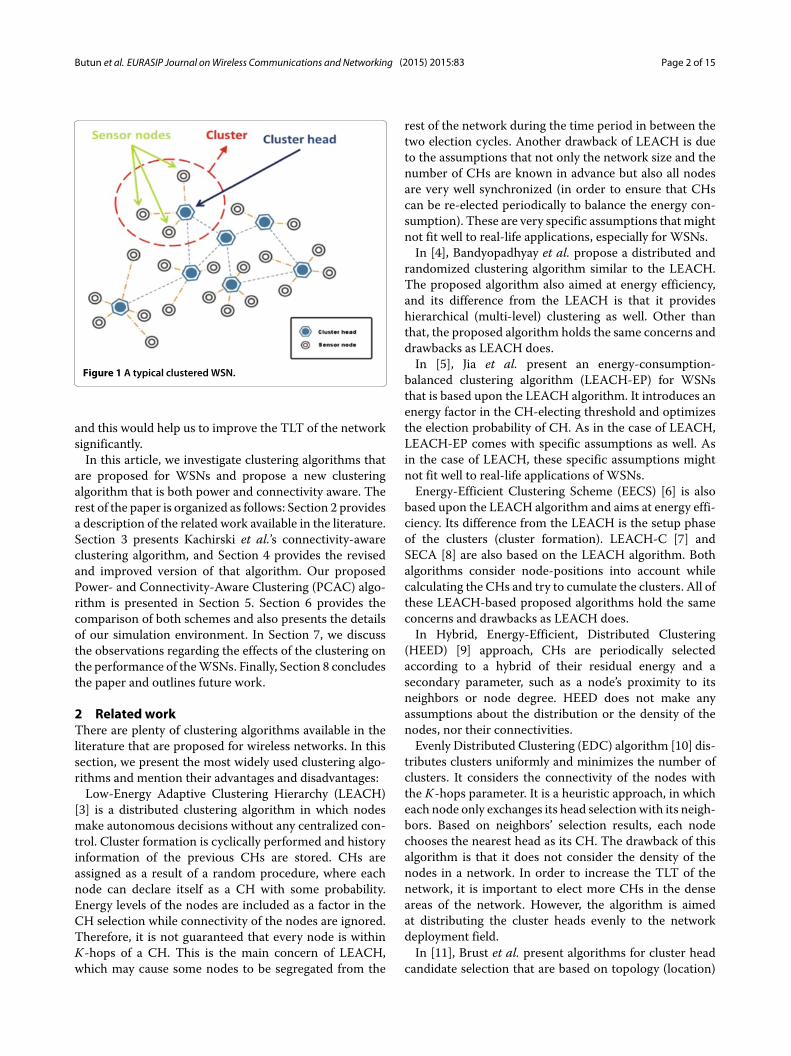
putational and energy resources, and an ad hoc networkoperational environment. They pose unique challenges,due to limited power supplies, low transmission band-width, small memory sizes, and limited energy; therefore,networking techniques used in traditional networks can-not be adopted directly [2]. So, new ideas and approaches(algorithms) are needed in order to increase the overallperformance of the network, especially in terms of totallife time (TLT). Clustering, is one of those techniques thatis very useful for WSNs in data aggregation and filteringand is the main focus of this paper.A clustered WSN is typically as shown in Figure 1. Each

cluster is a group of interconnected sensor nodes with a

*Correspondence: [email protected] of Information and Telecommunication Engineering, KunsanNational University, 573-701 Gunsan, South KoreaFull list of author information is available at the end of the article

dedicated node called cluster head (CH). CHs are respon-sible for the management of the cluster such as schedulingof the medium access, dissemination of the control mes-sages, and, the most important, data aggregation. The sizeof a cluster is defined as the hop distance from the CH tothe farthest node in the cluster. For example, in a three-hops cluster, the distance between the CH and the farthestnode is three-hops (four nodes are in the path includingthe end points). The clustered network shown in Figure 1has a one-hop distance in between CHs and the membersensor nodes.Clustering is the process of grouping the nodes in a

network that are within a specified hop distance or havesome shared common properties into clusters and electingCHs for each cluster. This election can be made perma-nent (static clustering) or repeated in some certain timeintervals (dynamic clustering). Clustering is used in manyapplications of wireless sensor networks in order to reducethe traffic load on the nodes through data aggregationprocess, to prolong total network life time, to balance thedata traffic in the network, and finally to increase the scal-ability (allows the deployment of hundreds or thousandsof nodes). Besides, clustering helps us to increase securityof the network by allowing implementation of complexcryptography algorithms. By using a clustered network-ing approach, power-consuming algorithms (such as dataaggregation and encryption) would be run on the CHs,

© 2015 Butun et al.; licensee Springer. This is an Open Access article distributed under the terms of the Creative CommonsAttribution License (http://creativecommons.org/licenses/by/4.0), which permits unrestricted use, distribution, and reproductionin any medium, provided the original work is properly credited.

mailto: [email protected]

http://creativecommons.org/licenses/by/4.0

Butun et al. EURASIP Journal onWireless Communications and Networking (2015) 2015:83 of 15

Figure 1 A typical clusteredWSN.

and this would help us to improve the TLT of the networksignificantly.In this article, we investigate clustering algorithms that

are proposed for WSNs and propose a new clusteringalgorithm that is both power and connectivity aware. Therest of the paper is organized as follows: Section 2 providesa description of the related work available in the literature.Section 3 presents Kachirski et al.’s connectivity-awareclustering algorithm, and Section 4 provides the revisedand improved version of that algorithm. Our proposedPower- and Connectivity-Aware Clustering (PCAC) algo-rithm is presented in Section 5. Section 6 provides thecomparison of both schemes and also presents the detailsof our simulation environment. In Section 7, we discussthe observations regarding the effects of the clustering onthe performance of theWSNs. Finally, Section 8 concludesthe paper and outlines future work.

2 Related workThere are plenty of clustering algorithms available in theliterature that are proposed for wireless networks. In thissection, we present the most widely used clustering algo-rithms and mention their advantages and disadvantages:Low-Energy Adaptive Clustering Hierarchy (LEACH)

[3] is a distributed clustering algorithm in which nodesmake autonomous decisions without any centralized con-trol. Cluster formation is cyclically performed and historyinformation of the previous CHs are stored. CHs areassigned as a result of a random procedure, where eachnode can declare itself as a CH with some probability.Energy levels of the nodes are included as a factor in theCH selection while connectivity of the nodes are ignored.Therefore, it is not guaranteed that every node is withinK-hops of a CH. This is the main concern of LEACH,which may cause some nodes to be segregated from the

rest of the network during the time period in between thetwo election cycles. Another drawback of LEACH is dueto the assumptions that not only the network size and thenumber of CHs are known in advance but also all nodesare very well synchronized (in order to ensure that CHscan be re-elected periodically to balance the energy con-sumption). These are very specific assumptions that mightnot fit well to real-life applications, especially for WSNs.In [4], Bandyopadhyay et al. propose a distributed and

randomized clustering algorithm similar to the LEACH.The proposed algorithm also aimed at energy efficiency,and its difference from the LEACH is that it provideshierarchical (multi-level) clustering as well. Other thanthat, the proposed algorithm holds the same concerns anddrawbacks as LEACH does.In [5], Jia et al. present an energy-consumption-

balanced clustering algorithm (LEACH-EP) for WSNsthat is based upon the LEACH algorithm. It introduces anenergy factor in the CH-electing threshold and optimizesthe election probability of CH. As in the case of LEACH,LEACH-EP comes with specific assumptions as well. Asin the case of LEACH, these specific assumptions mightnot fit well to real-life applications of WSNs.Energy-Efficient Clustering Scheme (EECS) [6] is also

based upon the LEACH algorithm and aims at energy effi-ciency. Its difference from the LEACH is the setup phaseof the clusters (cluster formation). LEACH-C [7] andSECA [8] are also based on the LEACH algorithm. Bothalgorithms consider node-positions into account whilecalculating the CHs and try to cumulate the clusters. All ofthese LEACH-based proposed algorithms hold the sameconcerns and drawbacks as LEACH does.In Hybrid, Energy-Efficient, Distributed Clustering

(HEED) [9] approach, CHs are periodically selectedaccording to a hybrid of their residual energy and asecondary parameter, such as a node’s proximity to itsneighbors or node degree. HEED does not make anyassumptions about the distribution or the density of thenodes, nor their connectivities.Evenly Distributed Clustering (EDC) algorithm [10] dis-

tributes clusters uniformly and minimizes the number ofclusters. It considers the connectivity of the nodes withthe K-hops parameter. It is a heuristic approach, in whicheach node only exchanges its head selectionwith its neigh-bors. Based on neighbors’ selection results, each nodechooses the nearest head as its CH. The drawback of thisalgorithm is that it does not consider the density of thenodes in a network. In order to increase the TLT of thenetwork, it is important to elect more CHs in the denseareas of the network. However, the algorithm is aimedat distributing the cluster heads evenly to the networkdeployment field.In [11], Brust et al. present algorithms for cluster head

candidate selection that are based on topology (location)


of the nodes. The algorithms aim to avoid selecting nodeslocated close to the network partition border becausethose nodes are more likely to move out of the partition,thus, causing a CH re-election. By using the connectiv-ity information, they propose three algorithms to find thestrong, weak, bridge, and board nodes in the network.Authors do not provide any information on how to selectthe CHs among their selection of nodes (strong, weak,bridge, and board nodes). Overall, this classification ofnodes for CH selection would be useful for the mobilead hoc networks (MANETs) where mobility is the primefactor that changes the network topology. However, thenetwork topology in WSNs is quite stable compared toMANETs, and therefore, this kind of node classificationis unnecessary and also expensive (power consuming) forCH selection.Energy-Efficient Unequal Clustering (EEUC) [12] is

proposed for periodically data-gathering WSNs. It parti-tions the nodes into clusters of unequal size, and clusterscloser to the base station have smaller sizes than those far-ther away from the base station. This way, CHs closer tothe base station can preserve some energy for inter-clusterdata forwarding.Hierarchical clustering proposed in [13] is a framework

based on two-level clustering, multi-hops clusters for dataaggregation (the first-level clustering), and one-hop clus-ters for intrusion detection (the second-level clustering).Although the idea sounds promising for some applica-tions of WSNs (especially for the industrial applications),the details of the formation algorithms for the multi-levelclustering were missing (we assume that this was left as afuture work).Kachirski et al.’s [14] clustering algorithm is based on

the connectivity of the nodes in the network. The higherthe connectivity (neighbors) a node has, the higher theprobability of it to be elected as the CH of a certainneighborhood (cluster). This algorithm is one of the bestchoices for us to work on for several reasons: first of all,it did not require probabilistic approach on clustering,and therefore, the result of the clustering would cover thewhole network. Secondly, the connectivity of the nodesare the main concern on the election of CHs, which isreasonable. In general, the nodes that have more con-nections would be rather elected as CHs. Finally, thealgorithm is easily implementable, which allows the proofof the theoretical work on both hardware and simulationenvironment.There are flaws in Kachirski et al.’s [14] clustering algo-

rithm: 1) nodes were not able to vote for themselvesthrough the election phase of the CHs. Thus, we fixedthis problem and called it as ‘revised version of Kachirskiet al.’s algorithm’. We showed geographically how thischange would result in a more logical cluster forma-tion. 2) There was no power awareness in their proposed

algorithm. Therefore, in this article, we propose our clus-tering algorithm that is built upon the revised version ofKachirski et al.’s algorithm. Our proposed PCAC algo-rithm is both power and connectivity aware, that is why itprovides maximum throughput while saving the energiesof the nodes, therefore, significantly increasing the TLT ofthe network.

3 Kachirski et al.’s connectivity-based approachfor clustering

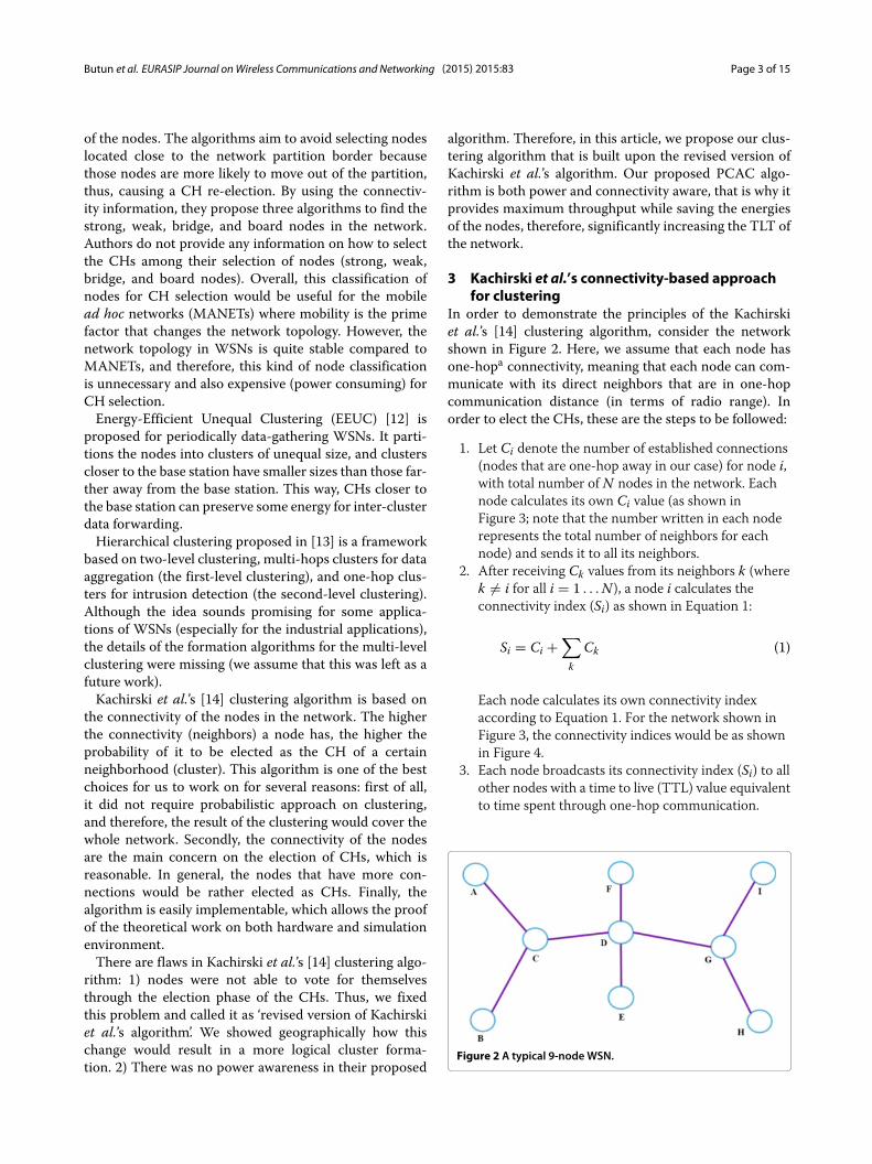
In order to demonstrate the principles of the Kachirskiet al.’s [14] clustering algorithm, consider the networkshown in Figure 2. Here, we assume that each node hasone-hopa connectivity, meaning that each node can com-municate with its direct neighbors that are in one-hopcommunication distance (in terms of radio range). Inorder to elect the CHs, these are the steps to be followed:

1. Let Ci denote the number of established connections(nodes that are one-hop away in our case) for node i,with total number of N nodes in the network. Eachnode calculates its own Ci value (as shown inFigure 3; note that the number written in each noderepresents the total number of neighbors for eachnode) and sends it to all its neighbors.

2. After receiving Ck values from its neighbors k (wherek �= i for all i = 1 . . .N), a node i calculates theconnectivity index (Si) as shown in Equation 1:

Si = Ci +∑k

Ck (1)

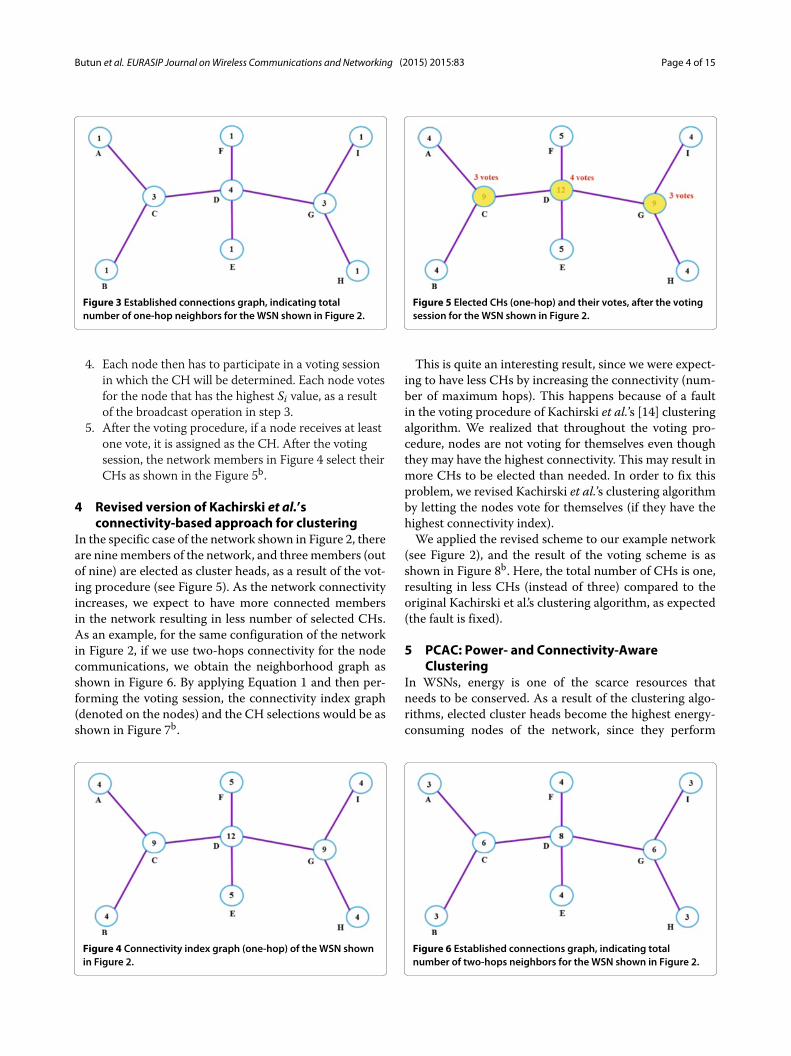
Each node calculates its own connectivity indexaccording to Equation 1. For the network shown inFigure 3, the connectivity indices would be as shownin Figure 4.

3. Each node broadcasts its connectivity index (Si) to allother nodes with a time to live (TTL) value equivalentto time spent through one-hop communication.

Figure 2 A typical 9-nodeWSN.


Figure 3 Established connections graph, indicating totalnumber of one-hop neighbors for the WSN shown in Figure 2.

4. Each node then has to participate in a voting sessionin which the CH will be determined. Each node votesfor the node that has the highest Si value, as a resultof the broadcast operation in step 3.

5. After the voting procedure, if a node receives at leastone vote, it is assigned as the CH. After the votingsession, the network members in Figure 4 select theirCHs as shown in the Figure 5b.

4 Revised version of Kachirski et al.’sconnectivity-based approach for clustering

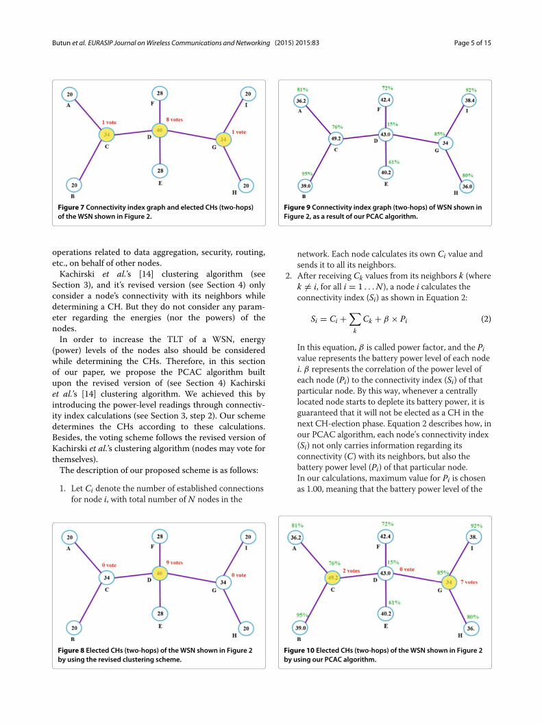
In the specific case of the network shown in Figure 2, thereare ninemembers of the network, and threemembers (outof nine) are elected as cluster heads, as a result of the vot-ing procedure (see Figure 5). As the network connectivityincreases, we expect to have more connected membersin the network resulting in less number of selected CHs.As an example, for the same configuration of the networkin Figure 2, if we use two-hops connectivity for the nodecommunications, we obtain the neighborhood graph asshown in Figure 6. By applying Equation 1 and then per-forming the voting session, the connectivity index graph(denoted on the nodes) and the CH selections would be asshown in Figure 7b.

Figure 4 Connectivity index graph (one-hop) of the WSN shownin Figure 2.

Figure 5 Elected CHs (one-hop) and their votes, after the votingsession for the WSN shown in Figure 2.

This is quite an interesting result, since we were expect-ing to have less CHs by increasing the connectivity (num-ber of maximum hops). This happens because of a faultin the voting procedure of Kachirski et al.’s [14] clusteringalgorithm. We realized that throughout the voting pro-cedure, nodes are not voting for themselves even thoughthey may have the highest connectivity. This may result inmore CHs to be elected than needed. In order to fix thisproblem, we revised Kachirski et al.’s clustering algorithmby letting the nodes vote for themselves (if they have thehighest connectivity index).We applied the revised scheme to our example network

(see Figure 2), and the result of the voting scheme is asshown in Figure 8b. Here, the total number of CHs is one,resulting in less CHs (instead of three) compared to theoriginal Kachirski et al.’s clustering algorithm, as expected(the fault is fixed).

5 PCAC: Power- and Connectivity-AwareClustering

In WSNs, energy is one of the scarce resources thatneeds to be conserved. As a result of the clustering algo-rithms, elected cluster heads become the highest energy-consuming nodes of the network, since they perform

Figure 6 Established connections graph, indicating totalnumber of two-hops neighbors for the WSN shown in Figure 2.


Figure 7 Connectivity index graph and elected CHs (two-hops)of the WSN shown in Figure 2.

operations related to data aggregation, security, routing,etc., on behalf of other nodes.Kachirski et al.’s [14] clustering algorithm (see

Section 3), and it’s revised version (see Section 4) onlyconsider a node’s connectivity with its neighbors whiledetermining a CH. But they do not consider any param-eter regarding the energies (nor the powers) of thenodes.In order to increase the TLT of a WSN, energy

(power) levels of the nodes also should be consideredwhile determining the CHs. Therefore, in this sectionof our paper, we propose the PCAC algorithm builtupon the revised version of (see Section 4) Kachirskiet al.’s [14] clustering algorithm. We achieved this byintroducing the power-level readings through connectiv-ity index calculations (see Section 3, step 2). Our schemedetermines the CHs according to these calculations.Besides, the voting scheme follows the revised version ofKachirski et al.’s clustering algorithm (nodes may vote forthemselves).The description of our proposed scheme is as follows:

1. Let Ci denote the number of established connectionsfor node i, with total number of N nodes in the

Figure 8 Elected CHs (two-hops) of the WSN shown in Figure 2by using the revised clustering scheme.

Figure 9 Connectivity index graph (two-hops) of WSN shown inFigure 2, as a result of our PCAC algorithm.

network. Each node calculates its own Ci value andsends it to all its neighbors.

2. After receiving Ck values from its neighbors k (wherek �= i, for all i = 1 . . .N), a node i calculates theconnectivity index (Si) as shown in Equation 2:

Si = Ci +∑k

Ck + β × Pi (2)

In this equation, β is called power factor, and the Pivalue represents the battery power level of each nodei. β represents the correlation of the power level ofeach node (Pi) to the connectivity index (Si) of thatparticular node. By this way, whenever a centrallylocated node starts to deplete its battery power, it isguaranteed that it will not be elected as a CH in thenext CH-election phase. Equation 2 describes how, inour PCAC algorithm, each node’s connectivity index(Si) not only carries information regarding itsconnectivity (C) with its neighbors, but also thebattery power level (Pi) of that particular node.In our calculations, maximum value for Pi is chosenas 1.00, meaning that the battery power level of the

Figure 10 Elected CHs (two-hops) of the WSN shown in Figure 2by using our PCAC algorithm.


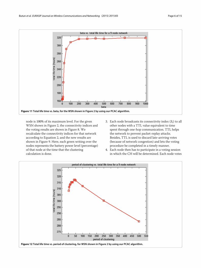
Figure 11 Total life time vs. beta, for the WSN shown in Figure 2 by using our PCAC algorithm.

node is 100% of its maximum level. For the givenWSN shown in Figure 2, the connectivity indices andthe voting results are shown in Figure 8. Werecalculate the connectivity indices for that networkaccording to Equation 2, and the new results areshown in Figure 9. Here, each green writing over thenodes represents the battery power level (percentage)of that node at the time that the clusteringcalculation is done.

3. Each node broadcasts its connectivity index (Si) to allother nodes with a TTL value equivalent to timespent through one-hop communication. TTL helpsthe network to prevent packet-replay attacks.Besides, TTL is used to discard late-arriving votes(because of network congestion) and lets the votingprocedure be completed in a timely manner.

4. Each node then has to participate in a voting sessionin which the CH will be determined. Each node votes

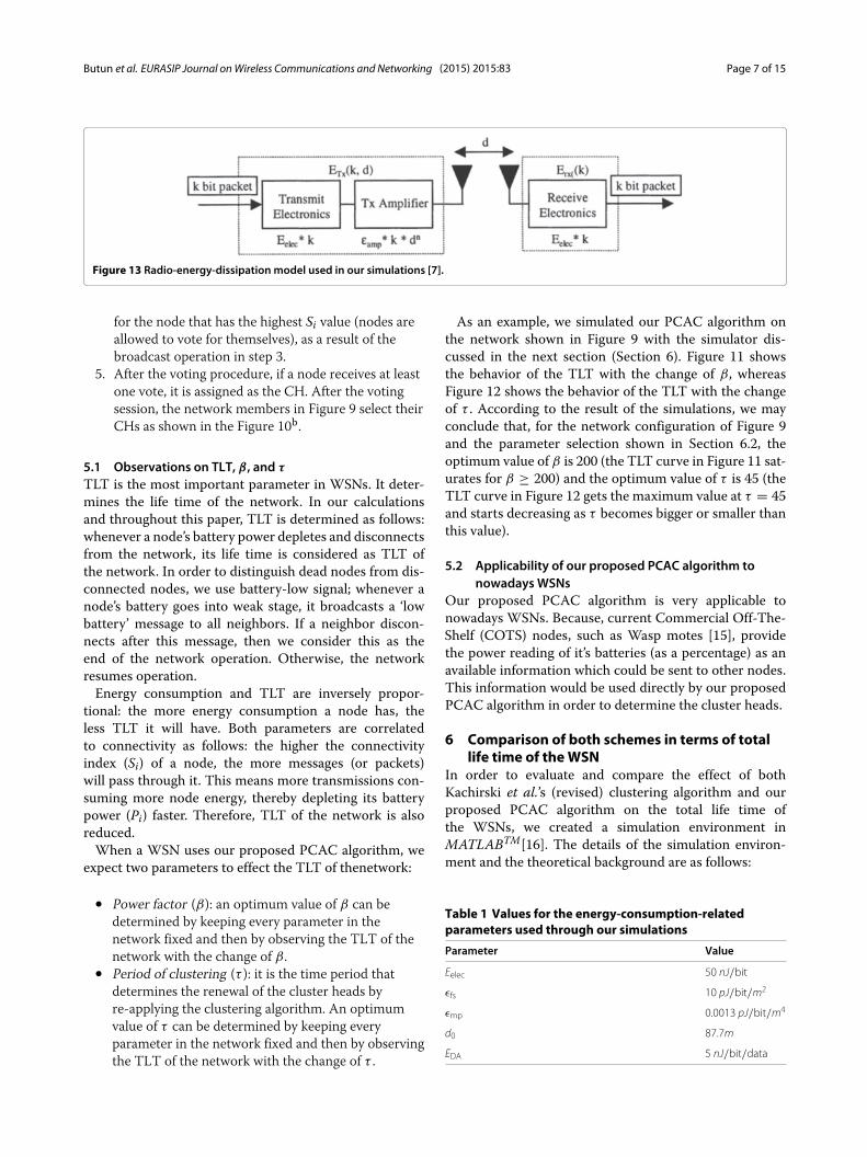
Figure 12 Total life time vs. period of clustering, for WSN shown in Figure 2 by using our PCAC algorithm.


Figure 13 Radio-energy-dissipation model used in our simulations [7].

for the node that has the highest Si value (nodes areallowed to vote for themselves), as a result of thebroadcast operation in step 3.

5. After the voting procedure, if a node receives at leastone vote, it is assigned as the CH. After the votingsession, the network members in Figure 9 select theirCHs as shown in the Figure 10b.

5.1 Observations on TLT, β, and τ

TLT is the most important parameter in WSNs. It deter-mines the life time of the network. In our calculationsand throughout this paper, TLT is determined as follows:whenever a node’s battery power depletes and disconnectsfrom the network, its life time is considered as TLT ofthe network. In order to distinguish dead nodes from dis-connected nodes, we use battery-low signal; whenever anode’s battery goes into weak stage, it broadcasts a ‘lowbattery’ message to all neighbors. If a neighbor discon-nects after this message, then we consider this as theend of the network operation. Otherwise, the networkresumes operation.Energy consumption and TLT are inversely propor-

tional: the more energy consumption a node has, theless TLT it will have. Both parameters are correlatedto connectivity as follows: the higher the connectivityindex (Si) of a node, the more messages (or packets)will pass through it. This means more transmissions con-suming more node energy, thereby depleting its batterypower (Pi) faster. Therefore, TLT of the network is alsoreduced.When a WSN uses our proposed PCAC algorithm, we

expect two parameters to effect the TLT of thenetwork:

• Power factor (β): an optimum value of β can bedetermined by keeping every parameter in thenetwork fixed and then by observing the TLT of thenetwork with the change of β .

• Period of clustering (τ ): it is the time period thatdetermines the renewal of the cluster heads byre-applying the clustering algorithm. An optimumvalue of τ can be determined by keeping everyparameter in the network fixed and then by observingthe TLT of the network with the change of τ .

As an example, we simulated our PCAC algorithm onthe network shown in Figure 9 with the simulator dis-cussed in the next section (Section 6). Figure 11 showsthe behavior of the TLT with the change of β , whereasFigure 12 shows the behavior of the TLT with the changeof τ . According to the result of the simulations, we mayconclude that, for the network configuration of Figure 9and the parameter selection shown in Section 6.2, theoptimum value of β is 200 (the TLT curve in Figure 11 sat-urates for β ≥ 200) and the optimum value of τ is 45 (theTLT curve in Figure 12 gets the maximum value at τ = 45and starts decreasing as τ becomes bigger or smaller thanthis value).

5.2 Applicability of our proposed PCAC algorithm tonowadays WSNs

Our proposed PCAC algorithm is very applicable tonowadays WSNs. Because, current Commercial Off-The-Shelf (COTS) nodes, such as Wasp motes [15], providethe power reading of it’s batteries (as a percentage) as anavailable information which could be sent to other nodes.This information would be used directly by our proposedPCAC algorithm in order to determine the cluster heads.

6 Comparison of both schemes in terms of totallife time of theWSN

In order to evaluate and compare the effect of bothKachirski et al.’s (revised) clustering algorithm and ourproposed PCAC algorithm on the total life time ofthe WSNs, we created a simulation environment inMATLABTM[16]. The details of the simulation environ-ment and the theoretical background are as follows:

Table 1 Values for the energy-consumption-relatedparameters used through our simulations

Parameter Value

Eelec 50 nJ/bit

εfs 10 pJ/bit/m2

εmp 0.0013 pJ/bit/m4

d0 87.7m

EDA 5 nJ/bit/data


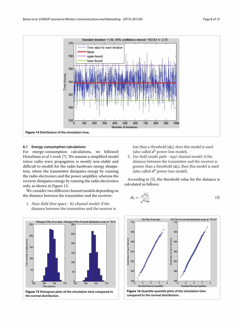
Figure 14 Distribution of the simulation time.

6.1 Energy-consumption calculationsFor energy-consumption calculations, we followedHeizelman et al.’s work [7]. We assume a simplified model(since radio wave propagation is mostly non-stable anddifficult to model) for the radio hardware energy dissipa-tion, where the transmitter dissipates energy by runningthe radio electronics and the power amplifier, whereas thereceiver dissipates energy by running the radio electronicsonly, as shown in Figure 13.We consider two different channelmodels depending on

the distance between the transmitter and the receiver:

1. Near-field (free space - fs) channel model : if thedistance between the transmitter and the receiver is

Figure 15 Histogram plots of the simulation time compared tothe normal distribution.

less than a threshold (d0), then this model is used(also called d2 power-loss model).

2. Far-field (multi-path - mp) channel model : if thedistance between the transmitter and the receiver isgreater than a threshold (d0), then this model is used(also called d4 power-loss model).

According to [5], the threshold value for the distance iscalculated as follows:

d0 =√

εfs√εmp

(3)

Figure 16 Quantile-quantile plots of the simulation timecompared to the normal distribution.


Figure 17 Location of the nodes and the BS throughout thesimulations.

where εfs and εmp are constants related to free-space lossand multi-path loss, respectively.In order to transmit m-bit data to a distance of d, the

radio spends:

ETx(m, d) = ETx−elec(m) + ETx−amp(m, d)

={mEelec + mεfsd2, d < d0mEelec + mεmpd4, d ≥ d0

(4)

In order to receive the same m-bit data, the radiospends:

ERx(m) = ERx−elec(m) = mEelec (5)

The energy spent on the radio electronics circuitry, Eelec,is due to the digital modulation (transmitter side), digi-

tal demodulation (receiver side), error correction codes,and filtering, whereas the amplifier energy, ETx−amp, is dueto the electromagnetic spreading of the signal into theair and depends on the distance as mentioned above (seeEquation 3).Assume that each CH has N member nodes. CH dissi-

pates energy by receiving the data from member nodes,aggregating those data, and finally transmitting the aggre-gate data to the base station (BS). We assume that BSis located far away from the nodes, and therefore, trans-mission between the CH and the BS follows the far-fieldchannel model (d4 power-loss model). During a singledata frame, we calculate the energy dissipated in the CHas follows:

ECH = {Eaggregating_data_from_member_nodes}+ {Etransmit_aggregate_data_to_BS}

= {N(mEelec + mEDA)} + {mEelec + mεmpd4toBS

}(6)

wherem represents the total number bits in a data frame,mEDA represents the energy dissipated during aggregat-ing m-bit data, and finally dtoBS represents the distancebetween the CH and the BS.Assume that each member node is located in the near

field of the CH so that near-field channel model (d2power-loss model) will be used for calculating the energydissipated during data transmission from the membernode towards the CH. Therefore, we calculate the energydissipated in each member node as follows:

Emember_node = mEelec + mεfsd2toCH (7)

where dtoCH represents the distance between the membernode and the CH, and therefore, it takes different valuesfor each node.

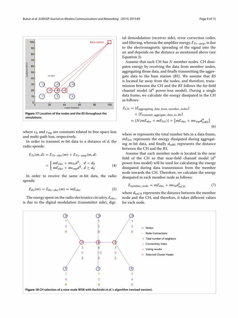
Figure 18 CH selection of a nine-nodeWSNwith Kachirski et al.’s algorithm (revised version).


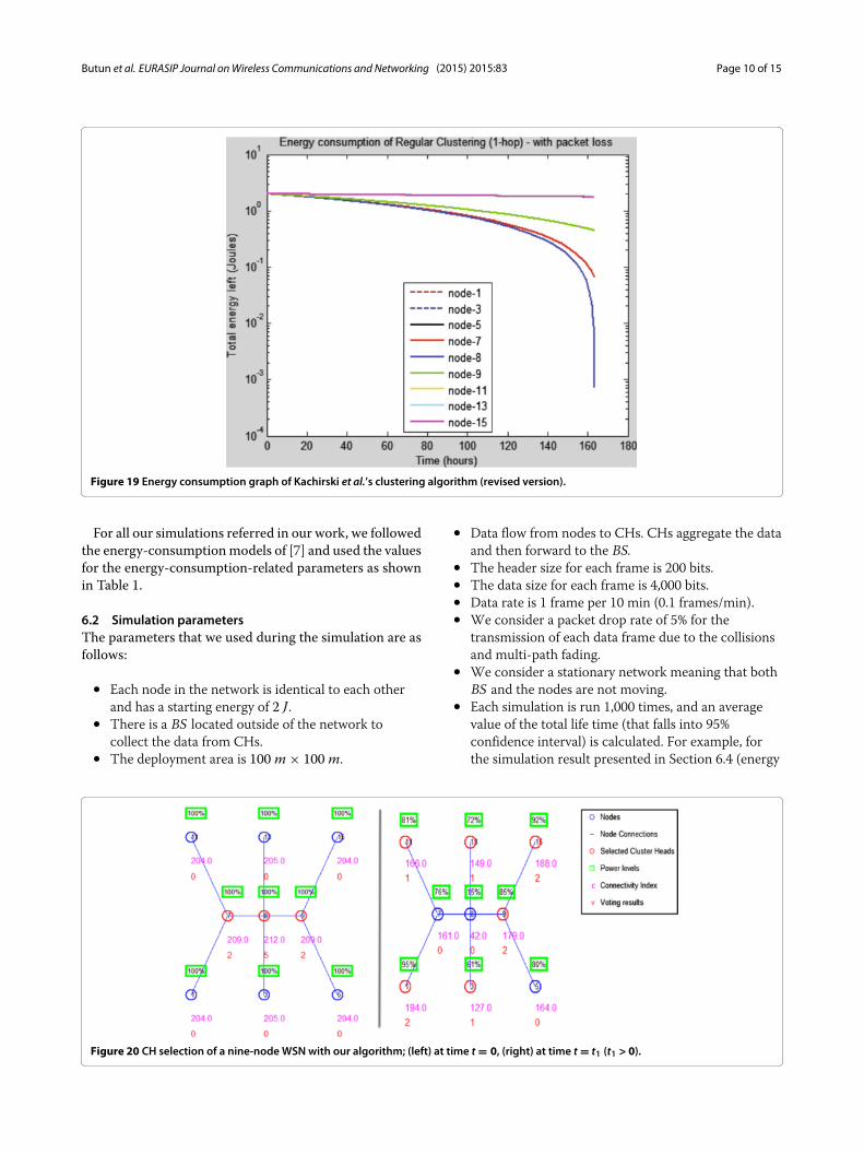
Figure 19 Energy consumption graph of Kachirski et al.’s clustering algorithm (revised version).

For all our simulations referred in our work, we followedthe energy-consumptionmodels of [7] and used the valuesfor the energy-consumption-related parameters as shownin Table 1.

6.2 Simulation parametersThe parameters that we used during the simulation are asfollows:

• Each node in the network is identical to each otherand has a starting energy of 2 J .

• There is a BS located outside of the network tocollect the data from CHs.

• The deployment area is 100m × 100m.

• Data flow from nodes to CHs. CHs aggregate the dataand then forward to the BS.

• The header size for each frame is 200 bits.• The data size for each frame is 4,000 bits.• Data rate is 1 frame per 10 min (0.1 frames/min).• We consider a packet drop rate of 5% for the

transmission of each data frame due to the collisionsand multi-path fading.

• We consider a stationary network meaning that bothBS and the nodes are not moving.

• Each simulation is run 1,000 times, and an averagevalue of the total life time (that falls into 95%confidence interval) is calculated. For example, forthe simulation result presented in Section 6.4 (energy

Figure 20 CH selection of a nine-nodeWSNwith our algorithm; (left) at time t = 0, (right) at time t = t1 (t1 > 0).


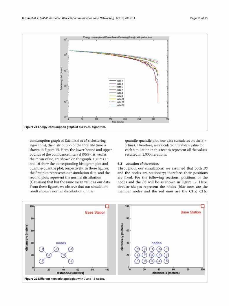
Figure 21 Energy-consumption graph of our PCAC algorithm.

consumption graph of Kachirski et al.’s clusteringalgorithm), the distribution of the total life time isshown in Figure 14. Here, the lower bound and upperbounds of the confidence interval (95%), as well asthe mean value, are shown on the graph. Figures 15and 16 show the corresponding histogram plot andquantile-quantile plot, respectively. In these figures,the first plot represents our simulation data, and thesecond plots represent the normal distribution(Gaussian) that has the same mean value as our data.From these figures, we observe that our simulationresult shows a normal distribution (in the

quantile-quantile plot, our data cumulates on the x =y line). Therefore, we calculated the mean value foreach simulation in this text to represent all the valuesresulted in 1,000 iterations.

6.3 Location of the nodesThroughout our simulations, we assumed that both BSand the nodes are stationary; therefore, their positionsare fixed. For the following sections, positions of thenodes and the BS will be as shown in Figure 17. Here,circular shapes represent the nodes (blue ones are themember nodes and the red ones are the CHs) CHs)

Figure 22 Different network topologies with 7 and 15 nodes.


whereas the square shape represents the BS. The redlines represent the connection between the CHs andthe BS, whereas the blue lines represent the connectionsbetween the CHs and their member nodes. The wholedeployment area is 100 m × 100 m, and the loca-tion of the BS is [ 100 m, 100 m]. The nodes aredeployed to the area with the following boundaries:[ 10 m, 10 m] , [ 10 m, 30 m] , [ 50 m, 10 m], and[ 50m, 30m].

6.4 Energy consumption of Kachirski et al.’s clusteringalgorithm (revised version)

We ran the revised version of Kachirski et al.’s clusteringalgorithm on our simulator with the parameters shown inSection 6.2 and the positions shown in Section 6.3. Weconsidered one-hop connectivity for all nodes in the net-work. Figure 18 shows the total number of neighbors foreach node (including the connection paths), connectivityindices, and results of the voting along with the electedCHs.Figure 19 shows the energy-consumption performance

of the mentioned algorithm with respect to time. Westopped the simulation whenever a single node dies (runsout of battery power), and we call this time as the ‘total lifetime of the network’, since at this point the network startsto disintegrate (segregation starts).In Figure 19, we can see that node 8 depleted its energy

faster than other nodes and therefore determined thenetwork’s total life time as 163.8 h.

6.5 Energy consumption of our proposed PCAC algorithmWe ran our proposed PCAC algorithm on our simula-tor with the parameters shown in Section 6.2 and thepositions shown in Section 6.3.We consider one-hop con-nectivity for all nodes in the network. As mentioned inSection 5, we selected β as 200 and τ is 45, in order toachieve the maximum TLT. Figure 20 shows the result ofthe clustering algorithm at times t = 0 and t = t1(t1 > 0).Figure 21 shows the energy-consumption performance ofour proposed algorithm with respect to time. In Figure 21,we can see that node 7 depleted its energy faster thanother nodes and therefore determined the network’s TLTas 316.66 h. When compared to the revised version ofKachirski et al.’s clustering algorithm (see previous sub-section), relative performance improvement in TLT of thenetwork is 93%.

Table 2 Relative performance improvements (%) on thelife time of the network when our PCAC algorithm is used

Maximum hops For 7-node network 9-node 15-node

One-hop 86 93 85

Two-hops 234 313 256

Three-hops 366 463 438

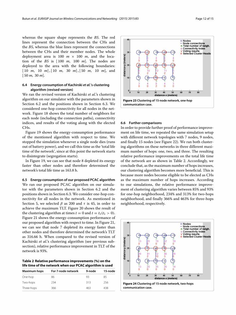
Figure 23 Clustering of 15-node network, one-hopcommunication case.

6.6 Further comparisonsIn order to provide further proof of performance improve-ment on life time, we repeated the same simulation setupwith different network topologies with 7 nodes, 9 nodes,and finally 15 nodes (see Figure 22). We ran both cluster-ing algorithms on these networks in three different maxi-mum number of hops: one, two, and three. The resultingrelative performance improvements on the total life timeof the network are as shown in Table 2. Accordingly, weconclude that, as the maximum number of hops increases,our clustering algorithm becomes more beneficial. This isbecause more nodes become eligible to be elected as CHsas the maximum number of hops increases. Accordingto our simulations, the relative performance improve-ment of clustering algorithm varies between 85% and 93%for one-hop neighborhood, 234% and 313% for two-hopsneighborhood, and finally 366% and 463% for three-hopsneighborhood, respectively.

Figure 24 Clustering of 15-node network, two-hopscommunication case.


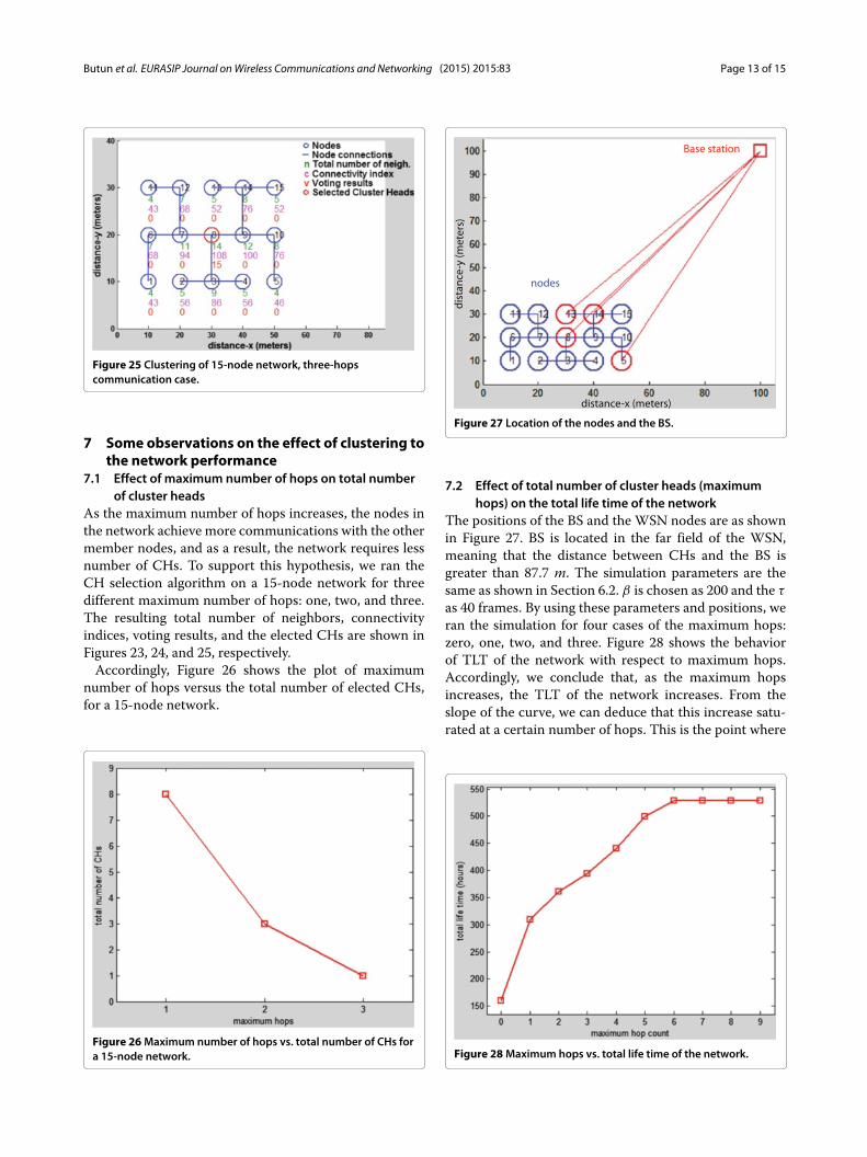
Figure 25 Clustering of 15-node network, three-hopscommunication case.

7 Some observations on the effect of clustering tothe network performance

7.1 Effect of maximum number of hops on total numberof cluster heads

As the maximum number of hops increases, the nodes inthe network achieve more communications with the othermember nodes, and as a result, the network requires lessnumber of CHs. To support this hypothesis, we ran theCH selection algorithm on a 15-node network for threedifferent maximum number of hops: one, two, and three.The resulting total number of neighbors, connectivityindices, voting results, and the elected CHs are shown inFigures 23, 24, and 25, respectively.Accordingly, Figure 26 shows the plot of maximum

number of hops versus the total number of elected CHs,for a 15-node network.

Figure 26Maximum number of hops vs. total number of CHs fora 15-node network.

Figure 27 Location of the nodes and the BS.

7.2 Effect of total number of cluster heads (maximumhops) on the total life time of the network

The positions of the BS and the WSN nodes are as shownin Figure 27. BS is located in the far field of the WSN,meaning that the distance between CHs and the BS isgreater than 87.7 m. The simulation parameters are thesame as shown in Section 6.2. β is chosen as 200 and the τ

as 40 frames. By using these parameters and positions, weran the simulation for four cases of the maximum hops:zero, one, two, and three. Figure 28 shows the behaviorof TLT of the network with respect to maximum hops.Accordingly, we conclude that, as the maximum hopsincreases, the TLT of the network increases. From theslope of the curve, we can deduce that this increase satu-rated at a certain number of hops. This is the point where

Figure 28Maximum hops vs. total life time of the network.


Figure 29 Total number of nodes vs. total life time of thenetwork.

each node can reach any node in the network (six-hops inthis case).

7.3 Effect of total number of nodes in a cluster on totallife time of the network

We wondered about the effect of total number of thenodes in the network on the TLT of the network. To inves-tigate this, we considered the same network shown inFigure 27 along with the simulation parameters the sameas Section 7.2. The only parameter that is different hereis the maximum hops. We kept it constant and equal tothree. Then, we started the simulation with 15 nodes, andthen, each time, we removed one of the end nodes and

repeated the simulation till we are left with one node inthe network. As a result, Figure 29 shows the behavior ofthe TLT of the network with respect to the total number ofnodes in the network. Accordingly, we conclude that thereis a certain number of nodes (six nodes in our case) in thenetwork that allow the network to achieve maximum TLT(519.15 h in our case).

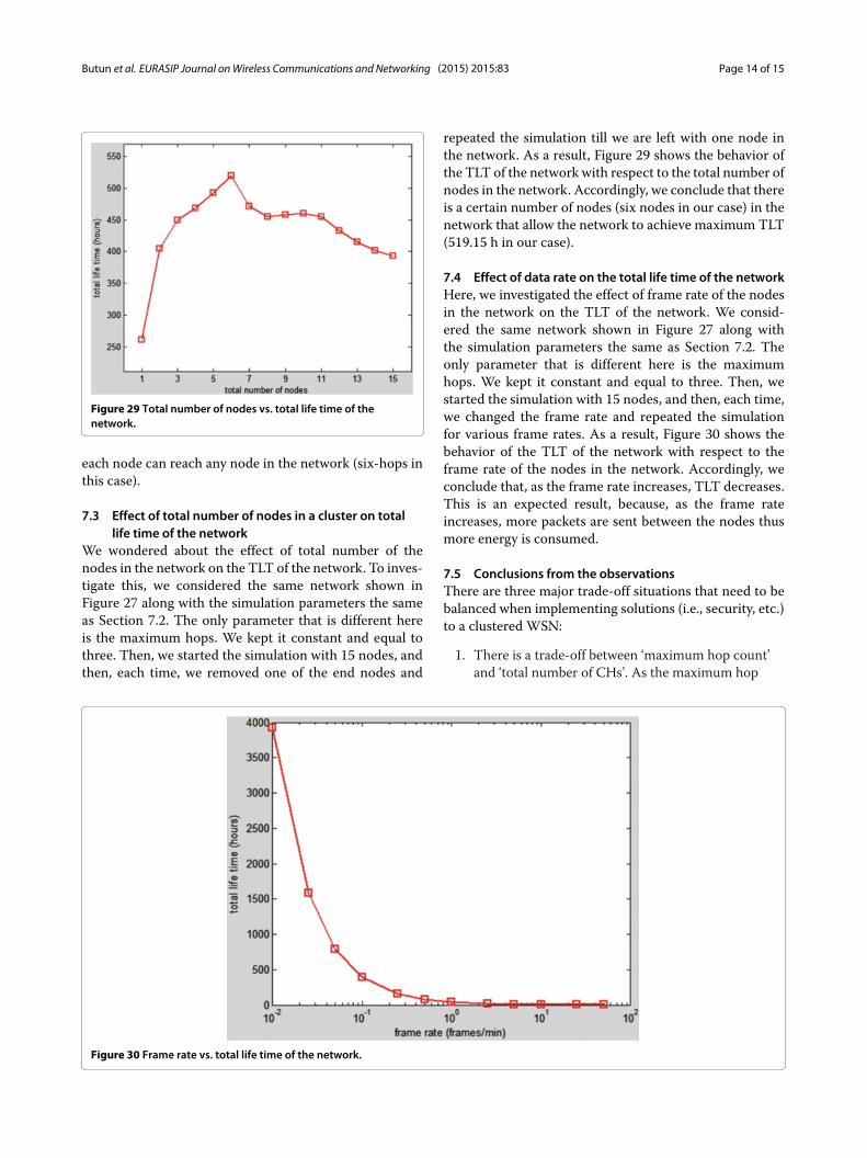
7.4 Effect of data rate on the total life time of the networkHere, we investigated the effect of frame rate of the nodesin the network on the TLT of the network. We consid-ered the same network shown in Figure 27 along withthe simulation parameters the same as Section 7.2. Theonly parameter that is different here is the maximumhops. We kept it constant and equal to three. Then, westarted the simulation with 15 nodes, and then, each time,we changed the frame rate and repeated the simulationfor various frame rates. As a result, Figure 30 shows thebehavior of the TLT of the network with respect to theframe rate of the nodes in the network. Accordingly, weconclude that, as the frame rate increases, TLT decreases.This is an expected result, because, as the frame rateincreases, more packets are sent between the nodes thusmore energy is consumed.

7.5 Conclusions from the observationsThere are three major trade-off situations that need to bebalanced when implementing solutions (i.e., security, etc.)to a clustered WSN:

1. There is a trade-off between ‘maximum hop count’and ‘total number of CHs’. As the maximum hop

Figure 30 Frame rate vs. total life time of the network.


count increases, total number of CHs decreases andvice versa.

2. There is a trade-off between ‘total number of CHs’and ‘TLT of the network’. There is an optimumnumber of CHs which lead the network to survivethe most TLT possible (without having anypartioning/segregation).

3. There is a trade-off between ‘data rate(frames/minute)’ and ‘TLT of the network’. As thedata rate increases, more data need to be processedand more packets need to be transmitted causingmore power to be spent; therefore, the TLT of thenetwork decreases.

8 ConclusionsIn this work, we provided the energy-consumption sim-ulation results of the revised version of Kachirski et al.’sclustering algorithm and our proposed PCAC algorithm.According to these results, our proposed PCAC algorithmout-performed the revised version of Kachirski et al.’sclustering algorithm in terms of energy efficiency and alsototal life time of the network.According to our simulation results, with our proposed

PCAC algorithm, relative performance improvement(compared to the revised version of Kachirski et al.’s clus-tering algorithm) in total life time of the network variesbetween 85% and 93% for one-hop neighborhood, 234%and 313% for two-hops neighborhood, and finally 366%and 463% for three-hops neighborhood, respectively.Here, we note that mobility can also be included as

an another parameter in CH calculations (in Equation 2)for MANETs. For example, highly mobile nodes (Waspmotes [17] provide three-axis accelerometer readingwhich would be used to measure mobility) may be electedas CHs, because they might be in contact with most ofthe nodes in a certain amount of time. Since WSNs aremostly stationary, we did not consider any mobility inour calculations and left this part as a future work to beconsidered.

EndnotesaThe same method would be applied in the case of

multiple-hops (2,3,. . . , etc.) connections if needed.bCHs are highlighted with yellow color and also the

votes they received are noted on top of them in red colorwriting.Competing interestsThe authors declare that they have no competing interests.

Authors’ informationIsmail Butun, [email protected]; In-ho Ra, [email protected]; Ravi Sankar,[email protected].

AcknowledgementsThis research was supported by Basic Science Research Program through theNational Research Foundation of Korea (NRF) funded by the Ministry ofEducation, Science and Technology (2013054460).

Author details1Department of Mechatronics Engineering, Bursa Technical University,Gaziakdemir M. Mudanya C. No:4/10, 16190 Osmangazi, Bursa, Turkey.2Department of Information and Telecommunication Engineering, KunsanNational University, 573-701 Gunsan, South Korea. 3Department of ElectricalEngineering, University of South Florida, 4202 E. Fowler Avenue, Tampa, FL33620, USA.

Received: 15 January 2015 Accepted: 5 March 2015

References1. I Butun, Y Wang, Y Lee, R Sankar, Intrusion prevention with two-level user

authentication in heterogeneous wireless sensor networks. Int. J. Secur.Netw. 7(2), 107–121 (2012)

2. I Butun, S Morgera, R Sankar, A survey of intrusion detection systems inwireless sensor networks. Commun. Surv. Tutorials. 16(1), 266–282 (2013)

3. WR Heinzelman, A Chandrakasan, H Balakrishnan, in System Sciences, 2000.Proceedings of the 33rd Annual Hawaii International Conference On.Energy-efficient communication protocol for wireless microsensornetworks (IEEE Piscataway, New Jersey, 2000), p. 10

4. S Bandyopadhyay, EJ Coyle, in INFOCOM 2003. Twenty-Second Annual JointConference of the IEEE Computer and Communications. IEEE Societies. Anenergy efficient hierarchical clustering algorithm for wireless sensornetworks, vol. 3 (IEEE Piscataways, New Jersey, 2003), pp. 1713–1723

5. J Jia, Z He, J Kuang, Y Mu, inWireless Communications Networking andMobile Computing (WiCOM), 2010 6th International Conference On. Anenergy consumption balanced clustering algorithm for wireless sensornetwork (IEEE Piscataway, New Jersey, 2010), pp. 1–4

6. M Ye, C Li, G Chen, J Wu, in Performance, Computing, and CommunicationsConference, 2005. IPCCC 2005. 24th IEEE International. EECS: an energyefficient clustering scheme in wireless sensor networks (IEEE Piscataway,New Jersey, 2005), pp. 535–540

7. WB Heinzelman, AP Chandrakasan, H Balakrishnan, Anapplication-specific protocol architecture for wireless microsensornetworks. IEEE Trans. Wireless Commun. 1(4) (2002)

8. J-Y Chang, P-H Ju, An efficient cluster-based power saving scheme forwireless sensor networks. J. Wireless Commun. Netw. 2012(1), 1–10 (2012)

9. O Younis, S Fahmy, HEED: a hybrid, energy-efficient, distributed clusteringapproach for ad hoc sensor networks. Mobile Comput. IEEE Trans. 3(4),366–379 (2004)

10. Q Chen, J Ma, Y Zhu, D Zhang, L Ni, An energy-efficient k-hop clusteringframework for wireless sensor networks. Wireless Sens. Networks. 4373,17–33 (2007)

11. MR Brust, A Andronache, S Rothkugel, Z Benenson, in CommunicationSystems Software andMiddleware, 2007. COMSWARE 2007. 2nd InternationalConference On. Topology-based clusterhead candidate selection inwireless ad-hoc and sensor networks (IEEE Piscataway, New Jersey, 2007),pp. 1–8

12. C Li, M Ye, G Chen, J Wu, inMobile Adhoc and Sensor Systems Conference,2005. IEEE International Conference On. An energy-efficient unequalclustering mechanism for wireless sensor networks (IEEE Piscataway, NewJersey, 2005)

13. S Shin, T Kwon, GY Jo, Y Park, H Rhy, An experimental study of hierarchicalintrusion detection for wireless industrial sensor networks. Ind. Inform.IEEE Trans. 6(4), 744–757 (2010)

14. O Kachirski, R Guha, in System Sciences, 2003. Proceedings of the 36thAnnual Hawaii International Conference On. Effective intrusion detectionusing multiple sensors in wireless ad hoc networks (IEEE Piscataway, NewJersey, 2003), p. 8

15. Libelium, Wasp mote - wireless sensor networks 802.15.4 ZigBee Mote.(Libelium Inc.) Available At: http://www.libelium.com/products/waspmote

16. Matlab, MATLAB simulation program by Mathworks Inc. (Mathworks Inc.)Available At: http://www.mathworks.com/

17. Libelium, Libelium Wasp mote with 3D accelerometer. (Libelium Inc.)Available At: http://www.libelium.com/video-accelerometer/

http://www.libelium.com/products/waspmote

http://www.libelium.com/products/waspmote

http://www.mathworks.com/

http://www.libelium.com/video-accelerometer/

PCAC: Power- and Connectivity-Aware Clustering for Wireless Sensor Networks

Documents

Transcript of PCAC: Power- and Connectivity-Aware Clustering for Wireless Sensor Networks