electronics

Article

On the Trade-Off between the Main Parameters ofPlanar Antenna Arrays

Daniele Pinchera

DIEI, University of Cassino and Southern Lazio and ELEDIA@UniCAS, via G. Di Biasio 43, 03043 Cassino, Italy;pinchera@unicas.it; Tel.: +39-0776-299-4348

Received: 20 April 2020; Accepted: 28 April 2020; Published: 30 April 2020�����������������

Abstract: The aim of this paper is two-fold. First, the trade-off between directivity, beam-width,side-lobe-level, number of radiating elements, and scanning range of planar antenna arrays isreviewed, and some simple ready-to-use formulas for the preliminary dimensioning of equispacedplanar arrays are provided. Furthermore, the synthesis of sparse planar arrays, and the issue of theirreduction in directivity, is analyzed. Second, a simple, yet effective, novel approach to overcomethe directivity issue is proposed. The presented method is validated by several synthesized layouts;the examples show that it is possible to synthesize sparse arrays, able to challenge with equispacedlattices in terms of directivity, with a significant reduction of the number of radiators.

Keywords: antenna arrays; sparse arrays; radar; pattern synthesis; signal processing

1. Introduction

There is no doubt that antenna arrays, thanks to their capability to provide a dynamical manipulationof the received and radiated field, have a strong potential for most communication applications. Antennaarrays have been studied for half of the last century, and all crucial high-performance applications,(radar [1], satellite communication [2], and astronomical observation [3]), have made use of them.

In the last decades, we have also seen the extension of antenna arrays to civil, low-cost applications(Wi-Fi networks, 4G [4] and 5G [5,6] networks); as a matter of fact, the achievement of the demands ofmodern communication systems (in terms of the number of terminals served, band, latency) requirethe aforementioned potential [7].

This trend is not going to stop, particularly now that we are moving towards the use of mm-wavefrequencies for communications [8], which require the use of arrays to obtain electronically focusablebeams with good directivity.

Roughly speaking, the more radiating elements, the more directivity is possible to achieve.Unfortunately, antenna arrays have a non-trivial cost, usually not related to the antenna itself, but to allthe amplifiers, phase shifters, beam forming networks that are required to operate the array. All thesedevices have a weight, occupy a volume, and require maintenance. In some applications, like satelliteones, payload reduction is a mandatory requirement; so, in general, the reduction of the elements’number is fundamental to lower the overall cost [9]. The choice of the number of radiators needs to bedone with judiciousness.

Furthermore, in many applications, we need to verify specific constraints in terms of beam-width(BW) and side-lobe-level (SLL), but their realization requires a tapering of the source, which is knownto reduce the directivity of the array [10]. Moreover, the design of an antenna array capable of scanningthe beam in a certain angular range requires particular care in the inter-elements distance otherwisegrating lobes could appear in the visible range of the antenna. This could be a very negative effect formost of the application cases.

Electronics 2020, 9, 739; doi:10.3390/electronics9050739 www.mdpi.com/journal/electronics

Electronics 2020, 9, 739 2 of 17

The difficulty of the array synthesis problem, particularly when non-regular lattices are used,is testified by a large number of papers on this topic that have been published in the last 60 years;many deterministic, evolutionary, and hybrid algorithms have been recently proposed [11–51].

Even if a large literature exists, the array dimensioning is still a non-trivial topic for antennaengineers; one may think that using the “right number” of radiators, half-wavelength equispaced,is the only thing to do, but this simplistic approach is not the best choice [52–54].

So, an antenna engineer dealing with the synthesis of an array radiating a pencil beam needsto take into account at least five parameters: the number of radiating elements that is possible touse, the required beam-width and side-lobe level, the necessary scanning range of the beam, and thedesired directivity. Obviously, those five parameters are not the only ones that could be taken intoaccount in the synthesis, but a more general analysis would be beyond the scope of these notes.

In this paper, in particular, the issue of the directivity decrease in sparse arrays will be analyzed,showing that with a novel approach to the synthesis it is possible to achieve sparse layouts that canchallenge with equispaced lattices in terms of directivity, with a significant reduction of the numberof radiators.

To achieve this task, the present manuscript is structured in the following way. In the first part(Section 2), the relationship between the relevant parameters is reviewed and simple ready-to-useformulas for the preliminary dimensioning of equispaced planar arrays are provided. In the secondpart (Section 3), we then focus on the synthesis of sparse arrays, showing that the reduction in thenumber of radiating elements is usually paid in terms of a reduction of the directivity, in particularwhen beams out of the broadside direction are considered. In the third part (Section 4), a novel designstrategy, for achieving very high directivity is introduced and discussed through numerical examples.Conclusions follow.

2. Planar Arrays with Regular Lattices

For the sake of simplicity, in the following sections we will focus on the radiation of planar arraysof isotropic elements: we will deal with the synthesis of the “array factor” (AF) [10]:

F(u, v) =N

∑n=1

a(n)ejβ(uxn+vyn) (1)

where β = 2π/λ is the free-space wavenumber, N is the number of radiating elements, a(n) isthe excitation of the n−th element, (xn, yn) are the coordinates of the n−th radiating element,u = sin θ cos φ and v = sin θ sin φ, with (θ,φ) the spherical coordinates with respect to thebroadside direction.

It must be recalled that the use of the AF for pattern synthesis is convenient also when dealingwith “real”, non-isotropic, radiating elements. In this case, we could apply the approach proposedin [40] to properly modify the power pattern mask guaranteeing the satisfaction of the side-lobe levelspecification for any direction within the maximum scanning angle.

Let us now consider the synthesis of a pencil beam with prescribed side-lobe level employing aregular lattice array. If we require that the beam scanning is performed using a linear phase shift of theexcitations, the synthesis problem can be written as:

F(0, 0) = 1 (2)

F(u, v) ≤ SLL f or w1 ≤ w ≤ 1 + ws (3)

where w =√

u2 + v2, SLL is the desired side-lobe level, and w1 defines the circular footprint of thepencil beam, which establishes the beam-width, and ws = sin(θs) with θs, the angle defining thescanning cone for the beam. Roughly speaking, we are increasing the region of the (u, v) plane wherewe impose the pattern constraints, to take into account the scanning of the beam.

Electronics 2020, 9, 739 3 of 17

2.1. The Choice of the Lattice

Once the synthesis problem is defined, the first question we do have to answer is: how manyantennas do we need? For square lattices (Figure 1a) we could use a Tchebyshev-based approach usedin [55] for linear arrays, finding that the maximum inter-element distance between elements must be:

dS =λ

1 + w1 + ws(4)

It is also possible to use a triangular lattice (Figure 1b) for the placing of elements on the plane;in this case, the required maximum distance must be:

dT =2λ√

3(1 + w1 + ws)(5)

It is interesting to note that dT is about 15% lager than dS.The inter-element distances dS and dT are such to have the grating lobes focused just outside the

region (w ≤ 1 + ws) that could be in the visible range when scanning the beam.In the case of a square lattice with dS, we could use a grid of NL,S × NL,S elements, with

NL,S = 1 +

⌈cosh−1 SLL

2dS/λ cosh−1((cos(πw1/2))−1)

⌉(6)

where dxe approximates x to the smallest integer larger than x.It turns out that to radiate a beam with a circular footprint, the entire N2

L,S elements square arrayis not necessary, so we could take only the elements of the rectangular lattice that fall into the circle ofradius RMAX = dSNL,S/2 (see Figure 1a). The approximate overall number of elements to use wouldbe equal to

NS ≈π

4N2

L,S (7)

but the exact effective number of radiators to use needs to be found numerically.Similarly, with the triangular lattice, we could start from a grid of NL,T ×

⌈NL,T√

3/2⌉

radiators, with

NL,T = 1 +

⌈cosh−1 SLL

2dT/λ cosh−1((cos(πw1/2))−1)

⌉(8)

and then taking only the elements of the lattice that fall into the circle of radius RMAX = dT NL,T/2(see Figure 1b). The approximate overall number of radiators to use would be equal to

NT ≈π√

38

N2L,S (9)

but, even in this case, the exact number of radiators to use needs to be found numerically.It is, again, interesting to observe that the triangular lattice allows a reduction of the number of

radiating elements of about 15% with respect to the square lattice.

Electronics 2020, 9, 739 4 of 17

Figure 1. Uniform lattices comparison. (a) Square, (b) triangular. The blue circles describe the radiatingelement positions, the red curve represents the limit circle of radius RMAX .

The relationships shown above allow us to make a first dimensioning of the parameters for twotypes of regular lattice arrays.

Given the beam-width, the SLL, and the scanning range, the found element number is theminimum that a regular lattice would require. As it will be shown later, this is not true for sparse orthinned arrays, but the number of elements of the regular lattices will represent a benchmark for the“sparsification” of the algorithm: it is possible to claim a reduction of the number of radiators only ifthe obtained layout uses fewer elements than the triangular equispaced lattice.

2.2. Calculation of the Excitations

Once the lattice has been chosen, it is possible to calculate the excitations of the elements.It is worth recalling that there could be many different set of excitations, satisfying the same

pattern specifications with the same elements’ positions, so we are going to choose the excitations tomaximize the broadside directivity of the array of isotropic elements:

D =|F(0, 0)|2∫ 2π

0

∫ π0 |F(θ, φ)|2 sin θ dθ dφ

=1

a†Sa(10)

where a is the vector of the elements’ excitations, and S is a square matrix in which the entries are:

sm,n =sin(βρm,n)

βρm,n(11)

with ρm,n =√(xm − xn)2 + (ym − yn)2 the distance between two elements, and we have

applied Equation (2). The relationship in Equation (11) can be obtained, exploiting the symmetry ofisotropic radiators, from the well-known formula for linear arrays [10], through a simple rotation ofthe coordinate system.

According to Equation (10), the maximization of the directivity requires the minimization of theterm a†Sa. The pencil beam synthesis, with the maximization of the directivity in Equation (10) andconstraints on BW and SLL (Equations (2) and (3)), turns out to be a convex problem, which can beefficiently solved by one of the efficient convex programming packages, like CVX for Matlab [56].

2.3. Comparing Directivities

Let us now apply the aforementioned procedure to the synthesis of a specific pattern. We wantto radiate a pencil beam with SLL lower than −20 dB for w ≥ 0.067, and we want to have the SLLspecification met for any beam focused in the conical region θ ≤ 50◦(deg). Using the aforementionedrules for the creation of the two lattices, it is possible to achieve a layout with a square lattice of

Electronics 2020, 9, 739 5 of 17

665 elements, and a layout with a triangular lattice of 571 elements (which are the ones depictedin Figure 1).

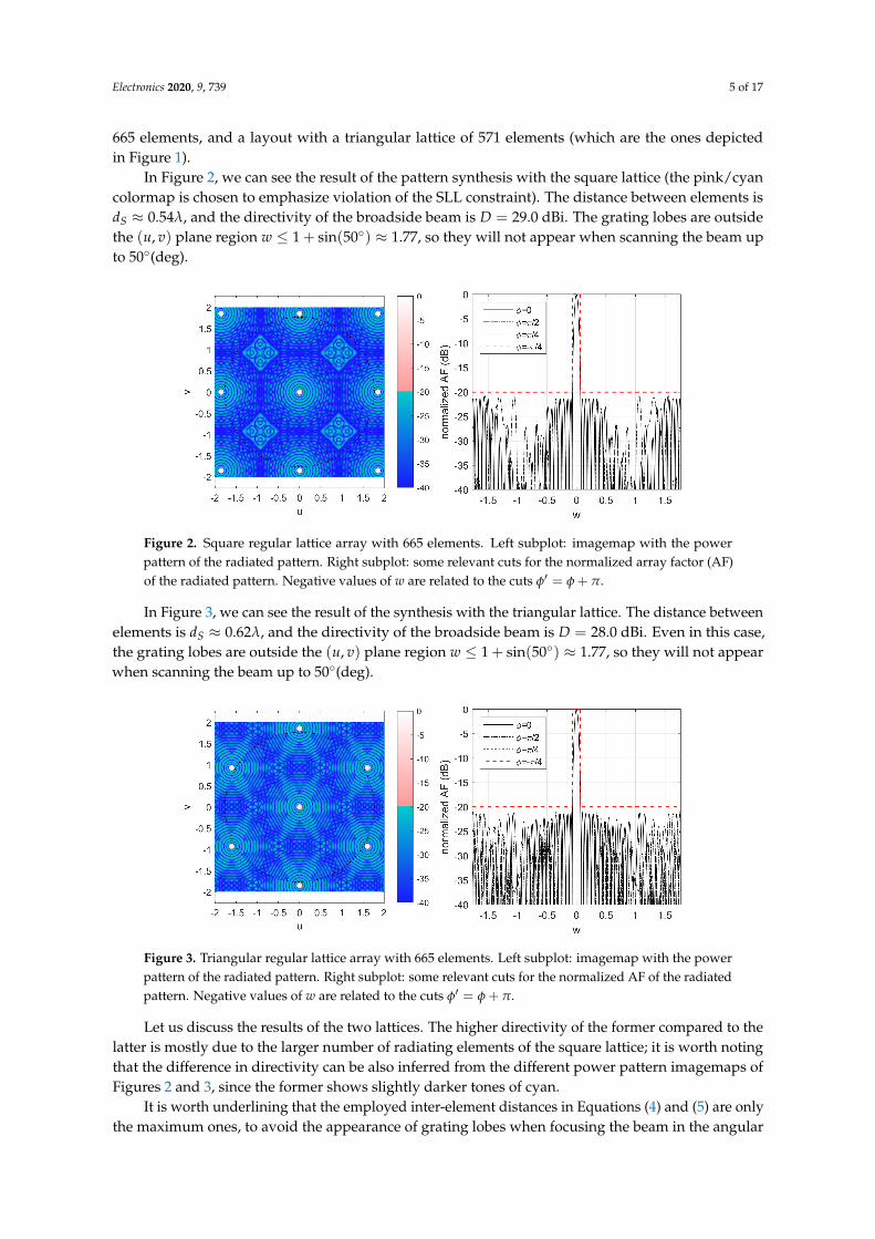
In Figure 2, we can see the result of the pattern synthesis with the square lattice (the pink/cyancolormap is chosen to emphasize violation of the SLL constraint). The distance between elements isdS ≈ 0.54λ, and the directivity of the broadside beam is D = 29.0 dBi. The grating lobes are outsidethe (u, v) plane region w ≤ 1 + sin(50◦) ≈ 1.77, so they will not appear when scanning the beam upto 50◦(deg).

Figure 2. Square regular lattice array with 665 elements. Left subplot: imagemap with the powerpattern of the radiated pattern. Right subplot: some relevant cuts for the normalized array factor (AF)of the radiated pattern. Negative values of w are related to the cuts φ′ = φ + π.

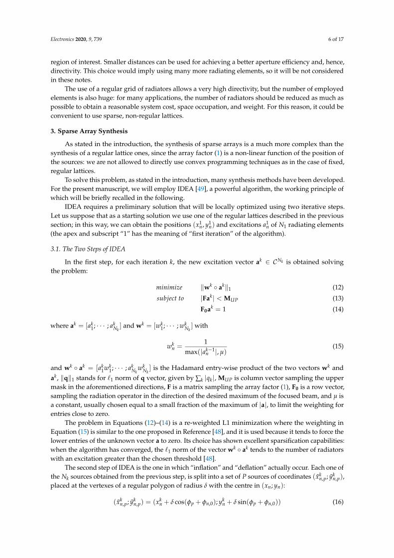
In Figure 3, we can see the result of the synthesis with the triangular lattice. The distance betweenelements is dS ≈ 0.62λ, and the directivity of the broadside beam is D = 28.0 dBi. Even in this case,the grating lobes are outside the (u, v) plane region w ≤ 1 + sin(50◦) ≈ 1.77, so they will not appearwhen scanning the beam up to 50◦(deg).

Figure 3. Triangular regular lattice array with 665 elements. Left subplot: imagemap with the powerpattern of the radiated pattern. Right subplot: some relevant cuts for the normalized AF of the radiatedpattern. Negative values of w are related to the cuts φ′ = φ + π.

Let us discuss the results of the two lattices. The higher directivity of the former compared to thelatter is mostly due to the larger number of radiating elements of the square lattice; it is worth notingthat the difference in directivity can be also inferred from the different power pattern imagemaps ofFigures 2 and 3, since the former shows slightly darker tones of cyan.

It is worth underlining that the employed inter-element distances in Equations (4) and (5) are onlythe maximum ones, to avoid the appearance of grating lobes when focusing the beam in the angular

Electronics 2020, 9, 739 6 of 17

region of interest. Smaller distances can be used for achieving a better aperture efficiency and, hence,directivity. This choice would imply using many more radiating elements, so it will be not consideredin these notes.

The use of a regular grid of radiators allows a very high directivity, but the number of employedelements is also huge: for many applications, the number of radiators should be reduced as much aspossible to obtain a reasonable system cost, space occupation, and weight. For this reason, it could beconvenient to use sparse, non-regular lattices.

3. Sparse Array Synthesis

As stated in the introduction, the synthesis of sparse arrays is a much more complex than thesynthesis of a regular lattice ones, since the array factor (1) is a non-linear function of the position ofthe sources: we are not allowed to directly use convex programming techniques as in the case of fixed,regular lattices.

To solve this problem, as stated in the introduction, many synthesis methods have been developed.For the present manuscript, we will employ IDEA [49], a powerful algorithm, the working principle ofwhich will be briefly recalled in the following.

IDEA requires a preliminary solution that will be locally optimized using two iterative steps.Let us suppose that as a starting solution we use one of the regular lattices described in the previoussection; in this way, we can obtain the positions (x1

n, y1n) and excitations a1

n of N1 radiating elements(the apex and subscript “1” has the meaning of “first iteration” of the algorithm).

3.1. The Two Steps of IDEA

In the first step, for each iteration k, the new excitation vector ak ∈ CNk is obtained solvingthe problem:

minimize ‖wk ◦ ak‖1 (12)

subject to |Fak| < MUP (13)

F0ak = 1 (14)

where ak = [ak1; · · · ; ak

Nk] and wk = [wk

1; · · · ; wkNk] with

wkn =

1max(|ak−1

n |, µ)(15)

and wk ◦ ak = [ak1wk

1; · · · ; akNk

wkNk] is the Hadamard entry-wise product of the two vectors wk and

ak, ‖q‖1 stands for `1 norm of q vector, given by ∑k |qk|, MUP is column vector sampling the uppermask in the aforementioned directions, F is a matrix sampling the array factor (1), F0 is a row vector,sampling the radiation operator in the direction of the desired maximum of the focused beam, and µ isa constant, usually chosen equal to a small fraction of the maximum of |a|, to limit the weighting forentries close to zero.

The problem in Equations (12)–(14) is a re-weighted L1 minimization where the weighting inEquation (15) is similar to the one proposed in Reference [48], and it is used because it tends to force thelower entries of the unknown vector a to zero. Its choice has shown excellent sparsification capabilities:when the algorithm has converged, the `1 norm of the vector wk ◦ ak tends to the number of radiatorswith an excitation greater than the chosen threshold [48].

The second step of IDEA is the one in which “inflation” and “deflation” actually occur. Each one ofthe Nk sources obtained from the previous step, is split into a set of P sources of coordinates (xk

n,p; ykn,p),

placed at the vertexes of a regular polygon of radius δ with the centre in (xn; yn):

(xkn,p; yk

n,p) = (xkn + δ cos(φp + φn,0); yk

n + δ sin(φp + φn,0)) (16)

Electronics 2020, 9, 739 7 of 17

where φp = 2pπ/P and φn,0 is an offset angle, which can be chosen randomly.The output of this inflation is an increased number of sources, from Nk to NkP. These new NkP

sources can well approximate the field of the starting Nk sources, and it is possible to demonstrate thatthe approximation error is proportional to (βδ)2.

Once the sources have been inflated, we can solve the following problem for each one of them:

minimize ‖wk ◦ ak‖1 (17)

subject to |Fak| < MUP (18)

F0ak = 1 (19)

where ak is the vector of the NkP excitations, F is the radiation operator for the sources of coordinates(xn,p; yn,p), A0 is a row vector, sampling the radiation operator in the direction of the maximum of thefocused beam and wk = [wk

1,1; · · · ; wkNk ,P] where

wkn,p =

1max(|ak

n|, µ). (20)

Once we have solved the problem in Equations(17)–(19), we can “deflate” the Nk polygons: wecan find the positions and excitations of the new Nk sources, of coordinates (xk+1

n ; yk+1n ) and excitation

ak+1n , that best approximate each set of P sources obtained by Equations (17)–(19).

This “deflation” can be performed numerically, looking for the coordinates (xk+1n ; yk+1

n ) andexcitations ak+1

n that minimize:

En = max

∣∣∣∣∣ak+1p ejβ(xk+1

n u+yk+1n v) −

P

∑p=1

akn,pejβ(xk

n,pu+ykn,pv)

∣∣∣∣∣ (21)

The minimization of Equation (21) has to be computed for the (u, v) values of interest and is fastto calculate since it can be solved as a local optimization, the starting point of which is given by theexcitation obtained from the first step.

3.2. The Sparsification Effect

The weighted `1 minimizations make the relative excitation ak+1n of some of the Nk points to be

very small; by choosing a threshold ε, we can start the first step of the successive iteration with onlythe Nk+1 excitations with an amplitude larger than ε.

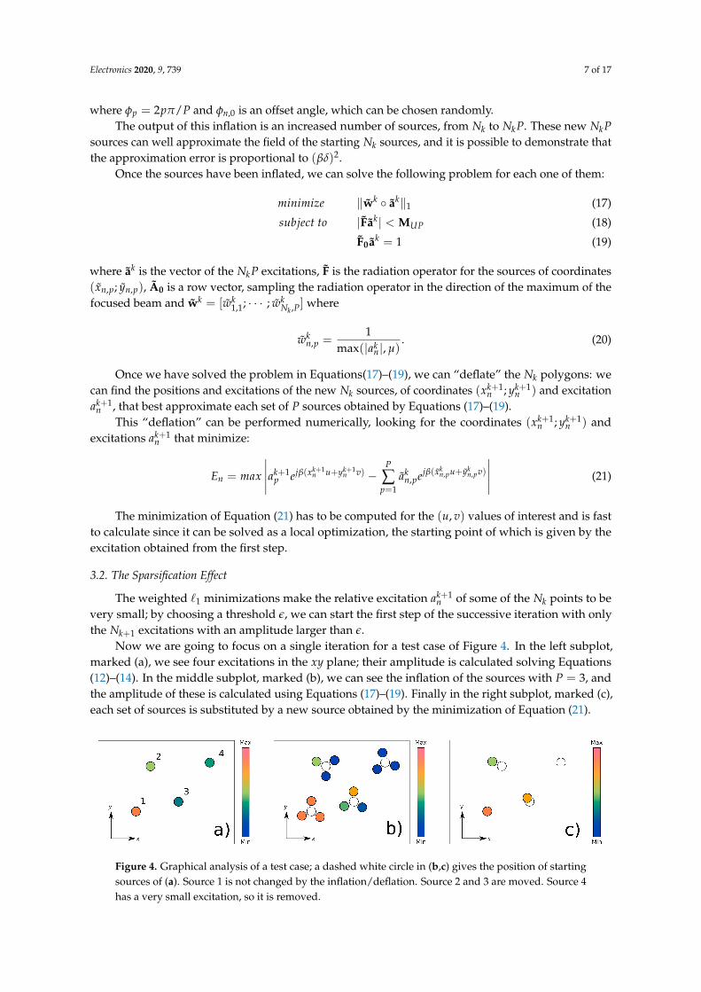
Now we are going to focus on a single iteration for a test case of Figure 4. In the left subplot,marked (a), we see four excitations in the xy plane; their amplitude is calculated solving Equations(12)–(14). In the middle subplot, marked (b), we can see the inflation of the sources with P = 3, andthe amplitude of these is calculated using Equations (17)–(19). Finally in the right subplot, marked (c),each set of sources is substituted by a new source obtained by the minimization of Equation (21).

Figure 4. Graphical analysis of a test case; a dashed white circle in (b,c) gives the position of startingsources of (a). Source 1 is not changed by the inflation/deflation. Source 2 and 3 are moved. Source 4has a very small excitation, so it is removed.

Electronics 2020, 9, 739 8 of 17

Summarizing, at each iteration, the Nk sources can be modified in two possible ways: they can bemoved, or they can be removed. This means that the overall number of sources can only be reducedduring the process of optimization, and the sparsification of the antenna can only increase. Then thealgorithm can be stopped when the solution found does not change anymore, or when a chosennumber of iterations has been performed.

3.3. A Synthesis Example

Now, let us consider the synthesis of a sparse array with the same specifications, beam-width,side-lobe level and scanning range, used for the regular lattices (all the layouts presented in thefollowing will comply with the same constraints to simplify the comparisons): SLL lower than −20 dBfor 0.067 ≤ w ≤ 1.77.

Using IDEA, it is possible to find a layout employing 213 elements only (see Figure 5). All thedata (elements’ positions and excitations) necessary to reproduce this layout, as well as the data forthe layouts that will be presented in the following, are given in Appendix A. The achieved layoutshows an excitation dynamic ρ = 15.9 dB, the minimum inter-element distance is 0.49λ. The overallcomputation time, on an Intel i7-8700 k 4.7 GHz processor, required about 50 min, and was performedusing P = 3, δ = λ/60, ε = max(ck)/1000, µ = max(ck)/1000; some computational remarks arediscussed in Appendix B.

Figure 5. The 213 elements sparse layout. Left subplot: position and normalized excitation amplitude(dB) of the synthesized layout; center subplot: normalized Array Factor in the uv plane; right subplot:some relevant cuts. Negative values of w are related to the cuts φ′ = φ + π.

Undoubtedly, the sparsification allows a huge reduction of the number of elements to the numberof radiators a regular lattice, from 665 to 213 radiators (a reduction of about 68%), but such a reductionhas a cost: the very low directivity of the obtained pattern, which is 23.6 dB only.

3.4. Directivity Constraint

A possibility to achieve a better sparse array consists of adding a directivity constraint duringthe synthesis.

It has been recalled that the directivity can be written as Equation (10). Since the form a†Sa isa quadratic form, a constraint like D ≥ Dtarget turns out to be a convex constraint that can be addedwith minimum effort to minimizations Equations (12) and (17).

As an example, we could start from the higher directivity layout of Figure 2, which presents665 elements, and impose as a constraint that the broadside directivity is always not lower than thedirectivity of the fully populated starting array.

The result of this synthesis is provided in Figure 6; the achieved layout employs 310 elementsand shows an excitation dynamic ρ = 8.8 dB, the minimum inter-element distance is 0.48λ, and thecomputation time was about eight hours. The beam-width and side-lobe level specifications areperfectly verified, even for the most scanned beam, and the directivity of the broadside beam is 29 dB,like the directivity of the fully populated array.

Electronics 2020, 9, 739 9 of 17

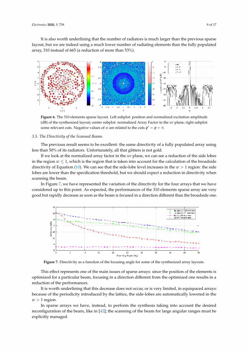
It is also worth underlining that the number of radiators is much larger than the previous sparselayout, but we are indeed using a much lower number of radiating elements than the fully populatedarray, 310 instead of 665 (a reduction of more than 53%).

Figure 6. The 310 elements sparse layout. Left subplot: position and normalized excitation amplitude(dB) of the synthesized layout; center subplot: normalized Array Factor in the uv plane; right subplot:some relevant cuts. Negative values of w are related to the cuts φ′ = φ + π.

3.5. The Directivity of the Scanned Beams

The previous result seems to be excellent: the same directivity of a fully populated array usingless than 50% of its radiators. Unfortunately, all that glitters is not gold.

If we look at the normalized array factor in the uv plane, we can see a reduction of the side lobesin the region w ≤ 1, which is the region that is taken into account for the calculation of the broadsidedirectivity of Equation (10). We can see that the side-lobe level increases in the w > 1 region: the sidelobes are lower than the specification threshold, but we should expect a reduction in directivity whenscanning the beam.

In Figure 7, we have represented the variation of the directivity for the four arrays that we haveconsidered up to this point. As expected, the performances of the 310 elements sparse array are verygood but rapidly decrease as soon as the beam is focused in a direction different than the broadside one.

Figure 7. Directivity as a function of the focusing angle for some of the synthesized array layouts.

This effect represents one of the main issues of sparse arrays: since the position of the elements isoptimized for a particular beam, focusing in a direction different from the optimized one results in areduction of the performances.

It is worth underlining that this decrease does not occur, or is very limited, in equispaced arrays:because of the periodicity introduced by the lattice, the side-lobes are automatically lowered in thew > 1 region.

In sparse arrays we have, instead, to perform the synthesis taking into account the desiredreconfiguration of the beam, like in [42]; the scanning of the beam for large angular ranges must beexplicitly managed.

Electronics 2020, 9, 739 10 of 17

A first choice, could be to manually increase the side-lobe level requirements for the w > 1 region,but this choice should be avoided since imposing such a constraint would require the use of a largerstarting array. Furthermore, lowering the threshold to a not-needed level could make us avoid somegood solutions.

A second possibility could be to explicitly optimize for a discrete set of scanning angles, but thischoice would increase the computational effort of the synthesis algorithm since we could not usesimple formulas like Equation (10).

Fortunately, it is possible to use a smart approach to this problem, which will be described in thenext section.

4. Improving the Scanning Performance of Sparse Arrays

If we look at Figure 6, we can see that the threshold on the directivity has lowered the side-lobesin the region w ≤ 1 compared to the sidelobes of the layout of Figure 5. This happens because thecompact formula D = 1/a†Sa is the result of the integration of the array factor in the visible range.

Imagine now to perform a “scaling” of the positions of the radiating elements of a factor ς, so thatthe scaled coordinates of the radiating elements are (x′n, y′n) = (ςxn, ςyn). If we chose ς = 1 + us,without changing the excitation of the radiators, we will obtain an array that radiates a “scaled” arrayfactor, that is shrunk of the same factor ς: the pattern radiated by the starting array in the angularregion w ≤ 1 + us will be radiated by the scaled array in the angular region w ≤ 1.

Let us now introduce a “dummy directivity”

Dς =1

a†Sςa(22)

with Sς is a square matrix, the entries of which are:

sς,m,n =sin(βςρm,n)

βςρm,n(23)

and obviously, Dς=1 = D.It turns out that the equation of dummy directivity has a form as simple as the directivity in

Equation (10), but allows a significant improvement of the scanning performances.To show this improvement, we will consider the synthesis of a new sparse array, in which

we add two further convex thresholds to the original IDEA. The first is Dς=1 ≥ 29, the second isDς=1.766 ≥ 28.4.

The obtained layout is shown in Figure 8; the achieved layout employs 346 elements and showsan excitation dynamic ρ = 6.1 dB, the minimum inter-element distance is 0.48λ, and the computationtime was about six hours; again, the beam-width and side-lobe level constraints are perfectly verified.

Figure 8. The 346 elements sparse layout. Left subplot: position and normalized excitation amplitude(dB) of the synthesized layout; center subplot: normalized Array Factor in the uv plane; right subplot:some relevant cuts. Negative values of w are related to the cuts φ′ = φ + π.

Electronics 2020, 9, 739 11 of 17

It is also possible to introduce further convex constraints using Equation (22). We can considerthe synthesis with the thresholds Dς=1 ≥ 29, Dς=1.766 ≥ 28.4 and Dς=1.383 ≥ 28.5.

The obtained layout is shown in Figure 9; it employs 370 elements and shows an excitationdynamic ρ = 5.9 dB, the minimum inter-element distance is 0.49λ, and the computation time wasabout four hours; even in this case, the beam-width and side-lobe level constraints are perfectly verified.

Figure 9. The 370 elements sparse layout. Left subplot: position and normalized excitation amplitude(dB) of the synthesized layout; center subplot: normalized Array Factor in the uv plane; right subplot:some relevant cuts. Negative values of w are related to the cuts φ′ = φ + π.

In Figure 10, we can see the comparison of the scanning performances of all the sparse layoutssynthesized up to this point. The use of the constraints on the dummy directivity allows to createarrays that have a much lower number of radiating elements than the fully populated array, but thedirectivity performance is very good.

Figure 10. Directivity as a function of the focusing angle for some of the synthesized array layouts.

The previous layouts were aimed to reduce the number of radiating elements as much as possible.In other applications, the number of radiators may not be the key parameter in the design, but wecould be interested in maximizing the directivity.

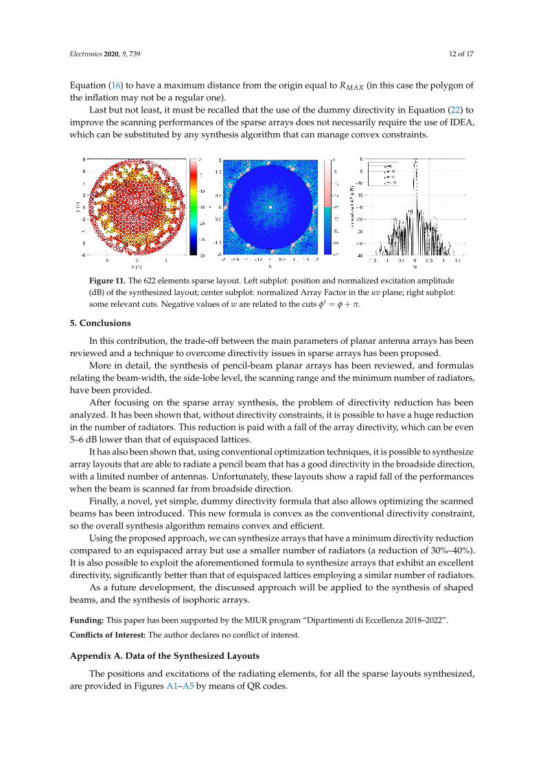
In this case, we could perform the synthesis maximizing the dummy directivity of the arrayDς=1.766, instead of performing the minimizations of (12) and (17). Applying this approach to thesame pattern specifications of the previous cases, it is possible to obtain an array of 622 elements(Figure 11), which shows an excitation dynamic ρ = 11.5 dB and a minimum inter-element distance of0.39λ; the computation time was about sixteen hours. Even in this case, the beam-width and side-lobelevel constraints are perfectly verified. The maximum directivity achieved is 29.3 dB, and such goodperformance is maintained for a very large scanning region since, for the most scanned angle, we havea directivity of 28.1 dB, about 2 dB better than the equispaced lattice of 665 elements (see Figure 10).

It is worth underlining that all the synthesized sparse layouts have the same size (the same of theequispaced lattices), so there are no variations of the occupation of the arrays. The fact that the arraysshare the same area occupation has been obtained by simply restricting the inflated set of sources of

Electronics 2020, 9, 739 12 of 17

Equation (16) to have a maximum distance from the origin equal to RMAX (in this case the polygon ofthe inflation may not be a regular one).

Last but not least, it must be recalled that the use of the dummy directivity in Equation (22) toimprove the scanning performances of the sparse arrays does not necessarily require the use of IDEA,which can be substituted by any synthesis algorithm that can manage convex constraints.

Figure 11. The 622 elements sparse layout. Left subplot: position and normalized excitation amplitude(dB) of the synthesized layout; center subplot: normalized Array Factor in the uv plane; right subplot:some relevant cuts. Negative values of w are related to the cuts φ′ = φ + π.

5. Conclusions

In this contribution, the trade-off between the main parameters of planar antenna arrays has beenreviewed and a technique to overcome directivity issues in sparse arrays has been proposed.

More in detail, the synthesis of pencil-beam planar arrays has been reviewed, and formulasrelating the beam-width, the side-lobe level, the scanning range and the minimum number of radiators,have been provided.

After focusing on the sparse array synthesis, the problem of directivity reduction has beenanalyzed. It has been shown that, without directivity constraints, it is possible to have a huge reductionin the number of radiators. This reduction is paid with a fall of the array directivity, which can be even5–6 dB lower than that of equispaced lattices.

It has also been shown that, using conventional optimization techniques, it is possible to synthesizearray layouts that are able to radiate a pencil beam that has a good directivity in the broadside direction,with a limited number of antennas. Unfortunately, these layouts show a rapid fall of the performanceswhen the beam is scanned far from broadside direction.

Finally, a novel, yet simple, dummy directivity formula that also allows optimizing the scannedbeams has been introduced. This new formula is convex as the conventional directivity constraint,so the overall synthesis algorithm remains convex and efficient.

Using the proposed approach, we can synthesize arrays that have a minimum directivity reductioncompared to an equispaced array but use a smaller number of radiators (a reduction of 30%–40%).It is also possible to exploit the aforementioned formula to synthesize arrays that exhibit an excellentdirectivity, significantly better than that of equispaced lattices employing a similar number of radiators.

As a future development, the discussed approach will be applied to the synthesis of shapedbeams, and the synthesis of isophoric arrays.

Funding: This paper has been supported by the MIUR program “Dipartimenti di Eccellenza 2018–2022”.

Conflicts of Interest: The author declares no conflict of interest.

Appendix A. Data of the Synthesized Layouts

The positions and excitations of the radiating elements, for all the sparse layouts synthesized,are provided in Figures A1–A5 by means of QR codes.

Electronics 2020, 9, 739 13 of 17

QR codes are more convenient than tables in terms of space and allow the interested reader toquickly import the data for comparing and checking the results, in an “open data” philosophy.

Figure A1. QR codes with the positions (x, y) and excitations (a) of the radiators for the 213 elementssparse layout.

Figure A2. QR codes with the positions (x, y) and excitations (a) of the radiators for the 310 elementssparse layout.

Figure A3. QR codes with the positions (x, y) and excitations (a) of the radiators for the 346 elementssparse layout.

Electronics 2020, 9, 739 14 of 17

Figure A4. QR codes with the positions (x, y) and excitations (a) of the radiators for the 370 elementssparse layout.

Figure A5. QR codes with the positions (x, y) and excitations (a) of the radiators for the 622 elementssparse layout. The position and excitations have been split in two sub-vectors (x = [x1, x2], y = [y1, y2],a = [a1, a2]).

Appendix B. Some Computational Remarks

Some comments on the computational aspects of the synthesis discussed in the paper are nowin order.

First of all, the memory use of IDEA, because of the reduction in the number of elements,slightly reduces at every iteration: the peak memory use, which occurs in the first iteration, has alwaysbeen around 16 GB of RAM for all the simulations that have been shown in this manuscript.

Roughly speaking, since the implemented version of IDEA uses CVX [56], and in particular,the MOSEK solver, an office PC with 32 GB of RAM is capable of synthesizing with ease planar arrayswith up to one thousand elements.

As it has been shown in the paper, the computational times are always limited (few hours inthe worst cases); the synthesis of arrays with a higher number of elements would be essentially aRAM-limited task.

In these cases, we would require the use of a computer with a larger memory; otherwise, wewould need to implement some modifications of the general algorithm, like the use of array geometrieswith specific symmetries, to reduce the number of variables.

Electronics 2020, 9, 739 15 of 17

References

1. Haykin, S.; Litva, J.; Shepherd, T.J. Radar Array Processing; Springer: Berlin/Heidelberg, Germany, 1993.2. Catalani, A.; Russo, L.; Bucci, O.; Isernia, T.; Perna, S.; Pinchera, D.; Toso, G.; Morabito, A.F. Sparse arrays

for satellite communications: From optimal design to realization. In Proceedings of the 32nd ESA AntennaWorkshop on Antennas for Space Applications, Noordwijk, The Netherlands, 5–8 October 2010; Volume 32.

3. Kant, G.W.; Patel, P.D.; Wijnholds, S.J.; Ruiter, M.; van der Wal, E. EMBRACE: A multi-beam 20,000-elementradio astronomical phased array antenna demonstrator. IEEE Trans. Antennas Propag. 2011, 59, 1990–2003.[CrossRef]

4. Boccardi, F.; Clerckx, B.; Ghosh, A.; Hardouin, E.; Jöngren, G.; Kusume, K.; Onggosanusi, E.; Tang, Y.Multiple-antenna techniques in LTE-advanced. IEEE Commun. Mag. 2012, 50, 114–121. [CrossRef]

5. Mumtaz, S.; Rodriguez, J.; Dai, L. MmWave Massive MIMO: A Paradigm for 5G; Academic Press: Cambridge,MA, USA, 2016.

6. Huo, Y.; Dong, X.; Xu, W. 5G cellular user equipment: From theory to practical hardware design. IEEE Access2017, 5, 13992–14010. [CrossRef]

7. Boccardi, F.; Heath, R.W.; Lozano, A.; Marzetta, T.L.; Popovski, P. Five disruptive technology directions for5G. IEEE Commun. Mag. 2014, 52, 74–80. [CrossRef]

8. Zhang, J.; Ge, X.; Li, Q.; Guizani, M.; Zhang, Y. 5G Millimeter-Wave Antenna Array: Design and Challenges.IEEE Wirel. Commun. 2017, 24, 106–112, doi:10.1109/MWC.2016.1400374RP. [CrossRef]

9. Toso, G.; Mangenot, C.; Roederer, A. Sparse and thinned arrays for multiple beam satellite applications.In Proceedings of the 2nd European Conference on Antennas and Propagation (EuCAP 2007), Edinburgh,UK, 11–16 November 2007; pp. 1–4.

10. Mailloux, R.J. Phased Array Antenna Handbook; Artech House: Boston, MA, USA, 2005; Volume 2.11. Leahy, R.M.; Jeffs, B.D. On the design of maximally sparse beamforming arrays. IEEE Trans. Antennas Propag.

1991, 39, 1178–1187. [CrossRef]12. Haupt, R.L. Thinned arrays using genetic algorithms. IEEE Trans. Antennas Propag. 1994, 42, 993–999.

[CrossRef]13. Holm, S.; Elgetun, B.; Dahl, G. Properties of the beampattern of weight-and layout-optimized sparse arrays.

IEEE Trans. Ultrason. Ferroelectr. Freq. Control 1997, 44, 983–991. [CrossRef]14. Trucco, A.; Omodei, E.; Repetto, P. Synthesis of sparse planar arrays. Electron. Lett. 1997, 33, 1834–1835.

[CrossRef]15. Bray, M.G.; Werner, D.H.; Boeringer, D.W.; Machuga, D.W. Optimization of thinned aperiodic linear phased

arrays using genetic algorithms to reduce grating lobes during scanning. IEEE Trans. Antennas Propag. 2002,50, 1732–1742. [CrossRef]

16. Marchaud, F.B.; De Villiers, G.D.; Pike, E.R. Element positioning for linear arrays using generalized Gaussianquadrature. IEEE Trans. Antennas Propag. 2003, 51, 1357–1363. [CrossRef]

17. Donelli, M.; Caorsi, S.; DeNatale, F.; Pastorino, M.; Massa, A. Linear antenna synthesis with a hybrid geneticalgorithm. Prog. Electromagn. Res. 2004, 49, 1–22. [CrossRef]

18. Caorsi, S.; Lommi, A.; Massa, A.; Pastorino, M. Peak sidelobe level reduction with a hybrid approach basedon GAs and difference sets. IEEE Trans. Antennas Propag. 2004, 52, 1116–1121. [CrossRef]

19. Chen, K.; He, Z.; Han, C.C. A modified real GA for the sparse linear array synthesis with multiple constraints.IEEE Trans. Antennas Propag. 2006, 54, 2169–2173. [CrossRef]

20. Quevedo-Teruel, O.; Rajo-Iglesias, E. Ant colony optimization in thinned array synthesis with minimumsidelobe level. IEEE Trans. Antennas Propag. 2006, 5, 349–352. [CrossRef]

21. D’Urso, M.; Isernia, T. Solving some array synthesis problems by means of an effective hybrid approach.IEEE Trans. Antennas Propag. 2007, 55, 750–759. [CrossRef]

22. Keizer, W.P. Linear array thinning using iterative FFT techniques. IEEE Trans. Antennas Propag. 2008,56, 2757–2760. [CrossRef]

23. Liu, Y.; Nie, Z.; Liu, Q.H. Reducing the number of elements in a linear antenna array by the matrix pencilmethod. IEEE Trans. Antennas Propag. 2008, 56, 2955–2962. [CrossRef]

24. Oliveri, G.; Donelli, M.; Massa, A. Linear array thinning exploiting almost difference sets. IEEE Trans.Antennas Propag. 2009, 57, 3800–3812. [CrossRef]

Electronics 2020, 9, 739 16 of 17

25. Cen, L.; Ser, W.; Yu, Z.L.; Rahardja, S.; Cen, W. Linear sparse array synthesis with minimum number ofsensors. IEEE Trans. Antennas Propag. 2010, 58, 720–726.

26. Goudos, S.K.; Siakavara, K.; Samaras, T.; Vafiadis, E.E.; Sahalos, J.N. Sparse linear array synthesis withmultiple constraints using differential evolution with strategy adaptation. IEEE Antennas Wirel. Propag. Lett.2011, 10, 670–673. [CrossRef]

27. Caratelli, D.; Vigano, M.C. A novel deterministic synthesis technique for constrained sparse array designproblems. IEEE Trans. Antennas Propag. 2011, 59, 4085–4093. [CrossRef]

28. Oliveri, G.; Massa, A. Bayesian compressive sampling for pattern synthesis with maximally sparsenon-uniform linear arrays. IEEE Trans. Antennas Propag. 2011, 59, 467–481. [CrossRef]

29. Yang, K.; Zhao, Z.; Liu, Y. Synthesis of sparse planar arrays with matrix pencil method. In Proceedingsof the 2011 International Conference on Computational Problem-Solving (ICCP), Chengdu, China, 21–23October 2011; pp. 82–85.

30. Zhang, W.; Li, L.; Li, F. Reducing the number of elements in linear and planar antenna arrays with sparsenessconstrained optimization. IEEE Trans. Antennas Propag. 2011, 59, 3106–3111. [CrossRef]

31. Fuchs, B. Synthesis of sparse arrays with focused or shaped beampattern via sequential convex optimizations.IEEE Trans. Antennas Propag. 2012, 60, 3499–3503. [CrossRef]

32. Prisco, G.; D’Urso, M. Maximally sparse arrays via sequential convex optimizations. IEEE Antennas Wirel.Propag. Lett. 2012, 11, 192–195. [CrossRef]

33. Bucci, O.M.; Perna, S.; Pinchera, D. Advances in the deterministic synthesis of uniform amplitude pencilbeam concentric ring arrays. IEEE Trans. Antennas Propag. 2012, 60, 3504–3509. [CrossRef]

34. Cen, L.; Yu, Z.L.; Ser, W.; Cen, W. Linear aperiodic array synthesis using an improved genetic algorithm.IEEE Trans. Antennas Propag. 2012, 60, 895–902. [CrossRef]

35. Bucci, O.M.; Pinchera, D. A generalized hybrid approach for the synthesis of uniform amplitude pencilbeam ring-arrays. IEEE Trans. Antennas Propag. 2012, 60, 174–183. [CrossRef]

36. Manica, L.; Anselmi, N.; Rocca, P.; Massa, A. Robust mask-constrained linear array synthesis throughaninterval-based particle SWARM optimisation. Microwaves Antennas Propag. IET 2013, 7, 976–984. [CrossRef]

37. Zhang, F.; Jia, W.; Yao, M. Linear aperiodic array synthesis using differential evolution algorithm.IEEE Antennas Wirel. Propag. Lett. 2013, 12, 797–800. [CrossRef]

38. Liu, J.; Zhao, Z.; Yang, K.; Liu, Q.H. A hybrid optimization for pattern synthesis of large antenna arrays.Prog. Electromagn. Res. 2014, 145, 81–91. [CrossRef]

39. Oliveri, G.; Bekele, E.T.; Robol, F.; Massa, A. Sparsening Conformal Arrays Through a Versatile-BasedMethod. IEEE Trans. Antennas Propag. 2014, 62, 1681–1689. [CrossRef]

40. Bucci, O.M.; Isernia, T.; Perna, S.; Pinchera, D. Isophoric sparse arrays ensuring global coverage in satellitecommunications. IEEE Trans. Antennas Propag. 2014, 62, 1607–1618. [CrossRef]

41. Araque Quijano, J.L.; Righero, M.; Vecchi, G. Sparse 2-d array placement for arbitrary pattern mask and withexcitation constraints: A simple deterministic approach. IEEE Trans. Antennas Propag. 2014, 62, 1652–1662.[CrossRef]

42. Bucci, O.M.; Perna, S.; Pinchera, D. Synthesis of isophoric sparse arrays allowing zoomable beams andarbitrary coverage in satellite communications. IEEE Trans. Antennas Propag. 2015, 63, 1445–1457. [CrossRef]

43. D’Urso, M.; Prisco, G.; Tumolo, R.M. Maximally Sparse, Steerable, and Nonsuperdirective Array Antennasvia Convex Optimizations. IEEE Trans. Antennas Propag. 2016, 64, 3840–3849. [CrossRef]

44. Pinchera, D.; Migliore, M.D.; Lucido, M.; Schettino, F.; Panariello, G. A Compressive-Sensing InspiredAlternate Projection Algorithm for Sparse Array Synthesis. Electronics 2016, 6, 3. [CrossRef]

45. Liu, Y.; You, P.; Zhu, C.; Tan, X.; Liu, Q.H. Synthesis of sparse or thinned linear and planar arrays generatingreconfigurable multiple real patterns by iterative linear programming. Prog. Electromagn. Res. 2016,155, 27–38. [CrossRef]

46. Pinchera, D.; Perna, S.; Migliore, M.D. A Lexicographic Approach for Multi-Objective Optimization inAntenna Array Design. Prog. Electromagn. Res. 2017, 59, 85–102. [CrossRef]

47. Bucci, O.; Perna, S.; Pinchera, D. Interleaved Isophoric Sparse Arrays for the Radiation of Steerable andSwitchable Beams in Satellite Communications. IEEE Trans. Antennas Propag. 2017, 65, 1163–1173. [CrossRef]

48. Pinchera, D.; Migliore, M.D.; Schettino, F.; Lucido, M.; Panariello, G. An Effective Compressed-SensingInspired Deterministic Algorithm for Sparse Array Synthesis. IEEE Trans. Antennas Propag. 2018, 66, 149–159,doi:10.1109/TAP.2017.2767621. [CrossRef]

Electronics 2020, 9, 739 17 of 17

49. Pinchera, D.; Migliore, M.D.; Panariello, G. Synthesis of Large Sparse Arrays Using IDEA (Inflating-DeflatingExploration Algorithm). IEEE Trans. Antennas Propag. 2018, 66, 4658–4668. [CrossRef]

50. Oliveri, G.; Gottardi, G.; Massa, A. A new meta-paradigm for the synthesis of antenna arrays for futurewireless communications. IEEE Trans. Antennas Propag. 2019, 67, 3774–3788. [CrossRef]

51. Marák, K.; Kracek, J.; Bilicz, S. Antenna Array Pattern Synthesis Using an Iterative Method.IEEE Trans. Magn. 2020, 56, 1–4. [CrossRef]

52. Hoydis, J.; Ten Brink, S.; Debbah, M. Massive MIMO: How many antennas do we need? In Proceedings of the2011 49th Annual Allerton Conference on Communication, Control, and Computing (Allerton), Monticello,IL, USA, 28–30 September 2011; pp. 545–550.

53. Huh, H.; Caire, G.; Papadopoulos, H.C.; Ramprashad, S.A. Achieving massive MIMO spectral efficiencywith a not-so-large number of antennas. IEEE Trans. Wirel. Commun. 2012, 11, 3226–3239. [CrossRef]

54. Pinchera, D.; Migliore, M.D.; Schettino, F.; Panariello, G. Antenna arrays for line-of-sight massive MIMO:Half wavelength is not enough. Electronics 2017, 6, 57. [CrossRef]

55. Pinchera, D.; Migliore, M.D. Comparison Guidelines and Benchmark Procedure for Sparse Array Synthesis.Prog. Electromagn. Res. 2016, 52, 129–139. [CrossRef]

56. Grant, M.; Boyd, S. CVX: Matlab Software for Disciplined Convex Programming, Version 2.1. 2014. Availableonline: http://cvxr.com/cvx (accessed on 29 June 2019).

c© 2020 by the authors. Licensee MDPI, Basel, Switzerland. This article is an open accessarticle distributed under the terms and conditions of the Creative Commons Attribution(CC BY) license (http://creativecommons.org/licenses/by/4.0/).