On the Relevance of Sophisticated Structural Annotations for Disulfide Connectivity Pattern...

On the Relevance of Sophisticated StructuralAnnotations for Disulfide Connectivity Pattern PredictionJulien Becker1, Francis Maes2,3, Louis Wehenkel2*

1 Bioinformatics and Modeling, GIGA-Research, University of Liege, Liege, Belgium, 2 Department of Electrical Engineering and Computer Science, Montefiore Institute,

University of Liege, Liege, Belgium, 3 DTAI, Departement Computerwetenschappen, University of Leuven, Leuven, Belgium

Abstract

Disulfide bridges strongly constrain the native structure of many proteins and predicting their formation is therefore a keysub-problem of protein structure and function inference. Most recently proposed approaches for this prediction problemadopt the following pipeline: first they enrich the primary sequence with structural annotations, second they apply a binaryclassifier to each candidate pair of cysteines to predict disulfide bonding probabilities and finally, they use a maximumweight graph matching algorithm to derive the predicted disulfide connectivity pattern of a protein. In this paper, we adoptthis three step pipeline and propose an extensive study of the relevance of various structural annotations and featureencodings. In particular, we consider five kinds of structural annotations, among which three are novel in the context ofdisulfide bridge prediction. So as to be usable by machine learning algorithms, these annotations must be encoded intofeatures. For this purpose, we propose four different feature encodings based on local windows and on different kinds ofhistograms. The combination of structural annotations with these possible encodings leads to a large number of possiblefeature functions. In order to identify a minimal subset of relevant feature functions among those, we propose an efficientand interpretable feature function selection scheme, designed so as to avoid any form of overfitting. We apply this schemeon top of three supervised learning algorithms: k-nearest neighbors, support vector machines and extremely randomizedtrees. Our results indicate that the use of only the PSSM (position-specific scoring matrix) together with the CSP (cysteineseparation profile) are sufficient to construct a high performance disulfide pattern predictor and that extremely randomizedtrees reach a disulfide pattern prediction accuracy of 58:2% on the benchmark dataset SPXz, which corresponds to z3:2%improvement over the state of the art. A web-application is available at http://m24.giga.ulg.ac.be:81/x3CysBridges.

Citation: Becker J, Maes F, Wehenkel L (2013) On the Relevance of Sophisticated Structural Annotations for Disulfide Connectivity Pattern Prediction. PLoSONE 8(2): e56621. doi:10.1371/journal.pone.0056621

Editor: Narcis Fernandez-Fuentes, Aberystwyth University, United Kingdom

Received September 17, 2012; Accepted January 14, 2013; Published February 15, 2013

Copyright: � 2013 Becker et al. This is an open-access article distributed under the terms of the Creative Commons Attribution License, which permitsunrestricted use, distribution, and reproduction in any medium, provided the original author and source are credited.

Funding: Julien Becker is recipient of a FRIA fellowship from the FRS-FNRS (http://www.frs-fnrs.be/). The funders had no role in study design, data collection andanalysis, decision to publish, or preparation of the manuscript.

Competing Interests: The authors have declared that no competing interests exist.

* E-mail: [email protected]

Introduction

A disulfide bridge is a covalent link resulting from an oxidation-

reduction process of the thiol group of two cysteine residues. Both

experimental studies in protein engineering [1–3] and theoretical

studies [4,5] showed that disulfide bridges play a key role in

protein folding and in tertiary structure stabilization. The

knowledge of the location of these bridges adds strong structural

constraints to the protein, which enable to drastically reduce the

conformational search space in the context of protein structure

prediction. Due to the technical difficulties and the expensive cost

of experimental procedures for determining protein structures (by

x-ray crystallography, NMR or mass spectrometry), machine

learning approaches have been developed to predict the formation

of disulfide bridges in an automatic way.

Given an input primary structure, the disulfide pattern

prediction problem consists in predicting the set of disulfide

bridges appearing in the tertiary structure of the corresponding

protein. This problem can be formalized as an edge prediction

problem in a graph whose nodes are cysteine residues, under the

constraint that a given cysteine is linked to at most to a single other

one. Most recent successful methods to solve this problem are

pipelines composed of three steps which are illustrated in Figure 1.

First, they enrich the primary structure using evolutionary

information and sometimes structural-related predictions. Second,

they apply a binary classifier to each pair of cysteines to estimate

disulfide bonding probabilities. Finally, they use a maximum

weight graph matching algorithm to extract a valid disulfide

pattern maximizing the sum of these probabilities.

The central component of this three step pipeline is the binary

classifier that predicts bonding probabilities for all cysteine pairs.

The wide majority of available binary classification algorithms

cannot process complex objects such as cysteine pairs natively,

hence they require the user to encode such objects into vectors of

(categorical or numerical) features. Since the way to perform this

encoding typically has a major impact on the classification

accuracy, a large body of work has been devoted to studying

different feature representations for cysteines and cysteine-pairs.

However, it is often the case that these different studies rely on

different kinds of binary classifiers and slightly differ in their

experimental protocol. Therefore, the comparison of the conclu-

sions of these works is difficult. In consequence, the relevance of

some features is still a subject under heavy debate. It is for example

not clear whether the use of (predicted) secondary structure or

(predicted) solvent accessibility can significantly improve disulfide

pattern predictors [6–8].

PLOS ONE | www.plosone.org 1 February 2013 | Volume 8 | Issue 2 | e56621

The main contribution of this paper is an extensive study which

aims at establishing the relevance of various structural-related

annotations and of various feature encodings in the context of a

disulfide pattern predictor such as the one presented in Figure 1.

We consider various structural annotations, some which were

already studied in the context of disulfide pattern prediction –

position-specific scoring matrix, secondary structure and solvent

accessibility – and some others which are more original in this

context: 8-class secondary structure, disordered regions and

structural alphabet. For each such annotation, we consider four

different procedures in order to encode it as a feature vector. The

combination of annotations with feature encodings leads to a large

set of possible feature functions. In order to identify a minimal

subset of feature functions that are relevant to disulfide pattern

prediction, we introduce a tractable and interpretable feature

selection methodology, based on forward selection of feature

functions. We adopt a computational protocol that avoids any risk

of overfitting and apply our approach in combination with two

usual classifiers: k-nearest neighbors (kNN) and support vector

machines (SVM), as well as with one classifier, which was not yet

considered for disulfide pattern prediction: extremely randomized

trees (ET) [9].

As a result of this study, we show that only a very limited

number of feature functions are sufficient to construct a high

performance disulfide pattern predictor and that, when using these

features, extremely randomized trees reach a disulfide pattern

accuracy of 58:2% on the benchmark dataset SPXz, which

corresponds to z3:2% improvement over the state of the art.

However, since SPXz only contains proteins with at least one

intrachain disulfide bridge, we further consider the more

heterogeneous and less redundant benchmark dataset SPX{

which also contains a significant number of proteins without any

intrachain bridge. We then investigate the behavior of our

disulfide pattern predictor on both datasets by coupling it with

filters predicting the presence of intrachain bridges and the

bonding states of individual cysteines. We consider both the case

where bonding states are known a priori and the case where

bonding states are estimated thanks to another predictor. We show

that predicting the bonding states significantly improves our

disulfide pattern predictor on SPX{, but slightly degrades it on

SPXz. When the bonding states are known a priori, we reach

very high accuracies: 89:9% on SPX{ and 75:8% on SPXz.

The following two sections give an overall view of related work

by first discussing multiple sub-problems of disulfide pattern

prediction and then presenting the kinds of features that have been

proposed to describe cysteines and cysteine pairs in supervised

learning approaches. We refer the reader to [10] for an extensive

recent overview of the field.

Disulfide bridge related prediction problemsWhile the ultimate goal of disulfide bridge prediction is to infer

correctly the whole connectivity pattern of any protein from its

primary sequence, several researchers have focused on interme-

diate simpler sub-problems, which are detailed below.

Chain classification. This sub-problem aims at predicting

for a given protein, whether (a) none of its cysteines participate to a

disulfide bridge, (b) some of its cysteines are involved in disulfide

bridges or (c) all of its cysteines are involved in disulfide bridges.

Frasconi et al. [11] proposed a support vector machine classifier to

solve this task. Fiser et al. [12] have exploited the key fact that free

cysteines (not involved in any bond) and oxidized cysteines

(involved in a bond but not necessarily an intra-chain disulfide

bridge) rarely co-occur and shown that theirs sequential environ-

ments are different. From those observations, subsequent studies

have reduced this sub-problem to a binary classification task: (a) or

(c).

Cysteine bonding state prediction. This second commonly

studied sub-problem consists in classifying cysteines into those that

are involved in a disulfide bridge and those that are not. To solve

this binary classification problem, several machine-learning

algorithms were proposed such as multi-layer neural networks

[13], two-stage support vector machines that exploit chain

classification predictions [11] and hidden neural networks [14].

Disulfide bonding prediction. While chain classification

works at the protein level and cysteine bonding state prediction

works at the cysteine level, disulfide bonding prediction works at

the level of cysteine pairs and aims at predicting the probability

that a specific pair of cysteines will form a disulfide bridge during

protein folding. Depending on the studies, some authors assume to

have an a priori knowledge on the bonding state of isolated

cysteines. This prior knowledge can be the actual state [15–17] or

a prediction made by a cysteine bonding state predictor [18].

Disulfide pattern prediction. Once one or several of the

previous tasks have been solved, the most challenging step is to

predict the disulfide connectivity pattern. Fariselli et al. [19] were

the first to relate the problem of predicting the disulfide pattern to

a maximal weight graph matching problem. Several authors have

since adopted this approach and proposed disulfide pattern

predictors that fit into the three step pipeline of Figure 1. Baldi

et al. [6,20] have used two-dimensional recursive neural networks

to predict bonding probabilities, which are exploited by a weighted

graph matching algorithm. Lin et al. [7,21] used the same graph

Figure 1. Three-step approach for disulfide pattern prediction. (A) an input primary structure, which contains four cysteine residues. (B) Thesequence is first enriched using evolutionary information and sometimes structural-related predictions such as the secondary structure. (C) A bridgeclassifier, then, predicts disulfide bonding probabilities for each cysteine pair and finally (D) a graph matching algorithm extracts the disulfide patternwith maximal weight.doi:10.1371/journal.pone.0056621.g001

Feature Functions for Disulfide Pattern Prediction


matching approach while predicting bonding probabilities with

support vector machines.

Features for cysteines and cysteine pairsMachine learning algorithms are rarely able to process complex

objects such as cysteine pairs directly, hence it is necessary to

define a mapping from these objects to vectors of features. A large

body of research on disulfide bridge prediction has been devoted

to the analysis of such encodings into feature vectors.

In 2004, Vullo et al. [15] suggested to incorporate evolutionary

information into features describing cysteines. For each primary

sequence, they generate a position-specific scoring matrix (PSSM)

from a multiple alignment against a huge non-redundant database

of amino-acid sequences. This evolutionary information was

shown to significantly improve the quality of the predicted

disulfide bridges, which led the large majority of authors to use

it in their subsequent studies. Generally, the PSI-BLAST program

[22] is used to perform multiple alignments against the SWISS-

PROT non-redundant database [23].

Zhao et al. [24] introduced cysteine separation profiles (CSPs) of

proteins. Based on the assumption that similar disulfide bonding

patterns lead to similar protein structures regardless of sequence

identity, CSPs encode sequence separation distances among

bonded cysteine residues. The CSP of a test protein is then

compared with all CSPs of a reference dataset and the prediction

is performed by returning the pattern of the protein with highest

CSP similarity. This approach assumes to have an a priori

knowledge on the bonding state of cysteines. In this paper, we

introduce a slightly different definition of CSPs based on

separation distances among all cysteine residues (see Candidate

feature functions).

From the earlier observation that there is a bias in the secondary

structure preference of bonded cysteines and non-bonded cyste-

ines, Ferre et al. [8] have developed a neural network using

predicted secondary structure in addition to evolutionary infor-

mation. Cheng et al. [6] proposed to also include predictions about

the solvent accessibility of residues. The predictions of secondary

structure and/or solvent accessibility used in their experiments

were however not accurate enough to obtain significant perfor-

mance improvements. Nevertheless, they observed that using the

true values of secondary structure and solvent accessibility can lead

to a small improvement of 1%. More recently, Lin et al. [7]

proposed an approach based on support vector machines with

radial basis kernels combined with an advanced feature selection

strategy. They observed a weak positive influence by using

predicted secondary structure descriptors, but their experimental

methodology could suffer from overfitting so that this result should

be taken with a grain of salt. Indeed, in this study, the same data is

used both for selecting features and for evaluating the prediction

pipeline. As detailed in [25], proceeding in this way often lead to

an overfitting effect and hence to over-optimistic scores. Notice

that the three studies [6–8] were all based on the secondary

structure predicted by the PSIPRED predictor [26].

More recently, Savojardo et al. [27] reported an improvement of

their predictive performance by taking into consideration the

relevance of protein subcellular localization since the formation of

disulfide bonds depends on the ambient redox potential.

Materials and Methods

Notations and problem statementThis section introduces notations and formalizes the disulfide

pattern prediction problem. Let P be the space of all proteins

described by their primary structure and P[P one particular

protein. We denote C(P)~(C1(P), . . . ,CnC(P)) the sequence of

nC~DC(P)D cysteine residues belonging to protein P, arranged in

the same order as they appear in the primary sequence. A disulfide

bonding connectivity pattern (or disulfide pattern) is an undirected

graph G~(C(P),B) whose nodes C(P) are cysteines and whose

edges B are the pairs of cysteines (f(Ci,Cj)g that form a disulfide

bridge.

Since a given cysteine can physically be bonded to at most one

other cysteine, valid disulfide patterns are those that respect the

constraint degree(Ci)ƒ1, Vi[½1,nC �. This constraint enables to

trivially derive an upper bound on the number b of disulfide

bridges given the number of cysteines: bƒtnc

2s, where t:s is the

floor function. If we know in advance the number b§1 of disulfide

bridges, we can derive the number of valid disulfide patterns using

the following closed form formula [28]:

C2bnC

Piƒb

i~1(2i{1), ð1Þ

where C2bnC

~nC !

(2b)!(nC{2b)!denotes the number of possible

subsets of size 2b of the set of nC cysteines. As an example, a

protein with nC~6 cysteines and b~3 bridges has 15 possible

disulfide patterns and a protein with nC~11 cysteines and b~5bridges has 11|945~10 395 possible patterns. Figure 2 illustrates

the three possible disulfide connectivity patterns of a protein with

four cysteines and two disulfide bridges.

When the number of bridges is unknown, the number of

possible disulfide connectivity patterns for a protein P with nC

cysteines becomes

XtnC=2s

b~1

C2bnC

Piƒb

i~12i{1ð Þz1: ð2Þ

Note that the term z1 represents the case where no cysteine

residue is bonded. As an example, a protein with nC~10 cysteines

has 45|1z210|3z210|15z45|105z1|945z1~9 496possible valid disulfide patterns.

We adopt a supervised-learning formulation of the problem,

where we assume to have access to a dataset of proteins

(represented by their primary structure) with associated disulfide

patterns. We denote this dataset D~f(P(i), B(i))gi[½1,N�, where

P(i)[P is the i-th protein and B(i) is the set of disulfide bridges

associated to that protein. We also denote n(i)C ~DC(P(i))D the

Figure 2. Example of disulfide patterns. A protein with twodisulfide bridges and its three possible disulfide connectivity patterns.doi:10.1371/journal.pone.0056621.g002



number of cysteines belonging to the protein P(i). Given the

dataset D, the aim is to learn a disulfide pattern predictor f (:): a

function that maps proteins P[P to sets of predicted bridges

BB~f (P). Given such a predicted set, we can define the predicted

connectivity pattern as following: GG~(C(P),BB).

We consider two performance measures to evaluate the quality

of predicted disulfide patterns: Qp and Q2. Qp is a protein-level

performance measure that corresponds to the proportion of

entirely correctly predicted patterns:

Qp~1

N

XN

i~1

B(i)~BB(i)� �

, ð3Þ

where Prf g is the indicator function whose value is 1 if Pr is true

or 0 otherwise. Q2 is a cysteine-pair level performance measure

that corresponds to the proportion of cysteine pairs that were

correctly labeled as bonded or non-bonded:

Q2~1PN

i~1

n(i)C (n

(i)C {1)=2

XN

i~1

Xn(i)C

j~1

Xn(i)C

k~jz1

(fCj ,Ckg[B(i))~(fCj ,Ckg[BB(i))� �

:

ð4Þ

Note that both Qp and Q2 belong to the interval ½0,1� and are

equal to 1 in case of perfectly predicted disulfide patterns. While

the ultimate goal of disulfide pattern prediction is to maximize Qp,

we will also often refer to Q2 since, in the pipeline depicted in

Figure 1, Q2 is directly related to the quality of the cysteine pair

classifier.

Disulfide pattern prediction pipelineThis section first presents the datasets and the five kinds of

structural-related predictions we consider. It then details the

different steps of our prediction pipeline: the dataset annotation,

the pre-processing step that enriches the primary structure with

evolutionary information and structural-related annotations, the

classification step of cysteine pairs that predicts bridge bonding

probabilities and the post-processing step that constructs a

disulfide pattern from these probabilities using maximum weight

graph matching.

Dataset and annotations. In order to assess our methods,

we use two datasets that have been built by Cheng et al. [6] and

extracted from the Protein Data Bank [29]. The first one, SPXz,

is a collection of 1 018 proteins that contain at least 12 amino acids

and at least one intrachain disulfide bridge. We use this dataset for

the problem of pattern prediction. However, since it does not

contain any protein without disulfide bridges it is not adapted to

address chain classification and cysteine bonding state prediction.

For these tasks, we use the other dataset, SPX{, which is made of

1 650 proteins that contain no disulfide bridge and 897 proteins

that contain at least one bridge. In order to reduce the over-

representation of particular protein families, both datasets were

filtered by UniqueProt [30], a protein redundancy reduction tool

based on the HSSP distance [31]. In SPX{, Cheng et al. used a

HSSP cut-off distance of 0 for proteins without disulfide bridge

and a cut-off distance of 5 for proteins with disulfide bridges. In

SPXz, the cut-off distance was set to 10. To properly compare

our experiments with those of Cheng et al., we use the same train/

test splits as they used in their paper. Statistics of the two datasets

are given in Table 1.

We enrich the primary structure (denoted as AA) by using two

kinds of annotations: evolutionary information in the form of a

position-specific scoring matrix (PSSM) and structural-related

predictions, such as predicted secondary structure or predicted

solvent accessibility. We computed the PSSMs by running three

iterations of the PSI-BLAST program [22] on the non-redundant

NCBI database. To produce structural-related predictions, we use

the iterative multi-task sequence labeling method developed by

Maes et al. [32]. This method enables to predict any number of

structural-related properties in a unified and joint way, which was

shown to raise state of the art results. We consider here five kinds

of predicted annotations: secondary structure (SS3, 3 labels), DSSP

secondary structure (SS8, 8 labels), solvent accessibility (SA, 2

labels), disordered regions (DR, 2 labels) and a structural alphabet

(StAl, 27 labels, see [33]). The two versions of secondary structure

give two different levels of granularity. The structural alphabet is a

discretization of the protein backbone conformation as a series of

overlapping fragments of four residues length. This representation,

as a prediction problem, is not common in the literature. Here, it is

used as a third level of granularity for local 3D structures. To our

best knowledge, predicted DSSP secondary structure, predicted

disordered regions and structural alphabet annotations have never

been investigated in the context of disulfide pattern prediction.

In order to train the system of Maes et al., we rely on supervision

information computed as follows: secondary structures and solvent

accessibility are computed using the DSSP program [34],

disordered regions and structural alphabet are computed by

directly processing the protein tertiary structure. Since the disorder

classes are not uniquely defined, we use the definition of the CASP

competition [35]: segments longer than three residues but lacking

atomic coordinates in the crystal structure were labelled as

disordered whereas all other residues were labelled as ordered.

Note that it is often the case that supervised learning algorithms

behave differently on training data than on testing data. For

example, the 1-nearest neighbor algorithm always has a training

accuracy of 100%, while its testing accuracy may be arbitrarily

low. In order to assess the relevance of predicted annotations, we

expect our input enrichment step to provide ‘‘true’’ predictions,

i.e., representative of predictions corresponding to examples that

were not part of training data.

We therefore use the cross-validation methodology proposed in

[36] that works as follows. First, we randomly split the dataset into

ten folds. Then, in order to generate ‘‘true’’ predictions for one

fold, we train the system of Maes et al. on all data except this fold.

This procedure is repeated for all ten folds and all predictions are

concatenated so as to cover to whole dataset.

Table 2 reports the cross-validation accuracies that we obtained

with this procedure. The default scoring measure is label accuracy,

i.e., the percentage of correctly predicted labels on the test set.

Since disordered regions labeling is a strongly unbalanced

problem, label accuracy is not appropriate for this task. Instead,

we used a classical evaluation measure for disordered regions

prediction: the Matthews correlation coefficient [37].

Candidate feature functions. The feature generation step

aims at describing cysteine pairs in an appropriate form for

classification algorithms. This encoding is performed through

cysteine-pair feature functions w : P|C|C?Rd that, given a protein

P and two of its cysteines (Ci,Cj), computes a vector of d real-

valued features. In our experiments, we extracted cysteine-pairs

(Ci,Cj) in such a way that 1ƒivjƒnC , where nC is the number

of cysteine residues of P. Consequently, we extractnC|(nC{1)

2



cysteine-pairs from P. The purpose of the feature selection

methodology described in the next section is to identify a subset of

relevant w functions among a large panel of candidate ones that we

describe now.

Our set of candidate feature functions is composed of primary-

structure related functions and annotation related functions. The

former are directly computed from the primary structure alone

and are the following ones:

N Number of residues: computes one feature which is the number of

residues in the primary structure.

N Number of cysteines: computes one feature which is the number of

cysteine residues in the primary structure.

N Parity of the number of cysteines: computes one feature which

indicates whether the number of cysteines is odd or even.

N Relative position of cysteines: computes two features which are the

residue indices of cysteines Ci and Cj , denoted pos(Ci) and

pos(Cj), divided by the protein length.

N Normalized position difference: returns one feature which corre-

sponds to the number of residues separating Ci from Cj in the

primary structure, i.e., pos(Cj){pos(Ci), divided by the protein

length. Note that as jwi and therefore pos(Cj)wpos(Ci), this

difference is always greater than zero.

N Relative indices of cysteines: computes two features which are the

cysteine indices i and j divided by the number of cysteines.

N Normalized index difference: computes one feature which corre-

sponds to the number of cysteines separating Ci from Cj

divided by the number of cysteines.

N Cysteine separation profile window: computes one feature per cysteine

Ck[fCi,Cjg and per relative position d[½{ W

2,W

2�,d=0 whose

value is the position difference pos(Ckzd){pos(Ck) divided by

the protein length, where Ww0 is called the window size

parameter.

Annotation-related feature functions are defined for each type

of annotation A[fAA, PSSM, SS3, SS8, SA, DR, StAlg of the

residues of the protein P. We denote by LA the set of labels

corresponding to annotation A and by LA~DLAD the size of this

set. For our annotations, we have: LAA~20, LPSSM~21 (the

twenty amino acids and the gap), LSS3~3, LSS8~8, LSA~2,

LDR~2 and LStAl~27. For a given primary structure of length

DPD, an annotation A is represented as a set of probabilities

aAp,l[½0,1� where p[½1,DPD� denotes the residue index and l[LA is a

label.

Note that in the general case, aAp,l probabilities may take any

value in range ½0,1� to reflect uncertainty about predictions. Since

the primary structure (AA) is always known perfectly, we have:

aAAp,l ~

1 if l is the residue at position p

0 otherwise:

�

For each annotation A, we have four different feature functions:

N Labels global histogram: returns one feature per label l[LA, equal

to1

DPD

XDPD

p~1aAp,l .

N Labels interval histogram: returns one feature per label l[LA equal

to

Ppos(Cj )

p~pos(Ci)aAp,l

pos(Cj){pos(Ci)z1.

N Labels local histogram: returns one feature per label l[LA and per

cysteine Ck[fCi,Cjg, equal to1

W

Xpos(Ck)zW=2

p~pos(Ck){W=2aAp,l and

one special feature equal to the percentage of out-of-bounds

positions, i.e., positions p such that p =[ ½1,DPD�.N Labels local window: returns one feature per label l[LA, per

cysteine Ck[fCi,Cjg and per relative position d[½{ W

2,W

2�,

equal to apos(Ck)zd,l . When the position is out-of-bounds, i.e.,

pos Ckð Þzd =[ 1,DPD½ �, the feature is set to 0.

Our candidate feature functions are summarized in Table 3.

Note that three of them are parameterized by window size

parameters. Figure 3 shows an illustration of the three kinds of

histograms. We will see how to tune window sizes and how to

select a minimal subset of feature functions in the next section.

Cysteine pair classifiers. Let fw1, . . . ,wmg be a subset of

the candidate feature functions described above and let di denote

the dimensionality of the i-th function of this set. A cysteine pair

classifier processes feature vectors of dimensionPm

i~1 di, in order

to predict disulfide bonding probabilities. In this study, we

consider three such binary classifiers:

Table 1. Dataset statistics.

Proteins CysteinesBonds perprotein

All None Mix Total Positive Negative Total

SPX{ 757 1 650 140 2 547 4 942 7 844 12 786 0.97+1.78

SPXz 718 0 300 1 018 5 082 901 5 983 2.50+2.14

All: proteins in which all cysteines are bonded. None: proteins with no disulfide bridges. Mix: proteins with both bonded cysteines and non-bonded cysteines. Positive:number of bonded cysteines. Negative: number of non-bonded cysteines.doi:10.1371/journal.pone.0056621.t001

Table 2. Cross-validated accuracies of annotations.

Annotation LA Measure SPXz SPX{

Secondary structure 3 Accuracy 73.50%+0.68% 68.00%+2.61%

Secondary structure 8 Accuracy 55.60%+0.76% 57.83%+2.10%

Solvent accessibility 2 Accuracy 77.45%+0.54% 77.82%+0.30%

Disorder regions 2 MCC 0.892+0.03 0.352+0.05

Structural alphabet 27 Accuracy 19.01%+0.30% 21.32%+0.47%

The scoring measure is label accuracy, i.e., the percentage of correctly predictedlabels on the test set except for disordered regions that use the Matthewscorrelation coefficient (MCC).doi:10.1371/journal.pone.0056621.t002



N K-nearest neighbors (kNN) is a simple and well-known method for

classification. In order to determine the disulfide bonding

probability of a new example, the algorithm first search for the

k nearest training samples and then returns the frequency of

bonded cysteines among these neighbors. The distance

between two feature vectors A and B is computed using a

normalized version of the l2-norm, which is defined as follows:

dist(A,B)~

ffiffiffiffiffiffiffiffiffiffiffiffiffiffiffiffiffiffiffiffiffiffiffiffiffiffiffiffiffiffiffiffiffiffiffiffiffiffiffiffiffiffiffiXm

i~1

1

di

Xdi

j~1

Aji{B

ji

sji

!2vuut ,

where Aji and B

ji denote the j-th components of the i-th feature

generator wi, and where sji denotes the empirical standard

deviation of this component, computed on the training data.

Since we are concataining feature functions with very different

dimensionalities (d varies from 1 to O(103)), the effect of the

traditional l2-norm would be largely dominated by high-

dimensional feature functions. The term1

di

enables to avoid

this problem. Dividing by the standard deviations sji is a

classical strategy to be less dependent on the domain of the

different features.

N Support vector machines (SVM) is also a well-established method

that constructs a hyperplane that maximizes the distance to the

nearest training samples of any class in a high-dimensional

space. The method has one hyper parameter that is a

regularization constant C. Among the common functions used

to cope with non-linear feature interactions, called kernel

functions, we use the Gaussian radial basis function

exp({c:dist(A,B)2), where cw0 is a bandwidth hyper-

parameter and where dist(:,:) is the same norm as previously.

Note that previous studies on disulfide pattern prediction

[7,38] also relied on the Gaussian radial basis function. In our

experiments, we used the well-known LibSVM implementa-

tion [39]. In order to convert SVM predictions into

probabilities, we use the default probability estimation method

of LibSVM, which was proposed by Platt [40] and Wu et al.

[41].

N Extremely randomized trees (ETs). This tree-based ensemble

method, proposed by Geurts et al. [9], is similar to the popular

Random Forests approach [42]. The main differences with the

latter are that ETs does not rely on bootstrap replicates (unlike

the Random Forests method, each tree is built using all

learning samples), and that cut-points are selected in a random

fashion, which was shown to lead to better generalization

performances. The method has three hyper-parameters: K , the

number of random splits tested per node creation, T , the

Figure 3. Example of local, interval and global histograms. C2 and C3 are the two cysteines of interest. In red, we show the labels localhistograms of size 11 of the secondary structure hlocal(SS3,11). In yellow, we show the labels interval histogram of the solvent accessibility annotationhinterval(SA). In green, we show the global histogram of the disordered regions sequence hglobal(DR).doi:10.1371/journal.pone.0056621.g003

Table 3. Feature functions used in our experiments to encode cysteine pairs.

Symbol Parameter d Description

DPD - 1 Number of residues

nC - 1 Number of cysteines

nC mod 2 - 1 Parity of the number of cysteines

pos(Ci)=DPD,pos(Cj )=DPD - 2 Relative position of cysteines

(pos(Cj ){pos(Ci))=DPD - 1 Position difference

i=nC ,j=nC - 2 Indices of cysteines

(i{j)=nC - 1 Index difference

csp(W ) window size 2(W{1) Cysteine separation profile window

hglobal (A) - LAz1 Labels global histogram

hinterval (A) - LA Labels interval histogram

hlocal (A,W ) window size 2LAz2 Labels local histogram

w(A,W ) window size 2WLA Labels local window

Symbols, parameters, number of features (d) and description of our candidate feature functions. Top: feature functions that are directly computed from the primarystructure. Bottom: feature functions defined for every kind of annotation A[fAA,PSSM,SS3,SS8,SA,DR,StAlg.doi:10.1371/journal.pone.0056621.t003



number of trees composing the ensemble, and Nmin, the

minimum number of samples required to allow for splitting a

node. We use the probabilistic version of ETs, in which each

leaf is associated to a bonding probability, which is the

empirical proportion of bonded cysteine pairs among the

training samples associated to that leaf. In order to make one

prediction, we traverse each of the T trees and return the

average of the bonding probabilities associated to the

corresponding T leaves. To our best knowledge, tree-based

ensemble methods, and in particular ETs, were not yet applied

to disulfide connectivity pattern prediction, despite the fact

that several studies have shown that these methods very often

outperform other methods such as support vector machines or

neural network [43].

Maximum weight graph matching. Given bonding prob-

abilities for every cysteine pair of a protein, the aim of this last step

of the disulfide pattern prediction pipeline is to select a subset of

disulfide bridges so as to respect the constraint

degree(Ci(P))ƒ1,Vi[½1,nC �. As proposed previously, this problem

is formalized as a maximum weight graph matching problem: the

weight of a disulfide pattern is defined as the sum of probabilities

attached to its edges and the aim is to find the valid pattern with

maximal weight.

A naive solution to solve the maximum weight graph matching

problem is to perform an exhaustive search over all valid disulfide

patterns. The complexity of this procedure is however exponential

in the number of cysteines, which is problematic for large proteins.

This issue is often solved using the maximum weight matching

algorithm of Gabow [44] whose time complexity is cubic w.r.t. the

number of cysteines nC and whose space complexity is linear w.r.t.

nC . In our experiments, we used Blossom V, which is a more

recent and optimized implementation proposed by Kolmogorov

[45].

Notice that, because this algorithm searches for a full matching,

i.e., where each cysteine is associated to another one, it cannot be

directly applied on proteins that have an odd number nC of

cysteines. To deal with such proteins, we run the matching

algorithm on each one of the nC subsets of nC{1 cysteines and

select the solution with maximal weight.

Forward feature function selectionThis section describes our forward feature function selection

algorithm, which aims at determining a subset of relevant feature

functions among those described above. Feature selection is an old

topic in machine learning and a common tool in bioinformatics

[46]. Our feature selection problem departs from traditional

feature selection w.r.t. three unique aspects:

N Feature function selection: we want to select feature functions

rather than individual features. Given that feature functions

can be parameterized by window sizes, our algorithm has to

perform two tasks simultaneously: determining a subset of

feature functions and determining the best setting for

associated window sizes.

N Insertion in a pipeline: we want to optimize the performance Qp of

the whole pipeline rather than the accuracy Q2 of the classifier

for which we perform feature selection. Preliminary studies

have shown that these two performance measures are not

perfectly correlated: a binary classifier with higher accuracy

can lead to worse disulfide pattern predictions when combined

with the graph matching algorithm, and conversely.

N Interpretability: our approach not only aims at constructing a

pipeline maximizing Qp, but also at drawing more general

scientific conclusions on the relevance of various annotations of

the primary structure. We thus require the result of the feature

selection process to be interpretable.

In order to fulfill these requirements, we adopt a wrapper

approach that repeatedly evaluates feature function subsets by

cross-validating the whole pipeline and that is directly driven by

the cross-validated Qp scores. In order to obtain interpretable

results, we rely on a rather simple scheme, which consists in

constructing the feature function set greedily in a forward way:

starting from an empty set and adding one element to this set at

each iteration.

In order to treat feature functions with parameters and those

without parameters in an unified way, we express the feature

functions as a set of parameterized feature functions

W~fW(1), . . . ,W(M)g where each W(i) contains a set of alternative

feature functions W(i)~fw(i)1 , . . . ,w(i)

aig. In the case where the

feature function has no parameters (e.g., number of residues or

labels global histogram), this set is a singleton W~fwg. Otherwise,

when the feature function is parameterized by a window size, there

is one alternative per possible window size, e.g.,

WcspW ~fcsp(1),csp(3), . . . ,csp(19)g.Our forward feature function selection approach is depicted in

Algorithm. We denote by S(:,:,:)[R the objective function that

evaluates the Qp score associated to a given set of feature

functions, based on a cysteine pair classifier C and a dataset of

proteins D. In our experiments, this objective function is computed

by performing a 10-fold cross-validation of the whole prediction

pipeline and by returning the test Qp scores averaged over the ten

folds.

Algrithm 1. Forward feature function selection algorithm.

Given a set of parameterized feature functions

W~fW(1), . . . ,W(M)gGiven an objective function S(:,:,:)[R

Given a cysteine pair classifier CGiven a dataset D

1: U/60 4initial empty feature function set

2: repeat

3: (i�,j�)/ argmaxi,j

S(U|fw(i)j g,C,D) 4evaluate candidate

w(i)j functions

4: U/U|fw(i�)j� g 4add the best feature function

5: W/W\w(i�)4remove the best parameterized feature

function

6: until some stopping criterion is fulfilled

7:return U 4return feature function set

The feature function is first initialized to an empty set 60 (line 1).

Each iteration then consists in inserting a candidate feature

functions w(i)j taken in the set W into U. For this, we try to add each

candidate w(i)j to the current feature function set and select the best

feature function w.r.t. the obtained cross-validation Qp scores (line

3). This feature function is then inserted into U (line 4) and the

corresponding set of alternatives W(i�) is removed from W. After a

given stopping criterion is fulfilled, the constructed function set Uis returned (line 7). In our experiments, this stopping criterion is

simply a fixed number of iterations. An alternative consists in

stopping the algorithm when no additional feature functions

enable to improve the S score.

Note that due to its greedy nature, our feature selection may fall

into local minima. However, compared to traditional feature

selection, it may be the case that selecting feature functions instead

of individual features significantly reduces the importance of this

problem (the dimensionality of our search problem is much



smaller than in the case of individual feature selection). We show

in the next section that this algorithm is a tractable feature

function selection approach that provides interpretable results,

from which we can draw some general conclusions about the

relevance of primary structure annotations.

Results: Disulfide Pattern Prediction

This section describes our experimental study on disulfide

pattern prediction using the SPXz benchmark dataset. We first

make an overall comparison of the three binary classification

algorithms described previously and show that extremely random-

ized trees lead to significantly better results than the two other

algorithms. We then apply our forward feature function selection

approach using this algorithm and show that only a few feature

functions are sufficient to construct a high performance disulfide

pattern predictor. We finally compare this predictor with the state

of the art and propose an analysis of the sensitivity of extremely

randomized trees w.r.t. their hyper-parameters. Note that, for the

moment, our prediction pipeline always tries to construct fully

connected disulfide patterns and that it does not enable predicting

partially connected disulfide patterns. We address this issue in the

next section, by coupling our predictor with filters based on the

bonding state of individual cysteines.

Comparison of the cysteine pair classifiersComparing cysteine pair classifiers in our context is not trivial

for two reasons. First, we are primarily interested in the Qp score

of the whole prediction pipeline rather than in the classification

accuracy. Second, we do not have a fixed feature representation

and different classification algorithms may require different feature

function sets to work optimally. To circumvent these difficulties,

we compare cross-validated Qp scores obtained with the three

classifiers on a large number of randomly sampled feature function

sets. To sample a feature function set of size m[½1,18�, we proceed

as follows. First, we draw a subset fW(1), . . . ,W(m)g from W. Then,

for each member W(i) of this subset, we select a feature function

w(i)j , using the following rules: (i) local window sizes are sampled

according to the Gaussian distribution N (15,152), (ii) local

histogram sizes are sampled according to N (51,502) and (iii)

CSP window sizes are sampled from N (7,112). These values were

chosen according to preliminary studies using the three classifiers.

We set the hyper-parameters in the following way:

N kNN. By studying the effect of k, we found out that large values

of k drastically decrease the performance of kNN and low

values do not enable to distinguish patterns well since the set of

possible predicted probabilities is limited to kz1 values. In the

following, we use the default value k~5, which we found to be

a generally good compromise.

N SVM. It turns out that the best setting for c and C is highly

dependent on the chosen feature function set. For each tested

set of feature functions, we thus tuned these two parameters by

testing all combinations of c[f2{14,2{7,20,27,214g and

C[f20,25,210,215g and by selecting the values of (c,C) that

led to the best Qp scores.

N ETs. We use a default setting that corresponds to an ensemble

of 1 000 fully developed trees (T~1 000,Nmin~2) and K is set

to the square root of the total number of featuresffiffiffidp

, as

proposed by Geurts et al [9].

The results of our comparison on SPXz are given in Figure 4.

As a first remark, note the large range in which the Qp scores lie:

from ^15% to ^60%. This shows that all three classifiers are

highly sensitive to the choice of the features used to describe

cysteine pairs, which is a major motivation for our work on feature

function selection. The experiments are color-encoded w.r.t the

size m of their feature function set. This color-encoding enables us

to notice that, in general, larger feature function sets lead to better

classifiers.

The mean and standard deviations of these results are

34:23%+7:45% for kNN classifiers, 43:96%+5:31% for SVM

classifiers and 47:85%+7:17% for ETs classifiers. In 73.25% of

the experiments, the best pattern accuracy is given by ETs and in

20.35% of them by SVMs. In the remaining 6.40% experiments,

exactly the same number of disulfide patterns were correctly

predicted by ETs and SVM. kNN was always outperformed by the

other two classifiers. We have used the paired t-test to assess the

significance of the out-performance of ETs. The p-value against

kNN is O(10{128) and the p-value against SVM is O(10{38),which make it clear that ETs significantly outperform kNN and

SVM. Moreover, ETs work well with a default setting contrarily to

SVM that required advanced, highly time-consuming, hyper-

parameters tuning.

Given those observations, we proceed in the remainder of this

study by restricting to the ETs method.

Feature functions selectionWe now apply our feature function selection approach on top of

extremely randomized trees. We rely on the set of parameterized

feature functions W described in Table 3 and consider the

following window size values:

N Cysteine separation profile window: 1, 3, 5, 7, 9, 11, 13, 15, 17, 19.

N Local histograms: 10, 20, 30, 40, 50, 60, 70, 80, 90.

N Local windows: 1, 5, 9, 11, 15, 19, 21, 25.

This setting leads to a total of 150 candidate features functions.

As cysteine pair classifier, we use ETs with the same default setting

as previously (T~1 000, K~ffiffiffidp

, Nmin~2).

The simplest way to apply our algorithm would be to apply it

once on the whole SPXz dataset. By proceeding in this way, the

same data would be used for both selecting the set of feature

functions and assessing the quality of this selected set. It has been

shown that this approach is biased due to using the same data for

selecting and for evaluating and that it could lead to highly over-

estimated performance scores [25].

To avoid this risk of overfitting, we adopted a more evolved

approach, which consists in running the feature selection

algorithm once for each of our 10 different train/test splits. In

this setting, the whole feature selection algorithm is executed on a

training dataset composed of 90% of the data and the

generalization performance of the selected feature functions is

evaluated using the remainder 10% of data. There are thus two

different objective functions. We call cross-validated score the value

returned by S(:,:,:), i.e., the 10 cross-validated Qp score using 90%

of the data, and we call verification score the Qp score computed over

the remainder 10% of the data.

Figure 5 shows the evolution of the cross-validated score and the

verification score for five iterations of the feature selection

algorithm on each of the 10 train/test splits. Note that, since the

cross-validated score is the score being optimized, its value

increases at every iteration of each of the 10 runs. The evolution of

the verification score, which represents the true generalization

performance, is far from being so clear, as, in most cases, the

optimum is not located after the fifth iteration.



Table 4 reports the selected feature functions for each of the 10

runs. We observe that the first selected feature function is always

w(PSSM,:) with a window size varying in f9,11,15,19g. This

means that, taken alone, the best individual feature function is

always a window over the position-specific scoring matrix. The

fact that this results was observed during each run is very strong,

since the selection algorithm has to select between 150 different

functions. Similarly, the second selected feature function is always

csp(:) with a window size varying in f9,13,17,19g.After the two first iterations, the selected feature functions

become more disparate and only lead to tiny improvements. This

probably indicates that the system starts to overfit, by selecting

feature functions that are specifically tailored to a specific subset of

the training proteins. In iterations 3–4, we note that hlocal(SS8,:)occurs slightly more often than the other feature functions (6 times

over 20). From the two last rows, which give the averaged cross-

validated scores and the averaged verification scores, we observe

that while the cross-validated score systematically increases, the

verification score becomes unstable after the two first iterations.

These observations reinforce the fact that the selected feature

functions become more and more specific to training samples.

From these results, it is clear that the feature functions w(PSSM,:)and csp(:) bring the major part of the predictive power that can be

obtained by our feature functions.

According to these results, we focus in the following on the

feature functions w(PSSM,15), csp(17) and hlocal(SS8,77), where

we chose windows sizes by taking the average sizes reported in

Table 4. Note that, contrarily to the observation of Figure 4 that

suggested large feature function sets, our method carefully selected

Figure 4. Qp scores for three binary classification algorithms and randomly sampled feature function sets. The experiments areperformed on the SPXz dataset. In bold, the means of the classifiers. The diagonal lines indicate situations where both classifiers have the samescore. The experiments are color-encoded w.r.t. the size of their feature function set.doi:10.1371/journal.pone.0056621.g004



a very small number of relevant feature functions that led to a

more simpler and still very accurate classifier.

Evaluation of the constructed prediction pipelineWe now compare our constructed prediction pipeline with the

state of the art. We consider three baselines that were evaluated

using the same experimental protocol as ours (10 cross-validated

Qp). The first baseline is the recursive neural network approach

proposed by Cheng et al. [6]. These authors, who introduced the

SPXz dataset, reached a pattern accuracy of 51% using the true

secondary structure and solvent accessibility information. Lin et al.

[7] proposed to predict the bonding state probabilities using a fine

tuned support vector machine. They obtained a pattern accuracy

of 54:5% by using the same data for feature selection and for

evaluation, making this results probably over-estimated. Vincent et

al. [47] proposed a simple approach based on a multiclass one-

nearest neighbor algorithm that relies on the fact that two proteins

tend to have the same disulfide connectivity pattern if they share a

similar cysteine environment. This method reaches a pattern

accuracy of 55%.

Table 5 reports the performance obtained by ETs with feature

functions w(PSSM,15), csp(17) and hlocal(SS8,77). We observe

that using only w(PSSM,15) already leads to a pattern accuracy

of 51:6%, which is better than the baseline of Cheng et al. [6]. A

significant improvement of z6:6% is achieved by adding the

feature function csp(17), which leads to a model that significantly

outperforms the state of the art. The feature function

hlocal(SS8,77) leads to small further improvement of the Qp

score, but due to the large variance, this improvement cannot be

shown to be significant.

From these results, we conclude that only the following two

feature functions are sufficient for high-quality disulfide pattern

prediction in combination with ETs: local PSSM windows and

CSP windows. Note that it might be the case that, by using larger

datasets, feature functions such as medium-size histograms on

predicted DSSP secondary structure could slightly improve the

quality of the system.

Table 6 reports the pattern accuracy as a function of the true

number of disulfide bridges. By comparing the results with the

three baselines, we observe that our method outperforms the

baselines, except for proteins with 4 potential disulfide bonds

where the approach proposed by Vincent et al. [47] obtains a

better pattern accuracy.

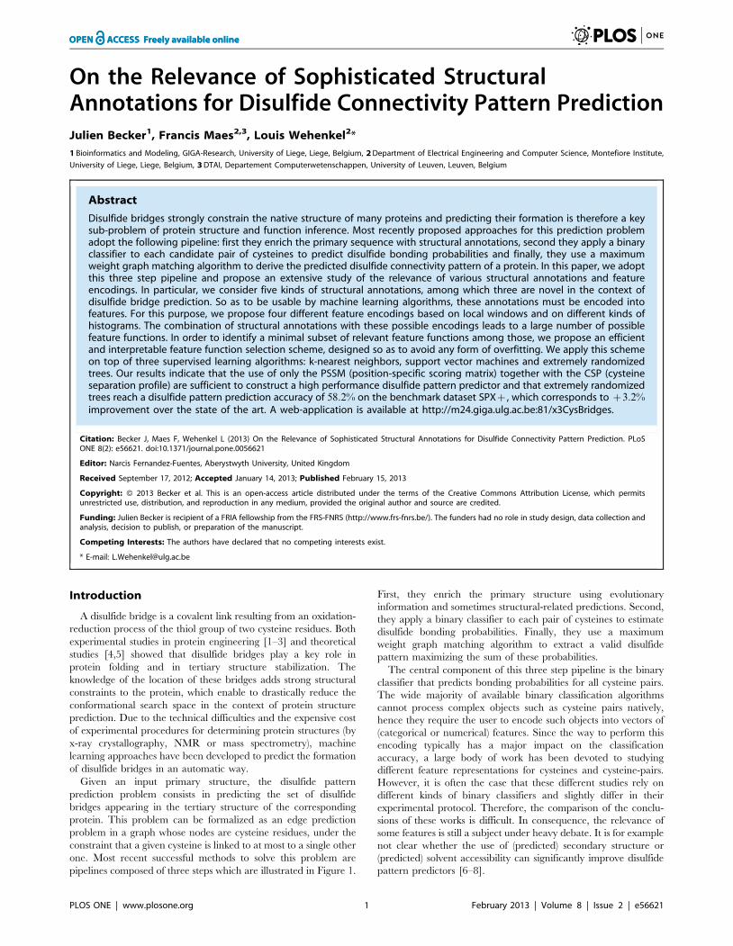
Sensitivity of extremely randomized trees to its hyper-parameters

This series of experiments aims at studying the impact of the

hyper-parameters (T , K and Nmin) when using the feature

functions fw(PSSM,15),csp(17)g. With these two feature func-

tions, the number of features is d~662. The default setting is

T~1 000,K~ffiffiffidp

, Nmin~2 and we study the parameters one by

one, by varying their values in ranges T[½10,104�, K[½1,d� and

Nmin[½2,100�.Figure 6 reports the Qp and Q2 scores in function of the three

hyper-parameters. As a matter of comparison, we also reported

the Qp scores of the three baseline described previously. We

observe that the Qp score grows (roughly) following a logarithmic

law w.r.t. T . The value of T~1 000 occurs to be very good

tradeoff between performance and model complexity. Concerning

K , we observe that the value maximizing Qp is K^50, which is a

bit larger than the default setting K~ffiffiffidp

. Note that the protein-

level performance measure Qp and the cysteine-pair level

performance measure Q2 do not correlate well in terms of the

effect of parameter K , which confirms the interest of directly

optimizing Qp in our feature function selection algorithm. Nmin

controls the complexity of built trees and, hence, the bias-variance

tradeoff by averaging output noise. It is usually expected that a

small value of Nmin improves performance. In our case, we

observe that increasing Nmin never improves the performance

measures and that Qp has a large variance.

Figure 5. Forward feature function selection with 10 train/test splits of the SPXz dataset. Each figure reports the results of five iterationsof our forward feature function selection algorithm on one of ten train/test splits. Solid red lines are the cross-validated scores and dashed blue linesare the verification scores.doi:10.1371/journal.pone.0056621.g005



Results: Chain Classification and CysteineBonding State Prediction

Until now, our pipeline relies on a perfect graph matching

algorithm that always attempts to predict patterns involving all

cysteines. Due to this, our approach is, for the moment, unable to

deal with partially connected disulfide patterns (except for proteins

with an odd number of cysteines having a single non-bonded

cysteine). This can be harmful, especially on datasets containing

many non-bonded cysteines. For example, if we apply our pipeline

to the SPX{ dataset, the pattern accuracy Qp is only 22%, since

most proteins of this dataset do not contain any disulfide bridges.

We now focus on this issue by coupling our predictor with filters

based on the output of a chain classifier and on the output of a

cysteine bonding state predictor. We first construct a chain

classifier and a cysteine bonding state predictor by applying our

feature function selection approach. We then study combinations

of these predictors with our disulfide pattern predictor.

Chain classificationWe consider the binary chain classification problem, which

consists in classifying proteins into those that have at least one

disulfide bridge and those that have no disulfide bridge. In order to

construct a chain classifier, we apply the same methodology as

before: we perform feature function selection on top of extremely

randomized trees. Since chain classification works at the level of

proteins, the set of candidate feature functions is restricted to labels

global histograms. We also include as candidates the simple

feature functions returning the number of residues, the number of

cysteines and the parity of the number of cysteines. We use the

following default setting for ETs: T~1 000,K~d and Nmin~2.

According to preliminary experiments, we found out K~d to be a

good default setting for this task. This is probably due to the fact

that we have far less features than we had before.

We performed ten runs of the feature function selection

algorithm on the SPX{ dataset, which contains both proteins

without disulfide bridge and proteins with disulfide bridges. The

performance measure is the accuracy, i.e., the percentage of

proteins that are correctly classified. In every feature function

selection run, the first selected feature function was hglobal(PSSM)

and the second one was hglobal(AA). Starting from the third

Table 4. Forward feature functions selection with 10 train/test splits of the SPXz dataset.

Fold Iteration 1 Iteration 2 Iteration 3 Iteration 4 Iteration 5

1 w(PSSM,15) csp(17) hinteval (AA) hlocal(SS8,90) w(SS3,25)

2 w(PSSM,15) csp(19) hlocal(SS8,80) w(AA,1) hlocal (SA,80)

3 w(PSSM,19) csp(19) hglobal (SA) hlocal(SS8,60) hlocal (AA,30)

4 w(PSSM,11) csp(9) hlocal (SA,90) hlocal (DR,60) pos(Ck)

5 w(PSSM,9) csp(13) hlocal (DR,90) w(SA,19) hlocal (PSSM,20)

6 w(PSSM,9) csp(19) hlocal(SS8,90) hlocal (SS3,30) w(SA,21)

7 w(PSSM,11) csp(13) hlocal(SS8,50) w(SS3,5) hlocal (PSSM,50)

8 w(PSSM,19) csp(17) hlocal (AA,80) hlocal (DR,50) w(SA,21)

9 w(PSSM,15) csp(19) hlocal (SS3,90) hlocal(SS8,90) pos(Ck)

10 w(PSSM,19) csp(17) hlocal (AA,50) hlocal (SS3,40) hlocal (SS8,70)

Mean

Cross-validated 51.8%+0.64% 56.9%+0.63% 58.3%+0.67% 58.6%+0.84% 58.9%+0.75%

Verification 51.6%+4.19% 57.8%+2.83% 57.4%+2.22% 58.7%+2.83% 58.0%+2.72%

In bold, the most frequent feature function (without consideration of the window size parameters) of each iteration. Mean: averages over the ten cross-validated scoresand the ten verification scores.doi:10.1371/journal.pone.0056621.t004

Table 5. Evaluation of the proposed prediction pipeline.

Features Qp

fw(PSSM,15)g 51.6%+3.58%

fw(PSSM,15),csp(17)g 58.2%+2.74%

fw(PSSM,15),csp(17),hlocal (SS8,77)g 58.3%+3.04%

Baseline

Vincent et al. [47] 55.0%

Lin et al. [7] 54.5%

Cheng et al. [6] 51.0%

We report the mean and standard deviation of the Qp scores obtained using 10-fold cross-validation on the SPXz dataset.doi:10.1371/journal.pone.0056621.t005

Table 6. Comparison of Qp scores on SPXz.

Number ofbridges Cheng et al. Vincent et al. Lin et al. Becker et al.

(2006) (2008) (2009) (2013)

1 59% 59% 60.6% 61.8%

2 59% 63% 65.9% 66.6%

3 55% 64% 59.8% 67.6%

4 34% 48% 36.4% 41.8%

all 51% 55% 54.5% 58.3%

Qp scores obtained using 10-fold cross-validation.

doi:10.1371/journal.pone.0056621.t006



iteration, the results are more diverse and the system starts to

overfit. By keeping the two first feature functions, we reach a 10

fold cross-validation accuracy of 79:5% on SPX{, which is not

very far from the 82% accuracy obtained by [47].

Cysteine bonding state predictionCysteine bonding state prediction consists in classifying cysteines

into those that are involved in a disulfide bridge and those that are

not. To address this task, we apply our feature function selection

approach on top of extremely randomized trees

(T~1 000,K~ffiffiffidp

and Nmin~2). The set of candidate feature

functions is composed of those depending only on the protein

(number of residues, number of cysteines, parity of the number of

cysteines, labels global histograms) and those depending on the

protein and on a single cysteine (labels local histograms, labels

local windows, cysteine separation profile window). We consider

the same window size values as in previous section. The evaluation

measure is binary accuracy, i.e., the percentage of cysteines that

are correctly classified.

We ran the feature selection algorithm once for each of the ten

different train/test splits of SPX{. We observed that the selected

feature functions set fw(PSSM,11),hglobal(PSSM),nCg led to a

binary accuracy of 87:4%, which outperforms the result of 87%obtained by Vincent et al. [47]. On SPXz, we obtain a similar

accuracy of 87:8%.

Note that once we have a cysteine bonding state predictor, we

can use it to also solve the chain classification task as follows. In

order to predict whether a protein contains disulfide bridges or

not, we run the cysteine bonding state predictor on each cysteine,

and see if at least one cysteine is predicted as being bonded. By

applying this strategy to SPX{, we obtain a chain classification

accuracy of 81:4%, which is comparable to the score of [47].

Table 7 summarizes the feature functions that were selected for

the three tasks that we consider in this paper.

Impact on pattern predictionNow that we have constructed a chain classifier and a disulfide

bonding state predictor, we focus on the question of how to exploit

the corresponding predictions in order to improve disulfide pattern

prediction. Note that, in some cases, the user may have prior

knowledge of either the chain class (whether the proteins contains

any disulfide bridges or not) or of the cysteine bonding states

(which are the cysteines that participate to disulfide bridges). To

take the different possible scenarios into account, we study the

following four settings:

N Chain class known: in this setting, we assume that the chain

classes are known a priori and simply filter out all proteins that

are known to not contain any disulfide bridge. For the proteins

that contain disulfide bridges, we run our disulfide pattern

predictor as in previous section.

N Chain class predicted: in this setting, we replace the knowledge of

the chain class by a prediction. We therefore rely on the chain

classifier derived from the cysteine bonding state predictor,

which obtained a chain classification accuracy of 81:4%.

N Cysteine states known: we here assume that the bonding states of

cysteines is known a priori. We modify the disulfide pattern

predictor by setting a probability of zero to any cysteine pair

containing at least one non-bonded cysteine.

N Cysteine states predicted: in this setting, we first run our cysteine

state predictor and then perform disulfide pattern prediction

by only considering cysteine pairs in which both cysteines

where predicted as bonded.

Figure 6. Sensitivity of ETs w.r.t. hyper-parameters. The experiments are performed on the SPXz dataset. We used the two feature functions

w(PSSM,15) and csp(17). (A) Impact of the number of trees T (from 10 to 10 000) with K~ffiffiffidp

and Nmin~1, where d~662 is the number offeatures. (B) Impact of K (from 1 to d) with T~1 000 and Nmin~1. (C) Impact of Nmin (from 2 to 101).doi:10.1371/journal.pone.0056621.g006

Table 7. Selected feature functions of the three tasks.

Task Features

Chain classification fhglobal (PSSM),hglobal (AA)gCysteine bonding state prediction fw(PSSM,11),hglobal (PSSM),nCgDisulfide pattern prediction fw(PSSM,15),csp(17)g

The feature functions were determined by the application of our selectionalgorithm on top of extremely randomized trees, using the SPX{ dataset forchain classification and cysteine bonding state prediction and the SPXz

dataset for disulfide pattern prediction.doi:10.1371/journal.pone.0056621.t007



Note that, since the SPXz dataset is entirely composed of

proteins with at least one bridge, our two first settings based on

chain classification are irrelevant for this dataset. In these

experiments, we learnt models using a 10-fold cross-validation of

ETs (T~1 000,Nmin~2 andffiffiffidp

).

Table 8 summarizes the results of our experiments on chain

classification, cysteine bonding state prediction and disulfide

pattern prediction with our four different settings. When the

chain classes are known, we observe a significant improvement of

the Qp score: from 22% to 82:5% on SPX{. When replacing the

true chain classes with predicted chain classes, we still have a

relatively high Qp score: 70:9%. This result is detailed in Table 9

as a function of the true number of disulfide bridges. We observe

that our method clearly outperforms the method of Vincent et al.

[47] on proteins containing one or two disulfide bonds and

performs slightly worst on proteins with three disulfide bonds.

Given that a majority of proteins in SPX{ contain less than two

bonds, these results leads to an overall score that is significantly

better than that of Vincent et al. When the cysteine bonding states

are known, we obtain impressive disulfide pattern accuracies:

more than 75% on SPXz and almost 90% on SPX{. When

using predicted cysteine bonding states, we still observe an

impressive improvement on SPX{: from 22% to 71:4%.

However, on SPXz, the score slightly degrades ({1:4%). This

is probably related to the fact that, as soon as one cysteine is falsely

predicted as being non-bonded, it becomes impossible to recover

the correct disulfide pattern.

Discussion

Disulfide connectivity pattern prediction is a problem of major

importance in bioinformatics. Recent state of the art disulfide

pattern predictors rely on a three step pipeline, in which the

central component is a binary classifier that predicts bridge

bonding probabilities given cysteine pair representations. Howev-

er, the comparison of the conclusions of these works is difficult

because it is often the case that these different studies rely on

different kinds of binary classifiers and slightly differ in their

experimental protocol. Therefore, the relevance of some features is

still a subject under heavy debate. This paper has proposed an

extensive study on the best way to represent cysteine pairs in the

form of features. We considered three classification algorithms: k-

nearest neighbors, support vector machines and extremely

randomized trees, and we proposed a forward feature function

selection algorithm that we applied on the standard benchmark

dataset SPXz.

Our experiments have shown that extremely randomized trees

(ETs) are highly promising in terms of predicted disulfide pattern

accuracy Qp. ETs are easy to tune and thanks to their use of

decision trees, they benefit from good scaling properties, making

them applicable to large sets of training proteins and large sets of

features. The result of our feature selection experiments with ETs

is that the primary structure related features functions

w(PSSM,15) (a local window of size 15 on the evolutionary

information) and csp(17) (a window of size 17 on the cysteine

separation profile) are sufficient to reach a very high performing

disulfide pattern predictor: ETs with these two kinds of features

predict correct disulfide connectivity patterns in 58:2% of proteins,

which outperforms the state of the art [47] with a z3:2%improvement. Furthermore, we showed that appending any other

feature function does not lead to significant subsequent improve-

ments or even decreases the accuracy.

We also investigated the question of how to exploit our disulfide

pattern predictor with filters based on the output of either a chain

classifier or of a cysteine bonding state predictor. Among the four

scenarios that we considered, we observed an important potential

for improvement when the cysteine bonding states are known,

with scores reaching 75% on SPXz and almost 90% on SPX{.

When using predicted cysteine bonding states, we still observe an

impressive improvement on SPX{ (from 22% to 71:4%) but the

score slightly degrades ({1:4%) on SPXz. This degradation is

probably due to the fact that, as soon as one cysteine is falsely

predicted as being non-bonded, it becomes impossible to construct

the correct disulfide pattern. Therefore, one direction of future

research is to develop more sophisticated methods to couple the

cysteine bonding state prediction task with the pattern prediction

task. One direction for such a better coupling is to apply the ideas

developed in [32] on multi-stage and multi-task prediction, e.g., by

iteratively re-estimating the disulfide bond probabilities.

Note that despite the fact that several studies have shown that

tree-based ensemble methods often reach state of the art results in

supervised learning (see e.g. [43]), these methods were surprisingly

few applied to structural bioinformatics problems yet. We believe

that ETs in combination with feature function selection provide a

general methodology that can be applied to a wide range of

protein related prediction problems and more generally to any

kind of classification problems involving many different possible

representations.

Table 8. Evaluation of the three tasks.

Filter SPX{ SPXz

Chain classification

– 79.5%+2.40% –

Cysteine states predicted 81.4%+2.66% –

Cysteine bonding state prediction

– 87.4%+1.14% 87.8%+2.20%

Disulfide pattern prediction (Qp)

– 22.0%+2.00% 58.2%+2.74%

Chain class known 82.5%+2.24% –

Chain class predicted 70.9%+3.10% –

Cysteine states known 89.9%+1.57% 75.8%+2.09%

Cysteine states predicted 71.4%+2.76% 56.8%+2.52%

We report the mean and standard deviation of the binary accuracy for chainclassification and cysteine bonding state prediction while the Qp score is usedfor disulfide pattern prediction. The symbol – indicates that all cysteines areused in the experiment.doi:10.1371/journal.pone.0056621.t008

Table 9. Comparison of Qp scores on SPX{ when chainclasses are predicted.

Number of bridges Vincent et al. Becker et al.

(2008) (2013)

1 30% 77.1%

2 49% 63.5%

3 61% 60.4%

4 37% 44.2%

all 39% 70.9%

Qp scores obtained using 10-fold cross-validation.

doi:10.1371/journal.pone.0056621.t009



Acknowledgments

This work was carried out at the GIGA-Bioinformatics platform of the

University of Liege. We would like to thank the cluster of the platform for

our intensive usage. We are grateful to Pierre Geurts who made available

his ETs software and provided precious advices about its utilization.

Author Contributions

Conceived and designed the experiments: JB FM. Performed the

experiments: JB. Analyzed the data: JB FM LW. Contributed reagents/

materials/analysis tools: JB FM. Wrote the paper: JB FM LW.

References

1. Anfinsen C (1973) Principles that govern the folding of protein chains. Science

181: 223–30.

2. Matsumura M, Signor G, Matthews B (1989) Substantial increase of protein

stability by multiple disulphide bonds. Nature 342: 291–293.

3. Klink T, Woycechowsky K, Taylor K, Raines R (2000) Contribution of disulfide

bonds to the conformational stability and catalytic activity of ribonuclease a.

European Journal of Biochemistry 267: 566–572.

4. Wedemeyer W, Welker E, Narayan M, Scheraga H (2000) Disulfide bonds and

protein folding. Biochemistry 39: 4207–4216.

5. Betz S (1993) Disulfide bonds and the stability of globular proteins. Protein Sci 2:

1551–8.

6. Cheng J, Saigo H, Baldi P (2006) Large-scale prediction of disulphide bridges

using kernel methods, two-dimensional recursive neural networks, and weighted

graph matching. Proteins: Structure, Function, and Bioinformatics 62: 617–629.

7. Lin H, Tseng L (2009) Prediction of disulfide bonding pattern based on support

vector machine with parameters tuned by multiple trajectory search. WSEAS

Transactions on Computers 8: 1429–1439.

8. Ferre F, Clote P (2005) Disulfide connectivity prediction using secondary

structure information and diresidue frequencies. Bioinformatics 21: 2336–2346.

9. Geurts P, Ernst D, Wehenkel L (2006) Extremely randomized trees. Machine

Learning 63: 3–42.

10. Elumalai P, Wu J, Liu H (2010) Current advances in disulfide connectivity

predictions. Journal of the Taiwan Institute of Chemical Engineers 41: 525–539.

11. Frasconi P, Passerini A, Vullo A (2002) A two-stage SVM architecture for

predicting the disulfide bonding state of cysteines. Neural Networks for Signal

Processing: 25–34.

12. Fiser A, Cserzo M, Tudos E, Simon I (1992) Different sequence environments of

cysteines and half cystines in proteins application to predict disulfide forming

residues. FEBS Letters 302: 117–120.

13. Fariselli P, Riccobelli P, Casadio R (1999) Role of evolutionary information in

predicting the disulfide-bonding state of cysteine in proteins. Proteins: Structure,

Function, and Bioinformatics 36: 340–346.

14. Martelli P, Fariselli P, Casadio R (2004) Prediction of disulfide-bonded cysteines

in proteomes with a hidden neural network. Proteomics 4: 1665–1671.

15. Vullo A, Frasconi P (2004) Disulfide connectivity prediction using recursive

neural networks and evolutionary information. Bioinformatics 20: 653–659.

16. Rama G, Shilton A, ParkerM, PalaniswamiM (2005) Disulphide bridge

prediction using fuzzy support vector machines. International Conference on

Intelligent Sensing and Information Processing 0: 48–54.

17. Lu C, Chen Y, Yu C, Hwang J (2007) Predicting disulfide connectivity patterns.

Proteins: Structure, Function, and Bioinformatics 67: 262–270.

18. Ceroni A, Passerini A, Vullo A, Frasconi P (2006) DISULFIND: a disulfide

bonding state and cysteine connectivity prediction server. Nucleic Acids

Research 34: W177–W181.

19. Fariselli P, Casadio R (2001) Prediction of disulfide connectivity in proteins.

Bioinformatics 17: 957–964.

20. Baldi P, Cheng J, Vullo A (2005) Large-scale prediction of disulphide bond

connectivity. In: Advances in Neural Information Processing Systems. MIT

Press, pp. 97–104.

21. Lin H, Tseng L (2010) DBCP: a web server for disulfide bonding connectivity

pattern prediction without the prior knowledge of the bonding state of cysteines.

Nucleic Acids Research 38: W503–W507.

22. Altschul S,Madden T, Schaffer A, Zhang J, Zhang Z, et al. (1997) Gapped

BLAST and PSI-BLAST: a new generation of protein database search

programs. Nucleic Acids Research 25: 3389–3402.

23. The UniProt Consortium (2011) Ongoing and future developments at the

universal protein resource. Nucleic Acids Research 39: D214–D219.

24. Zhao E, Liu H, Tsai C, Tsai H, Chan C, et al. (2004) Cysteine separationsprofiles on protein sequences infer disulfide connectivity. Bioinformatics 21:

1415–1420.25. Ambroise C, McLachlan GJ (2002) Selection bias in gene extraction on the basis

of microarray gene-expression data. Proceedings of the National Academy of

Sciences 99: 6562–6566.26. Jones D (1999) Protein secondary structure prediction based on position-specific

scoring matrices. Journal of Molecular Biology 292: 195–202.27. Savojardo C, Fariselli P, Alhamdoosh M, Martelli PL, Pierleoni A, et al. (2011)

Improving the prediction of disulfide bonds in eukaryotes with machine learningmethods and protein subcellular localization. Bioinformatics 27: 2224–2230.

28. Song J, Yuan Z, Tan H, Huber T, Burrage K (2007) Predicting disulfide

connectivity from protein sequence using multiple sequence feature vectors andsecondary structure. Bioinformatics 23: 3147–3154.

29. Berman H, Westbrook J, Feng Z, Gilliland G, Bhat T, et al. (2000) The proteindata bank. Nucleic Acids Research 28: 235–242.

30. Sven M, Burkhard R (2003) UniqueProt: creating representative protein

sequence sets. Nucleic Acids Res: 3789–3791.31. Sander C, Schneider R (1991) Database of homology-derived protein structures

and the structural meaning of sequence alignment. Proteins: Structure, Function,and Bioinformatics 9: 56–68.

32. Maes F, Becker J,Wehenkel L (2011) Iterative multi-task sequence labeling forpredicting structural properties of proteins. 17th European Symposium on

Artificial Neural Networks.

33. Camproux A, Gautier R, Tuffery P (2004) A hidden markov model derivedstructural alphabet for proteins. Journal of molecular biology 339: 591–606.

34. Kabsch W, Sander C (1983) Dictionary of protein secondary structure: patternrecognition of hydrogen-bonded and geometrical features. Biopolymers 22:

2577–2637.

35. Noivirt-Brik O, Prilusky J, Sussman J (2009) Assessment of disorder predictionsin CASP8. Proteins 77 Suppl 9: 210–6.

36. Cohen W, Carvalho V (2005) Stacked sequential learning. In: International JointConferences on Artificial Intelligence. pp. 671–676.

37. Adamczak R, Porollo A, Meller J (2005) Combining prediction of secondarystructure and solvent accessibility in proteins. Proteins.

38. Lin HH, Tseng LY (2012) Prediction of disulfide bonding pattern based on a

support vector machine and multiple trajectory search. Information Sciences199: 167–178.

39. Chang CC, Lin CJ (2011) LIBSVM: A library for support vector machines.ACM Transactions on Intelligent Systems and Technology 2: 27:1–27:27.

40. Platt JC (1999) Probabilistic outputs for support vector machines and

comparisons to regularized likelihood methods. In: Advances in large marginclassifiers. MIT Press, pp. 61–74.

41. Wu TF, Lin CJ, Weng RC (2004) Probability estimates for multi-classclassification by pairwise coupling. J Mach Learn Res 5: 975–1005.

42. Breiman L (2001) Random forests. In: Machine Learning. pp. 5–32.

43. Caruana R, Niculescu A (2006) An empirical comparison of supervised learningalgorithms. In: In Proc. 23 rd Intl. Conf. Machine learning (ICML’06). pp. 161–

168.44. Gabow H (1976) An efficient implementation of edmonds’ algorithm for

maximum matching on graphs. Journal of the ACM 23: 221–234.45. Kolmogorov V (2009) Blossom V: A new implementation of a minimum cost

perfect matching algorithm. Mathematical Programming Computation 1: 43–

67.46. Saeys Y, Inza I, Larranaga P (2007) A review of feature selection techniques in

bioinformatics. Bioinformatics 23: 2507–2517.47. Vincent M, Passerini A, Labbe M, Frasconi P (2008) A simplified approach to

disulfide connectivity prediction from protein sequences. BMC Bioinformatics:

20.



On the Relevance of Sophisticated Structural Annotations for Disulfide Connectivity Pattern...

Documents

Transcript of On the Relevance of Sophisticated Structural Annotations for Disulfide Connectivity Pattern...