1

On the Refinement of a Boundary-Fitted Shallow Water Model 1

2

Dongfang Liang*, †, §, Junqiang Xia*, Roger A Falconer‡ and Jingxin Zhang† 3

4

5

6

* State Key Laboratory of Water Resources and Hydropower Engineering Science, 7

Wuhan University, Wuhan 430072, China 8

9

† MOE Key Laboratory of Hydrodynamics, School of Naval Architecture, Ocean and 10

Civil Engineering, Shanghai Jiao Tong University, Shanghai 200240, China 11

12

‡ Cardiff School of Engineering, Cardiff University, 13

The Parade, Cardiff CF24 3AA, UK 14

15

§ d.liang@sjtu.edu.cn 16

17

2

Abstract 18

The two-dimensional shallow water equations were formulated and numerically 19

solved in an arbitrary curvilinear coordinate system, which offers a relatively high 20

degree of flexibility in representing the natural flow domains with structured meshes. 21

The model employs an efficient TVD-MacCormack scheme, which has second order 22

accuracy in both time and space. Refinements were made to enhance the model’s 23

accuracy and stability in computing the shallow wave dynamics in real-world scenarios, 24

with irregular boundaries and uneven beds. In particular, advanced open boundary 25

conditions have been proposed according to the method of characteristics, and rigorous 26

mass conservation has been enforced during the computation at both the inner-domain 27

and the boundaries. These refinements are necessary when modelling the flood 28

inundation over a large area and the tidal oscillation in a macro-tidal estuary. The 29

effectiveness of the refinements was verified by simulating the forced tidal resonance in 30

an idealised condition and the Malpasset dam-break flood. The application of the 31

refined model to the study of tidal oscillations in the Severn Estuary and Bristol 32

Channel can be found in the companion paper. 33

34

Keywords: TVD-MacCormack; Shallow water equations; Long waves; Dam-break; 35

Open boundary 36

37

1. Introduction 38

Depth-averaged models are frequently adopted in analysing environmental flows with 39

free surfaces, and they offer a good compromise between computational efficiency and 40

accuracy. With the help of shallow-water assumptions, the free surface elevations can 41

3

be conveniently computed according to the conservation of mass. These models are 42

valid when the horizontal length scale is much larger than the water depth and the 43

vertical acceleration of the flow is not significant, which are often the case in many 44

environmental flows. Typical depth-averaged models have been presented by McGuirk 45

and Rodi (1978), Falconer (1980), Molls and Chaudhry (1995). 46

However, these conventional numerical methods are unable to predict the rapid flows 47

that involve shocks, which are the discontinuities in the weak solutions to the 48

conservative formulation of the shallow water equations. Hydraulic jumps, flood fronts, 49

bores and breaking waves are naturally occurring discontinuities, and are formed in 50

trans-critical flows. Over these local flow features, mass and momentum are still 51

conserved, but certain amount of mechanical energy is lost. To predict these 52

discontinuities in the flow field, various shock-capturing schemes have been developed, 53

such as Fraccarollo and Toro (1995), Mingham and Causon (1998), and Liang et al. 54

(2006). 55

This study adopts an arbitrary boundary-fitted curvilinear computational mesh, which 56

closely follows the complex and irregular topography, thus reducing the inaccuracies 57

associated with the imperfect representation of the geometry and bathymetry. When 58

coastline and river boundaries are approximated by the curvilinear mesh, then a high 59

density of grid points can be automatically concentrated in the narrow areas of the 60

domain, which are often particularly important (Lin and Falconer, 1995; Harris et al., 61

2004, Liang et al. 2007a). The computation based on a high-quality curvilinear mesh 62

generally offers higher levels of accuracy and efficiency than that based on an 63

unstructured mesh. The more the grid lines are aligned with the direction of the flow, 64

the higher the accuracy of the computation. The disadvantage of the curvilinear mesh 65

4

lies in the difficulty and long time involved in generating a suitable mesh of good 66

quality. Most of the previous numerical models require the two families of grid lines to 67

be orthogonal to each other (e.g. Lin and Falconer, 1995), and they are based on the 68

alternating-direction-implicit scheme (e.g. Molls and Chaudhry, 1995), which has been 69

demonstrated to be unsuitable for transcritical flows (e.g. Liang et al., 2006). In 70

contrast, the numerical model employed here is based on a shock-capturing TVD-71

MacCormack scheme, which is extremely efficient and is second-order accurate. 72

Furthermore, this scheme does not contain any free parameters to adjust the amount of 73

artificial viscosity necessary for smoothing out the oscillations near steep variations. Its 74

good property has been proven in previous applications (e.g. Liang et al. 2007a, 2007b, 75

2010, 2012). 76

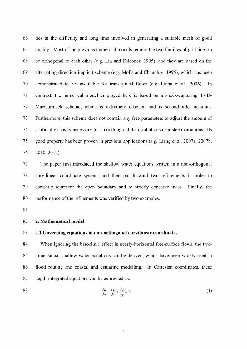
The paper first introduced the shallow water equations written in a non-orthogonal 77

curvilinear coordinate system, and then put forward two refinements in order to 78

correctly represent the open boundary and to strictly conserve mass. Finally, the 79

performance of the refinements was verified by two examples. 80

81

2. Mathematical model 82

2.1 Governing equations in non-orthogonal curvilinear coordinates 83

When ignoring the baroclinic effect in nearly-horizontal free-surface flows, the two-84

dimensional shallow water equations can be derived, which have been widely used in 85

flood routing and coastal and estuarine modelling. In Cartesian coordinates, these 86

depth-integrated equations can be expressed as: 87

0

y

q

x

p

t

(1) 88

5

fqCH

qpgp

xgH

yH

pq

x

H

p

t

p

22

22

2

(2) 89

fpCH

qpgq

ygH

y

H

q

xH

pq

t

q

22

22

2

(3) 90

where t is time; ζ is the water surface level above datum; p and q are the volumetric 91

discharges per unit width in the x and y directions, respectively; is the momentum 92

correction factor for the non-uniform velocity distribution over the depth, which was set 93

to unity in this study; g is gravitational acceleration; H is the total water depth; C is the 94

Chezy coefficient; and f (= sin2 ) is the parameter of the Coriolis acceleration, with 95

being the angular speed of the Earth’s rotation (7.29×10-5 rad/s) and being the 96

geographical angle of latitude. The two momentum equations (2-3) only include the 97

material acceleration, hydrostatic pressure gradient, bed friction, and Coriolis effects, 98

while neglecting the influences of the wind stress, eddy viscosity, etc. 99

In order to undertake the computation on boundary-fitted meshes, these equations 100

need to be transformed into the curvilinear coordinates. Introducing a geometric 101

mapping, the non-orthogonal curvilinear mesh in the physical plane (x, y) can be 102

transformed into the rectangular mesh in the computational plane (ξ, η). Defining the 103

Jacobian determinant as: 104

yxyxJ (4) 105

where the subscripts ξ and η denotes the differentiations with respective to ξ and η, 106

respectively. This Jacobian determinant carries the physical meaning as the area of each 107

curvilinear cell. Using the chain rule, the first-order spatial derivatives of any function 108

(x, y) can be expressed as: 109

6

yyJx

1 (5) 110

xxJy

1 (6) 111

The coefficients of the coordinate transformation, including J, x , x , y and y , are 112

related only to the mapping between the arbitrary quadrilateral grid cells in the (x, y) 113

plane and the uniform rectangular grid cells in the (ξ, η) plane, so they are independent 114

of time. 115

With the transformation rules of Equations (5-6), Equations (1) can be 116

straightforwardly transformed into the following form: 117

0

py

qx

qx

py

t

J (7) 118

Noting the relations yy and xx , then 119

0

xx

qyy

py

px

qx

qy

p (8) 120

Adding the left hand sides of Equations (7-8) yields: 121

0

yp

xq

py

qx

xq

yp

qx

py

t

J (9) 122

which can be further simplified into: 123

0

pyqxqxpy

t

J (10) 124

Similarly, the following equations, with the independent variables being t, ξ and η, can 125

be derived from Equations (2-3): 126

fqJ

CH

JqpgpgHygHy

yH

px

H

pqx

H

pqy

H

p

t

Jp

22

22

22

(11) 127

7

fpJ

CH

JqpgqgHxgHx

yH

pqx

H

qx

H

qy

H

pq

t

Jq

22

22

22

(12) 128

Equations (10-12) constitute the shallow water equations in the (ξ, η) frame, where 129

the numerical discretisation is carried out. After converting the governing equations 130

from physical coordinates into computational coordinates, the solution can be sought 131

based on uniform rectangular grids. The aforementioned coordinate transformation 132

does not have to be conformal, i.e. the corner angles of the grids in the (x, y) plane do 133

not have to be 90 degrees, lending extra flexibility in the mesh generation. It should be 134

noted that the above-formulated equation system does not take the conservative form. 135

However, Liang et al. (2007b) have shown that, if the right-hand-side derivatives are 136

discretised in a certain way, their finite difference form will be equivalent to that of the 137

conservatively formulated shallow water equations. Specifically, the coefficients before 138

the derivatives of ζ, e.g. gHy , gHx , gHy and gHx , need to be approximated by the 139

arithmetic average in the direction of differencing to ensure the conservative property of 140

the difference equations. The computation is more efficient when the discretisation is 141

based on the non-conservative form of the differential equations. Another noteworthy 142

aspect is that the present study chooses water surface level, rather than the water depth, 143

in expressing the mass conservation principle. Liang et al. (2006) showed that this 144

approach helps prevent the onset of unbalanced flows above uneven terrains at 145

quiescent conditions. There are also other numerical techniques to mitigate the flow 146

imbalances arising from the source terms of the equations, e.g. Pu et al. (2012) and 147

Liang (2012). 148

149

2.2 Overall numerical scheme 150

8

The numerical methods used are only briefly outlined herein. Readers are referred to 151

Liang et al. (2006, 2007a, 2007b) for details. Using the Strang splitting technique, the 152

solution to the above two-dimensional problem can be sought by solving two separate 153

one-dimensional problems. Each one-dimensional problem considers the variation in 154

only one direction, along either ξ or η coordinate. 155

qxpy

t

J (13) 156

fqJ

CH

JqpgpgHy

qxpyH

p

t

Jp

22

22

(14) 157

gHx

qxpyH

q

t

Jq (15) 158

and 159

pyqx

t

J (16) 160

gHy

pyqxH

p

t

Jp (17) 161

fpJ

CH

JqpgqgHx

pyqxH

q

t

Jq

22

22

(18) 162

Here, qxpy and pyqx carry clear physical meanings as the fluxes in the (ξ, η) 163

domain. Because J is essentially the area of the grid cell in the physical domain, 164

bzJ stipulates the water volume inside a grid cell. As J and bz are independent 165

of time, the change in J reflects the change in the amount of water inside a cell. 166

Water surface elevations and flow velocities often experience abrupt variations when 167

the tidal flow is restricted by landmass and when the flood wave is rapid, thus a shock-168

capturing numerical model has been adopted. The TVD-MacCormack scheme is used 169

9

to solve both sets of equations, which comprises a predictor step, a corrector step and a 170

TVD modification step in each round of time advancement. Because the main purpose 171

of this paper is to propose and test the following improvements to the existing shallow 172

water solver, the TVD-MacCormark scheme is not repeated herein. 173

174

2.3 Open boundary condition 175

Apart from combining the variable groups with clear physical meanings to improve 176

the computational efficiency and enhance the model interface with users, one biggest 177

refinement to the existing model is concerned with the implementation of open 178

boundary conditions. In the hydrodynamic study of semi-enclosed water bodies, such 179

as estuaries and harbours, it is common to specify the known water level variations at 180

the open boundary, as illustrated in Figure 1(a). To enable the finite difference 181

approximation at the inner nodes immediately adjacent to the open boundary, the 182

velocities, or unit-width discharges, at the boundary shall be calculated based on 183

appropriate boundary conditions. 184

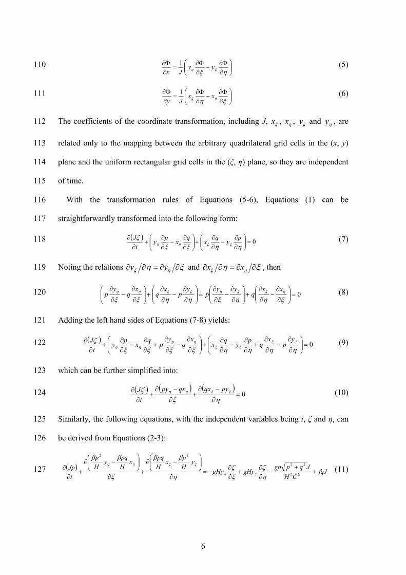
For any nodal point (xb, yb) at the boundary, its normal and tangential directions are 185

denoted as n and τ respectively, and its immediate inner node in the normal direction is 186

denoted as (xl, yl). Although the current numerical model permits arbitrary curvilinear 187

grids, care shall be taken to make the computational grids as orthogonal as possible. 188

Hence, points (xb, yb) and (xl, yl) can be regarded to be aligned in the n direction, along 189

which the one-dimensional Riemann problem is established to find the discharge 190

information at the boundary. As demonstrated in Figure 1(b), draw a positive 191

characteristic, I+, through point (xb, yb) at time tk+1, whose slope is given by 192

111

1

kb

kbk

b

kb gHgH

H

pqn

dt

dn (19) 193

10

where the subscripts and superscripts indicate the spatial locations and time levels of the 194

variables, respectively, and pqn is the projection of the unit-width discharge vector 195

along the n direction. Assuming the Froude number of the flow to be much less than 196

unity at the open boundary, then the contribution of the flow velocity to the slope of the 197

characteristic curve can be dropped; hence the approximate equal sign near the end of 198

Equation (19). For explicit numerical schemes, the Courant-Friedrichs-Lewy criterion 199

demands the point (xi, yi) on I+ at time tk to lie between (xb, yb) and (xl, yl). The distance 200

1n labelled in Figure 1(b) can thus be calculated by the known value of 1kbH . 201

1 kbi gHtn (20) 202

Then, the values of the variables at point (xi, yi) at time tk can be calculated by linear 203

interpolation 204

kb

kl

ikb

ki HH

n

nHH

, kb

kl

ikb

ki pp

n

npp

, kb

kl

ikb

ki qq

n

nqq

(21) 205

Subsequently, the unit-width discharge in the n direction at point (xi, yi) and time tk is 206

calculated 207

sincos ki

ki

ki qppqn (22) 208

where θ is angle between the n direction and positive x axis, as illustrated in Figure 1(a). 209

Ignoring any influence of the bed slope and friction, which is justifiable owing to the 210

small value of t and x , the characteristic relationship, dictated by the Riemann 211

invariant, along I+ states 212

kik

i

kik

bkb

kb gH

H

pqngH

H

pqn22 1

1

1

(23) 213

Therefore, the discharge normal to the boundary is 214

111 22

k

bkb

kik

i

kik

b HgHgHH

pqnpqn (24) 215

11

The velocity parallel to the boundary is simply advected by the flow, so the discharge 216

parallel to the boundary is 217

sincos11

1 ki

kik

i

kbk

iki

kbk

b pqH

Hpq

H

Hpq

(25) 218

Eventually, the boundary variables p and q at time tk+1 can be calculated by projecting 219

vector ( 1kbpqn , 1k

bpq ) along the x and y directions. 220

sincos 111 kb

kb

kb pqpqnp (26) 221

cossin 111 kb

kb

kb pqpqnq (27) 222

In most conventional shallow water models, e.g. Sanders (2002) and Xia et al. (2010a, 223

2010b), the Riemann invariants at position (xl, yl) at time tk and those at position (xb, yb) 224

at time tk+1 are simply equated to find the boundary unit-width discharges, rather than 225

first locate point (xi, yi) at time tk based on the slope of the characteristic curve. Such a 226

conventional treatment works fine if the Courant number of the computation is around 227

unity, in which case points (xi, yi) and (xl, yl) are very close to each other, or if the flow 228

at the boundary is nearly uniform, in which case variables at points (xi, yi) and (xl, yl) are 229

almost the same. Otherwise, errors arise from the boundary and may spoil the entire 230

computation. 231

232

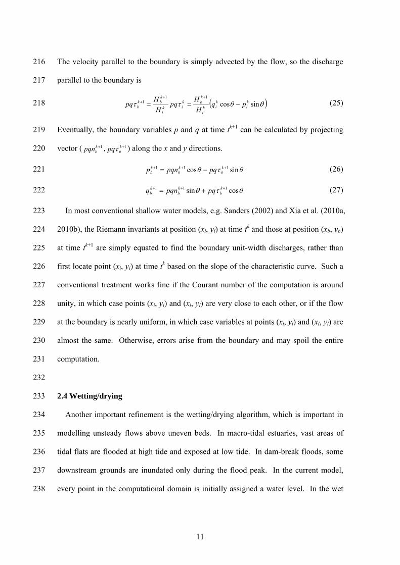
2.4 Wetting/drying 233

Another important refinement is the wetting/drying algorithm, which is important in 234

modelling unsteady flows above uneven beds. In macro-tidal estuaries, vast areas of 235

tidal flats are flooded at high tide and exposed at low tide. In dam-break floods, some 236

downstream grounds are inundated only during the flood peak. In the current model, 237

every point in the computational domain is initially assigned a water level. In the wet 238

12

area, the water levels are greater than the bed elevations. In the dry area, the water 239

levels are equal to the bed elevations. Wetting/dying may occur to any point in the 240

course of the simulation. If the water depth at a point is found to be lower than a 241

threshold value Δ (e.g. 1 mm), then the point is regarded to be dry. Dry points are 242

disregarded in the ongoing computation. Their water levels are frozen and the 243

momentum is set to zero. Solid-wall boundary conditions are imposed at the edge 244

between wet and dry cells. A wetting procedure is conducted at the beginning of every 245

time step, where the water level of a dry point, which is referred to as the frozen water 246

level henceforth, is compared with the highest water level of the neighbouring wet 247

points, which is called the free water level henceforth. If the free water level is found to 248

be over 2Δ higher than the frozen water level of a dry point, then a layer of water with 249

thickness Δ is shifted to the dry cell, and the water level on the corresponding wet cell is 250

lowered by Δ multiplied by the ratio of the Jacobian determinant between the dry cell 251

and the wet cell. In this way, the dry points may then be deemed wet and included in 252

the subsequent computation. It also ensures that the amount of water removed from the 253

wet cell is equal to the amount of water received by the dry cell. 254

255

3. Model validation – Boundary-forced tidal oscillation 256

In oceanography, a tidal resonance occurs when the tide excites one of the resonant 257

modes of a basin. Then, the incident tidal wave is reinforced by the reflected waves 258

from the solid boundary, resulting in a much higher tidal range inside the basin than that 259

in the open ocean. Chen et al. (2007) showed the importance of accurately resolving the 260

coastal geometry in reproducing the near-resonance tidal waves. Consider a coastal 261

basin that is bounded by solid walls on three sides and is connected to the ocean through 262

13

an open boundary, as shown in Figure 2. The inner and outer radii, L1 and L, were set at 263

90 km and 158 km, respectively, and the still water depth, H0, was set at a constant 264

value of 1 m. Such a shape can be conveniently described with the polar coordinates, so 265

the following equations are expressed in terms of the radius r and angle θ. A M2 tide 266

was specified at the open boundary, with the water surface position above the still water 267

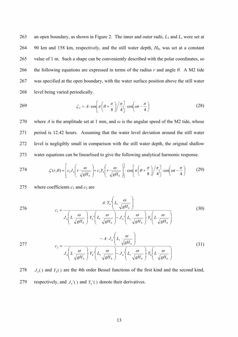
level being varied periodically. 268

4cos

48cos

tAb (28) 269

where A is the amplitude set at 1 mm, and ω is the angular speed of the M2 tide, whose 270

period is 12.42 hours. Assuming that the water level deviation around the still water 271

level is negligibly small in comparison with the still water depth, the original shallow 272

water equations can be linearlised to give the following analytical harmonic response. 273

4cos

48cos),(

0

42

0

41

tgH

rYcgH

rJcr (29) 274

where coefficients c1 and c2 are 275

0

4

0

14

0

14

0

4

0

14

1

''

'

gHLY

gHLJ

gHLY

gHLJ

gHLYA

c

(30) 276

0

4

0

14

0

14

0

4

0

14

2

''

'

gHLY

gHLJ

gHLY

gHLJ

gHLJA

c

(31) 277

)(4J and )(4Y are the 4th order Bessel functions of the first kind and the second kind, 278

respectively, and )('4J and )('4Y denote their derivatives. 279

14

As shown in Figure 2, the computational domain consisted of a total of 68×85 grid 280

cells, with an average side length of around 1 km. The time step was fixed at 3 min. 281

The computation started with water at rest. The aforementioned method was applied to 282

the introduction of open boundary conditions. In order to obtain the harmonic solution 283

to the problem, some degree of damping is necessary to allow the disturbance to peter 284

out in the transient process. This was achieved by including a small amount of bed 285

friction in the calculation. The Chezy coefficient was set at a large value of 1000 m1/2/s 286

in the present calculation, indicating an extremely smooth seabed and thus only limited 287

influence on the tidal oscillations at the eventual harmonic stage. To guarantee the 288

repetitive water level movement, a total of 100 tidal cycles were simulated. Water 289

surface shapes at four phases in the last cycle are presented in Figure 3. Because of the 290

near-resonance configuration, the tiny water level movement at the open boundary 291

induced significant oscillations inside the basin. The water level along the centreline of 292

the domain, with θ = 0, remained at still water level during the tidal oscillation. The 293

water surface takes on an antisymmetric pattern about the centreline, i.e. the oscillations 294

on the two sides have the same amplitude, but are out of phase. Figure 4 shows that a 295

good match is achieved between the analytical and computed amplitude distributions 296

across the basin. Consistent with the observations in Figure 3, the maximum oscillation 297

occurs in the vicinity of the two inner corners, where the amplitude exceeds 5 cm – 50 298

times greater than the amplitude specified at the open boundary. 299

300

4. Model validation – Malpasset dam-break flood 301

In this section, the capability of the refined model was further demonstrated by 302

simulating the Malpasset dam-break flood, which, owing to its complex topography and 303

15

availability of field data, was often selected as a benchmark for shock-capturing models 304

(e.g. Hervouet, 2000; Liang et al. 2007a). Moreover, it involves frequent 305

wetting/drying phenomena, which are also a process typical of the macro-tides in mild-306

slope coasts, such as the Severn Estuary and Bristol Channel. Located in a narrow 307

gorge of the Reyran river valley in France, the Malpasset dam failed in 1959 following 308

an exceptionally heavy rainfall event. The dam was a 66.5 m high arch structure, with a 309

crest length of 223 m. Little of the arch remained after the disaster, so this accident 310

offers a unique example of the total failure of an arch dam and thus a rare opportunity 311

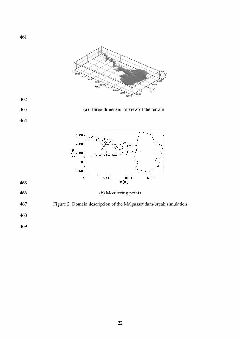
for model validation. Downstream of the dam, the Reyran river valley is very narrow 312

and has two consecutive sharp bends, before the valley widens and eventually reaches 313

the flat plain (see Fig. 5a). The flood completely changed the bottom of the Reyran 314

valley, and the river ceased flowing in the well-defined channel. Over three hundred 315

casualties were reported. At the points labelled in Figure 5(b), information is available 316

on the maximum water levels, or the flood wave arrival times, or both, through a field 317

survey and physical model experiments. 318

Fig. 5 shows that the computational domain was limited within an area of about 17 319

km by 8.5 km, covering both the reservoir and downstream valley. At time zero, water 320

was impounded in the reservoir, with a water surface level of 100 m, as if the dam were 321

still there. The initial water level in the sea was zero. The rest of the computational 322

domain was considered to be initially dry. Hervouet (2000) has shown that the initial 323

downstream river flow was negligible because of its small rate compared with the flow 324

caused by the dam failure. In consistency with some of the previous research studies, 325

the Manning’s coefficient was set at 0.033 s m-1/3 across the entire domain, based on 326

16

which Chezy coefficients were calculated. A total of 1092 × 201 grids cells were 327

employed, with the grid size ranging from 5 m to 50 m. The time step was 0.1 s. 328

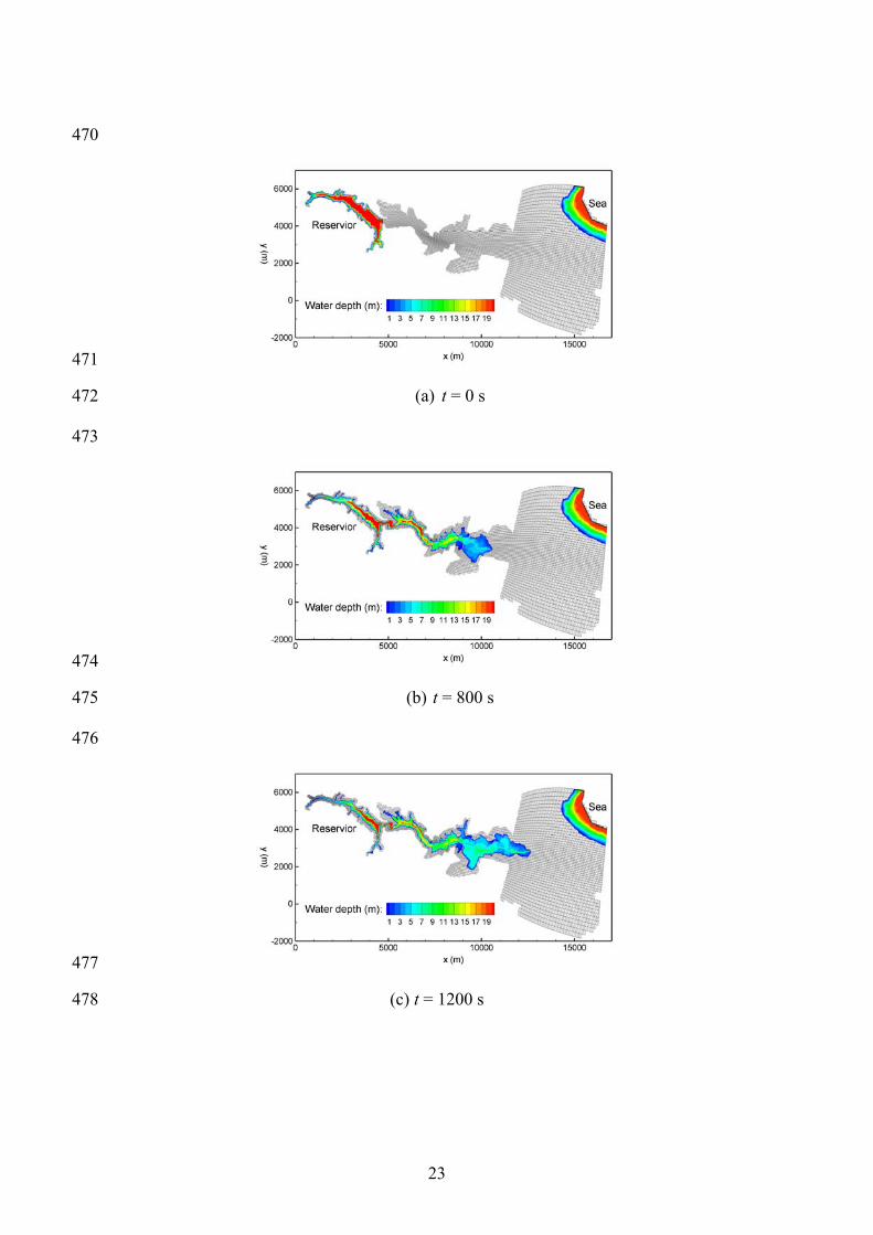
Snapshots of the inundated area and water depth distributions are illustrated in Fig. 6, 329

together with the background mesh deployed in the computation. The inactive grids, 330

which were part of the structured mesh but were never considered in the computation, 331

have been blanked out of the figure for a clearer view. For legibility, only every fourth 332

grid line was drawn in Fig. 6. The concrete remains were 56.8 m above sea level, so, 333

immediately after the dam-break at time zero, a 43.2 m high wall of water was created 334

at the location of the dam, as is shown in Figure 6(a). The flood propagated rapidly in 335

the steep and narrow valley, as is evident in Figure 6(b-c). When the flood wave 336

propagated over the broad coastal plain, before reaching the sea, the wave front spread 337

out and the propagation slowed down considerably, as is demonstrated in Figure 6(d-e). 338

As water travelled downstream, the reservoir was being emptied, with large areas of the 339

bed becoming dry (Figure 6e). The development of the flood inundation looks realistic, 340

with the main features of the flood wave being reproduced. 341

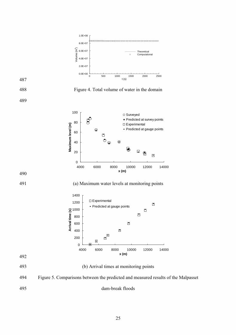
Duration the entire simulation, the flow was confined inside the computational 342

domain, so solid-wall conditions were imposed around the domain. Therefore, the total 343

quantity of water inside the domain should remain constant throughout the simulation, 344

enabling an easy check of the mass-balance property of the numerical model. Figure 7 345

proves that the refined TVD-MacCormack model possesses excellent quality of mass 346

conservation, not only during the normal computation at inner grid cells, but also along 347

the moving interface where wetting/drying processes occurred. The maximum capacity 348

of the reservoir behind the Malpasset dam was 5.5×107 m3, which is comparable with 349

17

the volume of 8.6×107 m3 shown in Figure 7. The difference is due to the seawater 350

included in the downstream part of computational domain. 351

Quantitative verification of the simulation was made by comparing the computed 352

maximum water level and wave front arrival time with the corresponding measured 353

values, as plotted in Figure 8. In the computation, the hydrographs at the monitoring 354

points labelled in Figure 5(b) were recorded, from which the arrival times and peak 355

water levels of the flood were extracted. Bearing in mind the crude nature of the field 356

survey and the outdated ground elevation data used, the discrepancy between the two 357

sets of data can be considered acceptable. Although the flood arrival time generally 358

follows the monotonic upward trend with the downstream distance, the maximum water 359

level shows more variability. Water levels at some nearby locations exhibit large 360

differences, which is a typical sign of supercritical flows. 361

362

5. Conclusions 363

This paper refined a two-dimensional depth-averaged model, which solved the 364

shallow water equations in a non-orthogonal curvilinear coordinate system using the 365

TVD-MacCormack scheme. The open boundary condition was enforced by faithfully 366

adhering to the method of characteristics. The paper elaborated how the flow rates 367

should be specified at the boundary when the boundary water levels were known. 368

Similar derivations can be made to find the boundary water levels from the known flow 369

rates. An improved wetting/drying algorithm was implemented, so that mass was 370

rigorously conserved in the wetting/drying process. These refinements were 371

subsequently validated. First, the near-resonance tidal oscillation in a hypothetical 372

coastal basin was simulated, and the predictions matched well with the analytical 373

18

solution. Then, the model was applied to reproduce the Malpalsset dam-break flood in 374

1959. Good agreement with the measurements was obtained, with the model 375

demonstrating precise mass conservation in simulating this rapid flow with continuous 376

shifting of the water/land edge. 377

These two refinements are particularly relevant to the simulation of tidal behaviour in 378

coastal regions with large tidal ranges, such as the Severn Estuary and Bristol Channel, 379

where the treatments of the open boundary and moving interface play an important role 380

in determining the accuracy of the overall computation. 381

382

Acknowledgements 383

We are grateful to the support by the National Natural Science Foundation of China 384

(Grant No. 51079103), and the Open Research Fund Program of the State Key 385

Laboratory of Water Resources and Hydropower Engineering Science, Wuhan 386

University (Grant No. 2011A005). 387

388

References 389

[1] Chen C, Huang H, Beardsley RC, Liu H, Xu Q, Cowles G. (2007). A finite 390

volume numerical approach for coastal ocean circulation studies: comparisons 391

with finite difference models. Journal of geophysical research, vol 112, article 392

number C03018 393

[2] Falconer RA. (1980). Numerical modelling of tidal circulation in harbours. 394

Journal of waterway, port, coastal and ocean division, ASCE, 106(WW1): 31-48 395

19

[3] Fraccarollo L and Toro EF. (1995). Experimental and numerical assessment of the 396

shallow wate model for two-dimensional dam-break type problems. Journal of 397

hydraulic research, 33: 843-864 398

[4] Harris E L, Falconer R A, Lin B L. (2004). Modelling hydro-environmental and 399

health risk assessment parameters along the South Wales coast. Journal of 400

Environmental Management , 73 (1): 61-70 401

[5] Hervouet JM. (2000). A high resolution 2-D dam-break model using 402

parallelization. Hydrological processes, 14: 2211-2230 403

[6] Liang D. (2012). Discussion of “Head Reconstruction Method to Balance Flux 404

and Source Terms in Shallow Water Equations” by E. Creaco, A. Campisano, A 405

Khe, C. Modica and G. Russo. Journal of engineering mechanics, 138: 552-553 406

[7] Liang D, Falconer R A, Lin B L. (2006). Comparison between TVD-407

MacCormack and ADI-type solvers of the shallow water equations. Advances in 408

Water Resources , 29 (12): 1833-1845 409

[8] Liang D, Lin B and Falconer RA. (2007a). A boundary-fitted numerical model 410

for flood routing with shock-capturing capability. Journal of hydrology, 332: 411

477-486 412

[9] Liang D, Lin B and Falconer RA. (2007b). Simulation of rapidly varying flow 413

using an efficient TVD-MacCormack scheme. International journal for 414

numerical methods in fluids, 53:811-826 415

[10] Liang D, Wang X, Falconer RA and Bockelmann-Evans BN. (2010). Solving the 416

depth-integrated solute transport equation with a TVD-MacCormack scheme, 417

Environmental modelling & Software, 25:1619-1629. 418

20

[11] Liang, D and Borthwick, AGL and Romer-Lee, JK. (2012). Run-up of solitary 419

waves on twin conical islands using a boussinesq model. Journal of Offshore 420

Mechanics and Arctic Engineering, 134: 1-9, Article No. 011102 421

[12] Lin B. and Falconer RA. (1995). Modelling sediment fluxes in estuarine waters 422

using a curvilinear co-ordinate grid system. Estuarine, coastal and shelf science, 423

41(4): 413-428 424

[13] McGuirk JJ and Rodi W. (1978). A depth-averaged mathematical model for the 425

near field of side discharges into open-channel flow. Journal of fluid mehcnaics, 426

86(4): 761-781 427

[14] Mingham CG and Causon DM. (1998). High-resolution finite volume method for 428

shallow water flows. Journal of hydraulic engineering, 124(6): 605-614 429

[15] Molls T, Chaudhry MH. (1995). Depth-averaged open-channel flow model. 430

Journal of hydraulic engineering, 121(6): 453-465 431

[16] Pu JH, Cheng NS, Tan SK and Shao S. (2012). Source term treatment of SWEs 432

using surface gradient upwind method. Journal of hydraulic research, 50(2): 145-433

153 434

[17] Sanders BF. (2002). Non-reflecting boundary flux function for finite volume 435

shallow-water models. Advances in water resources, 25: 195-202 436

[18] Xia J, Falconer R A, Lin B. (2010a). Numerical model assessment of tidal stream 437

energy resources in the Severn Estuary, UK, Proceedings of the Institution of 438

Mechanical Engineers, Part A: Power and Energy , 224 (7): 969-983 439

[19] Xia J, Falconer RA, Lin B. (2010b). Hydrodynamic impact of a tidal barrage in 440

the Severn Estuary, UK, Renewable Energy , 35 (7): 1455-1468 441

442

443

21

List of Figures 444

Figure 1. Illustration of the open boundary condition 445

Figure 2. Geometry and computational mesh in an idealised tidal basin 446

Figure 3. Variation of the water surface shape in a tidal cycle 447

Figure 4. Contour lines of the amplitude of the tide, with contour labels in meters 448

Figure 5. Domain description of the Malpasset dam-break simulation 449

Figure 6. Evolution of the inundation extent and water depth distribution 450

Figure 7. Total volume of water in the domain 451

Figure 8. Comparisons between the predicted and measured results of the Malpasset 452

dam-break floods 453

454

455

456

457

458

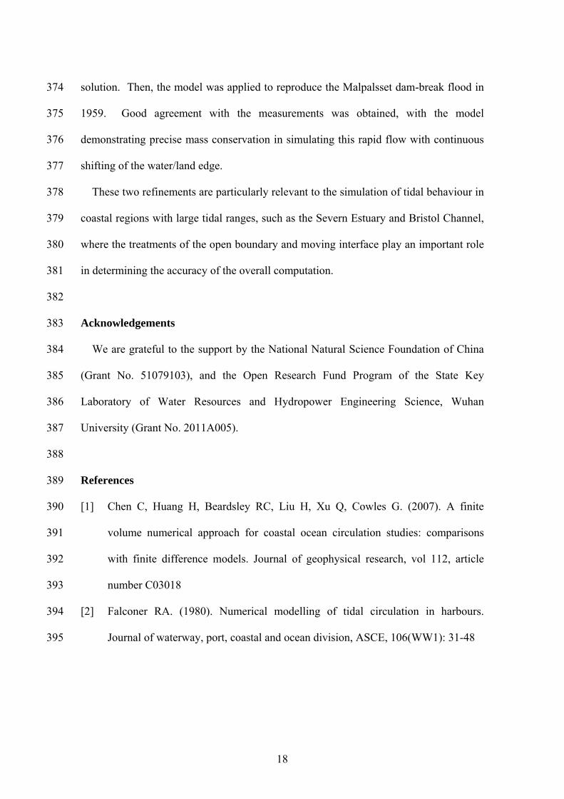
Figure 1. Map of the Bristol Channel and Severn Estuary 459

460

22

461

462

(a) Three-dimensional view of the terrain 463

464

465

(b) Monitoring points 466

Figure 2. Domain description of the Malpasset dam-break simulation 467

468

469

23

470

471

(a) t = 0 s 472

473

474

(b) t = 800 s 475

476

477

(c) t = 1200 s 478

24

479

(d) t = 1800 s 480

481

482

(e) t = 2500 s 483

Figure 3. Evolution of the inundation extent and water depth distribution 484

485

486

25

t (s)V

olu

me

(m3 )

0 500 1000 1500 2000 25000.0E+00

2.0E+07

4.0E+07

6.0E+07

8.0E+07

1.0E+08

TheoreticalComputational

487

Figure 4. Total volume of water in the domain 488

489

0

20

40

60

80

100

4000 6000 8000 10000 12000 14000x (m)

Ma

xim

um

leve

l (m

)

Surveyed

Predicted at survey points

Experimental

Predicted at gauge points

490

(a) Maximum water levels at monitoring points 491

0

200

400

600

800

1000

1200

1400

4000 6000 8000 10000 12000 14000x (m)

Arr

ival

tim

e (

s)

Experimental

Predicted at gauge points

492

(b) Arrival times at monitoring points 493

Figure 5. Comparisons between the predicted and measured results of the Malpasset 494

dam-break floods 495

26

496

497

(a) Overall view (b) Close-up view of the upstream part 498

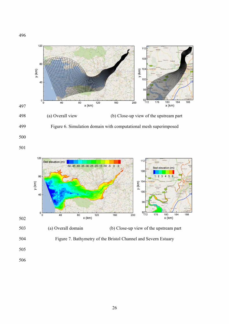
Figure 6. Simulation domain with computational mesh superimposed 499

500

501

502

(a) Overall domain (b) Close-up view of the upstream part 503

Figure 7. Bathymetry of the Bristol Channel and Severn Estuary 504

505

506

27

507

t (hour)

Wat

erle

vel(

m)

0 24 48 72 96 120 144 168 192 216 240 264 288 312 336-5

0

5

508

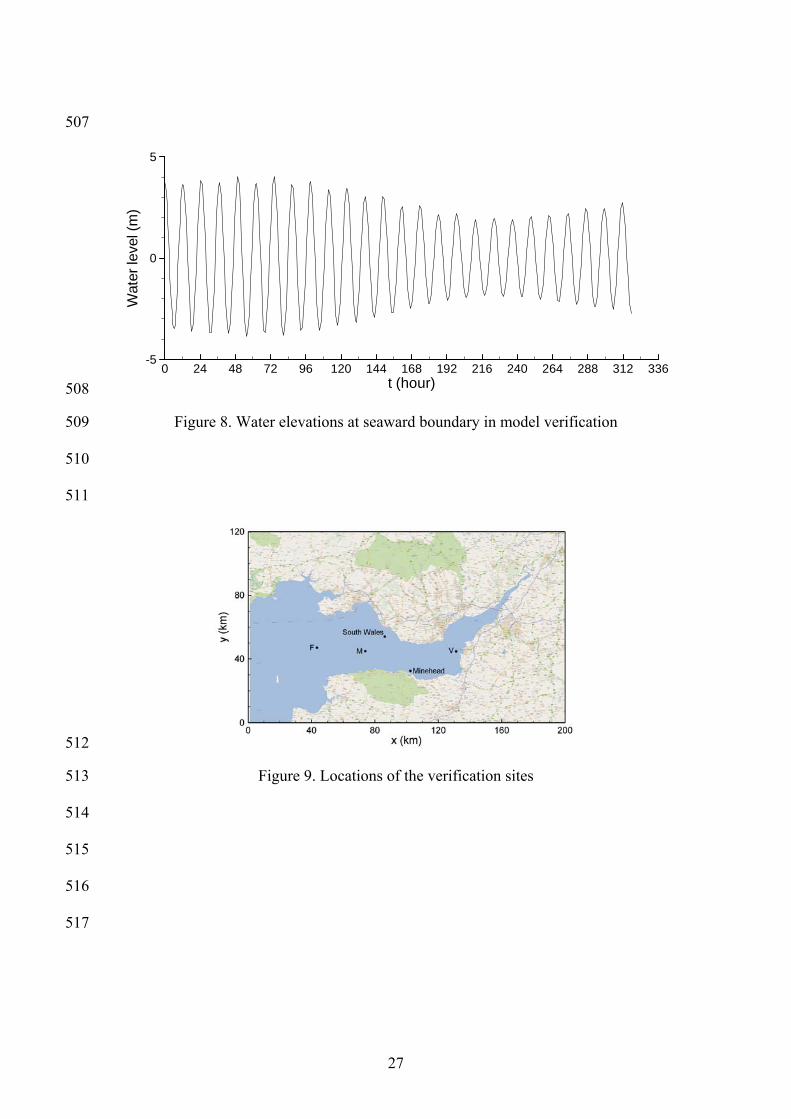
Figure 8. Water elevations at seaward boundary in model verification 509

510

511

512

Figure 9. Locations of the verification sites 513

514

515

516

517

28

t (hour)

Wat

erd

epth

(m)

80 85 90 95 10010

15

20

25

t (hour)

Cu

rren

tsp

eed

(m/s

)

80 85 90 95 1000

0.5

1

1.5

t (hour)

Cu

rren

tdir

ectio

n

80 85 90 95 100

-120

0

120

518

(a) South Wales site on 24th July 2001 519

520

t (hour)

Wat

erd

epth

(m)

130 135 140 145 15010

15

20

25

t (hour)

Cu

rren

tsp

eed

(m/s

)

130 135 140 145 1500

0.5

1

1.5

t (hour)

Cu

rren

tdir

ectio

n

130 135 140 145 150

-120

0

120

521

(b) South Wales site on 26th July 2001 522

523

t (hour)

Wat

erd

epth

(m)

225 230 235 240 24510

15

20

25

t (hour)

Cu

rren

tsp

eed

(m/s

)

225 230 235 240 2450

0.5

1

1.5

t (hour)

Cu

rren

tdir

ectio

n

225 230 235 240 245

-120

0

120

524

(c) Minhead site on 30th July 2001 525

t (hour)

Wat

erd

epth

(m)

275 280 285 290 29510

15

20

25

t (hour)

Cu

rren

tsp

eed

(m/s

)

275 280 285 290 2950

0.5

1

1.5

t (hour)

Cur

rent

dir

ectio

n

275 280 285 290 295

-120

0

120

526

(d) Minhead site on 1st August 2001 527

Figure 10. Model verification examples, where lines are predicted values and symbols 528

are measured values 529

29

530

531

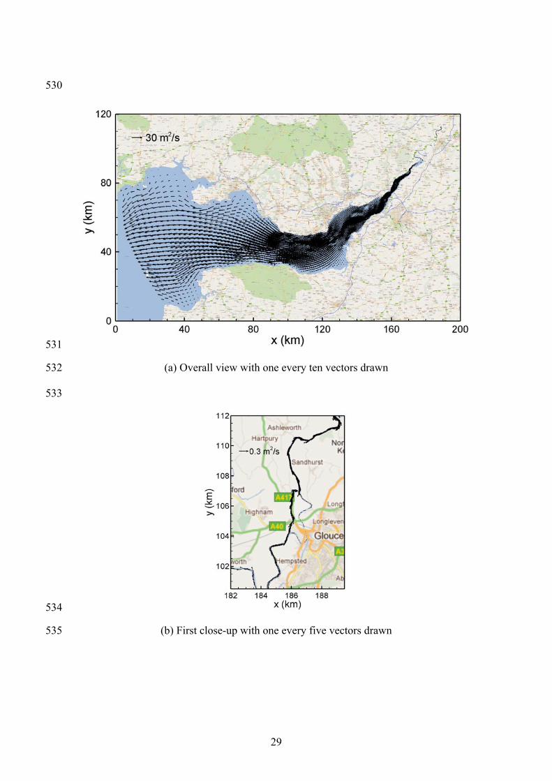
(a) Overall view with one every ten vectors drawn 532

533

534

(b) First close-up with one every five vectors drawn 535

30

536

(c) Second close-up with one every four vectors drawn 537

538

539

(d) Third close-up with all vectors drawn 540

Figure 11. Predicted tidal currents in the ebb tide at t = 227.5 hours 541

542

543

31

544

545

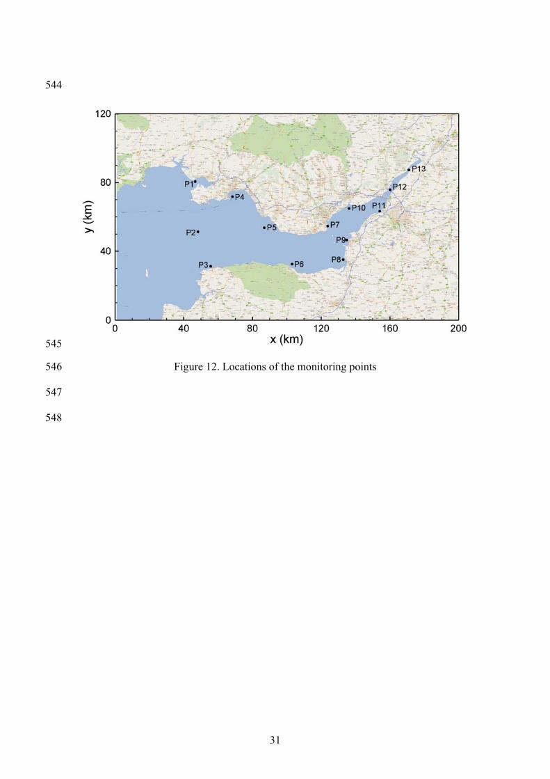
Figure 12. Locations of the monitoring points 546

547

548

32

549

t (hour)

Wat

erle

vel(

m)

36 42 48 54 60-3

-1.5

0

1.5

3

T = 1 hour

T = 4 hours

T = 8 hours

T = 16 hours

550

(a) Period = 1, 4, 8 or 16 hours 551

552

t (hour)

Wat

erle

vel(

m)

36 42 48 54 60-3

-1.5

0

1.5

3

T = 2 hours

T = 6 hours

T = 12 hours

T = 24 hours

553

(b) Period = 2, 6, 12 or 24 hours 554

Figure 13. Water elevation oscillations at Site P12 due to tides of different periods 555

556

557

33

558

1

1

1

11

1 1 1 1 1 11 1 1 1

2

2

2

22 2 2 2

22 2

2 2 2 2

3

3

3

33 3 3 3

33

3

3 3 3 3

4

4

4

44

44 4

44

4

44 4 4

5

5 5

55

55 5

5

55

55 5 5

6

6

66

6

66

6

6

6

6

6

66

6

7

7

7

7

7

77

7

7

7

7

7

77

7

8

8

88

8

8 8

8

8

8

8

8

88

8

9

9

99

9

9 9

9

9

9

9

9

99

9

X

X

XX

X

X X

X

X

X

X

X

XX

X

A

A

A

A

A

AA

A

A

A

A

A

AA

A

B

B

B

B

B

BB

B

B

B

B

B

BB

B

C

C

C

C

C

C

CC C

CC

C

CC

C

Period (hours)

Am

plif

icat

ion

Fac

tor

0 4 8 12 16 20 24 280

1

2

3P1P2P3P4P5P6P7P8P9P10P11P12P13

1

2

3

4

5

6

7

8

9

X

A

B

C

559

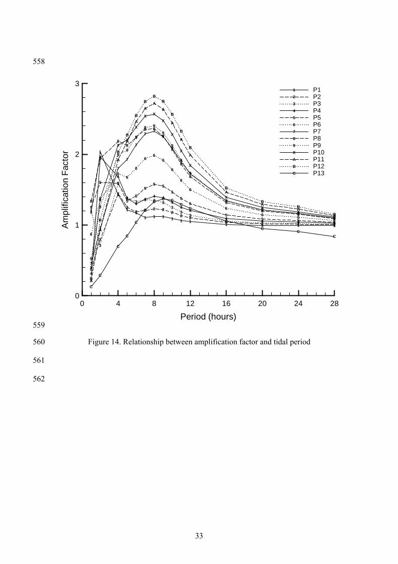
Figure 14. Relationship between amplification factor and tidal period 560

561

562

34

563

564

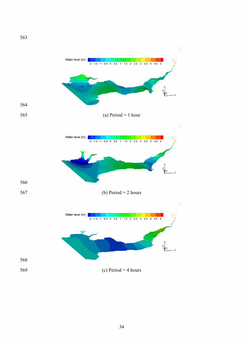
(a) Period = 1 hour 565

566

(b) Period = 2 hours 567

568

(c) Period = 4 hours 569

35

570

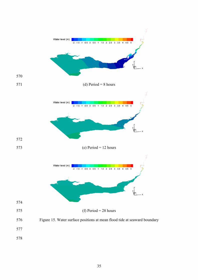
(d) Period = 8 hours 571

572

(e) Period = 12 hours 573

574

(f) Period = 28 hours 575

Figure 15. Water surface positions at mean flood tide at seaward boundary 576

577

578