On the Payne–Whitham differential model: stability constraints in one-class and two-class cases
27
Journal’s Title, Vol. x, 200x, no. xx, xxx - xxx ON THE PAYNE-WHITHAM DIFFERENTIAL MODEL: STABILITY CONSTRAINTS IN ONE-CLASS AND TWO-CLASS CASES Carlo Caligaris, Simona Sacone, and Silvia Siri Department of Communications, Computer and Systems Science University of Genova Via Opera Pia 13, 16145 Genova, Italy Abstract This paper deals with the classic second order Payne-Whitham macro- scopic model, commonly known as PW-Model, used to represent and forecast traffic conditions in a freeway. The results of the model may show a misbehavior similar to the instability of numerical solutions of partial differential equations. Since this model comes from a partial differential equation system, we use some stability rules to determine the conditions in order to avoid these errors in simulation. The work applies to the classic model, which considers a single class of vehicles, and to the two-class extension previously presented by the authors. Mathematics Subject Classification: 93A30, 93A15 Keywords: PW-Model, Differential Equations, Stability, Two-Class Traf- fic Flow. 1 Introduction The Payne-Witham Model is a macroscopic second-order model used to repre- sent the dynamic behaviour of traffic in highways or freeways. It was developed in the Seventies [16, 17] and it was experimented in many success cases (e.g. [5]). Strong criticisms on this theory arose as well (e.g. [6]). Although this model is widely used in its discrete form, it is important to remember that it is essentially obtained by discretizing both in time and space a set of differential (continuous) equations. It is common to work directly on the discrete model, almost forgetting the differential set [15]: this is normally accepted as long as simulation results fit real data.
Transcript of On the Payne–Whitham differential model: stability constraints in one-class and two-class cases
Journal’s Title, Vol. x, 200x, no. xx, xxx - xxx
ON THE PAYNE-WHITHAM DIFFERENTIAL
MODEL: STABILITY CONSTRAINTS
IN ONE-CLASS AND TWO-CLASS CASES
Carlo Caligaris, Simona Sacone, and Silvia Siri
Department of Communications, Computer and Systems ScienceUniversity of Genova
Via Opera Pia 13, 16145 Genova, Italy
Abstract
This paper deals with the classic second order Payne-Whitham macro-scopic model, commonly known as PW-Model, used to represent andforecast traffic conditions in a freeway. The results of the model mayshow a misbehavior similar to the instability of numerical solutions ofpartial differential equations. Since this model comes from a partialdifferential equation system, we use some stability rules to determinethe conditions in order to avoid these errors in simulation. The workapplies to the classic model, which considers a single class of vehicles,and to the two-class extension previously presented by the authors.
Mathematics Subject Classification: 93A30, 93A15
Keywords: PW-Model, Differential Equations, Stability, Two-Class Traf-fic Flow.
1 Introduction
The Payne-Witham Model is a macroscopic second-order model used to repre-sent the dynamic behaviour of traffic in highways or freeways. It was developedin the Seventies [16, 17] and it was experimented in many success cases (e.g.[5]). Strong criticisms on this theory arose as well (e.g. [6]). Although thismodel is widely used in its discrete form, it is important to remember that it isessentially obtained by discretizing both in time and space a set of differential(continuous) equations. It is common to work directly on the discrete model,almost forgetting the differential set [15]: this is normally accepted as long assimulation results fit real data.
2 Caligaris, Sacone, Siri
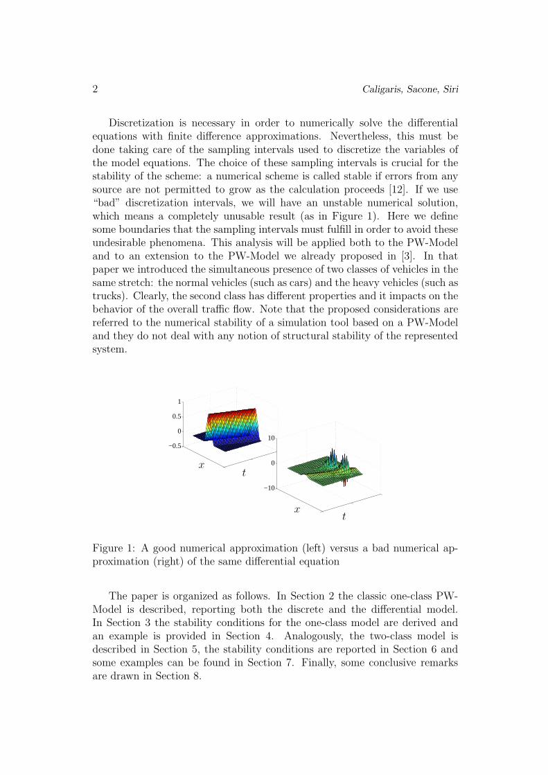
Discretization is necessary in order to numerically solve the differentialequations with finite difference approximations. Nevertheless, this must bedone taking care of the sampling intervals used to discretize the variables ofthe model equations. The choice of these sampling intervals is crucial for thestability of the scheme: a numerical scheme is called stable if errors from anysource are not permitted to grow as the calculation proceeds [12]. If we use“bad” discretization intervals, we will have an unstable numerical solution,which means a completely unusable result (as in Figure 1). Here we definesome boundaries that the sampling intervals must fulfill in order to avoid theseundesirable phenomena. This analysis will be applied both to the PW-Modeland to an extension to the PW-Model we already proposed in [3]. In thatpaper we introduced the simultaneous presence of two classes of vehicles in thesame stretch: the normal vehicles (such as cars) and the heavy vehicles (such astrucks). Clearly, the second class has different properties and it impacts on thebehavior of the overall traffic flow. Note that the proposed considerations arereferred to the numerical stability of a simulation tool based on a PW-Modeland they do not deal with any notion of structural stability of the representedsystem.
−0.5
0
0.5
1
−10
0
10
x
x
t
t
Figure 1: A good numerical approximation (left) versus a bad numerical ap-proximation (right) of the same differential equation
The paper is organized as follows. In Section 2 the classic one-class PW-Model is described, reporting both the discrete and the differential model.In Section 3 the stability conditions for the one-class model are derived andan example is provided in Section 4. Analogously, the two-class model isdescribed in Section 5, the stability conditions are reported in Section 6 andsome examples can be found in Section 7. Finally, some conclusive remarksare drawn in Section 8.
Numerical Stability of PW–Model 3
2 The PW-Model
The Payne-Whitham model is influenced by simple laws for fluid dynamics:the flow of cars is represented as the flow of a liquid in a pipe. In this paper wedo not deal with the advantages and the drawbacks of this assumption and wedo not deepen the theory of the model: many papers as [1, 6, 15] already didthis in an exhaustive way. For the same reason, we do not discuss the goodnessof the experimental results; you can find excellent application cases in [10] andmany other papers. Our aim is to define some numerical constraints in orderto run simulations not affected by numerical instability.
In the years, the model itself slightly changed, according to the preferencesof its users; we will try to work on the model firstly seen in [13] with a littlemodification introduced later in [15] about the so-called “steady state speed-density characteristic”. The papers cited above are also our suggested sourcesfor further details on some modelling choices.
2.1 The Model Variables
ρi, vi, qisi ri
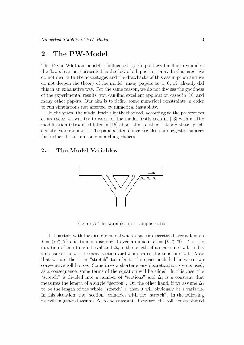
Figure 2: The variables in a sample section
Let us start with the discrete model where space is discretized over a domainI = {i ∈ N} and time is discretized over a domain K = {k ∈ N}. T is theduration of one time interval and ∆i is the length of a space interval. Indexi indicates the i-th freeway section and k indicates the time interval. Notethat we use the term “stretch” to refer to the space included between twoconsecutive toll houses. Sometimes a shorter space discretization step is used;as a consequence, some terms of the equation will be elided. In this case, the“stretch” is divided into a number of “sections” and ∆i is a constant thatmeasures the length of a single “section”. On the other hand, if we assume ∆i
to be the length of the whole “stretch” i, then it will obviously be a variable.In this situation, the “section” coincides with the “stretch”. In the followingwe will in general assume ∆i to be constant. However, the toll houses should
4 Caligaris, Sacone, Siri
always be at the beginning and/or at the end of a section. The model includesthree variables:
• vi(k)[km/h]: the mean speed of vehicles in section i in the [k, k+1) timeinterval;
• ρi(k)[veh/km]: the density of vehicles in section i in the [k, k + 1) timeinterval;
• qi(k)[veh/h]: the number of vehicles flowing through section i in the[k, k + 1) time interval.
Moreover, we must consider ri(k)[km/h] and si(k)[km/h] as the number ofvehicles accessing or leaving section i through on-ramps and off-ramps in the[k, k + 1) time interval.
2.2 The Discrete Model
The set of equations that constitute the PW-Model is the following:
ρi(k + 1) = ρi(k) +T
∆i
{[ρi−1(k)vi−1(k)
]−
[ρi(k)vi(k)
]+
[ri(k) − si(k)
]};
i = 1, . . . , N ; k = 0, 1, . . . , K − 1;(1)
vi(k + 1) = vi(k) +T
τ
[Vi(k) − vi(k)
]+
T
∆i
vi(k)[vi−1(k) − vi(k)
]+
−νT
τ∆i
ρi+1(k) − ρi(k)
ρi(k) + χ; i = 1, . . . , N ; k = 0, 1, . . . , K − 1; (2)
Vi(k) = vmax
{1 −
[ρi(k)
ρmax
]l}m
; i = 1, . . . , N ; k = 0, 1, . . . , K − 1; (3)
qi(k) = ρi(k) · vi(k); i = 1, . . . , N ; k = 0, 1, . . . , K − 1. (4)
where Equation (3) is the steady state speed-density characteristic. This equa-tion has been written in various forms since the introduction of this model[7, 8, 9, 11, 19]. In our work we refer to [14] in which a general form ofthe equation is given. By means of this particular equation older forms canbe easily obtained with proper adjustments of parameters. The parametersτ, ν, χ, vmax, ρmax, l, m depend on some physical characteristics of the freewaysection under concern, as well as on the traffic patterns typically present in
Numerical Stability of PW–Model 5
the section itself. The values of these parameters are determined through asuitable parameter identification procedure using real traffic data. Moreover,some of these parameters can be different in the different sections. In thiswork we do not consider these dependencies nor we go into details about theidentification of such parameters since these aspects do not affect our analysis.
We will refer to (1) as to the “first updating equation” and to (2) as tothe “second updating equation”. Equation (4) is a relation commonly used influid dynamics: there is no need to use this same equation (for instance, in [3]we used a slightly different one). However, this equation must be empiricallyvalidated.
2.3 The Differential Model
Here we recall the differential equations from which the discrete model is ob-tained. Note that the discrete model depends on the choice of the scheme usedin the finite difference approximation of the derivative terms. The PW-Modelis usually obtained by a “forward-backward” scheme (for further details on nu-merical approximations refer to [12] or to any other mathematical book aboutpartial differential equations and their numerical solutions).
Equation (1) acts as a conservation law. In physics, a conservation lawstates that a particular property of an isolated system does not change as thesystem evolves. Here, it states that cars in the overall freeway stretch cannotappear nor disappear without a pre-defined source or sink. Every car presentin a given section can come either from the preceding section or from theprevious on-ramp and it can go either to the next section or to the followingoff-ramp. The equation can be written as:
∂ρ(x, t)
∂t+
∂q(ρ(x, t))
∂x= r(x, t) − s(x, t) (5)
and Equation (1) easily comes from the coupling of the discretized form of (5)and (4).
Also Equation (2) depends on a differential equation; this one is drawn byobservations and its expression can be found, for example, in [2]:
∂v(x, t)
∂t+ v(x, t)
∂v(x, t)
∂x=
V (ρ) − v(x, t)
τ−
ν2
ρ(x, t)
∂ρ(x, t)
∂x. (6)
Table 1 shows, for each of the terms of Equation (6), the correspondingone in Equation (2).
Equations (3) and (4) can be easily generalized as follows:
V (ρ) = vmax
{1 −
[ρ
ρmax
]l}m
; (7)
6 Caligaris, Sacone, Siri
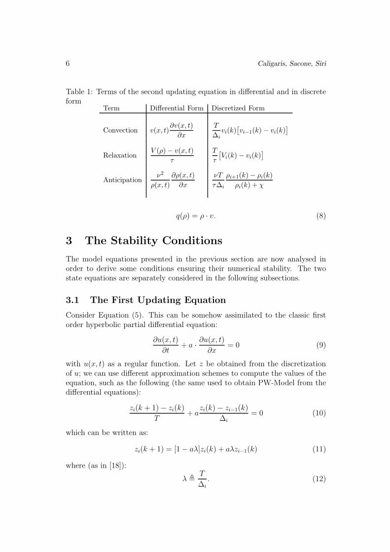
Table 1: Terms of the second updating equation in differential and in discreteform
Term Differential Form Discretized Form
Convection v(x, t)∂v(x, t)
∂x
T
∆ivi(k)
[vi−1(k) − vi(k)
]
RelaxationV (ρ) − v(x, t)
τ
T
τ
[Vi(k) − vi(k)
]
Anticipationν2
ρ(x, t)
∂ρ(x, t)
∂x
νT
τ∆i
ρi+1(k) − ρi(k)
ρi(k) + χ
q(ρ) = ρ · v. (8)
3 The Stability Conditions
The model equations presented in the previous section are now analysed inorder to derive some conditions ensuring their numerical stability. The twostate equations are separately considered in the following subsections.
3.1 The First Updating Equation
Consider Equation (5). This can be somehow assimilated to the classic firstorder hyperbolic partial differential equation:
∂u(x, t)
∂t+ a ·
∂u(x, t)
∂x= 0 (9)
with u(x, t) as a regular function. Let z be obtained from the discretizationof u; we can use different approximation schemes to compute the values of theequation, such as the following (the same used to obtain PW-Model from thedifferential equations):
zi(k + 1) − zi(k)
T+ a
zi(k) − zi−1(k)
∆i
= 0 (10)
which can be written as:
zi(k + 1) = [1 − aλ]zi(k) + aλzi−1(k) (11)
where (as in [18]):
λ ,T
∆i
. (12)
Numerical Stability of PW–Model 7
It can be proved that, in these equations, the Courant Number
µ , a · λ = a ·T
∆i
(13)
directly influences the stability of the numerical solution. A necessary condi-tion for stability is the CFL (Courant, Friedrichs, Lewy, [4]) condition (as seenin [12]):
|µ| ≤ 1. (14)
This is the constraint that pairs of T and ∆i must always satisfy. Workingon (5), we consider its homogeneous form assuming that values of entering andleaving vehicles do not influence the stability behavior. We can now rewritethis equation and slightly modify it by a simple derivative property:
∂ρ(x, t)
∂t+
∂q(ρ(x, t))
∂x= 0
∂ρ(x, t)
∂t+ q′
(ρ(x, t)
)∂ρ(x, t)
∂x= 0. (15)
By inspecting (9) and (15) we can compare the term q′(ρ(x, t)
)with a,
which is directly involved in the Courant Number. Note that a is constantwhile q′
(ρ(x, t)
)is a function of the density. However, if we can evaluate this
function over the interest domain, we will find the critical values which getthe Courant Number nearer to 1. The extension of CFL analysis to the casein which the Courant Number is not a constant is the main novelty of theapproach. Although there is no theoretical support on this point, it is reason-able to assume that Equation (15) should be discretized only if the solutionis stable for every possible value assumed by the q′ function. In this work, wescan all these possibilities to find the worst case, in which stability is harderto achieve. This is clearly a conservative criterion and some considerationsabout its sensitiveness will be held later. We will base on some qualitativeconsiderations and then we will prove validity of our results by showing theirapplication in a simulation tool. These critical values can be obtained by
studying max
{q′
(ρ(x, t)
)·
T
∆i
}.
We use Equations (7) and (8) to write an explicit function of q(ρ):
q(ρ) = ρ · v = ρ · vmax
{1 −
[ρ
ρmax
]l}m
(16)
8 Caligaris, Sacone, Siri
and:
a(ρ) = q′(ρ) = vmax
{1 −
[ρ
ρmax
]l}m
+
− vmax · m ·
{
1 −
[ρ
ρmax
]l}m−1
· l ·
[ρ
ρmax
]l
. (17)
Remembering (13) and (14) we must impose
∣∣∣∣a(ρ) ·T
∆i
∣∣∣∣ ≤ 1, which means:
max {|a(ρ)|} ·T
∆i
≤ 1. (18)
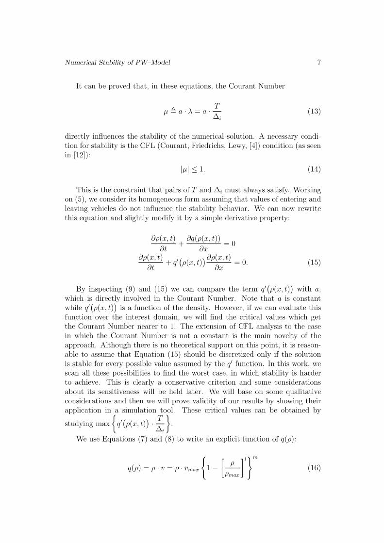
Then, we study a(ρ) by drawing a qualitative plot of its function in Figure3. In this case we used some standard values for the various parameters.
0
0
ρ[veh/km]
a(ρ)|a(ρ)|
ρρmax
vmax
a
Figure 3: Plot of a(ρ) and |a(ρ)| used to explicitly define the maximum valueof this function
To find the absolute maximum of |a(ρ)| in [0, ρmax] we must take into ac-
count the boundary values and the absolute value coming from da(ρ)dρ
= 0. Notethat we do not use the absolute value function in order to keep differentiability:in this way, actually, we will search for the minimum value of the function.
We begin by calculating the derivative term. The solution is (ρ, a(ρ)), asin the following:
ρ = eln s
l · ρmax with s =1 + l
1 + ml;
a = a(ρ)
= vmax
{[1 − s]m − [1 − s]m−1 · m · s · l
}. (19)
So, the absolute maximum value in our interval is:
max {a(0), |a(ρ)|, a(ρmax)} = max {vmax, |a|, 0}. (20)
Numerical Stability of PW–Model 9
Assuming that at least one parameter is greater than zero (vmax shouldalways be, by definition), we can consider only the first two terms of themaximum function. Moreover, in Figure 3 a is greater than vmax, but wewant to know whether this is always true. To find an answer, we must solve|a| > vmax, that is:
|[1 − s]m − [1 − s]m−1 · m · s · l| > 1 (21)
whose solution is:∣∣∣∣
[ml − l
ml + 1
]m−1
· (−l)
∣∣∣∣ > 1. (22)
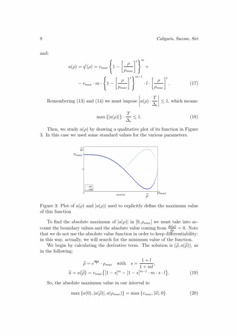
It is not possible to explicit (22) as a function of l or m but we can plot itin an interest domain and see by inspection when it is greater or lower than 1.Some typical values for l and m are, respectively, 3 and 1.8. So, in Figure 4 weplot Equation (22) in the following domain intervals: l ∈ [0, 6] and m ∈ [0, 3.6].The plot is not always greater than 1. In a restricted domain [2, 4]× [0.5, 2.5],representing the domain generally recommended, the surface is often greaterthan 1. This means that, in general, the value found with the derivative term ishigher than the one on the left boundaries, being so the absolute maximum inthe considered domain. However, this is not always true, so we write the finalcondition for this first differential equation in its more general form. Stability,for this sole equation, is guaranteed if:
max {vmax, |a|} ·T
∆i
≤ 1. (23)
0 0.51.8 2.5
3.6 0
23
4
6
01
lm
Figure 4: Plot of Equation (22)
3.2 The Second Updating Equation
The study for the second updating equation is analogous to the one just re-ported. Recalling Equation (6), we consider again its homogeneous form. Ac-tually, the anticipation term (see Table 1) contains a derivative as well; in this
10 Caligaris, Sacone, Siri
work we neglect it just as the other non-homogeneous terms and experimentalresults show the effectiveness of such a choice.
The homogeneous second updating equation looks like an inviscid Burger’sEquation [12] whose general form follows:
∂v(x, t)
∂t+ v(x, t)
∂v(x, t)
∂x= 0 (24)
where v(x, t) must be a regular function; considering v(x, t) as the speed func-tion, this is exactly the homogeneous form of the second updating Equation(6).
Almost every discretization scheme for this equation needs the followingcondition for stability: ∣∣∣∣
T
∆i
· vmax
∣∣∣∣ ≤ 1, (25)
which is quite similar to (14). Actually, it is much easier to study stabilityin this case. vmax is a parameter of our model and it is always greater thanzero. Thus, Equation (25) is the stability condition for the second updatingequation and the absolute value in it is trivial.
3.3 The Overall Constraint
We can couple the two constraints we have found, coming from the two ho-mogeneous differential equations of the model. If we look at Equations (23)and (25), we can realize that the second one is included in the first one. Thus,since we want to impose the simultaneous stability of the two equations, wecan say that (23) guarantees the needed requirements for both of them.
We end up this part by stating that the stability condition for the classicPW-Model is:
max {vmax, |a|} ·T
∆i
≤ 1. (26)
It is common to consider the model parameters as fixed numbers. Fur-thermore, T is usually imposed by the system to be monitored; being theinter-arrival time of data, it depends on the electronic system used on the roadto measure traffic data. ∆i is allegedly the only value we can change to makethe system simulations stable. If we use a constant space discretization step,varying the number of sections which build up every single stretch, then theconstraint could be rewritten as follows:
∆i ≥ max {vmax, |a|} · T. (27)
If we use a variable space discretization step, for example assuming everystep equal to the distance between two consecutive toll houses, we will have
Numerical Stability of PW–Model 11
to face the following condition:
mini
{∆i} ≥ max {vmax, |a|} · T. (28)
Actually, in order to apply the CFL condition, ∆i should always be con-stant. But, as we did in the variable Courant Number case, we search for anadmissible ∆i value that makes the condition more difficult to achieve. Thisvalue is the lowest ∆i, then we write the condition for its minimum value. Inconclusion, every time we deal with a variable in place of a constant, we searchfor the value of that variable that makes the constraint harder to be satisfiedand use it to rewrite the constraint in a conservative form.
4 Example for the One-Class Model
In this section we report some numerical examples we have realized in order toshow the effectiveness of the defined conditions for stability on the PW-Model.We consider a part of a freeway composed of 10 stretches; differently fromthe earlier definition of “stretch”, in this example not all the stretches haveon-ramps and off-ramps. The considered time horizon is 60 minutes; generally,it is difficult to work with such a long horizon, but in this experiment fidelityof results is not an issue. The time discretization step is 1 minute. We use aconstant space discretization step for each simulation run; in every simulationrun we change this step in order to have different values for the CourantNumber |µ|. The main parameters of the model are listed in Table 2.
Table 2: Parameters of the simulative exampleρmax = 300 veh/km vmax = 130 km/hτ = 0.1 h χ = 120 veh · km−1
ν = 35 km2 · h−1 l = 3m = 1.8 T = 1/60 h
We use a pair of l and m for which |a| > vmax, as shown in Figure 4.This is confirmed by the numerical calculation which provides |a| = 177.95,greater than the chosen vmax.
The threshold level such that |µ| = 1 is ∆thresholdi = 2.9658 km. When
∆i < ∆thresholdi we can have numerical instability. Actually, in our results, we
introduce threshold values for the Courant Number of both equations, beingthem different as seen in (23) and (25). We will refer to them as to µ1 and µ2.Equation (23) also states the stability of the first equation; with regard to thesecond equation of stability, we have ∆threshold
i = vmax · T = 2.1667 kmwhich is a strictless condition. As already told before, µ1 imposes a conditionwhich is at least as strict as the one imposed by µ2.
12 Caligaris, Sacone, Siri
1 2 3 4 5 6 7 8 9 10
111
2131
4151
61
20406080
100120
1 2 3 4 5 6 7 8 9 10
100
200
300
µ1 = 1.4829; µ2 = 1.0833
Sections
SectionsTime
Speed
Den
sit
y
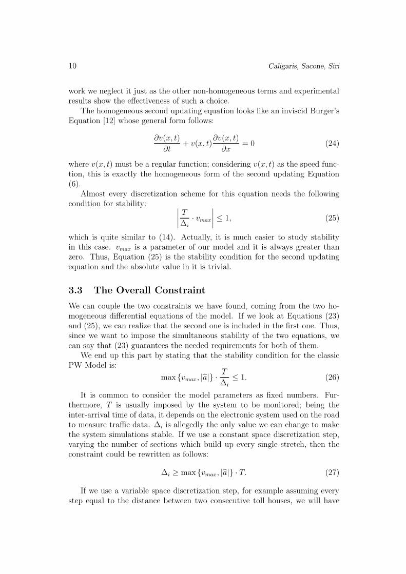
Figure 5: A simulation with total numerical instability
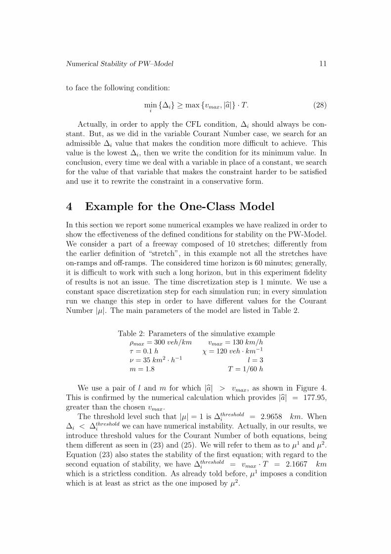
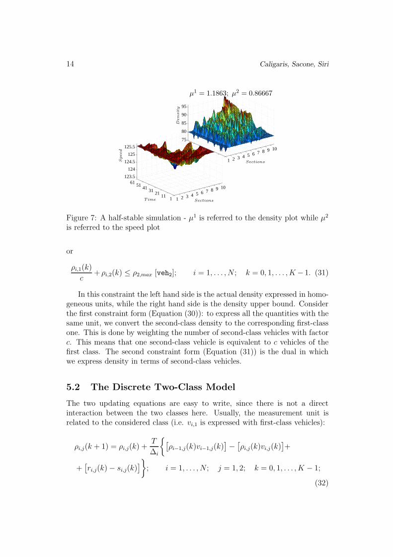
We run a first simulation using ∆i = 2 km: in this case we expectour results to be absolutely unusable, as confirmed by Figure 5. The secondsimulation run is held in a full-stable situation in which we choose the max-imum value for the discretization step, i.e. ∆i = 10 km, as shown inFigure 6. The results of the third simulation run are very interesting: we usea value of ∆i included between the threshold values found for the first andthe second equation. In particular, we use ∆i = 2.5 km and the result isshown in Figure 7. In this case we can observe how the equation for which theconstraint is fulfilled (the speed equation) is actually stable. On the contrary,the unstable equation shows an unreliable behavior. This makes us think thatall the simulations with Courant Numbers included in the interval (µ1, µ2)must be treated with caution. They could seem not completely unstable andthis could lead to trust their result. Actually, we can see how the plot of thespeed is somehow reliable, while the density one is not. Moreover, density isnot completely unstable as in the first simulation run. Probably, the reason isthe interaction between the two equations, one stable and one not: the stableresult may mitigate the instability of the other one.
5 The Two-Class PW-Model
In [3] we proposed an extension to the classic PW-Model. The classic modelassumes that the flow of vehicles can be considered and analyzed as an homo-geneous fluid. This assumption does not hold if vehicles are characterized bydifferent lengths and maximum speeds. In particular, heavy trucks are usu-ally slower than cars; if the percentage of heavy vehicles in the overall trafficvolume is high, then the behavior of faster vehicles certainly differs from the
Numerical Stability of PW–Model 13
1 2 3 4 5 6 7 8 9 10
111
2131
4151
61
124.5
125
125.5
1 2 3 4 5 6 7 8 9 10
80
85
90
µ1 = 0.29658; µ2 = 0.21667
Sections
SectionsTime
Speed
Den
sit
y
Figure 6: A full-stable simulation - µ1 is referred to the density plot while µ2
is referred to the speed plot
one sustainable without this “interference”. From now on, the class of fastervehicles will be addressed as “class 1” and the class of slower vehicles will beaddressed as “class 2”.
5.1 The State Variables
The scheme is the same presented in Figure 2 but the state variables and someof the parameters are “doubled”. The model variables are now: vi,j(k), ρi,j(k),qi,j(k), i = 1, . . . , N , j = 1, 2, k = 0, 1, . . . , K − 1, where index j refers to theclass of vehicles.
Similarly, ρj,max is the maximum density of the j-th class of vehicles in eachsection and it can be expressed in vehicles belonging to the first or the secondclass. In other words, this is the number of vehicles of the first or second classnecessary to fill up a section. The two cases are related by the ratio betweenthe occupance of vehicles of both classes:
c =ρ1,max[veh1]
ρ2,max[veh2](29)
where we have to highlight the measurement units and add an index to thenotation of the two maximum densities, since they essentially refer to the samequantity evaluated with different units.
The linear combination of the two densities cannot overcome the physicalcapacity of the section, then:
ρi,1(k)+c·ρi,2(k) ≤ ρ1,max [veh1]; i = 1, . . . , N ; k = 0, 1, . . . , K−1; (30)
14 Caligaris, Sacone, Siri
1 2 3 4 5 6 7 8 9 10
111
2131
4151
61123.5
124
124.5
125
125.5
1 2 3 4 5 6 7 8 9 10
75
80
85
90
95
µ1 = 1.1863; µ2 = 0.86667
Sections
SectionsTime
Speed
Den
sit
y
Figure 7: A half-stable simulation - µ1 is referred to the density plot while µ2
is referred to the speed plot
or
ρi,1(k)
c+ ρi,2(k) ≤ ρ2,max [veh2]; i = 1, . . . , N ; k = 0, 1, . . . , K − 1. (31)
In this constraint the left hand side is the actual density expressed in homo-geneous units, while the right hand side is the density upper bound. Considerthe first constraint form (Equation (30)): to express all the quantities with thesame unit, we convert the second-class density to the corresponding first-classone. This is done by weighting the number of second-class vehicles with factorc. This means that one second-class vehicle is equivalent to c vehicles of thefirst class. The second constraint form (Equation (31)) is the dual in whichwe express density in terms of second-class vehicles.
5.2 The Discrete Two-Class Model
The two updating equations are easy to write, since there is not a directinteraction between the two classes here. Usually, the measurement unit isrelated to the considered class (i.e. vi,1 is expressed with first-class vehicles):
ρi,j(k + 1) = ρi,j(k) +T
∆i
{[ρi−1,j(k)vi−1,j(k)
]−
[ρi,j(k)vi,j(k)
]+
+[ri,j(k) − si,j(k)
]}; i = 1, . . . , N ; j = 1, 2; k = 0, 1, . . . , K − 1;
(32)
Numerical Stability of PW–Model 15
vi,j(k + 1) = vi,j(k)+T
τ
[Vi,j(k) − vi,j(k)
]+
+T
∆i
vi,j(k)[vi−1,j(k) − vi,j(k)
]−
νT
τ∆i
ρi+1,j(k) − ρi,j(k)
ρi,j(k) + χi,j
;
i = 1, . . . , N ; j = 1, 2; k = 0, 1, . . . , K − 1;(33)
qi,j(k) = ρi,j(k) · vi,j(k) i = 1, . . . , N ; j = 1, 2; k = 0, 1, . . . , K − 1.(34)
The interaction of the two classes of vehicles is modelled in the steadystate speed-density characteristic (whose previous form was in Equation (3)).Actually, two different characteristics are needed, one for each class. Therelation for the first class follows:
Vi,1(k) = v1,max
{
1 −
[ρi,1(k) + c · ρi,2(k)
ρ1,max
]l}m
;
i = 1, . . . , N ; k = 0, 1, . . . , K − 1; (35)
and the one for the second class is:
Vi,2(k) = v2,max
1 −
[ρi,1(k)
c+ ρi,2(k)
ρ2,max
]l
m
;
i = 1, . . . , N ; k = 0, 1, . . . , K − 1. (36)
5.3 The Differential Two-Class Model
We originally developed this model considering its discrete form; however, thecontinuous model follows quite easily. The equations are usually doubled (onefor each class), but the overall considerations are the same as those explainedin the one-class case. Then, these are the differential equations:
∂ρj(x, t)
∂t+
∂qj
(ρj(x, t)
)
∂x= rj(x, t) − sj(x, t) (37)
∂vj(x, t)
∂t+ vj(x, t)
∂vj(x, t)
∂x=
=Vj(ρ1, ρ2) − vj(x, t)
τ−
ν2
ρj(x, t)
∂ρj(x, t)
∂x.
(38)
16 Caligaris, Sacone, Siri
The steady state speed-density characteristic is doubled as well, but weneed to write it explicitly in both cases, since expressions slightly change:
V1(ρ1, ρ2) = v1,max
{1 −
[ρ1 + c · ρ2
ρ1,max
]l}m
; (39)
V2(ρ1, ρ2) = v2,max
{1 −
[ ρ1
c+ ρ2
ρ2,max
]l}m
. (40)
It also holds:
q1(ρ1, ρ2) = ρ1 · v1, (41)
q2(ρ1, ρ2) = ρ2 · v2. (42)
6 The Stability Conditions
Analogously to the analysis realised for the one-class case, in the following sub-sections the stability conditions for the first and the second updating equationsare derived. Then, they are combined in order to obtain an overall constraintthat guarantees numerical stability.
6.1 The First Updating Equations
We have to face a problem similar to the one of Section 3 but a little morecomplex due to the two-dimensional functions we introduced. Again, we startfrom Equation (37), written in its homogeneous form. We transform it asfollows as we did in (15):
∂ρj(x, t)
∂t+
∂
∂ρj
qj
(ρ1(x, t), ρ2(x, t)
)∂ρj(x, t)
∂x= 0. (43)
The CFL condition imposes | ∂∂ρj
qj
(ρ1(x, t), ρ2(x, t)
)· λ| ≤ 1 (see (14)) and,
then, we impose max{| ∂∂ρj
qj
(ρ1(x, t), ρ2(x, t)
)|}· λ ≤ 1, just as we did for the
single class case in Equation (18). The main difference between this result andthe previous one is that now there is a dependence on on two variables. Sincethe two steady state characteristics have different expressions, we will have a
Numerical Stability of PW–Model 17
different formulation of qj for each j (i.e. for each class). These are the results:
a1(ρ1, ρ2) =∂
∂ρ1q1(ρ1, ρ2) =
d
dρ1ρ1 ·
{v1,max
{1 −
[ρ1 + c · ρ2
ρ1,max
]l}m}
=
= v1,max
{
1 −
[ρ1 + c · ρ2
ρ1,max
]l}m
+
− ρ1 · v1,max · m ·
{1 −
[ρ1 + c · ρ2
ρ1,max
]l}m−1
· l ·[ρ1 + c · ρ2]
l−1
ρl1,max
. (44)
a2(ρ1, ρ2) =∂
∂ρ2
q2(ρ1, ρ2) =d
dρ2
ρ2 ·
{v2,max
{1 −
[ ρ1
c+ ρ2
ρ2,max
]l}m}
=
= v2,max
{
1 −
[ ρ1
c+ ρ2
ρ2,max
]l}m
+
− ρ2 · v2,max · m ·
{1 −
[ ρ1
c+ ρ2
ρ2,max
]l}m−1
· l ·[ρ1
c+ ρ2]
l−1
ρl2,max
. (45)
Just as in (18), we want the stability constraint to be satisfied, so we searchfor the threshold values for which:
max {|a1(ρ1, ρ2)|, |a2(ρ1, ρ2)|} ·T
∆i
≤ 1. (46)
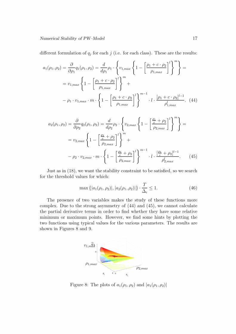
The presence of two variables makes the study of these functions morecomplex. Due to the strong asymmetry of (44) and (45), we cannot calculatethe partial derivative terms in order to find whether they have some relativeminimum or maximum points. However, we find some hints by plotting thetwo functions using typical values for the various parameters. The results areshown in Figures 8 and 9.
00
0
ρ2
ρ1
ρ2,max
ρ1,max
v1,maxa1
Figure 8: The plots of a1(ρ1, ρ2) and |a1(ρ1, ρ2)|
18 Caligaris, Sacone, Siri
00
0
ρ2ρ
1
ρ2,maxρ1,max
v2,maxa2
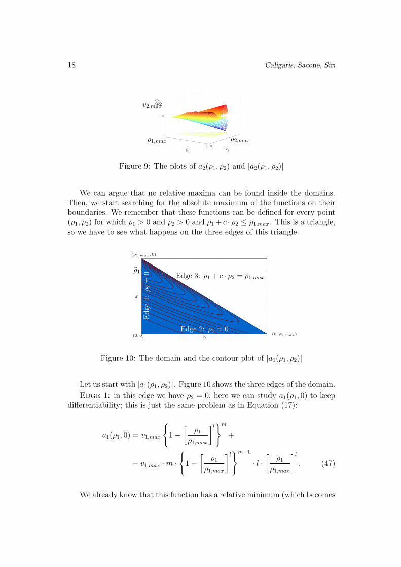
Figure 9: The plots of a2(ρ1, ρ2) and |a2(ρ1, ρ2)|
We can argue that no relative maxima can be found inside the domains.Then, we start searching for the absolute maximum of the functions on theirboundaries. We remember that these functions can be defined for every point(ρ1, ρ2) for which ρ1 > 0 and ρ2 > 0 and ρ1 + c · ρ2 ≤ ρ1,max. This is a triangle,so we have to see what happens on the three edges of this triangle.
ρ2
ρ 1
ρ1
Edge
1:ρ2
=0
Edge 2: ρ1 = 0
Edge 3: ρ1 + c · ρ2 = ρ1,max
(0, 0)
(ρ1,max, 0)
(0, ρ2,max)
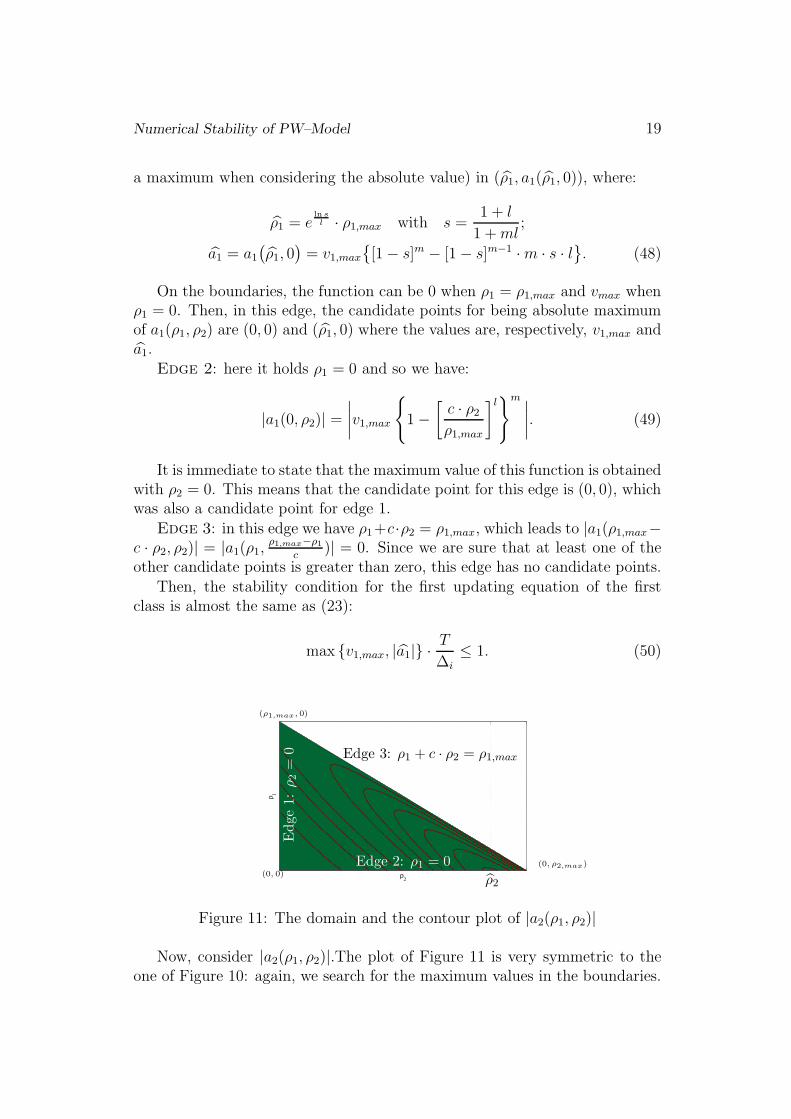
Figure 10: The domain and the contour plot of |a1(ρ1, ρ2)|
Let us start with |a1(ρ1, ρ2)|. Figure 10 shows the three edges of the domain.
Edge 1: in this edge we have ρ2 = 0; here we can study a1(ρ1, 0) to keepdifferentiability; this is just the same problem as in Equation (17):
a1(ρ1, 0) = v1,max
{
1 −
[ρ1
ρ1,max
]l}m
+
− v1,max · m ·
{1 −
[ρ1
ρ1,max
]l}m−1
· l ·
[ρ1
ρ1,max
]l
. (47)
We already know that this function has a relative minimum (which becomes
Numerical Stability of PW–Model 19
a maximum when considering the absolute value) in (ρ1, a1(ρ1, 0)), where:
ρ1 = eln s
l · ρ1,max with s =1 + l
1 + ml;
a1 = a1
(ρ1, 0
)= v1,max
{[1 − s]m − [1 − s]m−1 · m · s · l
}. (48)
On the boundaries, the function can be 0 when ρ1 = ρ1,max and vmax whenρ1 = 0. Then, in this edge, the candidate points for being absolute maximumof a1(ρ1, ρ2) are (0, 0) and (ρ1, 0) where the values are, respectively, v1,max anda1.
Edge 2: here it holds ρ1 = 0 and so we have:
|a1(0, ρ2)| =
∣∣∣∣v1,max
{1 −
[c · ρ2
ρ1,max
]l}m ∣∣∣∣. (49)
It is immediate to state that the maximum value of this function is obtainedwith ρ2 = 0. This means that the candidate point for this edge is (0, 0), whichwas also a candidate point for edge 1.
Edge 3: in this edge we have ρ1+c·ρ2 = ρ1,max, which leads to |a1(ρ1,max−c · ρ2, ρ2)| = |a1(ρ1,
ρ1,max−ρ1
c)| = 0. Since we are sure that at least one of the
other candidate points is greater than zero, this edge has no candidate points.Then, the stability condition for the first updating equation of the first
class is almost the same as (23):
max {v1,max, |a1|} ·T
∆i
≤ 1. (50)
ρ2
ρ 1
ρ2
Edge
1:ρ2
=0
Edge 2: ρ1 = 0
Edge 3: ρ1 + c · ρ2 = ρ1,max
(0, 0)
(ρ1,max, 0)
(0, ρ2,max)
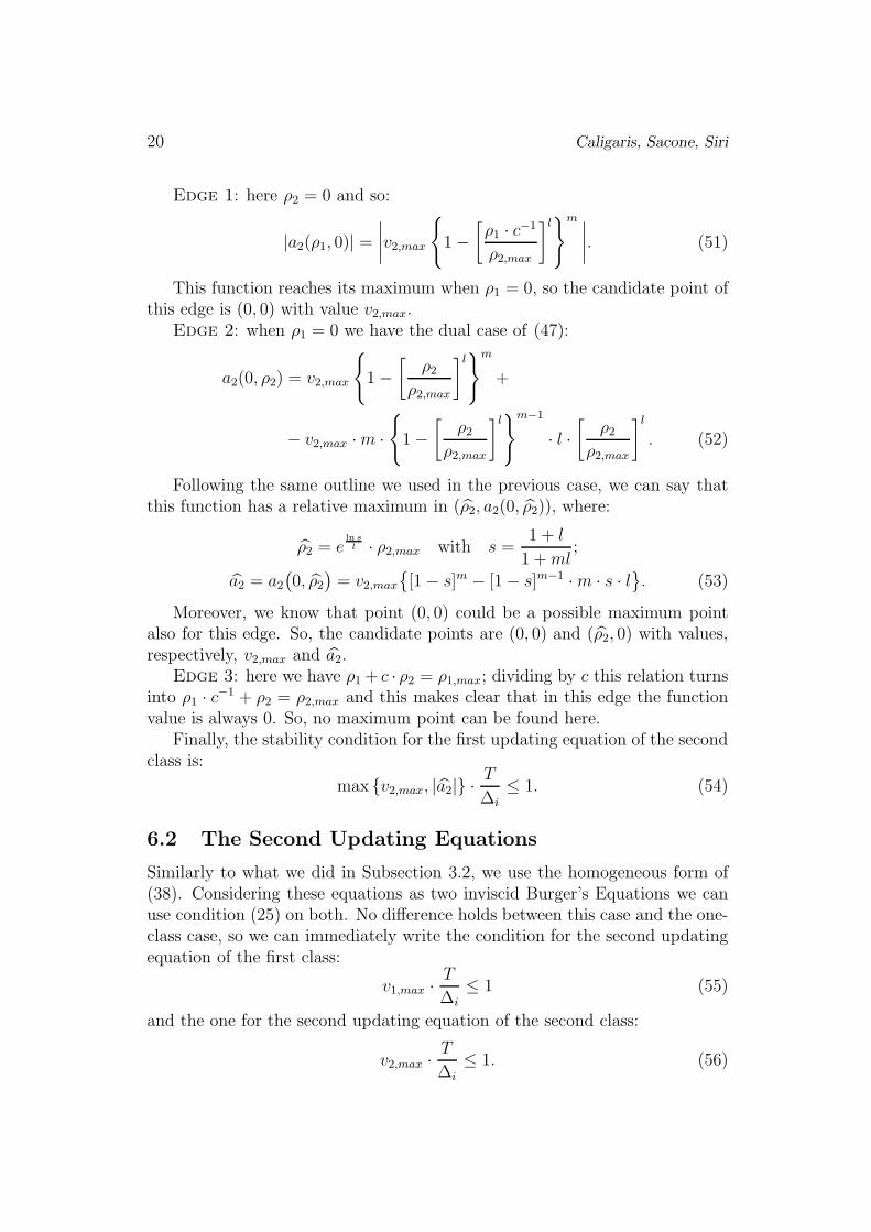
Figure 11: The domain and the contour plot of |a2(ρ1, ρ2)|
Now, consider |a2(ρ1, ρ2)|.The plot of Figure 11 is very symmetric to theone of Figure 10: again, we search for the maximum values in the boundaries.
20 Caligaris, Sacone, Siri
Edge 1: here ρ2 = 0 and so:
|a2(ρ1, 0)| =
∣∣∣∣v2,max
{
1 −
[ρ1 · c
−1
ρ2,max
]l}m ∣∣∣∣. (51)
This function reaches its maximum when ρ1 = 0, so the candidate point ofthis edge is (0, 0) with value v2,max.
Edge 2: when ρ1 = 0 we have the dual case of (47):
a2(0, ρ2) = v2,max
{1 −
[ρ2
ρ2,max
]l}m
+
− v2,max · m ·
{
1 −
[ρ2
ρ2,max
]l}m−1
· l ·
[ρ2
ρ2,max
]l
. (52)
Following the same outline we used in the previous case, we can say thatthis function has a relative maximum in (ρ2, a2(0, ρ2)), where:
ρ2 = eln s
l · ρ2,max with s =1 + l
1 + ml;
a2 = a2
(0, ρ2
)= v2,max
{[1 − s]m − [1 − s]m−1 · m · s · l
}. (53)
Moreover, we know that point (0, 0) could be a possible maximum pointalso for this edge. So, the candidate points are (0, 0) and (ρ2, 0) with values,respectively, v2,max and a2.
Edge 3: here we have ρ1 + c · ρ2 = ρ1,max; dividing by c this relation turnsinto ρ1 · c
−1 + ρ2 = ρ2,max and this makes clear that in this edge the functionvalue is always 0. So, no maximum point can be found here.
Finally, the stability condition for the first updating equation of the secondclass is:
max {v2,max, |a2|} ·T
∆i
≤ 1. (54)
6.2 The Second Updating Equations
Similarly to what we did in Subsection 3.2, we use the homogeneous form of(38). Considering these equations as two inviscid Burger’s Equations we canuse condition (25) on both. No difference holds between this case and the one-class case, so we can immediately write the condition for the second updatingequation of the first class:
v1,max ·T
∆i
≤ 1 (55)
and the one for the second updating equation of the second class:
v2,max ·T
∆i
≤ 1. (56)
Numerical Stability of PW–Model 21
6.3 The Overall Constraints
This model is actually composed of four differential equations; the stabilityconditions for all of them are (50), (54), (55) and (56). In Table 3 we sum upthe values of the various Courant Numbers we wrote in these equations.
Table 3: Stability Conditions; λ =T
∆i
Equation 1 Equation 2
Class 1 µ11 = max {v1,max, |a1|} · λ µ2
1 = v1,max · λ
Class 2 µ12 = max {v2,max, |a2|} · λ µ2
2 = v2,max · λ
In Section 4 we showed that every equation is characterized by its owncondition; this means that, if none of the above constraints is satisfied, thenresults are surely unstable. If only some equations have unstable conditions, wecan have uncertain simulation results: some plots will be unstable, some otherswill look like stable even showing (possibly mitigated) unstable behavior.
If we want our simulations to be completely stable, the four constraintsmust be simultaneously satisfied and this happens when:
max {v1,max, |a1|, v2,max, |a2|} · λ ≤ 1. (57)
We can reduce the number of arguments of this maximum function. First,we know that in the model v1,max > v2,max, so v2,max can be elided. For thesame reason, we can delete |a2| because
|a1| = |v1,max
{[1 − s]m − [1 − s]m−1 · m · s · l
}≥
≥ |v2,max
{[1 − s]m − [1 − s]m−1 · m · s · l
}= |a2|.
(58)
Finally, we can conclude that the stability condition for the two-class modelis essentially the same as the one for the one-class model, expressed in (23):
max {v1,max, |a1|} ·T
∆i
≤ 1. (59)
7 Example for the Two-Class Model
We use the same simulative layout reported in Section 4. The main parametersare included in Table 4. As in the previous example, we influence the CourantNumber by modifying the value of ∆i. The values of l and m we choose ensuresthat max {v1,max, |a1|} = |a1|; so, we can easily calculate the threshold values
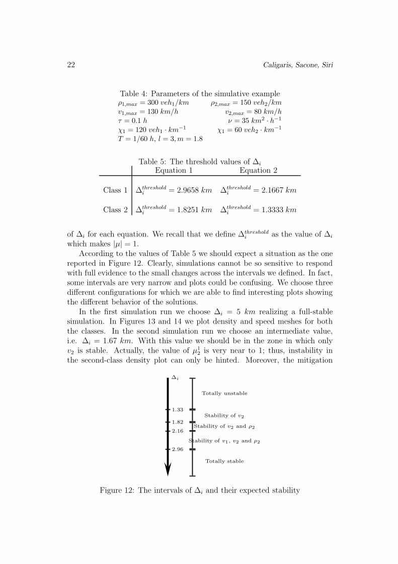
22 Caligaris, Sacone, Siri
Table 4: Parameters of the simulative exampleρ1,max = 300 veh1/km ρ2,max = 150 veh2/kmv1,max = 130 km/h v2,max = 80 km/hτ = 0.1 h ν = 35 km2 · h−1
χ1 = 120 veh1 · km−1 χ1 = 60 veh2 · km−1
T = 1/60 h, l = 3,m = 1.8
Table 5: The threshold values of ∆i
Equation 1 Equation 2
Class 1 ∆thresholdi = 2.9658 km ∆threshold
i = 2.1667 km
Class 2 ∆thresholdi = 1.8251 km ∆threshold
i = 1.3333 km
of ∆i for each equation. We recall that we define ∆thresholdi as the value of ∆i
which makes |µ| = 1.According to the values of Table 5 we should expect a situation as the one
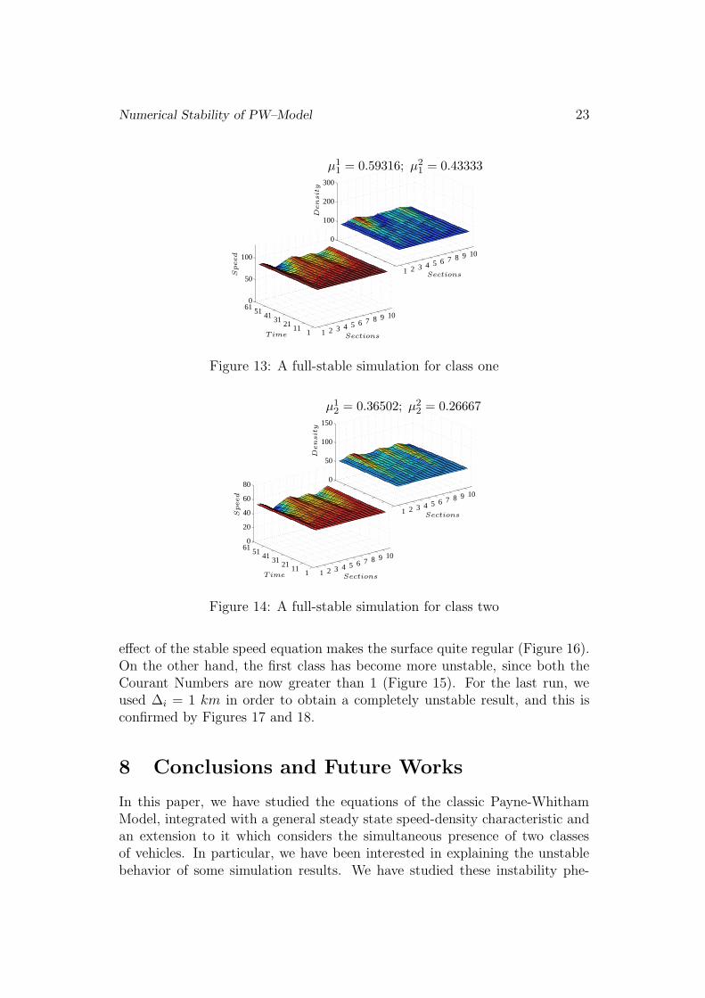
reported in Figure 12. Clearly, simulations cannot be so sensitive to respondwith full evidence to the small changes across the intervals we defined. In fact,some intervals are very narrow and plots could be confusing. We choose threedifferent configurations for which we are able to find interesting plots showingthe different behavior of the solutions.
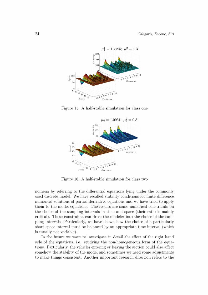
In the first simulation run we choose ∆i = 5 km realizing a full-stablesimulation. In Figures 13 and 14 we plot density and speed meshes for boththe classes. In the second simulation run we choose an intermediate value,i.e. ∆i = 1.67 km. With this value we should be in the zone in which onlyv2 is stable. Actually, the value of µ1
2 is very near to 1; thus, instability inthe second-class density plot can only be hinted. Moreover, the mitigation
∆i
1.33
Totally unstable
1.82
Stability of v2
2.16Stability of v2 and ρ2
2.96
Stability of v1, v2 and ρ2
Totally stable
Figure 12: The intervals of ∆i and their expected stability
Numerical Stability of PW–Model 23
1 2 3 4 5 6 7 8 9 10
11121
31415161
0
50
100
1 2 3 4 5 6 7 8 9 10
0
100
200
300
µ11 = 0.59316; µ2
1 = 0.43333
Sections
SectionsTime
Speed
Den
sit
y
Figure 13: A full-stable simulation for class one
1 2 3 4 5 6 7 8 9 10
11121
31415161
0
20
40
60
80
1 2 3 4 5 6 7 8 9 10
0
50
100
150
µ12 = 0.36502; µ2
2 = 0.26667
Sections
SectionsTime
Speed
Den
sit
y
Figure 14: A full-stable simulation for class two
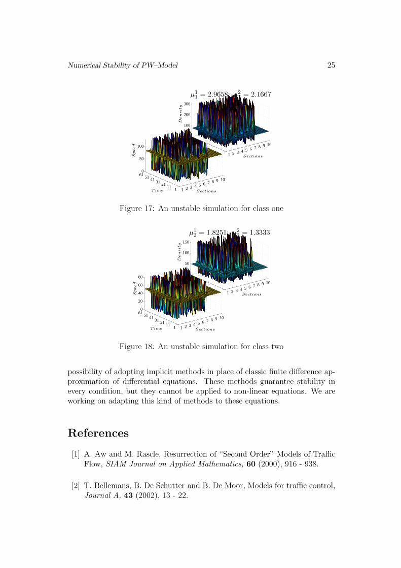
effect of the stable speed equation makes the surface quite regular (Figure 16).On the other hand, the first class has become more unstable, since both theCourant Numbers are now greater than 1 (Figure 15). For the last run, weused ∆i = 1 km in order to obtain a completely unstable result, and this isconfirmed by Figures 17 and 18.
8 Conclusions and Future Works
In this paper, we have studied the equations of the classic Payne-WhithamModel, integrated with a general steady state speed-density characteristic andan extension to it which considers the simultaneous presence of two classesof vehicles. In particular, we have been interested in explaining the unstablebehavior of some simulation results. We have studied these instability phe-
24 Caligaris, Sacone, Siri
1 2 3 4 5 6 7 8 9 10
11121
31415161
0
50
100
1 2 3 4 5 6 7 8 9 10
0
100
200
300
µ11 = 1.7795; µ2
1 = 1.3
Sections
SectionsTime
Speed
Den
sit
y
Figure 15: A half-stable simulation for class one
1 2 3 4 5 6 7 8 9 10
11121
31415161
0
20
40
60
80
1 2 3 4 5 6 7 8 9 10
0
50
100
150
µ12 = 1.0951; µ2
2 = 0.8
Sections
SectionsTime
Speed
Den
sit
y
Figure 16: A half-stable simulation for class two
nomena by referring to the differential equations lying under the commonlyused discrete model. We have recalled stability conditions for finite differencenumerical solutions of partial derivative equations and we have tried to applythem to the model equations. The results are some numerical constraints onthe choice of the sampling intervals in time and space (their ratio is mainlycritical). These constraints can drive the modeler into the choice of the sam-pling intervals. Particularly, we have shown how the choice of a particularlyshort space interval must be balanced by an appropriate time interval (whichis usually not variable).
In the future we want to investigate in detail the effect of the right handside of the equations, i.e. studying the non-homogeneous form of the equa-tions. Particularly, the vehicles entering or leaving the section could also affectsomehow the stability of the model and sometimes we need some adjustmentsto make things consistent. Another important research direction refers to the
Numerical Stability of PW–Model 25
1 2 3 4 5 6 7 8 9 10
11121
31415161
0
50
100
1 2 3 4 5 6 7 8 9 10
0
100
200
300
µ11 = 2.9658; µ2
1 = 2.1667
Sections
SectionsTime
Speed
Den
sit
y
Figure 17: An unstable simulation for class one
1 2 3 4 5 6 7 8 9 10
11121
31415161
0
20
40
60
80
1 2 3 4 5 6 7 8 9 10
0
50
100
150
µ12 = 1.8251; µ2
2 = 1.3333
Sections
SectionsTime
Speed
Den
sit
y
Figure 18: An unstable simulation for class two
possibility of adopting implicit methods in place of classic finite difference ap-proximation of differential equations. These methods guarantee stability inevery condition, but they cannot be applied to non-linear equations. We areworking on adapting this kind of methods to these equations.
References
[1] A. Aw and M. Rascle, Resurrection of “Second Order” Models of TrafficFlow, SIAM Journal on Applied Mathematics, 60 (2000), 916 - 938.
[2] T. Bellemans, B. De Schutter and B. De Moor, Models for traffic control,Journal A, 43 (2002), 13 - 22.
26 Caligaris, Sacone, Siri
[3] C. Caligaris, S. Sacone and S. Siri, Freeway Traffic Modeling: Extensionto Different Vehicle Classes and Numerical Analysis, Proc. of 10th Inter-
national IEEE Conference on Intelligent Transportation Systems, (2007),325 - 330.
[4] H.L. R. Courant, K. Friedrichs and H. Levy, On the partial differenceequations of mathematical physics, IBM Journal of Research and Devel-
opment, 11 (1967), 215 - 234.
[5] M. Cremer and M. Papageorgiou, Parameter identification for a trafficflow model, Automatica, 17 (1981), 837 - 843.
[6] C.F. Daganzo, Requiem for second-order fluid approximations of trafficflow, Transportation Research B: Methodological, 29 (1995), 277-286.
[7] D.R. Drew, Traffic flow theory and control, McGraw-Hill, New York, 1968.
[8] H. Greenberg, An analysis of traffic flows, Operations Research, 7 (1959),79 - 85.
[9] B.D. Greenshields, A study in highway capacity, Highway Research Board
Proc., 14 (1935), 448 - 477.
[10] A. Kotsialos, M. Papagergiou, C. Diakaki, Y. Pavlis and F. Middelham,Traffic flow modeling of large-scale motorway networks using the macro-scopic modeling tool metanet, IEEE Transactions on Intelligent Trans-
portation Systems, 3 (2002), 282 - 292.
[11] A.D. May, Freeway simulation models revisited, Transportation Research
Record, 1132 (1987), 94 - 99.
[12] B. Neta, Numerical Solution of Partial Differential Equations MA 3243
Lecture Notes, Department of Mathematics Naval Postgraduate School,2003.
[13] M. Papageorgiou, Applications of Automatic Control Concepts to Traffic
Flow Modeling and Control, Lecture Notes in Control and InformationSciencies, Springer-Verlag, 1983.
[14] M. Papageogiou and H. Haj-Salem, Ramp metering impact on urban cor-ridor traffic: field results, Transportation Research Part A: Policy and
Practice, 29 (1995), 303 - 319.
[15] M. Papageorgiou, Some remarks on macroscopic traffic flow modelling,Transportation Research Part A: Policy and Practice, 32 (1998), 323 -329.
Numerical Stability of PW–Model 27
[16] H.J. Payne, Models of freeway traffic and control, Mathematical Models
of Public Systems, Simulation Council Proceedings, (1971), 51 - 61.
[17] G.B. Whitham, Linear and Nonlinear Waves, John Wiley, New York,1974.
[18] L.N. Trefethen, Finite Difference and Spectral Methods for Ordinary and
Partial Differential Equations, C. University, Ed., 1996.
[19] R.T. Underwoo, Speed, volume and density relationships: quality andtheory of traffic flow, Yale Bureau of Highway Traffic, (1961), 141 - 188.
Received: Month xx, 200x