Admissible controls and attainable states for a class of nonlinear systems with general constraints

INTERNATIONAL JOURNAL OF ROBUST AND NONLINEAR CONTROL, VOL. 4, 267-288 (1994)

ADMISSIBLE CONTROLS AND ATTAINABLE STATES FOR A CLASS OF NONLINEAR SYSTEMS WITH

GENERAL CONSTRAINTS

M. E. ACHHAB,' F. M. CALLIER2 AND V. WERTZ' ' Centre for Systems Engineering and Applied Mechanics. UniversitP Cotholique de Louvoin, Brit. Mawwell. Ploce

du Levant, 3, B-1348 Louvoin-lo-Neuve, Belgium

Deportment of Mothemotics. FocuItPs Universitaires de Nomur, Remport de la Vierge, 8. 8-5000 Nomur, Belgium

SUMMARY We consider nonlinear control systems where the control and the state variables are submitted t o explicit constraints. This paper has two objectives. First, for a class of nonlinear systems with constraints, an existence result of nontrivial admissible controls and some of their interesting properties are proved. Then, we investigate the problem of local controllability in a neighbourhood of a n equilibrium point, while observing state and control constraints along the whole trajectory. An iterative procedure is also given, which allows one t o compute the steering admissible control function. This procedure is illustrated with a classical example.

KEY WORDS Nonlinear systems Admissible controls Local controllability Attainable states

1. INTRODUCTION

Given a control system i ( t ) = g(x ( t ) , u( t ) ) , where x ( t ) € IR", u( t ) € R"' and x(0) = qo € IR", a fundamental control problem is that of finding some admissible control u(. ) which steers the system from the initial state 70 to a desired final state qd in a given time, T. The problem is more realistic, and hence more interesting, in the case where we have constraints on the control and state variables. These constraints can arise for different reasons including physical considerations and technological limitations. Also, the constraints can be set to avoid large deviations from a nominal behaviour of the system (for example, in the case where such deviations would yield an unstable behaviour). In particular, if some of the state constraints are violated for any time t , serious consequences may ensue, including damage to physical components and loss of stability. Usually, it is assumed that the control lies in some bounded convex set W and that the corresponding state has to be in some closed domain A for every time t . The problem, important in itself, can also be combined with an optimization of some criterion to yield optimal control problems with fixed end points and explicit constraints on the state. Various results have been established in this case, including the maximum principle

This paper presents research results of the Belgian Programme on Interuniversity Poles of Attraction initiated by the Belgian State, Prime Minister's Office, Science Policy Programming. The scientific responsibility rests with its authors.

This paper was recommended for publication by editor B. D. 0. Anderson

CCC 1049-8923/94/020267-22 0 1994 by John Wiley & Sons, Ltd.

Received I September 1992 Revised 25 September 1992

268 M. E. ACHHAB, F. M. CALLIER AND V. WERTZ

of Pontryagin et al. and well-known optimality conditions (see, for example, Reference 4). Based on these results, some successful numerical methods have been developed, particularly by Gonzalez and Miele,' Mehra and Davis," Miele14 and Sakawa and Schindo. l6 Recently, Goh and Teo6 have provided a unified computational approach based on control parametrization. However, the existence of nontrivial admissible controls (controls such that both control and state constraints are satisfied) has not been given enough attention. Usually, the existence of such controls as well as some of their required properties are merely assumed from the start. Also, to develop some implementable control laws in such a situation, it is often assumed that the desired final state is attainable, while obeying the constraints. This is the case for example in Mayne and Michalska12 where the infinite horizon optimization of constrained nonlinear continuous time systems has been investigated.

This paper is concerned with nonlinear continuous time autonomous systems .k = g(x, u ) which have a known equilibrium point (2,ii) and satisfy suitable assumptions on g. By linearization around the equilibrium point (for which we, without loss of generality, take the origin), such systems can be reduced to the form (1) given below. In the first part, we give a precise definition of the class of admissible controls. Then, we give some properties of the set of admissible controls, including that this set has a non-empty interior and is closed for the usual topology. Under additional assumptions, we show that it is also a convex set. In the second part, we study the constrained controllability problem for the same class of nonlinear systems. We develop our approach in two different cases. First, assuming that the initial state is the origin, we prove that, in the neighbourhood of this equilibrium point, every attainable state using trajectories of the unconstrained linear part of the system is also attainable by trajectories of the whole system subject to the constraints. Later, we treat the case where the desired final state is the origin. It is shown that the origin is attainable using an admissible control from every neighbouring state, provided that this is also the case for the unconstrained linear part of the system. Finally, using these results, we derive iterative convergent procedures to compute the admissible steering control laws in each case.

Our methods are constructive and allow us to estimate lower bounds on the size of the set of admissible controls as well as of the set of attainable states. Most of the results described make use of the contraction mapping theorem as the principal mathematical tool. This functional analytic device has been applied (in an infinite-dimensional systems setting) in a completely different way by Magnusson et al." to solve some controllability problems. It should be noted that these authors do not consider the case where there are a priori constraints on the control and state variables. Also, the nonlinear part of their class of systems contains no terms involving the control. Analogous remarks can be made about the pioneering work of Hermes, where controllability of nonlinear affine control systems was first investigated.

The paper is organized as follows. In Section 2, we define the system we shall consider and give the basic assumptions and notation. We give a precise definition of admissible controls and state their useful properties in Section 3. Then, we prove and discuss the controllability results in Section 4. In particular, we outline the control algorithm and show its convergence around the equilibrium point. To illustrate our approach, a significant classical example will be treated in Section 5 . Last, we conclude by final remarks and suggestions in Section 6.

2. ASSUMPTIONS AND NOTATION

We consider the autonomous continuous time system described by the nonlinear differential equation

i ( t ) = Ax(t ) + Bu(t) + f ( x ( t ) , u(t) ) , x(0) = 0

0 < t < T

NONLINEAR SYSTEMS WITH GENERAL CONSTRAINTS 269

where A is a (n x n) real matrix, B is a (n x rn) real matrix and f is a vector-valued function from IR" x IR"' into R". The input of the system u( t ) E I R m is subject to the constraint u( t ) E %! for almost every t , where %is a compact convex subset of IR". The state of the system x ( t ) is constrained to belong to A for every t , 0 < t < T, where A is a closed connected domain of R".

2.1. Notation

We shall use the symbol 1 1 - 1 1 to denote any vector norm in I R p and the induced matrix norm. L"[O, T; IR"] is the space of all Lebesgue measurable and essentially bounded functions h: [0, TI -+ IR" with the norm 11 h 11" = ess sup0 t Q 7-11 h( t ) 11. C[O, T; R"] is the space of all continuous functions h: [O, TI -+ R" with the norm )I h IIs = maxo s r Q 7-11 h ( t ) 11. BP(z, P I , respectively &(z, p ) , will denote the open ball, respectively the closed ball, in I R p with centre z and radius p. B,(z,p) and Bs(z,p) are similarly defined in L"[O, T; IRml and CIO, T; R"1, respectively. If X, Y are normed linear spaces and G is a linear operator defined on 97 C X into Y, then G* will denote its dual operator.

2.2. Assumptions

We assume that % is a compact convex subset of I R m and that A is a closed domain of R". Moreover, the origin 0 is an interior point of the subsets @ and A, respectively. These assumptions include for example the usual case where the control u and the state must satisfy the inequality constraints 1) u 11 < 011 and 11 x 11 < (YZ, for some fixed positive real numbers a1 and (YZ. We also make the following two additional assumptions on the function f .

A.l. f(0,O) = 0 (i.e. the origin is an equilibrium point) A.2. There exist two positive functions k: IR' x IR' -+ R+ and j : R+ x IR' + IR+ such that

(i)

(ii) k(61,62) -+ 0 and j ( 6 1 , 6 2 ) + 0 as (61,62) -+ (0,O)

II f ( x , u ) - ftu, u ) I( < k(61, 6 2 ) 11 x - Y II + j ( h , 6 2 ) 11 u - u 11, for every II XI19 I I Y I I < 61 and II u I I 9 I I I I < 62

Note that these assumptions imply that f is differentiable at the origin (0,O). A typical example of such systems is the case where the function f ( x , u ) is given as power series in ( x , u) , which starts with second-order terms. The simplest case is given by Example2.1 below. Another meaningful example is given in the context of interconnected systems by Ikeda and Siljak,' where the nonlinear perturbations of the linear part of the plant appear as interconnections.

Example 2.1

y > 0 such that In the case where the nonlinear part of the system is bilinear, then f(0,O) = 0 and there exists

I I f ( x , u ) ) ) <yllx\111uII , for every xER" and u E R m

Writing f ( x , u ) - f ( y , u ) = f ( x - y, u ) + f ( y , u - u ) , one gets.

I I f(x9 u ) - f ( Y , u ) I1 G Y I1 u II II x - Y I 1 + Y I I Y I I II u - u I I Thus, the assumption A.2 is also satisfied with k(61,62) = y62 and j(61, 6 2 ) = 761.


Comment I

and that A common way to satisfy assumption A.2 is to assume that f is continously differentiable

af ax au a f (0,O) = - (0,O) = 0

in which case, it is sufficient to take

~ ( ~ 1 , ~ 2 ) = m ~ ~ l l f ( x , ~ ) - f ( ~ , ~ ) I 1 / I I x - ~ I I , x ~ ~ , I l x I I , l l ~ l I a 1 , l l U l I G62)

j ( ~ l , ~ 2 ) = m ~ ( l l f ( x , u ) - f ( x , ~ ) I I / l I u - ~ I I , u ~ v,Ilxll ~ ~ ~ ~ l l ~ l l ~ l l ~ l l and

An example illustrating this is given in Reference 1. With these assumptions, we are now ready to give a precise definition of the class of

admissible controls. This is done in the next section, where we also show that the set of admissible controls has a non-empty interior and is closed for the usual topology. Under additional hypotheses, this set is also convex. These results have been obtained previously in Reference 1.

3. ADMISSIBLE CONTROLS

3. I . Dejnition of admissible controls

Dejnition 3. I

A function u in L"[O, T; R"'] is an admissible control for the system (1) if

(i) u(t) E 42, for almost every t, 0 6 t < T; (ii) there exists v > 0 such that for such u ( - ) , system (1) has a unique solution in the ball

(iii) this unique solution satisfies x( t ) E R ( 0 , v) of C[O, T; n?"];

for all t, 0 < t < T.

Thus, a control is admissible if the control constraints are satisfied, but also provided the solution of the differential equation exists and has no finite escape time; moreover the state x ( t ) must satisfy the state constraints on the whole trajectory. The solution of system (1) corresponding to an admissible control is said to be an admissible trajectory. Let wad denote the set of all admissible controls in the sense of Definition 3.1. The fact that wad is a subset of the space L"[O, T; IR"'] allows us to take piecewise continuous controls with any countable number of discontinuities and satisfying constraints almost everywhere. This is very important from a practical point of view, since such controls occur in several applications. We outline below some properties of wad, beginning with the fact that it is not a trivial set.

3.2. General properties of wad

Proposition 3. I

Under the above assumptions, the set wad has a non-empty interior.

NONLINEAR SYSTEMS WITH GENERAL CONSTRAINTS 27 1

Proof. It is sufficient to prove that wad contains some ball B,(O, p) , for a well-chosen p > 0. For this, consider the function 4(x, u ) defined from C[O,T; W"] x Lm[O, T; W"] into C[O, T; I?"] by

Notice that for a given control u, a solution of the differential equation (1) (if it exists) is a fixed point of the function 4 ( . , u ) . It turns out that it is sufficient to show that for every control u in a well-chosen ball Bm(O,p), this function 4 ( . , u ) has a unique fixed point xu satisfying the constraints. More than merely an existence result, the following lemma allows us to give the size of a ball Bm(O,p) contained in u a d .

Lemma 3.2

There exist u > 0 and p = p ( u ) such that

(i) for every u ~ B ~ ( o , p ) , u ( t ) E % for almost every t; (ii) in this case, the function 4( - , u ) has a unique fixed point xu such that 11 xu I (s Q u and

(iii) the function r: B,(O, p ( v ) ) + &(O, u ) defined by r ( u ) = xu is Lipschitz and hence xu([) E dl for every t, 0 Q c Q T;

continuous.

Proof of Lemma 3.2. As k(&, 62) -, 0 when (&, 132) + (0,O) (by assumption A.2), there exist €1 > 0 and €2 > 0 such that

Since the origin is an interior point of the domains A and %, there exists an integer j such that &(O, e l / j ) c dl and B,(O, e ~ / j ) C 4Y. Put u = e ~ / j and f i = &/j; then for x and y in the ball &(O, u ) and u E B,(O, ei), we have,

II II f ( x ( s ) , u(s)) - f ( Y ( S ) , u(s ) ) II d s II 44x3 u ) - 4tv, u ) 11s Q max j ' 1 1 e A ( r - s )

o < t < T o

Using assumption A.2 and (3),

Q c1 I I x - Y 11s

Hence, 4(* , u ) : &(O, u ) + C[O, T; IR"] is a contraction mapping for every u in the ball B,(O, ~ i ) . On the other hand, f(0,O) = 0 implies that


Hence, defining

we have 4(x , u ) E &(O, v) whenever u E B,(O, F ) . Thus, for u E B,(O, p ) , +( * , u) : &(O, v) + &(O, v ) is a contraction mapping. By using the local contraction mapping theorem (see, for example, References 5 or 17), 4(*, u ) has a unique fixed point in the ball &(O, v ) which is the solution of the differential equation (1). Clearly, this solution satisfies the conditions of Definition 3.1.

To prove the final conclusion of our lemma, let us write

r(u) - w) = w w , u ) - ww, 0)

= mw, u ) - w w , u ) + MW, u ) - ww, u )

Then, by assumption A.2, we have for every u and u in the ball B,(O,p),

11 rw - r w iiS G c1 II r(u) - r ( ~ ) iiS + (c2 + P ) II u - u IL Consequently,

This ends the proof. 0

Proposition 3.3

Under the above assumptions, Uad is a closed subset of the space L"[O, T; IT?"]

To prove this result, we need the following lemma.

Lemma 3.4

Under the above assumptions, suppose that (up) is a Cauchy sequence in Uad. Let x,, for any integer p , denote the solution of the differential equation (1) corresponding to up. Then (xp) is a Cauchy sequence in C[O, T; IT?"].

Proof of Lemma 3.4. First, note that there exists M a 1 and a > 0 such that 11 eA' 11 < Me"', for t 2 0.


As up is an admissible control, we have by Definition 3.1. that there exist 61 > 0 and 62 > 0 such that for every p , 11 up@) 11 < 62 and 11 xp(t) 11 < 61, 0 < t < T. Then by assumption A.2,

I I f ( X p ( f ) , U P W ) - f ( X q ( f ) , &At)) I1 Q k(61,W II X P W - X q ( 0 II + j(Sl962) II U P ( t ) - U q ( 0 I 1 So writing

Thus applying Gronwall's inequality,

Hence,

So with

we get

Take now E > 0. Since (up) is a Cauchy sequence, there exists N(E') , where

such that p, q 2 N(E') implies 11 up - uq [ I m < E ' . So by (7),

II *P - xq I I S < E

for every p , q 2 N(E') . This shows that (xp ) is a Cauchy sequence in C[O, T; R"]. 0

Proof of Proposition 3.3. Let (up) be a convergent sequence in Uad with u = limp+ + m up in the L" norm. u is an element of L"[O, T; R"], since this space is complete. We have to show that u is in fact an element of Uad.


First, because 4Y is closed, we have u ( t ) E 4Y for almost every t , 0 < t < T. Let x, denote the solution of (1) corresponding to the control up.

Noting that (up) is a Cauchy sequence, we concluded by Lemma 3.2. that (xp) is also a Cauchy sequence in C[O, T; R"]. As this is a Banach space, (x,) converges to a unique x € C[O, T; R"]. To prove that u is admissible, it is sufficient to prove that x is the solution of (1) corresponding to u and that it satisfies the state variables constraints. For this, applying the Lebesgue dominated convergence theorem and the continuity of the function f, one can interchange the integration and the limit in (8) to obtain

,Finally, the fact that x( t ) E A, for every t follows from the fact that A is closed and from +(t ) E A, v t and for every integer p.

0 So, the control u is in u a d and Proposition 3.3. is proved.

3.3. Convexity of the set of admissible controls

set of admissible controls is convex. This is the purpose of our next result. We shall show, in this subsection, that if the controls are appropriately bounded, then the

Proposition 3.5

There exists a! > 0 such that if 4Y is contained in B m ( 0 , a), then Uad is a convex subset of L"[O, T; Rm].

Proof. Take u and u in (lad and X E 10, 1 [, we have to prove that (Xu + (1 - X ) u ) is an

First, for almost every t , (Xu + (1 - A)u)( t ) = Xu@) + (1 - X)v(t ) is an element of %2

Using the same arguments as in the proof of Lemma 3.1, there exist v > 0 and p = p ( v ) such

admissible control.

(because 91 is convex).

that Bn(0, v) c A and

11 r(u) 11s < cz+p 11 u llm 1 - c1

for every u E Bm(0, p ) . Taking

1 - c1 c z + P

a=-

and assuming that 4Y c Bm(O, a) we have, by the above inequality

Hence, the solution of (1) corresponding to (Xu + (1 - X ) u ) satisfies the state constraint, i.e. takes its values in the domain udl for all t .

This shows that (Xu + (1 - X ) u ) is an element of uad, which ends the proof.


Comment 2

In the proof of Lemma 3.1, we took

to ensure that our controls lie in fact that (Xu + (1 - X)o) satisfies of 42.

42 for almost every t . Here, this is not necessary since the the control constraint follows directly from the convexity

Comment 3

The convexity of Uad is not needed to prove other results in this paper. However, it is needed for the existence of optimal controls. In the case where there are no state constraints, the convexity of Uad is directly implied by the convexity of 42. But, in optimal control problems with control and state constraints, this property is usually made as an assumption from the start. Proposition 3.5 justifies such an assumption for the class of nonlinear systems considered in this work.

We have shown in this section that, given constraints on the control and state variables and under some reasonable assumptions, there exist admissible controls (i.e. controls such that the control constraints are satisfied, the state trajectory (solution of the differential equation (1)) exists and the state constraints are satisfied along the trajectory).

The problem to which we now turn our attention is that of determining a set of states that can be reached in a given time T, with these admissible controls. This is the subject of the next section.

4. LOCAL CONTROLLABILITY

Consider the linear part of the system (l),

i ( t ) = &(t) + Bu(t), z(0) = 0

0 < t < T

It is well known (see, for example, Reference 10) that if (10) is controllable (i.e. the pair ( A , B) is controllable), then system (1) without explicit (pointwise) constraints on the state variables is ‘small time locally controllable’ from the origin (an equilibrium point). The proof of this result is generally based on the implicit function theorem and so only establishes the existence of a neighbourhood of the origin in which every vector is an attainable state.

We investigate here the problem of finding an admissible control which steers the system from the origin to a desired final state in the case where we have control and state constraints. First, we prove that every attainable state for the linear system (10) in some neighbourhood of the origin is also attainable using admissible trajectories of system (1). Then, we give an iterative procedure to approximate the corresponding admissible steering control. Our method allows us to estimate a lower bound on the size of the neighbourhood of the origin in which the states are attainable and provides an algorithm to compute the steering controls. Hence, it can be used in some applications as a design technique. For convenience, we present our main results in different subsections.


4.1. Attainable states from the origin

Dejnition 4. I

z E A is an attainable state from the origin at the time T > 0 if there exists an admissible control u E Uad such that xu( T ) = z.

Let J ~ T denote the set of all attainable states from the origin at the time T. We examine in this subsection some properties of d ~ . Notice that the final time T is supposed to be given. We will discuss Iater the effect of this parameter on the size of d ~ .

Consider the reachability operator G defined from L2[0, T; IR"] into IR" by

then G is a bounded linear operator. Putting V = Im G, the range of G, then V is a linear subspace of R" and hence is a closed set. (Note that Vis the controllable subspace of (A, B).) So, the 'generalized inverse' of G is well defined. We shall denote it by F. We have in particular GF = Iv, where IV denotes the identity on the subspace V. (See Appendix 1 or Reference 2 for more details.)

In order to state our main results, consider the mapping # ( z , u ) defined from IR" x L2[0, T; Rm] into L2[0, T; IR"] by

where x ( - ) is the solution of the system (1) corresponding to the control function u ( * ) . Notice that #(z, u ) is well defined for every z E IR" and u E Uad.

Lemma 4.1

There exist v > 0, p = p ( v ) > 0 and 0 < c = c ( v ) < 1 such that

(9 B"(O, v) c A (ii) B d 0 , c ~ ) C Uad

(iii) for every z ~ B ~ ( 0 , v), and for every u, U E Bm(O,p), we have

II #(z, u ) - #k v ) Ilm G c II u - u 11- (13)

The proof of this technical result is given in the appendix 43. An immediate consequence of this lemma is the following.

Lemma 4.2

control 6 E B,(O, p ) satisfying #(z, 6) = 6 (where v and p are given in Lemma 4.1). There exists p = p ( p , v), 0 < p < v such that for every zEB,(O,p) , there exists a unique

Proof of Lemma 4.2. By the previous lemma, #(z, *): B m ( 0 , P ) + L"[O, T; R'"] is a

On the other hand, it follows from the proof of Lemma 4.1 that contraction mapping for every Z E R", )I z 1) < v.

I I #(z, u ) IIoD I I Fll I 1 z I I + c I I u 11- (14)

NONLINEAR SYSTEMS WITH GENERAL CONSTRAINTS

Choosing

277

(15)

we have that )I z 11 < p and 11 u 11.. 6 p imply

Q a (16)

Hence, $(z, u ) E B..(O, p), whenever z E Bn(0, p ) . Thus, $(z, -): B..(O, p ) + &(O, p ) is a contraction mapping for every z E IT?", ( 1 z 11 < p. Applying now the local contraction mapping theorem (see, for example, Reference 5 or 17), we conclude that $(z, -) has a unique fixed

Now, let us make the following additional assumption.

A.3 V(X, u ) E IT?" x Rm, f ( x , u ) E V where V = Im G, with G the reachability operator

point P in the ball &,(O, p), i.e. $(z, P) = P. This shows the desired conclusion.

defined by (1 1).

Comment 4

Assumption A.3 is obviously satisfied in the case where V = IT?", i.e. where the pair ( A , B ) is controllable. It means that the perturbing excitation f ( x , u ) of (1) lies in the controllable subspace of (A, B). Hence, with x(0) = 0, for all u ( - ) E Uad, any solution x&), t E [O, TI of (1) remains in V.

Theorem 4.3

Under the above assumptions, there exists p > 0 such that for every z E Bn(0, p ) n V, there exists a control P E wad satisfying x,i( T ) = z (where xri denotes the trajectory of system (1) corresponding to 6) .

Proof. Taking the same p as in the previous lemma, we have: for every z E Bn(0, p ) n V, there exists a control P E wad such that $(z, P) = P. This implies,

J = pz - p f (x (s ) , W)) ds (17) eA(T-S) soT Applying the operator G on both members and using the property GF = Iv, we get

T

0 z = GC + 1 eA(T-s) f ( x ( s ) , W)) d s (18)

which shows the desired conclusion. (Note that we implicitly used assumption A.3.)

Comment 5

In other words, the theorem says that the system (1) can be steered from the initial state to any final desired state zEBn(0,p) n V, using the admissible control law P. Moreover, this control law can be approached as close as desired by an iterative procedure based on the contraction mapping theorem, as will be shown in the next subsection.


Comment 6

Owing to the constraints on the control and on the state, the radius of the ball Bn(0, p ) will depend on the final time T. It can be shown that p is proportional to T so that for smaller values of the final time, the attainable states will be closer to the origin.

Corollary 4.4

If the pair ( A , B ) is controllable, then the set of attainable states C ~ T contains a neighbourhood of the origin. Thus, the nonlinear system described by (1) subject to the constraints is ‘small time locally controllable’ from its equilibrium point.

In the case where the pair ( A , B ) is controllable, we also have the following result.

Lemma 4.5

point of $(z, .), is Lipschitz continuous. The function 0: Bn(0,p) -+E,(O,p) defined by Q(z) = P(-) where a ( . ) is the unique fixed

Comment 7

Lemma 4.5 implies that for every sequence (zp) converging to the desired attainable final state z, the corresponding sequence (up(- ) ) of admissible controls which steer the state to zp converges to the control a ( . ) which steers the state to z. Note that the limit P(*) E Uad. This will be very useful in any iterative method concerned with steering system (1) from the origin to z. This also guarantees that any small error on the measurement of the final state z will not produce a large error on the values of 6.

Comment 8

If assumption A.3 is not satisfied, then Theorem 4.3 can be replaced by the following result. Let z E Bn(0, p ) and P E Uad be the fixed point of $(z, .) given by Lemma 4.2. Moreover, let


2 denote the trajectory of system (1) corresponding to ti. If

then z is attainable from the origin using the trajectory 2 (i.e. 2( T) = z). Moreover, condition (20) is necessary to reach the state z using control laws ii defined as the fixed points of (12).

4.2. States that are controllable to the origin

Let %'T be the set of all initial states 7 that are controllable to the origin in time T, using admissible controls in the sense of Definition 3.1. We prove here that if (A, B) is controllable, then WT contains a neighbourhood of the origin.

For this purpose, consider the controllability to the origin operator GI defined from L2[0 , T; R"] into R" by

T

GI@) = - e-ASBu(s) ds 0

then GI is a bounded linear operator. Putting VI = Im GI, the range of GI then VI is a linear subspace of R" and hence is a closed set. Moreover, because the controllable subspace V is eA'-invariant, we have VI = V. So, the pseudo-inverse FI of the operator GI is well defined and satisfies GI FI = Iv, where IV denotes the identity on the subspace V. (See Appendix 1 for more details.)

Now, consider the mapping A(7, u ) defined from R" x L2[0, T; IR"] into L 2 [0, T; R"] by T

0 u ) = FIT + FI 1 e-Asf(x(s), u(s ) ) d s

where x ( - ) is the solution of the nonlinear differential equation (1) corresponding to the control function u ( * ) and the initial state x(0) = 7. Then A(7, u ) is well defined for every 7 E IR" and u E Uad. Hence almost the same arguments as in the proofs of Lemma 4.1 and Lemma 4.2 lead to the next result.

Lemma 4.6

There exists p1 > 0 such that

(9 & ( O , P l ) c uu (ii) for every 7 E Bn(0, P I ) , there exists a unique control function ti E Uad satisfying

A(7, ti) = ti

Now, from the previous lemma, we have T

li = F I ~ + FI 1 e-Asf(x(s), l i ( s ) ) d s 0

Applying the mapping GI on both members and using the fact GIFl = Iv, we get T

0 GIG = 7 + e-Asf(x(s), ti@)) d s (24)


Applying the operator eAT on both members yields

Thus

= XG( T) This shows the following theorem.

Theorem 4.7

Under assumptions A.l, A.2 and A.3, there exists p1 > 0 such that for every 7 E Bn(0, p1) n V, there exists a control fi E Uad which steers the system (1) from the initial state x(0) = to the origin.

Consequently, we have the following result.

Corollary 4.8

If the pair ( A , B ) is controllable, then for every T > 0, the set %?T of states that are controllable to the origin (while obeying the constraints), contains a neighbourhood of the origin.

Comment 9

In fact, the result gives the size of a neighbourhood of an equilibrium point in which every state can be steered to this equilibrium using the admissible control law 6. Moreover, this control law can be approximated by an iterative procedure based on the contraction mapping theorem.

4.3. Iterative procedure

We now proceed to describe an iterative procedure that can be followed in order to construct the control function 6 defined through Theorem 4.3. Take z E Bn(0, p ) n V . Consider the sequence

[u"+l=+(z,u.) , n c N uo = 0

By Lemma 4.1 (see (13)), we have

11 Un+l- Un 11.. < C" \ I ~1 l lm (26)

Moreover, its limit is the unique fixed point a ( - ) of the mapping +(z, .) in B,(O, p), which

On the other hand, the solution Xn of (1) corresponding to the control Un(.) exists and

As 0 < c < 1, (Un) is a convergent sequence in L"[O, T; IR"].

is an admissible control for the system described by (1) subject to the constraints.

NONLINEAR SYSTEMS WITH GENERAL CONSTRAINTS

satisfies the constraints as proved in Lemma 3.1. Define now

We have then:

SO Xn( T) = z + & + I + En, which implies that & + I = En + (Z - X n ( 2')). Thus, we have the

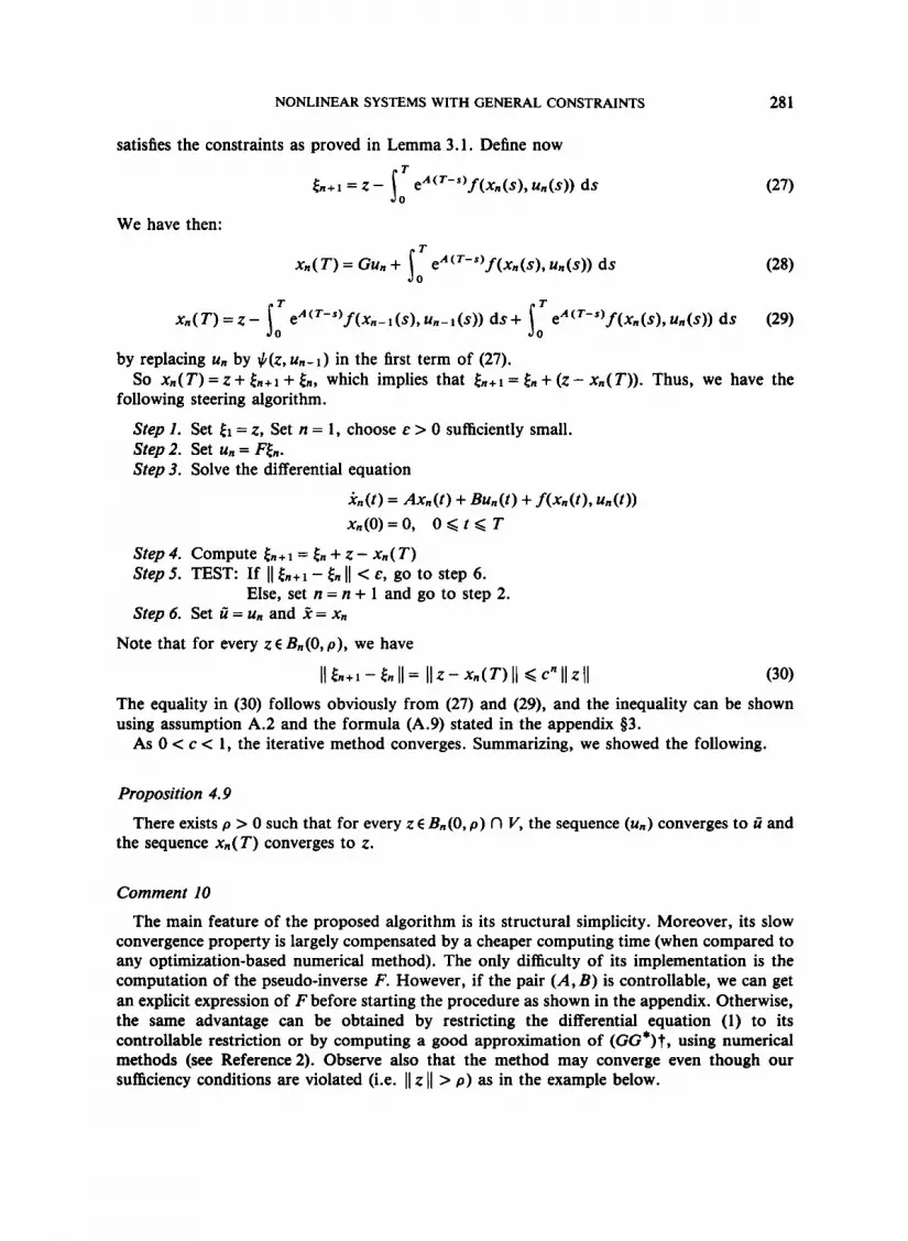
Step 1. Set € 1 = z, Set n = 1, choose E > 0 sufficiently small. Step 2. Set U n = F&. Step 3. Solve the differential equation

following steering algorithm.

k ( t ) = Axn(t) + Bun(t) + f(xn(t) , un(t)) Xn(0) = 0, 0 < t < T

Step 4. Compute En+ 1 = En + z - Xn( T ) Step 5. TEST: If 11 & + I -

Step 6. Set ii = Un and 2 = Xn

I( < E, go to step 6. Else, set n = n + 1 and go to step 2.

Note that for every z € Bn(0, p ) , we have

I l € n + l - € n I I = IIz-xn(T)II <c"IIzII (30)

The equality in (30) follows obviously from (27) and (29), and the inequality can be shown using assumption A.2 and the formula (A.9) stated in the appendix 43.

As 0 < c < 1, the iterative method converges. Summarizing, we showed the following.

Proposition 4.9

the sequence Xn( T) converges to z. There exists p > 0 such that for every z € Bn (0, p ) f l V, the sequence ( U n ) converges to 6 and

Comment 10

The main feature of the proposed algorithm is its structural simplicity. Moreover, its slow convergence property is largely compensated by a cheaper computing time (when compared to any optimization-based numerical method). The only difficulty of its implementation is the computation of the pseudo-inverse F. However, if the pair (A, B ) is controllable, we can get an explicit expression of F before starting the procedure as shown in the appendix. Otherwise, the same advantage can be obtained by restricting the differential equation (1) to its controllable restriction or by computing a good approximation of (GG*)t, using numerical methods (see Reference2). Observe also that the method may converge even though our sufficiency conditions are violated (i.e. 11 z 11 > p ) as in the example below.


With slight modifications, one can obtain an analogous algorithm which gives the steering control function ti, defined through Theorem 4.7. The remarks made in the previous comment remain valid. We conclude this section by the following possible extensions of the theory before illustrating it with an example.

Comment I1

Our results can be extended with slight modifications, to non-autonomous systems of the form i ( t ) = A( t )x ( t ) + B ( t ) u ( t ) + f ( x ( t ) , u(t) , t ) , x(0) = 0 with the assumption f ( O , O , t ) = 0, for all t and assumptions A.2 and A.3 satisfied uniformly with respect to t, (0 < t < T ) . Optimal control of such systems has been considered by Willemstein.

5 . EXAMPLE

Consider the following differential equations (see Reference 3) which describe the satellite angular momentum dynamics in the absence of flywheels:

p - wr - Xlqr = b,T, (3 1)

i + u p - X3pq = b,T,

where p , q and r represent the angular velocities of the satellite body; T,, T, and T, are the reaction jets; XI, XZ, X 3 , bx, by and b, are scalars depending on the moments of inertia of the satellite about its principal axes; and w is a coefficient depending on these moments of inertia and on the satellite orbital rate.

q - X2pr = byTy

Putting

xl ( t ) = p , x2(t) = q, x3(t) = r u l ( t ) = bxTx

x ( t ) = (::%) and u( t ) = (i:ii!) ~ 2 ( t ) = byTy, ~ ( t ) = bzTz

we have

where X ( t ) = Ax( t ) + Bu(t) + f ( x ( t ) ) , 0 < t < T

1 0 0 XlX2x3 B = 0 1 0 and f ( x ) = X2x3Xl

A = ( - ! i !)’ (0 0 1) (h3XIxi)

Note that’ the constants XI, XZ and X3 have the property

A1 + A2 + X3 = 0

The nonlinear part of the system satisfies assumption A.2 with k(61,62) = k(61) = 3x61, where X = max( I XI I, 1 A2 I, I X3 I). As the pair (A, B) is controllable, we can use the explicit expression of the pseudo-inverse given in the appendix in order to compute F. For this, one can easily


t

s’ K v H

0 1 2 3

0

-0.05

3 -0.1 K

-0.15

-0.2

t

state component x3(t)

1 2 t

stcerin controlu3 t -0.06 -1

t

state component x2(t)

n

e4 K c

0 1 2 3 t

x10-3 error convergence

.... .:. ........ ; .........

.........................

.... .:. ........ :. ........

1 2 3 4 5 iteration k

Figure 1. z=(-O.14, -0.10. -0.19). In this case, the value of u ~ ( t ) is (-0.033)

284 M. E. ACHHAB. F. M. CALLIER AND V. WERTZ

0.084 I 0.03

0.025

0.02

p.0 15

0.01

0.005

0

steering control u 1 (t)

I

0 1 2 3 0.078 1

t

0.25

0.2

0.15

0.1

0.05

0

s d K

state component xl(t)

steering control u3(t) 1

1 2 3 t

1 2 3 t

0.0 15

a 0.01

8

c 3 80.00s

(I

error convergence

..............

......... .......................... [ i 2 4 6 iteration k

Figure2. i= (0.25, -040.0). In this case, the value of uz(t) is (-0.133)


compute

cos wt 0 sin ot

Then, applying formula (A.4), we obtain for z = (zl, z2, ~ 3 ) ~

cos w ( T - s)zl -sin w ( T - s)z3

w ( ~ - s)zl+ cos w ( ~ - s)z3 (Fz)(s) = 2 2 -

Remark that the second component of (Fz) is a constant function of s. Now suppose that the domain UIl is defined by

A= ((XI, XZ, x3) E IR3 such that I XI I Q 0-3, I x2 I Q 0.4 and 1 x3 I Q 0.3) (33)

Then an appropriate choice of the magnitude of the torques Ui (t) (i = 1,2,3) in order to ensure that the state constraints are satisfied is p = [(l - 3Xv)/T] v, where v is chosen such that c1 = Tk(v) < 0.5 and &(O, v) c UIl. For the purpose of numerical simulation, we take the final time T to be 3 and we choose the following values of the different parameters as

w = O - 1 , X I = -0.05, X2= -0.1 and X3=0.15

In this case, X = 0.15 and Y can be chosen to be Y = 0.30. Hence, p = 0.26 and consequently, an estimate of p is given by

1 - c 3xv II FII 1 - ~ X V

p=- p = 0.22 where c = - = 0.15

The numerical results have been obtained for E = To illustrate our procedure, we have chosen two cases corresponding respectively to z = (- 0.14, - 0.10, - 0.19) and Z= (0.25, -0.40,O). The plots show the trajectory of the state and the computed control functions for the final iteration. The last graph illustrates the rate of convergence of the iterative procedure by plotting the error at time T for the successive iterations. Because, the steering control function u2(f) is constant, its plot is omitted. We give only its value in the figure caption.

In the first case (Figure l), where the final desired state is inside the region for which the sufficient conditions are satisfied, the state components satisfy the imposed constraints, namely

The second case (Figure 2) illustrates the fact that the iterative procedure can work even if the sufficient conditions are not satisfied, which is the case of f = (0-25,-0-40,0). Indeed 2 = (0.25,-0.40,0) does not belong to B. ( 0 , p ) ; still the state components satisfy the constraints along the trajectory.

I X I I Q 0.3, I xz I Q 0.4 and 1x3 I Q 0.3.

6. CONCLUSION

In this paper, we have considered a class of nonlinear autonomous systems with state and control constraints. We have defined admissible controls as functions u(t ) which satisfy the control constraints for almost every t and such that the system driven by these inputs obeys the state constraints along its trajectory. The problem of steering the state of the system from an equilibrium to a final desired state using admissible controls has been studied. The main results provide verifiable conditions under which a given neighbouring state is attainable from

286 M. E. ACHHAB. F. M. CALLIER AND V. WERTZ

the origin using an admissible control. Similar results have been obtained for the null controllability problem. Note that these are not only existence results since one obtains also the size of a neighbourhood in which the latter hold; moreover iterative procedures for computing the steering controls are given. This should give access to well-defined optimal control problems with fixed end points and explicit state constraints. The study of such problems is under investigation.

REFERENCES

1. Achhab, M. E., and V. Wertz. ‘On the admissible controls for a class of nonlinear systems with control and state constraints’, Proceedings of the 30th IEEE Conference on Decision and Control, Brighton 1991, pp. 2866-2871.

2. Ben Israel, A., and T. N. E. Greville, Generalized Inverses Theory and Applications, Wiley, New York, 1978. 3. Bourdache-Siguerdidjane, H., ‘On applications of a new method for computing optimal non-linear feedback

4. Bryson, A. E., and Y. Ho, Applied Optimal Control, Blaisdell, Waltham. 1969. 5. Curtain, R. F., and A. J. Pritchard, Functional Analysis in Modern Applied Mathematics, Academic Press,

London, 1978. 6. Goh, G. J., and K. L. Teo, ‘Control parametrization: a unified approach to optimal control problems with general

constraints’, Automatica, 24, 3-18 (1988). 7. Gonzalez, S., and A. Miele, ‘Sequential gradient-restoration algorithm for optimal control problems with general

boundary conditions’, Journal of Optimization Theory & Applications. 26, 395-425 (1978). 8. Hermes, H., ‘Controllability and the singular problem’, SIAM J. Control, 2. 241-260 (1965). 9. Ikeda, M., and D. D. Siljak, ‘Optimality and robustness of linear quadratic control for nonlinear systems’,

controls’, Optimal Control Applications & Methods, 8 , 397-409 (1987).

Autornatica, 26, 499-512 (1990). 10. Lee, E. B., and L. Markus, Foundations of Optimal Control Theory, Wiley, New York, 1967. 11. Magnusson, K.. A. J. Pritchard, and M. D. Quinn, ‘The application of fixed point theorems to global nonlinear

controllability problems’, Eanach Center Publications, 14, 319-344, Polish Scientific Publishers, Warsaw, 1985. 12. Mayne, D. Q., and H. Michalska, ‘Receding horizon control of constrained nonlinear systems’, Proceedings of

the European Control Conference, Grenoble, 1991, pp. 2037-2042. 13. Mehra. R. K.. and R. E. Davis, ‘A generalized method for optimal control problems with inequality constraints

and singular arcs’, IEEE Trans. Aut. Control, AC-17, 69-78 (1972). 14. Miele, A., ‘Gradient algorithms for the optimization of dynamic systems’, AC-Control and Dynamic Systems,

Vol. 16, C. T. Leondes (Ed.), Academic Press, New York, 1980, pp. 1-52. 15. Pontryagin, L. S., V. G. Boltyanskii, R. V. Gamkrelidze, and E. F. Mischechnko, The Mathematical Theory of

Optimal Processes, Pergamon, London, 1964. 16. Sakawa, Y.. and Y. Schindo, ‘On global convergence of an algorithm for optimal control’, IEEE Trans. Aut.

Contr., AC-25, 1149-1153 (1980). 17. Willemstein, A. P., ‘Optimal regulation of nonlinear dynamical systems on a finite interval’, SIAM J. Control

& Optimization, 15, 1050-1069 (1977). 18. Yosida. K., Functional Analysis, Springer Verlag, Berlin, 1978.

APPENDIX

I . Pseudo-inverse operators

Theorem (see, for example, Reference 2)

Let XI and S 2 be two Hilbert spaces and let G E S?(&, &) be a bounded linear operator such that the range of G, denoted by Im G, is closed. Then for each y 6 ai5, there exists a unique vector x1 of minimum norm satisfying

)I Gxl - Y I1 = min (I Gx - Y II X C S ,

De$nition The pseudo-inverse Gt of G is the operator mapping y into the corresponding XI as y varies over xi.


The pseudo-inverse possesses a number of useful properties, including the fact that G t is a linear bounded operator. Also, it can be shown that it satisfies,

(A. 1) G t = G*(GG*)t = (G*G)tG* where G* is the adjoint of G. In particular, if G is invertible; then, obviously, G t = G-' .

2. An explicit expression of the pseudo-inverse F

F = G*(GG*)-' , where We assume here that the pair ( A , B ) is controllable. Recall that then (GG*) is invertible and hence

Now standard analysis shows that the adjoint G* of G is given by G*: R" -+ L 2 [ 0 , T; R"]

z -+ (G*z)( - )

where (G*z)(t) = B * e A 8 ( T - % , 0 < t < T

Hence GG*: R" -+ IR" is given by

(GG*)(z) = ( j e~7BB*e~*7 d7) z, for all z E R" 0

Finally, F: IR" -+ L2[0 , T; R"] satisfies

('4.3)

and

~ I = I I ~ l l l l h ( . ) l l ~ ( ~ I , ~ Z ) < c By Lemma 3.2, there exist v = &/p, for some integer p and

p = p ( v ) = inf -,- Is ;2] such that B.(O, V ) C A and Bm(O, a ) C u a d . (Here, cz is defined +rough the equality a1 = 1) FI1 CZ.)

This proves (i) and (ii) of our lemma. Note here that we have B m ( 0 , p ) C Uad.

Now, putting = (c2 + p)/(1 - d2), we have by the proof of this lemma: for every u and u E B,(O, p ) , r(u) and r(u) belong to the ball B,(O, v ) and

l l r ( ~ ) - r ( u ) l l s < ~ l l ~ - u l l m (A. 9) where r ( w ) denotes the solution of the system (1) corresponding to the control w . Take Z E B.(O, v ) and


u, u~ B m ( 0 , P ) ; we have now

by assumption A.2. Hence, using the inequality (A.9), we obtain

Putting a2 = y 1) FII 11 h ( . ) 11 k(61,62), we can rewrite (A.10) as

We have a1 < E by (A.8) and by tedious computations, we can prove that we also have 012 < E.

II $(z, u ) - J.(z, u ) I1 6 (011 + a21 II U - IIOD

In fact,

(A. 1 1)

so,

a2 < E * ( P + c2) )I FII 11 h(.)II k(61,62) < ~ ( 1 - dz) * P II FII II h ( . ) I( k@1,62) + Cz II FII II h ( * ) I1 k(61,62) + ~ d 2 < E

0 dl + d3 + ~ d 2 < E

But, this last inequality is true because of (A.S), (A.6), (A.7) and the fact that 0 < E < 1. This shows that a2 < E. Thus, choosing E = $, (A. 11) implies

II $(z, U) - $(G v) I1 6 c II u - u Ilm (A.12)

where c = a1 + a2 < 1. This completes the proof.

Admissible controls and attainable states for a class of nonlinear systems with general constraints

Documents

Transcript of Admissible controls and attainable states for a class of nonlinear systems with general constraints