Deposited ANU Research repository

Archived in ANU Research repository

http://www.anu.edu.au/research/access/

This is the published version of:

Jerew, O. D., Jones, H. M. & Blackmore, K. L. (Oct. 2009). On the minimum

number of neighbours for good routing performance in MANETs.

Paper presented at IEEE 6th International Conference on Mobile Adhoc and

Sensor Systems (MASS 2009) (pp. 573-582). New York, NY: IEEE

© 2009 IEEE. Personal use of this material is permitted. However, permission to reprint/republish this material for advertising or promotional purposes or for creating new collective works for resale or redistribution to servers or lists, or to reuse any copyrighted component of this work in other works must be obtained from the IEEE.

This material is presented to ensure timely dissemination of scholarly and technical work.

Copyright and all rights therein are retained by authors or by other copyright holders. All

persons copying this information are expected to adhere to the terms and constraints

invoked by each author's copyright. In most cases, these works may not be reposted without

the explicit permission of the copyright holder.

978-1-4244-5113-5/09/$25.00 c©2009 IEEE

On the Minimum Number of Neighbours for GoodRouting Performance in MANETs

Oday D. JerewSchool of Engineering, CECS

The Australian National UniversityCanberra ACT 0200, AustraliaEmail: Oday.Jerew@anu.edu.au

Haley M. JonesSchool of Engineering, CECS

The Australian National UniversityCanberra ACT 0200, AustraliaEmail: Haley.Jones@anu.edu.au

Kim L. BlackmoreSchool of Engineering, CECS

The Australian National UniversityCanberra ACT 0200, Australia

Email: Kim.Blackmore@anu.edu.au

Abstract—In a mobile ad hoc network, where nodes are deployed without

any wired infrastructure and communicate via multihop wirelesslinks, the network topology is based on the nodes’ locations andtransmission ranges. The nodes communicate through wirelesslinks, with each node acting as a relay when necessary toallow multihop communications. The network topology can havea major impact on network performance. We consider theimpact of number and placement of neighbours on mobilenetwork performance. Specifically, we consider how neighbournode placement affects the network overhead and routing delay.We develop an analytical model, verified by simulations, whichshows widely varying performance depending on source nodespeed and, to a lesser extent, number of neighbour nodes.

Index Terms—MANET performance, neighbour node location,mobile routing, network mobility

I. INTRODUCTION

A mobile ad hoc network (MANET) is an autonomoussystem of mobile nodes that does not need any fixed infras-tructure. The mobile nodes use wireless transceivers to com-municate with each other, and communication between distantnodes is achieved using a sequence of intermediate nodes,called relays, to forward the packets from sender to receiver.Much MANET research focuses on the routing protocol, whichdetermines the sequences of intermediate nodes [18].

Most MANET routing protocols rely on the network topol-ogy, which is determined by node location and the nodes’communication transmission ranges. In many protocols, fullknowledge of the network topology is not available, so eachnode collects neighbourhood information through periodic,asynchronous messages. This localized information is usuallybased on 1-hop information (i.e., location information of allimmediate neighbours).

Routing protocols generally assume that the network is fullyconnected. Various approaches, such as continuum percolation[3], throughput maximization, and random graph theory [19],[13], are proposed for the evaluation of the minimum numberof neighbours needed for full connectivity in a wirelessnetwork [8], [17], [4], [10], [22] . It was first proposedby Kleinrock and Silvester in [8] that six was the “magicnumber”, i.e., on average every node should connect itself toits six nearest neighbours, and various papers since then haveargued for magic numbers between five and eight [15], [5],

[23], [14]. Doci et al. [2] introduced maximum node degreeas a mobility metric, which represents the maximum numberof neighbours for each node and an algorithm is designed tocompute that metric.

Topology control in MANETs generally refers to selectingan appropriate transmission power for each node in order toreduce energy consumption and signal interference withoutimpeding performance. Typically, each node selects a fewlogical neighbours from its 1-hop neighbours within the nor-mal transmission range, and the (smaller) actual transmissionrange of each node is set to be the distance to its farthestlogical neighbour. The schemes are designed to satisfy globalconstraints, such as network connectivity, reduced channelcontention and other reliability and throughput related mea-sures [9], [20], [11]. Blough et al. [1] showed that connectivityis preserved with high probability (95 percent) if every nodekeeps nine neighbours.

The majority of these approaches assume a static networkwithout mobility (even though they refer to Mobile Ad Hocnetworks). One exception is Wu and Dai [21], where thelogical neighbour set and transmission range are first computedfrom the neighbourhood information of each individual node,and then adjusted to compensate for node mobility. Again,this work focuses on achieving and maintaining networkconnectivity. Tian et al. [16] proposed a topology based modelto describe the mobility of networks by means of link durationand connectivity. Yanmaz [24] also proposed a topology basedmobility model, where static nodes in the network are assignedan importance metric. Mobile nodes move according to a typeof random walk, such that the probability distribution for thedirection depends on the locations of the static nodes. There-fore, the mobile nodes are likely to move towards or aroundmore important nodes, based on their individual connectivities.

We contend that, even with a fully connected network, sometopologies are superior to others, and that this is best evaluatedvia the standard routing protocol performance metrics, suchas routing overhead and routing delay. Within this context, weaim to study the performance of dynamic network topologies.

In this paper we propose an analytical model to evaluatethe effect of neighbour nodes on mobile network performance.Specifically, we explore how the number of neighbour nodesaffects the network overhead and routing delay. To investigate

573

this topic, the Destination Source Routing (DSR) protocol[7] is used for route establishment. While it is likely thatdifferent routing protocols will have different saturation levelsand route characteristics, the results obtained with DSR canbe generalised to most on-demand ad hoc routing protocols.

Our results show that for most speeds both overhead anddelay experience diminishing returns for having increasingnumbers of neighbours or, correspondingly, caching a greaternumber of routes. This becomes more pronounced with in-creasing mobility. We also show that greater benefit is derivedfrom having more neighbours when the connectivity of thenetwork is lower.

The remainder of this paper is organized as follows. Insection II we introduce the geometry of the source nodeand its neighbours, developing a statistical framework fordistances, locations and timing. In Section III we set upthe mathematical framework for later developing analyticalexpressions for overhead and delay. In section IV we developexpressions for expected overhead and delay, for single andmultiple routes stored in the source node cache, based on theframeworks set up in the previous sections. In Section V wepresent a comparison of theoretical and simulation results, withconclusions in Section VI.

II. TOPOLOGY SCENARIO

In this paper we assume the “transmission range” modelof signal transmission. That is, it is assumed that each nodeis equipped with an omnidirectional antenna and that signalattenuation is due only to path loss related to distance trans-mitted. We assume that the transmission ranges of all nodesare identical and equal to r. Consider, then, a source node,ns, with N neighbours distributed on a circle of radius r/2,centred on ns. We choose an initial separation distance of r/2so that the nodes are close enough to be communicating andwithout their links breaking too soon, but not so close thatneighbour location diversity is compromised.

We assume that the velocities of the neighbour nodes areslow enough to be considered stationary and that ns moveswith a constant speed v in a random direction θs. The scenariocould also be extended so that the speeds of the neighbouringnodes are combined with the speed of ns, such that v isthe relative speed. This scenario fits well with the randomwaypoint mobility model or for scenarios where packet arrivaltimes or the transmission range are small compared with nodespeeds. All node-to-node communications are assumed to bebi-directional.

In this section we derive or present expressions for therespective probability density functions (PDFs) and cumulativedistribution functions (CDFs) of the link breakage distance,link residual time neighbour node distance to destination nodeand packet arrival time. We use these expressions later inthe paper to evaluate the network routing performance as thenumber of neighbour nodes of the source node is varied.

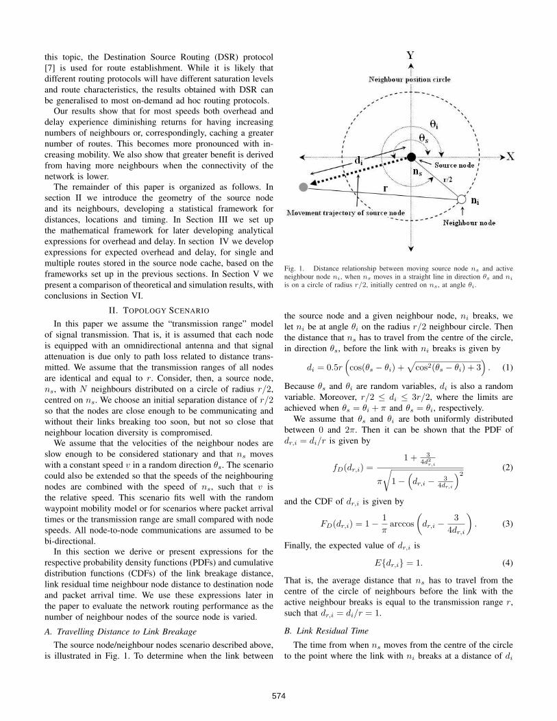
A. Travelling Distance to Link BreakageThe source node/neighbour nodes scenario described above,

is illustrated in Fig. 1. To determine when the link between

Fig. 1. Distance relationship between moving source node ns and activeneighbour node ni, when ns moves in a straight line in direction θs and ni

is on a circle of radius r/2, initially centred on ns, at angle θi.

the source node and a given neighbour node, ni breaks, welet ni be at angle θi on the radius r/2 neighbour circle. Thenthe distance that ns has to travel from the centre of the circle,in direction θs, before the link with ni breaks is given by

di = 0.5r(cos(θs − θi) +

√cos2(θs − θi) + 3

). (1)

Because θs and θi are random variables, di is also a randomvariable. Moreover, r/2 ≤ di ≤ 3r/2, where the limits areachieved when θs = θi + π and θs = θi, respectively.

We assume that θs and θi are both uniformly distributedbetween 0 and 2π. Then it can be shown that the PDF ofdr,i = di/r is given by

fD(dr,i) =1 + 3

4d2r,i

π

√1−

(dr,i − 3

4dr,i

)2(2)

and the CDF of dr,i is given by

FD(dr,i) = 1− 1π

arccos(

dr,i − 34dr,i

). (3)

Finally, the expected value of dr,i is

E{dr,i} = 1. (4)

That is, the average distance that ns has to travel from thecentre of the circle of neighbours before the link with theactive neighbour breaks is equal to the transmission range r,such that dr,i = di/r = 1.

B. Link Residual Time

The time from when ns moves from the centre of the circleto the point where the link with ni breaks at a distance of di

574

0 2 4 6 8 10 12 14 160

0.1

0.2

0.3

0.4

0.5

0.6

0.7

0.8

0.9

1

Link residual time

CD

FEffect of velocity on link residual time

v/r = 1v/r = 0.25v/r = 0.1

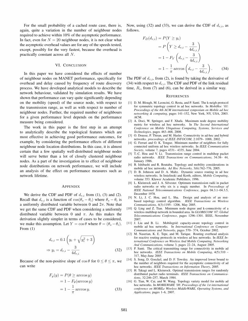
Fig. 2. The effect of velocity on the CDF of the link residual time, from (7)

is called the link residual time. The time required for ns tomove distance di at velocity v is given by

Ri =di

v=

dr,i

v/r. (5)

Because dr,i is a random variable, the link residual time, Ri,is also a random variable. The PDF of Ri can be shown to begiven by

fRi(ri) =vr + 3r

4vr2i

π

√1−

(vri

r − 3r4vri

)2(6)

with the CDF of Ri given by

FRi(ri) = 1− 1π

arccos(

vri

r− 3r

4vri

). (7)

Finally, the expected value of Ri is

E{Ri} =r

v. (8)

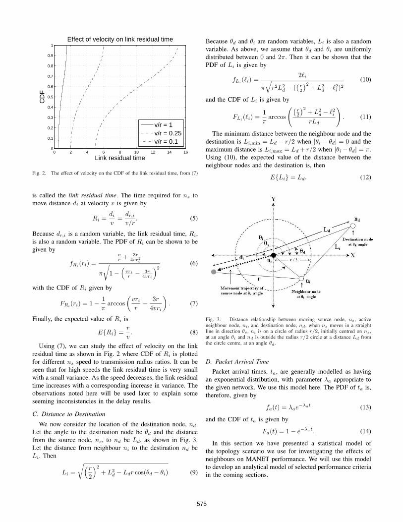
Using (7), we can study the effect of velocity on the linkresidual time as shown in Fig. 2 where CDF of Ri is plottedfor different ns speed to transmission radius ratios. It can beseen that for high speeds the link residual time is very smallwith a small variance. As the speed decreases, the link residualtime increases with a corresponding increase in variance. Theobservations noted here will be used later to explain someseeming inconsistencies in the delay results.

C. Distance to Destination

We now consider the location of the destination node, nd.Let the angle to the destination node be θd and the distancefrom the source node, ns, to nd be Ld, as shown in Fig. 3.Let the distance from neighbour ni to the destination nd beLi. Then

Li =

√(r

2

)2

+ L2d − Ldr cos(θd − θi) (9)

Because θd and θi are random variables, Li is also a randomvariable. As above, we assume that θd and θi are uniformlydistributed between 0 and 2π. Then it can be shown that thePDF of Li is given by

fLi(`i) =2`i

π

√r2L2

d − ((

r2

)2 + L2d − `2i )2

(10)

and the CDF of Li is given by

FLi(`i) =1π

arccos

((r2

)2 + L2d − `2i

rLd

). (11)

The minimum distance between the neighbour node and thedestination is Li,min = Ld − r/2 when |θi − θd| = 0 and themaximum distance is Li,max = Ld + r/2 when |θi− θd| = π.Using (10), the expected value of the distance between theneighbour nodes and the destination is, then

E{Li} = Ld. (12)

Fig. 3. Distance relationship between moving source node, ns, activeneighbour node, ni, and destination node, nd, when ns moves in a straightline in direction θs, ni is on a circle of radius r/2, initially centred on ns,at an angle θi and nd is outside the radius r/2 circle at a distance Ld fromthe circle centre, at an angle θd.

D. Packet Arrival Time

Packet arrival times, ta, are generally modelled as havingan exponential distribution, with parameter λa appropriate tothe given network. We use this model here. The PDF of ta is,therefore, given by

fa(t) = λae−λat (13)

and the CDF of ta is given by

Fa(t) = 1− e−λat. (14)

In this section we have presented a statistical model ofthe topology scenario we use for investigating the effects ofneighbours on MANET performance. We will use this modelto develop an analytical model of selected performance criteriain the coming sections.

575

III. ON-DEMAND ROUTING

In on-demand routing protocols, a source node attempts todiscover a route to a destination only when it is presented witha packet for forwarding to that destination. Usually a routecache is also employed to avoid carrying out a route discoveryfor every new packet to the same destination. However, cachedroutes may become outdated if, for example, two nodes in theroute have moved out of each others’ transmission ranges. Thisstale data may degrade performance, so a process for removingold routes is employed.

Overhead models for on-demand routing protocols are gen-erally based on the following principles [12].• When a source node, ns , initiates a new route discovery,

the consequent route request (RREQ) packet is broadcastthroughout the network. Any node receiving a duplicateRREQ discards the duplicate, so that each node is con-sidered to have only dealt with each RREQ once.

• When a destination node, nd, receives a RREQ from ns,it returns to ns a route reply (RREP) packet back alongthe route via which the RREQ arrived.

• If a node involved in forwarding a data packet alongan established route determines that the link of whichit is at the head is no longer valid, it returns an errorpacket (RERR) to ns back along the route. Monitoringthe correct operation of a route in use is referred to asroute maintenance [7].

Note that in the following analyses, all network traffic isignored except for the route discovery itself. This is to isolatethe effects of numbers and positions of neighbours.

A. Routing Overhead

When the details of an established route are saved in thecache, a route expiry time, T , is determined and saved for thatroute. After this time it is assumed that the route is no longervalid. If ns wishes to transmit to nd after this time it mustcarry out a new route discovery process. That is, if we let tabe the time of arrival of a new packet destined for nd, then, ifta < T and the cached route is not broken, no routing overheadis incurred in sending the new data packet. However, if ta > Ta route discovery process is automatically undertaken, usingflooding of RREQs, as discussed above. If there are n nodesin the network, n− 1 RREQ packets are transmitted during aflood (all nodes in the network receive the RREQ except forns), plus h RREPs where h is the number of hops between nd

and ns in the route chosen by nd as decided by the route ofthe first RREQ to reach nd. This scenario assumes that onlyone route is cached in any route discovery process.

In summary, the number of overhead packets generated byan on-demand routing protocol in response to a packet arrivalat time ta is given by,

OH =

{0 ta < T

n + h− 1 ta > T.(15)

Usually a third case, where ta < T but some later link inthe cached route is broken, should be considered. However

we discount this case because we wish to isolate the effect ofneighbour nodes on routing performance. We assume that alllinks in the active route remain intact except for the first link,that between ns and its active neighbour, ni.

B. Routing Delay

The routing delay is the time taken to transmit any controlpackets necessary to establish a route, before sending a datapacket between ns and nd. Since RREQ packets must prop-agate through the network to the destination, followed by thereturn of RREP packets, the routing delay is given by

D =

{0 ta < T

2thh ta > T,(16)

where h is the number of hops in the discovered path, and th isthe time taken for transmission over a single hop. We assumeth is a constant and the same for all hops in the network, andincludes processing time at the nodes at either end of the hopas well as propagation time.

As each wireless transmission has a maximum range, r,there is a strong relationship between the distance, Ld, fromns to nd and the minimum hop count. All routes must obey[6]

Number of hops in shortest path ≥ Ld

r. (17)

Most ad hoc routing protocols utilise hop count in their routeselection criteria. This approach minimises the total number oftransmissions required to send a packet on the selected path.If, in addition, the network is dense, then the number of hopsin the minimum hop path approaches L/r.

IV. ROUTING OVERHEAD AND DELAY

In this section we consider the expected overhead generatedand the expected delay incurred with the occurrence of anew route request. In each case, the expected value of theoverhead is equal to the cost of an individual route discoveryprocess, multiplied by the probability that the route discoveryis necessary. The probability of route discovery is determinedby the topology scenario and the caching strategy.

We consider two different caching strategies at the sourcenode. First, we assume that a single route to each destinationis stored in the source node cache. Next, we assume that thesource node cache holds multiple paths to each destination,each one commencing with one of its neighbour nodes.

A. One Route in Cache

1) Overhead: In this case we assume that the cache at nodens stores a single route for each destination nd, and that theroute commences with neighbour i with probability 1/N . Thatis, we assume that all of the neighbour nodes are equally likelyto be the first hop on the active route.

In order to incur routing overhead, the route must havebroken prior to the arrival of the next packet to send. That is,ns must have reached the breaking distance with respect to ni,such that Ri < ta. Then the expected value of the overhead,given link residual times R = (R1, R2, · · · , RN ) (i.e., given

576

that we know the position of each of the neighbour nodes andthe direction of travel of ns) is given by

E{OH|R = r}

=(n + h− 1)

N

N∑

i=1

[1− P (ta < ri)]

=(n + h− 1)

N

N∑

i=1

[1− Fa(ri)]

=(n + h− 1)

N

N∑

i=1

e−λari . (18)

We have used the fact that neighbour nodes are independentlyplaced, so link residual times are independent of each other.

The minimum distance travelled until a link breaks isdi,min = r/2 when |θs − θi| = π, such that dr,i,min = 1/2and the maximum travelled distance is di,max = 3r/2 whenθs = θi, such that dr,i,max = 3/2. The corresponding valuesof Ri are Ri,min = r/2v and Ri,max = 3r/2v. Using (6), andletting vr = v/r, the expected value of the routing overheadis, then

E{OH|one cached route}

=∫ R1,max

R1,min

· · ·∫ RN,max

RN,min

E{OH|R = r}fR(r)dr

=(n + h− 1)

π

∫ 3/2vr

1/2vr

e−λari

(vr + 3

4vrr2i

)√

1−(vrri − 3

4vrri

)2dri (19)

Unfortunately, there is no closed form solution to (19), soit must be calculated numerically. Note that the expectedoverhead is independent of the number of neighbours whenonly one route is cached.

2) Delay: When considering delay incurred with only onepath cached, we assume the routing protocol is configured toaggressively seek a minimum hop length path, which givesus a lower bound on delay. In this case the node ns cachesonly the route via the neighbour node with minimum distance(hops) to the destination. Once this route is broken, a newroute discovery process is necessary.

In order to calculate the expected route delay we need first tofind the distribution of the minimum distance Lmin = mini Li

between the neighbour nodes and the destination. Since neigh-bour node positions are independent and identically distributedin angle and distance from ns, we find that the CDF of theminimum distance is

FLmin(`) = 1− (1− FL(`))N (20)

and the PDF of the minimum distance is

fLmin(`) = N(1− FL(`))N−1fL(`). (21)

The expected value of the minimum distance between theneighbour nodes and the destination is, then

E{Lmin} =∫ Li,max

Li,min

`N(1− FL(`))N−1fL(`)d`. (22)

The hop between this closest neighbour to the destination andthe source node will be broken when the source node movestoo far away. Since the direction of movement of the sourcenode is independently distributed from the destination node,the link residual time is unaffected by the fact that we havechosen the closest neighbour to the destination. Hence theprobability that the link is broken when the route is needed isgiven by fRi

(ta). We have the expected delay

E{D|one cached route}

= 2th(E{Lmin}/r + 1)∫ 3/2vr

1/2vr

e−λatfRi(t)dt (23)

Comparing (23) with (19) we can see that the overhead anddelay for one cached route are identical in form, differing onlyby a constant factor.

B. Multiple Routes in CacheIn this case we assume that the routing protocol is con-

figured to avoid route discovery as long as possible. If thereare multiple routes in the cache, the moving source node willprogressively lose connection with the first hop in each route.If there are routes originating with each neighbour node, thelast route to be broken in this way will correspond to theclosest neighbour the direction of movement of the sourcenode.

1) Overhead: The cache at node ns stores multiple routesto nd, each commencing with a different neighbour node ni.A route to nd via neighbour node ni is stored with probabilityp. The probability that there are k routes cached is equal to

Pr(K = k) =N !

k!(N − k)!pk(1− p)N−k. (24)

In particular, if p = 1, then there are N cached routes withprobability 1.

As mentioned above, in this case the source node can usethe route through the neighbour closest to its direction ofmovement, θs, and no route discovery process is incurred untilthe link to that closest neighbour breaks. Let rmax k be themaximum Ri value, i ∈ {1, · · · , k}, for some k ≤ N .

Thus the expected value of the overhead, given Ri, i ={1, 2, · · · , N} is given by

E{OH|k = K,R = r}= E{OH|k = K,Rmax K = rmax K}= (n + h− 1)P{ta > rmax K}= (n + h− 1)(1− Fa(rmax K))

= (n + h− 1)e−λarmax K (25)

Since k > 0, the PDF of the maximum Rmax k is determinedby finding the CDF first, as follows.

FRmax k(t) = P{Rmax k < t}

= P{(R1 < t) ∪ (R2 < t) ∪ · · · ∪ (Rk < t)}

=k∏

i=1

P{Ri < t}

= F kRi

(t). (26)

577

Taking the derivative of (26) it can be seen that the PDF ofthe maximum Ri value is given by

fRmax k(t) = kF k−1

Ri(t)fRi(t), (27)

where FRi(ri) is from (7) and fRi

(ri) is from (6).Combining (25) and (27), we can determine an expression

for expected overhead when multiple paths are cached.

E{OH|many cached routes}

=N∑

K=0

∫ Ri,max

Ri,min

Pr(k = K)

· E{OH|k = K,Rmax k = t}· fRmax k

(t)dt

= (n + h− 1)[(1− p)N +

N∑

K=1

N !K!(N −K)!

pK(1− p)N−K

K

∫ 3/2vr

1/2vr

e−λatFK−1R (t)fR(t)dt

](28)

In the special case where p = 1, then k = N . That is, thesource node stores one route to the destination through eachneighbour node. We find that the expected overhead when allN neighbours have paths in the cache is

E{OH|N paths}

=∫ Ri,max

Ri,min

E{OH|R1 = r1, · · · , RN = rN}fRmax(t) dt

= (n + h− 1)N∫ Ri,max

Ri,min

e−λatFN−1Ri

(t)fRi(t)dt (29)

There is no closed form solution to either (28) or (29), sothey must be calculated numerically. Note that in both casesthe expected overhead is now dependent on the number ofneighbours.

2) Delay: Following similar reasoning to above, we findthat the expected value of the delay is equal to the expectedtime taken for an individual route discovery process, multipliedby the probability that the route discovery process is necessary.This probability is the same as in (29).

E{D|many routes}

= 2thE{h}N∫ Ri,max

Ri,min

e−λatFN−1Ri

(t)fRi(t)dt (30)

As discussed in section III-B, the expected number of hopsfrom the source to the destination is approximately E{Li}/r,where Li is the distance from the neighbour node i to thedestination node.

While the position of the neighbour node that is closestto the direction of movement of ns will tend towards thedirection of movement of the source node if N is large, thereis no dependence of the distance of this neighbour node tothe destination on N because the direction of the destinationnode from the source node, which also determines length Li,

is uniformly distributed independently of θs. Thus E{Li} isgiven in (21), and the expected route delay is

E{D|many routes}

= 2th(Ld/r)∫ Ri,max

Ri,min

Ne−λatFN−1Ri

(t)fRi(t)dt. (31)

Again, comparing (29) with (31) we can see that the overheadand delay for multiple cached routes are identical in form,differing only by a constant factor.

V. RESULTS

In this section we present and discuss results of compar-isons of theoretical calculations and Monte-Carlo simulations,conducted in Matlab, for the expected overhead and delay,discussed above. Note that the purpose of these simulationsis to validate the accuracy of the theoretical results, underthe given network assumptions, rather than provide a realisticnetwork simulation. More realistic simulation scenarios willbe the subject of future work.

The simulations were constructed based on the scenario inFigure 3 such that the relationship between the initial distanceof the source node to its neighbours and the transmission rangeis 1/2. The neighbour nodes are distributed around the sourcenode at uniformly distributed random angles. Note that nounits are specified as it is the relative and not absolute distancethat is important.

In order to have statistically accurate results, 10000 sim-ulation repetitions were carried out for each combination ofnumber of neighbour nodes and source node velocity. Thereported results are the average of those simulations. For eachsimulation repetition, the source node direction θs, ∼ u[0, 2π),and the neighbour node locations θi, ∼ u[0, 2π) are generated.These are used in equation (5) to calculate the link residualtimes. The packet arrival times, ta, at the source node arethen generated according to an exponential distribution withparameter λa = 0.1. The packet arrival times are comparedto the link residual times, and the overhead and delay areincremented if all routes in the cache have expired.

A. One Cached Route

The integral for the theoretical expression for expectedoverhead with one route saved in the cache, given in (19), wascalculated using a sum of the values of the integrand calculatedat incremental intervals. It was found that 105 incrementswere required for an accurate representation for one cachedpath. The overhead has been normalized by not including the(n + h− 1) factor.

Figure 4 compares the theoretical expression in (19) tosimulation results. It can be seen that the theoretical andsimulation results match very well. The overhead for onecached path increases with the ratio of source node velocity, v,to transmission range, r, reaching 90% of the maximum by thetime the ratio is equal to 1. The increase is quite steep initially,levelling off as v/r increases past 1. This makes sense as, asthe velocity increases, the difference between the link residualtime of the shortest possible link and the longest possible link

578

0 1 2 3 4 50

0.1

0.2

0.3

0.4

0.5

0.6

0.7

0.8

0.9

1

v/r

Ove

rhea

dOverhead with only one cached route

theorysimulation

Fig. 4. Normalized overhead as it varies with ratio of ns velocity totransmission range for a cached route from only one neighbour, from (19).

2 4 6 8 10 12 14 16 18 200

0.1

0.2

0.3

0.4

0.5

0.6

0.7

0.8

0.9

1

neighbours, N

Ove

rhea

d

Overhead with N cached routes

v/r = 5v/r = 2v/r = 1v/r = 0.5v/r = 0.25v/r = 0.1

Fig. 5. Normalized overhead as it varies with number of cached paths fromdifferent neighbour nodes, for various ratios of ns velocity to transmissionrange, from (29). Simulation results are depicted by markers while theoreticalresults are depicted by lines.

becomes more and more negligible. However, as mentioned inSection IV-A, there is no overhead benefit from having extraneighbours if only one path is cached.

The results for delay for only one cached route are shownin Figures 6 and 7, along with the delay for the N cachedroute case and are discussed in the next section.

B. N Cached Routes

1) Overhead: Similarly to the one cached route case, theintegral for the theoretical expression for the expected over-head for N cached routes, given in (29), was calculated usinga sum of the values of the integrand calculated at incrementalintervals. It was found that 106 increments were required foran accurate representation for N cached paths. Again, the

2 4 6 8 10 12 14 16 18 200

2

4

6

8

10

12

neighbours, N

Del

ay (

x t h )

Delay with N cached routes, h= 5

v/r = 1 Min. Hopv/r = 1 Avoid Discoveryv/r = 0.25 Min. Hopv/r = 0.25 Avoid Discoveryv/r = 0.1 Min. Hopv/r = 0.1 Avoid Discovery

Fig. 6. Delay as it varies with the number of cached paths from differentneighbour nodes, for h = Ld/r = 5 and various ratios of ns velocity totransmission range, from (23) and (31). Simulation results are depicted bymarkers while theoretical results are depicted by lines.

overhead has been normalized by not including the (n+h−1)factor. A comparison of theoretical and simulation results foroverhead for N cached routes is shown in Figure 5. Again thetheoretical and simulation results match very well. It can beseen that as the number of neighbouring nodes and, therefore,cached paths, increases, the overhead decreases. There isa levelling off of the overhead after an initial pronounceddecrease. The overhead decrease with increase in neighbours,N , is more pronounced with small v/r ratios. As v/r increasesthe difference in amount of overhead for different numbers ofcached paths becomes less pronounced to the point of beingalmost negligible when v/r = 5. Again, all of these trends areas would be expected. Except for the very slowest v/r ratiotested, the overhead is within 10% of its asymptotic valuewith 4 neighbour nodes. For the slowest ratio, 6 neighboursare required to reach this mark.

2) Delay: Figures 6 and 7 show comparisons of the the-oretical expressions for delay with one and N cached paths,respectively, given in (23) and (31), with simulation results.Note that the delay is shown in terms of th, the one-hop packettransmission time. In the simulations, th was arbitrarily set to1 time step. The “Avoid Discovery” case corresponds to the Ncached route case, described by (31) and the “Min. Hop” casecorresponds to the one cached route case, described by (31).Note that in Figure 6, the number of hops to the destinationwas kept small, at 5, and in Figure 7, the number of hops to thedestination was made larger, at 16. The results show that as thenumber of cached paths from neighbouring nodes increases,the delay decreases, with the decrease more pronounced forsmaller v/r ratios. Again the delay decreases with small v/rratios because of a decrease in the number of route discoveryprocesses required.

In both Figure 6 and Figure 7 it can be seen that the routedelay is almost always smaller when N routes were cached

579

2 4 6 8 10 12 14 16 18 200

5

10

15

20

25

30

35

40

45

neighbours, N

Del

ay (

x t h )

Delay with N cached routes, h= 16

v/r = 1 Min. Hopv/r = 1 Avoid Discoveryv/r = 0.25 Min. Hopv/r = 0.25 Avoid Discoveryv/r = 0.1 Min. Hopv/r = 0.1 Avoid Discovery

Fig. 7. Delay as it varies with the number of cached paths from differentneighbour nodes, for h = Ld/r = 16 and various ratios of ns velocity totransmission range, from (23) and (31). Simulation results are depicted bymarkers while theoretical results are depicted by lines.

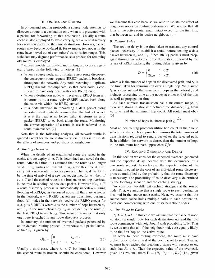
(“Avoid Discovery”) than when only the minimum hop route(one route) was cached. The only exception is for high v/rratio, for the smaller number of hops. However, both delaysare very close at high speeds and the switch is caused bya trade-off between the number of hops between neighbournodes and the destination node and the number of times anew route discovery process is required. Recall from Figure 2that for high velocities the link residual time is very small withonly a small variation over possible positions of the neighbournodes, meaning there will be little difference in how often anew route discovery process is required at such speeds. Also,the difference in number of hops between the routes to thedestination of the neighbour with the minimum number ofhops and that closest to the source (last route to fail when Nroutes are cached) is likely to be, at most, 2. So, in general,there is little delay benefit in caching only the minimum hoproute if the speed is high.

For the small number of hops case, except for the veryslowest speed v/r ratio tested, and only for the avoid discoverycase, the delay is within 10% of its asymptotic value with 4neighbour nodes. For the slowest ratio, for the avoid discoverycase, 6 neighbours are required to reach this mark.

For the large number of hops case, except for the veryslowest speed v/r ratio tested, and only for the avoid discoverycase, the delay is within 10% of its asymptotic value with 4neighbour nodes. For the slowest ratio, for the avoid discoverycase, 8 neighbours are required to reach this mark.

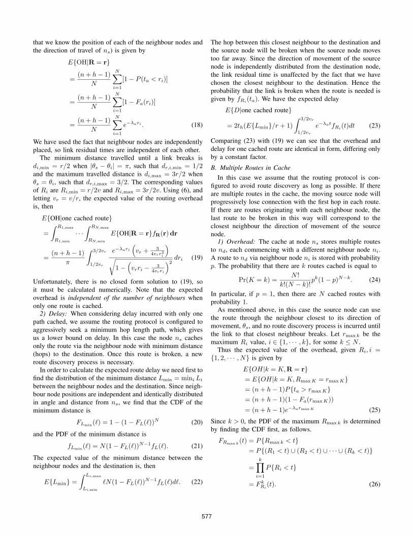
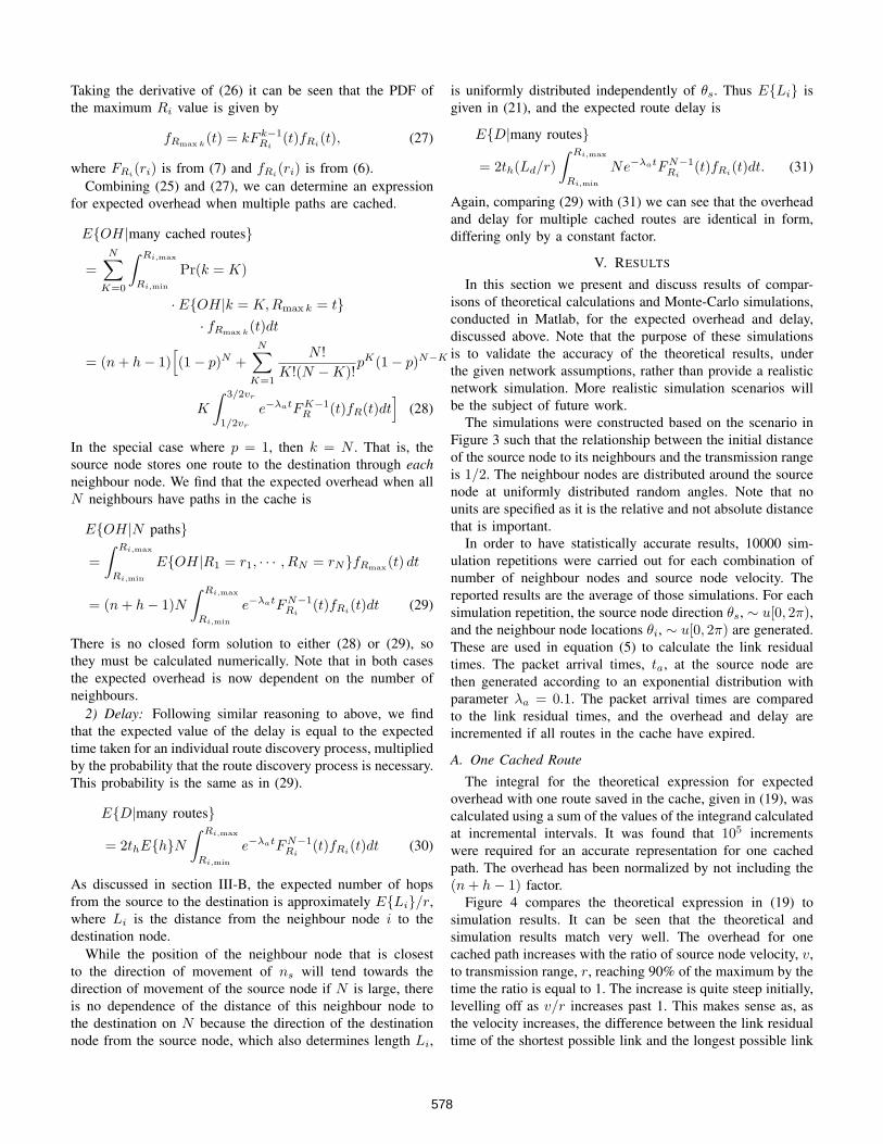
C. k Cached Routes

Figures 8 and 9 illustrate the overhead incurred when kroutes to the destination node are cached, from (28), withprobability of any particular neighbour node’s route beingchosen, of 0.2 and 0.7, respectively. These two cases could,for example, correspond to a poorly connected network and

2 4 6 8 10 12 14 16 18 200

0.1

0.2

0.3

0.4

0.5

0.6

0.7

0.8

0.9

1

neighbours, N

Ove

rhea

d

Overhead with k cached routes, p=0.2

v/r = 5v/r = 2v/r = 1v/r = 0.5v/r = 0.25v/r = 0.1

Fig. 8. Normalized overhead as it varies with the k cached paths fromdifferent neighbour nodes with probability of a path, p = 0.2, for variousratios of ns velocity to transmission range, from (28). Simulation results aredepicted by markers while theoretical results are depicted by lines.

2 4 6 8 10 12 14 16 18 200

0.1

0.2

0.3

0.4

0.5

0.6

0.7

0.8

0.9

1

neighbours, N

Ove

rhea

dOverhead with k cached routes, p=0.7

v/r = 5v/r = 2v/r = 1v/r = 0.5v/r = 0.25v/r = 0.1

Fig. 9. Normalized overhead as it varies with k cached paths from differentneighbour nodes with probability of a path, p = 0.7, for various ratios of ns

velocity to transmission range, from (28). Simulation results are depicted bymarkers while theoretical results are depicted by lines.

a well-connected network, respectively. As the number ofneighbour nodes increases, the number of cached paths fromneighbour nodes correspondingly increases, and it can be seenthat the overhead decreases. The overhead decrease is morepronounced with small v/r ratios, becoming almost negligiblewith larger speeds. In fact, with low speeds and low probabilityof any particular neighbour node having a cached route to thedestination, it is best for the source to have as many neighboursas possible. Further, the overhead is greater for all speeds andnumbers of neighbours when the probability of a route beingcached for any given neighbour is smaller. All of these trendsare as would be expected.

580

For the small probability of a cached route case, there is,again, quite a variation in the number of neighbour nodesrequired to achieve within 10% of the asymptotic performance.In fact, even for N = 20 neighbour nodes, it is not clear whatthe asymptotic overhead values are for any of the speeds tested,except, possibly for the very fastest, because the overhead ispractically constant across all N .

VI. CONCLUSION

In this paper we have considered the effects of numberof neighbour nodes on MANET performance, specifically foroverhead and delay caused by frequency of route discoveryprocess. We have developed analytical models to describe thenetwork behaviour, validated by simulation results. We haveshown that performance can vary quite significantly dependingon the mobility (speed) of the source node, with respect tothe transmission range, as well as with respect to number ofneighbour nodes. Further, the required number of neighboursfor a given performance level depends on the performancemeasure being considered.

The work in this paper is the first step in an attemptto analytically describe the topological features which aremost effective in achieving good performance outcomes, forexample, by considering the performance effects of differentneighbour node location distributions. In this case, it is almostcertain that a few spatially well-distributed neighbour nodeswill serve better than a lot of closely clustered neighbournodes. As a part of the investigation in to effect of neighbournode distributions on network performance, we will includean analysis of the effect on performance measures such asnetwork lifetime.

APPENDIX

We derive the CDF and PDF of dr,i from (1), (3) and (2).Recall that dr,i is a function of cos(θs − θi) where θs − θi isa uniformly distributed variable between 0 and 2π. Note thatwe get the same CDF and PDF when considering a uniformlydistributed variable between 0 and π. As this makes thederivation slightly simpler in terms of cases to be considered,we make this assumption. Let Y = cos θ where θ = (θs−θi).From (1)

dr,i = 0.1(

yi +√

y2i + 3

)

⇒ yi = dr,i − 34dr,i

(32)

Because of the non-positive slope of cos θ for 0 ≤ θ ≤ π, wecan write

Fy(y) = P (θ ≥ arccos y)= 1− Fθ(arccos y)

= 1− 1π

arccos y. (33)

Now, using (32) and (33), we can derive the CDF of dr,i, asfollows.

FD(dr,i) = P (Y ≥ yi)

= P

(Y ≥ dr,i − 3

4dr,i

)

= 1− FY

(dr,i − 3

4dr,i

)

= 1− 1π

arccos(

dr,i − 34dr,i

). (34)

The PDF of dr,i, from (2), is found by taking the derivative of(34) with respect to dr,i. The CDF and PDF of the link residualtime, Ri, from (7) and (6), can be derived in a similar way.

REFERENCES

[1] D. M. Blough, M. Leoncini, G. Resta, and P. Santi. The k-neigh protocolfor symmetric topology control in ad hoc networks. In MobiHoc ’03:Proceedings of the 4th ACM international symposium on Mobile ad hocnetworking & computing, pages 141–152, New York, NY, USA, 2003.ACM.

[2] A. Doci, W. Springer, and F. Xhafa. Maximum node degree mobilitymetric for wireless ad hoc networks. In The Second InternationalConference on Mobile Ubiquitous Computing, Systems, Services andTechnologies, pages 463–468, 2008.

[3] O. Dousse, P. Thiran, and M. Hasler. Connectivity in ad-hoc and hybridnetworks. proceedings of IEEE INFOCOM, 2:1079– 1088, 2002.

[4] G. Ferrari and O. K. Tonguz. Minimum number of neighbors for fullyconnected uniform ad hoc wireless networks. In IEEE CommunicationSociety, volume 7, pages 4331– 4335, June 2004.

[5] T.-C. Hou and V. Li. Transmission range control in multihop packetradio networks. IEEE Transactions on Communications, 34:38– 44,January 1986.

[6] B. Ishibashi and R. Boutaba. Topology and mobility considerations inmobile ad hoc networks. Ad Hoc Networks, 3(6):762–776, 2005.

[7] D. B. Johnson and D. A. Maltz. Dynamic source routing in ad hocwireless networks. In Imielinski and Korth, editors, Mobile Computing,volume 353. Kluwer Academic Publishers, 1996.

[8] L. Kleinrock and J. A. Silvester. Optimum transmission radii in packetradio networks or why six is a magic number. In Proceedings ofIEEE National Telecommunications Conference, pages 04.3.1–04.3.5,December 1978.

[9] N. Li, J. C. Hou, and L. Sha. Design and analysis of an mst-based topology control algorithm. IEEE Transactions on WirelessCommunications, 4(3):1195– 1206, May 2005.

[10] Q. Ling and Z. Tian. Minimum node degree and k-connectivity of awireless multihop network in bounded area. In GLOBECOM ’07: GlobalTelecommunications Conference, pages 1296–1301. IEEE, November2007.

[11] J. Liu and B. Li. Mobilegrid: capacity-aware topology control inmobile ad hoc networks. In International Conference on ComputerCommunications and Networks, pages 570– 574, October 2002.

[12] M. Naserian, K. E. Tepe, and M. Tarique. Routing overhead analysisfor reactive routing protocols in wireless ad hoc networks. In IEEE In-ternational Conference on Wireless And Mobile Computing, NetworkingAnd Communications, volume 3, pages 22–24, August 2005.

[13] P. Santi. The critical transmitting range for connectivity in mobile adhoc networks. IEEE Transactions on Mobile Computing, 4(5):310 –317, May-June 2005.

[14] S. Song, D. Goeckel, and D. F. Towsley. An improved lower bound tothe number of neighbors required for the asymptotic connectivity of adhoc networks. IEEE Transactions on Information Theory, 2005.

[15] H. Takagi and L. Kleinrock. Optimal transmission ranges for randomlydistributed packet radio terminals. IEEE Transactions on Communica-tions, 32:246–257, March 1984.

[16] G. Tian, W. Cai, and W. Wang. Topology variety model for mobile adhoc networks. In MOBILWARE ’08: Proceedings of the 1st internationalconference on MOBILe Wireless MiddleWARE, Operating Systems, andApplications, pages 1–6, 2007.

581

[17] O. K. Tonguz and G. Ferrari. Is the number of neighbors in ad hocwireless networks a good indicator of connectivity? IEEE InternationalZurich Seminar on Communications : Access-Transmission-Networking,18-20 Feb. 2004.

[18] J. Tsumochi, K. Masayama, H. Uehara, and M. Yokoyama. Impact ofmobility metric on routing protocols for mobile ad hoc networks. InProc. of IEEE PacRim ‘03, pages 322–325, Augest 2003.

[19] P.-J. Wan and C.-W. Yi. Asymptotic critical transmission radius andcritical neighbor number for k-connectivity in wireless ad hoc networks.International Symposium on Mobile Ad Hoc Networking and Computing,pages 1–8, May 2004.

[20] Y. Wang and X.-Y. Li. Distributed spanner with bounded degree forwireless ad hoc networks. Foundations of Computer Science, 14(2):183–200, 2003.

[21] J. Wu and F. Dai. Mobility-sensitive topology control in mobile adhoc networks. IEEE Transactions on Parallel and Distributed Systems,17(6):522–535, June 2006.

[22] J. Wu and D. R. Stinson. Minimum node degree and k-connectivityfor key predistribution schemes and distributed sensor networks. InWiSec ’08: Proceedings of the first ACM conference on Wireless networksecurity, pages 119–124. ACM, 2008.

[23] F. Xue and P. Kumar. The number of neighbors needed for connectivityof wireless networks. Wireless Networks, 10(2):169–181, March 2004.

[24] E. Yanmaz. Impact of topology-dependent and independent mobilitymodels on the connectivity of wireless networks. In Sarnoff Symposium,IEEE, pages 1–5, April 2008.

582