ON THE LOW-RANK APPROXIMATION OF DATA ON THE UNIT SPHERE

M. CHU∗, N. DEL BUONO† , L. LOPEZ‡ , AND T. POLITI§

Abstract. In various applications, data in multi-dimensional space are normalized to unit length. This paperconsiders the problem of best fitting given points on the m-dimensional unit sphere Sm−1 by k-dimensional greatcircles with k much less than m. The task is cast as an algebraically constrained low-rank matrix approximationproblem. Using the fidelity of the low-rank approximation to the original data as the cost function, this paperoffers an analytic expression of the projected gradient which, on one hand, furnishes the first order optimalitycondition and, on the other hand, can be used as a numerical means for solving this problem.

Key words. standardized data, linear model, factor analysis, low-rank approximation, latent semanticindexing, projected gradient

1. Introduction. Given n points on the unit sphere Sm−1 in Rm, we concern ourselvesin this paper with the question of best fitting these points by a “great circle” which is understoodto mean the intersection of Sm−1 with a certain k-dimensional subspace of Rm. Because theapproximation is by points restricted to Sm−1, we are not dealing with an ordinary data fittingproblem. Denoting the given points as rows of a data matrix A, the task of best fitting can berecast as a constrained low-rank matrix approximation problem as follows:

Given a matrix A ∈ Rn×m whose rows are of unit length, find an approximation

matrix Z ∈ Rn×m of A whose rows are also of unit length, but rank(Z) = k where

k < min{m,n}.

Structured low-rank approximation problems arise in many important applications [3, 4, 13,24, 33]. Some basic theory and computation schemes, including a generic alternating projectionalgorithm and a robust equality constrained optimization formulation, can be found in a recentarticle [9] by the first author and the references contained therein. The structure in our currentproblem assumes the form that each row of Z has unit length. A similar setting appears in anapplication to designing structured tight frames [34] where the alternating projection methodis used as an effective tool. When the row number n is much larger than the rank k, however,reformulations of this problem as the two schemes proposed in [9] would involve significant amountof redundancies in the constraints which, in turn, might cause computational difficulties. Theapproximation obtained by a linear combination of concept vectors generated by the sphericalk-means method [14], on the other hand, lacks the normalization and is limited only to thesubspace spanned by the concept vectors. In this paper we propose using the projected gradientapproach as an alternative means to tackle the problem. Three types of measurement of bestfitting will be used and their results will be compared.

The need of normalizing data before approximations can be performed emerges from manyapplications. See, for example, the book [12] about pattern classification, the monograph [21]and the vast literature on principal component analysis, the required goal in positive matrixfactorization [26], and the spherical k-means method for concept mining in [14]. It might beilluminating to brief readers by some simple examples of why such a normalized low-rank ap-

∗Department of Mathematics, North Carolina State University, Raleigh, NC 27695-8205. (chu@math.ncsu.edu)This research was supported in part by the NSF under grants DMS-0073056 and CCR-0204157, and in part bythe INDAM under the Visiting Professorship Program when the author visited the Department of Mathematicsat the University of Bari.

†Dipartimento di Matematica, Universita degli Studi di Bari, Via E. Orabona 4, I-70125 Bari, Italy. (del-buono@dm.uniba.it)

‡Dipartimento di Matematica, Universita degli Studi di Bari, Via E. Orabona 4, I-70125 Bari, Italy.(lopezl@dm.uniba.it)

§Dipartimento di Matematica, Politecnico di Bari, Via Amendola 126/B, 70126 Bari, Italy. (politi@poliba.it)

1

proximation problem is of importance in practice. To set the stage, let Y = [yij ] ∈ Rn×` denotethe matrix of “observed” data. The entry yij represents, in a broad sense, the standard score

obtained by entity j on variable i. By a standard score we mean that a raw score per variable hasbeen normalized to have mean 0 and standard deviation 1. After this normalization, the matrix

R :=1

`Y Y >, (1.1)

represents the correlation matrix of all n variables. Note that rii = 1 and |rij | ≤ 1 for alli, j = 1, . . . n. In a linear model, it is assumed that the score yij is a linearly weighted score byentity j based on several factors. We shall temporarily assume that there are m factors, but itis precisely the point that the factors are to be retrieved in the mining process. A linear model,therefore, assumes the relationship

Y = AF, (1.2)

where A = [aik] ∈ Rn×m is a loading matrix with aik denoting the influence of factor k on

variable i, and F = [fkj ] ∈ Rm×` is a scoring matrix with fkj denoting the response of entity jto factor k. Depending on the application, often only a portion of the matrices in equation (1.2)is known and the goal is to retrieve the remaining information. The linear model (1.2) can havedifferent interpretations. We sketch two scenarios below.

Scenario 1. Assume that each of the ` columns of the observed matrix Y represents thetranscript of a college student (an entity) at the end of freshman year on n fixed subjects (thevariables). It is generally believed that a college freshman’s academic performance depends on anumber of preexistent factors. Upon entering the college, each student could be asked to fill outa questionnaire inquiring his or her backgrounds (scores) with respect to these factors. Theseresponses are placed in the corresponding column of the scoring matrix F . What is not clear tothe administrators in the first place is how to choose the factors to compose the questionnaireor how each of the chosen factors would be weighted (the loadings) to reflect their effect on eachparticular subject. In practice, we usually do not have a priori knowledge about the number andcharacter of underlying factors in A. Sometimes we do not even know the factor scores in F .Only the data matrix Y is observable. Explaining the complex phenomena observed in Y withthe help of a minimal number of factors extracted from the data matrix is the primary and mostimportant goal of factor analysis.

To collectively gather students’ academic records from wide variations (of grading rules anddifficulties of subjects) for the purpose of analyzing some influential factors in A, it is essentialthat all these scores should be evaluated on the same basis. Otherwise, the factors cannot becorrectly revealed. Statistically, the same basis of scores means the standardization (of rows)of Y . For our purpose, it is reasonable to assume that all sets of factors being considered areuncorrelated with each other. (See [21] for the case of stochastic independence.) As such, rowsof F should be orthogonal to each other. We should further assume that the scores in F foreach factor are normalized. Otherwise, one may complain that the factors being consideredare not neutral to begin with and the analysis would be biased and misinformed. Under theseassumptions, we have

1

`FF> = Im, (1.3)

where Im stands for the identity matrix in Rm×m. It follows that the correlation matrix R canbe expressed directly in terms of the loading matrix A alone, i.e.,

R = AA>. (1.4)

2

Factor extraction now becomes a problem of decomposing the correlation matrix R into theproduct AA> using as few factors as possible [18]. Due to the normalization we point out that

the rows of A always are of unit length.

The kth column of A may be interpreted as correlations of the data variables with thatparticular kth factor. Those data variables with high factor loadings are considered to be moreinfluenced by the factor in some sense and those with zero or near-zero loadings are treatedas being unlike the factor. The quality of this likelihood, indicating the significance of thecorresponding factor, is measured by the norm of the kth column of A. One basic idea in factoranalysis is to rewrite the loadings of variables over some newly selected factors so as to manifestmore clearly the correlation between variables and factors [17, 21]. Those factors with smallersignificance are likely to be dropped to reduce the number of effectual factors. This notion of

factor reduction amounts to a low-rank approximation of A.

Scenario 2. Assume now that the textual documents are collected in an indexing matrix

H = [hik] in Rn×m. Each document is represented by one row in H. The entry hik representsthe weight of one particular term k in document i whereas each term could be defined by just onesingle word or a string of phrases. A natural choice of the weight hik is by counting the numberof times that the term k occurs in document i. Many more elaborate weighting schemes thatyield better performance have been devised in the literature. See, for example, lists in [23, 28]and comparisons in [31]. One commonly used term-weighting scheme to enhance discriminationbetween various documents and to enhance retrieval effectiveness is to define

hik = tikgkni, (1.5)

where tik captures the relative importance of term k in document i, gk weights the overallimportance of term k in the entire set of documents, and

ni =

(

m∑

k=1

tikgk

)−1/2

(1.6)

is the scaling factor for normalization. The normalization by (1.6) is necessary because, otherwise,one could artificially inflate the prominence of document i by padding it with repeated pages orvolumes. After the normalization, one sees that the rows of H are of unit length.

One usage of the indexing matrix is for information retrieval, particularly in the context oflatent semantic indexing (LSI) application [2, 16]. Each query is represented as a column vectorq>j = [q1j , . . . , qmj ] in Rm where qkj represents the weight of term k in the query j. Similar to(1.5), more elaborate schemes can also be employed to weight terms in a query. To measure howthe query qj matches the documents, we calculate the column vector

cj = Hqj (1.7)

and rank the relevance of documents to qj according to the scores in cj .To put the notation in the context of linear model (1.2), we observe the follow analogies

between the two examples:

indexing matrix H ←→ loading matrix A

document i←→ variable i

term k ←→ factor k

one query qj ←→ one column in scoring matrix F

weight hik of term k in document i←→ loading aik of factor k on variable i

weights qkj of term k in query qj ←→ response fkj of entity j to factor k

rank cij of document i in query qj ←→ score yij of variable i in entity j

3

It is important to note the different emphasis in the two examples. In Scenario 1 the datamatrix Y is given and the factors in A are to be retrieved while in Scenario 2 the terms in theindexing matrix H are predetermined and the scores cj are to be calculated.

The computation involved in the LSI application is more on the vector-matrix multiplication(1.7) than on factor retrieval, provided that H is a “reasonable” representation of the relationshipbetween documents and terms. In practice, however, the matrix H is never exact nor perfect.How to represent the indexing matrix and the queries in a more compact form so as to facilitatethe computation of the scores therefore become a major challenge in the field [14, 27]. Oneidea, with the backing of both statistical analysis [7] and empirical testing [2], is to represent Hby its low-rank approximation. A constrained low-rank approximation problem therefore arises.We shall point out in our numerical examples that the fidelity to H by merely normalizing atruncated singular value decomposition is not as high as what our method can achieve.

One final point connecting Scenario 1 to Scenario 2 is worth mentioning. It is plausible thatonce we have accumulated enough experiences C = [c1, . . . , c`] from queries q1, . . . ,q`, we shouldbe able to employ whatever factor retrieval techniques developed for Scenario 1 to reconstructterms (factors) for Scenario 2. That is, after the standardization of the scores, the informationgathered in C may be used as a feedback to the process of selecting newer and more suitable H.Recall from (1.4) that no reference to the queries is needed. This learning process with feedbackfrom C can be iterated to reduce and improve the indexing matrix H.

2. Low Rank Approximation. The linear model (1.2) can have a much broader in-terpretation than the two applications we have demonstrated. Its interpretation in Scenario 1for factor analysis manifests the critical role that the loading matrix A will play. Our low-rankapproximation problem means the need to retrieve a few principal factors to represent the origi-nal A. Likewise, the interpretation in Scenario 2 for the information retrieval suggests that theindexing matrix H is playing an equally important role as the loading matrix A. Our low-rankapproximation problem in the context of LSI means the need to derive an approximation of Hto allow fast computation. In this section, we introduce a notion that can be employed to dealwith this algebraically constrained low-rank approximation problem.

The quality of the approximation by a lower rank matrix Z to A can be measured in differentways. In the following, we shall describe three kinds of measurements and use them to form ourobjective functions. For convenience, the notation diag(M) henceforth refers to the diagonalmatrix of the matrix M .

2.1. Fidelity Test. Considering A as the indexing matrix in the LSI, one way to inferwhether Z is a good (but low-rank) representation of A is to use documents (rows) in A as queriesthemselves to inquire about document information from Z. If the document-term relationshipsembedded in Z adhere to those in A, then the scores of the query qj applied to Z, where q>

j

is the j-th row of A, should point to the most relevant document j. It should be so for eachj = 1, . . . , n. In other words, in the product ZA> the highest score per column should occurprecisely at the diagonal entry. This notion of self-examination is referred to as the fidelity testof Z to A.

Ideally, the fidelity test should product the maximum value 1 along the diagonal. Since theindexing matrix A is never perfect, we may as well be settled with the collective effect for the sakeof easy computation. We say that the approximation Z remains in “good” fidelity to the originalA if the trace of ZA> is sufficiently close to trace(AA>) = n. This low-rank approximationproblem therefore becomes the problem of maximizing

trace(ZA>) = 〈Z,A〉, (2.1)

where 〈M,N〉 stands for the Frobenius inner product of matrices M and N in Rn×m. Theobjective, in short, is to maximize the fidelity of Z to A while maintaining its low rank.

4

In order to characterize the properties that the matrix Z is of rank k with unit-length rows,we introduce the parametrization that

Z =(

diag(

USS>U>))−1/2

USV >, (2.2)

where U ∈ On, S ∈ Rk, V ∈ Om, and On denotes the group of orthogonal matrices of size n×n.The task now is equivalent to maximizing the functional

F (U, S, V ) := 〈(

diag(

USS>U>))−1/2

USV >, A〉, (2.3)

subject to the orthogonal conditions of U and V . In the above, we have used the same symbolS ∈ Rk to denote, without causing ambiguity, the “diagonal matrix” in Rn×m whose first k

diagonal entries are those of S. Observe that by limiting S to Rk, the rank of the matrixX = USV > ∈ Rn×m is guaranteed to be at most k, and is exactly k if S contains no zero entry.

The Frechet derivative of F at (U, S, V ) acting on any (H,D,K) ∈ Rn×n ×Rk ×Rm×m canbe considered as the sum of three operations,

F ′(U, S, V ).(H,D,K) =∂F

∂U.H +

∂F

∂S.D +

∂F

∂V.K, (2.4)

where the operation Λ.η denotes the result of the action by the linear operator Λ on the η. Forconvenience, define

α(U, S) :=(

diag(

USS>U>))−1

. (2.5)

We now calculate each action in (2.4) as follows.First, it is easy to see that

∂F

∂V.K = 〈α(U, S)1/2USK>, A〉. (2.6)

Using the property that

〈MN,P 〉 = 〈M,PN>〉 = 〈N,M>P 〉 (2.7)

for any matrices M , N and P of compatible sizes, it follows from the Riesz representation theoremthat, with respect to the Frobenius inner product, the partial gradient can be represented as

∂F

∂V= A>α(U, S)1/2US. (2.8)

Observe next that

∂F

∂S.D = 〈α(U, S)1/2UDV >, A〉+ 〈

(

∂α(U, S)1/2

∂S.D

)

USV >, A〉. (2.9)

By the chain rule we have

∂α(U, S)1/2

∂S.D =

1

2α(U, S)−1/2

(

−α(U, S)diag(

UDS>U> + USD>U>)

α(U, S))

= −1

2α(U, S)3/2diag

(

UDS>U> + USD>U>)

, (2.10)

where we have used the fact that diagonal matrices are commutable. Denoting the diagonalmatrix

ω(U, S, V ) := α(U, S)3/2diag(

AV S>U>)

, (2.11)

5

and taking advantage of the fact that 〈M,diag(N)〉 = 〈diag(M),diag(N)〉, the action in (2.9)can be expressed as

∂F

∂S.D = 〈D,U>α(U, S)1/2AV 〉 −

1

2〈UDS>U> + USD>U>, ω(U, S, V )〉

= 〈D,diag(

U>α(U, S)1/2AV)

〉 − 〈D,diag(

U>ω(U, S, V )US)

〉. (2.12)

We thus conclude that

∂F

∂S= diagk

(

U>α(U, S)1/2AV)

− diagk(

U>ω(U, S, V )US)

, (2.13)

where, for clarity, we use diagk to denote the first k diagonal elements and to emphasize that thepartial gradient ∂F

∂S is in fact a vector in Rk.Finally,

∂F

∂U.H = 〈α(U, S)1/2HSV >, A〉+ 〈

(

∂α(U, S)1/2

∂U.H

)

USV >, A〉, (2.14)

whereas by chain rule again we know that

∂α(U, S)1/2

∂U.H =

1

2α(U, S)−1/2

(

−α(U, S)diag(

HSS>U> + USD>H>)

α(U, S))

= −1

2α(U, S)3/2diag

(

HSS>U> + USS>H>)

. (2.15)

Together, we obtain

∂F

∂U.H = 〈H,α(U, S)1/2AV S>〉 −

1

2〈HSS>U> + USS>H>, ω(U, S, V )〉

= 〈H,α(U, S)1/2AV S>〉 − 〈H,ω(U, S, V )USS>〉, (2.16)

and hence

∂F

∂U= α(U, S)1/2AV S> − ω(U, S, V )USS>. (2.17)

Formulas (2.8), (2.13), and (2.17) constitute the gradient

∇F (U, S, V ) =

⟨

∂F

∂U,∂F

∂S,∂F

∂V

⟩

of the objection function F . Because our parameters (U, S, V ) must come from the manifoldOn × Rk ×Om, we want to know further the projection of ∇F into the feasible set.

By taking advantage of the product topology, the tangent space T(U,S,V )(On × Rk ×Om) of

the product manifold On × Rk × Om at (U, S, V ) ∈ On × Rk × Om can be decomposed as theproduct of tangent spaces, i.e.,

T(U,S,V )(On × Rk ×Om) = TUOn × Rk × TVOm. (2.18)

The projection of ∇F (U, S, V ) onto T(U,S,V )(On × Rk × Om), therefore, is the product of the

projections of ∂F∂U , ∂F

∂S , and ∂F∂V onto TUOn, Rk, and TVOm, respectively. Each of the projections

can easily be calculated by using the techniques developed in [8] which we summarize below.

6

Observe that any matrix M ∈ Rn×n has a unique orthogonal splitting,

M = U

{

1

2(U>M −M>U)

}

+ U

{

1

2(U>M + M>U)

}

, (2.19)

as the sum of elements from the tangent space TUOn and the normal space NUOn. Thus theprojection PTUOn

(M) of M onto TUOn is given by the matrix

PTUOn(M) = U

{

1

2(U>M −M>U)

}

. (2.20)

Replacing M by ∂F∂U in (2.20), we thus obtain the explicit formulation of the projection of ∂F

∂Uonto the tangent space TUOn, that is,

PTUOn(∂F

∂U)={

(

XXTω(U, S, V )−ω(U, S, V )XXT)

+(

α(U, S)1/2AXT−XATα(U, S)1/2)} U

2.

Similarly, the projection of ∂F∂V onto tangent spaces TVOm can be calculated. The projection of

∂F∂S onto Rk is just itself. These projections characterize precisely the projected gradient of theobjective function F (U, S, V ) on the manifold On × Rk ×Om.

The explicit formulation of the project gradient serves as the first order optimality conditionthat any local solution must satisfy. Many iterative methods making use of projected gradientfor constrained optimization are available in the literature [11, 19]. On the other hand, we findit most natural and convenient to use the dynamical system,

dU

dt= PTUOn

(∂F

∂U),

dS

dt=∂F

∂S, (2.21)

dV

dt= PTV Om

(∂F

∂V),

to navigate a flow on the manifold On × Rk × Om. The flow, called the fidelity flow for laterreference, moves along the steepest ascent direction to maximize the objective functional F . Since(2.21) defines an ascent flow by an analytic vector field, by the well-known ÃLojasiewicz-Simontheorem [6, 25, 30] the flow converges to a single point (U∗, S∗, V∗) of equilibrium at which

Z∗ =(

diag(

U∗S∗S>∗ U

>∗

))−1/2U∗S∗V

>∗ (2.22)

is locally the best rank k approximation to A subject to constraint of unit row vectors.

2.2. Nearness Test. In the context of LSI, each document is represented by a singlepoint in the term space Rm. It is natural to evaluate the quality of an approximation Z to A

by measuring how far Z is from A. The low-rank approximation problem therefore becomes theproblem of minimizing the functional

E(U, S, V ) :=1

2〈α(U, S)1/2USV > −A,α(U, S)1/2USV > −A〉, (2.23)

subject to the constraints that U ∈ On, S ∈ Rk, and V ∈ Om. This notion of finding low-rank matrices nearest to the given A is called the nearest test. Nearest low-rank approximationproblems under different (linear) structures have been considered in [9, 14, 27]. By a linearstructure, we mean that all matrices of the same structure form an affine subspace. Our structure,defined by the requirement that each row is of unit length, is not a linear structure.

7

We quickly point out the fact that

1

2〈Z −A,Z −A〉 =

1

2(〈Z,Z〉+ 〈A,A〉)− 〈Z,A〉. (2.24)

Note that 〈Z,Z〉 = 〈A,A〉 = n. Therefore, minimizing the functional E(U, S, V ) in (2.23) isequivalent to maximizing the functional F (U, S, V ) in (2.3). The fidelity test is exactly the sameas the nearest test under the Frobenius inner product.

2.3. Absolute Fidelity Test. The data matrix A in general might contain negativeentries. In this case, cancellations among terms in the trace calculation might inadvertentlyreduce the fidelity quality. To prevent cancellation, we might want to consider maximizing thesum of squares of the diagonal elements of ZA>. The objective functional to be maximized is

G(U, S, V ) :=1

2〈diag

(

α(U, S)1/2USV >A>)

,diag(

α(U, S)1/2USV >A>)

〉, (2.25)

subject to the constraints that U ∈ On, S ∈ Rk, and V ∈ Om. We remark in passing that ina certain sense the absolute fidelity test has the effect of rewarding both anti-correlation andpositive correlation between matrices A and Z. In certain applications, such as identifying geneswith similar functionalities, detecting anti-correlated gene clusters sometimes is as important asdetecting positively correlated genes [15].

Once again, denote the Frechet derivative of G at (U, S, V ) acting on any (H,D,K) ∈ Rn×n×Rk × Rm×m as

G′(U, S, V ).(H,D,K) =∂G

∂U.H +

∂G

∂S.D +

∂G

∂V.K. (2.26)

We can calculate each partial derivative in (2.26) to obtain the gradient ∇G.For convenience, denote

θ(U, S, V ) := diag(

α(U, S)1/2USV >A>)

. (2.27)

Observe that diag(·) is a linear operator, so its derivative is just itself. It follows that

∂G

∂V.K = 〈α(U, S)1/2USK>A>, θ(U, S, V )〉. (2.28)

Using (2.7) and the fact that diagonal matrices commute, we see that

∂G

∂V= A>θ(U, S, V )>α(U, S)1/2US = A>α(U, S)diag

(

USV >A>)

US. (2.29)

Likewise,

∂G

∂S.D = 〈diag

(

α(U, S)1/2UDV >A>)

, θ(U, S, V )〉+

+〈diag

((

∂α(U, S)1/2

∂S.D

)

USV >A>

)

, θ(U, S, V )〉,

whereas the action ∂α(U,S)1/2

∂S .D is already calculated in (2.10). Upon substitution, we obtain

∂G

∂S.D = 〈D,diag

(

U>α(U, S)1/2θ(U, S, V )AV)

〉

−1

2〈diag

(

UDS>U> + USD>U>)

, α(U, S)3/2θ(U, S, V )diag(

AV S>U>)

〉

= 〈D,diag(

U>α(U, S)1/2θ(U, S, V )AV)

〉

−〈D,diag(

U>α(U, S)3/2θ(U, S, V )diag(AV S>U>)US)

〉. (2.30)

8

We thus conclude that

∂G

∂S= diagk

(

U>α(U, S)1/2θ(U, S, V )AV)

−diagk

(

U>α(U, S)3/2θ(U, S, V )diag(

AV S>U>)

US)

. (2.31)

Finally,

∂G

∂U.H = 〈diag

(

α(U, S)1/2HSV >A>)

, θ(U, S, V )〉+

〈diag

((

∂α(U, S)1/2

∂U.H

)

USV >A>

)

, θ(U, S, V )〉.

Substituting the expression of ∂α(U,S)1/2

∂U .H computed in (2.15) and simplifying, we see that

∂G

∂U.H = 〈H,α(U, S)1/2θ(U, S, V )AV S>〉

−1

2〈diag

(

HSS>U> + USS>H>)

, α(U, S)3/2θ(U, S, V )AV S>U>〉

= 〈H,α(U, S)1/2θ(U, S, V )AV S>〉

−〈H,α(U, S)3/2θ(U, S, V )diag(

AV S>U>)

USS>〉

and obtain

∂G

∂U= α(U, S)1/2θ(U, S, V )AV S> − α(U, S)3/2θ(U, S, V )diag

(

AV S>U>)

USS>). (2.32)

Formulas (2.29), (2.31), and (2.32) constitute the gradient,

∇G =

⟨

∂G

∂U,∂G

∂S,∂G

∂V

⟩

,

of the objection function G in the general ambient space Rn×n × Rk × Rm×m. Similar to thepreceding section, we can express by using (2.20) the projected gradient of G in explicit formto establish the first order optimality condition. We can also formulate the absolute fidelity flowthat evolves on the manifold On × Rk ×Om to maximize G(U, S, V ).

We conclude this section by pointing out that the formulas of the vector fields discussedabove are not as computationally extensive as they appear to be. Many blocks of expressionsrepeat themselves in the formulas whereas all radicals of matrices acquired involve only diagonalmatrices.

3. Compact Form and Stiefel Manifold. The above discussion provides a basis forcomputing the low-rank approximation. We must notice, however, that the square matrices areemployed just for the sake of deriving the formulas. A lot of information computed is not neededin defining Z in (2.2). It suffices to know only a portion of columns of U ∈ On and V ∈ Om,particularly when the desirable rank k of Z is assumed to be much smaller than m and n. Indeed,we may write Z precisely in the same way as (2.2), but assume that

U ∈ O(n, k), S ∈ Rk, and V ∈ O(m, k), (3.1)

where

O(p, q) := {Q ∈ Rp×q|Q>Q = Iq} (3.2)

9

denotes the set of all p×q real matrices with orthonormal columns. This set, known as the Stiefelmanifold, forms a smooth manifold [32].

The set O(p, q) enjoys many properties similar to those of the orthogonal group. Upon closeexamination, it can be checked that all expressions derived above for the gradients of F (U, S, V )and G(U, S, V ) remain valid, even if we restrict U to O(n, k) and V to O(m, k). It only remainsto compute the projected gradients onto the Stiefel manifolds. We outline in this section somemain points for this purpose.

Embedding O(p, q) in the Euclidean space Rp×q which is equipped with the Frobenius innerproduct, it is easy to see that any vector H in the tangent space TQO(p, q) is necessarily of theform

H = QK + (Ip −QQ>)W, (3.3)

where K ∈ Rq×q and W ∈ Rp×q are arbitrary, and K is skew-symmetric. Furthermore, the spaceRp×q can be written as the direct sum of three mutually perpendicular subspaces

Rp×q = QS(q)⊕N (QT )⊕QS(q)⊥, (3.4)

where S(q) is subspace of q×q symmetric matrices, S(q)⊥ is the subspace of q×q skew-symmetricmatrices, and N (Q>) := {X ∈ Rp×q|Q>X = 0}. Any M ∈ Rp×q can be uniquely split as

M = QQ>M −M>Q

2+ (I −QQ>)M + Q

Q>M + M>Q

2. (3.5)

Similar to (2.20), it follows that the projection PO(p,q)(M) of M ∈ Rp×q onto the tangent spaceTQO(p, q) is given by

PO(p,q)(M) = QQ>M −M>Q

2+ (I −QQ>)M. (3.6)

Note that in case p = q so that Q is orthogonal, the second term in (3.6) is identically zero andthe above notion is identical to that of (2.20).

We may now project each of the partial gradients calculated in the preceding sections ontothe appropriate Stiefel subspace according to (3.6) and obtain projected gradient flows. The gainis that the dimensionality is much reduced and the computation is much more cost efficient. Fora given A ∈ Rn×m and a desirable rank k, the gradient flow on the orthogonal group wouldinvolve n2 + k + m2 dependent variables whereas the flow on the Stiefel manifold involves only(n + m + 1)k variables.

Be cautious that because O(m, k) is a subspace of Om, the projections onto O(m, k) andOm are different in general. The resulting dynamics of the gradient flows on the manifolds willbehave differently. For computation, we prefer the compacted flows on the Stiefel manifolds.

4. Numerical Experiments. The information of projected gradients can be utilized invarious ways to tackle the low-rank approximation problem. See, for example, the review article[20] where a variety of Lie group methods, continuous or discrete, have been discussed. Fordemonstration purpose, we report in this section some preliminary numerical results from usingthe gradient flow approach only. To make a distinction between the two gradient flows related to(2.3) and (2.25), we further denote the corresponding solutions by ZF and ZG, respectively. Forconvenience, we shall employ existing routines in Matlab as the ODE integrators, even thoughmore elaborate coding, especially the recently developed geometric integrators techniques, mightbe more effective. At the moment, our primary concern is to focus more on the dynamicalbehavior of the resulting flows than on the efficiency. Lots more can be done to improve theefficiency.

10

The ODE Suite [29] in Matlab contains several variable step-size solvers at our disposal.Considering the fact that the original data matrix A is not precise in its own right in practice, highaccuracy approximation of A is not needed. We set both local tolerance AbsTol = RelTol = 10−6

while maintaining all other parameters at the default values of the Matlab codes.

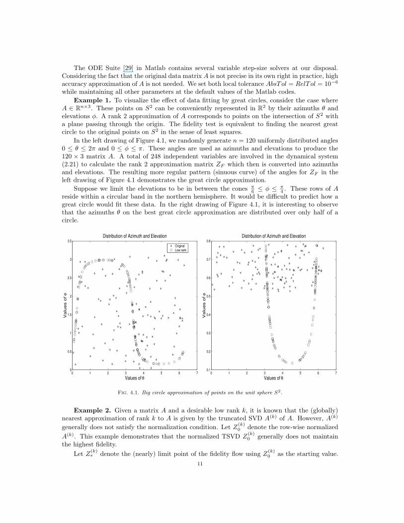
Example 1. To visualize the effect of data fitting by great circles, consider the case whereA ∈ Rn×3. These points on S2 can be conveniently represented in R2 by their azimuths θ andelevations φ. A rank 2 approximation of A corresponds to points on the intersection of S2 witha plane passing through the origin. The fidelity test is equivalent to finding the nearest greatcircle to the original points on S2 in the sense of least squares.

In the left drawing of Figure 4.1, we randomly generate n = 120 uniformly distributed angles0 ≤ θ ≤ 2π and 0 ≤ φ ≤ π. These angles are used as azimuths and elevations to produce the120 × 3 matrix A. A total of 248 independent variables are involved in the dynamical system(2.21) to calculate the rank 2 approximation matrix ZF which then is converted into azimuthsand elevations. The resulting more regular pattern (sinuous curve) of the angles for ZF in theleft drawing of Figure 4.1 demonstrates the great circle approximation.

Suppose we limit the elevations to be in between the cones π6 ≤ φ ≤ π

4 . These rows of Areside within a circular band in the northern hemisphere. It would be difficult to predict how agreat circle would fit these data. In the right drawing of Figure 4.1, it is interesting to observethat the azimuths θ on the best great circle approximation are distributed over only half of acircle.

0 1 2 3 4 5 6 70

0.5

1

1.5

2

2.5

3

3.5

Values of θ

Valu

es o

f φ

Distribution of Azimuth and Elevation

OriginalLow rank

0 1 2 3 4 5 6 70.1

0.2

0.3

0.4

0.5

0.6

0.7

0.8Distribution of Azimuth and Elevation

Values of θ

Valu

es o

f φ

Fig. 4.1. Big circle approximation of points on the unit sphere S2.

Example 2. Given a matrix A and a desirable low rank k, it is known that the (globally)nearest approximation of rank k to A is given by the truncated SVD A(k) of A. However, A(k)

generally does not satisfy the normalization condition. Let Z(k)0 denote the row-wise normalized

A(k). This example demonstrates that the normalized TSVD Z(k)0 generally does not maintain

the highest fidelity.

Let Z(k)∗ denote the (nearly) limit point of the fidelity flow using Z

(k)0 as the starting value.

11

rank k ‖A(k) −A‖2 ‖A(k) −A‖F ‖Z(k)0 −A‖F ‖Z

(k)∗ −A‖F ‖Z

(k)0 − Z

(k)∗ ‖F

1 1.5521 2.7426 3.4472 3.3945 0.92272 1.4603 2.2612 2.6551 2.5330 2.18663 1.3056 1.7264 1.9086 1.8588 0.80854 1.1291 1.1296 1.1888 1.1744 0.33415 0.0237 0.0343 0.0343 0.0343 5.5969× 10−7

6 0.0183 0.0248 0.0248 0.0248 2.1831× 10−7

7 0.0141 0.0167 0.0167 0.0167 1.1083× 10−7

8 0.0083 0.0089 0.0089 0.0089 6.4180× 10−9

9 0.0034 0.0034 0.0034 0.0034 2, 7252× 10−9

Table 4.1

Comparison of nearness of TSVD and fidelity flow

Table 4.1 compares the distances ‖A(k) − A‖F , ‖Z(k)0 − A‖F , ‖Z

(k)∗ − A‖F , and ‖Z

(k)0 − Z

(k)∗ ‖F

of a 10× 10 random matrix A with controlled singular values. For reference, we have also listed‖A(k) −A‖2 which is known to be the (k + 1)-th singular value of A.

Because∑10

i=1 σ2i = 10, we purposefully control the singular values of A so that five singular

values are relatively larger than the other five. We then notice that the gap ‖Z(k)0 − Z

(k)∗ ‖F is

relatively significant up to k = 4. Since the local tolerance in the ODE integrator is set only at

10−6, the difference between Z(k)0 and Z

(k)∗ is probably negligible when k ≥ 5.

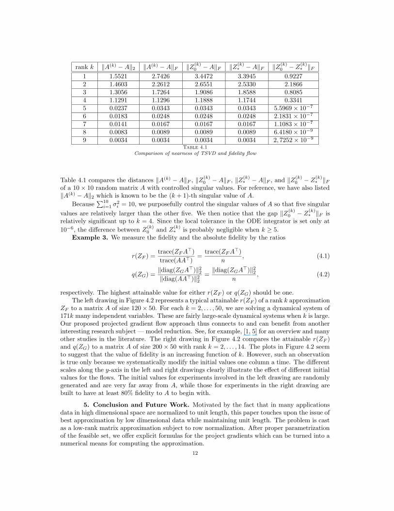
Example 3. We measure the fidelity and the absolute fidelity by the ratios

r(ZF ) =trace(ZFA

>)

trace(AA>)=

trace(ZFA>)

n, (4.1)

q(ZG) =‖diag(ZGA

>)‖22‖diag(AA>)‖22

=‖diag(ZGA

>)‖22n

, (4.2)

respectively. The highest attainable value for either r(ZF ) or q(ZG) should be one.The left drawing in Figure 4.2 represents a typical attainable r(ZF ) of a rank k approximation

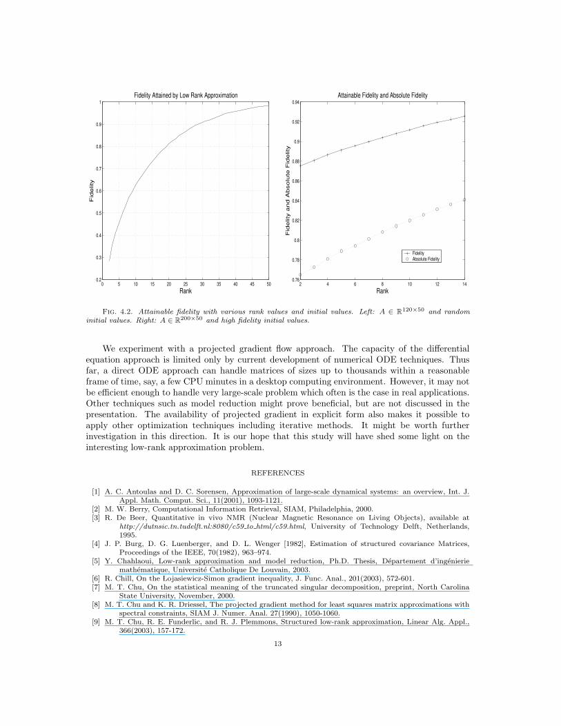
ZF to a matrix A of size 120× 50. For each k = 2, . . . , 50, we are solving a dynamical system of171k many independent variables. These are fairly large-scale dynamical systems when k is large.Our proposed projected gradient flow approach thus connects to and can benefit from anotherinteresting research subject — model reduction. See, for example, [1, 5] for an overview and manyother studies in the literature. The right drawing in Figure 4.2 compares the attainable r(ZF )and q(ZG) to a matrix A of size 200× 50 with rank k = 2, . . . , 14. The plots in Figure 4.2 seemto suggest that the value of fidelity is an increasing function of k. However, such an observationis true only because we systematically modify the initial values one column a time. The differentscales along the y-axis in the left and right drawings clearly illustrate the effect of different initialvalues for the flows. The initial values for experiments involved in the left drawing are randomlygenerated and are very far away from A, while those for experiments in the right drawing arebuilt to have at least 80% fidelity to A to begin with.

5. Conclusion and Future Work. Motivated by the fact that in many applicationsdata in high dimensional space are normalized to unit length, this paper touches upon the issue ofbest approximation by low dimensional data while maintaining unit length. The problem is castas a low-rank matrix approximation subject to row normalization. After proper parametrizationof the feasible set, we offer explicit formulas for the project gradients which can be turned into anumerical means for computing the approximation.

12

0 5 10 15 20 25 30 35 40 45 500.2

0.3

0.4

0.5

0.6

0.7

0.8

0.9

1

Rank

Fid

elit

yFidelity Attained by Low Rank Approximation

2 4 6 8 10 12 140.76

0.78

0.8

0.82

0.84

0.86

0.88

0.9

0.92

0.94

RankF

ide

lity a

nd

Ab

so

lute

Fid

elit

y

Attainable Fidelity and Absolute Fidelity

FidelityAbsolute Fidelity

Fig. 4.2. Attainable fidelity with various rank values and initial values. Left: A ∈ R120×50 and random

initial values. Right: A ∈ R200×50 and high fidelity initial values.

We experiment with a projected gradient flow approach. The capacity of the differentialequation approach is limited only by current development of numerical ODE techniques. Thusfar, a direct ODE approach can handle matrices of sizes up to thousands within a reasonableframe of time, say, a few CPU minutes in a desktop computing environment. However, it may notbe efficient enough to handle very large-scale problem which often is the case in real applications.Other techniques such as model reduction might prove beneficial, but are not discussed in thepresentation. The availability of projected gradient in explicit form also makes it possible toapply other optimization techniques including iterative methods. It might be worth furtherinvestigation in this direction. It is our hope that this study will have shed some light on theinteresting low-rank approximation problem.

REFERENCES

[1] A. C. Antoulas and D. C. Sorensen, Approximation of large-scale dynamical systems: an overview, Int. J.Appl. Math. Comput. Sci., 11(2001), 1093-1121.

[2] M. W. Berry, Computational Information Retrieval, SIAM, Philadelphia, 2000.[3] R. De Beer, Quantitative in vivo NMR (Nuclear Magnetic Resonance on Living Objects), available at

http://dutnsic.tn.tudelft.nl:8080/c59 to html/c59.html, University of Technology Delft, Netherlands,1995.

[4] J. P. Burg, D. G. Luenberger, and D. L. Wenger [1982], Estimation of structured covariance Matrices,Proceedings of the IEEE, 70(1982), 963–974.

[5] Y. Chahlaoui, Low-rank approximation and model reduction, Ph.D. Thesis, Departement d’ingenieriemathematique, Universite Catholique De Louvain, 2003.

[6] R. Chill, On the ÃLojasiewicz-Simon gradient inequality, J. Func. Anal., 201(2003), 572-601.[7] M. T. Chu, On the statistical meaning of the truncated singular decomposition, preprint, North Carolina

State University, November, 2000.[8] M. T. Chu and K. R. Driessel, The projected gradient method for least squares matrix approximations with

spectral constraints, SIAM J. Numer. Anal. 27(1990), 1050-1060.[9] M. T. Chu, R. E. Funderlic, and R. J. Plemmons, Structured low-rank approximation, Linear Alg. Appl.,

366(2003), 157-172.

13

[10] S. Deerwester, S. Dumais, G. Furnas, T. Landauer, and R. Harshman, Indexing by latent semantic analysis,J. Amer. Soc. Inform. Sci., 41(1990), 391-407.

[11] P. E. Gill, W. Murray, and M. H. Wright, Practical Optimization, Academic Press, London, 1981.[12] R. O. Duda, P. E. Hart, and D. G. Stork, Pattern Classification, Wiley, New York, 2001.[13] M. Dendrinos, S. Bakamidis, and G. Carayannis, Speech enhancement from noise: A regenerative approach,

Speech Communication 10(45-57), 1991.[14] I. S. Dhillon and D. M. Modha, Concept decompositions for large sparse text data using clustering, Machine

Learning J., 42(2001), 143-175.[15] I. S. Dhillon, E. M. Marcotte, and U. Roshan, Diametrical clustering for identifying anti-correlated gene

clusters, Bioinformatics, 19(2003), 1612-1619.[16] T. Hastie, R. Tibshirani, and J. Friedman, The Elements of Statistical Learning: Data Mining, Inference,

and Prediction, Springer-Verlag, New York, 2001.[17] P. Horst, Factor Analysis of Data Matrices, Holt, Rinehart and Winston, New York, 1965.[18] L. Hubert, J. Meulman and Willem Heiser, Two purposes for matrix factorization: A historical appraisal,

SIAM Review, 42(2000), 68-82.[19] A. N. Iusem, On the convergence properties of the projected gradient method for convex optimization,

Comput. Appl. Math., 22(2003), 37-52.[20] A. Iserles, H. Z. Munthe-Kass, S. P. Nørsett, and A. Zanna, Lie-group methods, Acta Numerica, 2000,

215-365.[21] I. T. Jolliffe, Principal Component Analysis, 2nd ed., Springer-Verlag, New York, 2002.[22] J. Kleinberg, C. Papadimitriou, and P. Raghavan, A microeconomic view of data mining, Data Mining and

Knowledge Discovery, 2(1998), 311-324.[23] T. G. Kolda and D. P. O’Leary, A semi-discrete matrix decomposition for latent semantic indexing in

information retrieval, ACM Transact. Inform. Systems, 16(1998), 322-346.[24] B. De Moor, Total least squares for affinely structured matrices and the noisy realization problem, IEEE

Trans. Signal Processing, 42(1994), 3104-3113.

[25] S. ÃLojasiewicz, Une propriete topologique des sous-ensembles analytiques reels, in Les Equations aux Derivees

Partielles (Paris, 1962), Vol. 117, 87-89, Editions du Centre National de la Recherche Scientifique, Paris,1963.

[26] P. Paatero, Least squares formulation of robust nonnegative factor analysis, Chemomet. Intell. Lab. Systems,37(1997), 23-35.

[27] H. Park, M. Jeon, and J. B. Rosen, Lower dimensional representation of text data in vector space basedinformation retrieval, in Computational Information Retrieval, ed. M. Berry, Proc. Comput. Inform.Retrieval Conf., SIAM, 2001, 3-23.

[28] G. Salton and M. McGill, Introduction to Modern Information Retrieval, McGraw-Hill, New York, 1983.[29] L. F. Shampine and M. W. Reichelt, The MATLAB ODE suite, SIAM J. Sci. Comput., 18(1997), 1-22.[30] L. Simon, Asymptotics for a class of nonlinear evolution equations with applications to geometric problems,

Annals Math., 118(1983), 525-571.[31] A. Singhal, C. Buckley, and M. Mitra, Pivoted document lenght normalization, in Proceedings of the 19th

ACM SIGIR Conference on Research and Development in Information Retrival, 1996, 21-29.[32] E. Stiefel, Richtungsfelder und fernparallelismus in n-dimensionalel manning faltigkeiten, Commentarii Math-

ematici Helvetici, 8(1935-1936), 305-353.[33] P. Stoica and M. Viberg, Maximum likelihood parameter and rank esitmation in reduced rank multivariate

linear regressions, IEEE Trans. Signal Process, 44(1996), 3069-3078.[34] J. Tropp,, I. Dhillon, R. Heath, T. Strohmer, Designing structured tight frames via an alternating projection

method, IEEE Trans. Info. Theory, to appear, 2004.

14