Munich Personal RePEc Archive

ON THE ECONOMIC

DETERMINANTS OF

PROSTITUTION: MARRIAGE

COMPENSATION AND UNILATERAL

DIVORCE IN U.S. STATES

Ciacci, Riccardo

12 December 2018

Online at https://mpra.ub.uni-muenchen.de/100392/

MPRA Paper No. 100392, posted 15 May 2020 05:10 UTC

ON THE ECONOMIC DETERMINANTS OFPROSTITUTION: MARRIAGE COMPENSATIONAND UNILATERAL DIVORCE IN U.S. STATES∗

Riccardo Ciacci1

1Dept. of Economics, Universidad Pontificia Comillas; email: rciacci@comillas.edu

March 14, 2020

Abstract

This paper studies the hypothesis that marriage opportunities are an economicdeterminant of female prostitution. I exploit differences in the timing of entry intoforce of unilateral divorce laws across U.S. states to explore the effect of such laws onfemale prostitution (proxied by arrests of female prostitutes). Using a difference-in-difference estimation approach, I find that unilateral divorce reduces prostitution by10%. My results suggest that unilateral divorce improves the option value of marriageby increasing wives’ welfare. As a result, the opportunity cost of becoming a femaleprostitute increases and the supply of prostitution declines.

Keywords: Prostitution, unilateral divorce, difference-in-difference, marriage compensa-tionJEL codes: J12, J16, K14, K15, K36

∗I would like to thank Juan J. Dolado for his generous advice and support during the different stagesof this project. I am also grateful to Andrea Ichino, Dominik Sachs and Francesco Fasani for valuablesuggestions that helped improve this paper as well as to Ines Berniell, Raul Sanchez de la Sierra, GabrielaGalassi and Gabriel Facchini for useful comments. Financial support from the Spanish Ministry of Science(PGC2018-093506-B-I00) is gratefully acknowledged.

1

1 Introduction

Prostitution is a gender issue. According to HG.org (2017), of the total arrests for

prostitution in the U.S., 70% are female prostitutes, 20% are either male prostitutes or

pimps and the remaining 10% are prostitutes’ clients.

Since the 1960s, combating prostitution has been a key target of many American policy

interventions (Shively et al. 2012).1 Recently, there have been important policy debates

on prostitution (Della Giusta 2016; Yttergren and Westerstrand 2016). In particular, in

2014, the European Parliament voted in favor of a resolution to criminalize the purchase

of prostitution. According to this school of thought, whether it is forced or voluntary,

prostitution is a violation of human rights and human dignity. Prostitution laws aside,

little is known about how to reduce prostitution.

In this paper, I study how a seemingly unrelated policy (namely, unilateral divorce) re-

duces prostitution. This result is aligned with a branch of the literature led by Edlund and

Korn (2002). Edlund and Korn (2002) suggest two mechanisms that might explain such a

reduction. I test several potential mechanisms, but I find empirical evidence in favor of

only one of the two mechanisms hypothesized by Edlund and Korn (2002). Specifically,

my results indicate that the enforcement of unilateral divorce laws ameliorates wives’

welfare, thereby improving one of the main economic determinants of prostitution: pros-

titutes’ outside options. Consequently, once prostitution is relatively less attractive, pros-

titution decreases.

Although the link between divorce regimes and prostitution may appear weak at first

glance, there are several channels through which such a relationship could be established.

For example, because the availability of unilateral divorce alters the bargaining position

of partners within married couples relative to more rigid divorce regimes where mutual

consent is required, introducing such a divorce law could impinge on prostitution via

downward shifts in its demand and supply. On the one hand, it could be argued that

those married men who are prostitutes’ clients become more reluctant to purchase their

services because their wives could dissolve their marriages more easily under unilateral

divorce. As a result, this change in clients’ behavior would translate into a reduction

in the demand for prostitution. On the other hand, the threat of unilateral divorce may

1The first “reverse sting” operation to catch prostitutes’ clients took place in Nashville, Tennessee, in1964. Ten years later, considerable financial resources were devoted to arresting male customers in St.Petersburg, Florida, based on some of the main principles that were later used in the so-called “NordicModel” (i.e., criminalizing the purchase of prostitution). In the same year, the first shaming campaign wasstarted in Eugene, Oregon, in which names and/or photos of prostitutes’ clients were publicized. Similarly,in 1995, the first school to re-educate arrested sex buyers opened in San Francisco. The vast majority ofthese policies were intended to combat prostitution by reducing its demand.

2

improve the conditions of married women and therefore make marriage a more attractive

option, leading to a fall in the supply of prostitution. In either of these two cases, the entry

into force of unilateral divorce laws reduces the amount of prostitution in equilibrium.

By the same token, there are reasonable alternative mechanisms that instead imply an

increase in the amount of prostitution. For instance, it could be argued that unilateral

divorce laws are likely to increase the number of divorces in the short term and therefore

lead to a rise in the share of single people in the population. To the extent that single

men demand more prostitution services than married men and insofar as single women

supply more prostitution services than married women, these two forces could jointly

lead to a larger amount of prostitution in equilibrium.

In view of the previous mechanisms, it seems relevant to determine the sign and size of

the causal effect of unilateral divorce on prostitution as well as to identify its underlying

mechanism. Indeed, the nature of this effect could change people’s prior beliefs on these

two issues. A negative effect could generate a trade-off for those who oppose divorce and

prostitution: barriers to divorce would imply higher levels of prostitution. Conversely, a

positive effect would reinforce their beliefs.

This paper addresses this issue by exploiting a quasinatural experiment provided by

differences in the timing of the implementation of unilateral divorce laws across U.S.

states. Such differences enable one to use a difference-in-difference approach (DiD here-

after) to identify the potential causal effect of such laws on the arrests of female pros-

titutes. Note that arrests for female prostitution are used as a proxy for the amount of

prostitution, an activity for which there is very scant information given its illegality.2 To

implement the DiD approach, two sources of data are combined: the month in which uni-

lateral divorce laws became effective in each U.S. state and information on arrests drawn

from the agency-level UCR (Uniform Crime Reporting) database. The evidence provided

in this paper relies on the plausible identification assumption that the month in which

unilateral divorce laws became effective in each state was correlated neither with any

crime pattern in general nor with any prostitution pattern in particular.

To assess the credibility of the previous identification assumption, I use an event study

methodology in a time window close to the date of the policy intervention. The evidence

obtained in this respect credibly shows that the effect on prostitutes’ arrests occurs after

the entry into force of the law and that prior to the intervention date, treated and control

groups share a common underlying trend.

2The two variables are bound to move together if the arrest intensity for prostitutes is fairly constantover time, an assumption that I cannot directly test but that I regard as plausible. Moreover, insofar asmy identifying variation – changes in unilateral divorce laws – does not covary with changes in the arrestintensity for prostitutes, my results are unaffected by changes to this intensity.

3

My main finding is that unilateral divorce laws reduce arrests for female prostitution

by roughly 10%. Such a reduction takes place in the first year after the implementation

of the law. Since approximately 60,000 female prostitutes are arrested on average in the

U.S. each year, the abovementioned estimate implies a reduction of approximately 6,000

women arrested for prostitution. Using statistics from one of the main American law

and government information sites, I find that this decrease yields a reduction in costs

of approximately $16.4 million for American taxpayers.3 It is possible to make a guess

regarding the decrease in the overall number of female prostitutes by using information

drawn from Fondation-Scelles (2012), which reports that there were approximately 1 mil-

lion prostitutes in the U.S. during the 2000s. Using such a figure and my estimated effect,

a simple back-of-the-envelope calculation indicates that unilateral divorce laws reduce

the number of prostitutes by 100,000.

However, since in various states no-fault divorce laws went into effect slightly before

unilateral divorce laws were enacted, one could be concerned that the former divorce

laws also played an important role in the decline in arrests of female prostitutes to the

extent that these laws reduced the cost of divorce relative to no-divorce (i.e., traditional)

regimes. Using the month in which no-fault divorce laws entered into force as a further

control in the DiD specification, I find that this factor does not change the previous esti-

mate of the causal effect. An interpretation of this result is that no-fault divorce laws do

not change the bargaining structure within couples but merely reduce the costs of filing

for a divorce.

Next, I consider the potential mechanisms that could be driving the results. These

mechanisms range from a general decline in the number of arrests for all types of crimes

to changes in both the demand and supply of prostitution. First, I examine the mecha-

nisms suggested by Edlund and Korn (2002). These are supply-driven mechanisms stem-

ming from changes in the value of marriage as an outside option to prostitution. Namely,

these two mechanisms are an increase in wives’ wages and an improvement of conditions

in marriage for wives (i.e., wives’ welfare) that results from wives’ greater bargaining

power when unilateral divorce laws enter into force. Using data on the real average wage

of wives across U.S. states, I do not find empirical evidence to support the notion that uni-

lateral divorce laws affect wives’ real wages. Then, I analyze whether there is evidence of

unilateral divorce law improving wives’ conditions in marriage. If this were the case, it

seems plausible to conjecture that only female prostitutes of marriageable and fertile age

would exit prostitution since they would be the main beneficiaries of an improvement in

wives’ welfare (Edlund and Korn 2002; Edlund 2013). To test this hypothesis, I divide the

3Statistics are drawn from HG.org (2017).

4

data on arrests of female prostitutes into different age groups and find that female pros-

titutes of marriageable and fertile age are the main drivers of the estimated reduction in

arrests of female prostitutes.

Second, I explore whether unilateral divorce laws led to a general reduction in ar-

rests for crimes not connected to prostitution per se. Using data on police officers and

on women arrested for robberies, drug crimes/usage and vandalism’ (three crimes with

higher frequency than prostitution), I find that these alternative crimes are not affected

by the implementation of unilateral divorce laws.

Finally, I examine whether unilateral divorce changed the demand for prostitution.

Three separate data sets are used to capture different features of such demand. In partic-

ular, data on the number of internet searches for several words connected to prostitution

are used to proxy for online demand for prostitution; panel-survey data are used to an-

alyze whether men’s views toward prostitution change after men are divorced, and data

on the number of unmarried men are used to proxy for the demand for prostitution by

unmarried men. I do not find empirical support in any of these exercises that unilateral

divorce decreases the demand for prostitution.

This paper contributes to three different lines of research. First, the empirical findings

of this paper complement scholarship on the determinants of prostitution and on the

relevance of several mechanisms at play in economic models of prostitution. There is a

growing literature in economics and other social sciences that has studied prostitution

from both theoretical and empirical perspectives (see, inter alia, Cameron 2002; Edlund

and Korn 2002; Cameron and Collins 2003; Moffatt and Peters 2004; Gertler et al. 2005;

Levitt and Venkatesh 2007; Arunachalam and Shah 2008; Della Giusta et al. 2009; Edlund

et al. 2009; Della Giusta 2010; de la Torre et al. 2010; Cunningham and Kendall 2010,

2011c,a; Gertler and Shah 2011; Islam and Smyth 2012; Cunningham and Kendall 2013;

Arunachalam and Shah 2013; Logan and Shah 2013; Shah 2013; Immordino and Russo

2014; Bisschop et al. 2015; Immordino and Russo 2015a,b; Cunningham and Shah 2016;

Sohn 2016; Cunningham and Shah 2017; Ciacci and Sviatschi 2016).

In particular, the literature has analyzed what is known as the prostitution wage pre-

mium puzzle: prostitution is low skilled, labor intensive, and female dominated but well

paid. Scholars have explained this puzzle with supply-side hypotheses. On the one hand,

Gertler et al. (2005) argue that prostitutes earn a wage premium by providing unprotected

sex. According to this hypothesis, prostitutes are willing to face the risk of contracting

sexually transmitted infections since customers are willing to pay more to avoid using

condoms. On the other hand, Della Giusta et al. (2009) claim that this wage premium can

be explained by the low reputation that prostitution has and the social stigma it faces.

5

Finally, Edlund and Korn (2002) suggest that marriage compensation is key to under-

standing the prostitution wage premium puzzle: marriage market prospects are an impor-

tant source of income for women, but by entering into prostitution, women compromise

such prospects. The present paper tests this third hypothesis and finds evidence in its

favor.4 In addition, a strand of the literature has focused on analyzing how policy inter-

ventions connected to prostitution regulation affect other crimes. For example, Jakobsson

and Kotsadam (2013); Cho et al. (2013); Lee and Persson (2015) study the link between

human trafficking and prostitution, while Ciacci and Sviatschi (2016); Cunningham and

Shah (2017); Bisschop et al. (2015) analyze how changes in prostitution policies or busi-

ness establishments connected to prostitution affect sex crimes. However, to the best of

my knowledge, this is the first paper that examines how a policy intervention outside the

prostitution market affects the latter.

Second, this paper contributes to a stream of research in sociology, law and economics

that evaluates the impact of unilateral divorce laws on various outcomes (see, e.g., Weitz-

man (1985); Gray (1998); Friedberg (1998); Edlund and Pande (2002); Gruber (2004); Rasul

(2004, 2005); Alesina and Giuliano (2007); Stevenson and Wolfers (2006, 2007); Stevenson

(2008); Wickelgren (2007); Voena (2015)). However, none on these papers addresses the

effects of these laws on prostitution.

Finally, the results of this paper also contribute to a growing line of the literature in

sociology, criminology and economics that studies the effect of changing the opportu-

nity cost of criminals on crime (see, e.g., Raphael and Weiman (2007); Raphael (2010);

Beauchamp and Chan (2014); Uggen and Shannon (2014); Cook et al. (2015); Doleac and

Hansen (2016); Doleac (2016); Agan and Starr (2017); Schnepel (2017); Yang (2017); Agan

and Makowsky (2018); Tuttle (2019)).

The remainder of the paper is organized as follows. Section 2 proposes a conceptual

framework explaining the main hypothesis tested throughout this paper. Section 3 de-

scribes the data sets used in this paper. Section 4 discusses the estimation approach and

the main results obtained. Section 5 examines the identification assumption of the re-

gression models. Section 6 tests the robustness of the results. In section 7, I empirically

explore the numerous underlying mechanisms that might explain the findings of the pa-

per. Finally, Section 8 concludes the paper.

4Specifically, the present paper also contributes to a specific line of research (Arunachalam and Shah2008; Cunningham and Kendall 2011b; Immordino and Russo 2015a) that tests the aforementioned mecha-nisms.

6

2 Conceptual framework: The link between unilateral di-

vorce and prostitution

This paper tests a specific mechanism that is a byproduct of two branches of the litera-

ture. The first studies the effect of unilateral divorce on several outcomes related to wives’

welfare. This line of research finds that unilateral divorce has a positive effect on wives’

welfare. The second branch analyzes the determinants of prostitution; namely, this line

of research explains the prostitution wage premium puzzle: prostitution is low skill, labor

intensive, female dominated, and well paid.5

The Coase theorem predicts that if there are zero transaction costs and transferable

utility, moving from mutual to unilateral divorce should not have any effect on divorce

rates. Unilateral divorce simply reassigns property rights but does not change the out-

come. Regardless of the divorce regime, only relationships with joint utility that is greater

under marriage than under divorce survive. Therefore, the divorce rate would not change.

However, both assumptions of the Coase theorem seem unrealistic in a marriage rela-

tionship. First, it is likely that bargaining is costly between spouses due to feelings and

disdain. Second, utility might not be transferable between spouses.

Despite the predictions of the Coase theorem, moving from mutual to unilateral di-

vorce entails huge redistributional differences between spouses. Under mutual consent

divorce, the spouse who wishes to dissolve the marriage should compensate the other

for the divorce. Conversely, unilateral divorce grants the property right to dissolve the

marriage to the spouse who is better off with a divorce. Then, the spouse who wishes

to remain married is the one who should compensate the partner to avoid divorce. Such

distributional changes imply that the party seeking a divorce would be the one benefiting

from the enforcement of a unilateral divorce law.

According to the literature, this party seems to be the wife. Indeed, the literature has

found that unilateral divorce laws increase wives’ welfare. Specifically, Stevenson and

Wolfers (2006) find that unilateral divorce laws decrease female suicides, the number of

women murdered by their partners and domestic violence, while Alesina and Giuliano

(2007) report evidence on how these laws decrease out-of-wedlock births and increase

fertility rates in the first years of marriage. They also document that unilateral divorce

laws reduce the number of never-married women. In line with these results, Stevenson

(2008) finds that unilateral divorce laws increase the labor participation of both married

and single women.

Regarding the prostitution market, scholars have explained the prostitution wage pre-

5Appendix Section A offers a brief overview of the prostitution market in the U.S.

7

mium puzzle with three supply-side hypotheses. First, Gertler et al. (2005) argue that pros-

titutes earn a wage premium by providing unprotected sex. This hypothesis states that

prostitutes are willing to face the risk of contracting sexually transmitted infections since

customers are eager to pay more to avoid using condoms. Second, Della Giusta et al.

(2009) claim that the premium obtained by prostitutes can be explained by the low reputa-

tion that prostitution has and the social stigma it incurs. Finally, Edlund and Korn (2002)

contend that choosing to be a prostitute jeopardizes one’s marriage market prospects.

Moreover, according to their paper, being a wife and a prostitute is largely incompati-

ble.6 As a result, female prostitutes earn high wages since they are being compensated for

forgone marriage opportunities, despite prostitution being low skill and labor intensive.

Another key feature of this model is that wives sell to husbands a share of their custodial

rights (i.e., reproductive sex) in exchange for marriage compensation (i.e., a level of wel-

fare) (Edlund 2013). Indeed, the custodial rights of children born out of wedlock formerly

belonged solely to the mother, while the custodial rights of children born in a marriage

belong to both parents. This result, combined with the fact that marriage has traditionally

been an important source of pecuniary and non-pecuniary resources for women, implies

that prostitution must pay better than other jobs to compensate for the opportunity cost

of forgone marriage market earnings.

Relying on the previous ideas, this paper suggests a mechanism that connects these

two lines of research; in doing so, this mechanism offers an empirical test of Edlund and

Korn (2002). The introduction of unilateral divorce increases the bargaining power of the

spouse seeking the divorce.7 Hence, in a unilateral divorce regime, wives know that they

will be able to be divorced irrespective of their earnings.8 This feature makes marriage

more attractive to women by facilitating the breakup of “wrong” marriages. Overall,

in line with the previous literature quoted above, the availability of unilateral divorce

boosts wives’ welfare. Therefore, the main beneficiaries of the introduction of unilateral

divorce are women who prefer to marry but would have opted to become prostitutes in

the absence of such a law. In so doing, these women are able to exchange a share of their

custodial rights for the marriage compensation. The main recipients of an increase in

wives’ welfare in marriage would be women who are able to marry and can exchange

6This claim, as the authors write, “rests on the assumption that men prefer their wives to be faithful (forinstance, from a desire to raise biological children)”.

7For further information on the introduction of unilateral divorce across U.S. states, Appendix SectionB discusses the legislative context that led to the enactment of such laws.

8Assuming that a husband’s earnings are higher than his wife’s, under a mutual consent divorce regime,if a husband wished to divorce, he could “bribe” his wife. However, a wife could not afford to do so. Underunilateral divorce, a husband could still compensate his wife financially to avoid divorce. However, thewife would need to consent.

8

their “share” of custodial rights.9

3 Data description

This section provides information about the data sets used throughout the paper. My

econometric analysis is based on two main data sets: the Uniform Crime Reporting pro-

gram, which contains information on the number of arrested prostitutes for each agency

level in the U.S., and the effective date of unilateral divorce laws across U.S. states. The

observations are matched at the county and month levels. Moreover, I use multiple data

sets to carefully explore each of the potential mechanisms behind my findings.

3.1 Arrests for prostitution

Since historical data on the number of female prostitutes are not available, I use the

number of female prostitutes’ arrests from agency-level UCR (Uniform Crime Reporting)

sources as a proxy for this missing variable. This database contains information about

monthly reports of arrests by age, sex, and race provided each year by law enforcement

agencies in the U.S. There are 29 main categories of offenses in this database. Such cat-

egories cover several types of offenses, ranging from vandalism to gambling and from

prostitution to larceny. In addition, they are divided into subcategories for a total of 43

different offenses.10 Each year, law enforcement agencies communicate their reports to

the Federal Bureau of Investigation (FBI), which compiles its database in the form of pe-

riodic nationwide assessments of reported crimes not available elsewhere in the criminal

justice system.

These data were downloaded from the Inter-university Consortium for Political and

Social Research (ICPSR) webpage. ICPSR stores such information each year, dividing

it into five different components: (i) summary data, (ii) county-level data, (iii) incident-

level data, the National Incident-Based Reporting System (NIBRS), (iv) hate crime data,

and (v) various, mostly nonrecurring, data collections. ICPSR recorded such data from

1980 to 2014 with the exception of 1984, for which data are missing.

With these available data sources, I construct a panel that includes monthly informa-

tion at the county level on the ratio between the number of female prostitutes’ arrests and

9A substantially different question is whether this mechanism occurs because prostitutes in a certainage group exit prostitution (i.e., a stock effect) or because “potential” prostitutes, in a younger age group,prefer not to enter prostitution (i.e., an inflow effect). I investigate this issue in Appendix Section C.

10In Appendix Section, D I provide a complete list of offenses recorded in this database.

9

the county population for the time period 1980-2014 (except 1984).11 Appendix Section E

presents detailed descriptive statistics of this data set.

3.2 Divorce laws

When coding unilateral divorce laws, two important decisions must be made: (i)

whether to use the enactment date or the effective date of the law and (ii) how to clas-

sify different unilateral divorce laws. Regarding (i), the enactment date is the date on

which a law is approved, while the effective date is the date on which a law enters into

effect. I use the effective date since this is when unilateral divorce petitions begin to be

filed. It could be that some divorce petitioners anticipated this change since the law was

already approved. However, they could not be divorced before the effective date.12

Regarding (ii), I focus on unilateral divorce laws without separation requirements to

compare identical laws. It is difficult to compare unilateral divorce laws with and without

separation requirements since the length of the required separation differs across states.

Thus, using unilateral divorce laws with separation requirements would require estab-

lishing criteria to compare (i) states with unilateral divorce laws without separation re-

quirements with states with unilateral divorce laws with separation requirements and

(ii) states with unilateral divorce laws with separation requirements of different lengths.

Since any of such criteria would be subjective, I prefer to focus on unilateral divorce laws

without separation requirements. Column (2) of Table 1 displays those states with uni-

lateral divorce laws that required separation of spouses (Caceres-Delpiano and Giolito

2012).

Therefore, my main explanatory variable in the regression models estimated through-

out the paper is a step dummy variable taking value 1 starting in the effective month of

the unilateral divorce law in a given state and taking value 0 previous to that date. This

variable was constructed by updating Gruber (2004)’s data. As shown in Table 1, during

my sample period, six states experienced a change in divorce law.

In addition, for comparability with unilateral divorce laws, I constructed a data set

for the dates of entry into force of no-fault divorce laws.13 After reviewing the literature,

11Note that using such data at the agency level does not affect the results.12There can be a lag of at most one year between the enactment date and the effective date. Furthermore,

the effective date might be postponed, rendering the enactment date even less important. For further detailsabout using effective dates instead of enactment dates, see Vlosky and Monroe (2002). It is important touse an objective criterion to classify these laws since it could impact my identification assumption andfindings, although in this setting, intuitively, it does not appear plausible that the effect is immediate; thus,using either of the two dates should not considerably affect the results.

13Coding these laws involves the problems discussed in Appendix Section A.

10

Vlosky and Monroe (2002) suggest a decision criterion to code no-fault divorce laws that

consists of four rules. Rule 1: In states where there is only a no-fault law, use the ef-

fective date of that law. Rule 2: In states where no-fault provision/s was/were added

to traditional fault divorce law, use the effective date of such provision/s. Rule 3: Use

the effective date for the law allowing the shortest separation period. Rule 4: Laws with

explicit no-fault provisions supplant laws with no-fault separate and apart provisions.14 I

follow their coding of no-fault divorce laws’ effective date and again restrict my attention

to laws without separation requirements (i.e., Rules 1 and 2).15

3.3 Supplementary data sets used

In addition to the data sets described above, I make use of information about arrests

for other crimes other than prostitution, the number of police officers hired in each state,

and proxies for both demand and supply of prostitution. Data on other crimes are drawn

from the agency-level UCR database, which allows me to compute crime rates at the

county level.

In this paper, I use “The Police Employee” data set to measure the number of officers

per state population. This data set contains annually collected data on law enforcement

officers and civilians employed by police departments and their respective rates per loca-

tion’s population from 1971 to 2016.16 The UCR Program defines law enforcement officers

as individuals who ordinarily carry a firearm and a badge, have full arrest powers, and are paid

from governmental funds set aside specifically for sworn law enforcement representatives. By

contrast, civilian employees include personnel such as clerks, radio dispatchers, meter

attendants, stenographers, jailers, corrections officers, and mechanics provided that they

are full-time employees of the agency. In addition, the totals given for sworn officers

comprise not only the patrol officers on the street but also the officers assigned to various

other duties such as administrative and investigative positions and special teams.

As a proxy for the demand for prostitution, I use data on searches of words connected

to the demand for prostitution on Google.com that are drawn from Google Trends. Since

those records are geo-located, I collect the counts for the number of times each word was

searched for on Google.com for each county and month in the U.S. These data span from

2004 to 2017.

14See Table 2 and Table 3 of Vlosky and Monroe (2002) for further information.15Appendix Section F presents further information about the classification followed to code unilateral

divorce laws across U.S. states.16The year 1972 is missing, although there is no reason to believe it is missing due to any special pattern

of hired officers.

11

Another data set used in this respect refers to divorcees’ opinions about prostitution

and is drawn from a longitudinal survey, precisely from the 1st, 2nd, 3rd and 4th waves of

the Youth Parent Socialization Survey (YPSS). This survey was designed to study political

socialization and was implemented by the Survey Research Center and Center for Politi-

cal Studies of the University of Michigan. This study started in 1965 and collected data in

three other different waves that took place in 1973, 1982 and 1997. There is a total of 934

respondents (458 men and 476 women) in the four waves. These data are also available

from the ICPSR web-page.

Since the YPSS data contain information on the marital status of their respondents, it

is known whether an individual who was previously married was divorced during the

subsequent waves. Further, this survey collected information on topics that respondents

disliked.17 Replies were classified into multiple categories, one of which was prostitu-

tion.18

The last database is the monthly Current Population Survey (CPS), which is an employment-

focused cross-sectional survey. The U.S. Census Bureau of Labor and Statistics adminis-

ters the CPS monthly to approximately 60,000 U.S. households. The survey collects infor-

mation on a number of variables connected to the employment status of each household

member aged 15 years or older. Such information is provided by an adult member of

the household. A multistage stratified statistical sampling scheme selects sample house-

holds. Such households are surveyed for 4 consecutive months, interviews are halted for

8 months, and households are eventually are resurveyed for 4 additional months. The

sample represents the civilian non-institutional population. The CPS data used in this

paper extend from 1980 to 2014.19

4 Estimation approach and main results

In this section, I explore the causal effect of unilateral divorce laws on the arrests of

female prostitutes. First, I present my identification strategy that exploits reasonable ex-

ogenous variation in the time at which unilateral divorce laws became effective across

U.S. states. Next, I discuss my econometric specification in detail. Finally, I report the

main empirical results uncovered by the regressions.

17Namely, the survey inquires into topics respondents were “least proud of”.18The survey question is as follows: “What are the things you are least proud of as an American”?

The answer connected to prostitution states: “Immorality in general; low morals; deterioration in moralstandards; also specific actions--e.g. drinking, gambling, overexposure; lewdness in behavior or in massmedia or literature; pornography, prostitution”.

19The CPS data used in this paper are drawn from the Uniform Extracts of the CPS ORG. Center forEconomic and Policy Research. 2017. CPS ORG Uniform Extracts, Version 2.2.1. Washington, DC.

12

4.1 Identification assumption and regression model

The results of this paper rely on the identification assumption that the months in

which unilateral divorce laws became effective in the six states treated during my sample

period were not chosen due to any reason related to crime in general or prostitution in

particular. However, this concern can easily be dismissed since, to the best of my knowl-

edge, there is no historical evidence that crime rates might have affected such effective

dates.

Knowledge of the legislative background is crucial to assessing the credibility of the

identification assumption. As I explain in Appendix Section A, “The Divorce Revolution”

was caused mainly by the inadequacy of traditional divorce laws and was driven by an

apolitical consensus among both liberals and conservatives. Fault grounds and mutual

agreement encouraged couples to even perjure themselves and falsify evidence to ob-

tain a divorce. The introduction of divorce laws, it was believed, would reduce perjury

by eliminating either mutual consensus, fault grounds or both. Moreover, conservatives

supported divorce since they saw it as an widening of personal rights, whereas liberals

backed it to prevent women from being locked into dismal marriages.

Another potential concern is that there could be an omitted variable simultaneously

affecting the effective date of unilateral divorce laws and female prostitutes’ arrests. For

example, it could be that the women’s rights movement affected both variables. How-

ever, this possibility again seems unlikely for two reasons. First, historically, women’s

rights movements were in favor of unilateral divorce but did not have a clear position

on prostitution: feminists had and have views both against and in favor of prostitution.

Therefore, it does not seem likely that the women’s right movement fostering the “The

Divorce Revolution” played any role in prostitution regulation. Second, despite “The

Divorce Revolution,” there has not yet been a “Prostitution Revolution” or any other

movement that has systematically changed prostitution laws.20

A final concern regarding my identification assumption is the displacement of fe-

male prostitutes, clients or police officers among different states. These issues should

be analyzed carefully since they could violate the stable unit treatment value assumption

(SUTVA). However, I found no evidence or any plausible reason suggesting that prosti-

tutes, clients or police officers moved across states based on their divorce regimes.21

20Currently, the only state in the U.S. that has legalized prostitution is Nevada. Nevada introducedunilateral divorce laws and legalized prostitution in different years: unilateral divorce law became effectivein 1967, while prostitution was legalized in 1971.

21Since this paper finds that unilateral divorce decreases prostitution by improving prostitutes’ outsideoptions, a possible concern could be that the entry into force of unilateral divorce could cause prostitutesfrom surrounding states to move to that state to exit prostitution. However, I did not find any evidence

13

Using data at the county level increases precision and improves comparability across

treated and control units. It is more reasonable to compare smaller geographical units,

such as counties, than states as a whole. In addition, if my specification were at the year

level, the identification assumption would be less plausible. Indeed, it seems likely that

other progressive social policies might have become effective in the same year in which

unilateral divorce entered into force. If this occurred systematically across the treated

states, my estimates might be capturing the joint effect of both unilateral divorce and

other progressive laws. However, it is much less likely that such changes in social policies

occurred exactly in the same month in which unilateral divorce law became effective.

Specifically, the identification assumption in this paper corresponds to the parallel

trends hypothesis in the DiD estimation approach. In other words, the only difference

among treated and control counties is that the former were treated. If they had not been

treated, they would have experienced the same evolution as the control counties.

This paper considers two control groups: those never treated and those treated before

1980. In fact, since this study makes use of data spanning from 1980 to 2014, whereas

many U.S. states promulgated unilateral divorce laws before 1980, I proceed to include

such states in the control group.

In particular, the following regression model is considered here:

log(1 + Prostcsmy) = βUnilatsmy + αm + αy + αc + αc ∗ y + εcsmy (1)

where Prostcsmy is the number of arrests of female prostitutes per 1,000,000 inhabitants

in county c of state s in month m of year y.22 αm, αy, αc, are month, year and county fixed

effects, respectively; αc ∗ y is a county-year linear trend; Unilatsmy is the main regressor of

interest, namely, a dummy variable taking value 0 before the effective month of unilateral

divorce and value 1 in the month in which the unilateral divorce law becomes effective

and afterwards. For states that were treated before 1980, Unilatsmy always takes value

1; however, for states that were treated after 2014 or have never been treated, Unilatsmy

takes value 0.

Taking the logarithmic transformation of the dependent variable is common in crime

economics, mainly because the data present extreme values that may skew the results.

In addition, since arrests might take value 0, I use log(1 + Prostcsmy) as the dependent

supporting this hypothesis.22Arrests of female prostitutes per 1,000,000 inhabitants are computed as the number of arrested female

prostitutes divided by population and multiplied by 1,000,000. The same computations are made for dataon other crimes in the rest of this paper.

14

variable.

Note that the specification considered in this paper is quite demanding since it takes

into account that crime patterns respond to seasonal changes (via the inclusion of month

fixed effects) and that these patterns might differ among counties within the same state

(via inclusion of county fixed effects and county-year trends). Moreover, as a robustness

check, I also check whether my findings are robust to the inclusion of year-month fixed

effects.

4.2 Results

Panel A of Table 2 shows the results of estimating model (1). Columns (1) and (2)

include county-year trends and county fixed effects; column (1) clusters variance at the

county level, while column (2) clusters variance at the state level. In both columns, the

estimated coefficient is significantly negative at standard significance levels. In column

(3), I add year fixed effects; in column (3), I introduce month fixed effects; and in column

(4), I add year-month fixed effects. In columns (1) and (2), the estimated coefficient is

significantly negative at the 1% and 5% levels, respectively. Moreover, the estimated co-

efficient is robust to the inclusion of seasonal fixed effects. In fact, after adding year and

month fixed effects, in columns (3) and (4), the estimated coefficient is similar in size and

significantly different from zero at the 10% level. There could be concerns regarding the

level of significance of these results, and hence, for ease of comparison, Table 2 reports

the p-values associated with the null of zero effect for each estimated coefficient. It is

reassuring that such p-values range between 0.046 and 0.055. In particular, note that the

significance of my results is not affected by the inclusion of year-month fixed effects (i.e.,

column (5)).

After simple back-of-the-envelope computations, the coefficient estimates in column

(3) indicate that unilateral divorce laws decrease the arrests of female prostitutes by roughly

10%.23 Since in my data set, on average, approximately 60,000 female prostitutes are ar-

rested each year in the U.S., this finding implies that the introduction of unilateral divorce

could cause a decrease of 6,000 women being arrested for prostitution in the whole coun-

try. According to HG.org (2017)’s estimates, this decrease could yield a reduction in costs

of approximately $15 million for American taxpayers.24 The size of this effect could be

23These computations simply take into account the structure of my dependent variable to compare it to

a standard log-level specification. Precisely, ∂ log(y)∂x

= ∂ log(1+y)∂x

∂ log(y)∂ log(1+y) = β 1+y

y≃ β 1+y

y= −6.8% 1+1.9

1.9 =

−10.4%24According to HG.org (2017), 80,000 arrests cost $200 million. Thus, 60,000 cost $150 million to the

taxpayers and a decrease of 10% implies a decrease of $15 million. At the state level, on average, such a

15

compared to the results presented by Allard and Herbon (2003), who found that prostitu-

tion arrests in 2001 caused an expense of $10.3 million in the city of Chicago alone. There-

fore, the introduction of unilateral divorce would help the U.S. to save approximately 1.5

times the cost of arrests for prostitutes in Chicago.

It is not straightforward to link these findings to the number of prostitutes based on

arrests for female prostitution. According to Fondation-Scelles (2012), there are approxi-

mately 1 million female prostitutes in the U.S. Hence, assuming that the observed effect

of a 10% reduction in arrests of female prostitutes is the same as that for the number of fe-

male prostitutes implies that the number of female prostitutes in the U.S. would decrease

by 100,000 if unilateral divorce were effective in all states.

My findings rely on the quasinatural experimental design given by the effective month

of unilateral divorce laws across U.S. states, but since my dependent variable spans from

1980 onward, my identifying variation comes from only six states and not from all the

adopting states. Thus, there might be the concern that these six states could have had a

specific reaction to the event. However, I did not find any evidence or plausible reason to

support this hypothesis.

It is important to stress that the external validity of my findings should be interpreted

with caution. The prostitution market works differently in developing and developed

countries (Farley et al. 2004). Further, unilateral divorce laws were enacted after a period

of discussion in the U.S. that led gradually to full social acceptance of divorce. It would be

difficult to extrapolate my results to developing countries and to countries that enforced

divorce due to foreign influence without having an internal social movement driving such

change.

There are several mechanisms that might explain the reduction in arrests of female

prostitutes associated with unilateral divorce laws. These mechanisms range from changes

in the number of police officers enforcing the law to shifts in either the demand for or

the supply of prostitution. After presenting evidence in favor of my identification as-

sumption (Section 5) and discussing the robustness of the results (Section 6), I thoroughly

explore each of these mechanisms in Section 7.

5 Concerns about the identification assumption: event study

To ascertain the plausibility of the identification assumption, this section reports an

event study analysis regarding the entry into force of unilateral divorce laws, leveraging

the high frequency of the data set. Namely, I group data into periods of 12 months to also

decrease would amount to $300,000.

16

explore the timing of the effect across years. As usual, the excluded indicator is t = −1

one year prior to unilateral divorce becoming effective.

Specifically, I estimate the following regression model:

log(1 + Prostcsmy) =5∑

j=−3

βUnilats,m,y+j + αm + αy + αc + αc ∗ y + εcsmy (2)

Figure 1 plots the estimated coefficients of this event study. The horizontal axis plots

the event time (the number of periods prior and posterior to the change in unilateral

divorce law), whereas the vertical axis presents the size of the coefficient measured ac-

cording to its effect on the dependent variable in the main specification. The solid line in

the graph depicts the estimated coefficients, and each coefficient is depicted with its own

confidence interval at 90% significance levels (dotted lines).

Figure 1 shows that coefficients prior to the occurrence of the event are positive, with

point estimates close to zero and statistically equal to zero, while the coefficients posterior

to the occurrence of the event are negative and statistically significant. Moreover, the size

of the effect is in line with the DiD coefficient. As a whole, these findings support the

identification assumption.

6 Robustness checks

This section addresses the robustness of the results. First, it explores whether these

results are robust to changes in the dependent variable. Next, it explores the extent to

which these results are sensitive to changes in the main specification.

6.1 Sensitivity to changes in the definition of the dependent variable

The concern might be raised that my findings rest on the chosen transformation of the

dependent variable (i.e., log (1 + y)). Thus, in what follows, I consider specifications of the

dependent variable to analyze whether the previous results persist. First, I consider the

inverse hyperbolic sine transformation. Second, I run a linear probability model. Finally,

I consider a specification where the dependent variable is given in levels.

The inverse hyperbolic sine transformation (hereafter, IHS) is an alternative to tak-

ing the log(1 + y) for dependent variables that take zero values. The IHS is defined as

log(y + (y2 + 1)

1

2

). Panel B of Table 2 shows the results from running the same regres-

sion as in Section 3 but taking the IHS of the dependent variable. As can be observed,

the findings using the IHS are similar in both sign and size to the those from the main re-

17

gression. In fact, after simple back-of-the-envelope computations similar to those for the

estimated coefficient of the main regression, the effect estimated by the IHS is −9.2%.25

Although the dependent variable is in logs, one might be concerned that the results are

driven by extreme observations of the dependent variable. To assess this issue, I replace

the dependent variable with a binary variable taking value 1 for every positive value of

the dependent variable and 0 otherwise. Panel C of Table 2 shows the results of running

a linear probability model (hereafter, LPM). Columns (1) and (2) of the table display the

estimated coefficient without year and month fixed effects. Column (1) clusters variance

at the county level, while column (2) clusters variance at the state level. As in Panel A

of the same table, column (3) adds year fixed effects, column (4) adds month fixed effects

and column (5) adds year-month fixed effects. The estimated coefficients are always neg-

ative and statistically different from zero at 5% at most. These results suggest that the

introduction of unilateral divorce law is associated with a 1.8 percentage point reduction

in the probability of arresting a female prostitute.

As a final robustness check, Panel D of Table 2 considers a specification where the de-

pendent variable is in levels (i.e., the number of arrests of female prostitutes per 1,000,000

inhabitants). Columns (1), (2), (3), (4) and (5) of Panel D of Table 2 show that the estimated

coefficients are negative and statistically significant. Column (4) considers the full spec-

ification, where the estimated coefficient is negative and statistically different from zero

at the 10% level. This coefficient is approximately −.77. On average, there are roughly 2

female prostitutes arrested per 1,000,000 inhabitants per county and month. Accordingly,

the decrease caused by the introduction of unilateral divorce is much larger than that

estimated in the other specifications. This might be due to the extreme values of the de-

pendent variable that are not transformed in this specification and drive up the estimated

coefficient.

In summary, the evidence presented in this subsection supports a negative causal ef-

fect of unilateral divorce on the arrests of female prostitutes, irrespective of the chosen

functional form of the dependent variable.

6.2 Sensitivity to model specification changes

Next, I analyze whether the results found in this paper depend on other specification

issues, such as the choice of the control group and choice of the treatment. It might be that

using only one of the two control groups would substantially change the results of the re-

gression. Further, since no-fault divorce and unilateral divorce reforms took place nearly

25Precisely, ∂ log(y)∂x

= ∂IHS(y)∂x

∂ log(y)∂IHS(y) = β

√1+y2

y≃ β

√1+y2

y= 8.1%

√1+(1.9)2

1.9 = −9.2%

18

contemporaneously, it might be that the estimated effect is due to the former instead of

the latter.

Table 3 shows the results of running the main regression using only one of the two con-

trol groups. The estimated coefficients of these regression models should be interpreted

with caution since they are computed using a biased, restricted sample. This exercise

is only useful to test whether the estimated coefficient from the main regression is sta-

tistically equal to the coefficients from the restricted samples. Column (1) only uses the

already-treated control group, whereas column (2) uses the never-treated control group.

Both columns show results for the full regression model (i.e., with all the controls used in

my main specification). The estimated coefficients are negative in both columns but dif-

ferent from zero only in column (1). More important, in both regressions, the estimated

coefficients are not statistically different from the estimated coefficient from the main re-

gression. Such evidence indicates that the two control groups produce similar results.

Regarding no-fault divorce laws, I exploit the effective month of no-fault divorce laws

in two different ways. First, I add no-fault divorce as a control variable. Second, I replace

the unilateral divorce dates with the no-fault divorce dates. Since no-fault divorce does

not need proof of wrongdoing or innocence, researchers have theorized that it does not

change the bargaining structure within a relationship (Gruber 2004). However, it reduces

bargaining costs and financial penalties. If the observed decline in arrests of female prosti-

tutes is caused by no-fault divorce laws instead of unilateral divorce laws, then using this

variable as a control should reduce (in absolute value) the size of the estimated coefficient

and its statistical significance. Table 4 displays the estimated coefficients from running

the main regression of the paper when adding no-fault divorce dates as a dichotomous

control. This control takes value 1 in the month that no-fault divorce law becomes effec-

tive and in the following months and value 0 before the effective date.26 As can be seen in

Table 4, the estimated coefficients are not statistically different from those from the main

regression.27 This finding supports the notion that no-fault divorce laws did not play an

important role in reducing the arrests of female prostitutes.

Table 5 shows the results of running a specification that replaces the effective month of

unilateral divorce laws with the effective month of no-fault divorce laws. There are two

insights from this specification. On the one hand, it can be viewed as a double check that

no-fault divorce laws are not leading to a reduction in the arrests of female prostitutes. In

fact, if this were the case, then the coefficient for months in which no-fault divorce became

effective should be negative and significantly different from zero. On the other hand, this

26Exactly as the treatment variable (i.e., unilateral divorce law).27The point estimate is even slightly larger in absolute value than that from the main specification.

19

regression can be seen as a placebo test. If unilateral divorce laws are not causing the

decline in the number of arrests of female prostitutes, replacing such dates with almost

contemporaneous dates should yield similar results.

As can be seen in Table 5, no-fault divorce laws do not appear to be responsible for the

reduction in the number of arrests of female prostitutes. Indeed, the estimated coefficients

in columns (1), (2), (3) and (4) are nonsignificant and much smaller in size than those from

the main regression.

In sum, the evidence provided above demonstrates the robustness of the main regres-

sion to the choice of the control group and to no-fault divorce laws.

7 Potential mechanisms

My main finding thus far is that the introduction of unilateral divorce decreased ar-

rests of female prostitutes in the U.S. Several mechanisms could have led to this decline.

This section explores each of them by combining multiple data sets.28

First, since the results found in this paper are in line with those of Edlund and Korn

(2002), I use a simplified version of their model to analyze the mechanisms at work in

my findings. Edlund and Korn (2002) argues that the aggregate demand for prostitution

D (p, n) is a function of p, the price of commercial sex, and n, the number of single men,

whereas the aggregate supply of prostitution S (n) is simply a function of the number of

unmarried (single) women n.29 Thus, p, n are endogenously determined in the model.

Since, in equilibrium, demand is equal to supply, equating them determines p as a

function of n (i.e., p = p (n) ). However, to compute the equilibrium values of p and n,

an additional equation is needed. According to their model, this equation is the non-

arbitrage condition that connects the marriage market to the prostitution market: in an

interior equilibrium, where there are both married women and prostitutes, revenues from

28This section does not explore any mechanism connected with migration. One might be concerned thatby making marriage more attractive to women, unilateral divorce laws affect the number of women livingin a certain state. If this were the case, the finding of this paper might be explained simply by an increasein the population in treated states. Moreover, this hypothesis would violate SUTVA since treatment in acertain state would affect the outcome in a different state. This mechanism seems unlikely because spousescan file for divorce in a different state from that where they were married as long as one of the spousesmeets the residency requirements of that state, so there would not be any incentive to move to a state tomarry due to its unilateral divorce law. However, I investigate this issue using, as the dependent variable,data on the number of men and women and the sex ratio in each state. If this mechanism were at work,my treatment variable would affect at least one of the three dependent variables listed above. As expected,I find no empirical evidence supporting this hypothesis. The relevant tables are available from the authorupon request.

29In their model, there are equal numbers of women and men, and since marriage is monogamous, thenumber of single men and single women is the same.

20

the two activities must be equal. As a consequence, p, the wage earned by prostitutes, is

equal to w, the wage earned in the labor market by wives, plus the compensation pm paid

in equilibrium to married women by their partners. These two curves (i.e., p = p (n),

computed from the equilibrium condition D (p, n) = S (n) and p = w + pm), determine

the equilibrium of the prostitution market, as shown in Figure 2.

Hence, according to this simple model, there are two mechanisms related to the pros-

titution market, and specifically to the supply of prostitution, that might explain the find-

ings of this paper:

• It might be that unilateral divorce increases w, that is, the wage earned by wives.

• It might be that unilateral divorce increases the compensation pm paid in equilib-

rium to wives by their husbands.

However, one might be concerned that my findings could be explained by mecha-

nisms not related to the supply of prostitution. Namely, there might be concerns that the

reduction in prostitution I observe is due either to crime patterns (I analyze this hypoth-

esis in the Fight against crime mechanism subsection) or to the demand for prostitution (I

analyze this hypothesis in the Demand mechanisms subsection). to this effect, if unilateral

divorce law decreases all types of crimes committed by women, then I would find a de-

crease in female prostitution arrests but this decrease would not be related to prostitution

per se. This is the first mechanism this section explores.

7.1 Supply mechanisms

As explained at the beginning of this section, there are two supply mechanisms sug-

gested by Edlund and Korn (2002): wives’ wage and marriage compensation. In this

subsection I test both of them.

7.1.1 Wives’ wage

The non-arbitrage condition between marriage and prostitution in Edlund and Korn

(2002) establishes that p, the wage earned by prostitutes, must be equal to w, the wage

earned in the labor market by wives, plus pm, the compensation paid in equilibrium in

the marriage market. If the introduction of unilateral divorce increases w, prostitution will

decrease in equilibrium.30 Thus, it seems plausible that since the enactment of unilateral

30An alternative mechanism, not supported by the literature, is that unilateral divorce increases women’swages (not only wives’ wages). This increase could in turn decrease prostitution insofar as legal jobs be-come more attractive to women and deter them from prostitution. I also explored this hypothesis and foundno evidence in its favor. The relevant tables are available upon request.

21

divorce bolsters women’s rights, it could lead to an increase in wives’ wages. An increase

in w makes marriage more attractive to women, meaning that some women might prefer

to exit prostitution. To test this hypothesis, this subsection makes use of monthly CPS

data to compute the average real wage of married women across states in the U.S. I run

the following specification:

Wsmy = βUnilateralsmy + αm + αy + αs + αs ∗ y + εsmy (3)

where Wsmy stands for wives’ average real wage in state s in month m of year y, while the

rest of the terms follow the same notation as in regression models (6) and (8). Column (1)

of Table 6 reports the results of this specification using as the dependent variable wives’

average real wage in logs, while column (2) reports results for wages in levels. Table 6

shows that the estimated coefficients of these regressions are both close to zero and not

statistically different from zero. Specifically, the upper bound of the 90% confidence inter-

val of the regression results reported in column (1) suggests the surge in wives’ wages is

at most 2.7%. Similarly, the same statistic for the regression reported in column (2), taking

into account the sample mean, suggests that the boost in wives’ wages is at most 2%. This

finding indicates that the decay found in the number of arrests of female prostitutes is not

caused by an increase in wives’ wages.31

7.1.2 Marriage compensation

As discussed in Section 2, an increase in wives’ welfare is tantamount to an increase in

pm. If the enactment of a unilateral divorce law increases pm, following Edlund and Korn

(2002), prostitution declines. I refer to this as the marriage compensation mechanism. The

compensation pm paid in equilibrium in the marriage market can be interpreted as the

compensation husbands pay (both pecuniary and non-pecuniary) to wives. According

to Edlund (2013), pm is compensation for custodial rights. In other words, traditionally,

women are the sole guardians of children for out-of-wedlock births (i.e., births outside

marriage), while, within marriage, the guardians of a child are her/his parents. Hence,

within marriage, women sell a share of their custodial rights to their husbands, and pm is

what they receive in exchange. Thus, if unilateral divorce increases pm, the main benefi-

ciaries will be women who can marry and have children, in other words, women who are

of marrying and fertile age. To test this hypothesis, I restrict my sample to women who

31Note that considering the impact of unilateral divorce on the labor force participation of wives wouldbe uninformative about this (i.e., the wives’ wage) mechanism. The labor force participation of wives mightrise after the introduction of unilateral divorce due to an improvement in wives’ bargaining position withinthe household.

22

are of both marrying and fertile age. In my sample period, the median marriage age in

the U.S. for women is 24.8 years old.32 In addition, Alesina and Giuliano (2007) studied

the effect of unilateral divorce on fertility and used 49 as the boundary age for women.

Accordingly, I restrict the analysis to women between ages of 25 and 49, and I refer to this

group as women of marrying-fertile age.33 If unilateral divorce increases pm, the reduction

in arrests of female prostitutes would be larger (in absolute value) in the marrying-fertile

age group than for other age groups. Thus, I estimate the main regression separately for

women of marrying-fertile age and of other ages. Edlund and Korn (2002)’s model aside,

running this regression also tests whether unilateral divorce has an impact on the supply

of prostitution as a whole. If unilateral divorce decreases the supply of prostitution as

a whole, without affecting marriage compensation, there is no reason to believe that the

effect of this law on prostitution differs across age groups. A comparison of the estimated

coefficients for the two groups determines whether the impact of unilateral divorce law

across these two age groups differs or is the same. Table 7 shows the results of estimat-

ing the main regression for these two samples of women. Columns (1) and (3) show

the results using log(1 + y) as the dependent variable, while columns (2) and (4) use the

IHS transformation. Comparing columns (1) and (3) and columns (2) and (4), I find that

the estimated coefficients for women of marrying-fertile age are much larger (in absolute

value) than their counterparts of other ages. It is important not to misinterpret the statis-

tical nonsignificance of the estimated coefficients of the regressions reported in columns

(1) to (4) as a lack of evidence supporting the marriage compensation mechanism. This

mechanism merely predicts that the effect across prostitutes of marrying-fertile age and

other ages is different; it does not hold that it should be significant. Indeed, both a z-test

and a system of seemingly unrelated regressions reject the notion that the estimated co-

efficients should be statistically indistinguishable across columns (1) and (3) (columns (2)

and (4)) at standard significance levels.34 Moreover, a careful comparison between table

7 and table 2 highlights that the lack of statistical significance in the estimates reported

in columns (1) and (2) of the former table might be due to statistical imprecision (larger

standard errors than those in Panel A of table 2 for regressions in logs and in Panel B of

32I computed the median age between 1980 and 2014 for women at first marriage from the U.S. CensusBureau. The median is 24.8 years, and the average is 24.5 years.

33The relative size of the two samples is fairly balanced since approximately 60% of my sample fallswithin the marrying-fertile age range (Table A.3). Moreover, it is important to note that only having dataon prostitutes’ prices would not be informative to assess the marriage compensation mechanism. A po-tential threat to this approach is that since according to Edlund et al. (2009), prostitutes’ prices are higherfor women between 21 and 40 years old, if unilateral divorce law decreases the number of prostitutes ofmarrying-fertile age due to a rise in pm, I might find an ebb in average prostitutes’ prices simply becausesome of the prostitutes with the highest prices are exiting the market.

34The p-values are available upon request.

23

the same table for regressions in IHS). However, the lack of significance of the estimates

reported in columns (3) and (4) does not derive from such a lack of precision.

To provide a further test to this end (i.e., improve precision), equation (6) presents a

regression model that pools all observations but separates the number of arrested pros-

titutes according to the two previously defined age groups using a dummy variable and

its interaction with the treatment. Specifically, I consider the following regression model:

log(1+Prostacsmy) = β1Unilatsmy+β2αa ∗Unilatsmy+αa+αm+αy+αc+αc ∗y+εacsmy

(4)

The difference with respect to the main specification (i.e., equation (1)) is that this regres-

sion model takes into account the age group a of the arrested prostitutes. αa is a dummy

variable taking value 1 if the arrested prostitutes are in the marrying-fertile age group

and 0 if they are not. Running this regression allows me to test, using the whole sam-

ple, whether unilateral divorce has a different effect according to the age group. Indeed,

β1 captures the effect of the introduction of unilateral divorce on arrested prostitutes not

in the marrying-fertile age group, while β1 + β2 captures the effect of such a law on ar-

rested prostitutes in the marrying-fertile age group. Hence, testing whether unilateral di-

vorce has a different effect on the arrests of prostitutes in the marrying-fertile age group is

equivalent to testing whether β2 is different from zero. Columns (5) and (6) estimate this

regression model using log(1 + y) and the IHS transformation as the dependent variable,

respectively. In both cases, the age fixed effect (i.e., αa) is positive and statistically signif-

icant, indicating that there are more arrests of prostitutes in that age group. Generally, in

both regressions, β1 is negative and statistically indistinguishable from zero, while β2 is

negative and different from zero at the 5% level, indicating that the reduction in the ar-

rested female prostitutes is larger (in absolute value) in the marrying-fertile age group.35

Next, I consider equation (2) for these two age groups. If the reduction in the number

of arrested prostitutes in the marrying-fertile age group is larger than the reduction in

other ages, the event study analysis will highlight it. With this aim in mind, figures 3

and 4 show the results of the event study for the marrying-fertile age group and other

ages, respectively. The results are clear and aligned with the marriage compensation

mechanism: the effect of unilateral divorce on the marrying-fertile age group is larger

in absolute value. One possible concern here is that these findings are driven by the in-

35In addition, Appendix Section G.2 replicates this analysis for indoor prostitution. The results do notchange. It could be argued that the model developed in Edlund and Korn (2002) is better suited to indoorprostitution than street prostitution. Thus, finding empirical evidence in favor of the same mechanism forindoor prostitution is reassuring.

24

clusion of arrested prostitutes older than 49 years in the comparison group (i.e., in the

group “Other ages”). To this extent, Appendix Section G.1 replicates the analysis using

only arrested prostitutes between 17 and 24 years of age in the comparison group. The

results do not change. The empirical evidence explored in this subsection suggests that

I cannot reject the marriage compensation mechanism. In other words, there is empiri-

cal evidence consistent with the hypothesis that unilateral divorce reduced prostitution

arrests because this law improved wives’ welfare. An important strand of the literature

is in line with this empirical evidence. Stevenson and Wolfers (2006) find that unilat-

eral divorce decreases female suicides, the number of women murdered by their partners

and domestic violence. According to Stevenson and Wolfers (2006), unilateral divorce

transfers bargaining power toward the abused spouse, potentially halting mistreatment

in extant relationships. As the abused spouse is usually the wife, this channel implies

an increase in wives’ welfare and consequently a rise in pm. Alesina and Giuliano (2007)

suggest that unilateral divorce makes marriage more attractive since the exit option is

easier. According to these authors, unilateral divorce makes people feel less locked into

marriages, so women (even women planning child bearing) are more likely to accept

marriage. Alesina and Giuliano (2007) find that unilateral divorce decreases both out-of-

wedlock fertility and never-married women, while it does not affect in-wedlock fertility.

Thereby, the total fertility rate declines. In other words, with an easier “exit option,” shot-

gun marriages become less threatening. Such results are consistent with my findings in

two ways. First, these results are in line with an increase in pm since they offer empir-

ical evidence that unilateral divorce makes marriage more attractive to women because

“exiting it” is easier. Second, a share of the decrease in never-married women could be

explained by the decrease in the number of female prostitutes caused by this law. Finally,

it might seem informative to check whether unilateral divorce increased marriages. How-

ever, this would not offer conclusive evidence on the marriage compensation mechanism.

The number of marriages is a composite result of the decisions of men and women of dif-

ferent backgrounds. On the one hand, unilateral divorce might have increased marriages

for potential prostitutes but decreased them for individuals from a different background,

making the sign of the total effect unclear. On the other hand, given the central assump-

tion that prostitution compromises female marriage market prospects, unilateral divorce

might lead women not to enter prostitution to avoid compromising such prospects; how-

ever, this does not imply that they will eventually marry.

25

7.2 Fight against crime mechanism

This subsection explores whether the decrease in arrested female prostitutes is related

to a general decrease in arrests. There are many factors that could cause a general decrease

in arrests. For instance, it might be that in the same month in which unilateral divorce

becomes effective in a certain state, the number of police officers decreases in the majority

of counties in that state.36 This seems unlikely since police officers are hired annually,

while unilateral divorce laws might become effective in any month of the year; however,

it could be an explanation for the results of the paper.37

To test whether unilateral divorce affects officers, I estimate a specification where the

dependent variable is the number of officers. Namely, since this data set is at the state-

year level, I consider the following regression model:

Officerssy = βUnilateralsy + αy + αs + αs ∗ y + εsy (5)

where Officerssy is the number of officers per 1,000 inhabitants in state s and year

y and the rest of the variables follow the same nomenclature as in the main regression.

This regression model captures any change in the number of officers due to the entry into

force of unilateral divorce at the state-year level. For example, if, systematically, in the

same year unilateral divorce laws become effective the number of police officers hired

decreases (increases), then we would expect β to be negative (positive). Table 8 displays

the results of estimating specification (2). Columns (1) to (4) show the results when using

the dependent variable in levels; columns (5) to (8) use the dependent variable in logs.

Columns (1) and (2) present the results for the sample period from 1971 to 2016 without

and with state-year trends, respectively. Columns (5) and (6) present results for this same

regression but using the dependent variable in logs. Across these four specifications,

the estimated coefficient changes sign, is small in absolute value and is not statistically

significant in any of them.

Since this data set spans from 1971 to 2016 but my main specification considers the

period from 1980 to 2014, one could be concerned that unilateral divorce decreases the

number of officers only during my sample period. To address this, I also estimate specifi-

cation (2) using the same sample period as in the main specification. Columns (3) and (4)

36A possible explanation is that states where unilateral divorce law becomes effective also reduce policebudgets. Note that this event would threaten my identification assumption if it occurs contemporaneouslywith the entry into force of unilateral divorce.

37There are alternative potential mechanisms involving police officers to explain the findings of the pa-per. For instance, it could be that, contemporaneously with the introduction of unilateral divorce in acertain state, police officers become less strict in arresting criminals or decrease their working hours. Evenif implausible, these mechanisms would be able to explain the findings of this paper.

26

show the results of estimating specification (2) in levels, using the restricted sample be-

tween the years 1980 and 2014, without and with state-year trends, respectively. Columns

(7) and (8) repeat this analysis but with the dependent variable in logs. Again in this case,

the estimated coefficient changes sign depending on the specification of the dependent

variable, and, more important, it is small in absolute value and statistically nonsignifi-

cant in all regressions.

On the whole, I do not find any empirical evidence supporting the notion that unilat-

eral divorce has an impact on the number of officers. Furthermore, the lower bound of

the 90% confidence interval of the main regression in Table 8 (Column (8)) indicates that

the reduction in the number of officers is at most 2.6%. Hence, specifically, I do not find

evidence that unilateral divorce decreases the number of police officers.38

Another potential mechanism is that unilateral divorce could decrease all types of

crimes committed by women. If this were true, the observed decline in arrests of female

prostitutes could be explained by a general reduction in crimes committed by women. If

unilateral divorce laws did not affect either police officers’ behavior or crimes committed

by women, running a regression with women arrested for crimes other than prostitution

would yield estimated coefficients that are statistically equal to zero.

To test this hypothesis, I consider a specification similar to the main regression but

where I change the dependent variable. I use three different dependent variables: women

arrested for robberies, vandalism and drug crimes/usage.39 If unilateral divorce laws are

shaping police officers’ behavior or decreasing their number, then I should observe a de-

crease for these crimes as well. In fact, robberies, vandalism and drug crimes occur more

frequently than prostitution and are easier to catch; therefore, if either police’s behavior

or women’s crime behavior are changing, these crimes would also change.40

38Appendix Section I.1 presents the results of the same analysis using the yearly change in (i.e., firstdifference of) the number of officers per 1,000 inhabitants and the growth rate of the number of officers per1,000 inhabitants as the dependent variables. Again, I find no evidence supporting this mechanism.

39This regression analysis has two main features. First, it uses crimes committed only by women sinceunilateral divorce might change men’s behavior. Indeed, assuming that, on average, male incarcerationdecreases the likelihood that women marry (Charles and Luoh 2010) and that, on average, women (i.e.,wives) used to own less resources than men (i.e., husbands) implies that the introduction of unilateral di-vorce should decrease crimes committed by men by increasing wives’ bargaining power (w.r.t. mutualconsent divorce). As a consequence, using crimes committed by men would be uninformative for studyingthe aforementioned mechanism. Second, this analysis makes use only of crimes not connected to prostitu-tion since crimes related to prostitution (e.g., rape, sexual offenses, loitering, homicides) could be affectedby unilateral divorce and not via a general decrease in arrests (Urban Justice Center 2005; Cunninghamet al. 2017; HG.org 2017).

40Therefore, there is no reason to believe that a lack of statistical significance in the regression resultsmight be due to low precision of the estimates, as this was not the case for a much rarer crime such asprostitution. In addition, Appendix Section I.2 presents results for each of the main categories of offensesrecorded by UCR. The findings do not change.

27

Table 9 shows the results of estimating my main regression using data on women

arrested for such crimes. Columns (1), (3) and (5) show the results using as the dependent

variable log (1 + y), while columns (2), (4) and (6) repeat these computations for the IHS

of the dependent variable. Regarding robberies, the estimated coefficients are statistically

equal to zero with point estimates close to zero for both regressions. Regarding drug

crimes, the estimated coefficients are also statistically nonsignificant but larger in absolute

value for both log (1 + y) and IHS. Finally, for vandalism, the two estimated coefficients

are positive and not statistically different from zero.

As a whole, the empirical evidence explored in this section suggests that unilateral di-

vorce laws do not have an effect on arrests or crimes generally but, rather, on prostitution

specifically. Therefore, according to these findings, the reduction in the number of ar-

rested prostitutes caused by unilateral divorce cannot be explained by a general decrease

in arrests or crimes.

7.3 Demand mechanisms

The estimated reduction in the arrests for female prostitution might be driven by a

decrease of the demand for prostitution. Indeed, there are many mechanisms through

which unilateral divorce could shift the demand for prostitution. For example, Edlund

and Korn (2002) assume that unmarried men demand more prostitution than married

men. Thus, by increasing the number of male divorcees and, as a result, the number of

single men, unilateral divorce may lead to a rise in the demand for prostitution. Another

example is that unilateral divorce laws change people’s attitudes, in turn driving up the

demand for prostitution.

In the sequel, I test whether this mechanism is supported by the data using three

different data sets that proxy for different features of the demand for prostitution.41

7.3.1 Internet searches

The first data set used is drawn from Google Trends. Cunningham and Kendall (2010,

2011c, 2013) contend that “overall, online solicitation represents an augmentation of the

prostitution market”.42 Indeed, according to these researchers, the advent of the internet

has allowed prostitutes to (i) more easily reach a larger pool of potential clients, (ii) build

reputations for their services and (iii) use screening to filter out unwanted clients.

41In addition, Appendix Section J explores a supplementary demand mechanism connected to Edlundand Korn (2002).

42Dank et al. (2014) also highlight the expansion of internet use to match clients and prostitutes.

28

Therefore, using Google Trends, I gather data on searches for different words that

might be used by prostitutes’ potential clients. The frequency with which these words are

searched online might proxy for the demand for prostitution. First, I consider different

synonyms of “prostitute”. Second, I consider the word “sex”. Next, I consider words

connected to indoor prostitution such as “stripper”, “strip club” and “escort”. Finally, I

consider words connected to websites known for matching customers and prostitutes.43

The Erotic Review is one of the most important websites that matches prostitutes and

clients in the U.S.44 It seems plausible that if the demand for prostitution exhibited a

change in those years, the searches for such words should have also changed.

Since the Google Trends data set is at the state-month level, in this case, the regression

is also estimated at that level. Then, I run the following regression:

Searchessmy = βUnilateralsmy + αm + αy + αs + αs ∗ y + εsmy (6)

where Searchessmy stands for the number of searches for a certain word in state s,

month m and year y; αm, αy and αs are month, year and state fixed effects, respectively;

and αs∗y is a state-year linear trend. If unilateral divorce increases (decreases) the demand

for prostitution, the estimated coefficient should be positive (negative) and significant.

Google Trends data are available since 2004. Table 10 displays the estimated coef-

ficients after running such regressions for the largest sample I have (i.e., 2004 to 2017).

While Table 11 displays the estimated coefficients after running such regressions until

2014 to partially match the sample period of my main regression, Panels A, B and C show

the results in levels, logs and IHS, respectively.45

There is no statistical evidence supporting the notion that unilateral divorce might

reduce the demand for prostitution. In fact, when considering words not connected to

websites that match customers and prostitutes, the estimated coefficients change signs

across regressions in both tables, and none is statistically negative. Regarding words

connected to the aforementioned websites, the only coefficient statistically different from

zero is that for “Backpage Erotic”. In both tables 10 and 11, this coefficient indicates that

43Namely, “The Erotic Review”, “Erotic Review” (easier and faster version to search on Google),“Craigslist”, “Backpage” and “Backpage erotic”. I cannot consider “Craigslist erotic” since it was notsearched in Google enough times (i.e., it was searched so rarely that Google does not index the numberof searches).

44This website has been used in the literature to collect data on prostitutes and customers (see, amongothers, Cunningham and Shah (2017)).

45The sample size varies across columns since Google Trends data are available only for states wherethe number of searches is not close to zero. Searches for certain words were close to zero in some states.However, this was not the case for any treated state. A list of missing state/s for each word is availableupon request.

29

unilateral divorce increases searches for such websites. Overall, these findings suggest

that unilateral divorce does not reduce the demand for prostitution.

7.3.2 Preferences of divorced men

Unilateral divorce law might indirectly affect the demand for prostitution. For exam-

ple, it could be that it is the act of being divorced, instead of unilateral divorce law per se,

that affects people’s attitudes.

To study this instance, I use data from the Youth Parent Socialization Survey (YPSS).

This survey started in 1965 and had three other waves: 1973, 1982 and 1997. Since the

YPSS followed individuals during these three waves, by using these data, it is possible

to study how the observable characteristics of divorced people changed after their di-

vorces.46

In particular, to proxy for the demand for prostitution, I use changes in the opinions

of male respondents about prostitution. This survey measures the dislike of their respon-

dents toward various issues, one of which is prostitution. Consequently, I can observe

whether, after being divorced, men report that they dislike prostitution more or less often

than before. It seems reasonable to assume that higher levels of dislike of prostitution

among male respondents might lead to reduced demand for prostitution, which could

explain the findings of this paper.

I run the following regression model:

Dislike Prostitutioniw = β1divorcediw + β2divorcediw ∗malei +Xiwδ + αi + αw + εiw (7)

where Dislike Prostitutioniw is a dummy variable taking value 1 if respondent i ex-

presses dislike of prostitution in survey wave w, Xiw is a vector of characteristics that

includes the sex of the respondent and marital status in wave w of the survey and αi, αw

are individual and wave fixed effects, respectively. Finally, divorcediw is a dichotomous

variable that takes value 1 if individual i was divorced in wave w of the survey. In addi-

tion, standard errors are clustered at the school code level.

This regression exploits the variation in being divorced across successive waves of the

survey for a given individual to compute the correlation between divorced males and

their aversion to prostitution. Namely, a positive β1 implies that marital dissolution, for

both men and women, correlates with aversion to prostitution. Similarly, a positive β2

implies that divorced men are more likely to dislike prostitution.

46This data set has been used by Edlund and Pande (2002) to show that, after being divorced, womenare more likely to support left-wing parties.

30

Column (1) of Table 12 shows the results of regression model (7), where divorcediw

takes value 1 only for divorced respondents. Both β1 and β2 are not statistically signif-

icant. However, β2 is positive, suggesting that divorced men might be more averse to

prostitution. To check whether these findings are stable, I run three additional regres-

sions. Column (2) of Table 12 pools respondents whose marital status is divorced or sep-

arated (i.e., divorcediw takes value 1 for both divorced and separated respondents). In this

specification, β2 is negative. Furthermore, the size of the standard errors is unchanged,

suggesting that the statistical nonsignificance of β2 is not due to a lack of precision.

Notwithstanding, the previous regressions treat as divorced those individuals who

were divorced in wave w of the survey. Hence, the same individual could be divorced in

wave w but then married in wave w + 1. It is more conservative to consider as divorced

(separated) individuals who were divorced (separated) at least once in the surveys. It

might even be the case that it is only after the first divorce (separation) that men change

their preferences toward prostitution.47 This could explain the change in sign of β2 across

columns (1) and (2).

Consequently, as a further check, the last two columns of Table 12 (i.e., namely, columns

(3) and (4)) consider respondents who claimed to be divorced/separated in a previous

wave of the YPSS as divorced and/or separated. As an example, suppose that individual

j was divorced in wave 2 and married again in wave 3; column (1) would consider this in-

dividual to be divorced in the former and married in the latter, whereas column (3) would

consider this individual to be divorced in both periods. Column (4) pools both divorced

and separated individuals. Columns (3) and (4) of Table 12 show that across both regres-

sions, β2 is negative.48 In addition, in these columns, both β1 and β2 are not statistically

different from zero, and the size of the standard errors is unchanged, suggesting that the

lack of statistical significance is not due to imprecision. Consistently, the upper bound

of the 90% confidence interval of the most conservative setting (column(4)) suggests that

men who are divorced or separated for the first time are associated with an increased dis-

like of prostitution at most by 0.7%. This result suggests that being divorced or separated

is not negatively associated with attitudes toward prostitution. Overall, these results do

not support the notion that being divorced reduces the demand for prostitution.

47Note that since the YPSS considers the marital status of respondents in wave w, if this were the case, itwould bias my results.

48This supports the hypothesis that it is the first divorce (separation) that changes males’ attitudes to-ward prostitution.

31

7.3.3 Unmarried men

The last dimension in which I test whether unilateral divorce shifts the demand for

prostitution uses data on unmarried men. According to Edlund and Korn (2002), unmar-

ried men demand more prostitution than married men. Hence, finding that unilateral

divorce is associated with a decrease in unmarried men might be evidence that the de-

mand for prostitution declines, leading to a reduction in arrests of female prostitutes.

To compute the number of unmarried men per state, I use monthly data from the

Current Population Survey (CPS) between 1980 and 2014. Therefore, since CPS data are

at the state level, I collapse my data set to the state level and run the following regression:

Unmarriedmensmy = βUnilateralsmy + αm + αy + αs + αs ∗ y + εsmy (8)

where Unmarriedmensmy is either the number of unmarried men per 1,000,000 inhabi-

tants in state s, month m and year y or its growth rate. The other variables follow the same

notation as in regression model (6). Columns (1) and (2) of Table 13 show the results when

using as the dependent variable the number of unmarried men per 1,000,000 inhabitants

and its growth rate, respectively.49 Column (3) shows the results for the logarithmic trans-

formation of the number of unmarried men per 1,000,000 inhabitants. As Table 13 shows,

the estimated coefficients are positive and not statistically different from zero. These find-

ings suggest there is no empirical evidence that unilateral divorce decreases the number

of unmarried men. Specifically, column (3) finds that the 90% confidence interval is plau-

sibly consistent with a decline at most 1.3%. These results suggest that unilateral divorce

does not reduce the number of unmarried men.50

In essence, this subsection does not find any empirical evidence that a unilateral di-

vorce law might cause a decline in the demand for prostitution. Thus, this evidence sup-

ports the notion that the decline observed in the number of arrested female prostitutes is

not caused by a decrease in the demand for prostitution.

49I estimate both regressions since it could be argued that the number of unmarried men does not varysubstantially across months.

50Note that this result does not contradict the marriage compensation mechanism since according to thismechanism, unilateral divorce improves wives’ welfare. First, the effect of unilateral divorce law on themarriage market is a composite effect depending on the effect of the law on other sub-populations (notonly on prostitutes). Second, it might be that prostitutes do not enter or exit prostitution in the hope ofbeing married but are not ultimately married.

32

8 Concluding remarks

This paper empirically explores the economic determinants of female prostitution us-

ing a quasinatural experimental setting provided by differences in the timing of entry into

force of unilateral divorce laws across U.S. states. Female prostitution is proxied by the

arrests of female prostitutes in the absence of any other reliable information on this illegal

activity. My main finding is that the introduction of unilateral divorce decreases female

prostitution arrests by roughly 10%. This estimate of the causal effect translates into a

reduction of approximately 6,000 women arrested for prostitution in the U.S. According

to HG.org (2017)’s estimates, this decrease in prostitution arrests yields a reduction of

approximately $15 million in costs for American taxpayers.

To explore the credibility of the identification assumption behind this causal effect, I

consider an event study analysis in a time window close to the policy intervention. I find

conclusive evidence that the causal effect occurs after the law entered into force.

Next, I carefully explore numerous underlying channels that could be driving the re-

sults. The explored mechanisms range from changes in police officers’ effectiveness in

fighting crime to shifts in the demand for and supply of prostitution. To identify the lat-

ter, I rely on the well-known model of the link between marriage and prostitution markets

proposed by Edlund and Korn (2002).

In line with Edlund and Korn (2002), the overall evidence analyzed in this paper sug-

gests that the main mechanism through which unilateral divorce laws have a causal ef-

fect on prostitution is by improving women’s compensation when married, which subse-

quently leads to a reduction in the supply of prostitution. Since the empirical evidence

presented above does not yield support for a decline in the demand for prostitution, re-

duced supply would translate into a smaller amount of prostitution in equilibrium. To the

best of my knowledge, this is one of the first papers to show that improving prostitutes’

outside options deters prostitution.

33

Tables & Figures

Table 1: Effective months of entry into force of unilateral divorce laws

(1) (2)

Alabama 1971Alaska 1935ArkansasArizona 1973California 1970Colorado 1972Connecticut 1973District of Columbia 1 year 1977Delaware 1968Florida 1971Georgia 1973Hawaii 1972Idaho 1971Illinois 2 years, August 1984Indiana 1973Iowa 1970Kansas 1969Kentucky 1972Louisiana 1 year, pre 1968Maine 1973Maryland 5 years; later 2 years pre-1968Massachusetts 1975Michigan 1972Minnesota 1974MississippiMissouri September 2009 2 years, 1973Montana 1973Nebraska 1972Nevada 1967New Hampshire 1971New Jersey January 2007 18 months, 1971New Mexico 1933New York October 2010North Carolina 1 year, pre-1968North Dakota 1971Ohio 1 year, 1974Oklahoma 1953Oregon 1971Pennsylvania 3 years, 1980; 2 years, January 1991Rhode Island 1975South Carolina 3 years; later 1 year, 1969South Dakota January 1985TennesseeTexas 1970Utah January 1987 3 years, pre-1968Vermont 6 months, pre-1968Virginia 2 years, pre-1968Washington 1973West Virginia September 2001 2 years; later 1 year, pre-1968Wisconsin 1978Wyoming 1977

Notes: This table reports the effective month of entry into force of unilateral divorce laws acrossU.S. states. It reports the effective year for states where unilateral divorce law entered into forceprior to 1980, and the effective month for states where unilateral divorce law entered into force

during my sample period (i.e., between 1980 and 2014). Column (1) of this table updates Gruber(2004) (without separation requirements), while column (2) updates Caceres-Delpiano and

Giolito (2012) (with separation requirements).

34

Table 2: Main results

Panel A: Log(1+y) (1) (2) (3) (4) (5)

Unilateral -0.0719*** -0.0719** -0.0687* -0.0682* -0.0685*(0.0188) (0.0351) (0.0349) (0.0349) (0.0349)[0.001] [0.046] [0.055] [0.056] [0.055]

Panel B: IHS (1) (2) (3) (4) (5)

Unilateral -0.0848*** -0.0848** -0.0814* -0.0808* -0.0812*(0.0201) (0.0413) (0.0411) (0.0411) (0.0411)[0.001] [0.046] [0.053] [0.055] [0.054]

Panel C: LPM (1) (2) (3) (4)

Unilateral -0.0179*** -0.0179** -0.0182** -0.0181** -0.0182**(0.0042) (0.0088) (0.0088) (0.0088) (0.0088)[0.001] [0.047] [0.043] [0.045] [0.044]

Panel D: Levels (1) (2) (3) (4) (5)

Unilateral -0.8309*** -0.8309* -0.7661* -0.7619* -0.7699*(0.1021) (0.4209) (0.4467) (0.4462) (0.4473)[0.001] [0.054] [0.093] [0.094] [0.092]

Observations 1,252,282 1,252,282 1,252,282 1,252,282 1,252,282Clustered variance at County level X

Clustered variance at State level X X X X

County FE X X X X X

County Year Trends X X X X X

Year FE X X

Month FE X

Year-Month FE X

Clustered standard errors in parentheses, p values in brackets.*** p<0.01, ** p<0.05, * p<0.1

Notes: This table displays the estimated coefficients of running specification (1). Data are at thecounty-month level. Columns (1) and (2) include county fixed-effects and county year trends.Column (3) adds year fixed effects, column (4) adds month fixed effects, and column (5) uses

year-month fixed effects. Standard errors are clustered at the county level in column (1) and atthe state level in columns (2), (3), (4) and (5). The coefficient of interest is statistically negative in

all regressions.

35

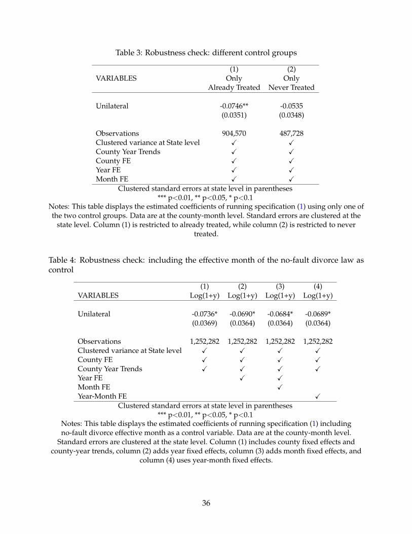
Table 3: Robustness check: different control groups

(1) (2)VARIABLES Only Only

Already Treated Never Treated

Unilateral -0.0746** -0.0535(0.0351) (0.0348)

Observations 904,570 487,728Clustered variance at State level X X

County Year Trends X X

County FE X X

Year FE X X

Month FE X X

Clustered standard errors at state level in parentheses*** p<0.01, ** p<0.05, * p<0.1

Notes: This table displays the estimated coefficients of running specification (1) using only one ofthe two control groups. Data are at the county-month level. Standard errors are clustered at the

state level. Column (1) is restricted to already treated, while column (2) is restricted to nevertreated.

Table 4: Robustness check: including the effective month of the no-fault divorce law ascontrol

(1) (2) (3) (4)VARIABLES Log(1+y) Log(1+y) Log(1+y) Log(1+y)

Unilateral -0.0736* -0.0690* -0.0684* -0.0689*(0.0369) (0.0364) (0.0364) (0.0364)

Observations 1,252,282 1,252,282 1,252,282 1,252,282Clustered variance at State level X X X X

County FE X X X X

County Year Trends X X X X

Year FE X X

Month FE X

Year-Month FE X

Clustered standard errors at state level in parentheses*** p<0.01, ** p<0.05, * p<0.1

Notes: This table displays the estimated coefficients of running specification (1) includingno-fault divorce effective month as a control variable. Data are at the county-month level.

Standard errors are clustered at the state level. Column (1) includes county fixed effects andcounty-year trends, column (2) adds year fixed effects, column (3) adds month fixed effects, and

column (4) uses year-month fixed effects.

36

Table 5: Robustness check: using the effective month of no-fault divorce law as treatment

(1) (2) (3) (4)VARIABLES Log(1+y) Log(1+y) Log(1+y) Log(1+y)

No-Fault -.00980 -0.0167 -0.0168 -0.0165(0.0111) (0.0129) (0.0129) (0.0128)

Observations 1,252,282 1,252,282 1,252,282 1,252,282Clustered variance at State level X X X X

County FE X X X X

County Year Trends X X X X

Year FE X X

Month FE X

Year-Month FE X

Clustered standard errors at state level in parentheses*** p<0.01, ** p<0.05, * p<0.1

Notes: This table displays the estimated coefficients of running specification (1) replacingno-fault divorce effective month as the main regressor (i.e., replacing unilateral divorce with

no-fault divorce). Data are at the county-month level. Standard errors are clustered at the statelevel. Column (1) includes county fixed effects and county-year trends, column (2) adds year

fixed effects, column (3) adds month fixed effects, and column (4) uses year-month fixed effects.

Table 6: Potential mechanisms: wives’ wage

(1) (2)Log

Average Married Average MarriedVARIABLES Women’s Real Wage Women’s Real Wage

Unilateral 0.000558 -0.0407(0.0162) (0.142)

Observations 20,400 20,400Clustered variance at State level X X

State FE X X

Year FE X X

Month FE X X

State Year Trends X X

Clustered standard errors at state level in parentheses*** p<0.01, ** p<0.05, * p<0.1

Notes: This table displays the estimated coefficients of running specification (3). Data are at thestate-month level. Standard errors are clustered at the state level. Each column of the table uses adifferent dependent variable. Column (1) uses the average married women’s real wage in logs;

column (2) uses the average married women’s real wage. Each column includes state fixedeffects, state-year trends, year fixed effects and month fixed effects.

37

Tab

le7:

Po

tential

mech

anism

s:m

arriage

com

pen

sation

(1) (2) (3) (4) (5) (6)VARIABLES Log(1+y) IHS Log(1+y) IHS Log(1+y) IHS

Marrying-Fertile age Marrying-Fertile age Other ages Other ages Joint regression Joint regression

Unilateral -0.0739 -0.0880 -0.0174 -0.0227 -0.0286 -0.0348(0.0466) (0.0555) (0.0158) (0.0187) (0.0242) (0.0287)

Dummy Marrying-Fertile age 0.0813*** 0.096***

(0.0174) (0.0207)

Unilateral*DummyMarrying-Fertile age -0.0402** -0.0476**

(0.0183) (0.0218)

Observations 1,252,282 1,252,282 1,252,282 1,252,282 2,504,564 2,504,564Clustered variance at State level X X X X X X

County FE X X X X X X

County Year Trends X X X X X X

Year FE X X X X X X

Month FE X X X X X X

Clustered standard errors at state level in parentheses*** p<0.01, ** p<0.05, * p<0.1

No

tes:T

his

table

disp

lays

the

estimated

coeffi

cients

of

run

nin

gsp

ecificatio

n(4)

for

marry

ing

-fertileag

esam

ple

and

for

“oth

erag

es”sam

ple.

Data

areat

the

cou

nty

-mo

nth

level.

Stan

dard

errors

areclu

steredat

the

statelev

el.E

achco

lum

no

fth

etab

leu

sesa

differen

td

epen

den

tv

ariable.

Co

lum

n(1)

uses

log(1

+y)

of

the

marry

ing

-fertileag

eg

rou

p,co

lum

n(2)

uses

the

IHS

transfo

rmatio

no

fth

em

arryin

g-fertile

age

gro

up

,colu

mn

(3)u

seslog

(1+y)

of

the

“oth

erag

es”g

rou

p,an

dco

lum

n(4)

uses

the

IHS

transfo

rmatio

no

fth

e“o

ther

ages”

gro

up

.C

olu

mn

s(5)

and

(6)sh

ow

the

results

of

run

nin

geq

uatio

n(6).

38

Tab

le8:

Po

tential

mech

anism

s:fi

gh

tag

ainst

crime

mech

anism

(1) (2) (3) (4) (5) (6) (7) (8)Log Log Log Log

VARIABLES Officers Officers Officers Officers Officers Officers Officers Officers

Unilateral -0.00382 0.0361 -0.0116 -0.0210 0.00713 0.0153 0.0207 0.0166(0.0702) (0.0849) (0.0846) (0.0752) (0.0580) (0.0762) (0.0427) (0.0262)

Observations 2,250 2,250 1,750 1,750 2,250 2,250 1,750 1,750Clustered variance at State level X X X X X X X X

State FE X X X X X X X X

Year FE X X X X X X X X

State Year Trends X X X X

Sample 1971-2016 1971-2016 1980-2014 1980-2014 1971-2016 1971-2016 1980-2014 1980-2014Clustered standard errors at state level in parentheses

*** p<0.01, ** p<0.05, * p<0.1

No

tes:T

his

table

disp

lays

the

estimated

coeffi

cients

of

run

nin

gsp

ecificatio

n(5).

Data

areat

the

state-year

level.

Stan

dard

errors

areclu

steredat

the

statelev

el.C

olu

mn

s(1)

to(4)

use

the

dep

end

ent

variab

lein

levels;co

lum

ns

(5)to

(8)u

seth

ed

epen

den

tv

ariable

inlo

gs.

39

Table 9: Potential mechanisms: fight against crime mechanism

(1) (2) (3) (4) (5) (6)VARIABLES Log(1+y) IHS Log(1+y) IHS Log(1+y) IHS

Robbery Robbery Drugs Drugs Vandalism Vandalism

Unilateral -0.00172 -0.00221 -0.0655 -0.0809 0.0256 0.0277(0.00836) (0.0102) (0.0906) (0.102) (0.0589) (0.0681)

Observations 1,252,282 1,252,282 1,252,282 1,252,282 1,252,282 1,252,282Clustered variance at State level X X X X X X

County FE X X X X X X

County Year Trends X X X X X X

Year FE X X X X X X

Month FE X X X X X X

Clustered standard errors at state level in parentheses*** p<0.01, ** p<0.05, * p<0.1

Notes: This table displays the estimated coefficients of running specification (1) using femalerobbery, vandalism and drug arrests as the dependent variables. Data are at the county-monthlevel. Standard errors are clustered at the state level. Columns (1), (3) and (5) use log (1 + y) as

the dependent variable, while columns (2), (4) and (6) use the IHS transformation as thedependent variable.

40

Tab

le10:

Po

tential

mech

anism

s:d

eman

dp

rox

iedb

yG

oo

gle

Tren

ds

data

(1) (2) (3) (4) (5) (6) (7) (8) (9) (10) (11) (12) (13) (14) (15) (16)Synonyms of prostitute Indoor prostitution Websites

VARIABLES Prostitute Bitch Call Girl Whore Hot babe Hooker Hustler Sex Stripper Strip club Escort The Erotic Review Erotic Review Craiglist Backpage Backpage Erotic

Panel A: Levels

Unilateral 1.548 2.343 -2.319 -0.990 2.811 3.317** -0.653 0.553 1.114** 3.012 1.029 -1.094 -4.382 0.495 3.525 5.044*(1.967) (2.817) (2.754) (1.647) (2.533) (1.454) (0.673) (1.970) (0.444) (3.207) (2.623) (4.080) (5.692) (6.766) (6.135) (2.442)

Panel B: Logs

Unilateral 0.0661 0.0449 -0.123 -0.00262 0.130*** 0.0600 0.00443 0.0120 0.0196 0.0389 0.0261 -0.0528 -0.0669 -0.0514 -0.0648 0.0492(0.0594) (0.0397) (0.0915) (0.0776) (0.0454) (0.0715) (0.0531) (0.0265) (0.0493) (0.0835) (0.0373) (0.215) (0.204) (0.196) (0.201) (0.0526)

Panel C: IHS

Unilateral 0.0641 0.0455 -0.145 -0.00180 0.140** 0.0560 0.00256 0.0179 0.0360 0.0268 -0.0524 -0.0666 -0.0667 -0.104 0.0235(0.0712) (0.0436) (0.118) (0.0931) (0.0627) (0.0869) (0.0678) (0.0629) (0.0982) (0.0393) (0.245) (0.228) (0.258) (0.244) (0.0700)

Observations 8,262 8,262 7,452 8,262 7,128 8,262 8,262 8,262 8,262 8,262 8,262 7,128 5,994 8,262 8,262 2,430Clustered variance at State level X X X X X X X X X X X X X X X X

State FE X X X X X X X X X X X X X X X X

Year FE X X X X X X X X X X X X X X X X

Month FE X X X X X X X X X X X X X X X X

State Year Trends X X X X X X X X X X X X X X X X

Clustered standard errors at state level in parentheses*** p<0.01, ** p<0.05, * p<0.1

No

tes:T

his

table

disp

lays

the

estimated

coeffi

cients

of

run

nin

gsp

ecificatio

n(6).

Data

areat

the

state-mo

nth

level.

Stan

dard

errors

areclu

steredat

the

statelev

el.E

achco

lum

nin

clud

esstate

fix

edeffects,state-y

eartren

ds,y

earfi

xed

effectsan

dm

on

thfi

xed

effects.S

amp

le:Jan

uary

2004to

Decem

ber

2017.

41

Tab

le11:

Po

tential

mech

anism

s:d

eman

dp

rox

iedb

yG

oo

gle

Tren

ds

data,

samp

le2004-

2014

(1) (2) (3) (4) (5) (6) (7) (8) (9) (10) (11) (12) (13) (14) (15) (16)Synonyms of prostitute Indoor prostitution Websites

VARIABLES Prostitute Bitch Call Girl Whore Hot babe Hooker Hustler Sex Stripper Strip club Escort The Erotic Review Erotic Review Craiglist Backpage Backpage Erotic

Panel A: Levels

Unilateral 0.715 2.192*** -1.204 -0.0193 5.390*** 1.167 0.880 1.589 0.772 2.527 1.749 -0.466 -4.501 3.638 3.019 8.429***(2.360) (0.807) (3.036) (2.210) (1.778) (3.396) (0.919) (3.102) (0.662) (5.095) (4.379) (4.820) (6.735) (7.269) (5.430) (0.710)

Panel B: Logs

Unilateral 0.0251 0.0709 -0.0843 0.0368 0.181*** 0.0444 0.0562 0.0322 0.0314 0.0572 0.0433 -0.0991 -0.105 -0.00573 -0.163 0.00747(0.0626) (0.0460) (0.0909) (0.0889) (0.0347) (0.0644) (0.0600) (0.0409) (0.0551) (0.106) (0.0583) (0.132) (0.174) (0.308) (0.291) (0.148)

Panel C: IHS

Unilateral 0.0641 0.0455 -0.145 -0.00180 0.140** 0.0560 0.00256 0.0179 0.0360 0.0268 -0.0524 -0.0666 -0.0667 -0.104 0.0235(0.0712) (0.0436) (0.118) (0.0931) (0.0627) (0.0869) (0.0678) (0.0629) (0.0982) (0.0393) (0.245) (0.228) (0.258) (0.244) (0.0700)

Observations 8,262 8,262 7,452 8,262 7,128 8,262 8,262 8,262 8,262 8,262 8,262 7,128 5,994 8,262 8,262 2,430Clustered variance at State level X X X X X X X X X X X X X X X X

State FE X X X X X X X X X X X X X X X X

Year FE X X X X X X X X X X X X X X X X

Month FE X X X X X X X X X X X X X X X X

State Year Trends X X X X X X X X X X X X X X X X

Clustered standard errors at state level in parentheses*** p<0.01, ** p<0.05, * p<0.1

No

tes:T

his

table

disp

lays

the

estimated

coeffi

cients

of

run

nin

gsp

ecificatio

n(6).

Data

areat

the

state-mo

nth

level.

Stan

dard

errors

areclu

steredat

the

statelev

el.E

achco

lum

nin

clud

esstate

fix

edeffects,state-y

eartren

ds,y

earfi

xed

effectsan

dm

on

thfi

xed

effects.S

amp

le:Jan

uary

2004to

Decem

ber

2014.

42

Table 12: Potential mechanisms: demand proxied by YPSS data on opinions

(1) (2) (3) (4)Dislike Dislike Dislike Dislike

VARIABLES Prostitution Prostitution Prostitution Prostitution

Divorced -0.0174 0.00623(0.0255) (0.0311)

Divorced & Male 0.0471 -0.0333(0.0395) (0.0383)

Divorced/Separated 0.0305 0.0153(0.0280) (0.0275)

Divorced/Separated & Male -0.0259 -0.0464(0.0319) (0.0320)

Observations 3,736 3,736 3,736 3,736Clustered variance at School-code level X X X X

Individual FE X X X X

Wave FE X X X X

Clustered standard errors at state level in parentheses*** p<0.01, ** p<0.05, * p<0.1

Notes: This table displays the estimated coefficients of running specification (7). Standard errorsare clustered at school-code level.

43

Table 13: Potential mechanisms: demand proxied by number of unmarried men

(1) (2) (3)Unmarried Unmarried

VARIABLES Unmarried growth Log(y)

Unilateral 421.7 0.00216 0.0119(487.1) (0.00186) (0.0149)

Observations 20,400 20,300 20,400Clustered variance at State level X X X

State FE X X X

Year FE X X X

Month FE X X X

State Year Trends X X X

Clustered standard errors at state level in parentheses*** p<0.01, ** p<0.05, * p<0.1

Notes: This table displays the estimated coefficients of running specification (8). Data are at thestate-month level. Standard errors are clustered at the state level. Each column of the table uses a

different dependent variable. Column (1) uses the number of unmarried men, column (2) usesthe growth rate of the number of unmarried men, while column (3) uses the number of

unmarried men in logs. Each column includes state fixed effects, state-year trends, year fixedeffects and month fixed effects.

44

Figure 1: Event study

Notes: This figure plots the estimated coefficients of the event study analysis. On the horizontalaxis, there is the event time in years (groups of 12 months). On the vertical axis, the coefficientsare measured in terms of their effect on the dependent variable. The coefficients are measuredrelative to the omitted coefficient (t = −1). For each coefficient, the solid line graphs the point

estimate, while dotted lines graph confidence intervals at the 90% level. The pattern of theestimated coefficients is consistent with the identification assumption: they show the absence of a

pretrend and a trend break after the entry into force of unilateral divorce law. In fact, the twocoefficients prior to the event (i.e., -3 and -2) are close to zero in the point estimate and

statistically zero, respectively, whereas the coefficients after the event (i.e., 0, 1, 3, 4, 5) arestatistically negative at standard significance levels. The solid red line is depicted at the height of

the DiD coefficient. Moreover, this line displays the DiD coefficient and its standard error. Thesize of the coefficient of the last period is in line with DiD results.

45

Figure 2: Marriage and prostitution market equilibrium

Source: Edlund and Korn (2002).

46

Figure 3: Event study: marrying-fertile age group

Notes: This figure plots the estimated coefficients of the event study analysis for arrestedprostitutes in the marrying-fertile age group. The horizontal axis presents the event time in years(groups of 12 months). On the vertical axis, the coefficients are measured in terms of their effect

on the dependent variable. The coefficients are measured relative to the omitted coefficient(t = −1). For each coefficient, the solid line graphs the point estimate, while dotted lines graphconfidence intervals at the 90% level. The pattern of the estimated coefficients is consistent withthe marriage compensation mechanism: they show the absence of a pre-trend and a trend breakafter the entry into force of unilateral divorce law. In fact, the two coefficients prior to the event(i.e., -3 and -2) are close to zero in the point estimate and statistically zero, respectively, whereas

the coefficients after the event (i.e., 0, 1, 2, 3, 4, 5) are statistically negative at standard significancelevels. The solid red line is depicted at the height of the DiD coefficient. Moreover, this line

displays the DiD coefficient and its standard error. The size of the coefficient of the last period isin line with DiD results.

47

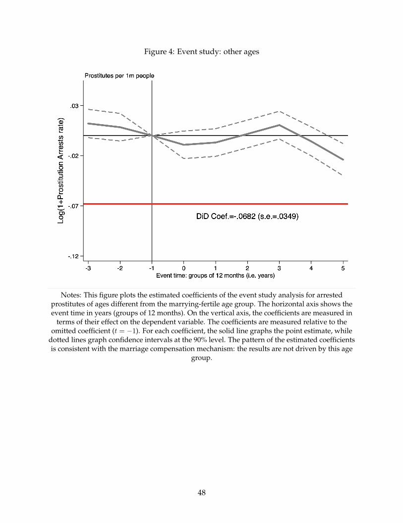
Figure 4: Event study: other ages

Notes: This figure plots the estimated coefficients of the event study analysis for arrestedprostitutes of ages different from the marrying-fertile age group. The horizontal axis shows theevent time in years (groups of 12 months). On the vertical axis, the coefficients are measured in

terms of their effect on the dependent variable. The coefficients are measured relative to theomitted coefficient (t = −1). For each coefficient, the solid line graphs the point estimate, while

dotted lines graph confidence intervals at the 90% level. The pattern of the estimated coefficientsis consistent with the marriage compensation mechanism: the results are not driven by this age

group.

48

References

Agan, A. and S. Starr (2017). Ban the box, criminal records, and racial discrimination: A

field experiment. The Quarterly Journal of Economics 133(1), 191–235.

Agan, A. Y. and M. D. Makowsky (2018). The minimum wage, eitc, and criminal recidi-

vism. Technical report, National Bureau of Economic Research.

Alesina, A. F. and P. Giuliano (2007). Divorce, fertility and the value of marriage. (mimeo).

Allard, P. and G. Herbon (2003). Prostitution enforcement in chicago: An examination of

costs and alternatives. Washington, DC: The Sentencing Project.

Arunachalam, R. and M. Shah (2008). Prostitutes and brides? The American Economic

Review 98(2), 516–522.

Arunachalam, R. and M. Shah (2013). Compensated for life sex work and disease risk.

Journal of Human Resources 48(2), 345–369.

Beauchamp, A. and S. Chan (2014). The minimum wage and crime. The BE Journal of

Economic Analysis & Policy 14(3), 1213–1235.

Bisschop, P., S. Kastoryano, and B. van der Klaauw (2015). Street prostitution zones and

crime.

Caceres-Delpiano, J. and E. Giolito (2012). The impact of unilateral divorce on crime.

Journal of Labor Economics 30(1), 215–248.

Cameron, S. (2002). The economics of sin: rational choice or no choice at all? Edward Elgar

Publishing.

Cameron, S. and A. Collins (2003). Estimates of a model of male participation in the

market for female heterosexual prostitution services. European Journal of Law and Eco-

nomics 16(3), 271–288.

Charles, K. K. and M. C. Luoh (2010). Male incarceration, the marriage market, and female

outcomes. The Review of Economics and Statistics 92(3), 614–627.

Cho, S.-Y., A. Dreher, and E. Neumayer (2013). Does legalized prostitution increase hu-

man trafficking? World Development 41, 67–82.

Ciacci, R. and M. M. Sviatschi (2016). The Effect of Adult Entertainment Establishments

on Sex Crime: Evidence from New York City. mimeo.

49

Cook, P. J., S. Kang, A. A. Braga, J. Ludwig, and M. E. OBrien (2015). An experimental

evaluation of a comprehensive employment-oriented prisoner re-entry program. Jour-

nal of Quantitative Criminology 31(3), 355–382.

Cunningham, S., G. DeAngelo, and J. Tripp (2017). Craigslist’s Effect on Violence Against

Women.

Cunningham, S. and T. D. Kendall (2010). Risk behaviours among internet-facilitated sex

workers: evidence from two new datasets. Sexually transmitted infections 86(Suppl 3),

iii100–iii105.

Cunningham, S. and T. D. Kendall (2011a). 10 prostitution, technology, and the law: new

data and directions. Research Handbook on the Economics of Family Law, 221.

Cunningham, S. and T. D. Kendall (2011b). Men in transit and prostitution: Using political

conventions as a natural experiment. The BE Journal of Economic Analysis & Policy 11(1).

Cunningham, S. and T. D. Kendall (2011c). Prostitution 2.0: The changing face of sex

work. Journal of Urban Economics 69(3), 273–287.

Cunningham, S. and T. D. Kendall (2013). Prostitution 3.0: A comment. Iowa L. Rev.

Bull. 98, 131.

Cunningham, S. and M. Shah (2016). The Oxford Handbook of the Economics of Prostitution.

Oxford University Press.

Cunningham, S. and M. Shah (2017). Decriminalizing indoor prostitution: Implications

for sexual violence and public health. The Review of Economic Studies 85(3), 1683–1715.

Dank, M. L., B. Khan, P. M. Downey, C. Kotonias, D. Mayer, C. Owens, L. Pacifici, and

L. Yu (2014). Estimating the size and structure of the underground commercial sex economy in

eight major US cities. Urban Institute Washington, DC.

de la Torre, A., A. Havenner, K. Adams, and J. Ng (2010). Premium sex: Factors influenc-

ing the negotiated price of unprotected sex by female sex workers in mexico. Journal of

Applied Economics 13(1), 67–90.

Della Giusta, M. (2010). Simulating the impact of regulation changes on the market for

prostitution services. European Journal of Law and Economics 29(1), 1–14.

Della Giusta, M. (2016). Demanding sex: critical reflections on the regulation of prostitution.

Routledge.

50

Della Giusta, M., M. L. Di Tommaso, and S. Strøm (2009). Who is watching? the market

for prostitution services. Journal of Population Economics 22(2), 501–516.

Doleac, J. (2016). Increasing employment for individuals with criminal records. Policy

Proposal, The Hamilton Project, Washington, DC.

Doleac, J. L. and B. Hansen (2016). Does ban the box help or hurt low-skilled workers?

statistical discrimination and employment outcomes when criminal histories are hid-

den. Technical report, National Bureau of Economic Research.

Edlund, L. (2013). The role of paternity presumption and custodial rights for understand-

ing marriage patterns. Economica 80(320), 650–669.

Edlund, L., J. Engelberg, and C. A. Parsons (2009). The wages of sin.

Edlund, L. and E. Korn (2002). A theory of prostitution. Journal of political Economy 110(1),

181–214.

Edlund, L. and R. Pande (2002). Why have women become left-wing? the political gender

gap and the decline in marriage. The Quarterly Journal of Economics 117(3), 917–961.

Elrod, L. D. and R. G. Spector (1997). A review in the year of family law: A search for

definitions and policy. Fam. LQ 31, 613.

Farley, M. (2003). Prostitution, trafficking and traumatic stress, Volume 2. Psychology Press.

Farley, M. (2004a). Bad for the body, bad for the heart: prostitution harms women even if

legalized or decriminalized. Violence against women 10(10), 1087–1125.

Farley, M. (2004b). Prostitution is sexual violence. Psychiatric Times 21(12), 7–8.

Farley, M. and E. Butler (2012). Prostitution and trafficking-quick facts. Prostitution Re-

search & Education.

Farley, M., A. Cotton, J. Lynne, S. Zumbeck, F. Spiwak, M. E. Reyes, D. Alvarez, and

U. Sezgin (2004). Prostitution and trafficking in nine countries: An update on violence

and posttraumatic stress disorder. Journal of Trauma Practice 2(3-4), 33–74.

Fondation-Scelles (2012). Rapport mondial sur l’exploitation sexuelle: la prostitution au coeur

du crime organise. Economica.

Friedberg, L. (1998). Did unilateral divorce raise divorce rates? evidence from panel data.

Technical report, National Bureau of Economic Research.

51

Gertler, P., M. Shah, and S. M. Bertozzi (2005). Risky business: the market for unprotected

commercial sex. Journal of political Economy 113(3), 518–550.

Gertler, P. J. and M. Shah (2011). Sex work and infection: what’s law enforcement got to

do with it? The Journal of Law and Economics 54(4), 811–840.

Gray, J. S. (1998). Divorce-law changes, household bargaining, and married women’s

labor supply. The American Economic Review 88(3), 628–642.

Gruber, J. (2004). Is making divorce easier bad for children? the long-run implications of

unilateral divorce. Journal of Labor Economics 22(4), 799–833.

HG.org (2017). Prostitution in the united states. https://www.hg.org/article.asp?id=

30997. Accessed: 2017-08-30.

Immordino, G. and F. F. Russo (2014). Prostitution policy. In The Oxford Handbook of the

Economics of Prostitution.

Immordino, G. and F. F. Russo (2015a). Laws and stigma: the case of prostitution. European

Journal of Law and Economics 40(2), 209–223.

Immordino, G. and F. F. Russo (2015b). Regulating prostitution: A health risk approach.

Journal of Public Economics 121, 14–31.

Islam, A. and R. Smyth (2012). The economic returns to good looks and risky sex in the

bangladesh commercial sex market. The BE Journal of Economic Analysis & Policy 12(1).

Jakobsson, N. and A. Kotsadam (2013). The law and economics of international sex slav-

ery: prostitution laws and trafficking for sexual exploitation. European Journal of Law

and Economics 35(1), 87–107.

Kempadoo, K. (1999). Slavery or work? reconceptualizing third world prostitution. posi-

tions 7(1), 225–237.

Kempadoo, K. (2007). The war on human trafficking in the caribbean. Race & Class 49(2),

79–85.

Kempadoo, K., J. Sanghera, and B. Pattanaik (2015). Trafficking and prostitution reconsidered:

New perspectives on migration, sex work, and human rights. Routledge.

Lee, S. and P. Persson (2015). Human trafficking and regulating prostitution.

52

Levitt, S. D. and S. A. Venkatesh (2007). An empirical analysis of street-level prostitution.

Preliminary draft, September.

Logan, T. D. and M. Shah (2013). Face value: information and signaling in an illegal

market. Southern Economic Journal 79(3), 529–564.

Marvell, T. B. (1989). Divorce rates and the fault requirement. Law and Society Review,

543–567.

Mazur-Hart, S. F. and J. J. Berman (1977). Changing from fault to no-fault divorce: An

interrupted time series analysis. Journal of Applied Social Psychology 7(4), 300–312.

Moffatt, P. G. and S. A. Peters (2004). Pricing personal services: An empirical study of

earnings in the uk prostitution industry. Scottish Journal of Political Economy 51(5), 675–

690.

Pearl, J. (1986). The highest paying customers: America’s cities and the costs of prostitu-

tion control. Hastings LJ 38, 769.

Raphael, S. (2010). Improving employment prospects for former prison inmates: Chal-

lenges and policy. In Controlling crime: Strategies and tradeoffs, pp. 521–565. University

of Chicago Press.

Raphael, S. and D. F. Weiman (2007). The impact of local labor market conditions on the

likelihood that parolees are returned to custody. Barriers to Reentry? The Labor Market

for Released Prisoners in Post-Industrial America, 304–332.

Rasul, I. (2004). The impact of divorce laws on marriage. Unpublished manuscript, Univer-

sity of Chicago.

Rasul, I. (2005). Marriage markets and divorce laws. Journal of Law, Economics, and organi-

zation 22(1), 30–69.

Rheinstein, M. (1955). The law of divorce and the problem of marriage stability. Vand. L.

Rev. 9, 633.

Rheinstein, M. (1972). Marriage stability, divorce, and the law.

Schnepel, K. T. (2017). Good jobs and recidivism. The Economic Journal 128(608), 447–469.

Shah, M. (2013). Do sex workers respond to disease? evidence from the male market for

sex. The American Economic Review 103(3), 445–450.

53

Shively, M., K. Kliorys, K. Wheeler, D. Hunt, et al. (2012). A national overview of prostitu-

tion and sex trafficking demand reduction efforts. Washington, DC: The National Institute

of Justice.

Sohn, K. (2016). Men’s revealed preferences regarding women’s ages: evidence from

prostitution. Evolution and Human Behavior 37(4), 272–280.

Stevenson, B. (2008). Divorce law and women’s labor supply. Journal of Empirical Legal

Studies 5(4), 853–873.

Stevenson, B. and J. Wolfers (2006). Bargaining in the shadow of the law: Divorce laws

and family distress. The Quarterly Journal of Economics 121(1), 267–288.

Stevenson, B. and J. Wolfers (2007). Marriage and divorce: Changes and their driving

forces. The Journal of Economic Perspectives 21(2), 27–52.

TheEconomist (2004). Sex is their business. http://www.economist.com/node/3151258.

Accessed: 2017-08-30.

Tuttle, C. (2019). Snapping back: Food stamp bans and criminal recidivism. American

Economic Journal: Economic Policy 11(2), 301–27.

Uggen, C. and S. K. Shannon (2014). Productive addicts and harm reduction: How work

reduces crime-but not drug use. Social Problems 61(1), 105–130.

Urban Justice Center (2005). Behind Closed Doors: An Analysis of Indoor Sex Work in

NYC.

Vlosky, D. A. and P. A. Monroe (2002). The effective dates of no-fault divorce laws in the

50 states. Family Relations 51(4), 317–324.

Voena, A. (2015). Yours, mine, and ours: Do divorce laws affect the intertemporal behav-

ior of married couples? The American Economic Review 105(8), 2295–2332.

Weitzman, L. J. (1985). The divorce revolution: The unexpected social and economic

consequences for women and children in america.

Wickelgren, A. L. (2007). Why divorce laws matter: Incentives for noncontractible marital

investments under unilateral and consent divorce. The Journal of Law, Economics, &

Organization 25(1), 80–106.

Yang, C. S. (2017). Local labor markets and criminal recidivism. Journal of Public Eco-

nomics 147, 16–29.

54

Yttergren, A. and J. Westerstrand (2016). The swedish legal approach to prostitution.

trends and tendencies in the prostitution debate. NORA-Nordic Journal of Feminist and

Gender Research 24(1), 45–55.

55

Online Appendix

A Background on the U.S. prostitution market

Prostitution is one of the most unsafe occupations in the U.S., worse than being an

Alaskan fisherman, logger, or oil rig worker. As reported by HG.org (2017), the death rate

for prostitutes in the U.S. is 204 out of every 100,000; that for Alaskan fishermen is 129 out

of every 100,000. Moreover, statistics on prostitutes are conservative since prostitution is

illegal in the U.S. (it is only allowed in Nevada in brothels and certain areas of the state).

Prostitutes facing violence have nowhere to go without risking arrest themselves.

Dank et al. (2014) found that, in 2007, in eight major U.S. cities, prostitution generated

a market value ranging from $39.9 to $290 million.51 Furthermore, Pearl (1986) estimated

that 16 U.S. cities spent on average $15.3 million each year on prostitution control. More

recently, Allard and Herbon (2003) found that prostitution arrests caused an expense of

$10.3 million in the city of Chicago alone. According to HG.org (2017), the annual aver-

age of approximately 70,000-80,000 arrests for prostitution costs American taxpayers $200

million. Unsurprisingly, prostitution moves huge amounts of money in the form of both

generated income and crime prevention.

The large amounts of money that prostitution moves around might originate from the

lack of agreement on prostitution law. Opponents of prostitution contend that prosti-

tution is dehumanizing (e.g., Farley et al. (2004); Farley (2003, 2004a); Farley and Butler

(2012)). According to this line of thought, prostitutes are victims of physical and psycho-

logical violence. For example, Farley (2004b) estimated that approximately 85% to 95%

of prostitutes wish to escape from prostitution but have no other options for survival. By

contrast, those supporting legalization of prostitution argue that prostitutes chose to ex-

change their time and services for money as in any other job (e.g., TheEconomist (2004);

Kempadoo (1999, 2007); Kempadoo et al. (2015)). Hence, it is the criminalization of pros-

titution that worsens prostitutes’ standard of living. They claim that since prostitution

cannot be stopped, legalizing it would be the only way to tax and “protect” prostitutes.

This ideological problem regarding how to regulate prostitution is all the more impor-

tant because the U.S. prostitution market is highly stratified. Thus, the effects of any given

regulation of the prostitution market might differ across market segments. The prostitu-

tion market in the U.S. can be divided into three segments. On the lowest tier, there are

street prostitutes. Street prostitutes are usually controlled by pimps and thus make the

51The eight cities in the study were Denver, CO; Washington, DC; San Diego, CA; Miami, FL; Seattle,WA; Dallas, TX; Kansas City, MO; and Atlanta, GA.

56

least money. Further, they lack control over their choice of clients and are more likely to

be victims of violence and to be arrested. Operating at the medium level are those work-

ing indoors in brothels, massage parlors, gentlemen’s clubs and strip clubs. They usually

enjoy better conditions than street prostitutes. Finally, escorts comprise the highest level

of prostitutes. In this market segment, prostitutes have control over their choice of clients

and “careers”; usually, they are not controlled by a pimp, earn high wages and are less

likely to be victims of violence. This group is the one that best fits the image of prosti-

tutes depicted by supporters of legalized prostitution. Prostitution in the medium and

high tiers of this stratification takes place indoors: this is why it is also known as indoor

prostitution, while street prostitution is also known as outdoor prostitution.52

This study makes use of data on female prostitution arrests, which are more likely to

represent outdoor prostitution than indoor prostitution. However, I build a proxy vari-

able for indoor prostitution when analyzing the mechanisms linking unilateral divorce

and prostitution.

B Legislative background: The Divorce Revolution

Traditionally, in the U.S., divorce was permitted only on grounds of demonstrating

guilt of misconduct by one of the two spouses and had to be agreed on mutually by both

spouses (i.e., consent of the innocent party was required before a divorce was granted).

Generally, such grounds were abandonment, cruelty, incurable mental illness, or adultery.

The law was regarded as inadequate due to the major emotional and financial transaction

costs involved in the verification of guilt of wrongdoing during the divorce process.

Thus, dissolution of marriages that were broken for mundane reasons (i.e., without

misconduct by any spouse) was only possible if one of the two parties declared herself

or himself guilty. In addition, since divorce had to be mutually agreed, the belief was

that whenever husbands wished to divorce, they would bribe their wives to obtain their

consent, while if wives wished to divorce, they could not afford to bribe their partners.

However, since divorce was considered to be against the public interest, civil courts

formerly denied a divorce if there was evidence of cooperation between the two spouses

or if they attempted to counterfeit the grounds for divorce. In fact, divorce could be

barred even if one of the two spouses was found guilty. The three main reasons for refus-

ing a divorce petition were as follows: recrimination, the suing spouse also being found

guilty; condonation, forgiving the misconduct explicitly or implicitly by continuing to

52For further details on the stratification of the prostitution market in the U.S., see Shively et al. (2012).

57

live with the partner after knowing of it; and connivance, participating in the fault, such

as organizing an act of adultery.

This law not only required marital wrongdoing to file the divorce petition but also

punished spouses for such misbehavior. Indeed, both husband and wife could be pun-

ished if they were found guilty of wrongdoing. If the husband was at fault, he usually

suffered the loss of child custody and the imposition of economic responsibilities; if the

wife was found at fault, she might suffer the loss of alimony and child custody.

There was the tacit perception that the abolition of fault grounds and mutual consent

would eliminate the hypocrisy that incited the use of perjury and the forgery of evidence

to surmount strict legal hurdles (Marvell 1989; Rheinstein 1955, 1972; Mazur-Hart and

Berman 1977). On the one hand, the guilt or innocence of the spouses would be irrelevant

if no-fault divorce were available. On the other hand, consent of the partner would be

useless if unilateral divorce were available.

In 1969, the California Family Law Act completely removed the requirements of fault

as the basis for divorce and allowed spouses to file for divorce without the consent of their

partner. This act established only two grounds for divorce: (i) irreconcilable differences;

(ii) incurable insanity. Following Weitzman (1985), researchers have viewed this reform

as the basis for both no-fault and unilateral divorce.

The focus of the reform was gender neutral: it assumed that the divorcee was eco-

nomically independent and employable. Consequently, this law established two major

bases for alimony awards: the divorcees’ employability and the length of the marriage. If

either of the divorcees were not economically independent, this law also helped her/him

to garner new-skills or to improve existing skills to become self-sufficient.

The California Family Law Act started a movement to reform divorce laws in the U.S.

known as “The Divorce Revolution”, and various states followed suit. The movement

gathered an apolitical consensus. Right-wingers viewed it as an expansion of personal

rights and freedom. Left-wingers promoted it to prevent women from being locked into

unfortunate marriages.

Unlike the case of California, “The Divorce Revolution” consisted of two steps: no-

fault divorce and unilateral divorce. First, states moved to no-fault divorce regimes,

which were already effective (to different degrees) in various states prior to 1950 while

retaining mutual agreement. Next, states moved to unilateral divorce, requiring the con-

sent of only one spouse to legally dissolve the marriage. This second step, which was

uncommon before the 1960s, started in 1969 immediately after the passage of the Califor-

nia Family Law Act.

No-fault divorce does not change the bargaining structure within a marriage relation-

58

ship. It solely reduces transaction costs by decreasing bargaining costs and eliminating

financial penalties that could no longer be inflicted on at-fault spouses. Indeed, a no-fault

divorce law eliminates the requirement of proof of guilt or innocence of either spouse. Af-

ter the introduction of no-fault divorce, marriage dissolution could be lodged on grounds

such as “incompatibility” or “irreconcilable differences”. However, it has to be agreed to

mutually by both partners. It was formulated simply to make marriage dissolution less

dolorous and mournful.

Unilateral divorce goes a step further. It removes the property rights that mutual

consent divorce grants either to the innocent spouse (for fault divorces) or to the spouse

who does not wish to get divorced (for no-fault divorces). Namely, unilateral divorce

could change spouses’ behavior in two different ways. First, it allows spouses who are

unable to prove the guilt of their partner or cannot afford to bribe their partner to file for

divorce. Second, it changes the bargaining power between the members of the couple.

Furthermore, no-fault divorces are more complex to code since the definition of what

constitutes a no-fault divorce is much broader than the definition of unilateral divorce.

The literature classifies no-fault divorce into four categories: (a) living separate and apart

as grounds for divorce; (b) incompatibility as grounds for divorce; (c) no-fault provisions

added to traditional grounds as grounds for divorce; (d) no-fault is the sole grounds for

divorce (Elrod and Spector 1997). These differences have given rise to widespread dis-

agreement among scholars using no-fault divorce dates (Vlosky and Monroe 2002). An

important point of divergence has been how to categorize fault-based laws that added

“living separate and apart” provisions as no-fault laws. Even if such settlements consent

to divorce without any proof of wrongdoing, the waiting period might be so long that it

renders the provision either too weak to be regarded as no-fault or tantamount to a fault

divorce law. The key difference is that true no-fault divorce laws are difficult to compare

to legislative changes that simply revise fault-based grounds.

Unilateral divorce laws are easier to code; the only difference is whether the provi-

sion requires a separation period. The literature has treated as unilateral divorce regimes

either both provisions with and without separation requirements or only provisions with-

out separation requirements. Following Gruber (2004), I use unilateral divorce laws with-

out separation for two reasons. First, since I code the law using a dummy variable, the

comparison of identical unilateral divorce laws seems more reasonable and accurate. Sec-

ond, even if unilateral divorce laws without separation requirements usually became ef-

fective later than those with separation requirements, I observe when such laws enter into

effect since my sample period spans from 1980 to 2014.

Finally, coding might differ on whether enactment dates or effective dates were used.

59

The enactment date is the date on which a law is approved, while the effective date is

the date on which a law enters into force. There can be a lag of months between the

enactment and the effective date. Coding the effective date is usually more laborious

than coding the enactment date since it necessitates a review of the session laws of each

state. Nevertheless, I use the effective date since it is the one that is crucial in legal actions.

C Nature of the effect: Inflow vs Stock

Figure A.1 shows the effect of unilateral divorce on prostitution across age groups.53.

As in the main regression, the dependent variable is in logs, each regression includes

county, year and month fixed effects and county-year trends, and variance is clustered at

the state level.

There are two ways in which unilateral divorce could affect prostitution: either by pre-

venting women from becoming prostitutes (i.e., inflow effect) or by affecting prostitutes

who are already in the market (i.e., stock effect). If unilateral divorce decreases young

(old) prostitutes’ arrests, it would support the former (latter) effect. Figure A.1 shows

that unilateral divorce mainly reduces prostitution in women between 25 and 29 years

old and in those between 45 and 49 years old.54 Hence, there is evidence in favor of both

effects.

In addition, Figure A.1 has two features worth mentioning. First, unilateral divorce

does not affect prostitutes aged 17 and 24 years old and prostitutes aged 50 and 65 years

old or older. In these two age groups, the point estimate is close to zero, and it is reassur-

ing to find that the standard errors are narrow. Second, in contrast, in the age group of

women age 25 and 49 years old, there seems to be a U-shaped curve, but standard errors

are not as precise.

53Age groups are classified according to UCR database as in Table A.3. Starting at 25 years old, ages aregrouped into five-year blocks: 25 to 29 years old, 30 to 34 years old, and so on and so forth.

54There could be the concern that there is no effect in the 17-24 age group since data are not pooled.However, Section G.1 presents the results of running a regression pooling together with arrests of femaleprostitutes between 17 and 24 years old and the results do not change.

60

Figure A.1: The effect of unilateral divorce on prostitution across age groups

Notes: This figure shows the effect of unilateral divorce on prostitution across age groups. Eachcoefficient and standard errors come from a regression, with the same structure as in the main

specification, where the dependent variable was computed using the age group indicated.Confidence intervals are at the 90% level. These results suggest that unilateral divorce bothprevents women from entering prostitution and affects women who are already prostitutes.

61

D List of crimes in UCR data set

Table A.1: List of offenses

Offense code Offense

01A Murder and non-negligent manslaughter01B Manslaughter by negligence02 Forcible rape03 Robbery04 Aggravated assault05 Burglary-breaking or entering06 Larceny-theft (not motor vehicles07 Motor vehicle theft08 Other assaults09 Arson10 Forgery and counterfeiting11 Fraud12 Embezzlement13 Stolen property-buy, receive, poss.14 Vandalism15 Weapons-carry, posses, etc.16 Prostitution and commercialized vice17 Sex offenses (not rape or prostitution)18 Total drug abuse violations180 Sale/manufacture (subtotal)185 Possession (subtotal)18A Sale/mfg-Opium, coke, and their derivatives18B Sale/mfg-Marijuana18C Sale/mfg-Truly addicting synthetic narcotics18D Sale/mfg-Other dangerous non-narc drugs18E Possession-Opium, coke, and their derivatives18F Possession-Marijuana18G Possession-Truly addicting synthetic narcotics18H Possession-Other dangerous non-narc drugs19 Gambling (total)19A Bookmaking (horse and sports)19B Number and lottery19C All other gambling20 Offenses against family and children21 Driving under the influence22 Liquor laws23 Drunkenness24 Disorderly conduct25 Vagrancy26 All other non-traffic offenses27 Suspicion28 Curfew and loitering violations29 Runaways

62

E Further information on the data set

E.1 Descriptive statistics

Table A.2 displays summary statistics for arrests of female prostitutes per 1,000,0000

inhabitants across treated and control states.55 Data are at the county-month level, and

treated states are disaggregated at pre- and post-treatment levels.

Table A.2: Summary statistics

(1) (2) (3) (4) (5)Never-treated Always-treated Treated

Arrests of female prostitutesper 1,000,000 inhabitants pre post all

Mean 1.87 1.80 3.19 0.88 2.29Std. dev. 13.83 20.44 16.27 6.39 13.38Obs. 347,712 764,554 85,642 54,374 140,016Max 2,042 3,969 1,058.22 484 1,058.22

Table A.3 shows summary statistics for arrests of female prostitutes per 1,000,0000 in-

habitants broken out by age group. Columns (1) to (4) respectively report mean, standard

deviation, minimum and maximum. Column (5) reports the share of each group, out of

the total arrests of female prostitutes, without taking into account the population.56

55Arrests of female prostitutes per 1,000,000 inhabitants is computed as the number of arrested femaleprostitutes divided by population and multiplied by 1,000,000. Same computations are made for data onother crimes.

56Age groups are defined according to the UCR database.

63

Table A.3: Summary statistics

(1) (2) (3) (4) (5)Arrests of female prostitutesper 1,000,000 inhabitants Mean Std. dev. Min Max Relative share (%)

Age group17 .0223 1.4267 0 1225.49 0.9318 0.0586 0.9967 0 222 3.1519 0.0809 1.3189 0 253.23 4.6520 0 .0885 1.6375 0 461.04 5.0721 0.099 2.1318 0 745.86 5.722 0.1017 2.2021 0 563.49 5.8923 0.0998 2.0089 0 485.63 5.6924 0.0979 1.7881 0 370.88 5.3725-29 0.4155 4.7445 0 889.3 22.8530-34 0.3216 3.8326 0 2849 17.0835-39 0.2219 2.1452 0 411.07 11.6440-44 0.1327 1.4215 0 309.26 6.945-49 0.0681 1.1198 0 545.55 3.3550-54 0.0243 0.5573 0 212.95 1.255-59 0.0084 0.4604 0 236.91 0.3760-64 0.0029 0.2399 0 122.44 0.1365 or older 0.0022 0.2487 0 134.12 0.07Total 1.87 18.11 0 3969.04 100

Figure A.2 displays arrests of female prostitutes per 1,000,0000 inhabitants (in the

same logarithmic transformation as the dependent variable) for the three groups of states:

treated, never treated and already treated. Vertical lines represent the year in which uni-

lateral divorce laws became effective in each of the treated states.

This figure cannot be used to assess whether the trends of treated and control groups

are parallel since the effective dates of unilateral divorce laws differ across states. How-

ever, it shows that, as many more states adopt unilateral divorce, treated states experience

a substantial decline in arrests of female prostitutes per 1,000,0000 inhabitants, in line with

my findings. In other words, as treated states adopt unilateral divorce, arrests of female

prostitutes decrease more severely there than in control states.

64

Figure A.2: Evolution of female prostitutes arrests in treated and control states

Notes: This figure plots arrests of female prostitutes per 1,000,0000 inhabitants, in the samelogarithmic transformation as the dependent variable, for the three groups of states analyzed inthe study: treated, never treated and already treated. Vertical lines represents the year in which

unilateral divorce law became effective in each of the treated states.

F Effective date of unilateral divorce laws across U.S. states

The effective date is established using Thomson Reuters Westlaw. In the section “Statutes

and Court rules”, Thomson Reuters Westlaw keeps track of different legislations and

when they became effective. This procedure establishes an effective month for each state

that experienced a change in divorce law during my sample period. Figure A.3 maps

treated and control states (i.e., never treated and already treated, respectively).

65

Figure A.3: Treated and control states

Notes: This figure maps U.S. states according to their treatment status.

G Comment on potential mechanisms: marriage compen-

sation mechanism

G.1 Comparison group

There could be the concern that the finding that unilateral divorce has a greater impact

on arrested prostitutes of marrying-fertile age is due to the choice of using arrested pros-

titutes of other ages as the comparison group. This latter group is composed of arrested

prostitutes either between 17 and 24 years old or strictly older than 49 years old since the

marrying-fertile age group is formed by prostitutes between 25 and 49 years old. The po-

tential concern is that results are driven by the inclusion of prostitutes strictly older than

49 years old that might seem less frequent than their younger counterparts.

To address this issue, this section presents the results of running equation (6) but using

arrested prostitutes between 17 and 24 years old only (i.e., arrested prostitutes older than

49 years old are excluded). Using only prostitutes between 17 and 24 years old signifies

66

using only prostitutes of fertile age but too young to get married.

Table A.4 shows the results of running the same analysis as before but for this age

group. Findings are qualitatively similar: there is evidence that unilateral divorce law has

a larger impact on arrested prostitutes of marrying-fertile age than on arrested prostitutes

of other ages. This evidence supports the marriage compensation mechanism.

Figure A.4 shows the results of running equation (2) for the “17-24 years old” sample.

In line with the marriage compensation mechanism, the coefficients show that the results

are not driven by this age group.

Figure A.4: Event study: “17-24 years old” sample

Notes: This figure plots the estimated coefficients of the event study analysis for arrestedprostitutes in the ”17-24 years old” sample. On the horizontal axis is the event time in years

(groups of 12 months). On the vertical axis, the coefficients are measured in terms of their effecton the dependent variable. The coefficients are measured relative to the omitted coefficient

(t = −1). For each coefficient, the solid line graphs the point estimate, while dotted lines graphconfidence intervals at the 90% level. The pattern of the estimated coefficients is consistent with

the marriage compensation mechanism: results are not driven by this age group.

67

Tab

leA

.4:P

oten

tialm

echan

isms:

marriag

eco

mp

ensatio

n

(1) (2) (3) (4) (5) (6)VARIABLES Log(1+y) IHS Log(1+y) IHS Log(1+y) IHS

Marrying-Fertile age Marrying-Fertile age 17-24 y.o. 17-24 y.o. Joint regression Joint regression

Unilateral -0.0800 -0.0945 -0.0176 -0.0230 -0.0282 -0.0345(0.0521) (0.0615) (0.0155) (0.0186) (0.0232) (0.0279)

Dummy Marrying-Fertile age 0.0774*** 0.0929***

(0.0163) (0.0197)

Unilateral*DummyMarrying-Fertile age -0.0352** -0.0422**

(0.0172) (0.0208)

Observations 1,252,282 1,252,282 1,252,282 1,252,282 2,504,564 2,504,564Clustered variance at State level X X X X X X

County FE X X X X X X

County Year Trends X X X X X X

Year FE X X X X X X

Month FE X X X X X X

Clustered standard errors at state level in parentheses*** p<0.01, ** p<0.05, * p<0.1

No

tes:T

his

table

disp

lays

the

estimated

coeffi

cients

of

run

nin

gsp

ecificatio

n(4)

for

marry

ing

-fertileag

esam

ple

and

for

the

“17-24y

earso

ld”

samp

le.D

ataare

atth

eco

un

ty-m

on

thlev

el.S

tand

arderro

rsare

clustered

atstate

level.

Each

colu

mn

of

the

table

uses

ad

ifferent

dep

end

ent

variab

le.C

olu

mn

(1)u

seslog

(1+y)

of

the

marry

ing

-fertileag

eg

rou

p,co

lum

n(2)

uses

the

IHS

transfo

rmatio

no

fth

em

arryin

g-fertile

age

gro

up

,colu

mn

(3)u

seslog

(1+y)

of

the

“17-24y

earso

ld”

gro

up

,and

colu

mn

(4)u

sesth

eIH

Stran

sform

ation

of

the

“17-24y

earso

ld”

gro

up

.C

olu

mn

s(5)

and

(6)sh

ow

the

results

of

run

nin

geq

uatio

n(6).

68

G.2 Indoor Prostitution

A potential concern could be that female prostitutes of marrying and fertile age be-

came more difficult to arrest for reasons disconnected to their opportunity cost of getting

married. As far as I can determine, there is no clear plausible mechanism that could sup-

port this explanation.57

CPS data provide information on the occupational code; this allows me to restrict the

sample to potential indoor prostitutes. Using the occupational code, I can restrict the sam-

ple to female respondents working in industrial sectors connected to indoor prostitution.

Hence, I obtain a reasonable proxy for potential indoor prostitutes.58

Namely, I consider the following regression model similar to regression model (4):

log(1 + Indoor Prostitutionsmy) = βUnilateralsmy + αm + αy + αs + αs ∗ y + εsmy (A.1)

where Indoor prostitutessmy is the number of women in occupational sectors that con-

tain indoor prostitution businesses per 1,000,000 inhabitants in state s, month m and year

y; αm, αy and αs are respectively month, year and state fixed effects; and αs ∗ y are state-

year linear trends. As in the previous analysis, I split the sample depending on the age of

female respondents. In particular, I split the sample into two groups: indoor prostitutes

of marrying-fertile age and indoor prostitutes of other ages.

Columns (1) and (4) of Table A.5 show the results of running equation (8) for marrying-

fertile age and other ages. The results show that unilateral divorce decreases potential

indoor prostitutes of marrying-fertile age but does not affect potential indoor prostitutes

of other ages. Columns (2) and (5) report results using IHS, while columns (3) and (6)

reports the results in levels. The results are stable across functional forms.

57 Cunningham and Kendall (2011a) hypothesized that “the Internet and other modern technologies aredrawing prime-aged (street) prostitutes into indoor work”. There could be the concern that this hypothesisis driving my findings. For this to occur, internet would need to be introduced simultaneously to unilateraldivorce laws. Using data on indoor prostitutes would shed light on this mechanism too.

58Appendix Section H provides the exact list of the occupational codes used.

69

Table A.5: Potential mechanisms: marriage compensation, CPS data

(1)

(2)

(3)

(4)

(5)

(6)

Lo

g(1

+y

)IH

SL

evel

sM

arry

ing

-fer

tile

Mar

ryin

g-f

erti

leM

arry

ing

-fer

tile

Lo

g(1

+y

)IH

SL

evel

sV

AR

IAB

LE

Sag

eag

eag

eO

ther

ages

Oth

erag

esO

ther

ages

Un

ilat

eral

-0.3

17**

-0.3

58**

-13.

01*

0.10

50.

115

9.48

0(0

.141

)(0

.159

)(7

.342

)(0

.117

)(0

.131

)(8

.799

)

Ob

serv

atio

ns

20,4

0020

,400

20,4

0020

,400

20,4

0020

,400

Clu

ster

edv

aria

nce

atS

tate

lev

elX

XX

XX

X

Sta

teF

EX

XX

XX

X

Yea

rF

EX

XX

XX

X

Mo

nth

FE

XX

XX

XX

Sta

teY

ear

Tre

nd

sX

XX

XX

X

Clu

ster

edst

and

ard

erro

rsat

stat

ele

vel

inp

aren

thes

es**

*p<

0.01

,**

p<

0.05

,*p<

0.1

Notes: This table displays the estimated coefficients of running specification (A.1). Data are at thestate-month level. Standard errors are clustered at the state level. Each column of the table uses a

different dependent variable. Columns (1), (2) and (3) respectively use number of potentialindoor prostitutes of marrying-fertile age in logs, IHS and levels. Columns (4), (5) and (6) use thesame variable but for potential indoor prostitutes of other ages. Each column includes state fixed

effects, state-year trends, year fixed effects and month fixed effects.

70

H Industry sectors used to measure indoor prostitution

To measure potential indoor prostitutes, I restrict CPS data to the following occupa-

tional codes in the table below. The names of the variables are drawn from the monthly

extracts of the CPS Uniform database of the Centre of Economic Policy Research (CEPR).59

In order to code such variables, it is useful to use both SIC and NAICS systems.

Specifically, I restrict my sample to women working in industry sectors composed of

strip clubs and escort-girl services (i.e., sectors that comprise indoor prostitution estab-

lishments). Note that these industry sectors are composed of various occupations, among

which there are strip clubs, massage parlors and escort-girls services. Hence, women in

this sample might be working in other occupations too. However, this sample is more

likely to be formed by prostitutes. Recall that in the U.S., the prostitution market is highly

stratified. Women arrested for prostitution are very likely street prostitutes, who make up

the low segment of the market. The sample I extract from CPS data is composed of strip

clubs, massage parlors and escort-girls services, who form the medium and high seg-

ments of the market. According to the theory, indoor prostitutes are as likely to respond

to an increase in pm as outdoor prostitutes.

Table A.6: Occupational codes used

Occupational code Strip-clubs Escort services

ind70 798 809ind80 791 810ind03, ind09, ind12, ind14 8590 9090

occ70 933occ80 469occ03, occ11, occ12 4520, 4650

For variables ind70 and ind80, strip clubs belong to an occupational sector named

“Miscellaneous entertainment and recreative services”, while escort services belong to

“Miscellaneous personal services”. In the last three variables, these names respectively

change to “Other amusement, gambling, and recreative services” and “Other personal

services”. 60 This sample spans from 1980 to 2014. Sectors for variables occ70 and occ80

59http://ceprdata.org/cps-uniform-data-extracts/60An example of the SIC code classification is https://www.osha.gov/pls/imis/sic_manual.display?

id=267&tab=description

71

are labeled as “Personal service occupations, not elsewhere classified”. Finally, Sectors

for variables occ03, occ11 and occ12 are labeled as “Miscellaneous personal appearance

workers” and ”Personal care and service workers, all other”.

I Comment on potential mechanisms: fight against crime

mechanism

I.1 Officers

There could be the concern that hired officers do not vary considerably over years and

that this lack of variation is driving the results of the police mechanism.

To address this issue, this section considers equation (2) but makes use of two different

transformations of the dependent variable. First, I use the first difference of officers per

1,000 inhabitants. In other words, I use the variation (i.e., increase/decrease) of hired

officers normalized by a state’s population. Second, I use the growth rate of officers per

1,000 inhabitants. Results are presented in the same fashion as in the police mechanism

analysis.

I find no empirical evidence supporting that unilateral divorce correlates with a re-

duction of officers.

72

Tab

leA

.7:P

oten

tialm

echan

isms:

fig

ht

again

stcrim

em

echan

ism

(1) (2) (3) (4) (5) (6) (7) (8)First Difference First Difference First Difference First Difference Growth rate Growth rate Growth rate Growth rate

VARIABLES Officers Officers Officers Officers Officers Officers Officers Officers

Unilateral 0.00535 -0.00554 -0.00758 -0.0166 -0.000861 -0.00181 -0.00607 -0.00792(0.00665) (0.00753) (0.00916) (0.0160) (0.00418) (0.00437) (0.00439) (0.00748)

Observations 2,150 2,150 1,750 1,750 2,150 2,150 1,750 1,750Clustered variance at State level X X X X X X X X

State FE X X X X X X X X

Year FE X X X X X X X X

State Year Trends X X X X

Sample 1971-2016 1971-2016 1980-2014 1980-2014 1971-2016 1971-2016 1980-2014 1980-2014Clustered standard errors at state level in parentheses

*** p<0.01, ** p<0.05, * p<0.1

No

tes:T

his

table

disp

lays

the

estimated

coeffi

cients

of

run

nin

gsp

ecificatio

n(5)

for

two

differen

ttran

sform

ation

so

fth

ed

epen

den

tv

ariable.

Data

areat

the

state-year

level.

Stan

dard

errors

areclu

steredat

statelev

el.C

olu

mn

s(1)

to(4)

use

the

dep

end

ent

variab

lein

levels;co

lum

ns

(5)to

(8)u

seth

ed

epen

den

tv

ariable

inlo

gs.

I.2O

the

rcrim

es

Th

issectio

np

resents

results

of

run

nin

gm

ym

ainsp

ecificatio

nu

sing

asd

epen

den

t

variab

leeach

of

the

main

catego

rieso

fo

ffenses

record

edb

yU

CR

(28m

aincateg

ories

of

73

offenses excluding prostitution).61 Such offenses are recorded in two panels depending on

whether there is evidence in the literature that they are connected to prostitution. Namely,

Panel A shows offenses not connected to prostitution, while Panel B displays offenses

connected to prostitution.

There is evidence in the literature (Urban Justice Center 2005; Dank et al. 2014; Cun-

ningham et al. 2017; HG.org 2017) that prostitution is connected to different crimes. Using

such literature, I divided offenses in two groups: connected and not connected to prosti-

tution, as shown in Table A.8.62

Each cell in the column shows the estimated coefficient, and its standard error, associ-

ated with unilateral divorce using the corresponding offense in the row as the dependent

variable transformed according to the corresponding column. In fact, each column shows

the results of running the abovementioned regression with a different functional form of

the dependent variable. Columns (1), (2) and (3) respectively use the dependent variable

in logs, IHS and levels. Each regression includes month and year fixed effects, county

fixed effects and linear trends, and variance is clustered at the state level.

61All the categories are reported in Appendix Section D62Two crimes in Panel A could have been in Panel B. First, for “total drug abuse” (i.e., drugs crimes/use),

there is evidence in the literature that both prostitutes and prostitutes’ clients make use of drugs. However,their relative percentage with respect to the whole “drugs market” is unclear. This is why such regressions’results also appear in Section 7. Second, “vagrancy” there is evidence in the literature that prostitutes’arrests are seldom reported as “loitering” (for example, the New York State Division of Criminal JusticeServices classifies “loitering” as including “loitering for prostitution”). Given the close connection between“vagrancy” and “loitering”, the former could also be considered as an offense connected to prostitution.

74

Table A.8: Potential mechanisms: fight against crime mechanism

(1) (2) (3)DEPENDENT VARIABLE Log(1+y) IHS Levels

Panel A: Crimes not connected to prostitutionRobbery -0.001721 -0.00221 -0.00031

(0.00836) (0.0102) ( 0.08983)Burglary 0.08697** 0.10148** 1.81443***

(0.03777) (0.04509) (0.58084)Larceny 0.03422 0.02712 9.46527*

(0.08818) (0.09835) (4.78697)Motor Theft 0.02040 0.02336 -0.60396

(0.02898) (0.034473) (1.49761)Other Assault -0.04920 -0.05902 0.98405

(0.09551) (0.10851) (4.30007)Arson 0.00079 0.00079 0.03033

(0.00734) (0.00891) (0.09112)Forgery -0.04906 -0.06002 0.39481

(0.05031) (0.05987) (0.64869)Fraud -0.24433 -0.27693 -1.49883

(0.14994) (0.16957) (6.56632)Embezzlement 0.00188 0.00162 0.09943

(0.03516) (0.04353) (0.22858)Stolen Property -0.00154 -0.00236 -0.21224

(0.01479) (0.01728) (0.36632)Vandalism 0.0256 0.0277 1.13909

(0.0589) (0.0681) (1.13533)Total Drug abuse -0.0655 -0.0809 -1.02097

(0.0906) (0.102) (6.01042)Gambling 0.00523 0.00664 -0.05416

(0.01352) (0.01642) (0.15739)Offences against family and children -0.27179 -0.32726 -1.91609

(0.1766) (0.21361) (1.65182)Driving under alcohol influence -0.33186 -0.38589 -7.97683

(0.23374) (0.26046) (10.0430)Liquor laws -0.06766 -0.09378 9.06771

(0.12086) (0 .14263) (10.6131)Drunkeness -0.02130 -0.02631 -2.41075

(0.07916) (0.09107) (3.63117)Disorder Conduct -0.01541 -0.01903 0.04367

(0.06861) (0.07877) (2.56150)Vagrancy -0.04257** -0.05104** -0.59007*

(0.01704) (0.02017) (0.33096)Other Non Traffic Offences -0.09939 -0.10798 -10.1071

(0.1476) (0.16343) (17.5948)Suspicion 0.00266 0.00378 -0.03259

(0.00336) (0.00387) (0.15955)Runaways -0.14292 -0.16488 -2.64762

(0.09808) (0.11373) (2.17062)

Panel B: Crimes connected to prostitutionHomicide -0.00891 -0.01068 -0.16131*

(0.00541) (0.00647) (0.08153)Rape -0.00333 -0.00412 0.01808

(0.00453) (0.00563) (0.03788)Assault -0.09301* -0.10923* -1.24446

(0.05274) (0.06289) (0.81679)Weapon -0.02623* -0.03184* -0.11522

(0.01409) (0.01687) (0.14296)Sex Offences -0.02103 -0.02563 0.0069

(0.03223) (0.03965) (0.27205)Curfew and Loitering violations -0.00365 -0.00546 -0.08268

(0.04229) (0.04943) (0.95489)Observations 1,252,282 1,252,282 1,252,282

Clustered standard errors at state level in parentheses*** p<0.01, ** p<0.05, * p<0.1

Notes: This table displays the estimated coefficients of running specification (1) for each eachoffense recorded by UCR (row) and functional form of the dependent variable (column).

75

J Comment on demand mechanisms

The demand function considered in Section 7 is a simplified version of the original one

discussed in Edlund and Korn (2002). In fact, in Edlund and Korn (2002), the demand for

prostitution is a weighted average of the demand for prostitution by unmarried men and

of the demand for prostitution by married men. Both demands are an increasing function

of men’s earnings. In addition, the demand of prostitution by married men is also a

decreasing function of pm.

As for the former, I run a regression using CPS data, where the dependent variable

is the average wage of men. The specification has the same structure as the specification

shown in equation (3). Table A.9 shows the results of running this equation for men’s

real wages in logs (column (1)) and in levels (column (2)), respectively. All in all, I do

not find suggestive evidence that unilateral divorce law decreases men’s earnings and,

as a consequence, the demand for prostitution. Indeed, the lower bounds of the 90%

confidence intervals associated with estimated coefficients of columns (1) and (2) suggest

that the reduction in men’s real wages is at most between 3.6% and 3.9%.63

As for the latter, it implies that an increase in pm could decrease the demand for prosti-

tution by married men as well as reduce the supply of prostitution. To study this channel,

I would need data on the demand for prostitution by married men, which I do not have.

Hence, it is important to note that finding that unilateral divorce reduces the demand for

prostitution by married men would not be inconsistent with the marriage compensation

channel.

63Each estimate corresponds to the lower bound of a confidence interval. The sample mean of the de-pendent variable used in column (2) (i.e., average men’s real wage) is 13.2.

76

Table A.9: Potential mechanisms: men’s wage

(1) (2)Log

VARIABLES Average Men’s Real Wage Average Men’s Real Wage

Unilateral -0.0127 -0.257(0.0145) (0.161)

Observations 20,400 20,400Clustered variance at State level X X

State FE X X

Year FE X X

Month FE X X

State Year Trends X X

Clustered standard errors at state level in parentheses*** p<0.01, ** p<0.05, * p<0.1

Notes: This table displays the estimated coefficients of running the specification (3) for men. Dataare at the state-month level. Standard errors are clustered at state level. Each column of the tableuses a different dependent variable. Column (1) uses average men’s real wage in logs; column (2)

uses average men’s real wage in levels. Each column includes state fixed effects, state-yeartrends, year fixed effects and month fixed effects.

77