Centre de Referència en Economia Analítica

Barcelona Economics Working Paper Series

Working Paper nº 87

On the Choice of an Exchange Regime: Target Zones Revisited

Jesús Rodríguez and Hugo Rodríguez

October 2003

On the Choice of an Exchange Regime:Target Zones Revisited

Jesús Rodríguez López∗

Universidad Pablo de Olavide and centrA

Hugo Rodríguez MendizábalUniversitat Autonoma de Barcelona and centrA

Barcelona Economics WP no 87October 11, 2003

Abstract

From the classical gold standard up to the current ERM2 arrangementof the European Union, target zones have been a widely used exchangeregime in contemporary history. This paper presents a benchmark modelthat rationalizes the choice of target zones over the rest of regimes: the fixedrate, the free float and the managed float. It is shown that the monetaryauthority may gain efficiency by reducing volatility of both the exchangerate and the interest rate at the same time. Furthermore, the model isconsistent with some known stylized facts in the empirical literature thatprevious models were not able to generate, namely, the positive relationbetween the exchange rate and the interest rate differential, the degree ofnon-linearity of the function linking the exchage rate to fundamentals andthe shape of the exchange rate stochastic distribution. Keywords: Targetzones, exchange rate agreements, monetary policy, time consistency. JELclassification: E52, F31, F33.

∗Corresponding author: Jesús Rodríguez López, Universidad Pablo de Olavide, Carretera deUtrera km. 1, 41013 Sevilla (Spain), jrodlop@dee.upo.es

1. Introduction

This paper tackles the question of the choice of an exchange regime, with a specialfocus on target zones. During the nineties, a large amount of literature analyzeda variety of issues regarding target zones, both from a theoretical perspective(i.e. mainly the properties of the model proposed by Krugman [15] and of itsvariants) as well as from an applied point of view (i.e. mainly the crisis of theEuropean Monetary System). The creation of the European Monetary Union ledexchange rate researchers to move their interests to other questions apart from theones proposed by the target zone literature. Yet, we believe there are still usefulinsights to be learnt on target zones. The reasons why we persist are threefold:

1. Target zones have been the predominant exchange rate agreement in theworld throughout contemporary history. Some recent analyses have reclas-sified exchange rate regimes focusing on what countries actually do ratherthan on what they say they do (see Calvo and Reinhart [6], Reinhart [23],Reinhart and Rogoff [24], Fischer [8] and Levy-Yeyati and Sturzenegger[17]). This implies a distinction between de jure and de facto typologies.De jure examples of target zones are numerous: the interwar Gold Stan-dard, the postwar Bretton Woods regime, the European monetary snakeof 1971, the European Monetary System (EMS) from 1978 to 1998, or theunilateral target zone of Sweden from August 1977, among others. On theother hand, the number of de facto examples of target zones is much larger.The aforementioned literature has stressed the fact that many of the de jurefree floaters strongly intervene to soften the fluctuations of the nominal ex-change rate. This has been labeled as fear of floating. The recent de factoclassification of Reinhart and Rogoff [24] confirms that most of the majorcurrencies are traded in an international exchange market characterized bybands of fluctuations (see their Appendix III). According to these authors,“...the most popular exchange rate regime over modern history has beenthe crawling peg or narrow crawling band, which accounts for over 26 per-cent of the observations”. In the Western Hemisphere, this accounts forabout a 42 percent of the observations. Their sample consists on market-determined paralell exchange rates observations of 153 countries from 1946through 2001.

2. Target zones shall probably be an important exchange rate agreement at leastin the nearby future. As an example, consider the ERM2 which, from Jan-

2

uary 1st 1999, is working as a “hub-and-spokes” zone between the euro andthose currencies of the European Union countries not participating in theMonetary Union (United Kingdom, Denmark and Sweden). Also, accessioncountries to the European Union shall commit to a target zone arrangementduring the transition period. Again, many other de facto examples couldbe quoted.

3. Any exchange rate regime can be seen as an special case of a target zone.Pegged rates can be seen as target zones with band widths equal to zeroand pure floating rates are equivalent to fluctuation bands with an infinitewidth. In between, dirty floats can be seen as implicit target zones withfinite bands while target zone regimes impose those bands explicitly. Thechoice of an exchange regime then consists on deciding how wide shouldthe bandwidth be. It must be clear that we will not try to give a typologyof exchange regimes alternative to the ones given by Reinhart and Rogoff[24] or by Levy-Yeyati and Sturzenegger [17]. Instead, what we do is toconstruct a general model able to represent any exchange agreement. Bydoing so, we can rationalize such a choice.

The need of a more formal target zone model becomes more important giventhat the extreme regimes (i.e. the fixed rate and the flexible rate) are only stan-dard textbook cases. While Obstfeld and Rogoff [22] predicted a world of widelyfloating exchange rates, given the removal of controls to international capital mo-bility, the fear of floating literature has pointed out that countries reveal a prefer-ence towards smoothing the dynamics of the exchange rate. Intermediate regimesseem to be defining the current world so that completely fixed or fully flexible rates(see Fischer [8]) are seldom observed. Pure fixed exchange rate regimes are rarelyused since they compromise a large amount of monetary independence. A mone-tary commitment that pegs the exchange rate to a low inflation foreign currencycan establish a disciplining effect that motivates a higher degree of credibility andprice stability (see Giavazzi and Pagano [12]). However, given the evidence on thechoice of currency regimes by central banks, it seems that the gains from stabilityof fixed exchange rates have not been big enough to dampen the losses from lessmonetary independence (see Svensson [30] for a detailed discussion). On the otherhand, pure free floating regimes are not observed either. Monetary authorities useto play leaning against the wind policies in an attempt to control the exchangerate around some target level, official or unofficially. Thus, it seems that hybridexchange regimes based on target zones have been widely used on the basis that

3

it apparently reaps the benefits of both flexible and fixed exchange rates.Krugman [15] presented the model that has become the standard tool to study

target zones regimes. The dynamics of the exchange rate were derived from alinear asset pricing relation and an arbitrage condition given by the uncoveredinterest rate parity. His model assumed that the central bank intervenes so asto maintain the exchange rate within the band. In this paper, we look at twoissues. First, we extend Krugman’s model in two directions: (i) we allow thecentral bank to perform intramarginal interventions, that is, to use its monetarypolicy to affect the exchange rate before it hits the limits of the band and, (ii) weintroduce lack of credibility of the target zone, that is, the perception by marketparticipants of the possibility that the central bank will not defend the band whenit has to. Unlike the literature following Krugman’s work that has concentratedon one of these extensions at a time, we show that both features are needed inorder to reconcile the model with data. As a second issue, we use the model torationalize the choice of target zones over the rest of regimes: the fixed rate, thefree float and the managed float. It is shown that, by imposing a target zone, themonetary authority may gain efficiency through reducing volatility of both theexchange rate and the interest rate simultaneously.The paper is organized as follows. Section 2 sets up the general model. Sub-

sections 2.2 to 2.4 show how the fixed rate, the managed float and the free floatcan be seen as extreme cases of a target zone. Section 2.5 develops the targetzone solution. Section 3 deals with the two questions outlined in the previousparagraph. The last section concludes.

2. Set up of the Model

2.1. General assumptions

The model represents a highly stylized dynamic stochastic general equilibriumeconomy. It can be thought of as a reduced form version of more complicatedfully optimizing models. Time is discrete. First, consider an equation specifyingequilibrium in the money market:

mt − pt = ϕyt − γit + ξt, (2.1)

where mt is money supply, pt is the domestic price level of yt, a tradable good,it is the domestic interest rate of a one period of maturity bond, and ξt is someshock to money demand. They are all expressed in logs, with the exception of

4

the interest rate. Parameters ϕ and γ are both positive: money demand increaseswith output because of a transaction motive and there is an implicit liquiditypreference behavior, meaning that money can be a substitute for a bond thatreturns a nominal interest it.Let xt be the log of the nominal exchange rate, expressing the price of one

unit of foreign currency in terms of domestic currency. The (log) real exchangerate is given by

qt = xt − pt + p∗t , (2.2)

where p∗t is the foreign price (variables with star will denote the foreign analogue).Call dt ≡ it−i∗, the interest rate differential, where i∗ is the foreign (constant)

rate, and assume perfect capital mobility, risk aversion and the uncovered interestrate parity condition (UIP)

dt = Et xt+1 − xt+ rt, (2.3)

where Et is the expectation operator conditional on information available at timet. Thus, the expected rate of depreciation must compensate for the interest ratedifferential plus the foreign premium, rt. We assume the variable rt to be exoge-nous and governed by a first order Markov process

rt = rt−1 + εt. (2.4)

The white noise εt is supposed to be Gaussian, εt ∼ N (0,σ2), for convenience.1Using (2.2), (2.3) and (2.1) one obtains

xt = ft + γEt xt+1 − xt , (2.5)

ft = mt + vt,

vt = θt + γrt,

θt = qt − p∗t − ϕyt + γi∗ − ξt.

1The foreign risk premium plays a key role in the current paper. In general, the UIP does nothold (see Ayuso and Restoy [1]). Conventional target zone models consider that deviations fromUIP are negligible in target zones (see Svensson [28]). A common practice in some credibilitytests of target zones relies in this idea (v.g. the simplest test, see Svensson [25], and the driftadjustment method of Bertola and Svensson [5]). However, Bekaert and Gray [3] find that therisk premia in a target zone are sizable and should not be ignored. They argue that this mightbe the reason of why the credibility tests run on EMS at the beginning of the nineties failed inanticipating the 1992-93 turbulences.

5

Total fundamentals ft amount to an endogenous process, mt, plus an exogenousprocess, vt. By iterating forward on xt we have that

xt = (1− ν)∞Xτ=0

ντEtft+τ = (1− ν)∞Xτ=0

ντEt mt+τ + vt+τ , (2.6)

with ν ≡ γ (1 + γ)−1. The forward looking behavior from UIP implies that thevalue of asset xt is the present discounted value of the future stream of funda-mentals. Notice that (1− ν)

P∞τ=0 ν

τ = 1, thus, if mt+τ were orthogonal to vt+τfor all t and τ , the long run effect of an increase in mt is to impulse xt by anequal amount. We assume that both the central bank and traders can observethe realization of θt and rt.The monetary authority must choose the path for money mt so to maximize

its preferences subject to the evolution of vt and the exchange rate regime.The objective is to set up these preferences to capture the degree of monetaryindependence that arises under alternative exchange rate regimes. As in Svensson[29], the concept of monetary independence is associated with the interest ratevariability. At one extreme, and in the absence of realignments, a fixed rateeliminates monetary independence. At the other extreme, a managed float regimeprovides the highest degree of independence. In between, a target zone gives somescope to focus the monetary policy on domestic problems. To capture this idea,the central bank (henceforth, CB) preferences are modeled to evaluate the trade-off between interest rate variability versus exchange rate variability

J =1

2Et

( ∞Xτ=0

βτ£d2t+τ + λ (xt+τ − ct)2

¤). (2.7)

The long run desirable target for the interest rate differential is zero. The targetfor the exchange rate is the central parity ct around which deviations are punishedby the relative penalty λ. The factor β ∈ (0, 1) is a time discount rate.We think of a very short maturity term for the bond in the UIP, say a few

days, a week or a month at most. The idea is that the CB controls some monetaryaggregate mt to target dt, xt. Output realizations and real fluctuations areobserved with some delay, and not available by the time monetary policy is decidedso the only available information at any period is θt, rt. From (2.3) and (2.5) itis easy to show that mt will respond one to one to the shock θt and the problemreduces to deciding how to split the shock rt between dt and xt. Thus, the CBjust needs to choose dt and xt every period given the value of rt to minimize

6

(2.7) subject to (2.3), (2.4) and the exchange regime which restricts the policiesavailable to the CB.In what follows, any of the exchange rate regimes can be characterized by the

triple λ, w,α. The first element is related to the preferences. The number wis the band width. The last term α is the probability that the CB defends thecurrency when it is outside the band and measures the credibility of the exchangeregime. This triple will adopt particular values for any of the exchange regimesconsidered.

2.2. The fixed exchange rate

Consider first a CB that can credibly commit to fix the exchange rate to ct = c.This regime appears as a particular case of the target zone when w = 0 and α = 1.Given the forward looking restriction of (2.3) and the pure random walk exhibitedby rt, the solution for dt and xt is

dt = rt and xt = c. (2.8)

That is, under a fixed exchange rate regime the nominal interest rate absorbs thewhole variability of rt. The expected value of the game under this regime is

Jc (rt) =1

2

µ1

1− β

¶·r2t +

β

1− βσ2¸. (2.9)

The variability of the interest rate is a source of time inconsistency. If theCB can commit to a rule like (2.8), it must exhibit a stronger response to therisk premium shock in an attempt to content the exchange rate at the centralparity. However, there arises the possibility of deviating from this simple rule inorder to reduce interest rate variability. If this temptation is captured by marketparticipants, the simple rule will no longer be credible. Hence, (2.8) would betime inconsistent.

2.3. The managed float

This regime is a particular case of the target zone when λ > 0, w→∞,α = 1.The solution is related to a managed or dirty floating rate where the CB exploitsthe trade-off between the variability of the exchange rate and the interest rateevery period. After the shock rt is realized and agents have formed their expec-tations on future values for the exchange rate, the CB must set the two target

7

variables dt+τ , xt+τ∞τ=0 with one instrument mt+τ∞τ=0, to minimize the loss(2.7) subject to the arbitrage condition (2.3) and the relation in (2.4). Notice theexchange regime does not impose additional restrictions.The optimality condition is given by the difference equation

xt = c+rtλ+1

λEt xt+1 − xt . (2.10)

The central parity is constant here since, with an infinitely-wide band, there willbe no realignments. Forward iteration yields

xt = c+1

1 + λEt

∞Xτ=0

rt+τ(1 + λ)τ

. (2.11)

It is useful to compare expression (2.11) to (2.6): the optimal exchange rate isequal to the central parity plus the present discounted value of the future stream offoreign risk premia which is the only fundamental shock that affects the exchangerate. From (2.4), a linear closed form solution of (2.11) is

xt = c+rtλ. (2.12)

The discretionary rate is then equal to the fixed rate plus a depreciation bias.Forming a one-period ahead expectation yields

Etxt+1 = c+rtλ= xt, (2.13)

so, from (2.3), the target variable dt is

dt = rt. (2.14)

A shock to the risk premium impulses exchange and interest rates in the samedirection. Combining (2.12) and (2.14), a linear control condition is given by

dt = λ (xt − c) , (2.15)

meaning that the interest rate differential is proportional to the depreciation (orappreciation) bias with respect to the central parity. This is just a leaning againstthe wind policy, where the interest rate differential is positive when the currencyis above the target and negative below. Under the uncovered interest rate parity,conditional on xt, the risk premium has a positive relation with dt. Similarly,

8

conditional on dt, rt has also a positive relation with xt. Therefore, a central bankthat is concerned about the volatility of interest rate differentials and of exchangerates will optimally split the variation of rt between dt and xt. This results in aregime of intra-marginal interventions or managed float. The higher the value ofλ, the smaller the variance for the exchange rate is.The explicit form for the expected value of the game under the discretionary

managed float is calculated as

Jmf (rt) =1 + λ

2λ

µ1

1− β

¶·r2t +

β

1− βσ2¸. (2.16)

It is straightforward to see that the previous fixed rate regime is a first best. Thereis no trade-off between the exchange rate and the interest rate. The attempt ofthe CB in giving the interest rate a lower volatility by trading with the exchangerate variance is a vain effort. It results in a discretionary time consistent solution,where the volatility of the interest rate is unaffected and the exchange rate beginsto float. The CB is worse off.Finally, once the target variables have been determined, equation (2.5) gives

us the optimal level for the monetary instrument. From (2.5), the CB will expandor absorb mt, according to

mt = c+ (1 + γλ)rtλ− θt . (2.17)

2.4. The pure free float

Consider now the case where the CB announces that the risk premium shocks willnot be dampened over the exchange rate, whatever the preference parameter λ is.That means

xt = c+ rt. (2.18)

This is a laissez faire solution. The slope of the exchange rate function withrespect to the fundamental is one. According to the UIP (2.3), the interest ratedifferential is again given by

dt = xt − c = rt.Is it a time consistent result? As with the fixed rate, the CB is not deciding

its monetary policy rule to optimize (2.7) and this may be a source of time in-consistency. The result in this regime, depends on the value of λ, though. For

9

the particular case λ = 1, free and managed float solutions are identical andconsistency over time is therefore preserved. However, for values of λ 6= 1, themarket will perceive that CB’s incentives to trade volatility of the exchange ratefor volatility of the interest rate are different than 1 and the announcement ofthe free float will be no longer credible. Notice, that the relevant regime to becompared with the target zone is the managed float.For the sake of completeness, we can compute the indirect value function for

the free float:

Jff (rt) =1

2

µ1 + λ

1− β

¶·r2t +

βσ2

1− β

¸. (2.19)

The relation between the values for the fixed, the managed and the free float rates,can be written as

Jff = λJmf = (1 + λ)Jc,

for any rt, see expressions (2.9), (2.16) and (2.19), respectively. Differences amongregimes will have to be found in the exchange rate dynamics since they imply thesame process for the interest rate differential. Clearly, the fixed rate is preferredover the two other regimes, although it is time inconsistent. The ordering of thelosses for the free float and the managed float will depend upon the value of λwith respect to 1. If λ < 1, the CB is better off with the free float. Otherwise,for λ ≥ 1, managed float is a better regime.

2.5. The target zone

In this case, the regime is characterized by λ ≥ 0, w ≥ 0,α ∈ [0, 1]. The firstelement is related to the preferences in (2.7). The number w is the band width.The last term α is the probability that the CB defends the currency when itis outside the band and measures the credibility of the exchange regime. Wesuppose that, within the bands, the CB defends the currency with probability 1.As stated in the introduction, the purpose is to construct a model able to generatea consistent target zone solution, in the sense that the CB finds it optimal todefend the target zone at the margins by probability α. There are not furtherincentives to renege from the target zone ex-post.From the previous discussion, both the exchange rate and the interest rate

differential will be functions of the shock rt. So, the timing of events at any timet will be as follows:

10

1. The shock rt is realized.

2. If the realization of the shock makes the exchange rate be within the targetzone, the CB solves a minimization problem. The process is as follows:

• The central parity from last period is left unaltered: ct = ct−1.

• Forward looking agents form expectations Etxt+1.

• For given Etxt+1, rt, ct, the CB chooses xt, dt by minimizing theloss (2.7) subject to the arbitrage condition (2.3), the relation in (2.4)and the additional restriction imposed by the target zone system.

3. If for that value of the shock the exchange rate should be outside a band[ct − w, ct + w], for instance, say it is above the upper limit ct + w, the CBcan do any of two actions:

• It defends the currency with probability α. This means that the ex-change rate is pegged at the edge of the band, xt = ct + w, and thecentral parity is not altered, ct = ct−1.

• It realigns the currency with probability (1− α). In this case, thecentral bank devalues the central parity by µ ≥ w, i.e. ct = ct−1 + µ,and situates the exchange rate at xt = ct.

4. Finally, for a given shock θt in the money demand equation (2.5), the CBsupplies the optimal quantity of money mt supporting the pair xt, dt.

To understand the way this economy works consider the following. Assumethe risk premium starts from r0 = 0. The CB can set the exchange rate atx0 = 0 and a target zone of width w around c0 = 0. Because of the symmetryof the forcing process, the interest rate differential is d0 = 0, which equals thetarget value for that variable. As time progresses, the risk premium wandersaround and the exchange rate moves away from its center c0 = 0. Given that theexchange rate is a function of the shock rt, the foreign risk premium must also befluctuating within a symmetric zone with center ρ0 = 0. This zone is denoted as[ρ0 − r, ρ0 + r]. How far the exchange rate wanders from the center of its bandshould be a function of the distance between the risk premium and ρ0. So, for theperiods before the first realignment, we could write

xt = c0 + u(rt − ρ0),

11

where u(rt − ρ0) is the function linking the exchange rate to the fundamentalprocess rt within the band.Imagine that at time t = τ , one of the limits of the exchange rate band is

reached. This means that rτ = ρ0 ± r two level conditions must be satisfiedu (−r) = −w, (2.20)

and

u (r) = w. (2.21)

When exchange rate is at the boundaries of the target zone, the CB could keep xtat the edge of its band. In such a case, all movements in rt will be transferred to theinterest rate differential. The other possibility implies the central bank realigningthe target zone. In such a case, the exchange rate jumps to cτ = cτ−1+µ, and thecenter of the band for the risk premium moves to ρτ = rτ . After the realignmenttakes place, the behavior of the exchange rate band within the target zone is againgoverned by the function u so we can write in general

xt = ct + u(rt − ρt).

Let x(rt) be the function relating the exchange rate to the risk premium atany time, that is, within as well as outside the target zone. This function satisfies

x (rt) = ct

+µ if rt > ρt + r with probability 1− α+w if rt > ρt + r with probability α+u (rt − ρt) if rt ∈ [ρt − r, ρt + r]−w if rt < ρt − r with probability α−µ if rt < ρt − r with probability 1− α.

(2.22)

The unknown continuous function u (rt − ρt) represents the CB’s best responsewhen the risk premium lies within its band [ρt − r, ρt + r]. To find it, we use thefirst order condition for values of rt ∈ [ρt − r, ρt + r],

(1 + λ) [u (rt − ρt)− ct] = rt +Et [x (rt+1)] . (2.23)

Outside of the band, condition (2.23) does no longer hold and the trade-off is notoptimal. In order to find out the particular form of the function u (rt − ρt), theband for the fundamental [−r, r] must be computed, given the level conditions(2.20) and (2.21). Forward recursion is used to solve for u (rt) with the first

12

order condition (2.23) subject to (2.22). Appendix A provides all the details forcomputation of the solution.From condition (2.23) and (2.3), it is straightforward to see that the model

produces a positive relation between the exchange rate of depreciation within theband and the interest rate differential:

dt = λ [u (rt − ρt)− ct] + ρt, (2.24)

outside the bands, the trade-off is not optimal and expression (2.24) does nothold.

3. Results

Before we start with the computations, let us first remind the reader about theimplications derived from the main features of Krugman’s model: the honey moonand the smooth pasting effects (see Svensson [27] and Krugman and Miller [16]).The first means that the response of the exchange rate to changes in fundamentalsis smaller than the response under the free floating regime. That is, as compared toa free floating, the band works as an exchange rate stabilizer. The smooth pastingimplies that the response of the exchange rate tends to zero as it approaches theedges of the band. This is because agents are forward looking and anticipate theintervention by the central bank when the exchange rate gets close to the limit ofthe band.Svensson [27] has summarized the testable implications of Krugman’s model.

First, the distributions of both the exchange rate and the interest rate are U -shaped. That is, the exchange rate tends to live close to the limits of the band.Second, there is a negative and deterministic relation between the exchange rateand the interest rate differential. This relation is given by the uncovered interestrate parity. Finally, the exchange rate exhibits a non-linearity in its univariateforecasting equation, which is a consequence of the smooth pasting effect. How-ever, empirical tests have challenged these predictions. The distribution of theexchange rate has been observed to be hump-shaped rather than U -shaped, so theexchange rate accumulates probability around the center of the band. Secondly,the relationship between the exchange rate and the interest rate is positive ratherthan negative. Finally, it seems that the effects of the smooth pasting conditionare not as relevant as predicted by theory and exchange rates are linear functionsof the fundamentals.

13

In what follows we calibrate our model and compare its predictions with thedata. Furthermore, we compute the losses (2.7) under different regimes and pro-vide a rationale as of why target zones may be widely used as an exchange ratesystem.

3.1. Parameters

The following values for the parameters are used in the numerical exercises of thissection. We think of a week as the time frequency. As in Svensson [29], the timediscount factor is set to β = 0.90

152 . We use this value to ease the calculations

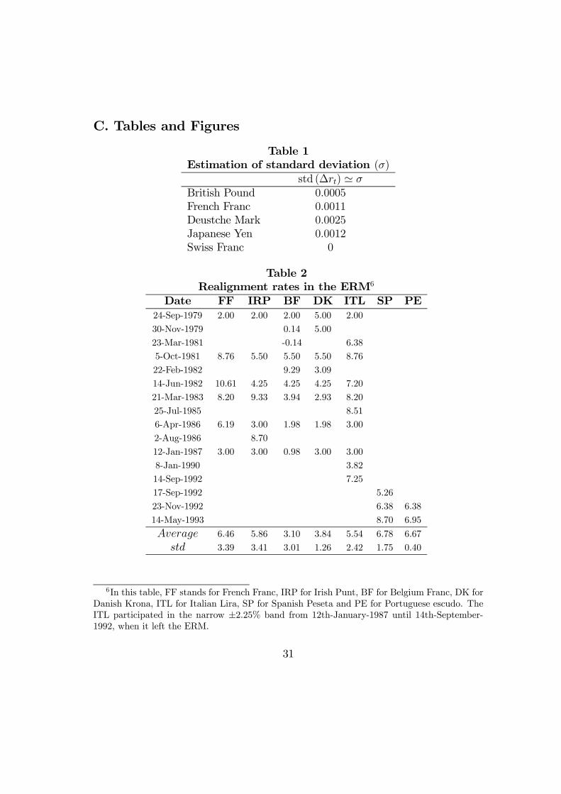
but the main results of the paper do not hinge on it.The selection of a standard deviation for the shock to the risk premium, σ, is a

troublesome task. Bekaert [2] reports an unconditional variance for a time invari-ant risk premium of 10.6222, for the Dollar/Yen rate. This figure yields a weeklystandard deviation of about σ = 0.002 basis points per week. Unfortunately, wehave not found an estimation of a time varying risk premium governed by a ran-dom walk structure, as assumed throughout this paper. As an approximation,we have used the ARCH-in-mean estimation by Domowitz and Hakkio [7], formonthly observations 1973:6-1982:8, of the British Pound, the French Franc, theDeustche Mark, the Japanese Yen and the Swiss Franc, all against the US Dollar.A Montecarlo simulation has been run in order to calculate this moment. Table1 reports the standard deviations for a first difference of rt. The Swiss Francpresents a time invariant risk premium. Hence, it seems reasonable to assume ana priori value σ = 0.002, as in Bekaert [2].Two bands are chosen, w = ±2.25% and ±6.00%, the widths experienced in

the ERM. The value of the constant µ is estimated depending on the band widthw. Tables 2 collects data of realignment rates for the currencies participating inthe ERM of the EMS, except for the Dutch Guilder. From this table it seems thatrealignment rates of ±4.5% and±6.3% for widths of ±2.25 and±6%, respectively,are consistent with the EMS historySince there is no prior for the relative weight of the exchange rate variability

in the preferences of the CB, we use a wide range of values within which theparameter λ is thought to be about. These values are λ = 0.2, 0.5, 1.0, 2.0 and5.0.

Tables 1 and 2 about here

14

3.2. Nonlinearities in the exchange rate function

Let us start examining the degree of nonlinearities in the exchange rate functionpredicted by our model.2 Figures 1 to 3 plot the function u (rt) for probabilities ofdefense α = 0, 1

2, and 1, together with the managed float and the free float. The

three figures differ on the value of λ which are 0.5, 1, and 2, respectively. The 45degree line corresponds to the free float. The other linear solution is the managedfloat. We can see that the relative slopes of these two solutions depend on thevalue of λ. Among the nonlinear solutions, the flattest function corresponds toα = 1, the target zone regime under perfect credibility. On the other extreme,the most sloping curve corresponds to the case where the currency is realigned forsure at margins, that is, α = 0. We can see that the degree of nonlinearity of thetarget zone solutions to be very small. Furthermore, as the value of λ increases,the target zone solutions get closer to the managed float which is the relevantregime to be compared with. This later result is independent of the credibility ofthe target zone.We also observe that the slope of the function u(rt) changes with r and this

change depends on the value of α. To make this result clearer, Figure 4 plotsu0 (rt) for λ = 1 and for values of α equal to 0, 14 ,

12, 34and 1. First, we see that for

α smaller than 34, the slope tends to increase as the exchange rate approaches the

limits of its band and we obtain the inverted S-curve as in Bertola and Caballero[4]. The opposite occurs when α is above 3

4. However, even in the fully credible

case, the slope does not reach zero at the edges, that is, there is no smoothpasting condition. Violation of smooth pasting in the standard model implied adiscontinuity jump in the expected rate of depreciation function. In our model,continuity of functions u (rt) and Etxt+1 is preserved under the level conditionu (r) = w, and the former arbitrage arguments do not apply here (see Appendix

2The empirical literature finds that the effects of the non-linearities from the smooth pastingcondition are not as much important as predicted. See, for example, Meese and Rose [21] forthree alternative regimes, the ±1% band of the Bretton Woods system, the gold standard forthe British Pound, the French Franc and the Deustche Mark (versus the US Dollar), and third,the EMS regime for the Dutch Guilder and the French Franc cases (versus the Deustche Mark).The null hypothesis of non linearities is rejected for the three regimes. Lewis [18] runs a varietyof tests for the G-3 case (US, Germany and Japan) in order to check for possible non linearitiesarising from implicit target bands and from the intervention policy. In all the cases, the exchangerate seemed to be a linear function of the estimated fundamentals. Evidence on rejection of thishypothesis is also reported in Lindberg and Söderlind [19] for Swedish data. Flood, Rose andMathieson [9] do not either find relevant evidence of the smooth pasting for three alternativemethods (graphical examination, parametric tests and forecasting analysis).

15

B for a detailed explanation justifying this non smooth pasting result).

Figures 1, 2, 3, 4 about here

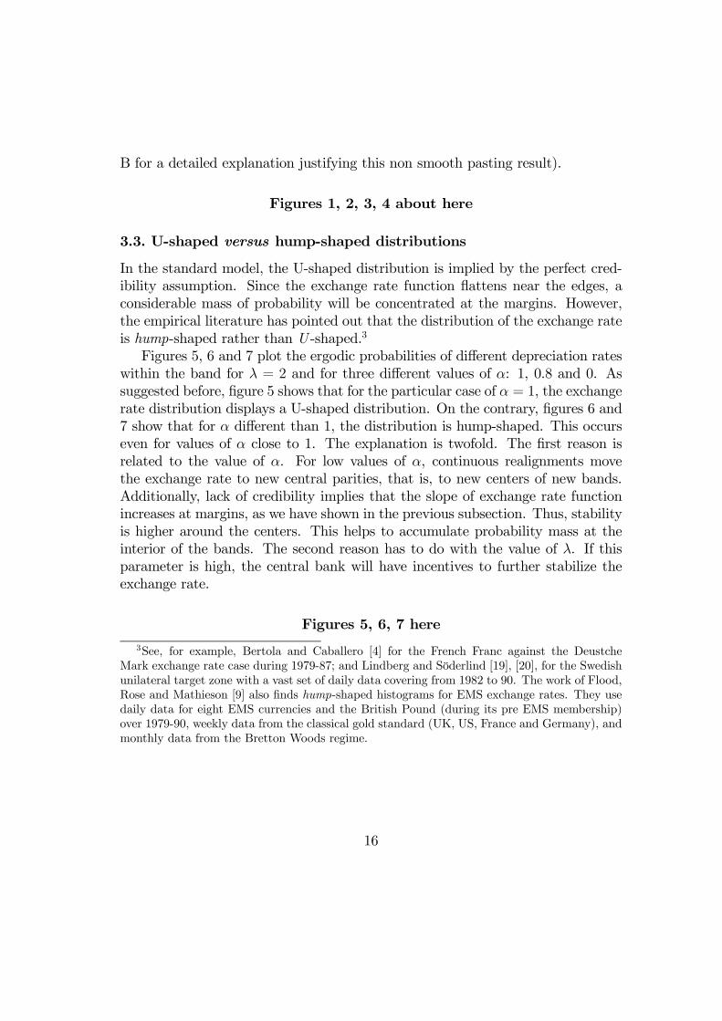
3.3. U-shaped versus hump-shaped distributions

In the standard model, the U-shaped distribution is implied by the perfect cred-ibility assumption. Since the exchange rate function flattens near the edges, aconsiderable mass of probability will be concentrated at the margins. However,the empirical literature has pointed out that the distribution of the exchange rateis hump-shaped rather than U -shaped.3

Figures 5, 6 and 7 plot the ergodic probabilities of different depreciation rateswithin the band for λ = 2 and for three different values of α: 1, 0.8 and 0. Assuggested before, figure 5 shows that for the particular case of α = 1, the exchangerate distribution displays a U-shaped distribution. On the contrary, figures 6 and7 show that for α different than 1, the distribution is hump-shaped. This occurseven for values of α close to 1. The explanation is twofold. The first reason isrelated to the value of α. For low values of α, continuous realignments movethe exchange rate to new central parities, that is, to new centers of new bands.Additionally, lack of credibility implies that the slope of exchange rate functionincreases at margins, as we have shown in the previous subsection. Thus, stabilityis higher around the centers. This helps to accumulate probability mass at theinterior of the bands. The second reason has to do with the value of λ. If thisparameter is high, the central bank will have incentives to further stabilize theexchange rate.

Figures 5, 6, 7 here3See, for example, Bertola and Caballero [4] for the French Franc against the Deustche

Mark exchange rate case during 1979-87; and Lindberg and Söderlind [19], [20], for the Swedishunilateral target zone with a vast set of daily data covering from 1982 to 90. The work of Flood,Rose and Mathieson [9] also finds hump-shaped histograms for EMS exchange rates. They usedaily data for eight EMS currencies and the British Pound (during its pre EMS membership)over 1979-90, weekly data from the classical gold standard (UK, US, France and Germany), andmonthly data from the Bretton Woods regime.

16

3.4. The relation between exchange rates and the interest rate differ-entials

Empirical observations have shown the existence of a positive relationship betweenthe exchange rate and the interest rate differential.4 Bertola and Svensson [5]suggest that incorporating a realignment risk premium may alter the sign of thecovariance between these two variables from negative to positive.In our model, this relation has always a positive sign, regardless the value of

the parameters. This is a consequence of intramarginal interventions, summarizedby the first order condition (2.15). Both the interest rate and the exchange rateare driven by the same variable, namely, the risk premium. The central bankdecides at each period how to distribute the shock on rt between xt and dt. Ex-pression (2.15) tells us that it is always optimal to move both variables on thesame direction with λ being the ratio between the two. This gives rise to a posi-tive linear relationship between the two variables. Hence, the honey moon effectis also transmitted to the interest rate smoothing.

3.5. On the choice of a target zone regime

In this subsection, we estimate the loss functions for the four regimes using the setof parameters early stated. Losses for the fixed rate, the managed float and thefree float are given by expressions (2.9), (2.16) and (2.19). The target zone loss isnumerically computed. We consider a starting point r0 = 0, and a time horizon of2000 periods. This time length accumulates a 91.2% from the total accruing valueand does not alter the ordinality of values for the exchange regimes. Calculationsof the indirect costs are reported in table 3 for w = ±2.25% and table 4 forw = ±6%. In each table, the first row refers to the cost of the fixed rate regime,Jc, and the following five rows represent the costs of a target zone for α = 0,14, 12, 34, and 1, respectively. The seventh and eighth rows collect the managed

float costs, Jmf , and the free float costs, Jff . From these tables we highlight thefollowing results.First, as it was mentioned above, the fixed rate is the regime with the lowest

value for the loss function.Second, with respect to the target zone regime, the closer α is to 1, the smaller

the losses are. This represents the gain from credibility of commitment to a zone.The slopes of both the exchange rate function and the interest rate differential

4See Svensson [26], Flood, Rose and Mathieson [9], Lindberg and Söderlind [19], and Bertolaand Caballero [4].

17

flatten for α approaching to 1. When market traders perceive that the CB willdefend the zone with a high probability, the realignment risk will be low and theexchange rate responses to changes in the foreign risk premium will be soft. Inturn, this perception will contribute to smooth the expected rate of depreciation.Hence, the outcome is that the interest rate differential will be more stable aswell.Third, for target zones very close to being credible (α close to 1), the present

value of the costs of a target zone are smaller than the costs of a managed float.Notice that, unlike the previous literature that used the free floating as an alter-native, the right regime to be compared with is the managed float. As with thesecond result, forward looking agents help stabilize the rate without pressuringthe interest rate, due to the honey moon effect.To make this point clearer, figures 8, 9 and 10 represent the contributions to

the loss functions due to the variability of the exchange rate and the interest ratefor all the regimes and values of λ equal to 0.5, 1, and 2, respectively. The circlecorresponds to the fixed rate, the square to the managed float and the trianglesare the target zones for different values of α. It is clear that there must be aninterval for α close to 1 that reduces the volatility of both the exchange rate andthe interest rate with respect to the managed float.

Table 4 and 5 hereFigures 8, 9 and 10 here

4. Conclusions

This paper presents a target zone model based on two extensions of Krugman’s[15] model. These extensions are the introduction of intramarginal interventionsand the lack of credibility of the target zone. These two features had been ana-lyzed separately by the literature. Here, we show that both extensions are neededto reconcile the model with the data. The leaning against the wind policy derivedfrom the time-consistent intramarginal intervention produces a positive relationbetween exchange rates and interest rates differentials as we observe in the dataas well as is behind the almost linear relation between exchange rates and fun-damentals. Furthermore, lack of credibility is responsible for the hump-shapedistribution of exchange rates.As a second application, the model provides a framework in which to evaluate

why target zones seem to be the dominant exchange rate regime in contemporary

18

history. First, we argue that target zones should be compared with the managedfloat which is the other time consistent exchange arrangement. For this compar-ison, we show that even not perfectly credible target zones may improve withrespect to the managed float in terms of reducing simultaneously the volatility ofboth exchange rates and interest rates differentials. In this way, we operationalizethe common view that target zones are preferred because they reap the benefitsof both flexible and fixed exchange rates, by stabilizing the exchange rate withoutloosing monetary independence. These two benefits are explicitely included in themodel and are a result of the interaction between the preferences of the centralbank and the credibility of its monetary policy.

Acknowledgements: For helpful comments and suggestions wethank all participants at the Workshop on Exchange Rates of centrA(Málaga, November 28th-29th 2001), and the I Workshop on Macroe-conomics of Universitat Autonoma de Barcelona (April 18th 2002).Specially, the comments from Consuelo Gámez, Javier Pérez, SimónSosvilla, Mark Taylor, and José Luis Torres have been very valuable.All remaining errors are ours. Both authors thank centrA for valuablefinancial aid.

References

[1] Ayuso, Juan and Fernando Restoy (1996) “Interest Rate Parity and ForeignExchange Risk Premia in the ERM”, Journal of International Economics,vol. 15 n. 3, pp. 369-382.

[2] Bekaert, Geert (1994) “Exchange Rate Volatility and Deviations from Unbi-asedness in a Cash-in-Advance Model”, Journal of International Economics,vol. 36, pp. 29-52.

[3] Bekaert, Geert and Stephen F. Gray (1999) “Target zones and ExchangeRates: An Empirical Investigation”, Journal of International Economics,vol. 45, pp. 1-35.

[4] Bertola, Giuseppe and Ricardo J. Caballero (1992) “Target Zones and Re-alignments”, American Economic Review, vol. 82, No. 6, pp. 520-536.

19

[5] Bertola, Giuseppe and Lars E. O (1993) “Stochastic Devaluation Risk andthe Empirical Fit of Target-Zone Models”, Review of Economic Studies vol.60, No. 3, pp. 689-712.

[6] Calvo, Guillermo and Carmen M. Reinhart (2002) “Fear of Floating”. Quar-terly Journal of Economics, vol. CXVII, pp. 379-408.

[7] Domowitz, Ian and Craig S. Hakkio (1985) “Conditional Variance and theRisk Premium in the Foreign Exchange Market”. Journal of InternationalEconomics, vol 19, pp. 47-66.

[8] Fischer, Stanley (2001) “Exchange Rate Regimes: Is the Bipolar View Cor-rect?”. Journal of Economic Perspectives vol. 15 (2), pp. 3-24.

[9] Flood, Robert P., Andrew K. Rose and Donald J. Mathieson (1990) “AnEmpirical Exploration of Exchange Rate Target Zones”, Carnegie-RochesterConference Series on Public Policy, vol. 35, pp. 7-66.

[10] Froot, Kenneth A. and Maurice Obstfeld (1991) “Stochastic Process Switch-ing: Some Simple Solutions”, Econometrica, vol. 59 (1), pp. 241-250.

[11] Froot, Kenneth A. and Maurice Obstfeld (1991) “Exchange rate dynamicsunder stochastic regime shifts: A unified approach”. Journal of InternationalEconomics, vol. 31, pp. 203-229.

[12] Giavazzi, Francesco and Marco Pagano (1988) “The Advantage of TyingOne’s Hands. EMS Discipline and Central Bank Credibility”, European Eco-nomic Review, vol. 32, pp. 1055-1082.

[13] Hawkins, David (1948) “Some Conditions of Macroeconomic Stability”.Econometrica Vol. 16, pp. 309-322.

[14] Hawkins, David and Simon, Herbert A.: “Note: Some Conditions of Macroe-conomic Stability”, in Input-Output Analysis, Vol. 1, Elgar Reference Collec-tion, Kurz, Dietzenbacher and Lager (eds.) (1998), pp. 142-145, (previouslypublished [1949]).

[15] Krugman, Paul (1991) “Target Zones and Exchange Rate Dynamics”, Quar-terly Journal of Economics, vol. 11, pp. 669-682.

20

[16] Krugman, Paul and Marcus Miller (1993) “Why Have a Target Zone?”,Carnegie-Rochester Conference Series on Public Policy, vol. 38, pp. 279-314.

[17] Levy-Yeyati, Eduardo and Federico Sturzenegger (2002) “Deeds versusWords: Classifying Exchange Rate Regimes”. Mimeo, Universidad TorcuatoDi Tella.

[18] Lewis, Karen K. (1995) ”Occasional Interventions to Target Rates”, Ameri-can Economic Review, vol. 85 (4), pp. 691-715.

[19] Lindberg, Hans and Paul Söderlind (1994) “Testing the Basic Target ZoneModel on Swedish Data 1982-1990”, European Economic Review, vol. 38, pp.1441-1469.

[20] Lindberg, Hans and Paul Söderlind (1994) ”Intervention Policy and MeanReversion in Exchange Rate Target Zones: The Swedish Case”, ScandinavianJournal of Economics, vol. 96(4), pp. 499-513.

[21] Meese, Richard A. and Andrew K. Rose (1990) ”Nonlinear, Nonparamet-ric, Nonessential Exchange Rate Estimation”, American Economic Review,Papers and Proceedings vol. 80 (2), pp. 192-196.

[22] Obstfeld, Maurice and Kenneth Rogoff (1995) “The Mirage of Fixed Ex-change Rates”. Journal of Economic Perspectives, vol. 9, no. 4, pp. 73-96.

[23] Reinhart, Carmen M.(2000) “The Mirage of Floating Exchange Rates”.American Economic Review Papers and Proceedings, vol. 90 No. 2, pp. 65-70.

[24] Reinhart, Carmen M. (2002) “The Modern History of Exchange Rate Ar-rangements: A Reinterpretation”. NBER working paper 8963.

[25] Svensson, Lars E. O. (1991) “The simplest test of target zone credibility”,IMF Staff Papers, vol. 38 n. 3, pp. 655-665.

[26] Svensson, Lars E. O. (1991) “The Term Structure of Interest Rate Differ-ential in a Target Zone: Theory and Swedish Data”, Journal of MonetaryEconomics, vol. 28, pp. 87-116.

[27] Svensson, Lars E. O. (1992) “An Interpretation of Recent Research on Ex-change Rate Target Zones”, Journal of Economic Perspectives, vol. 6, No. 6,pp. 119-144.

21

[28] Svensson, Lars E. O. (1992) “The foreign exchange risk premium in a targetzone model with devaluarion risk”, Journal of International Economics, vol.33, pp. 21-40.

[29] Svensson, Lars E. O. (1994) “Why Exchange Rate Bands?. Monetary In-dependence in Spite of Fixed Exchange Rates”. Journal of Monetary Eco-nomics, pp. 137-199.

[30] Svensson, Lars E. O. (1994) “Fixed Exchange Rates as a Means to PriceStability: What Have We Learned?”, European Economic Review, vol. 38,pp. 447-468.

A. Solution of the Target Zone

In this appendix we show how to make the computations for the solution of thetarget zone regime. Forward recursion in the first order condition (2.23) is usedto solve for u (rt) subject to (2.22). Let the expected rate of depreciation out ofthe band be given by

δτ ,τ−1 = αw [Pr (rt+τ > r|rt+τ−1)− Pr (rt+τ < −r|rt+τ−1)]+ (1− α)

Z −r

−∞µ (rt+τ )φ (rr+τ |rt+τ−1) drt+τ

+(1− α)

Z ∞

r

µ (rt+τ)φ (rr+τ |rt+τ−1) drt+τ .

Forward iteration of (2.23) leads to the following general solution

u (rt) =rt

1 + λ+

1

1 + λ

∞Xτ=1

F [rt+τ |Fτ ]

(1 + λ)−τ+

∞Xτ=1

F [δτ ,τ−1 |Fτ−1 ](1 + λ)−τ

, (A.1)

where the sequence Fτ≥0 represents filtered information sets of the next form:

F0 = rt , (A.2)

Fτ≥1 = rt+n ∈ [−r, r]τn=1 , rt . (A.3)

22

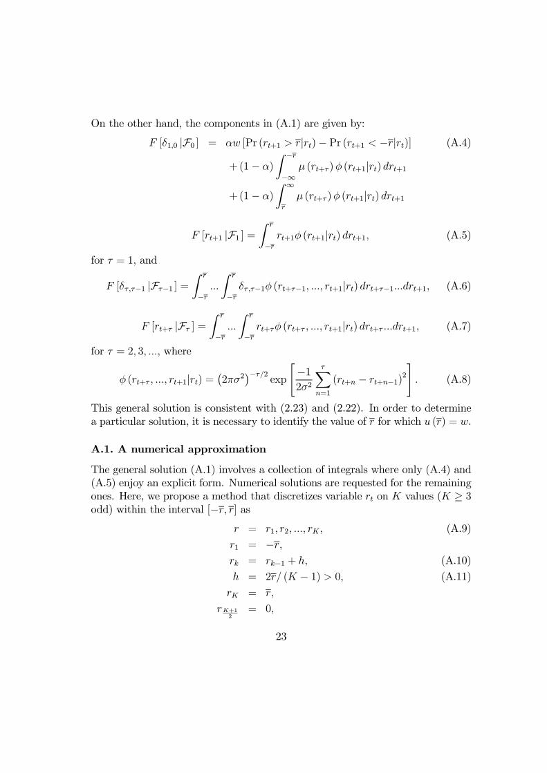
On the other hand, the components in (A.1) are given by:

F [δ1,0 |F0 ] = αw [Pr (rt+1 > r|rt)− Pr (rt+1 < −r|rt)] (A.4)

+(1− α)

Z −r

−∞µ (rt+τ)φ (rt+1|rt) drt+1

+(1− α)

Z ∞

r

µ (rt+τ)φ (rt+1|rt) drt+1

F [rt+1 |F1 ] =Z r

−rrt+1φ (rt+1|rt) drt+1, (A.5)

for τ = 1, and

F [δτ ,τ−1 |Fτ−1 ] =Z r

−r...

Z r

−rδτ ,τ−1φ (rt+τ−1, ..., rt+1|rt) drt+τ−1...drt+1, (A.6)

F [rt+τ |Fτ ] =

Z r

−r...

Z r

−rrt+τφ (rt+τ , ..., rt+1|rt) drt+τ ...drt+1, (A.7)

for τ = 2, 3, ..., where

φ (rt+τ , ..., rt+1|rt) =¡2πσ2

¢−τ/2exp

"−12σ2

τXn=1

(rt+n − rt+n−1)2#. (A.8)

This general solution is consistent with (2.23) and (2.22). In order to determinea particular solution, it is necessary to identify the value of r for which u (r) = w.

A.1. A numerical approximation

The general solution (A.1) involves a collection of integrals where only (A.4) and(A.5) enjoy an explicit form. Numerical solutions are requested for the remainingones. Here, we propose a method that discretizes variable rt on K values (K ≥ 3odd) within the interval [−r, r] as

r = r1, r2, ..., rK , (A.9)

r1 = −r,rk = rk−1 + h, (A.10)

h = 2r/ (K − 1) > 0, (A.11)

rK = r,

rK+12

= 0,

23

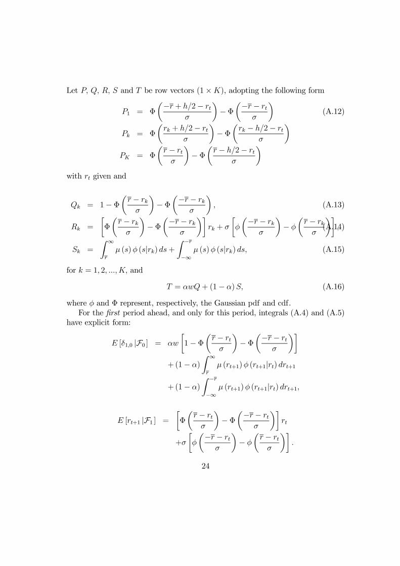
Let P, Q, R, S and T be row vectors (1×K), adopting the following form

P1 = Φ

µ−r + h/2− rtσ

¶− Φ

µ−r − rtσ

¶(A.12)

Pk = Φ

µrk + h/2− rt

σ

¶− Φ

µrk − h/2− rt

σ

¶PK = Φ

µr − rtσ

¶− Φ

µr − h/2− rt

σ

¶with rt given and

Qk = 1− Φ

µr − rkσ

¶− Φ

µ−r − rkσ

¶, (A.13)

Rk =

·Φ

µr − rkσ

¶− Φ

µ−r − rkσ

¶¸rk + σ

·φ

µ−r − rkσ

¶− φ

µr − rkσ

¶¸,(A.14)

Sk =

Z ∞

r

µ (s)φ (s|rk) ds+Z −r

−∞µ (s)φ (s|rk) ds, (A.15)

for k = 1, 2, ..., K, and

T = αwQ+ (1− α)S, (A.16)

where φ and Φ represent, respectively, the Gaussian pdf and cdf.For the first period ahead, and only for this period, integrals (A.4) and (A.5)

have explicit form:

E [δ1,0 |F0 ] = αw

·1− Φ

µr − rtσ

¶− Φ

µ−r − rtσ

¶¸+(1− α)

Z ∞

r

µ (rt+1)φ (rt+1|rt) drt+1

+(1− α)

Z −r

−∞µ (rt+1)φ (rt+1|rt) drt+1,

E [rt+1 |F1 ] =·Φ

µr − rtσ

¶− Φ

µ−r − rtσ

¶¸rt

+σ

·φ

µ−r − rtσ

¶− φ

µr − rtσ

¶¸.

24

For the second period ahead, a numerical approximation is given by

E [δ2,1 |F1 ] = TP 0,

E [rt+2 |F2 ] = RP 0.

This implies that the value of the integrals at t+2 is determined for any possiblemean at t+1, rt+1 ∈ [−r, r], and any of these means is weighted by a probabilityP , given a starting value rt at t.The loop becomes harder as the period ahead increases over three. In order

to solve this problem, we develope a backward recursion algorithm, for which thelast period integral is firstly solved and then proceed backward up to the first one.Thereby, consider the following non negative matrix M ∈ RK×K

M1,l = Φ

µ−r + h/2− rlσ

¶− Φ

µ−r − rlσ

¶,

Mk,l = Φ

µrk + h/2− rl

σ

¶− Φ

µrk − h/2− rl

σ

¶,

MK,l = Φ

µr − rlσ

¶− Φ

µr − h/2− rl

σ

¶,

for k, l = 1, 2, ...K, with the following properties: the sum over each column givesa row vector mc ∈ R1×K, with all its components lying within the (0, 1) interval

mc (l) =KXk=1

Mkl =

Z r

−rφ (s|rl) ds ∈ (0, 1) (A.17)

for l = 1, 2, ...,K. The proof follows. This property is sufficient to verify theHawkins-Simon condition (Brauer-Solow Theorem).Matrix M contains the transition probabilities in the intermediate periods

from τ up to τ + 1, within the interval [−r, r] and for any mean belonging to[−r, r]. Thus, the solution for the third period is given by

E [δ3,2 |F2 ] = TMP 0,E [rt+3 |F3 ] = RMP 0.

Again, the value of the integrals are first determined at t + 3 for any possiblemean at t + 2, rt+2 ∈ [−r, r], given by the columns of M . The vector P closesthe calculation for any possible mean at t+ 1, rt+1 ∈ [−r, r], for given a startingvalue rt.

25

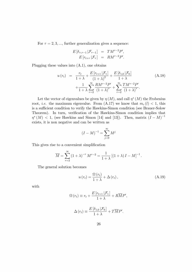
For τ = 2, 3, ..., further generalization gives a sequence:

E [δτ ,τ−1 |Fτ−1 ] = TMτ−2P 0,

E [rt+τ |Fτ ] = RM τ−2P 0.

Plugging these values into (A.1), one obtains

u (rt) =rt

1 + λ+E [rt+1 |F1 ](1 + λ)2

+E [δ1,0 |F0 ]1 + λ

(A.18)

+1

1 + λ

∞Xτ=2

RM τ−2P 0

(1 + λ)τ+

∞Xτ=2

TM τ−2P 0

(1 + λ)τ.

Let the vector of eigenvalues be given by η (M), and call η∗ (M) the Frobeniusroot, i.e. the maximum eigenvalue. From (A.17) we know that mc (l) < 1, thisis a sufficient condition to verify the Hawkins-Simon condition (see Brauer-SolowTheorem). In turn, verification of the Hawkins-Simon condition implies thatη∗ (M) < 1, (see Hawkins and Simon [14] and [13]). Then, matrix (I −M)−1exists, it is non negative and can be written as

(I −M)−1 =∞Xj=0

M j

This gives rise to a convenient simplification

M =∞Xτ=2

(1 + λ)−τ M τ−2 =1

1 + λ[(1 + λ) I −M ]−1 .

The general solution becomes

u (rt) =Ω (rt)

1 + λ+∆ (rt) , (A.19)

with

Ω (rt) ≡ rt + E [rt+1 |F1 ]1 + λ

+RMP 0,

∆ (rt) ≡ E [δ1,0 |F0 ]1 + λ

+ TMP 0.

26

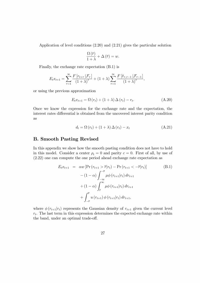
Application of level conditions (2.20) and (2.21) gives the particular solution

Ω (r)

1 + λ+∆ (r) = w.

Finally, the exchange rate expectation (B.1) is

Etxt+1 =∞Xτ=1

F [rt+τ |Fτ ]

(1 + λ)τ+ (1 + λ)

∞Xτ=1

F [δτ ,τ−1 |Fτ−1 ](1 + λ)τ

,

or using the previous approximation

Etxt+1 = Ω (rt) + (1 + λ)∆ (rt)− rt. (A.20)

Once we know the expression for the exchange rate and the expectation, theinterest rates differential is obtained from the uncovered interest parity conditionas

dt = Ω (rt) + (1 + λ)∆ (rt)− xt (A.21)

B. Smooth Pasting Revised

In this appendix we show how the smooth pasting condition does not have to holdin this model. Consider a center ρt = 0 and parity c = 0. First of all, by use of(2.22) one can compute the one period ahead exchange rate expectation as

Etxt+1 = αw [Pr (rt+1 > r|rt)− Pr (rt+1 < −r|rt)] (B.1)

− (1− α)

Z −r

−∞µφ (rt+1|rt) drt+1

+(1− α)

Z ∞

r

µφ (rt+1|rt) drt+1

+

Z r

−ru (rt+1)φ (rt+1|rt) drt+1,

where φ (rt+1|rt) represents the Gaussian density of rt+1 given the current levelrt. The last term in this expression determines the expected exchange rate withinthe band, under an optimal trade-off.

27

A second order expansion of u (rt+1) around a value of rt ∈ [−r, r], gives

u (rt+1) ' u (rt) + u0 (rt) (rt+1 − rt) + 12u00 (rt) (rt+1 − rt)2 + o (rt+1) . (B.2)

Weighting this expression by φ (rt+1|rt) and integrating for rt+1 ∈ [−r, r], yieldsZ r

−ru (rt+1)φ (rt+1|rt) drt+1 = u (rt) p (rt; r) + u

0 (rt)S1 (rt; r) (B.3)

+1

2u00 (rt)S2 (rt; r) ,

where

p (rt; r) = Pr [rt+1 ∈ [−r, r] |rt] (B.4)

= Φ

µr − rtσ

¶− Φ

µ−r − rtσ

¶,

which represents the probability the risk premium wanders between [−r, r] forthe next period, given the present level rt, and function S1 (rt; r) represents theexpected change of the risk premium:

S1 (rt; r) = p0 (rt; r) (B.5)

= σ

·φ

µ−r − rtσ

¶− φ

µr − rtσ

¶¸= p (rt; r)E [(rt+1 − rt) |rt+1 ∈ [−r, r] , rt] .

Function S2 (rt; r) represents the expected quadratic change of the risk premium:

S2 (rt; r) = p (rt; r)

·1 +

p00 (rt; r)p (rt; r)

¸σ2 (B.6)

= σ2p (rt; r)− σ

·φ

µ−r − rtσ

¶(r + rt) + φ

µr − rtσ

¶(r − rt)

¸= p (rt; r)E

£(rt+1 − rt)2 |rt+1 ∈ [−r, r] , rt

¤.

Functions (B.4), (B.5) and (B.6) are all continuous, a property that will resultrelevant to deal with the smooth pasting argument.

28

Plugging expressions (B.3) and (B.1) into the first order condition (2.23), forrt ∈ [−r, r] one obtains

(1 + λ)u (rt) = rt + αw [Pr (rt+1 > r|rt)− Pr (rt+1 < −r|rt)] (B.7)

− (1− α)

Z −r

−∞µφ (rt+1|r) drt+1

+(1− α)

Z ∞

r

µφ (rt+1|r) drt+1+u (rt) p (rt; r) + u

0 (rt)S1 (rt; r)

+1

2u00 (rt)S2 (rt; r) .

Now, we will approximate the particular solutions for the extreme case α = 1.Under perfect credibility, this model does not exhibit the S-shaped of the standardmodel. Let us first briefly remember the foundation of why the standard model iszero sloped at the edges and, later, see how the smooth pasting condition shouldbe reinterpreted within our model5.In the standard model, the exchange rate depends linearly of the fundamen-

tal and the expected rate of depreciation. The fundamental follows a regulatedBrownian motion such that, at margins, monetary policy push it back inside theband. If the slope of the exchange rate function were strictly positive at theseedges, the expected rate of depreciation would display a discontinuity. Hence, asure jump would be given towards the interior of the band, and would providesafe bets opportunities against the movement of the exchange rate. Therefore,in order to avoid such a discontinuity jump, arbitrage considerations require thatthe slope must be zero at margins.In our model, expectations are given to the CB and the exchange rate is de-

termined from the first order condition (2.23), subject to (2.22) and the levelconditions (2.20) and (2.21). The risk premium rt is a sufficient statistic to deter-mine the position of the exchange rate inside the band. The CB cannot governthis process and must ensure the equilibrium in the money market given in (2.1)by responding to variations in fundamental. Continuity of functions x (rt) andEt [xt+1] is not affected, no matter the value of slope u0 (r).The aforementioned argument can be developed by proving the continuity of

5The argument provided in this appendix widely follows that of Froot & Obstfeld [11].

29

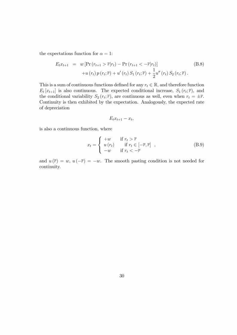
the expectations function for α = 1:

Etxt+1 = w [Pr (rt+1 > r|rt)− Pr (rt+1 < −r|rt)] (B.8)

+u (rt) p (rt; r) + u0 (rt)S1 (rt; r) +

1

2u00 (rt)S2 (rt; r) .

This is a sum of continuous functions defined for any rt ∈ R, and therefore functionEt [xt+1] is also continuous. The expected conditional increase, S1 (rt; r), andthe conditional variability S2 (rt; r), are continuous as well, even when rt = ±r.Continuity is then exhibited by the expectation. Analogously, the expected rateof depreciation

Etxt+1 − xt,

is also a continuous function, where

xt =

+w if rt > ru (rt) if rt ∈ [−r, r]−w if rt < −r

, (B.9)

and u (r) = w, u (−r) = −w. The smooth pasting condition is not needed forcontinuity.

30

C. Tables and Figures

Table 1Estimation of standard deviation (σ)

std (∆rt) ' σBritish Pound 0.0005French Franc 0.0011Deustche Mark 0.0025Japanese Yen 0.0012Swiss Franc 0

Table 2Realignment rates in the ERM6

Date FF IRP BF DK ITL SP PE24-Sep-1979 2.00 2.00 2.00 5.00 2.00

30-Nov-1979 0.14 5.00

23-Mar-1981 -0.14 6.38

5-Oct-1981 8.76 5.50 5.50 5.50 8.76

22-Feb-1982 9.29 3.09

14-Jun-1982 10.61 4.25 4.25 4.25 7.20

21-Mar-1983 8.20 9.33 3.94 2.93 8.20

25-Jul-1985 8.51

6-Apr-1986 6.19 3.00 1.98 1.98 3.00

2-Aug-1986 8.70

12-Jan-1987 3.00 3.00 0.98 3.00 3.00

8-Jan-1990 3.82

14-Sep-1992 7.25

17-Sep-1992 5.26

23-Nov-1992 6.38 6.38

14-May-1993 8.70 6.95

Average 6.46 5.86 3.10 3.84 5.54 6.78 6.67

std 3.39 3.41 3.01 1.26 2.42 1.75 0.40

6In this table, FF stands for French Franc, IRP for Irish Punt, BF for Belgium Franc, DK forDanish Krona, ITL for Italian Lira, SP for Spanish Peseta and PE for Portuguese escudo. TheITL participated in the narrow ±2.25% band from 12th-January-1987 until 14th-September-1992, when it left the ERM.

31

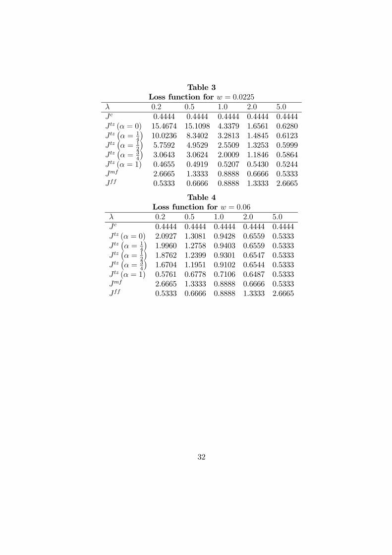
Table 3Loss function for w = 0.0225

λ 0.2 0.5 1.0 2.0 5.0Jc 0.4444 0.4444 0.4444 0.4444 0.4444J tz (α = 0) 15.4674 15.1098 4.3379 1.6561 0.6280J tz¡α = 1

4

¢10.0236 8.3402 3.2813 1.4845 0.6123

J tz¡α = 1

2

¢5.7592 4.9529 2.5509 1.3253 0.5999

J tz¡α = 3

4

¢3.0643 3.0624 2.0009 1.1846 0.5864

J tz (α = 1) 0.4655 0.4919 0.5207 0.5430 0.5244Jmf 2.6665 1.3333 0.8888 0.6666 0.5333Jff 0.5333 0.6666 0.8888 1.3333 2.6665

Table 4Loss function for w = 0.06

λ 0.2 0.5 1.0 2.0 5.0Jc 0.4444 0.4444 0.4444 0.4444 0.4444J tz (α = 0) 2.0927 1.3081 0.9428 0.6559 0.5333J tz¡α = 1

4

¢1.9960 1.2758 0.9403 0.6559 0.5333

J tz¡α = 1

2

¢1.8762 1.2399 0.9301 0.6547 0.5333

J tz¡α = 3

4

¢1.6704 1.1951 0.9102 0.6544 0.5333

J tz (α = 1) 0.5761 0.6778 0.7106 0.6487 0.5333Jmf 2.6665 1.3333 0.8888 0.6666 0.5333Jff 0.5333 0.6666 0.8888 1.3333 2.6665

32

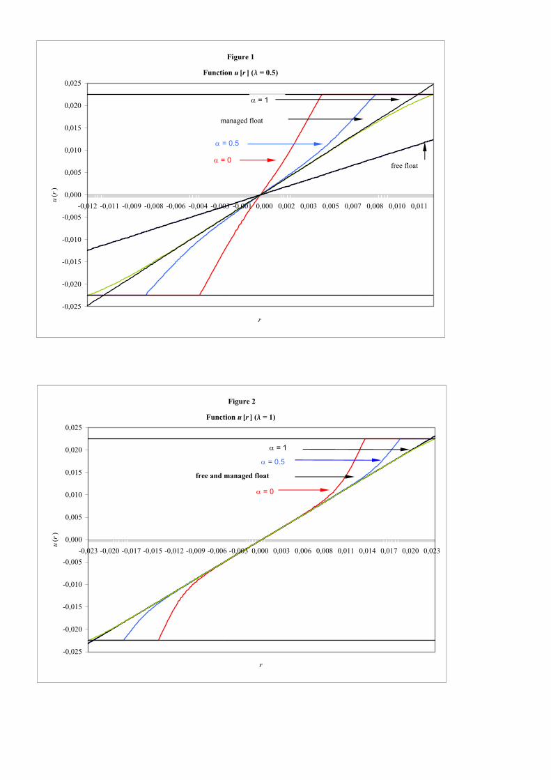
Figure 1

-0,025

-0,020

-0,015

-0,010

-0,005

0,000

0,005

0,010

0,015

0,020

0,025

-0,012 -0,011 -0,009 -0,008 -0,006 -0,004 -0,003 -0,001 0,000 0,002 0,003 0,005 0,007 0,008 0,010 0,011

r

u(r

)

α = 0.5

Function u [r ] (l = 0.5)

free float

α = 1

managed float

Figure 2

-0,025

-0,020

-0,015

-0,010

-0,005

0,000

0,005

0,010

0,015

0,020

0,025

-0,023 -0,020 -0,017 -0,015 -0,012 -0,009 -0,006 -0,003 0,000 0,003 0,006 0,008 0,011 0,014 0,017 0,020 0,023

r

u(r

)

α = 0.5

α = 1

free and managed float

α = 0

Function u [r ] (l = 1)

α = 0

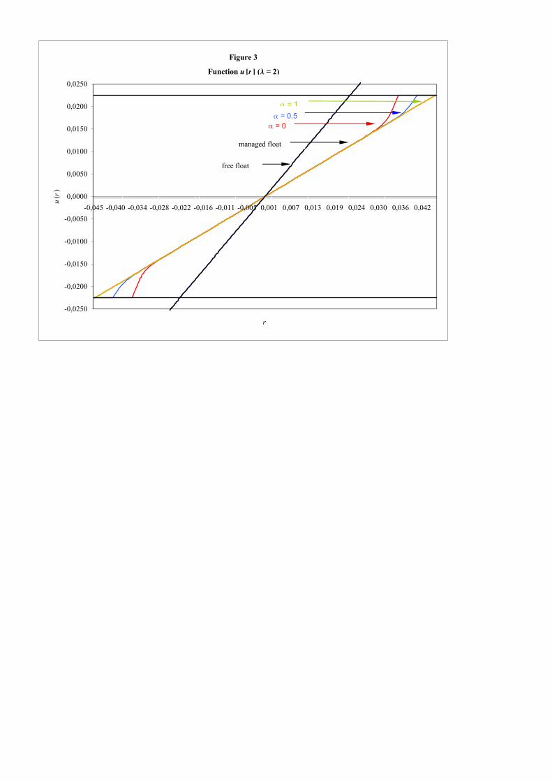
Figure 3

-0,0250

-0,0200

-0,0150

-0,0100

-0,0050

0,0000

0,0050

0,0100

0,0150

0,0200

0,0250

-0,045 -0,040 -0,034 -0,028 -0,022 -0,016 -0,011 -0,005 0,001 0,007 0,013 0,019 0,024 0,030 0,036 0,042

r

u(r

)

α = 0.5α = 1

managed float

α = 0

Function u [r ] (l = 2)

free float

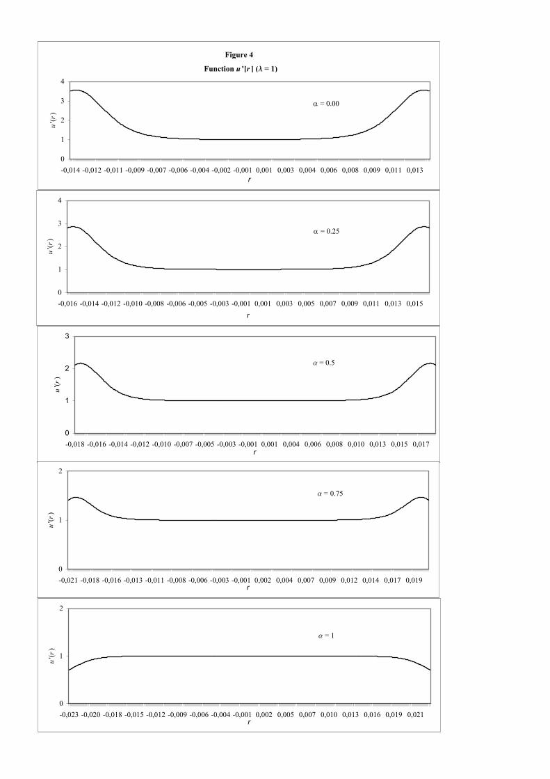
Figure 4

0

1

2

3

4

-0,014 -0,012 -0,011 -0,009 -0,007 -0,006 -0,004 -0,002 -0,001 0,001 0,003 0,004 0,006 0,008 0,009 0,011 0,013r

u'(r

)

Function u '[r ] (l = 1)

α = 0.00

0

1

2

3

4

-0,016 -0,014 -0,012 -0,010 -0,008 -0,006 -0,005 -0,003 -0,001 0,001 0,003 0,005 0,007 0,009 0,011 0,013 0,015r

u'(r

)

α = 0.25

0

1

2

3

-0,018 -0,016 -0,014 -0,012 -0,010 -0,007 -0,005 -0,003 -0,001 0,001 0,004 0,006 0,008 0,010 0,013 0,015 0,017r

u'(r

)

a = 0.5

0

1

2

-0,021 -0,018 -0,016 -0,013 -0,011 -0,008 -0,006 -0,003 -0,001 0,002 0,004 0,007 0,009 0,012 0,014 0,017 0,019r

u'(r

)

a = 0.75

0

1

2

-0,023 -0,020 -0,018 -0,015 -0,012 -0,009 -0,006 -0,004 -0,001 0,002 0,005 0,007 0,010 0,013 0,016 0,019 0,021r

u'(r

)

a = 1

Figure 5

0,000

0,050

0,100

0,150

0,200

0,250

0,300

0,350

0,400

0,450

-0,023 -0,020 -0,017 -0,014 -0,011 -0,008 -0,005 -0,002 0,001 0,004 0,007 0,010 0,013 0,016 0,018 0,021

x

prob

abili

ty

Stationary probability distribution (λ = 2; α = 1)

Figure 6

0,000

0,001

0,002

0,003

0,004

0,005

0,006

0,007

-0,023 -0,019 -0,016 -0,014 -0,011 -0,008 -0,005 -0,003 0,000 0,003 0,005 0,008 0,011 0,014 0,016 0,019 0,023

x

prob

abili

ty

Stationary probability distribution (λ = 2; α = 0.8)

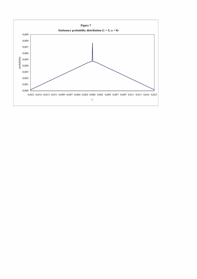
Figure 7

0,000

0,001

0,002

0,003

0,004

0,005

0,006

0,007

0,008

0,009

-0,023 -0,016 -0,013 -0,011 -0,009 -0,007 -0,004 -0,002 0,000 0,002 0,004 0,007 0,009 0,011 0,013 0,016 0,023

x

prob

abili

ty

Stationary probability distribution (λ = 2; α = 0)

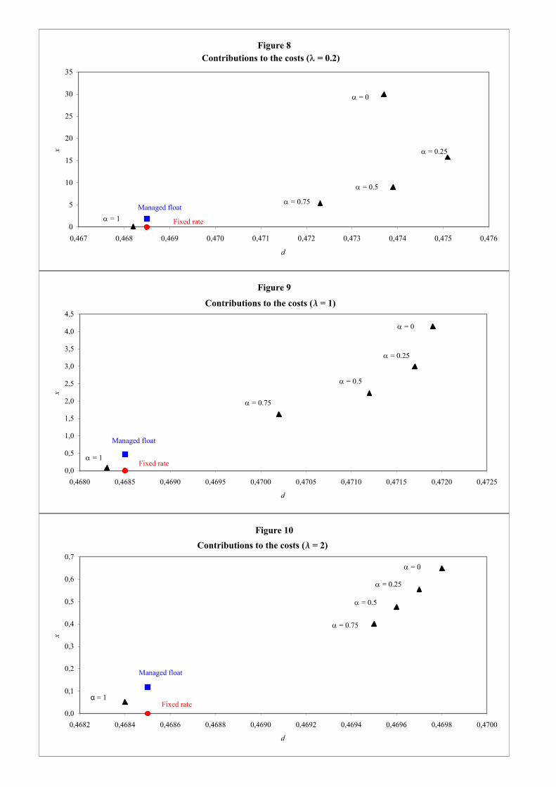
Figure 10

0,0

0,1

0,2

0,3

0,4

0,5

0,6

0,7

0,4682 0,4684 0,4686 0,4688 0,4690 0,4692 0,4694 0,4696 0,4698 0,4700

d

x

Contributions to the costs (l = 2)

α = 1

α = 0.75

α = 0.5

α = 0.25

α = 0

Managed float

Fixed rate

Figure 8

0

5

10

15

20

25

30

35

0,467 0,468 0,469 0,470 0,471 0,472 0,473 0,474 0,475 0,476

d

xContributions to the costs (λ = 0.2)

α = 1

α = 0.75

α = 0.5

α = 0.25

α = 0

Managed float

Fixed rate

Figure 9

0,0

0,5

1,0

1,5

2,0

2,5

3,0

3,5

4,0

4,5

0,4680 0,4685 0,4690 0,4695 0,4700 0,4705 0,4710 0,4715 0,4720 0,4725

d

x

Contributions to the costs (l = 1)

α = 1

α = 0.75

α = 0.5

α = 0.25

α = 0

Managed float

Fixed rate