DEPARTMENT OF OPERATIONS RESEARCHUNIVERSITY OF AARHUS

Working Paper no. 2005 / 3 2005 / 12 / 27

On the Bicriterion Multi Modal AssignmentProblem

Christian Roed Pedersen, Lars Relund Nielsenand Kim Allan Andersen

ISSN 1600-8987

Department of Mathematical Sciences Building 530, Ny MunkegadeTelephone: +45 8942 1111 DK-8000 Aarhus C, DenmarkE-mail: institut@imf.au.dk URL: www.imf.au.dk

On the Bicriterion Multi Modal Assignment

Problem

Christian Roed Pedersen

Department of Operations Research

University of Aarhus

Ny Munkegade, Building 1530

8000 Aarhus C

Denmark

Lars Relund Nielsen Kim Allan Andersen∗

Department of Accounting, Finance and Logistics

Aarhus School of Business

Fuglesangs Alle 4

DK-8210 Aarhus V

Denmark

December 22, 2005

Abstract

We consider the bicriterion multi modal assignment problem which is anew generalization of the classical linear assignment problem. A two-phasesolution method using an effective ranking scheme is presented. The algorithmis valid for generating all nondominated criterion points or an approximation.

Extensive computational results are conducted on a large library of testinstances to test the performance of the algorithm and to identify hard testinstances.

Also, test results of the algorithm applied to the bicriterion assignmentproblem is given. Here our algorithm outperforms all previously known exactsolution methods for this problem class.

Keywords: Bicriterion multi modal assignment problem, ranking, two-phase method.

∗Corresponding author, e-mail: kia@asb.dk.

1

1 Introduction

The linear assignment problem (AP) is a well-known combinatorial problem withapplications in a widespread field of operations. In its most classical formulation,AP is described as the problem of assigning n workers to n jobs such that cost isminimized.

In 1955 Kuhn [12, 13] presented the first polynomial solution method for AP,called the Hungarian method. Later, alternative AP algorithms have been presentedamong which some of the most efficient are the successive shortest path algorithms1,see e.g. Ahuja, Magnanti, and Orlin [1] and Jonker and Volgenant [11]. Dell’Amicoand Martello [5] give an annotated bibliography on AP, mentioning more than 100papers. An excellent survey is given by Dell’Amico and Toth [6] including compar-ative tests of several implementations of AP algorithms.

Different generalizations of AP have generated interest in the literature. Oneprominent research field considers ranking the K best assignments in nondecreasingorder of cost. Applications for ranking problems are numerous. For instance, theyare often used with success as subroutines for more complex optimization problems.Recent developments have been given by Pascoal, Captivo, and Clımaco [18] andPedersen, Nielsen, and Andersen [19].

In general a description of real world applications as single criterion optimiza-tion problems is seldom realistic, since they are often by nature imposed with moreobjectives to be simultaneously optimized. Assigning workers to jobs with minimalcost and time yields the bicriterion assignment problem (BiAP), which is anotherimportant generalization of AP. Within the last ten years focus on BiAP has risen.Ulungu and Teghem [24] presented the first exact solution method for BiAP, propos-ing a two-phase method identifying in phase one all supported efficient solutions andin phase two all unsupported efficient solutions. In that paper, a scheme resemblingtotal enumeration in all nonbasic variables is employed. The method in [24] wasimplemented by Tuyttens, Teghem, Fortemps, and Nieuwenhuyze [23], showing –with large CPU times – the limitations of this algorithm. Recently, an improvementof this algorithm was given in Przybylski, Gandibleux, and Ehrgott [20], proposingalso a two-phase method applying ranking for BiAP.

The main focus on BiAP in literature, however, seems to be on heuristical meth-ods. Tuyttens et al. [23] use a version of the MOSA method which is an extensionof simulated annealing to deal with multiple objectives. Gandibleux, Morita, andKatoh [8] use genetic information for BiAP, and population based heuristics usingpath relinking are described in Gandibleux, Morita, and Katoh [9] and Przybylskiet al. [20].

In this paper, we deal with another highly relevant extension of the classicalassignment problem, which has, to the best of our knowledge, not yet been discussedin literature. Imagine a large global company with n specialists spread across theworld and suppose that exactly n jobs have to be performed by these n specialists.Hence, each specialist must be assigned to exactly one job and furthermore suitablemodes of transportation must be chosen for the workers to travel to the destinationsof the jobs. For this problem, it seems relevant to consider two weight criteria to be

1Also known as shortest augmented path algorithms.

2

minimized simultaneously, namely travel time and travel or assignment cost. Sincea specialist i has possibly multiple modes of transportation and routes to choosefrom in order to reach the destination of job j, several two-dimensional cost vectorsexist for each i and j. Therefore, the bicriterion multi modal assignment problem(BiMMAP) is an extension of BiAP containing, in each assignment cell, severaltwo-dimensional cost vectors/points. The objective is to identify either all efficientassignments or all nondominated criterion points for the problem. Notice that thepredominant thought within bicriterion optimization is to identify all nondominatedpoints with one efficient solution corresponding to each nondominated point. Thisis equivalent to identifying a minimal complete set of efficient solutions [9, 10].

In this paper, we propose a two-phase method to identify all the nondominatedcriterion points for BiMMAP. Acknowledging that ranking procedures have been ap-plied with great success for other bicriterion optimization problems (see e.g. Nielsen,Andersen, and Pretolani [16]), we employ ranking of multi modal assignments as asubroutine. The subroutine is an efficient extension of the algorithm for finding theK best assignments by Pedersen et al. [19].

A method for finding an ε-approximation (Warburton [25]) of the set of nondom-inated points, which enable us to control the quality of the set of criterion pointsreported, is also presented. An approximation may be needed for large problem sizesif it is too time-consuming to find all nondominated criterion points.

Using a large library of test instances for BiMMAP, we give numerical resultsindicating the effectiveness of our method. The concept of approximating the non-dominated points is shown to have a large effect on the computational performance.Since BiMMAP is a generalization of BiAP, we also report computational resultsfor some BiAP instances previously solved in literature showing that our algorithmoutperforms all known exact solution methods.

The paper is organized as follows. In Section 2 we introduce the bicriterionmulti modal assignment problem and give a few theoretical results for this problemclass. In Section 3 we describe our two-phase method both for the exact and theapproximation solution method. Section 4 provides a description on how to rankmulti modal assignments. Computational results for BiMMAP and BiAP are givenin Section 5, and conclusions are drawn in Section 6.

2 The bicriterion multi modal assignment prob-

lem

In this section we give the mathematical formulation of the bicriterion multi modalassignment problem (BiMMAP), introduce the relevant terminology and give a fewtheoretical results.

Imagine a large global company with n specialists spread across the world andsuppose that exactly n jobs have to be performed by these n specialists. That is,each specialist must be assigned to exactly one job. Moreover, a specialist i has Lij

different mode choices of transportation for reaching the destination of job j withtravel or assignment cost c1

ijl and travel time c2ijl, l = 1, . . . , Lij .

BiMMAP is an extension of BiAP where, for each cell (i, j) in the assignment

3

i\j 1 · · · n

1

(

c1111

c2111

)

, . . . ,

(

c111L11

c211L11

)

· · ·

(

c11n1

c21n1

)

, . . . ,

(

c11nL1n

c21nL1n

)

......

. . ....

n

(

c1n11

c2n11

)

, . . . ,

(

c1n1Ln1

c2n1Ln1

)

. . .

(

c1nn1

c2nn1

)

, . . . ,

(

c1nnLnn

c2nnLnn

)

Figure 1: The cost matrix of BiMMAP.

cost matrix, we have several two-dimensional cost vectors as illustrated in Figure 1.The objective is to identify either all efficient minimal cost assignments or all non-dominated criterion points for the problem.

Let xijl be a binary variable with value 1, if i is assigned to j using mode choice l,and 0 otherwise. Obviously, exactly one i must be assigned to each j using a specificmode choice which gives us the following mathematical formulation of BiMMAP.

min

n∑

i=1

n∑

j=1

Lij∑

l=1

c1ijlxijl

minn

∑

i=1

n∑

j=1

Lij∑

l=1

c2ijlxijl

st.n

∑

j=1

Lij∑

l=1

xijl = 1, i = 1, 2, . . . , n

n∑

i=1

Lij∑

l=1

xijl = 1, j = 1, 2, . . . , n

xijl ∈ {0, 1} ∀i, j, l

(1)

We assume that for each cell (i, j) the costs satisfy

0 < c1ij1 < c1

ij2 < · · · < c1ijLij

and c2ij1 > c2

ij2 > · · · > c2ijLij

> 0 (2)

Moreover, c1ijl and c2

ijl are integer for all i, j and l.A feasible solution x to (1) is called a multi modal assignment or short an assign-

ment. An assignment may alternatively be written as a = {(1, j1, l1) , . . . , (n, jn, ln)}where (i, j, l) ∈ a if and only if xijl = 1.

Let the multi modal assignment polytope MMAP be the set of all feasiblesolutions to the continuous relaxation of (1). For x ∈ MMAP, we denote byy = (y1, y2) = (c1x, c2x) the corresponding objective vector (or criterion vector).Note that if Lij = 1 for all i, j, MMAP reduces to the assignment polytope, AP.

4

2.1 Methodology

For single criterion optimization, the concept of optimality is well-defined. However,minimizing a vector-valued objective function requires some more explanation sincethere is no complete order defined in Rp for p ≥ 2. Respecting common practicein the field of multicriteria optimization, we shall deploy the Pareto concept ofoptimality, which is based on the following binary relation. Let y1, y2 ∈ R2. Then

y1 ≤ y2 ⇔ y1r ≦ y2

r r = 1, 2 and y1 6= y2

A point y2 ∈ R2 is dominated by y1 ∈ R2 if y1 ≤ y2.Consider the following biobjective minimization problem:

min c1x

min c2x

s.t. x ∈ X

(3)

where X denotes the set of feasible solutions also referred to as the decision space.Let Y = {(y1, y2) ∈ R2 | y1 = c1x, y2 = c2x, x ∈ X} denote the correspondingcriterion space. The efficient set XE is defined as

XE = {x ∈ X | ∄x ∈ X : (c1x, c2x) dominates (c1x, c2x)},

and the nondominated set YN is given by

YN = {(y1, y2) ∈ R2 | y1 = c1x, y2 = c2x, x ∈ XE}.

The nondominated points in YN can be partitioned into supported and unsupportedpoints. The supported ones can be further subdivided into extreme and nonextreme.To this aim, let us define the following set

Y≥ = conv{

YN ⊕ {y ∈ R2 : y ≥ 0}}

where ⊕ denotes the usual direct sum. A point y ∈ YN is a supported nondominatedpoint if it is on the boundary of Y≥; otherwise it is unsupported. A supportednondominated point y is extreme if it is an extreme point of Y≥; otherwise it isnonextreme.

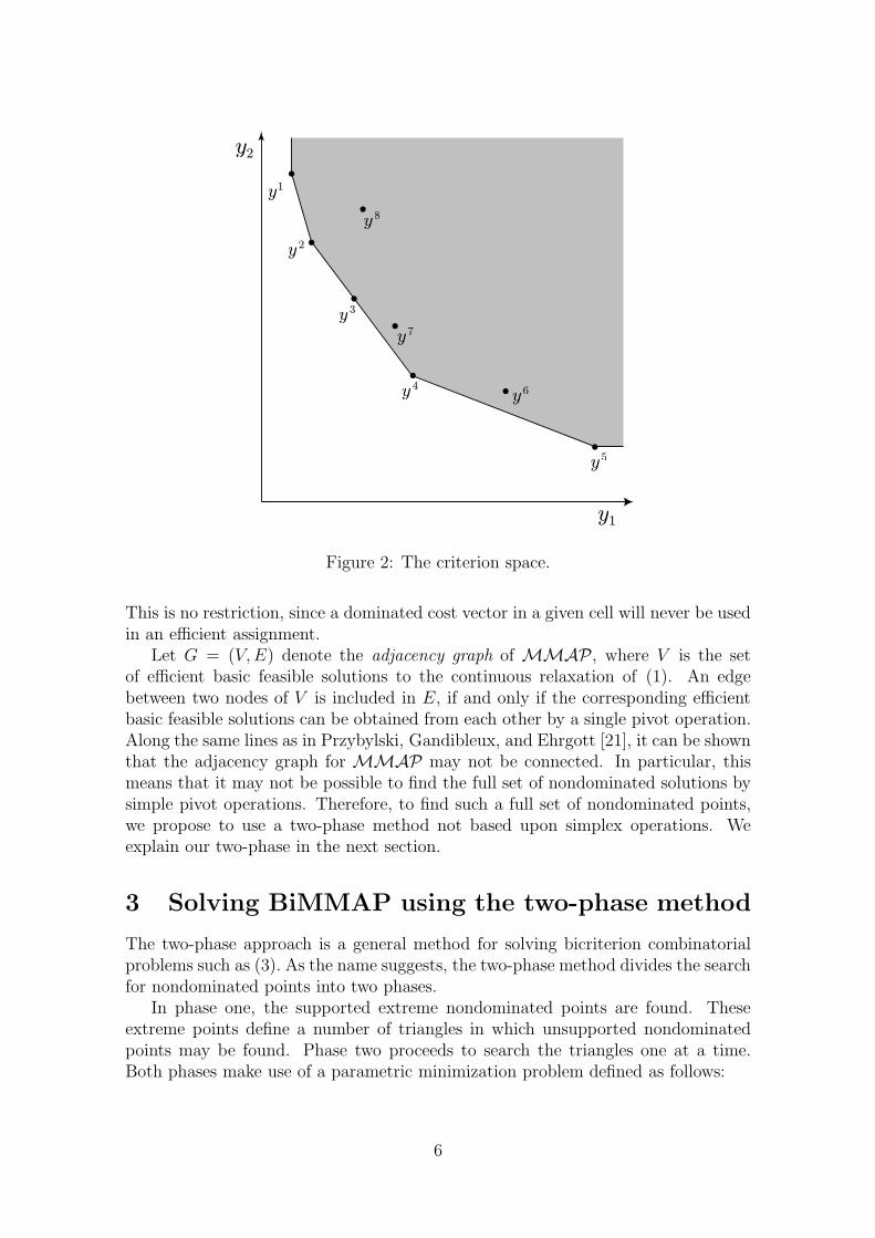
The criterion space is illustrated in Figure 2. Nondominated points are displayedas dots and Y≥ is the shaded area. Supported points are y1-y5 of which y3 is the onlynonextreme. Unsupported nondominated points are y6 and y7 while y8 is dominated.

In some cases it may be enough to find an approximation of the nondominatedset. In this case we need the concepts of ε-domination and ε-approximation intro-duced by Warburton [25]. A point y = (y1, y2) ε-dominates point y = (y1, y2) if(1− ε)y dominates y. A set Y1 is an ε-approximation of a nondominated set Y2, if,for each point y ∈ Y2, there exists y ∈ Y1 that ε-dominates it.

It is well-known that unsupported nondominated points may exist for BiAP [7],and hence also for BiMMAP. Also, due to the fact that BiMMAP is a generalizationof BiAP, it holds true that BiMMAP is intractable and NP-complete ([7, 22]).Moreover, because of (2), we have that all cost vectors for a cell are nondominated.

5

y2

y1

y1

y 3

y 2

y 5

y 6

y 7

y 8

y 4

Figure 2: The criterion space.

This is no restriction, since a dominated cost vector in a given cell will never be usedin an efficient assignment.

Let G = (V, E) denote the adjacency graph of MMAP, where V is the setof efficient basic feasible solutions to the continuous relaxation of (1). An edgebetween two nodes of V is included in E, if and only if the corresponding efficientbasic feasible solutions can be obtained from each other by a single pivot operation.Along the same lines as in Przybylski, Gandibleux, and Ehrgott [21], it can be shownthat the adjacency graph for MMAP may not be connected. In particular, thismeans that it may not be possible to find the full set of nondominated solutions bysimple pivot operations. Therefore, to find such a full set of nondominated points,we propose to use a two-phase method not based upon simplex operations. Weexplain our two-phase in the next section.

3 Solving BiMMAP using the two-phase method

The two-phase approach is a general method for solving bicriterion combinatorialproblems such as (3). As the name suggests, the two-phase method divides the searchfor nondominated points into two phases.

In phase one, the supported extreme nondominated points are found. Theseextreme points define a number of triangles in which unsupported nondominatedpoints may be found. Phase two proceeds to search the triangles one at a time.Both phases make use of a parametric minimization problem defined as follows:

6

y2

y1

y1

y 3y 2

y 5

y 6

y 7 y 8

y 9

y 10

y 4

f(λ)

Figure 3: The criterion space and its corresponding parametric space.

min fλ(x) = (λc1 + c2)x

s.t. x ∈ X(4)

The method is best illustrated using an example. Suppose that the points in theright side of Figure 3 represent the criterion space of the biobjective minimizationproblem (3). Points y1, y4, y5, y6 and y10 are supported nondominated points ofwhich y5 is the only nonextreme. y9 is the only unsupported nondominated point.The remaining points are dominated.

Consider the parametric problem (4). For a fixed criterion point y = (c1x, c2x),fλ(x) define a line with slope y1 = c1x and intersection y2 = c2x in the parametricspace as illustrated on the left side of Figure 3. The lower envelope of the lines in theparametric space defines a non-decreasing piecewise linear function f(λ) with breakpoints λi. Note that each line on f(λ) corresponds to an extreme nondominatedpoint. As a result, each extreme nondominated point can be found by identifyingthe point with minimal parametric weight for fixed λ values, i.e. solving (4). This isdone in phase one which uses a NISE2 like algorithm (see [3]) as shown in Figure 4.This idea was first applied to the bicriterion transportation problem by Aneja andNair [2].

The procedure first finds the upper/left and the lower/right point (y1 and y10

in Figure 3). Given two extreme nondominated points y+ and y−, we calculate thesearch direction λ defined by the slope of the line between the points and solve (4).That is, we find the value of λ where the two lines corresponding to y+ and y−

meet in the parametric space. If the optimal solution x⋆ of (4) corresponds to a

2Non-inferior set estimation.

7

1 procedure PhaseOne()

2 yUL:=(c1xUL, c2xUL), where xUL is optimal for lexmin(c1x, c2x);3 yLR:=(c1xLR, c2xLR), where xLR is optimal for lexmin(c2x, c1x);4 if (yUL=yLR) then stop (only one nondominated point);

5 Y:={

yUL, yLR}

;

6 y+:=yUL; y−:=yLR;

7 while (y+ 6= yLR) do

8 λ:=(y+2 − y−2 )/(y−1 − y+

1 );9 solve (4) with optimal decision x⋆ and cost y⋆ = (c1x⋆, c2x⋆);

10 if (fλ(x⋆) < y+1 λ + y+

2 ) then add y⋆ between y+ and y− in Y;11 else y+:=y−;12 y−:=Next(Y, y+);

13 end while

14 end procedure

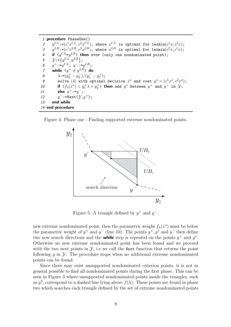
Figure 4: Phase one - Finding supported extreme nondominated points.

y+

y ---

UB1

UB0

search direction

y2

y1

Figure 5: A triangle defined by y+ and y−.

new extreme nondominated point, then the parametric weight fλ(x⋆) must be below

the parametric weight of y+ and y− (line 10). The points y+, y⋆ and y− then definetwo new search directions and the while step is repeated on the points y+ and y⋆.Otherwise no new extreme nondominated point has been found and we proceedwith the two next points in Y , i.e we call the Next function that returns the pointfollowing y in Y . The procedure stops when no additional extreme nondominatedpoints can be found.

Since there may exist unsupported nondominated criterion points, it is not ingeneral possible to find all nondominated points during the first phase. This can beseen in Figure 3 where unsupported nondominated points inside the triangles, suchas y9, correspond to a dashed line lying above f(λ). These points are found in phasetwo which searches each triangle defined by the set of extreme nondominated points

8

1 procedure PhaseTwo(△(y+, y−))2 λ:=(y+

2 − y−2 )/(y−1 − y+1 );

3 Y:={y+, y−};4 k:=1; LB:=λy+

1 + y+2 ; UB:=UpdateUB(Y);

5 while (LB ≤ UB) do

6 yk:=KBest(k, λ);7 if (NonDom(yk)) then

8 Y:=Y ∪ {yk};9 UB:=UpdateUB(Y);

10 end if

11 LB:=λyk1 + yk

2; k:=k + 1;12 end while

13 end procedure

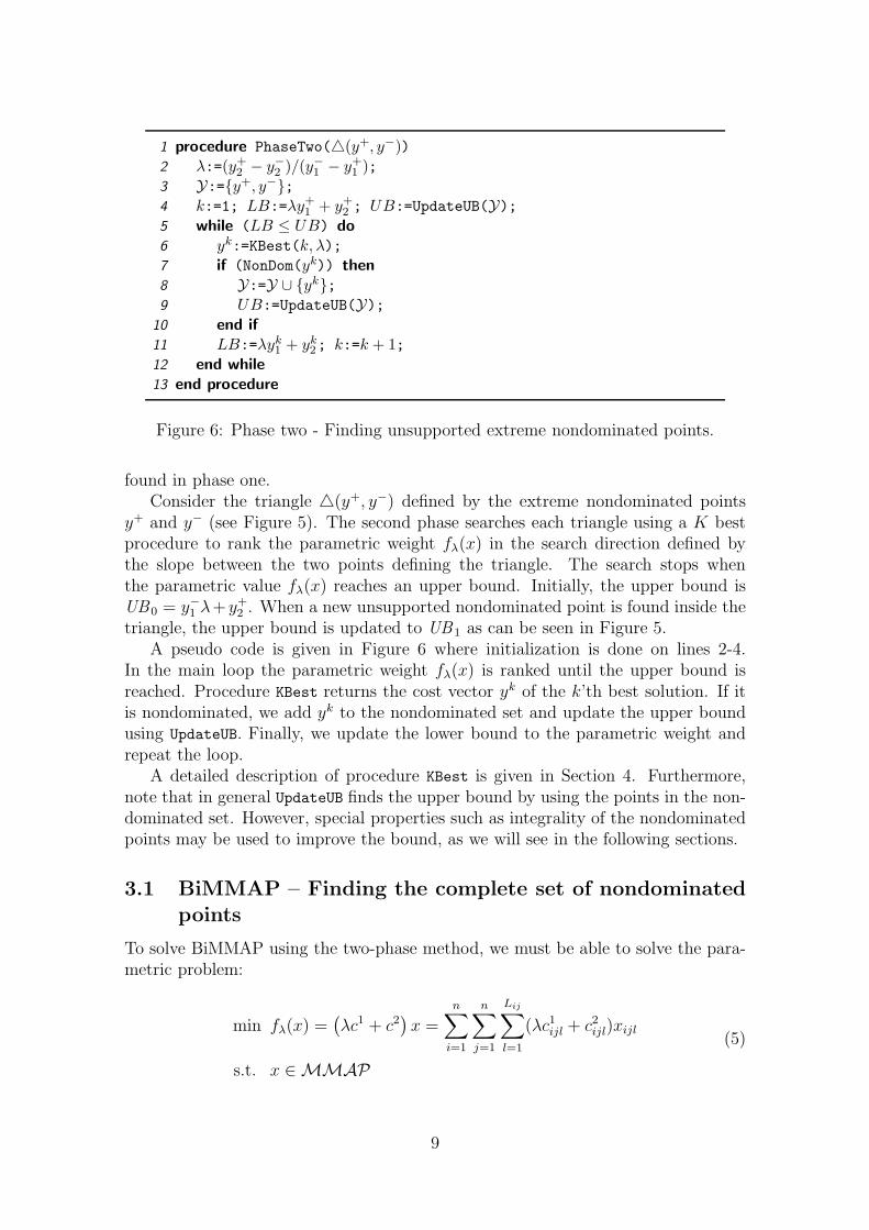
Figure 6: Phase two - Finding unsupported extreme nondominated points.

found in phase one.Consider the triangle △(y+, y−) defined by the extreme nondominated points

y+ and y− (see Figure 5). The second phase searches each triangle using a K bestprocedure to rank the parametric weight fλ(x) in the search direction defined bythe slope between the two points defining the triangle. The search stops whenthe parametric value fλ(x) reaches an upper bound. Initially, the upper bound isUB0 = y−1 λ+y+

2 . When a new unsupported nondominated point is found inside thetriangle, the upper bound is updated to UB1 as can be seen in Figure 5.

A pseudo code is given in Figure 6 where initialization is done on lines 2-4.In the main loop the parametric weight fλ(x) is ranked until the upper bound isreached. Procedure KBest returns the cost vector yk of the k’th best solution. If itis nondominated, we add yk to the nondominated set and update the upper boundusing UpdateUB. Finally, we update the lower bound to the parametric weight andrepeat the loop.

A detailed description of procedure KBest is given in Section 4. Furthermore,note that in general UpdateUB finds the upper bound by using the points in the non-dominated set. However, special properties such as integrality of the nondominatedpoints may be used to improve the bound, as we will see in the following sections.

3.1 BiMMAP – Finding the complete set of nondominated

points

To solve BiMMAP using the two-phase method, we must be able to solve the para-metric problem:

min fλ(x) =(

λc1 + c2)

x =

n∑

i=1

n∑

j=1

Lij∑

l=1

(λc1ijl + c2

ijl)xijl

s.t. x ∈MMAP

(5)

9

For a given value of λ and a given cell (i, j), define

l⋆(λ) = argmin1≤l≤Lij{λc1

ijl + c2ijl} (6)

That is, for a specific value of λ the minimal parametric cost entry, l⋆, in eachassignment cell (i, j) is chosen. It is straightforward to see that (5) reduces to thefollowing problem:

min fλ(x) =(

λc1 + c2)

x =n

∑

i=1

n∑

j=1

cijl⋆(λ)xijl⋆(λ)

s.t. x ∈ AP

(7)

which is a single criterion assignment problem. This is summarized in Proposition 1.

Proposition 1. The parametric problem min{fλ(x)|x ∈ MMAP} reduces to theclassical AP min{

∑

ijcijl⋆(λ)xijl⋆(λ)|x ∈ AP}.

Therefore, the minimal cost assignment for BiMMAP given a fixed value of λ

can be found in procedure PhaseOne by solving a single criterion AP. Moreover, sinceeach criterion point in BiMMAP is integer, the following obvious proposition maybe used to reduce the computational effort in phase one.

Proposition 2. Consider two extreme nondominated points y+ and y−. Then nofurther nondominated extreme points can be found below the line connecting y+ andy− in phase one, if any of the following conditions are fulfilled

y−1 − y+1 = 1 or y+

2 − y−2 = 1 (8)

That is, we simply skip the search between y+ and y− if (8) holds in phase one.Condition (8) may also be used in phase two to skip searching some triangles. If anyof the conditions in (8) are fulfilled, we do not have to apply procedure PhaseTwo

to triangle △(y+, y−) since no unsupported nondominated point can exist in thistriangle.

Observe that this also holds true even if the points y+ and y− are supportednonextreme nondominated points. Hence, storing such nonextreme points in phaseone (by using a ≤ sign instead of a < sign on line 10 in Figure 4) may reduce thecomputational effort in phase two. Furthermore, since all nondominated points haveinteger coordinates, the upper bound used in phase two may be improved.

Proposition 3. Given the triangle △(y+, y−) with previously found nondominatedpoints {y+ = y1, . . . , yq = y−} ordered in increasing order of the first objective anda search direction given by λ, define

UB IP = maxi=1,...,q−1

{λ(

yi+11 − 1

)

+(

yi2 − 1

)

}. (9)

Then all unsupported nondominated criterion points in △(y+, y−) have parametricweight below or equal to UB IP .

10

Proof. Consider a non-found nondominated point (y1, y2) located in △(y+, y−). Dueto integrality of y1 and y2 we have

∃i ∈ {1, . . . , q − 1} : y1 ≤ yi+11 − 1 ∧ y2 ≤ yi

2 − 1

⇓

λy1 + y2 ≤ λ(

yi+11 − 1

)

+(

yi2 − 1

)

Since nondominated points can be located between any two consecutive pointsyi and yi+1, we obtain expression (9) for the upper bound.

As a result, we can use (9) in function UpdateUB of procedure PhaseTwo. Further-more, note that upper bound (9) is valid for all bicriterion problems with integercriterion points and is an improvement to the upper bound previously reported inliterature [23, 24].

3.2 BiMMAP - Finding an approximation

In some cases it may be sufficient to find an approximation of the nondominatedset. In this section we consider the problem of finding an ε-approximation (ε > 0) ofthe nondominated set, which enables us to control the quality of the approximationreported. Only slightly modified versions of phase one and two are needed.

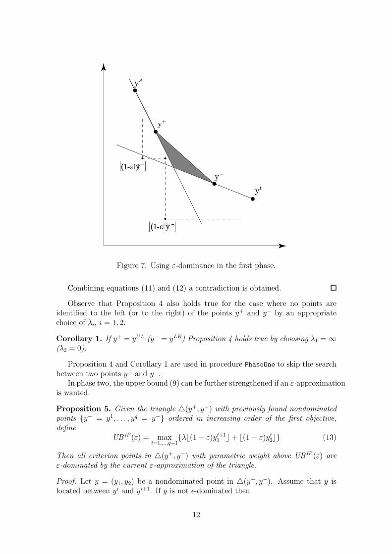
First, consider phase one and a set of extreme nondominated points found duringphase one as illustrated in Figure 7. Note that any new extreme nondominated pointbetween y+ and y− must belong to the shaded area in Figure 7. As a result we canskip searching for new extreme nondominated points between y+ and y− if thefollowing proposition is satisfied.

Proposition 4. Given extreme points {yUL, . . . , ys, y+, y−, yt, . . . , yLR} found dur-ing phase one, each extreme nondominated point between y+ and y−, i.e. inside theshaded area of Figure 7, is ε-dominated by either y+ or y− if

λ1

⌊

(1− ε) y−1⌋

+⌊

(1− ε) y+2

⌋

≤ λ1y+1 + y+

2

or λ2

⌊

(1− ε) y−1⌋

+⌊

(1− ε) y+2

⌋

≤ λ2y−1 + y−2

(10)

where λ1 is defined by the slope of the line between ys and y+ and λ2 is defined bythe slope of the line between y− and yt.

Proof. We only show the result if the first condition in (10) is satisfied. The secondcase is shown with similar arguments. Therefore, assume that λ1

⌊

(1− ε) y−1⌋

+⌊

(1− ε) y+2

⌋

≤ λ1y+1 + y+

2 . Furthermore, suppose that there exists a nondominatedpoint (y1, y2) in the shaded area between y+ and y− (see Figure 7), which is not ǫ-dominated by neither y+ nor y−. It follows that (1− ε) y−1 > y1 and (1− ε) y+

2 > y2.Due to integrality of y1 and y2, this means:

λ1y1 + y2 ≤ λ1

⌊

(1− ε) y−1⌋

+⌊

(1− ε) y+2

⌋

(11)

The nondominated point (y1, y2) is necessarily strictly above the line throughys and y+ (otherwise y+ is not an extreme point found before (y1, y2)). Therefore,λ1y1 + y2 > λ1y

+1 + y+

2 . This implies that

λ1

⌊

(1− ε) y−1⌋

+⌊

(1− ε) y+2

⌋

≤ λ1y+1 + y+

2 < λ1y1 + y2 (12)

11

y t

y+

y-

ys

y+(1-e)

y-(1-e) �

Figure 7: Using ε-dominance in the first phase.

Combining equations (11) and (12) a contradiction is obtained.

Observe that Proposition 4 also holds true for the case where no points areidentified to the left (or to the right) of the points y+ and y− by an appropriatechoice of λi, i = 1, 2.

Corollary 1. If y+ = yUL (y− = yLR) Proposition 4 holds true by choosing λ1 = ∞(λ2 = 0).

Proposition 4 and Corollary 1 are used in procedure PhaseOne to skip the searchbetween two points y+ and y−.

In phase two, the upper bound (9) can be further strengthened if an ε-approximationis wanted.

Proposition 5. Given the triangle △(y+, y−) with previously found nondominatedpoints {y+ = y1, . . . , yq = y−} ordered in increasing order of the first objective,define

UB IP (ε) = maxi=1,...,q−1

{λ⌊(1− ε)yi+11 ⌋+ ⌊(1− ε)yi

2⌋} (13)

Then all criterion points in △(y+, y−) with parametric weight above UB IP (ε) areε-dominated by the current ε-approximation of the triangle.

Proof. Let y = (y1, y2) be a nondominated point in △(y+, y−). Assume that y islocated between yi and yi+1. If y is not ǫ-dominated then

12

∃i ∈ {1, . . . , q − 1} : y1 < (1− ε) yi+11 ∧ y2 < (1− ε) yi

2

⇓ (since y is integral)

y1 ≤⌊

(1− ε) yi+11

⌋

∧ y2 ≤⌊

(1− ε) yi2

⌋

⇓

λy1 + y2 ≤ λ⌊(1− ε) yi+11 ⌋+ ⌊(1− ε) yi

2⌋

Since nondominated points can be located between any two consecutive pointsyi and yi+1, we obtain expression (13) for the upper bound.

It follows that for ε > 0 equation (13) can be used to find the upper bound infunction UpdateUB of procedure PhaseTwo. Also, note that if we consider the shadedarea between y+ and y− (see Figure 7) not searched in phase one (i.e. satisfying(10)), then UB IP(ε) for △(y+, y−) will be less than the parametric weight of y+.Therefore, △(y+, y−) is not searched in procedure PhaseTwo either. Furthermore,there can be some possible gains in storing nonextreme supported points in phaseone as well. The more supported nondominated points that are identified in the firstphase, the more likely are UB IP (ε) to be below the parametric weight of y+ andhence △(y+, y−) is not searched.

Note that, the approximation found in phase one is a subset of the supportednondominated points, since the optimal solution of (5) corresponds to an extremenondominated point. Moreover, because we apply a ranking procedure in the secondphase, a dominated point cannot be found before a point dominating it. Thesecomments provide us with the following result.

Proposition 6. The approximation of the nondominated set for an ε > 0 is a subsetof YN .

4 Finding the K best multi modal assignments

In this section, we describe our method for ranking multi modal assignments innondecreasing order of cost, used in phase two when searching a triangle. That is,ranking assignments using the single criterion parametric costs defined for a givenparameter λ.

Without loss of generality, assume that each cell (i, j) contains entries cij1 ≤. . . ≤ cijLij

. Our objective is to determine the K best assignments a1, a2, . . . , aK , ina single criterion multi modal assignment problem, such that

• c(ai) ≤ c(ai+1), i = 1, 2, . . . , K − 1

• c(aK) ≤ c(a), for any assignment a 6∈ {a1, . . . , aK}

where c(a) denotes the cost of assignment a.In general, ranking algorithms use a specific branching technique to partition

the set of possible solutions into smaller subsets and a solution technique to find theoptimal solution for each subset.

Let A denote the set of possible multi modal assignments. In this paper, we usea branching technique which is an extension of the branching technique originally

13

proposed by Murty [14]. Here we partition the set A into smaller subsets as follows:Given the optimal assignment a1 = {(1, j1, l1), (2, j2, l2), . . . , (n, jn, ln)} of A, the setA \ {a1} is partitioned into n− 1 disjoint subsets Ai, i = 1, . . . , n− 1, where

Ai = {a ∈ A | (1, j1, l1), . . . , (i− 1, ji−1, li−1) ∈ a, (i, ji, li) 6∈ a}, i = 1, . . . , n− 1

Clearly, the second best assignment a2 can be identified using a solution techniqueto find the minimal cost assignment in the sets Ai, i = 1, . . . , n− 1. Moreover, thebranching technique can be applied recursively to subsets Ai ⊂ A.

In general, the algorithm maintains a candidate set Φ of pairs (a, A), where a

is the minimum cost assignment in subset A. Suppose we have found the k − 1best assignments a1, . . . , ak−1, then the current candidate set Φ represents a disjointpartition of A \ {a1, . . . , ak−1}. The kth best assignment is then found as the pair(a, A) ∈ Φ which contains the assignment a with minimum cost c(a) among allassignments in the candidate set Φ.

Next let us consider the solution technique, i.e how to determine the minimumcost assignments in Ai when applying the branching technique to some subset A ⊂A. Without loss of generality, assume that the minimum cost assignment in subsetA is given by

a = {(1, j1, l1), (2, j2, l2), . . . , (n, jn, ln)}. (14)

Furthermore, assume that, according to previous partitions, no assignments in Acan contain (m1, p1, h1), . . . , (mq, pq, hq). Recall that any assignment belonging to

Ai must contain (1, j1, l1), . . . , (i − 1, ji−1, li−1). Assuming that Ai contains an as-signment, it can be found as follows:

1. Delete rows {1, 2, . . . , (i− 1)} and columns {j1, j2, . . . , ji−1} from the cost ma-trix.

2. The cost of entries (i, ji, li) and (m1, p1, h1), . . . , (mq, pq, hq) in the cost matrixis set to infinity.

Given a nonempty subset Ai, let MMAP(Ai) denote the multi modal assignmentproblem defined by the two steps above. Due to Proposition 1 we have the following.

Corollary 2. The minimal cost multi modal assignment in MMAP(Ai) can be foundby solving a classical assignment problem, denoted AP(Ai), using the minimal costof each cell in MMAP(Ai).

Due to Corollary 2, we can use an algorithm for ranking classic linear assign-ments with the slightly more general branching technique described above. Anefficient algorithm for ranking classic assignments is given by Pedersen et al. [19].The algorithm uses a reoptimization solution technique such that the minimal costassignments for the subsets can be found easily (see [19] for more details). Sincethe general branching technique described above does not create more subsets thanthe classic branching technique, the overall complexity for ranking the K best multimodal assignments is the same.

Corollary 3. The complexity for finding the K best assignments is O(Kn3).

14

Actually, in some cases the minimal cost assignment for subset Ai can be foundwithout solving an AP. Given subset A, assume without loss of generality that eachcell (i, j) in MMAP(A) contains Lij entries cij1 ≤ . . . ≤ cijLij

(not set to infinity).Moreover, let u and v denote the dual row and column variables of the optimalassignment (14) found by solving AP(A). Hence the corresponding reduced cost foreach cell (i, j) becomes cij = cij1 − ui − vj . If we disregard cell (i, j), the minimumreduced costs in row i and column j are

Ri = mint{cit | t 6= j} and Cj = min

t{ctj | t 6= i}.

Note that Ri, Cj ≥ 0, ∀i, j, due to optimality of u and v. Now, consider subset

Ai. In MMAP(Ai) we set ciji1 to infinity. If Liji> 1, we replace ciji1 with ciji2 in

AP(Ai). That is, AP(Ai) uses the same costs as AP(A) except in cell (i, ji) whereciji2 is used. We have the following proposition to enhance the performance of ourprocedure.

Proposition 7. Assume Liji> 1 and Ri +Cji

≥ ciji2− ciji1. Then an minimal cost

assignment for subset Ai is

ai = (a \ {(i, ji, 1)}) ∪ {(i, ji, 2)}

Proof. Define∆iji

= ciji2 − ciji1 ≥ 0

The assignment a of AP(A) is primal feasible and satisfies the complementary slack-ness conditions xij1cij = 0. Consider AP(Ai) with dual row and column variables u

and v. If ∆iji≤ Ri, set ui = ui+∆iji

and keep the remaining dual values unchanged.Then cit ≥ 0, ∀t 6= ji and

ciji= ciji2 − (ui + ∆iji

)− vji= ciji

= 0

Hence the assignment ai of AP(Ai) is primal feasible and satisfies the complementaryslackness conditions, i.e. ai is an optimal solution.

If ∆iji> Ri, we set ui = ui +Ri and vji

= vji+∆iji

−Ri and keep the remainingdual values unchanged. Hence cit ≥ 0 and

ciji= ciji2 − (ui + Ri)− (vji

+ ∆iji−Ri) = ciji

= 0

Again, assignment ai is optimal.

Using Proposition 7, we do not have to solve AP(Ai) if Ri + Cji≥ ciji2 − ciji1.

The minimal cost assignment ai is simply obtained by assigning the rows to the samecolumns as in assignment a and, in cell (i, ji), by using entry 2 instead of entry 1.

5 Computational results

In this section, we report the computational experience on BiMMAP test instances.Moreover, since BiMMAP is an extension of BiAP, we also report some results on testinstances for BiAP. All tests were performed on an Intel Xeon 2.67 GHz computerwith 6 GB RAM using a Red Hat Enterprise Linux version 4.0 operating system.

15

5.1 Implementation details

The algorithms have been implemented in C++ and compiled with the GNU C++compiler using optimize option -O.

The cost matrix of BiMMAP (see Figure 1) is stored using a two-dimensionalarray of Cell objects. Each Cell object contains an array holding the cost entriesand an ordered array holding the parametric costs of the entries for a specific λ.

In phase one, for a given search direction specified by λ, we update the parametriccosts and order them in nondecreasing order. Due to Proposition 1, we consider thesmallest entry in each cell and solve the resulting AP using the implementation givenby Jonker and Volgenant [11]. Furthermore, we take advantage of Proposition 2 orProposition 4 (if ε > 0) whenever possible.

In phase two, we, as in phase one, update the parametric costs and order them innondecreasing order for a given search direction specified by λ. Next, we use the Kbest multi modal assignment procedure described in Section 4 to search a triangle,using the upper bounds given in Proposition 3 or Proposition 5 (if ε > 0).

The K best multi modal assignment procedure was implemented using the re-optimization algorithm in Pedersen et al. [19] for ranking classic assignments, withthe slightly more general branching technique given in Section 4. In particular, notethat, when considering a subset where we remove an entry in the ordered array ofparametric costs, the new entry with minimal cost is the next cost in the array. Thatis, we just have to increase a local pointer by one to find the new minimal cost. SeePedersen et al. [19] for more details on the ranking implementation.

All nondominated points found by the ranking procedure are stored in a singlelinked list available in both phase one and two.

5.2 BiMMAP test instances

The bicriterion multi modal assignment problem has, to the best of our knowledge,not previously been studied in literature, and hence no available test instances existfor this problem. To facilitate a comprehensive computational study of our BiMMAPalgorithm, we build a problem generator, APGen, for this problem class.3 As a side-effect our generator can be used to generate a variety of BiAP instances. In thefollowing we give a brief description of the generator, and we refer readers requiringmore information on this topic, to the full documentation paper [17]. A BiMMAPinstance is generated specifying a number of parameters:

n – the size of the problem.

maxEnt – the maximal number of entries in each assignment cell.

minEnt – the minimal number of entries in each assignment cell (default 1).

maxCost – the maximal cost value for both objectives (minimum cost valueis 0).

3The problem generator and the test instances used in this paper are downloadable from thefollowing webpage http://www.research.relund.dk/.

16

0 2000 4000 6000 8000 10000

020

0040

0060

0080

0010

000

(a) shape = −60

0 2000 4000 6000 8000 10000

020

0040

0060

0080

0010

000

(b) shape = 0

0 2000 4000 6000 8000 10000

020

0040

0060

0080

0010

000

(c) shape = 60

Figure 8: Cell entries for method = 1.

method – a choice between three different ways of generating cell entries.

shape – for a given method, the shape parameter describes the shape of theentries in a given cell.

Obviously, for a given cell, no entries are allowed to be dominated by other entriesin that cell, since this would correspond to a dominated solution. The number ofentries in a cell is chosen randomly in the entry range {minEnt, . . . , maxEnt}.To describe best the six different versions of method and shape used for generatingBiMMAP instances, we have displayed all two-dimensional cost vectors for a givencell having 20 entries in Figures 8 to 10.

17

0 2000 4000 6000 8000 10000

020

0040

0060

0080

0010

000

(a) shape = 3

0 2000 4000 6000 8000 10000

020

0040

0060

0080

0010

000

(b) shape = 4

Figure 9: Cell entries for method = 2.

As can be seen in Figure 8, with method 1 the shape parameter describes thecurve of the function along which the entries are generated. A negative shape cor-responds to generating the entries along a concave-like function, using shape 0 gen-erates entries fluctuating along a straight line, and finally, a positive shape meansgenerating entries along a convex-like function. Therefore, using a negative (posi-tive) shape parameter tends to generate many unsupported (supported) entries inthe given cell. We shall see, that this has a strong influence on the difficulty of theconsidered problem and hence the computational performance of our algorithm.

For method 2, the entries in a given cell are generated in a number of groupsspecified by the shape parameter (see Figure 9). Note, to use method 2, the param-eter minEnt must be chosen sufficiently large, since at least 2 points have to be ineach group.

Finally, for method 3, the shape parameter has the same meaning as for method1. However, the entries fall either in the upper left corner of the cost-space or thelower right corner in consecutive cells. This can be seen in Figure 10, where wedisplay the entries in the four consecutive assignment cells (1, 1), . . . , (1, 4).

To provide a broad class of test instances and facilitate statistical analysis, wegenerated 100 instances of each of the following 80 possible configurations.

• n ∈ {4, 6, 8, 10}.

• Cost ranges : {0, . . . , 500} and {0, . . . , 10000}.

• Entry ranges : {2, . . . , 8} (not for method 2) and {10, . . . , 30}.

• (method, shape) ∈ {(1,−60), (1, 0), (1, 60), (2, 3), (2, 4), (3, 0)}.

The two different ranges of number of entries are chosen to reflect a situationclose to BiAP (few entries) and a situation very far away from BiAP (many entries),

18

0 2000 4000 6000 8000 10000

020

0040

0060

0080

0010

000

(a) cell (1, 1)

0 2000 4000 6000 8000 10000

020

0040

0060

0080

0010

000

(b) cell (1, 2)

0 2000 4000 6000 8000 10000

020

0040

0060

0080

0010

000

(c) cell (1, 3)

0 2000 4000 6000 8000 10000

020

0040

0060

0080

0010

000

(d) cell (1, 4)

Figure 10: Cell entries for cells (1, 1) to (1, 4) for method = 3 and shape = 0.

respectively. Note that the number of possible assignments increases exponentiallywith the number of entries in each cell. For a problem with n = 10 and entry range{10, . . . , 30}, the total number of assignments ranges between 10! · 1010 ≈ 3.6 · 1016

in the best case and 10! ·1030 ≈ 3.6 ·1036 in the worst case. In comparison, the BiAPwith size 10 has only 10! ≈ 3.6 · 106 feasible assignments.

5.3 BiMMAP test results

Giving the results of the extensive amount of tests, we first display the logarithm ofthe CPU time (in seconds) averaged over the 100 instances against problem size n for

19

size

log(

CP

U)

4 6 8 10

0

5

method and shapem=1, s=−60m=1, s=0m=1, s=60

m=2, s=3m=2, s=4m=3, s=0

Figure 11: Logarithm of average CPU against n (cost range {0, . . . , 10000} and entryrange {10, . . . , 30}).

the highest possible cost range and the highest possible entry range (Figure 11). Itcan be seen, that, for none of the six different classes, the running time is increasingexponentially with problem size. Also notice that the most difficult class is by farusing method 1 with shape −60, whereas the easiest class is method 1 and shape60.

To yield a possible explanation of the difference in difficulty of these two prob-lem classes, we direct the attention of the reader to Figure 12 where the nondom-inated points in the criterion space have been plotted for two test instances usingshape = −60 and shape = 60, respectively. Triangles are drawn between consecutivesupported extreme nondominated points.

For the test instance with shape = −60, only a limited number of supportedextreme nondominated criterion points exist. Notice that these extreme points arefar from each other resulting in large triangles to search in the second phase. Moreimportant, all the extreme supported nondominated points are almost on a straightline. Therefore, the search directions for the triangles are more or less the same. As a

20

1. criterion

2. c

riter

ion

0 20000 40000 60000 80000 100000

020

000

4000

060

000

8000

010

0000

(a) shape = −60

1. criterion

2. c

riter

ion

0 20000 40000 60000 80000

020

000

4000

060

000

8000

010

0000

(b) shape = 60

Figure 12: Nondominated points (method = 1, n = 10, entry range {10, . . . , 30}and cost range {0, . . . , 10000}).

21

result, the ranking procedure initiated in the first large triangle has to generate manypoints before reaching the upper bound of the triangle making this single trianglesearch extremely time consuming. Remember though, that nondominated pointsgenerated which are outside the triangle currently searched, are stored. This mayenable us to finish searching other triangles faster and hence enhance computationalperformance.

In contrast, the test instance with shape = 60 has more extreme nondominatedpoints in the criterion space, resulting in small triangles to search. Moreover, thesearch directions are more diverse and hence fewer points have to be generated whensearching a triangle.

Considering other instances the above relationships proved to have general valid-ity. The larger a triangle is, the longer the search in this triangle continues in phasetwo. Therefore, with many extreme points at termination of phase one, only smalltriangles need to be searched, resulting in a lower overall running time compared toan instance with a few extreme points and larger triangles. Moreover, test instanceswhere the search directions for the triangles are more or less the same are harder tosolve.

Comparing running times of phase one and two, phase two can be seen to bethe major time consumer. On average, phase two uses 98 per cent of the total CPUtime in the 8000 exactly solved instances.

Since method 1 shape −60 has established itself as the most difficult problemclass, we focus on this instance only from here on.

In Figure 13, we show the logarithm of average CPU time against the problemsize for the four different configurations of entry range and cost range. It can be seen,that the most difficult case is the one with the most entries and highest cost range.The most significant factor is the entry range, obviously resulting from the increasednumber of feasible solutions. Also, for a given number of entries, the most difficultcase arises with the highest possible cost range. In this respect, the BiMMAP followsthe classical single criterion assignment problem since this problem is known to beeasiest solvable with relatively small costs [11].

From here on, we focus on test instances using method = 1, shape = −60 costrange {0, . . . , 10000} and entry range {10, . . . , 30} only. In Table 1, we give thenumerical results for the exact solution of these instances. In the six columns aredepicted the size of the problem, average CPU time (seconds), maximal CPU time,average number of supported nondominated points, average number of unsupportednondominated points and average of the total number of nondominated points, re-spectively. Obviously, all columns are increasing in size. However, it is interestingto note the relatively high number of unsupported nondominated criterion points.

Now we describe the results for finding an approximation of the nondominatedset. Two small values 0.01 and 0.05 of ε are chosen to ensure that a sufficientlyaccurate approximation is found. We also include the results for the exact solvedinstances (ε = 0). In Figure 14, we display the logarithm of average CPU timeagainst size for all three ε values.

Finding an approximation can be seen to have a strong influence on the runningtime of the algorithm. Even for these small ε values (and hence good approxima-tions) there are significant savings in computation time. We note (not displayed)

22

size

log(

CP

U)

4 6 8 10

−5

0

5

cost and entriesc=0−10000, ent=10−30c=0−10000, ent=2−8

c=0−500, ent=10−30c=0−500, ent=2−8

Figure 13: Logarithm of average CPU against n (method = 1 and shape = −60).

size ave CPU max CPU ave SND ave USND ave ND

4 0.10 0.34 6.95 210.04 216.99

6 4.39 33.21 9.87 437.30 447.17

8 71.84 559.28 13.07 744.34 757.41

10 245.63 2967.09 16.23 1143.72 1159.95

Table 1: Exact results (method = 1, shape = −60, entry range {10, ..., 30} and costrange {0, ..., 10000}).

that the number of identified nondominated points obviously decreases with increas-ing ε, as some extreme supported nondominated points may not be considered in thefirst phase, and in the second phase, fewer alternatives for each triangle are ranked.

In Figure 15, we graph the empirical distribution functions of CPU time forthe 100 test instances for problem size 10. This clearly shows that the majority of

23

size

log(

CP

U)

4 6 8 10

−4

−2

0

2

4

epsilon00.010.05

Figure 14: Logarithm of average CPU against n (method = 1 and shape = −60).

ε = 0 ε = 0.01 ε = 0.05

size ave. 90% max ave. 90% max ave. 90% max

4 0.10 0.18 0.34 0.05 0.10 0.17 0.02 0.05 0.09

6 4.39 9.19 33.21 1.52 3.01 12.25 0.25 0.52 2.01

8 71.84 163.16 559.28 17.16 41.71 172.38 0.69 1.60 6.01

10 245.63 589.52 2967.09 34.61 85.72 420.15 0.29 0.66 2.82

Table 2: CPU times for ε = 0, 0.01 or 0.05 (method = 1, shape = −60, entry range{10, ..., 30} and cost range {0, ..., 10000}.

problems are solved fast, while only a few difficult instances are solved relativelyslowly. The numerical results are summarized in Table 2, giving for each ε theaverage CPU time (seconds), the 90 per cent fractile of CPU time and the maximumCPU time.

24

CPU

emp.

cum

. dis

t. fu

nc.

0 500 1000 1500 2000 2500 3000

0.0

0.2

0.4

0.6

0.8

1.0

epsilon00.010.05

Figure 15: Empirical distribution of CPU time for different ε values.

5.4 Results for BiAP

Since BiMMAP is an extension of BiAP, we found it natural to test the perfor-mance of our current implementation on this problem class. To yield consistencyin literature, we obtained the test instances used in [23] which are BiAP instancesof size {5, 10, . . . , 50}. Also previously used in literature are AP instances of size{60, 70, . . . , 100} found in [8].4 These instances have recently been solved by anexact method in [20] and by a heuristic in [9] acknowledging the current interest inthis field. For all the problem classes only one instance is solved, and hence limitedstatistics can be performed for those data sets. For all instances, costs are chosenrandomly in the rather narrow interval {0, . . . , 19}.

To provide our reader with statistics based on a broader class of instances, wegenerated 100 instances of each of the following sizes {5, 10, . . . , 100} with costsrandomly chosen in {0, . . . , 1000}. This wide interval leaves room for identifyinga large number of large triangles to search in phase two, and hence adds to the

4http://www.univ-valenciennes.fr/ROAD/MCDM/ListMOAP.html

25

1. cost

2. c

ost

0 200 400 600 800 1000

0

200

400

600

800

1000

(a) random.

1. cost

2. c

ost

0 200 400 600 800 1000

0

200

400

600

800

1000

(b) negatively correlated.

Figure 16: Cost generation for BiAP test instances.

difficulty of the problem. Also, to investigate the effect of negatively correlatedcosts, we generated 100 instances of each of the sizes {5, 10, . . . , 100}, again withcosts in the interval {0, . . . , 1000}. The difference in costs generated randomly andnegatively correlated is shown in Figure 16. We shall see that negatively correlatedcost vectors have a strong influence on the difficulty of the considered problem,and hence the running time of the algorithm. In general bicriterion problems withnegatively correlated costs are harder to solve, see e.g. [4].

26

size

CP

U

20 40 60 80 100

0

5

10

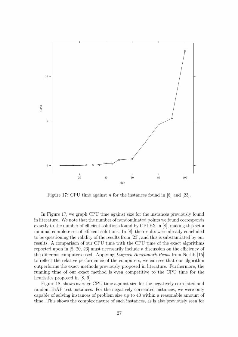
Figure 17: CPU time against n for the instances found in [8] and [23].

In Figure 17, we graph CPU time against size for the instances previously foundin literature. We note that the number of nondominated points we found correspondsexactly to the number of efficient solutions found by CPLEX in [8], making this set aminimal complete set of efficient solutions. In [8], the results were already concludedto be questioning the validity of the results from [23], and this is substantiated by ourresults. A comparison of our CPU time with the CPU time of the exact algorithmsreported upon in [8, 20, 23] must necessarily include a discussion on the efficiency ofthe different computers used. Applying Linpack Benchmark-Peaks from Netlib [15]to reflect the relative performance of the computers, we can see that our algorithmoutperforms the exact methods previously proposed in literature. Furthermore, therunning time of our exact method is even competitive to the CPU time for theheuristics proposed in [8, 9].

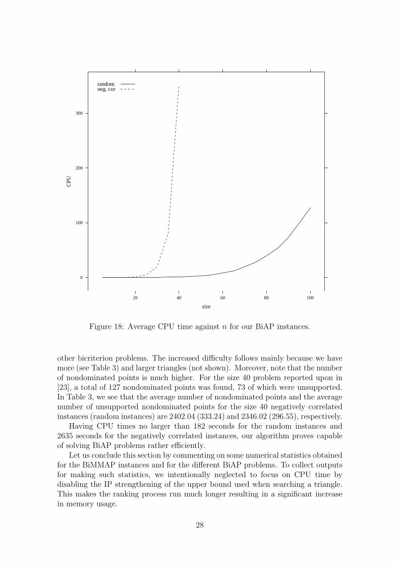
Figure 18, shows average CPU time against size for the negatively correlated andrandom BiAP test instances. For the negatively correlated instances, we were onlycapable of solving instances of problem size up to 40 within a reasonable amount oftime. This shows the complex nature of such instances, as is also previously seen for

27

size

CP

U

20 40 60 80 100

0

100

200

300

randomneg. cor

Figure 18: Average CPU time against n for our BiAP instances.

other bicriterion problems. The increased difficulty follows mainly because we havemore (see Table 3) and larger triangles (not shown). Moreover, note that the numberof nondominated points is much higher. For the size 40 problem reported upon in[23], a total of 127 nondominated points was found, 73 of which were unsupported.In Table 3, we see that the average number of nondominated points and the averagenumber of unsupported nondominated points for the size 40 negatively correlatedinstances (random instances) are 2402.04 (333.24) and 2346.02 (296.55), respectively.

Having CPU times no larger than 182 seconds for the random instances and2635 seconds for the negatively correlated instances, our algorithm proves capableof solving BiAP problems rather efficiently.

Let us conclude this section by commenting on some numerical statistics obtainedfor the BiMMAP instances and for the different BiAP problems. To collect outputsfor making such statistics, we intentionally neglected to focus on CPU time bydisabling the IP strengthening of the upper bound used when searching a triangle.This makes the ranking process run much longer resulting in a significant increasein memory usage.

28

neg. corr. data random data

size ave SND ave USND ave ND ave SND ave USND ave ND

5 5.56 14.86 20.42 3.67 2.44 6.11

10 13.23 115.44 128.67 7.80 16.58 24.38

15 20.12 294.78 314.90 12.23 40.83 53.06

20 27.89 539.18 567.07 17.56 72.43 89.99

25 34.95 877.59 912.54 22.68 118.64 141.32

30 41.83 1298.96 1340.79 27.17 167.41 194.58

35 48.63 1773.25 1821.88 32.65 230.82 263.47

40 56.02 2346.02 2402.04 36.69 296.55 333.24

Table 3: Exact results for our BiAP instances.

Calculating the number of times the IP upper bound would succeed in terminat-ing the search of a triangle when the bound without IP strengthening would fail anddividing this by the total number of iterations, the average ratio for all 8000 exactlysolved BiMMAP instances is 11.47 per cent. This corresponds to saying that, inmore than one out of 10 cases the search in a given triangle would be terminatedwhen using the integer based upper bound, whereas the upper bound without inte-grality would still be higher than the lower bound. The same ratio for our negativelycorrelated BiAP instances is 5.80 per cent, for our random instances 7.67 per centand finally, for the random BiAP instances found in literature, 79.55 per cent. Obvi-ously, since only a limited amount of instances have previously been reported uponin literature, this last number must be interpreted with caution. However, it seemslike the IP strengthening proves to be valuable for primarily instances having a nar-row cost range. This yields another explanation for our instances being significantlyharder than the instances previously seen in literature.

It is also interesting to consider the ratio between the number of efficient solutionsand the number of nondominated points. For BiMMAP instances, this ratio has anaverage of 1.01 and a maximum of 1.25 found for a size 8 instance using the lowestpossible cost range {0, . . . , 500} and highest possible entry range {10, . . . , 30}. Thisfits nicely with our intuition that a narrow cost range leads to many alternativeefficient solutions. Moreover, the high number of entries also yields a higher totalnumber of feasible solutions. For the 15 random generated BiAP instances from[8, 23], the average of this ratio is 2.11, and for both our random instances and ournegatively correlated instances, this ratio is very close to 1. The main factor hereis again the cost range. A narrow cost range gives a higher number of alternativeefficient solutions corresponding to the same nondominated point.

6 Conclusion

In this paper we have presented a two-phase method for solving a new bicrite-rion generalization of the classical linear assignment problem. The algorithm uti-

29

lizes a ranking scheme relying on reoptimization, which was previously shown to bevery efficient. Exploiting the integral nature of the criterion vectors allowed us tostrengthen an upper bound previously stated in literature. Our algorithm identifieseither the exact set of all nondominated points or an approximation of these withpredetermined approximation quality.

A large library of test instances for both BiMMAP and BiAP was provided bya new problem generator, and a diversity of numerical results was presented. Belowwe summarize the main results.

For BiMMAP the excessive group of test problems allowed us to identify theinstances with cell entries generated along a concave-like function (method 1 andshape −60) to be significantly harder than any other problem class. This mainlyfollows since the many unsupported cost vectors in each cell generate few extremesupported points located along an almost straight line in criterion space. Therefore,the search directions for the individual triangles become close to identical, resultingin long running times for the first large triangle investigated. Since phase two wasestablished as the main time consumer, this explains why such instances are verydifficult. In contrast, the instances with many supported cell entries (method 1 andshape 60) generate more supported extreme criterion vectors located along a convex-like function. Therefore, the triangles to search in the second phase are smaller andhave more diverse search directions, making these instances easier.

Considering two different ranges of costs and of number of entries in each as-signment cell, it was pointed out that high costs and many cell entries result in themost difficult instances. This was concluded to fit nicely with results for the singlecriterion AP and with the fact that the total number of feasible solutions growsrapidly with the number of cell entries.

For BiAP, the main knowledge gained by our numerical experiments is that in-stances with negatively correlated cost vectors by far exceed random BiAP instancesin difficulty. This mainly follows due to the higher number of large triangles to searchin the time-consuming second phase.

Our algorithm was concluded to perform very well even on BiMMAP instancesof high size, and was seen to outperform existing methods for BiAP. The integralstrengthening of the upper bound proved to be contributing significantly to theefficiency of our algorithm. Finding an approximation of the nondominated set wasseen to be a valuable tool to reduce the computation time significantly. The resultsreported here show the approximative algorithm to be a serious rival to heuristicalmethods. Note, applying an approximative scheme instead of a heuristical methodallows us to control the quality of the reported set of criterion points.

A natural extension of BiMMAP is the bicriterion multi modal transportationproblem which interests the authors of this paper. Also, under current investiga-tion is a bicriterion version of the directed Chinese Postman Problem (BiDCPP).Restricting the deviation in in- and out-degree for all nodes in the original post-man graph to be no larger than one, BiDCPP can be seen to yield an instance ofBiMMAP as a subproblem.

30

References

[1] R.K. Ahuja, T.L. Magnanti, and J.B. Orlin. Network Flows: Theory, Algo-rithms, and Applications. Prentice Hall, 1993.

[2] Y.P. Aneja and K.P.K. Nair. Bicriteria transportation problem. ManagementScience, 25(1):73–78, 1979.

[3] J. Cohen. Multiobjective Programming and Planning. Academic Press, NewYork, 1978.

[4] C. Gomes da Silva, J. Clımaco, and J. Figueira. A scatter search method for bi-criteria {0, 1}-knapsack problems. European Journal of Operational Research,169(2):373–391, 2006.

[5] M. Dell’Amico and S. Martello. Linear assignment. In M. Dell’Amico, F. Maf-fioli, and S. Martello, editors, Annotated Bibliographies in Combinatorial Opti-mization, pages 355–371. Wiley, Chichester, 1997.

[6] M. Dell’Amico and P. Toth. Algorithms and codes for dense assignment prob-lems: the state of the art. Discrete Appl. Math., 100(1-2):17–48, 2000. doi:10.1016/S0166-218X(99)00172-9.

[7] M. Ehrgott. Multicriteria optimization, volume 491 of Lecture Notes in Eco-nomics and Mathematical Systems. Springer-Verlag, Berlin, 2000.

[8] X. Gandibleux, H. Morita, and N. Katoh. Use of genetic heritage for solving theassignment problem with two objectives. Lecture Notes in Computer Science,2632:43–57, 2003.

[9] X. Gandibleux, H. Morita, and N. Katoh. A population-based metaheuristicfor solving assignment problems with two objectives. To appear in Journal ofMathematical Modelling and Algorithms, Revised 2005.

[10] P. Hansen. Bicriterion path problems. In Multiple Criteria Decision Making,Theory and Application, number 177 in Lecture Notes in Economics and Math-ematical Systems, pages 109–127. Springer-Verlag, Berlin, 1979.

[11] R. Jonker and A. Volgenant. A shortest augmenting path algorithm for denseand sparse linear assignment problems. Computing, 38:325–340, 1987.

[12] H.W. Kuhn. The hungarian method for the assignment problem. Naval ResearchLogistics Quart., 2:83–97, 1955.

[13] H.W. Kuhn. Variants of the hungarian method for the assignment problem.Naval Research Logistics Quart., 3:253–258, 1956.

[14] K.G Murty. An algorithm for ranking all the assignments in order of increasingcost. Operations Research, 16:682–687, 1968.

[15] Netlib. The performance database server. URL http://netlib.org/.

31

[16] L.R. Nielsen, K.A. Andersen, and D. Pretolani. Bicriterion shortest hyperpathsin random time-dependent networks. IMA Journal of Management Mathemat-ics, 14(3):271–303, 2003.

[17] L.R. Nielsen and C.R. Pedersen. APGen - an assignment problem generator.URL http://www.research.relund.dk. Reference manual.

[18] M. Pascoal, M. Eugenia Captivo, and J. Clımaco. A note on a new variant ofMurty’s ranking assignments algorithm. 4OR: Quarterly Journal of the Belgian,French and Italian Operations Research Societies, 1(3):243–255, 2003. doi: 10.1007/s10288-003-0021-7.

[19] C.R. Pedersen, L.R. Nielsen, and K.A. Andersen. A note on ranking assign-ments using reoptimization. Working Paper No. 2005/2, Department of Oper-ations Research, University of Aarhus, 2005.

[20] A. Przybylski, X. Gandibleux, and M. Ehrgott. The biobjective assignmentproblem. Research Report No 05.07, lina – Laboratoire D’Informatique deNantes-Atlantique, 2005.

[21] A. Przybylski, X. Gandibleux, and M. Ehrgott. The biobjective integer mini-mum cost flow problem - incorrectness of Sedeno-Noda and Gonzalez-Martın’salgorithm. Computers and Operations Research, in print, 2005.

[22] P. Serafini. Some considerations about computational complexity for multi ob-jective combinatorial problems. In J. Jahn and W. Krabs, editors, Recent Ad-vances and Historical Development of Vector Optimization, volume 294, pages222–232. Springer, Berlin, 1986.

[23] D. Tuyttens, J. Teghem, Ph. Fortemps, and K. Van Nieuwenhuyze. Perfor-mance of the MOSA method for the bicriteria assignment problem. Journal ofHeuristics, 6(3):295–310, 2000. doi: 10.1023/A:1009670112978.

[24] E.L. Ulungu and J. Teghem. The two phases method: An efficient procedure tosolve bi-objective combinatorial optimization problems. Foundations of Com-puting and Decision Sciences, 20(2):149–165, 1995.

[25] A. Warburton. Approximation of pareto optima in multiple-objective, shortest-path problems. Operations Research, 35(1):70–79, 1987.

32