On the Automatic Detection of Otolith Features for Fish ... - CORE
254
-
Upload
khangminh22 -
Category
Documents
-
view
1 -
download
0
Transcript of On the Automatic Detection of Otolith Features for Fish ... - CORE
PhD. Thesis
On the Automatic Detection of Otolith Features
for Fish Species Identi�cation
and their Age Estimation
Author:
José Antonio Soria Pérez
Advisor:
Vicenç Parisi Baradad
Advanced Hardware Architectures Group (AHA)
DEPARTMENT OF ENGINEERING ELECTRONICS
UNIVERSITAT POLITÈNICA DE CATALUNYA
Barcelona, October 2012
Acknowledgments
I am grateful to many people and institutions that, directly and indirectly, have made this
PhD. thesis possible.
I would like to acknowledge the help and support given by Universitat Politècnica de
Catalunya (UPC), particularly, the Departament d'Enginyeria Electrònica (EEL), the ad-
ministrative sta� and, above all, the Advanced Hardware Architectures Group (AHA). I
would also like to thank the Institut de Ciències del Mar (ICM-CMIMA) for providing the
AFORO database resources, without which I could not have developed this thesis.
I am very thankful to my advisor Vicenç Parisi. His personal vision regarding image and
signal processing applications has always made things look easier and his support helped me
through the di�cult periods. I am also thankful to Antoni Lombarte, from CMIMA, for
the help he provided in the biological interpretation of results, and to Gabriel Torres who
prepared the otolith images.
I would also like to thank the Institut Français de Recherche pour l'Explotation de la
MER (IFREMER), specially R. Fablet and H. de Pontual for letting me participate in the
AFISA project. I gleaned both experience and maturity in addressing real problems from
participating in the project.
I am thankful to Joan Cabestany for his useful intuitions and personal comments. I also
owe a great deal to my professors and o�ce-mates for the cheery company during so many
co�ees, lunches and class break talks. In this sense, the most signi�cant contributions have
been made by C. Raya, F.J. Ruiz, M. López and R. Ramos. My deepest gratitude for so
many talks, discussions, advice and good times in general.
I feel very much indebted to my parents Antonio and Maria. This PhD. thesis is specially
dedicated to my mother, for the zealous dedication, entirety and in�nite patience she showed
during such di�cult times.
Vilanova i la Geltrú, October 2012
José Antonio Soria Pérez
Resum
L'eix principal d'aquesta tesi tracta sobre la detecció automàtica d'irregularitats
en senyals, tant si s'extreuen de les imatges fotogrà�ques com si es capturen de sensors
electrònics, així com la seva possible aplicació en la detecció d'estructures morfològiques
en otòlits de peixos per identi�car espècies, i realitzar una estimació de l'edat en el
moment de la seva mort.
Des de la vesant més biològica, els otòlits, que son estructures calcàries que es
troben en el sistema auditiu de tots els peixos teleostis, constitueixen un dels elements
principals en l'estudi i la gestió de l'ecologia marina. En aquest sentit, l'ús combinat de
descriptors de Fourier i l'anàlisi de components es el primer pas i la clau per caracteritzar
la seva morfologia i identi�car espècies marines. No obstant, una de les limitacions
principals d'aquest sistema de representació consisteix en la interpretació limitada de
les irregularitats que pot desenvolupar, així com l'ús que es realitza dels coe�cients en
tasques de classi�cació, els quals, acostumen a ser seleccionats manualment tant pel que
respecta a la quantitat com la seva importància.
La detecció automàtica d'irregularitats en senyals, així com la seva interpretació, es
va tractar per primera vegada sota el marc del Best-Basis paradigm. En aquest sentit,
l'algorisme Local Discriminant Bases (LDB) de N. Saito es basa en la Transformada
Wavelet Discreta (DWT) per descriure el posicionament de característiques dintre de
l'espai temporal-freqüencial, i en una mesura discriminant basada en l'energia per guiar
la cerca automàtica de característiques dintre d'aquest domini. Propostes més recents
basades en funcions de densitat han tractat de superar les limitacions de les mesures
d'energia amb un èxit relatiu. No obstant, encara s'han de desenvolupar noves estratè-
gies que siguin més consistents amb la capacitat real de classi�cació i ofereixin més
generalització al reduir la dimensió de les dades d'entrada.
La proposta d'aquest treball es centra en un nou marc per senyals unidimensionals.
Una de las conclusions principals que s'extreu es que aquesta generalització passa per
establir un marc de mesures acotades on els valors re�ecteixin la densitat on cap classe
es solapa. Això condiciona bastant el procés de selecció de característiques i la mida del
vector necessari per identi�car les classes correctament, que s'han d'establir no només
en base a valors discriminants globals si no també en informació complementària sobre
la disposició de les mostres en el domini.
Les noves eines s'han utilitzat en diferents estudis d'espècies de lluç, on s'han
obtingut bons resultats d'identi�cació. No obstant, l'aportació principal consisteix
en la interpretació que l'eina extreu de les característiques seleccionades, i que inclou
l'estructura de les irregularitats, la seva posició temporal-freqüencial, extensió en l'eix
i grau de rellevància, el qual, es ressalta automàticament sobre les mateixa imatge o
iv
senyal.
En quan a l'àmbit de determinació de l'edat, s'ha plantejat una nova estratègia
de demodulació de senyals per compensar l'efecte del creixement no lineal en els per�ls
d'intensitat. Tot i que inicialment aquesta tècnica desenvolupa un procés d'optimització
capaç d'adaptar-se automàticament al creixement individual de cada peix, els resultats
amb el LDB suggereixen estudiar l'efecte de les condicions lumíniques sobre els otòlits
amb la �nalitat de dissenyar algorismes que redueixin la variació del contrast de les
imatges més �ablement.
Mentrestant s'ha plantejat una nova teoria per realitzar estimacions d'edat en peixos
en base als otòlits. Aquesta teoria suggereix que si la corba de creixement és coneguda,
el període regular dels anells en el per�l d'intensitat demodulat està relacionat amb
la longitud total de radi d'on s'agafa el per�l original. Per tant, si la periodicitat
es pot mesurar, es possible conèixer l'edat exacta del peix sense usar extractors de
característiques o classi�cadors, la qual cosa tindria implicacions importants en l'ús de
recursos computacionals i en les tècniques actuals d'estimació de l'edat.
Resumen
El eje principal de esta tesis trata sobre la detección automática de singularidades
en señales, tanto si se extraen de imágenes fotográ�cas como si se capturan de sensores
electrónicos, así como su posible aplicación en la detección de estructuras morfológicas
en otolitos de peces para identi�car especies, y realizar una estimación de la edad en el
momento de su muerte.
Desde una vertiente más biológica, los otolitos, que son estructuras calcáreas alojadas
en el sistema auditivo de todos los peces teleósteos, constituyen uno de los elementos
principales en el estudio y la gestión de la ecología marina. En este sentido, el uso
combinado de descriptores de Fourier y el análisis de componentes es el primer paso y la
clave para caracterizar su morfología e identi�car especies marinas. Sin embargo, una de
las limitaciones principales de este sistema de representación subyace en la interpretación
limitada que se puede obtener de las irregularidades, así como el uso que se hace de los
coe�cientes en tareas de clasi�cación que, por lo general, acostumbra a seleccionarse
manualmente tanto por lo que respecta a la cantidad y a su importancia.
La detección automática de irregularidades en señales, y su interpretación, se abordó
por primera bajo el marco del Best-Basis paradigm. En este sentido, el algoritmo Local
Discriminant Bases (LDB) de N. Saito utiliza la Transformada Wavelet Discreta (DWT)
para describir el posicionamiento de características en el espacio tiempo-frecuencia, y
una medida discriminante basada en la energía para guiar la búsqueda automática de
características en dicho dominio. Propuestas recientes basadas en funciones de densidad
han tratado de superar las limitaciones que presentaban las medidas de energía con
un éxito relativo. No obstante, todavía están por desarrollar nuevas estrategias más
consistentes con la capacidad real de clasi�cación y que ofrezcan mayor generalización
al reducir la dimensión de los datos de entrada.
La propuesta de este trabajo se centra en un nuevo marco para señales unidimen-
sionales. Una conclusión principal que se extrae es que dicha generalización pasa por
un marco de medidas de valores acotados que re�ejen la densidad donde las clases no
se solapan. Esto condiciona severamente el proceso de selección de características y el
tamaño del vector necesario para identi�car las clases correctamente, que se ha de es-
tablecer no sólo en base a valores discriminantes globales sino también en la información
complementaria sobre la disposición de las muestras en el dominio.
Las nuevas herramientas han sido utilizadas en el estudio biológico de diferentes
especies de merluza, donde se han conseguido buenos resultados de identi�cación. No
obstante, la contribución principal subyace en la interpretación que dicha herramienta
hace de las características seleccionadas, y que incluye la estructura de las irregular-
idades, su posición temporal-frecuencial, extensión en el eje y grado de relevancia, el
vi
cual, se resalta automáticamente sobre la misma imagen o señal.
Por lo que respecta a la determinación de la edad, se ha planteado una nueva estrate-
gia de demodulación para compensar el efecto del crecimiento no lineal en los per�les
de intensidad. Inicialmente, aunque el método implementa un proceso de optimización
capaz de adaptarse al crecimiento individual de cada pez automáticamente, resultados
preliminares obtenidos con técnicas basadas en el LDB sugieren estudiar el efecto de las
condiciones lumínicas sobre los otolitos con el �n de diseñar algoritmos que reduzcan la
variación del contraste de la imagen más �ablemente.
Mientras tanto, se ha planteado una nueva teoría para estimar la edad de los peces
en base a otolitos. Esta teoría sugiere que si la curva de crecimiento real del pez se
conoce, el período regular de los anillos en el per�l demodulado está relacionado con la
longitud total del radio donde se extrae el per�l original. Por tanto, si dicha periodicidad
es medible, es posible determinar la edad exacta sin necesidad de utilizar extractores de
características o clasi�cadores, lo cual tendría implicaciones importantes en el uso de
recursos computacionales y en las técnicas actuales de estimación de la edad.
Abstract
This thesis deals with the automatic detection of features in signals, either extracted
from photographs or captured by means of electronic sensors, and its potential applica-
tion in the detection of morphological structures in �sh otoliths so as to identify species
and estimate their age at death.
From a more biological perspective, otoliths, which are calci�ed structures located
in the auditory system of all teleostean �sh, constitute one of the main elements em-
ployed in the study and management of marine ecology. In this sense, the application of
Fourier descriptors to otolith images, combined with component analysis, is habitually
a �rst and key step towards characterizing their morphology and identifying �sh species.
However, some of the main limitations arise from the poor interpretation that is some-
times obtained with this representation and the use that is made of the coe�cients,
as they are usually selected manually for classi�cation purposes, both in quantity and
representativity.
The automatic detection of irregularities in signals, and their interpretation, was �rst
addressed in the so-called Best-Basis paradigm. In this sense, Saito's Local Discriminant
Bases algorithm (LDB) uses the Discrete Wavelet Packet Transform (DPWT) as the
main descriptive tool for positioning the irregularities in the time-frequency space, and
an energy-based discriminant measure to guide the automatic search of relevant features
in this domain. Current density-based proposals have tried to overcome the limitations
of energy-based functions but with relatively little success. However, other measuring
strategies which are more consistent with true classi�cation capability and which provide
generalization while at the same time reduce the dimensionality of input features, are
yet to be developed.
The proposal of this work focuses on a new framework for one-dimensional signals.
An important conclusion extracted therein is that such generalization involves a mea-
surement system of bounded values representing the density where no class overlaps.
This acutely determines the feature selection process and the vector size that is required
for proper class identi�cation, which must be implemented not only based on global dis-
criminant values but also on complementary information regarding the provision of
samples in the domain.
These new tools have been used in the biological study of di�erent species of hake,
and have yield good classi�cation results. However, a major contribution lies in the
further information the tool is able to interpret from the selected features, including the
shape of irregularities, their time-frequency position, extension support and degree of
importance, which is highlighted automatically on the same images or signals.
viii
As for aging applications, a new demodulation strategy for compensating the nonlin-
ear growth e�ect on the intensity pro�le has been developed. Although the new method
develops an optimization process which can, in principle, adapt automatically to the
speci�c growth of individual specimens, preliminary results with LDB-based techniques
suggest that the e�ect of lightning conditions on the otoliths should be studied to design
algorithms which reliably reduce image contrast variation.
In the meantime, a new theoretical framework for otolith-based �sh age estimation
has been presented. This theory suggests that if the true �sh growth curve is known,
the regular periodicity of age structures in the demodulated pro�le is related to the
radial length the original pro�le is extracted from. Therefore, if this periodicity can be
measured, it is possible to infer the exact age of the �sh and thus omit feature extractors
and classi�ers. This could have important implications in the use of computational
resources and current aging approaches.
Contents
Acknowledgements i
Abstract iii
Contents ix
List of Figures xv
List of Tables xxii
I Otoliths and Applications xxv
1 Introduction 1
1.1 The Importance of Otoliths . . . . . . . . . . . . . . . . . . . . . . . . . . . 1
1.2 The Use of Otoliths in Marine Applications . . . . . . . . . . . . . . . . . . 5
1.2.1 Identi�cation of Fish Species . . . . . . . . . . . . . . . . . . . . . . . 5
1.2.2 Aging Applications . . . . . . . . . . . . . . . . . . . . . . . . . . . . 6
1.3 On Pattern Recognition Systems . . . . . . . . . . . . . . . . . . . . . . . . 8
1.4 Motivations and Scope of the Thesis . . . . . . . . . . . . . . . . . . . . . . 11
1.5 Overview of this Document . . . . . . . . . . . . . . . . . . . . . . . . . . . 13
2 Acquisition of Otolith Data 15
2.1 Introduction . . . . . . . . . . . . . . . . . . . . . . . . . . . . . . . . . . . . 15
2.2 Basic Otolith Preparation . . . . . . . . . . . . . . . . . . . . . . . . . . . . 16
2.2.1 Direct Observation . . . . . . . . . . . . . . . . . . . . . . . . . . . . 16
2.2.2 Embedding for Incident-light Observations . . . . . . . . . . . . . . . 16
2.2.3 Manual Validation of Age Readings . . . . . . . . . . . . . . . . . . . 20
2.2.4 Image Quality Issues . . . . . . . . . . . . . . . . . . . . . . . . . . . 22
ix
x Contents
2.3 Contouring by Segmentation . . . . . . . . . . . . . . . . . . . . . . . . . . . 23
2.4 Extracting Age Signals . . . . . . . . . . . . . . . . . . . . . . . . . . . . . . 25
2.4.1 Nucleus Detection . . . . . . . . . . . . . . . . . . . . . . . . . . . . . 26
2.4.1.1 Maxima Removal and Grain Filtering . . . . . . . . . . . . 26
2.4.1.2 Principal Axis Proximity . . . . . . . . . . . . . . . . . . . . 27
2.4.1.3 Geometrical Statistical Selection . . . . . . . . . . . . . . . 28
2.4.2 Extraction and Preprocessing of Age Structures . . . . . . . . . . . . 31
2.4.2.1 One-dimensional Intensity Pro�les . . . . . . . . . . . . . . 31
2.4.2.2 Supervised Growth Demodulation (SGD) . . . . . . . . . . 32
2.4.2.3 Contrast cancellation . . . . . . . . . . . . . . . . . . . . . . 36
2.4.2.4 Peak-Based Representation (PB) . . . . . . . . . . . . . . . 37
2.5 Discussion . . . . . . . . . . . . . . . . . . . . . . . . . . . . . . . . . . . . . 38
II On Feature Extraction 41
3 Feature Extraction 43
3.1 Introduction . . . . . . . . . . . . . . . . . . . . . . . . . . . . . . . . . . . . 43
3.1.1 Why Wavelets . . . . . . . . . . . . . . . . . . . . . . . . . . . . . . . 44
3.1.2 Overview of this Chapter . . . . . . . . . . . . . . . . . . . . . . . . . 45
3.2 On Description Methods for Feature Extraction . . . . . . . . . . . . . . . . 45
3.2.1 Fourier Descriptors . . . . . . . . . . . . . . . . . . . . . . . . . . . . 47
3.2.2 STFT. The Short-Time Fourier Transform . . . . . . . . . . . . . . . 48
3.2.3 Wavelet Transforms . . . . . . . . . . . . . . . . . . . . . . . . . . . . 50
3.2.3.1 Discrete Wavelet Packet Transform (DWPT) . . . . . . . . 57
3.2.4 Block Transforms . . . . . . . . . . . . . . . . . . . . . . . . . . . . . 59
3.2.4.1 Block Orthogonal Basis . . . . . . . . . . . . . . . . . . . . 59
3.2.4.2 Cosine and Sine Transforms . . . . . . . . . . . . . . . . . . 60
3.2.4.3 Block Cosine Transform . . . . . . . . . . . . . . . . . . . . 63
3.2.4.4 Lapped Projectors . . . . . . . . . . . . . . . . . . . . . . . 64
3.2.4.5 Local Cosine Basis . . . . . . . . . . . . . . . . . . . . . . . 65
3.2.4.6 DCPT. Cosinus Packet Transform Computation . . . . . . . 66
3.3 On Feature Extraction Methods . . . . . . . . . . . . . . . . . . . . . . . . . 68
3.3.1 Best-Basis Selection (BB) . . . . . . . . . . . . . . . . . . . . . . . . 68
Algorithm 3.1: Best Basis . . . . . . . . . . . . . . . . . . . . . . . 69
3.3.1.1 Dimensionality Reduction . . . . . . . . . . . . . . . . . . . 70
Contents xi
3.3.1.2 Best-Basis Selection from a Library of Orthonormal Bases . 70
3.3.1.3 Karhunen-Loève Basis and Joint Best-Basis . . . . . . . . . 71
3.3.2 Linear Discriminant Analysis (LDA) . . . . . . . . . . . . . . . . . . 72
3.3.3 The Local Discriminant Basis (LDB) . . . . . . . . . . . . . . . . . . 73
3.3.3.1 Divide-and-Conquer . . . . . . . . . . . . . . . . . . . . . . 74
Algorithm 3.2: Local Discriminant Basis . . . . . . . . . . . . . . . 74
3.3.3.2 A Library of Local Discriminant Bases . . . . . . . . . . . . 75
3.4 Feature Representation Tools . . . . . . . . . . . . . . . . . . . . . . . . . . 76
3.4.1 Time-frequency Support . . . . . . . . . . . . . . . . . . . . . . . . . 77
3.4.2 Visualization of Data in RN . . . . . . . . . . . . . . . . . . . . . . . 78
3.5 Conclusions . . . . . . . . . . . . . . . . . . . . . . . . . . . . . . . . . . . . 79
4 Classi�ers 81
4.1 Introduction . . . . . . . . . . . . . . . . . . . . . . . . . . . . . . . . . . . . 81
4.2 Problem Formulation . . . . . . . . . . . . . . . . . . . . . . . . . . . . . . . 82
4.2.1 Estimation of Accuracy . . . . . . . . . . . . . . . . . . . . . . . . . . 82
4.2.2 The Bayes Rule . . . . . . . . . . . . . . . . . . . . . . . . . . . . . . 85
4.3 Bayes Classi�ers . . . . . . . . . . . . . . . . . . . . . . . . . . . . . . . . . . 86
4.3.1 Joint and Naive Classi�ers . . . . . . . . . . . . . . . . . . . . . . . . 86
4.3.2 LDA-Based Classi�ers . . . . . . . . . . . . . . . . . . . . . . . . . . 87
4.3.3 k -Nearest Neighbor (k -NN) . . . . . . . . . . . . . . . . . . . . . . . 88
4.4 Learning Vector Quantization (LVQ) . . . . . . . . . . . . . . . . . . . . . . 89
4.4.1 LVQ algorithms . . . . . . . . . . . . . . . . . . . . . . . . . . . . . . 90
4.4.1.1 The LVQ1 . . . . . . . . . . . . . . . . . . . . . . . . . . . . 90
4.4.1.2 2nd Version (the LVQ2) . . . . . . . . . . . . . . . . . . . . 91
4.4.1.3 3rd Version (the LVQ3) . . . . . . . . . . . . . . . . . . . . 91
4.4.1.4 Di�erences between LVQ1, LVQ2 and LVQ3 . . . . . . . . . 92
4.4.1.5 Optimizing the Learning Rate . . . . . . . . . . . . . . . . . 92
4.4.2 General Considerations . . . . . . . . . . . . . . . . . . . . . . . . . . 93
4.4.2.1 Initialization of Codebook Vectors . . . . . . . . . . . . . . 93
4.4.2.2 Learning and Stopping Rule . . . . . . . . . . . . . . . . . . 94
4.5 Conclusions . . . . . . . . . . . . . . . . . . . . . . . . . . . . . . . . . . . . 94
III Contributions 97
5 On LDB-based Pattern Recognition 99
xii Contents
5.1 Introduction . . . . . . . . . . . . . . . . . . . . . . . . . . . . . . . . . . . . 99
5.2 1st. Proposition: Size, Rotation and Translation Normalization . . . . . . . . 101
5.3 Density Estimation for Local Feature Description . . . . . . . . . . . . . . . 103
5.3.1 Histograms . . . . . . . . . . . . . . . . . . . . . . . . . . . . . . . . 103
5.3.1.1 Bin Width Selection by Cross-validation . . . . . . . . . . . 105
5.4 2nd. Proposition: Density Local Discriminant Basis . . . . . . . . . . . . . . 107
Hypothesis 1. Normalized density . . . . . . . . . . . . . . . . . . . 107
Hypothesis 2. Discrimination-Accuracy Correlation . . . . . . . . . 108
5.4.1 Towards the Standardization of δ . . . . . . . . . . . . . . . . . . . . 109
5.4.2 Node Selection Combined with Top-down Search . . . . . . . . . . . 110
Algorithm 5.1: Density Local Discriminant Basis . . . . . . . . . . 111
5.5 3th. Proposition: Automatic Growth Demodulation (AGD) . . . . . . . . . . 112
De�nition 5.1: Optimal Fish Growth Estimation . . . . . . . . . . . 113
5.6 Conclusions . . . . . . . . . . . . . . . . . . . . . . . . . . . . . . . . . . . . 114
IV Results and Conclusions 115
6 Fish Identi�cation and Age Estimation Results 117
6.1 Introduction . . . . . . . . . . . . . . . . . . . . . . . . . . . . . . . . . . . . 117
6.2 Application by Fish Identi�cation . . . . . . . . . . . . . . . . . . . . . . . . 120
6.2.1 Analysis of M. merluccius and G. morhua . . . . . . . . . . . . . . . 120
6.2.1.1 Results by Fourier Description . . . . . . . . . . . . . . . . 121
6.2.1.2 Results by PCA and LDA . . . . . . . . . . . . . . . . . . . 121
6.2.1.3 LDB and DLDB analysis . . . . . . . . . . . . . . . . . . . 123
6.2.1.4 Classi�cation of M. merluccius and G. morhua . . . . . . . 127
6.2.2 Results by Intra-speci�c and Inter-speci�c Analysis of Merluccius Pop-
ulations . . . . . . . . . . . . . . . . . . . . . . . . . . . . . . . . . . 130
6.2.2.1 Inter-speci�c Experimentation . . . . . . . . . . . . . . . . . 132
6.2.2.2 Intra-speci�c experimentation . . . . . . . . . . . . . . . . . 137
6.2.3 Discussion of Results . . . . . . . . . . . . . . . . . . . . . . . . . . . 143
6.2.3.1 Feature Selection Methodology . . . . . . . . . . . . . . . . 143
6.2.3.2 Ecological Signi�cance of Merluccius Populations . . . . . . 146
6.3 Application by Age Estimation . . . . . . . . . . . . . . . . . . . . . . . . . 147
6.3.1 Manual vs. Automatic Contrast Cancellation and Signal Demodulation 148
6.3.2 Discussion . . . . . . . . . . . . . . . . . . . . . . . . . . . . . . . . . 151
Contents xiii
6.4 Conclusions . . . . . . . . . . . . . . . . . . . . . . . . . . . . . . . . . . . . 152
6.4.1 Feature Extraction . . . . . . . . . . . . . . . . . . . . . . . . . . . . 152
6.4.2 Signal Demodulation . . . . . . . . . . . . . . . . . . . . . . . . . . . 154
7 Final Remarks and Further Development 157
7.1 General Conclusions . . . . . . . . . . . . . . . . . . . . . . . . . . . . . . . 157
7.2 Feature Extraction Methodology . . . . . . . . . . . . . . . . . . . . . . . . . 159
7.2.1 Input Data . . . . . . . . . . . . . . . . . . . . . . . . . . . . . . . . 159
7.2.2 Filter Design . . . . . . . . . . . . . . . . . . . . . . . . . . . . . . . 159
7.2.3 Translation Dependence . . . . . . . . . . . . . . . . . . . . . . . . . 160
7.2.4 Considerations for Multivariate Densities . . . . . . . . . . . . . . . . 160
7.2.5 Search Strategies for C Classes . . . . . . . . . . . . . . . . . . . . . 161
7.2.6 Future Proposal . . . . . . . . . . . . . . . . . . . . . . . . . . . . . . 164
Algorithm 7.1: The DLDB2 . . . . . . . . . . . . . . . . . . . . . . 164
7.3 Age Estimation . . . . . . . . . . . . . . . . . . . . . . . . . . . . . . . . . . 165
7.3.1 On Automatic Contrast Cancellation for Aging Technology . . . . . . 166
7.3.2 About the Use of Classi�ers for Aging Purposes . . . . . . . . . . . . 169
Hypothesis 3: De�nition of Fish Age . . . . . . . . . . . . . . . . . 169
7.4 Final Remark . . . . . . . . . . . . . . . . . . . . . . . . . . . . . . . . . . . 169
V Appendices 171
A Wavelet Design 173
A.1 Introduction . . . . . . . . . . . . . . . . . . . . . . . . . . . . . . . . . . . . 173
A.2 Multiresolution Signal Processing . . . . . . . . . . . . . . . . . . . . . . . . 173
A.2.1 Discrete Signals . . . . . . . . . . . . . . . . . . . . . . . . . . . . . . 175
A.2.2 FIR Filter Banks and Compactly Supported Wavelets . . . . . . . . . 177
A.2.2.1 Bases of Orthonormal Wavelets Constructed from Filter Banks180
A.2.3 General FIR Perfect Reconstruction Filter Banks . . . . . . . . . . . 182
A.2.3.1 Orthogonal or Paraunitary Filter Banks . . . . . . . . . . . 184
A.2.3.2 Biorthogonal or General Perfect Reconstruction Filter Banks 186
A.3 Filter Design . . . . . . . . . . . . . . . . . . . . . . . . . . . . . . . . . . . 190
A.3.1 Some Notes on Biorthogonal Filter Development . . . . . . . . . . . . 192
A.3.1.1 Linear Phase Filter Design with a Maximum Number of Zeros
at π . . . . . . . . . . . . . . . . . . . . . . . . . . . . . . . 193
A.3.1.2 Diophantine Equations and Complementary Filters . . . . . 194
xiv Contents
A.3.1.3 Discussion . . . . . . . . . . . . . . . . . . . . . . . . . . . . 196
B CWT Computation with the DWT 197
B.1 Finner Sampling in Scale . . . . . . . . . . . . . . . . . . . . . . . . . . . . . 197
B.2 Finner Sampling in Time: The �à trous� Algorithm . . . . . . . . . . . . . . 198
C Multivariate Density Algorithms 201
C.1 Introduction . . . . . . . . . . . . . . . . . . . . . . . . . . . . . . . . . . . . 201
C.2 Kernel Density Estimation (KDE) . . . . . . . . . . . . . . . . . . . . . . . . 202
C.3 The Nearest Neighbor Approach (k-NN) . . . . . . . . . . . . . . . . . . . . 206
Bibliography 209
Subject Index 229

List of Figures
1.1 Illustration of two common techniques for inter-speci�c and intra-speci�c analysis
of �sh specimens: a) Landmarks (from Thompson 1917); b) Outlines . . . . . . 2
1.2 Right inner ear of a Merluccius capensis specimen. All sensing maculae and
innervations of the nerves in the epithelium can be observed. as - asteriscus
otolith; lp - lapillus otolith; s, saccula; sc - semicircular channels; sg, sagitta
otolith (from Lombarte 1990). . . . . . . . . . . . . . . . . . . . . . . . . . . . . 3
1.3 Right sagitta otolith from a M. capensis specimen: ca - caudal area ; cc - collicum
caudal ; cl - collum; co - collicum-ostial ; dcm - dorso-caudal margin; drm - dorso-
rostral margin; ra - rostral area; sa - sulcus acusticus ; vc - ventral caudal ; vr -
ventral rostral (from Lombarte 1990) . . . . . . . . . . . . . . . . . . . . . . . . 3
1.4 Conventional terminology used to describe the shape of otolith outlines (from
Tuset et al. 2008). . . . . . . . . . . . . . . . . . . . . . . . . . . . . . . . . . . 4
1.5 Example of manual age estimation for a 5-year cod otolith (source: IBACS Euro-
pean project). . . . . . . . . . . . . . . . . . . . . . . . . . . . . . . . . . . . . 7
1.6 Ring extraction example in feature-based methods. Sector selection and unfold-
ing are common processes for both groups of techniques (feature-based and �lter-
based methods) and require manual implementation. An optimal contrast varia-
tion at the otolith border is critical for estimating the age. . . . . . . . . . . . . 7
1.7 Flow diagram of generalized pattern recognition systems (from Osuna 2005). Fea-
ture choice and model validation are the main theme of this thesis. . . . . . . . 9
2.1 Preparation of the catalyst. The volume required depends on the full amount of
polyester resin required according to Table 2.2 (from McCurdy et al. 2002) . . . . . . 18
xv
xvi List of Figures
2.2 Example of otolith embedding in an elastomer mould. a) A polymerized resin
layer (yellow arrow) is run on the bottom of each location before the otolith is
deposited on the bottom. b) The otolith is oriented and embedded in a second
layer. c) It should be made sure that the resin �lls the mould completely. In this
case the resin does not reach the edge so that it can be turned over to drive out
the air bubbles. d) Otolith de�nitively embedded (red arrow) (from McCurdy
et al. 2002) . . . . . . . . . . . . . . . . . . . . . . . . . . . . . . . . . . . . . . 20
2.3 The same plaice otolith image captured for aging tasks. (a) re�ected-light and (b)
transmitted-light, respectively. Gray-scale levels corresponding to translucent and
opaque regions are inverted. . . . . . . . . . . . . . . . . . . . . . . . . . . . . . 23
2.4 Example of image segmentation using the Otsu method: (a) Original gray-scale
image; (b) Binarized image. . . . . . . . . . . . . . . . . . . . . . . . . . . . . . 24
2.5 Nucleus detection algorithm scheme (from Cao and Fablet 2006). A dotted line
is used to indicate the 2nd pass by which the empirical probability E2 (S) is
calculated and the �nal shape for the nucleus (N ) determined. . . . . . . . . . . 27
2.6 Proximity to principal axis (from Cao and Fablet 2006). The black-�lled shape is
in E since in any direction orthogonal to 4, it is contained in the shape closest to
4 (the white one). For the same reason, the white shape belongs to E . On the
contrary, one can �nd a normal to 4 such that the gray-�lled shape is not closest
to 4 (since the white is closer). Therefore, it does not belong to E . . . . . . . . 28
2.7 Illustration of the template-based approach aimed at extracting a 1D signal repre-
sentation of the image content within a region of interest under transmitted-light
(from Fablet 2006). Yearly translucent rings are indicated by markers (left). The
relevant points of the region of interest are represented (right). . . . . . . . . . 31
2.8 Illustration of the unwarping (or demodulation) operation. The blue trace rep-
resents the original intensity pro�le, i. The irregular positions in l-domain are
changed to a new t-domain by means of the inverse of the otolith growth func-
tion, t = v−1(l), in order to obtain another pro�le, iDM , of regular growth rings 33
2.9 illustration of the peak-based representation for the otolith image represented in
Figure 2.7 (from Fablet 2006). a) Signal i(l) with its extracted maxima positions
(green markers), b) Associated peak-based representation iPB(l). . . . . . . . . . 38
3.1 Examples of basis functions available for feature description. From left to right:
the Daubechies 4 wavelet packet basis, the Haar basis and the discrete sine basis.
Top row: Translated basis functions. Bottom row: Basis functions with di�erent
frequencies. Horizontal axes indicate time in this �gure. . . . . . . . . . . . . . . 46
List of Figures xvii
3.2 Heisenberg boxes of two windowed Fourier atoms φu,ξ and φv,γ (from Mallat 1990). 50
3.3 Heisenberg boxes of two wavelets. Smaller scales decrease the time spread but
increase the frequency support, which is shifted towards the higher frequencies
(from Mallat 1990). . . . . . . . . . . . . . . . . . . . . . . . . . . . . . . . . . . 52
3.4 A decomposition of V0 into mutually orthogonal spaces using the wavelet trans-
form (with J = 3). The symbols in bold font represent the subspaces kept intact
by the discrete wavelet transform. . . . . . . . . . . . . . . . . . . . . . . . . . . 53
3.5 Fast discrete wavelet transform computation (fromMallat 1990); (a) A fast wavelet
transform is computed with a cascade of �lterings with h0′ and h1 followed by a
factor 2 sub-sampling; (b) A fast inverse wavelet transform reconstructs progres-
sively each aj by inserting zeros between samples of aj+1 and dj+1, �ltering with
g0 and g1, and adding both sequences. . . . . . . . . . . . . . . . . . . . . . . . 55
3.6 Variance translation in the computation of DWT (from Mallat 1990). If xτ (t) =
x (t− τ), uniformly sampling C2j ,u and C2j ,u−τ at u = n2j may yield very di�erent
values if τ 6= n2j . . . . . . . . . . . . . . . . . . . . . . . . . . . . . . . . . . . . 56
3.7 A decomposition of W0,0 into the tree-structured subspaces using the wavelet
packet transform (with J = 3) . . . . . . . . . . . . . . . . . . . . . . . . . . . . 57
3.8 Fast DWPT algorithm (from Mallat 1990); (a) A fast wavelet transform is com-
puted with a cascade of �lterings with h and g followed by a factor 2 sub-sampling;
(b) A fast inverse wavelet transform reconstructs progressively each aj by inserting
zeros between samples of aj+1 and dj+1, �ltering and adding both sequences. . . 58
3.9 Example of an admissible tree for a sequence of N=8, decomposed up to a maxi-
mum scale of J=3. The selection of nodes is carried out in a way such that the full
time and frequency axis is covered with N basis functions of di�erent time-scale
resolutions. . . . . . . . . . . . . . . . . . . . . . . . . . . . . . . . . . . . . . . 59
3.10 Signal extensions of the main cosinus transforms (from Mallat 1990); a) Extension
for the DCT-II; b) Extension for the DCT-IV. A cosine II extends x [n] into a signal
of period 2 which is symmetric around 0. The extension in a cosinus-IV, however,
is asymmetric with respect to N and of period 4. . . . . . . . . . . . . . . . . . 63
3.11 Each window gp has a support [ap − η, ap+1 + η] with an increasing pro�le and
decreasing pro�le over [ap − η, ap + η] and [ap+1 − η, ap+1 + η]. . . . . . . . . . 64
3.12 An admissible binary tree of local cosine spaces divides the time axis in windows
of dyadic lengths. . . . . . . . . . . . . . . . . . . . . . . . . . . . . . . . . . . . 67
3.13 Flow diagram for the Local Discriminant Basis feature selection algorithm. The
Best-Basis paradigm involves description and selection of features. Proposals for
the three �rst blocks are considered in this thesis (see chapter 5). . . . . . . . . 75
xviii List of Figures
5.1 Limitations of the use of the energy magnitude in the evaluation of discrimination
power. fa and fb are the density distributions of two well separated classes,
whereas fc and fd overlap each other, despite having much more energy . . . . . 100
5.2 Detailed diagram of the proposed feature extraction scheme in this thesis. Our
proposals involve methods for both �sh identi�cation and aging applications (blocks
highlighted in red) and extend the general diagram depicted in Fig. 3.13. The
new LDB implements the DWPT, density estimation, discriminant analysis and
a divide-and-conquer algorithm. Dimensionality reduction is developed manually. 101
5.3 Normalization by the semi-major axis of the �rst Fourier harmonic ellipse. Dis-
tance (OA) denotes the radial of this semi-major axis. Normalization is performed
rotating the otolith contour by ψ and shifting all coordinate point by the amount
of λ . . . . . . . . . . . . . . . . . . . . . . . . . . . . . . . . . . . . . . . . . . 102
6.1 World distribution of the tenMerluccius species considered in this work (based on
Lloris et al. 2005). a) North American Paci�c and Atlantic (Na1: M. productus,
Na2: M. bilinearis). b) Europe (Eu1: M. merluccius). c) South American Paci�c
and Atlantic (Sa1: M. gayi, Sa2: M. australis). d) Africa (Af1: M. senegalensis,
Af2: M.polli, Af3: M. capensis, Af4: M. paradoxus). . . . . . . . . . . . . . . . . 119
6.2 Normalized otolith contour examples fromMerluccius merluccius (blue) andGadus
morhua (green). a) Polar representation b) Clockwise representation of the radi-
als. The coordinates have been resampled to 256 points in order to use the 1D
version of the DLDB . . . . . . . . . . . . . . . . . . . . . . . . . . . . . . . . . 120
6.3 Fourier analysis of Merluccius merluccius (blue) and Gadus morhua (green) spec-
imens. a) the fourteen lowest frequency components (o�set component f0, not
included). b) Radial reconstruction using f0 − f8 . . . . . . . . . . . . . . . . . 121
6.4 PCA results for M. merluccius (blue) and G. morhua (green). The distribution
of STD and DFT coe�cients is represented by means of scatter maps (left and
right column, respectively). Results are presented for features a-b) f1 − f2; c-d)
f1 − f3 and e-f) the best 10 PCA coe�cients (represented in R2 by means of the
Sammon map dimension reduction technique) . . . . . . . . . . . . . . . . . . . 122
6.5 Admissible trees for the M. merluccius - G. morhua experiment using the re-
verse biorthogonal 3.1 wavelets. Best nodes are shown in black and the best �ve
coe�cients are shown in red for a) the DLDB, and b) the LDB. . . . . . . . . . 124
6.6 Waveform patterns for the �ve basis functions selected by the DLDB using the
rbior3.1 dictionary. a) These representations correspond to the atoms in table
6.3. b) Their frequency spectrum is calculated by means of DFT. . . . . . . . . 126
List of Figures xix
6.7 Detection of di�erences between cod (green) and hake (blue) at the otolith con-
tour. a) LDB, b) DLDB. Maximum discrimination is obtained for the rbior3.1
wavelets at the dorso-caudal and dorso-rostral margins. . . . . . . . . . . . . . 126
6.8 Scatter maps for cod (green) and hake (blue) features using DLDB. Representa-
tions are provided for a) the best two coe�cients and, b) the best �ve coe�cients
(represented in R2 by means of the Sammon map dimension reduction technique) 127
6.9 Matching the performance of LDB (left column) and DLDB (right column) with
classi�cation results. Discrimination values and identi�cation results for both
LVQ and k-NN are provided for all 256 selected coe�cients of the rbior3.1 wavelet
dictionary, a) and b), and all D dictionaries, c) and d), by decreasing importance. 129
6.10 Location of otolith di�erences in inter-speci�c M. albidus (blue) - M. bilinearis
(green), north-west Atlantic, USA. Feature location is expressed in terms of the
momentum, u, and its variance, σu, over the contour trace. The colored hot bar
indicates the signi�cance of discriminant measures. . . . . . . . . . . . . . . . . 133
6.11 Location of otolith di�erences in inter-speci�c M. capensis (blue) - M. paradoxus
(green), south-east Atlantic, Namibia. . . . . . . . . . . . . . . . . . . . . . . . 135
6.12 Location of otolith di�erences in inter-speci�c M. polli (blue)- M. senegalensis
(green), central-east Atlantic, Senegal. . . . . . . . . . . . . . . . . . . . . . . . 136
6.13 Location of otolith di�erences in inter-speci�cM. gayi (blue)- M. australis (green),
south-east Paci�c. . . . . . . . . . . . . . . . . . . . . . . . . . . . . . . . . . . . 138
6.14 Location of otolith di�erences in intra-speci�cM. merluccius, Mediterranean (blue)
and north-east Atlantic (green). . . . . . . . . . . . . . . . . . . . . . . . . . . . 140
6.15 Location of otolith di�erences in intra-speci�c M. bilinearis, north-west Atlantic,
USA (blue) and Canada (green). . . . . . . . . . . . . . . . . . . . . . . . . . . 141
6.16 Location of otolith di�erences in intra-speci�c M. gayi, south-west Paci�c, Chile
(blue) and Peru (green). . . . . . . . . . . . . . . . . . . . . . . . . . . . . . . . 142
6.17 Location of otolith di�erences in intra-speci�c M. productus, north-west Paci�c,
USA (blue) and Canada (green). . . . . . . . . . . . . . . . . . . . . . . . . . . 144
6.18 Example of automatic detection of the �rst year mark by means of AGD. The
otolith section correspond to a 3 year-old cod specimen. The one-dimensional
intensity signal has been extracted from the nucleus to the contour border (right
to left) following the green trace. Age information is provided by the expert (red
dots) in order to compare the detection of the �rst year period (red circle). . . . 147
6.19 Extracted intensity pro�le from the previous cod otolith section in Fig. 6.18. As
indicated by the expert (see red marks), year increments don't have a regular rate
because of the non-linear �sh growth. . . . . . . . . . . . . . . . . . . . . . . . . 148
xx List of Figures
6.20 Supervised vs. Automatic Growth Demodulation results. Original, manual and
automatically demodulated signals (red, blue and green traces, respectively) are
represented together with the histogram of autocorrelation lags (green stems).
The bin with the majority of elements sets the �rst year period in the demodulated
signal (�rst blue mark) and establishes an annual rate reference for the remaining
year marks. . . . . . . . . . . . . . . . . . . . . . . . . . . . . . . . . . . . . . . 149
6.21 Plaice otolith samples used in our experiments for di�erent age classes. (a) two
years; (b) three years; (c) �ve years; (d) six years or more. . . . . . . . . . . . . 150
6.22 Some otolith examples from di�erent taxonomic value. a1) Trachurus mediterra-
neus; a2) Trisopterus minutus; a3) Coris julis ; a4) Umbrina canariensis and a5)
Scomber colias. . . . . . . . . . . . . . . . . . . . . . . . . . . . . . . . . . . . . 154
7.1 Naive sequential feature selection example considering independent features. Only
the pair combination {x1, x4} can obtain full class separation . . . . . . . . . . . 162
7.2 Filter-based FSS and Wrapper-based FSS. The objective function of wrapper
techniques are based on the predictive accuracy, which is estimated by statistical
resampling or cross-validation methods (from Osuna 2005) . . . . . . . . . . . . 163
7.3 (a) Re�ected-light. (b) Refracted light . . . . . . . . . . . . . . . . . . . . . . . 167
7.4 (a) Specular re�ection. (b) Di�use re�ection (from Hecht 2000). . . . . . . . . . 167
7.5 Geometric models for surface reconstruction purposes. (a) central projection; (b)
orthogonal parallel projection. (from Klette et al. 1998) . . . . . . . . . . . . . . 168
A.1 Decomposition of V−1 into V0 using multirate �lters, and recombination to achieve
perfect reconstruction. H∗0H0x is the projection of the signal onto V0 and
H∗1H1x is the projection onto W0. . . . . . . . . . . . . . . . . . . . . . . . . . 177
A.2 Discrete wavelet transform on sequences. The half-band low-pass and high-pass
�lters are h0 [n] and h1 [n], respectively, and 2 ↓ means sub-sampling by 2 (drop-
ping odd-indexed samples). . . . . . . . . . . . . . . . . . . . . . . . . . . . . . 177
A.3 Scaling function generated by using (A.23) for h0 = [1, α, α, 1] and α ∈ {−3, 3}. 179
B.1 Dyadic wavelet transform; (a) The coe�cients are computed by cascading convo-
lutions with dilated �lters h(j)
0 and h(j)
1 ; (b) The original signal is reconstructed
through convolutions with g(j)0 and g(j)
1 . A multiplication by 1/2 is necessary to
recover subsequent �ner scales in aj. . . . . . . . . . . . . . . . . . . . . . . . . 199
C.1 The frequency polygon in a typical bin, h(m− 1
2
)≤ x < h
(m+ 1
2
), which is
derived from two adjacent histogram bins. . . . . . . . . . . . . . . . . . . . . . 202

List of Figures xxi
C.2 Example of a Gaussian kernel estimate showing the individual kernels for each
data point from (Osuna 2005). The kernel function determines the shapes of the
bumps, and the �smoothing� parameter, h, determines their width. . . . . . . . . 205
List of Tables
2.1 Standard mounting materials (from Mosegaard et al. 1998) . . . . . . . . . . . . 17
2.2 Simple dosage of polyester resin (in volume and/or weight) and catalyst (in drops)
depending on their ratio. The greater the quantity of catalyst the higher the speed
of setting (from Mosegaard et al. 1998) . . . . . . . . . . . . . . . . . . . . . . . 18
3.1 Summary of the correspondences between the conventional concepts and the new
concepts based on the Best-Basis paradigm (or �library� of bases) reviewed or
discussed in this chapter. . . . . . . . . . . . . . . . . . . . . . . . . . . . . . . . 79
6.1 Results by LDA analysis . . . . . . . . . . . . . . . . . . . . . . . . . . . . . . . 123
6.2 Evaluation of di�erent dictionaries with DLDB and LDB. These include the
Daubechies, Symlets, Coi�ets, Biorthogonal and Reverse Biorthogonal. Measure
values are provided considering the �ve best features in each dictionary. The best
results are in bold format . . . . . . . . . . . . . . . . . . . . . . . . . . . . . . 124
6.3 Information on the location and frequency properties of selected features. The
centering position of the atom (and its variability) is in radians. Discrete frequency
values have been normalized using 2ξ/N . . . . . . . . . . . . . . . . . . . . . . 125
6.4 Classi�cation results of M. merluccius and G. morhua. Identi�cation accuracy
is speci�ed in %. The standard deviation calculated by means of the 'hold-out'
method is also speci�ed (in brackets). . . . . . . . . . . . . . . . . . . . . . . . . 128
6.5 Available Merluccius material for the comparison studies developed in this chap-
ter. Source: AFORO database (http://aforo.cmima.csic.es) and Torres (1997) . 130
6.6 Expected relation between normalized discrimination value and classi�cation ac-
curacy for C classes. . . . . . . . . . . . . . . . . . . . . . . . . . . . . . . . . . 131
xxii
List of Tables xxiii
6.7 Feature extraction and identi�cation results in inter-speci�c M. albidus - M. bi-
linearis, north-west Atlantic, USA. Accuracy and discrimination values (Rcv and
δ) are speci�ed for each of the �ve basis function ψ, indexed by the triplet (j, k, l).
Locating positions (u) are provided in radians, and the normalization 2η/N has
been used in the discrete frequency. * The additional column shows results for
the vector,{f(1), . . . , f(5)
}, in R5. . . . . . . . . . . . . . . . . . . . . . . . . . . 133
6.8 Feature extraction and identi�cation results in inter-speci�c M. capensis - M.
paradoxus, south-east Atlantic, Namibia. . . . . . . . . . . . . . . . . . . . . . . 135
6.9 Feature extraction and identi�cation results in inter-speci�c M. polli - M. sene-
galensis, central-east Atlantic, Senegal. . . . . . . . . . . . . . . . . . . . . . . . 136
6.10 Feature extraction and identi�cation results in inter-speci�cM. gayi - M. australis,
south-east Paci�c. . . . . . . . . . . . . . . . . . . . . . . . . . . . . . . . . . . . 138
6.11 Feature extraction and identi�cation results in intra-speci�cM. merluccius, Mediter-
ranean and north-east Atlantic. . . . . . . . . . . . . . . . . . . . . . . . . . . . 140
6.12 Feature extraction and identi�cation results in intra-speci�c M. bilinearis, north-
west Atlantic, USA and Canada. . . . . . . . . . . . . . . . . . . . . . . . . . . 141
6.13 Feature extraction and identi�cation results in intra-speci�c M. gayi, south-west
Paci�c, Chile and Peru. . . . . . . . . . . . . . . . . . . . . . . . . . . . . . . . 142
6.14 Feature extraction and identi�cation results in intra-speci�c M. productus, north-
west Paci�c, USA and Canada. . . . . . . . . . . . . . . . . . . . . . . . . . . . 144
6.15 Aging precisions values combining DLDB with the four preprocessing methods:
MCE, SGD, AGF, AGD. All four methods are considered independently and
values are expressed in terms of agreement to expert estimations. . . . . . . . . 151
6.16 Fish aging results combining contrast cancellation and growth demodulation.
Classi�cation results are provided in terms of expert readings and their known
age precision error, R∗ = APE × Rcv (r), in terms of expert agreement which is
situated between 85% and 95% for plaice otoliths. . . . . . . . . . . . . . . . . . 151
7.1 A brief summary on common search strategies . . . . . . . . . . . . . . . . . . . 166
C.1 Some common an unusual Kernels. All kernels are supported on [-1,1] unless
noted otherwise . . . . . . . . . . . . . . . . . . . . . . . . . . . . . . . . . . . . 204


Part I
Otoliths and Applications
xxv

Chapter 1
Introduction
1.1 The Importance of Otoliths
The morphological description, analysis and classi�cation of geometrical shapes have be-
come essential tasks in taxonomic studies in biology. These studies can have many di�erent
purposes: comparing or identifying species (inter-speci�c analysis), detecting geographical re-
lationships between similar species (intra-speci�c analysis) or studying allometric variability
in growth of biological species, among other applications (MacLeod 2007).
The use of computer-based image processing tools has played an important role and, over
recent decades, has lead to signi�cant advances in the knowledge of �sh species (Chesmore
2007). For example, in marine applications two major approaches of shape analysis are
common tools for the inter-speci�c and intra-speci�c analysis of �sh worldwide: landmarks
and outlines .
In general, landmarks (Fig. 1.1a) are useful when studying the variations of homolo-
gous points in di�erent species. The goal is to deform the �sh contour shape by using some
type of axis transformation so that the new shape characteristics can be associated to other
species. Although it is an elegant idea, one of the main drawbacks is that the methodology
requires additional work to prove that a deterministic relationship exists between the species
under consideration (Bookstein 1984, Rohlf and Marcus 1993). On the other hand, the use
of outline techniques (Fig. 1.1b) has increased since otoliths became the principal object of
analysis in biological studies (Messieh et al. 1989, Lombarte and Castellón 1991, Campana
and Casselman 1993). These techniques are based on the simple idea of 'information extrac-
tion', where the goal is to characterize the structures of the �sh contour shape by means
of descriptors so that an analytical process can determine which of them are relevant for
explaining the di�erences of class species (Bookstein et al. 1982, Bookstein 1991).
1

2 Introduction
(a)
(b)
Figure 1.1: Illustration of two common techniques for inter-speci�c and intra-speci�c analysisof �sh specimens: a) Landmarks (from Thompson 1917); b) Outlines
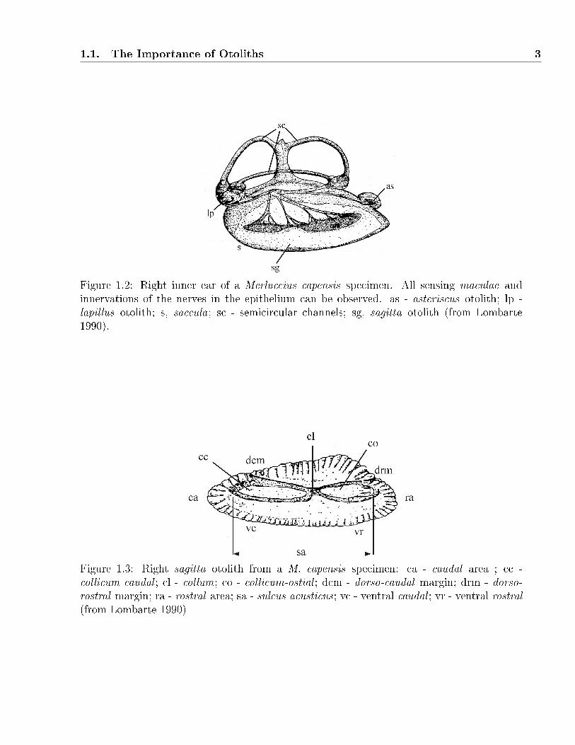
Otoliths are calci�ed structures located in the labyrinthic cavities of the inner ear of all
teleostean �sh (Blacker 1995, Norman and Greenwood 1975, Platt and Popper 1981). Each
ear contains a triplet: the sagitta, the asteriscus and the lapillus (Fig. 1.2) . The morphology
of the sagitae otolith is specially important for the study of taxonomic relationships between
species (Nolf 1985, Smale et al. 1995, Tuset et al. 2008). For this reason, a conventional
terminology exists to refer to its di�erent parts (Fig. 1.3) and its contour shape (Fig. 1.4)1.
The sensorial epithelium is joined to the sulcus acusticus, which is a cleft that crosses the
internal side of the otolith; the rostrum corresponds to the top frontal area, the left margin is
known as the caudal margin (or postrostrum); the dorsal area is the top part of the otolith;
and the ventral area is the bottom (Tuset et al. 2008).
More importantly is the fact that otoliths act as natural data loggers, recording infor-
mation of �sh life at di�erent rates related to their growth and environment (Kalish 1991,
Campana 1999). This information, which includes age and growth, movement patterns and
habitat interactions, can be interpreted in terms of ecology, demography or life history, and
has become of fundamental importance in �sh management and the protection of species.
1Although these de�nitions cover most of the otolith shapes, otoliths that do not �t exactly to theseforms include the word �to� between names to specify that the exact shape is intermediate between the twoforms. This notation is assumed in the results section.
1.1. The Importance of Otoliths 3
Figure 1.2: Right inner ear of a Merluccius capensis specimen. All sensing maculae andinnervations of the nerves in the epithelium can be observed. as - asteriscus otolith; lp -lapillus otolith; s, saccula; sc - semicircular channels; sg, sagitta otolith (from Lombarte1990).
Figure 1.3: Right sagitta otolith from a M. capensis specimen: ca - caudal area ; cc -collicum caudal ; cl - collum; co - collicum-ostial ; dcm - dorso-caudal margin; drm - dorso-rostral margin; ra - rostral area; sa - sulcus acusticus ; vc - ventral caudal ; vr - ventral rostral(from Lombarte 1990)
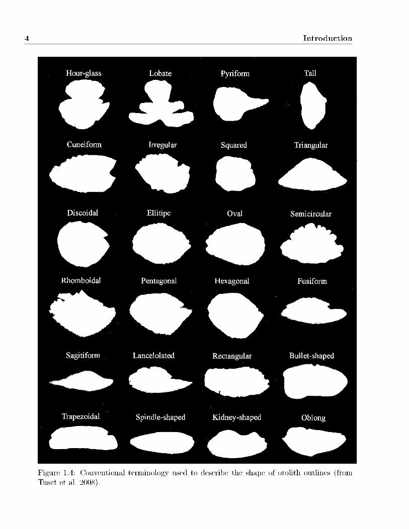
4 Introduction
Figure 1.4: Conventional terminology used to describe the shape of otolith outlines (fromTuset et al. 2008).

1.2. The Use of Otoliths in Marine Applications 5
1.2 The Use of Otoliths in Marine Applications
The �eld of otolith research and its applications to �sheries science has developed signi�cantly
in recent decades, to a great extent because of the technological advances in extracting in-
formation (Nolf 1985, Grant 1992, Secor et al. 1995a, Pan�li et al. 2002, Campana 2005).
Although applications have always been oriented to the sustainability of �sh stocks, very
frequently they are used to address a broad range of problems, ranging from the manage-
ment of �sheries to environmental change. These include, for example, the determination
of structures within population species (Blacker 1995, Norman and Greenwood 1975, Platt
and Popper 1981), inter-speci�c relationships between di�erent species in biology (Messieh
et al. 1989, Lombarte and Castellón 1991, Campana and Casselman 1993, DeVries et al.
2002, Cardinale et al. 2004, Poulet et al. 2004, Castonguay et al. 1991), the identi�cation
of species and fossils in paleontology (Slyke 1998, Carpenter et al. 2003), the assessment of
population dynamics (Dutil et al. 1999, Finstand 2003), or even the diet of predators (Fitch
and Lavenberg 1971, Cottrell et al. 1996, Beneditto et al. 2001).
1.2.1 Identi�cation of Fish Species
The exploitation of marine resources have long depended on inter-speci�c and intra-speci�c
studies (Wright et al. 2002). In these tasks, the correct identi�cation of species and popu-
lations (�sh from the same species inhabiting the same area, at a speci�c time and sharing
common morphological and genetic characteristics) is crucial in order to determine and es-
tablish not only how they should be managed, but also the �shing policy which should be
implemented.
In general, this can sometimes be achieved by using dynamic models, which must be
tuned appropriately. Several biological parameters are associated to the models (weight-size
relationship, growth, size at maturity and breeding periods, among others) and are used as
features in order to identify species correctly. However, in the particular case of cryptospecies ,
�shes which are morphologically similar but genetically di�erent, these parameters are insuf-
�cient and additional information from otoliths is necessary to avoid misclassi�cations that
can cause management errors.
Very often, this situation occurs when several species of the same genera share the in-
habiting area. For example, in the Merluccius genera (common hake), which is considered
a taxonomically complicated �sh group, the use of otoliths has been proved as highly spe-
ci�c and, therefore, adequate for the identi�cation of the di�erent hake groups in the world
(Mombeck 1970, Botha 1971, Lombarte and Castellón 1991, Torres et al. 2000a, Lloris et al.

6 Introduction
2005). For this reason, otoliths have acquired an important role in �sh identi�cation tasks
in recent decades (Tuset et al. 2010).
Although solutions based on taxonomic data are still used nowadays, in general it is
accepted that �nding an optimal set of otolith shape descriptors from the images, combined
with computer analytical tools, provides the best results (Bird et al. 1986, Cardinale et al.
2004, Parisi-Baradad et al. 2010). Nevertheless, the development of automatic tools that
allow the characterization of morphological di�erences may prove more interesting in order
to develop more reliable classi�cations. These characters should, in as far as it is possible, be
observable even for the species of the same genera whose irregularities are very cryptic and
di�cult to verify at a glance (Lloris et al. 2005).
Otolith structures serve to carry out identi�cation tasks, for many reasons: they have spe-
ci�c and population characteristics; they are easy to store and preserve (due to their reduced
size); and are available in many �shing institutions and centers for evaluation purposes. On
the other hand, a key challenge in the future is how to deal with the great variability existing
throughout populations and individual �sh growth to design more robust automatic tools.
1.2.2 Aging Applications
Another application of otoliths is related to the translucent and opaque rings that can be
observed in otolith sections (or on one side of the entire otolith in some �sh species). These
can be used to estimate both �sh age and growth during its life (Beamish 1979, Nolf 1985,
Gauldie 1994, Karlou-Riga 2000, Morita and Matsuishi 2001, Wilson and Neiland 2001,
Laidig et al. 2003). The process is very intuitive and consists of counting the potential rings
appearing on the surface of the otolith along its main radial (Fig. 1.5). This task is crucial
for the management of the seas as more than one million otoliths are read manually every
year in order to regulate �shing activities (Campana and Thorrold 2001, Morison et al. 2005).
In a more automated fashion, �sh age is best estimated by obtaining a one-dimensional
signal from the gray-scale image (Troadec 1991, Campana and Thorrold 2001, Morison et al.
2005). In this sense, computer aging methods address this problem from two di�erent per-
spectives: feature-based and �lter-based approach.
The �rst approach is very similar to that of �sh identi�cation explained above. After
obtaining the main signal of interest from the image (Fig. 1.6) and describing the feature
vector of interest, a classi�cation method is used to estimate the age class of the �sh. As
features from the intensity pro�le alone are not insu�cient to obtain good classi�cation
results, other general features from the �sh, such as size and weight, are introduced in the
classi�er. Morison et al. (1998) used a Neural Network to design a system based on reader

1.2. The Use of Otoliths in Marine Applications 7
Figure 1.5: Example of manual age estimation for a 5-year cod otolith (source: IBACSEuropean project).
Figure 1.6: Ring extraction example in feature-based methods. Sector selection and unfoldingare common processes for both groups of techniques (feature-based and �lter-based methods)and require manual implementation. An optimal contrast variation at the otolith border iscritical for estimating the age.
8 Introduction
experience information and Fourier descriptors. These limitations were demonstrated recently
in a study by Fablet and Josse (2005) who stressed the importance of treating age structures
beforehand.
The second approach deals with aspects of signal ampli�cation and noise cancellation,
among other quality issues of image and signal processing (Lagardère and Troadec 1997,
Welleman and Storbeck 1995, Troadec et al. 2000, Guillaud et al. 2002, Fablet 2006). The
goal is still to infer the �sh age but directly from the intensity pro�le, after removing the
irrelevant structures and compensating growth e�ects.
In general, aging experiments combine both techniques. In this sense, the most interesting
results were obtained by Fablet and Josse (2005) who correctly classi�ed almost 90% (in
terms of expert agreement) of plaice otoliths (Pleuronectes platessa ), ranging from 1 to 6-
year old �sh. These results were obtained by means of several processing tools, including:
image segmentation for canceling contrast; growth compensation techniques based on signal
demodulation; peak-based feature description methods combined with the cosinus transform;
and a Support-Vector-Machine classi�er (SVM). Although these results were satisfactory,
solutions for more complex species are aimed at eliminating discontinuity problems arising
from the ring pro�le and the poor contrast by means of statistical learning techniques (Fablet
2006).
The manual estimation of age from �sh otoliths has an annual cost of several million euros
at a European level, including the training and support from experienced age readers. Despite
this expenditure, only about 25% of the ICES (International Council for the Exploitation of
the Sea) stocks have low uncertainty (Campana and Thorrold 2001, Morison et al. 2005). As
such, the development of automatic tools that could improve the objectivity of the reader's
interpretation in the estimation of age would prove very useful (Reeves 2003).
1.3 On Pattern Recognition Systems
Taking into account all these problems, it is imperative the design of new standardized meth-
ods and software tools that assist in the interpretation of otolith data (Campana 2005). In
the �eld of image analysis and signal processing, the aim of feature extraction is to obtaining
short and useful descriptions from the data that can explain the cause of the problem at
hand.
This concept, often referred to as the dimensionality reduction problem, has intrigued
many scientists and several methods have been proposed. These methods, which share the
principle of function-cost maximization (or minimization), are generally used to guide the
automatic search of features. Feature extraction applications following this principle are
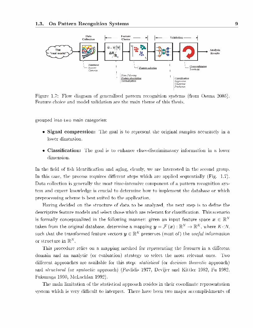
1.3. On Pattern Recognition Systems 9
Figure 1.7: Flow diagram of generalized pattern recognition systems (from Osuna 2005).Feature choice and model validation are the main theme of this thesis.
grouped into two main categories:
� Signal compression: The goal is to represent the original samples accurately in a
lower dimension.
� Classi�cation: The goal is to enhance class-discriminatory information in a lower
dimension.
In the �eld of �sh identi�cation and aging, clearly, we are interested in the second group.
In this case, the process requires di�erent steps which are applied sequentially (Fig. 1.7).
Data collection is generally the most time-intensive component of a pattern recognition sys-
tem and expert knowledge is crucial to determine how to implement the database or which
preprocessing scheme is best suited to the application.
Having decided on the structure of data to be analyzed, the next step is to de�ne the
descriptive feature models and select those which are relevant for classi�cation. This scenario
is formally conceptualized in the following manner: given an input feature space x ∈ RN
taken from the original database, determine a mapping y = F (x) : RN → RK , where K<N,
such that the transformed feature vectors y ∈ RK preserves (most of) the useful information
or structure in RN .
This procedure relies on a mapping method for representing the features in a di�erent
domain and an analytic (or evaluation) strategy to select the most relevant ones. Two
di�erent approaches are available for this step: statistical (or decision theoretic approach)
and structural (or syntactic approach) (Pavlidis 1977, Devijer and Kittler 1982, Fu 1982,
Fukunaga 1990, McLachlan 1992).
The main limitation of the statistical approach resides in their coordinate representation
system which is very di�cult to interpret. There have been two major accomplishments of
10 Introduction
this approach: the Karhumen-Loève Transform [also known as Principal Component Analysis
(PCA)] - most commonly used in signal compression applications (Jollife 1987); and the
Linear Discriminant Analysis (LDA) - which is best suited for classi�cation purposes (Fisher
1936).
Structural methods, on the other hand, are based on the philosophy of �analysis by syn-
thesis�. The philosophy underlying this approach is the existence of elementary and intuitive
building blocks that constitute the entire signals. For example, the Fourier Transform (FT)
describes the signals as a composition of di�erent sinusoids varying in terms of magnitude,
frequency and phase components (Cooley and Tukey 1965). Unlike statistical approaches,
the functionality of structural methods is purely descriptive, which means that no evaluation
of features is developed at all.
Although many description mechanisms base their operation on the estimation of fre-
quency content, very recently the use of methods determining the time-frequency components
have gain in popularity, and specially with the Wavelet transform (WT) (Mallat and Hwang
1992), which has led to the Best-Basis theory (Saito 1994, Saito and Coifman 1995).
Finally, the last stage of the pattern recognition process veri�es the selected models by
testing their e�ciency in the estimation of classes. This operation is supervised by means
of classi�ers, which must use representative data to obtain consistent results. This does
not represent a major problem provided that the number of samples is unlimited but very
often data collection is an arduous and expensive process. For this reason, more realistic
simulations use part of the data for con�guring the classi�er (the learning data set) and the
remaining samples to estimate its results (the validation data set).
A wide range classi�cation methods exists, and are grouped in two main categories:
Bayesian (or linear) classi�ers which estimate classes based on density functions and, and
non-linear classi�ers whose performance depends on the structured networks that are used to
estimate the class decision boundaries. Examples of the �rst group are LDA-based (Fisher
1936), Kernel or k -Nearest Neighbor (k -NN, Cover and Hart 1967) classi�ers, among others.
In the second group, the goal is to construct a network able to detect the class decision
boundaries (learning phase) and then use it to infer the classes (validation stage). Examples
of this approach are Classi�cation and Regression Trees (CART, Breiman et al. 1984), Neural
Networks (NN, Rosemblatt 1957) or Support Vector Machines (SVM, Boser et al. 1992,
Vapnik 1995), among others.
Learning Vector Quantization (LVQ, Kohonen et al. 1995), however, is in the middle of
both categories. It is also based on a blank network, but in the learning phase it uses the
original data to reproduce the true class distributions as faithfully as possible, whereas the
validation stage implements a linear classi�er (the k-NN approach). As such, it is possible to
1.4. Motivations and Scope of the Thesis 11
combine the advantages of both approaches in one single method.
1.4 Motivations and Scope of the Thesis
From a more physical perspective of the structures of signals, very often we are interested in
two main questions: what the physical di�erences in classes are and how signi�cant they are.
As mentioned above, there is no single method that provides relatively complete answers for
both questions. Either we decompose signals in known elementary structures or we evaluate
the separability of input data without knowing elementary structures. So the answer to the
previous questions often comes from the use of combined approaches.
This scenario has been addressed recently by the Best-Basis paradigm (Saito 1994, Saito
and Coifman 1995). This feature extraction philosophy consists of three main operations:
1) select an e�cient coordinate representation system of input data to solve the problem at
hand; 2) sort the coordinates by importance and discard the irrelevant ones; and �nally 3)
use the surviving coordinates to develop classi�cation tasks. The contention of this work is
that such a scenario is more �exible, and better suited towards this goal, than other classical
analytical methods only based exclusively on signal compositions of frequency components.
The Local Discriminant Bases algorithm (LDB), which belong to this approach, was
tested in the comparison of cod and hake otoliths, and for the extraction of age structures,
with promising results (Soria et al. 2008). However, its entropy-based criterion had a main
drawback. The use of the signal energy information is more suited to compression tasks
than those of classi�cation, so the measure may not provide useful information in certain
applications. A further re�nement improved this behavior by introducing an empirical es-
timation of feature densities using averaged shifted histograms (ASH) (Cocchi et al. 2001,
Saito et al. 2002), and more recently the Earth Mover's Distance algorithm (EMD) has been
proposed (Marchand and Saito 2012), but even with these improvements data generalization
still remains a problem.
In this sense, it would be preferable to develop discriminant measures of more general
behavior. By 'general behavior' we mean measurements speci�ed within boundaries which
monotonically increase with the separability of classes, ranging from zero (when features are
identical between classes) to one (if they are completely di�erent). This measure should be
independent of the description mechanism, as far as it is possible, in order to develop fully
automated feature extraction systems.
A new LDB algorithm is proposed in this thesis. This method includes three mechanisms,
all aimed at implementing the �rst two of the feature extraction process: a transformation
method for describing time-frequency atoms in signals (i.e. the discrete wavelet transform,

12 Introduction
DWT, or the Local cosinus/sinus transform, LCT/LST), a discriminant analysis based on
density distributions, and a feature selection algorithm. Its main advantage is a feature
evaluation system of measurements more consistent with the performance of linear classi�ers,
which makes it possible to select and to predict their classi�cation e�ciency before a classi�er
is used.
A main problem of PCA is that the covariance matrix is more oriented to compression
tasks rather than those of classi�cation. A similar inconsistency has been found with the
original LDB in the experiments of this work due to the fact that accumulating pairwise
measurements among several classes obscures the meaning of discrimination information,
and LDA does not have a comprehensive description of the signal components because or-
thogonality is lost within the description process.
In contrast, our density estimates are based on the use of histograms, which are evalu-
ated by means of normalized and bounded measurements, and a top-down search strategy
selects nodes within the space of tree-structured wavelets based on their most representative
coe�cients.
The main contributions have been restricted to the development of computer tools for
otolith-based �sh identi�cation experiments. The proposed tools are contrasted to other
standard tools used for the same purpose, and also to compare di�erent hake species in
real inter-speci�c and intra-speci�c experiments. The most signi�cant contributions lie on
the interpretation of irregularities: shape, time-frequency position, extension support and
degree of importance; which can be highlighted automatically on the same images or signals.
For this application, a new preprocessing tool of contour normalization is also proposed in
order to reduce the variance translation e�ects underlying the implementation of the discrete
wavelet transform.
Although aging applications are beyond the scope of this thesis, a new approach for com-
pensating the periodicity variation of age structures is presented. This variation is normally
caused by several natural phenomena, including environmental conditions of �sh habitat and
�sh genetics, among other factors (Morison et al. 1998, Troadec et al. 2000, Fablet et al.
2003). The developments in this case are based on the Von Bertanlan�y growth modulation
function (VBGF) (Beverton and Holt 1957).
Unlike the statistical approaches oriented to �nding global �sh group parameters, our
proposition tries to infer the growth of each single specimen. This strategy is justi�ed be-
cause the genetics are quite speci�c in single individuals, suggesting therefore a more speci�c
method that can cope with such singularities should be used.
The work developed in this thesis regarding this particular aspect is at an early stage.
However, it does suggests that to do this, the problem of separating image contrast and
1.5. Overview of this Document 13
demodulation operations must be dealt with �rst at the mechanical level of the image acqui-
sition.
Most of the developments included in this document have been supported and funded
by the AFORO3D project (Análisis de FORmas de Otolitos 3D, Ministerio de Economía y
Competitividad, CTM2010-19701) and the AFISA project from the European Union (Auto-
mated FISh Ageing, nº. 044132). In the latter case, some of the software tools and image
pattern recognition algorithms developed in this thesis have been integrated in the TNPC
software v4.0 from NOESIS (www.noesis.com).
1.5 Overview of this Document
The content has been divided into four main sections. The �rst section introduces current
otolith methodology commonly used in both �sh applications, the second one reviews feature
extraction methodology in general, the third describes our proposals and, �nally, the last
section illustrates results and discusses the existing limitations and improvements to be made
in future research.
A very general overview of otolith-based �sh identi�cation and aging applications, and
the pattern recognition steps have been presented in this chapter. Chapter 2 focuses on
the technical aspects of otolith preparations, conditioning, image acquisition and data pre-
processing. Certain de�nitions regarding manual aging precision errors will be necessary in
order to evaluate the performance of the proposed algorithms, and these de�nitions are also
provided in this chapter.
Chapter 3 reviews di�erent methods for constructing and analyzing feature models. Some
of them have been used with some success in otolith �sh applications problems, and others
are more common in image-audio applications, and their applicability to otoliths has yet to
be studied. Of course, the focus is on the Best-Basis paradigm, and in particular the LDB,
which is the object tool of our proposals, described in chapter 5.
The developed tool is calledDensity Local Discriminant Bases (DLDB) because of the new
way to represent the separability of class distributions. As this feature extraction mechanism
is expected to be equipped with better generalization capabilities than previous proposals,
we give a more formal de�nition of what 'generalization' means. The methods for the otolith
contour normalization and the demodulation of intensity pro�les are also presented in chapter
5.
Chapter 4 provides the basics of classi�ers, necessary in the validation of feature models
and discriminant measures. Former de�nitions for 'supervised learning' and the validation
stage are provided. Although not all the classi�cation methods can be covered, because there
14 Introduction
are too many, comparisons between linear and non-linear methodologies are made.
Experimental results are provided in chapter 6. The �rst experiment, shows the ad-
vantages of the DLDB compared to standard tools used in the �eld of otolith-based �sh
identi�cation. In particular, its ability for detecting and explaining signal irregularities and
its consistency with identi�cation results are proved. A further experiment uses DLDB to
compare the morphological otolith di�erences of Merluccius species. Conclusions about the
biological di�erences between hake species are provided. The chapter �nishes with the re-
sults on aging. The demodulation ability of our preprocessing tool is demonstrated and age
estimation results for plaice otoliths (Pleuronectes platessa) are discussed.
Of course, there are always limitations to every methodology and the proposals of this
work are no exception. The last chapter outlines some issues to be addressed in the future.
A possible improvement of DLDB is proposed and formalized, but the software still has to
be implemented.
Chapter 2
Acquisition of Otolith Data
2.1 Introduction
This chapter deals with the more technical operations involving the �rst and second stage
(see Fig. 1.7), and corresponds to the preparation of otoliths, their mechanical operations,
image acquisition techniques, segmentation algorithms and preprocessing techniques. All
them are intended to generate useful otolith digital data for its analysis.
While these operations are standard procedures well accepted today in this �eld, in the
case of aging our proposals will be purely experimental (see chapter 5). In general, the
identi�cation of �sh species lies in the use of otolith contour data, which is much easier to
obtain than the gray-scale data of aging applications.
In �sh identi�cation, an image with a nearly constant background is su�cient to ex-
tract contour points in favorable conditions, while in aging applications the chemicals used
for the preparation of otoliths, light conditions and the con�guration of the camera, which
conditionate the image quality, play an important role in the calculation of intensity pro�les.
These issues are considered in section 2.2. In addition to the factors already mentioned,
the discussion includes considerations on the conservation of otoliths and the manual valida-
tion of age readings. The latter is necessary to evaluate the performance quality of automatic
aging tools. Sections 2.3 and 2.4 are more concerned with the digitization of contour data
points and gray-scale one-dimensional intensity pro�les.
For the extraction of the contour points, any standard segmentation method may be
valid since light conditions are not too restrictive. Contour information also serve to delimit
the enclosing area age structures will be extracted from. Two preprocessing operations are
necessary to extract the intensity pro�le: 1) the detection of the otolith nucleus and, 2) the
preprocessing of translucent and opaque rings to obtain the one-dimensional signal. The �rst
15
16 Acquisition of Otolith Data
issue has been addressed successfully by Cao and Fablet (2006) with an algorithm that has
proved to be quite robust. The second issue, however, is currently under research. The work
developed by Fablet and Josse (2005) for plaice otoliths constitutes the main starting point
of our proposals.
Finally, section 2.5 summarizes the relevant points and looks at the present limitations
and future challenges of current experimental work.
2.2 Basic Otolith Preparation
2.2.1 Direct Observation
While otoliths can be observed directly in their original state with a simple optical mag-
ni�cation device, the development of analytical tasks based on computer-assisted imaging
techniques require certain preparations.
In general, otoliths are typically observed directly or immersed in a liquid observation
medium, con�guring proper lighting conditions, and using a low-power binocular microscope
with an embedded camera. When the full otolith is used, it is immersed in water, alcohol
or oil; and observed with either transmitted-light or re�ected-light techniques. The oil helps
to highlight the structures from the otolith surface and avoids re�ected glare. Historically,
these oils have included clove oil, �baby oil� or creosete, though the latter is no longer used.
It is also important to use a cold light source to prevent the evaporation of oil during the
observation.
This procedure is su�ce even for counting the rings from sagittae of �at�sh and certain
pelagic species, since their otoliths do not require sectioning.
2.2.2 Embedding for Incident-light Observations
Despite the simplicity of direct observation, otoliths are also elements included in a wide
range of databases and must be properly stored to prevent them from deteriorating, and to
ensure that any sectioning, grinding and/or polishing can be carried out safely at a later
date.
The operations necessary for their conservation form part of a process commonly referred
to as 'embedding'. This process can be complex and expensive, and requires of di�erent
laboratory tools and materials which need to be maintained in good working order. For
example, the resins required to immerse the otoliths, become opaque as they deteriorate and
so must be stored in cool dark places. Table 2.1 summarizes the principal embedding media
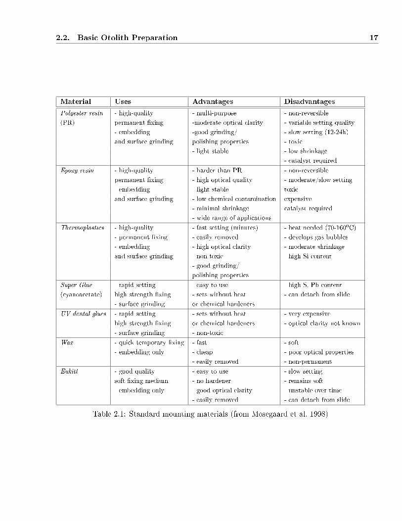
2.2. Basic Otolith Preparation 17
Material Uses Advantages Disadvantages
Polyester resin - high-quality - multi-purpose - non-reversible
(PR) permanent �xing -moderate optical clarity - variable setting quality
- embedding -good grinding/ - slow setting (12-24h)
and surface grinding polishing properties - toxic
- light stable - low shrinkage
- catalyst required
Epoxy resin - high-quality - harder than PR - non-reversible
permanent �xing - high optical quality - moderate/slow setting
- embedding - light stable toxic
and surface grinding - low chemical contamination expensive
- minimal shrinkage catalyst required
- wide range of applications
Thermoplastics - high-quality - fast setting (minutes) - heat needed (70-160ºC)
- permanent �xing - easily removed - develops gas bubbles
- embedding - high optical clarity - moderate shrinkage
and surface grinding - non-toxic - high Si content
- good grinding/
polishing properties
Super Glue - rapid setting - easy to use - high S, Pb content
(cyanoacetate) high strength �xing - sets without heat - can detach from slide
- surface grinding or chemical hardeners
UV dental glues - rapid setting - sets without heat - very expensive
high strength �xing or chemical hardeners - optical clarity not known
- surface grinding - non-toxic
Wax - quick temporary �xing - fast - soft
- embedding only - cheap - poor optical properties
- easily removed - non-permanent
Eukitt - good quality - easy to use - slow setting
soft �xing medium - no hardener - remains soft
- embedding only - good optical clarity - unstable over time
- easily removed - can detach from slide
Table 2.1: Standard mounting materials (from Mosegaard et al. 1998)

18 Acquisition of Otolith Data
Figure 2.1: Preparation of the catalyst. The volume required depends on the full amount of
polyester resin required according to Table 2.2 (from McCurdy et al. 2002)
Resin Resin Number of drops of catalystvolume (ml) weight (g) 1% mixture 2% mixture
91.0 ∼100 20 4045.5 ∼50 10 2023.3 ∼25 5 1011.5 ∼12.5 2.5 59.1 ∼10 2 4
Table 2.2: Simple dosage of polyester resin (in volume and/or weight) and catalyst (in drops)depending on their ratio. The greater the quantity of catalyst the higher the speed of setting(from Mosegaard et al. 1998)
and their applicability. The most frequently used resins are the hard and irreversible synthetic
ones (polyester, epoxy, etc). In general, the embedding operation proceeds as follows:
The �rst operation consists in the polymerization of the polyester by mixing the polyester
with 1-2% of catalyst (i.e. 25g of polyester resin and 0.2g of catalyst, Fig. 2.1). Table 2.2
provides some information on the proportions of quantities to be mixed, depending on this
ratio. Traditionally, the resin was dissolved in syrene, and the catalyst used an accelerator to
reduce the hardening time. However, as there is risk of explosion, current resins are supplied
pre-accelerated.
All the media with the catalyst should be mixed carefully in order to prevent bubbles
forming in the mixture, as they complicate the observation of calci�ed structures. The
mixture is then left to rest for a period of time to allow the biggest bubbles to burst. The
hardening time varies from a few seconds (Super Glue or UV dental glue) to a few hours
(epoxy or polyester) depending on the media used. A dry oven is often used to complete the

2.2. Basic Otolith Preparation 19
polymerization process and ensure the mixture has turned into gel. The polymerization of
polyester requires at least 24h in a dry oven (around 30ºC) for optimum results.
Resins can be colored by adding a pigment, generally black, or they can be purchased pre-
colored. When otoliths are embedded for posterior observation a high-transparency polyester
resin is normally used. Resins and catalysts are often known as 'hardeners' and are available,
along with mounting kits, from specialist suppliers.
When the polymerization is completed, the next step is to place the calci�ed structures in
cylindrical cavities on black plastic slides. Black slides provide better contrast for observations
of annuli in the case of age estimation. The slides are 65mm x 60mm in size, cut from 3mm-
thick PerspexTM sheet, and are normally machined in grids of 25 �at-bottomed cavities,
each 7mm in diameter and approximately 1.2mm deep. This provides su�cient room for a
reference number to be engraved on each slide with a hardened steel stylus or an electric
engraving tool.
Entire otoliths are positioned in the cavities on the plastic slide in pairs, with the sulcus
acusticus facing downwards and, therefore, not visible (Fig. 2.2a). Occasionally, small
otoliths acquire static electrical charges, making it more di�cult to position them in the
cavities. These problems can be resolved by increasing the humidity of the atmosphere or
changing the type of clothing worn during the placement operation.
A plastic pipette is used to drop the catalyzed clear resin into the cavities, covering the
otoliths and ensuring that the �oating ones are not re-positioned (Fig. 2.2b). The catalyzed
resin is dropped between otolith pairs to form a single layer of resin that completely covers
all otoliths on the slide. A custom-sized glass microscope cover slip is then �oated over the
resin (Fig. 2.2c) and left in the fume cabinet until completely set (Fig. 2.2d). Cover slips
generally deform above the cavities and may crack as the thicker layer of resin contracts
further on hardening. The resin will set �rmly within a few hours, but observations must not
begin until the resin has set and there is no risk of styrene being absorbed through the skin.
PerspexTM is expensive and a number of alternative plastics that bond equally well with
hardening resin are currently used, and injection-molded slides with embossed numbers are
commercially available at cheaper prices. When using machined slides, the plastic must be
hard enough and the drill su�ciently sharp to ensure the base of each pit is smooth and
level. If this is not done, thin patches of partial vacuum may form between the hardened
resin making it di�cult to observe calci�ed structures,since they will have the silvered e�ect
of a mirror.
These operations ensure that the otolith can be stored safely and used in future obser-
vations and is also valid for very small calci�ed structures, including many �at�sh species
(except the thicker otoliths) whose ring structures can be observed without the need of sec-

20 Acquisition of Otolith Data
Figure 2.2: Example of otolith embedding in an elastomer mould. a) A polymerized resinlayer (yellow arrow) is run on the bottom of each location before the otolith is deposited onthe bottom. b) The otolith is oriented and embedded in a second layer. c) It should be madesure that the resin �lls the mould completely. In this case the resin does not reach the edgeso that it can be turned over to drive out the air bubbles. d) Otolith de�nitively embedded(red arrow) (from McCurdy et al. 2002)
tioning operations (Parrish and Sharman 1959, Watson 1965). In such case, the operations
and materials di�er considerably from those presented in this section. The reader is referred
to McCurdy et al. (2002) for the details.
2.2.3 Manual Validation of Age Readings
Since age information forms the basis of most in�uential biological variables (growth rates,
�sh stocks, mortality and also �sheries productivity, among others) a variety of methods
exists through which manual age interpretations can be validated. These methods can be
classi�ed as either validating absolute age, validating the periodicity of growth increments or
of corroborating an existing set of age estimates.
Generally speaking, two types of errors can occur when �sh age is manually estimated: 1)
errors that a�ect accuracy of age readings, or closeness to the age estimate of the true value,
and 2) errors that a�ect the precision or the reproducibility of repeated measurements on a
2.2. Basic Otolith Preparation 21
given structure by the reader.
The �rst type is more associated to the limitations of the processes and techniques used
in the detection of ring structures, given that not all of them belong to the growth sequence
of the �sh. Thus, it is a deterministic error that the expert can reduce, or even eliminate, by
using the most appropriate validation method in each situation. In general, their goal is to
validate age structures, either by the assessment of the true absolute age, the periodicity of
growth increments.
In this sense, known-age-release (Tuskamoto and Kajihara 1987, Quinn et al. 1991, Cam-
pana 1999, Secor et al. 1995b), bomb radiocarbon (Kalish 1993, 1995a,b, Campana and Jones
1998) or radio-chemical dating (Bennett et al. 1982, Campana et al. 1990, Burton et al. 1999)
are very used in the �rst case; whereas mark-recapture of chemically-tagged �sh (Ge�en 1982,
Oliveira 1996, Natanson et al. 2002), discrete length modes (Morales-Nin 1989, Hanchet and
Uozumi 1996, Natanson et al. 2002), natural and data-speci�c markers (Blacker 1995, Cam-
pana and Neilson 1985, Wilson and McCormick 1997) and marginal increment analysis (MIA)
(Hyndres et al. 1992, Morales-Nin et al. 1998a, Carlson et al. 1999) are well known in the
second case.
Very brie�y, the idea of known-age-release is to know the absolute age of recaptured �sh
by calculating the incremental di�erence in relation to the time of release. This technique is
very used in juvenile specimens, as the exact age is determined without error whereas bomb
radiocarbon, although very expensive, is preferred for the older specimens because of their
lower recapture rates. Alternatively, mark-recapture of chemically-tagged �sh is best for
validating the periodicity of growth increments. The method is based on rapid incorporation
of calcium-binding chemicals, which are applied at the time of tagging into bones, scales
and otoliths. The result is a permanent and visible mark under �uorescent light at the
time of tagging which serve as a reference for determining posterior daily and annual growth
increments (Natanson et al. 2002). The reader is referred to Campana (2001) for an extended
summary of manual age validation techniques.
Precision errors, on the other hand, are associated with the reader subjectivity at the
time of counting and interpreting growth increments, and they can be biased or random
depending on whether the factors associated to the reader occur frequently or sporadically.
A common way to estimate this error is that several readers develop repeated age estimations
of the same specimen.
The average percent error (APE ) has been the traditional index for this measure. How-
ever, since many authors pointed out its inadequacy (Beamish and Fournier 1981, Chang
1982, Campana et al. 1979), and subsequently Beamish and Fournier (1981) introduced a
modi�cation, de�ned as
22 Acquisition of Otolith Data
APE =100
n×
n∑j=1
[1
r
r∑i=1
(|tij − tj|
tj
)], (2.1)
where tij corresponds to the i -th age determination of the j -th �sh for a total of n �shes,
tj is the mean age estimate of the j -th �sh, and r is the number of times each �sh is read
by di�erent readers. Chang (1982) suggested substituting the absolute deviation by the
standard deviation from the mean age. So the resulting equation produces an estimate of
the coe�cient variation (CV ), expressed as:
CVj =
√∑ri=1
(tij−tj)r−1
2
tj, (2.2)
where CVj is the age precision estimate for the j -th �sh. The index of precision D is similar
to CV but calculated as
D =100
n×
n∑j=1
CVj√r. (2.3)
In general, the design process of computer-based aging tools are mainly concerned with
accuracy errors. As in the manual case, results have to be provided in terms of the reader's
precision, since supervised classi�ers also require knowing class information to be properly
con�gured (Campana 2001).
For example, assume that the accuracy of classi�cation experiment is 88% in relation to
an inter-expert agreement of 95%. The expected success will be 83.6% taking into account
both �gures as part of the process of age estimation.
2.2.4 Image Quality Issues
Although images must meet a minimum quality for the relevant structures to be represented
optimally with digital data, their memory size do not need to large, since the control of
environmental under an homogeneous black background allow gray-scale colour images to be
used.
In practice, a minimum resolution of 640x480 pixels using gray-scale su�ces for both
tasks. The speci�cation of contrast, however, acquires a critical role in automatic aging, as
this parameter needs to be optimally con�gured in several ways for di�erent images not only
to highlight potential rings belonging to �sh age but also to ensure that the irrelevant rings
are removed.
Images can be obtained by using either transmitted or re�ected light (Fig. 2.3). In the
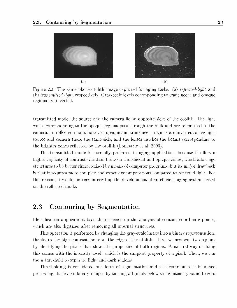
2.3. Contouring by Segmentation 23
(a) (b)
Figure 2.3: The same plaice otolith image captured for aging tasks. (a) re�ected-light and(b) transmitted-light, respectively. Gray-scale levels corresponding to translucent and opaqueregions are inverted.
transmitted mode, the source and the camera lie on opposite sides of the otolith. The light
waves corresponding to the opaque regions pass through the bulk and are re-emitted to the
camera. In re�ected mode, however, opaque and translucent regions are inverted, since light
source and camera share the same side, and the lenses catches the beams corresponding to
the brighter zones re�ected by the otolith (Lombarte et al. 2006).
The transmitted mode is normally preferred in aging applications because it o�ers a
higher capacity of contrast variation between translucent and opaque zones, which allow age
structures to be better characterized by means of computer programs, but its major drawback
is that it requires more complex and expensive preparations compared to re�ected light. For
this reason, it would be very interesting the development of an e�cient aging system based
on the re�ected mode.
2.3 Contouring by Segmentation
Identi�cation applications base their success on the analysis of contour coordinate points,
which are also digitized after removing all internal structures.
This operation is performed by changing the gray-scale image into a binary representation,
thanks to the high contrast found at the edge of the otolith. Here, we segment two regions
by identifying the pixels that share the properties of both regions. A natural way of doing
this comes with the intensity level, which is the simplest property of a pixel. Then, we can
use a threshold to separate light and dark regions.
Thresholding is considered one form of segmentation and is a common task in image
processing. It creates binary images by turning all pixels below some intensity value to zero
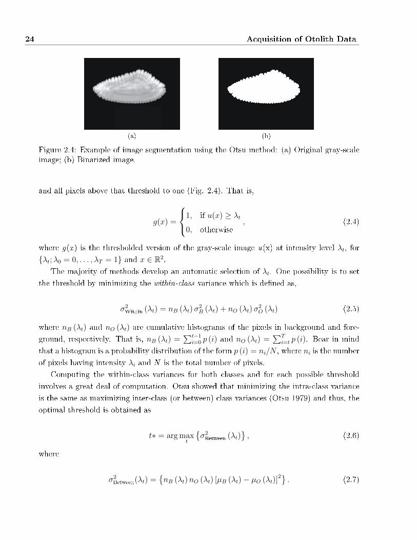
24 Acquisition of Otolith Data
(a) (b)
Figure 2.4: Example of image segmentation using the Otsu method: (a) Original gray-scaleimage; (b) Binarized image.
and all pixels above that threshold to one (Fig. 2.4). That is,
g(x) =
1, if u(x) ≥ λt
0, otherwise, (2.4)
where g(x ) is the thresholded version of the gray-scale image u(x) at intensity level λt, for
{λt;λ0 = 0, . . . , λT = 1} and x ∈ R2.
The majority of methods develop an automatic selection of λt. One possibility is to set
the threshold by minimizing the within-class variance which is de�ned as,
σ2Within
(λt) = nB (λt)σ2B (λt) + nO (λt)σ
2O (λt) (2.5)
where nB (λt) and nO (λt) are cumulative histograms of the pixels in background and fore-
ground, respectively. That is, nB (λt) =∑t−1
i=0 p (i) and nO (λt) =∑T
i=t p (i). Bear in mind
that a histogram is a probability distribution of the form p (i) = ni/N , where ni is the number
of pixels having intensity λi and N is the total number of pixels.
Computing the within-class variances for both classes and for each possible threshold
involves a great deal of computation. Otsu showed that minimizing the intra-class variance
is the same as maximizing inter-class (or between) class variances (Otsu 1979) and thus, the
optimal threshold is obtained as
t∗ = arg maxt
{σ2Between
(λt)}, (2.6)
where
σ2Between
(λt) ={nB (λt)nO (λt) [µB (λt)− µO (λt)]
2} . (2.7)
2.4. Extracting Age Signals 25
Here,µB(λt) and µO(λt) are the cluster means. So, for each potential threshold, λt, we
separate the pixels into two clusters, calculate their means, square the di�erences between
means and multiply by the number of pixels in one cluster times the number in the other.
Note that the calculations are dependent as we change from one threshold to another, since
all the quantities can be updated by simple recurrence relations as pixels move from one
cluster to another. That is,
nB (λt+1) = nB (λt) + nt, nO(λt+1) = nO (λt)− nt (2.8)
µB(λt+1) =µB (λt)nB (λt) + ntλt
nB (λt+1), µO (λt+1) =
µO (λt)nO (λt)− ntλtnO (λt+1)
, (2.9)
where nt is the proportion of pixels with intensity level T.
After image binarization, the contour silhouette is characterized by the coordinate points
at precisely the border of both regions. These points must change into a relative reference
axis, so the otolith center is estimated averaging the values in both coordinate axis. Let
{x (n) , y (n)} denote coordinate points for n ∈ (0, . . . , N − 1), that is µx = 1N
∑N−1n=0 x (n)
and µy = 1N
∑N−1n=0 y (n). Then, the otolith radials are calculated as,
ρ (n) =
√(x (n)− µx)2 + (y (n)− µy)2. (2.10)
In practice, when di�erent otolith pictures are processed with this framework, data will
not share the same properties of size, image orientation and starting point of contour samples.
This situation arises because such conditions are very di�cult to control mechanically during
the acquisition of images. As such, a preprocessing method of contour standardization, prior
to feature extraction, will be necessary.
2.4 Extracting Age Signals
It was pointed out in subsection 2.2.4 that the environmental conditions in which otoliths are
photographed play an important role in the detection of age. Light re�ection, otolith position
or alignment may cause some parts to be brighter (in the light) and opaque (in shadow) in
ways that have nothing to do with the real objects in the image and, therefore, may produce
signals with useless structures.
When this situation is controlled and the ring structures are well captured in the image,
the extraction of intensity pro�les comprises three main steps: 1) the determination of the
26 Acquisition of Otolith Data
otolith center from the image (also known as the nucleus); 2) the calculation of the gray-
scale values along the radials; and 3) the preprocessing of growth information in order to
demodulate the periodic age structures of this signal (Morales-Nin et al. 1998b).
2.4.1 Nucleus Detection
The automatic detection of the nucleus was �rst considered in Wellman and Storbeck (1995),
where looking for the darkest point centered on a prede�ned area of the image was pro-
posed. This simple approach was not as robust as expected and, later, Guillaud et al. (2002)
developed a detection method based on the use of agent systems. Here, the center was cal-
culated as a byproduct of the extraction of two-dimensional rings. Although interesting, the
con�guration of agents involved a very complex parametrization for it to work appropriately.
Recently, this issue has received thorough attention from Cao and Fablet (2006) in a
method that has proved very robust for transmitted light mode. This approach addresses
nucleus detection from the perspective of topographic maps, which provide an appropriate
framework for describing otolith structures at di�erent gray levels (Monasse and Guichard
2000).
Let u be a gray level image. An upper gray level, set at value l, is characterized by the
set of pixels,
Xλ(u) ={x ∈ R2, u(x) ≥ l
}. (2.11)
A topographic map is then de�ned as the collection of all image sets of di�erent levels up to
an increasing contrast change. Each level contains the interior part of all connected points
that form a shape, and the superior shapes are those that come from higher levels (Caselles
et al. 1999). With this de�nition in mind, the nucleus is then detected as an elliptical shape
of a dark region, not too eccentric, close to the semi-major axis of the otolith. Fig. 2.5
illustrates the main steps that select the optimal nucleus. This is a two-pass �ow which
eliminates structures sequentially until the �nal nucleus candidate is estimated.
2.4.1.1 Maxima Removal and Grain Filtering
Let S0 be the otolith itself extracted as the largest shape in the image and let E0 be the set
containing all the shapes included in S0. Also, let E1 denote the set of potential candidate
shapes for the nucleus in E0. These exclude all the bright shapes and the localized dark
shapes of a very small area. Of course, this is rather strict, since spurious noise creates many
of them.
Therefore, a grain �lter (Vincent 1993, Monasse and Guichard 2000) is used to ensure
that the dark region enclosing the nucleus is not eliminated, before the elimination of bright
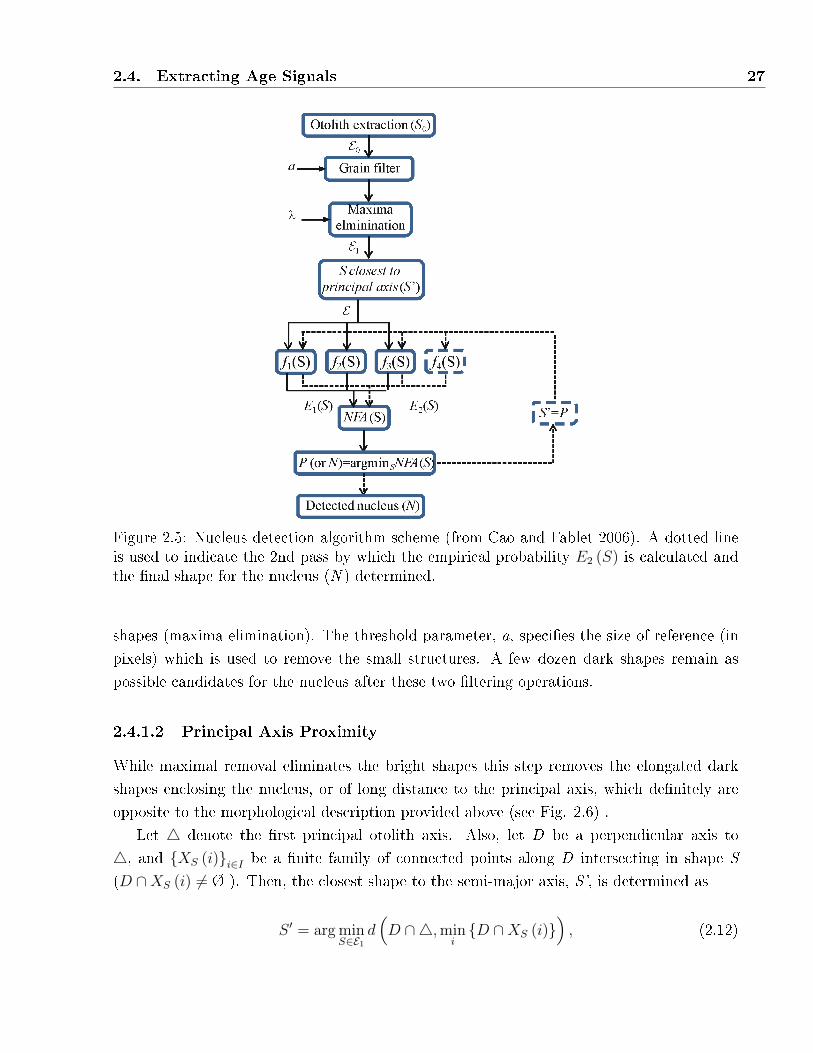
2.4. Extracting Age Signals 27
Figure 2.5: Nucleus detection algorithm scheme (from Cao and Fablet 2006). A dotted lineis used to indicate the 2nd pass by which the empirical probability E2 (S) is calculated andthe �nal shape for the nucleus (N ) determined.
shapes (maxima elimination). The threshold parameter, a, speci�es the size of reference (in
pixels) which is used to remove the small structures. A few dozen dark shapes remain as
possible candidates for the nucleus after these two �ltering operations.
2.4.1.2 Principal Axis Proximity
While maximal removal eliminates the bright shapes this step removes the elongated dark
shapes enclosing the nucleus, or of long distance to the principal axis, which de�nitely are
opposite to the morphological description provided above (see Fig. 2.6) .
Let 4 denote the �rst principal otolith axis. Also, let D be a perpendicular axis to
4, and {XS (i)}i∈I be a �nite family of connected points along D intersecting in shape S
(D ∩XS (i) 6= Ø ). Then, the closest shape to the semi-major axis, S', is determined as
S ′ = arg minS∈E1
d(D ∩4,min
i{D ∩XS (i)}
), (2.12)

28 Acquisition of Otolith Data
Figure 2.6: Proximity to principal axis (from Cao and Fablet 2006). The black-�lled shapeis in E since in any direction orthogonal to 4, it is contained in the shape closest to 4 (thewhite one). For the same reason, the white shape belongs to E . On the contrary, one can�nd a normal to 4 such that the gray-�lled shape is not closest to 4 (since the white iscloser). Therefore, it does not belong to E .
where d(A,B) denotes Euclidean distance between points A and B. The connected points
belonging to this shape will then establish the boundaries that will enclose potential candidate
shapes for the nucleus .Let E be the set containing all the shapes included within these
boundaries.
De�nition. 2.1 S ∈ E if S ∈ E1 and if for any axis D, perpendicular to 4 such that
D ∩ XS (i) 6= Ø, then there exists S ′ ∈ E1 such that S' has minimal distance to 4 on D
among the shapes of E1 and S ⊂ S ′.
The interpretation of this de�nition is very simple. Basically, if we start from4 and move
along its normal, then the �rst dark shape we encounter must contain potential candidates
for the nucleus.
2.4.1.3 Geometrical Statistical Selection
The last operation consists of selecting the most probable candidate shape for the nucleus. For
this purpose a geometrical evaluation of the remaining shapes is developed. These geometrical
properties are represented by means of three functions (fi; i = 1, . . . 3). They are 1) the area,
de�ned as
f1 (S) = |S| , (2.13)
2) the proximity of S to 4 which is measured relatively to the shape size
f2 (S) =|S|
maxi d (XS (i) , D ∩4)2 , (2.14)

2.4. Extracting Age Signals 29
and, �nally, 3) the �atness
f3 (S) =|S|
L (S,4⊥)2 , (2.15)
where L(S,4⊥
)corresponds to the diameter of the projection of S on the orthogonal direc-
tion of 4.According to Cao and Fablet (2006) a good nucleus should yield large values of fi. How-
ever, in order to avoid the use of thresholds for the fi, which may make the algorithms
numerically too sensitive, instead they develop a contrario hypothesis that the fi are statis-
tically independent. This idea is based upon the fact that size, proximity and �atness have
a common cause in any shape except for the nucleus, since generally otoliths grow outwards
in any direction from the nucleus.
In statistical theory, this is equivalent to testing the hypothesis H0, in the event that
�the fi are independent�, and then making decisions according to the 'null H0' assumption
(otherwise, verifying H1, �the fi are not independent�, would require a good otolith model
which is not easy to compute). A natural way to detect this violation of independence is
to use the shape values of the previous geometrical functions as thresholds to determine the
expectation of the event fi ≥ fi (S). Let Fi denote this value which is represented by the
empirical inverse repartition function of fi:
Fi (λ) =# {fi ≥ λ}
# {E}, (2.16)
where i ∈ [1, 3) and # denotes cardinality. Also, let
E1 (S) =(
maxiFi (fi (S))
)3
(2.17)
de�ne the empirical probability to observe the event fi ≥ fi (S) under the a contrario inde-
pendence hypothesis, computed for each shape S ∈ E . The best nucleus candidate will thenbe obtained as the least probable under this independence assumption, but we will need to
be sure that this probability is signi�cantly small. One possible way to address this matter
consists of calculating the 'number of false alarms' (NFA) of each S, which is de�ned as
NFA (S) = # {E}E1 (S) . (2.18)
Thus, a shape is said to be ε −meaningful if NFA (S) < ε, where ε is an error threshold
representing the expected number of shapes permitted outside the a contrario hypothesis.
Indeed, Cao and Fablet (2006) proved that the expectation of the number of ε−meaningful
30 Acquisition of Otolith Data
shapes in the independence model is always smaller than ε. As a consequence, a good strategy
is to set ε < 1 and check the condition NFA (N) < ε.
Now, we are able to provide a formal de�nition for the nucleus:
De�nition. 2.2 Let S be a candidate shape among all candidates in E, S ∈ E for the nucleus
P. This shape is said to be ε−meaningful if, and only if,
P = arg minS∈E
NFA (S) , (2.19)
provided that the condition NFA (S) < ε holds, for ε < 1.
In practice, however, there will be more shapes that meet these speci�cations of nucleus,
so an additional step is developed using the detected shape in (2.19) to re�ne the previous
prediction P of the nucleus. This re�nement assumes that the otolith grows asymmetrically
and the distribution of the nucleus position obtained from all selected shapes is clearly uni-
modal.
Therefore, an additional feature is introduced as a second pass of the a contrario frame-
work to select a more precise nucleus. This feature evaluates the distance between the center
of the candidate region and that of the predicted nucleus in the �rst pass
f4 (S) = −‖C (S)− C (P )‖ (2.20)
where C (·) denote center position calculated as the median value of the coordinate points of
S and P, respectively. However, since the horizontal orientation of the otolith is unknown
the preferred calculation is given by
f4 (S) = −min (‖C (SL)− C (PL)‖ , ‖C (SR)− C (PR)‖) (2.21)
where the index, L and R, denote position towards the left and right frame of the principal
axis, respectively. Thus, in this second pass the empirical probability of the a contrario
hypothesis of independence is calculated as
E2 (S) =
(maxi=1,3,4
Fi (fi (S))
)3
(2.22)
and used in 2.18 and 2.19 to determine the nucleus, N. Note that the independence criterion
is not considered for all i ∈ [1, 4), given that f2 and f4 are obviously dependent. On the
other hand, the independence between f1, f3 and f4 is more reasonable in the a contrario
detection approach.
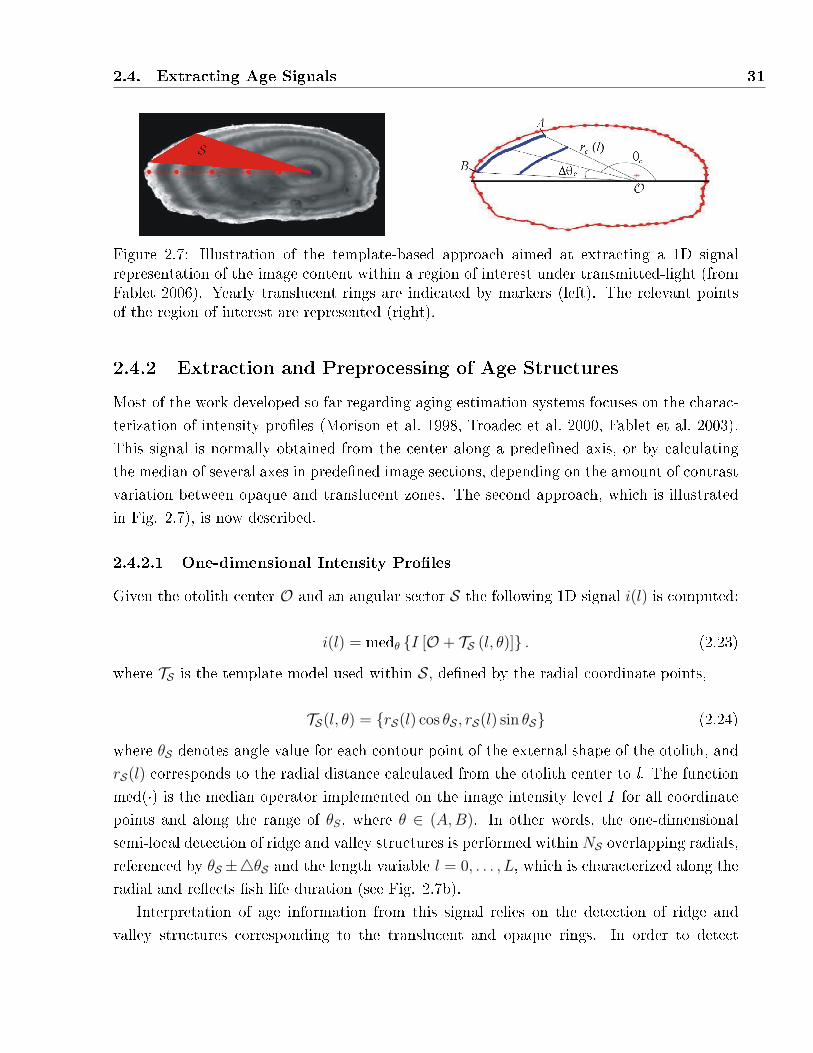
2.4. Extracting Age Signals 31
Figure 2.7: Illustration of the template-based approach aimed at extracting a 1D signalrepresentation of the image content within a region of interest under transmitted-light (fromFablet 2006). Yearly translucent rings are indicated by markers (left). The relevant pointsof the region of interest are represented (right).
2.4.2 Extraction and Preprocessing of Age Structures
Most of the work developed so far regarding aging estimation systems focuses on the charac-
terization of intensity pro�les (Morison et al. 1998, Troadec et al. 2000, Fablet et al. 2003).
This signal is normally obtained from the center along a prede�ned axis, or by calculating
the median of several axes in prede�ned image sections, depending on the amount of contrast
variation between opaque and translucent zones. The second approach, which is illustrated
in Fig. 2.7), is now described.
2.4.2.1 One-dimensional Intensity Pro�les
Given the otolith center O and an angular sector S the following 1D signal i(l) is computed:
i(l) = medθ {I [O + TS (l, θ)]} . (2.23)
where TS is the template model used within S, de�ned by the radial coordinate points,
TS(l, θ) = {rS(l) cos θS , rS(l) sin θS} (2.24)
where θS denotes angle value for each contour point of the external shape of the otolith, and
rS(l) corresponds to the radial distance calculated from the otolith center to l. The function
med(·) is the median operator implemented on the image intensity level I for all coordinate
points and along the range of θS, where θ ∈ (A,B). In other words, the one-dimensional
semi-local detection of ridge and valley structures is performed within NS overlapping radials,
referenced by θS±4θS and the length variable l = 0, . . . , L, which is characterized along the
radial and re�ects �sh life duration (see Fig. 2.7b).
Interpretation of age information from this signal relies on the detection of ridge and
valley structures corresponding to the translucent and opaque rings. In order to detect
32 Acquisition of Otolith Data
these structures within S, one needs to extract the meaningful extrema of i. In general this
is accomplished by determining the zero-crossings of derivative of i, but as otolith growth
decays with �sh age and the gray-scale intensity values are not stationary in terms of o�set, it
is necessary to adapt the periodicity at which age structures appear along the radial length,
and to �lter out the contrast variation.
2.4.2.2 Supervised Growth Demodulation (SGD)
Demodulation operations are carried out by means of a prototype model representing the �sh
growth, whose parameters should be tuned appropriately to obtain periodic representations
of age structures (Fablet and Josse 2005). In the supervised (or manual) mode, this process
is based on the use of known otolith age data, previously obtained by an expert.
Let i (l) = {i (l [0]) , . . . , i (l [N − 1])} ∈ RN be the growth-modulated intensity vector
at hand, computed from the previous template-based approach. Here, the length variable
l ∈ [0, L∞) has a total number of N samples and a regular grid, with l [N − 1] = L∞ being
the full length of the radial. So, the signal is also de�ned as in = {i0, . . . , iN−1} ; n ∈ Z.The main consideration underlying this scheme is that the growth is a monotonically
increasing function, l = v (t), whose rate decays with the time variable, t. To compensate
this e�ect, the original samples presenting a regular grid in l -domain are transformed to
those of the regular grid in t-domain (Fig. 2.8). Let i (v) = {i (v (t [0])) , . . . , i (v (t [N − 1]))}denote such a signal. This corresponds to the sample interpolation of the original signal in,
calculated in the linear case from
i (v) = in−1 + (v (t)− ln−1)in − in−1
ln − ln−1
, (2.25)
where i (v) is piecewise linear for v (t) ∈ [ln−1, ln) and t [n] = nT , for n ∈ [0, N − 1).
Since the true growth is unknown, the goal consists in �nding an estimation v(t) that
obtain the most possible periodic representation of age structures. Although several growth
curves may apply to this problem, the Von Bertanlan�y growth approach (VBGF) (Beverton
and Holt 1957) is, the reference for many �sh applications (Chen et al. 1992, Quinn and
Delriso 1999). In those cases however the observed radial length is de�ned for every i -th
otolith li, and is associated to age ti as
li = v (ti) + εi, εi ∼ N(0, σ2
l,i
). (2.26)
Then, the otolith growth model is de�ned by
v (t) = L∞ {1− exp [−k (t− t0)]} , (2.27)

2.4. Extracting Age Signals 33
Figure 2.8: Illustration of the unwarping (or demodulation) operation. The blue trace rep-resents the original intensity pro�le, i. The irregular positions in l-domain are changed to anew t-domain by means of the inverse of the otolith growth function, t = v−1(l), in order toobtain another pro�le, iDM , of regular growth rings
where β = (L∞, k, t0) represents the parameters to be estimated for this purpose, where
L∞ denotes theoretical maximum length, k corresponds to the Brody growth coe�cient
and t0 denotes an age for the initial �sh length. The coe�cient of variation of the normally
distributed process error, CVl, is assumed to be the same for all �shes. The standard deviation
of the process error in length for the i-individual, σl,i is, then, given by σl,i = CVlli.
Current VBGF estimation techniques use either nonlinear curve �tting or likelihood meth-
ods to �t deterministic relationships in �sh growth.
� The Levenberg-Marquardt algorithm (LMA)
The LMA is a very popular curve-�tting algorithm valid for estimating generic curves (Lev-
enberg 1944, Marquardt 1963). It provides a framework to the problem of minimizing a
function (in the least squares sense), generally non linear, over a space of parameters. More
precisely, given a set of N empirical datum pairs of independent and dependent variables
(lN , tN) corresponding to an unknown function, l = v(t), the problem consists of optimizing
the parameters β of a known growth curve model v(t, β) so that the sum of the squares of
the deviations,
ε (β) =N∑i=1
ε2i =
N∑i=1
[li − v (ti, β)]2 (2.28)
34 Acquisition of Otolith Data
becomes minimal.
Like many other minimization algorithms, a solution is reached after an iterative proce-
dure. To start a minimization, the user has to provide an initial guess for the parameter
vector β, along with the model prototype for v (t, β). In each step, the parameter vector β
is replaced by a new estimate β + δ.
To determine a suitable value for δ, the functions v (ti, β + δ) are replaced by their lin-
earizations,
v (ti, β + δ) ≈ v (ti, β) + Jiδ (2.29)
where,
Ji =∂v (ti, β)
∂β(2.30)
is the gradient of v with respect to β, which is expressed as a row-vector.
At the minimum of ε (β), its gradient with respect to δ will be zero. Then, the previous
linear approximation gives
ε (β + δ) ≈N∑i=1
(li − v (ti, β)− Jiδ)2 . (2.31)
Or in vector notation,
ε (β + δ) ≈ ‖l− v (β)− Jδ‖2 . (2.32)
Taking the derivative with respect to δ and equating to zero gives:
(JTJ
)δ = JT [l− v (β)] (2.33)
where J is the Jacobian matrix whose i -th row is Ji, and v and l are vectors with i -th
component v (ti, β) and li, respectively. This expression is a set of linear equations which can
be solved for determining δ, therefore providing the optimal increments for elements in β in
a column vector.
Usually, a unitary vector βT = (1, 1, 1) is normally used as an initial con�guration in very
simple problems. In practice, however, the algorithm converges if the initial value is already
close to the �nal solution. In order to solve this problem, Levenberg (1944) replaced the
previous equation by introducing a �damping factor�,
(JTJ + λI
)δ = JT [l− v (β)] , (2.34)
2.4. Extracting Age Signals 35
where I is the identity matrix. The damping factor λ is adjusted at each iteration. If ε reduces
rapidly, smaller values of λ are used. Levenberg's algorithm has the disadvantage that, for
very large λ, inverting JTJ + λI causes no movement of β. For that reason, Marquardt
replaced the identity matrix I with the diagonal of JTJ in order to scale each component
of the gradient so that there is larger movement along the directions where the gradient is
smaller. Thus, it avoids low convergence in the direction of small gradient.
Although further proposals for the damping factor were put forward, this modi�cation
constitutes the main LMA algorithm of many software packages. The LMA method is capable
of �nding good solutions even if it starts far from the �nal minimum but for commonly used
functions and reasonable starting parameters it tends to be a slightly slower than linear
methods, such as the Gauss-Newton algorithm (GNA) (Fletcher 1987).
� The likelihood approach
The likelihood approach is similar to LMA, excepting that the least square error in equation
2.28 is replaced by the likelihood function
` =N∏i=1
1√2πσl,i
exp
[−(li − v (ti, β))2
2σ2l,i
], (2.35)
which is maximized.
Traditionally, only one age per �sh is used to �t the VBGF. If multiple reads of each
individual are available from di�erent readers (ti,j : j = 1, . . . , r), the �sh age can be approx-
imated in three ways: a) the use of the readings of a representative reader, b) the average
value or c) the median value of multiple reads. A further re�nement, however, incorporates
reader precision error of age into the likelihood function to improve the estimation of the
growth function. In this case, a relationship between the observed and true ages can be
formulated as
ti,j = Tn + εT,ij, εT,ij ∼ N(0, σ2
T,i
), (2.36)
where the standard deviation of the age-reading error for the i -th �sh is σT,i = CVTTi (Piner
et al. 2005), being CVT the variation coe�cient of aging error. The estimated value of CVTis calculated for multiple age reads as
CV T =
√∑Nn=1CV
2t,n
N(2.37)
where CVt,n represents age coe�cient variation for the i-th �sh among all readers. In this
estimation, it is assumed that aging is unbiased.
36 Acquisition of Otolith Data
Given the models for the errors observed in lengths (Eqs. 2.26 and 2.27), and estimated
ages (Eq. 2.36), Cope and Punt (2007) provide a likelihood function which include the
distribution of the true ages.
` =N∏i=1
ˆ1√
2πσl,iexp
[−(li − v (ti, β))2
2σ2l,i
]r∏j=1
1√2πσT,i
[exp
(−(tij − Ti)2
2σ2T,i
)]f(T )dT
(2.38)
where f (T ) can be either the exponential or gamma pdf in age of the considered �sh sample.
2.4.2.3 Contrast cancellation
Another operation that is generally required to improve the representation of age structures
is the removal of the non uniform trending pro�le caused by image contrast variation. This
could be implemented either on original age data or on the demodulated signals {i (v)} ofthe previous method.
� Manual Contrast Extraction (MCE)
In a more manual fashion, the contrast pro�le can be by interpolating signi�cant points of
the contrast level, c. Let ck = {c0, . . . , cK} denote such points, where k<�<T. Then, the
contrast level iD is estimated as
iD (t) = ck−1 + (t− tk−1)ck − ck−1
ck − ck−1
, (2.39)
where iD is piecewise linear within t ∈ [tk−1, tk). As the goal is not to �t the pro�le but
to remove the contrast level, iC = i − iD the �t error is not a relevant information in this
operation.
� Adapted growth �ltering (AGF)
Another possibility is to directly estimate the contrast component by convolving with a
Gaussian kernel gC of large width σ2C : iC = gC ∗ i. Furthermore, this process can be also
used to �lter out quantization noise generated in the inner digitization of the image in the
gray-scale values, so the new intensity pro�le signal becomes
σ2Q : iQ = gQ ∗ (i− iC) , (2.40)
where gQ is another Gaussian kernel but of much lower variance (σQ � σC).
2.4. Extracting Age Signals 37
The processed signal iQ may o�er proper conditions to determine its frequency content, so
one could consider using feature extraction techniques. However, preliminary results for plaice
otoliths, using the discrete cosinus transform (see subsection 3.2.4.3 in chapter 3), suggest
that growth-adapted �ltering alone is not likely to improve classi�cation improvement (Fablet
and Josse 2005). As such, further preprocessing of the intensity pro�le is required.
2.4.2.4 Peak-Based Representation (PB)
A more advanced method tries to detect the exact position of translucent and opaque zones.
Fablet and Le Josse (2005) proposed a 'peak-based' representation method that calculates a
version of the signal, based on the assumption that the position of rings in iQ correspond to
the regular positions {l1, . . . , lk} of local maxima, calculated from the zero crossings of the
�rst-order derivative
lk =
{l :diQ (l)
dl= 0
}, (2.41)
for k ∈ Z. As lk also include the positions of local minima of iQ, only half of the the values
l∗k = l2k−1 should be considered. Thus, the peak-based representation iPB is then de�ned by
iPB (l) = mink
{fk∈{1,...,K−1}
}, (2.42)
where fk = f (l − lk−1) is a kernel function centered at lk, fk ∈ [lk−1, lk+1), being l0 = 0
and lK = L, respectively. Thus, the demodulated signal is changed by a synthetic function
of much more accentuated oscillatory trends, constructed from k piecewise functions whose
extrema positions are centered with �sh year marks (Fig. 2.9). Although the original proposal
used the kernel f(u) = 2 arctan(αu)/π, where α is a scaling parameter, Gaussian and other
trigonometric kernels are also possible. However, one important issue concerns the width
that the window should have, as a bad selection may alter the true frequency structures and,
subsequently, the �sh age.
This con�guration has proved to obtain the best classi�cation results for plaice otoliths,
using SVM's classi�ers (90%). However, this is considered a very �easy-to-read� species in
the �sheries industry (Fablet 2006) and the PB feature extraction methodology has not been
tested in more complicated ones.

38 Acquisition of Otolith Data
(a) (b)
Figure 2.9: illustration of the peak-based representation for the otolith image representedin Figure 2.7 (from Fablet 2006). a) Signal i(l) with its extracted maxima positions (greenmarkers), b) Associated peak-based representation iPB(l).
2.5 Discussion
The di�erent methods regarding the digitization and preprocessing of otolith application data
have been reviewed in this chapter. These include the manual preparation of otoliths, light-
ning conditions, image acquisition, noise removal and the preprocessing required to obtain
computer data. While extracting contour data from binarized images is only required in �sh
identi�cation applications, the preparations for the aging tasks are much more complex.
Extracting contour data points requires the combination of segmentation methods and
thresholding. Since light conditions can be easily controlled in this application, the main
problems arise in the form of translation and rotation e�ects. A possible solution is to
normalize the contour pro�le in terms of its size, orientation, and starting point. Although
the normalization problem is not the main purpose of this thesis, a new framework is proposed
for this problem in chapter 5.
The contour radials form the Standard Euclidean Basis (STD) in the �sh identi�cation
experiments of this work and constitute the main reference domain in the study ofMerluccius
species. Species of convex otoliths, which may require multivariate representation, are not
considered, as only feature extraction techniques valid for one-dimensional signals have been
developed.
Current �sh aging methodology, on the other hand, is based on transmitted-light mode
to increase contrast variation between the translucent and opaque ring structures observed
in the gray-scale otolith image. While the detection of the nucleus was extensively covered
2.5. Discussion 39
in the work of Cao and Fablet (2006), �sh growth estimation has become the main subject
of research in recent decades.
The main approach used in the generation of biological growth models is based on the
Von Bertanlan�y function. Di�erent solutions to this problem propose the use of di�erent
error cost functions, including among other parameters: seasonal variations (Pitcher and
McDonald 1973), individual variation (Wang and Thomas 1995, Pilling et al. 2002), stochastic
environmental �uctuations (Prajneshu and Venugopalan 1999) or reader age precision error
(Cope and Punt 2007). In our opinion, however, the extent to which these approaches can be
applied is questionable. The determination of a generalized single set of growth parameters
for all the specimens suggests that all specimens obey the same growth law, something very
hard to assume in practice, if we consider the deterministic role that genetic factors play in
individual specimens.
The decreasing trending pro�le of gray-scale values (Fig. 1.6) suggests the existence of an
image contrast whose magnitude varies along the radial. Thus, if σC is not properly tuned
at di�erent positions of the intensity pro�le, the signal may appear considerably distorted,
specially at the tail of the pro�le where specimens of large age concentrate the structures
of interest and the pro�le slope is steep. For the same reason, σQ must be large enough to
avoid the e�ect of quantization noise when computing derivatives, as well as low enough to
maintain the oscillatory components of interest. On the other hand, it is also very hard to
assume that the intensity pro�le can be literally changed for a synthetic signal. In this sense,
as year marks are represented by detected zero derivatives the role of feature extraction in
this framework is questionable.
In fact, the method has demonstrated to be robust only for plaice otoliths but has not
been extended to more complicated ring structures present in other species. This thesis
introduces a new approach of automatic aging system where growth functions are optimally
estimated individually for each single otolith. This approach tries to be consistent with the
assumption that genetic factors, combined with environmental conditions of �sh habitat,
may in�uence every single �sh di�erently. This is the reason why the estimation of VBGF
parameters needs to be tuned individually for each �sh, having a single an independent βifor every intensity pro�le i.
Part II
On Feature Extraction
41

Chapter 3
Feature Extraction
3.1 Introduction
Although te �eld of pattern recognition has been more concerned with signal detection, classi-
�cation, regression and machine learning, among other applications (Devijer and Kittler 1982,
Fukunaga 1990, McLachlan 1992); the topic of feature extraction has experienced signi�cant
development recently with the implementation of a wide range of automatic algorithms, all
of which serve to determine important information from data.
This chapter deals with these algorithms. Traditionally, although practical applications
have been associated to digital data compression/decompression systems (commonly known
as codecs in sound, image and video applications), pattern recognition, however, is more
concerned with the problem of making classi�cation information more �visible�. In this sense,
both problems are regarded as the dimensionality reduction problem, which is de�ned as
follows,
De�nition. 3.1 Given a feature space x ∈ RN , �nd a mapping y = f (x) : RN → RK,
where K<N, such that the transformed feature vector y ∈ RK preserves (most of ) the useful
information or structure in RN .
If the objective is to make data more compact, large energy components are represen-
tative quality factors that can be found in the data whereas for the case of obtaining class
information, discriminatory components are the perfect choice (Saito and Coifman 1995).
The latter group is what we are interested in. Finding di�erent and reduced data sets of
features that more accurately explain the nature of the problem is crucial in the presented
applications: otolith-based �sh identi�cation and age estimation. In general, the Standard
Euclidean Basis (STD) is insu�cient to attain this goal. Some potential reasons are: a) noisy
43
44 Feature Extraction
or irrelevant features will habitually impact negatively on accuracy, as things tend to look
more similar when the dimensionality increases (on average); and b) the retrieval time of
classi�cation results increases dramatically with the size of the feature vector used.
In this thesis, we have exploited the Best-basis paradigm (Coifman and Wickerhauser
1992, Meyer 1993), which follows these three main steps:
1. select a �best� basis (or coordinate system of features) for the problem at hand from a
library (a �xed yet �exible set of bases consisting of wavelet packets, local trigonometric
bases or any type of wavelets).
2. sort the coordinates by �importance� and discard the useless coordinates.
3. use the surviving coordinates to develop classi�cation tasks.
Although this procedure may be seen as a �ltering process, actually it is a mapping y = F (x).
That is, the �ltering process is guided by an objective function, which is maximized or min-
imized depending on the purpose at hand, in order to select the useful components. Clearly,
what is useful is de�ned in the objective function. This makes the Best-Basis paradigm
appropriate for clustering problems.
3.1.1 Why Wavelets
In general, data may be transformed to �nd better forms for describing its characteristics.
Fourier descriptors have been the common tools for this operation in many otolith-based
�sh identi�cation and aging tasks. When combined with statistical analysis such as PCA
or LDA they constitute a powerful tool for characterizing morphological di�erences of many
�sh species. Similarly, they allow inter-speci�c analysis for species recognition purposes.
When considering the frequency content, Fourier-based methods are only appropriate if
the oscillatory components remain within the whole time interval because the integral is
de�ned over the entire range (Mallat and Hwang 1992). However, for either the otolith
contour or the one-dimensional intensity pro�le, both of which come in all forms of edges,
spikes, and transients (Lombarte and Castellón 1991), basis functions able to �t to such
irregularities and detect their position are preferable. Wavelets and their relatives provide
such a �exible coordinate system, since they allow these kind of features to be captured in a
computationally e�cient manner (Mallat 1989, Parisi-Baradad et al. 2005).
This structural approach forms a description language that can be understood as follows:
the words (the elementary building blocks) are the functions that characterize the basis
vectors of the wavelets and their relatives. A collection of words de�nes a dictionary which
3.2. On Description Methods for Feature Extraction 45
corresponds to the set of bases speci�ed by their time-frequency location characteristics (Fig.
3.1). A library is a collection of dictionaries (or books), each containing a necessary language
to describe things, in the same way that each mother wavelet shape provides a basis function
of reference to explain irregularities. And, �nally, the necessary grammar for describing
certain types of things (or class of irregularities) is de�ned by the words (or selected basis
vectors) of one dictionary from the library.
This paradigm provides an array of tools that bridges between the �two extremes�, the
Standard Euclidean Basis (or position of irregularities) and the Fourier Basis (frequency
information); and leads to a vastly more e�cient form of representation and processing of
signals, compared with strategies con�ned to a single basis. If one succeeds in extracting the
correct words from the books of the library, the problem of pattern recognition is simpli�ed
and solved e�ciently.
3.1.2 Overview of this Chapter
Several methods for data analysis will be reviewed in this chapter. They include 1) descriptive
tools: Fourier, trigonometric and wavelet transforms; and 2) analytical tools: component
analysis and discriminant analysis.
The focus of our discussion is the wavelet transform, and specially, the discrete wavelet
packet transform (DWPT) withs its library variants (section 3.2). Section 3.3 introduces the
Best-Basis paradigm. The focus is on the selection of features for classi�cation purposes. This
will lead to the Local Discriminant Basis (LDB) algorithm, the main tool under consideration
in this thesis. We also provide graphical tools to determine some useful properties in data.
In particular, we explain how the location and frequency properties can be determined from
the basis functions (section 3.4). Drawbacks and advantages related to the di�erent feature
extraction schemes will be discussed in section 3.5.
3.2 On Description Methods for Feature Extraction
Most often, information is presented in the form of discrete sequences x [n] obtained from a
�nite resolution device (or analog-to-digital converter) which averages and samples an analog
signal. That is,
x (t) ≈ x (t) =N−1∑n=0
x [n]X (t− n) (3.1)
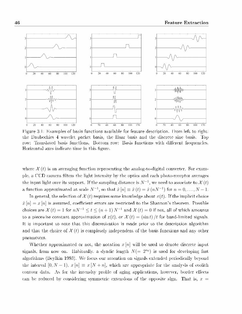
46 Feature Extraction
Figure 3.1: Examples of basis functions available for feature description. From left to right:the Daubechies 4 wavelet packet basis, the Haar basis and the discrete sine basis. Toprow: Translated basis functions. Bottom row: Basis functions with di�erent frequencies.Horizontal axes indicate time in this �gure.
where X (t) is an averaging function representing the analog-to-digital converter. For exam-
ple, a CCD camera �lters the light intensity by the optics and each photo-receptor averages
the input light over its support. If the sampling distance is N−1, we need to associate to X (t)
a function approximated at scale N−1, so that x [n] ≡ x (t) = x (nN−1) for n = 0, . . . , N − 1.
In general, the selection of X (t) requires some knowledge about x (t). If the implicit choice
x [n] = x [n] is assumed, coe�cient errors are restricted to the Shannon's theorem. Possible
choices are X (t) = 1 for nN−1 ≤ t ≤ (n+ 1)N−1 and X (t) = 0 if not, all of which amounts
to a piecewise constant approximation of x (t), or X (t) = (sin t) /t for band-limited signals.
It is important to note that this discretization is made prior to the description algorithm
and that the choice of X (t) is completely independent of the basis functions and any other
parameters.
Whether approximated or not, the notation x [n] will be used to denote discrete input
signals, from now on. Habitually, a dyadic length N(= 2n0) is used for developing fast
algorithms (Beylkin 1993). We focus our attention on signals extended periodically beyond
the interval [0, N − 1), x [n] ≡ x [N + n], which are appropriate for the analysis of otolith
contour data. As for the intensity pro�le of aging applications, however, border e�ects
can be reduced by considering symmetric extensions of the opposite sign. That is, x =
3.2. On Description Methods for Feature Extraction 47
{x [0] , . . . , x [N − 1] ,−x [N − 1] , . . . ,−x [0]}.
3.2.1 Fourier Descriptors
The Discrete Fourier Transform (DFT) decomposes an aperiodic signal into a sum of complex
exponential terms eiω. Basically, it changes the time (or space) representations of signals into
a representation of the angular frequency ω, commonly known as the frequency domain.
The DFT is widely employed in signal processing and related �elds to analyze the frequen-
cies contained in digital signals. Proof of the importance of this operation is the fact that the
term FFT (Fast Fourier transform) is often used to mean DFT in colloquial settings, even
though this term refers exactly to a family of algorithms that are computationally e�cient
(Good 1958, Cooley and Tukey 1965, Bruun 1978).
More formally, let x ≡ {x [0] , . . . , x [N − 1]} be a sequence of N samples. This sequence is
transformed into another sequence of N complex numbers {X [0] , . . . , X [N − 1]} accordingto the following expression of the DFT,
DFT : X [k] =N−1∑n=0
x [n] exp
[−i2π
Nkn
]k = 0, . . . , N − 1. (3.2)
where the exponential term constitutes the basis vectors. The inverse discrete Fourier trans-
form (IDFT) is given by
IDFT : x [n] =1
N
N−1∑k=0
X [k] exp
[i2π
Nkn
], (3.3)
and can be used to reconstruct the whole signal, or part of its components. A simple gen-
eralization of DFT is that the complex numbers X [k] represent the amplitude and phase
features corresponding to the sinusoidal components that makes x [n], and whose frequency
ω = 2πNk is indexed by k. The equations make use of the Euler notation to express this prin-
ciple because sinusoids are more e�ciently manipulated by means of complex exponentials.
However, by writing X [k] in polar form the sinusoid amplitude Ak/N and phase ϕk can be
derived, respectively, as
A [k] = |Xk| =√Re2X [k] + Im2X [k], (3.4)
and
ϕ [k] = arctan
(Im X [k]
Re X [k]
). (3.5)
48 Feature Extraction
The normalization factors multiplying the DFT and IDFT, here 1 and 1/N, and the signs
in the exponent are merely conventions, and are used di�erently depending on the application
type. In this sense, the equations for the the Fourier series are similar except that the term
1/N is included in the expression X [k] instead of the expression x [n]. A normalization of
1/√N makes the transform unitary, o�ering some theoretical advantages, but the previous
one is often more practical in terms of signal interpretation to perform the scaling all at
once, just as the term A [k] /N above. Additionally, the convention of a negative sign in the
exponent is preferable because in this case it means that X [k] is the amplitude of a positive
frequency ω = 2πk/N . In practice, however, the coe�cient values belonging to the negative
frequencies equal those of the positive ones, and the analysis thus will be restricted to N /2
coe�cients when N is even, or (N+1)/2 coe�cients if N is odd.
The coe�cients can be used for di�erent purposes, including: spectral analysis, data
compression, interpolation, or the multiplication of polynomial and or large integers; among
others. When the inverse operation (IDFT) is restricted to some �nite number of coe�cients,
�ltering operations are implemented over the initial signal.
3.2.2 STFT. The Short-Time Fourier Transform
The discrete short-time Fourier transform (STFT) is a Fourier-related transform that can
determine the variation of frequency and phase components of a signal as it changes over
time. This is possible because the coe�cients are evaluated at a given position (or time), u,
instead of the whole signal time support. Therefore, the STFT transform is given by
STFT : X [u, k] =N−1∑n=0
x [n] g [n− u] exp
[−i2π
Nkn
]. (3.6)
where g [n− u] corresponds to a symmetric window of period N centered at position u and
modulated in frequency by k, where 0 ≤ u < N and 0 ≤ k < N . Similar to the IDFT, the
original signal is reconstructed by the corresponding inverse short-time Fourier Transform
(ISTFT) as
ISTFT : x [n] =1
N
N−1∑u=0
N−1∑k=0
X [u, k] g [n− u] exp
[i2π
Nkn
](3.7)
In principle, this type of transform has the potential advantage that it can capture fre-
quency variations in time. The slice of information provided by the atom φ = g [n− u] ei2πNkn
in Eq. 3.6, corresponds to a region in a time-frequency plane (n, ω) whose location and width
depends on the time-frequency spread of φ. Since
3.2. On Description Methods for Feature Extraction 49
‖φ‖2 =N−1∑n=0
|φ [n]|2 = 1, (3.8)
|φ (n)|2 can be thought of as a probability distribution centered at
u =N−1∑n=0
n |φ [n]|2 . (3.9)
The spread around u is measured by the variance
σ2n =
N−1∑n=0
[n− u]2 |φ [n]|2 . (3.10)
The Plancherel formula proves that∑N−1
k=0
∣∣∣φ [k]∣∣∣2 = 2π ‖φ‖2, where φ denotes DFT of φ
(Plancherel and Le�er 1910). Considering only the analytical part, the center frequency of
φ is therefore de�ned by
ξ =
N/2∑k=0
k∣∣∣φ [k]
∣∣∣2 , (3.11)
where if N is even (or (N+1)/2 if N is odd). The spread around ξ is
σ2ω =
N/2∑k=0
[k − ξ]2∣∣∣φ [k]
∣∣∣2 . (3.12)
Habitually, the resolution of time-frequency components is expressed by the area of a
time-frequency box (sometimes referred to as Heisenberg box) centered at (u, ξ), and whose
area is established by σu and σω, respectively (Fig. 3.2). Since g is even, the size of the box
is independent of u and ξ, and it remains �xed. This means that all atoms in the STFT
have the same time-bandwidth resolution across the time-frequency plane. The uncertainty
principle excludes the possibility of having arbitrarily high resolutions, since in the best case
(a Gaussian window) the time-bandwidth product σuσω can not be lower than 1/2 (Wheeler
and Zureck 1983).
When using a discrete grid, STFTs can be highly redundant: small increments of u and
ω cause atoms to overlap so that x (n) can not be recovered exactly by means of ISTFT. The
solution to this problem resorts to using a frame such that the basis functions constitute an
orthonormal basis. Unfortunately, this is possible only if g(·) is badly localized in either time
or frequency, which normally is the reason why the STFT is oversampled. Thus, the use of

50 Feature Extraction
Figure 3.2: Heisenberg boxes of two windowed Fourier atoms φu,ξ and φv,γ (from Mallat1990).
STFT is limited to audio monitoring tools, such as spectrograms, which are implemented by
calculating the value |X [u, k]|2.
3.2.3 Wavelet Transforms
By varying the window width, time resolution can be traded for resolution in frequency or
vice-versa. In this sense, some short basis functions could be used to isolate discontinuities of
high frequency, while the remaining ones could be long functions to develop spectral analysis
towards the lower frequencies. An intuitive way to do this is by having both short high
frequency and long low frequency functions available. This is exactly what is achieved with
the wavelet transform (Daubechies 1988, Mallat 1989, Daubechies 1992, Mallat and Hwang
1992, Meyer 1990).
In a general sense, the Continuous Wavelet Transform (CWT) calculate the coe�-
cients as inner products of x against a family of dilated and translated wavelets. Its general
expression is given by
CWT : Cs,u =
ˆx (t)ψ∗u,s (t) dt, (3.13)
where the dilated and translated versions are obtained from a prototype wavelet (or mother
function) ψ (t), corresponding to a zero average high-pass �lter (∑
n ψ [n] = 0), given by the
model
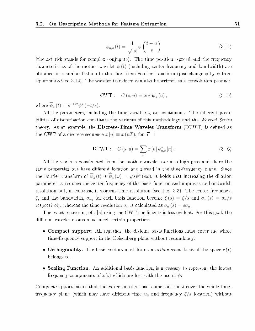
3.2. On Description Methods for Feature Extraction 51
ψu,s (t) =1√|s|ψ
(t− us
)(3.14)
(the asterisk stands for complex conjugate). The time position, spread and the frequency
characteristics of the mother wavelet ψ (t) (including center frequency and bandwidth) are
obtained in a similar fashion to the short-time Fourier transform (just change φ by ψ from
equations 3.9 to 3.12). The wavelet transform can also be written as a convolution product
CWT : C (s, u) = x ∗ψs (u) , (3.15)
where ψs (t) = s−1/2ψ∗ (−t/s).All the parameters, including the time variable t, are continuous. The di�erent possi-
bilities of discretization constitute the variants of this methodology and the Wavelet Series
theory. As an example, the Discrete-Time Wavelet Transform (DTWT) is de�ned as
the CWT of a discrete sequence x [n] ≡ x (nT ), for T=1
DTWT : C (s, u) =∑n
x [n]ψ∗u,s [n] . (3.16)
All the versions constructed from the mother wavelet are also high-pass and share the
same properties but have di�erent location and spread in the time-frequency plane. Since
the Fourier transform of ψs (t) is ψs (ω) =√sψ∗ (sω), it holds that increasing the dilation
parameter, s, reduces the center frequency of the basis function and improves its bandwidth
resolution but, in contrast, it worsens time resolution (see Fig. 3.3). The center frequency,
ξ, and the bandwidth, σω, for each basis function become ξ (s) = ξ/s and σω (s) = σω/s
respectively, whereas the time resolution σn is calculated as σn (s) = sσn.
The exact recovering of x [n] using the CWT coe�cients is less evident. For this goal, the
di�erent wavelet atoms must meet certain properties:
� Compact support: All together, the disjoint basis functions must cover the whole
time-frequency support in the Heisenberg plane without redundancy.
� Orthogonality. The basis vectors must form an orthonormal basis of the space x (t)
belongs to.
� Scaling Function. An additional basis function is necessary to represent the lowest
frequency components of x (t) which are lost with the use of ψ.
Compact support means that the extension of all basis functions must cover the whole time-
frequency plane (which may have di�erent time u0 and frequency ξ/s location) without
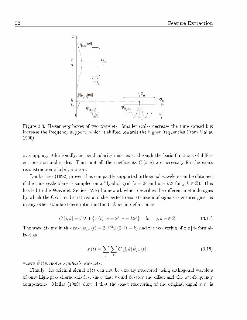
52 Feature Extraction
Figure 3.3: Heisenberg boxes of two wavelets. Smaller scales decrease the time spread butincrease the frequency support, which is shifted towards the higher frequencies (from Mallat1990).
overlapping. Additionally, perpendicularity must exist through the basis functions of di�er-
ent position and scales. Thus, not all the coe�cients C (s, u) are necessary for the exact
reconstruction of x [n], a priori.
Daubechies (1992) proved that compactly supported orthogonal wavelets can be obtained
if the time-scale plane is sampled on a �dyadic� grid (s = 2j and u = k2j for j, k ∈ Z). Thishas led to theWavelet Series (WS) framework which describes the di�erent methodologies
by which the CWT is discretized and the perfect reconstruction of signals is ensured, just as
in any other standard description method. A usual de�nition is
C [j, k] = CWT{x (t) ; s = 2j, u = k2j
}for j, k =∈ Z. (3.17)
The wavelets are in this case ψj,k (t) = 2−j/2ψ (2−jt− k) and the recovering of x [n] is formal-
ized as
x (t) =∑j
∑k
C [j, k] ψj,k (t) . (3.18)
where ψ (t)denotes synthesis wavelets.
Finally, the original signal x (t) can not be exactly recovered using orthogonal wavelets
of only high-pass characteristics, since that would destroy the o�set and the low-frequency
components. Mallat (1989) showed that the exact recovering of the original signal x (t) is
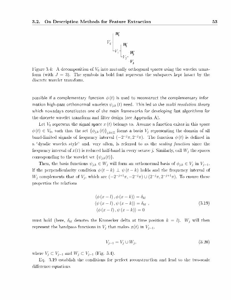
3.2. On Description Methods for Feature Extraction 53
Figure 3.4: A decomposition of V0 into mutually orthogonal spaces using the wavelet trans-form (with J = 3). The symbols in bold font represent the subspaces kept intact by thediscrete wavelet transform.
possible if a complementary function φ (t) is used to reconstruct the complementary infor-
mation high-pass orthonormal wavelets ψj,k (t) need. This led to the multi-resolution theory
which nowadays constitutes one of the main frameworks for developing fast algorithms for
the discrete wavelet transform and �lter design (see Appendix A).
Let V0 represent the signal space x (t) belongs to. Assume a function exists in this space
φ (t) ∈ V0, such that the set {φj,k (t)}j,k∈Z forms a basis Vj representing the domain of all
band-limited signals of frequency interval (−2−jπ, 2−jπ). The function φ (t) is de�ned in
a �dyadic wavelet style� and, very often, is referred to as the scaling function since the
frequency interval of x (t) is reduced half-band in every octave j. Similarly, callWj the spaces
corresponding to the wavelet set {ψj,k(t)}.Then, the basis functions ψj,k ∈ Wj will form an orthonormal basis of φj,k ∈ Vj in Vj−1,
if the perpendicularity condition φ (t− k) ⊥ ψ (t− k) holds and the frequency interval of
Wj complements that of Vj, which are (−2−j+1π,−2−jπ) ∪ (2−jπ, 2−j+1π). To ensure these
properties the relations
〈φ (x− l) , φ (x− k)〉 = δkl
〈ψ (x− l) , ψ (x− k)〉 = δkl
〈φ (x− l) , ψ (x− k)〉 = 0
, (3.19)
must hold (here, δkl denotes the Kronecker delta at time position k = l). Wj will then
represent the bandpass functions in Vj that makes x (t) in Vj−1,
Vj−1 = Vj ∪Wj, (3.20)
where Vj ⊂ Vj−1 and Wj ⊂ Vj−1 (Fig. 3.4).
Eq. 3.19 establish the conditions for perfect reconstruction and lead to the two-scale
di�erence equations
54 Feature Extraction
1√2φ (t/2) =
∑n
h0 [n]φ (t− n) = h0 ∗ φ, (3.21)
1√2ψ (t/2) =
∑n
h1 [n]φ (t− n) = h1 ∗ φ, (3.22)
where h0 and h1 are the �nite-length impulsional responses (FIR) corresponding to the low-
pass φ and high-pass ψ basis functions, respectively.
The design of these �lters is a major topic of research in wavelet analysis (Vetterli 1992),
and with their corresponding synthesis �lters, h0 and h1 (their reversed versions in the or-
thogonal case), form the two-channel �lter-bank necessary for the fast computation of the
Discrete Wavelet Transform (DWT). For this reason, they are sometimes referred to as
quadrature mirror �lters (QMF)
De�nition. 3.2 A Fast DWT algorithm is computed as
DWT{x [n] ; 2j, k2j
}= dj [k] =
∑n
x [n]h(j)1
[n− 2jk
](3.23)
aJ [k] =∑n
x [n]h(J)0
[n− 2Jk
], (3.24)
where h0 [n] =⟨2−1/2φ (t/2) , φ (t− n)
⟩and h1 [n] =
⟨2−1/2ψ (t/2) , φ (t− n)
⟩denote low-pass
and high-pass half-band FIR �lters, and at each octave j the �lter sequences are recomputed
as
h(1)1 [n] = h1 [n] , h
(1)0 [n] = h0 [n] ,
h(j+1)1 [n] =
∑l h
(j)1 [l]h1 [n− 2l] ,
h(j+1)0 [n] =
∑l h
(j)0 [l]h0 [n− 2l] .
(3.25)
The terms aj [k] and dj [k] denote �approximation� and �detail� coe�cients, respectively.
Although the �lter sequences should be calculated at each scale, the decomposition process
can be organized in a way that the original structure of h0 and h1 is maintained throughout
the dyadic scales.
Fig 3.5 illustrates this process. First, a0 [n] is initialized to some consistent discretization
of the input x [n] = x (nN−1). In this sense, it is possible to show that if the implicit choice
x [n] = x [n] is taken, errors can come from the distance of the scale function φ to an ideal
low-pass �lter, at various scales and �details� and, for this reason, Abry and Flandrin (1994)
proposed using the approximation
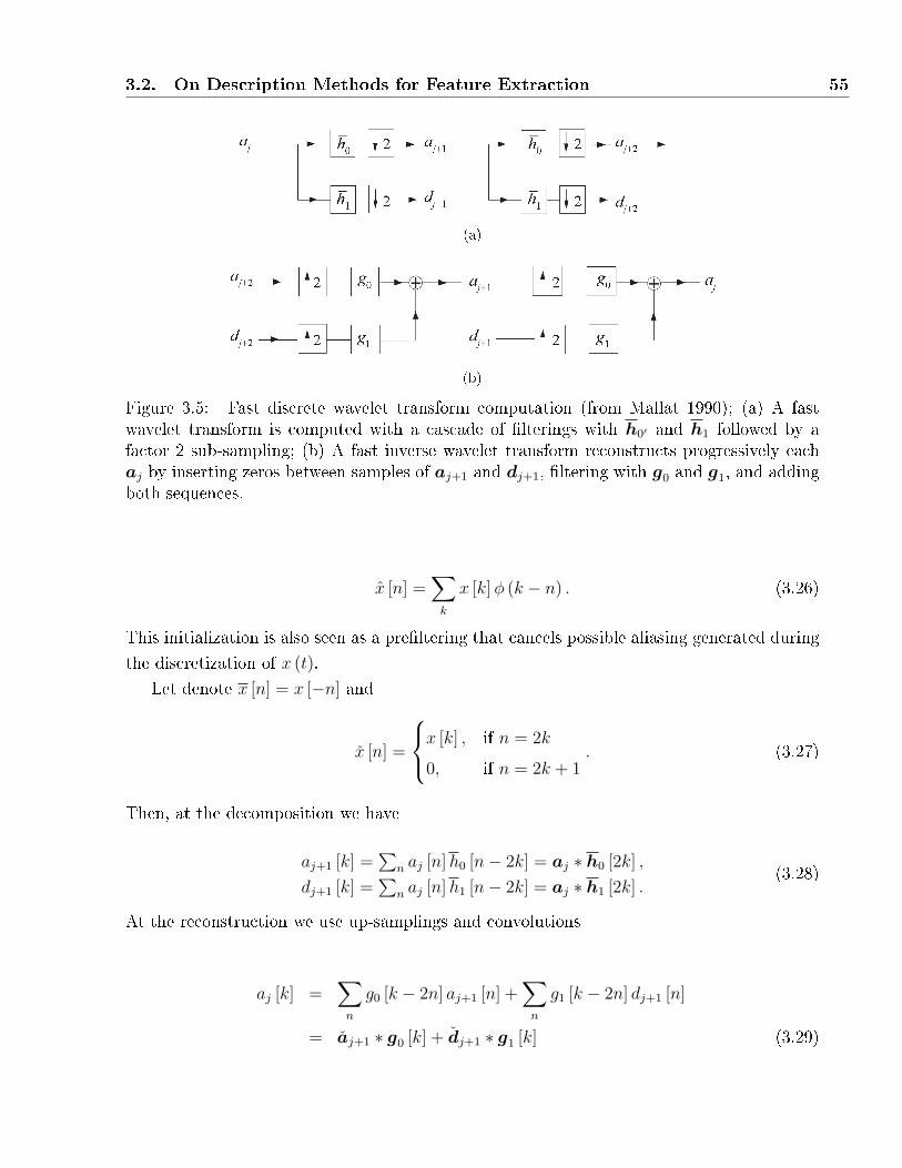
3.2. On Description Methods for Feature Extraction 55
(a)
(b)
Figure 3.5: Fast discrete wavelet transform computation (from Mallat 1990); (a) A fastwavelet transform is computed with a cascade of �lterings with h0′ and h1 followed by afactor 2 sub-sampling; (b) A fast inverse wavelet transform reconstructs progressively eachaj by inserting zeros between samples of aj+1 and dj+1, �ltering with g0 and g1, and addingboth sequences.
x [n] =∑k
x [k]φ (k − n) . (3.26)
This initialization is also seen as a pre�ltering that cancels possible aliasing generated during
the discretization of x (t).
Let denote x [n] = x [−n] and
x [n] =
x [k] , if n = 2k
0, if n = 2k + 1. (3.27)
Then, at the decomposition we have
aj+1 [k] =∑
n aj [n]h0 [n− 2k] = aj ∗ h0 [2k] ,
dj+1 [k] =∑
n aj [n]h1 [n− 2k] = aj ∗ h1 [2k] .(3.28)
At the reconstruction we use up-samplings and convolutions
aj [k] =∑n
g0 [k − 2n] aj+1 [n] +∑n
g1 [k − 2n] dj+1 [n]
= aj+1 ∗ g0 [k] + dj+1 ∗ g1 [k] (3.29)
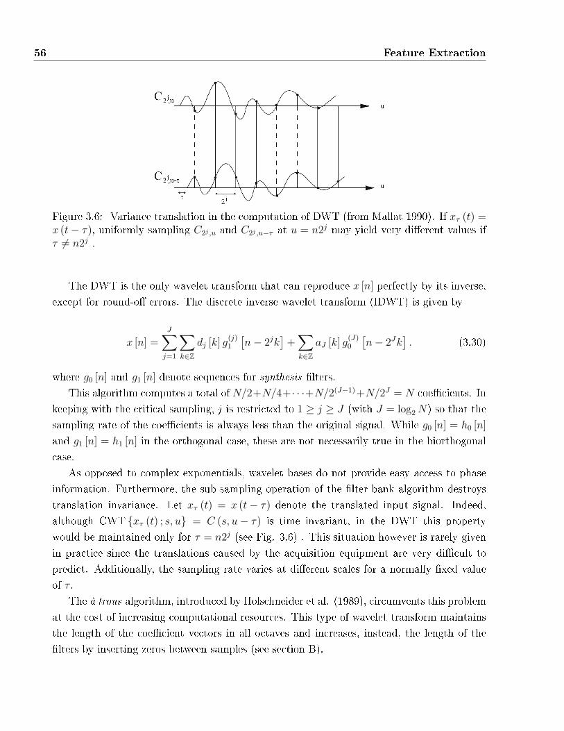
56 Feature Extraction
Figure 3.6: Variance translation in the computation of DWT (from Mallat 1990). If xτ (t) =x (t− τ), uniformly sampling C2j ,u and C2j ,u−τ at u = n2j may yield very di�erent values ifτ 6= n2j .
The DWT is the only wavelet transform that can reproduce x [n] perfectly by its inverse,
except for round-o� errors. The discrete inverse wavelet transform (IDWT) is given by
x [n] =J∑j=1
∑k∈Z
dj [k] g(j)1
[n− 2jk
]+∑k∈Z
aJ [k] g(J)0
[n− 2Jk
]. (3.30)
where g0 [n] and g1 [n] denote sequences for synthesis �lters.
This algorithm computes a total of N/2+N/4+· · ·+N/2(J−1)+N/2J = N coe�cients. In
keeping with the critical sampling, j is restricted to 1 ≥ j ≥ J (with J = log2N) so that the
sampling rate of the coe�cients is always less than the original signal. While g0 [n] = h0 [n]
and g1 [n] = h1 [n] in the orthogonal case, these are not necessarily true in the biorthogonal
case.
As opposed to complex exponentials, wavelet bases do not provide easy access to phase
information. Furthermore, the sub-sampling operation of the �lter-bank algorithm destroys
translation invariance. Let xτ (t) = x (t− τ) denote the translated input signal. Indeed,
although CWT {xτ (t) ; s, u} = C (s, u− τ) is time invariant, in the DWT this property
would be maintained only for τ = n2j (see Fig. 3.6) . This situation however is rarely given
in practice since the translations caused by the acquisition equipment are very di�cult to
predict. Additionally, the sampling rate varies at di�erent scales for a normally �xed value
of τ .
The à trous algorithm, introduced by Holschneider et al. (1989), circumvents this problem
at the cost of increasing computational resources. This type of wavelet transform maintains
the length of the coe�cient vectors in all octaves and increases, instead, the length of the
�lters by inserting zeros between samples (see section B).
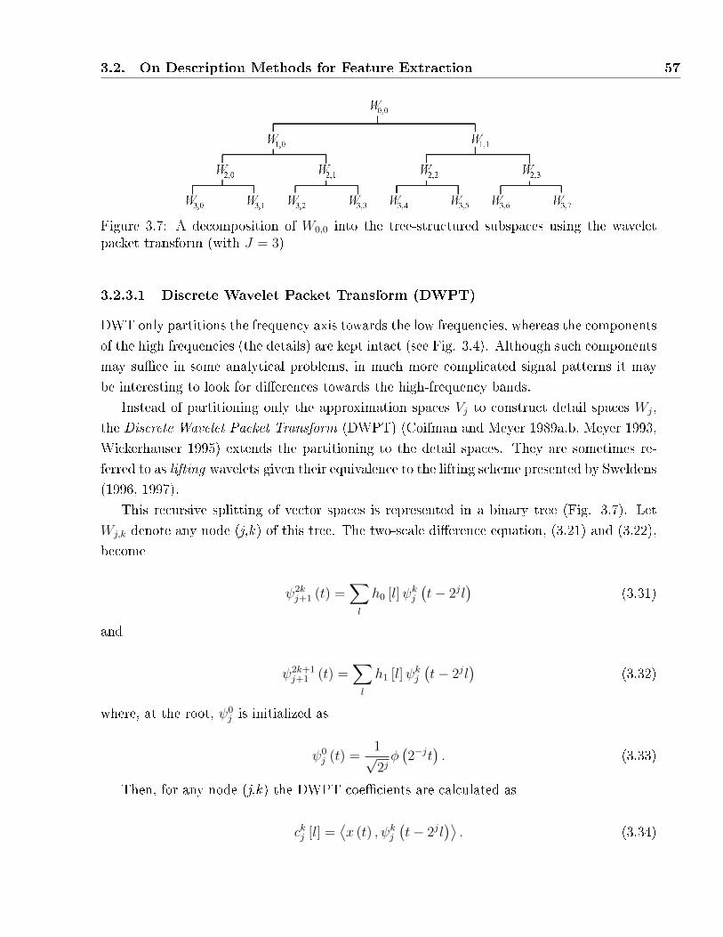
3.2. On Description Methods for Feature Extraction 57
Figure 3.7: A decomposition of W0,0 into the tree-structured subspaces using the waveletpacket transform (with J = 3)
3.2.3.1 Discrete Wavelet Packet Transform (DWPT)
DWT only partitions the frequency axis towards the low frequencies, whereas the components
of the high frequencies (the details) are kept intact (see Fig. 3.4). Although such components
may su�ce in some analytical problems, in much more complicated signal patterns it may
be interesting to look for di�erences towards the high-frequency bands.
Instead of partitioning only the approximation spaces Vj to construct detail spaces Wj,
the Discrete Wavelet Packet Transform (DWPT) (Coifman and Meyer 1989a,b, Meyer 1993,
Wickerhauser 1995) extends the partitioning to the detail spaces. They are sometimes re-
ferred to as lifting wavelets given their equivalence to the lifting scheme presented by Sweldens
(1996, 1997).
This recursive splitting of vector spaces is represented in a binary tree (Fig. 3.7). Let
Wj,k denote any node (j,k) of this tree. The two-scale di�erence equation, (3.21) and (3.22),
become
ψ2kj+1 (t) =
∑l
h0 [l]ψkj(t− 2jl
)(3.31)
and
ψ2k+1j+1 (t) =
∑l
h1 [l]ψkj(t− 2jl
)(3.32)
where, at the root, ψ0j is initialized as
ψ0j (t) =
1√2jφ(2−jt
). (3.33)
Then, for any node (j,k) the DWPT coe�cients are calculated as
ckj [l] =⟨x (t) , ψkj
(t− 2jl
)⟩. (3.34)
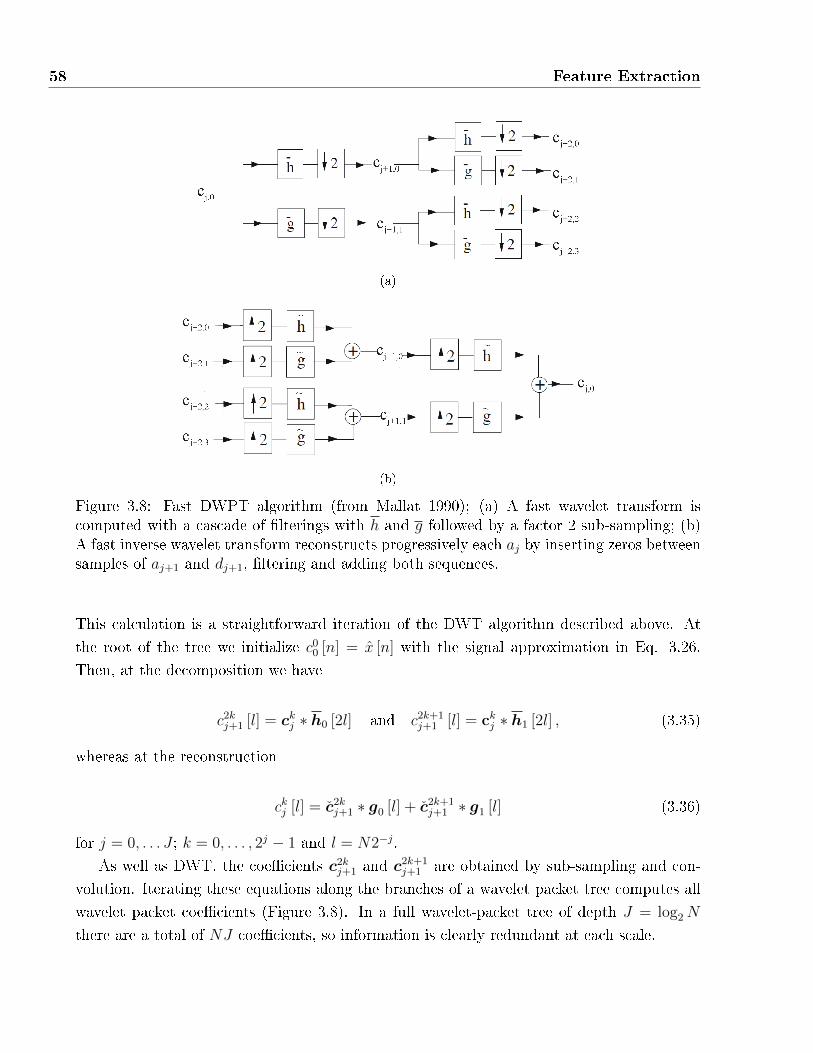
58 Feature Extraction
(a)
(b)
Figure 3.8: Fast DWPT algorithm (from Mallat 1990); (a) A fast wavelet transform iscomputed with a cascade of �lterings with h and g followed by a factor 2 sub-sampling; (b)A fast inverse wavelet transform reconstructs progressively each aj by inserting zeros betweensamples of aj+1 and dj+1, �ltering and adding both sequences.
This calculation is a straightforward iteration of the DWT algorithm described above. At
the root of the tree we initialize c00 [n] = x [n] with the signal approximation in Eq. 3.26.
Then, at the decomposition we have
c2kj+1 [l] = ckj ∗ h0 [2l] and c2k+1
j+1 [l] = ckj ∗ h1 [2l] , (3.35)
whereas at the reconstruction
ckj [l] = c2kj+1 ∗ g0 [l] + c2k+1
j+1 ∗ g1 [l] (3.36)
for j = 0, . . . J ; k = 0, . . . , 2j − 1 and l = N2−j.
As well as DWT, the coe�cients c2kj+1 and c2k+1
j+1 are obtained by sub-sampling and con-
volution. Iterating these equations along the branches of a wavelet packet tree computes all
wavelet packet coe�cients (Figure 3.8). In a full wavelet-packet tree of depth J = log2N
there are a total of NJ coe�cients, so information is clearly redundant at each scale.
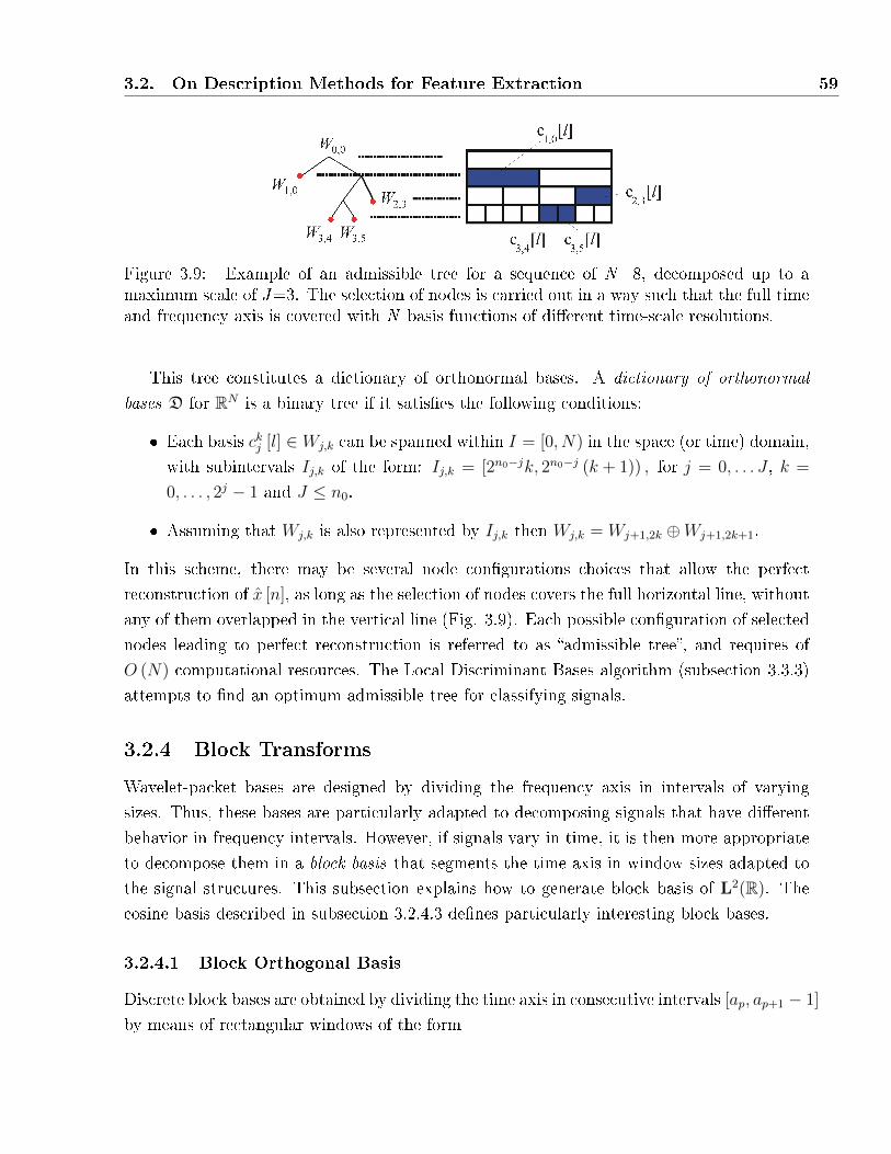
3.2. On Description Methods for Feature Extraction 59
Figure 3.9: Example of an admissible tree for a sequence of N=8, decomposed up to amaximum scale of J=3. The selection of nodes is carried out in a way such that the full timeand frequency axis is covered with N basis functions of di�erent time-scale resolutions.
This tree constitutes a dictionary of orthonormal bases. A dictionary of orthonormal
bases D for RN is a binary tree if it satis�es the following conditions:
� Each basis ckj [l] ∈ Wj,k can be spanned within I = [0, N) in the space (or time) domain,
with subintervals Ij,k of the form: Ij,k = [2n0−jk, 2n0−j (k + 1)) , for j = 0, . . . J , k =
0, . . . , 2j − 1 and J ≤ n0.
� Assuming that Wj,k is also represented by Ij,k then Wj,k = Wj+1,2k ⊕Wj+1,2k+1.
In this scheme, there may be several node con�gurations choices that allow the perfect
reconstruction of x [n], as long as the selection of nodes covers the full horizontal line, without
any of them overlapped in the vertical line (Fig. 3.9). Each possible con�guration of selected
nodes leading to perfect reconstruction is referred to as �admissible tree�, and requires of
O (N) computational resources. The Local Discriminant Bases algorithm (subsection 3.3.3)
attempts to �nd an optimum admissible tree for classifying signals.
3.2.4 Block Transforms
Wavelet-packet bases are designed by dividing the frequency axis in intervals of varying
sizes. Thus, these bases are particularly adapted to decomposing signals that have di�erent
behavior in frequency intervals. However, if signals vary in time, it is then more appropriate
to decompose them in a block basis that segments the time axis in window sizes adapted to
the signal structures. This subsection explains how to generate block basis of L2(R). The
cosine basis described in subsection 3.2.4.3 de�nes particularly interesting block bases.
3.2.4.1 Block Orthogonal Basis
Discrete block bases are obtained by dividing the time axis in consecutive intervals [ap, ap+1 − 1]
by means of rectangular windows of the form
60 Feature Extraction
gp [n] = 1[ap,ap+1−1] (n) , (3.37)
for all p ∈ Z and ap ∈ Z. For signals of dyadic length N, a common choice is to use p intervals
of width l = N2−j . In this case, the window boundaries are set to ap = pl for 0 ≤ p ≤ 2j.
Assuming that {ek,l}0≤k<l is an orthonormal basis of Cl for any l>0, it can be shown that
the set
{gp,k [n] = gp [n] ek,l [n− ap]}0≤k<l,p∈Z (3.38)
forms a block orthonormal basis on the space Wp. One set of discrete block basis is obtained
with the Fourier bases {ek,l [n] =
1√l
exp
(i2πkn
l
)}0≤k<l
. (3.39)
The block transform for this basis then becomes
X [p, k] =N−1∑n=0
x [n] g∗p,k [n] . (3.40)
This transform is a variant of the STFT with the di�erence that the range of admissible
frequencies in the basis functions are restricted to the window size. This characteristic enables
perfect reconstruction of x [n] which is obtained as
x [n] =∑p
∑k
X [p, k] gp,k [n] . (3.41)
The resulting block of Fourier vectors gp,k generate sharp transitions at the window border
that alter the frequency localization, producing generally large coe�cient values in this zone.
3.2.4.2 Cosine and Sine Transforms
Similar to the DFT, discrete cosine and sine transforms (DCT/DST) also have the ability
to express transient signal components in terms of sinusoids of di�erent frequencies and
magnitudes. The obvious distinction is that the former only uses real-valued cosine and sine
functions, instead of complex exponentials.
Discretizing the frequency domain of DCT/DST can also be thought of as a way of
implicitly extending the original signal beyond the last sample point. However, while DFT
doubles the length assuming periodical extensions of x [n], in the DCT/DST this extension
can be either symmetric or asymmetric in relation to both ends of the signal.
3.2. On Description Methods for Feature Extraction 61
For this reason, two issues arise at the time of setting the DCT/DST: 1) the type of
extension at both the left and right end of the signal; and 2) the sample position this extension
is applied. Extensions can be symmetric or asymmetric at both left and right ends of the
signal, whereas the position can be around the last point or half way between two data points
of both boundaries. Every combination corresponds to a speci�c type of DCT or DST. There
is a total of sixteen possibilities, half of which correspond to eight DCTs (those where the
left boundary is symmetric) and the other half to 8 DSTs (the left boundary is asymmetric).
However, not all of them have become practical in real applications. In particular, it is
well known that processing a signal by pieces introduces coe�cient distortion so that more
coe�cient terms are necessary to represent features accurately. This principle determines
the DFT-based strategy for implementing the DCT/DST algorithm, which tries to reduce
this distortion by some periodical extension of the initial signal. For all these reasons, only
four DCT and four DST transforms (denoted as DCT-I/IV and DST-I/IV) are of practical
utility, and constitute methodologies of this type of transform.
More formally, DCTs and DSTs implement invertible functions that transform a sequence
of N real numbers f : RN → RN . The four DCTs are
DCT-I: XI [k] =1
2
{x [0] + (−1)k x [N − 1]
}+
N−2∑n=1
x [n] cos
(πnk
N − 1
)k = 0, . . . , N − 1,
(3.42)
DCT-II XII [k] =N−1∑n=0
x [n] cos
[πk
N
(n+
1
2
)]k = 0, . . . , N − 1, (3.43)
DCT-III XIII [k] =1
2x [0] +
N−1∑n=1
x [n] cos
[πn
N
(k +
1
2
)]k = 0, . . . , N − 1, (3.44)
DCT-IV XIV [k] =N−1∑n=0
x [n] cos
[π
N
(n+
1
2
)(k +
1
2
)]k = 0, . . . , N − 1, (3.45)
and the four DSTs are
DST-I: XI [k] =N−1∑n=0
x [n] sin
[π
N + 1(n+ 1) (k + 1)
]k = 0, . . . , N − 1, (3.46)

62 Feature Extraction
DST-II: XII [k] =N−1∑n=0
x [n] sin
[π
N
(n+
1
2
)(k + 1)
]k = 0, . . . , N − 1, (3.47)
DST-III: XIII [k] =(−1)k
2x [N − 1]+
N−2∑n=0
x [n] sin
[π
N(n+ 1)
(k +
1
2
)]k = 0, . . . , N−1,
(3.48)
DST-IV: XIV [k] =N−1∑n=0
x [n] sin
[π
N
(n+
1
2
)(k +
1
2
)]k = 0, . . . , N − 1. (3.49)
In general, coe�cient distortion is minimized when extensions are even (Fig. 3.10a). This
explains why DCTs, and in particular the DCT-II generally have better coding performance
than DFT and DSTs, yielding smaller amplitude coe�cients at high frequency.
The use of DCT-II is widespread in image JPEG and video MPEG compression (Rao
and Yip 1990). It is also equivalent (up to an overall scale factor of 2) to a DFT of 4N real
inputs of even symmetry where the even-indexed elements are zero. That is, half of the DFT
coe�cients of the 4N inputs where x [n] = 0, x [2n-1] = x [n] for 0 ≤ n < N , and x [4N -n] =
x [n] for 0<n<2N. The inverse of DCT-II is DCT-III followed by a factor of 2/N, but some
authors prefer multiplying the term X [0] by 1/√
2 and X [k ] by√
2/N for 1 ≤ k ≤ N − 1 in
order to make DCT-II orthonormal. DCT-II then becomes
XII [k] = λk
√2
N
N−1∑n=0
x [n] cos
[kπ
N
(n+
1
2
)], with λk =
2−1/2 if k = 0
1 otherwise(3.50)
and is its inverse is
x [n] =
√2
N
N−1∑n=0
λkXII [k] cos
[kπ
N
(n+
1
2
)]. (3.51)
In this case, DCT-II and DCT-III are equivalent, but the correspondence with DFT calcula-
tions is broken. Similarly, a factor of√
2/N produces orthonormal basis for the DCT-IV
XIV [k] =
√2
N
N−1∑n=0
x [n] cos
[π
N
(n+
1
2
)(k +
1
2
)](3.52)
where
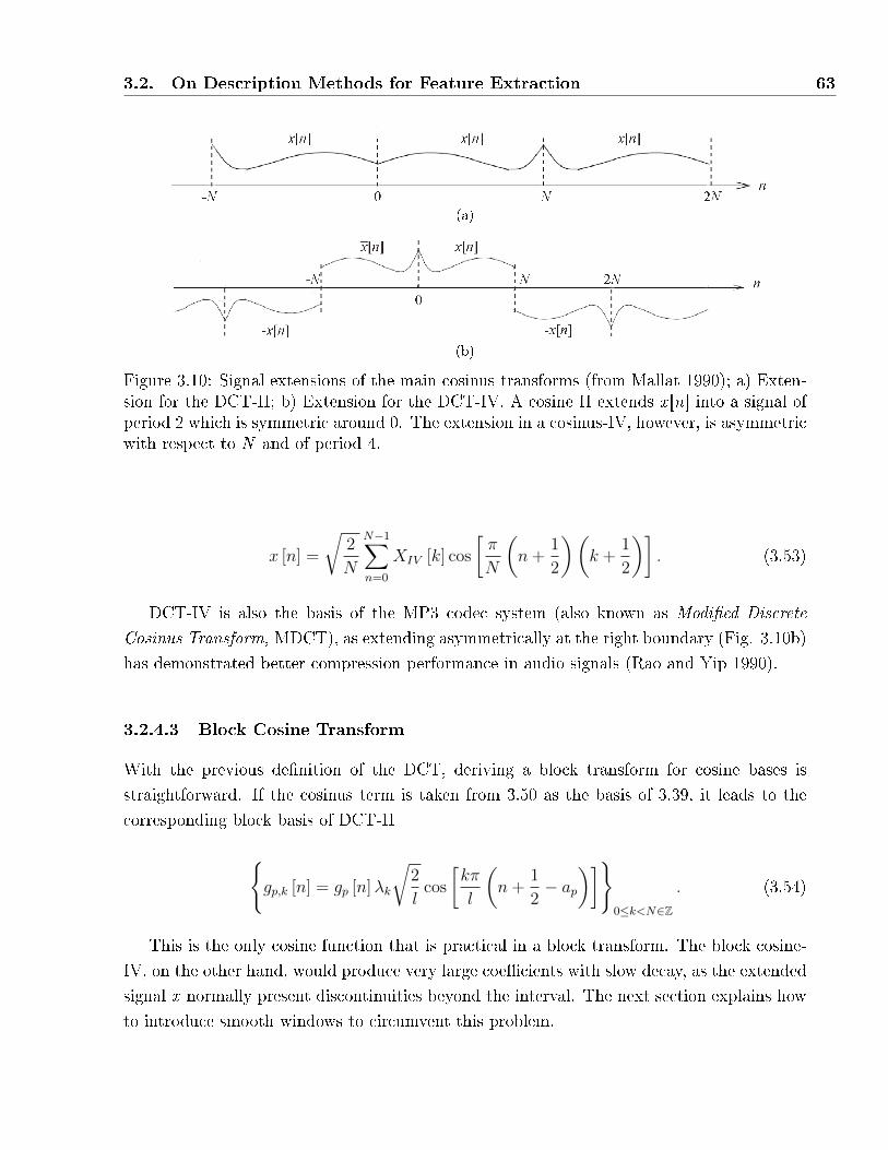
3.2. On Description Methods for Feature Extraction 63
(a)
(b)
Figure 3.10: Signal extensions of the main cosinus transforms (from Mallat 1990); a) Exten-sion for the DCT-II; b) Extension for the DCT-IV. A cosine II extends x [n] into a signal ofperiod 2 which is symmetric around 0. The extension in a cosinus-IV, however, is asymmetricwith respect to N and of period 4.
x [n] =
√2
N
N−1∑n=0
XIV [k] cos
[π
N
(n+
1
2
)(k +
1
2
)]. (3.53)
DCT-IV is also the basis of the MP3 codec system (also known as Modi�ed Discrete
Cosinus Transform, MDCT), as extending asymmetrically at the right boundary (Fig. 3.10b)
has demonstrated better compression performance in audio signals (Rao and Yip 1990).
3.2.4.3 Block Cosine Transform
With the previous de�nition of the DCT, deriving a block transform for cosine bases is
straightforward. If the cosinus term is taken from 3.50 as the basis of 3.39, it leads to the
corresponding block basis of DCT-II
{gp,k [n] = gp [n]λk
√2
lcos
[kπ
l
(n+
1
2− ap
)]}0≤k<N∈Z
. (3.54)
This is the only cosine function that is practical in a block transform. The block cosine-
IV, on the other hand, would produce very large coe�cients with slow decay, as the extended
signal x normally present discontinuities beyond the interval. The next section explains how
to introduce smooth windows to circumvent this problem.
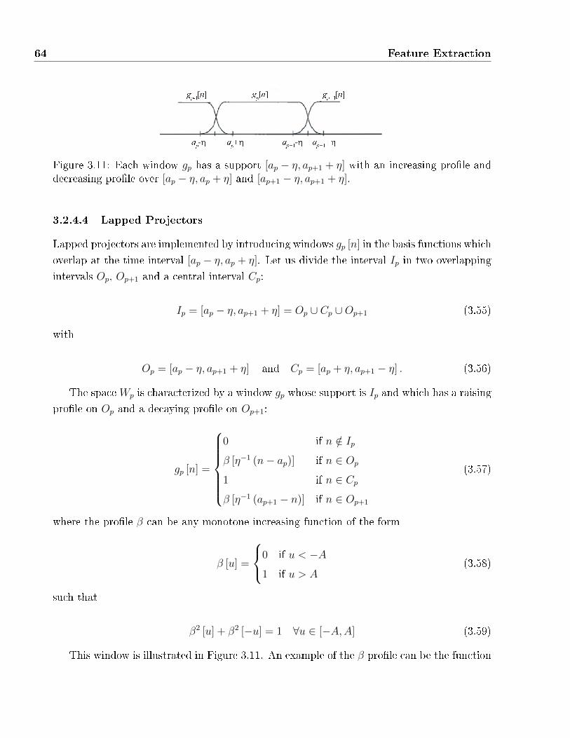
64 Feature Extraction
Figure 3.11: Each window gp has a support [ap − η, ap+1 + η] with an increasing pro�le anddecreasing pro�le over [ap − η, ap + η] and [ap+1 − η, ap+1 + η].
3.2.4.4 Lapped Projectors
Lapped projectors are implemented by introducing windows gp [n] in the basis functions which
overlap at the time interval [ap − η, ap + η]. Let us divide the interval Ip in two overlapping
intervals Op, Op+1 and a central interval Cp:
Ip = [ap − η, ap+1 + η] = Op ∪ Cp ∪Op+1 (3.55)
with
Op = [ap − η, ap+1 + η] and Cp = [ap + η, ap+1 − η] . (3.56)
The spaceWp is characterized by a window gp whose support is Ip and which has a raising
pro�le on Op and a decaying pro�le on Op+1:
gp [n] =
0 if n /∈ Ipβ [η−1 (n− ap)] if n ∈ Op
1 if n ∈ Cpβ [η−1 (ap+1 − n)] if n ∈ Op+1
(3.57)
where the pro�le β can be any monotone increasing function of the form
β [u] =
0 if u < −A
1 if u > A(3.58)
such that
β2 [u] + β2 [−u] = 1 ∀u ∈ [−A,A] (3.59)
This window is illustrated in Figure 3.11. An example of the β pro�le can be the function
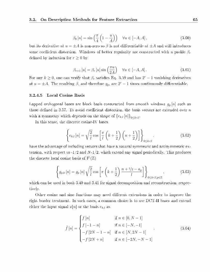
3.2. On Description Methods for Feature Extraction 65
β0 [n] = sin(π
4
(1− u
A
))∀u ∈ [−A,A] , (3.60)
but its derivative at u = ±A is non-zero so β is not di�erentiable at ±A and still introduces
some coe�cient distortion. Windows of better regularity are constructed with a pro�le βrde�ned by induction for r ≥ 0 by
βr+1 [u] = βr [u] sin(πu
2A
)∀u ∈ [−A,A] . (3.61)
For any k ≥ 0, one can verify that βr satis�es Eq. 3.59 and has 2r − 1 vanishing derivatives
at u = ±A. The resulting β, and therefore gp, are 2r − 1 times continuously di�erentiable.
3.2.4.5 Local Cosine Basis
Lapped orthogonal bases are block basis constructed from smooth windows gp [n] such as
those de�ned in 3.57. To avoid coe�cient distortion, the basis vectors are extended over n
with a symmetry which depends on the shape of {ek,l [n]}0≤k<l.
In this sense, the discrete cosine-IV bases{ek,l [n] =
√2
lcos
[π
l
(k +
1
2
)(n+
1
2
)]}0≤k<l
. (3.62)
have the advantage of including vectors that have a natural symmetric and antisymmetric ex-
tension, with respect to -1/2 and N -1/2, which extend any signal periodically. This produces
the discrete local cosine basis of l2 (Z){gp,k [n] = gp [n]
√2
lcos
[π
(k +
1
2
)n+ 1/2− ap
l
]}0≤k<l,p∈Z
, (3.63)
which can be used in both 3.40 and 3.41 for signal decomposition and reconstruction, respec-
tively.
Other cosine and sine functions may need di�erent extensions in order to improve the
right border treatment. In such cases, a common choice is to use DCT-II bases and extend
either the input signal x [n] or the basis ek,l as
f [n] =
f [n] if n ∈ [0, N − 1]
f [−1− n] if n ∈ [−N,−1]
−f [2N − 1− n] if n ∈ [N, 2N − 1]
−f [2N + n] if n ∈ [−2N,−N − 1]
. (3.64)
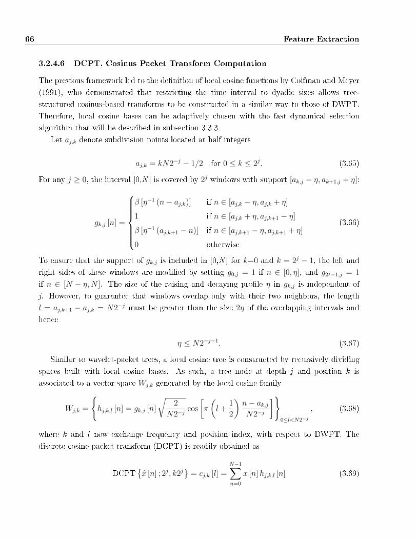
66 Feature Extraction
3.2.4.6 DCPT. Cosinus Packet Transform Computation
The previous framework led to the de�nition of local cosine functions by Coifman and Meyer
(1991), who demonstrated that restricting the time interval to dyadic sizes allows tree-
structured cosinus-based transforms to be constructed in a similar way to those of DWPT.
Therefore, local cosine bases can be adaptively chosen with the fast dynamical selection
algorithm that will be described in subsection 3.3.3.
Let aj,k denote subdivision points located at half integers
aj,k = kN2−j − 1/2 for 0 ≤ k ≤ 2j. (3.65)
For any j ≥ 0, the interval [0,N ] is covered by 2j windows with support [ak,j − η, ak+1,j + η]:
gk,j [n] =
β [η−1 (n− aj,k)] if n ∈ [aj,k − η, aj,k + η]
1 if n ∈ [aj,k + η, aj,k+1 − η]
β [η−1 (aj,k+1 − n)] if n ∈ [aj,k+1 − η, aj,k+1 + η]
0 otherwise
(3.66)
To ensure that the support of gk,j is included in [0,N ] for k=0 and k = 2j − 1, the left and
right sides of these windows are modi�ed by setting g0,j = 1 if n ∈ [0, η], and g2j−1,j = 1
if n ∈ [N − η,N ]. The size of the raising and decaying pro�le η in gk,j is independent of
j. However, to guarantee that windows overlap only with their two neighbors, the length
l = aj,k+1 − aj,k = N2−j must be greater than the size 2η of the overlapping intervals and
hence
η ≤ N2−j−1. (3.67)
Similar to wavelet-packet trees, a local cosine tree is constructed by recursively dividing
spaces built with local cosine bases. As such, a tree node at depth j and position k is
associated to a vector space Wj,k generated by the local cosine family
Wj,k =
{hj,k,l [n] = gk,j [n]
√2
N2−jcos
[π
(l +
1
2
)n− ak,jN2−j
]}0≤l<N2−j
, (3.68)
where k and l now exchange frequency and position index, with respect to DWPT. The
discrete cosine packet transform (DCPT) is readily obtained as
DCPT{x [n] ; 2j, k2j
}= cj,k [l] =
N−1∑n=0
x [n]hj,k,l [n] (3.69)
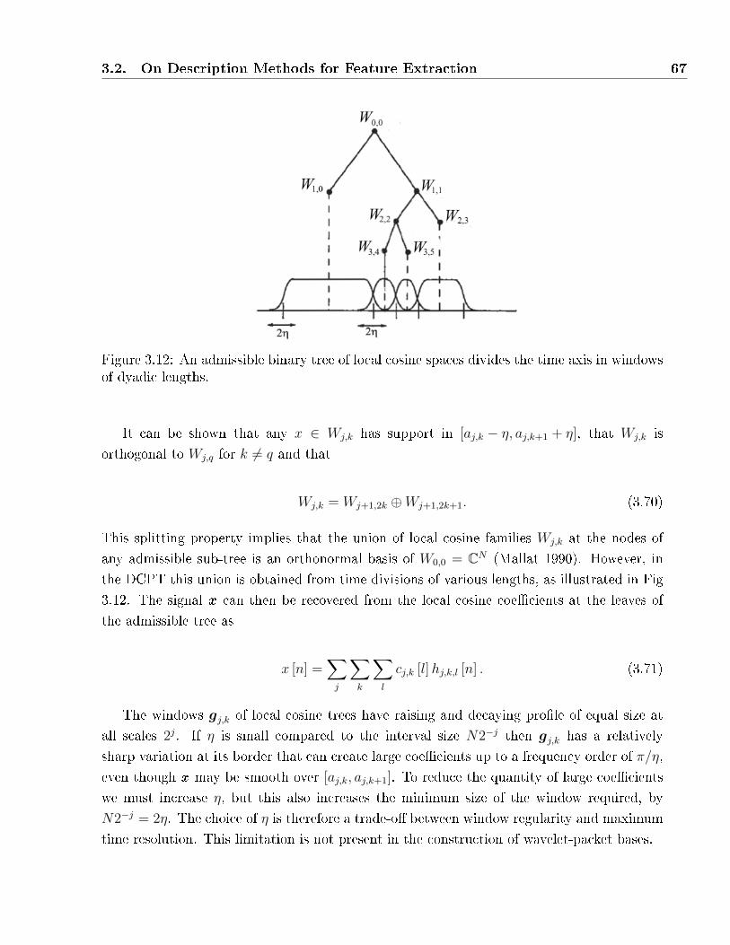
3.2. On Description Methods for Feature Extraction 67
Figure 3.12: An admissible binary tree of local cosine spaces divides the time axis in windowsof dyadic lengths.
It can be shown that any x ∈ Wj,k has support in [aj,k − η, aj,k+1 + η], that Wj,k is
orthogonal to Wj,q for k 6= q and that
Wj,k = Wj+1,2k ⊕Wj+1,2k+1. (3.70)
This splitting property implies that the union of local cosine families Wj,k at the nodes of
any admissible sub-tree is an orthonormal basis of W0,0 = CN (Mallat 1990). However, in
the DCPT this union is obtained from time divisions of various lengths, as illustrated in Fig
3.12. The signal x can then be recovered from the local cosine coe�cients at the leaves of
the admissible tree as
x [n] =∑j
∑k
∑l
cj,k [l]hj,k,l [n] . (3.71)
The windows gj,k of local cosine trees have raising and decaying pro�le of equal size at
all scales 2j. If η is small compared to the interval size N2−j then gj,k has a relatively
sharp variation at its border that can create large coe�cients up to a frequency order of π/η,
even though x may be smooth over [aj,k, aj,k+1]. To reduce the quantity of large coe�cients
we must increase η, but this also increases the minimum size of the window required, by
N2−j = 2η. The choice of η is therefore a trade-o� between window regularity and maximum
time resolution. This limitation is not present in the construction of wavelet-packet bases.
68 Feature Extraction
On the other hand, the translation of x also modi�es the coe�cient values of trigono-
metric bases, making therefore this type of transform not translation invariant. In this case,
the problem is that a translation of any cosine component spreads over vectors of di�erent
frequencies, questioning its use in pattern recognition applications.
3.3 On Feature Extraction Methods
In principle, all the description methods outlined above are not intended to evaluate signal
structures. They modify the coordinate system to another axis of representation that can
serve to reveal hidden structural components. However, determining whether these compo-
nents are useful for solving the problem at hand requires further analysis.
The analysis of structure information can be addressed in two ways, either in terms of
�signal similarities� (large components) or in terms of �signal singularities� (class di�erences).
For example, Principal Component Analysis (PCA) uses the covariance matrix as a similarity
measure to detect the best features for compressing information, whereas the measure used
in Linear Discriminant Analysis (LDA), the Fisher's separability measure (Fisher 1936), is
used to represent the class di�erences.
This subsection reviews some tools intended for developing data analysis. All of them
have in common the use of cost functions (or statistical information measures) which are
used to evaluate features and guide the selection process. When they take part in pattern
recognition systems, the role of automatic feature extraction is provided, freeing thus the user
from performing a manual selection of coe�cients. Although PCA and LDA are two popular
techniques used for this purpose, their main limitation lies in their lack of ability to explain
physical phenomena in data. The Best-Basis paradigm, and specially the Joint Best-Basis
and Local Discriminant Basis algorithms (LDB) are more recent designs that address this
problem.
3.3.1 Best-Basis Selection (BB)
The Best-Basis algorithm (Coifman and Wickerhauser 1992) was developed mainly for signal
compression. This method �rst expands a given single signal into a speci�ed dictionary of
orthonormal bases. Then a complete basis which minimizes the entropy cost function is
searched in the wavelet packet binary tree using a divide-and-conquer algorithm.
More precisely, let Aj,k denote a set of basis vectors belonging to space Wj,k arranged as
a matrix

3.3. On Feature Extraction Methods 69
Aj,k =(wj,k,0, . . . ,wj,k,N2−j−1
)T. (3.72)
where T denotes matrix transpose. Here, wj,k,l [n] can be vectors from a wavelet packet
dictionary ψkj [n− 2jl] or local cosine/sine functions hj,k,l [n]. Let (p) be an information cost
function measuring the �goodness� of compression of a sequence p. A common choice is the
Shannon entropy
(p) =∑i
− |pi|r log2 |pi|r . (3.73)
where the convention 0 log2 0 = 0 is used. (From now on, we use �log� for the logarithm of
base 2) Often r =1 or r = 2 is used. In this thesis we always use r = 2.
Now, let Bj,k denote the best basis for the signal x restricted to the span of Aj,k and
assume that the set B = (w0, . . . ,wN−1)T ∈ RN×N is initialized to store N basis functions
from {wj,k,l} corresponding to an admissible tree. Here, we changed wj,k,l to wn for notation
convenience. Then, the best-basis (BB) B corresponds to the admissible tree from the full
binary tree that minimizes the measure (Bx)
B = arg minB∈D
(Bx). (3.74)
where Bx also denotes expansion coe�cients for each wn computed from 3.35. The following
divide-and-conquer algorithm essentially performs 3.74 by comparing the e�ciency of each
parent node and its two children nodes:
Algorithm 3.1 Best-Basis (BB). Given a vector x :
� Step 0: Choose a dictionary of orthonormal bases D (i.e. specify QMF s for a WPT
dictionary or decide to use either a local cosine or sine dictionary) and specify the
maximum depth of decomposition J and an information cost function .
� Step 1: Expand x into the dictionary D and obtain the coe�cients {Aj,kx}0≤j≤J,0≤k≤2j−1.
� Step 2: Set BJ,k = AJ,k for k = 0, . . . , 2J − 1.
� Step 3: Determine the best subspace Bj,k for j = J − 1, . . . , 0; k = 0, . . . , 2j − 1 by
Bj,k =
Aj,k if (Aj,kx) ≤ (Bj+1,2kx ∪Bj+1,2k+1x) ,
Bj+1,2k ∪Bj+1,2k+1 otherwise.(3.75)
70 Feature Extraction
After this �pruning� process the best compressing features, which respond to a basis
con�guration of an admissible tree, are stored in B0,0. In addition, since the measurement
is additive
(Bj+1,2kx ∪Bj+1,2k+1x) = (Bj+1,2kx) + (Bj+1,2k+1x) , (3.76)
calculating measurements for joint nodes requires an addition at subsequent dyadic scales.
Thanks to this property, the divide-and-conquer algorithm can be implemented rapidly.
3.3.1.1 Dimensionality Reduction
Although B contains the coordinates with the highest possible compression e�ciency, in
practical applications it is preferable to use only the best k (≤ N) coordinates. This can be
done by evaluating the dictionary as
(Bx) =k∑
n=1
(n) (3.77)
where (i) denotes increasing rearrangement of . Another possibility is to take into account
the components that carry the signal energy larger than a certain threshold ρ > 0:
(Bx) =k∑
n=1
1(∣∣wT
(n)x∣∣2 ≥ ρ
)(n), (3.78)
The automatic selection of features should be completed by using an algorithm that
determines the optimal value for k. This problem turns out to be far more complicated
in classi�cation applications and, very recently it has been addressed by means of the so-
called minimum description length principle (MDL) (Rissanen 1983, Saito and Woei 2005).
Although this topic is beyond the scope this thesis and k has been manually �xed in all the
experiments. This issue will be discussed in the �nal chapter.
3.3.1.2 Best-Basis Selection from a Library of Orthonormal Bases
Given a method for choosing the Best-Basis from a dictionary, an obvious question arises.
How can we select the best dictionary from a library? The strategy of Coifman and Majid
(1993) is very simple: pick the one giving the minimum entropy among them.
More precisely, let L = {D1, . . . ,DM} denote a library of orthonormal bases where Dm
represents a dictionary of orthonormal bases. For each dictionary the best basis Bm of the
signal x is computed by Eq. 3.74. This generatesM di�erent sets of the expansion coe�cients
{Bmx}Mm=1. For each coe�cient set, the entropy de�ned in Eq. 3.73 is computed and then
3.3. On Feature Extraction Methods 71
the dictionary which gives the minimum entropy among M entropy values ,D∗, is selected as
the best dictionary. That is
D∗ = arg minDm∈L
(Bmx). (3.79)
3.3.1.3 Karhunen-Loève Basis and Joint Best-Basis
To compress a given set of signals {xi}Mi=1 rather than a single signal, one of the well-known
traditional methods is the Karhunen-Loève transform (Ahmed and Rao 1975, Fukunaga
1990). Let X be the input data matrix X = (x1, . . . ,xM) ∈ RN×M . Then, the Karhunen-
Loève basis (KLB) is de�ned as the eigenvectors {ϕi} ∈ RN of the symmetric positive de�nite
matrix called sample autocorrelation matrix
RX ,1
M
M∑i=1
xixT
i =1
MXXT. (3.80)
This basis is widely known for presenting the minimum entropy among all the orthonormal
bases associated with orthogonal transformations in RN (Watanabe 1967). The e�ciency of
this coordinate system is measured by the entropy of the total energy distribution γX , which
is de�ned by the normalized diagonal vector of RX
γX ,diag (RX)
‖diag (RX)‖. (3.81)
Watanabe (1967) proved that transforming the original signal space as C = ϕTX, produces
the minimum entropy (γϕTX
). As such, ϕT is often referred to as the KLB. Principal
Component Analysis (PCA) is very similar to KLB but the covariance matrix ΣX is preferred
rather than RX . The dependence of this method on the eigenvalue system creates signi�cant
problems. They include the computational cost of diagonalizing RX or the sensitivity to the
alignment of the signals.
Despite the analytical character of KLB, this tool is unable to capture localized features.
So Wickerhauser proposed extending the Best-Basis paradigm of section 3.3.1 to the Joint-
Best-Basis algorithm. The idea is to evaluate the energy distribution at any coe�cient,
de�ned as in 3.74, but changing the terms Aj,kx by
Aj,kx =M∑i=1
(wT
j,k,lxi)2
0≤l<N2−j, (3.82)
so that the divide-and-conquer algorithm can �nd an admissible tree minimizing such distri-
bution.
72 Feature Extraction
A joint Best-Basis as well as a KLB can also be computed after subtracting the mean
(1/M)∑M
i=1 xi from each signal. The entropy criterion used in the Best-Basis algorithm is
good for signal compression. However, it may not be necessarily good for other problems.
Section 3.3.3 extends this algorithm for classi�cation methods which are addressed in chapter
4.
3.3.2 Linear Discriminant Analysis (LDA)
Unlike PCA, the goal of LDA is to preserve as much of the class discriminatory information
as possible when the axis is rotated, by minimizing the scatter of samples within each class
and maximizing the scatter between classes, simultaneously.
This comes from Fisher's Linear separability measure (Fisher 1936) which tries to obtain
large values when the elements of the same class are close together as well as separated from
those of other classes. In this case, however, the resulting vector map is not necessarily an
orthogonal matrix as in PCA.
To be more precise, let µc = 1/Nc
∑Nci=1 xi be a mean vector of class c. Then the total
mean vector is calculated as µ =∑C
c=1 πcµc, where πc is the probability of class c (which
can be set to Nc/N without the knowledge of true prior probability). The scatter of samples
within each class can be measured by the within-class covariance matrix Σw =∑C
c=1 πcΣc,
where Σc denotes sample covariance matrix of class c:
Σc =1
Nc
Nc∑i=1
(x
(c)i − µc
)(x
(c)i − µc
)T.
The scatter of mean vectors around the total mean can be measured by the between-class
covariance matrix, Σb, is calculated as
Σb =C∑c=1
πc (µc − µ) (µc − µ)T .
One way to �nd out how much the classes are separated consists in maximizing the
Fisher's Linear separability index (Fisher 1936)(wTΣ−1
w w) (wTΣbw
). This requires solving
the generalized eigenvalue problem, in this case given by,
Σ−1w Σbw = λw,
to obtain the eigenvalues and eigenvectors denoted as λ and w , respectively. Finally, the
feature vector wTxi is computed for each signal i.
3.3. On Feature Extraction Methods 73
LDA calculates a total of C-1 basis vectors per signal in order to extract discriminatory
information. It is an optimal strategy if signal classes obey to multivariate normal distribu-
tions with di�erent mean vectors and equal covariance matrices (Fukunaga 1990, McLachlan
1992), but this condition is very hard to assume in practice. In addition, orthogonality is lost
and the signal structures represented by the eigenvectors do not have an easy interpretation.
LDA can also be regarded as a classi�er if the class of the closest mean vector is assigned
to each sample xi. That is,
r(x) = arg minc
{∥∥wTx−wTµc∥∥2}. (3.83)
This approach di�ers slightly from the Bayes-based LDA classi�er in the sense that the
mean class vectors act as nearest neighbors which assign classes to input samples (see section
4.3.2).
3.3.3 The Local Discriminant Basis (LDB)
The LDB algorithm (Saito 1994) attempts to �nd the most e�cient coordinate system for
classi�cation by looking for the orthonormal basis functions that maximize the energy of
class distributions in the time-frequency plane.
More precisely, let{x
(c)i
}Nci=1
be a training data set consisting for c = 1, . . . , C classes
with Nc signals in each class. The time-frequency energy distributions are estimated for
every basis function and each class as
Γ(c)j,k,l =
∑Nci=1
(wT
j,k,lx(c)i
)2
∑Nci=1
∥∥∥x(c)i
∥∥∥2 . (3.84)
Here, the square of the expansion coe�cients is accumulated and normalized by the global
energy in class c. Then, one way for determining discrimination capacity at each position in
the tree is by using discriminant measures of the form (p, q), where p and q denote elements
from two di�erent classes.
There are di�erent choices for depending on the nature of data and the application
problem at hand. Examples are the Hellinguer distance, the J -divergence (Kullback and
Liebler 1951) or the symmetric relative entropy which is de�ned as,
(p, q) = p logrp
q+ q logr
q
p. (3.85)
Normally, r=2 and the zero log convention is used. For many other possible choices the
reader is referred to Baseville (1989). In order to handle multiple classes, it is better to take
74 Feature Extraction
(C2
)pairwise combinations of . Therefore, the overall discrimination power measured at any
element in the nodes and the wavelet tree can be computed as
δj,k,l =C−1∑a=1
C∑b=a+1
(
Γ(a)j,k,l,Γ
(b)j,k,l
)(3.86)
In this case, feature selection is developed by �nding a set of basis functions in the
time-frequency dictionary that maximizes this measure. Let B = {w0, ...,wN−1} denote theadmissible tree represented by the basis vectors necessary to reconstruct the input domain
exactly, just as in BB, where B ∈ D. Let δn denote discrimination power for a single
coordinate wn in this set.
DWPT connects a node at one level (the parent node) to two adjacent nodes at the
subsequent level (the child nodes). Parent and children nodes correspond to two di�erent
representations of equivalent domains, so multiple admissible trees B exists. Thus, the best
tree discriminating among classes, denoted by B, corresponds to the set B with maximum
δ. That is,
B = arg maxB∈D
δ(Bx) (3.87)
where δ(Bx) is calculated as
δ(Bx) =2n0∑n=1
δn, (3.88)
3.3.3.1 Divide-and-Conquer
Because of the tree characteristics of the wavelet-packet decomposition scheme, the imple-
mentation of Eq. 3.87 requires a divide-and-conquer algorithm of di�erent performance
compared to that of BB. In this case, the pruning process must be developed eliminating
those nodes whose low δj,k do not make the di�erence among disjoint classes and, therefore,
are not useful for classi�cation.
Let Aj,k denote a set of basis vectors at the space Wj,k. Let Bj,k denote the LDB which
we are after, restricted to the span of Aj,k. Also, let ∆j,k be a work array containing dis-
criminant measures δj,k, where δj,k =∑2n0−j−1
l=0 δj,k,l. Then, for the training signals{x
(c)i
}Nci=1
the following procedure maximizes the discriminant measure on the time-frequency energy
distribution of classes:
Algorithm 3.2: Local Discriminant Basis (LDB)
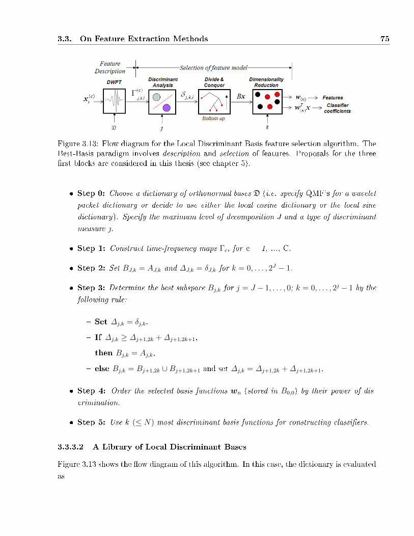
3.3. On Feature Extraction Methods 75
Figure 3.13: Flow diagram for the Local Discriminant Basis feature selection algorithm. TheBest-Basis paradigm involves description and selection of features. Proposals for the three�rst blocks are considered in this thesis (see chapter 5).
� Step 0: Choose a dictionary of orthonormal bases D (i.e. specify QMF's for a wavelet
packet dictionary or decide to use either the local cosine dictionary or the local sine
dictionary). Specify the maximum level of decomposition J and a type of discriminant
measure .
� Step 1: Construct time-frequency maps Γc, for c = 1, ..., C.
� Step 2: Set BJ,k = AJ,k and ∆J,k = δJ,k for k = 0, . . . , 2J − 1.
� Step 3: Determine the best subspace Bj,k for j = J − 1, . . . , 0; k = 0, . . . , 2j − 1 by the
following rule:
� Set ∆j,k = δj,k.
� If ∆j,k ≥ ∆j+1,2k + ∆j+1,2k+1,
� then Bj,k = Aj,k,
� else Bj,k = Bj+1,2k ∪Bj+1,2k+1 and set ∆j,k = ∆j+1,2k + ∆j+1,2k+1.
� Step 4: Order the selected basis functions wn (stored in B0,0) by their power of dis-
crimination.
� Step 5: Use k (≤ N) most discriminant basis functions for constructing classi�ers.
3.3.3.2 A Library of Local Discriminant Bases
Figure 3.13 shows the �ow diagram of this algorithm. In this case, the dictionary is evaluated
as
76 Feature Extraction
δ (Bx) =k∑
n=1
δ(n), (3.89)
and the values δ(i) are arranged in decreasing order so as to ease the implementation of dimen-
sionality reduction, but the selection of k is not evident since the classi�cation performance
decreases dramatically as basis functions of small δ are added to B .
Considering the basis of large energy components to attain certain degree of compression
is a possibility, just as in the Best-Basis method. That is,
δ (Bx) =k∑
n=1
1(Γ(n) ≥ ρ
)δ(n), (3.90)
where Γ(n) = 1∑Cc=1Nc
∑Mi=1
∣∣∣wT
(n)xi
∣∣∣2 corresponds to the energy associated to w(n) which has
discrimination power δ(n).
The preceding algorithm can be easily extended to a library of orthonormal bases. Let
L = {D1, . . . ,DM} denote a library, for m = 1, 2, . . .M dictionaries. Every LDB taken from
Dm has associated a discriminant value δ(Bx) and . Let δm denote this value. Then, the
optimal dictionary, D∗ (associated to the �best� LDB), is chosen by determining the index
m which gives the maximum discriminant value. That is
D∗ = arg maxDm∈L
δm (3.91)
3.4 Feature Representation Tools
When looking for patterns in data, it is sometimes useful to observe the physical structures
associated to the coe�cients, by means of a graphical tool. Two methods for the representa-
tion of time-frequency information and clusters, respectively, are described below.
The �rst method determines the time-frequency properties from the reconstructed basis
functions and use them to indicate their support on the original signals. The basis functions
are easily reconstructed by setting their corresponding coe�cient cell as cj,k [l] = 1. The
second method is able to transform cluster data from a higher dimension, RN , to another
dimension easily observed by the user ( in 2D or 3D representation) so that he can have a
better representation of the separability of classes from the higher domain.

3.4. Feature Representation Tools 77
3.4.1 Time-frequency Support
Wavelet packet as well as local cosine basis functions are indexed by means of three parame-
ters (j, k, l) which are used as a reference to indicate their representation in the tree structure.
Albeit rather roughly, it can be shown that these parameters are also a way of coding the
signal properties that coe�cients are representing. These properties are 1) the center of
wiggles and main lobes of the wavelet shape (u), 2) the number of oscillations (ξ) and 3)
both uncertainties of these parameters (σn and σω, respectively), which serve to establish the
extension support of the basis function in the time-frequency plane.
The momentum and variance of wavelet functions can be determined by two expressions
equivalent to 3.9 and 3.11. That is,
u =1∥∥ψj,k,l
∥∥2
2n0∑n=0
n |ψj,k,l [n]|2 (3.92)
and,
σn =1∥∥ψj,k,l
∥∥2
2n0∑n=0
(n− u)2 |ψj,k,l [n]|2 , (3.93)
where , ‖·‖ denotes L2 norm. Likewise, the frequency parameters, ξ and σξ are obtained by
using the frequency variable ω, instead of the position variable n, and the Fourier transform
ψj,k,l instead of ψj,k,l.
These equations are crucial in the parametrization of signal structures and di�erent arti-
facts. Since the triplet γ = (j, k, l) indexes all the coe�cients in the wavelet-packet tree, their
associated basis functions ψγ [n] can be reconstructed by setting the corresponding node cell
cj,k [l] to one (with the remaining elements set to zero) and using the inverse DWPT (IDWT).
Therefore, γ can also be seen as a way for parametrizing these structure patterns.
The index j denotes bandwidth resolution of the basis ψγ [n] in the time-frequency plane,
whereas k and l denote center frequency and center time position (u = 2jl), respectively. In
general, the greater j is the better the frequency resolution (low σξ), and vice-versa (the
lower j is the better the time resolution). Since the successive down-sampling operations
cause aliasing and alter the frequency content extracted with the �lter sequences h and g ,
the indexation of k must be corrected permuting it with the �Gray code�. (Wickerhauser
1995).
78 Feature Extraction
3.4.2 Visualization of Data in RN
When evaluating the classi�cation accuracy of features and/or contrasting their discriminant
values, it is sometimes useful to display the provision of samples. One way to take a quick
look at this provision is by plotting scatter maps but this form of interpretation becomes
more di�cult to observe and interpret above the 3rd dimension. A way for representing
clusters of several dimensions in a 2D (or 3D) dimension preserving most of the important
structure is provided by the Sammon maps (1969).
More precisely, assume that we have M vectors corresponding to input data in an N-
space, xi ∈ RN for i = 1, ..., M, and, corresponding to these, M output vectors in a D-space,
yi ∈ RD, are de�ned. Here, D can be either 2 or 3 depending on a bi-dimensional or three-
dimensional representation, respectively. The following non-linear mapping algorithm (NLM)
minimizes an error ε that represents how well the points in RD �t the original points in RN ,
and uses a steepest descent procedure to adjust yi accordingly.
Let d(f)ij be an Euclidean distance measure between two vectors
[f i,f j
]∈ Rq, de�ned as
d(f)ij =
√√√√ q∑k=1
(fik − fjk)2,
where fik is used to denote every single element from the i-th vector and its k-th dimension
(here, p = 1, . . . ,M ; and q = N for the input x and q = D for the output y).
First, an initial guess for the outputs ypq (0) in D-space must be provided. Although these
vectors could be �xed randomly, it is preferable to project the inputs x orthogonally onto a
D-space spanned by the D original coordinates of largest variance for a fast convergence of
the algorithm. Then, inter-point distance measurements between d(x)ij and d(y)
ij are compared
to reduce ε and modify yi accordingly in each iteration. Let ε (t) de�ne this error calculated
after the t-th iteration
ε (t) =1
c
M∑i 6=j
[d
(x)ij − d
(y)ij (t)
]2
d(x)ij
. (3.94)
where, c =∑M
i 6=j d(x)ij .
In order to modify ypq at step t +1 and minimize 3.94, the output is recalculated as
ypq (t+ 1) = ypq (t)− α∆pq (t) (3.95)
where

3.5. Conclusions 79
Object Conventional concept �Library� concept
Coordinate Standard Euclidean Basis (STD) Wavelet Packet Bases (WPT)System Fourier Basis (FT,STFT) Local Trigonometric Bases (CPT)
Compression Karhunen-Loève Basis (PCA) Joint Best-Basis (BB)Classi�cation Linear Discriminant Analysis (LDA) Local Discriminant Basis (LDB)
Table 3.1: Summary of the correspondences between the conventional concepts and the newconcepts based on the Best-Basis paradigm (or �library� of bases) reviewed or discussed inthis chapter.
∆pq (t) =∂ε(t)
∂ypq (t)/
∣∣∣∣∣ ∂2ε(t)
∂ypq (t)2
∣∣∣∣∣ (3.96)
and α is a factor (normally con�gured empirically to 0.3 or 0.4, depending on the desired
convergence). The partial derivatives are given by
∂ε
∂ypq= −2
c
N∑j=1j 6=p
[d
(x)pj − d
(y)pj
d(x)pj d
(y)p,j
](ypq − yjq) (3.97)
and
∂2ε
∂y2pq
= −2
c
N∑j=1j 6=p
1
d(x)pj d
(y)pj
[(d
(x)pj − d
(y)pj
)− (ypq − yjq)2
d(y)pj
(1 +
d(x)pj − d
(y)pj
d(y)pj
)]. (3.98)
These calculations can be iterated up to a certain value of t, or until ε converges at
some desired threshold. The error value ε (T ) at the end of the process can be a reference
indicating the accuracy of the new representation. Although the Sammon method can also
be regarded as a feature extraction method, given to the fact that the dimensionality of input
data is also reduced, the minimization process is more related to the �goodness of �t� of the
representation in the new domain. For this reason it is very used as a display tool rather
than a pattern recognition technique.
3.5 Conclusions
In this chapter, several methods related to feature extraction using a library of bases have
been reviewed. Table 3.1 summarizes the correspondences discussed in this chapter. The

80 Feature Extraction
philosophy, also referred to as the Best-Basis paradigm, consists in selecting the best co-
ordinate system of representation from a dictionary of basis functions, which contains the
words necessary to describe to describe the problem at hand. Wavelet-packet dictionaries
(including wavelet bases) and trigonometric bases are the main constituents of this library.
These bases are able to capture local features in data up to a certain accuracy, and provide
an interpretation of signal irregularities much closer to the physical structures. By combining
them with discriminant analysis, their degree of similarity (or di�erence) in relation to di�er-
ent signal classes can also be evaluated. As such, they should provide better understanding
and insight into underlying phenomena compared to other conventional techniques.
The uni�cation of the statistical and the library-based syntactic approach is intended
to solve di�cult problems in image analysis and signal processing applications in the near
future, as the library concept is vastly more e�cient compared with strategies con�ned to
a single basis. In addition, such strategy allow us to �nd small feature sets that reduce the
computational problems of many classi�cation methods as well as improving their accuracy.
Chapter 4
Classi�ers
4.1 Introduction
Information can come in the form of di�erent objects: statistical data, measurements, sensor
signals or random variables; and the the classi�cation problem consists in predicting which
class each object is in.
This chapter looks at supervised classi�ers. The word 'supervised' means that the object
class is known and used for two operations: 1) the con�guration of the algorithm; and 2)
the estimation of accuracy in the detection of classes. The �rst stage is often referred to as
the �learning stage� (or training) and depends on the framework of the chosen classi�cation
method. The second stage, however, is inherent to all supervised classi�ers and estimates the
e�ciency that the con�gured classi�er would obtain in a real experiment of unknown classes.
For this reason, this operation is referred to as the �validation stage�.
A more formal de�nition of a classi�er is provided in the next section, where the estimation
of accuracy will be the main topic of discussion. Traditionally, the Bayes probability concept
has been the reference tool for building classi�ers (Bayes 1764). The linear methods, such
as the naive Bayes classi�er, the LDA-based method or the k -Nearest Neighbor are some
examples of these. They are described in section 4.3.
In contrast, the more �exotic� classi�ers, such as Classi�cation-and-Regression-Trees (CART)
or Neural-Networks (NN), base their decision rules on very complex networks of nonlinear
functions and will not be considered in this thesis. The Learning Vector Quantization method
(Kohonen et al. 1992) is a special case, since its performance lies in the middle of both ap-
proaches, making it particularly interesting for the �sh experiments of this work. This method
is described in section 4.4.
81
82 Classi�ers
4.2 Problem Formulation
Let X be the space of all possible measurement vectors x ∈ RT and assume that each
measurement x ⊂ X can fall into one of C categories, say (1, . . . , C) classes. A systematic
way of predicting class membership is a rule that assigns a class to every measurement vector.
Thus,
De�nition. 4.1a A classi�er (or mapping rule) is a function, r (x), de�ned on X so that
for every x ⊂ X, a class c is assigned. r(x )=c for c ∈ {1, . . . , C}.
r(x) = c, for c ∈ {1, . . . , C} (4.1)
This systematic de�nition di�er from others in which classi�ers are seen as disjoint subsets
of the space X.
De�nition. 4.1b Let Ac de�ne the subset from X in which x falls into category c
Ac = {x; r(x) = c} , (4.2)
where {A1, . . . ,AC} are disjoint and X = ∪Ac. A classi�er is a partition of X into C
disjoint subsets, A1, . . . ,Ac, X = ∪Ac such that for every x ⊂ Ac the predicted class is c.
In principle, this framework is optimal for an idealistic precise estimation of accuracy.
However, one of the main problems found when constructing real classi�ers is that very often
we are limited to reduced sets with little prospect of obtaining large classi�ed samples. In the
systematic case, the knowledge for constructing classi�ers is based on past experience which
is summarized by a learning sample containing the measurement vectors X = (x1, . . . ,xN),
where X ∈ X, and its associated classi�cation (c1, . . . , cN). That is,
L = {(x1, c1) , . . . , (xN , cN)} , (4.3)
where L denotes learning set.
4.2.1 Estimation of Accuracy
Given a classi�er r, in order to estimate its accuracy R(r) will be de�ned as the true mis-
classi�cation rate. A more formal de�nition can be given to this parameter by looking for
an answer to the question: What is truth and how can it be estimated? This value can be
conceptualized in the following manner:
4.2. Problem Formulation 83
�Using a sample taken in an experiment from a real distribution, construct
a classi�er. Then, draw another sample from the same population as the orig-
inal sample was drawn from, and use the classi�er to predict classi�cation by
estimating the misclassi�ed proportion�
To make a more precise de�nition of the preceding concept a probability model is needed.
Assume that a sample set L has been taken from the relevant population X × C . Since this
sample comes from the relevant population, the couple (x, c) allows the partitioning of Lin di�erent class disjoint subsets of the form L = ∪Aj. Let P (A, c) be a probability that
an entity x taken at random from L belongs to class c. The interpretation of P (A, c) is
that a case x drawn at random from the relevant population has probability P (A, c) that
its measurement vector is in A and its associated class is c. The estimation of P (A, c) foreach one of the classes serves to construct r(x ). Then, take another sample of measurement
vectors (xs, cs), xs ∈ X, cs ∈ C from the relevant population X × C , so as to ensure this
new set is independent of L. And �nally, determine the misclassi�ed proportion as
R(r) = P (r (xs) 6= cs) (4.4)
Such estimation of the misclassi�cation error is optimal as long as the set L is represen-
tative of the true population in X. In practice, however, samples are habitually scarce and Lis often used both to construct r(x ) and to estimate R(r). Therefore, we use R(r) to refer to
this internal estimate instead of R(r), or the complement 1− R(r) to denote the proportion
of correct classi�cations.
In general, three types of internal estimate are of particular interest for the evaluation of
classi�cation accuracy. The re-substitution estimate (Smith 1947) is commonly used as the
�rst reference, but is the least accurate. This estimate uses all of the elements in L both to
construct the classi�er r (x) and to compute R (r). To put it into an equation form
R(r) =1
N
N∑i=1
1 (r (xi) 6= ci) (4.5)
where 1(·) de�nes the indicator function to be one if the statement inside the parentheses is
true, and zero otherwise.
The second estimate is known as the hold-out (or split-sample) method. Here, the cases
in L are divided into two subsets: Lt (training set) and Ls (validation or testing set). Only
the cases in Lt are used to construct r, whereas the elements in Ls serve to estimate R(r).
Assuming Ns cases in Ls, the holdout estimate, Rho(r), is calculated as

84 Classi�ers
Rho (r) =1
Ns
Ns∑i=1
1 (r (xi) 6= ci) (4.6)
In this method care needs to be taken so that the cases in Ls can be both independent of Ltand drawn from a representative distribution. A common way to ensure this is to take Lsas 1/3 of the cases in L at random, although there is no theoretical formalism to justify this
1/3, 2/3 split.
For smaller sample sizes, another method known as K-fold cross-validation is preferred
(Stone 1974). Here, the cases in L are randomly divided into K subsets of as equal size as
possible. Let Lk denote all these subsets, where k = 1, ..., K and assume that a classi�er for
each set rk is constructed using the sample set L � Lk. This set contains the cases in L that
are not included in Lk. Since none of the cases in Lk are used in the construction of rk, a
holdout estimate can be obtained for each classi�er by means of
Rcv (r) =1
K
K∑k=1
Rho (rk) (4.7)
where
Rho (rk) =1
Nk
Nk∑i=1
1 (rk (xi) 6= ci) . (4.8)
The K -fold cross-validation method is also known as the leave-one-out estimate (Lachen-
bruch 1965) when K = N. Here, only one element from L is set aside and the remaining N -
1 elements are used to construct rk. Then using each n-th case in Eq. 4.7 allows an estimate
R(r) to be determined.
In general, since all classi�cation methods attempt to minimize R(r), which is merely an
estimation of the true R(r), the true accuracy will di�er from that of simulation results. In
this sense, the re-substitution estimate is not practical because it produces very optimistic
results. To understand this, assume that r(x ) is de�ned by the partitions, A1, ...,AC con-
structed from all elements in L and the same elements are used to calculate R (r). Then,
R (r) = 0, but if new values of x di�erent from (x1, ...,xN) are assigned arbitrarily to one or
the other Ac, it is hard to believe that R(r) is anywhere near zero.
K -fold cross-validation is widely accepted as a good estimator and occasionally sub-
stituted for the split-sample approach to reduce processing time when large data sets are
available (Goutte 1997). Additionally, obtaining a mean value of Rho (r) (or Rcv (r)), instead
of a single estimate, is preferable to avoid accuracy bias and variance. So, habitually, both
4.2. Problem Formulation 85
hold-out and k -fold cross-validation are repeated several times for di�erent combinations of
Lt and Ls, averaging all results at the end of the process.
Another way to tackle the problem of bias in reduced data sets is to use the bootstrap
method. In this case, the size of the original set L is increased deliberately by repeating some
of the elements in L randomly, or creating new ones from changing some of its attributes
whenever possible (Efron 1983). However, it has been reported that this operation may be
very optimistic for certain classi�ers (Breiman et al. 1984, Kohavi 1995).
In practice, most frequently other factors such as processing speed, time and cost of
analysis in�uence decisions regarding this estimate. A summary and extensive bibliography
concerning this topic can be found in Toussaint (1974).
4.2.2 The Bayes Rule
The major guide used in the construction of classi�ers is the concept of the Bayes rule. This
concept states that when data is drawn from a probability distribution P (A, c), then the formof the most accurate classi�er can be given in terms of P (A, c). The rule that is inferred
from this de�nition is called the Bayes rule and is denoted as rB (x).
More precisely, let us assume that a sample (x ,c), x ∈ X, c ∈ C, is drawn from
the probability distribution P (A, c) (we changed xsinto x for notation convenience), i.e.,
P (x ∈ A, c = C) = P (A, c). Then, rB (x) will be a Bayes rule if for any other classi�er
r(x ),
P (rB (x) 6= c) ≤ P (r (x) 6= c) . (4.9)
and the probability value
RB = P (rB (x) 6= c) . (4.10)
is known as the Bayes misclassi�cation rate.
In general, the Bayes rule, rB (x), is obtained from the distribution P (A, c) assuming thatprior class probabilities πc are known. More precisely, if πc = P (c) for c ∈ C, the probabilitydistribution of the cth class measurement vectors is of the form P (A|c) = P (A, c) /πc andis obtained from the density fc (x),
P (A, c) =
ˆAfc (x) dx. (4.11)
Then, for A ⊂ X the Bayes rule is de�ned as
86 Classi�ers
rB (x) = c on Ac ={x; fc (x) πc = max
i(f iπi)
}. (4.12)
Under the assumption of (4.11), Breinman et al (1984) demonstrated that for any other
classi�er r,
P (r (x) = c) ≤ P (rB (x) = c) =
ˆmaxc
[fc (x) πc] dx, (4.13)
Therefore, the Bayes misclassi�cation rate is
RB = 1−ˆ
maxc
(f cπc) dx. (4.14)
The Bayes rule is also known as the maximum a-posteriori likelihood rule. That is, classify
x as that c for which fc (x)πc is maximum. Since RB is the minimum misclassi�cation rate
attainable, knowing the class distribution is useful in order to generate simulated data and
to compare the accuracy of di�erent classi�ers. However, neither πc nor fc (x) are known in
practice. The value πc can be assumed as the proportion of class c cases in L or supplied
through other knowledge of data, but �nding fc (x) is considered the major problem in
the development of classi�ers. In the following sections we explain how some classi�cation
methods address this problem.
4.3 Bayes Classi�ers
In general, a Bayes classi�er is a single probabilistic classi�er constructed from the Bayes
theorem. Such a classi�er, attempts to converge to the Bayes rule, using a very simple
probabilistic model of fc (x) that is calculated from the learning sample L. The most commonway of doing this consists in taking P (A, c) as the density estimator of class c in the form
of P (A, c) = P (A|c) πc.
4.3.1 Joint and Naive Classi�ers
Let X = {xi, ci} denote the input data set, where each vector xi ∈ RT is associated to class
ci, and i = 1, . . . , N . Assume that each class, c = 1, . . . , C, has a total of Nc samples, so
that the proportion of class c is πc = Nc/N . A Bayes classi�er is constructed by using a
learning set, Lt, and calculating the probability P ({x (1) , . . . , x (T )} |c) as the proportion of
cases in class c that (x (1) , . . . , x (T )) is repeated. Then, to predict the unknown class of a
new sample q = (x (1) , . . . , x (T )), simply choose the label containing the most records of q .
That is,
4.3. Bayes Classi�ers 87
rB (q) = arg maxc
(P (q (1) = x (1) , . . . , q (T ) = x (T ) |c) πc) . (4.15)
Very often, this rule is referred to as the Joint Bayes classi�er. In order to supervise the
process, q is taken from the testing set Ls. Since its true class is known, the misclassi�cationaccuracy RB can be estimated with some of the previous validation techniques exposed in
section 4.2.1.
Originally, the Bayes rule 4.15 was designed for categorical variables. In this case, each
attribute in q is limited to only a few di�erent values (say two or three, depending on the
application case). For real numbers, however, if the full vector does not match any of the
training set, then P(q |c) = 0 for all c and the assigned class is either unknown or chosen at
random.
This situation can be avoided partially if, instead of P ({q (1) , . . . , q (T )} |c), we use∏Ti=1 P (q (i) = x (i) |c). This last de�nition is known as the Naive Bayes classi�er since it
makes strong assumptions of independence between attributes. However, for a considerable
number of attributes this product tends to under�ow, so the preferred version of the Naive
classi�er introduces logs to the mapping rule such as
rB (q) = arg maxc
(lnπc +
T∑t=1
lnP (q (t) = x (t) |c)
). (4.16)
Of course, the Joint Bayes classi�er can also be implemented under real-valued inputs, but
it is necessary to discretize the attributes of x beforehand so that the distribution P(q |c)
can be calculated. Several choices are available depending on assumptions regarding the
structure of data. Methods such as �xed width interval, 1R or ChiMerge - among others; are
included in many statical software packages (Bishop 1995).
4.3.2 LDA-Based Classi�ers
Classi�ers based on linear discriminant analysis determine P(x |c) on the assumption of
Normal distribution of multivariate data, which is characterized by the common pooled co-
variance matrix Σ =∑C
c=1 πcΣc, and whose classes are separated by class mean vectors {µc}.As usual, this information is obtained by means of a training sample Lt in order to construct
the classi�er, whereas the remaining set Ls is used for validation. The Bayes rule
rB (q) = arg maxc
(ln πc + µTc Σ−1q − 1
2µTc Σ−1µc
), (4.17)
determines the class of the objects of this set and the misclassi�cation error RB establishes
its accuracy.
88 Classi�ers
In general, this version of LDA is widely accepted and used without regard to lack of
normality. It can not handle categorical variables since linear distribution are considered in
the prediction of x . However, when more than two classes come into play distributions of
data are di�cult to interpret.
4.3.3 k-Nearest Neighbor (k-NN)
Perhaps, the most straightforward classi�er in machine learning is the Nearest Neighbor
classi�er (Fix and Hodges 1951). This method develops the classi�cation procedure in a very
simple and intuitive way: it determines the nearest neighbors to the item being classi�ed and
assigns the most represented class among them. The examples from the learning set must
always be available in memory. Thus in this approach, learning means memorizing examples.
For this reason, it is sometimes referred as Memory-based classi�cation.
As usual, we have an input set L of labeled samples, xi ∈ RT and class ci ∈ C, which is
divided into a training set Lt and a testing set Ls. The goal is to classify an example q , in
Ls. Therefore, for each xi ∈ Lt we calculate the distances
d (q,xi) =∑t∈T
δ (q [t] , x [t])i (4.18)
where δ (q,x) de�ne some metric that serves to select the k nearest neighbors. There are
a large range of possibilities for distance metrics that can be used in many classi�cation
methods. A basic version for continuous and discrete attributes would be:
δ (q, xi) =
0, t discrete and u = xi
1, t discrete and u 6= xi
|u− xi| , t continuous
(4.19)
This is a special case of the Minkowski Distance metric, also known as the Manhattan
distance or the 1-norm (L1). The general formula for such distance is
dp (q,xi) =
(∑t∈T
|q [t]− xi [t]|p) 1
p
, (4.20)
where, if p=2 we have the Euclidean distance. In general, p is selected depending on knowl-
edge of data and the Euclidean distance value is adopted when this is unknown. Other
possibilities for such measures exist depending on the magnitudes that have to be handled
(Baseville 1989, McLachlan 1992).
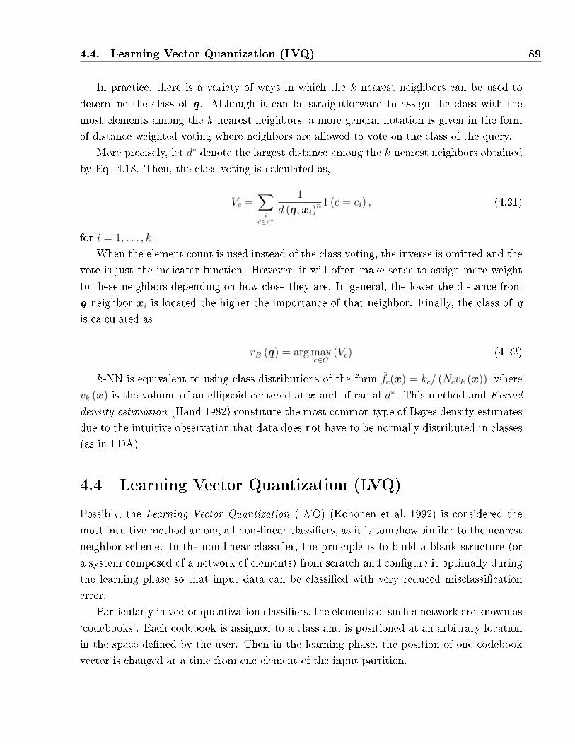
4.4. Learning Vector Quantization (LVQ) 89
In practice, there is a variety of ways in which the k nearest neighbors can be used to
determine the class of q . Although it can be straightforward to assign the class with the
most elements among the k nearest neighbors, a more general notation is given in the form
of distance weighted voting where neighbors are allowed to vote on the class of the query.
More precisely, let d∗ denote the largest distance among the k nearest neighbors obtained
by Eq. 4.18. Then, the class voting is calculated as,
Vc =∑i
d≤d∗
1
d (q,xi)n1 (c = ci) , (4.21)
for i = 1, . . . , k.
When the element count is used instead of the class voting, the inverse is omitted and the
vote is just the indicator function. However, it will often make sense to assign more weight
to these neighbors depending on how close they are. In general, the lower the distance from
q neighbor xi is located the higher the importance of that neighbor. Finally, the class of q
is calculated as
rB (q) = arg maxc∈C
(Vc) (4.22)
k -NN is equivalent to using class distributions of the form fc(x) = kc/ (Ncvk (x)), where
vk (x) is the volume of an ellipsoid centered at x and of radial d∗. This method and Kernel
density estimation (Hand 1982) constitute the most common type of Bayes density estimates
due to the intuitive observation that data does not have to be normally distributed in classes
(as in LDA).
4.4 Learning Vector Quantization (LVQ)
Possibly, the Learning Vector Quantization (LVQ) (Kohonen et al. 1992) is considered the
most intuitive method among all non-linear classi�ers, as it is somehow similar to the nearest
neighbor scheme. In the non-linear classi�er, the principle is to build a blank structure (or
a system composed of a network of elements) from scratch and con�gure it optimally during
the learning phase so that input data can be classi�ed with very reduced misclassi�cation
error.
Particularly in vector quantization classi�ers, the elements of such a network are known as
`codebooks'. Each codebook is assigned to a class and is positioned at an arbitrary location
in the space de�ned by the user. Then in the learning phase, the position of one codebook
vector is changed at a time from one element of the input partition.

90 Classi�ers
As usual, the elements come from the learning set Lt. When the training stage is com-
pleted new elements, now coming from the testing set Ls are classi�ed to determine the
identi�cation accuracy. In this case, however, the class is decided upon that of the closest
codebook vectors, and not directly upon the elements of the learning set.
4.4.1 LVQ algorithms
Let us assume that a certain number of codebook vectors, denoted bymi, are placed into the
same space of input data, wheremi ∈ RT . In general, several codebook vectors are assigned
to each class, and the input x is then decided to belong to the class ci ∈ [1, C) the nearest
mi belongs to. Let
r (q) = arg minci‖x−mi‖ , (4.23)
de�ne the nearestmi to x , denoted bymc. The valuesmi that approximately minimize the
misclassi�cation error of r(x ) can be found asymptotically in one of the following learning
processes.
4.4.1.1 The LVQ1
Let x(n) be an input sample from the learning set, and let mc(n) represent sequences of
mc in the discrete-time domain. Starting with properly de�ned initial values, the following
equations de�ne the LVQ learning algorithm which has the e�ect of dividing up the input
space in di�erent class groups:
mc (n+ 1) = mc (n) + α (n) [x (n)−mc (n)]
if x and mc belongs to the same class,
mc (n+ 1) = mc (n)− α (n) [x (n)−mc (n)] (4.24)
if x and mc belongs to the di�erent classes,
mi (n+ 1) = mi (n) for i 6= c
This algorithm corresponds to the most simple version of LVQ classi�er. Here, 0 < α(n) <
1 is known as the learning parameter, and α (t) may be constant or decrease monotonically
with n. In this version of LVQ, it is preferable to start with a value of α smaller than 0.1
(see subsection 4.4.1.5).
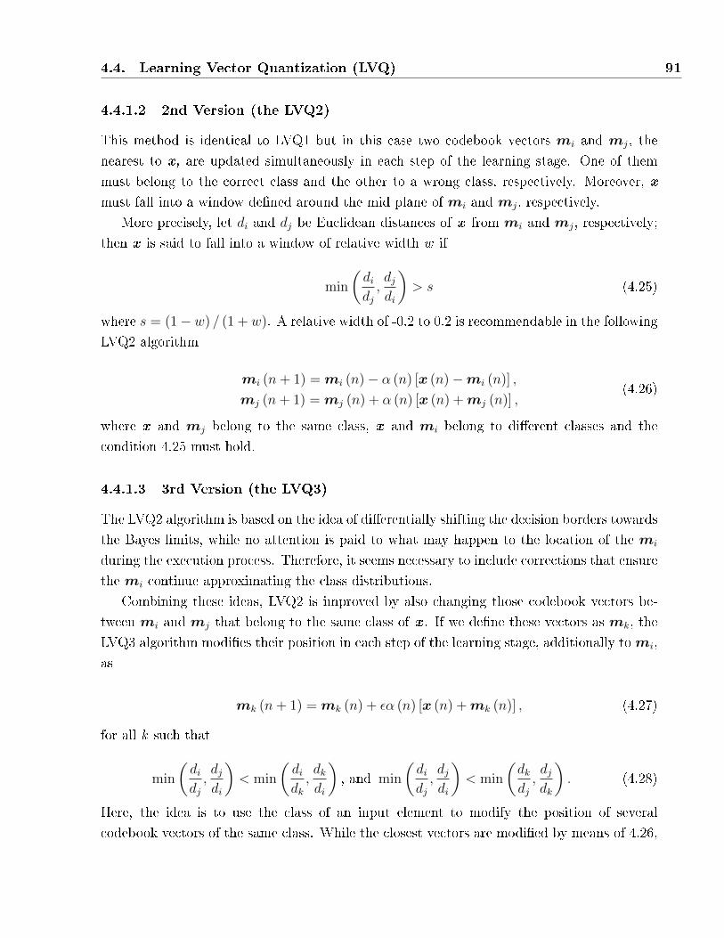
4.4. Learning Vector Quantization (LVQ) 91
4.4.1.2 2nd Version (the LVQ2)
This method is identical to LVQ1 but in this case two codebook vectors mi and mj, the
nearest to x, are updated simultaneously in each step of the learning stage. One of them
must belong to the correct class and the other to a wrong class, respectively. Moreover, x
must fall into a window de�ned around the mid plane of mi and mj, respectively.
More precisely, let di and dj be Euclidean distances of x from mi and mj, respectively;
then x is said to fall into a window of relative width w if
min
(didj,djdi
)> s (4.25)
where s = (1− w) / (1 + w). A relative width of -0.2 to 0.2 is recommendable in the following
LVQ2 algorithm
mi (n+ 1) = mi (n)− α (n) [x (n)−mi (n)] ,
mj (n+ 1) = mj (n) + α (n) [x (n) +mj (n)] ,(4.26)
where x and mj belong to the same class, x and mi belong to di�erent classes and the
condition 4.25 must hold.
4.4.1.3 3rd Version (the LVQ3)
The LVQ2 algorithm is based on the idea of di�erentially shifting the decision borders towards
the Bayes limits, while no attention is paid to what may happen to the location of the mi
during the execution process. Therefore, it seems necessary to include corrections that ensure
the mi continue approximating the class distributions.
Combining these ideas, LVQ2 is improved by also changing those codebook vectors be-
tween mi and mj that belong to the same class of x . If we de�ne these vectors as mk, the
LVQ3 algorithm modi�es their position in each step of the learning stage, additionally tomi,
as
mk (n+ 1) = mk (n) + εα (n) [x (n) +mk (n)] , (4.27)
for all k such that
min
(didj,djdi
)< min
(didk,dkdi
), and min
(didj,djdi
)< min
(dkdj,djdk
). (4.28)
Here, the idea is to use the class of an input element to modify the position of several
codebook vectors of the same class. While the closest vectors are modi�ed by means of 4.26,
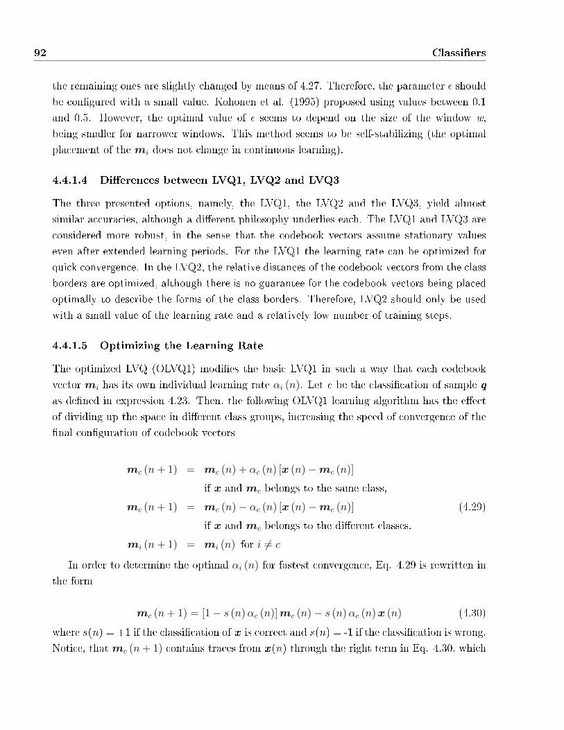
92 Classi�ers
the remaining ones are slightly changed by means of 4.27. Therefore, the parameter ε should
be con�gured with a small value. Kohonen et al. (1995) proposed using values between 0.1
and 0.5. However, the optimal value of ε seems to depend on the size of the window w,
being smaller for narrower windows. This method seems to be self-stabilizing (the optimal
placement of the mi does not change in continuous learning).
4.4.1.4 Di�erences between LVQ1, LVQ2 and LVQ3
The three presented options, namely, the LVQ1, the LVQ2 and the LVQ3, yield almost
similar accuracies, although a di�erent philosophy underlies each. The LVQ1 and LVQ3 are
considered more robust, in the sense that the codebook vectors assume stationary values
even after extended learning periods. For the LVQ1 the learning rate can be optimized for
quick convergence. In the LVQ2, the relative distances of the codebook vectors from the class
borders are optimized, although there is no guarantee for the codebook vectors being placed
optimally to describe the forms of the class borders. Therefore, LVQ2 should only be used
with a small value of the learning rate and a relatively low number of training steps.
4.4.1.5 Optimizing the Learning Rate
The optimized LVQ (OLVQ1) modi�es the basic LVQ1 in such a way that each codebook
vector mi has its own individual learning rate αi (n). Let c be the classi�cation of sample q
as de�ned in expression 4.23. Then, the following OLVQ1 learning algorithm has the e�ect
of dividing up the space in di�erent class groups, increasing the speed of convergence of the
�nal con�guration of codebook vectors
mc (n+ 1) = mc (n) + αc (n) [x (n)−mc (n)]
if x and mc belongs to the same class,
mc (n+ 1) = mc (n)− αc (n) [x (n)−mc (n)] (4.29)
if x and mc belongs to the di�erent classes,
mi (n+ 1) = mi (n) for i 6= c
In order to determine the optimal αi (n) for fastest convergence, Eq. 4.29 is rewritten in
the form
mc (n+ 1) = [1− s (n)αc (n)]mc (n)− s (n)αc (n)x (n) (4.30)
where s(n) = +1 if the classi�cation of x is correct and s(n) = -1 if the classi�cation is wrong.
Notice, thatmc (n+ 1) contains traces from x (n) through the right term in Eq. 4.30, which
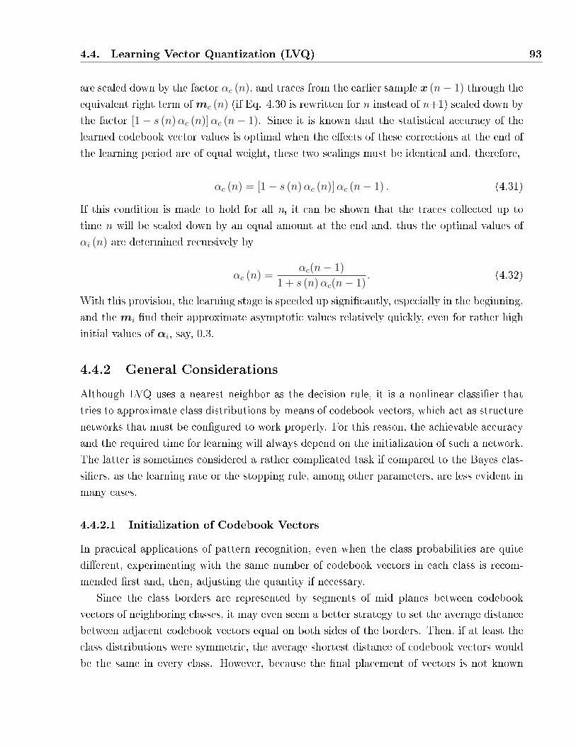
4.4. Learning Vector Quantization (LVQ) 93
are scaled down by the factor αc (n), and traces from the earlier sample x (n− 1) through the
equivalent right term ofmc (n) (if Eq. 4.30 is rewritten for n instead of n+1) scaled down by
the factor [1− s (n)αc (n)]αc (n− 1). Since it is known that the statistical accuracy of the
learned codebook vector values is optimal when the e�ects of these corrections at the end of
the learning period are of equal weight, these two scalings must be identical and, therefore,
αc (n) = [1− s (n)αc (n)]αc (n− 1) . (4.31)
If this condition is made to hold for all n, it can be shown that the traces collected up to
time n will be scaled down by an equal amount at the end and, thus the optimal values of
αi (n) are determined recursively by
αc (n) =αc(n− 1)
1 + s (n)αc(n− 1). (4.32)
With this provision, the learning stage is speeded up signi�cantly, especially in the beginning,
and the mi �nd their approximate asymptotic values relatively quickly, even for rather high
initial values of αi, say, 0.3.
4.4.2 General Considerations
Although LVQ uses a nearest neighbor as the decision rule, it is a nonlinear classi�er that
tries to approximate class distributions by means of codebook vectors, which act as structure
networks that must be con�gured to work properly. For this reason, the achievable accuracy
and the required time for learning will always depend on the initialization of such a network.
The latter is sometimes considered a rather complicated task if compared to the Bayes clas-
si�ers, as the learning rate or the stopping rule, among other parameters, are less evident in
many cases.
4.4.2.1 Initialization of Codebook Vectors
In practical applications of pattern recognition, even when the class probabilities are quite
di�erent, experimenting with the same number of codebook vectors in each class is recom-
mended �rst and, then, adjusting the quantity if necessary.
Since the class borders are represented by segments of mid planes between codebook
vectors of neighboring classes, it may even seem a better strategy to set the average distance
between adjacent codebook vectors equal on both sides of the borders. Then, if at least the
class distributions were symmetric, the average shortest distance of codebook vectors would
be the same in every class. However, because the �nal placement of vectors is not known

94 Classi�ers
until the end of the process, the optimal number of vectors for every class and thus their
distances cannot be determined before that. Therefore, the assignment of codebook vectors
to the various classes can only be made iteratively.
Once the number of codebook vectors has been �xed, for their initial values one can use
real values from samples in the training data set picked up from their respective classes.
Since the codebook vectors should always remain inside their respective class domain, only
the values corresponding to correctly classi�ed elements can be accepted. A possible strategy
may be to use some linear classi�er (i.e the k -NN) for one tentative sample against all the
other samples (by the leave-one-out method) in the training set and, then, accept this sample
as codebook vector if this classi�cation corresponds to the class of the sample.
It is also recommended to additionally compute the medians of the shortest distances
between the initial codebook vectors of each class. Then, if the distances turn out to be very
di�erent for the di�erent classes, new codebook vectors may be added to or old ones deleted
from the deviating classes. In general, for a satisfactory approximation of the borders the
medians of the shortest distances between the codebook vectors should be somewhat smaller
than the standard deviations of the input samples in all the respective classes.
4.4.2.2 Learning and Stopping Rule
When using LVQ to build a classi�er, it is recommended to start with the OLVQ1 in the
learning stage for fast convergence. Normally, its accepted asymptotic recognition accuracy
is achieved after completing a number of learning steps about 30 to 50 times the total number
of codebook vectors. In general, the OLVQ1 alone may be enough for practical applications.
However, in an attempt to improve recognition accuracy, one may continue the learning with
either the basic LVQ1, the LVQ2 or the LVQ3, using a low initial value of the learning rate.
However, if the learning continues beyond an optimal network con�guration, the algorithm
loses the ability to generalize and, therefore, accuracy starts to decrease. It is, therefore
convenient to stop after a certain number of steps. In the LVQ1, LVQ2 and LVQ3, the
number of steps can range from 50 to 200 times the total number of codebook vectors.
However, such a stopping rule can only be found by experience, and it also depends on the
input data.
4.5 Conclusions
Some algorithms for the identi�cation of classes and the validation of feature models have
been reviewed in this chapter. In general, class distributions can be characterized by their
4.5. Conclusions 95
extension area or their decision boundaries in the feature space.
Linear methods exploit the �rst strategy. In this case, estimated distributions depend
on the position of inputs from the learning set, and decision rules rely on the proximity
of the elements to be classi�ed to these inputs so, in general, the con�guration will not be
complex and the classi�cation algorithms have low computational cost. However, they lack
the capacity to �t to very complex distributions of data. In this case, it is much better to
use the second approach.
Although it may seem that the second group of classi�ers achieve high classi�cation rates,
a major problem is the lack of intuition to con�gure their learning stage so that the method
converges to an optimal solution. For example, in methods such as Neural-Networks, CART
or LVQ there is no single �rule-of-thumb� that speci�es the necessary number of layers and
perceptrons, the depth of the tree or the number of codebook vectors that are necessary for
the application (Breiman et al. 1984, Kohonen et al. 1995). In the context of this work, the
use of a representative coordinate feature system are aimed at reducing the complexity of
the classi�cation task.

Part III
Contributions
97

Chapter 5
On LDB-based Pattern Recognition
5.1 Introduction
Habitually, the process of looking structure patterns in data requires the extraction and val-
idation of the di�erent class features. Although the preprocessing tasks of �sh identi�cation
and aging di�er signi�cantly due to the nature of their data, the feature extraction and clas-
si�cation algorithms reviewed in previous chapters may be chosen for both the analysis of
contour irregularities and the intensity pro�le.
The Best-Basis paradigm and the LDB algorithm provide an interesting framework for
automating the selection of features in classi�cation tasks, as long as their limitations regard-
ing the reduction of dimensionality are solved. In particular, if we manage to �nd a reduced
vector presenting a clearly separated space distribution, not only will the classi�cation accu-
racy will improve considerably but also the computational cost will bene�t from the use of
very simple classi�cation methods.
Therefore, this chapter is dedicated to presenting our new LDB design, which addresses
three issues: the evaluation of coe�cients, the discriminant measures and the search algo-
rithm.
The �rst problem focuses on the evaluation of separability. In this sense, we believe that
evaluating probability distributions is more important than considering the amount of signal
energy. Figure 5.1 illustrates this problem, by means of two example distributions, which
assume two class Normal densities of equal variance but di�erent class mean. A coe�cient
may be selected on the basis of presenting high energy when its class distributions really
overlap each other, while another coe�cient may be discarded because of its low energy,
although it possess great separation capabilities.
Secondly, a mechanism for controlling the correlation between discriminant measurements
99
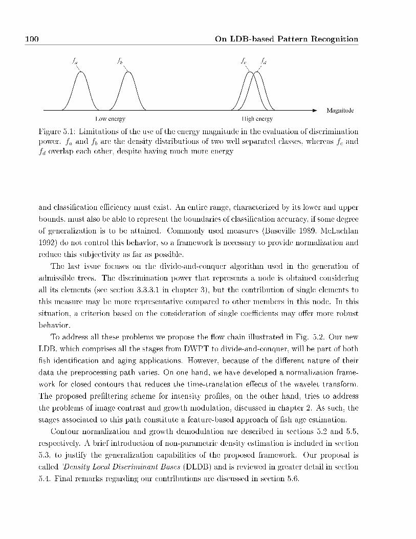
100 On LDB-based Pattern Recognition
Figure 5.1: Limitations of the use of the energy magnitude in the evaluation of discriminationpower. fa and fb are the density distributions of two well separated classes, whereas fc andfd overlap each other, despite having much more energy
and classi�cation e�ciency must exist. An entire range, characterized by its lower and upper
bounds, must also be able to represent the boundaries of classi�cation accuracy, if some degree
of generalization is to be attained. Commonly used measures (Baseville 1989, McLachlan
1992) do not control this behavior, so a framework is necessary to provide normalization and
reduce this subjectivity as far as possible.
The last issue focuses on the divide-and-conquer algorithm used in the generation of
admissible trees. The discrimination power that represents a node is obtained considering
all its elements (see section 3.3.3.1 in chapter 3), but the contribution of single elements to
this measure may be more representative compared to other members in this node. In this
situation, a criterion based on the consideration of single coe�cients may o�er more robust
behavior.
To address all these problems we propose the �ow chain illustrated in Fig. 5.2. Our new
LDB, which comprises all the stages from DWPT to divide-and-conquer, will be part of both
�sh identi�cation and aging applications. However, because of the di�erent nature of their
data the preprocessing path varies. On one hand, we have developed a normalization frame-
work for closed contours that reduces the time-translation e�ects of the wavelet transform.
The proposed pre�ltering scheme for intensity pro�les, on the other hand, tries to address
the problems of image contrast and growth modulation, discussed in chapter 2. As such, the
stages associated to this path constitute a feature-based approach of �sh age estimation.
Contour normalization and growth demodulation are described in sections 5.2 and 5.5,
respectively. A brief introduction of non-parametric density estimation is included in section
5.3, to justify the generalization capabilities of the proposed framework. Our proposal is
called 'Density Local Discriminant Bases (DLDB) and is reviewed in greater detail in section
5.4. Final remarks regarding our contributions are discussed in section 5.6.
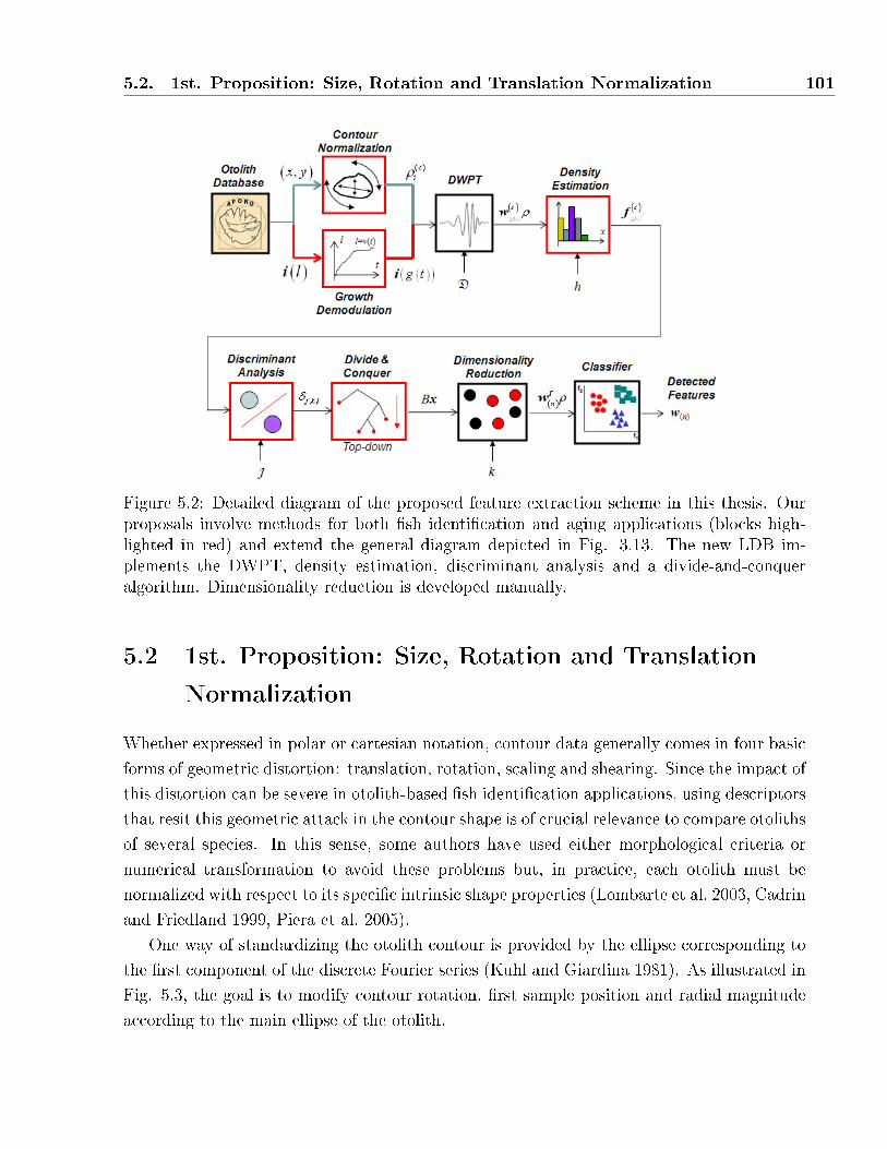
5.2. 1st. Proposition: Size, Rotation and Translation Normalization 101
Figure 5.2: Detailed diagram of the proposed feature extraction scheme in this thesis. Ourproposals involve methods for both �sh identi�cation and aging applications (blocks high-lighted in red) and extend the general diagram depicted in Fig. 3.13. The new LDB im-plements the DWPT, density estimation, discriminant analysis and a divide-and-conqueralgorithm. Dimensionality reduction is developed manually.
5.2 1st. Proposition: Size, Rotation and Translation
Normalization
Whether expressed in polar or cartesian notation, contour data generally comes in four basic
forms of geometric distortion: translation, rotation, scaling and shearing. Since the impact of
this distortion can be severe in otolith-based �sh identi�cation applications, using descriptors
that resit this geometric attack in the contour shape is of crucial relevance to compare otoliths
of several species. In this sense, some authors have used either morphological criteria or
numerical transformation to avoid these problems but, in practice, each otolith must be
normalized with respect to its speci�c intrinsic shape properties (Lombarte et al. 2003, Cadrin
and Friedland 1999, Piera et al. 2005).
One way of standardizing the otolith contour is provided by the ellipse corresponding to
the �rst component of the discrete Fourier series (Kuhl and Giardina 1981). As illustrated in
Fig. 5.3, the goal is to modify contour rotation, �rst sample position and radial magnitude
according to the main ellipse of the otolith.
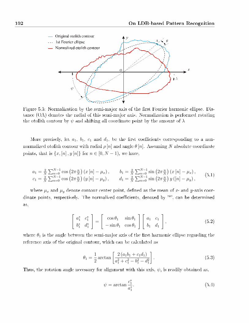
102 On LDB-based Pattern Recognition
Figure 5.3: Normalization by the semi-major axis of the �rst Fourier harmonic ellipse. Dis-tance (OA) denotes the radial of this semi-major axis. Normalization is performed rotatingthe otolith contour by ψ and shifting all coordinate point by the amount of λ
More precisely, let a1, b1, c1 and d1, be the �rst coe�cients corresponding to a non-
normalized otolith contour with radial ρ [n] and angle θ [n]. Assuming N absolute coordinate
points, that is {x, [n] , y [n]} for n ∈ [0, N − 1), we have,
a1 = 2N
∑N−1n=0 cos
(2π n
N
)(x [n]− µx) , b1 = 2
N
∑N−1n=0 sin
(2π n
N
)(x [n]− µx) ,
c1 = 2N
∑N−1n=0 cos
(2π n
N
)(y [n]− µy) , d1 = 2
N
∑N−1n=0 sin
(2π n
N
)y ([n]− µy) ,
(5.1)
where µx and µy denote contour center point, de�ned as the mean of x- and y-axis coor-
dinate points, respectively. The normalized coe�cients, denoted by '*', can be determined
as, [a∗1 c∗1b∗1 d∗1
]=
[cos θ1 sin θ1
− sin θ1 cos θ1
][a1 c1
b1 d1
], (5.2)
where θ1 is the angle between the semi-major axis of the �rst harmonic ellipse regarding the
reference axis of the original contour, which can be calculated as
θ1 =1
2arctan
[2 (a1b1 + c1d1)
a21 + c2
1 − b21 − d2
1
]. (5.3)
Thus, the rotation angle necessary for alignment with this axis, ψ, is readily obtained as,
ψ = arctanc∗1a∗1. (5.4)
5.3. Density Estimation for Local Feature Description 103
Full normalization is obtained by scaling the radials relatively to the otolith size and
shifting by λ, were λ = θ1N/2π denotes position of the �rst sample with respect to the
original reference expressed on a number-of-sample basis. These operations are in addition
to those of angle rotation. Therefore, full contour is characterized by the normalized contour
samples
ρN [n] =ρ [n− λ]
ρ0
(5.5)
and
θN [n] = θ [n− λ]− ψ, (5.6)
expressed on a polar coordinate system, and ρ0 = (a∗21 + b∗21 )1/2 corresponds to the radial of
the semi-major axis.
5.3 Density Estimation for Local Feature Description
Traditionally, two di�erent approaches for estimating distributions in data exist: nonpara-
metric and parametric. The focus of each other di�ers remarkably. In the latter, given a
family function, f(·|θ) such as the two-parameter Normal family N(µ, σ2) where θ = (µ, σ2),
the emphasis is on obtaining the best estimator, θ, of θ which makes f . In general, paramet-
ric approaches do not require large amounts of data but they do involve a lot of prior work
gathering previous expert knowledge and information in order to produce reliable templates.
The emphasis of nonparametric estimation, on the contrary, is on directly estimating a
version f of the true density function f from data, which thus eliminates the need for a
model speci�cation. Despite the large amount of data necessary, this approach is generally
very intuitive, �exible and often provides estimations close to true densities (Scott 1992).
5.3.1 Histograms
The most simple way to develop nonparametric estimation within LDB consists in build-
ing density histograms for each one of the di�erent basis functions in the wavelet tree.
The histogram is completely determined by the sample{x1, . . . , xNc
}and a choice of mesh
{tm,−∞ < m <∞}.Let Gm = [tm, tm+1) denote the m-th bin of �xed width h = tm+1 − tm for all m. A
density histogram uses building blocks of height 1/(nh) so that each block has an area equal
104 On LDB-based Pattern Recognition
to 1/n. Let vm denote the bin count of the m-th cell, that is, the number of samples falling
into Gm. Then, the estimated density functions at each point in the tree is de�ned as
f [x] =vmhNc
=1
hNc
Nc∑i=1
I[Gm) (xi) , (5.7)
where IA (x) = 1 if x ∈ A , and 0 otherwise.
Clearly, the usefulness of the estimation of f depends on an optimal choice of the bin
width h, very often referred to as the �smoothing� parameter since it controls the amount of
smoothness of the pro�le in f . The desire to compare di�erent estimators and to attempt
to identify the best one assumes the speci�cation of a criterion that can be optimized. Al-
though very simple ideas, such as the Sturges' number-of-bin rule (Sturges 1926), apply and
are con�gured in many software packages by default, data-based optimization methods try
to minimize the integrated square error (ISE) and/or its average value (MISE) which are
calculated estimating the bias and variance components. When the L2-norm is used, this
value is de�ned as
MISE =
ˆE[f − f
]2
dx. (5.8)
However, knowing the true density function f is considered to be one of the most di�cult
tasks a priori. In this sense, approximations are made assuming the existence of derivatives of
f and employing a variety of techniques known as cross-validation algorithms. Following this
norm, the asymptotic optimal width is de�ned as a function of the �rst derivative roughness
of f as
h∗ =
(6
φ (f ′)
)1/3
N−1/3, (5.9)
where φ denotes the roughness estimator adopted for the L2- norm of φ
φ (f ′) =
ˆf ′ (x)2 dx. (5.10)
and N is the total number of samples used in the construction of the histogram (Scott 1979,
Freedman and Diaconis 1981). With this estimator of the roughness and bin width, the
optimal asymptotic MISE (AMISE) is known to be
AMISE∗ = (3/4)2/3 φ (f ′)1/3N−2/3 (5.11)
5.3. Density Estimation for Local Feature Description 105
This result has led to the width of some standard distributions, such as the Normal case
with f = N (µ, σ2), being �xed. It can be shown that φ (f ′) = 1/ (4√πσ3)
1/3. Hence, from
Eq. 5.9 we obtain
h∗ =(24√πσ3/N
)1/3. (5.12)
This rule constitutes a reference for constructing histograms. One can �rst use the sample
standard deviation σ in (5.12) and estimate the Normal bin width as
hN ≈ 3.5σN−1/3, (5.13)
and then adapt it to more realistic distributions, such as lognormal or t-student.
Another possibility suggested by Terrel and Scott (1985) is to use hOS = 3.729σN−1/3,
which constitutes the mesh for over-smoothed histograms of �xed bin width. Any of these
rules can be modi�ed multiplying them by the skewness factor
β1 (σ) =21/3σ
e5σ2/4 (σ2 + 2)1/3 (eσ2 − 1)1/2, (5.14)
when data is skewed or the kurtosis factor
β2 = 3 +(d− 2)1/2B
(32, 2d+3
2
)d3/2B
(12, d+1
2
)2 , (5.15)
if data is heavy-tailed. Here, d denotes degrees of freedom of the t distribution, and B (a, b) =
Γ (x) Γ (y) /Γ (x+ y), with Γ being the gamma function.
5.3.1.1 Bin Width Selection by Cross-validation
More robust methods, however, calibrate the bin width automatically. They are known as
cross-validation algorithms. The goal is to produce bin widths that minimize the MISE by
reusing data (Scott and Terrell 1987). In the calculation of MISE a version of the roughness
for �nite samples is estimated.
Let f [x] be the constructed histogram with the data at hand using bin width h. An
estimation of f ′ [x] is then available based on a �nite di�erence of the histogram at the
midpoints of bins Gm and Gm+1, namely, f ′ [x] = [vm+1 − vm] / (nh2), so a potential estimate
of φ (f ′) is
φ1
(f′)
= h∑m
(f ′ [x]
)2
=1
N2h3
∑m
[vm+1 − vm]2 . (5.16)
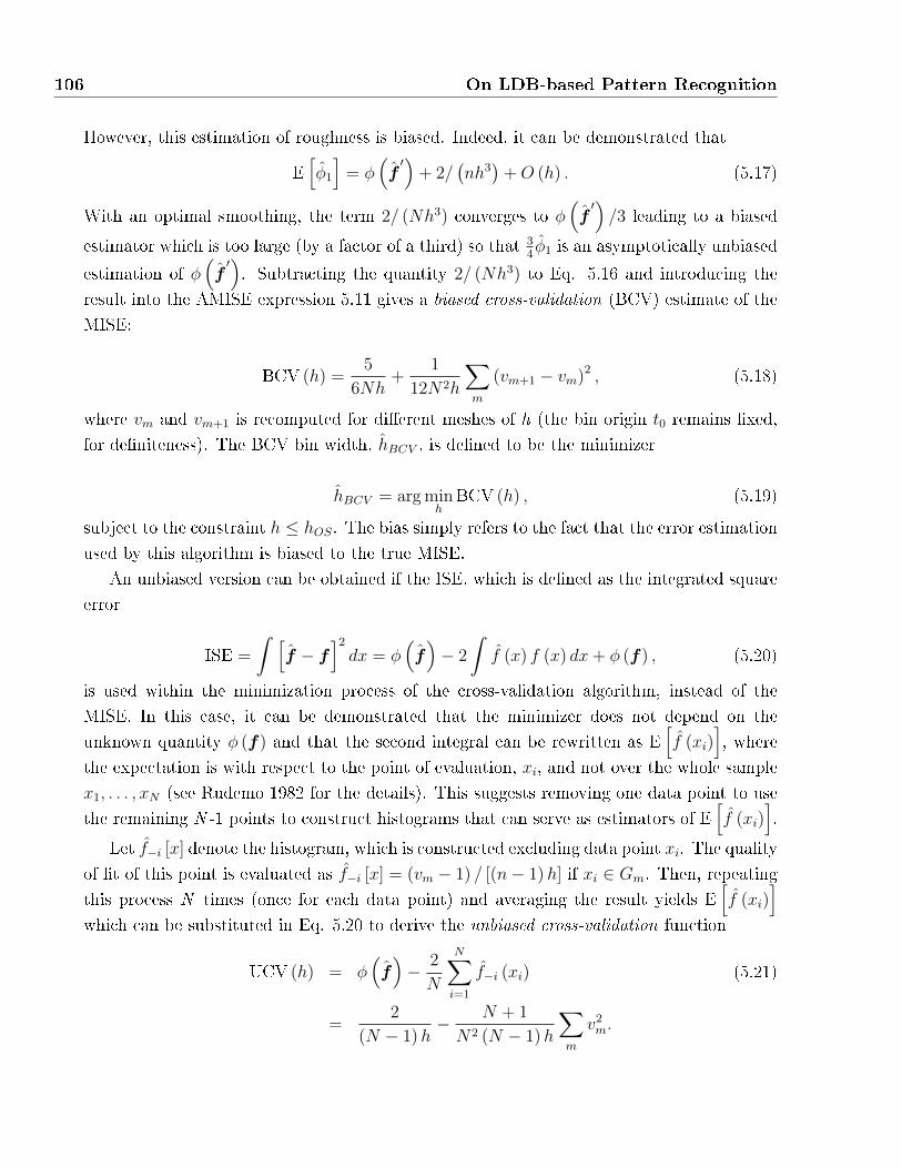
106 On LDB-based Pattern Recognition
However, this estimation of roughness is biased. Indeed, it can be demonstrated that
E[φ1
]= φ
(f′)
+ 2/(nh3)
+O (h) . (5.17)
With an optimal smoothing, the term 2/ (Nh3) converges to φ(f′)/3 leading to a biased
estimator which is too large (by a factor of a third) so that 34φ1 is an asymptotically unbiased
estimation of φ(f′). Subtracting the quantity 2/ (Nh3) to Eq. 5.16 and introducing the
result into the AMISE expression 5.11 gives a biased cross-validation (BCV) estimate of the
MISE:
BCV (h) =5
6Nh+
1
12N2h
∑m
(vm+1 − vm)2 , (5.18)
where vm and vm+1 is recomputed for di�erent meshes of h (the bin origin t0 remains �xed,
for de�niteness). The BCV bin width, hBCV , is de�ned to be the minimizer
hBCV = arg minh
BCV (h) , (5.19)
subject to the constraint h ≤ hOS. The bias simply refers to the fact that the error estimation
used by this algorithm is biased to the true MISE.
An unbiased version can be obtained if the ISE, which is de�ned as the integrated square
error
ISE =
ˆ [f − f
]2
dx = φ(f)− 2
ˆf (x) f (x) dx+ φ (f) , (5.20)
is used within the minimization process of the cross-validation algorithm, instead of the
MISE. In this case, it can be demonstrated that the minimizer does not depend on the
unknown quantity φ (f) and that the second integral can be rewritten as E[f (xi)
], where
the expectation is with respect to the point of evaluation, xi, and not over the whole sample
x1, . . . , xN (see Rudemo 1982 for the details). This suggests removing one data point to use
the remaining N -1 points to construct histograms that can serve as estimators of E[f (xi)
].
Let f−i [x] denote the histogram, which is constructed excluding data point xi. The quality
of �t of this point is evaluated as f−i [x] = (vm − 1) / [(n− 1)h] if xi ∈ Gm. Then, repeating
this process N times (once for each data point) and averaging the result yields E[f (xi)
]which can be substituted in Eq. 5.20 to derive the unbiased cross-validation function
UCV (h) = φ(f)− 2
N
N∑i=1
f−i (xi) (5.21)
=2
(N − 1)h− N + 1
N2 (N − 1)h
∑m
v2m.
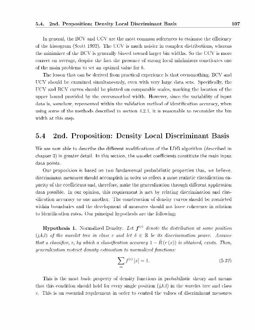
5.4. 2nd. Proposition: Density Local Discriminant Basis 107
In general, the BCV and UCV are the most common references to estimate the e�ciency
of the histogram (Scott 1992). The UCV is much noisier in complex distributions, whereas
the minimizer of the BCV is generally biased toward larger bin widths. So the UCV is more
correct on average, despite the fact the presence of strong local minimizers constitutes one
of the main problems to set an optimal value for h.
The lesson that can be derived from practical experience is that oversmothing, BCV and
UCV should be examined simultaneously, even with very large data sets. Speci�cally, the
UCV and BCV curves should be plotted on comparable scales, marking the location of the
upper bound provided by the oversmoothed width. However, since the variability of input
data is, somehow, represented within the validation method of identi�cation accuracy, when
using some of the methods described in section 4.2.1, it is reasonable to reconsider the bin
width at this step.
5.4 2nd. Proposition: Density Local Discriminant Basis
We are now able to describe the di�erent modi�cations of the LDB algorithm (described in
chapter 3) in greater detail. In this section, the wavelet coe�cients constitute the main input
data points.
Our proposition is based on two fundamental probabilistic properties that, we believe,
discriminant measures should accomplish in order to re�ect a more realistic classi�cation ca-
pacity of the coe�cients and, therefore, make the generalization through di�erent application
data possible. In our opinion, this requirement is met by relating discrimination and clas-
si�cation accuracy to one another. The construction of density curves should be restricted
within boundaries and the development of measures should not loose coherence in relation
to identi�cation rates. Our principal hypothesis are the following:
Hypothesis 1. Normalized Density. Let f (c) denote the distribution at some position
(j,k,l) of the wavelet tree in class c and let δ ∈ R be its discrimination power. Assume
that a classi�er, r, by which a classi�cation accuracy 1− R (r (x)) is obtained, exists. Then,
generalization restrict density estimation to normalized functions:∑m
f (c) [x] = 1. (5.22)
This is the most basic property of density functions in probabilistic theory and means
that this condition should hold for every single position (j,k,l) in the wavelet tree and class
c. This is an essential requirement in order to control the values of discriminant measures
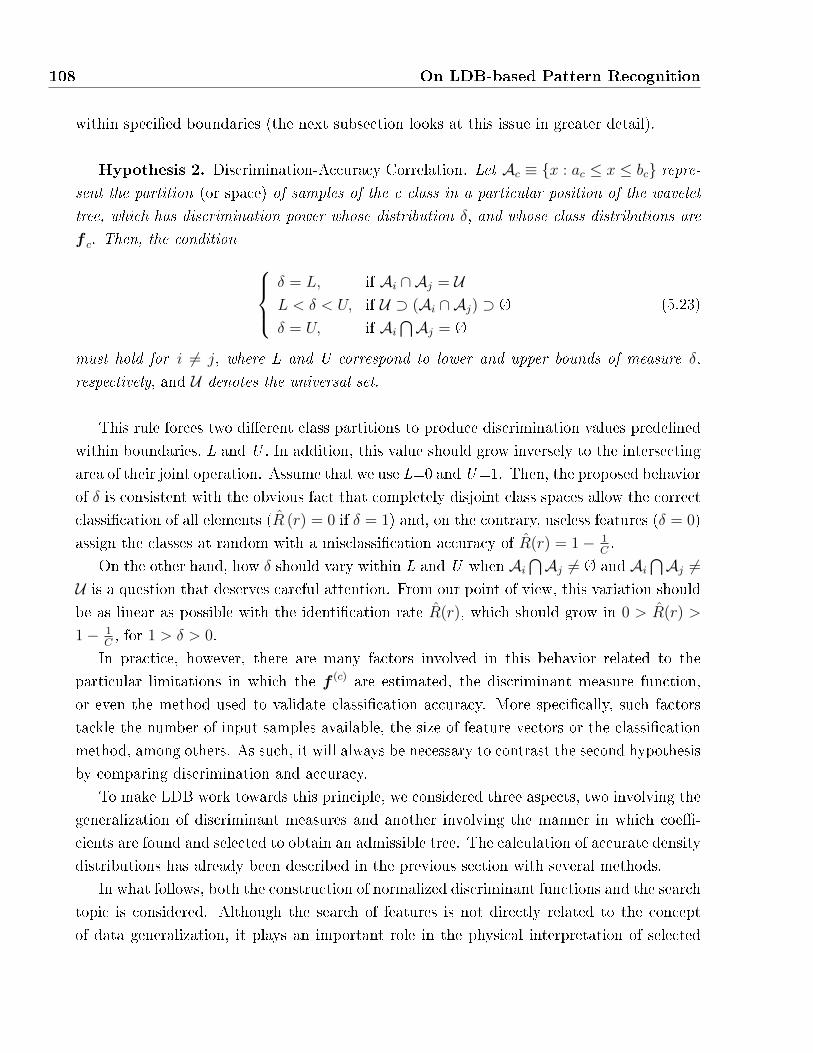
108 On LDB-based Pattern Recognition
within speci�ed boundaries (the next subsection looks at this issue in greater detail).
Hypothesis 2. Discrimination-Accuracy Correlation. Let Ac ≡ {x : ac ≤ x ≤ bc} repre-sent the partition (or space) of samples of the c class in a particular position of the wavelet
tree, which has discrimination power whose distribution δ, and whose class distributions are
f c. Then, the condition δ = L, if Ai ∩ Aj = UL < δ < U, if U ⊃ (Ai ∩ Aj) ⊃ Ø
δ = U, if Ai⋂Aj = Ø
(5.23)
must hold for i 6= j, where L and U correspond to lower and upper bounds of measure δ,
respectively, and U denotes the universal set.
This rule forces two di�erent class partitions to produce discrimination values prede�ned
within boundaries, L and U . In addition, this value should grow inversely to the intersecting
area of their joint operation. Assume that we use L=0 and U=1. Then, the proposed behavior
of δ is consistent with the obvious fact that completely disjoint class spaces allow the correct
classi�cation of all elements (R (r) = 0 if δ = 1) and, on the contrary, useless features (δ = 0)
assign the classes at random with a misclassi�cation accuracy of R(r) = 1− 1C.
On the other hand, how δ should vary within L and U when Ai⋂Aj 6= Ø and Ai
⋂Aj 6=
U is a question that deserves careful attention. From our point of view, this variation should
be as linear as possible with the identi�cation rate R(r), which should grow in 0 > R(r) >
1− 1C, for 1 > δ > 0.
In practice, however, there are many factors involved in this behavior related to the
particular limitations in which the f (c) are estimated, the discriminant measure function,
or even the method used to validate classi�cation accuracy. More speci�cally, such factors
tackle the number of input samples available, the size of feature vectors or the classi�cation
method, among others. As such, it will always be necessary to contrast the second hypothesis
by comparing discrimination and accuracy.
To make LDB work towards this principle, we considered three aspects, two involving the
generalization of discriminant measures and another involving the manner in which coe�-
cients are found and selected to obtain an admissible tree. The calculation of accurate density
distributions has already been described in the previous section with several methods.
In what follows, both the construction of normalized discriminant functions and the search
topic is considered. Although the search of features is not directly related to the concept
of data generalization, it plays an important role in the physical interpretation of selected
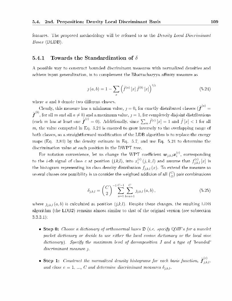
5.4. 2nd. Proposition: Density Local Discriminant Basis 109
features. The proposed methodology will be referred to as the Density Local Discriminant
Bases (DLDB).
5.4.1 Towards the Standardization of δ
A possible way to construct bounded discriminant measures with normalized densities and
achieve input generalization, is to complement the Bhattacharyya a�nity measure as
(a, b) = 1−∑x
(f (a) [x] f (b) [x]
)1/2
(5.24)
where a and b denote two di�erent classes.
Clearly, this measure has a minimum value, = 0, for exactly distributed classes (f(a)
=
f(b), for allm and all a 6= b) and a maximum value, = 1, for completely disjoint distributions
(each m has at least one f(c)
= 0). Additionally, since∑
m f(c) [x] = 1 and f [x] < 1 for all
m, the value computed in Eq. 5.24 is ensured to grow inversely to the overlapping range of
both classes, so a straightforward modi�cation of the LDB algorithm is to replace the energy
maps (Eq. 3.84) by the density estimate in Eq. 5.7, and use Eq. 5.24 to determine the
discrimination value at each position in the DWPT tree.
For notation convenience, let us change the WPT coe�cient wj,k,lx(c)i , corresponding
to the i -th signal of class c at position (j,k,l), into x(c)i (j, k, l) and assume that f (c)
j,k,l [x] is
the histogram representing its class density distribution fj,k,l (x). To extend the measure to
several classes one possibility is to consider the weighted addition of all(C2
)pair combinations
δj,k,l =
(C
2
)−1 C−1∑a=1
C∑b=a+1
j,k,l (a, b) , (5.25)
where j,k,l (a, b) is calculated at position (j,k,l). Despite these changes, the resulting LDB
algorithm (the LDB2) remains almost similar to that of the original version (see subsection
3.3.3.1):
� Step 0: Choose a dictionary of orthonormal bases D (i.e. specify QMF's for a wavelet
packet dictionary or decide to use either the local cosine dictionary or the local sine
dictionary). Specify the maximum level of decomposition J and a type of 'bounded'
discriminant measure .
� Step 1: Construct the normalized density histograms for each basis function, f(c)
j,k,l,
and class c = 1, ..., C and determine discriminant measures δj,k,l.
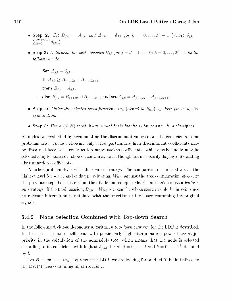
110 On LDB-based Pattern Recognition
� Step 2: Set BJ,k = AJ,k and ∆J,k = δJ,k for k = 0, . . . , 2J − 1 (where δj,k =∑2n0−j−1l=0 δj,k,l).
� Step 3: Determine the best subspace Bj,k for j = J − 1, . . . , 0; k = 0, . . . , 2j − 1 by the
following rule:
� Set ∆j,k = δj,k.
� If ∆j,k ≥ ∆j+1,2k + ∆j+1,2k+1,
� then Bj,k = Aj,k,
� else Bj,k = Bj+1,2k ∪Bj+1,2k+1 and set ∆j,k = ∆j+1,2k + ∆j+1,2k+1.
� Step 4: Order the selected basis functions wn (stored in B0,0) by their power of dis-
crimination.
� Step 5: Use k (≤ N) most discriminant basis functions for constructing classi�ers.
As nodes are evaluated by accumulating the discriminant values of all the coe�cients, some
problems arise. A node showing only a few particularly high discriminant coe�cients may
be discarded because it contains too many useless coe�cients, while another node may be
selected simply because it shows a certain average, though not necessarily display outstanding
discrimination coe�cients.
Another problem deals with the search strategy. The comparison of nodes starts at the
highest level (or scale) and ends up evaluating, W0,0, against the tree con�guration stored at
the previous step. For this reason, the divide-and-conquer algorithm is said to use a bottom-
up strategy. If the �nal decision, B0,0 = W0,0 is taken the whole search would be in vain since
no relevant information is obtained with the selection of the space containing the original
signals.
5.4.2 Node Selection Combined with Top-down Search
In the following divide-and-conquer algorithm a top-down strategy for the LDB is described.
In this case, the node coe�cients with particularly high discrimination power have major
priority in the calculation of the admissible tree, which means that the node is selected
according to its coe�cient with highest δj,k,l, for all j = 0, . . . , J and k = 0, . . . , 2j, denoted
by l.
Let B ≡ {w1, . . . ,wN} represent the LDB, we are looking for, and let T be initialized to
the DWPT tree containing all of its nodes,
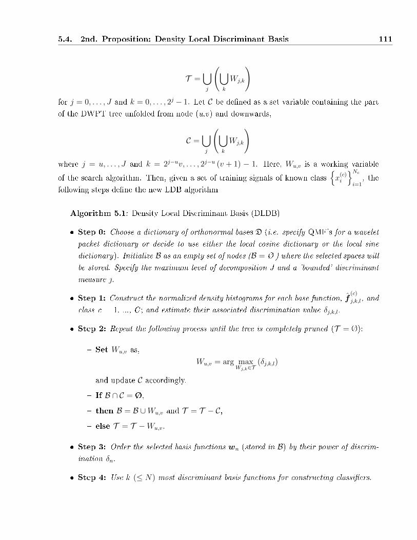
5.4. 2nd. Proposition: Density Local Discriminant Basis 111
T =⋃j
(⋃k
Wj,k
)for j = 0, . . . , J and k = 0, . . . , 2j − 1. Let C be de�ned as a set variable containing the part
of the DWPT tree unfolded from node (u,v) and downwards,
C =⋃j
(⋃k
Wj,k
)where j = u, . . . , J and k = 2j−uv, . . . , 2j−u (v + 1) − 1. Here, Wu,v is a working variable
of the search algorithm. Then, given a set of training signals of known class{x
(c)i
}Nci=1
, the
following steps de�ne the new LDB algorithm
Algorithm 5.1: Density Local Discriminant Basis (DLDB)
� Step 0: Choose a dictionary of orthonormal bases D (i.e. specify QMF's for a wavelet
packet dictionary or decide to use either the local cosine dictionary or the local sine
dictionary). Initialize B as an empty set of nodes (B = Ø ) where the selected spaces will
be stored. Specify the maximum level of decomposition J and a 'bounded' discriminant
measure .
� Step 1: Construct the normalized density histograms for each base function, f(c)
j,k,l, and
class c = 1, ..., C ; and estimate their associated discrimination value δj,k,l.
� Step 2: Repeat the following process until the tree is completely pruned (T = Ø):
� Set Wu,v as,
Wu,v = arg maxWj,k∈T
(δj,k,l)
and update C accordingly.
� If B ∩ C = Ø,
� then B = B ∪Wu,v and T = T − C,
� else T = T −Wu,v.
� Step 3: Order the selected basis functions wn (stored in B) by their power of discrim-
ination δn.
� Step 4: Use k (≤ N) most discriminant basis functions for constructing classi�ers.

112 On LDB-based Pattern Recognition
5.5 3th. Proposition: Automatic Growth Demodulation
(AGD)
It was already mentioned in chapter 2 that otolith growth is in�uenced by factors such as
habitat, water temperature, �sh diet or light, among others. In this case, the main problem
when estimating �sh age consists in how precise the Von Bertanlan�y parameters (Eq. 2.27)
can be estimated, while trying to avoid the negative e�ects of image contrast variation.
In general, it is unlikely that all specimens obey the same growth parameters, just as the
parametric method of section 2.4.2 suggests.
In our opinion, other ways of demodulating age structures which are much more consistent
with reality rely on the use of individualized growth functions, which assume the existence of
an independent growth variability for each otolith. That is, a di�erent βi for each specimen
using the same growth model template v (t, β). The philosophy underlying this approach
is more consistent with the fact that events during the �sh's life, combined with genetic
factors, have diverse in�uence on growth behavior, suggesting that the growth curve should
be adapted for each single �sh.
Recall that the �sh growth was de�ned as l = v (t [n]) for the intensity pro�le vector
i (l) = i [n], for n ∈ Z, where l and t represents otolith radial length and �sh age, respectively.Our proposed AGD algorithm attempts to estimate the growth of the �sh automatically. The
goal is to �nd the optimal growth parameters β∗ = {L∞, t0, k} that obtain the most regular
periodicity of age structures in the demodulated pro�le i (v (t, β)), but without knowing the
position of year marks li .
The autocorrelation function is often used in signal processing as a means of detecting
repeating patterns which have been buried under noise (Proakis and Manolakis 1996). In
this sense, the short-time auto correlation function (STACF), which is equivalent to the
autocorrelation of a windowed sequence (Rabiner and Schafer 2007), is used to represent the
periodicity at several positions along the demodulated intensity pro�le. That is
τm,β (k) =1
σ2
N−k∑n=0
(im,β [n]− µ) (im,β [n+ k]− µ) for k < N, (5.26)
where im,β [n] = i (v (t, β))w [n−m] denotes the piece of demodulated signal using growth
parameters β, with mean µ and variance σ2, for a rectangular window w [n] = 1[0,W ).
Note that all non-zero elements in τ are relative to the window, positioned at m, and we
have a total of M di�erent representations. So the �rst largest lag, that actually corresponds
to an oscillating year period, should present similar relative distance inside the windows if a
constant periodicity is to be present along the pro�le (otherwise, the lags would be di�used,
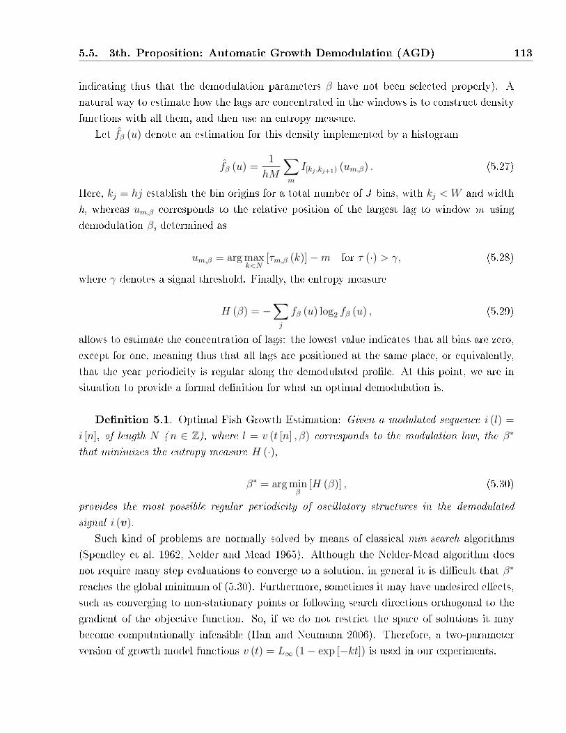
5.5. 3th. Proposition: Automatic Growth Demodulation (AGD) 113
indicating thus that the demodulation parameters β have not been selected properly). A
natural way to estimate how the lags are concentrated in the windows is to construct density
functions with all them, and then use an entropy measure.
Let fβ (u) denote an estimation for this density implemented by a histogram
fβ (u) =1
hM
∑m
I[kj ,kj+1) (um,β) . (5.27)
Here, kj = hj establish the bin origins for a total number of J bins, with kj < W and width
h, whereas um,β corresponds to the relative position of the largest lag to window m using
demodulation β, determined as
um,β = arg maxk<N
[τm,β (k)]−m for τ (·) > γ, (5.28)
where γ denotes a signal threshold. Finally, the entropy measure
H (β) = −∑j
fβ (u) log2 fβ (u) , (5.29)
allows to estimate the concentration of lags: the lowest value indicates that all bins are zero,
except for one, meaning thus that all lags are positioned at the same place, or equivalently,
that the year periodicity is regular along the demodulated pro�le. At this point, we are in
situation to provide a formal de�nition for what an optimal demodulation is.
De�nition 5.1. Optimal Fish Growth Estimation: Given a modulated sequence i (l) =
i [n], of length N (n ∈ Z), where l = v (t [n] , β) corresponds to the modulation law, the β∗
that minimizes the entropy measure H (·),
β∗ = arg minβ
[H (β)] , (5.30)
provides the most possible regular periodicity of oscillatory structures in the demodulated
signal i (v).
Such kind of problems are normally solved by means of classical min-search algorithms
(Spendley et al. 1962, Nelder and Mead 1965). Although the Nelder-Mead algorithm does
not require many step evaluations to converge to a solution, in general it is di�cult that β∗
reaches the global minimum of (5.30). Furthermore, sometimes it may have undesired e�ects,
such as converging to non-stationary points or following search directions orthogonal to the
gradient of the objective function. So, if we do not restrict the space of solutions it may
become computationally infeasible (Han and Neumann 2006). Therefore, a two-parameter
version of growth model functions v (t) = L∞ (1− exp [−kt]) is used in our experiments.
114 On LDB-based Pattern Recognition
5.6 Conclusions
Three new image and signal processing methods have been proposed in the context of �sh
otolith applications and have been formalized and fully described in this chapter. These
include 1) a normalization method for closed contours, 2) a method for demodulating the
periodicity of oscillatory structures in age signals (the AGD), and 3) a new LDB feature
extraction algorithm: the DLDB.
The goal of these algorithms is to provide e�cient coordinates of representation for signal
classi�cation. The normalization of contours is not only important to generalize among
otoliths of di�erent size and rotation but also to avoid the translation e�ect of the wavelet
packet transform, which is embedded within the DLDB method. Also, obtaining a regular
periodicity of age structures via signal demodulation is important to improve the estimation
of age in �shes. In this sense, the operation principle of AGD in the automatic demodulation
of growth structures has been presented.
The DLDB modi�es considerably the way coe�cients are evaluated compared to the
original LDB method: a completely di�erent and normalized discriminant measure and search
criterion in the feature space has been used. This approach constitutes the main core of both
applications, otolith-based �sh identi�cation and age estimation, and o�ers a new framework
to automating the selection of features in automatic algorithms of pattern recognition.
In principle, density-based techniques and bounded discriminant measures should provide
greater consistency in the evaluation of descriptor models, regardless the application we are
using. This property is necessary to obtain good generalization behavior. The last part of
this document (chapters 6 and 7) will be devoted to showing our results towards this property
and to proposing guidelines for future development.
Part IV
Results and Conclusions
115

Chapter 6
Fish Identi�cation and Age Estimation
Results
6.1 Introduction
In order to test the proposed feature extraction tools, results for otolith-based �sh iden-
ti�cation and aging applications are presented in this chapter. The main purpose of our
experimentation will be to evaluate the di�erent preprocessing frameworks presented previ-
ously and demonstrate the generalization capabilities of our feature extraction scheme, the
DLDB.
All the algorithms have been developed in MATLAB code and C language. The only
exception is the LVQ method where a version from the LVQ_PAK software, obtained from
the the author's web page (Kohonen et al. 1995), was used. The work of this thesis has
been developed in the context of the AFORO3D project (Análisis de FORmas de Otolitos
3D, Centro Superior de Investigacions Cientí�cas, CSIC) and the AFISA project from the
European Union (Automated FISH Aging, nº. 044132) in collaboration with several re-
search institutions: the French Research Institute for Exploitation of the Sea (IFREMER),
the Institute of Marine Research (IMR, Tromso-Norway), the Marine Research Institute of
Iceland (MRI), the Centre for the Environment, Fisheries and Aquaculture Science (CEFAS,
England), among others.
Some results included here have been published and presented in conferences (Soria et al.
2008, 2009, Soria and Parisi-Baradad 2011) and part of these tools, specially, the DLDB
and the demodulation tools, were included in the TNPC v4.0 NOESIS software package
(www.noesis.com).
In �sh identi�cation, we will evaluate the performance of di�erent descriptive an analytical
117
118 Fish Identi�cation and Age Estimation Results
tools: the Discrete Fourier Transform (DFT), the standard Principal Component Analysis
(PCA) and Linear Discriminant Analysis (LDA), which will be compared with the original
Local Discriminant Bases (LDB) and our proposal, the Density Local Discriminant Bases
(DLDB). In all the experiments, the otolith contour points form our Standard Eucliddean
Basis (STD).
For this purpose, a two-class classi�cation experiment has been set up with two �sh
species of di�erent genera, the Merluccius merluccius and Gadus morhua (common hake
and cod, respectively), whose otoliths are very di�erent from each other. From a biological
point of view this experiment may be of very little interest since identi�cation of both species
could be developed easily using the external �sh shape. But from the perspective of method
implementation it will bring more insight into the use of LDB methods. In particular, their
capacity in interpreting the physical structures of otolith irregularities and determining their
location on the image, the way to con�gure them or the improvements introduced with
DLDB, will be demonstrated. Two classi�cation methods will be used in this experiment:
the LVQ approach and the k-Nearest Neighbor method.
Another two-class identi�cation experiment will study the inter-speci�c and intra-speci�c
relations of Merluccius spp. from di�erent geographical locations in the world. Generally
speaking, Merluccius spp. are distributed in the Northern and Southern Hemisphere, on both
sides of the Atlantic Ocean, throughout the eastern Paci�c from the USA-Canadian border
to Cape Horn, along the Mediterranean and Black seas, and o� New Zealand (Fig 6.1).
In this case, eight inter-speci�c and intra-speci�c test pair groups were chosen. The species
used in the intra-speci�c tests were: 1) M. merluccius (Linnareus 1758); 2) M. bilinearis
(Mitchill 1818); 3) M. gayi (Guichenot 1848); and 4) M. productus (Ayres 1855). The test
pairs for the inter-speci�c tests were: 1) M. albidus (Mitchill 1814) and M. bilinearis from
north-west Atlantic; 2) M. capensis (Castelnau 1861) and M. paradoxus (Franca 1960) from
south-east Atlantic. 3) M. polli and M. senegalensis from central-east Atlantic (Cadenat
1950); and 4) M. gayi and M. australis from south-east Paci�c (Hutton 1872). These pair
groups were chosen because they have di�erent population characteristics, and are of very
important economic value in general. The hakes from the intra-speci�c pairs are found in
two di�erent world areas and, therefore, allow us to �nd environmental factors attributed
to the species, whereas in the inter-speci�c groups the two hake species show overlapped
geographical distributions (sympatric species).
The experiment will also serve to observe the behavior of DLDB under a more di�cult
identi�cation problem, and in particular the sympatric species, whose species inhabit the
same geographical region and are quite similar each other. In this case, the otolith is a
necessary element in order to succeed in their identi�cation.
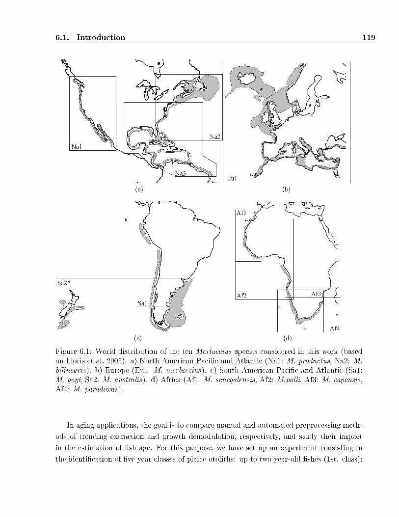
6.1. Introduction 119
(a) (b)
(c) (d)
Figure 6.1: World distribution of the ten Merluccius species considered in this work (basedon Lloris et al. 2005). a) North American Paci�c and Atlantic (Na1: M. productus, Na2: M.bilinearis). b) Europe (Eu1: M. merluccius). c) South American Paci�c and Atlantic (Sa1:M. gayi, Sa2: M. australis). d) Africa (Af1: M. senegalensis, Af2: M.polli, Af3: M. capensis,Af4: M. paradoxus).
In aging applications, the goal is to compare manual and automated preprocessing meth-
ods of trending extraction and growth demodulation, respectively, and study their impact
in the estimation of �sh age. For this purpose, we have set up an experiment consisting in
the identi�cation of �ve year classes of plaice otoliths: up to two year-old �shes (1st. class);
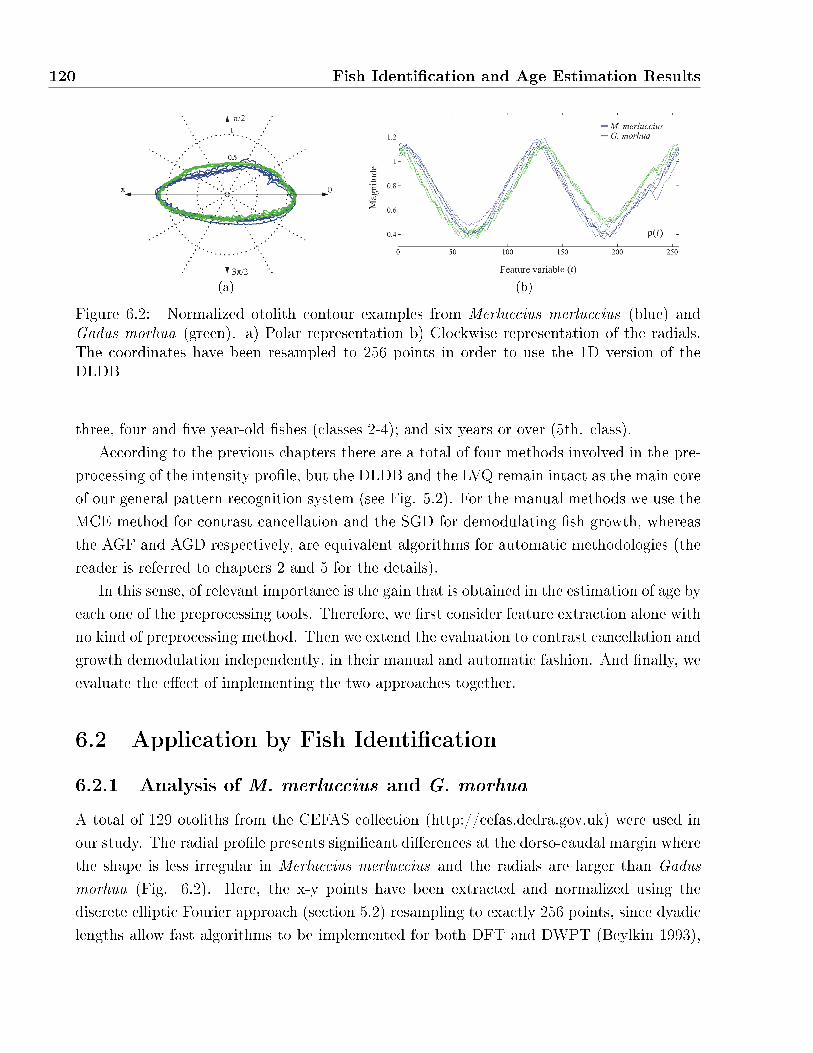
120 Fish Identi�cation and Age Estimation Results
(a) (b)
Figure 6.2: Normalized otolith contour examples from Merluccius merluccius (blue) andGadus morhua (green). a) Polar representation b) Clockwise representation of the radials.The coordinates have been resampled to 256 points in order to use the 1D version of theDLDB
three, four and �ve year-old �shes (classes 2-4); and six years or over (5th. class).
According to the previous chapters there are a total of four methods involved in the pre-
processing of the intensity pro�le, but the DLDB and the LVQ remain intact as the main core
of our general pattern recognition system (see Fig. 5.2). For the manual methods we use the
MCE method for contrast cancellation and the SGD for demodulating �sh growth, whereas
the AGF and AGD respectively, are equivalent algorithms for automatic methodologies (the
reader is referred to chapters 2 and 5 for the details).
In this sense, of relevant importance is the gain that is obtained in the estimation of age by
each one of the preprocessing tools. Therefore, we �rst consider feature extraction alone with
no kind of preprocessing method. Then we extend the evaluation to contrast cancellation and
growth demodulation independently, in their manual and automatic fashion. And �nally, we
evaluate the e�ect of implementing the two approaches together.
6.2 Application by Fish Identi�cation
6.2.1 Analysis of M. merluccius and G. morhua
A total of 129 otoliths from the CEFAS collection (http://cefas.dedra.gov.uk) were used in
our study. The radial pro�le presents signi�cant di�erences at the dorso-caudal margin where
the shape is less irregular in Merluccius merluccius and the radials are larger than Gadus
morhua (Fig. 6.2). Here, the x-y points have been extracted and normalized using the
discrete elliptic Fourier approach (section 5.2) resampling to exactly 256 points, since dyadic
lengths allow fast algorithms to be implemented for both DFT and DWPT (Beylkin 1993),
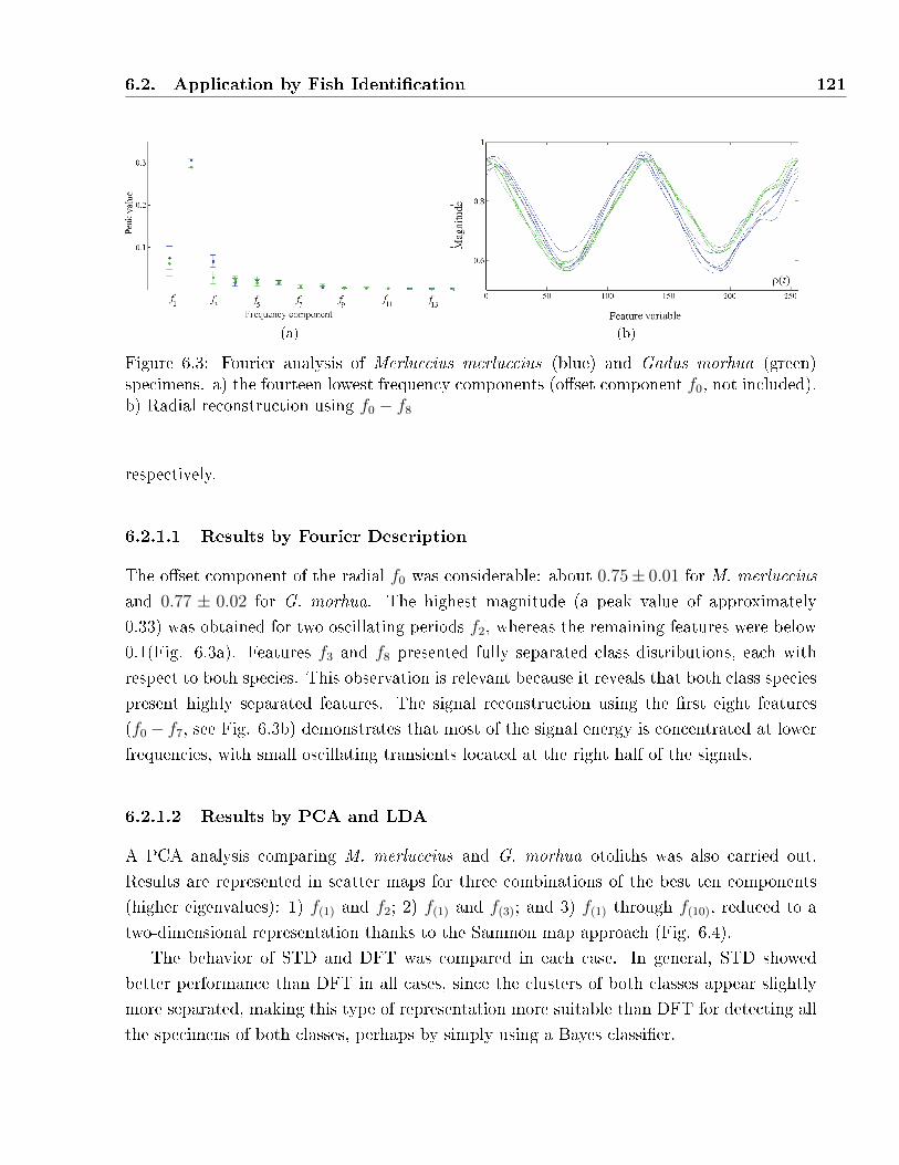
6.2. Application by Fish Identi�cation 121
(a) (b)
Figure 6.3: Fourier analysis of Merluccius merluccius (blue) and Gadus morhua (green)specimens. a) the fourteen lowest frequency components (o�set component f0, not included).b) Radial reconstruction using f0 − f8
respectively.
6.2.1.1 Results by Fourier Description
The o�set component of the radial f0 was considerable: about 0.75± 0.01 for M. merluccius
and 0.77 ± 0.02 for G. morhua. The highest magnitude (a peak value of approximately
0.33) was obtained for two oscillating periods f2, whereas the remaining features were below
0.1(Fig. 6.3a). Features f3 and f8 presented fully separated class distributions, each with
respect to both species. This observation is relevant because it reveals that both class species
present highly separated features. The signal reconstruction using the �rst eight features
(f0 − f7, see Fig. 6.3b) demonstrates that most of the signal energy is concentrated at lower
frequencies, with small oscillating transients located at the right half of the signals.
6.2.1.2 Results by PCA and LDA
A PCA analysis comparing M. merluccius and G. morhua otoliths was also carried out.
Results are represented in scatter maps for three combinations of the best ten components
(higher eigenvalues): 1) f(1) and f2; 2) f(1) and f(3); and 3) f(1) through f(10), reduced to a
two-dimensional representation thanks to the Sammon map approach (Fig. 6.4).
The behavior of STD and DFT was compared in each case. In general, STD showed
better performance than DFT in all cases, since the clusters of both classes appear slightly
more separated, making this type of representation more suitable than DFT for detecting all
the specimens of both classes, perhaps by simply using a Bayes classi�er.
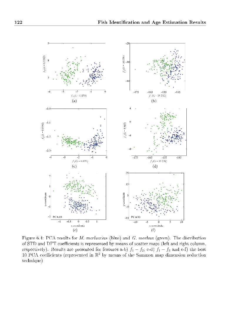
122 Fish Identi�cation and Age Estimation Results
(a) (b)
(c) (d)
(e) (f)
Figure 6.4: PCA results for M. merluccius (blue) and G. morhua (green). The distributionof STD and DFT coe�cients is represented by means of scatter maps (left and right column,respectively). Results are presented for features a-b) f1 − f2; c-d) f1 − f3 and e-f) the best10 PCA coe�cients (represented in R2 by means of the Sammon map dimension reductiontechnique)

6.2. Application by Fish Identi�cation 123
Inputdomain
λCoe�cients
M. merluccius G. morhuaMin. Max. Min. Max.
STD 18578 -85.34 -85.30 -83.70 -83.66DFT 17.25 0.399 0.466 0.497 0.579
Table 6.1: Results by LDA analysis
In STD, using either the �rst (Fig 6.4a) or third con�guration (6.4d) of features is recom-
mended, whereas in DFT, class distributions are a little more overlapped in all cases. The
results also demonstrate that PCA eigenvalues are not representative measures of class sep-
aration. As an example, the eigenvalue of the best DFT component f(1) is λ = 35.232, while
the best eigenvalue of the STD component is λ = 0.879 and o�ers better cluster separation.
A similar analysis was developed by means of LDA. In this case, the classes restrict the
number of output features to only C -1 coe�cients for each otolith, a single coe�cient in
this case. Since the value range of this coe�cient does not overlap (Table 6.1 ), all the M.
merluccius and G. morhua should be correctly identi�ed in the classi�cation phase either
by STD or DFT. The eigenvalue is also uncontrolled and can not be used for evaluation
purposes (STD and DFT have di�erent eigenvalues, λ = 18578 and λ = 17.25 respectively,
when both have the same discrimination). Therefore, the LDA eigenvectors are useful in the
characterization of both species.
6.2.1.3 LDB and DLDB analysis
M. merluccius and G. morhua were also analyzed by means of LDB and DLDB. All infor-
mation about results is provided through �gures 6.5 - 6.8 and tables 6.2-6.3.
A total of NJ = 256 × 8 = 2048 coe�cients were calculated for each otolith contour
using the reverse biorthogonal 3.1 wavelets (rbior3.1). This dictionary was chosen because
the �ve most relevant coe�cients obtained the highest discrimination results with DLDB,
δ (Bx) =∑5
n=1 δ(n) = 4.989 out of a maximum 5 (Table 6.2) .
LDB was con�gured with the symmetric Kullback Liebler criterion, whereas DLDB used
the Battacharyya criterion to evaluate density histograms of m = 9 bins, which was chosen
according to Sturge's rule. This con�guration allowed discriminant measures to be normalized
within the range [0,1).
The divide-and-conquer algorithm of both LDB and DLDB generated their respective
admissible trees (Fig. 6.5). While the black cells correspond to the selected nodes, the
previously mentioned �ve important coe�cients are highlighted by means of red marks.

124 Fish Identi�cation and Age Estimation Results
DLDB LDB DLDB LDBDictionary δ (Bx) Dictionary δ (Bx) Dictionary δ (Bx) Dictionary δ (Bx)
Daubechies Biorthogonaldb31 4.9287 db36 0.0580 bior3.9 4.9296 bior3.1 1.4933db35 4.7989 db42 0.0328 bior3.5 4.9296 bior3.5 0.7446db40 4.3242 db4 0.0326 bior2.8 4.3189 bior6.8 0.1099db8 3.2380 db5 0.0325 bior6.8 3.2448 bior1.1 0.0321db7 3.1107 db33 0.0321 bior4.4 3.2035 bior4.4 0.0045
Symlets Reverse Biorthogonalsym7 4.9331 sym27 0.0328 rbior3.1 4.989 rbior3.1 0.2688sym11 4.9266 sym11 0.0327 rbior1.5 4.7833 rbior4.4 0.1315sym2 3.9150 sym18 0.0326 rbior3.9 4.1210 rbior2.8 0.1044sym30 3.4440 sym9 0.0325 rbior4.4 3.3694 rbior3.3 0.0170sym14 3.2477 sym10 0.0324 rbior5.5 3.2572 rbior1.3 0.0045
Coi�etscoif4 3.5000 coif5 0.0326 coif2 3.4474 coif4 0.0325coif5 3.4744 coif3 0.0325 coif3 3.4445 coif1 0.0325coif1 3.4588 coif2 0.0325
Table 6.2: Evaluation of di�erent dictionaries with DLDB and LDB. These include theDaubechies, Symlets, Coi�ets, Biorthogonal and Reverse Biorthogonal. Measure values areprovided considering the �ve best features in each dictionary. The best results are in boldformat
(a) (b)
Figure 6.5: Admissible trees for the M. merluccius - G. morhua experiment using the reversebiorthogonal 3.1 wavelets. Best nodes are shown in black and the best �ve coe�cients areshown in red for a) the DLDB, and b) the LDB.
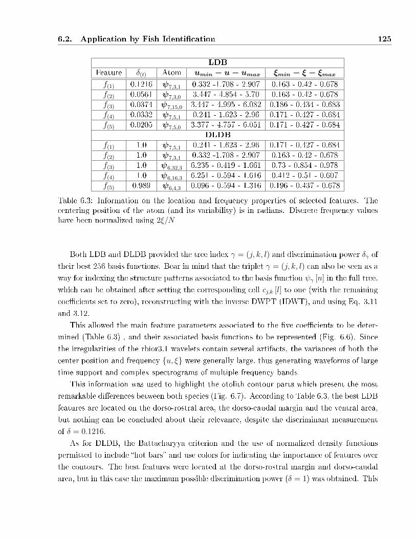
6.2. Application by Fish Identi�cation 125
LDBFeature δ(t) Atom umin − u− umax ξmin − ξ − ξmax
f(1) 0.1216 ψ7,3,1 0.332 -1.708 - 2.907 0.163 - 0.42 - 0.678f(2) 0.0561 ψ7,3,0 3.447 - 4.854 - 5.70 0.163 - 0.42 - 0.678f(3) 0.0374 ψ7,15,0 3.447 - 4.995 - 6.082 0.186 - 0.434 - 0.683f(4) 0.0332 ψ7,5,1 0.241 - 1.623 - 2.96 0.171 - 0.427 - 0.684f(5) 0.0205 ψ7,5,0 3.377 - 4.757 - 6.051 0.171 - 0.427 - 0.684
DLDBf(1) 1.0 ψ7,5,1 0.241 - 1.623 - 2.96 0.171 - 0.427 - 0.684f(2) 1.0 ψ7,3,1 0.332 -1.708 - 2.907 0.163 - 0.42 - 0.678f(3) 1.0 ψ6,32,3 6.235 - 0.419 - 1.661 0.73 - 0.854 - 0.978f(4) 1.0 ψ6,16,3 6.251 - 0.594 - 1.616 0.412 - 0.51 - 0.607f(5) 0.989 ψ6,4,3 0.096 - 0.594 - 1.316 0.196 - 0.437 - 0.678
Table 6.3: Information on the location and frequency properties of selected features. Thecentering position of the atom (and its variability) is in radians. Discrete frequency valueshave been normalized using 2ξ/N
Both LDB and DLDB provided the tree index γ = (j, k, l) and discrimination power δγ of
their best 256 basis functions. Bear in mind that the triplet γ = (j, k, l) can also be seen as a
way for indexing the structure patterns associated to the basis function ψγ [n] in the full tree,
which can be obtained after setting the corresponding cell cj,k [l] to one (with the remaining
coe�cients set to zero), reconstructing with the inverse DWPT (IDWT), and using Eq. 3.11
and 3.12.
This allowed the main feature parameters associated to the �ve coe�cients to be deter-
mined (Table 6.3) , and their associated basis functions to be represented (Fig. 6.6). Since
the irregularities of the rbior3.1 wavelets contain several artifacts, the variances of both the
center position and frequency {u, ξ} were generally large, thus generating waveforms of largetime support and complex spectrograms of multiple frequency bands.
This information was used to highlight the otolith contour parts which present the most
remarkable di�erences between both species (Fig. 6.7). According to Table 6.3, the best LDB
features are located on the dorso-rostral area, the dorso-caudal margin and the ventral area,
but nothing can be concluded about their relevance, despite the discriminant measurement
of δ = 0.1216.
As for DLDB, the Battacharyya criterion and the use of normalized density functions
permitted to include �hot bars� and use colors for indicating the importance of features over
the contours. The best features were located at the dorso-rostral margin and dorso-caudal
area, but in this case the maximum possible discrimination power (δ = 1) was obtained. This
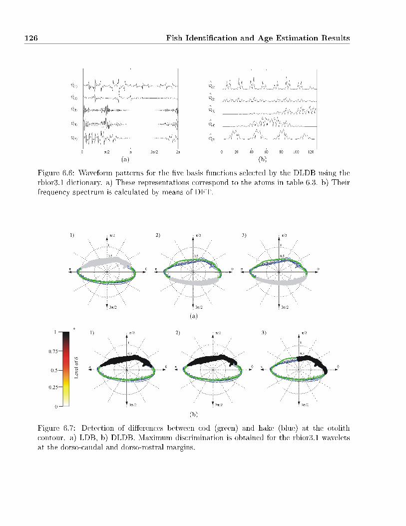
126 Fish Identi�cation and Age Estimation Results
(a) (b)
Figure 6.6: Waveform patterns for the �ve basis functions selected by the DLDB using therbior3.1 dictionary. a) These representations correspond to the atoms in table 6.3. b) Theirfrequency spectrum is calculated by means of DFT.
(a)
(b)
Figure 6.7: Detection of di�erences between cod (green) and hake (blue) at the otolithcontour. a) LDB, b) DLDB. Maximum discrimination is obtained for the rbior3.1 waveletsat the dorso-caudal and dorso-rostral margins.
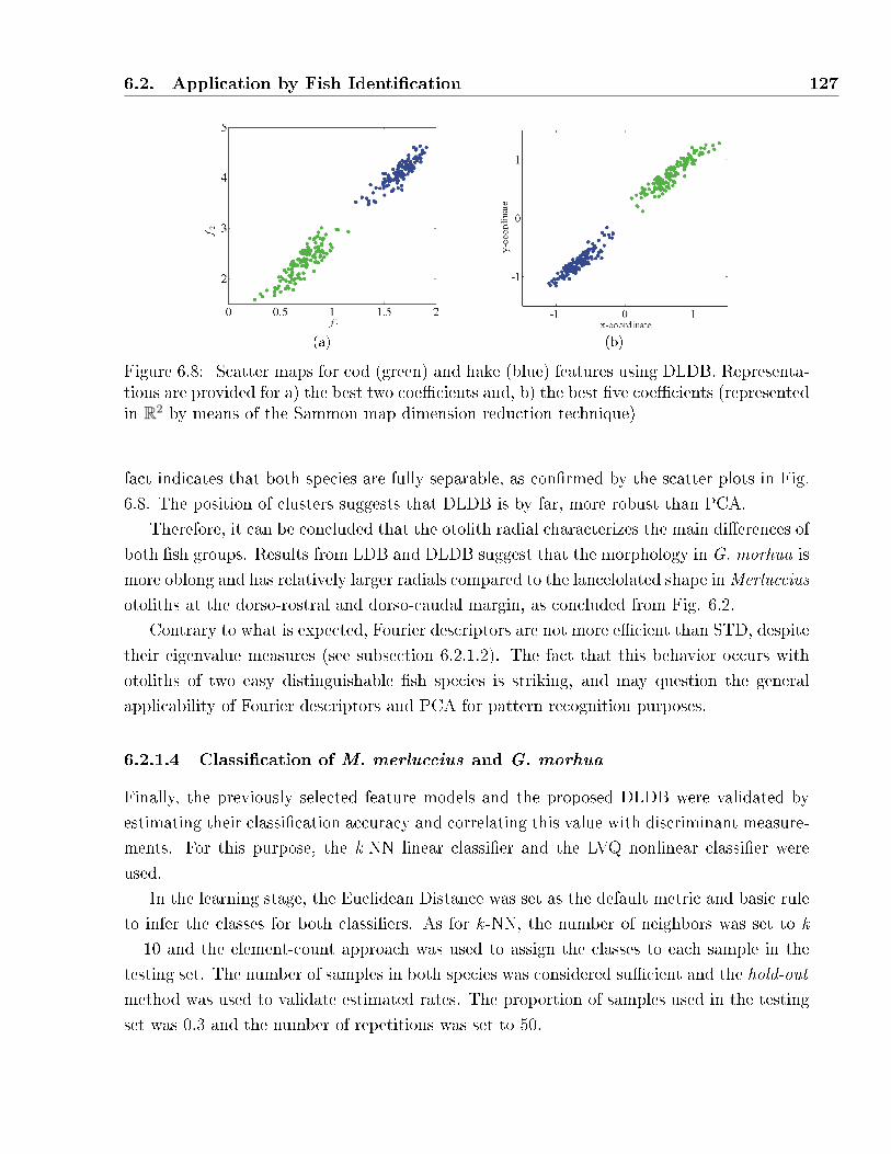
6.2. Application by Fish Identi�cation 127
(a) (b)
Figure 6.8: Scatter maps for cod (green) and hake (blue) features using DLDB. Representa-tions are provided for a) the best two coe�cients and, b) the best �ve coe�cients (representedin R2 by means of the Sammon map dimension reduction technique)
fact indicates that both species are fully separable, as con�rmed by the scatter plots in Fig.
6.8. The position of clusters suggests that DLDB is by far, more robust than PCA.
Therefore, it can be concluded that the otolith radial characterizes the main di�erences of
both �sh groups. Results from LDB and DLDB suggest that the morphology in G. morhua is
more oblong and has relatively larger radials compared to the lancelolated shape inMerluccius
otoliths at the dorso-rostral and dorso-caudal margin, as concluded from Fig. 6.2.
Contrary to what is expected, Fourier descriptors are not more e�cient than STD, despite
their eigenvalue measures (see subsection 6.2.1.2). The fact that this behavior occurs with
otoliths of two easy distinguishable �sh species is striking, and may question the general
applicability of Fourier descriptors and PCA for pattern recognition purposes.
6.2.1.4 Classi�cation of M. merluccius and G. morhua
Finally, the previously selected feature models and the proposed DLDB were validated by
estimating their classi�cation accuracy and correlating this value with discriminant measure-
ments. For this purpose, the k-NN linear classi�er and the LVQ nonlinear classi�er were
used.
In the learning stage, the Euclidean Distance was set as the default metric and basic rule
to infer the classes for both classi�ers. As for k -NN, the number of neighbors was set to k
= 10 and the element-count approach was used to assign the classes to each sample in the
testing set. The number of samples in both species was considered su�cient and the hold-out
method was used to validate estimated rates. The proportion of samples used in the testing
set was 0.3 and the number of repetitions was set to 50.
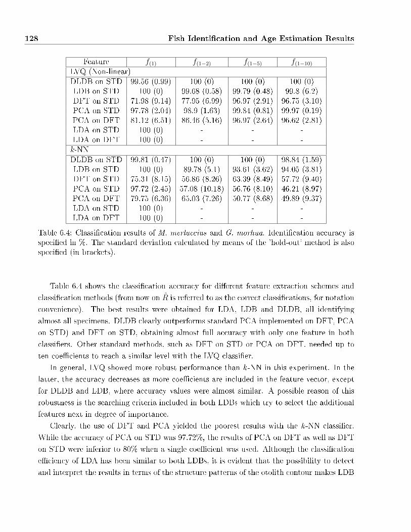
128 Fish Identi�cation and Age Estimation Results
Feature f(1) f(1−2) f(1−5) f(1−10)
LVQ (Non-linear)DLDB on STD 99.56 (0.99) 100 (0) 100 (0) 100 (0)LDB on STD 100 (0) 99.68 (0.58) 99.79 (0.48) 99.8 (6.2)DFT on STD 71.98 (9.14) 77.95 (6.99) 96.97 (2.91) 96.75 (3.10)PCA on STD 97.78 (2.04) 98.9 (1.63) 99.84 (0.81) 99.97 (0.19)PCA on DFT 81.12 (6.51) 86.46 (5.16) 96.97 (2.64) 96.62 (2.81)LDA on STD 100 (0) - - -LDA on DFT 100 (0) - - -k-NNDLDB on STD 99.81 (0.47) 100 (0) 100 (0) 98.84 (1.59)LDB on STD 100 (0) 89.78 (5.1) 93.61 (3.62) 94.05 (3.81)DFT on STD 75.31 (8.15) 56.86 (8.26) 63.39 (8.49) 57.72 (9.40)PCA on STD 97.72 (2.45) 57.08 (10.18) 56.76 (8.10) 46.21 (8.97)PCA on DFT 79.75 (6.36) 65.03 (7.26) 50.77 (8.68) 49.89 (9.37)LDA on STD 100 (0) - - -LDA on DFT 100 (0) - - -
Table 6.4: Classi�cation results of M. merluccius and G. morhua. Identi�cation accuracy isspeci�ed in %. The standard deviation calculated by means of the 'hold-out' method is alsospeci�ed (in brackets).
Table 6.4 shows the classi�cation accuracy for di�erent feature extraction schemes and
classi�cation methods (from now on R is referred to as the correct classi�cations, for notation
convenience). The best results were obtained for LDA, LDB and DLDB, all identifying
almost all specimens. DLDB clearly outperforms standard PCA implemented on DFT, PCA
on STD) and DFT on STD, obtaining almost full accuracy with only one feature in both
classi�ers. Other standard methods, such as DFT on STD or PCA on DFT, needed up to
ten coe�cients to reach a similar level with the LVQ classi�er.
In general, LVQ showed more robust performance than k -NN in this experiment. In the
latter, the accuracy decreases as more coe�cients are included in the feature vector, except
for DLDB and LDB, where accuracy values were almost similar. A possible reason of this
robustness is the searching criteria included in both LDBs which try to select the additional
features next in degree of importance.
Clearly, the use of DFT and PCA yielded the poorest results with the k -NN classi�er.
While the accuracy of PCA on STD was 97.72%, the results of PCA on DFT as well as DFT
on STD were inferior to 80% when a single coe�cient was used. Although the classi�cation
e�ciency of LDA has been similar to both LDBs, it is evident that the possibility to detect
and interpret the results in terms of the structure patterns of the otolith contour makes LDB

6.2. Application by Fish Identi�cation 129
(a) (b)
(c) (d)
Figure 6.9: Matching the performance of LDB (left column) and DLDB (right column) withclassi�cation results. Discrimination values and identi�cation results for both LVQ and k-NNare provided for all 256 selected coe�cients of the rbior3.1 wavelet dictionary, a) and b), andall D dictionaries, c) and d), by decreasing importance.
methods vastly superior.
Additionally, DLDB o�ered much better generalization behavior than LDB. This is proved
by estimating the individual accuracies of all 256 selected coe�cients and contrasting with
their decreasing discrimination pro�le (Figures 6.9a, and 6.9b). While LDB shows a noisy
pro�le, indicating randomness in the selection of coe�cients, the discrimination pro�le of
DLDB is consistent with our hypotheses of normalized density and discrimination-accuracy
correlation proposed in chapter 5 (see section 5.4). For this two-class experiment, the accu-
racy of individual features Rho decreases 1 to 1/2 as discrimination power reduces from 1 to
0.
The same relationship is not so evident when the length of the feature vector increases,
even for the new elements next in discriminant value. When the dictionaries were com-
pared (Figures 6.9c and 6.9d), about forty of them obtained a discrimination power of
4.75 < δ (Bx) < 5 with accuracies between 0.95 and 1 for the k -NN classi�er. This ob-
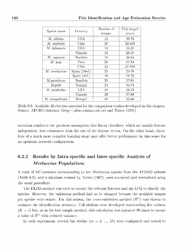
130 Fish Identi�cation and Age Estimation Results
Specie name CountryNumber of
images
Fish length
(cms)
M. albidus USA 12 39-73
M. australis Chile 20 33-109
M. bilinearis USA 13 25-31
Canada 18 26-50
M. capensis Namibia 18 30-85
M. gayi Peru 28 27-84
Chile 25 27-108
M. merluccius Spain (Med.) 25 25-78
Spain (Atl.) 19 18-70
M.paradoxus Namibia 20 27-85
M.polli Senegal 24 34-74
M. productus USA 21 34-74
Canada 23 37-69
M. senegalensis Senegal 21 35-66
Table 6.5: AvailableMerluccius material for the comparison studies developed in this chapter.Source: AFORO database (http://aforo.cmima.csic.es) and Torres (1997)
servation reinforces the previous assumption that linear classi�ers, which are mainly feature
independent, lose robustness with the size of the feature vector. On the other hand, classi-
�ers of a much more complex learning stage may o�er better performance in this sense for
an optimum network con�guration.
6.2.2 Results by Intra-speci�c and Inter-speci�c Analysis of
Merluccius Populations
A total of 287 contours corresponding to ten Merluccius species from the AFORO website
(Table 6.5), and a database created by Torres (1997), were extracted and normalized using
the usual procedure.
The DLDB method was used to extract the relevant features and the LVQ to classify the
species. However, the validation method had to be changed because the available images
per species were scarce. For this reason, the cross-validation method (Rcv) was chosen to
estimate the identi�cation accuracy. Calculations were developed constructing �ve subsets
(K = 5) but, as in the test sample method, this calculation was repeated 50 times to ensure
a value of Rcv with reduced variance.
In each experiment, several bin widths (m = 3, ..., 10) were con�gured and tested to
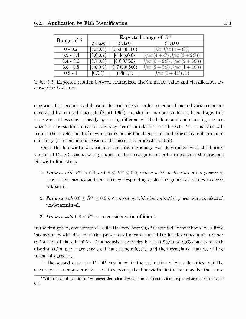
6.2. Application by Fish Identi�cation 131
Range of δExpected range of Rcv
2-class 3-class C -class0 - 0.2 [0.5,0.6) [0.333,0.466) [1/C, 1/5C (4 + C))0.2 - 0.4 [0.6,0.7) [0.466,0.6) [1/5C (4 + C) , 1/5C (3 + 2C))0.4 - 0.6 [0.7,0.8) [0.6,0.733) [1/5C (3 + 2C) , 1/5C (2 + 3C))0.6 - 0.8 [0.8,0.9) [0.733,0.866) [1/5C (2 + 3C) , 1/5C (1 + 4C))0.8 - 1 [0.9,1) [0.866,1) [1/5C (1 + 4C) , 1)
Table 6.6: Expected relation between normalized discrimination value and classi�cation ac-curacy for C classes.
construct histogram-based densities for each class in order to reduce bias and variance errors
generated by reduced data sets (Scott 1992). As the bin number could not be so large, this
issue was addressed empirically by testing di�erent widths beforehand and choosing the one
with the closest discrimination-accuracy match in relation to Table 6.6. Yet, this issue will
require the development of new measures or methodologies that addresses this problem more
e�ciently (the concluding section 7 discusses this in greater detail).
Once the bin width was set and the best dictionary was determined with the library
version of DLDB, results were grouped in three categories in order to consider the previous
bin width limitation:
1. Features with Rcv > 0.9, or 0.8 ≤ Rcv ≤ 0.9, with consistent discrimination power 1 δ,
were taken into account and their corresponding otolith irregularities were considered
relevant.
2. Features with 0.8 ≤ Rcv ≤ 0.9 not consistent with discrimination power were considered
undetermined.
3. Features with 0.8 < Rcv were considered insu�cient.
In the �rst group, any correct classi�cation rate over 90% is accepted unconditionally. A little
inconsistency with discrimination power may indicate that DLDB has developed a rather poor
estimation of class densities. Analogously, accuracies between 80% and 90% consistent with
discrimination power are very signi�cant to be rejected, and their associated features will be
taken into account.
In the second case, the DLDB has failed in the estimation of class densities, but the
accuracy is so representative. At this point, the bin width limitation may be the cause
1With the word 'consistent' we mean that identi�cation and discrimination are paired according to Table6.6.
132 Fish Identi�cation and Age Estimation Results
of this poor performance and the recommendation is to repeat the experiment with more
samples whenever possible. If not, the risk of validating such results should be taken into
account.
Finally, any result below 80% will be discarded. The observation of consistency, although
strange in such identi�cation rates, may indicate the presence of high heterogeneity within
class. However, verifying this hypotheses would also require the use of a representative set
of data, specially if the variances of classi�cation accuracy are large.
6.2.2.1 Inter-speci�c Experimentation
Results for the inter-speci�c experiments in sympatric species are provided in �gures 6.10 -
6.13; and tables 6.7-6.10. The information provided contains 1) the con�guration settings
of DWPT and DLDB: wavelet dictionaries and bin widths used in each experiment; 2) the
values associated to the best wavelet atoms: the triplet γ = (j, k, l), discrimination power
vs. identi�cation accuracy (calculated by DLDB and LVQ, respectively, so that the reader
can match discrimination and classi�cation results) and time-frequency support; and 3) the
�gures representing their extension of associated features on the otolith contour and their
signi�cance.
We do not provide any representation regarding the selected admissible trees of each exper-
iment and the waveform pro�le of selected basis functions, as this information is represented
perfectly by the dictionary name and the index triplet γ = (j, k, l) method performance. As
well as the previous M. merluccius-G. morhua experiment, the relevance of each feature is
indicated in the �gures by means of hot bars.
As expected, inter-speci�c results were generally more successful than intra-speci�c and
shape di�erences were recognized in three out of four experiments. All rates of correct
classi�cations were above 90% with the exception of M. gayi - M. australis (78%).
� M. albidus - M. bilinearis
The best atoms corresponded to larger scales in the time-frequency plane (j =5, 6 and 7,
see Table 6.7), of low position resolution (32, 64 and 128 contour points, respectively, see
Fig. 6.10) and high frequency resolution. The most relevant feature f(1) is centered at the
ventral side of the otolith and extended to the rostrum. f(2) and f(3) are centered along
the dorso-rostral margin, and f(4)- f(5) covers a small area of the rostrum (top and bottom,
respectively).
All coe�cients have maximum discrimination power (δ = 1), allowing the correct iden-
ti�cation of all specimens (Rcv = 1) when classifying with f(1), f(2) or f(5) alone. As such,
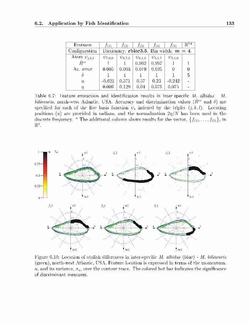
6.2. Application by Fish Identi�cation 133
Features f(1) f(2) f(3) f(4) f(5) R5*Con�guration Dictionary: rbior3.5. Bin width: m = 4.Atom ψj,k,l ψ7,0,0 ψ6,7,3 ψ6,1,3 ψ5,1,7 ψ5,1,0 -
Rcv 1 1 0.962 0.957 1 1Ac. error 0.005 0.003 0.019 0.025 0 0
δ 1 1 1 1 1 5u -0.621 0.571 0.57 0.23 -0.242 -η 0.009 0.129 0.04 0.075 0.075 -
Table 6.7: Feature extraction and identi�cation results in inter-speci�c M. albidus - M.bilinearis, north-west Atlantic, USA. Accuracy and discrimination values (Rcv and δ) arespeci�ed for each of the �ve basis function ψ, indexed by the triplet (j, k, l). Locatingpositions (u) are provided in radians, and the normalization 2η/N has been used in thediscrete frequency. * The additional column shows results for the vector,
{f(1), . . . , f(5)
}, in
R5.
Figure 6.10: Location of otolith di�erences in inter-speci�c M. albidus (blue) - M. bilinearis(green), north-west Atlantic, USA. Feature location is expressed in terms of the momentum,u, and its variance, σu, over the contour trace. The colored hot bar indicates the signi�canceof discriminant measures.
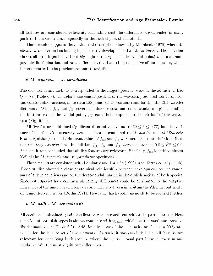
134 Fish Identi�cation and Age Estimation Results
all features are considered relevant, concluding that the di�erences are extended in many
parts of the contour trace, specially in the rostral part of the otolith.
These results supports the anatomical description showed by Mombeck (1970) where M.
albidus was described as having bigger rostral development than M. bilinearis. The fact that
almost all otolith parts had been highlighted (except near the caudal point) with maximum
possible discrimination, indicates di�erences relative to the otolith size of both species, which
is consistent with the previous contour description.
� M. capensis - M. paradoxus
The selected basis functions corresponded to the largest possible scale in the admissible tree
(j = 8) (Table 6.8). Therefore, the center position of the wavelets presented low resolution
and considerable variance, more than 128 points of the contour trace for the 'rbior3.1' wavelet
dictionary. While f(1) and f(3) covers the dorso-rostral and dorso-caudal margin, including
the bottom part of the caudal point, f(2) extends its support to the left half of the ventral
area (Fig. 6.11).
All �ve features obtained signi�cant discriminant values (0.69 ≤ δ ≤ 0.77) but the vari-
ance of identi�cation accuracy was considerable compared to M. albidus and M.bilinearis.
However, although the discriminant values of f(3) and f(5)were not consistent, their identi�ca-
tion accuracy was over 90%. In addition, f(1), f(2) and f(4) were consistent in 0.8 ≤ Rcv ≤ 0.9.
As such, it was concluded that all �ve features are relevant. Specially, f(5) identi�ed almost
93% of the M. capensis and M. paradoxus specimens.
These results are consistent with Lombarte and Fortuño (1992), and Torres et. al (2000b).
Those studies showed a close anatomical relationship between development on the caudal
part of sulcus acusticus and on the dorso-caudal margin in the otolith sagitta of both species.
Since both species have common phylogeny, di�erences could be attributed to the adaptive
characters of the inner ear and temperature e�ects between inhabiting the African continental
shelf and deep sea water (Botha 1971). However, this hypothesis needs to be studied further.
� M. polli - M. senegalensis
All coe�cients obtained good classi�cation results consistent with δ. In particular, the iden-
ti�cation of both �sh types is almost complete with ψ7,67,1, which has the maximum possible
discriminant value (Table 6.9). Additionally, none of the accuracies are below a 90%-rate,
except for the feature set of �ve elements. As such, it was concluded that all features are
relevant for identifying both species, where the central dorsal part between rostrum and
cauda contain the most signi�cant di�erences.
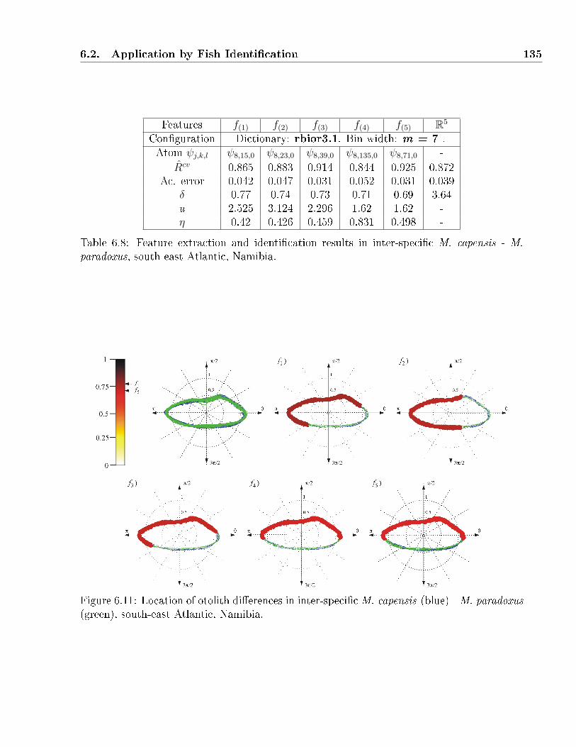
6.2. Application by Fish Identi�cation 135
Features f(1) f(2) f(3) f(4) f(5) R5
Con�guration Dictionary: rbior3.1. Bin width: m = 7 .Atom ψj,k,l ψ8,15,0 ψ8,23,0 ψ8,39,0 ψ8,135,0 ψ8,71,0 -
Rcv 0.865 0.883 0.914 0.844 0.925 0.872Ac. error 0.042 0.047 0.031 0.052 0.031 0.039
δ 0.77 0.74 0.73 0.71 0.69 3.64u 2.525 3.124 2.296 1.62 1.62 -η 0.42 0.426 0.459 0.831 0.498 -
Table 6.8: Feature extraction and identi�cation results in inter-speci�c M. capensis - M.paradoxus, south-east Atlantic, Namibia.
Figure 6.11: Location of otolith di�erences in inter-speci�cM. capensis (blue) - M. paradoxus(green), south-east Atlantic, Namibia.

136 Fish Identi�cation and Age Estimation Results
Features f(1) f(2) f(3) f(4) f(5) R5
Con�guration Dictionary: rbior3.1. Bin width: m = 6 .Atom ψj,k,l ψ7,67,1 ψ7,19,1 ψ7,11,1 ψ6,17,2 ψ7,7,1 -
Rcv 0.992 0.941 0.976 0.928 0.955 0.957Ac. error 0.016 0.029 0.013 0.023 0.013 0.009
δ 1 0.89 0.87 0.85 0.80 4.41u 1.606 1.707 -0.327 2.667 1.958 -η 0.832 0.459 0.426 0.498 0.417 -
Table 6.9: Feature extraction and identi�cation results in inter-speci�c M. polli - M. sene-galensis, central-east Atlantic, Senegal.
Figure 6.12: Location of otolith di�erences in inter-speci�c M. polli (blue)- M. senegalensis(green), central-east Atlantic, Senegal.

6.2. Application by Fish Identi�cation 137
Irregularities are found at the center on the top part of the otolith (π/2) between the
dorso-rostral and dorso-caudal margin with features f(1), f(2) and f(5), whereas f(3) extends
from the dorso-rostral margin, through the rostral and ventral area, and f(4) covers the
dorso-caudal margin (Fig. 6.12).
As in the M. capensis - M.paradoxus experiment, the same conclusion regarding the
morphological di�erences and habitat could be attributed. The pairM. polli - M.senegalensis
presents a depth distribution similar to these because they also belong to the African coast.
In addition, this conclusion is consistent with a study developed by Roldan et al. (1999) who
showed a similar phylogenetic relationship between both pairs. Therefore, the results of both
experiments can be equivalent.
� M. gayi - M. australis
The worst inter-speci�c result was obtained in theM. gayi - M. australis experiment. Feature
f(1) is the only one surpassing the value of 0.5 which represents an identi�cation rate of
approximately 75% (Table 6.10). Its atom is well localized at the ventral side near the cauda
(Figure 6.13). The use of the vector in R5 containing the best features did not account for
a signi�cant improvement (with an increase of only 3%). Even though all features appears
to be consistent with δ, except f(2), these values are too small. As such, the results were
considered as insu�cient, and the conclusion is that the method failed in the identi�cation
of M. gayi and M. australis otoliths.
The cause of such a poor performance could be attributed to the high variability in the
size of the species under consideration (see Table 6.5), which includes adult and juvenile
individuals, as observed by Lombarte and Castellón (1991). Another reason of such hetero-
geneity may be the presence of species in the area which have not previously been described,
such as M. patagonicus from Chile, which is often confused with M. australis or even M. gayi
(Lloris and Matallanas 2003). If this assumption could be contrasted experimenting with
supplementary and objective data, our results could serve to verify that the initial data set
may be erroneous for this reason. However, this hypothesis could not be proved.
6.2.2.2 Intra-speci�c experimentation
Intra-speci�c results are provided in �gures 6.14 - 6.17 and tables 6.11 - 6.14. As expected,
classi�cation values were generally inferior than inter-speci�c, due to the similarity of the
species compared. However, some conclusions could be taken from two experiments, which
may be related to geographical factors. These are the experiments corresponding to the
north-west Atlantic M. bilinearis and south-west Paci�c M. gayi where identi�cation rates
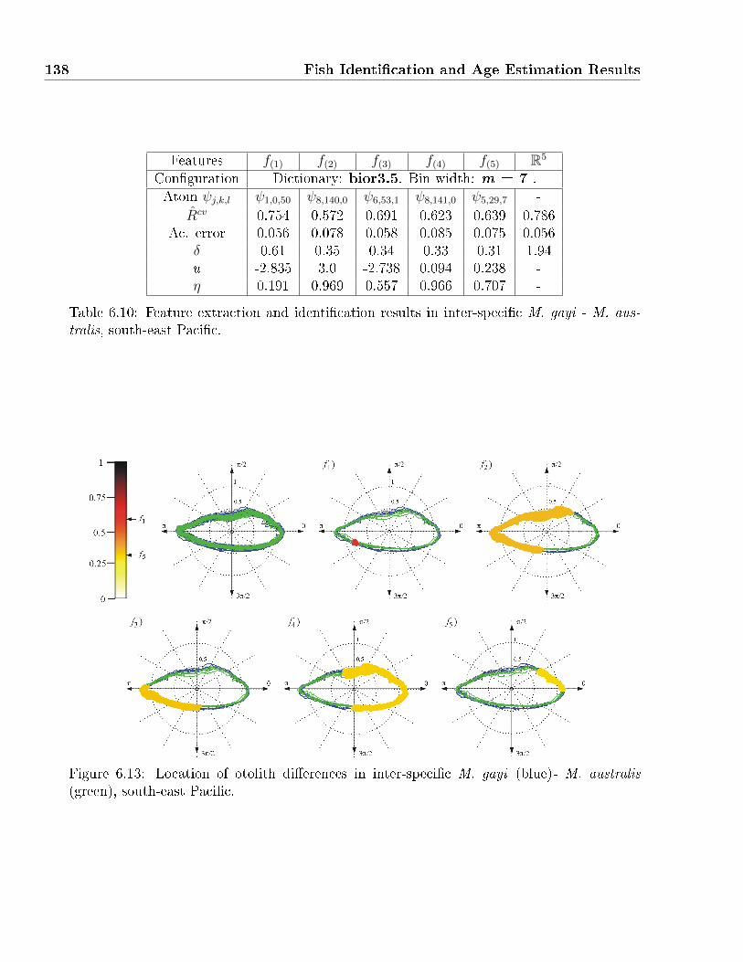
138 Fish Identi�cation and Age Estimation Results
Features f(1) f(2) f(3) f(4) f(5) R5
Con�guration Dictionary: bior3.5. Bin width: m = 7 .Atom ψj,k,l ψ1,0,50 ψ8,140,0 ψ6,53,1 ψ8,141,0 ψ5,29,7 -
Rcv 0.754 0.572 0.691 0.623 0.639 0.786Ac. error 0.056 0.078 0.058 0.085 0.075 0.056
δ 0.61 0.35 0.34 0.33 0.31 1.94u -2.835 3.0 -2.738 0.094 0.238 -η 0.191 0.969 0.557 0.966 0.707 -
Table 6.10: Feature extraction and identi�cation results in inter-speci�c M. gayi - M. aus-tralis, south-east Paci�c.
Figure 6.13: Location of otolith di�erences in inter-speci�c M. gayi (blue)- M. australis(green), south-east Paci�c.
6.2. Application by Fish Identi�cation 139
over 86% were observed.
� M. merluccius: Mediterranean and north-east Atlantic (Spain)
All discriminant values were below 0.5 (Table 6.11). The best feature f(1), which is positioned
along the dorso-caudal margin and extends along the middle of the ventral side (2π/3, see
Fig. 6.14), is consistent with δ but the accuracy of correct identi�cations is only about 72%.
The rest of the features were not consistent: f(2), which has a discrimination of 0.47 is only
61.5% accurate, whereas f(3) which has a discrimination of only 0.31 is 71.7% accurate. The
accuracy using all �ve coe�cients is approximately 80%.
Thus, these results were considered insu�cient and the experiment was unable to es-
tablish di�erences between the two Iberian M. merluccius populations, perhaps due to the
scarce availability of samples.
A similar experiment previously implemented by Torres et al (2000b) obtained better
results with the use of Fourier descriptors and LDA. Their work concluded that morphometric
descriptors, such as size and shape, tend to be larger in Mediterranean hake because they
are more sensitive to environmental factors, such as water temperature and depth. This may
be an explanation for our poor results, since the size of all otoliths was normalized.
Other studies, however, suggest that genetic factors are more closely related to otolith
morphology than water temperature and depth (Lombarte and Lleonart 1993, Roldan et al.
1999, Lombarte et al. 2003), which seems rather contradictory. So no conclusion could be
drawn regarding the contour areas highlighted by DLDB.
� M. bilinearis: north-west Atlantic (USA - Canada)
All coe�cients were consistent with the discriminant value δ but only the best feature f(1)
was signi�cant according to our three de�ned result categories (Table 6.12). The accuracies
of the remaining coe�cients were below 80%, and combining the coe�cients from all �ve
features did not improve correct classi�cation rates either.
Therefore, only the shape of the basis function belonging to f(1) (ψ8,179,0) which sup-
ports the dorso-rostral and dorso-caudal margins (Fig. 6.15), was considered relevant for
distinguishing M. bilinearis otoliths from USA and Canada (90% of correct classi�cations).
These species correspond to two stocks managed separately because of di�erences in the
exploitation patterns of both countries (Garrison and Link 2000). Although stock di�erences
were con�rmed by Bolles and Begg (2000) using the morphology of full otoliths and growth
rates, no formal de�nition in terms of structural otolith patterns have been provided. Our

140 Fish Identi�cation and Age Estimation Results
Features f(1) f(2) f(3) f(4) f(5) R5
Con�guration Dictionary: db16. Bin width: m = 5 .Atom ψj,k,l ψ8,27,0 ψ4,9,7 ψ7,12,1 ψ2,3,32 ψ6,17,1 -
Rcv 0.721 0.615 0.717 0.615 0.601 0.795Ac. error 0.060 0.086 0.060 0.084 0.079 0.038
δ 0.48 0.47 0.31 0.30 0.28 1.84u 3.052 2.762 -1.878 2.656 0.209 -η 0.068 0.905 0.065 0.62 0.492 -
Table 6.11: Feature extraction and identi�cation results in intra-speci�c M. merluccius,Mediterranean and north-east Atlantic.
Figure 6.14: Location of otolith di�erences in intra-speci�c M. merluccius, Mediterranean(blue) and north-east Atlantic (green).
results indicate a high probability that these pattern di�erences are associated to the dorso-
rostral and dorso-caudal margins.
� M. gayi : south-west Paci�c (Chile - Peru)
Three features, f(1) − f(3), presented signi�cant accuracy (between 80% and 87%). Unfor-
tunately, only the best one, f(1), was consistent with its discrimination value (0.66 against
an identi�cation probability of 86.6%, see Table 6.13). As such, this was the only relevant
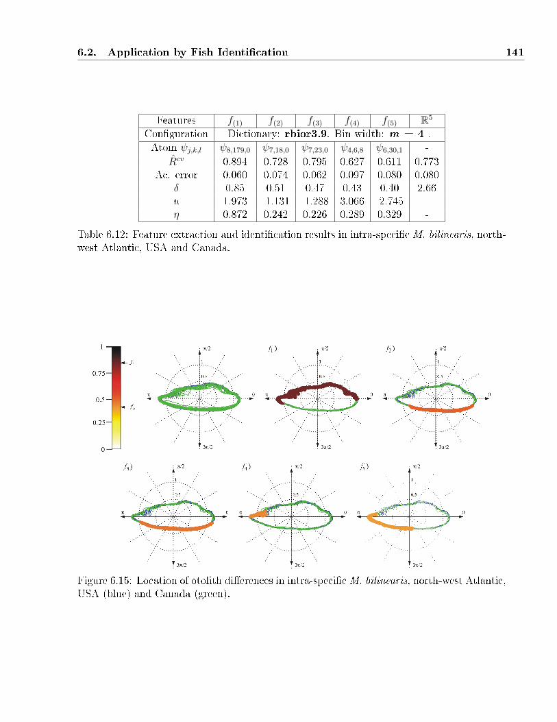
6.2. Application by Fish Identi�cation 141
Features f(1) f(2) f(3) f(4) f(5) R5
Con�guration Dictionary: rbior3.9. Bin width: m = 4 .Atom ψj,k,l ψ8,179,0 ψ7,18,0 ψ7,23,0 ψ4,6,8 ψ6,30,1 -
Rcv 0.894 0.728 0.795 0.627 0.611 0.773Ac. error 0.060 0.074 0.062 0.097 0.080 0.080
δ 0.85 0.51 0.47 0.43 0.40 2.66u 1.973 -1.131 -1.288 3.066 -2.745 -η 0.872 0.242 0.226 0.289 0.329 -
Table 6.12: Feature extraction and identi�cation results in intra-speci�c M. bilinearis, north-west Atlantic, USA and Canada.
Figure 6.15: Location of otolith di�erences in intra-speci�cM. bilinearis, north-west Atlantic,USA (blue) and Canada (green).
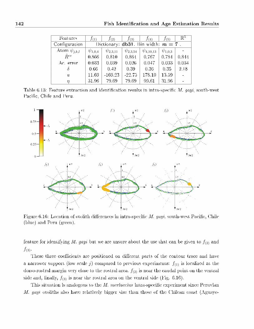
142 Fish Identi�cation and Age Estimation Results
Features f(1) f(2) f(3) f(4) f(5) R5
Con�guration Dictionary: db31. Bin width: m = 7 .Atom ψj,k,l ψ1,0,4 ψ2,3,11 ψ2,3,54 ψ4,10,13 ψ1,0,3 -
Rcv 0.866 0.810 0.864 0.767 0.784 0.844Ac. error 0.033 0.039 0.026 0.047 0.033 0.034
δ 0.66 0.42 0.39 0.36 0.35 2.18u 11.69 -169.23 -22.75 178.10 13.59 -η 31.96 79.69 79.69 99.61 31.96 -
Table 6.13: Feature extraction and identi�cation results in intra-speci�c M. gayi, south-westPaci�c, Chile and Peru.
Figure 6.16: Location of otolith di�erences in intra-speci�c M. gayi, south-west Paci�c, Chile(blue) and Peru (green).
feature for identifying M. gayi but we are unsure about the use that can be given to f(2) and
f(3).
These three coe�cients are positioned on di�erent parts of the contour trace and have
a narrower support (low scale j ) compared to previous experiments: f(1) is localized at the
dorso-rostral margin very close to the rostral area, f(2) is near the caudal point on the ventral
side and, �nally, f(3) is near the rostral area on the ventral side (Fig. 6.16).
This situation is analogous to the M. merluccius intra-speci�c experiment since Peruvian
M. gayi otoliths also have relatively bigger size than those of the Chilean coast (Aguayo-
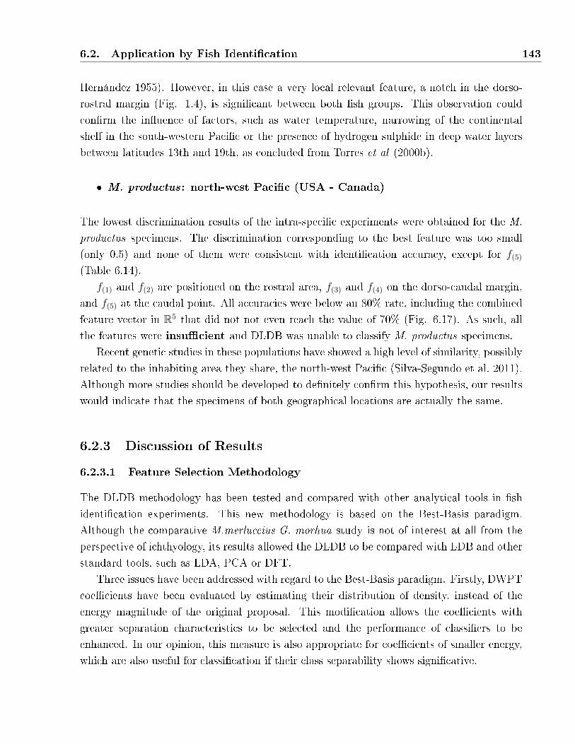
6.2. Application by Fish Identi�cation 143
Hernández 1955). However, in this case a very local relevant feature, a notch in the dorso-
rostral margin (Fig. 1.4), is signi�cant between both �sh groups. This observation could
con�rm the in�uence of factors, such as water temperature, narrowing of the continental
shelf in the south-western Paci�c or the presence of hydrogen sulphide in deep water layers
between latitudes 13th and 19th, as concluded from Torres et al (2000b).
� M. productus: north-west Paci�c (USA - Canada)
The lowest discrimination results of the intra-speci�c experiments were obtained for the M.
productus specimens. The discrimination corresponding to the best feature was too small
(only 0.5) and none of them were consistent with identi�cation accuracy, except for f(5)
(Table 6.14).
f(1) and f(2) are positioned on the rostral area, f(3) and f(4) on the dorso-caudal margin,
and f(5) at the caudal point. All accuracies were below an 80% rate, including the combined
feature vector in R5 that did not not even reach the value of 70% (Fig. 6.17). As such, all
the features were insu�cient and DLDB was unable to classify M. productus specimens.
Recent genetic studies in these populations have showed a high level of similarity, possibly
related to the inhabiting area they share, the north-west Paci�c (Silva-Segundo et al. 2011).
Although more studies should be developed to de�nitely con�rm this hypothesis, our results
would indicate that the specimens of both geographical locations are actually the same.
6.2.3 Discussion of Results
6.2.3.1 Feature Selection Methodology
The DLDB methodology has been tested and compared with other analytical tools in �sh
identi�cation experiments. This new methodology is based on the Best-Basis paradigm.
Although the comparative M.merluccius-G. morhua study is not of interest at all from the
perspective of ichthyology, its results allowed the DLDB to be compared with LDB and other
standard tools, such as LDA, PCA or DFT.
Three issues have been addressed with regard to the Best-Basis paradigm. Firstly, DWPT
coe�cients have been evaluated by estimating their distribution of density, instead of the
energy magnitude of the original proposal. This modi�cation allows the coe�cients with
greater separation characteristics to be selected and the performance of classi�ers to be
enhanced. In our opinion, this measure is also appropriate for coe�cients of smaller energy,
which are also useful for classi�cation if their class separability shows signi�cative.
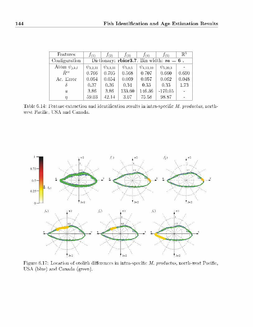
144 Fish Identi�cation and Age Estimation Results
Features f(1) f(2) f(3) f(4) f(5) R5
Con�guration Dictionary: rbior3.7. Bin width: m = 6 .Atom ψj,k,l ψ3,2,31 ψ3,3,31 ψ5,0,5 ψ4,13,10 ψ5,20,3 -
Rcv 0.766 0.705 0.568 0.707 0.660 0.690Ac. Error 0.064 0.054 0.069 0.057 0.062 0.048
δ 0.37 0.36 0.34 0.33 0.33 1.73u 3.86 3.86 133.60 146.36 -170.05 -η 59.03 42.14 3.07 75.58 98.87 -
Table 6.14: Feature extraction and identi�cation results in intra-speci�cM. productus, north-west Paci�c, USA and Canada.
Figure 6.17: Location of otolith di�erences in intra-speci�c M. productus, north-west Paci�c,USA (blue) and Canada (green).
6.2. Application by Fish Identi�cation 145
Secondly, the original bottom-up strategy has been replaced by a top-down algorithm
that selects DWPT nodes on the basis of their most signi�cant element. This was modi�ed
to permit the consideration of these coe�cients for classi�cation.
And �nally, the Kullback-Liebler metric was changed for a version supported on the
Battacharyaa a�nity measure (Eq. 5.24). The new measure has its own mechanism for rep-
resenting the lowest and highest discrimination capacity, a behavior necessary for achieving
data generalization and indicating the signi�cance of structure irregularities on the image.
Our proposal can provide further information on the physical structures that make up
the signals. Not only did the selected features obtained higher classi�cation accuracy, but
they also explained shape di�erences in terms of geometrical characters of the contour, such
as the position of oscillating of structures, more closely related to ecological and biological
aspects of �sh species. Inferring such kind of conclusions in methods such as PCA or LDA is
impossible since the eigenvectors, determined from between-class and within-class covariance
matrices, are di�cult to interpret from a physical point of view.
The cod-hake experiment showed that contour information is su�cient for fully identifying
both �sh species. The fact that STD can be even more e�ective than DFT (since only one
PCA coe�cient was necessary to obtain full identi�cation with LVQ, whereas DFT needed
of �ve coe�cients), suggests certain con�ict between PCA and DFT methods.
In fact, the implementation of PCA on DFT does not make much sense from the per-
spective of signal processing, as PCA also develops its own orthogonal projection, similar to
DFT, for representing the components of large variance. In LDA, however, the same is not
true because orthogonality is lost, making the output features very e�ective for classi�cation
purposes.
Analogously, these results also showed that compression and discrimination tools do not
necessarily have to be considered for di�erent purposes, since full identi�cation is also possible
for all PCA, LDA, LDB, and DLDB. From the author's point of view, this issue is conditioned
by the true nature of input data. In the cod-hake experiment, both classes are teleostean
species from species of di�erent taxonomy, so it would be reasonable to expect that the
covariance matrix ful�ll the same discrimination role.
Our identi�cation results also showed di�erences between the performance of linear and
nonlinear classi�ers. While LVQ proved to be more robust at increasing the input vector
with more features, the accuracy of k-NN decreased drastically. This is a typical perfor-
mance in nonlinear, which base their operation on the separation of class decision boundaries
and tend to produce more accurate density estimates than Bayesian methods. In contrast,
Bayesian methods are con�gured easily, have low computational cost and serve to obtain a
�rst reference estimate.
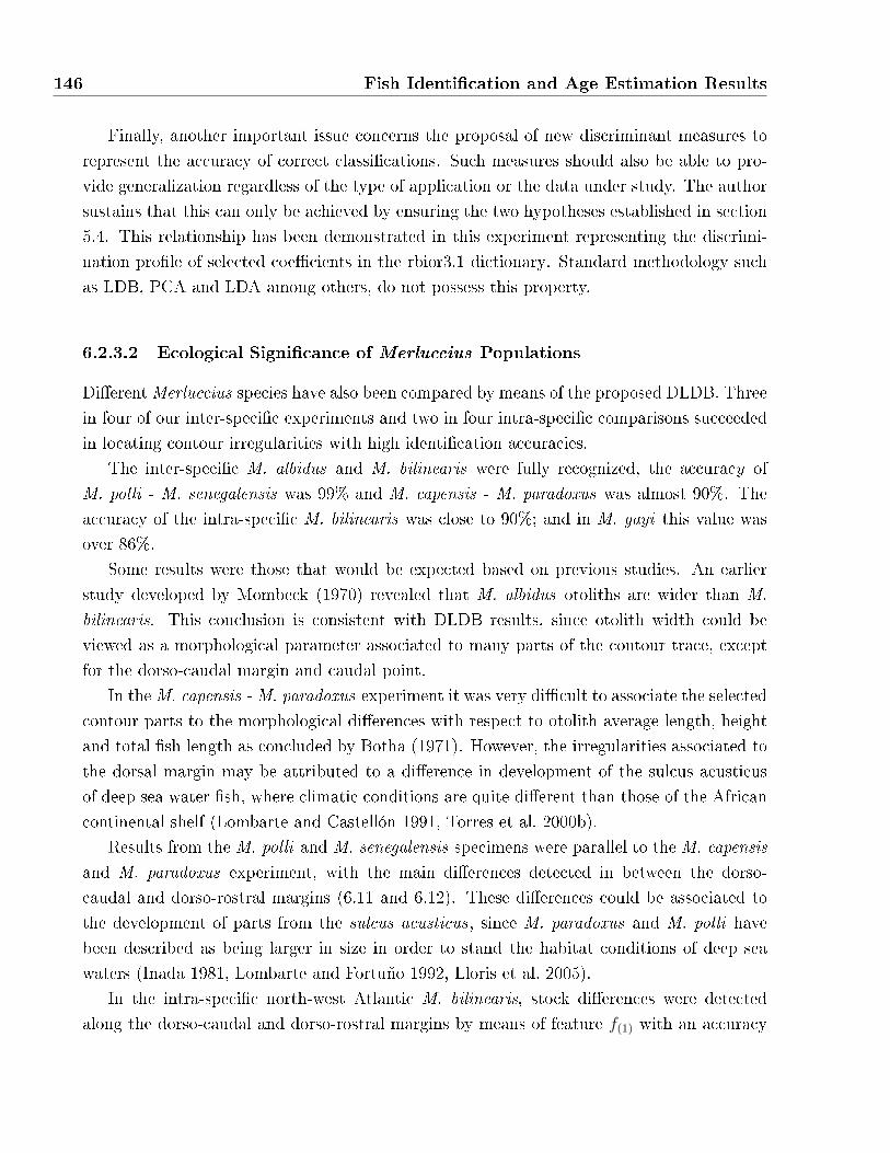
146 Fish Identi�cation and Age Estimation Results
Finally, another important issue concerns the proposal of new discriminant measures to
represent the accuracy of correct classi�cations. Such measures should also be able to pro-
vide generalization regardless of the type of application or the data under study. The author
sustains that this can only be achieved by ensuring the two hypotheses established in section
5.4. This relationship has been demonstrated in this experiment representing the discrimi-
nation pro�le of selected coe�cients in the rbior3.1 dictionary. Standard methodology such
as LDB, PCA and LDA among others, do not possess this property.
6.2.3.2 Ecological Signi�cance of Merluccius Populations
Di�erentMerluccius species have also been compared by means of the proposed DLDB. Three
in four of our inter-speci�c experiments and two in four intra-speci�c comparisons succeeded
in locating contour irregularities with high identi�cation accuracies.
The inter-speci�c M. albidus and M. bilinearis were fully recognized, the accuracy of
M. polli - M. senegalensis was 99% and M. capensis - M. paradoxus was almost 90%. The
accuracy of the intra-speci�c M. bilinearis was close to 90%; and in M. gayi this value was
over 86%.
Some results were those that would be expected based on previous studies. An earlier
study developed by Mombeck (1970) revealed that M. albidus otoliths are wider than M.
bilinearis. This conclusion is consistent with DLDB results, since otolith width could be
viewed as a morphological parameter associated to many parts of the contour trace, except
for the dorso-caudal margin and caudal point.
In theM. capensis -M. paradoxus experiment it was very di�cult to associate the selected
contour parts to the morphological di�erences with respect to otolith average length, height
and total �sh length as concluded by Botha (1971). However, the irregularities associated to
the dorsal margin may be attributed to a di�erence in development of the sulcus acusticus
of deep sea water �sh, where climatic conditions are quite di�erent than those of the African
continental shelf (Lombarte and Castellón 1991, Torres et al. 2000b).
Results from the M. polli and M. senegalensis specimens were parallel to the M. capensis
and M. paradoxus experiment, with the main di�erences detected in between the dorso-
caudal and dorso-rostral margins (6.11 and 6.12). These di�erences could be associated to
the development of parts from the sulcus acusticus , since M. paradoxus and M. polli have
been described as being larger in size in order to stand the habitat conditions of deep sea
waters (Inada 1981, Lombarte and Fortuño 1992, Lloris et al. 2005).
In the intra-speci�c north-west Atlantic M. bilinearis, stock di�erences were detected
along the dorso-caudal and dorso-rostral margins by means of feature f(1) with an accuracy

6.3. Application by Age Estimation 147
Figure 6.18: Example of automatic detection of the �rst year mark by means of AGD. Theotolith section correspond to a 3 year-old cod specimen. The one-dimensional intensity signalhas been extracted from the nucleus to the contour border (right to left) following the greentrace. Age information is provided by the expert (red dots) in order to compare the detectionof the �rst year period (red circle).
around 90% (Fig. 6.15), whereas in intra-speci�c north-west Paci�c M. gayi di�erences could
be associated to changes in temperature conditions of both stocks (Torres et al. 2000a).
DLDB was unsuccessful with inter-speci�c M. gayi - M. australis, intra-speci�c M. mer-
luccius and M. productus. In the latter, results may indicate that both otoliths from the
Paci�c in Canada are, in fact, from the same population. On the other hand, the consistency
with δ found in four selected features inM. gayi - M. australis may indicate that some kind of
speci�c variability exists within the same species. However, other tests of similarity should be
carried out to con�rm these hypothesis, since specimens from M. patagonicus, whose otoliths
have never been fully described, have been recently found inhabiting the same area.
6.3 Application by Age Estimation
In order to illustrate the performance of AGD, we �rst show the results for an image section
corresponding to a three-year-old cod otolith (Fig. 6.18) . Figure 6.19 represents its extracted
intensity pro�le i [n] along the main growth radial axis (green line in Fig. 6.18). The signal
was resampled to N=512 points and the radial length was normalized in the range [0, 1).
Information related to the position of year marks was also provided by the expert (red lines).
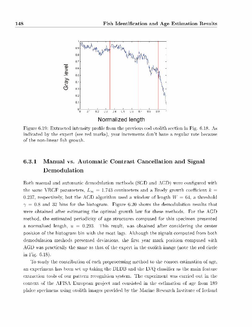
148 Fish Identi�cation and Age Estimation Results
Figure 6.19: Extracted intensity pro�le from the previous cod otolith section in Fig. 6.18. Asindicated by the expert (see red marks), year increments don't have a regular rate becauseof the non-linear �sh growth.
6.3.1 Manual vs. Automatic Contrast Cancellation and Signal
Demodulation
Both manual and automatic demodulation methods (SGD and AGD) were con�gured with
the same VBGF parameters, L∞ = 1.743 centimeters and a Brody growth coe�cient k =
0.237, respectively, but the AGD algorithm used a window of length W = 64, a threshold
γ = 0.8 and 32 bins for the histogram. Figure 6.20 shows the demodulation results that
were obtained after estimating the optimal growth law for these methods. For the AGD
method, the estimated periodicity of age structures computed for this specimen presented
a normalized length, u = 0.293. This result, was obtained after considering the center
position of the histogram bin with the most lags. Although the signals computed from both
demodulation methods presented deviations, the �rst year mark position computed with
AGD was practically the same as that of the expert in the otolith image (note the red circle
in Fig. 6.18).
To study the contribution of each preprocessing method to the correct estimation of age,
an experiment has been set up taking the DLDB and the LVQ classi�er as the main feature
extraction tools of our pattern recognition system. The experiment was carried out in the
context of the AFISA European project and consisted in the estimation of age from 189
plaice specimens using otolith images provided by the Marine Research Institute of Iceland
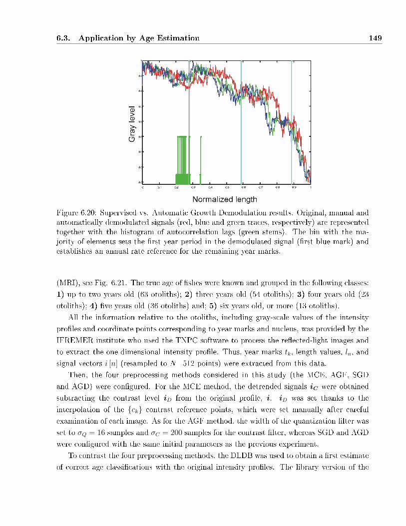
6.3. Application by Age Estimation 149
Figure 6.20: Supervised vs. Automatic Growth Demodulation results. Original, manual andautomatically demodulated signals (red, blue and green traces, respectively) are representedtogether with the histogram of autocorrelation lags (green stems). The bin with the ma-jority of elements sets the �rst year period in the demodulated signal (�rst blue mark) andestablishes an annual rate reference for the remaining year marks.
(MRI), see Fig. 6.21. The true age of �shes were known and grouped in the following classes:
1) up to two years old (63 otoliths); 2) three years old (54 otoliths); 3) four years old (23
otoliths); 4) �ve years old (36 otoliths) and; 5) six years old, or more (13 otoliths).
All the information relative to the otoliths, including gray-scale values of the intensity
pro�les and coordinate points corresponding to year marks and nucleus, was provided by the
IFREMER institute who used the TNPC software to process the re�ected-light images and
to extract the one-dimensional intensity pro�le. Thus, year marks tk, length values, ln, and
signal vectors i [n] (resampled to N=512 points) were extracted from this data.
Then, the four preprocessing methods considered in this study (the MCE, AGF, SGD
and AGD) were con�gured. For the MCE method, the detrended signals iC were obtained
subtracting the contrast level iD from the original pro�le, i. iD was set thanks to the
interpolation of the {ck} contrast reference points, which were set manually after careful
examination of each image. As for the AGF method, the width of the quantization �lter was
set to σQ = 16 samples and σC = 200 samples for the contrast �lter, whereas SGD and AGD
were con�gured with the same initial parameters as the previous experiment.
To contrast the four preprocessing methods, the DLDB was used to obtain a �rst estimate
of correct age classi�cations with the original intensity pro�les. The library version of the

150 Fish Identi�cation and Age Estimation Results
(a) (b)
(c) (d)
Figure 6.21: Plaice otolith samples used in our experiments for di�erent age classes. (a) twoyears; (b) three years; (c) �ve years; (d) six years or more.
DLDB evaluated the best type of standard basis function for a decomposition depth of J=9
levels in the DWPT tree, using 9-bin length histograms to determine the density distribution
of the coe�cients. The feature vector containing the �ve best discriminant coe�cients,{w(n)x
}∈ Rn for n=5, was introduced as input data to the LVQ classi�er to estimate
the age of all specimens. An average rate of correct classi�cation of 55% of the samples,
Rcv (r) = 0.55, was obtained after 50 trials with the 'k -fold cross-validation' method, using
K=5 groups with Ns ' N/K = 37 samples in each group.
The preceding con�guration was then used to evaluate the e�ciency of the four pre-
processing methods, �rst independently (Table 6.15), and then combining together contrast
cancellation and growth demodulation in their two modalities: manual and automated (Ta-
ble. 6.16). All aging rates were estimated for the 'symlet13' waletet packet dictionary, which
obtained the highest result (88.5%) when MCE and SGD were combined and the DLDB
was computed.
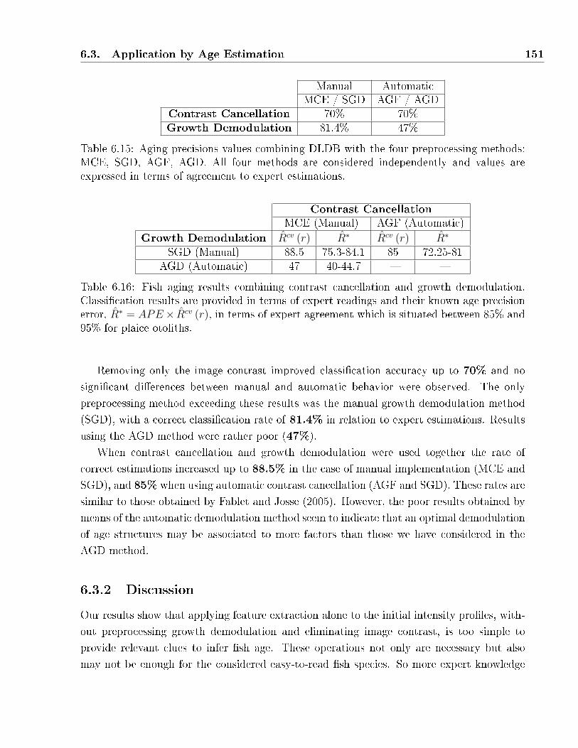
6.3. Application by Age Estimation 151
Manual AutomaticMCE / SGD AGF / AGD
Contrast Cancellation 70% 70%Growth Demodulation 81.4% 47%
Table 6.15: Aging precisions values combining DLDB with the four preprocessing methods:MCE, SGD, AGF, AGD. All four methods are considered independently and values areexpressed in terms of agreement to expert estimations.
Contrast CancellationMCE (Manual) AGF (Automatic)
Growth Demodulation Rcv (r) R∗ Rcv (r) R∗
SGD (Manual) 88.5 75.3-84.1 85 72.25-81AGD (Automatic) 47 40-44.7 � �
Table 6.16: Fish aging results combining contrast cancellation and growth demodulation.Classi�cation results are provided in terms of expert readings and their known age precisionerror, R∗ = APE× Rcv (r), in terms of expert agreement which is situated between 85% and95% for plaice otoliths.
Removing only the image contrast improved classi�cation accuracy up to 70% and no
signi�cant di�erences between manual and automatic behavior were observed. The only
preprocessing method exceeding these results was the manual growth demodulation method
(SGD), with a correct classi�cation rate of 81.4% in relation to expert estimations. Results
using the AGD method were rather poor (47%).
When contrast cancellation and growth demodulation were used together the rate of
correct estimations increased up to 88.5% in the case of manual implementation (MCE and
SGD), and 85% when using automatic contrast cancellation (AGF and SGD). These rates are
similar to those obtained by Fablet and Josse (2005). However, the poor results obtained by
means of the automatic demodulation method seem to indicate that an optimal demodulation
of age structures may be associated to more factors than those we have considered in the
AGD method.
6.3.2 Discussion
Our results show that applying feature extraction alone to the initial intensity pro�les, with-
out preprocessing growth demodulation and eliminating image contrast, is too simple to
provide relevant clues to infer �sh age. These operations not only are necessary but also
may not be enough for the considered easy-to-read �sh species. So more expert knowledge
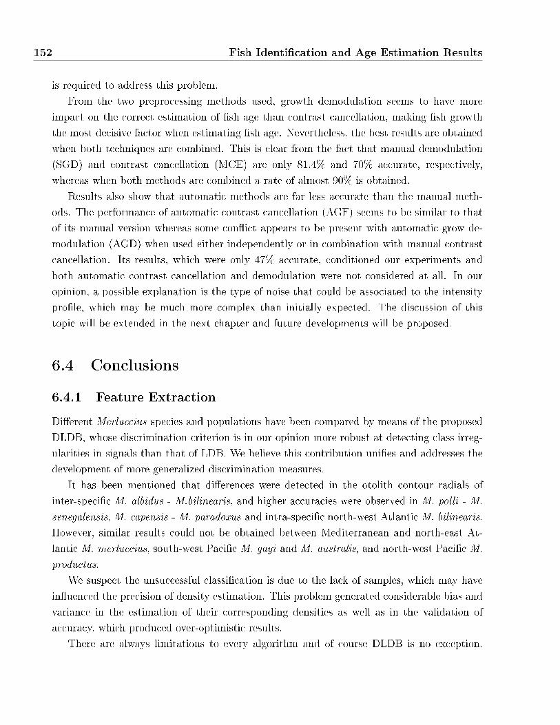
152 Fish Identi�cation and Age Estimation Results
is required to address this problem.
From the two preprocessing methods used, growth demodulation seems to have more
impact on the correct estimation of �sh age than contrast cancellation, making �sh growth
the most decisive factor when estimating �sh age. Nevertheless, the best results are obtained
when both techniques are combined. This is clear from the fact that manual demodulation
(SGD) and contrast cancellation (MCE) are only 81.4% and 70% accurate, respectively,
whereas when both methods are combined a rate of almost 90% is obtained.
Results also show that automatic methods are far less accurate than the manual meth-
ods. The performance of automatic contrast cancellation (AGF) seems to be similar to that
of its manual version whereas some con�ict appears to be present with automatic grow de-
modulation (AGD) when used either independently or in combination with manual contrast
cancellation. Its results, which were only 47% accurate, conditioned our experiments and
both automatic contrast cancellation and demodulation were not considered at all. In our
opinion, a possible explanation is the type of noise that could be associated to the intensity
pro�le, which may be much more complex than initially expected. The discussion of this
topic will be extended in the next chapter and future developments will be proposed.
6.4 Conclusions
6.4.1 Feature Extraction
Di�erent Merluccius species and populations have been compared by means of the proposed
DLDB, whose discrimination criterion is in our opinion more robust at detecting class irreg-
ularities in signals than that of LDB. We believe this contribution uni�es and addresses the
development of more generalized discrimination measures.
It has been mentioned that di�erences were detected in the otolith contour radials of
inter-speci�c M. albidus - M.bilinearis, and higher accuracies were observed in M. polli - M.
senegalensis, M. capensis - M. paradoxus and intra-speci�c north-west Atlantic M. bilinearis.
However, similar results could not be obtained between Mediterranean and north-east At-
lantic M. merluccius, south-west Paci�c M. gayi and M. australis, and north-west Paci�c M.
productus.
We suspect the unsuccessful classi�cation is due to the lack of samples, which may have
in�uenced the precision of density estimation. This problem generated considerable bias and
variance in the estimation of their corresponding densities as well as in the validation of
accuracy, which produced over-optimistic results.
There are always limitations to every algorithm and of course DLDB is no exception.
6.4. Conclusions 153
There are four main concerns which we are currently investigating. In particular, four issues
should be addressed in the future. The most important one focuses on the way of calculating
class densities, since estimating the precise true distributions is crucial in the automatic
selection of DWPT coe�cients. For now, we used histograms because they are the simplest
form and the �rst natural choice of non-parametric estimation, although they do present
some drawbacks.
On one hand, the discontinuities of the estimates are not due to the underlying density,
but to an artifact of the chosen bin locations delimited by the starting position (t0) and
the bin width (h). Its density estimate, f = vmhN
, becomes more accurate as we increase N
and reduce h. However, since N is �xed, to improve accuracy we could let h approach to
zero but then the region Gm∼= tm − tm−1 would become so small that it would yield no
samples (vm = 0). In practice, that means we need to �nd a compromise for N and h, which
should be large enough to include su�cient samples but also small enough to assume that f
is continuous within Gm.
The use of alternative methods, such as Kernel Density Estimation (KDE) or k-Nearest
Neighbor, and their capacity to improve this stage of the Best-Basis paradigm is discussed
in the next chapter.
Another limitation is associated to the translation dependence of the DWPT method.
This occurs because the sub-sampling operation destroys translation invariance of the wavelet
transform, which means the control over homology of geometrical shapes is lost.
Our way to tackle this problem was to use a normalization method based on the Fourier
ellipse, which modi�ed otolith size, sample position and orientation. However, addressing
this problem from other perspectives may be more e�ective for other types of signals. For
instance, the use of customized �lter-banks or the dyadic version of the wavelet transform,
the algorithm à trous , which does not use sub-sampling.
The third limitation is inherent to the selection of nodes and its search strategy . The
admissible tree varies signi�cantly with the number of signals N or the bin width con�guration
(h). This issue may be closely related with accuracy validation methods, such as hold-out or
cross-validation. In this sense, the introduction of such validation techniques within DLDB
could allow to develop a more robust selection based also on the variances of discriminant
measures, or to develop a new and completely di�erent classi�er, if a class decision rule is
included at the end of the process.
Another issue is related to the property of exact reconstruction. In this sense, one may
argue whether exact reconstruction is really necessary in classi�cation tasks. Our opinion
is that relaxing such condition may lead to more e�cient and faster search strategies, since
comparing parent and child nodes may no longer be necessary. This would allow density
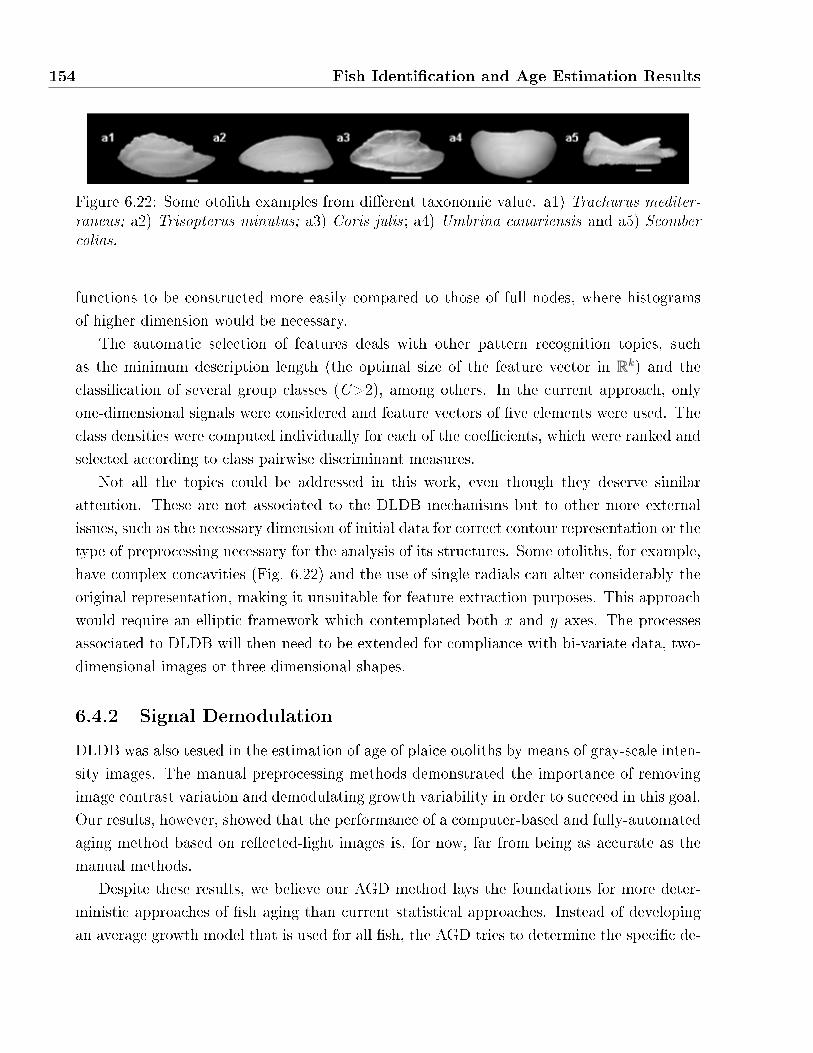
154 Fish Identi�cation and Age Estimation Results
Figure 6.22: Some otolith examples from di�erent taxonomic value. a1) Trachurus mediter-raneus; a2) Trisopterus minutus; a3) Coris julis ; a4) Umbrina canariensis and a5) Scombercolias.
functions to be constructed more easily compared to those of full nodes, where histograms
of higher dimension would be necessary.
The automatic selection of features deals with other pattern recognition topics, such
as the minimum description length (the optimal size of the feature vector in Rk) and the
classi�cation of several group classes (C>2), among others. In the current approach, only
one-dimensional signals were considered and feature vectors of �ve elements were used. The
class densities were computed individually for each of the coe�cients, which were ranked and
selected according to class pairwise discriminant measures.
Not all the topics could be addressed in this work, even though they deserve similar
attention. These are not associated to the DLDB mechanisms but to other more external
issues, such as the necessary dimension of initial data for correct contour representation or the
type of preprocessing necessary for the analysis of its structures. Some otoliths, for example,
have complex concavities (Fig. 6.22) and the use of single radials can alter considerably the
original representation, making it unsuitable for feature extraction purposes. This approach
would require an elliptic framework which contemplated both x and y axes. The processes
associated to DLDB will then need to be extended for compliance with bi-variate data, two-
dimensional images or three-dimensional shapes.
6.4.2 Signal Demodulation
DLDB was also tested in the estimation of age of plaice otoliths by means of gray-scale inten-
sity images. The manual preprocessing methods demonstrated the importance of removing
image contrast variation and demodulating growth variability in order to succeed in this goal.
Our results, however, showed that the performance of a computer-based and fully-automated
aging method based on re�ected-light images is, for now, far from being as accurate as the
manual methods.
Despite these results, we believe our AGD method lays the foundations for more deter-
ministic approaches of �sh aging than current statistical approaches. Instead of developing
an average growth model that is used for all �sh, the AGD tries to determine the speci�c de-
6.4. Conclusions 155
viations of periodicity of a single otolith along its intensity pro�le, and uses this information
to �nd its optimal growth function. In our opinion, this approach is necessary if we are to
develop more speci�c computer-based aging systems that can cope with the more intrinsic
and complex factors involving the growth variability of �shes.
Although manual methods seem to indicate that this growth variability may be the most
in�uential factor, the poor results obtained by AGD suggest that other unconsidered sources
of noise may be present. These sources will be investigated in the future. In this sense, the
decreasing trending pro�le observed along the intensity signal may be closely related with
image light conditions, since light is known to have a di�used re�ection which goes in many
di�erent directions, specially near the otolith border whose surface is very concave. In our
opinion, this is a problem closely related to the geometrical laws the entire acquisition system,
including otolith and camera, are subjected to.
So solutions resort to operations at the mechanical level of image acquisition. For ex-
ample, the development of an image acquisition interpolating several shots with di�erent
light settings may help to reduce (or eliminate) the high contrast variability near the contour
borders and, subsequently, the steep slope at the right end of the intensity signal.
Our current design develops an implementation which combines both �lter-based and
feature-based techniques. Future automated methods, however, are aimed at using only
�lter-based techniques to estimate the exact �sh age, something feasible if age structures can
be demodulated so as to appear periodically in the in tensity pro�le. We will come back to
this issue in the �nal chapter.
Chapter 7
Final Remarks and Further Development
7.1 General Conclusions
The problem of automatic detection and extraction of structure patterns from one-dimensional
signals has been addressed in this thesis. Our work, which is based on the Best-Basis
paradigm, was developed parallel to recent LDB proposals that do not address the prob-
lem of data generalization and measure standardization (Marchand and Saito 2012). These
limitations have been addressed with DLDB, which has been used in the �eld otolith-based
�sh identi�cation and aging.
In general, PCA and LDA methods do not attempt to interpret feature patterns in sig-
nals. The scatter plots only provide visual information about the separability of features,
and eigenvalues are not qualitative information measures for developing automatic feature
selection.
On the other hand, the e�ciency of many descriptive tools for representing structural
components in signals is very constrained. Although DFT is usually a good tool to describe
frequency and phase information, it is in fact unable to capture localized structures (edges,
spikes and ridges...) since the time domain is lost.
LDB tries to enhance classi�cation by using wavelet packet analysis (Coifman and Wick-
erhauser 1992, Saito 1994, Wickerhauser 1995) but its lack of generalization has been demon-
strated in this work. Its separability measures confuse energy distribution with energy mag-
nitude, which means useless coe�cients may be selected within the process, while useful ones
are discarded.
Our proposition was to exploit nonparametric density approaches and the use of bounded
measures, as suggested by Saito (Saito et al. 2002). With these ideas a new LDB algorithm,
the DLDB (Fig. 5.2), has been implemented. This scheme uses a new top-down strategy for
157
158 Final Remarks and Further Development
wavelet trees, which prioritizes the relevance of single coe�cients in the selection of nodes.
The new tool provided results consistent with some classi�ers, such as the k -NN and LVQ.
The DLDB was applied in �sh identi�cation and �sh aging, two important aspects of the
�sh industry. All the experiments were implemented in the context of the AFORO3D project
and the AFISA project from the European Union.
In the �rst application, a preprocessing method for the normalization of the otolith con-
tour was also developed. This step, which develops automatically, minimizes the contour
translation invariance of all otoliths by normalizing their size, rotation and translation. The
whole scheme was used to carry out two experiments, one to classify cod and hake species
to show the functionality of our proposition, and another to study the inter-speci�c and
intra-speci�c relationships of Merluccius �sh species.
In the �rst experiment, irregularities were found at the dorso-rostral and caudal margins
of both species, obtaining the highest possible discrimination rate in relation to the proposed
measure. This result was consistent with classi�cation results, as all the specimens of both
species were fully identi�ed (Table 6.6).
In the study of hake species, the best inter-speci�c identi�cation rate corresponded to
the M. albidus - M. bilinearis, followed by M. polli - M. senegalensis, and M. capensis - M.
paradoxus ; whereas the best intra-speci�c results were obtained forM. bilinearis andM. gayi.
As for the �eld of �sh aging, a very novel approach for automatic demodulation of growth
structures for re�ected-light images, the AGD, has been proposed. The method introduces a
new philosophy based on adapting template functions to the speci�c growth characteristics of
individual �sh. Although results were unsuccessful, this new philosophy represents a totally
di�erent approach of automatic aging compared with classical statistical methodology and
should lay the principles for single �sh growth estimation.
DLDB is a reference tool towards the full automation of signal detection. Not only it is
able to �nd class patterns in signals but also explains them in terms of physical composition.
AGD, on the other hand, represents a new philosophy for �sh growth estimation. Although
their use is restricted here to applications within the �sh industry, they can be exploited
in other �elds, such as the analysis of electrical signals, medical applications or geophysical
phenomena, among others.
In this sense, we believe they o�er scope for range of promising computer tools in signal
processing and pattern recognition, to be explored in the near future. The following sections
outline some of the current problems of both DLDB and AGD, and pose new challenges.

7.2. Feature Extraction Methodology 159
7.2 Feature Extraction Methodology
7.2.1 Input Data
As all our proposals work with one-dimensional signals, image data had to be transformed.
In �sh identi�cation applications, otolith contour coordinate points were changed to radial
data whereas aging applications moved from gray-scale images to intensity vectors.
The preparation of data may condition the whole analytical process of the recognition
system. In �sh identi�cation applications, for example, the use of contour radials in a very
concave otolith may lead to representations over-passing the contour trace, which would be
equivalent to modifying its structures deliberately. In addition, omitting angle information
may cause loss of control over homology. In this case, the undesired e�ect is that the struc-
tures being compared do not correspond to analogous positions in other otoliths, developing
thus misplaced comparisons.
The proposed normalization framework of otolith contours is only a minimizer of this
problem. However, before considering the analysis of full images or the use of very complex
invariant transformations one should look at polar or even Cartesian parametrizations, since
these may allow us to address this problem while, at the same time, saving computing
resources. In such situation, feature extraction mechanisms may need to be modi�ed slightly
in order to maintain performance, for example, by using histograms of several dimensions.
7.2.2 Filter Design
In wavelet analysis, multi-resolution approximation is normally seen as a smooth partition
of the frequency axis, where the band resolution of the �lters increases with decomposition
level. In practice, however, this scenario is altered signi�cantly by the process of �lter design
in order to ensure perfect reconstruction with convolution-sub-sampling operations.
To ensure perfect reconstruction of signals, a low-pass digital �lter {h [l]}L−1l=0 is designed
�rst to construct an interpolating function φ (t), which is then used to calculate the high-pass
�lter {g [l]}L−1l=0 ) and its corresponding wavelet ψ (t), by means of the two-scale di�erence
equations (3.21) and (3.22). The result of doing the process this way is that the mother
wavelet has poor regularity generally speaking, and also �tting its shape to structures com-
monly found in nature, is di�cult. In addition, the indexation of the di�erent dilated and
translated versions of this wavelet in the DWPT tree is too complex and for this reason Eq.
3.92 and 3.93 must be used to associate feature parameters.
The choice of particular wavelets is sometimes of importance in certain applications.
While complex wavelets are suitable to analyze the time evolution of frequency transients,
160 Final Remarks and Further Development
because they are capable of separating amplitude and phase components, real wavelets are
preferable to detect the sharp time transitions of signal structures, smoothness or even corre-
lation between signals. In this sense, the minimization of the approximation error has been a
goal behind the development of some standard basis functions, such as Daubechies wavelets,
Coi�ets or Symlets, among others (Daubechies 1988); included in most of the software pack-
ages. The basics for developing customized real time wavelets are outlined in appendix A.
7.2.3 Translation Dependence
Another issue associated to the normalization of contour data is that contour size, rotation
and translation alter coe�cient values in the discrete version of the wavelet transforms.
Another alternative to the elliptic Fourier series is known as spin cycle (Saito et al. 2002)
and consists in minimizing this drawback by including the shifted versions of input signals
in the LDB. This is equivalent to the 'bootstrap' validation approach presented in section
4.2.1. In this case, however, the problem may be that the discrimination e�ciency of the
coe�cients may decrease considerably.
Research on this topic is still at an early stage. Despite the computational cost, in our
opinion this problem is best addressed by means of time-invariant transforms. In this sense,
it may be useful to look for patterns at denser places of the time/scale plane than the dyadic
grid,
s = aj0, (7.1)
u = k, (7.2)
where 1 ≤ a0 ≤ 2. Appendix B summarizes how to compute a discrete version of the
continuous wavelet transform (CWT). In particular, The dyadic wavelet transform (also
referred to as the algoritme à trous in French, Holschneider et al. 1989) does not use sub-
sampling and, therefore, maintains translation invariance but a way to track the displacement
of coe�cients within vectors must be provided.
Despite these problems, wavelets descriptors are considered very �exible tools, suitable
for many kinds of signal structures (transients, spikes and other kind of irregularities) and
their use can be extended in a wide range of signal processing applications.
7.2.4 Considerations for Multivariate Densities
In general, histograms constitute the simplest form of non-parametric density estimation
that is developed nowadays. Its most important parameter corresponds to the bin width h,
7.2. Feature Extraction Methodology 161
since the point of origin t0 can be determined easily once the lower and upper boundaries are
known.
The main problem of multivariate densities is that the optimal bin number grows expo-
nentially. This drawback was coined by Bellman (1961) as the �curse of dimensionality�. In
our inter-speci�c/intra-speci�c Merluccius experiments (see chapter 6), the number of bins
was relatively too low (oscillating between m=3 and m=8), so there may be reasons to believe
that this problem may be behind our unsuccessful classi�cations.
In the �eld of density estimation, this problem can be addressed from two perspectives:
either we choose a �xed value of V and determine vm from the data, or 2) we can �x vmand calculate V. The �rst group is normally referred to as the Kernel Density Estimation in
the literature (KDE) (Scott 1985a,b), whereas the second group is known as the k-Nearest
Neighbor approach (k -NN) (Silverman 1986, Bishop 1995). Both apply to multivariate es-
timation and their variants address the problem of using small datasets with more, or less,
success. They are described in appendix C.
7.2.5 Search Strategies for C Classes
Our current approach may be su�cient for a small number of classes, say from two to four.
A major problem of using pairwise measures is that the more signal classes one has in a
problem, the more obscure their meaning becomes. In Eq. 5.25 a large value can be due
either to few signi�cant terms with negligible majority (a favorable case) or the accumulation
of many terms with relatively small values (an unfavorable case). Addressing this problem
not only involves the de�nition of more robust and normalized discrimination measures but
may also a�ect the true number of features necessary to classify data accurately.
Although both bottom-up and top-down divide-and-conquer strategies ensure a non-
redundant representation time/frequency support for perfect signal reconstruction, there are
three main issues which deserve thorough examination in order to develop more robust tech-
niques when working with C classes.
First, is compact support strictly necessary when the goal is to de�ne the best feature
models that represent the classes? Or in other words, can redundancy be considered if the
accuracy of correct classi�cation improves? In this sense, one could focus the search strategy
on any point of the wavelet-packet tree, without considering full nodes.
Secondly, divide-and-conquer methods are too restrictive in relation to feature depen-
dence. That is, they only consider discrimination power in the evaluation of coe�cients.
However, let us consider the following scenario with �ve classes and a feature vector of four
dimensions, x ∈ R4, showed in pairs of two-dimensional scatter plots (Fig. 7.1):

162 Final Remarks and Further Development
Figure 7.1: Naive sequential feature selection example considering independent features.Only the pair combination {x1, x4} can obtain full class separation
� The goal is to select the best set of two features identifying the �ve classes.
� In this situation, any reasonable discriminant measure will rank features according to
the sequence: δ(x1) > δ(x2) ≈ δ(x3) > δ(x4). Without doubt, x1 is the best feature since
it divides the class distributions in four groups: f1, f2, f3 and {f4, f5}. x2 and x3 have
similar e�ciency since classes are divided in three groups: {f1, f2}, f3 and {f4, f5} forx2; and f1, {f2, f3} and {f4, f5} for x3. Finally, x4 is the worst feature since it can only
separate f4 and f5.
� The optimal feature set turns out to be {x1, x4} because x4 is the only feature that can
provide the missing information in x1: the discrimination between class distributions
f4 and f5.
� However, if one were to choose two features according to the scores, δ, we would cer-
tainly pick {x1, x2} or {x1, x3} , leaving class distributions f4 and f5 non separable.
The strategy fails because it does not account for features of small discrimination value but
with useful �complementary information�.
In our opinion, Feature Subset Selection techniques (FSS) may eventually solve many of
these problems. In fact, all that is needed is a robust objective function able to generalize
among data and a good search strategy which uses this information as feedback signals to
select feature candidates.
In practice, objective functions are divided into two main groups: �lters and wrappers.
Filtering methods respond to the preceding approach (Fig. 7.2a). In this approach, objec-
tive functions typically measure inter-class distances, statistical dependence or information-

7.2. Feature Extraction Methodology 163
Figure 7.2: Filter-based FSS and Wrapper-based FSS. The objective function of wrappertechniques are based on the predictive accuracy, which is estimated by statistical resamplingor cross-validation methods (from Osuna 2005)
theoretic measures; whereas wrappers develop the same functionality by means of built-in
classi�ers (Fig. 7.2b).
The main advantage of �lter approaches lies in their non-iterative computation which,
obviously, is much faster than a classi�er learning-validation step. The �nal selected feature
set will exhibit more generality providing similar accuracies for a large number of classi�ers,
but there will be a tendency to select the full feature set, forcing the user to cut-o� at
an arbitrary number (as in our DLDB). In contrast, recognition rates tend to be higher in
wrappers, but only for the classi�er under consideration whose interactions are normally
tuned for the speci�c input dataset.
As for the search strategies, there is a large number of methods to be investigated under
the Best-Basis paradigm. In general, the algorithms can be grouped in three categories:
exponential , sequential and randomized . In exponential algorithms, the number of features
to evaluate grows exponentially with the dimensionality of the search space (Land and Doig
1960), whereas sequential methods add (or remove) features in each step but tend to become
trapped in local minima. This problem is solved partially by randomized algorithms (Banzhaf
et al. 1998).
Watanabe and Kaminuma (1988) suggested an interesting framework which can be ex-
tended to the Best-Basis paradigm (Saito et al. 2002) in order to address the problem of
detecting C>2 classes. Instead of constructing a feature extractor for the entire classi�ca-
tion problem, consider C sets of two-class problems by reorganizing the partition of the input
training set into c-class (c) and non-c-class (c). Then, each position of the DWPT tree can

164 Final Remarks and Further Development
be evaluated according to the previous two-class problem, selecting a total of C coe�cients
for solving the problem.
7.2.6 Future Proposal
As a concluding remark from this thesis, the following is a proposal to address the preceding
issues, and which may be considered in the future:
Algorithm. 7.1: The DLDB2. Let T = {wj,k,l} de�ne the set containing all basis
functions corresponding to every position in the wavelet-packet tree, for j = 0, . . . , J , k =
0, . . . , 2j − 1 and l = N/2j − 1. Assume that Bc is used to denote the set storing the best
features, at each step c, initialized to B0 ={/O}. The following procedure describes another
possible search strategy:
� Step 0: Choose a dictionary of orthonormal bases D (i.e. specify QMF's for a wavelet
packet dictionary or decide to use either the local cosine dictionary or the local sine
dictionary). Specify the maximum level of decomposition J and a 'bounded' discriminant
measure .
� Step 1: Construct normalized density histograms for both f(c)
w and f(c)
w distributions,
and for each class c = 1, ..., C compute its associated discrimination value as,
δc (w) = w (c, c) , (7.3)
where w is the separability measure discriminating among c-class and non-c-class (Eq.
5.24), associated to basis vector w .
� Step 2: For each class c = 1, . . . , C select the best feature wc isolating class c, according
to the following rule
wc = arg maxw∈T
(δc (w)) , (7.4)
and store the selected feature in B if needed. This means Bc = Bc−1 ∪wc, if wc /∈ Bc−1
(not stored previously) or set Bc = Bc−1 otherwise.
� Step 3: Use the discriminant basis functions stored in B for constructing classi�ers.
This theoretical approach of LDB is di�erent from the original proposals (Saito 1994, Saito
et al. 2002) and the framework proposed in this thesis. It performs Sequential Forward
Selection (SFS, Land and Doig 1960) over the full wavelet-packet-tree. In some way, it is
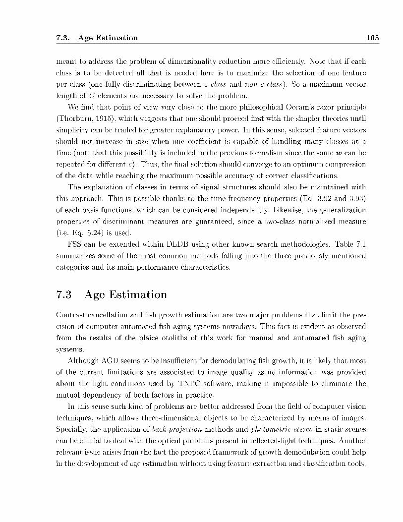
7.3. Age Estimation 165
meant to address the problem of dimensionality reduction more e�ciently. Note that if each
class is to be detected all that is needed here is to maximize the selection of one feature
per class (one fully discriminating between c-class and non-c-class). So a maximum vector
length of C elements are necessary to solve the problem.
We �nd that point of view very close to the more philosophical Occam's razor principle
(Thorburn, 1915), which suggests that one should proceed �rst with the simpler theories until
simplicity can be traded for greater explanatory power. In this sense, selected feature vectors
should not increase in size when one coe�cient is capable of handling many classes at a
time (note that this possibility is included in the previous formalism since the same w can be
repeated for di�erent c). Thus, the �nal solution should converge to an optimum compression
of the data while reaching the maximum possible accuracy of correct classi�cations.
The explanation of classes in terms of signal structures should also be maintained with
this approach. This is possible thanks to the time-frequency properties (Eq. 3.92 and 3.93)
of each basis functions, which can be considered independently. Likewise, the generalization
properties of discriminant measures are guaranteed, since a two-class normalized measure
(i.e. Eq. 5.24) is used.
FSS can be extended within DLDB using other known search methodologies. Table 7.1
summarizes some of the most common methods falling into the three previously mentioned
categories and its main performance characteristics.
7.3 Age Estimation
Contrast cancellation and �sh growth estimation are two major problems that limit the pre-
cision of computer automated �sh aging systems nowadays. This fact is evident as observed
from the results of the plaice otoliths of this work for manual and automated �sh aging
systems.
Although AGD seems to be insu�cient for demodulating �sh growth, it is likely that most
of the current limitations are associated to image quality as no information was provided
about the light conditions used by TNPC software, making it impossible to eliminate the
mutual dependency of both factors in practice.
In this sense such kind of problems are better addressed from the �eld of computer vision
techniques, which allows three-dimensional objects to be characterized by means of images.
Specially, the application of back-projection methods and photometric stereo in static scenes
can be crucial to deal with the optical problems present in re�ected-light techniques. Another
relevant issue arises from the fact the proposed framework of growth demodulation could help
in the development of age estimation without using feature extraction and classi�cation tools,
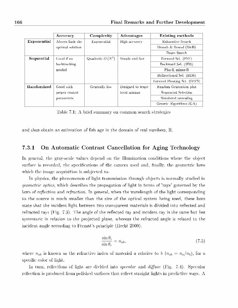
166 Final Remarks and Further Development
Accuracy Complexity Advantages Existing methods
Exponential Always �nds the Exponential High accuracy Exhaustive Search
optimal solution Branch & Bound (B&B)
Beam Search
Sequential Good if no Quadratic O(N2
)Simple and fast Forward Sel. (FSF)
backtracking Backward Sel. (SBS)
needed Plus-I, minus-R
Bidirectional Sel. (BDS)
Forward Floating Sel. (SFFS)
Randomized Good with Generally low Designed to scape Random Generation plus
proper control local minima Sequential Selection
parameters Simulated annealing
Genetic Algorithms (GA)
Table 7.1: A brief summary on common search strategies
and thus obtain an estimation of �sh age in the domain of real numbers, R.
7.3.1 On Automatic Contrast Cancellation for Aging Technology
In general, the gray-scale values depend on the illumination conditions where the object
surface is recorded, the speci�cations of the camera used and, �nally, the geometric laws
which the image acquisition is subjected to.
In physics, the phenomenon of light transmission through objects is normally studied in
geometric optics, which describes the propagation of light in terms of 'rays' governed by the
laws of re�ection and refraction. In general, when the wavelength of the light corresponding
to the source is much smaller than the size of the optical system being used, these laws
state that the incident light between two transparent materials is divided into re�ected and
refracted rays (Fig. 7.3). The angle of the re�ected ray and incident ray is the same but lies
symmetric in relation to the projected plane, whereas the refracted angle is related to the
incident angle according to Fermat's principle (Hecht 2000),
sin θisin θr
= nab, (7.5)
where nab is known as the refractive index of material a relative to b (nab = na/nb), for a
speci�c color of light.
In turn, re�ections of light are divided into specular and di�use (Fig. 7.4). Specular
re�ection is produced from polished surfaces that re�ect straight lights in predictive ways. A
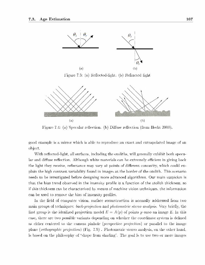
7.3. Age Estimation 167
(a) (b)
Figure 7.3: (a) Re�ected-light. (b) Refracted light
(a) (b)
Figure 7.4: (a) Specular re�ection. (b) Di�use re�ection (from Hecht 2000).
good example is a mirror which is able to reproduce an exact and extrapolated image of an
object.
With re�ected-light, all surfaces, including the otoliths, will generally exhibit both specu-
lar and di�use re�ection. Although white materials can be extremely e�cient in giving back
the light they receive, re�ectance may vary at points of di�erent concavity, which could ex-
plain the high contrast variability found in images at the border of the otolith. This scenario
needs to be investigated before designing more advanced algorithms. Our main suspicion is
that the bias trend observed in the intensity pro�le is a function of the otolith thickness, so
if this thickness can be characterized by means of machine vision techniques, the information
can be used to remove the bias of intensity pro�les.
In the �eld of computer vision, surface reconstruction is normally addressed from two
main groups of techniques: back-projection and photometric stereo analysis. Very brie�y, the
�rst group is the idealized projection model E = A (p) of points p onto an image E. In this
case, there are two possible variants depending on whether the coordinate system is de�ned
as either centered to the camera pinhole (perspective projection) or parallel to the image
plane (orthographic projection) (Fig. 7.5) . Photometric stereo analysis, on the other hand,
is based on the philosophy of �shape from shading�. The goal is to use two or more images

168 Final Remarks and Further Development
(a)
(b)
Figure 7.5: Geometric models for surface reconstruction purposes. (a) central projection; (b)orthogonal parallel projection. (from Klette et al. 1998)
of an object with di�erent light conditions in order to determine volume information (Jain
et al. 1995, Klette et al. 1998).
In general, otolith-based aging applications have addressed the problem of image quality
from the perspective of graphical enhancement tools, perhaps based on the believe that light
conditions are easily controlled for static images. However, in our opinion, it is reasonable
to expect that the characterization of age structures from entire otoliths may need the con-
sideration of thickness and surface volume information in order to determine the amount of
light that is projected from outside the camera focus, specially at the tail of the intensity
pro�les which may be the main cause for high contrast variability and thus the steep slope
at the right end of the intensity pro�le.
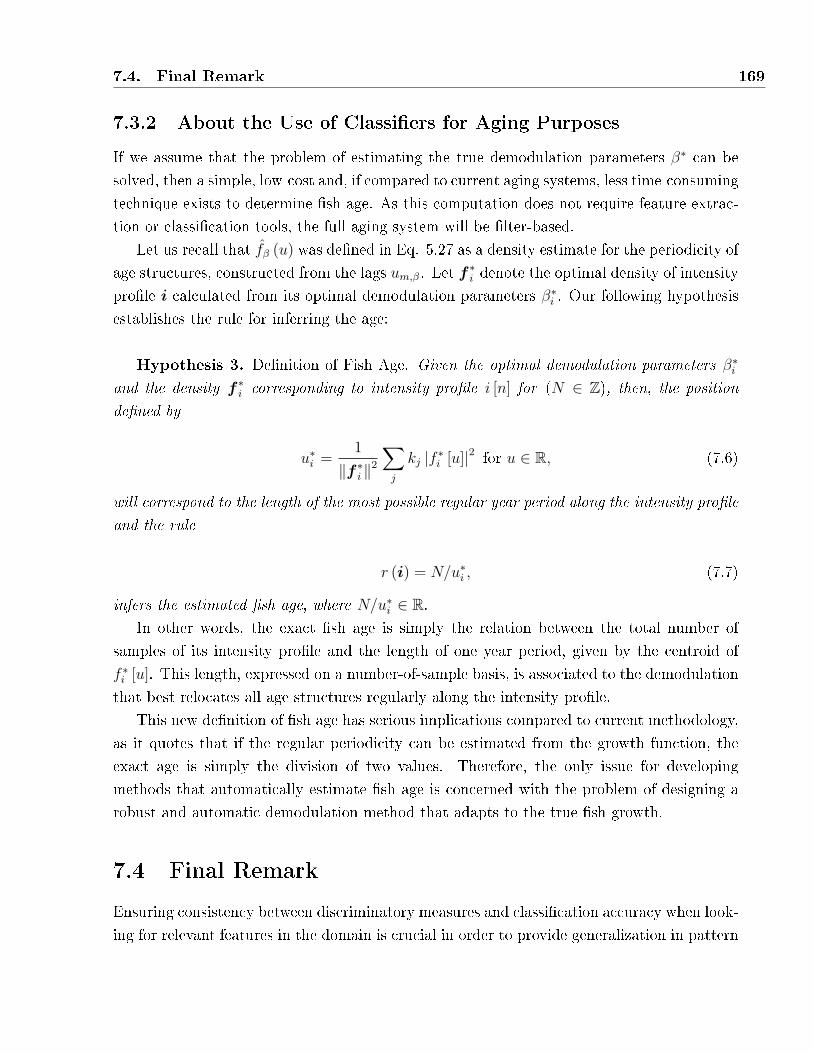
7.4. Final Remark 169
7.3.2 About the Use of Classi�ers for Aging Purposes
If we assume that the problem of estimating the true demodulation parameters β∗ can be
solved, then a simple, low-cost and, if compared to current aging systems, less time-consuming
technique exists to determine �sh age. As this computation does not require feature extrac-
tion or classi�cation tools, the full aging system will be �lter-based.
Let us recall that fβ (u) was de�ned in Eq. 5.27 as a density estimate for the periodicity of
age structures, constructed from the lags um,β. Let f∗i denote the optimal density of intensity
pro�le i calculated from its optimal demodulation parameters β∗i . Our following hypothesis
establishes the rule for inferring the age:
Hypothesis 3. De�nition of Fish Age. Given the optimal demodulation parameters β∗iand the density f ∗i corresponding to intensity pro�le i [n] for (N ∈ Z), then, the position
de�ned by
u∗i =1
‖f ∗i ‖2
∑j
kj |f ∗i [u]|2 for u ∈ R, (7.6)
will correspond to the length of the most possible regular year period along the intensity pro�le
and the rule
r (i) = N/u∗i , (7.7)
infers the estimated �sh age, where N/u∗i ∈ R.In other words, the exact �sh age is simply the relation between the total number of
samples of its intensity pro�le and the length of one year period, given by the centroid of
f ∗i [u]. This length, expressed on a number-of-sample basis, is associated to the demodulation
that best relocates all age structures regularly along the intensity pro�le.
This new de�nition of �sh age has serious implications compared to current methodology,
as it quotes that if the regular periodicity can be estimated from the growth function, the
exact age is simply the division of two values. Therefore, the only issue for developing
methods that automatically estimate �sh age is concerned with the problem of designing a
robust and automatic demodulation method that adapts to the true �sh growth.
7.4 Final Remark
Ensuring consistency between discriminatory measures and classi�cation accuracy when look-
ing for relevant features in the domain is crucial in order to provide generalization in pattern
170 Final Remarks and Further Development
recognition applications. This performance was demonstrated in two-class identi�cation ex-
periments, where the inter-speci�c and intra-speci�c studies of merluccius spp allowed the
otolith structures to be interpreted in terms of structural components and their ecological
di�erences.
The developed tools complement those of classical methodology. Although results demon-
strate the contributions towards the automated detection of signal and image patterns, the
methods are not intended to be contenders of the classical ones. The bridge between the
structural and statistical methods was decisive for evaluating the relevance of selected struc-
tural components. In this sense, we believe that combining both groups of tools is essential
to detect signal patterns and to develop more robust feature extraction systems in the future.
Class distributions have demonstrated themselves to be primary information source for
achieving measure normalization. This behavior is crucial in the development of more gener-
alized feature extractors. Here, the main goal is to derive a system capable of obtaining the
shortest possible feature vector that explains the class di�erences (Occam's razor principle).
In this sense, our contention is that the functionality of future extractor systems must
bridge the gap between linear and nonlinear classi�ers. This means that the method must be
automatic adaptable from an evaluation based on discriminant measures, to an evaluation
based on decision boundaries when class overlapping is detected. In addition, levels of priority
between both performances must be established to ensure that the shortest possible feature
length is able to detect all the classes.
The suggestions outlined in this chapter should allow new automatic pattern recognition
tools to be developed towards this goal. They address multi-class detection, time translation
and the description of time-frequency atoms, among other issues.
The estimation of �sh age, on the other hand, may not require the use of complex classi�ers
or feature extraction systems at all, as long as growth demodulation is addressed correctly for
each individual otolith, but image preprocessing will have to be previously addressed from
the more technical (or even mechanical) issues of acquisition systems and machine vision
applications in order to reduce the current problems of contrast variation.
Part V
Appendices
171

Appendix A
Wavelet Design
A.1 Introduction
From a signal processing point of view, a wavelet is a bandpass �lter. In the dyadic case
given in Eq. 3.17 it is actually an octave band �lter. Therefore, the wavelet transform can
be interpreted as a constant Q-�ltering with a set of octave �lters, followed by sampling at
the respective Nyquist frequencies, corresponding to the bandwidth of the particular octave
band.
The connection between wavelets, �lter-banks and multiresolution signal processing (Mal-
lat 1990, Meyer 1990) is shown in this appendix. Most of the theory of this framework is
described in the excellent work of Vetterli (1992) and is reproduced here since it consti-
tutes a main reference for the construction of customized real time wavelets and �lter-bank
design. Some methods based on algebraic structures will be reviewed in the last section.
These include, paraunitary �lter-banks and, regular �lter design and Diophantine equations
(Vaidyanathan 1990, Vetterli 1992).
A.2 Multiresolution Signal Processing
Let V0 de�ne the space of all band-limited signals with frequencies in the interval (−π, π).
Similarly, call V−1 the space of band-limited signals in (−2π, 2π). Then, the set of functions
φ (t− k) = sinc (t− k) =sin (π (t− k))
π (t− k), k ∈ Z (A.1)
forms an orthonormal basis for V0. Clearly, the set√
2sinc (2t− k), k ∈ Z is an orthonormal
basis for V−1. In particular, if x (t) ∈ V0, then x (2t) ∈ V−1. Now, callW0 the orthogonal space
173
174 Wavelet Design
of bandpass signals with frequencies in the interval (−2π,−π) ∪ (π, 2π), which complements
V0 in V−1,
V−1 = V0 ∪W0. (A.2)
In other words, V−1 is equivalent to V0 with some added details corresponding to W0. For
completeness cos (πt) has to be included in V0, and sin (πt) in W0. From the above it is clear,
by scaling, that if Vi represents the frequency interval (−2−jπ, 2−jπ), then
Vj ⊂ Vj−1 i ∈ Z (A.3)
Vj−1 = Vj ∪Wj i ∈ Z (A.4)
where Wi represents the interval (−2−j+1π,−2−jπ) ∪ (2−jπ, 2−j+1π). Moreover, we have
· · · ⊂ V2 ⊂ V1 ⊂ V0 ⊂ V−1 ⊂ V−2 · · ·
and by iterating A.4 it holds that the union
Vj = Wj+1 ∪Wj+2 ∪Wj+3 ∪ · · · (A.5)
for all Wj's, j = 1, . . . ,∞ is equivalent to the space of square integrable functions, L2 (R),
band limited to (−2−j+1π, 0) ∪ (0, 2−j+1π).
In the sampled version of V−1, φ (t) can be written as the interpolation, by φ (2t), of the
perfect half-band low-pass �lter with impulse response;
c [n] = 2−1/2 sin (πn/2)
πn/2≡ discrete halfband �lter . (A.6)
That is,
φ (t) =∞∑
n=−∞
c [n]φ (2t− n) −∞ < n <∞ (A.7)
for n ∈ Z. In other words, φ (t) derives an approximation of V0 in V−1. The orthogonal
complement, W0, will then be given by the half-band high-pass signals. In the sampled
domain, this is equivalent to modulating the low-pass �lter (Eq. A.6) by (−1)n, and shifting
the vector sequence by one (in order to include sin (πt)). Thus, ψ (t) is the interpolation
thereof, that is,
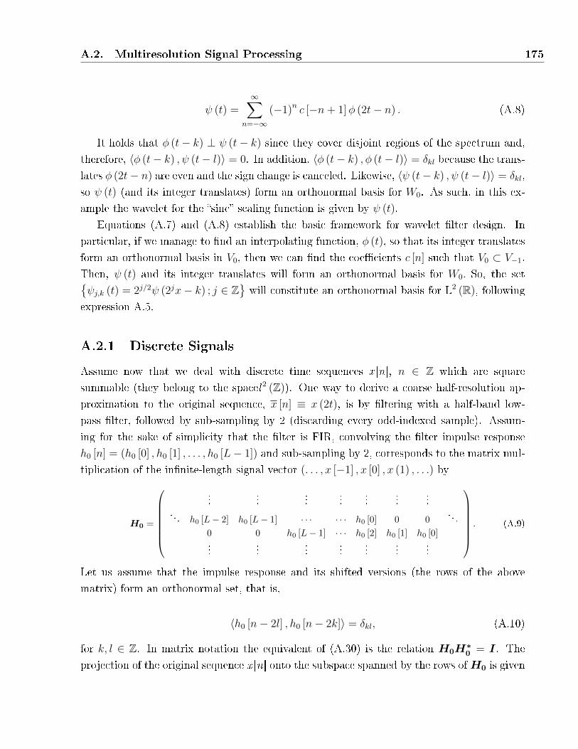
A.2. Multiresolution Signal Processing 175
ψ (t) =∞∑
n=−∞
(−1)n c [−n+ 1]φ (2t− n) . (A.8)
It holds that φ (t− k) ⊥ ψ (t− k) since they cover disjoint regions of the spectrum and,
therefore, 〈φ (t− k) , ψ (t− l)〉 = 0. In addition, 〈φ (t− k) , φ (t− l)〉 = δkl because the trans-
lates φ (2t− n) are even and the sign change is canceled. Likewise, 〈ψ (t− k) , ψ (t− l)〉 = δkl,
so ψ (t) (and its integer translates) form an orthonormal basis for W0. As such, in this ex-
ample the wavelet for the �sinc� scaling function is given by ψ (t).
Equations (A.7) and (A.8) establish the basic framework for wavelet �lter design. In
particular, if we manage to �nd an interpolating function, φ (t), so that its integer translates
form an orthonormal basis in V0, then we can �nd the coe�cients c [n] such that V0 ⊂ V−1.
Then, ψ (t) and its integer translates will form an orthonormal basis for W0. So, the set{ψj,k (t) = 2j/2ψ (2jx− k) ; j ∈ Z
}will constitute an orthonormal basis for L2 (R), following
expression A.5.
A.2.1 Discrete Signals
Assume now that we deal with discrete time sequences x [n], n ∈ Z which are square
summable (they belong to the spacel2 (Z)). One way to derive a coarse half-resolution ap-
proximation to the original sequence, x [n] ≡ x (2t), is by �ltering with a half-band low-
pass �lter, followed by sub-sampling by 2 (discarding every odd-indexed sample). Assum-
ing for the sake of simplicity that the �lter is FIR, convolving the �lter impulse response
h0 [n] = (h0 [0] , h0 [1] , . . . , h0 [L− 1]) and sub-sampling by 2, corresponds to the matrix mul-
tiplication of the in�nite-length signal vector (. . . , x [−1] , x [0] , x (1) , . . .) by
H0 =
......
......
......
.... . . h0 [L− 2] h0 [L− 1] · · · · · · h0 [0] 0 0
. . .
0 0 h0 [L− 1] · · · h0 [2] h0 [1] h0 [0]...
......
......
......
. (A.9)
Let us assume that the impulse response and its shifted versions (the rows of the above
matrix) form an orthonormal set, that is,
〈h0 [n− 2l] , h0 [n− 2k]〉 = δkl, (A.10)
for k, l ∈ Z. In matrix notation the equivalent of (A.30) is the relation H0H∗0 = I. The
projection of the original sequence x [n] onto the subspace spanned by the rows ofH0 is given

176 Wavelet Design
byH∗0H0x, where multiplication byH∗
0 corresponds to up-sampling by 2 followed by convo-
lution with a �lter of impulse response h0 [n] = (h0 [L− 1] , h0 [L− 2] , . . . , h0 [1] , h0 [0]), (the
time reversed input response of h0 [n]). Note that in order for the set {h0 (n− 2k) , k ∈ Z} toform an orthonormal basis L has to be even, or else 〈h0 [n] , h0 [n− L+ 1]〉 6= 0 unless either
h0 [0] or h0 [L− n− 1] was zero.
Note that if V0 is the subspace spanned by the rows ofH0, the �lter with impulse response
h1 [n] = (−1)1+n h0 [L− 1− n] and its shifted versions will form an orthonormal basis forW0.
The orthogonality of h0 and h1 with respect to even shifts is easily veri�ed, because of the
sign in h0:
〈h1 [n− 2l] , h0 [n− 2k]〉 = 0. (A.11)
for k, l ∈ Z. In matrix notation, this is equivalent toH0H∗1 = 0, where nowH∗
1 is the matrix
based on the reverse impulse response of h1 [n]. Then, from the orthonormality condition,
V0 ⊥ W0 it holds that
〈h1 [n− 2l] , h1 [n− 2k]〉 = δkl, (A.12)
for k, l ∈ Z; since the sign of h1 [n] is canceled.
In other words, based on an orthonormal basis for V0, we constructed an orthonormal
basis for W0, just as in the continuous time case. Again in matrix notation, H1H∗1 = I.
The coarse half-resolution approximation of the original signal is given by
x = H∗0H0x, (A.13)
whereas the di�erence (or �detail�) signal is determined as
d =(I −H∗
0H0
)= H∗
1H1x. (A.14)
But, because it is a perfect reconstruction system (x = x + d) it follows that H∗0H0 +
H∗1H1 = I and, therefore,
H∗1H1 = I −H∗
0H0. (A.15)
Fig. A.1 recapitulates the above relationships in standard digital processing notation,
using �lters and sampling rate changes to denote operators so far. As in the continuous
case, the direct sum of all Wi's is the space of square integrable functions l2 (Z). The
decomposition of V−1 into W0, W1, W2, etc, is essentially a wavelet transform on discrete
sequences (DWT). Actually, if the �lter h0 [n] is an ideal half-band low-pass �lter given by
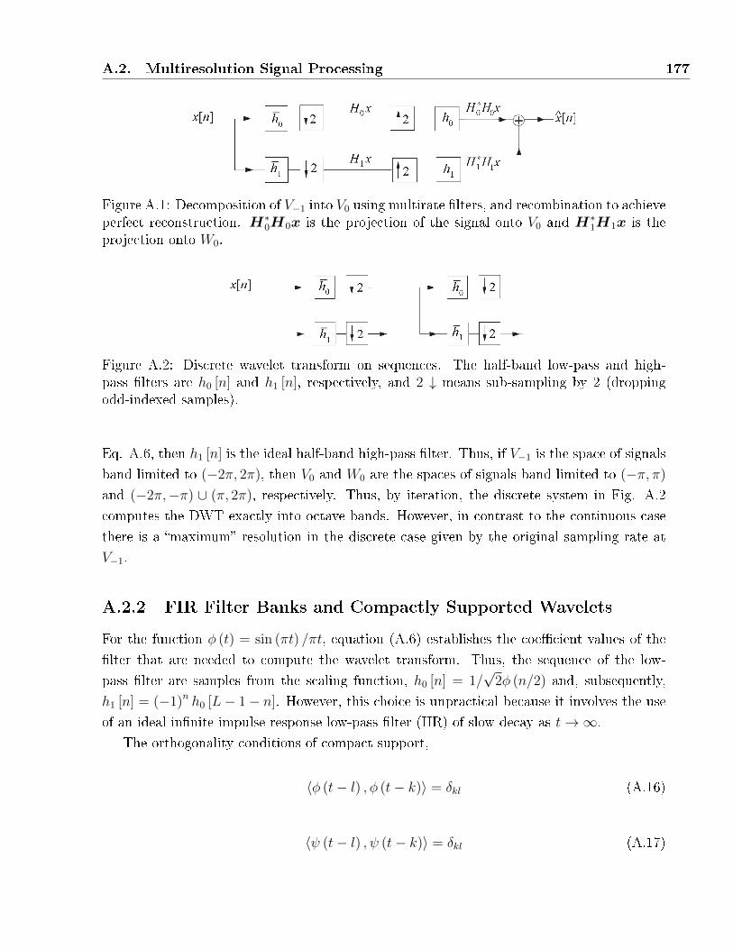
A.2. Multiresolution Signal Processing 177
Figure A.1: Decomposition of V−1 into V0 using multirate �lters, and recombination to achieveperfect reconstruction. H∗0H0x is the projection of the signal onto V0 and H∗1H1x is theprojection onto W0.
Figure A.2: Discrete wavelet transform on sequences. The half-band low-pass and high-pass �lters are h0 [n] and h1 [n], respectively, and 2 ↓ means sub-sampling by 2 (droppingodd-indexed samples).
Eq. A.6, then h1 [n] is the ideal half-band high-pass �lter. Thus, if V−1 is the space of signals
band limited to (−2π, 2π), then V0 and W0 are the spaces of signals band limited to (−π, π)
and (−2π,−π) ∪ (π, 2π), respectively. Thus, by iteration, the discrete system in Fig. A.2
computes the DWT exactly into octave bands. However, in contrast to the continuous case
there is a �maximum� resolution in the discrete case given by the original sampling rate at
V−1.
A.2.2 FIR Filter Banks and Compactly Supported Wavelets
For the function φ (t) = sin (πt) /πt, equation (A.6) establishes the coe�cient values of the
�lter that are needed to compute the wavelet transform. Thus, the sequence of the low-
pass �lter are samples from the scaling function, h0 [n] = 1/√
2φ (n/2) and, subsequently,
h1 [n] = (−1)n h0 [L− 1− n]. However, this choice is unpractical because it involves the use
of an ideal in�nite impulse response low-pass �lter (IIR) of slow decay as t→∞.
The orthogonality conditions of compact support,
〈φ (t− l) , φ (t− k)〉 = δkl (A.16)
〈ψ (t− l) , ψ (t− k)〉 = δkl (A.17)
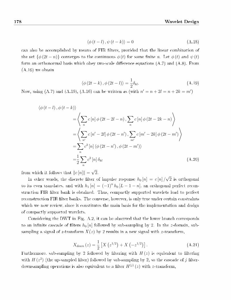
178 Wavelet Design
〈φ (t− l) , ψ (t− k)〉 = 0 (A.18)
can also be accomplished by means of FIR �lters, provided that the linear combination of
the set {φ (2t− n)} converges to the continuous φ (t) for some �nite n. Let φ (t) and ψ (t)
form an orthonormal basis which obey two-scale di�erence equations (A.7) and (A.8). From
(A.16) we obtain
〈φ (2t− k) , φ (2t− l)〉 =1
2δkl. (A.19)
Now, using (A.7) and (A.19), (A.16) can be written as (with n′ = n+ 2l = n+ 2k = m′)
〈φ (t− l) , φ (t− k)〉
=
⟨∑n
c [n]φ (2t− 2l − n) ,∑n
c [n]φ (2t− 2k − n)
⟩
=
⟨∑n′
c [n′ − 2l]φ (2t− n′) ,∑m′
c [m′ − 2k]φ (2t−m′)
⟩=∑n
c2 [n] 〈φ (2t− n′) , φ (2t−m′)〉
=1
2
∑n
c2 [n] δkl (A.20)
from which it follows that ‖c [n]‖ =√
2.
In other words, the discrete �lter of impulse response h0 [n] = c [n] /√
2 is orthogonal
to its even translates, and with h1 [n] = (−1)n h0 [L− 1− n], an orthogonal perfect recon-
struction FIR �lter bank is obtained. Thus, compactly supported wavelets lead to perfect
reconstruction FIR �lter banks. The converse, however, is only true under certain constraints
which we now review, since it constitutes the main basis for the implementation and design
of compactly supported wavelets.
Considering the DWT in Fig. A.2, it can be observed that the lower branch corresponds
to an in�nite cascade of �lters h0 [n] followed by sub-sampling by 2. In the z-domain, sub-
sampling a signal of z-transform X (z ) by 2 results in a new signal with z -transform,
Xdown (z) =1
2
[X(z1/2
)+X
(−z1/2
)]. (A.21)
Furthermore, sub-sampling by 2 followed by �ltering with H (z) is equivalent to �ltering
with H (z2) (the up-sampled �lter) followed by sub-sampling by 2, so the cascade of j �lter-
downsampling operations is also equivalent to a �lter H(j) (z) with z -transform,
A.2. Multiresolution Signal Processing 179
Figure A.3: Scaling function generated by using (A.23) for h0 = [1, α, α, 1] and α ∈ {−3, 3}.
H(j) (z) =
j−1∏l=0
H(z2l)j = 1, 2 · · · , (A.22)
followed by sub-sampling by 2j. De�ning H(0) (z) = 1 and assuming that H (z ) has length L,
it holds from A.56 that the length of H(j) (z) is L(j) = (2j − 1) (L− 1). Of course, as j →∞,
we obtain L(j) →∞. Let us consider the function f (j) (t), instead of the discrete time �lter,
which is constant on intervals of length 1/2j. That is,
f (j) (t) = 2j/2h(j) [n] for n/2j ≤ t ≤ (n+ 1) /2j. (A.23)
Clearly, f (j) (t) is supported in the interval [0,L-1]. The normalization factor 2j/2 ensures
that if∑(
h(j) [n])2
= 1 then´ (
f (j) (t))2dt = 1 as well. It can be shown that
∥∥h(j)∥∥
2= 1
when∥∥h(j−1)
∥∥2
= 1.
An important issue here is to �nd out what the function f (j) (t) converges to as j →∞.
Habitually, regular continuous functions are often preferred when constructing wavelets of
compact support, perhaps including derivatives also. This can be achieved imposing certain
regularity constraints in the initial �lter H(1) (z). However, one should be careful since, for
example, changing coe�cient signs may lead to shapes of quite di�erent irregularities (see
Fig. A.3).

180 Wavelet Design
First, assume that the �lter H (z ) has a zero at ω = π, or H (eiω) = 0. This is quite
reasonable if H (z ) is to be a half-band low-pass �lter; in fact such a zero is necessary if
f (j) (t) is to converge to a continuous function when j →∞ (Rioul 1993). This together with
the fact that impulse responses are orthogonal to even translates is equivalent to∑h [n] =
H (1) =√
2. De�ne the polynomial m0 (z) =(1/√
2)H (z), where m0 (1) = 1, and factorize
into its roots at π and the remainder polynomial R (z) as,
m0 (z) =[(
1 + z−1)/2]NR (z) . (A.24)
where N denotes number of vanishing moments. Now, call B the supremum of |R(z )| on the
unit circle,
B = supω∈[0,2π]
∣∣R (eiω)∣∣ . (A.25)
Then, the following result from Daubechies (1988) holds:
Remark. A.1: If B < 2N−1, then the piecewise function, f (j) (t), de�ned in (A.23) converge
point-wise to a continuous function, f (∞) (t).
This regularity condition is su�cient to ensure point-wise convergence by means of digital
FIR �lters and is often used as a test in the construction of wavelets. However, a more
accurate veri�cation is based on the estimation of a regularity index β such that ψ (t) and
φ (t) ∈ Cβ (Daubechies 1988, Rioul 1993). Such methods are potentially useful, in particular,
if a �lter fails to test condition A.1. The main reason is that a design criterion can be made
in order to place a maximum number of zeros at π so that an e�cient signal compression
can be reached through the wavelet transform (note that if m0 (z) has a zero of order N at
z=-1 then the wavelet will contain N consecutive vanishing moments, that is,´tkψ (t) dt =
0, k = 0, 1, . . . N − 1).
A.2.2.1 Bases of Orthonormal Wavelets Constructed from Filter Banks
Using (A.22) and (A.23) we get
f (j) (t) = 2j/2L−1∑m=0
h0 [m]h(j−1)0
[n− 2j−1m
], for n/2j ≤ t < (n+ 1) /2j.
The term h(j−1)0 [n− 2j−1m] can be written as a function of f (j−1) (2t−m) by means of (A.23)
using the change of variable n′ = n+ 2j−1l. That is,
f (j−1) (2t−m) = 2(j−1)/2h(j−1)0
[n′ − 2j−1m
], (A.26)
A.2. Multiresolution Signal Processing 181
for n′/2j ≤ t < (n′ + 1) /2j and, therefore,
f (j) (t) = 21/2
L−1∑m=0
h0 [m] f (j−1) (2t−m) . (A.27)
Since f (j) (t) tends to a continuous limit function φ (t) as j → ∞, the preceding relation
satis�es a two-scale di�erence equation,
1√2φ (t/2) =
L−1∑n=0
h0 [n]φ (t− n) = h0 ∗ φ. (A.28)
Similarly, the bandpass function are obtained as
1√2ψ (t/2) =
L−1∑n=0
h1 [n]φ (t− n) = h1 ∗ φ. (A.29)
These fundamental expressions establish the relations between the basis functions of two
consecutive octave scales. Furthermore, if h0 [n] and h1 [n] are orthogonal with respect to
even shifts,
〈hi [n− 2l] , hj [n− 2k]〉 = δijδkl, (A.30)
for k, l ∈ Z, it can be shown that φ (t− k) is orthogonal to integer translates of itself, ∀k, anψ (t) is orthogonal across scales.
Let us assume that f (j) (t)is orthogonal at the j th level,
⟨f (j) (t− l) , f (j) (t− k)
⟩= δkl. (A.31)
Then, it holds that f (j+1) (t) is also orthogonal,
⟨f (j+1) (t− l) , f (j+1) (t− k)
⟩=2∑n
∑m
h0 [n]h0 [m]⟨f (j) (2t− 2l − n) ,
f (j) (2t− 2k −m)⟩
=∑n
h0 [n]h0 [n+ 2l − 2k]
=δkl.
Hence, by induction equation (A.31) holds for all j. So in the limit (j →∞),

182 Wavelet Design
〈φ (t− l) , φ (t− k)〉 = δkl. (A.32)
The other orthogonality relations ψ (t) and φ (t) follow easily from (A.30),
〈ψ (x− l) , ψ (x− k)〉 = δkl (A.33)
〈φ (x− l) , ψ (x− k)〉 = 0 (A.34)
Finally, across one scale it holds that
〈ψ (t− l) , ψ (2t− k)〉 =
⟨∑n
h1 [n]φ (2t− 2l + n) , ψ (2t− k)
⟩=
∑n
h1 [n] 〈φ (2t− 2l + n) , ψ (2t− k)〉
= 0.
Similar reasoning shows that across several scales ψ (2jt− l) is orthogonal to ψ (2it− k) for
i 6= j and k 6= l. Additionally, completeness is required in order that {2−jψ (2jt− l) ; j, l ∈ Z}bean orthonormal basis for L2R. This is proved in (Daubechies 1988), so any signal x (t) ∈ L2Rcan be represented as compositions from the basis set
{2−j/2ψ (2jt− l) , j, l 3 Z
}:
x (t) =∑j
∑k
⟨2−j/2ψ
(2jt− k
), x (t)
⟩2−j/2ψ
(2jt− k
).
In summary, if the digital �lters h0 [n] and h1 [n] and their even translates form an or-
thonormal set in l2Z, orthogonal wavelet bases in L2R of di�erent integer translates can be
generated. The resulting �lter bank can be iterated in�nitely without loosing this orthogo-
nality condition, making it possible to generate wavelet bases for tree-structured transforms
with perfect reconstruction capabilities.
A.2.3 General FIR Perfect Reconstruction Filter Banks
Assume that we have a �lter bank as in Fig. A.1 with analysis �lters H0 (z) and H1 (z),
and general synthesis �lters G0 (z) and G1 (z) (instead of the orthogonal synthesis �lters
H∗0 (z) and H∗1 (z), respectively). Knowing that up-sampling by 2 corresponds to simply
replacing z by z2 in the z -transform, it is easily seen (by using A.21) that the output of the
analysis/synthesis system is given by
A.2. Multiresolution Signal Processing 183
X (z) =1
2
[G0 (z) G1 (z)
] [ H0 (z) H0 (−z)
H1 (z) H1 (−z)
][X (z)
X (−z)
]. (A.35)
Let us denote the above 2× 2 matrix Hm (z), where m indicates that it contains modulated
versions of the �lters H0 (z) and H1 (z). To perfectly reconstruct signals we need to cancel
the contribution of the alias term, represented by X (-z ). This can be done by relating the
synthesis �lters to the analysis �lters as follows,[G0 (z) , G1 (z)
]= C (z)
[H1 (−z) H0 (−z)
]. (A.36)
Note that
det [Hm (z)] = H0 (z)H1 (−z)−H0 (−z)H1 (z) (A.37)
= P (z)− P (−z) (A.38)
where P (z) = H0 (z)H1 (−z). At this point we introduce the so called poly-phase �lter
notation,
Hi (z) = Hi0
(z2)
+ z−1Hi1
(z2), (i = 0, 1) , (A.39)
where Hi0 (z) contains the even-indexed coe�cients of the �lter Hi (z), and Hi1 (z) the odd
ones. Thus, using (A.21) it follows that[H00 (z2) H01 (z2)
H10 (z2) H11 (z2)
]=
1
2
[H0 (z) H0 (−z)
H1 (z) H1 (−z)
][1 1
1 −1
][1 1
0 z
],
or equivalently,
Hp
(z2)
= 2−1Hm (z)
[1 1
1 −1
][1 1
0 z
],
where Hp (z) is called the poly-phase matrix. In particular,
det [Hm (z)] = −2z−1 det[Hp
(z2)]
(A.40)
and
det [Hp (z)] = H00 (z)H11 (z)−H01 (z)H10 (z)
=1
2z1/2
[P(z1/2
)− P
(−z1/2
)]. (A.41)
184 Wavelet Design
It is a well known fact that to obtain perfect reconstruction with FIR synthesis �l-
ters, after a FIR analysis, the following condition (Smith and Barnwell 1984, Vetterli 1986,
Vaidyanathan and Hoang 1988) is necessary,
det [Hm (z)] = cz−2l−1 l ∈ Z. (A.42)
Note that det [Hp (z)] is thus a pure delay as well. In order to make results less arbitrary,
the constant is �xed to c=2. From this and (A.37) it follows that P(z ) can have only a single
nonzero odd-indexed coe�cient:
P (z)− P (−z) = 2z−2l−1. (A.43)
A polynomial P(z ) satisfying this constraint is termed a valid polynomial. A factorization
such that P (z) = H0 (z)H1 (−z) will give a possible FIR perfect reconstruction �lter bank,
and H0 (z) and the complementary �lter H1 (z) will form a perfect reconstruction set. Addi-
tionally, note that H0 (z) and H1 (−z) are interchangeable. This constraint establishes two
possible scenarios of �lter design: 1) the factorization method where the goal consists in
�nding a valid P(z ) satisfying some design criteria, and then factoring it into H0 (z) and
H1 (−z); or 2) the complementary �lter method, which starts with a �lter H0 (z) and then
solves a system of linear equations to �nd the �lter H1 (z) leading to a valid P(z ). In either
case, once P(z ) is found and factored in terms of the analysis �lters H0 (z) and H1 (−z) the
synthesis �lters follow directly from (A.36), with C (z) = cz−l.
A.2.3.1 Orthogonal or Paraunitary Filter Banks
In the subsections above, we have shown that orthogonal �lters must be orthonormal with
respect to even translates. Using �ltering notation, this means that the even terms of the
autocorrelation Hi (z)Hi (z − 1) are all zero, with the exception of the central one which
equals unity (for normalized �lters). Thus, the condition (A.30) becomes
Hi (z)Hi
(z−1)
+Hi (−z)Hi
(−z−1
)= 2 i ∈ {0, 1} . (A.44)
Furthermore, the two �lters H0 (z) and H1 (z) are orthogonal to each other at even translates
(A.11), so the even terms of the cross correlation are all zero:
H0 (z)H1
(z−1)
+H0 (−z)H1
(−z−1
)= 0. (A.45)
Considering that h0 [n] is of even length, the term H0 (z)H1 (z−1) only presents odd
coe�cients, so it can be written as
A.2. Multiresolution Signal Processing 185
H0 (z)H1
(z−1)
= z−2n−1Q(z2),
which means that zeros must appear in pairs at z = α and z = −α, so that the low-pass
and high-pass �lters form an orthogonal basis in l2 (Z). However, H0 (z) alone cannot have
such a pair of zeros if perfect reconstruction is to be possible (see remark B.2.2 below), so
for every zero at z = α in H0 (z) there must be a corresponding zero at z = −α in H1 (z−1),
or equivalently, H1 (z) must have a zero at z = −1/α, which lead to
H1 (z) = z−2k−1H0
(−z−1
). (A.46)
In other words, the orthogonal high-pass �lter is the alternating �ip of the low-pass ones,
varying the sign of the odd-indexed elements: h1 [n] = (−1)n+1 h0 [L− 1− n]. Additionally,
the low-pass and high-pass synthesis FIR �lters are given by C (z) = cz−l so they correspond
to the reversed versions of the analytic ones: g0 [n] = h0 [n] and g1 [n] = h1 [n], respectively.
This constraint establishes the relation between the low-pass and high-pass �lters so that
their impulse responses and even translates form an orthogonal basis for l2 (Z). It also means
that H1 (z)is related to the poly-phase matrix as
H1 (z) = −z−2kH01
(z−2)
+ z−2k−1H00
(z−2).
Since det [Hp (z)] is symmetric and must also contain delays to be a perfect reconstruction
system, for k=0 we obtain
Hp (z) =
[H00 (z) H01 (z)
−H01 (z−1) H00 (z−1)
], (A.47)
and, therefore,
det [Hp (z)] = H00 (z)H00
(z−1)
+H01 (z)H01
(z−1)
= 1, (A.48)
which corresponds to the poly-phase equivalent of (A.44). On the unit circle z = eiω, this is
equivalent to
∣∣H00
(eiω)∣∣2 +
∣∣H01
(eiω)∣∣2 = 1.
Thus, the necessary form (A.46) also means that
z−2k−1[H0 (z)H0
(z−1)
+H0 (−z)H0
(−z−1
)]= 2z−2k−1,
or equivalently, on the unit circle
186 Wavelet Design
∣∣H0
(eiω)∣∣2 +
∣∣H0
(eiω+π
)∣∣2 = 2. (A.49)
In other words,Hp (z) is unitary on the unit circle. Note that the product [Hp (z−1)]THp (z)
corresponds to a 2 × 2 identity matrix. Such matrix is called paraunitary matrix (Vetterli
1986, Vaidyanathan 1990).
The above discussion indicates two possible �lter design approaches for orthogonal im-
plementations. The �rst consists in �nding a symmetric autocorrelation function with a
single even-indexed coe�cient (the central one) di�erent from zero (Smith and Barnwell
1984, Mintzer 1985). The zeros on the unit circle of its square roots, H0 (z) and H0 (z−1),
have to be double in order to prevent the function from changing sign. The second method
synthesizes paraunitary matrices by means of lattice structures from which factorizations
have been given by Vaidyanatan and Hoang (1988). Once the poly-phase matrix is obtained,
the �lters follow easily from (A.39).
A.2.3.2 Biorthogonal or General Perfect Reconstruction Filter Banks
In the biorthogonal case, the wavelet transform is invertible but not necessarily orthogonal.
The main reason is that giving up orthogonality allows the �lter design to be more �exible,
making possible the development of �lters of arbitrary size and symmetry while maintaining
the the linear phase property. This is preferred in order to increase compression e�ciency,
since the shape of the basis functions can then be modeled to �t more speci�c structures.
From equation (A.42) we know that perfect reconstruction requires det [Hm (z)] to be an
odd delay, and the synthesis �lters are C (z) = cz−l. Thus for l = 1, it can be shown that
G0 (z)H1 (z) and G1 (z)H0 (z) have only odd coe�cients, that is,
〈g0 [n− 2k] , h1 [n− 2l]〉 = 0, (A.50)
〈g1 [n− 2k] , h0 [n− 2l]〉 = 0, (A.51)
where x [n] = x [−n]. In matrix notation,
H0G1 = 0 = H1G0 (A.52)
where Hi and Gi are de�ned in a way similar to (A.9). Since it is a perfect reconstruction
system, the product G0 (z)H0 (z) = z−1H1 (−z)H0 (z) has a single nonzero odd coe�cient.
Similarly, the product G1 (z)H1 (z) = −z−1H0 (−z)H1 (z) has a single even-indexed coe�-
cient. Thus,
A.2. Multiresolution Signal Processing 187
〈gi [n− 2k] , hi [n− 2l]〉 = δkl. (A.53)
In operator notation, that is equivalent to
H0G0 = I = H1G1, (A.54)
G0H0 +H1G1 = I. (A.55)
The coe�cients of the low-pass �lter are unrelated to the high-pass one, requiring therefore
the use of an additional basis set. Nevertheless, some relation of orthogonality must exist
between the analysis and synthesis �lter if perfect reconstruction is to be obtained within tree-
structured transforms. Note that although H0G0and H1G1 are not necessarily orthogonal,
orthogonality exists through (A.50) (A.51) and (A.53) and, hence, the name biorthogonal. In
the special case where we have a paraunitary solution it holds that G0 = H∗0 and G1 = H∗
1 ,
leading to projections onto subspaces which are mutually orthogonal. The two most frequent
classes of biorthogonal �lters with linear phase are the following:
1. Both �lters, H0 (z) and H1 (z), are symmetric and of odd lengths, di�ering by an odd
multiple of 2.
2. One of the �lters is symmetric and the other antisymmetric; both lengths are even
although they can be either equal or di�ering by a multiple or 2.
Since the synthesis �lters are G0 (z) = H1 (−z) and G1 (z) = −H0 (z), in the �rst case we
use g0 [n] = (−1)n h1 [n] for the low-pass �lter, and g1 [n] = (−1)n+1 h0 [n] the high-pass
�lter, whereas in the second case both synthesis �lters alternate sign and, thus, g0 [n] =
(−1)n+1 h1 [n] and g1 [n] = (−1)n h0 [n], respectively.
Now we can show that in�nitely iterated biorthogonal perfect reconstruction �lter-banks
generate biorthogonal sets of functions. Let us denote as H(j)0 (z) and G
(j)0 (z) the �lters
which are equivalent to the cascade of j blocks of �ltering/sub-sampling in the analysis and
synthesis sections, but respectively. These �lters are assumed to be regular but each one
de�nes a di�erent piecewise constant function on the interval 1/2j,
f (j) (t) = 2j/2h(j)0 [n] n/2j ≤ t ≤ (n+ 1) /2j (A.56)
f (j) (t) = 2j/2g(j)0 [n] n/2j ≤ t ≤ (n+ 1) /2j. (A.57)
188 Wavelet Design
Since we are assuming regularity, both f (j) (t) and f (j) (t) converge to continuous functions
as j →∞. It can be shown, following the same analytical scheme of the preceding subsection
that these functions satisfy the two-scale di�erence equations,
φ (t) = 21/2
L−1∑n=0
h0 [n]φ (2t− n) (A.58)
φ (t) = 21/2
L−1∑n=0
g0 [n] φ (2t− n) . (A.59)
Similarly, the associated bandpass functions are de�ned by
ψ (t) = 21/2
L−1∑n=0
h1 [n]φ (2t− n) (A.60)
ψ (t) = 21/2
L−1∑n=0
g1 [n] φ (2t− n) . (A.61)
It can be shown inductively that φ (t) and φ (t) are orthogonal with respect to integer
shifts. At the 0th level, f (0) (t) and f (0) (t) are each equal to the indicator function on the
interval [0,1), so⟨f (0) (t− l) , f (0) (t− k)
⟩= δkl. Assuming orthogonality at the j th level,⟨
f (j) (t− l) , f (j) (t− k)⟩
= δkl, it holds that
⟨f (j+1) (t− l) , f (j+1) (t− k)
⟩=2
⟨∑n
g0 [n] f (j) (2t− 2l − n) ,
∑m
h0 [m] f (j) (2t− 2k −m)
⟩=∑n
g0 [n]h0 [n+ 2l − 2k]
=δkl.
Therefore, in the limit we obtain⟨φ (t− l) , φ (t− k)
⟩= δkl. (A.62)
Once this is established, the relation
A.2. Multiresolution Signal Processing 189
⟨ψ (t− l) , ψ (t− k)
⟩= δkl (A.63)
follows immediately from (A.53), whereas the relations
⟨φ [n− 2k] , ψ [n− 2l]
⟩= 0, (A.64)⟨
ψ [n− 2k] , φ [n− 2l]⟩
= 0, (A.65)
come from (A.50) and (A.51), respectively. Therefore, the conditions for perfect reconstruc-
tion on the �lter coe�cients lead to functions with biorthogonality properties as shown above.
Orthogonality across scales is also veri�ed following the analysis of subsection A.2.2.1:⟨2−j/2ψ
(2jt− l
), 2−i/2ψ
(2−it− k
)⟩= δijδkl. (A.66)
Thus the set{ψ (2jt− l) , ψ (2it− l) ; i, j, k, l ∈ Z
}is biorthogonal. Completeness can be
veri�ed as in the orthogonal case in (Cohen et al. 1992). Hence any function in L2R can be
written
x (t) =∑j
∑k
⟨2−j/2ψ
(2jt− k
), x (t)
⟩2−j/2ψ
(2jt− k
).
Additionally, note that ψ (t) and ψ (t) play interchangeable roles. So, regular biorthogonal
FIR �lters lead to biorthogonal bases of functions of �nite length. The converse is also true
and is shown brie�y. Assume that we have functions ψ (t)φ (t)φ (t)ψ (t) satisfying (A.58)
- (A.61) and (A.62) - (A.65). Then, it can be veri�ed that they can be used to generate
�lter-banks. For example, using (A.62)
⟨φ (t− l) , φ(j+1) (t− k)
⟩=
⟨∑n
g0 [n] φ(j) (2t− 2l − n) ,
∑m
h0 [m]φ(j) (2t− 2k −m)
⟩=∑n
∑m
g0 [n]h0 [m]⟨φ [2t− 2l − n] ,
φ [2t− 2k −m]〉
=∑n
g0 [n]h0 [n+ 2l − 2k] = δkl.
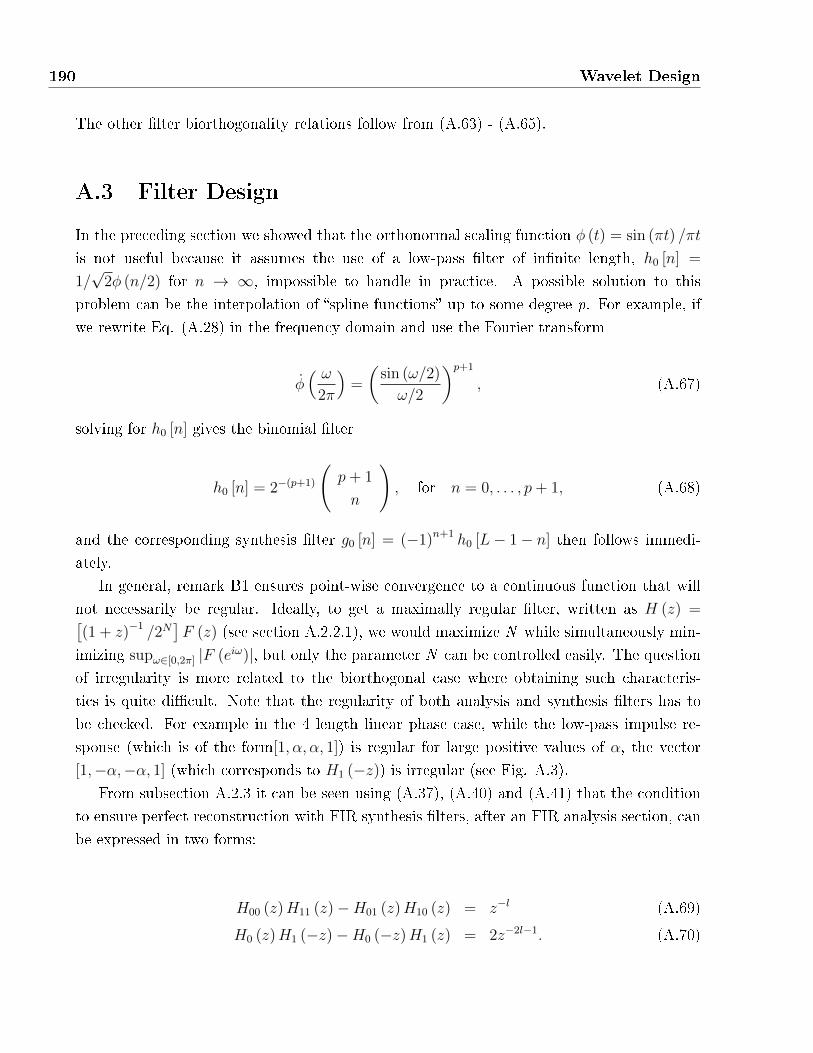
190 Wavelet Design
The other �lter biorthogonality relations follow from (A.63) - (A.65).
A.3 Filter Design
In the preceding section we showed that the orthonormal scaling function φ (t) = sin (πt) /πt
is not useful because it assumes the use of a low-pass �lter of in�nite length, h0 [n] =
1/√
2φ (n/2) for n → ∞, impossible to handle in practice. A possible solution to this
problem can be the interpolation of �spline functions� up to some degree p. For example, if
we rewrite Eq. (A.28) in the frequency domain and use the Fourier transform
φ( ω
2π
)=
(sin (ω/2)
ω/2
)p+1
, (A.67)
solving for h0 [n] gives the binomial �lter
h0 [n] = 2−(p+1)
(p+ 1
n
), for n = 0, . . . , p+ 1, (A.68)
and the corresponding synthesis �lter g0 [n] = (−1)n+1 h0 [L− 1− n] then follows immedi-
ately.
In general, remark B1 ensures point-wise convergence to a continuous function that will
not necessarily be regular. Ideally, to get a maximally regular �lter, written as H (z) =[(1 + z)−1 /2N
]F (z) (see section A.2.2.1), we would maximize N while simultaneously min-
imizing supω∈[0,2π] |F (eiω)|, but only the parameter N can be controlled easily. The question
of irregularity is more related to the biorthogonal case where obtaining such characteris-
tics is quite di�cult. Note that the regularity of both analysis and synthesis �lters has to
be checked. For example in the 4 length linear phase case, while the low-pass impulse re-
sponse (which is of the form[1, α, α, 1]) is regular for large positive values of α, the vector
[1,−α,−α, 1] (which corresponds to H1 (−z)) is irregular (see Fig. A.3).
From subsection A.2.3 it can be seen using (A.37), (A.40) and (A.41) that the condition
to ensure perfect reconstruction with FIR synthesis �lters, after an FIR analysis section, can
be expressed in two forms:
H00 (z)H11 (z)−H01 (z)H10 (z) = z−l (A.69)
H0 (z)H1 (−z)−H0 (−z)H1 (z) = 2z−2l−1. (A.70)

A.3. Filter Design 191
One equation implies the other and both can be used in di�erent ways to design the �lters,
depending on what is easier for us. In particular, they are special forms of what is known as
the Bezout identity equation (Kailath 1980, Schroeder 1986):
a (x) p (x) + b (x) q (x) = c (x) . (A.71)
When two of the polynomials are known, i.e. a(x ) and b(x ), it can be shown that a solution
for [p (x) , q (x)] exists if the greatest common divisor, gcd [a (x) , b (x)], divides c(x ). This
implication introduces the following constraints on the �lter-banks which are generally used
within the design process.
Remark. B.2: Assume that the �lters H0 (z) and H1 (z) are FIR and causal.
1. Then, given one of the pairs [H00 (z) , H01 (z)], [H00 (z) , H10 (z)], [H11 (z) , H01 (z)] or
[H11 (z) , H10 (z)] in order to achieve perfect reconstruction with the other pair it is
necessary and su�cient that the given pair be co-prime (except for possible zeros at
z =∞).
2. A �lter H0 (z) has a complementary �lter if and only if it has no zeros in pairs at z = α
and z = −α.
3. There is always a complementary �lter to the binomial �lter:
H0 (z) =(1 + z−1
)−k= H00
(z2)
+ z−1H01
(z2). (A.72)
That the poly-phase pair must be co-prime is easily obtained by using the previous Ben-
zout condition in (A.69). Since the gcd must divide the right hand of (A.69), the only factors
they can have in common are zeros at z = ∞. For the same reason, it should also be clear
that for H0 (z) and H1 (z) to form a perfect reconstruction pair it is necessary that they be
co-prime.
On the other hand, H0 (z) has a zero pair at (−α, α) if and only if it has a factor A (z2).
This can only happen if both H00 (z) and H01 (z) contain a common polynomial A (z) (they
are not co-prime), but this contradicts the �rst point of the remark. Thus, H0 (z) cannot
have zeros of the form (−α, α). Finally, if H00 (z) and H01 (z) had a common factor it would
appear as a pair of zeros of H0 (z) at (−α, α) but H0 (z) only has zeros at z=-1 when given
as (A.72), so they cannot have such a factor. Thus, if the low-pass �lter takes the form
H0 (z) = (1 + z−1)−k a complementary �lter H1 (z) exists.
In practice, these conditions serve to determine whether a complementary �lter exists in
relation to some chosen H0 (z). In the orthogonal case, the implications are tremendous since
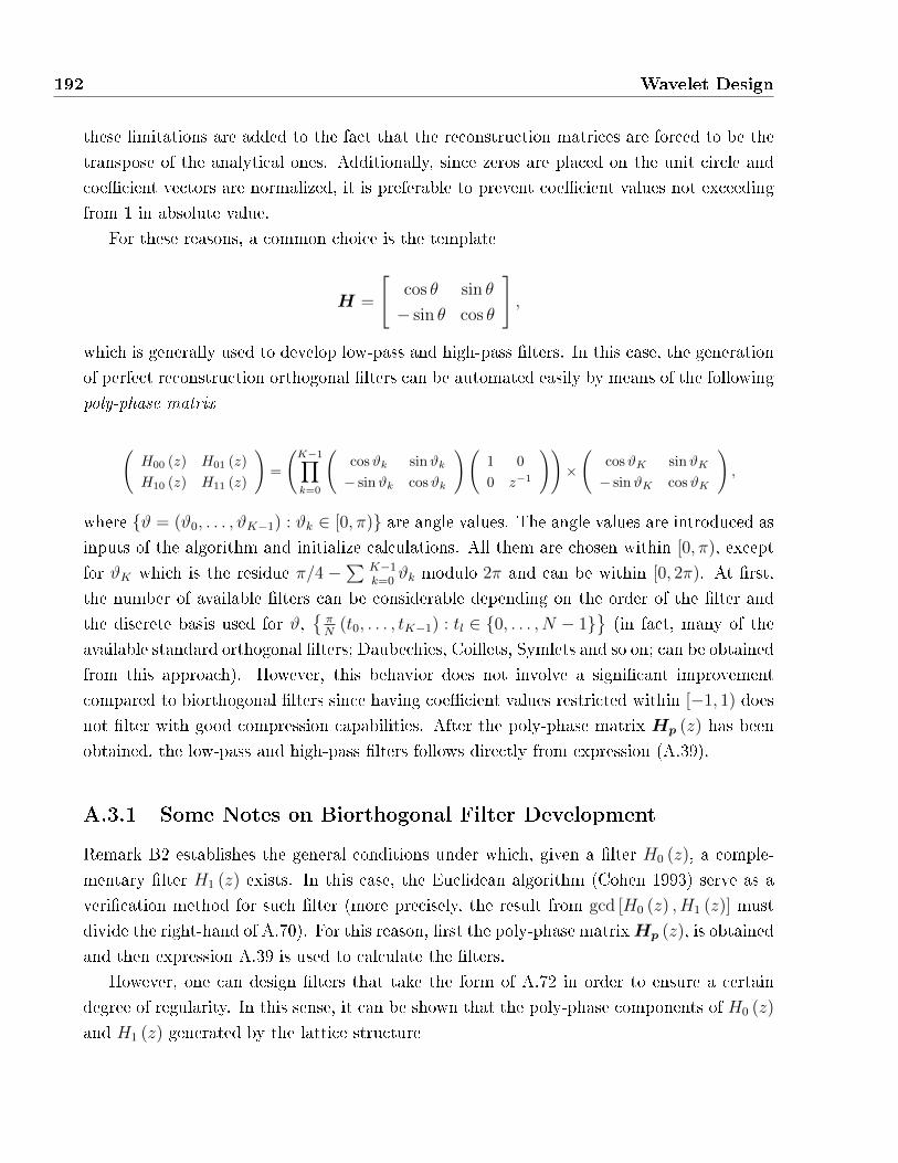
192 Wavelet Design
these limitations are added to the fact that the reconstruction matrices are forced to be the
transpose of the analytical ones. Additionally, since zeros are placed on the unit circle and
coe�cient vectors are normalized, it is preferable to prevent coe�cient values not exceeding
from 1 in absolute value.
For these reasons, a common choice is the template
H =
[cos θ sin θ
− sin θ cos θ
],
which is generally used to develop low-pass and high-pass �lters. In this case, the generation
of perfect reconstruction orthogonal �lters can be automated easily by means of the following
poly-phase matrix
(H00 (z) H01 (z)
H10 (z) H11 (z)
)=
(K−1∏k=0
(cosϑk sinϑk
− sinϑk cosϑk
)(1 0
0 z−1
))×
(cosϑK sinϑK
− sinϑK cosϑK
),
where {ϑ = (ϑ0, . . . , ϑK−1) : ϑk ∈ [0, π)} are angle values. The angle values are introduced as
inputs of the algorithm and initialize calculations. All them are chosen within [0, π), except
for ϑK which is the residue π/4 −∑ K−1
k=0ϑk modulo 2π and can be within [0, 2π). At �rst,
the number of available �lters can be considerable depending on the order of the �lter and
the discrete basis used for ϑ,{πN
(t0, . . . , tK−1) : tl ∈ {0, . . . , N − 1}}(in fact, many of the
available standard orthogonal �lters; Daubechies, Coi�ets, Symlets and so on; can be obtained
from this approach). However, this behavior does not involve a signi�cant improvement
compared to biorthogonal �lters since having coe�cient values restricted within [−1, 1) does
not �lter with good compression capabilities. After the poly-phase matrix Hp (z) has been
obtained, the low-pass and high-pass �lters follows directly from expression (A.39).
A.3.1 Some Notes on Biorthogonal Filter Development
Remark B2 establishes the general conditions under which, given a �lter H0 (z), a comple-
mentary �lter H1 (z) exists. In this case, the Euclidean algorithm (Cohen 1993) serve as a
veri�cation method for such �lter (more precisely, the result from gcd [H0 (z) , H1 (z)] must
divide the right-hand of A.70). For this reason, �rst the poly-phase matrixHp (z), is obtained
and then expression A.39 is used to calculate the �lters.
However, one can design �lters that take the form of A.72 in order to ensure a certain
degree of regularity. In this sense, it can be shown that the poly-phase components of H0 (z)
and H1 (z) generated by the lattice structure
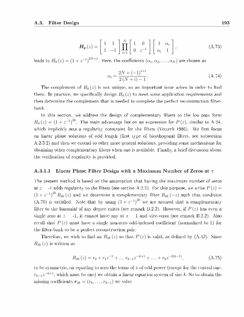
A.3. Filter Design 193
Hp (z) =
[1 1
1 −1
]N∏i=1
[1 0
0 z−1
][1 αi
αi 1
], (A.73)
leads to H0 (z) = (1 + z−1)2N+1. Here, the coe�cients (α1, α2, . . . , αN) are chosen as
αi =2N + (−1)i+1
2 (N + i)− 1. (A.74)
The complement of H0 (z) is not unique, so an important issue arises in order to �nd
them. In practice, we speci�cally design H0 (z) to meet some application requirements and
then determine the complement that is needed to complete the perfect reconstruction �lter-
bank.
In this section, we address the design of complementary �lters to the low-pass form
H0 (z) = (1 + z−1)2k. The main advantage lies on an expression for P (z), similar to A.24,
which implicitly sets a regularity constraint for the �lters (Vetterli 1986). We �rst focus
on linear phase solutions of odd length (�rst type of biorthogonal �lters, see subsection
A.2.3.2) and then we extend to other more general solutions, providing some mechanisms for
obtaining other complementary �lters when one is available. Finally, a brief discussion about
the veri�cation of regularity is provided.
A.3.1.1 Linear Phase Filter Design with a Maximum Number of Zeros at π
The present method is based on the assumption that having the maximum number of zeros
at z = -1 adds regularity to the �lters (see section A.2.2). For this purpose, we write P (z) =
(1 + z−1)2kR2k (z) and we determine a complementary �lter R2k (−z) such that condition
(A.70) is satis�ed. Note that by using (1 + z−1)2k we are assured that a complementary
�lter to the binomial of any degree exists (see remark B.2.3). However, if P (z) has even a
single zero at z = -1, it cannot have any at z = 1 and vice-versa (see remark B.2.2). Also
recall that P (z) must have a single non-zero odd-indexed coe�cient (normalized to 1) for
the �lter-bank to be a perfect reconstruction pair.
Therefore, we wish to �nd an R2k (z) so that P (z) is valid, as de�ned by (A.43). Since
R2k (z) is written as
R2k (z) = r0 + r1z−1 + . . . rk−1z
−k+1 + . . .+ r0z−2(k−1), (A.75)
to be symmetric, on equating to zero the terms of z of odd power (except for the central one,
rk−1z−k+1, which must be one) we obtain a linear equation system of size k. So to obtain the
missing coe�cients r2k = (r0, . . . , rk−1) we solve
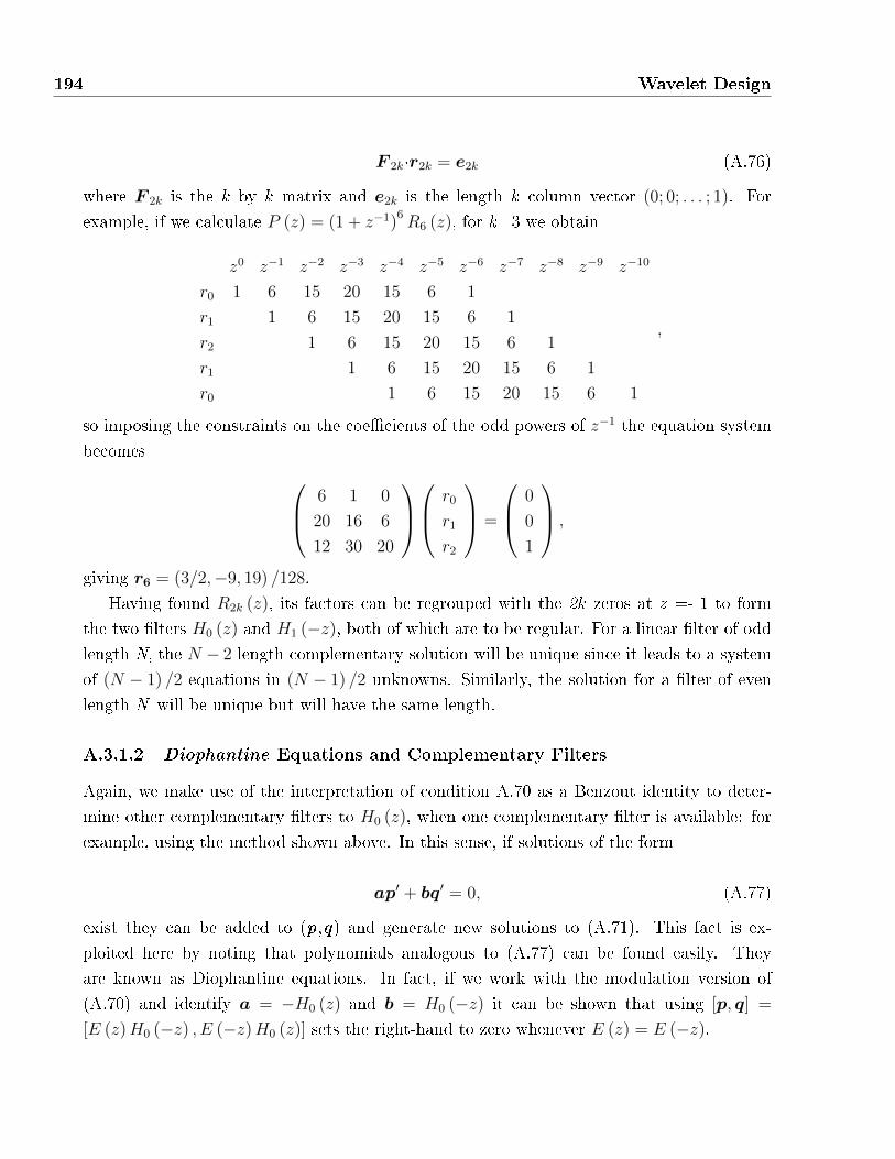
194 Wavelet Design
F 2k·r2k = e2k (A.76)
where F 2k is the k by k matrix and e2k is the length k column vector (0; 0; . . . ; 1). For
example, if we calculate P (z) = (1 + z−1)6R6 (z), for k=3 we obtain
z0 z−1 z−2 z−3 z−4 z−5 z−6 z−7 z−8 z−9 z−10
r0 1 6 15 20 15 6 1
r1 1 6 15 20 15 6 1
r2 1 6 15 20 15 6 1
r1 1 6 15 20 15 6 1
r0 1 6 15 20 15 6 1
,
so imposing the constraints on the coe�cients of the odd powers of z−1 the equation system
becomes 6 1 0
20 16 6
12 30 20
r0
r1
r2
=
0
0
1
,
giving r6 = (3/2,−9, 19) /128.
Having found R2k (z), its factors can be regrouped with the 2k zeros at z =- 1 to form
the two �lters H0 (z) and H1 (−z), both of which are to be regular. For a linear �lter of odd
length N, the N − 2 length complementary solution will be unique since it leads to a system
of (N − 1) /2 equations in (N − 1) /2 unknowns. Similarly, the solution for a �lter of even
length N will be unique but will have the same length.
A.3.1.2 Diophantine Equations and Complementary Filters
Again, we make use of the interpretation of condition A.70 as a Benzout identity to deter-
mine other complementary �lters to H0 (z), when one complementary �lter is available: for
example, using the method shown above. In this sense, if solutions of the form
ap′ + bq′ = 0, (A.77)
exist they can be added to (p,q) and generate new solutions to (A.71). This fact is ex-
ploited here by noting that polynomials analogous to (A.77) can be found easily. They
are known as Diophantine equations. In fact, if we work with the modulation version of
(A.70) and identify a = −H0 (z) and b = H0 (−z) it can be shown that using [p, q] =
[E (z)H0 (−z) , E (−z)H0 (z)] sets the right-hand to zero whenever E (z) = E (−z).
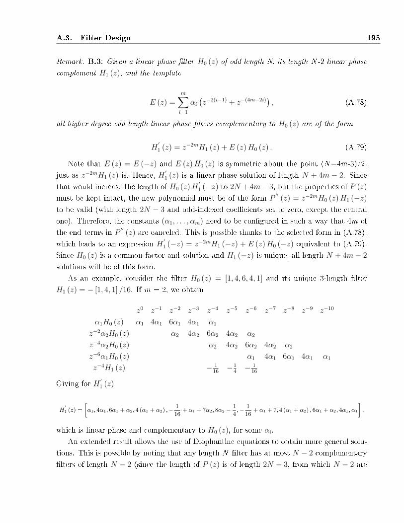
A.3. Filter Design 195
Remark. B.3: Given a linear phase �lter H0 (z) of odd length N, its length N -2 linear phase
complement H1 (z), and the template
E (z) =m∑i=1
αi(z−2(i−1) + z−(4m−2i)
), (A.78)
all higher degree odd length linear phase �lters complementary to H0 (z) are of the form
H′
1 (z) = z−2mH1 (z) + E (z)H0 (z) . (A.79)
Note that E (z) = E (−z) and E (z)H0 (z) is symmetric about the point (N+4m-3)/2,
just as z−2mH1 (z) is. Hence, H′1 (z) is a linear phase solution of length N + 4m − 2. Since
that would increase the length of H0 (z)H′1 (−z) to 2N + 4m− 3, but the properties of P (z)
must be kept intact, the new polynomial must be of the form P′′
(z) = z−2mH0 (z)H1 (−z)
to be valid (with length 2N − 3 and odd-indexed coe�cients set to zero, except the central
one). Therefore, the constants (α1, . . . , αm) need to be con�gured in such a way that 4m of
the end terms in P′′
(z) are canceled. This is possible thanks to the selected form in (A.78),
which leads to an expression H′1 (−z) = z−2mH1 (−z) + E (z)H0 (−z) equivalent to (A.79).
Since H0 (z) is a common factor and solution and H1 (−z) is unique, all length N + 4m− 2
solutions will be of this form.
As an example, consider the �lter H0 (z) = [1, 4, 6, 4, 1] and its unique 3-length �lter
H1 (z) = − [1, 4, 1] /16. If m = 2, we obtain
z0 z−1 z−2 z−3 z−4 z−5 z−6 z−7 z−8 z−9 z−10
α1H0 (z) α1 4α1 6α1 4α1 α1
z−2α2H0 (z) α2 4α2 6α2 4α2 α2
z−4α2H0 (z) α2 4α2 6α2 4α2 α2
z−6α1H0 (z) α1 4α1 6α1 4α1 α1
z−4H1 (z) − 116−1
4− 1
16
Giving for H′1 (z)
H′1 (z) =
[α1, 4α1, 6α1 + α2, 4 (α1 + α2) ,−
1
16+ α1 + 7α2, 8α2 −
1
4,− 1
16+ α1 + 7, 4 (α1 + α2) , 6α1 + α2, 4α1, α1
],
which is linear phase and complementary to H0 (z), for some αi.
An extended result allows the use of Diophantine equations to obtain more general solu-
tions. This is possible by noting that any length N �lter has at most N − 2 complementary
�lters of length N − 2 (since the length of P (z) is of length 2N − 3, from which N − 2 are

196 Wavelet Design
odd-indexed, the single nonzero odd-indexed coe�cient can be placed in any of these N − 2
positions, leading to N − 2 equation systems of size N − 2).
Remark. B.4: All �lters of length N + 2m − 2, complementary to a length N length �lter
H0 (z), have the form
H′
1 (z) = z−2kH1 (z) + E (z)H0 (z) (A.80)
where E (z) = E (−z) is a polynomial of the form
E (z) =m−1∑i=0
αiz−2i, (A.81)
k ∈ {0, 1, . . . ,m} and H1 (z) is a length N − 2 complementary �lter.
That this is a solution is veri�ed by direct substitution of E (z), which reduces the length
of P′′
(z) = H0 (z)[H′1 (−z)− E (z)H0 (−z)
]by 2m for some choice of αi. Since H0 (z) is
still a factor of both P (z) and P′′
(z), the remaining factor must be one of the N − 2 length
solutions, for which there are only N − 2.
A.3.1.3 Discussion
While the design procedure of the previous methods are fairly simple, the spectra of the
scaling function φ (ω) and the wavelet ψ (ω), may not be as one might wish from low-pass
and band-pass �lters. In the �rst method, it turns out that ensuring that both H0 (z) and
H1 (−z) meet the condition of remark B.1 can force one to choose �lters of quite unequal
length when k is small, and only when k increases does it becomes possible to obtain �lters
of quite regular wavelets.
However, other methods aimed at optimizing regularity permit more robust designs even
when failing in the veri�cation of this condition. Another possible approach is to note that
there is no need to place all of the zeros at z = −1 to start with. For example, we could
calculate the complementary �lter to a factor (1 + z−1)2k
[u1 (z) , u2 (z) , . . . , uj (z)]2 where
ui (z) represents a zero pair on the unit circle. We are then assured of having a factor
(1 + z−1)k
[u1 (z) , u2 (z) , . . . , uj (z)] to place in the stop band of each of the �lters.
Although higher degree solutions can give better results, in general FIR �lters lead to
very constrained solutions. Further methods on wavelet design can be found, for example, in
Strang and Nguyen (1996), Chui (1992) and Mallat (1990). If compact support is not desired,
similar techniques using IIR �lters generate orthogonal wavelets (Herley and Vetterli 1991,
1992).

Appendix B
CWT Computation with the DWT
Full discretization of the scale and time parameters is addressed by setting
s = aj0, (B.1)
u = k, (B.2)
where 1 ≤ a0 ≤ 2 and k = 1, . . . , N . However in a more practical implementation, full
discretization of the time-frequency plane is developed by maintaining a dyadic discretization
in one parameter, while the other takes denser values in the Wavelet Series approach. The
general case, which leads to the CWT computation, is obtained by combining both techniques.
B.1 Finner Sampling in Scale
Here, we maintain u = k2j, while the scale parameter is sampled according to
s = 2j+m/M , for m = 0, . . . ,M − 1 (B.3)
where m is called the �voice�.
The simplest way to compute WS coe�cients onM voices per octave consists in exploiting
the standard octave-by-octave algorithm as the main building function block. That is, for
each m replace ψ (t) by the slightly stretched wavelets 2−m/2Mψ(2−(j+m/M)t
)in Eq. 3.14.
Similarly, replace φ (t) by 2−m/2Mφ(2−(j+m/M)t
). Both scaling and wavelets basis functions
become
2−(j+m/M)/2φ(2−(j+m/M)t
)and 2−(j+m/M)/2ψ
(2−(j+m/M)t
)(B.4)
197
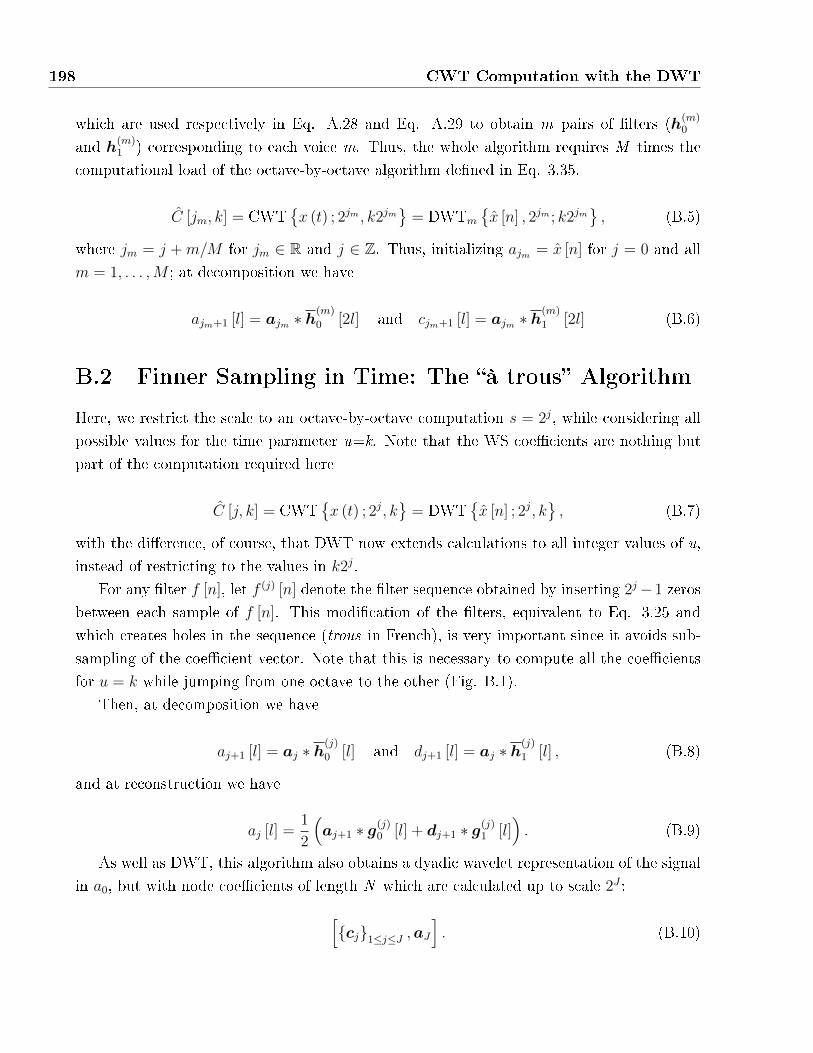
198 CWT Computation with the DWT
which are used respectively in Eq. A.28 and Eq. A.29 to obtain m pairs of �lters (h(m)0
and h(m)1 ) corresponding to each voice m. Thus, the whole algorithm requires M times the
computational load of the octave-by-octave algorithm de�ned in Eq. 3.35.
C [jm, k] = CWT{x (t) ; 2jm , k2jm
}= DWTm
{x [n] , 2jm ; k2jm
}, (B.5)
where jm = j + m/M for jm ∈ R and j ∈ Z. Thus, initializing ajm = x [n] for j = 0 and all
m = 1, . . . ,M ; at decomposition we have
ajm+1 [l] = ajm ∗ h(m)
0 [2l] and cjm+1 [l] = ajm ∗ h(m)
1 [2l] (B.6)
B.2 Finner Sampling in Time: The �à trous� Algorithm
Here, we restrict the scale to an octave-by-octave computation s = 2j, while considering all
possible values for the time parameter u=k. Note that the WS coe�cients are nothing but
part of the computation required here
C [j, k] = CWT{x (t) ; 2j, k
}= DWT
{x [n] ; 2j, k
}, (B.7)
with the di�erence, of course, that DWT now extends calculations to all integer values of u,
instead of restricting to the values in k2j.
For any �lter f [n], let f (j) [n] denote the �lter sequence obtained by inserting 2j−1 zeros
between each sample of f [n]. This modi�cation of the �lters, equivalent to Eq. 3.25 and
which creates holes in the sequence (trous in French), is very important since it avoids sub-
sampling of the coe�cient vector. Note that this is necessary to compute all the coe�cients
for u = k while jumping from one octave to the other (Fig. B.1).
Then, at decomposition we have
aj+1 [l] = aj ∗ h(j)
0 [l] and dj+1 [l] = aj ∗ h(j)
1 [l] , (B.8)
and at reconstruction we have
aj [l] =1
2
(aj+1 ∗ g(j)
0 [l] + dj+1 ∗ g(j)1 [l]
). (B.9)
As well as DWT, this algorithm also obtains a dyadic wavelet representation of the signal
in a0, but with node coe�cients of length N which are calculated up to scale 2J :[{cj}1≤j≤J ,aJ
]. (B.10)
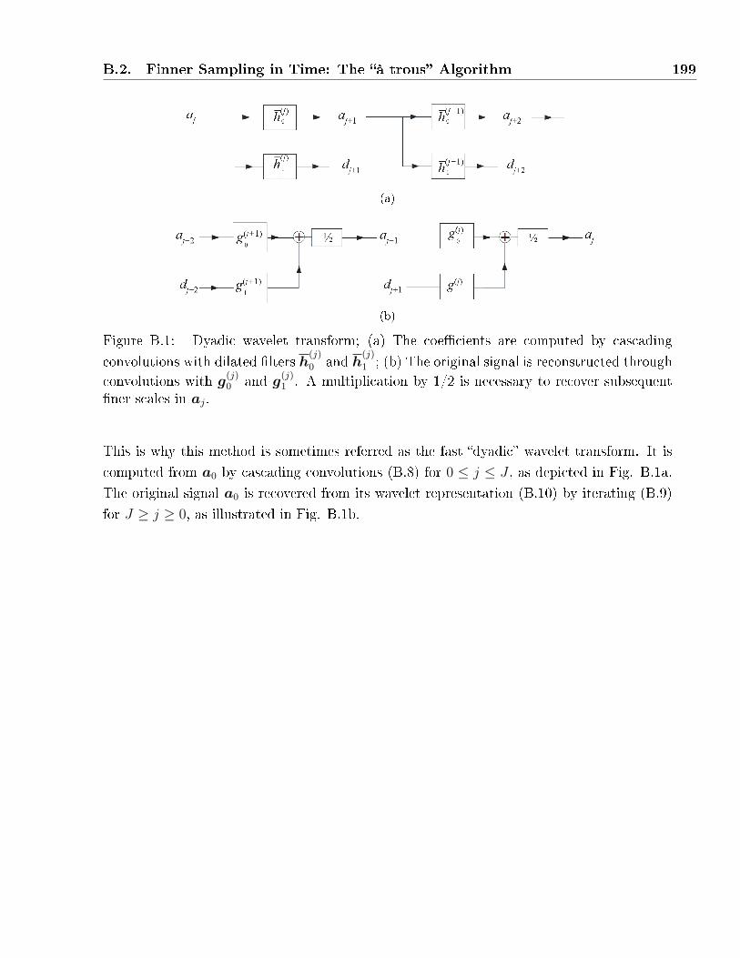
B.2. Finner Sampling in Time: The �à trous� Algorithm 199
(a)
(b)
Figure B.1: Dyadic wavelet transform; (a) The coe�cients are computed by cascading
convolutions with dilated �lters h(j)
0 and h(j)
1 ; (b) The original signal is reconstructed throughconvolutions with g(j)
0 and g(j)1 . A multiplication by 1/2 is necessary to recover subsequent
�ner scales in aj.
This is why this method is sometimes referred as the fast �dyadic� wavelet transform. It is
computed from a0 by cascading convolutions (B.8) for 0 ≤ j ≤ J , as depicted in Fig. B.1a.
The original signal a0 is recovered from its wavelet representation (B.10) by iterating (B.9)
for J ≥ j ≥ 0, as illustrated in Fig. B.1b.
Appendix C
Multivariate Density Algorithms
C.1 Introduction
In chapter 5 we introduced the basic framework for density estimates in one-dimensional
data. The extension of the AMISE calculation for the multivariate case is only slightly more
complicated. The corresponding framework was provided by Scott (1992).
Given a sample f (x), where x ∈ Rd, the histogram is determined by regular partitions in
the form of hyper-rectangles of size h1×h2×. . .×hd. Consider a generic hyper-rectangular binlabeled Gm containing vm points. As usual
∑m vm = N . Then, the multivariate histogram
is de�ned by
f (x) =vm
Nh1h2 · · ·hd, for x ∈ Gm. (C.1)
The asymptotically optimal bin widths, h∗k, and resulting AMISE* for Normal multivariate
data, X ∼ N (µ,Σ) and Σ = Diag (σ21, σ
22, . . . , σ
2d) are
h∗k = 2× 31/(2+d)πd/(4+2d)σkN−1/(2+d), (C.2)
AMISE* = 2−1/(1+d)32/(2+d)π−d2/(4+2d)c−1
d N−2/(2+d)
where cd = σ1σ2 · · ·σd. In this case, since the constant in the bandwidth increases slowly
from 3.4908 in one dimension to the limiting value 2√π = 3.545 as d→∞, a very useful bin
width expression is
h∗k ≈ 3.5σkN−1/(2+d). (C.3)
201
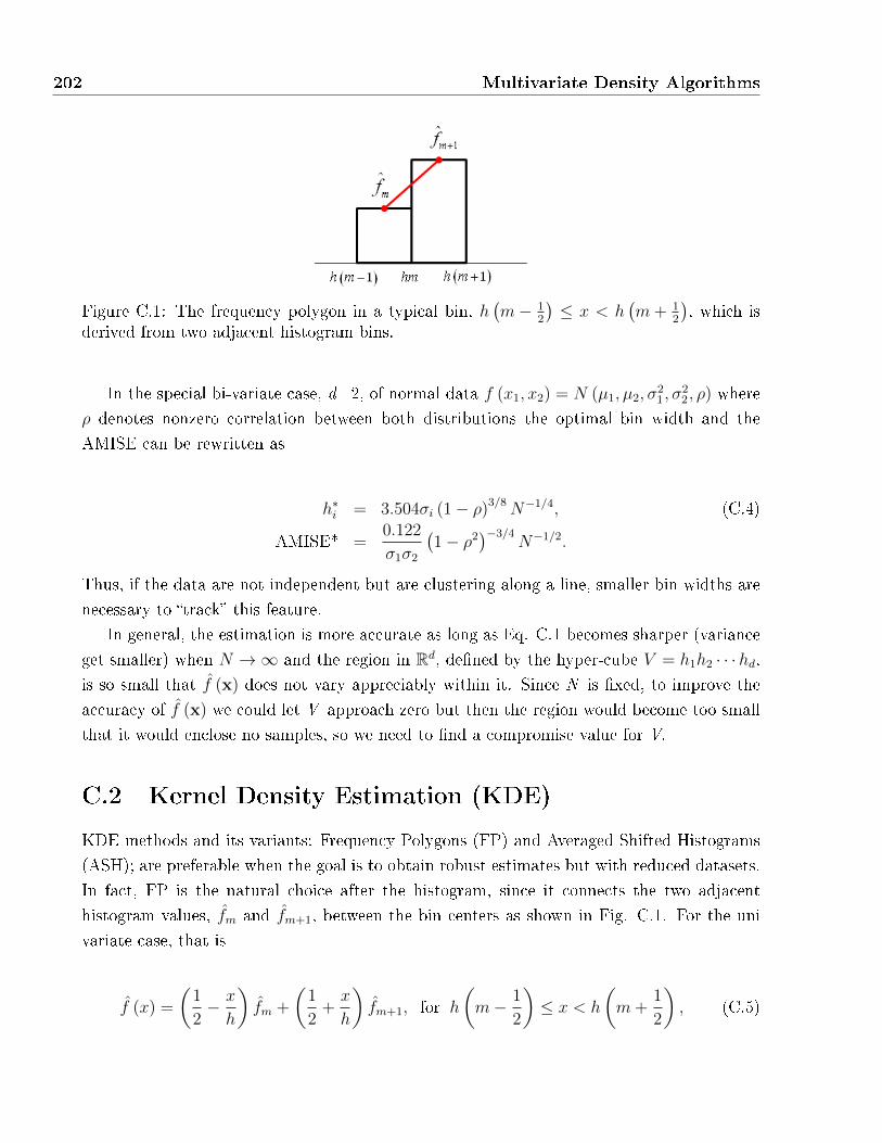
202 Multivariate Density Algorithms
Figure C.1: The frequency polygon in a typical bin, h(m− 1
2
)≤ x < h
(m+ 1
2
), which is
derived from two adjacent histogram bins.
In the special bi-variate case, d=2, of normal data f (x1, x2) = N (µ1, µ2, σ21, σ
22, ρ) where
ρ denotes nonzero correlation between both distributions the optimal bin width and the
AMISE can be rewritten as
h∗i = 3.504σi (1− ρ)3/8N−1/4, (C.4)
AMISE* =0.122
σ1σ2
(1− ρ2
)−3/4N−1/2.
Thus, if the data are not independent but are clustering along a line, smaller bin widths are
necessary to �track� this feature.
In general, the estimation is more accurate as long as Eq. C.1 becomes sharper (variance
get smaller) when N →∞ and the region in Rd, de�ned by the hyper-cube V = h1h2 · · ·hd,is so small that f (x) does not vary appreciably within it. Since N is �xed, to improve the
accuracy of f (x) we could let V approach zero but then the region would become too small
that it would enclose no samples, so we need to �nd a compromise value for V.
C.2 Kernel Density Estimation (KDE)
KDE methods and its variants: Frequency Polygons (FP) and Averaged Shifted Histograms
(ASH); are preferable when the goal is to obtain robust estimates but with reduced datasets.
In fact, FP is the natural choice after the histogram, since it connects the two adjacent
histogram values, fm and fm+1, between the bin centers as shown in Fig. C.1. For the uni
variate case, that is
f (x) =
(1
2− x
h
)fm +
(1
2+x
h
)fm+1, for h
(m− 1
2
)≤ x < h
(m+
1
2
), (C.5)
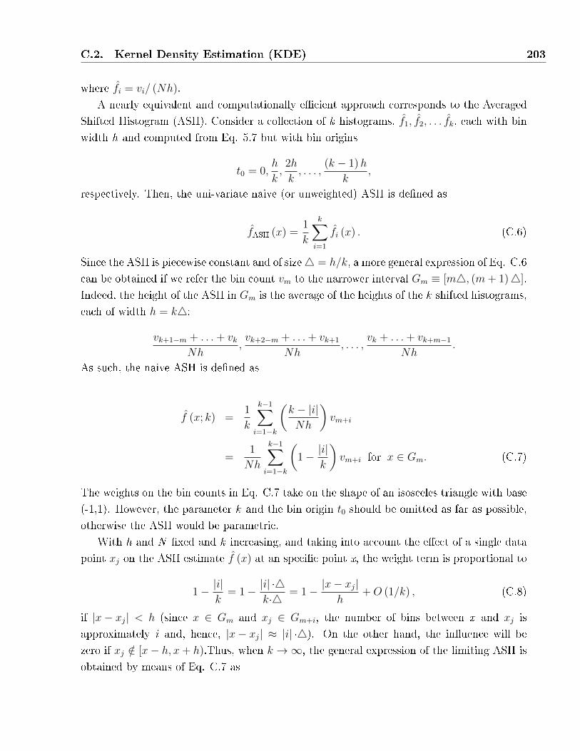
C.2. Kernel Density Estimation (KDE) 203
where fi = vi/ (Nh).
A nearly equivalent and computationally e�cient approach corresponds to the Averaged
Shifted Histogram (ASH). Consider a collection of k histograms, f1, f2, . . . fk, each with bin
width h and computed from Eq. 5.7 but with bin origins
t0 = 0,h
k,2h
k, . . . ,
(k − 1)h
k,
respectively. Then, the uni-variate naive (or unweighted) ASH is de�ned as
fASH (x) =1
k
k∑i=1
fi (x) . (C.6)
Since the ASH is piecewise constant and of size4 = h/k, a more general expression of Eq. C.6
can be obtained if we refer the bin count vm to the narrower interval Gm ≡ [m4, (m+ 1)4].
Indeed, the height of the ASH in Gm is the average of the heights of the k shifted histograms,
each of width h = k4:
vk+1−m + . . .+ vkNh
,vk+2−m + . . .+ vk+1
Nh, . . . ,
vk + . . .+ vk+m−1
Nh.
As such, the naive ASH is de�ned as
f (x; k) =1
k
k−1∑i=1−k
(k − |i|Nh
)vm+i
=1
Nh
k−1∑i=1−k
(1− |i|
k
)vm+i for x ∈ Gm. (C.7)
The weights on the bin counts in Eq. C.7 take on the shape of an isosceles triangle with base
(-1,1). However, the parameter k and the bin origin t0 should be omitted as far as possible,
otherwise the ASH would be parametric.
With h and N �xed and k increasing, and taking into account the e�ect of a single data
point xj on the ASH estimate f (x) at an speci�c point x, the weight term is proportional to
1− |i|k
= 1− |i| ·4k·4
= 1− |x− xj|h
+O (1/k) , (C.8)
if |x− xj| < h (since x ∈ Gm and xj ∈ Gm+i, the number of bins between x and xj is
approximately i and, hence, |x− xj| ≈ |i| ·4). On the other hand, the in�uence will be
zero if xj /∈ [x− h, x+ h).Thus, when k →∞, the general expression of the limiting ASH is
obtained by means of Eq. C.7 as
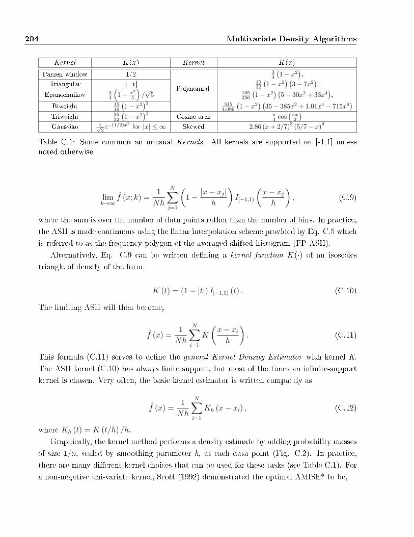
204 Multivariate Density Algorithms
Kernel K (x ) Kernel K (x )
Parzen window 1/2
Polynomial
34
(1− x2
),
Triangular 1-|x | 1532
(1− x2
) (3− 7x2
),
Epanechnikov 34
(1− x2
5
)/√5 105
256
(1− x2
) (5− 30x2 + 33x4
),
Biweight 1516
(1− x2
)2 3154.096
(1− x2
) (35− 385x2 + 1.01x4 − 715x6
)Triweight 35
32
(1− x2
)3Cosine arch π
4 cos(πx2
)Gaussian 1√
2e−(1/2)x
2
for |x| ≤ ∞ Skewed 2.86 (x+ 2/7)3(5/7− x)
9
Table C.1: Some common an unusual Kernels. All kernels are supported on [-1,1] unlessnoted otherwise
limk→∞
f (x; k) =1
Nh
N∑j=1
(1− |x− xj|
h
)I[−1,1)
(x− xjh
), (C.9)
where the sum is over the number of data points rather than the number of bins. In practice,
the ASH is made continuous using the linear interpolation scheme provided by Eq. C.5 which
is referred to as the frequency polygon of the averaged shifted histogram (FP-ASH).
Alternatively, Eq. C.9 can be written de�ning a kernel function K (·) of an isosceles
triangle of density of the form,
K (t) = (1− |t|) I|−1,1) (t) . (C.10)
The limiting ASH will then become,
f (x) =1
Nh
N∑i=1
K
(x− xih
). (C.11)
This formula (C.11) serves to de�ne the general Kernel Density Estimator with kernel K.
The ASH kernel (C.10) has always �nite support, but most of the times an in�nite-support
kernel is chosen. Very often, the basic kernel estimator is written compactly as
f (x) =1
Nh
N∑i=1
Kh (x− xi) , (C.12)
where Kh (t) = K (t/h) /h.
Graphically, the kernel method performs a density estimate by adding probability masses
of size 1/n, scaled by smoothing parameter h, at each data point (Fig. C.2). In practice,
there are many di�erent kernel choices that can be used for these tasks (see Table C.1). For
a non-negative uni-variate kernel, Scott (1992) demonstrated the optimal AMISE* to be,
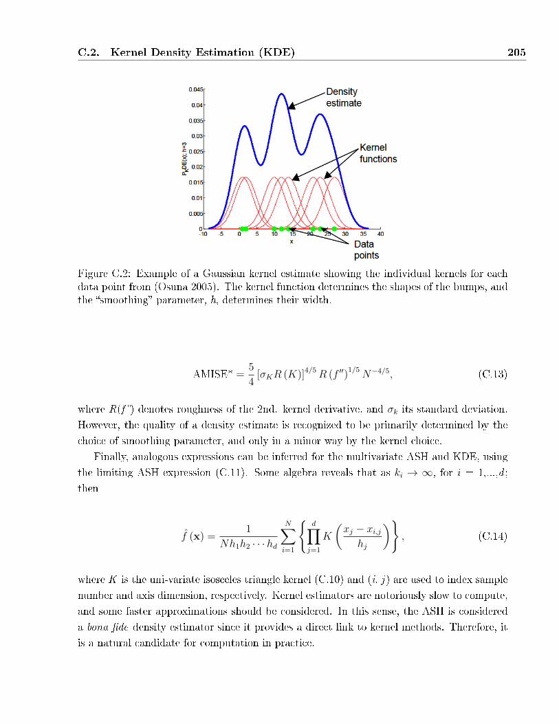
C.2. Kernel Density Estimation (KDE) 205
Figure C.2: Example of a Gaussian kernel estimate showing the individual kernels for eachdata point from (Osuna 2005). The kernel function determines the shapes of the bumps, andthe �smoothing� parameter, h, determines their width.
AMISE* =5
4[σKR (K)]4/5R (f ′′)
1/5N−4/5, (C.13)
where R(f �) denotes roughness of the 2nd. kernel derivative, and σk its standard deviation.
However, the quality of a density estimate is recognized to be primarily determined by the
choice of smoothing parameter, and only in a minor way by the kernel choice.
Finally, analogous expressions can be inferred for the multivariate ASH and KDE, using
the limiting ASH expression (C.11). Some algebra reveals that as ki → ∞, for i = 1,...,d ;
then
f (x) =1
Nh1h2 · · ·hd
N∑i=1
{d∏j=1
K
(xj − xi,j
hj
)}, (C.14)
where K is the uni-variate isosceles triangle kernel (C.10) and (i, j ) are used to index sample
number and axis dimension, respectively. Kernel estimators are notoriously slow to compute,
and some faster approximations should be considered. In this sense, the ASH is considered
a bona �de density estimator since it provides a direct link to kernel methods. Therefore, it
is a natural candidate for computation in practice.
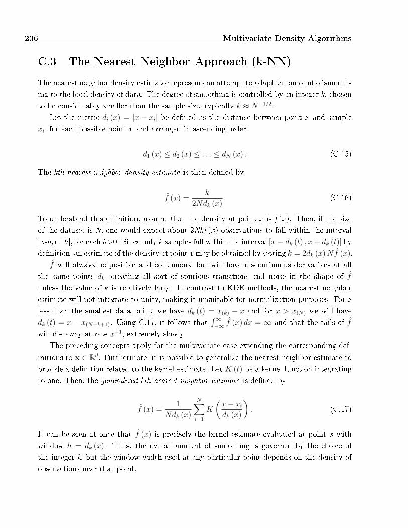
206 Multivariate Density Algorithms
C.3 The Nearest Neighbor Approach (k-NN)
The nearest neighbor density estimator represents an attempt to adapt the amount of smooth-
ing to the local density of data. The degree of smoothing is controlled by an integer k, chosen
to be considerably smaller than the sample size; typically k ≈ N−1/2.
Let the metric di (x) = |x− xi| be de�ned as the distance between point x and sample
xi, for each possible point x and arranged in ascending order
d1 (x) ≤ d2 (x) ≤ . . . ≤ dN (x) . (C.15)
The kth nearest neighbor density estimate is then de�ned by
f (x) =k
2Ndk (x). (C.16)
To understand this de�nition, assume that the density at point x is f (x ). Then, if the size
of the dataset is N, one would expect about 2Nhf (x ) observations to fall within the interval
[x -h,x+h], for each h>0. Since only k samples fall within the interval [x− dk (t) , x+ dk (t)] by
de�nition, an estimate of the density at point x may be obtained by setting k = 2dk (x)Nf (x).
f will always be positive and continuous, but will have discontinuous derivatives at all
the same points dk, creating all sort of spurious transitions and noise in the shape of f
unless the value of k is relatively large. In contrast to KDE methods, the nearest neighbor
estimate will not integrate to unity, making it unsuitable for normalization purposes. For x
less than the smallest data point, we have dk (t) = x(k) − x and for x > x(N) we will have
dk (t) = x − x(N−k+1). Using C.17, it follows that´∞−∞ f (x) dx = ∞ and that the tails of f
will die away at rate x−1, extremely slowly.
The preceding concepts apply for the multivariate case extending the corresponding def-
initions to x ∈ Rd. Furthermore, it is possible to generalize the nearest neighbor estimate to
provide a de�nition related to the kernel estimate. Let K (t) be a kernel function integrating
to one. Then, the generalized kth nearest neighbor estimate is de�ned by
f (x) =1
Ndk (x)
N∑i=1
K
(x− xidk (x)
). (C.17)
It can be seen at once that f (x) is precisely the kernel estimate evaluated at point x with
window h = dk (x). Thus, the overall amount of smoothing is governed by the choice of
the integer k, but the window width used at any particular point depends on the density of
observations near that point.
C.3. The Nearest Neighbor Approach (k-NN) 207
As a �nal remark, it can be said that the number of related density methods is large and
will not be reviewed further. There is the possibility to modify the kernel width from one data
point to another in order to achieve adaptive smoothing (Jones 1990), increasing the accuracy
of estimation even further at the expenses of a higher computational cost. Other approaches
estimate densities from a quite di�erent perspective. For example, Orthogonal Series Ap-
proximations (Kronmal and Tarter 1968, Watson 1969) are known to use kernels constructed
from Fouriers basis functions. Other authors use optimization techniques (Maximum penal-
ized likelihood estimators, MPL) to verify qualitative properties of density functions, such
as the con�ict between smoothness and goodness-of-�t (Delta methods, de Montricher et al.
1975, Good and Gaskings 1980, Klonias 1982).
Bibliography
P. Abry and P. Flandrin. On the initialization of the DiscreteWavelet Transform algorithm.
IEEE Sig. Proc. Letters, 1:32�34, 1994.
M. Aguayo-Hernández. Biology and �sheries of chilean hakes (merluccius gayi and merluccius
australis). In Hake: �sheries, ecology and markets, pages 23�67. London. Chapman and
Hall Book Series, 1955.
N. Ahmed and K.R. Rao. Orthogonal Transforms for Digital Signal Processing. Springer-
Verlag, New York, 1975.
W.O. Ayres. Description of the new species of california �shes. In Proceedings of California
Academy of Natural Sciences, volume 1, pages 23�67, 1855.
W. Banzhaf, P. Nordin, R. Keller, and F. Frankone. Genetic Programming. An Introduction.
Morgan Kaufmann, 1998.
M. Baseville. Distance measures for signal processing and pattern recognition. Signal Pro-
cessing, 18:349�369, 1989.
T. Bayes. An essay toward solving a problem in the doctrine of chances. Philosophical
Transactions of the Royal Society of London, 53:370�418, 1764.
R.J. Beamish. Di�erences in the age of paci�c hake (merluccius productus) using whole
otoliths and sections of otoliths. J. Fish. Res. Board Can., 36:141�151, 1979.
R.J. Beamish and D.A. Fournier. A method for comparing the precission of a set of age
determinations. Canadian Journal of Fisheries and Aquatic Sciences, 38:982�983, 1981.
R.E. Bellman. Adaptive Control Processes. 1961.
A.P.M. Di Beneditto, R.M.A. Ramos, and N.R. Wille-Lima. Os gol�nhos: origem, clas-
si�caçao, captura acidental, hábito alimentar. The Latin Americal Journal of Aquatic
Mammals, 2001.
209
210 Bibliography
J.T. Bennett, G.W. Boehlert, and K.K. Turekian. Con�rmation of longevity in sebastes
diplorproa (pisces: Scorpaenidae) from pb-210/ra-2226 measurements in otoliths. Marine
Biology, 71:209�215, 1982.
R.J.H. Beverton and S.J. Holt. On the dynamics of exploited �sh populations. Chapman and
Hall, London, UK, 1957.
G. Beylkin. Wavelets and fast numerical algorithms. In Proceedings of Symposia in Applied
Mathematics, 1993.
J.L. Bird, D.T. Eppler, and D.M. Checkley. Comparison of herring otoliths using Fourier
series shape analyses. Canadian Journal of Fisheries and Aquatic Sciences, 43:1228�1234,
1986.
C.M. Bishop. Probability density estimation. In Neural Networks for Pattern Recognition,
pages 33�73. Oxford University Press, 1995.
R.W. Blacker. Recent advances in otolith studies. In Sea Fisheries Research, pages 67�90.
Willey, 1995.
K.L. Bolles and G.A. Begg. Distinction between silver hake (meluccius bilinearis) stocks in
u.s. waters of the North-west Atlantic based on otolith morphometrics. Fish. Bull., 98:
451�462, 2000.
F.L. Bookstein. Tensor biometrics for changes in craneal shape. Annals of Human Biology,
11:413�437, 1984.
F.L. Bookstein. Morphometric Tools for landmark data: Geometry and Biology. Cambridge
University Press, 1991.
F.L. Bookstein, R.E. Strauss, J.M. Humphries, B. Cherno�, R.L. Elder, and G.R. Smith. A
comment upon the uses of Fourier methods in systematics. Systematic Zoology, 31:85�92,
1982.
B.E. Boser, I. Guyon, and V. Vapnik. A training algorithm for optimal margin classi�ers.
In Proceedings of the Fith Annual Workshop on Computational Learning., pages 144�152.
ACM Press, 1992.
L. Botha. Growth and otolith morphology of the cape hakes merluccius capensis cast. and
merluccius paradoxus franca. Technical report, Investigational Report of the Division of
Sea Fisheries in South Africa, 1971.
Bibliography 211
L. Breiman, J.H. Friedman, R.A. olshen, and C.J. Stone. Classi�cation and Regression Trees.
Chapman & Hall, 1984.
G. Bruun. Z-transforms DFT �lters and FFTs. IEEE Transactions on Acoustics, Speech
and Signal Processing, 26(1):56�63, 1978.
E.J. Burton, A.H. Andrews, H.K. Coale, and G.M. Cailliet. Application of radiometric
age determination to three long-lived �shes using pb-210/ra-226 disequilibria in calci�eed
structures: a review. American Fisheries Society Symposium, 23:77�87, 1999.
J. Cadenat. Note sur les merlus de la côte occidentale d'Afrique. In Congr. Pêche Pêcheries
Un. Franç., pages 128�130, 1950.
S.X. Cadrin and K.D. Friedland. The utility of image processing techniques for morphometric
analysis and stock identi�cation. Fish. Res., 43:129�139, 1999.
S.E. Campana. Chemistry and composition of �sh otoliths, pathways, mechanisms and
application. Marine Ecology-Progress Series, 188:263�297, 1999.
S.E. Campana. Accuracy, precission and quality control in age determination, including a
review of the use and abuse of ageing validation methods. Journal of Fish Biology, 59:
197�242, 2001.
S.E. Campana. Otolih science entering the 21st century. Marine and Freshwater research,
56 (Otolith Research And Applications - Special Issue)(56):485�495, 2005.
S.E. Campana and J.M. Casselman. Stock discrimination using otholit shape analysis. Cana-
dian Journal of Fisheries and Aquatic Sciences, 50:1062�1083, 1993.
S.E. Campana and C.M. Jones. Radiocarbon from nuclear testing applied to age validation
of black drum, pogonias cromis. Fishery Bulletin U.S., 96:185�192, 1998.
S.E. Campana and J.D. Neilson. Microstructures of �sh otoliths. Canadian Journal of
Fisheries and Aquatic Sciences, 42:1014�1032, 1985.
S.E. Campana and S.R. Thorrold. Increments and elements: Keys to a comprehensive un-
derstanding of �sh populations? Canadian Journal of Fisheries and Aquatic Sciences, 58:
30�38, 2001.
S.E: Campana, M.C. Annand, and J.I. McMillan. Graphical and statistical methods for
determining the consistency of age determinations. 36:141�151, 1979.
212 Bibliography
S.E. Campana, K.C.T. Zwanemburg, and J.N. Smith. Pb-210/ra-226 determination of
longevity in red�sh. Canadian Journal of Fisheries and Aquatic Sciences, 47:163�165,
1990.
F. Cao and R. Fablet. Automatic morphological detection of otolith nucleus. Pattern Recog-
nition letters, 27:658�666, 2006.
M. Cardinale, P. Doering-Arjes, M. Kastowsky, and H. Mosegaard. E�ects of sex, stock, and
environment on the shape of known-age Atlantic cod (gadus morhua) otoliths. Canadian
Journal of Fisheries and Aquatic Sciences, 61:158�167, 2004.
J.K. Carlson, E. Cortés, and A.G. Johnson. Age and growth of the blacknose shark, car-
charhinus acronotus, in the eastern gulf of Mexico. Copeia, 1999:684�691, 1999.
S.J. Carpenter, J.M Erickson, and F.D. Holland Jr. Migration of late cretaceous �sh. Nature,
423:70�74, 2003.
V. Caselles, T. Coll, and J. Morel. Topographic maps and local contrast changes in natural
images. Int. J. of Comp. Vision, 33(1):5�27, 1999.
M.F. Castelnau. Merluccius capensis (n. sp). In Mémoire sur les poissons de l'Afrique
australe, pages 68�69, 1861.
M. Castonguay, P. Simard, and P. Gagnon. Usefulness of Fourier analysis of otolith shape for
Atlantic mackerel (scomber scombrus) stock discrimination. Canadian Journal of Fisheries
and Aquatic Sciences, 48(48):296�302, 1991.
W. Y. B. Chang. A statistical method for evaluating the reproducibility of age determination.
Canadian Journal of Fisheries and Aquatic Sciences, 39:1208�1210, 1982.
Y. Chen, D.A. Jackson, and H.H. Harvey. A comparison of von Bertalan�y and polynomial
functions in modelling �sh growth data. Can. J. Fish. Aquat. Sci., 49:1228�1235, 1992.
D. Chesmore. The Automated Identi�cation of Taxa: Concepts and applications. In
CRC Press N. MacLeod, editor, Identi�cation is Systematics: Theory, approaches and
applications, pages 83�100. Academic Press, 2007.
NC. Chui. Wavelets: a tutorial in theory and applications. Academic Press, 1992.
M. Cocchi, R. Seeber, and A. Ulrici. Wpter: Wavelet-packet transform for e�cient pattern
recognition signals. Chemometrics and Intelligent Laboratory Systems, 57:97�119, 2001.
Bibliography 213
A. Cohen, I. Daubechies, and J.C. Feauveau. Biorthogonal bases of compactly supported
wavelets. Comm. Pure and Appl. Math., 45(5):485�560, 1992.
H. Cohen. A course in computational algebraic number theory. Springer Verlag, New York,
1993.
R.R. Coifman and F. Majid. Adapted waveform analysis and denoising. In Progress in
Wavelet Analysis and Applications, pages 63�76. Editions Frontieres, BB.P.33, 91192 Gif-
sur-Yvette Cedex, France, 1993.
R.R. Coifman and Y. Meyer. Nouvelles bases orthonormées de l2(r) la structure de systèm
de walsh. Technical report, Yale University, 1989a.
R.R. Coifman and Y. Meyer. Orthonormal wave packet bases. Technical report, Yale Uni-
versity (in ftp pascal.math.yale.edu/pub/wavelets/wavepkt.tex), 1989b.
R.R. Coifman and Y. Meyer. Remarques sur l'analyse de fourier a fenêtre. C.R. Acad. Sci.,
pages 54�81, 1991.
R.R. Coifman and M.V. Wickerhauser. Entropy-based algorithms for Best-Basis selection.
IEEE Transactions on Information Theory, 2:713�719, 1992.
J.W. Cooley and J.W. Tukey. An algorithm for the machine calculation of complex Fourier
series. Math. Comp., 19:297�301, 1965.
J.M. Cope and A.E. Punt. Admitting ageing error when �ttng growth curves: an example
using the von Betarlan�y growth function with random e�ects. Can. J. Fish. Aquat. Sci.,
64:205�218, 2007.
P.E. Cottrell, A.W. Trites, and E.H. Miller. Assessing the use of hard parts in faces to identify
harbour seal prey: results of captive feeding trials. Canadian Journal of Zoology-Revue
Canadien de Zoologie, 74:875�880, 1996.
T.M. Cover and P. Hart. Nearest neighbor pattern classi�cation. IEEE Transactions on
Information Theory, 13:21�27, 1967.
I. Daubechies. Orthonormal bases of compactly supported wavelets. Communications on
Pure and Applied Mathematics, 41:909�996, 1988.
I. Daubechies. Ten lectures on wavelets. In CBMS-NSF Regional Con�erence Series in
Applied Mathematics, volume 61, 1992.

214 Bibliography
G.F. de Montricher, R.A. Tapia, and J.R. Thompson. Nonparametric maximum likelihood
estimation of probability densities by penalty function methods. Ann. Statist., 3:1329�
1348, 1975.
P.A. Devijer and J. Kittler. Pattern recognition: A statistical approach. Prentice Hall Inter-
national Inc, London, 1982.
D.A. DeVries, C.B. Grimes, and M.H. Prager. Using otolith shape anlysis to distinguish
eastern gulf of Mexico and Atlantic Ocean stocks of king mackerel. Fisheries Research,
57:51�62, 2002.
J.D. Dutil, M. Castonguay, D. Gilbert, and D. Gascon. Growth, condition and environmental
relationships in Atlantic cod (gadus morhua) in the northen Golf of st. Lawrence and
implications for management strategies in the North-west Atlantic. Canadian Journal of
Marine Science, 60:1123�1138, 1999.
B. Efron. Estimating the error rate of a prediction rule: Improvement on cross-validation.
Journal of the American Statistical Association, 78:316�331, 1983.
R. Fablet. Statistical learning applied to computer-assisted �sh age and growth estimation
from otolith images. Fisheries Research, 81(81):219�228, 2006.
R. Fablet and N. Le Josse. Automated �sh age estimation from otolith image anlysis. Fish-
eries Research, 72:279�290, 2005.
R. Fablet, A. Benzinou, and C. Doncarli. Robust time-frequency estimation in otolith images
for �sh age and growth analysis. In Proc. of 10th Int. Conf. on Image Processing, 2003.
A.G. Finstand. Growth backcalculation based on otoliths incorporataing an age e�ect. Jour-
nal of Fish Biology, 62:1222�1225, 2003.
R.A. Fisher. The use of multiple measures in taxonomic problems. Annals of Eugenics, 7:
179�188, 1936.
J.E. Fitch and R.J. Lavenberg. Marine food and game �shes of California. The University
of Chicago Press, 1971.
E. Fix and J. Hodges. Discriminatory analysis, nonparametric discrimination: consistency
properties. Technical report, USAF School of Aviation Medicine, Randolph Field, Texas,
1951.
Bibliography 215
R. Fletcher. Pratical methods of optimization (2nd. Edition). John Wiley and Sons, New
York, p113, 1987.
P. Franca. Nova contribuiçao para o conhecimento do géneroMerluccius no Atlântico oriental
ao sul do Equador. Mem. Junta Invest. Ultram, 2(18):57�101, 1960.
J.H. Freedman and P. Diaconis. On the histogram as a density estimator: L2 theory.
Zeitschrift für Wahrscheinlichkeitssheorie und verwandte Gebiete, 57:453�476, 1981.
K.S. Fu. Syntactic Pattern recognition. Prentice Hall, Inc, N.J., 1982.
K. Fukunaga. Introduction to statistical pattern recognition. Academic Press, San Diego, CA,
1990.
L.P. Garrison and J.S. Link. Diet of �ve hake species in the North-east United States
continental shelf ecosystem. Mar. Ecol. Prog. Ser., 204:243�255, 2000.
R.W. Gauldie. The morphological basis of �sh age estimation methods based on the otolith
of nemadactylus macropterus. Canadian Journal of Fisheries and Aquatic Sciences, 51:
2341�2362, 1994.
A.J. Ge�en. Otolith ring deposition in relation to growth rate in herring (clupea harengus)
and turbot (scophtkalmus maximus) larvae. Marine Biology, 71:317�326, 1982.
I.J. Good. The interaction algorithm and practical Fourier analysis. J.R. Statist. Soc. B,
20(2):361�372, 1958.
I.J. Good and R.A. Gaskings. Density estimation and bump-hunting by the penalized likeli-
hood method exempli�ed by the scattering and meteorite data (with discussion). J. Amer.
Statist. Assoc., 75:42�73, 1980.
C. Goutte. Note on free lunches and cross-validation. Neural Computation, 9:1211�1215,
1997.
A. Grant. Age determination of growth in �sh and other aquatic animals. Australian Journal
of Marine and Freshwater Research, 43 (Special issue):879�1330, 1992.
A. Guichenot. Fauna Chilena. Peces. C. Gay, 1848.
A. Guillaud, A. Benzinou, H. Troadec, V. Rodin, and J.L. Bihan. Autonomous agents for
edge detection and continuity perception on otolith images. Image and Vision Computing,
20:955�968, 2002.
216 Bibliography
L. Han and M. Neumann. E�ect of dimensionality on the Nelder-Mead simplex method.
Optimization methods and software, 21(1):1�16, 2006.
S.M. Hanchet and Y. Uozumi. Age validation and growth of southern blue whiting, mi-
cromesitius australis, in New Zealand. New Zealand Journal of Marine and Freshwater
Research, 30:57�67, 1996.
D.J. Hand. Kernel discriminant analysis. Chichester: Research Studies Press, 1982.
E. Hecht. Optics, 3rd. edition. Pearson Education, 2000.
C. Herley and M. Vetterli. Linear phase wavelets: Theory and design. In Proc. IEEE Int.
Conf. ASSP (Toronto, Canada), pages 11�21, 1991.
C. Herley and M. Vetterli. Wavelets fractals and fourier transforms. In J.C.R. Hunt M. farge
and Eds. J.C. Vassilicos, editors, Biorthogonal bases of symmetric compactly supported
wavelets, pages 289�297. Oxford University Press, 1992.
M. Holschneider, R. Kronland-Martinet, J. Morlet, and P. Tchamitchian. A real-time algo-
rithm for signal analysis with the help of theWavelet transform. In A. Grossmann and Ph.
Tchamitchian, editors, Wavelets, Time-frequency methods and Phase space, pages 289�297.
Springer-Verlag, Berlin, 1989.
F.W. Hutton. Fishes of New Zealand. Catalogue with diagnoses of the species. Technical
report, Colonial Museum and Geological Survey Dep., 1872.
G.A. Hyndres, N.R: Loneragan, and I.C. Potter. In�uence of sectioning otoliths on marginal
increment trends and age and growth estimates for the �athead, platycephalus speculator.
Fisheries Bulletin U.S., 90:276�284, 1992.
T. Inada. Studies on the merluccid �shes. Bulletion of Far Seas Reserach laboratory
(Shimizu), 18:1�172, 1981.
R. Jain, R. Kasturi, and B.G. Schunck. Machine Vision. Mcgraw - Hill, 1995.
I.T. Jollife. Principal Component Analysis. Springer, 1987.
M.C. Jones. Variable kernel density estimates. Austral. J. Statist, 32:361�371, 1990.
T. Kailath. Linear Systems. Englewood Cli�s, NJ: Prentice Hall, 1980.
Bibliography 217
J.M. Kalish. Determinants of otolith chemistry: seasonal variation in the composition of
blood plasma, endolymph and otolith beareded rock cod. pseudophycis barbatus. Marine
Ecology-Progress Series, 74:137�159, 1991.
J.M. Kalish. Pre- and post-bomb radiocarbon in �sh otoliths. Earth and Planetary Science
Letters, 114:549�554, 1993.
J.M. Kalish. Application of the bom radiocarbon chronometer to the validation of red�sh
centroberyx a�nis age. Canadian Journal of Fihseries and Aquatic Sciences, 52:1399�1405,
1995a.
J.M. Kalish. Radiocarbon and �sh biology. In S.E. Campana D.H. Secor, J.M. Dean, editor,
Recent Developments in Fish Otolith Research, pages 637�653. UColumbia: University of
South Carolina Press, 1995b.
C. Karlou-Riga. Otolith morphology and age and growth of trachurus mediterraneus in the
Eastern Mediterranean. Fisheries Research, 46:69�82, 2000.
R. Klette, K. Schlüns, and A. Koschan. Computer Vision: Three-Dimensional data from
Images. Springer Verlag, 1998.
V.K. Klonias. Consistency of two nonparametric maximun penalized likelihood estimators
of the probability density function. Ann. Statist., 10:811�824, 1982.
R. Kohavi. A study of cross-validation and bootstrap for accuracy estimation and model
selection. In International Joint Conference on Arti�cial Intelligence, 1995.
T. Kohonen, J. Kangas, J. Laaksonen, and K. Torkkola. Lvqpak: A program package for
the correct application of Learning Vector Quantization algorithms. In Proceedings on
International Joint Conference on Neural Networks, 1992.
T. Kohonen, J. Hynninen, J. Kangas, Laaksonen J, and K. Torkkola. Lvqpak: A program
package for the correct application of Learning Vector Quantization algorithms, 1995.
URL http: //www.cis.hut.fi/research/lvqpak/. December 2009.
R.A. Kronmal and M.E. Tarter. The estimation of probability densities and cumulatives by
Fourier series methods. J. Amer. Statist. Assoc., 63:925�952, 1968.
F.P. Kuhl and C.R. Giardina. Elliptic Fourier features of a closed contour. Computer
Graphics and Image Processing, 18:236�258, 1981.
218 Bibliography
S. Kullback and R.A Liebler. On information and su�ciency. Annals of Mathematical and
Statistics, 22:79�86, 1951.
P.A. Lachenbruch. Estimation of error rates in discriminant analysis. PhD thesis, University
of California, Los Angeles, 1965.
F. Lagardère and H. Troadec. Age estimation in common sole (solea solea) larvae: validation
of daily increments and evaluation of a pattern recognition technique. Marine Ecology-
Progress Series, 155:223�237, 1997.
T.E. Laidig, D.E: Pearson, and L.L. Sinclair. Age and growth of blue rock�sh (sebastes
mistinus) from Central and Northern California. Fishery Bulletin, 101:800�808, 2003.
A.H. Land and A.G. Doig. An automatic method of solving discrete programming problems.
Econometrica, 28:497�520, 1960.
K. Levenberg. A method for the solution of certain problems in Least-Squares. The Quaterly
of Applied Mathematics, 2:164�168, 1944.
C. Linnareus. Systema Naturae, volume 1. �, 1758.
D. Lloris and J. Matallanas. Description of a new species of hake: merluccius patagonicus sp.
nov. (gadiformes, merluciidae) from the waters of argentina. Scientia Marina, 67:323�326,
2003.
D. Lloris, J. Matallanas, and P. Oliver. Hakes of the world (Family Merluciidae). An anno-
tated and ilustrated catalogue of Hake species known to date. FAO, 2005.
A. Lombarte. Efectos ambientales y �logenéticos en la morfología del laberinto audutivo de
los peces Teleósteos. PhD thesis, Universitat de Barcelona, 1990.
A. Lombarte and A. Castellón. Interspeci�c and intraspeci�c otolith variability in the genus
merluccius as determined by image analysis. Canadian Journal of Zoology-Revue Canadien
de Zoologie, 69(69):2442�2449, 1991.
A. Lombarte and J.M. Fortuño. Diferences in morphological features of the sacculus of the
inner ear of two hakes (Merluccius capensis andMerluccius paradoxus, gadiformes) inhabits
from di�erent depth of sea. J. Morphol., 214:97�107, 1992.
A. Lombarte and J. Lleonart. Interspeci�c and intra-speci�c otolith variability in the genus
Merluccius as determined by image analysis. Environmental Biology of Fishes, 37:297�306,
1993.
Bibliography 219
A. Lombarte, I. Olaso, and A. Bozzano. Ecomorphological trends in artedidraconidae (Pisces:
Pesciformes Notothenioidei) of the Weddell Sea. Antartic Science, 15, 2003.
A. Lombarte, Ò. Chic, V. Parisi-Baradad, R. Olivella, J. Piera, and E. Garcia-Ladona. A
web-based enviroment from shape analysis of �sh otoliths: TheAFORO database. Scientia
Marina, 70:147�152, 2006.
N. MacLeod. Automated Taxon Identi�cation is Systematics: Theory, approaches and appli-
cations. CRC Press, 2007.
S.G. Mallat. A theory for multiresolution signal decomposition: the wavelet representation.
IEEE Transactions on Pattern Analysis and Machine Learning, 11:674�693, 1989.
S.G. Mallat. A wavelet tour of signal processing. Academic Press, 1990.
S.G. Mallat and W.L. Hwang. Singularity detection and processing with wavelets. IEEE
Transactions on Information Theory, 32:617�643, 1992.
B. Marchand and N. Saito. Earth Mover's Distance-based Local Discriminant Bases, 2012.
URL www.math.ucdavis.edu. Springer to appear.
D. Marquardt. An algorithm for Least-Squares estimation of non-linear parameters. SIAM
journal of Applied Mathematics, 11:977�992, 1963.
W.J. McCurdy, J. Pan�li, E.J. Meunier, A.J. Ge�en, and H. de Pontual. Preparation of
calci�ed structures. In H Troadec P.J. Wright J. Pan�li, H de Pontual, editor, Manual of
�sh Sclerochronology, pages 331�357. Brest: France, Ifremer-IRD Coedition, 2002.
G.J. McLachlan. Discriminant analysis and statistical patern recognition. Wiley-Interscience
paperback series. J. Wiley and Sons, New York, 1992.
S.N. Messieh, C. McDougall, and R. Claytor. Separation of Atlantic herring (clupea haren-
gus) stocks in the Southern Gula of St. Lawrence using digitized otolith morphometrics
and discriminant function analysis. Canadian Technical Report of Fisheries and Aquatic
Sciences, 1647:1�22, 1989.
Y. Meyer. Wavelet and operators. Cambridge Univ. Press, New York, 1990.
Y. Meyer. Wavelets: Algorithms and applications. Technical report, SIAM, 1993.
F. Mintzer. Filters for distortion-free two-band multirate �lter banks. IEEE. Trans. Acoust.,
Speech, Signal Processing, 33:626�430, 1985.
220 Bibliography
J. Mitchill. Description of three species of �sh. J. Acad. Nat. Sci. Phila, 1:407�412, 1818.
S.L. Mitchill. Report in part on the �shes of New York. Trans. Lit. Phil. Soc., 1:7, 1814.
L.R. Mombeck. Notes on the distinction of the North-west Atlantic hakes, merluccius albidus
and merluccius bilinearis. International Convention of the Northwest Atlantic Fisheries,
8:87�89, 1970.
P. Monasse and F. Guichard. Fast computation of a contrast invariant representation. IEEE
Transactions on Image Processing, 9(5):860�872, 2000.
B. Morales-Nin. Growth determination of tropical marine �shes by means of otolith inter-
pretation and length frequency analysis. Aquatic Living Resources, 2:241�253, 1989.
B. Morales-Nin, G.J.Torres, A. lombarte, and L. Recasens. Otolith growth and age estimation
on european hake merluccius merluccius. Journal of Fish Biology, 53:1155�1168, 1998a.
B. Morales-Nin, A. Lombarte, and B. Japón. Approaches to otolith age determination: image,
signal treatement and age atribution. Scientia Marina, 62:247�256, 1998b.
A.K. Morison, S. Robertson, and D. Smith. An integrated system for production �sh aging:
image analysis and quality insurance. North American Journal of Fisheries Management,
18:587�598, 1998.
A.K. Morison, J. Burnett, W.J. McCurdy, and E. Mokness. Quality issues in the use of
otoliths for �sh age estimation. Marine and Freshwater research, 56 (Special Issue: Fish
Otolith Research and Applications):773�782, 2005.
K. Morita and T. Matsuishi. A new model of growth-back calculation incorporating age
e�ect based on otoliths. Canadian Journal of Fisheries and Aquatic Sciences, 60:1376�
1385, 2001.
H. Mosegaard, B. Morales-Nin, C. Weidman, A. Ge�en, E. Ameri, R. Millner, J. Pan�li, and
A. Folkvord. Otolith thin-section preparation: some problems and new developments. In
P.J. Wright, editor, Otolith preparation and analysis. Proceedings of European Fish Ageing
Network Workshop, volume 2, pages 11�21, 1998.
L.J. Natanson, J.J. Mello, and S.E. Campana. Validate age and growth of the porbeagle
shark, lamna nasus, in the Western North Atlantic Ocean. Fishery Bulletin U.S., 100:
266�278, 2002.
Bibliography 221
J.A. Nelder and R. Mead. A simplex method for function minimization. The Computer
Journal, 7(4):308�313, 1965.
D. Nolf. Otolith piscium. In H.P. Schultze, editor, Handbook of paleoichthyology, volume 10,
pages 1�145. Gustav Fisher Verlag, 1985.
J.R. Norman and P.H. Greenwood. A history of �shes. Ernst Bennt Lmtd., 1975.
K. Oliveira. Field validation of annular growth rings in the american eel, anguilla rostrata,
using tetracycline-marked otoliths. Fishery Bulletin U.S., 94:186�189, 1996.
R.G. Osuna. Prism: Pattern recognition and intelligent sensor systems. web, 2005. URL
http://research.cs.tamu.edu/prism/lectures/. Accessed on october 2011.
N. Otsu. A threshold selection method from gray-level histograms. IEEE Transactions on
Systems Man and Cybernetics Part A-Systems and Humans, 9(1):62�66, 1979.
J. Pan�li, H. de Pontual, H. Troadec, and P.J. Wright. Manual of Fish Sclerochronology.
Brest: France, Ifremer-IRD Coedition, 2002.
V. Parisi-Baradad, A. Lombarte, E. Garcia-Ladona, J. Cabestany, J. Piera, and O Chic.
Otolith shape contour analysis using a�ne transformation invariant Wavelet transforms
and Curvature scale space representation. Marine and Freshwater research, 56(56):795�
804, 2005.
V. Parisi-Baradad, A. Manjabacas, A. Lombarte, R. Olivella, Ò. Chic, J. Piera, and
E. García-Ladona. Automated taxon identi�cation of teleost �shes using and otolith online
database - AFORO. Fish. Res., 2010. doi: 10.1016/j.�shres.2010.02.005.
B.B. Parrish and D.P. Sharman. Otolith tupes among summer-autumm spawning herring in
the Northern North Sea. J. Cons. Int. Expl. Merc., 25:81�92, 1959.
T. Pavlidis. Structural Pattern recognition. Springer Verlag, New York, 1977.
J. Piera, V. Parisi, E. García-Ladona, A. Lombarte, L. Recasens, and J. Cabestany. Otolith
shape feature extraction oriented to automatic classi�cation with open distributed data.
Marine Freshwater Research, 56:805�814, 2005.
G.M. Pilling, G.P. Kirkwood, and S.G. Walker. An improved method for estimating individ-
ual growth variability in �sh, and the correlation between bertalan�y growth parameters.
Can. J. Fish. Aquat. Sci., 59(3):424�432, 2002.
222 Bibliography
K.R. Piner, O.S. Hamel, J.L. Menkel, J.R. Wallace, and C.E. Hutchinson. Age validation
of canary rock�sh (sebastes pinniger) from o� the Oregon Coast (USA) using the Bomb-
radiocarbon method. Can. J. Fish. Aquat. Sci., 62(5):1060�1066, 2005.
T.J. Pitcher and P.D.M. McDonald. Two models for seasonal growth in �shes. J. Appl. Ecol.,
10(2):599�606, 1973.
M. Plancherel and M. Le�er. Contribution à l'étude de la représentation d'une fonction
arbitraire par les intégrales dé�nies. Rendiconti del Circolo Matematico di Palermo, 30:
289�235, 1910.
C. Platt and A.N. Popper. Fine structure and function of the ear. In A.N. Popper
W.N. Tavolga and R.N. Fay, editors, Hearing and communication in �shes, pages 3�36.
Springer-Verlag, 1981.
N. Poulet, P. Berrebi, A.J. Crivelli, S. Lek, and C. Arguillier. Genetic and morphomet-
ric variations in the pikeperch (sander lucioperca l.) of a fragmented delta. Archiv Fur
Hidrobiologie, 159:531�554, 2004.
Prajneshu and R. Venugopalan. von Bertalan�y growth model in a random environment.
Can. J. Fish. Aquat. Sci., 56:1026�1030, 1999.
J.G. Proakis and D.G. Manolakis. Discrete-time signals and systems. In International Inc.
Prentice Hall, editor, Digital Signal Processing: Principles, algorithms and applications,
pages 22�27. Prentice Hall, International Inc., 1996.
T.J. Quinn and R.B. Delriso. Quantitative �sh dynamics. Oxford University Press, New
York, 1999.
T.P. Quinn, R.S. Nemeth, and D.O. McIsaac. Homing and straying patterns of fall chinook
salmon in the Lower Columbian River. Transactions of the American Fisheries Society,
120:150�156, 1991.
L.R. Rabiner and R.W. Schafer. Inroduction to digital signal processing. Foundations and
Trends in Signal Processing, 1(1-2):1�194, 2007.
K. R. Rao and P. Yip. Discrete Cosine transforms: Algorithms, advantages, applications.
Academic Press, 1990.
S. Reeves. A simulation of the implications of age-reading errors for stock assessment and
management advice. ICES Journal or Marine Science, 60:314�328, 2003.
Bibliography 223
O. Rioul. Regular wavelets: a discrete-time approach. IEEE Trans. Signal Processing, 41:
3572�3579, 1993.
J. Rissanen. A universal prior for integers and estimation by Minimum Description Length.
Ann. Statist., 11(2):416�431, 1983.
F.J. Rohlf and L.F. Marcus. A revolution in morphometrics. Trends in Ecology and Evolution,
8:129�132, 1993.
M.I. Roldan, J.L. Garcia-Marin, F.N. Utter, and C. Pla. Genetic relations among Merluccius
species. Heredity, 83:79�86, 1999.
F. Rosemblatt. The perceptron: A perceiving and recognizing automaton. Technical report,
Cornell Aeronautical Laboratory, 1957.
M. Rudemo. Empirical choice of histograms and kernel density estimators. Scandinavian
Journal of Statistics, 9:65�78, 1982.
N. Saito. Local Feature Extraction and its applications using a library of bases.
PhD thesis, Yale University. Department of Mathematics, 1994. Available at:
http://www.math.ucdavis.edu.
N. Saito and RR. Coifman. Local Discriminant Bases and their applications. J. Math.
Imaging Vis., 5:337�358, 1995.
N. Saito and E. Woei. Simultaneous segmentation, compression and denoising of signals using
polyharmonic Local Sine transformation and Minimum Description Length criterion. In
13th. IEEE Statistical signal processing workshop, pages 315�320, 2005.
N. Saito, RR. Coifman, F.B. Geshwind, and F.Warner. Discriminant feature extraction using
empirical probability density estimation and a local basis library. Pattern Recognition, 35:
2841�2852, 2002.
J.W. Sammon. A non-linear mapping for data structure analysis. IEEE Transactions on
Computers, 18(5):401�409, 1969.
M. R. Schroeder. Number theory in Science and Communications 2nd. Ed. New York:
Springer Verlag, 1986.
D.W. Scott. On optimal and data-based histograms. Biometrika, 66:605�610, 1979.
224 Bibliography
D.W. Scott. Frequency poligons. Journal of the American Statistical Association, 80:348�354,
1985a.
D.W. Scott. Averaged Shifted Histograms: E�ective nonparametric density estimation. An-
nals of Statistics, 13:1024�1040, 1985b.
D.W. Scott. Multivariate density estimation. Jon Willey & Sons, 1992.
D.W. Scott and G.R. Terrell. Biased and unbiased cross-validation in density estimation.
Journal of the American Statistical Association, 82:1131�1146, 1987.
D.H. Secor, , J.M. Dean, and S.E. Campana. Recent Developments in Fish Otolith Research.
University of South Carolina, 1995a.
D.H. Secor, E.D: Houde, and D.M. Monteleone. A mark-release experiment on larval stripped
bass Morone saxatilis in a Chesapeak bay tributary. ICES Journal of Marine Science, 52:
87�101, 1995b.
C.A. Silva-Segundo, M. Brito-Chavarria, E.F. Balart, I.A. Barriga-Sosa, R. Rojas-Equivel,
M.I. Roldán, G. Murugan, and J. Garcia de León. Clarifying taxonomic status of merluccius
spp. in the northeastern paci�c: a combined morphological and molecular approach. Rev.
Biol. Fish. Fisheries, 21:259�282, 2011.
B.W. Silverman. Density estimation for Statistics and Data analysis. Ckapman and Hall,
1986.
N.V. Slyke. A review of the analysis of �sh remains in Chumash sites. Paci�c Coast Arche-
ological Society Quaterly, 34:25�58, 1998.
M.J. Smale, G. Watson, and T. Hecht. Otolith atlas of Southern African Marine Fishes.
Ichthyological Monographs of the J.B.L. Smith Institute of Ichthyology, 1:1�232, 1995.
C. Smith. Some examples of discrimination. Ann. Eugen., 18:272�282, 1947.
M.J.T. Smith and T.P. Barnwell. A procedure for designing exact reconstruction �lter banks
for tree structres subband coders. In Proc. IEEE Int. Conf. ASSP, San Diego, Mar. 1984,
pages 27.1.1�27.1.4, 1984.
J.A. Soria and V. Parisi-Baradad. Best-Basis development towards the automatical detection
of otolith irregularities in �shes. In 7th International Conference on Next generation Web
Services and Practices, pages 332�337, 2011. doi: 10.1109/NWeSP.2011.6088200.
Bibliography 225
J.A. Soria, A. Lombarte, and V. Parisi. Local Discriminant Bases representation and non-
linear growth processing for species classi�cation and age estimation of �sh based on otolith
images. In MTS/IEEE Kobe Techno-Ocean 2008, volume 1-3, pages 312�317, 2008.
J.A. Soria, A. Lombarte, and V. Parisi-Baradad. Otolith identi�cation of Merluccius popu-
lations and sympatric species with Local Discriminant Bases. In 4th. International Sym-
posium on �sh otolith research and applications, Monterey-EEUU, 2009.
W. Spendley, G.R. Hext, and F.R. Himsworth. Sequential application of simplex designs
optimisation and evolutionary operation. Technometrics, 4(4):441�461, 1962.
C.J. Stone. Consistent non-parametric regression (with discussion). Annals of Statistics, 5:
595�645, 1974.
G. Strang and T. Nguyen. Wavelets and Filter Banks. Wesley-Cambridge Press, 1996.
H.A. Sturges. The choice of a class interval. Journal of the American Statistical Association,
21:65�66, 1926.
W. Sweldens. The lifting scheme: a custom-designed construction of biorthogonal wavelets.
J. of Appl. and Comput. Harmoniuc Analysis, 3(2):186�200, 1996.
W. Sweldens. The lifting scheme: a construction of second generation wavelets. SIAM J. of
Math. Analysis, 29(2):511�546, 1997.
G.R. Terrel and D.W. Scott. Oversmoothed nonparametric density estimation. J. Amer.
Statist. Assoc., 80:209�214, 1985.
D'A. W. Thompson. On growth and Form. Cambridge University Press, 1917.
W.M. Thorburn. Occam's razor. Mind, 24:287�288, 1915.
G.J. Torres. Variación intraespecí�ca e interespecí�ca de la morfología y de las pautas del
crecimiento del otolito sagitta en el género Merluccius (Gadiformes: Teleosti). PhD thesis,
Polytechnic University of Catalonia, 1997.
G.J. Torres, A. Lombarte, and B. Morales-Nin. Sagittal otolith size and shape variability
to identify geographical intra-speci�c di�erences in three species of the genus Merluccius.
Journal of the Marine Biological Association of the United Kingdom, 80:333�342, 2000a.
G.J. Torres, A. Lombarte, and B. Morales-Nin. Variability of the sulcus acusticus in the
sagitta otolith of the genus Merluccius. Fisheries Research, 46:5�13, 2000b.

226 Bibliography
G.T. Toussaint. Bibliography on estimation of misclassi�cation. IEEE Transactions on
Information Theory, 20:472�479, 1974.
H. Troadec. Frequency demodulation on otolith numerical images for the automation of �sh
age estimation. Aquatic Living Resources, 4:207�219, 1991.
H. Troadec, A. Benzinou, V. Rodin, and J.L. Bihan. Use of deformable templates for otolith
2D growth ring detection by digital image processing. Fisheries Research, 46:155�163,
2000.
V.A. Tuset, A. Lobarte, and A. Assis. Otolith atlas for the Western Mediterranean, North
and Central Eastern Atlantic. Canada Communication Group, 2008.
V.M. Tuset, S. Piretti, A. Lombarte, and J.A. Gonzalez. Using otoliths and eye diameter for
ecological characterization of depp-sea �sh: Aphonopus carbo and A. intermedius from NE
Atlantic waters. Scientia Marina, 74(4):807�814, 2010. doi: 10.3989/scimar.2010.74n4807.
K. Tuskamoto and T. Kajihara. Age determination of ayu with otolith. Nippon Suisan
Gakkaishi, 53:1985�1997, 1987.
P.P Vaidyanathan. Multirate digital �lters, �lter banks, polyphase networks and applications.
Proc. IEEE, 78:56�93, 1990.
P.P Vaidyanathan and P.Q. Hoang. Lattice structures for optimal design and robust im-
plementation of two-chanel perfect reconstruction qmf �lter banks. IEEE Trans. Acoust.
Speech Signal Process., 36:81�94, 1988.
V. Vapnik. The nature of statistical learning theory. Springer-Verlag, 1995.
M. Vetterli. Filter banks allowing perfect reconstruction. Signal Processing, 37:1057�1071,
1986.
M. Vetterli. Wavelets and �lter banks: Theory and design. IEEE Transactions on Signal
Processing, 40(9):2207�2231, 1992.
L. Vincent. Grayscale area openings and closings, their e�cient implementation and ap-
plications. In J. Serra and P. Salembier, editors, Proc. of the 1st. Workshop on Math.
Morphology and its App. to Sig. Proc., pages 22�27. 1993.
Y.-G. Wang and M.R: Thomas. Accounting for individual variability in the von Bertalan�y
growth model. Can. J. Fish. Aquat. Sci., 52:1368�1375, 1995.
Bibliography 227
S. Watanabe. Karhunen-loève expansion and factor analysis: theoretical remaks and appli-
cations. In Trans. 4th Prague Conf. Inform. Theory, Statist. Decision Functions , Random
Processes, pages 635�660. Publishing House of the Czechoslovak Academy of Sciences,
1967.
S. Watanabe and T. Kaminuma. Recent developments of the minimum entropy algorithm. In
Proceedings of the International Conference on Pattern Recognition, pages 536�540, 1988.
G.S. Watson. Density estimation by orthogonal series. Ann. Math. Statist., 40:1496�1498,
1969.
J.E. Watson. A technique for mounting and storing herring otoliths. Trans. Ann. Fish. Soc.,
94:267�268, 1965.
H. Welleman and F. Storbeck. Automatic ageing of plaice otoliths by means of image analysis.
In D. Dean and S.E. Campana, editors, Recent developments in �sh otolith research, pages
272�282. University of South Carolina Press, 1995.
J.A. Wheeler and H. Zureck. Quantum theory and measurement. Univ. Press, 1983.
M.V. Wickerhauser. Adapted wavelet analysis: From theory to software. Wellesley, 1995.
C.A. Wilson and D.L. Neiland. Age and growth of red snapper (lutjanus campechamus) from
the Northern Gulf of Mexico of Louisiana. Fishery Bulletin, 99:653�664, 2001.
D.T. Wilson and M.I. McCormick. Spatial and temporal validation of settlement marks in
the otoliths of red �shes. Marine Ecology Progress Series, 153:259�271, 1997.
P.J. Wright, J. Pan�li, B. Morales-Ni, and A.J. Ge�en. Otoliths. In J. Pan�li, H de Pontual,
H. Troadec, and P.J. Wright, editors,Manual of �sh sclerochronology, pages 31�57. Ifremer-
IRD coedition, 2002.
Subject Index
accuracy validation
bootstrap, 85
hold-out(split-sample), 83�84, 127, 153
K-fold cross-validation, 84, 104, 130,
150, 153, 163
leave-one-out, 84
re-substitution, 83
age estimation
advanced tools
Neural networks, NN, 6, 9, 95
Peak-based rprst., PB, 37�38
age structures, 6, 10�23, 30�38, 111�
114, 148�151, 168, 169
average percentage error(APE), 21
coe�cient variation(CV), 22, 33�35
conventional tools
Adapted-growth �lt., AGF, 36
LDA-based classi�er, 87
Levengberg-Marquardt algorithm, LMA,
33�36
Manual contrast extraction, MCE, 36
expert knowledge, 7�8, 32, 103, 147�
151
gray level, 6, 15�39, 159
growth estimation, 6, 11, 20�39, 100,
111�118, 147�170
image contrast, 6, 12, 19�26, 36�39,
112�120, 150�152, 165�170
intensity pro�le, 6, 12, 25�46, 100, 112�
120, 147�159, 168�169
inter-expert agreement, 22, 150
manual age validation, 20�22
nucleus detection, 26�30, 38
radial, 6, 31�33, 39, 112, 147
ring, 6�38
automatic, 5, 7�10, 15, 25, 39, 43, 70, 99,
105, 111, 114, 118, 132, 147, 154,
165, 166, 169
basis function
bi-orthogonal basis, 56, 123, 186�189,
192�196
compact support, 52, 153, 161, 177�
180, 196
orthogonality, 52�56, 66�72, 173�191
orthonormality, 49�76, 109�111, 175�
184
perfect reconstruction, 52�60, 176�193
Best-Basis paradigm
conventional component analysis, 9, 44,
70�73, 79, 121�123
de�nition, 8, 43
Earth mover's distance, EMD, 10
Karh.-Loeve Basis, KLB, 70�71
229

230 Subject Index
Local Discriminant Basis, LDB, 11�13,
46, 73�76, 79, 99
Thesis proposition
Density Local Discriminant Bases, DLDB,
107�111, 123�151
classi�cation, 1�12, 36�46, 71�170
classi�ers
Bayes rule, 9, 85�87, 93, 121
calibration set, 83�88, 94, 163
Learning Vector Quantization(LVQ), 10,
89�94
linear
k -Nearest Neighbor(k -NN), 9, 88�94
LDA-based, 73, 81�88
misclassi�cation rate, 82�90
partition, 82�89, 108, 163
supervised learning, 13, 81
testing set, 83�90, 127
validation of accuracy, 82�85
component analysis
between-class variance, 72, 145
covariance matrix, 68�73, 87, 145
discriminant components, LDA, 71�73,
79, 121�123
eigenvalues, 71�72, 127, 157
eigenvectors, 70�72, 145
Euclidean distance, 28, 78, 88
Fisher's separability index, 72�73
principal components, PCA, 9, 44, 68�
71, 79, 121�123
within-class variance, 24, 72, 145
contour normalization
elliptical Fourier series, 101, 120, 153,
160
homology, 153�159
radial, 101�103
rotation, 101�103, 114, 160
size, 101
translation invariance, 11, 38, 56, 67,
100�101, 153�160
data preprocessing
contour normalization, 101�103
contrast cancellation, 36�38, 120, 150�
152, 165�168
digitization, 46
from 2D to 1D, 31
segmentation, 15, 23�25, 38
signal demodulation, 12�13, 32�39, 100,
111�117, 148�158, 168
experiments and results
algorithms
AGD (example), 147�148
DFT, 121�129
k -NN, 127�129
LDB vs. DLDB, 123�129
LVQ, 127�129
PCA and LDA, 121�129
application to aging
DLDB and LVQ, 149�151
MCE, AGF, SGD and AGD, 148�151
inter-speci�c studies
M. albidus - M. bilinearis, 132�134
M. capensis - M. paradoxus, 134
M. gayi - M. australis, 137
M. polli - M. senegalensis, 134�137
intra-speci�c studies
M. bilinearis, 139
M. gayi, 139�143
M. merluccius, 138�139
M. productus, 143

Subject Index 231
validation of �sh studies, 130�132
feature extraction, 8�13, 25, 36�79, 95�
100, 114�143, 152�170
feature extraction: concepts
component analysis, 67�71
data compression, 8�12, 43�48, 62�79,
145, 180
decomposition/analysis, 46�67
density estimation, 9�11, 99�107, 201�
207
dimensionality reduction, 8�11, 43, 69�
79, 99, 161, 164
discriminant analysis, 71�73
information measures, 8�11, 68�76
reconstruction/synthesis, 46�67
�sh ear
epithelium, 2, 3
innervations, 2
labyrinthic cavities, 1
maculae, 2
nerves, 2
otolith, 1�44, 101�102, 111�169
�sh identi�cation
contour normalization, 12, 100�103, 114,
139
conventional tools
DFT, 47�48
landmarks, 1
LDA, 71�73
LDA classi�er, 87
outlines, 1
PCA, 70�71
inter-speci�c analysis, 1�3, 11, 44, 118,
130�147, 152�169
morphological studies, 2�5, 44, 101, 139�
146
radial length, 25, 101�103, 120�126, 152�
159
sympatric studies
geographical relation, 1, 118, 138�143
intra-speci�c analysis, 1�5, 11, 118,
130�147, 158�169
population dynamics, 3�5, 118, 130,
139�152
�sh species
Gadus morhua(cod), 118�127, 143
Merluccius spp.(hake), 2�5, 13, 38, 127�
158, 169
Pleuronectes platessa(plaice), 7�16, 36�
38, 119, 148�154, 165
growth estimation
curve �tting, 33�36
increment, 20�21, 147
model
Brody coe�cient, 33, 148
initial length, 33
maximum length L∞, 33
model template
Von Bertanlan�y function(VBGF), 11,
33, 112
modulation, 11�13, 100, 111�114, 166
rate, 3, 20, 32, 139�148
input data, 9�10, 54�94, 107, 145�163
Local discriminant Basis, LDB
Bhattacharyya's a�nity, 109
bottom-up search strategy, 110, 145
divide-and-conquer, 68�71, 74�76, 100,
110�111, 123, 161
232 Subject Index
energy map, 73, 109
Kullback-Liebler criterion, 123, 145
optimal trees, 59, 66�71, 100, 108�110,
123, 134, 153
parent nodes, 69, 74, 153
top-down search strategy, 11, 110�111,
145, 157, 161
non-parametric density functions
averaged shifted histogram(ASH), 10,
202�205
bin width, 103�107, 201�207
error estimation
bias and variance, 104�107
ISE, MISE and AMISE, 104�107, 201�
204
kurtosis and skewness factor, 105
roughness, 104, 205
FP-ASH, 204
frequency polygons (FP), 202
histogram, 24, 103�112, 130, 148�205
k -Nearest Neighbor(k -NN), 89, 206�207
kernel density estimation(KDE), 89, 153�
161, 202�206
probability distribution, 24�30, 49, 72,
81�89, 204
width selection rules
BCV and UCV, 106�107
oversmoothed width, 107
nucleus detection
cardinality, 29
contrario hypothesis, 29�30
geometrical selection, 28�30
grain �ltering, 26
maxima removal, 26
number of false alarms(NFA), 29
principal axis proximity, 26
semi-major axis, 26, 28
topographic map, 26
otoliths
asteriscus, 1
calci�ed structures, 1, 16�20
contour morphology, 2
�sheries management, 3, 20, 38, 117
lapillus, 2
marine applications
age estimation, 5�22, 38�43, 99, 114�
118, 147�166
�sh identi�cation, 5�25, 38�46, 99�
101, 114�120, 158�159
nomenclature
cauda, 2, 132�146, 158
collicum-ostial, 2
collum, 2
dorso-caudal margin, 2, 120�147
dorso-rostral margin, 2, 126�158
rostrum, 2
sulcus acusticus, 2, 134, 146
ventral, 2, 126, 132�143
nucleus, 15, 25�38, 149
preparations for observation
direct observation, 16
embedding, 16�20
re�ected-light, 16�22, 154, 158, 166�
167
transmitted-light, 16�26, 38
radial, 6, 25�39, 101�103, 112�127, 147�
159
sagittae, 1, 16
pattern recognition, 7�22, 43, 67�79, 93�
127, 148�160, 170
Subject Index 233
pattern recognition: methods
classi�cation techniques, 81�95
feature extraction techniques, 43�79
preprocessing techniques, 23�38, 101�
103, 111�113
preprocessing, 11�13, 15, 25, 38, 99, 117�
120, 148�154, 170
projects
AFISA, 12, 117, 148�158
AFORO3D, 12, 117, 130, 158
IBACS, 6
signal feature description
basis function, 45�79, 103�150, 160�164,
181�186, 197, 207
Best-Basis paradigm, 10�12, 44�46, 68�
79, 99, 143, 153�163
block-lapped transforms, 59�67
energy entropy, 10, 43, 68�76, 99, 109,
121, 143, 157
feature coe�cients, 46�77, 99�143, 173�
196
feature space, 8, 43�95, 108�114, 145,
173�187
�lter design, 190�196
�nite impulse response �lter, FIR, 54,
174�196
Fourier transform
FT and DFT, 6�9, 44�48
STFT, 48�49
frequency band, 56, 125�143
frequency domain, 9�10, 36�79, 120�
143, 157
graphical tools
sammon map, 77�79
scatter map, 77, 121�127, 157�161
spectrogram, 121, 125
time/frequency momentum, 76�77
irregularities, 125�146, 152�170, 179
Standard Euclidean Basis, STD, 38, 43�
45, 79, 117, 121�123, 127�129, 145
time domain, 9, 32, 47�67, 76�77, 120�
146, 157, 198�199
time-frequency plane, 11, 48�52, 73�77,
161�170, 175, 197
trigonometric bases
block cosinus-sinus transform, BCT/BST,
65�67
sine-cosine transforms, DCT,DST, 60�
62
wavelet series, WS, 50�59
Vector Quantization(VQ)
blank network, 9, 89�95
codebook vector, 89�94
convergence, 92�94
learning rate, 92�94
LVQ1, LVQ2, LVQ3, 90�92
stopping rule, 94
wavelets
à trous algorithm, 153, 160, 198�199
approximations-details, 46, 54�56, 159
continuous transform, CWT, 50�52
dictionary, 44�46, 58�59, 68�76, 109,
123, 129�146, 150, 164
discrete transform, DWT, 54�56, 59
Discrete-time transform, DTWT, 51
�lter design
analysis-synthesis �lter, 55, 182�199
coi�ets, 123, 160, 192
complementary �lter, 184�196
Daubechies, 52, 123, 160, 180, 192
234 Subject Index
Diophantine equations, 173, 194�196
�lter-bank, 54, 56, 173, 187�193
low-pass and high-pass, 54, 174�199
paraunitary, 173, 184�187
poly-phase matrix, 183�193
quadrature mirror �lter, QMF, 54, 69�
77, 109�111, 164
r-biorthogonal, 123
regularity, 159, 179�180, 187�196
symlets, 123, 150, 160, 192
�ner scale sampling, 197�198
library, 45, 70, 76, 79, 123, 149
mother wavelet ψ, 45, 50�54, 173�178,
180�182
multi-resolution theory, 52�56, 159, 173�
189
scaling function φ, 53�54, 173�179, 190
subspaces(nodes), 52�54, 57, 187
two-scale di�erence equations, 53�57,
159, 178�187
wavelet packet transform, WPT, 56