arX

iv:1

110.

6821

v3 [

mat

h.C

O]

28

Sep

2012

On fat Hoffman graphs with smallest

eigenvalue at least −3

Hye Jin Jang, Jack Koolen,Akihiro Munemasa and Tetsuji Taniguchi

September 25, 2012

Abstract

We investigate fat Hoffman graphs with smallest eigenvalue at least−3, using their special graphs. We show that the special graph S(H) ofan indecomposable fat Hoffman graph H is represented by the standardlattice or an irreducible root lattice. Moreover, we show that if thespecial graph admits an integral representation, that is, the latticespanned by it is not an exceptional root lattice, then the special graphS−(H) is isomorphic to one of the Dynkin graphs An, Dn, or extendedDynkin graphs An or Dn.

1 Introduction

Throughout this paper, a graph will mean an undirected graph without loopsor multiple edges.

Hoffman graphs were introduced by Woo and Neumaier [5] to extendthe results of Hoffman [3]. Hoffman proved what we would call Hoffman’slimit theorem (Theorem 2.14) which asserts that, in the language of Hoffmangraphs, the smallest eigenvalue of a fat Hoffman graph is a limit of the small-est eigenvalues of a sequence of ordinary graphs with increasing minimumdegree. Woo and Neumaier [5] gave a complete list of fat indecomposableHoffman graphs with smallest eigenvalue at least −1 −

√2. From their list,

we find that only −1,−2 and −1 −√2 appear as the smallest eigenvalues.

This implies, in particular, that −1,−2 and −1−√2 are limit points of the

1

smallest eigenvalues of a sequence of ordinary graphs with increasing mini-mum degree. It turns out that there are no others between −1 and −1−

√2.

More precisely, for a negative real number λ, consider the sequences

η(λ)k = inf{λmin(Γ) | min deg Γ ≥ k, λmin(Γ) > λ} (k = 1, 2, . . . ),

θ(λ)k = sup{λmin(Γ) | min deg Γ ≥ k, λmin(Γ) < λ} (k = 1, 2, . . . ),

where Γ runs through graphs satisfying the conditions specified above, namely,Γ has minimum degree at least k and Γ has smallest eigenvalue greater than(or less than) λ. Then Hoffman [3] has shown that

limk→∞

η(−2)k = −1, lim

k→∞θ(−1)k = −2,

limk→∞

η(−1−

√2)

k = −2, limk→∞

θ(−2)k = −1 −

√2.

In other words, real numbers in (−2,−1) and (−1−√2,−2) are ignorable if

our concern is the smallest eigenvalues of graphs with large minimum degree.Woo and Neumaier [5] went on to prove that

limk→∞

η(α)k = −1−

√2,

where α ≈ −2.4812 is a zero of the cubic polynomial x3 + 2x2 − 2x − 2.Recently, Yu [6] has shown that analogous results for regular graphs alsohold.

Woo and Neumaier [5, Open Problem 4] raised the problem of classifyingfat Hoffman graphs with smallest eigenvalue at least −3. They also proposeda generalization of a concept of a line graph based on a family of isomorphismclasses of Hoffman graphs. This enables one to define generalized line graphsin a very simple manner. As we shall see in Proposition 3.2, the knowledge ofµ-saturated indecomposable fat Hoffman graphs gives a description of all fatHoffman graphs with smallest eigenvalue at least µ. For µ = −3, this in turnshould give some information on the limit points of the smallest eigenvalues ofa sequence of ordinary graphs with increasing minimum degree. Also, usingthe generalized concept of line graphs, we can expect to give a description ofall graphs with smallest eigenvalue at least −3 and sufficiently large minimumdegree. Thus our ultimate goal is to classify (−3)-saturated indecomposablefat Hoffman graphs, as proposed by Woo and Neumaier [5].

2

The purpose of this paper is to begin the first step of this classification,by determining their special graphs for such Hoffman graphs having an inte-gral reduced representation. One of our main result is that the special graphS−(H) of such a Hoffman graph H is isomorphic to one of the Dynkin graphsAn, Dn, or extended Dynkin graphs An or Dn. We also show that, even whenthe Hoffman graph H does not admit an integral representation, its specialgraph S(H) can be represented by one of the exceptional root lattices En

(n = 6, 7, 8). This might mean that the rest of the work can be completedby a computer as in the classification of maximal exceptional graphs (see[1]). Indeed, if one attaches a fat neighbor to every slim vertex of an ordi-nary maximal exceptional graph, then we obtain a (−3)-indecomposable fatHoffman graph. However, maximal graphs among (−3)-indecomposable fatHoffman graphs represented in E8 are usually much larger (see Example 3.8and the comment following it), so the problem is not as trivial as it looks. Weplan to discuss in the subsequent papers the determination of these specialgraphs and the corresponding Hoffman graphs.

2 Hoffman graphs and their smallest eigen-

values

2.1 Basic theory of Hoffman graphs

In this subsection we discuss the basic theory of Hoffman graphs. Hoffmangraphs were introduced by Woo and Neumaier [5], and most of this section isdue to them. Since the sums of Hoffman graphs appear only implicitly in [5]and later formulated by Taniguchi [4], we will give proof of the results thatuse sums for the convenience of the reader.

Definition 2.1. A Hoffman graph H is a pair (H, µ) of a graph H = (V,E)and a labeling map µ : V → {f, s}, satisfying the following conditions:

(i) every vertex with label f is adjacent to at least one vertex with labels;

(ii) vertices with label f are pairwise non-adjacent.

We call a vertex with label s a slim vertex, and a vertex with label f afat vertex. We denote by Vs = Vs(H) (resp. Vf(H)) the set of slim (resp. fat)

3

vertices of H. The subgraph of a Hoffman graph H induced on Vs(H) is calledthe slim subgraph of H. If every slim vertex of a Hoffman graph H has a fatneighbor, then we call H fat.

For a vertex x of H we define Nf (x) = NfH(x) (resp. N s(x) = N s

H(x))the set of fat (resp. slim) neighbors of x in H. The set of all neighbors of xis denoted by N(x) = NH(x), that is N(x) = Nf (x) ∪ N s(x). In a similarfashion, for vertices x and y we define Nf (x, y) = Nf

H(x, y) to be the set of

common fat neighbors of x and y.

Definition 2.2. A Hoffman graph H1 = (H1, µ1) is called an (induced)Hoffman subgraph of another Hoffman graph H = (H, µ), ifH1 is an (induced)subgraph of H and µ(x) = µ1(x) for all vertices x of H1. Unless statedotherwise, by a subgraph we mean an induced Hoffman subgraph. For asubset S of Vs(H), we denote by 〈〈S〉〉H the subgraph of H induced on the setof vertices

S ∪(

⋃

x∈SNf

H(x)

)

.

Definition 2.3. Two Hoffman graphs H = (H, µ) and H′ = (H ′, µ′) are calledisomorphic if there exists an isomorphism from H to H ′ which preserves thelabeling.

An ordinary graph H without labeling can be regarded as a Hoffmangraph H = (H, µ) without any fat vertex, i.e., µ(x) = s for all vertices x.Such a graph is called a slim graph.

Definition 2.4. For a Hoffman graph H, let A be its adjacency matrix,

A =

(

As CCT O

)

in a labeling in which the fat vertices come last. Eigenvalues of H are theeigenvalues of the real symmetric matrix B(H) = As − CCT . Let λmin(H)denote the smallest eigenvalue of H.

Definition 2.5 ([5]). For a Hoffman graph H and a positive integer n, amapping φ : V (H) → Rn such that

(φ(x), φ(y)) =

m if x = y ∈ Vs(H),

1 if x = y ∈ Vf(H),

1 if x and y are adjacent in H,

0 otherwise,

4

is called a representation of norm m. We denote by Λ(H, m) the latticegenerated by {φ(x) | x ∈ V (H)}. Note that the isomorphism class of Λ(H, m)depends only on m, and is independent of φ, justifying the notation.

Definition 2.6. For a Hoffman graph H and a positive integer n, a mappingψ : Vs(H) → Rn such that

(ψ(x), ψ(y)) =

m− |NfH(x)| if x = y,

1− |NfH(x, y)| if x and y are adjacent,

−|NfH(x, y)| otherwise.

is called a reduced representation of norm m. We denote by Λred(H, m) thelattice generated by {ψ(x) | x ∈ Vs(H)}. Note that the isomorphism classof Λred(H, m) depends only on m, and is independent of ψ, justifying thenotation.

While it is clear that a representation of norm m > 1 is an injectivemapping, a reduced representation of norm m may not be. See Section 4 formore details.

Lemma 2.7. Let H be a Hoffman graph having a representation of norm m.Then H has a reduced representation of norm m, and Λ(H, m) is isomorphicto Λred(H, m)⊕ Z

|Vf (H)| as a lattice.

Proof. Let φ : V (H) → Rn be a representation of norm m. Let U be thesubspace of Rn generated by {φ(x) | x ∈ Vf (H)}. Let ρ, ρ⊥ denote theorthogonal projections from Rn onto U , U⊥, respectively. Then ρ⊥ ◦ φis a reduced representation of norm m, ρ⊥(Λ(H, m)) ∼= Λred(H, m), andρ(Λ(H, m)) ∼= Z

|Vf (H)|.

Theorem 2.8. For a Hoffman graph H, the following conditions are equiv-alent:

(i) H has a representation of norm m,

(ii) H has a reduced representation of norm m,

(iii) λmin(H) ≥ −m.

5

Proof. From Lemma 2.7, we see that (i) implies (ii).Let ψ be a reduced representation of H of norm m. Then the matrix

B(H)+mI is the Gram matrix of the image of ψ, and hence positive semidef-inite. This implies that B(H) has smallest eigenvalue at least −m and henceλmin(H) ≥ −m. This proves (ii) =⇒ (iii).

The proof of equivalence of (i) and (iii) can be found in [5, Theorem 3.2].

From Theorem 2.8, we obtain the following lemma:

Lemma 2.9. If G is a subgraph of a Hoffman graph H, then λmin(G) ≥λmin(H) holds.

Proof. Let m := −λmin(H). Then H has a representation φ of norm m byTheorem 2.8. Restricting φ to the vertices of G we obtain a representationof norm m of G, which implies λmin(G) ≥ −m by Theorem 2.8.

In particular, if Γ is the slim subgraph of H, then λmin(Γ) ≥ λmin(H).Under a certain condition, equality holds in Lemma 2.9. To state this

condition we need to introduce decompositions of Hoffman graphs. This wasformulated first by the third author [4], although it was already implicit in[5].

Definition 2.10. Let H be a Hoffman graph, and let H1 and H2 be two non-empty induced Hoffman subgraphs of H. The Hoffman graph H is said to bethe sum of H1 and H2, written as H = H1 ⊎ H2, if the following conditionsare satisfied:

(i) V (H) = V (H1) ∪ V (H2);

(ii) {Vs(H1), Vs(H2)} is a partition of Vs(H);

(iii) if x ∈ Vs(Hi), y ∈ Vf (H) and x ∼ y, then y ∈ Vf (H

i);

(iv) if x ∈ Vs(H1), y ∈ Vs(H

2), then x and y have at most one common fatneighbor, and they have one if and only if they are adjacent.

If H = H1 ⊎ H2 for some non-empty subgraphs H1 and H2, then we call Hdecomposable. Otherwise H is called indecomposable. Clearly, a disconnectedHoffman graph is decomposable.

6

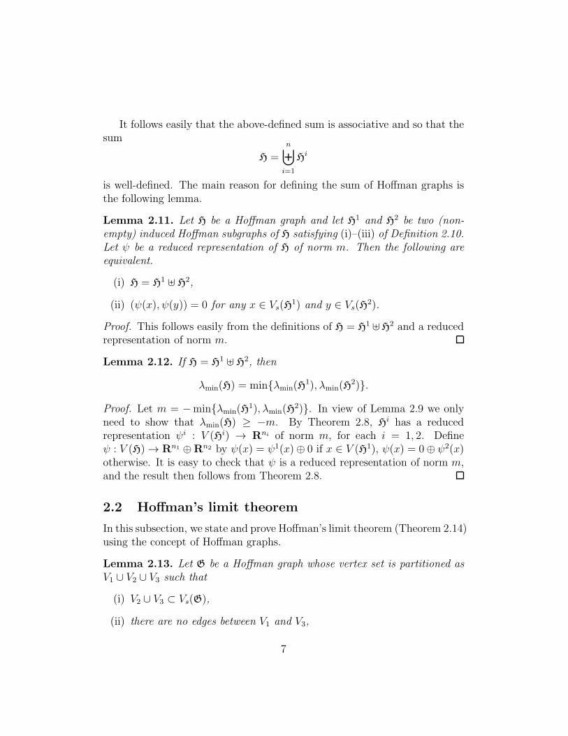
It follows easily that the above-defined sum is associative and so that thesum

H =

n⊎

i=1

Hi

is well-defined. The main reason for defining the sum of Hoffman graphs isthe following lemma.

Lemma 2.11. Let H be a Hoffman graph and let H1 and H2 be two (non-empty) induced Hoffman subgraphs of H satisfying (i)–(iii) of Definition 2.10.Let ψ be a reduced representation of H of norm m. Then the following areequivalent.

(i) H = H1 ⊎ H2,

(ii) (ψ(x), ψ(y)) = 0 for any x ∈ Vs(H1) and y ∈ Vs(H

2).

Proof. This follows easily from the definitions of H = H1 ⊎H2 and a reducedrepresentation of norm m.

Lemma 2.12. If H = H1 ⊎ H2, then

λmin(H) = min{λmin(H1), λmin(H

2)}.

Proof. Let m = −min{λmin(H1), λmin(H

2)}. In view of Lemma 2.9 we onlyneed to show that λmin(H) ≥ −m. By Theorem 2.8, Hi has a reducedrepresentation ψi : V (Hi) → Rni of norm m, for each i = 1, 2. Defineψ : V (H) → Rn1 ⊕Rn2 by ψ(x) = ψ1(x)⊕ 0 if x ∈ V (H1), ψ(x) = 0⊕ ψ2(x)otherwise. It is easy to check that ψ is a reduced representation of norm m,and the result then follows from Theorem 2.8.

2.2 Hoffman’s limit theorem

In this subsection, we state and prove Hoffman’s limit theorem (Theorem 2.14)using the concept of Hoffman graphs.

Lemma 2.13. Let G be a Hoffman graph whose vertex set is partitioned asV1 ∪ V2 ∪ V3 such that

(i) V2 ∪ V3 ⊂ Vs(G),

(ii) there are no edges between V1 and V3,

7

(iii) every pair of vertices x ∈ V2 and y ∈ V3 are adjacent,

(iv) V3 is a clique.

Let H be the Hoffman graph with the set of vertices V1∪V2 together with a fatvertex f /∈ V (G) adjacent to all the vertices of V2. If G has a representationof norm m, then H has a representation of norm

m+(m− 1)|V2||V3|+m− 1

.

Proof. Let φ : V (G) → Rd be a representation of norm m, and let

P =

P1

P2

P3

be the |V (G)| × d matrix whose rows are the images of V (G) = V1 ∪ V2 ∪ V3under φ. Set

u =1

√

|V3|(|V3|+m− 1)

∑

x∈V3

φ(x),

ǫ1 = 1−√

|V3||V3|+m− 1

,

ǫ2 =

√

m− 1

|V3|+m− 1.

Let j denote the row vector of length |V2| all of whose entries are 1. Then

uuT = 1,(1)

P1uT = 0,(2)

P2uT = (1− ǫ1)j

T ,(3)

ǫ22 = 2ǫ1 − ǫ21.(4)

Fix an orientation of the complete digraph on V2, and let B be the |V2|×(|V2|

2

)

matrix defined by

Bα,(β,γ) = δαβ − δαγ (α, β, γ ∈ V2, β 6= γ).

8

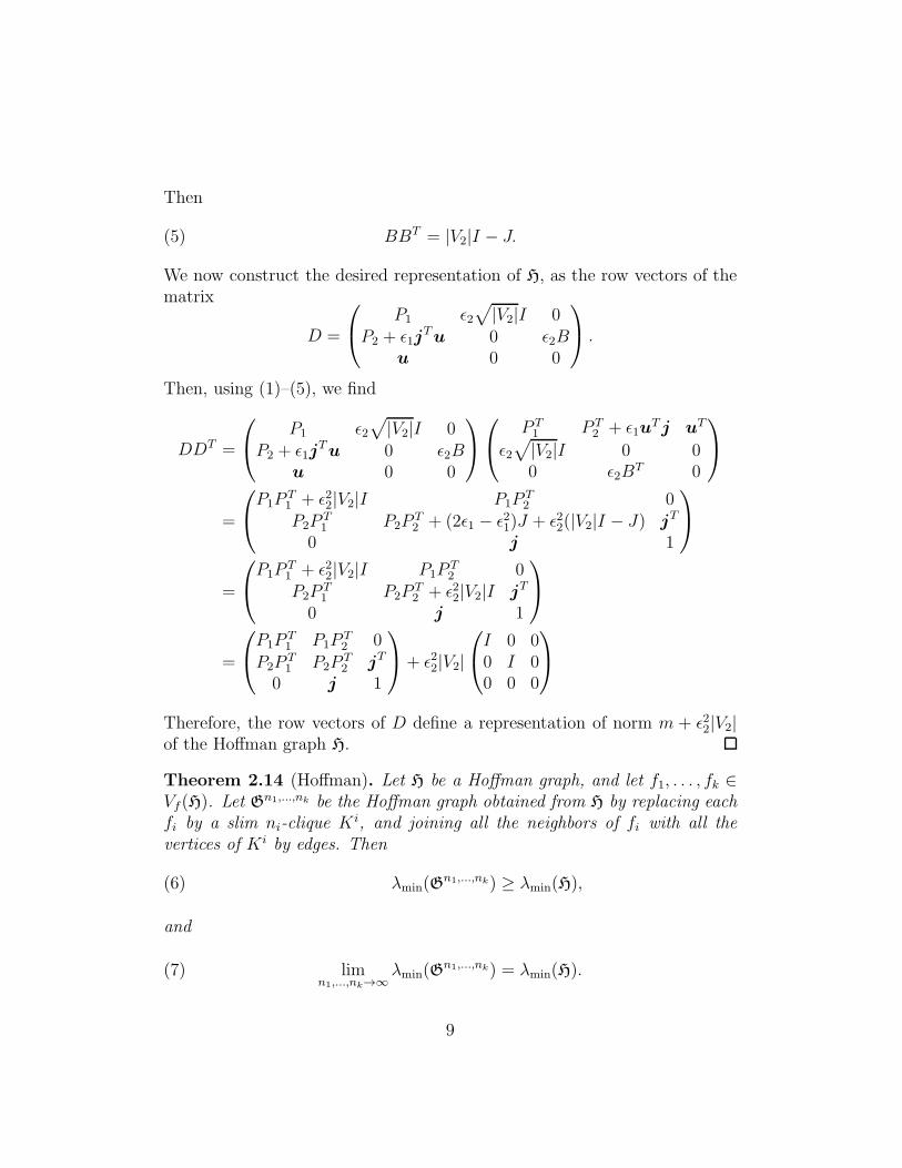
Then

(5) BBT = |V2|I − J.

We now construct the desired representation of H, as the row vectors of thematrix

D =

P1 ǫ2√

|V2|I 0P2 + ǫ1j

Tu 0 ǫ2Bu 0 0

.

Then, using (1)–(5), we find

DDT =

P1 ǫ2√

|V2|I 0P2 + ǫ1j

Tu 0 ǫ2Bu 0 0

P T1 P T

2 + ǫ1uTj uT

ǫ2√

|V2|I 0 00 ǫ2B

T 0

=

P1PT1 + ǫ22|V2|I P1P

T2 0

P2PT1 P2P

T2 + (2ǫ1 − ǫ21)J + ǫ22(|V2|I − J) jT

0 j 1

=

P1PT1 + ǫ22|V2|I P1P

T2 0

P2PT1 P2P

T2 + ǫ22|V2|I jT

0 j 1

=

P1PT1 P1P

T2 0

P2PT1 P2P

T2 jT

0 j 1

+ ǫ22|V2|

I 0 00 I 00 0 0

Therefore, the row vectors of D define a representation of norm m + ǫ22|V2|of the Hoffman graph H.

Theorem 2.14 (Hoffman). Let H be a Hoffman graph, and let f1, . . . , fk ∈Vf(H). Let G

n1,...,nk be the Hoffman graph obtained from H by replacing eachfi by a slim ni-clique K

i, and joining all the neighbors of fi with all thevertices of Ki by edges. Then

λmin(Gn1,...,nk) ≥ λmin(H),(6)

and

limn1,...,nk→∞

λmin(Gn1,...,nk) = λmin(H).(7)

9

Proof. We prove the assertions by induction on k. First suppose k = 1. Letµn = −λmin(G

n). Let Hn denote the Hoffman graph obtained from H byattaching a slim n-clique K to the fat vertex f1, joining all the neighbors off1 and all the vertices of K by edges. Then Hn contains both H and Gn assubgraphs, and Hn = H⊎H′, where H′ is the subgraph induced on K ∪ {f1}.Since λmin(H

′) = −1, Lemma 2.12 implies

λmin(H) = λmin(Hn) ≤ λmin(G

n) = −µn.

Thus (6) holds for k = 1. Since n is arbitrary and {−µn}∞n=1 is decreasing,we see that limn→∞ µn exists and

(8) λmin(H) ≤ − limn→∞

µn.

Since Gn has a representation of norm µn, it follows from Lemma 2.13that H has a representation of norm

µn +(µn − 1)|NH(f)|n+ µn − 1

.

By Theorem 2.8, we have

λmin(H) ≥ −µn −(µn − 1)|NH(f)|n+ µn − 1

,

which implies

(9) λmin(H) ≥ − limn→∞

µn.

Combining (9) with (8), we conclude that (7) holds for k = 1.Next, suppose k ≥ 2. Let Gn1,...,nk−1 be the Hoffman graph obtained from

H by replacing each fi (1 ≤ i ≤ k − 1) by a slim ni-clique Ki, and joining

all the neighbors of fi with all the vertices of Ki by edges. Then Gn1,...,nk isobtained from Gn1,...,nk−1 by replacing fk by a slim nk-clique K

k, and joiningall the neighbors of fk with all the vertices of Kk by edges. Then it followsfrom the assertions for k = 1 that

λmin(Gn1,...,nk) ≥ λmin(G

n1,...,nk−1),(10)

and

limnk→∞

λmin(Gn1,...,nk) = λmin(G

n1,...,nk−1).

10

This means that, for any ǫ > 0, there exists N1 such that

nk ≥ N1 =⇒ 0 ≤ λmin(Gn1,...,nk)− λmin(G

n1,...,nk−1) < ǫ.

By induction, we have

λmin(Gn1,...,nk−1) ≥ λmin(H),(11)

and

limn1,...,nk−1→∞

λmin(Gn1,...,nk−1) = λmin(H).(12)

Combining (10) with (11), we obtain (6), while (11) and (12) imply thatthere exists N0 such that

n1, . . . , nk−1 ≥ N0 =⇒ 0 ≤ λmin(Gn1,...,nk−1)− λmin(H) < ǫ.

Setting N = max{N0, N1}, we see that

n1, . . . , nk ≥ N =⇒ 0 ≤ λmin(Gn1,...,nk)− λmin(H) < 2ǫ.

This establishes (7).

Corollary 2.15. Let H be a Hoffman graph. Let Γn be the slim graph ob-tained from H by replacing every fat vertex f of H by a slim n-clique K(f),and joining all the neighbors of f with all the vertices of K(f) by edges. Then

λmin(Γn) ≥ λmin(H),

and

limn→∞

λmin(Γn) = λmin(H).

In particular, for any ǫ > 0, there exists a natural number n such that, everyslim graph ∆ containing Γn as an induced subgraph satisfies

λmin(∆) ≤ λmin(H) + ǫ.

Proof. Immediate from Theorem 2.14.

11

3 Special graphs of Hoffman graphs

Definition 3.1. Let µ be a real number with µ ≤ −1 and let H be a Hoffmangraph with smallest eigenvalue at least µ. Then H is called µ-saturated if nofat vertex can be attached to H in such a way that the resulting graph hassmallest eigenvalue at least µ.

Proposition 3.2. Let µ be a real number, and let H be a family of indecom-posable fat Hoffman graphs with smallest eigenvalue at least µ. The followingstatements are equivalent:

(i) every fat Hoffman graph with smallest eigenvalue at least µ is a sub-graph of a graph H =

⊎n

i=1Hi such that Hi is a member of H for all

i = 1, . . . , n.

(ii) every µ-saturated indecomposable fat Hoffman graph is isomorphic to asubgraph of a member of H .

Proof. First suppose (i) holds, and let H be a µ-saturated indecomposablefat Hoffman graph. Then H is a fat Hoffman graph with smallest eigenvalueat least µ, hence H is a subgraph of H′ =

⊎n

i=1Hi, where Hi is a member

of H for i = 1, . . . , n. Since H is µ-saturated, it coincides with the sub-graph 〈〈Vs(H)〉〉H′ of H′. Since H is indecomposable, this implies that H is asubgraph of Hi for some i.

Next suppose (ii) holds, and let H be a fat Hoffman graph with smallesteigenvalue at least µ. Without loss of generality we may assume that H isindecomposable and µ-saturated. Then H is isomorphic to a subgraph of amember of H , hence (i) holds.

Definition 3.3. For a Hoffman graph H, we define the following three graphsS−(H), S+(H) and S(H) as follows: For ǫ ∈ {−,+} define the special ǫ-graphSǫ = (Vs(H), E

ǫ) as follows: the set of edges Eǫ consists of pairs {s1, s2} ofdistinct slim vertices such that sgn(ψ(s1), ψ(s2)) = ǫ, where ψ is a reducedrepresentation of H of norm m. The graph S(H) := S+(H) ∪ S−(H) =(Vs(H), E

− ∪ E+) is the special graph of H.

Note that the definition of the special graph S(H) is independent of thechoice of the norm m of a reduced representation ψ.

It is easy to determine whether a Hoffman graph H is decomposable ornot.

12

Lemma 3.4. Let H be a Hoffman graph. Let Vs(H) = V1 ∪V2 be a partition,and set Hi = 〈〈Vi〉〉H for i = 1, 2. Then H = H1 ⊎ H2 if and only if there areno edges connecting V1 and V2 in S(H). In particular, H is indecomposableif and only if S(H) is connected.

Proof. This is immediate from Definition 2.10(iv) and Definition 3.3.

For an integer t ≥ 1, let H(t) be the fat Hoffman graph with one slimvertex and t fat vertices.

Figure 1:

H(1), λmin = −1 H(2), λmin = −2 H(3), λmin = −3

Lemma 3.5. Let t be a positive integer. If H is a fat Hoffman graph withλmin(H) ≥ −t containing H(t) as a Hoffman subgraph, then H = H(t) ⊎H′ forsome subgraph H′ of H. In particular, if H is indecomposable, then H = H(t).

Proof. Let x be the unique slim vertex of H(t). Let ψ be a reduced represen-tation of norm t of H. Then ψ(x) = 0, hence x is an isolated vertex in S(H).Thus H = H(t) ⊎ 〈〈Vs(H) \ {x}〉〉H by Lemma 3.4.

Lemma 3.6. Let H be a fat Hoffman graph with smallest eigenvalue at least−3. Let ψ be a reduced representation of norm 3 of H. Then for any distinctslim vertices x, y of H, (ψ(x), ψ(y)) ∈ {1, 0,−1}.

Proof. Since H is fat, we have (ψ(x), ψ(x)) ≤ 2 for all x ∈ Vs(H). Thus|(ψ(x), ψ(y))| ≤ 2 for all x, y ∈ Vs(H) by Schwarz’s inequality. Equalityholds only if ψ(x) = ±ψ(y) and (ψ(x), ψ(x)) = 2. The latter conditionimplies |Nf

H(x)| = 1, hence |NfH(x, y)| ≤ 1. Thus (ψ(x), ψ(y)) ≥ −1, while

(ψ(x), ψ(y)) = 2 cannot occur unless x = y, by Definition 2.6. Therefore,|(ψ(x), ψ(y))| < 2, and the result follows.

13

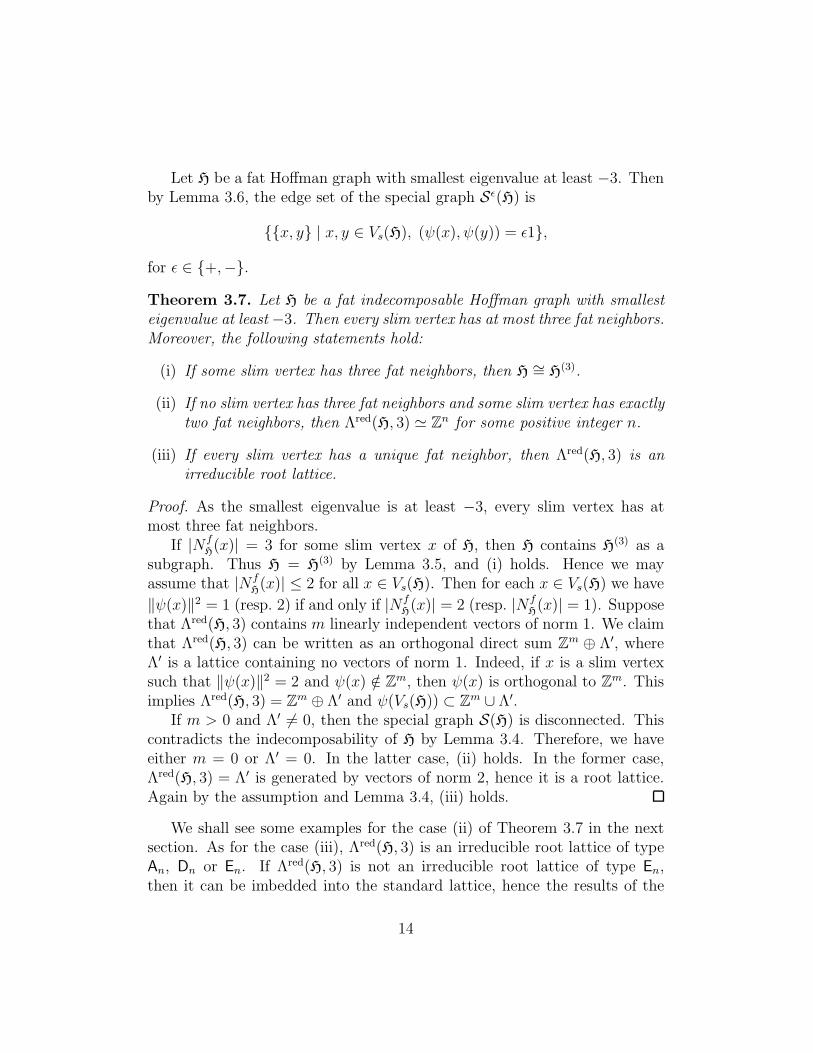
Let H be a fat Hoffman graph with smallest eigenvalue at least −3. Thenby Lemma 3.6, the edge set of the special graph Sǫ(H) is

{{x, y} | x, y ∈ Vs(H), (ψ(x), ψ(y)) = ǫ1},

for ǫ ∈ {+,−}.

Theorem 3.7. Let H be a fat indecomposable Hoffman graph with smallesteigenvalue at least −3. Then every slim vertex has at most three fat neighbors.Moreover, the following statements hold:

(i) If some slim vertex has three fat neighbors, then H ∼= H(3).

(ii) If no slim vertex has three fat neighbors and some slim vertex has exactlytwo fat neighbors, then Λred(H, 3) ≃ Z

n for some positive integer n.

(iii) If every slim vertex has a unique fat neighbor, then Λred(H, 3) is anirreducible root lattice.

Proof. As the smallest eigenvalue is at least −3, every slim vertex has atmost three fat neighbors.

If |NfH(x)| = 3 for some slim vertex x of H, then H contains H(3) as a

subgraph. Thus H = H(3) by Lemma 3.5, and (i) holds. Hence we mayassume that |Nf

H(x)| ≤ 2 for all x ∈ Vs(H). Then for each x ∈ Vs(H) we have

‖ψ(x)‖2 = 1 (resp. 2) if and only if |NfH(x)| = 2 (resp. |Nf

H(x)| = 1). Supposethat Λred(H, 3) contains m linearly independent vectors of norm 1. We claimthat Λred(H, 3) can be written as an orthogonal direct sum Z

m ⊕ Λ′, whereΛ′ is a lattice containing no vectors of norm 1. Indeed, if x is a slim vertexsuch that ‖ψ(x)‖2 = 2 and ψ(x) /∈ Z

m, then ψ(x) is orthogonal to Zm. This

implies Λred(H, 3) = Zm ⊕ Λ′ and ψ(Vs(H)) ⊂ Z

m ∪ Λ′.If m > 0 and Λ′ 6= 0, then the special graph S(H) is disconnected. This

contradicts the indecomposability of H by Lemma 3.4. Therefore, we haveeither m = 0 or Λ′ = 0. In the latter case, (ii) holds. In the former case,Λred(H, 3) = Λ′ is generated by vectors of norm 2, hence it is a root lattice.Again by the assumption and Lemma 3.4, (iii) holds.

We shall see some examples for the case (ii) of Theorem 3.7 in the nextsection. As for the case (iii), Λred(H, 3) is an irreducible root lattice of typeAn, Dn or En. If Λred(H, 3) is not an irreducible root lattice of type En,then it can be imbedded into the standard lattice, hence the results of the

14

next section applies. On the other hand, if Λred(H, 3) is an irreducible rootlattice of type En, then it is contained in the irreducible root lattice of typeE8, and hence there are only finitely many possibilities. For example, LetΓ be any ordinary graph with smallest eigenvalue at least −2 (see [1] for adescription of such graphs). Attaching a fat neighbor to each vertex of Γgives a fat Hoffman graph with smallest eigenvalue at least −3. However,this Hoffman graph may not be maximal among fat Hoffman graphs withsmallest eigenvalue at least −3. Therefore, we aim to classify fat Hoffmangraphs with smallest eigenvalue at least −3 which are maximal in E8. Thismay seem a computer enumeration problem, but it is harder than it looks.

Example 3.8. Let Π denote the root system of type E8. Fix α ∈ Π. Thenthere are elements βi ∈ Π (i = 1, . . . , 28) such that

{β ∈ Π | (α, β) = 1} =28⋃

i=1

{βi, α− βi}.

Let V denote the set of 57 roots consisting of the above set and α. Then Vis a reduced representation of a fat Hoffman graph H with 29 fat vertices.The fat vertices of H are fi (i = 0, 1, . . . , 28), f0 is adjacent to α, and fiis adjacent to βi, α − βi (i = 1, . . . , 28). It turns out that H is maximalamong fat Hoffman graphs with smallest eigenvalue at least −3. Indeed, nofat vertex can be attached, since the root lattice of type E8 is generated byV \ {γ} for any γ ∈ V , and attaching another fat neighbor to γ would meanthe existence of a vector of norm 1 in the dual lattice E∗

8 of E8. Since E∗8 = E8,

there are no vectors of norm 1 in E∗8. This is a contradiction. If a slim vertex

can be attached, then it can be represented by δ ∈ Π with (α, δ) = 0. Thenthere exists i ∈ {1, . . . , 28} such that (βi, δ) = ±1. Exchanging βi with α−βiif necessary, we may assume (βi, δ) = −1. This implies that βi and δ have acommon fat neighbor. Since (βi, α−βi) = −1, βi and α−βi have a commonfat neighbor. Since βi has a unique fat neighbor, δ and α−βi have a commonfat neighbor, contradicting (δ, α− βi) = 1.

On the other hand, it is known that there is a slim graph Γ with 36vertices represented by the root system of type E8 (see [1]). Attaching afat neighbor to each vertex of Γ gives a fat Hoffman graph H′ with smallesteigenvalue −3 such that Λred(H′, 3) is isometric to the root lattice of typeE8. The graph H′ is not contained in H, so there seems a large number ofmaximal fat Hoffman graphs represented in the root lattice of type E8.

15

4 Integrally represented Hoffman graphs

In this section, we consider a fat (−3)-saturated Hoffman graph H such thatΛred(H, 3) is a sublattice of the standard lattice Z

n. Since any of the ex-ceptional root lattices E6,E7 and E8 cannot be embedded into the standardlattice (see [2]), this means that, in view of Theorem 3.7, Λred(H, 3) is isomet-ric to Z

n or a root lattice of type An or Dn. Note that Λred(H, 3) cannot beisometric to the lattice A1, since this would imply that H has a unique slimvertex with a unique fat neighbor, contradicting (−3)-saturatedness. Thefollowing example gives a fat (−3)-saturated graph H with Λred(H, 3) ∼= Z.

Example 4.1. Let H be the Hoffman graph with vertex set Vs(H) ∪ Vf(H),where Vs(H) = Z/4Z, Vf(H) = {fi | i ∈ Z/4Z}, and with edge set

{{0, 2}, {1, 3}} ∪ {{i, fj} | i = j or j + 1}.

Then H is a fat indecomposable (−3)-saturated Hoffman graph such thatΛred(H, 3) is isomorphic to the standard lattice Z. Since S−(H) has edgeset {{i, i + 1} | i ∈ Z/4Z}, S−(H) is isomorphic to the Dynkin graph A3.Theorem 4.8 below implies that H is maximal, in the sense that no fat inde-composable (−3)-saturated Hoffman graph contains H.

For the remainder of this section, we let H be a fat indecomposable (−3)-saturated Hoffman graph such that Λred(H, 3) is isomorphic to a sublatticeof the standard lattice Z

n. Let φ be a representation of norm 3 of H. Thenwe may assume that φ is a mapping from V (H) to Z

n ⊕ ZVf (H), where its

composition with the projection Zn ⊕Z

Vf (H) → Zn gives a reduced represen-

tation ψ : Vs(H) → Zn. It follows from the definition of a representation of

norm 3 thatφ(s) = ψ(s) +

∑

f∈NfH(s)

ef ,

ψ(s) =n∑

j=1

ψ(s)jej ,

ψ(s)j ∈ {0,±1},and

(13) |{j | j ∈ {1, . . . , n}, ψ(s)j ∈ {±1}}| = 3− |NfH(s)| ≤ 2.

16

Lemma 4.2. If i ∈ {1, . . . , n} and ψ(s)i 6= 0 for some s ∈ Vs(H), then thereexist s1, s2 ∈ Vs(H) such that ψ(s1)i = −ψ(s2)i = 1.

Proof. By way of contradiction, we may assume without loss of generalitythat i = n, and ψ(s)n ∈ {0, 1} for all s ∈ Vs(H). Let G be the Hoffmangraph obtained from H by attaching a new fat vertex g and join it to allthe slim vertices s of H satisfying ψ(s)n = 1. Then the composition ofψ : Vs(H) = Vs(G) → Z

n and the projection Zn → Z

n−1 gives a reducedrepresentation of norm 3 of G. By Theorem 2.8, G has smallest eigenvalueat least −3. This contradicts the assumption that H is (−3)-saturated.

Proposition 4.3. The graph S−(H) is connected.

Proof. Before proving the proposition, we first show the following claim.

Claim 1. Let s1 and s2 be two slim vertices such that φ(s1)i = 1 and φ(s2)i =−1 for some i ∈ {1, . . . , n}. Then the distance between s1 and s2 is at most2 in S−(H).

By (13), we have (ψ(s1), ψ(s2)) ∈ {0,−1}. If (ψ(s1), ψ(s2)) = −1, thens1 and s2 are adjacent in S−(H) by the definition, hence the distance equalsone. If (ψ(s1), ψ(s2)) = 0, then there exists a unique j ∈ {1, . . . , n} such thatφ(s1)j = φ(s2)j = ±1. From Lemma 4.2, there exists a slim vertex s3 suchthat φ(s3)j = −φ(s1)j . If φ(s3)i 6= 0, then (ψ(sq), ψ(s3)) ∈ {±2} for someq ∈ {1, 2}, which is a contradiction. Hence φ(s3)i = 0. This implies that(ψ(si), ψ(s3)) = −1 for i = 1, 2, or equivalently, s3 is a common neighbor ofs1 and s2 in S−(H). This shows the claim.

Since H is indecomposable, S(H) is connected by Lemma 3.4. Thus, inorder to show the proposition, we only need to show that slim vertices s1and s2 with (ψ(s1), ψ(s2)) = 1 are connected by a path in S−(H). Thereexists i ∈ {1, . . . , n} such that φ(s1)i = φ(s2)i = ±1. From Lemma 4.2, thereexists a slim vertex s3 such that φ(s3)i = −φ(s1)i, and hence the distancesbetween s1 and s3 and between s3 and s2 are at most 2 in S−(H) by Claim 1.Therefore, s1 and s2 are connected by a path of length at most 4 in S−(H).

Lemma 4.4. Let H be a fat indecomposable (−3)-saturated Hoffman graph.Then the reduced representation of norm 3 of H is injective unless H is iso-morphic to a subgraph of the graph given in Example 4.1.

Proof. Suppose that the reduced representation ψ of norm 3 of H is notinjective. Then there are two distinct slim vertices x and y satisfing ψ(x) =ψ(y). Then (ψ(x), ψ(y)) = 0 or 1.

17

If (ψ(x), ψ(y)) = 0, then ψ(x) = ψ(y) = 0, hence both x and y areisolated vertices, contradicting the assumption that H is indecomposable.

Suppose (ψ(x), ψ(y)) = 1. Since S−(H) is connected by Proposition 4.3,there exists a slim vertex z such that (ψ(x), ψ(z)) = −1. Then we mayassume

φ(x) = e1 + ef1 + ef2 ,

φ(y) = e1 + ef3 + ef4 ,

φ(z) = −e1 + ef1 + ef3 .

If H has another slim vertex w, then

φ(w) = −e1 + ef2 + ef4 ,

and no other possibility occurs. Therefore, H is isomorphic to either thegraph given in Example 4.1, or its subgraph obtained by deleting one slimvertex.

Lemma 4.5. Suppose that s ∈ Vs(H) has exactly two fat neighbors in H.Then the following statements hold.

(i) for each f ∈ NfH(s), |NS−(H)(s) ∩N s

H(f)| ≤ 2,

(ii) |NS−(H)(s)| ≤ 4, and if equality holds, then S−(H) is isomorphic to the

graph D4,

(iii) if |NS−(H)(s)| = 3, then two of the vertices in NS−(H)(s) have s as theirunique neighbor in S−(H).

Proof. Let ψ be the reduced representation of norm 3 of H. Since s hasexactly two fat neighbors, (ψ(s), ψ(s)) = 1. This means that we may assumewithout loss of generality ψ(s) = e1.

Let f ∈ NfH(s). If t1 and t2 are distinct vertices of NS−(H)(s) ∩ N s

H(f),then

1 ≥ (φ(t1), φ(t2))

≥ (ψ(t1) + ef , ψ(t2) + ef )

= (ψ(t1), ψ(t2)) + 1,

18

Thus we have (ψ(t1), ψ(t2)) ≤ 0. Since t1, t2 ∈ NS−(H)(s), we have (ψ(s), ψ(t1))= (ψ(s), ψ(t2)) = −1, and hence we may assume without loss of generalitythat

ψ(t1) = −e1 + e2,(14)

ψ(t2) = −e1 − e2.(15)

Now it is clear that there cannot be another t3 ∈ NS−(H)(s). Thus |NS−(H)(s)∩N s

H(f)| ≤ 2. This proves (i).

As for (ii), let NfH(s) = {f, f ′}. Then

|NS−(H)(s)| ≤ |NS−(H)(s) ∩N sH(f)|+ |NS−(H)(s) ∩N s

H(f′)| ≤ 4

by (i). To prove (iii) and the second part of (ii), we may assume that {t1, t2} =NS−(H)(s)∩NH(f). We claim that neither t1 nor t2 has a neighbor in S−(H)other than s. Suppose by contradiction, that t3 6= s is a neighbor in S−(H)of t1. By (14) (resp. (15)), f is the unique fat neighbor of t1 (resp. t2). Inparticular, f is also a neighbor of t3. Observe

1 ≥ (φ(s), φ(t3)) ≥ (ψ(s), ψ(t3)) + 1,

1 ≥ (φ(ti), φ(t3)) = (ψ(ti), ψ(t3)) + 1 (i = 1, 2).

Thus

(e1, ψ(t3)) ≤ 0,

(−e1 ± e2, ψ(t3)) ≤ 0.

These imply (e1, ψ(t3)) = (e2, ψ(t3)) = 0. But then −1 = (ψ(t1), ψ(t3)) =(−e1+e2, ψ(t3)) = 0. This is a contradiction, and we have proved our claim.Now (iii) is an immediate consequence of this claim.

Continuing the proof of the second part of (ii), if |NS−(H)(s)| = 4, thenwe may assume

ψ(t′1) = −e1 + e3,

ψ(t′2) = −e1 − e3,

where {t′1, t′2} = NS−(H)(s) ∩ N sH(f

′). It follows that t1, t2, t′1, t

′2 are pairwise

non-adjacent in S−(H). By our claim, none of t1, t2, t′1, t

′2 is adjacent to any

vertex other than s in S−(H). Since S−(H) is connected by Proposition 4.3,S−(H) is isomorphic to the graph D4.

19

Lemma 4.6. Suppose that slim vertices s, t+, t− share a common fat neighborand that they are represented as

ψ(s) = e1 + e2,

ψ(t±) = −e1 ± e3.

If there exists a slim vertex t with

ψ(t) = −e2 + ej for some j /∈ {1, 2, 3},

then the vertices t± have s as their unique neighbor in S−(H).

Proof. Note that each of the vertices s, t±, t has a unique fat neighbor. Since(ψ(s), ψ(t±)) = (ψ(s), ψ(t)) = −1, these vertices share a common fat neigh-bor f . Suppose that there exists a slim vertex t′ adjacent to t− in S−(H).This means (ψ(t′), ψ(t−)) = −1. Since f is the unique fat neighbor of t−, t′

is adjacent to f , and hence (ψ(t′), ψ(u)) ≤ 0 for u ∈ {t, t+, s}. This is im-possible. Similarly, there exists no slim vertex adjacent to t+ in S−(H).

Lemma 4.7. Suppose that s ∈ Vs(H) has exactly one fat neighbor in H.Then the following statements hold:

(i) |NS−(H)(s)| ≤ 4, and if equality holds, then S−(H) is isomorphic to the

graph D4,

(ii) if |NS−(H)(s)| = 3, then two of the vertices in NS−(H)(s) have s as theirunique neighbor in S−(H).

Proof. Let ψ be the reduced representation of norm 3 of H. Since s hasexactly one fat neighbor, (ψ(s), ψ(s)) = 2. This means that we may assumewithout loss of generality ψ(s) = e1 + e2. Let f be the unique fat neighborof s. If t ∈ NS−(H)(s), then t is adjacent to f , hence

(16) ψ(t) ∈ {−e1,−e2} ∪ {−ei ± ej | 1 ≤ i ≤ 2 < j ≤ n}.

If t, t′ ∈ NS−(H)(s) are distinct, then

1 ≥ (φ(t), φ(t′))

≥ (ψ(t) + ef , ψ(t′) + ef )

= (ψ(t), ψ(t′)) + 1,

20

Thus we have (ψ(t), ψ(t′)) ≤ 0. If |NS−(H)(s)| ≥ 3, then by (16), we mayassume without loss of generality that there exists t ∈ NS−(H)(s) with ψ(t) =−e1 + e3. Then ψ(NS−(H)(s) \ {t}) is contained in

{−e2 − e3}, {−e2,−e1 − e3}, or {−e1 − e3} ∪ {−e2 ± ej}

for some j with 3 ≤ j ≤ n. Thus |NS−(H)(s)| ≤ 4, and equality holds only if

ψ(NS−(H)(s)) = {−e1 ± e3,−e2 ± ej}

for some j with 3 ≤ j ≤ n. In this case, Lemma 4.6 implies that each ofthe vertices in NS−(H)(s) has s as a unique neighbor. This means that S−(H)

contains a subgraph isomorphic to the graph D4 as a connected component.Since S−(H) is connected by Proposition 4.3, we have the desired result.

To prove (ii), suppose |NS−(H)(s)| = 3. Then we may assume without lossof generality that NS−(H)(s) = {t, t+, t−}, where ψ(t±) = −e2 ± e4. Then byLemma 4.6, the vertices t± have s as their unique neighbor in S−(H).

Theorem 4.8. Let H be a fat indecomposable (−3)-saturated Hoffman graphsuch that Λred(H, 3) is isomorphic to a sublattice of the standard lattice Z

n.Then S−(H) is a connected graph which is isomorphic to Am,Dm, Am or Dm

for some positive integer m.

Proof. From Proposition 4.3, S−(H) is connected. First we suppose that themaximum degree of S−(H) is at most 2. Then S−(H) ∼= Am or S−(H) ∼= Am

for some positive integer m.Next we suppose that the degree of some vertex s in S−(H) is at least 3.

From Lemma 4.5(ii) and Lemma 4.7(i), degS−(H)(s) ≤ 4, and S−(H) ∼= D4 ifdegS−(H)(s) = 4. Thus, for the remainder of this proof, we suppose that themaximum degree of S−(H) is 3 and degS−(H)(s) = 3.

It follows from Lemma 3.5 that if H has a subgraph isomorphic to H(3),then H ∼= H(3), in which case S−(H) consists of a single vertex, and theassertion holds. Hence it remains to consider two cases: s is adjacent toexactly two fat vertices, and s is adjacent to exactly one fat vertex. In eithercases, by Lemma 4.5(iii) or Lemma 4.7(ii), s has at most one neighbor twith degree greater than 1. Thus, the only way to extend this graph is byadding a slim neighbor adjacent to t. We can continue this process, but oncewe encounter a vertex of degree 3, then the process stops by Lemma 4.5(iii)or Lemma 4.7(ii). Thus, S−(H) is isomorphic to one of the graphs Dm orDm.

21

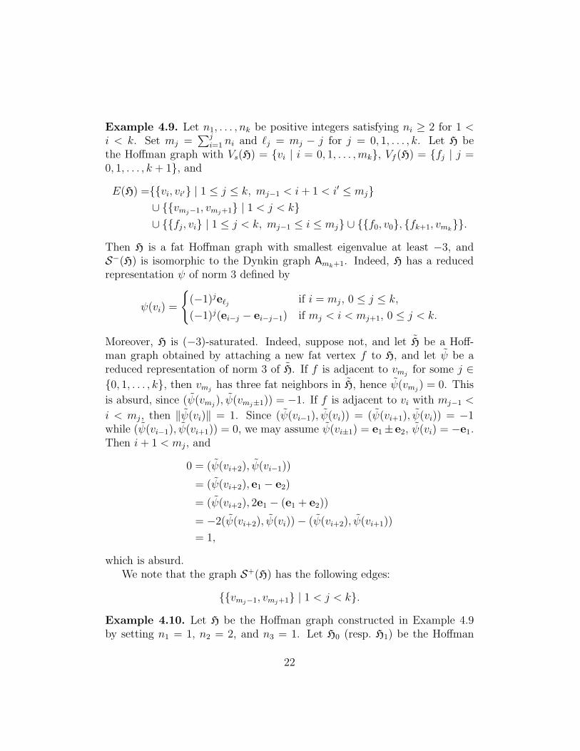
Example 4.9. Let n1, . . . , nk be positive integers satisfying ni ≥ 2 for 1 <i < k. Set mj =

∑j

i=1 ni and ℓj = mj − j for j = 0, 1, . . . , k. Let H bethe Hoffman graph with Vs(H) = {vi | i = 0, 1, . . . , mk}, Vf (H) = {fj | j =0, 1, . . . , k + 1}, and

E(H) ={{vi, vi′} | 1 ≤ j ≤ k, mj−1 < i+ 1 < i′ ≤ mj}∪ {{vmj−1, vmj+1} | 1 < j < k}∪ {{fj, vi} | 1 ≤ j < k, mj−1 ≤ i ≤ mj} ∪ {{f0, v0}, {fk+1, vmk

}}.

Then H is a fat Hoffman graph with smallest eigenvalue at least −3, andS−(H) is isomorphic to the Dynkin graph Amk+1. Indeed, H has a reducedrepresentation ψ of norm 3 defined by

ψ(vi) =

{

(−1)jeℓj if i = mj , 0 ≤ j ≤ k,

(−1)j(ei−j − ei−j−1) if mj < i < mj+1, 0 ≤ j < k.

Moreover, H is (−3)-saturated. Indeed, suppose not, and let H be a Hoff-man graph obtained by attaching a new fat vertex f to H, and let ψ be areduced representation of norm 3 of H. If f is adjacent to vmj

for some j ∈{0, 1, . . . , k}, then vmj

has three fat neighbors in H, hence ψ(vmj) = 0. This

is absurd, since (ψ(vmj), ψ(vmj±1)) = −1. If f is adjacent to vi with mj−1 <

i < mj , then ‖ψ(vi)‖ = 1. Since (ψ(vi−1), ψ(vi)) = (ψ(vi+1), ψ(vi)) = −1while (ψ(vi−1), ψ(vi+1)) = 0, we may assume ψ(vi±1) = e1±e2, ψ(vi) = −e1.Then i+ 1 < mj , and

0 = (ψ(vi+2), ψ(vi−1))

= (ψ(vi+2), e1 − e2)

= (ψ(vi+2), 2e1 − (e1 + e2))

= −2(ψ(vi+2), ψ(vi))− (ψ(vi+2), ψ(vi+1))

= 1,

which is absurd.We note that the graph S+(H) has the following edges:

{{vmj−1, vmj+1} | 1 < j < k}.

Example 4.10. Let H be the Hoffman graph constructed in Example 4.9by setting n1 = 1, n2 = 2, and n3 = 1. Let H0 (resp. H1) be the Hoffman

22

graph obtained from H by identifying the fat vertices f4 and f0 (resp. f4and f1), and adding edges {v0, v2}, {v2, v4}. Then H0 and H1 are fat (−3)-saturated Hoffman graphs and S−(Hi) is isomorphic to the Dynkin graph A5

for i = 0, 1. We note that S+(Hi) has two edges {v0, v2}, {v2, v4}.

Examples 4.9 and 4.10 indicate that H is not determined by S±(H). Weplan to discuss the classification of fat indecomposable (−3)-saturated Hoff-man graphs with prescribed special graph in the subsequent papers.

References

[1] D. Cvetkovic, P. Rowlinson, S. K. Simic, Spectral Generalizations of LineGraphs — On Graphs with Least Eigenvalue −2, Cambridge Univ. Press,2004.

[2] W. Ebeling, Lattices and Codes, Vieweg, 2nd ed. Friedr. Vieweg & Sohn,Braunschweig, 2002.

[3] A. J. Hoffman, On graphs whose least eigenvalue exceeds −1−√2, Linear

Algebra Appl. 16 (1977), 153–165.

[4] T. Taniguchi, On graphs with the smallest eigenvalue at least −1 −√2,

part I, Ars Math. Contemp. 1 (2008), no.1, 81–98.

[5] R. Woo and A. Neumaier, On graphs whose smallest eigenvalue is at least−1−

√2, Linear Algebra Appl. 226-228 (1995), 577–591 .

[6] H. Yu, On the limit points of the smallest eigenvalues of regular graphs,Designs, Codes Cryptogr., published online, DOI: 10.1007/s10623-011-9575-0.

23