A fast algorithm for computing the smallest eigenvalue of a symmetric positive-definite Toeplitz...

A Fast Algorithm for Computing the

Smallest Eigenvalue of a Symmetric

Positive Definite Toeplitz Matrix

Nicola Mastronardi Marc Van BarelRaf Vandebril

Report TW493, May 2007

n Katholieke Universiteit LeuvenDepartment of Computer Science

Celestijnenlaan 200A – B-3001 Heverlee (Belgium)

A Fast Algorithm for Computing the

Smallest Eigenvalue of a Symmetric

Positive Definite Toeplitz Matrix

Nicola Mastronardi Marc Van BarelRaf Vandebril

Report TW493, May 2007

Department of Computer Science, K.U.Leuven

AbstractRecent progress in signal processing and estimation has gener-

ated considerable interest in the problem of computing the smallesteigenvalue of a symmetric positive definite Toeplitz matrix. Severalalgorithms have been proposed in the literature. Many of them com-pute the smallest eigenvalue in an iterative fashion, relying on theLevinson–Durbin solution of sequences of Yule–Walker systems.

Exploiting the properties of two algorithms recently developedfor estimating a lower and an upper bound of the smallest singu-lar value of upper triangular matrices, respectively, an algorithm forcomputing bounds to the smallest eigenvalue of a symmetric pos-itive definite Toeplitz matrix has been recently derived [20]. Thealgorithm relies on the computation of the R factor of the QR–factorization of the Toeplitz matrix and the inverse of R. The simul-taneous computation of R and R−1 is efficiently accomplished by thegeneralized Schur algorithm. Unfortunately, due to the weak stabil-ity of the generalized Schur algorithm, only a rough approximationof the smallest eigenvalue can be computed. In this paper, exploit-ing the properties of the latter algorithm, a numerical method tocompute the smallest eigenvalue and the corresponding eigenvectorof symmetric positive definite Toeplitz matrices in an accurate wayis proposed.

Keywords : Toeplitz matrix, symmetric positive definite matrix, generalizedSchur algorithm, eigenvalues, incremental norm estimation, signal processing.AMS(MOS) Classification : Primary : 65F05, Secondary : 65F15, 65F35.

A FAST ALGORITHM FOR COMPUTING THE SMALLESTEIGENVALUE OF A SYMMETRIC POSITIVE DEFINITE TOEPLITZ

MATRIX∗

N. MASTRONARDI†‡ , M. VAN BAREL‡ , AND R. VANDEBRIL‡

Abstract. Recent progress in signal processing and estimation has generated considerableinterest in the problem of computing the smallest eigenvalue of a symmetric positive definite Toeplitzmatrix. Several algorithms have been proposed in the literature. Many of them compute the smallesteigenvalue in an iterative fashion, relying on the Levinson–Durbin solution of sequences of Yule–Walker systems.

Exploiting the properties of two algorithms recently developed for estimating a lower and anupper bound of the smallest singular value of upper triangular matrices, respectively, an algorithmfor computing bounds to the smallest eigenvalue of a symmetric positive definite Toeplitz matrixhas been recently derived [20]. The algorithm relies on the computation of the R factor of the QR–factorization of the Toeplitz matrix and the inverse of R. The simultaneous computation of R andR−1 is efficiently accomplished by the generalized Schur algorithm. Unfortunately, due to the weakstability of the generalized Schur algorithm, only a rough approximation of the smallest eigenvaluecan be computed. In this paper, exploiting the properties of the latter algorithm, a numerical methodto compute the smallest eigenvalue and the corresponding eigenvector of symmetric positive definiteToeplitz matrices in an accurate way is proposed.

AMS subject classifications. 65F05, 65F15, 65F35.

Key words. Toeplitz matrix, symmetric positive definite matrix, generalized Schur al-gorithm, eigenvalues, incremental norm estimation, signal processing.

1. Introduction. The problem of computing the smallest eigenvalue of a sym-metric positive definite (SPD) Toeplitz matrix and the corresponding eigenvector isof considerable interest in signal processing and estimation applications.

Given the covariance sequence of observed data, Pisarenko [26] suggested a methodto determine the sinusoidal frequencies from the eigenvector associated to the smallesteigenvalue of the covariance matrix, a symmetric positive definite Toeplitz matrix T.

Some results on the localization of the smallest eigenvalue of T are presented in[23, 24].

Many algorithms have been proposed in the literature to compute the smallesteigenvalue of T [4, 5, 10, 11, 13, 14, 15, 16, 17, 18, 21, 22, 23, 24, 25, 28, 29, 30, 31].

Given A ∈ Rm×n, m � n, b ∈ Rm, and given a lower bound σ of the smallestsingular value of A, a way to compute a lower bound of the smallest singular valueσ of the augmented matrix [A|b] is proposed in [6]. The latter lower bound is, quite

∗The research of the first author was partially supported by MIUR, grant number 2004015437.The research of the last two authors was partially supported by the Research Council K.U.Leuven,project OT/05/40 (Large rank structured matrix computations), CoE EF/05/006 Optimization inEngineering (OPTEC), by the Fund for Scientific Research–Flanders (Belgium), G.0455.0 (RHPH:Riemann-Hilbert problems, random matrices and Pade-Hermite approximation), G.0423.05 (RAM:Rational modelling: optimal conditioning and stable algorithms), and by the Interuniversity At-traction Poles Programme, initiated by the Belgian State, Science Policy Office, Belgian NetworkDYSCO (Dynamical Systems, Control, and Optimization). The third author has a grant as “Post-doctoraal Onderzoeker” from the Fund for Scientific Research–Flanders (Belgium). The scientificresponsibility rests with the authors.

†Istituto per le Applicazioni del Calcolo “M. Picone”, sede di Bari, Consiglio Nazionale delleRicerche, Via G. Amendola, 122/I, I-70126 Bari, Italy. email:[email protected]

‡Department of Computer Science, Katholieke Universiteit Leuven, Celestijnenlaan200A, B-3001 Leuven (Heverlee), Belgium. email: {Raf.Vandebril, Marc.VanBarel,Nicola.Mastronardi}@cs.kuleuven.be

1

2 N. MASTRONARDI, M. VAN BAREL AND R. VANDEBRIL

often, a good approximation of the smallest singular value of the augmented matrix.Recursively repeating the procedure, an algorithm for computing a lower bound of thesmallest singular value of a SPD Toeplitz matrix is proposed in [20]. The algorithmrelies on the simultaneous computation of the matrix R of the QR–factorization ofthe Toeplitz matrix and its inverse R−1 by means of the generalized Schur algorithm(GSA).

The generalized Schur algorithm is a fast algorithm for computing such kindof factorizations for matrices having small displacement rank [12]. It relies on theknowledge of the so called generators of the matrix rather than the matrix itself.

In this paper, taking the algorithm described in [20] into account and exploitingthe properties of the generators of the matrix, we propose a fast algorithm for com-puting the smallest eigenvalue and corresponding eigenvector of symmetric positivedefinite Toeplitz matrices in an accurate way.

The paper is organized as follows. In § 2 the algorithm described in [6] forcomputing the lower bound of the smallest singular value of the augmented matrix[A|b] is shortly introduced. The particular version of GSA is described in § 3. Anextensive version of the latter three paragraphs can be found in [20]. We include themhere to make the paper self–contained. The proposed algorithm is described in § 4followed by the numerical examples, reported in § 5, and by the conclusions.

2. Computing a lower bound for the smallest singular value. A lowerbound for the smallest singular value σ(A) of the augmented matrix A ≡ [A|b], A ∈Rm×n, m � n, b ∈ Rm is derived in [6], known a lower bound of the smallest singularvalue σ(A) of A. It relies on the following theorem.

Theorem 2.1. [6]. Let δ > 0, δ ∈ R. Let A ∈ Rm×n, m � n, be a full–rankmatrix and let b ∈ Rm. Let σ(A) and σ(A) be the smallest positive singular values ofA and A ≡ [A|b], respectively and σ(A) > δ > 0. Let

x = arg minx‖Ax− b‖2 and ρ = b−Ax.

Then

σ(A) > δ if ‖ρ‖2 = 0,

σ(A) > min{δ, ‖ρ‖2} if ‖ρ‖2 > 0 and ‖x‖2 = 0,σ(A) > δ

√E(δ, x, ρ) if ‖ρ‖2 > 0 and ‖x‖2 > 0,

with

E(δ, x, ρ) = 1 +12

(B(δ, x, ρ)−

√B2(δ, x, ρ) + 4‖x‖22

)and

B(δ, x, ρ) = ‖x‖22 +‖ρ‖22δ2

− 1.

Based on this theorem, an algorithm∗ for estimating a lower bound of the smallestsingular value of a full–rank matrix can be easily derived.

∗The algorithms in this paper are written in a matlab–like style. Matlab is a registered trademarkof The MathWorks, Inc.

COMPUTING THE SMALLEST EIGENVALUE OF SPD TOEPLITZ MATRICES 3

%Algorithm 1. Lower bound of the smallest singular value of a full–rank matrix A.%Input: R, the R factor of the QR–factorization of A.%Output: δ, a lower bound of the smallest singular value of A.function[δ] =fassino(R);

δ = |R(1, 1)|;for k = 1 : n− 1,

X(1 : k, k + 1) = R−1(1 : k, 1 : k)R(1 : k, k + 1);ρ = |R(k + 1, k + 1)|;δ = δ

√E(δ,X(1 : k, k + 1), ρ);

end

The algorithm requires to compute the n × n upper matrix of the R factor ofthe QR–factorization of A. This is accomplished with standard techniques, e.g., see[9], in 2n2(m− n/3) floating point operations. Moreover, at step k, the linear systemR(1 : k, 1 : k)X(1 : k, k +1) = R(1 : k, k +1) needs to be solved, which requires O(k2)operations. Therefore the complexity of Algorithm 1 is O(mn2 + n3). The followinglemma emphasizes the relationship between R and the strictly upper triangular matrixX.

Lemma 2.1. [20]. Let R be a nonsingular upper triangular matrix and X be thestrictly upper triangular matrix computed by Algorithm 1 with input the matrix R.Then

X(1 : k, k + 1) = −R(k + 1, k + 1)R−1(1 : k, k + 1), k = 1, 2, . . . , n− 1. (2.1)

The strictly upper triangular part of the matrix X, i.e., the sequence of vectorscomputed in Algorithm 1, are the columns of the strictly upper triangular part of theinverse of R, scaled by the entries in the main diagonal, respectively.

Hence, the computational complexity of Algorithm 1 can be reduced if the inverseof R can be computed in a fast way and given as input to an adapted version ofAlgorithm 1.

%Algorithm 2. Lower bound of the smallest singular value of a full–rank matrix A.%Input: R,R−1, with R the R factor of the QR–factorization of A.%Output: δ, a lower bound of the smallest singular value of A.function[δ] =fassino adapted(R,R−1);

δ = |R(1, 1)|;for k = 1 : n− 1,

X(1 : k, k + 1) = −R(k + 1, k + 1)R−1(1 : k, k + 1);ρ = |R(k + 1, k + 1)|;δ = δ

√E(δ,X(1 : k, k + 1), ρ);

end

We observe that only the diagonal entries of the matrix R are involved in Algo-rithm 2. These entries can be also computed as the reciprocal of the diagonal entriesof R−1.

In Section 3 we show that the R factor of the QR–factorization of a nonsingularToeplitz matrix T and the inverse of R can be computed with O(n2) computationalcomplexity by means of the generalized Schur algorithm.


3. Generalized Schur Algorithm. Let

T =

t1 t2

. . . tn

t2 t1. . . . . .

. . . . . . . . . t2

tn. . . t2 t1

. (3.1)

Define

M =[

TT T In

In 0n

]. (3.2)

The R factor of the QR–factorization of T and its inverse R−1 can be retrieved fromthe LDLT factorization, with L lower triangular and D diagonal matrices, respec-tively, of the following block–structured matrix,

M =[

TT T In

In 0n

]= LDLT ,

with In and 0n the identity matrix and the null matrix of order n, respectively. Infact, it can be easily shown that

M = LDLT =[

RT

R−1 R−1

] [In

−In

] [R R−T

R−T

]. (3.3)

Therefore, to compute R and R−1 it is sufficient to compute the first n columns ofL. This can be accomplished with O(n2) floating point operations by means of thegeneralized Schur algorithm (GSA).

In this section we describe how GSA can be used to compute R and its inverseR−1. A comprehensive treatment of the topic can be found in, e.g., [12].

Let Z ∈ Rn×n be the shift matrix

Z =

0 0 · · · · · · 0

1. . . . . . . . . 0

0. . . . . . . . .

......

. . . 1. . .

...0 · · · 0 1 0

and

Φ = Z ⊕ Z. (3.4)

It turns out that

M − ΦMΦT = GDGT ,

with D = diag(1, 1,−1,−1) and G ∈ R2n×4 called a generator matrix.


Denote v = TT (T (:, 1)). The columns of G can be chosen as

G(:, 1) = 1√v(1)

[v

e(n)1

], G(:, 2) =

0t2...tn0...0

,

G(:, 3) =[

0G(2 : 2n− 1, 1)

], G(:, 4) =

0tn...t20...0

.

(3.5)

Let w ∈ R2. In the sequel, we denote by giv the function that computes the parame-ters [cG, sG] of the Givens rotation G:

[cG, sG] = giv(w1, w2) such that[

cG sG

−sG cG

] [w1

w2

]=[ √

w21 + w2

2

0

].

Moreover, suppose w1 > w2. We denote by hyp the function that computes the pa-rameters [cH , sH ] of the hyperbolic† rotation H,

[cH , sH ] = hyp(w1, w2) such that[

cH −sH

−sH cH

] [w1

w2

]=[ √

w21 − w2

2

0

].

Let function[G] = gener(T ) be the matlab–like function with input the SPD ToeplitzT and output the corresponding generator matrix G. Since the number of columnsof the generator matrix G is 4 � n, the GSA for computing R and R−1 has O(n2)computational complexity. It can be summarized in the following algorithm.

% Algorithm 3. Generalized Schur algorithm.% Input: G, the generator matrix of the Toeplitz matrix T.% Output: R and R−1, with R the R factor of a QR–factorization of T.function[R,R−1, z1, z2] =schur(G);

(A.1) for k = 1 : n,(A.2) [cG, sG] = giv(G(k, 1), G(k, 2));

(A.3) G(k : n + k, 1 : 2) = G(k : n + k, 1 : 2)[

cG sG

−sG cG

];

(A.4) [cG, sG] = giv(G(k, 3), G(k, 4));

(A.5) G(k : n + k − 1, 3 : 4) = G(k : n + k − 1, 3 : 4)[

cG sG

−sG cG

];

(A.6) if i == n,

†Hyperbolic rotations can be computed in different ways. For “stable” implementations see [1, 3].


(A.7) z1 = G(n + 1 : 2n, 1);(A.8) z1 = G(n + 1 : 2n, 1);(A.9) end(A.10) [cH , sH ] = hyp(G(k, 1), G(k, 3));

(A.11) G(k : n + k, [1, 3]) = G(k : n + k, [1, 3])[

cH −sH

−sH cH

];

(A.12) R(k, k : n) = G(k : n, 1)T ;

(A.13) R−1(1 : k, k) = G(n + 1 : n + k, 1);

(A.14) G(:, 1) = ΦG(:, 1);(A.15) end

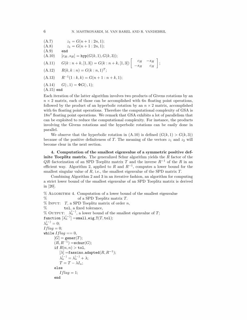
Each iteration of the latter algorithm involves two products of Givens rotations by ann × 2 matrix, each of those can be accomplished with 6n floating point operations,followed by the product of an hyperbolic rotation by an n × 2 matrix, accomplishedwith 6n floating point operations. Therefore the computational complexity of GSA is18n2 floating point operations. We remark that GSA exhibits a lot of parallelism thatcan be exploited to reduce the computational complexity. For instance, the productsinvolving the Givens rotations and the hyperbolic rotations can be easily done inparallel.

We observe that the hyperbolic rotation in (A.10) is defined (G(k, 1) > G(k, 3))because of the positive definiteness of T. The meaning of the vectors z1 and z2 willbecome clear in the next section.

4. Computation of the smallest eigenvalue of a symmetric positive def-inite Toeplitz matrix. The generalized Schur algorithm yields the R factor of theQR–factorization of an SPD Toeplitz matrix T and the inverse R−1 of the R in anefficient way. Algorithm 2, applied to R and R−1, computes a lower bound for thesmallest singular value of R, i.e., the smallest eigenvalue of the SPD matrix T.

Combining Algorithm 2 and 3 in an iterative fashion, an algorithm for computinga strict lower bound of the smallest eigenvalue of an SPD Toeplitz matrix is derivedin [20].

% Algorithm 4. Computation of a lower bound of the smallest eigenvalue% of a SPD Toeplitz matrix T.% Input: T, a SPD Toeplitz matrix of order n,% tol, a fixed tolerance,% Output: λ

(−)n , a lower bound of the smallest eigenvalue of T ;

function [λ(−)n ] =small eig T(T, tol);

λ(−)n = 0;

Iflag = 0;while Iflag == 0,

[G] = gener(T );(R,R−1) =schur(G);if R(n, n) > tol,

[λ] =fassino adapted(R,R−1);λ

(−)n = λ

(−)n + λ;

T = T − λIn;else

Iflag = 1;end


end

Unfortunately, since Algorithms 1 and 2 suffer from a loss of accuracy (see theerror analysis in [6]) and because of the weak stability of GSA [27], respectively, thethreshold tol was chosen equal to

√n× 10−6.

Starting from the approximation of the smallest eigenvalue of T yielded by al-gorithm 4, we now show how to compute the latter eigenvalue in a more accurateway.

Let T (0) = T. Define T (i) as the symmetric positive matrix generated at the i–thiteration of the latter algorithm and let λ

(i)j , j = 1, . . . , n be the eigenvalues of T (i),

with

λ(i)1 ≥ λ

(i)2 ≥ · · · ≥ λ

(i)n−1 ≥ λ(i)

n > 0.

Suppose, without loss of generality, λ(i)n−1 > λ

(i)n (see remark 4.1). The following

theorem holds.Theorem 4.1. Let

{T (i)

}∞i=0

be the sequence of SPD Toeplitz matrices generatedat each iteration of Algorithm 4, with corresponding eigenvalues

λ(i)1 ≥ λ

(i)2 ≥ · · · ≥ λ

(i)n−1 > λ(i)

n > 0, (4.1)

such that

limi→∞

λ(i)n = 0.

Let r(i)n be the last column of R

(i)−1 ≡ R(i)−1

, the inverse of the R–factor of the QR–factorization of T (i). Moreover, let

T (i) = U (i)Λ(i)U (i)T

be the eigenvalue decomposition of T (i), with

Λ(i) = diag(λ(i)1 , λ

(i)2 , . . . , λ

(i)n−1, λ

(i)n ),

and

U (i) = [u(i)1 , u

(i)2 , . . . , u

(i)n−1, u

(i)n ]

the orthogonal matrix of the eigenvectors. Then

u(i)n → γ(n)r(i)

n as i →∞,

with γ(n) ∈ R, γ(n) 6= 0.Proof. Let

R(i) ≡[

S(i) r(i)

ρ(i)

], (4.2)

with S(i) ∈ R(n−1)×(n−1) upper triangular, r(i) ∈ Rn−1, and ρ(i) ∈ R. It turns out

R(i)−1 =

[S

(i)−1 s

(i)−1

ρ(i)−1

],


with S(i)−1 = S(i)−1

, ρ(i)−1 = ρ(i)−1

, and s(i)−1 = −ρ(i)−1

S(i)−1r(i). Therefore

r(i)n ≡

[s(i)−1

ρ(i)−1

].

Moreover,

(T (i)TT (i))−1 = R

(i)−1R

(i)−1

T=

[S

(i)−1S

(i)−1

T+ s

(i)−1s

(i)−1

Tρ(i)−1s

(i)−1

ρ(i)−1s

(i)−1

Tρ(i)−1

2

].

Therefore, the last column of (T (i)TT (i))−1, is

(T (i)TT (i))−1en = R

(i)−1R

(i)−1

Ten = ρ

(i)−1

[s(i)−1

ρ(i)−1

].

On the other hand,

(T (i)TT (i))−1en = U (i)Λ(i)−2

U (i)Ten

= [u(i)1 , . . . , u

(i)n−1, u

(i)n ]

1

λ(i)1

2

. . .1

λ(i)n−1

2

1

λ(i)n

2

[u(i)1 , . . . , u

(i)n−1, u

(i)n ]T en

=u

(i)1

Ten

λ(i)1

2 u(i)1 + · · ·+

u(i)n−1

Ten

λ(i)n−1

2 u(i)n−1 +

u(i)n

Ten

λ(i)n

2 u(i)n .

Thus if λ(i)n → 0,

(T (i)TT (i))−1en = ρ

(i)−1

[s(i)−1

ρ(i)−1

]→ u

(i)n

Ten

λ(i)n

2 u(i)n .

Thus, the last column of R(i)−1 becomes more and more parallel to u

(i)n as λ

(i)n goes

to 0.Remark 4.1. There is no loss of generality assuming the strict inequality between

the two smallest eigenvalues of T (i) in (4.1). In fact, if the smallest k eigenvaluesof T (i) are equal, k ≤ n, and λ

(i)j → 0, j = n − k + 1, n − k + 2, . . . , n − 1, n, then

the last k columns of (T (i)TT (i))−1 approximate the eigenvectors corresponding to

λ(i)j , j = n− k + 1, n− k + 2, . . . , n− 1, n, i.e.,

(T (i)TT (i))−1[en−k+1, . . . , en−1, en] = R

(i)−1R

(i)−1

T[en−k+1, . . . , en−1, en]

→ Wk[u(i)n−k+1, . . . , u

(i)n−1, u

(i)n ],

where Wk ∈ Rk×k is nonsingular.


¿From a theoretical point of view, the described GSA runs to the completion ifthe matrix T (i)T

T (i) is symmetric positive definite. As i →∞, the matrix T (i) tendsto become singular and λ

(i)n → 0.

Suppose λ(i)n−1 > λ

(i)n ≈ 0. The generalized Schur algorithm for computing si-

multaneously the R factor of T (i) and its inverse breaks down after the (n − 1)–thiteration.

In particular, if λ(i)n = 0, in the beginning of the nth iteration of GSA, it turns

out

‖G(n, 1 : 2)‖2 = ‖G(n, 3 : 4)‖2.

Therefore, after steps (A.2), (A.3), (A.4) and (A.5) of the n–th iteration of GSA, wehave

G(n, 1) = G(n, 3).

As a consequence, the hyperbolic rotation at step (A.10) of the nth iteration can notbe computed, generating a break–down in the algorithm [19, 7].

We will show that, this is a “lucky” break–down because the eigenvector corre-sponding to λ

(i)n = 0 can be easily retrieved. The following lemma holds.

Lemma 4.2. Suppose λ(i)n−1 > λ

(i)n = ε1, with ε1 very small. At the n–th step of

Algorithm 3, after steps (A.2), (A.3), (A.4) and (A.5) of the n–th iteration of GSA,we have

G(n, 1) = G(n, 3) + ε2, with ε2

√2G(n, 3)2 + ε2 ≤ ε1. (4.3)

Proof. Taking (4.2) into account,

T (i)T (i)T= R(i)R(i)T

=

[S(i)S(i)T

+ r(i)r(i)Tρ(i)r(i)

ρ(i)r(i)Tρ(i)2

]

=

[S(i)S(i)T

0

]+[

r(i)

ρ(i)

] [r(i)T

, ρ(i)

].

Denoted by QSΛSQTS the spectral decomposition of S(i)S(i)T

with QS ∈ R(n−1)×(n−1)

orthogonal, and ΛS = diag(µ1, µ2, . . . , µn−1), µ1 ≥ µ2 ≥ · · · ≥ µn−1 ≥ 0, then

T (i)T (i)T=[

QS

1

]([ΛS

0

]+[

z(i)

ρ(i)

] [z(i)T

, ρ(i)

] )[QS

1

]T

,

with z(i) = QTS r(i) ≡

[ζ1 ζ2 . . . ζn−1

]T. Thus, the eigenvalues of T (i)T (i)T

arethe zeros of the secular equation [8],

f(λ) = 1 +n−1∑j=1

ζ2j

µj − λ− ρ(i)2

λ.

Since

f(λ(i)n

2) = 1 +

n−1∑j=1

ζ2j

µj − λ(i)n

2 −ρ(i)2

λ(i)n

2 = 0,


it turns out

ρ(i)2 = λ(i)n

2

1 +n−1∑j=1

ζ2j

µj − λ(i)n

2

≤ λ(i)n

2. (4.4)

On the other hand, by (4.3),

ρ(i)2 = G(n, 1)2 −G(n, 3)2

= ε2

(2G(n, 3)2 + ε2

). (4.5)

Hence (4.3) follows from (4.4) and (4.5).At step (A.5) of the n–th iteration of GSA, the corresponding hyperbolic rotation

to apply to G(n : 2n, 1) and G(n : 2n, 3) is

Hn =G(n, 3)√

ε22 + 2G(n, 3)ε2

[1 + ε2

G(n,3) −1−1 1 + ε2

G(n,3)

].

As λ(i)n = ε1 becomes closer and closer to 0, and, as a consequence, ε2 becomes closer

and closer to 0, the last column of R(i)−1, i.e., the vector made up by the entries of

G(:, 1) from n + 1 up to 2n after the multiplication of the matrix having G(:, 1) andG(:, 3) as columns, by Hn, becomes more and more parallel to u

(i)n . Since τu

(i)n is also

an eigenvector of T (i) corresponding to λ(i)n , with τ 6= 0, the same approximation of

the eigenvector can be obtained if step (5) of the n–th step of GSA, replacing Hn inthe multiplication by the first and third generator columns, by the matrix

Hn =

[1 + ε2

G(n,3) −1−1 1 + ε2

G(n,3)

].

If λ(i)n = 0, the matrix Hi becomes

Hn =[

1 −1−1 1

], (4.6)

i.e., a well–conditioned one. Thus, a multiple of the eigenvector corresponding toλ

(i)n = 0 can be easily retrieved replacing the computation of the elements of the

hyperbolic rotation in step (A.11) of Algorithm 3 (GSA) by the elements of the matrixin (4.6).

4.1. Properties of the eigenvectors of symmetric Toeplitz matrices. LetJp be the exchange matrix of order n, i.e.,

Jp =

1

1. . .

1

.

A matrix A ∈ Rn×n is said centrosymmetric if A = JpAJp. An even vector v ∈ Rn isa vector such that

Jpv = v.


An odd vector w ∈ Rn is a vector such that

Jpw = −w.

Given a real symmetric centrosymmetric matrix A ∈ Rn×n, with A = UΛUT itseigendecomposition, it is well–known [2] that, bn

2 c eigenvectors of U are even andn− bn

2 c eigenvectors of U are odd.Therefore, if x is a “good” approximation of an eigenvector u of T, the sign

structure of its entries can be either odd or even. Thus, the following scheme usuallyyields a better approximation y of the eigenvector than x.

function (x) = odd even(x, n);for i = 1 : bn/2c,

t = (|x(i)|+ |x(n + 1− i)|) /2;y(i) = sign(x(i))t;y(n + 1− i) = sign(x(n + 1− i))t;

end

4.2. Iterative refinement. At each step of algorithm 4, the R factor and itsinverse of the QR factorization of T (i) are computed. The latter algorithm endsyielding an approximation of the smallest eigenvalue of T, and an approximation ofthe corresponding eigenvector in the last column of R

(i)−1. Therefore, the obtained

approximations can be refined via the following scheme.% Iterative refinementfunction (x) = iter refine(R, x, l);% Input: R, the R factor of the QR factorization of T% x, an approximation of the eigenvector% corresponding to the smallest eigenvalue% l, number of iterations% Output: x, an approximation of the eigenvector corresponding% to the smallest eigenvalue

for i = 1 : l,x = RT \x;x = R\x;x = x/‖x‖2;

endUsually, two iterations of iterative refinement at most are needed to compute the

eigenvector corresponding to the smallest eigenvalue of T in an accurate way. Thecomputational complexity of each iteration of iterative refinement is n2.

In the sequel, the proposed algorithm is described in a matlab–like fashion.

% Algorithm 5. Computation of the smallest eigenvalue of% of a SPD Toeplitz matrix T.% Input: T, a SPD Toeplitz matrix of order n,% tol1, tol2, fixed tolerances,% Output: λ

(N)n , the smallest singular value of T ;

% z(o)1 , the corresponding eigenvector.

function [λ(N)n , z

(o)1 ] =small eig T(T, n, tol1, tol2);

(B.1) λ(N)n = 0;


(B.2) Iflag = 0;(B.3) R0 = 0; z

(o)1 = 0; z

(o)2 = 0; z

(o)3 = 0;

(B.4) iter = 0;(B.5) while Iflag == 0,(B.6) iter = iter + 1;(B.7) [G] = gener(T );(B.8) (R1, R

−11 , z

(n)1 , z

(n)2 ) =schur(G);

(B.9) if R1(n, n) > tol1 & λinc > tol2

(B.10) R0 = R1; z(o)1 = z

(n)1 ; z

(o)2 = z

(n)2 ;

(B.11) [λinc] =fassino adapted(R0, R−10 );

(B.12) λ(N)n = λ

(N)n + λinc;

(B.13) T = T − λ(N)n In;

(B.14) else(B.15) Iflag = 1;(B.16) if iter == 1,(B.17) [λ(N)] = newton smallest(T, 0);(B.18) else

(B.19) z(o)1 = z

(o)1 − z

(o)2 ;

(B.20) [z(o)1 ] = odd even(z(o)

1 );(B.21) [z(o)

1 ] = iter refine(R0, z(o)1 , l);

(B.22) [z(o)1 ] = odd even(z(o)

1 );

(B.23) λ(N) = (z(o)1

TTz

(o)1 )/(z(o)

1

TTz

(o)1 ); % Rayleigh quotient

(B.24) end(B.25) end(B.26) end

The sequence of the values λinc, generated in (11), decreases with the number ofiterations. The algorithm stops if R1(n, n) < tol1 or λinc < tol2. In the numericalexperiments, tol1 =

√n × 10−6 and tol2 = 7.8 × 10−8. The algorithm fails to

compute in an accurate way the smallest eigenvalue if it is smaller than tol2 andR1(n, n) < tol1. In this case, the smallest eigenvalue of T and the correspondingeigenvector are computed in (B.17) by the Newton method described in [18, 17], sinceit requires very few iterations if λn ≤ 7.8× 10−8. The vectors z

(n)1 and z

(n)2 are made

by the entries n+1 up to 2n of the generators G(:, 1) and G(:, 3), respectively, beforestep (A.11) of the nth iteration of Algorithm 4. In the row (B.19), the approximationof the eigenvector corresponding to λn is computed as the first column of the productof [z(o)

1 , z(o)2 ] by the matrix in (4.6). Once the approximation of the eigenvector is

computed ((B.21) and (B.22)), the final approximation of the smallest eigenvalue ofT can be obtained as the Rayleigh quotient (B.23).

5. Numerical examples. In this section we present some numerical results. Wetested Algorithm 5 with the matrices considered in [5]. More precisely, we generatedthe following random SPD Toeplitz matrices‡

Tn = mn∑

k=1

wkT2πθk, (5.1)

‡These matrices can be generated by the matlab gallery toolbox by using toeppd as an inputparameter.


where n is the dimension, m is chosen so that T is normalized in order to have theentries on the main diagonal of the matrix equal to 1,

Tθ = (tij)=(cos((i− j) · θ)),

and wk and θk are uniformly distributed random numbers taken from [0, 1] generatedby the matlab function rand.

For each n = 128, 256, 512, 1024, we generated 100 SPD Toeplitz matrices of type(5.1). For each Toeplitz matrix, we construct a matrix Q ∈ Rn×n, having as first n−1columns the eigenvectors corresponding to the largest n− 1 eigenvalues, computed bythe function eig of matlab, and as last column the eigenvector corresponding to thesmallest eigenvalue, computed by Algorithm 5, respectively.

In Table 5.1 we report the average of the absolute errors, the relative errors, theorthogonality of the matrix Q, and the number of iterations, respectively, computingthe approximation λ

(N)n by the proposed algorithm, supposing as the exact smallest

eigenvalue λn, the one computed by the matlab function eig. The results show that

n |λn − λ(N)n | |λn − λ

(N)n |/λn ‖QT QT − In‖2/n % Iterations

128 3.84× 10−16 8.52× 10−12 1.24× 10−11 4.35256 3.96× 10−16 1.37× 10−11 6.90× 10−11 4.46512 8.34× 10−16 2.24× 10−11 2.31× 10−10 4.631024 2.19× 10−15 5.94× 10−11 8.46× 10−10 4.74

Table 5.1Average of the absolute errors, the relative errors, orthogonality of the matrix Q, and the number

of iterations, respectively, computing the approximation λ(N)n by the proposed algorithm

the proposed algorithm computes accurately the smallest eigenvalue of SPD Toeplitzmatrices.

6. Conclusions. An algorithm for computing the smallest eigenvalue of sym-metric positive definite Toeplitz matrices is presented in this paper. It relies on analgorithm proposed in [6] to compute a lower bound of the smallest singular value offull-rank rectangular matrices and a suitable version of the generalized Schur algo-rithm.

REFERENCES

[1] A.W. Bojanczyk, R.P. Brent, P. Van Dooren, F.R. de Hoog, A note on downdating theCholesky factorization, SIAM J. Sci. Statist. Comput. 8 (1987), no. 3,, 210–221.

[2] A. Cantoni, F. Butler, Eigenvalues and eigenvectors of symmetric centrosymmetric matri-ces, Linear Algebra Appl. 13 (1976), 275-288.

[3] S. Chandrasekaran, A. Sayed, Stabilizing the Generalized Schur Algorithm, SIAM J. MatrixAnal. Appl. 17 (1996), no. 4, 950–983.

[4] G. Cybenko, On the eigenstructure of Toeplitz matrices, IEEE Trans. Acoust. Speech SignalProc., ASSP, 31 (1984), pp. 910–920.

[5] G. Cybenko and C. F. Van Loan, Computing the minimum eigenvalue of a symmetric positivedefinite Toeplitz matrix, SIAM J. Sci. Stat. Comp., 7 (1986), pp 123–131.

[6] C. Fassino, On updating the least singular value: a lower bound, Calcolo 40 (2003), no. 4,213–229.

[7] K. Gallivan, A. Vandendorpe, and P. Van Dooren, Model reduction via truncation: aninterpolation point of view, Linear Algebra Appl., 375 (2003), 115–134.

[8] G. H. Golub, Some Modified Matrix Eigenvalue Problems, SIAM Review 15 (1973) pp. 275-584.


[9] G. H. Golub and C. F. Van Loan, Matrix Computations, Third ed., The John HopkinsUniversity Press, Baltimore, MD, 1996.

[10] Y.H. Hu and S.Y. Kung, Computation of the minimum eigenvalue of a Toeplitz matrix by theLevinson algorithm, Proocedings SPIE 25th International Conference (Real Time SignalProcessing), San Diego, August 1980, pp. 40–45.

[11] Y.H. Hu and S.Y. Kung, A Toeplitz eigensystem solver, IEEE Trans. Acoust. Speech SignalProc., ASSP 33 (1986), pp. 485–491.

[12] T. Kailath and A. H. Sayed, Fast reliable algorithms for matrices with structure, SIAM,Philadelphia, USA, 1999.

[13] A. Kostic and H. Voss, Recurrence relations for the even and odd characteristic polynomialsof a symmetric Toeplitz matrix, J. Comput. Appl. Math. 173 (2005), no. 2, 365–369.

[14] A. Kostic and H. Voss, A method of order 1 +√

3 for computing the smallest eigenvalue ofa symmetric Toeplitz matrix, WSEAS Trans. Math. 1 (2002), no. 1-4, 1–6.

[15] W. Mackens and H. Voss, The Minimum Eigenvalue of a Symmetric Positive–DefiniteToeplitz Matrix and Rational Hermitian Interpolation, SIAM J. Matrix Anal. Appl., 18(1997), pp. 521–534.

[16] W. Mackens and H. Voss, A projection method for computing the minimum eigenvalueof a symmetric positive definite Toeplitz matrix, Proceedings of the Sixth Conference ofthe International Linear Algebra Society (Chemnitz, 1996). Linear Algebra Appl. 275/276(1998), 401–415.

[17] W. Mackens and H. Voss, Computing the minimum eigenvalue of a symmetric positivedefinite Toeplitz matrix by Newton-type methods, SIAM J. Sci. Comput. 21 (1999/00), no.4, 1650–1656.

[18] N. Mastronardi and D. Boley, Computing the smallest eigenpair of a symmetric positivedefinite Toeplitz matrix, SIAM J. Sci. Comput. 20 (1999), no. 5, 1921–1927.

[19] N. Mastronardi, D. Kressner, V. Sima, P. Van Dooren, and S. Van Huffel, A fastalgorithm for state-space identification via exploitation of the displacement structure, J.Comp. Appl. Math., 132(1):71–81, 2001.

[20] N. Mastronardi, M. Van Barel, and R. Vandebril, A Schur-based algorithm for comput-ing the smallest eigenvalue of a symmetric positive definite Toeplitz matrix, K.U.Leuven,Department of Computer Science, Report TW 461, May, 2006, accepted for publication inLinear Algebra Appl.

[21] A. Melman, Computation of the Newton step for the even and odd characteristic polynomialsof a symmetric positive definite Toeplitz matrix, Math. Comp. 75 (2006), no. 254, 817–832.

[22] A. Melman, Computation of the smallest even and odd eigenvalues of a symmetric positive-definite Toeplitz matrix, SIAM J. Matrix Anal. Appl. 25 (2004), no. 4, 947–963.

[23] A. Melman, Extreme eigenvalues of real symmetric Toeplitz matrices, Math. Comp. 70 (2001),no. 234, 649–669.

[24] A. Melman, Spectral functions for real symmetric Toeplitz matrices, J. Comput. Appl. Math.98 (1998), no. 2, 233–243.

[25] M.K. Ng, Preconditioned Lanczos methods for the minimum eigenvalue of a symmetric positivedefinite Toeplitz matrix, SIAM J. Sci. Comput. 21 (2000), no. 6, 1973–1986.

[26] V.F. Pisarenko, The retrieval of harmonics from a covariance function, Geophysical J. RoyalAstronomical Soc., 33 (1973), pp. 347–366.

[27] M. Stewart and P. Van Dooren, Stability issues in the factorization of structured matrices,SIAM J. Matrix Anal. Appl., 18(1) (1997), pp. 104–118.

[28] W.F. Trench, Numerical solution of the eigenvalue problem for Hermitian Toeplitz matrices,SIAM J. Matrix Anal. Appl., 10, No. 2 (1989), pp. 135–146.

[29] W.F. Trench, Numerical solution of the eigenvalue problem for efficiently structured Hermi-tian matrices, Linear Algebra Appl., 154–156 (1991), pp. 415–432.

[30] H. Voss, A symmetry exploiting Lanczos method for symmetric Toeplitz matrices, Mathemat-ical journey through analysis, matrix theory and scientific computation (Kent, OH, 1999).Numer. Algorithms 25 (2000), no. 1-4, 377–385.

[31] H. Voss, Symmetric schemes for computing the minimum eigenvalue of a symmetric Toeplitzmatrix, Special issue celebrating the 60th birthday of Ludwig Elsner. Linear Algebra Appl.287 (1999), no. 1-3, 359–371.

A fast algorithm for computing the smallest eigenvalue of a symmetric positive-definite Toeplitz...

Documents

Transcript of A fast algorithm for computing the smallest eigenvalue of a symmetric positive-definite Toeplitz...