On a class of ill-posed minimization problems in image processing

G. Aubert∗, A. El Hamidi†, C. Ghannam‡and M. Ménard§

Abstract

In this paper, we show that minimization problems involving sublinear regularizingterms are ill-posed, in general, although numerical experiments in image processinggive very good results. The energies studied here are inspired by image restorationand image decomposition. Rewriting the nonconvex sublinear regularizing terms asweighted total variations, we give a new approach to perform minimization via the well-known Chambolle’s algorithm. The approach developed here provides an alternativeto the well-known half-quadratic minimization one.

Keywords: Bounded variation, nonconvex regularization, Chambolle’s projection, texture.Mathematics Subject Classification (2000): 35J, 35L, 35Q, 49J, 49N.

1 IntroductionIn this paper, we are interested in the non convex minimization problem:

infu∈BV (Ω)

J(u), (1)

whereJ(u) := N (f −Ru) +

∫Ω

Φ(|Du|).

Here, N will denote the norm of the Lebesgue space L2(Ω) or the Meyer space G(Ω), whichis more adapted to capture oscillating signals, like textures. The functional space BV (Ω) isthe space of functions with bounded variation BV (Ω) [2].The set Ω is a bounded domain of RN , N ≥ 2, f is a given function in BV (Ω), which mayrepresent an observed image (for N = 2) and R is a linear operator representing the blur.The first term in J(u) measures the fidelity to the data while the second one is a nontrivialsmoothing term involving the generalized gradient Du of the function u.In what follows, we will assume the following hypotheses on the smooth function Φ:

(H1) Φ : R+ −→ R+ and Φ(0) = Φ′(0) = 0

(H2) Φ is sublinear at infinity, i.e. lims→+∞

Φ(s)

s= 0

∗Laboratoire J. A. Dieudonne, University de Nice, France. Email: gaubert@math.unice.fr†LMA, Université de La Rochelle, France. Email: aelhamid@univ-lr.fr‡LMA, Université de La Rochelle, France. Email: clara.ghannam@univ-lr.fr§L3I, Université de La Rochelle, France. Email: mmenard@univ-lr.fr

1

The condition (H1) implies that the function Φ is quadratic at the origine. In image restora-tion, this means that at locations where the variations of the intensity are weak (low gra-dients), we would like to encourage smoothing, the same in all directions. Conversely, thecondition (H2) means that the "cost" of edges is "low" and consequently, the correspondingregularizing term preserves edges.It is clear that Φ can not be convex since the unique convex function satisfying the conditions(H1) and (H2) is the trivial function. This fact implies that there is no hope to recover thelower semicontinuity of J with respect to the weak * convergence of M(Ω,RN), the spaceof all N -vector bounded measures. More precisely, in [9, 4, 10, 8] functionals of the form

F (λ) :=

∫X

f

(x,dλ

dµ

)dµ+

∫X

f∞(x,

dλs

d|λs|

)d|λs| (2)

have been studied, where X is a locally compact space, µ is a given positive measure inM(X,RN), f∞ is the recession function of f with respect to its second variable and λ =(dλ/dµ) · µ + λs is the Lebesgue-Nikodym decomposition of λ into absolutely continuousand singular parts with respect to µ. It is shown that for functionals of the form (2),the convexity of f is a necessary condition to guarantee the lower semicontinuity in theweak * convergence ofM(X,RN). Moreover, every convex and weak * lower semicontinuousfunctional F : M(X,RN) −→ [0,+∞] is representable in the form (2) with a suitableconvex function f , provided the additivity condition

F (λ1 + λ2) = F (λ1) + F (λ2), for every λ1, λ2 ∈M(X,RN) with λ1 ⊥ λ2,

is satisfied.For the reader’s convenience, we recall some background facts used here. Let us define

K(Ω,RN

):=

ϕ ∈ C

(Ω,RN

): supp(ϕ) ⊂ Ω

,

BC(Ω,RN

):=

ϕ ∈ C

(Ω,RN

): ‖ϕ‖∞ := supx∈Ω

√∑Ni=1 ϕi(x)2 < +∞

,

where supp(ϕ) denotes the support of ϕ. The space C0

(Ω,RN

)is the closure of K

(Ω,RN

)in BC

(Ω,RN

)with respect to the uniform norm. The RN -valued Borel measures µ ∈

M(Ω,RN

)represent the dual of C0

(Ω,RN

). The norm of µ is then

‖µ‖ := sup〈µ , ϕ〉 : ‖ϕ‖∞ ≤ 1.

The variation |µ| ∈ M(Ω,RN

)is defined by its values on open subsets of Ω

|µ|(ω) := sup〈µ , ϕ〉 : ‖ϕ‖∞ ≤ 1, supp(ϕ) ⊂ ω.

Then ‖µ‖ = |µ|(Ω) is the total variation of µ.In the sequel, for every u ∈ L1

loc(Ω), Du will denote the distributional derivative of u.

BV (Ω,RN) := u ∈ L1(Ω,R) : Du ∈M(Ω,RN

)

Let us mention here that, in the literature, there is no general definition for the term∫Ω

Φ(|Du|). This is due to the non convexity and the sublinearity of the function Φ. Inthis paper, we will propose some possible definitions and show that in all cases, the problem(1) is ill-posed, in the sense that the infimum is never attained in BV (Ω) for general data.

2

2 Case 1: The Lebesgue norm caseIn this section, we start with the simplest definition of the term

∫Ω

Φ(|Du|), which consiststo ignore the singular part of the measure Du and the fidelity to the data term in J(u) isthe L2 norm.

Definition 1. Let u ∈ BV (Ω) and let Du ∈ M(Ω,RN

)be its distributional derivative.

The measure Φ(|Du|) is defined as Φ(|∇u|)dx where Du = (∇u) dx + ν is the Lebesguedecomposition of Du with ∇u : Ω −→ RN is Borel measurable, integrable with respect tothe Lebesgue measure dx. The measures ν and dx are mutually singular.

It follows from the precedent definition that

J(u) :=1

2

∫Ω

(Ru− f)2 dx+

∫Ω

Φ(|∇u|) dx. (3)

Remark that for every u and v in BV (Ω), one has

Φ(|D(u+ v)|) = Φ(|∇u+∇v|). (4)

Indeed, using the Lebesgue decomposition of Du and Dv

Du = ∇u dx+ νu, Dv = ∇v dx+ νv, with νu ⊥ dx, νv ⊥ dx,

and the fact that ∇u and ∇v belong to L1(Ω,RN ; dx

), we get easily that

D(u+ v) = ∇(u+ v) dx+ (νu + νv), with ∇(u+ v) ∈ L1(Ω,RN ; dx

)and (νu + νv) ⊥ dx;

the uniqueness of the Lebesgue decomposition implies then (4).

Lemma 1. If the function Φ is C1(R+,R+) then the functional J is Gâteaux derivable.Moreover, if (un)n converges to u in BV (Ω) then

limn→+∞

J ′(un)(v) = J ′(u)(v), ∀ v ∈ BV (Ω),

where J is given by (3).

Proof.It is clear that the functional J is Gâteaux derivable onBV (Ω) and that for every u ∈ BV (Ω),the Gâteaux derivative of J at u is given by

J ′(u) : v ∈ BV (Ω) 7−→∫

Ω

(Ru− f)Rv dx+

∫Ω

Φ′(|∇u|)|∇u|

∇u · ∇v dx.

Of course, the integrandΦ′(|∇u(x)|)|∇u(x)|

∇u(x) · ∇v(x)

vanishes for all points x ∈ Ω where the gradient ∇u(x) = 0.Indeed, let u ∈ BV (Ω) and x ∈ Ω. Consider any v ∈ BV (Ω) such that ∇v(x) 6= 0.

3

• If ∇u(x) 6= 0 then for every real number t 6= 0, one has

Φ(|∇u(x) + t∇v(x)|) = Φ(√〈∇u(x) + t∇v(x) ; ∇u(x) + t∇v(x)〉

)= Φ

(|∇u(x)|+ t

∇u(x) · ∇v(x)

|∇u(x)|+ t ε(t)

)with lim

t→0ε(t) = 0

= Φ(|∇u(x)|) + Φ′(|∇u(x)|)(t∇u(x) · ∇v(x)

|∇u(x)|+ t ε(t)

).

Thenlimt→0

Φ(|∇u(x) + t∇v(x)|)− Φ(|∇u(x)|)t

= Φ′(|∇u(x)|)∇u(x) · ∇v(x)

|∇u(x)|.

• If ∇u(x) = 0 then for every real number t 6= 0, one has

limt→0

Φ(|∇u(x) + t∇v(x)|)− Φ(|∇u(x)|)t

= limt→0

Φ(|t∇v(x)|)t

= Φ′(0)×∇v(x) = 0.

Notice that our claim is trivially satisfied if ∇v(x) = 0.Now, let (un)n ⊂ BV (Ω) be a sequence converging strongly to u ∈ BV (Ω) and let anarbitrary v ∈ BV (Ω). On one hand, one has∣∣∫

ΩR(un − u)Rv dx

∣∣ ≤ ‖R(un − u)‖L2(Ω)‖Rv‖L2(Ω)

≤ ||R||2L„L

NN−1 (Ω),L2(Ω)

«||un − u||L

NN−1 (Ω)

||v||L

NN−1 (Ω)

≤ ||R||2L„L

NN−1 (Ω),L2(Ω)

«‖un − u‖BV (Ω)‖v‖BV (Ω) → 0 as n→ +∞.

On the other hand, it is known that the sequence (∇un) converges to (∇u) in L1(Ω,RN ; dx)and consequently converges to ∇u in the sense of measure, that is

∀ η > 0, limn→+∞

dxx ∈ Ω : |∇un −∇u| > η = 0.

Consider the continuous and sublinear function

Ψ : RN −→ Rx 7−→ Φ′(|x|)

|x| x · ∇v·

We claim thatlim

n→+∞

∫Ω

(Ψ(∇un)−Ψ(∇u)) dx = 0.

To show this, we use arguments inspired by [23]. On one hand, for every bounded subset Aof L1(Ω,RN), it holds that Ψ(A) is equi-integrable, that is:

∀ ε > 0, ∃ δ > 0 : meas(ω) < δ =⇒ supg∈A

∫ω

|Ψ(g(x))| dx ≤ ε.

Indeed, let ε > 0 and R > 0 such that for every ξ ∈ RN , with |ξ| > R one has

|Ψ(ξ)| ≤ ε|ξ|2|A|

,

4

where |A| = supg∈A ‖ g‖L1(Ω,RN ). If we impose δ ≤ ε2 sup|ξ|≤R |Ψ(ξ)| and consider ω ⊂ Ω such

that meas(ω) < δ, it follows∫ω

|Ψ(g(x))| dx ≤∫ω∩x,|g(x)|≤R

|Ψ(g(x))| dx+

∫ω∩x,|g(x)|>R

|Ψ(g(x))| dx

≤ meas(ω) sup|ξ|≤R|Ψ(ξ)|+ ε

2|A|

∫ω

|g(x)| dx

≤ ε

2+ε

2= ε.

On the other hand, we set

A = ∇u, ∇un, n ∈ N ⊂ L1(Ω,RN).

It is clear that |A| = supg∈A ‖ g‖L1(Ω,RN ) < +∞.let ε > 0 and R > 0 such that

|Ψ(ξ)| ≤ ε|ξ|8|A|

, ∀ ξ ∈ RN with |ξ| > R.

The uniform continuity of Ψ on B(0, 2R) = ξ ∈ RN , |x| < 2R implies that there is α ∈ R,with 0 < α < R such that

∀ (ξ, χ) ∈ B(0, 2R)2, |ξ − χ| < α =⇒ |Ψ(ξ)−Ψ(χ)| < ε

4meas(Ω).

Since Ψ is sublinear, then there is a constant C > 0 such that Ψ(ξ) ≤ C + |ξ|, ∀ ξ ∈ RN .We set Anα = x ∈ Ω, |∇un(x) − ∇u(x)| ≥ α and consider n0 be an integer such that forevery n ≥ n0, one has

meas(Anα) ≤ min

ε

8 sup|ξ|≤R|Ψ(ξ)|

,ε

8(C + |A|)

.

At this stage, we split Ω =i=4⋃i=1

Ωi, where Ω1 = x ∈ Ω, |∇un(x) −∇u(x)| < α, |∇un(x)| <

2R, |∇u(x)| < 2R, Ω2 = x ∈ Ω, |∇un(x)−∇u(x)| ≥ α, |∇un(x)| < 2R, |∇u(x)| < 2R,Ω3 = x ∈ Ω, |∇un(x) − ∇u(x)| < α and (|∇un(x)| ≥ 2R or |∇u(x)| ≥ 2R) and Ω4 =x ∈ Ω, |∇un(x)−∇u(x)| ≥ α and (|∇un(x)| ≥ 2R or |∇u(x)| ≥ 2R).Therefore, for every n ≥ n0, it holds∫

Ω1

|Ψ(∇un(x))−Ψ(∇u(x))| dx ≤ ε

4meas(Ω)×meas(Ω) =

ε

4,

∫Ω2

|Ψ(∇un(x))−Ψ(∇u(x))| dx ≤ 2 sup|ξ|<2R

|Ψ(ξ)| ×meas(Anα) ≤ ε

4,

Since 0 < α < R, it follows that if x ∈ Ω3 then (|∇un(x)| > R and |∇u(x)| > R), therefore∫Ω3

|Ψ(∇un(x))−Ψ(∇u(x))| dx ≤ ε

8|A|

∫Ω3

(|∇un(x)|+ |∇u(x)|) dx ≤ ε

4,

5

∫Ω4

|Ψ(∇un(x))−Ψ(∇u(x))| dx ≤∫

Ω4

(2C + |∇un(x)|+ |∇u(x)|) dx

≤ 2(C + |A|)×meas(Anα) ≤ ε

4.

Hence, for every ε > 0 there is an integer n0 such that for every n ≥ n0 we have∫

Ω|Ψ(∇un(x))−

Ψ(∇u(x))| dx ≤ ε, which achieves the claim.Therefore

limn→+∞

J ′(un)(v) = J ′(u)(v),

which ends the proof. In this case, using standard arguments, we can verify that every critical point of J is a weaksolution of the partial differential equation with Neumann boundary conditions

R∗Ru− div(

Φ′(|∇u|)|∇u| ∇u

)= R∗f in Ω

Φ′(|∇u|)|∇u|

∂u∂n

= 0 on ∂Ω

where n is the ouward normal to the boundary ∂Ω and (∇u)dx is the regular part of Du.Now, we introduce the following subspace of L

NN−1 (Ω):

X := u ∈ BV (Ω) : ∇u ≡ 0. (5)

Remark 1. The space X contains all step functions on Ω. Moreover, since the algebra ofstep functions on Ω is dense in L

NN−1 (Ω), with respect to the norm ‖ . ‖

LNN−1 (Ω)

, then X is

too. In particular, the space X is dense in(BV (Ω), ‖ . ‖

LNN−1 (Ω)

).

It is clear that R(X) is a convex and closed subset of L2(Ω), then the orthogonal projectionoperator on R(X), that is ΠR(X) : L2(Ω) −→ L2(Ω), is uniquely defined.At this stage, we are in position to state and show the following

Theorem 1. Consider the functional J defined by (3) and let f be an arbitrary function inL2(Ω). Then

infu∈BV (Ω)

J(u) =1

2

∥∥∥f − ΠR(X)(f)∥∥∥2

L2(Ω). (6)

Moreover Problem infu∈BV (Ω)

J(u) has a solution if and only if ΠR(X)(f) ∈ R(X). Furthermore,

if R is injective then this solution is unique.

Proof. Let f be an arbitrary function in L2(Ω). We start with the first claim (6). Let(un) ⊂ X such that

Run −→ ΠR(X)(f) in L2(Ω).

Then J(un) converges to 12||f − ΠR(X)(f)||2L2(Ω) as n goes to +∞. It follows that

infu∈BV (Ω)

J(u) ≤ 1

2

∥∥∥f − ΠR(X)(f)∥∥∥2

L2(Ω).

6

On the other hand, let u be an arbitrary element in BV (Ω). As it is quoted in Remark 1,

the space X is dense in(BV (Ω), ‖ . ‖

LNN−1 (Ω)

). Then there is a sequence (un) ⊂ X such

that un −→ u in LNN−1 (Ω). Therefore, using the continuity of R from L

NN−1 (Ω) to L2(Ω),

we get

limn→+∞

1

2||f −Run||2L2(Ω) =

1

2||f −Ru||2L2(Ω),

which implies that limn→+∞ J(un) ≤ J(u). But, since for every n, one has Run ∈ R(X) ⊂R(X), it follows that

1

2

∥∥∥f − ΠR(X)(f)∥∥∥2

L2(Ω)≤ J(un), for every n

we conclude that1

2

∥∥∥f − ΠR(X)(f)∥∥∥2

L2(Ω)≤ lim

n→+∞J(un) ≤ J(u),

which achieves the claim.Let us show the second claim. If ΠR(X)(f) ∈ R(X) then there is u ∈ X such that Ru =

ΠR(X)(f). Then

J(u) =1

2||f −Ru||2L2(Ω) +

∫Ω

Φ(|∇u|) dx =1

2||f − ΠR(X)(f)||2L2(Ω),

which implies that u is a solution of (1). Conversely, let u ∈ BV (Ω) be a solution of (1).

Then infu∈BV (Ω)

J(u) = J(u) =1

2||f − Ru||2L2(Ω) +

∫Ω

Φ(|∇u|) dx. Let (un) ⊂ X converging

to u in LNN−1 (Ω), then J(un) = 1

2||f − Ru||2L2(Ω) + on(1) ≥ 1

2||f − Ru||2L2(Ω) +

∫Ω

Φ(|∇u|) dx.Therefore, one has necessarily ∫

Ω

Φ(|∇u|) dx = 0.

Using the fact that Φ ≥ 0 and Φ(t) = 0 if and only if t = 0, we deduce that ∇u ≡ 0.Finally, if R is injective and u and v are two solutions of (1), then one gets necessarilyRu = Rv = ΠR(X)(f), which implies that u = v. This ends the proof.

Remark 2. Consider the case N = 2 and R is the identity operator of L2(Ω) (i.e., puredenoising). The precedent theorem shows that if the data f /∈ X, in particular if f /∈ BV (Ω),then the minimization problem has no solution in BV (Ω). Moreover, if the data f ∈ X (theCantor function, for example) then the solution of the minimization problem is the dataitself.

To give a more general definition of the regularizing term∫

ΩΦ(|Du|), we will recall some

fine properties of functions of bounded variation [5, 1]. Let u ∈ BV (Ω), we define theapproximate upper limit u+ and the the approximate lower limit u− of u on Ω as thefollowing:

u+(x) := inf

t ∈ [−∞,+∞] : lim

r→0

meas[u > t ∩B(x, r)]

rN= 0

,

u−(x) := sup

t ∈ [−∞,+∞] : lim

r→0

meas[u < t ∩B(x, r)]

rN= 0

,

7

where B(x, r) is the ball of center x and radius r. In particular, Lebesgue points in Ω arethose which verify u+(x) = u−(x). We denote by Su the jump set, that is, the complement,up to a set of HN−1 measure zero, of the set of Lebesgue points

Su := x ∈ Ω : u+(x) > u−(x),

where HN−1 is the (N − 1)−dimensional Hausdorff measure. The set Su is countably recti-fiable, and for HN−1 almost everywhere x ∈ Ω, we can define a normal vector nu(x). In [1],L. Ambrosio showed that for every u ∈ BV (Ω), the singular part of the finite measure Ducan also be decomposed into a jump Ju part and a Cantor part Cu

Du = (∇u) dx+ (u+ − u−) nuHN−1|Su

+ Cu. (7)

The jump part Ju = (u+ − u−) nuHN−1|Su

and the Cantor part Cu are mutually singular.Moreover, the measure Cu is diffuse, i.e., Cu(x) = 0 for every x ∈ Ω and Cu(B) = 0 forevery B ⊂ Ω such that HN−1(B) < +∞, that is, when the support of Cu is not empty, itsHausdorff dimension is strictly greater than N − 1.At this stage, we can give the more general definition:

Definition 2. Let u ∈ BV (Ω) and let Du ∈M(Ω,RN

)be its distributional derivative. We

define the measure Φ(|Du|) as follows:

Φ(|Du|) := Φ(|∇u|)dx+ Φ1

(u+ − u−

)dHN−1|Su

+ Φ2(|Cu|),

where Du is decomposed as in (7) and Φi are any nonnegative functions satisfying Φi(t) = 0if and only if t = 0, i=1, 2.

Remark 3. The motivation of this general definition is the following: since we will showthat minimization problems, involving sublinear regularizing terms, are ill-posed, we wantthat our results covers a broad class of possible definitions of Φ(|Du|).Notice that Definition 2 is in accordance with well-known definitions in the literature. Forexample, if Φ(s) = s then the standard definition of Φ(|Du|) is

Φ(|Du|) := |∇u| dx+(u+ − u−

)dHN−1|Su

+ |Cu|.

More generally, let Φ : R −→ R+ is a convex, even, nondecreasing on R+ with lineargrowth at infinity, and Φ∞ be the recession function of Φ defined by Φ∞(z) := lim

s→∞Φ(s z)/s.

Then for every u ∈ BV (Ω) the standard definition of the measure Φ(|Du|) := Φ(|∇u|)dx +Φ∞(1) (u+ − u−) dHN−1

|Su+ Φ∞(1) |Cu|, where the constant Φ∞(1) is not other than the slope

of Φ at infinity. Under these conditions, the functions Φ1(s) = Φ2(s) = Φ∞(1)× s, for everys ≥ 0.

In the rest of this section, the functional to minimize is given by:

J(u) :=1

2

∫Ω

(f − u)2 dx+

∫Ω

Φ(|∇u|) dx+

∫Su

Φ1

(u+ − u−

)dHN−1 +

∫Ω\Su

Φ2(|Cu|). (8)

In this general situation, we will replace the sublinearity condition by a strong sublinearityone

(H3) Φ is bounded on R+, i.e., ∃M > 0, such that Φ ≤M.

8

Theorem 2. Consider the functional J defined by (8), where Φ satisfies (H1) and (H3). Letf be an arbitrary function in L∞(Ω). Then

infu∈BV (Ω)

J(u) = 0 (9)

Moreover Problem infu∈BV (Ω)

J(u) has a solution if and only if f is a constant; that is the

minimization problem is ill-posed if the data f is not constant.

Proof. The following proof is inspired by ideas developed in [20, 28] for minimization onSobolev spaces. For simplicity, we give the proof in the case N = 2 and Ω = [a, b] × [c, d]with a < b and c < d. Let f be an arbitrary function in L∞(Ω).For every integer n, we consider the following finite partition of Ω: Anij := [xni , x

ni+1[×[yni , y

ni+1[,

with xni = a+ i×hn and yni = c+ i× kn, hn = (b− a)/n, kn = (d− c)/n, for every 0 ≤ i ≤ nand 0 ≤ j ≤ n.Let (un) ∈ BV (Ω) such that un|Aij is constant, for every 0 ≤ i ≤ n and 0 ≤ j ≤ n,‖un‖∞ ≤ ‖f‖∞ and

un −→ f in L2(Ω), asn→∞.For n sufficiently large, let δn := min(hn, kn) < 1. Using elementary geometrical properties,we can construct a sequence of continuous functions (vn) such that vn = un on each rectangleBnij := [xi + δ2

n/2, xi+1 − δ2n/2[×[yi + δ2

n/2, yi+1 − δ2n/2[ with vn affine on Anij \Bn

ij, moreover,the slope of these affine functions are controlled by the inverse of δ2

n multiplied by the jumpof un from a rectangle to its neighbors. Also, (vn − un) converges to 0 in L2(Ω) as n goes to+∞, since

‖vn − un‖L2(Ω) ≤ ‖f‖∞n∑

i,j=0

δ2n(hn + kn) ≤ 2meas(Ω) ‖f‖∞ δn −→ 0 asn→∞.

Therefore,vn −→ f in L2(Ω), asn→∞.

Then,

J(vn) =1

2

∫Ω

(f − vn)2 dx+

∫Ω\(∪i,jBnij)

Φ(|∇vn|) dx.

But ∫Ω\(∪i,jBnij)

Φ(|∇vn|) dx ≤ 2M meas(Ω)δn −→ 0 asn→∞.

Then J(vn) converges to 0 as n goes to +∞.Finally, if f is constant then f ∈ BV (Ω) and J(f) = 0, conversely, if inf

u∈BV (Ω)J(u) has a

minimizer u, then u = f , ∇u = 0, u+ = u− and Cbu = 0. It follows that u is constant.

3 Case 2: Meyer’s space of texturesThe space G(R2), more adapted to capture oscillating signals in a minimization process, wasintroduced by Y. Meyer in [27]. It consists to the following set of distributions:

G(R2) := div([L∞(R2)]2)

.

9

Endowed with the norm

‖v‖G(R2) := inf‖ξ‖∞ : ξ ∈ ([L∞(R2)]2

, v = div(ξ),

the space G(R2) is a Banach space. In this section, we focus ourselves to the case N = 2,in particular Ω is a bounded domain in R2. To guarantee that functions (distributions) ofG(Ω) have well-defined traces on the boundary ∂Ω and a zero mean value on Ω, J. F. Aujoland the first author proposed the following characterization of this space [3]:

G(Ω) := v = div(ξ), ξ ∈ L∞(Ω,RN), ξ · n = 0 on ∂Ω,

where n is the outward normal to ∂Ω. The space G(Ω) is endowed with a similar norm

‖v‖G(Ω) := inf‖ξ‖∞ : ξ ∈ ([L∞ (Ω)]2 , v = div(ξ), ξ|∂Ω= 0.

In the same paper, using a result due to J. Bourgain and H. Brézis [11], the authors gave amore simple characterization of G(Ω):

G(Ω) = v ∈ L2(Ω) :

∫Ω

v(x) dx = 0.

In [11], it is shown that for a given v ∈ G(Ω), there is ξ ∈ [L∞ (Ω)]2 with ξ|∂Ω= 0 such that

v = div(ξ). Moreover, the continuity dependence of the data holds true, that is, there is aconstant C(Ω) > 0 such that

‖v‖G(Ω) ≤ ‖ξ‖L∞(Ω) ≤ C(Ω)‖v‖L2(Ω). (10)

In this context, it is proved in [3] that the decomposition problem (texture+geometry)

inf(u,v)∈BV (Ω)×G(Ω)

u+v=f

‖v‖G(Ω) +

∫Ω

|Du|dx

has a solution. We mention here that the identity function used in the second term is notsublinear. We will show that the sublinearity of Φ implies the absence of solutions to ourminimization problems.In this section, we will study the non convex decomposition/minimization problem:

inf(u,v)∈BV (Ω)×G(Ω)

Ru+v=f

‖v‖G(Ω) +

∫Ω

Φ(|∇u|)dx, (11)

where f is a given function in L2(Ω) and R is a linear continuous operator from L2(Ω) toitself. Moreover, since the operator R represents a blur, a natural assumption is that R doesnot annihilate constants [14], i. e., R · 1 6= 0.For this, we introduce the equivalent formulation

infu∈BVf (Ω)

E(u), (12)

where BVf (Ω) := u ∈ BV (Ω) : Ru = f − v, with v ∈ G(Ω) and

E(u) := ‖f −Ru‖G(Ω) +

∫Ω

Φ(|∇u|)dx.

10

We denote by Kf the convex subset of G(Ω) defined by

Kf := v ∈ G(Ω) : v = f −Ru, with u ∈ X

andXf := BVf (Ω) ∩X,

where X is defined by (5) .

Theorem 3. Let f be an arbitrary function in L2(Ω). Then

infu∈BVf (Ω)

E(u) = d(0, Kf ) := infv∈Kf

‖v‖G(Ω) (13)

Moreover, problem (12) has a solution if and only if d(0, Kf ) is achieved by an element ofKf .

Proof. Let f be an arbitrary function in L2(Ω). We start with the first claim (13). Let(vn) ⊂ Kf such that

‖vn‖G(Ω) −→ d(0, Kf ), as n→∞

and (un) ⊂ Xf with vn := f −Run. Then

E(un) = ‖vn‖G(Ω) −→ d(0, Kf ),

and this implies that d(0, Kf ) ≥ infu∈BVf (Ω)

E(u).

On the other hand, Xf is dense in(BVf (Ω), ‖ . ‖L2(Ω)

). Indeed, let u ∈ BVf (Ω) and v ∈ G(Ω)

such that Ru = f − v. Let (un) ⊂ X which converges to u with respect to the L2(Ω) norm.We set vn := f −Run. Then∣∣∣∣∫

Ω

vn dx

∣∣∣∣ =

∣∣∣∣∫Ω

(vn − v) dx

∣∣∣∣ =

∣∣∣∣∫Ω

R(un − u) dx

∣∣∣∣→ 0 as n→ +∞.

We define the function

un := un +1

R · 1×∫

Ωvn dx

|Ω|.

It is clear that un converges to u in L2(Ω) and

f −R un = vn −∫

Ωvn dx

|Ω|∈ G(Ω), i. e., un ∈ Xf ,

which gives the sought density.Now, let u be an arbitrary element in BVf (Ω), then there is a sequence (un) ⊂ Xf such thatun −→ u in L2(Ω). Using the continuity dependence of the data (10), and the continuity ofR from L2(Ω) to L2(Ω), we get

||vn − v||G(Ω) ≤ ||vn − v||L2(Ω) = ||Run −Ru||L2(Ω) −→ 0, as n→∞.

Hence,E(un) = ||vn||G(Ω) ≤ ||v||G(Ω) + ||vn − v||G(Ω) ≤ E(u) + ||vn − v||G(Ω),

11

which implies that limn→+∞

E(un) ≤ E(u). Since (un) ⊂ Xf and consequently (vn) ⊂ Kf itholds that

d(0, Kf ) ≤ ||vn||G(Ω) = E(un), for every n.

Therefore d(0, Kf ) ≤ E(u) which achieves the first claim.If d(0, Kf ) is achieved by an element of Kf then there is u ∈ Xf such that f−Ru = d(0, Kf ).Then

E(u) = ‖f −Ru‖G(Ω) = d(0, Kf ) = infu∈BVf (Ω)

E(u)

which implies that u is a solution of (12). Conversely, let u ∈ BVf (Ω) be a solution of (12).Then E(u) = d(0, Kf ) = ‖f−Ru‖G(Ω) +

∫Ω

Φ(|∇u|). Now, let (un) ⊂ Xf such that un −→ uin L2(Ω). Using the inequality (10)

‖f −Ru‖G(Ω) ≤ ‖f −Run‖G(Ω) + on(1) ≤ ‖f −Ru‖G(Ω) + 2× on(1)

where on(1) = ‖(f −Run)− (f −Ru)‖G(Ω) ≤ ‖Run −Ru‖L2(Ω) → 0 as n → ∞. Usingthe fact that f − Run ∈ Kf , for every n, it follows: d(0, Kf ) ≤ lim

n→∞‖f −Run‖G(Ω) =

‖f −Ru‖G(Ω). Therefore, if we set v := f −Ru, we get

d(0, Kf ) = ‖v‖G(Ω) and∫

Ω

Φ(|∇u|) = 0.

Since Φ ≥ 0 and Φ(t) = 0 if and only if t = 0, we deduce that ∇u ≡ 0. Then v ∈ Kf , whichends the proof. Let us define the functional

F (u) := ‖f − u‖G(Ω) +

∫Ω

Φ(|∇u|) dx+

∫Su

Φ1

(u+ − u−

)dHN−1 +

∫Ω\Su

Φ2(|Cu|), (14)

where Φ1 and Φ2 are as described before. Then we have the following result:

Theorem 4. Consider the functional F defined by (14), where Φ satisfies (H1) and (H3).Let f be an arbitrary function in L∞(Ω). Then

infu∈BVf (Ω)

F (u) = 0. (15)

Moreover problem infu∈BVf (Ω)

F (u) has a solution if and only if f is a constant; that is the

minimization problem is ill-posed if the data f is not constant.

Proof. Applying similar arguments developed above, we obtain the result.

Although the problems we studied in the continuous case are ill-posed, in the discrete casethe situation is quite different. Indeed, as it was quoted in [5], discrete problems with non-convex functions Φ satisfying (H1) and (H2) give very good results in image processing andare often used in experiments. In the next section, we will present a new approach based onthe efficient Chambolle’s projection algorithm [15].

Several methods have been proposed to minimize the ROF model: Chan, Golub and Mulet(CGM’s scheme), Chambolle’s projection and Darbon and Sigelle algorithm based on graph

12

cuts. Chambolle’s model use the exact scalar TV norm, whereas CGM’s model regularizesit before the minimization process. The CGM’s scheme is quadratic whereas Chambolle’sprojection is linear. There have been numerous numerical algorithms proposed for minimiz-ing the ROF objective [12, 18, 21, 26, 32, 19, 29, 15]. Most of them fall into the three mainapproaches, namely, direct optimization, solving the associated Euler-Lagrange equationsand using the dual variable explicitly in the solution process.

4 Numerical algorithms for sublinear minimization prob-lems

This section is devoted to the regularization of images based on a dual formulation of theTV norm. In [12], Bresson and Chan propose a regularization algorithm for color/vectorialimages. The model is a natural extension of the scalar TV to vectorial case. The set offunctions g used in [12] is :

G2(Ω) := g ∈ C1c (Ω; RM×N) : ‖g‖2 ≤ 1,

where ‖ . ‖2 denotes the Euclidean norm (Shur’s norm of matrices). The vectorial TV basedon G2(Ω) introduces a coupling between channels. In this paper, we propose a differentversion of coupling. Indeed, we use for each channel the set defined by

G∞(Ω) := g ∈ C1c (Ω; RN) : ‖g‖∞ ≤ 1,

where ‖ . ‖∞ is the uniform norm. So we use the classical scalar TV norm. The couplingis defined by the "weight" matrix A between the channels. The matrix A determines theshape of g that is compatible with the constraint ||A−1g||∞ ≤ 1.Our approach extends nicely several models. It allows to improve the robustness of ROFmodel, respect desired geometric properties during the restoration, and control more pre-cisely the regularization process by stopping the decomposition on edges. Each channeluse information coming from others channels to improve the denoising model. Moreover, itprovide a new approach to perform minimization in the non convex case via Chambolle’salgorithm.Let us consider the functional J defined from BV (Ω) to R+ by :

J(u) :=

∫Ω

θ(x) d|Du(x)|+ λ

2

∫Ω

(u(x)− f(x))2 dx, with θ ∈ C1(Ω,R+),

where Ω is a domain of RN and f is a given function in L2(Ω). The first term in J can beseen as a weighted total variation. We give here a direct proof of Chambolle’s projection inthe weighted total variation case [15]. In [13], the authors showed that:∫

Ω

ϕ(x) d|Du(x)| := sup~g∈C1

c (Ω,RN )‖~g‖∞≤1

∫Ω

u div (ϕ~g) dx, ∀ϕ ∈ C1(Ω,R+).

We denote by u ∈ BV (Ω) the unique minimizer of infJ(u), u ∈ BV (Ω). Since the function

Ψ(u,~g) :=

∫Ω

u div(θ ~g) dx+λ

2

∫Ω

(u− f)2 dx

13

is convex in u and concave in ~g it follows that

infu∈BV (Ω)

J(u) = sup~g∈C1

c (Ω,R2)‖~g‖≤1

(inf

u∈BV (Ω)Ψ(u,~g)

).

Moreover, the infimum infu∈BV (Ω)

Ψ(u,~g) is realized by

u = f − 1

λdiv (θ ~g).

Direct computations give

infu∈BV (Ω)

J(u) = sup~g∈C1

c (Ω,R2)‖~g‖≤1

(∫Ω

f(x)div(θ ~g) dx− 1

2λ

∫Ω

(div(θ ~g))2 dx

)

and ∫Ω

fdiv(θ ~g) dx− 1

2λ

∫Ω

(div(θ ~g))2 dx = −λ2

∫Ω

(f − 1

λdiv(θ ~g)

)2

dx+ C,

where C is a constant which is independent of g. So, it follows that

sup~g∈C1

c (Ω,R2)‖~g‖≤1

(∫Ω

fdiv(θ ~g) dx− 1

2λ

∫Ω

(div(θ ~g))2 dx dy

)=

−λ2

inf~g∈C1

c (Ω,R2)‖~g‖≤1

∫Ω

(f − 1

λdiv(θ ~g)

)2

dx dy + C.

Therefore, the function realizing the infimum

inf~g∈C1

c (Ω,R2)‖~g‖≤1

∫Ω

(f − 1

λdiv(θ ~g)

)2

dx

is not other than the projection of f on Kλ := div(θ ~g/λ), |~g| ≤ 1, that we set ΠKλ(f).Hence, the infimum inf

u∈BV (Ω)J(u) is realized by

u = f − ΠKλ(f). (16)

In [15], A. Chambolle provided an efficient algorithm to compute this projection.Let us write, for every u ∈ BV (Ω):

Φ(|Du|) := |Du|Ψ(|Du|) whereΨ is a positive and continuous function onR+.

This holds, for example, for the function Φ(s) = s2/(1 + s2) which gives good results inimage restoration and image decomposition [5].In practice, an image is a two-dimensional vector of size n×n. We denote by U the euclideanspace Rn×n and V := U × U . The spaces U and V are endowed with the standard scalarproducts 〈 , 〉U and 〈 , 〉V . If u ∈ U , the gradient ∇u is a vector in V . The notions ofdiscrete gradient, divergence and total variation are very standard, we refer the reader to

14

[5].

To compute the discrete solution in U of the minimization problem

J(u) :=

∫Ω

Φ(|∇u|)dx+λ

2

∫Ω

(u(x)− f(x))2 dx,

we proceed iteratively. For u0 ∈ U given, we determine uk ∈ U in terms of uk−1, k ≥ 1 asthe minimizer of

J(u) :=

∫Ω

θ(x) |∇u(x)|dx+λ

2

∫Ω

(u(x)− f(x))2 dx, where θ(x) :=Φ(|∇uk−1(x)|)|∇uk−1(x)|

,

which is given by the formula (16) and can be computed efficiently by the algorithm describedin [15].Although the function θ defined previously is not necessarily of class C1, our algorithms givegood results. Now, we briefly discuss extension to multi-valued images. In order to operatefor color images, it is necessary to use the gradient norm of a color image [22] in the calculusof θ(x). It is a natural extension of the concept of gradient for multi-valued images (cf. alsosection 4.2). This formulation allows to propose a projection scheme for color image. Thus,rewriting the non convex sublinear regularizing terms as weighted total variations, is veryattractive for color images since we can also use Chambolle?s projection.

For weighted total variations, if θ(x) is a nonnegative real function and ~g(x) ∈ R2 is avectorial function, the product θ(x) × ~g(x) will be denoted in a matrix × vector form:A(x)~g(x), where

A(x) :=

(θ(x) 0

0 θ(x)

).

Therefore, ∫Ω

θ(x) d|Du(x)| := sup~g∈C1

c (Ω,RN )

‖A−1~g‖∞≤1

∫Ω

u div (~g) dx.

To define anisotropic total variations, we will use symmetric nondiagonal matrices, this givesan extended total variation (TV).In the next subsection, we briefly discuss some interesting results regarding some constraintsof the proposed Extended TVmodel. The motivation is to increase the robustness of the ROFmodel, respect to desired geometric properties, and control more precisely the regularizationprocess by stopping the decomposition on edges. In order to understand the regularizationcontrol behavior we give several examples for the matrix A.

4.1 Robust Restoration

In order to stop the diffusion on edges, we propose :

A−1(x) =

(C(|∇u(x)|) 0

0 C(|∇u(x)|)

)(17)

where C : R → R is a function which takes huge values on edges (high gradients) in orderto decrease the regularization. Extended TV reduces to the standard definition of total

15

variation on quite regular regions (low gradients). For example, C can be defined as follows :

C(|∇u|) = exp

(|∇u|2

µ

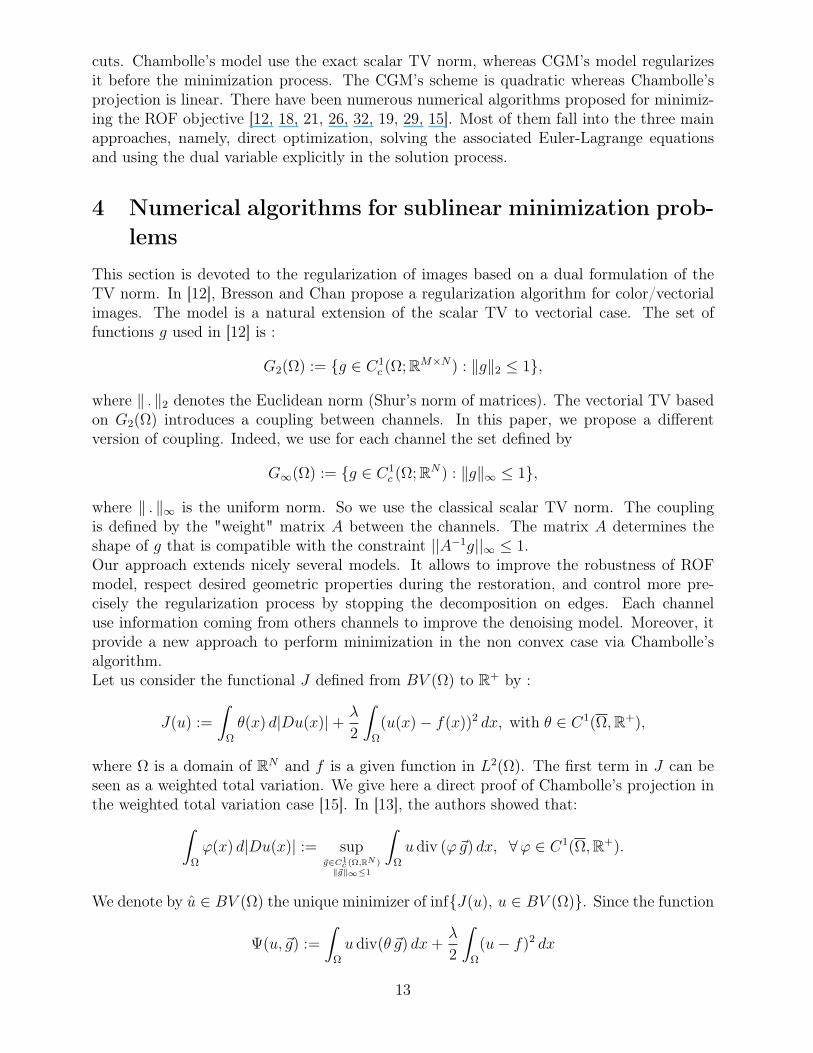
)where µ is a fixed gradient threshold that differentiates homogeneous areas and regions ofcontours.In practice, the behavior is more robust on edges. One sees on figure 1 that the restored imagehas been more regularized with the classical model (ROF) than with this new model. Toshow the robustness, the scale parameter λ is not well adjusted voluntary. In this case ROFalgorithm can yield to oversmoothing edges. On the contrary, our new denoising algorithmclearly outperforms ROF model. The parameter µ is less sensitive that λ to variations ofimages. It depends on the gradient level that we want to preserve. As for λ, it depends onnoise level within the image (i.e., image corrupted by Gaussian noise of variance σ2 [29]).

Figure 1: Robust restoration. Top. Original image. Bottom. Left : Regularized with classicTV formulation. Right : Regularized image with Extended TV formulation. The scaleparameter is voluntary huge to show the robustness (λ = 140).

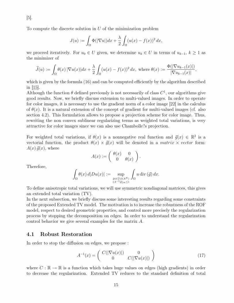
Others control functions can be defined. To steer the evolution of all channels in a multi-valued image (i.e., all channels have to be coupled), we propose (cf. Fig. 2) :

|∇u| =√λ+ + λ−

which defines the gradient norm of a multi-valued image [22]. This is a natural extension ofthe concept of gradient for multi-valued images. In order to evaluate how a vector-valuedimage varies, it is necessary to introduce the structure tensor [30, 33, 22]

T (u) =n∑i=1

∇ui ×∇uit

16

where each ∇ui corresponds to the gradient of the canal i. Then the gradient of a multi-valued image is define by the eigenvalues of T, (λ+, λ−).With classic TV formulation, Chambolle’s projection cannot operate for multi-valued images.Then it is necessary to use a digital total variation filter defined by [16]. Extended TVformulation allows to propose a projection scheme. The constraint |A−1g| steers the evolutionof all channels which become coupled.

Figure 2: Multi-valued image regularization with a projection algorithm. Left : Originalimage. Right : Regularized image.

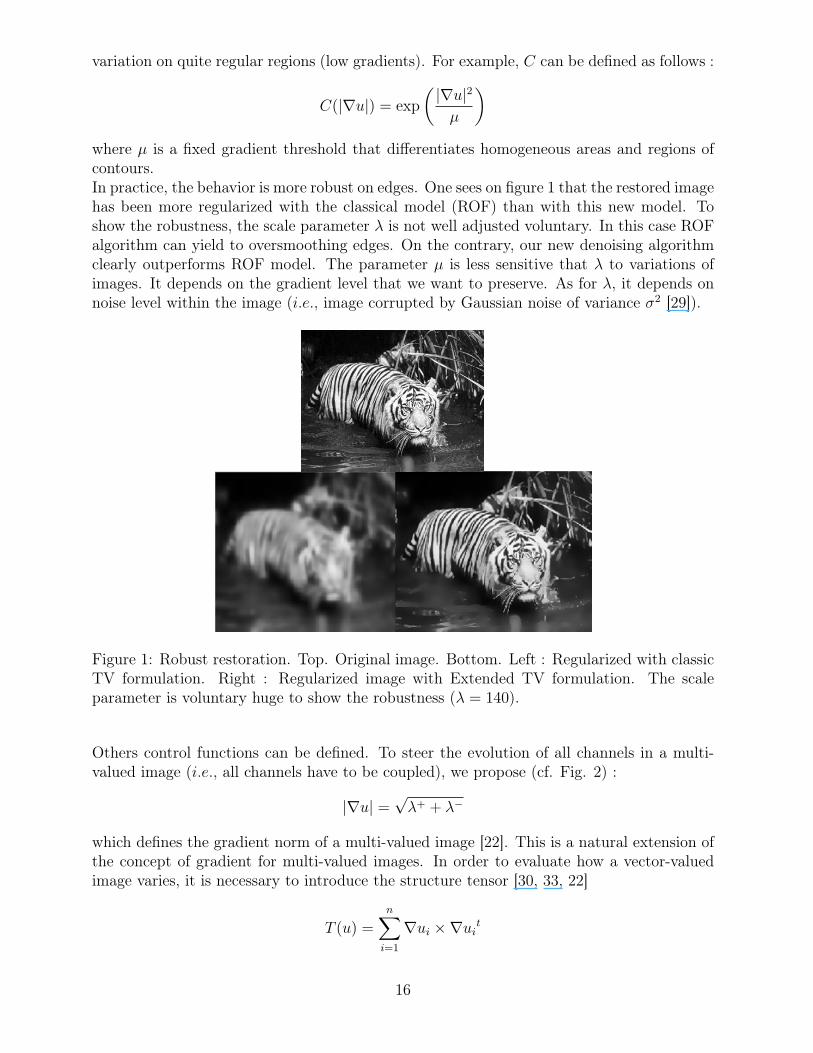
One sees on Fig. 3 the restored image with the nonconvex regularized Φ(s) = s2/(1 + s2) byusing a projection scheme.

Figure 3: An example of applying the nonconvexe robust regularization with a projectionapproach.

4.2 Anisotropic texture decomposition

4.2.1 Decomposition models

Another way of looking at denoising problems is by separating a given noisy image f intocomponents. Decomposing an image into meaningful components is an important and chal-lenging inverse problem in image processing. As described previously, Meyer has recentlyintroduced an image decomposition model [27] for splitting an image into two components:

17

a geometrical component and a texture component. Inspired by this work, numerical modelshave been developed to carry out the decomposition of grayscale images.

In [6], Aujol and Chambolle propose a decomposition model which splits a grayscale imageinto three components: a first one, u ∈ BV , containing the structure of the image, a secondone, v ∈ G 1, the texture, and the third one, w ∈ E 2, the noise. The discretized functionalfor splitting a grayscale image f into a geometrical component u, a texture component v anda noise component w is given by :

inf(u, v, w) ∈ U3

F (u) + F ∗

(v

µ

)+B∗

(wλ

)+

1

2α||f − (u+ v + w)||L2

(18)

where F (u) is the total variation for the extraction of the geometrical component, F ∗(vµ

),

B∗(wλ

)are the Legendre-Fenchel transform of respectively F and B for the extraction of

texture and noise components [24], the parameter α controls the L2-norm of the residualf − (u + v + w), and U is the discrete euclidean space Rn×n for image size n × n. Forminimizing (18), Chambolle’s projection [15] is used.

In [7], Aujol and Ha Kang, introduced an algorithm for a color decomposition model whichsplits a color image into only two components: geometrical and texture. For this decompo-sition, they use a generalization of Meyer’s G-norm to RGB vectorial color image, and useChromaticity and Brightness color model with total variation minimization. They proposethe following functional [7]:

inf(u, v) ∈ U2

F (u) + F ∗

(v

µ

)+

1

2α||f − (u+ v)||L2

(19)

To minimize (19), they use a digital total variation filter defined by Chan [16, 17]. Indeed,as shown in previously, Chambolle’s projection algorithm cannot operate for multi-valuedimages (i.e., it cannot steer the evolution of all channels). However, if we use Extended TVformulation, it is possible to use a projection algorithm.

In [25], the authors use a connection, given by Weickert [34], between wavelet shrinkageand non linear diffusion filtering to introduce the noise component in image decompositionmodel. Indeed, by considering an explicit discretisation and relating it to wavelet shrinkage,Weickert gives shrinkage rules where all channels are coupled. The formula states a generalcorrespondence between a shrinkage function Sθ and the total variation diffusivity h of anexplicit nonlinear diffusion scheme. It leads to novel, diffusion-inspired shrinkage functions.In [25], in order to steer the evolution of all three channels, the following shrinkage functionSθ for the wavelet coefficient wrx is proposed :

Sθ (wrx) = wrx

1− 12τg

√ ∑c∈r,g,b

wc2x + wc2y + 2wc2xy

(20)

1G is the space introduced by Meyer for oscillating patterns. In such a space oscillating patterns have asmall G-norm.

2E is another dual space to model oscillating patterns: E =.

B∞−1,∞, dual of the Besov space

.

B1

1,1.

18

When this function is incorporated in Aujol’s algorithm, the noise component can be ex-tracted.

4.2.2 Anisotropic texture decomposition and Extended total variation

In this section, we present an extension of the decomposition algorithm for color images.More precisely, we propose an anisotropic version of ROF model. The motivation is toprivilege certain directions. This algorithm may be seen as the decomposition of an imagef along defined directions depending themselves on the local configuration of the pixelsintensities. Basically, we want to decompose f while preserving its edges (i.e., performa decomposition mostly along directions of the edges and avoid decomposing along thedirections orthogonal to the discontinuities in image intensities.We can then rewrite the problem as :

inf(u, v, w) ∈ U3

FA(u) + FA∗

(v

µ

)+B∗

(wλ

)+

1

2α||f − u− v − w||L2

(21)

where FA(u) is an extended TV and FA∗ is its Legendre-Fenchel transform.Following Tchumperlé [31], we have first to retrieve the local geometry of the image f =f1, ..., fn. For the case of multi-valued images f , the local geometry of f is obtained bythe computation of the field T of structure tensors :

∀x ∈ Ω, T (f)(x) =∑

i = 1n∇fi(x)×∇fi(x)t. (22)

A gaussian-smoothed version Gσ = Gσ ∗ T is usually computed to retrieve a more coherentgeometry. The spectral elements of Gσ give at the same time the vector-valued variations:

• the eigenvectors θ+(x), θ−(x) give the local maximum and minimum variations of theimage intensities at x.

• the eigenvalues λ+(x), λ−(x) measure the effective variations of the image intensitiesalong θ+(x) and θ−(x) respectively.

• a field T of diffusion tensors specifying the local geometry drives the decompositionprocess. It is defined as follows:

∀x ∈ Ω, T (x) = f−(λ+ + λ−)θ− · θ− + f+(λ+ + λ−)θ+ · θ+. (23)

f+/− designates two functions which set the strengths of the decomposition along the re-spective directions θ−, θ+. In what follows, we design and study several functions f+/−.We propose :

• Φ(s) = s2/(1 + s2) which gives f−1 =√

1+s2

s2, f+

1 = 1+s2

s2

• Φ(s) = 1/(1 + s2) which gives f−2 =√

1 + s2, f+2 = 1 + s2

In order to use a projection approach, the matrix A is now defined by

A = (T + Id)−1

19

where Id is identity matrix.The constraint A−1~g can be written :

A−1 ~g = [T + Id]

(g1

g2

)The decomposition behavior is intended to be (Fig. 4–6) :

• if a pixel x is located on an image contour (λ+(x) is high), the decomposition on x wouldbe performed mostly along the direction θ−(x) of this contour with a decompositionstrength inversely proportional to the contour strength (i.e., components of A−1 arehigh.)

• if a pixel x is located on a homogeneous region λ+(x) is low), the decomposition onx would be performed in all direction (isotropic decomposition, i.e., A is the identitymatrix.

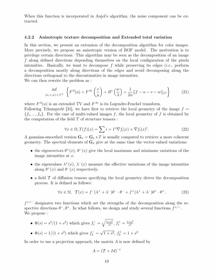
In the u+ v+w decomposition model, A−1~g penalizes edges that are not considered as partof the texture component. As shown in Figures 4, 5 and 6, this new formalism contributes topreserve image structures in texture decomposition. It allows to use conjointly the diffusiontensors of Tchumperlé and image decomposition approach.

Figure 4: Anisotropic multi-valued decomposition with f+1 and f−1 . Top: Original image.

Texture. Bottom : Structure. Noise

5 ConclusionIn this paper, we presented a way to design a new extended TV formulation based onconstraints. We proposed a generic constrained regularization formalism able to

• decompose anisotropically multi-valued images,

20

Figure 5: Anisotropic multi-valued decomposition with f+2 and f−2 . Top: Original image.

Texture. Bottom : Structure. Noise

• increase the robustness on edges denoising algorithms based on convex regularizationfunction,

• and propose projection schemes for nonconvex regularization and multi-valued images.

This new formalism contributes to

• preserve image structures in texture decomposition,

• allows to use conjointly the diffusion tensors of Tchumperlé and image decompositionapproach,

• propose a practical implementation for all these approaches by using projection schemeswhich have efficient properties in term of processing time,

• opens new ways in introducing nonconvex TV regularization in denoising image.

We have shown the efficiency of the algorithms with some numerical examples.

Acknowledgements. The authors wish to express their gratitude to the anonymous refereefor the careful reading of the manuscript and for the helpful comments; also for drawing ourattention to the reference [12].

References[1] L. Ambrosio, Existence theory for a new class of variational problems, Arch. Rational

Mech. Anal. 111 (1990) 291–322.

21

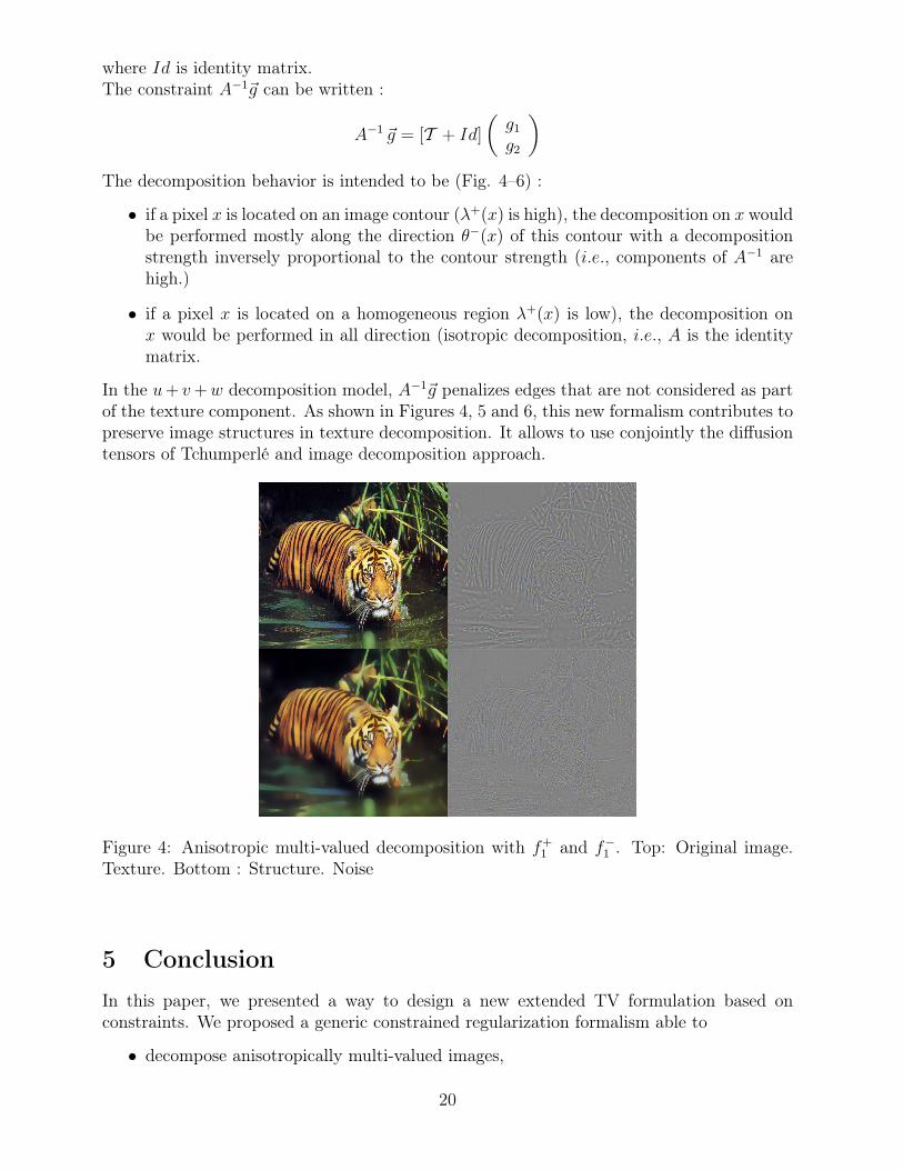
Figure 6: Anisotropic multi-valued decomposition (structure, texture, noise) with Top : f+1

and f−1 ; Bottom: f+2 and f+

2 . Original image is presented on Figure 2

[2] L. Ambrosio, N. Fusco, D. Pallara, Functions of bounded variation and free discontinuityproblems, Oxford Mathematical Monographs. Oxford University Press, 2000.

[3] G. Aubert, J. F. Aujol, Modeling very oscillating signals. Application to image process-ing, Applied Mathematics and Optimization, 51 (2005) 163–182.

[4] L. Ambrosio, G. Buttazzo, Weak lower semicontinuous envelope of functionals definedon a space of measures, Ann. Mat. Pura Appl. 150 (1988) 311–339.

[5] G. Aubert, P. Kornprobst, Mathematical Problems in Image Processing, Springer, 2006.

[6] J. F. Aujol, A. Chambolle, Dual norms and image decomposition models, InternationalJournal of Computer Vision, 63 (2005) 85–104.

[7] J. F. Aujol, S. Ha Kang, Color image decomposition and restoration, Journal of VisualCommunication and Image Representation, 17 (2006) 916–928.

[8] G. Bouchitté, G. Buttazzo, New lower semicontinuity results for nonconvex functionalsdefined on measures, Nonlinear Anal. 15 (1990) 679–692.

[9] G. Bouchitté, G. Buttazzo, Integral representation of nonconvex functionals defined onmeasures, Ann. Inst. H. Poincaré Anal. Non Linéaire 9 (1992) 101–117.

[10] G. Bouchitté, M. Valadier, Multifonctions s.c.i. et régularisée s.c.i. essentielle, Ann.Inst. H. Poincaré Anal. Non Linéaire 6 (1989), suppl., 123–149.

[11] J. Bourgain, H. Brézis, On the equation div Y = f and application to control of phases,J. Amer. Math. Soc. 16 (2003) 393–426.

[12] X. Bresson, T. F. Chan, Fast minimization of the vectorial total variation norm andapplications to color image processing, (preprint)

22

[13] G. Carlier, M. Comte, On a weighted total variation minimization problem, J. Funct.Anal. 250 (2007) 214–226.

[14] A. Chambolle, P. L. Lions, Image recovery via total variation minimization and relatedproblems, Numer. Math. 76 (1997), no. 2, 167–188.

[15] A. Chambolle, An algorithm for total variation minimization and applications, J. Math.Imaging Vision, 20 (2004) 89–97.

[16] T. F. Chan, S. Osher, J. Shen, The digital TV filter and nonlinear denoising, IEEETrans. Image Process. 10 (2001) 231–241.

[17] T.F. Chan, J. Shen, Image processing and analysis. Variational, PDE, wavelet, andstochastic methods, SIAM. 2005.

[18] T. F. Chan, G. H. Golub, P. Mulot, A nonlinear primal-dual method for total variation-based image restoration., SIAM J. Sci. Comp. 20 (1999) 1964–1977.

[19] J. Carter, Dual methods for total variation-based images restoration. PhD thesis, UCLA,Los Angeles, CA, 2001.

[20] M. Chipot, R. March, M. Rosati, G. V. Caffarelli, Analysis of a nonconvex problemrelated to signal selective smoothing, Math. Models Methods Appl. Sci. 7 (1997) 313–328.

[21] J. Darbon, M. Sigelle, Image restoration with discrete constrained total variation. Part 1:Fast and Exact Optimization, J. Math. Imaging Vision, 26 (2006) 277–291.

[22] S. Di Zenzo, a note on the gradient of a multi-image, Computer Vision, Graphics, andImage processing, 33 (1986) 116–125.

[23] F. Demengel, J. Rauch, Weak convergence of asymptotically homogeneous functions ofmeasures, Nonlinear Anal. 15 (1990), 1–16.

[24] I. Ekeland , R. Temam, Analyse convexe et problèmes variationnels, Dunod-Gauthier-Villars, 1974.

[25] M. Lugiez, S. Dubois, M. Ménard, A. El Hamidi, Spatiotemporal extension of colordecomposition and dynamic color structure-texture extraction, CGIV2008. 4th EuropeanConference on Colour in Graphics, Imaging, and Vision. June 09-13, Barcelona, Spain.2008.

[26] A. Masquina, S. Osher, Explicit algorithms for a new time dependent model based onlevel set motion for nonlinear deblurring and noise removal, SIAM J. Sci. Comp. 22(2000) 387-405.

[27] Y. Meyer, Oscillating patterns in image processing and nonlinear evolution equations,volume 22 of University Lecture Series. AMS, Providence, RI, 2001.

[28] M. Rosati, Asymptotic behavior of a Geman and McClure discrete model, Appl. Math.Optim. 41 (2000) 51–85.

23

[29] L. Rudin, S. Osher, E. Fatemi, Nonlinear total variation based noise removal, PhysicaD, 60 (1992) 259–269.

[30] D.Tschumperlé, R. Deriche, Diffusion PDE’s on Vector-Valued images, IEEE signalprocessing agazine, 19 (2002) 16–25.

[31] D.Tschumperlé, PDE’s based regularization of multi-valued images and applications,PhD. Thesis, University of Nice-Sophia Antipolis/France, December 2002.

[32] C. Vogel, M. Oman, Iterative methods for total variation denoising SIAM J. Sci. Comp.17 (1996) 227–238.

[33] J. Weickert, Anisotropic diffusion in image processing, Teubner-Verlag, Stuttgart, 1998.

[34] J. Weickert, G. Steidl, P. Mrazek, M. Welk, T. Brox, Diffusion filters and wavelets: Whatcan they learn from each other?, Chapter 1 of "Handbook of Mathematical Models inComputer Vision" (2006) 1–16.

24