Oil revenues for public investment in Africa: targeting urban or rural areas?
33
Oil revenues for public investment in Africa: targeting urban or rural areas? Marcus Böhme, Clemens Breisinger, Rainer Schweickert, Manfred Wiebelt No. 1623 | May 2010
Transcript of Oil revenues for public investment in Africa: targeting urban or rural areas?

Oil revenues for public investment in Africa: targeting urban or rural areas?
Marcus Böhme, Clemens Breisinger, Rainer Schweickert, Manfred Wiebelt
No. 1623 | May 2010

Kiel Institute for the World Economy, Düsternbrooker Weg 120, 24105 Kiel, Germany
Kiel Working Paper No. 1623| March 2010
Oil revenues for public investment in Africa: targeting urban or rural areas?
Marcus Böhme, Clemens Breisinger, Rainer Schweickert, Manfred Wiebelt
Abstract: This paper investigates the effects of oil financed public investment on poverty using a dynamic multisectoral general equilibrium model featuring inter-temporal productivity spillovers, which may exhibit a sector-specific and regional bias. In general, the results bear out the expectation that a surge of oil revenues leads to a real appreciation, distorting incentives which favor nontradable activities over export agriculture and manufacturing thereby increasing rural and national poverty. Whereas this result is familiar from other recent studies, the simulations show that beyond the short run, when conventional demand-side Dutch disease effects are present, the relationship between resource-rent flows and real exchange rates, output growth, and poverty is less straightforward than simple models of the "resource curse" suggest. Taking Ghana as a stylized agriculture-based economy with poverty most pronounced in a region with home biased agricultural production, a policy mix of smoothing the real exchange rate shock and an allocation of infrastructure spending in rural areas seems to be the most promising public investment strategy to enhance growth and reduce poverty.
Keywords: oil revenue, public investment, productivity, Africa, agricultural development, poverty
JEL classification: H4, O5, Q3 C. Breisinger International Food Policy Research Institute Washington, D.C., USA Phone: +1/202/862-4638/-8113 E-mail: [email protected]
M. Böhme, R. Schweickert, M. Wiebelt Kiel Institute for the World Economy 24100 Kiel, Germany Phone: +49/431/8814-571/-494/-211: E-mail: [email protected] [email protected] [email protected]
____________________________________ The responsibility for the contents of the working papers rests with the author, not the Institute. Since working papers are of a preliminary nature, it may be useful to contact the author of a particular working paper about results or caveats before referring to, or quoting, a paper. Any comments on working papers should be sent directly to the author.
Coverphoto: uni_com on photocase.com
1
I. Introduction
The limited success of “Washington Consensus” type reforms in promoting growth and
reducing poverty has reemphasized the importance of a more active role of the state in
development (World Bank 2005; Rodrik 2007; Lin 2010). A more active role can entail
enhancing budget neutral reforms, such as improvements in legislation, regulations and rules
to attract private investments. It can also imply the scaling-up of public spending, either
related to shifts in existing budgets and/or through acquiring additional resources. There is
broad consensus in the development economics literature that especially productivity-
enhancing public investments to support private-sector led are key for growth and job creation
(Syrquin 1988; World Bank 1993; Collier 2006; Breisinger and Diao 2009).
However, scaling up of public investments raises important questions on the fiscal
implications and institutional requirements to translate additional resources into development
outcomes. Additional financial resources for public investments can come from a variety of
sources, including domestic sources (taxes) or foreign inflows (grants, bonds, resource rents).
For many African countries, the possibilities of raising additional income is restricted to
grants and revenues from natural resources given the generally limited scope for tax increases
and limited access to international financial markets. However, several African countries are
experiencing or are about to experience a surge in foreign inflows. For example, in Ghana and
Uganda oil has been discovered, which is expected to significantly boost government
incomes.
Yet, using such foreign exchange inflows to finance public investments can have adverse
implications for development. Empirical evidence of whether foreign inflows are good or bad
for growth is inconclusive. While Sachs and Warner (1999, 2001) find that countries with
high resource-exports-to-GDP ratios experience lower growth rates, other research shows that
resource abundance has a neutral or even positive effect on growth (Davis 1995; Lederman
and Maloney 2003). The reasons for explaining potential negative impacts on growth are
twofold: a lack of absorptive and managerial capacity of overstretched public sectors and the
negative impact of the windfall revenues on policy choice1 or, alternatively, Dutch Disease
1 Windfall income or the expectations of such income generated by a discovery of natural resources might
induce the country to neglect the need for sound economic management and institutional quality (Gylfason 2001). A false sense of security might lead governments to undervalue the importance of human capital, institutional quality and long run growth (Rodriguez and Sachs 1999; Sachs and Warner 2001). In addition, adverse results may be the effect of an interplay of rent-seeking groups and weak institutions (Auty 2000).

2
effects in the form of reduced savings and distortions of relative prices with a bias against
export oriented production.2
Public investment decisions are also made on the basis of their growth and poverty effect, and
an important policy question is where to invest? Broadly speaking, public investments can be
directed to rural or urban areas and sectors. The related debate on is perhaps best reflected in
the World Development Reports (WDR) 2008 and 2009. These reports convey two rather
different messages of how to accelerate growth and poverty reduction in developing countries
(World Bank 2008; World Bank 2009). The WDR 2008 sees “agriculture as a vital
development tool for achieving the Millennium Development Goals (MDGs)”, while the
WDR 2009 concludes that “Growing cities, ever more mobile people, and increasingly
specialized products are integral to development”.
The WDR 2009 argues that in leading (often urban) areas, investment in places should be
emphasized—durable investments that increase national economic growth (World Bank
2009). The rationale behind this is that high population densities lead to agglomeration effects
and industrial clustering, thereby increasing innovation and productivity. According to this
line of thought, public investments need to focus on increasing density, i.e. managing urban
expansion and congestion by connecting different parts of a city. However, much of the
empirical evidence suggests that agriculture-led growth has large multiplier effects, is most
poverty reducing , and has high returns to investment, especially in African countries (World
Bank 2008; Diao 2008). Evidence from China and Uganda shows that it is often the low-cost
types of infrastructure that have highest returns to investment in terms of growth and poverty
reduction (Fan and Zhang 2004). In the case of China, rural road investment contributes not
only to rural growth and poverty reduction, but also to growth and poverty reduction in urban
areas. The spatial allocation of public investments also often matters. Evidence for China,
India, Thailand, and Vietnam indicates that most types of investments in less-developed areas
offer the largest poverty reduction per unit of spending and the highest economic returns (Fan
et al.; 2008; Fan et al. 2000; Fan and Zhang 2004; Mogues et al. 2008).
There are only few analytical attempts to compare public investments in urban and rural areas.
Dorosh and Thurlow find for Uganda that improving agricultural productivity generates more
2 Recent publications present evidence that natural resources diminish the need for investment and savings
because of the expected future income (Gylfason and Zoega 2006). Hence, at least part of the windfalls will be consumed and expectations about additional economic growth driven by the full extent of the windfall spend for investment may be exaggerated (see, e.g., Sachs and Warner 1997, Edwards 1989, Brunstad and Dyrstad 1997, Bjørnland 1998, Hutchinson 1994, Usui 1997 and Jahan-Parvar and Mohammadi 2009).

3
broad-based welfare improvements in both rural and urban areas than investing in the capital
city. While investing in Kampala accelerates economic growth, it has little effect on other
regions’ welfare because of the city’s weak regional growth linkages and small
migration effects (Dorosh and Thurlow 2009). Evidence from Peru suggests that investing in
the leading (more urbanized) region Peru may undermine the economy in the lagging (mostly
rural) region by increasing import competition and internal migration (Thurlow et al. 2008).
The study also shows that for reducing the divergence between the leading and lagging
region, investing in the lagging region’s productivity through extension services and
improved rural roads is critical. This brief overview of the literature suggests that public
investments in rural areas and agriculture are critical parts of development strategies in
Africa. Yet, scaling up investments in either rural or urban areas is often complicated by the
fact that financial resources come as foreign inflows, a fact not often captured in the literature.
To address this gap, we choose Ghana as a stylized agriculture based economy and its newly
discovered oil as an example for scaling up of public investments that are based on foreign
exchange inflows. To jointly assess the macroeconomic, growth, spatial and poverty impacts
of rural versus urban biased investment strategies, we use a dynamic computable general
equilibrium model. Ghana is a good case study for several reasons. Current conditions in
Ghana seem favorable to avoiding the resource curse caused by institutional and/or political
factors. Ghana’s economic structure is also comparable to many other African countries.
Agriculture plays an important role for the economy and contributes about one-third of total
GDP. Agricultural exports are concentrated in one crop (cocoa), which, together with gold,
constitutes more than 60 percent of total exports. In 2007 oil was discovered off the coast of
Ghana, with total reserves estimated at between 500 million and 1.5 billion barrels and the
potential for future government revenues estimated at US$ 1–1.5 billion annually (Osei and
Domfe 2008; World Bank; IMF 2009). Measured by a modest long-term oil price of US$ 60
per barrel over the next 20 years, oil revenues will add around 30 percent to government
income annually and constitute 10 percent of GDP over the exploitation period. Although the
relative amount of expected oil revenue is smaller than in some other resource-rich countries
(e.g., Angola, Botswana, and Nigeria), the expectations that additional oil revenue will help
the country further accelerate growth and reduce poverty are high.
4
II. The Simulation Model
Methodologically, our work is closest in spirit to Adam and Bevan (2006), who investigate
the supply-side impact of aid-financed public expenditure if public infrastructure generates an
intertemporal productivity spillover, which may exhibit an export or domestic bias. Given the
emphasis of the paper on income distribution and poverty, the main distinguishing feature of
our model is its detailed representation of agricultural production in different agro-ecological
zones and of the extended functional distribution of income that takes into account informal
production activities in agriculture. In addition, we explicitly link government infrastructure
spending and productivity changes.
Private production and consumption Producers and consumers are assumed to enjoy no market power in world markets, so the
terms of trade are independent of domestic policy choices. Firms in each of the 15 sectors and
agricultural subsectors (see Table 1) are assumed to be perfectly competitive, producing a
single good that can be sold to either the domestic or the export market.3 Production in each
sector i is determined by a CES production function of the form:
(1) Qi = Ai · Σf{δfi · Ffi-ρi}-1/ρi
where f is a set of factors consisting of land, different types of capital and different labor
categories, Qi is the sectoral activity level, Ai the sectoral total factor productivity, Ffi the
quantity of factor f demanded from sector i, and δfi and ρfi are the distributional and elasticity
parameters of the CES production function, respectively. The model considers different types
of labor forces, such as self-employed agricultural workers, unskilled workers employed in
both agriculture and non-agriculture, and skilled non-agricultural workers. Only production in
the rural food and cash crop sectors (cereals, root crops, other staple crops, and cocoa)
requires land with overall supply fixed in perpetuity. Private sector capital endowments are
fixed in each period but evolve over time through depreciation and investment. Land markets
within each agro-ecological region and labor markets for skilled and unskilled labor are
competitive so that these factors are employed in each sector up to the point that they are paid
the value of their marginal product. However, capital is assumed to be sector-specific and
3 Appendix Tables 1 and 2 provide some indicators on the export orientation of individual sectors and the
import dependence of domestic demand, together with information on sectoral and regional production, employment and cost structure. Besides mining, cocoa, forestry and livestock are the most export oriented sectors, exporting between 25 and 85 percent of their production, with the bulk of export production stemming from agro-ecological zones 1 to 3 while the poor zone 4 (Northern savanna) is producing almost exclusively for the domestic market.
5
immobile within each period, earning a quasi-rent in the short term while sectoral rental rates
adjust to the economy-wide average rental rate in the long term. Self-employed agricultural
workers are assumed to be sector-specific and immobile, both in the short and long term.
Their remuneration is determined by demand rather than the marginal value product.
Whenever demand slackens, lower product prices will immediately reduce income of these
workers. Finally, we assume that total sector factor productivity Ai depends on the availability
of public infrastructure. This detailed sector and regional structure allows the DCGE model to
analyze sector and sub-sector specific growth strategies and their contribution to income
distribution.
Table 1 — Classification of the CGE Model Activities/Goods and Services Production Factors Economic Agents
Agriculture, partly informal diff. by 4 agro‐ecological zones
4 self‐employed immobile rural labor types
90 households by regional affiliation and income deciles
Cereals Self‐employed1 50 urban, 40 rural
Root crops Self‐employed2 Accra
Staple crops Self‐employed3 Urban coast
Cocoa Self‐employed4 Urban forest
Livestock 2 mobile labor types Urban south
Forestry Skilled labor Urban north
Fishing Unskilled labor Rural coast
Non‐Agriculture 2 capital types Rural forest
Gold mining Non‐agr. capital Rural south
Other mining Services capital Rural north
Food processing 4 agro‐ecological regions Government
Other manufacturing Land (coast) Rest of the world
Construction Land (forest)
Utilities Land (South. savanna)
Private services Land (North. savanna)
Public services
The distributional consequences of external shocks and public policies are tracked through
their impact on 90 household types differentiated by regional affiliation and income levels
(see Table 1).
Consumption for each household type is defined by a constant elasticity of substitution linear
expenditure system, which allows for the income elasticity of demand for different goods to
deviate from unity. The income elasticity is estimated from a semi-log inverse function
suggested by King and Byerlee (1978) and based on the data of GLSS 5 (2005-06). The
estimated results, together with the average budget share for each individual commodity

6
consumed by each individual household group determine the marginal budget shares applied
in the model.
There are several alternative approaches to the analysis of the poverty effects of policy
changes and exogenous shocks in CGE models (see e.g. Roland-Holst 2004). A popular
approach in the CGE literature consists in specifying a relatively large number of
homogenous household groups and calculating average income for each group following a
shock and treating the group as a whole as being poor if average income is lower than a given
poverty line. This is the procedure followed, for instance, by Adelman and Robinson (1978),
in their pioneering CGE analysis of income distribution in Korea.4 Here, the poverty effects of
shocks are rather assessed by linking the simulation results of the CGE model to the results of
the 2005-06 Ghana household survey (GSS 2008).
Macroeconomic closure and dynamics
The model has a neoclassical closure in which total private investment is constrained by total
savings net of public investment, where household savings propensities are exogenous. This
rule, broadly consistent with conditions in poorer countries where unrationed access to world
capital markets is virtually zero and domestic private saving is relatively interest inelastic,
means that any shortfall of government savings relative to the cost of government capital
formation, net of exogenous foreign savings, directly crowds out private investment (and
excess of government savings directly crowds in private investment).
The model has a simple recursively dynamic structure. Each solution run tracks the economy
over 20 periods (from 2008 to 2027) from the initial policy change, each period may be
thought of as a fiscal year. Within-year public and private capital stocks are fixed, and the
model is solved given the parameters of the experiment (e.g., the change in oil revenues and
the corresponding public expenditure response). This solution defines a new vector of prices
and quantities for the economy, including the level of public and private-sector investment,
which feed into the equations of motion for sectoral capital stocks:
(2) Ki,t = Ki,t-1(1-μi) + ΔKi,t-j
where Ki,t is the capital stock, μi denotes the sector-specific rate of depreciation, and t-j
measures the gestation lag on investment.
4 Recently, Rutherford et al. (2004) have constructed a model for Russia that endogenously includes over
55,000 households.
7
The final element is an externality resulting from public investment in infrastructure, health,
education, and agriculture. Public investment is assumed to generate a Hicks-neutral
improvement in total factor productivities. Specifically, equation (1) above assumes that Αi,t =
Αi for non-spillover sectors, while in the spillover sector, denoted s, total factor productivities
evolve according to
(3) As,t = As · Πg{(Kgt/K
g0)/(Qs,t/Qs,0)}
ρsg
where g denotes a set of public capital stocks defined over infrastructure, health, education,
and agriculture, Kg, and Qs, are the public capital stocks and sectoral output levels under the
simulation experiment, and Kg0, and Qs,0 are the correspondingly defined public capital stocks
and output levels in the base period. The terms ρsg measure the extent of the spillovers. If ρsg
= ρs, = 0, there is no spillover from public investment in infrastructure, health, education, and
agriculture. The higher ρsg, the higher are spillovers.
III. Macroeconomic Implications of Alternative Spending Scenarios
The core simulations are presented in Table 2.5 The DCGE model is first applied to a scenario
(labeled BASE) in which the sectoral level growth rate is consistent with the growth trends
observed in Ghana in recent years (between 2001 and 2007). Newly found oil is not
considered in this scenario. Along this business as usual growth path, the model is calibrated
to feature Ghana’s recent (non-oil) economic development reflected by annual economic
growth of 5 percent over the next 20 years until 2027. As located off-shore and demanding
equipments and expertise not yet available in Ghana, the extraction of oil will not generate
significant backward linkages in terms of demand for domestic inputs and upstream activities
in the short to medium term. And unlike gas, forward linkages and related downstream
activities are also expected to be minimal, but through their impact on the budget (World
Bank 2009). We therefore choose not to introduce a domestic oil producing activity in the
model. Rather, we assume that the main impact from oil will occur through an increase in
foreign exchange revenues to the government.
5 For each simulation, the impact effect (years 2008-10) and the evolution of the economy until years 2015,
2020, and 2027 are reported. To simplify the presentation, the focus is on changes in only a small number of key aggregates: the trade weighted real exchange rate, the volume of exports, real GDP, private investment, the fiscal balance, the aggregated sectoral real value added, rural and urban household welfare measured by the equivalent variation (Table 1) and the incidence of poverty (poverty headcount; Table 2). Additional Tables in the Appendix report on the disaggregated factor income distribution, poverty depth, and poverty severety.

8
Given these assumptions, there is some modest structural change shown by the average
sectoral growth rates in Table 2. As can be seen, the agricultural sector grows less than the
industry and the service sectors. At the same time, there is also a modest real devaluation of
about 5 percent over the 20 years simulation period (Figure 1). These results are driven by
exogenous increases in labor and land supply, endogenously determined capital accumulation,
and exogenously defined total factor productivity parameters, which reflect relatively low
total factor productivity growth in agriculture compared to, e.g., construction. As a
consequence, the Balassa-Samuelson effect is reversed due to weak performance of the
tradable goods sectors.6
Six scenarios, labelled OIL1 through OIL6, contain alternative assumptions about
productivity spillovers, complementary spending, and smoothing of public spending on
infrastructure investment financed by the windfall gains from oil. Oil inflows start in 2010
and amount to a foreign exchange inflow of 8 percent of nominal GDP and 24 percent of
government revenue in the base run.7 In all cases the oil revenues are used exclusively to
finance an increase in public infrastructure investment, holding tax rates and all other
components of public expenditure, except O&M expenditure in OIL5, constant. As can be
seen in Table 2, the effects on private investment differ between the OIL scenarios. This is
basically due to two effects. First, the government in this model is a net seller of foreign
exchange and, hence, a real exchange rate appreciation reduces the domestic value of the
budget balance and therefore increases domestic financing requirements and crowding out of
private investment. Second, investment is based on inputs from heavy manufacturing and the
construction sector, with the latter being a pure nontradable sector. Hence, investment demand
has strong price effects and corresponding general equilibrium effects also modify the
outcome for private investment. Third, different assumptions about productivity effects of
investment also impact on private demand for investment goods.
6 For a similar result in the case of home driven productivity increases, see, e.g. Adam and Bevan (2006). 7 For details, see Breisinger et al. (2009). The simulations neglect the phasing in and out of the actually
expected stream of Government revenue, which consists of two successive temporary increases in foreign exchange revenues to the government, yielding four years of peak revenue, to be followed by a continues decline of revenue afterwards (World Bank 2009).

9
Table 2 — Simulation Results of the Effects of a Temporary Increase in Government Oil Revenues (percent)
Period BASE OIL1 OIL2 OIL3 OIL4 OIL5 OIL6
Public investment bias Non‐Agri Neutral Region4 Neutral Neutral
Prices and quantities
Export weighted real 2008‐10 100.8 89.2 89.2 89.2 89.2 89.2 92.6
exchange rate index 2008‐15 103.7 100.9 102.0 98.9 99.9 97.6 99.4
(Pt/Pd) 2008‐20 105.0 105.5 106.4 103.6 104.5 102.4 103.3
2008‐27 105.2 108.0 108.8 106.2 107.0 105.1 105.5
Total exports 2008‐10 5.9 ‐6.7 ‐6.7 ‐6.7 ‐6.7 ‐6.7 ‐2.8
2008‐15 5.6 3.9 5.2 6.0 5.6 5.6 6.4
2008‐20 5.4 5.1 5.9 6.3 6.1 6.0 6.3
2008‐27 5.1 5.3 5.8 6.0 5.9 5.9 6.0
Real GDP 2008‐10 5.4 5.7 5.7 5.7 5.7 5.7 5.7
2008‐15 5.2 6.2 6.9 7.2 7.1 7.1 7.0
2008‐20 5.1 5.9 6.3 6.5 6.4 6.4 6.4
2008‐27 5.0 5.5 5.8 5.9 5.9 5.9 5.9
Investment 2008‐10 5.7 2.2 2.2 2.2 2.2 2.2 3.8
2008‐15 5.3 6.6 8.0 8.2 8.1 7.5 8.7
2008‐20 4.9 6.4 7.2 7.4 7.3 7.0 7.7
2008‐27 4.2 5.6 6.1 6.3 6.2 6.1 6.6
Budget balance 2008‐10 0.2 ‐1.6 ‐1.6 ‐1.6 ‐1.6 ‐1.6 ‐0.9
(percent of GDP) 2008‐15 0.3 1.0 1.8 1.6 1.7 0.9 1.6
2008‐20 ‐0.2 1.7 2.5 2.5 2.5 1.8 2.2
2008‐27 ‐1.8 1.0 1.8 1.8 1.8 1.3 1.5
Equivalent variation
Rural 2008‐10 8.6 13.8 13.8 13.8 13.8 13.8 12.0
2008‐15 34.6 36.8 41.2 46.9 45.4 46.6 46.4
2008‐20 67.3 70.7 76.6 84.1 82.3 83.6 83.5
2008‐27 127.8 133.2 141.6 152.4 150.1 151.6 151.6
Urban 2008‐10 11.5 20.5 20.5 20.5 20.5 20.5 17.5
2008‐15 46.3 53.7 59.5 62.7 61.5 63.2 60.9
2008‐20 90.7 101.8 110.3 113.9 112.5 113.7 111.7
2008‐27 173.7 190.8 203.6 208.4 206.6 207.5 205.8
Total 2008‐10 10.2 17.4 17.4 17.4 17.4 17.4 14.9
2008‐15 40.8 45.8 51.0 55.3 53.9 55.4 54.1
2008‐20 79.8 87.3 94.5 100.0 98.4 99.6 98.5
2008‐27 152.2 163.8 174.5 182.1 180.1 181.3 180.4
Real value added
Agriculture 2008‐10 4.5 0.5 0.5 0.5 0.5 0.5 1.7
2008‐15 4.5 3.8 4.2 6.2 5.8 6.1 6.4
2008‐20 4.5 4.2 4.4 5.7 5.4 5.7 5.8
2008‐27 4.5 4.4 4.5 5.4 5.3 5.4 5.4
Industry 2008‐10 5.7 10.9 10.9 10.9 10.9 10.9 9.7
2008‐15 5.4 8.3 9.1 8.9 8.9 8.3 8.2
2008‐20 5.2 7.1 7.6 7.4 7.5 7.1 7.1
2008‐27 4.9 6.1 6.5 6.4 6.4 6.2 6.2
Services 2008‐10 5.9 3.6 3.6 3.6 3.6 3.6 4.2
2008‐15 5.8 5.7 6.6 6.1 6.2 6.5 6.1
2008‐20 5.7 6.0 6.5 6.2 6.2 6.3 6.1
2008‐27 5.5 5.8 6.2 6.0 6.0 6.0 5.9
Source: Authors' analysis based on the model described in the text

10
In OIL1, the infrastructure investment increases the economy’s total capital stock but has no
effect on private total factor productivity. In the short-run, oil inflows lead to a 10.8 percent
appreciation of the real exchange rate and a sizable contraction in exports of 6.7 percent in
favor of higher production of domestic goods (see Figures 1 and 2). The rising capital stock
ensures that the initial decline in export performance is reversed. Especially the construction
sector attracts both capital and labour. In the long run, the resulting supply effect even
outperforms the initial demand effect driven by additional public infrastructure investment.
As shown in Table 2, additional growth of about 0.5 percentage points on average in the long-
run, i.e. from 2008 to 2027, is driven by an increase in the growth of investment spending
from 2.2 to 5.6 percent. At the same time, there is almost no impact on total exports and
additional home driven growth takes place in the industry and service sectors while growth in
agriculture is even (slightly) reduced.
Figure 1 — Trade Weighted Real Exchange Rate Response to Oil‐Financed Public Investment (Pt/Pd)

11
Figure 2 — Total Export response to Oil‐Financed Public Investment
Contrary to OIL1, scenarios OIL2 through OIL6 assume that infrastructure investment
enhances private-sector productivity. In terms of equation 2, this means that the public capital
stock Kg, varies depending on the type of government infrastructure investment. Together
with the spillover parameter ρsg, it determines the extent of the sectoral productivity effect.
There is little consensus on the size of the productivity effects of infrastructure investment in
low-income countries. The assumed value for this parameter is ρsg, = 0.5 for industrial and the
private services sector, comparatively higher than the values estimated in Hulten’s (1996)
study of infrastructure capital and economic growth. This higher baseline value reflects the
expectation of a higher marginal product of public capital for countries with a severely
depleted capital stock. It is also closer to the value of comparable parameters that have been
estimated for agriculture in Ghana. For all rural areas in Ghana, the marginal effect of public
agricultural investment spending has been estimated by Benin et al. (2008) at 0.54.

12
OIL2 through OIL4 scenarios vary in terms of the allocation of infrastructure investment:
OIL2 applies the current bias in public investment spending pattern against
agriculture. Here, only 5.2 percent of overall public development spending is used to
finance agricultural infrastructure while about 94.8 percent is allocated to urban
infrastructure investment.
OIL3 assumes that the spending pattern is neutral and government now spends 33
percent (instead of 5.2 percent) of oil revenues for investment in agricultural
infrastructure while only 67 percent are allocated to non-agriculture. This reflects the
share of agricultural in total value added.
OIL 4 assumes the same spending pattern between agriculture and non-agriculture as
OIL3 but one that is biased within agriculture towards productivity-enhancing
agricultural infrastructure in the north of Ghana, which has the highest poverty rates.
There is now fairly substantial compound growth in GDP over the 20 years, some
improvement in the fiscal balance, and a marked increase in private investment.8 As a
consequence, while the impact effects on the real exchange rate and on exports are identical to
those in OIL1, because of the time lag before the productivity effects kick in, the impacts
diverge sharply over time. All of the real exchange rate appreciation has been unwound by the
end of year 2015 (except in OIL3) and the real exchange rate is further depreciating
afterwards. Moreover, even though the real exchange rate remains somewhat appreciated
relative to its baseline value in the medium-run (except in OIL2), the initial 6.7 percent fall in
export volumes is reversed moving to a 5.2-6.0 percent increase. Over the whole simulation
period, exports growth is about 1 percentage points higher than in the base run.
Comparing these spending scenarios, it is evident that, from a macroeconomic point of view,
OIL3 seems to be superior. It results in the highest growth rates in terms of trade, investment
and GDP. In addition, it has the highest sectoral growth for agricultural products although real
appreciation in the short and long run is clearly stronger. Hence, appreciation seems not to
hurt the agricultural sector, at least, not in a way that would overcompensate the positive
investment effect of a neutral allocation of public investment funds. To the contrary, scenario
OIL2 with the highest level of exchange rate devaluation is in favor of the industry and
8 Government revenue grows as real incomes and expenditures grow while, after the initial step changes in
year 2010, real government spending does not. Savings available for private investment grow partly with GDP but also because of crowding-in from the improvement in the fiscal balance. It is a consequence of the closure rule mentioned earlier that these resources are duly invested.

13
service sectors, i.e. in favor of home based growth. At the same time, a pro-poor bias in public
investment spending as in OIL4 does not have obvious macroeconomic advantages.
Compared to OIL3, export expansion is less pronounced and industrial growth even benefits
at the cost of agricultural production.
As a consequence, we based the OIL5 and OIL6 scenarios on the allocative assumptions of
OIL3. OIL5 re-runs OIL3 but now assumes that an increased public capital stock entails a
higher level of operations and maintenance (O&M) expenditure. This is calibrated on the
basis of evidence on the recurrent expenditure requirements of World Bank financed capital
projects compiled by Hood et al. (2002). The baseline assumption is that these additional
O&M costs of 10 percent of the increase in public capital stocks are financed through
increases in the domestic budget deficit, thereby crowding out private investment. As shown
in Figure 1 and Table 2, the increasing current expenditures induce an extended appreciation
of the real exchange rate, a decline in public savings, and, consequently additional crowding-
out of private investment.
Finally, we consider in the OIL6 scenario that the government, rather than spending all oil
revenues as they emerge, saves a significant share of 30 percent in an external oil fund, while
only 70 percent plus the interest income earned from the fund are allocated to the government
budget for financing infrastructure investment based on the neutral assumptions as in OIL3.
As can be seen, the smoothing feature of building up an oil fund moderates short-run
absorption effects and, hence, real appreciation. It is not surprising that OIL6 provides
superior results concerning export expansion. The immediate contraction is more than halved
without a loss of export dynamics in the medium run. However, smoothing oil spending also
implies higher growth of private investment because, compared to OIL2-4 scenarios, the
increase in the budget deficit and, hence, crowding out, is less pronounced.
All in all, from a macroeconomic point of view the alternative oil scenarios reveal different
patterns for the real exchange rate and total investment while average growth rates for the
medium run rather converge towards 5.2 to 6.4 percent, at least for those scenarios
considering productivity spillovers. OIL2, the scenario with the strongest devaluation shows
advantages in term of industrial and services sector growth, OIL 3 not discriminating against
agriculture is superior in terms of medium run export, investment, and GDP growth. While a
pro-poor bias in infrastructure spending has no macroeconomic advantages, smoothing oil
spending improves trade dynamics by moderating the short run appreciation and the
consequent contraction. In addition, the advantages of stretching oil funds beyond 2027 does

14
not have significant repercussion: the difference in average growth compared to OIL3 ranges
between 0.1 and 0.2 percentage points depending on the time horizon (Table 2).
IV. Poverty Implications of Alternative Scenarios
While total household income and welfare increase in the short and long term in all oil
scenarios, compared to the base run, the gains are not distributed equally across all household
groups. Rural households actually experience a decline in income and welfare relative to
urban households (see Figures 3 and 4 and Table 2). The principal reason is that the demand
effects from increased government and private expenditures fall disproportionately on sectors,
which intensively use factors supplied by urban households, and on intermediate goods from
the manufacturing and services sectors. In addition, backward linkages from urban sectors to
the rural sectors are extremely weak. Thus, agriculture and rural households depending on it
do not benefit significantly from increased income but are hurt by higher prices for
intermediate inputs and consumer goods.
If public infrastructure investment confers no productivity spillovers, as in scenario OIL1, real
agricultural value added not only declines relative to non-agricultural value added, but also
absolutely compared to the base run, both in the short and long term (see Table 2). The
worsening of agricultural terms of trade is also reflected in the functional distribution of
income with mobile factors, such as skilled and unskilled labor improving their relative
income position while the income shares of sector-specific factors employed in agriculture
(self-employed workers and land) are decreasing (see Appendix Table 3). Thus, the
improvement in rural household welfare shown in Table 2 is almost exclusively due to
increasing wages for (inter-sectoral mobile) unskilled workers. By contrast, immobile poor
rural households depending on self-employment income are largely by-passed by the income
effects of additional demand but are negatively affected by higher input prices. This is
reflected in the poverty indicators (see Table 3 and Appendix Tables 4-5).
Compared to the base-run, the resource boom increases the incidence, depth, and severity of
poverty on a national scale, both in the short and medium term. This worsening of the poverty
situation can be solely traced back to higher poverty in rural households, both in the North
and non-North, while urban poverty is slightly reduced. The initial real appreciation strongly
discriminates the export-oriented cocoa, forestry, and fishing sectors. Although producers of
cereals, root crops, and other staple crops benefit from higher private demand, the sole

15
beneficiaries are those rural households which predominantly earn unskilled labor income
while poor households are negatively affected by lower self-employment income and lower
land rentals. The situation improves and rural poverty rates move towards their base-run
values in the long-run, i.e. after the year 2020 when the real exchange rate appreciation has
been unwound. Hence, it is to be expected that the real exchange rate effects discussed in
Chapter III have a significant impact on poverty results.
Figure 3 — Household Incomes in Response to Oil‐Financed Public Investment
16
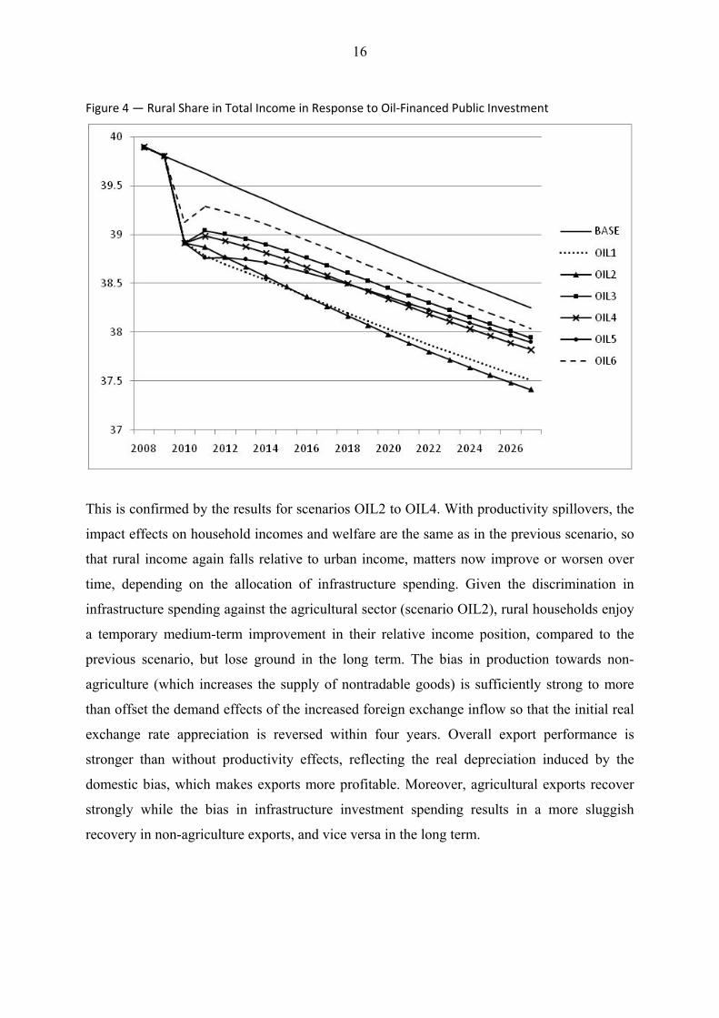
Figure 4 — Rural Share in Total Income in Response to Oil‐Financed Public Investment
This is confirmed by the results for scenarios OIL2 to OIL4. With productivity spillovers, the
impact effects on household incomes and welfare are the same as in the previous scenario, so
that rural income again falls relative to urban income, matters now improve or worsen over
time, depending on the allocation of infrastructure spending. Given the discrimination in
infrastructure spending against the agricultural sector (scenario OIL2), rural households enjoy
a temporary medium-term improvement in their relative income position, compared to the
previous scenario, but lose ground in the long term. The bias in production towards non-
agriculture (which increases the supply of nontradable goods) is sufficiently strong to more
than offset the demand effects of the increased foreign exchange inflow so that the initial real
exchange rate appreciation is reversed within four years. Overall export performance is
stronger than without productivity effects, reflecting the real depreciation induced by the
domestic bias, which makes exports more profitable. Moreover, agricultural exports recover
strongly while the bias in infrastructure investment spending results in a more sluggish
recovery in non-agriculture exports, and vice versa in the long term.
17
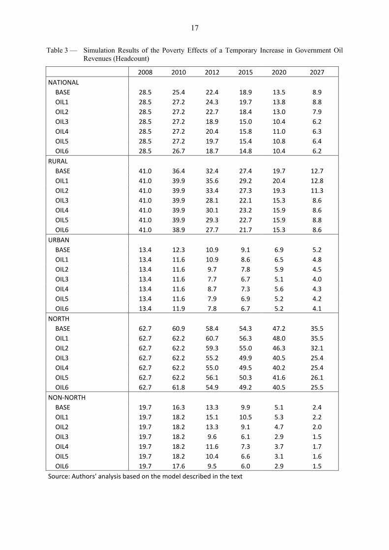
Table 3 — Simulation Results of the Poverty Effects of a Temporary Increase in Government Oil Revenues (Headcount)
2008 2010 2012 2015 2020 2027
NATIONAL
BASE 28.5 25.4 22.4 18.9 13.5 8.9
OIL1 28.5 27.2 24.3 19.7 13.8 8.8
OIL2 28.5 27.2 22.7 18.4 13.0 7.9
OIL3 28.5 27.2 18.9 15.0 10.4 6.2
OIL4 28.5 27.2 20.4 15.8 11.0 6.3
OIL5 28.5 27.2 19.7 15.4 10.8 6.4
OIL6 28.5 26.7 18.7 14.8 10.4 6.2
RURAL
BASE 41.0 36.4 32.4 27.4 19.7 12.7
OIL1 41.0 39.9 35.6 29.2 20.4 12.8
OIL2 41.0 39.9 33.4 27.3 19.3 11.3
OIL3 41.0 39.9 28.1 22.1 15.3 8.6
OIL4 41.0 39.9 30.1 23.2 15.9 8.6
OIL5 41.0 39.9 29.3 22.7 15.9 8.8
OIL6 41.0 38.9 27.7 21.7 15.3 8.6
URBAN
BASE 13.4 12.3 10.9 9.1 6.9 5.2
OIL1 13.4 11.6 10.9 8.6 6.5 4.8
OIL2 13.4 11.6 9.7 7.8 5.9 4.5
OIL3 13.4 11.6 7.7 6.7 5.1 4.0
OIL4 13.4 11.6 8.7 7.3 5.6 4.3
OIL5 13.4 11.6 7.9 6.9 5.2 4.2
OIL6 13.4 11.9 7.8 6.7 5.2 4.1
NORTH
BASE 62.7 60.9 58.4 54.3 47.2 35.5
OIL1 62.7 62.2 60.7 56.3 48.0 35.5
OIL2 62.7 62.2 59.3 55.0 46.3 32.1
OIL3 62.7 62.2 55.2 49.9 40.5 25.4
OIL4 62.7 62.2 55.0 49.5 40.2 25.4
OIL5 62.7 62.2 56.1 50.3 41.6 26.1
OIL6 62.7 61.8 54.9 49.2 40.5 25.5
NON‐NORTH
BASE 19.7 16.3 13.3 9.9 5.1 2.4
OIL1 19.7 18.2 15.1 10.5 5.3 2.2
OIL2 19.7 18.2 13.3 9.1 4.7 2.0
OIL3 19.7 18.2 9.6 6.1 2.9 1.5
OIL4 19.7 18.2 11.6 7.3 3.7 1.7
OIL5 19.7 18.2 10.4 6.6 3.1 1.6
OIL6 19.7 17.6 9.5 6.0 2.9 1.5
Source: Authors' analysis based on the model described in the text

18
Although the income gains from higher productivity are partly transmitted to the poor, these
are insufficient to compensate for the short-run income losses of poor rural households that
result from the demand effects discussed above. Thus, while rural poverty is reduced over
time, it still increases relative to the base run in the short to medium term (until 2014; see
Table 3). The reason is that at the current allocation of public infrastructure spending, the
welfare-enhancing productivity effects in agriculture do not generate sufficient agricultural
growth to lift poor households, which primarily depend on self-employment income, above
the poverty line. Medium term growth of agriculture real value added is still 0.3 percentage
points lower than in the base run (see Table 2). In addition, the major beneficiaries of the
current allocation of infrastructure spending are mobile unskilled workers whose relative
income position improves while poor self-employed farmers loose against other households
(see Appendix Table 3). Thus, while the current allocation of public infrastructure investment
leads to a reduction of urban poverty in the short, medium, and long term, it temporarily
increases rural poverty and reduces the incidence of poverty on the country-side only slightly
in the long term.
Not surprisingly, the results are more pro-poor if oil-financed public infrastructure spending is
allocated neutrally between agriculture and non-agriculture, as in scenarios OIL3 and OIL4,
and if it is biased toward the poor Northern region within agriculture, as in scenario OIL4. As
expected, when there is less increase in the productivity of less export-oriented (industrial)
sectors, this leads to a more appreciated path for the export-weighted real exchange rate in
both scenarios. The appreciation is less pronounced in OIL4 because the Northern region
largely produces food crops (cereals, root crops, other staple crops, and livestock) for the
domestic market. Hence, although agricultural export performance is stronger in both
scenarios because of higher productivity growth, industrial and private services exports are hit
relatively hard, compared to the OIL2-scenario, because of the extended real appreciation.
The most striking difference between these two scenarios and the previous one, though, is the
effect on sectoral income distribution and poverty. A neutral allocation of infrastructure
spending (OIL 3) leaves private investment and real GDP growth almost unaffected but
drastically changes the sectoral distribution of value added in the medium and long term with
real agricultural value added rising from 4.5 percent in the base run to 6 and 5.4 percent on
average in the medium and long term (see Table 2). This change in the sectoral distribution of
income is also reflected in changes in poverty indicators with the incidence of both rural and
urban poverty decreasing in the medium and long term. Because agriculture is export-
oriented, the increase in productivity that results from a neutral allocation of public

19
infrastructure spending primarily leads to an output expansion, higher remuneration of self-
employed workers and higher land rentals, rather than decreasing prices. Looking at the
medium and long run implications for poverty, Table 3 clearly reveals that the combination of
productivity spillovers and price increases curbed by world market competition yield the
lowest headcounts, except for the North.
These effects are somehow moderated if public infrastructure investment is biased within
agriculture toward the Northern region. As in OIL3, rural poverty is decreasing in the medium
and long run, compared to the base-run scenario. While the poverty rate in the Northern
region persists on its base-run value over the medium term in scenario OIL3, the headcount is
reduced drastically in OIL4. However, additional poverty reduction is rather moderate. In the
long run, headcount for OIL3 and OIL4 are the same. Because agriculture is home biased in
the North, the economy’s increased ability to produce agricultural goods shifts the domestic
terms of trade in favor of those consuming the now relatively cheaper agricultural goods
(both, rural and urban households) and against those producing them (rural households).
Additionally, reducing poverty in the Northern region is not costless but increases urban and
non-North rural poverty.
As noted above, demand-side effects imply a tendency for urban households to gain
disproportionately from oil-financed increases in infrastructure because of low backward
linkages from government expenditures to the rural sector of the economy. The relative price
movements induced by additional recurrent public expenditures for the operation and
maintenance of a higher public infrastructure capital stock (O&M expenditure) in scenario
OIL5 exacerbate these weak linkages.9 Additional recurrent spending involve a worsening of
the fiscal budget, a crowding-out of private investment and a more appreciated real exchange
rate as resources, particularly scarce skilled labor, are relocated from tradable sectors to the
nontradable public sector. Compared to OIL3, this implies a worsening of the income
distribution and higher rural poverty rates.
It is worth highlighting one important feature of the results for all scenarios discussed so far:
the relative decline in rural incomes in these scenarios is immediate and persistent, as clearly
shown in Figure 4. In contrast to what is happening elsewhere in the economy, it is this
demand effects rather than the supply factors that drive rural incomes in both the short and the
long term. This is seen very clearly from the fact that alternative public infrastructure
investment patterns alter the pattern of incomes very little indeed. However, they do have
9 Scenarios OIL4 and OIL5 assume the same infrastructure spending pattern as scenario OIL3.
20
implications for poverty reduction. Thus, an important element of any policy to contain
increasing poverty during resource booms should be to combine policies to contain real
exchange rate appreciation and measures to increase rural productivity.
Therefore, OIL6 investigates the case where part (30 percent) of the oil revenue is saved in an
external resource fund while the rest as well as interest income from the fund is allocated
neutrally to public infrastructure investment in agriculture and non-agriculture, as in scenario
OIL3. There is now less initial appreciation of the export weighted real exchange rate, some
improvement in the fiscal balance, and a marked increase in private investment. As a
consequence, the short to medium term impacts diverge sharply. Virtually all of the real
exchange rate appreciation has been unwound by the 2015. As a result, agricultural and export
growth is much higher than in scenario OIL3. While the impact and long-term effect on
household incomes is negative, so that both urban and rural incomes fall, compared to OIL3,
headcounts match those of OIL3 for the years 2020 and 2027 respectively. Even more
importantly, the moderation of real appreciation produces, with only one exeption, the lowest
headcounts for the short run, i.e. up to 2015. For the North, the moderation of the real
appreciation is even more effective in reducing poverty rates than investment targeting as in
OIL4. Finally, the accumulation of savings in an oil fund allows the country to continue to
enjoy the income generated from oil even after the end of the oil era, this scenario suggests
that it is an option that might be the best for growth and poverty reduction in the long run.
VI. Summary and Conclusions
This paper has addressed specific questions within the much broader discussion of
development financed by foreign exchange inflows in developing countries. The short to long
term impacts of oil-financed public infrastructure investment in Ghana was analyzed
numerically using a dynamic computable general equilibrium model featuring intertemporal
productivity effects, which may exhibit a sector and regional specific bias depending on
public spending schemes. The analysis was carried out on a fifteen sectors, 12 factors, and 90
households level aggregation that takes into account the structural characteristics of the
Ghanaian economy, most importantly, the sectoral composition of agricultural production in
four agro-ecological zones and the informal nature of large parts of agricultural production. In
addition the CGE results were combined with individual household characteristics from the
Ghana Living Standards Survey to calculate so-called FGT (Foster, Greer, and Thorbecke)

21
poverty indices, which take into account the full functional and spatial diversity of household
income. Several conclusions emerge from the simulations presented in this paper.
First, a resource boom and the accompanying developmental and/or recurrent public
expenditures, besides direct effects, induce short and longer term general equilibrium
repercussions which have large and generally negative indirect effects on agriculture as well
as on rural income and poverty. However, when developmental expenditures in public
infrastructure augment the productivity of private factors, and when there is an initial scarcity
of public infrastructure, there are potentially large medium to long-run welfare gains from a
resource boom − despite the presence of short-run Dutch disease effects − if at least part of
the resource revenue is used to finance public investment.
Second, the dynamic and distributional consequences of this investment are highly sensitive
to the location of productivity effects and the characteristics of demand. The presence of an
industrial bias in the aggregate supply response, while broadly beneficial to the economy in
terms of boosting aggregate growth and investment, welfare, and exports and moderating the
appreciation of the real exchange rate, leads to an increase in the incidence of poverty in rural
areas and in the poor North in the medium term while it reduces poverty only slightly over the
long term, compared to the base run.
Third, across all scenarios, particularly when there is an industrial bias in public investment
spending, the agricultural sectors do not share proportionately in the aggregate income gains
to the economy. The economy as a whole enjoys a large medium term supply response, but at
the cost of increasing rural poverty and a sharp worsening of the distribution of income
between agriculture and the rest of the economy.
Fourth, a bias in infrastructure investment toward the Northern poverty region has important
drawbacks. Reducing poverty via targeted investment increases rural poverty because
increased productivity leads to a worsening of the terms of trade of agricultural products. In
the short run, smoothing the real appreciation by investing part of the oil windfall into an oil
fund is even superior in terms of poverty reduction in the North.
Finally, our results confirm other results showing little if any drawbacks in the short run while
negative structural implications of spending all oil money as it becomes available has negative
effects for the rural economy, the agricultural sector and, hence, poverty rates at least in the
short run.
22
All in all, taking Ghana as a stylized agriculture-based economy with poverty most
pronounced in a region with home biased agricultural production, a policy mix of smoothing
the real exchange rate shock and an allocation of infrastructure spending which ends the bias
against agriculture seems to be superior to other spending paths. Recognizing the importance
of economic structure in determining the final sectoral, distributional and poverty effects of a
resource boom also demonstrates that targeting infrastructure spending may have important
drawbacks in terms of poverty reduction which may require complementary intervention.

23
References
Adam, C., and Bevan, D. (2006). Aid and the supply side: Public investment, export
performance, and Dutch disease in low-income countries. The World Bank Economic Review, 20, 2: 261-290.
Adelman, I., and Robinson, S. (1978). Income distribution policy in developing countries: A case study of Korea. World Bank Research Publication, Stanford University Press.
Agosin, M.R., and Mayer, R. (2000). Foreign investment in developing countries: Does it crowd in domestic investment? UNCTAD Discussion Paper UNCTAD/OSG/DP/146.
Antle, J. (1984). Human capital, infrastructure, and the productivity of Indian rice farmers. Journal of Development Economics, 14: 163–181.
Aschauer, D. (1989). Is public expenditure productive? Journal of Monetary Economics, 23: 177-200.
Auty, R. (2000). How natural resources affect economic development. Development Policy Review, 18, 4: 347-364.
Auty, R. (2001). The political state and the management of mineral rents in capital-surplus economies: Botswana and Saudi Arabia. Resources Policy, 27, 2: 77-86.
Benin, S., Mogues, T., Cudjoe, G., and Randriamamonjy, J. (2008). Reaching middle-income status in Ghana by 2015. IFPRI Discussion Paper 811, International Food Policy Research Institute, Washington, DC.
Binswanger, H.P., Khandker, S.R., and Rosenzweig, M.R. (1993). How infrastructure and financial institutions affect agricultural output and investment in India. Journal of Development Economics, 41: 337–366.
Bjørnland, H. (1998). The economic effects of North Sea oil on the manufacturing sector. Scottish Journal of Political Economy, 45, 5: 553-585.
Breisinger, C., and Diao, X. (2009). Economic transformation in theory and practice: What are the messages for Africa? IFPRI Discussion Paper 797, International Food Policy Research Institute, Washington, D.C.
Breisinger, C., Diao, X., Schweickert, R., and Wiebelt, M. (2009). Managing future oil revenues in Ghana — An assessment of alternative allocation options. IFPRI Discussion Paper 893, International Food Policy Research Institute, Washington, D.C.
Breisinger C., Diao X., Thurlow J, Hassan R.A. 2008. Agriculture for development in Ghana. New opportunities and challenges. IFPRI Discussion Paper 784. Washington D.C.
Brundstad, R. and Dyrstad, J. (1997). Booming sector and wage effects: An empirical analysis on Norwegian data. Oxford Economic Papers, 49, 1: 89.
Brunnschweiler, C. (2008). Cursing the blessings? Natural resource abundance, institutions, and economic growth. World Development, 36, 3: 399-419.
Bulte, E., Damania, R., and Deacon, R. (2005). Resource intensity, institutions, and development. World Development, 33, 7: 1029-1044.
Byerlee, D., de Janvry, A. and Sadoulet, E. (2009). Agriculture for development: Toward a new paradigm. Annual Review of Resource Economics, 1: 15-31.

24
Calderón, C., and Servén, L. (2004). The effects of infrastructure development on growth and income distribution. World Bank Policy Research Working Paper, W3400. The World Bank. Washington D.C.
Canning, D. (1999). Infrastructure’s contribution to aggregate output. World Bank Policy Research Working Paper, W2246. The World Bank. Washington D.C.
Collier, P (2006). African growth: Why a big push? Journal of African Economies (AERC Supplement 2): 188–211.
Collier, P., and Gunning, J.W. (1998a). 'Trade shocks in developing countries, Vol. 1, Africa', Oxford University Press, New York.
Collier, P., and Gunning, J.W. (1998b). 'Trade shocks in developing countries. Vol. 2, Asia and Latin America', Oxford University Press, New York.
Davis, J., Ossowski, R., Daniel, J., and Barnett, S. (2001). Stabilization and savings funds for nonrenewable resources: Experiences and fiscal policy implications. IMF, Occasional Paper 205. International Monetary Fund. Washington D.C.
Davis, G.A. (1995). Learning to love the Dutch disease: Evidence from the mineral economies. World Development 23, 10: 1765-1779.
Diao, X., P. Hazell, D. Resnick, and Thurlow, J. (2007). The role of agriculture in development: Implications for Sub-Saharan Africa. IFPRI Research Report No. 153. Washington, D.C.
Dorosh, P., and Thurlow, J. (2009). Agglomeration, migration, and regional growth. A CGE analysis for Uganda. IFPRI Discussion Paper 848. International Food Policy Research Institute. Washington D.C.
Easterly, W., and Rebelo, S. (1993). Fiscal policy and economic growth: An empirical investigation. Journal of Monetary Economics, 32: 417-458.
Edwards, S. (1989). Commodity export boom and the real exchange rate: The money-inflation link. NBER Working Papers, W1741. National Bureau of Economic Research.
Fan, S., Hazell, P., and Thorat, S. (2000). Government spending, growth, and poverty in rural India. American Journal of Agricultural Economics, 82, 4: 1038–1051.
Fan, S. and Zhang, X. (2008). Public expenditure, growth, and poverty reduction in rural Uganda. African Development Review, 20, 3, 466 – 496.
Fan, Shenggen, Yu, B., and Saurkar, A. (2008). Public spending in developing countries: trends, determination and impact. In Fan, S. (ed.). Public expenditures, growth, and poverty: Lessons from developing countries. Baltimore, MD: Johns Hopkins University Press.
Fasano, U. (2000). Review of the experience with oil stabilization and savings funds in selected countries. IMF, Working Paper, WP 00112. International Monetary Fund. Washington D.C.
Fay, M., and Yepes, T. (2003). Investing in infrastructure : what is needed from 2000 to 2010? World Bank Policy Research Working Paper, W3102. The World Bank. Washington D.C.
Gelb, A., and Grassman, S. (2008). Confronting the oil curse. Draft Paper for AFD/EUDN Conference.
GSS (2008). Ghana living standards survey round 5 (GLSS5). Ghana Statistical Survey, Accra.

25
Gylfason, T. (2001). Natural resources, education, and economic development. European Economic Review, 45, 4-6: 847-859.
Gylfason, T. and Zoega, G. (2006). Natural resources and economic growth: The role of investment. The World Economy, 29, 8: 1091-1115.
Gylfason, T., Herbertsson, T.T., and Zoega, G. (1997). A mixed blessing: Natrual resources and economic growth. Centre for Economic Policy Research, Discussion Paper 1668.
Hood, R., Husband, D., and Yu, F. (2002). Recurrent expenditure requirements of capital projects. World Bank, Policy Research Working Paper 2938. The World Bank. Washington D.C.
Hulten, C. (1996). Infrastructure capital and economic growth: How well you use it may be more important than how much you have. NBER Working Paper 5847. National Bureau of Economic Research.
Humphreys, M., and Sandbu, M.E. (2007). Should you establish natural resource funds? In: Humphreys, M., Sachs, J. and Stiglitz, J. (eds.), Escaping the Resource Curse. New York, Columbia University Press.
Hutchinson, M. (1994). Manufacturing sector resiliency to energy booms: Empirical evidence from Norway, the Netherlands, and the United Kingdom. Oxford Economic Papers, 46, 2: 311-329.
Jahan-Parvar, M., and Mohammadi, H. (2009). Oil prices and competitiveness: time series evidence from six oil-producing countries. Journal of Economic Studies, 36, 1: 98-118.
Jalan, J., and Ravallion, M. (2003). Does piped water reduce diarrhea for children in rural India? Journal of Econometrics, 112, 1: 153-173.
King, R., and Byerlee, D. (1978). Factor intensities and locational linkages of rural consumption patterns in Sierra Leone. American Journal of Agricultural Economics, 60, 2: 197-206.
Larsen, E. (2006). Escaping the resource curse and the Dutch disease? American Journal of Economics and Sociology, 65, 3: 605-640.
Lederman, D., and W. Maloney (2003). Trade structure and growth. Policy Research Working Paper 3025. The World Bank. Washington D.C.
Lin J. 2010. New structural economics. A framework for rethinking development. Policy Research Working Paper 5197. The World Bank. Washington D.C.
Mundlak, Y., Larson, D., and Butzer, R. (2002). Determinants of agricultural growth in Indonesia, the Philippines, and Thailand. Policy Research Working Paper 2803. The World Bank. Washington D.C.
Renkow, M., Hallstroma, D.G., and Karanjab, D. (2004). Rural infrastructure, transactions costs and market participation in Kenya. Journal of Development Economics, 73, 1: 349-367.
Rioja, F. (2003). The penalties of inefficient infrastructure. Review of Development Economics, 7, 1: 127-137.
Rodriguez, F., and Sachs, J. (1999). Why do resource-abundant economies grow more slowly? Journal of Economic Growth, 4, 3: 277-303.
Rodrik. D. (2006). Goodbye Washington Consensus, Hello Washington Confusion? A review of the World Bank’s economic growth in the 1990s: Learning from a decade of reform. Journal of Economic Literature, XLIV (December 2006): 973-987.

26
Roland-Holst, D. (2004). CGE methods for poverty incidence analysis: An application to Vietnam’s WTO accession. Paper presented at the Seventh Annual Conference on Global Economic Analysis: Trade, Poverty, and the Environment, June 17-19. The World Bank, Washington, D.C.
Rutherford, T.F., Shepotylo, O., and Tarr, D. (2004). Poverty effects of Russia's WTO accession: Modeling 'real' households and endogenous productivity effects. Policy Research Working Paper 3473. The World Bank, Washington, D.C.
Sachs, J. and Warner, A. (1995). Natural resource abundance and economic growth. NBER Working Paper, W5398. Natnal Bureau of Economic Research.
Sachs, J. and Warner, A. (1997). Sources of slow growth in African economies. Journal of African Economies, 6, 3: 335-376.
Sachs, J. and Warner, A. (2001). The curse of natural resources. European Economic Review, 45, 4-6: 827-838.
Syrquin, M. (1988). Patterns of structural change, in: Handbook of Development Economics, Vol. 1, Chap. 7: 203-273.
Temple, J. (2003). Growing into trouble: Indonesia after 1966. In: Dani Rodrik (ed.), In search of prosperity: analytic narratives on economic growth. Princeton University Press, Princeton: 152-183.
Thurlow, J., Morley, Samuel, Pratt, Alejandro Nin (2008). Lagging regions and development strategies. IFPRI Discussion Paper 898. International Food Policy Research Institute. Washington D.C..
Usui, N. (1997). Dutch disease and policy adjustments to the oil boom: a comparative study of Indonesia and Mexico. Resources Policy, 23, 4: 151-162.
Van Wijnbergen S.J. (1984). The 'Dutch disease': A Disease after all? Economic Journal 94, 373: 41-55.
Williamson J. (1990). Latin American adjustment: How much has it happened? Institute for International Economics.Washington DC.
World Bank 1993. World Development Report 1993. The World Bank. Washington D.C.
World Bank 2005. Economic growth in the 1990s: Learning from a decade of reform. The World Bank. Washington D.C.
World Bank 2007. Agriculture for development. World Development Report 2008. The World Bank. Washington D.C.
World Bank 2008. Reshaping economic geography. World Development Report 2009. The World Bank. Washington D.C.
World Bank (2009). Economy-wide impact of oil discovery in Ghana. Report No. 47321-GH. The World Bank. Washington D.C.

27
Appendix Table 1 — Production and Trade Structure, Ghana 2007
Sector VAshr PRDshr EMPshr EXPshr EXP-
OUTshr IMPshr
IMP-DEMshr
Cereals 3.0 2.4 1.2 4.8 46.4 Root crops 8.1 6.6 3.5 Staple crops 8.2 6.8 3.7 2.8 8.3 Cocoa 5.6 4.7 2.7 20.1 85.5 Livestock 2.5 2.3 4.1 2.7 32.3 Forestry 3.7 3.0 5.0 10.8 72.5 Fishing 1.8 1.5 3.2 2.0 26.9 Gold mining 7.8 6.5 3.7 30.7 97.1 Other mining 0.4 0.4 0.3 1.5 77.5
Food processing 3.7 5.8 5.0 5.2 18.3 12.3 50.0
Other manufacturing 6.6 12.8 7.8 8.1 12.9 75.3 72.3
Construction 10.5 7.6 10.9
Utilities 3.3 4.5 2.7
Private services 18.1 24.3 23.4 18.9 15.9 4.9 7.5
Public services 16.6 10.8 22.8
Total 100.0 100.0 100.0 100.0 20.3 100.0 32.6
Agriculture 33.0 27.3 23.4 35.7 26.3 7.5 13.6
Non-Agriculture 67.0 72.7 76.6 64.3 18.1 92.5 37.3
Total 100.0 100.0 100.0 100.0 20.3 100.0 32.6
VAshr: value added share; PRDshr: production share; EMPshr: employment share; EXPshr: share
in total exports; EXP-OUTshr: share of exports in sectoral production; IMPshr: share in total
imports; IMP-DEMshr: share of imports in domestic demand.
Source: Ghana Social Accounting Matrix, 2007 (unpublished).

28
Appendix Table 2 — Output, Input, and Trade Structure of Agriculture, Ghana, 2007 (percent)
Zone1 Zone2 Zone3 Zone4 EXP-OUTshr IMP-DEMshr
Structure of output Trade orientation
Cereals 8.9 5.8 6.4 16.7 46.4 Root crops 27.0 47.7 68.0 52.4 Oth staple crops 46.1 33.8 20.0 27.2 8.3 Cocoa 1.1 5.1 1.9 85.5 Livestock 4.5 2.0 0.7 3.3 32.3 Forestry 0.4 5.3 2.1 0.2 72.5 Fishing 12.2 0.4 0.9 0.2 26.9
Total
100.0 100.0 100.0 100.0 26.3 13.6
Structure of input cost Intermediates 39.2 36.4 36.4 43.2 Self-empl labor 0.9 1.0 0.8 1.7 Skilled labor 6.9 0.7 1.4 0.3 Unskilled labor 22.3 21.8 18.4 23.0 Agr capital 3.1 4.9 5.2 4.3 Non-agr capital 0.0 0.0 0.0 0.0 Services capital 0.2 0.3 0.2 0.0 Land 27.5 34.9 37.6 27.6
Total 100.0 100.0 100.0 100.0
Source: Ghana Social Accounting Matrix, 2007 (unpublished)

29
Appendix Table 3 — Change in Disaggregated Factor Income Distribution
INITIAL BASE OIL1 OIL2 OIL3 OIL4 OIL5 OIL62008-10
labself1 0.05 -0.01 -0.01 -0.01 -0.01 -0.01 -0.01labself2 0.24 -0.03 -0.03 -0.03 -0.03 -0.03 -0.02labself3 0.12 -0.02 -0.02 -0.02 -0.02 -0.02 -0.01labself4 0.15 -0.02 -0.02 -0.02 -0.02 -0.02 -0.01labskll 10.03 0.09 0.63 0.63 0.63 0.63 0.63 0.48labunsk 42.97 0.39 0.39 0.39 0.39 0.39 0.39 0.44capn 26.23 -0.56 1.57 1.57 1.57 1.57 1.57 0.88caps 2.40 -0.04 0.12 0.12 0.12 0.12 0.12 0.07land1 1.64 0.02 -0.20 -0.20 -0.20 -0.20 -0.20 -0.14land2 8.20 0.05 -1.43 -1.43 -1.43 -1.43 -1.43 -0.99land3 5.53 -0.03 -0.71 -0.71 -0.71 -0.71 -0.71 -0.51land4 2.45 0.07 -0.27 -0.27 -0.27 -0.27 -0.27 -0.17
2008-15 labself1 0.05 -0.01 -0.01 -0.01 -0.01 -0.01 -0.01 -0.01labself2 0.24 0.01 -0.01 -0.01 -0.02 -0.01 labself3 0.12 -0.01 -0.01 -0.01 -0.01 labself4 0.15 0.01 -0.01 -0.01 -0.01 0.01 -0.02 -0.01labskll 10.03 0.36 0.60 0.59 0.49 0.51 1.08 0.43labunsk 42.97 1.20 2.37 2.52 2.50 2.47 2.18 2.22capn 26.23 -1.65 -1.53 -1.57 -2.06 -1.92 -2.08 -2.06caps 2.40 -0.13 -0.12 -0.12 -0.16 -0.15 -0.16 -0.16land1 1.64 0.07 -0.05 -0.03 0.09 0.06 0.11land2 8.20 0.07 -0.75 -0.86 -0.46 -0.59 -0.58 -0.28land3 5.53 -0.18 -0.53 -0.54 -0.50 -0.62 -0.57 -0.42land4 2.45 0.24 0.04 0.05 0.14 0.33 0.10 0.18
2008-20 labself1 0.05 -0.01 -0.01 -0.01 -0.02 -0.02 -0.02 -0.02labself2 0.24 0.02 0.01 0.01 -0.01 0.01 0.02labself3 0.12 -0.01 -0.01 -0.01 0.01labself4 0.15 0.01 -0.01 -0.01 0.02 -0.01 -0.01labskll 10.03 0.72 0.77 0.76 0.63 0.66 1.04 0.56labunsk 42.97 1.76 3.52 3.81 3.67 3.66 3.33 3.35capn 26.23 -2.46 -3.14 -3.20 -3.73 -3.59 -3.93 -3.85caps 2.40 -0.20 -0.26 -0.27 -0.31 -0.30 -0.33 -0.32land1 1.64 0.10 0.03 0.03 0.16 0.07 0.21 0.24land2 8.20 0.02 -0.60 -0.78 -0.27 -0.42 -0.16 0.04land3 5.53 -0.38 -0.58 -0.62 -0.54 -0.68 -0.60 -0.51land4 2.45 0.42 0.28 0.28 0.41 0.61 0.45 0.51
2008-27 labself1 0.05 -0.02 -0.02 -0.02 -0.02 -0.02 -0.02 -0.02labself2 0.24 0.03 0.02 0.01 0.02 0.02 0.02 0.01labself3 0.12 -0.01 -0.01 labself4 0.15 0.01 -0.01labskll 10.03 1.36 1.22 1.21 1.06 1.40 1.08 0.63labunsk 42.97 2.21 4.37 4.76 4.55 4.21 4.24 3.32capn 26.23 -3.32 -4.54 -4.63 -5.17 -5.05 -4.95 -3.56caps 2.40 -0.28 -0.39 -0.39 -0.44 -0.43 -0.42 -0.30land1 1.64 0.15 0.10 0.11 0.22 0.21 0.22 0.17land2 8.20 -0.10 -0.57 -0.78 -0.21 -0.25 -0.16 -0.17land3 5.53 -0.71 -0.79 -0.85 -0.76 -0.80 -0.76 -0.51land4 2.45 0.67 0.60 0.60 0.75 0.72 0.75 0.43
Source: Authors' analysis based on the model described in the text

30
Appendix Table 4 — Simulation Results of the Poverty Effects of a Temporary Increase in Government Oil Revenues (Poverty Depth)
2008 2010 2012 2015 2020 2027
NATIONAL BASE 9.6 8.4 7.3 5.9 4.2 2.5 OIL1 9.6 8.9 7.9 6.3 4.3 2.4 OIL2 9.6 8.9 7.4 5.8 3.9 2.2 OIL3 9.6 8.9 6.0 4.7 3.1 1.7 OIL4 9.6 8.9 6.3 4.8 3.1 1.7 OIL5 9.6 8.9 6.3 4.9 3.2 1.7 OIL6 9.6 8.8 5.9 4.6 3.0 1.7
RURAL BASE 14.1 12.4 10.8 8.8 6.1 3.5 OIL1 14.1 13.5 12.0 9.5 6.4 3.5 OIL2 14.1 13.5 11.1 8.8 5.9 3.1 OIL3 14.1 13.5 9.1 7.0 4.5 2.3 OIL4 14.1 13.5 9.5 7.2 4.6 2.4 OIL5 14.1 13.5 9.6 7.4 4.7 2.4 OIL6 14.1 13.2 8.8 6.9 4.5 2.3
URBAN BASE 3.8 3.4 3.0 2.6 2.0 1.5 OIL1 3.8 3.1 2.9 2.5 1.9 1.4 OIL2 3.8 3.1 2.7 2.2 1.7 1.3 OIL3 3.8 3.1 2.2 1.9 1.4 1.0 OIL4 3.8 3.1 2.4 2.0 1.5 1.1 OIL5 3.8 3.1 2.3 1.9 1.5 1.1 OIL6 3.8 3.2 2.2 1.9 1.4 1.0
NORTH BASE 28.2 26.4 24.5 21.6 16.6 10.2
OIL1 28.2 27.9 26.2 22.7 17.1 10.1
OIL2 28.2 27.9 25.0 21.6 16.0 9.2
OIL3 28.2 27.9 22.0 18.3 12.8 7.0
OIL4 28.2 27.9 21.9 18.3 12.8 7.1
OIL5 28.2 27.9 22.7 19.0 13.2 7.2
OIL6 28.2 27.6 21.5 18.1 12.7 7.0
NON-NORTH
BASE 4.8 3.8 2.9 2.0 1.0 0.6
OIL1 4.8 4.1 3.3 2.1 1.0 0.5
OIL2 4.8 4.1 2.9 1.8 0.9 0.5
OIL3 4.8 4.1 2.0 1.2 0.6 0.4
OIL4 4.8 4.1 2.3 1.4 0.7 0.4
OIL5 4.8 4.1 2.1 1.3 0.7 0.4
OIL6 4.8 4.0 1.9 1.2 0.6 0.4
Source: Authors' analysis based on the model described in the text
31
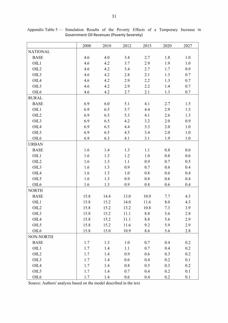
Appendix Table 5 — Simulation Results of the Poverty Effects of a Temporary Increase in Government Oil Revenues (Poverty Severety)
2008 2010 2012 2015 2020 2027
NATIONAL BASE 4.6 4.0 3.4 2.7 1.8 1.0 OIL1 4.6 4.2 3.7 2.9 1.9 1.0 OIL2 4.6 4.2 3.4 2.7 1.7 0.9 OIL3 4.6 4.2 2.8 2.1 1.3 0.7 OIL4 4.6 4.2 2.9 2.2 1.3 0.7 OIL5 4.6 4.2 2.9 2.2 1.4 0.7 OIL6 4.6 4.2 2.7 2.1 1.3 0.7
RURAL BASE 6.9 6.0 5.1 4.1 2.7 1.5 OIL1 6.9 6.5 5.7 4.4 2.9 1.5 OIL2 6.9 6.5 5.3 4.1 2.6 1.3 OIL3 6.9 6.5 4.2 3.2 2.0 0.9 OIL4 6.9 6.5 4.4 3.3 2.0 1.0 OIL5 6.9 6.5 4.5 3.4 2.0 1.0 OIL6 6.9 6.3 4.1 3.1 1.9 1.0
URBAN BASE 1.6 1.4 1.3 1.1 0.8 0.6 OIL1 1.6 1.3 1.2 1.0 0.8 0.6 OIL2 1.6 1.3 1.1 0.9 0.7 0.5 OIL3 1.6 1.3 0.9 0.7 0.6 0.4 OIL4 1.6 1.3 1.0 0.8 0.6 0.4 OIL5 1.6 1.3 0.9 0.8 0.6 0.4 OIL6 1.6 1.3 0.9 0.8 0.6 0.4
NORTH BASE 15.8 14.4 13.0 10.9 7.7 4.3 OIL1 15.8 15.2 14.0 11.6 8.0 4.3 OIL2 15.8 15.2 13.2 10.8 7.3 3.9 OIL3 15.8 15.2 11.1 8.8 5.6 2.8 OIL4 15.8 15.2 11.1 8.8 5.6 2.9 OIL5 15.8 15.2 11.6 9.2 5.9 2.9 OIL6 15.8 15.0 10.9 8.6 5.6 2.8
NON-NORTH BASE 1.7 1.3 1.0 0.7 0.4 0.2 OIL1 1.7 1.4 1.1 0.7 0.4 0.2 OIL2 1.7 1.4 0.9 0.6 0.3 0.2 OIL3 1.7 1.4 0.6 0.4 0.2 0.1 OIL4 1.7 1.4 0.8 0.5 0.3 0.2 OIL5 1.7 1.4 0.7 0.4 0.2 0.1 OIL6 1.7 1.4 0.6 0.4 0.2 0.1
Source: Authors' analysis based on the model described in the text