Oil refining in the EU in 2020, with perspectives to 2030

The oil companies’ European association for Environment, Health and Safety in refining and distribution

report no. 1/13

conservation of clean air and water in europe © CONCAWE

report no. 1/13

I

Oil refining in the EU in 2020, with perspectives to 2030

Prepared for the CONCAWE Refinery Management Group by its Refinery Technology Support Group:

F. Calzado Catalá (Chairman) R. Flores de la Fuente W. Gardzinski J. Kawula A. Hille A. Iglesias Lopez G. Lambert F. Leveque C. Lyde A.R.D. Mackenzie W. Mirabella A. Orejas Núñez R. Quiceno Gonzalez M.S. Reyes H.-D. Sinnen R. Sinnen K. de Vuyst A. Reid (Technical Coordinator) K.D. Rose (Technical Coordinator) M. Fredriksson (Consultant) Reproduction permitted with due acknowledgement

CONCAWE Brussels April 2013

report no. 1/13

II

ABSTRACT

In the two decades to 2030, the EU refining industry will face significant changes in product demand, both in absolute terms and with regard to the relative demand for gasoline and diesel. The introduction of increasingly stringent product quality specifications, notably regarding the sulphur content of marine fuels, will impose additional challenges on the ability of the industry to satisfy both demand and quality requirements. This report assesses the possible impact of these changes on EU refining, focusing on the estimated capital investment requirements in the sector as well as the expected trends in energy consumption and CO2 emissions through to 2030. Sensitivity cases are included to explore potential alternative scenarios for product demand and quality around the 2020 base scenario.

KEYWORDS

Demand, refined product, alternative fuels, refinery production, energy consumption, CO2 emissions, capital investment, diesel/gasoline ratio

INTERNET

This report is available as an Adobe pdf file on the CONCAWE website (www.concawe.org).

NOTE Considerable efforts have been made to assure the accuracy and reliability of the information contained in this publication. However, neither CONCAWE nor any company participating in CONCAWE can accept liability for any loss, damage or injury whatsoever resulting from the use of this information. This report does not necessarily represent the views of any company participating in CONCAWE.

report no. 1/13

III

CONTENTS Page

SUMMARY V

1. CONTEXT AND BACKGROUND 1

2. MODELLING METHODOLOGY 2 2.1. REFINERY CAPACITY EVOLUTION 2008-2015 3

3. CORE ASSUMPTIONS FOR EU OIL PRODUCTS: DEMAND, QUALITY AND FEEDSTOCK SUPPLY 7 3.1. BASE CASE 2008 7 3.2. PRODUCT QUALITY LEGISLATION 7 3.3. PRODUCT DEMAND INCLUDING BIOFUELS 9 3.3.1. Estimating road fuels demand with the “Fleet & Fuels” (F&F)

model 10 3.3.2. Estimating marine fuel demand 14 3.4. DEMAND FOR BIOFUELS AND OTHER RENEWABLES 17 3.5. DEMAND FOR REFINED PRODUCTS 19 3.6. EU CRUDE OIL SUPPLY 23 3.7. OTHER FEEDSTOCKS 24 3.8. PRODUCT IMPORTS/EXPORTS 25

4. FIXED DEMAND SCENARIO 27 4.1. REFINERY THROUGHPUT AND PRODUCTION 28 4.1.1. Refinery throughput compared to PRIMES 2011 scenarios for

EC Energy Roadmap 2050 31 4.2. PROCESS UNIT THROUGHPUT TRENDS 32 4.3. POTENTIAL INVESTMENT IN NEW PLANTS 35 4.4. SULPHUR REMOVAL AND HYDROGEN PRODUCTION

TRENDS 37 4.5. REFINERY ENERGY CONSUMPTION AND CO2

EMISSIONS 39 4.6. SENSITIVITY CASES 43 4.6.1. Refined road diesel to gasoline (D/G) demand ratio in 2020 43 4.6.2. On-board scrubbers to meet IMO specifications 48 4.6.3. Gasoline octane qualities in 2020 50 4.6.4. Jet fuel sulphur reduction in 2020 54 4.6.5. Road diesel poly-aromatic hydrocarbons (PAH) reduction in

2020 57 4.6.6. Heating oil sulphur reduction in 2020 60 4.6.7. Inland heavy fuel oil sulphur reduction in 2020 64 4.6.8. High biofuels 68 4.6.9. Reduced gasoline exports in 2020 73 4.6.10. Refinery energy efficiency improvements 76

5. LIMITED INVESTMENT SCENARIO 79

6. PETROCHEMICALS 85

7. COMPARISON WITH PREVIOUS STUDIES 88

8. CONCLUSIONS 91

9. GLOSSARY 92

report no. 1/13

IV

10. REFERENCES 95

APPENDIX 1 CONCAWE REFINING MODEL: MAJOR UNIT CAPACITIES 97

APPENDIX 2 REFERENCE PRICE SET 98

APPENDIX 3 PRODUCT QUALITY LEGISLATION AND QUALITY LIMIT TARGETS FOR MODELLING 99

APPENDIX 4 KEY INPUT ASSUMPTIONS FOR THE FLEET & FUELS (F&F) MODEL 101

APPENDIX 5 EU27+2 REFINING MODEL CRUDE QUANTITIES, SULPHUR CONTENTS AND LOWER HEATING VALUES 102

APPENDIX 6 DISTILLATE MARINE FUEL “DMA”SPECIFICATION 103

APPENDIX 7 EU-27+2 DEMAND, TRADE AND REFINERY PRODUCTION 104

APPENDIX 8 EU REFINING CAPACITY EXPANSIONS, PERMANENT CLOSURES, AND TEMPORARY CLOSURES (“IDLED” CAPACITY) BETWEEN 2009 AND 2015 105

APPENDIX 9 IMPACT OF ON-BOARD SCRUBBERS ON BUNKER TONNAGE, QUALITY AND CO2 EMISSIONS IN 2020 107

report no. 1/13

V

SUMMARY

This study evaluates the impacts of changes in product quality legislation and market demand on the EU refining industry from 2010 through to 2030. Although this subject was analysed up to 2020 in previous CONCAWE studies [10, 11], the present study extends the time horizon to 2030 and re-evaluates the refining impacts in the light of legislative measures to implement alternative fuels and improve vehicle efficiency, major changes to the future demand scenario and announced changes in refining capacities.

EU demand for refined products1 is in decline, caused in large part by legislative

mandates to increase the use of alternative fuels and improve vehicle efficiency. This results in a substantial decrease in refinery throughput, from 709 Mt in 2008 to 603 Mt in 2030. This fall in throughput corresponds to the combined capacity of the 6 largest EU refineries or the 30 smallest EU refineries. Almost half of this fall occurs in the short period from 2008 through 2010 and is attributable to the impact of the economic crisis on EU demand for oil products.

In contrast to the declining refining throughput, the fraction of light products shows a steady increase, driven by the declining demand for residual fuels in the inland market as well as in marine fuels. Another notable demand trend is the relentless increase of the middle distillate to gasoline demand ratio, driven by the declining demand for refined gasoline as the EU passenger car fleet becomes increasingly dieselised.

Modelling of EU refining using the CONCAWE refining model shows contrasting trends in refinery process unit throughputs over the 2008-2030 study period. On the one hand there is a trend towards severe under-utilisation of key refinery units such as Crude Distillation units (CDU), Reforming (REF) and Fluid Catalytic Cracking (FCC) units. On the other hand, there are substantial increases in throughputs of conversion units such as Distillate Hydrocracking (DHC), Coking (COK), Residue Desulphurisation (RES HDS) and Hydrogen production units (H2U), far exceeding their current capacity. It would require a major adaptation of EU refineries to completely accommodate these throughput trends, by investing in additional DHC, COK, RES HDS and H2U unit capacity while at the same time closing unused CDU, REF and FCC unit capacity.

Capital expenditure projects amounting to an estimated total of 30 G$2011 (21 G€2011)

2 have been announced for the 2009-2015 period to increase capacities of

EU refinery units that boost distillate production and reduce residue production. Conversely, significant capacity reductions have been announced in units that boost gasoline production and distil crude. The announced refining capacity additions are a major contribution to meeting future requirements. However, the additional equipment needs for marine fuel sulphur reduction in 2020 are not met by the announced capacity additions for COK and RES HDS units.

The cumulative refining investment required from 2008 to 2020 is estimated at 51 G$2011 (36 G€2011), excluding the costs incurred by refiners to achieve compliance

1 Throughout this report the term “refined products” and “refined fuels” refers to products and fuels produced by

refineries from fossil-based feeds. This distinction is particularly important when referring to road fuels demand, which can be satisfied by a combination of refined fuels and alternative fuels (biofuels, electricity, compressed natural gas, etc.).

2 Prices and costs are expressed in US$ in the model. The conversion to Euro in this report is based on an average 2011 exchange rate of 1.4 US$ per Euro. The SI symbol G is used throughout to signify billion (thousand million).

report no. 1/13

VI

with revised pollutant emission limit values under the terms of the Industrial Emissions Directive (IED). The majority of this capital expenditure is required to address the challenges imposed by the production of marine fuel to the new IMO sulphur specifications in 2015 and 2020.

Part of the cumulative refining investment of 51 G$2011 in 2020 is likely to be under-utilised by 2030 as a result of declining demand. The prospect of under-utilisation of added capacity is likely to have a negative influence on investment decisions prior to 2020, with the potential outcome that total cumulative investment in 2020 could fall short of 51 G$2011.

The specific energy requirement of EU refineries (expressed as energy consumed per tonne of feed) increases by 4% as more energy-intensive processing is required to satisfy the increasing demand for lighter and lower sulphur products. However, the total energy requirement decreases by 12% from 2008 to 2030, assuming no improvement in refinery energy efficiency.

Total CO2 emissions from EU refining are expected to grow by 8% over the 2008-2020 period to reach a peak of 163 Mt in 2020, in spite of the overall decrease in total refinery energy consumption. With the decline in refining throughput beyond 2020, total refining CO2 emissions will fall by 6% from the 2020 peak to 154 Mt in 2030.

SENSITIVITY CASES

The fixed demand scenario is founded on a set of base assumptions affecting refinery operation and trends in refined product demand and quality. The effects of alternative assumptions were explored in ten sensitivity cases summarised below. Only the maximum range of each sensitivity case is shown in Table 0.1 and Figure 0.1.

Table 0.1 Summary of sensitivity case results in the fixed demand scenario

Emissions Capital

CO2 Expenditure

Mt G$

1 D/G demand ratio 2.4 14.8Diesel/Gasoline demand ratio increased to 5.0 in 2020 (base case 2.8) due to

increased penetration of diesel passenger car sales to 90% (base case 50%)

2 On-board scrubbers -16.7 -19.1On-board scrubbers operate on 100% of vessels fuelling residual marine fuel at EU

ports in 2020 (base case 0%)

3 Gasoline octane 1.0 0.2 Finished product gasoline octane increased to 100 RON in 2020 (base case 97 RON)

4 Jet fuel sulphur 2.2 6.9 Sulphur content of Jet Fuel reduced to 10ppm in 2020 (base case 700ppm)

5 Diesel PAH 9.2 19.2 PAH content of road diesel reduced to 2% in 2020 (base case 8%)

6 Heating Oil sulphur 2.1 5.2 Sulphur content of Heating Oil reduced to 10ppm in 2020 (base case 1000ppm)

7 Inland HFO sulphur 9.5 13.1 Sulphur content of Inland Heavy Fuel Oil reduced to 0.1% in 2020 (base case 1.0%)

8 High biofuels (2030) -1.4 -0.5E20 blend introduced from 2020 (base case E10), increasing ethanol consumption by

60% in 2030

9 Low gasoline exports -6.6 -3.6 Gasoline exports to the US reduced to 0 Mt in 2020 (base case 22 Mt)

10 Energy efficiency -6.6 1.6 Refinery energy efficiency improved by 0.5% per year from 2008 (base case 0%)

Changes compared to

2020 base case (or

2030 in the high

biofuels case)

Case

numberCase description

report no. 1/13

VII

Figure 0.1 Changes in EU27+2 refinery emissions and refinery capital expenditure in each sensitivity case relative to the base case

Refined road diesel to gasoline (D/G) demand ratio in 2020

The main factor determining the diesel to gasoline (D/G) demand ratio reached in 2020 in the study base case was the assumed 50% penetration of diesel vehicles in new car sales in 2020. This sensitivity case explored the impact of alternative diesel penetration assumptions, all other things being equal. If diesel vehicles in new car sales in 2020 are higher than the 50% level assumed in the base case then the refining investment burden could increase by up to 15 G$ (in the case of 90% diesel in new car sales) and refining CO2 emissions could increase by up to 2.4 Mt, relative to the 2020 base case. Conversely, lower diesel penetration in 2020 new car sales would reduce refining investment requirements by up to 1.4 G$ (in the 10% case) and increase refining CO2 emissions by only 0.7 Mt. These estimated impacts assume that EU refining unit investments and throughputs are sufficient to exactly match refining production to the shifts in diesel and gasoline demand. If they are not sufficient then the demand shifts would need to be satisfied by increasing imports of diesel and exports of gasoline, incurring investments and CO2 emissions in refineries outside the EU.

On-board scrubbers to meet IMO specifications

IMO low sulphur marine fuel regulations allow for on-board exhaust gas scrubbing to be used to achieve the required emissions abatement while allowing the continued use of less expensive high sulphur marine fuel. The base case of the fixed demand scenario assumed that no ships will be equipped with on-board scrubbers. This sensitivity case explored the opposite extreme, assuming that 100% of ships affected by IMO marine fuel regulations are equipped with on-board scrubbers by 2020 and thereby obviating the need for refiners to reduce the sulphur content of marine fuel. The resulting reduction in required refining investment is estimated at 19 G$. Refining CO2 emissions are also reduced by about 17 Mt/a relative to the base case without scrubbers. This saving in refinery emissions far outweighs the additional 8 Mt/a of CO2 emissions from combustion of the fuel in the case with on-

-20

-15

-10

-5

0

5

10

15

20

D/G

dem

and

rat

io

On

-boa

rd s

cru

bbe

rs

Gas

olin

e o

ctan

e

Jet

fuel

su

lphu

r

Die

sel P

AH

He

atin

g O

il su

lph

ur

Inla

nd

HFO

su

lph

ur

Hig

h b

iofu

els

(203

0)

Low

gas

olin

e ex

port

s

Ener

gy e

ffic

ienc

y

1 2 3 4 5 6 7 8 9 10

Emissions CO2 Mt Capital Expenditure G$

report no. 1/13

VIII

board scrubbers, giving a net “well-to-propeller” advantage of 9 Mt/a of CO2 emissions for on-board scrubbers.

Gasoline octane qualities in 2020

This sensitivity examined two potential developments in 95RON gasoline octane number specifications in 2020 and assessed their impact on EU refining. In the first case, the model found that the removal of the Motor Octane Number (MON) specification would result in a small reduction in refining CO2 emissions (0.6 Mt/a) and a minor saving in operating costs (5 $/t gasoline). In the second case, an increase in the Research Octane Number (RON) of from 95 to 100 in 2020 could be achieved by the model with limited investment but it would incur increases in refining CO2 emissions (1.0 Mt/a) and operating costs (13 $/t gasoline). It should be borne in mind that the model achieves this 5 RON increase in finished gasoline after ethanol addition by increasing the RON of ethanol-free refined product gasoline by only about 3 RON, from 94 RON in the base case to 97 RON in the sensitivity case. The high octane contribution of ethanol raises the 97 RON refined product gasoline to 100 RON finished gasoline after ethanol addition. It should further be noted that potential additional closures of refineries or gasoline-producing process units would make the associated RON-boosting capacity of these units permanently unavailable, making the RON increase considerably more difficult and more costly than portrayed by the refining model.

Jet fuel sulphur reduction in 2020

Jet fuel sulphur reduction requires an increasing amount of processing by kerosene hydrotreating (KHT) units. This sensitivity case evaluated the additional refinery processing and investment that would be required to reduce jet fuel sulphur from the base case of 700ppm to 300ppm, 100ppm and 10ppm in 2020. The production of jet fuel in the 10ppm case would require an increase of 53 Mt in KHT unit throughput and 7 G$2011 of capital expenditure in additional unit capacity.

The annualised capital investment cost in the 10ppm sulphur case is estimated at 1.0 G$/a. Additional operating costs such as catalysts and chemicals, energy, maintenance and CO2 credits bring the total estimated incremental production cost for 10ppm jet to 1.9 G$/a or 28 $/t of Jet fuel sales in 2020.

Refinery CO2 emissions are estimated to increase by 1.3% to reach 10ppm sulphur compared to the 700ppm base case.

Road diesel poly-aromatic hydrocarbons (PAH) reduction in 2020

The hydrotreatment of road diesel to meet the current 10ppm sulphur limit also removes a sufficient proportion of poly-aromatic hydrocarbons (PAH) to achieve an EU average PAH content well within the current 8% maximum limit of the EN590 specification.

This sensitivity case indicated that reducing the PAH content to 2% by 2020 would require investment in hydrodearomatisation (HDA) units at an estimated annualised capital cost of 2.9 G$/a. Including other operating costs such as catalysts and chemicals, energy, maintenance and CO2 credits brings the total estimated incremental production cost to 5.5 G$/a or 0.019 EUR/l of road diesel. The increase in EU refining CO2 emissions is estimated at 5.6%.

report no. 1/13

IX

Heating oil sulphur reduction in 2020

The sulphur content of heating oil used in EU Member States is limited to 0.1% m/m (1000ppm) since 1 January 2008. A small number of EU countries have introduced lower limits (50ppm or 10ppm) to enable the use of high-efficiency condensation boilers. The capacity of hydrodesulphurisation (HDS) and distillate hydrocracking (DHC) units in EU refineries is used to its maximum possible extent in 2020 due to the increasing proportion of low sulphur distillate products in the total demand pool of refined products. An EU-wide reduction in heating oil sulphur content will therefore require investment in new or expanded HDS unit capacity in EU refineries.

This sensitivity case indicated that reducing the sulphur content of heating oil in 2020 to 50ppm would require additional capital investment of 4.4 G$ in desulphurisation and related refining unit capacity, adding 9% to the estimated total investment of 51 G$ in the 2020 base case. Heating oil production costs would increase by 27 $/t (0.017 EUR/l) and refining CO2 emissions would increase by 1.5 Mt (0.9%). Final use energy efficiency improvements could mitigate these effects to some extent by reducing the EU demand for heating oil, but it would take several years for these mitigating effects to materialise. A further reduction to 10ppm sulphur would impose significant additional costs and emissions with no compensating final use efficiency benefits compared to 50ppm.

Inland heavy fuel oil sulphur reduction in 2020

This sensitivity case evaluated the impact of a potential requirement to produce low sulphur inland heavy fuel oil (HFO) in 2020 to meet more stringent SOx emissions limits imposed on HFO consumers. A reduction in the sulphur content of inland HFO can only be achieved by processing the “straight-run” residue blend components in residue hydrodesulphurisation (RES HDS) units. The capacity of RES HDS units is already used to its maximum possible extent in 2020 due to the reduction of the sulphur content of residual marine fuel to 0.5%. Any further reduction in HFO sulphur content will therefore require investment in new or expanded RES HDS unit capacity in EU refineries.

Reducing the inland HFO sulphur content to the same level as heating oil (0.1% sulphur) by 2020 would require capital expenditure of about 13 G$ in additional desulphurisation and related refining unit capacity, adding 25% to the estimated total investment of 51 G$ in the 2020 base case. Inland HFO production costs would increase by 329 $/t and refining CO2 emissions would increase by 9.5 Mt (6%). This level of refinery expenditure and the accompanying increase in HFO production costs are unlikely to be economically justifiable in comparison with the alternative options available to HFO consumers, such as the installation of flue gas desulphurisation equipment or substitution of HFO by natural gas.

High biofuels

The high biofuels sensitivity case assumed the introduction of an E20 grade in 2020, causing the total ethanol content of gasoline E grades (excluding E85) to increase to 17%v/v by 2030 compared to 9%v/v in the base case, and reducing refinery gasoline production by 3% in 2030 . This has a relatively minor effect on EU refining in the period 2020-2030. The resultant decrease in refinery throughput and processing intensity leads to a 0.9% reduction in CO2 emissions and a 1.1% reduction in investments in 2030 compared to the base case.

report no. 1/13

X

Reduced gasoline exports in 2020

EU gasoline production exceeded demand by 43 Mt in 2008, according to Eurostat statistics. The main importer of EU gasoline is the US, at about 22 Mt in 2008, but forecasts by industry analysts such as Wood Mackenzie point to a rapid decline in US gasoline imports by 2020.

This sensitivity case evaluates the possible effect of the elimination of the US gasoline deficit by 2020, without any compensating increase in gasoline imports in other regions of the world. This could lead to a decrease in EU refinery throughput of 24 Mt, equivalent to the total throughput of 3 average-sized EU refineries. The refinery utilisation rate would fall by almost 4% on average, but the actual reductions in utilisation rate would vary widely between refineries. Diesel-oriented refineries with DHC and/or COK units should be able to maintain maximum utilisation while gasoline-oriented FCC refineries would see reductions in utilisation rate significantly higher than 4%, leading to reduced operating margins which could threaten the economic viability of some sites.

Refinery energy efficiency improvements

The study base case assumed no improvement in refinery energy efficiency from 2008 to 2030. This sensitivity case evaluated the impact of an assumed continuation of the historic refinery energy efficiency improvement trend of about 0.5% per year. This is shown to mitigate the increases in refining energy intensity and, to a lesser extent, CO2 emissions intensity resulting from the growing diesel to gasoline demand ratio and more stringent marine fuel sulphur limits. In spite of these potential energy efficiency improvements, the 2020 peak in CO2 emissions would still be 5 Mt higher than the 2008 base case.

LIMITED INVESTMENT SCENARIO

This scenario estimated the changes in imports and exports and refinery throughputs that would result if EU refinery unit investments were limited to the 30 G$ of announced projects in the 2009-2015 period.

The announced projects appear to adequately equip EU refining with the appropriate conversion unit capacity to satisfy the product demand and quality changes up to 2020 while maintaining the import/export quantities unchanged, with the notable exception of the IMO marine fuel sulphur reduction to 0.5%. Without further investment beyond 2015, the available conversion and desulphurisation capacity would permit the production of only 10% of the estimated demand for low sulphur marine fuel in 2020 without increasing EU dependence on imported diesel. If EU refining were required to produce 100% of the 2020 demand for low sulphur marine fuel in this limited investment scenario it would incur a four-fold increase in imported diesel and a 10% decrease in EU refining capacity utilisation, reaching 71% in 2020. This is significantly lower than the typical utilisation rates of 84-86% seen in the 2000-2008 period and would create unsustainable conditions that would present severe challenges for the EU refining industry.

PETROCHEMICALS

Although the annual EU propylene demand only increases by 2.5% over the 2010-2015 period, steam crackers and other associated technologies (e.g. metathesis and propane dehydrogenation) will be expected to increase annual production by 10% to compensate for declining propylene production from refinery FCC units,

report no. 1/13

XI

which currently provide about 30% of the total EU demand. Existing EU steam cracker capacity is considered sufficient to meet the additional olefins demand.

BTX (benzene, toluene, and xylene) demand in the EU is expected to grow at an average of about 0.9%pa from 2010 through to 2030, dominated by strong growth in demand for xylenes. Almost half the demand for BTX is currently met by production from refinery Reforming units with BTX extraction and this proportion is expected to grow slightly through to 2030. About two-thirds of the 3 Mt increase in BTX demand over the 2010-2030 period is expected to be supplied by additional extraction of BTX from refinery reformate, requiring increases in refinery BTX extraction capacity, which are included in the refinery investment figures in all the modelled scenarios and sensitivity cases.

report no. 1/13

1

1. CONTEXT AND BACKGROUND

In the first two decades of the 21st century the European refining industry is under

growing pressure to adapt to major changes in product quality legislation and market demand. Product quality pressure is mainly focussed on reducing the sulphur content of refined fuels, while the main sources of market demand pressure are the steadily growing demand for jet fuel and diesel road fuel (at the expense of declining gasoline demand), the growing share of alternative road fuels (at the expense of refined road fuels) and the declining demand for heavy fuel oils (partly in response to legislative pressure to reduce air pollutant emissions and partly due to competition from natural gas).

Almost all EU refineries have already invested in new or expanded desulphurisation unit capacity to satisfy the new 10ppm sulphur limit for road fuels. Many refineries have also taken steps to redress the growing imbalance between refinery production of diesel and gasoline and the EU market demand. However, further adaptation will be called for in this decade to meet more stringent sulphur limits on marine fuels in an environment of declining market demand for refined products.

CONCAWE routinely monitors and evaluates the major factors affecting the EU refining industry. The CONCAWE Refinery Technology Support Group (RTSG) has conducted several studies evaluating the potential impacts on the refining industry of the legislative and market challenges affecting refined fuel qualities and quantities. The most recent studies were published in 2008 and 2009 (CONCAWE Reports 8/08 [10] and 3/09 [11]) and investigated the impact of quality and demand changes up to 2020. These studies were based on information available at the time and showed optimistic prospects for future growth in the demand for refined products.

The reality of the years since the 2008/2009 studies has diverged markedly from the forecasts in many respects. Major economic events, combined with legislative mandates for improved vehicle efficiencies and increased use of alternative fuels, have radically changed the market demand picture for refined products in both the short-term and the long-term. In addition, refinery restructuring and investments have accelerated at an unprecedented pace, having both negative and positive effects on the industry’s ability to respond to this changing environment.

The present study re-evaluates the impacts on the EU refining industry in the context of the changed demand scenario and the announced changes in refining capacities. The study horizon is extended to 2030 to show the continuing effects of market demand pressures beyond 2020 and also to allow for comparison with the demand projections of the EU Roadmap 2050 [5]. Alternative outcomes at the 2020 horizon are also explored, assessing the impact of different (unlegislated) product quality requirements, further reductions in refined gasoline demand and limited levels of further refining investment.

report no. 1/13

2

2. MODELLING METHODOLOGY

The study was carried out with the CONCAWE EU-wide refining model which uses the linear programming technique to simulate the whole of the European refining industry, encompassing the EU-27 members, plus Norway and Switzerland. The modelling of Europe is segmented into 9 regions, as shown in Table 2.1, each of which is represented by a composite refinery having the combined processing capacity of all the refineries in the region as well as the complete product demand slate relevant to the region. Details of model capacities by region for major conversion units are given in Appendix 1. Some blending streams and some finished product can be transported at a cost from one region to another to simulate real transport links.

Table 2.1 The 9 regions of the CONCAWE EU refining model (EU-27+2)

The model is fed with crude and feedstock representing the expected quality of the European crude slate as well as the imports of feedstocks such as gasoil, kerosene and natural gas. Europe has a structural shortage of distillate products and an excess of gasoline products. This is represented by allowing imports of gas oil and kerosene as well as exports of gasoline, initially fixed at a typical level close to the real trade figures in 2008. It is generally accepted that the biggest importer of EU gasoline, the US, is likely to significantly reduce its imports in this decade due to improved vehicle efficiency and higher penetration of biofuels. This study addresses this eventuality with a sensitivity case in which gasoline exports to the US trend to zero by 2020, compared to about 22 Mt in 2008.

The quality of the crude processed in EU refineries is represented by a mix of 6 model crudes. The crude mix composition is set to reflect the overall quality of crude entering the European system. It remains unchanged in all cases while the total quantity of crude varies as a direct function of the market demand for finished products.

The model was allowed to optimise the distribution of the crude and feedstock imports and gasoline exports among the 9 regions according to the refining capacity and market demand in each region.

The optimisation of the EU refining system is treated by the model as a cost minimisation problem. Prices are fixed in US dollars for all inputs and outputs as shown in Appendix 2. Operating costs per tonne of unit throughput are factored

Region Code Countries (1)

kbbl/sd Mt/a (2)

% of total

Baltic A Denmark, Finland, Norway, Sweden, Estonia, Latvia, Lithuania 1421 66 9%

Benelux B Belgium, Netherlands, Luxembourg 2083 97 13%

Germany C Germany 2436 113 15%

Central Europe D Austria, Switzerland, Czech, Hungary, Poland, Slovakia 1312 61 8%

UK & Ireland E United Kingdom, Ireland 1839 86 11%

France F France 2045 95 13%

Iberia G Spain, Portugal 1699 79 10%

Mediterranean H Italy, Greece, Slovenia, Malta, Cyprus 2895 135 18%

South East Europe J Bulgaria, Romania 595 28 4%

Total 16325 760 100%(1)

Countries in italic have no refineries(2)

Indicative number based on a notional 340 operating days per year and 7.3 bbl per tonne

Total primary distillation capacity

2008

report no. 1/13

3

from the capital cost of new process units, with the addition of catalyst costs where relevant. CO2 emissions incur a cost of 40 $/t CO2 (about 29 €/t).

The market demand for each fuel product in each region was translated into its energy equivalent and the model was constrained to satisfy the regional demand for each product in energy terms. This meant that if the energy content of a product changed between cases as a result of re-optimisation of its blend composition or changes to product specifications (e.g. reduced sulphur content), the product quantity in tonnes was adjusted such that the total energy requirement remained fixed. Furthermore, as the model is carbon and hydrogen balanced, it was possible to monitor changes in CO2 emissions due to changes in product specifications, even when the market demand remained unchanged.

The production of fossil-based gasoline and diesel by the European refining system has been adjusted to account for the amount of biofuel that is expected to be incorporated in fuels. In the case of gasoline and diesel the product qualities of the fossil portion were adjusted to reflect the level of ethanol and FAME in the final product, assuming that the current EN228 and EN590 specifications would apply to the final products.

The model includes a representation of the European chemical steam cracker industry with olefins and aromatics recovery in addition to traditional fuel refining process units, thereby reflecting the important interaction between refineries and petrochemical complexes. This means that some chemical feedstock streams produced by refining (e.g. naphtha) are consumed by the chemical industry and do not feature as product.

In this study two different approaches were used in running the refining model for each of the two scenarios studied:

Fixed Demand scenario: The objective of this scenario was to estimate unit investment and throughput requirements and resultant CO2 emissions incurred in meeting product demand without changing the import/export balance. All product quantities were fixed in energy terms, except sulphur. Import quantities were fixed but crude and residue quantities were allowed to float while maintaining the same composition. Process unit capacities were set at the 2008 starting point plus or minus any known expansion or closure projects in the 2009-2015 period. The model was allowed to purchase additional process unit capacity if required to meet the fixed product demand, incurring capital costs based on periodically published typical installed costs and construction cost indices of new units.

Limited Investment scenario: The objective of this scenario was to estimate the changes in imports and exports and refinery throughputs that would result if unit investments were limited to the known expansion or closure projects. Product and import/export quantities were fixed in the same way as the fixed demand scenario but some flexibility was allowed to vary the quantities of diesel imports, gasoline exports and low/high sulphur residual marine fuel. Process unit capacities were set in the same way as the fixed demand scenario but the model was not allowed to purchase additional process unit capacity.

2.1. REFINERY CAPACITY EVOLUTION 2008-2015

Refiners are responding to the changing demand and quality requirements of the refined products market by making selective capital investments or divestments.

report no. 1/13

4

Investments in European refineries are currently aimed at building new process units such as Distillate Hydrocrackers (DHC), Residue Hydrocrackers (RHC), Diesel Hydrodesulphurisation (HDS) and Coking (COK) units that increase the ability of existing refineries to produce clean distillate products (jet fuel and diesel) and reduce the production of heavy fuel oil. Since these units consume hydrogen (with the exception of Coking), investment in new or expanded hydrogen production unit (H2U) capacity is usually needed as part of new process unit projects. In parallel with this drive to invest in new process unit capacity, the declining EU market demand for refined products and for gasoline in particular is driving some refiners to respond by closing smaller, low-margin refineries and/or closing gasoline-producing Fluid Catalytic Cracking (FCC) units in larger refineries.

The 32 most important announced EU refining expansion/closure projects in the 2009-2015 timeframe are detailed in Appendix 8 and summarised in Figure 2.1.1 and Figure 2.1.2. The majority of the projects are already completed or are due for completion in 2012, with only two due for completion in 2014 and 2015.

Figure 2.1.1 Refining process unit1 capacity additions and reductions (Mt/a)

(Source: CONCAWE/Wood Mackenzie)

1 CDU=Crude Distillation Unit, VDU=Vacuum Distillation Unit, REF=Reforming unit, DHC=Distillate Hydrocracker,

RHC=Residue Hydrocracker, FCC=Fluid Catalytic Cracker, COK=Coker, HDS=Diesel Hydrodesulphurisation, VIS=Visbreaking, H2U=Hydrogen production (steam reforming unit). Note that H2U capacity additions are shown as Mt/a x 10, the actual H2U capacity addition being 0.7 Mt/a hydrogen.

-40

-30

-20

-10

0

10

20

CDU VDU REF DHC RHC FCC COK VIS HDS H2U(Mt/a

x10)

Cap

acit

y ch

ange

(M

t/a)

EU27+2 Refinery Projects 2009-2015Capacity change by process unit versus year-end 2008

Capacity additions

Capacity reductions

Net change

report no. 1/13

5

Figure 2.1.2 Refining process unit capacity additions and reductions (%) (Source: CONCAWE/Wood Mackenzie)

The known capacity additions for major process units amount to a total of 83 Mt, of which expansion projects in Spain account for 34 Mt or almost 40%. The biggest percentage increases in capacity are in Hydrogen, RHC and Coking units, at 47%, 38% and 35% respectively relative to 2008. Three of the five Coking unit projects are in Spain, where 79% of the additional EU Coking capacity is built. Investment in new or revamped DHC units results in 18 Mt of additional DHC capacity, a 28% increase on the 2008 year-end total DHC capacity.

The known capacity reductions reach a total of 70 Mt of major process units capacity and affect eight refineries, of which six are permanent closures

2 (two in

France, one in UK, one in Germany, one in Italy and one in Romania) and two are partial closures (one in France and one in Romania). Although these reductions are significant in terms of crude distillation unit (CDU) and FCC unit capacity (36 Mt/a and 8 Mt/a respectively), they represent only a small percentage reduction (5% and 6% respectively). Much of the reduction in CDU capacity is offset by 19 Mt of CDU capacity expansion projects, mostly in Spain, Greece and Poland.

Only the “known” or “firm” capacity changes announced before May 2012 were built into the refining model as adjustments to the baseline available capacity in the model runs. In the “Limited Investment” scenario, the unit capacities were capped at this adjusted baseline including known investments/closures and the model was not allowed to purchase additional capacity.

It should be noted that these “known” or “firm” refinery closures included in the model baseline capacity do not take into account nine additional refineries listed in

2 This is the status of the closure projects at end-April 2012. Three additional closures were announced in May and

September 2012 (TotalErg Rome, Petroplus Coryton and ENI Porto Marghera), bringing the total to nine permanent closures representing 104 Mt of major process unit capacity.

-10%

0%

10%

20%

30%

40%

50%

CDU VDU REF DHC RHC FCC COK VIS HDS H2U

Cap

acit

y ch

ange

(%

)

EU27+2 Refinery Projects 2009-2015Capacity change by process unit versus year-end 2008

Capacity additionsCapacity reductionsNet change

report no. 1/13

6

Appendix 8 that have been temporarily closed (“idled”) or severely cut back in 2011-2012 due to adverse economic conditions. The future of these refineries is uncertain. Some may resume refining operations while others may be permanently closed or converted to storage terminals. In the worst-case scenario, the permanent closure of these refineries would more than double the CDU and FCC capacity reductions in the 2009-2015 period, reaching a total of 12% compared to the 2008 year-end total CDU and FCC capacity of EU27+2 refineries.

In summary, the most significant increases in EU refining capacity in the 2009-2015 period are in units that boost distillate production (18 Mt of additional DHC capacity) and reduce residue production (12 Mt total additional RHC and COK capacity), while the most significant capacity reductions are in units that boost gasoline production (8 Mt of closed FCC capacity) and distil crude (36 Mt of closed CDU capacity). The CDU and FCC capacity reductions could more than double if the nine refineries temporarily closed in 2011-2012 are not restarted.

report no. 1/13

7

3. CORE ASSUMPTIONS FOR EU OIL PRODUCTS: DEMAND, QUALITY AND FEEDSTOCK SUPPLY

3.1. BASE CASE 2008

The year 2008 was used as the starting point for the refining study. A complete set of EU product demand data was available for this year, which provided a sound basis for the calibration of the CONCAWE refining model (see Appendix 7 for demand and production details). In addition, the model CO2 emissions could be compared and adjusted against a complete set of verified refinery CO2 emissions data collected by CONCAWE to determine the EU ETS refining benchmark. The total verified CO2 emissions from refineries in EU27 and Norway for 2008 amounted to 150.2 Mt, including emissions associated with net imports of electricity and heat. The calibrated EU27+2 refining model gave CO2 emissions of 151.4 Mt for 2008, including estimated emissions for the two Swiss refineries.

3.2. PRODUCT QUALITY LEGISLATION

The introduction of sulphur-free road fuels (<10ppm sulphur) in 2009 was the culmination of the major EU-legislated changes to the quality of road fuels introduced over the past 15 years. At this stage, no further changes are foreseen for the sulphur content of road fuels and the focus is moving towards sulphur reduction in marine and non-road fuels.

Appendix 3, Table A3.1 shows the chronological sequence of specification changes of various fuel products from 1995 through to 2025 as implied by enacted or proposed legislation.

“Fuels Quality Directive” (FQD)

The various dispositions of Directive 98/70/EC promulgated as a result of the first Auto-Oil programme came into force between 2000 and 2005 affecting road fuels. The second Auto-Oil programme resulted in a first revision, including the introduction of sulphur-free road fuels (<10 ppm). The final version of the FQD, adopted as Directive 2009/30/EC, included further limits on road fuels, non-road mobile machinery fuels and inland waterways fuels. A review of the FQD expected in 2014 may result in revised limits on certain qualities of road and non-road fuels. The potential impacts of such revisions are examined as sensitivity cases in this study (see further in Sections 4.7.3 and 4.7.5).

“Sulphur in Liquid Fuels Directive” (SLFD)

Directive 1999/32/EC affects heating oil, industrial gasoils, inland heavy fuel oils and marine fuels. The amendment in Directive 2005/33/EC includes specific limits on the sulphur content of marine fuels and the amendment in Directive 2009/30/EC includes sulphur limits on gasoil used in inland waterways.

“European Industrial Emissions Directive” (IED)

Directive 2010/75/EU provides for Emissions Limit Values (ELVs) to be set for SO2, NOx and particulate matter from boilers and furnaces, based on Best Available Techniques (BAT). Current proposals for SO2 emissions limits suggest that compliance with the IED will require the sulphur content of heavy fuel oil supplied to consumers such as power plants to be reduced to between 0.2% and 0.5% by 2016.

report no. 1/13

8

Heavy fuel oil consumers would need to install flue gas desulphurisation equipment to be permitted to burn fuel with a higher sulphur content.

Marine fuels legislation (IMO)

The sulphur content of marine fuels is regulated on a worldwide basis through the International Maritime Organisation (IMO). An agreement under the International Convention for the Prevention of Pollution from Ships (MARPOL), known as MARPOL Annex VI, introduced a global sulphur content cap of 4.5% m/m from May 2005. It also introduced the concept of Emission Control Areas (ECAs) which are designated sea areas where ship sulphur emissions are consistent with a fuel having a maximum sulphur content of 1.5% m/m. The Baltic and North Sea have been designated as ECAs. Following its ratification in 2005, MARPOL Annex VI came into force as of May 2006 for the Baltic Sea and November 2007 for the North Sea. A revision process of that legislation was initiated by IMO’s Marine Environment Protection Committee (MEPC) in July 2005.

In addition, the EU adopted Directive 2005/33/EC regarding the sulphur content of marine fuels which extends the IMO 1.5% m/m sulphur limit to “passenger ships on a regular service to or from an EU port” (further referred to as “ferries”) and came into effect in August 2006.

In October 2008 the IMO’s MEPC adopted a proposal to decrease the maximum sulphur content in ECAs to 1.0% by July 2010 and 0.1% by 2015 and to decrease the global marine fuels sulphur cap to 3.5% by 2012 and down to 0.5% by 2020 or 2025 at the latest (subject to a review in 2018). In July 2011 the EC proposed a draft amendment to Directive 2005/33/EC which would align the Directive with the stricter IMO rules and extend the ECA sulphur reduction schedule to non-ECA “ferries” with a 5 year delay. The compromise amendment adopted by the European Parliament in September 2012 confirmed the sulphur reduction to 0.5% by 2020 in EU waters but did not include the extension of the ECA sulphur limits to non-ECA ferries. Fuel used by non-ECA ferries is therefore subject to the same sulphur content limits as all other non-ECA vessels when operating in EU waters, i.e. 3.5% in 2012 and 0.5% from 2020.

The above limits on sulphur content apply equally to residual marine fuels (RMF) and distillate marine fuels (DMF). However, the EU “SLFD” Directive 1999/32/EC imposes an additional requirement on the latter category, limiting the maximum sulphur content to 0.1% m/m for marine gas oils (MGO) used in EU territory from 1 January 2008. Directive 2005/33/EC extended this 0.1% limit to MGO placed on the market in EU Member States’ territory from 1 January 2010. Marine gas oils correspond to the lighter DMX and DMA grades (density 890 kg/m

3 @15°C) in the

ISO 8217:2010 distillate marine fuels specifications, as opposed to marine diesel oils (MDO) which correspond to the heavier DMB grade (density 900 kg/m

3 @15°C).

Statistics are not available on the relative shares of MGO and MDO in the EU DMF market but CONCAWE member company estimates suggest that MGO constitutes more than 90% of the DMF market. For this reason all DMF production in this study was assumed to be MGO (DMA grade) subject to a sulphur limit of 0.1% from 2008 onwards.

It should be noted that, outside the ECAs, the IMO cap reduction proposal and the Directive do not directly mandate the indicated fuel sulphur content but rather emissions consistent with these sulphur contents. This therefore leaves open the possibility to use on-board scrubbers, a number of which have been developed to

report no. 1/13

9

full scale demonstration stage. This study considers the fuel sulphur reduction option as the base case, and examines on-board scrubbers as a sensitivity case.

No significant quality changes are foreseen for other products in current EU legislation. This includes jet fuel, the maximum sulphur content of which is assumed to remain at 0.3% m/m over the entire period. However, the effects of additional quality changes are examined in selected sensitivity cases, as discussed in Section 4.7. Appendix 3 Table A3.2 shows the detail of the specifications and corresponding quality targets used in the model, the difference representing the usual level of operating quality margins that refineries have to use in order to ensure on-spec products.

3.3. PRODUCT DEMAND INCLUDING BIOFUELS

European petroleum product demand is shaped by three main trends:

Declining total demand,

Gradual erosion of demand for heavy fuels and concomitant development of markets for light products,

Within the light products market, a steady increase of demand for “middle distillates” particularly automotive diesel and jet fuel, and a corresponding decrease of motor gasoline demand.

These trends are largely expected to continue as illustrated in Figure 3.3.1 (a more comprehensive table is also included in Appendix 7). The first of these trends has been accentuated by the current economic crisis. Overall demand growth in the EU27+2 is expected to be essentially flat through to 2015, and then become increasingly negative in the period to 2030, as improvements in new car fuel economy spread through the entire fleet.

Figure 3.3.1 EU27+2 petroleum product demand evolution 2000-2030 (Mt/a) (“Petrochemicals” includes light olefins and aromatics)

320 353339 365 374 367 356

132116

88 80 7363

56

694720

641 638 629605

583

0

100

200

300

400

500

600

700

800

2000 2005 2010 2015 2020 2025 2030

LPG

Gasoline

Petrochemicals

Middle distillates

Residual marine fuel

Residual inland fuel

Others

Source: Wood Mackenzie, CONCAWE

Total demandincluding biofuels

in EU27 + 2(Mt/a)

Source: Wood Mackenzie, CONCAWE

Total demandincluding biofuels

in EU27 + 2(Mt/a)

report no. 1/13

10

The trend towards a higher fraction of light products in the overall demand slate is best illustrated in terms of the percentage of each product type, as shown in Figure 3.3.2, which also shows the historic and predicted steady increase of the ratio between middle distillates and gasoline demand. This increasing trend is primarily the result of a steady erosion of gasoline demand, reflecting the continuing dieselisation of the passenger car fleet and the steadily improving fuel economy of gasoline vehicles.

Figure 3.3.2 EU27+2 petroleum product demand evolution 2000-2030 (%) (“Petrochemicals” includes light olefins and aromatics)

These demand trends are based on data from Wood Mackenzie (July 2011) [1], with the exception of the gasoline and road diesel demand trends which were estimated by CONCAWE using a bottom-up model of the EU vehicle fleet, called the “Fleet & Fuels” (F&F) model.

3.3.1. Estimating road fuels demand with the “Fleet & Fuels” (F&F) model

The Fleet and Fuels (F&F) model is a simulation tool developed as a cooperative effort by the JEC consortium (JRC-EUCAR-CONCAWE). It was used to evaluate scenarios for vehicle fleet development and penetration of alternative fuel types, including biofuels, in EU27+2 (Norway and Switzerland), the resulting demand for fossil fuels and alternative fuels up to 2020 and the corresponding level of achievement of the EU mandatory targets for renewable energy and greenhouse gas emissions savings in transport. The results were published in a JRC report [4] released in May 2011. The modelling was extended to 2030 by CONCAWE for the purposes of this EU refining study.

The key assumptions used in the F&F model are summarised in Appendix 4, Table A4.1.

A key input parameter in the F&F model is the evolution of new passenger car CO2 emissions, which are assumed to improve by 4.0%/year from 2010 to meet the 2020 target of 95 gCO2/km set by EC Regulation 443/2009. A reduced improvement rate

46% 49% 53% 57% 59% 61% 61%

19% 16% 14% 13% 12% 10% 10%

0.0

1.0

2.0

3.0

4.0

5.0

6.0

7.0

0%

10%

20%

30%

40%

50%

60%

70%

80%

90%

100%

2000 2005 2010 2015 2020 2025 2030

Mid

dle

dis

tillate

/ G

aso

lin

e d

em

an

d r

ati

o

LPG

Gasoline

Petrochemicals

Middle distillates

Residual marinefuelResidual inlandfuelOthers

MD/Gasoline ratio(RH axis)

Source: Wood Mackenzie, CONCAWE

Total demandincluding biofuels

in EU27 + 2(% m/m)

Source: Wood Mackenzie, CONCAWE

report no. 1/13

11

of 2.3%/year is assumed for 2020-2030, reaching 75 gCO2/km in 2030. Since these are NEDC test cycle emission figures, a “real-world factor” of 1.10 is applied in the F&F model to estimate the actual consumption of road fuels.

Another important input assumption is the evolution of the share of diesel vehicles in new car sales. It was assumed in the 2011 JEC Biofuels Study [4] that the increased cost of NOx abatement on diesel cars and improvements in gasoline engine efficiency would slow the growth in diesel penetration in the coming years, reaching a ceiling at 50% of conventional new car sales in 2020 (compared to 49% in 2010). CONCAWE extended this assumption of 50% diesel in conventional new car sales to 2030. Under this assumption, the overall share of gasoline vehicles in the conventional car fleet continues to decline from the 2010 level of 63% down to 52% in 2020 and bottoming out at 50% in 2030. Other plausible scenarios for the evolution of diesel vehicle penetration can be postulated, including scenarios in which there is a swing in consumer preference back to gasoline vehicles. It is important to note that the effect of such a swing in new car sales would take many years to have a material effect on the overall fleet and on road fuels demand. The demand ratio of diesel to gasoline fuel would continue to grow, albeit at a slower rate. The decline in total road fuels demand would be virtually unaffected, since this is driven by the CO2 emissions targets for the total new car fleet.

Alternative fuel vehicles are assumed to make up an increasing share of passenger car sales, reaching 10% in 2020 (5.6% of the car fleet) and 15% in 2030 (11.5% of the car fleet). Figure 3.3.1.1 shows the levels of penetration assumed for each type of alternative vehicle. The 2020 levels were agreed in consultation with EUCAR and the JRC for the 2011 JEC Biofuels Study [4] (which is under revision in 2013) while the 2030 levels were estimated by CONCAWE.

Figure 3.3.1.1 Penetration of alternative passenger car fuel types in the F&F model base case

The penetration levels assumed for electric vehicles (EVs) are in the middle of the range of milestones set by ERTRAC in the recently published 2

nd edition of the

Electrification of Road Transport report (2012) [6]. The ERTRAC milestones

0%

1%

2%

3%

4%

5%

6%

%sales %fleet %sales %fleet %sales %fleet %sales %fleet

Flex Fuel Vehicles CNG Vehicles LPG Vehicles Electric Vehicles(Battery EVs and

Plug-in HybridEVs)

% o

f p

asse

nge

r ca

rs

2010 2020 2030

report no. 1/13

12

represent a range between a lower bound scenario of “evolutionary development” and an upper bound scenario “reaching the major technological breakthroughs” and indicate accumulated numbers of EVs on European roads of between 1 and 5 million by 2020 and between 3 and 15 million by 2025. Under the F&F model assumptions for sales of EVs (3% in 2020 in the 2011 JEC Biofuels study, extended by CONCAWE to 4.5% in 2025 and 6% in 2030) the accumulated number of EVs reaches 2.8 million by 2020 and 6.8 million by 2025. In order to reach the upper bound of the ERTRAC milestones, the EV sales assumptions would need to be increased to 8.5% in 2020 and 10.8% in 2025.

The assumed level of penetration of CNG vehicles by 2020 (6 million vehicles or 2.0% of the total vehicle fleet) results in a 1.5% energy share of CNG in road transport by 2020, which is modest compared to the possible vehicle fleet share of 5% (15 million vehicles) proposed by the European Expert Group on Future Transport Fuels in January 2011 [7]. The total fleet of CNG vehicles is assumed to continue growing after 2020, reaching 13 million vehicles or 4.0% of the total vehicle fleet by 2030. Although this remains low compared to the total market share of 9% by 2030 quoted in the June 2012 IGU report on Natural Gas Vehicles [8], it nevertheless corresponds to 7 Mtoe of CNG consumed in road transport in 2030, representing 2.8% of the total energy in EU road fuels.

The effects of these assumed trends in the EU vehicle fleet on the relative demand for gasoline and diesel road fuels are illustrated in Figure 3.3.1.2. Total annual demand for gasoline and diesel road fuels declines by almost 50 Mt (17%) from 2005 to 2030, in spite of an increase in the total vehicle fleet. The decrease in energy use of passenger cars is even higher, falling by 36% between 2005 and 2030 whereas the energy use of heavy duty road transport (including vans) increases by 9%. The ratio of diesel to gasoline demand steadily increases, in line with the increasing share of diesel vehicles in the passenger vehicle fleet and the steady growth of heavy duty road transport.

report no. 1/13

13

Figure 3.3.1.2 Demand for gasoline and diesel road fuels in EU27+2, including biofuels

It should be noted that the 2005-2030 decrease of 17% in total road fuel energy use estimated by the F&F Model is considerably more severe than the decrease of 1% in the PRIMES “EU27: Current Policy Initiatives” scenario of the EU Energy Roadmap 2050 [5], which is split between a 12% decrease in energy use for passenger cars and a 17% increase for trucks and public road transport. However, the F&F Model results are relatively close to the PRIMES “EU27: Energy Efficiency” scenario which shows a total decrease in road fuel energy use of 14% between 2005 and 2030, split between a 29% decrease for passenger cars and a 10% increase for trucks and public road transport. The comparison between the F&F Model outcomes and the PRIMES “EU27: Energy Efficiency” scenario is shown in Figure 3.3.1.3. The PRIMES energy use figures for passenger cars are consistently higher than the F&F model results and consistently lower for trucks and public road transport. This would lead to a higher demand for gasoline and a lower demand for road diesel in PRIMES compared to the F&F model outcomes.

0.0

0.5

1.0

1.5

2.0

2.5

3.0

3.5

0

50

100

150

200

250

300

2005 2010 2020 2030

Die

sel /

Gas

olin

e d

eman

d ra

tio

Ro

ad fu

el d

eman

d (M

t/a)

CNG

Total Diesel (fossil+FAME+HVO+BTL)

LPG

Total Gasoline (fossil+EtOH)

Diesel to Gasoline ratio, incl. biofuels

report no. 1/13

14

Figure 3.3.1.3 Comparison between the F&F Model outcomes and the PRIMES “EU27: Energy Efficiency” (2011) scenario.

3.3.2. Estimating marine fuel demand

An important new factor that will come into play in the coming decade is the implementation of IMO and EU regulations requiring 0.1% sulphur marine fuel to be used in ECA areas and for EU ferries. This will entail a shift from residual to distillate marine bunkers, accentuating the erosion of heavy fuel demand and the increase in demand for distillate fuels.

Evaluation of the impact of marine fuel legislation requires estimating regional demand volumes for the various fuel grades, including demand in ECAs as well as additional demand for “ferries”.

Demand for bunker fuel in the ECAs was based on Wood Mackenzie estimates of the fraction of ECA quality fuel in the bunker sales of each of the countries bordering on the ECA regions. In total, an estimated 39% of residual bunker sales in these countries are of ECA quality, amounting to 11 Mt in 2010 and growing to 14 Mt in 2015. The IMO regulations require the sulphur content of these ECA fuels to be reduced to 0.1% in 2015. Residual crude fractions are too high in sulphur to be included in 0.1%S fuel and residue desulphurisation technology would only be able to achieve the required sulphur level for a very small proportion of the crudes processed in the EU. For these reasons, this study assumed that the 0.1%S ECA bunker will be produced as a distillate marine fuel grade (see specification in Appendix 6) containing low sulphur VGO and middle distillate components but excluding residual components.

The additional bunker demand for “ferries” that operate within European waters but outside ECAs was estimated at 4 Mt in 2015 and 2020. This was based on the estimation in the BMT report [12] that about 30% of total bunker fuel in Europe is consumed by “RoRo” (Roll-on/Roll-off) and cruise ships. Of this overall segment, passenger ships represent roughly 50% according to a survey of shipping in the

-50

0

50

100

150

200

250

300

350F&

F m

ode

l

PR

IMES

De

lta

F&F

mo

del

PR

IMES

De

lta

F&F

mo

del

PR

IMES

De

lta

F&F

mo

del

PR

IMES

De

lta

F&F

mo

del

PR

IMES

De

lta

F&F

mo

del

PR

IMES

De

lta

2005 2010 2015 2020 2025 2030

EU E

ne

rgy

De

man

d in

Ro

ad T

ran

spo

rt (M

toe

/a)

Trucks + PublicRoad Transport

Private cars

report no. 1/13

15

Mediterranean by ENTEC [13] for CONCAWE, from which we concluded that the EU demand share of passenger ships on a regular service to or from an EU port was 15% (50% x 30%). In order to avoid double counting this percentage was only taken into account for areas not affected by the ECA regulation. On the basis of the July 2011 draft Directive on the sulphur content of marine fuels it was assumed that the maximum allowable sulphur content of marine fuel for use in non-ECA ferries would be aligned with the limit applicable in ECAs (0.1%) from 2020

3.

The base case demand for the various marine fuel segments and the corresponding sulphur specifications are shown in Table 3.3.2.1 which is summarised graphically in Figure 3.3.2.1 and Figure 3.3.2.2.

Table 3.3.2.1 Marine fuel demand by fuel type and sulphur content in the study base case3

3 The requirement for non-ECA ferries to use 0.1% sulphur marine fuel from 2020 was subsequently removed from the

final draft Directive adopted by the European Parliament in September 2012. Ferries operating in EU waters outside ECAs will be required to use the same 0.5% sulphur marine fuel as other non-ECA vessels from 2020. The present study was at an advanced stage of completion when this development occurred so it could not be included in the results presented in this report.

Year 2008 2010 2015 2020 2025 2030

Sales in EU27+2 (Mt/a) 61.9 52.9 56.8 59.4 60.9 61.5

Inland Waterway Diesel 5.0 4.8 6.1 6.1 5.8 5.3

Distillate Marine Fuel 7.4 6.3 6.8 7.2 7.4 7.6

ECA Bunker (Residual) 13.4 11.3

ECA Bunker (Distillate) 13.2 14.0 14.7 15.1

Non-ECA Ferries Bunker (Residual) 5.4 4.6 3.7

Non-ECA Ferries Bunker (Distillate) 3.6 3.7 3.8

Residual Bunker Global non-ECA 30.6 26.0 27.1 28.4 29.2 29.7

Maximum Sulphur Limits (%m/m) 2.7 2.1 1.8 0.3 0.3 0.3

Inland Waterway Diesel 0.1 0.1 0.001 0.001 0.001 0.001

Distillate Marine Fuel 0.1 0.1 0.1 0.1 0.1 0.1

ECA Bunker (Residual) 1.5 1.0

ECA Bunker (Distillate) 0.1 0.1 0.1 0.1

Non-ECA Ferries Bunker (Residual) 1.5 1.5 1.5

Non-ECA Ferries Bunker (Distillate) 0.1 0.1 0.1

Residual Bunker Global non-ECA 4.5 3.5 3.5 0.5 0.5 0.5

report no. 1/13

16

Figure 3.3.2.1 EU27+2 Marine fuel demand by fuel type in the study base case

Figure 3.3.2.2 EU27+2 Marine fuel demand by sulphur content in the study base case

Residual Bunker

Global non-ECA

Non-ECA Ferries

Bunker (Residual)

ECA Bunker

(Residual)

Non-ECA Ferries

Bunker (Distillate)

ECA Bunker

(Distillate)

Distillate Marine

Fuel

Inland Waterway

Diesel

0

10

20

30

40

50

60

70

2008 2010 2015 2020 2025 2030

EU M

arin

e F

ue

ls S

ale

s (M

t/a)

4.5% S 3.5% S

1.5% S

1.0% S

0.5% S

0.1% S

0.001% S

2.7%

2.1%

1.8%

0.3% 0.3% 0.3%

0.0%

0.5%

1.0%

1.5%

2.0%

2.5%

3.0%

0

10

20

30

40

50

60

70

2008 2010 2015 2020 2025 2030

Ma

xim

um

Su

lph

ur

of

EU

Ma

rin

e F

ue

ls

(% m

/m)

EU M

arin

e Fu

els

Sale

s (M

t/a)

Maximum %S of EU marine fuels

report no. 1/13

17

3.4. DEMAND FOR BIOFUELS AND OTHER RENEWABLES

The JEC Biofuels study mentioned in Section 3.3 included nine scenarios for biofuels penetration, one of which was selected as the base case for this EU Refining study. The selected scenario no. 3 achieves a total renewable energy share in transport of 10.3% in 2020, just meeting the target of 10% set by the Renewable Energy Directive (RED). The energy share of 10.3% was calculated according to the RED which allows for 2x and 2.5x multipliers to be applied to energy from advanced biofuels

4 and renewable electricity in road transport

respectively. For simplicity, this study disregards these multipliers and shows energy percentages simply based on physical quantities.

Ethanol blending in gasoline for non flex-fuel vehicles is assumed to remain at E5 (protection grade) and E10 (for vehicle vintages 2005+) levels through to 2030. In addition, ethanol in E85 for flex-fuel vehicles constitutes a growing share of the total ethanol use in road fuels, reaching 12% in 2020 and 21% in 2030. A small amount of E95 (95% ethanol, 5% diesel) is also assumed to be consumed by heavy duty vehicles, growing from 5% of total ethanol use in 2020 to 14% in 2030.

FAME blending in diesel is assumed to be limited to B7 (protection grade) level until 2017 when B10 becomes available (for vehicle vintages 2017+).

Under these assumptions, the total share of ethanol and FAME in road transport energy increases from 5.1% in 2010 to 7.1% in 2020 and 8.5% in 2030 (without allowing for the RED double-counting factor for advanced biofuels). There is growing global concern about the use of food crops for biofuel production and the resulting potential for food price increases. At the time of writing this report, the European Commission published revision proposals for the RED and FQD (Fuels Quality Directive) [9] which limit the use of food-based biofuels to lower levels than those assumed in this study (i.e. maximum 5% of transport energy in 2020). This could result in a small increase in refined product demand in some member states, depending on the extent to which member states will reduce their support for first generation biofuels, but the magnitude of this demand change and its impact on refining have not yet been evaluated.

In addition to the share of conventional renewables such as ethanol and FAME in road fuels, advanced alternative fuels such as HVO, BTL, DME and electricity are expected to make a small but growing contribution. The supply of these advanced alternative fuels is assumed to continue growing beyond 2020, reaching an energy share of 2.8% of transport fuels in 2030 compared to 1.3% in 2020.

The assumed demand quantities and percentages of ethanol, FAME and other non-fossil alternatives in road fuels for the study base case are shown in Table 3.4.1 and summarised in Figure 3.4.1. These figures do not include non-road transport fuels and do not include the 2x and 2.5x factors applied in the RED calculation for advanced biofuels and renewable electricity. The figure for 2020 of 8.4% alternative fuels in road fuel energy is therefore lower than the 10% RED target, although the underlying alternative fuels figures do meet the RED target when these factors are included in the calculation.

4 Advanced biofuels are defined in the RED as "biofuels produced from wastes, residues, non-food cellulosic material,

and ligno-cellulosic material".

report no. 1/13

18

Table 3.4.1 Ethanol, FAME and other non-fossil alternative fuel quantities and percentages in the study base case

Figure 3.4.1 Energy demand for road fuels in the study base case, including CNG, refined road fuels and non-fossil alternative road fuels

The energy contribution of non-fossil alternative fuels in road transport increases by 27 Mtoe between 2005 and 2030, reaching 11.3% of the total road fuel energy use in 2030. Adding the contribution of CNG in road fuels brings the total of non-refinery products up to 14.1% of road fuel energy in 2030. It should be noted that the refinery modelling in this study did not take into account the potential effects of renewable fuel costs on product prices. The products represented in the refining model are pure hydrocarbons produced from fossil feedstocks and the product prices are net of biofuels or other renewables.

Totals (EU27+2) 2005 2010 2015 2020 2025 2030

Gasoline demand (incl. ethanol) Mt 116 88 80 73 63 56

Fossil gasoline demand Mt 115 84 73 65 55 49

Ethanol in gasoline Mt 1.1 3.8 7.5 8.0 7.6 7.3

%v/v 0.9% 4.1% 8.9% 10.4% 11.6% 12.5%

Ethanol in gasoline excluding E85 Mt 1.1 3.6 7.0 7.0 6.2 5.5

%v/v 0.9% 3.9% 8.3% 9.3% 9.7% 9.8%

Oxygen in gasoline excluding E85 %m/m 0.3% 1.4% 3.1% 3.4% 3.6% 3.6%

Road diesel demand (incl. biofuels) Mt 178 185 194 198 191 185

FAME in road diesel Mt 1.7 13.5 14.2 16.6 17.8 18.4

%v/v 0.9% 6.9% 6.9% 7.9% 8.8% 9.4%

Ethanol in road diesel (E95) Mt 0.0 0.0 0.2 0.4 0.7 1.1

%v/v 0.0% 0.0% 0.1% 0.2% 0.4% 0.7%

FAME+ethanol in road fuels Mtoe 2.2 14.4 17.4 19.9 21.0 21.6

%energy 0.7% 5.1% 6.2% 7.1% 7.9% 8.5%

Mtoe 0.0 1.0 2.3 3.7 5.4 7.2

%energy 0.0% 0.4% 0.8% 1.3% 2.0% 2.8%

Mtoe 2.2 15.4 19.8 23.7 26.4 28.9

%energy 0.7% 5.5% 7.0% 8.4% 9.9% 11.3%

Other non-fossil alternative fuels in road

fuels (HVO, BTL, DME & Electricity)

All non-fossil alternative fuels in road

fuels

306

281 283 281

266

255

0%

2%

4%

6%

8%

10%

12%

200

220

240

260

280

300

320

2005 2010 2015 2020 2025 2030

Bio

& n

on

-fo

ss

il a

lte

rnati

ve

ro

ad

fu

els

(%

en

erg

y)

CNG in road fuels

Bio & non-fossilalternative road fuels

Refined road fuels

Bio & non-fossilalternative road fuels,%energy (RH axis)

Total demandfor road fuels

in EU27 + 2(Mtoe/a)

report no. 1/13

19

3.5. DEMAND FOR REFINED PRODUCTS

The increasing use of alternative sources of energy for road transport accentuates the decline in demand for fossil-based refined road fuels. In domestic heating and industrial applications the demand for refined fuels is also in decline due to energy efficiency improvements and the increasing use of natural gas and other alternative fuels instead of liquid fuels.

The evolution of EU27+2 refined products demand in shown in Figure 3.5.1 and Figure 3.5.2. Declining demand for refined products is mirrored by a declining utilisation rate of crude distillation unit (CDU) capacity, assuming that there are no further CDU capacity closures beyond the announced projects in the 2009-2015 period. The refined products middle distillates/gasoline demand ratio follows the same upward trend as the MD/G demand ratio including biofuels (see Section 3.3), although the values are slightly higher, reaching 6.9 in 2030 compared to 6.3 including biofuels.

Figure 3.5.1 EU27+2 Refined products demand (Mt) and CDU utilisation rate (%) trends

351

333

115

48

717

552

70%

75%

80%

85%

90%

0

100

200

300

400

500

600

700

800

2000 2005 2010 2015 2020 2025 2030

CD

U u

tili

sati

on

ra

te (%

)LPG

Gasoline

Petrochemicals

Middledistillates

Residualmarine fuel

Residual inlandfuel

Others

CDU utilisationrate (%)

Source: Wood Mackenzie, CONCAWE

Total demandfor refined products

in EU27 + 2(Mt/a)

report no. 1/13

20

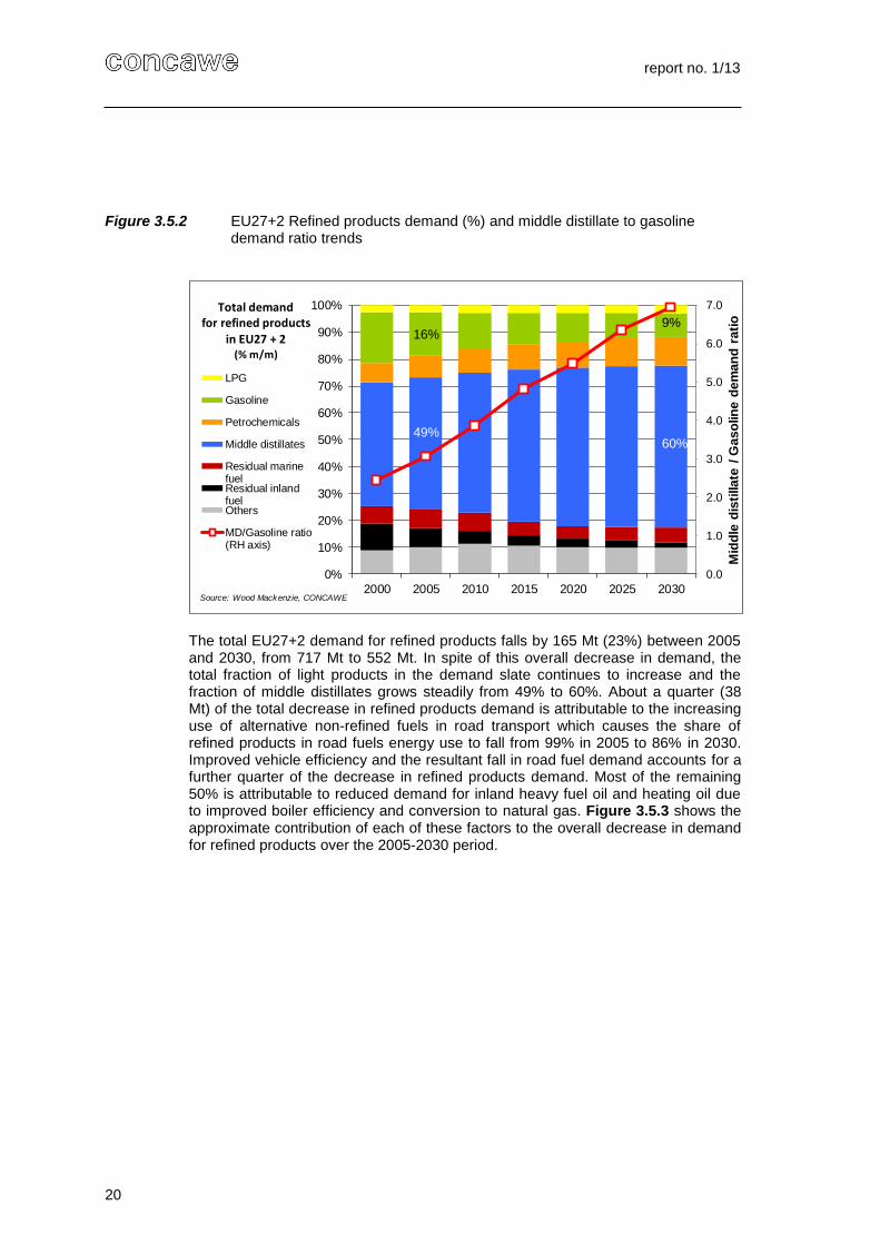
Figure 3.5.2 EU27+2 Refined products demand (%) and middle distillate to gasoline demand ratio trends

The total EU27+2 demand for refined products falls by 165 Mt (23%) between 2005 and 2030, from 717 Mt to 552 Mt. In spite of this overall decrease in demand, the total fraction of light products in the demand slate continues to increase and the fraction of middle distillates grows steadily from 49% to 60%. About a quarter (38 Mt) of the total decrease in refined products demand is attributable to the increasing use of alternative non-refined fuels in road transport which causes the share of refined products in road fuels energy use to fall from 99% in 2005 to 86% in 2030. Improved vehicle efficiency and the resultant fall in road fuel demand accounts for a further quarter of the decrease in refined products demand. Most of the remaining 50% is attributable to reduced demand for inland heavy fuel oil and heating oil due to improved boiler efficiency and conversion to natural gas. Figure 3.5.3 shows the approximate contribution of each of these factors to the overall decrease in demand for refined products over the 2005-2030 period.

49%60%

16%9%

0.0

1.0

2.0

3.0

4.0

5.0

6.0

7.0

0%

10%

20%

30%

40%

50%

60%

70%

80%

90%

100%

2000 2005 2010 2015 2020 2025 2030

Mid

dle

dis

tillate

/ G

aso

lin

e d

em

an

d r

ati

o

LPG

Gasoline

Petrochemicals

Middle distillates

Residual marinefuelResidual inlandfuelOthers

MD/Gasoline ratio(RH axis)

Source: Wood Mackenzie, CONCAWE

Total demandfor refined products

in EU27 + 2(% m/m)

report no. 1/13

21

Figure 3.5.3 Approximate breakdown of factors contributing to the total fall of 165 Mt in the demand for refined products between 2005 and 2030

The evolution of demand for refined middle distillate products is of particular importance for EU refiners. The term “middle distillates” or MD covers the range of refined products from kerosene (for heating fuel or aviation fuel) to diesel fuel (for road and non-road vehicles) and heating oil (typically used in oil-fired domestic boilers). The EU refining system has reached the upper physical limit of its ability to produce sufficient middle distillates to satisfy the growing demand, with the result that the EU has become dependent on imports to complement domestic production. Additional middle distillate production in EU refineries to reduce this import dependence would require major investment in new or expanded process unit capacity. Such investments can only be justified if they are supported by positive long term demand prospects for middle distillates.

The positive factors for refined middle distillate demand over the 2005-2030 period are aviation fuel (an increase of 28% or 16 Mt) and distillate marine fuel (an increase of 280% or 20 Mt). The latter product benefits from the switch to 0.1% marine fuel for ECAs in 2015 and for ferries in 2020. Refined road diesel demand decreases by 14 Mt (8%) between 2005 and 2030 and non-road diesel demand declines by 8 Mt (27%). A substantial decrease in heating oil demand of 32 Mt (39%) is forecast between 2005 and 2030 due to natural gas substitution and improvements in thermal insulation in buildings.

The net effect of these contrasting factors on refined middle distillate products demand over the 2005-2030 period is a decrease of 18 Mt (11%). It must be stressed, however, that the overall refined products demand declines at more than double this rate (23% or 166 Mt) over the same period. The demand for refined middle distillates as a percentage of total refined products demand therefore grows markedly, from 49% in 2005 to 60% in 2030. This means that EU refiners would need to increase the share of middle distillates in their production by about 10% in order to at least keep pace with demand, while at the same time reducing total production by 22%. This will place a considerable strain on the refining system, as declining demand will lead to refinery closures and the distillate production capacity

-23%

-26%-24%

-21%

-8%

Factors contributing to fall in EU refined products demand 2005-2030 (%)

Penetration of alternativeroad fuels

Reduced road fuel demand

Reduced inland heavy fuel oildemand

Reduced heating oil demand

Reduced demand for otherproducts

report no. 1/13

22

lost in closed refineries will need to be replaced with even more distillate production capacity in the remaining refineries.

The EU27+2 demand scenario for refined middle distillates is shown in Figure 3.5.4 (in Mt/a) and in Figure 3.5.5 (in % of the total refined products demand).

Figure 3.5.4 Evolution of U27+2 refined middle distillate demand in Mt/a

Figure 3.5.5 Evolution of U27+2 refined middle distillate demand in % of total refined products demand

320

351

325

348 354345

333

0

50

100

150

200

250

300

350

400

2000 2005 2010 2015 2020 2025 2030

Distillate marine bunker

Heating oil

Diesel (non-road, railand inland water)

Jet/Kero

Diesel (road)

Source: Wood Mackenzie, CONCAWE

Distillates demand(refined products

only)in EU27 + 2

(Mt/a)

46.1%48.9%

52.1%

56.7%58.9% 59.9% 60.3%

0%

10%

20%

30%

40%

50%

60%

70%

2000 2005 2010 2015 2020 2025 2030

Distillate marinebunker

Heating oil

Diesel (non-road, railand inland water)

Jet/Kero

Diesel (road)

Source: Wood Mackenzie, CONCAWE

Distillates demandin EU27 + 2

(% m/m of total

refined products demand)

Source: Wood Mackenzie, CONCAWE

report no. 1/13

23

3.6. EU CRUDE OIL SUPPLY

Crude oil is a worldwide commodity. Although most grades are traded on a wide geographical basis, consuming regions tend, for logistic and geopolitical reasons, to have preferred supply sources. The favourable geographic location of Europe in relation to light and sweet crude producing regions (North Sea, North and West Africa) has resulted in a fairly light crude diet in the past two to three decades. Crudes from the Caspian Sea area have recently become a feature of the European crude diet and are expected to grow in importance, compensating the steady decline of North Sea crude production.

North Sea: This is indigenous production for which Western Europe has a clear logistic advantage. Although some North Sea crude finds its way to the US, the bulk is consumed in Europe. These crudes are mostly light and low sulphur. Production is in decline, as the inexorable depletion of existing reserves is not compensated by the discoveries of new reserves.

Africa: North African crudes (Algeria, Libya, Egypt) are naturally part of Southern Europe’s “captive” production. West African crudes can profitably go either to North America or to Europe and the market is divided between these two destinations. There is a wide range of quality amongst these crudes from very light and low sulphur Algerian grades to fairly heavy and sour Egyptians.

Middle East: The region is an important supplier, mainly of heavy, high-sulphur grades, typically used for the manufacture of bitumen or base oils for lubricant production and by refineries with appropriate desulphurisation and residue conversion facilities.

Russia: Russia is a steady and growing supplier of medium quality crude to Europe, partly through an extensive inland pipeline system extending to most former East European block countries.

Caspian: The Caspian basin is becoming a major producer of light sweet crudes. Geographical proximity and favourable logistics make Europe a natural and growing consumer of these crudes.

The EU27+2 refineries processed about 660 Mt of crude oil and feedstocks in 2010. This is set to shrink to 650 Mt in 2020 and 600 Mt in 2030, due mainly to improvements in vehicle efficiency and increasing penetration of biofuels and other alternative fuels. The sources of supply for Europe will change, with declining North Sea production being replaced by increased production in other regions such as West Africa and the Caspian basin. Crude supply forecasts by Wood Mackenzie [1] suggest that these changes in the origin of the crude oil will not significantly affect the average quality of the EU crude slate, which is expected to remain close to the 2010 levels of density and sulphur content. It should be possible to maintain the current proportion of around 50% to 55% of sweet (i.e. low sulphur) crudes over the next two decades.

The modelled crude slate percentages were as shown in Figure 3.6.1. The detailed quantities and sulphur contents are shown in Appendix 5. During the model calibration exercise the average sulphur content of the combined crude and residue feedstock was matched with actual 2008 figures. The proportion of residual material in the combined feedstock was adjusted through the addition of 57 Mt/a of North

report no. 1/13

24

Sea residue to match the actual 2008 residue yield figures. The crude feed is processed by the Crude Distillation Unit (CDU) while the residue feedstock is processed in refinery units downstream of the CDU or used as blendstock for heavy fuel oil products.

The calibrated model required a total of 709 Mt of crude and residue feed to match the 2008 production from EU27+2 refineries. The Eurostat statistic for total crude and feedstock to EU27 refineries in 2008 is 697 Mt. Allowing an additional 18 Mt for feeds to refineries in Norway and Switzerland (not reported in Eurostat) brings the EU27+2 Eurostat total to 715 Mt. The calibrated model’s estimate of 709 Mt for EU27+2 refining feed was therefore considered to be within the statistical uncertainties of the production and feed data.

Figure 3.6.1 Model crude and residue percentages for EU27+2

3.7. OTHER FEEDSTOCKS

In addition to crude oil and residues a number of additional feed streams and blending components were provided and essentially kept constant throughout the study except in specific sensitivity cases.

4.7 Mt/a imports of methane (natural gas) for either hydrogen production or consumed fuel

2.5 Mt/a imports of ethane as steam cracker feedstock, directed in fixed amounts towards the Baltic (1.0 Mt) and UK & Ireland (1.5Mt) regions only.

Note that it was assumed that no naphtha imports were required from 2010 onwards. The declining EU demand for gasoline is expected to provide a surplus of refinery-produced naphtha which eliminates the need for imports as petrochemical feedstock.

0%

10%

20%

30%

40%

50%

60%

70%

80%

90%

100%

2008 2010 2015 2020 2025 2030

Shar

e o

f to

tal E

U2

7+2

re

fin

ery

fee

d (%

m/m

)

North Sea & Caspian

Light Middle East

Nigerian

Russian

Heavy Middle East

North Sea atmosphericresidueNorth Sea vacuumresidue

Source: Wood Mackenzie, CONCAWE

report no. 1/13

25

Ethanol and FAME required to meet mandated biofuel specs were not included in the modelling but their consequences on refinery production volumes and qualities were taken into account. For simplicity, this study has assumed that the biofuels mandates are met by blending ethanol only, although in reality this will be a combination of ETBE and ethanol.

3.8. PRODUCT IMPORTS/EXPORTS

Net import/export flows of finished or semi-finished refined products are necessary in the EU market to compensate for shortfalls in refinery production versus demand (imports of distillates, i.e. diesel, heating oil and jet fuel) or, inversely, to provide an outlet for refinery production that is in excess of EU demand (exports of gasoline and heavy fuel oil). These trade flows were modelled in the study as the fixed quantities indicated below, which were based on the actual flows in the 2008 base year and were kept constant through to 2030. This is admittedly an over-simplified, static view which ignores the potential for other regions to modify the quantities supplied to the EU or imported from the EU. The advantage of this approach is that it reduces the number of variables affecting refinery operation, concentrating the entire burden on refining to adjust to shifts in EU demand. A more rigorous, dynamic approach would have required a global model of refinery capacity and demand growth in every region of the world.

10 Mt/a imports of road quality diesel (10 ppm S)

10 Mt/a imports of heating oil (1000 ppm S)

15 Mt/a imports of jet fuel. Jet fuel imports were not allowed as blend components for other products, e.g. diesel or heating oil.

43 Mt/a exports of gasoline. This was modelled as a single grade of low sulphur (100ppm), low aromatics (28%v/v) and low olefins (10%v/v) quality. About 22 Mt/a of the gasoline exports in 2008 were destined for the USA. A sensitivity case was run to assess the impact of the possible disappearance of the US gasoline deficit by 2020, as a result of shrinking US gasoline demand, growing ethanol share and growing refining capacity (see Section 4.6.10).

4 Mt/a exports of high sulphur heavy fuel oil (HSHFO). This is the net of Eurostat residual fuel oil exports minus imports averaged over 2007-2008. It was modelled as a single grade of 1.5% sulphur residual fuel oil. The model was allowed to replace part or all of the HSHFO export quantity with an equivalent energy value of petroleum coke. This was done to allow flexibility in coke production and thereby allow the model to invest in additional coking unit capacity as an option for reducing residual fuel oil production.

Figure 3.8.1 shows the net effect of these import/export flows on refinery production of middle distillates and gasoline compared to market demand. The imports of road quality diesel, jet fuel and heating oil are grouped into the middle distillates category which also includes non-road diesel and distillate marine fuel (DMF).

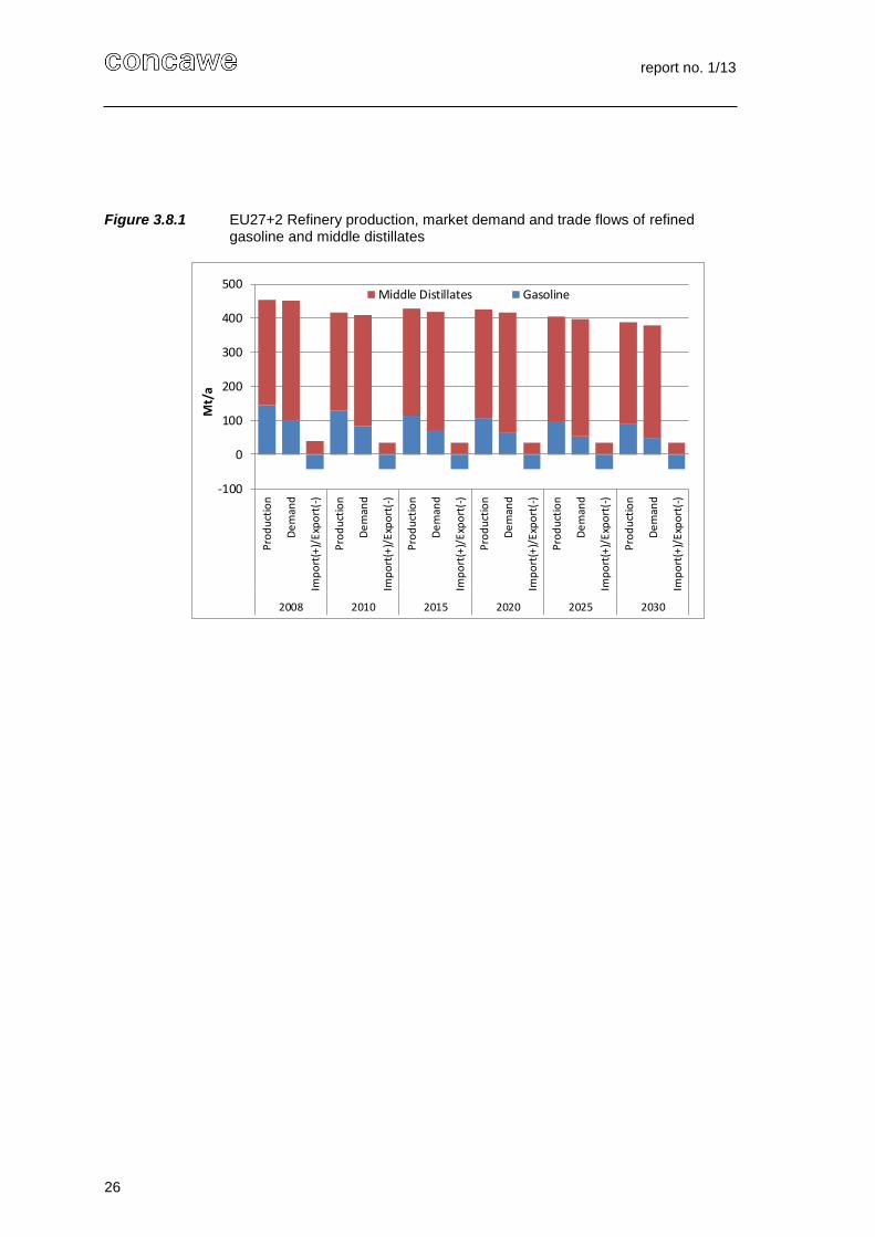
report no. 1/13

26

Figure 3.8.1 EU27+2 Refinery production, market demand and trade flows of refined gasoline and middle distillates

-100

0

100

200

300

400

500

Pro

du

ctio

n

De

man

d

Imp

ort

(+)/

Exp

ort

(-)

Pro

du

ctio

n

De

man

d

Imp

ort

(+)/

Exp

ort

(-)

Pro

du

ctio

n

De

man

d

Imp

ort

(+)/

Exp

ort

(-)

Pro

du

ctio

n

De

man

d

Imp

ort

(+)/

Exp

ort

(-)

Pro

du

ctio

n

De

man

d

Imp

ort

(+)/

Exp

ort

(-)

Pro

du

ctio

n

De

man

d

Imp

ort

(+)/

Exp

ort

(-)

2008 2010 2015 2020 2025 2030

Mt/

a

Middle Distillates Gasoline

report no. 1/13

27

4. FIXED DEMAND SCENARIO

The first part of the refining study was intended to represent the evolution of EU refineries over the years as known legislation measures come into force and as demand evolves. The total period between 2010 and 2030 was divided into 5-year periods in which demand was kept constant and the quality changes were introduced in chronological order.

The “demand” step at the beginning of each period included the quality changes introduced in the previous step. The 2008 starting point included the FQD requirement for 10ppm road fuels from 1 January 2009. Other legislated product quality changes were introduced in separate step-out cases depending on their effective dates, thereby separating their impact from the demand changes. The full set of cases is shown graphically in Figure 4.1.

Figure 4.1 Time-bound model cases for fixed demand scenario

The refinery configuration in place in 2008 and in each 5-year demand step was the actual installed capacity available in that year, including any publicly announced investments and closures. Since the visibility of announced investments is limited to 2015 at best, installed capacity was left unchanged from 2015 onwards. The demand and quality changes imposed on the model were in most cases only achievable with additional new capacity, so the refining model was allowed to

Reference year

for demand

2008

2009 2010 (July)

FQD: Diesel PAH

8%

IMO: 1.0% S ECA

Marine fuel

2011 2011 2015

FQD: Inland

waterways GO

10 ppm S

FQD: Non-road

diesel 10 ppm S

IMO: 0.1% S ECA

marine fuel

(distillate)

2020 2020

0.1% S ferries

marine fuel

(distillate)

IMO: 0.5% S

all non-ECA

marine fuels

2025

2030

Legislated product quality changes

and effective dates

2010

2015

2020

report no. 1/13

28

purchase additional capacity at an annualised investment plus operating cost based on 2011 unit construction prices.

It should be noted that the refineries’ performance in energy terms was kept constant in the fixed demand scenario runs, i.e. no improvement in refinery energy efficiency was assumed compared to 2008 for which the model was calibrated. The effect of improved refinery efficiency was assessed in a sensitivity case which was run on the same set of cases, assuming steady improvements in refinery energy efficiency.

Additional sensitivity cases were included to investigate the impact of introducing additional product quality changes at the 2020 horizon, as well as the use of on-board scrubbers to meet IMO bunker sulphur emissions. These sensitivity cases are described in detail in Section 4.6.

4.1. REFINERY THROUGHPUT AND PRODUCTION

As indicated in Section 2, the CONCAWE refining model includes both refineries and petrochemical plants producing light olefins (steam crackers) and aromatics. In this and the following sections, we focus on refining impacts. The specific share of petrochemicals is discussed in Section 6.

Refinery crude throughput is chiefly determined by the overall product demand imposed on EU refining in each time-period, with the addition of a certain fraction of crude that is consumed internally in the form of fuel (refinery fuel gas, fuel oil and FCC coke). Throughputs of individual units are determined by the range of products in the demand pool and the severity of the product specifications.

Declining demand for refined products results in a substantial decrease in refinery throughput, from 709 Mt in 2008 to 603 Mt in 2030. This fall in throughput is equivalent to the combined capacity of the 6 largest EU refineries or the 30 smallest EU refineries. Almost half of this fall occurs in the short period from 2008 through 2010 and is attributable to the impact of the economic crisis on EU demand for oil products. Table 4.1.1 shows the evolution of total throughput, production and crude diet in the 2008 base year and in each of the 5-year periods.

In contrast to the declining refining throughput, the fraction of light products produced shows a steady increase, driven by the declining demand for residual fuels in the inland market as well as in marine fuels. This is especially evident in 2015, when the switch to 0.1% S distillate marine fuels in the ECAs causes a downward step change in residual fuel demand, effectively eliminating about 30% of the residual marine fuel production and contributing to an almost 3% increase in the fraction of light products compared to 2010.

report no. 1/13

29

Table 4.1.1 EU27+2 Refinery total throughput and production

The most notable change in terms of demand is the relentless increase of the middle distillate to gasoline production ratio. This makes it increasingly difficult for EU refineries to produce the required product slate and would require massive investments in new refinery process units as well as additional processing energy, additional hydrogen production and ultimately additional CO2 emissions if the demand changes are met entirely by EU refineries.

As discussed in Section 3, the demand ratio of refined middle distillate (including jet fuel, diesel, heating oil and marine distillate fuel) to gasoline (MD/G ratio) increases steadily as the demand for refinery-produced gasoline is eroded by the penetration of ethanol, by the continuing dieselisation of the passenger car fleet and by the steadily improving fuel economy of gasoline vehicles. This growth is shown graphically in Figure 4.1.1. In 2010 the MD/G demand ratio is about 3.9 (325 Mt of MD vs. 84 Mt of G) and in 2030 it reaches 6.9 (333 Mt of MD vs. 48 Mt of G). It can be seen that this growth is mostly due to the fall in gasoline demand, as the middle distillates demand remains fairly constant.

2008 2010 2015 2020 2025 2030

Crude input Mt/a 652 606 606 598 575 554

Specific gravity 0.858 0.858 0.858 0.858 0.858 0.858

API gravity 33.4 33.4 33.4 33.4 33.4 33.4

Proportion of low sulphur crude 43% 43% 43% 43% 43% 43%

Sulphur content %m/m 1.03% 1.03% 1.03% 1.03% 1.03% 1.03%

Atmospheric residue yield(1) %m/m 45.1% 45.1% 45.1% 45.1% 45.1% 45.1%

Vacuum residue yield(2) %m/m 18.0% 18.0% 18.0% 18.0% 18.0% 18.0%

Other refinery feedstocks(3) Mt/a 57 53 53 52 50 48

Total throughput Mt/a 709 659 659 650 625 603

Total production(4) Mt/a 645 597 592 581 558 537

Fraction of light products(5) 80.8% 81.8% 84.6% 86.0% 86.1% 86.2%

Production ratios(6)

Diesel/Gasoline 1.4 1.4 1.6 1.7 1.8 1.8

Gasoils/Gasoline 1.9 1.9 2.3 2.5 2.6 2.6

Middle distillates/Gasoline 2.2 2.3 2.7 3.0 3.2 3.3

Light/Heavy products 4.2 4.5 5.5 6.1 6.2 6.2

(1) Residue yield at 370 C cutpoint

(2) Residue yield at 555 C cutpoint

(3) Feedstocks modelled as atmospheric and vacuum residues

(4) Production includes petrochemicals and excludes own fuel consumption and losses in refineries and petrochemical plants

(5) Light products include gasoils and lighter products such as gasoline, LPG and petrochemicals and exclude own fuel consumption

(6) Diesel includes road and non-road diesel; Gasoils include diesel, marine distillate and heating oil; Middle distillates include gasoils

and jet fuel; Heavy products include all products heavier than gasoils such as heavy fuel oil, bitumen and sulphur and exclude own fuel

consumption

report no. 1/13

30

Figure 4.1.1 Evolution of the middle distillate / gasoline EU27+2 demand ratio for refined products only

A different picture is obtained when the growth of the MD/G ratio is expressed in terms of refinery production. We have assumed that EU countries will continue to import the same amount of refined middle distillates (35 Mt/a) and export the same amount of refined gasoline (43 Mt/a) through to 2030. The cushioning effect of these trade flows reduces the MD/G production ratio, mainly by allowing refineries to maintain a relatively high level of gasoline production. Figure 4.1.2 shows the refined MD/G production ratio increasing from 2.3 in 2010 to 3.3 in 2030, a more moderate trend than the 3.9 to 6.9 increase in the MD/G demand ratio over the same period. However, it should be stressed that this apparently modest shift in the refinery production MD/G ratio is strongly dependent on the assumption that there is a secure supply of middle distillate imports and that gasoline export markets are able to absorb such high volumes.

320 351 325 348 354 345 333

132

11584

73 64 5448

0.0

1.0

2.0

3.0

4.0

5.0

6.0

7.0

0

50

100

150

200

250

300

350

400

450

500

2000 2005 2010 2015 2020 2025 2030

Mid

dle

dis

tilla

te /

Ga

so

lin

e r

ati

o

Gasolinedemand

Middle distillatesdemand

MD/Gasolinedemand

Source: Wood Mackenzie, CONCAWE

Total demand

for refined Gasoline & MDs

in EU27 + 2(Mt/a)

Source: Wood Mackenzie, CONCAWE

report no. 1/13

31

Figure 4.1.2 Evolution of the middle distillate / gasoline production ratio for refined products only

4.1.1. Refinery throughput compared to PRIMES 2011 scenarios for EC Energy Roadmap 2050

The European Commission adopted the Communication “Energy Roadmap 2050” on 15 December 2011. In this Communication the EC explores the challenges posed by delivering the EU's decarbonisation objective to reduce greenhouse gas emissions to 80-95% below 1990 levels by 2050. The Communication was accompanied by a two-part Impact Assessment, of which Part 2 [5] shows numerical details of the PRIMES modelling results for each of the scenarios studied.

It is useful to compare the EU refining inputs resulting from the CONCAWE fixed demand scenario with the refining inputs resulting from some of the PRIMES scenarios. Of the seven PRIMES scenarios listed in the Impact Assessment, we have selected the following three as representative of the range of decarbonisation severity in the Energy Roadmap:

Reference scenario: A business-as-usual projection of developments in the absence of new policies beyond those adopted by March 2010.

Current Policy Initiatives (CPI) scenario: A revised projection taking into account the most recent developments (higher energy prices and effects of Fukushima) and the latest policies on energy efficiency, energy taxation and infrastructure adopted or planned after March 2010. Final energy demand is reduced by 4% in 2030 relative to the Reference scenario.

High Energy Efficiency scenario: Includes a very stringent implementation of the Energy Efficiency Plan, aimed at reaching close to 20% energy savings by 2020 with strong energy efficiency policies being pursued thereafter. Final energy demand is reduced by 14% in 2030 relative to the Reference scenario.

307 313 290 313 319 310 298

148 153127

116 107 9791

0.0

1.0

2.0

3.0

4.0

5.0

6.0

7.0

0

50

100

150

200

250

300

350

400

450

500

2000 2005 2010 2015 2020 2025 2030

Mid

dle

dis

tilla

te /

Ga

so

lin

e r

ati

o

GasolineProduction

Middle distillatesproduction

MD/Gasolineproduction

Source: Eurostat, Wood Mackenzie, CONCAWE

Total production

of refinedGasoline & MDs

in EU27 + 2(Mt/a)

report no. 1/13

32

The impact of these PRIMES scenarios on refinery throughput is shown in Figure 4.1.1.1, compared to the CONCAWE fixed demand scenario throughput. It should be noted that the PRIMES scenarios cover the EU27 countries, whereas the CONCAWE fixed demand scenario covers EU27+2, including Switzerland and Norway for which the total throughput is about 18 Mtoe/a.

Figure 4.1.1.1 Comparison of EU refining input in CONCAWE Fixed Demand scenario with PRIMES 2011 scenarios

The CONCAWE fixed demand scenario has a lower 2010 starting point than the PRIMES scenarios, but this lower 2010 throughput of 673 Mtoe/a (659 Mt/a) for EU27+2 is consistent with the Eurostat statistic of 645 Mt/a for EU27 refining throughput in 2010. The trend in refinery throughput shows a decrease of 9% between 2010 and 2030 in the CONCAWE fixed demand scenario, which is slightly higher than the 7-8% decrease in the PRIMES Reference and CPI scenarios but much lower than the 19% decrease in the PRIMES High Energy Efficiency scenario.

4.2. PROCESS UNIT THROUGHPUT TRENDS

Each process unit in a refinery plays a specific role in satisfying the overall product demand structure and meeting the product quality specifications. A detailed view of the throughput trends of the major process units can reveal much about the demand and quality pressures placed on the refinery and the solutions found by the model to address them. By construction, no products are allowed to go to waste, so the crude oil throughput of the Crude Distillation Unit (CDU) is adjusted to exactly meet the throughput needs of the downstream units which upgrade the raw product streams from the CDU.

Figure 4.2.1 shows the model CDU throughput dropping steeply between 2008 and 2010, stabilising up to 2015 and declining through to 2030. Since CDU capacity closures amounted to only 8 Mt (net) between 2008 and 2010 compared to a decrease of 46 Mt in CDU throughput, the CDU utilisation rate falls sharply from 86% in 2008 to 81% in 2010. With further announced capacity closures of 8 Mt (net) between 2010 and 2015 there is a small recovery in utilisation rate to 82% in 2015.

670

659

718

583

673

615

550

600

650

700

750

2010 2015 2020 2025 2030

EU r

efi

nin

g to

tal

inp

ut

(Mto

e/a

)

PRIMES EU27Reference scenario

PRIMES EU27 CurrentPolicy Initiativesscenario

PRIMES EU27 HighEnergy Efficiencyscenario

CONCAWE EU27+2Fixed Demand scenario

report no. 1/13

33

Without any further CDU capacity closures the utilisation rate could shrink to 76% in 2030, representing a capacity-throughput gap of 190 Mt compared to 108 Mt in 2008.

Figure 4.2.1 Trends in Crude Distillation Unit (CDU) capacity, throughput and utilisation rate in the fixed demand scenario

The throughput needs of the process units downstream of the CDU are closely linked to the demand and quality requirements of each product group (gasoline, distillates, heavy fuel oil) and depend on each unit’s product yield specialisation, ability to reduce sulphur content and ability to upgrade heavy streams to lighter products.

If demand or quality pressures require an increase in unit throughput beyond the available unit capacity, including the known 2009-2015 projects, then the model can choose to purchase additional capacity for that unit at a defined annualized cost. Since the model optimizes to minimize cost, it will choose the quantities and types of unit capacity purchases so as to meet the product demand and quality constraints in the most economically efficient manner.

The changing trends in unit throughputs are shown relative to the 2008 starting point in Figure 4.2.2 (in Mt/a) and in Figure 4.2.3 (in %).

760752 744

CDU capacity Mt/a 744

652

606 CDU throughput Mt/a

554

85.8%

80.7%CDU utilisation

%

74.5%

70%

75%

80%

85%

90%

500

550

600

650

700

750

800

2008 2010 2015 2020 2025 2030

CD

U C

apac

ity

Uti

lisat

ion

Rat

e (%

)

Cru

de

Dis

tilla

tio

n U

nit

Cap

acit

y o

r Th

rou

ghp

ut

(Mt/

a)

report no. 1/13

34

Figure 4.2.2 Throughput trends for major refinery process units in Mt/a relative to the 2008 base case. Solid lines show actual capacity addition projects for DHC and COK units. Note that the hydrogen unit (H2U) throughput is expressed in Mt/a of hydrogen production.

Figure 4.2.3 Throughput trends for major refinery process units in % change relative to the 2008 base case

These unit throughput plots show contrasting trends. On the one hand they show a trend towards severe under-utilisation of key refinery units such as Crude Distillation units (CDU), Reforming (REF) and Fluid Catalytic Cracking (FCC) units. The steep downward trend in CDU throughput closely matches the trend in total product demand, while the throughputs of gasoline-producing REF and FCC units reflect the declining gasoline demand. On the other hand, there are substantial increases in throughputs of conversion units such as Distillate Hydrocracking (DHC), Coking (COK), Residue Desulphurisation (RES HDS) and Hydrogen production (H2U), far exceeding their current capacity. The throughput trend of the low sulphur diesel and jet fuel producing DHC unit reflects the growth in demand for low sulphur distillates.

CDU

FCC

H2U

DHC

COK

REF

-100

-75

-50

-25

0

25

2008Base case

2010ECA bunker

1.0%S

2015ECA bunker

0.1%S

2020General

bunker 0.5%S

2025 2030

Unit t

hro

ughput (M

t/a)

FCC

H2U

DHC

RES HDS

CDU

COK

-40%

-20%

0%

20%

40%

60%

80%

100%

120%

2008Base case

2010ECA bunker

1.0%S

2015ECA bunker

0.1%S

2020General

bunker 0.5%S

2025 2030

Unit t

hro

ughput ch

ange (

%)

report no. 1/13

35

Reductions in heavy fuel oil demand and sulphur content call for increased throughput of COK units, which eliminate residual fuel components, and RES HDS units which reduce the sulphur content of residual components. A significant increase in hydrogen production from H2 units is required to satisfy the demand for hydrogen in the desulphurisation and cracking reactions of RES HDS and DHC units.

It would require a major adaptation of EU refineries to completely accommodate these throughput trends, by investing in additional process unit capacity while at the same time closing unused CDU, REF and FCC capacity.

The announced refining capacity additions in the 2009-2015 period are a major contribution to meeting future requirements. The known additional DHC capacity of 18 Mt/a is adequate to meet future growth in the share of low sulphur distillates. The low sulphur residual product from DHC units (DHC bottoms) will also make a major contribution to reducing residual marine fuel sulphur content in 2020. However, the additional equipment needs of marine fuel sulphur reduction in 2020 are not met by the known capacity additions for COK and RES HDS units (8 Mt/a and 0 Mt/a respectively), which fall short of the required increase of 21 Mt in COK throughput and 3 Mt/a in RES HDS throughput. Similarly, the known H2U production capacity additions of 0.7 Mt/a by 2015 are adequate for EU road fuel demand and quality changes but fall well short of the total additional hydrogen requirement of 1.6 Mt/a by 2020 for marine fuels.

On the capacity reduction side, known CDU capacity net reductions amount to only 17 Mt/a by 2015, whereas the reduction in CDU throughput is 46 Mt/a in 2015 compared to 2008. This will translate into a net 4% decrease in CDU utilisation rate by 2015 compared to 2008. However, if all the 57 Mt/a of “idled” CDU capacity (see Section 2.1) is permanently closed by 2015 then CDU utilisation rate would increase by 2%. FCC capacity utilisation is projected to fall by 8% in 2015 compared to 2008, with the 17 Mt/a decrease in throughput far exceeding the known FCC closures of 8 Mt/a.

4.3. POTENTIAL INVESTMENT IN NEW PLANTS

The scale of investment that would be required to meet all demand and quality constraints is illustrated in Figure 4.3.1, which details the contribution of each quality or demand change to the cumulative investment requirements over the whole time period. Each of the quality-related or demand-related bars on the graph corresponds to a step-wise progression of individual runs in which only the single set of parameters indicated on the y-axis is changed from one run to the next. The length of each bar is the difference in total investment requirement from one run step to the next. The cumulative investment required from 2008 to 2020 is estimated at 51 G$, of which about 30 G$ is already committed in announced projects.

The vast majority (41 G$) of the total investment over the 2008-2020 period is required to address the challenges imposed by the production of marine fuel to the new IMO specifications in 2015 and 2020.

With declining demand for refined products beyond 2020 and no further product quality changes, the discrete model runs representing 2025 demand and 2030 demand give progressively lower estimates of total investments needed to meet product demand and quality in 2025 and 2030. While a total investment of 51 G$ is required to meet demand and quality in 2020, the total investment required in 2025 to meet the same product quality but lower demand is only 48 G$, and the total

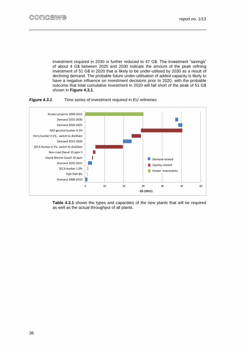
report no. 1/13

36

investment required in 2030 is further reduced to 47 G$. The investment “savings” of about 4 G$ between 2020 and 2030 indicate the amount of the peak refining investment of 51 G$ in 2020 that is likely to be under-utilised by 2030 as a result of declining demand. The probable future under-utilisation of added capacity is likely to have a negative influence on investment decisions prior to 2020, with the probable outcome that total cumulative investment in 2020 will fall short of the peak of 51 G$ shown in Figure 4.3.1.

Figure 4.3.1 Time series of investment required in EU refineries

Table 4.3.1 shows the types and capacities of the new plants that will be required as well as the actual throughput of all plants.

0 10 20 30 40 50 60

Demand 2008-2010

FQD PAH 8%

SECA bunker 1.0%

Demand 2010-2015

Inland Marine Gasoil 10 ppm

Non-road Diesel 10 ppm S

SECA bunker 0.1%, switch to distillate

Demand 2015-2020

Ferry bunker 0.1% , switch to distillate

IMO general bunker 0.5%

Demand 2020-2025

Demand 2025-2030

Known projects 2009-2015

G$ (2011)

Demand-related

Quality-related

Known investments

report no. 1/13

37

Table 4.3.1 Process unit throughput and additional capacity

The projected capital expenditure is aimed almost entirely at increasing the processing capacity of five types of refinery process unit: coking, distillate hydrocracking, residue desulphurisation/conversion, middle distillate hydrotreating and hydrogen production. Announced expenditures in firm projects are sufficient to satisfy unit capacity needs up to 2015 but additional expenditures are required to meet the capacity needs for production of 0.5% sulphur marine fuel by 2020, particularly in coking and hydrogen production unit capacity.

4.4. SULPHUR REMOVAL AND HYDROGEN PRODUCTION TRENDS

The average sulphur content of the crude and residue feedstock to EU refineries is assumed to be unchanged over the study period (see Section 3.6). With increasingly stringent sulphur limits imposed on refined products, the only option available for refineries is to remove sulphur by means of additional processing in refinery hydrodesulphurisation units. These units remove sulphur by reacting the sulphur-containing compounds with hydrogen to form hydrogen sulphide (H2S).

2008 2010 2015 2020 2025 2030

Base

case

ECA

bunker

1.0%S

ECA

bunker

0.1%S

General

bunker

0.5%S

Process unit throughput (Mt/a)

652 606 607 598 575 554

279 265 265 264 254 244

78 74 69 49 45 43

Coking 21 22 26 42 42 42

126 114 106 103 97 91

65 72 81 84 83 83

16 13 12 23 22 22

86 75 70 69 65 62

11 10 11 12 14 15

Isomerisation / Alkylation 16 12 11 10 9 8

180 175 183 189 183 175

1419 1588 1706 2750 2737 2661

64 66 73 73 73 73

-3 -17 -17 -17 -17

5 9 9 9 9

0 -4 -4 -4 -4

Coking 1 8 21 21 21

-2 -7 -7 -7 -7

9 18 19 18 18

0 4 7 6 6

-1 -3 -3 -3 -3

0 1 2 3 4

Isomerisation / Alkylation 0 0 0 0 0

7 7 12 8 8

391 796 1641 1518 1413

0 0 0 0 0

12.6 32.0 50.5 48.3 46.7

(1) Hydrogen units include steam methane reforming (SMR) and partial oxidation (POX) units

Relative to base 2008

Timeline

Additional process unit capacity including

firm projects (Mt/a)

Relative to base 2008Capital expenditure

including firm projects (G$)

Middle distillate hydrotreating

Hydrogen(1) (in kt/a of H2 produced)

Steam cracker

FCC

Distillate Hydrocracking

Residue desulphurisation/conversion

Reforming

Aromatics extraction

Hydrogen(1)

(in kt/a of H2 produced)

Steam cracker

Crude atmospheric distillation

Vacuum distillation

Visbreaking

Distillate Hydrocracking

Residue desulphurisation/conversion

Reforming

Aromatics extraction

Middle distillate hydrotreating

Crude atmospheric distillation

Vacuum distillation

Visbreaking

FCC

report no. 1/13

38

Subsequent processing in sulphur recovery units (SRUs) converts the hydrogen sulphide to pure elemental sulphur which is sold as a refining by-product.

The production of elemental sulphur by EU refineries is set to increase by 20% (0.8 Mt) between 2010 and 2020, with a corresponding decrease in the sulphur contained in refined marine fuel over the same period. These trends are shown in Figure 4.4.1 which also shows the steep increase in the total percentage of feed sulphur that must be removed by refineries as pure sulphur product, from 52% in 2008 to 67% in 2020.

In the absence of further changes to product sulphur limits the sulphur production declines after 2020 in line with the general downward trend in refinery production.

Figure 4.4.1 Sulphur contained in products from EU27+2 refineries, excluding sulphur in refinery fuel.

An adequate supply of hydrogen is essential to satisfy the growing demand for sulphur removal by hydrodesulphurisation. This is an important driver for additional hydrogen production capacity requirements, as shown in Figure 4.4.2 in which the incremental hydrogen unit production requirement relative to the 2008 base case is compared to the incremental percentage sulphur removed. Other important drivers for additional hydrogen production capacity are conversion units such as distillate hydrocracking and residue conversion, which consume about half of the total refinery hydrogen production. Additional hydrogen production unit capacity is also required to compensate for 0.2 Mt of reduced hydrogen production from gasoline reforming units due to the declining gasoline demand.

Sulphur as pure product

Inland & Export HFO

Marine Fuel

Bitumen, Lubricants & Wax

Petroleum Coke

52%

54%

57%

67% 67% 66%

50%

55%

60%

65%

70%

0

1

2

3

4

5

6

7

8

2008 2010 2015 2020 2025 2030

% s

ulp

hu

r re

mo

ved

as

pro

du

ct

Sulp

hu

r in

ref

ined

pro

du

cts

(Mt/

a)

Sulphur as pure product Gasoline, Jet Fuel, Diesel & Heating OilInland & Export HFO Marine FuelBitumen, Lubricants & Wax Petroleum Coke% sulphur removed as product (RH axis)

report no. 1/13

39

Figure 4.4.2 Hydrogen production and % sulphur removal required in EU27+2 refineries relative to the 2008 base case.

Of the 1.6 Mt of incremental hydrogen production capacity required to meet the demands imposed by the marine fuel 0.5% sulphur limit in 2020, only 0.7 Mt are included in the announced refinery projects from 2009 to 2015. Without additional expenditure to expand hydrogen production the ability of EU refining to reduce refined product sulphur content will be severely limited.

4.5. REFINERY ENERGY CONSUMPTION AND CO2 EMISSIONS

The total energy requirement of a given refinery is mostly dependent on its throughput and can vary hugely depending on the refinery’s size and complexity. A declining total EU refining throughput can therefore be expected to translate into a steady decrease in total energy requirement. This is shown in Figure 4.5.1, where the total energy requirement of EU refineries decreases from 45 Mtoe/a in 2008 to 39 Mtoe/a in 2030. However, the specific energy requirement (expressed as energy consumed per tonne of feed) increases slightly from 6.3% of total feed in 2008 to 6.6% in 2030, as more energy-intensive processing is required to satisfy the increasing demand for lighter and lower sulphur products. It should be noted that these trends assume a constant level of refinery energy efficiency, so the observed shapes of the curves are entirely attributable to the changes in throughput and the changing configuration of EU refineries.

0%

2%

4%

6%

8%

10%

12%

14%

16%

18%

0

200

400

600

800

1000

1200

1400

1600

1800

2008 2010 2015 2020 2025 2030

Incr

eme

nta

l %su

lph

ur

rem

ove

d

Incr

emen

tal h

ydro

gen

pro

du

ctio

n (k

t/a)

Incremental hydrogen production (kt/a) Incremental %sulphur removed

report no. 1/13

40

Figure 4.5.1 Evolution of total energy requirement (Mtoe/a) and specific energy requirement (toe/kt feed) in EU refineries (no energy efficiency improvement)

Total EU refining CO2 emissions fell by about 6 Mt from 2008 to 2010, tracking the steep decrease in demand and refinery throughput and the consequent decrease in energy consumption. The demand-related decrease in emissions was 7 Mt, mitigated by a 1 Mt increase due to the introduction of the 1.0% S specification for ECA marine bunker.

Total CO2 emissions from EU refining are expected to grow from 151 Mt in 2008 to 163 Mt in 2020, in spite of the overall decrease in total refinery energy consumption in the 2008-2020 period. This increase of 12 Mt is the net result of a 19 Mt increase in emissions related to hydrogen manufacture and a 7 Mt decrease in emissions related to energy consumption in all other refinery units. With the decline in refining throughput beyond 2020, total refining CO2 emissions will fall by about 9 Mt from the 2020 peak, ending at 154 Mt in 2030.

Refinery CO2 emissions per tonne of throughput will increase in line with the increasing middle distillate to gasoline (MD/G) and middle distillate to residue (MD/R) production ratios, mainly due to the switch from residual to distillate marine fuel, as illustrated in Figure 4.5.2. This is a result of the high incremental input of energy and hydrogen required to produce an incremental tonne of light products, particularly middle distillates, from residual product streams.

Total Refinery Energy (LH axis)

Specific Energy Requirement

(RH axis)

63.0

63.5

64.0

64.5

65.0

65.5

66.0

66.5

37

38

39

40

41

42

43

44

45

46

2008 2010 2015 2020 2025 2030

Spec

ific

En

ergy

Req

uir

emen

t (to

e/kt

fee

d)

Tota

l Re

fin

ery

En

erg

y C

on

sum

pti

on

(Mto

e/a

)

report no. 1/13

41

Figure 4.5.2 Evolution of middle distillate / gasoline and middle distillate / residue5

production ratios relative to EU refinery CO2 emissions per tonne of throughput

The steady increase in refinery CO2 emissions per tonne of throughput shown in Figure 4.5.2 suggests that there would be a corresponding steady increase in total refinery CO2 emissions through to 2030. This is the case in the period up to 2020 (when increases in CO2 emissions are mainly driven by requirements to reduce marine fuel sulphur) but from 2020 to 2030 the primary driver of total refinery CO2 emissions is the total refining throughput, which falls steeply. This overwhelms the combined effect of the increasing MD/G ratio and the increasing light product fraction and the net result is a 6% fall in total refinery CO2 emissions from 2020 to 2030, as shown in Figure 4.5.3.

5 Residue products have higher densities and higher boiling ranges than distillates and include residual marine fuel,

heavy fuel oil, bitumen, coke, lubricants and waxes.

CO2 emissions in kg/t (LH axis)

Middle distillates / Gasoline Production

Ratio (RH axis)

2.2

2.4

2.6

2.8

3.0

3.2

3.4

3.6

3.8

4.0

4.2

4.4

210

215

220

225

230

235

240

245

250

255

260

265

2010 2015 2020 2025 2030

Pro

du

ctio

n r

atio

of

MD

to

Gas

oli

ne

or

Re

sid

ue

CO

2 e

mis

sio

ns

(kg

pe

r to

nn

e t

hro

ugh

pu

t)

Middle Distillates / Residue ProductionRatio (RH axis)

report no. 1/13

42

Figure 4.5.3 Evolution of total EU27+2 refinery throughput and total refinery CO2 emissions

The chronological contributions of demand and quality changes to the evolution of EU refining CO2 emissions are shown in Figure 4.5.4. The major events contributing to increasing CO2 emissions are the marine bunker sulphur reductions in 2015 and 2020, with a combined impact of 15 Mt of additional CO2 emissions from EU refining.

Figure 4.5.4 Step-wise evolution of total CO2 emissions from EU27+2 refineries (no energy efficiency improvement)

Total CO2 emissions (LH

axis) Throughput (RH axis)

590

600

610

620

630

640

650

660

670

140

145

150

155

160

165

2010 2015 2020 2025 2030

Re

fin

ery

th

rou

ghp

ut

(Mt)

Re

fin

ery

CO

2 e

mis

sio

ns

(Mt)

140 145 150 155 160 165

Base case - 2008

Demand 2010

FQD PAH 8%

ECA bunker 1.0%

Demand 2010-2015

Inland Waterway Gasoil 10 ppm

Non-road Diesel 10 ppm S

ECA bunker 0.1%, switch to distillate

Demand 2015-2020

IMO general bunker 0.5%, Ferry bunker 0.1%

Demand 2020-2025

Demand 2025-2030

CO2 emissions from EU27+2 Refineries (Mt/a)

Demand-related

Quality-related

report no. 1/13

43

Hydrogen production units (steam methane reforming and partial oxidation units) are by far the biggest contributors to the increase in EU refining CO2 emissions. The CO2 emissions from other process units actually decrease by 14 Mt (11%) between 2008 and 2030 whereas emissions from hydrogen production units increase by 17 Mt (94%). The need for more hydrogen production is almost entirely driven by the marine bunker sulphur reductions in 2015 and 2020. Figure 4.5.5 shows the evolution of the relative quantities of CO2 emissions from hydrogen production units and other process units.

Figure 4.5.5 Relative contributions of hydrogen production units (H2U) and other process units to total CO2 emissions from EU refineries (no energy efficiency improvement)

4.6. SENSITIVITY CASES

The fixed demand scenario is founded on a set of base assumptions affecting refinery operation and refined product demand and quality trends. The effects of alternative assumptions were explored in ten sensitivity cases detailed below.

4.6.1. Refined road diesel to gasoline (D/G) demand ratio in 2020

As discussed in Section 3.3.1, the road fuels demand projection in the base case of the fixed demand scenario is based on the assumption that diesel passenger cars would make up 50% of new conventional car sales in 2020, virtually unchanged from the level of 49% in 2010. Although the share of diesel in new car sales is stable over the 2010-2020 period, the share of diesel in the total car fleet grows from a relatively low starting point of 31% (87 million cars) in 2010 to reach 48% (126 million cars) in 2020, almost catching up with the 50% share in new car sales. As the share of diesel in the car fleet grows, so does the demand for refined diesel fuel, from 41% of the total passenger car refined fuel demand in 2010 to 51% in 2020. With the addition of diesel for heavy-duty vehicles (65% of the total refined road diesel demand in 2010 and 63% in 2020), the share of diesel in total refined road fuels demand grows from 67% in 2010 to 73% in 2020. The growth in the diesel

Emissions from hydrogen

production units

Emissions from other process units

12%

14%

17%

22% 22% 22%

10%

12%

14%

16%

18%

20%

22%

24%

0

20

40

60

80

100

120

140

160

180

2008 2010 2015 2020 2025 2030

Hyd

roge

n p

rodu

ctio

n u

nit

em

issi

on

s vs

tota

l (%

)

Re

fin

ery

CO

2 e

mis

sio

ns

by

pro

cess

un

it t

ype

(Mt/

a)

report no. 1/13

44

demand share is obviously accompanied by a decline in the share of gasoline. Expressed as the demand ratio of refined road diesel to gasoline (the D/G demand ratio), this translates into a growth in D/G demand ratio from 2.0 in 2010 to 2.8 in 2020.

Alternative scenarios for the evolution of diesel passenger vehicle penetration can be postulated, depending on the assumed evolution of consumer preference for diesel or gasoline vehicles. These scenarios would result in different D/G demand ratios in 2020. This sensitivity case evaluates the impact of such alternative D/G demand ratios on EU refining.

The Fleet & Fuels model was used to simulate the effect of different diesel penetration trends through to 2020. The diesel in new car sales in 2020 was varied between 10% and 90% and a linear progression was assumed from 2010 to the 2020 diesel penetration value chosen in each case. The CO2 emissions target of 95 gCO2/km in 2020 was exactly met by the resulting mix of diesel and gasoline new cars in each case. The total passenger car vehicle fleet stock and vehicle-km travelled were kept constant at the 2020 base values in all the cases. Diesel demand in heavy-duty vehicles was also held constant. Details of the Fleet & Fuels model base case assumptions are shown in Appendix 4.

The shift in demand for refined road diesel and gasoline resulting from changing passenger car diesel penetration in 2020 is shown in Figure 4.6.1.1. Note that the sensitivity range from 10% to 90% was chosen for symmetrical convenience around the 50% base case.

Figure 4.6.1.1 Effect of changing diesel penetration in conventional new car sales in 2020 on EU27+2 demand for refined gasoline and diesel

The effect of these alternative D/G demand scenarios on EU refining was modelled by running a set of EU refining model cases in which the required tonnages of diesel and gasoline production were set in line with D/G demand ratios ranging from 1.7 to 5.0. The total demand was kept constant in energy terms at 252 Mtoe/a (about 242

Refined Diesel to

HDVs

Refined Diesel to

cars

Refined Gasoline to

cars

1.7

2.8

Refined Road Diesel/Gasoline

demand ratio (RH axis)

5.0

0

1

2

3

4

5

6

0

50

100

150

200

250

300

10% 30% 50% 70% 90%

Re

fin

ed

Ro

ad

Die

sel/

Ga

solin

e d

em

an

d r

ati

o

Ref

ined

ro

ad f

uel

dem

and

in 2

020

(Mt)

%Diesel in conventional new car sales in 2020

46% 46%46%

17%

37%26%

17%

37%28%

2020 base case: 50% diesel

report no. 1/13

45

Mt/a at the base D/G value of 2.8) of road diesel and gasoline. Imports and exports of road diesel and gasoline were assumed to remain unchanged at 10 Mt/a and 43 Mt/a, respectively. The total production of road diesel and gasoline from EU refining was therefore held constant at about 242 + 43 - 10 = 275 Mt/a. The split between diesel and gasoline production and demand is shown in Figure 4.6.1.2 for each of the modelled cases. The production of all other refined products was held at the same level as in the 2020 base case, except for sulphur production which was allowed to float. The model was allowed to adjust the total crude and residue throughput to satisfy the differing energy requirements of each case.

Figure 4.6.1.2 Road diesel and gasoline demand and production in the Diesel to Gasoline demand ratio sensitivity cases

The highest D/G demand ratio case, at 5.0, corresponds to an increase in the diesel penetration in new car sales to 90% in 2020. At this high D/G ratio the model is required to produce 24 Mt more road diesel and 24 Mt less gasoline than in the 2020 base case. At the low end of the D/G scale, the 1.7 D/G case (10% diesel in new car sales) requires the model to produce 26 Mt less road diesel and 26 Mt more gasoline. In each of these sensitivity cases the model achieves the required changes in refined diesel and gasoline production by making changes to unit throughputs and internal unit operation with, where necessary, additional investment in unit capacities. Raising diesel production requires increased DHC (Distillate Hydrocracker) throughput with the accompanying requirement to produce additional hydrogen for the hydrocracking reactions. Lowering gasoline production requires reduced throughput in FCC (Fluid Catalytic Cracker) and REF (Reforming) units. The REF unit produces hydrogen as a product of its gasoline reforming reactions, so reducing REF throughput puts additional strain on the refinery hydrogen balance. The effects of changing D/G ratios on unit throughputs are shown in Figure 4.6.1.3. In addition to throughput adjustments, FCC unit operation is modified to maximise the yield of distillate components and minimise the yield of gasoline components by reducing conversion, adjusting cutpoints between FCC products and selecting different feed types and qualities.

0

50

100

150

200

250

300

1.5 2.0 2.5 3.0 3.5 4.0 4.5 5.0 5.5

EU2

7+2

de

man

d o

r re

fin

ery

pro

du

ctio

n (

Mt/

a)

Road Diesel to Gasoline demand ratio in 2020

Total road diesel + gasoline production Total road diesel + gasoline demand

Diesel production (road) Diesel demand (road)

Gasoline production Gasoline demand

2020 Base case D/G = 2.8

Exports:43 Mt/a

Imports:10 Mt/a

Exports -Imports:33 Mt/a

report no. 1/13

46

Figure 4.6.1.3 Effect of the refined road diesel to gasoline demand ratio on unit throughputs relative to the 2020 base case

Utilisation of DHC and hydrogen units is at the maximum of the available capacity in the 2020 base case, so any additional throughput requirement can only be achieved by investment in additional unit capacity. In the maximum D/G case this additional investment amounts to almost 15 G$ over and above the 51 G$ investment in the 2020 base case, as shown in Figure 4.6.1.4. Most of this additional investment is made up of additional capacity in distillate hydrocracker (DHC), hydrodesulphurisation (HDS) and hydrogen units. In the minimum D/G cases the investment requirements are up to 1.4 G$ lower than the 2020 base case, mainly through reduced hydrogen unit investments. DHC investments cannot be reduced below the 2020 base case level because this level corresponds to the already committed investments in the 2009-2015 period.

-300

-200

-100

0

100

200

300

400

-15

-10

-5

0

5

10

15

20

1.5 2.0 2.5 3.0 3.5 4.0 4.5 5.0 5.5

Hyd

roge

n p

rod

uct

ion

ch

ange

vs

bas

e c

ase

(kt

/a)

Un

it t

hro

ugh

pu

t ch

ange

vs

bas

e c

ase

(M

t/a)

Refined Road Diesel to Gasoline demand ratio in 2020

Hydrogen (RH axis)

DHC

FCC

REF

2020 basecase:

D/G = 2.8

report no. 1/13

47

Figure 4.6.1.4 Effect of road diesel to gasoline demand ratio on EU refining investments relative to the 2020 base case

Refining CO2 emissions are sensitive to unit throughputs, in particular the throughputs of energy-intensive, hydrogen-consuming processes such as DHC and HDS which increase when increased diesel production is required. Additional hydrogen must be produced to feed the hydrocracking and hydrodesulphurisation reactions in these units, which results in significant additional CO2 emissions (about 11 t of CO2 per t of hydrogen produced). Gasoline-producing FCC and REF units are also energy-intensive, but REF units produce some hydrogen (about 2.5% m/m pure hydrogen yield on feed) in a less CO2-intensive process than dedicated hydrogen production units. Reducing REF and FCC unit throughputs to reduce gasoline production therefore reduces CO2 emissions from these units but these savings are eliminated by the need to produce more hydrogen to compensate the lost production of hydrogen from REF units. The overall balance tends towards increased CO2 emissions at high D/G ratios, as shown in Figure 4.6.1.5. Annual CO2 emissions from EU refining would increase by about 2.4 Mt if diesel penetration in new car sales reached 90% in 2020 (5.0 D/G demand ratio) instead of 50%, while a reduction in diesel penetration to 10% in 2020 (1.7 D/G demand ratio) would increase refining CO2 emissions by only 0.7 Mt, all other things being equal.

-2

0

2

4

6

8

10

12

14

16

1.5 2.0 2.5 3.0 3.5 4.0 4.5 5.0

Ch

ange

in C

apit

al In

vest

me

nt

(G$

)

Refined Road Diesel to Gasoline demand ratio in 2020

report no. 1/13

48

Figure 4.6.1.5 Effect of road diesel to gasoline demand ratio on refinery CO2 emissions relative to the 2020 base case

In summary, if the penetration of diesel vehicles in new car sales in 2020 is higher than the 50% level assumed in the base case then the refining investment burden could increase by up to 15 G$ (in the case of 90% diesel in new car sales) and refining CO2 emissions could increase by up to 2.4 Mt, relative to the 2020 base case. Lower diesel penetration in 2020 new car sales would reduce refining investment requirements by up to 1.4 G$ (in the 10% case) and increase refining CO2 emissions by only 0.7 Mt. These estimated impacts assume that EU refining unit investments and throughputs are sufficient to exactly match refining production to the shifts in diesel and gasoline demand. If they are not sufficient then the demand shifts would need to be satisfied by increasing imports of diesel and exports of gasoline, incurring investments and CO2 emissions in refineries outside the EU.

4.6.2. On-board scrubbers to meet IMO specifications

Regulation 4 of the IMO revised MARPOL Annex VI of 10 October 2008 allows for alternative emission abatement methods to be used on board ships if they are at least as effective in reducing emissions as the use of low sulphur bunker fuel. On-board exhaust gas scrubbing equipment can achieve the required emissions abatement while allowing the continued use of less expensive high sulphur bunker fuel.

It is unknown to what extent on-board scrubbing will be implemented by ship owners as an alternative to purchasing low sulphur fuel. In the fixed-demand scenario base case we assumed 0% implementation of on-board scrubbers on ships fuelling at EU ports, placing the burden entirely on the EU refining industry to achieve the IMO emissions reductions by producing a lower sulphur bunker fuel.

-3.0

-2.0

-1.0

0.0

1.0

2.0

3.0

-30

-20

-10

0

10

20

30

1.5 2.0 2.5 3.0 3.5 4.0 4.5 5.0 5.5 Re

fin

ery

CO

2 e

mis

sio

ns

cha

ng

e v

s b

ase

ca

se (

Mt/

a)

Die

sel

or

gaso

line

pro

du

ctio

n c

han

ge v

s b

ase

case

(Mt/

a)

Refined Road Diesel to Gasoline demand ratio in 2020

Diesel production (road) Gasoline production CO2 emissions (RH axis)

report no. 1/13

49

In this sensitivity case, by contrast, we have assumed the opposite extreme: that on-board scrubbers would be installed on all ships operating on residual marine fuel affected by future IMO and EU specification changes in 2015 (from 1.0%S to 0.1%S in 2015 for ships in ECAs) and in 2020 (from 3.5%S to 0.5%S for ships outside ECAs and from 1.5%S to 0.1%S for ferries). This implies that EU refiners would be unaffected by future IMO specification changes and would continue to supply high sulphur residual bunker fuel from 2015 onwards. Ship owners would be able to use a less expensive residual fuel but they would see an increase in consumption of about 2% [16] due to the additional energy consumption related to the operation of the on-board scrubbing equipment.

The details of the differences in bunker tonnage, qualities and CO2 emissions between the sensitivity cases with and without scrubbers are shown in Appendix 9. Of particular interest is the increase of 8 Mt/a in CO2 emissions from the combustion of bunkers in the case with scrubbers. About 5 Mt/a of this increase arises from the higher CO2 emission factor of the high sulphur fuel, and the remaining 3 Mt/a from the 2% additional energy consumption for operation of the scrubbing equipment.

This increase in CO2 emissions from ships equipped with on-board scrubbers is more than compensated by significantly reduced CO2 emissions from refining, since refinery operation is less energy-intensive when there is no requirement to produce low sulphur bunker fuel. Figure 4.6.2.1 shows the evolution in refinery CO2 emissions for the cases with and without on-board scrubbers. In 2020 the emissions with scrubbers are about 17 Mt/a lower than without scrubbers. This saving in refinery emissions far outweighs the additional 8 Mt/a of CO2 emissions from combustion of the fuel in the case with on-board scrubbers, giving a net “well-to-propeller” advantage of 9 Mt/a of CO2 emissions for scrubbers.

Figure 4.6.2.1 Effect of on-board scrubbers on EU refinery CO2 emissions

130

135

140

145

150

155

160

165

2008Base Case

2010 2015 2020 2025 2030

Re

fin

ery

CO

2e

mis

sio

ns

(Mt/

a)

Without scrubbers

With scrubbers

17 Mt/a

report no. 1/13

50

Refinery investment costs in 2020 without scrubbers are about 19 G$ higher than with scrubbers

6, as shown in Figure 4.6.2.2. The main contributors to this increase

are investments in Cokers (7.4 G$), Hydrogen POX units (5.5 G$) and Gas turbine POX units (1.6 G$). Refinery production of coke and sulphur also increase significantly without scrubbers, reaching 10.6 Mt/a coke and 4.5 Mt/a sulphur in 2020 compared to 7.0 Mt/a coke and 3.5 Mt/a sulphur with scrubbers.

Figure 4.6.2.2 Effect of on-board scrubbers on EU refinery investment costs

Total refining operating costs are reduced in the case with scrubbers, as the higher energy cost of producing a slightly higher tonnage of high sulphur bunker is far outweighed by the reduced energy requirements and operating costs of the conversion units associated with producing low sulphur bunker.

4.6.3. Gasoline octane qualities in 2020

Today, the knock resistance of gasoline is characterized by its Research Octane Number (RON), Motor Octane Number (MON), and octane sensitivity (that is, RON minus MON). As far as can be determined, RON is still considered to be the best available parameter for describing the knock resistance and combustion efficiency of modern downsized and turbocharged engines. Although MON is believed to be the best available parameter for describing low- and high-speed pre-ignition, some recent studies suggest that MON and octane sensitivity will be less important for future downsized and boosted engines compared to today’s engines.

Today’s modern engines are equipped with sophisticated fuel injection and engine management systems and there are indications from the published literature that MON may be less important in these newer engines. For this reason, gasoline manufactured without a minimum MON specification may be possible in the future if this is compensated by an increase in RON to improve combustion and fuel

6 The refinery investment cost of 19 G$ without scrubbers is higher than the total installed cost of retrofitting scrubbers

on all ships fuelling with residual marine fuel at EU ports, estimated by CONCAWE at 9 G$, excluding on-shore facilities required to process the scrubber effluent. This estimate is based on a top-down calculation assuming a scrubber installed cost of 200 $/kW (this is a rough average of the range given in [14] between 260 $/kW for 10 MW and 124 $/kW for 50 MW, total residual marine fuel demand at EU ports of 46 Mt in 2020, average fuel consumption of 200 g/kWh [14] delivered, average 7000 operating hours per year, average 70% of nominal power use in operation, resulting in an estimated total nominal engine capacity of the fleet of 47 GW.

0

10

20

30

40

50

60

2008Base Case

2010 2015 2020 2025 2030

Re

fin

ery

inve

stm

en

t (G

$)

Without scrubbers

With scrubbers

19 G$

report no. 1/13

51

efficiency. In this section, some sensitivity cases are examined that are associated with these potential developments in gasoline RON/MON specifications and assessed for their impact on EU refining.

Starting from the 2020 base case, the first sensitivity step examines the potential impact on refining of dropping the current 85 MON specification in EN228 without changing the 95 RON minimum specification. The second step evaluates the effect of raising RON specification of the finished gasoline from 95 to 100. Only the RON and MON specifications in EN228 were changed in these two sensitivity steps and more work would be needed to fully evaluate how corresponding changes in other parameters would affect these two cases. All other parameters, including product demand, remained identical to the 2020 base case.

The refining model produces Premium gasoline blendstock to a specification which ensures that the finished product is on-specification after the addition of the maximum allowable 10%v/v of ethanol. At this level of addition the ethanol gives a RON “boost” of about 3 points so the minimum RON of the Premium gasoline blendstock produced by the refinery is 92 RON for 95 RON finished E10 product. The ethanol MON boost is only about 1 point, so the required minimum MON of the Premium blendstock is 84 RON for 85 MON finished E10 product. It was assumed that the ethanol RON boost would remain at about 3 points for the 100 RON finished product case, so the model specification for Premium gasoline blendstock was set at 97 RON in this case. The specifications and actual model results are summarised in Table 4.6.3.1 for each of the sensitivity cases.

Table 4.6.3.1 Minimum octane specifications and actual model results for final Premium E10 gasoline and refinery BOB (Blendstock for Oxygenate Blending)

Generally speaking, the gasoline blending components in EU refineries are long on RON but short on MON, which is exacerbated by the addition of ethanol in the final product. As a result, the finished Premium E10 gasoline is estimated to be at the 85 MON minimum limit in the 2020 base case while the RON is 97, a “quality giveaway” of 2 points versus the minimum 95 RON specification.

2020 Base

Case

RON 97

MON 85

RON 95

MON 83

RON 100

MON 87

RON 95 95 100

MON 85 no spec no spec

RON 92 92 97

MON 84 no spec no spec

RON 94 92 97

MON 84 82 86

RON 97 95 100

MON 85 83 87

(1) Red bolded figures are constraining at the specification limit

Actual refinery BOB octane results

estimated by model (1)

Actual final product octane estimated from

model BOB octane results (1)

2020 Sensitivity cases

Premium gasoline

RON/MON options

Final product octane specification

Refinery BOB specification to meet final

product spec with 10%v/v ethanol

report no. 1/13

52

When the MON specification is removed in the first sensitivity step the RON of the blended E10 gasoline falls to the specification minimum of 95 while the MON falls to 83. The model achieves this by reducing the throughput of process units that provide a MON boost to the gasoline blending pool, such as reforming (REF), alkylation (ALK) and isomerisation (ISOM) units. The total throughput reduction to these units amounts to about 5 Mt, which represents a saving in energy consumption and a corresponding reduction in CO2 emissions of about 0.6 Mt. The reduced unit activity gives rise to a production cost saving of about 5 $/t of gasoline.

In the second sensitivity step the model achieves the increase to 100 RON by increasing the throughput of those units that provide a cost-effective RON boost. In this case the biggest throughput increases are in the FCC, Alkylation (ALK) and Isomerisation (ISOM) units at about 3 Mt each. There are significant changes in the Premium gasoline blendstock composition, including the disappearance of straight-run crude naphtha components and the doubling of the alkylate content, from 7%m/m to 14%m/m. The total unit throughput increase amounts to about 10 Mt compared to the 2020 base case, requiring increased energy consumption and a corresponding increase in CO2 emissions of about 1.0 Mt. It should be noted that the MON of the finished gasoline reaches 87 in the 100 RON case, despite the absence of a MON specification.

The effects of the gasoline RON/MON sensitivities on unit throughputs and CO2 emissions are shown in Figure 4.6.3.1 and Figure 4.6.3.2.

Figure 4.6.3.1 Effect of Premium unleaded octane specification changes on EU refinery unit throughputs in 2020, compared to 2020 base case

-3

-2

-1

0

1

2

3

4

RON 97MON 85

RON 95MON 83

RON 100MON 87

Unit t

hro

ughput ch

ange (

Mt/

a)

FCC

REF

ISOM

ALK

2020 base case:

MON spec 85 (constraining)

RON spec 95

2020 RON/MON

sensitivity #1:No MON spec

RON spec 95

2020 RON/MON

sensitivity #2:No MON spec

RON spec 100

RON and MON

of blended gasoline:

report no. 1/13

53

Figure 4.6.3.2 Effect of Premium unleaded octane specification changes on EU refinery CO2 emissions in 2020, compared to 2020 base case

The model requires a negligible amount of capital investment in 2020 to achieve the above throughput increases in gasoline-producing units in the 100 RON case. Low demand for gasoline in 2020 results in under-utilisation of these units, so the model has spare capacity available to accommodate throughput increases. However, there is an increase in operating costs due to higher energy consumption and variable costs such as catalysts and chemicals. These additional operating costs are estimated at about 13 $ per tonne (or 0.7 Euro cents per litre, assuming 1.4 $/EUR) of Premium gasoline sales in the 100 RON case.

The incremental production costs for both sensitivity cases are shown in Table 4.6.3.2.

Table 4.6.3.2 Incremental production costs for Premium gasoline RON and MON sensitivity cases compared to 2020 base case

-0.8

-0.6

-0.4

-0.2

0.0

0.2

0.4

0.6

0.8

1.0

1.2

RON 97MON 85

RON 95MON 83

RON 100MON 87

Del

ta C

O2

emis

sio

ns

(Mt/

a)

RON and MON of blended gasoline:

2020 base case:MON spec 85 (constraining)RON spec 95

2020 RON/MON sensitivity #1:No MON spec RON spec 95

2020 RON/MON sensitivity #2:No MON spec RON spec 100

2020 Base

Case

RON 97

MON 85

RON 95

MON 83

RON 100

MON 87

Annualised capital investment cost $/t -0.5 0.6

Other operating costs $/t -5.2 12.5

Total incremental production cost $/t -5.7 13.1

Incremental production costs of Premium gasoline

sales compared to 2020 base case

(US$ 2011)

2020 Sensitivity cases

Premium gasoline

report no. 1/13

54

In summary, the MON sensitivity suggested that the removal of the 85MON specification would theoretically result in a small reduction in refining CO2 emissions (0.6 Mt/a) and a minor saving in operating costs (5 $/t gasoline). The increased RON sensitivity indicated that an increase in finished Premium gasoline RON from 95 to 100 (from 94RON to 97RON ex-refinery) could theoretically be achieved with no investment but it would incur increases in refining CO2 emissions (1.0 Mt/a) and operating costs (13 $/t gasoline). It should be noted that potential additional closures of refineries or gasoline-producing process units would make the associated RON-boosting capacity of these units permanently unavailable, making the RON increase considerably more difficult and more costly than portrayed by the refining model.

4.6.4. Jet fuel sulphur reduction in 2020

The maximum sulphur content specification for jet fuel worldwide is 3000ppm (0.3%m/m), although the current average sulphur content of jet fuel produced by EU refineries is about 700 ppm. Recent studies [2] [3] have suggested that a reduction in the jet fuel maximum sulphur content could have human health benefits. This sensitivity case assesses the potential impact on EU refining of an enforced reduction in jet fuel by 2020. Four cases were compared, having identical 2020 EU product demand requirements and differing only in the maximum allowable sulphur content of jet fuel production:

Maximum 700ppm S (2020 base case)

Maximum 300ppm S

Maximum 100ppm S

Maximum 10ppm S

In each of these cases the EU demand for jet fuel in 2020 was fixed at 68 Mt, of which 15 Mt was satisfied by imports. It was assumed that the imports would remain at 700ppm S and would therefore require further refinery processing to meet the reduced sulphur specification in each case. The remaining 53 Mt was produced by EU refineries. The crude composition was fixed but the total crude throughput was allowed to vary in order to accommodate the increasing energy requirements of jet fuel sulphur reduction.

The sulphur content of jet fuel produced by an EU refinery is dependent on the crude slate and the final processing of the raw or “straight-run” kerosene from the Crude Distillation Unit (CDU) into finished jet fuel. Two separate processes can be used for the final processing of jet fuel. A given refinery will normally be equipped with either one or the other of these processes but rarely both:

“Merox sweetening”, a low pressure, low temperature process which eliminates undesirable sulphur compounds but has little or no effect on the product sulphur content. The sulphur in the jet fuel produced by refineries equipped with Merox sweetening is entirely determined by the sulphur content of the crude and is typically in the range of 500-2000 ppm.

“Hydrotreatment”, a high pressure, high temperature process which removes more than 90% of the sulphur from the jet fuel by reacting it with hydrogen. The sulphur in the jet fuel produced by refineries equipped with hydrotreatment units is practically independent of the crude and is typically less than 100 ppm.

As shown in Figure 4.6.4.1, jet fuel sulphur reduction requires an increasing amount of processing by kerosene hydrotreating (KHT) units, reaching 100%

report no. 1/13

55

hydrotreatment for the production of jet fuel in the 10ppm case. This represents an increase of 53 Mt in KHT throughput in the 10ppm case compared to the 700ppm 2020 base case. The European refining industry would need to progressively replace Merox sweetening capacity with at least 53 Mt of new KHT capacity to make this possible by 2020. Additional hydrogen production capacity will also be required to satisfy the increased demand for hydrogen feed to KHT units.

Figure 4.6.4.1 Change in Kerosine Hydrotreating (KHT) unit throughput relative to 2020 base case in reduced jet fuel sulphur sensitivity cases

The corresponding capital investment required to achieve each level of jet fuel sulphur is shown in Figure 4.6.4.2 relative to the 2020 base case. Additional KHT unit capacity constitutes the vast majority (6.7 G$) of the total required investment of 6.9 G$ in the 10ppm case, with hydrogen production capacity constituting most of the remaining 0.2 G$ of investment.

0

10

20

30

40

50

60

0100200300400500600700

KH

T u

nit t

hro

ughput ch

ange (

Mt/

a)

Jet fuel sulphur content (ppm)

report no. 1/13

56

Figure 4.6.4.2 Reduced jet fuel sulphur content sensitivity cases: Incremental capital investment required relative to 2020 base case, in 2011 US dollars

Assuming an annual capital charge factor of 15%, the annualised capital investment cost in the 10ppm sulphur case is estimated at 1.0 G$/a. Other operating costs such as catalysts and chemicals, energy, maintenance and CO2 credits contribute an additional 0.9 G$/a, bringing the total estimated incremental production cost for 10ppm jet to 1.9 G$/a. Averaged over the 68 Mt/a of Jet fuel sales in 2020 this equates to an additional production cost of 28 $/t or 8.5 cUS/USgal or 1.6 Euro cents per litre (assuming 1.4 $/EUR). The additional production costs for all three sensitivity cases are shown in Table 4.6.4.1.

Table 4.6.4.1 Additional production costs for reduced jet fuel sulphur content in 2020 compared to the 700ppm base case

The inevitable consequence of additional refinery processing is increased refinery energy consumption and CO2 emissions. The incremental emissions to reach 10ppm sulphur are estimated at 2.2 Mt CO2 compared to the 700ppm base case, which is an increase of 1.3%. These additional emissions are due to the energy consumption associated with the operation of KHT and hydrogen production units as well as the CO2-releasing chemical reactions taking place in the processes used for incremental hydrogen production.

The results of this sensitivity case are summarised in Table 4.6.4.2.

Other Units

Kerosine Hydrotreating

Units

0

1

2

3

4

5

6

7

8

700ppm 300ppm 100ppm 10ppm

Capital In

vest

ment

(G$)

Jet fuel sulphur content

300ppm S 100ppm S 10ppm S

Annualised capital investment cost $/t 4.0 10.3 15.3

Other operating costs $/t 3.3 8.6 12.9

Total incremental production cost $/t 7.3 18.9 28.3

2020 Sensitivity casesIncremental production costs of jet fuel sales

compared to 700ppm S base case

(US$ 2011)

report no. 1/13

57

Table 4.6.4.2 Summarised results of 2020 reduced jet fuel sulphur content sensitivity cases

We estimate that the impact of reduced sulphur on other jet fuel properties such as density and aromatics would be negligible. However, no attempt has been made to assess other potential quality impacts such as lubricity or corrosivity, which are beyond the scope of this study.

In summary, the production of 10ppm sulphur jet fuel in 2020 would require an increase of 53 Mt in KHT unit throughput and 7 G$2011 of capital expenditure in additional unit capacity, compared to the 2020 base case. The annualised capital investment cost is estimated at 1.0 G$/a. Additional operating costs such as catalysts and chemicals, energy, maintenance and CO2 credits bring the total estimated incremental production cost for 10ppm jet fuel to 1.9 G$/a or 28 $/t of jet fuel sales in 2020. Refinery CO2 emissions in 2020 are estimated to increase by 1.3% to reach 10ppm sulphur compared to the 700ppm base case.

4.6.5. Road diesel poly-aromatic hydrocarbons (PAH) reduction in 2020

The maximum poly-aromatic hydrocarbons (PAH) content of road diesel is limited to 8%m/m by Directive 2009/30/EC, reduced from the previous limit of 11%m/m. In practice, the hydrotreatment of road diesel to meet the 10ppm sulphur limit also removes a sufficient proportion of PAH to achieve an EU average PAH content well within the 8% limit. The 2009 EU Fuel Quality Monitoring surveys showed an EU average PAH content under 4% but with maximum values reaching 7% in a few EU member countries.

There is currently no legislative requirement to further reduce the PAH content of road diesel. However, this sensitivity case assesses the impact on EU refining of a potential requirement to reduce the maximum road diesel PAH content to 4% or 2% by 2020. The PAH limit was the only parameter that was changed in each of these

2020 Base

Case

700ppm S 300ppm S 100ppm S 10ppm S

Jet fuel sales Mt 67.8 67.8 67.7 67.7D vs. 2020 base case Mt 0.02 -0.01 -0.05

Jet fuel sulphur content ppm (m) 700 300 100 10

D vs. 2020 base case ppm (m) -400 -600 -690

D vs. 2020 base case % -57.1% -85.7% -98.6%

Crude+residue throughput Mt 649.9 650.1 650.3 650.5

D vs. 2020 base case Mt 0.2 0.4 0.6

Total investment 2009-2020 G$ 50.5 52.3 55.1 57.4

D vs. 2020 base case G$ 1.8 4.7 6.9

D vs. 2020 base case % 3.6% 9.2% 13.7%

Refinery energy consumption PJ 1772 1777 1786 1794

D vs. 2020 base case PJ 4.9 14.0 21.8

D vs. 2020 base case % 0.3% 0.8% 1.2%

CO2 emissions Mt 163.2 163.7 164.6 165.3

D vs. 2020 base case Mt 0.6 1.4 2.2

D vs. 2020 base case % 0.3% 0.9% 1.3%

2020 Sensitivity cases

report no. 1/13

58

cases, while EU product demand and import/export trade requirements remained identical to the 2020 base case. The crude composition was fixed but the total crude throughput was allowed to vary in order to accommodate the increasing energy requirements of diesel PAH reduction.

The PAH content of diesel can only be reduced by adding a hydrodearomatisation (HDA) processing step in EU refineries after the existing hydrodesulphurisation (HDS) process. The HDA process consists of a high pressure (50-60 bar) reactor in which the diesel is reacted with hydrogen over a noble metal catalyst (typically platinum/palladium). The poly-aromatic compounds are “saturated” by the reaction with hydrogen, converting them to paraffinic or naphthenic compounds. This is accompanied by some improvement in other qualities such as density, cetane, carbon content and heating value.

EU refineries are not equipped with HDA units, with the exception of Sweden where a low-aromatics diesel specification applies. The introduction of a reduced PAH limit would therefore require investment in a large number of new HDA units and additional hydrogen production capacity in EU refineries. The required throughput of HDA units is estimated at 7 Mt for a 4% limit, increasing steeply to 91 Mt for a 2% limit, as shown in Figure 4.6.5.1. In the 2% case, this means that about 50% of the total road diesel demand would need to be processed in HDA units. This is likely to be an optimistic estimate, since the PAH reduction performance of HDA units in the model was assumed to be 99%. The model HDA product therefore contains less than 0.1% PAH, which allows the 2% PAH limit to be met by blending HDA product with non-dearomatised 10ppm diesel.

Figure 4.6.5.1 Throughput of HDA (hydrodearomatisation) units in road diesel poly-aromatics (PAH) reduction sensitivity cases

The estimated level of capital investment required to meet the reduced PAH limits is shown in Figure 4.6.5.2, relative to the 2020 base case. Additional HDA unit capacity constitutes 87% of the 19 G$ total investment in the 2% PAH case. The remaining 13% (2.4 G$) consists mainly of investment in additional hydrogen production capacity.

0

10

20

30

40

50

60

70

80

90

100

2%4%6%8%

HD

A u

nit t

hro

ughput ch

ange

(Mt/

a)

Road diesel PAH limit (%m/m)

report no. 1/13

59

Figure 4.6.5.2 Estimated capital investment requirements relative to the 2020 base case in road diesel poly-aromatics (PAH) reduction sensitivity cases

Assuming an annual capital charge factor of 15%, the annualised capital investment cost in the 2% PAH case is estimated at 2.9 G$/a. Other operating costs such as catalysts and chemicals, energy, maintenance and CO2 credits contribute an additional 2.6 G$/a, bringing the total estimated incremental production cost for 2% PAH road diesel to 5.5 G$/a. Averaged over the 177 Mt/a of road diesel sales in 2020 this equates to an additional production cost of 31 $/t or 0.019 EUR/l (assuming 1.4 $/EUR). The additional production costs for all three sensitivity cases are shown in Table 4.6.5.1.

Table 4.6.5.1 Additional production costs for reduced road diesel PAH content in 2020 compared to the 8% PAH base case

The inevitable consequence of additional refinery processing is increased refinery energy consumption and CO2 emissions. These additional emissions are due to the energy consumption associated with the operation of HDA and hydrogen production units as well as the CO2-releasing chemical reactions taking place in the processes used for incremental hydrogen production. The incremental emissions to reach 2% PAH in road diesel are estimated at 9.2 Mt CO2 compared to the 8% PAH base case. This represents an increase of 5.6% in total EU refining emissions or an

Other Units

Hydro-dearomatisation

Units

0

2

4

6

8

10

12

14

16

18

20

8% 6% 4% 2%

Capital In

vest

ment (G

$)

Road diesel PAH limit (%m/m)

2020 Base

Case

8% PAH 4% PAH 2% PAH

Annualised capital investment cost $/t 2 16

Other operating costs $/t 2 15

Total incremental production cost $/t 4 31

Incremental production costs of road diesel

sales compared to 8% PAH base case

(US$ 2011)

2020 Sensitivity cases

report no. 1/13

60

additional 52 kg of CO2 per tonne of road diesel sold. This increase in the refining GHG intensity of diesel is partially offset by a slight decrease in combustion emissions due to the lower carbon content of the finished diesel.

The results of this sensitivity case are summarised in Table 4.6.5.2.

Table 4.6.5.2 Summarised results of 2020 reduced road diesel PAH content sensitivity cases

Although it is technically feasible to reduce the PAH content of road diesel, the outcomes of these sensitivity cases show that PAH reduction would be accompanied by significant additional production costs and increases in CO2 emissions. The actual impacts on individual refineries are likely to be more severe than suggested by these model results since actual PAH levels are highly dependent on the crudes processed and this variability cannot be captured by the small selection of model crudes. Refineries with cokers are likely to experience more difficulty in meeting reduced PAH levels because coker distillate products have a higher PAH content than straight-run distillates.

4.6.6. Heating oil sulphur reduction in 2020

The sulphur content of heating oil used in EU Member States is limited to 0.1% m/m (1000ppm) since 1 January 2008 by the Sulphur in Liquid Fuels Directive 1999/32/EC. This limit applies to the use of “gas oils” which fall into the “category of middle distillates intended for use as fuel and of which at least 85% by volume (including losses) distils at 350 °C by the ASTM D86 method”.

In practice, the actual heating oil sulphur limit ranges between 10ppm in Austria and Finland, 50ppm in Germany and 1000ppm in most other EU countries. The lower 10ppm and 50ppm limits are promoted by tax incentives and were introduced to enable the use of high-efficiency condensation boilers. A 50ppm sulphur limit in the fuel to such boilers is generally considered adequate to achieve the full gain in efficiency and to ensure that the acid content of the condensed water is low enough to allow for its disposal in standard waste-water piping networks. No additional efficiency benefit can be obtained by using 10ppm sulphur fuel.

2020 Base

Case

8% PAH 4% PAH 2% PAH

Road diesel sales Mt 178.3 178.0 177.4

PJ 7753 7753 7753

Crude+residue throughput Mt 649.9 650.1 651.2

D vs. 2020 base case Mt 0.1 1.3

Total investment 2009-2020 G$ 50.5 52.9 69.6

D vs. 2020 base case G$ 2.4 19.2

D vs. 2020 base case % 4.8% 38.0%

Refining CO2 emissions Mt 163.2 164.1 172.4

D vs. 2020 base case Mt 0.9 9.2

D vs. 2020 base case % 0.5% 5.6%

D CO2 per t road diesel sales kg CO2/t 5 52

Refining CO2 emissions intensity tCO2/t crude 0.251 0.252 0.265

2020 Reduced PAH

Sensitivity cases

report no. 1/13

61

The EU27+2 heating oil market is expected to shrink from 67 Mt in 2010 to about 57 MT in 2020, due to energy efficiency improvements and competition from natural gas. Germany will remain the single largest consuming country, with a share of 31% (18 Mt) of the EU market in 2020. The average sulphur content of heating oil in the EU is estimated at about 700ppm in 2010 and 2020, due to the large share of German 50ppm heating oil.

There is currently no legislative requirement to further reduce the sulphur content of “gas oil” type heating oil. However, this sensitivity case assesses the impact on EU refining of a potential requirement to reduce the EU heating oil sulphur limit from 1000ppm to 500ppm, 50ppm or 10ppm by 2020 (note that the contribution of the German 50ppm heating oil would bring the EU average maximum sulphur content to 360ppm in the 500ppm case). The heating oil sulphur limit was the only parameter that was changed in each of these cases, while EU product demand and import/export trade requirements remained identical to the 2020 base case. No improvement in final use energy efficiency was included in the heating oil demand figures. The crude composition was fixed but the total crude throughput was allowed to vary in order to accommodate the increasing energy requirements of heating oil sulphur reduction.

The sulphur content of heating oil is controlled in refineries by blending partially desulphurised distillate components with unprocessed “straight-run” components. Distillate components used for heating oil blending can range from lighter kerosene cuts to heavier diesel or FCC light cycle oil cuts. A reduction in sulphur content can only be achieved by producing more low sulphur distillate components in hydrodesulphurisation (HDS) and distillate hydrocracking (DHC) units. The capacity of HDS and DHC units is already used to its maximum possible extent in 2020 due to the increasing proportion of low sulphur distillate products in the total demand pool of refined products. Any further reduction in heating oil sulphur content will therefore require investment in new or expanded HDS unit capacity in EU refineries. In the 2020 base case the model already processes about 36 Mt (64%) of the total heating oil production in HDS units to meet the 1000ppm sulphur limit. Reducing the sulphur limit to 500ppm would require the HDS unit throughput to increase by 6 Mt to 42 Mt (74%), while the 10ppm sulphur limit requires HDS processing to increase to 57 Mt or 100% of the heating oil production, an increase of 21 Mt compared to the 2020 base case, as shown in Figure 4.6.6.1. At the very low 50ppm and 10ppm sulphur limits the supply of low sulphur distillate components needs to be supplemented by additional production from DHC units, requiring 2 Mt of additional DHC unit throughput. The additional desulphurization reactions taking place in these units must be accompanied by additional hydrogen production, reaching 0.08 Mt in the 10ppm case (for reference, this corresponds to about 10% of the total known hydrogen capacity build in the 2008-2015 period).

report no. 1/13

62

Figure 4.6.6.1 Throughput changes of major refining units in heating oil sulphur reduction sensitivity cases compared to the 1000ppm sulphur 2020 base case

The estimated level of capital investment required to meet the reduced heating oil sulphur limits is shown in Figure 4.6.6.2, relative to the 2020 base case. Investment in additional distillate HDS unit capacity constitutes 3.7 G$ or 70% of the 5 G$ total investment in the 10ppm sulphur case.

HDS (Mt/a)

DHC (Mt/a)

H2U (Mt/a x100)

0

5

10

15

20

25

01002003004005006007008009001000

Unit t

hro

ughput ch

anges

(Mt/

a o

r M

t/a x

100)

Heating Oil Sulphur limit (ppm)

report no. 1/13

63

Figure 4.6.6.2 Estimated capital investment requirements relative to the 2020 base case in heating oil sulphur reduction sensitivity cases

Assuming an annual capital charge factor of 15%, the annualised capital investment cost in the 10ppm case is estimated at 0.8 G$/a. Other operating costs such as catalysts and chemicals, energy, maintenance and CO2 credits contribute an additional 0.8 G$/a, bringing the total estimated incremental production cost for 10ppm heating oil to 1.6 G$/a. Averaged over the 57 Mt/a of heating oil sales in 2020 this equates to an additional production cost for 10ppm heating oil of 35 $/t. The additional production cost for 10ppm heating oil is 27% (8 $/t) higher than the additional cost for 50ppm. No compensating energy efficiency gains are expected for boilers using 10ppm fuel instead of 50ppm. The additional production costs for all the sensitivity cases are shown in Table 4.6.6.1.

Table 4.6.6.1 Additional production costs for reduced heating oil sulphur content in 2020 compared to the 1000ppm 2020 base case

The inevitable consequence of additional refinery processing is increased refinery energy consumption and CO2 emissions. The incremental EU refining emissions to reach 50ppm sulphur heating oil are estimated at 1.5 Mt CO2 compared to the 1000ppm base case. This represents an increase of 0.9% in total EU refining

Distillate HDS

Units

Other Units (e.g.

DHC, VGO HDS, Residue HDS)

Hydrogen Units

0

1

2

3

4

5

6

1000 900 800 700 600 500 400 300 200 100 10

Capital In

vest

ment (G

$)

Heating Oil Sulphur limit (pmm)

500ppm 50ppm 10ppm

Annualised capital investment cost $/t 5 14 17

Other operating costs $/t 3 13 18

Total incremental production cost $/t 8 27 35

Incremental production costs of heating oil sales compared

to 1000ppm base case

(US$ 2011)

2020 Sulphur Reduction

Sensitivity cases

report no. 1/13

64

emissions, or an additional 26 kg of CO2 per tonne of heating oil sold. This assumes that there is no change in the total demand for heating oil in energy terms between the 1000ppm case and the 50ppm case. In reality, boiler energy efficiency improvements could be expected to reduce the demand for heating oil and partially compensate the increase in refinery emissions. However, these final use efficiency improvements would take effect only gradually and would depend on the replacement rate of existing boilers whereas the additional refinery emissions will materialise as soon as the specification change is introduced. The additional refinery CO2 emissions for 10ppm heating oil are 44% (0.6 Mt) higher than the additional emissions for 50ppm. No compensating energy efficiency gains are expected for boilers using 10ppm fuel instead of 50ppm.

The results of this sensitivity case are summarised in Table 4.6.6.2.

Table 4.6.6.2 Summarised results of 2020 reduced heating oil sulphur content sensitivity cases

In summary, reducing the sulphur content of heating oil in 2020 to 50ppm would require additional capital investment of 4.4 G$ in desulphurisation and related refining unit capacity, adding 9% to the estimated total investment of 51 G$ in the 2020 base case. Heating oil production costs would increase by 27 $/t and refining CO2 emissions would increase by 1.5 Mt (0.9%). Final use energy efficiency improvements could compensate these effects to some extent by reducing the EU demand for heating oil, but it would take several years for these compensating effects to materialise. A further reduction to 10ppm sulphur would impose significant additional costs and emissions with no compensating final use efficiency benefit compared to 50ppm.

4.6.7. Inland heavy fuel oil sulphur reduction in 2020

The sulphur content of heavy fuel oil (HFO) used in EU Member States is limited to 1.0% m/m since 1 January 2003 by the Sulphur in Liquid Fuels Directive 1999/32/EC, where “heavy fuel oil” is defined as “the category of heavy oils intended for use as fuel and of which less than 65% by volume (including losses) distils at 250 °C by the ASTM D86 method”. This limit does not apply to heavy fuel oil used by seagoing ships. The Directive allows heavy fuel oil with a sulphur content higher than 1% to be used in existing plants provided that sulphur dioxide emissions do not exceed 1700 mg/Nm

3, but this would in practice require the plant to be equipped

with flue gas desulphurisation, also referred to as flue gas scrubbing.

2020 Base

Case

1000ppm 500ppm 50ppm 10ppm

Heating oil sales Mt 57 57 57 57

Crude+residue throughput Mt 649.9 650.0 650.2 650.4

D vs. 1000ppm base case Mt 0.1 0.3 0.5

Total investment 2009-2020 G$ 50.5 52.1 54.9 55.7

D vs. 1000ppm base case G$ 1.7 4.4 5.2

D vs. 1000ppm base case % 3.3% 8.8% 10.3%

Refining CO2 emissions Mt 163.2 163.5 164.6 165.3

D vs. 1000ppm base case Mt 0.3 1.5 2.1

D vs. 1000ppm base case % 0.2% 0.9% 1.3%

D Refining CO2 emissions per t heating oil kg CO2/t 5 26 37

Refining CO2 emissions intensity tCO2/t crude 0.251 0.252 0.253 0.254

2020 Reduced HO sulphur

Sensitivity cases

report no. 1/13

65

This sensitivity case concerns only the EU27+2 market for 1% sulphur inland HFO, which is expected to shrink from 25 Mt in 2010 to about 13 MT in 2020, mainly due to substitution of liquid fuels by natural gas, especially in electricity generation.

There is currently no legislative requirement to further reduce the sulphur content of 1% sulphur inland HFO. However, to comply with the new SOx emission limit values under the IED legislation, HFO consumers may require refineries to supply HFO with a much lower sulphur content. This sensitivity case assesses the impact on EU refining of a potential requirement to reduce the inland HFO sulphur content to 0.5%, or 0.1% by 2020. It was assumed that all inland HFO consumers would switch to the reduced sulphur content fuel oil to comply with IED emission limits in preference to installing flue gas scrubbing equipment or switching to natural gas firing. The inland HFO sulphur limit was the only parameter that was changed in each of these cases, while EU product demand and import/export trade requirements remained identical to the 2020 base case. The crude composition was fixed but the total crude throughput was allowed to vary in order to accommodate the increasing energy requirements of HFO sulphur reduction.

EU refineries generally produce 1% sulphur HFO by blending unprocessed “straight-run” residue components from selected low sulphur crude oils. These components are often supplemented by low sulphur heavy cracked products from FCC, Visbreaker and DHC units. A reduction in sulphur content to 0.5% can be achieved mainly by processing the “straight-run” residue components in residue hydrodesulphurisation (RES HDS) units and by some re-allocation of very low sulphur blending components such as DHC bottoms. The capacity of residue HDS units is already used to its maximum possible extent in 2020 due to the reduction of the sulphur content of residual marine fuel to 0.5%. A reduction in inland HFO sulphur content to 0.5% will therefore require investment in new or expanded residue HDS unit capacity in EU refineries. A further reduction to 0.1% would require the use of distillate blend components, since RES HDS units are not able to desulphurise residual components to the required 0.1% sulphur content. The required additional residue HDS unit throughput is estimated at 8 Mt for a 0.5% sulphur limit, increasing to 11 Mt for a 0.1% sulphur limit, as shown in Figure 4.6.7.1. The additional desulphurisation reactions taking place in these units must be accompanied by additional hydrogen production, reaching 0.3 Mt in the 0.1% sulphur case (about 40% of the total additional hydrogen capacity build in the 2008-2015 period).

report no. 1/13

66

Figure 4.6.7.1 Throughput changes of major refining units in inland heavy fuel oil sulphur reduction sensitivity cases

The estimated level of capital investment required to meet the reduced inland HFO sulphur limits is shown in Figure 4.6.7.2, relative to the 2020 base case. Investment in additional residue HDS unit capacity constitutes 9.4 G$ or about 70% of the 13 G$ total investment in the 0.1% sulphur case.

H2U (Mt/a x10)

RES HDS (Mt/a)

COK (Mt/a)

0

2

4

6

8

10

12

1.0% 0.5% 0.1%

Unit t

hro

ughput ch

anges

(Mt/

a o

r M

t/a x

10)

Inland Heavy Fuel Oil Sulphur limit (% m/m)

report no. 1/13

67

Figure 4.6.7.2 Estimated capital investment requirements relative to the 2020 base case in inland heavy fuel oil sulphur reduction sensitivity cases

Assuming an annual capital charge factor of 15%, the annualised capital investment cost in the 0.1% case is estimated at 2.0 G$/a. Other operating costs such as catalysts and chemicals, energy, maintenance and purchase of ETS CO2 credits contribute an additional 2.0 G$/a, bringing the total estimated incremental production cost for 0.1% sulphur inland HFO to 4.0 G$/a. Averaged over the 13 Mt/a of inland HFO sales in 2020 this equates to an additional production cost for 0.1% sulphur inland HFO of 329 $/t. The additional production costs for all the sensitivity cases are shown in Table 4.6.7.1.

Table 4.6.7.1 Additional production costs for reduced inland heavy fuel oil sulphur content in 2020 compared to the 1.0% sulphur 2020 base case

The inevitable consequence of additional refinery processing is increased refinery energy consumption and CO2 emissions. The incremental emissions to reach 0.1% sulphur in inland HFO are estimated at 9.5 Mt CO2 compared to the 1.0% sulphur base case. This represents an increase of 6% in total EU refining emissions,

Residue HDS Units

0

2

4

6

8

10

12

14

1.0% 0.9% 0.8% 0.7% 0.6% 0.5% 0.4% 0.3% 0.2% 0.1%

Capital In

vest

ment (G

$)

Inland Heavy Fuel Oil Sulphur limit (% m/m)

0.5% 0.1%

Annualised capital investment cost $/t 86 161

Other operating costs $/t 54 167

Total incremental production cost $/t 140 329

Incremental production costs of inland HFO sales

compared to 1.0% base case

(US$ 2011)

2020 Reduced HFO

sulphur Sensitivity

cases

report no. 1/13

68

translating to an additional 785 kg of CO2 per tonne of inland HFO sold. This increase in the refining GHG intensity of inland HFO is only partially offset by a decrease in combustion emissions due to the lower carbon content of the finished inland HFO.

The results of this sensitivity case are summarised in Table 4.6.7.2.

Table 4.6.7.2 Summarised results of 2020 reduced inland heavy fuel oil sulphur content sensitivity cases

In summary, reducing the sulphur content of inland HFO in 2020 to the same level as heating oil (0.1% sulphur) would require additional capital investment of about 13 G$ in desulphurisation and related refining unit capacity, adding 25% to the estimated total investment of 51 G$ in the 2020 base case. Inland HFO production costs would increase by 329 $/t and refining CO2 emissions would increase by 9.5 Mt (6%). This level of refinery expenditure and the accompanying increase in HFO production costs are unlikely to be economically justifiable in comparison with the alternative options available to HFO consumers, such as the installation of flue gas desulphurisation equipment or substitution of HFO by natural gas.

4.6.8. High biofuels

In the base case of the fixed demand scenario the contribution of alternative fuels to the transport fuel demand mix is assumed to just satisfy the RED target of a 10% energy share in 2020. There are assumed to be no new biofuel blend grades higher than E10 and B10 introduced in the 2020-2030 period, so the increase in the total share of ethanol and FAME in road transport energy is relatively modest, from 7.1% in 2020 to 8.5% in 2030 (see Section 3.4). This growth is mainly attributable to the steady growth in the number of vehicles compatible with B10 (2017+ vintage vehicles) and E85 (flex-fuel vehicles).

This high biofuels sensitivity case evaluates the impact of a hypothetical increase in the share of biofuels in road fuels in the 2020-2030 period, although there is currently no mandate for such an increase. As in the base case, the Fleet & Fuels model was used to simulate the demand for road fuels and the split between biofuels and fossil fuels. An additional E20 grade was assumed to be introduced from 2020, compatible with 2020+ vintage vehicles, with the E10 grade becoming

2020 Base

Case

1.0% 0.5% 0.1%

Inland Heavy Fuel Oil sales Mt 13.0 12.7 12.2

Crude+residue throughput Mt 649.9 650.3 652.5

D vs. 2020 base case Mt 0.3 2.6

Total investment 2009-2020 G$ 50.5 57.7 63.5

D vs. 2020 base case G$ 7.2 13.1

D vs. 2020 base case % 14% 26%

Refining CO2 emissions Mt 163.2 166.5 172.7

D vs. 2020 base case Mt 3.3 9.5

D vs. 2020 base case % 2% 6%

D CO2 per t HFO sales kg CO2/t 264 785

Refining CO2 emissions intensity tCO2/t crude 0.251 0.256 0.265

2020 Sulphur

Reduction Sensitivity

cases

report no. 1/13

69

the protection grade from 2019. This scenario was considered the most feasible in view of the long lead times required to develop and approve a new E20 specification and to design and produce the new E20-compatible vehicles. The growth of E85 demand was assumed to remain unchanged. No new biodiesel grade was considered beyond the base case B10 grade assumed to be introduced in 2017. All other Fleet & Fuels model parameters remained unchanged compared to the base case (see Table A4.1, Appendix 4). The total energy consumption of the vehicle fleet was unchanged, as the new E20 grade was assumed to have no effect on vehicle energy efficiency compared to the E10 and E5 grades.

The introduction of the E20 grade increases the consumption of ethanol by 60% (4.4 Mt or 2.8 Mtoe) in 2030 and reduces the fossil gasoline demand by 6% (2.7 Mt or 2.8 Mtoe) compared to the base case. The total ethanol content of the gasoline E grades (excluding E85) increases to 17.2%v/v in 2030, compared to 9.4%v/v in the base case. The total gasoline demand including ethanol increases by 1.7 Mt due to the lower energy content of the ethanol, although the total gasoline demand remains unchanged in energy terms. The biofuel demand figures for the high biofuels case are summarised in Table 4.6.8.1 (for comparison with Table 3.4.1) and compared with the base case in Figure 4.6.8.1.

Table 4.6.8.1 Ethanol and FAME quantities and percentages in the high biofuels sensitivity case

EU27+2 2005 2010 2015 2020 2025 2030

Total gasoline demand (incl. ethanol) Mt 116 88 80 73 64 58

Total fossil gasoline demand Mt 115 84 73 64 53 46

Total ethanol in gasoline Mt 1.1 3.8 7.5 9.1 10.7 11.7

%v/v 0.9% 4.1% 8.9% 11.8% 16.1% 19.6%

Ethanol in gasoline excluding E85 Mt 1.1 3.6 7.0 8.1 9.3 9.9

%v/v 0.9% 3.9% 8.3% 10.7% 14.3% 17.2%

Oxygen in gasoline excluding E85 %m/m 0.3% 1.4% 3.1% 3.9% 5.3% 6.3%

Total road diesel demand (incl. biofuels) Mt 178 185 194 198 191 185

FAME in road diesel Mt 1.7 13.5 14.2 16.6 17.8 18.5

%v/v 0.9% 6.9% 6.9% 7.9% 8.8% 9.4%

report no. 1/13

70

Figure 4.6.8.1 Fossil gasoline and ethanol demand in the base case and the high biofuels sensitivity case

The EU refining model was modified for the high biofuels sensitivity case to include the revised fossil gasoline demand figures and revised BOB specifications for all EU grades to allow for the higher gasoline ethanol content in the post-2020 runs. The qualities of the finished 92RON, 95RON and 98RON gasoline-ethanol blends were assumed to be unchanged compared to the base case, allowing the RON and MON of the 95RON BOB to be 1 point lower in the 2030 case. All other model assumptions remained identical to the base case.

The impact on EU refining throughputs is relatively minor: the 2.7 Mt reduction in refined gasoline demand by 2030 translates into a 0.5% (2.9 Mt) reduction in crude distillation unit (CDU) throughput and a 1.3% (1.2 Mt) reduction in gasoline-producing FCC unit throughput compared to the base case 2030 throughputs. In contrast, the throughput of diesel-producing DHC units remains essentially unchanged. Figure 4.6.8.2 shows the unit throughput changes for selected units compared to the base case results for the corresponding year in the 2020-2030 period.

0

20

40

60

80

100

120

2005 2010 2015 2020 2025 2030

EU2

7+2

de

man

d (

Mt/

a)

Fossil gasoline demand - High Biofuels case

Fossil gasoline demand - Base case

Ethanol demand - High Biofuels case

Ethanol demand - Base case

report no. 1/13

71

Figure 4.6.8.2 Unit throughput changes in the High Biofuels sensitivity case compared to the Base case

The impact on refining investments is small, amounting to a saving of about 0.5 G$ in 2030 compared to the base case, of which about two-thirds is attributable to a reduction in new Residue HDS capacity investment due to the reduced crude throughput and the consequent reduction in high sulphur residue production from crude distillation.

The impact on CO2 emissions is also relatively minor, amounting to a fall of 1.4 Mt CO2 in 2030 compared to the base case. About 60% of this reduction is attributable to the reduction in crude throughput and the remaining 40% is due to the reduction in processing intensity associated with the reduced FCC and Residue HDS activity. Figure 4.6.8.3 shows the changes in total refining CO2 emissions compared to the base case emissions for the corresponding year in the 2020-2030 period.

CDU

FCC

DHC

ALK

RES HDS

-3.0

-2.5

-2.0

-1.5

-1.0

-0.5

0.0

0.5

2020High biofuels

2025High biofuels

2030High biofuels

Un

it t

hro

ugh

pu

t ch

ange

(Mt/

a)

report no. 1/13

72

Figure 4.6.8.3 Refining CO2 emissions and fossil gasoline production changes in the High Biofuels sensitivity case compared to the Base case

The results of this sensitivity case are summarised in Table 4.6.8.2.

Table 4.6.8.2 Summarised results of high biofuels sensitivity case

In summary, the high biofuels sensitivity has a relatively minor effect on EU refining in the period 2020-2030. The assumed introduction of an E20 grade in 2020 causes the total ethanol content of gasoline E grades (excluding E85) to increase to 17%v/v by 2030, reducing refinery gasoline production by 3% in 2030. The resultant decrease in refinery throughput and processing intensity leads to a 0.9% reduction in CO2 emissions and a 1.1% reduction in investments in 2030 compared to the base case.

-0.46

-0.97

-1.39

-0.7

-1.9

-2.7

-3.0

-2.5

-2.0

-1.5

-1.0

-0.5

0.0

-1.6

-1.4

-1.2

-1.0

-0.8

-0.6

-0.4

-0.2

0.0

2020High biofuels

2025High biofuels

2030High biofuels

Ch

ange

in f

oss

il ga

solin

e p

rod

uct

ion

(M

t/a)

Ch

ange

in C

O2

emis

sio

ns

(Mt/

a)

Change in CO2 emissions (LH axis)

Change in fossil gasoline production (RH axis)

2020 2025 2030 2020 2025 2030

Fossil gasoline production Mt 107.2 97.0 90.7 106.5 95.1 88.0

D vs. same year in base case Mt -0.7 -1.9 -2.7

D vs. same year in base case % -0.6% -2.0% -3.0%

Crude+residue throughput Mt 649.9 625.2 602.6 649.1 623.0 599.5

D vs. same year in base case Mt -0.8 -2.2 -3.2

D vs. same year in base case % -0.1% -0.4% -0.5%

Total investment G$ 50.5 48.3 46.7 50.4 47.9 46.2

D vs. same year in base case G$ -0.1 -0.4 -0.5

D vs. same year in base case % -0.1% -0.9% -1.1%

Refinery CO2 emissions Mt 163.2 158.5 153.7 162.7 157.6 152.3

D vs. same year in base case Mt -0.5 -1.0 -1.4

D vs. same year in base case % -0.3% -0.6% -0.9%

High Biofuels sensitivitity

case

Base case

report no. 1/13

73

4.6.9. Reduced gasoline exports in 2020

EU gasoline production exceeded demand by 43 Mt in 2008, according to Eurostat statistics. In the base case of the fixed demand scenario it was assumed that the net export of gasoline from EU refineries would remain constant at this level through to 2030. This was a simplifying assumption to reduce the number of variables affecting the analysis of this scenario. The main importer of EU gasoline is the US, at about 22 Mt in 2008, but forecasts by industry analysts such as Wood Mackenzie point to a rapid decline in US gasoline imports by 2020 due to gasoline vehicle efficiency improvements, the increasing share of ethanol in gasoline and higher refinery capacity utilisation. A reduction in US gasoline imports would inevitably reduce EU gasoline exports by a similar amount, as little growth is expected in gasoline deficits in other regions in the world to compensate for the shrinkage of the US import market.

This sensitivity case assesses the potential impact in 2020 of a reduction in US gasoline imports by 50% and 100%, which reduces EU gasoline exports to 32 Mt and 21 Mt. The fixed demand 2020 case was run with 43 Mt, 32 Mt and 21 Mt of fixed gasoline exports and with no other demand or quality changes. The 32 Mt and 21 Mt cases represent a reduction in total EU gasoline production relative to the 2020 base case of 10% and 20% respectively. The model was allowed to adjust the total crude and residue feedstock volume in each case, while maintaining a constant feed composition and constant imports of diesel, heating oil and jet fuel.

The resulting production ratio of middle distillates to gasoline (MD/G) increases from 3.0 in the 2020 base case to 3.7 in the 21 Mt gasoline exports case, as shown in Figure 4.6.9.1. This is entirely due to the reduced production of gasoline, while middle distillates production remains unchanged.

Figure 4.6.9.1 EU refining production of gasoline and middle distillate production in reduced gasoline export sensitivity cases

The reduction in gasoline production is achieved by reducing total crude throughput by 12 Mt and 24 Mt relative to the 2020 base case, which is equivalent to a 3% reduction in CDU utilisation rate. Throughputs of downstream units are reduced

318 318 318

107 96 86

2.9

3.0

3.1

3.2

3.3

3.4

3.5

3.6

3.7

3.8

0

50

100

150

200

250

300

350

400

450

43 Mt exports2020 Base Case

32 Mt exports50% lower US

imports

21 Mt exports100% lower US

imports

MD

/G p

rod

uct

ion

rat

io

Pro

du

ctio

n (

Mt/

a)

Total gasolineproduction

Total middledistillates

production

MD/Gproduction

ratio (RH axis)

report no. 1/13

74

accordingly, with the highest reductions in units that are specialised in gasoline production (e.g. FCC and REF units). Details of the throughput changes relative to the 2020 base case are presented in Figure 4.6.9.2 (in Mt/a) and in Figure 4.6.9.3 (in %).

Figure 4.6.9.2 Unit throughput changes in Mt/a relative to the 2020 base case in the reduced gasoline export sensitivity cases

Figure 4.6.9.3 Unit throughput changes in % relative to the 2020 base case in the reduced gasoline export sensitivity cases

CDU

FCC

H2DHC

COK

REF

-25

-20

-15

-10

-5

0

5

43 Mt exports2020 Base Case

32 Mt exports50% lower US imports

21 Mt exports100% lower US imports

Unit t

hro

ughput ch

ange (

Mt/

a)

FCC

H2

DHC

REF

CDU

COK

-10%

-8%

-6%

-4%

-2%

0%

2%

43 Mt exports2020 Base Case

32 Mt exports50% lower US imports

21 Mt exports100% lower US imports

Unit t

hro

ughput ch

ange (

%)

report no. 1/13

75

There is little change in the throughputs of process units that specialise in distillate production (DHC units) and residual fuel destruction (COK units). This is the result of the model’s ability to preferentially route vacuum gasoil (VGO) and long residue (LR) feed streams away from the gasoline producing FCC unit and towards DHC and COK units, compensating for the reduction in VGO and LR production from the CDU.

It must be emphasised that in reality such internal flexibility to re-route VGO or LR feed streams is not available because most EU refineries only have an FCC unit and cannot re-route unprocessed FCC feed to other units if the FCC throughput is reduced. The only options available to these refineries would be to reduce overall refinery throughput in proportion to the FCC throughput reduction or to transport excess VGO or LR feed to refineries equipped with a DHC or COK unit. The former option would heavily penalise the utilisation rates and operating margins of such refineries and would allow better-equipped refineries to increase their utilisation rates to compensate for this lost production. The latter option would add transport costs and would require that adequate transport logistics be available. Heavy gasoil or residual products can only be transported by pipeline over short distances, so ship or barge transport would be the only practicable option.

Investment in additional unit capacity in 2020 is reduced by 2.5 G$ in the 32 Mt exports case and by 3.6 G$ in the 21 Mt case relative to the 2020 base case total investment of 51 G$. These savings are mainly due to the reduced need for additional residue HDS unit capacity as a result of the lower crude and residue throughput.

Emissions of CO2 trend downwards as gasoline exports are reduced, mirroring the downward trend in unit throughputs and in total unit energy consumption. The reductions relative to the 2020 base case are 3.2 Mt CO2 (2.0%) and 6.6 Mt CO2 (4.1%) in the 32 Mt and 21 Mt exports cases. The percentage reductions are higher than the throughput reductions (1.8% and 3.7%), reflecting the higher than average CO2 intensity of gasoline production.

The results of this sensitivity case are summarised in Table 4.6.9.1.

report no. 1/13

76

Table 4.6.9.1 Summarised results of 2020 reduced gasoline exports sensitivity cases

In summary, the outcomes of this sensitivity case indicate that the disappearance of the US gasoline deficit by 2020 would lead to a decrease in EU refinery throughput of 24 Mt, equivalent to the total throughput of 3 average-sized EU refineries. The refinery utilisation rate would fall by almost 4% on average, but the actual reductions in utilisation rate would vary widely between refineries. Diesel-oriented refineries with DHC and/or COK units should be able to maintain maximum utilisation while gasoline-oriented FCC refineries would see reductions in utilisation rate significantly higher than 4%, leading to reduced operating margins which could threaten the economic viability of some sites.

4.6.10. Refinery energy efficiency improvements

Increasing energy efficiency, i.e. using less energy to deliver the same service, is undoubtedly a no-regret option when it can be achieved in a cost-effective manner, and it is the only one that offers both energy and GHG emission savings. This is an on-going pursuit in an industry where fuel represents the single highest cost item, exceeding 50% of operating costs at current price levels. Between 1992 and 2010, EU refiners have increased the efficiency of their operations by an estimated 10%. Part of this is the result of a sustained focus on energy saving in everyday operation as well as investments in improved heat integration or energy efficient pumps and compressors. The “low-hanging fruits” have long been picked though, and improvements in recent years have already involved complex and expensive schemes. A significant part of the efficiency improvements has been achieved by installing highly efficient combined heat and power plants (CHP) in replacement of simple steam boilers and imported electricity. Further opportunities still exist but are increasingly difficult to achieve and less cost-effective.

The extra cost of energy brought about by CO2 pricing will provide an additional incentive for energy saving projects. Energy management is, however, a site-specific issue and it is difficult to take an overall view of what might be achievable. Starting from the historical figure above, we have assumed for this sensitivity case a continuation of the long-term trend of 0.5% improvement per year. It has to be emphasised that this is not a forecast based on hard technical data, but is rather a

2020 Base

Case

25% reduction 50% reduction

Gasoline exports Mt 43.0 32.2 21.5

D vs. 2020 base case Mt -10.8 -21.5

D vs. 2020 base case % -25.0% -50.0%

Gasoline production Mt 107.2 96.4 85.7

D vs. 2020 base case Mt -10.8 -21.5

D vs. 2020 base case % -10.0% -20.0%

Crude+residue throughput Mt 649.9 638.1 626.2

D vs. 2020 base case Mt -11.8 -23.8

D vs. 2020 base case % -1.8% -3.7%

Total investment 2009-2020 G$ 50.5 48.0 46.9

D vs. 2020 base case G$ -2.5 -3.6

D vs. 2020 base case % -4.9% -7.1%

CO2 emissions Mt 163.2 160.0 156.5

D vs. 2020 base case Mt -3.2 -6.6

D vs. 2020 base case % -2.0% -4.1%

2020 Reduced Gasoline Export

Sensitivity cases

report no. 1/13

77

challenging scenario based on the optimistic assumption that historical improvement trends can continue to be achieved in the future. Figures 4.6.10.1 and 4.6.10.2 illustrate the impact of such potential efficiency improvements in terms of refining energy consumption and CO2 emissions relative to the base scenario with no efficiency improvements.

Figure 4.6.10.1 Impact of energy efficiency (EE) improvement measures on EU refining energy consumption

Figure 4.6.10.2 Impact of energy efficiency (EE) improvement measures on EU refining CO2

emissions

35

37

39

41

43

45

2008 2010 2015 2020 2025 2030

Re

fin

ing

en

erg

y co

nsu

mp

tio

n

(Mto

e/a

)

No EE improvement

EE improvement @ 0.5% pa

130

135

140

145

150

155

160

165

2008 2010 2015 2020 2025 2030

Re

fin

ery

CO

2e

mis

sio

ns

(Mt/

a)

No EE improvement

EE improvement @ 0.5% pa

report no. 1/13

78

The total improvement in energy consumption reaches 10% (4.0 Mtoe) in 2030 compared to the base case, while the improvement in CO2 emissions in 2030 is a more modest 7.5% (11.5 Mt). This is due to the unchanged base load of “chemical” CO2 emissions generated by hydrogen production units. The throughputs and hydrogen requirements of desulphurisation units are unaffected by the energy efficiency improvements which affect only the energy-related combustion CO2 emissions. In the improved energy efficiency case the total EU refining CO2 emissions return to their 2008 level by 2025.

The results of this sensitivity case are shown in Table 4.6.10.1, compared to the base case energy consumption and CO2 emissions.

Table 4.6.10.1 Summarised results of refinery energy efficiency improvement sensitivity case compared to the base case

In summary, a continuation of the historic refinery energy efficiency improvement trend of about 0.5% per year could mitigate the increases in refining energy intensity and, to a lesser extent, CO2 emissions intensity resulting from the growing diesel to gasoline demand ratio and more stringent marine fuel sulphur limits. In spite of these potential energy efficiency improvements, the 2020 peak in CO2 emissions would still be 5 Mt higher than the 2008 base case.

2008 2010 2020 2030 2010 2020 2030

Crude+residue throughput Mt 709 659 650 603 659 648 599

D vs. same year in base case Mt -0.5 -2.1 -3.7

Total investment 2009-2020 G$ 12.6 50.5 46.7 12.4 52.1 50.9

D vs. same year in base case G$ -0.3 1.6 4.2

D vs. same year in base case % -2.0% 3.3% 9.0%

Refining energy consumption Mtoe 45.1 41.8 42.3 39.7 41.5 40.1 35.8

D vs. same year in base case Mtoe -0.3 -2.2 -4.0

D vs. same year in base case % -0.6% -5.2% -10.0%

Refining CO2 emissions Mt 151.4 145.0 163.2 153.7 143.7 156.6 142.2

D vs. same year in base case Mt -1.3 -6.6 -11.5

D vs. same year in base case % -0.9% -4.1% -7.5%

Refining CO2 emissions

intensity

tCO2 per

t crude0.214 0.220 0.251 0.255 0.218 0.242 0.237

D vs. same year in base case % -0.8% -3.7% -6.9%

Improved Refinery

Energy Efficiency CaseBase Case

report no. 1/13

79

5. LIMITED INVESTMENT SCENARIO

The Limited Investment scenario of the refining study assesses the extent to which EU refineries would be able to satisfy demand and quality requirements in 2020 if no additional investment were to take place beyond the known projects listed in Appendix 8 for the 2009-2015 timeframe. This scenario can be regarded as the opposite extreme to the fixed demand scenario, which assumed that EU refining will fully meet the investment requirements to satisfy product demand and quality in 2020 and beyond. The fixed demand scenario represents the high end of the scale in terms of EU refining investments and CO2 emissions, while the limited investment scenario represents the low end of this scale. While not suggesting that such an extreme low-end investment scenario will occur in 2020, this analysis is intended to illustrate the potential outcomes if additional investment projects are not launched in good time or are not considered to be economically viable. In view of the uncertainties surrounding future refining investments it was not considered realistic to extend this low-end investment assumption beyond 2020.

The limited investment scenario was modelled with the same EU feedstock composition and product demand basis as the 2020 fixed demand scenario. However, in contrast to the Fixed Demand scenario, the model was not allowed to invest in additional process unit capacity beyond the known 2009-2015 projects, thereby imposing a significant handicap on its ability to meet the 2020 demand and quality requirements. Under these investment conditions the EU refining model was allowed to compensate for the lack of production capacity by increasing imports of high quality products (e.g. road diesel) and exporting products that do not meet new 2020 specifications (e.g. high sulphur marine fuel) or are in excess of local demand (e.g. gasoline). This assumes that markets would exist outside the EU for these products in 2020, in particular for the imports of diesel and 0.5%S marine fuel that would be needed to address the production shortfall. Although it is highly unlikely that other regions in the world will have excess diesel and 0.5%S marine fuel available for export to Europe, this assumption was necessary to allow the model enough flexibility to reach a feasible solution while satisfying EU market demand.

This import/export flexibility was allowed in the model by a step-wise relaxation of the 2020 Fixed Demand scenario constraints on road diesel imports, gasoline exports and residual marine fuel (non-ECA) sulphur content, as shown in Table 5.1. In the first case, L1, the diesel and gasoline import/export quantities remained fixed but the model was allowed to split the total production of 28 Mtoe of residual marine fuel between a 0.5%S grade and a 3.5%S grade, with a 30% price discount for the latter grade. The model therefore had an economic incentive to maximise production of the 0.5%S grade, but the quantity of this grade that could be produced was limited by the available capacity of crucial equipment (e.g. hydrocrackers and cokers) required to produce low sulphur fuel blend components and to eliminate high sulphur fuel blend components. In the second case, L2, the model was forced to produce only 0.5%S marine fuel but it was allowed flexibility to achieve this by adjusting the quantities of diesel imports and gasoline exports.

report no. 1/13

80

Table 5.1 Definition of limited investment 2020 cases: L1 has fixed diesel and gasoline import/export quantities but flexible low/high sulphur marine fuel quantities; L2 has flexible diesel and gasoline import/export quantities but fixed low sulphur marine fuel quantities

Fixed Demand

2020

Limited investment 2020 cases

L1 L2

Additional investment allowed beyond known 2009-2015 projects?

Yes No

Total crude+residue feedstock to refineries

Variable Variable Variable

Road Diesel Import 10 Mt 10 Mt Variable

Gasoline Export 43 Mt 43 Mt Variable

Residual Marine Fuel (RMF) Production

0.5%S 28 Mtoe Variable 28 Mtoe

3.5%S 0 Mtoe Variable 0 Mtoe

Total RMF (0.5%S + 3.5%S) production 28 Mtoe

In this step-wise analysis the intention was to find a solution in each step that would make the maximum possible use of available unit capacity to produce the maximum achievable volume of 0.5%S RMF. The road diesel import was priced at a premium over road diesel sales to discourage the model from adopting the facile option of importing large quantities of road diesel to allow the routing of internally produced low sulphur gasoil components to 0.5%S RMF blending instead of to diesel blending.

The results of these cases are summarised in Table 5.2 and in Figure 5.1. The first case, L1, shows that less than 10% (2 Mtoe) of the EU market demand for 0.5%S RMF can be produced in 2020 without additional refining investments and without changing refinery throughput and imports/exports of diesel and gasoline. This limited ability to produce 0.5%S RMF is entirely determined by the physical capacity limits of refinery conversion and desulphurisation units and is unaffected by product price differentials. In the final L2 case the full quantity of 28 Mtoe of 0.5%S RMF model is produced at the cost of a massive increase in diesel import to 41 Mt and a reduction of 74 Mt in total refinery feedstock, which is equivalent to the total throughput of about 9 average-sized EU refineries and corresponds to a decrease of 9% in utilisation rate.

report no. 1/13

81

Table 5.2 Results of limited investment 2020 cases: L1 has fixed diesel and gasoline import/export quantities but flexible low/high sulphur marine fuel quantities; L2 has flexible diesel and gasoline import/export quantities but fixed low sulphur marine fuel quantities

Fixed Demand

2020

Limited investment 2020 cases

L1 L2

Additional investment allowed beyond known 2009-2015 projects?

Yes No

Total crude+residue feedstock to refineries

650 Mt 650 Mt 576 Mt

Total crude feedstock 598 Mt 598 Mt 530Mt

Total residue feedstock 52 Mt 52 Mt 46 Mt

Road Diesel Import 10 Mt 10 Mt 41 Mt

Gasoline Export 43 Mt 43 Mt 6 Mt

Residual Marine Fuel (RMF) Production

0.5%S 28 Mtoe 2 Mtoe 28 Mtoe

3.5%S 0 Mtoe 26 Mtoe 0 Mtoe

Total RMF (0.5%S + 3.5%S) production 28 Mtoe

Figure 5.1 Results of limited investment 2020 case L2 (flexible diesel and gasoline

import/export quantities but fixed low sulphur marine fuel quantities) compared to fixed demand 2020 base case

2020Base Case

2020Limited Inv L2 Case

Delta:Limited Inv L2 Case

- Base Case

Refining Throughput 650 576 -74

Diesel Import -10 -41 -31

Gasoline Export 43 6 -37

-100

0

100

200

300

400

500

600

700

Mt/

a

report no. 1/13

82

These cases illustrate the difficulties faced by EU refineries if they are not adequately equipped to meet the 2020 demand or quality constraints. The available “wiggle room” to reduce the sulphur content of residual marine fuel is limited by hard constraints in both the input and the output of sulphur-containing residual components.

On the input side, EU refining has very little flexibility to reduce the sulphur content and residue yield of crudes processed in the EU as a whole. This is the “zero sum game” nature of the international crude market. A limited amount of low sulphur crude is produced in the world, so EU refineries cannot unilaterally process a higher proportion of the world production of low sulphur crudes in order to meet tighter marine fuel sulphur specifications. This would inevitably reduce the availability of low sulphur crudes for refineries in other regions confronted by the same tighter sulphur specifications, which is an untenable situation. Even if this flexibility were available, there are very few crudes on the market with sufficiently low sulphur content to meet the 0.5%S RMF specification.

On the output side, high sulphur fuel oil components have a limited number of exit routes from the refinery. These components are mainly produced at an early stage in the refining process as bottom products (or “residues”) of the distillation of high sulphur crudes. Long residue (LR) is the bottom product of the atmospheric distillation unit and short residue (SR) is the bottom product of the next stage of distillation, the vacuum distillation unit. The available exit routes are:

As blend components for high sulphur fuel oil products. The demand for these products is fixed and their sulphur content cannot exceed a specified maximum, which places a limit on the quantity of high sulphur residual components that they can absorb. In 2020 the fuel oil product blending outlets will be drastically reduced by the reduction in non-ECA marine fuel sulphur content from 3.5% to 0.5%.

As blend components for refinery fuel. The sulphur content of refinery fuel must be kept below a maximum limit to meet SOx emissions constraints, which limits this outlet for high sulphur components.

As blend components for bitumen products. The demand for these products is fixed and the range of suitable blending components is limited to a small number of high sulphur crude residues.

As feed to process units that either reduce the sulphur content by reaction with hydrogen (hydrodesulphurisation or HDS units) or convert the residue to other forms such as solid high sulphur coke and lighter liquid products (coking units) or synthesis gas (partial oxidation or POX units). These outlets are limited by the available physical capacity of the process units. Although currently operating residue HDS units can achieve sulphur removal levels of between 70-75% (SR HDS units) and 85-90% (LR HDS units), the residue product from these units still contains a significant amount of sulphur, depending on the sulphur content of the residue feed. In general, to reach 0.5%S in the residue product requires that the feed sulphur content does not exceed about 2.6%S for LR HDS units and 1.2%S for SR HDS units.

Producing the full quantity of 28 Mtoe of 0.5%S RMF in the L2 case requires the removal of about 0.6 Mt of sulphur from residual fuel blending components, reducing the total sulphur contained in residual fuel oil products by two-thirds, from 0.9 Mt to 0.3 Mt. Without additional processing capacity in coking, hydrocracking or residue HDS units to remove this quantity of sulphur the model is obliged to reduce total feed throughput by 10%, effectively removing 0.6 Mt of sulphur from residual fuel by

report no. 1/13

83

not processing the corresponding amount of feedstock. The model compensates for the resulting shortfall in residual fuel production versus demand by shifting low sulphur distillate components into fuel oil products. The reduction in feed throughput also reduces the production of diesel, requiring road diesel imports to be increased four-fold to 41 Mt to keep the EU market demand satisfied. The throughput reduction also affects gasoline production, shrinking gasoline exports from 43 Mt to 6 Mt.

In both of the Limited Investment cases the maximum possible use is made of available unit capacity to process residues and produce the maximum amount of 0.5%S RMF, as shown in Table 5.3 and in Figure 5.2. In the L2 case the substantial reduction in CDU throughput has a knock-on effect on downstream units that process naphtha and gasoil fractions produced by crude distillation, as seen by the reduced utilisation rates in REF and HDS units. However, there is no shortage of high sulphur residues to fill the residue processing units, RHC, RHDS and COK, as seen by their high utilisation rates. DHC unit utilisation is kept close to maximum in order to maximise diesel production and minimise the import of diesel. Since DHC and FCC units share common feedstocks produced by the CDU, maintaining maximum DHC unit utilisation can only be achieved at the expense of a sharp drop in FCC utilisation to 62%. Hydrogen unit utilisation is maximised to ensure an adequate supply of hydrogen for the DHC, RHC, RHDS and HDS units, and to compensate for the fall in hydrogen production from REF units. The large decrease in VIS utilisation is partly the result of the ban on the use of visbroken residue for 0.5%S RMF blending due to fuel instability concerns.

Table 5.3 Capacities and utilisation rates of key units in limited investment 2020 cases L1 (3.5%S RMF production allowed) and L2 (only 0.5%S RMF production allowed)

2010 2015 2020 L1 L2

Crude Distillation Unit CDU 752 744 744 80% 71%

Reforming REF 99 97 97 71% 58%

Distillate Hydrocracking DHC 71 84 84 100% 98%

Residue Hydrocracking RHC 10 13 13 100% 100%

Residue Hydrodesulphurisation RHDS 6 6 6 100% 100%

Fluid Catalytic Cracking FCC 130 124 124 88% 62%

Coking COK 22 29 29 100% 100%

Visbreaking/Thermal Cracking VIS 91 87 87 73% 58%

Diesel Hydrodesulphurisation HDS 188 190 190 98% 91%

Hydrogen unit (Steam Reforming) H2 1.6 2.1 2.1 100% 100%

2020 Utilisation Rate

in Limited Investment

cases

(% of 2020 capacity)

Key Refinery Units

Unit Capacity

(Mt/a including known

projects)

report no. 1/13

84

Figure 5.2 Utilisation rates of key units in limited investment 2020 case L2 (only 0.5%S RMF production allowed) compared to the fixed demand 2020 base case

In summary, the announced projects through to 2015 appear to adequately equip EU refining with the appropriate conversion unit capacity to satisfy the product demand and quality changes through to 2020 while maintaining the import/export quantities unchanged, with the notable exception of the IMO marine fuel sulphur reduction to 0.5%. Without further investment beyond 2015, the available conversion and desulphurisation capacity would permit the production of only 10% (2 Mt) of the estimated demand for 0.5%S marine fuel in 2020 without increasing EU dependence on imported diesel. If EU refining were required to produce 100% of the 2020 demand for 0.5%S marine fuel in this limited investment scenario it would incur a four-fold increase in imported diesel and a 10% decrease in EU refining capacity utilisation from 81% in 2010 to 71% in 2020. This is dramatically lower than the typical utilisation rates of 84-86% seen in the 2000-2008 period and would create unsustainable conditions that would present severe challenges for the EU refining industry.

CDU

REF

FCC

DHDS

50%

60%

70%

80%

90%

100%

2008 2010 2015 2020

Un

it U

tili

sati

on

(% o

f av

aila

ble

cap

acit

y u

sed

)

Dashed lines show the limited investment L2 case

report no. 1/13

85

6. PETROCHEMICALS

As was mentioned in Section 2, the CONCAWE refining model includes petrochemical operations for light olefins and aromatics production. These petrochemical operations consist of steam crackers and downstream units for aromatics extraction and pyrolysis gasoline hydrotreatment. The model performs an integrated optimisation, routing refinery-produced naphtha and other feedstocks directly to the steam crackers which produce light olefins (ethylene, propylene and butylenes) and heavier fractions such as aromatics for separation into BTX (benzene, toluene and xylenes) as well as heavier components for gasoline blending (pyrolysis gasoline) and fuel oil (pyrolysis fuel oil). Table 6.1 summarises the feed and production figures relevant to petrochemicals for the main time series up to 2030. The demand projections in this analysis do not take into account the potential impact of the increased availability of feedstocks from shale gas in the US on demand for petrochemicals in the EU.

Table 6.1 Summary of Petrochemicals plant operation (EU27+2)

Note that the energy consumption and CO2 emission figures in this table include the activities of steam crackers as well as associated aromatics extraction and hydrotreating plants. Energy consumption is assumed to remain constant relative to feed at 2008 levels. A sensitivity case with improving energy efficiency is included in Section 4.6.10.

EU demand for olefins (ethylene, propylene and butylene) is expected to grow at about 1.1% per year between 2010 and 2015, then remain flat through to 2030. The strongest growth among the olefins is expected to be in ethylene, at 1.6%pa, followed by propylene at 0.5%pa. Although the annual EU propylene demand only increases by 0.4 Mt over the 2010-2015 period, steam crackers and other associated technologies (e.g. metathesis and propane dehydrogenation) will be expected to increase annual production by 1.0 Mt to compensate for declining propylene production from refining due to decreasing FCC unit throughput. This assumes that FCC unit propylene yields remain essentially unchanged at about 6%m/m and that FCC units or operations are not modified to maximise olefin production. Existing EU steam cracker capacity is considered sufficient to meet the additional olefins demand. Figure 6.1 shows the projected trend in propylene sales to 2030 and the supply from steam cracking and refining. Propylene supply from refining decreases from 33% of total sales in 2008 to 25% in 2030.

2008 2010 2015 2020 2025 2030

Steam crackers feed Mt/a 63.9 66.5 72.8 72.9 73.0 73.0

Ethane and LPG 13% 9% 12% 11% 11% 10%

Light naphtha 41% 39% 40% 38% 37% 34%

Heavy naphtha 40% 46% 42% 47% 50% 53%

Hydrocracker bottoms 6% 5% 6% 3% 3% 2%

Steam crackers and

aromatics plant production Mt/a 63.9 66.5 72.8 72.9 73.0 73.0

Olefins (ethylene, propylene, butylene) 41.4 43.0 46.9 47.0 47.0 47.0

BTX (benzene, toluene, xylene) 7.6 7.9 8.7 8.8 8.9 8.9

Heavy aromatics & gasoline components 2.2 2.5 2.6 2.6 2.7 2.7

Pyrolysis fuel oil 2.6 2.8 3.1 2.9 2.9 2.9

Hydrogen & off-gas 10.1 10.3 11.5 11.5 11.6 11.5

Energy consumption Mtoe/a 22.4 23.1 25.3 25.2 25.2 25.1

CO2 emissions Mt/a 44.4 45.9 49.5 48.4 48.4 48.3

report no. 1/13

86

Figure 6.1 Propylene sales and supply from steam cracking and refining (EU27+2)

The demand for BTX (benzene, toluene and xylene) in the EU is expected to grow at an average of about 0.9%pa from 2010 through to 2030, from 14.5 Mt to 17.5 Mt, dominated by strong growth in demand for xylenes. About 45% of the demand for BTX is currently met by production from refinery reforming units with BTX extraction and this proportion is expected to grow slightly to 49% in 2030. About two-thirds of the 3 Mt increase in BTX demand over the 2010-2030 period is expected to be supplied by refining, as a result of the declining demand for gasoline. Reformate produced by refinery reforming units is a highly aromatic, high octane component that is mainly used in refinery gasoline blending. Reforming units are also major producers of hydrogen which is of increasing importance in desulphurisation and hydrocracking operations. The declining demand for gasoline as a road fuel and the increasing demand for hydrogen in refining provide an incentive to exploit alternative outlets for the reformate product in order to maintain the reforming units’ hydrogen production activity. The extraction of BTX from reformate is a natural choice, requiring increases in refinery BTX extraction capacity, which are included in the refinery investment figures in all the modelled scenarios and sensitivity cases.

10.4 10.811.8 11.8 11.8 11.8

5.0 4.53.9 3.9 3.9 3.9

0

2

4

6

8

10

12

14

16

18

2008 2010 2015 2020 2025 2030

Pro

pyl

en

e s

ale

s (M

t/a)

Refining

Steam Cracking

report no. 1/13

87

Figure 6.2 BTX (benzene, toluene and xylene) sales and supply from steam cracking and refining (EU27+2)

7.6 7.9 8.7 8.8 8.9 8.9

7.7 6.66.3 7.1 7.8 8.6

0

2

4

6

8

10

12

14

16

18

20

2008 2010 2015 2020 2025 2030

BT

X s

ale

s (M

t/a

)

Refining

Steam Cracking

report no. 1/13

88

7. COMPARISON WITH PREVIOUS STUDIES

CONCAWE has, in recent years, carried out several studies to evaluate the impact of specific measures on EU refineries. The most recent study, published in 2008 as CONCAWE Report 8/08 [10], used a step-wise approach to evaluate quality and demand changes, similar to the present study. The 2008 study did not extend further than the 2020 horizon, whereas the present study extends to 2030. Many other aspects of both the underlying model data and the base scenario have been updated in terms e.g. of energy consumption, future demand, investment costs and product prices.

A comparison is presented in Table 7.1 below of the impacts in terms of CO2 emissions, as found in the present study and previous CONCAWE work.

Table 7.1 Comparison of CO2 emissions impacts with previous studies

There is quite close agreement between the studies on the total emission increase from 2010 to 2020, although the individual impacts are in some cases quite different. The demand 2010-2015 impact is much smaller in the present work due to significantly lower demand growth. The impact of IMO ECA bunker 0.1% S in 2015 is higher in the present work due to the assumption that this product will be entirely a distillate grade marine fuel, requiring more residue upgrading with accompanying CO2 emissions. This accentuates the impact of the 0.1% S ECA bunker in 2015 but it has a mitigating effect on the impact of 0.5% S IMO general bunker in 2020. This is because the additional hydrocracking activity required to produce the 0.1% S distillate bunker in 2015 also produces a very low sulphur hydrocracker residue stream which is blended into 0.5% S bunker in 2020 with no additional CO2 emissions. The ferries bunker 0.1% S step in 2020 in the present study was not considered in the 2008 study since ferries bunker was assimilated to the 0.5% S IMO general bunker quality. The 2008 study is more accurate in this respect because the requirement for non-ECA ferries to use 0.1% sulphur bunker from 2020 was removed from the final draft Directive on the sulphur content of marine fuels adopted in September 2012. Ferries operating in EU waters outside ECAs will be required to use the same 0.5% sulphur marine fuel as other non-ECA vessels from 2020. The present study was at an advanced stage of completion when this

This report CONCAWE

report 8/08

Delta

Mt CO2/a Mt CO2/a Mt CO2/a

FQD: Non-road diesel 10 ppm S 0.4 1.7 1.3

IMO SECA bunker 1.0%S 0.9 0.5 -0.4

Demand 2010-2015 0.5 5.5 5.0

IMO SECA bunker 0.1%S 8.0 2.6 -5.4

Demand 2015-2020 1.3 0.5 -0.8

IMO general bunker 0.5%S 5.3 7.0 1.7

Ferries bunker 0.1%S 2.2 -2.2

Total emission increase

2010-2020

18.4 17.7 -0.7

IMO general bunker 0.5%S

as marine distillate fuel

29.8

Demand or quality step

report no. 1/13

89

development occurred so it could not be included in the results presented in this report.

An earlier EU refining study, released in 2007 as CONCAWE Report 1/07 [15], included an analysis of the effect of changing the refined gasoil

7 to gasoline (GO/G)

production ratio in 2015 in response to potential increases in diesel penetration in passenger car sales. The study concluded that high GO/G production ratios could increase refining investment requirements relative to the 2015 base case by up to 35 G$ and raise annual refining CO2 emissions by up to 13 Mt. The biggest impacts were seen in the Low Demand scenario of the 2007 study, in which the predicted 2015 demand was adjusted downward to allow for the effects of accelerated vehicle efficiency improvements, the introduction of alternative fuels and other demand reduction measures. The current study shows more modest effects of increased passenger vehicle dieselisation on refining investment (up to 15 G$ additional investment) and CO2 emissions (up to 2.4 Mt/a additional emissions), as discussed in Section 4.6.1. The CO2 emissions impacts in the two studies are compared in Figure 7.1.

Figure 7.1 The effect of refined gasoil to gasoline production ratio on refining CO2 emissions in the current study (with 2020 demand base case) compared to the 2007 CONCAWE study Reference and Low Demand scenarios (with 2015 demand base case)

The gasoil to gasoline production ratio sensitivity points in the 2013 study and the 2007 study Reference scenario show similar CO2 emissions changes, up to a GO/G production ratio of about 3.5. Above this level the two studies diverge significantly in terms of their assumptions relating to demand, exports and imports. The production assumptions used in the 2007 study were more extreme, leading the model to seek extreme solutions to satisfy the required production levels. This is particularly noticeable in the 2007 study Low Demand scenario, where the base case starting

7 The term “gasoil” refers here to the total of road and non-road diesel, rail diesel, inland waterway diesel, marine

distillate fuel and heating oil.

-15

-10

-5

0

5

10

15

1.5 2.0 2.5 3.0 3.5 4.0 4.5

Re

fin

ery

CO

2 e

mis

sio

ns

chan

ge v

s b

ase

cas

e (

Mt/

a)

Refined Gasoil to Gasoline production ratio

2013 study

2007 study Reference scenario

2007 study Low Demand scenario

2013 study

base case:GO/G = 2.5

2007 study Ref

base case:GO/G = 2.6

2007 study Low

Demand base case:GO/G = 3.4

report no. 1/13

90

point for the sensitivity cases is at a gasoil/gasoline production ratio of 3.4, already close to the highest level explored in the 2013 study sensitivity case. Despite its name, this Low Demand scenario used assumptions for gasoil demand growth to 2015 that now appear optimistic. Updated demand projections and improved modelling of vehicle fleet and fuel demand growth now support lower gasoil to gasoline production ratios than those explored in the 2007 sensitivity cases. Table 7.2 shows a comparison of the demand and productions assumptions underlying the GO/G and D/G ratios explored in the 2007 and 2013 studies.

Table 7.2 Comparison of demand and production of diesel, gasoil and gasoline in the current (2013) and the previous (2007) CONCAWE study cases

A further contributing factor to the lower CO2 impact at high GO/G ratios in the present study is the improved flexibility in FCC operation built into the current refining model. This reflects the ability of FCC units to increase to some extent the yield of distillate components and decrease the yield of gasoline components. This added flexibility means that the model can find operational solutions which achieve the required reductions in gasoline production and increases in gasoil production with less severe changes in unit throughputs and hence lower incremental CO2 emissions than in the 2007 study.

2013 study 2013 study 2013 study

EU27+2

Ref. Low

demand

Ref. Low

demand

Ref. Low

demand

Refined gasoline demand Mt/a 64 97 62 90 112 76 40 83 58

Refined road diesel demand Mt/a 178 207 181 153 194 169 202 219 185

Diesel/Gasoline (D/G) demand

ratio 2.8 2.1 2.9 1.7 1.7 2.2 5.0 2.6 3.2

Total refined road diesel +

gasoline demand Mt/a 243 304 243 243 305 245 242 302 242

Demand for other refined gasoils Mt/a 107 127 127 107 127 127 107 127 127

Total refined gasoils demand Mt/a 285 334 308 259 320 296 309 346 312

Gasoline exports Mt/a 43 22 22 43 32 42 43 5 12

Gasoil imports (diesel + heating

oil) Mt/a 20 20 20 20 30 40 20 4 10

Refined gasoline production Mt/a 107 119 84 133 144 118 83 89 70

Refined gasoils production Mt/a 265 313 288 239 290 255 289 342 302

Gasoil/Gasoline (GO/G)

production ratio 2.5 2.6 3.4 1.8 2.0 2.2 3.5 3.9 4.3

Total refined gasoil + gasoline

production Mt/a 372 432 372 372 434 373 372 430 371

2020

Demand

2015 Demand

Base case Lowest D/G case Highest D/G case2007 study

2020

Demand

2015 Demand

2007 study

2020

Demand

2015 Demand

2007 study

report no. 1/13

91

8. CONCLUSIONS

The EU refining industry has announced new conversion and desulphurisation unit capacity in some existing refineries from 2009 to 2015 totalling capital expenditures estimated at 30 G$2011 (21 G€2011). This high level of expenditure is mainly driven by the need to increase the share of middle distillate products in the total refinery product pool at the expense of gasoline and heavy fuel oil products and to satisfy lower product sulphur limits (notably the 0.1% limit in ECA marine fuels from 2015).

Although capital expenditure projects are underway in some refineries, the recent sharp decline in EU market demand for refined products and the accompanying reduction in utilisation rates are leading several sites into severe economic difficulties and permanent closure.

The long-term demand scenario evaluated in this study suggests that the decline in refined products demand will continue, exacerbated by legislative mandates on alternative fuels and vehicle efficiency improvements. The utilisation rates of distillation units and gasoline-oriented process units will continue to follow a downward trend through to 2030, which could threaten the economic viability of an increasing number of refineries.

The estimated 30 G$2011 of refining capacity additions up to 2015 represent a major contribution to meeting future refined product requirements. However, the outcomes of the base scenario of this study indicate that a further 21 G$2011 (15 G€2011) of capital expenditure could be required to meet the 0.5% sulphur limit on marine fuels by 2020, while the results of the sensitivity cases point towards further potential investment requirements. Refiners could have difficulty justifying this additional expenditure in a post-2015 environment marked by declining demand, uncertainties regarding the implementation of on-board scrubbers and risks of future under-utilisation of capacity. If these additional capital expenditures do not materialise then the 2020 market demand would need to be satisfied by substantial increases in diesel imports and a further reduction in refinery utilisation rates.

In a context of legislative requirements to reduce CO2 emissions from refining by 2020, this study shows that the operations required in EU refineries to satisfy changes in demand and quality constraints are increasingly energy-intensive and CO2-intensive. In spite of declining throughput and potential energy efficiency improvements, total CO2 emissions from EU refining are estimated to increase through to 2020. Declining demand will subsequently lead to a reduction in emissions to levels in 2030 that are, at best, close to those of 2010.

report no. 1/13

92

9. GLOSSARY

ALK Alkylation unit

B7, B10 Biodiesel fuel blends for diesel vehicles, with a maximum FAME content of 7%v/v and 10%v/v, respectively

BOB Blendstock for Oxygenate Blending

BREF Best Available Techniques (BAT) reference document

BTL Biomass-to-Liquid fuel

BTX Benzene, Toluene and Xylenes

CDU Crude Distillation Unit

CHP Combined Heat and Power plant

CNG Compressed Natural Gas

CO2 Carbon dioxide

COK Coking Unit

DHC Distillate Hydrocracker unit

DHDS Diesel Hydrodesulphurisation unit

DMA, DMB, DMX

Distillate Marine Fuel grades in the ISO 8217:2010 specification

DME Dimethyl Ether

DMF Distillate Marine Fuel

E5, E10, E85 Ethanol fuel blends for gasoline vehicles, with a maximum ethanol content of 5%v/v, 10%v/v and 85%v/v, respectively

E95 Ethanol fuel blend for adapted diesel vehicles, containing 95%v/v ethanol and 5%v/v ignition improver

ECA Emission Control Area

EE Energy Efficiency

ELV Emissions Limit Values

ETBE Ethyl tertiary butyl ether

ETS Emissions Trading Scheme

EU European Union

EU27+2 EU 27 Member States plus Norway and Switzerland

EV Electric Vehicle

FAME Fatty Acid Methyl Esters

FCC Fluid Catalytic Cracker

report no. 1/13

93

FQD Fuels Quality Directive, directive 1998/70/EC of the European Parliament and Council

GHG Greenhouse gases

H2U Hydrogen production unit

HDA Hydrodearomatisation unit

HDS Hydrodesulphurisation unit

HFO Heavy Fuel Oil

HSHFO High Sulphur Heavy Fuel Oil

HVO Hydrogenated Vegetable Oil

IED Industrial Emissions Directive, directive 2010/75/EU of the European Parliament and Council

IMO International Maritime Organisation

ISOM Isomerisation unit

JEC JRC-EUCAR-CONCAWE consortium

KHT Kerosene Hydrotreating unit

LPG Liquid Petroleum Gas

LR Long Residue (residue product of atmospheric distillation)

MARPOL International Convention for the Prevention of Pollution from Ships

MD Middle Distillate

MDO Marine Diesel Oil

MEPC IMO Marine Environment Protection Committee

MGO Marine Gas Oil

MON Motor Octane Number

Mt/a Million tonnes per annum

NEDC New European Drive Cycle

NOx Nitrogen oxides

PAH Poly-aromatic Hydrocarbon

POX Partial Oxidation unit

ppm Parts per million

RED Renewable Energy Directive, directive 2009/28/EC of the European Parliament and Council

REF Reforming unit

RHC Residue Hydrocracker unit

RES HDS or Residue Hydrodesulphurisation unit

report no. 1/13

94

RHDS

RHC Residue Hydrocracker unit

RMF Residual Marine Fuel

RON Research Octane Number

SLFD Sulphur in Liquid Fuels Directive, directive 1999/32/EC of the European Council

SMR Steam Methane Reforming unit

SO2 Sulphur dioxide

SR Short Residue (residue product of vacuum distillation)

toe Tonne of oil equivalent (= 10 Gcal or 41.868 GJ)

VDU Vacuum Distillation Unit

VGO Vacuum Gas Oil

VIS Visbreaking Unit

report no. 1/13

95

10. REFERENCES

1. McManus, G. et al (2011) Product markets service - country report: Europe, July 2011. London: Wood Mackenzie

2. Gilmore, C.K. et al (2011) Environmental cost-benefit analysis of ultra low sulfur jet fuel. Report no. PARTNER-COE-2011-006. Cambridge MA: The partnership for AiR transportation noise and emissions reduction (PARTNER)

3. EASA (2009) Reduction of sulphur limits in aviation fuel standards. Report QinetiQ/09/01835 Issue 1.1. Köln: European Aviation Safety Agency

4. Lonza, L. et al (2011) EU renewable energy targets in 2020: analysis of scenarios for transport, JEC Biofuels Programme. Ispra: Joint Research Centre

5. EU (2011) Commission staff working paper, impact assessment, energy roadmap 2050. SEC(2011) 1565, Part 2/2. Brussels: European Commission

6. ERTRAC (2012) European roadmap, electrification of road transport, 2nd edition. Brussels: European Commission

7. EU (2011) Future transport fuels, report of the European expert group on future transport fuels. Brussels: European Commission

8. Pronin, E. et al (2012) Natural gas for vehicles (NGV). Joint report of IGU (International Gas Union) and UN ECE (United Nations Economic Commission for Europe). Fornebu: IGU & Geneva: UN ECE

9. EU (2012) Proposal for a directive of the European parliament and of the council amending directive 98/70/EC relating to the quality of petrol and diesel fuels and amending directive 2009/28/EC on the promotion of the use of energy from renewable sources. COM(2012) 595 final. Brussels: European Commission

10. CONCAWE (2008) Impact of product quality and demand evolution on EU refineries at the 2020 horizon - CO2 emissions trend and mitigation options. Report No. 8/08. Brussels: CONCAWE

11. CONCAWE (2009) Impact of marine fuels quality legislation on EU refineries at the 2020 horizon. Report No. 3/09. Brussels: CONCAWE

12. Davies, M. E. et al (2000) Study on the economic, legal, environmental and practical implications of a European Union system to reduce ship emissions of SO2 and NOx, Final Report for European Commission Contract B4-3040/98/000839/MAR/B1. Teddington: BMT Group Ltd

13. Whall, C. et al (2007) Ship emissions inventory – Mediterranean Sea. Final report for CONCAWE. London: Entec UK Limited

14. Gregory, D. (2012) Marine exhaust gas cleaning systems, an overview of the challenges & solutions. Presentation to The European Fuels Conference, Paris, March 2012. Staines: Exhaust Gas Cleaning Systems Association

15. CONCAWE (2007) Oil Refining in the EU in 2015. Report No. 1/07. Brussels: CONCAWE

report no. 1/13

96

16. Hamworthy (2007) Sea water scrubbing – does it contribute to increased global CO2 emissions. Littlehampton: Hamworthy Krystallon Limited

report no. 1/13

97

APPENDIX 1 CONCAWE REFINING MODEL: MAJOR UNIT CAPACITIES

Refinery configuration in 2008 base year, per model region

Notes:

1. The list of countries included in each region is shown in Table 2.1. 2. The number of refineries in each region includes small bitumen and lube-oil refineries.

Each region is modelled as a single refinery.

total average FCC DHC COK total

Baltic A 12 66 5.5 15% 11% 2% 28%

Benelux B 9 97 10.8 13% 10% 2% 25%

Germany C 15 113 7.6 15% 8% 6% 28%

Central Europe D 12 61 5.1 13% 17% 2% 32%

UK & Ireland E 11 86 7.8 28% 2% 4% 34%

France F 13 95 7.3 22% 4% 26%

Iberia G 11 79 7.2 15% 8% 3% 26%

Mediterranean H 19 135 7.1 15% 11% 2% 29%

South East Europe J 7 28 4.0 29% 11% 40%

Total 109 760 7.0 17% 8% 3% 29%

Number

of

refineries

CDU capacity

Mt/a

Major conversion unit capacity

as % of CDU capacity Region Code

report no. 1/13

98

APPENDIX 2 REFERENCE PRICE SET

North West Europe, 2008 average All figures in $/t except when otherwise stated

Note: The price shown for Bunker Low Sulphur is used for 1.5%S, 1.0%S and 0.5%S residual marine fuels. The price shown for Marine Diesel is used for 0.1%S bunker (e.g. ECA marine fuel from 2015 onwards). The price of EU-ETS CO2 allowances is 40 $/t.

Feedstocks and components Products

North Sea/Low Sulphur 738 LPG 741

West African 731 Ethylene 1329

Russian 675 Propylene 1236

Middle East medium sour 704 Butylenes 830

Middle East sour 688 Benzene 1041

Condensate 852 Toluene 897

Crude input average 707 Xylenes 986

$/bbl 96.8 Chemical Products average 1187

Chemical Naphtha 791 Gasoline Regular 92 unleaded 822

Natural Gas 683 Gasoline Premium 95 unleaded 831

Atm Residue (North Sea) 571 Gasoline Premium 98 unleaded 840

Ethanol 450 Gasoline Export (US) unleaded 825

Other Feed average 595 Gasoline average 829

Jet fuel 989 Jet fuel 990

Road diesel 10ppm S 932 Road Diesel 932

Heating Oil 1000ppm S 885 Non Road Diesel 932

Blendstock Import average 943 Heating Oil 888

All Input 705 Marine Diesel 889

Diesel & Heating Oil average 919

Fuel Oil 0.6% Sulphur 516

Fuel Oil 1.0% Sulphur 508

Fuel Oil 3.5% Sulphur 446

Export Fuel Oil 1.5% Sulphur 470

Bunker Low sulphur 507

Bunker High Sulphur 490

Fuel Oil average 500

Bitumen 440

Lubricant base oils 884

Pet Coke HS Fuel grade 126

Sulphur 50

report no. 1/13

99

APPENDIX 3 PRODUCT QUALITY LEGISLATION AND QUALITY LIMIT TARGETS FOR MODELLING

Table A3.1 Chronology of specification changes

Year Product(s) Legislation Spec changes Shorthand

1995 Gasoline EN 228-1995 500 ppm S in gasoline EN228-1995

1996 Diesel EN 590-1996 500 ppm S in diesel EN590-1996

2000 Gasoline /

Diesel

Directive 98/70/EC on fuels quality: Auto Oil 1 phase 1 150/350 ppm S in gasoline/diesel

Gasoline 1% benzene, 42%

aromatics and lead banned

FQD: Auto Oil 1-2000

2000 GO/Heating oil Directive 1999/32/EC on sulphur in liquid fuels Heating oil and Marine Gasoil

0.2% S

SLFD: Heating oil 0.2% S

2003 HFO Directive 1999/32/EC on sulphur in liquid fuels Inland HFO 1% S SLFD: Inland HFO 1% S

2005 Gasoline /

Diesel

Directive 98/70/EC on fuels quality: Auto Oil 1 phase 2 50 ppm S in gasoline/diesel

35% aromatics in gasoline

FQD: Auto Oil 1-2005

2006-7 Marine fuels Marpol Annex VI, Directive 2005/33/EC on the sulphur

content of marine fuels: sulphur restrictions in Baltic and

North Sea ECAs and for EU ferries

1.5% S in marine fuel for ECA &

Ferries

IMO: 1.5% S ECA &

Ferries

2008 GO/Heating oil Directive 1999/32/EC on sulphur in liquid fuels

(includes Marine Gasoil used in EU waters)

Heating oil and MGO 0.1% S SLFD: Heating oil 0.1% S

2008 Non-road diesel Directive 2003/17/EC on fuels quality: Non-road mobile

machinery

0.1% S in non-road diesel FQD: Non-road 0.1% S

2009 Gasoline / Directive 2003/17/EC on fuels quality: Auto Oil 2 10 ppm S in gasoline/diesel FQD: Auto Oil 2

2009 Gasoline /

Diesel

Directive 2009/30/EC on fuels quality: Diesel PAH limit 8% m/m PAH in road diesel FQD: Road diesel PAH

8%

2010 Marine fuels IMO: Sulphur restriction in ECAs from 1 July 2010

Directive 2005/33/EC on the sulphur content of marine fuels:

restriction for ships at berth from 1 January 2010

1.0% S in marine fuel for ECAs

0.1% S for ships at berth

IMO: 1.0% S ECA

2011 Non-road diesel Directive 2009/30/EC on fuels quality: Non-road mobile

machinery and inland waterways diesel

10 ppm S in non-road & inland

waterways diesel

FQD: Non-road GO 10

ppm S

2012 Marine fuels IMO: Global sulphur cap 3.50% S in all marine fuels IMO: 3.5% S all marine

fuels

2015 Marine fuels IMO: Sulphur restriction in ECAs 0.1% S in marine fuel for ECAs IMO: 0.1% S ECA

2020

or

2025

Marine fuels IMO: Global sulphur cap 0.5% S in all marine fuels outside

ECAs (including passenger ships)

IMO: 0.5% S all marine

fuels

report no. 1/13

100

Table A3.2 Product specification limits and the corresponding limits applied in the refining model

(*)The model constraint for the sulphur content of marine fuel used by non-ECA ferries from 2020 was set in expectation of a 0.1% limit in the revised Sulphur Content of Marine Fuels directive. However, against expectations, the compromise amendment adopted by the European Parliament in September 2012 did not include the extension of the ECA sulphur limits of 0.1% to non-ECA ferries. Instead, the sulphur limit for non-ECA ferries from 2020 will be the same as the global non-ECA cap of 0.5%.

Specifications

FQ

D:

Auto

Oil

1-

2000

SLF

D:

Heating

oil

0.2

% S

SLF

D:

Inla

nd

HF

O 1

% S

FQ

D:

Auto

Oil

1-

2005

SLF

D:

1.5

% S

SE

CA

& F

err

ies

SLF

D:

Heating

oil

0.1

% S

FQ

D:

Auto

Oil-

2

FQ

D:

AG

O P

AH

8%

, N

RD

10

ppm

S

SLF

D:

1.0

% S

SE

CA

FQ

D:

Inla

nd

wate

rways G

O

10 p

pm

S

SLF

D:

0.1

% S

SE

CA

SLF

D:

0.5

% S

all

mari

ne f

uels

1999 2000 2000 2003 2005 2006 2008 2009 2009 2010 2011 2015 2020

Gasoline

Sulphur ppm 500 150 150 150 50 50 50 10 10 10 10 10 10

Vap. Pres. kPa 70 60 60 60 60 60 60 60 60 60 60 60 60

Benzene % v/v 5 1 1 1 1 1 1 1 1 1 1 1 1

Aromatics % v/v 42 42 42 35 35 35 35 35 35 35 35 35

Olefins % v/v 18 18 18 18 18 18 18 18 18 18 18 18

Diesel

Density kg/m3

860 845 845 845 845 845 845 845 845 845 845 845 845

Sulphur ppm 500 350 350 350 50 50 50 10 10 10 10 10 10

Cetane number 46 51 51 51 51 51 51 51 51 51 51 51 51

PAH % m/m 11 11 11 11 11 11 11 8 8 8 8 8

Heating Oil

Sulphur % m/m 0.5 0.5 0.2 0.2 0.2 0.2 0.1 0.1 0.1 0.1 0.1 0.1 0.1

Marine Gasoil

Inland Sulphur % m/m 0.5 0.5 0.2 0.2 0.2 0.2 0.1 0.1 0.1 0.1 0.001 0.001 0.001

Other Sulphur % m/m 0.5 0.5 0.2 0.2 0.2 0.2 0.1 0.1 0.1 0.1 0.1 0.1 0.1

Inland HFO

Sulphur % m/m 3.5 3.5 3.5 1.0 1.0 1.0 1.0 1.0 1.0 1.0 1.0 1.0 1.0

Marine fuels

Global cap Sulphur % m/m 4.5 4.5 4.5 4.5 4.5 3.5 3.5 3.5 0.5

SECAs Sulphur % m/m 4.5 1.5 1.5 1.5 1.5 1.0 1.0 0.1 0.1

Ferries Sulphur % m/m 4.5 1.5 1.5 1.5 1.5 1.5 1.5 1.5 0.5

Model constraints

Gasoline

Sulphur ppm 140 140 140 40 40 40 7 7 7 7 7 7

Vap. Pres. kPa 58 58 58 58 58 58 58 58 58 58 58 58

Benzene % v/v 0.9 0.9 0.9 0.9 0.9 0.9 0.9 0.9 0.9 0.9 0.9 0.9

Aromatics % v/v 40 40 40 33 33 33 33 33 33 33 33 33

Olefins % v/v 17 17 17 17 17 17 17 17 17 17 17 17

Diesel

Density kg/m3

840 840 840 840 840 840 840 840 840 840 840 840

Sulphur ppm 340 340 340 40 40 40 7 7 7 7 7 7

Cetane index 49 49 49 49 49 49 49 49 49 49 49 49

PAH % m/m 11 11 11 11 11 11 11 7 7 7 7 7

Heating Oil

Sulphur % m/m 0.48 0.18 0.18 0.18 0.18 0.09 0.09 0.09 0.09 0.09 0.09 0.09

Marine Gasoil

Inland Sulphur % m/m 0.48 0.18 0.18 0.18 0.18 0.09 0.09 0.09 0.09 0.0007 0.0007 0.0007

Other Sulphur % m/m 0.48 0.18 0.18 0.18 0.18 0.09 0.09 0.09 0.09 0.09 0.09 0.09

Inland HFO

Sulphur % m/m 3.2 3.2 0.9 0.9 0.9 0.9 0.9 0.9 0.9 0.9 0.9 0.9

Marine fuels

Global cap Sulphur % m/m 4.2 4.2 4.2 4.2 4.2 3.2 3.2 3.2 0.4

SECA Sulphur % m/m 4.2 1.4 1.4 1.4 1.4 0.9 0.9 0.09 0.09

Ferries Sulphur % m/m 4.2 1.4 1.4 1.4 1.4 1.4 1.4 1.4 0.09 *

Incremental Changes

report no. 1/13

101

APPENDIX 4 KEY INPUT ASSUMPTIONS FOR THE FLEET & FUELS (F&F) MODEL

Table A4.1 Fleet & Fuels model input assumptions for modelling of EU road fuels demand to 2030. Assumptions to 2020 are from the 2011 JEC Biofuels study [4]. Assumptions to 2030 were made by CONCAWE for the purposes of this refining study.

Passenger

cars

Vans Heavy-

duty

vehicles

(1)

Passenger

cars

Vans Heavy-

duty

vehicles

(1)

Passenger

cars

Vans Heavy-

duty

vehicles

(1)

gCO2/km 143 203 95 (2) 175 (3) 75 155

%/a trend -4.0%

(2011-20)

-1.1%

(2011-20)

-1.45%

(2011-20)

-2.3%

(2021-30)

-1.2%

(2021-30)

-1.45%

(2021-30)

%sales 51%/49% 25%/75% 0%/100% 50%/50% 25%/75% 0%/100% 50%/50% 24%/76% 0%/100%

%fleet 63%/37% 31%/69% 0%/100% 52%/48% 34%/66% 0%/100% 50%/50% 38%/62% 0%/100%

New vehicle sales million/a 17.1 1.3 0.5 20.2 1.5 1.0 20.4 1.9 0.9

Total vehicle fleet million 238 24 12 270 28 15 279 33 18

Fleet km/a growth %/a 2.25%

(2011-20)

1.2%

(2011-20)

0.5%

(2021-30)

1.2%

(2021-30)

Fleet tkm/a growth %/a 2.25%

(2011-20)

0.8%

(2021-30)

%sales 0.4% 0.0% 1.0% 1.0% 1.6% 2.1%

%fleet 0.1% 0.0% 0.5% 0.3% 1.2% 1.0%

%sales 1.3% 1.7% 0.1% 4.0% 4.0% 1.5% 5.3% 5.3% 3.0%

%fleet 0.3% 0.5% 0.2% 2.1% 1.7% 0.5% 4.2% 3.8% 1.4%

%sales 1.9% 0.5% 2.2% 1.0% 2.5% 1.6%

%fleet 1.8% 0.1% 2.0% 0.4% 2.3% 0.9%

%sales 0.0% 0.0% 3.0% 2.0% 6.0% 5.3%

%fleet 0.0% 0.0% 1.0% 0.4% 3.8% 2.2%

%sales 3.6% 2.2% 0.1% 10.2% 8.0% 1.5% 15.4% 14.3% 3.0%

%fleet 2.2% 0.6% 0.2% 5.6% 2.8% 0.5% 11.5% 7.9% 1.4%

(3) Regulation (EU) 510/2011 sets a limit of 175g CO2/km for the average CO2 emissions from 100% of new vans from 2017, and sets a long-term target of

147g CO2/km from 2020 subject to confirmation of its feasibility

(1) Includes buses and coaches

(2) Regulation (EC) 443/2009 sets a long-term target of 95g CO2/km from 2020 subject to a review of the modalities for reaching this target in a cost-effective

2020 2030

%gasoline/%diesel in

conventional vehicles

Flex Fuel Vehicles

CNG Vehicles

LPG Vehicles

Electric Vehicles (Battery

EVs and Plug-in Hybrid EVs)

New vehicle average CO2

emissions

Total alternative vehicles

2010

report no. 1/13

102

APPENDIX 5 EU27+2 REFINING MODEL CRUDE QUANTITIES, SULPHUR CONTENTS AND LOWER HEATING VALUES

2008 2010 2015 2020 2025 2030 %sulphur LHV GJ/t

North Sea & Caspian crude Mt/a 213 198 198 195 188 181 0.35 43.3

Light Middle East crude Mt/a 160 148 148 146 141 136 1.46 42.5

Nigerian crude Mt/a 32 30 30 29 28 27 0.15 42.8

Russian crude Mt/a 206 191 191 188 181 175 1.23 42.6

Heavy Middle East crude Mt/a 41 38 38 38 36 35 2.60 42.1

Total crude Mt/a 652 606 606 598 575 554 1.03 42.8

North Sea atmospheric residue Mt/a 14 13 13 13 13 12 0.78 42.4

North Sea vacuum residue Mt/a 43 40 40 39 38 36 1.16 41.3

Total residue feedstocks Mt/a 57 53 53 52 50 48 1.07 41.6

Mt/a 709 659 659 650 625 603

Mtoe/a 723 673 673 663 638 615

%S 1.03 1.03 1.03 1.03 1.03 1.03

LHV GJ/t 42.7 42.7 42.7 42.7 42.7 42.7

Total crude + residue feed

report no. 1/13

103

APPENDIX 6 DISTILLATE MARINE FUEL “DMA”SPECIFICATION

The limit values listed below are from the ISO 8217:2010 specification and were met by the model for all distillate marine fuel production from 2008 onwards and for all ECA marine fuel production from 2015 onwards. The sulphur content was limited to 0.1% from 2008.

Property Units Minimum Maximum

Density kg/m3 @15 °C 890

Viscosity Cst @40 °C 6

Pour Point (Summer) °C 0

Pour Point (Winter) °C -6

Cetane index 40

report no. 1/13

104

APPENDIX 7 EU-27+2 DEMAND, TRADE AND REFINERY PRODUCTION

Demand including biofuels (Mt/a)

Year => 2008 2010 2015 2020 2025 2030

LPG 26.0 26.0 24.5 25.1 24.6 24.2

Ethylene 21.4 22.3 24.2 24.2 24.2 24.2

Propylene 15.4 15.3 15.7 15.7 15.7 15.7

Butylenes 2.7 2.6 2.6 2.6 2.6 2.6

Benzene 8.5 7.8 7.8 8.3 8.7 9.1

Toluene 2.8 2.7 2.7 2.7 2.7 2.8

Xylenes 4.0 3.9 4.5 4.8 5.2 5.6

Chemical Products total 54.8 54.6 57.5 58.3 59.1 59.9

Gasoline EU Regular 92RON 5.3 2.7 2.7 2.4 2.1 1.8

Gasoline EU Premium 95RON 94.2 82.8 74.6 67.6 57.7 51.6

Gasoline EU Super 98RON 3.4 2.7 2.4 2.1 1.8 1.6

Gasoline total 102.9 88.1 79.8 72.2 61.6 55.0

Jet fuel & kerosene 60.1 56.4 63.0 67.8 71.8 72.0

Road Diesel 191.1 182.5 191.9 195.4 188.4 182.2

Non-road Diesel 23.5 21.5 21.1 20.4 19.3 18.0

Inland Waterway Diesel 5.3 5.2 6.5 6.6 6.4 5.9

Diesel total 219.8 209.2 219.5 222.4 214.1 206.1

Heating Oil (HO) 72.2 67.0 61.1 57.2 53.4 49.9

Distillate Marine Fuel (DMF) 7.4 6.3 20.3 25.1 26.1 27.0

Gasoils total (diesel+HO+DMF) 299.5 282.5 300.9 304.7 293.6 283.0

Middle Distillates total (gasoil+jet/kero) 359.5 338.9 363.8 372.4 365.4 355.0

Inland Heavy Fuel Oil 0.6% Sulphur 0.4 0.3 0.3 0.2 0.2 0.2

Inland Heavy Fuel Oil 1.0% Sulphur 29.1 25.4 18.2 13.0 9.7 7.4

Inland Heavy Fuel Oil High Sulphur 3.7 2.2 2.4 1.7 1.4 1.2

Inland Heavy Fuel Oil total 33.2 27.9 21.0 14.9 11.3 8.7

Residual Marine Fuel (ECAs) 13.2 11.1 0.0 0.0 0.0 0.0

Residual Marine Fuel (non-ECA Ferries) 5.4 4.6 3.7 0.0 0.0 0.0

Residual Marine Fuel (non-ECA General) 31.0 26.4 27.4 27.6 28.4 28.9

Residual Marine Fuel total 49.6 42.1 31.1 27.6 28.4 28.9

Bitumen 20.7 19.3 19.4 18.4 17.6 16.9

Lubricant base oils 5.8 5.1 5.1 4.9 4.7 4.5

Trade (Mt/a)

Year => 2008 2010 2015 2020 2025 2030

Gasoline Export 43.0 43.0 43.0 43.0 43.0 43.0

Heavy Fuel Oil (HFO) Export 4.3 4.1 2.5 0.0 0.0 0.0

Naphtha import 5.8 0.0 0.0 0.0 0.0 0.0

Ethane import 2.5 2.5 2.5 2.5 2.5 2.5

Natural gas import 4.7 4.7 4.7 4.7 4.7 4.7

Jet fuel Import 16.8 15.0 15.0 15.0 15.0 15.0

Road diesel import 11.3 10.0 10.0 10.0 10.0 10.0

Heating oil import 11.0 10.0 10.0 10.0 10.0 10.0

Alternative Fuels (Mt/a)

Year => 2008 2010 2015 2020 2025 2030

Gasoline alternative (Ethanol) 2.2 3.8 7.5 8.0 7.6 7.3

Diesel alternative (FAME, DME, HVO, etc.) 9.2 14.5 16.4 19.7 21.9 23.5

Refinery and Petrochemical production (Mt/a)

Year => 2008 2010 2015 2020 2025 2030

LPG 26.0 26.0 24.5 25.1 24.6 24.2

Chemical Products total 54.8 54.6 57.5 58.3 59.1 59.9

Gasoline total 143.7 127.4 115.2 107.2 97.0 90.7

Jet fuel & kerosene 43.3 41.4 48.0 52.8 56.8 57.0

Diesel total 199.3 184.7 193.1 192.8 182.2 172.7

Heating Oil & Distillate Marine Fuel total 68.6 63.3 71.4 72.3 69.5 66.9

Gasoils total (Diesel+HO+DMF) 267.9 248.0 264.5 265.0 251.7 239.6

Inland & Export Heavy Fuel Oil total 37.5 32.1 23.5 14.9 11.3 8.7

Residual Marine Fuel total 49.6 42.1 31.1 27.6 28.4 28.9

Bitumen 20.7 19.3 19.4 18.4 17.6 16.9

Lubricant base oils 5.8 5.1 5.1 4.9 4.7 4.5

report no. 1/13

105

APPENDIX 8 EU REFINING CAPACITY EXPANSIONS, PERMANENT CLOSURES, AND TEMPORARY CLOSURES (“IDLED” CAPACITY) BETWEEN 2009 AND 2015

Cru

de

Dis

tilla

tio

n U

nit

Vac

uu

m D

isti

llati

on

Un

it

Re

form

ing

Dis

tilla

te H

ydro

crac

kin

g

Re

sid

ue

Hyd

rocr

acki

ng

Flu

id C

atal

ytic

Cra

ckin

g

Co

kin

g

Vis

bre

akin

g/

The

rmal

Cra

ckin

g

Die

sel

Hyd

rod

esu

lph

uri

sati

on

Hyd

roge

n U

nit

(ste

am r

efo

rmin

g)

Country Company Refinery Year CDU VDU REF DHC RHC FCC COK VIS HDSH2U

(Mt/a x10)

Belgium ExxonMobil Antwerp 2011 2.1

Lukoil Burgas 2010 1.6

Lukoil Burgas 2015 2.5 0.6

Total Dunkirk 2010 -7.1 -2.5 -1.0 -2.5 -2.4

Total Gonfreville 2012 -4.7 0.4 -2.6

Petroplus Reichstett 2011 -4.3 -1.8 -0.5 -0.7 -1.1 -1.1

Total Leuna 2009 1.0

Shell Harburg 2012 -5.4 -2.4 -0.8 -0.9 -0.8 -2.2

Hellenic Thessaloniki 2011 1.0 0.2

Hellenic Elefsis 2012 2.4 2.1 1.2 0.7 0.9

MOH Corinth 2011 3.0

Hungary MOL Duna 2014 0.5 0.3 1.5 0.4 0.4

ENI Sannazzaro 2009 2.5 1.5

ENI Taranto 2009 0.9 0.5

ENI Sannazzaro 2012 1.2 0.8

MOL Mantova 2009 0.9

Tamoil Cremona 2012 -4.7 -0.6 -2.1 -1.8

Lotos Gdansk 2010 4.5 2.3 2.3 2.5 0.6

PKN Plock 2010 1.0 0.4

Galp Sines 2012 0.2 2.4 0.6

Galp Porto 2011 2.2 0.9

Rompetrol Petromidia (Constanta) 2012 1.7 0.7 0.3

OMV Arpechim (Pitesti) 2011 -3.5 -2.1 -0.5 -1.0 -0.7 -0.9

OMV Petrobrazi (Ploiesti) 2012 -0.2

BP Castellon 2009 1.2

CEPSA San Roque (Algeciras) 2009 1.4 0.8

Repsol Somorrostro (Bilbao) 2011 2.0 0.1

CEPSA La Rabida (Huelva) 2011 4.5 1.6 2.2 1.6 0.3

Repsol Cartagena 2012 5.5 5.0 2.5 3.0 2.8 1.4

Total Humberside 2010 1.0 0.2

Petroplus Teesside 2010 -5.9 -1.2

TOTAL ADDITIONS 2009-2015 19.0 17.9 0.2 18.2 3.7 7.7 0.9 15.9 6.9

TOTAL CLOSURES 2009-2015 -35.7 -8.8 -3.4 -7.7 -4.6 -9.6

TOTAL NET CAPACITY CHANGE 2009-2015 -16.7 9.1 -3.2 18.2 3.7 -7.7 7.7 -3.7 6.3 6.9

TOTAL Y/E 2008 CAPACITY OF EU27+2 REFINERIES 760 345 100 65 10 132 21 91 183 14

TOTAL NET %CHANGE ON Y/E 2008 CAPACITY 2009-2015 -2.2% 2.6% -3.2% 27.9% 37.7% -5.8% 36.3% -4.1% 3.4% 48.9%

Announced EU refining capacity

investments and closures

2009-2015

(Mt/year)

Portugal

Romania

Spain

UK

Bulgaria

France

Germany

Greece

Italy

Poland

report no. 1/13

106

Cru

de

Dis

tilla

tio

n U

nit

Vac

uu

m D

isti

llati

on

Un

it

Ref

orm

ing

Dis

tilla

te H

ydro

crac

kin

g

Res

idu

e H

ydro

crac

kin

g

Flu

id C

atal

ytic

Cra

ckin

g

Co

kin

g

Vis

bre

akin

g/

Ther

mal

Cra

ckin

g

Die

sel

Hyd

rod

esu

lph

uri

sati

on

Hyd

roge

n U

nit

(ste

am r

efo

rmin

g)

Country Company Refinery Year CDU VDU REF DHC RHC FCC COK VIS HDSH2U

(Mt/a x10)

Belgium Gunvor Antwerp 2012 -5.2 -3.1 -0.4 -1.6

LyondellBasell Berre 2012 -7.0 -7.8 -0.8 -1.1 -1.5

Petroplus Petit Couronne 2012 -6.8 -6.2 -1.1 -1.2 -1.8 -0.2

Gunvor Ingolstadt 2012 -4.9 -2.0 -0.8 -1.4 -2.4 -0.1

Hestya Wilhelmshaven 2011 -11.7 -4.6 -1.7 -3.6

ENI Gela 2012 -6.0 -2.8 -0.6 -1.9 -1.9 -2.7 -2.2 -0.4

TotalErg Rome 2012 -4.3 -0.6 -0.6 -1.4

Switzerland Varo Holdings Cressier 2012 -3.0 -1.3 -0.7 -1.3

UK Petroplus Coryton 2012 -7.8 -2.7 -0.8 -3.1 -2.8

TOTAL IDLED CAPACITY 2011-2012 -56.7 -31.1 -7.6 -1.9 -8.6 -2.7 -18.6 -0.7

TOTAL Y/E 2008 CAPACITY OF EU27+2 REFINERIES 760 345 100 65 10 132 21 91 183 14

TOTAL %CHANGE ON Y/E 2008 CAPACITY 2011-2012 -7.5% -9.0% -7.6% -3.0% -6.5% -12.6% -10.2% -5.1%

Germany

France

Idled EU refining capacity

2011-2012

(Mt/year)

Italy

report no. 1/13

107

APPENDIX 9 IMPACT OF ON-BOARD SCRUBBERS ON BUNKER TONNAGE, QUALITY AND CO2 EMISSIONS IN 2020

2020

Without

IMO sulphur

limits

2020

With IMO,

Without

scrubbers

(base case)

A

2020

With IMO,

With

scrubbers

B

Delta

(abs.)

B-A

Delta

(%)

(B-A)/A

Consumption Mt/a 18.8 17.8 19.2 1.4 7.8%

Heating Value MJ/kg 40.6 42.8 40.5 -2.3 -5.3%

Energy Delivered PJ/a 761 760 776 15.5 2.0%

Sulphur Content % 1.0 0.1 2.3 2.2

Carbon Content % 88.4 87.6 87.7 0.0 0.1%

CO2 Emission Factor tCO2/TJ 80.0 75.1 79.4 4.3 5.7%

Consumption Mt 28.8 27.6 29.2 1.5 5.6%

Heating Value MJ/kg 40.4 42.1 40.7 -1.4 -3.4%

Energy Delivered PJ/a 1163 1163 1186 23.7 2.0%

Sulphur Content % 2.7 0.5 2.8 2.3

Carbon Content % 87.2 88.1 86.7 -1.4 -1.6%

CO2 Emission Factor tCO2/TJ 79.2 76.8 78.2 1.4 1.8%

Consumption Mt 47.6 45.4 48.3 2.9 6.4%

Heating Value MJ/kg 40.4 42.4 40.6 -1.8 -4.1%

Energy Delivered PJ/a 1924 1923 1962 39.2 2.0%

Sulphur Content % 2.1 0.3 2.6 2.3

Carbon Content % 87.7 87.9 87.1 -0.8 -0.9%

CO2 Emission Factor tCO2/TJ 79.5 76.1 78.7 2.5 3.3%

Combustion Emissions MtCO2/a 152.9 146.4 154.4 8.0 5.4%

Impact of scrubbers on ships normally

operating on residual marine fuel, allowing

for a 2% increase in energy consumption for

on-board scrubbing equipment

ECA

an

d F

erri

es

Mar

ine

Fuel

No

n-E

CA

Mar

ine

Fuel

Tota

l Mar

ine

Fuel

report no. 1/13

108

CONCAWE Boulevard du Souverain 165

B-1160 Brussels Belgium

Tel: +32-2-566 91 60 Fax: +32-2-566 91 81

e-mail: info@concawe.org website: http://www.concawe.org