Dehydration of natural gas stored in underground gas storages
Upload
khangminh22Category
view
3download
0
Oil & Natural Gas Technology
DOE Award No.: DE-NT0006553
Progress Report First Half 2011
ConocoPhillips Gas Hydrate
Production Test
Submitted by: ConocoPhillips 700 G Street
Anchorage, AK 99501 Principal Investigator: David Schoderbek
Prepared for:
United States Department of Energy National Energy Technology Laboratory
July 31, 2011
Office of Fossil Energy

Disclaimer This report was prepared as an account of work sponsored by an agency of the United States Government. Neither the United States Government nor any agency thereof, nor their employees, makes any warranty, express or implied, or assumes any legal liability or responsibility for the accuracy, completeness, or usefulness of any information, apparatus, product, or process disclosed, or represents that its use would not infringe privately owned rights. Reference herein to any specific commercial product, process, or service by trade name, trademark, manufacturer, or otherwise does not necessarily constitute or imply its endorsement, recommendation, or favoring by the United States Government or any agency thereof. The view and opinions expressed herein do not necessarily state of reflect those of the United States Government or any agency thereof.
Executive Summary Accomplishments
• Continuation Application submitted by COP and approved by NETL/DOE • Final Well Design and draft Test Design completed and reviewed by NETL/DOE • Hydrate test well (COP-Iġnik Sikumi #1) was drilled, logged, completion
installed, cemented, and temporarily suspended with no health, safety, or environmental incidents.
Current Status
• Securing permits for well testing activities in Q1/Q2 2012 • Designing 2012 activities including perforating, injection, drawdown, data
gathering/management, and abandonment activities, and engineering design of high-pressure injection, metering, and data systems.
• Simulation to predict reservoir performance
Introduction
Work began on the ConocoPhillips Gas Hydrates Production Test (DE-NT0006553) on October 1, 2008. This report is the eighth progress report for the project and summarizes project activities from January 1, 2011 to June 31, 2011. The most significant milestone in this period was drilling, logging, completion installation and temporary suspension of Iġnik Sikumi #1 in Prudhoe Bay Unit, Alaska North Slope (see Figure 1). Another major milestone was approval of Continuation Application to close Phase 2 and enter Phase 3A. Detailed work on the well design resulted in the well being reconfigured for injection of CO2 at low rates required by low in-situ reservoir permeability. The redesigned wellbore was reviewed with NETL on December 1, 2010. To accommodate the reconfiguration and minimize technical uncertainty, the test will now be conducted over two winter seasons. The well was drilled and completed in 2011, with perforation, injection, flow back, and depressurization to be conducted in 2012.

Figure 1: Iġnik Skiumi #1 Task 5 (Phase 2): Detailed Well Planning/Engineering: UNDERWAY Well planning and engineering for Iġnik Sikumi #1 were completed prior to April 9 spud. Several critical engineering challenges were encountered and accommodated during drilling, logging, and casing operations, summarized under Task 8. Design and planning for winter 2012 injection, flowback, and drawdown operations continued through the reporting period, are still in progress, and are summarized below: Basis of Design (BOD) for the 2012 field trial was completed in February 2011. Equipment will be sourced to handle the following injection and flowback rates:
N2 (gpm) CO2 (gpm) Injection 0.25 – 2 0.25 – 2
Qg (MCFPD) Qw (BWPD) Flowback Above PGHS 7.5 – 100 0 – 50 Flowback Below PGHS 50 – 140 50 – 400
Artificial Lift options to provide drawdown and lifting of produced fluids include a hydraulic-drive mechanical pump and a reverse jet pump. The hydraulic-drive mechanical pump will utilize the ¾”chemical injection line to supply power fluid and the lower end of a conventional sucker-rod pump. One advantage of hydraulic-drive pump, which has a maximum capacity estimated at 75 BWPD (with limited gas capacity), is the ability to pump fluid without contact between and mixing of power fluid and pumped fluid. The reverse jet pump will straddle the gas lift mandrel and will accommodate the

upper range of produced water and gas capacity to meet the Basis Of Design. Power fluid for the reverse jet pump will be recycled produced water, pumped down the annulus and into the gas-lift mandrel. Process Flow Diagram, graphically describing surface equipment, is under development and is a key planning tool for illustrating the field trial flow handling requirements. High Pressure Pumping Skid is in detailed engineering design. The HPP skid will provide high pressure pumping for N2, CO2, wellbore heating fluid circulation, and reverse jet pump power fluid. Flow Back system is a standard well testing package including a 1440 psi separator, produced water tanks, metering/gas chromatographs, and flare stack. Distributed Temperature Sensor (DTS) Cable and Down-Hole Gauges will be continuously monitored by a DTS engineer during the field trial to manage downhole temperature and pressure, key feedback elements for injection, flowback, and drawdown testing. Periodic surveillance of DTS and down-hole gauges is ongoing. Camp has been identified to provide onsite accommodations for operations personnel. Task 6 (Phase 2): Pre-Drill Estimation of Reservoir Behavior: COMPLETED Two important aspects of predictive reservoir behavior have been recently completed. Six laboratory experiments designed to evaluate issues relevant to the Winter 2012 Field Trial were completed during Q1/Q2 2011, testing N2 and mixed CO2/N2 gas injection into hydrate-bearing sandstones and sandpacks. Results confirmed that mixed CO2/N2 gas exchanges more efficiently than liquid CO2, on a mole-per-mole basis, despite its lower CO2 concentration. Q1/Q2 2011 laboratory results are summarized in Appendix 1. Modeling of phase behavior inside wellbore tubulars, between the surface and the reservoir, was performed with ProsperTM software. Results confirm that at low injection rates, the relatively long residence time in the tubing is sufficient to condition injected fluids to reservoir temperature, provided liquid/vapor phase transitions in the wellbore are avoided. Wellbore tubular modeling details are presented in Appendix 2. Task 7 (Phase 3A): Establishment of Test Site Infrastructure: COMPLETED Initial surveying Iġnik Sikumi #1 location was completed October 21, 2010. Pre-construction staking was completed March 2 (see Figure 2). Federal, State and local permits acquisition was completed March 7, and icepad construction started March 3. Ice pad construction was completed March 15 (see Figure 3), and conductor/cellar setting operations were completed March 22 (see Figure 4). Pre-construction survey, post-construction icepad survey, and final “as-built” survey plats are included as Figures 5, 6, and 7, respectively.

Figure 2: Pre-construction surveying

Figure 3: Ice-pad construction completion
Figure 4: Cellar-setting operation; PBU L-pad facilities in background

Figure 5: Iġnik Sikumi #1 Pre-construction survey plat

Figure 6: Iġnik Sikumi #1 Post-icepad construction plat

Figure 7: Iġnik Sikumi #1“As-built” survey plat

Task 8 (Phase 3A): Drilling of Production Test Well: COMPLETED Most significant milestone in report period was drilling, logging, completion installation and temporary suspension of Iġnik Sikumi #1 in Prudhoe Bay Unit, Alaska North Slope, accomplished without any health, safety, or environmental incidents. Iġnik Sikumi #1 was spud by Nordic-Calista Rig 3 on April 9 and reached TD (2597ft MD) April 16. Openhole logging was completed April 21, lower completion was cemented April 25, and rig moved off after release April 28. Mudlogging, logging-while-drilling (LWD), and openhole wireline and drillpipe-conveyed logging results are described in Task 9. Numerous engineering challenges developed during drilling that required creative resolution, but mud-chilling was the most relevant to project objectives. Drilling with OBM (oil-based mud) commenced with drill-out of 10¾” surface casing at 1473ft MD. Plans called for pumping 20°F chilled OBM and monitoring mud temperature coming out of the hole to ensure sub-freezing (30°F) returns. After several attempts to cool OBM back into 20°F/30°F specifications by pulling up and circulating inside casing, bottomhole assembly (BHA) was tripped to eliminate two heat sources: mud motor and small bit nozzles. Mud motor was eliminated from BHA and larger jets were installed in bit. Upon resumption of drilling, mud continued to warm outside of design criteria and consensus was reached to relax outcoming mud criteria to 40°F return temperature. Drilling proceeded cautiously ahead with several cycles of pulling back up into casing and circulating through mud chillers until mud was back in specifications before resuming drilling. Since drilling deeper exposed incrementally warmer strata, and hydrate/water contact had already been imaged and identified by LWD measurements, consensus was reached to call TD at 2597ft MD instead of drilling ahead to 2825ft and risking dissociation of hydrate-bearing sandstones and further melting of overlying ice-bearing sandstones already exposed in the wellbore. Task 9 (Phase 3A): Pre-Test Reservoir Characterization (logging): COMPLETED Mudlogging, logging-while-drilling (LWD) of 13½” hole and 9⅞”hole, and full wireline logging suite in 9⅞”hole, were performed according to plans. Mudlogging, under the supervision of ConocoPhillips wellsite geologist, was conducted from bottom of conductor (110ft MD) to total depth of 2597ft. Mudloggers caught samples for real-time geologist review, archival storage, and to fulfill USGS geochemical sampling protocol. Preserved wet cuttings were canned every 60ft above surface casing point (1482ft MD) and every 30ft from surface casing point to TD (2597ft MD), treated with biocide, frozen, and sent to USGS for headspace gas analysis. In addition, canisters of gas agitated from the mud stream (Isotubes) were recovered with the same frequency and shipped to IsoTech Laboratories for compositional and isotopic analysis, per USGS sampling protocol. Mudlog over hydrate-bearing interval of Sagavanirktok sandstones, depicting rate of penetration, interpreted lithology, quantitative gas-show measurements, and sample description, is Figure 8.

Figure 8: Mudlog through hydrate-bearing Sagavanirktok sandstones

Schlumberger’s Platform Express (PEX), Combinable Magnetic Resonance (CMR), Pressure Express (XPT) and Modular Dynamic Tool (MDT) were run as planned, with slight revisions to depths, as summarized in Table 1. Surface casing was set in 13½” hole at 1473ft MD, landed in the 150ft-thick mudstone just above the ice-saturated “Sagavanirktok F” sands. Subsequent “production hole” was drilled with a 9⅞” bit and chilled oil-based drilling mud (OBM) to 2597ft MD, slightly shallower than planned 2825ft TD, because mud-chilling was not as effective as expected. After logging, a tapered 7⅝” x 4½” casing string was run and cemented with low heat-of-hydration cement. Logging Run Vendor Hole Size Tool Measurement Interval
Mudlogging CanRig/Epoch 13½" & 9⅞" Mudlogger ROP, mudgas, sample descriptions 110ft-2597ft
LWD Run 1 Sperry (Halliburton) 13½" Gamma Ray GR 110ft-1482ft Resistivity pre-invasion Rt 110ft-1482ft Density-Neutron ΦD, ΦN 110ft-1482ft LWD Run 2 Sperry (Halliburton) 9⅞" Gamma Ray GR 1473ft-2597ft Resistivity pre-invasion Rt 1473ft-2597ft Wireline Run 1 Schlumberger 9⅞" Gamma Ray GR 1473ft-2597ft Sonic Scanner ΔtC, ΔtS 1473ft-2597ft OBMI (+ GPIT) Hi-Res image 1473ft-2597ft Rt Scanner Vertical & horizontal resistivity 1473ft-2597ft Wireline Run 2 Schlumberger 9⅞" PEX ΦD, ΦN 1473ft-2597ft HNGS natural gamma spectroscopy 1473ft-2597ft CMR distribution of relaxation times 1473ft-2597ft XPT P, T, fluid mobility selected points Drillpipe Schlumberger 9⅞" TLC Drillpipe conveyance Gamma Ray GR Run 3A MDT mini-Frac P, T, fluid sampling selected points Run 3B MDT mini-DST frac/breakdown pressures selected points
Table 1: Iġnik Sikumi #1 Openhole Data Collection Task 10 (Phase 3A): Initial Log Data Review: COMPLETED Initial Log Data Review was completed and results presented at ConocoPhillips Houston offices on May 25. Tim Collett (USGS), Ray Boswell (DOE/NETL), and ConocoPhillips stakeholders/petrophysicists were joined by Schlumberger’s Richard Birchwood and Ahmad Latifzai, who summarized their processing and interpretation of MDT MiniFrac and XPT/MDT Drawdown Test results, respectively. MDT Mini-Frac interpretation is summarized in Appendix 4 and XPT/MDT Mini-DST/Drawdown analyses are summarized in Appendix 5. Schlumberger also provided interpretation of OBMI, Rt Scanner, Sonic Scanner, and CMR datasets, reported in Appendix 6. ConocoPhillips presented preliminary log analyses focused on hydrate saturation calculations (see Figure 9) and Tim Collett summarized initial isotube compositional analyses (see Figure 10).

Figure 9: Initial petrophysical evaluation: COP - Iġnik Sikumi #1

Figure 10: Iġnik Sikumi #1 isotube gas composition analyses (source: USGS) Task 11 (Phase 3A)– Well Preparation and Completion: COMPLETED Upon completion of openhole logging operations, well was re-entered with drillstring, circulated with OBM (oil-based mud) and prepared for completion installation. Production casing, consisting of cemented 7⅝” x 4½” tapered and instrumented casing string, is referred to as “lower completion.” “Upper completion” refers to 4½” tubing , connected to lower completion by seal bore assembly, creating 4½” monobore from surface to plugged-back TD (PBTD 2371ft MD). Figure 11 summarizes completion as installed. The lower completion, which was cemented (with full cement returns to surface) with low heat-of-hydration cement, includes fiber-optic Distributed Temperature Sensor (DTS) cable, carefully clamped outside the tapered casing, which extends from TD to surface. Three surface-readout pressure/temperature gauges, ported to the casing interior, were run on the 4½” casing. Electronic lines for gauges were also clamped to the outside of the tapered string. The bottom gauge (2285ft MD), located below planned Sagavanirktok Upper C Sand perforations, is deployed primarily to monitor fluid fill-up during completion and production testing operations. Both the upper (2034ft MD) and central (2226ft MD) gauge were positioned above the planned perforation interval in Upper C sand. The central gauge is placed between the 3.735” nipple at 2224ft MD and the 3.675” polish-bore receptacle at 2278ft MD, which reflect the top and bottom of a sand-control screen to be run prior to the final depressurization step. The central gauge will allow pressure and temperature monitoring behind the sand-control screen. The upper gauge will allow pressure and temperature monitoring above the sand-control screen.

Figure 11: Completion Installation

Electronic lines for pressure-temperature gauges and fiber-optic DTS cables were monitored during running to ensure integrity. Monitoring continued until the well was temporarily suspended; gauges/DTS were also interrogated May 30. Once the lower completion was installed, the 2⅞” tubing string was picked-up and circulation was re-established with chilled OBM. Initial plans to use a cement retainer had been upgraded to packoff/stringer combination, and 2⅞” was subsequently stung into packoff bushing (2371ft MD) to displace OBM and slightly warm and pre-condition annulus prior to cementing. Cementing of 7⅝” x 4½” tapered casing “lower completion” proceeded mostly according to plan, although emplaced cement was warmer than designed. Cementing plans called for mixing -5°F bulk cement with 37°F lake water to yield a 40°F slurry. Upon mixing of ingredients and shearing to ensure uniform properties, slurry temperature at the surface rose to nearly 80°F before decision was made to pump cement downhole. Data capture from DTS cable during cementing (and all subsequent wellsite operations) documented maximum recorded temperature of 75°F at 2483ft MD. Hydrate-bearing strata in the Sagavanirktok Upper C Sandstone naturally cooled back into the hydrate stability zone within 18 hours. Shortly after cement circulation in the annulus ceased, 2⅞” tubing was pulled up the hole to 1800ft MD (above hydrate-bearing Sagavanirktok sandstones) and circulation was reestablished inside the casing with 90°F OBM to inhibit pre-hydration cement freezing in the annulus. Circulation of warm OBM proceeded for 10 hours, followed by displacement of OBM in casing (at 2364ft MD, near PBTD) with corrosion-inhibited KCl brine. KCl brine was specified for pumping at 50°F, and cold lake water was again used. Unfortunately heat of mixing, heat of salt dissolution, and frictional heating inside 2⅞” tubing combined to yield fluid warmer than design. Maximum temperature measured downhole by DTS is 64°F at 2338ft MD. Temperatures recorded outside the casing opposite hydrate-bearing strata were above 50°F for 12hours, though hydrated cement thermally insulated prospective targets from warm wellbore fluids. Each operational event after installation of DTS cable with lower completion is well-documented by DTS data (see Figure 12).

Figure 12: Ignik Sikumi #1 DTS data: April 26-April 30, 2011

Following cementing of 7⅝” x 4½” tapered casing, the upper completion was installed on 4½” tubing. This tubing string, when stung into a polish-bore receptacle seal assembly (at the 7⅝” x 4½” crossover) converts the wellbore to a 4½” monobore which simplifies perforation, injection, and flowback testing. Clamped to the outside of the tubing, bound together in a triple flatpack, are three ¾” tubing strings. Two ¾” strings (shown in red) are run open-ended to facilitate fluid circulation and heating of the annulus. This “heater string” allows the 7⅝” x 4½” annulus to act as a heat exchanger, facilitating the delivery of injected fluids at the desired temperature. The chemical injection mandrel (shown in red) has a variable back-pressure valve, which is critical to the delivery of injected fluids to the perforations at sub-breakdown pressure. The chemical injection mandrel is connected to the third ¾” tubing string (shown in blue). This line facilitates the delivery of injection fluids at low to moderate rates. The gas-lift mandrel (shown in blue) serves four functions: evacuation of fluid from the annulus, artificial lift of fluid in the 4½” tubing, installation of an additional pressure-temperature gauge, and as a circulation port for cementing during plug and abandonment (P&A) operations. Following installation of upper completion, Cement Bond Logs (Halliburton CBL and CASTM tools) were run May 1 to confirm casing-to-annular-cement and annular cement-to-formation bonding. CBL indicated excellent bonding throughout the length of the cemented lower completion. Task 12 – Temporary Well Suspension: COMPLETED Iġnik Sikumi #1 was temporarily suspended May 5, 2011. Lower completion (from 1957ft MD to 2371ft MD (PBTD)) is filled with 9.5ppg corrosion-inhibited 6% KCl brine. Following installation of upper completion, 7⅝” by 4½” annulus was displaced over to 6.8ppg diesel for freeze protection. Electronic line and fiber-optic DTS cable were terminated with plug-ins for surface readout, and wellhead was “raven-proofed” with heavy duty plastic sheeting (see Fig 13). The icepad was bladed to remove surface spots with removed material hauled to Kuparuk River Unit for disposal. ConocoPhillips KRU environmental staff has “closed out” pad for season. Interim readings of DTS cable and electronic gauges are anticipated. Iġnik Sikumi #1 is temporarily suspended until planned reentry for injection/flowback/drawdown production testing under Phase 3B.

Figure 13: Iġnik Sikumi wellhead prepared for Temporary Suspension (scaffolding/barricades/cones have been removed)

Cost Status Expenses incurred during this period were below the Baseline Cost Plan as shown in Exhibit 1.
Exhibit 1: Cost Plan/Status Milestone Status The Milestone Status is shown in Exhibit 2 below.
Exhibit 2: Milestone Status

Appendix 1: Laboratory Experimental Results Prepared by James Howard and Keith Hester, ConocoPhillips (Bartlesville) A series of experiments were completed in Q1/Q2 2011 to evaluate several issues associated with the North Slope hydrate exchange field trial (see Table 1-1). The first set of lab tests addressed challenges associated with adding a hydrate-forming fluid into hydrate-bearing sediments containing excess water, which increases the potential for blockage in the near-well region. A second set of experiments dealt with the operational issue of replacing liquid CO2 as the injectant with a CO2/N2 gas mixture. This issue evolved when it was determined that supplying liquid CO2 to the reservoir would be difficult, both in terms of the temperature of the liquid and the pressure due to the weight of the liquid column in the borehole. At reservoir conditions the CO2/N2 mixture falls in the gas region of the phase diagram, reducing the pressure due to the head in the borehole while still retaining sufficient amounts of CO2 to affect the exchange with the hydrate.
Test Sample Swi Fluid Remarks Feb_2011 Sandstone 0.5 N2 Inject N2 to displace excess water Mar_2011 Sandstone 1.0 N2; CO2(l) Inject 1 PV N2 preflush followed by CO2(l) April_2011 Sandpack 0.26 CO2/N2 Test of DTS, CO2 leakage around rubber sleeve May_2011_A Sandpack 0.45 Test of new 4-port cell and DTS Formed
hydrate, numerous leaks. May_2011_B Sandpack 0.63 CO2/N2 60/40 CO2/N2 injected at various flow rates June_2011_A Sandpack 0.58 CO2(l) Compare with CO2/N2 mixture Table 1.1: Q1/Q2 Laboratory Experiments Additional tests were completed in March and April to evaluate the experimental cell setup, in particular the use of Teflon shrink-wrap. Standard coreflood cells use rubber sleeves to ensure a tight fit between the sample and the pressure-containment cell. Rubber sleeves are very sensitive to CO2, which either corrodes the sleeve or permeates through it. Experiments conducted in prior years utilized Teflon shrink-wrap instead of rubber sleeves, since the former is impervious to CO2. Teflon shrink-wrap worked well on sandstone core plugs that were relatively rigid and easy to shrink the Teflon around. The introduction of unconsolidated sandpacks resulted in poor fits between the Teflon and the sample, which led to leakage of the confining fluid into the sample. Testing of rubber sleeves yielded no acceptable materials; final resolution involved use of a thinner, more flexible Teflon as the seal. The Feb_2011 experiment was designed to test the effectiveness of N2 pre-flush to displace excess water in the hydrate-saturated pore system. Methane hydrate was formed in a Bentheim sandstone whole core with an initial water saturation of 50% at a pore pressure of 8.3 MPa (1200 psi) and 4oC. Most of the available water was converted to hydrate (Figure 1-1A). After hydrate formation, the core was flooded with 20 cm3 of water at an injection rate of 0.5cm3/min. MRI images document a uniform distribution of water in the core (Figure 1-1B). Nitrogen was injected at a low rate, 0.05cm3/min, for several days. After three days the MRI images show evidence of hydrate dissociation, particularly at the inlet end (Figure 1-1C).

Figure 1-1A-C (top-bottom): MRI 2-D sagittal images of sandstone core at several stages of hydrate formation and fluid injection. Presence of hydrate shown by the absence of signal, while water and methane are the sources of MRI intensity. End of hydrate formation (top) shows remaining water distributed uniformly along length of core with excess methane in spacers at each end. Subsequent injection of additional water (middle) produces additional signal, especially along the inlet end (left) and along the bottom of sleeve. The injection of nitrogen (bottom) resulted in hydrate dissociation into its components of water and methane. The Mar_2011 experiment extended testing of a nitrogen pre-flush stage to displace excess water in the hydrate-saturated pores. Approximately 1 pore volume was injected over a short period of time prior to injection of CO2. Several modifications to the experimental apparatus were added to this test, including a wire in the outlet end platen designed to heat the lines in case of line blockage. The small N2 pre-flush did not cause any significant dissociation of the hydrate or displacement of the water (Figure 1-2). Injection of CO2 resulted in almost immediate blockage, most likely in the flowlines. Additional N2 was injected in an effort to remove the blockages, but with limited success. A review of the pump pressures suggested that a bypass between the sample and sleeve was created, and the experiment was terminated.

0
0.02
0.04
0.06
0.08
0.1
0.12
0 20 40 60 80 100 120 140
Length (pixels)
MR
I Int
ensi
ty
3/7/11 11:113/7/11 11:283/7/11 11:453/7/11 12:023/7/11 12:213/7/11 12:383/7/11 12:563/7/11 13:133/7/11 13:30
Figure 1-2: 1-D profiles along length of core during 2-hour injection of N2 pre-flush. Nearly uniform magnetic resonance intensity indicates no dissociation of hydrate nor appreciable displacement of excess water. The Apr_2011 experiment was the first to include installation of a fiber-optic distributed temperature sensor (DTS) wire, which was inserted down the length of the sandpack. The fiber-optic system uses a back-scattered reflectance method to determine temperature (and potentially strain) at 1cm spatial resolution and with 0.1oC detection limit. Several alternative approaches to embedding the thin fiber (165 micron diameter) in the sandpack without damaging it or subjecting it to excessive and/or variable stress were attempted. The optimal design included building the sandpack around a thin thermoplastic (PEEK) tube, stretched along the length of the core-holder, upon which the sample was packed. The optical fiber threaded into the tube with relative ease, providing the tube remained straight and without kinks. This sandpack test with a low initial water saturation (26%) and formed methane hydrate quickly. A power failure in the lab shortly after the initiation of the 60/40 CO2/N2 gas injection unfortunately compromised much of the subsequent data. Leaking around the rubber sleeve led to termination of the test after CO2/N2 injection. The May_2011_A experiment was the first to evaluate a new four-port sample holder along with the DTS system. The multiple inlets on the end pieces allow for greater flexibility in setting up experiments, with two ports dedicated to fluids, one port for the DTS, and the fourth for connections to ultrasonic transducers or resistivity electrodes. During hydrate formation the heats of formation were sensed by the DTS system in the center of the core and at positions in front and back platens. The sensor in the core even

measured the heat of solution as methane was dissolved into the water. The thermal perturbations matched changes in the CH4 consumption curve as methane was dissolved in the water, followed by two periods of hydrate growth (Figure 1-3).
0
20
40
60
80
100
120
140
160
0 2 4 6 8 10 12 14 16 18 20Time (hr)
Pum
p vo
lum
e (m
L)
-30
-25
-20
-15
-10
-5
0
Tem
pera
ture
cha
nge
(o C)
Pump Volume Front PlatenCore Back Platen
Hydrate nucleation
CH4 dissolving in H2O
Cooling
Figure 1-3: Temperature in the sandpack and sample end pieces during hydrate formation in May_2011 experiment. The temperature curves are compared with the CH4 volume curve generated as methane was consumed during solution and hydrate formation. The May_2011_B experiment continued efforts with the new sample holder to measure the effectiveness of CO2/N2 mixed gas on the exchange with methane hydrate. Initial water saturation was 63%, which converted to an initial hydrate saturation of 58%, since not all of the water converted to hydrate. There was no excess water in the sandpack, rather the remaining pore space was filled with gas. The introduction of CO2/N2 mixture started before the initial CH4 hydrate formation had stabilized, though much of the original water clearly had already converted into hydrate (Figure 1-4). The CO2/N2 mixture did not alter the water and hydrate saturation in any appreciable manner, in part due to the low free water saturation at this point (Figure 1-5).

May_2011_B
0
0.02
0.04
0.06
0.08
0.1
0.12
0.14
5/31/11 0:00 6/2/11 0:00 6/4/11 0:00 6/6/11 0:00 6/8/11 0:00 6/10/11 0:00 6/12/11 0:00 6/14/11 0:00 6/16/11 0:00
Time
MR
I Int
ensi
ty
CO2/N2 Injection0.063 cm3/min
Short High Flux Injection (0.5 cm3/min)
Depressurize
Figure 1-4: Progress of May_2011_B experiment as monitored with MRI.
CO2/N2 Injection
0
0.001
0.002
0.003
0.004
0.005
0.006
6/5/11 12:00 6/6/11 0:00 6/6/11 12:00 6/7/11 0:00 6/7/11 12:00 6/8/11 0:00 6/8/11 12:00 6/9/11 0:00 6/9/11 12:00 6/10/11 0:00
Time
Ave
rage
Mat
rix In
tens
ity
Figure 1-5. MRI intensity in May_2011_2 sandpack after hydrate formation and during the initial stages of CO2/N2 injection. The absence of change in intensity indicates that no additional hydrate formed upon introduction of CO2.

The June_2011_A experiment was a continuation of the tests to evaluate the effectiveness of the mixed CO2/N2 gas versus liquid CO2 for CO2/CH4 exchange. The initial parameters were very similar to those used in the May_2011_B test, but in this case liquid CO2 was used. No excess water was introduced into the sandpack after hydrate formation. After initial hydrate formation, liquid CO2 was injected at of 0.01cm3/min. Pressure buildup developed when the rate was increased to 0.05cm3/min, a result of back-pressure regulator failure due to diaphragm expansion from contact with CO2. The diaphragm was replaced with a Teflon seal and the CO2 injection continued. The introduction of CO2 converted remaining water in the system to CO2-hydrate, indicated by additional loss of MRI intensity (Figure 1-6).
June_2011_A
0
0.05
0.1
0.15
0.2
0.25
6/15/11 0:00 6/16/11 0:00 6/17/11 0:00 6/18/11 0:00 6/19/11 0:00 6/20/11 0:00 6/21/11 0:00 6/22/11 0:00 6/23/11 0:00 6/24/11 0:00
Time
Ave
rage
Inte
nsity
Start CO2 Flood
0.01 cm3/min to 0.05 cm3/min
Initiate Depressurization
Figure 1-6: Progress of June_2011_A experiment as monitored by MRI intensity. A comparison of the produced methane from the two experiments suggests that the CO2/N2 60-40 mixture is as efficient as liquid CO2 with respect to the rate and extent of exchange with methane hydrate (Figure 1-7). The initial displacement of methane from pores is independent of injectant volume, corrected for experimental conditions. After that initial displacement stage, injection of liquid CO2 yielded the same molar volume of CH4 as the CO2/N2 mixture, but with one-quarter of the injected volume.

0
0.05
0.1
0.15
0.2
0.25
0.3
0.35
0 100 200 300 400 500 600 700 800 900Volume of injectant (mL, injection conditions)
Mol
es o
f CH
4 pro
duce
d
CO2 (liq)
CO2-N2 (gas)
Figure 1-7: Volumetric comparison of methane production from experimental injection of liquid CO2 and CO2/N2 gas mixture. When the injected volumes of the liquid and gas mixture are converted into moles of CO2, the gas mixture appears more efficient in terms of total moles of available CO2 in the production of the CH4 (Figure 1-8). In this experiment much of the liquid CO2 was forced through the system before it had time it interact with CH4-hydrate sites, thereby limiting its exchange efficiency.

0
0.05
0.1
0.15
0.2
0.25
0.3
0.35
0 1 2 3 4 5 6 7
Moles of CO2 injected
Mol
es o
f CH
4 pr
oduc
ed
CO2-N2 (gas)
CO2 (liq)
Figure 1-8: Molar comparison of methane production from experimental injection of liquid CO2 and CO2/N2 mixed gas. Similar exchange rates indicate that, after the initial sweep of free CH4 from pores, mixed CO2/N2 gas is just as efficient as denser liquid CO2. This comparison indicates that the exchange process is less affected by the driving force, as represented by the moles of available CO2, than by the reactivity. Surface area and abundance of interfaces as determined by SWi are the same for these both tests.

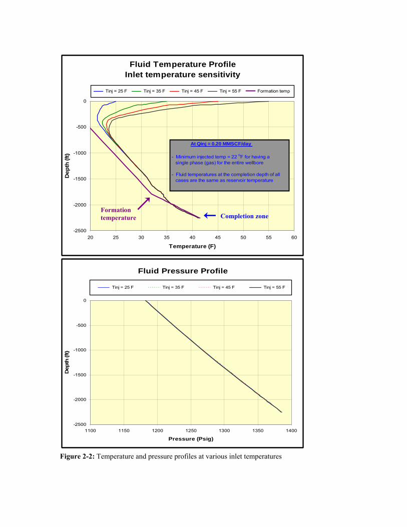
Appendix 2: Wellbore Tubular (ProsperTM) Modeling Prepared by Suntichai Silpngarmlert, ConocoPhillips (Houston) Gas hydrates in nature exist in a relatively narrow range of (low) temperature and (high) pressure, and their stability is very sensitive to pressure and temperature. If temperature of injected fluid (when it enters formation) is warmer than ~50°F, it could trigger hydrate dissociation in the formation. On the other hand, if the fluid temperature is too low, it could freeze free water in the formation resulting in significant injectivity reduction. It is important, therefore, to maintain injected fluid temperatures within a narrow range to avoid these problems. Fluid temperatures at surface during pumping and at the perforation/completion depth are different due to heat generation from friction and heat transfer between fluid in the wellbore and the tubing and surrounding annular materials. Wellbore modeling was used to estimate fluid temperature at the completion depth for a range of surface fluid temperatures, injection rates, and fluid compositions. The main objective of this simulation study is to calculate fluid temperature at the completion zone based on different inlet temperatures, injection rates, and fluid compositions. This information will be used to determine the required heating capacity of heat exchanger system at the surface (the estimated surface temperature is 15oF during the test). First of all, benchmarking study of three wellbore simulators was conducted to determine the best simulator for this study. The three simulators are: 1) ProsperTM, 2) WellCatTM, and 3) CO2Well (research code developed by CSIRO, Australia). The benchmark study indicates that ProsperTM is the best tool as the other two simulators do not accurately represent phase transition (from single gas phase to gas and liquid phase) prediction inside the wellbore. Therefore, this wellbore simulation study was conducted using ProsperTM. Tables 2-1and 2-2 summarize formation thermal properties and temperature gradients used in this study. Thermal conductivity of cement and casing used in this study are 0.5 BTU/hr-ft-oF and 26 BTU/hr-ft-oF, respectively. Wellbore schematic of the test is illustrated in Figure 2-1. Annular fluid is modeled as water, since ProsperTM does not support modeling of water/glycol mixture, which will be in the annulus during injection/flowback operations. Bottomhole fluid temperature has been determined in this study based on different inlet temperatures (fluid temperature at surface), injection rates, and injected fluid compositions (CO2/N2). In this study, the bottom-hole pressure (BHP) was fixed 1385 psi for all simulation cases. Note that BHP value was only used for calculating fluid pressure within the wellbore. It was not used to calculate the injection rate (i.e., BHP and injection rate are not related), both BHP and injection rate are independent variables. Figure 2-2 compares temperature and pressure profiles at different inlet temperatures when injection rate is 0.2 MMSCF/day and fluid composition is 60% CO2 and 40% N2 (weight %). The results indicate that even though the inlet temperatures are different, the

predicted bottom hole fluid temperatures are very close to formation temperature (42oF). This matches expectations, since high inlet-temperature case experiences higher heat transfer (cools down faster) than low inlet-temperature case. Figure 2-3 shows temperature and pressure profiles at different injection rates when inlet temperature is 35oF and fluid composition is 60% CO2 and 40% N2 (weight %). The results illustrate that slower injection rate case cools down faster (in permafrost zone) as it has more time for heat transfer. But again, the plot shows that predicted bottom hole fluid temperature are very close to formation temperature and are not very sensitive to injection rate. Table 2-1: Formation thermal properties
Formation type Bottom depth (ft)
Thermal conductivity
(BTU/hr-ft-oF)
Specific heat (BTU/hr-ft)
Permafrost 1790 2.30 0.216 Siltstone/Shale 1900 1.50 0.239
Hydrate 1950 1.07 0.387 Siltstone/Shale 2050 1.50 0.239
Hydrate 2100 1.07 0.387 Hydrate 2250 1.07 0.387 Hydrate 2400 1.07 0.387
Sandstone/Siltstone/Shale 3525 1.50 0.239 Table 2: Formation temperatures True Vertical Depth (ft) Temperature ( oF )
0 15 1790 32 2280 42 2825 54

Figure 2-1: Wellbore schematic of the test

Figure 2-4 shows temperature and pressure profiles at different injected fluid compositions when inlet temperature is 35oF and injection rate is 0.2 MMSCF/day. In this case, the profiles become more different when phase change takes place (from single gas phase to gas + liquid phase) in the wellbore. However, the results still indicate that predicted bottom hole fluid temperature will be very close to formation temperature.
Conclusions A fundamental design criterion of ConocoPhillips’ CO2/CH4 exchange test is that bottom hole temperature of injected fluid is close to ambient formation temperature, a condition inside the hydrate stability field. These analyses demonstrate that fluids (mixed CO2 and N2 gas) injected at different inlet temperatures, at different rates, or with different fluid compositions all reach formation temperature by the time they reach the perforations. Based on the rates modeled in these analyses, injected fluid only requires heating up to the temperature that achieves single phase condition at the surface (which depends on fluid composition) to avoid any technical challenges related to managing two-phase fluid at the perforations.
Fluid Pressure Profile
-2500
-2000
-1500
-1000
-500
0
1100 1150 1200 1250 1300 1350 1400
Pressure (Psig)
Dep
th (f
t)
Tinj = 25 F Tinj = 35 F Tinj = 45 F Tinj = 55 F
Figure 2-2: Temperature and pressure profiles at various inlet temperatures
Fluid Temperature ProfileInlet temperature sensitivity
-2500
-2000
-1500
-1000
-500
0
20 25 30 35 40 45 50 55 60
Temperature (F)
Dep
th (f
t)
Tinj = 25 F Tinj = 35 F Tinj = 45 F Tinj = 55 F Formation temp
At Qinj = 0.20 MMSCF/day
- Minimum injected temp = 22 oF for having a single phase (gas) for the entire wellbore
- Fluid temperatures at the completion depth of all cases are the same as reservoir temperature
Completion zone Formation temperature

Fluid Pressure Profile
-2500
-2000
-1500
-1000
-500
0
1100 1150 1200 1250 1300 1350 1400
Pressure (Psig)
Dep
th (f
t)
0.1 MMSCF/day 0.2 MMSCF/day 0.3 MMSCF/day
Figure 2-3: Temperature and pressure profiles at various injection rates
Fluid Temperature ProfileInjection rate sensitivity
-2500
-2000
-1500
-1000
-500
0
20 25 30 35 40 45 50 55 60
Temperature (F)
Dep
th (f
t)
0.1 MMSCF/day 0.2 MMSCF/day 0.3 MMSCF/day Formation temp
Effects from injection rates
- Slower injection rate has faster temperature drop, but fluid temperatures of all cases converge to the same value at the bottom of permafrost
- Fluid temperatures at the completion depth of all cases are very closed to the reservoir temperature
Completion zone

Figure 2-4: Temperature and pressure profiles at various injected fluid composition
Fluid Pressure Profile
-2500
-2000
-1500
-1000
-500
0
900 950 1000 1050 1100 1150 1200 1250 1300 1350 1400
Pressure (Psig)
Dep
th (f
t)
CO2/N2 = 60:40 CO2/N2 = 65:35 CO2/N2 = 70:30 CO2/N2 = 75:25
Phase of fluid in the wellbore (liq. or gas) is very sensitive to injection pressure. Adjusting wellhead pressure to match BHP at 1400 psi was difficult.
Fluid Temperature ProfileInjectant composition sensitivity (% wt)
-2500
-2000
-1500
-1000
-500
0
20 25 30 35 40 45 50
Temperature (F)
Dep
th (f
t)
CO2/N2 = 60:40 CO2/N2 = 65:35 CO2/N2 = 70:30 CO2/N2 = 75:25 Formation temp
Effects from injectant composition
- At 35 F inlet temperature, max. CO2 compostion is about 65% wt in order to have a single gas phase for the entire wellbore
- Fluid temperatures at the completion depth of all cases are very closed to the reservoir temperature
Completion zone
Phase change

Appendix 3: Iġnik Sikumi Daily Operations Summaries

Field:Well:
24 Hr Summary Report
Report Header
IGNIK
SIKUMI 1
PRUDHOE BAY UNIT DRILLING
ORIGINAL
Job Type:
Page 1 of 38/4/2011Printed:
NORDIC 3
Rig Name:
4/5/2011 4:30:00 PM
Rig Accept:
4/28/2011 9:00:00 PM
Rig Release:
Brett Packer
Rig Supervisor:
24 hr Summary: Date
Move rig from 2V pad to CPF-2. Crew changeout. Check air in tires, grease planetaries. Move rig from
CPF-2 to Oliktok Y. Standby w/ crews for CPAI crew changeout. Move Rig from Oliktok Y to KCC. Set rig
down, grease planetaries, check tires. Move rig from KCC towards 1D pad.
04/04/2011
Moved Rig to 1J access road. Greased planetaries and check tires, service rig. Moved rig from 1J access
road to Milne Pt. turnoff. Check equipment, meet w/ security. Move rig f/ Milne Pt. turnoff to Ignik Sikumi #1.
Lay out herculite & T-mats, stack double rig mats. Continue to double stack rig mats and build ramp.
PJSM, move rig over well. Spot & level rig. Rig Accepted at 16:30 hrs on 4/5/11. NU diverter, spot
equipment, berm equipment.
04/05/2011
Finish NU diverter. Changeout saver sub & grabber box dies. Spot Drill Cool units w/ crane & berm up
around Drill Cool units. Cont. to spot MI filter unit, MI vac unit, and other 3rd party equipment around rig.
Spot upright tanks and berm up. Load MWD tools, load casing spider slips w/ crane. Offload 5" HWDP & 5"
DP. Load 5" drillpipe into pipe shed, rack & tally drillpipe. Load tools, troubleshoot stabbing board, now
functioning properly.
04/06/2011
Function test stabbing board. Install wood steps over wires running to MWD shack. Install 4" valve on
conductor. PJSM. Pick up drillpipe, calibrate MWD to block height. PU 5" drillpipe, torque up and rack
back in derrick. Load 290 bbls spud mud into upright tank. PJSM. Slip & cut drilling line. Test Diverter.
RIH tag cement at 96.44'. Est. 12' cement to conductor shoe. PJSM. Rack & tally 5" HWDP. PJSM.
Rack & tally 10-3/4" casing. Pressure test mud pumpst to 2000 psi.
04/07/2011
Load casing, rack & tally. MU & break out new HWDP, drift to 2.867. Service top drive, washpipe. Install
Totco monitors in mud shack and MWD shack. Load casing equipment, bring cement head to rig floor. Load
hanger into pipe shed. Continue to load spud mud into pits. Load 20' casing pup and Landing Joint. PJSM.
PU & MU BHA #1, fill hole w/ water. Dry run 10-3/4" fluted hanger and land. Top of Landing Ring at 30.88'
RKB, top of load shoulder at 31.25' RKB. Work on Totco system, fix stroke counter and flapper sensor.
Other Totco functions failed. Stroke counter and gain/loss functions won't zero. Troubleshooting Totco.
04/08/2011
Continue troubleshooting Totco system. Swapped computer module for older version, reloaded Totco and
re-input well info. Totco fixed. Function tested Totco sensors, loaded 10 bbls into trip tank, tested PVT,
block height, traveling speed. Verified can zero stroke counter and gain/loss functions. PJSM. Spudded well
at 02:45 am. Cleanout conductor shoe track f/ 96' to 108'. Drilling ahead f/ 108' to 239'. Back ream out of
hole f/ 239' to 165' Blow down top drive. POOH f/ 239' to surface. PU & MU BHA #2 and TIH to 132'. Upload
MWD. PU single & pulse test. Bring pumps online and survey at 132'. Service Rig. PJSM on radioactive
sources. Load MWD radioactive source and RIH to 170'. Survey at 170'. RBIH to 239', Circulate well clean.
Auger plugged. Unplug same. Directional drill f/ 239' to 379'. Auger loaded up w/ gravel, belt broken.
Replace Belt / unplug auger. Directional drill f/ 379' to 411'. Auger loaded up again. Noticed grinding in the
gear box, begin changing out gear box on auger. Continue to reciprocate and circulate pipe at 1 BPM.
04/09/2011
Cont. to work on auger system, finished installing new gear box. Driller looked down hole and noticed no
flow. Increased pump strokes to 2 BPM and pump pressure spiked to 2500 psi. Shut down pumps and bled
off. Top drive frozen. Set pipe in slips, installed TIW valve and 2" circulation hose, confirmed circulation.
Lowered top drive to rig floor. Disconnected kelly hose, began flushing ice chunks from kelly hose w/ steam.
Clear ice from top drive w/ steam. Continue steaming ice from kelly hose. Attached 2nd steam hose to
pump manifold and applied steam to standpipe. Used infrared temperature sensor to check standpipe
temperature. Standpipe temperature 20' off rig floor @ 120°F, 40' off rig floor 100°F, then immediately above
belly board @ 40' dropped to 20°F. Hoisted rig hand on man-rider to put hands on standpipe and verify
frozen. Confirmed. Finished thawing out Kelly hose & standpipe. Circulate down HWDP @ 3 BPM / 150
psi. Pressure test kelly hose to 2500 psi. Directional drill f/ 411' to 1087', backreaming full stand prior to
every connection. ADT: 9.26 hrs @ midnight.
04/10/2011
Page 1 of 3

Cont. directional drilling f/ 1087' to TD at 1482'. Circulate bottoms up. Blow down top drive, monitor well.
Static. POOH f/ 1482' to 300' on elevators, slight hangup at 1020 ft, worked through. RBIH to TD at 1482'.
Circulate at 15.5 BPM, raise pump rate to 16.1 BPM, rotate & reciprocate. Continue to circulate at 16 BPM.
Pump a 10.9 ppg sweep. Chase sweep with 9.4 ppg mud. Rotate & reciprocate at 45 RPM's. Blow down
top drive, monitor well. Static. POOH f/ 1482' to 975'. RBIH f/ 975' to 1477'. Circulate new 9.1 ppg mud.
Blow down top drive. POOH f/ 1477' to 220'. PJSM on radioactive sources. Continue POOH laying down 8"
MWD tools. Remove nukes, dowload MWD data. Continue to lay down BHA #2.
04/11/2011
Ran 10 3/4" Surface Casing Down to 1,473' MD. Circulated 100 bbls of 10.0 ppg Mud Push follow by 299 bbls
of 11.2 ppg Arctic Lite Crete, pumped addition 65.2 bbls of 12.0 ppg Deep Crete, chased with 128 bbls of 8.8
ppg OBM, bump plug and pressure up to 1010 psi and held pressure for 5 mins. RDMO Cementing Crew and
Equipment.
04/12/2011
Rigged down and Shipped out Diverter. Installed FMC Gen 5 Wellhead System. NU 11" 5M BOP's and
Crossover flow nipple with Annular. Started BOP testing.
04/13/2011
Finish Initial BOP Test. RIH With Production Drilling Assembly and Drilled out the wiper plug, float colllar,
landing collar and shoe. Drilled addition 30' ft of new hole from bottom of shoe at 1,473' to 1,502' and preform
LOT/FIT test. Continue drilling new production hole from 1,502' ft with 8.8 ppg OBM.
04/14/2011
Drilled a Total of 647' ft of New 9 7/8" Production Hole. Had problems keeping 8.8 ppg OBM chilled during
drilling operation. TOOH to remove mud motor, found cone drag on Bit, replace with new bit with 1 ( 14 ) and
3 ( 20 ) nozzle jets. Lay down SperryDrill motor. TIH and continue with Drilling operation until midnight with
very little cooling issue. 24 hour Drilled Section 1,530' ft to 2,220' ft.
04/15/2011
Drilled a Total of 377' of new 9 7/8" hole f/ 2220' to 2597' .Called TD of well at 2,597 ft after dealing with fluid
cooling condition for most of the day while Drilling.Made Several Attempts to keep fluid cool with drill cool unit
to proper temp with little success. CBU until clean, while conditioning well bore. Monitor well for flow, well
static. Wiper trip to 10-3/4" shoe, no hole problems. POOH f/ 2,597 to BHA at 92.80' and Downloaded
recorded data from LWD tools. Break down and lay down Drilling assembly.
04/16/2011
MIRU Schlumberger Wireline Equipment. MU and RIH logging BHA #1 to 2600', Made main pass log from
2600' to surface, found 10-3/4" CSG on depth at 1,473'. . MU and RIH BHA #2 to 2450'. Perform rad check in
CSG, and log correction pass. Measure pressure and mobility with pressure express tool.
04/17/2011
Finish Logging operation with logging assembly #2. Log CMR/PEX/HNGS and 17 pressures with XPT to
obtain mobilities in hydrate zone. POOH and lay down logging assembly #2. MU TLC-MDT logging assembly
#3 and rih 2,259', SLB adjusted tool setting and logged hole to 1,977', x2. RIH and set packer on depth at
2071-2074 feet, start first stage of Mini-Frac. Release packer and rih and correlated for next packer depth.
Stop & parked DP with center of packer at 2202 feet..
04/18/2011
Finished the second stage of the Mini-Frac and Obtain in-situ measurement.MU Schlumberger TLC-MDT
logging assembly #4 and RIH to 2,235' dpmd and started Modular Dynamics Testing with tools setting at
2260'-2263'. After several hours, downhole modular pump not working properly, functioning very slowly. TOOH
to swap out with downhole modular pump from logging assembly #3.
04/19/2011
POOH with MDT testing assembly. Remove modular pump from MDT assembly #4 and Replace with modular
pump from MDT assembly #3. RIH to 1546' and installed side entry port and pump e-line cable and wet
connection head & latched into logging assembly. Correlate depth and position center packer at 2261' ft and
start MDT testing. Stage test area 2260'-2263', Unable obtain sample at stage. Release packer and RIH to
next stage area, and place center of packer at 2303 ft.Start MDT testing at stage area 2302-2304 ft.
04/20/2011
Finished Modular Dynamics Testing on desired zone. Rig down and Release SLB logging Crew and Logging
Equipment. Started Weekly BOP test and safety alarm system testing.
04/21/2011
Continue with testing BOP's. Observed upper rams and annular failed. Change out Upper rams and annular
bag. Resume testing BOP's. Test Annular Upper pipe rams with 2 7/8'', 4 1/2'', 5'' test joints. 250 / 3500 PSI.
Perform Koomey test. Initial 200 PSI in 18 seconds, with full 3000 PSI in 85 seconds. 4 Nitrogen bottle with
and avg PSI of 2075. Witness of test waived by AOGCC rep John Crisp @ 1645 HRS 4/21/11. Make up 9 7/8''
Cleanout BHA with bit #2RR1, and trip in hole with no issues in open hole, proper displacement. Circulate
bottoms up,mix and pump Hi Visc sweep @ 500 GPM's - 950 PSI. Reciprocate & rotate drill string. POOH
laying down drill pipe and pigging every joint to remove oil base mud before laying DP to storage area.
04/22/2011
Continue POOH laying down 5'' DP. Utilize Vac system to clean OBM from joints before removing from pipe
shed. Install & test 7 5/8'' Upper rams. Rig up to run 4 1/2'' x 7 5/8'' casing assembly. Held PJSM with all
personnel. Make up shoe track assembly, fill pipe & check floats. Good. Continue RIH picking up 4 1/2''
casing installing protector clamps as per detail Make up Pinnacle gauge carriers,and splice TEC wire as
needed. Operation at midnight. Just finish the 4 1/2" Completion section of the production string, all three
stages of the Pinnacle Gauge assembly is complete and secured. Start making up the 7 5/8" section.
04/23/2011
Page 2 of 3

Continue run 4 1/2'' x 7 5/8'' casing string with TEC & DTS wires, attaching protector clamps as per detail.
MU Casing hanger and landing joint. Terminate lines for hanger penetration. Secure & test same to 5000 PSI.
RIH land casing hanger. UP / DN WT = 98K. Verify landed hanger as per FMC. RILDS. RU Schlumberger
wireliners, and run GR-CCL log to correlate PIP tag and blank pipe depths. Observed 1/2' foot difference than
pipe tally with wireline measurement. WLOH rig down Schlumberger. Nipple down, splitting the spools. .
Nipple up, and test void on spools as per FMC to 5000 PSI. Utilize crane to off load all spools from rig floor,
and load Flatpak spool with spool & cage. Load Upper 4.5" completion string and jewelry.
04/24/2011
Pull DTS & TEC wires through casing spool side ports as planned. Attach same. Terminate lines, and
connect to there monitors to check for communication to the downhole gauges. Loaded and tallied 4.5" Upper
completion. Removed 7 5/8" ram's and installed 2 7/8" x 5' vbr's and tested 250/3500 psi. Pickup and run in
hole with 2 7/8" fox cementing work string with a baker 2.38" slick stinger down to top of baker packoff
bushing at 2370 ft and string into packoff bushing and no-go 10 ft deeper. Establish circulation @ 3-4 bpm
and condition chilled mud. Sting into packoff bushing, and establish circulation to 3 BPM for full circulation.
Batch mis Mud Push & cement. Pump a total of 75 BBLS of mud push and 153 BBLS of Litecrete cement,
observing 10 BBLS of 11.0 PPG cement to surface. CIP at 15:37 HRS. Floats held. Pull stinger, and reverse
circulate with no cementg returns. Lay down tbg back to 1800' MD. Circulate 90 Deg OBM as per rig
engineer. Blow down & RD DrillCool units.
04/25/2011
Circulated 90 deg heated OBM for a total of 10 hours. RIH w/ 2 7/8" work string down to 2364 ft.
Displacement fluid after mixing surfactant was 57 deg, bring out more fluid, circulate pits to cool to 52 degree.
Mix and circulate 40 bbls spacer of safe-surf, circulate 250 bbls of 52 deg. fresh water, displacing OBM until
clean returns observed. Displace 7 5/8'' to brine, spotting 15 bbls of brine with corrosion inhibitor in the 4.5''
casing section. POOH, laying down 2 7/8'' work string. Ready rig floor and 4.5'' equipment. Make up 4.5'' pipe
handling equipment. Make up Baker seal assembly and lower completion jewelry as per Baker rep.
04/26/2011
Land 4.5'' completion with Chemical injection mandrel, and FlatPak assembly. Install clamps at mid joint as
per procedure. Terminate lines to hanger and test lines to 5, 000 psi. Pump down each Flatpak line @ 30
GPM - 2,150 psi, pump total of 6.2 bbls. RILDS. Test tubing to 3,000 psi for 30 mins, good test, bleed to
2,000 psi. Test IA to 3,000 psi for same, good test. Bleed tubing to zero and shear SOV. ND BOP stack. NU
tree and test to 5,000 psi. Start freeze protect of well with diesel.
04/27/2011
Complete freeze protect of well TBG/ Casing with diesel. Secure wellhead and test below BPV to 3,000 psi.
RDMO Nordic rig.
04/28/2011
Page 3 of 3

Appendix 4: Schlumberger “Interpretation of Iġnik Sikumi #1 MDT Micro-fracturing Tests,” by Richard Birchwood, Vasudev Singh, and Osman Hamid

Interpretation of MDT Micro-
fracturing Tests in the Well Ignik
Sikumi #1, Prudhoe Bay, North Slope,
Alaska
prepared for
Houston, TX
Richard Birchwood Vasudev Singh
Senior Geomechanics Specialist Geomechanics Engineer
Project Leader
Osman Hamid
Geomechanics Engineer
May 2011
Data & Consulting Services

ConocoPhillips Page i
TABLE OF CONTENTS
Disclaimer ...................................................................................................................... ii
1 SUMMARY ............................................................................................................. 1
2 NOMENCLATURE ................................................................................................. 2
3 BRIEF DESCRIPTION OF MICRO-FRACTURING TESTS .................................... 3
4 FLOW RATE CORRECTIONS ............................................................................... 4
5 TEST RESULTS .................................................................................................... 5 5.1 Test Results at 2071.95 ft ............................................................................................... 5
5.1.1 Overview .............................................................................................................. 5 5.1.2 Packer Inflation ..................................................................................................... 6 5.1.3 Filtration test (Cycle 0) .......................................................................................... 8 5.1.4 Cycle 1 10 5.1.5 Cycle 2 15 5.1.6 Cycle 3 18 5.1.7 Cycle 4 21 5.1.8 Cycle 5 24 5.1.9 Cycle 6 27 5.1.10 Cycle 7 30
5.2 Test Results at 2,202.58 ft ............................................................................................ 34
5.2.1 Overview ............................................................................................................ 34 5.2.2 Packer Inflation (Event 0) ................................................................................... 37 5.2.3 Filtration tests (Cycle 0) ...................................................................................... 38 5.2.4 Cycle 1 40 5.2.5 Cycle 2 43 5.2.6 Cycle 3 45 5.2.7 Cycle 4 48 5.2.8 Cycle 5 51 5.2.9 Cycle 6 54 5.2.10 Rebound Test (Event 1) ..................................................................................... 56 5.2.11 Cycle 7 58 5.2.12 Cycle 8 61 5.2.13 Cycle 9 64
6 CONCLUSIONS ................................................................................................... 69
7 APPENDIX A ....................................................................................................... 70 7.1 MDT micro-fracturing operational procedure ................................................................. 70
8 APPENDIX B – Toolstring Used for Micro-fracturing Tests ............................. 76

ConocoPhillips Page ii
Disclaimer
The following disclaimer applies to this report and any interpretation provided by Schlumberger
DCS Geomechanics:
ANY INTERPRETATION, RESEARCH, ANALYSIS, DATA, RESULTS, ESTIMATES, OR
RECOMMENDATION FURNISHED WITH THE SERVICES OR OTHERWISE
COMMUNICATED BY SCHLUMBERGER TO CUSTOMER AT ANY TIME IN
CONNECTION WITH THE SERVICES ARE OPINIONS BASED ON INFERENCES FROM
MEASUREMENTS, EMPIRICAL RELATIONSHIPS AND/OR ASSUMPTIONS, WHICH
INFERENCES, EMPIRICAL RELATIONSHIPS AND/OR ASSUMPTIONS ARE NOT
INFALLIBLE, AND WITH RESPECT TO WHICH PROFESSIONALS IN THE INDUSTRY
MAY DIFFER. ACCORDINGLY, SCHLUMBERGER CANNOT AND DOES NOT WARRANT
THE ACCURACY, CORRECTNESS OR COMPLETENESS OF ANY SUCH
INTERPRETATION, RESEARCH, ANALYSIS, DATA, RESULTS, ESTIMATES OR
RECOMMENDATION.
CUSTOMER ACKNOWLEDGES THAT IT IS ACCEPTING THE SERVICES "AS IS", THAT
SCHLUMBERGER MAKES NO REPRESENTATION OR WARRANTY, EXPRESS OR
IMPLIED, OF ANY KIND OR DESCRIPTION IN RESPECT THERETO. SPECIFICALLY,
CUSTOMER ACKNOWLEDGES THAT SCHLUMBERGER DOES NOT WARRANT THAT
ANY INTERPRETATION, RESEARCH, ANALYSIS, DATA, RESULTS, ESTIMATES, OR
RECOMMENDATION IS FIT FOR A PARTICULAR PURPOSE, INCLUDING BUT NOT
LIMITED TO COMPLIANCE WITH ANY GOVERNMENT REQUEST OR REGULATORY
REQUIREMENT. CUSTOMER FURTHER ACKNOWLEDGES THAT SUCH SERVICES ARE
DELIVERED WITH THE EXPLICIT UNDERSTANDING AND AGREEMENT THAT ANY
ACTION TAKEN BASED ON THE SERVICES RECEIVED SHALL BE AT ITS OWN RISK
AND RESPONSIBILITY AND NO CLAIM SHALL BE MADE AGAINST SCHLUMBERGER
AS A CONSEQUENCE THEREOF.
CUSTOMER CONFIRMS THAT SCHLUMBERGER DCS GEOMECHANICS HAS MADE NO
PROMISE OR STATEMENT REGARDING THE SERVICES THAT IS INCONSISTENT WITH
THESE TERMS OR THE SERVICE ORDER, OR THAT HAS CREATED, OR AMOUNTED TO
A WARRANTY THAT THE SERVICES WOULD CONFORM TO ANY SUCH PROMISE OR
STATEMENT, AND SCHLUMBERGER DCS DISCLAIMS ANY AND ALL WARRANTIES
REGARDING THE SAME.
Schlumberger DCS Geomechanics is an industry leader in working jointly with clients to solve
reservoir and production problems associated with oil and gas field development in a fully
integrated manner that provides process controlled innovative, practical and cost-effective
solutions.

ConocoPhillips Page iii
LIST OF TABLES
Table 5.1: Cycle 0 Results..................................................................................... 8
Table 5.2: Cycle 1 Results................................................................................... 13
Table 5.3: Cycle 2 Results................................................................................... 15
Table 5.4: Cycle 3 Results. .................................................................................. 18
Table 5.5: Cycle 4 Results................................................................................... 21
Table 5.6: Cycle 5 Results................................................................................... 25
Table 5.7: Cycle 6 Results................................................................................... 27
Table 5.8: Cycle 7 Results................................................................................... 30
Table 5.9: Cycle 0 Results. .................................................................................. 38
Table 5.10: Cycle 1 Results ................................................................................. 40
Table 5.11: Cycle 2 Results ................................................................................. 43
Table 5.12: Cycle 3 Results ................................................................................. 45
Table 5.13: Cycle 4 Results ................................................................................. 48
Table 5.14: Cycle 5 Results ................................................................................. 51
Table 5.15: Cycle 6 Results ................................................................................. 54
Table 5.16: Cycle 7 Results ................................................................................. 58
Table 5.17: Cycle 8 Results ................................................................................. 61
Table 5.18: Cycle 9 Results ................................................................................. 64

ConocoPhillips Page iv
List of Figures
Figure 5.1: Logs in vicinity of Station 1. ................................................................. 5
Figure 5.2: Overview of data acquired at Test Station 1 located at 2071.95 ft MD. .......................................................................................................... 6
Figure 5.3: Packer and interval pressures versus time. Difference between packer pressure and interval pressure also shown. .................................... 7
Figure 5.4:Packer Inflation (Event 0) ...................................................................... 7
Figure 5.5: Cycle 0. Final filtration test.................................................................. 8
Figure 5.6: Plot of interval pressure vs. pumped volume during the filtration phase (red curve). A linear fit to this curve is shown in purple. Orange line shows location of departure of curve from linearity. The flow rate into the interval (blue curve) is also shown referenced to the right hand vertical axis. ......................................................................... 9
Figure 5.7: Plots of interval pressure (red curve) and its derivative (purple curve) versus square root of shut-in time. ................................................... 9
Figure 5.8: Cycle 1. Breakdown of the formation. ............................................... 11
Figure 5.9: Packer and interval pressures versus time during Cycle 1. (a) Pressures in vicinity of first peak. (b) Pressures in vicinity of second peak.......................................................................................................... 12
Figure 5.10: Packer pressure minus interval pressure during Cycle 1. ................ 13
Figure 5.11: Plot of interval pressure vs. pumped volume during Cycle 1 (red curve). A linear fit to this curve shown in purple. The volume at which the curve departs from linearity shown by orange line. The flow rate into the interval (blue curve) is shown referenced to the right hand vertical axis. ............................................................................. 14
Figure 5.12: Pressure versus square root of time (red curve) during shut-in phase of Cycle 1. Pressure derivative is also shown (purple curve). ........ 14
Figure 5.13: Cycle1-G-Function Interpretation. .................................................... 15
Figure 5.14: Cycle 1. Propagation of the fracture. .............................................. 16
Figure 5.15: Plot of interval pressure vs. pumped volume during Cycle 2 (red curve). A linear fit to this curve shown in purple. The volume at which the curve departs from linearity shown by orange line. The flow rate into the interval (blue curve) is shown referenced to the right hand vertical axis. ............................................................................. 16
Figure 5.16: Pressure versus square root of time (red curve) during shut-in phase of Cycle 2. Pressure derivative is also shown (purple curve). ........ 17
Figure 5.17: Cycle 2-G-Function Interpretation. ................................................... 17
Figure 5.18: Cycle 3. Propagation of the fracture. Interval pressure (PAQP), pump motor speed (POUDMS), pump hydraulic pressure

ConocoPhillips Page v
(POUDHP), flow rate (Flowrate_corrected), and interval valve position (PAVP) are shown. ...................................................................... 18
Figure 5.19: Interval pressure (PAQP), flow rate (Flowrate_corrected), and interval valve position (PAVP) during injection phase of Cycle 3. .............. 19
Figure 5.20: Plot of interval pressure vs. pumped volume during Cycle 3 (red curve). A linear fit to this curve shown in purple. The volume at which the curve departs from linearity shown by orange line. The flow rate into the interval (blue curve) is shown referenced to the right hand vertical axis. ............................................................................. 19
Figure 5.21: Pressure versus square root of time (red curve) during shut-in phase of Cycle 3. Pressure derivative is also shown (purple curve). ........ 20
Figure 5.22: Cycle 3-G-Function Interpretation. ................................................... 20
Figure 5.23: Cycle 4. Propagation of the fracture. Interval pressure (PAQP), pump motor speed (POUDMS), pump hydraulic pressure (POUDHP), flow rate (POTFR), and interval valve position (PAVP) are shown. ................................................................................................ 21
Figure 5.24: Interval pressure (PAQP), flow rate (POTFR), and interval valve position (PAVP) during injection phase of Cycle 4. .......................... 22
Figure 5.25: Plot of interval pressure vs. pumped volume during Cycle 4 (red curve). A linear fit to this curve shown in purple. The volume at which the curve departs from linearity shown by orange line. The flow rate into the interval (blue curve) is shown referenced to the right hand vertical axis. ............................................................................. 22
Figure 5.26: Pressure versus square root of time (red curve) during shut-in phase of Cycle 4. Pressure derivative is also shown (purple curve). ........ 23
Figure 5.27: Cycle 4-G-Function Interpretation. ................................................... 24
Figure 5.28: Cycle 5. Propagation of the fracture. .............................................. 25
Figure 5.29: Plot of interval pressure vs. pumped volume during Cycle 5 (red curve). A linear fit to this curve shown in purple. The volume at which the curve departs from linearity shown by orange line. The flow rate into the interval (blue curve) is shown referenced to the right hand vertical axis. ............................................................................. 26
Figure 5.30: Pressure versus square root of time (red curve) during shut-in phase of Cycle 5. Pressure derivative is also shown (purple curve). ........ 26
Figure 5.31: Cycle 5-G-Function Interpretation. ................................................... 27
Figure 5.32: Cycle 6. Propagation of the fracture. .............................................. 28
Figure 5.33: Plot of interval pressure vs. pumped volume during Cycle 6 (red curve). A linear fit to this curve shown in purple. The volume at which the curve departs from linearity shown by orange line. The flow rate into the interval (blue curve) is shown referenced to the right hand vertical axis. ............................................................................. 28
Figure 5.34: Pressure versus square root of time (red curve) during shut-in phase of Cycle 6. Pressure derivative is also shown (purple curve). ........ 29

ConocoPhillips Page vi
Figure 5.35: Cycle 6. G-Function Interpretation. ................................................. 29
Figure 5.36: Cycle 7. Propagation of the fracture. .............................................. 30
Figure 5.37: Plot of interval pressure vs. pumped volume during Cycle 7 (red curve). A linear fit to this curve shown in purple. The volume at which the curve departs from linearity shown by orange line. The flow rate into the interval (blue curve) is shown referenced to the right hand vertical axis. ............................................................................. 31
Figure 5.38: Pressure versus square root of time (red curve) during shut-in phase of Cycle 7. Pressure derivative is also shown (purple curve). ........ 31
Figure 5.39: Cycle 7-G-Function Interpretation .................................................... 32
Figure 5.40: Reconciliation plot for Test Station 1. (a) All parameters. (b) Pressures only. ......................................................................................... 33
Figure 5.41: Logs in vicinity of Test Station 2. ..................................................... 34
Figure 5.42: Overview of data acquired at Test Station 2 located at 2202.58 ft MD. .......................................................................................... 35
Figure 5.43: Packer pressure minus interval pressure vs. time. ........................... 36
Figure 5.44: Interval (blue) and packer (purple) pressures during instances when the packer pressure fell below the interval pressure. (a) During Cycle 2 shut-in period. (b) During rebound test following Cycle 6 (c) During Cycle 7 shut-in period. (d) During Cycle 8 shut-in period. ...................................................................................................... 37
Figure 5.45: Packer Inflation. ............................................................................... 38
Figure 5.46: Filtration tests (Cycle 0). The first filtration test started at 3071 s and the second started at 3397 s. .......................................................... 39
Figure 5.47: Plot of interval pressure vs. pumped volume (brown curve) during the filtration test (Cycle 0 ). A linear fit to this curve shown in red. The volume at which the curve departs from linearity shown by grey cross-hairs. The flow rate into the interval (purple curve) is shown referenced to the right hand vertical axis. ...................................... 39
Figure 5.48: Plots of interval pressure (red curve) and its derivative (purple curve) versus square root of shut-in time. ................................................. 40
Figure 5.49: Cycle 1. Breakdown of the formation. ............................................. 41
Figure 5.50: Plot of interval pressure vs. pumped volume (brown curve) during Cycle 1. A linear fit to this curve shown in red. The volume at which the curve departs from linearity shown by grey cross-hairs. The flow rate into the interval (purple curve) is shown referenced to the right hand vertical axis. ....................................................................... 41
Figure 5.51: Plots of interval pressure (red curve) and its derivative (purple curve) versus square root of shut-in time. ................................................. 42
Figure 5.52: Interpretation of fracture closure during Cycle 1 using the G-function. .................................................................................................... 42
Figure 5.53: Cycle 2. Propagation of the fracture. .............................................. 43

ConocoPhillips Page vii
Figure 5.54: Plot of interval pressure vs. pumped volume during Cycle 2 (red curve). A linear fit to this curve shown in purple. The volume at which the curve departs from linearity shown by orange vertical line. The flow rate into the interval (blue curve) is shown referenced to the right hand vertical axis. ....................................................................... 44
Figure 5.55: Plots of interval pressure (red curve) and its derivative (purple curve) versus square root of shut-in time. ................................................. 44
Figure 5.56: Cycle 2-Depth 2-G-Function Interpretation. ..................................... 45
Figure 5.57: Raw data from Cycle 3. Interval pressure (PAQP), pump motor speed (POUDMS), pump hydraulic pressure (POUDHP), flow rate (POTFR), and interval valve position (PAVP) are shown. .................. 46
Figure 5.58: Interval pressure (PAQP), flow rate (Flowrate_corrected), and interval valve position (PAVP) during injection phase of Cycle 3. .............. 46
Figure 5.59: Plot of interval pressure vs. pumped volume during Cycle 3 (red curve). A linear fit to this curve shown in purple. The volume at which the curve departs from linearity shown by orange vertical line. The flow rate into the interval (blue curve) is shown referenced to the right hand vertical axis. ....................................................................... 47
Figure 5.60: Plots of interval pressure (red curve) and its derivative (purple curve) versus square root of shut-in time. ................................................. 47
Figure 5.61: Cycle 3-Depth 2-G-Function Interpretation. ..................................... 48
Figure 5.62: Raw data from Cycle 4. Interval pressure (PAQP), pump motor speed (POUDMS), pump hydraulic pressure (POUDHP), flow rate (Flowrate_corrected), and interval valve position (PAVP) are shown. ...................................................................................................... 49
Figure 5.63: Interval pressure (PAQP), flow rate (Flowrate_corrected), and interval valve position (PAVP) during injection phase of Cycle 4. .............. 49
Figure 5.64: Plot of interval pressure vs. pumped volume during Cycle 4 (red curve). A linear fit to this curve shown in purple. The volume at which the curve departs from linearity shown by orange vertical line. The flow rate into the interval (blue curve) is shown referenced to the right hand vertical axis. ....................................................................... 50
Figure 5.65: Plots of interval pressure (red curve) and its derivative (purple curve) versus square root of shut-in time. ................................................. 50
Figure 5.66: Cycle 4-Depth 2-G-Function Interpretation. ..................................... 51
Figure 5.67: Raw data from Cycle 5. Interval pressure (PAQP), pump motor speed (POUDMS), pump hydraulic pressure (POUDHP), flow rate (POTFR), and interval valve position (PAVP) are shown. .................. 52
Figure 5.68: Interval pressure (PAQP), flow rate (Flowrate_corrected), and interval valve position (PAVP) during injection phase of Cycle 5. .............. 52
Figure 5.69: Plot of interval pressure vs. pumped volume during Cycle 5 (red curve). A linear fit to this curve shown in purple. The volume at which the curve departs from linearity shown by orange vertical line.

ConocoPhillips Page viii
The flow rate into the interval (blue curve) is shown referenced to the right hand vertical axis. ....................................................................... 53
Figure 5.70: Plots of interval pressure (red curve) and its derivative (purple curve) versus square root of shut-in time. ................................................. 53
Figure 5.71: Cycle 5-Depth 2-G-Function Interpretation. ..................................... 54
Figure 5.72: Raw data from Cycle . Interval pressure (PAQP), pump motor speed (POUDMS), pump hydraulic pressure (POUDHP), flow rate (Flowrate_corrected), and interval valve position (PAVP) are shown. ....... 55
Figure 5.73: Interval pressure (PAQP), flow rate (Flowrate_corrected), and interval valve position (PAVP) during injection phase of Cycle 6. .............. 55
Figure 5.74: Plot of interval pressure vs. pumped volume during Cycle 6 (red curve). A linear fit to this curve shown in purple. The volume at which the curve departs from linearity shown by orange vertical line. The flow rate into the interval (blue curve) is shown referenced to the right hand vertical axis. ....................................................................... 56
Figure 5.75: Cycle 6 followed by Rebound Test. ................................................. 57
Figure 5.76: Plot of interval pressure (red curve) versus time during rebound test (Event 1). Grey horizontal line represents approximate asymptotic value of the pressure (1210 psi). ............................................. 57
Figure 5.77: Raw data from Cycle 7. Interval pressure (PAQP), pump motor speed (POUDMS), pump hydraulic pressure (POUDHP), flow rate (Flowrate_corrected), and interval valve position (PAVP) are shown. ...................................................................................................... 58
Figure 5.78: Interval pressure (PAQP), flow rate (Flowrate_corrected), and interval valve position (PAVP) during injection phase of Cycle 3. .............. 59
Figure 5.79: Plot of interval pressure vs. pumped volume during Cycle 7 (red curve). A linear fit to this curve shown in purple. The volume at which the curve departs from linearity shown by orange vertical line. The flow rate into the interval (blue curve) is shown referenced to the right hand vertical axis. ....................................................................... 59
Figure 5.80: Plots of interval pressure (red curve) and its derivative (purple curve) versus square root of shut-in time. ................................................. 60
Figure 5.81: Cycle 7-Depth 2-G-Function Interpretation. .................................... 60
Figure 5.82: Raw data from Cycle 8. Interval pressure (PAQP), pump motor speed (POUDMS), pump hydraulic pressure (POUDHP), flow rate (Flowrate_corrected), and interval valve position (PAVP) are shown. ...................................................................................................... 61
Figure 5.83: Interval pressure (PAQP), flow rate (Flowrate_corrected), and interval valve position (PAVP) during injection phase of Cycle 8. .............. 62
Figure 5.84: Plot of interval pressure vs. pumped volume during Cycle 8 (red curve). A linear fit to this curve shown in purple. The volume at which the curve departs from linearity shown by orange vertical line.

ConocoPhillips Page ix
The flow rate into the interval (blue curve) is shown referenced to the right hand vertical axis. ....................................................................... 62
Figure 5.85: Plots of interval pressure (red curve) and its derivative (purple curve) versus square root of shut-in time. ................................................. 63
Figure 5.86: Cycle 8-Depth 2-G-Function Interpretation. ..................................... 63
Figure 5.87: Raw data from Cycle 9. Interval pressure (PAQP), pump motor speed (POUDMS), pump hydraulic pressure (POUDHP), flow rate (Flowrate_corrected), and interval valve position (PAVP) are shown. ...................................................................................................... 64
Figure 5.88: Interval pressure (PAQP), flow rate (Flowrate_corrected), and interval valve position (PAVP) during injection phase of Cycle 9. .............. 65
Figure 5.89: Plot of interval pressure vs. pumped volume during Cycle 3 (red curve). A linear fit to this curve shown in purple. The volume at which the curve departs from linearity shown by orange vertical line. The flow rate into the interval (blue curve) is shown referenced to the right hand vertical axis. ....................................................................... 65
Figure 5.90: Plots of interval pressure (red curve) and its derivative (purple curve) versus square root of shut-in time. ................................................. 66
Figure 5.91: Cycle 9-Depth 2-G-Function Interpretation. ..................................... 66
Figure 5.92: Reconciliation Plot at Test Station 2. ............................................... 67
Figure 5.93: Reconciliation Plot at Test Station 2. Pressures only. ...................... 68

ConocoPhillips Page 1
1 SUMMARY
This report describes the results of micro-fracturing tests carried out on April 18-19, 2011 in the
vertical well Ignik Sikumi #1 for purposes of measuring the minimum horizontal stress. The well
was drilled with oil-based mud in the Prudhoe Bay Unit of the North Slope, Alaska and attained a
total depth of 2600 ft RKB. Fractures were generated by pressurizing an interval approximately 3
ft in length isolated between the dual packers of the MDT tool. The nominal diameter of the
borehole was 9.88 in. Micro-fracturing tests were carried out at two stations located at 2071.95 and
2202.58 ft RKB in order of chronology (the rig kelly bushing was 30.7 ft above ground level). The
tool string used in both tests is shown in Appendix B.
Both tests were performed in open-hole conditions. The formation at the first test station was a gas
hydrate bearing D-sand. A siltstone resided at the second test location. Because the tests were
performed in soft sediments, problems with seal integrity, fracture initiation, and sticking were
anticipated. Sealing problems did occur, but they were of limited duration and had minimal impact
on the test. The other two problems did not occur. However irregular flow due to half-stroking of
pumps was a frequent occurrence. This problem was probably caused by interaction of solids in
the mud with pump check valves. Half-stroking complicated interpretation of corroborative
parameters such as the leak-off pressure. However this problem did not affect the inference of the
most crucial parameter, i.e., the closure stress. Therefore the main objective of these tests was
satisfied. The tests yielded minimum horizontal stress estimates of 1364 psi (12.7 ppg) and 1625
psi (14.2 ppg) at the first and second test stations respectively.

ConocoPhillips Page 2
2 NOMENCLATURE
C0, C1,C2,.. – Cycle 0, Cycle 1, Cycle2, etc.
CloseG – Closure pressure determined from Nolte (G-function) plot
CloseSq – Closure pressure determined from plot of pressure versus square root of shut-in time
E1 – Event 1
ISIP - Instantaneous shut-in pressure
LOP - interval pressure at start of fracture propagation (leak-off pressure)
LOV - volume of fluid pumped prior to fracture propagation
MRFC – Flow control module
MRPA - Dual packer module
MRPOUD/MRPOUD2/MRPOUD3 - Pump-out unit
PAFP - Packer valve status
PAHP - Dual Packer Inflate Pressure
PAQP - MRPA Quartz guage interval pressure
PAVP - Interval valve status
P_Close - Closure pressure determined from plot of pressure versus square root of shut-in time
P_Close_G-function - Closure pressure determined from Nolte (G-function) plot
Peak, Peak_P - Maximum pressure attained prior to unstable fracture propagation.
P_HYD - Hydrostatic pressure
POTFR – Total flow rate
POUDHP/POUDHP2 – MRPOUD/MRPOUD2 hydraulic pressure
POUDMS/POUDMS2 – MRPOUD/MRPOUD2 motor speed
P_Reb - Rebound pressure
Prop, Prop_P – Fracture propagation pressure
Reb – Rebound pressure
Stiff,Stiffness – Measure of wellbore stiffness equal to the gradient of the pressure vs. volume
curve prior to fracture initiation
Vfrac, VL_Frac – Volume of fluid pumped into fracture

ConocoPhillips Page 3
3 BRIEF DESCRIPTION OF MICRO-FRACTURING TESTS
In this section a brief description of the test procedures employed in Ignik Sikumi #1 is provided.
For more details of micro-fracturing test procedures and apparatus, please consult Appendix A. The
micro-fracturing test at each station commenced with inflation of the packers for the purpose of
sealing an interval approximately 3 ft long. This was followed by a sequence of operations in which
pressure in the test interval1 between the packers was manipulated using three dual pump-out
modules (MRPOUD, MRPOUD2, MRPOUD3). The operations were as follows:
1. Filtration tests in which the interval pressure was raised to a value less than that required
to break down the formation followed by shutting in of the interval. This test is conducted
in order to allow the packers to seat themselves properly against the formation, verify the
integrity of the packer seal, and establish a baseline rate of pressure decline through the
wellbore wall prior to fracturing.
2. Injection into the interval until initiation or propagation of a fracture occurred.
3. Propagation of the fracture for a designated period.
4. Cessation of pumping, isolation of the test interval, and observation of pressure decline.
5. Extension of the fracture by repeated execution of steps 2, 3, and 4.
In addition to these operations, a rebound test was conducted at the second station (2202.58 ft)
whereby a fracture was propagated, fluid was suddenly withdrawn from the interval and the interval
was shut-in. The interval pressure initially decreased rapidly and then rebounded. The final
pressure approached during the shut-in period represents a lower bound on the closure stress.
In the proceeding discussion we adopt the convention that all episodes consisting of pressurization of
the interval followed by shut-in and pressure decline are referred to as cycles. All other episodes,
such as those involving packer inflation or withdrawal of fluid from the interval are referred to as
events.
1 Hereafter the test interval will be referred to simply as the interval.

ConocoPhillips Page 4
4 FLOW RATE CORRECTIONS
Special care was taken to ensure that flow rates generated by the dual pump-out modules were
accurately computed. Corrections were introduced to remove irregularities in computed flow rates
due to disruption of flow by shutting of valves while the pump was running. For example, the flow
delivered to the interval was set to zero whenever the interval valve was shut. Additional
corrections to the flow rate were made to account for half-stroking of the pump piston. Half-
stroking occurs when mud-check valves in the pump do not seal properly. As a result, fluid is not
delivered by the pump. This problem occurred frequently, and may have been caused by exposure
of mud check valves to solids in the mud. Half-stroking can be diagnosed be examining the pump
hydraulic pressure. This pressure is unusually low when half-stroking occurs. In order to correct
for this problem, the flow rate was set to zero whenever the hydraulic pressure fell below a
designated cutoff.
.

ConocoPhillips Page 5
5 TEST RESULTS
5.1 Test Results at 2071.95 ft
5.1.1 Overview
This test was carried out in a gas hydrate bearing sand. Figure 5.1 shows the location of the test
interval. The borehole is slightly under-gauged, possibly due to mudcake build-up or creep. A
small amount of separation between resistivity curves at the test location indicates mud invasion
and possibly, some gas hydrate dissociation near the wellbore. The dynamic Young’s modulus of
the formation is approximately 7.6 GPa, which is typical of weakly consolidated sediments.
Figure 5.1: Logs in vicinity of Station 1.
The test interval was located in a gas hydrate bearing interval between 2069.9 and 2073.1 ft.
TRACK 1: Measured Depth with respect to KB. TRACK 2: Dual caliper measurements
C1_OBMT, C2_OBMT and bit size, BS. Shading reflects difference between each caliper
measurement and the bit size. TRACK 3: Gas hydrate saturation, SHY, density, RHOZ, and
gamma ray, GR. TRACK 4: Resistivities measured at various depths of investigation from shallow
(A010) to deep (AO90) TRACK 5: Compressional (DTCO) and shear (DTSM) wave slownesses.
TRACK 6: Dynamic Young’s modulus.
2050
2060
2070
2080
2090
Test
interval
MD
ft

ConocoPhillips Page 6
Figure 5.2: Overview of data acquired at Test Station 1 located at 2071.95 ft MD.
Figure 5.2 presents an overview of the most important data acquired during the test. The time
corresponding to the peak interval pressure (green curve) roughly divides the test into two equal
parts. The earlier part consisted of packer inflation and filtration tests. The later part consisted of
fracture propagation/shut-in cycles. A total of seven fracture propagation /shut-in cycles were
performed during the test. The static pressure of the mud column at the start of the test was 975.4
psi.
Figure 5.3 provides an overview of the packer pressure, interval pressure, and the difference
between them. The packer pressure is generally higher than the interval pressure. This indicates
that the packer is functioning as designed and provides some assurance that a proper seal is being
maintained. However Figure 5.3 also shows a brief episode during the first injection cycle in
which the packer pressure dropped below the interval pressure. This was most likely due to a
temporary loss of seal. This problem will be highlighted later.
5.1.2 Packer Inflation
Figure 5.4 shows the packer inflation event. The packer was inflated over a period of more than
6000 s. A primary objective of this procedure was to avoid over-inflation of the packer that could
cause it to stick or make poor contact with the borehole wall due to excessive yielding of the
formation. Satisfying this objective involved determining the minimum packer pressure required to
maintain adequate contact with the borehole wall. The initial pressure of the mud column was
975.65 psi. The packer was inflated in stages to 1250 psi. Whenever the pump was switched off,
PO
TC
V (
cm3
)
PO
TF
R (
cm
3/s
)
PAQ
P (
psi
)
Time (s)
Interval
pressure,
PAQP
Interval valve
position, PAVP
Flow rate,
POTFR
Total
pumpout
volume,
POTCV
Inflate valve
position, PAVP

ConocoPhillips Page 7
the packer pressure declined gradually. This is because the interval pressure declines due to
leakoff to the formation and the packer pressure follows the interval pressure.
Figure 5.3: Packer and interval pressures versus time. Difference between packer pressure and interval pressure also shown.
Figure 5.4:Packer Inflation (Event 0)
Time (s)
Pump motor speed
Packer pressurePacker valve
position
Interval
pressure
Interval valve
position
Hydrostatic
pressureFlow rate

ConocoPhillips Page 8
After the final inflation step, the packer pressure remained above the interval pressure and the seal
was judged to be adequate for the next stage of the test.
5.1.3 Filtration test (Cycle 0)
Figure 5.5 presents the results of a filtration test conducted prior to breaking down the formation.
Fluid was pumped into the interval at a rate of 5.5 cc/s for about 50 s and then the interval was shut
in. Figure 5.6 plots the interval pressure versus the volume of fluid pumped into the interval. The
curve is nonlinear indicating that the formation might be yielding or that the rate of fluid loss
through the formation is high relative to the pump rate. Figure 5.7 shows the pressure during the
shut in phase versus the square root of shut-in time. The derivative of the pressure with respect to
the square root of shut-in time is also shown. Table 5.1 summarizes the results of this cycle.
Figure 5.5: Cycle 0. Final filtration test.
Table 5.1: Cycle 0 Results
PO
UD
MS
(c/m
in)
PO
TF
R (
cm
3/s
)
PAQ
P (
psi
)
PO
UD
HP
(p
si)
Interval
pressure,
PAQP
Interval valve
position, PAVP
Flow rate,
POTFR
Hydraulic
pressure,
POUDHP
Motor
speed,
POUDMS
Time (s)
Stiff
(psi/cc)
LOP
(psi)
LOV
(cc)
VL_frac
(cc)
Peak_P
(psi)
Prop_P
(psi)
ISIP
(psi)
P_close
(psi)
P_clos_G-
function
(psi)
0.8405 1210 54 N/A N/A N/A N/A N/A N/A

ConocoPhillips Page 9
Figure 5.6: Plot of interval pressure vs. pumped volume during the filtration phase (red curve). A linear fit to this curve is shown in purple. Orange line shows location of departure of curve from
linearity. The flow rate into the interval (blue curve) is also shown referenced to the right hand vertical axis.
Figure 5.7: Plots of interval pressure (red curve) and its derivative (purple curve) versus square root of shut-in time.
-1
0
1
2
3
4
5
6
7
1140
1160
1180
1200
1220
1240
1260
1280
1300
1320
0 50 100 150 200 250 300
Flo
w R
ate
(cc
/s)
Inte
rva
l Pre
ssu
re (
Psi
)
Pumped Volume (cc)
BHP Vs Pumped Volume
Linear Fit
Flow Rate Vs Pumped Volume
1200
1220
1240
1260
1280
1300
1320
2 4 6 8 10 12 14 16 18 20 22 24
Inte
va
l P
res
su
re
Sqrt of Shut-in Time (s^0.5)
-10
-9
-8
-7
-6
-5
-4
-3
-2
BHP (psi) BHP Deri. (psi/s)

ConocoPhillips Page 10
5.1.4 Cycle 1
Figure 5.8 shows the results from Cycle 1. The interval pressure was raised until the formation
appeared to break down at 11931 s at a peak pressure of 1985 psi. However as pumping continued,
the pressure subsequently attained a much higher peak value of 2068 psi at 12064 s. There are
three possible reasons for this:
1. The pump sputtered at the first peak leading to a premature decline in the pressure.
2. The packer seal was breached at the first peak leading to a premature decline in the
pressure.
3. A fracture was formed at the first peak, but was bridged off from the interval by solids in
the mud making it difficult to propagate.
The first explanation is ruled out on the basis that the pump maintained a hydraulic pressure well
above the threshold for a malfunction (the threshold is typically ~ 100-300 psi). Figure 5.8 shows
that the pump hydraulic pressure was above 1500 psi when the first peak pressure was attained.
The second explanation, a breach in the packer seal, can occur as a result of the packer fracturing
the formation (a so-called “sleeve fracture”), or due to a loss of contact pressure between the
packer and the formation caused by plastic yielding of the formation. However in both these cases,
the pressure in the packer should drop before the pressure in the interval. Figure 5.9(a) shows that
the pressure in the packer continued to rise for about 5 seconds after the interval pressure began to
level off. Hence the second scenario seems unlikely.
The third explanation is the most likely one. It is also consistent with evidence of filtercake
formation discussed in relation to later cycles. A filtercake probably formed either inside the
fracture or at the mouth of the fracture soon after it was created. This process of bridging would
have been encouraged by the drop in pressure that occurred right after breakdown. The filtercake
sealed off the tip of the fracture from the wellbore. A higher wellbore pressure was thus required
to further propagate the fracture.

ConocoPhillips Page 11
Figure 5.8: Cycle 1. Breakdown of the formation.
Interval valve
position, PAVP
PO
UD
MS
(c/
min
)
PO
UD
HP
(p
si)
PO
TF
R (
cm
3/s
)
PAQ
P (
psi
)
Motor speed,
POUDMS
Hydraulic
pressure,
POUDHP
Flow rate,
POTFR
Interval pressure,
PAQP

ConocoPhillips Page 12
Figure 5.9: Packer and interval pressures versus time during Cycle 1. (a) Pressures in vicinity of first peak. (b) Pressures in vicinity of second peak.
Figure 5.9(b) shows the packer and interval pressures in the vicinity of the second peak pressure
shown in Figure 5.8. A rapid decline in both pressures occurred at 12063 s. In this case, the
packer pressure reached a plateau while the interval pressure was rising, indicating that events at
the packer level were responsible for the sudden decline in pressure. It is probable that a temporary
breach of seal occurred at the second peak. Additional evidence for a loss of seal can be found in
the fact that the packer pressure momentarily dropped below the interval pressure (Figure 5.10).
This is frequently an indication that the seal has been broken. This loss of seal may have been
caused by the packer reseating itself against the formation or fracturing of the formation by the
packer.
Figure 5.11 shows the interval pressure plotted against the volume of fluid pumped into the
interval. The formation response is quite linear until the breakdown pressure is attained. Figure
Figure 5.12 plots the shut-in phase of the cycle. An inflection point associated with closure of the
fracture is identified at 1444 psi. An alternative construction using the G-function yields a closure
pressure of 1442 psi (Figure 5.13). Table 5.2 summarizes the results of this cycle.
Packer pressure
Interval pressure
Plateau
(b)
Packer pressure
(smoothed)
Interval pressure
(a)
Interval pressure
starts levelling off

ConocoPhillips Page 13
Table 5.2: Cycle 1 Results
Figure 5.10: Packer pressure minus interval pressure during Cycle 1.
Stiff
(psi/cc)
LOP
(psi)
LOV
(cc)
VL_frac
(cc)
Peak_P
(psi)
Prop_P
(psi)
ISIP
(psi)
P_clos
(psi)
P_clos_G-
function
(psi)
0.4208 1970 1750 2211.9 1985.2 N/A 1476 1444.1 1442

ConocoPhillips Page 14
Figure 5.11: Plot of interval pressure vs. pumped volume during Cycle 1 (red curve). A linear fit to this curve shown in purple. The volume at which the curve departs from linearity shown by orange line. The flow rate into the interval (blue curve) is shown referenced to the right hand vertical axis.
Figure 5.12: Pressure versus square root of time (red curve) during shut-in phase of Cycle 1. Pressure derivative is also shown (purple curve).
-2
0
2
4
6
8
10
12
14
1420
1520
1620
1720
1820
1920
2020
2120
2220
0 1000 2000 3000 4000
Flo
w R
ate
(cc
/s)
Inte
rva
l Pre
ssu
re (
Psi
)
Pumped Volume (cc)
BHP Vs Pumped
VolumeLinear Fit
Flow Rate Vs
Pumped Volume
1380
1400
1420
1440
1460
1480
1500
19 21 23 25 27 29 31 33 35 37
Inte
rna
l P
res
su
re (
psi)
Sqrt of (Pump + Shut-in Time) (s^0.5)
-180
-160
-140
-120
-100
-80
-60
-40
-20
0
BH
P D
eri
(p
si/
s^
0.5
)
BHP (psi) BHP Deri. (psi/s)
Closure:1444.08
Sqrt of Shut-in Time (s^0.5)

ConocoPhillips Page 15
Figure 5.13: Cycle1-G-Function Interpretation.
5.1.5 Cycle 2
The interval was again pressurized and the fracture created in Cycle 1 was propagated for 130 s.
Figure 5.14 shows key data from this test. During injection, the pump half-stroked twice as
evidenced by sharp drops in the pump hydraulic pressure. During these episodes, the interval
pressure to dipped and then recovered as pumping resumed. Figure 5.15 shows a plot of interval
pressure versus pumped volume. In spite of the half-stroking of the pump, this curve maintains an
almost constant gradient until the fracture reopens at 1511 psi. Figure 5.16 shows the plot of
pressure versus square root of time for the shut-in phase. The fracture appears to close at 1459 psi.
An alternative construction using the G-function yields a closure pressure of 1456 psi (Figure
5.17). Table 5.3 summarizes the principal results of this cycle.
Table 5.3: Cycle 2 Results
GdP/dG
dP/dG
ISIP at 1476 psi
Bottom Hole Pressure
Fracture Closure Pressure at 1442 psi
Stiff
(psi/cc)
LOP
(psi)
LOV
(cc)
VL_frac
(cc)
Peak_P
(psi)
Prop_P
(psi)
ISIP
(psi)
P_clos
(psi)
P_clos_G-
function
(psi)
0.677 1511.0 180.0 1265.0 1531.3 1518.7 1494 1459.3 1456

ConocoPhillips Page 16
Figure 5.14: Cycle 1. Propagation of the fracture.
Figure 5.15: Plot of interval pressure vs. pumped volume during Cycle 2 (red curve). A linear fit to this curve shown in purple. The volume at which the curve departs from linearity shown by orange line. The flow rate into the interval (blue curve) is shown referenced to the right hand vertical axis.
PO
TF
R (
cm
3/s
)
PO
UD
HP
(p
si)
PO
UD
MS
(c/
min
)
PAQ
P (
psi
)
Flow rate,
POTFRHydraulic pressure,
POUDHP
Interval
pressure, PAQP
Interval valve
position, PAVP
Motor
speed,
POUDMS
Time (s)
0
2
4
6
8
10
12
1420
1440
1460
1480
1500
1520
1540
1560
1580
0 250 500 750 1000 1250 1500
Flo
w R
ate
(cc
/s)
Inte
rva
l Pre
ssu
re (
psi
)
Pumped Volume (cc)
BHP Vs Pumped Volume
Linear Fit
Flow Rate Vs Oumoed Volume

ConocoPhillips Page 17
Figure 5.16: Pressure versus square root of time (red curve) during shut-in phase of Cycle 2. Pressure derivative is also shown (purple curve).
Figure 5.17: Cycle 2-G-Function Interpretation.
1400
1420
1440
1460
1480
1500
1520
0 10 20 30 40 50
Inte
rva
l P
res
su
re
Sqrt of Shut-in Time (s^0.5)
-100
-80
-60
-40
-20
0
BHP (psi) BHP Deri. (psi/s)
Closure:1459.30
GdP/dG
dP/dG
ISIP at 1494 psi
Bottom Hole Pressure
Fracture Closure Pressure at 1456 psi

ConocoPhillips Page 18
5.1.6 Cycle 3
Figures 5.18 and 5.19 show the raw data from the injection phase of Cycle 3. Injection occurred
over a period of approximately 150 s. The pump half-stroked several times (Figure 5.18) causing
the interval pressure to dip (Figure 5.19). Figure 5.20 shows the plot of interval pressure versus
pumped volume. The fracture reopened at 1495 psi. Figure 5.21 shows pressure vs. square root of
time. The fracture appeared to close at 1463 psi. An alternative construction using the G-function
yielded a closure pressure of 1460 psi (Figure 5.22). Table 5.4 summarizes the results for this
cycle.
Table 5.4: Cycle 3 Results.
Figure 5.18: Cycle 3. Propagation of the fracture. Interval pressure (PAQP), pump motor speed (POUDMS), pump hydraulic pressure (POUDHP), flow rate (Flowrate_corrected), and interval valve
position (PAVP) are shown.
Stiff
(psi/cc)
LOP
(psi)
LOV
(cc)
VL_frac
(cc)
Peak_P
(psi)
Prop_P
(psi)
ISIP
(psi)
P_clos
(psi)
P_clos_G-
function
(psi)
0.8224 1495 130 866 1528.7 1519.7 1496 1463.3 1460
-2
0
2
4
6
8
10
12
14
0
500
1000
1500
2000
2500
15330 15350 15370 15390 15410 15430 15450 15470 15490
Flo
w R
ate
(cc
/s)/
PA
VP
Pre
ssu
re (
psi
)/ M
oto
r S
pe
ed
(c/
min
)
TIME (s)
PAQP
POUDMS
POUDHP
Flowrate_corrected
PAVP

ConocoPhillips Page 19
Figure 5.19: Interval pressure (PAQP), flow rate (Flowrate_corrected), and interval valve position (PAVP) during injection phase of Cycle 3.
Figure 5.20: Plot of interval pressure vs. pumped volume during Cycle 3 (red curve). A linear fit to this curve shown in purple. The volume at which the curve departs from linearity shown by orange line. The flow rate into the interval (blue curve) is shown referenced to the right hand vertical axis.
-2
0
2
4
6
8
10
12
14
1380
1400
1420
1440
1460
1480
1500
1520
1540
15330 15350 15370 15390 15410 15430 15450 15470 15490
Flo
w R
ate
(cc
/s)/
PA
VP
Pre
ssu
re (
psi
)/ M
oto
r S
pe
ed
(c/
min
)
Time (s)
PAQP
Flowrate_corrected
PAVP
-6
-4
-2
0
2
4
6
8
10
12
1380
1400
1420
1440
1460
1480
1500
1520
1540
1560
0 200 400 600 800 1000
Flo
w R
ate
(cc
/s)
Inte
rva
l Pre
ssu
re (
Psi
)
Pumped Volume (cc)
BHP Vs Pumped Volume
Linear Fit
Flow Rate Vs Pumped Volume
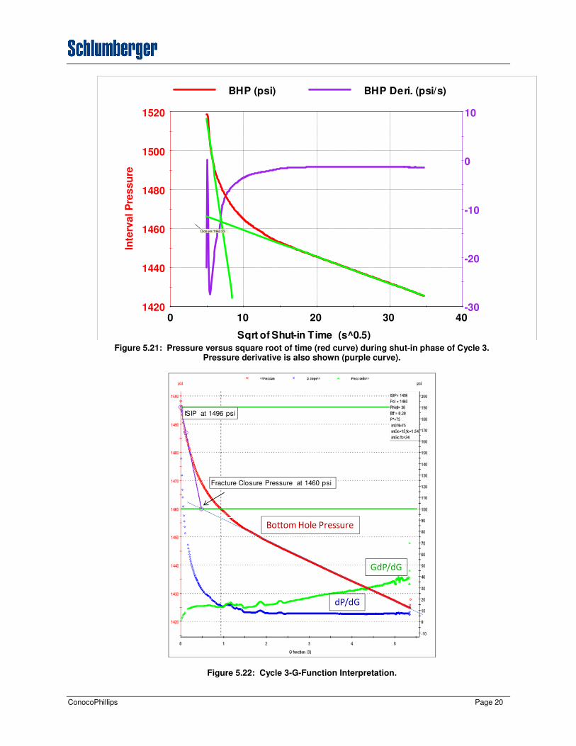
ConocoPhillips Page 20
Figure 5.21: Pressure versus square root of time (red curve) during shut-in phase of Cycle 3.
Pressure derivative is also shown (purple curve).
Figure 5.22: Cycle 3-G-Function Interpretation.
1420
1440
1460
1480
1500
1520
0 10 20 30 40
Inte
rva
l P
res
su
re
Sqrt of Shut-in Time (s^0.5)
-30
-20
-10
0
10
BHP (psi) BHP Deri. (psi/s)
Closure:1463.33
GdP/dG
dP/dG
ISIP at 1496 psi
Fracture Closure Pressure at 1460 psi
Bottom Hole Pressure

ConocoPhillips Page 21
5.1.7 Cycle 4
Figures 5.23 and 5.24 show the raw data from Cycle 4. Injection occurred over a period of
approximately 125 s and the pump half-stroked in the middle of this phase (Figure 5.23) causing
the interval pressure to dip (Figure 5.24). Figure 5.25 shows the plot of interval pressure versus
pumped volume. The fracture reopened at 1484 psi. Figure 5.26 shows pressure vs. square root of
time. The fracture closed at 1462 psi. An alternative construction using the G-function yields a
closure pressure of 1460 psi (Figure 5.27). Table 5.5 summarizes the results for this cycle.
Table 5.5: Cycle 4 Results
Figure 5.23: Cycle 4. Propagation of the fracture. Interval pressure (PAQP), pump motor speed (POUDMS), pump hydraulic pressure (POUDHP), flow rate (POTFR), and interval valve position (PAVP)
are shown.
Stiff
(psi/cc)
LOP
(psi)
LOV
(cc)
VL_frac
(cc)
Peak_P
(psi)
Prop_P
(psi)
ISIP
(psi)
P_clos
(psi)
P_clos_G-
function
(psi)
0.7319 1484.1 84 666 1525.4 1525.2 1500 1461.7 1460
-2
0
2
4
6
8
10
12
0
200
400
600
800
1000
1200
1400
1600
16685 16705 16725 16745 16765 16785 16805 16825
Flo
w R
ate
(cc
/s)/
PA
VP
Pre
ssu
re (
psi
)/ M
oto
r S
pe
ed
(c/
min
)
Time (s)
PAQP POUDMS POUDHP POTFR PAVP

ConocoPhillips Page 22
Figure 5.24: Interval pressure (PAQP), flow rate (POTFR), and interval valve position (PAVP) during injection phase of Cycle 4.
Figure 5.25: Plot of interval pressure vs. pumped volume during Cycle 4 (red curve). A linear fit to this curve shown in purple. The volume at which the curve departs from linearity shown by orange line. The flow rate into the interval (blue curve) is shown referenced to the right hand vertical axis.
-2
0
2
4
6
8
10
12
1400
1420
1440
1460
1480
1500
1520
1540
16685 16705 16725 16745 16765 16785 16805 16825
Flo
w R
ate
(cc
/s)/
PA
VP
Pre
ssu
re (
psi
)/ M
oto
r S
pe
ed
(c/
min
)
TIME (s)
PAQP POTFR PAVP
-2
0
2
4
6
8
10
12
1400
1420
1440
1460
1480
1500
1520
1540
0 250 500 750
Flo
w R
ate
(cc
/s)
Inte
rva
l Pre
ssu
re (
Psi
)
Pumped Volume (cc)
BHP Vs Pumped Volume
Linear Fit
Flow Rate Vs Pumped Volume

ConocoPhillips Page 23
Figure 5.26: Pressure versus square root of time (red curve) during shut-in phase of Cycle 4. Pressure derivative is also shown (purple curve).
1400
1420
1440
1460
1480
1500
1520
0 10 20 30 40
Inte
rva
l P
res
su
re
Sqrt of Shut-in Time (s^0.5)
-40
-30
-20
-10
0
BHP (psi) BHP Deri. (psi/s)
Closure:1461.70

ConocoPhillips Page 24
Figure 5.27: Cycle 4-G-Function Interpretation.
5.1.8 Cycle 5
Figure 5.28 shows the raw data from Cycle 5. Injection occurred over a period of approximately
120 s. The pump half-stroked briefly at 18450 s causing the interval pressure to dip slightly
(Figure 5.28). Figure 5.29 shows a plot of interval pressure versus pumped volume. The fracture
reopened at 1494 psi. Figure 5.30 shows pressure vs. square root of time. A peculiar feature
appears at the end of this curve – the interval pressure suddenly stabilized at about 1380 psi. Yet
no such stabilization occurred during the filtration test carried out at much lower interval pressures
(Figure 5.7). This suggests that a filtercake built up at the wellbore wall between the filtration test
and the end of Cycle 5.
According to Figure 5.30, the fracture closed at 1446 psi. This value is significantly less than the
closure pressure of 1462 psi recorded during the previous cycle. An alternative construction using
the G-function yields an even lower closure pressure of 1432 psi (Figure 5.31). The fracture
appears to be growing into a region with a lower stress. Table 5.6 summarizes the results of the
current cycle.
GdP/dG
dP/dG
ISIP at 1500 psi
Fracture Closure Pressure at 1460 psi
Bottom Hole Pressure

ConocoPhillips Page 25
Table 5.6: Cycle 5 Results
Figure 5.28: Cycle 5. Propagation of the fracture.
Stiff
(psi/cc)
LOP
(psi)
LOV
(cc)
VL_frac
(cc)
Peak_P
(psi)
Prop_P
(psi)
ISIP
(psi)
P_clos
(psi)
P_clos_G-
function
(psi)
0.8511 1494 92 1063 1534.5 1532.7 1505 1445.5 1432
PO
TF
R (
cm
3/s
)
PAQ
P (
psi
)
PO
UD
MS (
c/m
in)
PO
UD
HP
(p
si)
Interval valve
position, PAVP
Hydraulic pressure,
POUDHP
Interval pressure,
PAQP
Flow rate,
POTFR
Motor speed,
POUDMS

ConocoPhillips Page 26
Figure 5.29: Plot of interval pressure vs. pumped volume during Cycle 5 (red curve). A linear fit to this curve shown in purple. The volume at which the curve departs from linearity shown by orange line. The flow rate into the interval (blue curve) is shown referenced to the right hand vertical axis.
Figure 5.30: Pressure versus square root of time (red curve) during shut-in phase of Cycle 5. Pressure derivative is also shown (purple curve).
-2
0
2
4
6
8
10
12
1400
1420
1440
1460
1480
1500
1520
1540
1560
1580
1600
0 250 500 750 1000
Flo
w R
ate
(cc
/s)
Inte
rva
l Pre
ssu
re (
Psi
)
Pumped Volume (cc)
BHP Vs Pumped Volume
Linear Fit
Flow Rate Vs Pumped Volume
1380
1400
1420
1440
1460
1480
1500
1520
0 10 20 30 40
Inte
rna
l P
res
su
re (
psi)
Sqrt of Shut-in Time (s^0.5)
-25
-21
-17
-13
-9
-5
-1
3
BH
P D
eri
(p
si/s
^0.5
)
BHP (psi) BHP Deri. (psi/s)
Closure:1445.47

ConocoPhillips Page 27
Figure 5.31: Cycle 5-G-Function Interpretation.
5.1.9 Cycle 6
Figure 5.32 shows the raw data from Cycle 6. Injection occurred over a period of approximately
150 s. Some minor half-stroking occurred three times causing the interval pressure to dip
temporarily (Figure 5.32). Figure 5.33 shows the plot of interval pressure versus pumped volume.
The fracture reopened at 1460 psi. Figure 5.34 shows a plot of pressure vs. square root of time.
Similar to the previous cycle, the interval pressure suddenly stabilized at about 1310 psi. The
fracture closed at 1351 psi. This closure pressure is significantly less than the corresponding value
of 1446 psi recorded during the previous cycle. An alternative construction using the G-function
yields a comparable closure pressure of 1352 psi (Figure 5.35). Table 5.7 summarizes the results
of the current cycle.
Table 5.7: Cycle 6 Results
GdP/dG
dP/dG
ISIP at 1505 psi
Bottom Hole Pressure
Fracture Closure Pressure at 1432 psi
Stiff
(psi/cc)
LOP
(psi)
LOV
(cc)
VL_frac
(cc)
Peak_P
(psi)
Prop_P
(psi)
ISIP
(psi)
P_clos
(psi)
P_clos_G-
function
(psi)
0.8965 1459.8 95.92 1426.6 1520.0 1508.4 1470 1350.8 1352

ConocoPhillips Page 28
Figure 5.32: Cycle 6. Propagation of the fracture.
Figure 5.33: Plot of interval pressure vs. pumped volume during Cycle 6 (red curve). A linear fit to this curve shown in purple. The volume at which the curve departs from linearity shown by orange line. The flow rate into the interval (blue curve) is shown referenced to the right hand vertical axis.
PO
UD
MS
(c/
min
)
PAQ
P (
psi
)
PO
TF
R (
cm
3/s
)
PO
UD
HP
(p
si)
Hydraulic
pressure,
POUDHP
Hydraulic pressure,
POUDHP
Motor speed,
POUDMS
Flow rate,
POTFR
Interval valve
position, PAVP
-2
0
2
4
6
8
10
12
14
1360
1380
1400
1420
1440
1460
1480
1500
1520
1540
1560
1580
0 250 500 750 1000 1250 1500
Flo
w R
ate
(cc
/s)
Inte
rva
l Pre
ssu
re (
Psi
)
Pumped Volume (cc)
BHP VS Pumped Volume
Linear Fit
Flow Rate Vs Pumped Volume

ConocoPhillips Page 29
Figure 5.34: Pressure versus square root of time (red curve) during shut-in phase of Cycle 6. Pressure derivative is also shown (purple curve).
Figure 5.35: Cycle 6. G-Function Interpretation.
1300
1350
1400
1450
1500
0 10 20 30 40
Inte
rva
l P
res
su
re
Sqrt of Shut-in Time (s^0.5)
-60
-50
-40
-30
-20
-10
0
10
BHP (psi) BHP Deri. (psi/s)
Closure:1350.82 de
riv
ati
ve
(p
si/s
^0
.5)
(psi/s^0.5)
GdP/dG
dP/dG
ISIP at 1470 psi
Bottom Hole Pressure
Fracture Closure Pressure at 1352 psi

ConocoPhillips Page 30
5.1.10 Cycle 7
Figure 5.36 shows the raw data from Cycle 7. Injection occurred over a period of approximately
160 s. The pump half-stroked briefly four times causing the interval pressure to dip momentarily
(Figure 5.36). Figure 5.37 shows a plot of interval pressure versus pumped volume. The fracture
reopened at 1485 psi. Figure 5.38 shows pressure vs. square root of time. The fracture closed at
1382 psi. An alternative construction using the G-function yields a closure pressure of 1372 psi
(Figure 5.39: Cycle 7-G-Function Interpretation. Unlike the previous cycles, the pressure in the
interval did not stabilize during shut-in. Table 5.8 summarizes the results for this cycle.
Table 5.8: Cycle 7 Results
Figure 5.36: Cycle 7. Propagation of the fracture.
Stiff
(psi/cc)
LOP
(psi)
LOV
(cc)
VL_frac
(cc)
Peak_P
(psi)
Prop_P
(psi)
ISIP
(psi)
P_clos
(psi)
P_clos_G-
function
(psi)
0.7178 1485 243 1446 1510.6 1510.3 1459 1382.1 1372
PO
TF
R (
cm
3/s
)
PO
UD
HP
(p
si)
PO
UD
MS
(c/
min
)
PAQ
P (
psi
)
Interval valve
position,
PAVP
Hydraulic
pressure,
POUDHP
Interval
pressure,
PAQPFlow rate,
POTFR
Motor speed,
POUDMS

ConocoPhillips Page 31
Figure 5.37: Plot of interval pressure vs. pumped volume during Cycle 7 (red curve). A linear fit to this curve shown in purple. The volume at which the curve departs from linearity shown by orange line. The flow rate into the interval (blue curve) is shown referenced to the right hand vertical axis.
Figure 5.38: Pressure versus square root of time (red curve) during shut-in phase of Cycle 7. Pressure derivative is also shown (purple curve).
0
2
4
6
8
10
12
14
16
1300
1350
1400
1450
1500
1550
0 250 500 750 1000 1250 1500 1750
Flo
w R
ate
(cc
/s)
Inte
rva
l Pre
ssu
re (
Psi
)
Pumped Volume (cc)
BHP Vs Pumped Volume
Linear Fit
Flow Rate Vs Pumped Volume
1250
1300
1350
1400
1450
1500
4 6 8 10 12 14 16 18 20 22 24 26 28
Inte
rva
l P
res
su
re
Sqrt of Shut-in Time (s^0.5)
-40
-30
-20
-10
0
BHP (psi) BHP Deri. (psi/s)
Closure:1382.13

ConocoPhillips Page 32
Figure 5.40 shows a reconciliation plot summarizing key diagnostic information from all 8 cycles.
The closure pressures ascertained using square root of time plots (magenta triangles) and G-plots
(brown triangles) are generally bounded above by the peak pressures (green triangles), leak-off
pressures (orange triangles), ISIP’s (black triangles), and propagation pressures (blue triangles).
The system stiffness (yellow triangles) varied between 0.421 psi/cc and 0.896 psi/cc and did not
exhibit any particular pattern (Figure 5.40a) .
It is seen that during injection cycles, the amount of fluid injected into the fracture ranged between
666 cc and 2212 cc (red triangles, Figure 5.40a). A total of 8.94 liters was pumped into the fracture
in order to propagate it away from the near-wellbore stress concentration. However for the first
four cycles the leak-off, peak, propagation, instantaneous shut-in, and closure pressures appear to
be fairly constant (Figure 5.40b). This suggests that the fracture was growing away from the
wellbore very slowly. This slow growth may be due to high rates of leak-off through the wellbore
wall and the fracture faces. However as was discussed in relation to Cycle 5 (Section 5.1.8), during
later cycles leak-off was reduced by the action of filtercake. This allowed more of the injected
fluid volume to be utilized in growing the fracture. Between Cycles 4 and 6 the fracture appeared
to move quickly away from the wellbore and the closure pressure decreased rapidly. By Cycle 6
the fracture appears to be sensing the far-field condition. Figure 5.40(b) shows a horizontal line
corresponding to 1364 psi, the average of the closure pressures determined in Cycles 6 and 7. This
is the best estimate of the closure stress in the far-field.
Figure 5.39: Cycle 7-G-Function Interpretation
GdP/dG
dP/dG
ISIP at 1459 psi
Bottom Hole Pressure
Fracture Closure Pressure at 1372 psi

ConocoPhillips Page 33
Figure 5.40: Reconciliation plot for Test Station 1. (a) All parameters. (b) Pressures only.
(a)
1364 psi
(b)

ConocoPhillips Page 34
5.2 Test Results at 2,202.58 ft
5.2.1 Overview
This test was carried out in a silty formation. No gas hydrate was present. Figure 5.41 shows the
location of the test interval. The borehole is in-gauge at the test location, but slighty undergauged
at several locations above and below the test site. This may be due to mudcake build-up or creep.
The resistivity curves at the test location exhibit negligible separation indicating little or no mud
invasion. The dynamic Young’s modulus is 4 GPa, which is typical of unconsolidated sediments.
Figure 5.41: Logs in vicinity of Test Station 2.
The test interval was located between 2200.5 and 2203.8 ft. TRACK 1: Measured Depth with
respect to KB. TRACK 2: Dual caliper measurements C1_OBMT, C2_OBMT and bit size, BS.
Shading reflects difference between each caliper measurement and the bit size. TRACK 3: Gas
hydrate saturation, SHY, density, RHOZ, and gamma ray, GR. TRACK 4: Resistivities measured
at various depths of investigation from shallow (A010) to deep (AO90) TRACK 5: Compressional
(DTCO) and shear (DTSM) wave slownesses. TRACK 6: Dynamic Young’s modulus.
MD
ft
2230
2180
2190
2200
2210
2220
Test
interval

ConocoPhillips Page 35
Figure 5.42: Overview of data acquired at Test Station 2 located at 2202.58 ft MD.
Figure 5.42 presents an overview of the most important data acquired during the test. The time
corresponding to the peak interval pressure (blue curve) divides the test into two parts. The earlier
part consisted of packer inflation and filtration tests. The later part consisted of fracture
propagation/shut-in cycles and a rebound test. A total of nine fracture propagation /shut-in cycles
were performed during the test. Pressures in the interval tended to decrease with each new
injection cycle. This decrease is probably caused by propagation of the fracture away from the
near-wellbore stress concentration.
PO
TF
R (
cm
3/s
)
PA
QP
(p
si)
Interval
pressure,
PAQP Interval
valve
position,
PAVP
Flow rate,
POTFR
Total pumpout
volume, POTCV
Packer valve
position, PAVP
PO
TC
V (
cm3
)

ConocoPhillips Page 36
Figure 5.43: Packer pressure minus interval pressure vs. time.
Figure 5.43 shows the difference between the packer pressure and the interval pressure. After the
commencement of the first fracture propagation cycle at 4030 s, the packer pressure is generally
higher than the interval pressure. This indicates that the packer is functioning as designed and
provides some assurance that a proper seal is being maintained. However Figure 5.43 also shows
some episodes during which the packer pressure dropped below the interval pressure. These
episodes are shown in Figure 5.44. For three of the cases shown in Figures 5.44 (a), (c), and (d) the
decrease in the packer pressure had no impact on the interval pressure suggesting that no leak
occurred. These occurrences may have been caused by temporary reseating of the packers.
However some leakage may have occurred during the rebound test (Figure 44(b)) and also very
briefly at 12044 s during the shut-in period of Cycle 7 (Figure 5.44(c)).

ConocoPhillips Page 37
Figure 5.44: Interval (blue) and packer (purple) pressures during instances when the packer pressure fell below the interval pressure. (a) During Cycle 2 shut-in period. (b) During rebound test following
Cycle 6 (c) During Cycle 7 shut-in period. (d) During Cycle 8 shut-in period.
5.2.2 Packer Inflation (Event 0)
Figure 5.45 shows the packer inflation event. A primary objective of this procedure was to avoid
over-inflation of the packer that could cause it to stick in the unconsolidated silt or make poor
contact with the borehole wall due to excessive yielding of the formation. The low Young’s
modulus of the formation (Section 5.2.1) made it imperative to maintain the packer pressure at the
minimum value required to seal the interval. The initial pressure of the mud column was 1035 psi.
The packer was inflated in stages to 1220 psi. During inflation the pump half-stroked several
times, as evidenced by the flow rate going to zero while the pump motor was running. The interval
pressure rose with the packer pressure and declined quickly due to leak-off when the pump was
switched off. The packer pressure also declined during pumps off periods in response to the
decrease in interval pressure. After the final inflation step, the packer pressure was judged to be
stable enough to begin pumping into the interval.
(a) (b)
(c)(d)

ConocoPhillips Page 38
Figure 5.45: Packer Inflation.
5.2.3 Filtration tests (Cycle 0)
Figure 5.46 shows the two filtration tests performed prior to breaking down the formation. The
pump half-stroked during the second test, so a total of three pressure build-up phases can be
observed. During all three pressure build-ups, the packer pressure lagged slightly below the
interval pressure. However the packer pressure caught up with the interval pressure during
pressure relaxation periods. This made it possible for a seal to be maintained during the first and
third relaxation periods. However a rapid drop in pressure indicates that the seal broke during the
second relaxation period. This occurred because the packer pressure was too close to the interval
pressure to maintain a seal. However by the final filtration test, the pressure appeared to bleed off
normally. Figure 5.47 shows a plot of interval pressure vs. volume. The curve is initially linear
but departs from linearity when the pressure is 1265 psi. Since the interval pressure is far below
the fracture breakdown pressure, the departure from linearity is probably due to yielding of the
formation against the packers, rather than fracture initiation. Figure 5.48 shows the bleed-off phase
after the final pressure build-up. From the derivative plot it is possible to show that the rate of
pressure decline ranged between 2.5 psi/ft and 0.05 psi/ft. Table 5.9 summarizes the results for this
cycle.
Table 5.9: Cycle 0 Results.
Pump motor speedPacker pressure
Packer valve
positionInterval
pressure
Interval valve
position
Hydrostatic
pressure
Flow rate
Stiff
(psi/cc)
LOP
(psi)
LOV
(cc)
VL_frac
(cc)
Peak_P
(psi)
Prop_P
(psi)
ISIP
(psi)
P_clos
(psi)
P_clos_G-
function
(psi)
0.9409 1265 54 N/A N/A N/A N/A N/A N/A

ConocoPhillips Page 39
Figure 5.46: Filtration tests (Cycle 0). The first filtration test started at 3071 s and the second started at 3397 s.
Figure 5.47: Plot of interval pressure vs. pumped volume (brown curve) during the filtration test (Cycle 0 ). A linear fit to this curve shown in red. The volume at which the curve departs from linearity
shown by grey cross-hairs. The flow rate into the interval (purple curve) is shown referenced to the right hand vertical axis.
Pump motor speed
Packer pressure
Packer valve position
Interval
pressure
Interval valve
position
Hydrostatic
pressureFlow rate

ConocoPhillips Page 40
Figure 5.48: Plots of interval pressure (red curve) and its derivative (purple curve) versus square root of shut-in time.
5.2.4 Cycle 1
Figure 5.49 shows the raw data from the injection phase of Cycle 1. Injection occurred over a
period of approximately 400 s however the flow into the interval during this period was
intermittent due to half-stroking of the pump (Figure 5.49). Half-stroking caused the interval
pressure to dip several times. Figure 5.50 shows the plot of interval pressure versus pumped
volume. The formation broke down at 1970 psi. Figure 5.51 shows pressure vs. square root of
time during pressure decline. According to this construction, the fracture closed at 1726 psi. An
alternative construction using the G-function yields a closure pressure of 1723 psi (Figure 5.52).
Table 5.10 summarizes the results for this cycle.
Table 5.10: Cycle 1 Results
1240
1250
1260
1270
1280
1290
1300
1310
1320
0 2 4 6 8 10 12 14 16 18 20 22
Inte
rva
l P
res
su
re
Sqrt of Shut-in Time (s^0.5)
-10
-8
-6
-4
-2
0
2
BHP (psi) BHP Deri. (psi/s)
de
riv
ati
ve
(p
si/s
^0
.5)
Stiff
(psi/cc)
LOP
(psi)
LOV
(cc)
VL_frac
(cc)
Peak_P
(psi)
Prop_P
(psi)
ISIP
(psi)
P_clos
(psi)
P_clos_G-
function
(psi)
0.2602 1970 2600 1066 1970.0 1867.1 1864 1725.9 1723

ConocoPhillips Page 41
Figure 5.49: Cycle 1. Breakdown of the formation.
Figure 5.50: Plot of interval pressure vs. pumped volume (brown curve) during Cycle 1. A linear fit to this curve shown in red. The volume at which the curve departs from linearity shown by grey cross-
hairs. The flow rate into the interval (purple curve) is shown referenced to the right hand vertical axis.
Pump motor speed
Packer pressure
Packer valve position
Interval
pressure
Interval valve
position
Hydrostatic
pressure
Flow rate

ConocoPhillips Page 42
Figure 5.51: Plots of interval pressure (red curve) and its derivative (purple curve) versus square root
of shut-in time.
Figure 5.52: Interpretation of fracture closure during Cycle 1 using the G-function.
1600
1700
1800
1900
10 12 14 16 18 20 22 24 26 28 30 32 34 36 38
Inte
rva
l P
res
su
re
Sqrt of Shut-in Time (s^0.5)
-70
-60
-50
-40
-30
-20
-10
0
BHP (psi) BHP Deri. (psi/s)
Closure:1725.94
de
riv
ati
ve
(p
si/s
)
GdP/dG
dP/dG
ISIP at 1864 psi
Bottom Hole Pressure
Fracture Closure Pressure at 1723 psi

ConocoPhillips Page 43
5.2.5 Cycle 2
The interval was again pressurized and the fracture created in Cycle 1 was propagated for
approximately 240 s. Figure 5.53 shows key data from this test. During injection, the pump half-
stroked several times, particularly in the latter half of the injection phase. Figure 5.54 shows a plot
of interval pressure versus pumped volume. The fracture appears to reopen at 1655 psi. This
figure is much lower than the previous closure pressure. Figure 5.55 shows q plot of pressure
versus square root of time for the shut-in phase. The fracture appears to close at 1683 psi. An
alternative construction using the G-function yields a closure pressure of 1675 psi (Figure 5.56).
Table 5.11 summarizes the principal results of this cycle.
Table 5.11: Cycle 2 Results
Figure 5.53: Cycle 2. Propagation of the fracture.
Stiff
(psi/cc)
LOP
(psi)
LOV
(cc)
VL_frac
(cc)
Peak_P
(psi)
Prop_
P
(psi)
ISIP
(psi)
P_clos
(psi)
P_clos_G-
function
(psi)
0.914 1654.5 48.3 858.58 1769.14 N/A 1732 1683.3 1675
PO
TFR
( c
m3/s
)
PO
UD
HP
2 (
psi
)
PO
UD
MS
2 (
c/m
in)
PAQ
P (
psi
)
Flow rate,
POTFR
Hydraulic pressure,
POUDHP2
Interval
pressure, PAQPInterval valve
position, PAVP
Motor
speed,
POUDMS2
Time (s)

ConocoPhillips Page 44
Figure 5.54: Plot of interval pressure vs. pumped volume during Cycle 2 (red curve). A linear fit to this curve shown in purple. The volume at which the curve departs from linearity shown by orange
vertical line. The flow rate into the interval (blue curve) is shown referenced to the right hand vertical axis.
Figure 5.55: Plots of interval pressure (red curve) and its derivative (purple curve) versus square root of shut-in time.
-1
0
1
2
3
4
5
6
7
8
1600
1620
1640
1660
1680
1700
1720
1740
1760
0 200 400 600 800 1000
Flo
w R
ate
(cc
/s)
Inte
rva
l Pre
ssu
re (
psi
)
Pumped Volume (cc)
BHP Vs Volume Pumped
Linear Fit
Interval Flow rate
1610
1630
1650
1670
1690
1710
1730
1750
10 12 14 16 18 20 22 24 26 28 30 32 34 36 38
Inte
rna
l P
res
su
re (
ps
i)
Sqrt of Shut-in Time (s^0.5)
-50
-40
-30
-20
-10
0
BH
P D
eri
(p
si/
s^
0.5
)
BHP (psi) BHP Deri. (psi/s)
Closure:1683.34

ConocoPhillips Page 45
Figure 5.56: Cycle 2-Depth 2-G-Function Interpretation.
5.2.6 Cycle 3
Figures 5.57 and 5.58 show the raw data from the injection phase of Cycle 3. Injection occurred
over a period of approximately 175 s. The pump half-stroked several times (Figure 5.57) causing
the interval pressure to dip (Figure 5.58). Figure 5.59 shows a plot of interval pressure versus
pumped volume. The fracture reopened at 1679 psi. Figure 5.60 shows pressure vs. square root of
time. The fracture appears to close at 1682 psi. An alternative construction using the G-function
yields a closure pressure of 1680 psi (Figure 5.61). Table 12 summarizes the principal results of
this cycle.
Table 5.12: Cycle 3 Results
GdP/dG
dP/dG
ISIP at 1732 psi
Bottom Hole Pressure
Fracture Closure Pressure at 1675 psi
Stiff
(psi/cc)
LOP
(psi)
LOV
(cc)
VL_frac
(cc)
Peak_P
(psi)
Prop_
P
(psi)
ISIP
(psi)
Piccolos
(psi)
P_clos_G-
function
(psi)
0.375 1678.66 347.84 1680.05 1744.89 N/A 1700 1681.7 1680

ConocoPhillips Page 46
Figure 5.57: Raw data from Cycle 3. Interval pressure (PAQP), pump motor speed (POUDMS), pump hydraulic pressure (POUDHP), flow rate (POTFR), and interval valve position (PAVP) are shown.
Figure 5.58: Interval pressure (PAQP), flow rate (Flowrate_corrected), and interval valve position (PAVP) during injection phase of Cycle 3.
-5
0
5
10
15
20
25
30
0
200
400
600
800
1000
1200
1400
1600
1800
2000
7200 7250 7300 7350 7400
Flo
w R
ate
(cc
/s)
Pre
ssu
re (
psi
)/ M
oto
r S
pe
ed
(c/
min
)
TIME (s)
PAQP
POUDMS
POUDHP
Flowrate_corrected
PAVP
-5
0
5
10
15
20
25
30
1600
1620
1640
1660
1680
1700
1720
1740
1760
7200 7250 7300 7350 7400
Flo
w R
ate
(cc
/s)
Pre
ssu
re (
psi
)
TIME (s)
PAQP
Flowrate_corrected
PAVP

ConocoPhillips Page 47
Figure 5.59: Plot of interval pressure vs. pumped volume during Cycle 3 (red curve). A linear fit to this curve shown in purple. The volume at which the curve departs from linearity shown by orange
vertical line. The flow rate into the interval (blue curve) is shown referenced to the right hand vertical axis.
Figure 5.60: Plots of interval pressure (red curve) and its derivative (purple curve) versus square root of shut-in time.
-5
0
5
10
15
20
25
30
1600
1620
1640
1660
1680
1700
1720
1740
1760
0 500 1000 1500 2000 2500
Flo
w R
ate
(cc
/s)
Inte
rva
l Pre
ssu
re (
psi
)
Pumped Volume (cc)
BHP Vs Volume Pumped
Linear Fit
Interval Flow rate
1630
1650
1670
1690
1710
9 11 13 15 17 19 21 23 25 27 29 31 33
Inte
rnal P
ressu
re (
psi)
Sqrt of Shut-in Time (s^0.5)
-60
-50
-40
-30
-20
-10
0
BH
P D
eri
(p
si/s^0.5
)
BHP (psi) BHP Deri. (psi/s)
Closure:1681.78

ConocoPhillips Page 48
Figure 5.61: Cycle 3-Depth 2-G-Function Interpretation.
5.2.7 Cycle 4
Figures 5.62 and 5.63 show the raw data from the injection phase of Cycle 4. Injection occurred
over a period of approximately 175 s and the pump half-stroked in the middle of this operation
(Figure 5.62) causing the interval pressure to dip (Figure 5.63). Figure 5.64 shows the plot of
interval pressure versus pumped volume. The fracture reopened at 1673 psi. Figure 5.65 shows
pressure vs. square root of time during the shut-in period. The fracture appears to close at 1630 psi.
An alternative construction using the G-function yields a closure pressure of 1631 psi (Figure
5.66). Table 13 summarizes the principal results of this cycle.
Table 5.13: Cycle 4 Results
A peculiar feature appears at the end of the pressure decline curves in Figure 5.65 and 5.66. The
interval pressure suddenly stabilized at about 1580 psi. Yet no such stabilization occurred during
the filtration test at much lower interval pressures (Figure 5.48). This suggests that a filtercake
built up at the wellbore wall between the filtration test and the end of Cycle 4.
GdP/dG
dP/dG
ISIP at 1700 psi
Bottom Hole Pressure
Fracture Closure Pressure at 1680 psi
Stiff
(psi/cc)
LOP
(psi)
LOV
(cc)
VL_frac
(cc)
Peak_P
(psi)
Prop_P
(psi)
ISIP
(psi)
P_clos
(psi)
P_clos_G-
function
(psi)
1.0199 1672.9 185.55 810.38 1724.12 1715.1 1698 1630.35 1631

ConocoPhillips Page 49
Figure 5.62: Raw data from Cycle 4. Interval pressure (PAQP), pump motor speed (POUDMS), pump hydraulic pressure (POUDHP), flow rate (Flowrate_corrected), and interval valve position (PAVP) are
shown.
Figure 5.63: Interval pressure (PAQP), flow rate (Flowrate_corrected), and interval valve position (PAVP) during injection phase of Cycle 4.
0
2
4
6
8
10
12
14
16
18
20
100
600
1100
1600
2100
2600
3100
3600
4100
8418 8468 8518 8568 8618
Flo
w R
ate
(cc
/s)/
PA
VP
Pre
ssu
re (
psi
)/ M
oto
r S
pe
ed
(c/
min
)
TIME (s)
PAQP
POUDMS
POUDHP
Flowrate_corrected
PAVP
0
2
4
6
8
10
12
14
16
18
20
1600
1620
1640
1660
1680
1700
1720
1740
8418 8468 8518 8568 8618
Flo
w R
ate
(cc
/s)/
PA
VP
Pre
ssu
re (
psi
)
TIME (s)
PAQP
Flowrate_corrected
PAVP

ConocoPhillips Page 50
Figure 5.64: Plot of interval pressure vs. pumped volume during Cycle 4 (red curve). A linear fit to this curve shown in purple. The volume at which the curve departs from linearity shown by orange
vertical line. The flow rate into the interval (blue curve) is shown referenced to the right hand vertical axis.
Figure 5.65: Plots of interval pressure (red curve) and its derivative (purple curve) versus square root of shut-in time.
-5
0
5
10
15
20
1600
1620
1640
1660
1680
1700
1720
1740
0 200 400 600 800 1000 1200
Flo
w R
ate
(cc
/s)
Inte
rva
l Pre
ssu
re (
psi
)
Pumped Volume (cc)
BHP Vs Volume Pumped
Linear Fit
Interval Flow rate
1560
1580
1600
1620
1640
1660
1680
1700
10 12 14 16 18 20 22 24 26 28 30 32
Inte
rva
l P
res
su
re
Sqrt of Shut-in Time (s^0.5)
-40
-30
-20
-10
0
10
BHP (psi) BHP Deri. (psi/s)
Closure:1630.35

ConocoPhillips Page 51
Figure 5.66: Cycle 4-Depth 2-G-Function Interpretation.
5.2.8 Cycle 5
Figures 5.67 and 5.68 show the raw data from the injection phase of Cycle 5. Injection occurred
over a period of approximately 170 s. The pump half-stroked a few times (Figure 5.67) causing the
interval pressure to dip slightly (Figure 5.68). Figure 5.69 shows a plot of interval pressure versus
pumped volume. The fracture reopened at 1684 psi. Figure 5.70 shows pressure vs. square root of
time during the shut-in phase. The same stabilization of pressure seen in the previous cycle
appears at the end of this cycle. Before this happens the fracture appears to close at 1629 psi. An
alternative construction using the G-function yields a closure pressure of 1625 psi (Figure 5.71).
Table 14 summarizes the principal results of this cycle.
Table 5.14: Cycle 5 Results
GdP/dG
dP/dG
ISIP at 1698 psi
Bottom Hole Pressure
Fracture Closure Pressure at 1631 psi
Stiff
(psi/cc)
LOP
(psi)
LOV
(cc)
VL_frac
(cc)
Peak_P
(psi)
Prop_P
(psi)
ISIP
(psi)
P_clos
(psi)
P_clos_G-
function
(psi)
0.8525 1683.5 112.32 991.37 1710.87 1707.7 1656 1629.0 1625

ConocoPhillips Page 52
Figure 5.67: Raw data from Cycle 5. Interval pressure (PAQP), pump motor speed (POUDMS), pump hydraulic pressure (POUDHP), flow rate (POTFR), and interval valve position (PAVP) are shown.
Figure 5.68: Interval pressure (PAQP), flow rate (Flowrate_corrected), and interval valve position (PAVP) during injection phase of Cycle 5.
0
5
10
15
20
25
0
500
1000
1500
2000
2500
3000
3500
4000
9650 9700 9750 9800 9850 9900
Flo
w R
ate
(cc
/s)/
PA
VP
Pre
ssu
re (
psi
)/ M
oto
r S
pe
ed
(c/
min
)
TIME (s)
PAQP
POUDMS
POUDHP
Flowrate_corrected
PAVP
0
5
10
15
20
25
1560
1580
1600
1620
1640
1660
1680
1700
1720
9650 9700 9750 9800 9850 9900
Flo
w R
ate
(cc
/s)/
PA
VP
Pre
ssu
re (
psi
)
TIME (s)
PAQP
Flowrate_corrected
PAVP

ConocoPhillips Page 53
Figure 5.69: Plot of interval pressure vs. pumped volume during Cycle 5 (red curve). A linear fit to this curve shown in purple. The volume at which the curve departs from linearity shown by orange
vertical line. The flow rate into the interval (blue curve) is shown referenced to the right hand vertical axis.
Figure 5.70: Plots of interval pressure (red curve) and its derivative (purple curve) versus square root of shut-in time.
-5
0
5
10
15
20
25
30
1560
1580
1600
1620
1640
1660
1680
1700
1720
1740
0 200 400 600 800 1000 1200
Flo
w R
ate
(cc
/s)
Inte
rva
l Pre
ssu
re (
psi
)
Pumped Volume (cc)
BHP Vs Volume Pumped
Linear Fit
Interval Flow rate
1550
1570
1590
1610
1630
1650
1670
9 11 13 15 17 19 21 23 25 27 29 31
Inte
rnal P
ressu
re (
psi)
Sqrt of Shut-in Time (s^0.5)
-80
-60
-40
-20
0
BH
P D
eri (p
si/s
^0.5
)
BHP (psi) BHP Deri. (psi/s)
Closure:1629.04

ConocoPhillips Page 54
Figure 5.71: Cycle 5-Depth 2-G-Function Interpretation.
5.2.9 Cycle 6
Figures 5.72 and 5.73 show the raw data from Cycle 6. Injection occurred over a period of
approximately 230 s. The pump was then reversed and fluid was evacuated from the interval
causing the pressure to decrease sharply (Figure 5.73). This rebound test will be discussed in the
next section. Half-stroking occurred several times during the injection phase (Figure 5.72). Figure
5.74 shows the plot of interval pressure versus pumped volume. The fracture reopened at 1660 psi.
Table 15 summarizes the principal results of this cycle.
Table 5.15: Cycle 6 Results
GdP/dG
dP/dG
ISIP at 1656 psi
Bottom Hole Pressure
Fracture Closure Pressure at 1625 psi
Stiff
(psi/cc)
LOP
(psi)
LOV
(cc)
VL_frac
(cc)
Peak_P
(psi)
Prop_P
(psi)
ISIP
(psi)
P_clos
(psi)
P_clos_G-
function
(psi)
0.394 1660.3 288.9 2928.5 1702.1 1698.88 N/A N/A N/A

ConocoPhillips Page 55
Figure 5.72: Raw data from Cycle . Interval pressure (PAQP), pump motor speed (POUDMS), pump hydraulic pressure (POUDHP), flow rate (Flowrate_corrected), and interval valve position (PAVP) are
shown.
Figure 5.73: Interval pressure (PAQP), flow rate (Flowrate_corrected), and interval valve position (PAVP) during injection phase of Cycle 6.
0
5
10
15
20
25
30
0
500
1000
1500
2000
2500
3000
3500
4000
10750 10800 10850 10900 10950 11000 11050 11100
Flo
w R
ate
(cc
/s)/
PA
VP
Pre
ssu
re (
psi
)/ M
oto
r S
pe
ed
(c/
min
)
TIME (s)
PAQP
POUDMS
POUDHP
Flowrate_corrected
PAVP
0
5
10
15
20
25
30
1100
1200
1300
1400
1500
1600
1700
10750 10800 10850 10900 10950 11000 11050 11100
Flo
w R
ate
(cc
/s)/
PA
VP
Pre
ssu
re (
psi
)
TIME (s)
PAQPFlowrate_correctedPAVP

ConocoPhillips Page 56
Figure 5.74: Plot of interval pressure vs. pumped volume during Cycle 6 (red curve). A linear fit to this curve shown in purple. The volume at which the curve departs from linearity shown by orange
vertical line. The flow rate into the interval (blue curve) is shown referenced to the right hand vertical axis.
5.2.10 Rebound Test (Event 1)
Figure 5.75 shows data from the rebound test and the preceding cycle (Cycle 6). During
evacuation of the fluid from the interval, the pressure dropped to a minimum value of 1123 psi at
which point the pump was stopped. This minimum value is well above the initial pressure of the
mud column (1035 psi). After pumping ceased the pressure climbed quickly at first and then more
slowly towards the end of the shut-in period. The pressure can only climb in this manner as a
result of fluid supplied to the wellbore by the fracture. Moreover if the packers were not sealing
properly, the pressure would tend to fall to the hydrostatic pressure in the mud column rather than
rise. Thus the rebound phenomenon provides confidence that a fracture exists and that the packers
are sealing properly. At the end of the shut-in period the pressure was still climbing slowly. A
rough estimate of the asymptotic value approached by the interval pressure is 1210 psi. This
constitutes a lower bound on the closure pressure.
-10
-5
0
5
10
15
20
25
30
35
40
45
1100
1200
1300
1400
1500
1600
1700
0 500 1000 1500 2000 2500 3000 3500
Flo
w R
ate
(cc
/s)
Inte
rva
l Pre
ssu
re (
psi
)
Pumped Volume (cc)
BHP Vs Volume Pumped
Linear Fit
Interval Flow rate

ConocoPhillips Page 57
Figure 5.75: Cycle 6 followed by Rebound Test.
Figure 5.76: Plot of interval pressure (red curve) versus time during rebound test (Event 1). Grey horizontal line represents approximate asymptotic value of the pressure (1210 psi).
Evacuation of
fluid
Pressure
rebounds
Injection of fluid
Cycle 6 Rebound test
Inte
rva
l Pre
ssu
re (
psi
)
Flo
w R
ate
( c
c/s)
Interval pressure
Flow
rate
1210 psi

ConocoPhillips Page 58
5.2.11 Cycle 7
Figures 5.77 and 5.78 show the raw data from Cycle 7. Injection occurred over a period of
approximately 300 s and the pump half-stroked several times (Figure 5.77) causing the interval
pressure to dip (Figure 5.78). Figure 5.79 shows a plot of interval pressure versus pumped volume.
A subtle change of slope occurs at 1552 psi, however this value is much lower than the fracture
reopening pressure recorded in preceding and subsequent cycles. Consequently, fracture reopening
was interpreted to occur at a much higher pressure of 1680 psi. Figure 5.80 shows pressure vs.
square root of time during the shut-in phase. The fracture appears to close at 1632 psi. An
alternative construction using the G-function yields a closure pressure of 1627 psi (Figure 5.81).
Table 5.16 summarizes the principal results of this cycle.
Table 5.16: Cycle 7 Results
Figure 5.77: Raw data from Cycle 7. Interval pressure (PAQP), pump motor speed (POUDMS), pump hydraulic pressure (POUDHP), flow rate (Flowrate_corrected), and interval valve position (PAVP) are
shown.
Stiff
(psi/cc)
LOP
(psi)
LOV
(cc)
VL_frac
(cc)
Peak_P
(psi)
Prop_P
(psi)
ISIP
(psi)
P_clos
(psi)
P_clos_G-
function
(psi)
0.2795 1680 1710 1490 1699.34 1695.2 1693 1631.9 1627
0
5
10
15
20
25
30
0
500
1000
1500
2000
2500
3000
3500
4000
11535 11585 11635 11685 11735 11785 11835 11885
Flo
w R
ate
(cc
/s)/
PA
VP
Pre
ssu
re (
psi
)/ M
oto
r S
pe
ed
(c/
min
)
TIME (s)
PAQP
POUDMS
POUDHP
Flowrate_corrected
PAVP

ConocoPhillips Page 59
Figure 5.78: Interval pressure (PAQP), flow rate (Flowrate_corrected), and interval valve position (PAVP) during injection phase of Cycle 3.
Figure 5.79: Plot of interval pressure vs. pumped volume during Cycle 7 (red curve). A linear fit to this curve shown in purple. The volume at which the curve departs from linearity shown by orange
vertical line. The flow rate into the interval (blue curve) is shown referenced to the right hand vertical axis.
0
5
10
15
20
25
30
1200
1250
1300
1350
1400
1450
1500
1550
1600
1650
1700
11535 11585 11635 11685 11735 11785 11835 11885
Flo
w R
ate
(cc
/s)/
PA
VP
Pre
ssu
re (
psi
)/ M
oto
r S
pe
ed
(c/
min
)
TIME (s)
PAQPFlowrate_correctedPAVP
-10
-5
0
5
10
15
20
25
30
1200
1300
1400
1500
1600
1700
1800
0 500 1000 1500 2000 2500 3000 3500
Flo
w R
ate
(cc
/s)
Inte
rva
l Pre
ssu
re (
psi
)
Pumped Volume (cc)
BHP Vs Volume Pumped
Linear Fit
Flow Rate Vs Volume Pumped
Change
of slope
Fracture
reopening

ConocoPhillips Page 60
Figure 5.80: Plots of interval pressure (red curve) and its derivative (purple curve) versus square root of shut-in time.
Figure 5.81: Cycle 7-Depth 2-G-Function Interpretation.
1520
1540
1560
1580
1600
1620
1640
1660
1680
1700
9 11 13 15 17 19 21 23 25 27 29
Inte
rna
l P
res
su
re (
ps
i)
Sqrt of Shut-in Time (s^0.5)
-70
-50
-30
-10
10
BH
P D
eri (p
si/s
^0.5
)
BHP (psi) BHP Deri. (psi/s)
Closure:1631.90
Time:26.12,Deri.:-2.23
GdP/dG
dP/dG
ISIP at 1693 psi
Bottom Hole Pressure
Fracture Closure Pressure at 1627 psi

ConocoPhillips Page 61
5.2.12 Cycle 8
Figures 5.82 and 5.83 show the raw data for Cycle 8. Injection occurred over a period of
approximately 280 s and the pump half-stroked several times (Figure 5.82) causing the interval
pressure to dip (Figure 5.83). Figure 5.84 shows a plot of interval pressure versus pumped volume.
The fracture reopened at 1641 psi. Figure 5.80 shows pressure vs. square root of time during
pressure relaxation. The fracture appears to close at 1622 psi. An alternative construction using
the G-function yields a closure pressure of 1640 psi (Figure 5.86). Table 5.17 summarizes the
principal results of this cycle.
Table 5.17: Cycle 8 Results
Figure 5.82: Raw data from Cycle 8. Interval pressure (PAQP), pump motor speed (POUDMS), pump hydraulic pressure (POUDHP), flow rate (Flowrate_corrected), and interval valve position (PAVP) are
shown.
Stiff
(psi/cc)
LOP
(psi)
LOV
(cc)
VL_frac
(cc)
Peak_P
(psi)
Prop_P
(psi)
ISIP
(psi)
P_clos
(psi)
P_clos_G-
function
(psi)
0.8349 1640.7 163.21 1672.9 1689.5 1687.58 1696 1622.4 1640
0
2
4
6
8
10
12
14
0
500
1000
1500
2000
2500
12550 12600 12650 12700 12750 12800 12850
Flo
w R
ate
(cc
/s)/
PA
VP
Pre
ssu
re (
psi
)/ M
oto
r S
pe
ed
(c/
min
)
TIME (s)
PAQP
POUDMS
POUDHP
Flowrate_corrected
PAVP

ConocoPhillips Page 62
Figure 5.83: Interval pressure (PAQP), flow rate (Flowrate_corrected), and interval valve position (PAVP) during injection phase of Cycle 8.
Figure 5.84: Plot of interval pressure vs. pumped volume during Cycle 8 (red curve). A linear fit to this curve shown in purple. The volume at which the curve departs from linearity shown by orange
vertical line. The flow rate into the interval (blue curve) is shown referenced to the right hand vertical axis.
0
2
4
6
8
10
12
14
1520
1540
1560
1580
1600
1620
1640
1660
1680
1700
12550 12600 12650 12700 12750 12800 12850
Flo
w R
ate
(cc
/s)/
PA
VP
Pre
ssu
re (
psi
)/ M
oto
r S
pe
ed
(c/
min
)
TIME (s)
PAQPFlowrate_correctedPAVP
-10
-5
0
5
10
15
20
25
30
1500
1525
1550
1575
1600
1625
1650
1675
1700
1725
0 500 1000 1500 2000
Flo
w R
ate
(cc
/s)
Inte
rva
l Pre
ssu
re (
psi
)
Pumped Volume (cc)
BHP Vs Volume Pumped
Linear Fit
Interval Flow rate

ConocoPhillips Page 63
Figure 5.85: Plots of interval pressure (red curve) and its derivative (purple curve) versus square root of shut-in time.
Figure 5.86: Cycle 8-Depth 2-G-Function Interpretation.
1440
1460
1480
1500
1520
1540
1560
1580
1600
1620
1640
1660
12 14 16 18 20 22 24 26 28 30
Inte
rna
l P
res
su
re (
ps
i)
Sqrt of Shut-in Time (s^0.5)
-90
-70
-50
-30
-10
10
BH
P D
eri
(p
si/
s^
0.5
)
BHP (psi) BHP Deri. (psi/s)
Closure:1622.44
GdP/dG
dP/dG
ISIP at 1696 psi
Bottom Hole Pressure
Fracture Closure Pressure at 1640 psi

ConocoPhillips Page 64
5.2.13 Cycle 9
Figures 5.87 and 5.88 show the raw data for Cycle 9. Injection occurred over a period of
approximately 230 s and the pump half-stroked twice (Figure 5.87) causing the interval pressure to
dip (Figure 5.88). Figure 5.89 shows the plot of interval pressure versus pumped volume. The
fracture reopened at 1580 psi. Figure 5.90 shows pressure vs. square root of time during the shut-
in phase. The fracture appears to close at 1608 psi. The G-function however did not yield a
definitive closure pressure (Figure 5.91). Table 5.18 summarizes the principal results of this cycle.
Table 5.18: Cycle 9 Results
Figure 5.87: Raw data from Cycle 9. Interval pressure (PAQP), pump motor speed (POUDMS), pump hydraulic pressure (POUDHP), flow rate (Flowrate_corrected), and interval valve position (PAVP) are
shown.
Stiff
(psi/cc)
LOP
(psi)
LOV
(cc)
VL_frac
(cc)
Peak_P
(psi)
Prop_P
(psi)
ISIP
(psi)
P_clos
(psi)
P_clos_G-
function
(psi)
0.3112 1580 508.25 1261 1675.8 1674.3 1655 1608.1 N/A
0
5
10
15
20
25
30
0
500
1000
1500
2000
2500
3000
3500
4000
4500
13625 13675 13725 13775 13825
Flo
w R
ate
(cc
/s)/
PA
VP
Pre
ssu
re (
psi
)/ M
oto
r S
pe
ed
(c/
min
)
TIME (s)
PAQP POUDMS POUDHP Flowrate_corrected PAVP

ConocoPhillips Page 65
Figure 5.88: Interval pressure (PAQP), flow rate (Flowrate_corrected), and interval valve position (PAVP) during injection phase of Cycle 9.
Figure 5.89: Plot of interval pressure vs. pumped volume during Cycle 3 (red curve). A linear fit to this curve shown in purple. The volume at which the curve departs from linearity shown by orange
vertical line. The flow rate into the interval (blue curve) is shown referenced to the right hand vertical axis.
0
5
10
15
20
25
30
1400
1450
1500
1550
1600
1650
1700
13625 13675 13725 13775 13825
Flo
w R
ate
(cc
/s)/
PA
VP
Pre
ssu
re (
psi
)
TIME (s)
PAQP Flowrate_corrected PAVP
-10
-5
0
5
10
15
20
25
30
35
1390
1440
1490
1540
1590
1640
1690
0 500 1000 1500 2000
Flo
w R
ate
(cc
/s)
Inte
rva
l Pre
ssu
re (
psi
)
Pumped Volume (cc)
BHP Vs Volume Pumped
Linear Fit
Interval Flow rate

ConocoPhillips Page 66
Figure 5.90: Plots of interval pressure (red curve) and its derivative (purple curve) versus square root of shut-in time.
Figure 5.91: Cycle 9-Depth 2-G-Function Interpretation.
1420
1460
1500
1540
1580
1620
1660
10 12 14 16 18 20 22 24 26 28 30 32 34 36
Inte
rnal
Pre
ssu
re (
psi)
Sqrt of Shut-in Time (s^0.5)
-100
-80
-60
-40
-20
0
20
BH
P D
eri
(p
si/
s^
0.5
)
BHP (psi) BHP Deri. (psi/s)
Closure:1608.07
GdP/dG
dP/dG
ISIP at 1655psi
Bottom Hole Pressure

ConocoPhillips Page 67
Figure 5.92 shows a reconciliation plot summarizing key diagnostic information from all Events
and Cycles. The closure pressures ascertained using square root of time plots (magenta triangles)
and G-plots (brown triangles) are generally bounded above by the peak pressures (green triangles) ,
leak-off pressures (orange triangles), ISIP’s (black triangles) and propagation pressures (blue
triangles). The sole rebound pressure obtained at the second test station is also shown on the plot.
As expected, it provides a lower bound on the closure stress, albeit a wide one. The system
stiffness (yellow triangles) varied between 0.26 psi/cc and 1.02 psi/cc and did not exhibit any
particular pattern.
It is seen that during injection cycles, the amount of fluid injected into the fracture ranged between
810 cc and 2928 cc (red triangles). A total of 12.8 liters was pumped into the fracture in order to
propagate it away from the near-wellbore stress concentration. The objective of escaping the near-
well stress concentration appears to have been achieved by Cycle 4. Figure 5.93 shows that from
Cycles 4 through Cycle 8, the closure pressures fluctuated around 1625 psi. The leak-off pressure,
ISIP and peak stress are also fairly constant over this range of cycles while the propagation
pressure appears to decline slowly with cycle. However Cycle 9 departs from the general trend.
Pressures extracted during this cycle were somewhat lower than those obtained during preceding
cycles. The closure pressure for this cycle identified using a square root of time plot was 1608 psi,
but the fact that the G-function did not show any closure throws this interpretation into doubt. The
reopening pressure for this cycle was also well below the trend established during previous cycles.
It is possible that the fracture may have penetrated into a lower stress region. Whatever the reason,
the results of Cycle 9 will be treated as outliers from the main trend. A value of 1625 psi is the best
estimate of the closure pressure away from the near-wellbore stress concentration.
Figure 5.92: Reconciliation Plot at Test Station 2.

ConocoPhillips Page 68
Figure 5.93: Reconciliation Plot at Test Station 2. Pressures only.
1625 psi

ConocoPhillips Page 69
6 CONCLUSIONS
� The best estimate of the minimum principal stress at 2071.95 ft MD is 1364 psi, equivalent to
12.7 ppg.
� The best estimate of the minimum principal stress at 2202.58 ft MD is 1625 psi, equivalent to
14.2 ppg.
� Since the inferred minimum principal stresses are much less than typical estimates of overburden
pressure, these stresses are most likely equal to the minimum far-field horizontal stresses at their
respective depths.
� Half-stroking of the pumps complicated the interpretation of fracture reopening and propagation
pressures. However it did not affect interpretation of the closure stress.
� Some leakage through the packers did occur at both stations. However this leakage was of very
limited duration and did not have a detectable impact on the most decisive, latter stages of these
tests.
� Significant leak-off rates were observed at both test stations suggesting that permeability was not
negligible.
� Evidence of filtercake formation was seen in the form of below gauge caliper measurements, twin
breakdown peaks, and a marked decrease in leak-off rates with time.

ConocoPhillips Page 70
7 APPENDIX A
7.1 MDT micro-fracturing operational procedure
MDT micro-fracturing configuration
The MDT (Modular Dynamics Tester) represents the latest generation of wireline formation testers
and it consists of a series of modules, each designed to perform specific functions, which can be
configured for the desired objectives. The MDT tool is controlled in real time by software
commands from the logging unit during the entire test sequence.
Basic MDT micro-frac configuration is with Dual Packer and Pumpout modules:
• Dual Packer Module: The Dual Packer Module has two rubber straddle packers that allow
one meter section of wellbore to be isolated. The Dual Packer Module is equipped with a
dual system of sensors (Strain Gauge and CQG* Crystal Quartz Gauge) to measure
pressure in the tested interval in real time. The pressure in the packers is also monitored for
quality control. When the test is complete the packers can be deflated and the tool string
can be moved to another test interval.
Basic MDT micro-frac configuration schematic

ConocoPhillips Page 71
• Pumpout Module: The Pump-out Module is used to inflate the rubber elements of the Dual
Packer Module and to pressurise the test interval to create the hydraulic fracture. Due to the
fact that the pump is downhole, wellbore storage effects are limited.
Standard MDT micro-fracturing procedure
Packer Inflation: once the tool has been properly positioned, the interval to be tested is isolated by
inflating the straddle packer arrangement until the pressure in the interval starts to rise. The
subsequent pressure decline is then observed to check the quality of the packer seal. Packers are
further pressurized if the seal is not satisfactory.
Leak-Off Cycles: a series of increasing pressure steps to a level well below the formation
breakdown is performed, in order to test that the packer seal is holding and also to test the fluid
leak off into the formation.
Hydraulic Fracturing: fluid is again injected into the interval at a constant flow rate and up to the
initiation of a tensile fracture. Fracture initiation is recognized either by a breakdown or by a
pressure plateau. The fracture is then extended for 1 to 5 minutes before the interval is isolated and
the pump stopped.

ConocoPhillips Page 72
Fall-off: When the pump is stopped the pressure is allowed to fall-off to a pressure level that
ensures that the fracture is closed. In low permeability formations, fracture closure may take a long
time due to low fluid filtration, and as contingency, a Flow Control Module can be used to
withdraw the fluid at a low, constant rate in order to close the fracture and obtain a fall off curve
that can be analyzed.
Fracture Reopening, Propagation, Fall-off Cycles: A series of such injection/falloff cycles
followed by reopening, further propagation, and closure of the fracture are instigated to check that
the test is repeatable and possibly change the injection parameters (flow rate and injected volume).

ConocoPhillips Page 73
Packer Deflation: Once the operator and reservoir domain expert is satisfied that good quality data
were acquired, packers are deflated and the tool is moved to the next interval.
A typical micro-frac test comprises of 2 to 5 injection/propagation/fall-off cycles, and it can usually
take from 1 to 3 hours.
Alternate MDT micro-frac procedures
Sleeve Fracturing: if the mud cake is nearly impermeable, or if the formation itself is nearly
impermeable, the classic procedure may lead to fracture initiation under the packer elements and
premature failure of the test. This situation can be easily recognized during the leak-off cycles, with
no pressure decline observed. Experience shows that a mud with an API leak-off parameter of less
than 2.5 ml/30 min will form a mudcake that is impermeable for MDT stress test purposes.
In such cases a sleeve fracturing procedure can be followed: fluid is pumped at a constant rate into
one of the packers up to the maximum allowable inflatable pressure. This may result in initiation of
a stable fracture. The packer can then be deflated and the tool positioned so that the interval is at
the level of the created fracture. This procedure ensures that fracture extension will start at the
interval level. The traditional procedure can then be applied: packer inflation, leak-off cycles, and
hydraulic fracturing cycles.
Flowback/Pressure Rebound: when injection is stopped, fluid can be quickly withdrawn from the
fracture to close it in the vicinity of the wellbore only (the remainder of the fracture stays
pressurized above the closure stress, and hence, remains open). Fluid withdrawal is then stopped so
that the fracture produces back to the wellbore, resulting in a pressure rebound. A rebound to a
pressure level much higher than the mud pressure is a good indicator that a hydraulic fracture has
indeed been created and it can provide a lower bound on the minimum stress, if the rebound
procedure has been correctly followed.

ConocoPhillips Page 74
MDT micro-fracturing interpretation methodology
Stress test interpretation is carried out analyzing each hydraulic fracturing cycle and determining, if
possible, the following parameters: breakdown pressure, propagation pressure, instantaneous shut-
in pressure (ISIP), closure pressure, reopening pressure and rebound pressure. This is followed by a
“reconciliation phase” where all quantities for all cycles are considered together, to determine the
consistency of the data and the magnitude of minimum stress.
The Breakdown pressure is the pressure at which the fracture is created. It is characterized by a
sharp pressure drop while fluid is flowing into the interval.
If fluid injection is maintained after breakdown the wellbore pressure should stabilize and the
fracture propagates continuously. A Propagation Pressure can be determined.
Once injection has stopped, the pressure in the wellbore will quickly stabilize to a value called the
Instantaneous Shut-In Pressure or ISIP. The Closure Pressure is the pressure at which the fracture
closes after injection has stopped. Fluid leak off in the formation or drawdown with a Flow Control
will deplete the fluid contained into the fracture. At some point, the fluid pressure in the fracture
will equal the opposing in situ stress acting on the fracture and the fracture will close. The wellbore
pressure at this point is called the Closure Pressure and is assumed to be a reliable estimate of the
average stress acting on the fracture surface.
To determine closure pressure, the square root plot method is used. Other methods can be found in
the literature but this method is quite robust for determining the closure pressure. Plotting interval
pressure against the square root of the time since shut-in, the interval pressure will follow a straight
line until the fracture is closed. Departure from this linear behavior is taken as the point at which
the fracture mechanically closes for the first time, and the pressure value at that point is chosen as
an estimate for the closure stress.
The Reopening Pressure is the pressure at which a pre-existing fracture opens. This corresponds to
a change in the stiffness of the tested interval. Normally it is identified as the point at which the
pressure during injection deviates from linearity with respect to the injected volume.
Reconciliation Plot
No single parameter (inferred closure pressure, ISIP, etc.) determined from a single hydraulic
fracturing cycle provides a reliable estimate of the actual closure stress. Once each cycle has been
analyzed separately, the stress test record should be interpreted in its entirety to determine the best
possible estimate of the closure stress. All estimates are plotted for every event along the time axis
in a reconciliation plot. A reconciliation plot summarizing events during the test is included below.
It makes it possible to check that the fracture has grown away from the influence of the near-
wellbore stress. Once the fracture is mostly sensing the far field stresses, estimates of the closure
pressure stop varying from one cycle to the next. If no consistency (repeating of the values for a
certain parameter like closure stress within a certain range) is found on the reconciliation plot, the
data cannot be considered representative and are discarded.

ConocoPhillips Page 75
Determination of breakdown pressure, propagation pressure, instantaneous shut-in pressure (ISIP), closure pressure, reopening pressure in MDT micro-frac tests cycles
Example of reconciliation plot for three cycles

ConocoPhillips Page 76
8 APPENDIX B – Toolstring Used for Micro-fracturing Tests

Appendix 5: Schlumberger “Iġnik Sikumi #1 XPT/MDT Pretest and Sampling Report,” by Ahmad Latifzai

Ignik Sikumi #1, Pretest and Sampling Report Page 1
ConocoPhillips Alaska, Inc.
Ignik Sikumi #1
Logging Date: April, 17th 2011
Pretest and Sampling Report
Pressure Measurement
The objectives of formation testing in this well were divided into three categories:
• Stress testing
• Formation pressure
• Formation permeability
• Formation fluid sampling both above and below hydrate dissociation pressure
Modular dynamics tester (MDT) and pressure express (XPT) tools were employed to meet these
objectives. The XPT tool was employed to measure formation pressure above the hydrate dissociation
pressure, this process also allowed for the evaluation of formation mobility. The formation was expected
to have low permeability above hydrate dissociation pressure. The operation requirements called for
making the pressure and mobility measurement above the hydrate dissociation pressure. In the past
inflatable packers were used to perform this task due inflatable packers ability to the expose large area of
the formation. The XPT allows for very low fluid flow rate which is controlled from surface by the user.
In addition the large area packer modification (Figure 1) increased the formation area exposed to the
probe barrel. Both lower flow rate and larger area allowed for smaller drawdown pressure as shown by
D’Arcy’s equation.
�� �� � µ
� � �
Equation 1:D’Arcy’s equation where: ∆P is pressure drawdown, Q is flowrate, µ is fluid viscosity, A is
area, and k is formation permeability.
Figure 1: Probe comparison. Note the area exposed by the large area packer is significantly more than
that of the conventional probe.

Ignik Sikumi #1, Pretest and Sampling Report Page 2
Mobility of the formation is defined as the permeability divided by the viscosity of fluid
withdrawn from the formation during the pretest period. Since the viscosity of fluid withdrawn during the
pretest period is unknown it’s not possible to calculate formation permeability using the mobility data.
The viscosity of an immiscible fluid mixture in most cases can be higher than the viscosity of each
individual fluid component. The depth of investigation (DOI) of each pretest is within one to two
wellbore diameters, which is relatively shallow when compared to drill stem testing (DST) or miniDST
performed using the MDT toolstring. The DOI of pretest mobility data is near that of the permeability
measured by the nuclear magnetic resonance (NMR) tools. A comparison of these two measurements has
been shown in Figure 2 below keeping in mind the differences in measurement techniques. In the top sand
(2065 to 2130 ft) the pretest mobility and NMR permeability are in good agreement. In the lower sand
(2235 ft to 2370 ft) these two measurement techniques display a difference on one order of magnitude
while they are in agreement at other depths.
During a number of pretests the formation pressure stabilized at a value very close to hydrostatic
pressure. These pressures were assumed to be lost seals due to possible fluid flow from the wellbore
around the packer and into the probe barrel where the pressure gauge is located. Examples of these tests
will be shown during the detailed pretest section of this report. One possible explanation for this
phenomenon is lack of mud cake. All lost seals are indicated by the red pips in the pressure track (Figure
2). Note the CMR permeability is measured to be less the 0.2 mD. In low permeability formations since
little or no filtrate invasion takes place it’s also not possible to form competent mud cake.
Figure 2: Pressure, mobility and NMR data plotted for comparison. Note the agreement of mobility and
NMR permeability in the top sand. The majority of the data in the lower sand differ by an order of
magnitude.

Ignik Sikumi #1, Pretest and Sampling Report Page 3
The mobility data were used when changes to the toolstring became necessary when flow back
tests became impossible due to the failure of the flow control module. Since the mobility of the formation
was determined to be higher than expected, flowback tests were unnecessary during the stress test
operation. As a precaution the toolstring was reconfigured to allow flowback tests. A separate report
showing the analysis of the stress test data will be submitted. The mobility data were also used to select
sampling station depths.
Individual pretest stations of the XPT
The XPT tool was installed in the same toolstring as the CMR and HNGS (Figure 3).
Figure 3: Toolstring containing the XPT, CMR and HNGS
The XPT packer and flowline was tested in the casing show to check for leaks in the flowline. Figure 4
(file 33) shows that the sealing system of the XPT was intact before proceeding with the operation. Note
that the flowline pressure was lowered to less than 120 psi to be certain all portions of the sealing system
were capable of operating under the stress of large pressure differentials.

Ignik Sikumi #1, Pretest and Sampling Report Page 4
Figure 4: Data from file 30 showing the sealing system of the XPT tool.
2320 ft
The toolstring was conveyed to the lower sand and after correlation station depth at 2320 ft was
chosen to test first. Initially the pressure in the flowline was drawn to 1060 psi and allowed to buildup and
stabilize (figure 5). The flow rate of the pretest was set to 0.05 cc/s, which is the minimum flow rate
achievable by the XPT tool. The tool also allows the user to set maximum pretest volume and minimum
flowline pressure limits which either one of which could stop the pretest piston. In this case the
volumetric limit was reached first. A second pretest with larger volumetric limit was performed. The last
buildup pressure was 1061.43 psi. A final pretest was performed to confirm the last build up pressure
value from the previous pretest. The final pressure value of this station was 1061.41 psi. The mobility
values of the second and third pretest (1.54 and 1.06 mD/cP respectively) were on the same order of
magnitude when compared to each other.
Figure 5: Pretest station 2320ft, file 42

Ignik Sikumi #1, Pretest and Sampling Report Page 5
2306 ft
The tool was then moved to 2306 ft, a number of pretests were performed at this depth (Figure 6)
all of which stabilized at a pressure very close to hydrostatic pressure. While it’s possible that the
hydrostatic pressure and the formation pressure are very close it’s more likely that the wellbore is not
completely isolated from the formation. This results in wellbore fluids leaking through pore throats and
possible fractures and vugs in the formation into probe barrel.
Figure 6: Pretest station 2306ft, file 43
2305 ft
The tool was moved to 2305 ft to perform a pretest and obtain formation pressure data. A number
of pretests were performed at this station depth as well (Figure 7). Similar to station depth at 2306 ft, the
last buildup pressure from each pretest stabilized near the hydrostatic pressure. This is also indicative of
leaky mud cake seal.

Ignik Sikumi #1, Pretest and Sampling Report Page 6
Figure 7: Station depth 2305 ft, file 44.
2282 ft
The tool was moved to 2282 ft where a number of pretests were performed. The last build up
pressure is only 3 psi lower than the hydrostatic pressure. The data from this station depth must also be
excluded due to possible leak in the mud cake.
Figure 8: Station depth 2282 ft, file 45
2284 ft
The tool was moved to a nearby depth to the previous station depth. The volumetric limit was
increased to 10cc, the buildup pressure was very close to the hydrostatic pressure (Figure 9). Therefore
the data from this station depth must be excluded.

Ignik Sikumi #1, Pretest and Sampling Report Page 7
Figure 9: Station depth 2284 ft, file 46
2324 ft
The tool was lowered to 2324 ft which is very close the first station depth of the program. The
purpose of this station was to test the seal system of the tool and mud cake. Two pretests were performed
at this depth (Figure 10) to confirm the last build up pressure. The first pretest stabilized at 1044.44 psi
while the second pretest stabilized at 1044.29 psi. P* was calculated to be 1044.27 psi. The drawdown
mobility of the first and second pretest are 5 and 6 mD/cP respectively. Spherical and radial mobility was
calculated 6.6 mD/cP and 6.2 mD ft/cP.
Figure 10: Station depth 2324 ft, file 47. Derivative plot (right)

Ignik Sikumi #1, Pretest and Sampling Report Page 8
2272 ft
The tool was conveyed to 2272 ft after confirming the seal system at the previous station depth.
Multiple pretests were performed to confirm the pressure data (Figure 11). Last buildup pressures from
the first two pretests did not stabilize at similar values therefore a third pretest was performed which
confirmed the second pretest.
Figure 11: Station depth 2272 ft, file 48.
The formation pressure from this station is 1087.67 psi. The drawdown mobility was calculated to be 8
mD/cP.
2267 ft
The tool was moved to the next station depth at 2267ft where two pretests were performed. The
drawdown period of the second pretest displayed steady state flow where the reservoir provided fluid as
the rate which the pretest mechanism demanded (Figure 11). The derivative plot shows a long radial
regime while the spherical regime is short of nonexistent. This could be due to a very thin section.
Figure 11: Station depth 2267 ft, file 50. Derivative plot on the right.

Ignik Sikumi #1, Pretest and Sampling Report Page 9
The final buildup pressure was 1082.23 psi, while the P* from the radial flow was 1082.63 psi.
The drawdown mobility was calculated to be 6.9 mD/cP while the radial mobility is 2.7 mD ft/cP.
2262.1 ft
The tool was moved to the next station depth at 2262.1 ft slightly shallower than the previous
station depth. Two pretests were performed at this depth as well, the last build pressure from both pretests
stabilized at similar values (Figure 12).
Figure 12: Station depth 2262.1, file 51. Derivative plot on the right.
The derivative plot shows a very short to nonexistent spherical flow regime while the radial flow
regime is longer indicating a possible thin section. The last build up pressure was 1091.45 psi while the
P* was calculated to be 1091.45 psi as well. The drawdown mobility was calculated to be 17 mD/cP
while the radial mobility was calculated to be 7.2 mD ft/cP.
2251 ft
At 2251 multiple pretests were performed (Figure 13) all of which stabilized at similar pressure
values, however these values were within 3 psi of the hydrostatic pressure. It’s possible that fluid from the
wellbore is leaking through the mud cake and into probe barrel. This results in a lost seal similar to the
behavior seen at 2284 ft. The data from this station must be excluded.

Ignik Sikumi #1, Pretest and Sampling Report Page 10
Figure 13: Station depth 2251 ft, file 52.
2243 ft
The tool was moved to the next station depth at 2243 ft where two subsequent pretests were
performed. Both of the buildup periods stabilized at similar pressure values (Figure 14). The last buildup
pressure stabilized at 1076.99 psi while the drawdown mobility was calculated to be 10.6 mD/cP. The
derivative plot was inconclusive.
Figure 14: Station depth 2243 ft, file 53.
2127 ft
The tool was moved to the shallower sand where the first station depth was at 2127 ft. Two
pretest stations were performed at this depth (Figure 15). Note in both cases the pressure stabilized at
similar values indicating that the flowline pressure was decompressed below reservoir pressure. During
the drawdown periods of both tests steady state flow behavior was seen. The derivative plots were

Ignik Sikumi #1, Pretest and Sampling Report Page 11
inconclusive. Last build up pressure was 958.37 psi while the drawdown mobility was calculated to be 4
mD/cP
Figure 15: Station depth 2127 ft, file 54.
2101 ft
The tool was moved to the next station depth at 2101 ft and two subsequent pretests were
performed at this depth. Both pretests stabilized at similar values (Figure 16). The derivative plot shows
both spherical and radial flow regimes. The large difference between the spherical and radial regime
occurrence could be an indication of this sand. The last buildup pressure was measured to be 965.41 psi
while P* from the radial calculation was 963.98 psi. The drawdown mobility was calculated to be 2.5
mD/cP, spherical mobility was 2.3 mD/cP while the radial mobility was calculated to be 0.64 mD ft/cP.
Figure 16: Station depth 2101 ft, file 55. Derivative plot on the right.

Ignik Sikumi #1, Pretest and Sampling Report Page 12
2091 ft
The probe was moved to the next station depth at 2091 ft and two subsequent pretests were
performed at this depth. Buildup pressures from both pretests stabilized at similar values (Figure 17)
960.00 psi. The mobility was calculated to be 2.6 mD/ cP. The derivative plots were inconclusive.
Figure 17: Station depth 2091 ft, file 56.
2082 ft
The probe was moved to the next station depth at 2082 ft where two subsequent pretests were
performed. The buildup pressures from both pretests stabilized at similar values (Figure 18) 972.65 psi.
The mobility was calculated to be 2.8 mD/cP. The derivative plots were inconclusive.
Figure 18: Station depth 2082 ft, file 57.

Ignik Sikumi #1, Pretest and Sampling Report Page 13
2064 ft
The probe was moved to the next station depth at 2064 ft where three subsequent pretests were
performed. The buildup pressures from the final two pretests stabilized at similar pressure values (Figure
19) 945.77 psi. The mobility is was calculated to be 12 mD/cP. The derivative plots were inconclusive.
Figure 19: Station depth 2064 ft, file 58.
2029 ft
The probe was moved to the caprock at 2029 ft to determine the mobility of the formation. The
pressure response indicated very low mobility formation.
Figure 20: Station depth 2029 ft, file 59.

Ignik Sikumi #1, Pretest and Sampling Report Page 14
2356 ft
The probe was lowered to the lower most wet sand at 2356 ft. Multiple pretests were performed at
this depth until two subsequent buildup pressures repeated (Figure 21) indicating that the flowline has
been decompressed sufficiently. The final buildup pressure was 1057.48 psi while the drawdown mobility
was calculated to be 45 mD/cP. The derivative plots were inconclusive.
Figure 21: Station depth 2356 ft, file 61.
2340 ft
The probe was moved to the next station depth in the water sand at 2340 ft. Three pretests were
performed at this depth (Figure 22). The final two buildup pressures were in agreement indicating the
flowline had been decompressed below reservoir pressure. The final buildup pressure was measured to be
1050.12 psi while the mobility was calculated to be 75 mD/cP. The derivative plots were inconclusive.
Figure 22: Station depth 2340 ft, file 62.

Ignik Sikumi #1, Pretest and Sampling Report Page 15
2328 ft
The probe was moved to the next station depth in the water sand at 2328 ft. Two subsequent
pretests were performed both resulting similar final buildup pressures (Figure 23). The final buildup
pressure was measured to be 1045.54 psi while the drawdown mobility was calculated to be 4.7 mD/cP.
The derivative plots were inconclusive.
Figure 23: Station depth 2328 ft, file 63.
2073 ft
After the completion of the pressure survey, an attempt to determine the hydrate dissociation
pressure was made using the XPT tool. Hydrate dissociation pressure requires lowering the flowline
pressure below the dissociation pressure at which point gas flow may result in increase of mobility by an
order of magnitude. Since the compressibility of gas is also significantly higher than liquid the flowing
pressure curve is also expected to behave similar to steady state flow. This technique is only possible with
the XPT due to its capacity to decompress the flowline slowly.
The probe was moved to 2073 ft in the hydrate zone, where the flowline decompressed using
pretest mechanism to a pressure below 700 psi. The attempt was unsuccessful since multiple pretests at
different rates were attempted (Figure 24) and the pretest volume was exhausted. The flowline pressure
was not lowered below the expected dissociation pressure. The probe was retracted and set again at the
same depth (Figure 25) and the flowline was decompressed at the maximum capacity of the XPT tool.
There was a seal failure (Figure 25) resulting in the flowline pressure to stabilize at the hydrostatic
pressure. Due to the sharp decrease in the hydraulic oil pressure coinciding with the sharp increase in
flowline pressure it’s possible that the formation near the probe collapsed resulting in the loss of seal.

Ignik Sikumi #1, Pretest and Sampling Report Page 16
Figure 24: Station depth 2073, file 64.
Figure 25: Station depth at 2073, file 65.

Ignik Sikumi #1, Pretest and Sampling Report Page 17
Fluid Sampling
The inflatable packers were used to obtain fluid samples from the formation. The objective was to
obtain free water sample, and water sample below hydrate dissociation pressure. Due to the
unconsolidated nature of the formation it was necessary to install redundant modules in the toolstring
(Figure 26)
Figure 26: Sampling toolstring
Additional pump, multi-sample module and fluid analyzer were installed both above and below the
inflatable packer module for redundancy. A probe was also installed in the toolstring for water sampling
in case evacuation of the packer interval required significant pumping time. Seven inch TAM packer
elements were installed on the inflatable packer module. Low flow pumps were used to minimize both
drawdown and sand production.

Ignik Sikumi #1, Pretest and Sampling Report Page 18
Sampling Operation
2261.5 ft
Wellbore fluid was to be used to inflate the packer elements. The formation was expected to be
unconsolidated and thought to produce sand once reservoir fluid was entered the flowline. Therefore low
flow pumps were used to allow the fluid sufficient residence time in the packer element interval to trap
solid particle before their entry into the flowline. Due to the low flow rate pump the time requirement for
the inflation was significant. The operation was further complicated due to the existence of fines in the
mud system. LCM was not present in the mud system therefore the pump issues must have been due to
solid particles in the mud systems if the cuttings had not been circulated out. The pump had numerous
issues during packer inflation process therefore it was decided to trip out of the well to clear the pumps.
Due to the low flow rate pumps it was also not possible to clear the pumps using high flow rate fluids.
On surface a large amount of sand particles were discovered to have been trapped in the mud
check valves (MCV) of the pump. The debris was cleared and a high flow rate pump was installed in the
toolstring since the mobility was higher than expected. The packer elements were inflated successfully at
2303 ft and an attempt was made to drawdown fluid from the formation for drawdown and buildup test
(Figure 27) near 10,000 seconds.
Figure 27: Station depth 2261.4 ft, file 45.
The buildup analysis from the inflatable packers calculated a mobility of 3.3 mD/cP and
measured a last buildup pressure of 1020.01 psi. When compared to the XPT data from the same depth
the overbalance when the inflatable packers were used is 43 psi while the same parameter is between 10
to 20 psi. The mobility on the other hand is comparable from both tools. It’s advisable to use the pressure
measured by the inflatable packers in the analysis of the reservoir.

Ignik Sikumi #1, Pretest and Sampling Report Page 19
After the buildup period fluid flow from the formation was attempted. The pumps during this
period had a few issues due to sand production, however the pressure response fluctuated (Figure 27) due
to pump half stroking and possible fluid leak from the wellbore through the formation and into the
flowline. This could have been caused by poor mud cake or formation collapsing around the packer
interval or both. After 25,000 seconds it was not possible to pumps were not longer able to displace fluid
from the interval into the wellbore efficiently and finally at 28,000 seconds both pumps failed completely
resulting in abandonment of this station.
2303.7 ft
The packers were conveyed to this depth and inflated. In this portion of the sand there were a
number of issues with lost seals during the XPT run. Short buildup stations were attempted (Figure 28),
however the packers were not able to maintain seal (10,000 seconds Figure 28).
Figure 28: Station depth 2303.7 ft, file 47
For the remainder of the operation the pumps were half stroking however the interval was never
cleared from wellbore fluids allowing the entry of formation fluids into the flowline. At 35,000 seconds
the pumps were completely plugged and the station was abandoned after 40,000 seconds.
2340 ft
The probe was used to attempt obtaining formation water from the water zone. After the pretest
period the pump was started (Figure 29) which resulted in sharp decline of pressure in the flowline. The
probe was perhaps plugged. The station was abandoned. The fluid analyzer show a small amount of water
mixed with hydrocarbons possible oil based mud (OBM) filtrate. Upon the arrival of the tools on surface

Ignik Sikumi #1, Pretest and Sampling Report Page 20
the pump displacement unit was checked for possible traces of water however only mud was discovered.
If the displacement unit contained any water it might have leaked during the conveyance out of the well.
Figure 29: Station depth 2340 ft, file 50.

Ignik Sikumi #1, Pretest and Sampling Report Page 21
Conclusions and recommendations
• The XPT tool performed well when obtaining formation pressure and mobility.
• The formation mobilities were higher than expected.
• The possible capability of the XPT to detect hydrate dissociation pressure needs to be explored
further.
• Continue the use of large area packers for the XPT.
• The mud system must be clear from all possible debris and LCM.
• The newly designed MCV needs to be installed in the toolstring on all future jobs.
• XPT mobility data must be reviewed before selecting displacement units for the downhole
pumps.
• Mobility data from small scale (CMR) to intermediate scale (XPT) to larger scale (inflatable
packers) must be reconciled to determine possible the amount of heterogeneity of the formation.

Appendix 6: Schlumberger “Iġnik Sikumi #1 Interpretation Report (OBMI, Rt Scanner, Sonic Scanner, & CMR)”, by Jason Burt, Doug Hupp, Mai ElFouly, Ray Heath, and June Wu

Company: CPAI Well: Ignik Sikumi #1 Field Prudhoe Bay State: Alaska Country: USA Date: 27-May-2011
Schlumberger Data and Consulting Services 2525 Gambell Street Suite 400 Anchorage, Alaska 99503
Ignik Sikumi #1 Interpretation Report (OBMI, Rt Scanner, Sonic Scanner, & CMR)
Jason Burt, Doug Hupp, Mai ElFouly, Ray Heath, and June Wu


`
3
Sch
lum
be
rger C
on
fiden
tial
Table of Contents

`
4
Sch
lum
be
rger C
on
fiden
tial
`
5
Sch
lum
be
rger C
on
fiden
tial

`
6
Sch
lum
be
rger C
on
fiden
tial
Well Ignik Sikumi #1
Date Logged 17-Apr-11
Logging Interval 1490 - 2592 ft MD
Maximum deviation 9.95 deg
Bit Size 9.88 in
Mud Type OBM

`
7
Sch
lum
be
rger C
on
fiden
tial
Ignik Sikumi #1 Formation Tops Depth (ft)
MD TVD
Sagavanirktok 143 59
Mid-Eocene Shale Marker 1,473 1,389
Sagavanirktok "F" 1,572 1,488
Sagavanirktok "E" 1,920 1,836
Sagavanirktok "D" 2,060 1,976
Sagavanirktok "Upper C" 2,214 2,130
Sagavanirktok "Lower C" 2,278 2,194
Sagavanirktok "B" Sand 2,550 2,466

`
8
Sch
lum
be
rger C
on
fiden
tial

`
9
Sch
lum
be
rger C
on
fiden
tial

`
10
Sch
lum
be
rger C
on
fiden
tial
Feature Name Description Symbol Sedimentary Dips: Sand Internal sand bedding (e.g. Laminations, cross bedding)
Shale Internal shale bedding and lamination
Deformed sand Relatively high angle irregular bedding in sand beds
Bed Top Planar (non-erosional) upper sand bed lithological/facies contact
Bed Base Planar (non-erosional) lower sand bed lithological/facies contact
Structural Dips: Conductive Fracture Continuous / discontinuous planar feature cutting
bedding. Conductive indicates open 9or shale fill). No sense of offset
Resistive Fracture Continuous / discontinuous planar feature cutting bedding. Resistive indicates cement. No sense of offset
Possible Micro Fault Continuous planar feature cutting bedding, minimal offset, minor drag features

`
11
Sch
lum
be
rger C
on
fiden
tial

`
12
Sch
lum
be
rger C
on
fiden
tial
Zone Formation Interval (ft) Dips Used Mean Dip Mean Azimuth
Zone 1 Mid-Eocene Shale 1,504 - 1,572 Shale 10.02 359.70
Zone 2 Sagavanirktok F 1,572 - 1,920 Shale 7.40 32.40
Zone 3.1 Sagavanirktok E 1,920 - 1987 Shale 6.32 26.14
Zone 3.2 Sagavanirktok E 1,987 - 2,011 Shale 8.80 338.2
Zone 3.3 Sagavanirktok E 2,011 - 2,060 Shale 10.39 27.64
Zone 4 Sagavanirktok D 2,060 - 2,214 Shale 10.61 71.20
zone 5.1 Sagavanirktok C 2,214 - 2,483 Shale 7.98 18.50
zone 5.2 Sagavanirktok C 2,483 - 2,550 Shale 5.70 56.90

`
13
Sch
lum
be
rger C
on
fiden
tial

`
14
Sch
lum
be
rger C
on
fiden
tial

`
15
Sch
lum
be
rger C
on
fiden
tial
Facies Color and Pattern Image Description
Deformed Sandstone
Resistive sand with over-steepened / Contorted bedding
Concretion
Thin (2 in) high resistive layers or nodules
Cross-bedded Sandstone
Resistive formation with clean gamma ray, high sand count, and cross stratified features.
Shaly Sandstone
Resistive layers with thin layers or clusters of conductive mud
Laminated Sandstone
Resistive laminated layers with clean gamma ray and larger amounts of sand sized particles
Massive Sandstone
Thick resistive layers with clean gamma ray and larger amounts of sand sized particles
Laminated Silt
Laminated Conductive silt with moderate amounts of clay and sand particles
Massive Silt
Conductive thick silt with moderate amounts of clay and sand particles
Laminated Shale
Conductive laminated mudrock with high gamma ray values, low resistivity, and large amounts of clay
Massive Shale
Conductive mudrocks with large amount of clay, high gamma ray, and low resistivity values

`
16
Sch
lum
be
rger C
on
fiden
tial

`
17
Sch
lum
be
rger C
on
fiden
tial

`
18
Sch
lum
be
rger C
on
fiden
tial

`
19
Sch
lum
be
rger C
on
fiden
tial

`
20
Sch
lum
be
rger C
on
fiden
tial

`
21
Sch
lum
be
rger C
on
fiden
tial

`
22
Sch
lum
be
rger C
on
fiden
tial

`
23
Sch
lum
be
rger C
on
fiden
tial
Shear
Signal

`
24
Sch
lum
be
rger C
on
fiden
tial

`
25
Sch
lum
be
rger C
on
fiden
tial
.

`
26
Sch
lum
be
rger C
on
fiden
tial

`
27
Sch
lum
be
rger C
on
fiden
tial
Fast shear azimuth

`
28
Sch
lum
be
rger C
on
fiden
tial

`
29
Sch
lum
be
rger C
on
fiden
tial

`
30
Sch
lum
be
rger C
on
fiden
tial

`
31
Sch
lum
be
rger C
on
fiden
tial

`
32
Sch
lum
be
rger C
on
fiden
tial

`
33
Sch
lum
be
rger C
on
fiden
tial

`
34
Sch
lum
be
rger C
on
fiden
tial

`
35
Sch
lum
be
rger C
on
fiden
tial

`
36
Sch
lum
be
rger C
on
fiden
tial

`
37
Sch
lum
be
rger C
on
fiden
tial

`
38
Sch
lum
be
rger C
on
fiden
tial

`
39
Sch
lum
be
rger C
on
fiden
tial

`
40
Sch
lum
be
rger C
on
fiden
tial

`
41
Sch
lum
be
rger C
on
fiden
tial

`
42
Sch
lum
be
rger C
on
fiden
tial

`
43
Sch
lum
be
rger C
on
fiden
tial

`
44
Sch
lum
be
rger C
on
fiden
tial

`
45
Sch
lum
be
rger C
on
fiden
tial

Copyright © 2022 FDOKUMEN