Atmos. Chem. Phys. Discuss., 10, 7265–7322, 2010www.atmos-chem-phys-discuss.net/10/7265/2010/© Author(s) 2010. This work is distributed underthe Creative Commons Attribution 3.0 License.

AtmosphericChemistry

and PhysicsDiscussions

This discussion paper is/has been under review for the journal Atmospheric Chemistryand Physics (ACP). Please refer to the corresponding final paper in ACP if available.

Observations of OH and HO2 radicalsover West AfricaR. Commane1,*, C. F. A. Floquet1,**, T. Ingham1,2, D. Stone1,3, M. J. Evans3, andD. E. Heard1,2

1School of Chemistry, University of Leeds, Leeds, UK2National Centre for Atmospheric Science, University of Leeds, Leeds, UK3Institute for Climate And Atmospheric Science, School of Earth & Environment,University of Leeds, Leeds, UK*now at: School of Engineering & Applied Sciences, Harvard University, Cambridge, USA**now at: National Oceanography Centre, University of Southampton, Southampton, UK

Received: 11 February 2010 – Accepted: 11 March 2010 – Published: 18 March 2010

Correspondence to: D. E. Heard (d.e.heard@leeds.ac.uk)

Published by Copernicus Publications on behalf of the European Geosciences Union.

7265

Abstract

The hydroxyl radical (OH) plays a key role in the oxidation of trace gases in the tro-posphere. However, observations of OH and the closely related hydroperoxy radical(HO2) have been sparse, especially in the tropics. Based on a low-pressure laser-induced fluorescence technique (FAGE – Fluorescence Assay by Gas Expansion), an5

instrument has been developed to measure OH and HO2 aboard the Facility for Air-borne Atmospheric Measurement (FAAM) BAe-146 research aircraft. The instrumentis described and the calibration method is discussed. During the African Monsoon Mul-tidisciplinary Analyses (AMMA) campaign, observations of OH and HO2 (HOx) weremade in the boundary layer and free troposphere over West Africa on 13 flights dur-10

ing July and August 2006. Mixing ratios of both OH and HO2 were found to be highlyvariable but followed a diurnal cycle, with a median HO2/OH ratio of 95. Daytime OHobservations were compared with the primary production rate of OH from ozone pho-tolysis in the presence of water vapour. Daytime HO2 observations were generallyreproduced by a simple steady-state HOx calculation, where HOx was assumed to be15

formed from the primary production of OH and lost through HO2 self-reaction. De-viations between the observations and this simple model were found to be groupedinto a number of specific cases: (a) in the presence of high levels of isoprene in theboundary layer, (b) within a biomass burning plume and (c) within cloud. In the forestedboundary layer, HO2 was underestimated at altitudes below 500 m but overestimated20

between 500 m and 2 km. In the biomass burning plume, OH and HO2 were both sig-nificantly reduced compared to calculations. HO2 was sampled in and around cloud,with significant short-lived reductions of HO2 observed. HO2 observations were betterreproduced by a steady state calculation with heterogeneous loss of HO2 onto clouddroplets included. Up to 9 pptv of HO2 was observed at night, increasing early in the25

morning. Potential sources of high altitude HO2 at night are also discussed.

7266

1 Introduction

The concentration of the hydroxyl radical (OH) determines the daytime oxidative capac-ity of the atmosphere. Reaction with OH is the major removal pathway for trace gasessuch as methane (CH4), carbon monoxide (CO), Volatile Organic Compounds (VOCs)and some halocarbons, often as the first and rate-determining step in their oxidation. A5

deeper knowledge of the distribution of the concentration of OH and HO2 (collectivelyknown as HOx) helps our understanding of atmospheric oxidation and fast photochem-ical processes.

Usually the primary production pathway of OH in the troposphere, P(OH), is throughthe photolysis of ozone (O3) and the subsequent reaction of O(1D) with water vapour10

(Ehhalt, 1999):

O3 + hν(λ < 340 nm) −→ O(1D) + O2 (R1)

O(1D) + H2O −→ 2 OH (R2)

O(1D) + M −→ O(3P) + M (R3)

The fraction of O(1D) reacting with water vapour to produce OH (FOH) rather than be-15

ing quenched to O(3P) (R3) depends on the water vapour concentration present andis 0.1–0.15 in typical boundary layer conditions. From this, the primary rate of OHproduction can then be calculated as:

P(OH) = 2 J(O1D) [O3] FOH (1)

OH is quickly converted to the hydroperoxy radical (HO2) by reaction with CO (Wein-20

stock, 1969):

OH + CO −→ H + CO2 (R4)

H + O2M−→ HO2 (R5)

7267

The reaction of OH with VOCs (Volatile Organic Compounds) produces peroxy radicals(RO2), which, in the presence of NO (nitric oxide), leads to the formation of HO2. NOis also important as it rapidly recycles HO2 to form OH, allowing OH and HO2 to beconsidered as a combined HOx family. The ultimate fate of the HOx radicals is tobecome a water soluble species such as H2O2 (through HO2 self reaction) or HNO35

(through the reaction of NO2 with OH under high NOx conditions), both of which canbe wet or dry deposited.

Tropical regions with high levels of solar irradiation, and often high humidity, have thehighest formation rates of OH (Bloss et al., 2005). The presence of high concentra-tions of OH and large surface areas allow tropical regions to dominate global oxidation10

of long-lived species. The rate of oxidation of CH4 by OH is also highly dependenton temperature and 80% of this important climate gas is oxidised in the tropical tro-posphere (Bloss et al., 2005). The tropics also contain large regions of forest, whichare a large source of global biogenic VOCs (Fehsenfeld et al., 1992; Guenther et al.,1995), with isoprene (C5H8) contributing about 40% of global VOC emissions (Guen-15

ther et al., 2006; Kesselmeier, 1999). Most biogenic emissions are controlled by solarirradiation and temperature (Kesselmeier, 1999; Fuentes et al., 2000). Global mod-els calculate that over regions with high concentrations of biogenic VOCs, OH will bedepleted compared to concentrations at similar latitudes (Poisson et al., 2000; vonKuhlmann et al., 2004; Lelieveld et al., 2002; Karl et al., 2007). However, while there20

have been some observations of HOx in the mid-latitudes (e.g. Heard and Pilling, 2003,and references therein), observations in the tropics have been less extensive. In trop-ical marine air, OH mixing ratios up to 0.8 pptv and HO2 mixing ratios between 2 and45 pptv were observed during the PEM-Tropics-B (Tan et al., 2001) and INTEX-B (Maoet al., 2009) aircraft campaigns over the Pacific, while maximum OH and HO2 mixing25

ratios of 0.37 pptv and 24 pptv respectively were observed at a surface site in the NorthAtlantic ocean (Whalley et al., 2009). However, Lelieveld et al. (2008) found that mix-ing ratios of OH and HO2 observed in the presence of high concentrations of isopreneover the rainforests of Suriname were not depleted to the extent expected. OH mixing

7268

ratios up to 0.8 pptv and HO2 mixing ratios up to 80 pptv were observed (Martinez et al.,2008), much higher than calculated in modelling studies (Kubistin et al., 2008).

This paper presents airborne observations of OH and HO2 radicals. The observa-tions were made over tropical West Africa using a Fluorescence Assay by Gas Ex-pansion (FAGE) instrument flown aboard the BAe-146 as part of the AMMA (African5

Monsoon Multidisciplinary Analyses) Special Observation Period 2 (SOP-2) intensivein July and August 2006. The instrument and the associated calibration procedure aredescribed in some detail (Sect. 2). The radical concentrations reported from this in-strument are presented in Sect. 3. The variation of HOx with altitude is presented inSect. 3.2 and is interpreted in terms of the changing chemical environment, detailed10

previously in Stewart et al. (2008), Capes et al. (2009) and Reeves et al. (2010). OHmixing ratios are compared to the primary production rate, while HO2 mixing ratios arecompared to a simple steady-state calculation. From these comparisons, a number ofinteresting cases were identified for further examination. These include observationsof HOx in the boundary layer over forested regions (Sect. 4.1), HOx observations in15

a biomass burning plume (Sect. 4.2), HO2 observed in and around cloud (Sect. 4.3)and HO2 at night (Sect. 4.4). In an accompanying paper, Stone et al. (2010) com-pare the HOx observations presented here with a comprehensive box model using thedetailed Master Chemical Mechanism (MCM). A inter-comparison of HO2 and peroxyradicals observed on two aircraft flying close together during AMMA is discussed in20

Andres-Hernandez et al. (2010).

2 Experimental

The Leeds Aircraft FAGE instrument was designed to be flown aboard the BAe-146research aircraft operated by FAAM (Facility for Airborne Atmospheric Measurements).The instrument will be described in more detail in Ingham et al. (2010).25

Fluorescence Assay by Gas Expansion (FAGE) is an on-resonance low pressurelaser-induced fluorescence technique for the measurement of OH and HO2 (Hard et al.,

7269

1984). The strong A2Σ+(ν′=0)←X2Πi (ν′′=0) Q1(2) transition of an OH molecule is ex-

cited by radiation at λ≈308 nm and the subsequent fluorescence is also detected atλ≈308 nm. The fluorescence cell is maintained at low pressure (ranging from 1.5 Torrat 9 km to 2.5 Torr at sea level) to ensure the fluorescence from the OH molecule lastslonger than the laser excitation pulse, which allows for temporal gating of the fluores-5

cence detection. OH and HO2 are detected simultaneously with two excitation axes inseries. After the OH detection axis, NO is added to the air flow to titrate HO2 in thesample gas to OH, which is detected in the HO2 axis.

HO2 + NO −→ OH + NO2 (R6)

The sensitivity of the instrument to OH and HO2 must be determined by calibration.10

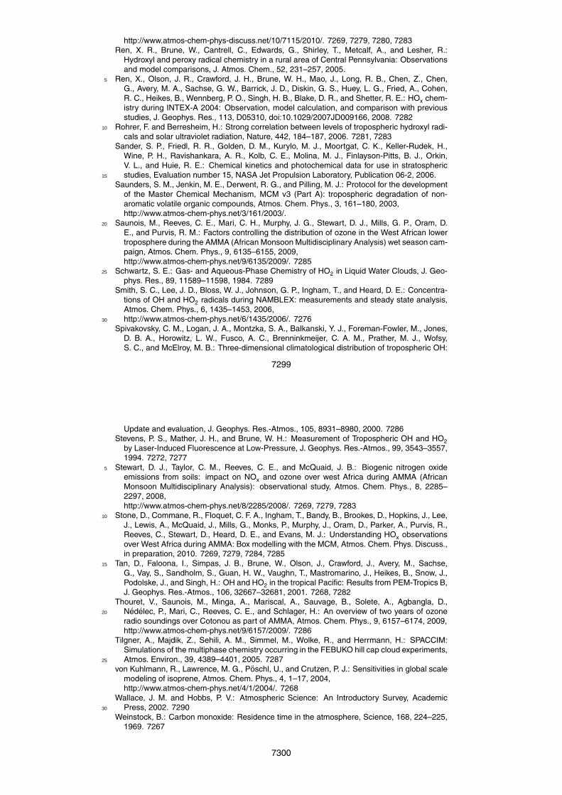
Figure 1 shows the instrument set-up. The instrumentation is installed on two 19 inchaircraft racks, located behind the fluorescence cell sampling point with pumps locatedbelow the fluorescence cell.

2.1 HOx radical sampling

Ambient air from outside the aircraft is sampled through an inlet (adapted from Eisele15

et al., 1997) mounted on a window blank on the starboard side of the BAe-146, closeto the front of the aircraft. Using two concentric tubes with restrictions, the inlet slowsthe air prior to sampling, while minimising turbulence, and hence wall contact, and theassociated loss of OH radicals.

Air is drawn in through a pinhole (0.75 mm diameter) to a fluorescence cell main-20

tained at reduced pressure by a rotary pump (Leybold Trivac D25B) coupled with asupercharger (Eaton M90). In order to extend outside the aircraft skin and deliver OHto the excitation axis, a tube made of anodised aluminium (internal diameter=5 cm;length=50 cm) was added to the fluorescence cell. Characterisation tests on the cell(Ingham et al., 2010) have shown significant OH loss on contact with the internal tube25

walls, thus reducing the instrument sensitivity to OH. No solar scattered light has beendetected at either the OH or HO2 detection axes when the instrument was operated on

7270

the aircraft. A fluorescence cell for the detection of RO2 is shown in Fig. 1 but is not yetoperational.

2.2 Laser excitation of OH

Laser light at λ≈308 nm was generated by a laser system consisting of a Nd:YAG(Neodymium-ion doped Yttrium Aluminium Garnet (Y3Al5O12) DS20-532, Photonics5

Industries) pumped Titanium Sapphire (Ti:Sapp) laser (TU-UV 308 nm, Photonics In-dustries). The YAG laser typically produces 9–10 W of light at λ=532 nm and a PulseRepetition Frequency (PRF) of 5 kHz, which is used to pump the Ti:Sapp laser. TheTi:Sapp output wavelength of λ≈924 nm is selected through the use of a diffractiongrating and is passed through the first of two non-linear harmonic generation stages10

consisting of a Cerium Lithium Borate (CLBO) crystal, generating the second harmonicat λ≈462 nm. A half wave plate corrects the polarisation of the light to allow the secondcrystal to perform sum-frequency mixing of the second harmonic (λ≈462 nm) with thefundamental (λ≈924 nm), producing light at λ≈308 nm.

Under optimal conditions, ∼100 mW of UV radiation is produced with a pulse width of15

35 ns (Full Width Half Maximum, FWHM) and a laser linewidth of 0.065 cm−1. However,during the observations presented here, typical powers observed after adjustment var-ied from 30 mW to 50 mW at λ≈308 nm. Dielectric coated beam splitting mirrors splitthe UV beam before launching the light into fibre optic cables (Oz Optics) in the ratio60%:36%:4% for use within the OH and HO2 axes and the reference cell respectively.20

Upon exiting the fibre optic cable, the laser beam entering each detection cell is col-limated and baffled before intersecting the air sample. After traversing the excitationregion, the beam exits the cell through another baffled arm and is directed (via a 45◦

mirror) into a calibrated UV photodiode (UDT – 555UV, Optoelectronics), allowing real-time measurement of the laser power. The measured laser power is used to normalise25

the fluorescence signal for fluctuations in laser power.

7271

2.3 Fluorescence detection

In the fluorescence cell (Fig. 2), the UV fluorescence is collected and passedthrough an interference filter (Barr Associates ∼50% transmission at λ=308 nm, FWHMca. 5 nm centered at λ=308 nm). A back reflecting mirror (CVI Optics) improves thesignal collection efficiency. The fluorescence signal is then focused onto the Channel5

Photomultiplier (CPM) (Perkin-Elmer 943P, ∼5×108 gain), where the electron pulsesgenerated from a single photon are counted with a photon-counting card (PMS 400,Becker and Hickl). To prevent saturation, the CPM is turned off by a high voltageswitching circuit (“gating box”, designed and built in-house) from the time the laser istriggered until ∼60 ns after the laser pulse (FWHM=35 ns). The use of a temporal gat-10

ing allows sensitive measurement of the fluorescence emitted from the electronicallyexcited OH and discrimination against laser scattered light.

2.4 Reference cell

The wavelength of the laser is changed by a stepper motor which controls the an-gle of the diffraction grating within the Ti:Sapp laser cavity. The absolute wavelength15

of the second harmonic of the Ti: Sapp (λ≈462 nm) is monitored by a wavemeter(Wavemaster 33–2650, Coherent). However, the resolution of this wavemeter (preci-sion ±0.001 nm, accuracy ±0.005 nm) is insufficient to locate the OH Q1(2) rotationalline (λ=307.995 nm). The reference cell facilitates scanning over and identification ofthe Q1(2) peak. With the reference cell maintained at low pressure (∼3 Torr), humidi-20

fied cabin air is passed over an electrically heated 80:20 Ni:Chrome filament, produc-ing OH radicals by pyrolysis of water vapour (Stevens et al., 1994; Wennberg et al.,1994). The reference cell receives 2–3 mW (∼4%) of the total UV radiation. The OHfluorescence signal is filtered and focussed on to a CPM perpendicular to the laserbeam. The resulting signal is recorded using a photon-counting card. Because of the25

high concentration of OH radicals produced in the reference cell, discriminating the OH

7272

fluorescence signal from the background laser scatter does not require gating of theCPM.

Figure 3 shows the signal observed in the reference cell for a two minute measure-ment cycle. The OH signal in the reference cell is typically 20 000 cts s−1 above thelaser scatter background of approximately 7000 cts s−1. The first 55 points on the fig-5

ure show the OH fluorescence while scanning over the Q1(2) rotational line of OHto locate the wavelength of the peak fluorescence (finding line: from λ=307.990 nmto λ=308.000 nm). Points ∼55–175 show the online fluorescence signal (and back-ground) as the laser wavelength is tuned to the peak of fluorescence. Points ∼175–235show the fluorescence as the laser wavelength is tuned to a wavelength which does10

not induce fluorescence to measure the background signal (offline).The signal in the reference cell varies with aircraft cabin pressure due to changes

in the laser wavelength. The variation in the wavelength generated by the laser isdue to the changing refractive index of the cabin air with pressure compared with thematerial of the laser grating. This change in wavelength away from the maximum of the15

OH transition results in the signal due to OH fluorescence varying with cabin pressure.Independent of this laser wavelength change with pressure, fluctuations in cell pressurewill also alter the instrument sensitivity. While the effect of changing cell pressure onsensitivity can be determined by calibration, it cannot be decoupled from changes inwavelength during AMMA as the Ti:Sapp laser cavity was not kept at constant pressure,20

so only data recorded on level flights (with constant laser wavelength) are considered.

2.5 Data analysis

The laser is operated at a pulse repetition frequency of 5 kHz and the contribution ofthe solar and dark counts (CPM thermal noise) to the observed signal is determinedfor each laser pulse. The fluorescence signal is collected for 1 µs (Gate A). After a25

5 µs gap the non-laser background signal is recorded for 20 µs (Gate B) and the signal

7273

solely due to OH fluorescence and laser background, Sigfl, is calculated:

Sigfl = SigA −SigB

20, (2)

where SigA (cts) is the number of counts in the 1 µs collection Gate A (cts s−1) andSigB/20 is the number of counts in the 20 µs collection gate (typically 0–1 cts s−1). Thetotal signal, Sigfl (cts s−1), is then recorded at 1 Hz and normalised for laser power5

(P, mW). For OH, the normalised offline signal OH Sigoffline is subtracted from thenormalised online signal OH Sigonline, leaving the signal solely due to OH (OH Sig,cts s−1 mW−1):

OHSig = OHSigonline − OHSigoffline (3)

HO2Sig is the difference in normalised online signal observed with NO injected10

(HO2+OH) and without NO added (OH only). The concentration of OH isthen calculated using the experimentally determined instrument sensitivity (COH,cts s−1 mW−1 molecule−1 cm3):

[OH] =OHSig

COH(4)

The concentration of HO2 is calculated using the experimentally determined instrument15

sensitivity HO2 (CHO2, cts s−1 mW−1 molecule−1 cm3):

[HO2] =HO2Sig

CHO2

(5)

2.6 Calibration

Before and after deployment, the instrument sensitivity was determined over the rangeof cell pressures experienced during the AMMA campaign (between 1.5 and 2.1 Torr,20

equivalent to 2–2.8 hPa) using a method similar to that employed by Faloona et al.7274

(2004) and Martinez et al. (2008). Pinholes with diameters between 0.65 and 0.85 mmwere used to obtain cell pressures between 1.5 and 2.7 Torr (2–3.6 hPa) respectively.

By varying the lamp current supplied to a low-pressure mercury lamp, a range ofconcentrations of OH and HO2 were produced from the photolysis of humidified air(constant [H2O]) at λ≈184.9 nm:5

[OH] = [HO2] = [H2O] σH2O φOH F δt (6)

where σH2O is the absorption cross-section of water at λ=184.9 nm (7.14±0.2×10−20

molecule−1 cm2; Cantrell et al., 1997a), φOH and φHO2are the photodissociation quan-

tum yields of OH and HO2 respectively (=1), F is the photon flux of the mercury lamp(photon cm−2 s−1) at λ=184.9 nm and δt is the residence time in the photolysis region.10

Figure 4 shows the experimental set-up of the calibration system. A known flow(ca. 50 slm: L min−1 at standard temperature and pressure) of ultra high-purity air(BTCA 178, BOC Special Gases) is introduced into the system, with a variable fractionof the flow diverted (through bypass valves) to a bubbler containing distilled water inorder to humidify the air. After mixing, most of the calibration gas passes through a15

1.27 cm×1.27 cm black-anodised square aluminium tube 30 cm long, where the gas isphotolysed by the λ=184.9 nm emission of a mercury lamp of known actinic flux (seebelow) to produce equal concentrations of OH and HO2 before delivery to the FAGEsampling point. Immediately prior to the air entering the calibration tube, a small flow isdiverted to a dew-point hygrometer (CR4, Buck Research Instruments) to measure the20

concentration of water vapour in the flow. There are three 3.81 cm Suprasil® windowsseparated by equal distance down the length of the calibration tube. At high flow ratesthrough the calibration tube, the gas was found to have a uniform velocity profile con-sistent with turbulent flow. The mercury lamp is housed in a nitrogen-purged aluminiumcasing, and usually mounted over the window closest to the exit of the calibration tube.25

This purged housing is heated to maintain a stable lamp temperature (±1 ◦C), whilethe nitrogen flow prevents both ozone formation within the housing and absorption ofradiation by ambient water vapour and oxygen prior to the light entering the calibration

7275

tube. The lamp is collimated using thin walled tubes (3 mm diameter, 8 mm length)packed together in front of the lamp. These tubes are used to create a more uniformactinic flux in the photolysis region.

Prior to calibration, the lamp flux at λ=184.9 nm was determined by N2O actinometrythrough the generation of a quantifiable mixing ratio of NO from the photolysis of 10%5

N2O in air. The theory and method of this technique has been described extensively inprevious publications (e.g. Edwards et al., 2003; Faloona et al., 2004; Glowacki et al.,2007; Whalley et al., 2007). Two corrections were made in the calculation of the flux,F . In the NOx analyser (Thermo Electro 42C; detection limit/precision ∼50 pptv) usedto measure the NO produced, the introduction of high concentrations of N2O results in10

the reporting of artificially low NO mixing ratios. This is due to increased quenching ofthe electronically excited NO2 fluorescence by N2O within the analyser. The effect ofthis quenching was characterised and the corrected NO mixing ratios were calculated.The second correction accounted for absorption of the light flux by N2O across thewidth of the photolysis area (Edwards et al., 2003). A linear relationship between the15

lamp current supplied to the lamp and the flux was observed after corrections, allowingthe lamp current to be varied to generate various concentrations of HOx.

Calibrations were conducted over a range of water vapour mixing ratios from330 ppmv to 10 000 ppmv. Figure 5 shows a typical multi-point calibration for the lowestwater vapour used (332 ppmv). The instrument sensitivity to OH is a function of water20

vapour in the gas flow (Smith et al., 2006) due to quenching of electronically excitedOH by the water vapour. Using a constant concentration of water vapour during cali-brations ensures a linear relationship between the observed signal and concentrationof OH or HO2.

Over the pressure range observed in the fluorescence cell during AMMA, the sen-25

sitivity of the instrument did not vary significantly (Fig. 6) and the mean sensitivitiesof the instrument to OH (COH=6.29 (±0.95) ×10−8 cts s−1 mW−1 molecule−1 cm3, ±1σstandard deviation) and HO2 (CHO2

=1.17 (±0.23)×10−7 cts s−1 mW−1 molecule−1 cm3)were determined. Calibrations before and after the campaign did not show any

7276

degradation in the instrument sensitivity, and while in-flight calibrations were not pos-sible during the AMMA campaign, instrumentation to allow calibration during flight iscurrently being developed. The instrument sensitivity to OH is half that of HO2 andis due to a higher loss of OH compared to HO2 on the surface of the cell betweensampling and detection.5

2.7 Limit of detection

It is possible to calculate the instrumental Limit Of Detection (LOD) for OH and HO2

by carrying out a t-test between an observations value and zero (0 molecule cm−3),assuming the variance in the background is constant throughout the measurementcycle and is represented by the variance in the offline measurement. For unequal10

sample sizes (online and offline), the minimum detectable HOx, Sigmin, for a givenconfidence interval can be calculated:

Sigmin = TCI

√1n+

1m

σbg (7)

where TCI is the T value for a given confidence interval (T69%=1), n and m are thesample sizes online and offline respectively defined by the sampling frequency and σbg15

is the standard deviation of the background, which is assumed to be representative ofthe standard deviation of the background signal during the online sample. Previousstudies have assumed the background signal obeys Poisson statistics (Stevens et al.,1994; Faloona et al., 2004; Martinez et al., 2008) and:

σbg =√

(Slb + Ssb + Sdc) (8)20

where Slb is the signal due to laser scatter, Ssb is the signal due to solar backgroundand Sdc are the dark counts of the CPM.

Sigmin is converted into a minimum detectable concentration of OH (and HO2) by:

[OHmin] =OHSigmin

COH P(9)

7277

[HO2 min] =HO2Sigmin

CHO2P

(10)

where COH and CHO2are the instrument sensitivity to OH and HOx

(cts s−1 mW−1 molecule−1 cm3) respectively and P is the laser power in the cell (mW).Using a confidence interval of 69% (T value =1), a limit of detection is calculated for

each measurement cycle (∼5 min). Table 1 shows the OH and HO2 LODs calculated for5

a typical measurement cycle during the AMMA aircraft campaign (July–August 2006).During the campaign the mean OH LOD was 7.1×105 molecule cm−3 and the meanHO2 LOD was 7.5×105 molecule cm−3 for a one minute integration time. In order toimprove sensitivity to HO2, the time between laser trigger and fluorescence collectionis shortened, compared to that set for OH, which increases the background signal (and10

therefore σbg) and hence limit of detection but will also increase the sensitivity to HO2.This shortened delay time is suitable for HO2 observations, as a typical concentration ofHO2 in the atmosphere is around two orders of magnitude greater than the calculatedLOD.

During AMMA, the performance of the YAG laser was degraded during flight in line15

with an increase in cabin temperature, which often increased from 15 ◦C to 35 ◦C duringa flight. The reduced power output from the YAG resulted in the Ti:Sapphire laser takinglonger to reach the lasing threshold. The time delay between the laser trigger and thelaser pulse was found to increase by several tens of nanoseconds during a given flight,an increase large enough to increase the laser background signal and affect both the20

sensitivity of the instrument to HOx and the instrumental limit of detection. As thebackground is recorded at the end of the measurement cycle, it is possible that anincrease in background signal throughout a measurement cycle could also lead to aslight underestimation of the OH concentration.

Since the AMMA campaign, a diagnostic system coupling a fast photodiode (Hama-25

matsu, S6468) to an oscilloscope (Waverunner LT372, Le Croy) has been developed tomonitor the timing of the CPM gate trigger relative to the laser pulse and not the laser

7278

trigger. This technique allows the time between the laser pulse itself and the CPM gatetrigger to be adjusted automatically in flight every 10 s, thus maintaining a constant timedelay. A similar system is now used in the Leeds ground-based FAGE instrument andis described in detail in Whalley et al. (2009). Using this system, the sensitivity of theinstrument to the time interval between the laser pulse and the fluorescence collection5

was investigated. Figure 7 shows how the background signal increases dramaticallyas the time between the laser pulse and fluorescence collection decreases and moreof the laser pulse is detected. The limit of detection is also shown to worsen at shortertime intervals (Fig. 7).

Under normal operating conditions (delay of 60 ns), the instrumental LOD for OH10

(∼7×105 molecule cm−3) is below peak concentrations of OH observed in the tropics(e.g. [OH]=9×106 molecule cm−3 observed at a tropical marine site in summer, Whal-ley et al., 2009). However, as the delay time decreases, the LOD becomes comparableto ambient concentrations of OH. Ambient concentrations of HO2 are much greaterthan the HO2 LOD (e.g. [HO2]=6×108 molecule cm−3, Whalley et al., 2009) and the15

relative increase of HO2 LOD compared to ambient concentrations has far less of animpact than for OH.

2.8 Ancillary measurements

J(O1D) was provided by the University of Leicester. J(O1D) is the combination ofthe upward and downward welling observations. During the campaign the down-20

ward welling J(O1D) actinometer failed and subsequent observations were scaledto the combined J(NO2) observations, as described in Stone et al. (2010). Coreaircraft data such as temperature, pressure, CO (Aerolaser AL5002 instrument), O3(TECO 49UV photometery instrument) and liquid water content (Johnson Williams Liq-uid Water Content probe) were provided by the Facility of Airborne Atmospheric Mea-25

surements (FAAM) (Reeves et al., 2010), PAN data were provided by the Universityof York (Stewart et al., 2008) and NOx, NOy (Stewart et al., 2008), acetonitrile and

7279

isoprene (Proton Transfer Mass Spectrometry – PTr-MS; Murphy et al., 2010) wereprovided by the University of East Anglia.

3 Results: observations of OH and HO2 radicals

The Leeds aircraft FAGE instrument observed OH and HO2 over a range of altitudes(500 m–9 km) and through various airmasses over West Africa. The observed signal5

was processed and the concentration of OH and HO2 calculated using the instrumentsensitivity determined by calibration, as described in Sect. 2.6. The 1 Hz mixing ratiosof OH and HO2 were calculated using the temperature and pressure recorded on theaircraft and averaged over 60 s. The 1 Hz HO2 data were used directly in the study ofHO2 in clouds (Sect. 4.3).10

HOx observations were made on 13 flights during July and August 2006, with flightsboth during day and at night. Figure 8 shows the spatial distribution of HO2 observedover West Africa during the AMMA campaign. The aircraft was based in Niamey, Nigerand HOx observations were made over barren soil in the north (Sahel region of north-ern Niger and Mali), over regions of forest (Benin) and out over the Gulf of Guinea to15

the south. An overview of the aircraft measurements can be found in Reeves et al.(2010).

Figure 9 is an example of a typical OH and HO2 time series for a flight on 17 Au-gust 2006. The aircraft sampled between 500 m and 6 km over the forested region tothe north of Benin (7–13◦N). The O3 mixing ratios were found to increase with altitude.20

OH mixing ratios were generally above the limit of detection and HO2 mixing ratioswere found to be highly variable on a 10 s time scale. At the level run at 1.5 km, lightcloud was encountered and HO2 mixing ratios were found to rapidly decrease. Thiswill be studied in more detail in Sect. 4.3.

Overall during the campaign, the mixing ratios of OH and HO2 were variable. Fig-25

ure 10 shows the probability density function of the complete dataset of OH and HO2mixing ratios, with the median of the limit of detection. OH mixing ratios (Fig. 10a) from

7280

−0.27 pptv to 1.34 pptv were observed (but with very few points above 1 pptv) and themost probable value was observed at 0.15 pptv. HO2 mixing ratios (Fig. 10b) variedfrom −0.32 pptv to 42.65 pptv, with the highest frequency observed at 1.5 pptv. Forsignificant periods, the OH observations were close to the limit of detection of the in-strument due to problems with the instability of the timing of the fluorescence detection5

(as discussed in Sect. 2.7). However, as most HO2 is well above the limit of detection,conclusions can be drawn with more confidence.

3.1 Diurnal variation

Although complex mechanisms determine the in situ concentrations of OH and HO2,daytime OH production is generally dominated by the photolysis of ozone and often10

exhibits a strong diurnal profile (Rohrer and Berresheim, 2006). Figure 11 shows thediurnal profile of the entire dataset of OH and HO2 radicals as a function of local solartime. Both OH and HO2 were highly variable throughout the day, with the maximumOH mixing ratio (∼1 pptv) coinciding with solar noon, while maximum HO2 mixing ratio(40 pptv) occurred shortly after solar noon. Mixing ratios of HO2 up to 9 pptv with a15

mean of 3 pptv were observed at night. The observations of HO2 at night will bediscussed in detail in Sect. 4.4.

3.2 HOx observations as a function of altitude

Figure 12 shows the daytime altitude profiles of (a) OH, (b) HO2 and (c) the HO2/OHratio for data between 09:00 and 15:00 LT (Local Time), with the median value for a20

given 500 m altitude bin also shown.OH mixing ratios (binned for 500 m altitude bins up to 6 km) are highly variable but

the median OH is relatively constant with altitude at about 0.2 pptv, except for a largeincrease at the top of the boundary layer at 2 km to 0.7 pptv and distinct decrease at5 km to less than 0.05 pptv. These observations of OH compare well with previous25

OH observations made using other instruments. Observations over the mid-latitude

7281

and tropical Pacific Ocean found that median OH was relatively constant with altitudeat ∼0.1–0.2 pptv, increasing from ∼0.1 pptv below 2 km to ∼0.2 pptv at 7 km (INTEX-Band PEM-Tropics-B campaigns, Mao et al., 2009; Tan et al., 2001, respectively). Overcontinental mid-latitudes, median OH was again relatively constant at all altitudes butat a slightly higher mixing ratio at ∼0.2–0.3 pptv (INTEX-A campaign, Ren et al., 2008).5

However, boundary layer OH mixing ratios varied significantly from 0.01–0.6 pptv. Ob-servations over a tropical forested region (GABRIEL campaign, Martinez et al., 2008)found much higher OH mixing ratios with median OH increasing from ≈0.4 pptv in theboundary layer, peaking at 0.75 pptv at 3–4 km and dropping to ∼0.25 pptv at 8 km.

HO2 mixing ratios were also variable at all altitudes and median HO2 varied between10

5 and 30 pptv for 500 m altitude bins up to 7 km. The lowest observed mixing ratios ofHO2 were found within 500 m of the forest surface, but the highest HO2 mixing ratioswere observed between 500 m and 1 km above the forest. At altitudes above 6 km, indi-vidual HO2 data points varied from below the limit of detection to over 30 pptv HO2, witha median value of ∼5 pptv. Previous observations of HO2 generally show a decrease15

with altitude in all locations. Over the mid-latitude North Pacific HO2 steadily decreasedfrom ∼20 pptv at 2 km to ∼7 pptv at 10 km (INTEX-B campaign, Mao et al., 2009), whileover continental mid-latitudes, median HO2 steadily decreased from ∼30 pptv near thesurface (ranging from ∼2–60 pptv) to ∼10 pptv at 10 km (INTEX-A campaign, Ren et al.,2008) and over tropical rainforests median HO2 was found to decrease from ∼40 pptv20

in the boundary layer to ∼10 pptv at 8 km (GABRIEL campaign, Martinez et al., 2008).However, observations over the tropical south Pacific Ocean show a slightly differentprofile; HO2 increased from ∼10 pptv at the surface to ∼20 pptv at 3 km before steadilydecreasing again with altitude to ∼5 pptv at 11 km (PEM-Tropics-B campaign, Tan et al.,2001).25

The HO2/OH ratio was highly variable at all altitudes, ranging from 5 to 5 000 witha median value of 95. While HOx production is dominated by O3 photolysis, the cy-cling between OH and HO2 is closely related to the abundance of CO and NO present(Ehhalt, 1999). At the altitudes considered here, overall O3 varied between 10 and

7282

100 ppbv and median values gradually increased with altitude to 7 km. CO variedbetween 50 and 450 ppbv, but overall decreased slightly with altitude (Reeves et al.,2010). Median NO and total NOx both decreased with altitude to the top of the bound-ary layer (2 km). Total NOx is constant with altitude from 2 to 7 km, while NO increasesslightly above 5.5 km (Stewart et al., 2008).5

3.3 Steady state calculations

As discussed earlier, the photolysis of ozone in the presence of water vapour is themain production pathway of OH in the unpolluted troposphere (Eq. 1). Figure 13 showsthe correlation between OH and P(OH). OH mixing ratios were highly variable but weregenerally found to increase with increasing P(OH). In contrast to here, previous ob-10

servations at ground sites with relatively constant OH sinks, found that the observedvariation in OH was largely explained by corresponding variations in P(OH) (Rohrerand Berresheim, 2006).

In a clean airmass, the production of HO2 is closely linked to P(OH) and the loss isdominated by the HO2 self reaction:15

HO2 + HO2 −→ H2O2 + O2 (R7)

Assuming this production of HO2 (∼P(OH)) and loss of HO2 through self-reaction (Re-action R7) are equal, a steady state concentration in clean air, HO2 ss, can be calcu-lated:

HO2 ss =

√P(OH)

2 kR7=

√2 J(O1D) [O3] FOH

2 kHO2+HO2

(11)20

Figure 14 shows that HO2 ss correlates well with the observed HO2 (R=0.57) and theslope of 0.61 indicates that overall HO2 ss is overestimating HO2, suggesting missingsinks of HO2. This is not unexpected, given that the rapid loss of HO2 by reactionwith species such as RO2 or NO2 or other sinks of HOx radicals such as heteroge-neous chemistry. From Fig. 14, a number of distinct groups have been identified. HO225

7283

is generally reproduced by HO2 ss in areas of high mixing ratios of isoprene (green)(Sect. 4.1). However, the HO2/HO2 ss ratio is much less for observations in a biomassburning plume, suggesting the presence of significant HO2 sinks (Sect. 4.2). Stoneet al. (2010) describe how the observed photolysis rates were generally slightly lowerthan calculated from the Tropospheric Ultraviolet and Visible (TUV) Radiation model.5

However, on part of one particular flight (B228, shown in white in Fig. 14) the obser-vations exceeded the calculated J(O1D) by a factor of 1.5. Thus, it is possible that theP(OH) calculated at this time is significantly overestimated.

This simple analysis is suitable for the examination of the overall HOx behaviourbut detailed interpretation requires a more comprehensive chemical modelling study.10

However, the comprehensive analysis of Stone et al. (2010) implies that, for muchof the air over tropical West Africa, the HO2 concentrations is controlled by relativelysimple processes.

4 Discussion

A number of case studies have been identified in Sect. 3 and will now be examined in15

detail. Compared with P(OH) and HO2 ss, both OH and HO2 are enhanced in the pres-ence of high isoprene (Sect. 4.1), but are depleted within a biomass burning plume(with acetonitrile higher than 250 pptv) (Sect. 4.2). A reduction in HO2 was also ob-served when sampling in cloud (Sect. 4.3) and HO2 was observed at night (Sect. 4.4).

4.1 OH and HO2 with isoprene20

Figure 15 shows the latitudinal variation of OH and HO2 and highlights how the maxi-mum mixing ratios of both OH and HO2 were found in the boundary layer of the south-ern end of the forest region. The West African Monsoon (WAM) brings the majority ofrainfall to the continent and produces a strong latitudinal gradient in vegetation and bio-genic emissions such as isoprene: Murphy et al. (2010) show that the highest mixing25

7284

ratios of isoprene were observed in the boundary layer above the southern forest re-gions (9–11◦N).

Modelling studies of the latitudinal gradient of West Africa predict minimal HOx con-centrations over the forested regions due to isoprene scavenging of OH (Saunois et al.,2009). Isoprene reacts quickly with OH (k=1.0×10−10 cm3 s−1 at 294 K; Karl et al.,5

2004) and, given the concentrations of isoprene in the boundary layer above forests,this reaction should result in significant depletion of OH.

However, the observations presented here suggest that neither OH nor HO2 mix-ing ratios are significantly depleted. Lelieveld et al. (2008) also observed higher thanexpected mixing ratios of HOx over forests in Suriname and suggested that additional10

production of OH from the degradation products of isoprene (Dillon and Crowley, 2008;Peeters et al., 2009; Paulot et al., 2009; da Silva et al., 2010) could explain the highconcentrations of HOx. Given the complex nature of the oxidation of VOCs, the inter-pretation of these HOx mixing ratios requires a more comprehensive modelling studythan presented here. Stone et al. (2010) presents a detailed chemical box modelling15

study, based on the master chemical mechanism, to explore the interpretation of theHOx observations presented here.

4.2 Biomass burning plume

As highlighted in Figs. 13 and 14, OH and HO2 sampled in a biomass burning plumeshowed some of the largest disagreement for the steady state calculations. The20

biomass burning plume was sampled at two altitudes over the Gulf of Guinea. At analititude of 4–5 km, the mean O3 mixing ratio was ∼50 ppbv and the mean CO mixingratio was 150 ppbv. At an altitude of 3.5 km, mixing ratios of O3 and CO were some ofthe highest observed during the campaign (100 ppbv and 300 ppbv respectively). Co-incident with these observations was a sharp increase in NO, acetonitrile (CH3CN) and25

7285

Peroxyacetyl Nitrate (PAN). Acetonitrile has been identified as a tracer for airmassesaffected by biomass burning (de Gouw et al., 2003).

Figure 16 shows the time series of O3, CO, OH and P(OH) and HO2 and HO2 ss. Thebiomass burning plume was sampled at two altitudes, with the highest concentrationsof both O3 and CO observed at an altitude of 3–4 km (indicated as BB between the5

blues dashed lines). Within the plume at 3.5 km , 400 pptv CH3CN was observed (upfrom 100 pptv outside the plume) and 600 pptv PAN was observed (up from 50 pptvoutside the plume). The increase in observed OH within the plume at 3.5 km comparedto 4.5 km coincides with an increase in NO at the lower altitude. The calculation ofHO2 ss does not incorporate the loss of HOx through reactions such as RO2+HO2,10

OH+VOC, OH+NO2 or reactions with aerosols, so it is not surprising that HO2 ss issignificantly higher than the observed HO2.

Previous observations of VOCs within aged biomass burning plumes (de Gouw et al.,2003) found that the OH inferred from the degradation of species such as benzene andtoluene was a factor of 4 lower than that calculated by a OH climatology model (Spi-15

vakovsky et al., 2000). While Forberich et al. (1996) measured reduced levels of OHin a biomass burning plume on one afternoon, a systematic observation of oxidationin biomass burning plumes would help in our understanding of these events. Littlebiomass burning takes place in West Africa during the monsoon wet season and withinthe plume, NO mixing ratios reach a maximum of 200 pptv (NO2 observations were20

not available at this time), while PAN mixing ratios increased to over 700 pptv, suggest-ing that this biomass burning plume was transported from the Southern Hemisphere(Thouret et al., 2009; Liousse et al., 2010).

In this plume, HO2 mixing ratios are much lower than HO2 ss, as expected as HO2 ssdoes not include all possible HOx loss processes. The mixing ratios of a number of25

VOCs were observed to be greatly increased within the plume compared to outsidethe plume. Within the plume the greatest increase was observed in acetylene (factorof 7.5), followed by methanol (4.2), acetonitrile (3), benzene (2.9), ethane (2.9) andacetone (2.4). The CO mixing ratio increased from a mean of 98 ppbv outside the

7286

plume to 245 ppbv within the plume. The rate of production of HO2 from the OH reactionwith CO can be compared to the rate of production of RO2 through the reaction of OHwith VOCs.

The reactivity of OH with various VOCs can be estimated as a fraction of the OHreactivity with CO:5

RVOC =

i∑ki [VOC]ikCO+OH

[CO] (12)

where ki is the rate constant for the reaction of the VOCi with OH andi∑ki [VOC]i

is the sum over all the products of the VOC concentration and the appropriate ratecoefficient for the reaction of OH with the VOC in question. From this ratio, the impactof enhanced VOC concentrations on OH can be examined. The reaction of OH with10

CO forms HO2, thus conserving the HOx budget. However, the reaction of OH with anyof the VOCs enhanced in this plume does not immediately form HOx and results in HOxdepletion. The VOC/CO ratio was found to be 1.6 times higher within the plume (71)than outside (43), consistent with the observed HOx depletion within the plume.

4.3 HO2 in cloud15

When sampling in and around clouds, HO2 was found to rapidly decrease for shortepisodes, before returning to the previous higher levels again. The background signaldid not change when sampling around clouds, suggesting that this effect was not aninstrumental artefact. Studies of a similar FAGE instrument have shown no responseof the instrument sensitivity to aerosol loading (Whalley et al., 2010). Modelling studies20

have shown that gaseous HO2 concentrations can be significantly reduced by aqueousphase chemistry, specifically through the efficient uptake of HO2 onto cloud droplets(Tilgner et al., 2005). These aqueous phase models combine detailed microphysicsand multiphase chemistry but few experimental observations exist to validate the modelcalculated depletion of radical species in clouds. Figure 17 shows the 1 s time series of25

7287

the observed HO2, steady state calculated HO2 ss mixing ratios and the Liquid WaterContent (LWC, g m−3) observed between 13:00 and 13:30 UTC at a constant altitude of1.5 km over northern Benin (10.9–12.5◦N) (Flight B235A, 17 August 2006). Figure 17highlights how the timing of the short-lived reduction in HO2 observed when samplingin cloud is reproduced by HO2 ss but, as seen earlier, HO2 ss is consistently greater5

than HO2. Much of the variability in HO2 ss is driven by changes in J(O1D), whichvaried greatly in and out of cloud, depending on the cloud thickness. O3 was generallyfound to rapidly decrease in cloud, while the fraction of O(1D) reacting with H2O vapourto form OH, FOH, generally increased quickly due to higher water vapour, counteractingthe decrease in ozone and J(O1D) to an extent. Overall these fast changes in P(OH)10

resulted in short-lived reductions in HO2ss. However, the observed reduction in HO2

was much greater than that seen in HO2 ss. Thus the relative change in the HO2/HO2 ssratio is considered for each cloud encounter, as this removes any variation due tochanges in the HOx production rates.

Figure 18a shows the 1 Hz time series of the HO2/HO2 ss ratio and the simultane-15

ously observed liquid water content. The magnitude of the short-lived decreases inHO2 inside the cloud are not reproduced in the calculated HO2 ss, resulting in a de-crease in the HO2/HO2 ss ratio. These rapid decreases in the HO2/HO2 ss ratio gen-erally coincide with increases in liquid water and may be due to the heterogeneousuptake of HO2 onto the cloud aerosol surface. Figure 18b shows the HO2/HO2ss

ra-20

tio as a function of liquid water content. While the values of HO2/HO2 ss ratio arehighly variable, the highest ratios (median of 0.47) are found for low liquid water (be-low 0.2 g m−3) and the lowest ratios (median of 0.25) are found for higher liquid watercontent (greater than 0.2 g m−3).

The reduction in HO2 in clouds has been observed previously using both FAGE and25

CIMS instruments (e.g. Mauldin et al., 1999; Olson et al., 2004) and this loss of HO2has been attributed to heterogeneous uptake of HO2 onto the cloud aerosol. Duringthe TRACE-P (Transport and Chemical Evolution over the Pacific) campaign, Olsonet al. (2004) found that the observed HO2 was much lower than that calculated by a

7288

comprehensive chemistry model. For each 1 min data point, observations within cloudwere identified. The observed-to-modelled HO2 ratio was found to be significantly re-duced when sampling clouds with an increased liquid water content but appeared tobe independent of the duration of cloud sampling. The time resolution of many speciesrequired to calculate HO2 in chemical models is too low to interpret the short-lived de-5

pletions in HO2 observed during AMMA (e.g. minimum 15 s for isoprene observed byPTR-MS). Therefore these rapid reductions in HO2 are unlikely to provide any morethan a qualitative sense of the heterogeneous uptake of HO2 by cloud droplets.

The impact of HO2 loss due to uptake on liquid cloud was investigated. The first orderloss to surfaces was calculated with the diffusion of cloud droplets included (Schwartz,10

1984):

k′loss =A

4cgγ

+ rDg

(13)

where k′loss is the rate constant for the loss of HO2 to cloud droplets (s−1), A is thecloud droplet surface area per unit volume (m2 m−3), γ is the uptake coefficient to liquidwater, r is the droplet radius (m) and Dg is the diffusion coefficient (for cloud droplets15

∼1×10−6 m2 s−1, Ravishankara, 1997). The uptake of HO2 onto cloud is not tightlyconstrained and the uptake coefficient is thought to vary between 0.1 and 1 (Jacob,2000; Morita et al., 2004). The mean molecular speed of the gas, cg (m s−1) is:

cg =

√8 RTπMw

(14)

where R is the universal gas constant, T is the temperature and Mw is the molecular20

weight of HO2.Unfortunately no information was available on the size or number concentration of

cloud droplets encountered for the observation period examined here but the HOx ob-servations were made over the continent of West Africa and typical continental values

7289

of cloud droplet size (10 µm) and concentration (1.5×108 droplets m−3) have been as-sumed in the calculation of k′loss (Wallace and Hobbs, 2002). The main productionand loss mechanisms of HO2 were calculated for all HO2 data where the liquid watercontent was greater than 0.2 g m−3 and an assumed mid-range γ of 0.5.

Using these constraints, the mean rate of HO2 loss to cloud droplets was cal-5

culated to be 4.2×106 molecule cm−3 s−1, slightly greater than the primary produc-tion rate (4.1×106 molecule cm−3 s−1) but much larger than the HO2 self reaction(0.89×106 molecule cm−3 s−1). Therefore it is reasonable to assume that the uptakeof HO2 onto cloud droplets is a major sink of HO2 within a cloud. Without the inclusionof HO2 uptake on clouds, the mean steady state calculated HO2 mixing ratio, HO2 ss,10

is 35 pptv, much higher than the observed mean HO2 mixing ratio of 10.6 pptv. It ispossible to calculate a cloud-influenced HO2 mixing ratio, HO2 cloud, assuming that theprimary production of HO2 (through OH) is equal to the loss of HO2 from both selfreaction and uptake on clouds:

P(OH) = k′loss[HO2] + 2 kHO2+HO2[HO2]2 (15)15

With the inclusion of HO2 uptake onto cloud droplets in the calculation of HO2, themean HO2 cloud mixing ratio was calculated to be 8.84 pptv, in closer agreement with themean observed HO2 mixing ratio (10.6 pptv), than the previous steady state calculationof 35 pptv. It is possible that the accurate knowledge of the cloud droplet size andconcentration and better understanding of γ would improve agreement even further.20

Therefore in order to fully understand the role of clouds on the oxidative capacity ofthe troposphere, a more comprehensive field study of HO2 and the properties of clouddroplets is required.

4.4 HO2 at night

HO2 was observed at night on a number of flights. A maximum HO2 mixing ratio25

of 9.2 pptv was observed in the hour after sunset and a median HO2 mixing ratio of

7290

2.2 pptv observed overall at night. Figure 19 shows the time series of HO2 after sunset,showing that HO2 mixing ratios decrease as the night progresses, with the suggestionof an increase again just before dawn.

At night HO2 can be generated from the ozonolysis of alkenes, (e.g. isoprene) andterpenes. Isoprene emissions are strongly dependent on sunlight, unlike terpene emis-5

sions which are also a function of temperature (Guenther et al., 2006). When night-time temperatures remain high, terpene emission may continue into the night and thereaction of these alkenes and terpenes with ozone leads to the production of HOx.Mixing ratios of HO2 in excess of that reported here have been observed at night pre-viously at surface sites (e.g. 1–4 pptv HO2 was observed in mid-latitude deciduous10

forest (Faloona et al., 2001), up to 10 pptv HO2 was observed on Rishiri Island, Japan,(Kanaya et al., 2002) and over 10 pptv HO2 observed in China, (Hofzumahaus et al.,2009)). However, to the best of our knowledge, no altitude profiles of night-time HO2have been reported previously.

Figure 20 shows the altitude profile of (a) HO2 (pptv), and (b) O3 (ppbv) observed15

at night. The greatest HO2 mixing ratio observed (less than an hour after dusk) waswithin 500 m of the surface. O3 mixing ratios were lowest (<20 pptv) at the surfaceand increased steadily with altitude through the boundary layer. Isoprene, emitted fromthe surface, and Methyl Vinyl Ketone (MVK), a degradation product of isoprene, werehighest in the boundary layer and generally decreased with altitude. This suggests that20

alkene ozonolysis may play a role as a source of HO2 at night in the forest boundarylayer. Between 6 and 8 km, both isoprene and MVK were observed to increase slightly.As there is no source of isoprene at these altitudes, these species may have beenconvectively injected into the mid troposphere (Murphy et al., 2010), resulting in theproduction of HO2 at higher altitude at night.25

7291

5 Conclusions

The Leeds aircraft FAGE instrument successfully measured tropospheric OH and HO2over west Africa during the summer monsoon in 2006. The instrument was deployedaboard the BAe-146 research aircraft as part of the African Monsoon MultidisciplinaryAnalyses (AMMA) campaign. For calibrations, known concentrations of HOx were5

generated by the photolysis of water vapour by mercury lamp, with the lamp flux de-termined by NO actinometry. The instrument sensitivity did not change appreciablyover the pressure range observed in the fluorescence cell during the campaign (1.5–2.1 Torr). The mean instrumental limit of detection observed during the campaign was7.1×105 molecule cm−3 for OH (60 s integration time) and 7.5×105 molecule cm−3 for10

HO2 (60 s integration time).HOx observations were made during 13 flights, ranging from 50 m to over 9 km. The

aircraft sampled air over the Sahel (18◦N), forest (8–12◦N) and out over the ocean(4◦N). OH and HO2 mixing ratios show a diurnal profile but were highly variable. Ob-servations of OH and HO2 were compared with steady state calculation of HOx and15

differences highlighted a number of case studies. High mixing ratios of OH and HO2were observed in areas of high isoprene, in sharp contrast to the depletion calculatedby models. Within a biomass burning plume, HOx was found to be depleted. Calcu-lations show that OH was 1.6 times more likely to react with VOCs than CO, resultingin the observed depletion of HOx. HO2 data recorded at 1 Hz showed evidence of20

short-lived reductions in the observed HO2 in and around cloud, which could not beexplained by changing primary production rates within the cloud. The heterogeneousuptake of HO2 onto the cloud surface was included in the steady state HOx calcula-tion and improved the agreement with the observed short-lived reductions of HO2 incloud. However, a more comprehensive field study of HO2 and the properties of cloud25

droplets is required to fully understand the role of clouds on the oxidative capacity ofthe troposphere. Mixing ratios of HO2 of 9 pptv were observed at night and the first

7292

altitude profile of HO2 at night is presented. Up to 7 pptv of HO2 was observed above6 km, consistent with the convective uplift of HO2 precursors such as isoprene.

Acknowledgements. The authors would like to thank M. Darling and the staff of Avalon Aerofor help in the integration of the instrument and Jack Fox and NCAR workshops for the designand manufacture of the inlet. Thanks to the staff of FAAM, Directflight and the AMMA AOC5

for all of their hard work in making the detachment possible. We would like to thank all of thescientists who worked on the BAe-146 for their hard work in making this project a success. Wethank D. Brookes and P. Monks for providing J(O1D) data, J. Murphy and D. Oram for providingisoprene and acetonitrile data, D. Stewart for NOx data, J. McQuaid for PAN data and A. Lewis,J. Lee and J. Hopkins for hydrocarbon data.10

Based on a French initiative, AMMA was built by an international scientific group and wasfunded by a large number of agencies, especially from France, the UK, the US and Africa. Thiswork was funded by the EU and by the UK Natural Environment Research Council through theAMMA-UK Consortium grant and the National Centre for Atmospheric Science.

References15

Andres-Hernandez, M. D., Stone, D., Brookes, D. M., Commane, R., Reeves, C. E., Huntrieser,H., Heard, D. E., Monks, P. S., Burrows, J. P., Schlager, H., Kartal, D., Evans, M. J., Floquet,C. F. A., Ingham, T., Methven, J., Parker, A. E.: Peroxy radical partitioning during the AMMAintercomparison exercise, submitted, Atmos. Chem. Phys. Discuss., 2010. 7269

Bloss, W. J., Evans, M. J., Lee, J. D., Sommariva, R., Heard, D. E., and Pilling, M. J.: The20

oxidative capacity of the troposphere: Coupling of field measurements of OH and a globalchemistry transport model, Faraday Discuss., 130, 130/22, 2005. 7268

Butler, T. M., Taraborrelli, D., Bruhl, C., Fischer, H., Harder, H., Martinez, M., Williams, J.,Lawrence, M. G., and Lelieveld, J.: Improved simulation of isoprene oxidation chemistry withthe ECHAM5/MESSy chemistry-climate model: lessons from the GABRIEL airborne field25

campaign, Atmos. Chem. Phys., 8, 4529–4546, 2008,http://www.atmos-chem-phys.net/8/4529/2008/.

Capes, G., Murphy, J. G., Reeves, C. E., McQuaid, J. B., Hamilton, J. F., Hopkins, J. R., Crosier,J., Williams, P. I., and Coe, H.: Secondary organic aerosol from biogenic VOCs over West

7293

Africa during AMMA, Atmos. Chem. Phys., 9, 3841–3850, 2009,http://www.atmos-chem-phys.net/9/3841/2009/. 7269

Cantrell, C. A., Shetter, R. E., Calvert, J. G., and Tanner, F. L. E. A. J.: Some considerations ofthe origin of nighttime peroxy radicals observed in MLOPEX, J. Geophys. Res.-Atmos., 102,15899–15913, 1997. 72755

Creasey, D. J., Heard, D. E., and Lee, J. D.: Eastern Atlantic Spring Experiment 1997(EASE97), 1. Measurements of OH and HO2 concentrations at Mace Head, Ireland, J. Geo-phys. Res.-Atmos., 107, 4091, doi:10.1029/2001JD000892, 2002.

Crawford, J., Davis, D., Olson, J., Chen, G., Liu, S., Gregory, G., Barrick, J., Sachse, G.,Sandholm, S., Heikes, B., Singh, H., and Blake, D.: Assessment of upper tropospheric HOx10

sources over the tropical Pacific based on NASA GTE/PEM data: Net effect on HOx andother photochemical parameters, J. Geophys. Res.-Atmos., 104, 16255–16273, 1999.

da Silva, G., Graham, C., and Wang, Z.-F.: Unimolecular β-Hydroxyperoxy Radical Decompo-sition with OH Recycling in the Photochemical Oxidation of Isoprene, Environ. Sci. Technol.,44, 250–256, 2010. 728515

de Gouw, J. A., Warneke, C., Parrish, D. D., Holloway, J. S., Trainer, M., and Fehsenfeld, F. C.:Emission sources and ocean uptake of acetonitrile (CH3CN) in the atmosphere, J. Geophys.Res., 108, 4329, doi:10.1029/2002JD002897, 2003. 7286

Dillon, T. J. and Crowley, J. N.: Direct detection of OH formation in the reactions of HO2with CH3C(O)O2 and other substituted peroxy radicals, Atmos. Chem. Phys., 8, 4877–4889,20

2008,http://www.atmos-chem-phys.net/8/4877/2008/. 7285

Dusanter, S., Vimal, D., Stevens, P. S., Volkamer, R., Molina, L. T., Baker, A., Meinardi, S.,Blake, D., Sheehy, P., Merten, A., Zhang, R., Zheng, J., Fortner, E. C., Junkermann, W.,Dubey, M., Rahn, T., Eichinger, B., Lewandowski, P., Prueger, J., and Holder, H.: Measure-25

ments of OH and HO2 concentrations during the MCMA-2006 field campaign - Part 2: Modelcomparison and radical budget, Atmos. Chem. Phys., 9, 6655–6675, 2009,http://www.atmos-chem-phys.net/9/6655/2009/.

Edwards, G., Cantrell, C., Stephens, S., Hill, B., Goyea, O., Shetter, R., Mauldin, R., Kosciuch,E., Tanner, D., and Eisele, F.: Chemical Ionization Mass Spectrometer Instrument for the30

Measurement of Tropospheric HO2 and RO2, Anal. Chem., 75, 5317–5327, 2003. 7276Ehhalt, D. H.: Photooxidation of trace gases in the troposphere, Phys. Chem. Chem. Phys., 1,

5401–5408, 1999. 7267, 7282

7294

Eisele, F. L., Mauldin, R. L., Tanner, D. J., Fox, J. R., Mouch, T., and Scully, T.: An inlet/samplingduct for airborne OH and sulfuric acid measurements, J. Geophys. Res.-Atmos., 102, 27993–28001, 1997. 7270

Faloona, I., Tan, D., Brune, W., Hurst, J., Barket, D., Couch, T. L., Shepson, P., Apel, E.,Riemer, D., Thornberry, T., Carroll, M. A., Sillman, S., Keeler, G. J., Sagady, J., Hooper, D.,5

and Paterson, K.: Nighttime observations of anomalously high levels of hydroxyl radicalsabove a deciduous forest canopy, J. Geophys. Res.-Atmos., 106, 24315–24333, 2001. 7291

Faloona, I. C., Tan, D., Lesher, R. L., Hazen, N. L., Frame, C. L., Simpas, J. B., Harder, H., Mar-tinez, M., Di Carlo, P., Ren, X., and Brune, W. H.: A laser induced fluorescence instrumentfor detecting tropospheric OH and HO2: Characteristics and calibration, J. Atmos. Chem.,10

47, 139–167, 2004. 7274, 7276, 7277Fehsenfeld, F., Calvert, J., Fall, R., Goldan, P., Guenther, A., Hewitt, C., Lamb, B., Liu, S.,

Trainer, M., Westberg, H., and Zimmerman, P.: Emissions of volatile organic compoundsfrom vegetation and the implications for atmospheric chemistry., Global Biogeochem. Cy., 6,389–430, 1992. 726815

Forberich, W. J. and Comes, F. J.: Measurement of OH concentration during a forest fireepisode: atmospheric implications for biomass burning, Chem. Phys. Lett., 259, 408–414,doi:DOI:10.1016/0009-2614(96)00805-6, 1996. 7286

Fuentes, J. D., Lerdau, M., Atkinson, R., Baldocchi, D., Bottenheim, J. W., Ciccioli, P., Lamb, B.,Geron, C., Gu, L., Guenther, A., Sharkey, T. D., and Stockwell, W.: Biogenic hydrocarbons20

in the atmospheric boundary layer: A review, B. Am. Meteorol. Soc., 81, 1537–1575, 2000.7268

Glowacki, D. R., Goddard, A., Hemavibool, K., Malkin, T. L., Commane, R., Anderson, F., Bloss,W. J., Heard, D. E., Ingham, T., Pilling, M. J., and Seakins, P. W.: Design of and initial resultsfrom a Highly Instrumented Reactor for Atmospheric Chemistry (HIRAC), Atmos. Chem.25

Phys., 7, 5371–5390, 2007,http://www.atmos-chem-phys.net/7/5371/2007/. 7276

Guenther, A., Hewitt, N. C., Erickson, D., Fall, R., Geron, C., Graedel, T., Harley, P., Klinger, L.,Lerdau, M., McKay, W. A., Pierce, T., Scholes, B., Steinbrecher, R., Tallamraju, R., Taylor,J., and Zimmerman, P.: A global model of natural volatile organic compound emissions, J.30

Geophys. Res.-Atmos., 100, 8873–8892, 1995. 7268Guenther, A., Karl, T., Harley, P., Wiedinmyer, C., Palmer, P. I., and Geron, C.: Estimates

of global terrestrial isoprene emissions using MEGAN (Model of Emissions of Gases and

7295

Aerosols from Nature), Atmos. Chem. Phys., 6, 3181–3210, 2006,http://www.atmos-chem-phys.net/6/3181/2006/. 7268, 7291

Hard, T. M., O’Brien, R. J., Chan, C. Y., and Mehrabzadeh, A. A.: Tropospheric Free-RadicalDetermination by FAGE, Environ. Sci. Technol., 18, 768–777, 1984. 7269

Heard, D. E. and Pilling, M. J.: Measurement of OH and HO2 in the Troposphere, Chem. Rev.,5

103, 5163–5198, 2003. 7268Hofzumahaus, A., Rohrer, F., Lu, K., Bohn, B., Brauers, T., Chang, C.-C., Fuchs, H., Holland, F.,

Kita, K., Kondo, Y., Li, X., Lou, S., Shao, M., Zeng, L., Wahner, A., and Zhang, Y.: AmplifiedTrace Gas Removal in the Troposphere, Science, 324, 1702–1704, doi:10.1126/science.1164566, 2009. 729110

Holland, F., Hofzumahaus, A., Schafer, R., Kraus, A., and Patz, H. W.: Measurements of OHand HO2 radical concentrations and photolysis frequencies during BERLIOZ, J. Geophys.Res.-Atmos., 108, 8246, doi:10.1029/2001JD001393, 2003.

Hopkins, J. R., Evans, M. J., Lee, J. D., Lewis, A. C., Marsham, J., McQuaid, J. B., Parker, D.J., Stewart, D. J., Reeves, C. E., and Purvis, R. M.: Direct estimates of emissions from the15

megacity of Lagos, Atmos. Chem. Phys., 9, 8471–8477, 2009,http://www.atmos-chem-phys.net/9/8471/2009/.

Hurst, J. M., Barket, D. J., Herrera-Gomez, O., Couch, T. L., Shepson, P. B., Faloona, I., Tan,D., Brune, W., Westberg, H., Lamb, B., Biesenthal, T., Young, V., Goldstein, A., Munger,J. W., Thornberry, T., and Carroll, M. A.: Investigation of the nighttime decay of isoprene, J.20

Geophys. Res.-Atmos., 106, 24335–24346, 2001.Ingham, T., Vaughan, S., Commane, R., Edwards, P., Evans, M. J., Floquet, C. F. A., and

Heard, D. E.: Aircraft instrument to measure OH and HO2, Atmos. Meas. Tech. Discuss., inpreparation, 2010. 7269, 7270

Jacob, D. J.: Heterogeneous chemistry and tropospheric ozone, Atmos. Environ., 34, 2131–25

2159, 2000. 7289Kanaya, Y., Nakamura, K., Kato, S., Matsumoto, J., Tanimoto, H., and Akimoto, H.: Nighttime

variations in HO2 radical mixing ratios at Rishiri Island observed with elevated monoterpenemixing ratios, Atmos. Environ., 36, 4929–4940, 2002. 7291

Karl, M., Brauers, T., Dorn, H. P., Holland, F., Komenda, M., Poppe, D., Rohrer, F., Rupp,30

L., Schaub, A., and Wahner, A.: Kinetic Study of the OH-isoprene and O-isoprene re-action in the atmosphere simulation chamber, SAPHIR, Geophys. Res. Lett., 31, L05117,doi:10.1029/2003GL019189, 2004. 7285

7296

Karl, T., Guenther, A., Yokelson, R. J., Greenberg, J., Potosnak, M., Blake, D. R., and Artaxo,P.: The Tropical forest and fire emissions experiment: Emission, Chemistry and transport ofbiogenic volatile organic compounds in the lower atmopsphere over Amazonia, J. Geophys.Res.-Atmos., 112, D18302, doi:10.1029/2007JD008539, 2007. 7268

Kesselmeier, J. and Staudt, M.: Biogenic volatile organic compounds (VOC): An overview on5

emission, physiology and ecology, J. Atmos. Chem., 33, 23–88, 1999. 7268Kubistin, D., Harder, H., Martinez, M., Rudolf, M., Sander, R., Bozem, H., Eerdekens, G.,

Fischer, H., Gurk, C., Klupfel, T., Konigstedt, R., Parchatka, U., Schiller, C. L., Stickler, A.,Taraborrelli, D., Williams, J., and Lelieveld, J.: Hydroxyl radicals in the tropical troposphereover the Suriname rainforest: comparison of measurements with the box model MECCA,10

Atmos. Chem. Phys. Discuss., 8, 15239–15289, 2008,http://www.atmos-chem-phys-discuss.net/8/15239/2008/. 7269

Lelieveld, J., Butler, T. M., Crowley, J. N., Dillon, T. J., Fischer, H., Ganzeveld, L., Harder,H., Lawrence, M. G., Martinez, M., Taraborrelli, D., and Williams, J.: Atmospheric oxidationcapacity sustained by a tropical forest, Nature, 452, 737–740, doi:10.1038/nature06870,15

2008. 7268, 7285Lelieveld, J., Peters, V., Dentener, F. J., and Krol, M.: Stability of tropospheric hydroxyl chem-

istry, J. Geophys. Res., 107(D23), 4715, doi:10.1029/2002JD002272, 2002. 7268Liousse, C., Guillaume, B., Gregoire, J. M., Mallet, M., Galy, C., Poirson, A., Solmon, F., Pont, V.,

Mariscal, A., Dungal, L., Rosset, R., Yoboue, V., Bedou, X., Sera, D., Konare, A., Granier, C.,20

and Mieville, A.: African aerosols modeling during the EOP-AMMA campaign with updatedbiomass burning emission inventories, Atmos. Chem. Phys. Discuss., submitted, 2010. 7286

Mao, J., Ren, X., Brune, W. H., Olson, J. R., Crawford, J. H., Fried, A., Huey, L. G., Cohen,R. C., Heikes, B., Singh, H. B., Blake, D. R., Sachse, G. W., Diskin, G. S., Hall, S. R., andShetter, R. E.: Airborne measurement of OH reactivity during INTEX-B, Atmos. Chem. Phys.,25

9, 163–173, 2009,http://www.atmos-chem-phys.net/9/163/2009/. 7268, 7282

Mari, C. H., Cailley, G., Corre, L., Saunois, M., Attie, J. L., Thouret, V., and Stohl, A.: Tracingbiomass burning plumes from the Southern Hemisphere during the AMMA 2006 wet seasonexperiment, Atmos. Chem. Phys., 8, 3951–3961, 2008,30

http://www.atmos-chem-phys.net/8/3951/2008/.Martinez, M., Harder, H., Kubistin, D., Rudolf, M., Bozem, H., Eerdekens, G., Fischer, H.,

Gurk, C., Klupfel, T., Konigstedt, R., Parchatka, U., Schiller, C. L., Stickler, A., Williams, J.,

7297

and Lelieveld, J.: Hydroxyl radicals in the tropical troposphere over the Suriname rainforest:airborne measurements, Atmos. Chem. Phys. Discuss., 8, 15491–15536, 2008,http://www.atmos-chem-phys-discuss.net/8/15491/2008/. 7269, 7275, 7277, 7282

Mauldin, R. L., Tanner, D. J., and Eisele, F. L.: Measurements of OH during PEM-Tropics A, J.Geophys. Res.-Atmos., 104, 5817–5827, 1999. 72885

Morita, A., Kanaya, Y., and Francisco, J. S.: Uptake of the HO2 radical by water: Moleculardynamics calculations and their implications for atmospheric modeling, J. Geophys. Res.,109, D09201, doi:10.1029/2003JD004240, 2004. 7289

Murphy, J. G., Oram, D. E., and Reeves, C. E.: Measurements of volatile organic compoundsover West Africa, Atmos. Chem. Phys. Discuss., 10, 3861–3892, 2010,10

http://www.atmos-chem-phys-discuss.net/10/3861/2010/. 7280, 7284, 7291Olson, J. R., Crawford, J. H., Chen, G., Fried, A., Jordan, M. J. E. C. E., Sandholm, S. T., Davis,

D. D., Avery, B. E. A. M. A., Barrick, J. D., Blake, D. R., Brune, W. H., Eisele, F. L., Flocke,F., Harder, H., Jacob, D. J., Lefer, Y. K. A. L., Martinez, M., Mauldin, R. L., Sachse, G. W.,Shetter, R., Singh, H. B., Talbot, R. W., and Tan, D.: Testing fast photochemical theory during15

TRACE-P based on measurements of OH, HO2 and CH2O, J. Geophys. Res.-Atmos., 109,D15S10, doi:10.1029/2003JD004278, 2004. 7288

Paulot, F., Crounse, J. D., Kjaergaard, H. G., Kurten, A., St. Clair, J. M., Seinfeld, J. H., andWennberg, P. O.: Unexpected Epoxide Formation in the Gas-Phase Photooxidation of Iso-prene, Science, 325, 730, doi:10.1126/science.1172910, 2009. 728520

Peeters, J., Nguyen, T. J., and Vereecken, L.,: HOx radical regeneration in the oxidation ofisoprene, Phys. Chem. Chem. Phys., 11, 5935–5939, 2009. 7285

Poisson, N., Kanakaidou, M., and Crutzen, P.: Impact of Non-Methane Hydrocarbons on Tro-pospheric Chemistry and the Oxidizing Power of the Global Troposphere: 3-DimensionalModelling Results, J. Atmos. Chem., 36, 157–230, 2000. 726825

Ravishankara, A. R.: Heterogeneous and multiphase chemistry in the troposphere, Science,276, 1058–1065, Science, 1997. 7289

Reeves, C. E., Formenti, P., Afif, C., Ancellet, G., Attie, J.-L., Bechara, J., Borbon, A., Cairo,F., Coe, H., Crumeyrolle, S., Fierli, F., Flamant, C., Gomes, L., Hamburger, T., Lambert, C.,Law, K. S., Mari, C., Matsuki, A., Methven, J., Mills, G. P., Minikin, A., Murphy, J. G., Nielsen,30

J. K., Oram, D. E., Parker, D. J., Richter, A., Schlager, H., Schwarzenboeck, A., and Thouret,V.: Chemical and aerosol characterisation of the troposphere over West Africa during themonsoon period as part of AMMA, Atmos. Chem. Phys. Discuss., 10, 7115–7183, 2010,

7298

http://www.atmos-chem-phys-discuss.net/10/7115/2010/. 7269, 7279, 7280, 7283Ren, X. R., Brune, W., Cantrell, C., Edwards, G., Shirley, T., Metcalf, A., and Lesher, R.:

Hydroxyl and peroxy radical chemistry in a rural area of Central Pennsylvania: Observationsand model comparisons, J. Atmos. Chem., 52, 231–257, 2005.

Ren, X., Olson, J. R., Crawford, J. H., Brune, W. H., Mao, J., Long, R. B., Chen, Z., Chen,5

G., Avery, M. A., Sachse, G. W., Barrick, J. D., Diskin, G. S., Huey, L. G., Fried, A., Cohen,R. C., Heikes, B., Wennberg, P. O., Singh, H. B., Blake, D. R., and Shetter, R. E.: HOx chem-istry during INTEX-A 2004: Observation, model calculation, and comparison with previousstudies, J. Geophys. Res., 113, D05310, doi:10.1029/2007JD009166, 2008. 7282

Rohrer, F. and Berresheim, H.: Strong correlation between levels of tropospheric hydroxyl radi-10

cals and solar ultraviolet radiation, Nature, 442, 184–187, 2006. 7281, 7283Sander, S. P., Friedl, R. R., Golden, D. M., Kurylo, M. J., Moortgat, C. K., Keller-Rudek, H.,

Wine, P. H., Ravishankara, A. R., Kolb, C. E., Molina, M. J., Finlayson-Pitts, B. J., Orkin,V. L., and Huie, R. E.: Chemical kinetics and photochemical data for use in stratosphericstudies, Evaluation number 15, NASA Jet Propulsion Laboratory, Publication 06-2, 2006.15

Saunders, S. M., Jenkin, M. E., Derwent, R. G., and Pilling, M. J.: Protocol for the developmentof the Master Chemical Mechanism, MCM v3 (Part A): tropospheric degradation of non-aromatic volatile organic compounds, Atmos. Chem. Phys., 3, 161–180, 2003,http://www.atmos-chem-phys.net/3/161/2003/.

Saunois, M., Reeves, C. E., Mari, C. H., Murphy, J. G., Stewart, D. J., Mills, G. P., Oram, D.20

E., and Purvis, R. M.: Factors controlling the distribution of ozone in the West African lowertroposphere during the AMMA (African Monsoon Multidisciplinary Analysis) wet season cam-paign, Atmos. Chem. Phys., 9, 6135–6155, 2009,http://www.atmos-chem-phys.net/9/6135/2009/. 7285

Schwartz, S. E.: Gas- and Aqueous-Phase Chemistry of HO2 in Liquid Water Clouds, J. Geo-25

phys. Res., 89, 11589–11598, 1984. 7289Smith, S. C., Lee, J. D., Bloss, W. J., Johnson, G. P., Ingham, T., and Heard, D. E.: Concentra-

tions of OH and HO2 radicals during NAMBLEX: measurements and steady state analysis,Atmos. Chem. Phys., 6, 1435–1453, 2006,http://www.atmos-chem-phys.net/6/1435/2006/. 727630

Spivakovsky, C. M., Logan, J. A., Montzka, S. A., Balkanski, Y. J., Foreman-Fowler, M., Jones,D. B. A., Horowitz, L. W., Fusco, A. C., Brenninkmeijer, C. A. M., Prather, M. J., Wofsy,S. C., and McElroy, M. B.: Three-dimensional climatological distribution of tropospheric OH:

7299

Update and evaluation, J. Geophys. Res.-Atmos., 105, 8931–8980, 2000. 7286Stevens, P. S., Mather, J. H., and Brune, W. H.: Measurement of Tropospheric OH and HO2

by Laser-Induced Fluorescence at Low-Pressure, J. Geophys. Res.-Atmos., 99, 3543–3557,1994. 7272, 7277

Stewart, D. J., Taylor, C. M., Reeves, C. E., and McQuaid, J. B.: Biogenic nitrogen oxide5

emissions from soils: impact on NOx and ozone over west Africa during AMMA (AfricanMonsoon Multidisciplinary Analysis): observational study, Atmos. Chem. Phys., 8, 2285–2297, 2008,http://www.atmos-chem-phys.net/8/2285/2008/. 7269, 7279, 7283

Stone, D., Commane, R., Floquet, C. F. A., Ingham, T., Bandy, B., Brookes, D., Hopkins, J., Lee,10

J., Lewis, A., McQuaid, J., Mills, G., Monks, P., Murphy, J., Oram, D., Parker, A., Purvis, R.,Reeves, C., Stewart, D., Heard, D. E., and Evans, M. J.: Understanding HOx observationsover West Africa during AMMA: Box modelling with the MCM, Atmos. Chem. Phys. Discuss.,in preparation, 2010. 7269, 7279, 7284, 7285

Tan, D., Faloona, I., Simpas, J. B., Brune, W., Olson, J., Crawford, J., Avery, M., Sachse,15

G., Vay, S., Sandholm, S., Guan, H. W., Vaughn, T., Mastromarino, J., Heikes, B., Snow, J.,Podolske, J., and Singh, H.: OH and HO2 in the tropical Pacific: Results from PEM-Tropics B,J. Geophys. Res.-Atmos., 106, 32667–32681, 2001. 7268, 7282

Thouret, V., Saunois, M., Minga, A., Mariscal, A., Sauvage, B., Solete, A., Agbangla, D.,Nedelec, P., Mari, C., Reeves, C. E., and Schlager, H.: An overview of two years of ozone20

radio soundings over Cotonou as part of AMMA, Atmos. Chem. Phys., 9, 6157–6174, 2009,http://www.atmos-chem-phys.net/9/6157/2009/. 7286

Tilgner, A., Majdik, Z., Sehili, A. M., Simmel, M., Wolke, R., and Herrmann, H.: SPACCIM:Simulations of the multiphase chemistry occurring in the FEBUKO hill cap cloud experiments,Atmos. Environ., 39, 4389–4401, 2005. 728725

von Kuhlmann, R., Lawrence, M. G., Poschl, U., and Crutzen, P. J.: Sensitivities in global scalemodeling of isoprene, Atmos. Chem. Phys., 4, 1–17, 2004,http://www.atmos-chem-phys.net/4/1/2004/. 7268

Wallace, J. M. and Hobbs, P. V.: Atmospheric Science: An Introductory Survey, AcademicPress, 2002. 729030

Weinstock, B.: Carbon monoxide: Residence time in the atmosphere, Science, 168, 224–225,1969. 7267

7300

Wennberg, P. O., Cohen, R. C., Hazen, N. L., Lapson, L. B., Allen, N. T., Hanisco, T. F., Oliver,J. F., Lanham, N. W., Demusz, J. N., and Anderson, J. G.: Aircraft-borne laser inducedfluorescence instrument for the in situ detection of hydroxyl and hydroperoxy radicals, Rev.Sci. Instrum., 65, 1858–1876, 1994. 7272

Whalley, L. K., Baeza-Romero, M. T., George, I., Brooks, B., and Heard, D. E.: Do ambient5

aerosols influence the sensitivity of laser-induced fluorescence instruments for the measure-ment of tropospheric OH and HO2 radicals?, Atmos. Meas. Tech. Discuss., in preparation,2010. 7287

Whalley, L. K., Furneaux, K. L., Goddard, A., Lee, J. D., Mahajan, A., Oetjen, H., Read, K. A.,Kaaden, N., Carpenter, L. J., Lewis, A. C., Plane, J. M. C., Saltzman, E. S., Wiedensohler,10

A., and Heard, D. E.: The chemistry of OH and HO2 radicals in the boundary layer over thetropical Atlantic Ocean, Atmos. Chem. Phys., 10, 1555–1576, 2010,http://www.atmos-chem-phys.net/10/1555/2010/. 7268, 7279

Whalley, L. K., Furneaux, K. L., Gravestock, T., Atkinson, H. M., Bale, C. S. E., Ingham, T.,Bloss, W. J., and Heard, D. E.: Detection of Iodine Monoxide Radicals in the Marine Bound-15

ary Layer using Laser Induced Fluorescence Spectroscopy, J. Atmos. Chem., 58, 19–39,2007. 7276

7301

Table 1. Limit Of Detection (LOD) for a 60 s integration calculated for a typical run on 17 Au-gust 2006.

Parameter OH HO2

T69% 1 1P /mW 10.7 5.7CHOx

(10−7 cts s−1 mW−1 molecule−1 cm3) 0.63 1.17m 1 1n 1 1σbg/cts s−1 8.1 33.9[HOx]min (106 molecule cm−3) 0.6 1.2

7302

!"#$%&'()'*)+"#),'-)

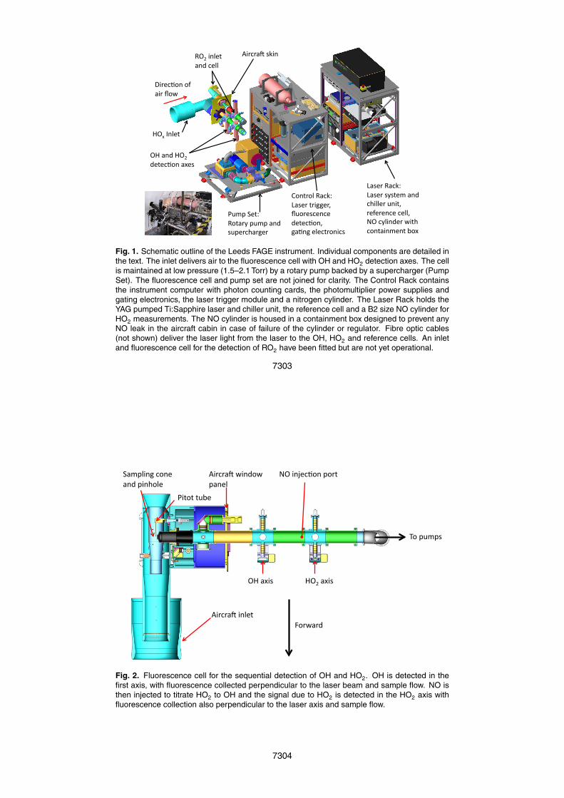
.+/$#)0+%12)))))))))

.+/$#)/3/4$5)+(6)%7"88$#)9("4:)#$*$#$(%$)%$88:));<)%38"(6$#)-"47)%'(4+"(5$(4)='>)

?'(4#'8)0+%12).+/$#)4#"@@$#:),9'#$/%$(%$))6$4$%&'(:))@+&(@)$8$%4#'("%/)

A95B)C$42)0'4+#3)B95B)+(6)/9B$#%7+#@$#)

D<>)E(8$4)

<D)+(6)D<F)6$4$%&'()+>$/)

G"#%#+H)/1"()0<F)"(8$4)+(6)%$88)

Fig. 1. Schematic outline of the Leeds FAGE instrument. Individual components are detailed inthe text. The inlet delivers air to the fluorescence cell with OH and HO2 detection axes. The cellis maintained at low pressure (1.5–2.1 Torr) by a rotary pump backed by a supercharger (PumpSet). The fluorescence cell and pump set are not joined for clarity. The Control Rack containsthe instrument computer with photon counting cards, the photomultiplier power supplies andgating electronics, the laser trigger module and a nitrogen cylinder. The Laser Rack holds theYAG pumped Ti:Sapphire laser and chiller unit, the reference cell and a B2 size NO cylinder forHO2 measurements. The NO cylinder is housed in a containment box designed to prevent anyNO leak in the aircraft cabin in case of failure of the cylinder or regulator. Fibre optic cables(not shown) deliver the laser light from the laser to the OH, HO2 and reference cells. An inletand fluorescence cell for the detection of RO2 have been fitted but are not yet operational.

7303

!"#$%&$'#

()#*+,'# )(-#*+,'#

."/0*/1#2,/3/*4#,5678#

9,8"8#8%:7#

;*&$6,5<#3"57#*51#$,5="67#

2,/3/*4#0,51"0#$*576#

>(#,5?73@"5#$"/8#

Fig. 2. Fluorescence cell for the sequential detection of OH and HO2. OH is detected in thefirst axis, with fluorescence collected perpendicular to the laser beam and sample flow. NO isthen injected to titrate HO2 to OH and the signal due to HO2 is detected in the HO2 axis withfluorescence collection also perpendicular to the laser axis and sample flow.

7304

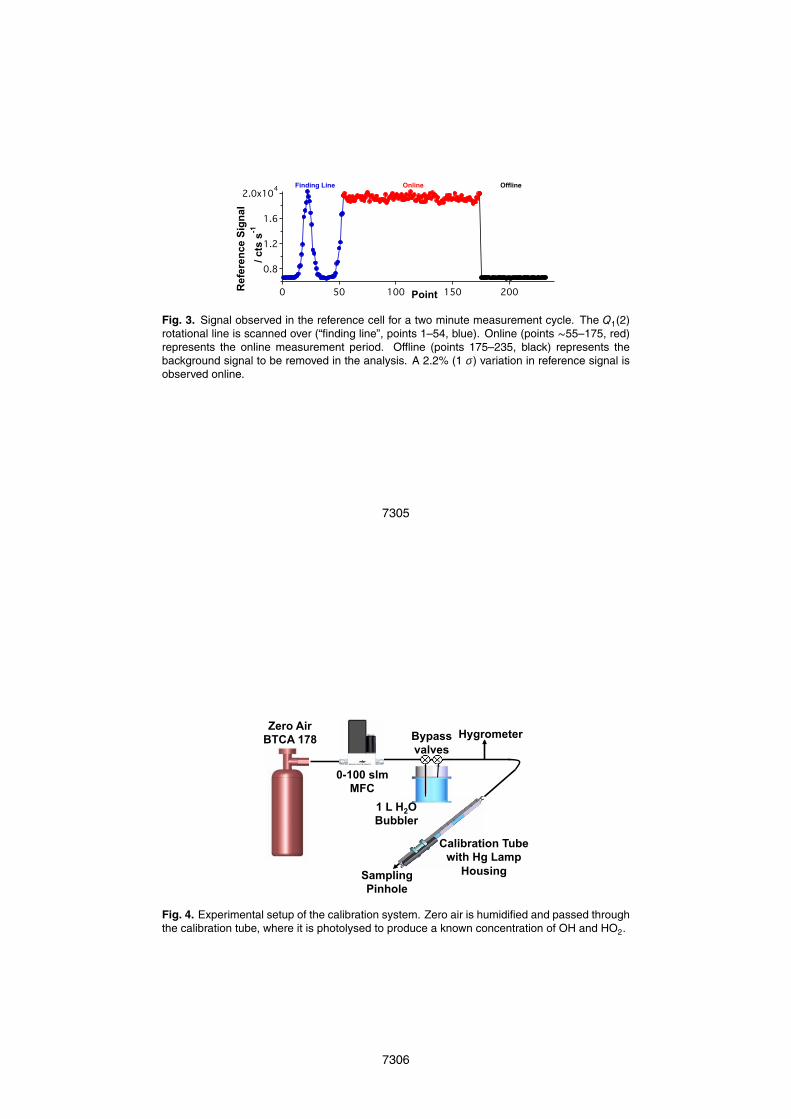
2.0x104

1.6

1.2

0.8

Re

fere

nc

e S

ign

al

200150100500 Point

Finding Line Online Offline

/ c

ts s

-1

Fig. 3. Signal observed in the reference cell for a two minute measurement cycle. The Q1(2)rotational line is scanned over (“finding line”, points 1–54, blue). Online (points ∼55–175, red)represents the online measurement period. Offline (points 175–235, black) represents thebackground signal to be removed in the analysis. A 2.2% (1 σ) variation in reference signal isobserved online.

7305

Zero Air BTCA 178

0-100 slm MFC

Hygrometer

Sampling Pinhole

1 L H2O Bubbler

Calibration Tube with Hg Lamp

Housing

Bypass valves

Fig. 4. Experimental setup of the calibration system. Zero air is humidified and passed throughthe calibration tube, where it is photolysed to produce a known concentration of OH and HO2.

7306

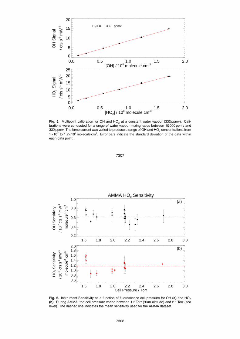
0.0 0.5 1.0 1.5 2.0[OH] / 108 molecule cm-3

0

5

10

15

20

OH

Sig

nal

/ c

ts s

-1 m

W-1 H2O = 332 ppmv

0.0 0.5 1.0 1.5 2.0[HO2] / 108 molecule cm-3

05

10

15

2025

HO

2 S

igna

l

/ cts

s-1 m

W-1

Fig. 5. Multipoint calibration for OH and HO2 at a constant water vapour (332 ppmv). Cali-brations were conducted for a range of water vapour mixing ratios between 10 000 ppmv and332 ppmv. The lamp current was varied to produce a range of OH and HO2 concentrations from1×107 to 1.7×108 molecule cm3. Error bars indicate the standard deviation of the data withineach data point.

7307

AMMA HOx Sensitivity

1.6 1.8 2.0 2.2 2.4 2.6 2.8 3.00.2

0.4

0.6

0.8

1.0

OH

Sen

sitiv

ity

/ 1

0-7 c

ts s

-1 m

W-1

m

olec

ule-1

cm

3

1.6 1.8 2.0 2.2 2.4 2.6 2.8 3.0Cell Pressure / Torr

0.60.81.01.21.41.61.82.0

HO

2 S

ensi

tivity

/ 10-7

cts

s-1 m

W-1

m

olec

ule-1

cm

3

(a)

(b)

Fig. 6. Instrument Sensitivity as a function of fluorescence cell pressure for OH (a) and HO2(b). During AMMA, the cell pressure varied between 1.5 Torr (9 km altitude) and 2.1 Torr (sealevel). The dashed line indicates the mean sensitivity used for the AMMA dataset.

7308

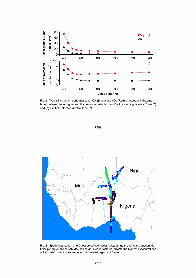
80

60

40

20

0 Bac

kgro

un

d S

ign

al

140120100806040

Delay Time / ns

5x106

4

3

2

1

0Lim

it o

f D

etec

tio

n

140120100806040

(a)

(b)

HO2

OH

/ m

ole

cu

le c

m-3

/ c

ts s

-1 m

W-1

Fig. 7. Typical instrument performance for OH (Black) and HO2 (Red) changes with the time in-terval between laser trigger and fluorescence collection. (a) Background signal (cts s−1 mW−1)and (b) Limit of Detection (molecule cm−3).

7309

Niger

Nigeria

Mali

Fig. 8. Spatial distribution of HO2 observed over West Africa during the African Monsoon Mul-tidisciplinary Analyses (AMMA) campaign. Redder colours indicate the highest concentrationsof HO2, which were observed over the forested regions of Benin.

7310

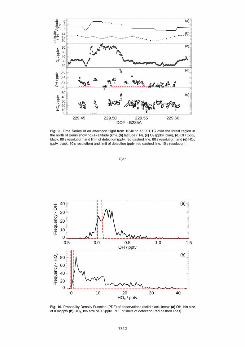
229.45 229.50 229.55 229.60

246

Alti

tude

/ km

229.45 229.50 229.55 229.60

101214

Latit

ude

/ o N

229.45 229.50 229.55 229.60

2030405060

O3

/ ppb

v

229.45 229.50 229.55 229.60

0.00.20.40.6

OH

/ pp

tv

229.45 229.50 229.55 229.60DOY - B235A

01020304050

HO

2 / p

ptv

(a)

(b)

(c)

(d)

(e)

Fig. 9. Time Series of an afternoon flight from 10:40 to 15:00 UTC over the forest region inthe north of Benin showing (a) altitude (km), (b) latitude (◦N), (c) O3 (ppbv, blue), (d) OH (pptv,black, 60 s resolution) and limit of detection (pptv, red dashed line, 60 s resolution) and (e) HO2(pptv, black, 10 s resolution) and limit of detection (pptv, red dashed line, 10 s resolution).

7311

-0.5 0.0 0.5 1.0 1.5OH / pptv

0

10

20

30

40

Fre

quen

cy -

OH

0 10 20 30 40HO2 / pptv

0

20

40

60

80

Fre

quen

cy -

HO

2

(a)

(b)

Fig. 10. Probability Density Function (PDF) of observations (solid black lines): (a) OH, bin sizeof 0.02 pptv (b) HO2, bin size of 0.5 pptv. PDF of limits of detection (red dashed lines).

7312

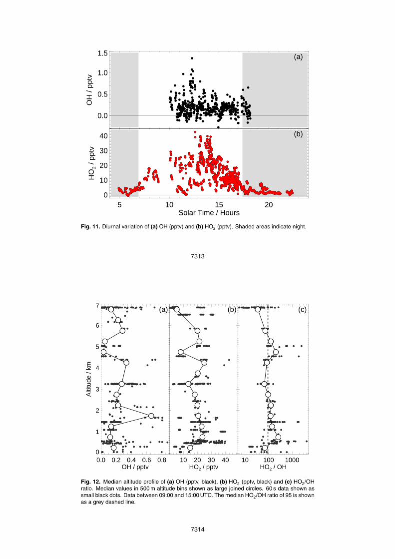
5 10 15 20

0.0

0.5

1.0

1.5

OH

/ pp

tv

5 10 15 20Solar Time / Hours

0

10

20

30

40

HO

2 / p

ptv

(a)

(b)

Fig. 11. Diurnal variation of (a) OH (pptv) and (b) HO2 (pptv). Shaded areas indicate night.

7313

0.0 0.2 0.4 0.6 0.8OH / pptv

0

1

2

3

4

5

6

7

Alti

tude

/ km

10 20 30 40HO2 / pptv

0

1

2

3

4

5

6

7

10 100 1000HO2 / OH

0

1

2

3

4

5

6

7

(a) (b) (c)

Fig. 12. Median altitude profile of (a) OH (pptv, black), (b) HO2 (pptv, black) and (c) HO2/OHratio. Median values in 500 m altitude bins shown as large joined circles. 60 s data shown assmall black dots. Data between 09:00 and 15:00 UTC. The median HO2/OH ratio of 95 is shownas a grey dashed line.

7314

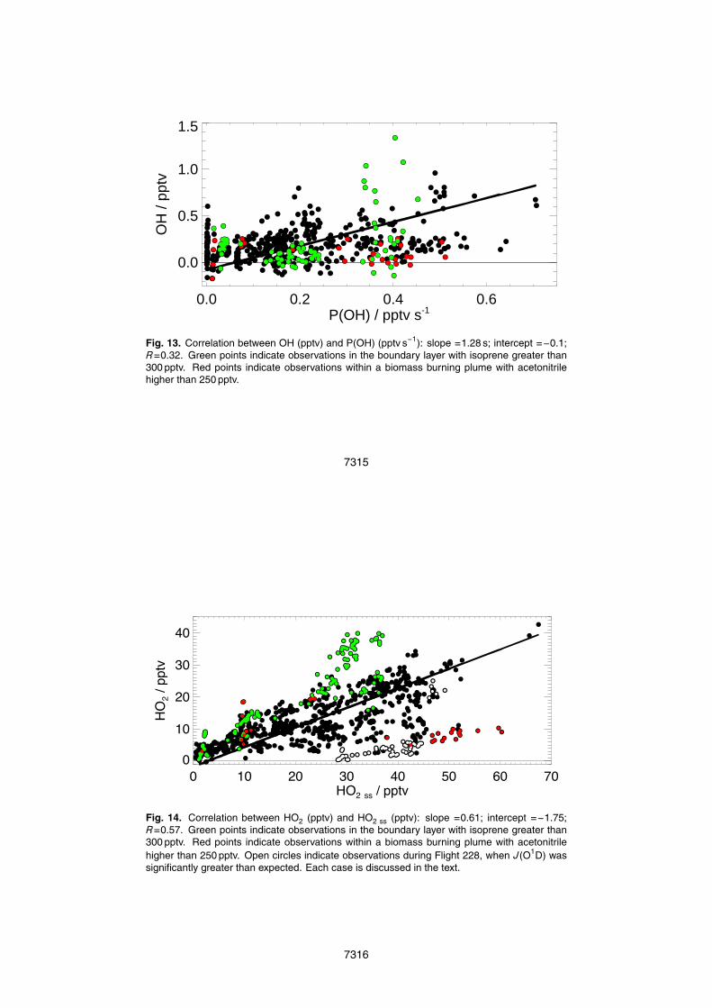
0.0 0.2 0.4 0.6P(OH) / pptv s-1

0.0

0.5

1.0

1.5

OH

/ pp

tv

Fig. 13. Correlation between OH (pptv) and P(OH) (pptv s−1): slope =1.28 s; intercept =−0.1;R=0.32. Green points indicate observations in the boundary layer with isoprene greater than300 pptv. Red points indicate observations within a biomass burning plume with acetonitrilehigher than 250 pptv.

7315

0 10 20 30 40 50 60 70HO2 ss / pptv

0

10

20

30

40

HO2 /

ppt

v

Fig. 14. Correlation between HO2 (pptv) and HO2 ss (pptv): slope =0.61; intercept =−1.75;R=0.57. Green points indicate observations in the boundary layer with isoprene greater than300 pptv. Red points indicate observations within a biomass burning plume with acetonitrilehigher than 250 pptv. Open circles indicate observations during Flight 228, when J(O1D) wassignificantly greater than expected. Each case is discussed in the text.

7316

4 6 8 10 12 14 16 18

0.0

0.5

1.0

1.5

OH

/ pp

tv

4 6 8 10 12 14 16 18Latitude / oN

0

10

20

30

40

HO

2 / p

ptv

(a)

(b)

Fig. 15. Latitudinal variation of (a) OH and (b) HO2 mixing ratio. Observations in the boundarylayer are shown for data collected above the Sahel (13.75–18◦ N, white), Forest (7.3–13.2◦N,green), Ocean (4–6◦N, blue) and Urban areas (6–7.3◦N and 13.2–13.75◦ N, red). Observationsin the free troposphere in all regions are shown in black.

7317

11.8 12.0 12.2 12.4 12.6 12.8 13.0050

100

150

200

250

300

CO

/ pp

bvO

3 / p

pbv

COO3

11.8 12.0 12.2 12.4 12.6 12.8 13.00102030405060

HO

2 / p

ptv

HO

2ss

/ ppt

v

HO2ss

HO2

11.8 12.0 12.2 12.4 12.6 12.8 13.0Time / Hours

0.00.1

0.2

0.3

0.4

0.50.6

OH

/ pp

tvP

(OH

) / p

ptv

s-1

Alti

tude

/ km

/10 P(OH)

OH

(a)

(b)

(c)

BB

Fig. 16. Time series within and around a Biomass Burning Plume with (a) CO (ppbv, black),and O3 (ppbv, red), (b) HO2 (pptv, black) and HO2 ss (pptv, red), (c) OH (pptv, black) and P(OH)(pptv s−1, red). On all graphs altitude is indicated by a dashed line. 60 s observations.

7318

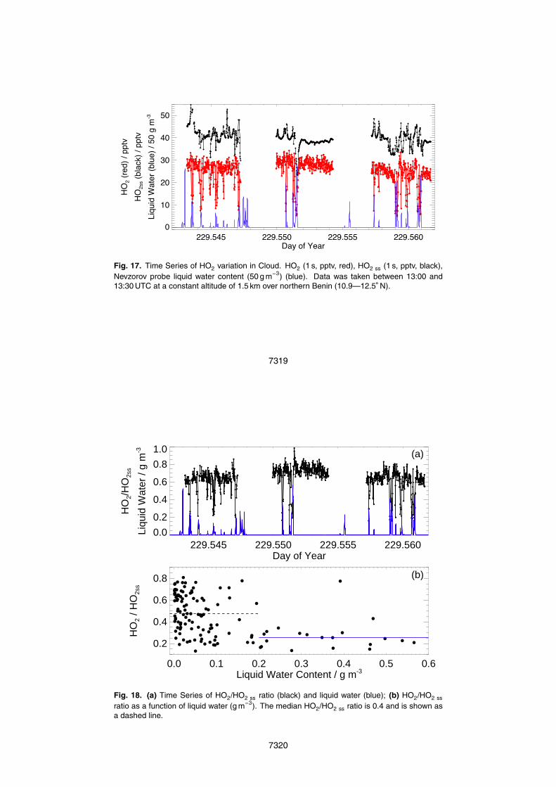
229.545 229.550 229.555 229.560Day of Year

0

10

20

30

40

50HO

2 (re

d) /

pptv

HO2s

s (bl

ack)

/ pp

tvLi

quid

Wat

er (b

lue)

/ 50

g m

-3

Fig. 17. Time Series of HO2 variation in Cloud. HO2 (1 s, pptv, red), HO2 ss (1 s, pptv, black),Nevzorov probe liquid water content (50 g m−3) (blue). Data was taken between 13:00 and13:30 UTC at a constant altitude of 1.5 km over northern Benin (10.9—12.5◦ N).

7319

229.545 229.550 229.555 229.560Day of Year

0.0

0.2

0.4

0.6

0.8

1.0

HO

2/H

O2s

s

Liqu

id W

ater

/ g

m-3

0.0 0.1 0.2 0.3 0.4 0.5 0.6Liquid Water Content / g m-3

0.2

0.4

0.6

0.8

HO

2 / H

O2s

s

(a)

(b)

Fig. 18. (a) Time Series of HO2/HO2 ss ratio (black) and liquid water (blue); (b) HO2/HO2 ss

ratio as a function of liquid water (g m−3). The median HO2/HO2 ss ratio is 0.4 and is shown asa dashed line.

7320

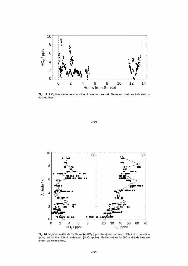
0 2 4 6 8 10 12 14Hours from Sunset

0

2

4

6

8

10

HO

2 / p

ptv

Fig. 19. HO2 time series as a function of time from sunset. Dawn and dusk are indicated bydashed lines.

7321

0 2 4 6 8HO2 / pptv

0

2

4

6

8

10

Alti

tude

/ km

20 30 40 50 60 70O3 / ppbv

0

2

4

6

8

10

(a) (b)

Fig. 20. Night-time Altitude Profiles of (a) HO2 (pptv, black) and maximum HO2 limit of detection(pptv, red) for the night-time dataset. (b) O3 (ppbv). Median values for 500 m altitude bins areshown as white circles.

7322