Object reconstruction by incorporating geometricconstraints in reverse engineeringNaoufel Werghi, Robert Fisher, Craig Robertson and Anthony AshbrookUniversity of EdinburghDivision of Informatics5 Forrest Hill, Edinburgh EH1 2QL, UKTel: 44 131 650 4504FAX: 44 131 650 6899Email: fnaoufelw, rbf, craigr, anthonyag@dai.ed.ac.uk

AbstractThis paper deals with the constrained reconstruction of 3D geometric models ofobjects from range data. It describes a new technique of global shape improvementbased upon feature positions and geometric constraints. It suggests a general incre-mental framework whereby constraints can be added and integrated in the modelreconstruction process, resulting in an optimal trade-o� between minimization of theshape �tting error and the constraint tolerances. After de�ning sets of constraintsfor planar and special case quadric surface classes based on feature coincidence,position and shape, the paper shows through application on synthetic model thatour scheme is well behaved. The approach is then validated through experimentson di�erent real parts. This work is the �rst to give such a large framework for theintegration of geometric relationships in object modelling. The technique is expec-ted to have a great impact in reverse engineering applications and manufacturedobject modelling where the majority of parts are designed with intended featurerelationships. KeywordsReverse engineering, Geometric constraints, constrained shape reconstruction,shape optimization.

2

INTRODUCTION AND RELATED WORKThe use of constraints in object modelling is an important topic in the CADliterature. In this area, engineering concepts and shape constraints are trans-formed into shape models through mechanisms of checking, incorporating andsolving constraints in the modelling process. Constraints in this area includespeci�cation of the geometric relationships between object features as well asengineering constraints (dimensions, material strength and machining para-meters) [2, 17].Finding geometric con�gurations that satisfy the constraints is the crucialissue and much research has been dedicated to di�erent mechanisms for con-straint solving. There are two main strategies for solving constraint problemsaccording to the classi�cation mentioned in [33]. The �rst strategy, referredas the instance solver, uses speci�c values of the constraints and looks forgeometric con�gurations satisfying these constraints. In the second strategy,the generic solver investigates �rst whether the geometric elements could beplaced given the constraints independently of their values. After checking thatthe problem is well-constrained, the speci�c placements of the geometric ele-ments are then determined. In CAD literature, these two strategies have beenimplemented through di�erent approaches.The numerical approaches given in [9, 32, 42, 58] are typical instance solv-ers. Constraints are translated into a set of algebraic equations and are usu-ally solved simultaneously by means of iterative techniques, for instance theNewton-Raphson algorithm. This approach can deal with general cases, over-constrained systems and inconsistent constraint problems. A good initial valueis required for such solvers and the algorithm should be applied with care sinceit may face an ill-conditioned problem.Symbolic methods [1, 13, 39, 60] are hybrid methods in the sense that theycan involve both the generic solver strategy and instance solver strategy. Thesemethods also transform the geometric constraints into algebraic equations butinstead of numerical techniques, general symbolic methods are �rst used toput the set of equations into a new form which is easy to solve. The setof equations is sequentially reduced by solving the simplest one at each stepas far as possible. The �nal set can be then solved numerically. Comparedto numerical approaches, they are not subject to numerical instabilities andcan locate all solutions to the constraint equations. However, they tend tobe computationally expensive. This often restricts the types of geometricelements and types of constraints allowed to be involved.A more recent approach solves the constraints through sequential geometricconstructions, as most con�gurations in engineering drawing are solvable byruler, compass and protractor. These approaches can be roughly divided intotwo categories: the rule-based [3, 57, 66] and graph-based [10, 16, 24, 25, 33,34, 35] approaches. In the �rst category constraints are expressed by rulesor predicates. The procedure starts from an initial set of predicates de�ningthe constraints and sequentially derives a new set of predicates by applying3

logical reasoning techniques, with the predicates converging towards de�nedpositions for all the characteristic features. However since only constructivegeometries can be handled by these methods they may not be very e�cientfor large systems of constraints.The graph-based approaches handle the problem in a more methodical way.They start by forming a graph representation of the problem. In this grapheach node represents a geometric element and the edges linking these nodesindicate the constraints between the associated geometric elements. Each edgeis labelled with the constraint's type. In a �rst phase the graph is analysed andif it is well-constrained a set of sequential construction steps are derived fromit. This phase depends only on the type and the number of constraints, so itis considered a generic constraint solver. In the second phase the constructionsteps are carried out integrating the actual values of the constraints to derivethe solution shape.In the Computer Vision community, constraints are mainly used in model-based recognition and localization of objects or environments more generally.They are used as a priori information to reduce the search space between,for example, the model features (already stored and known CAD models)and the extracted features from visual sensor output (grey level image, 3Drange data, etc.) [5, 7, 8, 23, 27, 43]. Some of the approaches for objectrecognition in particular [30, 53] use a notion of graph representation closeto the one used in the graph-based approaches for constraint solving, wherethe nodes represent object primitives (e.g. points, lines, etc.) and the arcspresent geometric relationships between them (e.g. adjacency, parallelism,perpendicularity, etc.).Constraints can be de�ned over the geometric and topological relationshipsbetween the the object model features (the a priori information) and theextracted features from the input data. These relationships are derived eitherfrom the properties of the geometric transformation between the vision sensorframe and the scene frame or the transformation between two vision sensorframes (stereo-vision) or the intrinsic structure of the objects [31].So we can conclude that when computer vision applications deal withmodel-based recognition and localization, the de�nition and the concept ofconstraints are wider than those considered in CAD applications, althoughthey may share the same terminology.There is one area where Computer Aided Design and Computer Visionshare a similar interpretation of geometric constraints, namely reverse en-gineering referred to as 3D geometric model reconstruction within the visioncommunity. Reverse engineering is typically concerned with parts and in-dustrial objects, whereas 3D geometric model reconstruction is a larger �eldwhich includes built environments. But the two terms point to the same goal,which is the transformation of a real object (in the large sense of the word) toa model and concept. In parts manufacturing reverse engineering deals withmeasuring an existing object so that a surface or solid model can be deduced inorder to take advantage of CAD/CAM technologies. It is also often necessary4

to produce a copy of a part when no original drawings or documentation areavailable. In other cases we may want to re-engineer an existing part, whenanalysis and modi�cations are required to construct a new improved product.Even though it is possible to turn to a computer-aided design to fashion anew part, it is only after the real object is made and evaluated that we cansee if the object �ts with real world. For this reason designers rely on real 3Dobjects (real scale wood or clay models) as starting points. This procedure isparticularly important to areas involving aesthetic design e.g automobile in-dustry or generation of custom �ts to human surfaces such as helmets, spacesuits or prostheses.A review of the main research in the CAD community [20, 51, 54, 67] andthe Vision community [11, 22, 40] (for reconstruction from single range images)and [14, 55, 56, 62] (for reconstruction from multiple range images) revealedthat the exploitation of geometric constraints has not been fully investigated.This lack was noted in the survey work of Varady et al[61].The �rst motivation behind considering geometric constraints in this workis that models needed by industry are generally designed with intended featurerelationships so this aspect should be exploited rather than ignored. The con-sideration of these relationships is actually necessary because some attributesof the object would have no sense if the object modelling scheme did not takeinto account these constraints. For example, take the case when we want toestimate the distance between two parallel planes: if the plane �tting resultsgave two planes which are not parallel, then the distance measured betweenthem would have no signi�cance. Furthermore exploiting the available knownrelationships would be useful for reducing the e�ects of registration errors andmis-calibration, thus improving the accuracy of the estimated part features'parameters and consequently the quality of the modelling.The second motivation is that generally in the manufacturing process, oncethe part is produced many improvement are carried manually to optimize thepart and make it �t with the real world (e.g. �t with another part, adjust thepart to �t particular customer). These improvements could be representedby new constraints on the shape of the part. By integrating these constraintsinto the CAD process the work piece optimization would be reduced and hencemany cycles in the part production process would be saved. In other cases,such improvement could not be achieved by hand due to the complexity of theobject or when we want to extend the application of the process to complexenvironments such as buildings or industrial plants.From a CAD viewpoint the way with which the constraint problem ishandled is close to the numerical constraint solver. However it di�ers rad-ically from this scope on two levels. First on the level of the componentsof the problem. In our case we have already a real object whose shape weare trying to reconstruct, hence the object real data is used to constraint theshape. Thus, the solution has to satisfy proximity to measured points as wellas the constraints. Second the numerical technique used to �nd the solutionovercomes ill-conditioning problems. 5

The approach for incorporating geometric relationships in object modellinghas to tackle two problems. The �rst is how to represent the constraints. Thesecond is how to integrate these constraints into the shape �tting process.These two aspects are not entirely independent, the shape �tting techniqueimposes restrictions on the constraint representation and vice versa.A �rst step in the direction of incorporating constraints for assuring theconsistency of the reconstruction was done by Porrill [46]. He linearized a setof nonlinear constraints and combined them with a Kalman �lter, as appliedto wire frame model construction. Porrill's method takes advantage of therecursive linear estimation of the Kalman �lter, but guarantees satisfaction ofthe constraints only to linearized �rst order. Additional iterations are neededat each step if more accuracy is required. This last condition has been takeninto account in the work of De Geeter et al [15] by de�ning a \Smoothly Con-strained Kalman Filter". The key idea of their approach is to replace a non-linear constraint by a set of linear constraints applied iteratively and updatedby new measurements in order to reduce the linearization error. However, thecharacteristics of Kalman �ltering make these methods essentially adapted foriteratively acquired data and many data samples. Moreover, there was nomechanism for determining how successfully the constraints were satis�ed andonly lines and planes were considered in both of the above works.The constraints considered by Bolle et al [6] in their approach to 3D ob-ject position covered only the shape of the surfaces. They chose a speci�crepresentation for the treated features: plane, cylinder and sphere.Compared to Porrill's and De Geeter's work, our approach avoids thedrawbacks of linearization, since the constraints are completely implemented.Moreover, our approach covers a larger category of feature shapes. Regard-ing the work of Bolle [6], the type of constraints which can be held by ourapproach go beyond the restricted set of surface shapes and cover also thegeometric relationships between object features. The proposed approach hasbeen successfully applied �rst on polyhedral objects [65]. To our knowledgethe work appears the �rst to give such a large framework for the integra-tion of geometric relationships for object reconstruction in the �eld of reverseengineering.Although this work is mainly intended for object modelling, it can also�nd many other many useful applications, e.g. in object localisation. In re-gistration tasks, the features represented in di�erent views need to be putinto a single reference frame. For this purpose the transformation betweendi�erent views is recovered by matching between the related frames. Since areference frame is built from object features, e.g. normals of surfaces whichare supposed to be orthogonal, the estimation of the surfaces has to satisfythe orthogonality constraints. The proposed paradigm may be extended aswell to any constrained built environment application like creating \as built"CAD models of a plant for planning new building work. A current methoduses a motorised camera head to create highly detailed panoramic imageswhich are then used to extract CAD models. Since the di�erent captured6

parts of a plant (pipes, reservoirs, etc.) have many geometric relationshipsbetween them, using these constraints in the reconstruction process will helpto have a consistent whole model. The same is true as well for modelling dif-ferent compartments of buildings or cities. The current methods of extracting,matching and estimation of large scale buildings' features from aerial imageshave reached reasonable level. This make the application of our method formodelling di�erent compartments of buildings or cities possible as well.The organisation of the rest of paper will be as follows: the next sectiongives some preliminaries on planes and quadric surfaces and gives the paramet-rization of such surfaces. The aim is to make clear the relationship betweenthe constraint formulation and the surface representations. We then statethe problem and develop the proposed approach. Next we de�ne and clas-sify the di�erent types of constraints. Lastly, we demonstrate the process onseveral synthetic and real objects to evaluate the accuracy, the convergence,repeatability and consistency of the approach.PRELIMINARIESThis section gives a brief overview about constraining planes, general quadricsand some particular quadric shapes. A full treatment of these surfaces canbe found in [4]. While the material contained here is is largely elementarygeometry, we present it in order to make clear how the set of constraints usedfor each surface type and relationship relate to the parameters of the genericquadric.The lineA line is de�ned by the following equations :x� x0l = y � y0m = z � z0n (1)where ~X0 = [x0; y0; z0]T is an arbitrary point of the line and the vector ~p =[l; m; n]T de�nes the orientation of the line.The planeA plane surface can be represented by this equation:f(x; y; z) = nxx + nyy + nzz + d = 0 (2)where ~n = [nx; ny; nz]T is the unit normal vector to the plane and d is thedistance to the origin. A plane can have two di�erent representations (~n; d) and(�~n;�d). This ambiguity is easily removed by orienting the normal towardthe outside of the object. 7

Given N data points the best parameters which satisfy (2) in the leastsquares sense are those minimizing the criterion:NXi=1 f(xi; yi; zi)2 = ~pTH~p (3)where ~p = [nx; ny; nz; d]T is the parameter vector and H is the data matrixde�ned by H = NXi=1 ~hi ~hiT ; ~hi = [xi; yi; zi; 1]T (4)H is symmetric and positive de�nite.The quadricsA general quadric surface is represented by the following quadratic equation:f(x; y; z) = ax2+by2+cz2+2hxy+2gxz+2fyz+2ux+2vy+2wz+d = 0 (5)which can be written : XTAX + 2XTB + C = 0 (6)where A = 264 a h gh b fg f c 375 ; B = [u; v; w]T ; C = d; X = [x; y; z]T (7)The type of the quadric depends on the discriminant of the quadric �, thecubic discriminant D :� = ��������� a h g uh b f vg f c wu v w d ��������� D = ������� a h gh b fg f c ������� (8)and the cofactors of D:A = bc� f 2;B = ac� g2;C = ab� h2; F = gh� af;G = hf � bg; (9)H = gf � ch;Similarly to the plane case, the best parameters which satisfy (5) for Ndata points in the least squares sense are those minimizing the criterion:NXi=1 f(xi; yi; zi)2 = ~pT ( NXi=1 ~hi ~hiT )~p = ~pTH~p (10)where ~p = [a; b; c; h; g; f; u; v; w; d]Tand hiT = [xi2; yi2; zi2; 2xiyi; 2xizi; 2yizi; 2xi; 2yi; 2zi; 1]8

The cylinderThe quadric is a cylinder when � = D = 0, uA + vH + wG = 0 andA+ B + C > 0. The equation of the cylinder axis isx� ufF1=F = y � vgG1=G = z � whH1=H (11)This means that the cylinder axis has the direction vector [1=F ; 1=G; 1=H]Tand passes through the point ~Xo= [ufF ; vgG ; whH ]T . The axis orientation corres-ponds to the eigenvector related to the null eigenvalue of the matrix A. Thetwo other eigenvalues are positive.The circular cylinderFor a circular cylinder, we can show that the parameters of the quadric shouldalso satisfy the following conditions:agh+ f(g2 + h2) = 0bhf + g(h2 + f 2) = 0 cfg + h(f 2 + g2) = 0 (12)uf + vg + wh = 0The matrix A (see (7)) has two identical eigenvalues � and the radius canbe expressed by r2 = (u2f=F + v2g=G + w2h=H + d)=� (13)A circular cylinder may be also represented by the canonical form:(x�x0)2+(y�y0)2+(z�z0)2�(nx(x�x0)+ny(y�y0)+nz(z�zo))2�r2 = 0(14)where ~Xo = [x0; y0; z0]T is an arbitrary point on the axis, ~n = [nx; nz; ny]T isa unit vector along the axis and r is the radius of the cylinder.This form has the advantage of having a minimal number of parameters.However its implementation in the optimization algorithm may cause somecomplexity, indeed it is not possible with this form to get separate terms forthe data and the parameters as in (10) (which allows the data terms to becomputed o� line). Consequently this may increase the computational costdramatically.The expansion of (14) and the identi�cation with (5) yieldsa = 1� n2xb = 1� n2yc = 1� n2z h = �nxny (15)g = �nxnzf = �nynz9

The coneA cone surface satis�es � 6= 0;D = 0. The apex of the cone is given by:~Xo = A�1B (16)The axis of the cone corresponds to the eigenvector related to the negativeeigenvalue of the matrix A. The two other eigenvalues are positive.Circular coneFor a circular cone the parameters of the quadric equation have to satisfy thefollowing conditions af � ghf = bg � hfg = ch� fgh (17)As for the cylinder case, a circular cone equation has a more compact form:[(x�xo)2+(y�yo)2+(z�zo)2]cos2(�)�[nx(x�xo)+ny(y�yo)+nz(z�zo)]2 = 0(18)where [xo; yo; zo]T is the apex of the cone, [nx; ny; nz]T is the unit vector de-�ning the orientation of the cone axis and � is the semi-vertical angle. Thequadric equation parameters can thus be expressed explicitly as a function ofthe above terms by :a = n2x � cos2�b = n2y � cos2�c = n2z � cos2� h = nxny (19)g = nxnzf = nynzFor the same reasons as mentioned in the cylinder case, the compact form ofthe cone equation is not adequate for the optimization algorithm. Neverthelessit is useful to implicitly impose the conic circularity constraints.The sphereA sphere is characterized by equal coe�cients for x2, y2 and z2 terms and van-ishing coe�cients for the cross product terms xy, xz and yz, so the parametersh, g and f are all equal to zero. The equation of a sphere can be written as:a(x2 + y2 + z2) + 2ux+ 2vy + 2wz + d = 0 (20)The centre of the sphere is:~Xo = [�u=a;�v=a;�w=a]T (21)and the radius is: r2 = u2 + v2 + w2 � ada2 (22)10

THE GEOMETRIC CONSTRAINTSThe set of constraints associated with a given object can be divided mainly intotwo categories. The �rst one is the surface intrinsic constraints covering thegeometric properties which re ect the speci�c shapes of the surfaces. Examplesof these constraints will be given in the next subsection. The second categorynamed the feature extrinsic constraints, de�nes the geometric and topologicalrelationships between the di�erent object features.Speci�c shape constraintsIn the text below, when we say that an equation (or set of equations) canbe used as a constraint, we mean that the property f(~p) = 0 can be used tode�ne a constraint C(~p) on the object parameters ~p by lettingC(~p) = f(~p)Circularity of a cylinderThe circularity of a cylinder can be imposed using either equations (12) orequations (15). The last equations have the advantage of imposing implicitlythe circularity constraints of the cylinder and avoid the problem when one ofthe parameters (f; g; h) vanishes. Besides, they make concrete the geometricrelationships between the cylinder and other object features as we will see inSection 6 (the half cylinder).Circularity of a coneThis property can be expressed using either equations (17) or (19). Similarlyto the cylinder case the last equations are more convenient.Sphere ConstraintTo require that an ellipsoidal patch represents a perfect sphere, equation (20)can be used.Feature extrinsic constraintsThese constraints re ect the geometric or topological relationships betweenthe di�erent features of one object. Table 1 summarizes the relationships thatwe have considered. We notice here that points and lines in this table maybe either physical features of the object like cone apexes and edges or implicitfeatures like centres, axes of symmetry. This list is not exhaustive and theclassi�cation may not be unique. Nevertheless it covers a large number ofconstraints in manufactured objects. 11

Coincidence constraintsIt is common that a part contains features which are associated with thesame geometric entity (Figure.3.a) or which coincide at the same position(Figure.3.b). In the �rst case these constraints are implicitly imposed byconsidering the same parameters for each feature. In the second case theparameters associated to each feature are equated and the resulting equationshave then to be satis�ed.Inclusion constraintsA particular feature point may be included in an object feature e.g line, planeor quadric patch. The inclusion constraint requires that the point satis�es thefeature's equation.A feature line may be included in a plane or a particular quadric surface.Fig.4 shows an example of this in cylinders. By considering Equations (1) and(2), the condition that a line should lie in a plane is:( nxl + nym+ nzn = 0nxx0 + nyy0 + nzz0 + d = 0 (23)A necessary and su�cient condition that a line be included in a cylindersurface is that the line and the cylinder have the same orientation and anarbitrary point of the line (X0; Y0; Z0)T satis�es the cylinder equation. Thus,from equations (1), (5) and (11) these conditions can be expressed by( [l; m; n]T = [1=F ; 1=G; 1=H]Tf(X0; Y0; Z0)T = 0 (24)A line is included in a cone if and only if the orientation vector of theline satis�es the homogeneous equation of the cone (Equation (5) without theu; v; w and d terms) and it passes through the cone summit. This is formulatedthen by ( fhomogeneous(~p) = 0(X0; Y0; Z0) = cone summit; (25)Relative orientation constraintThere are many orientation relationships which can be deduced and exploitedin a given part. In particular, the two common particular cases of parallelismand orthogonality (Fig.5.a). The presence of these two characteristics is easilydetected in an object. More generally, given a pair of features (Fi; Fj) whoseorientations are de�ned respectively by two vectors (~ni; ~nj) which make anangle �, the relative orientation constraint is expressed by~nTi ~nj = cos(�) (26)12

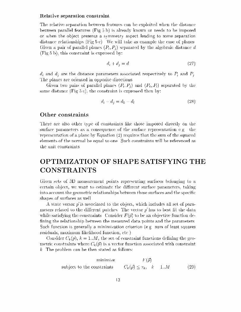
Relative separation constraintThe relative separation between features can be exploited when the distancebetween parallel features (Fig.5.b) is already known or needs to be imposedor when the object presents a symmetry aspect leading to some separationdistance relationships (Fig.5.c). We will take as example the case of planes.Given a pair of parallel planes (Pi; Pj) separated by the algebraic distance d(Fig.5.b), this constraint is expressed by:di + dj = d (27)di and dj are the distance parameters associated respectively to Pi and Pj.The planes are oriented in opposite directions.Given two pairs of parallel planes (Pi; Pj) and (Pk; Pl) separated by thesame distance (Fig.5.c), the constraint is expressed then by:di + dj = dk + dl (28)Other constraintsThere are also other type of constraints like those imposed directly on thesurface parameters as a consequence of the surface representation e.g. therepresentation of a plane by Equation (2) requires that the sum of the squaredelements of the normal be equal to one. Such constraints will be referenced asthe unit constraints.OPTIMIZATION OF SHAPE SATISFYING THECONSTRAINTSGiven sets of 3D measurement points representing surfaces belonging to acertain object, we want to estimate the di�erent surface parameters, takinginto account the geometric relationships between these surfaces and the speci�cshapes of surfaces as well.A state vector ~p is associated to the object, which includes all set of para-meters related to the di�erent patches. The vector ~p has to best �t the datawhile satisfying the constraints. Consider F (~p) to be an objective function de-�ning the relationship between the measured data points and the parameters.Such function is generally a minimization criterion (e.g. sum of least squaresresiduals, maximum likelihood function, etc.).Consider Ck(~p), k = 1::M , the set of constraint functions de�ning the geo-metric constraints where Ck(~p) is a vector function associated with constraintk. The problem can be then stated as follows:minimize F (~p)subject to the constraints Ck(~p) � �k; k = 1::M (29)13

Here �k represents the tolerance related to the constraint Ck. Ideally thetolerances have zero values, but practically, for geometric constraints they areassigned certain values which re ects the geometric inaccuracies in the relativelocations and shapes of features. It is up to the designer to set the tolerances,however an appropriate de�nition of the tolerances for a given object can beset up by using the scheme developed by Requicha [48].When faced with an optimization problem it is necessary to know the char-acteristics of the components of the problem since techniques that solve theproblem more e�ciently depend mainly on these characteristics. The compon-ents of the problem are the objective function and the constraint functions.The characteristics to be investigated are the properties of these functionswhich include, linearity, smoothness or continuity, di�erentiability and up towhat degree and the form of these functions, quadratic, sum of squared terms,etc.The computation time of the technique should be taken into account aswell. For a reverse engineering task that uses an interactive user environ-ment, designers could not a�ord to spend hours waiting to get the optimizedshape. So a reasonable processing time (in the order of minutes) is a necessaryrequirement for the optimization technique.In order to de�ne the appropriate approach let's examine �rst the compon-ents of the problem, the objective function and the constraint functions.The objective functionConsider S1; :; :SN the set of surfaces and ~p1; :; : ~pN the set of parameter vectorsrelated to them. Each vector ~pi has to minimize a given surface �t errorcriterion Ji associated with the surface Si. The set of the parameter vectorshas then to minimize the following object function:J = J1 + J2 + :::::::JN (30)By considering a polynomial description of the surfaces, each surface Sican be represented by: ~hiT ~pi = 0 (31)where ~hi is the measurement vector with each component of the form x�y�z for some (�; �; ).The advantage of this formulation is that it leads to a compact quadricexpression of the objective function because of the linearity (with respect tothe parameters) of surface equation (31). Indeed, given mi measurements, theleast squares criterion related to this equation isJi = miXl=1(~hliT ~pi)2 = ~piTHi~pi Hi = miXl=1(~hli~hliT ) (32)Hi represents the sample covariance matrix of the surface Si. By concatenatingall the vectors ~piT into one vector ~p = [~p1T ; ~p2T ; :; :; :; ~pNT ]T equation (30) can14

be written as a function of the parameter vector ~p and we get the followingobjective function:F (~p) = J = ~pTH~p; H = 26664 H1 (0) : (0)(0) H2 : (0)(0) : : (0)(0) : (0) HN 37775 (33)Under the above form, the objective equation contains separate terms forthe data and the parameters. The data matrix H can be thus computedo�-line before the optimization.The inconvenience of the polynomial representation (31) of the surfaces isthat it may over-parametrize the surface. For example a circular cone andcircular cylinder have 10 parameters if they are represented by the quad-ric equation (5) whereas they actually need only 7 parameters (see (14) and(18)). Furthermore, the reduced representation imposes implicitly the circu-larity constraint consequently there is no need to formulate this constraintwithin a constraint function. However, the implementation of the reducedform in the optimization algorithm may cause some complexity, indeed be-cause of the nonlinearity of the these forms, it has not been possible to getan objective function with separated terms for the data and the parameters.Thus, the data terms could not be computed o�-line. This may increase thecomputational cost dramatically.The objective function could be taken as the likelihood of the range datagiven the parameters (with a negative sign since we want to minimize). Thelikelihood function has the advantage of accounting for the statistical aspect ofthe measurements. As a �rst step, we have chosen the least squares function.The integration of the data noise characteristics in the LS function can bedone afterwards with no particular di�culty, leading to the same estimationof the likelihood function in the case of the Gaussian distribution.The constraint functionsThe geometric constraints include some linear constraints (e.g. the relativeseparation constraint) and mainly non-linear constraints (e.g. relative orient-ation constraint).A matrix representation can hold all the types of the constraints mentionedearlier. It leads to a compact form and avoid expressions with many variables.As it will be shown later in the experiment sections, a close examination ofthe non-linear constraints shows that they can be represented by expressionscontaining cross-product terms of at most 2 parameters. Thus they can rep-resented by the quadratic vector function:~pTA~p+BT~p+ C (34)where A and B are respectively a square matrix and a vector having the samedimension than the parameter vector ~p, C is a scalar. This representation15

can also include linear constraints by setting the matrix A to zero. In thenext sections the constraint functions will use the matrix and vector notationde�ned in Appendix.1.ExampleThe slot shown in Figure 1 contains three surfaces. The two parallel surfaces(S1; S2) have been associated with a single normal vector ~n1 and the surfaceS3 is oriented by the normal ~n3. The three surfaces are then de�ned respect-ively by ( ~n1; d1), ( ~n1; d2) and ( ~n3; d3). The parameters of the slot can bethen encapsulated in the vector ~p = [ ~n1T ; d1; d2; ~n3T ; d3]T . The �xed distanceconstraint between the surfaces S1 and S2 and the orthogonality constraintbetween (S1; S2) and S3 are represented respectively by :d2 � d1 = d~n1T ~n3 = 0The �rst constraint is linear and can be put into the formBT ~p+ C = 0; B = [0; 0; 0;�1; 1; 0; 0; 0; 0]T ; A = [0]; C = �dThe second constraint is non-linear and can written under the quadratic form:~pTA~p = 0 A =

266666666666666640 0 0 0 0 1 0 0 00 0 0 0 0 0 1 0 00 0 0 0 0 0 0 1 00 0 0 0 0 0 0 0 00 0 0 0 0 0 0 0 01 0 0 0 0 0 0 0 00 1 0 0 0 0 0 0 00 0 1 0 0 0 0 0 00 0 0 0 0 0 0 0 0

37777777777777775 B = [0]; C = 0The optimization techniquesOptimization techniques fall into two broad branches namely Operation Re-search techniques and the recent evolutionary techniques.Evolutionary computation techniques [28, 44] have been having increasingattraction for their potential to solve complex problems. In short they arestochastic optimization methods. They are conveniently presented using themetaphor of natural evolution: they start from a randomly generated set ofpoints or solutions of the search space (population of individuals). Then thisset evolves following a process close the natural selection principle. At eachstage a new set of population is generated using simulated genetic operationssuch as mutation or crossover. The probability of survival of the new solu-tions depends on how well they �t a given evaluation function. The best are16

kept with high probability and the worst are discarded. This process is re-peated until the set of solutions converges to the one best �tting the evaluationfunction.The main advantages of the evolutionary techniques is that they do nothave much mathematical requirements about the optimization problem. Theyare 0-order methods, in the sense that they operate only on the objectivefunction and they can handle linear or nonlinear problems, constrained orunconstrained.The main drawback of these techniques is that they are highly time con-suming. This is due to the fact that to ensure convergence, the number ofgenerated solutions has to be high, and at each iteration all the solutions haveto be evaluated. This increases the computation time dramatically.In CAD applications these techniques, and in particular the genetic al-gorithms have been used in product shape design [59], manufacturing featureextraction [38], description capture from range data [49] and design speci�ca-tion and evaluation [63].The second branch of the optimization techniques are the classical op-eration research techniques. They are more mature than the evolutionarytechniques. They involve search techniques, numerical analysis and di�eren-tial tools. Most of these techniques use an iterative scheme. A reasonableinitialisation causes signi�cant speedup in convergence. A detailed review andanalysis of these optimization techniques could be found in [21, 26]. Descentmethods, for instance the Newton-Raphson minimization was used in con-straint solving [32, 42] and surface meshing [41]. Quadratic programming andsequential quadratic programming were used for curve and surface optimiza-tion [45, 64].Which technique should be adopted ?We believe that the evolutionary techniques are suitable mainly to the op-timization cases where objective functions and constraints are very complex,presenting hard-handled aspects such nonlinearity, non-di�erentiability, or dohave not explicit forms. Indeed the earlier mentioned characteristics of thesetechniques allow them to by-pass these problems.As our optimization problem does not have these problems, the operationalresearch techniques are more appropriate. This argument is supported by thetime-consuming characteristic of the evolutionary techniques, where the aver-age scale of the processing time is on the order of hours. This characteristicmakes these methods not appropriate for interactive user environment and im-practical for a static veri�cation and checking of the results when experimentshave to be repeated many times. The other important reason for opting forsearch techniques is that we can obtain a reasonable initial estimate of themodel parameters. This initial solution is the estimation of the model para-meters without considering the constraints. This estimation is not far awayfrom the optimal one since it is obtained from the real object prototype.17

The optimization algorithmTheoretically a solution of the problem stated in (29) is given by �nding theset (~p; �1; �2; :; :; �k) minimizing the following equation:E(~p) = F (~p) + MXk=1�kCk(~p)F (~p) = ~pTH~p (35)Ck(~p = ~pTAk~p+BTk ~P + CkUnder the Khun-Tucker conditions [21](Chapter 9), namely that the ob-jective function and the constraint functions are continuously di�erentiableand the gradients of the constraint functions are linearly independent, theoptimal set (~p; �1; �2; :; :; �k) minimizing (35) is solution of the system:@F@~p + MXk=1�k@Ck@~p = 0 (36)In some particular cases it is possible to get a closed form solution for (36)such as the generalized eigenvalues methods. This depends on the character-istics of the constraint functions and whether it is possible to combine theme�ciently with the objective function. When the constraints are linear (havingthe form A~p+B = 0) the standard quadratic programming methods could beapplied to solve this system.However the geometric constraints are mainly non-linear. Generally it isnot trivial to develop an analytical solution for such problem. In this case analgorithmic numerical approach could be of great help taking into account theincreasing capabilities of computing.Now if we look to the objective function and the constraint functions in (35)we see that they are explicitly de�ned in function of the parameters, they aresmooth, di�erentiable and they both have a quadratic structure. From (32)we can notice that each submatrix Hi of H in (33) is the sum of cross-productterms ~hli~hliT . Thus Hi as well as H is positive de�nite. Consequently theobjective function is convex. Such functions could be e�ciently minimized.Besides it has the important property that its minimum is global. If theconstraint functions are also convex, the optimization problem (35) would be aconvex optimization problem for �k > 0. For such problem an optimal solutionexists, moreover this solution corresponds to the solution of the system (36)de�ned by the Khun-Tucker conditions [50](section 27,28).The constraint functions are not necessarily convex since their related mat-rix A is not necessarily positive de�nite. However the squared constraint func-tion will have a Hessian matrix which is positive and de�nite, so is a convexfunction. The whole optimization function E(~p) in (35) will be then a con-vex function. So by considering the squared constraint function the problem18

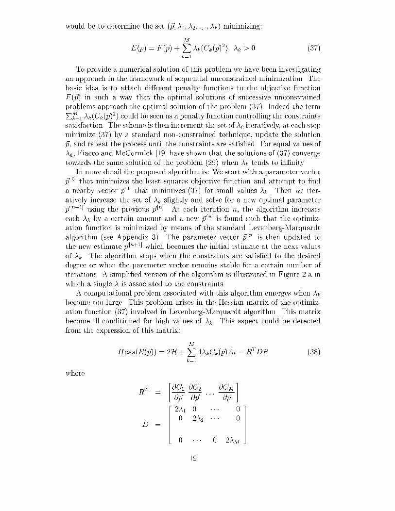
would be to determine the set (~p; �1; �2; :; :; �k) minimizing:E(~p) = F (~p) + MXk=1�k(Ck(~p)2); �k > 0 (37)To provide a numerical solution of this problem we have been investigatingan approach in the framework of sequential unconstrained minimization. Thebasic idea is to attach di�erent penalty functions to the objective functionF (~p) in such a way that the optimal solutions of successive unconstrainedproblems approach the optimal solution of the problem (37). Indeed the termPMk=1 �k(Ck(~p)2) could be seen as a penalty function controlling the constraintssatisfaction. The scheme is then increment the set of �k iteratively, at each stepminimize (37) by a standard non-constrained technique, update the solution~p, and repeat the process until the constraints are satis�ed. For equal values of�k, Fiacco and McCormick [19] have shown that the solutions of (37) convergetowards the same solution of the problem (29) when �k tends to in�nity.In more detail the proposed algorithm is: We start with a parameter vector~p [0] that minimizes the least squares objective function and attempt to �nda nearby vector ~p [1] that minimizes (37) for small values �k. Then we iter-atively increase the set of �k slightly and solve for a new optimal parameter~p [n+1] using the previous ~p [n]. At each iteration n, the algorithm increaseseach �k by a certain amount and a new ~p [n] is found such that the optimiz-ation function is minimized by means of the standard Levenberg-Marquardtalgorithm (see Appendix 3). The parameter vector ~p [n] is then updated tothe new estimate ~p [n+1] which becomes the initial estimate at the next valuesof �k. The algorithm stops when the constraints are satis�ed to the desireddegree or when the parameter vector remains stable for a certain number ofiterations. A simpli�ed version of the algorithm is illustrated in Figure 2.a inwhich a single � is associated to the constraints.A computational problem associated with this algorithm emerges when �kbecome too large. This problem arises in the Hessian matrix of the optimiz-ation function (37) involved in Levenberg-Marquardt algorithm. This matrixbecome ill-conditioned for high values of �k. This aspect could be detectedfrom the expression of this matrix:Hess(E(~p)) = 2H + MXk=1 4�kCk(~p)Ak +RTDR (38)where RT = "@C1@~p @C2@~p : : : @CM@~p #D = 266664 2�1 0 � � � 00 2�2 � � � 0... ... ... ...0 � � � 0 2�M 37777519

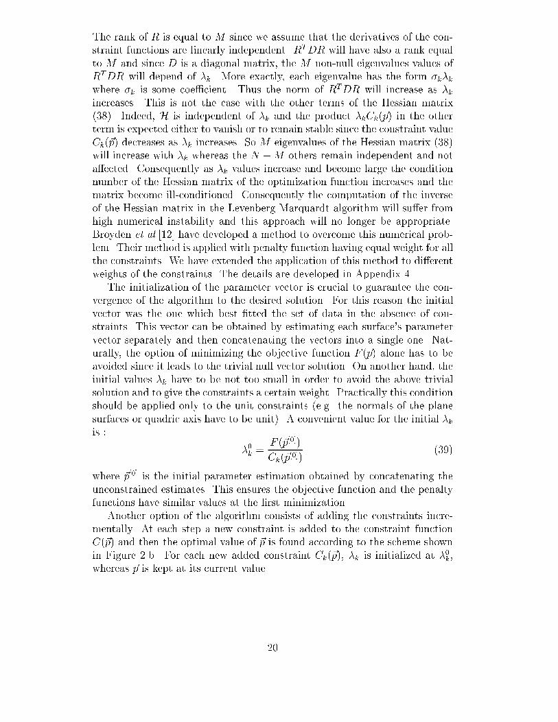
The rank of R is equal to M since we assume that the derivatives of the con-straint functions are linearly independent. RTDR will have also a rank equalto M and since D is a diagonal matrix, the M non-null eigenvalues values ofRTDR will depend of �k. More exactly, each eigenvalue has the form �k�kwhere �k is some coe�cient. Thus the norm of RTDR will increase as �kincreases. This is not the case with the other terms of the Hessian matrix(38). Indeed, H is independent of �k and the product �kCk(~p) in the otherterm is expected either to vanish or to remain stable since the constraint valueCk(~p) decreases as �k increases. So M eigenvalues of the Hessian matrix (38)will increase with �k whereas the N �M others remain independent and nota�ected. Consequently as �k values increase and become large the conditionnumber of the Hessian matrix of the optimization function increases and thematrix become ill-conditioned. Consequently the computation of the inverseof the Hessian matrix in the Levenberg-Marquardt algorithm will su�er fromhigh numerical instability and this approach will no longer be appropriate.Broyden et al [12] have developed a method to overcome this numerical prob-lem. Their method is applied with penalty function having equal weight for allthe constraints. We have extended the application of this method to di�erentweights of the constraints. The details are developed in Appendix 4.The initialization of the parameter vector is crucial to guarantee the con-vergence of the algorithm to the desired solution. For this reason the initialvector was the one which best �tted the set of data in the absence of con-straints. This vector can be obtained by estimating each surface's parametervector separately and then concatenating the vectors into a single one. Nat-urally, the option of minimizing the objective function F (~p) alone has to beavoided since it leads to the trivial null vector solution. On another hand, theinitial values �k have to be not too small in order to avoid the above trivialsolution and to give the constraints a certain weight. Practically this conditionshould be applied only to the unit constraints (e.g. the normals of the planesurfaces or quadric axis have to be unit). A convenient value for the initial �kis : �0k = F (~p[0])Ck(~p[0]) (39)where ~p[0] is the initial parameter estimation obtained by concatenating theunconstrained estimates. This ensures the objective function and the penaltyfunctions have similar values at the �rst minimization.Another option of the algorithm consists of adding the constraints incre-mentally. At each step a new constraint is added to the constraint functionC(~p) and then the optimal value of ~p is found according to the scheme shownin Figure 2.b. For each new added constraint Ck(~p), �k is initialized at �0k,whereas ~p is kept at its current value.20

EXPERIMENTSThe experiments were carried out on both synthetic and real data. The realdata was acquired from test objects with a 3D triangulation range sensor. Therange measurements were already segmented into point sets associated withsurfaces by means of the rangeseg [36] program.The �rst experiments aimed to check the behaviour and the convergenceof the algorithm. These experiments were applied on surfaces extracted froma single view of polyhedral objects. Through these experiments the perform-ances of the batch version of the algorithm (optim1) and the sequential version(optim2) were compared (see section \The step model object" ).In the second series of experiments (second subsection) we have gone fur-ther in complexity, �rstly on the level of features types. Thus, objects contain-ing quadric features were examined. Secondly the range data was collectedand registered from di�erent views. Thus, the data was additionally corrup-ted by the registration errors. So one objective was to test the robustness ofthe algorithm toward the complexity of the features (thus the diversity of theconstraints) and the registration errors.At �rst objects containing single quadric feature were studied. Section\half cylinder" and Section \the cone object" deal with the cylinder and thecone case respectively. Multi-quadric objects were examined afterwards (Sec-tions \Multi-quadric object 1" and \Multi-quadric object 2"). For the �rstcategory we have compared results issued from a single view with those ob-tained from multiple views. For both categories we checked the impact ofconstraint satisfaction on the quality of object shape attribute estimation.Other tests were carried out in order to give answers to the following ques-tions:1. What happens when some features are left unconstrained? What is theimpact on the other constrained features and more generally on the objectshape estimation? Reciprocally what is the impact of the constrainedfeatures on the non-constrained ones?2. How stable is the algorithm?3. How optimal is the solution?4. What happens if some constraints are invalid or inconsistent?Experiments carried on the synthetic polyhedral object (step model object)will give preliminary answers to question 1. Trials on real multi-quadric objects(Sections \Multi-quadric object 1" and \Multi-quadric object 2") will bringadditional con�rmation.Answers to questions 2, 3 4 will be developed in the experiments of Section\multi-quadric object 2".21

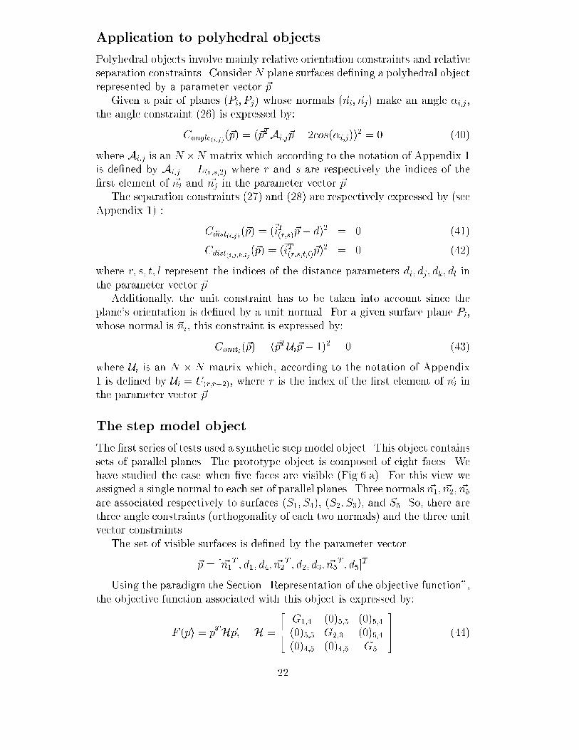
Application to polyhedral objectsPolyhedral objects involve mainly relative orientation constraints and relativeseparation constraints. Consider N plane surfaces de�ning a polyhedral objectrepresented by a parameter vector ~p.Given a pair of planes (Pi; Pj) whose normals (~ni; ~nj) make an angle �i;j,the angle constraint (26) is expressed by:Cangle(i;j)(~p) = (~pTAi;j~p� 2cos(�i;j))2 = 0 (40)where Ai;j is an N �N matrix which according to the notation of Appendix.1is de�ned by Ai;j = L(r;s;2) where r and s are respectively the indices of the�rst element of ~ni and ~nj in the parameter vector ~p.The separation constraints (27) and (28) are respectively expressed by (seeAppendix 1) : Cdist(i;j)(~p) = (~iT(r;s)~p� d)2 = 0 (41)Cdist(i;j;k;l)(~p) = (~iT(r;s;t;l)~p)2 = 0 (42)where r; s; t; l represent the indices of the distance parameters di; dj; dk; dl inthe parameter vector ~p.Additionally, the unit constraint has to be taken into account since theplane's orientation is de�ned by a unit normal. For a given surface plane Pi,whose normal is ~ni, this constraint is expressed by:Cuniti(~p) = (~pTUi~p� 1)2 = 0 (43)where Ui is an N � N matrix which, according to the notation of Appendix1 is de�ned by Ui = U(r;r+2), where r is the index of the �rst element of ~ni inthe parameter vector ~p.The step model objectThe �rst series of tests used a synthetic step model object. This object containssets of parallel planes. The prototype object is composed of eight faces. Wehave studied the case when �ve faces are visible (Fig.6.a). For this view weassigned a single normal to each set of parallel planes. Three normals ~n1; ~n2; ~n5are associated respectively to surfaces (S1; S4), (S2; S3), and S5. So, there arethree angle constraints (orthogonality of each two normals) and the three unitvector constraints.The set of visible surfaces is de�ned by the parameter vector~p = [ ~n1T ; d1; d4; ~n2T ; d2; d3; ~n5T ; d5]TUsing the paradigm the Section \Representation of the objective function",the objective function associated with this object is expressed by:F (~p) = ~pTH~p; H = 264 G1;4 (0)5;5 (0)5;4(0)5;5 G2;3 (0)5;4(0)4;5 (0)4;5 G5 375 (44)22

whereG1;4 = 264 H1 +H4 h1 h4hT1 N1 0hT4 0 N4 375 ; G2;3 = 264 H2 +H3 h2 h3hT2 N2 0hT3 0 N3 375G5 = " H5 h5hT5 N5 # (45)and Hk = PNki (Xki )(Xki )T ; hk = PNki Xki .Xki is a data point which belongs to the plane surface Sk and Nk is the numberof points of the plane Sk.The normals ~n1; ~n2; ~n5 are orthogonal and have to be unit so we set thefollowing constraint functionsCunit1(~p) = (~pTU1~p� 1)2 = 0 (46)Cunit2(~p) = (~pTU2~p� 1)2 = 0 (47)Cunit5(~p) = (~pTU5~p� 1)2 = 0 (48)Cangle1(~p) = Cangle(1;2)(~p) = (~pTA1;2~p� 2cos(�=2))2 = 0 (49)Cangle2(~p) = Cangle(1;5)(~p) = (~pTA1;5~p� 2cos(�=2))2 = 0 (50)Cangle3(~p) = Cangle(2;5)(~p) = (~pTA2;5~p� 2cos(�=2))2 = 0 (51)Since the unit constraints are used mainly to avoid the null solution, a single� is associated to them. The optimization function is thenE(~p) = ~pTH~p+ �1(Cunitl + Cunit2 + Cunit5)(~p)+�2Cangle1(~p) + �3Cangle2(~p) + �4Cangle3(~p)The results shown below are the average of 100 trials. At each trial thesurfaces' points are randomly corrupted with a Gaussian noise of 3 mm stand-ard deviation. Then optim1 and optim2 are applied to the same set of datapoints.Figure 6 shows some results obtained with the algorithm optim1. Theseresults represent the variation and the behaviour of some constraint functionsduring the algorithmwith respect of their associated �. Other results representthe variation of the estimation error of some of the object parameters e.g. onesurface's normal. The actual normals are known since the object is simulated.Figure 6.b shows the decrease of the unit constraint function (46) as �1increases, similarly for the angle constraint function (50) which decreases asthe associated weight �3 increases in Figure 6.c. We notice that both functionsare decreasing nearly linearly at a logarithmic scale. This suggests that it ispossible to enforce the constraint to any level of tolerance until the numericalaccuracy of the algorithm is compromised. The orientation error related tothe surface normal ~n1 and represented here by the angle formed by the actualnormal and the estimated one decreases and stabilizes to a relatively low value(around 0:06degree) in �gure 6.d. This error is computed as follows: at each23

iteration of the algorithm optim1 the estimated normal ~n1 is extracted fromthe solution ~p and then the error with respect to the actual simulated ~n1is computed. At each iteration the values of the di�erent � change, but theorientation error is mapped as function of �1 just to show its variation althoughit is not depending on �1 in particular.Similar behaviour is observed for the other parameter vectors but theyare not shown here to save space. This �rst observation of the constraintsbehaviour and the parameter estimation is encouraging because it means thatthe part's shape and position stabilizes as a whole. This fact will be con�rmedin next experiments with other objects.The three �gures Fig.7, Fig.8 and Fig.9 illustrate respectively the variationof the angle constraints values Cangle1 (49) Cangle2 (50) and Cangle3 (51) duringthe application of the sequential version optim2. The optimization processhas four steps, �rst the unit constraints are inserted then the three angleconstraints are applied one by one. So that at the �rst step the optimizationfunction is E(~p) = ~pTH~p+ �1(Cunitl + Cunit2 + Cunit5)(~p) (52)In the second step it will beE(~p) = ~pTH~p+ �1(Cunitl + Cunit2 + Cunit5)(~p) + +�2Cangle1(~p) (53)and so on.The �gures shows clearly the signi�cant decrease of the constraint valuewhen the related constraint function is added to the optimization function.It is seen also that once the constraint is satis�ed the addition of the otherconstraints only a�ects the level of tolerance previously reached by a verysmall degree.In Figure 7, it is noticed that at the end of step 2 (Fig.7.b) the constraintCangle1 is well satis�ed although the two others are not yet. Similarly, Fig.8.(c)shows that at the end of step 3 the constraint Cangle2 is well satis�ed while theconstraint Cangle3 is not yet implemented.Figure 9 shows that during step 2 and step 3 (when Cangle1 and Cangle2 areapplied) the constraint Cangle3 almost keeps stable at a reasonable value. Thismeans that the satisfaction of some constraints is not performed at much costto the unconstrained features.Figure 10 shows the the variation of the estimation error of one normal~n1 along the four steps of the algorithm. Similar results are obtained for theother normals. Similar to experiment with optim1, �gure 10.d shows that atthe end of the optimization the error in ~n1 estimation stabilizes at a low value.The same is noticed for the other normals.So the experiments carried out on the step model object have provided evid-ence of the applicability of both versions optim1 and optim2 of the algorithm.Both versions o�ers high satisfaction of the constraints, moreover the estim-ated orientation of the object surfaces extracted from the algorithm's solutionsare close to the actual one in both versions. This goes towards saying that24

the satisfaction of object shape requirements is not performed at the expenseof object localization, although the purpose of the algorithm is not to recoverthe object localization.However, optim2 is more time-consuming than optim1 (around N times,where N is the number of constraints). So, since both estimations of optim1and optim2 are acceptable, we have preferred to use optim1 for the rest of thework.The tetrahedronThe second polyhedral object tested is a real tetrahedron. The data has beenextracted from a view representing three visible faces S1; S2; S3 (Figure 11).The parameter vector is ~p = [~p1T ; ~p2T ; ~p3T ]T .In this view, the object surfaces have three angle constraints represented bythe three angles 90o , 90o and 120o between the three surface normals, as wellas the unit vector constraints. So we de�ne the following constraint functionsCunit1(~p) = (~pTU1~p� 1)2 = 0 (54)Cunit2(~p) = (~pTU2~p� 1)2 = 0 (55)Cunit3(~p) = (~pTU3~p� 1)2 = 0 (56)Cangle1(~p) = Cangle(1;2)(~p) = (~pTA1;2~p� 2cos(2�=3))2 = 0 (57)Cangle2(~p) = Cangle(1;3)(~p) = (~pTA1;3~p� 2cos(�=2))2 = 0 (58)Cangle3(~p) = Cangle(2;3)(~p) = (~pTA2;3~p� 2cos(�=2))2 = 0 (59)The application of the paradigm developed in Section \Representation of theobjective function" is straightforward for this object and we get easily thefollowing optimization function:~pTH~p+ �1 3Xl=1 Unitl(~p) + 4Xl=2 �lCanglel�1(~p) (60)where H = 264 G1 (0)4 (0)4(0)4 G2 (0)4(0)4 (0)4 G3 375and Gk have the same structure as in equation (45). All the constraints wereapplied simultaneously according to algorithm optim1. The results are theaverage of 100 trials. At each trial the initial vector ~p[0] is corrupted by auniform deviation of scale 5%. These 100 trials are a quantitative criterionfor testing the stability of the algorithm with respect to the perturbations inthe initial value of the solution. Here again all the di�erent constraints valuesdecrease during the optimization. This is illustrated through the two examplesshown in Fig.12.(a,b) where the unit constraint Cunit1 (54) and the angleconstraints Cangle1 (57) are mapped in function of their associated weighting25

values �1 and �2. Figure 12.c represent the variation of the objective function(the least squares function) ~pTH~p during the optimization process; it increasesslightly then it stabilizes. Figure 12.d shows the evolution of the sum of allthe constraints during the algorithm application. Since at each iteration ofthe algorithm optim1 the �k values increase, the variation of the objectivefunction and the sum of the constraints during the optimization is mapped infunction of one of the �k, (�2).It is seen that the sum of the constraint values converges to zero at theend of the optimization. It is also noticed that the constraint values could bedecreased further while the least squares error remains stable. Thus, the �nalpart shape now satis�es the shape constraints at a slight increase in the leastsquares �tting error.Application to surfaces having quadric surfacesCompared to polyhedral objects this category has more complex constraintssince the objects contain di�erent types of surfaces and consequently moregeometric features. So, besides the constraints related to the plane surfacesother constraints de�ning properties and relationships between quadric fea-tures could be de�ned as well as relationships between quadric features andplane features. The objects studied in this section contain cylindrical, conicaland spherical patches. In this section, the constraints' expressions will use thenotation of Appendix 1.Also, for all objects, the results of the proposed approach have been com-pared with object estimation methods which do not consider constraints, inparticular the least squares technique applied to each surface separately.The half cylinderThis object is composed of four surfaces. Three patches S1, S2 and S3 havebeen extracted from two views represented in Figure 13(a,c). These surfacescorrespond respectively to the base plane S2, lateral plane S1 and the cyl-indrical surface S3 (Figure 13.b). The parameter vector is ~p = [~p1T ; ~p2T ; ~p3T ]T ,where ~p1 = [ ~n1T ; d1]T , ~p2 = [ ~n2T ; d2]T and ~p3 = [a; b; c; h; g; f; u; v; w; d]T . Theleast squares error function is given by:F (~p) = ~pTH~p; H = 264 H1 O(4;4) O(4;10)O(4;4) H2 O(4;10)OT(4;10) OT(4;10) H3 375 (61)where H1, H2, H3 are the data matrices related respectively to S1, S2, S3.This object has the following constraints:1. S1 and S2 are perpendicular.2. The cylinder axis is parallel to S1's normal.26

3. The cylinder axis lies on the surface S2.4. The cylinder is circular.Constraint 1 is expressed by the following conditionCang(~p) = ( ~n1T ~n2)2 = (~pTL(1;5;2)~p)2 = 0Constraint 2 is satis�ed by equating the unit vector ~n in (14) to S1's normal~n1. Constraints 3 and 4 are represented respectively by:Caxe(~p) = (~i8T ~p� ~pTL(5;15;2)~p)2 = 0Ccirc(~p) = 6Xk=1Ccirck(~p) = 0(see Appendix 2 for details )Finally the normals ~n1 and ~n2 have to be unit. This is represented by:Cunit(~p) = (~pTU(1;3)~p� 1)2 + (~pTU(5;7)~p� 1)2 = 0Thus, the optimisation function is:E(~p) = ~pTH~p+ �1Cunit(~p) + �2Cang(~p) + �3Caxe(~p) + �4Ccirc(~p)ExperimentsIn the �rst test, algorithm optim1 has been applied to data extracted froma single view (Figure 13.c). In Figure 14 the behaviour of the di�erent con-straints during the optimization have been mapped as a function of the as-sociated �k as well as the least squares residual (61) and the sum of theconstraint functions. The �gures show a nearly linear logarithmic decrease ofthe constraints. It is also noticed that at the end of the optimization all theconstraints are highly satis�ed. The least squares error converges to a stablevalue and the constraint function vanishes at the end of the optimization. The�gures also show that it is possible to continue the optimization further until ahigher tolerance is reached, however this is limited by the numerical accuracyof the machine.In the second test, registered data from view 1 (Figure 13.a) and view 2(Figure 13.c) was used. The registration was carried out by hand. Resultssimilar to the �rst test were obtained for the constraints.Tables 2 and 3 present the values of some object characteristics obtainedfrom an estimation without considering the constraints and from the presen-ted optimization algorithm. These are shown for the �rst and second testrespectively.The characteristics examined are the angle between plane S1 and plane S2,the distance between the cylinder axis's point Xo (see Section \The cylinder"(14)) and the plane S2 and the radius of the cylinder. The comparison of thetables' values for the two approaches show the clear improvement made by27

the proposed technique. This is noticed in particular for the radius for whichthe actual value is 30mm, although the extracted surface covers considerablyless than a half of a cylinder. As we constrained the angle and distancerelations, we expect these to be satis�ed and they are to almost an arbitrarilyhigh tolerance, as seen in Fig.14. The radius was not constrained but theother constraints on the cylinder have allowed the least squares �tting of theunconstrained parameters to achieve a much more accurate estimation of thecylinder radius in both cases.Multi-quadric objectsThe third series of tests have been carried out on more complicated objectswith several quadric surface patches. For these objects, all of the surfaces havebeen considered. The registration of the di�erent views was done manually,thus the registered is expected to be corrupted by an additionally systematicerror. By this way we can judge the performances of the algorithm in thepresence of such errors.Multi-quadric object 1This object (Fig.15) comprises two lateral planes S1 and S2, a back planeS3, a bottom plane S4, a cylindrical surface S5 and a conic surface S6. Thecylindrical patch is less than a half cylinder (40% arc), the conic patch occupiesa small area of the whole cone (less then 30%).The vector parameter for this object is ~pT = [~p1T ; ~p2T ; ~p3T ; ~p4T ; ~p5T ; ~p6T ]where ~pi is the parameter vector associated to the surface Si.The surfaces of the object have the following constraints:1. S1 makes an angle of 120o1 with S2.2. S1 and S2 are perpendicular to S3.3. S1 and S2 make an angle of 120o with S4.4. S3 is perpendicular to S4.5. The axis of the cylindrical patch S5 is parallel to S3's normal.6. The axis of the cone patch S6 is parallel to S4's normal.7. The cylindrical patch is circular.8. The cone patch is circular.The �rst four angle constraints are grouped into a single angle constraintfunction: Cangl(~p) = 4Xi=1Cangli(~p)1We consider the angle between normals. 28

Constraints 5 and 6 are imposed by associating the normals ~n3 and ~n4respectively to the unit vectors of the cylinder axis and the cone axis (seeparagraphs circular cylinder and circular cone in Section \Preliminaries").The circularity of the cylinder and the cone are expressed respectively by:Ccirccyl(~p) = 6Xk=1Ccirccylk(~p)Ccirccone(~p) = 6Xk=1Ccircconek (~p)see Appendix 2 for the development of all these constraints.Finally the unit constraints on the surface normals have to be taken intoaccount. This leads to the following unit constraint function:Cunit(~p) = (~pTU(1;3)~p�1)2+(~pTU(5;7)~p�1)2+(~pTU(9;11)~p�1)2+(~pTU(13;15)~p�1)2The complete optimisation function is then given by the expression:E(~p) = ~pTH~p+ �1Cunit(~p) + �2Cang(~p) + �3Ccirccyl(~p) + �4Ccirccone(~p)ExperimentsSince the surfaces cannot be recovered from a single view, four views (Fig.15)have been registered by hand. 100 estimations were carried out. At each trial50% of the surface's points are selected randomly. Thus the algorithm startswith a di�erent initialization each time. The results shown in this section arethe average of these estimations. So by examining the mean of the estimationswe can have a judgement on the algorithm convergence.The results regarding the algorithm convergence are shown in Figure 16.All of the constraint functions vanish and are highly satis�ed.The angles between the di�erent �tted planes are presented in Table 4. Itshould be noticed that all the angles converge to the actual values. Table 5and Table 6 contain the estimated values of some attributes of the cylinderand the cone. The values show that each of the axis constraints are perfectlysatis�ed, the estimated radius and the cone half angle � improve when theconstraints are introduced. We notice the good shape improvement, relativeto the unconstrained least squares method, given by a reduction of bias ofabout 22mm and 30 respectively in the radius and the half angle estimation.The standard deviation of the estimations have been reduced as well.The radius estimation is within the hoped tolerances, a systematic error ofabout 0:5mm is quite nice. However the cone half angle estimation involvesa larger systematic error (about 1:8o). Two factors may contribute to this.The registration error may be too large since the registration was done byhand and the limited area of the cone patch which covers less then 30 % ofthe whole cone. It is known that when a quadric patch does not containenough information concerning the curvature, the estimation is very biased,even when robust techniques are applied, because it is not possible to predictthe variation of the surface curvature.29

Leaving some features unconstrainedWe have also investigated whether leaving some of the features unconstraineda�ects the estimation since one can worry that the satisfaction of the otherconstraints may push the unconstrained surfaces away from their actual pos-itions. To investigate this, we have left the angles between the pair of planes(S1; S2) and (S1; S3) unconstrained. The results are shown in Table 7. We seethat the estimated unconstrained angles are still close to the actual ones andthe accuracy is improved compared to the non-constrained method.Multi-quadric object 2This object (Fig.17) contains six plane surfaces S1; S2; S3; S4; S5; S6, a cyl-indrical surface S7 and a spherical surface S8. The surfaces S1; S2; S3; S4; S5form a square prism, the surface S5 is a square plane surface.The cylindrical patch is a whole cylinder and the spherical patch occupiesa half sphere.The surfaces of the object have the following relationships:1. S1; S3 are parallel.2. S2; S4 are parallel.3. S5; S6 are parallel.4. S1; S3 are orthogonal to S2; S4.5. S5; S6 are orthogonal to S1; S3 and S2; S4.6. S1; S3 and S2; S4 are separated by the same distance.7. The cylinder axis is parallel to S1; S2; S3 and S4 and orthogonal to S5; S6.8. The cylinder axis is located midway between S1 and S3 and midwaybetween S2 and S4.9. The cylindrical patch is circular.10. The sphere centre lies on the cylinder axis.11. The radius of the cylinder is equal to the radius of sphere.12. The length diagonal of surface S5 is equal to the cylinder diameter.The constraints 1; 2 and 3 allow a single normal to be associated with each ofthe pair of planes (S1; S3), (S2; S4) and (S5; S6). Consequently the parametervector of the object could be de�ned as:~p = [ ~n1T ; d1; d3; ~n2T ; d2; d4; ~n5T ; d5; d6; ~p7T ; ~p8T ]Twhere ~n1 is the normal associated to the pair of planes (S1; S3), d1 is theparameter distance of S1, d3 is the parameter distance of S3, ~n2 is the normalassociated to the pair of planes (S2; S4), d2 is the parameter distance of S2,d4 is the parameter distance of S4, ~n5 is the normal associated to the pair ofplanes (S5; S6), d5 is the parameter distance of S5, d6 is the parameter distance30

of S6, ~p7 is the parameter vector associated to the cylindrical patch S7 and ~p8is the parameter vector associated to the spherical patch S8.The constraints 4 and 5 are expressed by:Cangl(~p) = 3Xi=1Cangli(~p)The 6th constraint is formulated by:Cdist(~p) = (~iT(4;5;9;10)~p)2 = 0The 7th constraint is imposed by associating the normal ~n5 to the unit vector ofthe cylinder axis (see paragraph circular cylinder in Section \Preliminaries").The constraints 8; 9; 10; 11 and 12 are expressed respectively by:Caxe pos(~p) = (�2~pTL(1;22;2)~p+ iT(4;�5)~p)2 + (�2~pTL(6;22;2)~p+ iT(9;�10)~p)2 = 0Ccirc(~p) = 6Xk=1Ccirck(~p) = 0Csphcenter(~p) = (~pTT(11;12;22;23)~p)2 + (~pTT(11;13;22;24)~p)2 + (~pTT(12;13;23;24)~p)2 = 0Cequradius(~p) = (~iT(25;30)~p+ ~pTU(27;29;22;24)~p)2 = 0Cmedian(~p) = (~pT (I(4;1) � 2U(22;24))~p+ 2~iT25~p)2 = 0Finally the unit constraints related to the planes' normals and the unitconstraint of the coe�cient a of the sphere are grouped into the following unitconstraintCunit(~p) = (~pTU(1;3)~p�1)2+(~pTU(6;8)~p�1)2+(~pTU(11;13)~p�1)2+(~pTU(26;26)~p�1)2The optimization function is then:E(~p) = ~pTH~p+ �1Cunit(~p) + �2Cangl(~p) + �3Cdist(~p) + �4Caxe pos(~p)+�5Ccirc(~p) + �6Csphcenter(~p) + �7Cequradius(~p) + �8Cmedian(~p)The details concerning the formulation of all the above constraints are inAppendix 2.ExperimentsThe surfaces of the objects were recovered from 4 views shown in Figure 17 andthe registration of the range data was done by hand. Similarly to the previousobject 100 trials were performed. At each of them 50% of the surfaces's pointsare selected randomly leading to a di�erent initialisation each trial. In all thetrials, the decrease of all the constraint errors and the high level of satisfactionof the constraints at the end of the optimization for a slight increase of the leastsquares error is essentially similar to that observed in the previous experimentsand so similar graphs are not shown here.31

Through these di�erent tests and trials we have been investigating:1. How stable is the convergence of the algorithm ?2. How close is the estimation to the actual optimal value ?3. What are the e�ects of leaving some features unconstrained ?4. What is the e�ect of constraint invalidity ?5. What is the e�ect of constraint inconsistency ?Lastly, some results concerning the global shape improvement of t theobject model will be presented.Stability of the convergenceThe previous experiments performed each over 100 trials have shown thatthe mean of the estimated shapes obtained form these trials converges closeto the actual solution which satis�es the constraints. The initial solution ineach trial has a di�erent value since the data points are selected randomly.This experiment aims to check the sensitivity of the algorithm with respectto the initial value, to test the stability of the convergence of the algorithmwith respect to changes in the initial estimation. One way is to do so is tocompute the di�erence between the maximum and the minimum value of eachparameter in the set of di�erent solutions. A second way is to examine stat-ically the \closeness" of the di�erent estimates to the mean solution, knownin the statistic terminology as the distribution of the solutions. This distribu-tion could be obtained by computing the variance of each parameter from thesolutions issued from the 100 trials. Figure 18.a shows the maximum and theminimum value (scaled by the absolute value of the mean) for each parameter.The extrema of the di�erent parameters vary at a very low scale around themean solution, in a range lower than 2%. The same is noticed in the standarddeviations of the parameters illustrated in Figure 18.b. This aspect is fur-ther con�rmed in the distribution of the least squares errors of the di�erentestimations shown in Figure 19. The related relative variance is 1.94%.Closeness to the actual optimal solutionBy actual optimal solution we mean the estimate obtained from a processwhere the constraints are implicitly built into the least squares model. Thesolution provided in this case always completely satis�es the constraints. Soone may ask how close is the estimate issued from our approach to this optimalsolution. As we have mentioned previously, such an ideal and elegant formula-tion is di�cult or impossible to achieve for many objects due to the complexityand to the non-linearity of the geometric constraints. In fact one purpose andmotivation of our approach is to overcome this problem. Nevertheless it ispossible for some simple particular cases to combine the constraints with theleast squares error.So, in order to make a comparison with the optimal solution a sub-partof the multi-quadric object 2 was considered. It is composed of the two par-32

allel planes S1 and S3. The objective is to estimate the planes' orientationtaking into account the parallel constraints. For the �rst case, the parallelconstraint is implicitly considered by associating one normal to both planes.The optimization function is then:~nTH~n+ �(1� ~nT~n)where H is the appropriate data matrix. The second term of the functionis the unit constraint. A closed form solution is provided by the eigenvaluemethod.In the second case each plane was assigned a di�erent normal vector. Theequality of the two normals has to be satis�ed through the optimization pro-cess. According to our approach the objective function is:~n1TH1 ~n1 + ~n3TH3 ~n3 + �1(1� ~n1T ~n1)2 + �2(1� ~n3T ~n3)2 + �3(1� ~n1T ~n3)2100 tests were applied for each of the two cases. The average of the resultsare summarized in Table 8. The estimations are similar in the two cases.This shows that both solutions converge to the same value and almost equallyminimize the least squares error. The LS of the second solution is slightlylower than the optimal solution one. This is because in the optimal case theconstraint is perfectly satis�ed so the least squares error has to absorb all theerror. The same convergence of the two solutions is further con�rmed fromthe distribution of the angle (~n; ~nc), where ~nc is the mean of ~n1 and ~n3, andthe distribution of the di�erence between the LS error related to each of them,LS and LSi (Fig.20). These distributions are issued from 100 trials.Leaving some features unconstrainedAnother series of tests has been performed without considering the medianconstraint (constraint 12). This is in order to check if this will a�ect the pos-ition of the four plane surfaces with respect to the cylinder axis and thereforethe estimation of the edge of the square surface S5. Results are shown inTable 9 with the previous results for comparison. It is noticed that the radiusestimation is not a�ected but the incorporation of the additional constraintsslightly reduces the diagonal length error.Invalidity of the constraintsSuppose that one or more constraints do not re ect the actual relationshipsbetween features and therefore are invalid. What would be the behaviour ofthe algorithm? Will these \false constraints" be satis�ed? What could be theresulting estimated model ?To answer these questions, some angle constraints were set to an incorrectvalues. Three tests was carried out, in the �rst the angle ( ~n1; ~n2) was set to�=3, in the second the angle ( ~n1; ~n5) was set to �=3 and in the third test both33

angles ( ~n1; ~n5) and ( ~n2; ~n5) were set to �=3 (the right values are �=2 for bothangles).In all these tests the behaviour and the convergence of the algorithm werequalitatively similar to those of the previous experiments. The algorithmconverges, the least squares error stabilizes and all the constraints are satis�edat the end of the process although the least squares error is greater than thevalid constraints case (Figure 21). Table 10 summarizes the estimated modelcharacteristics in each of the three tests.An examination of Table 10 leads to the following observations:1. In all of the three tests the cylinder and the sphere characteristics are nota�ected by the invalid constraints.2. The normal ~n1 which is involved in each of the invalid constraints is a�ectedin three tests.3. The normal ~n2 is changed in the �rst and third test where it is involved inthe invalid constraints whereas it is unchanged in the second test where it isnot involved.4. The normal ~n5 is kept unchanged in all the tests even in those where it isinvolved in the inconsistent constraints.From these observations we can deduce that invalid constraints a�ect theobject feature's locations by shifting the involved features toward positionswhere the invalid constraints are satis�ed. Consequently, this will increase theleast squares error (Figure 21). The locations and the characteristics of thesurfaces which are not involved in the invalid constraints are not a�ected (thesphere and the cylinder). However the normal ~n5 seems not to satisfy this rulesince its orientation stays unchanged for all the cases where it is involved inan inconsistent constraint. This is explained by the fact that unlike ~n1 and ~n2,~n5 is also involved in other constraints, in particular it is constrained to havethe same orientation as the cylinder axis. The satisfaction of this constraintkeeps it collinear to the cylinder axis and prevents its orientation from beinga�ected. Thus the algorithm satis�es the invalid constraints in which ~n5 isinvolved by acting on the other normals involved in these constraints.Inconsistency of the constraintsIn this test we investigated what would be the behaviour of the algorithmwhen some constraints are inconsistent and have a con ict between them. Forthis purpose we introduced two additional inconsistent angle constraints byimposing the angles ( ~n1; ~n2) and ( ~n1; ~n5) to be �=3, which con icts with thetwo other consistent constraints de�ning each pair of ( ~n1; ~n2) and ( ~n1; ~n5) asorthogonal vectors. The trial carried out with these inconsistent constraintsrevealed that the algorithm converges normally (Figure 22) both the leastsquares and the constraint functions stabilizing at the end of the algorithm.From Figure 22.a we notice that the angle constraints are not satis�ed. Thisis obvious because it is not possible to satisfy con icting constraints simul-taneously. The converging value of the constraint function (the sum of all the34

constraints, Figure 22.b) and the angle constraints error are practically equalat the end of the optimization process. This shows that the other consistentconstraints are satis�ed. This suggests that an inconsistent set of constraintscan be detected by observing the convergence of the constraint error ratherthan its reduction to zero.Global shape improvementThe di�erent tables shown in this section compare the geometric character-istics of the object issued from an optimization with constraints and an op-timization without and show the improvement of the object characteristicsestimates when constraints are applied. The results presented in the tablesare the average of the 100 estimations. The angles between each pair of sur-faces (S1; S2); (S1; S5) and (S2; S5) were set as constraints and the constraintswere nearly perfectly satis�ed. From Table 11 we notice the satisfaction of thesquare property of the prism, illustrated by the equality of the two distancesseparating (S1; S3) and (S2; S4), their values which is close to the actual lengthof the edge of the square plane S5 and closeness of the estimated value of thediagonal of S5 to the actual value when the constraints are considered. Thedistances between these last surfaces for an optimization without constraintsis not mentioned in this table since the estimated surfaces are not parallel.The improvement of the quadric surfaces estimation is con�rmed again forthis object ( Table 12 and Table 13). The radius estimation error is less than0:04mm for both the cylinder and the sphere. The standard deviations of thecylinder and the sphere radius have been signi�cantly reduced as well.CONCLUSIONThis work presents a framework for the reconstruction of object models incor-porating geometric constraints. It can hold a large number of varied constrainttypes and incorporates them integrally without the need for linearization. Thegeometric constraints are formulated in quadratic matrix functions which arecontinuous, di�erentiable and ensure a compact expression of the constraintsand easy handling by the optimization process.The proposed optimization algorithm belongs to sequential nonlinear pro-gramming. Theoretically, the characteristics of the objective function and theconstraint functions satisfy the requirements for an e�cient application of thealgorithm. The availability of a good initial solution obtained from the meas-urement data ensures the convergence of the algorithm towards the optimalsolution. However, the last condition make it inappropriate for constrainedobject design applications where a reasonable initial solution is not available.The practical di�culties of the algorithm manifested in the ill-conditionedHessian matrix in the Levenberg-Marquardt algorithm is overcome by usingan appropriate numerical technique. 35

The constraints can be integrated in a batch form at once or sequentially.In the sequential version the addition of a new constraint does not a�ect thesatisfaction of the previously implemented constraints.The experiments carried out on the di�erent objects empirically con�rmthe convergence of the algorithm. The parameter optimization search doesproduce shape �tting that satis�es almost perfectly the constraints. They showin particular that the least squares error grows slightly as the constraints areapplied and the weighting values increased, but this stabilizes above certainvalues of the �k while the constraint errors are still decreasing. Thus it ispossible to satisfy the constraints up to the desired tolerance without seriouslya�ecting the quality of the data �tting.The above observations suggest that the proposed approach allows exibil-ity in the incorporation of the constraints, as well as in their satisfaction. Thesequential version of the constraint implementation allows a human reverseengineer to supply them interactively whereas the batch form of constraintincorporation is suitable for being inferred by a knowledge-based system reas-oning from general engineering principles. The stabilization of the increase ofthe least squares error while the constraint errors are still decreasing as �k in-creases o�ers the possibility that the user can control the degree of satisfactionof the constraints and to set the tolerances as high as necessary.Regarding the slight increases of the LS error, we have to bear in mindthat the increase of the least squares residuals value may not re ect a badestimation in the case when measurement errors are systematic, e.g. mis-calibration and registration error. This last type of error is expected in ourdata since the registration process is performed by hand. We believe that theslight increase of the least squares error as a consequence of the constraintssatisfaction is a result of the object being located more accurately. Futurework could investigate a more robust form for the objective function involvingthe data noise statistics.The di�erent trials applied on the multi-quadric objects empirically con-�rm the stability of the convergence of the algorithm. The low values of theparameters' variances illustrates the stability of the solution provided by theoptimization search process. On the level of the object shape, this aspect isre ected by the small values of the standard deviations of the object shapecharacteristics. The tests have shown as well that the proposed approach leadsto an estimate which is close to the optimal solution (e.g. the solution givenwhen the constraints could be combined with the least squares error). The ex-periments also show that applying the constraints to only some features doesnot seriously a�ect the estimation of the unconstrained surfaces. The estima-tion is still improved compared to the case of unconstrained optimization.The examination of some constraint invalidity cases has shown the con-straints are always satis�ed whether they are valid or not and the behaviourof the algorithm is typically the same. The satisfaction of invalid constraintsleads to the relocation of the involved and less constrained features (havingmore degrees of freedom) toward positions where the inconsistency is removed.36

However this will result in a false object model. The trial performed with con-straint inconsistencies case revealed the same behaviour regarding the conver-gence of the algorithm but the inconsistent constraints are not satis�ed at theend of the optimization. This suggests that constraint validity and consistencychecking have to be done before starting the optimization process.Regarding the model estimation accuracy, the comparison of the objectdimension estimates with those from unconstrained �tting con�rms that theproposed approach improves the quality of the model construction to a highdegree. For the second-quadric object the radius of the cylinder and the spherehave an estimation error in the range of 0:04mm, the edge of the square prismhas an estimation error around 0:1mm. The radius of the cylinder patchestimated from the registered half cylinder has an estimation error around0:01mm. For a single a view it is less than 0:5mm. The same range of error isobtained for the radius of the cylinder patch of the �rst multi-quadric object.Results for the cone patches are reasonable for the cone object, the halfangle estimation error is less than 0:50, but less satisfactory for the �rst multi-quadric object. This is mainly due to the relatively small area of the conicpatch. In fact, the comparison of the estimation error for the quadric surfacesshows that the larger the quadric patch, the smaller the estimation error. Weintentionally chose to work with small patches because unconstrained �ttingsurface techniques fail to give reasonable estimates in this case (see the radiusestimate in Table 5) even with robust algorithms due to the \poorness" of theinformation embodied in the patch.Regarding the constraint representation, it is noticed that some constraintsinvolve a large number of equations, in particular for the circularity constraint.One solution is to implicitly impose those constraints through the representa-tion of the quadric equation ((X �Xo)T (I � ~n~nT )(X �Xo)� r2 = 0 ) for thecylinder and ((X �Xo)T (~n~nT � cos2(�))(X �Xo) = 0) for the cone, where ~nis the unit orientation vector of the cylinder or the cone axis, Xo is a point onthe cylinder axis in the cylinder case and is the apex for the cone case. Themain problem encountered with this representation is the complexity of therelated objective function and the di�culty of separating the data terms fromthe parameter terms. It will be also worthwhile investigating some topologicalconstraints between surfaces which have a common intersection.Although the experiments presented in this work were performed on singleobjects, the proposed approach can optimize multiple objects simultaneously.Generally industrial parts are designed to �t to each other, so geometric rela-tionships between the parts may be considered and the resulting constraintscan be incorporated as well in the optimization process.Another area we are starting to investigate is how one might automatic-ally identify inter-surface relationships that can have a constraint applied. Inmanufacturing objects, simple angular and spatial relationships are given bydesign. So, it should be straightforward to de�ne simple Mahalanobis distancetests that hypothesize standard feature relationships, subject to the feature'sstatistical position distribution. With this analysis, a computer program could37

propose a variety of constraints that a human could either accept or reject,after which shape reconstruction could occur.It is very likely that the consideration of the constraints tends to shiftthe object localization towards the actual position. The experiments carriedout with the synthetic polyhedral objects provides evidence for this. It seemsthat the incorporation of the constraints compensate up to certain degree forthe e�ect of the systematic errors and allows better estimation, although theauthors have not yet a theoretical proof of this interpretation. This issuewas partially justi�ed in the work of Bolle et al [6], but only for the intrinsicconstraints, namely the circularity of the cylinder and perfect sphere. Byconsidering a larger set of constraints, the proposed framework generalizesthe concept of object localization considering the constraints and make a steptoward a framework which uni�es object localization and object modelling.All the algorithm procedures have been implemented with C++. The com-putation time for the reconstruction on a 200Mhz sun Ultrasparc workstationis typically few minutes or less (1-5 minutes), which is suitable for CAD work.ACKNOWLEDGEMENTThe work presented in this paper was funded by UK EPSRC grant GR /L25110.References[1] R. Anantha, G.A. Kramer, R.H. Crawford. Assembly modelling by geo-metric constraint satisfaction. CAD, Vol.28, No.9, pp 707-722, 1996.[2] R. Anderl, R Mendegen. Modelling with constraints: Theoretical found-ation and application. CAD, Vol. 28, No 3, pp 155-168 1996.[3] F. Arbab, B. Wang. Reasoning about geometric constraints. In H.Yoishikawa and T.Holden (eds), Intelligent CAD II, North Holland, pp.93-107, 1990.[4] R.J.Bell. An elementary treatise on coordinate geometry. McMillan andCo, London, 1910.[5] P.J Besl, R.C. Jain. Three dimensional object recognition. ACM Com-puting Surveys, Vol.17, No.1, pp.75-145, 1985.[6] R.M.Bolle, D.B.Cooper. On Optimally Combining Pieces of Information,with Application to Estimating 3-D Complex-Object Position from RangeData. IEEE Trans. PAMI, Vol.8, No.5, pp.619-638, September 1986.[7] R.C. Bolles, R.A. Cain. Recognizing and locating partially visible objects.Int. Journal of Robotics Research, Vol.1, No.3, pp. 57-82, 1982.[8] R. C. Bolles, P. Horaud. 3DPO, a three dimensional part orientationsystem. Int. Journal of Robotics Research, Vol.5, No.3, pp. 3-26, 1986.[9] A.H. Boring. The programming language aspect of ThingLab, a con-strained oriented simulation laboratory. ACM TOPALS, Vol.3, No.4,pp.353-387, 1981. 38

[10] W. Bouma, I. Fudos, C. Ho�man, J. Cai, R. Paige. Geometric constraintsolver. CAD, Vol. 27, No.6, pp 487-501, 1995.[11] K.L.Boyer, M.J.Mirza, G.Ganguly. The Robust Sequential Estimator.IEEE Trans. PAMI, Vol.16, No.10, pp.987-1001, October 1994.[12] C.G Broyden, N.F. Attia. Penalty Functions, Newton's Method andQuadratic Programming. Journal of optimization theory and applica-tions, Vol.58, No.3, 1988.[13] B. Buchberger. Application of Grobner basis in non-linear computationalgeometry. In D. Kapur and and J. Mundy (eds), Geometric Reasoning,MIT press, 1989.[14] Y.Chen, G.Medioni. Object Modeling by Registration of Multiple RangeImages. Proc. IEEE Int. Conf. Robotics and Automation, Vol.2 pp.724-729, April 1991.[15] J.De Geeter, H.V.Brussel, J.De Schutter, M. Decreton. A SmoothlyConstrained Kalman Filter. IEEE Trans. PAMI pp.1171-1177, No.10,Vol.19, October 1997.[16] L. Eggli, C.Y. Hsu, B.D. Bruderlin, G. Elbert. Inferring 3D models fromfreehand sketches and constraints. CAD, Vol.29, No.2 pp. 101-112, 1997.[17] C.X Feng, A. Kusiak. Constraints-based design of parts. CAD, Vol 27No 5 1995 pp 343 -352, 1995.[18] M. Ferri, F. Magnilli, G. Viano. Projective pose estimation of linear andquadratic primitives in monocular computer vision. Image understand-ing, Vol.58, No.1, pp.66-84, 1993.[19] A.V Fiacco, G.P McCormick. Nonlinear Programming: Sequential Un-constrained Minimization Techniques. John Wiley and Sons, NewYork1968.[20] A.F. Fitzgibbon, D.W. Eggert, R.B. Fisher. High-level CAD modelacquisition from range images. CAD, Vol.29, No.4, pp.321-330, 1997.[21] R.Fletcher. Practical Methods of Optimization. John Wiley & Sons,1987.[22] P.J.Flynn, A.K.Jain. Surface Classi�cation: Hypothesizing and Para-meter Estimation. Proc. IEEE Comp. Soc. CVPR, pp. 261-267. June1988.[23] D. Forsyth, J.L. Mundy, A. Zisserman, C. Coelho, A. Heller, C. Rothwell.invariant descriptors for 3D object recognition and pose. IEEE PAMI,Vol.13, No.10, pp. 971-991, October 1991.[24] I. Fudos, C.Ho�man. Constraints-based parametric conics for CAD.CAD, Vol.28, No.2 pp. 91-100, 1996.[25] X.S. Gao, S.C.Chou. Solving geometric constraint systems. I. A globalpropagation approach. CAD, Vol.30, No.1, pp.47-54, 1988.[26] P.E.Gill, W.Murray, M.H.Wright. Practical Optimization. AcademicPress, 1981.[27] W.E. Grimson. The role of geometric constraints. MIT press, London,1990.[28] D.E. Goldberg. Genetic Algorithms in Search, Optimization and MachineLearning. Addison-Wesley, Reading, MA, 1989.39

[29] G.H. Golub, C.F. Van Loan Matrix Computations. John HopkinsUniversity Press, 3rd edition, 1996.[30] E.Gmur, H.Bunke. 3D Object Recognition Based on Subgraph matchingin Polynomial time. In Sanfeliu, Mohr, Pavildis (eds), Structural PatternAnalysis, pp.131-147, World Scienti�c Publications. 1990.[31] I. Herman. The use of projective geometry in computer graphics. Lecturenotes in computer science 564. Springer Verlag. 1992.[32] A. Heydon, G.Nelson. The Juno-2 Constraint-Based-Drawings Editor.SRC research report 131a, 1994.[33] C.M.Ho�mann, P.J. Vermeer. Geometric constraint solving inR2 and R3In Du Dingzhu and Hwang Frank (eds), Computing in Euclidean Geo-metry, 2nd edition, World Scienti�c Publishing, 1995.[34] C.M.Ho�mann, P.J. Vermeer. A spatial constraint problem. Proc.2nd Workshop on Computational Kinematics, pp.83-92, Sophia Antipolis,1995.[35] C.M. Ho�mann, A. Lomonosov, M. Sitharan. Finding Solvable Subsetsof Constraint Graphs. Springer LNCS 1330, G. Smoka eds, pp.463-477,1997.[36] A. Hoover, G. Jean-Baptiste, X. Jiang, P. J. Flynn, H. Bunke. D. Goldgof,K. Bowyer, D. Eggert, A. Fitzgibbon, R. Fisher. An Experimental Com-parison of Range Segmentation Algorithms. IEEE Trans. PAMI, Vol.18,No.7, pp.673-689, July 1996.[37] S.L.S. Jacoby, J.S Kowalik, J.T.Pizzo. Iterative Methods for NonlinearOptimization Problems. Prentice-Hall, Inc. Englewood Cli�s, New Jersey,1972.[38] D.Jian, S.Vijayan. Manufacturing feature determination and extraction,Part I: optimal volume segmentation. CAD, Vol.29, Vol.6, 1997,pp.427-440.[39] K. Kondo. Algebraic method for manipulation of dimensional relation-ships in geometric models. Geometric Aided Design, Vol.24 No.3 pp141-147, 1992.[40] S.Kumar, S.Han, D.Goldgof, K.Boyer. On Recovering Hyperquadricsfrom Range data. IEEE Trans. PAMI, Vol.17, No.11, pp.1079-1083,November 1995.[41] K.L Lawrence, S.N Muthukrishna, R.V Nambiar. Re�nement of 3Dmeshes at surface intersections. CAD, Vol. 27, No. 8 , 1995.[42] R.A Light, D.C Gossard. Modi�cation of geometric models throughvariational geometry. CAD, Vol. 14, No. 4 , pp. 209-214, 1982.[43] D.G. Lowe. Fitting parameterized three dimensional models to images.IEEE PAMI, Vol.13, No.5, pp. 441-450, 1991.[44] Z. Michalewicz. Genetic Algorithms + Data Structures = Evolution Pro-grams. Springer-Verlag, 1996[45] C.J.Ong, Y.S.Wong, H.T. Loh, X.G.Hong. An optimization approachfor biarc curve-�tting of B-spline curves. CAD, Vol. 28 , No. 12, pp.951-959, 1996. 40

[46] J.Porrill. Optimal Combination and Constraints for Geometrical SensorData. International Journal of Robotics Research, Vol.7, No.6, pp.66-78,1988.[47] L. Quan. Conic reconstruction and correspondence from two views.IEEE PAMI, Vol.18, No.2, pp. 151-160, 1996.[48] A.A.G. Requicha. Reprsentation of Tolerances in Solid Modelling: Is-sues and Alternative Approaches. In J.W.Boyse amd M.S.Pickett (Eds),Solid Modelling by Computers: from Theory to Applications, New York:Plenum, 1984, pp.3-22.[49] C. Robertson, R.B. Fisher, D. Corne, N. Werghi, A.P. Ashbrook. Invest-igating Evolutionary Optimisation of Constrained Functions to CaptureDescriptions from Range Data. Proc. 3rd On-line World Conference onSoft Computing (WSC3), 1998.[50] R.T. Rockafellar. Convex Analysis. Princton University Press, 1970.[51] A.P. Rockwood, J. Winget. Three-dimensional object reconstructionfrom two-dimensional images. CAD, Vol.29, No.4, pp.279-286, 1997.[52] R. Safee-Rad, I. Tchoukanov, K.C. Smith, B. Benhabib. Constraints onquadratic-curved features under perspective projection. Image and Visioncomputing, Vol.10, No.8, pp. 532-548, 1992.[53] L.G Shapiro, R.M Haralick. Structural descriptions and inexact match-ing. IEEE PAMI, Vol.3, No.5, pp.504-419, september 1981.[54] B.S. Shin, Y.G. Shin. Fast 3D solid model reconstruction from ortho-graphic views. CAD, Vol.30, No.1, pp.63-76, 1998.[55] H.Y.Shun, K.Ikeuchi, R.Reddy. Principal Component Analysis withMissing Data and its Application to Polyhedral Object Modelling. IEEETrans. PAMI, Vol.17, No.9, pp.855-867. 1995.[56] M.Soucy, D.Laurendo. Surface Modelling from Dynamic Integration ofMultiple Range Views. Proc 11th Int. Conf. Pattern Recognition, pp.449-452, 1992.[57] G. Sunde. Speci�cation of shape by dimensions and other geometricconstraints. In M.J Vozny et al(eds) Geometric Modelling for CADapplications, pp. 199-213, North Holland, 1988.[58] I.E Sutherland. Sketchpad: A man-machine graphical communicationsystem. Proc. Joint Computer Conference, pp.329-346, 1963.[59] T.Taura, I.Nagasaka, A.Yamagishi. Application of evolutionary pro-gramming to shape design. CAD, Vol.30, No.1, pp. 29-35, 1988.[60] W.T Wu. Basic principles of mechanical theorem proving in geometry.Springer Verlag, 1993.[61] T. Varady, R. R. Martin, J. Cox. Reverse engineering of geometricmodels, an introduction. CAD, Vol.29, No.24, pp. 255-268, 1997.[62] B.C.Vemuri, J.K Aggrawal. 3D Model Construction from Multiple ViewsUsing Range and Intensity Data. Proc. CVPR, pp.435-437, 1986.[63] D.R Wallace, M.J Jakiela, W.C.Flowers. Design search under probab-ilistic speci�cations using genetic algorithms. CAD, Vol.28, No.5, pp.405-421, 1996. 41

[64] X.Wang, F. Cheng, B. Brian. Energy and B-spline interproximation.CAD, Vol.29, No.7, pp. 405-421, 1997.[65] N. Werghi, R.B.Fidher, C.Robertson, A.Ashbrook. Improving ModelShape Acquisition by Incorporating Geoemetric constraints. Proc.BMVC, pp.530-539, Essex, September 1997[66] R.C. Wetkamp. Geometric constraint management with quanta. in D.CBrown et al(eds) Intelligent Computer Aided Design, pp. 409-426, NorthHolland, 1992.[67] Q.W. Yan, C.L.P. Chen, Z. Tang. Reconstruction of 3D objects fromorthographic projections. CAD, Vol.26, No.9, 1994.

42

Appendix 1: Notation~ir is a vector in which all the elements are zero except the rth element whichis equal to 1.~i(r;s) is a vector in which all the elements are zero except the rth and the sthelements which are equal to 1~i(r;�s) is a vector in which all the elements are zero except the rth and the sthelements which are equal to 1 and �1 respectively.~i(r;s;t;l) is a vector in which all the elements are zero except for the rth; sth; tthand lth elements which are equal to 1; 1;�1 and �1 respectively.M(r;s) is a diagonal matrix in which all the elements are zero except the rthand the sth elements which are equal to 1 and �1 respectively.U(r;s) is a diagonal matrix de�ned by:U(r;s) = ( U(i; i) = 1 if r � i � sU(i; i) = 0 otherwiseI(r;s) a symmetric matrix de�ned by:I(r;s) = ( I(i; j) = I(j; i) = 1 for r � i � s; r � j � sI(i; j) = 0 otherwiseU(r;s;p;t) is a diagonal matrix de�ned by:U(r;s;p;t) = 8><>: U(i; i) = 1 if r � i � sU(i; i) = �1 if p � i � tU(i; i) = 0 otherwiseL(r;s;p) a symmetric matrix de�ned by:L(r;s;p) = ( L(i; j) = L(j; i) = 1=2 fot r � i � r + p; s � j � s+ pL(i; j) = L(j; i) = 0 otherwiseT(r;s;p;t) a symmetric matrix de�ned by:T(r;s;p;t) = ( T (r; t+ 5) = T (t+ 5; r) = T (s; p) = T (p; s) = 1=2T (r; t) = T (t; r) = T (s; p+ 5) = T (p+ 5; s) = �1=243

Appendix 2: Constraints de�nitionThe half cylinderConstraint 3 is represented by two conditions: axis vector ~n is orthogonal toS2's normal ~n2, and one point of the axis satis�es S2's equation. The �rstcondition is guaranteed by constraint 2 since ~n2 is orthogonal to ~n1. For thesecond condition the point Xo in Section \The cylinder" has to satisfy theequation: Caxe(~p) = (XTo ~n2 + d2)2 = 0Using equations (9) and (15) this equation can be written asCaxe(~p) = (�[u; v; w]T ~n2 + d2)2 = (~i8T~p� ~pTL(5;15;2)~p)2 = 0The cylinder circularity constraint is implicitly de�ned by the equations(15). From these equations we extract the following constraints on the para-meter vector ~p:Ccirc1(~p) = (~i9T ~p+ ~pTU(1;1)~p� 1)2 = 0Ccirc2(~p) = ( ~i10T ~p+ ~pTU(2;2)~p� 1)2 = 0Ccirc3(~p) = ( ~i11T ~p+ ~pTU(3;3)~p� 1)2 = 0 Ccirc4(~p) = ( ~i12T ~p+ ~pTL(1;2;0)~p)2 = 0Ccirc5(~p) = ( ~i13T ~p+ ~pTL(1;3;0)~p)2 = 0Ccirc6(~p) = ( ~i14T ~p+ ~pTL(2;3;0)~p)2 = 0We group these six constraints into a single one:Ccirc(~p) = 6Xk=1Ccirck(~p) = 0The cone objectEliminating cos2� from the cone circularity equations (19) and taking intoconsideration constraint 1, the circularity constraints are formulated as:a� b = n21x � n21ya� c = n21x � n21zb� c = n21y � n21z h = n1xn1yg = n1xn1zf = n1yn1zA matrix formulation of these constraints as a function of the parametervector ~p is:Ccirc1(~p) = ( ~j(5;�6)T~p� ~pTM(1;2)~p)2 = 0Ccirc2(~p) = ( ~j(5;�7)T~p� ~pTM(1;3)~p)2 = 0Ccirc3(~p) = ( ~j(6;�7)T~p� ~pTM(2;3)~p)2 = 0 Ccirc4(~p) = (~i8T~p� ~pTL(1;2;0)~p)2 = 0Ccirc5(~p) = (~i9T~p� ~pTL(1;3;0)~p)2 = 0Ccirc6(~p) = ( ~i10T~p� ~pTL(2;3;0)~p)2 = 044

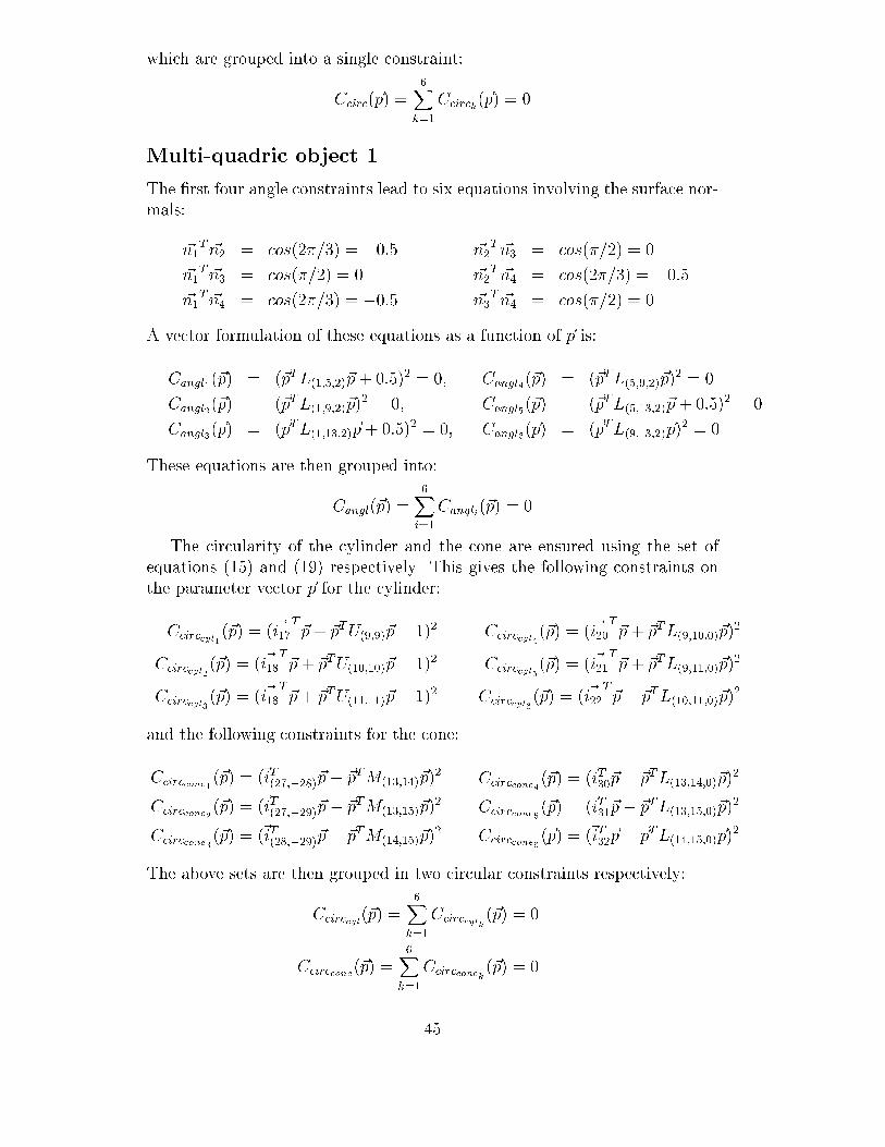
which are grouped into a single constraint:Ccirc(~p) = 6Xk=1Ccirck(~p) = 0Multi-quadric object 1The �rst four angle constraints lead to six equations involving the surface nor-mals:~n1T ~n2 = cos(2�=3) = �0:5~n1T ~n3 = cos(�=2) = 0~n1T ~n4 = cos(2�=3) = �0:5 ~n2T ~n3 = cos(�=2) = 0~n2T ~n4 = cos(2�=3) = �0:5~n3T ~n4 = cos(�=2) = 0A vector formulation of these equations as a function of ~p is:Cangl1(~p) = (~pTL(1;5;2)~p+ 0:5)2 = 0;Cangl2(~p) = (~pTL(1;9;2)~p)2 = 0;Cangl3(~p) = (~pTL(1;13;2)~p+ 0:5)2 = 0; Cangl4(~p) = (~pTL(5;9;2)~p)2 = 0Cangl5(~p) = (~pTL(5;13;2)~p+ 0:5)2 = 0Cangl6(~p) = (~pTL(9;13;2)~p)2 = 0These equations are then grouped into:Cangl(~p) = 6Xi=1Cangli(~p) = 0The circularity of the cylinder and the cone are ensured using the set ofequations (15) and (19) respectively. This gives the following constraints onthe parameter vector ~p for the cylinder:Ccirccyl1(~p) = ( ~i17T ~p+ ~pTU(9;9)~p� 1)2Ccirccyl2(~p) = ( ~i18T~p+ ~pTU(10;10)~p� 1)2Ccirccyl3(~p) = ( ~i18T~p+ ~pTU(11;11)~p� 1)2 Ccirccyl4(~p) = ( ~i20T ~p + ~pTL(9;10;0)~p)2Ccirccyl5(~p) = ( ~i21T ~p + ~pTL(9;11;0)~p)2Ccirccyl6(~p) = ( ~i22T ~p+ ~pTL(10;11;0)~p)2and the following constraints for the cone:Ccirccone1 (~p) = (~iT(27;�28)~p� ~pTM(13;14)~p)2Ccirccone2 (~p) = (~iT(27;�29)~p� ~pTM(13;15)~p)2Ccirccone3 (~p) = (~iT(28;�29)~p� ~pTM(14;15)~p)2 Ccirccone4 (~p) = (~iT30~p� ~pTL(13;14;0)~p)2Ccirccone5 (~p) = (~iT31~p� ~pTL(13;15;0)~p)2Ccirccone6 (~p) = (~iT32~p� ~pTL(14;15;0)~p)2The above sets are then grouped in two circular constraints respectively:Ccirccyl(~p) = 6Xk=1Ccirccylk(~p) = 0Ccirccone(~p) = 6Xk=1Ccircconek (~p) = 045

Multi-quadric object 2The orthogonality constraints (4 and 5) between planes are formulated as:~n1T ~n2 = ~n1T ~n5 = ~n2T ~n5 = 0which can be written the following vector formulation.Cangl1(~p) = (~pTL(1;6;2)~p)2 = 0Cangl2(~p) = (~pTL(1;11;2)~p)2 = 0Cangl3(~p) = (~pTL(6;11;2)~p)2 = 0and grouped into a single angle constraint functionCangl(~p) = 3Xi=1Cangli(~p) = 0The 6th constraint can be expressed according tod1 + d3 = d2 + d4and then formulated by: Cdist(~p) = (~iT(4;5;9;10)~p)2 = 0Since we assume that the cylinder axis is parallel to the planes S1; S2; S3; S4,the distance from the cylinder axis to one of these planes could be de�ned asthe distance from one particular point Xo of the axis and the given plane. The8th constraint can be formulated by:d(Xo; S1) = d(Xo; S3); d(Xo; S2) = d(Xo; S4)Taking into account that S1; S3 have opposite orientation as well as S2; S4,these equations can be written as:XTo ~n1 + d1 = �XTo ~n1 + d3; XTo ~n2 + d2 = �XTo ~n2 + d4leading to: 2XTo ~n1 + d1 � d3 = 0; 2XTo ~n2 + d2 � d4 = 0By considering Xo as de�ned in Section \The cylinder" and by using the setof equations (9) and (15) the last equations are written as:�2[u; v; w]T ~n1 + d1 � d3 = 0; �2[u; v; w]T ~n2 + d2 � d4 = 0where u; v; w are the cross coe�cients of the cylinder equation. A vectorformulation of these equations is then given by:Caxe pos1(~p) = (�2~pTL(1;22;2)~p+ iT(4;�5)~p)2 = 0Caxe pos2(~p) = (�2~pTL(6;22;2)~p+ iT(9;�10)~p)2 = 046

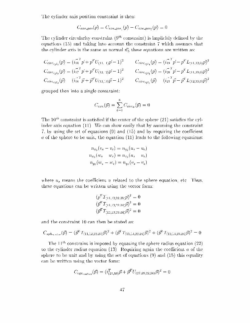
The cylinder axis position constraint is then:Caxe pos(~p) = Caxe pos1(~p) + Caxe pos2(~p) = 0The cylinder circularity constraint (9th constraint) is implicitly de�ned by theequations (15) and taking into account the constraint 7 which assumes thatthe cylinder axis is the same as normal ~n5 these equations are written as:Ccirccyl1(~p) = ( ~i16T~p+ ~pTU(11;11)~p� 1)2Ccirccyl2(~p) = ( ~i17T~p+ ~pTU(12;12)~p� 1)2Ccirccyl3(~p) = ( ~i18T~p+ ~pTU(13;13)~p� 1)2 Ccirccyl4(~p) = ( ~i19T ~p+ ~pTL(11;12;0)~p)2Ccirccyl5(~p) = ( ~i20T ~p+ ~pTL(11;13;0)~p)2Ccirccyl6(~p) = ( ~i21T ~p+ ~pTL(12;13;0)~p)2grouped then into a single constraint:Ccirc(~p) = 6Xk=1Ccirck(~p) = 0The 10th constraint is satis�ed if the center of the sphere (21) satis�es the cyl-inder axis equation (11). We can show easily that by assuming the constraint7, by using the set of equations (9) and (15) and by requiring the coe�cienta of the sphere to be unit, the equation (11) leads to the following equations:nx5(vs � vc) = ny5(us � uc)nx5(ws � wc) = nz5(us � uc)ny5(ws � wc) = ny5(vs � vc)where us means the coe�cient u related to the sphere equation, etc. Thus,these equations can be written using the vector form:(~pTT(11;12;22;23)~p)2 = 0(~pTT(11;13;22;24)~p)2 = 0(~pTT(12;13;23;24)~p)2 = 0and the constraint 10 can then be stated as:Csphcenter(~p) = (~pTT(11;12;22;23)~p)2 + (~pTT(11;13;22;24)~p)2 + (~pTT(12;13;23;24)~p)2 = 0The 11th constraint is imposed by equating the sphere radius equation (22)to the cylinder radius equation (13). Requiring again the coe�cient a of thesphere to be unit and by using the set of equations (9) and (15) this equalitycan be written using the vector form:Cequradius(~p) = (~iT(25;30)~p+ ~pTU(27;29;22;24)~p)2 = 047

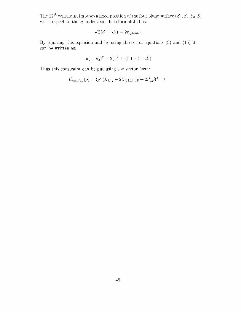
The 12th constraint imposes a �xed position of the four plane surfaces S1; S2; S3; S4with respect to the cylinder axis. It is formulated as:p2(d1 + d3) = 2rcylinderBy squaring this equation and by using the set of equations (9) and (15) itcan be written as: (d1 + d3)2 = 2(u2c + v2c + w2c � d2c)Thus this constraint can be put using the vector form:Cmedian(~p) = (~pT (I(4;1) � 2U(22;24))~p+ 2~iT25~p)2 = 0

48

Appendix 3: Levenberg-Marquadt algorithmHere are the main steps of the Levenberg-Marquardt algorithm applied to asimple optimization function:E(~p) = F (~p) + C(~p)� = �0 % initializationEdecrease = big valuewhile Edecrease > � % a thresholdDo GE=Grad(E(~p) = @@~p(E(~p))Loop: HE=Hessian(E(~p)) = @2@2~p(E(~p))HE = HE + �(diag(HE))solve HE ~�p = �GE~pupdated = ~p+ ~�pEdecrease = E(~pupdated)� E(~p)if Edecrease > 0increase �go to Loopelse ~p = ~pupdateddecrease �end ifend whileHere a simple example of an optimization function and its derivatives:E(~p) = F (~p) + C(~p)F (~p) = ~pTH~p the least squares functionC(~p) = �(~pTA~p� 1)2 the weighted constraint functionGE = 2H~p+ 4�A~p(~pTA~p� 1)HE = 2H + �[4(~pTA~p� 1)AT + 8(A~p)(A~p)T ]From this example we can notice the usefulness of the matrix formulation: theoptimization function is compact, its derivatives are easy to compute usingelementary matrix algebra rules and all the data terms are encapsulated intoH (which needs to be calculated only once).49

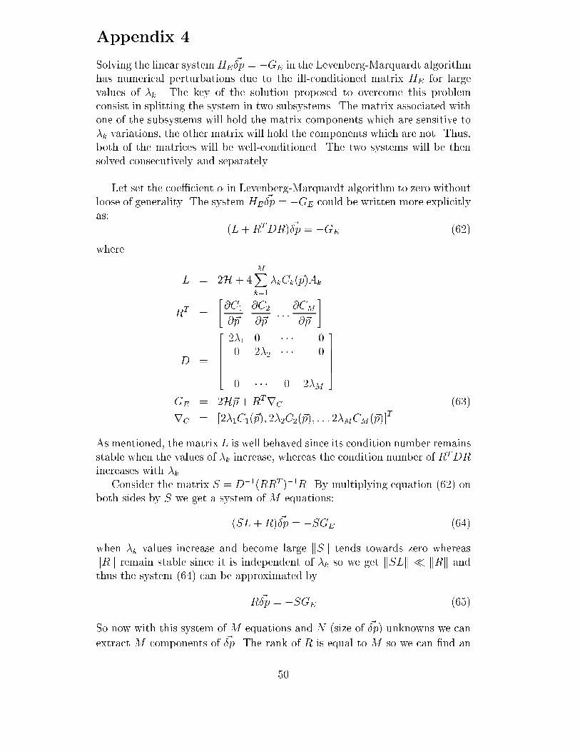
Appendix 4Solving the linear systemHE ~�p = �GE in the Levenberg-Marquardt algorithmhas numerical perturbations due to the ill-conditioned matrix HE for largevalues of �k. The key of the solution proposed to overcome this problemconsist in splitting the system in two subsystems. The matrix associated withone of the subsystems will hold the matrix components which are sensitive to�k variations, the other matrix will hold the components which are not. Thus,both of the matrices will be well-conditioned. The two systems will be thensolved consecutively and separately.Let set the coe�cient � in Levenberg-Marquardt algorithm to zero withoutloose of generality. The system HE ~�p = �GE could be written more explicitlyas: (L+RTDR) ~�p = �GE (62)where L = 2H + 4 MXk=1�kCk(~p)AkRT = "@C1@~p @C2@~p : : : @CM@~p #D = 266664 2�1 0 � � � 00 2�2 � � � 0... ... ... ...0 � � � 0 2�M 377775GE = 2H~p+RTrC (63)rC = [2�1C1(~p); 2�2C2(~p); : : : 2�MCM(~p)]TAs mentioned, the matrix L is well behaved since its condition number remainsstable when the values of �k increase, whereas the condition number of RTDRincreases with �k.Consider the matrix S = D�1(RRT )�1R. By multiplying equation (62) onboth sides by S we get a system of M equations:(SL+R) ~�p = �SGE (64)when �k values increase and become large kSk tends towards zero whereaskRk remain stable since it is independent of �k so we get kSLk � kRk andthus the system (64) can be approximated byR~�p = �SGE (65)So now with this system of M equations and N (size of ~�p) unknowns we canextract M components of ~�p. The rank of R is equal to M so we can �nd an50

orthogonal matrix Q such: QRT = " U[0] # (66)where U is an (M;M) upper triangular non-singular matrix.Since QQT = I, (65) can be written asRQTQ~�p = �SGE (67)By splitting Q~�p into [ ~�z1; ~�z2] where ~�z1 and ~�z2 have a size of respectivelyM and N �M we get from (67)UT ~�z1 = �SGE (68)and then ~�z1 could be deduced from this equation. Now it remains to compute� ~z2.Consider the matrix V whose columns are the basis of the null space of R.We have RV = [0]. By multiplying (62) by V T we get:V TL~�p = �V TGE (69)Now since RV = RQTQV = [0] by using (66) and splitting QV into [JT1 ; JT2 ]T ,where J1 and J2 are respectively (M;M) and (N �M;M) matrices we get[UT ; [0]T ] " J1J2 # = [0]This implies that J1 = [0] since U is non singular and J2 could be set to anarbitrarily value say I. Then we can set QV = [[0]T ; IT ]TThe system (69) can be written:V TQTQLQTQ~�p = �V TGE(QV )T (QLQT )Q~�p = �V TGEh[0]T ; IT iQLQT " ~�z1~�z2 # = �V TGEIf we denote the matrix QLQT by W such as: W = " W11 W12W21 W22 #we get: [[0]T ; IT ] " W11 W12W21 W22 # " ~�z1~�z2 # = �V TGEfrom which we extract the systemW22 ~�z2 = �V TGE �W21 ~�z1 (70)and �z2 can be then computed. 51

The computation of the term SGE in (68) is expensive. Practically it isfaster to use a simpli�ed expression. From (63) we getSGE = D�1(RRT )�1R(2H~p+RTrC) (71)= D�1(2(RRT )�1RH~p+rC)= D�1(2(RQTQRT )�1RQTQH~p+rC)= D�1(2[U�1; [0]]QH~p +rC)By splitting QH~p into [~l1T ; ~l2T ]T where ~l1 and ~l2 have respectively sizes ofM and N �M we get SGE = D�1(2U�1~l1 +rC) (72)and ~�z1 can be then computed with:UT ~�z1 = �D�1(2U�1~l1 +rC) (73)Similarly the expression of V TGE in (70) can be simpli�ed :V TGE = V T (2H~p+RTrC) (74)= 2V TH~p; since RV = [0]= 2V TQTQH~p= 2[[0]T ; IT ] " ~l1~l2 #= 2~l2and the computation of �z2 is the performed with the following systemW22 ~�z2 = �2~l2 �W21 ~�z1 (75)Once ~�z2 and ~�z1 are computed the ~�p vector is deduced with~�p = QT �z (76)To recapitulate, the resolution of the equationHE ~�p = �GE in the Levenberg-Marquardt algorithm has to be performed through the following steps :1) Compute D, rC , R.2) Compute Q and U from R using elementary geometric transformation (e.g.Householder transformation [29](p.224)).3) Compute QH~p and extract ~l1T and ~l2.4) Compute ~�z1 from (73).5) Compute W = QLQT and extract W22 and W21.6) Compute ~�z2 from (75).7) Compute ~�p from (76). 52

List of Tables1 Relationships between features. . . . . . . . . . . . . . . . . . . . . 542 Improvement in shape and placement parameters with and without con-straints from data from single view of the half cylinder object. . . . . . 553 Improvement in shape and placement parameters with and without con-straints from data merged from two views of the half cylinder object. . . 554 The surface's relative angle estimation with and without constraints. . . 565 The cylinder characteristic estimates with and without constraints. . . . 566 The cone characteristic estimates with and without constraints. . . . . 567 Improvement of non-constrained angle estimates. . . . . . . . . . . . 568 mean estimates of S1 and S3 normal and LS error in the two type ofsolutions. . . . . . . . . . . . . . . . . . . . . . . . . . . . . . . 579 comparison of the estimation without median constraints with previousresults. . . . . . . . . . . . . . . . . . . . . . . . . . . . . . . . 5710 The object characteristic estimates for invalid constraints and true con-straints (last row). . . . . . . . . . . . . . . . . . . . . . . . . . . 5811 Improvement of the prism characteristic estimates. . . . . . . . . . . 5912 Improvement of the cylinder characteristic estimates. . . . . . . . . . 5913 Improvement of the sphere characteristic estimates. . . . . . . . . . . 59

53

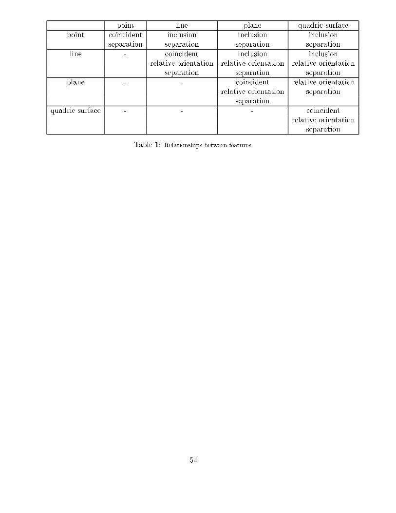
point line plane quadric surfacepoint coincident inclusion inclusion inclusionseparation separation separation separationline - coincident inclusion inclusionrelative orientation relative orientation relative orientationseparation separation separationplane - - coincident relative orientationrelative orientation separationseparationquadric surface - - - coincidentrelative orientationseparationTable 1: Relationships between features.

54

view2 angle(S1; S2)(degree) distance(Xo; S2)(mm) radius(mm)without constraints 90.84 6.32 26.98with constraints 90:00� 2 0:00� 29.68actual values 90 0 30Table 2: Improvement in shape and placement parameters with and without constraints from datafrom single view of the half cylinder object.registered view1 and view2 angle(S1; S2)(degree) distance(Xo; S2)(mm) radius(mm)without constraints 89.28 2.23 30.81with constraints 90:00� 0:00� 30.06actual values 90 0 30Table 3: Improvement in shape and placement parameters with and without constraints from datamerged from two views of the half cylinder object.

2* means that the estimated value has been constrained to be the true value55

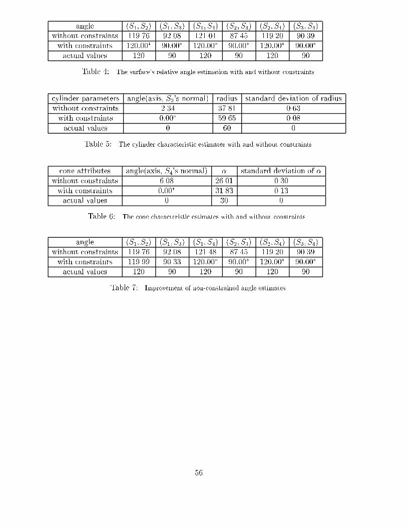
angle (S1; S2) (S1; S3) (S1; S4) (S2; S3) (S2; S4) (S3; S4)without constraints 119.76 92.08 121.01 87.45 119.20 90.39with constraints 120:00� 90:00� 120:00� 90:00� 120:00� 90:00�actual values 120 90 120 90 120 90Table 4: The surface's relative angle estimation with and without constraints.cylinder parameters angle(axis, S3's normal) radius standard deviation of radiuswithout constraints 2.34 37.81 0.63with constraints 0:00� 59.65 0.08actual values 0 60 0Table 5: The cylinder characteristic estimates with and without constraints.cone attributes angle(axis, S4's normal) � standard deviation of �without constraints 6.08 26.01 0.30with constraints 0:00� 31.83 0.13actual values 0 30 0Table 6: The cone characteristic estimates with and without constraints.angle (S1; S2) (S1; S3) (S1; S4) (S2; S3) (S2; S4) (S3; S4)without constraints 119.76 92.08 121.48 87.45 119.20 90.39with constraints 119.99 90.33 120:00� 90:00� 120:00� 90:00�actual values 120 90 120 90 120 90Table 7: Improvement of non-constrained angle estimates.

56

~ni ~n1 ~n3 angle( ~n1; ~n3) (degree) LS error1st case 0:53160:67330:5139 - - - 9.072nd case - 0:53160:67330:5139 0:53160:67330:5139 0.00 9.06Table 8: mean estimates of S1 and S3 normal and LS error in the two type of solutions.distance(S1; S3) distance(S2; S4) diagonal of S5 cylinder radiuswithout constraints { { { 14.64with all constraints 21.17 21.17 29.94 14.97without median constraint 21.15 21.15 29.91 14.97actual values 21.28 21.28 30.02 15.01Table 9: comparison of the estimation without median constraints with previous results.

57

~n1 ~n2 ~n5 Rcyl Rsph axecyl Centersph( ~n1; ~n2) = �=3 �0:61�0:47�0:62 �0:580:52�0:62 0:72�0:02�0:69 14.97 14.97 0:72�0:02�0:69 86:30�87:3817:44( ~n1; ~n5) = �=3 �0:08�0:60�0:78 �0:460:72�0:50 0:72�0:02�0:69 14.97 14.97 0:72�0:02�0:69 86:31�87:4117:44( ~n1; ~n5) = �=3( ~n2; ~n5) = �=3 �0:02�0:68�0:72 0:050:72�0:68 0:72�0:02�0:69 14.97 14.97 0:72�0:02�0:69 86:31�87:4217:44true constraints �0:52�0:67�0:51 �0:450:73�0:50 0:72�0:02�0:69 14.97 14.97 0:72�0:02�0:69 86:30�87:3817:44Table 10: The object characteristic estimates for invalid constraints and true constraints (last row).

58

distance(S1; S3) distance(S2; S4) diagonal of S5with constraints 21.17 21.17 29.95standard deviation/mean 0.03 % 0.03% 0.03%actual values 21.28 21.28 30.02Table 11: Improvement of the prism characteristic estimates.cylinder parameters angle(axis, S5's normal) radius (mm) �/mean (radius)without constraints 1.55 14.64 0.12%with constraints 0:00� 14.97 0.03 %actual values 0 15.01 0Table 12: Improvement of the cylinder characteristic estimates.sphere parameters distance(center, cylinder axis) radius (mm) �/mean (radius)without constraints 1.36 16.02 0.11%with constraints 0:00� 14.97 0.03 %actual values 0 15.01 0Table 13: Improvement of the sphere characteristic estimates.

59

List of Figures1 A slot with two parallel planes orthogonal to a third plane. . . 622 (a): optim1 - batch constraint optimization algorithm. (b): optim2 -sequential constraint introduction optimization algorithm. . . . . . . . 633 (a): The two edges E1 and E2 belongs to the same in�nite line. The twofaces P1 and P2 lie in the same in�nite plane. (b) The centres of the circlesCir1 and Cir2 coincide at the same point C. The cylinders Cyl1 and Cyl2have a common axis. . . . . . . . . . . . . . . . . . . . . . . . . 644 (a): The axis of the cylinder patch Cyl is included in the plane P . (b)The line associated with the edge E is included in the cylinder Cyl. . . . 655 (a): Each pair of planes (P1; P2; P3) makes an angle of 90o, the axis of thecylinder Cyl is orthogonal to P1. (b): The planes (P1; P2) are separatedby distance d. (c): Each pair of parallel planes of the hexagonal prism isseparated by the same distance. . . . . . . . . . . . . . . . . . . . . 666 (a): The step model object. (b): variation of the unit constraint error asa function of the related �. (c): Variation of the angle constraint error (~n1; ~n2) as a function of the related �. (d): error of the estimated orient-ation of the normal ~n1 (the error is represented by the angle between theestimated normal and the actual one). . . . . . . . . . . . . . . . . 677 Variation of the angle constraint value Cangle1 (50) at the four steps ofthe algorithm. Step1 (a) : Only the unit constraints are considered inthe optimization function (see (52)). Step2 (b) : the angle constraintfunction Cangle1 is added to the optimization function (see (53)). Step3(c): addition of the constraint function Cangle2 and Step4 (d): addition ofthe constraint function Cangle3 . . . . . . . . . . . . . . . . . . . . 688 Variation of the angle constraint value Cangle2 (50) at the four steps ofthe algorithm optim2. . . . . . . . . . . . . . . . . . . . . . . . 699 Variation of the angle constraint value Cangle3 (51) at the four steps ofthe algorithm optim2. . . . . . . . . . . . . . . . . . . . . . . . 7010 Variation of the orientation error in the estimation of ( ~n1) at the foursteps of the algorithm optim2. . . . . . . . . . . . . . . . . . . . . 7111 A top view of the tetrahedron and the extracted surfaces. . . . . . . 7212 (a): Decrease of the unit constraint function (54) with respect to �1.(b): Decrease of the angle constraint function (57) with respect to �2. (c)and (d) variation of the objective function ~pTH~p and the sum of all theconstraint functions C(~p) =P3l=1 Unitl(~p)+P4l=2 Anglel�1(~p) during theoptimization. These functions are mapped in function of �2 just to showtheir evolution all along the optimization process but they do not dependspeci�cally on �2. . . . . . . . . . . . . . . . . . . . . . . . . . . 7313 Two views of the half cylinder and the extracted surfaces. . . . . . . 7414 Shape Optimization of the half cylinder object. (a),(b),(c),(d): decreaseof the di�erent constraints with respect to the related �. (e),(f): variationof least squares function and the constraint function. . . . . . . . . . . 7515 Four views of the multi-quadric object 1. . . . . . . . . . . . 7660

16 Shape optimization of multi-quadric object 1. a,b,c,d : Decrease of thedi�erent constraint functions with respect to the associated �k. e,f : Vari-ation of least squares error and the sum of all the constraint values duringthe optimization. . . . . . . . . . . . . . . . . . . . . . . . . . . 7717 Four views of the multi-quadric object 2. . . . . . . . . . . . 7818 (a): maximum (+) and minimum (o) value for each parameter scaled bythe absolute value of the mean. (b): relative standard deviation of theparameters. . . . . . . . . . . . . . . . . . . . . . . . . . . . . 7919 distribution of the least squares errors. . . . . . . . . . . . . . . . . 8020 (a): distribution of the estimation di�erence. (b): distribution of the LSresiduals di�erence. . . . . . . . . . . . . . . . . . . . . . . . . . 8121 (a):Constraint error function and least squares error function function forvalid constraints. (b):Constraint error and least squares error function forinvalid constraints (3rd test). . . . . . . . . . . . . . . . . . . . . . 8222 Results for inconsistent constraints (a): The sum of the angle constraints'errors. (b): the sum of all the constraint functions. (c) the least squreserror. . . . . . . . . . . . . . . . . . . . . . . . . . . . . . . . . 83

61

d

S1

S3

n3

n2

S2

n1

Figure 1: A slot with two parallel planes orthogonal to a third plane.Computer-Aided DesignNaoufel Werghi, Robert Fisher, Craig Robertson and Anthony Ashbrook

62

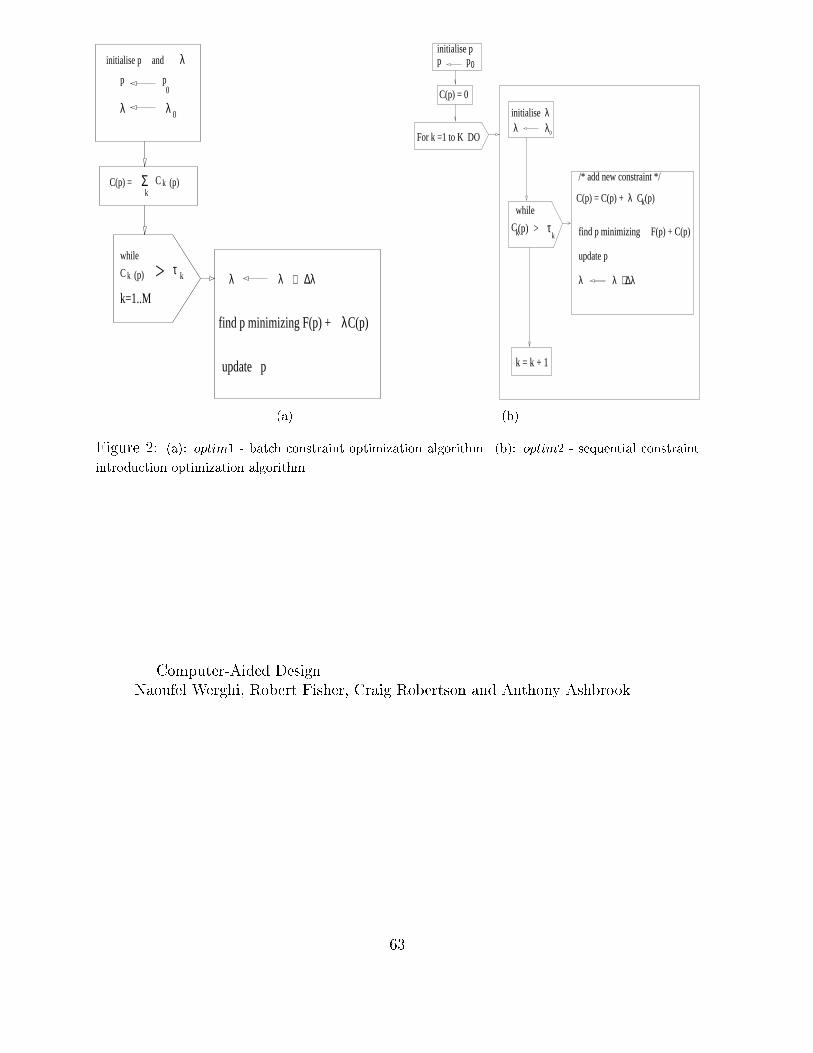
k (p)C

λ initialise p and

p0

p

λ λ 0

k (p)CΣk

C(p) =

find p minimizing F(p) + C(p) λ

kτ> λ λ + ∆λ

while

k=1..M

update p

0λ λ

τk

λ + ∆λλ

C(p) = C(p) + λ C (p) k

(p) >

C(p) = 0

initialise pp p0

For k =1 to K DO

λ initialise

while

Ck

update p

find p minimizing F(p) + C(p)

/* add new constraint */

k = k + 1 (a) (b)Figure 2: (a): optim1 - batch constraint optimization algorithm. (b): optim2 - sequential constraintintroduction optimization algorithm.

Computer-Aided DesignNaoufel Werghi, Robert Fisher, Craig Robertson and Anthony Ashbrook

63

E E

P

1

1

2

2P+

Cyl

Cyl

CirCir

C

D

2

1

12

(a)

(b)Figure 3: (a): The two edges E1 and E2 belongs to the same in�nite line. The two faces P1 and P2 liein the same in�nite plane. (b) The centres of the circles Cir1 and Cir2 coincide at the same point C.The cylinders Cyl1 and Cyl2 have a common axis.

Computer-Aided DesignNaoufel Werghi, Robert Fisher, Craig Robertson and Anthony Ashbrook

64

P

axecyl

CylCyl

E

(a)(b)Figure 4: (a): The axis of the cylinder patch Cyl is included in the plane P . (b) The line associatedwith the edge E is included in the cylinder Cyl.

Computer-Aided DesignNaoufel Werghi, Robert Fisher, Craig Robertson and Anthony Ashbrook

65

PP

P

Cyl

1

2 3

P

P

1

d

2

P

P P

P

PP1

2

3 4

5

6

(a) (b) (c)

d

Figure 5: (a): Each pair of planes (P1; P2; P3) makes an angle of 90o, the axis of the cylinder Cyl isorthogonal to P1. (b): The planes (P1; P2) are separated by distance d. (c): Each pair of parallel planesof the hexagonal prism is separated by the same distance.

Computer-Aided DesignNaoufel Werghi, Robert Fisher, Craig Robertson and Anthony Ashbrook

66

S1

S4S2

S3

S57 8 9 10 11 12 13

−14

−12

−10

−8

−6

−4

−2

log10

(λ1 )

log 10

(C_u

nit_

1)

unit constraint n1

(a) (b)

7 8 9 10 11 12 13−15

−10

−5

log10

(λ3 )

log 10

(C_a

ngle

_2)

angle constraint (n1,n

5)

7 8 9 10 11 12 13−1.3

−1.2

−1.1

−1

−0.9

−0.8

−0.7

−0.6

log10

(λ1 )

log 10

(ang

le(n

1,n1 ex

act)

n1 estimation error

(c) (d)Figure 6: (a): The step model object. (b): variation of the unit constraint error as a function of therelated �. (c): Variation of the angle constraint error ( ~n1; ~n2) as a function of the related �. (d): error ofthe estimated orientation of the normal ~n1 (the error is represented by the angle between the estimatednormal and the actual one).Computer-Aided DesignNaoufel Werghi, Robert Fisher, Craig Robertson and Anthony Ashbrook

67

7 8 9 10 11 12 13−4.7

−4.65

−4.6

−4.55

−4.5

−4.45

log10

(λ1 )

log 10

( C_a

ngle

_1 )

step1: addition of the unit constraints

7 8 9 10 11 12 13−15

−10

−5

log10

(λ2 )

log 10

( C_a

ngle

_1 )

step2: addition of the angle constraint (n1,n2)

(a) (b)

7 8 9 10 11 12 13−14.485

−14.484

−14.483

−14.482

−14.481

−14.48

−14.479

log10

(λ3 )

log 10

( C_a

ngle

_1 )

step3: addition of the angle constraint (n1,n5)

7 8 9 10 11 12 13−14.4862

−14.4861

−14.486

−14.4859

−14.4858

−14.4857

−14.4856

−14.4855

−14.4854

−14.4853

log10

(λ4 )

10

step4: addition of the angle constraint (n2,n5)

(c) (d)Figure 7: Variation of the angle constraint value Cangle1 (50) at the four steps of the algorithm. Step1(a) : Only the unit constraints are considered in the optimization function (see (52)). Step2 (b) : theangle constraint function Cangle1 is added to the optimization function (see (53)). Step3 (c): addition ofthe constraint function Cangle2 and Step4 (d): addition of the constraint function Cangle3 .Computer-Aided DesignNaoufel Werghi, Robert Fisher, Craig Robertson and Anthony Ashbrook

68

7 8 9 10 11 12 13−4.7

−4.65

−4.6

−4.55

−4.5

−4.45

−4.4

log10

(λ1 )

log 10

( C_a

ngle

_2 )

step1: addition of the unit constraints

7 8 9 10 11 12 13−4.457

−4.4565

−4.456

−4.4555

−4.455

−4.4545

−4.454

−4.4535

−4.453

log10

(λ2 )

log 10

( C_a

ngle

_2 )

step2: addition of the angle constraint (n1,n2)

(a) (b)

7 8 9 10 11 12 13−16

−14

−12

−10

−8

−6

−4

log10

(λ3 )

log 10

( C_a

ngle

_2 )

step3: addition of the angle constraint (n1,n5)

7 8 9 10 11 12 13−14.365

−14.36

−14.355

−14.35

−14.345

−14.34

−14.335

log10

(λ4 )

log 10

( C_a

ngle

_2 )

step4: addition of the angle constraint (n2,n5)

(c) (d)Figure 8: Variation of the angle constraint value Cangle2 (50) at the four steps of the algorithm optim2.Computer-Aided DesignNaoufel Werghi, Robert Fisher, Craig Robertson and Anthony AshbrookComputer-Aided Design 69

7 8 9 10 11 12 13−4.75

−4.7

−4.65

−4.6

−4.55

−4.5

−4.45

−4.4

log10

(λ1 )

log 10

( C_a

ngle

_3 )

step1: addition of the unit constraints

7 8 9 10 11 12 13−4.4343

−4.4342

−4.4341

−4.434

−4.4339

−4.4338

−4.4337

−4.4336

−4.4335

log10

(λ2 )

log 10

( C_a

ngle

_3 )

step2: addition of the angle constraint (n1,n2)

(a) (b)

7 8 9 10 11 12 13−4.452

−4.45

−4.448

−4.446

−4.444

−4.442

−4.44

log10

(λ3 )

log 10

( C_a

ngle

_3 )

step3: addition of the angle constraint (n1,n5)

7 8 9 10 11 12 13−14

−12

−10

−8

−6

−4

log10

(λ4 )

log 10

( C_a

ngle

_3 )

step4: addition of the angle constraint (n2,n5)

(c) (d)Figure 9: Variation of the angle constraint value Cangle3 (51) at the four steps of the algorithm optim2.Naoufel Werghi, Robert Fisher, Craig Robertson and Anthony Ashbrook

70

7 8 9 10 11 12 13−0.4248

−0.4248

−0.4248

−0.4248

−0.4248

−0.4248

log10

(λ1 )

log 10

(ang

le(n

1,n1 ex

act)

step1: addition of the unit constraints

7 8 9 10 11 12 13−0.52

−0.515

−0.51

−0.505

−0.5

−0.495

−0.49

−0.485

log10

(λ2 )

log 10

(ang

le(n

1,n1 ex

act)

step2: addition of the angle constraint (n1,n2)

(a) (b)

7 8 9 10 11 12 13−1.3

−1.2

−1.1

−1

−0.9

−0.8

−0.7

−0.6

log10

(λ3 )

log 10

(ang

le(n

1,n1 ex

act)

step3: addition of the angle constraint (n1,n5)

7 8 9 10 11 12 13−1.21

−1.205

−1.2

−1.195

−1.19

−1.185

log10

(λ4 )

log 10

(ang

le(n

1,n1 ex

act)

step4: addition of the angle constraint (n2,n5)

(c) (d)Figure 10: Variation of the orientation error in the estimation of ( ~n1) at the four steps of the algorithmoptim2.Computer-Aided DesignNaoufel Werghi, Robert Fisher, Craig Robertson and Anthony Ashbrook

71

S1

S2

S3

TetrahedronFigure 11: A top view of the tetrahedron and the extracted surfaces.

Computer-Aided DesignNaoufel Werghi, Robert Fisher, Craig Robertson and Anthony Ashbrook

72

4 5 6 7 8 9 10 11−9

−8

−7

−6

−5

−4

−3

log10

(λ1 )

log 10

( C_u

nit_

1 )

unit constraint 1

4 5 6 7 8 9 10 11−6

−5

−4

−3

−2

−1

0

log10

(λ2 )

log 10

( C_a

ngle

_1 )

angle constraint 1

(a) (b)

4 5 6 7 8 9 10 111.4

1.5

1.6

1.7

1.8

1.9

2

2.1

log10

(λ2 )

log 10

(Lea

st s

quar

es e

rror

func

tion)

least squares error function

4 5 6 7 8 9 10 11−3.5

−3

−2.5

−2

−1.5

−1

−0.5

0

0.5

1

1.5

log10

(λ2 )

log 10

( C(p

) )

sum of the constraint functions

(c) (d)Figure 12: (a): Decrease of the unit constraint function (54) with respect to �1. (b): Decrease ofthe angle constraint function (57) with respect to �2. (c) and (d) variation of the objective function~pTH~p and the sum of all the constraint functions C(~p) =P3l=1 Unitl(~p) +P4l=2 Anglel�1(~p) during theoptimization. These functions are mapped in function of �2 just to show their evolution all along theoptimization process but they do not depend speci�cally on �2.Computer-Aided DesignNaoufel Werghi, Robert Fisher, Craig Robertson and Anthony Ashbrook

73

half cylinderS3

1

2

n

nn

S2

S1

(a) (b) (c)Figure 13: Two views of the half cylinder and the extracted surfaces.

Computer-Aided DesignNaoufel Werghi, Robert Fisher, Craig Robertson and Anthony Ashbrook

74

8 9 10 11 12 13 14−20

−18

−16

−14

−12

−10

−8

log10

(λ2 )

log 10

( C_a

ng )

angle constraint

8 9 10 11 12 13 14−12

−11

−10

−9

−8

−7

−6

−5

log10

(λ1 )

log 10

( C_u

nit )

unit constraint

(a): Cang (b):Cunit

8 9 10 11 12 13 14−22

−20

−18

−16

−14

−12

−10

log10

(λ3 )

log 10

( C_a

xe )

cylinder axis constraint

8 9 10 11 12 13 14−14

−13

−12

−11

−10

−9

−8

−7

−6

−5

log10

(λ4 )

log 10

( C_c

irc )

cylinder circularity constraint

(c): Caxe (d): Ccirc

8 9 10 11 12 13 145.2

5.3

5.4

5.5

5.6

5.7

5.8

5.9

log10

(λ2 )

log 10

(ls fu

nctio

n)

ls function

8 9 10 11 12 13 14−12

−11

−10

−9

−8

−7

−6

−5

−4

log10

(λ2 )

log 10

( sum

of t

he c

onst

rain

t fun

ctio

ns) sum of the constraint functions

(e): LS error (f):PConstraint(~p)Figure 14: Shape Optimization of the half cylinder object. (a),(b),(c),(d): decrease of the di�erentconstraints with respect to the related �. (e),(f): variation of least squares function and the constraintfunction. 75

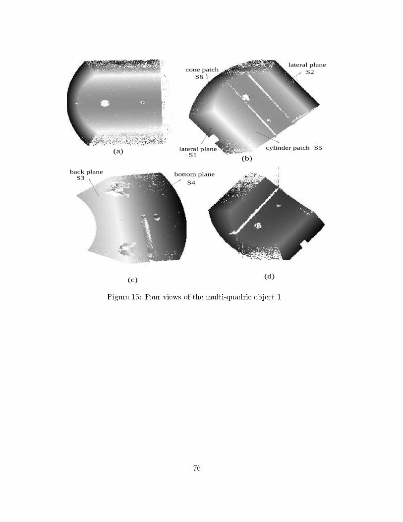
(a)(b)

(c) (d)

lateral plane

S1cylinder patch

S2cone patch

S5

S6

back planeS3

bottom plane

S4

lateral plane

Figure 15: Four views of the multi-quadric object 1.

76

8 9 10 11 12 13 14 15−16

−14

−12

−10

−8

−6

−4

log10

(λ2 )

log 10

( C_a

ng )

angle constraint

8 9 10 11 12 13 14 15−14

−13

−12

−11

−10

−9

−8

−7

−6

−5

log10

(λ1 )

log 10

( C_u

nit )

unit constraint

(a) (b)

8 9 10 11 12 13 14 15−14

−12

−10

−8

−6

−4

−2

log10

(λ3 )

log 10

( C_c

irc_c

yl )

cylinder circularity constraint

8 9 10 11 12 13 14 15−16

−14

−12

−10

−8

−6

−4

log10

(λ4 )

log 10

(C_c

irc_c

onex

)

cone circularity constraint

(c) (d)

8 9 10 11 12 13 14 157.075

7.08

7.085

7.09

7.095

log10

(λ2 )

log 10

( F(p

) )

objective function

8 9 10 11 12 13 14 15−14

−12

−10

−8

−6

−4

−2

log10

(λ2 )

log 10

Sum

(C(p

))

sum of the constraint functions

(e) (f)Figure 16: Shape optimization of multi-quadric object 1. a,b,c,d : Decrease of the di�erent constraintfunctions with respect to the associated �k . e,f : Variation of least squares error and the sum of all theconstraint values during the optimization.77

plane S1

plane S2plane S5 plane S6

plane S3

plane S4 sphere patch S8

cylinder patch S7

Figure 17: Four views of the multi-quadric object 2.

78

0 5 10 15 20 25 300.95

1

1.05

parameters

sca

led

ma

x a

nd

min

0 5 10 15 20 25 300

0.5

1

1.5

2

parameters

sta

nd

ard

de

via

tio

n (

%)

(a) (b)Figure 18: (a): maximum (+) and minimum (o) value for each parameter scaled by the absolute valueof the mean. (b): relative standard deviation of the parameters.Computer-Aided DesignNaoufel Werghi, Robert Fisher, Craig Robertson and Anthony Ashbrook

79

7.5 8 8.5

x 105

0

5

10

15

LS error distributionFigure 19: distribution of the least squares errors.Computer-Aided DesignNaoufel Werghi, Robert Fisher, Craig Robertson and Anthony Ashbrook

80

−5 −4.8 −4.6 −4.4 −4.2 −4 −3.80

2

4

6

8

10

12

14

16

log10

(angle(nc,n ))

−5 −4.5 −4 −3.5 −30

2

4

6

8

10

12

14

log10

(|LSc − LS

i|/mean(LS

i))(a) (b)Figure 20: (a): distribution of the estimation di�erence. (b): distribution of the LS residuals di�erence.

Computer-Aided DesignNaoufel Werghi, Robert Fisher, Craig Robertson and Anthony Ashbrook

81

6 7 8 9 10 11 12 13−14

−12

−10

−8

−6

−4

−2

0

log10

(λ2 )

log

10(

sum

(C(p

)) )

sum of the constraint functions

6 7 8 9 10 11 12 136.14

6.15

6.16

6.17

6.18

6.19

6.2

log10

(λ2 )

log

10(|

lea

st s

qu

are

s e

rro

r|)

least squares function

(a)

6 7 8 9 10 11 12 13−12

−10

−8

−6

−4

−2

0

2

log10

(λ2 )

log

10(

sum

(C(p

)) )

sum of the constraint functions

6 7 8 9 10 11 12 136.22

6.24

6.26

6.28

6.3

6.32

6.34

6.36

6.38

6.4

log10

(λ2 )

log

10(|

lea

st s

qu

are

s e

rro

r|)

least squares function

(b)Figure 21: (a):Constraint error function and least squares error function function for valid constraints.(b):Constraint error and least squares error function for invalid constraints (3rd test).Computer-Aided DesignNaoufel Werghi, Robert Fisher, Craig Robertson and Anthony Ashbrook

82

6 7 8 9 10 11 12 13−0.5

−0.45

−0.4

−0.35

−0.3

−0.25

−0.2

−0.15

log10

(λ2 )

log

10(

C_

an

gl(p

) )

angle constraint function

6 7 8 9 10 11 12 13−0.4

−0.2

0

0.2

0.4

0.6

0.8

1

log10

(λ2 )

log

10(

su

m (

C(p

)) )

sum of the constraint functions

6 7 8 9 10 11 12 136.24

6.26

6.28

6.3

6.32

6.34

6.36

6.38

6.4

6.42

log10

(λ2 )

log

10(|

lea

st

sq

ua

res e

rro

r|)

least squares function

(a) (b) (c)Figure 22: Results for inconsistent constraints (a): The sum of the angle constraints' errors. (b): thesum of all the constraint functions. (c) the least squres error.Computer-Aided DesignNaoufel Werghi, Robert Fisher, Craig Robertson and Anthony Ashbrook

83