Object Identi�cation: A Bayesian Analysiswith Application to Tra�c Surveillance 1Timothy Huang and Stuart Russell 2Computer Science DivisionUniversity of California, Berkeley, CA 94720, USAAbstractObject identi�cation|the task of deciding that two observed objects are in factone and the same object|is a fundamental requirement for any situated agent thatreasons about individuals. Object identity, as represented by the equality operatorbetween two terms in predicate calculus, is essentially a �rst-order concept. Rawsensory observations, on the other hand, are essentially propositional|especiallywhen formulated as evidence in standard probability theory. This paper describespatterns of reasoning that allow identity sentences to be grounded in sensory obser-vations, thereby bridging the gap. We begin by de�ning a physical event space overwhich probabilities are de�ned. We then introduce an identity criterion, which se-lects those events that correspond to identity between observed objects. From this,we are able to compute the probability that any two objects are the same, given astream of observations of many objects. We show that the appearance probability,which de�nes how an object can be expected to appear at subsequent observationsgiven its current appearance, is a natural model for this type of reasoning. We applythe theory to the task of recognizing cars observed by cameras at widely separatedsites in a freeway network, with new heuristics to handle the inevitable complexityof matching large numbers of objects and with online learning of appearance prob-ability models. Despite extremely noisy observations, we are able to achieve highlevels of performance.Key words: Object identi�cation; Matching; Data association; Bayesian inference;Tra�c surveillance1 This work was sponsored by JPL's New Tra�c Sensor Technology program, byCalifornia PATH under MOU 152/214, and by ONR Contract N00014-97-1-0941.2 Now at the Department of Mathematics and Computer Science, Middlebury Col-lege, Middlebury, VT 05753.Preprint submitted to Elsevier Preprint 9 June 1998

1 IntroductionObject identi�cation|the task of deciding that two observed objects are infact one and the same object|is a fundamental requirement for any situatedagent that reasons about individuals. Our aim in this paper is to establish thepatterns of reasoning involved in object identi�cation. To avoid possibly emptytheorizing, we couple this investigation with a real application of economicsigni�cance: identi�cation of vehicles in freeway tra�c. Each re�nement of thetheoretical framework is illustrated in the context of this application. We beginwith a general introduction to the identi�cation task. Section 2 provides aBayesian foundation for computing the probability of identity. Section 3 showshow this probability can be expressed in terms of appearance probabilities,and Section 4 describes our implementation. Section 5 presents experimentalresults in the application domain. Related work is discussed in Section 6.1.1 Conceptual and theoretical issuesThe existence of individuals is central to our conceptualization of the world.While object recognition deals with assigning objects to categories, such as 1988Toyota Celicas or adult humans, object identi�cation deals with recognizingspeci�c individuals, such as one's car or one's spouse. One can have speci�crelations to individuals, such as ownership or marriage. Hence, it is oftenimportant to be fairly certain about the identity of the particular objects oneencounters.Formally speaking, identity is expressed by the equality operator of �rst-orderlogic. Having detected an object C in a parking lot, one might be interestedin whether C =MyCar. Because mistaken identity is always a possibility, thisbecomes a question of the probability of identity: what isP (C =MyCarj all available evidence)?There has been little work on this question in AI. 3 The approach we will take(Section 2) is the standard Bayesian approach: de�ne an event space, assign aprior, condition on the evidence, and identify the events corresponding to thetruth of the identity sentence. The key step is the last, and takes the form ofan identity criterion. Once we have a formula for the probability of identity,we must �nd a way to compute it in terms of quantities that are available3 In contrast, reasoning about category membership based on evidence is the canon-ical task for probabilistic inference. Proposing that MyCar is just a very smallcategory misses the point. 2

in the domain model. Section 3 shows that one natural quantity of interest isthe appearance probability. This quantity, which covers diverse domain-speci�cphenomena ranging from the e�ects of motion, pose, and lighting to changesof address of credit applicants, seems to be more natural and usable thanthe usual division into sensor and motion models, which require calibrationagainst ground truth.1.2 ApplicationThe authors are participants in Roadwatch, a major project aimed at theautomation of wide-area freeway tra�c surveillance and control [7]. Objectidenti�cation is required for two purposes: �rst, to measure link travel time|the actual time taken for tra�c to travel between two �xed points on thefreeway network; and second, to provide origin/destination (O/D) counts|the total number of vehicles traveling between any two points on the network ina given time interval. The sensors used in this project are video cameras placedon poles beside the freeway (Figure 1). The overall system design is shown inFigure 2. In addition to the real surveillance system, we also implemented acomplete microscopic freeway simulator capable of simulating several hundredvehicles in realistic tra�c patterns. The simulator includes virtual camerasthat can be placed anywhere on the freeway network and that transmit real-time streams of vehicle reports to the Tra�c Management Center (TMC). Thereported data can be corrupted by any desired level of noise. We found thesimulator to be an invaluable tool for designing and debugging the surveillancealgorithms.Obviously, a license-plate reader would render the vehicle identi�cation tasktrivial, but for political and technical reasons, this is not feasible. In fact, be-cause of very restricted communication bandwidth, the vehicle reports sent tothe TMC can contain only about one hundred bytes of information. In addi-tion, the measurements contained in the reports are extremely noisy, especiallyin rainy, foggy, and night-time conditions. Thus, with thousands of vehiclespassing each camera every hour, there may be many possible matches for eachvehicle. This leads to a combinatorial problem|�nding most likely consistentassignments between two large sets of vehicles|that is very similar to thatfaced in data association, a form of the object identi�cation problem arisingin radar and sonar tracking. Section 6 explores this connection in more detail.We adopt a solution from the data association literature, but also introducea new \leave-one-out" heuristic for selecting reliable matches. This, togetherwith a scheme for online learning of appearance models to handle changingviewing and tra�c conditions, yields a system with performance good enoughfor practical deployment (Section 5). 3

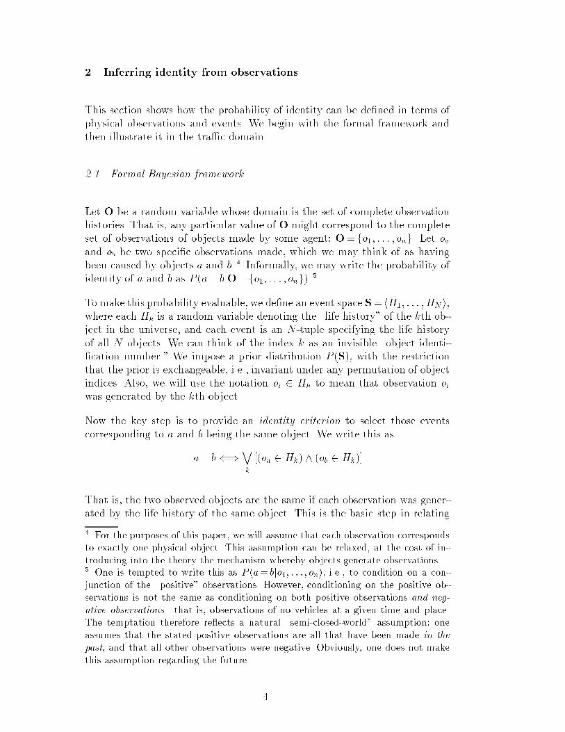
2 Inferring identity from observationsThis section shows how the probability of identity can be de�ned in terms ofphysical observations and events. We begin with the formal framework andthen illustrate it in the tra�c domain.2.1 Formal Bayesian frameworkLet O be a random variable whose domain is the set of complete observationhistories. That is, any particular value of O might correspond to the completeset of observations of objects made by some agent: O= fo1; : : : ; ong. Let oaand ob be two speci�c observations made, which we may think of as havingbeen caused by objects a and b. 4 Informally, we may write the probability ofidentity of a and b as P (a= bjO= fo1; : : : ; ong). 5To make this probability evaluable, we de�ne an event space S= hH1; : : : ;HN i,where each Hk is a random variable denoting the \life history" of the kth ob-ject in the universe, and each event is an N -tuple specifying the life historyof all N objects. We can think of the index k as an invisible \object identi-�cation number." We impose a prior distribution P (S), with the restrictionthat the prior is exchangeable, i.e., invariant under any permutation of objectindices. Also, we will use the notation oi 2 Hk to mean that observation oiwas generated by the kth object.Now the key step is to provide an identity criterion to select those eventscorresponding to a and b being the same object. We write this asa= b()_k [(oa 2 Hk) ^ (ob 2 Hk)]That is, the two observed objects are the same if each observation was gener-ated by the life history of the same object. This is the basic step in relating4 For the purposes of this paper, we will assume that each observation correspondsto exactly one physical object. This assumption can be relaxed, at the cost of in-troducing into the theory the mechanism whereby objects generate observations.5 One is tempted to write this as P (a= bjo1; : : : ; on), i.e., to condition on a con-junction of the \positive" observations. However, conditioning on the positive ob-servations is not the same as conditioning on both positive observations and neg-ative observations|that is, observations of no vehicles at a given time and place.The temptation therefore re ects a natural \semi-closed-world" assumption: oneassumes that the stated positive observations are all that have been made in thepast, and that all other observations were negative. Obviously, one does not makethis assumption regarding the future. 4

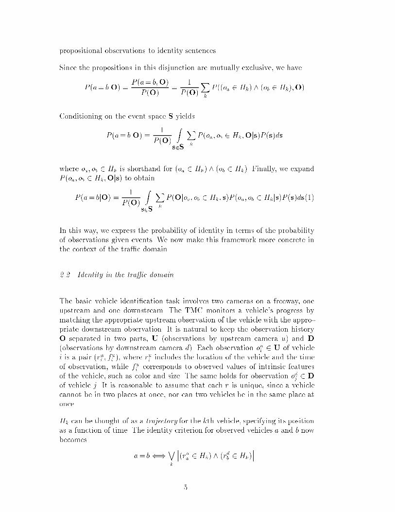
propositional observations to identity sentences.Since the propositions in this disjunction are mutually exclusive, we haveP (a= bjO) = P (a= b;O)P (O) = 1P (O)Xk P ((oa 2 Hk) ^ (ob 2 Hk);O)Conditioning on the event space S yieldsP (a= bjO) = 1P (O) Zs2S Xk P (oa; ob 2 Hk;Ojs)P (s)dswhere oa; ob 2 Hk is shorthand for (oa 2 Hk) ^ (ob 2 Hk). Finally, we expandP (oa; ob 2 Hk;Ojs) to obtainP (a= bjO) = 1P (O) Zs2S Xk P (Ojoa; ob 2 Hk; s)P (oa; ob 2 Hkjs)P (s)ds(1)In this way, we express the probability of identity in terms of the probabilityof observations given events. We now make this framework more concrete inthe context of the tra�c domain.2.2 Identity in the tra�c domainThe basic vehicle identi�cation task involves two cameras on a freeway, oneupstream and one downstream. The TMC monitors a vehicle's progress bymatching the appropriate upstream observation of the vehicle with the appro-priate downstream observation. It is natural to keep the observation historyO separated in two parts, U (observations by upstream camera u) and D(observations by downstream camera d). Each observation oui 2 U of vehiclei is a pair (rui ; fui ), where rui includes the location of the vehicle and the timeof observation, while fui corresponds to observed values of intrinsic featuresof the vehicle, such as color and size. The same holds for observation odj 2 Dof vehicle j. It is reasonable to assume that each r is unique, since a vehiclecannot be in two places at once, nor can two vehicles be in the same place atonce.Hk can be thought of as a trajectory for the kth vehicle, specifying its positionas a function of time. The identity criterion for observed vehicles a and b nowbecomes a= b()_k h(rua 2 Hk) ^ (rdb 2 Hk)i5

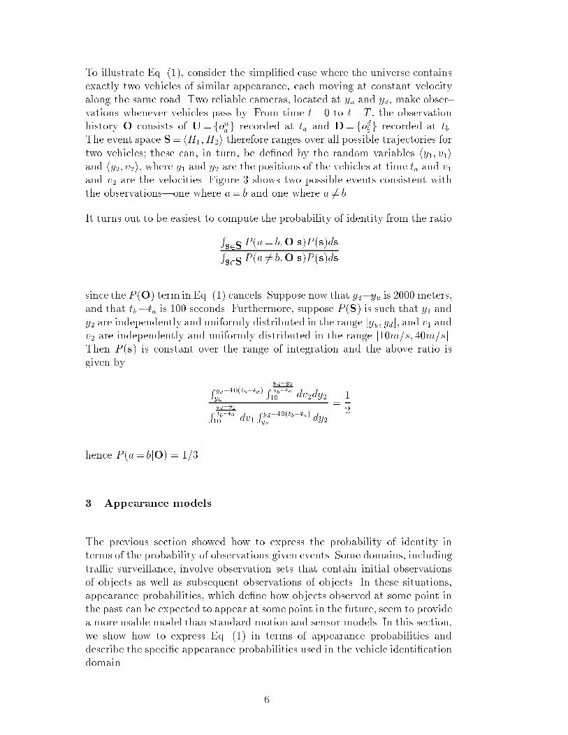
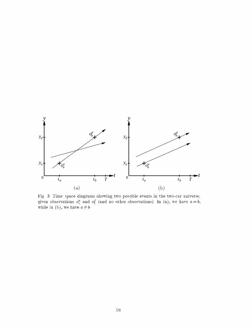
To illustrate Eq. (1), consider the simpli�ed case where the universe containsexactly two vehicles of similar appearance, each moving at constant velocityalong the same road. Two reliable cameras, located at yu and yd, make obser-vations whenever vehicles pass by. From time t=0 to t=T , the observationhistory O consists of U= fouag recorded at ta and D= fodbg recorded at tb.The event space S= hH1;H2i therefore ranges over all possible trajectories fortwo vehicles; these can, in turn, be de�ned by the random variables hy1; v1iand hy2; v2i, where y1 and y2 are the positions of the vehicles at time ta and v1and v2 are the velocities. Figure 3 shows two possible events consistent withthe observations|one where a= b and one where a 6= b.It turns out to be easiest to compute the probability of identity from the ratioRs2S P (a= b;Ojs)P (s)dsRs2S P (a 6= b;Ojs)P (s)dssince the P (O) term in Eq. (1) cancels. Suppose now that yd�yu is 2000 meters,and that tb� ta is 100 seconds. Furthermore, suppose P (S) is such that y1 andy2 are independently and uniformly distributed in the range [yu; yd], and v1 andv2 are independently and uniformly distributed in the range [10m=s; 40m=s].Then P (s) is constant over the range of integration and the above ratio isgiven by R yd�10(tb�ta)yu R yd�y2tb�ta10 dv2dy2R yd�y2tb�ta10 dv1 R yd�10(tb�ta)yu dy2 = 12hence P (a= bjO) = 1=3.3 Appearance modelsThe previous section showed how to express the probability of identity interms of the probability of observations given events. Some domains, includingtra�c surveillance, involve observation sets that contain initial observationsof objects as well as subsequent observations of objects. In these situations,appearance probabilities, which de�ne how objects observed at some point inthe past can be expected to appear at some point in the future, seem to providea more usable model than standard motion and sensor models. In this section,we show how to express Eq. (1) in terms of appearance probabilities anddescribe the speci�c appearance probabilities used in the vehicle identi�cationdomain. 6

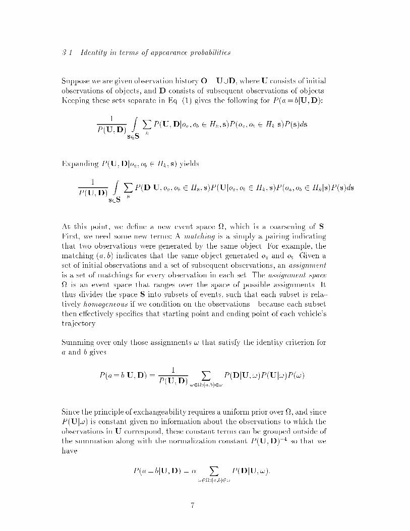
3.1 Identity in terms of appearance probabilitiesSuppose we are given observation historyO=U[D, whereU consists of initialobservations of objects, and D consists of subsequent observations of objects.Keeping these sets separate in Eq. (1) gives the following for P (a= bjU;D):1P (U;D) Zs2S Xk P (U;Djoa; ob 2 Hk; s)P (oa; ob 2 Hkjs)P (s)dsExpanding P (U;Djoa; ob 2 Hk; s) yields1P (U;D) Zs2S Xk P (DjU; oa; ob 2 Hk; s)P (Ujoa; ob 2 Hk; s)P (oa; ob 2 Hkjs)P (s)dsAt this point, we de�ne a new event space , which is a coarsening of S.First, we need some new terms: A matching is a simply a pairing indicatingthat two observations were generated by the same object. For example, thematching (a; b) indicates that the same object generated oa and ob. Given aset of initial observations and a set of subsequent observations, an assignmentis a set of matchings for every observation in each set. The assignment space is an event space that ranges over the space of possible assignments. Itthus divides the space S into subsets of events, such that each subset is rela-tively homogeneous if we condition on the observations|because each subsetthen e�ectively speci�es that starting point and ending point of each vehicle'strajectory.Summing over only those assignments ! that satisfy the identity criterion fora and b givesP (a= bjU;D) = 1P (U;D) X!2:(a;b)2!P (DjU; !)P (Uj!)P (!)Since the principle of exchangeability requires a uniform prior over , and sinceP (Uj!) is constant given no information about the observations to which theobservations in U correspond, these constant terms can be grouped outside ofthe summation along with the normalization constant P (U;D)�1 so that wehave P (a= bjU;D) = � X!2:(a;b)2!P (DjU; !):7

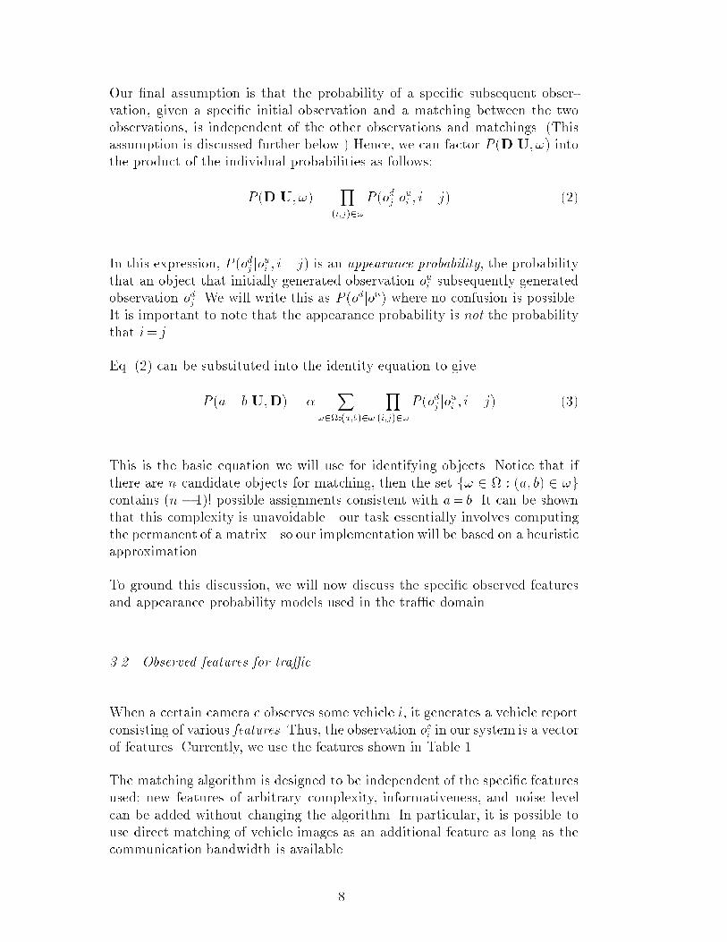
Our �nal assumption is that the probability of a speci�c subsequent obser-vation, given a speci�c initial observation and a matching between the twoobservations, is independent of the other observations and matchings. (Thisassumption is discussed further below.) Hence, we can factor P (DjU; !) intothe product of the individual probabilities as follows:P (DjU; !) = Y(i;j)2!P (odj joui ; i= j) (2)In this expression, P (odj joui ; i= j) is an appearance probability, the probabilitythat an object that initially generated observation oui subsequently generatedobservation odj . We will write this as P (odjou) where no confusion is possible.It is important to note that the appearance probability is not the probabilitythat i= j.Eq. (2) can be substituted into the identity equation to giveP (a= bjU;D) = � X!2:(a;b)2! Y(i;j)2!P (odj joui ; i= j) (3)This is the basic equation we will use for identifying objects. Notice that ifthere are n candidate objects for matching, then the set f! 2 : (a; b) 2 !gcontains (n � 1)! possible assignments consistent with a= b. It can be shownthat this complexity is unavoidable|our task essentially involves computingthe permanent of a matrix|so our implementation will be based on a heuristicapproximation.To ground this discussion, we will now discuss the speci�c observed featuresand appearance probability models used in the tra�c domain.3.2 Observed features for tra�cWhen a certain camera c observes some vehicle i, it generates a vehicle reportconsisting of various features. Thus, the observation oci in our system is a vectorof features. Currently, we use the features shown in Table 1.The matching algorithm is designed to be independent of the speci�c featuresused; new features of arbitrary complexity, informativeness, and noise levelcan be added without changing the algorithm. In particular, it is possible touse direct matching of vehicle images as an additional feature as long as thecommunication bandwidth is available.8

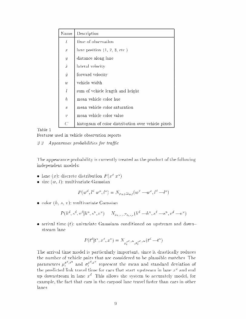
Name Descriptiont time of observationx lane position (1, 2, 3, etc.)y distance along lane_x lateral velocity_y forward velocityw vehicle widthl sum of vehicle length and heighth mean vehicle color hues mean vehicle color saturationv mean vehicle color valueC histogram of color distribution over vehicle pixelsTable 1Features used in vehicle observation reports.3.3 Appearance probabilities for tra�cThe appearance probability is currently treated as the product of the followingindependent models:� lane (x): discrete distribution P (xdjxu)� size (w, l): multivariate GaussianP (wd; ldjwu; lu) = N�w;l;�w;l(wd � wu; ld � lu)� color (h, s, v): multivariate GaussianP (hd; sd; vdjhu; su; vu) = N�h;s;v;�h;s;v(hd � hu; sd � su; vd � vu)� arrival time (t): univariate Gaussians conditioned on upstream and down-stream lane P (tdjtu; xd; xu) = N�xd;xut ;�xd;xut (td � tu)The arrival time model is particularly important, since it drastically reducesthe number of vehicle pairs that are considered to be plausible matches. Theparameters �xd ;xut and �xd;xut represent the mean and standard deviation ofthe predicted link travel time for cars that start upstream in lane xu and endup downstream in lane xd. This allows the system to accurately model, forexample, the fact that cars in the carpool lane travel faster than cars in otherlanes. 9

Our assumption that vehicle trajectories are independent, used in Eq. (2),would make little sense for tra�c, were it not for the fact that the appearanceprobability submodel for arrival time is parameterized by �xd;xut , the currentaverage travel time for the link. Clearly, the trajectories of consecutive carsin a stream of heavy tra�c are highly correlated rather than independent,but we subsume most of this correlation in the current average travel time.The assumption of independence given average travel time is identical to theassumption made by Petty et al. [8], whose work is discussed in Section 6.In examining the empirical distributions for the appearance probability, wewere surprised by the level of noise and lack of correlation in measurementsof the same feature at two di�erent cameras. Some features, such as colorsaturation and vehicle width, appear virtually uncorrelated. In all, we estimatethat the size and color features provide only about 3 to 4 bits of information.3.4 Online learning of appearance modelsBecause tra�c and lighting conditions change throughout the day, our sys-tem uses online (recursive) estimation for the appearance probability modelparameters. As new matches are identi�ed by the vehicle matcher, the pa-rameters are updated based on the observed feature values at the upstreamand downstream sites. Figure 4 shows a sample set of x values for matchedvehicles, from which P (xdjxu) can be estimated, as well as a sample set of huevalues for matched vehicles, from which P (hdjhu) can be estimated. To adaptto changing conditions, our system uses online exponential forgetting. For ex-ample, if a new match is found for a vehicle in lane xu upstream and lane xddownstream, with link travel time t, then the mean travel time is updated asfollows: �xu;xdt �xu;xdt + (1� )tThe parameter, which ranges from 0.0 to 1.0, controls the e�ective \windowsize" over which previous readings are given signi�cant weight.The above assumes that the match found is in fact correct. In practice, wecan never be certain of this. A better motivated approach to model updateswould be to weight each update by the probability that the match is correct.An approach that avoids matching altogether is described in Section 6.10

4 Matching algorithmWe begin by describing the simplest case, where all vehicles detected at theupstream camera are also detected downstream, and there are no onramps oro�ramps. We then describe the extension to handle onramps and o�ramps.4.1 Matching with full correspondenceThe aim is to �nd pairs of vehicles a and b such that P (a= bjU;D)> 1 � �for some small �. We have derived an equation (3) for this quantity, undercertain independence assumptions, and shown how to compute the appearanceprobabilities that are used in the equation. As mentioned earlier, the problemthat we now face is the intractability of computing the summation involved.The core of the approach is the observation, due to Cox and Hingorani [5],that a most probable assignment (pairing all n vehicles) can be found in timeO(n3) by formulating the problem as a weighted bipartite matching problemand using any of several well-known algorithms for this task. To do this, weconstruct an association matrix M of appearance probabilities, where eachentry Mij = � log P (odj joui ), so that the assignment with least total weight inthe matrix corresponds to the most probable assignment, according to Eq. (2).For our purposes, knowing the most likely assignment is not enough. It caneasily happen that some c of the n vehicles are all very similar and fairlyclose to each other on the freeway|a situation that we call a clique. Onecommon example might be cliques of yellow cabs on the freeways leading tomajor airports. Given a clique of size c, there will be c! assignments all havingroughly the same probability as the most probable assignment. Since matcheswithin the clique may be very unreliable, we employ a leave-one-out heuristicthat \forbids," in turn, each match contained in the best assignment. Foreach forbidden match, we measure the reduction in likelihood for the newbest assignment. Matches whose forbidding results in a signi�cant reductionare deemed reliable, since this corresponds to a situation where there appearsto be no other reasonable assignment for the upstream vehicle in question.11

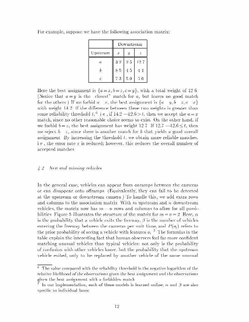
For example, suppose we have the following association matrix:DownstreamUpstream x y za 3.2 2.5 12.7b 8.5 4.5 4.4c 7.3 5.0 5.0Here the best assignment is fa=x; b= z; c= yg, with a total weight of 12.6.(Notice that a= y is the \closest" match for a, but leaves no good matchfor the others.) If we forbid a=x, the best assignment is fa= y; b= z; c=xgwith weight 14.2. If the di�erence between these two weights is greater thansome reliability threshold t, 6 i.e., if 14:2 � 12:6> t, then we accept the a=xmatch, since no other reasonable choice seems to exist. On the other hand, ifwe forbid b= z, the best assignment has weight 12.7. If 12:7 � 12:6� t, thenwe reject b= z, since there is another match for b that yields a good overallassignment. By increasing the threshold t, we obtain more reliable matches,i.e., the error rate � is reduced; however, this reduces the overall number ofaccepted matches.4.2 New and missing vehiclesIn the general case, vehicles can appear from onramps between the camerasor can disappear onto o�ramps. (Equivalently, they can fail to be detectedat the upstream or downstream camera.) To handle this, we add extra rowsand columns to the association matrix. With m upstream and n downstreamvehicles, the matrix now has m + n rows and columns to allow for all possi-bilities. Figure 5 illustrates the structure of the matrix for m=n=2. Here, �is the probability that a vehicle exits the freeway, � is the number of vehiclesentering the freeway between the cameras per unit time, and P (oi) refers tothe prior probability of seeing a vehicle with features oi. 7 The formulas in thetable explain the interesting fact that human observers feel far more con�dentmatching unusual vehicles than typical vehicles: not only is the probabilityof confusion with other vehicles lower, but the probability that the upstreamvehicle exited, only to be replaced by another vehicle of the same unusual6 The value compared with the reliability threshold is the negative logarithm of therelative likelihood of the observations given the best assignment and the observationsgiven the best assignment with a forbidden match.7 In our implementation, each of these models is learned online; � and � are alsospeci�c to individual lanes. 12

appearance, can be discounted because the extra multiplicative P (oi) factorfor an unusual vehicle would be tiny.5 ResultsWe tested the vehicle matcher with data from a region-based vehicle trackeron video sequences from the sites in Figure 1.On any given run, the number of matches proposed by the vehicle matcher de-pends on the reliability threshold selected for that run. In the results discussedbelow, coverage refers to the fraction of vehicles observed by both cameras forwhich matches were proposed, and accuracy refers to the fraction of proposedmatches that were in fact correct. In general, the coverage goes down as thereliability threshold is increased, but the accuracy goes up.To verify the accuracy of the matcher, the ground-truth matches were deter-mined by a human viewing the digitized sequences with the aid of a frame-based movie viewer. Since this method required about 3 hours of viewing tomatch each minute of video, it was used only during the early stages of test-ing. In subsequent testing, we �rst ran the matcher on the vehicle report dataand then used the frame-based movie viewer to verify whether the suggestedmatches were correct.Testing our system involved a start-up phase during which it estimated theappearance probability models online. For the results shown in Figure 6, wetrained our system on a pair of 60-second video sequences and then ran iton the immediately following 60-second sequences. The sequences contained29 vehicles detected at both cameras, along with over 40 vehicles that eitherentered or exited the freeway in between the cameras. The resulting accu-racy/coverage curve in Figure 6(a) shows that despite very noisy sensors, thesystem achieved 100% accuracy with a coverage of 14%, and 50% accuracywith a coverage of 80%. To simulate performance on freeway sections with-out onramps and o�ramps, we also tried removing the tracks of entering andexiting vehicles from the data stream. This makes the problem substantiallyeasier: we achieved 100% accuracy with a coverage of 37%, and 64% accuracywith a coverage of 80% (Figure 6(b)). The boxed vehicles in Figure 1 show apair of vehicles correctly matched by our system.Link travel times between each camera pair are currently calculated by av-eraging the observed travel times for matched vehicles. These times were ac-curate to within 1% over a distance of two miles, over a wide range of cov-erage/accuracy tradeo� points. This suggests that matched vehicles are rep-resentative of the tra�c ow|that is, the matching process does not select13

vehicles with a biased distribution of speeds.6 Related workThe vehicle matching problem is closely related to the traditional \data associ-ation" problem from the tracking literature, in which new \observations" (fromthe downstream camera) must be associated with already-established \tracks"(from the upstream camera). Radar surveillance for air tra�c control is a typ-ical application: the radar dish determines an approximate position for eachaircraft every few seconds, and each new set of positions must be associatedwith the set of existing tracks. There is a large literature on data association|typically over 100 papers per year. The standard text is by Bar-Shalom andFortmann [3], and recent developments appear in [2]. Ingemar Cox [4] surveysand integrates various developments, deriving formulas very similar to thosein Figure 5. Cox's aim in his review paper is to present the ideas from thedata association �eld to the computer vision and robotics community, wherethey might be used to resolve problems of identifying visual features seen intemporally separated images by a moving robot. Major di�erences betweenour work and \standard" data association include the following:(1) Sensor noise and bias are large, unknown, time-varying, site-dependent,and camera-dependent, and sensor observations are high-dimensional.(2) In radar tracking, the distance moved by each object between observa-tions is typically small compared to inter-object distances; in freewaytra�c, the opposite is true.(3) Tra�c observations are asynchronous.(4) Vehicle trajectories in tra�c are highly correlated.As explained in Section 3, this last problem is dealt with in our approachby conditioning trajectories on the current average link travel time. This is adevice that may prove to be useful in many other applications involving themodelling of very large systems using aggregate parameters.The most closely related work on statistical estimation of travel time is byPetty et al. [8]. They have shown that it is possible to estimate travel timesusing an \ensemble" matching approach that detects downstream propagationof distinct arrival time patterns instead of individual vehicles. Because it usesonly the arrival times, it can operate using data from loops|that is, inductioncoils placed under the road surface that indicate the passage of a vehicle. Usingthis technique, travel times were estimated accurately over a wide range oftra�c conditions. The method is, however, limited to loops that are fairlyclose together and have no intervening onramps or o�ramps.14

We are currently collaborating with the authors of the \ensemble" approachto develop a system that combines the two approaches and may overcomemany of the shortcomings of each. The basic idea, due primarily to Ritov, isto use a Monte Carlo Markov Chain algorithm to approximate the sum overassignments in Eq. (3). The states of the Markov chain are complete assign-ments and the transitions exchange pairings between two pairs of vehicles.The transition probabilities are de�ned such that detailed balance is main-tained and the fraction of time during which any given state is occupied isproportional to the probability of the corresponding assignment. Hence, theprobability of any given proposition (such as a= b) can be estimated as thefraction of time spent in states where it is true. Results due to Jerrum andSinclair [6] show that the Monte Carlo method applied this particular chaingives polynomial-time convergence.This approach can in fact estimate travel times and O/D counts without everselecting likely vehicle matches at all: simply compute the average travel timeand average O/D counts over all the assignments visited by the chain. Simi-larly, the appearance probability models can be updated after each transitionas if the assignment were correct; in the limit, the updated models will re ectthe observed data correctly. Since changing the appearance models changesthe transition probabilities of the chain, the process must be iterated untilconvergence. This is an instance of the EM algorithm, where the hidden vari-ables are the link travel times. We are currently experimenting to see if thisapproach can be used in a real-time setting where the structure of the Markovchain is continually changing as new vehicles are detected.7 Conclusions and further workThis paper has described the patterns of reasoning involved in establishingidentity from observations of objects. We proposed a formal foundation basedon a prior over the space of physical events, together with an identity criterionde�ning those events that correspond to observations of the same object. Inthe case of vehicle matching, the events are the di�erent sets of trajectories ofvehicles in a given freeway network. When a single trajectory passes throughtwo vehicle observations, that implies that the observations correspond to thesame object. This general approach makes it possible to de�ne the probabil-ity of identity and to integrate the necessary patterns of reasoning into anintelligent agent.This research can be seen as another step in the Carnapian tradition thatviews a rational agent as beginning with uninformative prior beliefs and thenapplying Bayesian updating throughout its lifetime. The general relationshipbetween perception and the formation of internal models is a subject that15

needs much more investigation [1].We showed that the abstract probability of identity can be expressed in termsof measurable appearance probabilities, which de�ne how, when, or whereobjects that were observed at some point in the past are expected to appearat some point in the future. These appearance probabilities can be learnedonline to adapt to changing conditions in the environment|such as changingweather, lighting, and tra�c patterns.We have implemented and tested a system for vehicle matching using an ef-�cient algorithm based on bipartite matching combined with a leave-one-outheuristic. Despite very noisy feature measurements from the cameras, our sys-tem achieved a high level of accuracy in matching individual vehicles, enablingus to build the �rst reliable video-based system for measuring link travel times.Although experimental camera data were not available for the system to do so,it is already capable of tracking the path of a vehicle over a sequence of camerasites. Thus, O/D counts for a time period can be computed by examining thecomplete set of recorded paths during that time period. For successful O/Dmeasurement over a long sequence of cameras, however, we need to improveboth matching coverage and the detection rate of the tracking subsystem. Wecan perform a crude analysis as follows: if the coverage for the vehicle matcheris c, and the matching accuracy is a, and the single-camera vehicle detectionrate is p, then the probability that a vehicle is correctly tracked across nsites is pnan�1cn�1 (assuming independence). Suppose now that n=10. Toachieve 90% accuracy in O/D counts, we need a9=0:9 or a � 0:988 as wellas a su�ciently high number of tracked vehicles in order to keep samplingerror low. The required percentage of vehicles to be tracked across the 10 siteswill depend on ow rates and the length of the reporting period. To track,say, 10% of vehicles across 10 sites we need p10c9=0:1. Given p=0:95, thismeans we need c � 0:82. Currently, simultaneous achievement of 98.8% accu-racy and 82% coverage is not feasible. However, we anticipate that improvedmeasurement of features such as width and height would provide dramaticimprovement in coverage and accuracy. Other possibilities include selectinga subset of pixels from the rear plane of each vehicle to be used as a matchfeature.The patterns of reasoning described here have broad applicability to otherdomains. For example, the object identi�cation problem occurs in databasemanagement, where it is possible that two di�erent records could correspondto the same entity. Thus, US credit reporting agencies record over 500 mil-lion credit-using Americans, of whom only about 100{120 million are actuallydistinct individuals. Applying our approach to this problem could help withmaintaining database consistency and with consolidating multiple databasescontaining overlapping information. 16

References[1] Fahiem Bacchus, Joseph Y. Halpern, and Hector Levesque. Reasoningabout noisy sensors in the situation calculus. In Proceedings of the Four-teenth International Joint Conference on Arti�cial Intelligence (IJCAI-95), pages 1933{1940, Montreal, Canada, August 1995. Morgan Kaufmann.[2] Yaakov Bar-Shalom, editor. Multitarget multisensor tracking: Advancedapplications. Artech House, Norwood, Massachusetts, 1992.[3] Yaakov Bar-Shalom and Thomas E. Fortmann. Tracking and Data Asso-ciation. Academic Press, New York, 1988.[4] I. J. Cox. A review of statistical data association techniques for motion cor-respondence. International Journal of Computer Vision, 10:53{66, 1993.[5] I. J. Cox and S. L. Hingorani. An e�cient implementation and evaluationof Reid's multiple hypothesis tracking algorithm for visual tracking. InProceedings of the 12th IAPR International Conference on Pattern Recog-nition, volume 1, pages 437{442, Jerusalem, Israel, October 1994.[6] M. Jerrum and A. Sinclair. The Markov chain Monte Carlo method. InD. S. Hochbaum, editor, Approximation Algorithms for NP-hard Problems.PWS Publishing, Boston, 1997.[7] Jitendra Malik and Stuart Russell. Tra�c surveillance and detection tech-nology development: New sensor technology �nal report. Research ReportUCB-ITS-PRR-97-6, California PATH Program, 1997.[8] K. F. Petty, P. Bickel, M. Ostland, J. Rice, Y. Ritov, and F. Schoenberg.Accurate estimation of travel times from single-loop detectors. Transporta-tion Research, Part A, 32A(1):1{17, 1998.

17

(a) (b)Fig. 1. Images from upstream (a) and downstream (b) surveillance cameras roughlytwo miles apart on Highway 99 in Sacramento, California. The boxed vehicle hasbeen identi�ed at both cameras.vehiclereportstream

DISPLAY

Flow params

Link travel times

O/D counts

paths withglobal IDs

tracks withlocal IDs

matchinge.g. a = 2

camera

1

camera 2

a

b

c

1

2

3

a2Fig. 2. Overall design of our tra�c surveillance system. The video streams areprocessed at each camera site by vehicle tracking software running on customizedparallel hardware. The resulting streams of chronologically ordered vehicle reportsare sent to the TMC (Tra�c Management Center). The TMC uses these reportsto determine when a vehicle detected at one camera has reappeared at another.These matches are used to build up a path for each vehicle as it travels through thefreeway network. The set of paths can be queried to compute link travel times andO/D counts as desired. The output of the system is a tra�c information display,updated in real time for use by tra�c operations managers or by individual drivers.18

0 T

y

yd

t

yu

at tb

uao

odb

0 T

y

yd

t

yu

at tb

uao

odb

(a) (b)Fig. 3. Time{space diagrams showing two possible events in the two-car universe,given observations oua and odb (and no other observations). In (a), we have a= b,while in (b), we have a 6= b.19

0

2

4

6

8

10

12

14

16

18

0 2 4 6 8 10 12 14 16 18

X p

ositi

on a

t dow

nstr

eam

cam

era

X position at upstream camera

-0.3

-0.25

-0.2

-0.15

-0.1

-0.05

0

0.05

0.1

0.15

-0.3 -0.25 -0.2 -0.15 -0.1 -0.05 0 0.05 0.1

Dat

a at

sec

ond

cam

era

Data at first camera

’hue.data’x

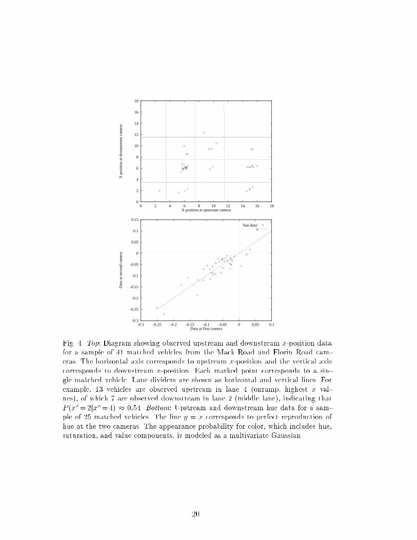
Fig. 4. Top: Diagram showing observed upstream and downstream x-position datafor a sample of 41 matched vehicles from the Mack Road and Florin Road cam-eras. The horizontal axis corresponds to upstream x-position and the vertical axiscorresponds to downstream x-position. Each marked point corresponds to a sin-gle matched vehicle. Lane dividers are shown as horizontal and vertical lines. Forexample, 13 vehicles are observed upstream in lane 4 (onramp, highest x val-ues), of which 7 are observed downstream in lane 2 (middle lane), indicating thatP (xd=2jxu=4) � 0:54. Bottom: Upstream and downstream hue data for a sam-ple of 25 matched vehicles. The line y = x corresponds to perfect reproduction ofhue at the two cameras. The appearance probability for color, which includes hue,saturation, and value components, is modeled as a multivariate Gaussian.20

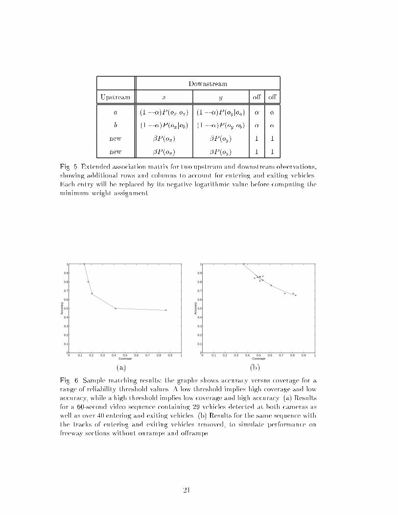
DownstreamUpstream x y o� o�a (1� �)P (oxjoa) (1� �)P (oy joa) � �b (1� �)P (oxjob) (1� �)P (oy job) � �new �P (ox) �P (oy) 1 1new �P (ox) �P (oy) 1 1Fig. 5. Extended association matrix for two upstream and downstream observations,showing additional rows and columns to account for entering and exiting vehicles.Each entry will be replaced by its negative logarithmic value before computing theminimum weight assignment.0 0.1 0.2 0.3 0.4 0.5 0.6 0.7 0.8 0.9 1

0

0.1

0.2

0.3

0.4

0.5

0.6

0.7

0.8

0.9

1

Coverage

Acc

urac

y

0 0.1 0.2 0.3 0.4 0.5 0.6 0.7 0.8 0.9 10

0.1

0.2

0.3

0.4

0.5

0.6

0.7

0.8

0.9

1

Coverage

Acc

urac

y(a) (b)Fig. 6. Sample matching results: the graphs shows accuracy versus coverage for arange of reliability threshold values. A low threshold implies high coverage and lowaccuracy, while a high threshold implies low coverage and high accuracy. (a) Resultsfor a 60-second video sequence containing 29 vehicles detected at both cameras aswell as over 40 entering and exiting vehicles. (b) Results for the same sequence withthe tracks of entering and exiting vehicles removed, to simulate performance onfreeway sections without onramps and o�ramps.21