Rochester Institute of Technology Rochester Institute of Technology

RIT Scholar Works RIT Scholar Works

Theses

6-2014

Object Detection using Dimensionality Reduction on Image Object Detection using Dimensionality Reduction on Image

Descriptors Descriptors

Riti Sharma

Follow this and additional works at: https://scholarworks.rit.edu/theses

Recommended Citation Recommended Citation Sharma, Riti, "Object Detection using Dimensionality Reduction on Image Descriptors" (2014). Thesis. Rochester Institute of Technology. Accessed from

This Thesis is brought to you for free and open access by RIT Scholar Works. It has been accepted for inclusion in Theses by an authorized administrator of RIT Scholar Works. For more information, please contact ritscholarworks@rit.edu.

Object Detection using Dimensionality Reduction on Image Descriptors

By

Riti Sharma

A Thesis Submitted in Partial Fulfillment of the Requirements for the Degree of

Master of Science in Computer Engineering

Supervised by

Dr. Andreas Savakis

Department of Computer Engineering

Kate Gleason College of Engineering

Rochester Institute of Technology

Rochester, NY

June, 2014

Approved By:

____________________________________________________Date:_______ _______

Dr. Andreas Savakis

Primary Advisor – R.I.T. Dept. of Computer Engineering

____________________________________________________Date:_______ _______

Dr. Raymond Ptucha

Secondary Advisor – R.I.T. Dept. of Computer Engineering

____________________________________________________Date:_______ _______

Dr. Shanchieh Jay Yang

Secondary Advisor – R.I.T. Dept. of Computer Engineering

ii

Dedicated to my parents Dr. Shakti Datt Sharma, Dr. Puja Sharma

and my sister Kriti Sharma

iii

Acknowledgements

First and foremost, I would like to express my gratitude to my advisor and mentor, Dr. Andreas

Savakis, for his invaluable guidance, patience, and immense knowledge. His confidence and

faith in me, encouraged me. He supported me throughout my research and allowed me to grow

and I thank him for his invaluable advice. Without his supervision and expertise; this work

would not have been possible. I am extremely grateful to Dr. Ray Ptucha for his advice, and

support on both academic and personal level. I thank him for his confidence in me and for

serving as my committee. I would also like to thank Dr. Shanchieh Jay Yang, for serving as my

thesis committee. His guidance motivated me.

I am extremely grateful to Richard Tolleson for his help throughout my work and I would also

like to thank my fellow lab mates in Real Time Vision and Image Processing Lab- Bret

Minnehan, Faiz Quraishi, Henry Spang, Ethan Peters, and Jack Stokes for their support, endless

discussions and all the fun that we had in the lab.

I have no words to express my gratitude to my family for their endless love, concern, support and

strength all these years and my friends for their continued encouragement.

iv

Abstract

The aim of object detection is to recognize objects in a visual scene. Performing reliable object

detection is becoming increasingly important in the fields of computer vision and robotics.

Various applications of object detection include video surveillance, traffic monitoring, digital

libraries, navigation, human computer interaction, etc. The challenges involved with detecting

real world objects include the multitude of colors, textures, sizes, and cluttered or complex

backgrounds making objects difficult to detect.

This thesis contributes to the exploration of various dimensionality reduction techniques on

descriptors for establishing an object detection system that achieves the best trade-offs between

performance and speed. Histogram of Oriented Gradients (HOG) and other histogram-based

descriptors were used as an input to a Support Vector Machine (SVM) classifier to achieve good

classification performance. Binary descriptors were considered as a computationally efficient

alternative to HOG. It was determined that single local binary descriptors in combination with

Support Vector Machine (SVM) classifier don’t work as well as histograms of features for object

detection. Thus, histogram of binary descriptors features were explored as a viable alternative

and the results were found to be comparable to those of the popular Histogram of Oriented

Gradients descriptor.

Histogram-based descriptors can be high dimensional and working with large amounts of data

can be computationally expensive and slow. Thus, various dimensionality reduction techniques

were considered, such as principal component analysis (PCA), which is the most widely used

technique, random projections, which is data independent and fast to compute, unsupervised

v

locality preserving projections (LPP), and supervised locality preserving projections (SLPP),

which incorporate non-linear reduction techniques.

The classification system was tested on eye detection as well as different object classes. The eye

database was created using BioID and FERET databases. Additionally, the CalTech-101 data set,

which has 101 object categories, was used to evaluate the system. The results showed that the

reduced-dimensionality descriptors based on SLPP gave improved classification performance

with fewer computations.

vi

Table of Contents

Acknowledgements ........................................................................................................................ iii

Abstract .......................................................................................................................................... iv

Table of Contents ........................................................................................................................... vi

List of Figures ................................................................................................................................ ix

List of Tables ................................................................................................................................ xii

1. Introduction ................................................................................................................................. 1

1.1 Why is Object Detection Important? ................................................................................ 2

1.2 Methodology .................................................................................................................... 4

1.3 Thesis Contributions ........................................................................................................ 6

1.4 Thesis Outline .................................................................................................................. 7

2. Related Work .............................................................................................................................. 9

3. Image Descriptors ..................................................................................................................... 12

3.1 Low Level Image Descriptors ........................................................................................ 12

3.2 Histogram of Oriented Gradients ................................................................................... 13

3.3 Binary Descriptors.......................................................................................................... 16

3.4 Local Binary Patterns ..................................................................................................... 16

3.5 BRISK & BRIEF Descriptors ........................................................................................ 20

3.6 FREAK Descriptor ......................................................................................................... 20

vii

4. Dimensionality Reduction ........................................................................................................ 23

4.1 Principal Component Analysis ....................................................................................... 24

4.2 Random Projections ....................................................................................................... 25

4.3 Manifold Learning.......................................................................................................... 27

4.4 Locality Preserving Projections (LPP) ........................................................................... 28

5. Classification............................................................................................................................. 30

5.1 Support Vector Machines ............................................................................................... 31

5.1.1 Statistical Learning Theory ..................................................................................... 31

5.1.2 SVM Mathematical Representation ........................................................................ 33

5.1.3 Non Linear SVM..................................................................................................... 35

5.1.4 Multiclass SVM ...................................................................................................... 36

5.2 Bootstrapping ................................................................................................................. 37

5.3 SVM Usage .................................................................................................................... 38

6. Eye Detection ............................................................................................................................ 39

6.1 Motivation ...................................................................................................................... 39

6.2 Approach ........................................................................................................................ 40

7. Experimental Results and Discussion ....................................................................................... 43

7.1 Datasets .......................................................................................................................... 43

7.1.1 BioID....................................................................................................................... 43

7.1.2 FERET .................................................................................................................... 44

viii

7.1.3 CalTech-101 ............................................................................................................ 44

7.2 Eye Detection ................................................................................................................. 45

7.3 CalTech-101 Testing ...................................................................................................... 59

7.4 Image Descriptors .......................................................................................................... 61

7.5 Dimensionality Reduction .............................................................................................. 64

8. Conclusions ............................................................................................................................... 66

References ..................................................................................................................................... 68

ix

List of Figures

Figure 1.1: Example of Object Detection. ...................................................................................... 1

Figure 1.2: Images from CalTech-101 showing Objects at different Distances. ............................ 3

Figure 1.3: Images from CalTech-101 showing Objects with different Viewpoints. ..................... 3

Figure 1.4: Images from CalTech-101 showing Intra Class Variation. .......................................... 3

Figure 1.5: Image from CalTech-101 showing Object with Cluttered Background. ...................... 4

Figure 1.6: Sliding Window Example. ........................................................................................... 4

Figure 1.7: Sliding Window Detection Process. ............................................................................. 5

Figure 3.1: Images from CalTech-101, (a) Original Image, its variations due to (b) Rotation, (c)

Illumination, and (d) Scale. ........................................................................................................... 12

Figure 3.2: Process of formation of Histogram of Oriented Gradients feature descriptor. .......... 14

Figure 3.3: Rectangular and Circular Cells, used in Histogram of Oriented Gradients. .............. 15

Figure 3.4: Sample Images and their HOG Descriptor. ................................................................ 15

Figure 3.5: Example to find LBP Descriptor for a given Image. .................................................. 17

Figure 3.6: Sample Image and its LBP Descriptor. ...................................................................... 18

Figure 3.7: Process to create Histogram of LBP Descriptor. ........................................................ 19

Figure 3.8: Process to create Histogram of FREAK Descriptor. .................................................. 22

Figure 4.1: Principal Components of an Example Data. .............................................................. 24

Figure 4.2: Manifold to Euclidean Space. .................................................................................... 27

Figure 5.1: Classification Example. .............................................................................................. 30

Figure 5.2: Two Class Classification Example using Support Vector Machine. .......................... 32

Figure 5.3: Example to show Support Vectors, Margin and Decision Boundary......................... 32

x

Figure 5.4: Non-Linear Classification using SVM. ...................................................................... 35

Figure 5.5: Multi-class Classification using SVM. ....................................................................... 36

Figure 5.6: Flowchart for Bootstrapping Algorithm. .................................................................... 37

Figure 6.1: Eye Detection System. .............................................................................................. 40

Figure 6.2: Example (a) Eye and (b) Non-Eye Training Samples. .............................................. 41

Figure 7.1: Example Images from BioID. ................................................................................... 43

Figure 7.2: Example Images from FERET. ................................................................................. 44

Figure 7.3: Example Images from CalTech-101. ......................................................................... 45

Figure 7.4: Eye Detection Accuracy Results with different Descriptors and Dimensionality

Reduction methodologies.............................................................................................................. 46

Figure 7.5: Eye Detection False Positives with different Descriptors and Dimensionality

Reduction methodologies.............................................................................................................. 46

Figure 7.6: Detection Accuracy as Cell Size and Block Size were varied. ................................. 47

Figure 7.7: Accuracy as Number of Features is varied. ................................................................ 47

Figure 7.8: Accuracy and False Positives with Histogram of Oriented Gradients. ...................... 48

Figure 7.9: Accuracy and False Positives with FREAK. .............................................................. 49

Figure 7.10: Accuracy and False Positives with Histogram of FREAK. ...................................... 51

Figure 7.11: Accuracy and False Positives with LBP. .................................................................. 52

Figure 7.12: Accuracy and False Positives with Histogram of LBP. ........................................... 53

Figure 7.13: Eye Detector examples in BioID database (a) HOG Descriptor, (b) HOG-SLPP

Descriptor, (c) HOG-LPP Descriptor, (d) HOG-PCA Descriptor, (e) HOG-RP Descriptor, and (f)

Examples of False Positives.......................................................................................................... 56

xi

Figure 7.14: Eye Detector examples in FERET database (a) HOG Descriptor, (b) HOG-SLPP

Descriptor, (c) HOG-LPP Descriptor, (d) HOG-PCA Descriptor, (e) HOG-RP Descriptor, and (f)

Examples of False Positives.......................................................................................................... 58

Figure 7.15: Accuracy for CalTech-101 as Cell Size and Bin Size was varied for HOG-SLPP. . 61

Figure 7.16: Accuracy for CalTech-101 as Cell Size and Bin Size was varied for H-FREAK –

SLPP. ............................................................................................................................................ 62

Figure 7.17: Accuracy for CalTech-101 as Cell Size and Bin Size was varied for H-LBP –

SLPP. ............................................................................................................................................ 62

Figure 7.18: Accuracy for CalTech-101 with different Descriptors. ............................................ 63

Figure 7.19: Eye Detection Results. ............................................................................................. 63

Figure 7.20: Graph showing Accuracy as we increase the Number of Components CalTech - 101.

....................................................................................................................................................... 64

Figure 7.21: Results with different Descriptors and Dimensionality Reduction techniques for

CalTech-101. ................................................................................................................................. 65

xii

List of Tables

Table 7.1: Accuracy Results with HOG and different SVM Kernels. .......................................... 45

Table 7.2: Confusion Matrix for Eye Detection using HOG Descriptor. ..................................... 48

Table 7.3: Confusion Matrix for Eye Detection using HOG –PCA Descriptor. .......................... 48

Table 7.4: Confusion Matrix for Eye Detection using HOG-RP Descriptor. ............................... 48

Table 7.5: Confusion Matrix for Eye Detection using HOG – LPP Descriptor. .......................... 48

Table 7.6: Confusion Matrix for Eye Detection using HOG – SLPP Descriptor. ........................ 49

Table 7.7: Confusion Matrix for Eye Detection using FREAK Descriptor. ................................. 49

Table 7.8: Confusion Matrix for Eye Detection using FREAK –PCA Descriptor. ...................... 50

Table 7.9: Confusion Matrix for Eye Detection using FREAK -RP Descriptor. ......................... 50

Table 7.10: Confusion Matrix for Eye Detection using FREAK – LPP Descriptor. .................... 50

Table 7.11: Confusion Matrix for Eye Detection using FREAK – SLPP Descriptor. .................. 50

Table 7.12: Confusion Matrix for Eye Detection using Histogram of FREAK Descriptor. ........ 51

Table 7.13: Confusion Matrix for Eye Detection using Histogram of FREAK-PCA Descriptor. 51

Table 7.14: Confusion Matrix for Eye Detection using Histogram of FREAK-RP Descriptor. .. 51

Table 7.15: Confusion Matrix for Eye Detection using Histogram of FREAK-LPP Descriptor. 51

Table 7.16: Confusion Matrix for Eye Detection using Histogram of FREAK-SLPP Descriptor.

....................................................................................................................................................... 52

Table 7.17: Confusion Matrix for Eye Detection using LBP Descriptor. .................................... 52

Table 7.18: Confusion Matrix for Eye Detection using LBP –PCA Descriptor. .......................... 52

Table 7.19: Confusion Matrix for Eye Detection using LBP -RP Descriptor. ............................. 53

Table 7.20: Confusion Matrix for Eye Detection using LBP – LPP Descriptor. .......................... 53

xiii

Table 7.21: Confusion Matrix for Eye Detection using LBP – SLPP Descriptor. ....................... 53

Table 7.22: Confusion Matrix for Eye Detection using Histogram of LBP Descriptor. .............. 54

Table 7.23: Confusion Matrix for Eye Detection using Histogram of LBP –PCA Descriptor. ... 54

Table 7.24: Confusion Matrix for Eye Detection using Histogram of LBP -RP Descriptor. ....... 54

Table 7.25: Confusion Matrix for Eye Detection using Histogram of LBP – LPP Descriptor. ... 54

Table 7.26: Confusion Matrix for Eye Detection using Histogram of LBP – SLPP Descriptor. . 54

Table 7.27: Eye Detection Results on BioID with HOG and different Dimensionality Reduction

Techniques. ................................................................................................................................... 55

Table 7.28 Comparison of BioID Results using Different Approaches. ...................................... 57

Table 7.29: Eye Detection Results on FERET with HOG and different Dimensionality Reduction

Techniques. ................................................................................................................................... 57

Table 7.30: Comparison of FERET Results using Different Approaches. ................................... 59

Table 7.31: Results with CalTech-101, 10-Fold Cross Validation, 30 Samples per Category. ... 60

Table 7.32: Results with CalTech-101, 30 Training Samples and 50 Testing Samples. .............. 60

Table 7.33: Comparison of Classification Results of CalTech-101 with Different Approaches. . 60

Table 7.34: Results with CalTech-101.......................................................................................... 64

1

Chapter 1

Introduction

Vision is one of the most important senses used by humans. The human brain can recognize

many objects effortlessly, even though the objects may appear differently depending upon the

viewpoint, illumination, etc. Objects can even be detected if there are occlusions caused by other

objects. We can group instances of objects, such as fruits, pedestrians, cars, etc. into a single

object class and can still differentiate between specific objects like “my own car” and “some

other car”. This is far from straight forward for a computer. There are so many efforts being

made to build machines that can see as humans do, yet we cannot escape that such capability is

still far ahead of us.

Figure 1.1: Example of Object Detection.

2

Object detection can be divided into two categories. The first category involves detecting an

object class, for example detecting bananas from a fruit basket, and the second is detecting or

recognizing a specific object, for example detecting a specific book from a book shelf.

1.1 Why is Object Detection Important?

Object detection is of great importance in the field of computer vision and robotics. It helps

robots understand and interpret the world around them. Various applications include video

surveillance, biometrics, traffic monitoring, digital libraries, navigation, interacting with human-

computer interaction, etc.

We encounter applications using object detection in our daily lives, for example automatic

driving and driver assistance systems in high end cars, human-robot interaction, immersive

interactive entertainments, smart homes, assistance for senior citizens that live alone, and people

finding for surveillance, security and military applications.

There are various challenges involved regarding detection of real world objects such as vehicles,

animals, birds, people, etc. Real world objects have a lot of variation in terms of color, texture,

shape and other properties. Also, objects can even have a wide variability in their appearance

characteristics, due to lighting, size, pose, etc. The backgrounds against which the objects lie are

often complex and cluttered as shown in Figure 1.5. For example, it might be easier for a robot to

find or detect a book with nothing else present on a table, and quite difficult to detect the same

book on a table that is cluttered by other objects. Images from Caltech-101 [53] database of

objects at different distances and different viewpoints are shown in Figure 1.2 and 1.3

respectively. Figure 1.4 shows intra class variation.

3

Figure 1.2: Images from CalTech-101 showing Objects at different Distances.

Figure 1.3: Images from CalTech-101 showing Objects with different Viewpoints.

Figure 1.4: Images from CalTech-101 showing Intra Class Variation.

4

Figure 1.5: Image from CalTech-101 showing Object with Cluttered Background.

Figure 1.6: Sliding Window Example.

1.2 Methodology

In this thesis, sliding window based detectors are used. The entire image is scanned to extract

patches, and these patches are classified into object or non-object category. The sliding window

detection approach is shown in Figure 1.6.

This process can be broadly separated into the three stages of feature extraction, dimensionality

reduction and classification. Figure 1.7 shows the process of detecting object from a given

image.

5

In the feature extraction stage, the window of a fixed size is moved over an image, and for each

location a feature descriptor is extracted. In this thesis, a histogram of binary descriptors is

considered for object detection - in particular, the histogram of LBP and histogram of FREAK,

are compared with the Histogram of Oriented Gradient descriptor.

Figure 1.7: Sliding Window Detection Process.

The objective of dimensionality reduction is to project the data on a lower dimensional space

while retaining the important properties of the data for the problem under consideration.

Working with high dimensional data can be computationally intensive and slow. In cases where

Input Image

Extract Local Window

Compute Feature

Descriptor

Reduce Dimensions

SVM Classifier

Detected Object

6

the feature space is extremely large, the effect known as the Curse of Dimensionality may result

in lower performance compared to that of a lower dimensional feature space.

Dimensionality reduction offers computational benefits obtained by processing a smaller amount

of data. A secondary benefit of dimensionality reduction is that some noise and redundancies in

the features are eliminated after reducing the feature space. As a result, the data can be

represented in a more compact and effective way, which can improve classifier performance.

Techniques such as Principal Component Analysis (PCA), Linear Discriminant Analysis, and

Manifold Learning have been used for subspace learning and dimensionality reduction [11, 12].

1.3 Thesis Contributions

This work proposes a holistic approach towards detecting object from images. The approach

integrates different image feature descriptors with various dimensionality reduction techniques.

The following summarize the contributions made in this thesis.

Eye Detection

o Efficient approach to detecting eyes using dimensionality-reduced Histogram of

Oriented Gradients as feature descriptor

o Evaluation of Principal Component Analysis, Random Projections, Locality

Preserving Projections (LPP), and Supervised Locality Preserving Projections

(SLPP) on image descriptors for eye detection.

o The HOG-PCA descriptor, published by A. Savakis, R. Sharma, and M. Kumar,

“Efficient Eye Detection using HOG-PCA Descriptor.” IS&T/SPIE Electronic

Imaging Conference, Imaging and Multimedia Analytics in a Web and Mobile

World, 2014 [44].

7

Image descriptors

o Proposed histogram-based FREAK descriptor as a feature descriptor for

successful object detection.

o Analysis of HOG, LBP, Histogram of LBP (H-LBP), FREAK, and Histogram of

FREAK (H-FREAK) for the purpose of detecting objects.

Dimensionality Reduction

o Evaluation and analysis of various dimensionality reduction techniques,

specifically PCA, Random Projections, LPP and SLPP for object detection.

1.4 Thesis Outline

Following the introduction, Chapter 2 gives a background about different approaches to object

detection and discusses various methodologies.

Chapter 3 gives an overview of the different feature descriptors used in this thesis. It begins with

the basic descriptor on a raw image and then migrates to the more sophisticated descriptors, such

as Histogram of Oriented Gradients (HOG), Local Binary Patterns (LBP), and Fast Retina

Keypoint (FREAK) descriptors.

Chapter 4 covers fundamental concepts of dimensionality reduction. It begins with the need and

advantages of dimensionality reduction and gives an overview of the different dimensionality

reduction techniques used in the thesis such as PCA, Random Projections, and Manifold

Learning using LPP.

Chapter 5 discusses the support vector machine classifier. It begins with the basic idea behind the

SVM classifier. It discusses the statistical learning theory behind the support vector machines

8

and goes over the mathematics involved. It also discusses the bootstrap technique and various

classification approaches.

Chapter 6 presents the eye detection system developed in this work. It begins with the motivation

and related work for eye detection. It then presents the detailed approach for eye detection.

Chapter 7 discusses the different datasets used in this work for evaluation of the system and the

results of using different descriptors for object detection. It also discusses the effects of using

different dimensionality reduction techniques with these descriptors.

The Conclusion chapter summarizes the work of this thesis, discusses the key findings and offers

some directions for future work.

9

Chapter 2

Related Work

Object detection has received a lot of attention in the field of computer vision. Learning

algorithms used for object detection vary from simple k-nearest neighbor [3] to random forests

[7, 8] and neural networks [19, 54]. The most popular among these classification methods is

Support Vector Machines (SVM) [34, 35, 46, 47] which was introduced in [43] by Boser, Guyon

and Vapnik.

In parts-based object detection, the object is treated as collection of different parts. Different

parts are extracted from the object and detection is done using appearance and geometric

information between parts. A popular and successful approach is the deformable parts model

(DPM) [49]. The DPM breaks up the appearance of an object class into sub-classes which

correspond to a different structure or pose. A part-based approach for human detection was used

in [49], where a person was divided into components such as arms, legs, head, etc., and then

support vector machine classifier was used in human detection. A sparse parts-based object

detection was used in [45] to detect cars.

Bags-of-words descriptor with SVM classification is another popular approach for object

recognition and is taken from text analysis. It converts the image into bag-of-words using three

basic steps: feature detection which detects distinctive and repeatable image features from the

image, feature description which extracts a feature descriptor from an image patch, and feature

quantization which is used to quantize the descriptor into a word defined in a given codebook.

10

[68] use bag-of-word model with SIFT features and SVM for object detection. Also, bag-of-

words descriptor is used in [67] for action recognition.

The approaches using parts-based model and bag-of-words model are efficient but more complex

and computationally expensive. Furthermore, it is hard for these models to cope with a limited

set of training data, whereas object detection based on treating objects as a single unit is simple

and involves fewer computations.

Feature descriptors are used in many real world applications such as object detection, object

tracking, etc. The emphasis is to learn features that are invariant to scale, viewpoint,

illumination, etc., and thus are efficient. One popular feature is Scale Invariant Feature

Transform, SIFT. In [36], an object recognition system was developed based on SIFT

descriptors. Many variants to SIFT descriptor have also been proposed, such as Speeded Up

Robust Features (SURT) [37] which was developed as a computationally efficient alternative.

Dimensionality reduction in the form of Principal Component Analysis (PCA) was utilized to

obtain PCA-SIFT [37], a descriptor with fewer components that offers good performance.

Another popular feature descriptor is the Histogram of Oriented Gradients (HOG). It was

initially proposed for pedestrian detection by Dalal and Triggs [5]. Since then it has been

adopted in the context of various classification problems [40, 41]. Dalal & Triggs [5] used

histogram of oriented gradients with support vector machines classifier in a sliding window

framework for pedestrian detection. A multi-scale part based object detection system using

Latent SVM and HOG was built in [49] and is considered the state-of-the-art in object detection.

Recently there is work done with structured learning to improve detection performance. In [16]

Uricar and Franc proposed the use of structured SVMs for facial landmark detection and [9]

11

employs structured learning for 2D pose estimation to improve pedestrian detection technique.

The authors in [1] propose an approach in which separate SVM classifiers are trained for each

object instance, and each of these classifiers consists of a single positive example and many

negative examples.

In contrast to SIFT, HOG is a dense descriptor and this encouraged the use of dense binary

descriptors for object detection. Local Binary Pattern has been popular in many classification

problems, such as texture classification [32], face recognition [31], etc. Recently, HOG-LBP

based descriptor was also used for object localization [30, 29].

Other binary descriptors include BRIEF [28] which uses binary tests between pixels in a patch to

build a descriptor that is robust to lighting, blur and perspective distortion; BRISK [10] produces

keypoints that are scale invariant. Recently FREAK [39] was introduced as a robust binary

descriptor and it is invariant to viewpoints, illumination or rotation variations.

However, there is a lack of approaches that consider binary descriptors for object detection. Most

importantly, which binary features are stable and flexible for object detection or recognition still

remains an unanswered question. Since binary descriptors are computationally efficient, this

thesis considers histogram of binary descriptors as an alternative to HOG for object detection in

addition to the exploration of dimensionality reduction techniques.

12

Chapter 3

Image Descriptors

To be able to successfully detect an object or classify objects into different categories, we must

be able to describe the properties of an object in a unique manner. In order to accomplish this,

the descriptors must have certain properties that make them unique, reproducible, invariant and

efficient. Firstly, similar objects should have similar descriptors. Thus, objects should be

classified to a particular category only if they have similar descriptors. Secondly, the descriptors

should be invariant to scale, rotation, and illumination. In addition, they should be invariant to

perspective changes as the object could be observed from a different viewpoint. The descriptors

should be compact and should only contain the information that makes the object unique. Figure

3.1 shows an example image and its variation due to rotation, illumination and scale.

(a) (b) (c) (d)

Figure 3.1: Images from CalTech-101, (a) Original Image, its variations due to (b) Rotation, (c)

Illumination, and (d) Scale.

3.1 Low Level Image Descriptors

The low level image descriptors are computed directly from the image pixels. For example a

color histogram is a low level feature extraction method. Low level image descriptors are defined

to capture a certain visual property of an image either globally for the entire image or locally for

13

a group of pixels in a particular region. These local features are based on color, texture, shape,

motion etc. [5]. These descriptors have been used extensively for image retrieval. For example

[59] uses color, texture and shape features combined for content based image retrieval. [25] uses

texture based features to classify maritime pine forests images. These descriptors are not well

suited for object detection and thus there is a need for better image descriptors.

3.2 Histogram of Oriented Gradients

The success and broad application of the SIFT keypoint descriptors [36] has motivated the

development of various local descriptors based on edge orientations. The Scale Invariant Feature

Descriptor was introduced by David Lowe and is designed to be invariant to translation, scaling,

rotation and to some extent, illumination. Keypoint detection is the first stage of SIFT feature

extraction which identifies key locations as maxima and minima of the result of difference of

Gaussians (DOG) function, applied in scale space to a series of smoothed and resampled images.

Low contrast candidate points and edge response points along an edge are discarded. Dominant

orientations are assigned to localized keypoints and a feature vector is formed by specifying the

orientation relative to the keypoint, essentially making the vector rotation invariant. The major

drawback of SIFT feature descriptor is that it is computationally expensive. SIFT was originally

developed for image stitching and used for panorama construction [55], while object detection

was considered as a secondary application. SIFT is designed to be a sparse descriptor that

identifies keypoints of interest, which is a different approach than that of dense descriptors such

as HOG, which was developed with object detection in mind.

The Histogram of Oriented Gradients is a popular descriptor that was initially proposed for

pedestrian detection by Dalal and Triggs [5]. Since then it has been adopted for various

classification problems. In [26] HOG features were used for detection of human cells, and in [27]

14

for vehicle detection. In [2] HOG features were proposed for face recognition. The process of

generating HOG Descriptor for an image is shown in Figure 3.2.

Figure 3.2: Process of formation of Histogram of Oriented Gradients feature descriptor.

To obtain the HOG features, the gradient of the image is computed by applying an edge mask. A

simple 1-D mask of the form [-1, 0, 1] works well. More complex masks, such as Sobel operator

and others were tested in [5], but the simple, centered, 1-D derivative mask works the best. The

resulting gradient image is divided into smaller non overlapping spatial regions called cells.

These cells can be rectangular, which results in the R-HOG descriptor, or circular, which results

in the C-HOG descriptor, as shown in Figure 3.3. Each pixel in the cell casts a vote that is

weighted by its gradient magnitude, and contributes to an orientation aligned with the closest bin

in the range 0-180 (unsigned) or 0-360 (signed). The orientations of the bins are evenly spaced

and generate an orientation histogram. This step is known as Orientation Binning. After

Orientation Binning, the cell histograms are normalized, for better invariance to illumination and

contrast. The cells are grouped together in 2x2 overlapping blocks and each of these blocks is

Input Image

Compute Gradients

Orientation Binning

Block Normalization

HOG Descriptor

15

normalized individually. The overlapping of blocks ensures that there is no loss of local

variations and there is a consistency across the whole image.

Figure 3.3: Rectangular and Circular Cells, used in Histogram of Oriented Gradients.

Figure 3.4: Sample Images and their HOG Descriptor.

Figure 3.4 shows examples of images and their HOG descriptor. The HOG descriptor has

proven effective for classification purposes and has been applied on a variety of problems. Its

main disadvantage is the associated computational load. When considering invariance, HOG

features are somewhat invariant to illumination.

Cell

Block

16

3.3 Binary Descriptors

In Histogram of Oriented Gradients, the gradient of each pixel in a patch needs to be computed.

This makes it computationally expensive and thus, is not fast enough for some of the

applications. Local binary descriptors, where most of the information can be encoded into a

binary string using comparison operations, are more computationally efficient. In addition,

matching between binary descriptions can be done by the Hamming distance, i.e. just counting

the number of bits by which they differ. This is the same as using the sum of the XOR operation

between two binary strings.

Binary descriptors are composed of three parts: sampling pattern, the pattern by which points

need to be sampled in a given region; sampling pairs, these are the pairs which are compared in

order to build the descriptor; and orientation compensation, the method used to make the

descriptor rotation invariant or algorithm to find the orientation of a given keypoint. In order to

construct a binary string, we compare the intensity values at the two given points. If the intensity

value of the first point is greater than the second, we add a 1 to the binary string; else we add a 0

to the binary string. Examples of binary descriptors include LBP, BRISK, FREAK, etc.

3.4 Local Binary Patterns

The Local Binary Pattern (LBP) descriptor is the simplest binary descriptor and is a popular

feature to describe the texture of an image. It converts each pixel into a binary number by

thresholding the neighborhood of each pixel. In this descriptor the given image is divided into

integer blocks. For each of these blocks, the center pixel is considered as the threshold value and

its other neighboring pixels are assigned 0 or 1 depending upon the intensity value of the center

pixel. This results in a p-bit binary number, where p is the number of neighboring pixels. Figure

17

3.5 shows an example to generate LBP descriptor. It is invariant to any monotonic gray level

change and is simple to compute.

8 0 9 1 0 1 1 2 4 1 0 4

5 6 6 → 0 1 * 8 16 = 0 16

1 2 3 1 0 0 32 64 128 32 0 0

Figure 3.5: Example to find LBP Descriptor for a given Image.

The derivation of Local Binary Pattern descriptor as described in [42] is as follows:

Let ( ) be an image and let be the gray level of an arbitrary pixel ( ). Let be the

gray value of a sampling point in an evenly spaced circular neighborhood of sampling points

and radius around the point ( ).

( ) (3.1)

( ) (3.2)

( ) (3.3)

Assuming that the local texture of the image ( ) is characterized by the joint distribution of

gray values of ( ) pixels:

( ) (3.4)

Without loss of information, the center pixel value can be subtracted from the neighborhood:

( ) (3.5)

Now, the joint distribution is approximated by assuming the center pixel to be statistically

independent of the differences, which allows for factorization of the distribution

18

( ) ( ) (3.6)

The first term ( ) is the intensity distribution over ( ) and contains no useful information.

Thus, ( ) or the second term can be used to model the local

texture. This can also be written as:

( ( ) ( ) ( )) (3.7)

(a) (b)

Figure 3.6: Sample Image and its LBP Descriptor.

Where, s(z) is the thresholding (step) function

( ) {

(3.8)

Thus,

( ) ∑ ( )

(3.9)

Hence, the signs of the differences in a neighborhood are interpreted as a P-bit binary number,

resulting in 2p distinct values for the LBP code.

( ( )) (3.10)

19

A variation based on the local binary pattern descriptor is the Histogram of LBP. In order to

compute this histogram, the LBP descriptor of the given image is found and then it is divided

into non-overlapping blocks of same size, where, represent the number of

rows and columns of blocks respectively. For each block, the histogram of local binary pattern is

computed. These histograms are then normalized and concatenated into one large feature

descriptor as shown in Figure 3.7.

The histograms provide three different levels of locality description of the image- pixel level

information represented by histogram labels, regional level information represented by labels

summed over a region, and global description which is built by concatenating the regional

histograms. Thus, histogram of LBP provides information regarding the local micro patterns,

such as edges, spots, etc. over the entire image. In [6] histogram of LBP is used for face

authentication.

Figure 3.7: Process to create Histogram of LBP Descriptor.

20

3.5 BRISK & BRIEF Descriptors

BRIEF stands for Binary Robust Independent Elementary Features and was introduced in [28] by

Calonder, Lepetit, Strecha and Fua. It is a simple binary descriptor which does not have any

sampling pattern or an orientation compensation mechanism. Sampling pairs are chosen at any

point in a patch and the descriptor is an n-dimensional bit string as shown in [28].

( ) ∑ ( )

(3.11)

( ) { ( ) ( )

(3.12)

BRISK [10] is another binary descriptor which stands for Binary Robust Invariant Scalable

Keypoints. It uses concentric rings as sampling pattern and uses this sampling pattern to find

long and short pairs. It uses long pairs to determine the orientation and short pairs for intensity

comparisons which builds the descriptor.

3.6 FREAK Descriptor

FREAK is a more sophisticated descriptor and outperforms other binary descriptors when there

are viewpoint, rotation or illumination variations. It is more robust and it uses lower memory

load [39].

The FREAK descriptor was introduced by Alahi, Ortiz and Vandergheynst [39]. This descriptor

is inspired by the retina of human eye. It learns the sampling pairs by considering the pairs which

are uncorrelated such that the resulting pairs match the model of the human retina. A circular

retinal sampling grid is used which has high density of points near the center. Gaussian kernel is

used in order to smooth each sampling point. Our eye tries to locate the object of interest first by

using the peri-foveal receptive fields and then it performs the validation in the fovea using denser

21

receptive fields. Similarly, FREAK first compares the sampling points in the outer region and

then in the inner region. In order to make FREAK rotation invariant, the orientation of keypoint

is measured and then the sampling pairs are rotated by that angle.

The belief that details from an image are extracted by human retina by using difference of

Gaussians (DOG) of different sizes motivated the design of FREAK descriptor. In order to

construct the descriptor, a circular retinal sampling grid is used with higher density of points near

the center. Sampling points are smoothed in order to make it less sensitive to noise and every

sampling point has a different kernel size to match it to retina model. Also, it uses overlapping

receptive fields to increase performance.

The FREAK binary descriptor is constructed by using difference of Gaussians (DoG) with size

and as the pair of receptive fields, as shown in equation below [39]

∑ ( )

(3.13)

( ) { ( (

) ( ))

(3.14)

Where ( )is the smoothed intensity of the first receptive field of the pair .

In this thesis, the FREAK descriptor was varied to form Histogram of FREAK descriptor. In

order to compute Histogram of FREAK descriptor, the given image was divided into overlapping

cells, such that these cells overlap by a fixed number of pixels. The FREAK descriptor is then

found for all these cells with center of the cell as the keypoint. After that, for each of these

22

keypoints, the histogram of their respective FREAK descriptor is computed. These histograms

are then normalized and concatenated into one large feature descriptor as shown in Figure 3.8.

FREAK

Descriptor

H-FREAK

Descriptor

.

.

.

Figure 3.8: Process to create Histogram of FREAK Descriptor.

In the next chapter, fundamental concepts of dimensionality reduction are discussed.

Width 64-bytes

Height

23

Chapter 4

Dimensionality Reduction

Data in the real world generally can be very high dimensional. Working with high dimensional

data can be computationally intensive and slow. In order to handle large amounts of such data,

e.g. descriptors of digital images and video sequences, their dimensions need to be reduced. In

cases where the feature space is extremely large, the effect known as the curse of dimensionality

may result in lower performance compared to that of a lower dimensional feature space. The

term “Curse of Dimensionality” was first introduced by Richard Bellman in 1961 [38] to refer to

the problems caused by rapid increase in the data dimensions. A solution to this problem is to

reduce the data by eliminating the dimensions that seem irrelevant. Thus, the aim of

dimensionality reduction is to transform the high dimensional data to a lower dimensional space

while retaining the important properties of the data for the problem under consideration.

Dimensionality reduction offers computational benefits obtained by processing a smaller amount

of data. A secondary benefit of dimensionality reduction is that some noise and redundancies in

the features are eliminated after reducing the feature space. As a result, the data can be

represented in a more compact and effective way, which can improve classifier performance.

Techniques such as Principal Component Analysis (PCA), Linear Discriminant Analysis (LDA),

and Manifold Learning have been used for subspace learning and dimensionality reduction [12].

More formally, we let the input feature space contain n samples , each of D

dimensions. These n samples need to be projected onto a lower dimensional space Y which has

dimensions . Thus, the samples are transformed to , each of dimension . In

24

matrix notation, the input feature space X, is described by , where the row represents

input sample and column represents the feature. Hence, the lower dimensional feature

matrix is given as, , with dimensions and A is the transformation matrix.

4.1 Principal Component Analysis

Principal Component Analysis was first introduced by Pearson in 1901 and is the most often

used dimensionality reduction method. Principal component analysis (PCA) transforms the data

dimensions by retaining the first few principal components, which account for most of the

variation in the original data. PCA is a well-established and effective technique, but it has the

limitation of requiring knowledge of the data statistics.

Figure 4.1: Principal Components of an Example Data.

Let be the original set of data in D dimensional space and let be the

representation of this data into some subspace which has dimension such that the

reconstruction error given in Equation (4.1) is minimum, where is the mean and is a

matrix with orthonormal vectors.

∑‖ ‖

(4.1)

First Principal Component

Second Principal Component

25

PCA finds a linear projection of high dimensional data into a lower dimensional subspace such

that the variance retained is maximized and the least square reconstruction error is minimized,

i.e.

( )

(4.2)

Rewriting in terms of covariance matrix, we get

( ) ( ) (4.3)

Where, is the covariance matrix of and is the largest eigenvalue. In general

( ) ( ) (4.4)

Where is the largest eigenvalue of .

In matrix notation,

( ) (4.5)

Where, [ | | is the matrix whose columns are the eigenvectors of , the covariance of

the original data, and is the mean of the original data.

When the mean and covariance of the testing samples do not accurately match these of the

training data, this approach could lead to errors.

4.2 Random Projections

Random Projection is another linear dimensionality reduction technique. It is based on the

Johnson-Lindenstrauss (JL) lemma [14] which states that for a set of points of size n in D-

26

dimensional Euclidean space there exists a linear transformation of the data into a d-

dimensional space, d ≥ O(log(n)/ε2), that preserves distances up to a factor of and for all x,

y:

( )√ ⁄

‖ ‖

‖ ‖ ( )√

⁄ (4.6)

The random matrix has elements that are drawn as independent, identically distributed

(i.i.d) samples from a zero mean distribution with bounded variance. Random Projection

transformation preserves distances, within some bounds, in the reduced dimensional space.

From the implementation perspective, there exists a computationally efficient method for

computing the projection matrices of the RP transformation. In [38] it was shown that the

elements of can be drawn i.i.d from either of the following distributions:

{

(4.7)

or

√ {

(4.8)

The transformation based on an RP matrix with coefficients following Equation (4.8) is

particularly efficient, since it discards 2/3 of the data that correspond to multiplication by zero.

Furthermore, if the scaling coefficient is factored out, the transformation can be implemented

using fixed point arithmetic operations consisting of only additions and subtractions.

There are some notable advantages to using RP transformations for dimensionality reduction.

Both PCA and RPs involve linear transformations and thus offer fast application through matrix

27

multiplications. The nature of the RP projection matrix is such that the computations are more

efficient as the RP matrix consists of zeroes and ones. Furthermore, unlike PCA, RPs is data-

independent, i.e. it is does not require training on a particular dataset and thus allows better

generalization.

4.3 Manifold Learning

There may be cases when linear dimensionality reduction techniques such as PCA, RP, etc,

might not be adequate for capturing the data structure into lower dimensional space. For

example, the lower dimensional data space may not reside on a Euclidean data space but instead

may be on a non-linear manifold. A manifold is a topological space in which each point has a

neighborhood that is homeomorphic to a Euclidean space. Homeomorphism between two

geometrical objects or topological spaces is a continuous stretching or bending of one object or

space into other space or object. There are various algorithms for manifold learning such as

Isomap [60], Locally Linear Embedding, and Laplacian Eigenmaps [61]. These algorithms

model the given data by a weighted adjacency graph with input samples as vertices and the edges

represent the proximity between vertices.

Figure 4.2: Manifold to Euclidean Space.

28

4.4 Locality Preserving Projections (LPP)

The linear dimensionality reduction methods such as PCA, RP, etc. are adequate when the given

data is linear whereas non-linear dimensionality reduction methods such as Isomaps, LLE, etc.

perform better when dealing with non-linear data. Linear methods have their limitations as most

of the real world datasets are highly non-linear, whereas non-linear dimensionality reduction

techniques are computationally complex as compared to the linear dimensionality reduction

techniques. Locality Preserving Projection is a linear method of dimensionality reduction and it

aims at preserving the local manifold structure of the given data while transforming them into a

new space and was introduced by He and Niypgi in [15]. It builds a graph incorporating the

neighborhood information of the data and then finds a linear transformation matrix which is used

to transform the high dimensional data to a lower dimensional space.

The algorithm described in [15] is as follows. Given a set , we need to find a

transformation matrix A which maps these m points to a set of points (

) such that

(4.9)

1. Construct an Adjacency graph: Let G be a graph with m nodes and there is an edge

between nodes i and j if and are close to each other. There are two variations:

a. Є-neighborhoods (parameter ): Nodes i and j are connected by an edge if

‖ ‖

, where the norm is Euclidean norm in .

b. k-nearest neighbors (parameter ): Nodes i and j are connected by an edge if i

is among k nearest neighbors of j or vice versa.

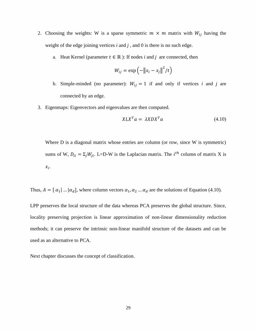
29

2. Choosing the weights: W is a sparse symmetric matrix with having the

weight of the edge joining vertices i and j , and 0 is there is no such edge.

a. Heat Kernel (parameter ): If nodes i and j are connected, then

( ‖ ‖ )

b. Simple-minded (no parameter): if and only if vertices i and j are

connected by an edge.

3. Eigenmaps: Eigenvectors and eigenvalues are then computed.

(4.10)

Where D is a diagonal matrix whose entries are column (or row, since W is symmetric)

sums of W, . L=D-W is the Laplacian matrix. The column of matrix X is

.

Thus, [ | | , where column vectors are the solutions of Equation (4.10).

LPP preserves the local structure of the data whereas PCA preserves the global structure. Since,

locality preserving projection is linear approximation of non-linear dimensionality reduction

methods; it can preserve the intrinsic non-linear manifold structure of the datasets and can be

used as an alternative to PCA.

Next chapter discusses the concept of classification.

30

Chapter 5

Classification

In the world today there exists a large variety of data and this data is collected and recorded on

every aspect of human endeavor. Banking, communication, the internet, visual information, etc.,

are various examples of such aspects. Thus, to be able to make sense of any of these domains,

the ability to process and interpret a large amount of data is required. Classification is the

problem of automatically assigning an object to one of several (often pre-defined) categories

based on the attributes of the object.

Figure 5.1: Classification Example.

In the classification problem we are generally given a training set of objects and their attributes

are called features. Along with this we are given the categories or class labels of each object. A

classifier is then constructed based on the training set. When a training dataset has class labels, it

Training

Set

Testing

Set

Learn

Model

Use

Model

Learning

Algorithm Mode

31

is known as supervised classification. There are several methods of classification, example

support vector machines, nearest neighbors, decision trees, neural networks, etc.

Classification is a two-step process as shown in Figure 5.1. First step is model construction.

Model construction describes a set of predetermined classes. Each sample in this is assumed to

belong to a predefined class, as determined by the class label attribute. The model is represented

as classification rules, etc. The second step is model usage. This step is used for classifying

future or unknown objects.

5.1 Support Vector Machines

The Support Vector Machine (SVM) was first introduced by Boser, Guyon and Vapnik in [43]

and since then, it is very popular due to its simplicity and excellent performance. SVM was

developed from Statistical Learning Theory. It is a supervised learning algorithm which is used

for classification and regression and belongs to the family of generalized linear classifiers.

5.1.1 Statistical Learning Theory

Statistical learning theory models data as a function estimation problem and is described as a

system that receives some data as input and outputs a function that can be used to predict some

features of future data. Thus, a set of training patterns or the training data

{( ) ( ) ( )} is given, where is the training sample and is the class

label associated with training sample. Thus, SVM finds an optimal separating hyperplane or

the hypothesis that is able to correctly classify the given training data.

32

Figure 5.2: Two Class Classification Example using Support Vector Machine.

As seen from Figure 5.2 there could be many hyperplanes which can classify a given set of data.

However, there is only one of these that achieve the maximum separation. SVM finds an optimal

separating hyperplane that maximizes the margin, where margin is the distance between support

vectors and the support vectors are the examples closest to the hyperplane.

Figure 5.3: Example to show Support Vectors, Margin and Decision Boundary.

Class +1

Class -1

Class +1

Class -1

Support

Vectors

33

5.1.2 SVM Mathematical Representation

Let there be a set of training patterns { } assigned to one of the two classes

and , with labels are given, such that

(5.1)

(5.2)

Where, w is the parameter vector and b is the offset vector. Thus for all training samples,

( ) (5.3)

To classify the given dataset, we need to find a linear discriminant function, or decision

boundary such that

( ) (5.4)

This desired hyperplane which maximizes the margin also bisects the lines between closest

points on convex hull of the two datasets. The distance of a closest point on a hyperplane to the

origin can be found by maximizing x, as x is on the hyperplane. Similarly for points on the other

side, we have a similar scenario. Thus, solving and subtracting the two distances we get the

summed distance from the separating hyperplane to nearest points. Maximum Margin = M = 2 /

||w||

In order to maximize the margin, we need to find a solution that minimizes the ||w||, subject to

constraints

34

( ) (5.5)

This leads to a quadratic optimization problem with linear constraints. The solution involves

determining the saddle point of function using Lagrange multipliers

∑ ( (

) )

(5.6)

Where

∑

(5.7)

∑

(5.8)

Since, only the support vectors have

The solution has the form

∑

∑

(5.9)

And b can be found using ( ) where is the support vector.

Thus, the decision rule is given as

( ) {

{

(5.10)

35

5.1.3 Non Linear SVM

For linear data, a separating hyperplane may be used to classify the data. However, often the data

is non-linear. To classify a non-linear dataset, the input data is mapped to another high

dimensional feature space where the data is linearly separable.

Figure 5.4: Non-Linear Classification using SVM.

If the feature space is chosen suitably, classification can be easy. This is also known as the

Kernel trick and the mapping is defined by the kernel

( ) ( ) ( ) (5.11)

Thus, the data is mapped or transformed to a higher dimensional feature space and then the

hyperplane is constructed in that feature space such that all other above equations are the same.

Thus, the decision rule is given as

( ( )) ( ) {

{

(5.12)

This is known as the Kernel Trick. Some of the kernel functions are:

: x (x)

36

Polynomial – ( ) (⟨ ⟩ ) where c, d are constants

Gaussian Radial Basis Function – ( ) ( ‖ ‖

)

Exponential Radial Basis Function – ( ) ( ‖ ‖

)

Multi-Layer Perceptron – ( ) ( ⟨ ⟩ )

5.1.4 Multiclass SVM

SVM is a binary classifier in which there can be only two classes. However, in most of the real

world problems like handwritten digit classification, optical character recognition, etc. there are

more than two classes. Thus, in multiclass SVM, each training point belongs to one of different

classes and the goal is to construct a function which, given a new data point, will correctly

predict the class to which the new point belongs.

Figure 5.5: Multi-class Classification using SVM.

In order to solve a multiclass classification problem, different binary classifiers are built and

each of these classifiers is built to separate one class from the others. These N classifiers are then

Class 1

Class 2

Class 3

Boundary between

Class 1 and others

Boundary between Class 2 and others

Boundary between Class 3 and others

37

combined to get a multi-class classifier. Thus, for the ith

classifier, the positive examples are all

the samples in class i, and the negative examples are all the samples which are not in class i.

5.2 Bootstrapping

The term bootstrapping came from “pulling oneself up by the strap of the boot” in early 19th

century. It is a method to incrementally train a classifier from a large set of training set of

samples. In order to train a classifier it is good to have as many training samples as possible, but

there are many limitations to having a large set of training data, such as storage or computation

resources.

Figure 5.6: Flowchart for Bootstrapping Algorithm.

Collecting object or positive class samples is easier as there could be a limited number of

samples for objects. But, collecting non object or negative class samples could be trickier as

Initial Training

Subset, I

Train with I

Test on

Random

Find

misclassified

samples, M

M >

Thresh

No

Yes

𝐼 𝐼 ∪𝑀

Save Training

Model

38

every image patch that does not contain the object can be added to the negative class sample.

This may result in an exhaustively large set of samples. Thus, in order to restrict the amount of

data samples in the negative class category, we use the “bootstrapping” algorithm which selects

only the required non object patterns from a given training set.

It is an iterative algorithm in which the classifier is given an initial set of random samples from

the large training set. In order to improve the performance, the misclassified samples are added

to the initial training set and the classifier is retrained. The algorithm is as shown in Figure 5.6.

5.3 SVM Usage

In this thesis, we use the LIBSVM [58] library for support vector machine classification. Support

vector machines were preferred over other methods as they aim to maximize the distance

between the positive class and negative training samples. Support vector machines also give the

option of various different kinds of kernels which can be used to improve the classification

performance.

In training, initial positive and negative training data are extracted by using the location of the

object of interest, as provided by the training dataset. The negative training examples are

extracted by using random windows that do not contain the object. There can be many such

windows and it is not always possible to store all the negative training examples and thus the

bootstrapping technique was used to collect only the samples which are relevant and hence help

in learning a stronger classifier.

39

Chapter 6

Eye Detection

6.1 Motivation

With the proliferation of webcams and mobile devices, eye detection is becoming increasingly

important for human computer interaction and augmented reality applications. Human eyes play

an important role in face detection/recognition, face tracking, facial expression recognition. In

the context of mobile interfaces, eye detection provides cues on whether or not the user is

looking at the screen [20]. Furthermore, eye detection is the starting point for gaze estimation

and eye tracking. Following face detection, eye locations can be used for face alignment,

normalization, pose estimation, or initial placement of Active Shape/Active Appearance Models

for efficient convergence. Several eye detection systems are relying on infrared light emitting

diodes, but in general it cannot be assumed that such devices are available.

Eyes are the most prominent facial feature and their localization has received considerable

attention in the computer vision literature. Eye detection methods include active approaches that

require infrared illumination [21], model-based approaches, such as active shape models [22],

methods based on geometrical features, such as eye corners or iris detection [23], and methods

based on feature classification [24], for example using Support Vector Machine (SVM)

classifiers. Methods relying on corners or circles are susceptible to noise, low resolution or poor

illumination. Active Shape models require good initialization and may be computationally

intensive. In this thesis, we consider a computationally efficient approached to eye detection.

40

6.2 Approach

In this work, a robust and efficient eye detector operating on images or video was developed

based on feature classification using Support Vector Machines. The overall eye detection system

is shown in Figure 6.1. The left path in the diagram outlines the training process, while the right

path outlines the testing process.

Figure 6.1: Eye Detection System.

In order to train the SVM classifier, different eye and non-eye patches were collected from the

BioID and FERET [50] databases as shown in Figure 6.2. A feature descriptor was computed for

all these patches. In order to make the descriptor computationally efficient and improve the

Collect Training Samples

Feature Extraction

Dimensionality Reduction

Bootstrapping

Test Image

Face Detection

Feature Extraction

Dimensionality Reduction

SVM

Detected Eye

41

classification performance, dimensionality reduction techniques were used to reduce the number

of features.

(a)

(b)

Figure 6.2: Example (a) Eye and (b) Non-Eye Training Samples.

During the final stage of testing, the bootstrap technique [56] was used to reduce the number of

false positives. The bootstrapping method was performed as follows:

a) A subset of samples was taken from the original training set and the classifier was trained

on this subset.

b) This classifier was tested on a random subset of samples.

c) If the number of false positives were less than the specified threshold, the algorithm was

stopped.

42

d) Otherwise, the false positives were added to the training set, a new classifier was trained

and step b) was repeated.

To test the eye detector on a face image, a sliding window of varying size is used for extracting

image patches for feature extraction and classification. This process can be computationally

intensive and thus is combined with face detection to reduce the search area for faster processing.

A face detector based on the Viola-Jones detector [57] is used to identify the face region. After

face detection, the face region is normalized to a standard size and the local windows for eye

detection are extracted from the upper portion of the face region. The feature descriptor is

computed for each local window and a linear SVM classifier is used to classify the patches into

eyes or non-eyes. After identifying the top 5 patches that are classified as eyes based on the

probability estimates, i.e. probability that the testing instance is in a class, (returned by the

LIBSVM [58] classifier), we cluster them to determine the location of the eye.

43

Chapter 7

Experimental Results and Discussion

7.1 Datasets

7.1.1 BioID

The results were evaluated using the BioID Face Database and the FERET Database. The BioID

database consists of 1521 frontal images of 23 different persons. The images are grayscale and

have size 384x286 pixels. The database includes annotations of 20 locations of facial feature

points for each image.

Figure 7.1: Example Images from BioID.

44

7.1.2 FERET

The FERET database contains both frontal as well as posed faces. The database contains 1564

sets of images with 365 duplicate sets. The duplicate sets contain images of a person already in

the database, but taken on a different day. For some individuals, the time elapsed between their

first and last sitting was over a year in order to accommodate the changes in appearance over

time.

Figure 7.2: Example Images from FERET.

7.1.3 CalTech-101

The CalTech-101 dataset consists of 102 object categories and each category consists of 31 to

800 images per category. These are colored images with size around 300 x 200 pixels.

Additionally, an outline of each object is provided. Figure 7.3 shows some example images from

CalTech-101.

45

Figure 7.3: Example Images from CalTech-101.

7.2 Eye Detection

The training set consisted of 8,258 eye samples and 9,836 non-eye samples extracted from the

BioID and FERET databases. The extracted eye and non-eye patches were normalized to

compensate for variations in illumination. The classification performance was tested using 10-

fold cross validation technique. Figure 7.4 shows accuracy results and Figure 7.5 shows

false positives of eye detection with various image descriptors and dimensionality reduction

techniques. Table 7.1 shows accuracy results with different SVM kernels.

Table 7.1: Accuracy Results with HOG and different SVM Kernels.

Kernels Linear Radial Basis Sigmoid

Accuracy 98.91 97.82 97.59

46

Figure 7.4: Eye Detection Accuracy Results with different Descriptors and Dimensionality

Reduction methodologies.

Figure 7.5: Eye Detection False Positives with different Descriptors and Dimensionality

Reduction methodologies.

0102030405060708090

100

HoG FREAK H-FREAK LBP H-LBP

Orignal 98.91 86.59 98.3 87.18 98.74

PCA 98.16 83.42 97.77 63.29 98.19

RP 98.11 83.22 97.24 53.92 97.92

LPP 98.71 83.22 95.22 60.26 98.47

SLPP 98.7 93.84 99.62 77.42 99.28

Acc

ura

cy (

%)

0

5

10

15

20

25

30

35

40

HoG FREAK H-FREAK LBP H-LBP

Orignal 1.52 16.17 2.51 13.12 1.82

PCA 1.91 18.26 1.87 29.09 2.45

RP 1.03 21.19 2.3 35.29 2.69

LPP 1.53 18.67 3.87 29.79 2.03

SLPP 0.91 12.67 0.03 21.73 1.73

47

HOG Descriptor

The HOG descriptor was found using the cell size as 8, block size as 2 and bin size as 9. Thus,

the descriptor length was found to be 648 for patch size of 25 x 50 and this was reduced to 130

(20%) using different dimensionality reduction techniques. Tables 7.2-7.6 show the confusion

matrices with Histogram of Oriented descriptor.

Figure 7.6: Detection Accuracy as Cell Size and Block Size were varied.

Figure 7.7: Accuracy as Number of Features is varied.

1x1

2x2

3x3

4x46x6

8x810x10

96.8 96.91 95.89

94.65

98.9 98.8

98.91 96.81

98.1 98.01 95.89 96.8

Blo

ck S

ize

Cell Size

85

87

89

91

93

95

97

99

101

5 10 20 30 40 50 60 70 80 90 100

Acc

ura

cy (

%)

Number of Features (%)

48

Figure 7.8: Accuracy and False Positives with Histogram of Oriented Gradients.

Table 7.2: Confusion Matrix for Eye Detection using HOG Descriptor.

Eyes Non Eyes

Eyes 98.91 1.09

Non Eyes 1.52 98.48

Table 7.3: Confusion Matrix for Eye Detection using HOG –PCA Descriptor.

Eyes Non Eyes

Eyes 98.16 1.84

Non Eyes 1.91 98.09

Table 7.4: Confusion Matrix for Eye Detection using HOG-RP Descriptor.

Eyes Non Eyes

Eyes 98.11 1.89

Non Eyes 1.03 98.97

Table 7.5: Confusion Matrix for Eye Detection using HOG – LPP Descriptor.

Eyes Non Eyes

Eyes 98.71 1.29

Non Eyes 1.53 98.47

98.91 98.7 98.71 98.16 98.11

1.52 0.91 1.53 1.91 1.03

False Positives

Accuracy

49

Table 7.6: Confusion Matrix for Eye Detection using HOG – SLPP Descriptor.

Eyes Non Eyes

Eyes 98.7 1.3

Non Eyes 0.91 99.09

FREAK Descriptor

The FREAK descriptor was computed in Matlab using the inbuilt function with radius 21. Since,

the radius of the descriptor was fixed; the patch size was made as 50 x 50 in order to match the

radius. The descriptor length was found to be 512 and was reduced to 102 using different

dimensionality reduction techniques. Tables 7.7-7.11 show the confusion matrices with FREAK

descriptor.

Figure 7.9: Accuracy and False Positives with FREAK.

Table 7.7: Confusion Matrix for Eye Detection using FREAK Descriptor.

Eyes Non Eyes

Eyes 86.59 13.41

Non Eyes 16.17 83.83

86.59 93.84 83.22 83.42 83.22

16.17 12.67 18.67 18.26 21.19

False Positives

Accuracy

50

Table 7.8: Confusion Matrix for Eye Detection using FREAK –PCA Descriptor.

Eyes Non Eyes

Eyes 83.42 16.58

Non Eyes 18.26 81.74

Table 7.9: Confusion Matrix for Eye Detection using FREAK -RP Descriptor.

Eyes Non Eyes

Eyes 83.22 16.78

Non Eyes 21.19 78.81

Table 7.10: Confusion Matrix for Eye Detection using FREAK – LPP Descriptor.

Eyes Non Eyes

Eyes 83.22 16.78

Non Eyes 18.67 81.33

Table 7.11: Confusion Matrix for Eye Detection using FREAK – SLPP Descriptor.

Eyes Non Eyes

Eyes 93.84 6.16

Non Eyes 12.67 87.33

Histogram of FREAK Descriptor

The Histogram of FREAK descriptor was found using the cell size as 4, block size as 2 and bin

size as 20. Thus, the descriptor length was found to be 728 and this was reduced to 145 using

different dimensionality reduction techniques. Tables 7.12-7.16 show the confusion matrices

with this descriptor.

51

Figure 7.10: Accuracy and False Positives with Histogram of FREAK.

Table 7.12: Confusion Matrix for Eye Detection using Histogram of FREAK Descriptor.

Eyes Non Eyes

Eyes 98.30 1.7

Non Eyes 2.51 97.49

Table 7.13: Confusion Matrix for Eye Detection using Histogram of FREAK –PCA Descriptor.

Eyes Non Eyes

Eyes 97.77 2.23

Non Eyes 1.87 98.13

Table 7.14: Confusion Matrix for Eye Detection using Histogram of FREAK -RP Descriptor.

Eyes Non Eyes

Eyes 97.24 2.76

Non Eyes 2.3 97.70

Table 7.15: Confusion Matrix for Eye Detection using Histogram of FREAK – LPP Descriptor.

Eyes Non Eyes

Eyes 95.22 4.78

Non Eyes 3.87 96.13

98.3 99.62 95.22 97.77 97.24

2.51 0.03 3.87 1.87 2.3

False Positives

Accuracy

52

Table 7.16: Confusion Matrix for Eye Detection using Histogram of FREAK – SLPP Descriptor.

Eyes Non Eyes

Eyes 99.62 0.38

Non Eyes 0.03 99.97

LBP Descriptor

The LBP descriptor was found using the 3x3 block with patch size 25x50. The descriptor length

was found to be 1250 and was reduced to 625 using different dimensionality reduction

techniques. Tables 7.17-7.21 show the confusion matrices with LBP descriptor.

Figure 7.11: Accuracy and False Positives with LBP.

Table 7.17: Confusion Matrix for Eye Detection using LBP Descriptor.

Eyes Non Eyes

Eyes 87.18 12.82

Non Eyes 13.12 86.88

Table 7.18: Confusion Matrix for Eye Detection using LBP –PCA Descriptor.

Eyes Non Eyes

Eyes 63.29 36.71

Non Eyes 29.09 70.91

LBP LBP-SLPP LBP-LPP LBP-PCA LBP-RP

87.18 77.42

60.26 63.29 53.92

13.12 21.73 29.79 29.09 35.29

False Positives

Accuracy

53

Table 7.19: Confusion Matrix for Eye Detection using LBP -RP Descriptor.

Eyes Non Eyes

Eyes 53.92 46.08

Non Eyes 35.29 64.71

Table 7.20: Confusion Matrix for Eye Detection using LBP – LPP Descriptor.

Eyes Non Eyes

Eyes 60.26 39.74

Non Eyes 29.79 70.21

Table 7.21: Confusion Matrix for Eye Detection using LBP – SLPP Descriptor.

Eyes Non Eyes

Eyes 77.42 22.18

Non Eyes 21.73 78.27

Histogram of LBP Descriptor

The Histogram of LBP descriptor was found using the cell size as 8, block size as 2 and bin size

as 9. Thus, the descriptor length was found to be 648 and this was reduced to 130 using different

dimensionality reduction techniques. Tables 7.22-7.26 show the confusion matrices with this

descriptor.

Figure 7.12: Accuracy and False Positives with Histogram of LBP.

98.74 99.28 98.47 98.19 97.92

1.82 1.73 2.03 2.45 2.69

False Positives

Accuracy

54

Table 7.22: Confusion Matrix for Eye Detection using Histogram of LBP Descriptor.

Eyes Non Eyes

Eyes 98.74 1.26

Non Eyes 1.82 98.18

Table 7.23: Confusion Matrix for Eye Detection using Histogram of LBP –PCA Descriptor.

Eyes Non Eyes

Eyes 98.19 1.81

Non Eyes 2.45 97.55

Table 7.24: Confusion Matrix for Eye Detection using Histogram of LBP -RP Descriptor.

Eyes Non Eyes

Eyes 97.92 2.08

Non Eyes 2.69 97.31

Table 7.25: Confusion Matrix for Eye Detection using Histogram of LBP – LPP Descriptor.

Eyes Non Eyes

Eyes 98.47 1.53

Non Eyes 2.03 97.97

Table 7.26: Confusion Matrix for Eye Detection using Histogram of LBP – SLPP Descriptor.

Eyes Non Eyes

Eyes 99.28 0.72

Non Eyes 1.73 98.27

Our results demonstrate that eye detection using dimensionality reduction gave results which are

comparable to that of the feature descriptor alone while the feature dimensionality is

significantly reduced. The histogram based features are discriminative and efficient, which

makes them good candidates for real time eye detection.

It was observed that with the use of supervised locality preserving projections (SLPP), false

positives were reduced. With SLPP, the number of false positives were 0.91% for HOG, 0.03%

55

for histogram of FREAK, and 1.73% for histogram of LBP. Without using SLPP, the number of

false positives were 1.52% for HOG, 2.51% for histogram of FREAK, and 1.82% for histogram

of LBP.

To demonstrate the effectiveness of the eye detector on full images, we used a sliding window

approach along with the SVM classification. The eye detection results for representative images

from the BioID database and the FERET database, are shown in Figures 7.13 and 7.14

respectively. The results for BioID and FERET datasets are shown in Table 7.27 and 7.29

respectively.

Table 7.27: Eye Detection Results on BioID with HOG and different Dimensionality Reduction

Techniques.

Method Percent Correct

Left Eye Right Eye Both Eyes

HOG 97.14 96.32 96.25

HOG-SLPP 96.65 96.38 96.18

HOG-LPP 95.63 92.28 91.54

HOG-PCA 96.79 96.25 96.04

HOG-RP 96.32 96.05 95.63

56

(a) HOG descriptor results

(b) HOG-SLPP descriptor results

(c) HOG-LPP descriptor results

(d) HOG-PCA descriptor results

(e) HOG-RP descriptor results

(f) Examples of false positives

Figure 7.13: Eye Detector examples in BioID database (a) HOG Descriptor,

(b) HOG-SLPP Descriptor, (c) HOG-LPP Descriptor, (d) HOG-PCA Descriptor, (e) HOG-RP

Descriptor, and (f) Examples of False Positives.

57

Table 7.28 shows a comparison of eye detection results on the BioID dataset using our approach

and other state-of-the-art approaches. The method in [24] used Haar wavelet coefficients with

SVM classifier and achieved an accuracy of 96.1% on the BioID dataset, while the method of

[64] achieved an accuracy of 91.78% in locating eyes using SVM classifier. The approach in

[23] uses isocentric patterns to locate the eye center and achieved an accuracy of 91.67%.

Table 7.28 Comparison of BioID Results using Different Approaches.

Authors Method Accuracy

Wang, Yang [64] Clustering and binary template matching 91.78%

Campadelli, Lanzarotti,

Lipori [24]

Support Vector Machine

with Haar Wavelet coefficient

96.1%

Valenti, Gevers [23] Isocentric Patterns 91.67%

Our Approach [44] Support Vector Machine with HOG 96.25%

Table 7.29: Eye Detection Results on FERET with HOG and different Dimensionality Reduction

Techniques.

Method Percent Correct

Left Eye Right Eye Both Eyes

HOG 98.95 98.33 98.06

HOG-SLPP 99.11 98.99 98.59

HOG-LPP 98.76 97.7 97.62

HOG-PCA 98.68 97.89 97.45

HOG-RP 98.68 98.07 97.62

58

(a) HOG descriptor results

(b) HOG-SLPP descriptor results

(c) HOG-LPP descriptor results

(d) HOG-PCA descriptor results

(e) HOG-RP descriptor results

(f) Examples of false positives

Figure 7.14: Eye Detector examples in FERET database (a) HOG Descriptor,

(b) HOG-SLPP Descriptor, (c) HOG-LPP Descriptor, (d) HOG-PCA Descriptor, (e) HOG-RP

Descriptor, and (f) Examples of False Positives.

59

Table 7.30 shows a comparison of eye detection results on the FERET dataset using our

approach and other state-of-art approaches. The method in [24] used Haar wavelet coefficients

with SVM classifier and achieved an accuracy of 96.4% on the FERET dataset, while the method

of [65] achieved an accuracy of 98.3% in locating eyes using SVM classifier. The approach in

[23] uses isocentric patterns to locate the eye center and achieved an accuracy of 96.27%.

Table 7.30: Comparison of FERET Results using Different Approaches.

Authors Method Accuracy

Monzo, Albiol, Sastre [65] Adaboost + Haar, SVM + HOG 98.3%

Campadelli, Lanzarotti,

Lipori [24]

Support Vector Machine with Haar Wavelet

coefficient 96.4%

Valenti, Gevers [23] Isocentric Patterns 96.27%

Our Approach [44] Support Vector Machine with HOG+SLPP 98.59%

The eye detection results in the BioID and FERET database demonstrate that the HOG, HOG-

SLPP, HOG-PCA and HOG-RP descriptors perform well and their accuracy results are

comparable within one percent. The overall performance of detector is a bit lower than the

detector performance using 10-fold cross validation for patch classification due to wider

variability in the appearance of patches in full images.

7.3 CalTech-101 Testing

The CalTech-101 dataset consists of 102 object categories and each category consists of 31 to

800 images per category. These are colored images with size around 200 x 300 pixels and were

converted to gray scale and normalized to size 50 x 75. Table 7.31 shows accuracy results with

60

10-fold cross validation with 30 samples per category with HOG descriptor. Table 7.32 shows

accuracy with 30 samples for training and 50 for testing with HOG-SLPP descriptor.

Table 7.31: Results with CalTech-101, 10-Fold Cross Validation, 30 Samples per Category.

SLPP LPP PCA RP

78.3 % 63.4 % 67 % 58 %

Table 7.32: Results with CalTech-101, 30 Training Samples and 50 Testing Samples.

Method SLPP

Overlap 91 %

No-overlap 64 %

Table 7.33: Comparison of Classification Results of CalTech-101 with Different Approaches.

Authors Method Training Accuracy

Zeiler, Fergus

[63] Convolutional Networks

Train – 30

Test – 50 86.5%

Yang, Li, Tian,

Duan, Gao [62]

Multiple Kernel Learning with

SIFT and PHOG

Train – 30

Test - 15 84.3%

Bos, Zisserman,

Munoz [66]

Random forests and ferns with

PHOG for image classification

Train – 30

Test - 50 81.3%

Our Approach Support Vector Machine with

HOG+SLPP

Train – 30

Test - 50

Overlap 91%

No-overlap 64%

10-fold CV All Data 96%

30 samples 78.3%

Table 7.33 shows a comparison of classification results on Caltech-101 dataset using our

approach and other state-of-art approaches. The method in [63] uses convolutional networks for

61

classification and achieved an accuracy of 86.5% on the Caltech-101, while the method of [62]

achieved an accuracy of 84.3% using group sensitive multiple kernel learning approach which

accommodates intra-class diversity and inter-class correlation for object recognition. The

approach in [66] uses random forest and ferns with PHOG for image classification and achieved

an accuracy of 81.3%.

7.4 Image Descriptors

In this section, the performance of different image feature descriptors is evaluated and compared.

The evaluation was done using 10-fold cross validation technique on the eye database created

from BioID and FERET database and Caltech-101.

Figure 7.15: Accuracy for CalTech-101 as Cell Size and Bin Size was varied for HOG-SLPP.

10

12

14

4x46x6

8x810x10

98.78 93.78

87.66 82.01

99.45 95.06

89.16 84.25

99.7 96

90.54 86.12

Bin

Siz

e

Cell Size

62

Figure 7.16: Accuracy for CalTech-101 as Cell Size and Bin Size was varied for H-FREAK –

SLPP.

Figure 7.17: Accuracy for CalTech-101 as Cell Size and Bin Size was varied for H-LBP – SLPP.

10

12

14

4x46x6

8x810x10

96

84.07

70.24

56.22

98.11

87.77

75.98

62.65

99.15 91.42

80.17

69.11

Bin

Siz

e

Cell Size

10

12

14

4x46x6

8x810x10

97.86 90.75

82.87

73.5

98.88 93.31

86.54

77.7

99.36 94.52

87.02 79.06

Bin

Siz

e

Cell Size

63

Figure 7.18: Accuracy for CalTech-101 with different Descriptors.

Figure 7.19: Eye Detection Results.

It was found from the experiments that Histogram of Oriented Gradients feature descriptor

outperforms the binary feature descriptors. An accuracy of 98.91% was achieved with the eye

database and accuracy of 75.08% was achieved with CalTech-101 dataset. In addition, it was

observed that histogram of binary descriptors outperformed binary descriptors for object

detection. Accuracy of 87.18% and 86.59% was achieved with Local Binary pattern and FREAK

descriptor respectively whereas this was increased to 98.74% and 98.3% when histogram of LBP

HoG H-LBP H-FREAK

75.08

60.02

48.26

HoG LBP H-LBP FREAK H-FREAK

98.91 87.18

98.74 86.59

98.3

1.52 13.12 1.82 16.17 2.51

False Positives

Accuracy

64

and Histogram of FREAK was used as a feature descriptor respectively. This was because

support vector machines use Euclidean distance as the distance measure.

7.5 Dimensionality Reduction

In this section, performance of different dimensionality reduction methodologies is evaluated and

compared. The evaluation was done using 10-fold cross validation technique on Caltech-101.

The object images were cropped using the given annotations and were resized to 50 x 75. The

classification performance was tested using 10-fold cross validation technique. Histogram of

descriptors was found using cell size 6, block size 2 and bin size 14. The results with different

descriptors are as shown in Table 7.34.

Figure 7.20: Graph showing Accuracy as we increase the Number of Components CalTech-101.

It was found by experiments that the dimensions of the data can be reduced to 5% using different

dimensionality reduction techniques.

Table 7.34: Results with CalTech-101.

Descriptor Original S-LPP LPP PCA RP

HOG 75.08 96 75.93 78.12 78.15

H-LBP 60.2 94.52 43.59 62.38 47.76

H-FREAK 48.26 91.42 51.25 49.8 45.27

70

72

74

76

78

80

1 3 5 10 20 40 60 80 100

Acc

ura

cy (

%)

Number of Features (%)

65

Figure 7.21: Results with different Descriptors and Dimensionality Reduction techniques for

CalTech-101.

Experimental results showed that using dimensionality reduction increases the performance of

classification. It was observed that dimensionality reduction with histogram of oriented gradients

gave better accuracy as compared to histogram of oriented gradients alone. Increase of 20.9%,

0.85%, 0.04%, and 0.07% was observed with supervised Locality preserving projection,

unsupervised locality preserving projections, principal component analysis and random

projections respectively.

It was found that supervised locality preserving projections worked best as compared to other

dimensionality reduction techniques. With SLPP the classification accuracy was increased by

20.9%, 34.32% and 43.16% with histogram of oriented gradients, histogram of LBP and

histogram of FREAK feature descriptor respectively for Caltech-101. Additionally, it was

observed that Random Projections was fast to compute and gave comparable results as principal

component analysis and unsupervised locality preserving projections.

0

20

40

60

80

100

Hog H-LBP H-FREAK

Acc

ura

cy (

%)

Original

SLPP

LPP

PCA

RP

66

Chapter 8

Conclusions

This thesis explores object detection using different dimensionality reduction techniques on

HOG or binary image descriptors. The major contributions of this thesis include an efficient eye

detection approach using dimensionality reduction on histogram of oriented gradients as a

feature descriptor. Also, histogram based FREAK descriptor was proposed as a feature descriptor

for successful object detection. Furthermore, different feature descriptors and different

dimensionality reduction techniques were analyzed and evaluated for object detection.

Histogram based feature descriptors such as Histogram of Oriented Gradients (HOG), histogram

of FREAK (H-FREAK) and histogram of Local Binary Pattern (H-LBP) were explored as good

features for object detection. It was found that Histogram of Oriented gradients worked best both

in accuracy and speed as compared to binary descriptors. Accuracy of 75% was obtained by

using Histogram of Oriented Gradients as a feature descriptor for CalTech-101 dataset whereas

Histogram of FREAK and Histogram of LBP descriptor gave an accuracy of 48.26 % and 60.2%

respectively. In case of eye detection, accuracy of 98.91% was achieved with HOG and accuracy

of 98.3% and 98.7% was achieved with H-FREAK and H-LBP feature descriptor respectively.

Also, since histogram based descriptors can be of large dimensions, different dimensionality

reduction techniques were explored in order to reduce the dimensions of the image descriptors.

Experimental results showed that supervised locality preserving projections worked best as

compared to other dimensionality reduction techniques. With SLPP the classification accuracy

was increased by 43.16% with H-FREAK feature descriptor for Caltech-101. Furthermore, it was

67

observed that Random Projections was fast to compute and gave comparable results as principal

component analysis.

The future challenges to this work involve using binary descriptors with Hamming distance as

the distance measure in support vector machines and compare these results for object detection

with Euclidean distance as the distance measure in support vector machines. Another challenge

in the improvement of the object detection system would be to use deformable parts model with

Histogram based descriptors and supervised locality preserving projection as the dimensionality

reduction technique.

68

References

[1] T. Malisiewicz, A. Gupta and A. Efros, "Ensemble of Exemplar-SVMs for Object

Detection and Beyond," in International Conference on Computer Vision, Spain, 2011.

[2] P. Deniz, G. Bueno, J. Salido and F. Torre, "Face Recognition using Histogram of

Oriented Gradients," Pattern Recognition Letters, vol. 32, no. 12, pp. 1598-1603, 2011.

[3] J. M. Keller, M. R. Gray and J. A. Givens, "A fuzzy k-nearest neighbor algorithm," IEEE

Transactions on Systems, Man and Cybernetics, vol. 4, pp. 580-585, 1985.

[4] M. Mitchell, J. Dodge, A. Goyal, K. Yamaguchi, K. Stratos, X. Han, A. Mensch, A.

Berg, T. Berg and H. Daume, "Midge: Generating Image Descriptors from Computer

Vision Detections," in European Chapter of the Association for Computational

Linguistics, France, 2012.

[5] N. Dalal and B. Triggs, "Histogram of Oriented Gradients for Human Detection," in

IEEE Computer Vision and Pattern Recognition, California, 2005.

[6] Y. Rodriguez and S. Marcel, "Face Authentication using Adapted Local Binary Pattern

Histograms," in European Conference on Computer Vision, Graz, Austria, 2006.

[7] J. Gall, A. Yao, N. Razavi and V. Gool, "Hough Forests for Object detection, tracking

and action recognition," in IEEE Transaction on Pattern Analysis and Machine

Intelligence, 2011.

[8] J. Gall and V. Lempitsky, "Class-specific hough forests for object detection," in Decision

Forests for Computer Vision and Medical Image Analysis, London, 2013.

[9] D. Tran and D. Forsyth, "Configuration Estimates Improve Pedestrian Finding," in

Neural Information Processing Systems, Vancouver, 2007.

69

[10] S. Leutenegger, C. Margarita and R. Y. Siegwart, "Brisk: Binary Robust Invariant

Scalable Keypoints," in IEEE International Conference on Computer Vision, Spain,

2011.

[11] R. O. Duda, P. E. Hart and D. G. Stork, Pattern Classification, Wiley, 2000.

[12] A. Ghodsi, "Dimensionality Reduction: A Short Tutorial," Department of Actuarial

Science, University of Waterloo, Ontario, Canada, 2006.

[13] E. Bingham and H. Mannila, "Random Projection in Dimensionality Reduction:

Application to Image and Text Data," in ACM International Conference on Knowledge

Discovery and Data Minning, San Francisco, CA, 2001.

[14] D. Achlioptas, "Database-friendly Random Projections: Johnson-Lindenstrauss with

Binary Coins," Journal of Computer and System Sciences, vol. 4, no. 66, pp. 671-687,

2003.

[15] X. He and P. Niyogi, "Locality Preserving Projections," Neural Information Processing

Systems, vol. 16, pp. 234-241, 2003.

[16] M. Uricar, V. Franc and V. Hlavac, "Detector of Facial Landmarks Learned by the

Structured Output SVM," in International Conference on Computer Vision Theory and

Applications (VISAPP), Rome, 2012.

[17] J. Shermina, "Application of Locality Preserving Peojections in Face Recognition,"

International Journal of Advanced Computer Science and Applications, vol. 1, no. 3,

2010.

[18] C. Papageorgiou and T. Poggio, "A Trainable System for Object Detection,"

International Journal of Computer Vision, vol. 38, no. 1, pp. 15-30, 2000.

70

[19] . A. Rowley, S. Baluja and T. Kanade, "Neural Network based Face Detection," IEEE

Transaction on Pattern Analysis and Machine Intelligence, vol. 20, no. 1, pp. 29-38,

1998.

[20] E. Miluzzo, T. Wang and A. T. Campbell, "EyePhone: Activating Mobile Phones with

your Eyes," in ACM SIGCOMM Workshop on Networking Systems, and Applications on

Mobile Handhelds, New Delhi, 2010.

[21] Z. Zhu and Q. Ji, "Robust Real-Time Eye Detection and Tracking under variable

Lighting Conditions and various Face Orientations," Computer Vision and Image

Understanding, vol. 98, no. 1, pp. 124-154, 2005.

[22] T. F. Cootes and C. J. Taylor, "Active Shape Models Search using Local Grey-Level

Models: A Quantitative Evaluation," British Machine Vision Conference, vol. 93, pp.

639-648, 1993.

[23] R. Valenti and T. Gevers, "Accurate Eye Center Location through Invariant Isocentric

Patterns," IEEE Transaction on Pattern Analysis and Machine Intelligence, vol. 34, no.

9, pp. 1785-1798, 2012.

[24] P. Campadelli, R. Lanzarotti and G. Lipori, "Precise Eye Localization through a General-

to-Specific Model Definition," British Machine Vision Conference, pp. 187-196, 2006.

[25] O. Regniers, J. Costa, G. Grenier and L. Bombrun, "Texture based Image Retrieval and

Classification of Very High Resolution Maritime Pine Forest Images," in IEEE

International Geoscience and Remote Sensing Symposium, Melbourne, 2013.

[26] T. Barbu, "SVM-based Human Cell Detection technique using Histogram of Oriented

Gradients," in WEAS International Conference on Mathematical Methods for Information

Sciences and Economics, 2012.

71

[27] X. Cao, C. Wu, P. Yan and X. Li, "Linear SVM Classification using Boosting HOG

Features for Vehicle Detection in Low Altitude Airborne Videos," in IEEE International

Conference on Image Processing, Orlando, 2011.

[28] M. Calonder, V. Lepetit, C. Strecha and P. Fua, "BRIEF: Binary Robust Independent

Elementary Features," in European Conference on Computer Vision, Berlin, 2010.

[29] J. Zhang, K. Huang, Y. Yu and T. Tan, "Boosted Local Structured HOG-LBP for Object

Localization," in IEEE Conference on Computer Vision and Pattern Recognition, Rhode

Island, 2011.

[30] X. Wang, T. X. Han and S. Yan, "An HOG-LBP Human Detector with Partial Occlusion

Handling," in IEEE International Conference on Computer Vision, Kyoto, Japan, 2009.

[31] T. Ahonen, A. Haddid and M. Pietikainen, "Face Description with Local Binary Patterns:

Application to Face Recognition," IEEE Transaction on Pattern Analysis and Machine

Intelligence, vol. 28, no. 12, pp. 2037-2041, 2006.

[32] T. Ojala and M. Pietikainen, "Multiresolution Gray-Scale and Rotation Invariant Texture

Classification with Local Binary Patterns," IEEE Transaction on Pattern Analysis and

Machine Intelligence, vol. 24, no. 7, pp. 971-987, 2002.

[33] L. Szasz-Toth, "Combination of Classifier Cascades and Training Sample Selection for

Robust Face Detection," in Universitat Karlsruhe, Germany, 2009.

[34] A. Bosch, A. Zisserman and X. Munoz, "Representing Shape with a Spatial Pyramid

Kernel," in ACM International Conference on Image and Video Retrieval, Amsterdam,

2007.

72

[35] M. Marszalek, C. Schmid, H. Harzallah and J. Weijer, "Learning Object Representations

for Visual Object Class Recognition," in Visual Recognition Challenge Workshop, in

conjunction with ICCV, Brazil, 2007.

[36] D. G. Lowe, "Distinctive Image Features from Scale-Invariant Keypoints," International

Journal of Computer Vision, vol. 60, no. 2, pp. 91-110, 2004.

[37] Y. Ke and R. Sukthankar, "PCA-SIFT: A more distinctive representation for Local Image

Descriptors," in IEEE Computer Society Conference on Computer Vision and Pattern

Recognition, Washington DC, 2004.

[38] J. Lin and D. Gunopulos, "Dimensionality Reduction by Random Projection and Latent

Semantic Indexing," in SIAM International Conference on Data Mining, San Francisco,

2003.

[39] A. Alahi, R. Ortiz and P. Vandergheynst, "FREAK: Fast Retina Keypoint," in IEEE

Conference on Computer Vision and Pattern Recognition, Rhode Island, 2012.

[40] A. Vedaldi, V. Gulshan, M. Varma and A. Zisserman, "Multiple Kernel for Object

Detection," in IEEE International Conference on Computer Vision, Kyoto, Japan, 2009.

[41] W. R. Schwartz, A. Kembhavi, D. Hardwood and L. S. Davis, "Human Detection using

Partial Least Square Analysis," in IEEE International Conference on Computer Vision,

Kyoto, Japan, 2009.

[42] M. Pietikainen, A. Hadid, G. Zhao and T. Ahonen, "Local Binary Patterns for Still

Images," Computer Vision using Local Binary Patterns, vol. 40, pp. 13-47, 2011.

[43] B. E. Boser, I. M. Guyon and V. N. Vapnik, "A Training Algorithm for Optimal Margin

Classifiers," in Proceedings of the Conference on Learning Theory, 1992.

73

[44] A. Savakis, R. Sharma and M. Kumar, "Efficient Eye Detection using HOG-PCA

Descriptor," in IS&T/SPIE Electronic Imaging Conference, Imaging and Multimedia

Analytics in a Web and Mobile World , San Francisco, 2014.

[45] S. Agarwal and A. Awan, "Learning to Detect Objects in Images via a Sparse, Part Based

Representation," IEEE Transaction on Pattern Analysis and Machine Intelligence, vol.

26, no. 11, pp. 1475-1490, 2004.

[46] X. R. Chen and A. Yuille, "Detecting and Reading Text in Natural Scenes," in IEEE

International Conference on Computer Vision and Pattern Recognition, Washington DC,

2004.

[47] E. Osuna, R. Freund and F. Girosi, "Training Support Vector Machines: An Application

to Face Detection," in IEEE Conference on Computer Vision and Pattern Recognition,

Puerto Rico, 1997.

[48] C. P. Papageorgiou and T. Poggio, "A Trainable Object Detection System: Car Detection

in Static Images," MIT AI Memo, no. 180, 1999.

[49] P. F. Felzenszwalb, D. A. McAllester and D. Ramanan, "A Discriminatively Trained,

Multiscale, Deformable Part Model," in IEEE International Conference on Computer

Vision and Pattern Recognition, Alaska, 2008.

[50] P. J. Philips, H. Wechsler, J. Huang and P. J. Rauss, "The FERET database and

Evaluation procedure for Face Recognition Algorithms," Image and Vision Computing

Journal, vol. 16, no. 5, pp. 296-306, 1998.

[51] P. J. Philips, H. Moon, S. A. Rizvi and P. J. Rauss, "The FERET Evaluation

Methodology for Face Recognition Algorithms," IEEE Transaction on Pattern Analysis

and Machine Intelligence, vol. 22, pp. 1090-1104, 2000.

74

[52] D. Comaniciu and P. Meer, "Robust Analysis of Feature Spaces: Color Image

Segmentation," IEEE Transaction on Pattern Analysis and Machine Intelligence, vol. 24,

pp. 603-619, 2002.

[53] L. Fei-Fei, R. Fergus and P. Perona, "One-Shot Learning of Object Categories," IEEE

Transaction on Pattern Analysis and Machine Intelligence, vol. 28, no. 4, pp. 594-611,

2006.

[54] C. Garcia and M. Delakis, "Convolutional Face Finder: A Neural Architecture for Fast

and Robust Face Detection," IEEE Transaction on Pattern Analysis and Machine

Intelligence, vol. 26, no. 11, pp. 1408-1423, 2004.

[55] M. Brown and D. G. Lowe, "Automatic Panoramic Image Stitching using Invariant

Features," International Journal of Computer Vision, vol. 74, no. 1, pp. 59-73, 2007.

[56] T. Vetter, M. J. Jones and T. Poggio, "A Bootstrapping Algorithm for Learning Linear

Models of Object Classes," in IEEE Conference on Computer Vision and Pattern

Recognition, Puerto Rico, 1997.

[57] P. Viola and M. J. Jones, "Robust Real-Time Face Detection," International Journal of

Computer Vision, vol. 57, no. 2, pp. 137-154, 2004.

[58] C. C. Chang and C. J. Lin, "LIBSVM: A Library for Support Vector Machines," ACM

Transactions on Intelligent Systems and Technology, vol. 2, no. 3, 2011.

[59] P. S. Hiremath and J. Pujari, "Content Based Image Retrieval using Color, Texture and

Shape Features," in IEEE International Conference on Advanced Computing and

Communications, Guwahati, India, 2007.

[60] A. Saxena, A. Gupta and A. Mukerjee, "Non-Linear Dimensionality Reduction by

Locally Linear Isomaps," in Neural Information Processing Systems, Berlin, 2004.

75

[61] M. Belkin and P. Niyogi, "Laplacian Eigenmaps for Dimensionality Reduction and Data

Representation," Neural Computation, vol. 15, no. 6, pp. 1372-1396, 2003.

[62] J. Yang, Y. Li, Y. Tian, L. Duan and W. Gao, "Group-Sensitive Multiple Kernel

Learning for Object Categorization," in IEEE International Conference on Computer

Vision, Kyoto, Japan, 2009.

[63] M. D. Zeiler and R. Fergus, "Visualizing and Understanding Convolutional Networks," in

ARXIV, 2013.

[64] Q. Wang and J. Yang, "Eye Detection in Facial Images with Unconstrained Background,"

Journal of Pattern Recognition Research, vol. 22, no. 3, pp. 471-480, 2011.

[65] D. Monzo, A. Albiol and J. Sastre, "Precise Eye Localization using HOG Descriptors,"

Machine Vision and Applications, vol. 22, no. 3, pp. 471-480, 2011.

[66] A. Bosch, A. Zisserman and Z. Munoz, "Image Classification using Random Forests and

Ferns," in IEEE International Conference on Computer Vision, Brazil, 2007.

[67] P. Scovanner, S. Ali and S. M. Shah, "A 3-Dimensional SIFT Descriptor and its

Application to Action Recognition," in ACM International Conference on Multimedia,

Germany, 2007.

[68] J. Sivic, B. C. Russell, A. A. Efros, A. Zisserman and W. T. Freeman, "Discovering

Objects and their Location in Images," in IEEE International Conference on Computer

Vision, Beijing, 2005.