CBMM Memo No. 058 February 7, 2017

Why and When Can Deep – but Not Shallow – Networks Avoid theCurse of Dimensionality: a Review

by

Tomaso Poggio1 Hrushikesh Mhaskar2 Lorenzo Rosasco1 Brando Miranda1 Qianli Liao1

1Center for Brains, Minds, and Machines, McGovern Institute for Brain Research,Massachusetts Institute of Technology, Cambridge, MA, 02139.

2Department of Mathematics, California Institute of Technology, Pasadena, CA 91125;Institute of Mathematical Sciences, Claremont Graduate University, Claremont, CA 91711

Abstract: The paper characterizes classes of functions for which deep learning can be exponentially better than shallow learning. Deepconvolutional networks are a special case of these conditions, though weight sharing is not the main reason for their exponential advantage.

This work was supported by the Center for Brains, Minds and Machines (CBMM), fundedby NSF STC award CCF - 1231216. H.M. is supported in part by ARO Grant W911NF-15-1-0385.

1

arX

iv:1

611.

0074

0v5

[cs

.LG

] 4

Feb

201

7

Why and When Can Deep – but Not Shallow – Networks Avoid theCurse of Dimensionality: a Review

Tomaso Poggio1 Hrushikesh Mhaskar2 Lorenzo Rosasco1 Brando Miranda1 Qianli Liao1

1Center for Brains, Minds, and Machines, McGovern Institute for Brain Research, Massachusetts Institute of Technology, Cambridge, MA, 02139.2Department of Mathematics, California Institute of Technology, Pasadena, CA 91125; Institute of Mathematical Sciences, Claremont Graduate University, Claremont, CA 91711

Abstract: The paper characterizes classes of functions for which deep learning can be exponentially better than shallow learning. Deep convolutional networks are aspecial case of these conditions, though weight sharing is not the main reason for their exponential advantage.

Keywords: Deep and Shallow Networks, Convolutional Neural Networks, Function Approximation, Deep Learning

1 A theory of deep learning

1.1 Introduction

There are at three main sets of theory questions about Deep NeuralNetworks. The first set of questions is about the power of the archi-tecture – which classes of functions can it approximate and learnwell? The second set of questions is about the learning process: whyis SGD (Stochastic Gradient Descent) so unreasonably efficient, atleast in appearance? The third, more important question is aboutgeneralization. Overparametrization may explain why minima areeasy to find during training but then why does overfitting seems tobe less of a problem than for classical shallow networks? Is this be-cause deep networks are very efficient algorithms for HierarchicalVector Quantization?

In this paper we focus especially on the first set of questions, sum-marizing several theorems that have appeared online in 2015[1, 2, 3],and in 2016[4, 5]). We then describe additional results as well as afew conjectures and open questions. The main message is that deepnetworks have the theoretical guarantee, which shallow networksdo not have, that they can avoid the curse of dimensionality for animportant class of problems, corresponding to compositional func-tions, that is functions of functions. An especially interesting subsetof such compositional functions are hierarchically local composi-tional functions where all the constituent functions are local in thesense of bounded small dimensionality. The deep networks that canapproximate them without the curse of dimensionality are of thedeep convolutional type (though weight sharing is not necessary).

Implications of the theorems likely to be relevant in practice are:

1. Certain deep convolutional architectures have a theoreticalguarantee that they can be much better than one layer archi-tectures such as kernel machines;

2. the problems for which certain deep networks are guar-anteed to avoid the curse of dimensionality (see for anice review [6]) correspond to input-output mappings thatare compositional. The most interesting set of problemsconsists of compositional functions composed of a hier-archy of constituent functions that are local: an exam-ple is f(x1, · · · , x8) = h3(h21(h11(x1, x2), h12(x3, x4)),h22(h13(x5, x6), h14(x7, x8))). The compositional functionf requires only “local” computations (here with just dimen-sion 2) in each of its constituent functions h;

3. the key aspect of convolutional networks that can give theman exponential advantage is not weight sharing but locality ateach level of the hierarchy.

2 Previous theoretical work

Deep Learning references start with Hinton’s backpropagation andwith Lecun’s convolutional networks (see for a nice review [7]).Of course, multilayer convolutional networks have been around atleast as far back as the optical processing era of the 70s. TheNeocognitron[8] was a convolutional neural network that wastrained to recognize characters. The property of compositional-ity was a main motivation for hierarchical models of visual cortexsuch as HMAX which can be regarded as a pyramid of AND andOR layers[9], that is a sequence of conjunctions and disjunctions.Several papers in the ’80s focused on the approximation power andlearning properties of one-hidden layer networks (called shallownetworks here). Very little appeared on multilayer networks, (butsee [10, 11, 12]), mainly because one hidden layer nets performed em-pirically as well as deeper networks. On the theory side, a reviewby Pinkus in 1999[13] concludes that “...there seems to be reasonto conjecture that the two hidden layer model may be significantlymore promising than the single hidden layer model...”. A versionof the questions about the importance of hierarchies was askedin [14] as follows: “A comparison with real brains offers another,and probably related, challenge to learning theory. The “learn-ing algorithms” we have described in this paper correspond toone-layer architectures. Are hierarchical architectures with morelayers justifiable in terms of learning theory? It seems that thelearning theory of the type we have outlined does not offer anygeneral argument in favor of hierarchical learning machines forregression or classification. This is somewhat of a puzzle since theorganization of cortex – for instance visual cortex – is stronglyhierarchical. At the same time, hierarchical learning systems showsuperior performance in several engineering applications.” Be-cause of the great empirical success of deep learning over the lastthree years, several papers addressing the question of why hierar-chies have appeared. Sum-Product networks, which are equivalentto polynomial networks (see [15, 16]), are a simple case of a hierar-chy that was analyzed[17] but did not provide particularly usefulinsights. Montufar and Bengio[18] showed that the number of linearregions that can be synthesized by a deep network with ReLU non-linearities is much larger than by a shallow network. The meaningof this result in terms of approximation theory and of our results isat the moment an open question1. Relevant to the present review isthe work on hierarchical quadratic networks[16], together with func-tion approximation results[19, 13]. Also relevant is the conjecture byShashua (see [20]) on a connection between deep learning networksand the hierarchical Tucker representations of tensors. In fact, ourtheorems describe formally the class of functions for which theconjecture holds. This paper describes and extends results pre-

1We conjecture that the result may be similar to other examples in section 4.2. It saysthat among the class of functions that are piecewise linear, there exist functions that canbe synthesized by deep networks with a certain number of units but require a much largenumber of units to be synthesized by shallow networks

sented in[21, 22, 23] and in[24, 4] which derive new upper bounds forthe approximation by deep networks of certain important classes offunctions which avoid the curse of dimensionality. The upper boundfor the approximation by shallow networks of general functionswas well known to be exponential. It seems natural to assume that,since there is no general way for shallow networks to exploit a com-positional prior, lower bounds for the approximation by shallownetworks of compositional functions should also be exponential.In fact, examples of specific functions that cannot be representedefficiently by shallow networks have been given very recently byTelgarsky [25] and by Shamir [26]. We provide in theorem 5 anotherexample of a class of compositional functions for which there is agap between shallow and deep networks.

3 Function approximation by deep networks

In this section, we state theorems about the approximation proper-ties of shallow and deep networks.

3.1 Degree of approximation

The general paradigm is as follows. We are interested in determin-ing how complex a network ought to be to theoretically guaranteeapproximation of an unknown target function f up to a given accu-racy ε > 0. To measure the accuracy, we need a norm ‖ · ‖ on somenormed linear space X. As we will see the norm used in the resultsof this paper is the sup norm in keeping with the standard choicein approximation theory. Notice, however, that from the point ofview of machine learning, the relevant norm is the L2 norm. In thissense, several of our results are stronger than needed. On the otherhand, our main results on compositionality require the sup normin order to be independent from the unknown distribution of theinputa data. This is important for machine learning.

Let VN be the be set of all networks of a given kind with complexityN which we take here to be the total number of units in the network(e.g., all shallow networks with N units in the hidden layer). Itis assumed that the class of networks with a higher complexityinclude those with a lower complexity; i.e., VN ⊆ VN+1. Thedegree of approximation is defined by

dist(f, VN ) = infP∈VN

‖f − P‖. (1)

For example, if dist(f, VN ) = O(N−γ) for some γ > 0, thena network with complexity N = O(ε

− 1γ ) will be sufficient to

guarantee an approximation with accuracy at least ε. Since f isunknown, in order to obtain theoretically proved upper bounds, weneed to make some assumptions on the class of functions fromwhich the unknown target function is chosen. This a priori infor-mation is codified by the statement that f ∈W for some subspaceW ⊆ X. This subspace is usually a smoothness class characterizedby a smoothness parameter m. Here it will be generalized to asmoothness and compositional class, characterized by the parame-ters m and d (d = 2 in the example of Figure 1; in general is thesize of the kernel in a convolutional network).

3.2 Shallow and deep networks

This section characterizes conditions under which deep networksare “better” than shallow network in approximating functions. Thuswe compare shallow (one-hidden layer) networks with deep net-works as shown in Figure 1. Both types of networks use the samesmall set of operations – dot products, linear combinations, a fixednonlinear function of one variable, possibly convolution and pool-ing. Each node in the networks we consider usually corresponds to

a node in the graph of the function to be approximated, as shown inthe Figure. In particular each node in the network contains a certainnumber of units. A unit is a neuron which computes

(〈x,w〉+ b)+, (2)

where w is the vector of weights on the vector input x. Both t andthe real number b are parameters tuned by learning. We assume herethat each node in the networks computes the linear combination ofr such units

r∑i=1

ci(〈x, ti〉+ bi)+ (3)

Notice that for our main example of a deep network correspondingto a binary tree graph, the resulting architecture is an idealizedversion of the plethora of deep convolutional neural networks de-scribed in the literature. In particular, it has only one output at thetop unlike most of the deep architectures with many channels andmany top-level outputs. Correspondingly, each node computes asingle value instead of multiple channels, using the combinationof several units (see Equation 3). Our approach and basic resultsapply rather directly to more complex networks (see third note insection 6). A careful analysis and comparison with simulations willbe described in future work.

The logic of our theorems is as follows.

• Both shallow (a) and deep (b) networks are universal, that isthey can approximate arbitrarily well any continuous functionof n variables on a compact domain. The result for shallownetworks is classical. Since shallow networks can be viewedas a special case of deep networks, it clear that for any contin-uous function of n variables, there exists also a deep networkthat approximates the function arbitrarily well on a compactdomain.

• We consider a special class of functions of n variables on acompact domain that are a hierarchical compositions of localfunctions such as

f(x1, · · · , x8) = h3(h21(h11(x1, x2), h12(x3, x4)),

h22(h13(x5, x6), h14(x7, x8))) (4)

The structure of the function in equation 4 is represented by agraph of the binary tree type. This is the simplest example ofcompositional functions, reflecting dimensionality d = 2 forthe constituent functions h. In general, d is arbitrary but fixedand independent of the dimensionality n of the compositionalfunction f . In our results we will often think of n increasingwhile d is fixed. In section 4 we will consider the more generalcompositional case.

• The approximation of functions with a compositional struc-ture – can be achieved with the same degree of accuracy bydeep and shallow networks but that the number of parametersare much smaller for the deep networks than for the shallownetwork with equivalent approximation accuracy. It is intu-itive that a hierarchical network matching the structure of acompositional function should be “better” at approximatingit than a generic shallow network but universality of shallownetworks asks for non-obvious characterization of “better”.Our result makes clear that the intuition is indeed correct.

x1 x2 x3 x4 x5 x6 x7 x8

a b c

….∑

x1 x2 x3 x4 x5 x6 x7 x8

….….

…....... ... ...

∑

...

...

...

∑

x1 x2 x3 x4 x5 x6 x7 x8x1 x2 x3 x4 x5 x6 x7 x8

x1 x2 x3 x4 x5 x6 x7 x8 x1 x2 x3 x4 x5 x6 x7 x8

Figure 1 The top graphs are associated to functions; each of the bottom diagrams depicts the ideal network approximating the function above. In a) a shallow universalnetwork in 8 variables and N units approximates a generic function of 8 variables f(x1, · · · , x8). Inset b) shows a binary tree hierarchical network at the bottomin n = 8 variables, which approximates well functions of the form f(x1, · · · , x8) = h3(h21(h11(x1, x2), h12(x3, x4)), h22(h13(x5, x6), h14(x7, x8))) asrepresented by the binary graph above. In the approximating network each of the n− 1 nodes in the graph of the function corresponds to a set of Q = N

n−1ReLU

units computing the ridge function∑Qi=1 ai(〈vi,x〉+ ti)+, with vi,x ∈ R2, ai, ti ∈ R. Each term in the ridge function corresponds to a unit in the node (this is

somewhat different from todays deep networks, but equivalent to them, see text and note in 6). In a binary tree with n inputs, there are log2n levels and a total of n− 1nodes. Similar to the shallow network, a hierarchical network is universal, that is, it can approximate any continuous function; the text proves that it can approximate acompositional functions exponentially better than a shallow network. No invariance – that is weight sharing – is assumed here. Notice that the key property that makesconvolutional deep nets exponentially better than shallow for compositional functions is the locality of the constituent functions – that is their low dimensionality.Weight sharing corresponds to all constituent functions at one level to be the same (h11 = h12 etc.). Inset c) shows a different mechanism that can be exploited by thedeep network at the bottom to reduce the curse of dimensionality in the compositional function at the top: leveraging different degrees of smoothness of the constituentfunctions, see Theorem 6 in the text. Notice that in c) the input dimensionality must be≥ 2 in order for deep nets to have an advantage over shallow nets. The simplestexamples of functions to be considered for a), b) and c) are polynomials with a structure corresponding to the graph at the top.

In the perspetive of machine learning, we assume that the shallownetworks do not have any structural information on the function tobe learned (here its compositional structure), because they cannotrepresent it directly and cannot exploit the advantage of a smallernumber of parameters. In any case, in the context of approximationtheory, we will exhibit and cite lower bounds of approximation byshallow networks for the class of compositional functions. Deepnetworks with standard architectures on the other hand do representcompositionality in their architecture and can be adapted to thedetails of such prior information.

We approximate functions of n variables of the form of Equation(4) with networks in which the activation nonlinearity is a smoothedversion of the so called ReLU, originally called ramp by Breimanand given by σ(x) = x+ = max(0, x) . The architecture of thedeep networks reflects Equation (4) with each node hi being a ridgefunction, comprising one or more neurons.

Let In = [−1, 1]n, X = C(In) be the space of all continuousfunctions on In, with ‖f‖ = maxx∈In |f(x)|. Let SN,n denotethe class of all shallow networks with N units of the form

x 7→N∑k=1

akσ(〈wk, x〉+ bk),

where wk ∈ Rn, bk, ak ∈ R. The number of trainable parametershere is (n+2)N ∼ n. Letm ≥ 1 be an integer, andWn

m be the setof all functions of n variables with continuous partial derivativesof orders up to m <∞ such that ‖f‖+

∑1≤|k|1≤m ‖D

kf‖ ≤ 1,where Dk denotes the partial derivative indicated by the multi-integer k ≥ 1, and |k|1 is the sum of the components of k.

For the hierarchical binary tree network, the analogous spaces aredefined by considering the compact set Wn,2

m to be the class ofall compositional functions f of n variables with a binary treearchitecture and constituent functions h in W 2

m. We define thecorresponding class of deep networks DN,2 to be the set of alldeep networks with a binary tree architecture, where each of theconstituent nodes is in SM,2, where N = |V |M , V being the setof non–leaf vertices of the tree. We note that in the case when n isan integer power of 2, the total number of parameters involved in adeep network in DN,2 – that is, weights and biases, is 4N .

Two observations are critical to understand the meaning of ourresults:

• compositional functions of n variables are a subset of func-tions of n variables, that is Wn

m ⊇Wn,2m . Deep networks can

exploit in their architecture the special structure of compo-sitional functions, whereas shallow networks are blind to it.Thus from the point of view of shallow networks, functions inWn,2m are just functions in Wn

m; this is not the case for deepnetworks.

• the deep network does not need to have exactly the same com-positional architecture as the compositional function to beapproximated. It is sufficient that the acyclic graph represent-ing the structure of the function is a subgraph of the graphrepresenting the structure of the deep network. The degreeof approximation estimates depend on the graph associatedwith the network and are thus an upper bound on what couldbe achieved by a network exactly matched to the functionarchitecture.

The following two theorems estimate the degree of approximationfor shallow and deep networks.

3.3 Shallow networks

The first theorem is about shallow networks.

Theorem 1. Let σ : R→ R be infinitely differentiable, and not apolynomial. For f ∈Wn

m the complexity of shallow networks thatprovide accuracy at least ε is

N = O(ε−n/m) and is the best possible. (5)

Notes In [27, Theorem 2.1], the theorem is stated under the conditionthat σ is infinitely differentiable, and there exists b ∈ R such thatσ(k)(b) 6= 0 for any integer k ≥ 0. It is proved in [28] that thesecond condition is equivalent to σ not being a polynomial. Theproof in [27] relies on the fact that under these conditions on σ, thealgebraic polynomials in n variables of (total or coordinatewise)degree < q are in the uniform closure of the span of O(qn) func-tions of the form x 7→ σ(〈w, x〉 + b) (see Appendix 4.1). Theestimate itself is an upper bound on the degree of approximationby such polynomials. Since it is based on the approximation of thepolynomial space contained in the ridge functions implementedby shallow networks, one may ask whether it could be improvedby using a different approach. The answer relies on the concept ofnonlinear n–width of the compact set Wn

m (cf. [29, 4]). The n-widthresults imply that the estimate in Theorem (1) is the best possibleamong all reasonable [29] methods of approximating arbitrary func-tions in Wn

m. � The estimate of Theorem 1 is the best possible ifthe only a priori information we are allowed to assume is that thetarget function belongs to f ∈Wn

m. The exponential dependenceon the dimension n of the number ε−n/m of parameters needed toobtain an accuracy O(ε) is known as the curse of dimensionality.Note that the constants involved in O in the theorems will dependupon the norms of the derivatives of f as well as σ.

A simple but useful corollary follows from the proof of Theorem1 about polynomials (which are a smaller space than spaces ofSobolev functions). Let us denote with Pnk the linear space ofpolynomials of degree at most k in n variables. Then

Corollary 1. Let σ : R → R be infinitely differentiable, and nota polynomial. Every f ∈ Pnk can be realized with an arbitraryaccuracy by shallow network with r units, r =

(n+kk

)≈ kn.

3.4 Deep hierarchically local networks

Our second and main theorem is about deep networks with smoothactivations and is recent (preliminary versions appeared in [3, 2, 4]).We formulate it in the binary tree case for simplicity but it ex-tends immediately to functions that are compositions of constituentfunctions of a fixed number of variables d instead than of d = 2variables as in the statement of the theorem (in convolutional net-works d corresponds to the size of the kernel).

Theorem 2. For f ∈ Wn,2m consider a deep network with the

same compositonal architecture and with an activation function σ :R→ R which is infinitely differentiable, and not a polynomial. Thecomplexity of the network to provide approximation with accuracyat least ε is

N = O((n− 1)ε−2/m). (6)

Proof To prove Theorem 2, we observe that each of the constituentfunctions being in W 2

m, (1) applied with n = 2 implies that eachof these functions can be approximated from SN,2 up to accuracyε = cN−m/2. Our assumption that f ∈WN,2

m implies that each ofthese constituent functions is Lipschitz continuous. Hence, it is easyto deduce that, for example, if P , P1, P2 are approximations to the

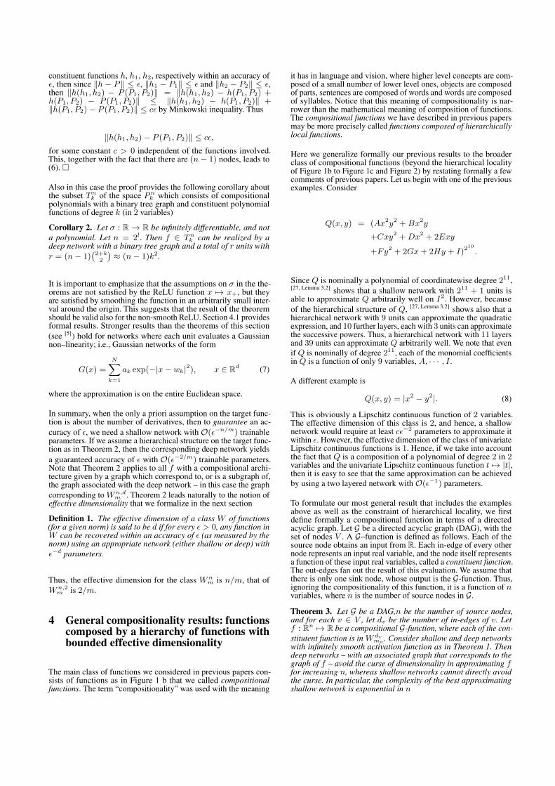
constituent functions h, h1, h2, respectively within an accuracy ofε, then since ‖h − P‖ ≤ ε, ‖h1 − P1‖ ≤ ε and ‖h2 − P2‖ ≤ ε,then ‖h(h1, h2) − P (P1, P2)‖ = ‖h(h1, h2) − h(P1, P2) +h(P1, P2) − P (P1, P2)‖ ≤ ‖h(h1, h2) − h(P1, P2)‖ +‖h(P1, P2)− P (P1, P2)‖ ≤ cε by Minkowski inequality. Thus

‖h(h1, h2)− P (P1, P2)‖ ≤ cε,for some constant c > 0 independent of the functions involved.This, together with the fact that there are (n− 1) nodes, leads to(6). �

Also in this case the proof provides the following corollary aboutthe subset Tnk of the space Pnk which consists of compositionalpolynomials with a binary tree graph and constituent polynomialfunctions of degree k (in 2 variables)

Corollary 2. Let σ : R → R be infinitely differentiable, and nota polynomial. Let n = 2l. Then f ∈ Tnk can be realized by adeep network with a binary tree graph and a total of r units withr = (n− 1)

(2+k2

)≈ (n− 1)k2.

It is important to emphasize that the assumptions on σ in the the-orems are not satisfied by the ReLU function x 7→ x+, but theyare satisfied by smoothing the function in an arbitrarily small inter-val around the origin. This suggests that the result of the theoremshould be valid also for the non-smooth ReLU. Section 4.1 providesformal results. Stronger results than the theorems of this section(see [5]) hold for networks where each unit evaluates a Gaussiannon–linearity; i.e., Gaussian networks of the form

G(x) =

N∑k=1

ak exp(−|x− wk|2), x ∈ Rd (7)

where the approximation is on the entire Euclidean space.

In summary, when the only a priori assumption on the target func-tion is about the number of derivatives, then to guarantee an ac-curacy of ε, we need a shallow network with O(ε−n/m) trainableparameters. If we assume a hierarchical structure on the target func-tion as in Theorem 2, then the corresponding deep network yieldsa guaranteed accuracy of ε with O(ε−2/m) trainable parameters.Note that Theorem 2 applies to all f with a compositional archi-tecture given by a graph which correspond to, or is a subgraph of,the graph associated with the deep network – in this case the graphcorresponding to Wn,d

m . Theorem 2 leads naturally to the notion ofeffective dimensionality that we formalize in the next section

Definition 1. The effective dimension of a class W of functions(for a given norm) is said to be d if for every ε > 0, any function inW can be recovered within an accuracy of ε (as measured by thenorm) using an appropriate network (either shallow or deep) withε−d parameters.

Thus, the effective dimension for the class Wnm is n/m, that of

Wn,2m is 2/m.

4 General compositionality results: functionscomposed by a hierarchy of functions withbounded effective dimensionality

The main class of functions we considered in previous papers con-sists of functions as in Figure 1 b that we called compositionalfunctions. The term “compositionality” was used with the meaning

it has in language and vision, where higher level concepts are com-posed of a small number of lower level ones, objects are composedof parts, sentences are composed of words and words are composedof syllables. Notice that this meaning of compositionality is nar-rower than the mathematical meaning of composition of functions.The compositional functions we have described in previous papersmay be more precisely called functions composed of hierarchicallylocal functions.

Here we generalize formally our previous results to the broaderclass of compositional functions (beyond the hierarchical localityof Figure 1b to Figure 1c and Figure 2) by restating formally a fewcomments of previous papers. Let us begin with one of the previousexamples. Consider

Q(x, y) = (Ax2y2 +Bx2y

+Cxy2 +Dx2 + 2Exy

+Fy2 + 2Gx+ 2Hy + I)210

.

Since Q is nominally a polynomial of coordinatewise degree 211,[27, Lemma 3.2] shows that a shallow network with 211 + 1 units isable to approximate Q arbitrarily well on I2. However, becauseof the hierarchical structure of Q, [27, Lemma 3.2] shows also that ahierarchical network with 9 units can approximate the quadraticexpression, and 10 further layers, each with 3 units can approximatethe successive powers. Thus, a hierarchical network with 11 layersand 39 units can approximate Q arbitrarily well. We note that evenif Q is nominally of degree 211, each of the monomial coefficientsin Q is a function of only 9 variables, A, · · · , I .

A different example is

Q(x, y) = |x2 − y2|. (8)

This is obviously a Lipschitz continuous function of 2 variables.The effective dimension of this class is 2, and hence, a shallownetwork would require at least cε−2 parameters to approximate itwithin ε. However, the effective dimension of the class of univariateLipschitz continuous functions is 1. Hence, if we take into accountthe fact that Q is a composition of a polynomial of degree 2 in 2variables and the univariate Lipschitz continuous function t 7→ |t|,then it is easy to see that the same approximation can be achievedby using a two layered network with O(ε−1) parameters.

To formulate our most general result that includes the examplesabove as well as the constraint of hierarchical locality, we firstdefine formally a compositional function in terms of a directedacyclic graph. Let G be a directed acyclic graph (DAG), with theset of nodes V . A G–function is defined as follows. Each of thesource node obtains an input from R. Each in-edge of every othernode represents an input real variable, and the node itself representsa function of these input real variables, called a constituent function.The out-edges fan out the result of this evaluation. We assume thatthere is only one sink node, whose output is the G-function. Thus,ignoring the compositionality of this function, it is a function of nvariables, where n is the number of source nodes in G.

Theorem 3. Let G be a DAG,n be the number of source nodes,and for each v ∈ V , let dv be the number of in-edges of v. Letf : Rn 7→ R be a compositional G-function, where each of the con-stitutent function is in W dv

mv . Consider shallow and deep networkswith infinitely smooth activation function as in Theorem 1. Thendeep networks – with an associated graph that corresponds to thegraph of f – avoid the curse of dimensionality in approximating ffor increasing n, whereas shallow networks cannot directly avoidthe curse. In particular, the complexity of the best approximatingshallow network is exponential in n

x1 x2 x3 x4 x5 x6 x7 x8

+

x1 x2 x3 x4 x5 x6 x7 x8

+

x1 x2 x3 x4 x5 x6 x7 x8

+

x1 x2 x3 x4 x5 x6 x7 x8

Figure 2 The figure shows the graphs of functions that may have small effectivedimensionality, depending on the number of units per node required for goodapproximation.

Ns = O(ε−nm ), (9)

where m = minv∈V mv , while the complexity of the deep networkis

Nd = O(∑v∈V

ε−dv/mv ). (10)

Following definition 1 we call dv/mv the effective dimension offunction v. Then, deep networks can avoid the curse of dimen-sionality if the constituent functions of a compositional functionhave a small effective dimension; i.e., have fixed, “small” dimen-sionality or fixed, “small” “roughness. A different interpretation ofTheorem 3 is the following.

Proposition 1. If a family of functions f : Rn 7→ R of smooth-ness m has an effective dimension < n/m, then the functionsare compositional in a manner consistent with the estimates inTheorem 3.

Notice that the functions included in this theorem are functionsthat are either local or the composition of simpler functions or both.Figure 2 shows some examples in addition to the examples at thetop of Figure Figure 1.

As before, there is a simple corollary for polynomial functions:

Corollary 3. Let σ : R→ R be infinitely differentiable, and not apolynomial. With the set up as in Theorem 3, let f be DAG polyno-mial; i.e., a DAG function, each of whose constituent functions is apolynomial of degree k. Then f can be represented by a deep net-work with O(|VN |kd) units, where |VN | is the number of non-leafvertices, and d is the maximal indegree of the nodes.

For example, if G is a full binary tree with 2n leaves, then thenominal degree of the G polynomial as in Corollary 3 is kk

n

, andtherefore requires a shallow network with O(k2k

n

) units, while adeep network requires only O(nk2) units.

Notice that polynomials in Snk are sparse with a number of termswhich is not exponential in n, that is it is not O(kn) but linear in n(that is O(nk)) or at most polynomial in n.

4.1 Approximation results for shallow and deep net-works with (non-smooth) ReLUs

The results we described so far use smooth activation functions. Wealready mentioned why relaxing the smoothness assumption shouldnot change our results in a fundamental way. While studies on theproperties of neural networks with smooth activation abound, theresults on non-smooth activation functions are much more sparse.Here we briefly recall some of them.

In the case of shallow networks, the condition of a smooth activa-tion function can be relaxed to prove density (see [13], Proposition3.7):

Proposition 2. Let σ =: R→ R be in C0, and not a polynomial.Then shallow networks are dense in C0.

In particular, ridge functions using ReLUs of the form∑ri=1 ci(〈wi, x〉+ bi)+, with wi, x ∈ Rn, ci, bi ∈ R are dense in

C.

Networks with non-smooth activation functions are expected todo relatively poorly in approximating smooth functions such aspolynomials in the sup norm. “Good” degree of approximation rates(modulo a constant) have been proved in the L2 norm. Define B theunit ball in Rn. Call Cm(Bn) the set of all continuous functionswith continuous derivative up to degree m defined on the unit ball.We define the Sobolev space Wm

p as the completion of Cm(Bn)

with respect to the Sobolev norm p (see for details [13] page 168).We define the space Bmp = {f : f ∈ Wm

p , ‖f‖m,p ≤ 1} and theapproximation error E(Bm2 ;H;L2) = infg∈H ‖f − g‖L2 . It isshown in [13, Corollary 6.10] that

Proposition 3. ForMr : f(x) =∑ri=1 ci(〈wi, x〉+bi)+ it holds

E(Bm2 ;Mr;L2) ≤ Cr−mn for m = 1, · · · , n+3

2.

These approximation results with respect to the L2 norm cannot beapplied to derive bounds for compositional networks. Indeed, in thelatter case, as we remarked already, estimates in the uniform normare needed to control the propagation of the errors from one layerto the next, see Theorem 2. Results in this direction are given in [30],and more recently in [31] and [5] (see Theorem 3.1). In particular,using a result in [31] and following the proof strategy of Theorem 2it is possible to derive the following results on the approximationof Lipshitz continuous functions with deep and shallow ReLUnetworks that mimics our Theorem 2:

Theorem 4. Let f be a L-Lipshitz continuous function of n vari-ables. Then, the complexity of a network which is a linear combi-nation of ReLU providing an approximation with accuracy at leastε is

Ns = O(( ε

L

)−n),

wheres that of a deep compositional architecture is

Nd = O((

n− 1)(ε

L

)−2).

Our general Theorem 3 can be extended in a similar way. Theorem4 is an example of how the analysis of smooth activation functionscan be adapted to ReLU. Indeed, it shows how deep compositionalnetworks with standard ReLUs can avoid the curse of dimension-ality. In the above results, the regularity of the function class isquantified by the magnitude of Lipshitz constant. Whether the latteris the best notion of smoothness for ReLU based networks, andif the above estimates can be improved, are interesting questionsthat we defer to a future work. A result that is more intuitive andmay reflect what networks actually do is described in Appendix 4.3.Though the construction described there provides approximation inthe L2 norm but not in the sup norm, this is not a problem underany discretization of real number required for computer simulations(see Appendix).

Figures 3, 4, 5, 6 provide a sanity check and empirical support forour main results and for the claims in the introduction.

Figure 4 An empirical comparison of shallow vs 2-layers binary tree networks in the approximation of compositional functions. The loss function is the standardmean square error (MSE). There are several units per node of the tree. In our setup here the network with an associated binary tree graph was set up so that each layerhad the same number of units and shared parameters. The number of units for the shallow and binary tree neural networks had the same number of parameters. Onthe left the function is composed of a single ReLU per node and is approximated by a network using ReLU activations. On the right the compositional function isf(x1, x2, x3, x4) = h2(h11(x1, x2), h12(x3, x4)) and is approximated by a network with a smooth ReLU activation (also called softplus). The functions h1, h2,h3 are as described in Figure 3. In order to be close to the function approximation case, a large data set of 60K training examples was used for both training sets. Weused for SGD the Adam[32] optimizer. In order to get the best possible solution we ran 200 independent hyper parameter searches using random search [33] and reportedthe one with the lowest training error. The hyper parameters search was over the step size, the decay rate, frequency of decay and the mini-batch size. The exponentialdecay hyper parameters for Adam were fixed to the recommended values according to the original paper [32]. The implementations were based on TensorFlow [34].

Figure 5 Another comparison of shallow vs 2-layers binary tree networks in the learning of compositional functions. The set up of the experiment was the same as in theone in figure 4 except that the compositional function had two ReLU units per node instead of only one. The right part of the figure shows a cross section of the functionf(x1, x2, 0.5, 0.25) in a bounded interval x1 ∈ [−1, 1], x2 ∈ [−1, 1]. The shape of the function is piecewise linear as it is always the case for ReLUs networks.

0 10 20 30 40 50 60

Epoch

0.25

0.3

0.35

0.4

0.45

0.5

0.55

0.6

0.65

0.7

0.75

Tra

inin

g e

rro

r o

n C

IFA

R-1

0

ShallowFC, 2 Layers, #Params 1577984

DeepFC, 5 Layers, #Params 2364416

DeepConv, No Sharing, #Params 563888

DeepConv, Sharing, #Params 98480

0 10 20 30 40 50 60

Epoch

0.2

0.25

0.3

0.35

0.4

0.45

0.5

0.55

0.6

0.65

0.7

Va

lida

tio

n e

rro

r o

n C

IFA

R-1

0

ShallowFC, 2 Layers, #Params 1577984

DeepFC, 5 Layers, #Params 2364416

DeepConv, No Sharing, #Params 563888

DeepConv, Sharing, #Params 98480

Figure 6 We show that the main advantage of deep Convolutional Networks (ConvNets) comes from "hierarchical locality" instead of weight sharing. We train two5-layer ConvNets with and without weight sharing on CIFAR-10. ConvNet without weight sharing has different filter parameters at each spatial location. There are 4convolutional layers (filter size 3x3, stride 2) in each network. The number of feature maps (i.e., channels) are 16, 32, 64 and 128 respectively. There is an additionalfully-connected layer as a classifier. The performances of a 2-layer and 5-layer fully-connected networks are also shown for comparison. Each hidden layer of thefully-connected network has 512 units. The models are all trained for 60 epochs with cross-entropy loss and standard shift and mirror flip data augmentation (duringtraining). The training errors are higher than those of validation because of data augmentation. The learning rates are 0.1 for epoch 1 to 40, 0.01 for epoch 41 to 50 and0.001 for rest epochs. The number of parameters for each model are indicated in the legends. Models with hierarchical locality significantly outperform shallow andhierarchical non-local networks.

Figure 3 The figure shows on the top the graph of the function to be approxi-mated, while the bottom part of the figure shows a deep neural network with thesame graph structure. The left and right node inf the first layer has each n unitsgiving a total of 2n units in the first layer. The second layer has a total of 2nunits. The first layer has a convolution of size n to mirror the structure of thefunction to be learned. The compositional function we approximate has the formf(x1, x2, x3, x4) = h2(h11(x1, x2), h12(x3, x4)) with h11, h12 and h2

as indicated in the figure.

4.2 Lower bounds and gaps

So far we have shown that there are deep networks – for instance ofthe convolutional type – that can avoid the curse of dimensionalityif the functions they are learning are blessed with compositionality.There are no similar guarantee for shallow networks: for shallownetworks approximating generic continuous functions the lower andthe upper bound are both exponential[13]. From the point of view ofmachine learning, it is obvious that shallow networks, unlike deepones, cannot exploit in their architecture the reduced number ofparameters associated with priors corresponding to compositionalfunctions. In past papers we listed a few examples, some of whichare also valid lower bounds from the point of view of approximationtheory:

• The polynomial considered earlier

Q(x1, x2, x3, x4) = (Q1(Q2(x1, x2), Q3(x3, x4)))1024,

can be approximated by deep networks with a smaller numberof parameters than shallow networks is based on polynomialapproximation of functions of the type g(g(g())). Here, how-ever, a formal proof of the impossibility of good approxima-tion by shallow networks is not available. For a lower boundwe need at least one example of a compositional functionwhich cannot be approximated by shallow networks with anon-exponential degree of approximation.

• Such an example, for which a proof of the lower bound existssince a few decades, consider a function which is a linearcombination of n tensor product Chui–Wang spline wavelets,where each wavelet is a tensor product cubic spline. It isshown in [11, 12] that is impossible to implement such a func-tion using a shallow neural network with a sigmoidal activa-tion function using O(n) neurons, but a deep network withthe activation function (x+)2 can do so. In this case, as wementioned, there is a formal proof of a gap between deep

and shallow networks. Similarly, Eldan and Shamir [35] showother cases with separations that are exponential in the inputdimension.

• As we mentioned earlier, Telgarsky proves an exponentialgap between certain functions produced by deep networksand their approximation by shallow networks. The theorem[25] can be summarized as saying that a certain family ofclassification problems with real-valued inputs cannot beapproximated well by shallow networks with fewer than expo-nentially many nodes whereas a deep network achieves zeroerror. This corresponds to high-frequency, sparse trigonomet-ric polynomials in our case. His upper bound can be proveddirectly from our main theorem by considering the real-valuedpolynomials x1x2...xd defined on the cube (−1, 1)d which isobviously a compositional function with a binary tree graph.

• We exhibit here another example to illustrate a limitation ofshallow networks in approximating a compositional function.

Let n ≥ 2 be an integer, B ⊂ Rn be the unit ball of Rn.We consider the class W of all compositional functions f =f2 ◦ f1, where f1 : Rn → R, and

∑|k|≤4 ‖D

kf1‖∞ ≤ 1,f2 : R→ R and ‖D4f2‖∞ ≤ 1. We consider

∆(AN ) := supf∈W

infP∈AN

‖f − P‖∞,B ,

whereAN is either the class SN of all shallow networks withN units or DN of deep networks with two layers, the firstwith n inputs, and the next with one input. The both cases,the activation function is a C∞ function σ : R → R that isnot a polynomial.

Theorem 5. There exist constants c1 > 0 such that for N ≥c1,

∆(SN ) ≥ d2−N/(n−1)e, (11)

In contrast, there exists c3 > 0 such that

∆(DN ) ≤ c3N−4/n. (12)

The constants c1, c2, c3 may depend upon n.

PROOF. The estimate (12) follows from the estimates alreadygiven for deep networks. To prove (11), we use Lemma 3.2in [12]. Let φ be a C∞ function supported on [0, 1], and weconsider fN (x) = φ(|4Nx|2). We may clearly choose φ sothat ‖fN‖∞ = 1. Then it is clear that each fN ∈W . Clearly,

∆(SN ) ≥ infP∈SN

maxx∈B|fN (x)− P (x)|. (13)

We choose P ∗(x) =∑Nk=1 σ(〈w∗k, x〉+ b∗k) such that

infP∈SN

maxx∈B|fN (x)−P (x)| ≥ (1/2) max

x∈B|fN (x)−P ∗(x)|.

(14)Since fN is supported on {x ∈ Rn : |x| ≤ 4−N}, wemay imitate the proof of Lemma 3.2 in [12] with g∗k(t) =σ(t+b∗k). Let x0 ∈ B be such that (without loss of generality)fN (x0) = maxx∈B |fN (x)|, and µ0 be the Dirac measuresupported at x0. We group {w∗k} in m = dN/(n − 1)edisjoint groups of n − 1 vectors each. For each group, wetake vectors {v`} such that v` is orthogonal to the w∗k’s ingroup `. The argument in the proof of Lemma 3.2 in [12] canbe modified to get a measure µ with total variation 2m suchthat∫B

fN (x)dµ(x) = ‖fN‖∞,∫B

g∗k(x)dµ(x) = 0, k = 1, · · · , N.

It is easy to deduce from here as in [12] using the dualityprinciple that

maxx∈B|fN (x)− P ∗(x)| ≥ c2−m.

Together with (13) and (14), this implies (11).

So by now plenty of examples of lower bounds exist showing a gapbetween shallow and deep networks. A particularly interesting caseis the product function, that is the monomial f(x1, · · · , xn) =x1x2 · · ·xn which is, from our point of view, the prototypical com-positional functions. Keeping in mind the issue of lower bounds,the question here has to do with the minimum integer r(n) such thatthe function f is in the closure of the span of σ(〈wk, x〉+bk), withk = 1, · · · , r(n), and wk, bk ranging over their whole domains.Such a result has been claimed for the case of smooth ReLUs, usingunusual group techniques and is sketched in the Appendix of [36].

Notice, in support of the conjecture, that assuming that a shal-low network with (non-smooth) ReLUs has a lower bound ofr(q) = O(q) will lead to an apparent contradiction with Hastad the-orem (which is about representation not approximation of Booleanfunctions) by restricting xi from xi ∈ (−1, 1) to xi ∈ {−1,+1}.Hastad theorem [37] establishes the inapproximability of the parityfunction by shallow circuits of non-exponential size.

4.3 Messy graphs and densely connected deep net-works

As mentioned already, the approximating deep network does notneed to exactly match the architecture of the compositional functionas long as the graph or tree associated with the function is containedin the graph associated with the network. This is of course goodnews: the compositionality prior embedded in the architecture ofthe network does not to reflect exactly the graph of a new functionto be learned. We have shown that for a given class of composi-tional functions characterized by an associated graph there exista deep network that approximates such a function better than ashallow network. The same network approximates well functionscharacterized by subgraphs of the original class.

The proofs of our theorems show that linear combinations of com-positional functions are universal in the sense that they can ap-proximate any function and that deep networks with a number ofunits that increases exponentially with layers can approximate anyfunction. Notice that deep compositional networks can interpolateif they are overparametrized with respect to the data, even if thedata reflect a non-compositional function.

As an aside, note that the simplest compositional function – addition– is trivial in the sense that it offers no approximation advantageto deep networks. The key function is multiplication which is forus the prototypical compositional functions. As a consequence,polynomial functions are compositional – they are linear combi-nations of monomials which are compositional. However, theircompositional structure does not confer any advantage in termsof approximation, because of the exponential number of composi-tional terms.

As we mentioned earlier, networks corresponding to graphs thatinclude the graph of the function to be learned can exploit com-positionality. The relevant number of parameters to be optimized,however, is the number of parameters r in the network and not thenumber of parameters r∗ (r∗ < r) of the optimal deep networkwith a graph exactly matched to the graph of the function to belearned. As an aside, the price to be paid in using a non-optimalprior depend on the learning algorithm. For instance, under sparsity

constraints it may be possible to pay a smaller price than r (buthigher than r∗).

In this sense, some of the densely connected deep networks usedin practice – which contain sparse graphs possibly relevant for thefunction to be learned and which are still “smaller” than the expo-nential number of units required to represent a generic function ofn variables – may be capable in some cases of exploiting an un-derlying compositionality structure without paying an exhorbitantprice in terms of required complexity.

5 Connections with the theory of Booleanfunctions

The approach followed in our main theorems suggest the follow-ing considerations (see Appendix 1 for a brief introduction). Thestructure of a deep network is reflected in polynomials that are bestapproximated by it – for instance generic polynomials or sparsepolynomials (in the coefficients) in d variables of order k. The treestructure of the nodes of a deep network reflects the structure of aspecific sparse polynomial. Generic polynomial of degree k in dvariables are difficult to learn because the number of terms, train-able parameters and associated VC-dimension are all exponentialin d. On the other hand, functions approximated well by sparsepolynomials can be learned efficiently by deep networks with a treestructure that matches the polynomial. We recall that in a similarway several properties of certain Boolean functions can be “readout” from the terms of their Fourier expansion corresponding to“large” coefficients, that is from a polynomial that approximateswell the function.

Classical results [37] about the depth-breadth tradeoff in circuitsdesign show that deep circuits are more efficient in representingcertain Boolean functions than shallow circuits. Hastad proved thathighly-variable functions (in the sense of having high frequenciesin their Fourier spectrum), in particular the parity function cannoteven be decently approximated by small constant depth circuits(see also [38]). A closely related result follow immediately fromour main theorem since functions of real variables of the formx1x2...xd have the compositional form of the binary tree (for deven). Restricting the values of the variables to −1,+1 yields anupper bound:

Proposition 4. The family of parity functions x1x2...xd withxi ∈ {−1,+1} and i = 1, · · · , xd can be represented with expo-nentially fewer units by a deep than a shallow network.

Notice that Hastad’s results on Boolean functions have been oftenquoted in support of the claim that deep neural networks can repre-sent functions that shallow networks cannot. For instance Bengioand LeCun [39] write “We claim that most functions that can berepresented compactly by deep architectures cannot be representedby a compact shallow architecture”.”.

Finally, we want to mention a few other observations on Booleanfunctions that shows an interesting connection with our approach.It is known that within Boolean functions the AC0 class of poly-nomial size constant depth circuits is characterized by Fouriertransforms where most of the power spectrum is in the low ordercoefficients. Such functions can be approximated well by a poly-nomial of low degree and can be learned well by considering onlysuch coefficients. There are two algorithms [40] that allow learningof certain Boolean function classes:

1. the low order algorithm that approximates functions by con-sidering their low order Fourier coefficients and

2. the sparse algorithm which learns a function by approximat-ing its significant coefficients.

Decision lists and decision trees can be learned by the first algo-rithm. Functions with small L1 norm can be approximated wellby the second algorithm. Boolean circuits expressing DNFs can beapproximated by the first one but even better by the second. In fact,in many cases a function can be approximated by a small set ofcoefficients but these coefficients do not correspond to low-orderterms. All these cases are consistent with the notes about sparsefunctions in section 6.

6 Notes on a theory of compositional compu-tation

The key property of the theory of compositional functions sketchedhere is that certain deep networks can learn them avoiding the curseof dimensionality because of the blessing of compositionality via asmall effective dimension.

We state here several comments and conjectures.

1. General comments

• Assumptions of the compositionality type may havemore direct practical implications and be at least aseffective as assumptions about function smoothness incountering the curse of dimensionality in learning andapproximation.

• The estimates on the n–width imply that there is somefunction in either Wn

m (theorem 1) or Wn,2m (theorem

2) for which the approximation cannot be better thanthat suggested by the theorems.

• The main question that may be asked about the rele-vance of the theoretical results of this paper and net-works used in practice has to do with the many “chan-nels” used in the latter and with our assumption thateach node in the networks computes a scalar function– the linear combination of r units (Equation 3). Thefollowing obvious but interesting extension of Theo-rem 1 to vector-valued functions says that the numberof hidden units required for a given accuracy in eachcomponent of the function is the same as in the scalarcase considered in our theorems (of course the numberof weigths is larger):Corollary 4. Let σ : R → R be infinitely differen-tiable, and not a polynomial. For a vector-valued func-tion f : Rn → Rq with components fi ∈ Wn

m, i =1, · · · , q the number of hidden units in shallow net-works with n inputs, q outputs that provide accuracy atleast ε in each of the components of f is

N = O(ε−n/m) . (15)

The demonstration follows the proof of theorem 1, seealso Appendix 4.1. It amounts to realizing that the hid-den units (or linear combinations of them) can be equiv-alent to the monomials of a generic polynomial of de-gree k in n variables that can be used by a differentset of coefficients for each of the fi. This argumentof course does not mean that during learning this iswhat happens; it provides one way to perform the ap-proximation and an associated upper bound. The corol-lary above leads to a simple argument that generalizesour binary tree results to standard, multi-channel deepconvolutional networks by introducing a set of virtual

linear units as ouputs of one layer and inputs of thenext one. This in turn leads to the following predic-tion: for consistent approximation accuracy across thelayers, the rank of the weights matrices between unitsin successive layers should have a rank in the orderof the number of the dimensionality in the first layer(inputs and outputs have to be defined wrt support ofthe convolution kernel). This suggests rank-deficientweight matrices in present networks.

• We have used polynomials (but see Appendix 4.3) toprove results about complexity of approximation in thecase of neural networks. Neural network learning withSGD may or may not synthesize polynomial, depend-ing on the smoothness of the activation function andon the target. This is not a problem for theoretically es-tablishing upper bounds on the degree of convergencebecause results using the framework on nonlinear widthguarantee the “polynomial” bounds are optimal.

• Both shallow and deep representations may or may notreflect invariance to group transformations of the in-puts of the function ([41, 22]). Invariance – also calledweight sharing – decreases the complexity of the net-work. Since we are interested in the comparison ofshallow vs deep architectures, we have considered thegeneric case of networks (and functions) for which in-variance is not assumed. In fact, the key advantage ofdeep vs. shallow network – as shown by the proof ofthe theorem – is the associated hierarchical locality (theconstituent functions in each node are local that is havea small dimensionality) and not invariance (which des-ignates shared weights that is nodes at the same levelsharing the same function). One may then ask aboutthe relation of these results with i-theory[42]. The origi-nal core of i-theory describes how pooling can provideeither shallow or deep networks with invariance andselectivity properties. Invariance of course helps butnot exponentially as hierarchical locality does.

• There are several properties that follow from the the-ory here which are attractive from the point of view ofneuroscience. A main one is the robustness of the re-sults with respect to the choice of nonlinearities (linearrectifiers, sigmoids, Gaussians etc.) and pooling.

• In a machine learning context, minimization over atraining set of a loss function such as the square lossyields an empirical approximation of the regressionfunction p(y/x). Our hypothesis of compositionalitybecomes an hypothesis about the structure of the condi-tional probability function.

2. Spline approximations, Boolean functions and tensors

• Consider again the case of section 4 of a multivari-ate function f : [0, 1]d → R. Suppose to discretize itby a set of piecewise constant splines and their tensorproducts. Each coordinate is effectively replaced by nboolean variables.This results in a d-dimensional tablewith N = nd entries. This in turn corresponds to aboolean function f : {0, 1}N → R. Here, the assump-tion of compositionality corresponds to compressibilityof a d-dimensional table in terms of a hierarchy ofd− 1 2-dimensional tables. Instead of nd entries thereare (d − 1)n2 entries. This has in turn obvious con-nections with HVQ (Hierarchical Vector Quantization),discussed in Appendix 5.

• As Appendix 4.3 shows, every function f can be ap-proximated by an epsilon-close binary function fB .Binarization of f : Rn → R is done by using k parti-tions for each variable xi and indicator functions. Thusf 7→ fB : {0, 1}kn → R and sup|f − fB | ≤ ε, withε depending on k and bounded Df .

• fB can be written as a polynomial (a Walsh decompo-sition) fB ≈ pB . It is always possible to associate a pbto any f , given ε.

• The binarization argument suggests a direct way toconnect results on function approximation by neuralnets with older results on Boolean functions. The latterare special cases of the former results.

• One can think about tensors in terms of d-dimensionaltables. The framework of hierarchical decompositionsof tensors – in particular the Hierarchical Tucker format– is closely connected to our notion of compositionality.Interestingly, the hierarchical Tucker decompositionhas been the subject of recent papers on Deep Learning(for instance see [20]). This work, as well more classicalpapers [43], does not characterize directly the class offunctions for which these decompositions are effective.Notice that tensor decompositions assume that the sumof polynomial functions of order d is sparse (see eq. attop of page 2030 of [43]). Our results provide a rigorousgrounding for the tensor work related to deep learning.There is obviously a wealth of interesting connectionswith approximation theory that should be explored.Notice that the notion of separation rank of a tensor isvery closely related to the effective r in Equation 26.

3. Sparsity

• We suggest to define binary sparsity of f , in terms ofthe sparsity of the boolean function pB ; binary sparsityimplies that an approximation to f can be learned bynon-exponential deep networks via binarization. Noticethat if the function f is compositional the associatedBoolean functions fB is sparse; the converse is not true.

• In may situations, Tikhonov regularization correspondsto cutting high order Fourier coefficients. Sparsity ofthe coefficients subsumes Tikhonov regularization inthe case of a Fourier representation. Notice that as an ef-fect the number of Fourier coefficients is reduced, thatis trainable parameters, in the approximating trigono-metric polynomial. Sparsity of Fourier coefficients is ageneral constraint for learning Boolean functions.

• Sparsity in a specific basis. A set of functions may bedefined to be sparse in a specific basis when the num-ber of parameters necessary for its ε-approximationincreases less than exponentially with the dimension-ality. An open question is the appropriate definitionof sparsity. The notion of sparsity we suggest here isthe effective r in Equation 26. For a general functionr ≈ kn; we may define sparse functions those forwhich r << kn in

f(x) ≈ P ∗k (x) =

r∑i=1

pi(〈wi, x〉). (16)

where P ∗ is a specific polynomial that approximatesf(x) within the desired ε. Notice that the polynomialP ∗k can be a sum of monomials or a sum of, for instance,orthogonal polynomials with a total of r parameters. Ingeneral, sparsity depends on the basis and one needsto know the basis and the type of sparsity to exploitit in learning, for instance with a deep network withappropriate activation functions and architecture.There are function classes that are sparse in every bases.Examples are compositional functions described by abinary tree graph.

4. The role of compositionality in generalization by multi-classdeep networksMost of the succesfull neural networks exploit compo-sitionality for better generalization in an additional im-portant way (see [44]). Suppose that the mappings to

be learned in a family of classification tasks (for in-stance classification of different object classes in Imagenet)may be approximated by compositional functions suchas f(x1, · · · , xn) = hl · · · (h21(h11(x1, x2), h12(x3, x4)),h22(h13(x5, x6), h14(x7, x8) · · · )) · · · ), where hl dependson the task (for instance to which object class) but all the otherconstituent functions h are common across the tasks. Undersuch an assumption, multi-task learning, that is training simul-taneously for the different tasks, forces the deep network to“find” common constituent functions. Multi-task learning hastheoretical advantages that depends on compositionality: thesample complexity of the problem can be significantly lower(see [45]). The Maurer’s approach is in fact to consider theoverall function as the composition of a preprocessor func-tion common to all task followed by a task-specific function.As a consequence, the generalization error, defined as thedifference between expected and empirical error, averagedacross the T tasks, is bounded with probability at least 1− δ(in the case of finite hypothesis spaces) by

1√2M

√ln|H|+

ln|G|+ ln( 1δ)

T, (17)

where M is the size of the training set, H is the hypothesisspace of the common classifier and G is the hypothesis spaceof the system of constituent functions, common across tasks.The improvement in generalization error because of the mul-titask structure can be in the order of the square root of thenumber of tasks (in the case of Imagenet with its 1000 ob-ject classes the generalization error may tyherefore decreasebt a factor ≈ 30). It is important to emphasize the dual ad-vantage here of compositionality, which a) reduces general-ization error by decreasing the complexity of the hypothe-sis space G of compositional functions relative the space ofnon-compositional functions and b) exploits the multi taskstructure, that replaces ln|G| with ln|G|

T.

We conjecture that the good generalization exhibited by deepconvolutional networks in multi-class tasks such as CiFARand Imagenet are due to three factors:

• the regularizing effect of SGD• the task is compositional• the task is multiclass.

5. Deep Networks as memoriesNotice that independently of considerations of generalization,deep compositional networks are expected to be very efficientmemories – in the spirit of hierarchical vector quantization –for associative memories reflecting compositional rules (seeAppendix 5 and [46]). Notice that the advantage with respectto shallow networks from the point of view of memory capac-ity can be exponential (as in the example after Equation 32showing mshallow ≈ 10104mdeep).

6. Theory of computation, locality and compositionality

• From the computer science point of view, feedforwardmultilayer networks are equivalent to finite state ma-chines running for a finite number of time steps[47, 48].This result holds for almost any fixed nonlinearity ineach layer. Feedforward networks are equivalent to cas-cades without loops (with a finite number of stages) andall other forms of loop free cascades (i.e. McCulloch-Pitts nets without loops, perceptrons, analog percep-trons, linear threshold machines). Finite state machines,cascades with loops, and difference equation systemswhich are Turing equivalent, are more powerful thanmultilayer architectures with a finite number of layers.The latter networks, however, are practically universal

computers, since every machine we can build can be ap-proximated as closely as we like by defining sufficientlymany stages or a sufficiently complex single stage. Re-current networks as well as differential equations areTuring universal.In other words, all computable functions (by a Turingmachine) are recursive, that is composed of a smallset of primitive operations. In this broad sense all com-putable functions are compositional (composed from el-ementary functions). Conversely a Turing machine canbe written as a compositional function y = f (t(x, p)where f : Zn×Pm 7→ Zh×P k, P being parametersthat are inputs and outputs of f . If t is bounded we havea finite state machine, otherwise a Turing machine. interms of elementary functions. As mentioned above,each layer in a deep network correspond to one timestep in a Turing machine. In a sense, this is sequen-tial compositionality, as in the example of Figure 1 c.The hierarchically local compositionality we have intro-duced in this paper has the flavour of compositionalityin space.Of course, since any function can be approximatedby polynomials, and a polynomial can always be cal-culated using a recursive procedure and a recursiveprocedure can always be unwound as a “deep network”,any function can always be approximated by a compo-sitional function of a few variables. However, genericcompositionality of this type does not guarantee goodapproximation properties by deep networks.

• Hierarchically local compositionality can be related tothe notion of local connectivity of a network. Connec-tivity is a key property in network computations. Localprocessing may be a key constraint also in neuroscience.One of the natural measures of connectivity that can beintroduced is the order of a node defined as the numberof its distinct inputs. The order of a network is then themaximum order among its nodes. The term order datesback to the Perceptron book ([49], see also [48]). Fromthe previous observations, it follows that a hierarchicalnetwork of order at least 2 can be universal. In thePerceptron book many interesting visual computationshave low order (e.g. recognition of isolated figures).The message is that they can be implemented in a sin-gle layer by units that have a small number of inputs.More complex visual computations require inputs fromthe full visual field. A hierarchical network can achieveeffective high order at the top using units with low or-der. The network architecture of Figure 1 b) has loworder: each node in the intermediate layers is connectedto just 2 other nodes, rather than (say) all nodes in theprevious layer (notice that the connections in the treesof the figures may reflect linear combinations of theinput units).

• Low order may be a key constraint for cortex. If it cap-tures what is possible in terms of connectivity betweenneurons, it may determine by itself the hierarchicalarchitecture of cortex which in turn may impose com-positionality to language and speech.

• The idea of functions that are compositions of “sim-pler” functions extends in a natural way to recurrentcomputations and recursive functions. For instanceh(f (t)g((x))) represents t iterations of the algorithmf (h and g match input and output dimensions to f ).

7 Why are compositional functions so com-mon?

Let us provide a couple of simple examples of compositional func-tions. Addition is compositional but the degree of approximation

does not improve by decomposing addition in different layers of anetwork; all linear operators are compositional with no advantagefor deep networks; multiplication as well as the AND operation (forBoolean variables) is the prototypical compositional function thatprovides an advantage to deep networks. So compositionality isnot enough: we need certain sublasses of compositional functions(such as the hierarchically local functions we described) in order toavoid the curse of dimensionality.

It is not clear, of course, why problems encountered in practiceshould match this class of functions. Though we and others haveargued that the explanation may be in either the physics or theneuroscience of the brain, these arguments (see Appendix 2) arenot (yet) rigorous. Our conjecture at present is that compositionalityis imposed by the wiring of our cortex and is reflected in languageand the common problems we worry about. Thus compositionalityof several – but not all – computations on images many reflect theway we describe and think about them.

Acknowledgment

This work was supported by the Center for Brains, Minds andMachines (CBMM), funded by NSF STC award CCF – 1231216.HNM was supported in part by ARO Grant W911NF-15-1-0385.We thank O. Shamir for useful emails that prompted us to clarifyour results in the context of lower bounds and for pointing out anumber of typos and other mistakes.

References[1] F. Anselmi, L. Rosasco, C. Tan, and T. Poggio, “Deep convolutional

network are hierarchical kernel machines,” Center for Brains, Minds andMachines (CBMM) Memo No. 35, also in arXiv, 2015.

[2] T. Poggio, L. Rosasco, A. Shashua, N. Cohen, and F. Anselmi, “Notes onhierarchical splines, dclns and i-theory,” tech. rep., MIT Computer Scienceand Artificial Intelligence Laboratory, 2015.

[3] T. Poggio, F. Anselmi, and L. Rosasco, “I-theory on depth vs width: hier-archical function composition,” CBMM memo 041, 2015.

[4] H. Mhaskar, Q. Liao, and T. Poggio, “Learning real and boolean func-tions: When is deep better than shallow?,” Center for Brains, Minds andMachines (CBMM) Memo No. 45, also in arXiv, 2016.

[5] H. Mhaskar and T. Poggio, “Deep versus shallow networks: an approxima-tion theory perspective,” Center for Brains, Minds and Machines (CBMM)Memo No. 54, also in arXiv, 2016.

[6] D. L. Donoho, “High-dimensional data analysis: The curses and blessingsof dimensionality,” in AMS CONFERENCE ON MATH CHALLENGESOF THE 21ST CENTURY, 2000.

[7] Y. LeCun, Y. Bengio, and H. G., “Deep learning,” Nature, pp. 436–444,2015.

[8] K. Fukushima, “Neocognitron: A self-organizing neural network for amechanism of pattern recognition unaffected by shift in position,” Biologi-cal Cybernetics, vol. 36, no. 4, pp. 193–202, 1980.

[9] M. Riesenhuber and T. Poggio, “Hierarchical models of object recognitionin cortex,” Nature Neuroscience, vol. 2, pp. 1019–1025, Nov. 1999.

[10] H. Mhaskar, “Approximation properties of a multilayered feedforwardartificial neural network,” Advances in Computational Mathematics, pp. 61–80, 1993.

[11] C. Chui, X. Li, and H. Mhaskar, “Neural networks for localized approx-imation,” Mathematics of Computation, vol. 63, no. 208, pp. 607–623,1994.

[12] C. K. Chui, X. Li, and H. N. Mhaskar, “Limitations of the approxima-tion capabilities of neural networks with one hidden layer,” Advances inComputational Mathematics, vol. 5, no. 1, pp. 233–243, 1996.

[13] A. Pinkus, “Approximation theory of the mlp model in neural networks,”Acta Numerica, vol. 8, pp. 143–195, 1999.

[14] T. Poggio and S. Smale, “The mathematics of learning: Dealing withdata,” Notices of the American Mathematical Society (AMS), vol. 50, no. 5,pp. 537–544, 2003.

[15] B. B. Moore and T. Poggio, “Representations properties of multilayer feed-forward networks,” Abstracts of the First annual INNS meeting, vol. 320,p. 502, 1998.

[16] R. Livni, S. Shalev-Shwartz, and O. Shamir, “A provably efficient algo-rithm for training deep networks,” CoRR, vol. abs/1304.7045, 2013.

[17] O. Delalleau and Y. Bengio, “Shallow vs. deep sum-product networks,”in Advances in Neural Information Processing Systems 24: 25th AnnualConference on Neural Information Processing Systems 2011. Proceedingsof a meeting held 12-14 December 2011, Granada, Spain., pp. 666–674,2011.

[18] R. Montufar, G. F.and Pascanu, K. Cho, and Y. Bengio, “On the number oflinear regions of deep neural networks,” Advances in Neural InformationProcessing Systems, vol. 27, pp. 2924–2932, 2014.

[19] H. N. Mhaskar, “Neural networks for localized approximation of realfunctions,” in Neural Networks for Processing [1993] III. Proceedings ofthe 1993 IEEE-SP Workshop, pp. 190–196, IEEE, 1993.

[20] N. Cohen, O. Sharir, and A. Shashua, “On the expressive power of deeplearning: a tensor analysis,” CoRR, vol. abs/1509.0500, 2015.

[21] F. Anselmi, J. Leibo, L. Rosasco, J. Mutch, A. Tacchetti, and T. Poggio,“Unsupervised learning of invariant representations with low sample com-plexity: the magic of sensory cortex or a new framework for machinelearning?.,” Center for Brains, Minds and Machines (CBMM) Memo No. 1.arXiv:1311.4158v5, 2014.

[22] F. Anselmi, J. Z. Leibo, L. Rosasco, J. Mutch, A. Tacchetti, and T. Poggio,“Unsupervised learning of invariant representations,” Theoretical ComputerScience, 2015.

[23] T. Poggio, L. Rosaco, A. Shashua, N. Cohen, and F. Anselmi, “Notes onhierarchical splines, dclns and i-theory,” CBMM memo 037, 2015.

[24] Q. Liao and T. Poggio, “Bridging the gap between residual learning, re-current neural networks and visual cortex,” Center for Brains, Minds andMachines (CBMM) Memo No. 47, also in arXiv, 2016.

[25] M. Telgarsky, “Representation benefits of deep feedforward networks,”arXiv preprint arXiv:1509.08101v2 [cs.LG] 29 Sep 2015, 2015.

[26] I. Safran and O. Shamir, “Depth separation in relu networks for approxi-mating smooth non-linear functions,” arXiv:1610.09887v1, 2016.

[27] H. N. Mhaskar, “Neural networks for optimal approximation of smoothand analytic functions,” Neural Computation, vol. 8, no. 1, pp. 164–177,1996.

[28] E. Corominas and F. S. Balaguer, “Condiciones para que una funcion in-finitamente derivable sea un polinomio,” Revista matemática hispanoamer-icana, vol. 14, no. 1, pp. 26–43, 1954.

[29] R. A. DeVore, R. Howard, and C. A. Micchelli, “Optimal nonlinear approx-imation,” Manuscripta mathematica, vol. 63, no. 4, pp. 469–478, 1989.

[30] H. N. Mhaskar, “On the tractability of multivariate integration and ap-proximation by neural networks,” J. Complex., vol. 20, pp. 561–590, Aug.2004.

[31] F. Bach, “Breaking the curse of dimensionality with convex neural net-works,” arXiv:1412.8690, 2014.

[32] D. P. Kingma and J. Ba, “Adam: A method for stochastic optimization,”CoRR, vol. abs/1412.6980, 2014.

[33] J. Bergstra and Y. Bengio, “Random search for hyper-parameter optimiza-tion,” J. Mach. Learn. Res., vol. 13, pp. 281–305, Feb. 2012.

[34] M. Abadi, A. Agarwal, P. Barham, E. Brevdo, Z. Chen, C. Citro, G. S. Cor-rado, A. Davis, J. Dean, M. Devin, S. Ghemawat, I. Goodfellow, A. Harp,G. Irving, M. Isard, Y. Jia, R. Jozefowicz, L. Kaiser, M. Kudlur, J. Lev-enberg, D. Mané, R. Monga, S. Moore, D. Murray, C. Olah, M. Schuster,J. Shlens, B. Steiner, I. Sutskever, K. Talwar, P. Tucker, V. Vanhoucke,V. Vasudevan, F. Viégas, O. Vinyals, P. Warden, M. Wattenberg, M. Wicke,Y. Yu, and X. Zheng, “TensorFlow: Large-scale machine learning on het-erogeneous systems,” 2015. Software available from tensorflow.org.

[35] R. Eldan and O. Shamir, “The power of depth for feedforward neuralnetworks,” arXiv preprint arXiv:1512.03965v4, 2016.

[36] M. Lin, H.and Tegmark, “Why does deep and cheap learning work sowell?,” arXiv:1608.08225, pp. 1–14, 2016.

[37] J. T. Hastad, Computational Limitations for Small Depth Circuits. MITPress, 1987.

[38] N. Linial, M. Y., and N. N., “Constant depth circuits, fourier transform,and learnability,” Journal of the ACM, vol. 40, no. 3, p. 607–620, 1993.

[39] Y. Bengio and Y. LeCun, “Scaling learning algorithms towards ai,” inLarge-Scale Kernel Machines (L. Bottou, O. Chapelle, and J. DeCoste,D.and Weston, eds.), MIT Press, 2007.

[40] Y. Mansour, “Learning boolean functions via the fourier transform,” inTheoretical Advances in Neural Computation and Learning (V. Roychowd-hury, K. Siu, and A. Orlitsky, eds.), pp. 391–424, Springer US, 1994.

[41] S. Soatto, “Steps Towards a Theory of Visual Information: Active Percep-tion, Signal-to-Symbol Conversion and the Interplay Between Sensing andControl,” arXiv:1110.2053, pp. 0–151, 2011.

[42] F. Anselmi and T. Poggio, Visual Cortex and Deep Networks. MIT Press,2016.

[43] L. Grasedyck, “Hierarchical Singular Value Decomposition of Tensors,”SIAM J. Matrix Anal. Appl., no. 31,4, pp. 2029–2054, 2010.

[44] B. M. Lake, R. Salakhutdinov, and J. B. Tenenabum, “Human-level con-cept learning through probabilistic program induction,” Science, vol. 350,no. 6266, pp. 1332–1338, 2015.

[45] A. Maurer, “Bounds for Linear Multi-Task Learning,” Journal of MachineLearning Research, 2015.

[46] F. Anselmi, L. Rosasco, and T. Tan, C.and Poggio, “Deep ConvolutionalNetworks are Hierarchical Kernel Machines,” Center for Brains, Mindsand Machines (CBMM) Memo No. 35, also in arXiv, 2015.

[47] S. Shalev-Shwartz and S. Ben-David, Understanding Machine Learning:From Theory to Algorithms. Cambridge eBooks, 2014.

[48] T. Poggio and W. Reichardt, “On the representation of multi-input sys-tems: Computational properties of polynomial algorithms.,” BiologicalCybernetics, 37, 3, 167-186., 1980.

[49] M. Minsky and S. Papert, Perceptrons: An Introduction to ComputationalGeometry. Cambridge MA: The MIT Press, ISBN 0-262-63022-2, 1972.

[50] D. Ruderman, “Origins of scaling in natural images,” Vision Res., pp. 3385– 3398, 1997.

[51] F. Girosi, M. Jones, and T. Poggio, “Regularization theory and neuralnetworks architectures,” Neural Computation, vol. 7, pp. 219–269, 1995.

[52] T. Poggio and F. Girosi, “A theory of networks for approximation andlearning,” Laboratory, Massachusetts Institute of Technology, vol. A.I.memo n1140, 1989.

[53] J. Mihalik, “Hierarchical vector quantization. of images in transform do-main.,” ELEKTROTECHN. CA5, 43, NO. 3. 92,94., 1992.

[54] F. Girosi and T. Poggio, “Representation properties of networks: Kol-mogorov’s theorem is irrelevant,” Neural Computation, vol. 1, no. 4,pp. 465–469, 1989.

[55] F. Girosi and T. Poggio, “Networks and the best approximation property,”Biological Cybernetics, vol. 63, pp. 169–176, 1990.

[56] M. Anthony and P. Bartlett, Neural Network Learning - Theoretical Foun-dations. Cambridge University Press, 2002.

Appendix: observations,theorems and conjectures

1 Boolean Functions

One of the most important tools for theoretical computer scientistsfor the study of functions of n Boolean variables, their related cir-cuit design and several associated learning problems, is the Fouriertransform over the Abelian group Zn2 . This is known as Fourieranalysis over the Boolean cube {−1, 1}n. The Fourier expansion ofa Boolean function f : {−1, 1}n → {−1, 1} or even a real-valuedBoolean function f : {−1, 1}n → [−1, 1] is its representation as areal polynomial, which is multilinear because of the Boolean natureof its variables. Thus for Boolean functions their Fourier represen-tation is identical to their polynomial representation. In this paperwe use the two terms interchangeably. Unlike functions of realvariables, the full finite Fourier expansion is exact, instead of an ap-proximation. There is no need to distingush between trigonometricand real polynomials. Most of the properties of standard harmonicanalysis are otherwise preserved, including Parseval theorem. Theterms in the expansion correspond to the various monomials; thelow order ones are parity functions over small subsets of the vari-ables and correspond to low degrees and low frequencies in thecase of polynomial and Fourier approximations, respectively, forfunctions of real variables.

2 Does Physics or Neuroscience imply compo-sitionality?

It has been often argued that not only text and speech are compo-sitional but so are images. There are many phenomena in naturethat have descriptions along a range of rather different scales. Anextreme case consists of fractals which are infinitely self-similar,iterated mathematical constructs. As a reminder, a self-similar ob-ject is similar to a part of itself (i.e. the whole is similar to one ormore of the parts). Many objects in the real world are statisticallyself-similar, showing the same statistical properties at many scales:clouds, river networks, snow flakes, crystals and neurons branch-ing. A relevant point is that the shift-invariant scalability of imagestatistics follows from the fact that objects contain smaller clus-ters of similar surfaces in a selfsimilar fractal way. Ruderman [50]

analysis shows that image statistics reflects what has been knownas the property of compositionality of objects and parts: parts arethemselves objects, that is selfsimilar clusters of similar surfaces inthe physical world. Notice however that, from the point of view ofthis paper, it is misleading to say that an image is compositional: inour terminology a function on an image may be compositional butnot its argument. In fact, functions to be learned may or may not becompositional even if their input is an image since they depend onthe input but also on the task (in the supervised case of deep learn-ing networks all weights depend on x and y). Conversely, a networkmay be given a function which can be written in a compositionalform, independently of the nature of the input vector such as thefunction “multiplication of all scalar inputs’ components”. Thusa more reasonable statement is that “many natural questions onimages correspond to algorithms which are compositional”. Whythis is the case is an interesting open question. An answer inspiredby the condition of “locality” of the constituent functions in ourtheorems and by the empirical success of deep convolutional net-works has attracted some attention. The starting observation is thatin the natural sciences– physics, chemistry, biology – many phe-nomena seem to be described well by processes that that take placeat a sequence of increasing scales and are local at each scale, inthe sense that they can be described well by neighbor-to-neighborinteractions.

Notice that this is a much less stringent requirement than renormal-izable physical processes [36] where the same Hamiltonian (apartfrom a scale factor) is required to describe the process at eachscale (in our observation above, the renormalized Hamiltonian onlyneeds to remain local at each renormalization step)2. As discussedpreviously [3] hierarchical locality may be related to propertiesof basic physics that imply local interactions at each level in asequence of scales, possibly different at each level. To completethe argument one would have then to assume that several differentquestions on sets of natural images may share some of the initialinference steps (first layers in the associated deep network) andthus share some of features computed by intermediate layers of adeep network. In any case, at least two open questions remain thatrequire formal theoretical results in order to explain the connectionbetween hierarchical, local functions and physics:

• can hierarchical locality be derived from the Hamiltonians ofphysics? In other words, under which conditions does coarsegraining lead to local Hamiltonians? According to Tegmarklocality of the Hamiltonian ensures locality at every stage ofcoarse graining.

• is it possible to formalize how and when the local hierarchicalstructure of computations on images is related to the hierarchyof local physical process that describe the physical worldrepresented in the image?

It seems to us that the above set of arguments is unsatisfactoryand unlikely to provide the answer. One of the arguments is thatiterated local functions (from Rn to Rn with n increasing withoutbound) can be Turing universal and thus can simulate any physicalphenomenon (as shown by the game Life which is local and Turinguniversal). Of course, this does not imply that the simulation willbe efficient but it weakens the physics-based argument. An alterna-tive hypothesis in fact is that locality across levels of explanationoriginates from the structure of the brain – wired, say, similarly toconvolutional deep networks – which is then forced to use localalgorithms of the type shown in Figure 14. Such local algorithmsallow the organism to survive because enough of the key problemsencountered during evolution can be solved well enough by them.So instead of claiming that all questions on the physical world arelocal because of its physics we believe that local algorithms aregood enough over the distribution of evolutionary relevant prob-lems. From this point of view locality of algorithms follows fromthe need to optimize local connections and to reuse computationalelements. Despite the high number of synapses on each neuron itwould be impossible for a complex cell to pool information acrossall the simple cells needed to cover an entire image, as needed by asingle hidden layer network.

3 Splines: some notes

3.1 Additive and Tensor Product Splines

Additive and tensor product splines are two alternatives to radialkernels for multidimensional function approximation. It is wellknown that the three techniques follow from classical Tikhonovregularization and correspond to one-hidden layer networks witheither the square loss or the SVM loss.

We recall the extension of classical splines approximation tech-niques to multidimensional functions. The setup is due to Jones et

2Tegmark and Lin [36] have also suggested that a sequence of generative processes can beregarded as a Markov sequence that can be inverted to provide an inference problem witha similar compositional structure. The resulting compositionality they describe does not,however, correspond to our notion of hierarchical locality and thus our theorems cannot beused to support their claims.

al. (1995) [51].

3.1.1 Tensor product splines

The best-known multivariate extension of one-dimensional splinesis based on the use of radial kernels such as the Gaussian or themultiquadric radial basis function. An alternative to choosing aradial function is a tensor product type of basis function, that is afunction of the form

K(x) = Πdj=1k(xj)

where xj is the j-th coordinate of the vector x and k(x) is theinverse Fourier transform associated with a Tikhonov stabilizer(see [51]).

We notice that the choice of the Gaussian basis function for k(x)leads to a Gaussian radial approximation scheme with K(x) =

e−‖x‖2

.

3.1.2 Additive splines

Additive approximation schemes can also be derived in the frame-work of regularization theory. With additive approximation wemean an approximation of the form

f(x) =

d∑µ=1

fµ(xµ) (18)

where xµ is the µ-th component of the input vector x and the fµare one-dimensional functions that will be defined as the additivecomponents of f (from now on Greek letter indices will be used inassociation with components of the input vectors). Additive modelsare well known in statistics (at least since Stone, 1985) and can beconsidered as a generalization of linear models. They are appeal-ing because, being essentially a superposition of one-dimensionalfunctions, they have a low complexity, and they share with linearmodels the feature that the effects of the different variables canbe examined separately. The resulting scheme is very similar toProjection Pursuit Regression. We refer to [51] for references anddiscussion of how such approximations follow from regularization.

Girosi et al. [51] derive an approximation scheme of the form (withi corresponding to spline knots – which are free parameters foundduring learning as in free knots splines - and µ corresponding tonew variables as linear combinations of the original components ofx):

f(x) =

d′∑µ=1

n∑i=1

cµiK(〈tµ, x〉−bµ) =∑µ=1

∑i=1

cµiK(〈tµ, x〉−bµi ) .

(19)

Note that the above can be called spline only with a stretch of theimagination: not only the wµ but also the tµ depend on the data ina very nonlinear way. In particular, the tµ may not correspond atall to actual data point. The approximation could be called ridgeapproximation and is related to projection pursuit. When the basisfunction K is the absolute value that is K(x − y) = |x − y| thenetwork implements piecewise linear splines.

3.2 Hierarchical Splines

Consider an additive approximation scheme (see subsection) inwhich a function of d variables is approximated by an expressionsuch as

f(x) =

d∑i

φi(xi) (20)

where xi is the i-th component of the input vector x and the φiare one-dimensional spline approximations. For linear piecewisesplines φi(xi) =

∑j cij |x

i − bji |. Obviously such an approxima-tion is not universal: for instance it cannot approximate the functionf(x, y) = xy. The classical way to deal with the problem is touse tensor product splines. The new alternative that we proposehere is hierarchical additive splines, which in the case of a 2-layershierarchy has the form

f(x) =

K∑j

φj(

d∑i

φi(xi)). (21)

and which can be clearly extended to an arbitrary depth. The intu-ition is that in this way, it is possible to obtain approximation of afunction of several variables from functions of one variable becauseinteraction terms such as xy in a polynomial approximation of afunction f(x, y) can be obtained from terms such as elog(x)+log(y).

We start with a lemma about the relation between linear rectifiers,which do not correspond to a kernel, and absolute value, which is akernel.

Lemma 1 Any given superposition of linear rectifiers∑i c′i(x − b

′i)+ with c′i, b′i given, can be represented

over a finite interval in terms of the absolute value kernelwith appropriate weights. Thus there exist ci, b

i such that∑i c′i(x− b

′i)+ =∑i ci|x− b

i|.

The proof follows from the facts that a) the superpositionsof ramps is a piecewiselinear function, b) piecewise linearfunctions can be represented in terms of linear splines and c) thekernel corresponding to linear splines in one dimension is theabsolute value K(x, y) = |x− y|.

Now consider two layers in a network in which we assume degen-erate pooling for simplicity of the argument. Because of Lemma 1,and because weights and biases are arbitrary we assume that the thenonlinearity in each edge is the absolute value. Under this assump-tion, unit j in the first layer, before the non linearity, computes

f j(x) =∑i=1

cji |⟨ti, x

⟩− bi|, (22)

where x and w are vectors and the ti are real numbers. Then thesecond layer output can be calculated with the nonlinearity | · · · |instead of (·)2.

In the case of a network with two inputs x, y the effective outputafter pooling at the first layer may be φ(1)(x, y) = t1|x + b1| +t2|y + b2|, that is the linear combination of two “absolute value”functions. At the second layer terms like φ(2)(x, y) = |t1|x+b1|+

t2|y + b2| + b3| may appear. The output of a second layer stillconsists of hyperplanes, since the layer is a kernel machine with anoutput which is always a piecewise linear spline.

Networks implementing tensor product splines are universal in thesense that they approximate any continuous function in an interval,given enough units. Additive splines on linear combinations ofthe input variables of the form in eq. (22) are also universal (useTheorem 3.1 in [13]). However additive splines on the individualvariables are not universal while hierarchical additive splines are:

Theorem Hierarchical additive splines networks are universal.

4 On multivariate function approximation

Consider a multivariate function f : [0, 1]d → R discretized bytensor basis functions:

φ(i1,...,id)(x1, ..., xd) :=

d∏µ=1

φiµ(xµ), (23)

with φiµ : [0, 1]→ R, 1 ≤ iµ ≤ nµ, 1 ≤ µ ≤ d

to provide

f(x1, ..., xd) =

n1∑i1=1

· · ·nd∑id=1

c(i1, ..., id)φ(i1, ..., id)(x1, ..., xd).

(24)

The one-dimensional basis functions could be polynomials (asabove), indicator functions, polynomials, wavelets, or other setsof basis functions. The total number N of basis functions scalesexponentially in d as N =

∏dµ=1 nµ for a fixed smoothness class

m (it scales as dm

).

We can regard neural networks as implementing some form of thisgeneral approximation scheme. The problem is that the type ofoperations available in the networks are limited. In particular, mostof the networks do not include the product operation (apart from“sum-product” networks also called “algebraic circuits”) which isneeded for the straightforward implementation of the tensor prod-uct approximation described above. Equivalent implementationscan be achieved however. In the next two sections we describehow networks with a univariate ReLU nonlinearity may performmultivariate function approximation with a polynomial basis andwith a spline basis respectively. The first result is known and wegive it for completeness. The second is simple but new.

4.1 Neural Networks: polynomial viewpoint

One of the choices listed above leads to polynomial basis functions.The standard approach to prove degree of approximations usespolynomials. It can be summarized in three steps:

1. Let us denote with Hk the linear space of homogeneous

polynomials of degree k in Rn and with Pk =⋃ks=0Hs

the linear space of polynomials of degree at most k in nvariables. Set r =

(n−1+k

k

)= dimHk and denote by πk

the space of univariate polynomials of degree at most k. Werecall that the number of monomials in a polynomial in dvariables with total degree ≤ N is

(d+Nd

)and can be written

as a linear combination of the same number of terms of theform (〈w, x〉+ b)N .We first prove that

Pk(x) = span((⟨wi, x

⟩)s : i = 1, · · · , r, s = 1, · · · , k

(25)and thus, with, pi ∈ πk,

Pk(x) =

r∑i=1

pi(〈wi, x〉). (26)

Notice that the effective r, as compared with the theoreticalr which is of the order r ≈ kn, is closely related to theseparation rank of a tensor. Also notice that a polynomialof degree k in n variables can be represented exactly by anetwork with r = kn units.

2. Second, we prove that each univariate polynomial can beapproximated on any finite interval from

N (σ) = span{σ(λt− θ)}, λ, θ ∈ R (27)

in an appropriate norm.

3. The last step is to use classical results about approximationby polynomials of functions in a Sobolev space:

E(Bmp ;Pk;Lp) ≤ Ck−m (28)

where Bmp is the Sobolev space of functions supported on theunit ball in Rn.

The key step from the point of view of possible implementationsby a deep neural network with ReLU units is step number 2. Aunivariate polynomial can be synthesized – in principle – via thelinear combination of ReLUs units as follows. The limit of thelinear combination σ((a+h)x+b)−σ(ax+b)

hcontains the monomial

x (assuming the derivative of σ is nonzero). In a similar way oneshows that the set of shifted and dilated ridge functions has the fol-lowing property. Consider for ci, bi, λi ∈ R the space of univariatefunctions

Nr(σ) =

{r∑i=1

ciσ(λix− bi)

}. (29)

The following (see Propositions 3.6 and 3.8 in [13]) holds

Proposition 5. If σ ∈ C(R) is not a polynomial and σ ∈ C∞, theclosure ofN contains the linear space of algebraic polynomial ofdegree at most r − 1.

Since r ≈ kn and thus k ≈ r1/n equation 28 gives

E(Bmp ;Pk;Lp) ≤ Cr−mn . (30)

4.2 Neural Networks: splines viewpoint

Another choice of basis functions for discretization consists ofsplines. In particular, we focus for simplicity on indicator functionson partitions of [0, 1], that is piecewise constant splines. Anotherattractive choice are Haar basis functions. If we focus on the binarycase, section 4.3 tells the full story that does not need to be repeatedhere. We just add a note on establishing a partition

Suppose that a = x1 < x2 · · · < xm = b are given points, and set∆x the maximum separation between any two points.

• If f ∈ C[a, b] then for every ε > 0 there is a δ > 0 such thatif ∆x < δ, then |f(x)−Sf(x)| < ε for all x ∈ [a, b], whereSf is the spline interpolant of f .

• if f ∈ C2[a, b] then for all x ∈ [a, b]

|f(x)− Sf(x)| ≤ 1

8(∆x)2maxa≤z≤b|f ′′(z)|

The first part of the Proposition states that piecewise linear interpo-lation of a continuous function converges to the function when thedistance between the data points goes to zero. More specifically,given a tolerance, we can make the error less than the toleranceby choosing ∆x sufficiently small. The second part gives an upperbound for the error in case the function is smooth, which in thiscase means that f and its first two derivatives are continuous.

4.3 Non-smooth ReLUs: how deep nets may work inreality

Our main theorem (2) in this paper is based on polynomial approx-imation. Because of the n-width result other approaches to approxi-mation cannot yield better rates than polynomial approximation. Itis, however, interesting to consider other kinds of approximationthat may better capture what deep neural network with the ReLUactivation functions implement in practice as a consequence ofminimizing the empirical risk.

Our construction shows that a network with non-smooth ReLUactivation functions can approximate any continuous function witha rate similar to our other results in this paper. A weakness of thisresults wrt to the other ones in the paper is that it is valid in theL2 norm but not in the sup norm. This weakness does not matterin practice since a discretization of real number, say, by using 64bits floating point representation, will make the class of functions afinite class for which the result is valid also in the L∞ norm. Thelogic of the argument is simple:

• Consider the constituent functions of the binary tree, that isfunctions of two variables such as g(x1, x2). Assume that gis Lipschitz with Lipschitz constant L. Then for any ε it ispossible to set a partition of x1, x2 on the unit square thatallows piecewise constant approximation of g with accuracyat least ε in the sup norm.

• We show then that a multilayer network of ReLU units cancompute the required partitions in the L2 norm and performpiecewise constant approximation of g.

Notice that partitions of two variables x and y can in principle bechosen in advance yielding a finite set of points 0 =: x0 < x1 <· · · < xk := 1 and an identical set 0 =: y0 < y1 < · · · < yk := 1.In the extreme, there may be as little as one partition – the binary

case. In practice, the partitions can be assumed to be set by thearchitecture of the network and optimized during learning. Thesimple way to choose partitions is to choose an interval on a regulargrid. The other way is an irregular grid optimized to the localsmoothness of the function. As we will mention later this is thedifference between fixed-knots splines and free-knots splines.

We describe next a specific construction.

Here is how a linear combination of ReLUs creates a unit that isactive if x1 ≤ x ≤ x2 and y0 ≤ y ≤ y1. Since the ReLU activationt+ is a basis for piecewise linear splines, an approximation to anindicator function (taking the value 1 or 0, with knots at x1, x1 +η,x2 x2 + η, ) for the interval between x1 and x2 can be synthesizedusing at most 4 units in one layer. A similar set of units creates anapproximate indicator function for the second input y. A set of 3ReLU’s can then perform a min operations between the x and they indicator functions, thus creating an indicator function in twodimensions.

In greater detail, the argument is as follows: For any ε > 0, 0 ≤x0 < x1 < 1, it is easy to construct an ReLU network Rx0,x1 with4 units as described above so that

‖χ[x0,x1) −R‖L2[0,1] ≤ ε.

We define another ReLU network with two inputs and 3 units by

φ(x1, x2) := (x1)+ − (−x1)+ − (x1 − x2)+ = min(x1, x2)

=x1 + x2

2+|x1 − x2|

2.

Then, with I = [x0, x1)×[y0, y1), we define a two layered networkwith 11 units total by

ΦI(x, y) = φ(Rx0,x1(x), Ry0,y1(y)).

Then it is not difficult to deduce that

‖χI − ΦI‖2L2([0,1]2) =

∫ 1

0

∫ 1

0

|min(χ[x0,x1)(x), χ[y0,y1)(y))−min(Rx0,x1(x), Ry0,y1(y))|2dxdy ≤ cε2.

Notice that in this case dimensionality is n = 2; notice that in gen-eral the number of units is proportional to kn which is of the sameorder as

(n+kk

)which is the number of parameters in a polynomial

in n variables of degree k. The layers we described compute theentries in the 2D table corresponding to the bivariate function g.One node in the graph (there are n− 1 nodes in a binary tree withn inputs) contains O(k2) units; the total number of units in thenetwork is (n− 1)O(k2). This construction leads to the followingresults.

Proposition 6. Compositional functions on the unit cube with anassociated binary tree graph structure and constituent functionsthat are Lipschitz can be approximated by a deep network of ReLUunits within accuracy ε in the L2 norm with a number of units inthe order of O((n − 1)Lε−2), where L is the worse – that is themax – of the Lipschitz constant among the constituent functions.

Of course, in the case of machine numbers – the integers – wecan think of zero as a very small positive number. In this case, thesymmetric difference ratio ((x+ ε)+− (x− ε)+)/(2ε) is the hardthreshold sigmoidal function if ε is less than this smallest positivenumber. So, we have the indicator function exactly as long as westay away from 0. From here, one can construct a deep network asusual.

Notice that the number of partitions in each of two variables that areinput to each node in the graph is k = L

εwhere L is the Lipschitz

constant associated with the function g approximated by the node.Here the role of smoothness is clear: the smaller L is, the smalleris the number of variables in the approximating Boolean function.Notice that if g ∈W 2

1 , that is g has bounded first derivatives, then gis Lipschitz. However, higher order smoothness beyond the boundon the first derivative cannot be exploited by the network becauseof the non-smooth activation function3.

We conjecture that the construction above that performs piecewiseconstant approximation is qualitatively similar to what deep net-works may represent after training. Notice that the partitions weused correspond to a uniform grid set a priori depending on globalproperties of the function such as a Lipschitz bound. In supervisedtraining of deep network the location of each partition is likely tobe optimized in a greedy way as a function of the performance onthe training set and therefore as a function of inputs and output.Our Theorem 2 and Theorem 6 are obtained under this assumption.In any case, their proofs suggest two different ways of how deepnetworks could perform function approximations, the first by usingderivatives and the second by using piecewise linear splines. In thelatter case, optimizing the partition as a function of the input-outputexamples correspond to free-knots splines. The case in which thepartitions depend on the inputs but not the target, correspond toclassical fixed-knots splines. As an aside, one expects that networkswith smooth ReLUs will perform better than networks with non-smooth ReLUs in the approximation of very smooth functions.

Still another way to create with ReLUs a discrete table correp-sonding to the multiplication of two variables, each taking discretevalues on a bounded interval is hash the two dimensional table intoa one dimensional table. For instance assume that x and y takeinteger values between [0, 9]. Set the variable z = 10x+ y. Thisis a one dimensional table equivalent to the 2-dimensional tablex × y. This Cantor-like mapping idea works only if restricted tomachine numbers, that is to the integers.

5 Vector Quantization and Hierarchical Vec-tor Quantization

Let us start with the observation that a network of radial Gaussian-like units become in the limit of σ → 0 a look-up table with entriescorresponding to the centers. The network can be described interms of soft Vector Quantization (VQ) (see section 6.3 in Poggioand Girosi, [52]). Notice that hierarchical VQ (dubbed HVQ) canbe even more efficient than VQ in terms of storage requirements(see e.g. [53]). This suggests that a hierarchy of HBF layers may besimilar (depending on which weights are determined by learning)to HVQ. Note that compression is achieved when parts can bereused in higher level layers as in convolutional networks. Noticethat the center of one unit at level n of a “convolutional” hierarchyis a combinations of parts provided by each of the lower unitsfeeding in it. This may even happen without convolution andpooling as shown in the following extreme example.

Example Consider the case of kernels that are in the limitdelta-like functions (such as Gaussian with very small variance).Suppose that there are four possible quantizations of the inputx: x1, x2, x3, x4. One hidden layer would consist of fourunits δ(x − xi), i = 1, · · · , 4. But suppose that the vectorsx1, x2, x3, x4 can be decomposed in terms of two smaller parts orfeatures x′ and x”, e.g. x1 = x′⊕x”, x2 = x′⊕x′, x3 = x”⊕x”

3 In the case of univariate approximation on the interval [−1, 1], piecewise linearfunctions with inter-knot spacing h gives an accuracy of (h2/2)M , whereM is the maxabsolute value of f ′′ . So, a higher derivative does lead to better approximation : we need√

2M/ε units to give an approximation of ε. This is a saturation though. Even highersmoothness does not help.

and x4 = x” ⊕ x′. Then a two layer network could have twotypes of units in the first layer δ(x − x′) and δ(x − x”); in thesecond layer four units will detect the conjunctions of x′ andx” corresponding to x1, x2, x3, x4. The memory requirementswill go from 4N to 2N/2 + 8 where N is the length of thequantized vectors; the latter is much smaller for large N . Memorycompression for HVQ vs VQ – that is for multilayer networks vsone-layer networks – increases with the number of (reusable) parts.Thus for problems that are compositional, such as text and images,hierarchical architectures of HBF modules minimize memoryrequirements.

Classical theorems (see refrences in [54, 55] show that one hiddenlayer networks can approximate arbitrarily well rather generalclasses of functions. A possible advantage of multilayer vs one-layer networks that emerges from the analysis of this paper ismemory efficiency which can be critical for large data sets and isrelated to generalization rates.

6 Approximating compositional functionswith shallow and deep networks: numeri-cal experiments

Figures 3, 4 , 10, 5, 7, 8, 9 11, and 12 show some of our numericalexperiments.

7 Compositional functions and scalable algo-rithms

We formalize the requirements on the algorithms of local com-positionality is to define scalable computations as a subclass ofnonlinear discrete operators, mapping vectors from Rn into Rd (forsimplicity we put in the following d = 1). Informally we call analgorithm Kn : Rn 7→ R scalable if it maintains the same “form”when the input vectors increase in dimensionality; that is, the samekind of computation takes place when the size of the input vectorchanges. This motivates the following construction. Consider a“layer” operator H2m : R2m 7→ R2m−2 for m ≥ 1 with a specialstructure that we call “shift invariance”.

Definition 2. For integer m ≥ 2, an operator H2m is shift-invariant if H2m = H ′m ⊕H ′′m where R2m = Rm⊕Rm, H ′ =H ′′ and H ′ : Rm 7→ Rm−1. An operator K2M : R2M → R iscalled scalable and shift invariant if K2M = H2 ◦ · · ·H2M whereeach H2k, 1 ≤ k ≤M , is shift invariant.

We observe that scalable shift-invariant operators K : R2m 7→ Rhave the structure K = H2 ◦ H4 ◦ H6 · · · ◦ H2m, with H4 =H ′2 ⊕H ′2, H6 = H ′′2 ⊕H ′′2 ⊕H ′′2 , etc..

Thus the structure of a shift-invariant, scalable operator consists ofseveral layers; each layer consists of identical blocks; each blockis an operator H : R2 7→ R: see Figure 14 . We note also that analternative weaker constraint on H2m in Definition 2, instead ofshift invariance, is mirror symmetry, that is H ′′ = R ◦H ′, whereR is a reflection. Obviously, shift-invariant scalable operator areequivalent to shift-invariant compositional functions. Obviously thedefinition can be changed in several of its details. For instance fortwo-dimensional images the blocks could be operators H : R5 →R mapping a neighborhood around each pixel into a real number.

The final step in the argument uses the results of previous sectionsto claim that a nonlinear node with two inputs and enough units

Figure 14 A shift-invariant, scalable operator. Processing is from the bottom(input) to the top (output). Each layer consists of identical blocks, each block hastwo inputs and one output; each block is an operatorH2 : R2 7→ R. The step ofcombining two inputs to a block into one output corresponds to coarse-grainingof a Ising model.

can approximate arbitrarily well each of the H2 blocks. This leadsto conclude that deep convolutional neural networks are naturalapproximators of scalable, shift-invariant operators.

8 Old-fashioned generalization bounds

Our estimate of the number of units and parameters needed fora deep network to approximate compositional functions with anerror εG allow the use of one of several available bounds for thegeneralization error of the network to derive sample complexitybounds. It is important to notice however that these bounds do notapply to the networks used today, since they assume a number ofparameters smaller than the size of the training set. We report themfor the interest of the curious reader. Consider theorem 16.2 in [56]

which provides the following sample bound for a generalizationerror εG with probability at least 1−δ in a network in which theWparameters (weights and biases) which are supposed to minimizethe empirical error (the theorem is stated in the standard ERMsetup) are expressed in terms of k bits:

M(εG, δ) ≤2

ε2G(kW log 2 + log(

2

δ)) (31)

This suggests the following comparison between shallow and deepcompositional (here binary tree-like networks). Assume a networksize that ensure the same approximation error ε .

Then in order to achieve the same generalization error εG, thesample size Mshallow of the shallow network must be much largerthan the sample size Mdeep of the deep network:

Mdeep

Mshallow≈ εn. (32)

This implies that for largish n there is a (large) range of trainingset sizes between Mdeep and Mshallow for which deep networkswill not overfit (corresponding to small εG) but shallow networkswill (for dimensionality n ≈ 104 and ε ≈ 0.1 Equation 32 yieldsmshallow ≈ 10104mdeep).

A similar comparison is derived if one considers the best possibleexpected error obtained by a deep and a shallow network. Suchan error is obtained finding the architecture with the best trade-off

Figure 7 An empirical comparison of shallow vs 3-layers binary tree networks in the learning of compositional functions. The loss function is the the standard meansquare error (MSE). There are several units per node of the tree. In our setup here the network with an associated binary tree graph was set up so that each layer had thesame number of units. The number of units for the shallow and binary tree neural network were chosen such that both architectures had the approximately same numberof parameters. The compositional function is f(x1, · · · , x8) = h3(h21(h11(x1, x2), h12(x3, x4)), h22(h13(x5, x6), h14(x7, x8))) and is approximatedby a network with ReLU activations. A description of the compositional function is as follows: the first layer units h11, h12, h13, h14 are equal to h1(x, y) =0.59cos(1.5π(x+ y)), the second layer units h21, h22 are equal to h2(x, y) = 1.1(x+ y)2− 1 and the final layer unit h3 is also h3(x, y) = 1.1(x+ y)2− 1.The training and test sets both had 60K training examples. The variant of SGD that was used was the Adam [32] optimizer for both experiments. In order to get the bestsolution possible we ran 200 independent hyper parameter searches using random search [33] and then reported the one with the lowest training error for both tasks. Thehyper parameters included the step size, the decay rate, frequency of decay and the mini-batch size. The exponential decay hyper parameters for Adam were kept fixedto the recommended values according to the original paper [32]. The implementations were based on TensorFlow [34].

Figure 8 An empirical comparison of shallow vs 3-layers binary tree networks in the learning of compositional functions. The loss function is the the standard mean squareerror (MSE). There are several units per node of the tree. In our setup here the network with an associated binary tree graph was set up so that each layer had the samenumber of units. The number of units for the shallow and binary tree neural network were chosen such that both architectures had the approximately the same numberof parameters. The compositional function is f(x1, · · · , x8) = h3(h21(h11(x1, x2), h12(x3, x4)), h22(h13(x5, x6), h14(x7, x8))) and is approximated by anetwork with ReLU activations. A description of the compositional function is as follows: the first layer units h11, h12, h13, h14 are equal to h1(x, y) = 0.7(x+2y)2,the second layer units h21, h22 are equal to h2(x, y) = 0.6(1.1x+ 1.9y)3 and the final layer unit h3 is also h3(x, y) = 1.3

√1.2x+ 1.3. The experiment setup

(training and evaluation) was the same as in 7.

Figure 9 An empirical comparison of shallow vs 3-layers binary tree networks in the learning of compositional functions with Gaussian noise. The loss function is thethe standard mean square error (MSE). There are several units per node of the tree. In our setup here the network with an associated binary tree graph was set up so thateach layer had the same number of units. The number of units for the shallow and binary tree neural network were chosen such that both architectures had the samenumber of parameters. The noisy compositional function is f(x1, · · · , x8) = h3(h21(h11(x1, x2), h12(x3, x4)), h22(h13(x5, x6), h14(x7, x8))) + ε and islearned by a network with ReLU activations. The functions h1, h2, h3 are as described in Figure 8. The training and test sets both had 2K training examples. Thevariant of SGD that was used was the Adam [32] optimizer for both experiments. In order to get the best solution possible we ran 200 independent hyper parametersearches using random search [33]. For the left figure we choose the hyper parameter selection that resulted in the lowest training error. For the right figure choose ch thehyper parameter selection that resulted in the lowest validation error. For both we reported the corresponding training and test error. The hyper parameters included thestep size, the decay rate, frequency of decay and the mini-batch size. The exponential decay hyper parameters for Adam were the recommended values according to theoriginal paper [32]. Its interesting to note that when the training error was used as a selection criterion, overfitting seemed to happen for both the shallow and binary treenetwork. However, when the validation set is used as the selection criterion overfitting is not observed anymore for either model. In addition, the test error for the binarytree neural network noticeably decreases while it does not for the shallow network.

between the approximation and the estimation error. The latter isessentially of the same order as the generalization bound impliedby inequality (31), and is essentially the same for deep and shallownetworks, that is

rn√M, (33)

where we denoted by M the number of samples. For shallow net-works, the number of parameters corresponds to r units of n di-mensional vectors (plus off-sets), whereas for deep compositionalnetworks the number of parameters corresponds to r units of 2dimensional vectors (plus off-sets) in each of the n−1 units. Usingour previous results on degree of approximation, the number ofunits giving the best approximation/estimation trade-off is

rshallow ≈(√

M

n

) nm+n

and rdeep ≈(√

M) 2m+2

(34)for shallow and deep networks, respectively. The corresponding(excess) expected errors E are

Eshallow ≈(

n√M

) mm+n

(35)

for shallow networks and

Edeep ≈(

1√M

) mm+2

(36)

for deep networks. For the expected error, as for the generalizationerror, deep networks appear to achieve an exponential gain. Theabove observations hold under the assumption that the optimizationprocess during training finds the optimum parameters values forboth deep and shallow networks. Taking into account optimization,e.g. by stochastic gradient descent, requires considering a furthererror term, but we expect that the overall conclusions about gener-alization properties for deep vs. shallow networks should still holdtrue.

9 Future work

As we mentioned in the introduction, a theory of Deep Learningshould consist of at least three main parts: Approximation, Opti-mization of the Empirical Risk and Generalization.

This paper is mainly concerned with the first part – ApproximationTheory. We summarize briefly ongoing work, soon to be published,on the two other parts.

Theory II: Landscape of the Empirical Risk

We assume a deep networks of the binary tree type with weightsharing. We also assume overparametrization, that is more param-eters than data points, since this is how successful deep networkshave been used.

In general, under these conditions, we expect that zeros of theempirical error yield a set of quasi-polynomial equations (atthe zeros) that have an infinite number of solutions (for thenetwork weights) and are sparse because of ReLUs (the argu-ments of some of the ReLUs are negative and thus the value ofthe corresponding ReLUs is zero). The equations have the formc1ABCA+ c2ABCdc3A

′BC′b+ ... = y with coefficients repre-senting components of the data vectors (one vector per data point);the unknowns are A,B,C,B′, · · · . The system of equations is lin-ear in the monomials with nonlinear constraints e.g. ABCD = z1,ABCd = z2 on the unknown weights A,B,C · · · . It is underde-termined (more unknowns than equations, e.g. data points) becauseof the assumed overparametrization. We use Bezout theorem toestimate an upper bound in the number of real zeros.

Theory III: Generalization by SGD

Part III deals with the puzzle that solutions found by “repeat SGD”in underdetermined situations (fewer data points e.g. equationsthan unknown parameters) empirically generalize well on newdata. Our key result is to show that repeat SGD is CVloo stableon a empirical risk which has many degenerate global minima. It

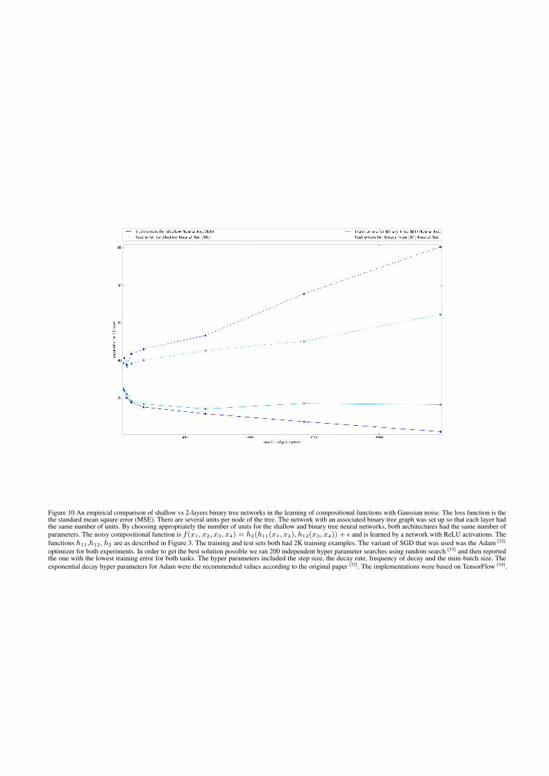
Figure 10 An empirical comparison of shallow vs 2-layers binary tree networks in the learning of compositional functions with Gaussian noise. The loss function is thethe standard mean square error (MSE). There are several units per node of the tree. The network with an associated binary tree graph was set up so that each layer hadthe same number of units. By choosing appropriately the number of units for the shallow and binary tree neural networks, both architectures had the same number ofparameters. The noisy compositional function is f(x1, x2, x3, x4) = h2(h11(x1, x2), h12(x3, x4)) + ε and is learned by a network with ReLU activations. Thefunctions h11,h12, h2 are as described in Figure 3. The training and test sets both had 2K training examples. The variant of SGD that was used was the Adam [32]

optimizer for both experiments. In order to get the best solution possible we ran 200 independent hyper parameter searches using random search [33] and then reportedthe one with the lowest training error for both tasks. The hyper parameters included the step size, the decay rate, frequency of decay and the mini-batch size. Theexponential decay hyper parameters for Adam were the recommended values according to the original paper [32]. The implementations were based on TensorFlow [34].

Figure 11 Here we empirically show that depth of the network and compositionality of the function are important. We compare shallow vs 3-layers binary tree networks inthe task of approximating a function that is not compositional. In particular the function is a linear combination of 100 ReLU units f(x) =

∑100i=1 ci(〈wi, x〉+ bi)+.

The loss function is the the standard mean square error (MSE). The training set up was the same as in figure 8. This experiment shows that when compositionality is notpresent in the function to be approximated then having depth in the network can actually worsen performance of the network (confront with in 8).

Figure 12 The figure suggests again that that depth of the network and compositionality of the function are important. The figure compares shallow vs a 3-layersbinary tree networks in the task of approximating a function that lacks the structure of local hierarchy and compositionality. In particular if the compositionality of thefunction presented in figure 8 is missing, 3-layered binary tree networks show a decreased approximation accuracy (see left figure). However, the performance of shallownetworks remain completely unchanged as shown on the right figure. Compositionality of the function in 8 was broken by shuffling the input coordinates x ∈ R8

randomly but uniformly across all the training examples. More precisely a fixed shuffling function shuffle(x) was selected and the deep and shallow networks weretrained with the data set X = {(shuffle(xi), f(xi)}60,000i=1 . The figure on the left shows that the binary tree network was not able to do better than the shallownetwork once compositionality was missing from the data. The figure on the right shows that this did not change the performance of the shallow network.

Figure 13 This figure shows a situation in which the structure of the neural network does not match exactly the structure of the function to be learned. In particular, wecompare the approximation accuracy of networks that contain the original function as a function of increasing in similarity between the network graph and the functiongraph. The function being approximated is the same as in 8.d. The network subgraphs 4 and 5 have the same convolution structure on the first layer with filter size 4. Forthe second layer subgraph 5 has more connections than subgraph 4, which reflects the higher error of subgraph 5. More precisely, subgraph 4 has a filter of size of twounits with stride of two units while subgraph 5 has filter size of three units and stride of size one. This figure shows that even when the structure of the networks does notmatch exactly the function graph, the accuracy is still good.

therefore generalizes. In other words we have the following claim

Claim: Suppose that ISn [f ] has M (convex, possibly degenerate)global minima. Then repeat SGD on Sn has CVloo, Eloo, andEEloo stability and generalizes.

Noteworthy features of generalization by “repeat SGD” is that theintrinsic noise associated with SGD wrt GD is the key to its general-ization properties. The intuition is that because of the implicit noise,SGD finds with high probability structurally stable zeros (that arerobust wrt to perturbations of the weights) and these coincide withCVloostable solutions.