Numerical simulations of the planar contraction flow for a polyethylene melt using the XPP model

J. Non-Newtonian Fluid Mech. 117 (2004) 73–84

Numerical simulations of the planar contraction flowfor a polyethylene melt using the XPP model

Wilco M.H. Verbeeten, Gerrit W.M. Peters∗, Frank P.T. Baaijens

Materials Technology, Faculty of Mechanical Engineering, Eindhoven University of Technology, P.O. Box 513, 5600 MB Eindhoven, The Netherlands

Received 10 February 2003; received in revised form 19 December 2003

Abstract

The Discrete Elastic Viscous Stress Splitting Technique in combination with the Discontinuous Galerkin (DEVSS/DG) method is used tosimulate a low density polyethylene melt flowing in a transient contraction flow problem. Numerical results using the original and a modifiedform of the eXtended Pom–Pom (XPP) model are compared to numerical results obtained with the exponential form of the Phan–Thien Tanner(PTT-a) and the Giesekus model and to experimental data of velocities and stresses. These models are known to be well capable of predictingall characteristic features encountered experimentally. Curiously, the eXtended Pom–Pom mode, formulated with the same non-affine orirreversible stretch dynamics as the original Pom–Pom model, encounters convergence problems using the DEVSS/DG method. A slightmodification of the stretch dynamics such that it becomes consistent with other viscoelastic models and in agreement with a modification ofthe stretch dynamics based on non-equilibrium thermodynamics by Van Meerveld [J. Non-Newtonian Fluid Mech. 108 (2002) 291] gives amore numerical stable behaviour and steady state could be reached. From this it is clear that physical and numerical issues still play a mixedrole in numerical viscoelastic flow problems.© 2004 Elsevier B.V. All rights reserved.

Keywords:DEVSS/DG method; Constitutive models; Differential models; eXtended Pom–Pom model; PTT-a model; Giesekus model; Polymer melt;Contraction flow; Numerical–experimental comparison; Convergence problems

1. Introduction

In recent years, the performance of numerical methods forviscoelastic flow analysis has improved significantly. A re-view on mixed finite element methods for viscoelastic flowanalysis is given in Baaijens[3]. Furthermore, constitutivemodels have become available that are able to quantitativelydescribe the behaviour of polyethylene melts over a widerange of rheological data, e.g. the molecular stress func-tion (MSF) model by Wagner et al.[29] and the eXtendedPom–Pom model (XPP)[7,14,18,27]. Both a robust numer-ical method and a reliable constitutive model are crucial inpredictive modelling of viscoelastic materials.

The robustness and efficiency of the Discrete Elastic Vis-cous Stress Splitting Technique in combination with the Dis-continuous Galerkin method (DEVSS/DG) has been shownin several studies[2,4,5,11]. A drawback of the method isthat it is not unconditionally stable in transient calculations

∗ Corresponding author.E-mail address:[email protected] (G.W.M. Peters).

URL: http://www.mate.tue.nl/.

at high Weissenberg numbers, as shown by Bogaerds et al.[10]. They found a temporal instability in a simple couetteflow for a single-mode upper convected Maxwell (UCM)model depending on the amount of elasticity. However, theDEVSS/DG method has proven to be very robust and accu-rate in non-smooth problems[2]. This contrary to numericaltechniques that apply the SUPG method for handling theconvective terms in the constitutive equation.

As a constitutive model, the multi-mode eXtendedPom–Pom model is capable of quantitatively describingthe rheological behaviour of polyethylene melts over a fullrange of well-defined rheometric experiments[27,28]. Goodagreement is found for transient and steady state shear, in-cluding reversed flow, and different elongational flows withthis model. More conventional models, such as the Giesekusand exponential Phan–Thien Tanner (PTT-a) models yieldless satisfactory results in describing the non-linear be-haviour in both shear and elongation simultaneously[4,28].

In a recent study, Bishko et al.[6] calculated the flow of ahighly branched polymer in a 4:1 contraction geometry usinga single-mode version of the original differential Pom–Pommodel. Their results were promising and they predicted in

0377-0257/$ – see front matter © 2004 Elsevier B.V. All rights reserved.doi:10.1016/j.jnnfm.2003.12.003

74 W.M.H. Verbeeten et al. / J. Non-Newtonian Fluid Mech. 117 (2004) 73–84

a good qualitative sense all the specific features observed inexperiments for low density polyethylene (LDPE) melts.

Verbeeten et al.[28] performed calculations for a com-mercial grade LDPE melt flowing through two benchmarkcomplex flow geometries, the confined flow around a cylin-der and the cross-slot flow, using the XPP model and theDEVSS/DG method. Comparison between numerical andexperimental results showed a good qualitative, and to alarge extent alsoquantitative, agreement with the velocitiesand stresses in the two complex flow geometries.

Motivated by the results of Verbeeten et al.[27], Bishkoet al. [6] and Verbeeten et al.[28], a contraction flow prob-lem will be investigated. Furthermore, this prototype indus-trial flow problem is also of interest due to the presenceof a corner singularity, which makes it numerically moreinteresting, and because it is the most widely investigatedgeometry, closely related to real industrial applications. Theobjective of this study is to investigate the performanceof the multi-mode eXtended Pom–Pom model represent-ing a commercial grade LDPE melt using the DEVSS/DGmethod. Results will be compared against experimentaldata taken from Schoonen[22] and the performance of thePTT-a and Giesekus models.

Unfortunately, for transient calculations using the combi-nation of the XPP model as given in Verbeeten et al.[27] andthe chosen numerical method convergence problems occurfor the contraction flow problem at the Weissenberg num-ber calculated in this study. Unphysical negative backbonestretch values are encountered near the re-entrant corner ofthe contraction, i.e. the geometrical singularity, and alongthe top wall after the re-entrant corner leading to divergenceof the numerical solution. Similar negative backbone stretchvalues were also found by Verbeeten et al.[28] at the frontand back stagnation points in the flow around a cylinder.The contraction flow problem is known to have a thin shearstress boundary layer, situated along the top wall after there-entrant corner, like the stress boundary layer in the cylin-der flow problem. Additionally, the contraction flow prob-lem has a geometrical singularity.

Although the DEVSS/DG method is known for not be-ing unconditionally stable, it is, however, difficult to demon-strate if a temporal or physical instability is the cause ofdivergence, since no analytical solution is at hand.

Standard solutions, such as mesh refinement, time stepreduction, addition of solvent viscosity, and rounding off there-entrant corner to eliminate the geometrical singularity didnot solve the divergence problem. Van Meerveld[25] lookedat the integral Pom–Pom model from a GENERIC point ofview. He proposed the small change in the evolution equationfor the backbone stretch. By incorporating this modification,a more stable behaviour was achieved and the steady statesolution could be reached.

In Section 2, the problem definition and the constitutiveequations are outlined. The computational method is shortlydescribed inSection 3and can be found in more detail inBogaerds et al.[11]. The material characterisation and the

performance of the three constitutive models in simple rhe-ological flows is given inSection 4. Section 5describes theperformance of both the XPP and PTT-a model in the tran-sient contraction flow problem. The conclusions are givenin Section 6. Depending on the used model, its structure,and its strain hardening behaviour, calculations with the DE-VSS/DG method can reach the steady state solution.

2. Problem definition

Isothermal and incompressible fluid flows, neglecting in-ertia, are described by the equations for conservation of mo-mentum(1) and mass(2):

∇ · T = 0, (1)

∇ · u = 0, (2)

with ∇ the gradient operator,T the Cauchy stress tensor andu the velocity field. The Cauchy stress tensorT is definedfor polymer melts by:

T = −pI + 2ηsD +M∑i=1

τi. (3)

Here,p is the pressure,I the unit tensor,ηs denotes theviscosity of the purely viscous (or solvent) contribution,D = 1/2(L + LT) the rate of deformation tensor, in whichL = ( ∇u)T is the velocity gradient tensor and(·)T denotesthe transpose of a tensor. The visco-elastic contribution ofthe ith relaxation mode is denoted byτi andM is the to-tal number of different modes. The multi-mode approach isnecessary for most polymeric fluids to give a realistic de-scription of stresses over a broad range of deformation rates.The visco-elastic contributionτi still has to be defined by aconstitutive model.

2.1. Constitutive models

Within the scope of this work, a sufficiently general ex-pression for the extra stress tensor of theith relaxation modeis given by:

∇τi + Bi · τi + τi · BT

i + Gi(Bi + BTi ) = 2Gi(1 − ξi)D,

(4)

with Bi the averaged, macroscopic slip tensor,Gi the plateaumodulus, andξi a slip parameter that, if non-zero, accountsfor the Gordon–Schowalter derivative. The upper convectedtime derivative of the extra stressτi

∇ is defined as:

∇τi = τi − L · τi − τi · LT

= ∂τi

∂t+ u · ∇τi − L · τi − τi · LT, (5)

with t denoting time. The slip tensorBi defines the chosenconstitutive equation.

W.M.H. Verbeeten et al. / J. Non-Newtonian Fluid Mech. 117 (2004) 73–84 75

The eXtended Pom–Pom model[27] is a modification ofthe differential version of the original Pom–Pom model byMcLeish and Larson[18] incorporating branch-point with-drawal as introduced by Blackwell et al.[7]. The basic ideaof this model is that the rheological properties of entangledpolymer melts depend on the topological structure of thepolymer molecules. The simplified topology consists of abackbone tube with a number of dangling arms at both endsand is called a Pom–Pom molecule. A key feature is the sep-aration of relaxation times for the stretch and orientation. Forthe Pom–Pom model, in which the slip parameter is not usedand equalsξi = 0, the extra stress tensor is expressed as:

τi = σi − GiI = 3GiΛ2i Si − GiI, (6)

with Λi the backbone tube stretch, defined as the length ofthe backbone tube divided by the length at equilibrium, andSi denoting the orientation tensor. The evolution equationsfor the orientation tensorSi and backbone tube stretchΛi

are given by:

∇Si + 2[D : Si]Si + Bi · Si + Si · BT

i − 2[Bi : Si]Si = 0,(7)

Λi = Λi[D : Si] − Λi[Bi : Si]. (8)

In the original Pom–Pom model[18] and in the eXtendedPom–Pom model introduced by Verbeeten et al.[27], theslip tensorBi is given by:

Bi = αi

2Giλb,iσi +

[1 − αi − 3αiΛ

4i Tr(Si · Si)

2λb,iΛ2i

+ rieνi(Λi−1)

λb,i

(1 − 1

Λi

)]I − Gi(1 − αi)

2λb,iσ−1i . (9)

Here,αi is an adjustable parameter,λb,i the relaxation timeof the backbone tube orientation equal to the linear relax-ation timeλi, andσi is defined according toEq. (6). Both theplateau modulusGi and the relaxation timeλi are obtainedfrom the linear relaxation spectrum determined by dynamicmeasurements, whileαi controls the anisotropic drag, simi-lar to the Giesekus model.ri = λb,i/λs,i is the ratio betweenthe orientation relaxation time and the stretch relaxationtimeλs,i, andνi = 2/qi is a parameter denoting the influenceof the surrounding polymer chains on the backbone tubestretch withqi the amount of arms at the end of a backbone.

The expression(9) for the slip tensorBi was chosen suchthat the non-affine or irreversible stretch dynamics to be pro-portional to [Λi − 1]. This is determined only by the termwith λs in Eq. (9) and this term does not contribute to theorientation evolution,Eq. (7). However, this choice is notconsistent with the irreversible stretch dynamics as found forthe other viscoelastic models such as the PTT-a, Giesekusand UCM model (see the end of this section for the for-mal expressions). To make it consistent the term [Λi − 1]should be replaced by [Λi − (1/Λi)]. This introduces a sin-gularity for Λi = 0 and guarantees thatΛi > 0. The same

result was found by Van Meerveld[25] who analyzed the in-tegral Pom–Pom model using the thermodynamical frame-work GENERIC. He pointed out that it may be of importancefor contraction/expansion flows, in which Wapperom andKeunings[30] detected a negative affine motion. Physically,this change in the stretch dynamics means a faster relaxationtowards its equilibrium state when the backbone is stretchedor compressed. This could be favourable in circumstancesthat the stretch increases very fast, as is the case during uni-axial elongation and close to geometrical singularities. Infact we have detected that this seemingly small change in theconstitutive equation marks the difference between reachingconverged results and divergence of the numerical scheme.The slip tensorBi for the modified XPP model, i.e. includ-ing the modified stretch dynamics, is then given by:

Bi = αi

2Giλb,iσi +

[1 − αi − 3αiΛ

4i Tr(Si · Si)

2λb,iΛ2i

+ rieνi(Λi−1)

λb,i

(1 − 1

Λ2i

)]I − Gi(1 − αi)

2λb,iσ−1i .

(10)

Due to its different structure from most differential con-stitutive equations and non-zero initial conditions, it maybe cumbersome to implement the above double-equationformulation consisting ofEqs. (7), (8) and (10)in FE pack-ages. However, the XPP model can also be written in afully equivalent single-equation fashion by substituting theslip tensor ofEq. (10) into Eq. (4). A numerically consis-tent implementation of the backbone stretch values are thencalculated fromEq. (6):

Λ2i = 1 + Tr(τi)

3Gi

. (11)

and

Λi =√

1 + |Tr(τi)|3Gi

≥ 1, (12)

which is only present in the exponential term and securesits minimum atΛi = 1. Notice, that for this definitionof the backbone stretch, we avoid numerical problems ifTr(τi)/3Gi < −1. Theoretically, Tr(τi) is always 0 orpositive. However, numerically we have encountered theseunrealistic values near the re-entrant corner in the contrac-tion flow and at the front and back stagnation points in theflow around a cylinder for high enough flow rates, both forthe XPP model as well as the Giesekus and PTT-a models.

For the Giesekus model,ξi = 0 and the tensorBi isdefined as:

Bi = αi

2Giλi

σi + (1 − 2αi)

2λi

I − Gi(1 − αi)

2λi

σ−1i , (13)

with αi an adjustable parameter, which controls theanisotropic drag. Notice that forαi = 0, the upper convectedMaxwell model is retrieved.


For the exponential PTT model,Bi is defined as:

Bi = −ξiD + e(εiTr(τi)/Gi)

2λi

I − Gie(εiTr(τi)/Gi)

2λi

σ−1i . (14)

with εi an adjustable parameter, controlling the amount ofstrain softening.

Similar to the XPP model, both the Giesekus and PTT-amodels can be split up in an orientation and stretch equa-tion. Substitution ofEq. (13) (for the Giesekus model) orEq. (14) (for the PTT-a model) into theEqs. (7) and (8)result in the evolution equations for the backbone orienta-tion and backbone stretch. To illustrate the differences andsimilarities between the three models, the backbone stretchequations are shown for the Giesekus:

Λi = Λi[D : Si] − 1

2λi

(3Λ2

i αiTr(Si · Si)

+(1 − 2αi)Λi − (1 − αi)

Λi

), (15)

and for the PTT-a model:

Λi = Λi[(1 − ξi)D : Si] − eεiTr(τi)Gi

2λi

(Λi − 1

Λi

). (16)

If Eq. (11)is used, the expression for the PTT-a model canalso be written as:

Λi = Λi[(1 − ξi)D : Si] − eν∗i (Λ

2i −1)

2λi

(Λi − 1

Λi

),

ν∗i = 3εi. (17)

Notice that the stretch relaxation for the Giesekus and PTT-amodels are also proportional to [Λi − (1/Λi)].

3. Computational method

The DEVSS/DG method, Baaijens et al.[4], is applied.This method efficiently handles multiple relaxation modesand is robust near geometrical singularities. It is a combi-nation of the Discrete Elastic Viscous Stress Splitting Tech-nique of Guénette and Fortin[12] and the DiscontinuousGalerkin method, developed by Lesaint and Raviart[16].Application to the single-equation XPP model is discussed inthis section. The weak formulation and solution strategy forthe Giesekus and PTT-a models is similar and can be foundin more detail in Bogaerds et al.[11] and Baaijens et al.[4].

3.1. DEVSS/DG method

Consider the problem described by theEqs. (1), (2),(4) and (10). Following common FE techniques, theseequations are converted into a mixed weak formulation:

3.1.1. Problem DEVSS/DGFind (u, p, D, τi) for any timet such that for all admis-

sible test functions (v, q,E, si),

(Dv,2ηsD + 2η(D − D) +

M∑i=1

τi

)− (∇ · v, p) = 0,

(18)

(q,∇ · u) = 0, (19)

(E, D − D) = 0, (20)

(si,

∇τ i + αi

λb,iGi

τi · τi + 1

λb,i

[2rie

νi(Λi−1)

(1 − 1

Λ2i

)

+ 1

Λ2i

− αiTr(τi · τi)

3G2i Λ

2i

]τi

+ 1

λb,i

[2rie

νi(Λi−1)

(1 − 1

Λ2i

)+ 1

Λ2i

−αiTr(τi · τi)

3G2i Λ

2i

− 1

]GiI − 2GiD

)

−K∑

e=1

∫Γ e

in

si : u · n(τi − τexti )dΓ = 0

∀ i ∈ 1,2, . . . ,M. (21)

Here,(·, ·) denotes theL2-inner product on the domainΩ,Dv = 1/2( ∇v+( ∇v)T), η an auxiliary viscosity chosen to beη = ∑M

i=1 Giλi, Γ ein is the inflow boundary of elementΩe,

n the unit vector pointing outward normal on the boundaryof the element (Ωe) andτext

i denote the extra stress tensorof the neighbouring, upstream element.

Time discretisation of the constitutive equation is attainedusing an semi-implicit Euler scheme. In this scheme most ofthe variables are updated implicitly with the exception of theexternal componentτext

i which is taken explicitly (i.e.τexti =

τexti (tn). Furthermore, the equation for the discrete rate of

deformationD is decoupled from the ‘Stokes’ problem andthus updated explicitly.

3.2. Solution strategy

A two-dimensional flow domain is divided into quadri-lateral elements as a spatial discretisation. The interpola-tion of the velocity fieldu is bi-quadratic, the pressurepand discrete rate of deformation fieldsD are interpolatedbi-linearly, while the extra stress tensorτi field has a dis-continuous bi-linear interpolation. TheEqs. (18)–(21)areintegrated over elements using a 3× 3-Gauss quadraturerule.

The non-linear equations are solved using a one stepNewton–Raphson iteration. Within the linearized set ofequations, the extra stress related variableτi forms a blockdiagonal structure due to the fact that the components in theupstream elements are taken explicitly. This enables elimi-nation of the extra stress variable at element level. A furtherreduction of the system matrix is obtained by a decoupling


approach. First, the ‘Stokes’ problem (u, p) is solved, afterwhich the updated solution is used to find a new approx-imation for D. Notice, that this introduces a small extrainconsistency for the stabilization term 2η(D − D) in themomentumEq. (18), sinceD is taken at timetn+1, while D

is taken at timetn. Finally, the nodal increments of the ori-entation tensor and backbone stretch are retrieved elementby element.

To solve the non-symmetrical system of the ‘Stokes’problem (u, p) an iterative solver is used based on theBi-CGSTAB method of Van der Vorst[24]. The symmet-rical set of algebraic equations of problem(D) is solvedusing a conjugate-gradient solver. Incomplete LU precon-ditioning is applied to both solvers. In order to enhance thecomputational efficiency of the Bi-CGSTAB solver, staticcondensation of the centre-node velocity variables resultsin filling of the zero block diagonal matrix in the ‘Stokes’problem and, in addition, achieves a further reduction ofglobal degrees of freedom. The above decoupling proce-dure enables the use of iterative solvers. The use of theBi-CGSTAB solver in combination with the incomplete LUpreconditioning on the problem (u, p, D) was unsuccessful.For more details, we refer to[11,28].

To solve the above sets of algebraic equations, both es-sential and natural boundary conditions must be imposed onthe boundaries of the flow channels. At the entrance of theflow channel the velocity profile is prescribed. At the exit,either the velocity profile is prescribed together with a pres-sure point that is set to zero, or the velocities perpendicularto the outflow directions are suppressed. At the entrance, thevalues of the extra stress tensor of a few elements down-stream the inflow channel are prescribed along the inflowboundary, imposing a periodic boundary condition for thestress variable.

Calculations were stopped when the variables had reachedsteady state values. The steady state convergence criteriumis established by calculating the least square differencebetween the solution of the actual and previous iterationstep, divided by the least square actual solution, and check-ing if it is smaller than a certain convergence criteriumε:√∑N

i=1(un+1i − un

i )2√∑N

i=1(un+1i )2

≤ ε, (22)

Table 1Linear and non-linear parameters for fitting of the DSM Stamylan LD 2008 XC43 LDPE melt

i Maxwell parameters mXPP Giesekus Exp. PTT

Gi (Pa) λi (s) qi λb,i/λs,i αi αi εi ξi

1 7.2006× 104 3.8946× 10−3 1 1.0 0.30 0.30 0.30 0.082 1.5770× 104 5.1390× 10−2 1 1.0 0.30 0.30 0.20 0.083 3.3340× 103 5.0349× 10−1 2 1.0 0.15 0.25 0.02 0.084 3.0080× 102 4.5911× 100 10 1.0 0.03 0.04 0.02 0.08

T = 170C. νi = 2/qi. Activation energy:E0 = 48.2 kJ/mol. WLF-shift parameters:C1 = 14.3 K, C2 = 480.8 K.

with N being the total number of nodes in the mesh. For cal-culations presented in this paper, the convergence criteriumis chosen to beε = 10−7.

4. Material characterisation

Since a multi-mode approach is necessary for a re-alistic description of polymer melts, we will investigatemulti-mode calculations. Parameters are identified for acommercial grade polymer melt, a low density polyethylene(DSM, Stamylan LD 2008 XC43), subsequently referred toas LDPE. This long-chain branched material has been ex-tensively characterised by Schoonen[22] and is also givenin Peters et al.[21].

The parameters for a four mode Maxwell model are ob-tained from dynamic measurements at a temperature ofT =170C. The non-linearity parametersqi and the ratiori =λb,i/λs,i for the XPP model andαi for the Giesekus modelare determined using the transient uniaxial elongational data[31] only. For the PTT-a modelεi andξi are identified byusing transient uniaxial elongational and shear data. Sincesecond planar elongational or second normal stress differ-ence data is not available for this material, the anisotropyparameterαi in the XPP model is chosen as 0.3/qi, similarto Verbeeten et al.[28]. All parameters are given inTable 1.

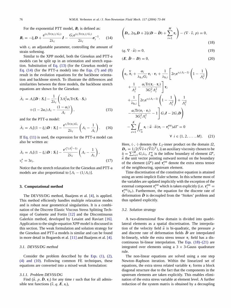
Fig. 1 shows the rheological behaviour of the three con-stitutive models and measured data in uniaxial and simpleshear behaviour. The ‘steady state’ data points in the uni-axial elongational viscosity plot are the end points of thetransient curves. Since the samples break at the end of thetransient measurements, it is hard to say if steady state hastruly been reached. However, sometimes it is claimed thatsteady state coincides with break-up of the samples[17].

All three models can satisfactorily predict the uniax-ial elongational data in a transient sense. However, noticethat the PTT-a model is showing an upswing towards thequasi-steady state values that is a little too soon in time.Furthermore, for the high elongation rateε = 30 s−1, forwhich no experimental data is available, the Giesekus modelshows a much higher upswing compared to the other twomodels. For the quasi-steady state data, the XPP modelpredicts the most smooth and realistic curve. With this setof relaxation times and these parameters, the PTT-a modeldemonstrates a more non-smooth behaviour, reflecting the


Fig. 1. Transient (a) and quasi-steady state (b) uniaxial viscosityηu, transient (c) and steady state (d) shear viscosityηs, and transient (e) and steadystate (f) first normal stress coefficientΨ1 at T = 170C of the mXPP, Giesekus and PTT-a models for DSM Stamylan LD2008 XC43 LDPE melt.

individual relaxation times due to the excessive elongationalthinning behaviour of the model at high strain rates. Thisnon-smooth behaviour could be reduced by incorporatingmore modes, however at the cost of a significant increase ofthe computational time. As expected and also indicated bythe transient model predictions at the high elongation rate,the Giesekus model predicts the wrong shape of the steadystate curve, as it ends in a plateau for high strain rates.Low density polyethylene melts are in general elongationalthinning in a steady state sense at high strain rates (see for

example data from Münstedt and Laun[19] and Hachmann[13]).

For simple shear, all models show a rather good agreementwith the measured data (Fig. 1(c) and (d)). For intermediateshear rates, the Giesekus and PTT-a models somewhat overpredict the measurements. At shear rates over 102 s−1, thecurves for all models drop rapidly (seeFig. 1d), as here onlythe last mode of the relaxation spectrum is active, showinga too steep slope of−1. For the contraction flow problem atthe chosen Weissenberg number, using the definition for the


flow

direction

h

H

0 x/h

0

y/h

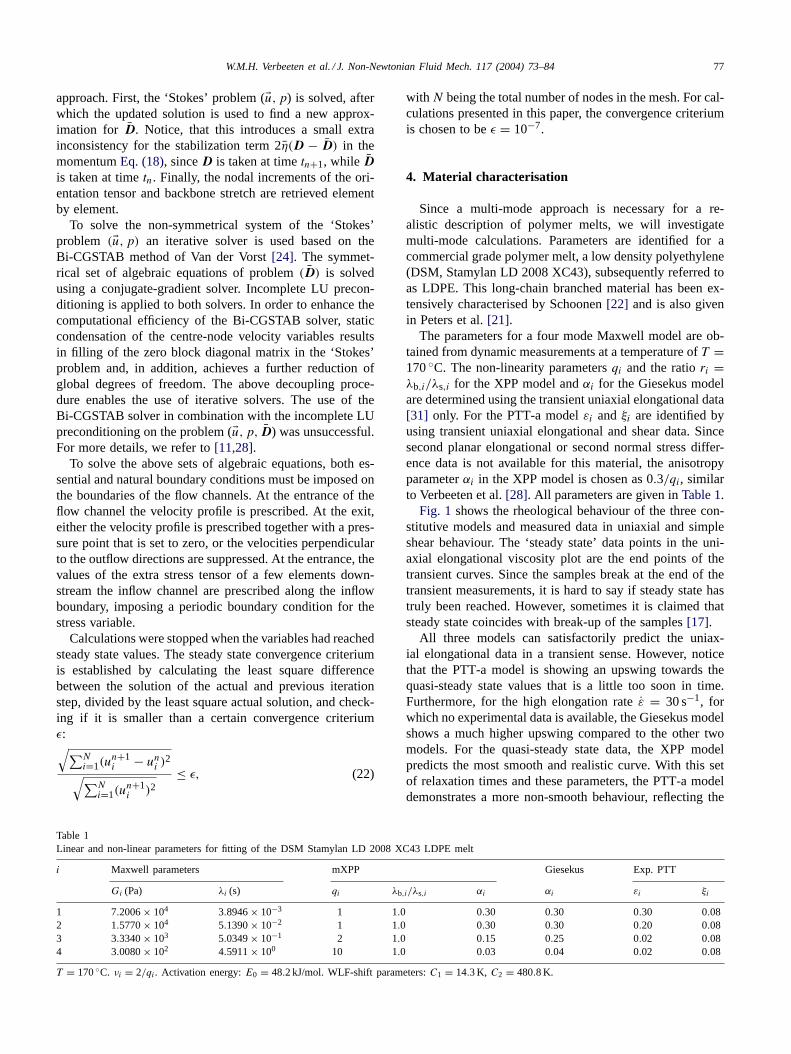
Fig. 2. Schematic of half the planar contraction flow. The origin of thecoordinate system is at the centre of the contraction plane. T = 170 C,λ = 1.7415 s, u2D = 7.47 mm/s, h = 0.775 mm, H = 2.55 mm,d = 40 mm.

effective strain rate εeff = 1/2√

2D : D, maximum shearand strain rates of γmax ≈ 50 s−1 and εmax ≈ 40 s−1 wereobserved around the re-entrant corner. Thus, calculations allfall within the range of the chosen relaxation spectrum ca-pable of predicting the experimental data. In order to ob-tain a good fit of the shear data for the PTT-a model, thenon-linearity parameter ξ is larger than ε for the two longestrelaxation times. Although difficult to observe in Fig. 1(c),this results in oscillations in transient start-up of simple shear(see also Appendix A in Verbeeten et al. [28]).

For the first normal stress difference (Fig. 1(e) and (f)),the XPP model shows the best agreement for intermediateshear rates, while the PTT-a model performs better at lowand high shear rates. Note that the experimental data keepson decreasing at larger times. This is most probably due toinstabilities at the free surface in the cone-plate experiments,see for example Pahl et al. [20].

Although similar discrepancies between the experimentaldata and the calculated results exist for all models, in ouropinion, the XPP model shows the best overall agreementwith experimental rheological data. This opinion is formedmostly due to the most smooth and realistic curve for thesteady state elongational viscosity and its capability forsimultaneously describing the shear and elongational ex-perimental data of other low density polyethylene melts inquantitative sense.

5. Planar contraction flow problem

The planar contraction benchmark flow is known to haveregions with pure simple shear flow, pure planar elongationand combinations thereof. It also has a corner singularitywhich makes it numerically challenging.

A schematic of half the flow geometry and its char-acteristics are given in Fig. 2. Experiments were per-formed at a temperature of T = 170 C, resulting ina viscosity averaged relaxation time for the material of

λ =(∑M

i=1 λ2i Gi

)/(∑M

i=1 λiGi

)= 1.7415 s. The down-

stream and upstream half heights of the geometry are h =0.775 mm and H = 2.55 mm, respectively, giving an ac-tual contraction ratio of 3.29. The average two-dimensionalmean upstream velocity is equal to U2D = 2.27 mm/s, and

consequently the average downstream velocity is u2D =7.47 mm/s. The depth of the flow cell equals d = 40 mmto create a nominally two-dimensional flow, resulting ina depth-to-height ratio of 7.84 upstream and 25.81 down-stream. This depth-to-height ratio reduces the influence ofthe front and back walls to about 6% maximum on theisochromatic stress patterns with the flow rate investigatedin this work (see [11,23]). This is a sufficiently small devi-ation to compare experimental results to two-dimensionalcalculations.

By taking half the downstream channel height and thedownstream two-dimensional mean velocity as characteris-tic values, the flow averaged dimensional Weissenberg num-ber, indicating the shear strength of the flow, results in:

Wi = λu2D

h= 16.8. (23)

The maximum averaged Weissenberg number of the flow,using the longest relaxation time, is:

Wimax = λmaxu2D

h= 44.3. (24)

If related to the local shear rate γ = ∂u/∂x, higher Weis-senberg numbers can even be found in the flow.

Particle tracking velocimetry (PTV) was used to obtain theexperimental velocities. Stresses were measured using thefield-wise flow induced birefringence (FIB) method record-ing isochromatic fringe patterns. To link these fringe pat-terns to calcuted stresses, we have used the semi-empericalstress optical rule. For two-dimensional flows, the stress op-tical rule simplifies to:

τFRG =√

4τ2xy + N2

1 = kϑ

dC, (25)

with τFRG defined as the isochromatic fringe stress, τxy theshear stress in the xy-plane, N1 = τxx − τyy the first normalstress difference, ϑ the wave length of the light used in themeasurements, d the light path length in the birefringentmedium, which in this case is the depth of the flow cell, C =1.47×10−9 Pa−1 the stress optical coefficient (identified byPeters et al. [21]), and k the fringe order of the observed darkfringe bands where extinction of the light occurs. For moredetails on the experimental aspects and more experimentalresults, we refer to Schoonen [22].

5.1. Original XPP model

For the original eXtended Pom–Pom mode, as given byVerbeeten et al. [27,28], convergence problems occurred andno steady state results could be reached. It was difficult todetect the exact reason for the onset of divergence, as variouspossibilities interact at the same time.

Divergence problems may be accounted for by a temporalinstability of the DEVSS/DG method as found in simplecouette flows for a single-mode UCM model by Bogaerdset al. [10]. Moreover, it could be due to the highly strain


hardening behaviour or anisotropy with the chosen set ofparameters.

The onset of divergence may have been provoked byTr(τi)/3Gi < −1 resulting in negative backbone stretch val-ues near the re-entrant corner singularity. This occurrencewas detected for both the original XPP model as well as forthe Giesekus and PTT-a models. However, for the PTT-amodel the negative backbone stretch values disappeared af-ter sufficient iteration steps and steady state results couldbe reached. This contrary to the Giesekus and the originalXPP model, where negative backbone stretch values weredetected well before the onset of divergence. These nega-tive backbone stretch values were only encountered for themode with the largest relaxation time.

Various attempts were made to overcome the convergenceproblems for the contraction flow problem. Mesh refinement,decreasing the time step, changing the boundary conditions,or adding a little solvent viscosity at best delayed the onset ofdivergence. Reaching full convergence within each time stepusing multiple Newton iterations instead of only one, didnot resolve the convergence problems either. By choosingα = 0, which means no anisotropy, calculations divergedeven sooner, which rejects the idea that anisotropy has anegative effect on the numerical stability.

The influence of a rounded corner was investigated tosee if the corner singularity was the cause of divergence.Surprisingly, by rounding of the re-entrant corner divergenceoccurred even sooner in time. Higher stresses and stressgradients appeared in the simulations and that may influenceconvergence in a negative sense.

Although fully equivalent to the single-equation for-mulation, the double-equation formulation of the originaleXtended Pom–Pom model shows different numerical re-sponse. Unfortunately, for the double-equation formulation,negative backbone stretch values were also encountered,although they appeared only just before onset of divergence.

Possibly the convergence problem is caused by an insuf-ficiently fine mesh or too large time step. Hence, the nu-merical scheme may not be capable of coping with the highstress gradients due to the high strain hardening behaviour of

-3 -2 -1 0 1 20

0.5

1

1.5

2

2.5

3

x/h

y/h

M1

-3 -2 -1 0 1 20

0.5

1

1.5

2

2.5

3

x/h

y/h

M2

(a) (b)

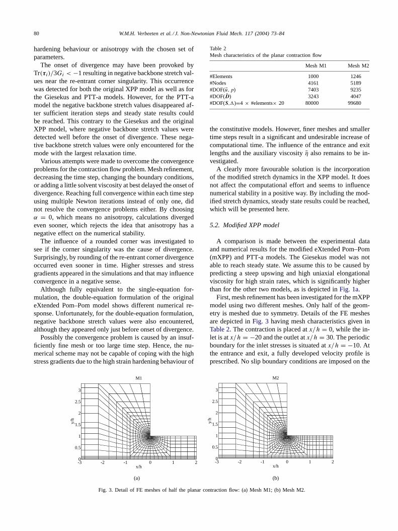
Fig. 3. Detail of FE meshes of half the planar contraction flow: (a) Mesh M1; (b) Mesh M2.

Table 2Mesh characteristics of the planar contraction flow

Mesh M1 Mesh M2

#Elements 1000 1246#Nodes 4161 5189#DOF(u, p) 7403 9235#DOF(D) 3243 4047#DOF(S,.)=4 × #elements× 20 80000 99680

the constitutive models. However, finer meshes and smallertime steps result in a significant and undesirable increase ofcomputational time. The influence of the entrance and exitlengths and the auxiliary viscosity η also remains to be in-vestigated.

A clearly more favourable solution is the incorporationof the modified stretch dynamics in the XPP model. It doesnot affect the computational effort and seems to influencenumerical stability in a positive way. By including the mod-ified stretch dynamics, steady state results could be reached,which will be presented here.

5.2. Modified XPP model

A comparison is made between the experimental dataand numerical results for the modified eXtended Pom–Pom(mXPP) and PTT-a models. The Giesekus model was notable to reach steady state. We assume this to be caused bypredicting a steep upswing and high uniaxial elongationalviscosity for high strain rates, which is significantly higherthan for the other two models, as is depicted in Fig. 1a.

First, mesh refinement has been investigated for the mXPPmodel using two different meshes. Only half of the geom-etry is meshed due to symmetry. Details of the FE meshesare depicted in Fig. 3 having mesh characteristics given inTable 2. The contraction is placed at x/h = 0, while the in-let is at x/h = −20 and the outlet at x/h = 30. The periodicboundary for the inlet stresses is situated at x/h = −10. Atthe entrance and exit, a fully developed velocity profile isprescribed. No slip boundary conditions are imposed on the


top confining wall, and the velocity in y-direction is sup-pressed for the symmetry line y/h = 0.

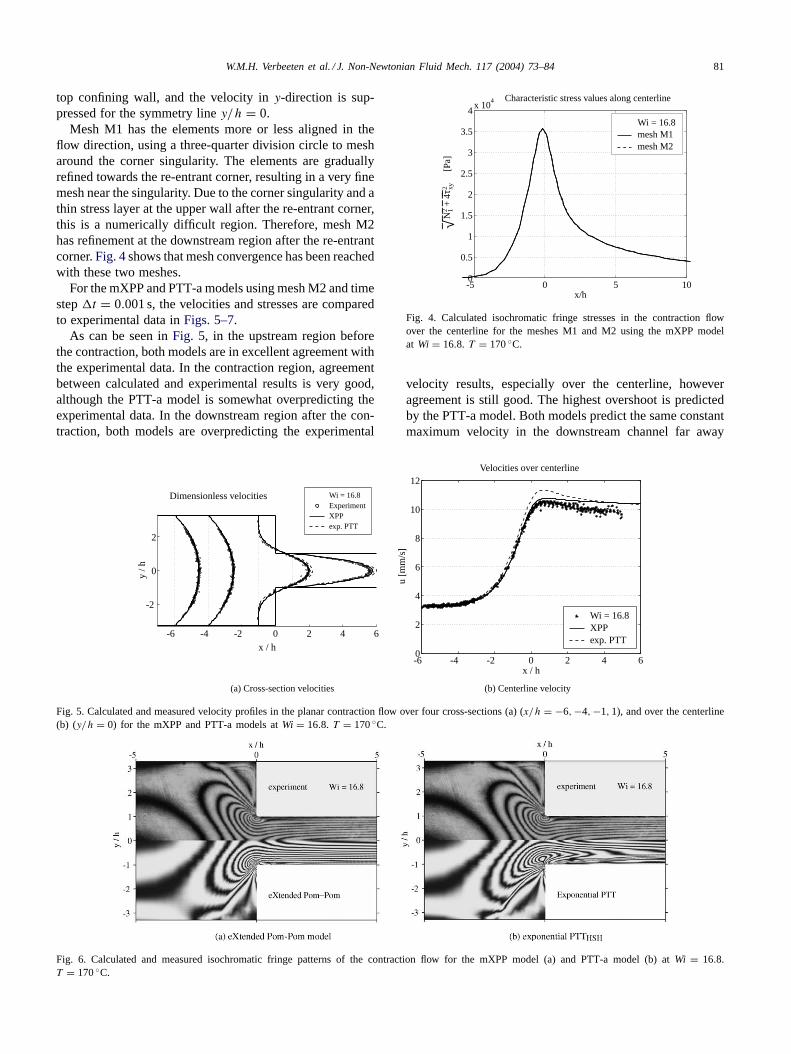
Mesh M1 has the elements more or less aligned in theflow direction, using a three-quarter division circle to mesharound the corner singularity. The elements are graduallyrefined towards the re-entrant corner, resulting in a very finemesh near the singularity. Due to the corner singularity and athin stress layer at the upper wall after the re-entrant corner,this is a numerically difficult region. Therefore, mesh M2has refinement at the downstream region after the re-entrantcorner. Fig. 4 shows that mesh convergence has been reachedwith these two meshes.

For the mXPP and PTT-a models using mesh M2 and timestep 0t = 0.001 s, the velocities and stresses are comparedto experimental data in Figs. 5–7.

As can be seen in Fig. 5, in the upstream region beforethe contraction, both models are in excellent agreement withthe experimental data. In the contraction region, agreementbetween calculated and experimental results is very good,although the PTT-a model is somewhat overpredicting theexperimental data. In the downstream region after the con-traction, both models are overpredicting the experimental

-6 -4 -2 0 2 4 6

-2

0

2

Dimensionless velocities

x / h

y / h

Wi = 16.8ExperimentXPPexp. PTT

-6 -4 -2 0 2 4 60

2

4

6

8

10

12Velocities over centerline

x / h

u [m

m/s

]

Wi = 16.8XPPexp. PTT

(a) Cross-section velocities (b) Centerline velocity

Fig. 5. Calculated and measured velocity profiles in the planar contraction flow over four cross-sections (a) (x/h = −6,−4,−1, 1), and over the centerline(b) (y/h = 0) for the mXPP and PTT-a models at Wi = 16.8. T = 170 C.

Fig. 6. Calculated and measured isochromatic fringe patterns of the contraction flow for the mXPP model (a) and PTT-a model (b) at Wi = 16.8.T = 170 C.

-5 0 5 100

0.5

1

1.5

2

2.5

3

3.5

4x 10

4 Characteristic stress values along centerline

x/h

√

N12

+ 4

τ xy2

[

Pa]

Wi = 16.8mesh M1mesh M2

Fig. 4. Calculated isochromatic fringe stresses in the contraction flowover the centerline for the meshes M1 and M2 using the mXPP modelat Wi = 16.8. T = 170 C.

velocity results, especially over the centerline, howeveragreement is still good. The highest overshoot is predictedby the PTT-a model. Both models predict the same constantmaximum velocity in the downstream channel far away


-5 0 5 100

1

2

3

4

5x 10

4 Characteristic stress values along centerline

x/h

√

N12

+ 4

τ xy2

[

Pa]


-5 -4 -3 -2 -1 00

0.5

1

1.5

2

2.5

3x 10

5 Characteristic stress values at y/h=1

x / h

√

N12

+ 4

τ xy2

[

Pa]


(a) Centerline (y / h = 0) (b) Cross-section (y / h = 1)

(d) Cross-section (x / h = 4.8)(d) Cross-section (x / h = 0)

-1 -0.5 0 0.5 10

0.5

1

1.5

2

2.5

3x 10

5 Characteristic stress values at cross section x=0

y / h

√

N12

+ 4

τ xy2

[

Pa]


-1 -0.5 0 0.5 10

5

10

15x 10

4 Characteristic stress values at x/h=4.8

y / h

√

N12

+ 4

τ xy2

[

Pa]


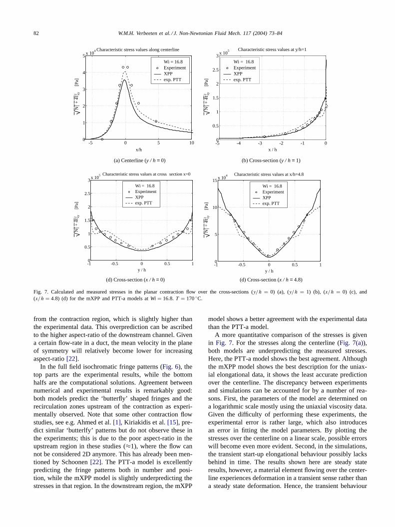
Fig. 7. Calculated and measured stresses in the planar contraction flow over the cross-sections (y/h = 0) (a), (y/h = 1) (b), (x/h = 0) (c), and(x/h = 4.8) (d) for the mXPP and PTT-a models at Wi = 16.8. T = 170 C.

from the contraction region, which is slightly higher thanthe experimental data. This overprediction can be ascribedto the higher aspect-ratio of the downstream channel. Givena certain flow-rate in a duct, the mean velocity in the planeof symmetry will relatively become lower for increasingaspect-ratio [22].

In the full field isochromatic fringe patterns (Fig. 6), thetop parts are the experimental results, while the bottomhalfs are the computational solutions. Agreement betweennumerical and experimental results is remarkably good:both models predict the ‘butterfly’ shaped fringes and therecirculation zones upstream of the contraction as experi-mentally observed. Note that some other contraction flowstudies, see e.g. Ahmed et al. [1], Kiriakidis et al. [15], pre-dict similar ‘butterlfy’ patterns but do not observe these inthe experiments; this is due to the poor aspect-ratio in theupstream region in these studies (≈1), where the flow cannot be considered 2D anymore. This has already been men-tioned by Schoonen [22]. The PTT-a model is excellentlypredicting the fringe patterns both in number and posi-tion, while the mXPP model is slightly underpredicting thestresses in that region. In the downstream region, the mXPP

model shows a better agreement with the experimental datathan the PTT-a model.

A more quantitative comparison of the stresses is givenin Fig. 7. For the stresses along the centerline (Fig. 7(a)),both models are underpredicting the measured stresses.Here, the PTT-a model shows the best agreement. Althoughthe mXPP model shows the best description for the uniax-ial elongational data, it shows the least accurate predictionover the centerline. The discrepancy between experimentsand simulations can be accounted for by a number of rea-sons. First, the parameters of the model are determined ona logarithmic scale mostly using the uniaxial viscosity data.Given the difficulty of performing these experiments, theexperimental error is rather large, which also introducesan error in fitting the model parameters. By plotting thestresses over the centerline on a linear scale, possible errorswill become even more evident. Second, in the simulations,the transient start-up elongational behaviour possibly lacksbehind in time. The results shown here are steady stateresults, however, a material element flowing over the center-line experiences deformation in a transient sense rather thana steady state deformation. Hence, the transient behaviour


of the consitutive models is of importance in this complexflow. And third, the three-dimensional effects are mostpronounced in this region as velocities increase. To drawmore confident conclusions regarding these last effects, fullthree-dimensional calculations would provide more insight.

Over the line y/h = 1 towards the contraction singularity(Fig. 7(b)), the mXPP model shows the best agreement. Itcan be seen that both models encounter oscillations near thegeometrical singularity, which seems to be more pronounedfor the PTT-a model. Possibly more mesh refinement in thatregion could avoid these oscillations. However, that wouldalso mean an increase in computational time, which is al-ready quite considerable.

For the cross-section x/h = 0 and x/h = 4.8 (Fig. 7(c)and (d)), the PTT-a model shows a better agreement nearthe centerline, while the mXPP model predicts the experi-mental data better away from the centerline near the upperwalls. The PTT-a model shows a ‘ long-wave’ sort of os-cillation towards the upper confining walls. Since this is ashear dominated region, these oscillations may be ascribedto the oscillations in the start-up of transient shear flows forthis model (see Fig. 1(c) and (e)). However, further investi-gation is necessary regarding this phenomenon to underlinethis statement with more confidence.

In general, both the mXPP and PTT-a models show agood to excellent agreement between the numerical and ex-perimental results, both for the velocity and stress data.

6. Discussions and conclusions

The transient flow in a contraction problem is investi-gated using the DEVSS/DG method in combination with theeXtended Pom–Pom model with the modified stretch dy-namics. Steady state numerical results using a sufficientlyfine mesh and time step 0t = 0.001 s are compared to thevelocity and stress experimental data and the well-knownconventional exponential form of the Phan–Thien Tannermodel. Results of both constitutive models are in good agree-ment with the experimental data and all the typical experi-mental features are also predicted by the numerical models.Although the mXPP model shows a good agreement withuniaxial viscosity data, experimental stresses over the cen-terline are surprisingly underpredicted, which is also thecase for the PTT-a model. This discrepancy is expected toarise from three-dimensional effects. More investigation isneeded to confirm that assumption.

Numerical simulations using the Giesekus model showedconvergence problems and no steady state results could bereached. This was also encountered for the for the originalXPP model. Negative backbone stretch values were encoun-tered near the re-entrant corner singularity. It is difficult topoint out the exact cause of the onset of divergence. It maybe due to the locally very high stress gradients which themesh is unable to resolve, given a certain time step. On theother hand, the temporal instability of the DG method as

was found by Bogaerds et al. [10] may influence divergenceof the problem. Recently, Bogaerds et al. [8] showed thatinstabilities are also dependent on the shape of the elementsin the mesh; long shaped elements in the flow direction in-crease stability.

No numerical remedy was encountered to overcome di-vergence of the calculations. Mesh refinement, decreasingthe time step, or changing the boundary conditions at bestdelayed divergence. By increasing 0t and having more iter-ations per time step, or adding solvent viscosity divergencewas encountered even sooner. Rounding off the re-entrantcorner to remove the geometrical singularity also causedmore difficulties in resolving the problem. Loss of con-vergence was probably encountered sooner because of anenhanced convection into the downstream flow channel ofhigh stresses imposed by the re-entrant corner.

Simulations with both the single-equation as well as thedouble-equation version of the eXtended Pom–Pom modelwere performed. Although fully equivalent, they showdifferent numerical responses. For the double-equation ver-sion, negative backbone stretch values are only encounteredjust before onset of divergence. Since the backbone stretchvalues in the single-equation version are derived fromTr(τi) instead of calculated directly, negative values are en-countered already earlier in the calculations. This leads tocomplex backbone stretch values and numerical inconsis-tencies. The Giesekus and PTT-a models also suffer fromthis numerical artefact, which for the Giesekus model hasled to divergence of the numerical solution.

For transient calculations, the DEVSS/DG method be-comes more unstable at higher elasticities (see [10]), i.e.higher flow rates in the flow geometry or higher stresses asa consequence of higher strain hardening behaviour. This isconsistent with observations of Verbeeten [26] that calcu-lations with the single-equation formulation converge if aparameter set is chosen that describes a lower strain harden-ing behaviour of the material, and a steady state solution isreached. This holds both for a geometry with a corner sin-gularity as well as a rounded re-entrant corner. However, toour surprise, steady state solutions for the double-equationformulation were never reached, no matter if a low or highstrain hardening parameter set was chosen. Most probably,the extra stress variables Λi and Si stay about the same or-der in magnitude, hardly influenced by a change of materialparameters.

In the presented solution method, the ‘Stokes’ problem(u, p) and the discrete rate of deformation problem (D) aredecoupled. As a result, the stabilization term 2η(D − D) inthe momentum equation((18)) is inconsistent: D is taken attime tn+1, while D is taken at time tn. This decoupling mayinfluence stability of the numerical scheme. By choosing adifferent preconditioner, the coupled problem (u, p, D) canbe solved while still using iterative solvers.

The DEVSS/DG method shows divergence problems,depending on the constitutive model, the mesh, the timestep, and the material behaviour. More stable methods may


improve convergence when solving complex flows. Re-cently, Bogaerds et al. [9] proposed a new time marchingscheme for the time dependent simulation of viscoelasticflows governed by constitutive equations of the differentialform. This method does not show the temporal instabil-ity problems in simple shear flows which are encounteredfor the DEVSS/DG method. Moreover, it uses a differentpreconditioner which is able to solve the coupled problem(u, p, D). However, since it is a SUPG-based method, it isless robust for non-smooth flow geometries.

References

[1] R. Ahmed, R.F. Liang, M.R. Mackley, The experimental observationand numerical prediction of planar entry flow and die swell for moltenpolyethylenes, J. Non-Newtonian Fluid Mech. 59 (1995) 129–153.

[2] F.P.T. Baaijens, An iterative solver for the DEVSS/DG method withapplication to smooth and non-smooth flows of the upper convectedMaxwell fluid, J. Non-Newtonian Fluid Mech. 75 (1998) 119–138.

[3] F.P.T. Baaijens, Mixed finite element methods for viscoelastic flowanalysis: a review, J. Non-Newtonian Fluid Mech. 79 (1998) 361–386.

[4] F.P.T. Baaijens, S.H.A. Selen, H.P.W. Baaijens, G.W.M. Peters,H.E.H. Meijer, Viscoelastic flow past a confined cylinder of a LDPEmelt, J. Non-Newtonian Fluid Mech. 68 (1997) 173–203.

[5] C. Béraudo, A. Fortin, T. Coupez, Y. Demay, B. Vergnes, J.F. Agas-sant, A finite element method for computing the flow of multi-modeviscoelastic fluids: comparison with experiments, J. Non-NewtonianFluid Mech. 75 (1998) 1–23.

[6] G.B. Bishko, O.G. Harlen, T.C.B. McLeish, T.M. Nicholson, Nu-merical simulation of the transient flow of branched polymermelts through a planar contraction using the ‘pom-pom’ model, J.Non-Newtonian Fluid Mech. 82 (1999) 255–273.

[7] R.J. Blackwell, T.C.B. McLeish, O.G. Harlen, Molecular drag-straincoupling in branched polymer melts, J. Rheol. 44 (1) (2000) 121–136.

[8] A.C.B. Bogaerds, A.M. Grillet, G.W.M. Peters, F.P.T. Baaijens, Sta-bility analysis of polymer shear flows using the eXtended Pom-Pomconstitutive equations, J. Non-Newtonian Fluid Mech. 108 (1–3)(2002).

[9] A.C.B. Bogaerds, M.A. Hulsen, G.W.M. Peters, F.P.T. Baaijens, Timedependent finite element analysis of the linear stability of viscoelasticflows with interfaces, J. Non-Newtonian Fluid Mech. 116 (1) (2003)33–54.

[10] A.C.B. Bogaerds, W.M.H. Verbeeten, F.P.T. Baaijens, Successes andfailures of discontinuous Galerkin methods in viscoelastic fluid anal-ysis, in: B. Cockburn, G.E. Karniadakis, C.-W. Shu (Eds.), Discon-tinuous Galerkin Methods, Springer, 1999, pp. 264–270.

[11] A.C.B. Bogaerds, W.M.H. Verbeeten, G.W.M. Peters, F.P.T. Baaijens,3D viscoelastic analysis of a polymer solution in a complex flow,Comp. Meth. Appl. Mech. Eng. 180 (3–4) (1999) 413–430.

[12] R. Guénette, M. Fortin, A new mixed finite element method forcomputing viscoelastic flows, J. Non-Newtonian Fluid Mech. 60(1995) 27–52.

[13] P. Hachmann, Multiaxiale Dehnung von Polymerschmelzen, Ph.D.thesis, Dissertation ETH Zürich No. 11890, 1996.

[14] N.J. Inkson, T.C.B. McLeish, O.G. Harlen, D.J. Groves, Predictinglow density polyethylene melt rheology in elongational and shearflows with “pom-pom” constitutive equations, J. Rheol. 43 (4) (1999)873–896.

[15] D.G. Kiriakidis, H.J. Park, E. Misoulis, B. Vergnes, J.F. Agassant, Astudy of stress distribution in contraction flows of an LLDPE melt,J. Non-Newtonian Fluid Mech. 47 (1993) 339–356.

[16] P. Lesaint, P.A. Raviart, On a Finite Element Method for Solv-ing the Neutron Transport Equation, Academic Press, New York,1974.

[17] G.H. McKinley, O. Hassager, The Considere condition and rapidstretching of linear and branched polymer melts, J. Rheol. 43 (5)(1999) 1195–1212.

[18] T.C.B. McLeish, R.G. Larson, Molecular constitutive equations for aclass of branched polymers: the pom-pom polymer, J. Rheol. 42 (1)(1998) 81–110.

[19] H. Münstedt, H.M. Laun, Elongational behaviour of a low densitypolyethylene melt II, Rheol. Acta 18 (1979) 492–504.

[20] M. Pahl, W. Gleissle, H.M. Laun, Praktische Rheologie der Kust-stoffe und Elastomere, VDI-Gesellschaft Kunststofftechnik, fourthed., 1995, Chapter 3.8.3, pp. 86–88.

[21] G.W.M. Peters, J.F.M. Schoonen, F.P.T. Baaijens, H.E.H. Meijer, Onthe performance of enhanced constitutive models for polymer meltsin a cross-slot flow, J. Non-Newtonian Fluid Mech. 82 (1999) 387–427.

[22] J.F.M. Schoonen, Determination of Rheological Constitutive Equa-tions using Complex Flows, Ph.D. thesis, Eindhoven University ofTechnology, 1998.

[23] J.F.M. Schoonen, F.H.M. Swartjes, G.W.M. Peters, F.P.T. Baaijens,H.E.H. Meijer, A 3D numerical/experimental study on a stagnationflow of a polyisobuthylene solution, J. Non-Newtonian Fluid Mech.79 (1998) 529–562.

[24] H.A. van der Vorst, Bi-CGSTAB: a fast and smoothly convergingvariant of Bi-CG for the solution of nonsymmetrical linear systems,SIAM J. Scientific Stat. Comput. 13 (1992) 631–644.

[25] J. Van Meerveld, Note on thermodynamic consistency of the integralpom-pom model, J. Non-Newtonian Fluid Mech. 1080 (2002) 291–299.

[26] W.M.H. Verbeeten, Computational Polymer Melt Rheology, Ph.D.thesis, Eindhoven University of Technology, 2001.

[27] W.M.H. Verbeeten, G.W.M. Peters, F.P.T. Baaijens, Differential con-stitutive equations for polymer melts: The extended Pom-Pom model,J. Rheol. 45 (4) (2001) 823–843.

[28] W.M.H. Verbeeten, G.W.M. Peters, F.P.T. Baaijens, Viscoelas-tic analysis of complex polymer melt flows using the eXtendedPom-Pom model, J. Non-Newtonian Fluid Mech. 108 (2002) 301–326.

[29] M.H. Wagner, P. Rubio, H. Bastian, The molecular stress functionmodel for polydisperse polymer melts with dissipative convectiveconstraint release, J. Rheol. 45 (6) (2001) 1387–1412.

[30] P. Wapperom, R. Keunings, Numerical simulation of branched poly-mer melts in transient complex flow using pom-pom models, J.Non-Newtonian Fluid Mech. 97 (2001) 267–281.

[31] W.F. Zoetelief, J.H.M. Palmen, Experimental results/personal com-munication, 2000 (DSM Research).

Numerical simulations of the planar contraction flow for a polyethylene melt using the XPP model

Documents

Transcript of Numerical simulations of the planar contraction flow for a polyethylene melt using the XPP model