ORI GIN AL PA PER

Numerical simulation of air–soil two-phase flow basedon turbulence modeling

Yu Huang • Hu Zheng • Wuwei Mao • Guanghui Li • Bin Ye

Received: 20 October 2010 / Accepted: 12 November 2010 / Published online: 1 December 2010� Springer Science+Business Media B.V. 2010

Abstract Soil flow and induced air blasts are of great harm to humanity, and historically

they have caused a lot of damage to infrastructure. However, these phenomena cannot be

described by traditional analog modeling methods that limit their use in disaster prevention

efforts. Computational fluid dynamics (CFD) is an applied technique commonly used in a

range of fields including the chemical industry, and aircraft and automobile manufacturing,

but little is reported on the use of this method to simulate flowing soil in geotechnical

engineering applications. The CFD method can effectively make up for the deficiency of

normal calculation methods in the analysis of soil flow and air blasts. This paper uses the

FLUENT (version 6.3) CFD calculation software to simulate the processes of soil flow and

induced air blast changes during soil flow with an Eulerian air–soil two-phase model

included in a standard k-e turbulence model. Velocity vectors of air blasts at different times

during soil flow are obtained, and the characteristics of turbulent flow can be found based

on the velocity vectors. The numerical simulation techniques adopted in this paper cap-

tured precise configurations of soil flow. The results show that the CFD method is espe-

cially suitable for simulating the process of soil flow; hazard assessments can be

implemented, and the performance of structures involved with disaster prevention can be

improved based on the numerical simulation of changing air blasts.

Keywords Soil flow � Air blast � Computational fluid dynamics � Eulerian two-phase

model � k-e Turbulence model � Numerical simulation

Y. Huang (&) � B. YeKey Laboratory of Geotechnical and Underground Engineering of the Ministry of Education,Tongji University, Shanghai 200092, Chinae-mail: yhuang@tongji.edu.cn

Y. Huang � H. Zheng � W. Mao � G. Li � B. YeDepartment of Geotechnical Engineering, Tongji University, Shanghai 200092, China

G. LiShanghai Harbour Engineering Design and Research Institute, Shanghai 200032, China

123

Nat Hazards (2011) 58:311–323DOI 10.1007/s11069-010-9669-4

1 Introduction

Many large landslides have occurred in recent years, such as the landslides triggered during

the 1999 Chi-Chi earthquake (Lin et al. 2003) and the 2008 Wenchuan earthquake (Huang

et al. 2010a) that led to great human disasters (Kawagoe et al. 2009; Dai et al. 2010). Most

of these landslides had a high sliding velocity. Slippage often reached several kilometers—

sometimes even tens of kilometers—with a sliding velocity of over 100 km/h on flat

ground. The air waves and debris flow caused by high-speed landslides extend from the

affected area to places far away from the landslide area. In this way, secondary air waves

can cause great disasters in their own right.

For example, on July 10, 1996, a rock fall happened at Happy Isles in Yosemite

National Park, California; the air blast had velocities exceeding 110 m/s and toppled or

snapped about 1,000 trees. Even at distances of 0.5 km from the impact, wind velocities

were great enough to snap or topple large trees, causing one fatality and several serious

injuries beyond the Happy Isles Nature Center (Wieczorek et al. 2000). During the Chi-Chi

earthquake in Taiwan, there were almost ten thousand landslides triggered, each of which

was larger than 625 m2 in areal extent; many villages were damaged by the air blast under

the sliding mass (Hung 2000). In 2008, a rare magnitude 8.0 earthquake occurred in the

Wenchuan area of Sichuan Province in China. During this earthquake, the Wangjiayan

landslide resulted in the deaths of 1,600, many due to the destruction of buildings by the

induced air wave located beyond the destructive scope of the landslide itself (Huang et al.

2010a).

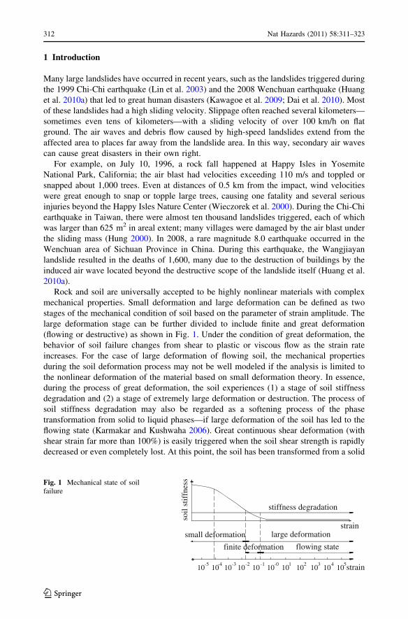
Rock and soil are universally accepted to be highly nonlinear materials with complex

mechanical properties. Small deformation and large deformation can be defined as two

stages of the mechanical condition of soil based on the parameter of strain amplitude. The

large deformation stage can be further divided to include finite and great deformation

(flowing or destructive) as shown in Fig. 1. Under the condition of great deformation, the

behavior of soil failure changes from shear to plastic or viscous flow as the strain rate

increases. For the case of large deformation of flowing soil, the mechanical properties

during the soil deformation process may not be well modeled if the analysis is limited to

the nonlinear deformation of the material based on small deformation theory. In essence,

during the process of great deformation, the soil experiences (1) a stage of soil stiffness

degradation and (2) a stage of extremely large deformation or destruction. The process of

soil stiffness degradation may also be regarded as a softening process of the phase

transformation from solid to liquid phases—if large deformation of the soil has led to the

flowing state (Karmakar and Kushwaha 2006). Great continuous shear deformation (with

shear strain far more than 100%) is easily triggered when the soil shear strength is rapidly

decreased or even completely lost. At this point, the soil has been transformed from a solid

soil

stif

fnes

s

stiffness degradation

small deformation large deformation

finite deformation flowing state

-410 10 10 10 10 10 10 10 10 10 10

-5 -3 -2 -1 -0 1 2 3 4 5

strain

strain

Fig. 1 Mechanical state of soilfailure

312 Nat Hazards (2011) 58:311–323

123

to a fluid. However, it is difficult to calculate or predict the complicated mechanical

behavior of flowing material reasonably through traditional methods of solid mechanics,

let alone explain secondary disasters caused by air blasts resulting from the high-speed

landslides.

Computational fluid dynamics (CFD) is a computer-based applied method that makes

use of theoretical fluid dynamics and mathematical analytical methods; numerical simu-

lation methods acquire numerical or approximate solutions in accordance with a control

equation that describes the flow phenomenon (Kolaczkowski et al. 2007). In the past, CFD

has been used for modeling multiphase flows to compute the flow of gas and solid in

spouted beds, and bubbling and circulating fluidized beds (Peirano et al. 2002; Benyahia

et al. 2005; Lindborg et al. 2007). Recently, several researchers (Zeghal and Shamy 2008;

Karmakar et al. 2007) have identified defects in solid mechanics techniques and have

started to use the CFD method to simulate soil flow properties. For example, Hamada et al.

(1996) found that shear strain rate has a linear relationship with shear strain in solid flow

and the adoption of a fluid model results in a more accurate description of solid flow

properties; Quecedo et al. (2004), based on a Navier–Stokes control equation, adopted the

Taylor-Galekin algorithm to develop 2D numerical simulations of geological disasters such

as landslides and avalanches. These examples support the effectiveness of CFD in the

calculation of geological disasters, but little has been found on the use of CFD methods to

simulate an air blast caused by soil flow.

In view of the above, the limitations of solid mechanics methods for nonlinear and soil

flow analysis have been readily improved. In this study, the entire process of soil flow was

analyzed based upon CFD theory. In the analysis, soil was assumed to be a two-phase fluid.

An Eulerian-Eulerian model for air–soil two-phase flow was introduced, and a standard k-emodel was used to compute the soil flow. The numerical results are compared with the

experimental data to verify the accuracy of the CFD model. The CFD simulations in this

paper capture the fundamental dynamic behavior of soil flow and related air blast, from

which hazard assessments can be implemented, and the performance of structures involved

with disaster prevention can be improved.

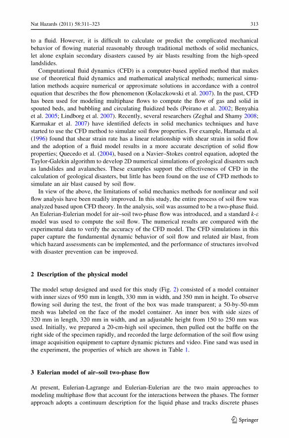
2 Description of the physical model

The model setup designed and used for this study (Fig. 2) consisted of a model container

with inner sizes of 950 mm in length, 330 mm in width, and 350 mm in height. To observe

flowing soil during the test, the front of the box was made transparent; a 50-by-50-mm

mesh was labeled on the face of the model container. An inner box with side sizes of

320 mm in length, 320 mm in width, and an adjustable height from 150 to 250 mm was

used. Initially, we prepared a 20-cm-high soil specimen, then pulled out the baffle on the

right side of the specimen rapidly, and recorded the large deformation of the soil flow using

image acquisition equipment to capture dynamic pictures and video. Fine sand was used in

the experiment, the properties of which are shown in Table 1.

3 Eulerian model of air–soil two-phase flow

At present, Eulerian-Lagrange and Eulerian-Eulerian are the two main approaches to

modeling multiphase flow that account for the interactions between the phases. The former

approach adopts a continuum description for the liquid phase and tracks discrete phases

Nat Hazards (2011) 58:311–323 313

123

using Lagrangian particle trajectory analysis (Zhang and Ahmadi 2005). It hypothesizes

that the discrete phases rate is very low (Kitagawa et al. 2001); therefore, the hypothesis is

not suited to the soil flow issue because of the high rate of discrete phases. The Eulerian-

Eulerian approach treats both phases, including the particulates, as interpenetrating con-

tinua; each phase is described in an Eulerian coordinate system (Cao and Ahmadi 2000;

Buwa et al. 2006). There are three main models for the Eulerian-Eulerian approach. These

are as follows: (1) the volume of fluid (VOF) model, (2) the mixture model, and (3) the

Eulerian model (Chiesa et al. 2005). The Eulerian model differs from other two models in

two respects: (i) It allows the phases to move at different velocities. (ii) There is an

interaction of the interphase mass, momentum, and energy transfer in the Eulerian model.

This paper hypothesizes that soil particles cannot be compressed and also that air dis-

tributes through soil and model box uniformly. The continuity and momentum equations of

each phase are defined as:

(a) First phase:

oqf

otþr � ðqf uf Þ ¼ 0 no phase transformationð Þ ð1Þ

qf ouf

otþ uf � r� �

uf

� �¼ qf g� F þr � 1� ap

� �Tf

� �; and ð2Þ

(b) Second phase:

oqp

otþr � ðqpupÞ ¼ 0 no phase transformationð Þ ð3Þ

qp oup

otþ ðup � rÞup

� �¼ qpgþ F þr � apTp

� �ð4Þ

where

Fig. 2 Model testing equipment

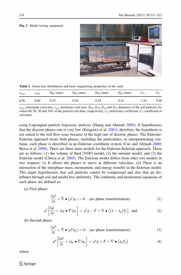
Table 1 Grain-size distribution and basic engineering properties of the sand

emax emin D60 (mm) D50 (mm) D30 (mm) D10 (mm) CU CC

0.96 0.60 0.25 0.24 0.19 0.16 1.56 0.90

emax maximum void ratio, emin minimum void ratio, D60, D50, D30 and D10 diameters of the soil particles forwhich 60, 50, 30 and 10% of the particles are finer, respectively, CU uniformity coefficient, CC coefficient ofcurvature

314 Nat Hazards (2011) 58:311–323

123

qf ¼ qf ð1� apÞ ð5Þ

is the local density of the first phase and

qp ¼ qpap ð6Þ

is the local density of the second phase, F is the interaction force between two phases of

unit volume, Tp is the stress tensor of the first phase, Tf is the stress tensor of the second

phase.

4 Standard k-e model for the Eulerian flow

A standard k-e turbulence model is derived from the instantaneous Navier–Stokes equa-

tions by Jones and Launder (1972). There are two additional transport equations for tur-

bulent parameters: turbulent kinetic energy k and its dissipation rate e. The coefficient of

turbulent viscosity can be calculated by equations k and e, and then the turbulent stress

obtained. This model is useful as the computer hardware requirements are not so

demanding, and the model itself is applicable for a wide range of fluid flow settings.

Extensive work (Nere et al. 2003; Aubin et al. 2004) has utilized the standard k-e model.

The standard k-e turbulence model can get a precise result for the free shear layer when the

pressure gradient is not large. Regarding the wall flow, the result computed by the standard

k-e turbulence model is compared with the experimental result. They inosculate with each

other, when the pressure gradient is zero or close to zero. The fundamental equations of the

standard k-e turbulence model are given below:

qdk

dt¼ o

oxilþ lt

rk

� ok

oxi

� �þ Gk þ Gb � qe� YM ð7Þ

qdedt¼ o

oxilþ lt

re

� oeoxi

� �þ C1s

ekðGk þ C3sGbÞ � C2sq

e2

kð8Þ

where

lt ¼ qClk2

eð9Þ

is the turbulent viscosity, k is turbulent kinetic energy, e is turbulent dissipation rate, q is

density, rk is the Prandtl number of turbulent kinetic energy, re is the Prandtl number of

turbulent kinetic rate, C1e, C2e, C3e, and Cl are empirically defined constants in the stan-

dard k-e model, YM is compressibility effects (activated when ideal fluid is used), Gk is the

turbulent kinetic energy produced by the mean velocity gradient, and Gb is the turbulent

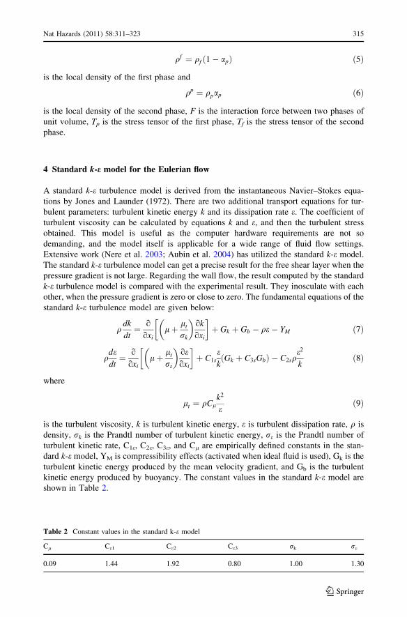
kinetic energy produced by buoyancy. The constant values in the standard k-e model are

shown in Table 2.

Table 2 Constant values in the standard k-e model

Cl Ce1 Ce2 Ce3 rk re

0.09 1.44 1.92 0.80 1.00 1.30

Nat Hazards (2011) 58:311–323 315

123

5 Solution of the numerical models

5.1 Numerical methods

The CFD module of the program FLUENT (version 6.3) was used to model soil flow.

FLUENT is a general finite-volume code that can be used to model a wide range of fluid

flow problems. The control-volume-based technique was used to solve the equations

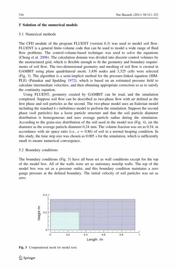
(Cheng et al. 2006). The calculation domain was divided into discrete control volumes by

the unstructured grid, which is flexible enough to fit the geometry and boundary require-

ments of soil flow. The two-dimensional geometry and meshing of soil flow is crested in

GAMBIT using plane quadrilateral mesh; 3,456 nodes and 3,325 cells were selected

(Fig. 3). The algorithm is a semi-implicit method for the pressure-linked equation (SIM-

PLE) (Patankar and Spalding 1972), which is based on an estimated pressure field to

calculate intermediate velocities, and then obtaining appropriate correction so as to satisfy

the continuity equation.

Using FLUENT, geometry created by GAMBIT can be read, and the simulation

completed. Suppose soil flow can be described as two-phase flow with air defined as the

first phase and soil particles as the second. The two-phase model uses an Eulerian model

including the standard k-e turbulence model to perform the simulation. Suppose the second

phase (soil particles) has a loose particle structure and that the soil particle diameter

distribution is homogeneous and uses average particle radius during the simulation.

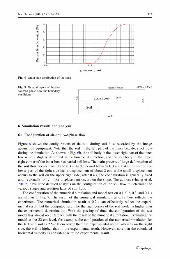
According to the grain-size distribution of the soil used in the model test (Fig. 4), set the

diameter as the average particle diameter 0.24 mm. The volume fraction was set as 0.54, in

accordance with air space ratio (i.e., e = 0.86) of soil in a normal heaping condition. In

this study, the time step size was chosen as 0.005 s for the simulation, which is sufficiently

small to ensure numerical convergence.

5.2 Boundary conditions

The boundary conditions (Fig. 5) have all been set as wall conditions except for the top

of the model box. All of the walls were set as stationary nonslip walls. The top of the

model box was set as a pressure outlet, and this boundary condition maintains a zero

gauge pressure at the defined boundary. The initial velocity of soil particles was set as

zero.

Length /m

Hei

ght /

m

0 0.2 0.4 0.6 0.8 1

0

0.2

0.4

Fig. 3 Computational mesh for model tests

316 Nat Hazards (2011) 58:311–323

123

6 Simulation results and analysis

6.1 Configuration of air–soil two-phase flow

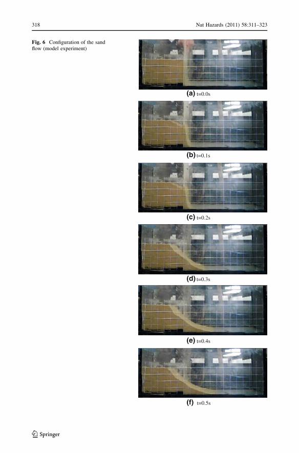
Figure 6 shows the configurations of the soil during soil flow recorded by the image

acquisition equipment. Note that the soil in the left part of the inner box does not flow

during the simulation. As shown in Fig. 6b, the soil body in the lower right part of the inner

box is only slightly deformed in the horizontal direction, and the soil body in the upper

right corner of the inner box has partial soil loss. The main process of large deformation of

the soil flow occurs from 0.2 to 0.3 s. In the period between 0.3 and 0.4 s, the soil on the

lower part of the right side has a displacement of about 2 cm, while small displacement

occurs to the soil on the upper right side; after 0.4 s, the configuration is generally fixed

and, regionally, only minor displacement occurs on the slope. The authors (Huang et al.

2010b) have done detailed analysis on the configuration of the soil flow to determine the

various stages and reaction laws of soil flow.

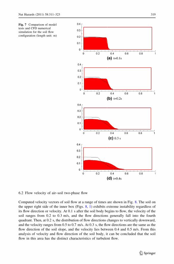
The configuration of the numerical simulation and model test on 0.1, 0.2, 0.3, and 0.4 s

are shown in Fig. 7. The result of the numerical simulation at 0.1 s best reflects the

experiment. The numerical simulation result at 0.2 s can effectively reflect the experi-

mental result, but the computed result for the right corner of the soil model is higher than

the experimental determination. With the passing of time, the configuration of the test

model has almost no difference with the result of the numerical simulation. Evaluating the

model at the 22 cm level, for example, the configuration of the numerical simulation for

the left side soil is 2.5–3.0 cm lower than the experimental result, whereas on the right

side, the soil is higher than in the experimental result. However, note that the calculated

horizontal velocity is consistent with the experimental result.

11.00.010

20

40

60

80

100

Prec

ent f

iner

by

wei

ght (

%)

grain size (mm)

Fig. 4 Grain-size distribution of the sand

Soil

Air

Pressure outlet

Wall

Wall (0.32m,0.20m)

(0.95m,0.35m)

Wall

Fig. 5 General layout of the air–soil two-phase flow and boundaryconditions

Nat Hazards (2011) 58:311–323 317

123

t=0.0s

t=0.1s

t=0.2s

t=0.3s

t=0.4s

t=0.5s

(a)

(b)

(c)

(d)

(e)

(f)

Fig. 6 Configuration of the sandflow (model experiment)

318 Nat Hazards (2011) 58:311–323

123

6.2 Flow velocity of air–soil two-phase flow

Computed velocity vectors of soil flow at a range of times are shown in Fig. 8. The soil on

the upper right side of the inner box (Figs. 8, 1) exhibits extreme instability regardless of

its flow direction or velocity. At 0.1 s after the soil body begins to flow, the velocity of the

soil ranges from 0.2 to 0.3 m/s, and the flow directions generally fall into the fourth

quadrant. Then, at 0.2 s, the distribution of flow directions changes to vertically downward,

and the velocity ranges from 0.5 to 0.7 m/s. At 0.3 s, the flow directions are the same as the

flow direction of the soil slope, and the velocity lies between 0.4 and 0.5 m/s. From this

analysis of velocity and flow direction of the soil body, it can be concluded that the soil

flow in this area has the distinct characteristics of turbulent flow.

Fig. 7 Comparison of modeltests and CFD numericalsimulation for the soil flowconfiguration (length unit: m)

Nat Hazards (2011) 58:311–323 319

123

Fig. 8 Soil flow velocity vectors at selected times

320 Nat Hazards (2011) 58:311–323

123

The flow directions and velocity of the soil on the lower right side of the inner box

(Figs. 8, 2) did not change much during the soil flow. The maximum velocity of the soil of

this area at 0.1, 0.2, and 0.3 s was 0.592, 0.893, and 1.06 m/s, respectively. Also, the

amplification of the velocity during the period from 0.2 to 0.3 s is smaller than over the

period between 0.1 and 0.2 s. Therefore, the velocity of the soil flow is seen to gradually

stabilize.

The flow velocity of the soil body on the left side of the model box is comparatively

small, and the flow directions tend to be stable during the whole process of the soil flow.

This is in accordance with the practical soil flow shown in Fig. 8.

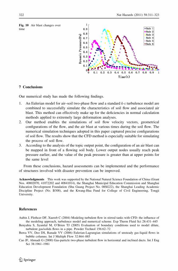
6.3 Air blast pressure of air–soil two-phase flow

Figure 9 shows representative nodes chosen to investigate air blast pressure changes in

front of the soil in the model container. The left bottom is set as the coordinate origin; the

coordinates of each output node are shown in Table 3.

Air blast pressure changes occurring during the process of larger deformation of soil

flow are shown in Fig. 10. During the soil flowing, the place of air in front of the soil is

occupied by the sliding mass very fast, which may cause air to move directly. This in turn

leads to an air pressure difference in the whole model container. Therefore, even at the

very beginning, although the soil flow does not reach the representative nodes, the air

pressure there has increased correspondingly. Both the largest air blast pressure and the

maximum velocity of the rapidly flowing soil occur at the tip of the flowing soil, i.e., the

soil–air interface, and are related to the form of the flowing soil. As seen in Fig. 10, during

the process of soil flow, a peak pressure event occurs at each output node immediately

preceding the node nearest the soil–air interface; the largest (0.899 Pa) results from the

greater velocity and smaller curvature radius at the front-end of the solid when the solid

flow is in this position. Because the tip of the soil body pushes forward as a streamlined

body, the lower output nodes usually reach peak pressure earlier than the upper ones on the

same level.

Soil Node 1

Node 2

Node 3

Node 4

Node 5

Node 6

Air

X

Y

(0.32m,0.20m)

(0.95m,0.35m)

o

Fig. 9 Output nodes for analysisresults

Table 3 Coordinate of output nodes for analysis result

Coordinate Node 1 (cm) Node 2 (cm) Node 3 (cm) Node 4 (cm) Node 5 (cm) Node 6 (cm)

X 47 47 62 62 77 77

Y 7.5 5.0 7.5 5.0 7.5 5.0

Nat Hazards (2011) 58:311–323 321

123

7 Conclusions

Our numerical study has made the following findings.

1. An Eulerian model for air–soil two-phase flow and a standard k-e turbulence model are

combined to successfully simulate the characteristics of soil flow and associated air

blast. This method can effectively make up for the deficiencies in normal calculation

methods applied to extremely large deformation analyses.

2. Our method enables the simulations of soil flow velocity vectors, geometrical

configurations of the flow, and the air blast at various times during the soil flow. The

numerical simulation techniques adopted in this paper captured precise configurations

of soil flow. The results show that the CFD method is especially suitable for simulating

the process of soil flow.

3. According to the analysis of the topic output point, the configuration of an air blast can

be mapped in front of a flowing soil body. Lower output nodes usually reach peak

pressure earlier, and the value of the peak pressure is greater than at upper points for

the same level

From these conclusions, hazard assessments can be implemented and the performance

of structures involved with disaster prevention can be improved.

Acknowledgments This work was supported by the National Natural Science Foundation of China (GrantNos. 40802070, 41072202 and 40841014), the Shanghai Municipal Education Commission and ShanghaiEducation Development Foundation (Shu Guang Project No. 08SG22), the Shanghai Leading AcademicDiscipline Project (No. B308), and the Kwang-Hua Fund for College of Civil Engineering, TongjiUniversity.

References

Aubin J, Flethcer DF, Xuereb C (2004) Modeling turbulent flow in stirred tanks with CFD: the influence ofthe modeling approach, turbulence model and numerical scheme. Exp Therm Fluid Sci 28:431–445

Benyahia S, Syamlal M, O’Brien TJ (2005) Evaluation of boundary conditions used to model dilute,turbulent gas/solids flows in a pipe. Powder Technol 156:62–72

Buwa VV, Deo DS, Ranade VV (2006) Eulerian-Lagrangian simulations of unsteady gas-liquid flows inbubble columns. Int J Multiph Flow 32:864–885

Cao JF, Ahmadi G (2000) Gas-particle two-phase turbulent flow in horizontal and inclined ducts. Int J EngSci 38:1961–1981

Fig. 10 Air blast changes overtime

322 Nat Hazards (2011) 58:311–323

123

Cheng XJ, Chen YC, Luo L (2006) Numerical simulation of air-water two-phase flow over stepped spill-ways. Science in China Series E: Technological Sciences 49(6):674–684

Chiesa M, Mathiesen Vidar, Melheim JA, Halvorsen B (2005) Numerical simulation of particulate flow bythe Eulerian-Lagrangian and the Eulerian-Eulerian approach with application to a fluidized bed.Comput Chem Eng 29:291–304

Dai FC, Xua C, Yao X, Xu L, Tu XB, Gong QM (2010) Spatial distribution of landslides triggered by the2008 Ms 8.0 Wenchuan earthquake, China. J Asian Earth Sci. doi:10.1016/j.jseaes.2010.04.010

Hamada M, Isoyama R, Wakamatsu K (1996) Liquefaction induced ground displacement and its relateddamage to lifeline facilities. Soil Found 36(1):81–97

Huang Y, Chen W, Liu JY (2010a) Secondary geological hazard analysis in Beichuan after the Wenchuanearthquake and recommendations for reconstruction. Environ Earth Sci. doi:10.1007/s12665-010-0612-5

Huang Y, Li GH, Zheng H (2010b) Model tests on sand flow. Chin J Undergr Space Eng 6(1):65–69 (inChinese)

Hung JJ (2000) Chi-Chi earthquake induced landslides in Taiwan. Earthq Eng Eng Seismol 2(2):25–33Karmakar S, Kushwaha RL (2006) Dynamic modeling of soil–tool interaction: an overview from a fluid

flow perspective. J Terramech 43:411–425Karmakar S, Kushwaha RL, Lague C (2007) Numerical modeling of soils tress and pressure distribution on

a flat tillage tool using computational fluid dynamics. Biosyst Eng 97:407–414Kawagoe S, Kazama S, Sarukkalige PR (2009) Assessment of snowmelt triggered landslide hazard and risk

in Japan. Cold Reg Sci Technol 58:120–129Kitagawa A, Murai Y, Yamamoto F (2001) Two-way coupling of Eulerian-Lagrangian model for dispersed

multiphase flows using filtering functions. Int J Multiph Flow 27:2129–2153Kolaczkowski ST, Chao R, Awdry S, Smith A (2007) Application of a CFD code (FLUENT) to formulate

models of catalytic gas phase reactions in porous catalyst pellets. Inst Chem Eng 85(A11):1539–1552Lin CW, Shieh CL, Yuan BD, Shieh YC, Liu SH, Lee SY (2003) Impact of Chi-Chi earthquake on the

occurrence of landslides and debris flows: example from the Chenyulan River watershed, Nantou,Taiwan. Eng Geol 71:49–61

Lindborg H, Lysberg M, Jakobsen HA (2007) Practical validation of the two-fluid model applied to densegas-solid flows in fluidized beds. Chem Eng Sci 62:5854–5869

Nere NK, Patwardhan AW, Joshi JB (2003) Liquid-phase mixing in stirred vessels: turbulent flow regime.Ind Eng Chem Res 42:2661–2698

Patankar SV, Spalding DB (1972) A calculation procedure for heat, mass and momentum transfer in three-dimensional parabolic flows. Heat Mass Transf 15:1787–1806

Peirano E, Delloume V, Johnsson F, Leckner B, Simonin O (2002) Numerical simulation of the fluiddynamics of a freely bubbling fluidized bed: influence of the air supply system. Powder Technol122:69–82

Quecedo M, Pastor M, Herreros MI (2004) Numerical modeling of the propagation of fast landslides usingthe finite element method. Int J Numer Methods Eng 59:755–794

Wieczorek GF, Snyder JB, Waitt RB, Morrissey MM, Uhrhammer RA, Harp EL, Norris RD, Bursik MI,Finewood LG (2000) Unusual July 10, 1996, rock fall at Happy Isles, Yosemite National Park,California. Geol Soc Am Bull 112(1):75–85

Zeghal M, Shamy EIU (2008) Liquefaction of saturated loose and cemented granular soils. Powder Technol184:254–265

Zhang XY, Ahmadi G (2005) Eulerian-Lagrangian simulations of liquid-gas-solid flows in three-phaseslurry reactors. Chem Eng Sci 60:5089–5104

Nat Hazards (2011) 58:311–323 323

123