arX

iv:1

006.

3081

v1 [

gr-q

c] 1

5 Ju

n 20

10

Numerical relativity for D dimensional space-times:

head-on collisions of black holes and gravitational wave extraction

Helvi Witek,1, ∗ Miguel Zilhao,2, † Leonardo Gualtieri,3, ‡ Vitor Cardoso,1,4, §

Carlos Herdeiro,2, ¶ Andrea Nerozzi,1, ∗∗ and Ulrich Sperhake5, 6, 4, ††

1 Centro Multidisciplinar de Astrofısica — CENTRADepartamento de Fısica, Instituto Superior Tecnico — IST

Av. Rovisco Pais 1, 1049-001 Lisboa, Portugal2 Centro de Fısica do Porto — CFPDepartamento de Fısica e Astronomia

Faculdade de Ciencias da Universidade do Porto — FCUPRua do Campo Alegre, 4169-007 Porto, Portugal

3 Dipartimento di Fisica, Universita di Roma “Sapienza” & SezioneINFN Roma1, P.A. Moro 5, 00185, Roma, Italy

4 Department of Physics and Astronomy, The University of MississippiUniversity, MS 38677-1848, USA

5 Institut de Ciencies de l’Espai (CSIC-IEEC)Facultat de Ciencies, Campus UAB

Torre C5 parells, E-08193 Bellaterra, Spain6 California Institute of Technology

Pasadena, CA 91125, USA(Dated: June 2010)

Black objects in higher dimensional space-times have a remarkably richer structure than theirfour dimensional counterparts. They appear in a variety of configurations (e.g. black holes, blackbranes, black rings, black Saturns), and display complex stability phase diagrams. They might alsoplay a key role in high energy physics: for energies above the fundamental Planck scale, gravity isthe dominant interaction which, together with the hoop-conjecture, implies that the trans-Planckianscattering of point particles should be well described by black hole scattering. Higher dimensionalscenarios with a fundamental Planck scale of the order of TeV predict, therefore, black hole pro-duction at the LHC, as well as in future colliders with yet higher energies. In this setting, accuratepredictions for the production cross-section and energy loss (through gravitational radiation) inthe formation of black holes in parton-parton collisions is crucial for accurate phenomenologicalmodelling in Monte Carlo event generators.

In this paper, we use the formalism and numerical code reported in [1] to study the head-oncollision of two black holes. For this purpose we provide a detailed treatment of gravitational waveextraction in generic D dimensional space-times, which uses the Kodama-Ishibashi formalism. Forthe first time, we present the results of numerical simulations of the head-on collision in five space-time dimensions, together with the relevant physical quantities. We show that the total radiatedenergy, when two black holes collide from rest at infinity, is approximately (0.089 ± 0.006)% of thecentre of mass energy, slightly larger than the 0.055% obtained in the four dimensional case, andthat the ringdown signal at late time is in very good agreement with perturbative calculations.

PACS numbers: 04.25.D-, 04.25.dg, 04.50.-h, 04.50.Gh

∗Electronic address: helvi.witek@ist.utl.pt†Electronic address: mzilhao@fc.up.pt‡Electronic address: leonardo.gualtieri@roma1.infn.it§Electronic address: vitor.cardoso@ist.utl.pt¶Electronic address: crherdei@fc.up.pt∗∗Electronic address: andrea.nerozzi@ist.utl.pt††Electronic address: sperhake@tapir.caltech.edu

2

Contents

1. Introduction 2

2. Gravitational wave extraction in D dimensional axially symmetric space-times 42.1. Coordinate frames 42.2. Harmonic expansion 72.3. Implementation of axisymmetry 82.4. Extracting gravitational waves at infinity 10

3. Head-on collision from rest in D = 4 113.1. Tests on the numerical coordinates 123.2. Waveforms 133.3. Radiated energy 14

4. Head-on collision from rest in D = 5 154.1. Tests on the numerical coordinates 164.2. Newtonian collision time 174.3. Waveforms 174.4. Radiated energy 20

5. Discussion 22

Acknowledgments 23

A. Coordinate transformation 24

B. Harmonic expansion of axisymmetric tensors in D dimensions 25

References 28

1. INTRODUCTION

High energy physics scenarios, such as the gauge-gravity duality [2] or TeV gravity models[3–7], suggest that dynamical processes involving higher dimensional black holes (BHs) may berelevant for understanding the physics under experimental scrutiny at particle colliders, such asthe Large Hadron Collider (LHC) or the Relativistic Heavy Ion Collider (RHIC). These processescan be quite violent and highly non-linear, as in the case of BH collisions. Numerical relativity,which solves Einstein’s equations on supercomputers, is therefore the only available tool for high-precision studies of such BH systems. Fortunately, the field of numerical relativity has maturedconsiderably over the last five years (see Refs. [8, 9] for reviews), and its techniques can nowbe extended to a much wider class of space-times. Space-times of generic dimensionality orwith more general asymptotics, feature most prominently among such generalizations. Recentapplications to the study of higher dimensional BH instabilities may be found in Refs. [10, 11],using the formalism developed in Ref. [12]; an application to the study of AdS-like asymptoticsmay be found in Ref. [13]. Further applications of numerical relativity to more general types ofspace-times have been discussed in Ref. [1], hereafter denoted as Paper I, wherein we have starteda long-term effort to evolve BH space-times in higher dimensions numerically, and developed aframework to perform numerical simulations of D dimensional space-times with an SO(D − 2)isometry group (for D ≥ 5) or SO(D − 3) (for D ≥ 6).

3

One scenario in which BH collisions play a very well defined role is that of TeV-scale gravity,i.e. scenarios in which the fundamental Planck scale is of the order of the TeV. The beginningof the scientific runs at the Large Hadron Collider makes accurate theoretical modelling of theexperimental signatures of this scenario for LHC collisions very timely. In this scenario, forcentre of mass energies well above the TeV threshold (recall that LHC collisions will reach 14TeV), parton-parton collision will be dominated by the gravitational interaction, and should bewell described by any classical gravitational objects with the same gravitational energy. Formodelling simplicity, it is convenient to choose these objects to be BHs [14–26]. Due to thedominance of the gravitational interaction, we may further neglect the electric charge of theholes; charge dependant effects should give sub-leading corrections to the relevant observables.For sufficiently small impact parameters, these trans-Planckian collisions are expected to form aBH [15, 16], as follows from Thorne’s hoop conjecture [27] which recently has received supportfrom the numerical work of Choptuik and Pretorius [28]. Therefore, there is substantial evidencethat modelling the individual partons as BHs is not biasing the final result of the parton scatteringprocess towards BH formation. Indeed, this is the idea that, above the fundamental Planck scale,matter does not matter ; it only matters the gravitational energy that each parton carries.After formation, the BH should then decay via Hawking evaporation. In order to filter ex-

perimental data, this process has been modelled by dedicated Monte Carlo event generators,such as Truenoir, Catfish, Charybdis2 or Blackmax [16, 29–32]. The latter two are beingused by the ATLAS experiment at the LHC. These generators clearly exhibit the very distinctexperimental signatures of BH evaporation, including higher multiplicity of jets and larger trans-verse momentum than those produced by any standard model process [33]. The event generatorsalso model the BH production phase from the parton-parton scattering, for which they needas an input the threshold impact parameter for BH formation and the energy lost in gravi-tational radiation during the parton-parton collision. At the moment, the best estimates forthese quantities are based on trapped surface methods [34]. Accurate results can, however, beobtained from full-blown numerical simulations, as has already been seen in four dimensions[35–37]. Such results will be instrumental in a more accurate phenomenological modelling of BHproduction/evaporation in particle colliders. Observe that, even if no evidence for BH forma-tion/evaporation is found at the LHC, such accurate modelling will matter for setting preciselower bounds on the fundamental Planck scale.In this paper we present the first fully non-linear treatment of a head-on collision of BHs in

a higher dimensional space-time, together with an analysis of the relevant physical quantities.This is achieved by solving the corresponding Einstein equations numerically, for which we usethe formalism and code reported in Paper I. Once given the numerically constructed space-time,one is still left with the question of extracting physically meaningful (and in particular gaugeinvariant) quantities, such as the energy and linear and angular momentum carried away by thegravitational radiation.In four space-time dimensions, two distinct formalisms have been developed to extract the

physical information (see e.g. Ref. [38] for a review of both formalisms). One is based on theRegge-Wheeler-Zerilli perturbation theory for the Schwarzschild BH [39, 40]; the other is basedon the Newman-Penrose formalism [41], which was used by Teukolsky to study perturbations ofalgebraically special space-times [42], a class which includes the Kerr BH. A higher dimensionalgeneralization of the Newman-Penrose formalism has been developed in Refs. [43–46]. Unfor-tunately, the condition of being algebraically special does not seem to be as powerful for thestudy of exact solutions or their perturbations in higher dimensions as it was in four dimensions.For instance, the Goldberg-Sachs theorem is not valid any longer in higher dimensions [45, 46].For the study we present herein, however, it suffices to use the higher dimensional generalisa-tion of the Regge-Wheeler-Zerilli formalism, because the final result of a head-on collision oftwo D dimensional, non-spinning BHs approaches, at late times, a D dimensional Schwarzschild(i.e. Tangherlini [47]) BH. Fortunately, the perturbation theory of the latter BH has been fully

4

developed, in arbitrary dimensions, by Kodama and Ishibashi [48]. Our remaining task is to ob-tain the relevant gauge-invariant quantities from our numerical data, a procedure that we shalldescribe in detail in this paper.After implementing this wave-extraction formalism we apply it to study the head-on collision

of two BHs in four and five dimensional space-times. In four dimensions (D = 4) we recoverprevious results in the literature, and we perform a number of tests on the (numerical) coordinatesystem, to ensure it is appropriate for the wave extraction formalism. We estimate that around0.055% of the centre of mass energy is radiated when two BHs, at rest at infinity, collide. Thisresult is in good agreement with those reported in the literature [49]. The five dimensional resultsare entirely new. We show that the kinematics of the BHs before the merging follow, to a goodprecision, the Newtonian prediction. We estimate that around 0.089% of the centre of massenergy is radiated as gravitational waves, when two BHs collide from rest at infinity, and presentthe associated waveforms. We stress that these results refer to a fully non-linear evolution ofEinstein’s field equations.This paper is organized as follows. In Section 2 we apply the Kodama-Ishibashi (KI) formal-

ism to the space-times considered in Paper I. By assuming that the numerical space-time is asmall deviation from the Tangherlini solution, one is able to relate (see relations (2.3)) the nu-merical metric to the KI metric perturbations and to compute gauge-invariant quantities usingEqs. (2.28), (2.29). These are then used to construct a master function Φ (see Eq. (2.54)) fromwhich all relevant information about the radiation can be computed. In Sections 3, 4 we presentresults obtained from the evolution of Brill-Lindquist initial data in D = 4, 5 respectively, thatrepresents the collision of two equal-mass, non-spinning BHs which are initially at rest. In or-der to calibrate the accuracy of the wave extraction formalism, we perform a number of tests,including tests on the numerical coordinates themselves. We compute the time derivative of themaster function Φ, energy fluxes and total energy radiated. We give some final remarks in Sec. 5and discuss future steps in this research program. Two appendices cover technical details on thecoordinate transformation between the numerical and wave extraction frames (Appendix A) andon the D dimensional harmonic expansion of axisymmetric tensors (Appendix B).

2. GRAVITATIONAL WAVE EXTRACTION IN D DIMENSIONAL AXIALLY

SYMMETRIC SPACE-TIMES

2.1. Coordinate frames

In the approach developed in Paper I, we perform a dimensional reduction by isometry onthe (D − 4)-sphere SD−4, in such a way that the D dimensional vacuum Einstein equationsare rewritten as an effective 3 + 1 dimensional time evolution problem with source terms thatinvolve a scalar field. The evolution equations are expressed in the Baumgarte-Shapiro-Shibata-Nakamura (BSSN) formulation [50, 51], and numerically implemented using a modification ofthe Lean code [49].In Paper I we considered different generalizations of “axial symmetries” to higher dimensions:

either D ≥ 5 dimensional space-times with SO(D − 2) isometry group, or D ≥ 6 dimensionalspace-times with SO(D − 3) isometry group. In this work we only study the former case, whichallows us to model head-on collisions of non-spinning BHs; we dub hereafter these space-times asaxially symmetric. Although the corresponding symmetry manifold is the (D− 3)-sphere SD−3,the quotient manifold in our dimensional reduction is its submanifold SD−4. The coordinateframe in which the numerical simulations are performed is

(xµ, φ1, . . . , φD−4) = (t, x, y, z, φ1, . . . , φD−4) , (2.1)

5

where the angles φ1, . . . , φD−4 describe the quotient manifold SD−4 and do not appear explicitlyin the simulations. Here, z is the symmetry axis, i.e. the collision line.In the frame (2.1), the space-time metric has the form (cf. Eqs. (2.14) and (2.21) of Paper I)

ds2 = gµν(xα)dxµdxν+λ(xµ)dΩD−4 = −α2dt2+γij(dx

i+βidt)(dxj+βjdt)+λ(xµ)dΩD−4 , (2.2)

where xµ = (t, xi), λ(xµ) is a scalar field and α, βi are the lapse function and the shift vector,respectively. It is worth noting that, although in D = 4 a general axially symmetric space-timehas non-vanishing mixed components of the metric (like gtφ), in D ≥ 5 such components vanishin an appropriate coordinate frame, as we have shown in Paper I.With an appropriate transformation of the four dimensional coordinates xµ, the residual

symmetry left after the dimensional reduction on SD−4 can be made manifest: xµ → (xµ, θ)(µ = 0, 1, 2),

gµν(xα)dxµdxν = gµν(x

α)dxµdxν + gθθ(xα)dθ2 (2.3)

and

λ(xµ) = sin2 θgθθ(xα) , (2.4)

so that Eq. (2.2) takes the form ds2 = gµνdxµdxν + gθθdΩD−3, as discussed in Paper I.

To extract the gravitational waves far away from the symmetry axis we employ the KI for-malism [48], which generalizes the Regge-Wheeler-Zerilli [39, 40] approach to higher dimensions.We require that the space-time, far away from the BHs, is approximately spherically symmetric.Note, that spherical symmetry in D dimensions means symmetry with respect to rotations onSD−2; this is an approximate symmetry which holds asymptotically far away from the axis andwhich is manifest in the coordinate frame:

(xa, θ, θ, φ1, . . . , φD−4) = (t, r, θ, θ, φ1, . . . , φD−4) . (2.5)

Note that xa = t, r and that we have introduced polar-like coordinates θ, θ ∈ [0, π] to “build up”the manifold SD−2 in the background, together with a radial spherical coordinate r, which is theareal coordinate in the background.The coordinate frame (2.5) is defined in such a way that the metric can be expressed as a

stationary background (ds(0))2 (i.e., the Tangherlini metric) plus a perturbation (ds(1))2 whichdecays faster than 1/rD−3 for large r:

(ds(0))2 = g(0)ab dx

adxb + r2dΩD−2 = g(0)tt dt

2 + g(0)rr dr2 + r2dΩD−2

= g(0)tt dt

2 + g(0)rr dr2 + r2

(

dθ2 + sin2 θdΩD−3

)

= −(

1− rD−3S

rD−3

)

dt2 +

(

1− rD−3S

rD−3

)−1

dr2 + r2[

dθ2 + sin2 θ(

dθ2 + sin2 θdΩD−4

)]

,

(2.6)

(ds(1))2 = habdxadxb + haθdx

adθ + hθθdθ2 + hθθdΩD−3 . (2.7)

Here, the Schwarzschild radius rS replaces the parameter µ used in Paper I and is related to theADM mass M by

rD−3S =

16πM

(D − 2)AD−2, (2.8)

where AD−2 is the area of the (D − 2)-sphere (see Eq. (B20)). For instance, rS = 2M in D = 4

and rS =√

8M/(3π) in D = 5.

6

When we define the coordinate frame (2.5), we also require that the coordinate θ in this framecoincides with the coordinate θ appearing in Eq. (2.3). With this choice, the axial symmetry ofthe space-time implies that

haθ = hθθ = 0 , (2.9)

as in Eq. (2.7), and λ = sin2 θgθθ, i.e. Eq. (2.4).The transformation from the coordinates xµ = (t, x, y, z) in which the numerical simulation is

implemented to the coordinates (xa, θ, θ) = (t, r, θ, θ) in which the wave extraction is performedis given by

x = R sin θ cos θ , (2.10)

y = R sin θ sin θ , (2.11)

z = R cos θ , (2.12)

where R =√

x2 + y2 + z2 and by the reparametrization of the radial coordinate

R = R(r) . (2.13)

We note that Eqs. (2.1), (2.13) correctly transform the three-metric γij describing the initialdata

γijdxidxj = ψ

4

D−3 (dR2 +R2(dθ2 + sin2 θdθ2)) , (2.14)

where, as discussed in Paper I, we choose Brill-Lindquist initial data,

ψ = 1 +rD−3S,1

4rD−31

+rD−3S,2

4rD−32

, (2.15)

in order to simulate a head-on collision of BHs starting from rest. Here, rS,i and ri denote theSchwarzschild radius and the initial position of the i-th BH, respectively. Far away from theaxis the conformal factor is given by ψ → 1 + perturbations. Therefore, the splitting of themetric into a Tangherlini background plus an (axisymmetric) perturbation, Eqs. (2.6)-(2.7), canbe recovered on the initial time-slice, if we define the reparametrization (2.13) appropriately.Our (reasonable) guess is that the transformation (2.1), (2.13) yields the “Tangher-

lini+perturbation” splitting (2.6), (2.7) during the entire evolution of the system. This statementcan be checked numerically by verifying the following relations (see Appendix B):

Gtt ≡1

K0Dπ

∫ π

0

dθ sinD−3 θ

∫ π

0

dθgtt(θ, θ)− g(0)tt = 0 , (2.16)

Gtr ≡ 1

K0Dπ

∫ π

0

dθ sinD−3 θ

∫ π

0

dθgtR(θ, θ) = 0 , (2.17)

Grr ≡ 1

K0Dπ

∫ π

0

dθ sinD−3 θ

∫ π

0

dθgRR(θ, θ)− g(0)rr = 0 , (2.18)

where K0D =∫ π

0dθ(sin θ)D−3, together with the axisymmetry conditions (2.4), (2.9). As we

will discuss in Section 3, Eqs. (2.4), (2.9), (2.16)–(2.18) are indeed satisfied with high accuracythroughout the numerical evolution. The preservation of the above identities during the numer-ical evolution justifies also the identification of the time coordinate in the numerical and waveextraction frames, and our use of the KI formalism.

7

Finally, Eqs. (2.2), (2.6), (2.7) yield the 3 + 1 splitting

ds2 = (ds(0))2 + (ds(1))2 = gµνdxµdxν + (r2 sin2 θ + hθθ)dΩD−3

= gµνdxµdxν + (r2 sin2 θ + hθθ)(dθ

2 + sin2 θdΩD−4)

= −α2dt2 + γij(dxi + βidt)(dxj + βjdt) + λdΩD−4 , (2.19)

where xµ = (t, r, θ). With the 3 + 1 splitting, the axisymmetry conditions (2.4), (2.9) take theform

λ = γθθ sin2 θ , γRθ = γθθ = βθ = 0 . (2.20)

The variable r can be determined from the angular components of the metric (2.19), by averagingout hθθ, hθθ (see Appendix B); its explicit expression is given by

(r(R))2 =1

(D − 2)K0D

∫ π

0

dθ[

γθθ(sin θ)D−3 + (D − 3)γθθ(sin θ)

D−5]

. (2.21)

As we will discuss in Section 3, we find that the areal radius r is very close to R.

2.2. Harmonic expansion

In the KI formalism [48] (see also [52]), the background space-time has the form (2.6)

(ds(0))2 = g(0)ABdx

AdxB = g(0)ab dx

adxb + r2dΩD−2 = g(0)ab dx

adxb + r2γijdφidφj , (2.22)

i.e. the Tangherlini metric, where the xA coordinates refer to the full space-time. The space-timeperturbations can be decomposed into spherical harmonics on the (D − 2)-sphere SD−2. They

are functions of the D−2 angles φi = (θ, θ, φ1, . . . , φD−4). We denote the metric of SD−2 by γij ,and with a subscript :i the covariant derivative with respect to this metric. Finally, we denote

the covariant derivative with respect to the metric g(0)ab with a subscript |a.

As discussed in [48], there are three types of spherical harmonics:

• The scalar harmonics S(φi), which are solutions of

2S = γ ijS:ij = −k2S , (2.23)

with k2 = l(l +D − 3), l = 0, 1, 2, . . . . The scalar harmonics S depend on the integer land on other indices; we leave such dependence implicit. We also define

Si = − 1

kS,i , Sij =

1

k2S:ij +

1

D − 2γijS . (2.24)

Observe that γ ijSij = 0.

Each harmonic mode of the metric perturbation δgMN = hMN can be decomposed as

δgab = hab = fabS , (2.25)

δgai = hai = rfaSi , (2.26)

δgij = hij = 2r2(HLγijS +HTSij) , (2.27)

(note that in each of these expressions there is a sum over the indices of the harmonic),where fab, fa, HL, HT are functions of xa = (t, r).

8

For l > 1, the metric perturbations can be expressed in terms of the following gauge-invariant variables [52]

F = HL +1

D − 2HT +

1

rXar

|a ,

Fab = fab +Xa|b +Xb|a , (2.28)

where we have defined

Xa =r

k

(

fa +r

kHT |a

)

. (2.29)

• The vector harmonics Vi(φi), solutions of

γ ijVk:ij = −k2V Vk , (2.30)

with k2V = l(l +D − 3)− 1, l = 1, 2, . . . . These harmonics satisfy the relation

V i:i = 0 . (2.31)

The harmonic expansion of the corresponding metric perturbations is given by Eqs. (2.26)-(2.27), with Si replaced by Vi, Sij replaced by

Vij = − 1

2kV(Vi:j + Vj :i) , (2.32)

and HL = 0.

• The tensor harmonics Tij(φi), solutions of

γ ijTrs:ij = −k2TTrs , (2.33)

with k2T = l(l +D − 3)− 2, l = 1, 2, . . . . These harmonics satisfy,

γ ijTij = 0 , T :ij:j

= 0 . (2.34)

In the D = 4 case, they vanish. The harmonic expansion of the corresponding metricperturbations is given by (2.27), with Sij replaced by Tij and HL = 0.

2.3. Implementation of axisymmetry

In an axially symmetric space-time, the metric perturbations are symmetric with respect toSD−3. Therefore, the harmonics in the expansion of hMN depend only on the angle θ (whichdoes not belong to SD−3). Furthermore, since there are no off-diagonal terms in the metric (cf.Paper I), the only non-vanishing gai components are gaθ; the only components gij are eitherproportional to γij , or all vanishing but gθθ. This implies that only scalar spherical harmonicscan appear in the expansion of the metric perturbations. Indeed, if

V i = (V θ, 0, . . . , 0) , V i = V i(θ) , (2.35)

then Eq. (2.31) gives

V i:i = V θ

,θ = 0 ⇒ V θ = 0 ⇒ V i = 0 . (2.36)

9

Similarly, from Eq. (2.34) we obtain Tij = 0.

The scalar harmonics, solutions of Eq. (2.23) and which depend only on the coordinate θ, are

given by the Gegenbauer polynomials C(D−3)/2l , as discussed in Refs. [53–55]; writing explicitly

the index l, they take the form

Sl(θ) = (K lD)−1/2C(D−3)/2l (cos θ) , (2.37)

where the normalization K lD is chosen such that∫

dΩD−2SlSl′ = δll′ ,

∫

dΩD−2Sl ,θSl′ ,θ = δll′k2 , (2.38)

and k2 = l(l + D − 3) (see Appendix B). By computing Sl i, Sl ij from Eqs. (2.24) (usingEq. (2.23)) we find

Sl θθ =D − 3

k2(D − 2)Wl , (2.39)

Sl θθ = − sin2 θ

k2(D − 2)Wl , (2.40)

where we have defined

Wl(θ) = Sl ,θθ − cot θSl ,θ . (2.41)

Therefore, the metric perturbations are given by

hab = f labSl(θ) , (2.42)

haθ = rf laSl(θ)θ = − 1

krf l

aSl(θ),θ , (2.43)

hθθ = 2r2(H lLSl(θ) +H l

TSl(θ)θθ) = 2r2(

H lLSl(θ) +H l

T

D − 3

k2(D − 2)Wl(θ)

)

, (2.44)

hθθ = 2r2(H lL sin2 θSl(θ) +H l

TSl(θ)θθ) = 2r2 sin2 θ

(

H lLSl(θ)−H l

T

1

k2(D − 2)Wl(θ)

)

. (2.45)

The quantities fab, fa, HL, HT are (see Appendix B):

f lab(t, r) =

AD−3√K lD

∫ π

0

dθ(sin θ)D−3habC(D−3)/2l , (2.46)

fa(t, r) = − 1√

l(l +D − 3)r

AD−3√K lD

∫ π

0

dθ(sin θ)D−3haθC(D−3)/2

l ,θ(cos θ) , (2.47)

HL(t, r) =1

2(D − 2)r2AD−3√K lD

∫ π

0

dθ(sin θ)D−3

[

hθθ +D − 3

sin2 θhθθ

]

C(D−3)/2l (cos θ) , (2.48)

HT (t, r) =1

2r2(k2 −D + 2)

AD−3√K lD

∫ π

0

dθ(sin θ)D−3

[

hθθ −1

sin2 θhθθ

]

Wl(θ) , (2.49)

where hab = hab(t, r, θ), haθ = haθ(t, r, θ), hθθ = hθθ(t, r, θ), hθθ = hθθ(t, r, θ) and C(D−3)/2l =

C(D−3)/2l (cos θ).In terms of these quantities, using Eqs. (2.28), (2.29), we get the gauge-invariant quantities F ,

Fab.

10

As we have discussed above, this approach has been developed for D > 4, since in D = 4 theoff-diagonal terms gtφ, grφ are not vanishing in general axially symmetric space-times. However,we can extend our framework to D = 4 if we restrict ourselves to axially symmetric space-timeswith gtφ = grφ = 0. In this way, we can test our formalism by comparing our results to theexisting literature. For instance, we note that in D = 4 the perturbation functions are relatedto the expressions in Ref. [56], with the identifications

f lab = H0, H1, H2 , (2.50)

− r

kf la = h0, h1 , (2.51)

2HT

k2= G , (2.52)

2HL +HT = K . (2.53)

We also remark that in the transverse-traceless gauge, only HT is non-vanishing, but in a genericgauge (like the one used in the numerical simulations) all these quantities are in principle non-vanishing.

2.4. Extracting gravitational waves at infinity

In the KI framework, the emitted gravitational waves are described by the master function Φ.To compute Φ in terms of the gauge-invariant quantities F , Fab one should perform a Fouriertransform or a time integration (see [48]). This can be avoided if we compute directly Φ,t, givenby1

Φ,t = (D − 2)r(D−4)/2 −F rt + 2rF,t

k2 −D + 2 + (D−2)(D−1)2

rD−3

S

rD−3

, (2.54)

where k2 = l(l +D − 3). In the TT-gauge, the gravitational perturbation is described by HT ,which decays as r(D−2)/2 with increasing r, whereas the other perturbation functions have afaster decay (see [53]). In this gauge, the asymptotic behaviour of the master function is

Φ ≃ 2r(D−2)/2HT

k2, (2.55)

and tends to an oscillating function with constant amplitude as r → ∞. The asymptotic be-haviour of Φ has been checked numerically (cf. Section 3).Writing the index l explicitly, the energy flux in each l−multipole is [53]

dEl

dt=

1

32π

D − 3

D − 2k2(k2 −D + 2)(Φl

,t)2 . (2.56)

The total energy emitted in the process is then

E =

∞∑

l=2

∫ +∞

−∞

dtdEl

dt. (2.57)

1 Note that there is a factor r missing in Eq. (3.15) of Ref. [48].

11

Run D Grid Setup d/rS L/rS

HD4c 4 (128, 64, 32, 16, 8) × (1, 0.5, 0.25), h = rS/80 5.257 7.154

HD4m 4 (128, 64, 32, 16, 8) × (1, 0.5, 0.25), h = rS/88 5.257 7.154

HD4f 4 (128, 64, 32, 16, 8) × (1, 0.5, 0.25), h = rS/96 5.257 7.154

HD5a 5 (256, 128, 64, 32, 16, 8, 4) × (0.5, 0.25), h = rS/84 1.57 1.42

HD5b 5 (256, 128, 64, 32, 16, 8, 4) × (0.5, 0.25), h = rS/84 1.99 1.87

HD5c 5 (256, 128, 64, 32, 16, 8, 4)× (1, 0.5), h = rS/84 2.51 2.41

HD5d 5 (256, 128, 64, 32, 16, 8, 4)× (1, 0.5), h = rS/84 3.17 3.09

HD5ec 5 (256, 128, 64, 32, 16, 8)× (2, 1, 0.5), h = rS/60 6.37 6.33

HD5em 5 (256, 128, 64, 32, 16, 8)× (2, 1, 0.5), h = rS/72 6.37 6.33

HD5ef 5 (256, 128, 64, 32, 16, 8)× (2, 1, 0.5), h = rS/84 6.37 6.33

HD5f 5 (256, 128, 64, 32, 16, 8)× (2, 1, 0.5), h = rS/84 10.37 10.35

TABLE I: Grid structure and initial parameters of the head-on collisions starting from rest in D = 4and D = 5. The grid setup is given in terms of the “radii” of the individual refinement levels, in unitsof rS, as well as the resolution near the punctures h (see Sec. II E in [49] for details). d is the initialcoordinate separation of the two punctures and L denotes the proper initial separation.

3. HEAD-ON COLLISION FROM REST IN D = 4

The numerical simulations of head-on collisions of equal-mass binaries starting from rest havebeen performed with the Lean code originally introduced in Ref. [49], modified along Sec. III ofRef. [57] and adapted to higher dimensional space-times in Paper I. The Lean code is based onthe Cactus computational toolkit [58] and uses the Carpet mesh refinement package [59, 60], theapparent horizon finder AHFinderDirect [61, 62] and the puncture initial data solver of Ref. [63].Head-on collisions in four dimensional space-times have been studied extensively in the literatureand provide valuable opportunities to calibrate the wave extraction formalism. These tests arethe subject of the remainder of this Section, while we discuss our new results for five dimensionalspace-times in Sec. 4 below.In order to test our implementation of the KI formalism in D = 4, we have simulated head-on

collision of an equal-mass, non spinning BH binary initially at rest. The parameters used inthis simulation are shown in Table I. This particular system is well understood and enables usto compare our results derived from the KI formalism against those obtained using both, theRegge-Wheeler-Zerilli wave extraction and the Newman-Penrose framework; cf. [56] and [49] forcorresponding literature studies.In order to perform these tests, we need to relate our master function Φ of Sec. 2.4 to the

variables used in traditional four dimensional studies. Specifically, a straightforward calculationshows that the Zerilli wavefunction Φ adopted in Ref. [56] for l = 2 multipoles and the outgoingWeyl scalar Ψ4 used in [49] can be expressed in terms of Φ according to

Φ = 6Φ , (3.1)

rΨ4 =√6Φ,tt . (3.2)

Note that the imaginary part of Ψ4 vanishes in the case of a head on collision, due to symmetry.The resolution is h = rS/96 for all results reported in this section except for the convergence

study in Sec. 3.3 which also uses the lower resolutions hc = rS/80 and hm = rS/88.2 Gravita-

2 In order to ensure that our fundamental unit is of physical dimension length for all values of space-time dimension

12

-50 -25 0 25 50 75 100t / rS

-0.2

-0.15

-0.1

-0.05

0

0.05

0.1

Rex

/rS G

tt

Rex = 30 rSRex = 40 rSRex = 50 rS

50 75 100-0.02

-0.01

0

∆0 50 100 150

t / rS

1.008

1.01

1.012

1.014

1.016

1.018

1.02

r (R

ex)

/ Rex

Rex = 30 rSRex = 40 rSRex = 50 rS

FIG. 1: (Color online) Left panel: Gtt calculated from Eq. (2.16) for D = 4, at different extraction radii.This quantity has been shifted in time to account for the different extraction radii and re-scaled by thecorresponding Rex. The late time behavior is shown in the inset. Right panel: time evolution of arealradius (cf. (2.21)) extracted at the radii Rex = 30rS (black solid line), Rex = 40rS (red dashed line) andRex = 50rS (green dashed-dotted line).

tional waves have been extracted at three different coordinate radii R (cf. Eq. 2.13), which wedenote by Rex = 30 rS , 40 rS , 50 rS.

3.1. Tests on the numerical coordinates

The procedure described in Section 2 assumes that the numerical space-time consists of a smalldeviation from the Schwarzschild-Tangherlini metric. In order to ensure that the gravitationalwaves are extracted in an appropriate coordinate system we perform a number of checks. Wefirst test the relations (2.16), (2.17) and (2.18). In Fig. 1 we show Gtt, i.e., the difference betweenthe numerical gtt, averaged over the extraction sphere and the corresponding component of theassumed background metric. Here we evaluate the background metric by assuming, as a firstapproximation, that the Schwarzschild radius of the BH is rS = rS,1 + rS,2.The deviation of the full 4-metric from the Schwarzschild-Tangherlini background decreases as

the extraction radius increases. Indeed, a straightforward calculation shows that a deviation δrSof the Schwarzschild radius from the background value leads to Gtt ∼ δrD−3

S /rD−3, i. e. δrS/rfor D = 4. In the left panel of Fig. 1 we therefore show the deviation Gtt re-scaled by r. Wefurther apply a time shift to account for the different propagation time of the wave to reach theextraction radii. As shown in the figure, the deviation from the Schwarzschild line element is

small and decreases ∼ 1/r in accordance with our expectation. We also note that a deviationδrS represents a monopole perturbation of the background which decouples from the quadrupolewave signal at perturbative order, so that its impact on our results is further reduced.In summary, we can give an uncertainty estimate for the approximation rS = rS,1 + rS,2 for

the Schwarzschild radius of the final BH, which ignores the energy loss through gravitational

D, we believe it convenient to express our results in units of the radius rS (given by rD−3S

≡ rD−3S,1

+ rD−3S,2

) of

the “total” event horizon as opposed to the total BH mass M commonly used in four dimensional numericalrelativity. In D = 4, of course, rS = 2M .

13

0 25 50 75 100 125 150t / rS

-0.15

-0.1

-0.05

0

0.05

0.1

6 Φ,Φ, t

t

0 25 50 75 100 125 150t / rS

-0.03

-0.02

-0.01

0

0.01

0.02

0.03

61/2 Φ, Ψ4r rS

ttrS

FIG. 2: (Color online) Left panel: Time derivatives of the l = 2 modes of the KI function Φ (blacksolid line), and of the Zerilli function Φ (red dashed line) extracted for model HD4f at Rex = 30rS .The KI function has been re-scaled by a constant factor (cf. (3.1)) which accounts for the differentnormalizations of both formulations. Right panel: comparison of the second time derivative Φ,tt withthe outgoing Newman-Penrose scalar Ψ4 for the same model. The KI wavefunction has been re-scaledaccording to Eq. (3.2).

radiation. As demonstrated by the left panel of Fig. 1, at late times |Rex/rS Gtt| ∼ 0.01, and,since r ≃ Rex (as we discuss below), we obtain the upper bound

δrSrS

.r

rSGtt ∼ 0.01 . (3.3)

This crude analysis sets an upper bound of ∼ 1% on the fraction of the centre of mass energyradiated as gravitational waves. We further note that the close agreement between gtt and itsTangherlini counterpart implies that the time coordinate employed in the numerical simulationand the Tangherlini coordinate time coincide. By analysing Gtr and Grr in the same manner, wefind that relations (2.16)-(2.18) are satisfied with an accuracy of one part in 102 throughout theevolution, and one part in 103 at late times, when the space-time consists of a single distortedblack hole.In practice, gravitational waves are extracted on spherical shells of constant coordinate radius.

The significance of the areal radius associated with such a coordinate sphere in the context ofextrapolation of GW signals has been studied in detail in Ref. [64]. For our purposes, the mostimportant question is to what extent gauge effects change the areal radius (2.21) of our extractionspheres. For this purpose, we show its time evolution in the right panel of Fig. 1 for differentvalues of Rex. The reassuring result is that the areal radius exceeds its coordinate counterpartby about 1 % at Rex = 50 rS and remains nearly constant in time.

3.2. Waveforms

As a benchmark for our wave extraction, we compare our results obtained with independentwave extraction tools; (i) the explicitly four dimensional Zerilli formalism and (ii) the Newman-Penrose scalars. For this purpose we have evolved model HD4f and extracted the Zerilli functionaccording to the procedure described in [56] (see also Eqs. (2.50) - (2.53) above) and the NewmanPenrose scalar Ψ4 as summarized in [49]. These are compared with the KI wave function Φ,t andits time derivative Φ,tt in Fig. 2. Except for a small amount of high frequency noise in the junk

14

-25 0 25 50 75 100 125t / rS

-0.015

-0.01

-0.005

0

0.005

0.01

Φ,

Rex = 30 rSRex = 40 rSRex = 50 rS

t

∆

FIG. 3: (Color online) The l = 2 component of the KI wave function Φ,t extracted at the radii Rex = 30rS(black solid line), Rex = 40rS (red dashed line) and Rex = 50rS (green dashed-dotted line). They havebeen shifted in time by the corresponding Rex.

radiation at t ≈ 25rS , we observe excellent agreement between the different extraction methods.Next we consider the dependence of the wave signal on the extraction radius. In Fig. 3 we showthe l = 2 component of Φ,t extracted at three different radii and shifted in time by Rex. As isapparent from the figure, the wave function shows little variation with Rex at large distances, inagreement with expectations.A further test of the wave signal arises from its late-time behaviour which is dominated by

the BH ringdown [65], an exponentially damped sinusoid of the form e−iωt, with ω being acharacteristic frequency called quasinormal mode (QNM) frequency. Using well-known methods[65–67], we estimate this frequency to be rS ω ∼ 0.746± 0.002 − i (0.176 ± 0.002). This can becompared with theoretical predictions from a linearized approach, yielding rS ω = 0.747344 −i 0.177925. Finally, we consider the numerical convergence of our results. In Fig. 4, we plotthe differences obtained for Φ,t extracted at Rex = 30 rS, using the different resolutions of thethree models HD4 listed in Table I. The differences thus obtained are consistent with 4th orderconvergence. This implies a discretization error in the l = 2 component of Φ,t of about 4% forthe grid resolutions used in this work.

3.3. Radiated energy

Once the KI function Φ,t is known, the energy flux can be computed from Eq. (2.56). Forcomparison, we have also determined the flux from the outgoing Newman Penrose scalar Ψ4

according to Eq. (22) in Ref. [13]. The flux and energy radiated in the l = 2 multipole, obtainedwith the two methods at Rex = 50 rS is shown in Fig. 5 and demonstrates agreement withinthe numerical uncertainties of about 4 % for either result. We obtain an integrated energy of5.5×10−4 M and 5.3×10−4 M , respectively, for the gravitational wave energy radiated in l = 2,where M denotes the centre of mass energy.The energy in the l = 2 mode is known to contain more than 99% of the total radiated energy

[49]. Our analysis is compatible with this finding; while the energy in the l = 3 mode is zero by

15

0 25 50 75 100 125 150t / rS

-0.0001

-5e-05

0

5e-05

0.0001

∆ Φ

,

hc - hm1.58 (hm - hf)

t

FIG. 4: (Color online) Convergence analysis of the l = 2 component of Φ,t extracted at Rex = 30 rS.We plot the differences between the low and medium resolution (black solid line) and medium and highresolution (red dashed line) run. The latter is re-scaled by the factor Q = 1.58 expected for 4th orderconvergence [13].

0 25 50 75 100 125 150t / rS

0

1e-05

2e-05

3e-05

4e-05

5e-05

6e-05

dE /

dt

KINP

0 25 50 75 100 125 150t / rS

0e+00

1e-04

2e-04

3e-04

4e-04

5e-04

6e-04

E /

M

KINP

FIG. 5: (Color online) Energy flux (left panel) and radiated energy (right panel) for the l = 2 modeextracted at Rex = 50rS from the KI wave function Φ,t (black solid curve) and the Newman Penrosescalar Ψ4 (red dashed curve).

symmetry, our result for the energy in the l = 4 mode obtained from the KI master function isthree orders of magnitude smaller than that of the l = 2 contribution.

4. HEAD-ON COLLISION FROM REST IN D = 5

Having tested the wave extraction formalism in four dimensions, we now turn our attentionto the new results obtained for head-on collisions of BHs in five dimensional space-times. Asbefore, we consider non-spinning BH binaries initially at rest with coordinate separation d. Notethat in five space-time dimensions the Schwarzschild radius is related to the ADM mass M via

16

0 50 100 150 200 250 300t / rS

1

1.0002

1.0004

1.0006

1.0008

r (R

ex)

/ Rex

Rex = 20 rS

Rex = 40 rS

Rex = 60 rS

-100 -50 0 50 100 150 t / rS

-0.5

0

0.5

1

1.5

R2 ex

/ r2 S

Gtt

Rex = 20 rSRex = 40 rSRex = 60 rS

100 125 150-0.05

0

0.05

∆

FIG. 6: (Color online) Left panel: Time evolution of the areal radius r in units of the extraction radiusaveraged over coordinate spheres at Rex = 20 rS (black solid), 40 rS (red dashed) and 60 rS (green dash-dotted curve). Right panel: Deviation of the metric component R2

ex/r2SGtt calculated from Eq. (2.16) at

the same extraction radii and shifted in time to account for differences in the propagation time of thewave signal.

Eq. (2.8),

r2S =8M

3π. (4.1)

We therefore define the “total” Schwarzschild radius rS such that r2S = r2S,1+ r2S,2. By using this

definition, rS has physical dimension of length and provides a suitable unit for measuring both,results and grid setup.As summarized in Table I, we consider a sequence of BH binaries with initial coordinate

separation ranging from d = 3.17 rS to d = 10.37 rS. The table further lists the proper separationL along the line of sight between the holes and the grid configurations used for the individualsimulations.

4.1. Tests on the numerical coordinates

In order to verify the assumptions underlying our formalism, we have analysed the coordinatesystem in analogy to Sec. 3.1. First, we have evaluated the averaged areal radius on extractionspheres of constant coordinate radius.The result shown in the left panel of Fig. 6 demonstrates that the coordinate and areal radius

agree within about 1 part in 104 for Rex ≥ 40 rS . The Tangherlini coordinate r equals byconstruction the areal radius and our approximation of setting r ≈ Rex in the wave extractionzone is satisfied with high precision.Second, we evaluate the deviation of the metric components according to Eqs. (2.16)-(2.18).

From the discussion in Sec. 3.1 we expect Gtt ∼ r2/r2S in D = 5. Our results in the right panelof Fig. 6 confirm this expectation and demonstrate that our space-time is indeed perturbativelyclose to that of a Tangherlini metric at sufficient distances from the black holes; deviations inGtt are well below 1 part in 103 at Rex = 60 rS . Furthermore, we can estimate the crudeness ofthe approximation r2S = r2S,1 + r2S,2 for the Schwarzschild radius of the final BH: as shown in the

right panel of Fig. 6, at late times |R2ex/r

2SGtt| ∼ 0.01; this value gives an upper bound on the

radiated energy.

17

For the third test, we recall that our higher dimensional implementation does not employ thefull isometry group of the S2 sphere in D = 5 dimensions and axial symmetry manifests itselfinstead in the conditions (2.20) on the metric components and the scalar field. We find theseconditions to be satisfied within 1 part in 108 and 1 part in 1016, respectively, in our numericalsimulations which thus represent axially symmetric configurations with high precision.

4.2. Newtonian collision time

An estimate of the time at which the holes “collide”, can be obtained by considering a Newto-nian approximation to the kinematics of two point particles in D = 5. In the weak-field regime,Einstein’s equations reduce to “Newton’s law” a = −∇B(x), with h00 = −2B(x) = rD−3

S /2rD−3.The Newtonian time it takes for two point-masses (with Schwarzschild parameters rS,1 and rS,2)to collide from rest with initial distance L in D dimensions is then given by

tfree-fallrS

=I

D − 3

(

L

rS

)

D−1

2

, (4.2)

where rD−3S = rD−3

S,1 + rD−3S,2 and

I =

∫ 1

0

√

z5−D

D−3

1− zdz =

√πΓ(12 + 1

D−3 )

Γ(1 + 1D−3 )

. (4.3)

For D = 4, one recovers the standard result tfree-fall = π√

L3/r3SrS , whereas for D = 5 we get

tfree-fall = (L/rS)2 rS . (4.4)

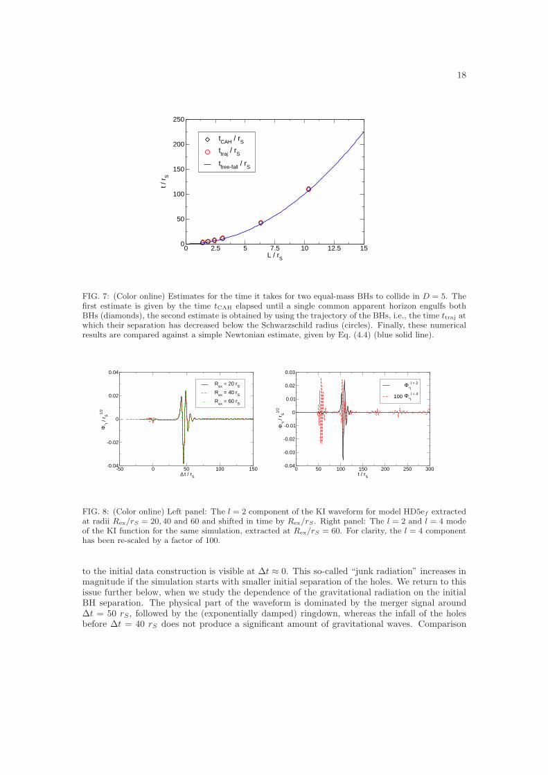
In general relativity, BH trajectories and merger times are intrinsically observer dependent quan-tities. For our comparison with Newtonian estimates we have chosen relativistic trajectories asviewed by observers adapted to the numerical coordinate system. While the lack of fundamentallygauge invariant analogues in general relativity prevents us from deriving rigorous conclusions,we believe such a comparison to serve the intuitive interpretation of results obtained withinthe “moving puncture” gauge. Bearing in mind these caveats, we plot in Fig. 7 the analyticalestimate of the Newtonian time of collision, together with the numerically computed time of for-mation of a common apparent horizon. Also shown in Fig. 7 is the time at which the separationbetween the individual hole’s puncture trajectory decreases below the Schwarzschild parameterrS . The remarkable agreement provides yet another example of how well numerically successfulgauge conditions appear to be adapted to the black hole kinematics. It is beyond the scope ofthis paper to investigate whether this is coincidental or whether such agreement is necessary orat least helpful for gauge conditions to ensure numerical stability. Suffice it to say at this stagethat similar conclusions were reached by Anninos et al. [68] and Lovelace et al. [69] in similarfour dimensional scenarios.

4.3. Waveforms

We now discuss in detail the gravitational wave signal generated by the head-on collision oftwo BHs in five dimensions. For this purpose, we plot in Fig. 8 the l = 2 multipole of the KIfunction Φ,t for model HD5ef obtained at different extraction radii. Qualitatively, the signallooks similar to that shown in the left panel of Fig. 2 for D = 4. A small spurious wavepulse due

18

0 2.5 5 7.5 10 12.5 15L / rS

0

50

100

150

200

250

t / r

S

tCAH / rS

ttraj / rS

tfree-fall / rS

FIG. 7: (Color online) Estimates for the time it takes for two equal-mass BHs to collide in D = 5. Thefirst estimate is given by the time tCAH elapsed until a single common apparent horizon engulfs bothBHs (diamonds), the second estimate is obtained by using the trajectory of the BHs, i.e., the time ttraj atwhich their separation has decreased below the Schwarzschild radius (circles). Finally, these numericalresults are compared against a simple Newtonian estimate, given by Eq. (4.4) (blue solid line).

-50 0 50 100 150 t / rS

-0.04

-0.02

0

0.02

0.04

t / r S

1/2

Rex = 20 rS

Rex = 40 rS

Rex = 60 rS

Φ,

∆0 50 100 150 200 250 300

t / rS

-0.04

-0.03

-0.02

-0.01

0

0.01

0.02

0.03

t / r S

1/2

,tl = 2

100 ,tl = 4

Φ,

Φ

Φ

FIG. 8: (Color online) Left panel: The l = 2 component of the KI waveform for model HD5ef extractedat radii Rex/rS = 20, 40 and 60 and shifted in time by Rex/rS. Right panel: The l = 2 and l = 4 modeof the KI function for the same simulation, extracted at Rex/rS = 60. For clarity, the l = 4 componenthas been re-scaled by a factor of 100.

to the initial data construction is visible at ∆t ≈ 0. This so-called “junk radiation” increases inmagnitude if the simulation starts with smaller initial separation of the holes. We return to thisissue further below, when we study the dependence of the gravitational radiation on the initialBH separation. The physical part of the waveform is dominated by the merger signal around∆t = 50 rS , followed by the (exponentially damped) ringdown, whereas the infall of the holesbefore ∆t = 40 rS does not produce a significant amount of gravitational waves. Comparison

19

0 50 100 150 200 250 300t / rS

-0.003

-0.002

-0.001

0

0.001

0.002

0.003

t / r S

1/2

hc - hm1.97 (hm - hf)2.33 (hm - hf)

∆ Φ

,

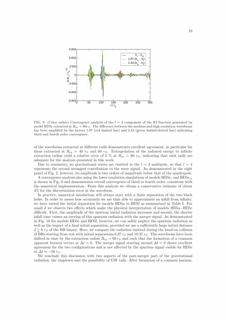
FIG. 9: (Color online) Convergence analysis of the l = 2 component of the KI function generated bymodel HD5e extracted at Rex = 60rS . The difference between the medium and high resolution waveformshas been amplified by the factors 1.97 (red dashed line) and 2.33 (green dashed-dotted line) indicatingthird and fourth order convergence.

of the waveforms extracted at different radii demonstrates excellent agreement, in particular forthose extracted at Rex = 40 rS and 60 rS . Extrapolation of the radiated energy to infiniteextraction radius yield a relative error of 5 % at Rex = 60 rS , indicating that such radii areadequate for the analysis presented in this work.Due to symmetry, no gravitational waves are emitted in the l = 3 multipole, so that l = 4

represents the second strongest contribution to the wave signal. As demonstrated in the rightpanel of Fig. 2, however, its amplitude is two orders of magnitude below that of the quadrupole.A convergence analysis also using the lower resolution simulations of models HD5ec and HD5em

is shown in Fig. 9 and demonstrates overall convergence of third to fourth order, consistent withthe numerical implementation. From this analysis we obtain a conservative estimate of about4% for the discretization error in the waveform.In practice, numerical simulations will always start with a finite separation of the two black

holes. In order to assess how accurately we are thus able to approximate an infall from infinity,we have varied the initial separation for models HD5a to HD5f as summarized in Table I. Forsmall d we observe two effects which make the physical interpretation of models HD5a−HD5cdifficult. First, the amplitude of the spurious initial radiation increases and second, the shorterinfall time causes an overlap of this spurious radiation with the merger signal. As demonstratedin Fig. 10 for models HD5e and HD5f, however, we can safely neglect the spurious radiation aswell as the impact of a final initial separation, provided we use a sufficiently large initial distanced & 6 rS of the BH binary. Here, we compare the radiation emitted during the head-on collisionof BHs starting from rest with initial separations 6.37 rS and 10.37 rS . The waveforms have beenshifted in time by the extraction radius Rex = 60 rS and such that the formation of a commonapparent horizon occurs at ∆t = 0. The merger signal starting around ∆t = 0 shows excellentagreement for the two configurations and is not affected by the spurious signal visible for HD5eat ∆t ≈ −50 rS .We conclude this discussion with two aspects of the post-merger part of the gravitational

radiation, the ringdown and the possibility of GW tails. After formation of a common horizon,

20

-50 -25 0 25 50 t / rS

-0.04

-0.03

-0.02

-0.01

0

0.01

0.02

0.03

t / r S

1/2

HD5efHD5f

Φ,

∆

FIG. 10: (Color online) The l = 2 components of the KI function as generated by a head-on collision ofBHs with initial (coordinate) distance d = 6.37 rS (black solid line) and d = 10.37 rS (red dashed line).The wave functions have been shifted in time such that the formation of a common apparent horizoncorresponds to ∆t = 0 (and taking into account the time it takes for the waves to propagate up to theextraction radius Rex = 60 rS).

the waveform is dominated by an exponentially damped sinusoid, as the merged hole rings downinto a stationary state. By fitting our results with a exponentially-damped sinusoid, we obtaina characteristic frequency

rS ω = 0.955± 0.005− i (0.255± 0.005) . (4.5)

This value is in excellent agreement with perturbative calculations, which predict a lowest quasi-normal frequency rS ω = 0.9477− i 0.2561 for l = 2 [55, 65, 70].A well known feature in gravitational waveforms generated in BH space-times with D = 4

as well as D > 4 are the so-called power-law tails [71–74]. In odd dimensional space-times anadditional, different kind of late-time power tails arises, which does not depend on the presenceof a BH. These are due to a peculiar behavior of the wave-propagation in flat odd dimensionalspace-times because the Green’s function has support inside the entire light-cone [74]. We haveattempted to identify such power-law tails in our signal at late-times, by subtracting a best-fitringdown waveform. Unfortunately, we cannot, at this stage, report any evidence of such apower-law in our results, most likely because the low amplitude tails are buried in numericalnoise.

4.4. Radiated energy

Comparison of Figs. 3 and 10 for the GW quadrupole in D = 4 and D = 5 shows a largerwave amplitude in the five dimensional case and thus indicates that this case may radiate moreenergy. We now investigate this question quantitatively by calculating the energy flux from theKI master function via Eq. (2.56). The fluxes thus obtained for the l = 2 multipole of modelsHD5ef and HD5f in Table I, extracted at Rex = 60 rS, are shown in Fig. 11. As in the case of

21

-25 0 25 50 t / rS

0e+00

1e-04

2e-04

3e-04

4e-04

(dE

/ dt

) / r

S

HD5efHD5f

∆

FIG. 11: (Color online) Energy flux in the l = 2 component of the KI wave function Φ,t, extracted atRex = 60 rS, for models HD5ef (black solid line) and HD5f (red dashed line) in Table I. The fluxeshave been shifted in time by the extraction radius Rex = 60 rS and the time tCAH at which the commonapparent horizon forms.

-50 -25 0 25 50 t / rS

0e+00

2e-04

4e-04

6e-04

8e-04

1e-03

E /

M

HD5efHD5f

∆0 25 50 75 100 125 150

t / rS

10-4

10-3

10-2

10-1

1 -

MA

H /

M

HD5efHD5f

∆

FIG. 12: (Color online) Left panel: Fraction of the centre of mass energy, Erad/M , radiated in the l = 2mode of the KI function shifted in time such that the origin of the time axis corresponds to the formationof a common apparent horizon. Right panel: Fraction of the centre of mass energy 1−MAH/M radiatedduring the collision, estimated using apparent horizon information. The oscillations in this diagnosticquantity have a frequency comparable to the l = 2 quasinormal mode frequency.

the KI master function in Fig. 10, we see no significant variation of the flux for the two differentinitial separations. The flux reaches a maximum value of dE/dt ∼ 3.4 × 10−4 rS , and is thendominated by the ringdown flux. The energy flux from the l = 4 mode is typically four orders ofmagnitude smaller; this is consistent with the factor of 100 difference of the corresponding wavemultipoles observed in Fig. 8, and the quadratic dependence of the flux on the wave amplitude.The total integrated energy emitted throughout the head-on collision is presented in the left

22

D rS ω(l = 2) Erad/M(%) Earea/M(%) Eradl=4/E

radl=2

4 0.7473 − i 0.1779 0.055 29.3 < 10−3

5 0.9477 − i 0.2561 0.089 20.6 < 10−4

TABLE II: Main results for head-on collisions in D = 4 and 5 dimensions. We list the ring downfrequency ω, the total energy radiated in gravitational waves, the upper bound Earea on the radiatedenergy obtained from Hawking’s area theorem and the fractional energy in the l = 4 multipole relativeto the quadrupole radiation.

panel of Fig. 12. We find that a fraction of Erad/M = (8.9 ± 0.6)× 10−4 of the centre of massenergy is emitted in the form of gravitational radiation. We have verified for these models thatthe amount of energy contained in the spurious radiation is about three orders of magnitudesmaller than in the physical merger signal.An independent estimate for the radiated energy can be obtained from the apparent horizon

area A4 in the effective four dimensional space-time by using the spherical symmetry of thepost-merger remnant hole. Energy balance then implies that the energy E radiated in the formof GWs is given by

E

M= 1− MAH

M= 1− 8

3π

A4

4πr2S, (4.6)

where MAH is the apparent horizon mass. The estimate E/M is shown in Fig. 12 and reveals abehavior qualitatively similar to a damped sinusoid with constant offset. Indeed, by using a leastsquare fit, we obtain a complex frequency rS ω ∼ 0.97− i 0.29, again similar to the fundamentall = 2 quasinormal mode frequency (see discussion around Eq. (4.5)). At late times, 1−MAH/Masymptotes to 1−MAH/M ∼ (7.9± 0.8)× 10−4 which agrees with the GW estimate within thenumerical uncertainties.

5. DISCUSSION

In this paper we have developed a formalism to extract gravitational radiation observablesfrom numerical simulations of head-on collisions of BHs in D dimensions. Moreover, we haveperformed such simulations in D = 4, 5. The D = 4 case serves as a test of our formalism anddemonstrates consistency of our results with the literature. The D = 5 case is entirely new.Besides obtaining the corresponding waveforms, we have shown that the total energy releasedin the form of gravitational waves is approximately (0.089 ± 0.006)% of the initial centre ofmass energy of the system, for a head-on collision of two BHs starting from rest at very largedistances. As a comparison, the analogous process in D = 4 releases a slightly smaller quantity:(0.055±0.006)%. We summarize the main results for head-on collisions of two BHs starting fromrest in four and five space-time dimensions in Table II.We have further performed a variety of tests of the wave extraction formalism. Besides testing

the proximity of the numerical coordinate system to the Tangherlini background space-time, wehave demonstrated good agreement between the radiated energy as derived directly from the KImaster function with the values obtained from the horizon area of the post-merger remnant hole.Finally, the ringdown part of the waveform yields a quasinormal mode frequency in excellentagreement with predictions from BH perturbation theory.The radiative efficiency Erad/M in Table II shows that head-on collisions starting from rest in

five dimensions generate about 1.6 times as much GW energy as their four dimensional counter-parts. It will be very interesting to investigate to what extent this observation holds for widerclasses of BH collisions. We can compare the radiation efficiency with the upper limit derived by

23

Hawking [75] from the requirement that the horizon area must not decrease in the collision. This

leads to the area bound Earea

M ≤ 1− 2−1

D−2 . Evidently, this bound decreases with dimensionality,while in the present computation it increases when going from D = 4 to D = 5. As also shownin the table, the generation of GWs in head-on collisions starting from rest is about 3 orders ofmagnitude below this bound. In four dimensions it has already been demonstrated that thereexist more violent processes which release more radiation than the head-on collisions consideredin this work [35–37].In the context of this work, it would be particularly interesting to compute the gravitational

radiation emitted when a point particle falls into a higher dimensional BH (the four dimensionalcalculation is done in the classic work by Davis et al [76]). This analysis can be done by linearizingEinstein’s equations. While such an analysis was done for infall at high energies [53, 54], it hasnot been done for infalls from rest. The four dimensional case shows that by scaling the point-particle results properly with the reduced mass, one gets surprisingly good agreement with fullnon-linear studies [77]. An obvious question is whether such an agreement extends to genericnumber of space-time dimensions. Investigations with a similar purpose, but using a differenttechnique, were carried out in Refs. [78, 79].The numbers reported here for the total energy loss in gravitational waves should increase

significantly in high energy collisions, which are the most relevant scenarios for the applicationsdescribed in the Introduction. Indeed, in the four dimensional case, it is known that ultra-relativistic head-on collisions of equal mass non-rotating BHs release up to 14% of the initialcentre of mass energy into gravitational radiation [35]. The analogous number in higher dimen-sions is as yet unknown and will be subject of the next stages of our research programme. Evenmore energy may be released in high energy collisions with non-vanishing impact parameter. In[36, 37] it was shown that this number can be as large as 35% in D = 4. The formalism developedin Paper I allows, in principle, the study of analogous processes in D ≥ 6. We hope to be ableto report on these results in the near future.

Acknowledgments

A.N., H.W. and M.Z. would like to express their gratitude to the Department of Physics andAstronomy of the University of Mississippi for their hospitality during the last stages of the work.We thank Emanuele Berti and Marco Cavaglia for useful conversations and suggestions. M.Z. andH.W. are funded by FCT through grants SFRH/BD/43558/2008 and SFRH/BD/46061/2008.V.C. acknowledges financial support from Fundacao Calouste Gulbenkian through a short-termscholarship. V.C. and C.H. are supported by a “Ciencia 2007” research contract. A.N. isfunded by FCT through grant SFRH/BPD/47955/2008. U.S. acknowledges support from theRamon y Cajal Programme of the Ministry of Education and Science of Spain, NSF grants PHY-0601459, PHY-0652995 and the Fairchild Foundation to Caltech. This work was partially sup-ported by FCT - Portugal through projects PTDC/FIS/098025/2008, PTDC/FIS/098032/2008PTDC/CTE-AST/098034/2008, CERN/FP/109306/2009, CERN/FP/109290/2009 as well asNSF grant PHY-0900735. This research was supported by an allocation through the TeraGridAdvanced Support Program under grant PHY-090003. Computations were performed on theTeraGrid clusters TACC Ranger and NICS Kraken and at Magerit in Madrid. The authorsthankfully acknowledge the computer resources, technical expertise and assistance provided bythe Barcelona Supercomputing Centre—Centro Nacional de Supercomputacion.

24

Appendix A: Coordinate transformation

In order to extract gravitational radiation using the KI formalism one has to perform a coordi-nate transformation from Cartesian coordinates (which are used during the numerical evolution)to those adapted for wave extraction. The physical 3-metric γij , the lapse function α and theshift vector βi computed on our Cartesian grid are interpolated onto a Cartesian patch. In termsof these quantities we compute the 4-metric gµν in Cartesian coordinates according to Eq. (2.2):

gµνdxµdxν = (−α2 + γijβ

iβj)dt2 + γijβidtdxj + γijβ

jdtdxi + γijdxidxj . (A1)

Then, we transform the 4-metric in Cartesian coordinates into spherical coordinates, defined byEq. (2.1)

x = R sin θ cos θ , (A2)

y = R sin θ sin θ , (A3)

z = R cos θ , (A4)

where θ, θ ∈ [0, π] and R =√

x2 + y2 + z2. If we denote the metric in spherical coordinates by

gSµν and define ρ ≡√

x2 + y2, the explicit form of the transformation is

gStR = gtx sin θ cos θ + gty sin θ sin θ + gtz cos θ , (A5)

gStθ = z(gtx cos θ + gty sin θ)− ρgtz , (A6)

gStθ = −ygtx + xgty , (A7)

gSRR = gxx sin2 θ cos2 θ + 2gxy sin

2 θ cos θ sin θ + 2gxz sin θ cos θ cos θ

+gyy sin2 θ sin2 θ + 2gyz sin θ sin θ cos θ + gzz cos

2 θ , (A8)

gSRθ = z(gxx sin θ cos2 θ + 2gxy sin θ cos θ sin θ + gyy sin θ sin

2 θ

+gxz cos θ cos θ + gyz cos θ sin θ)− (xgxz + ygyz + zgzz) sin θ , (A9)

gSRθ = (−ygxx sin θ cos θ + xgxy sin θ cos θ − ygxy sin θ sin θ

+xgyy sin θ sin θ − ygxz cos θ + xgyz cos θ) , (A10)

gSθθ = z2(gxx cos2 θ + 2gxy cos θ sin θ + gyy sin

2 θ)

−2z(xgxz + ygyz) + ρ2gzz , (A11)

gSθθ = z(−ygxx cos θ + xgxy cos θ − ygxy sin θ + xgyy sin θ)

+ρ(ygxz − xgyz) , (A12)

gSθθ = R2 sin2 θ(gxx sin2 θ − 2gxy cos θ sin θ + gyy cos

2 θ) . (A13)

Henceforth, we will drop the superscript S and use gµν for the metric in spherical coordinates.The areal radius r is related to R by a reparametrization R = R(r), given by Eq. (B50), which

depends on the components gθθ, gθθ only. As shown in Section 3, we find that this reparametriza-tion is nearly constant throughout our numerical simulations. Therefore, the quantities grr, gtr,grθ, grθ can be obtained from gRR, gtR, gRθ, gRθ by a simple rescaling: because

dR

dr≃ 1 , (A14)

we have grr ≃ gRR, and similar relations hold for the other components.

25

Appendix B: Harmonic expansion of axisymmetric tensors in D dimensions

As discussed in Section 2.3, scalar spherical harmonics in D dimensions Sl(θ, θ, φ1, . . . , φD−4)

are solutions of Eq. (2.23)

2Sl = γ ijSl :ij = −k2Sl , (B1)

with k2 = l(l+D− 3). Axisymmetric scalar spherical harmonics are functions of the coordinateθ only, Sl = Sl(θ). Therefore, Eq. (B1) becomes

2Sl(θ) = Sl ,θθ + (D − 3) cot θSl ,θ = −k2Sl , (B2)

since

Sl :θθ = Sl ,θθ (B3)

Sl :θθ = −ΓθθθSl ,θ = sin θ cos θSl ,θ , (B4)

Sl :φ1φ1 = −Γθφ1φ1Sl ,θ = sin2 θ sin θ cos θSl ,θ , (B5)

etc. The quantities Sl ij defined in Eq. (2.24) are then

Sl ij =1

k2Sl :ij +

1

D − 2γijSl =

1

k2(D − 2)

(

(D − 2)Sl :ij + k2γijSl

)

=1

k2(D − 2)diag

(

(D − 3)Wl,− sin2 θWl,− sin2 θ sin2 θWl, . . .)

(B6)

where

Wl(θ) = Sl ,θθ − cot θSl ,θ = sin θ

( Sl ,θ

sin θ

)

,θ

. (B7)

Indeed, using Eq. (B2) one finds

k2(D − 2)Sl θθ = (D − 2)Sl ,θθ + k2Sl = (D − 3)(Sl ,θθ − cot θSl ,θ) , (B8)

k2(D − 2)Sl θθ = (D − 2)Sl ,θθ + k2 sin2 θSl = sin2 θ((D − 2) cot θSl ,θ + k2Sl)

= sin2 θ(−Sl ,θθ + cot θSl ,θ) , (B9)

and therefore

Sl θθ =D − 3

k2(D − 2)Wl , (B10)

Sl θθ =− sin2 θ

k2(D − 2)Wl , (B11)

and likewise for the other components.Axisymmetric scalar spherical harmonics, as discussed in Sec. 2.3, can be written in terms of

Gegenbauer polynomials (cf. (2.37)):

Sl(θ) = (K lD)−1/2C(D−3)/2l (cos θ) . (B12)

If we define

Wl(cos θ) = C(D−3)/2

l ,θθ(cos θ)− cot θC

(D−3)/2

l ,θ(cos θ) , (B13)

26

we have

Wl(θ) = (K lD)−1/2W(D−3)/2l (cos θ) . (B14)

We impose the normalization (2.38)∫

dΩD−2SlSl′ = δll′ ,

∫

dΩD−2Sl ,θSl′ ,θ = δll′k2 . (B15)

Using∫ π

0

dθ(sin θ)D−3C(D−3)/2l (cos θ)C

(D−3)/2l′ (cos θ) = δll′K

lD , (B16)

∫ π

0

dθ(sin θ)D−3C(D−3)/2

l ,θ(cos θ)C

(D−3)/2

l′ ,θ(cos θ) = δll′k

2K lD , (B17)

and

K lD =24−DπΓ(l +D − 3)

(

l + D−32

) (

Γ(

D−32

))2Γ(l + 1)

, (B18)

we have

K lD = K lDAD−3 , (B19)

where

AD−3 =2π(D−2)/2

Γ(

D−22

) , (B20)

is the surface of the (D− 3)-sphere SD−3. Note that∫

dΩD−2(· · · ) = AD−3

∫

dθ(sin θ)D−3(· · · ).With the definitions (2.24) Sl i = − 1

kSl ,i,

∫ π

0

dθ(sin θ)D−3Sl(θ)Sl′ (θ) = δll′A−1D−3 , (B21)

∫ π

0

dθ(sin θ)D−3γ ijSl iSl′ j =

∫ π

0

dθ(sin θ)D−3Sl θ(θ)Sl′ θ(θ) = δll′A−1D−3 . (B22)

Furthermore, we note that Eqs. (B2) and (B7) imply

Wl + (D − 2) cot θSl ,θ + k2Sl = 0 , (B23)

so that

Wl ,θ + (D − 2) cot θSl ,θθ −D − 2

sin2 θSl ,θ + k2Sl ,θ

= Wl ,θ + (D − 2) cot θWl + (k2 −D + 2)Sl ,θ , (B24)

and therefore∫ π

0

dθ(sin θ)D−3WlWl′ =

∫ π

0

dθ(sin θ)D−3Wl sin θ

(Sl′ ,θ

sin θ

)

,θ

= −(D − 2)

∫ π

0

dθ(sin θ)D−3Wl cot θSl′ ,θ −∫ π

0

dθ(sin θ)D−3Wl ,θSl′ ,θ

= (k2 −D + 2)

∫ π

0

dθ(sin θ)D−3Sl ,θSl′ ,θ = δll′A−1D−3 k

2(k2 −D + 2) . (B25)

27

We thus obtain∫

dΩD−2WlWl′ = δll′k2(k2 −D + 2) . (B26)

The perturbations f lab(t, r), f

la(t, r), H

lL(t, r), H

lT (t, r) appearing in the expansion of the metric

perturbations (2.3)

hab = f labSl(θ) , (B27)

haθ = − 1

krf l

aSl(θ),θ , (B28)

hθθ = 2r2(

H lLSl(θ) +H l

T

D − 3

k2(D − 2)Wl(θ)

)

, (B29)

hθθ = 2r2 sin2 θ

(

H lLSl(θ)−H l

T

1

k2(D − 2)Wl(θ)

)

. (B30)

are given by the following integrals, as follows from Eqs. (B12), (B14), (B15), (B26):

f lab(t, r) =

∫

dΩD−2habSl =AD−3√K lD

∫ π

0

dθ(sin θ)D−3habC(D−3)/2l , (B31)

fa(t, r) = − 1

kr

∫

dΩD−2haθSl ,θ (B32)

= − 1

kr

AD−3√K lD

∫ π

0

dθ(sin θ)D−3haθC(D−3)/2

l ,θ, (B33)

HL(t, r) =1

2(D − 2)r2

∫

dΩD−2

[

hθθ +D − 3

sin2 θhθθ

]

Sl (B34)

=1

2(D − 2)r2AD−3√K lD

∫ π

0

dθ(sin θ)D−3

[

hθθ +D − 3

sin2 θhθθ

]

C(D−3)/2l , (B35)

HT (t, r) =1

2r2(k2 −D + 2)

∫

dΩD−2

[

hθθ −1

sin2 θhθθ

]

Wl (B36)

=1

2r2(k2 −D + 2)

AD−3√K lD

∫ π

0

dθ(sin θ)D−3

[

hθθ −1

sin2 θhθθ

]

Wl , (B37)

where hab = hab(t, r, θ), haθ = haθ(t, r, θ), hθθ = hθθ(t, r, θ), hθθ = hθθ(t, r, θ), C(D−3)/2l =

C(D−3)/2l (cos θ) and Wl =Wl(cos θ).We also note that the background Tangherlini metric depends on the l = 0 harmonic only;

the integral of its components over l ≥ 2 harmonics vanish. Therefore, if we decompose the

space-time metric (see Appendix A) as gµν = g(0)µν + hµν with µ, ν = (t, r, θ, θ) and g

(0)µν is the

28

Tangherlini background metric, we can compute the integrals (B) in terms of the metric gµν

ftt =1

π

AD−3√K lD

∫

dθ(sin θ)D−3C(D−3)/2l

∫

dθgtt(θ, θ) , (B38)

ftr =1

π

AD−3√K lD

∫

dθ(sin θ)D−3C(D−3)/2l

∫

dθgtr(θ, θ) , (B39)

frr =1

π

AD−3√K lD

∫

dθ(sin θ)D−3C(D−3)/2l

∫

dθgrr(θ, θ) , (B40)

ft = − 1

krπ

AD−3√K lD

∫

dθ(sin θ)D−3∂θC(D−3)/2l

∫

dθgtθ(θ, θ) , (B41)

fr = − 1

krπ

AD−3√K lD

∫

dθ(sin θ)D−3∂θC(D−3)/2l

∫

dθgrθ(θ, θ) , (B42)

HL =1

2(D − 2)r2π

AD−3√K lD

∫

dθ(sin θ)D−3C(D−3)/2l

∫

dθ

(

gθθ(θ, θ) + (D − 3)gθθ(θ, θ)

sin2 θ

)

,

(B43)

HT =1

2(k2 −D + 2)r2π

AD−3√K lD

∫

dθ(sin θ)D−3Wl

∫

dθ

(

gθθ(θ, θ)−gθθ(θ, θ)

sin2 θ

)

. (B44)

Furthermore, from Eqs. (2.28) and (B38) - (B44) we deduce

F,t = ∂tHL +1

D − 2∂tHT +

1

kf(r)

(

∂tfr +r

k∂t∂rHT

)

, (B45)

F rt = f(r)

(

frt +r

k(∂tfr + ∂rft) +

1

kft +

2r

k2(∂tHT + r∂t∂rHT )

)

− r

k∂rf(r)

(

ft +r

k∂tHT

)

. (B46)

Conversely, since the perturbations do not depend on the l = 0 harmonic, the background metricgµν can be obtained as follows:

g(0)tt =

1

K0Dπ

∫ π

0

dθ sinD−3 θ

∫ π

0

dθgtt(θ, θ) , (B47)

g(0)tr = 0 =

1

K0Dπ

∫ π

0

dθ sinD−3 θ

∫ π

0

dθgtr(θ, θ) , (B48)

g(0)rr =1

K0Dπ

∫ π

0

dθ sinD−3 θ

∫ π

0

dθgrr(θ, θ) . (B49)

Finally, to compute the areal radius r we note that gθθ = r2 + hθθ and gθθ = r2 sin2 θ + hθθ.Both the perturbations hθθ and hθθ contain harmonics of different type (Sl, Sl ,ij); to extract thebackground we need the combination in Eq. (B43):

r2 =1

(D − 2)K0Dπ

∫ π

0

dθ sinD−3 θ

∫ π

0

dθ

[

gθθ + (D − 3)gθθ

sin2 θ

]

. (B50)

[1] M. Zilhao et al., “Numerical relativity for D dimensional axially symmetric space-times: formalismand code tests,” Phys. Rev. D81 (2010) 084052, arXiv:1001.2302 [gr-qc].

29

[2] J. M. Maldacena, “The large N limit of superconformal field theories and supergravity,” Adv. Theor.Math. Phys. 2 (1998) 231–252, arXiv:hep-th/9711200.

[3] I. Antoniadis, “A Possible new dimension at a few TeV,” Phys. Lett. B246 (1990) 377–384.[4] N. Arkani-Hamed, S. Dimopoulos, and G. R. Dvali, “The hierarchy problem and new dimensions at

a millimeter,” Phys. Lett. B429 (1998) 263–272, arXiv:hep-ph/9803315.[5] I. Antoniadis, N. Arkani-Hamed, S. Dimopoulos, and G. R. Dvali, “New dimensions at a millimeter

to a Fermi and superstrings at a TeV,” Phys. Lett. B436 (1998) 257–263, arXiv:hep-ph/9804398.[6] L. Randall and R. Sundrum, “A large mass hierarchy from a small extra dimension,”

Phys. Rev. Lett. 83 (1999) 3370–3373, arXiv:hep-ph/9905221.[7] L. Randall and R. Sundrum, “An alternative to compactification,”

Phys. Rev. Lett. 83 (1999) 4690–4693, arXiv:hep-th/9906064.[8] F. Pretorius, “Binary Black Hole Coalescence,” arXiv:0710.1338 [gr-qc].[9] I. Hinder, “The Current Status of Binary Black Hole Simulations in Numerical Relativity,”

arXiv:1001.5161 [gr-qc].[10] M. Shibata and H. Yoshino, “Nonaxisymmetric instability of rapidly rotating black hole in five

dimensions,” arXiv:0912.3606 [gr-qc].[11] M. Shibata and H. Yoshino, “Bar-mode instability of rapidly spinning black hole in higher dimen-

sions: Numerical simulation in general relativity,” arXiv:1004.4970 [gr-qc].[12] H. Yoshino and M. Shibata, “Higher-dimensional numerical relativity: Formulation and code tests,”

Phys. Rev. D80 (2009) 084025, arXiv:0907.2760 [gr-qc].[13] H. Witek et al., “Black holes in a box: towards the numerical evolution of black holes in AdS,”

arXiv:1004.4633 [hep-th].[14] T. Banks and W. Fischler, “A model for high energy scattering in quantum gravity,”

arXiv:hep-th/9906038.[15] S. B. Giddings and S. D. Thomas, “High energy colliders as black hole factories: The end of short

distance physics,” Phys. Rev. D65 (2002) 056010, arXiv:hep-ph/0106219.[16] S. Dimopoulos and G. L. Landsberg, “Black Holes at the LHC,” Phys. Rev. Lett. 87 (2001) 161602,

arXiv:hep-ph/0106295.[17] J. L. Feng and A. D. Shapere, “Black hole production by cosmic rays,”

Phys. Rev. Lett. 88 (2002) 021303, arXiv:hep-ph/0109106.[18] E.-J. Ahn, M. Ave, M. Cavaglia, and A. V. Olinto, “TeV black hole fragmentation and detectability

in extensive air-showers,” Phys. Rev. D68 (2003) 043004, arXiv:hep-ph/0306008.[19] E.-J. Ahn, M. Cavaglia, and A. V. Olinto, “Brane factories,” Phys. Lett. B551 (2003) 1–6,

arXiv:hep-th/0201042.[20] A. Chamblin, F. Cooper, and G. C. Nayak, “SUSY production from TeV scale blackhole at LHC,”

Phys. Rev. D70 (2004) 075018, arXiv:hep-ph/0405054.[21] V. Cardoso, M. C. Espirito Santo, M. Paulos, M. Pimenta, and B. Tome, “Microscopic black

hole detection in UHECR: The double bang signature,” Astropart. Phys. 22 (2005) 399–407,arXiv:hep-ph/0405056.

[22] M. Cavaglia, “Black hole and brane production in TeV gravity: A review,”Int. J. Mod. Phys. A18 (2003) 1843–1882, arXiv:hep-ph/0210296.

[23] P. Kanti, “Black holes in theories with large extra dimensions: A Review,”Int. J. Mod. Phys. A19 (2004) 4899–4951, arXiv:hep-ph/0402168.

[24] P. Kanti, “Black Holes at the LHC,” Lect. Notes Phys. 769 (2009) 387–423,arXiv:0802.2218 [hep-th].

[25] S. N. Solodukhin, “Classical and quantum cross-section for black hole production in particle colli-sions,” Phys. Lett. B533 (2002) 153–161, arXiv:hep-ph/0201248.

[26] S. D. H. Hsu, “Quantum production of black holes,” Phys. Lett. B555 (2003) 92–98,arXiv:hep-ph/0203154.

[27] K. S. Thorne, “Nonspherical gravitational collapse: a short review,”. In *J. R. Klauder, MagicWithout Magic*, San Francisco 1972, 231-258.

[28] M. W. Choptuik and F. Pretorius, “Ultra Relativistic Particle Collisions,”Phys. Rev. Lett. 104 (2010) 111101, arXiv:0908.1780 [gr-qc].

[29] M. Cavaglia, R. Godang, L. Cremaldi, and D. Summers, “Catfish: A Monte Carlo simulator forblack holes at the LHC,” Comput. Phys. Commun. 177 (2007) 506–517, arXiv:hep-ph/0609001.

[30] J. A. Frost et al., “Phenomenology of Production and Decay of Spinning Extra- Dimensional Black

30

Holes at Hadron Colliders,” JHEP 10 (2009) 014, arXiv:0904.0979 [hep-ph].[31] D.-C. Dai et al., “BlackMax: A black-hole event generator with rotation, recoil, split branes and

brane tension,” Phys. Rev. D77 (2008) 076007, arXiv:0711.3012 [hep-ph].[32] D.-C. Dai et al., “Manual of BlackMax, a black-hole event generator with rotation, recoil, split

branes, and brane tension,” arXiv:0902.3577 [hep-ph].[33] The ATLAS Collaboration, G. Aad et al., “Expected Performance of the ATLAS Experiment -

Detector, Trigger and Physics,” arXiv:0901.0512 [hep-ex].[34] H. Yoshino and V. S. Rychkov, “Improved analysis of black hole formation in high-energy particle

collisions,” Phys. Rev. D71 (2005) 104028, arXiv:hep-th/0503171.[35] U. Sperhake, V. Cardoso, F. Pretorius, E. Berti, and J. A. Gonzalez, “The high-energy collision of

two black holes,” Phys. Rev. Lett. 101 (2008) 161101, arXiv:0806.1738 [gr-qc].[36] M. Shibata, H. Okawa, and T. Yamamoto, “High-velocity collision of two black holes,”

Phys. Rev. D78 (2008) 101501, arXiv:0810.4735 [gr-qc].[37] U. Sperhake et al., “Cross section, final spin and zoom-whirl behavior in high- energy black hole

collisions,” Phys. Rev. Lett. 103 (2009) 131102, arXiv:0907.1252 [gr-qc].[38] M. Alcubierre, Introduction to 3+1 numerical relativity. International series of monographs on

physics. Oxford Univ. Press, Oxford, 2008.[39] T. Regge and J. A. Wheeler, “Stability of a Schwarzschild singularity,”

Phys. Rev. 108 (1957) 1063–1069.[40] F. J. Zerilli, “Effective potential for even parity Regge-Wheeler gravitational perturbation equa-

tions,” Phys. Rev. Lett. 24 (1970) 737–738.[41] E. Newman and R. Penrose, “An Approach to gravitational radiation by a method of spin coeffi-

cients,” J. Math. Phys. 3 (1962) 566–578.[42] S. A. Teukolsky, “Perturbations of a rotating black hole. 1. Fundamental equations for gravitational

electromagnetic and neutrino field perturbations,” Astrophys. J. 185 (1973) 635–647.[43] A. Coley, R. Milson, V. Pravda, and A. Pravdova, “Classification of the Weyl tensor in higher-

dimensions,” Class. Quant. Grav. 21 (2004) L35–L42, arXiv:gr-qc/0401008.[44] R. Milson, A. Coley, V. Pravda, and A. Pravdova, “Alignment and algebraically special tensors in

Lorentzian geometry,” Int. J. Geom. Meth. Mod. Phys. 2 (2005) 41–61, arXiv:gr-qc/0401010.[45] V. Pravda, A. Pravdova, A. Coley, and R. Milson, “Bianchi identities in higher dimensions,”

Class. Quant. Grav. 21 (2004) 2873–2898, arXiv:gr-qc/0401013.[46] M. Ortaggio, V. Pravda, and A. Pravdova, “Ricci identities in higher dimensions,”

Class. Quant. Grav. 24 (2007) 1657–1664, arXiv:gr-qc/0701150.[47] F. R. Tangherlini, “Schwarzschild field in n dimensions and the dimensionality of space problem,”

Nuovo Cim. 27 (1963) 636–651.[48] H. Kodama and A. Ishibashi, “A master equation for gravitational perturbations of max-

imally symmetric black holes in higher dimensions,” Prog. Theor. Phys. 110 (2003) 701–722,arXiv:hep-th/0305147.

[49] U. Sperhake, “Binary black-hole evolutions of excision and puncture data,”Phys. Rev. D76 (2007) 104015, arXiv:gr-qc/0606079.

[50] M. Shibata and T. Nakamura, “Evolution of three-dimensional gravitational waves: Harmonic slicingcase,” Phys. Rev. D52 (1995) 5428–5444.

[51] T. W. Baumgarte and S. L. Shapiro, “On the numerical integration of Einstein’s field equations,”Phys. Rev. D59 (1999) 024007, arXiv:gr-qc/9810065.

[52] H. Kodama, A. Ishibashi, and O. Seto, “Brane world cosmology: Gauge-invariant formalism forperturbation,” Phys. Rev. D62 (2000) 064022, arXiv:hep-th/0004160.

[53] E. Berti, M. Cavaglia, and L. Gualtieri, “Gravitational energy loss in high energy particle colli-sions: Ultrarelativistic plunge into a multidimensional black hole,” Phys. Rev. D69 (2004) 124011,arXiv:hep-th/0309203.

[54] V. Cardoso and J. P. S. Lemos, “Gravitational radiation from collisions at the speed oflight: A massless particle falling into a Schwarzschild black hole,” Phys. Lett. B538 (2002) 1–5,arXiv:gr-qc/0202019.

[55] H. Yoshino, T. Shiromizu, and M. Shibata, “The close limit analysis for head-on collision oftwo black holes in higher dimensions: Brill-Lindquist initial data,” Phys. Rev. D72 (2005) 084020,arXiv:gr-qc/0508063.

[56] U. Sperhake, B. J. Kelly, P. Laguna, K. L. Smith, and E. Schnetter, “Black hole head-on col-

31

lisions and gravitational waves with fixed mesh-refinement and dynamic singularity excision,”Phys. Rev. D71 (2005) 124042, arXiv:gr-qc/0503071.

[57] U. Sperhake et al., “Eccentric binary black-hole mergers: The transition from inspiral to plunge ingeneral relativity,” Phys. Rev. D78 (2008) 064069, arXiv:0710.3823 [gr-qc].

[58] “Cactus Computational Toolkit.” http://www.cactuscode.org/.[59] E. Schnetter, S. H. Hawley, and I. Hawke, “Evolutions in 3D numerical relativity using fixed mesh

refinement,” Class. Quant. Grav. 21 (2004) 1465–1488, arXiv:gr-qc/0310042.[60] “Mesh refinement with Carpet.” http://www.carpetcode.org/.[61] J. Thornburg, “Finding apparent horizons in numerical relativity,”

Phys. Rev. D54 (1996) 4899–4918, arXiv:gr-qc/9508014.[62] J. Thornburg, “A Fast Apparent-Horizon Finder for 3-Dimensional Cartesian Grids in Numerical

Relativity,” Class. Quant. Grav. 21 (2004) 743–766, arXiv:gr-qc/0306056.[63] M. Ansorg, B. Bruegmann, and W. Tichy, “A single-domain spectral method for black hole puncture

data,” Phys. Rev. D70 (2004) 064011, arXiv:gr-qc/0404056.[64] M. Boyle and A. H. Mroue, “Extrapolating gravitational-wave data from numerical simulations,”

Phys. Rev. D80 (2009) 124045, arXiv:0905.3177 [gr-qc].[65] E. Berti, V. Cardoso, and A. O. Starinets, “Quasinormal modes of black holes and black branes,”

Class. Quant. Grav. 26 (2009) 163001, arXiv:0905.2975 [gr-qc].[66] E. Berti, V. Cardoso, and C. M. Will, “On gravitational-wave spectroscopy of massive black holes

with the space interferometer LISA,” Phys. Rev. D73 (2006) 064030, arXiv:gr-qc/0512160.[67] E. Berti, V. Cardoso, J. A. Gonzalez, and U. Sperhake, “Mining information from binary

black hole mergers: a comparison of estimation methods for complex exponentials in noise,”Phys. Rev. D75 (2007) 124017, arXiv:gr-qc/0701086.

[68] P. Anninos, D. Hobill, E. Seidel, L. Smarr, and W.-M. Suen, “The Headon collision of two equalmass black holes,” Phys. Rev. D52 (1995) 2044–2058, arXiv:gr-qc/9408041.

[69] G. Lovelace et al., “Momentum flow in black-hole binaries: II. Numerical simulations of equal-mass,head-on mergers with antiparallel spins,” arXiv:0907.0869 [gr-qc].

[70] V. Cardoso, J. P. S. Lemos, and S. Yoshida, “Scalar gravitational perturbations and quasi-normal modes in the five dimensional Schwarzschild black hole,” JHEP 12 (2003) 041,arXiv:hep-th/0311260.

[71] B. S. DeWitt and R. W. Brehme, “Radiation damping in a gravitational field,”Ann. Phys. 9 (1960) 220–259.

[72] R. H. Price, “Nonspherical perturbations of relativistic gravitational collapse. 1. Scalar and gravi-tational perturbations,” Phys. Rev. D5 (1972) 2419–2438.

[73] E. S. C. Ching, P. T. Leung, W. M. Suen, and K. Young, “Wave propagation in gravitationalsystems: Late time behavior,” Phys. Rev. D52 (1995) 2118–2132, arXiv:gr-qc/9507035.

[74] V. Cardoso, S. Yoshida, O. J. C. Dias, and J. P. S. Lemos, “Late-time tails of wave propagation inhigher dimensional spacetimes,” Phys. Rev. D68 (2003) 061503, arXiv:hep-th/0307122.

[75] S. W. Hawking, “Gravitational radiation from colliding black holes,”Phys. Rev. Lett. 26 (1971) 1344–1346.

[76] M. Davis, R. Ruffini, W. H. Press, and R. H. Price, “Gravitational radiation from a particle fallingradially into a schwarzschild black hole,” Phys. Rev. Lett. 27 (1971) 1466–1469.

[77] P. Anninos, D. Hobill, E. Seidel, L. Smarr, and W.-M. Suen, “The Collision of two black holes,”Phys. Rev. Lett. 71 (1993) 2851–2854, arXiv:gr-qc/9309016.

[78] M. E. Araujo and S. R. Oliveira, “Static axisymmetric approach for the headon collision of twoblack holes,” Phys. Rev. D52 (1995) 816–820.

[79] O. M. Moreschi and S. Dain, “Estimates of the total gravitation radiation in the head- on blackhole collision,” Phys. Rev. D53 (1996) 1745–1749, arXiv:gr-qc/0203071.