Numerical modelling of climate change impacts on freshwater lenses on the North Sea Island of Borkum...

Hydrol. Earth Syst. Sci., 16, 3621–3643, 2012www.hydrol-earth-syst-sci.net/16/3621/2012/doi:10.5194/hess-16-3621-2012© Author(s) 2012. CC Attribution 3.0 License.

Hydrology andEarth System

Sciences

Numerical modelling of climate change impacts on freshwater lenseson the North Sea Island of Borkum using hydrological andgeophysical methods

H. Sulzbacher1, H. Wiederhold1, B. Siemon2, M. Grinat 1, J. Igel1, T. Burschil1, T. Gunther1, and K. Hinsby3

1Leibniz Institute for Applied Geophysics, Hannover, Germany2Federal Institute for Geosciences and Natural Resources, Hannover, Germany3Geological Survey of Denmark and Greenland, Copenhagen, Denmark

Correspondence to:H. Sulzbacher ([email protected])

Received: 21 February 2012 – Published in Hydrol. Earth Syst. Sci. Discuss.: 15 March 2012Revised: 31 July 2012 – Accepted: 26 August 2012 – Published: 16 October 2012

Abstract. A numerical, density dependent groundwatermodel is set up for the North Sea Island of Borkum to es-timate climate change impacts on coastal aquifers and espe-cially the situation of barrier islands in the Wadden Sea. Thedatabase includes information from boreholes, a seismic sur-vey, a helicopter-borne electromagnetic (HEM) survey, mon-itoring of the freshwater-saltwater boundary by vertical elec-trode chains in two boreholes, measurements of groundwa-ter table, pumping and slug tests, as well as water samples.Based on a statistical analysis of borehole columns, seis-mic sections and HEM, a hydrogeological model is set up.The groundwater model is developed using the finite-elementprogramme FEFLOW. The density dependent groundwatermodel is calibrated on the basis of hydraulic, hydrologicaland geophysical data, in particular spatial HEM and localmonitoring data. Verification runs with the calibrated modelshow good agreement between measured and computed hy-draulic heads. A good agreement is also obtained betweenmeasured and computed density or total dissolved solids datafor both the entire freshwater lens on a large scale and in thearea of the well fields on a small scale.

For simulating future changes in this coastal groundwatersystem until the end of the current century, we use the cli-mate scenario A2, specified by the Intergovernmental Panelon Climate Change and, in particular, the data for the GermanNorth Sea coast. Simulation runs show proceeding salinisa-tion with time beneath the well fields of the two waterworksWaterdelle and Ostland.

The modelling study shows that the spreading of wellfields is an appropriate protection measure against excessivesalinisation of the water supply until the end of the currentcentury.

1 Introduction

Investigation of the impact of climate change and the result-ing sea level rise on the freshwater resources of the southernNorth Sea Region including the Danish coastal area (Northand western Baltic Sea) is aim of the Interreg project CLI-WAT (http://www.cliwat.eu). In particular, the drinking waterresources of barrier islands like the German North Sea Islandof Borkum (Fig. 1) are endangered by enhanced sea waterintrusion and enhanced upconing of sea water in the vicin-ity of the water supply well fields. Vulnerable areas have tobe identified and mitigation measures need to be defined andadopted.

The future development of the salinity distribution in thesubsurface can be simulated using a numerical density de-pendent groundwater flow model (e.g., Oude Essink et al.,2010). Numerous density dependent groundwater modelshave been developed in the last decades (de Louw et al.,2011; Post and Abarca, 2010; Post, 2005; Thorenz, 2001;Bear et al., 1999; Holzbecher, 1998; Lee and Cheng, 1974;Cooper et al., 1964). However, most of these applicationsare afflicted with a poor database of field data. In particular,depth-dependent densities, which are composed mainly of

Published by Copernicus Publications on behalf of the European Geosciences Union.

http://www.cliwat.eu

3622 H. Sulzbacher et al.: Numerical modelling of climate change impacts on freshwater lenses on Borkum

33

1

2

Figure 1. Top panel: location map of study area, bottom panel: North Sea Island of Borkum 3

with its two waterworks (WW): WW I Waterdelle and WW II Ostland and the two major 4

rivers. 5

6

Fig. 1. Top panel: location map of study area, bottom panel: North Sea Island of Borkum with its two waterworks (WW): WW I Waterdelleand WW II Ostland and the two major rivers.

sea salt or comprehensive data of chloride distribution cover-ing the total modelling area, are often missing.

Nevertheless, a good database is required to calibrate agroundwater model capable of a reliable forecast. Recentgeophysical techniques, e.g., helicopter-borne electromag-netic (HEM) surveys (Siemon et al., 2009b) and real timeelectrical data, monitored via vertical electrode chains inboreholes (Grinat et al., 2010), are essential for the calibra-tion of groundwater models using density data.

The groundwater model for Borkum has been set up utilis-ing the finite-element programme FEFLOW® (http://www.feflow.de). A comprehensive database of hydraulic, hydro-logical and geophysical field measurements, mainly obtainedin the time period from 2008 to 2010, constitutes the basicdata used for the model setup.

Great attention was paid to the model calibration, whichis highly critical for the prognosis capability and the progno-sis accuracy of the model. The focus of this work is essen-tially on the calibration process, particularly the density (ormass) calibration. New methods that enable the inclusion ofthe comprehensive geophysical database into the calibrationprocedure are presented in this study.

For model simulations of future changes in this coastalgroundwater system until the year 2100 we use the A2 cli-mate scenario from the Intergovernmental Panel on ClimateChange IPCC (IPCC, 2007). Proceeding investigations andestimations suggest saltwater intrusion particularly aroundthe waterworks until the end of this century caused by cli-mate change and overexploitation. Making use of the nu-merical model as management tool it is demonstrated how

Hydrol. Earth Syst. Sci., 16, 3621–3643, 2012 www.hydrol-earth-syst-sci.net/16/3621/2012/

http://www.feflow.de

http://www.feflow.de

H. Sulzbacher et al.: Numerical modelling of climate change impacts on freshwater lenses on Borkum 3623

mitigation measures at the well field configuration ensuresufficient water quality until 2100 without the need of re-ducing the wells production rates.

The freshwater lenses of the German East Frisian barrierislands have been in the focus of water supplier and researchsince Herzberg (1901) discovered here that the depth of thefreshwater-saltwater interface in coastal aquifers is propor-tional to the elevation of the water table above sea level.Some modelling studies were done on neighbouring islandsto Borkum (Fein et al., 2008; Petersen et al., 2003) but ourwork is the first study comprising the entire groundwaterbody (flow and density) of a German Wadden Sea island.

The present study has two major goals. The first one isto illustrate the geophysical and hydrological methods andhow they contribute to develop a density dependent numeri-cal model. The second one is to describe the simulation re-sults with respect to the impact of climate change.

2 Geological background and groundwater situation

The southern North Sea coast developed after the last glacia-tions in the Holocene. With rising sea level the North Seaexpanded to the south. Today’s coastline was nearly reachedabout 6000 BC. After that time sea level rising diminishedand the interplay of transgression and regression developedthe barrier islands (Behre, 2008). The East Frisian Islands aredune islands and presumably younger than 2000 yr. Borkumis the westernmost and largest of these German islands,stretching 10 km from east to west and up to 7 km from northto south. It covers an area of about 31 km2. It is a typical bar-rier island with dunes to the sea side and a low-lying marsh-land area located to the mainland side (Streif, 1990).

The settlement and low-lying meadows in the centre ofthe island are protected by the great south dike and to thenorth by a belt of dunes ranging up to 21 m. The southerndike was built in 1934 to prevent the meadows and marshlandof central Borkum from regularly flooding during high tide.Before construction of the dike, the island consisted more orless of two main parts.

The drinking water supply of Borkum is autonomous andthere are two waterworks (WW) (Fig. 1). The 29 wells ofWW I (Waterdelle), located in the western part, reach downto a depth of 9 m and the 11 wells of WW II (Ostland), lo-cated in the eastern part, reach a depth of 41 m below sur-face. WW I started water abstraction in 1900 and WW IIin 1965. From WW I an average amount of 340 000 m3 a−1

drinking water is delivered (400 000 m3 a−1 are permittedby the authorities) and from WW II an average amount of530 000 m3 a−1 (permitted is 900 000 m3 a−1) (Fig. 2, toppanel). According to the seasonal pattern of the tourism, theannual variation of the abstraction is considerable (Fig. 2,bottom panel) and varies usually during one year between30 000 and 125 000 m3 month−1 for all supply wells (Winter,2008a, 2009) (Fig. 2, bottom panel). In general, the delivered

water is of good quality and the chloride concentration in allwells is lower than 100 mg l−1. However, high concentrationsof iron occur in several wells. After delivery the water has tobe treated by standard procedures.

Historical maps and archive reports show that prior to theconstruction of WW I at the beginning of the last century thefreshwater lens of Borkum had been in a steady state. Hydro-logical milestones in the history of Borkum were the start ofdrinking water abstraction at WW I, the construction of thegreat south dike, and the initiation of operation of WW II.

Recent studies (Winter, 2008a, 2009) indicate a limitedfresh groundwater resource and a level of water abstractionthat is just in balance with the amount of recharge. Climatechanges are expected to adversely affect this balance in fu-ture and decrease the potential freshwater supply by salin-isation although increasing precipitation on the island willpartly counteract this development. A similar result was ob-tained by numerical simulations on a small island in theBaltic Sea (Rasmussen et al., 2012).

3 Material and methods

3.1 Mapping the freshwater lens and the geologicalenvironment

3.1.1 Geological, hydrogeological and hydrologicalmeasurements

For the geologic model a database with 381 boreholes wasavailable from the Geological Survey of Lower Saxony (Lan-desamt fur Bergbau, Energie und Geologie, LBEG). Mostof them (350) were shallower than 40 m, 256 even shal-lower than 20 m. Only eight reached 70 to 80 m and were re-stricted to the water supply area Ostland. Five offshore bore-holes were more than 3000 m deep, but with only poor in-formation for the first hundred metres. Generally, at Borkumthe base of Holocene fine sediments is found at a depth ofabout 10 m b.m.s.l. (below mean sea level) (Streif, 1990),and the base of Quaternary at about−50 m m.s.l. (LBEGdatabase,http://nibis.lbeg.de/cardomap3/). At greater deptha salt structure has pierced Tertiary sediments. The top ofthis salt structure is found at−500 m m.s.l. (Streif, 1990).

Topographic data of the whole Island of Borkumwere taken from the dgm5 ATKIS model (DigitaleGelandemodelle – DGM – ATKIS, LGN Niedersachsen).The data are gridded on a rectangular 12.5 m× 12.5 m gridand exhibit a resolution of better than± 0.5 m in horizontaland vertical direction.

Long-term average data of the groundwater rechargewere obtained from the LBEG map-server (modelGROWA06V2 1961-90). The maximum recharge of300 mm a−1 occurs in the area of the dune belt, whereas inthe marshlands values below 50 mm a−1 are found. Here,silt and clay predominate near the surface of the terrain

www.hydrol-earth-syst-sci.net/16/3621/2012/ Hydrol. Earth Syst. Sci., 16, 3621–3643, 2012

http://nibis.lbeg.de/cardomap3/


34

1

Figure 2. Top panel: Annual delivery rates [1000 m³/a] for WW I (Waterdelle), blue bars, and 2

WW II (Ostland), dark red bars, bottom panel: monthly delivery rates for 2009. 3

4

Fig. 2.Top panel: Annual delivery rates [1000 m3 a−1] for WW I (Waterdelle), blue bars, and WW II (Ostland), dark red bars, bottom panel:monthly delivery rates for 2009.

and most of the precipitation is drained before reaching theground water table.

Historical data of the well field abstractions from the be-ginning of the delivery in 1900 until March 2010 were ob-tained from the local drinking water supplier.

In order to get a better understanding of the hydraulic com-position of the aquifer, a series of 12 pumping tests was car-ried out all over the island in March and September 2009.Transmissivities are computed and summarised in Table 1.According to the configuration of the respective pumpingtest for all locations of the loggers in the draw down area,with 2, 5, 10 m (and so on) distance to the pumping location,transmissivitiesT (2 m),T (5 m),T (10 m) (and so on) werecomputed and averaged to one transmissivityT at the pump-ing location. In addition, hydraulic conductivities on threevertical profiles were available from slug tests. Results andmethods of pumping and mini slug tests are described anddiscussed in detail by Sulzbacher (2011). The mini slug testmethod is described by Hinsby et al. (1992).

Although the local drinking water supplier, the StadtwerkeBorkum GmbH, operates a network of more than 100 perma-nent groundwater observation wells, these are located moreor less inside or close to the catchment areas of the well fieldWW I and WW II. Due to the lack of water table measure-ments covering the whole island, a comprehensive geodetic

field campaign was carried out in June 2009 (133 altitudemeasurements at the groundwater table including levels ofopen water such as lakes, rivers, creeks, canals and drainageditches).

In March 2010 156 groundwater and open water levelmeasurements were carried out. For this purpose holes weredrilled down to the groundwater level by means of a handauger drill in areas with poor information of the groundwa-ter table. The altitude measurements of the groundwater ta-ble were carried out with high precision Trimble GPS equip-ment. The altitude accuracy of these data is up to± 6 cm.For the hydraulic calibration at reference time (March 2010),overall 258 reference date measurements of the groundwaterlevel were available. The altitude of the groundwater tableof the upper aquifer varies from about 0 m in the marsh-land behind the great south dike and meadows to about+3.5 m m.s.l. in the dune areas (Fig. 3).

During February 2008, Direct Push vertical soundingswere conducted on Borkum near and directly on the fresh-to-salt interface by GEOLOG GmbH on behalf of the watersupplier (Winter, 2008b). The data were used to investigatethe progressing salinisation of the groundwater caused by astorm flood in the course of the winter storm Kyrill in Jan-uary 2007. The soundings deliver vertical profiles where theelectrical conductivity of the “non-saturated” and saturated



Table 1.Transmissivity (T ) obtained from pumping tests. According to the configuration of the pumping test for all locations of the loggersin the draw down area with 2, 5, 10 m (and so on) distance to the pumping location, transmissivitiesT (2 m),T (5 m),T (10 m) (and so on)were computed and averaged to one transmissivityT at the pumping location.

No. T (2 m) T (5 m) T (10 m) T (20 m) T (100 m) pumped aquifer T [m2 s−1] location

P01 4.61E-4 5.50E-4 5.60E-4 1 5.24E-4 Horse PastureP02 5.48E-4 4.28E-4 6.04E-4 1 5.39E-4 Fish PondP03 2.07E-3 2.05E-3 2.54E-3 2.43E-3 2.39E-3 1 2.03E-3 SewageP04 2.18E-3 2.63E-3 2.76E-3 1 1.89E-3 Land FillP05 2.64E-3 3.10E-3 1 2.87E-3 South East DunesP06 5.0E-3 5.30E-3 5.12E-3 6.80E-3 1 5.56E-3 North BeachP07 1.00E-3 1.09E-3 1.39E-3 2.30E-3 1 1.45E-3 Bantje-DunesP08 2.29E-3 1.47E-3 1.44E-3 2.78E-3 1.61E-3 1 1.92E-3 Lake TuskendorP-OD22 no draw down recognized 1 Dunes OstlandP-OD33 6.37E-4 6.38E-4 1 6.38E-4 Dunes OstlandP-OD35 disturbed by tidal fluctuations, evaluation of draw 2 Kobbe-Dunes

downs not possible, no draw downs in aquifer 1P-Br38a 2.50E-3 (CLIWAT-IIa), 1.90E-3 (OD8) 1 2.20E-3 OstbakeP-Br38b 2.00E-3 (CLIWAT-IIb), 2.19E-3 (OD8) 2 2.10E-3 Ostbake

35

1

Figure 3. Groundwater table of the upper aquifer during March 2010 (water supply wells 2

marked by red circles, location of CLIWAT drillings marked by black stars, mean sea level 3

marked by dashed line). 4

5

Fig. 3. Groundwater table of the upper aquifer during March 2010 (water supply wells marked by red circles, location of CLIWAT drillingsmarked by black stars, mean sea level marked by dashed line).

sediments was recorded continuously down to a depth of usu-ally 15–25 m. 41 of these vertical profiles were performedacross the border of the freshwater lens in the vicinity ofWW I and II. Additionally, several in situ measurements ofthe electrical conductivity from water samples were takenfrom nearly all of these vertical profiles. The water samplescan be compared with computed pore water electrical con-ductivities at the same temperature for model verification.

Runoff measurements from the open water system, avail-able from field work carried out on Borkum 2009 and 2010,were included in the hydraulic calibration procedure. Themeasurements were carried out systematically at rivers Hoppand Tuskendorkill (Fig. 1), covering nearly the whole catch-ment area of open water on the island (Sulzbacher, 2011).

Simultaneously to the groundwater level measurementswater electrical conductivity values were gauged at the



36

1

Figure 4. Observation points of electrical water conductivity (ec) and temperature at the 2

surface of the groundwater table during June 2009 and March 2010, all 260 locations are 3

represented. 4

5

Fig. 4.Observation points of electrical water conductivity (ec) and temperature at the surface of the groundwater table during June 2009 andMarch 2010, all 260 locations are represented.

surface of the groundwater table and open water in June 2009and March 2010. Including 41 Direct Push samples overall260 values of the pore water conductivity were obtained. Fig-ure 4 shows locations, sampling type and time of these mea-surements (Sulzbacher, 2011).

3.1.2 Geophysical methods

An excellent overview of the spatial distribution of the elec-trical conductivity was provided by a helicopter-borne elec-tromagnetic survey carried out by the German Federal In-stitute for Geosciences and Natural Resources (BGR, Han-nover) in March 2008 (Siemon et al., 2009a). The entire is-land and parts of the adjacent Wadden Sea were covered by35 NW–SE lines with 250 m spacing and 11 SW–NE tie lineswith 500 m spacing. In total 550 line-km were flown coveringan area of 75 km2. From these HEM data smooth electricalconductivity models with 15 layers were derived (Siemon etal., 2009b) and displayed as conductivities at several depthsbelow sea level which clearly show the spatial variation ofthe freshwater lens (Fig. 5).

Two new drillings together with geophysical logging wereestablished in 2009: CLIWAT I located in Waterdelle, 67 mdeep, and CLIWAT II in Ostland, 77 m deep (Fig. 3). Twovertical electrode chains have been installed in the transition

zone from freshwater to saltwater at a depth between 45 and65 m to monitor the spatiotemporal behaviour of the electri-cal conductivity of the saturated sediments with a samplinginterval of 5 h (Sudekum et al., 2009; Grinat et al., 2010).

As the information on the deeper subsurface is relativelypoor, we measured a 0.5 km long high-resolution seismic re-flection profile with P-waves as well as with S-waves. Asseismic source we used the electrodynamic vibrator systemELVIS (Polom et al., 2011; Krawczyk et al., 2012). Wereached a depth of 300 m with P-waves and about 50 m withS-waves.

In the north-east, north and north-west part of the island,the near surface was also investigated by ground-penetratingradar (GPR) with a total of 20 km constant-offset profilesmeasured in September 2009. The elevation of the ground-water table was mapped on most of the profiles and is in goodaccordance with the groundwater monitoring measurementsand hand drillings in the region. A sharp and strong horizon-tal reflection at a depth of−0.5 m to 1 m m.s.l. can be seenon most of the profiles and was identified as a 0.20 m thicksilt loam layer by hand drillings (Igel et al., 2012).

Magnetic resonance soundings (MRS) are capable of ob-taining a model of water content (porosity) and decay timeas a function of depth. Both are related to the hydraulic con-ductivity of the aquifer and can, after calibration, provide



37

1

Figure 5. Top panel: Electrical conductivity (σ) maps at different depths derived from 2

helicopter-borne electromagnetic survey, bottom panel: cross sectional view along transects 3

T13.9 and L29.1. 4

5

Fig. 5. Top panel: Electrical conductivity (σ ) maps at different depths derived from helicopter-borne electromagnetic survey, bottom panel:cross sectional view along transects T13.9 and L29.1.

non-invasive estimates of the hydraulic parameters (Guntherand Muller-Petke, 2012). In a preliminary study, four sound-ings have been carried out, one of them at the CLIWAT IIborehole and one at an existing well. Results of pumpingtests P-Br38a and P-Br38b, carried out near the CLIWAT-II drilling, as well as pumping test P-OD33 were used toachieve calibration. The measurements were jointly invertedwith vertical electrical soundings. As a result, lithology canbe differentiated from salinity and total dissolved solids(TDS) concentrations as well as sediment porosities can bepredicted (Gunther and Muller-Petke, 2012). However, dueto the extremely limited data, the results were solely usedfor corroboration of the model results. A comparison showsremarkably good agreement with the hydraulic model.

3.2 Surface mass concentration map

As the accuracy of the density distribution at the model topsurface is essential for the precision of the prognosis simu-lations (Sect. 6) it is described in more detail in the follow-ing. HEM data are of great importance for the constructionof mass transport boundary conditions at the surface of theaquifer.

As a first step the different measurements of electrical con-ductivity need to be adjusted concerning temperature, which

was measured in situ together with the electrical conductiv-ities at the water table. During March 2008, when the HEMsurvey was performed, average aquifer temperature and tem-perature of the sea water close to the surface amounted toapproximately 5◦C (BSH, 2009). Because electrical conduc-tivities strongly depend on temperature and rise by about4 %/1◦C, pore water electrical conductivities of manual mea-surements at the surface of the groundwater table as well asDirect Push and laboratory water analysis had to be trans-ferred into values referring to 5◦C.

In this way, it is possible to compare later the computedwith the measured pore water densities which is necessary toverify the calibrated model.

The second step is to regionalise the measured pore wa-ter conductivity data at the surface of the aquifer (Fig. 4).We do this with the help of the HEM data. Therefore, wedefine the ratio of the pore water conductivityσw and theconductivity of the saturated sedimentsσb, measured by geo-physical methods like HEM asFa =σw/σb. In the literatureFa is known as apparent formation factor (Katsube et al.,2000; Repsold, 1990). It should be emphasized, however,that this factor is used here for the regionalisation of the sur-face electric conductivity data regardless of its hydrogeolog-ical meaning.



38

1

Figure 6. Regionalization of electrical conductivity data at the water table by means of data 2

from helicopter-borne electromagnetics (HEM) and apparent formation factors. Top left 3

panel: electrical conductivities at 0 m m.s.l. from HEM, (bottom left panel) locations of 4

electrical conductivity from manual readings at the water table (see Fig. 4), top right panel: 5

apparent formation factors at the water table, bottom right panel: regionalized conductivity 6

map at the surface of the groundwater table. 7

8

Fig. 6. Regionalisation of electrical conductivity data at the water table by means of data from helicopter-borne electromagnetics (HEM)and apparent formation factors. Top left panel: electrical conductivities at 0 m m.s.l. from HEM, (bottom left panel) locations of electricalconductivity from manual readings at the water table (see Fig. 4), top right panel: apparent formation factors at the water table, bottom rightpanel: regionalised conductivity map at the surface of the groundwater table.

Moreover, HEM electrical conductivities according to anaquifer depth of 0 m m.s.l. are assumed to be the same elec-trical conductivities than those of the aquifer at the surfaceof the groundwater table. The cross-sections of Fig. 5 showthe validity of this approximation.Fa can now be computedfrom the individually measured pore water conductivity dataσw (Fig. 6, bottom left panel) andσb measured by HEM(Fig. 6, top left panel) at the same locations at the surfaceof the groundwater table.

Inside the island, in particular inside the area of the fresh-water lens, the calculated values ofFa vary relatively weaklyin the range of about 1–2 (average value: 1.53, aquifer: 0.95,open water: 2.29) which means that the pore water exhibitsapproximately the same electrical conductivity as the con-ductivity of the saturated sediments obtained from HEM dataat these locations (see Sulzbacher, 2011). The relatively lowapparent formation factors at the surface of the aquifer aredue to the fact that the near-surface layer exhibits high con-tent of cohesive material like silt and clay, which is con-firmed by the statistical analysis of the drilling results (seeSect. 4, Fig. 7, left panel). Low apparent formation factors

in the same order of magnitude have also been observed inwide areas of the marshlands of the German North Sea coast(Repsold, 1990) or in the area of the Belgium and DutchNorth Sea coast (Geirnaert and Vandenberghe, 1988; vanOvermeeren et al., 1991; TNO-IGG, 1992).

Due to the approximately seasonal stability of the salin-ity of the aquifer at the surface, at least beside the open wa-ter, all data from both campaigns June 2009 and March 2010were used for the construction of a contour map of the elec-trical conductivity. Although intensive sampling on the sur-face of the aquifer was conducted, data coverage was notdense enough and the variation of the measured values wastoo high for a reliable regionalisation of the data with a con-touring algorithm in areas with low data coverage. Instead,it is possible to interpolate the relatively low varying forma-tion factors in a reliable way with a Kriging algorithm asshown in Fig. 6 (top right panel). Offshore sea water con-ductivity at 5◦C is assumed to be 3120 mS m−1 accordingto TDS of 35 000 mg l−1, the mean salinity of the North Sea(e.g., Heyen and Dippner, 1998). Manual measurements ofthe electrical conductivity at the sea water near the shore of



39

1

Figure 7. Left panel: Statistical evaluation of drillings and hydrogeological model, (top right 2

panel) data values, (bottom right panel) schematic cross section of the aquifer for two 3

dimensional numerical simulations. 4

5

Fig. 7.Left panel: statistical evaluation of drillings and hydrogeological model, (top right panel) data values, (bottom right panel) schematiccross-section of the aquifer for two dimensional numerical simulations.

Borkum and the analysis of sea water samples in the labo-ratory at Geozentrum in Hannover show that this is approx-imately the case, also in the Wadden Sea around Borkum.Submarine fresh water breakouts from the aquifer, therefore,play a negligible role.

To obtain supporting points for the sea region, addi-tional apparent formation factors were gained by dividingsea water electrical conductivity by the corresponding HEMconductivity.

Figure 6 (top left panel) shows that HEM electrical con-ductivities in shallow sea water are considerably influencedby the sediments of the sea bottom beneath shallow sea water,particularly in the Wadden Sea. Electrical conductivities con-ductivities in these areas are only a fraction of those valuestypical for sea water, wherefore apparent formation factors inthis region are considerably greater than the theoretical valueof 1 as shown in Fig. 6 (top right panel).

In a next step all values of HEM electrical conductivity atdepth 0 m and computed on a 69× 100 grid (Fig. 6, top leftpanel) are multiplied cell by cell with formation factorsFa on

the same grid (Fig. 6, top right panel) to obtain the desiredpore water conductivities (Fig. 6, bottom right panel). Thefigure shows contour lines and fringes of the electrical con-ductivity at the water table referring to water temperatures of5◦C. It is a map of measured pore water conductivities inter-polated and extrapolated with information obtained by HEMmeasurements.

The last step is to transfer these conductivity values intoTDS values by multiplying all of them with a constant,temperature-dependent factorM. In total 124 water sam-ples analyses were conducted from sea water at differentlocations, from water supply wells, new drillings or Di-rect Push measurements and evaluated in the laboratory atGeozentrum in Hannover. From electric conductivities at5◦C and TDS values, the dimensionless factorM was deter-mined. For water temperatures of 5◦C and typical sea water,NaCl-dominated brackish or NaCl contaminated freshwaterit amounts toM = 11.23, valid forσ given in mS m−1 and theTDS in mg l−1.



40

1

Figure 8. Seismic results, (left) P-wave section, (right) S-wave section (note the different 2

depth scales). 3

4

Fig. 8.Seismic results, (left panel) P-wave section, (right panel) S-wave section (note the different depth scales).

From TDS values, mass transport initial and boundaryconditions at the surface are constructed for the current nu-merical model as described in Sect. 4.2.

4 Model setup

4.1 Hydrogeological model setup

For the setup of the hydrogeological model the borehole in-formation was statistically analysed. In so doing, the aquiferwas divided into depth intervals of 2.5 m and for each intervalthe number of drillings containing cohesive material, such asclay or silt, was set in relation to all drillings intersecting thisinterval (Fig. 7, right panel). The first of this interval is lo-cated 0–2.5 m m.s.l., representing the freshwater lens abovesea level and the last interval ends at−180 m m.s.l., at thebottom of the aquifer. The zones with high clay/silt frac-tion are regarded as aquitards. The evaluation result yieldsan aquifer roughly divided into four parts, each separated bymore or less leaky aquitards. In the area of the water sup-ply well fields, there are extended clay layers protecting thedrinking water from pollution from above and upconing saltfrom below. The uppermost three Quaternary aquifers areused for drinking water supply and reach down to a depthof about 60 m. It should be mentioned that there is only verypoor information about the fourth aquifer.

The geological model, shown in Fig. 7 (left panel) is, ofcourse, a rather simplified, schematic imagination. In real-ity, hydrogeological features are much more complex. In thenumerical model (Sect. 5) the horizontal and vertical hetero-geneity of hydrogeological parameters, like hydraulic con-ductivities and transmissivities, is implemented sufficientlyclose to reality to meet accuracy demands for the progno-sis results (see Sects. 5 and 6). Further, as pointed out by

Voss (2011a,b), too many details do not necessarily improvethe models prognosis capabilities.

Two-dimensional density dependent numerical model cal-culations with FEFLOW indicate that the aquitards consistof non-persistent cohesive material (predominantly clay, so-called patch rock), schematically shown in Fig. 7 (bottomright panel). The models were designed as vertical NW–SEcross sections through Borkums aquifer in the appropriatespatial dimension and set up with FEFLOW standard val-ues for all parameters like hydraulic conductivity, porosity orspecific yield.

This concept is supported by the results of the seismic re-flection profile with P- and S-waves (Fig. 8). The distinct re-flector at 180 m depth in the P-wave section marks the base-ment of the model. The Quaternary base, located at a depthof about 60 m, separating the deepest aquifer IV from theaquifer III, is unequivocally shown in the same seismic sec-tion also as a significant reflector (Fig. 8, left panel). Theaquitard, at a depth of about 20–25 m, separating aquifer IIIand aquifer II, can be observed in the P-wave section asfirst clearly observable reflector. The latter can be seen moreclearly in the higher resolution S-wave section (Fig. 8, rightpanel). And the aquitard located at a depth of about 7–10 mcan also be resolved in the seismic S-wave section as wellas in the HEM data (shallow conductors in cross-sections ofFig. 5).

The results of the pumping tests are in accordance with thismodel concept. In particular the large transmissivities deter-mined by the tests in the coastal region (P06 in Table 1) arein agreement with the idea of leaky or missing aquitards inthis region as is demonstrated in Fig. 7 (bottom right panel).In the centre of the island the smaller transmissivities (P01,P02, P-OD33 in Table 1) suggest that layers separating theaquifers also act as hydraulic barriers and therefore exhibitrather the character of aquicludes (Sulzbacher, 2011).



41

1

Figure 9. Setup of the numerical model, left panel: horizontal discretization and mass 2

transport boundary conditions. The blue marked cells represent sea water boundary conditions 3

at a depth of 1 m (TDS = 35000 mg/l), right panel: discretization of model in areas with high 4

complexity. The model consists of 39 superposed horizontal layers, downwards with 5

increasing thickness with depth. 6

7

Fig. 9. Setup of the numerical model, left panel: horizontal discretisation and mass transport boundary conditions. The blue marked cellsrepresent sea water boundary conditions at a depth of 1 m (TDS = 35 000 mg l−1), right panel: discretisation of model in areas with highcomplexity. The model consists of 39 superposed horizontal layers, downwards with increasing thickness with depth.

For the model setup it is important that in the WaddenSea around Borkum the water depth everywhere is relativelyshallow and amounts to only some metres or less below sealevel, which can be seen in Fig. 9 (left panel). Here, the seawater at 1 m depth is marked with blue mass transport bound-ary conditions. It is obvious that the aquifer (not coloured)extends at this depth considerably beyond the shoreline ofBorkum.

4.2 Numerical model

The setup of the three-dimensional numerical model with thefinite element code FEFLOW is designed according to thehydrogeological model. The model area incorporates wideparts of the Wadden Sea and is approximately three times aslarge as the Island of Borkum itself (Fig. 9, left panel). Thefigure shows boundary conditions for the sea water – aquiferinterface at 1 m depth (constant head and constant masstransport). It can be seen that this important “natural” bound-ary extends at low water depth over wide parts off the Islandof Borkum, also beyond the borders of the modelling area.The correct location of the interface between aquifer and seain the model is important with respect to the simulation ac-curacy and can be realised only by a large model area. Thisis necessary to guarantee that “artificial NoFlow” boundaryconditions for flow and mass transport at the outer edge of themodel do not affect model calibration and simulation results.

Due to numerical stability reasons and the need to resolve thehydrogeological layers and the vertical screens of the watersupply wells of the waterworks, the model was set up with39 horizontal layers (Fig. 9, right panel). A high degree ofdiscretisation was chosen in order to assure numerical stabil-ity and to be able to resolve the network of open water and thecomplex course of the coast line also in horizontal direction(Fig. 9, right panel). In particular, this was necessary in ar-eas where high gradients of freshwater-saltwater distributionwere detected. Cell sizes down to 10 m were implementedin order to meet the Peclet’s criterion for the maintenance ofnumerical stability (e.g., Kinzelbach, 1987). In outer regionsof the Wadden Sea without significant flow a relative coarsenet of cell sizes of about 200 m was used.

In all model layers at all depths the seawater was designedwith constant head and constant mass transport boundaryconditions of 35 000 mg l−1, according to the average NorthSea TDS concentration. Constant mass transport boundaryconditions with values of the corresponding aquifer massconcentration, derived from surface conductivity measure-ments and HEM electrical conductivities, as described inSect. 3.3, were assigned to the surface nodes of the ground-water table. In doing so, all processes of salinisation at thewater table including spray salt, regular flooding by the sea,rain events or river upconing are taken into account. Togetherwith precipitation, realized by the Neumann flux boundaryconditions at the water table, the mass concentration flow



Table 2.Fixed flow parameters.

kfx /kfy [m2 s−1] 1

Density ratio 0.0270Specific yield[1] 0.25Compressibility[1 m−1

] 0.001

into the deeper aquifer is properly computed. This approachassumes that the TDS concentration at the water table issubjected to only small seasonal fluctuations, an assumptionwhich is supported by the field measurements carried out onBorkum (Sect. 3.12).

Significant changes of the TDS concentrations at the wa-ter table, caused by important hydrological changes in theupper aquifer such as engineering constructions or sea levelchanges have to be implemented by a readjustment or timedependency of this kind of boundary condition in the model.This has been done for the construction of the great southdike in 1934 during model calibration (Sect. 5) and for thesimulation of the climate scenarios (Sect. 6).

This method is common praxis in density dependentgroundwater modelling, as documented in the technicalreference manual of the modelling code by DHI WASYGmbH (2009).

The network of open water could be implemented byCauchy boundary conditions, Lake Tuskendor and the lowerreaches of the rivers Hopp and Tuskendorkill (Fig. 1) by con-stant head boundary condition (see Agmon et al., 1959; Bearet al., 1999 for a more detailed description of this technique).

On the whole, about 1.5 million triangular finite elementswere necessary to construct the three dimensional finite ele-ments grid. The upper limiting surface (slice) of the top layeris treated as topography. The aquifer is considered as uncon-fined where it is located beneath the top slice or treated asconfined where it would be above. In areas above the freeaquifer, an unsaturated zone has to be considered during sim-ulation. The method as well as the used default parametersare described in the technical reference manual of the mod-elling code by DHI WASY GmbH (2009).

Fixed flow parameters which were used in the model forall 4 aquifers are summarised in Table 2. Hydraulic con-ductivitieskf were determined by model calibration. Start-ing values stem from pumping test transmissivities (Table 1)and aquifer thicknesses from the hydrogeological model(Fig. 7). For the horizontal hydraulic conductivity, horizon-tal isotropy kf x/kfy = 1 was assumed, whereas a verticalanisotropykf x/kf z of 1–20 was determined by model cal-ibration (Sect. 5). A value of 0.25 is assigned to the spe-cific yield for all four aquifers which is in accordance withthe pumping test results (Sulzbacher, 2011). Mass trans-port parameters are presented in Table 3. A porosity valueof 0.25 was assumed for the whole ground water body, which

Table 3.Fixed mass transport parameters.

Porosity[1] 0.25Diffusion [m s−1

] 1E-9Long. dispersion[m] 5Trans. dispersion[m] 0.5

is consistent with the results of the MRS measurements(Sect. 3.1.2).

5 Calibration results

5.1 Hydraulic calibration

Due to the fact that during the wet season (February/March)the most comprehensive dataset was available and also HEMand Direct Push data were recorded at this time, March 2010was selected as reference time for both hydraulic and massconcentration calibration.

Hydraulic heads of 256 reference date measurements wereincorporated into the calibration process. Moreover, hy-draulic conductivities derived from pumping and slug tests,recharge data and runoff measurements of the open watersystem were incorporated and adjusted inside the confidencerange in order to attain the optimum calibration results.

The transient hydraulic calibration was conducted begin-ning with the time after the construction of the great southdike in 1934 until March 2010, the latter being the referencetime. The calibration was carried out using large time stepsfor the discretisation of the delivery rate (Fig. 2), in the begin-ning (firstly 64 yr and then 10 yr) followed by shorter steps(three steps of one year and then three steps of one month).Due to the inertia of the system, a calibration with a finertime discretisation of the abstraction pattern does not yieldbetter calibration accuracy. Each of these delivery intervalswas further discretised by the automatic time step control ofFEFLOW into about 45 further time steps, resulting in a totalof about 360 time steps for one calibration run for the timespan between the dike construction and reference time.

The resulting horizontal hydraulic conductivitieskf arein the range of 2× 10−4–1× 10−8 m s−1. The verticalanisotropy ratio ofkf , ranges from 1 (clay) to 20 (stratifiedsediments with alternating clay layers). The distribution ofthis factor was also determined by model calibration.

The quality of the calibration can be inferred from a scat-ter plot, where computed hydraulic heads are plotted againstmeasured ones (Fig. 10). The lower the scattering the higheris the quality of the calibration. The achieved average cali-bration error (measured minus computed) amounts to about0.2 m and is lower than the average error resulting from



42

1

Figure 10. Statistical results for the hydraulic calibration. 2

3

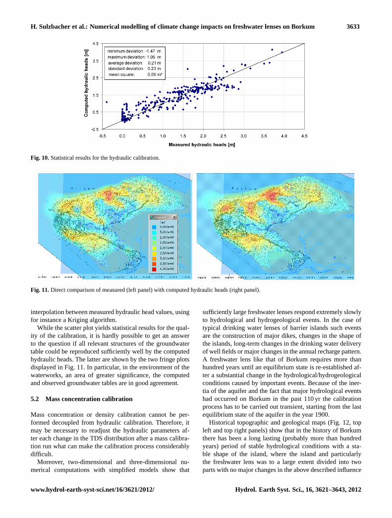
Fig. 10.Statistical results for the hydraulic calibration.

Fig. 11.Direct comparison of measured (left panel) with computed hydraulic heads (right panel).

interpolation between measured hydraulic head values, usingfor instance a Kriging algorithm.

While the scatter plot yields statistical results for the qual-ity of the calibration, it is hardly possible to get an answerto the question if all relevant structures of the groundwatertable could be reproduced sufficiently well by the computedhydraulic heads. The latter are shown by the two fringe plotsdisplayed in Fig. 11. In particular, in the environment of thewaterworks, an area of greater significance, the computedand observed groundwater tables are in good agreement.

5.2 Mass concentration calibration

Mass concentration or density calibration cannot be per-formed decoupled from hydraulic calibration. Therefore, itmay be necessary to readjust the hydraulic parameters af-ter each change in the TDS distribution after a mass calibra-tion run what can make the calibration process considerablydifficult.

Moreover, two-dimensional and three-dimensional nu-merical computations with simplified models show that

sufficiently large freshwater lenses respond extremely slowlyto hydrological and hydrogeological events. In the case oftypical drinking water lenses of barrier islands such eventsare the construction of major dikes, changes in the shape ofthe islands, long-term changes in the drinking water deliveryof well fields or major changes in the annual recharge pattern.A freshwater lens like that of Borkum requires more thanhundred years until an equilibrium state is re-established af-ter a substantial change in the hydrological/hydrogeologicalconditions caused by important events. Because of the iner-tia of the aquifer and the fact that major hydrological eventshad occurred on Borkum in the past 110 yr the calibrationprocess has to be carried out transient, starting from the lastequilibrium state of the aquifer in the year 1900.

Historical topographic and geological maps (Fig. 12, topleft and top right panels) show that in the history of Borkumthere has been a long lasting (probably more than hundredyears) period of stable hydrological conditions with a sta-ble shape of the island, where the island and particularlythe freshwater lens was to a large extent divided into twoparts with no major changes in the above described influence



Fig. 12. Inclusion of important factors of hydrological milestones of Borkum into the density calibration by construction of a historicalmodel. Top left and right panels: topographic maps of Borkum 1891 and 1925, bottom panel: historical model of Borkum for the time beforethe construction of the great south dike (1934), (bottom left panel) TDS distribution at the surface of the groundwater table, bottom rightpanel: cross-section with TDS distribution A–B through the historical model.

factors. Before WW I started operation at the beginning ofthe 20th century (Fig. 2, top panel) the freshwater lens wasin an equilibrium state.

Due to the abstraction of WW I, the fresh water lens statewas changed into a transient one. The most important hydro-logical event, however, undoubtedly occurred with the con-struction of the great south dike. The centre of the islandwas now protected from permanent flooding by sea waterand consequently the two divided freshwater lenses began todeform into a single lens. In deeper areas of the lens this pro-cess is not yet finished and the freshwater lens is still dividedinto two parts. A view down to deeper regions of the aquiferis like a view back in time (Fig. 5, top panel, Fig. 13, leftpanel). In the marshland area, however, the freshwater lensis thinned due to upconing of sea water from below by thesystem of drains and creeks. This feature is clearly visible inthe HEM results.

In 1965 WW II started operation, which had an immenseeffect on the shape of the freshwater lens. This process is notin a steady state yet.

Consequently, the calibration runs of the TDS distribu-tion have to be performed in transient state, beginning in the

year 1900 when the freshwater lens was in an equilibriumstate, and ending at the reference time in March 2010.The hydrological/hydrogeological parameters of the “undis-turbed” steady state lens at the beginning of the 20th cen-tury, previous to the commencing of the delivery of WW I,were translated into initial and boundary conditions of a so-called “historical model”. The model then runs until the timeof the dike construction in 1934, which includes the deliveryof WW I.

For the calibration period, after the dike construction, themodel was rebuilt taking into account the changed hydro-logical features at the surface of the island by adjusting thechanged initial and boundary conditions at the surface. Theseare the initial and boundary conditions for the current, al-ready hydraulically calibrated model as shown in Fig. 9.

The following steps are necessary for the TDS calibration:

1. Construction of constant mass transport boundary con-ditions from the resulting TDS distribution at the sur-face layer which has been computed in Sect. 3 usingHEM data.



45

1

Figure 13. Comparison between electrical conductivities derived from HEM data (left panel) 2

and computed by the model (right panel) at different depths below sea level. Time of 3

comparison is March 2008. 4

5

Fig. 13. Comparison between electrical conductivities derivedfrom HEM data (left panel) and computed by the model (rightpanel) at different depths below sea level. Time of comparison isMarch 2008.

2. Setup of the historical model. This means that thehead and mass transport boundary conditions of thefirst layers, in particular those of the top layer of thecurrent, already hydraulically calibrated model, have tobe adapted to the different historical hydrological con-ditions by using historical maps from the time beforethe great south dike was constructed. As no historicalrecharge data are available, recharge data of the cur-rent model (average data for the time period 1961–1990) are used. Hydraulic conductivity values for thehistorical model are also obtained from the currentmodel. The aquifer in this model is filled with sea wa-ter (TDS = 35 000 mg l−1) and the hydraulic head as-signed a value of zero. In the next step the model isrun until the equilibrium state is attained. This is pos-sible because in steady state models initial conditions

are arbitrary. Figure 12 (bottom left panel) shows den-sities for constant mass transport boundary conditionsadapted to this historical model. The lower, right sec-tion of the figure displays a cross-section through themodel in an equilibrium state. The upconing of saltwa-ter underneath the rivers Hopp and Tuskendorkill can beclearly seen.

3. Implementation of the delivery data of WW I into thehistorical steady state model and subsequent transientrun until 1934.

4. The so computed density distributions for layers 2–39are exported from the historical model and importedinto the current model. Transient calibration run of thecurrent model to the reference date March 2010 follows,including the delivery pattern of WW I and after 1965the delivery pattern of WW II (Fig. 2, top panel). Themore in the past, the more the fluctuations of the de-livery rate of the waterworks can be averaged withoutaffecting the calibration accuracy. The discretisation ofthe delivery rate and the automatic time stepping of theprogramme during the calibration of the mass concen-tration is the same as the one used for the hydraulic cal-ibration (see Sect. 5.1).

5. Comparison of computed TDS distribution with fielddata for all layers. Estimated model parameters, suchas densities, transmissivities or river leakage, have to beadjusted within the confidence intervals (steps 2–5) toget an optimum fit.

Figure 13 shows the result of the TDS calibration of thecurrent model at the time when the HEM campaign was car-ried out in March 2008. The main structures of the computedfreshwater lens (Fig. 13, right panel) match acceptably wellthe measured ones (Fig. 13, left panel). Differences mainlyresult from the fact that electromagnetic methods like HEMreveal the bulk electrical conductivity, i.e., it is difficult todistinguish between clay saturated with freshwater and sandsaturated with saltwater. These differences are described bythe apparent formation factorFa.

TDS values, inferred from WW water probes and DirectPush water samples, agree with the computed ones, in therange of acceptable calibration accuracy, taking into accountthe underlying uncertainties. This is the case for the well fieldof WW I Waterdelle as well as for all well groups of WW IIOstland. The results for WW II are presented in Fig. 14.Figure 14 (top left panel) shows a comparison of measuredTDS values from Direct Push water samples (DP 60 andDP 37) and a TDS concentration obtained from a manualdrilling (B 47a) with computed TDS values in the adjacentscreens of wells group 1 + 2 of the shallow wells of WW II.Figure 14 (bottom left panel) displays computed TDS val-ues compared with laboratory water sampling results in allscreens of WW II Ostland, well fields 3 + 4. The agreement is



DP 37DP 60B 47a

Well groups 1 + 2 shallow wells

WW II - OstlandWW II - Ostland

323134

33

35

3736

323134

33

35

3736

Well groups 3+4 deep wells

3839

40

4138

39 40

41

TDS from Direct Push and hand drilling water samples

TDS computed

layer 38 39 40 41 depth

1 3.8

2 -0.2

3 -1

4 -2

5 -3

6 -5

7 -7.5

8 -9

9 -10

10 -12.5

11 -15

12 -17.5

13 -20

14 -22.5

15 -25

Deep wells (groups 3+4) configuration of screens

aa a

well 40 a+bwell 39 a+b

well 41

TDS from laboratory water samples

TDS computed

well 38 a+b

15 -25

16 -27.5

17 -30

18 -32.5

19 -35

20 -37.5

21 -40

22 -42.5

23 -45

24 -50

25 -55

26 -60

27 -65

bb b

Fig. 14.Comparison of measured and computed TDS concentrations of WW II Ostland, top left panel: well groups 1 + 2, bottom left panel:well groups 3 + 4, top right panel: location of the well fields, (right) configuration of the well screens for well groups 3 + 4. (Depths are givenin m m.s.l.)

acceptable considering that the water samples originate fromboth screens in the upper and lower aquifer of wells no. 38–41, i.e., the analysed water is a mixture of water from theupper and the lower aquifers.

For the calibration of the TDS concentration in the envi-ronment of WW I and II, additional data of the electricalconductivity of the saturated sediments from the two verti-cal electrode chains, buried in the wells CLIWAT I and IIwere used. These data offer a high resolution in space andtime and are available at a depth between 45 and 65 m belowsurface, i.e., at the freshwater-saltwater interface. The TDSvalues of the pore water, which are computed using the nu-merical model, are transferred into electrical conductivitiesby a temperature-dependent factor (Sect. 3.2) and comparedwith HEM or electrode chain electrical conductivities of thesaturated sediments.

The comparison of the computed electrical conductivitiesof the pore water with the HEM conductivity model at thelocation of the vertical electrode chain (CLIWAT II) revealsa satisfying agreement in the range of the expected calibra-tion accuracy (Fig. 15). Best fit between HEM and computed

electric conductivity is achieved at the top slice (the water ta-ble) where a comprehensive high resolution dataset is avail-able. In particular, the apparent formation factor as definedand determined in Sect. 3.1 is known at this location (Fig. 6,top right panel). The match between calculated electric con-ductivities and those obtained by the vertical electrode chainsof CLIWAT I and II is also acceptable. Differences betweenthe smoothed HEM model, electric chain data, and computedvalues at the freshwater-saltwater interface are mainly causedby apparent formation factors. The latter vary between 1and 4 for both electrical chain and HEM conductivities,which is typical for salt- and brackish water saturated sed-iments (Repsold, 1990; Geirnaert and Vandenberghe, 1988;van Overmeeren et al., 1991; TNO-IGG, 1992). Differencesbetween HEM electrical conductivities and the computedones may also result from the fact that the nearest HEMmodel has a distance of 89 m to the CLIWAT II location.

Moreover, during drilling of the CLIWAT I and II bore-holes in September 2009 a considerable amount of low con-ductive drilling mud was pressed through the open holeinto the rock, which is still affecting the conductivity data



47

1

Figure 15. Comparison of HEM conductivities (green) and CLIWAT II vertical electrode 2

chain conductivities (black) with conductivities computed by the model (blue). 3

4

Fig. 15.Comparison of HEM conductivities (green) and CLIWAT IIvertical electrode chain conductivities (black) with conductivitiescomputed by the model (blue).

recorded by the vertical chain, especially in deeper regionsof the freshwater lens. A detailed transient analysis of thevertical chain data shows that at recording time (27 Au-gust 2010) the freshwater lens had not yet recovered fromthese disturbances. The obvious trend of increasing conduc-tivities may still last several years.

6 Simulation results

6.1 Simulations for future climate scenarios

The Norddeutsches Klimaburo provides climate change sce-narios for the German North Sea coastal area (http://www.norddeutscher-klimaatlas.de). According to this, an increasein the average annual temperature of 2.9◦C and for theannual precipitation of about 10 % (summer−5 % and win-ter +25 %) is expected until the year 2100. These values arethe possible mean change depending on results from severalregional climate calculations based on multiple emission sce-narios including the A2 scenario. Climate change effects ongroundwater recharge and discharge to streams will vary sea-sonally due to wetter winters and dryer summers.

From a groundwater perspective, rising sea level has spe-cial significance to low-lying coastal areas and to islands.The amount of local sea level rise is dependent on the pre-dicted worldwide sea level response on climate change andthe local land subsidence/uplift.

The amount of sea-level rise for the German North Seausing the IPCC scenarios has been computed by Rahm-storf (2007). According to the A2 scenario, including landsubsidence, the sea level will rise by 1 m from 1995 until2100 or 0.94 m from 2010 to the year 2100. This value is used

in our study for the simulations with the numerical model ofBorkum.

The altitude of the groundwater table was mapped and vi-sualised. Due to the enhanced annual precipitation scenarioswe used an enhanced, linearly increasing annual groundwaterrecharge of +10 % for 2100 (average scenario) and an an-nual recharge of +5 % for 2100 (conservative scenario).For the delivery rates of WW I and WW II a constantvalue of 380 000 m3 a−1 (average delivery 1934–2010) and480 000 m3 a−1 (average delivery 1971–2010) was used, re-spectively. Model computations reveal that due to the inertiaof the freshwater lens model seasonal variations of the de-livery rates are negligible. To achieve correct prognosis re-sults, the level of constant head boundary conditions repre-senting the surface of the sea water was shifted for each timestep during simulation by means of a linear function, begin-ning with 0 m in the year 2010 and ending with 0.96 in theyear 2100. Moreover, the area covered by boundary condi-tions of this type had to be extended more towards the shoreaccording to the risen mean sea level (Fig. 17, right panel).Additionally, the mass transport boundary conditions wereadapted to the full sea water concentration in areas consis-tent with the progressed mean high tide for 2100 (blue areain Fig. 17, right panel).

The simulation results show that the general shape of thegroundwater table will be affected only slightly as shown inFig. 16. Due to the enhanced recharge and the increased sealevel the groundwater table will rise until 2100 in the duneareas by about 0.4 m for the average scenario and 0.3 m forthe conservative scenario. This can be seen in the fringe plotby the colour transition from yellow to orange to red. In thedrained marshlands behind the dikes it will be nearly not af-fected (Fig. 16). But enhanced drainage is necessary and theoutflow from the open water will increase by about 50 % forboth the average and the conservative scenario.

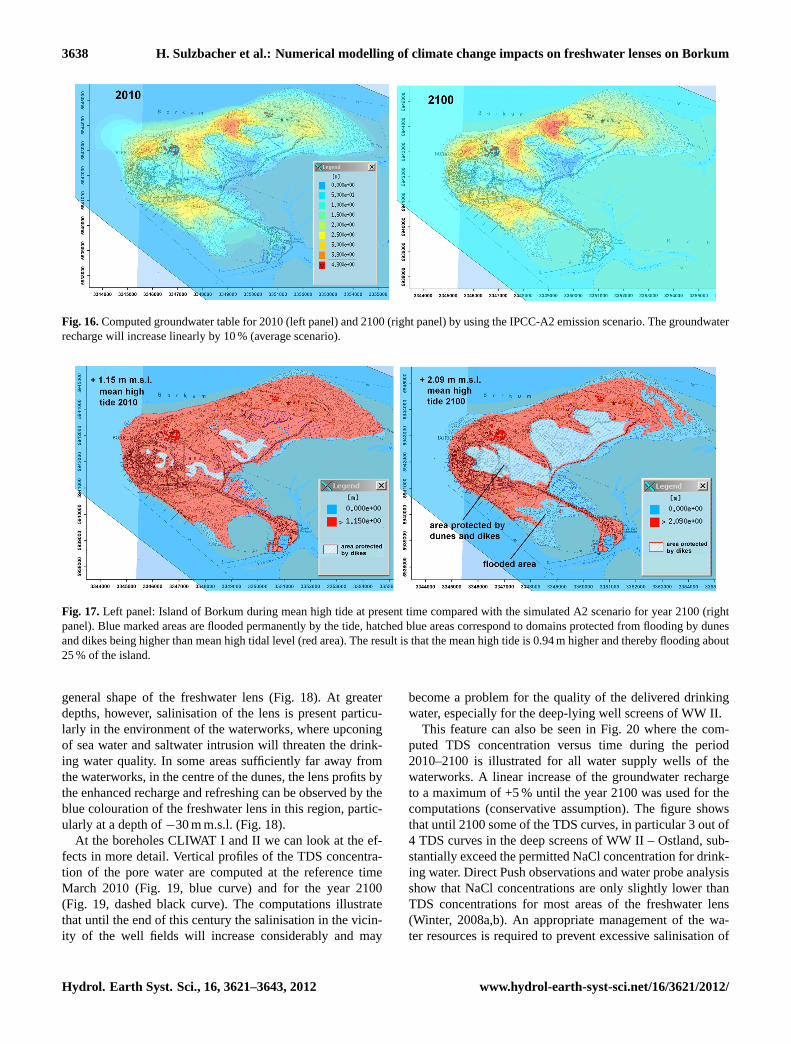
Figure 17 (left panel) shows the island during mean hightide today (2010). The sea level according to these periodicalevents amounts to +1.15 m m.s.l. Areas higher than this levelare marked red while areas below mean high tide, which areregularly flooded, are marked blue. The figure shows that atthis time only some small strips of the beaches are floodedregularly, whereas lower laying areas which are located moreinside the island (marked with hatched blue) are protectedby the south dike and the dunes. Compared to the situationin 2010, the situation in 2100 will change considerably (av-erage scenario: recharge +10 %). The result is that the meanhigh tide will rise by 0.94 m to a flooding level of 2.09 mand, thereby flooding about 25 % of the island occurs outsidethe protecting dunes and dikes (Fig. 17, right panel). Withoutprotection measures like fillings with sand or other appropri-ate material large parts of the low-lying natural reserves andbeaches in the south and north east regions of the island willbe covered by the Wadden Sea.

The model results for the year 2100 in terms of TDS showthat sea-level rise until 2100 will not affect essentially the


http://www.norddeutscher-klimaatlas.de

http://www.norddeutscher-klimaatlas.de


Fig. 16.Computed groundwater table for 2010 (left panel) and 2100 (right panel) by using the IPCC-A2 emission scenario. The groundwaterrecharge will increase linearly by 10 % (average scenario).

Fig. 17.Left panel: Island of Borkum during mean high tide at present time compared with the simulated A2 scenario for year 2100 (rightpanel). Blue marked areas are flooded permanently by the tide, hatched blue areas correspond to domains protected from flooding by dunesand dikes being higher than mean high tidal level (red area). The result is that the mean high tide is 0.94 m higher and thereby flooding about25 % of the island.

general shape of the freshwater lens (Fig. 18). At greaterdepths, however, salinisation of the lens is present particu-larly in the environment of the waterworks, where upconingof sea water and saltwater intrusion will threaten the drink-ing water quality. In some areas sufficiently far away fromthe waterworks, in the centre of the dunes, the lens profits bythe enhanced recharge and refreshing can be observed by theblue colouration of the freshwater lens in this region, partic-ularly at a depth of−30 m m.s.l. (Fig. 18).

At the boreholes CLIWAT I and II we can look at the ef-fects in more detail. Vertical profiles of the TDS concentra-tion of the pore water are computed at the reference timeMarch 2010 (Fig. 19, blue curve) and for the year 2100(Fig. 19, dashed black curve). The computations illustratethat until the end of this century the salinisation in the vicin-ity of the well fields will increase considerably and may

become a problem for the quality of the delivered drinkingwater, especially for the deep-lying well screens of WW II.

This feature can also be seen in Fig. 20 where the com-puted TDS concentration versus time during the period2010–2100 is illustrated for all water supply wells of thewaterworks. A linear increase of the groundwater rechargeto a maximum of +5 % until the year 2100 was used for thecomputations (conservative assumption). The figure showsthat until 2100 some of the TDS curves, in particular 3 out of4 TDS curves in the deep screens of WW II – Ostland, sub-stantially exceed the permitted NaCl concentration for drink-ing water. Direct Push observations and water probe analysisshow that NaCl concentrations are only slightly lower thanTDS concentrations for most areas of the freshwater lens(Winter, 2008a,b). An appropriate management of the wa-ter resources is required to prevent excessive salinisation of



Fig. 18.Computed freshwater lens in 2010 (left panel) and 2100 (right panel).

the drinking water resources and deterioration of the ground-water chemical status according to the EU GroundwaterDirective.

6.2 Possible solutions for the future

On Borkum protection measures are necessary to preventthe water supply from excessive salinisation caused by over-exploitation and sea level rise. Utilising the density depen-dent groundwater flow model the location of the respectivewater supply wells in the waterworks can be optimised toprevent exceeding salinisation beyond the permitted limits.For the case of EU member states this includes not onlythe EU drinking water standards, but also properly derivedgroundwater threshold values according to the EU WaterFramework and Groundwater directives (Hinsby et al., 2008;Wendland et al., 2008).

Figure 21 (left panel) shows the supply wells of WW I(top) and WW II (below) (red circles) together with the TDS

distribution computed for 2100 at depths of the waterworksscreens. Possible locations for new wells which could re-lieve the waterwork and prevent the wells field from upcon-ing of saltwater are marked blue and are located at positionswhere sufficient water quality can be expected for 2100.Wells which should be closed because of excessive salinisa-tion until 2100 are marked brown. The computed TDS curvesfor all water supply wells (Fig. 21, right panel) demonstratethat solutions for the well field configuration can be found tokeep water quality below the required limit for NaCl concen-tration. In this way it is possible to maintain drinking waterquality without being forced to reduce the amount of extrac-tion for more than 100 yr. Numerical simulations can help tofind adequate locations for possible new wells.

In regards to the certainty of these results the evolutionof the future recharge is a sensitive key parameter estimatedonly from precipitation, which implies much insecurity. Tosee how certain the computed density distribution for thenew well configuration is, additional sea-level rise scenarios



51

1

Figure 19. Spatiotemporal evolution of the vertical mass concentration (TDS) for the years 2

2010 and 2100 at the wells CLIWAT I and II. The concentrations are computed using the 3

groundwater model. 4

5

Fig. 19.Spatiotemporal evolution of the vertical mass concentration (TDS) for the years 2010 and 2100 at the wells CLIWAT I and II. Theconcentrations are computed using the groundwater model.

52

1

Figure 20. TDS concentration [mg/l] computed in the screen of the water supply wells of WW 2

I Waterdelle (top left panel) and WW II Ostland (below left panel). In the right part of the 3

figure location maps of the well fields are presented. 4

5

Fig. 20. TDS concentration [mg l−1] computed in the screen of the water supply wells of WW I Waterdelle (top left panel) and WW IIOstland (below left panel). In the right part of the figure location maps of the well fields are presented.



53

1

Figure 21. Spreading of well fields as protection measure from excessive salinization of the 2

water supply. Location of old wells, new wells and closed wells (left panel), development of 3

TDS concentration in the supply wells with time (right). WW I Waterdelle (top panel), WW II 4

Ostland (below panel). 5

6

Fig. 21.Spreading of well fields as protection measure from excessive salinisation of the water supply. Location of old wells, new wells andclosed wells (left panel); the deep screens of WW II (Fig. 14, bottom right panel) were also closed. Development of TDS concentration inthe supply wells with time (right panel). WW I Waterdelle (top panel), WW II Ostland (below panel).

with different recharge rates from 2010 until 2100 (extremelydry scenario with no recharge increase, average scenariowith linear recharge increase of 0–10 % and linear increaseof recharge 0–15 %, wet scenario) were simulated. Modelresults show that for all these scenarios the obtained wellconfigurations for both water works (Fig. 21) are valid andthe salinisation of the drinking water for all delivery wellsremains below the permitted limit.

The topography of low-lying areas predominantly locatedin the south and northeast of the island and endangered byflooding under an increased sea level (Fig. 17) should beadapted to the rising sea level by sand fillings as it has beenalready carried out successfully on other barrier islands likeSylt.

The North Sea region, in particular the German Bight,can be a target of heavy storm flood events. Under extremeweather conditions and an enhanced sea level of 1 m, stormfloods can attain altitudes in the order of 4 m m.s.l. (one-in-50-yr event). It is clear that protection measures are neces-sary. The altitudes of the dikes have to be controlled and

adapted where required. Moreover, dune valleys potentiallybeing gateways for the flood have to be banked up with ap-propriate material such as sand to maintain their protectivefunction.

7 Summary and conclusions

We developed a density dependent groundwater flow modelfor the North Sea Island of Borkum. The model was success-fully calibrated on the basis of hydrological and geophysi-cal data. Verification runs of the calibrated model with thedata obtained from field work show a good agreement for themeasured and computed hydraulic heads as well as for themeasured and computed density distributions.

The integration of large-scale HEM data covering the en-tire model area and electrical conductivity data obtained fromvertical electrode chains CLIWAT I and II on a local scale hasproven to be very valuable for a reliable model calibration.Moreover, the integration of these geophysical data providesa better understanding of the hydrological processes involvedin the spatiotemporal evolution of the islands freshwater lens.



These processes have to be taken into consideration for thetransient model calibration.

The thoroughly calibrated groundwater flow model is ca-pable of predicting the spatial and temporal development ofparameters like hydraulic heads, electrical conductivity andsalinity under changing climate conditions and sea level.

Of particular interest will be the development of the fu-ture concentrations of total dissolved solids in the delivereddrinking water from the waterworks supply wells. Modellingresults obtained in this study demonstrate the progressingsalinisation of the groundwater along the vertical profilesof the two CLIWAT boreholes beneath the waterworks withtime until the year 2100. This NaCl concentration of the ex-tracted water could become a serious problem for the drink-ing water supply, and the groundwater chemical status. Effec-tive measures will be necessary to properly tackle this severeproblem in order to ensure good drinking water quality andcomply with the requirements of EU directives.

The results provide an important input and a strong toolfor current and future quantitative and chemical status as-sessments of groundwater according to the Water FrameworkDirective and Groundwater Directive, as well as for the plan-ning of strategies for flood defence. The results will also beaccompanied with guidelines and recommendations for themanagement of the water supply and the protection of thegroundwater resources.

Our approach is essentially consistent with the recommen-dations towards best practice for assessing the impacts of cli-mate change on groundwater given by Holman et al. (2012)and for the application of, e.g., electromagnetic measure-ments in model calibration (Carrera et al., 2010).

Based on modelling results, the groundwater resources inBorkum must be protected to meet the current and future de-mands for domestic water.

The need to progressively adapt to the predicted climatechanges is urgent. This modelling study and other results ofthe CLIWAT project (de Louw et al., 2011; Oude Essink etal., 2010) provide a robust basis on which future adaptationscan be made.

The results of the model analysis are also applicable toother typical barrier island of the North Sea Region, espe-cially the East Frisian Islands.

Acknowledgements.CLIWAT is co-financed by the EuropeanUnion under the Interreg IVB North Sea Region Programme(project ID 35-2-1-08). We thank the engineering office Hydroge-ology Sebastian Winter and the water supplier “Wirtschaftsbetriebeder Stadt Nordseeheilbad Borkum Stadtwerke Borkum GmbH”(Axel Held) for data supply and extensive support during fieldwork. The drilling data were provided by the “Landesamt furBergbau, Energie und Geologie (LBEG)” in Hannover. Last notleast we thank the anonymous referees for their thorough review ofthis work.

Edited by: P. de Louw

References

Agmon, S., Douglis, A., and Nirenberg, L.: Estimates near theboundary for solutions of elliptic partial differential equationssatisfying general boundary conditions, Comm. Pure Appl.Math., 12, 623–727,doi:10.1002/cpa.3160120405, 1959.

Bear, J., Cheng, A. H.-D., Sorek, S., Ouazar, D., and Herrera,I. (Eds.): Seawater Intrusion in Coastal Aquifers – Concepts,Methods and Practices, Kluwer Academic Publishers, 1999.

Behre, K.-E.: (Landschaftsgeschichte Norddeutschlands,Wachholtz-Verlag, Neumunster, 2008.

BSH Bundesamt fur Seeschifffahrt und Hydrographie:Meeresoberflachentemperatur, http://www.bsh.de/de/Meeresdaten/Beobachtungen/Meeresoberflaechentemperatur/anom.jsp#SSTM(last access: 7 March 2012), 2009.

Carrera, J., Hidalgo, J. J., Slooten, L. J., and Vazquez-Sune, E.:Computational and conceptual issues in the calibration of seawa-ter intrusion models RID E-7251-2011, Hydrogeol. J., 18, 131–145, 2010.

Cooper Jr., H. H., Kohout, F. A., Henry, H. R., and Glover, R. E.:Sea water in coastal aquifers, US Geol. Survey Water-Supply Pa-per 1613 C, Washington, 1964.

de Louw, P. G. B., Eeman, S., Siemon, B., Voortman, B. R., Gun-nink, J., van Baaren, E. S., and Oude Essink, G. H. P.: Shal-low rainwater lenses in deltaic areas with saline seepage, Hy-drol. Earth Syst. Sci., 15, 3659–3678,doi:10.5194/hess-15-3659-2011, 2011.

DHI Wasy GmbH, http://www.feflow.info/uploads/media/whitepapersvol1 01.pdf(last access: 8 October 2012), 2009.

Fein, E., Krohn, K. P., Noseck, U., and Schneider, A.: Modelling offield-scale pollutant transport, Final Report, Ges. fur Anlagen-und Reaktorsicherheit, GRS, Braunschweig, 2008.

Geirnaert, W. and Vandenberghe, J.: Applied Geophysics forGroundwater Exploration and Geological Mapping, Instituutvoor Aardwetenschappen, Vrije Universiteit, Amsterdam, 1988.

Grinat, M., Sudekum, W., Epping, D., Grelle, T., and Meyer, R.:An automated electrical resistivity tomography system to moni-tor the freshwater/saltwater zone on a North Sea Island, Ext. Ab-str., A20, Near Surface Geoscience Division of EAGE, Zurich,2010.

Gunther, T. and Muller-Petke, M.: Hydraulic properties at theNorth Sea island of Borkum derived from joint inversion ofmagnetic resonance and electrical resistivity soundings, Hy-drol. Earth Syst. Sci., 16, 3279–3291,doi:10.5194/hess-16-3279-2012, 2012.

Herzberg, B.: Die Wasserversorgung einiger Nordseebader, J. Gas-bel. Wasservers., 44, 815–819, 1901.

Heyen, H. and Dippner, J. W.: Salinity variability in the GermanBight in relation to climate variability, Tellus A, 50, 545–556,1998.

Hinsby, K., Bjerg, P. L., Andersen, L. K., Skov, B., and Clausen, E.V.: A mini slug test method for determination of a local hydraulicconductivity of an unconfined sandy aquifer, Journal of Hydrol-ogy, Elsevier Science Publishers B.V., Amsterdam, 36, 87–106,1992.

Hinsby, K., de Melo, M. T. C., and Dahl, M.: European case stud-ies supporting the derivation of natural background levels andgroundwater threshold values for the protection of dependentecosystems and human health RID C-1806-2008, Sci. Total En-viron., 401, 1–20, 2008.


http://dx.doi.org/10.1002/cpa.3160120405

http://www.bsh.de/de/Meeresdaten/Beobachtungen/Meeresoberflaechentemperatur/anom.jsp#SSTM



http://dx.doi.org/10.5194/hess-15-3659-2011


http://www.feflow.info/uploads/media/white_papers_vol1_01.pdf

http://www.feflow.info/uploads/media/white_papers_vol1_01.pdf




Holman, I. P., Allen, D. M., Cuthbert, M. O., and Goderniaux, P.:Towards best practice for assessing the impacts of climate changeon groundwater, Hydrogeol. J., 20, 1–4, 2012.

Holzbecher, E.: Modeling density-driven flow in porous media: ba-sics, numerics, software, Springer Verlag, Berlin, Heidelberg,New York, 1998.

Igel, J., Gunther, T., and Kuntzer, M.: Ground-penetrating radarinsight into a coastal aquifer: the freshwater lens of BorkumIsland, Hydrol. Earth Syst. Sci. Discuss., 9, 3691–3720,doi:10.5194/hessd-9-3691-2012, 2012.

IPCC: Synthesis Report, Summary for Policymakers. Assessmentof Working Groups I, II, and III to the Fourth Assessment Reportof the IPCC, Cambridge University Press, New York, NY, USA,2007.

Katsube, T. J., Issler, D. R., Loman, J., and Cox, W. C.: Apparentformation-factor and porosity variation with pressure for Creta-ceous shale of the Western Canada Sedimentary Basin, south-ern Alberta, Current Research 2000-E6, Geological Survey ofCanada, Natural Resources Canada, Ottawa, 2000.

Krawczyk, C. M., Polom, U., Trabs, S., and Dahm, T.: Sink-holes in the city of Hamburg – New urban shear-wavereflection seismic system enables high-resolution imagingof subrosion structures, J. Appl. Geophys., 78, 133–143,doi:10.1016/j.jappgeo.2011.02.003, 2012.

Kinzelbach, W. K. H.: Methods for simulation of pollutant trans-port in ground water, A model comparison, in: Proc. SolvingGround Water Problems With Models, Conference and Exposi-tion, Vol. 1, Denver, Colorado, USA, 656–675, 1987.

Lee, C. H. and Cheng, R. T. S.: On seawater encroachment in coastalaquifers, Water Resour. Res., 10, 1039–1043, 1974.

Oude Essink, G. H. P., van Baaren, E. S., and de Louw, P. G. B.: Ef-fects of climate change on coastal groundwater systems: A mod-eling study in the Netherlands, Water Resour. Res., 46, W00F04,doi:10.1029/2009WR008719, 2010.

Petersen, J., Pott, R., Janiesch, P., and Wolff, J. (Eds.):Umweltvertragliche Grundwasserbewirtschaftung inhydrogeologisch undokologisch sensiblen Bereichen derNordseekuste, Husum Druck- und Verlagsgesellschaft, Husum,Germany, 2003.

Polom, U., Druivenga, G., Großmann, E., Gruneberg, S., and Rode,W.: (in German) Transportabler Scherwellenvibrator, DPMAPatentschrift DE10327757B4, DPMA Munchen, 26 May 2011.

Post, V. E. A.: Fresh and saline groundwater interaction in coastalaquifers: Is our technology ready for the problems ahead, Hydro-geol. J., 13, 120–123,doi:10.1007/s10040-004-0417-2, 2005.

Post, V. E. A. and Abarca, E.: Preface: Saltwater and freshwa-ter interactions in coastal aquifers, Hydrogeol. J., 18, 1–14,doi:10.1007/s10040-009-0561-9, 2010.

Rahmstorf, S.: A Semi-Empirical Approach to Project-ing Future Sea-Level Rise, Science, 315, 368–370,doi:10.1126/science.1135456, 2007.

Rasmussen, P., Sonnenborg, T. O., Goncear, G., and Hinsby, K.: As-sessing impacts of climate change, sea level rise, and drainagecanals on saltwater intrusion to coastal aquifer, Hydrol. EarthSyst. Sci. Discuss., 9, 7969–8026,doi:10.5194/hessd-9-7969-2012, 2012.

Repsold, H.: Geoelektrische Untersuchungen zur Bestimmung derSußwasser-/Salzwasser-Grenze im Gebiet zwischen Cuxhavenund Stade, Geologisches Jahrbuch Reihe C, Heft 56, Hannover,1990.

Siemon, B., Ibs-von Seht, M., Meyer, U., Pielawa, J., Steuer, A.,Voß, W., and Wiederhold, H.: Technischer Bericht zur Befliegungder Insel Borkum Marz 2008, Technical Report, BGR archivesno. 0128656, Hannover, 2009a.

Siemon, B., Christiansen, A. V., and Auken, E.: A review ofhelicopter-borne electromagnetic methods for groundwater ex-ploration, Near Surf. Geophys., 7, 629–646, 2009b.

Streif, H.: Das ostfriesische Kustengebiet, 2. Auflage,Gebr. Borntrager, Berlin, Stuttgart, 1990.

Sudekum, W., Grinat, M., Winter, S., Epping, D., Grelle, T., andMeyer, R.: Vertikale Elektrodenstrecken zur Erkundung vonAnderungen im Salz-Sußwasser-Ubergangsbereich auf Borkum,bbr Fachmagazin fur Brunnen und Leitungsbau, Bonn, 12, 68–71, 2009.

Sulzbacher, H.: Technical report on Field Work in CLIWAT Area DBorkum, Technical Report 2009–2010, Technical Report, LIAG,Hannover 2011.

Thorenz, C.: Model adaptive simulation of multiphase and densitydriven flow in fractured and porous media. Dissertation, Institutfur Stromungsmechanik Universitat Hannover, 2001.

TNO-IGG: Introduction to geophysical well logs, a practical coursefor groundwater studies, TNO Instituut voor Grondwater en Geo-Energie, Delft, 1992.

van Overmeeren, R. A., Mulder, M. H., and Meekes, J. A. C.: Com-puter aided analysis and interpretation of geophysical data, Di-enst Grondwaterverkenning TNO, Delft, 1991.

Voss, C.: Editor’s message: Groundwater modeling fantasies –part 1, a drift in the details, Hydrogeol. J., 19, 1281–1284, 2011a.

Voss, C.: Editor’s message: Groundwater modeling fantasies –part 2, down to earth, Hydrogeol. J., 19, 1455–1458, 2011b.

Wendland, F., Berthold, G., Blum, A., Elsass, P., Fritsche, J.,Kunkel, R., and Wolter, R.: Derivation of natural backgroundlevels and threshold values for groundwater bodies in the UpperRhine Valley (France, Switzerland and Germany) RID C-4939-2008 RID C-4934-2008, Desalination, 226, 160–168, 2008.

Winter, S.: Erkundung und Bewertung von Grundwasserbelastun-gen im Bereich der Sußwasserlinsen Borkum, HydrogeologieSebastian Winter, Ingenieurburo fur Hydrologie, Sedimentologieund Wasserwirtschaft, Leer, 2008a.

Winter, S.: Erkundung und Bewertung von Grundwasserbelas-tungen im Bereich der Sußwasserlinsen Borkum – TeilprojektDirect-Push-Sondierung – Ergebnisbericht, Hydrogeologie Se-bastian Winter, Ingenieurburo fur Hydrologie, Sedimentologieund Wasserwirtschaft, Leer, 2008b.

Winter, S.: Hydraulische Tests an den Tiefbrunnen 38 und 40des Ostlandes – Ergebnisbericht, Hydrogeologie Sebastian Win-ter, Ingenieurburo fur Hydrologie, Sedimentologie und Wasser-wirtschaft, Leer, 2009.


http://dx.doi.org/10.5194/hessd-9-3691-2012

http://dx.doi.org/10.1016/j.jappgeo.2011.02.003

http://dx.doi.org/10.1029/2009WR008719

http://dx.doi.org/10.1007/s10040-004-0417-2

http://dx.doi.org/10.1007/s10040-009-0561-9

http://dx.doi.org/10.1126/science.1135456



Numerical modelling of climate change impacts on freshwater lenses on the North Sea Island of Borkum...

Documents

Transcript of Numerical modelling of climate change impacts on freshwater lenses on the North Sea Island of Borkum...