numerical investigation of ecbm recovery and co2 ...
101
NUMERICAL INVESTIGATION OF ECBM RECOVERY AND CO 2 SEQUESTRATION A THESIS SUBMITTED TO THE GRADUATE SCHOOL OF APPLIED SCIENCES OF NEAR EAST UNIVERSITY By SAMUEL ADAMU ABUBAKAR In Partial Fulfilment of the Requirements for the Degree of Master of Science in Petroleum and Natural Gas Engineering NICOSIA, 2021 SAMUEL ADAMU ABUBAKAR NUMERICAL INVESTIGATION OF ECBM RECOVERY AND CO 2 SEQUESTRATION NEU 20 2 1
-
Upload
khangminh22 -
Category
Documents
-
view
3 -
download
0
Transcript of numerical investigation of ecbm recovery and co2 ...
NUMERICAL INVESTIGATION OF ECBM
RECOVERY AND CO2 SEQUESTRATION
A THESIS SUBMITTED TO THE GRADUATE
SCHOOL OF APPLIED SCIENCES
OF
NEAR EAST UNIVERSITY
By
SAMUEL ADAMU ABUBAKAR
In Partial Fulfilment of the Requirements for
the Degree of Master of Science
in
Petroleum and Natural Gas Engineering
NICOSIA, 2021
SA
MU
EL
AD
AM
U
AB
UB
AK
AR
NU
ME
RIC
AL
INV
ES
TIG
AT
ION
OF
EC
BM
RE
CO
VE
RY
AN
D C
O2 S
EQ
UE
ST
RA
TIO
N
NE
U
2021
NUMERICAL INVESTIGATION OF ECBM
RECOVERY AND CO2 SEQUESTRATION
A THESIS SUBMITTED TO THE GRADUATE
SCHOOL OF APPLIED SCIENCES
OF
NEAR EAST UNIVERSITY
By
SAMUEL ADAMU ABUBAKAR
In Partial Fulfilment of the Requirements for
the Degree of Master of Science
in
Petroleum and Natural Gas Engineering
NICOSIA, 2021
Samuel Adamu ABUBAKAR: NUMERICAL INVESTIGATION OF ECBM
RECOVERY AND CO2 SEQUESTRATION
Approval of Director of Institute of
Graduate Studies
Prof. Dr. K. Hüsnü Can BAŞER
We certify that this thesis is satisfactory for the award of the degree of Masters of
Science in Petroleum and Natural Gas Engineering
Examining Committee in Charge:
Prof. Dr. Cavit ATALAR Committee Chairman, Department of Petroleum
and Natural Gas Engineering, NEU
Assoc. Prof. Dr. Kamil DİMİLİLER Automotive Engineering Department, NEU
Assist. Prof. Dr. Serhat CANBOLAT Supervisor, Department of Petroleum and Natural
Gas Engineering, NEU

I hereby declare that all information in this document has been obtained and presented in
accordance with academic rules and ethical conduct. I also declare that, as required by these
rules and conduct, I have fully cited and referenced all material and results that are not
original to this work.
Name, Last name: Samuel Adamu ABUBAKAR
Signature:
Date: 29/06/2021

ii
ACKNOWLEDGEMENTS
First and foremost, I want to thank my supervisor, Assist. Prof. Dr. Serhat CANBOLAT, for
teaching, guiding and helping me in every step of the way, without his help I would not have
been able to complete this thesis. Secondly, I want to thank Prof. Dr. Cavit ATALAR, the
head of the department of Petroleum and Natural Gas Engineering, NEU for being like a
father to me throughout my undergraduate and master’s degree. I also thank
Assoc.Prof.Dr.Kamil DIMILILER for his support throughout my thesis.
I also want to extend my appreciation to the other lecturers present in my thesis seminar:
Prof. Dr. Salih SANER and Dr. Yashar OSGOUEI. Their revisions were key in shaping and
correcting this thesis.
Finally, I want to thank my parents, Mr. and Mrs. Abubakar ADAMU, for their constant
support, love and encouragement when I was about to give up.

iii
To my Family…
iv
ABSTRACT
The need for unconventional hydrocarbon resources such as Coal Bed Methane (CBM),
shale gas/oil, tight sand gas and gas hydrates in recent times cannot be overemphasized.
Depleting amounts of conventional resources with simultaneous increasing energy demand
necessitates a thorough look into these unconventional resources in an effort to produce them
economically and in considerable amounts. In an attempt at finding ways to deploy properly
unconventional resources, this thesis will be focused on the development of CBM.
This thesis aims to discuss the mechanisms involved in CBM and CO2-ECBM (enhanced
coal bed methane) production and by performing simulations using CMG GEM, compare
the results from both of these to find the best method of producing from CBM as well as
finding out the best well orientation/configuration. The characteristics of the Onyeama
coalbed field in Enugu, Nigeria was used to create ten scenarios to make these comparisons.
These scenarios each had different arrangements and numbers for the producer and injector
wells and therefore had different results.
It was seen from the simulation that it is possible to produce a lot of methane while
sequestering large volumes of carbon dioxide. Analysing the amount of methane that could
be produced and the amount of carbon that could be sequestered showed that the tenth
scenario performed the best in terms of both. However, the economical analysis showed that
the third scenario was the most profitable. The effect of pressure on the performance of
CBM/ECBM processes was also investigated.
Keywords: CBM; ECBM; carbondioxide sequestration; CMG GEM; coal; economical
analysis
v
ÖZET
Son zamanlarda Kömür Yatağı Metanı (KYM), kaya gazı / petrol, sıkı kum gazı ve gaz
hidratları gibi geleneksel olmayan hidrokarbon kaynaklarına duyulan ihtiyaç fazlasıyla
artmıştır. Aynı anda artan enerji talebiyle geleneksel kaynakların miktarlarının tükenmesi,
ekonomik ve önemli miktarlarda üretme çabası içinde bu konvansiyonel olmayan
kaynakların kapsamlı bir şekilde incelenmesini gerektirir. Geleneksel (konvansiyonel)
olmayan kaynakları uygun şekilde bularak üretim yollarını araştıran bu tezde KYM'nın
geliştirilmesine odaklanılacaktır.
Bu tez, KYM ve CO2-GKYM (geliştirilmiş kömür yatağı metanı) üretiminde yer alan
mekanizmaları tartışmayı ve CMG GEM programı kullanarak oluşturulan saha modeli
kesitiyle simülasyonlar gerçekleştirerek, KYM'dan en iyi üretim yöntemini ve aynı zamanda
en iyi kuyu yönlendirmesini / konfigürasyonunu bularak, bunların sonuçlarını
karşılaştırmayı amaçlamaktadır. Nijerya Enugu'da bulunan Onyeama kömür yatağının
özellikleri, bu karşılaştırmaları yapmak için on değişik senaryo için kullanıldı. Bu
senaryoların her biri, üretim ve enjeksiyon kuyuları için farklı düzenlemelere ve sayılara
sahip olduğundan farklı sonuçlara ulaşıldı.
Simülasyonlarda, bu farklı senaryolarda büyük miktarlarda karbondioksit tutulurken çok
fazla metan üretmenin de mümkün olduğu görüldü. Üretilebilecek metan ve depolanacak
karbondioksit miktarının analizi, onuncu senaryoda en iyi performansın elde edildiğini
gösterdi. Fakat, ekonomik analizden sonra, üçüncü senaryonun aslında en karlı olduğu
ortaya çıktı. KYM / GKYM süreçlerinin performansı üzerindeki basınç etkisi de araştırıldı.
Anahtar Kelimeler: KYM; GKYM; karbondioksit depolaması; CMG GEM; kömür;
ekonomik analiz
vi
TABLE OF CONTENTS
ACKNOWLEDGEMENTS .......................................................................................... ii
ABSTRACT ................................................................................................................... iv
ÖZET.......... .................................................................................................................... v
TABLE OF CONTENTS .............................................................................................. vi
LIST OF TABLES ......................................................................................................... ix
LIST OF FIGURES ....................................................................................................... x
LIST OF SYMBOLS AND ABBREVIATIONS ........................................................ xiii
CHAPTER 1: INTRODUCTION
1.1. Background .............................................................................................................. 1
1.2. Thesis Problem ......................................................................................................... 2
1.3. Aim and Importance of the Study ............................................................................ 2
1.4. Hypothesis ................................................................................................................ 3
1.5. Structure of the Thesis .............................................................................................. 3
1.6. Limitations of the Research ...................................................................................... 4
CHAPTER 2: LITERATURE REVIEW
2.1. Coal as an Energy Source ......................................................................................... 5
2.2. Coal Bed Methane (CBM) ....................................................................................... 9
2.3. Enhanced Coal Bed Methane (ECBM) .................................................................. 18
2.3.1. Carbon dioxide enhanced coal bed methane (CO2-ECBM) ...................... 19
2.3.2. Nitrogen enhanced coal bed methane (N2-ECBM) ................................... 22
2.3.3. Carbon dioxide-nitrogen hybrid enhanced coal bed methane............ .........
(CO2-N2-ECBM) ....................................................................................... 22
2.4. Case Study of the Onyeama Coalbed Field ............................................................ 24
vii
CHAPTER 3: METHODOLOGY
3.1. Scenario 1 ............................................................................................................... 33
3.2. Scenario 2 ............................................................................................................... 34
3.3. Scenario 3 ............................................................................................................... 34
3.4. Scenario 4 ............................................................................................................... 35
3.5. Scenario 5 ............................................................................................................... 36
3.6. Scenario 6 ............................................................................................................... 38
3.7. Scenario 7 ............................................................................................................... 38
3.8. Scenario 8 ............................................................................................................... 39
3.9. Scenario 9 ............................................................................................................... 39
3.10. Scenario 10 ........................................................................................................... 39
CHAPTER 4: RESULTS AND DISCUSSIONS
4.1. Effect of Pressure on CBM .................................................................................... 41
4.2. Best Scenario for Gas Production and Carbon Sequestration ................................ 43
CHAPTER 5: ECONOMICAL ANALYSIS
CHAPTER 6: CONCLUSIONS AND RECOMMENDATIONS
6.1. Conclusions ............................................................................................................ 63
6.2. Recommendations .................................................................................................. 64
REFERENCES ............................................................................................................ 65
APPENDICES
Appendix 1: CMG Data File For Scenario 10 ............................................................... 75

viii
Appendix 2: Similarity Report ...................................................................................... 84
Appendix 3: Ethical Approval Letter ............................................................................ 85

ix
LIST OF TABLES
Table 2.1: Carbon content for different coal rank .......................................................... 7
Table 3.1: Reservoir model parameters .......................................................................... 32
Table 4.1: Result summary of best scenario for Onyeama CBM development ............. 55
Table 4.2: Scaling the model to field .............................................................................. 56
Table 5.1: Variables used in economical analysis .......................................................... 60
Table 5.2: Result of economic analysis .......................................................................... 61
x
LIST OF FIGURES
Figure 2.1: Conventional and unconventional hydrocarbon resources ............................ 5
Figure 2.2: Relationship between coalition conditions and rank of coal formed ............. 7
Figure 2.3: Pressure gradient and its influence on water and gas production .................. 11
Figure 2.4: Flow process of CO2 and CH4 in coal seams ................................................. 19
Figure 2.5: Optimization of ECBM recovery through combination of CO2-ECBM...........
and N2-ECBM ............................................................................................. 23
Figure 2.6: Comparison of methane production rates with different ........................
CO2-N2-ECBM combinations ..................................................................... 24
Figure 2.7: Map showing the location of the Onyeama coal field .................................. 25
Figure 2.8: Detailed map of the Onyeama field location ................................................ 26
Figure 3.1: 3D view of the reservoir model .................................................................... 28
Figure 3.2: Matrix porosity of the reservoir model ......................................................... 28
Figure 3.3: Fracture porosity of the reservoir model ....................................................... 29
Figure 3.4: Matrix permeability of the reservoir model .................................................. 29
Figure 3.5: Horizontal Fracture permeability of the reservoir model ............................. 30
Figure 3.6: Matrix water saturation of the reservoir model............................................. 30
Figure 3.7: Fracture water saturation of the reservoir model .......................................... 31
Figure 3.8: Top view of reservoir model for scenario1 ................................................... 33
Figure 3.9: Top view of reservoir model for scenario 2 .................................................. 34
Figure 3.10: Top view of reservoir model for scenario 3 ................................................ 35
Figure 3.11: Top view of reservoir model for scenario 4 ................................................ 36
Figure 3.12: Top view of reservoir model for scenario 5 ................................................ 37
Figure 3.13: Top view of reservoir model for scenario 6 ................................................ 37
Figure 3.14: Top view of reservoir model for scenario 7 ................................................ 38
Figure 3.15: Top view of reservoir model for scenario 8 ................................................ 39
Figure 3.16: Top view of reservoir model for scenario 9 ................................................ 40
Figure 3.17: Top view of reservoir model for scenario 10 .............................................. 40
Figure 4.1: Pressure at the middle of the reservoir for high, low and medium..............
pressure conditions ...................................................................................... 42
xi
Figure 4.2: Cumulative gas produced for high, low and medium pressure ..................
conditions .................................................................................................... 42
Figure 4.3: Amount of methane adsorbed to coal for high, low and medium...............
pressure conditions ...................................................................................... 43
Figure 4.4: Cumulative gas production with time ........................................................... 44
Figure 4.5: Cumulative amount of methane produced .................................................... 44
Figure 4.6: Cumulative carbon dioxide injected with time ............................................. 46
Figure 4.7: Amount of adsorbed methane at the beginning of the simulation life .......... 47
Figure 4.8: Amount of adsorbed methane at the end of the simulation life for.............
scenario 1 .................................................................................................... 47
Figure 4.9: Amount of adsorbed methane at the end of the simulation life for ...........
scenario 2 .................................................................................................... 48
Figure 4.10: Amount of adsorbed methane at the end of the simulation life for .................
scenario 3 .................................................................................................... 48
Figure 4.11: Amount of adsorbed carbon dioxide at the end of the simulation...................
life for scenario 3 ........................................................................................ 49
Figure 4.12: Amount of adsorbed methane at the end of the simulation life for.......................
scenario 4 .................................................................................................... 49
Figure 4.13: Amount of adsorbed carbon dioxide at the end of the simulation.....................
life for scenario 4 ........................................................................................ 50
Figure 4.14: Amount of adsorbed methane at the end of the simulation life for .............
scenario 5 .................................................................................................... 50
Figure 4.15: Amount of adsorbed methane at the end of the simulation life for ..............
scenario 6 ................................................................................................... 51
Figure 4.16: Amount of adsorbed methane at the end of the simulation life for ....................
scenario 7 ................................................................................................... 51
Figure 4.17: Amount of adsorbed carbon dioxide at the end of the simulation....................
life for scenario 7 ........................................................................................ 52
Figure 4.18: Amount of adsorbed methane at the end of the simulation life for .....................
scenario 8 .................................................................................................... 52
Figure 4.19: Amount of adsorbed carbon dioxide at the end of the simulation....................
life for scenario 8 ........................................................................................ 53

xii
Figure 4.20: Amount of adsorbed methane at the end of the simulation life for....................
scenario 9 .................................................................................................... 53
Figure 4.21: Amount of adsorbed methane at the end of the simulation life for.....................
scenario 10 .................................................................................................. 54
Figure 4.22: Amount of adsorbed carbon dioxide at the end of the simulation...................
life for scenario 10 ......................................................................................... 54
Figure 5.1: Graph of NPV calculations ............................................................................ 59
xiii
LIST OF SYMBOLS AND ABBREVIATIONS
CAPEX: Capital Expenditures
CBM: Coal Bed Methane
CSS: Carbon Sequestration and Storage
ECBM: Enhanced Coal Bed Methane
EGR Enhanced Gas Recovery
EOR: Enhanced Oil Recovery
GHG: Green House Gases
IRR: Initial Rate of Return
NPV: Net Prevent Value
OPEX: Operating Expenses
ROI: Rate of Investment
1
CHAPTER 1
INTRODUCTION
To be an engineer means to be a problem solver, which means engineers are constantly
seeking new approaches to solving problems. Petroleum engineers are no different. With the
constant depletion of hydrocarbon resources, one major problem petroleum engineers are
faced with is how to produce more hydrocarbons safely and economically. Attempts to solve
this problem include the application of secondary recovery methods, Enhanced Oil Recovery
(EOR) methods and development of unconventional hydrocarbon resources. This
introductory chapter will give the background information for this thesis and as such, make
the reader have a better understanding of the thesis subject matter.
1.1. Background
There was a time when the existence of hydrocarbon was seen through the presence of oil
seepages at the surface, after some time, wells had to be drilled into conventional reservoirs
for hydrocarbon extraction, then secondary recovery and EOR was developed and at some
point, even that was not enough so the option of unconventional resources had to be
explored. At this point, the distinction between conventional and unconventional
hydrocarbon resources needs to be made.
The main difference between conventional and unconventional resources is the ease of
extraction. Because the ease of extraction is greatly linked to the permeability/porosity of
the reservoir, that is also a big difference between them. Conventional reservoirs are easier
to develop and have higher permeabilities while unconventional reservoirs are more difficult
to develop and have lower permeabilities. It is important to note that the hydrocarbon
resources that are described by the term “unconventional” is subject to change as technology
advances and more complex hydrocarbon plays are developed.
These unconventional hydrocarbon resources include tight sand gas, coal bed methane
(CBM), shale gas and gas hydrates. For perspective, the permeabilities of these
unconventional resources range from less than 0.1md to up to values of 1nd and porosities

2
of less than 10% (Law & Curtis, 2002; Smith et al., 2009) whereas, the permeabilities of
conventional reservoirs range from 0.1md to over 10D (Gluyas & Swarbrick, 2013).
As seen mentioned previously, the continous depletion of conventional hydrocarbon
reservoirs necessitates finding new sources of hydrocarbon. This is why even though
unconventional resources are harder to develop than the conventional rescourses, constant
attempts are being made to develop them.
Of the four unconventional hydrocarbon resources mentioned above, the focus of this thesis
will be Coal Bed Methane (CBM). Since these CBM plays have such low permeability
values, the obvious issue that arises is how to recover commercial amounts of natural gas
from such tight formations. Usually, the permeability is increased by fracturing the
formation which also reduces the pressure, consequently allowing desorption of gases from
the coal. This method is the conventional coal bed methane production method. There is
another method for CBM production called Enhanced Coal Bed Methane (ECBM) where
carbondioxide (CO2 or N2) is injected into the coal seams to take advantage of the preferential
adsorption of CO2 or N2 to coal. During this process, CO2 is injected into the coal seams and
methane (CH4) is released in exchange. These mechanisms will be detailed in Chapter 2.
1.2. Thesis Problem
Due to the declining conventional reserves, the need to develop unconventional hydrocarbon
resources cannot be over emphasized. The problem this thesis aims to solve is presenting the
best method of production of CBM plays in terms of gas recovery and economic feasibility.
It is therefore important to analyse the two methods of CBM production which are outlined
above – conventional CBM and ECBM – to see which one is more suitable and under what
conditions for producing the Onyeama Coalbed Field in Nigeria.
1.3. Aim and Importance of the Study
As mentioned in the preceding sections, pressure depletion (CBM) and preferential
adsorption (ECBM) are the two main options for the extraction of methane from coal.
Obviously, the method chosen for application will be the one that is able to produce as much
methane as possible in an economic and safe manner.
3
This thesis will be a comparative study on conventional and unconventional CBM
production under high pressures to see which is better in terms of amount of methane
produced. This will be done using CMG GEM - compositional and unconventional simulator
- to provide a better understanding and decision making of which is better.
Some of the questions which this research aims to answer includes:
Is ECBM actually better than CBM in terms of gas production/ reduction of gas in
place? If so, which form of ECBM gives the best results
What is the best well configuration/orientation for producing this CBM/ECBM?
How viable is ECBM production as a method of carbon sequestration?
To what degree does pressure affect the outcome of the CBM/ECBM performance?
1.4. Hypothesis
Because of the preferential adsorption mechanism associated with ECBM production, the
reservoir pressure is preserved and as such used to drive out more methane from the reservoir
than if conventional pressure decline CBM production was employed.
But are there underlying factors that could reduce production, such as permeability reduction
of coal seams due to the presence of CO2 associated with ECBM?
1.5. Structure of the Thesis
The thesis topic is introduced in the first chapter: background information of CBM and the
research on CBM to be done is given. The second chapter contains literature review of past
research on CBM and ECBM, the third chapter contains the detailed methodology of the
reservoir simulation used to achieve the aim of the thesis and the fourth chapter contains in-
depth analysis of the results of the reservoir simulation. The fifth chapter describes the
economic analysis done to check the economic feasibility of all the scenarios used to develop
the field and finally the sixth chapter gives conclusions of the research and possible
recommendations.

4
1.6. Limitations of the Research
One limitation to this study is that data collection was done from review of previous literature
because it was not possible to get reservoir field data from a company. Considering that not
all the required data for the research will be available, realistic range of the values for some
of the unavailable data will be taken.
Another limitation is that only a numerical simulator will be used (without being
accompanied by a laboratory study). Since reservoir simulation models have some
limitations to how accurately they capture the interaction of CO2 injection with coal, there
will be a limit to the accuracy of the results gotten from this simulation.
5
CHAPTER 2
LITERATURE REVIEW
This chapter contains a review of past published literature on coal – an introduction to coal,
its formation process, types, its energy potential, recovery methods CBM and ECBM, as
well as lessons learnt from the previous pilot and full-scale applications, laboratory
experiments and simulations of CBM and ECBM processes and the presentation of a case
study to be used in this thesis.
2.1. Coal as an Energy Source
Because of the non-renewable nature of hydrocarbon resources as well as the rapidly
increasing energy demand, the gradual but certain decline of hydrocarbon resources as time
progresses comes as no surprise. Therefore, it is extremely important to keep looking out for
new and viable sources of energy to make up for this decline. This is why unconventional
resources and Enhanced Oil Recovery (EOR) methods have become more and more popular
in recent times. These unconventional resources include Coal Bed Methane (CBM), shale
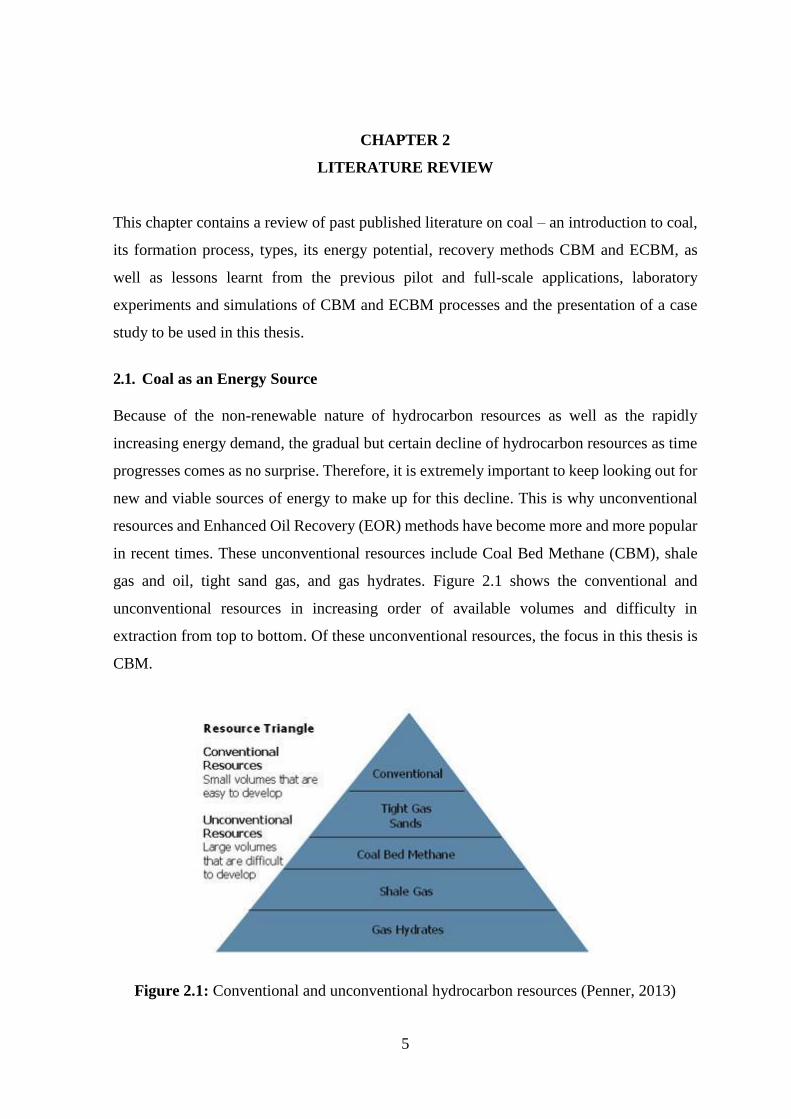
gas and oil, tight sand gas, and gas hydrates. Figure 2.1 shows the conventional and
unconventional resources in increasing order of available volumes and difficulty in
extraction from top to bottom. Of these unconventional resources, the focus in this thesis is
CBM.
Figure 2.1: Conventional and unconventional hydrocarbon resources (Penner, 2013)
6
Coal is a combustible, black, organic, sedimentary rock with high amounts of carbon. Dead
plants and animals subjected to high temperatures and pressure over time - millions of years,
are converted to peat and then into coal in a process known as coalification (Steyn, 2019).
Schopf (1956) defined coal as a readily combustible rock with over 50% by weight and over
70% by volume of carbonaceous material formed from compaction and induration of
variously altered plant remains similar to those in peaty deposits. As such, coal is composed
of mostly carbon as well as hydrogen, sulphur, oxygen and nitrogen. From the composition
of coal, it is obvious that when burnt directly, it releases large amounts of greenhouse gases
such as carbon dioxide (CO2) and Sulphur dioxide (SO2) which harmfully affects the
environment (Steyn, 2019).
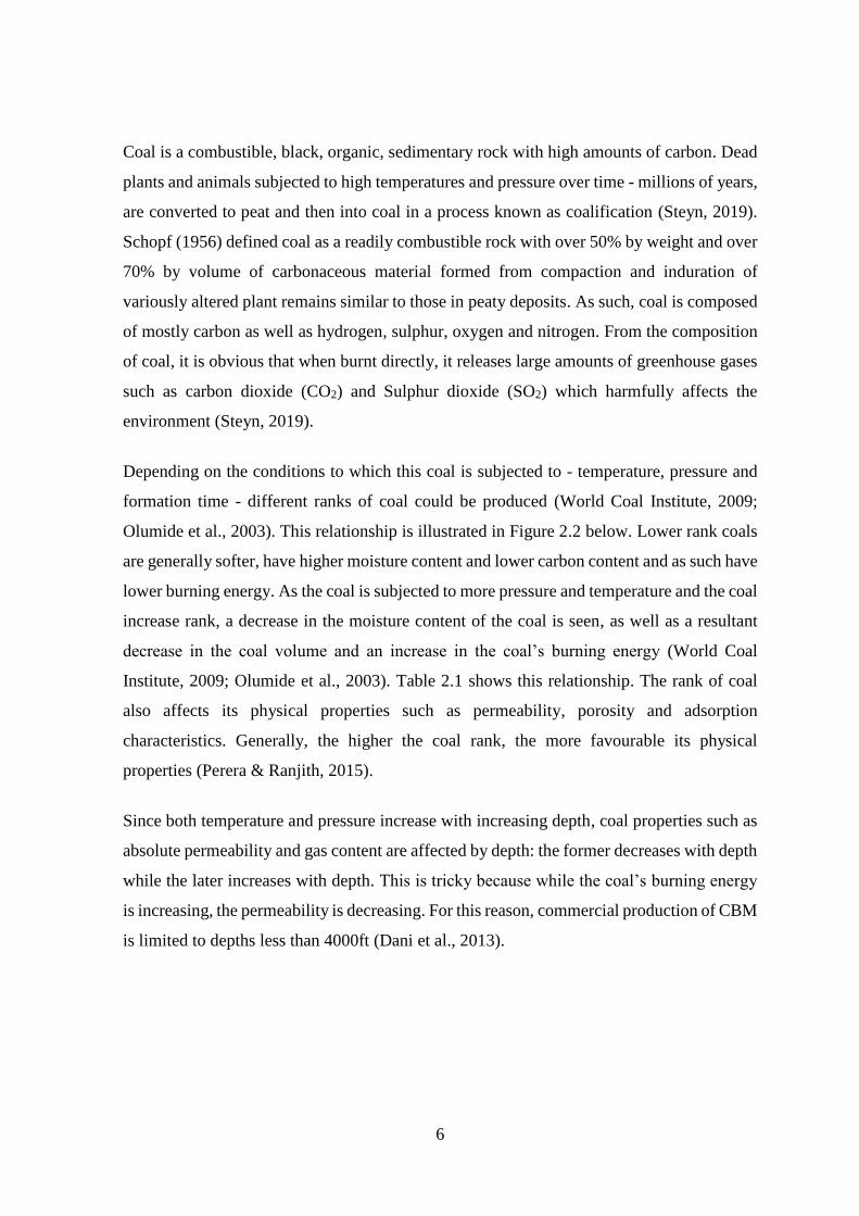
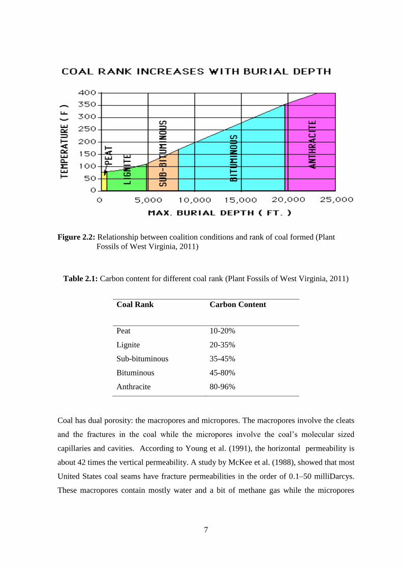
Depending on the conditions to which this coal is subjected to - temperature, pressure and
formation time - different ranks of coal could be produced (World Coal Institute, 2009;
Olumide et al., 2003). This relationship is illustrated in Figure 2.2 below. Lower rank coals
are generally softer, have higher moisture content and lower carbon content and as such have
lower burning energy. As the coal is subjected to more pressure and temperature and the coal
increase rank, a decrease in the moisture content of the coal is seen, as well as a resultant
decrease in the coal volume and an increase in the coal’s burning energy (World Coal
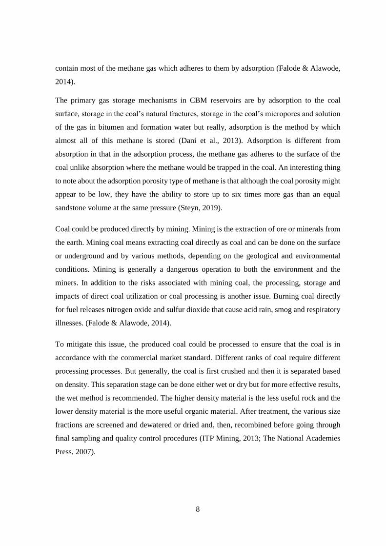
Institute, 2009; Olumide et al., 2003). Table 2.1 shows this relationship. The rank of coal
also affects its physical properties such as permeability, porosity and adsorption
characteristics. Generally, the higher the coal rank, the more favourable its physical
properties (Perera & Ranjith, 2015).
Since both temperature and pressure increase with increasing depth, coal properties such as
absolute permeability and gas content are affected by depth: the former decreases with depth
while the later increases with depth. This is tricky because while the coal’s burning energy
is increasing, the permeability is decreasing. For this reason, commercial production of CBM
is limited to depths less than 4000ft (Dani et al., 2013).
7
Figure 2.2: Relationship between coalition conditions and rank of coal formed (Plant
Fossils of West Virginia, 2011)
Table 2.1: Carbon content for different coal rank (Plant Fossils of West Virginia, 2011)
Coal Rank Carbon Content
Peat 10-20%
Lignite 20-35%
Sub-bituminous 35-45%
Bituminous 45-80%
Anthracite 80-96%
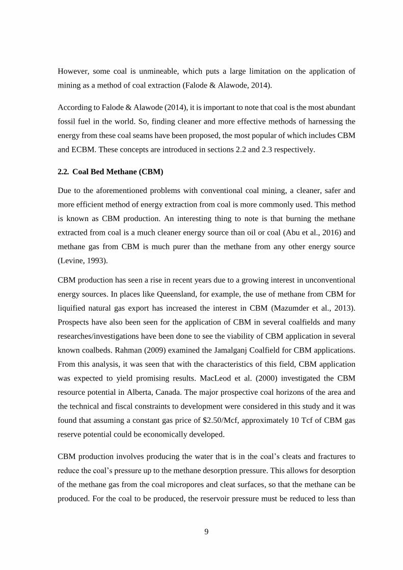
Coal has dual porosity: the macropores and micropores. The macropores involve the cleats
and the fractures in the coal while the micropores involve the coal’s molecular sized
capillaries and cavities. According to Young et al. (1991), the horizontal permeability is
about 42 times the vertical permeability. A study by McKee et al. (1988), showed that most
United States coal seams have fracture permeabilities in the order of 0.1–50 milliDarcys.
These macropores contain mostly water and a bit of methane gas while the micropores
8
contain most of the methane gas which adheres to them by adsorption (Falode & Alawode,
2014).
The primary gas storage mechanisms in CBM reservoirs are by adsorption to the coal
surface, storage in the coal’s natural fractures, storage in the coal’s micropores and solution
of the gas in bitumen and formation water but really, adsorption is the method by which
almost all of this methane is stored (Dani et al., 2013). Adsorption is different from
absorption in that in the adsorption process, the methane gas adheres to the surface of the
coal unlike absorption where the methane would be trapped in the coal. An interesting thing
to note about the adsorption porosity type of methane is that although the coal porosity might
appear to be low, they have the ability to store up to six times more gas than an equal
sandstone volume at the same pressure (Steyn, 2019).
Coal could be produced directly by mining. Mining is the extraction of ore or minerals from
the earth. Mining coal means extracting coal directly as coal and can be done on the surface
or underground and by various methods, depending on the geological and environmental
conditions. Mining is generally a dangerous operation to both the environment and the
miners. In addition to the risks associated with mining coal, the processing, storage and
impacts of direct coal utilization or coal processing is another issue. Burning coal directly
for fuel releases nitrogen oxide and sulfur dioxide that cause acid rain, smog and respiratory
illnesses. (Falode & Alawode, 2014).
To mitigate this issue, the produced coal could be processed to ensure that the coal is in
accordance with the commercial market standard. Different ranks of coal require different
processing processes. But generally, the coal is first crushed and then it is separated based
on density. This separation stage can be done either wet or dry but for more effective results,
the wet method is recommended. The higher density material is the less useful rock and the
lower density material is the more useful organic material. After treatment, the various size
fractions are screened and dewatered or dried and, then, recombined before going through
final sampling and quality control procedures (ITP Mining, 2013; The National Academies
Press, 2007).
9
However, some coal is unmineable, which puts a large limitation on the application of
mining as a method of coal extraction (Falode & Alawode, 2014).
According to Falode & Alawode (2014), it is important to note that coal is the most abundant
fossil fuel in the world. So, finding cleaner and more effective methods of harnessing the
energy from these coal seams have been proposed, the most popular of which includes CBM
and ECBM. These concepts are introduced in sections 2.2 and 2.3 respectively.
2.2. Coal Bed Methane (CBM)
Due to the aforementioned problems with conventional coal mining, a cleaner, safer and
more efficient method of energy extraction from coal is more commonly used. This method
is known as CBM production. An interesting thing to note is that burning the methane
extracted from coal is a much cleaner energy source than oil or coal (Abu et al., 2016) and
methane gas from CBM is much purer than the methane from any other energy source
(Levine, 1993).
CBM production has seen a rise in recent years due to a growing interest in unconventional
energy sources. In places like Queensland, for example, the use of methane from CBM for
liquified natural gas export has increased the interest in CBM (Mazumder et al., 2013).
Prospects have also been seen for the application of CBM in several coalfields and many
researches/investigations have been done to see the viability of CBM application in several
known coalbeds. Rahman (2009) examined the Jamalganj Coalfield for CBM applications.
From this analysis, it was seen that with the characteristics of this field, CBM application
was expected to yield promising results. MacLeod et al. (2000) investigated the CBM
resource potential in Alberta, Canada. The major prospective coal horizons of the area and
the technical and fiscal constraints to development were considered in this study and it was
found that assuming a constant gas price of $2.50/Mcf, approximately 10 Tcf of CBM gas
reserve potential could be economically developed.
CBM production involves producing the water that is in the coal’s cleats and fractures to
reduce the coal’s pressure up to the methane desorption pressure. This allows for desorption
of the methane gas from the coal micropores and cleat surfaces, so that the methane can be
produced. For the coal to be produced, the reservoir pressure must be reduced to less than
10
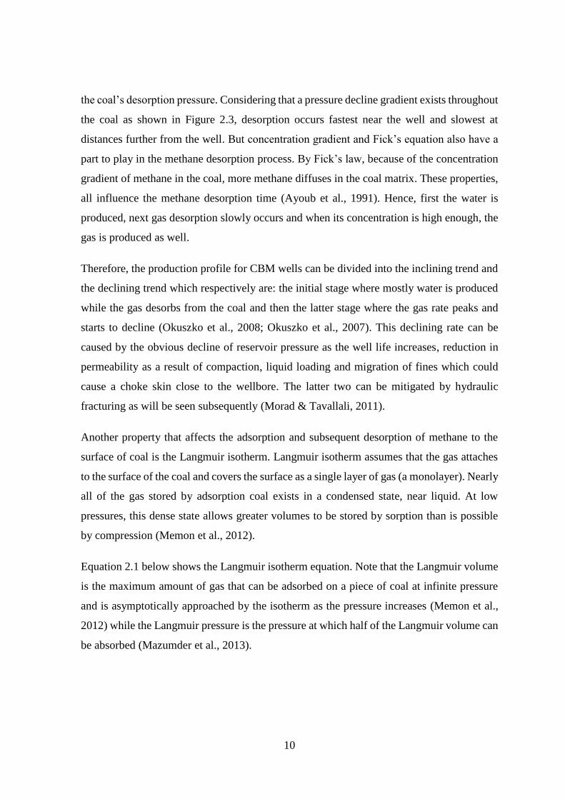
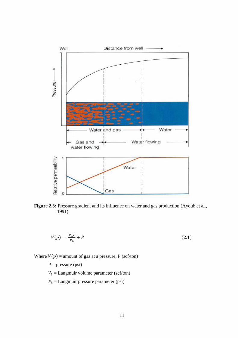
the coal’s desorption pressure. Considering that a pressure decline gradient exists throughout
the coal as shown in Figure 2.3, desorption occurs fastest near the well and slowest at
distances further from the well. But concentration gradient and Fick’s equation also have a
part to play in the methane desorption process. By Fick’s law, because of the concentration
gradient of methane in the coal, more methane diffuses in the coal matrix. These properties,
all influence the methane desorption time (Ayoub et al., 1991). Hence, first the water is
produced, next gas desorption slowly occurs and when its concentration is high enough, the
gas is produced as well.
Therefore, the production profile for CBM wells can be divided into the inclining trend and
the declining trend which respectively are: the initial stage where mostly water is produced
while the gas desorbs from the coal and then the latter stage where the gas rate peaks and
starts to decline (Okuszko et al., 2008; Okuszko et al., 2007). This declining rate can be
caused by the obvious decline of reservoir pressure as the well life increases, reduction in
permeability as a result of compaction, liquid loading and migration of fines which could
cause a choke skin close to the wellbore. The latter two can be mitigated by hydraulic
fracturing as will be seen subsequently (Morad & Tavallali, 2011).
Another property that affects the adsorption and subsequent desorption of methane to the
surface of coal is the Langmuir isotherm. Langmuir isotherm assumes that the gas attaches
to the surface of the coal and covers the surface as a single layer of gas (a monolayer). Nearly
all of the gas stored by adsorption coal exists in a condensed state, near liquid. At low
pressures, this dense state allows greater volumes to be stored by sorption than is possible
by compression (Memon et al., 2012).
Equation 2.1 below shows the Langmuir isotherm equation. Note that the Langmuir volume
is the maximum amount of gas that can be adsorbed on a piece of coal at infinite pressure
and is asymptotically approached by the isotherm as the pressure increases (Memon et al.,
2012) while the Langmuir pressure is the pressure at which half of the Langmuir volume can
be absorbed (Mazumder et al., 2013).
11
Figure 2.3: Pressure gradient and its influence on water and gas production (Ayoub et al.,
1991)
𝑉(𝑝) = 𝑉𝐿𝑃
𝑃𝐿+ 𝑃 (2.1)
Where 𝑉(𝑝) = amount of gas at a pressure, P (scf/ton)
P = pressure (psi)
𝑉𝐿 = Langmuir volume parameter (scf/ton)
𝑃𝐿 = Langmuir pressure parameter (psi)
12
The premise of dewatering CBM wells seems simple when it is thought of as just the
conventional pumping of water from a well. However, for CBM wells (whether vertical or
horizontal), it is a very different case. Neglecting to take basic precautions could lead to
complications. First, it is important to know the nature of the coal in question. Different coal
types mean different types of solid control methods needed and different wellbore
stabilization technology that could prevent severity levels of potential sloughing. The idea
of drilling a CBM well is not just for gas production but also for opening the surface area of
coal which leads to better gas production and for housing the artificial lift system. When
designing the wellbore, it is important to not only consider the production techniques and
equipment needed immediately, but also the equipment and/or processes that could take
place throughout the life of the well. Things such as sands reducing the hole diameter as time
goes on, the need for better artificial lift systems as the well life progresses, future
stimulation should be considered as opposed to just thinking of the immediate needs.
Although this might mean larger initial costs, the flexibility provided by taking these into
consideration more than makes up for the cost. In a scenario where the engineers decide to
develop the well thinking of just the present conditions, what then happens when the well
reaches its economic limit and the well is not designed to fit the new system needed?
(Bassett, 2006).
To achieve the best results, the well design should take into consideration the need for gas
separation from the water before the water enters the pump since pumps are not designed for
two phase flow. Various pumps can be used: progress cavity pump, rod pump, jet pump or
CBM electric submersible pump. It is also possible to use a gas lift method to try to reduce
the fluid gradient. It is important for the engineer to consider the CBM field being developed
and choose the best one for that field keeping in mind the limitations of these pumps in
relation to CBM wells as opposed to their limitations in either oil field production or purely
water wells (Bassett, 2006).
CBM production potential is determined by a number of factors that vary from basin to basin,
and include fracture permeability, development history, gas migration, coal maturation, coal
distribution, geologic structure, well completion options, hydrostatic pressure, and produced
water management. In most areas, naturally developed fracture networks are the most
13
sought-after areas for CBM development. Areas where geologic structures and localized
faulting have occurred tend to induce natural fracturing, which increases the production
pathways within the coal seam.
According to the Sydney Catchment Authority (2012), a coal seam suitable for CBM
development should contain high gas content, preferably between 15 and 30 m3/ton of
methane (Scott, 2002), have good permeability usually greater than 1 mD (Brown et al.,
1996), have sufficient thickness usually greater than 30m (Sharma, 1996) and lateral
continuity for easy movement of gas into wells, and be located between 250 and 1000 m
below the surface.
Although this method is a considerably preferable alternative to mining, producing coal in
this way presents its own challenges. First, even though CBM produces more from coal that
conventional mining, there is still considerable amount of methane left behind after
production done by the CBM method. Due to large amounts of pressure depletion (usually
about 70-80%), only less than 50% of the gas in place can be recovered using CBM, which
means that even after the economic lifetime is reached, there is still considerable amount of
methane left in these coal seams (Yan, 2015). Again, taking into consideration the large
volumes of produced water associated with conventional CBM and the number of impurities
such as sodium, potassium, magnesium, calcium, carbonate, bicarbonate, chlorine and
sulphate ions, the problem of safely disposing the produced water arises disposal of CBM
water with groundwater without treatment causes contamination of this ground water which
makes it unsafe for the residents of that area. Proper treatment and disposal of this produced
water is also a huge environmental concern in CBM. For context, on average, CBM wells in
the USA produce about 1.74cm3 of water per m3 of gas (Memon et al., 2012).
Additionally, an immense source of environmental concern is that due to the micro porosities
of coal, hydraulic fracturing is usually done in CBM to increase permeability. Because of
the micro-porosity of coal, hydraulic fracturing is usually done in CBM cases. Hydraulic
fracturing is a method by which water sand and other chemicals are injected into the reservoir
through a well at a pressure above the formation fracture pressure. The artificially created
fractures could expand and affect fresh water aquifers (Steyn, 2019).
14
Previous studies have shown that hydraulic fracturing produces more hydrocarbon and are
especially effective in unconventional reservoirs where permeabilities are in the range of
nano Darcy.
A look at some of the previously published literature on stimulating CBM wells shows
without a doubt just how effective this process is in increasing the gas recovery. Hydraulic
fracturing not only improves the permeability of coal by improving the coal fracture
network, it also helps to clean up the wellbore and the neighboring zones. Morad & Tavallali
(2011) carried out a study by conducting a series of simulations on the CMG GEM simulator
to see the effects of fracturing vertical and horizontal wells after loss of productivity begins
to take place. This study showed that refracturing a well after a decline in production starts
shows considerable increase in well gas productivity and practically reverses the
permeability loss. Considering the difference between conventional and unconventional
reservoirs, hydraulic fracturing mechanisms are obviously different which means that care
must be taken when performing simulations to ensure that the fracturing mechanisms of
CBM reservoirs are adequately captured. Han et al. (2020) investigated the use of hydraulic
fracturing in a CBM reservoir in Ordos Basin, China. These reservoirs typically have
unfavourable properties: low permeability, small pore size and low reservoir pressure. It was
seen from this study that the cleats present in coal formations causes premature leak-off and
consequently the premature screeen-out during hydraulic fracturing processes which limits
fracture growth and propagation. To try to mitigate this problem, Han et al. (2020) proposed
that the design objective should be longer fracture length and high net pressure so that even
with this limitation, the fracture will still be within reasonable limits.
Additionally, the effects of multi-stage hydraulic fracturing at the Dawson Valley CBM
project in the Bowen Basin in Queensland, Australia was studied in a research. It was seen
from this research that hydraulic fracturing improved the productivity of the CBM wells and
it was also interestingly noticed that water volume and not sand volume influences the
effectiveness of the fracture stimulation (McMillan & Palanyk, 2007). In a study of advanced
multi-lateral horizontal well in CBM reservoir using a simulation model, it was observed
that while the rate of gas production increases with an increase in the number of branches
that the wellbore has, a threshold exists. It was also observed in this study that threshold
15
pressure gradient and gas slippage effect not being considered could lead to huge errors
during simulations (Zheng & Xue, 2012).
Pulse fracturing has also been looked into as a technology for CBM. Pulse fracturing
involves raising the pressure up to several thousands of psi in microseconds to create
multiple fractures. Although a relatively new technology, it has been seen in many studies
to be more effective than conventional hydraulic fracturing and has even been represented
with a numerical model successfully (Tariq et al., 2019; Li et al., 2020; Sheng et al., 2019;
Li et al., 2014). This study however, will not implement this technology as the commercial
simulator used was not equipped with this feature.
As with any other investment, before the CBM is implemented, some prediction must be
done to determine how profitable an investment in this will be. It is important to know with
reasonable certainty, how much of this CBM can be produced and the best method(s) of
production. This prediction acts as a determinant for whether or not this CBM will be
implemented in a coalfield. Obviously, the CBM volumes need to be estimated but an
economic analysis must also be done in order to decide whether the process of producing
this methane will be too expensive to warrant undergoing this process or if it will be
beneficial to go through with it. This estimation requires certain data such as geological
parameters, CBM specific parameters and production history (Dani et al., 2013). The
conventional analysis tools developed for conventional reservoirs have to be modified for
use in CBM reservoirs as key reservoir characteristics such as relative permeability, absolute
permeability, the stress-permeability and desorption-permeability relationship during
depletion and the anisotropy of permeability vary widely in coalbeds which could lead to
grossly inaccurate prediction (Haskett & Brown, 2005; Clarkson & McGovern, 2005). This
is one of the reasons why pilots are essential in CBM exploration: they help to reduce
uncertainties of the key reservoir parameters mentioned above as well as test for the most
cost-effective completion and drilling method (Dani et al., 2013).
Four methods are generally implemented in assessing CBM reserves: volumetric method,
material balance method, production data analysis (PDA), reservoir simulation, depending
on the stage of CBM reservoir development. The volumetric and reservoir simulation could
be applied at all stages of development but as production progresses and more data becomes
16
available. The other two methods listed can be implemented only after certain data is
available (such as production data, flowing and shut-in pressure) in considerable amounts
(Dani et al., 2013).
Conventional material balance and PDA methods of reservoir evaluation have been modified
for CBM reservoirs. These advancements allows the determination of reservoir properties
such as permeability, drainage radius and original gas in place (OGIP) (Clarkson et al., 2007;
Clarkson et al., 2008). Mazumder et al. (2013) did a PDA of existing CBM wells in the Surat
Basin in Queensland whose gas is composed of about 97% of methane and about 3% of
impurities. The PDA methods utilized in this analysis involved the flow regime
identification, Fetkovich Type-curves, analytical history matching and material balance. To
be sure that these PDA gave good reservoir characterization, it was compared to other
methods of determining the derived properties. These include comparison of type-curves
method and well deliverability history match for permeability with the drill stem test (DST)
permeability results, comparison of OGIP from flowing material balance method with the
well deliverability history matched forecast method. These results showed that PDA
methods could be used reliably for CBM reservoir evaluation.
Clarkson et al. (2008) also investigated the use of PDA techniques in characterizing the
reservoirs. They pointed out that during the application of these techniques, the coal storgae
and transportation properties must be taken into consideration. This was shown for a two
phase CBM well in Eastern Wyoming with encouraging results. Even in the less common
single phase (gas) CBM reservoirs, it is possible to use PDA techniques for reservoir
characteristics determination as was seen in the Horseshoe Canyon coals of Western Canada
(Clarkson et al., 2007). Another study was done on PDA of Horizontal CBM wells in the
Arkoma Basin of Southeastern Oklahoma which showed that PDA techniques can be applied
on horizontal CBM wells with reasonable results (Mutalik & Magness, 2006). Therefore,
PDA techniques can be modified to fit different scenarios of complex CBM reservoir with a
limitation being the assumption of a single-layer reservoir behavoir unlike the actual multi-
layer behaviour usually encountered (Clarkson et al., 2008).
Analysis of the production decline of CBM has been used as an evaluation method of CBM
reserves. But a longstanding issue with this is the whether the production profile is
17
exponential or hyperbolic. It was seen in a research by Okuszko et al. (2008) that despite the
more complex production mechanisms of CBM reservoirs, the decline behaviour is similar
to that of conventional gas. As with conventional gas production, CBM production decline
usually matches a hyperbolic decline exponent (0-0.5) during the decline trend of the
production profile but during the inclining trend, it may appear to be exponential. It was also
noted that while the Langmuir volume does not affect the b value, an inverse relationship
exists between the b value and the Langmuir pressure. In addition to this, like the layered
conventional gas reservoirs, layered CBM reservoirs exhibit b values greater than 0.5 when
the layers have a high degree of heterogeniety. Generally, lower drawdown in the reservor
causes a more exponential behaviour while increased drawdown casuses a more hyperbolic
behavior (b approximately 0.5) (Okuszko et al., 2008; Okuszko et al., 2007).
Since proper decription of a reservoir rock is necessary for any successful hydrocarbon
recovery project, it is important to ensure that the model to be used, matches the reservoir
that is being modelled. This becomes tricky as unconventional reservoirs have more complex
features and more complex production mechanisms compared to conventional reservoirs and
therefore care must be taken to model them accordingly. Warren & Root (1963) in an attempt
to model dual pososity reservoirs developed a mathematical model which has a shape factor
to control the drainage rate from the reservoir matrix to it’s fractures and they also gave
formulas to be used in calculating shape factors. Many other formulas have been given for
calculating the shape factor which resulted in an obvious confusion about which one is
accurate. Mora & Wattenbarger (2006) conducted an investigation to find out which of these
formulas was most correct. It was seen that diferent boundary conditions gave different
values for the shape factor: for a constant pressure boundary condition, the formulas from
the studies by Zimmerman et al. (1993) and Lim & Aziz (1995) gave similar results, while
for a constant rate boundary condition, Coats (1989) gave similar results (Mora &
Wattenbarger, 2009; Mora & Wattenbarger, 2006).
An additional attempt to get an accurate description of the CBM reservoir was the creation
of empirical or theoritical models which accounted for changes in relative permeability as a
result of the matrix shrinkage/swelling that could occur during CBM/ECBM processes.
Clarkson et al. (2010) created a model to predict permeability growth as a result of depletion
18
in CBM and the additional gas rates resulting from this. This model was incorporated into
an analytical simulator and was used to predict and match the permeability changes in a
CBM well in the Fruitland Coal fairway of the San Juan Basin in the USA. This of course
shows that this model is promising.
Roy & Parulkar (2012) did a simulation of a coalfield in the Bokaro Basin in India using the
CMG’s option for CBM for GEM. From this study and others done, one notable challenge
observed with simulation of CBM in many cases, is the absence of production history which
limits history matching to the initial production testing profile. Even with this limitation, the
simulation produced reasonably accurate results because the most important data for history
matching is water production rate with time.
Although CBM is considerably better than mining for energy production from coal, due to
the problems associated with CBM production, ECBM is a considerably better alternative to
both.
2.3. Enhanced Coal Bed Methane (ECBM)
The unconventional CBM production method, which also serves as a method of carbon
sequestration, involves the injection of liquefied CO2/N2 into the coal which is preferentially
adsorbed by the coal. Because of this preferential adsorption, rather than depressurizing the
reservoir to allow for methane desorption, the methane gas is released as CO2/N2 is injected
as a kind of exchange (Godee et al., 2014). This unconventional method of CBM is called
Enhanced Coal Bed Methane (ECBM) production.
Interestingly, the ratio of replacement of CO2 molecule to methane molecule is 2:1 and 5:1
at depths of about 700m and 1500m respectively but beyond 2000m depth, increasing
temperature and pressure places a limit on the coal methane content and reduces the coal
seam permeability respectively (Bergen et al., 2000). It was seen in a study on the CO2
flooding in the Allison Unit of the San Juan Basin that the ratio of injected CO2 to produced
methane was about 3.1:1.0 (Journal of Petroleum Technology, 2005). These ratios are just
average values as the maturity of the coal plays a great part in adsorption/desorption process.
19
Primary recovery of CBM typically recovery up to 20-60 percent of the OGIP and in the San
Juan basin in the U.S.A., primary recovery methods will leave up to 10Tcf of natural gas
behind. It is important to note that the problem of water disposal is greatly reduced by ECBM
as compared to conventional CBM production. Another noteworthy fact is that many
previous studies done on these suggests that ECBM is a kind of EGR (Enhanced Gas
Recovery) process in which the CO2/N2 can produce the methane from unmineable coal
seams as well as coal that has undergone CBM processes. To put this in perspective,
conventional CBM typically produces less than 50% of the gas in place and ECBM records
up to 90% recovery of the gas place (Falode & Alawode, 2014; Godee et al., 2014; Reeves,
2003) and over 94% of the OGIP in some cases (Kovscek et al., 2005).
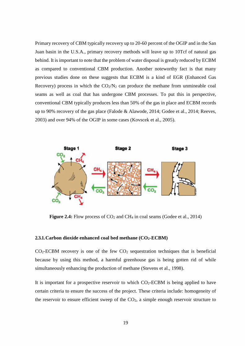
Figure 2.4: Flow process of CO2 and CH4 in coal seams (Godee et al., 2014)
2.3.1. Carbon dioxide enhanced coal bed methane (CO2-ECBM)
CO2-ECBM recovery is one of the few CO2 sequestration techniques that is beneficial
because by using this method, a harmful greenhouse gas is being gotten rid of while
simultaneously enhancing the production of methane (Stevens et al., 1998).
It is important for a prospective reservoir to which CO2-ECBM is being applied to have
certain criteria to ensure the success of the project. These criteria include: homogeneity of
the reservoir to ensure efficient sweep of the CO2, a simple enough reservoir structure to
20
prevent the CO2 from being diverted from the reservoir and although CBM reservoirs have
typically low permeabilities, it is also important to have about 5mD at least to allow for
passage of the CO2 into the reservoir (Stevens et al., 1998).
As with any other hydrocarbon production process, being able to properly capture the
various processes going on in the reservoir while making a model is important for the success
of that project. This is to say, understanding the mechanisms of ECBM processes are key in
successful modelling and application of this process. One of such attempts was an
observation by Clarkson et al. (2008) that the Palmer-Mansoori equation which is commonly
used in CBM reservoir modelling works best if the stress-dependent permeability term is
ignored and if the coal porosity is below 0.1% which begs the question: if this equation has
problem with CBM, how effective will it’s applicability to CO2 sequestration be? It is
important for observations like this to be considered if the model created is expected to be
successful. Because of this, several attempts have been made to understand these
mechanisms (Ozdemir, 2009).
In a study undertaken to investigate the variation in the structure and density of coal during
CBM/ECBM processes with X-ray experiments, it was noticed that net stress, gas adsorption
capacity and production history all cause change in coal density and density distributions
(Guo & Kantzas, 2008).
In some studies, CO2 injection led to reduction in permeability of the coal which placed a
restriction on the production of methane (Godee et.al., 2014). It has also been seen that
significant permeability changes occur during the adsorption-desorption process that
accompanies ECBM processes (Journal of Petroleum Technology, 2005). Coal swelling
during CO2 injection is also an important phenomenon to consider as this swelling leads to
reduction in coal permeability. CO2 could cause the coal to swell up to three times the
swelling caused by methane and in the Allison CO2-CBM pilot, CO2 injection was seen to
cause a 99% permeability decrease (Mitra & Harpalani, 2007). Modelling this swelling is
obviously important if the simulations are expected to give reliable results. Mitra &
Harpalani (2007) showed that although the extended Langmuir theory gave some errors in
modelling coal swelling as a result of CO2 injection, it still gave reliable enough results that
it can be used until a better way of representing this sorption-strain relationship is found.
21
A question that could arise in the mind of the reader at this point, is where the CO2 for the
ECBM process comes from. One important source is from flue gases. In some countries, like
Nigeria, most of the recovered gas is flared as opposed to being processed. This burnt gas
contains CO2 which is extremely harmful to the environment but very useful in secondary
recovery, EOR processes, as well as in EGR processes. These flue gases can be from power
plants, industrial cogeneration plants (like gas and steam turbines), waste incineration plants
and chemical industry (Lako, 2002). A very optimistic picture that could be drawn in the
mind of the reader is a methane power plant where the CO2 emissions from the power plants
can be injected into the coal seam where the methane was gotten from. Another source of
CO2 could be from naturally occurring high pressure CO2 from underground reservoirs. This
is the most cost-effective way if the CO2 reservoir is close enough to the CBM site to avoid
additional transportation costs (Stevens et al., 1998).
CO2-ECBM injection has been applied in many places: The United States’ San Juan Basin
and Uinta and Raton Basins, the Bowen and Sydney basins in Australia, the Ordos Basin in
China, Mannville coal in Western Canada and so on. The results from these have shown the
effectiveness of ECBM recovery and increased interests in researching and pursuing this
area (Stevens et al., 1998).
Taking the permeability reduction issue previously mentioned into consideration, it makes
one wonder if this process is actually effective especially in highly ranked coals. A review
of past literature clears this doubt. For example, the highly volatile B bitumen rank of the
Mannville coal of the Western Canada sedimentary basin and the anthracite rank coal of the
No. 3 coal of the Qinshui basin in China had micropilot programs that showed that the
sequestration potential exists even in highly ranked coals (Journal of Petroleum Technology,
2005). An attempt at mitigating this permeability reduction problem will be seen in section
2.3.3. A study by Godee et al. (2014) on the coal seams of the Allison unit of the San Juan
basin showed that CO2 injection can improve methane recovery from 77% using
conventional CBM method to about 95% using ECBM method. This study also showed that
CO2 injection could lead to permeability reduction which in turn could lead to loss of
injectivity of the coal seams but there a recovery was seen in the injectivity of the coal as
methane production progressed.

22
2.3.2. Nitrogen enhanced coal bed methane (N2-ECBM)
Although, CO2 is typically used in these ECBM recovery processes, nitrogen (N2) can also
be injected into CBM for EGR processes. The main sources of N2 are atmospheric
precipitation, geological sources, agricultural land, livestock and poultry operations and
urban waste (Ghaly & Ramakrishnan, 2015). One challenge associated with the use of N2 is
that it is less available and more costly than CO2. Settari et al. (2010) analyzed the use of
nitrogen stimulation in the Horseshoe Canon coal seams in Alberta. From this research, it
was seen that the controlling mechanisms of this process are permeability-stress relationship
of the coal as well as the permeability anisotropy as shown from the use of a geomechnical
model. Although this process of nitrogen injection has shown success, it was observed that
for proper modelling, sufficient data is required to calibrate geomechanical models for
reliable prediction of results (Settari et al., 2010). Godee et al. (2014) also did a study on the
injection of N2 into coal seams in the Tiffany unit in the San Juan basin . This study showed
that N2 injection leads to a rapid increase in methane production – even more than the CO2-
ECBM - with an accompanying rapid increase in permeability and consequently rapid
breakthrough of N2.
2.3.3. Carbon dioxide-nitrogen hybrid enhanced coal bed methane (CO2-N2-ECBM)
Considering the issue of permeability reduction associated with CO2 injection (Godee et al.,
2014) and the contrasting increase in permeability and early breakthrough associated with
N2 injection (Godee et al., 2014; Zhou et al., 2013), researchers have implemented the hybrid
CO2-N2-CBM method. Production rate of both CO2 and N2 ECBM depends on the injection
pressure, efficiency of movement of the CBM from the adsorbed state in the coal matrix into
the cleat or the fracture system of the coal, the permeability of the cleats and the pathway to
the borehole.
Various studies have been done to investigate this hybrid method. Kovscek et al. (2005)
performed some experiments and simulations to understand the adsorption/desorption
mechanism of methane/CO2/N2 in coals. From this research, it was seen that due to the
piston-like movement of CO2 in CBM reservoirs, breakthrough happens slowly unlike with
N2 which displays a more dispersed front and has quicker breakthrough and that CO2
23
adsorption to coal could be up to 3 times more than for methane and 7 times more than for
N2 for the coal from the Wyoming Powder River Basin. Laboratory experiments conducted
by Sim et al. (2009) on gas-gas displacement also showed similar results with Kovscek et al.
(2005) in terms of nitrogen and carbondioxide breakthrough time. It also showed that gas-
gas displacement in an attempt to increase gas recovery and extend reservoir life could give
very positive results even under low pressure and low flow velocity. Another research of
interest in the ECBM mechanism is one done by Mavor et al. (2004) on two wells in the
Manville coal in Canada. Cyclic CO2 and N2 injection performed on these wells showed that
the injectivity of CO2 is greater tham that of N2 and that even with a permeability as low as
1md, the injection increased the absolute and effective permeability to gas to where easy
injection could be done. These proved that although coal seams with very low permeabilities
could not be produced using conventional CBM method, ECBM could allow for commercial
production of methane from these coals (Mavor et al. 2004).
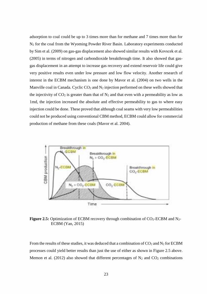
Figure 2.5: Optimization of ECBM recovery through combination of CO2-ECBM and N2-
ECBM (Yan, 2015)
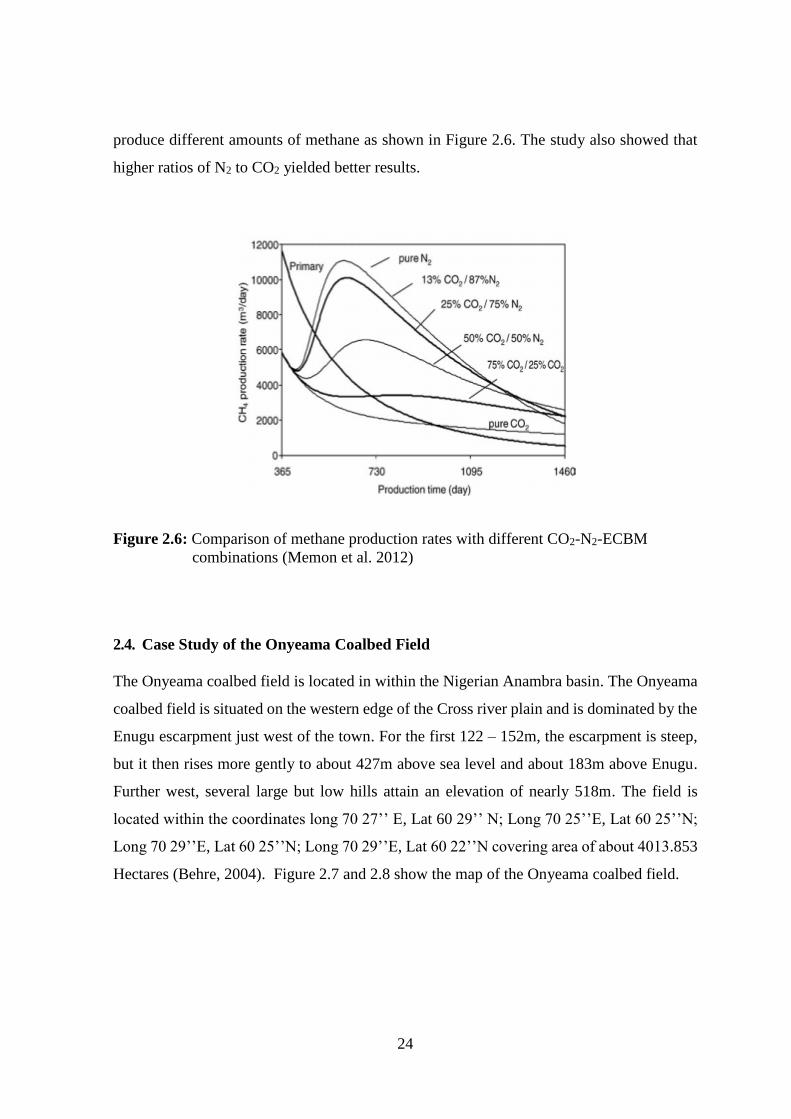
From the results of these studies, it was deduced that a combination of CO2 and N2 for ECBM
processes could yield better results than just the use of either as shown in Figure 2.5 above.
Memon et al. (2012) also showed that different percentages of N2 and CO2 combinations
24
produce different amounts of methane as shown in Figure 2.6. The study also showed that
higher ratios of N2 to CO2 yielded better results.
Figure 2.6: Comparison of methane production rates with different CO2-N2-ECBM
combinations (Memon et al. 2012)
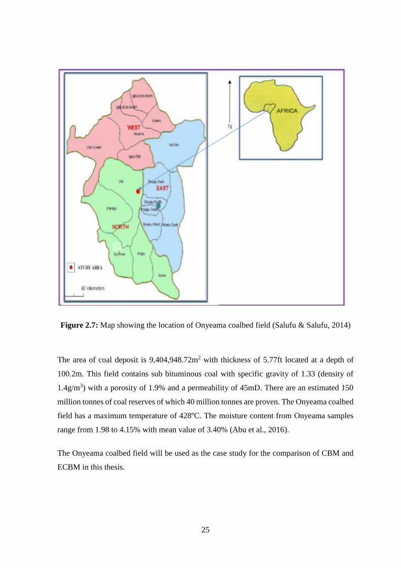
2.4. Case Study of the Onyeama Coalbed Field
The Onyeama coalbed field is located in within the Nigerian Anambra basin. The Onyeama
coalbed field is situated on the western edge of the Cross river plain and is dominated by the
Enugu escarpment just west of the town. For the first 122 – 152m, the escarpment is steep,
but it then rises more gently to about 427m above sea level and about 183m above Enugu.
Further west, several large but low hills attain an elevation of nearly 518m. The field is
located within the coordinates long 70 27’’ E, Lat 60 29’’ N; Long 70 25’’E, Lat 60 25’’N;
Long 70 29’’E, Lat 60 25’’N; Long 70 29’’E, Lat 60 22’’N covering area of about 4013.853
Hectares (Behre, 2004). Figure 2.7 and 2.8 show the map of the Onyeama coalbed field.
25
Figure 2.7: Map showing the location of Onyeama coalbed field (Salufu & Salufu, 2014)
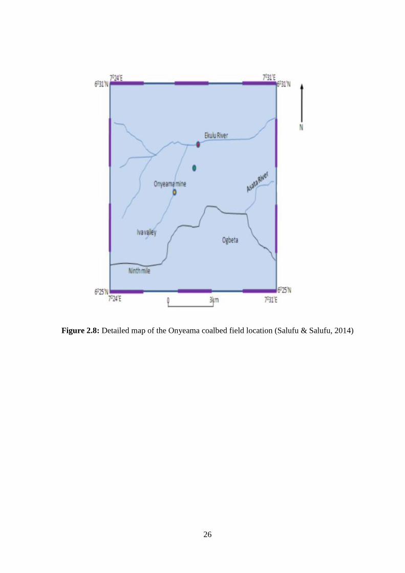
The area of coal deposit is 9,404,948.72m2 with thickness of 5.77ft located at a depth of
100.2m. This field contains sub bituminous coal with specific gravity of 1.33 (density of
1.4g/m3) with a porosity of 1.9% and a permeability of 45mD. There are an estimated 150
million tonnes of coal reserves of which 40 million tonnes are proven. The Onyeama coalbed
field has a maximum temperature of 428oC. The moisture content from Onyeama samples
range from 1.98 to 4.15% with mean value of 3.40% (Abu et al., 2016).
The Onyeama coalbed field will be used as the case study for the comparison of CBM and
ECBM in this thesis.
26
Figure 2.8: Detailed map of the Onyeama coalbed field location (Salufu & Salufu, 2014)
27
CHAPTER 3
METHODOLOGY
This chapter details the procedures followed to solve the previously outlined thesis problem.
Parameter selection, the simulation model, the simulation constraints, the simulation
software and how these are used in the comparison of CBM/ECBM efficiency are discussed
in detail in this chapter.
The Onyeama coalbed field in Enugu, Nigeria is an unmineable coal in which CBM and
ECBM can be successfully applied – this chapter will focus on this application. The
characteristics of this field were mentioned in Section 2.4 above. As stated in Section 2.4,
the model created was based on reservoir data gotten from literature review on the Onyeama
coalbed field in Nigeria and as expected, not all the data needed to construct a model to
accurately capture the reservoir properties were available. Still, the model created was good
enough to achieve the aim of this thesis.
In this chapter, the use of both horizontal and vertical wells for CBM and CO2-ECBM will
be investigated using the CMG GEM 2010 reservoir simulator. Ten scenarios will be
presented to compare how much production of methane and injection of carbon dioxide is
possible using different well orientations. The result of these models is explained in chapter
4.
A two-dimensional cartesian model with uniform grid size, single permeability, single
porosity and single water saturation was created. The dimension of the model was 16 by 16
by 1 (as can be seen in Figure 3.1) with each grid block having a width of 670.75ft in both
the x and y directions and a thickness of 5.77ft. The model was simulated to originally
contain a single hydrocarbon phase (methane) and water. The original gas in place (OGIP)
of the model was 9.118 * 109 scf.
Table 3.1 summarizes the properties of the constructed model and Figures 3.1, 3.2, 3.3, 3.4,
3.5, 3.6 and 3.7 show the 3D view, matrix and fracture porosity, matrix and fracture
permeability and matrix and fracture saturation of the model respectively.

28
Figure 3.1: 3D view of the reservoir model (generated from CMG builder)
Figure 3.2: Matrix porosity of the reservoir model (generated from CMG builder)
29
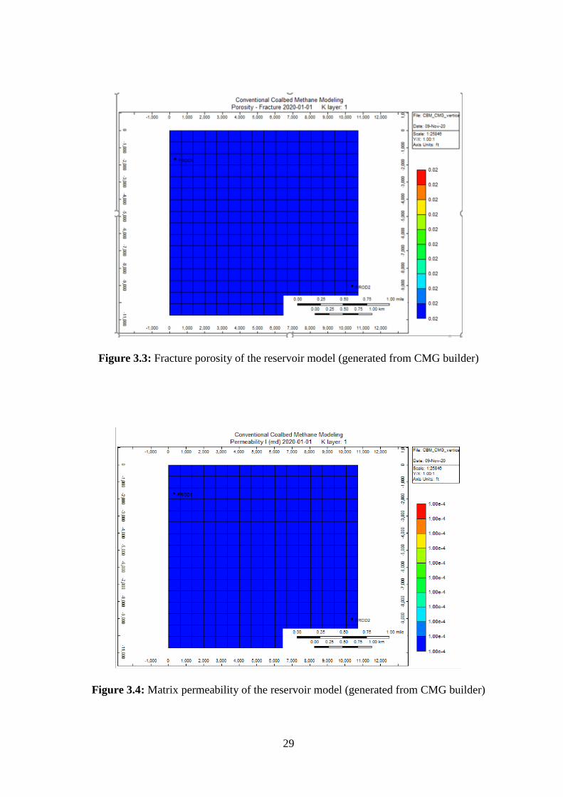
Figure 3.3: Fracture porosity of the reservoir model (generated from CMG builder)
Figure 3.4: Matrix permeability of the reservoir model (generated from CMG builder)
30
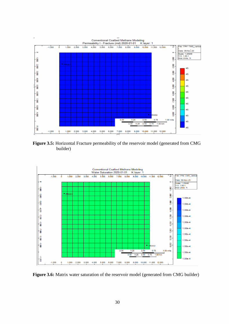
Figure 3.5: Horizontal Fracture permeability of the reservoir model (generated from CMG
builder)
Figure 3.6: Matrix water saturation of the reservoir model (generated from CMG builder)
31
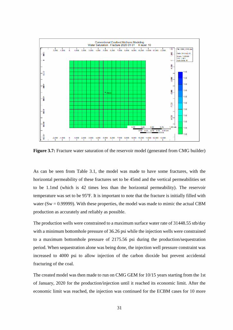
Figure 3.7: Fracture water saturation of the reservoir model (generated from CMG builder)
As can be seen from Table 3.1, the model was made to have some fractures, with the
horizontal permeability of these fractures set to be 45md and the vertical permeabilities set
to be 1.1md (which is 42 times less than the horizontal permeability). The reservoir
temperature was set to be 95oF. It is important to note that the fracture is initially filled with
water (Sw = 0.99999). With these properties, the model was made to mimic the actual CBM
production as accurately and reliably as possible.
The production wells were constrained to a maximum surface water rate of 31448.55 stb/day
with a minimum bottomhole pressure of 36.26 psi while the injection wells were constrained
to a maximum bottomhole pressure of 2175.56 psi during the production/sequestration
period. When sequestration alone was being done, the injection well pressure constraint was
increased to 4000 psi to allow injection of the carbon dioxide but prevent accidental
fracturing of the coal.
The created model was then made to run on CMG GEM for 10/15 years starting from the 1st
of January, 2020 for the production/injection until it reached its economic limit. After the
economic limit was reached, the injection was continued for the ECBM cases for 10 more
32
years. Other than the first scenario which was run for 15 years, all the other CBM scenarios
were run for 10 years before they reached economic limit and production was stopped. For
the ECBM scenarios, they were run for 15 years each with injection of CO2 and production
of methane before they reached their economic limit and production was stopped. After this
economic limit was reached, carbon dioxide was sequestered for the next 10 years in the
reservoir. The 10 years were chosen for sequestration because this was the time that was
roughly taken for the reservoir pressure to reach the formation fracture pressure.
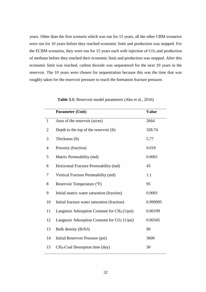
Table 3.1: Reservoir model parameters (Abu et al., 2016)
Parameter (Unit) Value
1 Area of the reservoir (acres) 2664
2 Depth to the top of the reservoir (ft) 328.74
3 Thickness (ft) 5.77
4 Porosity (fraction) 0.019
5 Matrix Permeability (md) 0.0001
6 Horizontal Fracture Permeability (md) 45
7 Vertical Fracture Permeability (md) 1.1
8 Reservoir Temperature (oF) 95
9 Initial matrix water saturation (fraction) 0.0001
10 Initial fracture water saturation (fraction) 0.999995
11 Langmuir Adsorption Constant for CH4 (1/psi) 0.00199
12 Langmuir Adsorption Constant for CO2 (1/psi) 0.00345
13 Bulk density (lb/ft3) 90
14 Initial Reservoir Pressure (psi) 3600
15 CH4-Coal Desorption time (day) 30
33
The method of injection/production followed by stopping production and injecting alone was
chosen because while injection/production occurs, some of the carbon dioxide being injected
was produced together with the methane. This defeated the purpose of injecting gas for
sequestration. When sequestration was done without production, the carbon stayed in the
reservoir.
The reservoir properties were kept constant for the ten scenarios while the well configuration
was changed for each scenario to compare their results and thereby find the most ideal
configuration.
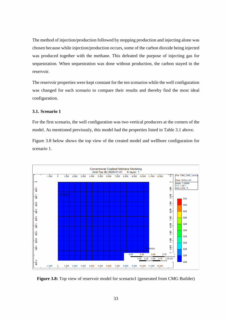
3.1. Scenario 1
For the first scenario, the well configuration was two vertical producers at the corners of the
model. As mentioned previously, this model had the properties listed in Table 3.1 above.
Figure 3.8 below shows the top view of the created model and wellbore configuration for
scenario 1.
Figure 3.8: Top view of reservoir model for scenario1 (generated from CMG Builder)
34
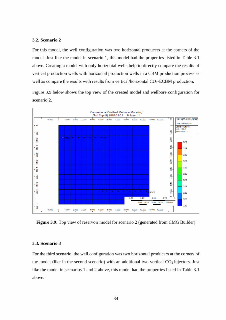
3.2. Scenario 2
For this model, the well configuration was two horizontal producers at the corners of the
model. Just like the model in scenario 1, this model had the properties listed in Table 3.1
above. Creating a model with only horizontal wells help to directly compare the results of
vertical production wells with horizontal production wells in a CBM production process as
well as compare the results with results from vertical/horizontal CO2-ECBM production.
Figure 3.9 below shows the top view of the created model and wellbore configuration for
scenario 2.
Figure 3.9: Top view of reservoir model for scenario 2 (generated from CMG Builder)
3.3. Scenario 3
For the third scenario, the well configuration was two horizontal producers at the corners of
the model (like in the second scenario) with an additional two vertical CO2 injectors. Just
like the model in scenarios 1 and 2 above, this model had the properties listed in Table 3.1
above.
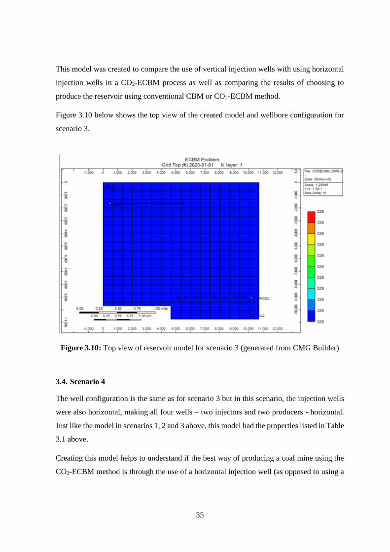
35
This model was created to compare the use of vertical injection wells with using horizontal
injection wells in a CO2-ECBM process as well as comparing the results of choosing to
produce the reservoir using conventional CBM or CO2-ECBM method.
Figure 3.10 below shows the top view of the created model and wellbore configuration for
scenario 3.
Figure 3.10: Top view of reservoir model for scenario 3 (generated from CMG Builder)
3.4. Scenario 4
The well configuration is the same as for scenario 3 but in this scenario, the injection wells
were also horizontal, making all four wells – two injectors and two producers - horizontal.
Just like the model in scenarios 1, 2 and 3 above, this model had the properties listed in Table
3.1 above.
Creating this model helps to understand if the best way of producing a coal mine using the
CO2-ECBM method is through the use of a horizontal injection well (as opposed to using a
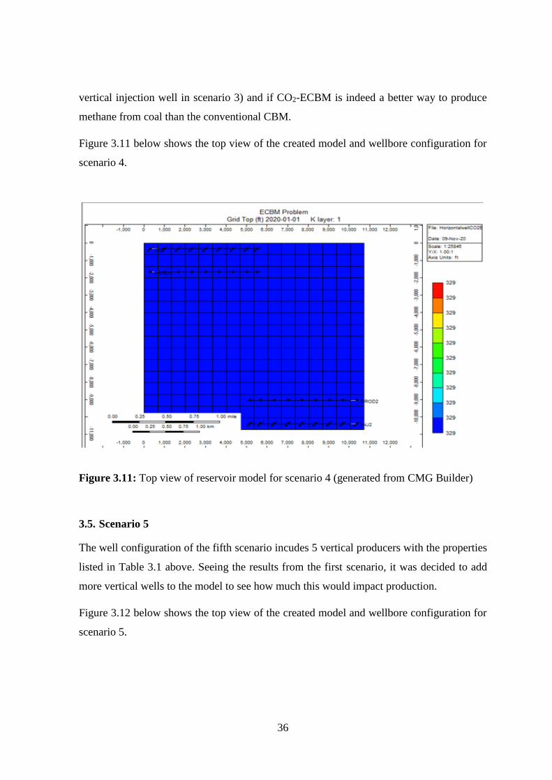
36
vertical injection well in scenario 3) and if CO2-ECBM is indeed a better way to produce
methane from coal than the conventional CBM.
Figure 3.11 below shows the top view of the created model and wellbore configuration for
scenario 4.
Figure 3.11: Top view of reservoir model for scenario 4 (generated from CMG Builder)
3.5. Scenario 5
The well configuration of the fifth scenario incudes 5 vertical producers with the properties
listed in Table 3.1 above. Seeing the results from the first scenario, it was decided to add
more vertical wells to the model to see how much this would impact production.
Figure 3.12 below shows the top view of the created model and wellbore configuration for
scenario 5.
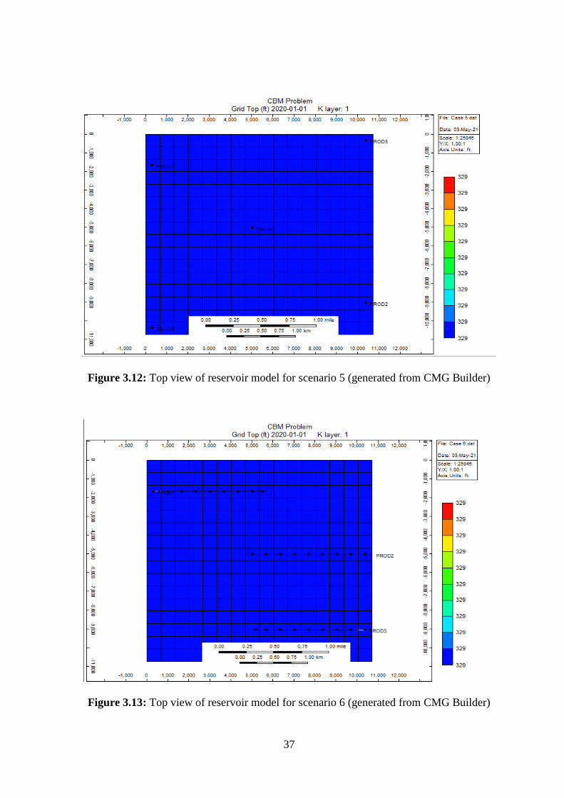
37
Figure 3.12: Top view of reservoir model for scenario 5 (generated from CMG Builder)
Figure 3.13: Top view of reservoir model for scenario 6 (generated from CMG Builder)
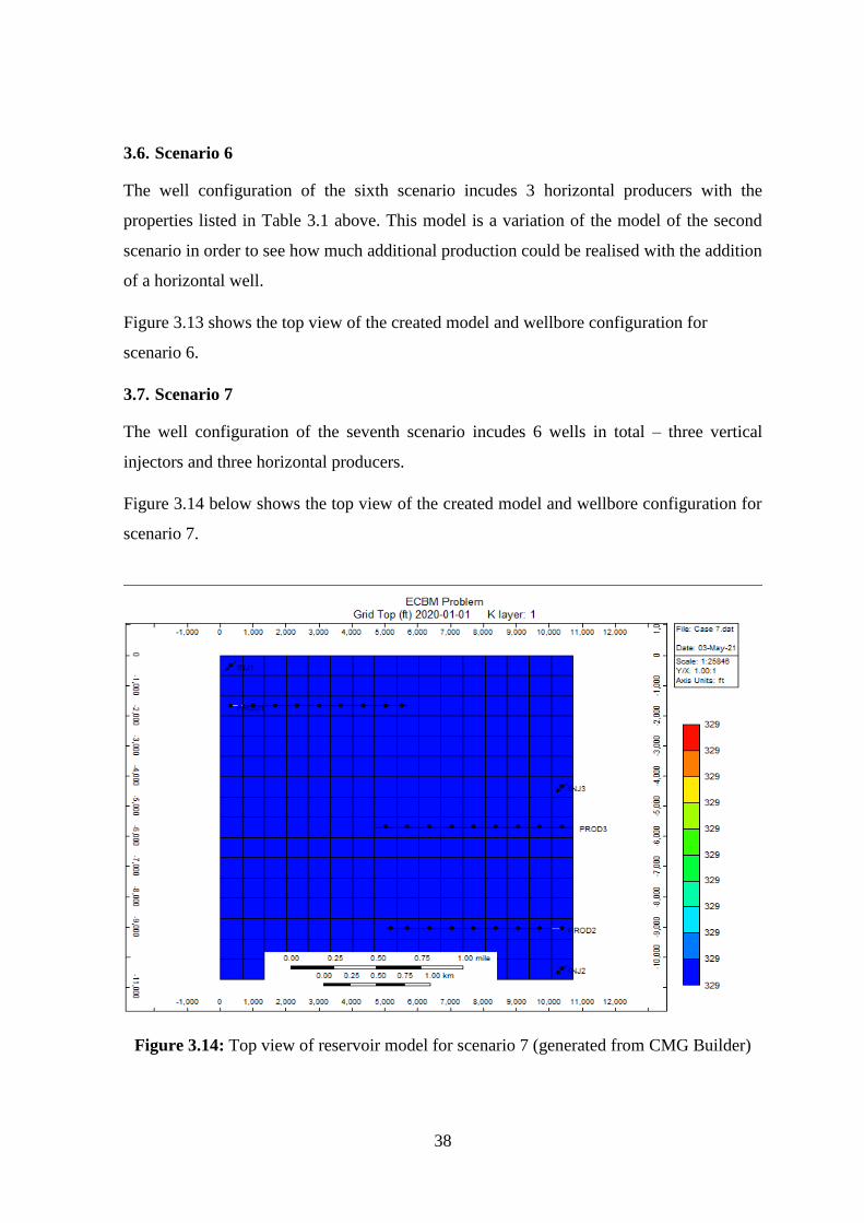
38
3.6. Scenario 6
The well configuration of the sixth scenario incudes 3 horizontal producers with the
properties listed in Table 3.1 above. This model is a variation of the model of the second
scenario in order to see how much additional production could be realised with the addition
of a horizontal well.
scenario 6.
3.7. Scenario 7
The well configuration of the seventh scenario incudes 6 wells in total – three vertical
injectors and three horizontal producers.
Figure 3.14 below shows the top view of the created model and wellbore configuration for
scenario 7.
Figure 3.14: Top view of reservoir model for scenario 7 (generated from CMG Builder)
Figure 3.13 shows the top view of the created model and wellbore configuration for
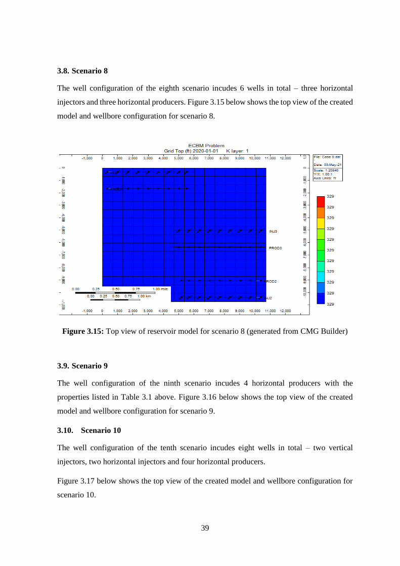
39
3.8. Scenario 8
The well configuration of the eighth scenario incudes 6 wells in total – three horizontal
injectors and three horizontal producers. Figure 3.15 below shows the top view of the created
model and wellbore configuration for scenario 8.
Figure 3.15: Top view of reservoir model for scenario 8 (generated from CMG Builder)
3.9. Scenario 9
The well configuration of the ninth scenario incudes 4 horizontal producers with the
properties listed in Table 3.1 above. Figure 3.16 below shows the top view of the created
model and wellbore configuration for scenario 9.
3.10. Scenario 10
The well configuration of the tenth scenario incudes eight wells in total – two vertical
injectors, two horizontal injectors and four horizontal producers.
Figure 3.17 below shows the top view of the created model and wellbore configuration for
scenario 10.
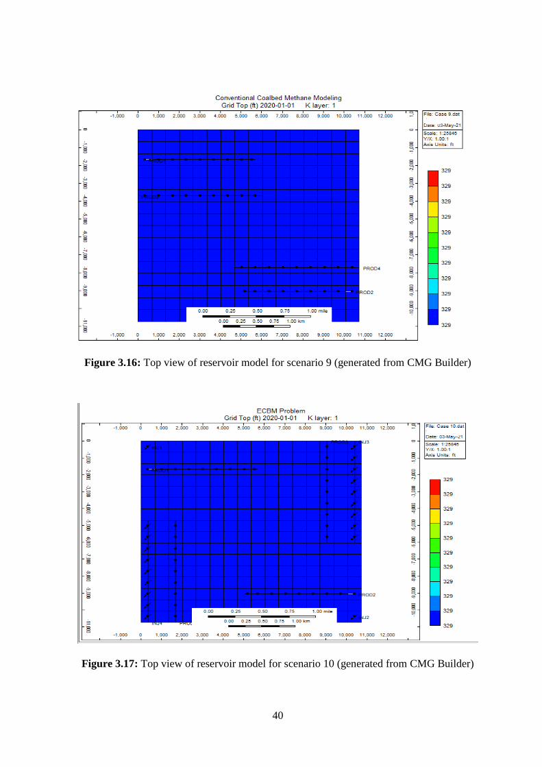
40
Figure 3.16: Top view of reservoir model for scenario 9 (generated from CMG Builder)
Figure 3.17: Top view of reservoir model for scenario 10 (generated from CMG Builder)
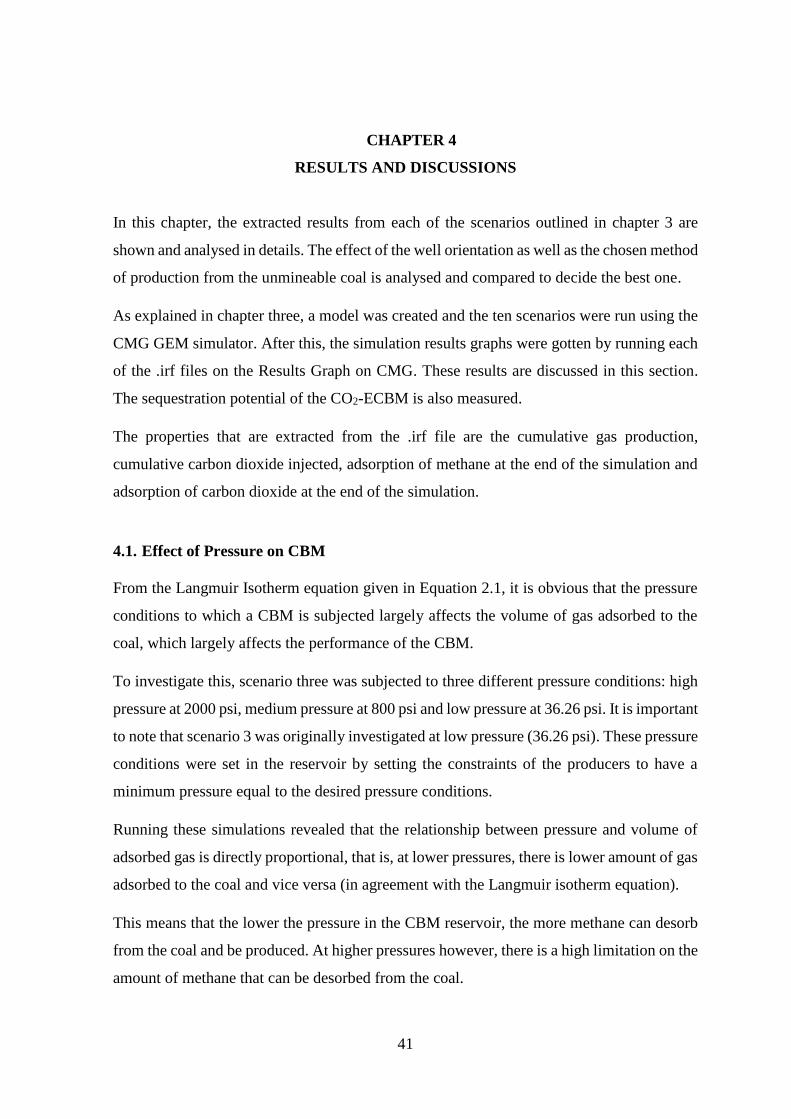
41
CHAPTER 4
RESULTS AND DISCUSSIONS
In this chapter, the extracted results from each of the scenarios outlined in chapter 3 are
shown and analysed in details. The effect of the well orientation as well as the chosen method
of production from the unmineable coal is analysed and compared to decide the best one.
As explained in chapter three, a model was created and the ten scenarios were run using the
CMG GEM simulator. After this, the simulation results graphs were gotten by running each
of the .irf files on the Results Graph on CMG. These results are discussed in this section.
The sequestration potential of the CO2-ECBM is also measured.
The properties that are extracted from the .irf file are the cumulative gas production,
cumulative carbon dioxide injected, adsorption of methane at the end of the simulation and
adsorption of carbon dioxide at the end of the simulation.
4.1. Effect of Pressure on CBM
From the Langmuir Isotherm equation given in Equation 2.1, it is obvious that the pressure
conditions to which a CBM is subjected largely affects the volume of gas adsorbed to the
coal, which largely affects the performance of the CBM.
To investigate this, scenario three was subjected to three different pressure conditions: high
pressure at 2000 psi, medium pressure at 800 psi and low pressure at 36.26 psi. It is important
to note that scenario 3 was originally investigated at low pressure (36.26 psi). These pressure
conditions were set in the reservoir by setting the constraints of the producers to have a
minimum pressure equal to the desired pressure conditions.
Running these simulations revealed that the relationship between pressure and volume of
adsorbed gas is directly proportional, that is, at lower pressures, there is lower amount of gas
adsorbed to the coal and vice versa (in agreement with the Langmuir isotherm equation).
This means that the lower the pressure in the CBM reservoir, the more methane can desorb
from the coal and be produced. At higher pressures however, there is a high limitation on the
amount of methane that can be desorbed from the coal.
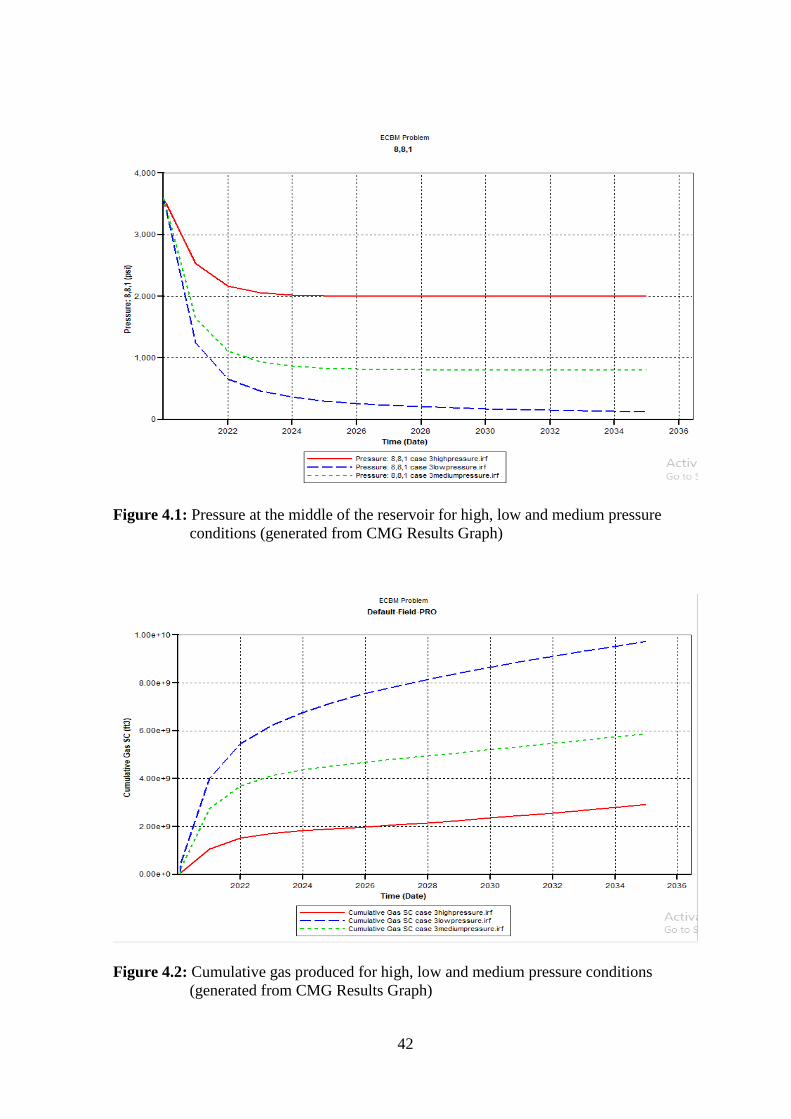
42
Figure 4.1: Pressure at the middle of the reservoir for high, low and medium pressure
conditions (generated from CMG Results Graph)
Figure 4.2: Cumulative gas produced for high, low and medium pressure conditions
(generated from CMG Results Graph)
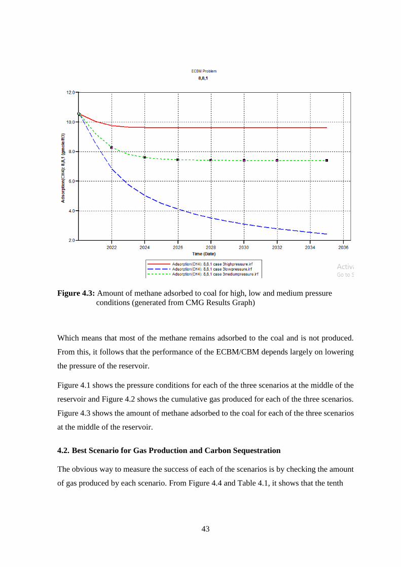
43
Figure 4.3: Amount of methane adsorbed to coal for high, low and medium pressure
conditions (generated from CMG Results Graph)
Which means that most of the methane remains adsorbed to the coal and is not produced.
From this, it follows that the performance of the ECBM/CBM depends largely on lowering
the pressure of the reservoir.
Figure 4.1 shows the pressure conditions for each of the three scenarios at the middle of the
reservoir and Figure 4.2 shows the cumulative gas produced for each of the three scenarios.
Figure 4.3 shows the amount of methane adsorbed to the coal for each of the three scenarios
at the middle of the reservoir.
4.2. Best Scenario for Gas Production and Carbon Sequestration
The obvious way to measure the success of each of the scenarios is by checking the amount
of gas produced by each scenario. From Figure 4.4 and Table 4.1, it shows that the tenth
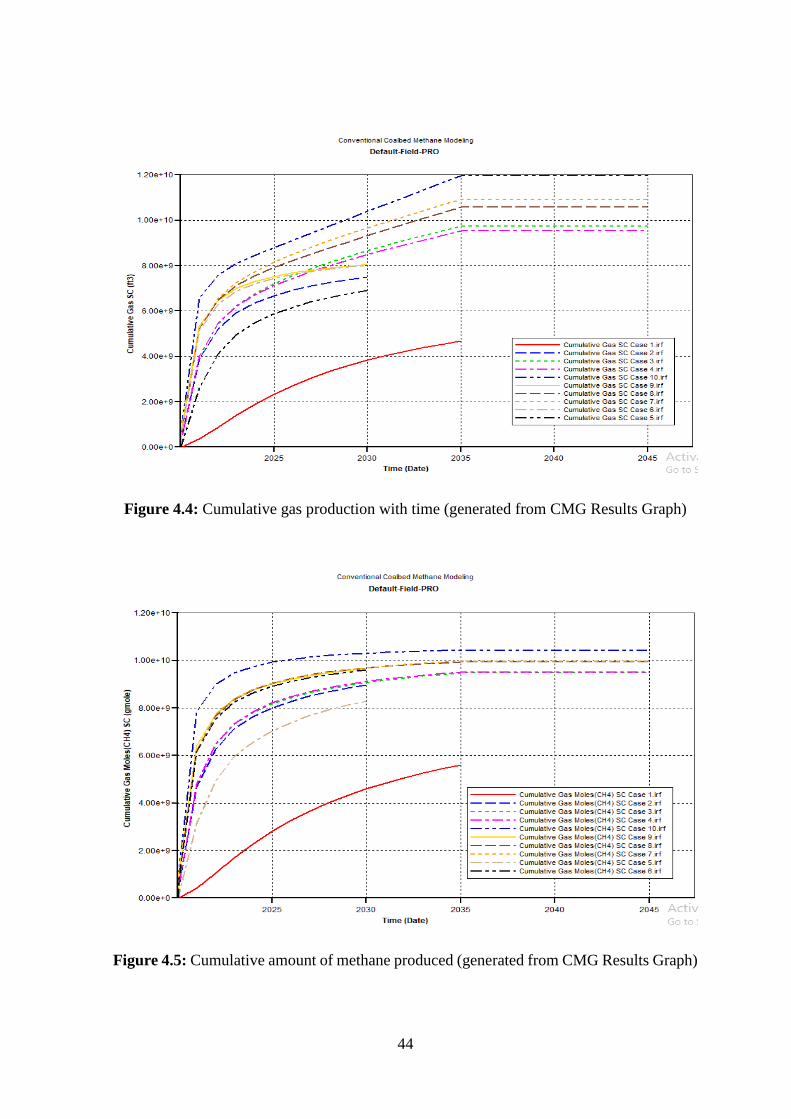
44
Figure 4.4: Cumulative gas production with time (generated from CMG Results Graph)
Figure 4.5: Cumulative amount of methane produced (generated from CMG Results Graph)
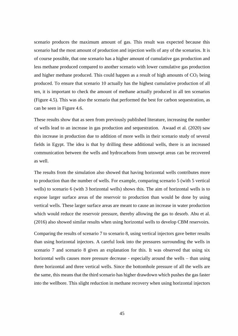
45
scenario produces the maximum amount of gas. This result was expected because this
scenario had the most amount of production and injection wells of any of the scenarios. It is
of course possible, that one scenario has a higher amount of cumulative gas production and
less methane produced compared to another scenario with lower cumulative gas production
and higher methane produced. This could happen as a result of high amounts of CO2 being
produced. To ensure that scenario 10 actually has the highest cumulative production of all
ten, it is important to check the amount of methane actually produced in all ten scenarios
(Figure 4.5). This was also the scenario that performed the best for carbon sequestration, as
can be seen in Figure 4.6.
These results show that as seen from previously published literature, increasing the number
of wells lead to an increase in gas production and sequestration. Awaad et al. (2020) saw
this increase in production due to addition of more wells in their scenario study of several
fields in Egypt. The idea is that by drilling these additional wells, there is an increased
communication between the wells and hydrocarbons from unswept areas can be recovered
as well.
The results from the simulation also showed that having horizontal wells contributes more
to production than the number of wells. For example, comparing scenario 5 (with 5 vertical
wells) to scenario 6 (with 3 horizontal wells) shows this. The aim of horizontal wells is to
expose larger surface areas of the reservoir to production than would be done by using
vertical wells. These larger surface areas are meant to cause an increase in water production
which would reduce the reservoir pressure, thereby allowing the gas to desorb. Abu et al.
(2016) also showed similar results when using horizontal wells to develop CBM reservoirs.
Comparing the results of scenario 7 to scenario 8, using vertical injectors gave better results
than using horizontal injectors. A careful look into the pressures surrounding the wells in
scenario 7 and scenario 8 gives an explanation for this. It was observed that using six
horizontal wells causes more pressure decrease - especially around the wells – than using
three horizontal and three vertical wells. Since the bottomhole pressure of all the wells are
the same, this means that the third scenario has higher drawdown which pushes the gas faster
into the wellbore. This slight reduction in methane recovery when using horizontal injectors
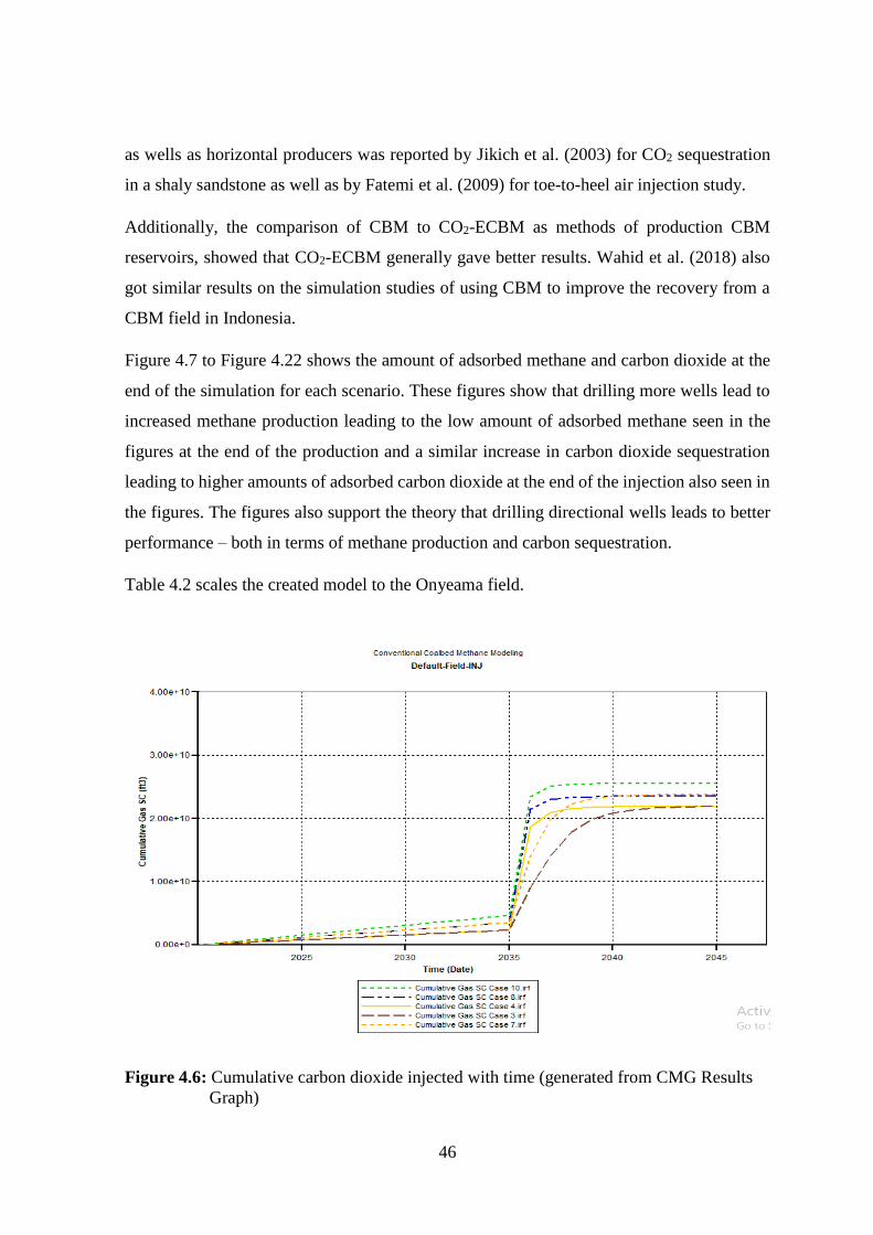
46
as wells as horizontal producers was reported by Jikich et al. (2003) for CO2 sequestration
in a shaly sandstone as well as by Fatemi et al. (2009) for toe-to-heel air injection study.
Additionally, the comparison of CBM to CO2-ECBM as methods of production CBM
reservoirs, showed that CO2-ECBM generally gave better results. Wahid et al. (2018) also
got similar results on the simulation studies of using CBM to improve the recovery from a
CBM field in Indonesia.
Figure 4.7 to Figure 4.22 shows the amount of adsorbed methane and carbon dioxide at the
end of the simulation for each scenario. These figures show that drilling more wells lead to
increased methane production leading to the low amount of adsorbed methane seen in the
figures at the end of the production and a similar increase in carbon dioxide sequestration
leading to higher amounts of adsorbed carbon dioxide at the end of the injection also seen in
the figures. The figures also support the theory that drilling directional wells leads to better
performance – both in terms of methane production and carbon sequestration.
Table 4.2 scales the created model to the Onyeama field.
Figure 4.6: Cumulative carbon dioxide injected with time (generated from CMG Results
Graph)
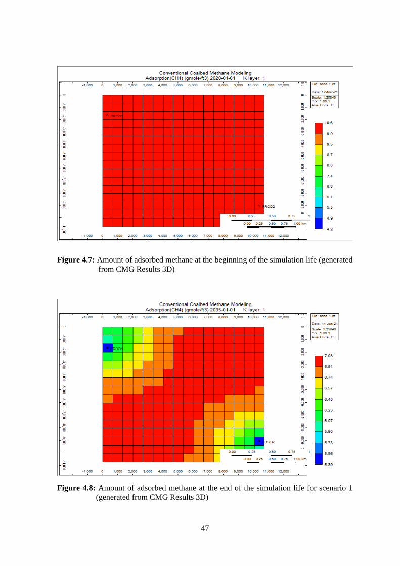
47
Figure 4.7: Amount of adsorbed methane at the beginning of the simulation life (generated
from CMG Results 3D)
Figure 4.8: Amount of adsorbed methane at the end of the simulation life for scenario 1
(generated from CMG Results 3D)
48
Figure 4.9: Amount of adsorbed methane at the end of the simulation life for scenario 2
(generated from CMG Results 3D)
Figure 4.10: Amount of adsorbed methane at the end of the simulation life for scenario 3
(generated from CMG Results 3D)
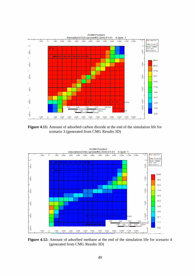
49
Figure 4.11: Amount of adsorbed carbon dioxide at the end of the simulation life for
scenario 3 (generated from CMG Results 3D)
Figure 4.12: Amount of adsorbed methane at the end of the simulation life for scenario 4
(generated from CMG Results 3D)
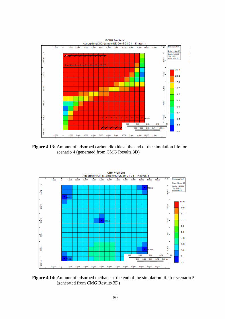
50
Figure 4.13: Amount of adsorbed carbon dioxide at the end of the simulation life for
scenario 4 (generated from CMG Results 3D)
Figure 4.14: Amount of adsorbed methane at the end of the simulation life for scenario 5
(generated from CMG Results 3D)
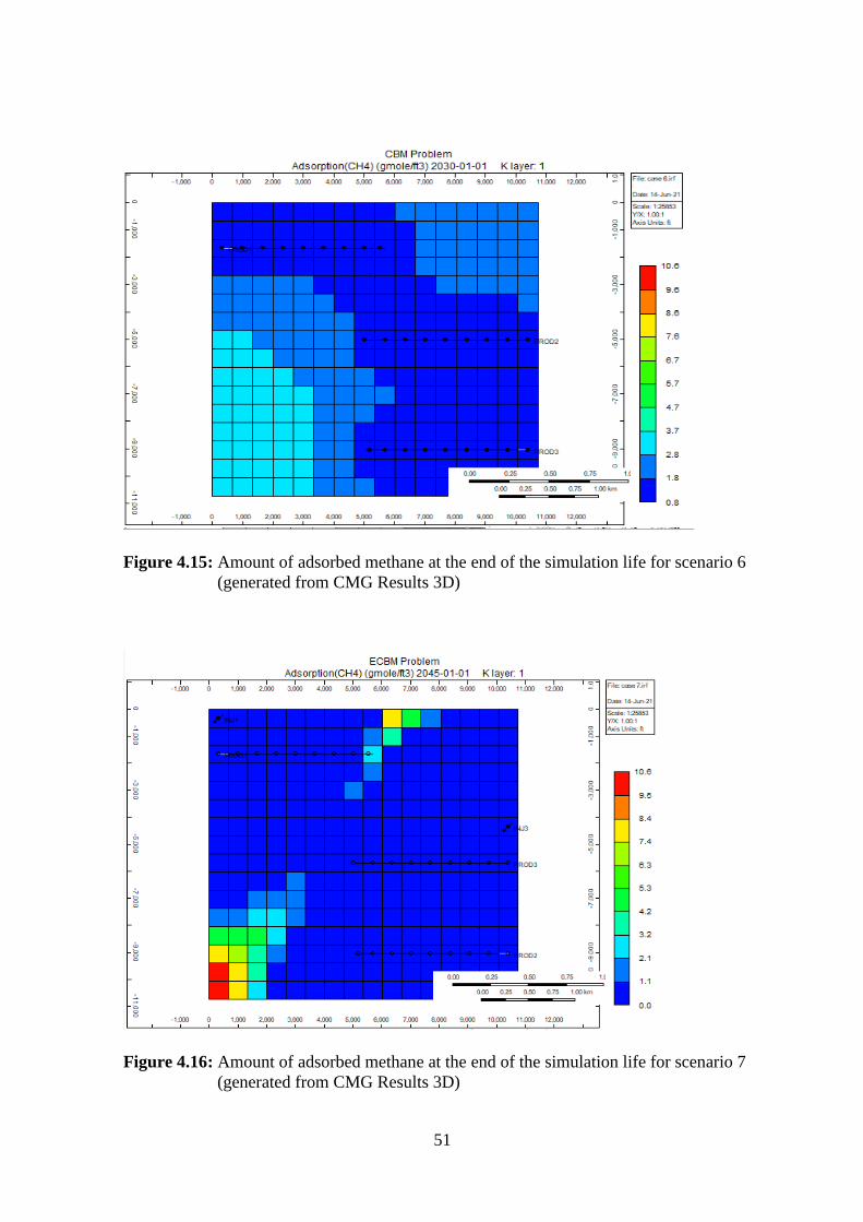
51
Figure 4.15: Amount of adsorbed methane at the end of the simulation life for scenario 6
(generated from CMG Results 3D)
Figure 4.16: Amount of adsorbed methane at the end of the simulation life for scenario 7
(generated from CMG Results 3D)
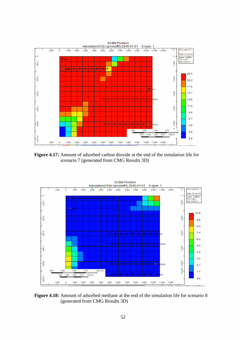
52
Figure 4.17: Amount of adsorbed carbon dioxide at the end of the simulation life for
scenario 7 (generated from CMG Results 3D)
Figure 4.18: Amount of adsorbed methane at the end of the simulation life for scenario 8
(generated from CMG Results 3D)
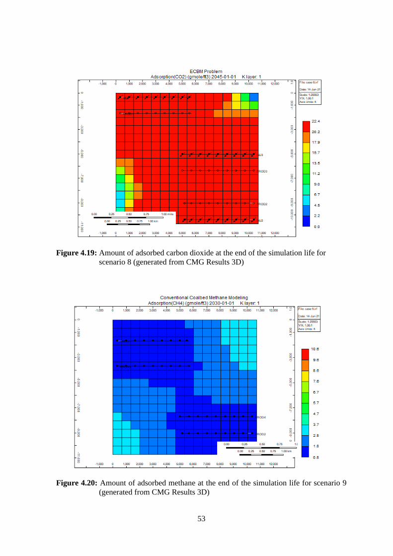
53
Figure 4.19: Amount of adsorbed carbon dioxide at the end of the simulation life for
scenario 8 (generated from CMG Results 3D)
Figure 4.20: Amount of adsorbed methane at the end of the simulation life for scenario 9
(generated from CMG Results 3D)
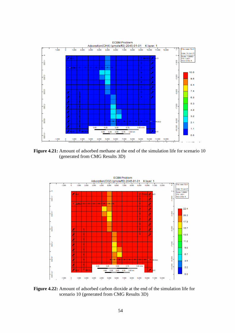
54
Figure 4.21: Amount of adsorbed methane at the end of the simulation life for scenario 10
(generated from CMG Results 3D)
Figure 4.22: Amount of adsorbed carbon dioxide at the end of the simulation life for
scenario 10 (generated from CMG Results 3D)
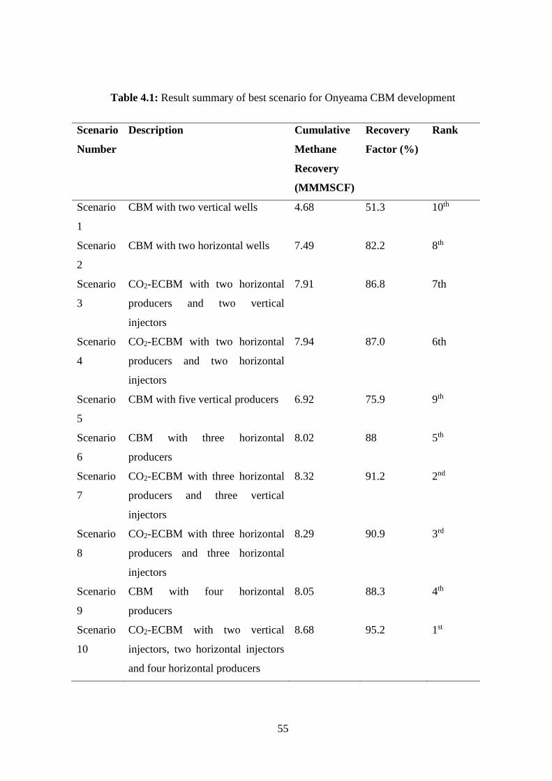
55
Table 4.1: Result summary of best scenario for Onyeama CBM development
Scenario
Number
Description Cumulative
Methane
Recovery
(MMMSCF)
Recovery
Factor (%)
Rank
Scenario
1
CBM with two vertical wells 4.68 51.3 10th
Scenario
2
CBM with two horizontal wells 7.49 82.2 8th
Scenario
3
CO2-ECBM with two horizontal
producers and two vertical
injectors
7.91 86.8 7th
Scenario
4
CO2-ECBM with two horizontal
producers and two horizontal
injectors
7.94 87.0 6th
Scenario
5
CBM with five vertical producers 6.92 75.9 9th
Scenario
6
CBM with three horizontal
producers
8.02 88 5th
Scenario
7
CO2-ECBM with three horizontal
producers and three vertical
injectors
8.32 91.2 2nd
Scenario
8
CO2-ECBM with three horizontal
producers and three horizontal
injectors
8.29 90.9 3rd
Scenario
9
CBM with four horizontal
producers
8.05 88.3 4th
Scenario
10
CO2-ECBM with two vertical
injectors, two horizontal injectors
and four horizontal producers
8.68 95.2 1st
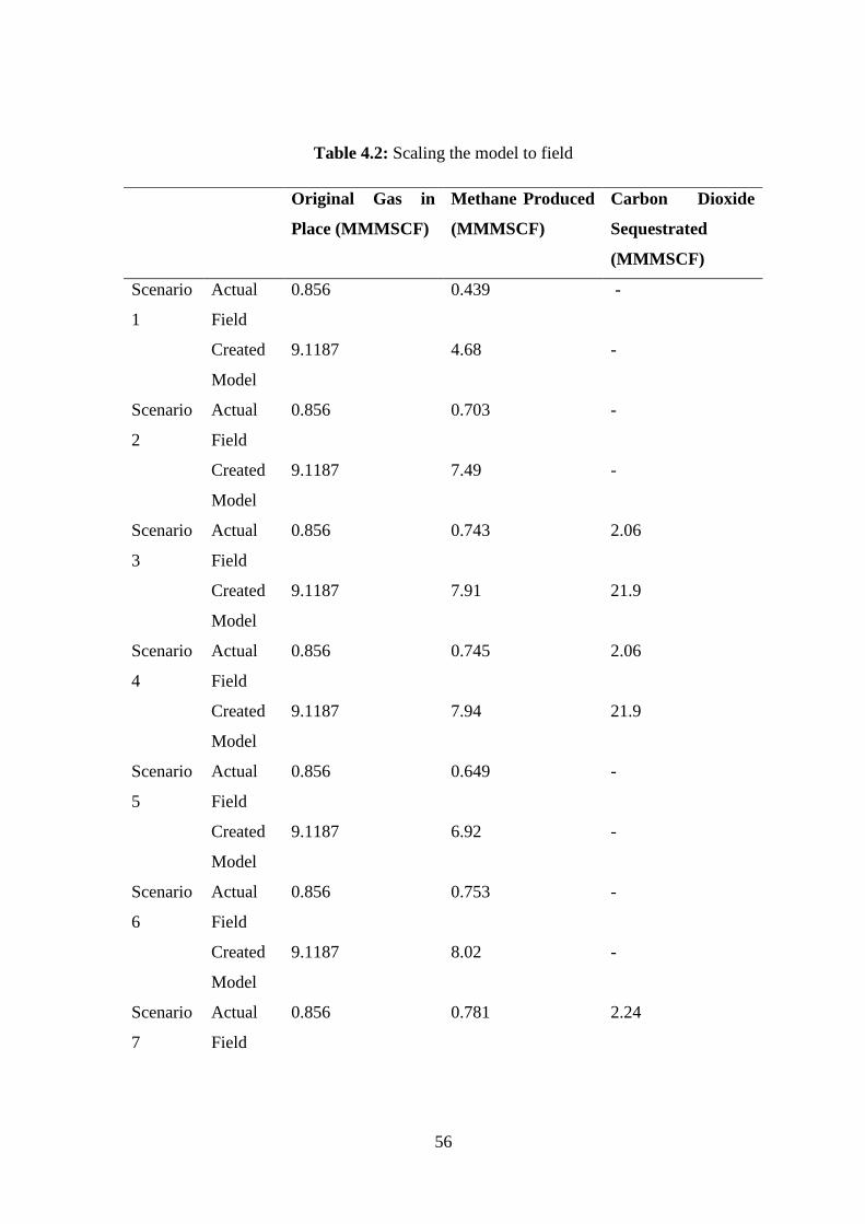
56
Table 4.2: Scaling the model to field
Original Gas in
Place (MMMSCF)
Methane Produced
(MMMSCF)
Carbon Dioxide
Sequestrated
(MMMSCF)
Scenario
1
Actual
Field
0.856 0.439 -
Created
Model
9.1187 4.68 -
Scenario
2
Actual
Field
0.856 0.703 -
Created
Model
9.1187 7.49 -
Scenario
3
Actual
Field
0.856 0.743 2.06
Created
Model
9.1187 7.91 21.9
Scenario
4
Actual
Field
0.856 0.745 2.06
Created
Model
9.1187 7.94 21.9
Scenario
5
Actual
Field
0.856 0.649 -
Created
Model
9.1187 6.92 -
Scenario
6
Actual
Field
0.856 0.753 -
Created
Model
9.1187 8.02 -
Scenario
7
Actual
Field
0.856 0.781 2.24
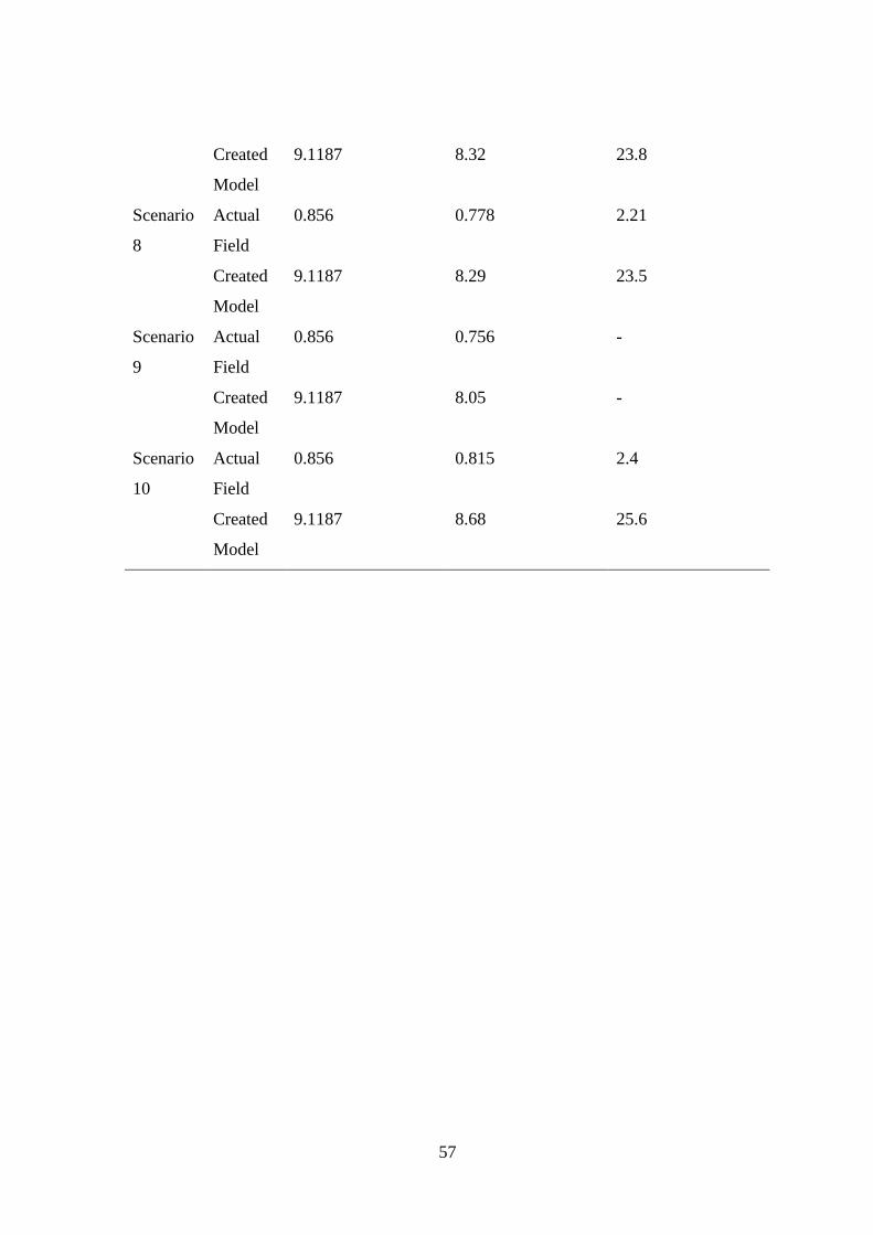
57
Created
Model
9.1187 8.32 23.8
Scenario
8
Actual
Field
0.856 0.778 2.21
Created
Model
9.1187 8.29 23.5
Scenario
9
Actual
Field
0.856 0.756 -
Created
Model
9.1187 8.05 -
Scenario
10
Actual
Field
0.856 0.815 2.4
Created
Model
9.1187 8.68 25.6
58
CHAPTER 5
ECONOMICAL ANALYSIS
An economical analysis is important to determine which of the ten alternatives mentioned in
Chapter 3 and 4 is the most economically advantageous for producing the Onyeama coalbed
field. In this section, the costs and benefits for each alternative will be checked and analysed
to make the best selection.
CAPEX is the money spent by a business to acquire assets that could be beneficial for a long
period of time. Examples of CAPEX include money spent buying a building or buying
equipment needed for the business. For instance, in the petroleum industry, CAPEX includes
the cost of drilling and completing a well. It is important to note that these capital
expenditures do not include periodic payments (Collaborative Minds Blog, 2020). The
drilling costs comprises about 30-40% of the total well costs, completion costs include about
55-70% of the total well costs and other facility costs such as artificial lift systems,
separators, dehydrators, etc. comprise about 7-8% of the total well cost (U.S. Energy
Information Administration, 2016).
OPEX is the money spent periodically to ensure the smooth running of the day-to-day
business. Examples of OPEX includes maintenance/repair of the equipment needed for the
business and in the petroleum industry could include fees for oil and water hauling and
facility electricity (Collaborative Minds Blog, 2020). OPEX can be divided into fixed OPEX
and variable OPEX. Operating costs vary depending on location, well size, well productivity
and other factors. These OPEX can be fixed (such as artificial lift, well maintenance and
workover activities) or variable (such as gas gathering, process, transport and compression)
(U.S. Energy Information Administration, 2016).
The most recent and accurate data that could be found for the economical analysis of the ten
gas production scenarios (as shown in Table 5.1) and calculations were done for each
scenario depending on the conditions of production (amount of gas injected, well oritntation
and length of wellbore) as shown in Table 5.2. Three variables commonly considered in
economical analysis are the net prevent value (NPV), initial rate of return (IRR) and rate of
investment (ROI). The NPV reperesnts the difference in cash inflows and outflows over a
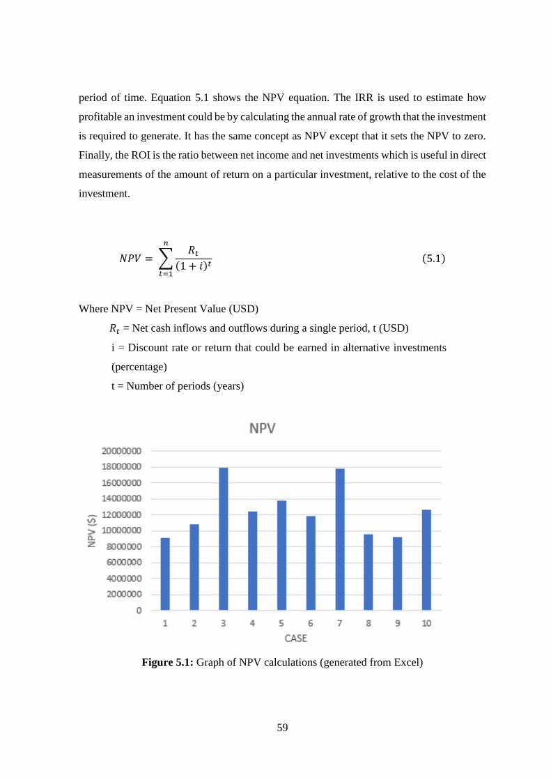
59
period of time. Equation 5.1 shows the NPV equation. The IRR is used to estimate how
profitable an investment could be by calculating the annual rate of growth that the investment
is required to generate. It has the same concept as NPV except that it sets the NPV to zero.
Finally, the ROI is the ratio between net income and net investments which is useful in direct
measurements of the amount of return on a particular investment, relative to the cost of the
investment.
𝑁𝑃𝑉 = ∑𝑅𝑡
(1 + 𝑖)𝑡
𝑛
𝑡=1
(5.1)
Where NPV = Net Present Value (USD)
𝑅𝑡 = Net cash inflows and outflows during a single period, t (USD)
i = Discount rate or return that could be earned in alternative investments
(percentage)
t = Number of periods (years)
Figure 5.1: Graph of NPV calculations (generated from Excel)
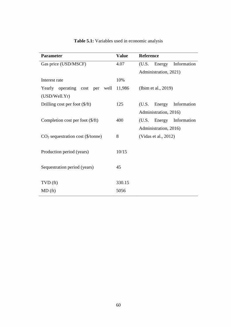
60
Table 5.1: Variables used in economic analysis
Parameter Value Reference
Gas price (USD/MSCF) 4.07 (U.S. Energy Information
Administration, 2021)
Interest rate 10%
Yearly operating cost per well
(USD/Well.Yr)
11,986 (Ibim et al., 2019)
Drilling cost per foot ($/ft) 125 (U.S. Energy Information
Administration, 2016)
Completion cost per foot ($/ft) 400 (U.S. Energy Information
Administration, 2016)
CO2 sequestration cost ($/tonne) 8 (Vidas et al., 2012)
Production period (years) 10/15
Sequestration period (years) 45
TVD (ft) 330.15
MD (ft) 5056
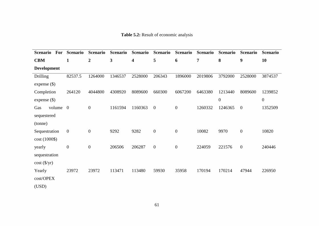
61
Table 5.2: Result of economic analysis
Scenario For
CBM
Development
Scenario
1
Scenario
2
Scenario
3
Scenario
4
Scenario
5
Scenario
6
Scenario
7
Scenario
8
Scenario
9
Scenario
10
Drilling
expense ($)
82537.5 1264000 1346537 2528000 206343 1896000 2019806 3792000 2528000 3874537
Completion
expense ($)
264120 4044800 4308920 8089600 660300 6067200 6463380 1213440
0
8089600 1239852
0
Gas volume
sequestered
(tonne)
0 0 1161594
1160363
0 0 1260332
1246365
0 1352509
Sequestration
cost (1000$)
0 0 9292 9282 0 0 10082 9970 0 10820
yearly
sequestration
cost ($/yr)
0 0 206506 206287 0 0 224059 221576 0 240446
Yearly
cost/OPEX
(USD)
23972 23972 113471 113480 59930 35958 170194 170214 47944 226950
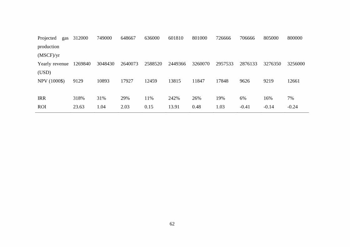
62
Projected gas
production
(MSCF)/yr
312000 749000 648667 636000 601810 801000 726666 706666
805000 800000
Yearly revenue
(USD)
1269840 3048430 2640073 2588520 2449366 3260070 2957533 2876133 3276350 3256000
NPV (1000$) 9129
10893 17927 12459 13815 11847 17848 9626 9219 12661
IRR 318% 31% 29% 11% 242% 26% 19% 6% 16% 7%
ROI 23.63 1.04 2.03 0.15 13.91 0.48 1.03 -0.41 -0.14 -0.24
63
CHAPTER 6
CONCLUSIONS AND RECOMMENDATIONS
6.1. Conclusions
This study compared the efficiency of using CBM and CO2-ECBM recovery with both
horizontal and vertical injectors as a method of producing more methane from the Onyeama
coalbed field in Enugu, Nigeria while simultaneously sequestering carbon in this field. This
is a particularly beneficial study in Nigeria because of the large amounts of unmineable coal
as well as the large amounts of GHG emission due to gas flaring.
The key lessons learnt from this study:
1. In the choice between conventional CBM and CO2-ECBM for producing from
unmineable coalbed reservoirs, it was seen that CO2-ECBM generally performed better
in terms of gas production with the best scenario for CBM giving 630 MMSCF less gas
than the best scenario for CO2-ECBM but CBM is a cheaper method since no injection
wells have to be drilled.
2. Although the use of horizontal wells is generally believed to produce better results than
vertical wells, certain factors could discredit this. This study showed that the seventh
scenario performed better than the eighth scenario with a difference of 30MMSCF. This
performance could be attributed to the small drawdown when four horizontal injectors
are used, which leads to less gas flow into the producer.
3. It was seen that large amount of CO2 (up to 2.4 MMMSCF) could be sequestered into
the Onyeama CBM reservoir without reaching the reservoir fracture pressure. This
showed potential for using CBM in Nigeria as a method of CSS to make up for the large
volumes of flared gas.
4. Subjecting the reservoir to high pressure conditions leads to lower gas recovery because
most of the gas stays adsorbed to the coal surface. On the other hand, subjecting the
reservoir to low pressure conditions leads to higher gas recovery since more desorption
can occur under this condition.
5. Although the tenth scenario performed best in terms of production and injection, the
economic analysis showed that was not the most economically feasible. Generally, it can
64
be seen that CBM scenarios were more economically advantageous than the ECBM
scenarios. This is because of the cost of drilling additional wells to serve as injection
wells and the cost of injection operations. The NPV analysis showed that the most
profitable of the ten scenarios is the third scenario.
6.2. Recommendations
More detailed reservoir data would help to make a more accurate description of the reservoir
on the simulator which would lead to more exact results. An accompanying laboratory study
will help to understand more about the effect of CO2 on the coal structure for example the
permeability increase.
65
REFERENCES
Abu, R. N., Mbanefo, I. O., & Adeloye, O. M. (2016, November). Coalbed Methane
Production in Nigeria: Onyeama Coalbed. International Journal of Scientific &
Engineering Research, 7(11), 377-383.
Ayoub, J., Colson, L., Hinkel, J., & Levine, J. (1991). Learning to Produce Coalbed Methane.
Oilfield Review, 3(1), 27-40.
Bassett, L. (2006). Guidelines to Successful Dewatering of CBM Wells. SPE Eastern
Regional Meeting. Ohio: Society of Petroleum Engineers. doi:10.2118/104290-MS
Behre, D. (2004). Feasibility of Nigerian Coal Resources Development,. Retrieved August
27, 2020, from Global Methane Initiative:
http://www.globalmethane.org/documents/toolsres_coal_overview_ch 24.pdf(2004)
Brown, K., Casey, D., & Enever, J. (1996). New South Wales Coal Seam Methane Potential.
Sydney: New South Wales Department of Mineral Resources.
Clarkson, C. R., & McGovern, J. M. (2005). Optimization of CBM Reservoir Exploration
and Development Strategies through Integration of Simulation and Economics. SPE
Reservoir Evaluation & Engineering, 8(6), 502-519. doi:10.2118/88843-PA
Clarkson, C. R., Jordan, C. L., Gierhart, R. R., & Seidle , J. P. (2008). Production Data
Analysis of Coalbed-Methane Wells. SPE Reservoir Evaluation & Engineering,
11(02), 311 - 325. doi:10.2118/107705-PA
Clarkson, C. R., Pan, Z., Palmer, I. D., & Harpalani, S. (2010). Predicting Sorption-Induced
Strain and Permeability Increase With Depletion for Coalbed-Methane Reservoirs.
Society of Petroleum Engineers, 15(01), 152-159. doi:10.2118/114778-PA
Clarkson, C., Bustin, M. R., & Seidle, J. P. (2007). Production-Data Analysis of Single-
Phase (Gas) Coalbed-Methane Wells. Society of Petroleum Engineers, 10(03), 312 -
331. doi:10.2118/100313-PA
Coats, K. (1989). Implicit Compositional Simulation of Single-Porosity and Dual-Porosity
Reservoirs. SPE Symposium on Reservoir Simulation. Texas: Society of Petroleum
Engineers. doi:10.2118/18427-MS

66
Collaborative Minds Blog. (2020, December 1). What is CapEx and OpEx. Retrieved
January 25, 2021 , from Collaborative Minds Blog:
https://www.comindware.com/blog-what-is-capex-and-opex/
Dani, K., Baskaran, V., Varyani, S., Kumar, K., & Takru, L. (2013). Modern Practices in
Estimation of Explored Petroleum Resources in Sedimentary Basins Including CBM
Fields. SPE Middle East Oil and Gas Show and Conference. Manama, Bahrain:
Society of Petroleum Engineers. doi:10.2118/164448-MS
Falode, O., & Alawode, A. (2014). Potentials, Prospects and Challenges of Geologic CO2
Sequestration for Enhanced Coal-bed Methane Recovery in Nigeria . American
Journal of Science and Technology, 145-150.
Fatemi, S., Ghotbi, C., & Kharrat, R. (2009). Effect of Wells Arrangement on the
Performance of Toe-To-Heel Air Injection. Brazilian Journal of Petroleum and Gas,
3(1), 11-28.
Ghaly, A., & Ramakrishnan, V. (2015). Journal of Pollution Effects & Control. Nitrogen
Sources and Cycling in the Ecosystem and its Role in Air, Water and Soil Pollution:
A Critical Review, 3(2), 1-26. doi: 10.4172/2375-4397.1000136
Gluyas, J., & Swarbrick, R. (2013). Petroleum Geoscience. New Jersey, NJ: Blackwell
Science Ltd.
Godee, M., Koperna, G., & Gale, J. (2014). CO2-ECBM: A Review of its Status and Global
Potential. Elsevier, 5858-5869.
Guo, R., & Kantzas, A. (2008). The Stress and Gas Adsorptive Effect on Coal Densities in
Laboratory CBM/ECBM Processes. Canadian International Petroleum Conference.
Alberta: Petroleum Society of Canada. doi:10.2118/2008-142
Han, J., Liu, C., Wu, J., Liu, Y., Niu, L., & Wang, W. (2020). Fracturing in Coalbed Methane
Formations in Ordos Basin: Observations, Simulation, and Improvement Plan.
International Petroleum Technology Conference. Dhahran: International Petroleum
Technology Conference. doi:10.2523/IPTC-19664-MS

67
Haskett, W. J., & Brown, P. J. (2005). Evaluation of Unconventional Resource Plays. SPE
Annual Technical Conference and Exhibition. Texas: Society of Petroleum
Engineers. doi:10.2118/96879-MS
Ibim, G. A., Kelechi, U. U., & Ndu, I. B. (2019). Economic Analysis of Natural Gas Reserves
Addition from Coal Bed Methane in Nigeria. European Journal of Engineering
Research and Science, 4(4), 31-34. doi:10.24018/ejers.2019.4.4.1080
ITP Mining. (2013, November 3). Energy and Environmental Profile of the U.S. Mining
Industry. Retrieved July 12, 2020, from Energy.gov:
https://www.energy.gov/sites/prod/files/2013/11/f4/coal.pdf
Jikich, S. A., Smith, D. H., Sams, W. N., & Bromhal, G. S. (2003). Enhanced Gas Recovery
(EGR) with Carbon Dioxide Sequestration: A Simulation Study of Effects of
Injection Strategy and Operational Parameters. SPE Eastern Regional Meeting.
Pennsylvania: Society of Petroleum Engineers. doi:10.2118/84813-MS
Journal of Petroleum Technology. (2005). Techbits: Coalbed-Methane Recovery and CO2
Sequestration Raise Economic, Injectivity Concerns. Journal of Petroleum
Technology, 57(03), 26-71. doi:10.2118/0305-0026-JPT
Kovscek, A. R., Tang, G.-Q., & Jessen, K. (2005). Laboratory and Simulation Investigation
of Enhanced Coalbed Methane Recovery by Gas Injection. SPE Annual Technical
Conference and Exhibition. Texas: Society of Petroleum Engineers.
doi:10.2118/95947-MS
Lako, P. (2002). Option for CO2 Sequestration and Enhanced Fuel Supply. Monograph in
the Framework of the VLEEM Project ECN-C--01-113.
Law, B., & Curtis, J. (2002). Introduction to Unconventional Petroleum Systems. AAPG
Bulletin, 86(11), 1851-1852. doi:https://doi.org/10.1306/61EEDDA0-173E-11D7-
8645000102C1865D
Levine, J. (1993). Coalification; the evolution of coal as source rock. AAPG Studies in
Geology, 38, 39-77.
68
Li, Q., Lin, B., & Zhai, C. (2014). The Effect of Pulse Frequency on the Fracture Extension
during Hydraulic Fracturing. Journal of Natural Gas Science and Engineering, 21,
296–303.
Li, Y., Peng, G., Jia, D., Zhang, J., Cong, Z., Fu, X., . . . Tang, J. (2020). Numerical
Simulation of Fracture Initiation and Propagation in Pulse Fracturing in Coal Seam.
U.S. Rock Mechanics/Geomechanics Symposium. American Rock Mechanics
Association.
Lim, K., & Aziz, K. (1995). Matrix-Fracture Transfer Shape Factors for Dual-Porosity
Simulators. Journal of Petroleum Science and Engineering, I69- 178.
MacLeod, R. K., Cech, R., & Hughes, D. (2000). CBM Resource Potential in the Plains Area
of Alberta. SPE/CERI Gas Technology Symposium. Alberta: Society of Petroleum
Engineers. doi:10.2118/59784-MS
Mavor, M., Gunter, W., & Robinson, J. (2004). Alberta Multiwell Micro-Pilot Testing for
CBM Properties, Enhanced Methane Recovery and CO2 Storage Potential. SPE
Annual Technical Conference and Exhibition. Texas: Society of Petroleum
Engineers.
Mazumder, S., Jiang, J., Sharma, V., & Sugiarto, I. (2013). Production Data Analysis of
CBM Wells in Surat Basin. SPE Unconventional Resources Conference and
Exhibition-Asia Pacific,. Brisbane: Society of Petroleum Engineers.
doi:10.2118/167076-MS
McKee, C., Bumb, A., & Koenig, R. (1988). Stress-Dependent Permeability and Porosity of
Coal and Other Geologic Formation. Society of Petroleum Engineers., 3(1).
doi:10.2118/12858-PA
McMillan, D. W., & Palanyk, V. S. (2007). CBM: Fracture Stimulation--An Australian
Experience. SPE Annual Technical Conference and Exhibition. California: Society
of Petroleum Engineers. doi:10.2118/110137-MS
Memon, A., Memon, B. S., Soomro, S., Unar , F., & Bano, S. (2012). Energy Generation
and Coal Bed Methane Recovery via CO2- N2 Sequestration and Their
69
Environmental Consequences. SPE/PAPG Annual Technical Conference.
Islamabad: Society of Petroleum Engineers. doi:10.2118/163133-MS
Mitra, A., & Harpalani, S. (2007). Modeling Incremental Swelling of Coal Matrix with CO2
Injection in Coalbed Methane Reservoirs. SPE Eastern Regional Meeting. Kentucky:
Society of Petroleum Engineers. doi:10.2118/111184-MS
Mora, C., & Wattenbarger, R. (2006). Analyst and Verification of Dual Porosity and CBM
Shape Factors. Canadian International Petroleum Conference. Alberta: Petroleum
Society of Canada. doi:10.2118/2006-139
Mora, C., & Wattenbarger, R. (2009). Analysis and Verification of Dual Porosity and CBM
Shape Factors. Journal of Canadian Petroleum Technology, 48(02), 17 - 21.
doi:10.2118/09-02-17
Morad, K., & Tavallali, M. (2011). The Benefits of Reworking Declining CBM Wells.
Canadian Unconventional Resources Conference. Alberta: Society of Petroleum
Engineers. doi:10.2118/148952-MS
Mutalik , P., & Magness, W. D. (2006). Production Data Analysis of Horizontal CBM Wells
in Arkoma Basin. SPE Annual Technical Conference and Exhibition. Texas: Society
of Petroleum Engineers. doi:10.2118/103206-MS
Okuszko, K., Gault, B., & Mattar, L. (2007). Production Decline Performance of CBM
Wells. Canadian International Petroleum Conference. Alberta: Petroleum Society
of Canada. doi:10.2118/2007-078
Okuszko, K., Gault, B., & Mattar, L. (2008). Production Decline Performance of CBM
Wells. Journal of Canadian Petroleum Technology, 47(07), 57-61. doi:10.2118/08-
07-57
Olumide, A. J., Oludare, A. C., & Olufemi, B. (2003). A Review of Technical Poetntial for
Coal Production and Coal Degasification - A Conventional Source of Methane - In
Nigeria. Energy and Environment, 14(1), 59-67. doi:10.1260/095830503764929677
Ozdemir, E. (2009). Modelling of Coal Bed Methane (CBM) Production and CO2
Sequestration in Coal Seams. International Journal of Coal Geology, 145-152.
70
Penner, E. (2013, August 22). Daily Blog. Retrieved June 24, 2020, from RBN Energy:
https://rbnenergy.com/the-truth-is-out-there-unconventional-production-economics-
part-1-drilling
Perera, M., & Ranjith, P. (2015). Enhanced Coal Bed Methane Recovery Using Injection of
Nitrogen and Carbondioxide Mixture. In J. Yan, Handbook of Clean Energy Systems
(pp. 1-19). West Sussex: John Wiley & Sons, Ltd. doi:
10.1002/9781118991978.hces218
Plant Fossils of West Virginia. (2011, January 20). Articles. Retrieved June 22, 2020, from
Plant Fossils of West Virginia:
https://www.geocraft.com/WVFossils/coal_rank.html
Rahman, M. H. (2009). Coalbed Methane(CBM) Prospect In Jamalganj Coal Field,
Bangladesh. 2009 SEG Annual Meeting. Texas: Society of Exploration
Geophysicists.
Reeves, S. (2003). Assessment of CO2 Sequestration and ECBM Potential of U.S. Coalbeds.
United States: Advanced Resources International, Incorporated. doi:10.2172/923256
Reeves, S. (2003). Coal-Seq Project Update: Field Studies of Ecbm Recovery/CO2
Sequestration in Coalseams. Greenhouse Gas Control Technologies - 6th
International Conference (pp. 557-562). Kyoto: Elsevier. doi:10.1016/B978-
008044276-1/50089-1
Roy, K. K., & Parulkar, S. N. (2012). CBM Prediction: A Case Study of Field Scale
Development in Bokaro Basin, India. SPE Oil and Gas India Conference and
Exhibition. Mumbai, India: Society of Petroleum Engineers. doi:10.2118/153971-
MS
Salufu, S. O., & Salufu, E. O. (2014). Integrated Study of Acid Mine Drainage and Its
Environmental Effects on Onyeama Mine and Environs, Enugu, Nigeria. Journal of
Multidisciplinary Engineering Science and Technology, 1(5), 7-12.
Schopf, J. M. (1956). A Definition of Coal. Economic Geology, 51(6), 521–527.
doi:https://doi.org/10.2113/gsecongeo.51.6.521
71
Settari, A., Bachman, R. C., & Bothwell, P. (2010). Analysis of Nitrogen Stimulation
Technique in Shallow CBM Formations. Society of Petroleum Engineers. Florence:
SPE Annual Technical Conference and Exhibition. doi:10.2118/135683-MS
Sharma, D. (1996). Geologic Assessment of Coal Bed Methane Potential in India:. Offshore
South Asian Conference, (pp. 11-48).
Sheng, M., Tian, S., Cheng, Z., & Ge, H. (2019). Insights into the Influence of Fluid
Imbibition on Dynamic Mechanics of Tight Shale. Journal of Petroleum Science and
Engineering, 173, 1031-1036.
Sim, S., Turtata, A., Singhal, A., & Hawkins, B. (2009). Enhanced Gas Recovery: Factors
Affecting Gas-Gas Displacement Efficiency. Journal of Canadian Petroleum
Technology, 48(08), 49-55. doi:10.2118/09-08-49
Smith, T. M., Sayers, C. M., & Sondergel, C. H. (2009). Rock Properties in Low-
Porosity/Low-Permeability Sandstones. The Leading Edge, 28(1), 48-59.
doi:10.1190/1.3064146
Stevens, S. H., Spector, D., & Riemer, P. (1998). Enhanced Coalbed Methane Recovery
Using CO2 Injection: Worldwide Resource and CO2 Sequestration Potential. SPE
International Oil and Gas Conference and Exhibition. Beijing: Society of Petroleum
Engineers. doi:10.2118/48881-MS
Steyn, J. (2019, June 3). Comparison of Coal-bed Methane to Other Energy Resources.
Retrieved June 27, 2020, from Owner Team Consultation:
https://www.ownerteamconsult.com/wp-content/uploads/2019/06/Insight-Article-
062-CBM-compared-to-Other-Energy-Sources.pdf
Sydney Catchment Authority. (2012). Literature Review: Coal Seam Gas Impacts on Water
Resources. Sydney: Sydney Catchment Authority.
Tariq, Z., Mahmoud, M., Abdulraheem, A., Al-Nakhli, A., & Bataweel, M. (2019). A
Review of Pulse Fracturing Treatment: An Emerging Stimulation Technique for
Unconventional Reservoirs. SPE Middle East Oil and Gas Show and Conference.
Manama: Society of Petroleum Engineers. doi:10.2118/194870-MS
72
The National Academies Press. (2007, January 27). Coal: Research and Development to
Support National Energy Policy. Retrieved July 12, 2020, from The National
Academies Press: https://www.nap.edu/read/11977/chapter/15
U.S. Energy Information Administration. (2016). Trends in U.S. Oil and Natural Gas
Upstream Costs. U.S. Energy Information Administration.
U.S. Energy Information Administration. (2021). Natural Gas. Retrieved January 20, 2021,
from U.S. Energy Information Administration:
https://www.eia.gov/dnav/ng/hist/n3035us3A.htm
Vidas, H., Hugman, B., Chikkatur, A., & Venkatesh, B. (2012). Analysis of the Costs and
Benefits of CO2 Sequestration on the U.S. Outer Continental Shelf. Virginia: U.S.
Department of the Interior, Bureau of Ocean Energy Management.
Warren, J., & Root, P. (1963). The Behavior of Naturally Fractured Reservoirs. Society of
Petroleum Engineers Journal, 3(03), 245 - 255. doi:10.2118/426-PA
World Coal Institute. (2009, June 03). Coal. Retrieved June 22, 2020, from Wold Coal
Association:
https://www.worldcoal.org/file_validate.php?file=coal_resource_overview_of_coal
_report(03_06_2009).pdf
Yan, J. (2015). Handbook of Clean Energy Systems. United Kingdom: John Wiley and Sons.
Young, G., McElhiney, J., Dhir, R., Mavor, M., & Anbouba, I. (1991). Coal bed Methane
Production Potential of the Rock Springs Formation, Great Divide Basin, Sweetwater
County, Wyoming. SPE Gas Technology Symposium (pp. 55-62). Texas: Society of
Petroleum Engineers. doi:https://doi.org/10.2118/21487-MS
Zheng, S.-y., & Xue, L. (2012). An Advanced Multi-lateral Horizontal Well Coupled
Coalbed Methane (CBM) Simulation Model and its Application in Qinshui Basin of
China. SPE/EAGE European Unconventional Resources Conference and Exhibition.
Austria: Society of Petroleum Engineers. doi:10.2118/149956-MS
Zhou, F., Le-Hussain, F., & Cinar, Y. (2013). Injecting Pure N2 and CO2 to Coal for
Enhanced Coalbed Methane: Experimental Observations and Numerical Simulation.

73
International Journal of Coal Geology, 116-117, 53-62.
doi:10.1016/j.coal.2013.06.004
Zimmerman, R. W., Chen, G., Hadgu, T., & Bodvarsson, G. S. (1993). A Numerical Dual-
Porosity Model with Semianlytical Treatment of Fracture/Matrix Flow. Water
Resources Research, 29(7), 2127-2137. doi:10.1029/93WR00749

74
APPENDICES
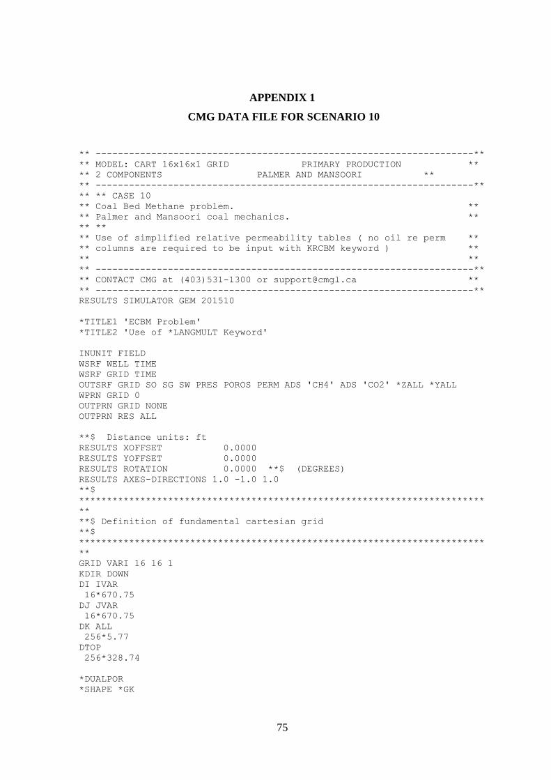
75
APPENDIX 1
CMG DATA FILE FOR SCENARIO 10
** --------------------------------------------------------------------**
** MODEL: CART 16x16x1 GRID PRIMARY PRODUCTION **
** 2 COMPONENTS PALMER AND MANSOORI **
** --------------------------------------------------------------------**
** ** CASE 10
** Coal Bed Methane problem. **
** Palmer and Mansoori coal mechanics. **
** **
** Use of simplified relative permeability tables ( no oil re perm **
** columns are required to be input with KRCBM keyword ) **
** **
** --------------------------------------------------------------------**
** CONTACT CMG at (403)531-1300 or [email protected] **
** --------------------------------------------------------------------**
RESULTS SIMULATOR GEM 201510
*TITLE1 'ECBM Problem'
*TITLE2 'Use of *LANGMULT Keyword'
INUNIT FIELD
WSRF WELL TIME
WSRF GRID TIME
OUTSRF GRID SO SG SW PRES POROS PERM ADS 'CH4' ADS 'CO2' *ZALL *YALL
WPRN GRID 0
OUTPRN GRID NONE
OUTPRN RES ALL
**$ Distance units: ft
RESULTS XOFFSET 0.0000
RESULTS YOFFSET 0.0000
RESULTS ROTATION 0.0000 **$ (DEGREES)
RESULTS AXES-DIRECTIONS 1.0 -1.0 1.0
**$
*************************************************************************
**
**$ Definition of fundamental cartesian grid
**$
*************************************************************************
**
GRID VARI 16 16 1
KDIR DOWN
DI IVAR
16*670.75
DJ JVAR
16*670.75
DK ALL
256*5.77
DTOP
256*328.74
*DUALPOR
*SHAPE *GK
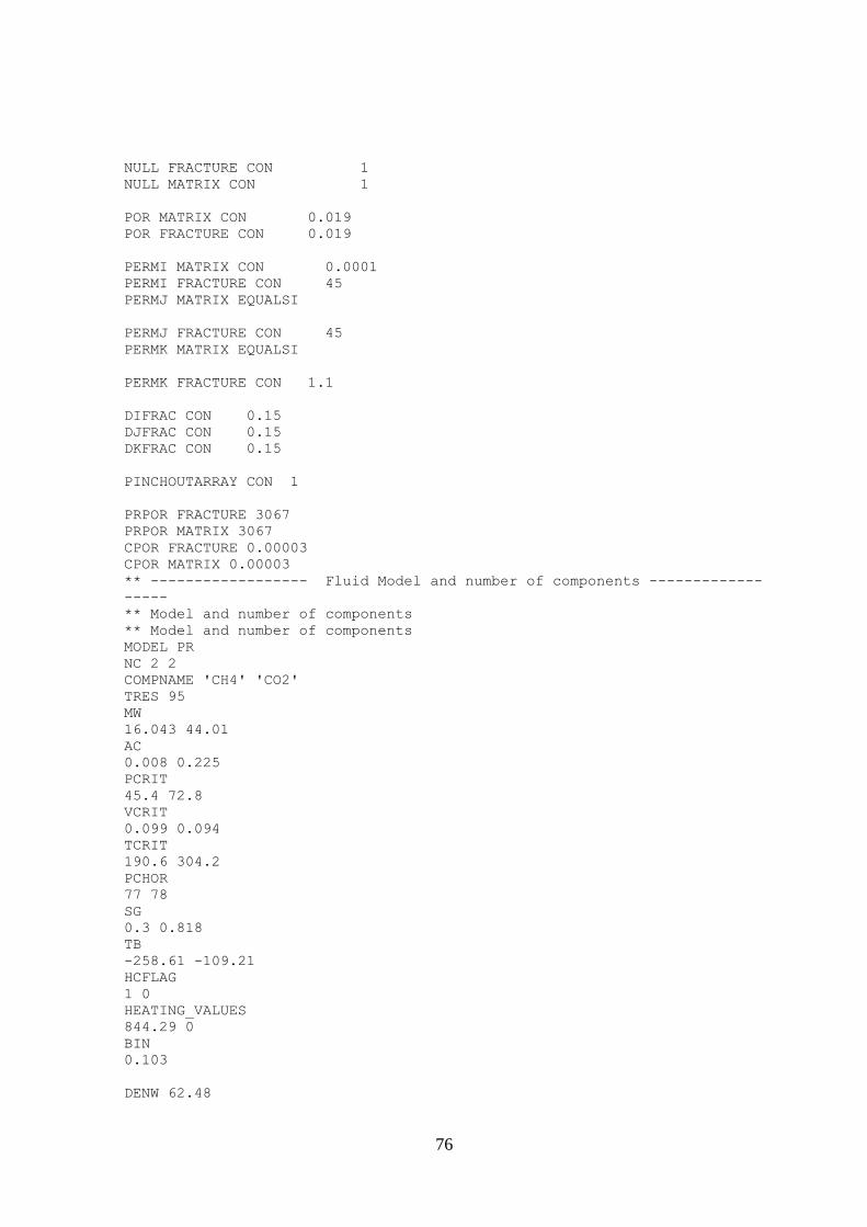
76
NULL FRACTURE CON 1
NULL MATRIX CON 1
POR MATRIX CON 0.019
POR FRACTURE CON 0.019
PERMI MATRIX CON 0.0001
PERMI FRACTURE CON 45
PERMJ MATRIX EQUALSI
PERMJ FRACTURE CON 45
PERMK MATRIX EQUALSI
PERMK FRACTURE CON 1.1
DIFRAC CON 0.15
DJFRAC CON 0.15
DKFRAC CON 0.15
PINCHOUTARRAY CON 1
PRPOR FRACTURE 3067
PRPOR MATRIX 3067
CPOR FRACTURE 0.00003
CPOR MATRIX 0.00003
** ------------------ Fluid Model and number of components -------------
-----
** Model and number of components
** Model and number of components
MODEL PR
NC 2 2
COMPNAME 'CH4' 'CO2'
TRES 95
MW
16.043 44.01
AC
0.008 0.225
PCRIT
45.4 72.8
VCRIT
0.099 0.094
TCRIT
190.6 304.2
PCHOR
77 78
SG
0.3 0.818
TB
-258.61 -109.21
HCFLAG
1 0
HEATING_VALUES
844.29 0
BIN
0.103
DENW 62.48
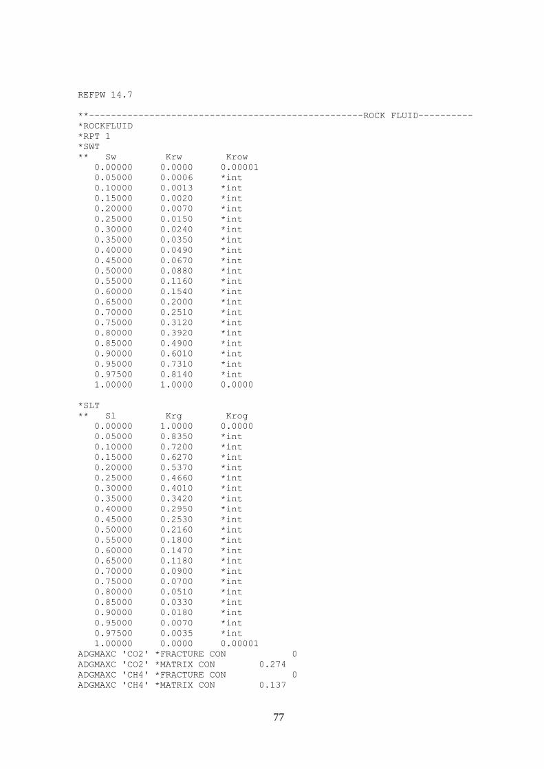
77
REFPW 14.7
**--------------------------------------------------ROCK FLUID----------
*ROCKFLUID
*RPT 1
*SWT
** Sw Krw Krow
0.00000 0.0000 0.00001
0.05000 0.0006 *int
0.10000 0.0013 *int
0.15000 0.0020 *int
0.20000 0.0070 *int
0.25000 0.0150 *int
0.30000 0.0240 *int
0.35000 0.0350 *int
0.40000 0.0490 *int
0.45000 0.0670 *int
0.50000 0.0880 *int
0.55000 0.1160 *int
0.60000 0.1540 *int
0.65000 0.2000 *int
0.70000 0.2510 *int
0.75000 0.3120 *int
0.80000 0.3920 *int
0.85000 0.4900 *int
0.90000 0.6010 *int
0.95000 0.7310 *int
0.97500 0.8140 *int
1.00000 1.0000 0.0000
*SLT
** Sl Krg Krog
0.00000 1.0000 0.0000
0.05000 0.8350 *int
0.10000 0.7200 *int
0.15000 0.6270 *int
0.20000 0.5370 *int
0.25000 0.4660 *int
0.30000 0.4010 *int
0.35000 0.3420 *int
0.40000 0.2950 *int
0.45000 0.2530 *int
0.50000 0.2160 *int
0.55000 0.1800 *int
0.60000 0.1470 *int
0.65000 0.1180 *int
0.70000 0.0900 *int
0.75000 0.0700 *int
0.80000 0.0510 *int
0.85000 0.0330 *int
0.90000 0.0180 *int
0.95000 0.0070 *int
0.97500 0.0035 *int
1.00000 0.0000 0.00001
ADGMAXC 'CO2' *FRACTURE CON 0
ADGMAXC 'CO2' *MATRIX CON 0.274
ADGMAXC 'CH4' *FRACTURE CON 0
ADGMAXC 'CH4' *MATRIX CON 0.137
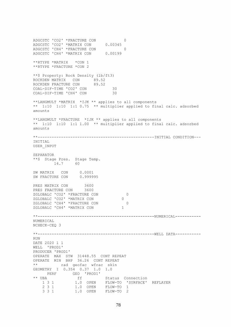
78
ADGCSTC 'CO2' *FRACTURE CON 0
ADGCSTC 'CO2' *MATRIX CON 0.00345
ADGCSTC 'CH4' *FRACTURE CON 0
ADGCSTC 'CH4' *MATRIX CON 0.00199
**RTYPE *MATRIX *CON 1
**RTYPE *FRACTURE *CON 2
**$ Property: Rock Density (lb/ft3)
ROCKDEN MATRIX CON 89.52
ROCKDEN FRACTURE CON 89.52
COAL-DIF-TIME 'CO2' CON 30
COAL-DIF-TIME 'CH4' CON 30
**LANGMULT *MATRIX *IJK ** applies to all components
** 1:10 1:10 1:1 0.75 ** multiplier applied to final calc. adsorbed
amounts
**LANGMULT *FRACTURE *IJK ** applies to all components
** 1:10 1:10 1:1 1.00 ** multiplier applied to final calc. adsorbed
amounts
**--------------------------------------------------INITIAL CONDITION---
INITIAL
USER_INPUT
SEPARATOR
**$ Stage Pres. Stage Temp.
14.7 60
SW MATRIX CON 0.0001
SW FRACTURE CON 0.999995
PRES MATRIX CON 3600
PRES FRACTURE CON 3600
ZGLOBALC 'CO2' *FRACTURE CON 0
ZGLOBALC 'CO2' *MATRIX CON 0
ZGLOBALC 'CH4' *FRACTURE CON 0
ZGLOBALC 'CH4' *MATRIX CON 1
**--------------------------------------------------NUMERICAL-----------
NUMERICAL
NCHECK-CEQ 3
**--------------------------------------------------WELL DATA-----------
RUN
DATE 2020 1 1
WELL 'PROD1'
PRODUCER 'PROD1'
OPERATE MAX STW 31448.55 CONT REPEAT
OPERATE MIN BHP 36.26 CONT REPEAT
** rad geofac wfrac skin
GEOMETRY I 0.354 0.37 1.0 1.0
PERF GEO 'PROD1'
** UBA ff Status Connection
1 3 1 1.0 OPEN FLOW-TO 'SURFACE' REFLAYER
2 3 1 1.0 OPEN FLOW-TO 1
3 3 1 1.0 OPEN FLOW-TO 2
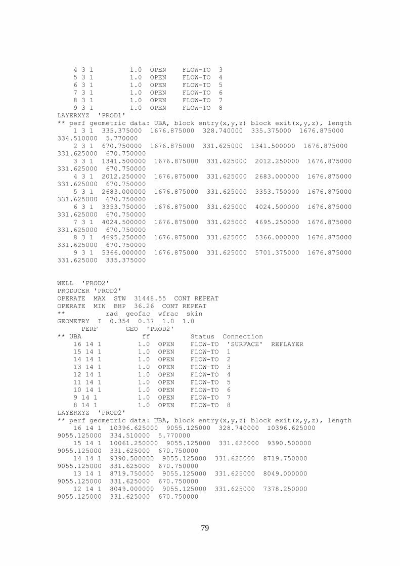
79
4 3 1 1.0 OPEN FLOW-TO 3
5 3 1 1.0 OPEN FLOW-TO 4
6 3 1 1.0 OPEN FLOW-TO 5
7 3 1 1.0 OPEN FLOW-TO 6
8 3 1 1.0 OPEN FLOW-TO 7
9 3 1 1.0 OPEN FLOW-TO 8
LAYERXYZ 'PROD1'
** perf geometric data: UBA, block entry(x,y,z) block exit(x,y,z), length
1 3 1 335.375000 1676.875000 328.740000 335.375000 1676.875000
334.510000 5.770000
2 3 1 670.750000 1676.875000 331.625000 1341.500000 1676.875000
331.625000 670.750000
3 3 1 1341.500000 1676.875000 331.625000 2012.250000 1676.875000
331.625000 670.750000
4 3 1 2012.250000 1676.875000 331.625000 2683.000000 1676.875000
331.625000 670.750000
5 3 1 2683.000000 1676.875000 331.625000 3353.750000 1676.875000
331.625000 670.750000
6 3 1 3353.750000 1676.875000 331.625000 4024.500000 1676.875000
331.625000 670.750000
7 3 1 4024.500000 1676.875000 331.625000 4695.250000 1676.875000
331.625000 670.750000
8 3 1 4695.250000 1676.875000 331.625000 5366.000000 1676.875000
331.625000 670.750000
9 3 1 5366.000000 1676.875000 331.625000 5701.375000 1676.875000
331.625000 335.375000
WELL 'PROD2'
PRODUCER 'PROD2'
OPERATE MAX STW 31448.55 CONT REPEAT
OPERATE MIN BHP 36.26 CONT REPEAT
** rad geofac wfrac skin
GEOMETRY I 0.354 0.37 1.0 1.0
PERF GEO 'PROD2'
** UBA ff Status Connection
16 14 1 1.0 OPEN FLOW-TO 'SURFACE' REFLAYER
15 14 1 1.0 OPEN FLOW-TO 1
14 14 1 1.0 OPEN FLOW-TO 2
13 14 1 1.0 OPEN FLOW-TO 3
12 14 1 1.0 OPEN FLOW-TO 4
11 14 1 1.0 OPEN FLOW-TO 5
10 14 1 1.0 OPEN FLOW-TO 6
9 14 1 1.0 OPEN FLOW-TO 7
8 14 1 1.0 OPEN FLOW-TO 8
LAYERXYZ 'PROD2'
** perf geometric data: UBA, block entry(x,y,z) block exit(x,y,z), length
16 14 1 10396.625000 9055.125000 328.740000 10396.625000
9055.125000 334.510000 5.770000
15 14 1 10061.250000 9055.125000 331.625000 9390.500000
9055.125000 331.625000 670.750000
14 14 1 9390.500000 9055.125000 331.625000 8719.750000
9055.125000 331.625000 670.750000
13 14 1 8719.750000 9055.125000 331.625000 8049.000000
9055.125000 331.625000 670.750000
12 14 1 8049.000000 9055.125000 331.625000 7378.250000
9055.125000 331.625000 670.750000
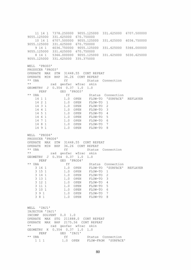
80
11 14 1 7378.250000 9055.125000 331.625000 6707.500000
9055.125000 331.625000 670.750000
10 14 1 6707.500000 9055.125000 331.625000 6036.750000
9055.125000 331.625000 670.750000
9 14 1 6036.750000 9055.125000 331.625000 5366.000000
9055.125000 331.625000 670.750000
8 14 1 5366.000000 9055.125000 331.625000 5030.625000
9055.125000 331.625000 335.375000
WELL 'PROD3'
PRODUCER 'PROD3'
OPERATE MAX STW 31448.55 CONT REPEAT
OPERATE MIN BHP 36.26 CONT REPEAT
** UBA ff Status Connection
** rad geofac wfrac skin
GEOMETRY J 0.354 0.37 1.0 1.0
PERF GEO 'PROD3'
** UBA ff Status Connection
14 1 1 1.0 OPEN FLOW-TO 'SURFACE' REFLAYER
14 2 1 1.0 OPEN FLOW-TO 1
14 3 1 1.0 OPEN FLOW-TO 2
14 4 1 1.0 OPEN FLOW-TO 3
14 5 1 1.0 OPEN FLOW-TO 4
14 6 1 1.0 OPEN FLOW-TO 5
14 7 1 1.0 OPEN FLOW-TO 6
14 8 1 1.0 OPEN FLOW-TO 7
14 9 1 1.0 OPEN FLOW-TO 8
WELL 'PROD4'
PRODUCER 'PROD4'
OPERATE MAX STW 31448.55 CONT REPEAT
OPERATE MIN BHP 36.26 CONT REPEAT
** UBA ff Status Connection
** rad geofac wfrac skin
GEOMETRY J 0.354 0.37 1.0 1.0
PERF GEO 'PROD4'
** UBA ff Status Connection
3 16 1 1.0 OPEN FLOW-TO 'SURFACE' REFLAYER
3 15 1 1.0 OPEN FLOW-TO 1
3 14 1 1.0 OPEN FLOW-TO 2
3 13 1 1.0 OPEN FLOW-TO 3
3 12 1 1.0 OPEN FLOW-TO 4
3 11 1 1.0 OPEN FLOW-TO 5
3 10 1 1.0 OPEN FLOW-TO 6
3 9 1 1.0 OPEN FLOW-TO 7
3 8 1 1.0 OPEN FLOW-TO 8
WELL 'INJ1'
INJECTOR 'INJ1'
INCOMP SOLVENT 0.0 1.0
OPERATE MAX STG 211888.0 CONT REPEAT
OPERATE MAX BHP 2175.56 CONT REPEAT
** rad geofac wfrac skin
GEOMETRY K 0.354 0.37 1.0 1.0
PERF GEO 'INJ1'
** UBA ff Status Connection
1 1 1 1.0 OPEN FLOW-FROM 'SURFACE'
81
WELL 'INJ2'
INJECTOR 'INJ2'
INCOMP SOLVENT 0.0 1.0
OPERATE MAX STG 211888.0 CONT REPEAT
OPERATE MAX BHP 2175.56 CONT REPEAT
** rad geofac wfrac skin
GEOMETRY K 0.354 0.37 1.0 1.0
PERF GEO 'INJ2'
** UBA ff Status Connection
16 16 1 1.0 OPEN FLOW-FROM 'SURFACE'
WELL 'INJ3'
INJECTOR 'INJ3'
INCOMP SOLVENT 0.0 1.0
OPERATE MAX STG 211888.0 CONT REPEAT
OPERATE MAX BHP 2175.56 CONT REPEAT
** UBA ff Status Connection
** rad geofac wfrac skin
GEOMETRY J 0.354 0.37 1.0 1.0
PERF GEO 'INJ3'
** UBA ff Status Connection
16 1 1 1.0 OPEN FLOW-TO 'SURFACE'
16 2 1 1.0 OPEN FLOW-TO 1
16 3 1 1.0 OPEN FLOW-TO 2
16 4 1 1.0 OPEN FLOW-TO 3
16 5 1 1.0 OPEN FLOW-TO 4
16 6 1 1.0 OPEN FLOW-TO 5
16 7 1 1.0 OPEN FLOW-TO 6
16 8 1 1.0 OPEN FLOW-TO 7
16 9 1 1.0 OPEN FLOW-TO 8
WELL 'INJ4'
INJECTOR 'INJ4'
INCOMP SOLVENT 0.0 1.0
OPERATE MAX STG 211888.0 CONT REPEAT
OPERATE MAX BHP 2175.56 CONT REPEAT
** UBA ff Status Connection
** rad geofac wfrac skin
GEOMETRY J 0.354 0.37 1.0 1.0
PERF GEO 'INJ4'
** UBA ff Status Connection
1 16 1 1.0 OPEN FLOW-TO 'SURFACE' REFLAYER
1 15 1 1.0 OPEN FLOW-TO 1
1 14 1 1.0 OPEN FLOW-TO 2
1 13 1 1.0 OPEN FLOW-TO 3
1 12 1 1.0 OPEN FLOW-TO 4
1 11 1 1.0 OPEN FLOW-TO 5
1 10 1 1.0 OPEN FLOW-TO 6
1 9 1 1.0 OPEN FLOW-TO 7
1 8 1 1.0 OPEN FLOW-TO 8
*AIMSET *FRACTURE *CON 3
*AIMSET *MATRIX *CON 3
DATE 2020 2 1
DATE 2021 1 1
DATE 2022 1 1
82
DATE 2023 1 1
DATE 2024 1 1
DATE 2025 1 1
DATE 2026 1 1
DATE 2027 1 1
DATE 2028 1 1
DATE 2029 1 1
DATE 2030 1 1
DATE 2031 1 1
DATE 2032 1 1
DATE 2033 1 1
DATE 2034 1 1
DATE 2035 1 1
**SHUTIN WELLS
SHUTIN 'PROD1'
SHUTIN 'PROD2'
SHUTIN 'PROD3'
SHUTIN 'PROD4'
WELL 'INJ1'
INJECTOR 'INJ1'
INCOMP SOLVENT 0.0 1.0
OPERATE MAX BHP 4000 STOP
** rad geofac wfrac skin
GEOMETRY K 0.354 0.37 1.0 1.0
PERF GEO 'INJ1'
** UBA ff Status Connection
1 1 1 1.0 OPEN FLOW-FROM 'SURFACE'
WELL 'INJ2'
INJECTOR 'INJ2'
INCOMP SOLVENT 0.0 1.0
OPERATE MAX BHP 4000 STOP
** rad geofac wfrac skin
GEOMETRY K 0.354 0.37 1.0 1.0
PERF GEO 'INJ2'
** UBA ff Status Connection
16 16 1 1.0 OPEN FLOW-FROM 'SURFACE'
WELL 'INJ3'
INJECTOR 'INJ3'
INCOMP SOLVENT 0.0 1.0
OPERATE MAX BHP 4000 STOP
** UBA ff Status Connection
** rad geofac wfrac skin
GEOMETRY J 0.354 0.37 1.0 1.0
PERF GEO 'INJ3'
** UBA ff Status Connection
16 1 1 1.0 OPEN FLOW-TO 'SURFACE'
16 2 1 1.0 OPEN FLOW-TO 1
16 3 1 1.0 OPEN FLOW-TO 2
16 4 1 1.0 OPEN FLOW-TO 3
16 5 1 1.0 OPEN FLOW-TO 4
16 6 1 1.0 OPEN FLOW-TO 5
16 7 1 1.0 OPEN FLOW-TO 6
16 8 1 1.0 OPEN FLOW-TO 7
16 9 1 1.0 OPEN FLOW-TO 8
83
WELL 'INJ4'
INJECTOR 'INJ4'
INCOMP SOLVENT 0.0 1.0
OPERATE MAX BHP 4000 STOP
** UBA ff Status Connection
** rad geofac wfrac skin
GEOMETRY J 0.354 0.37 1.0 1.0
PERF GEO 'INJ4'
** UBA ff Status Connection
1 16 1 1.0 OPEN FLOW-TO 'SURFACE' REFLAYER
1 15 1 1.0 OPEN FLOW-TO 1
1 14 1 1.0 OPEN FLOW-TO 2
1 13 1 1.0 OPEN FLOW-TO 3
1 12 1 1.0 OPEN FLOW-TO 4
1 11 1 1.0 OPEN FLOW-TO 5
1 10 1 1.0 OPEN FLOW-TO 6
1 9 1 1.0 OPEN FLOW-TO 7
1 8 1 1.0 OPEN FLOW-TO 8
DATE 2036 1 1
DATE 2037 1 1
DATE 2038 1 1
DATE 2039 1 1
DATE 2040 1 1
DATE 2041 1 1
DATE 2042 1 1
DATE 2043 1 1
DATE 2044 1 1
DATE 2045 1 1
STOP
RESULTS SPEC 'Permeability K' MATRIX
RESULTS SPEC SPECNOTCALCVAL -99999
RESULTS SPEC REGION 'All Layers (Whole Grid)'
RESULTS SPEC REGIONTYPE 'REGION_WHOLEGRID'
RESULTS SPEC LAYERNUMB 0
RESULTS SPEC PORTYPE 1
RESULTS SPEC EQUALSI 0 1
RESULTS SPEC SPECKEEPMOD 'YES'
RESULTS SPEC STOP
RESULTS SPEC 'Permeability J' MATRIX
RESULTS SPEC SPECNOTCALCVAL -99999
RESULTS SPEC REGION 'All Layers (Whole Grid)'
RESULTS SPEC REGIONTYPE 'REGION_WHOLEGRID'
RESULTS SPEC LAYERNUMB 0
RESULTS SPEC PORTYPE 1
RESULTS SPEC EQUALSI 0 1
RESULTS SPEC SPECKEEPMOD 'YES'
RESULTS SPEC STOP
84
APPENDIX 2
SIMILARITY REPORT
85
APPENDIX 3
ETHICAL APPROVAL LETTER
YAKIN DOĞU ÜNiVERSiTESi ETHICAL APPROVAL DOCUMENT
Date 29/06/2021
To the Graduate School of Applied Sciences
The research project titled "NUMERICAL INVESTIGATION OF ECBM RECOVERY AND
CO2 SEQUESTRATION" has been evaluated. Since the researchers will not collect any data
from humans, animals, plants or earth, this project does not need through the ethics
committee.
Title: Assist. Prof. Dr.
Name Surname: Serhat CANBOLAT
Signature:
Role in the Research Project: Supervisor