Numerical case studies for civil enginering
53
8.2 GREENHOUSE GASES AND RAINWATER 205 these approaches may also interject a critical delay in the procedure. This shortcoming is relevant to the secant method, which also needs two initial estimates. In contrast, the Newton-Raphson method requires only one guess for the root. The ideal gas law could be employed to obtain this guess at the initiation of the process. Then, assuming that the time frame is short enough so that pressure and temperature do not vary wildly between computations, the previous root solution would provide a good guess for the next application. Thus, the close guess that is often a prerequisite for convergence of the Newton-Raphson method would automatically be available. All the above considera- tions would greatly favor the Newton-Raphson technique for such problems. 8.2 GREENHOUSE GASES AND RAINWATER (CIVIL/ENVIRONMENTAL ENGINEERING) Background. Civil engineering is a broad field that includes such diverse areas as structural, geotechnical, transportation, water-resources, and environmental engineering. The last area has traditionally dealt with pollution control. However, in recent years, environmental engineers (as well as chemical engineers) have addressed broader problems such as climate change. It is well documented that the atmospheric levels of several greenhouse gases has been increasing over the past 50 years. For example, Fig. 8.1 shows data for the partial pressure of carbon dioxide (CO 2 ) collected at Mauna Loa, Hawaii from 1958 through 2003. The trend in the data can be nicely fit with a quadratic polynomial (In Part Five, we will learn how to determine such polynomials), p CO 2 = 0.011825(t - 1980.5) 2 + 1.356975(t - 1980.5) + 339 where p CO 2 = the partial pressure of CO 2 in the atmosphere [ppm]. The data indicates that levels have increased over 19% during the period from 315 to 376 ppm. FIGURE 8.1 Average annual partial pressures of atmospheric carbon dioxide (ppm) measured at Mauna Loa, Hawaii. 310 330 350 370 1950 1960 1970 1980 1990 2000 2010 p CO 2 (ppm)
-
Upload
independent -
Category
Documents
-
view
2 -
download
0
Transcript of Numerical case studies for civil enginering
8.2 GREENHOUSE GASES AND RAINWATER 205
these approaches may also interject a critical delay in the procedure. This shortcoming isrelevant to the secant method, which also needs two initial estimates.
In contrast, the Newton-Raphson method requires only one guess for the root. Theideal gas law could be employed to obtain this guess at the initiation of the process. Then,assuming that the time frame is short enough so that pressure and temperature do not varywildly between computations, the previous root solution would provide a good guess forthe next application. Thus, the close guess that is often a prerequisite for convergence ofthe Newton-Raphson method would automatically be available. All the above considera-tions would greatly favor the Newton-Raphson technique for such problems.
8.2 GREENHOUSE GASES AND RAINWATER(CIVIL/ENVIRONMENTAL ENGINEERING)
Background. Civil engineering is a broad field that includes such diverse areas as structural,geotechnical, transportation, water-resources, and environmental engineering. The last area hastraditionally dealt with pollution control. However, in recent years, environmental engineers(as well as chemical engineers) have addressed broader problems such as climate change.
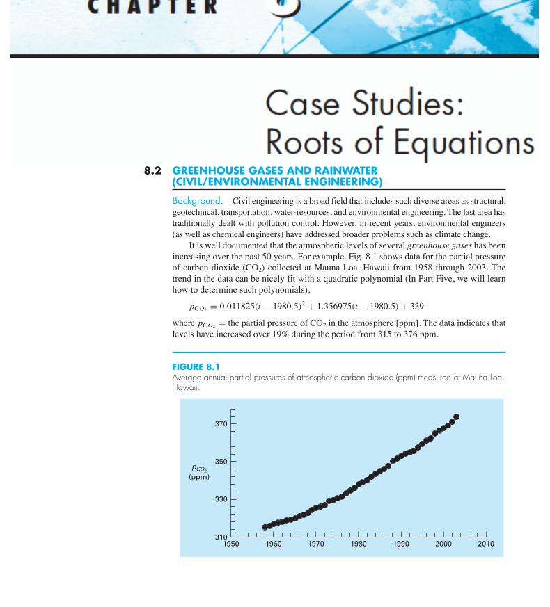
It is well documented that the atmospheric levels of several greenhouse gases has beenincreasing over the past 50 years. For example, Fig. 8.1 shows data for the partial pressureof carbon dioxide (CO2) collected at Mauna Loa, Hawaii from 1958 through 2003. Thetrend in the data can be nicely fit with a quadratic polynomial (In Part Five, we will learnhow to determine such polynomials),
pC O2 = 0.011825(t ! 1980.5)2 + 1.356975(t ! 1980.5) + 339
where pC O2 = the partial pressure of CO2 in the atmosphere [ppm]. The data indicates thatlevels have increased over 19% during the period from 315 to 376 ppm.
FIGURE 8.1Average annual partial pressures of atmospheric carbon dioxide (ppm) measured at Mauna Loa,Hawaii.
310
330
350
370
1950 1960 1970 1980 1990 2000 2010
pCO2(ppm)
cha01064_ch08.qxd 3/20/09 11:54 AM Page 205
Toshiba
Stamp
Aside from global warming, greenhouse gases can also influence atmospheric chemistry.One question that we can address is how the carbon dioxide trend is affecting the pH of rain-water. Outside of urban and industrial areas, it is well documented that carbon dioxide is theprimary determinant of the pH of the rain. pH is the measure of the activity of hydrogen ionsand, therefore, its acidity. For dilute aqueous solutions, it can be computed as
pH = ! log10[H+] (8.5)
where [H+] is the molar concentration of hydrogen ions. The following five nonlinear system of equations govern the chemistry of rainwater,
K1 = 106 [H+][HCO!3 ]
K H pC O2
(8.6)
K2 =[H+]
$CO2!
3%
[HCO!3 ]
(8.7)
Kw = [H+][OH!] (8.8)
cT = K H pC O2
106 + [HCO!3 ] +
$CO2!
3%
(8.9)
0 = [HCO!3 ] + 2
$CO2!
3%+ [OH!] ! [H+] (8.10)
where K H = Henry’s constant, and K1, K2 and Kw are equilibrium coefficients. The fiveunknowns are cT = total inorganic carbon, [HCO!
3 ] = bicarbonate, [CO2!3 ] = carbonate,
[H+] = hydrogen ion, and [OH!] = hydroxyl ion. Notice how the partial pressure of CO2shows up in Eqs. (8.6) and (8.9).
Use these equations to compute the pH of rainwater given that K H = 10!1.46,K1 = 10!6.3, K2 = 10!10.3, and Kw = 10!14. Compare the results in 1958 when the pC O2
was 315 and in 2003 when it was 375 ppm. When selecting a numerical method for yourcomputation, consider the following:
• You know with certainty that the pH of rain in pristine areas always falls between 2 and 12.• You also know that your measurement devices can only measured pH to two places of
decimal precision.
Solution. There are a variety of ways to solve this nonlinear system of five equations.One way is to eliminate unknowns by combining them to produce a single function thatonly depends on [H+]. To do this, first solve Eqs. (8.6) and (8.7) for
[HCO!3 ] = K1
106[H+]K H pC O2 (8.11)
[CO2!3 ] = K2[HCO!
3 ][H+]
(8.12)
Substitute Eq. (8.11) into (8.12)$CO2!
3%
= K2 K1
106[H+]2 K H pC O2 (8.13)
206 CASE STUDIES: ROOTS OF EQUATIONS
cha01064_ch08.qxd 3/20/09 11:54 AM Page 206
8.3 DESIGN OF AN ELECTRIC CIRCUIT 207
Equations (8.11) and (8.13) can be substituted along with Eq. (8.8) into Eq. (8.10) to give
0 = K1
106[H+]K H pCO2 + 2
K2 K1
106[H+]2 K H pC O2+Kw
[H+]! [H+] (8.14)
Although it might not be apparent, this result is a third-order polynomial in [H+]. Thus, itsroot can be used to compute the pH of the rainwater.
Now we must decide which numerical method to employ to obtain the solution. Thereare two reasons why bisection would be a good choice. First, the fact that the pH alwaysfalls within the range from 2 to 12, provides us with two good initial guesses. Second,because the pH can only be measured to two decimal places of precision, we will be satis-fied with an absolute error of Ea,d = 0.005. Remember that given an initial bracket and thedesired relative error, we can compute the number of iterations a priori. Using Eq. (5.5),the result is n = log2(10)/0.005 = 10.9658. Thus, eleven iterations of bisection will pro-duce the desired precision.
If this is done, the result for 1958 will be a pH of 5.6279 with a relative error of0.0868%. We can be confident that the rounded result of 5.63 is correct to two decimalplaces. This can be verified by performing another run with more iterations. For example,if we perform 35 iterations, a result of 5.6304 is obtained with an approximate relative errorof !a = 5.17 # 10!9%. The same calculation can be repeated for the 2003 conditions togive pH = 5.59 with !a = 0.0874%.
Interestingly, these results indicate that the 19% rise in atmospheric CO2 levels hasproduced only a 0.67% drop in pH. Although this is certainly true, remember that the pHrepresents a logarithmic scale as defined by Eq. (8.5). Consequently, a unit drop in pH rep-resents a 10-fold increase in hydrogen ion. The concentration can be computed as[H+] = 10!pH and the resulting percent change can be calculated as 9.1%. Therefore, thehydrogen ion concentration has increased about 9%.
There is quite a lot of controversy related to the true significance of the greenhouse gastrends. However, regardless of the ultimate implications, it is quite sobering to realizethat something as large as our atmosphere has changed so much over a relatively short timeperiod. This case study illustrates how numerical methods can be employed to analyze andinterpret such trends. Over the coming years, engineers and scientists can hopefully usesuch tools to gain increased understanding and help rationalize the debate over theirramifications.
8.3 DESIGN OF AN ELECTRIC CIRCUIT(ELECTRICAL ENGINEERING)
Background. Electrical engineers often use Kirchhoff’s laws to study the steady-state(not time-varying) behavior of electric circuits. Such steady-state behavior will be exam-ined in Sec. 12.3. Another important problem involves circuits that are transient in naturewhere sudden temporal changes take place. Such a situation occurs following the closingof the switch in Fig. 8.2. In this case, there will be a period of adjustment following theclosing of the switch as a new steady state is reached. The length of this adjustment periodis closely related to the storage properties of the capacitor and the inductor. Energy storage
cha01064_ch08.qxd 3/20/09 11:54 AM Page 207
PROBLEMS 215
Determine h given r = 2 m, L = 5 m, and V = 8 m3. Note that ifyou are using a programming language or software tool that is notrich in trigonometric functions, the arc cosine can be computedwith
cos!1 x = '
2! tan!1
!x$
1 ! x2
"
8.9 The volume V of liquid in a spherical tank of radius r is relatedto the depth h of the liquid by
V = 'h2(3r ! h)
3
Determine h given r = 1 m and V = 0.5 m3.8.10 For the spherical tank in Prob. 8.9, it is possible to developthe following two fixed-point formulas:
h =-
h3 + (3V/')
3r
and
h = 3
(
3!
rh2 ! V'
"
If r = 1 m and V = 0.75 m3, determine whether either of these isstable, and the range of initial guesses for which they are stable.8.11 The Ergun equation, shown below, is used to describe theflow of a fluid through a packed bed. (P is the pressure drop, # isthe density of the fluid, Go is the mass velocity (mass flow ratedivided by cross-sectional area), Dp is the diameter of the particleswithin the bed, µ is the fluid viscosity, L is the length of the bed,and ! is the void fraction of the bed.
(P#
G2o
Dp
L!3
1 ! != 150
1 ! !
(DpGo/µ)+ 1.75
Given the parameter values listed below, find the void fraction ! ofthe bed.
DpGo
µ= 1000
(P#Dp
G2o L
= 10
8.12 The pressure drop in a section of pipe can be calculated as
(p = fL#V 2
2D
where (p = the pressure drop (Pa), f = the friction factor, L =the length of pipe [m], # = density (kg/m3), V = velocity (m/s),and D = diameter (m). For turbulent flow, the Colebrook equationprovides a means to calculate the friction factor,
1$f
= !2.0 log!
!
3.7D+ 2.51
Re$
f
"
where ! = the roughness (m), and Re = the Reynolds number,
Re = #VDµ
where µ = dynamic viscosity (N · s/m2).(a) Determine (p for a 0.2-m-long horizontal stretch of smooth
drawn tubing given# = 1.23 kg/m3,µ = 1.79 #10!5 N · s/m2,D = 0.005 m, V = 40 m/s, and ! = 0.0015 mm. Use a numer-ical method to determine the friction factor. Note that smoothpipes with Re < 105, a good initial guess can be obtained usingthe Blasius formula, f = 0.316/Re0.25.
(b) Repeat the computation but for a rougher commercial steelpipe (! = 0.045 mm).
8.13 The operation of a constant density plug flow reactor for theproduction of a substance via an enzymatic reaction is described bythe equation below, where V is the volume of the reactor, F is theflow rate of reactant C, Cin and Cout are the concentrations of reac-tant entering and leaving the reactor, respectively, and K and kmaxare constants. For a 500-L reactor, with an inlet concentration ofCin = 0.5 M, an inlet flow rate of 40 L/s, kmax = 5 # 10!3 s!1 , andK = 0.1 M, find the concentration of C at the outlet of the reactor.
VF
= !/ Cout
Cin
KkmaxC
+ 1kmax
dC
Civil and Environmental Engineering8.14 In structural engineering, the secant formula defines the forceper unit area, P/A, that causes a maximum stress )m in a columnof given slenderness ratio L/k:
PA
= )m
1 + (ec/k2) sec[0.5$
P/(E A)(L/k)]
where ec/k2 = the eccentricity ratio and E = the modulus of elas-ticity. If for a steel beam, E = 200,000 MPa, ec/k2 = 0.4, and)m = 250 MPa, compute P/A for L/k = 50. Recall that sec x =1/cos x .8.15 In environmental engineering (a specialty area in civilengineering), the following equation can be used to compute theoxygen level c (mg/L) in a river downstream from a sewagedischarge:
c = 10 ! 20(e!0.15x ! e!0.5x )
where x is the distance downstream in kilometers.(a) Determine the distance downstream where the oxygen level
first falls to a reading of 5 mg/L. (Hint: It is within 2 km of thedischarge.) Determine your answer to a 1% error. Note that lev-els of oxygen below 5 mg/L are generally harmful to gamefishsuch as trout and salmon.
(b) Determine the distance downstream at which the oxygen is at aminimum. What is the concentration at that location?
cha01064_ch08.qxd 3/20/09 11:54 AM Page 215
216 CASE STUDIES: ROOTS OF EQUATIONS
8.16 The concentration of pollutant bacteria c in a lake decreasesaccording to
c = 75e!1.5t + 20e!0.075t
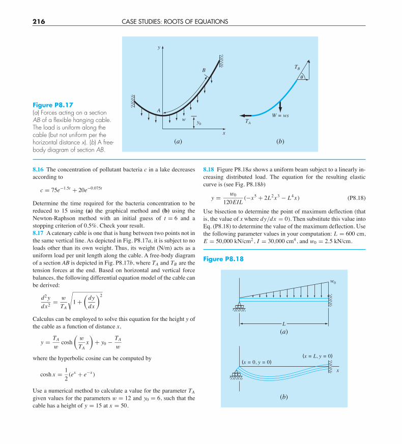
Determine the time required for the bacteria concentration to bereduced to 15 using (a) the graphical method and (b) using theNewton-Raphson method with an initial guess of t = 6 and astopping criterion of 0.5%. Check your result.8.17 A catenary cable is one that is hung between two points not inthe same vertical line. As depicted in Fig. P8.17a, it is subject to noloads other than its own weight. Thus, its weight (N/m) acts as auniform load per unit length along the cable. A free-body diagramof a section AB is depicted in Fig. P8.17b, where TA and TB are thetension forces at the end. Based on horizontal and vertical forcebalances, the following differential equation model of the cable canbe derived:
d2 ydx2 = w
TA
(
1 +!
dydx
"2
Calculus can be employed to solve this equation for the height y ofthe cable as a function of distance x,
y = TA
wcosh
!w
TAx"
+ y0 ! TA
w
where the hyperbolic cosine can be computed by
cosh x = 12(ex + e!x )
Use a numerical method to calculate a value for the parameter TAgiven values for the parameters w = 12 and y0 = 6, such that thecable has a height of y = 15 at x = 50.
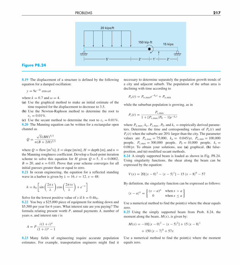
8.18 Figure P8.18a shows a uniform beam subject to a linearly in-creasing distributed load. The equation for the resulting elasticcurve is (see Fig. P8.18b)
y = w0
120EIL(!x5 + 2L2x3 ! L4x) (P8.18)
Use bisection to determine the point of maximum deflection (thatis, the value of x where dy/dx = 0). Then substitute this value intoEq. (P8.18) to determine the value of the maximum deflection. Usethe following parameter values in your computation: L = 600 cm,E = 50,000 kN/cm2, I = 30,000 cm4, and w0 = 2.5 kN/cm.
w0
L(a)
(x = 0, y = 0)(x = L, y = 0)
x
(b)
Figure P8.18
y
B
A
TA
W = wsw y0
x(a) (b)
TB
!
Figure P8.17(a) Forces acting on a sectionAB of a flexible hanging cable.The load is uniform along thecable (but not uniform per thehorizontal distance x). (b) A free-body diagram of section AB.
cha01064_ch08.qxd 3/20/09 11:54 AM Page 216
PROBLEMS 217
8.19 The displacement of a structure is defined by the followingequation for a damped oscillation:
y = 9e!kt cos *t
where k = 0.7 and * = 4.(a) Use the graphical method to make an initial estimate of the
time required for the displacement to decrease to 3.5.(b) Use the Newton-Raphson method to determine the root to
!s = 0.01%.(c) Use the secant method to determine the root to !s = 0.01%.8.20 The Manning equation can be written for a rectangular openchannel as
Q =$
S(BH)5/3
n(B + 2H)2/3
where Q = flow [m3/s], S = slope [m/m], H = depth [m], and n =the Manning roughness coefficient. Develop a fixed-point iterationscheme to solve this equation for H given Q = 5, S = 0.0002,B = 20, and n = 0.03. Prove that your scheme converges for allinitial guesses greater than or equal to zero. 8.21 In ocean engineering, the equation for a reflected standingwave in a harbor is given by + = 16, t = 12, v = 48:
h = h0
+sin
!2'x+
"cos
!2' tv
+
"+ e!x
,
Solve for the lowest positive value of x if h = 0.4h0.8.22 You buy a $25,000 piece of equipment for nothing down and$5,500 per year for 6 years. What interest rate are you paying? Theformula relating present worth P, annual payments A, number ofyears n, and interest rate i is
A = Pi(1 + i)n
(1 + i)n ! 1
8.23 Many fields of engineering require accurate populationestimates. For example, transportation engineers might find it
necessary to determine separately the population growth trends ofa city and adjacent suburb. The population of the urban area isdeclining with time according to
Pu(t) = Pu,maxe!ku t + Pu,min
while the suburban population is growing, as in
Ps(t) = Ps,max
1 + [Ps,max/P0 ! 1]e!ks t
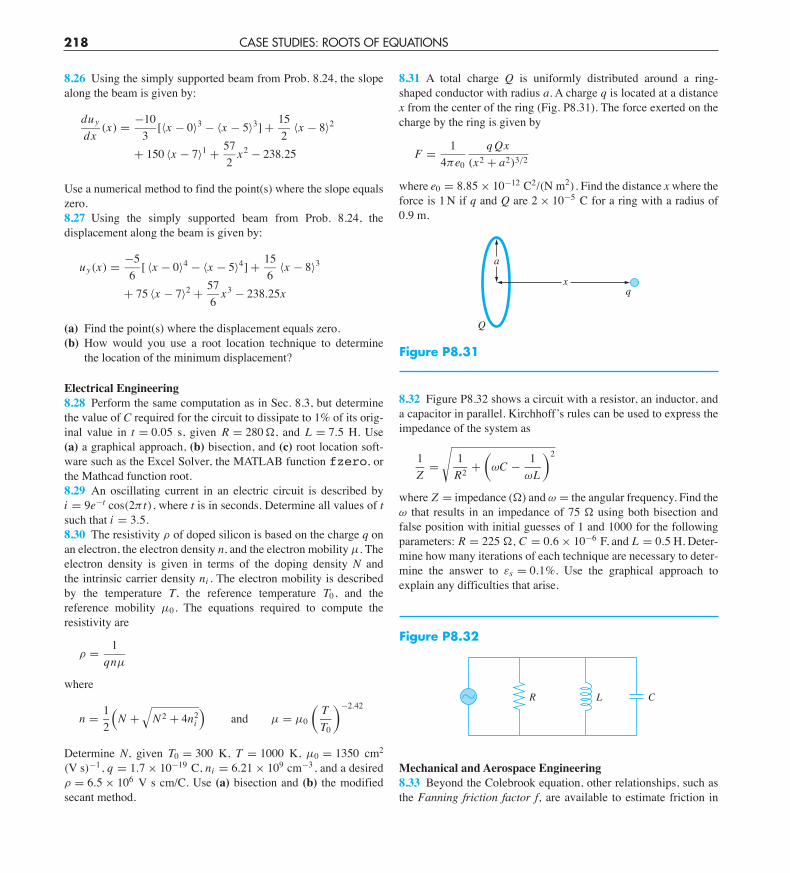
where Pu,max, ku , Ps,max, P0, and ks = empirically derived parame-ters. Determine the time and corresponding values of Pu(t) andPs(t) when the suburbs are 20% larger than the city. The parametervalues are Pu,max = 75,000, ku = 0.045/yr, Pu,min = 100,000people, Ps,max = 300,000 people, P0 = 10,000 people, ks =0.08/yr. To obtain your solutions, use (a) graphical, (b) false-position, and (c) modified secant methods.8.24 A simply supported beam is loaded as shown in Fig. P8.24.Using singularity functions, the shear along the beam can beexpressed by the equation:
V (x) = 20[&x ! 0'1 ! &x ! 5'1] ! 15 &x ! 8'0 ! 57
By definition, the singularity function can be expressed as follows:
&x ! a'n =0
(x ! a)n when x > a0 when x ( a
#
Use a numerical method to find the point(s) where the shear equalszero.8.25 Using the simply supported beam from Prob. 8.24, themoment along the beam, M(x), is given by:
M(x) = !10[&x ! 0'2 ! &x ! 5'2] + 15 &x ! 8'1
+ 150 &x ! 7'0 + 57x
Use a numerical method to find the point(s) where the momentequals zero.
20 kips/ft
150 kip-ft 15 kips
5’ 2’ 1’ 2’
Figure P8.24
cha01064_ch08.qxd 3/20/09 11:55 AM Page 217
218 CASE STUDIES: ROOTS OF EQUATIONS
8.26 Using the simply supported beam from Prob. 8.24, the slopealong the beam is given by:
duy
dx(x) = !10
3[&x ! 0'3 ! &x ! 5'3] + 15
2&x ! 8'2
+ 150 &x ! 7'1 + 572
x2 ! 238.25
Use a numerical method to find the point(s) where the slope equalszero.8.27 Using the simply supported beam from Prob. 8.24, thedisplacement along the beam is given by:
uy(x) = !56
[ &x ! 0'4 ! &x ! 5'4] + 156
&x ! 8'3
+ 75 &x ! 7'2 + 576
x3 ! 238.25x
(a) Find the point(s) where the displacement equals zero.(b) How would you use a root location technique to determine
the location of the minimum displacement?
Electrical Engineering8.28 Perform the same computation as in Sec. 8.3, but determinethe value of C required for the circuit to dissipate to 1% of its orig-inal value in t = 0.05 s, given R = 280 ", and L = 7.5 H. Use(a) a graphical approach, (b) bisection, and (c) root location soft-ware such as the Excel Solver, the MATLAB function fzero, orthe Mathcad function root. 8.29 An oscillating current in an electric circuit is described byi = 9e!t cos(2' t), where t is in seconds. Determine all values of tsuch that i = 3.5.8.30 The resistivity # of doped silicon is based on the charge q onan electron, the electron density n, and the electron mobility µ. Theelectron density is given in terms of the doping density N andthe intrinsic carrier density ni . The electron mobility is describedby the temperature T, the reference temperature T0, and thereference mobility µ0. The equations required to compute theresistivity are
# = 1qnµ
where
n = 12
1N +
2N 2 + 4n2
i
3and µ = µ0
!TT0
"!2.42
Determine N, given T0 = 300 K, T = 1000 K, µ0 = 1350 cm2
(V s)!1, q = 1.7 # 10!19 C, ni = 6.21 # 109 cm!3 , and a desired# = 6.5 # 106 V s cm/C. Use (a) bisection and (b) the modifiedsecant method.
8.32 Figure P8.32 shows a circuit with a resistor, an inductor, anda capacitor in parallel. Kirchhoff’s rules can be used to express theimpedance of the system as
1Z
=
(1R2 +
!*C ! 1
*L
"2
where Z = impedance (") and * = the angular frequency. Find the* that results in an impedance of 75 " using both bisection andfalse position with initial guesses of 1 and 1000 for the followingparameters: R = 225 ", C = 0.6 # 10!6 F, and L = 0.5 H. Deter-mine how many iterations of each technique are necessary to deter-mine the answer to !s = 0.1%. Use the graphical approach toexplain any difficulties that arise.
x
a
Q
q
Figure P8.31
R L C!
Figure P8.32
Mechanical and Aerospace Engineering8.33 Beyond the Colebrook equation, other relationships, such asthe Fanning friction factor f, are available to estimate friction in
8.31 A total charge Q is uniformly distributed around a ring-shaped conductor with radius a. A charge q is located at a distancex from the center of the ring (Fig. P8.31). The force exerted on thecharge by the ring is given by
F = 14'e0
q Qx(x2 + a2)3/2
where e0 = 8.85 # 10!12 C2/(N m2). Find the distance x where theforce is 1 N if q and Q are 2 # 10!5 C for a ring with a radius of 0.9 m.
cha01064_ch08.qxd 3/20/09 11:55 AM Page 218

and the rate of mass flow out is
Q12c1 + Q15c1
Because the system is at steady state, the inflows and outflows must be equal:
5(10) + Q31c3 = Q12c1 + Q15c1
or, substituting the values for flow from Fig. 12.3,
6c1 ! c3 = 50
Similar equations can be developed for the other reactors:
!3c1 + 3c2 = 0!c2 + 9c3 = 160!c2 ! 8c3 + 11c4 ! 2c5 = 0!3c1 ! c2 + 4c5 = 0
A numerical method can be used to solve these five equations for the five unknownconcentrations:
{C}T = "11.51 11.51 19.06 17.00 11.51#
In addition, the matrix inverse can be computed as
[A]!1 =
!
""""#
0.16981 0.00629 0.01887 0 00.16981 0.33962 0.01887 0 00.01887 0.03774 0.11321 0 00.06003 0.07461 0.08748 0.09091 0.045450.16981 0.08962 0.01887 0 0.25000
$
%%%%&
Each of the elements aij signifies the change in concentration of reactor i due to a unitchange in loading to reactor j. Thus, the zeros in column 4 indicate that a loading to reac-tor 4 will have no impact on reactors 1, 2, 3, and 5. This is consistent with the system con-figuration (Fig. 12.3), which indicates that flow out of reactor 4 does not feed back into anyof the other reactors. In contrast, loadings to any of the first three reactors will affect theentire system as indicated by the lack of zeros in the first three columns. Such informationis of great utility to engineers who design and manage such systems.
12.2 ANALYSIS OF A STATICALLY DETERMINATE TRUSS(CIVIL/ENVIRONMENTAL ENGINEERING)
Background. An important problem in structural engineering is that of finding the forcesand reactions associated with a statically determinate truss. Figure 12.4 shows an exampleof such a truss.
The forces (F ) represent either tension or compression on the members of the truss. Ex-ternal reactions (H2, V2, and V3) are forces that characterize how the truss interacts with thesupporting surface. The hinge at node 2 can transmit both horizontal and vertical forces to thesurface, whereas the roller at node 3 transmits only vertical forces. It is observed that the ef-fect of the external loading of 1000 lb is distributed among the various members of the truss.
318 CASE STUDIES: LINEAR ALGEBRAIC EQUATIONS
cha01064_ch12.qxd 3/20/09 12:30 PM Page 318
Toshiba
Stamp
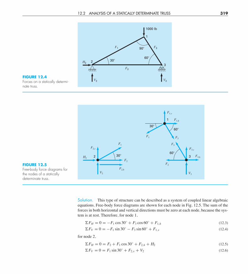
Solution. This type of structure can be described as a system of coupled linear algebraicequations. Free-body force diagrams are shown for each node in Fig. 12.5. The sum of theforces in both horizontal and vertical directions must be zero at each node, because the sys-tem is at rest. Therefore, for node 1,
!FH = 0 = !F1 cos 30$ + F3 cos 60$ + F1,h (12.3)!FV = 0 = !F1 sin 30$ ! F3 sin 60$ + F1,v (12.4)
for node 2,
!FH = 0 = F2 + F1 cos 30$ + F2,h + H2 (12.5)!FV = 0 = F1 sin 30$ + F2,v + V2 (12.6)
12.2 ANALYSIS OF A STATICALLY DETERMINATE TRUSS 319
FIGURE 12.4Forces on a statically determi-nate truss.
1000 lb
23
1
30!60!
90! F3F1
F2
H2
V2 V3
FIGURE 12.5Free-body force diagrams forthe nodes of a staticallydeterminate truss.
2 F3,h
F1,v
F1,h
F2
F2,h
F1F2,v
H2
V2
F3F1
F3,v
F3
F2
V3
1
30!
30!
60!
60!
3
cha01064_ch12.qxd 3/20/09 12:30 PM Page 319
for node 3,
!FH = 0 = !F2 ! F3 cos 60$ + F3,h (12.7)!FV = 0 = F3 sin 60$ + F3,v + V3 (12.8)
where Fi,h is the external horizontal force applied to node i (where a positive force is fromleft to right) and F1,v is the external vertical force applied to node i (where a positive forceis upward). Thus, in this problem, the 1000-lb downward force on node 1 corresponds toF1,v = !1000. For this case all other Fi,v’s and Fi,h’s are zero. Note that the directions ofthe internal forces and reactions are unknown. Proper application of Newton’s laws re-quires only consistent assumptions regarding direction. Solutions are negative if the direc-tions are assumed incorrectly. Also note that in this problem, the forces in all members areassumed to be in tension and act to pull adjoining nodes together. A negative solution there-fore corresponds to compression. This problem can be written as the following system ofsix equations and six unknowns:
!
""""""#
0.866 0 !0.5 0 0 00.5 0 0.866 0 0 0
!0.866 !1 0 !1 0 0!0.5 0 0 0 !1 0
0 1 0.5 0 0 00 0 !0.866 0 0 !1
$
%%%%%%&
'(((((()
((((((*
F1F2F3H2V2V3
+((((((,
((((((-
=
'(((((()
((((((*
0!1000
0000
+((((((,
((((((-
(12.9)
Notice that, as formulated in Eq. (12.9), partial pivoting is required to avoid divisionby zero diagonal elements. Employing a pivot strategy, the system can be solved using anyof the elimination techniques discussed in Chap. 9 or 10. However, because this problem isan ideal case study for demonstrating the utility of the matrix inverse, the LU decomposi-tion can be used to compute
F1 = !500 F2 = 433 F3 = !866H2 = 0 V2 = 250 V3 = 750
and the matrix inverse is
[A]!1 =
!
""""""#
0.866 0.5 0 0 0 00.25 !0.433 0 0 1 0!0.5 0.866 0 0 0 0!1 0 !1 0 !1 0
!0.433 !0.25 0 !1 0 00.433 !0.75 0 0 0 !1
$
%%%%%%&
Now, realize that the right-hand-side vector represents the externally applied horizontaland vertical forces on each node, as in
{F}T = "F1,h F1,v F2,h F2,v F3,h F3,v# (12.10)
Because the external forces have no effect on the LU decomposition, the method neednot be implemented over and over again to study the effect of different external forces on thetruss. Rather, all that we have to do is perform the forward- and backward-substitution stepsfor each right-hand-side vector to efficiently obtain alternative solutions. For example,
320 CASE STUDIES: LINEAR ALGEBRAIC EQUATIONS
cha01064_ch12.qxd 3/20/09 12:30 PM Page 320
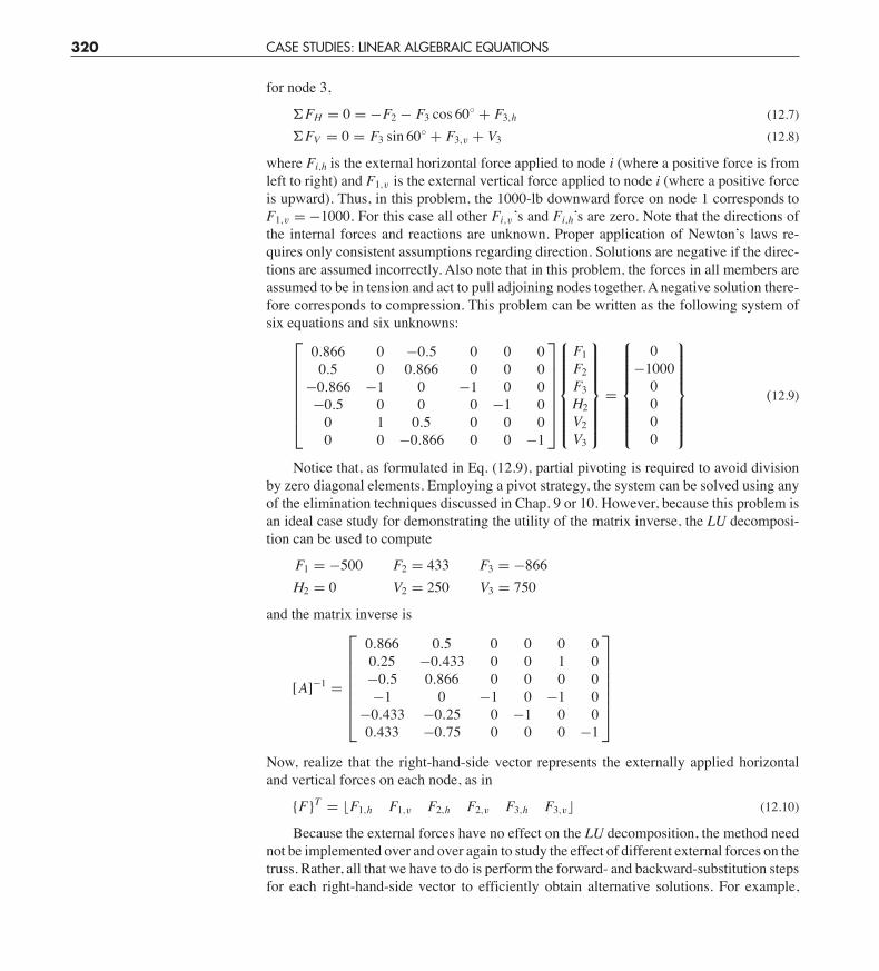
we might want to study the effect of horizontal forces induced by a wind blowing from leftto right. If the wind force can be idealized as two point forces of 1000 lb on nodes 1 and 2(Fig. 12.6a), the right-hand-side vector is
{F}T = "!1000 0 1000 0 0 0#
which can be used to compute
F1 = 866 F2 = 250 F3 = !500H2 = !2000 V2 = !433 V3 = 433
For a wind from the right (Fig. 12.6b), F1,h = !1000, F3,h = !1000, and all other externalforces are zero, with the result that
F1 = !866 F2 = !1250 F3 = 500H2 = 2000 V2 = 433 V3 = !433
The results indicate that the winds have markedly different effects on the structure. Bothcases are depicted in Fig. 12.6.
The individual elements of the inverted matrix also have direct utility in elucidatingstimulus-response interactions for the structure. Each element represents the change of oneof the unknown variables to a unit change of one of the external stimuli. For example, ele-ment a!1
32 indicates that the third unknown (F3) will change 0.866 due to a unit change ofthe second external stimulus (F1,v). Thus, if the vertical load at the first node were in-creased by 1, F3 would increase by 0.866. The fact that elements are 0 indicates that certainunknowns are unaffected by some of the external stimuli. For instance a!1
13 = 0 means thatF1 is unaffected by changes in F2,h. This ability to isolate interactions has a number ofengineering applications, including the identification of those components that are mostsensitive to external stimuli and, as a consequence, most prone to failure. In addition, it canbe used to determine components that may be unnecessary (see Prob. 12.18).
12.2 ANALYSIS OF A STATICALLY DETERMINATE TRUSS 321
FIGURE 12.6Two test cases showing (a) winds from the left and (b) winds from the right.
(a) (b)
866
2000 1000
1000
250
500
433 433
866
2000 1000
1000
1250500
433 433
cha01064_ch12.qxd 3/20/09 12:30 PM Page 321
The foregoing approach becomes particularly useful when applied to large complexstructures. In engineering practice, it may be necessary to solve trusses with hundreds oreven thousands of structural members. Linear equations provide one powerful approach forgaining insight into the behavior of these structures.
12.3 CURRENTS AND VOLTAGES IN RESISTOR CIRCUITS (ELECTRICAL ENGINEERING)
Background. A common problem in electrical engineering involves determining thecurrents and voltages at various locations in resistor circuits. These problems are solvedusing Kirchhoff’s current and voltage rules. The current (or point) rule states that the alge-braic sum of all currents entering a node must be zero (see Fig. 12.7a), or
!i = 0 (12.11)
where all current entering the node is considered positive in sign. The current rule is anapplication of the principle of conservation of charge (recall Table 1.1).
The voltage (or loop) rule specifies that the algebraic sum of the potential differences(that is, voltage changes) in any loop must equal zero. For a resistor circuit, this isexpressed as
!" ! !i R = 0 (12.12)
where " is the emf (electromotive force) of the voltage sources and R is the resistance ofany resistors on the loop. Note that the second term derives from Ohm’s law (Fig. 12.7b),which states that the voltage drop across an ideal resistor is equal to the product of the cur-rent and the resistance. Kirchhoff’s voltage rule is an expression of the conservation ofenergy.
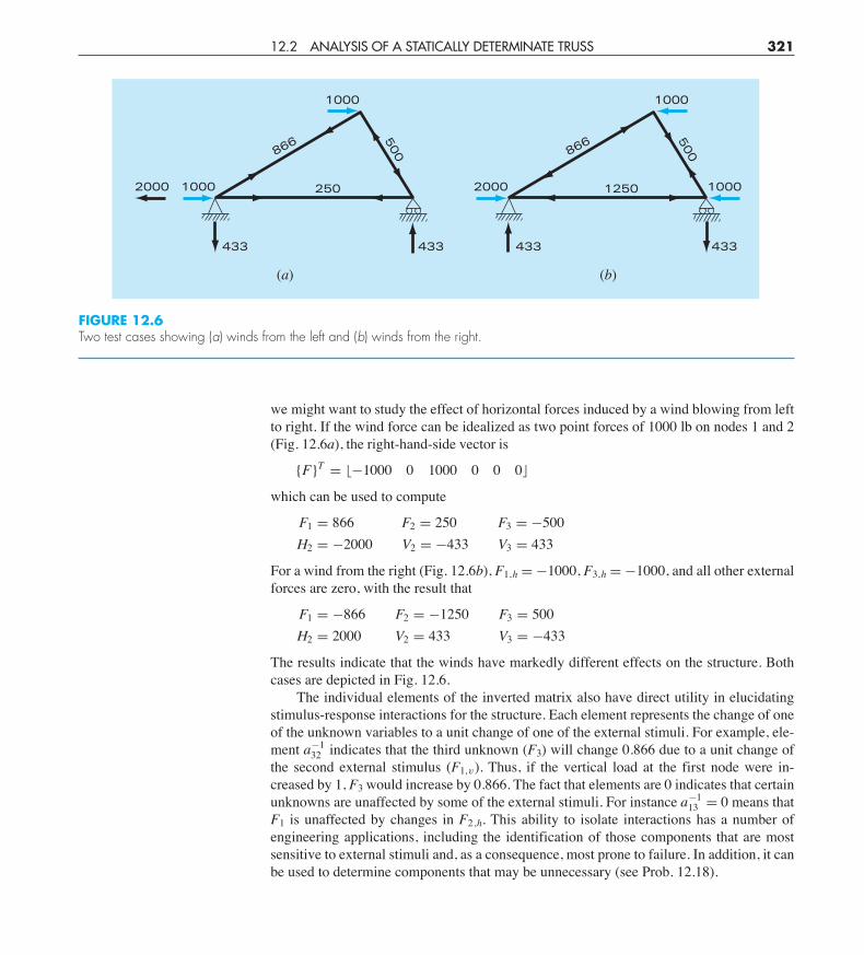
Solution. Application of these rules results in systems of simultaneous linear algebraicequations because the various loops within a circuit are coupled. For example, considerthe circuit shown in Fig. 12.8. The currents associated with this circuit are unknown bothin magnitude and direction. This presents no great difficulty because one simply assumesa direction for each current. If the resultant solution from Kirchhoff’s laws is negative,then the assumed direction was incorrect. For example, Fig. 12.9 shows some assumedcurrents.
322 CASE STUDIES: LINEAR ALGEBRAIC EQUATIONS
FIGURE 12.7Schematic representations of(a) Kirchhoff’s current rule and(b) Ohm’s law.
i1 i3
i2
Vi VjRij
iij
(a)
(b)
FIGURE 12.8A resistor circuit to be solved using simultaneous linear algebraic equations.
R = 5 " R = 10 "
R = 10 "3 2 1
4 5 6R = 15 "
R = 5 "V1 = 200 V
V6 = 0 VR = 20 "
cha01064_ch12.qxd 3/20/09 12:30 PM Page 322
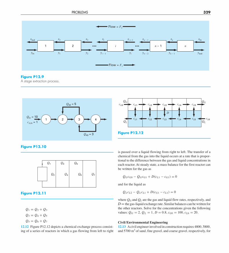
Figure P12.10
1 2 3 4Qin = 10
Q32 = 5
Q43 = 3
cA,in = 1
Figure P12.11
Q1 Q3 Q5
Q2 Q4 Q6 Q7
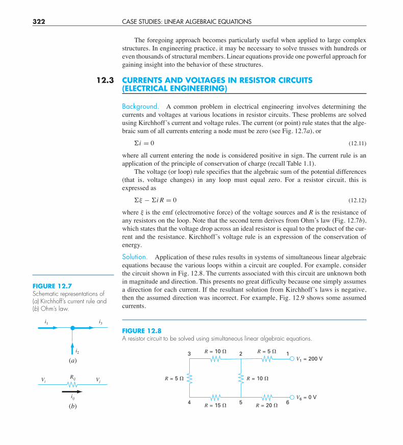
Figure P12.9A stage extraction process.
Flow = F1
Flow = F2
x2xout x3 xi xi + 1 xn – 1 xn xin
y1yin y2 yi – 1 yi yn – 2 yn – 1 yout
1 02 0n0i n – 1••• •••
Figure P12.12
cG1cG0 cG2 cG3 cG4
QGQG
QL
cG5
QL
D
cL1 cL2 cL3 cL4 cL5 cL6
PROBLEMS 329
is passed over a liquid flowing from right to left. The transfer of achemical from the gas into the liquid occurs at a rate that is propor-tional to the difference between the gas and liquid concentrations ineach reactor. At steady state, a mass balance for the first reactor canbe written for the gas as
QGcG0 ! QGcG1 + D(cL1 ! cG1) = 0
and for the liquid as
QLcL2 ! QLcL1 + D(cG1 ! cL1) = 0
where QG and QL are the gas and liquid flow rates, respectively, andD= the gas-liquid exchange rate. Similar balances can be written forthe other reactors. Solve for the concentrations given the followingvalues: QG = 2, QL = 1, D = 0.8, cG0 = 100, cL6 = 20.
Civil/Environmental Engineering12.13 Acivil engineer involved in construction requires 4800, 5800,and 5700 m3 of sand, fine gravel, and coarse gravel, respectively, for
Q1 = Q2 + Q3
Q3 = Q4 + Q5
Q5 = Q6 + Q7
12.12 Figure P12.12 depicts a chemical exchange process consist-ing of a series of reactors in which a gas flowing from left to right
cha01064_ch12.qxd 3/24/09 5:57 PM Page 329
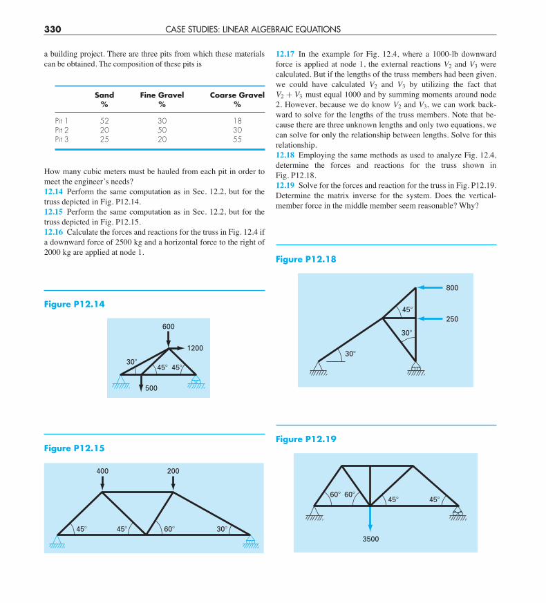
Figure P12.18
45!
800
250
30!
30!
Figure P12.19
60!45! 45!
60!
3500
Figure P12.15
400 200
45! 60!45! 30!
Figure P12.14
600
1200
500
30!45! 45!
330 CASE STUDIES: LINEAR ALGEBRAIC EQUATIONS
a building project. There are three pits from which these materialscan be obtained. The composition of these pits is
Sand Fine Gravel Coarse Gravel% % %
Pit 1 52 30 18Pit 2 20 50 30Pit 3 25 20 55
How many cubic meters must be hauled from each pit in order tomeet the engineer’s needs?12.14 Perform the same computation as in Sec. 12.2, but for thetruss depicted in Fig. P12.14.12.15 Perform the same computation as in Sec. 12.2, but for thetruss depicted in Fig. P12.15.12.16 Calculate the forces and reactions for the truss in Fig. 12.4 ifa downward force of 2500 kg and a horizontal force to the right of2000 kg are applied at node 1.
12.17 In the example for Fig. 12.4, where a 1000-lb downwardforce is applied at node 1, the external reactions V2 and V3 werecalculated. But if the lengths of the truss members had been given,we could have calculated V2 and V3 by utilizing the fact thatV2 + V3 must equal 1000 and by summing moments around node2. However, because we do know V2 and V3, we can work back-ward to solve for the lengths of the truss members. Note that be-cause there are three unknown lengths and only two equations, wecan solve for only the relationship between lengths. Solve for thisrelationship.12.18 Employing the same methods as used to analyze Fig. 12.4,determine the forces and reactions for the truss shown inFig. P12.18.12.19 Solve for the forces and reaction for the truss in Fig. P12.19.Determine the matrix inverse for the system. Does the vertical-member force in the middle member seem reasonable? Why?
cha01064_ch12.qxd 3/20/09 12:30 PM Page 330
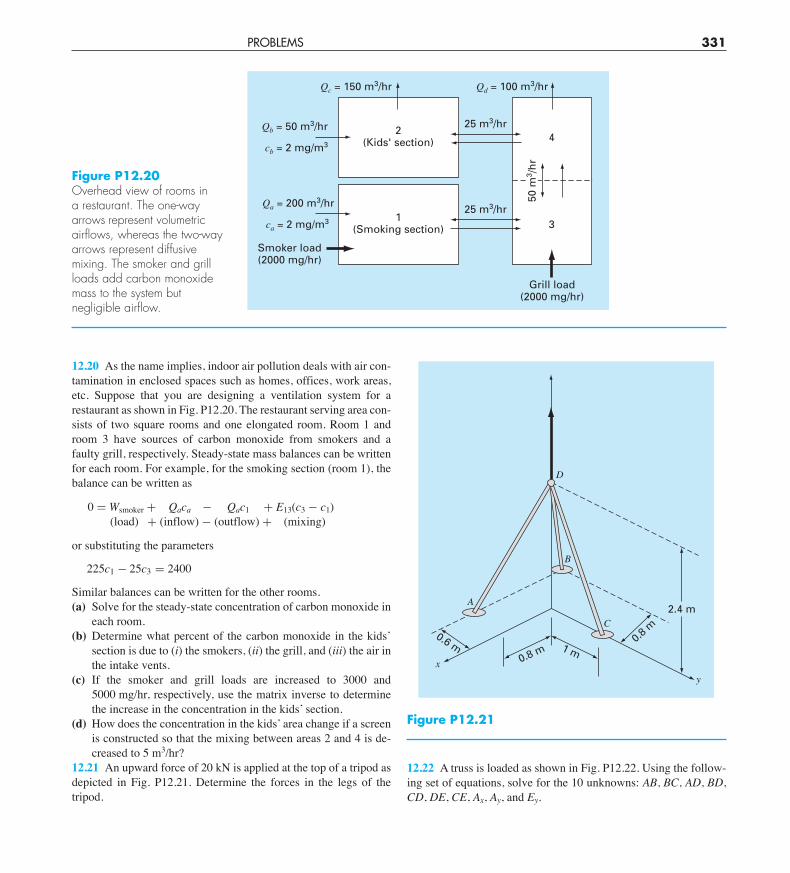
Figure P12.20Overhead view of rooms ina restaurant. The one-wayarrows represent volumetricairflows, whereas the two-wayarrows represent diffusivemixing. The smoker and grillloads add carbon monoxidemass to the system butnegligible airflow.
Qc = 150 m3/hr
2(Kids' section)
1(Smoking section)
Grill load(2000 mg/hr)
Smoker load(2000 mg/hr)
4
25 m3/hr
25 m3/hr
3
Qb = 50 m3/hr
cb = 2 mg/m3
Qa = 200 m3/hr
ca = 2 mg/m3
Qd = 100 m3/hr
50 m
3 /hr
Figure P12.21
D
B
C
A
xy
0.6 m
2.4 m
0.8 m0.8
m
1 m
PROBLEMS 331
12.20 As the name implies, indoor air pollution deals with air con-tamination in enclosed spaces such as homes, offices, work areas,etc. Suppose that you are designing a ventilation system for arestaurant as shown in Fig. P12.20. The restaurant serving area con-sists of two square rooms and one elongated room. Room 1 androom 3 have sources of carbon monoxide from smokers and afaulty grill, respectively. Steady-state mass balances can be writtenfor each room. For example, for the smoking section (room 1), thebalance can be written as
0 & Wsmoker + Qaca ! Qac1 + E13(c3 ! c1)(load) + (inflow) ! (outflow) + (mixing)
or substituting the parameters
225c1 ! 25c3 = 2400
Similar balances can be written for the other rooms.(a) Solve for the steady-state concentration of carbon monoxide in
each room.(b) Determine what percent of the carbon monoxide in the kids’
section is due to (i) the smokers, (ii) the grill, and (iii) the air inthe intake vents.
(c) If the smoker and grill loads are increased to 3000 and5000 mg/hr, respectively, use the matrix inverse to determinethe increase in the concentration in the kids’ section.
(d) How does the concentration in the kids’ area change if a screenis constructed so that the mixing between areas 2 and 4 is de-creased to 5 m3/hr?
12.21 An upward force of 20 kN is applied at the top of a tripod asdepicted in Fig. P12.21. Determine the forces in the legs of thetripod.
12.22 A truss is loaded as shown in Fig. P12.22. Using the follow-ing set of equations, solve for the 10 unknowns: AB, BC, AD, BD,CD, DE, CE, Ax, Ay, and Ey.
cha01064_ch12.qxd 3/20/09 12:30 PM Page 331

Figure P12.25
20 "
5 "
10 "
10 "20 "
5 "
5 "
50 "
0 "4 7 9
2
1
8
3 6 15 "
5
V2 = 40V1 = 110
Figure P12.24
R = 7 "R = 5 " R = 10 "
R = 30 "3 2 1
4 5 6
R = 15 "
R = 35 "V1 = 10 volts
V6 = 200 voltsR = 5 "
Figure P12.22
3 m 3 m
4 m
DA E
CB74 kN
24 kN
Figure P12.23
R = 2 " R = 5 "
R = 20 "3 2 1
4 5 6
R = 5 "
R = 10 "V1 = 150 volts
V6 = 0 voltsR = 25 "
Metal, Plastic, Rubber,Component g/component g/component g/component
1 15 0.25 1.02 17 0.33 1.23 19 0.42 1.6
If totals of 2.12, 0.0434, and 0.164 kg of metal, plastic, and rubber,respectively, are available each day, how many components can beproduced per day?12.27 Determine the currents for the circuit in Fig. P12.27.12.28 Determine the currents for the circuit in Fig. P12.28.12.29 The following system of equations was generated by applyingthe mesh current law to the circuit in Fig. P12.29:
55I1 ! 25I4 = !200!37I3 ! 4I4 = !250!25I1 ! 4I3 + 29I4 = 100
Solve for I1, I3, and I4.
332 CASE STUDIES: LINEAR ALGEBRAIC EQUATIONS
Ax + AD = 0Ay + AB = 074 + BC + (3/5)BD = 0!AB ! (4/5)BD = 0!BC + (3/5)CE = 0
!24 ! CD ! (4/5)CE = 0!AD + DE ! (3/5)BD = 0CD + (4/5)BD = 0!DE ! (3/5)CE = 0Ey + (4/5)CE = 0
Electrical Engineering12.23 Perform the same computation as in Sec. 12.3, but for thecircuit depicted in Fig. P12.23.12.24 Perform the same computation as in Sec. 12.3, but for thecircuit depicted in Fig. P12.24.12.25 Solve the circuit in Fig. P12.25 for the currents in each wire.Use Gauss elimination with pivoting.12.26 An electrical engineer supervises the production of three typesof electrical components. Three kinds of material—metal, plastic, andrubber—are required for production. The amounts needed to produceeach component are
cha01064_ch12.qxd 3/20/09 12:30 PM Page 332

Toshiba
Stamp
16.2 LEAST-COST TREATMENT OF WASTEWATER(CIVIL/ENVIRONMENTAL ENGINEERING)
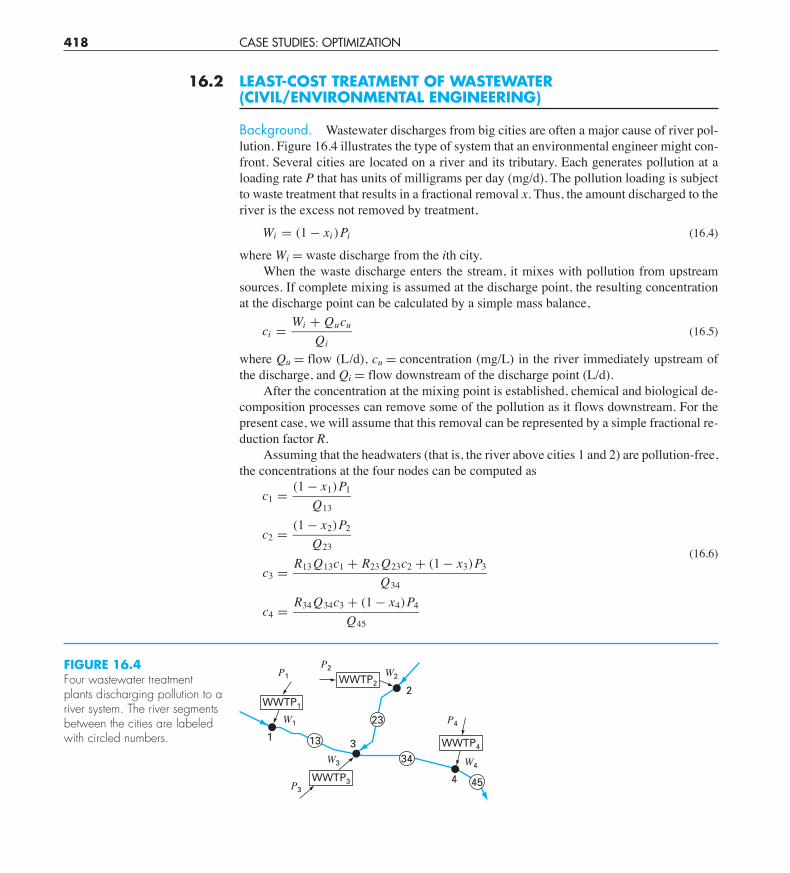
Background. Wastewater discharges from big cities are often a major cause of river pol-lution. Figure 16.4 illustrates the type of system that an environmental engineer might con-front. Several cities are located on a river and its tributary. Each generates pollution at aloading rate P that has units of milligrams per day (mg/d). The pollution loading is subjectto waste treatment that results in a fractional removal x. Thus, the amount discharged to theriver is the excess not removed by treatment,
Wi = (1 ! xi )Pi (16.4)
where Wi = waste discharge from the ith city.When the waste discharge enters the stream, it mixes with pollution from upstream
sources. If complete mixing is assumed at the discharge point, the resulting concentrationat the discharge point can be calculated by a simple mass balance,
ci = Wi + Qucu
Qi(16.5)
where Qu = flow (L/d), cu = concentration (mg/L) in the river immediately upstream ofthe discharge, and Qi = flow downstream of the discharge point (L/d).
After the concentration at the mixing point is established, chemical and biological de-composition processes can remove some of the pollution as it flows downstream. For thepresent case, we will assume that this removal can be represented by a simple fractional re-duction factor R.
Assuming that the headwaters (that is, the river above cities 1 and 2) are pollution-free,the concentrations at the four nodes can be computed as
c1 = (1 ! x1)P1
Q13
c2 = (1 ! x2)P2
Q23 (16.6)c3 = R13 Q13c1 + R23 Q23c2 + (1 ! x3)P3
Q34
c4 = R34 Q34c3 + (1 ! x4)P4
Q45
418 CASE STUDIES: OPTIMIZATION
FIGURE 16.4Four wastewater treatmentplants discharging pollution to ariver system. The river segmentsbetween the cities are labeledwith circled numbers.
4
P1
3
2
P4
P2
P3
W1
W2
W3 W434
23
13
45
WWTP2
1
WWTP1
WWTP4
WWTP3
cha01064_ch16.qxd 3/20/09 12:41 PM Page 418
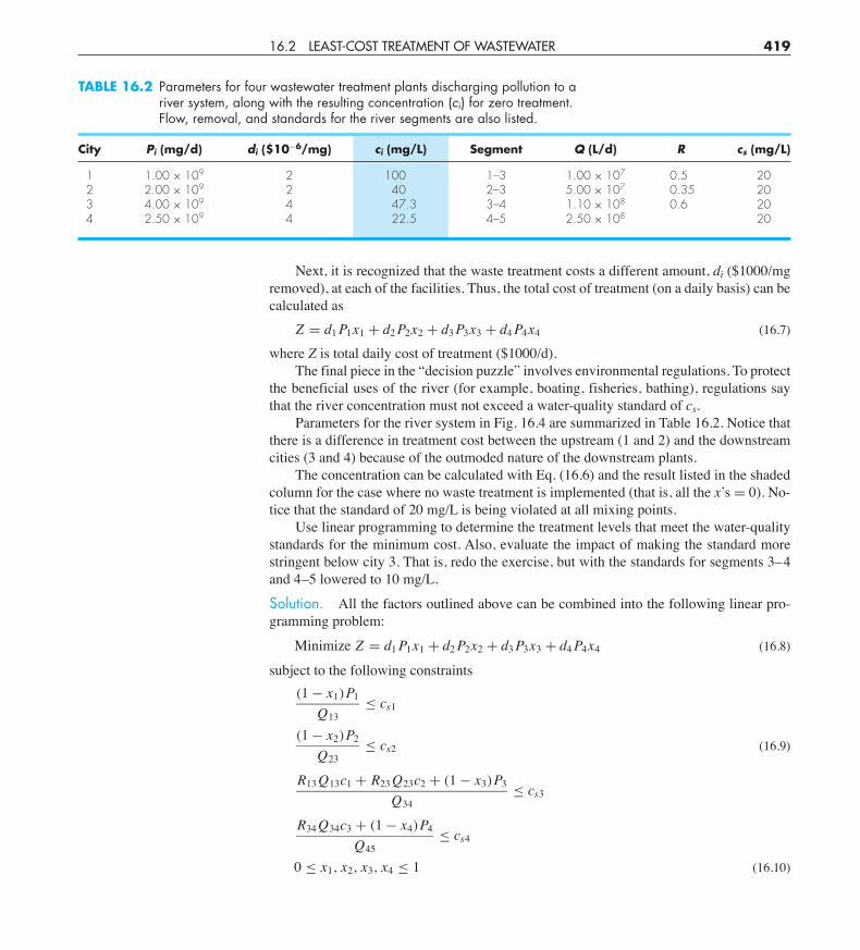
16.2 LEAST-COST TREATMENT OF WASTEWATER 419
Next, it is recognized that the waste treatment costs a different amount, di ($1000/mgremoved), at each of the facilities. Thus, the total cost of treatment (on a daily basis) can becalculated as
Z = d1 P1x1 + d2 P2x2 + d3 P3x3 + d4 P4x4 (16.7)
where Z is total daily cost of treatment ($1000/d).The final piece in the “decision puzzle” involves environmental regulations. To protect
the beneficial uses of the river (for example, boating, fisheries, bathing), regulations saythat the river concentration must not exceed a water-quality standard of cs.
Parameters for the river system in Fig. 16.4 are summarized in Table 16.2. Notice thatthere is a difference in treatment cost between the upstream (1 and 2) and the downstreamcities (3 and 4) because of the outmoded nature of the downstream plants.
The concentration can be calculated with Eq. (16.6) and the result listed in the shadedcolumn for the case where no waste treatment is implemented (that is, all the x’s = 0). No-tice that the standard of 20 mg/L is being violated at all mixing points.
Use linear programming to determine the treatment levels that meet the water-qualitystandards for the minimum cost. Also, evaluate the impact of making the standard morestringent below city 3. That is, redo the exercise, but with the standards for segments 3–4and 4–5 lowered to 10 mg/L.
Solution. All the factors outlined above can be combined into the following linear pro-gramming problem:
Minimize Z = d1 P1x1 + d2 P2x2 + d3 P3x3 + d4 P4x4 (16.8)
subject to the following constraints(1 ! x1)P1
Q13" cs1
(1 ! x2)P2
Q23" cs2 (16.9)
R13 Q13c1 + R23 Q23c2 + (1 ! x3)P3
Q34" cs3
R34 Q34c3 + (1 ! x4)P4
Q45" cs4
0 " x1, x2, x3, x4 " 1 (16.10)
TABLE 16.2 Parameters for four wastewater treatment plants discharging pollution to ariver system, along with the resulting concentration (ci) for zero treatment.Flow, removal, and standards for the river segments are also listed.
City Pi (mg/d) di ($10!6/mg) ci (mg/L) Segment Q (L/d) R cs (mg/L)
1 1.00 # 109 2 100 1–3 1.00 # 107 0.5 202 2.00 # 109 2 40 2–3 5.00 # 107 0.35 203 4.00 # 109 4 47.3 3–4 1.10 # 108 0.6 204 2.50 # 109 4 22.5 4–5 2.50 # 108 20
cha01064_ch16.qxd 3/20/09 12:41 PM Page 419
Thus, the objective function is to minimize treatment cost [Eq. (16.8)] subject to theconstraint that water-quality standards must be met for all parts of the system [Eq. (16.9)].In addition, treatment cannot be negative or greater than 100% removal [Eq. (16.10)].
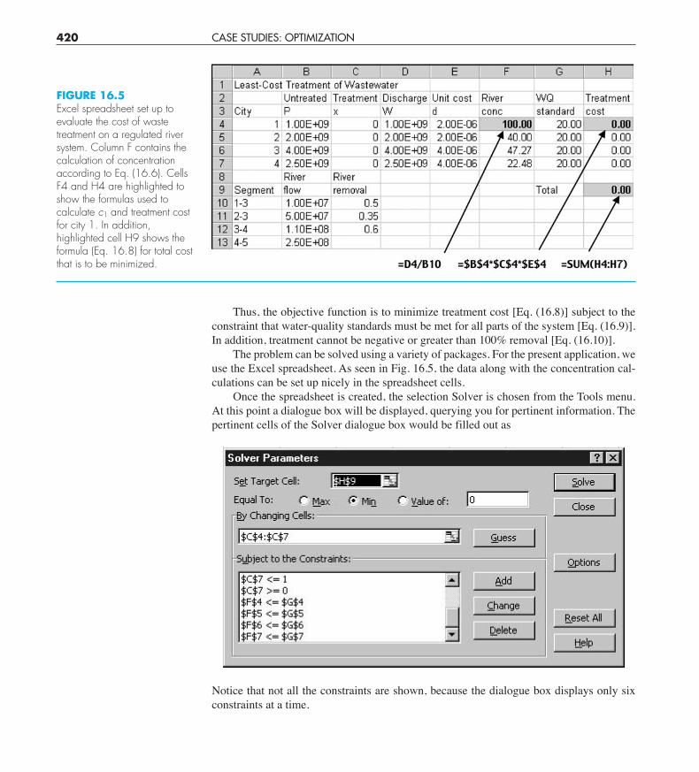
The problem can be solved using a variety of packages. For the present application, weuse the Excel spreadsheet. As seen in Fig. 16.5, the data along with the concentration cal-culations can be set up nicely in the spreadsheet cells.
Once the spreadsheet is created, the selection Solver is chosen from the Tools menu.At this point a dialogue box will be displayed, querying you for pertinent information. Thepertinent cells of the Solver dialogue box would be filled out as
Notice that not all the constraints are shown, because the dialogue box displays only sixconstraints at a time.
420 CASE STUDIES: OPTIMIZATION
FIGURE 16.5Excel spreadsheet set up toevaluate the cost of wastetreatment on a regulated riversystem. Column F contains thecalculation of concentrationaccording to Eq. (16.6). CellsF4 and H4 are highlighted toshow the formulas used tocalculate c1 and treatment costfor city 1. In addition,highlighted cell H9 shows theformula (Eq. 16.8) for total costthat is to be minimized.
cha01064_ch16.qxd 3/20/09 12:41 PM Page 420
16.2 LEAST-COST TREATMENT OF WASTEWATER 421
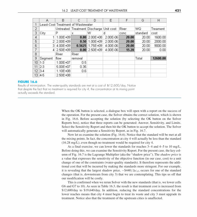
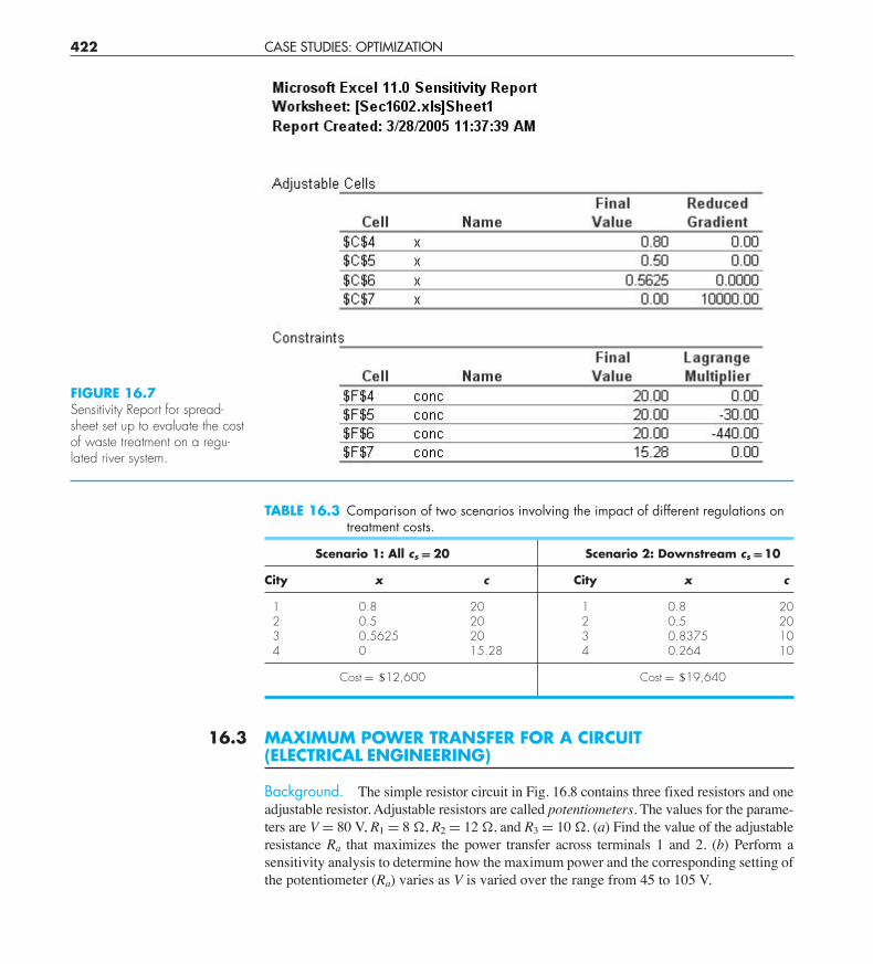
When the OK button is selected, a dialogue box will open with a report on the success ofthe operation. For the present case, the Solver obtains the correct solution, which is shownin Fig. 16.6. Before accepting the solution (by selecting the OK button on the SolverReports box), notice that three reports can be generated: Answer, Sensitivity, and Limits.Select the Sensitivity Report and then hit the OK button to accept the solution. The Solverwill automatically generate a Sensitivity Report, as in Fig. 16.7.
Now let us examine the solution (Fig. 16.6). Notice that the standard will be met at allthe mixing points. In fact, the concentration at city 4 will actually be less than the standard(16.28 mg/L), even though no treatment would be required for city 4.
As a final exercise, we can lower the standards for reaches 3–4 and 4–5 to 10 mg/L.Before doing this, we can examine the Sensitivity Report. For the present case, the key col-umn of Fig. 16.7 is the Lagrange Multiplier (aka the “shadow price”). The shadow price isa value that expresses the sensitivity of the objective function (in our case, cost) to a unitchange of one of the constraints (water-quality standards). It therefore represents the addi-tional cost that will be incurred by making the standards more stringent. For our example,it is revealing that the largest shadow price, !$440/$cs3, occurs for one of the standardchanges (that is, downstream from city 3) that we are contemplating. This tips us off thatour modification will be costly.
This is confirmed when we rerun Solver with the new standards (that is, we lower cellsG6 and G7 to 10). As seen in Table 16.3, the result is that treatment cost is increased from$12,600/day to $19,640/day. In addition, reducing the standard concentrations for thelower reaches means that city 4 must begin to treat its waste and city 3 must upgrade itstreatment. Notice also that the treatment of the upstream cities is unaffected.
FIGURE 16.6Results of minimization. The water-quality standards are met at a cost of $12,600/day. Noticethat despite the fact that no treatment is required for city 4, the concentration at its mixing pointactually exceeds the standard.
cha01064_ch16.qxd 3/20/09 12:41 PM Page 421
16.3 MAXIMUM POWER TRANSFER FOR A CIRCUIT(ELECTRICAL ENGINEERING)
Background. The simple resistor circuit in Fig. 16.8 contains three fixed resistors and oneadjustable resistor. Adjustable resistors are called potentiometers. The values for the parame-ters are V= 80 V, R1 = 8 !, R2 = 12 !, and R3 = 10 !. (a) Find the value of the adjustableresistance Ra that maximizes the power transfer across terminals 1 and 2. (b) Perform asensitivity analysis to determine how the maximum power and the corresponding setting ofthe potentiometer (Ra) varies as V is varied over the range from 45 to 105 V.
422 CASE STUDIES: OPTIMIZATION
FIGURE 16.7Sensitivity Report for spread-sheet set up to evaluate the costof waste treatment on a regu-lated river system.
TABLE 16.3 Comparison of two scenarios involving the impact of different regulations ontreatment costs.
Scenario 1: All cs = 20 Scenario 2: Downstream cs =10
City x c City x c
1 0.8 20 1 0.8 202 0.5 20 2 0.5 203 0.5625 20 3 0.8375 104 0 15.28 4 0.264 10
Cost = $12,600 Cost = $19,640
cha01064_ch16.qxd 3/24/09 7:17 PM Page 422
PROBLEMS 431
16.14 Find the optimal dimensions for a heated cylindrical tankdesigned to hold 10 m3 of fluid. The ends and sides cost $200/m2
and $100/m2, respectively. In addition, a coating is applied to theentire tank area at a cost of $50/m2.
Civil/Environmental Engineering16.15 A finite-element model of a cantilever beam subject to load-ing and moments (Fig. P16.15) is given by optimizing
f(x, y) = 5x2 ! 5xy + 2.5y2 ! x ! 1.5y
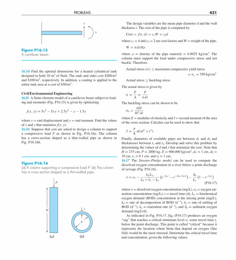
where x = end displacement and y = end moment. Find the valuesof x and y that minimize f(x, y).16.16 Suppose that you are asked to design a column to supporta compressive load P as shown in Fig. P16.16a. The columnhas a cross-section shaped as a thin-walled pipe as shown inFig. P16.16b.
Figure P16.16(a) A column supporting a compressive load P. (b) The columnhas a cross section shaped as a thin-walled pipe.
(a)
H
P
(b)
d
t
Figure P16.15A cantilever beam.
x
y
The design variables are the mean pipe diameter d and the wallthickness t. The cost of the pipe is computed by
Cost = f(t, d) = c1W + c2d
where c1 = 4 and c2 = 2 are cost factors and W = weight of the pipe,
W = #dt H!
where ! = density of the pipe material = 0.0025 kg/cm3. Thecolumn must support the load under compressive stress and notbuckle. Therefore,
Actual stress (& ) " maximum compressive yield stress= &y = 550 kg/cm2
Actual stress " buckling stress
The actual stress is given by
& = PA
= P#dt
The buckling stress can be shown to be
&b = #EIH 2 dt
where E = modulus of elasticity and I = second moment of the areaof the cross section. Calculus can be used to show that
I = #
8dt (d2 + t2)
Finally, diameters of available pipes are between d1 and d2 andthicknesses between t1 and t2. Develop and solve this problem bydetermining the values of d and t that minimize the cost. Note thatH = 275 cm, P = 2000 kg, E = 900,000 kg/cm2, d1 = 1 cm, d2 =10 cm, t1 = 0.1 cm, and t2 = 1 cm.16.17 The Streeter-Phelps model can be used to compute thedissolved oxygen concentration in a river below a point dischargeof sewage (Fig. P16.16),
o = os ! kd Lo
kd + ks ! ka
6e!ka t ! e!(kd +ks )t
7! Sb
ka
61 ! e!ka t7
(P16.17)
where o = dissolved oxygen concentration (mg/L), os = oxygen sat-uration concentration (mg/L), t = travel time (d), Lo = biochemicaloxygen demand (BOD) concentration at the mixing point (mg/L),kd = rate of decomposition of BOD (d!1), ks = rate of settling ofBOD (d!1), ka = reaeration rate (d!1), and Sb = sediment oxygendemand (mg/L/d).
As indicated in Fig. P16.17, Eq. (P16.17) produces an oxygen“sag” that reaches a critical minimum level oc some travel time tcbelow the point discharge. This point is called “critical” because itrepresents the location where biota that depend on oxygen (likefish) would be the most stressed. Determine the critical travel timeand concentration, given the following values:
cha01064_ch16.qxd 3/20/09 12:41 PM Page 431
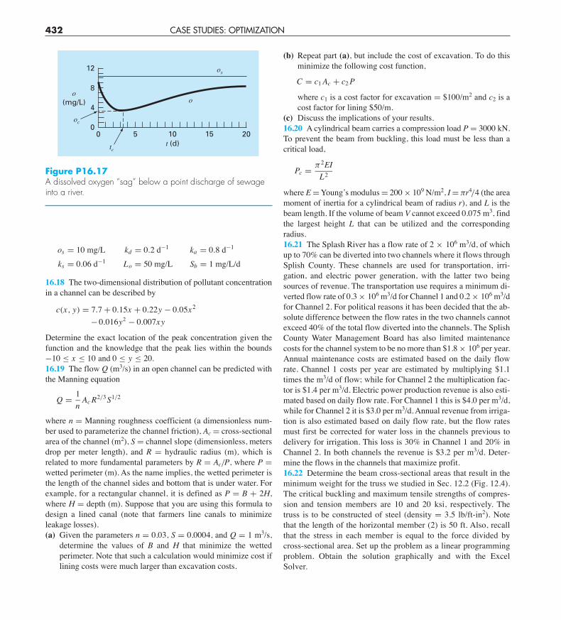
os = 10 mg/L kd = 0.2 d!1 ka = 0.8 d!1
ks = 0.06 d!1 Lo = 50 mg/L Sb = 1 mg/L/d
16.18 The two-dimensional distribution of pollutant concentrationin a channel can be described by
c(x, y) = 7.7 + 0.15x + 0.22y ! 0.05x2
! 0.016y2 ! 0.007xy
Determine the exact location of the peak concentration given thefunction and the knowledge that the peak lies within the bounds!10 " x " 10 and 0 " y " 20.
16.19 The flow Q (m3/s) in an open channel can be predicted withthe Manning equation
Q = 1n
Ac R2/3S1/2
where n = Manning roughness coefficient (a dimensionless num-ber used to parameterize the channel friction), Ac = cross-sectionalarea of the channel (m2), S = channel slope (dimensionless, metersdrop per meter length), and R = hydraulic radius (m), which isrelated to more fundamental parameters by R = Ac/P, where P =wetted perimeter (m). As the name implies, the wetted perimeter isthe length of the channel sides and bottom that is under water. Forexample, for a rectangular channel, it is defined as P = B + 2H,where H = depth (m). Suppose that you are using this formula todesign a lined canal (note that farmers line canals to minimizeleakage losses).(a) Given the parameters n = 0.03, S = 0.0004, and Q = 1 m3/s,
determine the values of B and H that minimize the wettedperimeter. Note that such a calculation would minimize cost iflining costs were much larger than excavation costs.
(b) Repeat part (a), but include the cost of excavation. To do thisminimize the following cost function,
C = c1 Ac + c2 P
where c1 is a cost factor for excavation = $100/m2 and c2 is acost factor for lining $50/m.
(c) Discuss the implications of your results.16.20 A cylindrical beam carries a compression load P = 3000 kN.To prevent the beam from buckling, this load must be less than acritical load,
Pc = #2EIL2
where E = Young’s modulus = 200 # 109 N/m2, I = #r4/4 (the areamoment of inertia for a cylindrical beam of radius r), and L is thebeam length. If the volume of beam V cannot exceed 0.075 m3, findthe largest height L that can be utilized and the correspondingradius.16.21 The Splash River has a flow rate of 2 # 106 m3/d, of whichup to 70% can be diverted into two channels where it flows throughSplish County. These channels are used for transportation, irri-gation, and electric power generation, with the latter two beingsources of revenue. The transportation use requires a minimum di-verted flow rate of 0.3 # 106 m3/d for Channel 1 and 0.2 # 106 m3/dfor Channel 2. For political reasons it has been decided that the ab-solute difference between the flow rates in the two channels cannotexceed 40% of the total flow diverted into the channels. The SplishCounty Water Management Board has also limited maintenancecosts for the channel system to be no more than $1.8 # 106 per year.Annual maintenance costs are estimated based on the daily flowrate. Channel 1 costs per year are estimated by multiplying $1.1times the m3/d of flow; while for Channel 2 the multiplication fac-tor is $1.4 per m3/d. Electric power production revenue is also esti-mated based on daily flow rate. For Channel 1 this is $4.0 per m3/d,while for Channel 2 it is $3.0 per m3/d. Annual revenue from irriga-tion is also estimated based on daily flow rate, but the flow ratesmust first be corrected for water loss in the channels previous todelivery for irrigation. This loss is 30% in Channel 1 and 20% inChannel 2. In both channels the revenue is $3.2 per m3/d. Deter-mine the flows in the channels that maximize profit.16.22 Determine the beam cross-sectional areas that result in theminimum weight for the truss we studied in Sec. 12.2 (Fig. 12.4).The critical buckling and maximum tensile strengths of compres-sion and tension members are 10 and 20 ksi, respectively. Thetruss is to be constructed of steel (density = 3.5 lb/ft-in2). Notethat the length of the horizontal member (2) is 50 ft. Also, recallthat the stress in each member is equal to the force divided bycross-sectional area. Set up the problem as a linear programmingproblem. Obtain the solution graphically and with the ExcelSolver.
432 CASE STUDIES: OPTIMIZATION
Figure P16.17A dissolved oxygen “sag” below a point discharge of sewageinto a river.
15 20
8
12
00
t (d)5
4
10
o(mg/L) o
os
tc
oc
cha01064_ch16.qxd 3/20/09 12:41 PM Page 432

Toshiba
Stamp
20.2 USE OF SPLINES TO ESTIMATE HEAT TRANSFER 565
may not be compatible with linearization) and nonlinear regression could represent theonly feasible option for obtaining a least-squares fit.
20.2 USE OF SPLINES TO ESTIMATE HEAT TRANSFER(CIVIL/ENVIRONMENTAL ENGINEERING)
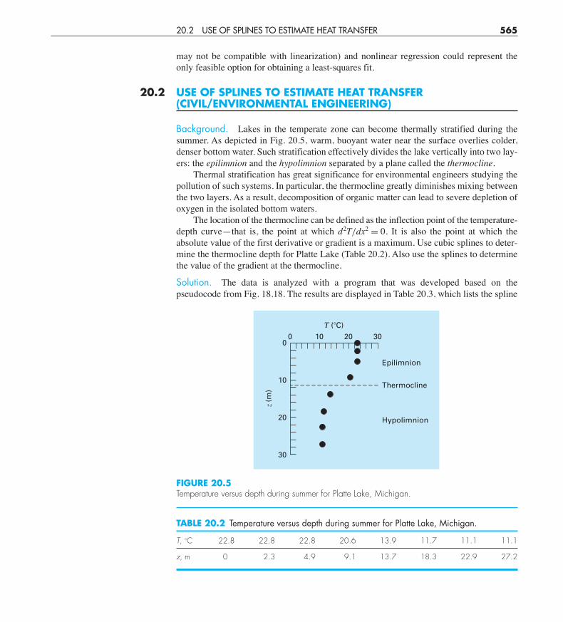
Background. Lakes in the temperate zone can become thermally stratified during thesummer. As depicted in Fig. 20.5, warm, buoyant water near the surface overlies colder,denser bottom water. Such stratification effectively divides the lake vertically into two lay-ers: the epilimnion and the hypolimnion separated by a plane called the thermocline.
Thermal stratification has great significance for environmental engineers studying thepollution of such systems. In particular, the thermocline greatly diminishes mixing betweenthe two layers. As a result, decomposition of organic matter can lead to severe depletion ofoxygen in the isolated bottom waters.
The location of the thermocline can be defined as the inflection point of the temperature-depth curve—that is, the point at which d2T/dx2 = 0. It is also the point at which theabsolute value of the first derivative or gradient is a maximum. Use cubic splines to deter-mine the thermocline depth for Platte Lake (Table 20.2). Also use the splines to determinethe value of the gradient at the thermocline.
Solution. The data is analyzed with a program that was developed based on thepseudocode from Fig. 18.18. The results are displayed in Table 20.3, which lists the spline
FIGURE 20.5Temperature versus depth during summer for Platte Lake, Michigan.
z (m
)
0
10
20
30
0 10
Epilimnion
Thermocline
Hypolimnion
! (#C)20 30
TABLE 20.2 Temperature versus depth during summer for Platte Lake, Michigan.
T, "C 22.8 22.8 22.8 20.6 13.9 11.7 11.1 11.1
z, m 0 2.3 4.9 9.1 13.7 18.3 22.9 27.2
cha01064_ch20.qxd 3/20/09 12:56 PM Page 565
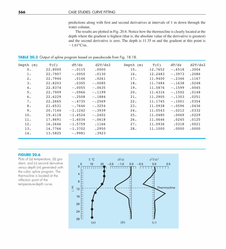
predictions along with first and second derivatives at intervals of 1 m down through thewater column.
The results are plotted in Fig. 20.6. Notice how the thermocline is clearly located at thedepth where the gradient is highest (that is, the absolute value of the derivative is greatest)and the second derivative is zero. The depth is 11.35 m and the gradient at this point is!1.61°C/m.
566 CASE STUDIES: CURVE FITTING
FIGURE 20.6Plots of (a) temperature, (b) gra-dient, and (c) second derivativeversus depth (m) generated withthe cubic spline program. Thethermocline is located at theinflection point of thetemperature-depth curve.
z, m
0
8
16
4
12
24
20
28
0
(a)
10
Thermocline
T, #C20 – 2.0
(b)
– 1.0dT/dz
0.0 – 0.5
(c)
0.0d2T/dz2
0.5
TABLE 20.3 Output of spline program based on pseudocode from Fig. 18.18.
Depth (m) T(C) dT/dz d2T/dz2 Depth (m) T(C) dT/dz d2T/dz20. 22.8000 !.0115 .0000 15. 12.7652 !.6518 .30041. 22.7907 !.0050 .0130 16. 12.2483 !.3973 .20862. 22.7944 .0146 .0261 17. 11.9400 !.2346 .11673. 22.8203 .0305 !.0085 18. 11.7484 !.1638 .02484. 22.8374 !.0055 !.0635 19. 11.5876 !.1599 .00455. 22.7909 !.0966 !.1199 20. 11.4316 !.1502 .01486. 22.6229 !.2508 !.1884 21. 11.2905 !.1303 .02517. 22.2665 !.4735 !.2569 22. 11.1745 !.1001 .03548. 21.6531 !.7646 !.3254 23. 11.0938 !.0596 .04369. 20.7144 !1.1242 !.3939 24. 11.0543 !.0212 .033210. 19.4118 !1.4524 !.2402 25. 11.0480 .0069 .022911. 17.8691 !1.6034 !.0618 26. 11.0646 .0245 .012512. 16.2646 !1.5759 .1166 27. 11.0936 .0318 .002113. 14.7766 !1.3702 .2950 28. 11.1000 .0000 .000014. 13.5825 !.9981 .3923
cha01064_ch20.qxd 3/20/09 12:56 PM Page 566
PROBLEMS 573
Using this approach, experimental data that is well defined willproduce a good match of the data points and the analytic curve. Usethis new relationship and again plot the stress versus strain datapoints and this new analytic curve.20.17 The thickness of the retina changes during certain eye dis-eases. One way to measure retinal thickness is to shine a low-energylaser at the retina and record the reflections on film. Because of theoptical properties of the eye, the reflections from the front surfaceof the retina and the back surface of the retina will appear as two lineson the film separated by a distance. The distance between the lines onthe film is proportional to the thickness of the retina. Below is datataken from the scanned film. Fit two Gaussian-shaped curves ofarbitrary height and location to the data and determine the distancebetween the centers of the two peaks. A Gaussian curve has the form
f(x) = ke!k2(x!a)2
&&
where k and a are constants that relate to the peak height and thecenter of the peak, respectively.
Light LightPosition Intensity Position Intensity
0.17 5.10 0.31 25.310.18 5.10 0.32 23.790.19 5.20 0.33 18.440.20 5.87 0.34 12.450.21 8.72 0.35 8.220.22 16.04 0.36 6.120.23 26.35 0.37 5.350.24 31.63 0.38 5.150.25 26.51 0.39 5.100.26 16.68 0.40 5.100.27 10.80 0.41 5.090.28 11.26 0.42 5.090.29 16.05 0.43 5.090.3 21.96 0.44 5.09
Civil/Environmental Engineering20.19 The shear stresses, in kilopascals (kPa), of nine specimenstaken at various depths in a clay stratum are listed below. Estimatethe shear stress at a depth of 4.5 m.
Depth, m 1.9 3.1 4.2 5.1 5.8 6.9 8.1 9.3 10.0
Stress, kPa 14.4 28.7 19.2 43.1 33.5 52.7 71.8 62.2 76.6
20.20 A transportation engineering study was conducted to deter-mine the proper design of bike lanes. Data were gathered on bike-lane widths and average distance between bikes and passing cars.The data from nine streets are
Distance, m 2.4 1.5 2.4 1.8 1.8 2.9 1.2 3 1.2
Lane width, m 2.9 2.1 2.3 2.1 1.8 2.7 1.5 2.9 1.5
(a) Plot the data.(b) Fit a straight line to the data with linear regression. Add this
line to the plot.(c) If the minimum safe average distance between bikes and pass-
ing cars is considered to be 2 m, determine the correspondingminimum lane width.
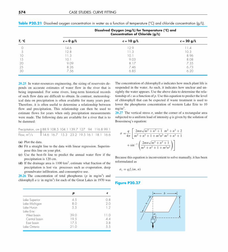
20.21 The saturation concentration of dissolved oxygen in wateras a function of temperature and chloride concentration is listed inTable P20.21. Use interpolation to estimate the dissolved oxygenlevel for T = 18°C with chloride = 10 g/L.20.22 For the data in Table P20.21, use polynomial regression toderive a third-order predictive equation for dissolved oxygen con-centration as a function of temperature for the case where chlorideconcentration is equal to 10 g/L. Use the equation to estimate thedissolved oxygen concentration for T = 8°C.20.23 Use multiple linear regression to derive a predictive equa-tion for dissolved oxygen concentration as a function of tempera-ture and chloride based on the data from Table P20.21. Use theequation to estimate the concentration of dissolved oxygen for achloride concentration of 5 g/L at T = 17°C.20.24 As compared to the models from Probs. 20.22 and 20.23, asomewhat more sophisticated model that accounts for the effect ofboth temperature and chloride on dissolved oxygen saturation canbe hypothesized as being of the form,
os = a0 + f3(T ) + f1(c)
That is, a constant plus a third-order polynomial in temperature anda linear relationship in chloride are assumed to yield superiorresults. Use the general linear least-squares approach to fit thismodel to the data in Table P20.21. Use the resulting equation toestimate the dissolved oxygen concentration for a chloride concen-tration of 10 g/L at T = 20°C.
20.18 The data tabulated below was generated from an experimentinitially containing pure ammonium cyanate (NH4OCN). It isknown that such concentration changes can be modeled by thefollowing equation:
c = c0
1 + kc0twhere c0 and k are parameters. Use a transformation to linearizethis equation. Then use linear regression to predict the concentra-tion at t = 160 min.
t (min) 0 20 50 65 150
c (mole/L) 0.381 0.264 0.180 0.151 0.086
cha01064_ch20.qxd 3/20/09 12:56 PM Page 573
574 CASE STUDIES: CURVE FITTING
20.25 In water-resources engineering, the sizing of reservoirs de-pends on accurate estimates of water flow in the river that isbeing impounded. For some rivers, long-term historical recordsof such flow data are difficult to obtain. In contrast, meteorolog-ical data on precipitation is often available for many years past.Therefore, it is often useful to determine a relationship betweenflow and precipitation. This relationship can then be used toestimate flows for years when only precipitation measurementswere made. The following data are available for a river that is tobe dammed:
Precipitation, cm 88.9 108.5 104.1 139.7 127 94 116.8 99.1
Flow, m3/s 14.6 16.7 15.3 23.2 19.5 16.1 18.1 16.6
(a) Plot the data.(b) Fit a straight line to the data with linear regression. Superim-
pose this line on your plot. (c) Use the best-fit line to predict the annual water flow if the
precipitation is 120 cm. (d) If the drainage area is 1100 km2, estimate what fraction of the
precipitation is lost via processes such as evaporation, deepgroundwater infiltration, and consumptive use.
20.26 The concentration of total phosphorus (p in mg/m3) andchlorophyll a (c in mg/m3) for each of the Great Lakes in 1970 was
p c
Lake Superior 4.5 0.8Lake Michigan 8.0 2.0Lake Huron 5.5 1.2Lake Erie:
West basin 39.0 11.0Central basin 19.5 4.4East basin 17.5 3.8
Lake Ontario 21.0 5.5
The concentration of chlorophyll a indicates how much plant life issuspended in the water. As such, it indicates how unclear and un-sightly the water appears. Use the above data to determine the rela-tionship of c as a function of p. Use this equation to predict the levelof chlorophyll that can be expected if waste treatment is used tolower the phosphorus concentration of western Lake Erie to 10mg/m3.20.27 The vertical stress $z under the corner of a rectangular areasubjected to a uniform load of intensity q is given by the solution ofBoussinesq’s equation:
$ = q4&
12mn
&m2 + n2 + 1
m2 + n2 + 1 + m2n2m2 + n2 + 2m2 + n2 + 1
+ sin!1
22mn
&m2 + n2 + 1
m2 + n2 + 1 + m2n2
34
Because this equation is inconvenient to solve manually, it has beenreformulated as
$z = q fz(m, n)
Table P20.21 Dissolved oxygen concentration in water as a function of temperature (°C) and chloride concentration (g/L).
Dissolved Oxygen (mg/L) for Temperature (°C) andConcentration of Chloride (g/L)
T, !C c = 0 g/L c = 10 g/L c = 20 g/L
0 14.6 12.9 11.45 12.8 11.3 10.3
10 11.3 10.1 8.9615 10.1 9.03 8.0820 9.09 8.17 7.3525 8.26 7.46 6.7330 7.56 6.85 6.20
b
za
"z
Figure P20.27
cha01064_ch20.qxd 3/20/09 12:56 PM Page 574

PROBLEMS 575
can then be substituted into Hooke’s law to determine the mast’sdeflection, 'L = strain % L, where L = the mast’s length. If thewind force is 25,000 N, use the data to estimate the deflection of a9-m mast.20.30 Enzymatic reactions are used extensively to characterizebiologically mediated reactions in environmental engineering.Proposed rate expressions for an enzymatic reaction are givenbelow where [S] is the substrate concentration and v0 is the initialrate of reaction. Which formula best fits the experimental data?
v0 = k[S] v0 = k[S]K + [S]
v0 = k[S]2
K + [S]2 v0 = k[S]3
K + [S]3
[S], M Initial Rate, 10!6 M/s
0.01 6.3636 % 10!5
0.05 7.9520 % 10!3
0.1 6.3472 % 10!2
0.5 6.00491 17.6905 24.425
10 24.49150 24.500
100 24.500
20.31 Environmental engineers dealing with the impacts of acidrain must determine the value of the ion product of water Kw as afunction of temperature. Scientists have suggested the followingequation to model this relationship:
! log10 Kw = aTa
+ b log10 Ta + cTa + d
where Ta = absolute temperature (K), and a, b, c, and d are para-meters. Employ the following data and regression to estimate theparameters:
Table P20.27
m n = 1.2 n = 1.4 n = 1.6
0.1 0.02926 0.03007 0.030580.2 0.05733 0.05894 0.059940.3 0.08323 0.08561 0.087090.4 0.10631 0.10941 0.111350.5 0.12626 0.13003 0.132410.6 0.14309 0.14749 0.150270.7 0.15703 0.16199 0.165150.8 0.16843 0.17389 0.17739
Ta (K) 273.15 283.15 293.15 303.15 313.15
Kw 1.164 % 10!15 2.950 % 10!15 6.846 % 10!15 1.467 % 10!14 2.929 % 10!14
20.32 An environmental engineer has reported the data tabulatedbelow for an experiment to determine the growth rate of bacteria, k,as a function of oxygen concentration, c. It is known that such datacan be modeled by the following equation
k = kmaxc2
cs + c2
where cs and kmax are parameters. Use a transformation to linearizethis equation. Then use linear regression to estimate cs and kmax andpredict the growth rate at c = 2 mg/L.
20.29 The mast of a sailboat has a cross-sectional area of 10.65 cm2
and is constructed of an experimental aluminum alloy. Tests wereperformed to define the relationship between stress and strain. Thetest results are
Strain, cm/cm 0.0032 0.0045 0.0055 0.0016 0.0085 0.0005
Stress, N/cm2 4970 5170 5500 3590 6900 1240
The stress caused by wind can be computed as F/Ac; where F =force in the mast and Ac = mast’s cross-sectional area. This value
where fz(m, n) is called the influence value and m and n aredimensionless ratios, with m = a/z and n = b/z and a and b asdefined in Fig. P20.27. The influence value is then tabulated, aportion of which is given in Table P20.27. If a = 4.6 and b = 14,use a third-order interpolating polynomial to compute $z at adepth 10 m below the corner of a rectangular footing that issubject to a total load of 100 t (metric tons). Express your answerin tonnes per square meter. Note that q is equal to the load perarea.20.28 Three disease-carrying organisms decay exponentially inlake water according to the following model:
p(t) = Ae!1.5t + Be!0.3t + Ce!0.05t
Estimate the initial population of each organism (A, B, and C)given the following measurements:
t, hr 0.5 1 2 3 4 5 6 7 9
p (t) 6.0 4.4 3.2 2.7 2.2 1.9 1.7 1.4 1.1
cha01064_ch20.qxd 3/20/09 12:56 PM Page 575
c (mg/L) 0.5 0.8 1.5 2.5 4
k (per day) 1.1 2.4 5.3 7.6 8.9
20.33 The following model is frequently used in environmentalengineering to parameterize the effect of temperature, T (°C), onbiochemical reaction rates, k (per day),
k = k20(T !20
where k20 and ( are parameters. Use a transformation to linearizethis equation. Then employ linear regression to estimate k20 and (and predict the reaction rate at T = 17°C.
T (°C) 6 12 18 24 30
k (per day) 0.14 0.20 0.31 0.46 0.69
20.34 As a member of Engineers Without Borders, you are workingin a community that has contaminated drinking water. At t = 0, youadd a disinfectant to a cistern that is contaminated with bacteria. Youmake the following measurements at several times thereafter:
t (hrs) 2 4 6 8 10
c (#/100 mL) 430 190 80 35 16
If the water is safe to drink when the concentration falls below 5 #/100 mL, estimate the time at which the concentration will fallbelow this limit.
Electrical Engineering20.35 Perform the same computations as in Sec. 20.3, but analyzedata generated with f (t) = 4 cos(5t) ! 7 sin(3t) + 6.20.36 You measure the voltage drop V across a resistor for a num-ber of different values of current i. The results arei 0.25 0.75 1.25 1.5 2.0
V !0.45 !0.6 0.70 1.88 6.0
Use first- through fourth-order polynomial interpolation to estimatethe voltage drop for i = 1.15. Interpret your results.20.37 Duplicate the computation for Prob. 20.36, but use polyno-mial regression to derive best fit equations of order 1 through 4using all the data. Plot and evaluate your results.20.38 The current in a wire is measured with great precision as afunction of time:
t 0 0.1250 0.2500 0.3750 0.5000
i 0 6.24 7.75 4.85 0.0000
Determine i at t = 0.23.20.39 The following data was taken from an experiment that mea-sured the current in a wire for various imposed voltages:
V, V 2 3 4 5 7 10
i, A 5.2 7.8 10.7 13 19.3 27.5
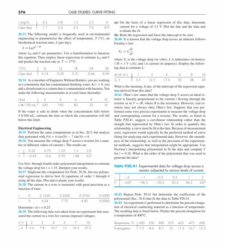
(a) On the basis of a linear regression of this data, determinecurrent for a voltage of 3.5 V. Plot the line and the data andevaluate the fit.
(b) Redo the regression and force the intercept to be zero.20.40 It is known that the voltage drop across an inductor followsFaraday’s law:
VL = Ldidt
where VL is the voltage drop (in volts), L is inductance (in henrys;1 H = 1 V· s/A), and i is current (in amperes). Employ the follow-ing data to estimate L:
di/dt, A/s 1 2 4 6 8 10
VL, V 5.5 12.5 17.5 32 38 49
What is the meaning, if any, of the intercept of the regression equa-tion derived from this data?20.41 Ohm’s law states that the voltage drop V across an ideal re-sistor is linearly proportional to the current i flowing through theresistor as in V = iR, where R is the resistance. However, real re-sistors may not always obey Ohm’s law. Suppose that you per-formed some very precise experiments to measure the voltage dropand corresponding current for a resistor. The results, as listed inTable P20.41, suggest a curvilinear relationship rather than thestraight line represented by Ohm’s law. In order to quantify thisrelationship, a curve must be fit to the data. Because of measurementerror, regression would typically be the preferred method of curvefitting for analyzing such experimental data. However, the smooth-ness of the relationship, as well as the precision of the experimen-tal methods, suggests that interpolation might be appropriate. UseNewton’s interpolating polynomial to fit the data and compute Vfor i = 0.10. What is the order of the polynomial that was used togenerate the data?
576 CASE STUDIES: CURVE FITTING
Table P20.41 Experimental data for voltage drop across aresistor subjected to various levels of current.
i !2 !1 !0.5 0.5 1 2
V !637 !96.5 !20.5 20.5 96.5 637
20.42 Repeat Prob. 20.41 but determine the coefficients of thepolynomial (Sec. 18.4) that fit the data in Table P20.41.20.43 An experiment is performed to determine the percent elonga-tion of electrical conducting material as a function of temperature.The resulting data is listed below. Predict the percent elongation fora temperature of 400°C.
Temperature, °C 200 250 300 375 425 475 600
% elongation 7.5 8.6 8.7 10 11.3 12.7 15.3
cha01064_ch20.qxd 3/20/09 12:56 PM Page 576
24.2 EFFECTIVE FORCE ON THE MAST OF A RACING SAILBOAT 673
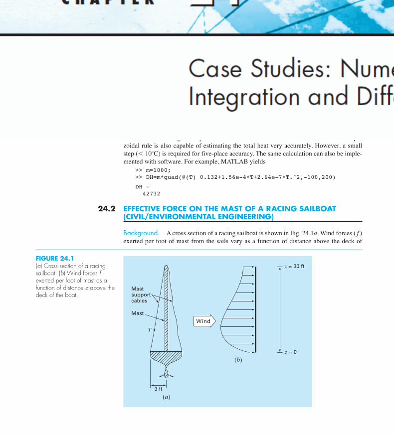
FIGURE 24.1(a) Cross section of a racingsailboat. (b) Wind forces fexerted per foot of mast as afunction of distance z above thedeck of the boat.
Wind
z = 30 ft
z = 0
Mastsupportcables
Mast
T
3 ft
(b)
(a)
TABLE 24.1 Results using the trapezoidal rule with various step sizes.
Step Size, !C #H ""t (%)
300 96,048 125150 43,029 0.7100 42,864 0.350 42,765 0.0725 42,740 0.01810 42,733.3 #0.01
5 42,732.3 #0.011 42,732.01 #0.010.05 42,732.00003 #0.01
The results using the trapezoidal rule are listed in Table 24.1. It is seen that the trape-zoidal rule is also capable of estimating the total heat very accurately. However, a smallstep (# 10!C) is required for five-place accuracy. The same calculation can also be imple-mented with software. For example, MATLAB yields
>> m=1000;>> DH=m*quad(@(T) 0.132+1.56e-4*T+2.64e-7*T.^2,-100,200)
DH =42732
24.2 EFFECTIVE FORCE ON THE MAST OF A RACING SAILBOAT(CIVIL/ENVIRONMENTAL ENGINEERING)
Background. A cross section of a racing sailboat is shown in Fig. 24.1a. Wind forces ( f )exerted per foot of mast from the sails vary as a function of distance above the deck of
cha01064_ch24.qxd 3/25/09 11:19 AM Page 673
Toshiba
Stamp
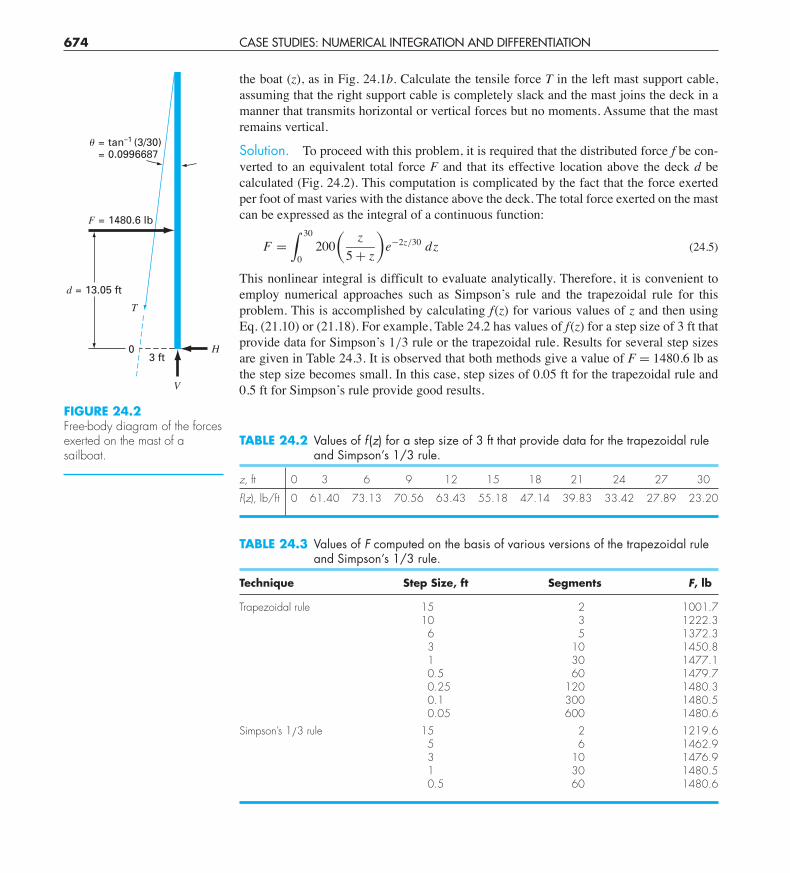
674 CASE STUDIES: NUMERICAL INTEGRATION AND DIFFERENTIATION
the boat (z), as in Fig. 24.1b. Calculate the tensile force T in the left mast support cable,assuming that the right support cable is completely slack and the mast joins the deck in amanner that transmits horizontal or vertical forces but no moments. Assume that the mastremains vertical.
Solution. To proceed with this problem, it is required that the distributed force f be con-verted to an equivalent total force F and that its effective location above the deck d becalculated (Fig. 24.2). This computation is complicated by the fact that the force exertedper foot of mast varies with the distance above the deck. The total force exerted on the mastcan be expressed as the integral of a continuous function:
F =! 30
0200
"z
5 + z
#e"2z/30 dz (24.5)
This nonlinear integral is difficult to evaluate analytically. Therefore, it is convenient toemploy numerical approaches such as Simpson’s rule and the trapezoidal rule for thisproblem. This is accomplished by calculating f (z) for various values of z and then usingEq. (21.10) or (21.18). For example, Table 24.2 has values of f (z) for a step size of 3 ft thatprovide data for Simpson’s 1/3 rule or the trapezoidal rule. Results for several step sizesare given in Table 24.3. It is observed that both methods give a value of F = 1480.6 lb asthe step size becomes small. In this case, step sizes of 0.05 ft for the trapezoidal rule and0.5 ft for Simpson’s rule provide good results.
TABLE 24.2 Values of f (z) for a step size of 3 ft that provide data for the trapezoidal ruleand Simpson’s 1/3 rule.
z, ft 0 3 6 9 12 15 18 21 24 27 30
f (z), lb/ft 0 61.40 73.13 70.56 63.43 55.18 47.14 39.83 33.42 27.89 23.20
TABLE 24.3 Values of F computed on the basis of various versions of the trapezoidal ruleand Simpson’s 1/3 rule.
Technique Step Size, ft Segments F, lb
Trapezoidal rule 15 2 1001.710 3 1222.3
6 5 1372.33 10 1450.81 30 1477.10.5 60 1479.70.25 120 1480.30.1 300 1480.50.05 600 1480.6
Simpson’s 1/3 rule 15 2 1219.65 6 1462.93 10 1476.91 30 1480.50.5 60 1480.6
FIGURE 24.2Free-body diagram of the forcesexerted on the mast of asailboat.
03 ft
d = 13.05 ft
V
T
H
F = 1480.6 lb
! = tan–1 (3/30)= 0.0996687
cha01064_ch24.qxd 3/25/09 11:19 AM Page 674
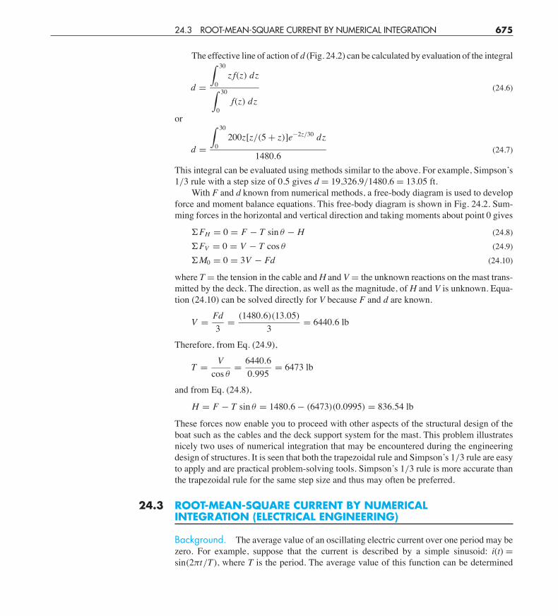
24.3 ROOT-MEAN-SQUARE CURRENT BY NUMERICAL INTEGRATION 675
The effective line of action of d (Fig. 24.2) can be calculated by evaluation of the integral
d =
! 30
0z f(z) dz
! 30
0f(z) dz
(24.6)
or
d =
! 30
0200z[z/(5 + z)]e"2z/30 dz
1480.6(24.7)
This integral can be evaluated using methods similar to the above. For example, Simpson’s1/3 rule with a step size of 0.5 gives d = 19,326.9/1480.6 = 13.05 ft.
With F and d known from numerical methods, a free-body diagram is used to developforce and moment balance equations. This free-body diagram is shown in Fig. 24.2. Sum-ming forces in the horizontal and vertical direction and taking moments about point 0 gives
"FH = 0 = F " T sin # " H (24.8)"FV = 0 = V " T cos # (24.9)"M0 = 0 = 3V " Fd (24.10)
where T = the tension in the cable and H and V = the unknown reactions on the mast trans-mitted by the deck. The direction, as well as the magnitude, of H and V is unknown. Equa-tion (24.10) can be solved directly for V because F and d are known.
V = Fd3
= (1480.6)(13.05)
3= 6440.6 lb
Therefore, from Eq. (24.9),
T = Vcos #
= 6440.60.995
= 6473 lb
and from Eq. (24.8),
H = F " T sin # = 1480.6 " (6473)(0.0995) = 836.54 lb
These forces now enable you to proceed with other aspects of the structural design of theboat such as the cables and the deck support system for the mast. This problem illustratesnicely two uses of numerical integration that may be encountered during the engineeringdesign of structures. It is seen that both the trapezoidal rule and Simpson’s 1/3 rule are easyto apply and are practical problem-solving tools. Simpson’s 1/3 rule is more accurate thanthe trapezoidal rule for the same step size and thus may often be preferred.
24.3 ROOT-MEAN-SQUARE CURRENT BY NUMERICALINTEGRATION (ELECTRICAL ENGINEERING)
Background. The average value of an oscillating electric current over one period may bezero. For example, suppose that the current is described by a simple sinusoid: i(t) =sin(2$t/T ), where T is the period. The average value of this function can be determined
cha01064_ch24.qxd 3/25/09 11:19 AM Page 675
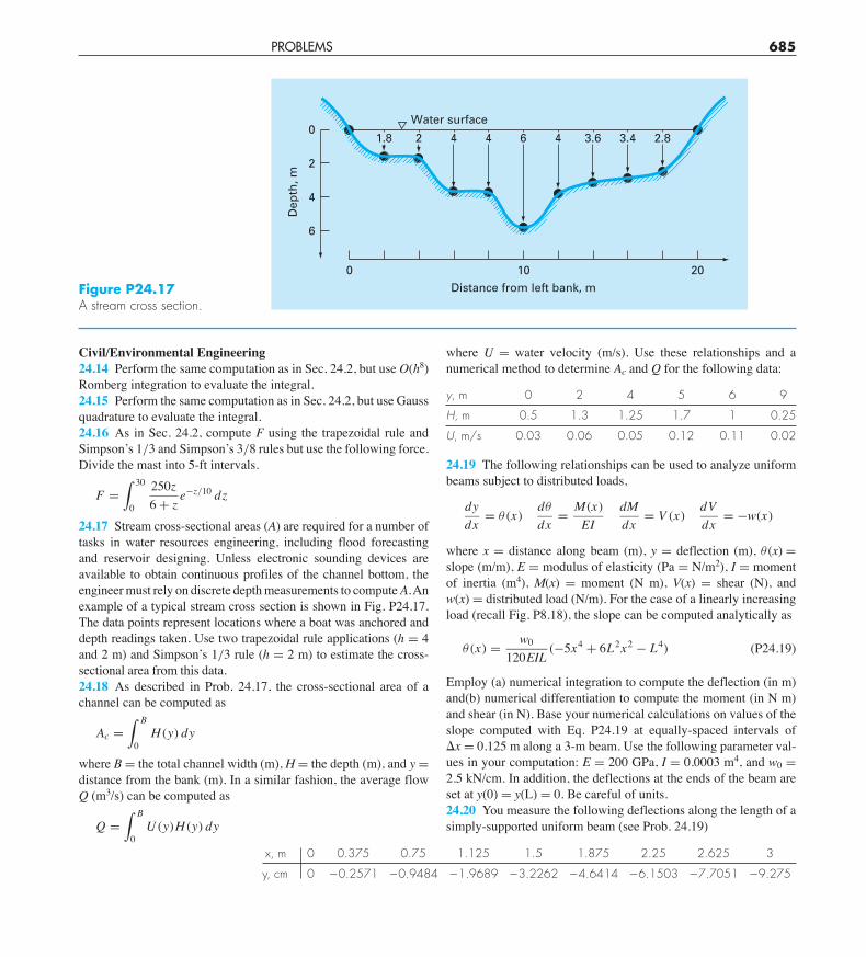
PROBLEMS 685
Civil/Environmental Engineering24.14 Perform the same computation as in Sec. 24.2, but use O(h8)Romberg integration to evaluate the integral. 24.15 Perform the same computation as in Sec. 24.2, but use Gaussquadrature to evaluate the integral.24.16 As in Sec. 24.2, compute F using the trapezoidal rule andSimpson’s 1/3 and Simpson’s 3/8 rules but use the following force.Divide the mast into 5-ft intervals.
F =! 30
0
250z6 + z
e"z/10 dz
24.17 Stream cross-sectional areas (A) are required for a number oftasks in water resources engineering, including flood forecastingand reservoir designing. Unless electronic sounding devices areavailable to obtain continuous profiles of the channel bottom, theengineer must rely on discrete depth measurements to compute A.Anexample of a typical stream cross section is shown in Fig. P24.17.The data points represent locations where a boat was anchored anddepth readings taken. Use two trapezoidal rule applications (h = 4and 2 m) and Simpson’s 1/3 rule (h = 2 m) to estimate the cross-sectional area from this data.24.18 As described in Prob. 24.17, the cross-sectional area of achannel can be computed as
Ac =! B
0H(y) dy
where B = the total channel width (m), H = the depth (m), and y =distance from the bank (m). In a similar fashion, the average flowQ (m3/s) can be computed as
Q =! B
0U(y)H(y) dy
where U = water velocity (m/s). Use these relationships and anumerical method to determine Ac and Q for the following data:
y, m 0 2 4 5 6 9
H, m 0.5 1.3 1.25 1.7 1 0.25
U, m/s 0.03 0.06 0.05 0.12 0.11 0.02
24.19 The following relationships can be used to analyze uniformbeams subject to distributed loads,
dydx
= #(x)d#
dx= M(x)
EIdMdx
= V (x)dVdx
= "w(x)
where x = distance along beam (m), y = deflection (m), # (x) =slope (m/m), E = modulus of elasticity (Pa = N/m2), I = momentof inertia (m4), M(x) = moment (N m), V(x) = shear (N), and w(x) = distributed load (N/m). For the case of a linearly increasingload (recall Fig. P8.18), the slope can be computed analytically as
#(x) = w0
120EIL("5x4 + 6L2x2 " L4) (P24.19)
Employ (a) numerical integration to compute the deflection (in m)and(b) numerical differentiation to compute the moment (in N m)and shear (in N). Base your numerical calculations on values of theslope computed with Eq. P24.19 at equally-spaced intervals of%x = 0.125 m along a 3-m beam. Use the following parameter val-ues in your computation: E = 200 GPa, I = 0.0003 m4, and w0 =2.5 kN/cm. In addition, the deflections at the ends of the beam areset at y(0) = y(L) = 0. Be careful of units.24.20 You measure the following deflections along the length of asimply-supported uniform beam (see Prob. 24.19)
Figure P24.17A stream cross section.
2010
Water surface1.8 2 4 4 6 4 3.6 3.4 2.8
6
4
2
Dep
th, m
0
Distance from left bank, m0
x, m 0 0.375 0.75 1.125 1.5 1.875 2.25 2.625 3
y, cm 0 !0.2571 !0.9484 !1.9689 !3.2262 !4.6414 !6.1503 !7.7051 !9.275
cha01064_ch24.qxd 3/25/09 11:20 AM Page 685

686 CASE STUDIES: NUMERICAL INTEGRATION AND DIFFERENTIATION
Table P24.21 Traffic flow rate (cars/min) for an intersection measured at various timeswithin a 24-h period.
Time Rate Time Rate Time Rate
12:00 midnight 2 9:00 A.M. 11 6:00 P.M. 202:00 A.M. 2 10:30 A.M. 4 7:00 P.M. 104:00 A.M. 0 11:30 A.M. 11 8:00 P.M. 85:00 A.M. 2 12:30 P.M. 12 9:00 P.M. 106:00 A.M. 6 2:00 P.M. 8 10:00 P.M. 87:00 A.M. 7 4:00 P.M. 7 11:00 P.M. 78:00 A.M. 23 5:00 P.M. 26 12:00 midnight 3
Employ numerical differentiation to compute the slope, themoment (in N m), the shear (in N) and the distributed load (inN/m). Use the following parameter values in your computation:E = 200 GPa, and I = 0.0003 m4.24.21 A transportation engineering study requires the calculationof the total number of cars that pass through an intersection over a24-h period. An individual visits the intersection at various timesduring the course of a day and counts the number of cars that passthrough the intersection in a minute. Utilize the data summarized inTable P24.21, to estimate the total number of cars that pass throughthe intersection per day. (Be careful of units.)24.22 A wind force distributed against the side of a skyscraper ismeasured as
p(z) = 'g(D " z) (P24.23)
where p(z) = pressure in pascals (or N/m2) exerted at an elevation zmeters above the reservoir bottom; ' = density of water, which forthis problem is assumed to be a constant 103 kg/m3; g = accelerationdue to gravity (9.8 m/s2); and D = elevation (in m) of the watersurface above the reservoir bottom. According to Eq. (P24.23), pres-sure increases linearly with depth, as depicted in Fig. P24.23a.Omitting atmospheric pressure (because it works against both sidesof the dam face and essentially cancels out), the total force ft can bedetermined by multiplying pressure times the area of the dam face(as shown in Fig. P24.23b). Because both pressure and area varywith elevation, the total force is obtained by evaluating
Height, l, m 0 30 60 90 120 150 180 210 240
Force, F(l ), N/m 0 340 1200 1600 2700 3100 3200 3500 3800
Figure P24.23Water exerting pressure on the upstream face of a dam: (a) side view showing force increasing linearly with depth; (b) front view showing width of dam in meters.
0
(a) (b)
60
40
20
122130135160175190200
Compute the net force and the line of action due to this distributedwind.24.23 Water exerts pressure on the upstream face of a dam asshown in Fig. P24.23. The pressure can be characterized by
ft =! D
0'gw(z)(D " z) dz
where w(z) = width of the dam face (m) at elevation z (Fig. P24.23b).The line of action can also be obtained by evaluating
cha01064_ch24.qxd 3/25/09 11:20 AM Page 686
PROBLEMS 687
d =
! D
0'gzw(z)(D " z) dz
! D
0'gw(z)(D " z) dz
Use Simpson’s rule to compute ft and d. Check the results with yourcomputer program for the trapezoidal rule.24.24 To estimate the size of a new dam, you have to determine thetotal volume of water (m3) that flows down a river in a year’s time.You have available the following long-term average data for theriver:
Mid- Mid- Mid- Mid- Mid- Mid- Mid- Mid- Mid-Date Jan. Feb. Mar. Apr. June Sept. Oct. Nov. Dec.
Flow, m3/s 30 38 82 125 95 20 22 24 35
Determine the volume. Be careful of units, and take care to make aproper estimate of flow at the end points.24.25 The data listed in the following table gives hourly measure-ments of heat flux q (cal/cm2/h) at the surface of a solar collector. Asan architectural engineer, you must estimate the total heat absorbedby a 150,000-cm2 collector panel during a 14-h period. The panelhas an absorption efficiency eab of 45%. The total heat absorbed isgiven by
h = eab
! t
0q A dt
where A = area and q = heat flux.
t 0 2 4 6 8 10 12 14
q 0.10 5.32 7.80 8.00 8.03 6.27 3.54 0.20
24.26 The heat flux q is the quantity of heat flowing through a unitarea of a material per unit time. It can be computed with Fourier’slaw,
J = "kdTdx
where J has units of J/m2/s or W/m2 and k is a coefficient of ther-mal conductivity that parameterizes the heat-conducting propertiesof the material and has units of W/(°C · m). T = temperature (°C);and x = distance (m) along the path of heat flow. Fourier’s law isused routinely by architectural engineers to determine heat flowthrough walls. The following temperatures are measured from thesurface (x = 0) into a stone wall:
x, m 0 0.08 0.16
T, °C 20 17 15
If the flux at x = 0 is 60 W/m2, compute k.24.27 The horizontal surface area As (m2) of a lake at a particulardepth can be computed from volume by differentiation,
As(z) = "dVdz
(z)
where V = volume (m3) and z = depth (m) as measured from the sur-face down to the bottom. The average concentration of a substancethat varies with depth c̄ (g/m3) can be computed by integration
c̄ =
! Z
0c(z)As(z) dz
! Z
0As(z) dz
where Z = the total depth (m). Determine the average concentra-tion based on the following data:
z, m 0 4 8 12 16
V, 106 m3 9.8175 5.1051 1.9635 0.3927 0.0000
c, g/m3 10.2 8.5 7.4 5.2 4.1
Electrical Engineering24.28 Perform the same computation as in Sec. 24.3, but for thecurrent as specified by
i(t) = 5e–1.25t sin 2$ t for 0 % t % T/2i(t) = 0 for T/2 < t % T
where T = 1 s. Use five-point Gauss quadrature to estimate theintegral.24.29 Repeat Prob. 24.28, but use five applications of Simpson’s1/3 rule.24.30 Repeat Prob. 24.28, but use Romberg integration to %s = 1%.24.31 Faraday’s law characterizes the voltage drop across an in-ductor as
VL = Ldidt
where VL = voltage drop (V), L = inductance (in henrys; 1 H = 1 V ·s/A), i = current (A), and t = time (s). Determine the voltage drop asa function of time from the following data for an inductance of 4 H.
t 0 0.1 0.2 0.3 0.5 0.7
i 0 0.16 0.32 0.56 0.84 2.0
24.32 Based on Faraday’s law (Prob. 24.31), use the followingvoltage data to estimate the inductance in henrys if a current of 2 Ais passed through the inductor over 400 milliseconds.
t, ms 0 10 20 40 60 80 120 180 280 400
V, volts 0 18 29 44 49 46 35 26 15 7
24.33 Suppose that the current through a resistor is described bythe function
i(t) = (60 " t)2 + (60 " t) sin($
t)
cha01064_ch24.qxd 3/25/09 11:20 AM Page 687
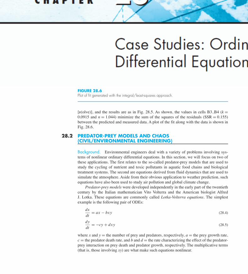
28.2 PREDATOR-PREY MODELS AND CHAOS 815
[s(olve)], and the results are as in Fig. 28.5. As shown, the values in cells B3..B4 (k =0.0915 and n = 1.044) minimize the sum of the squares of the residuals (SSR = 0.155)between the predicted and measured data. A plot of the fit along with the data is shown inFig. 28.6.
28.2 PREDATOR-PREY MODELS AND CHAOS(CIVIL/ENVIRONMENTAL ENGINEERING)
Background. Environmental engineers deal with a variety of problems involving sys-tems of nonlinear ordinary differential equations. In this section, we will focus on two ofthese applications. The first relates to the so-called predator-prey models that are used tostudy the cycling of nutrient and toxic pollutants in aquatic food chains and biologicaltreatment systems. The second are equations derived from fluid dynamics that are used tosimulate the atmosphere. Aside from their obvious application to weather prediction, suchequations have also been used to study air pollution and global climate change.
Predator-prey models were developed independently in the early part of the twentiethcentury by the Italian mathematician Vito Volterra and the American biologist AlfredJ. Lotka. These equations are commonly called Lotka-Volterra equations. The simplestexample is the following pair of ODEs:
dxdt
= ax ! bxy (28.4)
dydt
= !cy + dxy (28.5)
where x and y = the number of prey and predators, respectively, a = the prey growth rate,c = the predator death rate, and b and d = the rate characterizing the effect of the predator-prey interaction on prey death and predator growth, respectively. The multiplicative terms(that is, those involving xy) are what make such equations nonlinear.
10
c
5
0t20100
FIGURE 28.6Plot of fit generated with the integral/least-squares approach.
cha01064_ch28.qxd 3/25/09 12:56 PM Page 815
Toshiba
Stamp
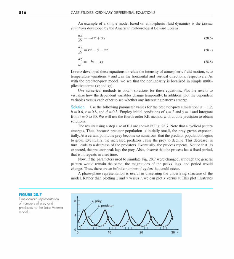
816 CASE STUDIES: ORDINARY DIFFERENTIAL EQUATIONS
An example of a simple model based on atmospheric fluid dynamics is the Lorenzequations developed by the American meteorologist Edward Lorenz,
dxdt
= !" x + " y (28.6)
dydt
= r x ! y ! xz (28.7)
dzdt
= !bz + xy (28.8)
Lorenz developed these equations to relate the intensity of atmospheric fluid motion, x, totemperature variations y and z in the horizontal and vertical directions, respectively. Aswith the predator-prey model, we see that the nonlinearity is localized in simple multi-plicative terms (xz and xy).
Use numerical methods to obtain solutions for these equations. Plot the results tovisualize how the dependent variables change temporally. In addition, plot the dependentvariables versus each other to see whether any interesting patterns emerge.
Solution. Use the following parameter values for the predator-prey simulation: a = 1.2,b = 0.6, c = 0.8, and d = 0.3. Employ initial conditions of x = 2 and y = 1 and integratefrom t = 0 to 30. We will use the fourth-order RK method with double precision to obtainsolutions.
The results using a step size of 0.1 are shown in Fig. 28.7. Note that a cyclical patternemerges. Thus, because predator population is initially small, the prey grows exponen-tially. At a certain point, the prey become so numerous, that the predator population beginsto grow. Eventually, the increased predators cause the prey to decline. This decrease, inturn, leads to a decrease of the predators. Eventually, the process repeats. Notice that, asexpected, the predator peak lags the prey. Also, observe that the process has a fixed period,that is, it repeats in a set time.
Now, if the parameters used to simulate Fig. 28.7 were changed, although the generalpattern would remain the same, the magnitudes of the peaks, lags, and period wouldchange. Thus, there are an infinite number of cycles that could occur.
A phase-plane representation is useful in discerning the underlying structure of themodel. Rather than plotting x and y versus t, we can plot x versus y. This plot illustrates
FIGURE 28.7Time-domain representationof numbers of prey and predators for the Lotka-Volterramodel.
8
4
0t30200 10
x, preyy, predator
cha01064_ch28.qxd 3/25/09 12:56 PM Page 816

28.2 PREDATOR-PREY MODELS AND CHAOS 817
the way that the state variables (x and y) interact, and is referred to as a phase-planerepresentation.
Figure 28.8 shows the phase-plane representation for the case we are studying. Thus,the interaction between the predator and the prey defines a closed counterclockwise orbit.Notice that there is a critical or rest point at the center of the orbit. The exact location ofthis point can be determined by setting Eqs. (28.4) and (28.5) to steady state (dy/dt =dx/dt = 0) and solving for (x, y) = (0, 0) and (c/d, a/b). The former is the trivial result thatif we start with neither predators nor prey, nothing will happen. The latter is the more in-teresting outcome that if the initial conditions are set at x = c/d and y = a/b, the derivativewill be zero and the populations will remain constant.
Now, let us use the same approach to investigate the trajectories of the Lorenz equa-tions with the following parameter values: " = 10, b = 2.666667, and r = 28. Employ ini-tial conditions of x = y = z = 5 and integrate from t = 0 to 20. Again, we will use thefourth-order RK method with double precision to obtain solutions.
The results shown in Fig. 28.9 are quite different from the behavior of the Lotka-Volterra equations. The variable x seems to be undergoing an almost random pattern of os-cillations, bouncing around from negative values to positive values. However, even though
FIGURE 28.8Phase-plane representationfor the Lotka-Volterra model. 4
y
2
0x62
Criticalpoint
0 4
FIGURE 28.9Time-domain representation of xversus t for the Lorenz equa-tions. The solid time series is forthe initial conditions (5, 5, 5).The dotted line is where the ini-tial condition for x is perturbedslightly (5.001, 5, 5).
20x
0
10
– 20
– 10
20 t155 10
cha01064_ch28.qxd 3/25/09 12:56 PM Page 817
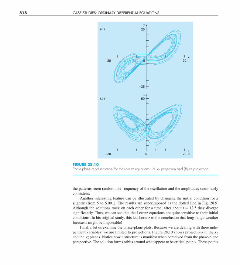
818 CASE STUDIES: ORDINARY DIFFERENTIAL EQUATIONS
the patterns seem random, the frequency of the oscillation and the amplitudes seem fairlyconsistent.
Another interesting feature can be illustrated by changing the initial condition for xslightly (from 5 to 5.001). The results are superimposed as the dotted line in Fig. 28.9.Although the solutions track on each other for a time, after about t = 12.5 they divergesignificantly. Thus, we can see that the Lorenz equations are quite sensitive to their initialconditions. In his original study, this led Lorenz to the conclusion that long-range weatherforecasts might be impossible!
Finally, let us examine the phase-plane plots. Because we are dealing with three inde-pendent variables, we are limited to projections. Figure 28.10 shows projections in the xyand the xz planes. Notice how a structure is manifest when perceived from the phase-planeperspective. The solution forms orbits around what appear to be critical points. These points
25y
– 25
x20– 20
(a)
0
50z
x20– 20
(b)
0
FIGURE 28.10Phase-plane representation for the Lorenz equations. (a) xy projection and (b) xz projection.
cha01064_ch28.qxd 3/25/09 12:56 PM Page 818
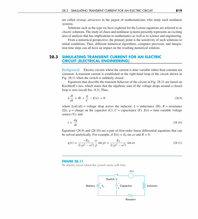
28.3 SIMULATING TRANSIENT CURRENT FOR AN ELECTRIC CIRCUIT 819
are called strange attractors in the jargon of mathematicians who study such nonlinearsystems.
Solutions such as the type we have explored for the Lorenz equations are referred to aschaotic solutions. The study of chaos and nonlinear systems presently represents an excitingarea of analysis that has implications to mathematics as well as to science and engineering.
From a numerical perspective, the primary point is the sensitivity of such solutions toinitial conditions. Thus, different numerical algorithms, computer precision, and integra-tion time steps can all have an impact on the resulting numerical solution.
28.3 SIMULATING TRANSIENT CURRENT FOR AN ELECTRICCIRCUIT (ELECTRICAL ENGINEERING)
Background. Electric circuits where the current is time-variable rather than constant arecommon. A transient current is established in the right-hand loop of the circuit shown inFig. 28.11 when the switch is suddenly closed.
Equations that describe the transient behavior of the circuit in Fig. 28.11 are based onKirchhoff’s law, which states that the algebraic sum of the voltage drops around a closedloop is zero (recall Sec. 8.3). Thus,
Ldidt
+ Ri + qC
! E(t) = 0 (28.9)
where L(di/dt) = voltage drop across the inductor, L = inductance (H), R = resistance(#), q = charge on the capacitor (C), C = capacitance (F), E(t) = time-variable voltagesource (V), and
i = dqdt
(28.10)
Equations (28.9) and (28.10) are a pair of first-order linear differential equations that canbe solved analytically. For example, if E(t) = E0 sin $t and R = 0,
q(t) = !E0
L(p2 ! $2)
$
psin pt + E0
L(p2 ! $2)sin $t (28.11)
Switch
Resistor
Capacitor–
+V0
E(t)
–
+Battery Inductor
FIGURE 28.11An electric circuit where the current varies with time.
cha01064_ch28.qxd 3/25/09 12:56 PM Page 819
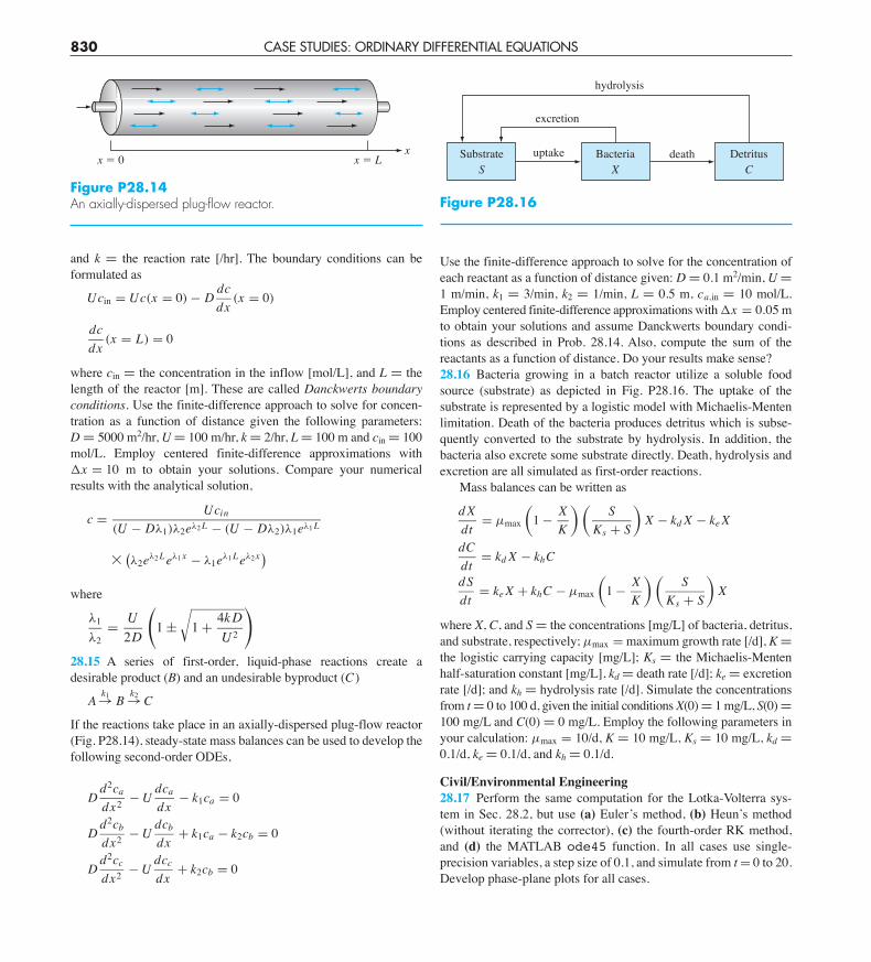
830 CASE STUDIES: ORDINARY DIFFERENTIAL EQUATIONS
Use the finite-difference approach to solve for the concentration ofeach reactant as a function of distance given: D = 0.1 m2/min, U =1 m/min, k1 = 3/min, k2 = 1/min, L = 0.5 m, ca,in = 10 mol/L.Employ centered finite-difference approximations with *x = 0.05 mto obtain your solutions and assume Danckwerts boundary condi-tions as described in Prob. 28.14. Also, compute the sum of thereactants as a function of distance. Do your results make sense?28.16 Bacteria growing in a batch reactor utilize a soluble foodsource (substrate) as depicted in Fig. P28.16. The uptake of thesubstrate is represented by a logistic model with Michaelis-Mentenlimitation. Death of the bacteria produces detritus which is subse-quently converted to the substrate by hydrolysis. In addition, thebacteria also excrete some substrate directly. Death, hydrolysis andexcretion are all simulated as first-order reactions.
Mass balances can be written as
d Xdt
= µmax
11 ! X
K
21S
Ks + S
2X ! kd X ! ke X
dCdt
= kd X ! khC
dSdt
= ke X + khC ! µmax
11 ! X
K
21S
Ks + S
2X
where X, C, and S = the concentrations [mg/L] of bacteria, detritus,and substrate, respectively; µmax = maximum growth rate [/d], K =the logistic carrying capacity [mg/L]; Ks = the Michaelis-Mentenhalf-saturation constant [mg/L], kd = death rate [/d]; ke = excretionrate [/d]; and kh = hydrolysis rate [/d]. Simulate the concentrationsfrom t = 0 to 100 d, given the initial conditions X(0) = 1 mg/L, S(0) =100 mg/L and C(0) = 0 mg/L. Employ the following parameters inyour calculation: µmax = 10/d, K = 10 mg/L, Ks = 10 mg/L, kd =0.1/d, ke = 0.1/d, and kh = 0.1/d.
Civil/Environmental Engineering28.17 Perform the same computation for the Lotka-Volterra sys-tem in Sec. 28.2, but use (a) Euler’s method, (b) Heun’s method(without iterating the corrector), (c) the fourth-order RK method,and (d) the MATLAB ode45 function. In all cases use single-precision variables, a step size of 0.1, and simulate from t = 0 to 20.Develop phase-plane plots for all cases.
and k = the reaction rate [/hr]. The boundary conditions can beformulated as
Ucin = Uc(x = 0) ! Ddcdx
(x = 0)
dcdx
(x = L) = 0
where cin = the concentration in the inflow [mol/L], and L = thelength of the reactor [m]. These are called Danckwerts boundaryconditions. Use the finite-difference approach to solve for concen-tration as a function of distance given the following parameters:D = 5000 m2/hr, U = 100 m/hr, k = 2/hr, L = 100 m and cin = 100mol/L. Employ centered finite-difference approximations with*x = 10 m to obtain your solutions. Compare your numericalresults with the analytical solution,
c = Ucin
(U ! D!1)!2e!2 L ! (U ! D!2)!1e!1 L
! !!2e!2 L e!1x ! !1e!1 L e!2x"
where
!1
!2= U
2D
71 ±
51 + 4k D
U 2
8
28.15 A series of first-order, liquid-phase reactions create adesirable product (B) and an undesirable byproduct (C)
Ak1% B
k2% C
If the reactions take place in an axially-dispersed plug-flow reactor(Fig. P28.14), steady-state mass balances can be used to develop thefollowing second-order ODEs,
Dd2ca
dx2 ! Udca
dx! k1ca = 0
Dd2cb
dx2 ! Udcb
dx+ k1ca ! k2cb = 0
Dd2cc
dx2 ! Udcc
dx+ k2cb = 0
x ! 0 x ! Lx
Figure P28.14An axially-dispersed plug-flow reactor.
hydrolysis
excretion
deathuptakeSubstrateS
BacteriaX
DetritusC
Figure P28.16
cha01064_ch28.qxd 3/25/09 12:56 PM Page 830
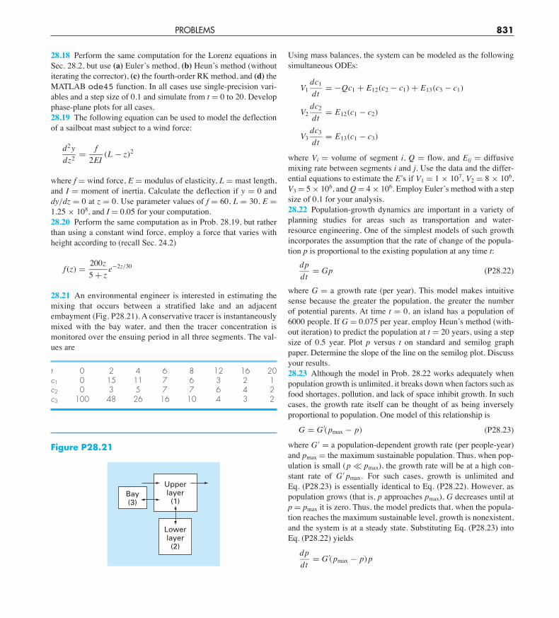
PROBLEMS 831
28.18 Perform the same computation for the Lorenz equations inSec. 28.2, but use (a) Euler’s method, (b) Heun’s method (withoutiterating the corrector), (c) the fourth-order RK method, and (d) theMATLAB ode45 function. In all cases use single-precision vari-ables and a step size of 0.1 and simulate from t = 0 to 20. Developphase-plane plots for all cases.28.19 The following equation can be used to model the deflectionof a sailboat mast subject to a wind force:
d2 ydz2 = f
2EI(L ! z)2
where f = wind force, E = modulus of elasticity, L = mast length,and I = moment of inertia. Calculate the deflection if y = 0 anddy/dz = 0 at z = 0. Use parameter values of f = 60, L = 30, E =1.25 $ 108, and I = 0.05 for your computation.28.20 Perform the same computation as in Prob. 28.19, but ratherthan using a constant wind force, employ a force that varies withheight according to (recall Sec. 24.2)
f(z) = 200z5 + z
e!2z/30
28.21 An environmental engineer is interested in estimating themixing that occurs between a stratified lake and an adjacentembayment (Fig. P28.21). A conservative tracer is instantaneouslymixed with the bay water, and then the tracer concentration ismonitored over the ensuing period in all three segments. The val-ues are
t 0 2 4 6 8 12 16 20c1 0 15 11 7 6 3 2 1c2 0 3 5 7 7 6 4 2c3 100 48 26 16 10 4 3 2
Bay(3)
Upperlayer(1)
Lowerlayer(2)
Figure P28.21
Using mass balances, the system can be modeled as the followingsimultaneous ODEs:
V1dc1
dt= !Qc1 + E12(c2 ! c1) + E13(c3 ! c1)
V2dc2
dt= E12(c1 ! c2)
V3dc3
dt= E13(c1 ! c3)
where Vi = volume of segment i, Q = flow, and Eij = diffusivemixing rate between segments i and j. Use the data and the differ-ential equations to estimate the E’s if V1 = 1 $ 107, V2 = 8 $ 106,V3 = 5 $ 106, and Q = 4 $ 106. Employ Euler’s method with a stepsize of 0.1 for your analysis.28.22 Population-growth dynamics are important in a variety ofplanning studies for areas such as transportation and water-resource engineering. One of the simplest models of such growthincorporates the assumption that the rate of change of the popula-tion p is proportional to the existing population at any time t:
dpdt
= Gp (P28.22)
where G = a growth rate (per year). This model makes intuitivesense because the greater the population, the greater the numberof potential parents. At time t = 0, an island has a population of6000 people. If G = 0.075 per year, employ Heun’s method (with-out iteration) to predict the population at t = 20 years, using a stepsize of 0.5 year. Plot p versus t on standard and semilog graphpaper. Determine the slope of the line on the semilog plot. Discussyour results.28.23 Although the model in Prob. 28.22 works adequately whenpopulation growth is unlimited, it breaks down when factors such asfood shortages, pollution, and lack of space inhibit growth. In suchcases, the growth rate itself can be thought of as being inverselyproportional to population. One model of this relationship is
G = G '(pmax ! p) (P28.23)
where G ' = a population-dependent growth rate (per people-year)and pmax = the maximum sustainable population. Thus, when pop-ulation is small (p ( pmax), the growth rate will be at a high con-stant rate of G ' pmax. For such cases, growth is unlimited andEq. (P28.23) is essentially identical to Eq. (P28.22). However, aspopulation grows (that is, p approaches pmax), G decreases until atp = pmax it is zero. Thus, the model predicts that, when the popula-tion reaches the maximum sustainable level, growth is nonexistent,and the system is at a steady state. Substituting Eq. (P28.23) intoEq. (P28.22) yields
dpdt
= G '(pmax ! p)p
cha01064_ch28.qxd 3/25/09 12:57 PM Page 831
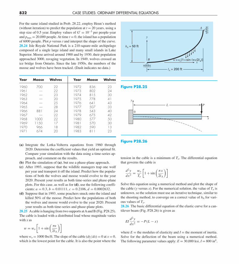
832 CASE STUDIES: ORDINARY DIFFERENTIAL EQUATIONS
For the same island studied in Prob. 28.22, employ Heun’s method(without iteration) to predict the population at t = 20 years, using astep size of 0.5 year. Employ values of G' = 10!5 per people-yearand pmax = 20,000 people. At time t = 0, the island has a populationof 6000 people. Plot p versus t and interpret the shape of the curve.28.24 Isle Royale National Park is a 210-square-mile archipelagocomposed of a single large island and many small islands in LakeSuperior. Moose arrived around 1900 and by 1930, their populationapproached 3000, ravaging vegetation. In 1949, wolves crossed anice bridge from Ontario. Since the late 1950s, the numbers of themoose and wolves have been tracked. (Dash indicates no data.)
Year Moose Wolves Year Moose Wolves
1960 700 22 1972 836 231961 — 22 1973 802 241962 — 23 1974 815 301963 — 20 1975 778 411964 — 25 1976 641 431965 — 28 1977 507 331966 881 24 1978 543 401967 — 22 1979 675 421968 1000 22 1980 577 501969 1150 17 1981 570 301970 966 18 1982 590 131971 674 20 1983 811 23
(a) Integrate the Lotka-Volterra equations from 1960 through2020. Determine the coefficient values that yield an optimal fit.Compare your simulation with the data using a time-series ap-proach, and comment on the results.
(b) Plot the simulation of (a), but use a phase-plane approach.(c) After 1993, suppose that the wildlife managers trap one wolf
per year and transport it off the island. Predict how the popula-tions of both the wolves and moose would evolve to the year2020. Present your results as both time-series and phase-planeplots. For this case, as well as for (d), use the following coeffi-cients: a = 0.3, b = 0.01111, c = 0.2106, d = 0.0002632.
(d) Suppose that in 1993, some poachers snuck onto the island andkilled 50% of the moose. Predict how the populations of boththe wolves and moose would evolve to the year 2020. Presentyour results as both time-series and phase-plane plots.
28.25 Acable is hanging from two supports atAand B (Fig. P28.25).The cable is loaded with a distributed load whose magnitude varieswith x as
w = wo
91 + sin
1(x2lA
2:
where wo = 1000 lbs/ft. The slope of the cable (dy/dx) = 0 at x = 0,which is the lowest point for the cable. It is also the point where the
tension in the cable is a minimum of To. The differential equationthat governs the cable is
d2 ydx2 = wo
To
91 + sin
1(x2lA
2:
Solve this equation using a numerical method and plot the shape ofthe cable (y versus x). For the numerical solution, the value of To isunknown, so the solution must use an iterative technique, similar tothe shooting method, to converge on a correct value of hA for vari-ous values of To.28.26 The basic differential equation of the elastic curve for a can-tilever beam (Fig. P28.26) is given as
EId2 ydx2 = !P(L ! x)
where E = the modulus of elasticity and I = the moment of inertia.Solve for the deflection of the beam using a numerical method.The following parameter values apply: E = 30,000 ksi, I = 800 in4,
L Py
x
0
Figure P28.26
w = wo[1 + sin ("x/2la)]
lA = 200 ft
xB
A
y
hA = 50 ft
Figure P28.25
cha01064_ch28.qxd 3/25/09 12:57 PM Page 832
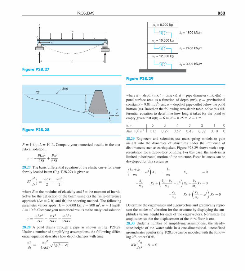
PROBLEMS 833
P = 1 kip, L = 10 ft. Compare your numerical results to the ana-lytical solution,
y = ! PLx2
2EI+ Px3
6EI
28.27 The basic differential equation of the elastic curve for a uni-formly loaded beam (Fig. P28.27) is given as
EId2 ydx2 = wLx
2! wx2
2
where E = the modulus of elasticity and I = the moment of inertia.Solve for the deflection of the beam using (a) the finite-differenceapproach (*x = 2 ft) and (b) the shooting method. The followingparameter values apply: E = 30,000 ksi, I = 800 in4, w = 1 kip/ft,L = 10 ft. Compare your numerical results to the analytical solution,
y = wLx3
12EI! wx4
24EI! wL3x
24EI28.28 A pond drains through a pipe as shown in Fig. P28.28.Under a number of simplifying assumptions, the following differ-ential equation describes how depth changes with time:
dhdt
= ! (d2
4A(h)
;2g(h + e)
m3 = 8,000 kg
k3 = 1800 kN/m
k2 = 2400 kN/m
k1 = 3000 kN/m
m2 = 10,000 kg
m1 = 12,000 kg
Figure P28.29
L
y
w
x0
Figure P28.27
e
d
h
A(h)
Figure P28.28
where h = depth (m), t = time (s), d = pipe diameter (m), A(h) =pond surface area as a function of depth (m2), g = gravitationalconstant (= 9.81 m/s2), and e = depth of pipe outlet below the pondbottom (m). Based on the following area-depth table, solve this dif-ferential equation to determine how long it takes for the pond toempty given that h(0) = 6 m, d = 0.25 m, e = 1 m.
h, m 6 5 4 3 2 1 0
A(h), 104 m2 1.17 0.97 0.67 0.45 0.32 0.18 0
28.29 Engineers and scientists use mass-spring models to gaininsight into the dynamics of structures under the influence ofdisturbances such as earthquakes. Figure P28.29 shows such a rep-resentation for a three-story building. For this case, the analysis islimited to horizontal motion of the structure. Force balances can bedeveloped for this system as1
k1 + k2
m1! $2
2X1 ! k2
m1X2 = 0
! k2
m2X1 +
1k2 + k3
m2! $2
2X2 ! k3
m2X3 = 0
! k3
m3X2 +
1k3
m3! $2
2X3 = 0
Determine the eigenvalues and eigenvectors and graphically repre-sent the modes of vibration for the structure by displaying the am-plitudes versus height for each of the eigenvectors. Normalize theamplitudes so that the displacement of the third floor is one.28.30 Under a number of simplifying assumptions, the steady-state height of the water table in a one-dimensional, unconfinedgroundwater aquifer (Fig. P28.30) can be modeled with the follow-ing 2nd-order ODE,
K h̄d2hdx2 + N = 0
cha01064_ch28.qxd 3/25/09 12:57 PM Page 833
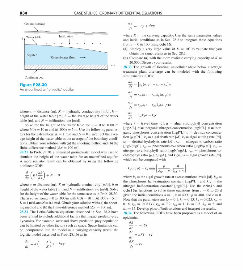
834 CASE STUDIES: ORDINARY DIFFERENTIAL EQUATIONS
where x = distance (m), K = hydraulic conductivity [m/d], hh =height of the water table [m], h̄ = the average height of the watertable [m], and N = infiltration rate [m/d].
Solve for the height of the water table for x = 0 to 1000 mwhere h(0) = 10 m and h(1000) = 5 m. Use the following parame-ters for the calculation: K = 1 m/d and N = 0.1 m/d. Set the aver-age height of the water table as the average of the boundary condi-tions. Obtain your solution with (a) the shooting method and (b) thefinite-difference method (*x = 100 m).28.31 In Prob. 28.30, a linearized groundwater model was used tosimulate the height of the water table for an unconfined aquifer.A more realistic result can be obtained by using the followingnonlinear ODE:
ddx
1K h
dhdx
2+ N = 0
where x = distance (m), K = hydraulic conductivity [m/d], h =height of the water table [m], and N = infiltration rate [m/d]. Solvefor the height of the water table for the same case as in Prob. 28.30.That is solve from x = 0 to 1000 m with h(0) = 10 m, h(1000) = 5 m,K = 1 m/d, and N = 0.1 m/d. Obtain your solution with (a) the shoot-ing method and (b) the finite-difference method (*x = 100 m).28.32 The Lotka-Volterra equations described in Sec. 28.2 havebeen refined to include additional factors that impact predator-preydynamics. For example, over and above predation, prey populationcan be limited by other factors such as space. Space limitation canbe incorporated into the model as a carrying capacity (recall thelogistic model described in Prob. 28.16) as in
dxdt
= a<
1 ! xK
=x ! bxy
dydt
= !cy + dxy
where K = the carrying capacity. Use the same parameter valuesand initial conditions as in Sec. 28.2 to integrate these equationsfrom t = 0 to 100 using ode45.(a) Employ a very large value of K = 108 to validate that you
obtain the same results as in Sec. 28.2.(b) Compare (a) with the more realistic carrying capacity of K =
20,000. Discuss your results.28.33 The growth of floating, unicellular algae below a sewagetreatment plant discharge can be modeled with the followingsimultaneous ODEs:
dadt
=>kg(n, p) ! kd ! ks
?a
dndt
= rnckhc ! rnakg(n, p)a
dpdt
= rpckhc ! rpakg(n, p)a
dcdt
= rcakda ! khc
where t = travel time [d], a = algal chlorophyll concentration[µgA/L], n = inorganic nitrogen concentration [µgN/L], p = inor-ganic phosphorus concentration [µgP/L], c = detritus concentra-tion [µgC/L], kd = algal death rate [/d], ks = algal settling rate [/d],kh = detrital hydrolysis rate [/d], rnc = nitrogen-to-carbon ratio[µgN/µgC], rpc = phosphorus-to-carbon ratio [µgP/µgC], rna =nitrogen-to-chlorophyll ratio [µgN/µgA], rpa = phosphorus-to-chlorophyll ratio [µgP/µgA], and kg(n, p) = algal growth rate [/d],which can be computed with
kg(n, p) = kg min@
pksp + p
,n
ksn + n
A
where kg = the algal growth rate at excess nutrient levels [/d], ksp =the phosphorus half-saturation constant [µgP/L], and ksn = thenitrogen half-saturation constant [µgN/L]. Use the ode45 andode15s functions to solve these equations from t = 0 to 20 dgiven the initial conditions a = 1, n = 4000, p = 400, and c = 0.Note that the parameters are kd = 0.1, ks = 0.15, kh = 0.025, rnc =0.18, rpc = 0.08333, rna = 7.2, rpa = 1, kg = 0.5, ksp = 2, and ksn = 15. Develop plots of both solutions and interpret the results. 28.34 The following ODEs have been proposed as a model of anepidemic:
dSdt
= !aSI
d Idt
= aSI ! r I
d Rdt
= r I
Ground surface
Water table Infiltrationh
x
Confining bed
AquiferGroundwater flow
Figure P28.30An unconfined or “phreatic” aquifer
cha01064_ch28.qxd 3/25/09 12:57 PM Page 834
PROBLEMS 835
where S = the susceptible individuals, I = the infected, R = therecovered, a = the infection rate, and r = the recovery rate. A cityhas 10,000 people, all of whom are susceptible.(a) If a single infectious individual enters the city at t = 0,
compute the progression of the epidemic until the number ofinfected individuals falls below 10. Use the following parame-ters: a = 0.002/(person·week) and r = 0.15#d. Develop time-series plots of all the state variables. Also generate a phase-plane plot of S versus I versus R.
(b) Suppose that after recovery, there is a loss of immunity thatcauses recovered individuals to become susceptible. This rein-fection mechanism can be computed as +R, where + = thereinfection rate. Modify the model to include this mechanismand repeat the computations in (a) using + = 0.015/d.
Electrical Engineering28.35 Perform the same computation as in the first part of Sec. 28.3,but with R = 0.025 #.28.36 Solve the ODE in the first part of Sec. 8.3 from t = 0 to 0.5using numerical techniques if q = 0.1 and i = !3.281515 at t = 0.Use an R = 50 along with the other parameters from Sec. 8.3.28.37 For a simple RL circuit, Kirchhoff’s voltage law requiresthat (if Ohm’s law holds)
Ldidt
+ Ri = 0
where i = current, L = inductance, and R = resistance. Solve for i,if L = 1, R = 1.5, and i(0) = 0.5. Solve this problem analyticallyand with a numerical method. Present your results graphically.28.38 In contrast to Prob. 28.37, real resistors may not alwaysobey Ohm’s law. For example, the voltage drop may be nonlinearand the circuit dynamics is described by a relationship such as
Ldidt
+ R
BiI
!1
iI
23C
= 0
where all other parameters are as defined in Prob. 28.37 and I is aknown reference current equal to 1. Solve for i as a function of timeunder the same conditions as specified in Prob. 28.37. 28.39 Develop an eigenvalue problem for an LC network similarto the one in Fig. 28.14, but with only two loops. That is, omit thei3 loop. Draw the network, illustrating how the currents oscillate intheir primary modes.28.40 Just as Fourier’s law and the heat balance can be employedto characterize temperature distribution, analogous relationshipsare available to model field problems in other areas of engineering.For example, electrical engineers use a similar approach whenmodeling electrostatic fields. Under a number of simplifyingassumptions, an analog of Fourier’s law can be represented in one-dimensional form as
D = !,dVdx
where D is called the electric flux density vector, , = permittivityof the material, and V = electrostatic potential. Similarly, aPoisson equation for electrostatic fields can be represented in onedimension as
d2Vdx2 = !+v
,
where +v = charge density. Use the finite-difference techniquewith *x = 2 to determine V for a wire where V (0) = 1000, V(20)= 0, , = 2, L = 20, and +v = 30.
Mechanical/Aerospace Engineering28.41 Perform the same computation as in Sec. 28.4 but for a 1-m-long pendulum.28.42 The rate of cooling of a body can be expressed as
dTdt
= !k(T ! Ta)
where T = temperature of the body (°C), Ta = temperature of thesurrounding medium (°C), and k = the proportionality constant(min!1). Thus, this equation specifies that the rate of cooling is pro-portional to the difference in temperature between the body and thesurrounding medium. If a metal ball heated to 90°C is dropped intowater that is held at a constant value of Ta = 20°C, use a numericalmethod to compute how long it takes the ball to cool to 40°C ifk = 0.25 min!1.28.43 The rate of heat flow (conduction) between two points on acylinder heated at one end is given by
dQdt
= !AdTdx
where ! = a constant, A = the cylinder’s cross-sectional area,Q = heat flow, T = temperature, t = time, and x = distance fromthe heated end. Because the equation involves two derivatives, wewill simplify this equation by letting
dTdx
= 100(L ! x)(20 ! t)100 ! xt
where L is the length of the rod. Combine the two equations andcompute the heat flow for t = 0 to 25 s. The initial condition isQ(0) = 0 and the parameters are ! = 0.5 cal · cm/s, A = 12 cm2,L = 20 cm, and x = 2.5 cm. Plot your results.28.44 Repeat the falling parachutist problem (Example 1.2), butwith the upward force due to drag as a second-order rate:
Fu = !cv2
cha01064_ch28.qxd 3/25/09 12:57 PM Page 835
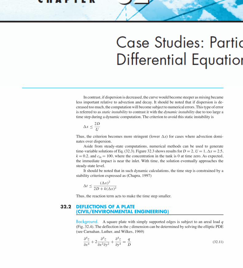
In contrast, if dispersion is decreased, the curve would become steeper as mixing becameless important relative to advection and decay. It should be noted that if dispersion is de-creased too much, the computation will become subject to numerical errors. This type of erroris referred to as static instability to contrast it with the dynamic instability due to too large atime step during a dynamic computation. The criterion to avoid this static instability is
!x # 2DU
Thus, the criterion becomes more stringent (lower !x) for cases where advection domi-nates over dispersion.
Aside from steady-state computations, numerical methods can be used to generatetime-variable solutions of Eq. (32.3). Figure 32.3 shows results for D = 2, U = 1, !x = 2.5,k = 0.2, and cin = 100, where the concentration in the tank is 0 at time zero. As expected,the immediate impact is near the inlet. With time, the solution eventually approaches thesteady-state level.
It should be noted that in such dynamic calculations, the time step is constrained by astability criterion expressed as (Chapra, 1997)
!t # (!x)2
2D + k(!x)2
Thus, the reaction term acts to make the time step smaller.
32.2 DEFLECTIONS OF A PLATE(CIVIL/ENVIRONMENTAL ENGINEERING)
Background. A square plate with simply supported edges is subject to an areal load q(Fig. 32.4). The deflection in the z dimension can be determined by solving the elliptic PDE(see Carnahan, Luther, and Wilkes, 1969)
"4z"x4 + 2
"4z"x2"y2 + "4z
"y4 = qD
(32.11)
32.2 DEFLECTIONS OF A PLATE 917
FIGURE 32.3Concentration versus distanceat different times during thebuildup of chemical in areactor.
c
100
100 x
Steady statet = 0.4
t = 0.8 t = 1.6 t = 3.2t = 0.2
cha01064_ch32.qxd 3/25/09 1:21 PM Page 917
Toshiba
Stamp
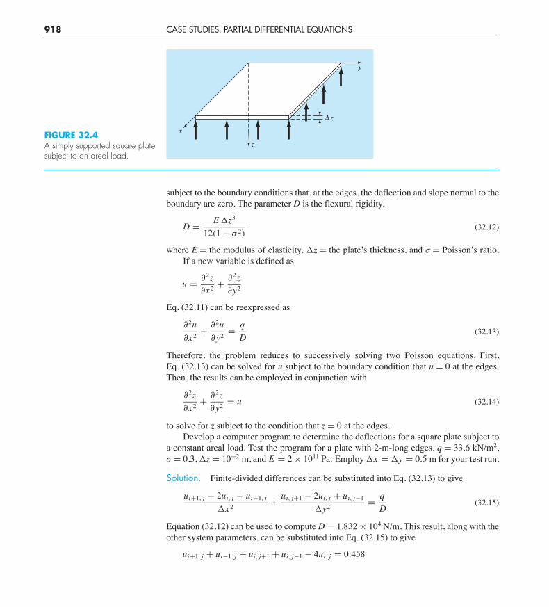
918 CASE STUDIES: PARTIAL DIFFERENTIAL EQUATIONS
subject to the boundary conditions that, at the edges, the deflection and slope normal to theboundary are zero. The parameter D is the flexural rigidity,
D = E !z3
12(1 ! # 2)(32.12)
where E = the modulus of elasticity, !z = the plate’s thickness, and # = Poisson’s ratio.If a new variable is defined as
u = "2z"x2 + "2z
"y2
Eq. (32.11) can be reexpressed as
"2u"x2 + "2u
"y2 = qD
(32.13)
Therefore, the problem reduces to successively solving two Poisson equations. First, Eq. (32.13) can be solved for u subject to the boundary condition that u = 0 at the edges.Then, the results can be employed in conjunction with
"2z"x2 + "2z
"y2 = u (32.14)
to solve for z subject to the condition that z = 0 at the edges.Develop a computer program to determine the deflections for a square plate subject to
a constant areal load. Test the program for a plate with 2-m-long edges, q = 33.6 kN/m2,# = 0.3, !z = 10!2 m, and E = 2 $ 1011 Pa. Employ !x = !y = 0.5 m for your test run.
Solution. Finite-divided differences can be substituted into Eq. (32.13) to give
ui+1, j ! 2ui, j + ui!1, j
!x2 + ui, j+1 ! 2ui, j + ui, j!1
!y2 = qD
(32.15)
Equation (32.12) can be used to compute D = 1.832 $ 104 N/m. This result, along with theother system parameters, can be substituted into Eq. (32.15) to give
ui+1, j + ui!1, j + ui, j+1 + ui, j!1 ! 4ui, j = 0.458
FIGURE 32.4A simply supported square platesubject to an areal load.
y
z
x
!z
cha01064_ch32.qxd 3/25/09 1:21 PM Page 918
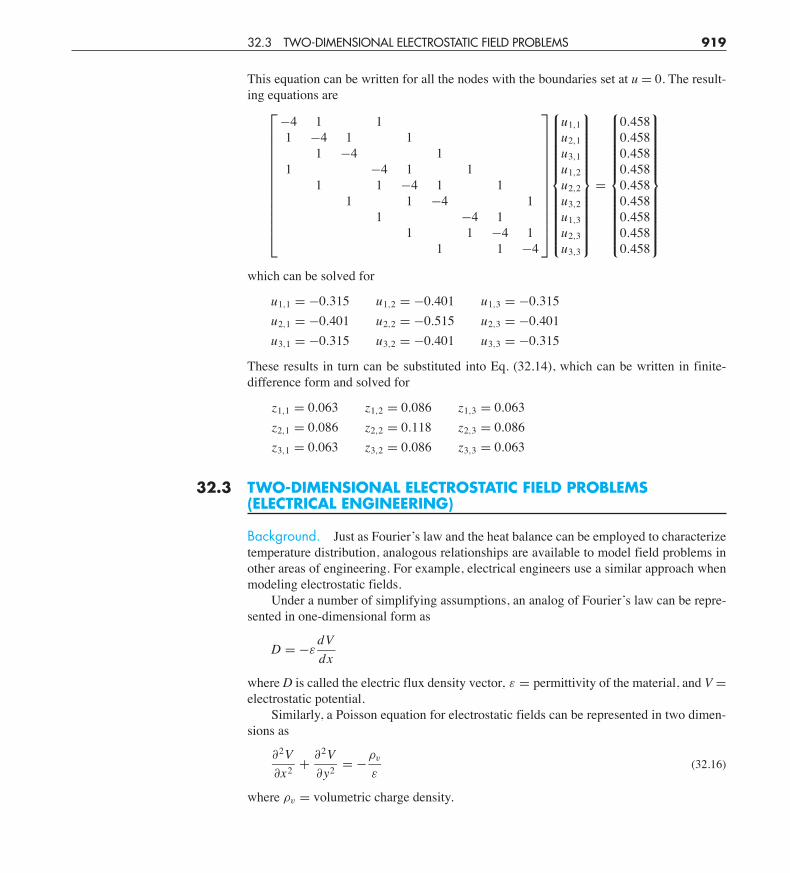
This equation can be written for all the nodes with the boundaries set at u = 0. The result-ing equations are
)
************+
!4 1 11 !4 1 1
1 !4 11 !4 1 1
1 1 !4 1 11 1 !4 1
1 !4 11 1 !4 1
1 1 !4
,
------------.
/0000000000001
0000000000002
u1,1u2,1u3,1u1,2u2,2u3,2u1,3u2,3u3,3
30000000000004
0000000000005
=
/0000000000001
0000000000002
0.4580.4580.4580.4580.4580.4580.4580.4580.458
30000000000004
0000000000005
which can be solved for
u1,1 = !0.315 u1,2 = !0.401 u1,3 = !0.315u2,1 = !0.401 u2,2 = !0.515 u2,3 = !0.401u3,1 = !0.315 u3,2 = !0.401 u3,3 = !0.315
These results in turn can be substituted into Eq. (32.14), which can be written in finite-difference form and solved for
z1,1 = 0.063 z1,2 = 0.086 z1,3 = 0.063z2,1 = 0.086 z2,2 = 0.118 z2,3 = 0.086z3,1 = 0.063 z3,2 = 0.086 z3,3 = 0.063
32.3 TWO-DIMENSIONAL ELECTROSTATIC FIELD PROBLEMS(ELECTRICAL ENGINEERING)
Background. Just as Fourier’s law and the heat balance can be employed to characterizetemperature distribution, analogous relationships are available to model field problems inother areas of engineering. For example, electrical engineers use a similar approach whenmodeling electrostatic fields.
Under a number of simplifying assumptions, an analog of Fourier’s law can be repre-sented in one-dimensional form as
D = !$dVdx
where D is called the electric flux density vector, $ = permittivity of the material, and V =electrostatic potential.
Similarly, a Poisson equation for electrostatic fields can be represented in two dimen-sions as
"2V"x2 + "2V
"y2 = !%v
$(32.16)
where %v = volumetric charge density.
32.3 TWO-DIMENSIONAL ELECTROSTATIC FIELD PROBLEMS 919
cha01064_ch32.qxd 3/25/09 1:21 PM Page 919
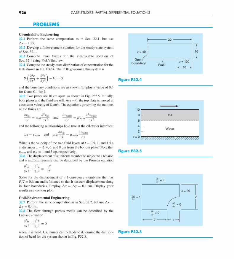
926 CASE STUDIES: PARTIAL DIFFERENTIAL EQUATIONS
Chemical/Bio Engineering32.1 Perform the same computation as in Sec. 32.1, but use !x = 1.25.32.2 Develop a finite-element solution for the steady-state systemof Sec. 32.1.32.3 Compute mass fluxes for the steady-state solution ofSec. 32.1 using Fick’s first law.32.4 Compute the steady-state distribution of concentration for thetank shown in Fig. P32.4. The PDE governing this system is
D'
"2c"x2 + "2c
"y2
(! kc = 0
and the boundary conditions are as shown. Employ a value of 0.5for D and 0.1 for k.32.5 Two plates are 10 cm apart, as shown in Fig. P32.5. Initially,both plates and the fluid are still. At t = 0, the top plate is moved ata constant velocity of 8 cm/s. The equations governing the motionsof the fluids are
"voil
"t= µoil
"2voil
"x2 and"vwater
"t= µwater
"2vwater
"x2
and the following relationships hold true at the oil-water interface:
voil = vwater and µoil"voil
"x= µwater
"vwater
"x
What is the velocity of the two fluid layers at t = 0.5, 1, and 1.5 sat distances x = 2, 4, 6, and 8 cm from the bottom plate? Note thatµwater and µoil = 1 and 3 cp, respectively.32.6 The displacement of a uniform membrane subject to a tensionand a uniform pressure can be described by the Poisson equation
"2z"x2 + "2z
"y2 = ! PT
Solve for the displacement of a 1-cm-square membrane that hasP!T = 0.6/cm and is fastened so that it has zero displacement alongits four boundaries. Employ !x = !y = 0.1 cm. Display yourresults as a contour plot.
Civil/Environmental Engineering32.7 Perform the same computation as in Sec. 32.2, but use !x =!y = 0.4 m.32.8 The flow through porous media can be described by theLaplace equation
"2h"x2 + "2h
"y2 = 0
where h is head. Use numerical methods to determine the distribu-tion of head for the system shown in Fig. P32.8.
Figure P32.4
30
10
10
Openboundary Wall
c = 40
c = 100
Figure P32.5
Oil
Water
10
8
6
4
2
x = 0
Figure P32.8
2
= 0
12
"h"y
= 0
h = 20
"h"n
= 0"h"y
= 1"h"x
PROBLEMS
cha01064_ch32.qxd 3/25/09 1:21 PM Page 926
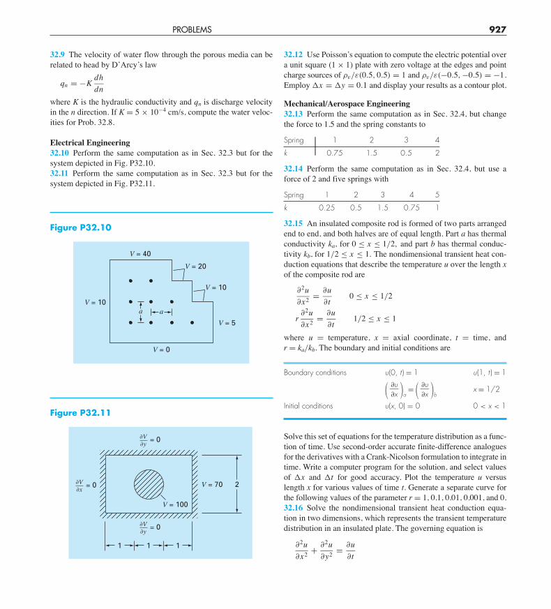
PROBLEMS 927
Figure P32.10
aV = 10
V = 0
V = 5
V = 40
V = 20
a
V = 10
Figure P32.11
2
= 0
111
"V"y
= 0"V"y
= 0"V"x
V = 70
V = 100
32.9 The velocity of water flow through the porous media can berelated to head by D’Arcy’s law
qn = !Kdhdn
where K is the hydraulic conductivity and qn is discharge velocityin the n direction. If K = 5 $ 10!4 cm/s, compute the water veloc-ities for Prob. 32.8.
Electrical Engineering32.10 Perform the same computation as in Sec. 32.3 but for thesystem depicted in Fig. P32.10.32.11 Perform the same computation as in Sec. 32.3 but for thesystem depicted in Fig. P32.11.
32.12 Use Poisson’s equation to compute the electric potential overa unit square (1 $ 1) plate with zero voltage at the edges and pointcharge sources of %v/$(0.5, 0.5) = 1 and %v/$(!0.5,!0.5) = !1.Employ !x = !y = 0.1 and display your results as a contour plot.
Mechanical/Aerospace Engineering32.13 Perform the same computation as in Sec. 32.4, but changethe force to 1.5 and the spring constants to
Spring 1 2 3 4
k 0.75 1.5 0.5 2
32.14 Perform the same computation as in Sec. 32.4, but use aforce of 2 and five springs with
Spring 1 2 3 4 5
k 0.25 0.5 1.5 0.75 1
32.15 An insulated composite rod is formed of two parts arrangedend to end, and both halves are of equal length. Part a has thermalconductivity ka, for 0 # x # 1/2, and part b has thermal conduc-tivity kb, for 1/2 # x # 1. The nondimensional transient heat con-duction equations that describe the temperature u over the length xof the composite rod are
"2u"x2 = "u
"t0 # x # 1/2
r"2u"x2 = "u
"t1/2 # x # 1
where u = temperature, x = axial coordinate, t = time, and r = ka/kb. The boundary and initial conditions are
Boundary conditions u(0, t ) = 1 u(1, t ) = 1
" #a= " #b
x = 1/2
Initial conditions u(x, 0) = 0 0 < x < 1
Solve this set of equations for the temperature distribution as a func-tion of time. Use second-order accurate finite-difference analoguesfor the derivatives with a Crank-Nicolson formulation to integrate intime. Write a computer program for the solution, and select valuesof !x and !t for good accuracy. Plot the temperature u versuslength x for various values of time t. Generate a separate curve forthe following values of the parameter r = 1, 0.1, 0.01, 0.001, and 0.32.16 Solve the nondimensional transient heat conduction equa-tion in two dimensions, which represents the transient temperaturedistribution in an insulated plate. The governing equation is
"2u"x2 + "2u
"y2 = "u"t
"u#"x
"u#"x
cha01064_ch32.qxd 3/25/09 1:21 PM Page 927