Numerical Analysis - University of Utah Math Dept.
363
Numerical Analysis Second Edition L. Ridgway Scott October 9, 2017
-
Upload
khangminh22 -
Category
Documents
-
view
0 -
download
0
Transcript of Numerical Analysis - University of Utah Math Dept.

Numerical AnalysisSecond Edition
L. Ridgway Scott
October 9, 2017

Copyright c© 2017 by Princeton University PressPublished by Princeton University Press, 41 William Street,Princeton, New Jersey 08540In the United Kingdom: Princeton University Press, 6 Oxford Street,Woodstock, Oxfordshire OX20 1TWpress.princeton.edu
All Rights ReservedLibrary of Congress Control Number: 2010943322?
ISBN: 978-0-691-14686-7British Library Cataloging-in-Publication Data is available
The publisher would like to acknowledge the author of this volume for typesetting this bookusing LATEX and Dr. Janet Englund and Peter Scott for providing the cover photograph
Printed on acid-free paper ∞
Printed in the United States of America
10 9 8 7 6 5 4 3 2 1

Dedication
To the memory of Ed Conway1 who, along with his colleagues at Tulane University, provideda stable, adaptive, and inspirational starting point for my career.
1Edward Daire Conway, III (1937–1985) was a student of Eberhard Friedrich Ferdinand Hopf at theUniversity of Indiana. Hopf was a student of Erhard Schmidt and Issai Schur.
iii

Draft October 9, 2017, do not distribute Page iv

Contents
1 Numerical Algorithms 11.1 Finding roots . . . . . . . . . . . . . . . . . . . . . . . . . . . . . . . . . . . 2
1.1.1 Relative versus absolute error . . . . . . . . . . . . . . . . . . . . . . 41.1.2 Scaling Heron’s algorithm . . . . . . . . . . . . . . . . . . . . . . . . 4
1.2 Analyzing Heron’s algorithm . . . . . . . . . . . . . . . . . . . . . . . . . . . 41.2.1 Local error analysis . . . . . . . . . . . . . . . . . . . . . . . . . . . . 51.2.2 Global error analysis . . . . . . . . . . . . . . . . . . . . . . . . . . . 5
1.3 Where to start . . . . . . . . . . . . . . . . . . . . . . . . . . . . . . . . . . 61.3.1 Another start . . . . . . . . . . . . . . . . . . . . . . . . . . . . . . . 61.3.2 The best start . . . . . . . . . . . . . . . . . . . . . . . . . . . . . . . 71.3.3 Solving the optimization problem . . . . . . . . . . . . . . . . . . . . 81.3.4 Using the best start . . . . . . . . . . . . . . . . . . . . . . . . . . . . 9
1.4 An unstable algorithm . . . . . . . . . . . . . . . . . . . . . . . . . . . . . . 91.5 General roots: effects of floating-point . . . . . . . . . . . . . . . . . . . . . 101.6 Exercises . . . . . . . . . . . . . . . . . . . . . . . . . . . . . . . . . . . . . . 111.7 Solutions . . . . . . . . . . . . . . . . . . . . . . . . . . . . . . . . . . . . . . 14
2 Nonlinear Equations 172.1 Fixed-point iteration . . . . . . . . . . . . . . . . . . . . . . . . . . . . . . . 18
2.1.1 Verifying the Lipschitz condition . . . . . . . . . . . . . . . . . . . . 202.1.2 Second-order iterations . . . . . . . . . . . . . . . . . . . . . . . . . . 212.1.3 Higher-order iterations . . . . . . . . . . . . . . . . . . . . . . . . . . 21
2.2 Particular methods . . . . . . . . . . . . . . . . . . . . . . . . . . . . . . . . 222.2.1 Newton’s method . . . . . . . . . . . . . . . . . . . . . . . . . . . . . 222.2.2 Stability of Newton’s method . . . . . . . . . . . . . . . . . . . . . . 242.2.3 Other second-order methods . . . . . . . . . . . . . . . . . . . . . . . 242.2.4 Secant method . . . . . . . . . . . . . . . . . . . . . . . . . . . . . . 25
2.3 Complex roots . . . . . . . . . . . . . . . . . . . . . . . . . . . . . . . . . . . 272.4 Error propagation . . . . . . . . . . . . . . . . . . . . . . . . . . . . . . . . . 272.5 More reading . . . . . . . . . . . . . . . . . . . . . . . . . . . . . . . . . . . 282.6 Exercises . . . . . . . . . . . . . . . . . . . . . . . . . . . . . . . . . . . . . . 282.7 Solutions . . . . . . . . . . . . . . . . . . . . . . . . . . . . . . . . . . . . . . 31
3 Linear Systems 353.1 Gaussian elimination . . . . . . . . . . . . . . . . . . . . . . . . . . . . . . . 36
3.1.1 Elimination algorithm . . . . . . . . . . . . . . . . . . . . . . . . . . 36
v

CONTENTS CONTENTS
3.1.2 Backward substitution . . . . . . . . . . . . . . . . . . . . . . . . . . 37
3.2 Factorization . . . . . . . . . . . . . . . . . . . . . . . . . . . . . . . . . . . 38
3.2.1 Proof of the factorization . . . . . . . . . . . . . . . . . . . . . . . . . 38
3.2.2 Using the factors . . . . . . . . . . . . . . . . . . . . . . . . . . . . . 40
3.2.3 Operation estimates . . . . . . . . . . . . . . . . . . . . . . . . . . . 40
3.2.4 Multiple right-hand sides . . . . . . . . . . . . . . . . . . . . . . . . . 41
3.2.5 Computing the inverse . . . . . . . . . . . . . . . . . . . . . . . . . . 42
3.3 Triangular matrices . . . . . . . . . . . . . . . . . . . . . . . . . . . . . . . . 42
3.4 Pivoting . . . . . . . . . . . . . . . . . . . . . . . . . . . . . . . . . . . . . . 43
3.4.1 When no pivoting is needed . . . . . . . . . . . . . . . . . . . . . . . 44
3.4.2 Partial pivoting . . . . . . . . . . . . . . . . . . . . . . . . . . . . . . 45
3.4.3 Full pivoting and matrix rank . . . . . . . . . . . . . . . . . . . . . . 45
3.4.4 The one-dimensional case . . . . . . . . . . . . . . . . . . . . . . . . 46
3.4.5 Uniqueness of the factorization . . . . . . . . . . . . . . . . . . . . . 47
3.5 More reading . . . . . . . . . . . . . . . . . . . . . . . . . . . . . . . . . . . 49
3.6 Exercises . . . . . . . . . . . . . . . . . . . . . . . . . . . . . . . . . . . . . . 49
3.7 Solutions . . . . . . . . . . . . . . . . . . . . . . . . . . . . . . . . . . . . . . 51
4 Direct Solvers 53
4.1 Direct factorization . . . . . . . . . . . . . . . . . . . . . . . . . . . . . . . . 53
4.1.1 Doolittle factorization . . . . . . . . . . . . . . . . . . . . . . . . . . 54
4.1.2 Memory references . . . . . . . . . . . . . . . . . . . . . . . . . . . . 55
4.1.3 Cholesky factorization and algorithm . . . . . . . . . . . . . . . . . . 57
4.2 Caution about factorization . . . . . . . . . . . . . . . . . . . . . . . . . . . 58
4.3 Banded matrices . . . . . . . . . . . . . . . . . . . . . . . . . . . . . . . . . 59
4.3.1 Banded Cholesky . . . . . . . . . . . . . . . . . . . . . . . . . . . . . 61
4.3.2 Work estimates for banded algorithms . . . . . . . . . . . . . . . . . 61
4.4 More reading . . . . . . . . . . . . . . . . . . . . . . . . . . . . . . . . . . . 61
4.5 Exercises . . . . . . . . . . . . . . . . . . . . . . . . . . . . . . . . . . . . . . 62
4.6 Solutions . . . . . . . . . . . . . . . . . . . . . . . . . . . . . . . . . . . . . . 64
Draft October 9, 2017, do not distribute Page vi

CONTENTS CONTENTS
5 Vector Spaces 675.1 Normed vector spaces . . . . . . . . . . . . . . . . . . . . . . . . . . . . . . . 68
5.1.1 Examples of norms . . . . . . . . . . . . . . . . . . . . . . . . . . . . 695.1.2 Unit balls . . . . . . . . . . . . . . . . . . . . . . . . . . . . . . . . . 695.1.3 Seminorms . . . . . . . . . . . . . . . . . . . . . . . . . . . . . . . . . 70
5.2 Proving the triangle inequality . . . . . . . . . . . . . . . . . . . . . . . . . . 705.2.1 The Rogers-Holder inequality . . . . . . . . . . . . . . . . . . . . . . 715.2.2 Minkowski’s inequality . . . . . . . . . . . . . . . . . . . . . . . . . . 72
5.3 Relations between norms . . . . . . . . . . . . . . . . . . . . . . . . . . . . . 725.3.1 Continuity of norms . . . . . . . . . . . . . . . . . . . . . . . . . . . 735.3.2 Norm equivalence . . . . . . . . . . . . . . . . . . . . . . . . . . . . . 73
5.4 Inner-product spaces . . . . . . . . . . . . . . . . . . . . . . . . . . . . . . . 745.4.1 Inductive orthonormalization . . . . . . . . . . . . . . . . . . . . . . 755.4.2 Orthogonal projections . . . . . . . . . . . . . . . . . . . . . . . . . . 755.4.3 Least squares . . . . . . . . . . . . . . . . . . . . . . . . . . . . . . . 765.4.4 The QR decomposition . . . . . . . . . . . . . . . . . . . . . . . . . . 77
5.5 More reading . . . . . . . . . . . . . . . . . . . . . . . . . . . . . . . . . . . 785.6 Exercises . . . . . . . . . . . . . . . . . . . . . . . . . . . . . . . . . . . . . . 785.7 Solutions . . . . . . . . . . . . . . . . . . . . . . . . . . . . . . . . . . . . . . 80
6 Operators 836.1 Operators . . . . . . . . . . . . . . . . . . . . . . . . . . . . . . . . . . . . . 84
6.1.1 Operator norms . . . . . . . . . . . . . . . . . . . . . . . . . . . . . . 846.1.2 Operator norms and eigenvalues . . . . . . . . . . . . . . . . . . . . . 856.1.3 Proof of the theorem . . . . . . . . . . . . . . . . . . . . . . . . . . . 86
6.2 Schur decomposition . . . . . . . . . . . . . . . . . . . . . . . . . . . . . . . 886.2.1 Nearly diagonal matrices . . . . . . . . . . . . . . . . . . . . . . . . . 896.2.2 The spectral radius is nearly a norm . . . . . . . . . . . . . . . . . . 896.2.3 Derivation of the Schur decomposition . . . . . . . . . . . . . . . . . 906.2.4 Schur decomposition and flags . . . . . . . . . . . . . . . . . . . . . . 926.2.5 Example of Schur decomposition . . . . . . . . . . . . . . . . . . . . 92
6.3 Convergent matrices . . . . . . . . . . . . . . . . . . . . . . . . . . . . . . . 936.4 Powers of matrices . . . . . . . . . . . . . . . . . . . . . . . . . . . . . . . . 936.5 Defective matrix powers . . . . . . . . . . . . . . . . . . . . . . . . . . . . . 966.6 Exercises . . . . . . . . . . . . . . . . . . . . . . . . . . . . . . . . . . . . . . 986.7 Solutions . . . . . . . . . . . . . . . . . . . . . . . . . . . . . . . . . . . . . . 101
7 Nonlinear Systems 1037.1 Functional iteration for systems . . . . . . . . . . . . . . . . . . . . . . . . . 104
7.1.1 Limiting behavior of fixed-point iteration . . . . . . . . . . . . . . . . 1067.1.2 Multi-index notation . . . . . . . . . . . . . . . . . . . . . . . . . . . 1067.1.3 Higher-order convergence . . . . . . . . . . . . . . . . . . . . . . . . . 1087.1.4 Particular methods . . . . . . . . . . . . . . . . . . . . . . . . . . . . 109
7.2 Newton’s method . . . . . . . . . . . . . . . . . . . . . . . . . . . . . . . . . 1097.2.1 Tensors . . . . . . . . . . . . . . . . . . . . . . . . . . . . . . . . . . 1097.2.2 Quadratic convergence of Newton’s method . . . . . . . . . . . . . . 110
Draft October 9, 2017, do not distribute Page vii

CONTENTS CONTENTS
7.2.3 No other methods . . . . . . . . . . . . . . . . . . . . . . . . . . . . . 1127.2.4 Eigen problems . . . . . . . . . . . . . . . . . . . . . . . . . . . . . . 1127.2.5 An example . . . . . . . . . . . . . . . . . . . . . . . . . . . . . . . . 113
7.3 Limiting behavior of Newton’s method . . . . . . . . . . . . . . . . . . . . . 1137.4 Mixing solvers . . . . . . . . . . . . . . . . . . . . . . . . . . . . . . . . . . . 115
7.4.1 Approximate linear solves . . . . . . . . . . . . . . . . . . . . . . . . 1167.4.2 Approximate Jacobian . . . . . . . . . . . . . . . . . . . . . . . . . . 116
7.5 More reading . . . . . . . . . . . . . . . . . . . . . . . . . . . . . . . . . . . 1167.6 Exercises . . . . . . . . . . . . . . . . . . . . . . . . . . . . . . . . . . . . . . 1177.7 Solutions . . . . . . . . . . . . . . . . . . . . . . . . . . . . . . . . . . . . . . 119
8 Iterative Methods 1238.1 Stationary iterative methods . . . . . . . . . . . . . . . . . . . . . . . . . . . 124
8.1.1 An algorithm . . . . . . . . . . . . . . . . . . . . . . . . . . . . . . . 1258.1.2 General matrices . . . . . . . . . . . . . . . . . . . . . . . . . . . . . 125
8.2 General splittings . . . . . . . . . . . . . . . . . . . . . . . . . . . . . . . . . 1268.2.1 Jacobi method . . . . . . . . . . . . . . . . . . . . . . . . . . . . . . 1268.2.2 Gauss-Seidel method . . . . . . . . . . . . . . . . . . . . . . . . . . . 1288.2.3 Convergence of general splittings . . . . . . . . . . . . . . . . . . . . 129
8.3 Necessary conditions for convergence . . . . . . . . . . . . . . . . . . . . . . 1318.3.1 Generalized diagonal dominance . . . . . . . . . . . . . . . . . . . . . 1328.3.2 Estimating the spectral radius . . . . . . . . . . . . . . . . . . . . . . 1338.3.3 Convergence conditions . . . . . . . . . . . . . . . . . . . . . . . . . . 1358.3.4 Perron-Frobenius theorem . . . . . . . . . . . . . . . . . . . . . . . . 135
8.4 More reading . . . . . . . . . . . . . . . . . . . . . . . . . . . . . . . . . . . 1368.5 Exercises . . . . . . . . . . . . . . . . . . . . . . . . . . . . . . . . . . . . . . 1368.6 Solutions . . . . . . . . . . . . . . . . . . . . . . . . . . . . . . . . . . . . . . 139
9 Conjugate Gradients 1419.1 Minimization methods . . . . . . . . . . . . . . . . . . . . . . . . . . . . . . 141
9.1.1 Descent methods . . . . . . . . . . . . . . . . . . . . . . . . . . . . . 1429.1.2 Descent directions . . . . . . . . . . . . . . . . . . . . . . . . . . . . . 1449.1.3 The gradient descent method . . . . . . . . . . . . . . . . . . . . . . 1449.1.4 Gradient-descent asymptotics . . . . . . . . . . . . . . . . . . . . . . 145
9.2 Conjugate Gradient iteration . . . . . . . . . . . . . . . . . . . . . . . . . . . 1469.2.1 The basic iteration . . . . . . . . . . . . . . . . . . . . . . . . . . . . 1469.2.2 Orthogonality relations . . . . . . . . . . . . . . . . . . . . . . . . . . 1489.2.3 Further orthogonalities . . . . . . . . . . . . . . . . . . . . . . . . . . 1499.2.4 New formulas for α and β . . . . . . . . . . . . . . . . . . . . . . . . 150
9.3 Optimal approximation of CG . . . . . . . . . . . . . . . . . . . . . . . . . . 1509.3.1 Operator calculus . . . . . . . . . . . . . . . . . . . . . . . . . . . . . 1519.3.2 CG error representation . . . . . . . . . . . . . . . . . . . . . . . . . 1519.3.3 Spectral theory . . . . . . . . . . . . . . . . . . . . . . . . . . . . . . 1529.3.4 CG error estimates . . . . . . . . . . . . . . . . . . . . . . . . . . . . 1549.3.5 Preconditioned Conjugate Gradient iteration . . . . . . . . . . . . . . 155
9.4 Comparing iterative solvers . . . . . . . . . . . . . . . . . . . . . . . . . . . 156
Draft October 9, 2017, do not distribute Page viii

CONTENTS CONTENTS
9.5 More reading . . . . . . . . . . . . . . . . . . . . . . . . . . . . . . . . . . . 157
9.6 Exercises . . . . . . . . . . . . . . . . . . . . . . . . . . . . . . . . . . . . . . 157
9.7 Solutions . . . . . . . . . . . . . . . . . . . . . . . . . . . . . . . . . . . . . . 159
Draft October 9, 2017, do not distribute Page ix

CONTENTS CONTENTS
10 Polynomial Interpolation 161
10.1 Local approximation: Taylor’s theorem . . . . . . . . . . . . . . . . . . . . . 161
10.2 Distributed approximation: interpolation . . . . . . . . . . . . . . . . . . . . 162
10.2.1 Existence of interpolant . . . . . . . . . . . . . . . . . . . . . . . . . 162
10.2.2 Error expression . . . . . . . . . . . . . . . . . . . . . . . . . . . . . . 163
10.2.3 Newton’s divided differences . . . . . . . . . . . . . . . . . . . . . . . 164
10.3 Behavior of Lagrange interpolation . . . . . . . . . . . . . . . . . . . . . . . 166
10.3.1 Norms in infinite-dimensional spaces . . . . . . . . . . . . . . . . . . 166
10.3.2 Instability of Lagrange interpolation . . . . . . . . . . . . . . . . . . 167
10.3.3 Data-dependence of Lagrange interpolation . . . . . . . . . . . . . . . 169
10.3.4 Runge versus Gauss . . . . . . . . . . . . . . . . . . . . . . . . . . . . 169
10.4 More reading . . . . . . . . . . . . . . . . . . . . . . . . . . . . . . . . . . . 172
10.5 Exercises . . . . . . . . . . . . . . . . . . . . . . . . . . . . . . . . . . . . . . 172
10.6 Solutions . . . . . . . . . . . . . . . . . . . . . . . . . . . . . . . . . . . . . . 175
11 Chebyshev and Hermite Interpolation 179
11.1 Chebyshev interpolation . . . . . . . . . . . . . . . . . . . . . . . . . . . . . 180
11.1.1 Error term ω . . . . . . . . . . . . . . . . . . . . . . . . . . . . . . . 180
11.1.2 Chebyshev asymptotics . . . . . . . . . . . . . . . . . . . . . . . . . . 182
11.1.3 Application to CG . . . . . . . . . . . . . . . . . . . . . . . . . . . . 182
11.2 Chebyshev basis functions . . . . . . . . . . . . . . . . . . . . . . . . . . . . 183
11.3 Lebesgue function . . . . . . . . . . . . . . . . . . . . . . . . . . . . . . . . . 184
11.4 Generalized interpolation . . . . . . . . . . . . . . . . . . . . . . . . . . . . . 186
11.4.1 Existence of interpolant . . . . . . . . . . . . . . . . . . . . . . . . . 186
11.4.2 Applications . . . . . . . . . . . . . . . . . . . . . . . . . . . . . . . . 188
11.4.3 Numerical differentiation . . . . . . . . . . . . . . . . . . . . . . . . . 189
11.5 More reading . . . . . . . . . . . . . . . . . . . . . . . . . . . . . . . . . . . 190
11.6 Exercises . . . . . . . . . . . . . . . . . . . . . . . . . . . . . . . . . . . . . . 190
11.7 Solutions . . . . . . . . . . . . . . . . . . . . . . . . . . . . . . . . . . . . . . 193
12 Approximation Theory 195
12.1 Best approximation by polynomials . . . . . . . . . . . . . . . . . . . . . . . 195
12.2 Weierstrass and Bernstein . . . . . . . . . . . . . . . . . . . . . . . . . . . . 201
12.2.1 Bernstein polynomials . . . . . . . . . . . . . . . . . . . . . . . . . . 201
12.2.2 Modulus of continuity . . . . . . . . . . . . . . . . . . . . . . . . . . 202
12.3 Least squares . . . . . . . . . . . . . . . . . . . . . . . . . . . . . . . . . . . 204
12.3.1 Polynomials as inner-product spaces . . . . . . . . . . . . . . . . . . 204
12.3.2 Orthogonal polynomials . . . . . . . . . . . . . . . . . . . . . . . . . 205
12.3.3 Roots of orthogonal polynomials . . . . . . . . . . . . . . . . . . . . . 206
12.4 Piecewise polynomial approximation . . . . . . . . . . . . . . . . . . . . . . 206
12.5 Adaptive approximation . . . . . . . . . . . . . . . . . . . . . . . . . . . . . 208
12.6 More reading . . . . . . . . . . . . . . . . . . . . . . . . . . . . . . . . . . . 209
12.7 Exercises . . . . . . . . . . . . . . . . . . . . . . . . . . . . . . . . . . . . . . 209
12.8 Solutions . . . . . . . . . . . . . . . . . . . . . . . . . . . . . . . . . . . . . . 212
Draft October 9, 2017, do not distribute Page x

CONTENTS CONTENTS
13 Numerical Quadrature 217
13.1 Interpolatory quadrature . . . . . . . . . . . . . . . . . . . . . . . . . . . . . 217
13.1.1 Newton-Cotes formulas . . . . . . . . . . . . . . . . . . . . . . . . . . 218
13.1.2 Order of exactness . . . . . . . . . . . . . . . . . . . . . . . . . . . . 219
13.1.3 Gaussian quadrature . . . . . . . . . . . . . . . . . . . . . . . . . . . 220
13.1.4 Hermite quadrature . . . . . . . . . . . . . . . . . . . . . . . . . . . . 221
13.1.5 Composite rules . . . . . . . . . . . . . . . . . . . . . . . . . . . . . . 222
13.2 Peano kernel theorem . . . . . . . . . . . . . . . . . . . . . . . . . . . . . . . 223
13.2.1 Continuity of Peano kernels . . . . . . . . . . . . . . . . . . . . . . . 224
13.2.2 Examples of Peano kernels . . . . . . . . . . . . . . . . . . . . . . . . 226
13.2.3 Uniqueness of Peano kernels . . . . . . . . . . . . . . . . . . . . . . . 226
13.2.4 Composite Peano kernels . . . . . . . . . . . . . . . . . . . . . . . . . 227
13.3 Gregorie-Euler-Maclaurin formulas . . . . . . . . . . . . . . . . . . . . . . . 228
13.3.1 More operator calculus . . . . . . . . . . . . . . . . . . . . . . . . . . 228
13.3.2 Product formula . . . . . . . . . . . . . . . . . . . . . . . . . . . . . 230
13.3.3 Inverse operators . . . . . . . . . . . . . . . . . . . . . . . . . . . . . 231
13.3.4 The Euler-Maclaurin formula . . . . . . . . . . . . . . . . . . . . . . 232
13.3.5 Euler’s constant γ . . . . . . . . . . . . . . . . . . . . . . . . . . . . . 233
13.3.6 Integrating a Gaussian . . . . . . . . . . . . . . . . . . . . . . . . . . 234
13.3.7 Gregorie’s quadrature . . . . . . . . . . . . . . . . . . . . . . . . . . . 235
13.4 Other quadrature rules . . . . . . . . . . . . . . . . . . . . . . . . . . . . . . 236
13.4.1 Chebyshev quadrature . . . . . . . . . . . . . . . . . . . . . . . . . . 237
13.4.2 Bernstein quadrature . . . . . . . . . . . . . . . . . . . . . . . . . . . 237
13.5 More reading . . . . . . . . . . . . . . . . . . . . . . . . . . . . . . . . . . . 237
13.6 Exercises . . . . . . . . . . . . . . . . . . . . . . . . . . . . . . . . . . . . . . 238
13.7 Solutions . . . . . . . . . . . . . . . . . . . . . . . . . . . . . . . . . . . . . . 240
14 Eigenvalue Problems 243
14.1 Eigenvalue examples . . . . . . . . . . . . . . . . . . . . . . . . . . . . . . . 243
14.1.1 Mechanical resonance . . . . . . . . . . . . . . . . . . . . . . . . . . . 243
14.1.2 Quality rankings . . . . . . . . . . . . . . . . . . . . . . . . . . . . . 244
14.1.3 Not so sparse eigenvalue problems . . . . . . . . . . . . . . . . . . . . 245
14.2 Gershgorin’s theorem . . . . . . . . . . . . . . . . . . . . . . . . . . . . . . . 245
14.2.1 Ovals of Cassini . . . . . . . . . . . . . . . . . . . . . . . . . . . . . . 246
14.2.2 Eigenvalue continuity . . . . . . . . . . . . . . . . . . . . . . . . . . . 248
14.3 Solving separately . . . . . . . . . . . . . . . . . . . . . . . . . . . . . . . . . 250
14.4 How not to eigen . . . . . . . . . . . . . . . . . . . . . . . . . . . . . . . . . 250
14.5 Reduction to Hessenberg form . . . . . . . . . . . . . . . . . . . . . . . . . . 251
14.5.1 Lanczos-Arnoldi algorithm . . . . . . . . . . . . . . . . . . . . . . . . 252
14.5.2 Optimality of Lanczos-Arnoldi . . . . . . . . . . . . . . . . . . . . . . 253
14.6 More reading . . . . . . . . . . . . . . . . . . . . . . . . . . . . . . . . . . . 255
14.7 Exercises . . . . . . . . . . . . . . . . . . . . . . . . . . . . . . . . . . . . . . 255
14.8 Solutions . . . . . . . . . . . . . . . . . . . . . . . . . . . . . . . . . . . . . . 258
Draft October 9, 2017, do not distribute Page xi

CONTENTS CONTENTS
15 Eigenvalue Algorithms 259
15.1 Power method . . . . . . . . . . . . . . . . . . . . . . . . . . . . . . . . . . . 259
15.1.1 Rayleigh quotient . . . . . . . . . . . . . . . . . . . . . . . . . . . . . 260
15.1.2 Back to the power method . . . . . . . . . . . . . . . . . . . . . . . . 261
15.1.3 Eigenvector convergence . . . . . . . . . . . . . . . . . . . . . . . . . 262
15.1.4 Power method convergence . . . . . . . . . . . . . . . . . . . . . . . . 263
15.1.5 Power method limitations . . . . . . . . . . . . . . . . . . . . . . . . 265
15.1.6 Defective matrices . . . . . . . . . . . . . . . . . . . . . . . . . . . . 265
15.2 Inverse iteration . . . . . . . . . . . . . . . . . . . . . . . . . . . . . . . . . . 267
15.2.1 The nearly singular system . . . . . . . . . . . . . . . . . . . . . . . . 268
15.2.2 Rayleigh quotient iteration . . . . . . . . . . . . . . . . . . . . . . . . 269
15.3 Singular value decomposition . . . . . . . . . . . . . . . . . . . . . . . . . . 270
15.4 Comparing factorizations . . . . . . . . . . . . . . . . . . . . . . . . . . . . . 271
15.5 More reading . . . . . . . . . . . . . . . . . . . . . . . . . . . . . . . . . . . 271
15.6 Exercises . . . . . . . . . . . . . . . . . . . . . . . . . . . . . . . . . . . . . . 271
15.7 Solutions . . . . . . . . . . . . . . . . . . . . . . . . . . . . . . . . . . . . . . 274
16 Ordinary Differential Equations 275
16.1 Basic theory of ODEs . . . . . . . . . . . . . . . . . . . . . . . . . . . . . . . 275
16.2 Existence and uniqueness of solutions . . . . . . . . . . . . . . . . . . . . . . 277
16.3 Basic discretization methods . . . . . . . . . . . . . . . . . . . . . . . . . . . 279
16.3.1 Nonuniqueness of the time step . . . . . . . . . . . . . . . . . . . . . 281
16.3.2 Near uniqueness of the time step . . . . . . . . . . . . . . . . . . . . 282
16.4 Convergence of discretization methods . . . . . . . . . . . . . . . . . . . . . 283
16.4.1 Global error estimates . . . . . . . . . . . . . . . . . . . . . . . . . . 284
16.4.2 Interpretation of error estimates . . . . . . . . . . . . . . . . . . . . . 285
16.4.3 Discretization error example . . . . . . . . . . . . . . . . . . . . . . . 286
16.5 More reading . . . . . . . . . . . . . . . . . . . . . . . . . . . . . . . . . . . 286
16.6 Exercises . . . . . . . . . . . . . . . . . . . . . . . . . . . . . . . . . . . . . . 286
16.7 Solutions . . . . . . . . . . . . . . . . . . . . . . . . . . . . . . . . . . . . . . 289
17 Higher-order ODE Discretization Methods 293
17.1 Higher-order discretization . . . . . . . . . . . . . . . . . . . . . . . . . . . . 294
17.1.1 An unstable scheme . . . . . . . . . . . . . . . . . . . . . . . . . . . . 296
17.1.2 Improved Euler . . . . . . . . . . . . . . . . . . . . . . . . . . . . . . 297
17.2 Convergence conditions . . . . . . . . . . . . . . . . . . . . . . . . . . . . . . 298
17.2.1 Constant solutions . . . . . . . . . . . . . . . . . . . . . . . . . . . . 298
17.2.2 Consistency . . . . . . . . . . . . . . . . . . . . . . . . . . . . . . . . 300
17.2.3 Unbounded discrete solutions . . . . . . . . . . . . . . . . . . . . . . 300
17.2.4 Zero stability . . . . . . . . . . . . . . . . . . . . . . . . . . . . . . . 301
17.2.5 Absolute stability regions . . . . . . . . . . . . . . . . . . . . . . . . 302
17.3 Backward differentiation formulas . . . . . . . . . . . . . . . . . . . . . . . . 304
17.4 More reading . . . . . . . . . . . . . . . . . . . . . . . . . . . . . . . . . . . 305
17.5 Exercises . . . . . . . . . . . . . . . . . . . . . . . . . . . . . . . . . . . . . . 305
17.6 Solutions . . . . . . . . . . . . . . . . . . . . . . . . . . . . . . . . . . . . . . 308
Draft October 9, 2017, do not distribute Page xii

CONTENTS CONTENTS
18 Floating Point 31118.1 Floating-point arithmetic . . . . . . . . . . . . . . . . . . . . . . . . . . . . . 311
18.1.1 Summation . . . . . . . . . . . . . . . . . . . . . . . . . . . . . . . . 31218.1.2 Summation application . . . . . . . . . . . . . . . . . . . . . . . . . . 31518.1.3 Better summation algorithms . . . . . . . . . . . . . . . . . . . . . . 31718.1.4 Solving ODEs . . . . . . . . . . . . . . . . . . . . . . . . . . . . . . . 318
18.2 Errors in solving systems . . . . . . . . . . . . . . . . . . . . . . . . . . . . . 31918.2.1 Condition number . . . . . . . . . . . . . . . . . . . . . . . . . . . . . 31918.2.2 A posteriori estimates and corrections . . . . . . . . . . . . . . . . . . 32018.2.3 Pivoting . . . . . . . . . . . . . . . . . . . . . . . . . . . . . . . . . . 321
18.3 More reading . . . . . . . . . . . . . . . . . . . . . . . . . . . . . . . . . . . 32218.4 Exercises . . . . . . . . . . . . . . . . . . . . . . . . . . . . . . . . . . . . . . 32218.5 Solutions . . . . . . . . . . . . . . . . . . . . . . . . . . . . . . . . . . . . . . 324
19 Notation 327
Index 341
Draft October 9, 2017, do not distribute Page xiii

CONTENTS CONTENTS
Draft October 9, 2017, do not distribute Page xiv

Preface
“...by faith and faith alone, embrace, believing where we cannot prove,”from In Memoriam by Alfred Lord Tennyson, a memorial to ArthurHallum.
Numerical analysis provides the foundations for a major paradigm shift in what we under-stand as an acceptable “answer” to a scientific or technical question. In classical calculus welook for answers like
√sinx, that is, answers composed of combinations of names of functions
that are familiar. This presumes we can evaluate such an expression as needed, and indeednumerical analysis has enabled the development of pocket calculators and computer softwareto make this routine. But numerical analysis has done much more than this. We will see thatfar more complex functions, defined, e.g., only implicitly, can be evaluated just as easily andwith the same technology. This makes the search for answers in classical calculus obsolete inmany cases. This new paradigm comes at a cost: developing stable, convergent algorithms toevaluate functions is often more difficult than more classical analysis of these functions. Forthis reason, the subject is still being actively developed. However, it is possible to presentmany important ideas at an elementary level, as is done here.
Today there are many good books on numerical analysis at the graduate level, includinggeneral texts [49, 139] as well as more specialized texts. We reference many of the latterat the ends of chapters where we suggest further reading in particular areas. At a moreintroductory level, the recent trend has been to provide texts accessible to a wide audience.The book by Burden and Faires [29] has been extremely successful. It is a tribute to theimportance of the field of numerical analysis that such books and others [136] are so popular.However, such books intentionally diminish the role of advanced mathematics in the subjectof numerical analysis. As a result, numerical analysis is frequently presented as an elementarysubject. As a corollary, most students miss exposure to numerical analysis as a mathematicalsubject. We hope to provide an alternative.
Several books written some decades ago addressed specifically a mathematical audience,e.g., [83, 87, 89]. These books remain valuable references, but the subject has changedsubstantially in the meantime.
We have intentionally introduced concepts from various parts of mathematics as theyarise naturally. In this sense, this book is an invitation to study more deeply advancedtopics in mathematics. It may require a short detour to understand completely what is beingsaid regarding operator theory in infinite-dimensional vector spaces or regarding algebraicconcepts like tensors and flags. Numerical analysis provides, in a way that is accessibleto advanced undergraduates, an introduction to many of the advanced concepts of modernanalysis.
We have assumed that the general style of a course using this book will be to prove
xv

CONTENTS CONTENTS
theorems. Indeed, we have attempted to facilitate a “Moore2 method” style of learning byproviding a sequence of steps to be verified as exercises. This has also guided the set oftopics to some degree. We have tried to hit the interesting points, and we have kept the listof topics covered as short as possible. Completeness is left to graduate level courses usingthe texts we mention at the end of many chapters.
The prerequisites for the course are not demanding. We assume a sophisticated under-standing of real numbers, including compactness arguments. We also assume some familiaritywith concepts of linear algebra, but we include derivations of most results as a review. Wehave attempted to make the book self-contained. Solutions of many of the exercises areprovided.
About the name: the term “numerical” analysis is fairly recent. A classic book [179] onthe topic changed names between editions, adopting the “numerical analysis” title in a lateredition [180]. The origins of the part of mathematics we now call analysis were all numerical,so for millennia the name “numerical analysis” would have been redundant. But analysislater developed conceptual (non-numerical) paradigms, and it became useful to specify thedifferent areas by names.
There are many areas of analysis in addition to numerical, including complex, convex,functional, harmonic, and real. Some areas, which might have been given such a name, havetheir own names (such as probability, instead of random or stochastic analysis). There is nota line of demarcation between the different areas of analysis. For example, much of harmonicanalysis might be characterized as real or complex analysis, with functional analysis playinga role in modern theories. The same is true of numerical analysis, and it can be viewed inpart as providing motivation for further study in all areas of analysis.
The subject of numerical analysis has ancient roots, and it has had periods of intensedevelopment followed by long periods of consolidation. In many cases, the new developmentshave coincided with the introduction of new forms of computing machines. For example,many of the basic theorems about computing solutions of ordinary differential equationswere proved soon after desktop adding machines became common at the turn of the 20thcentury. The emergence of the digital computer in the mid-20th century spurred interest insolving partial differential equations and large systems of linear equations, as well as manyother topics. The advent of parallel computers similarly stimulated research on new classesof algorithms. However, many fundamental questions remain open, and the subject is anactive area of research today. One particular emerging area is algorithms for computingexpressions with the least energy consumption.
All of analysis is about evaluating limits. In this sense, it is about infinite objects, unlike,say, some parts of algebra or discrete mathematics. Often a key step is to provide uniformbounds on infinite objects, such as operators on vector spaces. In numerical analysis, theinfinite objects are often sets of algorithms which are themselves finite in every instance.The objective is often to show that the algorithms are well-behaved uniformly and provide,in some limit, predictable results.
In numerical analysis there is sometimes a cultural divide between courses that empha-
2Robert Lee Moore (1882–1974) was born in Dallas, Texas, and did undergraduate work at the Universityof Texas in Austin where he took courses from L. E. Dickson, who recieved the first Ph. D. in mathematicsfrom the University of Chicago, in 1896. Moore got his Ph.D. in 1905 at the University of Chicago, studyingwith E. H. Moore and Oswald Veblen, and eventually returned to Austin where he continued to teach untilhis 87th year.
Draft October 9, 2017, do not distribute Page xvi

CONTENTS CONTENTS
size theory and ones that emphasize computation. Ideally, both should be intertwined, asnumerical analysis could well be called computational analysis because it is the analysis ofcomputational algorithms involving real numbers. We present many computational algo-rithms and encourage computational exploration. However, we do not address the subjectof software development (a.k.a., programming). Strictly speaking, programming is not re-quired to appreciate the material in the book. However, we encourage mathematics studentsto develop some experience in this direction, as writing a computer program is quite similarto proving a theorem. Computer systems are quite adept at finding flaws in one’s reasoning,and the organization required to make software readable provides a useful model to followin making complex mathematical arguments understandable to others.
There are several important groups this text can serve. It is very common today forpeople in many fields to study mathematics through the beginning of real analysis, as mightbe characterized by the extremely popular “little Rudin” book [147]. Our book is intended tobe at a comparable level of difficulty with little Rudin and can provide valuable reinforcementof the ideas and techniques covered there by applying them in a new domain. In this way, itis easily accessible to advanced undergraduates. It provides an option to study more analysiswithout raising the level of difficulty as occurs in a graduate course on measure theory.
People who go on to graduate work with a substantial computational component oftenneed to progress further in analysis, including a study of measure theory and the Lebesgueintegral. This is often done in a course at the “big Rudin” [148] level. Although the directprogression from little to big Rudin is a natural one, this book provides a way to interpolatebetween these levels while at the same time introducing ideas not found in [147] or [148] (orcomparable texts [111, 126]). Thus the book is also appropriate as a course for graduatestudents interested in computational mathematics but with a background in analysis onlyat the level of [147].
We have included quotes at the beginning of each chapter and frequent footnotes givinghistorical information. These are intended to be entertaining and perhaps provocative, butno attempt has been made to be historically complete. However, we give references to severalworks on the history of mathematics that we recommend for a more complete picture. Weindicate several connections among various mathematicians to give a sense of the personalinteractions of the era. We use the terms “student” and “advisor” to describe generalmentoring relationships which were sometimes different from what the terms might connotetoday. Although this may not be historically accurate in some cases, it would be tedious touse more precise terms to describe the relationships in each case in the various periods. Wehave used the MacTutor History of Mathematics archive extensively as an initial source ofinformation but have also endeavored to refer to archival literature whenever possible.
In practice, numerical computation remains as much an art as it is a science. We focuson the part of the subject that is a science. A continuing challenge of current research is totransform numerical art into numerical analysis, as well as extending the power and reach ofthe art of numerical computation. Recent decades have witnessed a dramatic improvementin our understanding of many topics in numerical computation, and there is reason to expectthat this trend will continue. Techniques that are supported only by heuristics tend to losefavor over time to ones that are understood rigorously. One of the great joys of the subjectis when a heuristic idea succumbs to a rigorous analysis that reveals its secrets and extendsits influence. It is hoped that this book will attract some new participants in this process.
Draft October 9, 2017, do not distribute Page xvii

CONTENTS CONTENTS
Acknowledgments
I have gotten suggestions from many people regarding topics in this book, and my memoryis not to be trusted to remember all of them. However, above all, Todd Dupont provided themost input regarding the book, including draft material, suggestions for additional topics,exercises, and overall conceptual advice. He regularly attended the fall 2009 class at theUniversity of Chicago in which the book was given a trial run. I also thank all the studentsfrom that class for their influence on the final version.
Randy Bank, Carl de Boor and Nick Trefethen suggested novel approaches to particulartopics. Although I cannot claim that I did exactly what they intended, their suggestions didinfluence what was presented in a substantial way.
Draft October 9, 2017, do not distribute Page xviii


CONTENTS CONTENTS
Draft October 9, 2017, do not distribute Page 2

Chapter 1
Numerical Algorithms
The word “algorithm” derives from the name of the Persian mathemati-cian (Abu Ja’far Muhammad ibn Musa) Al-Khwarizmi who lived fromabout 790 CE to about 840 CE. He wrote a book, Hisab al-jabr w’al-muqabala, that also named the subject “algebra.”
Numerical analysis is the subject which studies algorithms for computing expressionsdefined with real numbers. The square-root
√y is an example of such an expression; we
evaluate this today on a calculator or in a computer program as if it were as simple as y2. Itis numerical analysis that has made this possible, and we will study how this is done. Butin doing so, we will see that the same approach applies broadly to include functions thatcannot be named, and it even changes the nature of fundamental questions in mathematics,such as the impossibility of finding expressions for roots of order higher than 4.
There are two different phases to address in numerical analysis:
• the development of algorithms and
• the analysis of algorithms.
These are in principle independent activities, but in reality the development of an algorithmis often guided by the analysis of the algorithm, or of a simpler algorithm that computes thesame thing or something similar.
There are three characteristics of algorithms using real numbers that are in conflict tosome extent:
• the accuracy (or consistency) of the algorithm,
• the stability of the algorithm, and
• the effects of finite-precision arithmetic (a.k.a. round-off error).
The first of these just means that the algorithm approximates the desired quantity to anyrequired accuracy under suitable restrictions. The second means that the behavior of thealgorithm is continuous with respect to the parameters of the algorithm. The third topicis still not well understood at the most basic level, in the sense that there is not a well-established mathematical model for finite-precision arithmetic. Instead, we are forced to usecrude upper bounds for the behavior of finite-precision arithmetic that often lead to overlypessimistic predictions about its effects in actual computations.
1

1.1. FINDING ROOTS CHAPTER 1. NUMERICAL ALGORITHMS
We will see that in trying to improve the accuracy or efficiency of a stable algorithm, oneis often led to consider algorithms that turn out to be unstable and therefore of minimal (ifany) value. These various aspects of numerical analysis are often intertwined, as ultimatelywe want an algorithm that we can analyze rigorously to ensure it is effective when usingcomputer arithmetic.
The efficiency of an algorithm is a more complicated concept but is often the bottom linein choosing one algorithm over another. It can be related to all of the above characteristics,as well as to the complexity of the algorithm in terms of computational work or memoryreferences required in its implementation.
Another central theme in numerical analysis is adaptivity. This means that the compu-tational algorithm adapts itself to the data of the problem being solved as a way to improveefficiency and/or stability. Some adaptive algorithms are quite remarkable in their ability toelicit information automatically about a problem that is required for more efficient solution.
We begin with a problem from antiquity to illustrate each of these components of numer-ical analysis in an elementary context. We will not always disentangle the different issues,but we hope that the differing components will be evident.
1.1 Finding roots
People have been computing roots for millennia. Evidence exists [66] that the Babylonians,who used base-60 arithmetic, were able to approximate
√2 ≈ 1 +
24
60+
51
602+
10
603(1.1)
nearly 4000 years ago. By the time of Heron1 a method to compute square-roots was estab-lished [27] that we recognize now as the Newton-Raphson-Simpson method (see section 2.2.1)and takes the form of a repeated iteration
x← 12(x+ y/x), (1.2)
where the backwards arrow ← means assignment in algorithms. That is, once the computa-tion of the expression on the right-hand side of the arrow has been completed, a new valueis assigned to the variable x. Once that assignment is completed, the computation on theright-hand side can be redone with the new x.
The algorithm (1.2) is an example of what is known as fixed-point iteration, in which onehopes to find a fixed point, that is, an x where the iteration quits changing. A fixed point isthus a point x where
x = 12(x+ y/x). (1.3)
More precisely, x is a fixed point x = f(x) of the function
f(x) = 12(x+ y/x), (1.4)
defined, say, for x 6= 0. If we rearrange terms in (1.3), we find x = y/x, or x2 = y. Thus afixed point as defined in (1.3) is a solution of x2 = y, so that x = ±√y.
1A.k.a. Hero, of Alexandria, who lived in the 1st century CE.
Draft October 9, 2017, do not distribute Page 2

CHAPTER 1. NUMERICAL ALGORITHMS 1.1. FINDING ROOTS
√2 approximation absolute error
1.50000000000000 8.5786e-021.41666666666667 2.4531e-031.41421568627451 2.1239e-061.41421356237469 1.5947e-121.41421356237309 -2.2204e-16
Table 1.1: Results of experiments with the Heron algorithm applied to approximate√
2 usingthe algorithm (1.2) starting with x = 1. The boldface indicates the leading incorrect digit.Note that the number of correct digits essentially doubles at each step.
To describe actual implementations of these algorithms, we choose the scripting syntaximplemented in the system octave. As a programming language, this has some limitations,but its use is extremely widespread. In addition to the public domain implementation ofoctave, a commercial interpreter (which predates octave) called Matlab is available. How-ever, all computations presented here were done in octave.
We can implement (1.2) in octave in two steps as follows. First, we define the function(1.4) via the code
function x=heron(x,y)
x=.5*(x+y/x);
To use this function, you need to start with some initial guess, say, x = 1, which is writtensimply as
x=1
(Writing an expression with and without a semicolon at the end controls whether the inter-preter prints the result or not.) But then you simply iterate:
x=heron(x,y)
until x (or the part you care about) quits changing. The results of doing so are given intable 1.1.
We can examine the accuracy by a simple code
function x=errheron(x,y)
for i=1:5
x=heron(x,y);
errheron=x-sqrt(y)
end
We show in table 1.1 the results of these computations in the case y = 2. This algorithmseems to “home in” on the solution. We will see that the accuracy doubles at each step.
Draft October 9, 2017, do not distribute Page 3

1.2. ANALYZING HERON’S ALGORITHMCHAPTER 1. NUMERICAL ALGORITHMS
1.1.1 Relative versus absolute error
We can require the accuracy of an algorithm to be based on the size of the answer. Forexample, we might want the approximation x of a root x to be small relative to the size ofx:
x
x= 1 + δ, (1.5)
where δ satisfies some fixed tolerance, e.g., |δ| ≤ ε. Such a requirement is in keeping withthe model we will adopt for floating-point operations (see (1.39) and section 18.1).
We can examine the relative accuracy by the simple code
function x=relerrher(x,y)
for i=1:6
x=heron(x,y);
errheron=(x/sqrt(y))-1
end
We leave as exercise 1.2 comparison of the results produced by the above code relerrher
with the absolute errors presented in table 1.1.
1.1.2 Scaling Heron’s algorithm
Before we analyze how Heron’s algorithm (1.2) works, let us enhance it by a prescaling. Tobegin with, we can suppose that the number y whose square root we seek lies in the interval[12, 2]. If y < 1
2or y > 2, then we make the transformation
y = 4ky (1.6)
to get y ∈ [12, 2], for some integer k. And of course
√y = 2k
√y. By scaling y in this way, we
limit the range of inputs that the algorithm must deal with.In table 1.1, we showed the absolute error for approximating
√2, and in exercise 1.2 the
relative errors for approximating√
2 and√
12
are explored. It turns out that the maximum
errors for the interval [12, 2] occur at the ends of the interval (exercise 1.3). Thus five iterations
of Heron, preceded by the scaling (1.6), are sufficient to compute√y to 16 decimal places.
Scaling provides a simple example of adaptivity for algorithms for finding roots. Withoutscaling, the global performance (section 1.2.2) would be quite different.
1.2 Analyzing Heron’s algorithm
As the name implies, a major objective of numerical analysis is to analyze the behaviorof algorithms such as Heron’s iteration (1.2). There are two questions one can ask in thisregard. First, we may be interested in the local behavior of the algorithm assuming thatwe have a reasonable start near the desired root. We will see that this can be done quitecompletely, both in the case of Heron’s iteration and in general for algorithms of this type(in chapter 2). Second, we may wonder about the global behavior of the algorithm, that is,how it will respond with arbitrary starting points. With the Heron algorithm we can give afairly complete answer, but in general it is more complicated. Our point of view is that the
Draft October 9, 2017, do not distribute Page 4

CHAPTER 1. NUMERICAL ALGORITHMS1.2. ANALYZING HERON’S ALGORITHM
global behavior is really a different subject, e.g., a study in dynamical systems. We will seethat techniques like scaling (section 1.1.2) provide a basis to turn the local analysis into aconvergence theory.
1.2.1 Local error analysis
Since Heron’s iteration (1.2) is recursive in nature, it it natural to expect that the errors canbe expressed recursively as well. We can write an algebraic expression for Heron’s iteration(1.2) linking the error at one iteration to the error at the next. Thus define
xn+1 = 12(xn + y/xn), (1.7)
and let en = xn − x = xn −√y. Then by (1.7) and (1.3),
en+1 =xn+1 − x = 12(xn + y/xn)− 1
2(x+ y/x)
= 12(en + y/xn − y/x) = 1
2
(en +
y(x− xn)
xxn
)= 1
2
(en −
xenxn
)= 1
2en
(1− x
xn
)= 1
2
e2n
xn.
(1.8)
If we are interested in the relative error,
en =enx
=xn − xx
=xnx− 1, (1.9)
then (1.8) becomes
en+1 = 12
xe2n
xn= 1
2(1 + en)−1 e2
n. (1.10)
Thus we see that
the error at each step is proportional tothe square of the error at the previous step;
for the relative error, the constant of proportionality tends rapidly to 12. In (2.20), we will
see that this same result can be derived by a general technique.
1.2.2 Global error analysis
In addition, (1.10) implies a limited type of global convergence property, at least for xn >x =√y. In that case, (1.10) gives
|en+1| = 12
e2n
|1 + en|= 1
2
e2n
1 + en≤ 1
2en. (1.11)
Thus the relative error is reduced by a factor smaller than 12
at each iteration, no matterhow large the initial error may be. Unfortunately, this type of global convergence propertydoes not hold for many algorithms. We can illustrate what can go wrong in the case of theHeron algorithm when xn < x =
√y.
Draft October 9, 2017, do not distribute Page 5

1.3. WHERE TO START CHAPTER 1. NUMERICAL ALGORITHMS
Suppose for simplicity that y = 1, so that also x = 1, so that the relative error isen = xn − 1, and therefore (1.10) implies that
en+1 =(1− xn)2
2xn=
(en)2
2xn. (1.12)
As xn → 0, en+1 → ∞, even though |en| < 1. Therefore, convergence is not truly globalfor the Heron algorithm. On the other hand, the only way that we can have xn → 0 is forn = 0, that is, for the initial guess. But after that, we always have xn > 1 for n > 0.
What happens if we start with x0 near zero? We obtain x1 near ∞. From then on, theiterations satisfy xn >
√y, so the iteration is ultimately convergent. But the number of
iterations required to reduce the error below a fixed error tolerance can be arbitrarily largedepending on how small x0 is. By the same token, we cannot bound the number of requirediterations for arbitrarily large x0. Fortunately, we will see that it is possible to choose goodstarting values for Heron’s method to avoid this potential bad behavior.
1.3 Where to start
With any iterative algorithm, we have to start the iteration somewhere, and this choicecan be an interesting problem in its own right. Just like the initial scaling described insection 1.1.2, this can affect the performance of the overall algorithm substantially.
For the Heron algorithm, there are various possibilities. The simplest is just to takex0 = 1, in which case
e0 =1
x− 1 =
1√y− 1. (1.13)
This gives
e1 = 12xe2
0 = 12x
(1
x− 1
)2
= 12
(x− 1)2
x. (1.14)
We can use (1.14) as a formula for e1 as a function of x (it is by definition a function ofy = x2); then we see that
e1(x) = e1(1/x) (1.15)
by comparing the rightmost two terms in (1.14). Note that the maximum of e1(x) on[2−1/2, 21/2] occurs at the ends of the interval, and
e1(√
2) = 12
(√
2− 1)2
√2
= 34
√2− 1 ≈ 0.060660 . (1.16)
Thus the simple starting value x0 = 1 is remarkably effective. Nevertheless, let us see if wecan do better.
1.3.1 Another start
Another idea to start the iteration is to make an approximation to the square-root functiongiven the fact that we always have y ∈ [1
2, 2] (section 1.1.2). Since this means that y is near
1, we can write y = 1 + t (i.e., t = y − 1), and we have
x =√y =√
1 + t = 1 + 12t+O(t2)
= 1 + 12(y − 1) +O(t2) = 1
2(y + 1) +O(t2).
(1.17)
Draft October 9, 2017, do not distribute Page 6

CHAPTER 1. NUMERICAL ALGORITHMS 1.3. WHERE TO START
Thus we get the approximation x ≈ 12(y + 1) as a possible starting guess:
x0 = 12(y + 1). (1.18)
But this is the same as x1 if we had started with x0 = 1. Thus we have not really foundanything new.
1.3.2 The best start
Our first attempt (1.18) based on a linear approximation to the square-root did not producea new concept since it gives the same result as starting with a constant guess after oneiteration. The approximation (1.18) corresponds to the tangent line of the graph of
√y at
y = 1, but this may not be the best affine approximation to a function on an interval. So letus ask the question, What is the best approximation to
√y on the interval [1
2, 2] by a linear
polynomial? This problem is a miniature of the questions we will address in chapter 12.The general linear polynomial is of the form
f(y) = a+ by. (1.19)
If we take x0 = f(y), then the relative error e0 = e0(y) is
e0(y) =x0 −
√y
√y
=a+ by −√y√y
=a√y
+ b√y − 1. (1.20)
Let us write eab(y) = e0(y) to be precise. We seek a and b such that the maximum of |eab(y)|over y ∈ [1
2, 2] is minimized.
Fortunately, the functions
eab(y) =a√y
+ b√y − 1 (1.21)
have a simple structure. As always, it is helpful to compute the derivative:
e′ab(y) = −12ay−3/2 + 1
2by−1/2 = 1
2(−a+ by)y−3/2. (1.22)
Thus e′ab(y) = 0 for y = a/b; further, e′ab(y) > 0 for y > a/b, and e′ab(y) < 0 for y < a/b.Therefore, eab has a minimum at y = a/b and is strictly increasing as we move away fromthat point in either direction. Thus we have proved that
min eab = min eba = eab(a/b) = 2√ab− 1. (1.23)
Thus the maximum values of |eab| on [12, 2] will be at the ends of the interval or at y = a/b
if a/b ∈ [12, 2]. Moreover, the best value of eab(a/b) will be negative (exercise 1.10). Thus we
consider the three values
eab(2) =a√2
+ b√
2− 1,
eab(12) = a
√2 +
b√2− 1,
−eab(a/b) = 1− 2√ab.
(1.24)
We have thus shown that
mina,b
max|eab(x)|
∣∣ x ∈ [12, 2]
= mina,b
maxeab(2), eab(
12), 1− 2
√ab. (1.25)
Note that eab(2) = eba(1/2).
Draft October 9, 2017, do not distribute Page 7

1.3. WHERE TO START CHAPTER 1. NUMERICAL ALGORITHMS
1.3.3 Solving the optimization problem
Introduce the new parameter c = ab, so that a = c/b. Now we think of b and c as theindependent parameters, with a determined from them. Then
eab(2) =c√2b
+√
2b− 1, eab(12) =
√2c
b+
b√2− 1. (1.26)
Define
φ(b, c) = max
c√2b
+√
2b− 1,
√2c
b+
b√2− 1
(1.27)
and ψ(c) = 1− 2√c. Thus
mina,b
max|eab(x)|
∣∣ x ∈ [12, 2]
= minb,c
max φ(b, c), ψ(c)
= minc
max
minbφ(b, c), ψ(c)
,
(1.28)
where the last equality uses exercises 1.20 and 1.21. Then we define
fc(b) = eab(2) =c√2b
+√
2b− 1, gc(b) = eab(12) =
2c√2b
+
√2b
2− 1. (1.29)
Note that fc(b) = gc(b) when b =√c, and fc > gc when b >
√c, and conversely, fc < gc
when b <√c. Thus
φ(b, c) = max fc(b), gc(b)is minimized when the two terms are equal, with b =
√c, so that
mina,b
max|eab(x)|
∣∣ x ∈ [12, 2]
= minc
maxfc(√c), ψ(c)
= min
cmax
3√2
√c− 1, 1− 2
√c
.
(1.30)
The final expression is the maximum of functions linear in√c, one increasing and the other
decreasing, so the minimum occurs when they are equal:
3√2
√c− 1 = 1− 2
√c, (1.31)
which is easily solved. Note that b =√c implies a =
√c as well. Thus the optimal values of
a and b are characterized by
a = b =(
34
√2 + 1
)−1
≈ 0.48528. (1.32)
There is a more geometric approach to solving this optimization problem, which is de-veloped in a series of exercises. Similar to exercise 1.10, it is possible to show that if a+ byis the best linear approximation to
√y in terms of relative error on [1
2, 2], then
eab(12) = eab(2) = −eab(a/b), (1.33)
cf. exercises 1.11 and 1.12. This is done just by adding a linear function to the error function,which is equivalent to adjusting the parameters a and b. Therefore, the optimal values ofa and b must be the same: a = b (exercise 1.13), and the optimum a can be identified(exercise 1.14). Note that (1.33) already provides an equation for the optimal value of a.
Draft October 9, 2017, do not distribute Page 8

CHAPTER 1. NUMERICAL ALGORITHMS 1.4. AN UNSTABLE ALGORITHM
1.3.4 Using the best start
Recall that the simple idea of starting the Heron algorithm with x0 = 1 yielded an error
|e1| ≤ γ = 34
√2− 1, (1.34)
and that this was equivalent to choosing a = 12
in the current scheme. Note that the optimala = 1/(γ + 2), only slightly less than 1
2, and the resulting minimum value of the maximum
of |eaa| is
1− 2a = 1− 2
γ + 2=
γ
γ + 2. (1.35)
Thus the optimal value of a reduces the previous error of γ (for a = 12) by nearly a factor of
12, despite the fact that the change in a is quite small. The benefit of using the better initial
guess is of course squared at each iteration, so the reduced error is nearly smaller by a factorof 2−2k after k iterations of Heron. We leave as exercise 1.15 the investigation of the effectof using this optimal starting place in the Heron algorithm.
1.4 An unstable algorithm
Heron’s algorithm has one drawback in that it requires division. One can imagine that asimpler algorithm might be possible such as
x← x+ x2 − y. (1.36)
Before experimenting with this algorithm, we note that a fixed point
x = x+ x2 − y (1.37)
does have the property that x2 = y, as desired. Thus we can assert the accuracy of thealgorithm (1.36), in the sense that any fixed point will solve the desired problem. However,it is easy to see that the algorithm is not stable, in the sense that if we start with an initialguess with any sort of error, the algorithm fails. Table 1.2 shows the results of applying (1.36)starting with x0 = 1.5. What we see is a rapid movement away from the solution, followed bya catastrophic blowup (which eventually causes failure in a fixed-precision arithmetic system,or causes the computer to run out of memory in a variable-precision system). The error isagain being squared, as with the Heron algorithm, but since the error is getting bigger ratherthan smaller, the algorithm is useless. In section 2.1 we will see how to diagnose instability(or rather how to guarantee stability) for iterations like (1.36).
Although the iteration (1.36) is unstable, variants of it are not. For example, considerthe iteration [152]
x← x+ β(y − x2).
Then this is stable provided 0 < βx < 1, as will become clear in the next chapter. Thismeans that there is an open interval of stability around the root x =
√y provided that
0 < β < 1/√y.
Draft October 9, 2017, do not distribute Page 9
1.5. GENERAL ROOTS: EFFECTS OF FLOATING-POINTCHAPTER 1. NUMERICAL ALGORITHMS
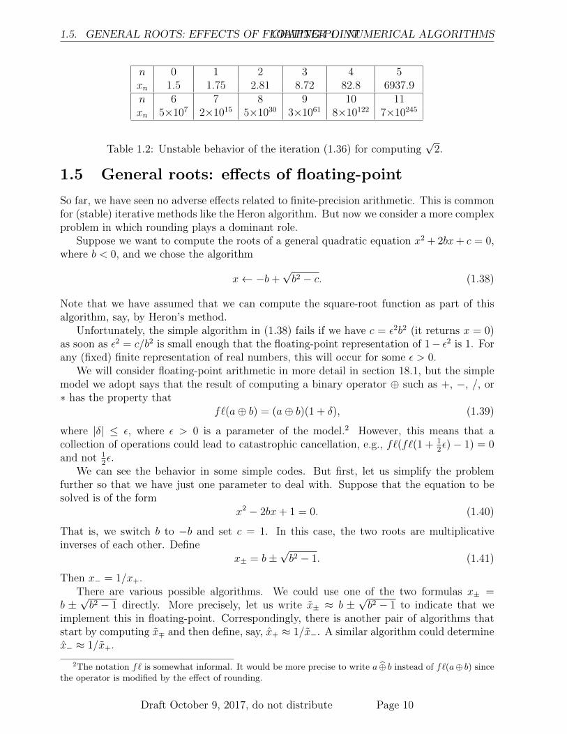
n 0 1 2 3 4 5xn 1.5 1.75 2.81 8.72 82.8 6937.9n 6 7 8 9 10 11xn 5×10⁷ 2×10¹⁵ 5×1030 3×1061 8×10122 7×10245
Table 1.2: Unstable behavior of the iteration (1.36) for computing√
2.
1.5 General roots: effects of floating-point
So far, we have seen no adverse effects related to finite-precision arithmetic. This is commonfor (stable) iterative methods like the Heron algorithm. But now we consider a more complexproblem in which rounding plays a dominant role.
Suppose we want to compute the roots of a general quadratic equation x2 + 2bx+ c = 0,where b < 0, and we chose the algorithm
x← −b+√b2 − c. (1.38)
Note that we have assumed that we can compute the square-root function as part of thisalgorithm, say, by Heron’s method.
Unfortunately, the simple algorithm in (1.38) fails if we have c = ε2b2 (it returns x = 0)as soon as ε2 = c/b2 is small enough that the floating-point representation of 1− ε2 is 1. Forany (fixed) finite representation of real numbers, this will occur for some ε > 0.
We will consider floating-point arithmetic in more detail in section 18.1, but the simplemodel we adopt says that the result of computing a binary operator ⊕ such as +, −, /, or∗ has the property that
f`(a⊕ b) = (a⊕ b)(1 + δ), (1.39)
where |δ| ≤ ε, where ε > 0 is a parameter of the model.2 However, this means that acollection of operations could lead to catastrophic cancellation, e.g., f`(f`(1 + 1
2ε)− 1) = 0
and not 12ε.
We can see the behavior in some simple codes. But first, let us simplify the problemfurther so that we have just one parameter to deal with. Suppose that the equation to besolved is of the form
x2 − 2bx+ 1 = 0. (1.40)
That is, we switch b to −b and set c = 1. In this case, the two roots are multiplicativeinverses of each other. Define
x± = b±√b2 − 1. (1.41)
Then x− = 1/x+.There are various possible algorithms. We could use one of the two formulas x± =
b ±√b2 − 1 directly. More precisely, let us write x± ≈ b ±
√b2 − 1 to indicate that we
implement this in floating-point. Correspondingly, there is another pair of algorithms thatstart by computing x∓ and then define, say, x+ ≈ 1/x−. A similar algorithm could determinex− ≈ 1/x+.
2The notation f` is somewhat informal. It would be more precise to write a ⊕ b instead of f`(a⊕ b) sincethe operator is modified by the effect of rounding.
Draft October 9, 2017, do not distribute Page 10

CHAPTER 1. NUMERICAL ALGORITHMS 1.6. EXERCISES
All four of these algorithms will have different behaviors. We expect that the behaviorsof the algorithms for computing x− and x− will be dual in some way to those for computingx+ and x+, so we consider only the first pair.
First, the function minus implements the x− square-root algorithm:
function x=minus(b)
% solving = 1-2bx +x^2
x=b-sqrt(b^2-1);
To know if it is getting the right answer, we need another function to check the answer:
function error=check(b,x)
error = 1-2*b*x +x^2;
To automate the process, we put the two together:
function error=chekminus(b)
x=minus(b);
error=check(b,x)
For example, when b = 106, we find the error is −7.6 × 10⁻⁶. As b increases further, theerror increases, ultimately leading to complete nonsense. For this reason, we consider analternative algorithm suitable for large b.
The algorithm for x− is given by
function x=plusinv(b)
% solving = 1-2bx +x^2
y=b+sqrt(b^2-1);
x=1/y;
Similarly, we can check the accuracy of this computation by the code
function error=chekplusinv(b)
x=plusinv(b);
error=check(b,x)
Now when b = 106, we find the error is −2.2 × 10⁻¹⁷. And the bigger b becomes, the moreaccurate it becomes.
Here we have seen that algorithms can have data-dependent behavior with regard to theeffects of finite-precision arithmetic. We will see that there are many algorithms in numericalanalysis with this property, but suitable analysis will establish conditions on the data thatguarantee success.
1.6 Exercises
Exercise 1.1 How accurate is the approximation (1.1) if it is expressed as a decimal ap-proximation (how many digits are correct)?
Exercise 1.2 Run the code relerrher starting with x = 1 and y = 2 to approximate√
2.Compare the results with table 1.1. Also run the code with x = 1 and y = 1
2and compare the
results with the previous case. Explain what you find.
Draft October 9, 2017, do not distribute Page 11

1.6. EXERCISES CHAPTER 1. NUMERICAL ALGORITHMS
Exercise 1.3 Show that the maximum relative error in Heron’s algorithm for approximating√y for y ∈ [1/M,M ], for a fixed number of iterations and starting with x0 = 1, occurs at
the ends of the interval: y = 1/M and y = M . (Hint: consider (1.10) and (1.14) and showthat the function
φ(x) = 12(1 + x)−1x2 (1.42)
plays a role in each. Show that φ is increasing on the interval [0,∞[.)
Exercise 1.4 It is sometimes easier to demonstrate the relative accuracy of an approxima-tion x to x by showing that
|x− x| ≤ ε′|x| (1.43)
instead of verifying (1.5) directly. Show that if (1.43) holds, then (1.5) holds with ε =ε′/(1− ε′).
Exercise 1.5 There is a simple generalization to Heron’s algorithm for finding kth roots asfollows:
x← 1
k((k − 1)x+ y/xk−1). (1.44)
Show that, if this converges, it converges to a solution of xk = y. Examine the speed ofconvergence both computationally and by estimating the error algebraically.
Exercise 1.6 Show that the error in Heron’s algorithm for approximating√y satisfies
xn −√y
xn +√y
=
(x0 −
√y
x0 +√y
)2n
(1.45)
for n ≥ 1. Note that the denominator on the left-hand side of (1.45) converges rapidly to2√y.
Exercise 1.7 We have implicitly been assuming that we were attempting to compute a pos-itive square-root with Heron’s algorithm, and thus we always started with a positive initialguess. If we give zero as an initial guess, there is immediate failure because of division byzero. But what happens if we start with a negative initial guess? (Hint: there are usuallytwo roots to x2 = y, one of which is negative.)
Exercise 1.8 Consider the iteration
x← 2x− yx2 (1.46)
and show that, if it converges, it converges to x = 1/y. Note that the algorithm does notrequire a division. Determine the range of starting values x0 for which this will converge.What sort of scaling (cf. section 1.1.2) would be appropriate for computing 1/y before startingthe iteration?
Exercise 1.9 Consider the iteration
x← 32x− 1
2yx3 (1.47)
and show that, if this converges, it converges to x = 1/√y. Note that this algorithm does not
require a division. The computation of 1/√y appears in the Cholesky algorithm in (4.12).
Draft October 9, 2017, do not distribute Page 12

CHAPTER 1. NUMERICAL ALGORITHMS 1.6. EXERCISES
Exercise 1.10 Suppose that a+by is the best linear approximation to√y in terms of relative
error on [12, 2]. Prove that the error expression eab has to be negative at its minimum. (Hint:
if not, you can always decrease a to make eab(2) and eab(12) smaller without increasing the
maximum value of |eab|.)
Exercise 1.11 Suppose that a+by is the best linear approximation to√y in terms of relative
error on [12, 2]. Prove that the value eab(a/b) of eab at its minimum satisfies
eab(a/b) = −maxeab(12), eab(2).
(Hint: if not, adjust a to decrease the maximum value of |eab|.)
Exercise 1.12 Suppose that a+by is the best linear approximation to√y in terms of relative
error on [12, 2]. Prove that
eab(12) = eab(2) = −eab(a/b).
(Hint: if not, adjust a and b to decrease the maximum value of |eab|.)
Exercise 1.13 Suppose that a+ by is any linear approximation to√y satisfying
eab(12) = eab(2).
Prove that a = b. (Hint: just use the formula (1.24).)
Exercise 1.14 Suppose that a+ay is the best linear approximation to√y in terms of relative
error on [12, 2]. Prove that the error expression satisfies
eaa(1) = −eaa(2), (1.48)
and then solve for a. (Hint: simplify the error terms using a = b to get something like(1.30).)
Exercise 1.15 Consider the effect of the best starting value of a in (1.32) on the Heronalgorithm. How many iterations are required to get 16 digits of accuracy? And to obtain 32digits of accuracy?
Exercise 1.16 Change the function minus for computing x− and the function plusinv forcomputing x− to functions for computing x+ (call that function plus) and x+ (call thatfunction minusinv). Use the check function to see where they work well and where they fail.Compare that with the corresponding behavior for minus and plusinv.
Exercise 1.17 The iteration (1.36) can be implemented via the function
function y =sosimpl(x,a)
y=x+x^2-a;
Use this to verify that sosimpl(1,1) is indeed 1, but if we start with
x=1.000000000001
and then repeatedly apply x=sosimpl(x,1), the result ultimately diverges.
Draft October 9, 2017, do not distribute Page 13

1.7. SOLUTIONS CHAPTER 1. NUMERICAL ALGORITHMS
Exercise 1.18 Suppose that we start the Heron algorithm with x0 = 1. Then the error afterone step is e1 = 1
2(1 + y)−√y. Define φ(y) = 1
2(1 + y)−√y. Show that φ has a minimum
at y = 1 and evaluate it at y = 0, 12, 1, 2 and make a plot. Prove that φ(y)→∞ as y →∞,
and in particular that
limy→∞
φ(y)
y=
1
2.
Exercise 1.19 Let y > 0. Prove that there is a unique y satisfying 12< y ≤ 2 such that
y = 4ky for some integer k.
Exercise 1.20 Let f ∈ C0(R) be bounded below, and let C ∈ R. Prove that the min andmax commute:
minb
max f(b), C = max
minbf(b), C
. (1.49)
Exercise 1.21 Suppose that g ∈ C0(R2) has a minimum at a finite point in R2. Prove that
minb,c
g(b, c) = mincf(c), (1.50)
where f(c) = minb g(b, c).
Exercise 1.22 Solve the problem
minc‖f − c‖max,[1/2,2] (1.51)
for the optimal constant c, where f(y) =√y. What is the optimal value of c? Why is it
optimal?
1.7 Solutions
Solution of Exercise 1.3. The function φ(x) = 12(1 + x)−1x2 is increasing on the interval
[0,∞[ since
φ′(x) = 12
2x(1 + x)− x2
(1 + x)2= 1
2
2x+ x2
(1 + x)2> 0 (1.52)
for x > 0. The expression (1.10) says that
en+1 = φ(en), (1.53)
and (1.14) says thate1 = φ(x− 1). (1.54)
Thuse2 = φ(φ(x− 1)). (1.55)
By induction, defineφ[n+1](t) = φ(φ[n](t)), (1.56)
where φ[1](t) = φ(t) for all t. Then, by induction,
en = φ[n](x− 1) (1.57)
Draft October 9, 2017, do not distribute Page 14

CHAPTER 1. NUMERICAL ALGORITHMS 1.7. SOLUTIONS
for all n ≥ 1. Since the composition of increasing functions is increasing, each φ[n] is in-creasing, by induction. Thus en is maximized when x is maximized, at least for x > 1. Notethat
φ(x− 1) = φ((1/x)− 1), (1.58)
so we may also writeen = φ[n]((1/x)− 1). (1.59)
Thus the error is symmetric via the relation
en(x) = en(1/x). (1.60)
Thus the maximal error on an interval [1/M,M ] occurs simultaneously at 1/M and M .
Solution of Exercise 1.6. Define dn = xn + x. Then (1.45) in exercise 1.6 is equivalent tothe statement that
endn
=
(e0
d0
)2n
. (1.61)
Thus we compute
dn+1 =xn+1 + x = 12(xn + y/xn) + 1
2(x+ y/x) = 1
2(dn + y/xn + y/x)
= 12
(dn +
y(x+ xn)
xxn
)= 1
2
(dn +
ydnxxn
)= 1
2
(dn +
xdnxn
)= 1
2dn
(1 +
x
xn
)= 1
2dn
(xn + x
xn
)= 1
2
d2n
xn.
(1.62)
Recall that (1.8) says that en+1 = 12e2n/xn, so dividing by (1.62) yields
en+1
dn+1
=
(endn
)2
(1.63)
for any n ≥ 0. A simple induction on n yields (1.61), as required.
Draft October 9, 2017, do not distribute Page 15

1.7. SOLUTIONS CHAPTER 1. NUMERICAL ALGORITHMS
Draft October 9, 2017, do not distribute Page 16

Chapter 2
Nonlinear Equations
“A method algebraically equivalent to Newton’s method was known tothe 12th century algebraist Sharaf al-Din al-Tusi ... and the 15th centuryArabic mathematician Al-Kashi used a form of it in solving xp−N = 0to find roots of N” [183].
Kepler’s discovery that the orbits of the planets are elliptical introduced a mathematicalchallenge via his equation
x− E sinx = τ, (2.1)
which defines a function φ(τ) = x. Here E =√
1− b2/a2 is the eccentricity of the ellipticalorbit, where a and b are the major and minor axis lengths of the ellipse and τ is proportionalto time. See figure 2.1 regarding the notation [155]. Much effort has been expended in tryingto find a simple representation of this function φ, but we will see that it can be viewed asjust like the square-root function from the numerical point of view. Newton1 proposed aniterative solution to Kepler’s equation [183]:
xn+1 = xn +τ − xn + E sinxn
1− E cosxn. (2.2)
We will see that this iteration can be viewed as a special case of a general iterative techniquenow known as Newton’s method.
We will also see that the method introduced in (1.2) as Heron’s method, namely,
xn+1 = 12
(xn +
y
xn
), (2.3)
can be viewed as Newton’s method for computing√y. Newton’s method provides a general
paradigm for solving nonlinear equations iteratively and changes qualitatively the notion of“solution” for a problem. Thus we see that Kepler’s equation (2.1) is itself the solution, justas if it had turned out that the function φ(τ) = x was a familiar function like square root orlogarithm. If we need a particular value of x for a given τ , then we know there is a machineavailable to produce it, just as in computing
√y on a calculator.
First, we develop a general framework for iterative solution methods, and then we showhow this leads to Newton’s method and other iterative techniques. We begin with oneequation in one variable and later extend to systems in chapter 7.
1 Isaac Newton (1643–1727) was one of the greatest and best known scientists of all time, to the point ofbeing a central figure in popular literature [157].
17

2.1. FIXED-POINT ITERATION CHAPTER 2. NONLINEAR EQUATIONS
K
xS
P
Figure 2.1: The notation for Kepler’s equation. The sun is at S (one of the foci of theelliptical orbit), the planet is at P , and the point K lies on the indicated circle that enclosesthe ellipse of the orbit; the horizontal coordinates of P and K are the same, by definition.The angle x is between the principal axis of the ellipse and the point K.
2.1 Fixed-point iteration
This goes by many names, including functional iteration, but we prefer the term fixed-pointiteration because it seeks to find a fixed point
α = g(α) (2.4)
for a continuous function g. Fixed-point iteration
xn+1 = g(xn) (2.5)
has the important property that, if it converges, it converges to a fixed point (2.4) (assumingonly that g is continuous). This result is so simple (see exercise 2.1) that we hesitate to callit a theorem. But it is really the key fact about fixed-point iteration.
We now see that Heron’s algorithm (2.3) may be written in this notation with
g(x) = 12
(x+
y
x
). (2.6)
Similarly, the method (2.2) proposed by Newton to solve Kepler’s equation (2.1) can bewritten as
g(x) = x+τ − x+ E sinx
1− E cosx. (2.7)
The choice of g is not at all unique. One could as well approximate the solution of Kepler’sequation (2.1) via
g(x) = τ + E sinx. (2.8)
In table 2.1, the methods (2.8) and (2.7) are compared. We find that Newton’s methodconverges much faster, comparable to the way that Heron’s method does, in that the numberof correct digits doubles at each step.
Draft October 9, 2017, do not distribute Page 18

CHAPTER 2. NONLINEAR EQUATIONS 2.1. FIXED-POINT ITERATION
n xn from (2.8) xn from (2.2)0 1.00 1.001 1.084147098480790 1.0889532638373732 1.088390486229308 1.0885977582695523 1.088588138978555 1.0885977523978944 1.088597306592452 1.0885977523978945 1.088597731724630 1.0885977523978946 1.088597751439216 1.0885977523978947 1.088597752353437 1.0885977523978948 1.088597752395832 1.0885977523978949 1.088597752397798 1.088597752397894
Table 2.1: Computations of solutions to Kepler’s equation (2.1) for E = 0.1 and τ = 1 viaNewton’s method (2.2) (third column) and by the fixed-point iteration (2.8). The boldfaceindicates the leading incorrect digit. Note that the number of correct digits essentiallydoubles at each step for Newton’s method but increases only by about 1 at each step of thefixed-point iteration (2.8).
The rest of the story about fixed-point iteration is then to figure out when and how fastit converges. For example, if g is Lipschitz2-continuous with constant λ < 1, that is,
|g(x)− g(y)| ≤ λ|x− y|, (2.9)
then convergence will happen if we start close enough to α. This is easily proved by defining,as we did for Heron’s method, en = xn − α and estimating
|en+1| = |g(xn)− g(α)| ≤ λ|en|, (2.10)
where the equality results from subtracting (2.4) from (2.5). Thus, by induction,
|en| ≤ λn|e0| (2.11)
for all n ≥ 1. Thus we have proved the following.
Theorem 2.1 Suppose that α = g(α) and that the Lipschitz estimate (2.9) holds with λ < 1for all x, y ∈ [α−A,α+A] for some A > 0. Suppose that |x0−α| ≤ A. Then the fixed-pointiteration defined in (2.5) converges according to (2.11).
Proof. The only small point to be sure about is that all the iterates stay in the interval[α− A,α + A], but this follows from the estimate (2.11) once we know that |e0| ≤ A, as wehave assumed. QED
2Rudolf Otto Sigismund Lipschitz (1832–1903) had only one student, but that was Felix Klein.
Draft October 9, 2017, do not distribute Page 19

2.1. FIXED-POINT ITERATION CHAPTER 2. NONLINEAR EQUATIONS
2.1.1 Verifying the Lipschitz condition
A Lipschitz-continuous function need not be C1, but when a function is C1, its derivativegives a good estimate of the Lipschitz constant. We formalize this simple result to highlightthe idea.
Lemma 2.2 Suppose g ∈ C1 in an interval around an arbitrary point α. Then for anyε > 0, there is an A > 0 such that g satisfies (2.9) in the interval [α − A,α + A] withλ ≤ |g′(α)|+ ε.
Proof. By the continuity of g′, we can pick A > 0 such that |g′(t) − g′(α)| < ε for allt ∈ [α− A,α + A]. Therefore,
|g′(t)| ≤ |g′(α)|+ |g′(t)− g′(α)| < |g′(α)|+ ε (2.12)
for all t ∈ [α− A,α + A]. Let x, y ∈ [α− A,α + A], with x 6= y. Then∣∣∣∣g(x)− g(y)
x− y
∣∣∣∣ =
∣∣∣∣ 1
x− y
∫ x
y
g′(t) dt
∣∣∣∣≤ max
|g′(t)|
∣∣ t ∈ [α− A,α + A]
≤ |g′(α)|+ ε,
(2.13)
by using (2.12). QED
As a result, we conclude that the condition |g′(α)| < 1 is sufficient to guarantee con-vergence of fixed-point iteration, as long as we start close enough to the root α = g(α)(cf. exercise 2.2).
On the other hand, the Lipschitz constant λ in (2.9) also gives an upper bound for thederivative:
|g′(α)| ≤ λ (2.14)
(cf. exercise 2.3). Thus if |g′(α)| > 1, fixed-point iteration will likely not converge since theLipschitz constant for g will be greater than 1 in any such interval. If we recall the iterationfunction g(x) = x+x2−y in (1.36), we see that g′(
√y) = 1 + 2
√y > 1. Thus the divergence
of that algorithm is not surprising.It is not very useful to develop a general theory of divergence for fixed-point iteration,
but we can clarify this by example. It is instructive to consider the simple case
g(x) := α + λ(x− α), (2.15)
where for simplicity we take λ > 0. Then for all n we have
|xn − α| = |g(xn−1)− α| = λ|xn−1 − α|, (2.16)
and by induction|xn − α| = λn|x0 − α|, (2.17)
where x0 is our starting value. If λ < 1, this converges, but if λ > 1, this diverges.The affine example (2.15) not only gives an example of divergence when |g′(α)| > 1 but
also suggests the asymptotic behavior of fixed-point iteration. When 0 < |g′(α)| < 1, theasymptotic behavior of fixed-point iteration is (cf. exercise 2.4) given by
|xn − α| ≈ C|g′(α)|n (2.18)
as n→∞, where C is a constant that depends on g and the initial guess.
Draft October 9, 2017, do not distribute Page 20

CHAPTER 2. NONLINEAR EQUATIONS 2.1. FIXED-POINT ITERATION
2.1.2 Second-order iterations
What happens if g′(α) = 0? By Taylor’s theorem,
g(x)− α = 12(x− α)2g′′(ξ) (2.19)
for some ξ between x and α, and thus the error is squared at each iteration:
en = 12(en−1)2g′′(ξn), (2.20)
where ξn → α if the iteration converges. Of course, squaring the error is not a good thing ifit is too large initially (with regard to the size of g′′).
We can now see why Heron’s method converges so rapidly. Recall that g(x) = 12(x+y/x),
so that g′(x) = 12(1− y/x2) = 0 when x2 = y. Moreover, g′′(x) = y/x3, so we could derive a
result analogous to (1.8) from (2.20).
2.1.3 Higher-order iterations
It is possible to have even higher-order iterations. If g(α) = α and g′(α) = g′′(α) = 0, thenTaylor’s theorem implies that
g(x)− α = O((x− α)3). (2.21)
In principle, any order of convergence could be obtained [8]. However, while there is aqualitative change from geometric convergence to quadratic convergence, all higher-ordermethods behave essentially the same. For example, given a second-order method, we canalways create one that is fourth-order just by taking two steps and calling them one. Thatis, we define
xn+1 = g(g(xn)). (2.22)
We could view this as introducing a “half-step”
xn+1/2 = g(xn) and xn+1 = g(xn+1/2). (2.23)
Applying (2.20) twice, we see that xn+1−α = C(xn−α)4. We can also verify this by definingG(x) = g(g(x)) and evaluating derivatives of G:
G′(x) = g′(g(x))g′(x)
G′′(x) = g′′(g(x))g′(x)2 + g′(g(x))g′′(x)
G′′′(x) = g′′′(g(x))g′(x)3 + 3g′′(g(x))g′(x)g′′(x) + g′(g(x))g′′′(x).
(2.24)
Using the facts that g(α) = α and g′(α) = 0, we see that G′(α) = G′′(α) = G′′′(α) = 0. Thus,if ε is the initial error, then the sequence of errors in a quadratic method (suitably scaled) isε, ε2, ε4, ε8, ε16, . . . , whereas for a fourth-order method the sequence of errors (suitably scaled)is ε, ε4, ε16, . . . . That is, the sequence of errors for the fourth-order method is just a simplesubsequence (omit every other term) of the sequence of errors for the quadratic method.
What is not so clear at this point is that it is possible to have fractional orders ofconvergence. In section 2.2.4 we will introduce a method with this property to illustrate howthis is possible.
Draft October 9, 2017, do not distribute Page 21

2.2. PARTICULAR METHODS CHAPTER 2. NONLINEAR EQUATIONS
x x xn+1 n
Figure 2.2: The geometric, or chord, method for approximating the solution of nonlinearequations. The slope of the dashed line is s.
2.2 Particular methods
Now we consider solving a general nonlinear equation of the form
f(α) = 0. (2.25)
Several methods use a geometric technique, known as the chord method, designed to pointto a good place to look for the root:
xn+1 = xn −f(xn)
s, (2.26)
where s is the slope of a line drawn from the point (xn, f(xn)) to the next iterate xn+1, asdepicted in figure 2.2. This line is intended to intersect the x-axis at, or near, the root of f .This is based on the idea that the linear function ` with slope s which is equal to f(xn) atxn vanishes at xn+1 (so `(x) = s(xn+1 − x)).
The simplest fixed-point iteration might be to choose g(x) = x − f(x). The geometricmethod can be viewed as a damped version of this, where we take instead g(x) = x−f(x)/s.You can think of s as an adjustment parameter to help with convergence of the standardfixed-point iteration. The convergence of the geometric method is thus determined by thevalue of
g′(α) = 1− f ′(α)/s. (2.27)
Ideally, we would simply pick s = f ′(α) if we knew how to compute it. We now considervarious ways to approximate this value of s. These can all be considered different adaptivetechniques for approximating s ≈ f ′(α).
2.2.1 Newton’s method
The method in question was a joint effort of many people, including Newton and his contem-porary Joseph Raphson3 [33, 163]. In addition, Simpson4 was the first (in 1740) to introduceit for systems of equations [102, 183]. Although Newton presented solutions most commonly
3According to the mathematical historian Florian Cajori [33], the approximate dates for the life of JosephRaphson are 1648–1715, but surprisingly little is known about his personal life [163].
4Thomas Simpson (1710–1761); see the quote on page 103.
Draft October 9, 2017, do not distribute Page 22

CHAPTER 2. NONLINEAR EQUATIONS 2.2. PARTICULAR METHODS
for polynomial equations, he did suggest the method in (2.2). Newton’s method for poly-nomials is different from what we describe here, but perhaps it should just be viewed asan additional method, slightly different from the one suggested by Raphson. Both becauseNewton is better known and because the full name is a bit long, we tend to abbreviate itby dropping Raphson’s name, but for now let us retain it. We also add Simpson’s name assuggested in [183].
The Newton-Raphson-Simpson method chooses the slope adaptively at each stage:
s = f ′(xn). (2.28)
The geometric method can be viewed as a type of difference approximation to this since wechoose
s =0− f(xn)
xn+1 − xn, (2.29)
and we are making the approximation f(xn+1) ≈ 0 in defining the difference quotient.
The Newton-Raphson-Simpson method is sufficiently important that we should write outthe iteration in detail:
xn+1 = xn −f(xn)
f ′(xn). (2.30)
This is fixed-point iteration with the iteration function g = N f defined by
g(x) = N f(x) = x− f(x)
f ′(x). (2.31)
We can think of N as mapping the set of functions
V (I) =f ∈ Ck+1(I)
∣∣ f ′(x) 6= 0 ∀x ∈ I
(2.32)
to Ck(I) for a given interval I and any integer k ≥ 0. More generally, we can think ofNewton’s method as mapping problems of the form “find a root of f(x) = 0” to algorithmsusing fixed-point iteration with g = N f . We will not try to formalize such a space of problemsor the space of such algorithms, but it is easy to see that Newton’s method operates at ahigh level to solve a very general set of problems.
If xn → α, then f ′(xn) → f ′(α), and so (2.27) should imply that the method is second-order convergent. Again, the second-order convergence of Newton’s method is sufficientlyimportant that it requires an independent computation:
g′(x) = 1− f ′(x)2 − f(x)f ′′(x)
f ′(x)2
=f(x)f ′′(x)
f ′(x)2.
(2.33)
We conclude that f(α) = 0 implies g′(α) = 0, provided that f ′(α) 6= 0. Thus Newton’smethod is second-order convergent provided f ′(α) 6= 0 at the root α of f(α) = 0.
Draft October 9, 2017, do not distribute Page 23

2.2. PARTICULAR METHODS CHAPTER 2. NONLINEAR EQUATIONS
To estimate the convergence rate, we simply need to calculate g′′:
g′′(x) =d
dx
(f(x)f ′′(x)
f ′(x)2
)=f ′(x)3f ′′(x) + f(x)f ′(x)2f (3)(x)− 2f(x)f ′(x)f ′′(x)2
f ′(x)4
=f ′′(x)
f ′(x)+
f(x)
f ′(x)3
(f ′(x)f (3)(x)− 2f ′′(x)2
).
(2.34)
Assuming f ′(α) 6= 0, this simplifies for x = α:
g′′(α) =f ′′(α)
f ′(α). (2.35)
From (2.20), we expect that Newton’s method converges asymptotically like
en+1 ≈ 12
f ′′(α)
f ′(α)e2n, (2.36)
where we recall that en = xn − α.
We can see that Heron’s method is the same as Newton’s method if we take f(x) = x2−y.We have
g(x) = x− f(x)
f ′(x)= x− x2 − y
2x= 1
2x− y
2x. (2.37)
Recall that g′(x) = 12(1− y/x2), so that g′′(x) = y/x3 = 1/
√y when x =
√y. Thus we can
assert that Heron’s method is precisely second-order.
2.2.2 Stability of Newton’s method
The mapping N f(x) = x− f(x)f ′(x)
specified in (2.31) is not well-defined when f ′(x) = 0. When
this occurs at a root of f (f(x) = 0) it destroys the second-order convergence of Newton’smethod (see exercise 2.5). But it can cause a more serious defect if it occurs away froma root of f . For example, consider f(x) = x − cosx (cf. exercise 2.6). The root wherex = cosx does not have f ′(x) = 0, but f ′(x) = 1 + sin x = 0 for an infinite number of values.Just by drawing the graph corresponding to figure 2.2, we see that if we start near one ofthese roots of f ′(x) = 0, then the next step of Newton’s method can be arbitrarily largein magnitude (both negative and positive values are possible). Contrast this behavior withthat of fixed-point iteration (cf. exercise 2.6).
2.2.3 Other second-order methods
The Steffensen iteration uses an adaptive difference:
s =f(xn + f(xn))− f(xn)
f(xn)(2.38)
Draft October 9, 2017, do not distribute Page 24

CHAPTER 2. NONLINEAR EQUATIONS 2.2. PARTICULAR METHODS
in which the usual ∆x = f(xn) (which will go to zero: very clever). The iteration thus takesthe form
xn+1 = xn −f(xn)2
f(xn + f(xn))− f(xn). (2.39)
We leave as exercise 2.10 verification that the iteration (2.39) is second-order convergent.Steffensen’s method is of the same order as Newton’s method, but it has the advantage
that it does not require evaluation of the derivative. If the derivative of f is hard to evaluate,this can be an advantage. On the other hand, it does require two function evaluations eachiteration, which could make it comparable to Newton’s method, depending on whether itis easier or harder to evaluate f ′ versus f . Unfortunately, Steffensen’s method does notgeneralize to higher dimensions, whereas Newton’s method does (section 7.1.4).
2.2.4 Secant method
The secant method approximates the slope by a difference method:
s =f(xn)− f(xn−1)
xn − xn−1
. (2.40)
The error behavior is neither first- nor second-order but rather something in between. Letus derive an expression for the sequence of errors.
First, consider the method in the usual fixed-point form:
xn+1 = xn −(xn − xn−1) f(xn)
f(xn)− f(xn−1). (2.41)
Subtracting α from both sides and inserting α− α in the numerator on the right-hand sideand expanding, we find
en+1 = en −(en − en−1) f(xn)
f(xn)− f(xn−1)
=−enf(xn−1) + en−1f(xn)
f(xn)− f(xn−1)
=xn − xn−1
f(xn)− f(xn−1)
−enf(xn−1) + en−1f(xn)
xn − xn−1
=xn − xn−1
f(xn)− f(xn−1)
en (f(α)− f(xn−1)) + en−1 (f(xn)− f(α))
xn − xn−1
=xn − xn−1
f(xn)− f(xn−1)
enen−1
xn − xn−1
(f(α)− f(xn−1)
en−1
− f(α)− f(xn)
en
).
(2.42)
In going from the third line to the fourth line, the term enf(α)−en−1f(α) is added in, whichdoes not at first appear to be zero. But you need to remember that f(α) = 0.
By Taylor’s Theorem, we can estimate the expression (exercise 2.11)
f(xn)− f(xn−1)
xn − xn−1
≈ f ′(α). (2.43)
Draft October 9, 2017, do not distribute Page 25

2.2. PARTICULAR METHODS CHAPTER 2. NONLINEAR EQUATIONS
In section 10.2.3, we will formally define this approximation as the first divided differencef [xn−1, xn], and we will also identify the expression
1
xn − xn−1
(f(α)− f(xn−1)
en−1
− f(α)− f(xn)
en
)=
1
xn − xn−1
(−f(α)− f(xn−1)
α− xn−1
+f(α)− f(xn)
α− xn
) (2.44)
as the second divided difference f [α, xn−1, xn] ≈ 12f ′′(α) (cf. (10.27)).
Rather than get involved in all the details, let us just use these approximations to seewhat is going on. Thus we find
en+1 ≈ 12
f ′′(α)
f ′(α)enen−1. (2.45)
Thus the error is quadratic in the previous errors, but it is not exactly the square of theprevious error. Instead, it is a more complicated combination.
Let M be an upper bound for 12f ′′/f ′ in an interval containing all the iterates. Then,
analogous to (2.45), one can prove (see exercise 2.13) that
|en+1| ≤M |en| |en−1|. (2.46)
To understand how the error is behaving, define a scaled error by εn = M |en|. Then (2.46)means that
εn+1 ≤ εnεn−1 (2.47)
for all n. If δ = maxε0, ε1, then (2.47) means that ε2 ≤ δ2, ε3 ≤ δ3, ε4 ≤ δ5, and so forth.In general, εn ≤ δfn , where fn is the Fibonacci sequence defined by
fn+1 = fn + fn−1, (2.48)
with f0 = f1 = 1. Quadratic convergence would mean that εn ≤ δ2n , but the Fibonaccisequence grows more slowly than 2n. However, it is possible to determine the asymptoticgrowth exactly. In fact, we can write (exercise 2.14)
fn−1 =1√5
(rn+ − rn−
), r± =
1±√
5
2≈
1.6180 (+)
−0.6180 (−).(2.49)
Since rn− → 0 as n → ∞, fn ≈ Crn+. Thus the errors for the secant method go to zero like(exercise 2.15)
en+1 ≈ Cer+n . (2.50)
One iteration of the secant method requires only one function evaluation, so it can bemore efficient than second-order methods. Two iterations of the secant method often requirework comparable to one iteration of the Newton method, and thus a method in which oneiteration is two iterations of the secant method has a faster convergence rate since 2r+ > 2.
Draft October 9, 2017, do not distribute Page 26

CHAPTER 2. NONLINEAR EQUATIONS 2.3. COMPLEX ROOTS
2.3 Complex roots
Let us consider the situation when there are complex roots of equations. For example, whathappens when we apply Heron’s algorithm with y < 0? Let us write y = −t (t > 0) to clarifythings, so that
xn+1 = 12(xn − t/xn). (2.51)
Unfortunately, for real values of x0, the sequence generated by (2.51) does not converge toanything. On the other hand, if we take x0 = iρ, where i =
√−1 and ρ is real, then
x1 = 12(x0 − t/x0) = 1
2(iρ− t/(iρ)) = 1
2i(ρ+ t/ρ) (2.52)
since 1/i = −i. By induction, if xn = iρn, where ρn is real, then xn+1 = iρn+1, where ρn+1
is also real. More precisely,
xn+1 = 12(xn − t/xn) = 1
2(iρn − t/(iρn)) = 1
2i(ρn + t/ρn), (2.53)
so that
ρn+1 = 12(ρn + t/ρn). (2.54)
We see that (2.54) is just the Heron iteration for approximating ρ =√t. Thus convergence
is assured as long as we start with a nonzero value for ρ (cf. exercise 1.7).The fact that Heron’s method does not converge to an imaginary root given a real starting
value is not spurious. Indeed, it is easy to see that Heron’s method for a real root also doesnot converge if we start with a pure imaginary starting value. The set of values for which aniterative method converges is a valid study in dynamics, but here we are mostly interestedin the local behavior, that is, convergence given a suitable starting guess. It is not hard tosee that reasonable methods converge when starting within some open neighborhood of theroot.
For a general complex y and a general starting guess x0, it is not hard to see how Heron’salgorithm will behave. Write zn = xn/
√y. Then
zn+1 = xn+1/√y =
1
2√y
(xn + y/xn) = 12(zn + 1/zn). (2.55)
Thus to study the behavior of Heron’s method for complex roots, it suffices to study itsbehavior in approximating the square-root of one with a complex initial guess (exercise 2.16).
2.4 Error propagation
Suppose that the function g is not computed exactly. What can happen to the algorithm?Again, the affine function in (2.15) provides a good guide. Let us suppose that our computedfunction g satisfies
g(x) = g(x) + δ(x) = α + λ(x− α) + δ(x) (2.56)
for some error function δ(x). If, for example, we have δ(x) = δ > 0 for all x, then g(α) = αimplies that
α = g(α) = α + λ(α− α) + δ = α(1− λ) + λα + δ, (2.57)
Draft October 9, 2017, do not distribute Page 27

2.5. MORE READING CHAPTER 2. NONLINEAR EQUATIONS
so that
α = α +δ
1− λ. (2.58)
Thus the accuracy can degrade if λ is very close to one, but for a second-order method this isnot an issue. A general theory can be found in [89] (see Theorem 3 on page 92 and equation(18) there), and (2.58) shows that the results there can be sharp.
The only problem with functional iteration in floating-point is that the function maynot really be continuous in floating-point. Therefore it may be impossible to achieve trueconvergence in floating-point, in the sense that f`(x) = g(f`(x)), where by g here we meanthe computer implementation of the true function g in floating-point. Thus iterations shouldbe terminated when the differences between successive iterates is on the order of the floating-point accuracy.
The effect of this kind of error on Newton’s method is not so severe. Suppose that whatwe really compute is f = f + δ. Then Newton’s method converges to a root f(α) = 0, anddoing a Taylor expansion of f around α, we find that
α− α ≈ δ
f ′(α). (2.59)
2.5 More reading
The concept of stability in numerical analysis can be explored further in [76]. Techniquesfor iteratively computing functions have been essential for providing software (and firmware)to compute square-roots, reciprocals, and other basic mathematical operations. For furtherreading, see the books [37, 63, 81, 117]. The book [89] relates Steffensen’s method to a generalacceleration process due to Aitken5 to accelerate convergence of sequences. The method offalse position, or regula falsi, is a slight modification of the secant method in which xν−1 isreplaced by xk, where k is the last value where f(xk) has a sign opposite f(xν) [54]. Forother generalizations of the secant method, see [22, 105].
2.6 Exercises
Exercise 2.1 Suppose that g is a continuous function. Prove that, if fixed-point iteration(2.5) converges to some α, then α is a fixed point, i.e., it satisfies (2.4).
Exercise 2.2 Suppose that g is a C1 function such that α = g(α) and with the property that|g′(α)| < 1. Prove that fixed-point iteration (2.5) converges if x0 is sufficiently close to α.(Hint: note by lemma 2.2 that g is Lipschitz-continuous with a constant λ < 1 in an interval[α− A,α + A] for some A > 0.)
5Alexander Craig Aitken (1895–1967) was born in New Zealand and studied at the University of Edin-burgh, where his thesis was considered so impressive that he was both appointed to a faculty position thereand elected a fellow of the Royal Society of Edinburgh, in 1925, before being awarded a D.Sc. degree in 1926.He was elected to the Royal Society of London in 1936 for his work on statistics, algebra, and numericalanalysis. Aitken was reputedly one of the best mental calculators known [62, 88]. He was an accomplishedwriter, being elected to the Royal Society of Literature in 1964 in response to the publication of his warmemoirs [4].
Draft October 9, 2017, do not distribute Page 28

CHAPTER 2. NONLINEAR EQUATIONS 2.6. EXERCISES
Exercise 2.3 Suppose that g is a C1 function such that the Lipschitz estimate (2.9) holdsan interval [α − A,α + A] for some A > 0. Prove that |g′(α)| ≤ λ. (Hint: consider thedifference quotients used to define g′(α).)
Exercise 2.4 Suppose that g is a C2 function such that α = g(α) and with the property that0 < |g′(α)| < 1. Prove that fixed-point iteration (2.5) converges asymptotically according to(2.18), that is,
limn→∞
|xn − α||g′(α)|n
= C, (2.60)
where C is a constant depending only on g and the initial guess x0.
Exercise 2.5 Consider Newton’s method for solving f(α) = 0 in the case that f ′(α) = 0.Show that second-order convergence is lost. In particular, if p is the smallest positive integersuch that f (p)(α) 6= 0, show that the convergence is geometric with rate 1 − 1/p. (Hint:expand both f and f ′ in Taylor series around α, which both start with the terms involvingf (p)(α) as the first nonzero term.)
Exercise 2.6 Consider fixed-point iteration to compute the solution of
cosα = α,
using g(x) = cos x. Prove that this converges for any starting guess. Compute a few iterationsto see what the approximate value of α is.
Exercise 2.7 A function f is said to be Holder-continuous of exponent α > 0 provided that
|f(x)− f(y)| ≤ λ|x− y|α (2.61)
for all x and y in some interval. Show that the result (2.60) still holds as long as g′ isHolder-continuous of exponent α > 0.
Exercise 2.8 Consider fixed-point iteration x← y/x for computing
x =√y.
Explain its behavior. Why does it not contradict the result in exercise 2.2? (Hint: defineg(x) = y/x and verify that a fixed point x = g(x) must satisfy x2 = y. Perform a fewiterations of x← y/x and describe what you see. Evaluate g′ at the fixed point.)
Exercise 2.9 Prove that the iteration (2.2) is Newton’s method as defined in (2.30) forapproximating the solution of Kepler’s equation (2.1).
Exercise 2.10 Prove that Steffensen’s iteration (2.39) is second-order convergent providedthat f ′(α) 6= 0 at the root f(α) = 0 and f ∈ C2 near the root. (Hint: write Steffensen’siteration as a fixed-point iteration xν+1 = g(xν) and show that g′(α) = 0 at the fixed pointα = g(α)).
Exercise 2.11 Verify the approximation (2.43). (Hint: write two Taylor expansions aroundα, one for f(xn) and one for f(xn−1), and subtract them.)
Draft October 9, 2017, do not distribute Page 29

2.6. EXERCISES CHAPTER 2. NONLINEAR EQUATIONS
Exercise 2.12 Investigate the fixed point(s) of the function
g(x) =1
e−x − 1+
1
ex − 1+ 1. (2.62)
What is the value of g′ at the fixed point(s)? (Hint: find a common denominator and simplify;see the solution to exercise 13.17 for an application of this important function.)
Exercise 2.13 Prove that (2.46) holds.
Exercise 2.14 Prove that the Fibonacci numbers satisfy (2.49). (Hint: see section 17.2.4;relate (2.48) with (17.7).)
Exercise 2.15 Prove that the error in the secant method behaves as predicted in (2.50).(Hint: first prove (2.45).)
Exercise 2.16 Investigate the behavior of the iteration (2.55) for various starting values ofz0. For what values of z0 does the iteration converge? For what values of z0 does the iterationnot converge?
Exercise 2.17 Develop algorithms to solve x5− x+ b = 0 for arbitrary b ∈ R (cf. (14.35)).
Exercise 2.18 The expressionf(x) =
√1 + x− 1
arises in many computations. Unfortunately, for x small, round-off makes the obvious algo-rithm inaccurate; note that f(x) ≈ 1
2x for x small. Develop an algorithm to compute f that
is accurate for |x| ≤ 12. (Hint: write t =
√1 + x− 1 and observe that (1 + t)2 − 1− x = 0.
Try Newton’s method starting with a good initial guess for t = f(x).)
Exercise 2.19 Consider the function
f(x) =1
x
(√x2 + 1− |x− 1|
). (2.63)
Develop an algorithm to compute f(x) with uniform accuracy for all 0 < x < ∞. You maymake reasonable assumptions about the accuracy of computing
√y but be explicit about them.
(Hint: show that f(1/x) = xf(x) and that f(x) ≈ 1 + 12x+O(x3) for x small.)
Exercise 2.20 Consider fixed-point iteration xn+1 = g(xn) for finding a fixed point α =g(α). Suppose that the initial starting point x0 > α and that g′(x) > 0 for x > α. Prove thatxn > α for all n ≥ 0. (Hint: write
xn+1 − α = g(xn)− g(α) =
∫ xn
α
g′(t) dt
and use induction.)
Exercise 2.21 In many applications in which roots f(x) = 0 are sought, the cost of com-puting f (and f ′) is very large. You can simulate this via a loop
Draft October 9, 2017, do not distribute Page 30

CHAPTER 2. NONLINEAR EQUATIONS 2.7. SOLUTIONS
function y = f(x,n)
for i=1:n
t = exp(x);
y = log(t);
end
y=y*y-2;
This computes the function f(x) = x2 − 2 but can take arbitrarily long to do so. Use anexample like this to compare the efficiency of the Steffensen and secant methods for variousvalues of n.
Exercise 2.22 We have seen that the critical factor in the success of fixed point iterationxn+1 = g(xn) is that the derivative of g be less than 1 in an interval containing the root.Consider g(x) = 1
2(x+y/x) from Heron’s algorithm. Show that there is an interval I = [a,∞[
where |g′(x)| ≤ 12
for all x ∈ I, with a <√y. Also show that xn ∈ I for all n > 0 for any
x0 > 0.
2.7 Solutions
Solution of Exercise 2.4. We have
xn+1 − α = g(xn)− g(α) = g′(ξn)(xn − α) (2.64)
for some ξn between xn and α. By induction, we thus find that
xn+1 − α =
(n∏i=0
g′(ξi)
)(x0 − α). (2.65)
Define ri = |g′(ξi)/g′(α)|. Then
|xn+1 − α||g′(α)|n
=
(n∏i=0
ri
)|x0 − α|. (2.66)
By (2.11), we know that |ξn − α| ≤ λn|e0|. Therefore,
|g′(ξn)− g′(α)| = |g′′(ξn)(ξn − α)| ≤ |g′′(ξn)|λn|e0|. (2.67)
for some ξn between ξn and α, and therefore between xn and α. Therefore, |rn − 1| ≤ Cλn,where C is chosen to be larger than |e0g
′′(ξn)/g′(α)| for all n. Since rn → 1 as n → ∞, wecan be assured that rn > 0 for n sufficiently large. If rn = 0 for some value of n, then wehave xn+i = α for all i ≥ 1, so we can take the constant C in (2.60) to be zero. If all rn > 0,then we can take the logarithm of the product in (2.66) to get
log
(n∏i=0
ri
)=
n∑i=0
log ri. (2.68)
Draft October 9, 2017, do not distribute Page 31

2.7. SOLUTIONS CHAPTER 2. NONLINEAR EQUATIONS
Thus it suffices to prove that the sum on the right-hand side of (2.68) converges. Since wehave an estimate on ri − 1, we write ri = 1 + εi, where |εi| ≤ Cλi. Note that log(1 + x) ≤ xfor all x > 0. To get such a bound for x < 0, set t = −x and write
| log(1− t)| = − log(1− t) =
∫ 1
1−t
dx
x≤ t
1− t. (2.69)
Thus | log(1 + x)| ≤ 2|x| for |x| ≤ 12. Therefore, | log ri| ≤ 2|1 − ri| ≤ Cλi for i sufficiently
large, and thus the sum on the right-hand side of (2.68) converges to some value γ. DefineC = eγ|x0 − α|.
Solution of Exercise 2.6. Define g(x) = cosx. Then a solution to x = g(x) is what weare seeking, and we can apply fixed-point iteration xn+1 = g(xn). This can be computed inoctave by simply repeating the command x=cos(x), having started with, say, x = 1. Afterabout 40 iterations, it converges to α = 0.73909. We have g′(α) = − sinα ≈ −0.67362. Thusit is clear that fixed-point iteration is locally convergent.
The set of values xn generated by fixed-point iteration always lie in [−1, 1], the rangeof g(·) = cos ·. But we cannot easily assert global convergence because the values of g′
also extend over [−1, 1]. However, g maps [−1, 0] to [β, 1], where β = cos(−1) ≈ 0.54030.Similarly, g maps [0, 1] to [β, 1], but with the order reversed. Thus, regardless of the startingvalue x0, x1 ∈ [β, 1]. Moreover, this argument shows further that all subsequent xn ∈ [β, 1]as well. The maximum value of |g′(x)| = sinx on the interval [β, 1] occurs at x = 1, sincesin is strictly increasing on [β, 1], and sin 1 = 0.84147. Thus we conclude that fixed-pointiteration converges at least as fast as 0.84147n.
Solution of Exercise 2.18. We recall that
t = f(x) =√
1 + x− 1. (2.70)
We seek an algorithm that outputs t with the property that
|t− t| =∣∣∣√1 + x− 1− t
∣∣∣ ≤ 12ε|t|, (2.71)
where ε > 0 is a prescribed accuracy that we require to be sufficiently small. To begin with,we establish some inequalities of use later.
Adding 1 to both sides of (2.70) and squaring, we find that
(t+ 1)2 = 1 + x,
and thus
x = (t+ 1)2 − 1 = 2t+ t2 = t(2 + t). (2.72)
Therefore,x
f(x)=x
t= 2 + t = 1 +
√1 + x (2.73)
is a strictly increasing function of x. In particular,
|x/t| = |x/f(x)| ≤ 1 +√
3/2 < 2.3 (2.74)
Draft October 9, 2017, do not distribute Page 32

CHAPTER 2. NONLINEAR EQUATIONS 2.7. SOLUTIONS
for |x| ≤ 12. Similarly, f(x)/x is a strictly decreasing function of x. We thus have
|t| = |f(x)| ≤ 1
1 +√
1/2|x| < 0.6|x| (2.75)
for |x| ≤ 12. Therefore,
|t| ≤ 0.3 (2.76)
for |x| ≤ 12. Now let us define t. Taylor’s theorem shows that∣∣∣√1 + x− 1− 1
2x+ 1
8x2∣∣∣ ≤ 0.1
∣∣x3∣∣ (2.77)
for x ∈ [−0.1, 0.1]. This means that for |x| ≤√ε and ε ≤ 1/100, we can simply define
t = 12x− 1
8x2. (2.78)
Then (2.77) implies that ∣∣∣√1 + x− 1− t∣∣∣ ≤ 0.1|x|ε ≤ 1
4|t|ε, (2.79)
by (2.74). This proves (2.71) when |x| ≤√ε.
Thus we can turn our attention to the case where |x| >√ε. In view of (2.72), the function
φ(τ) = (1 + τ)2 − 1− x = 2τ + τ 2 − x = 0
when τ = t. Thus t = f(x) is the solution to φ(t) = 0, and we can consider using Newton’smethod to find t. Differentiating, we have φ′(τ) = 2 + 2τ . Thus Newton’s method is
tν+1 = tν −2tν + t2ν − x
2 + 2tν=
t2ν + x
2 + 2tν=: g(tν). (2.80)
Differentiating again, we find that
g′(τ) =2τ + τ 2 − x2(1 + τ)2
=φ(τ)
2(1 + τ)2=
1
2− x+ 1
2(1 + τ)2. (2.81)
Therefore, φ(t) = 0 implies g′(t) = 0, and differentiating yet again, we have
g(2)(τ) = −(x+ 1)(1 + τ)−3. (2.82)
Now let us consider using t0 = f`√f`(1 + x)− 1 as a starting guess. More precisely, we
define a = f`(1 +x), b = f`√a, and t0 = f`(b− 1). We assume an estimate like (2.71) holds
for all floating-point operations, namely, we assume that a = (1 +x)(1 + δ1), b =√a(1 + δ2),
and t0 = (b− 1)(1 + δ3), where |δi| ≤ ε. For simplicity, we write 1 + δ1 = (1 + δ1)2; that is,
δ1 =√
1 + δ1 − 1 = f(δ) ≈ 12δ1.
In particular, |δ1| ≤ 0.6δ1 as long as ε ≤ 12, by (2.76).
Draft October 9, 2017, do not distribute Page 33

2.7. SOLUTIONS CHAPTER 2. NONLINEAR EQUATIONS
Therefore,√a =√
1 + x(1 + δ1) and
b =√
1 + x(1 + δ1)(1 + δ2) =√
1 + x(
1 + δ1 + δ2 + δ1δ2
). (2.83)
Since t =√
1 + x− 1, we find
b− 1− t =√
1 + x(δ1 + δ2 + δ1δ2
). (2.84)
Recall that t0 = (b− 1)(1 + δ3), so that t0 − (b− 1) = (b− 1)δ3, and thus
t0 − t = t0 − (b− 1) + (b− 1)− t
= (b− 1)δ3 +√
1 + x(δ1 + δ2 + δ1δ2
)= tδ3 +
√1 + x
(δ1 + δ2 + δ1δ2
)(1 + δ3)
= tδ3 + (t+ 1)(δ1 + δ2 + δ1δ2
)(1 + δ3).
(2.85)
In particular, (2.85) shows why t0 cannot be used as a uniform approximation to t since thesecond term is multiplied by t + 1 and not t. However, if ε ≤ 10−2 (as we assumed above),then (2.85) implies that
|t0 − t| ≤ 2.41ε. (2.86)
If we define t1 by taking one Newton step (2.80), then (2.19) and (2.82) imply that
|t1 − t| ≤ 3ε2(x+ 1)(1 + ξ)−3 = 3ε2(t+ 1)2(1 + ξ)−3, (2.87)
where ξ lies between t0 and t. By (2.75), t ≥ −0.3, and certainly t0 > −0.31. Thus1 + ξ ≥ 0.69, and applying (2.86) shows that
1 + t
1 + ξ= 1 +
t− ξ1 + ξ
≤ 1 +2.41ε
1 + ξ≤ 1 +
2.41ε
0.69≤ 1 + 3.5ε. (2.88)
Therefore,(1 + t)2
(1 + ξ)3≤ (1 + 3.5ε)2 1
1 + ξ≤ 1.08
0.69< 1.57 . (2.89)
Applying this in (2.87) shows that (recall |x| >√ε)
|t1 − t| ≤ 4.72ε2 ≤ 4.72ε3/2|x| ≤ 11ε3/2|t|, (2.90)
by (2.73). This proves (2.71) provided ε ≤ 1/484, as we now require.Note that for |x| ≈
√ε, (2.86) implies that t0 is accurate to about half of the digits
required, but only half. One Newton step then provides the other half of the required digits.A similar statement can be made about (2.78). The term 1
2x provides a substantial fraction
of the required digits, and the correction term −18x2 provides the rest.
Draft October 9, 2017, do not distribute Page 34

Chapter 3
Linear Systems
“The Nine Chapters on the Mathematical Art has played a central rolein Oriental mathematics somewhat similar to Euclid’s Elements of Ge-ometry in the West. However, the Nine Chapters has always been moreinvolved in the methods for finding an algorithm to solve a problem, sothat its influence has been both pedagogical and practical. Instead oftheorems ... the Nine Chapters provides algorithmic Rules.” [95]
Most interesting problems involve more than one variable, so we now move to systems ofequations. Before we turn to nonlinear systems, we look in detail at algorithms for solvinglinear systems for two reasons. First, the linear case is a prerequisite to the nonlinear case;we will reduce the solution of nonlinear problems to an iteration involving the solution oflinear systems of equations. Second, this allows us to introduce ideas from linear algebrathat we need for subsequent developments.
This chapter formalizes the familiar method used to solve systems of equations by elim-ination. The basic elimination method is associated with the name of Gauss1 [7], althoughthe method was in use well before he lived. The fangcheng methods were known in Chinahundreds of years before the birth of Gauss [95]. The method is now found in the middle-school curriculum, so we review it quickly with a view to establishing notation that will beuseful to derive its fundamental properties.
Gaussian elimination can be applied to equations involving entities in any field F. Ourfocus here will be limited to the fields of real (R) and complex (C) numbers. We mightfurther limit our scope just to real numbers, but later we will want to consider methods forfinding eigenvalues and eigenvectors of matrices. Matrices with real entries can have complexeigenvalues and eigenvectors, so we are forced to consider complex numbers in working withthem.
Linear systems of n equations in n unknowns arise in many applications. Problems ofsize n ≈ 105 occur [58] even when the matrices are dense (i.e, have no substantial amountof entries known to be zero). We will see that with n = 105, the amount of computationrequired to solve such a system is near a petaflop (1015 floating-point operations). A typical(single) processor today can perform roughly one gigaflops (109 floating-point operations persecond). Thus problems of this size often require parallel computation [150].
1Johann Carl Friedrich Gauss (1777–1855) was one of the greatest scientists of all time and is celebratedboth in scientific and popular media [96].
35

3.1. GAUSSIAN ELIMINATION CHAPTER 3. LINEAR SYSTEMS
3.1 Gaussian elimination
A system of n linear equations in n unknowns can be written as
a11x1 + a12x2 + · · ·+ a1nxn = f1
a21x1 + a22x2 + · · ·+ a2nxn = f2
......
an1x1 + an2x2 + · · ·+ annxn = fn.
(3.1)
Here all entities aij, fi, and xi are in some field F, which we may assume for simplicity is eitherR or C. The principle of elimination is to subtract suitable multiples of the first equationfrom the remaining equations in such a way as to eliminate x1 from the later equations.More precisely, we subtract
ai1a11
(a11x1 + a12x2 + · · ·+ a1nxn = f1) (3.2)
from the ith equation for each i = 2, . . . , n. This converts the original tableau of expressionsto
a11x1 + a12x2 + · · ·+ a1nxn = f1
a22x2 + · · ·+ a2nxn = f2
......
an2x2 + · · ·+ annxn = fn,
(3.3)
where the hatted coefficients result from the appropriate subtractions.The key point is that the original system of n equations in n unknowns is converted to
one with only n − 1 equations in n − 1 unknowns. Continuing in this way, we eventuallyarrive at a simple equation for xn, and then this value can be used in the previous equationinvolving xn and xn−1 to solve for xn−1, and so on. Let us now write down all this as concisealgorithms.
3.1.1 Elimination algorithm
First, we can express the elimination algorithm as
ak+1ij = akij −mika
kkj ∀i = k + 1, . . . , n, j = k + 1, . . . , n,
fk+1i = fki −mikf
kk ∀i = k + 1, . . . , n,
(3.4)
where the multipliers mik are defined by
mik =akikakkk
∀i = k + 1, . . . , n, k = 1, . . . , n. (3.5)
Here a1ij = aij and f 1
ij = fij. Note that we have defined akij only for i ≥ k and j ≥ k. More
precisely, we have defined A[k] to be this (n + 1 − k) × (n + 1 − k) matrix. If we want tocomplete the n× n system, we set akij = ak−1
ij for other values of i and j and then set
ak+1ik = 0 for i > k. (3.6)
Draft October 9, 2017, do not distribute Page 36

CHAPTER 3. LINEAR SYSTEMS 3.1. GAUSSIAN ELIMINATION
The tableau (3.3) displays the case involving the terms a2ij, which define A[2] and A[2]. We
have glossed over the possibility that akkk = 0, which can certainly happen, but let us supposefor the moment that akkk does not vanish.
We can formalize the algorithm of elimination by saying that the input is an n×n matrix,A, and the output is an (n − 1) × (n − 1) matrix, A, together with a column vector m oflength n− 1. We iteratively apply this algorithm to A until n = 1.
After applying (3.4) for k = 1, . . . , n− 1, we have a triangular system of equations
a111x1 + a1
12x2 + · · ·+ a11nxn = f 1
1
a222x2 + · · ·+ a2
2nxn = f 22
......
annnxn = fnn .
(3.7)
This can be proved rigorously by observing that the elimination algorithm is applied induc-tively to the matrices A[k] for k = 1, 2, . . . , n− 1, which are of size (n+ 1− k)× (n+ 1− k),with A[1] = A. The induction step is the combination of (3.4) and (3.5). This will be coveredin more detail in section 3.2.1.
It is helpful to use matrix notation at this point. The original set of equations (3.1) canbe written in matrix-vector form as AX = F , where A is the matrix with entries (aij), X isthe vector with entries (xj), and F is the vector with entries (fi). Define the matrix U via
uij = aiij ∀i = 1, . . . , n and j = i, . . . , n (3.8)
(and zero elsewhere). Then (3.7) becomes UX = G, where G is the vector with entries (f ii ).By construction, U is an upper-triangular matrix.
Definition 3.1 A matrix B = (bij) is upper-triangular (respectively, lower-triangular) ifbij = 0 for all j > i (respectively, i > j).
3.1.2 Backward substitution
The key reason for reducing AX = F to the triangular form UX = G is that triangularsystems are easier to solve. In particular, upper-triangular systems can be solved by thebacksubstitution algorithm, which we write in equational form as
xn = gn/unn
xn−i =(gn−i −
n∑j=n−i+1
un−i,jxj
)/un−i,n−i ∀i = 1, . . . , n− 1.
(3.9)
A similar algorithm can be used to solve lower-triangular systems (exercise 3.1), which iscalled forward substitution.
Two corollaries of the algorithm (3.9) are as follows.
Corollary 3.2 A triangular matrix is singular if and only if one of its diagonal entries iszero.
Draft October 9, 2017, do not distribute Page 37
3.2. FACTORIZATION CHAPTER 3. LINEAR SYSTEMS
Proof. If none of the diagonal entries of U is zero, then (3.9) provides a way to determine asolution X for an arbitrary right-hand side G. Thus U is invertible. The converse is left asexercise 3.2. QED
Corollary 3.3 The diagonal entries of a triangular matrix are its eigenvalues.
Proof. The eigenvalues of T are the values λ such that T − λI is singular. But T − λI isalso triangular and so is singular only if λ is equal to one of the diagonal entries of T . QED
Corollary 3.4 The determinant of a triangular matrix is equal to the product of the diagonalentries of the triangular matrix.
Proof. It is a result of linear algebra that the product of eigenvalues of a matrix is equal tothe determinant, so the result follows from corollary 3.4. But this result from linear algebraneed not be invoked. Instead, the fact that detU =
∏ni=1 uii may be derived by a direct
proof using the fact that U is upper-triangular (exercise 3.3). QED
We will explore triangular matrices in more detail in section 3.3.
3.2 Factorization
Let us form the lower-triangular matrix L via
L =
1 0 · · · 0 0m21 1 · · · 0 0
...mn1 mn2 · · · mn,n−1 1
, (3.10)
where the multipliers mik are defined in (3.5).
Theorem 3.5 The matrices L and U defined via the elimination process form a multiplica-tive factorization of A = LU .
3.2.1 Proof of the factorization
Theorem 3.5 can be proved by multiplying the factors (exercise 3.4), but we prefer to givea more modern treatment that also can be used to generate code automatically [173]. Thisapproach also has the added benefit that it can be easily modified to identify a permutationmatrix that corresponds to pivoting (section 3.4 and exercise 3.5).
We will prove this by induction on n. The case n = 1 being trivial and not very instruc-tive, we consider the case n = 2; in this case, the statement is that
A =
(a11 a12
a21 a22
)=
(1 0
a21/a11 1
)(a11 a12
0 a22 − a12a21/a11
), (3.11)
which is easily verified by multiplying the factors on the right-hand side. The induction stepis very similar to this as well.
Draft October 9, 2017, do not distribute Page 38

CHAPTER 3. LINEAR SYSTEMS 3.2. FACTORIZATION
Suppose that A is an n× n matrix that we write in the form
A =
(a11 a1
T
a1 B
), (3.12)
where a1 and a1 are (column) vectors of length n − 1, with (a1)j = a1j and (a1)j = aj1,and B is an (n − 1) × (n − 1) matrix; we assume a11 6= 0. Then the first step of Gaussianelimination may be interpreted as forming the factorization
A =
(1 0
a−111 a
1 In−1
)(a11 a1
T
0 B − a−111 a
1 a1T
), (3.13)
where In−1 denotes the (n−1)×(n−1) identity matrix and (a1)j = aj1. That is, we first provethat the product of matrices on the right-hand side of (3.13) equals A (exercise 3.8). Thistakes some care in interpretation since the matrices have been represented in block form, butit is elementary to verify that matrix multiplication follows these block rules (exercise 3.7).Then by inspection we see that the second factor is the matrix we have identified in theelimination process as A[2]:
A[2] =
(a11 a1
T
0 B − a−111 a
1 a1T
)=
(a11 a1
T
0 A[2]
). (3.14)
By induction, we can now assume that A[2] = L[2]U [2], with L[2] defined in terms of thecorresponding multipliers and U [2] defined by the elimination process. Using the notationof (3.12), we can write the computation of the multipliers expressed as a lower-triangularmatrix M as in (3.10) via a matrix function M defined by
M =M(A) =
(1 0
a−111 a
1 M(A[2])
). (3.15)
Similarly, the upper-triangular matrix U can be defined by
U = U(A) =
(a11 a1
T
0 U(A[2])
). (3.16)
Thus we want to show that A =M(A)U(A). Using the induction hypothesis,
A =
(1 0
a−111 a
1 In−1
)(a11 a1
T
0 M(A[2])U(A[2])
)=
(1 0
a−111 a
1 In−1
)(1 0
0 M(A[2])
)(a11 a1
T
0 U(A[2])
)=
(1 0
a−111 a
1 M(A[2])
)(a11 a1
T
0 U(A[2])
)=M(A)U(A),
(3.17)
where the second and third equalities are left as exercise 3.9. QED
The inductive nature of the proof also corresponds to a recursive definition of the algo-rithm. The representation (3.12) provides the base case, and (3.13) provides the reduction
Draft October 9, 2017, do not distribute Page 39

3.2. FACTORIZATION CHAPTER 3. LINEAR SYSTEMS
to a smaller problem. We leave as an exercise the development of a factorization in this way(exercise 3.10).
The above argument directly establishes the existence of an LU factorization by induc-tion. The argument is complicated by the fact that we also want to identify the entitiesgenerated in the elimination process as the ingredients in the factorization. If one were will-ing to forget about the elimination process, the factorization could be derived more easily.We will see that the factors are the proper focus and indeed that there are other algorithmsfor determining factors that are more efficient than the elimination process (section 4.1.1).The introduction of Gaussian elimination is mainly done to connect the concept of the fac-torization with the approach that one uses by hand to solve small systems of linear equations.
3.2.2 Using the factors
There are several uses for the factorization of a matrix as a product of triangular matrices.For one thing, we can derive a simple formula for the determinant:
detA = detL detU =n∏i=1
uii. (3.18)
Here we have used corollary 3.4 together with the fact from linear algebra that the deter-minant of a product of matrices is the product of the determinants of the two matricesseparately.
The factorization can also provide an alternate way to solve equations. The originalequation AX = F can now be written as L(UX) = F , so if we write G = UX, then Gmust solve the lower-triangular system LG = F . Moreover, lower-triangular systems can besolved by an algorithm similar to (3.9) (see exercise 3.1).
Suppose that we had already performed elimination and had kept a copy of the multipli-ers. Then we can solve for X in two steps:
first solve LG = F ;
then solve UX = G.(3.19)
3.2.3 Operation estimates
One reason that the algorithm (3.19) is of interest is that it allows us to split the overall taskof solving linear systems into parts that have different operation estimates. Such estimatesgive upper bounds on the number of floating-point operations and memory references, whichin turn can be used to model the performance of an algorithm. For this reason, such estimatesare often called work estimates.
Operation estimates are done by counting the number of basic steps in an algorithm. Letus write the first line of (3.4) in a more algorithmic form as
For k = 1, . . . , n− 1,
For i = k + 1, . . . , n and j = k + 1, . . . , n,
aij ← aij −mik ∗ akj.(3.20)
Here the leftward-facing arrow ← means assignment. That is, the expression on the rightside of ← is computed and then deposited in the memory location allocated for aij. Notethat we are assuming that all the values akij are stored in the same location.
Draft October 9, 2017, do not distribute Page 40

CHAPTER 3. LINEAR SYSTEMS 3.2. FACTORIZATION
In the algorithm (3.20) for updating aij, there is one subtraction and one multiplication.In addition, three items have to be read from memory, and one written to memory at theend. We will discuss memory models in more detail in section 4.1.2. For now we simplyfocus on floating-point operations.
The innermost loop in (3.20) involves repeating the aij computation (n− k)2 times sinceit is done for i = k + 1, . . . , n and j = k + 1, . . . , n; this involves n − k values of i and j,independently. Since this is done (in the outer loop) n − 1 times for different values of k,the total number of multiplications (and subtractions) is
n−1∑k=1
(n− k)2 =n−1∑j=1
j2 = 13n3 − 1
2n2 + 1
6n (3.21)
(see exercise 3.11).The backsubstitution algorithm (3.9) can be analyzed similarly. For each i, there are i
product terms uijxj in the summation, and computing the sum requires at least i− 1 addi-tions. If we include the subtraction in the count of additions (it is a reasonable assumptionthat the costs of additions and subtractions are roughly the same), then we find a total ofi multiplications and additions in each case. Thus the total amount of multiplications andadditions is
n−1∑i=1
i = 12n(n− 1) = 1
2n2 − 1
2n. (3.22)
In addition, there are n divisions.The main conclusion from this exercise is that the amount of work required to factor an
n × n matrix is O(n3), whereas the amount of work required to perform backsubstitutionis only O(n2). We leave as exercise 3.14 the estimation of the work involved in computingthe multipliers (3.14). It is worth noting that in both the elimination and backsubstitutionalgorithms, multiplications come paired with additions. This fact has been exploited in somehardware systems which can perform a linked multiply-add pair faster than the sum of timesrequired to do each operation separately. For these reasons, it is sometimes useful to thinkof the multiply-add pair as a single type of operation.
3.2.4 Multiple right-hand sides
Note that if we defined aki,n+1 = fki , then the two equations in (3.4) could be written as one.Moreover, multiple right-hand sides fi,j could be treated similarly by writing aki,n+j = fki,j, inwhich case (3.4) becomes
ak+1ij = akij −mika
kkj ∀i = k + 1, . . . , n; j = k + 1, . . . , n+m; (3.23)
where m is the number of right-hand sides. Thus the elimination process can be used toreduce multiple systems to triangular form. However, using the algorithm (3.19), this canbe presented more simply.
Let us write the multiple right-hand sides in vector form as F (j) and suppose that wewant to solve AX(j) = F (j) for j = 1, . . . ,m. We take advantage of the factorization A = LUto factorize only once and solve multiple times via
first solve LG(j) = F (j),
then solve UX(j) = G(j),(3.24)
Draft October 9, 2017, do not distribute Page 41

3.3. TRIANGULAR MATRICES CHAPTER 3. LINEAR SYSTEMS
for j = 1, . . . ,m. See exercise 3.15 for an analysis of the operation counts.
3.2.5 Computing the inverse
One example with multiple right-hand sides arises in computation of the inverse of a matrix.The columns X(j) of the inverse of A satisfy AX(j) = E(j), where the E(j)’s are the standardbasis vectors for Rn: e
(j)i = δij, where δij denotes the Kronecker δ. Applying the algorithm
(3.24), we see that the inverse can be computed in (5/6)n3 +O(n2) operations, i.e., multiply-add pairs (exercise 3.15).
Thus, asymptotically, the amount of work required to compute the inverse of a matrixis less than twice the work needed just to solve a single system of equations. However,computing the inverse is not a good general approach to solving equations. For example,the number of multiply-add pairs required to multiply the inverse times the right-hand sideis n2, whereas the backsubstitution algorithm requires about half this much work. Withbanded matrices (section 4.3), the comparison can become much more dramatic.
3.3 Triangular matrices
The sets U and L of upper-triangular matrices and lower-triangular matrices, respectively,have a ring2 structure, as follows. For the time being, let T stand for one of these sets, i.e.,either U or L. Then we can add any two matrices in T componentwise, i.e, (T 1 + T 2)ij =T 1ij + T 2
ij. The fact that the sum is still triangular is obvious. What is somewhat surprisingis that the product of two triangular matrices is also triangular.
Suppose that A and B are upper-triangular matrices of the form
A =
a1 a12 a13 · · · a1n
0 a2 a23 · · · a2n...
......
......
0 0 0 · · · an
, B =
b1 b12 b13 · · · b1n
0 b2 b23 · · · b2n...
......
......
0 0 0 · · · bn
. (3.25)
Then (exercise 3.16) the product AB is (a) also an upper-triangular matrix with the property(b) that
AB =
a1b1 c12 c13 · · · c1n
0 a2b2 c23 · · · c2n...
......
......
0 0 0 · · · anbn
(3.26)
for some coefficients cij. That is,
the diagonal entries of the product are the products of the diagonal entries.
A similar formula holds for lower-triangular matrices.
2A ring is a set in which addition and multiplication are defined.
Draft October 9, 2017, do not distribute Page 42

CHAPTER 3. LINEAR SYSTEMS 3.4. PIVOTING
It is natural to guess that, if none of the diagonal entries of a matrix A is zero, then
A−1 =
a1 a12 a13 · · · a1n
0 a2 a23 · · · a2n...
......
......
0 0 0 · · · an
−1
=
a−1
1 b12 b13 · · · b1n
0 a−12 b23 · · · b2n
......
......
...0 0 0 · · · a−1
n
; (3.27)
that is, A−1 is also upper-triangular.
Lemma 3.6 Suppose that A is an upper-triangular (respectively, a lower-triangular) ma-trix with nonzero diagonal entries. Then A is invertible, and A−1 is also upper-triangular(respectively, a lower-triangular) and (3.27) holds.
Proof. The invertibility of a triangular matrix is determined by having nonzero diago-nal entries in view of corollary 3.2. Thus all we need to show is that the inverse has thecorresponding triangular structure. This is easily seen by examining the backsubstitutionalgorithm applied to the equations AX(k) = E(k) for the columns of the inverse (cf. sec-tion 3.2.5). Since the diagonal entries of A are nonzero, the algorithm will produce solutions
to AX = F for all F . Since e(k)j = 0 for j > k, we have x
(k)j = 0 for j > k. Thus the kth
column of A−1 is zero for j > k, and A−1 is upper-triangular; that is, A−1 must be of theform
A−1 =
b1 b12 b13 · · · b1n
0 b2 b23 · · · b2n...
......
......
0 0 0 · · · bn
. (3.28)
Using the product formula (3.26) completes the proof since A−1A = I. QED
3.4 Pivoting
By pivoting, we mean reordering of the unknowns in the system (3.1). The numberingscheme for the equations and unknowns does not affect the solutions, but it can affect theoutcome of the elimination algorithm. In particular, it may happen at a certain stage thatakkk = 0, at which point the elimination algorithm breaks down since the multipliers (3.5)become undefined. At such a point, we can choose among the remaining rows and columns(numbered i and j, respectively, such that i, j ≥ k) to find some value of i and j suchthat aki,j 6= 0. We can either imagine moving the required row and column into the rightposition or just keep track of a new numbering scheme. The row and/or column exchanges in
pivoting can be applied to the original matrix, which we denote by A, in which case Gaussianelimination with pivoting is just the original elimination algorithm applied to A (with nopivoting).
The imagined movement of rows and columns can be thought of as pivoting them aroundan imaginary midpoint. For example, if we do only row pivoting, we swap row k with rowi, pivoting around the row position 1
2(i + k) (which might be in between two rows if this is
not an integer). If we do only row or column pivoting (but not both) then it is called partialpivoting. Doing both is called full pivoting.
Draft October 9, 2017, do not distribute Page 43

3.4. PIVOTING CHAPTER 3. LINEAR SYSTEMS
Pivoting is an adaptive algorithm that attempts to keep elimination going when it mightotherwise fail. More generally, it can improve the quality of the solution process by mini-mizing the size of the multipliers mik in (3.5). We will say more about this in section 18.2.3.
Mathematically, we can express pivoting using permutation matrices. An n× n elemen-tary permutation matrix is of the form
Pjl =
δjl j 6= i, k
δil j = k
δkl j = i
, (3.29)
for all l = 1, . . . , n. Note that P has the i and k rows swapped, and for any n× n matrix A,the matrix PA is the same as A except that the i and k rows are swapped (exercise 3.6). Wecan interpret the row pivoting algorithm in terms of factorization by reviewing section 3.2.1.In particular, we see that (3.13) becomes
PA = L1
(a11 a1
T
0 A2
), (3.30)
and by iterating (induction) we conclude that for some permuation matrix P , we havePA = LU (exercise 3.5). Similarly, if we use column pivoting, we find AP = LU . Fullpivoting corresponds to PAQ = LU , where Q is another permutation matrix.
3.4.1 When no pivoting is needed
We now address the issue of what governs whether Gaussian elimination fails by havingakkk = 0 for some k ≥ 1. Define Ak to be the k × k upper-left minor of A, that is,
Ak =
a11 · · · a1k...
......
ak1 · · · akk
. (3.31)
It is easy to see that (Ak)k = (Ak)k, that is, doing Gaussian elimination on the k× k upper-
left minor of A yields the same result as the k× k upper-left minor of the result of Gaussianelimination on A. We can refer to (Ak)
k = (Ak)k simply as Akk. If Gaussian eliminationhas proceeded to step k without producing a zero value akkk, then we know that Ak must beinvertible.
Suppose that k is the first index where akkk = 0. We have a factorization Ak = LkUk,where Uk = Akk, since Gaussian elimination has proceeded successfully until this point. Butthe upper-triangular matrix Akk is singular since there is a zero on the diagonal. Therefore,Ak is singular for either of two reasons: (1) since Akk is obtained from Ak by elementary rowoperations, or (2) picking X 6= 0 such that UkX = AkkX = 0 and noting that we must haveAkX = LkUkX = 0. We can determine X by setting xk = 1 and then using backsubstitutionto solve UkX = 0. Thus we have proved the following result.
Lemma 3.7 Gaussian elimination using no pivoting proceeds with nonzero pivotal elementsto produce nonsingular factors A = LU if and only if each k × k upper-left minor Ak isnonsingular for k = 1, . . . , n.
One corollary of lemma 3.7 is that Gaussian elimination always succeeds without pivotingfor a positive definite matrix (exercise 3.17).
Draft October 9, 2017, do not distribute Page 44

CHAPTER 3. LINEAR SYSTEMS 3.4. PIVOTING
3.4.2 Partial pivoting
The following result shows that partial pivoting is sufficient to solve any invertible system.
Theorem 3.8 Gaussian elimination with partial pivoting (either row or column) proceeds
with nonzero pivotal elements to produce nonsingular factors A = LU if and only if A isnonsingular.
Theorem 3.8 refers to two algorithms involving partial pivoting: one in which row pivotingis done and the other in which column pivoting is done. It does not refer to some mixtureof the two. The only issue in question is whether or not there are nonzero pivotal elementsavailable.
Proof. If Gaussian elimination succeeds, then A is invertible because it is a permutation ofLU , both of which are invertible, so we need to address only the converse.
If we perform column pivoting and find at the kth stage that there are no nonzero pivotalelements available in the kth row, then it means that the entire kth row of Ak is zero, andhence A must have been singular to start with. Similarly, if we perform row pivoting and failat the kth stage to find a nonzero pivotal element, then the kth column of Ak is zero on andbelow the diagonal. We can write the upper part of the kth column as a linear combinationof the first k − 1 columns by solving a (k − 1) × (k − 1) triangular system using the upper(k− 1)× (k− 1) block of Ak, which we can assume is nonsingular by induction. Thus againA must be singular. QED
3.4.3 Full pivoting and matrix rank
Since partial pivoting succeeds for any nonsingular matrix, we might wonder about therole of full pivoting. We will see that there are two applications, one algebraic, which weexplore here, and the other analytic in nature, which we discuss in section 18.2.3. So letus assume that full pivoting is done, and at some point Gaussian elimination fails to finda nonzero pivotal element. If there is no element aki,j 6= 0, then this means that an entire(n− k+ 1)× (n− k+ 1) subblock of Ak is zero. In particular, it means that Akx = 0 for allx such that xj = 0 for j ≥ k. Since we have performed only row operations on A to defineAk, this means that the kernel of A is (at least) (n− k + 1)-dimensional.
Lemma 3.9 Suppose that Gaussian elimination with full pivoting succeeds (no divisionsby zero) until the k-th step. Then the null space of A has dimension n − k + 1, and theco-dimension of the range of A has the same dimension. Thus the rank of A is n− k + 1.
Proof. Without loss of generality, we can assume that all of the pivots have been appliedbefore Gaussian elimination begins. Thus we have
A =
(L UM O
)(3.32)
where O is an (n− k + 1)× (n− k + 1) matrix of all zeros.Since Gaussian elimination has succeded to this point, there are solutions Ax = f if and
only if fkj = 0 for j ≥ k. QED
Draft October 9, 2017, do not distribute Page 45

3.4. PIVOTING CHAPTER 3. LINEAR SYSTEMS
Although we will not make substantial use of these facts, we see that Gaussian eliminationallows us to find the rank of a matrix and to determine whether f satisfies the compatibilityconditions required to have a solution. Compare this with research on computing the rankof a general tensor (e.g., SIAM News, Volume 37, Number 9, November 2004).
We will see later that there are other benefits to full pivoting (cf. section 18.2.3) inaddition to the fact that it allows solution of rank-deficient systems (in exact arithmetic).Thus one might wonder why full pivoting is not the default approach. One reason is theincreased work, since it requires a comparison of (n − k)2 floating-point numbers, for k =1, . . . , n−1, and this essentially doubles the work. Partial pivoting reduces the extra work tocomparing only n−k floating-point numbers for each k, and this extra work is asymptoticallyhidden for large n.
3.4.4 The one-dimensional case
Let us work out some of the details in the simple case when the dimension of the null spaceof A is 1. Thus there is a solution x 6= 0 to Ax = 0, and all solutions y of Ay = 0 satisfyy = αx for some scalar α.
Lemma 3.10 Suppose that the dimension of the null space of A is 1. Then the codimensionof the range of A is also 1, and there is a vector g such that there is a solution y to
Ay = f if and only if g?f = 0. (3.33)
Proof. We can characterize g as a solution to A?g = 0, as follows. For each y ∈ Fn, letfy = Ay. Then
0 = g?fy = g?Ay = y?(A?g) ∀y ∈ Fn (3.34)
if and only if A?g = 0. Thus we need to see how to compute a null solution, something ofinterest in its own right.
If we do full pivoting, then Gaussian elimination proceeds to the end, with the onlyoddity being that unn = 0. But the matrix factor L is computed without incident; note thatthere is nothing to compute in the nth column of L (the only nonzero entry is lnn = 1). Ofcourse, A = LU implies that A? = U?L?, although now it is the upper-triangular factor (L?)that is 1 on the diagonal. Transposing the algorithm (3.19), we first solve U?w = 0 and thenL?g = w. Since L? is always invertible, there is no obstruction to obtaining g from w. Sothe constraint in (3.33) has to involve w. The null space of U? is easy to characterize: it isgenerated by the vector En = (0, 0, · · · , 0, 1)T. Thus g can be computed via
L?g = En. (3.35)
Note that g is unique only up to a scalar multiple. QED
In a similar way, we can compute a generator x for the null space of A. Thus we seek xsuch that L(Ux) = 0, and since L is invertible, we must have Ux = 0. We can take xn = 1since we have unn = 0. Then the second line in (3.9) can be used to generate the remainingvalues of xi, i = n− 1, . . . , 1; cf. exercise 3.19.
It is also easy to see that there is only one null vector in this case. Suppose y is anothernull vector, Ay = 0, and let w = y−ynx. Then Aw = 0 since w is a linear combination of nullvectors, and wn = 0. Thus we can compute wn−k via backsubstitution, for k = 1, . . . , n− 1,to find w = 0. Thus the null space of A is one-dimensional.
Draft October 9, 2017, do not distribute Page 46

CHAPTER 3. LINEAR SYSTEMS 3.4. PIVOTING
3.4.5 Uniqueness of the factorization
Suppose we assume that the row and/or column exchanges have been incorporated into A,so that Gaussian elimination with no pivoting factors A = LU . We now ask whether such afactorization is unique. Of course, different row and/or column exchanges will give in generala different factorization, but we assume that these exchanges are fixed for this discussion.
If L and U are two other triangular factors of A = LU with the property that the diagonalelements of L are also all 1’s, then we claim that L = L and U = U . To see this, writeLU = LU and multiply on the right by U−1 and on the left by L−1. We find UU−1 = L−1L.But UU−1 is upper-triangular and L−1L is lower-triangular (cf. section 3.3). To be equal,
they both must be diagonal. Since both L and L have only 1’s on the diagonal, this mustalso hold for L−1L; cf. (3.26) and (3.27). Thus UU−1 = L−1L = I.
The proof of uniqueness assumes that one of the upper-triangular factors, U or U , isnonsingular in the posited factorizations A = LU and A = LU . Uniqueness requires somesort of condition on the upper-triangular factor because if U = 0 then 0 = LU for any L.Thus what we have proved is the following.
Lemma 3.11 Suppose that A = LU , where the lower triangular factor L has only 1’s onthe diagonal and the upper triangular factor U is invertible. Then the factors are unique.
As discussed in section 3.4.3, it does make sense to have a factorization A = LU in whichunn = 0, and Gaussian elimination will compute such factors. We now examine whethersuch a factorization is unique.
So suppose that A = LU = LU where we assume that both L and L are all ones on thediagonal and
U =
(U w0T 0
)and U =
(V x0T α
),
with U invertible. Note that we assume only that U is upper triangular; V need not beinvertible. Since L is invertible, we have
U = L−1LU . (3.36)
Now we multiply (3.36) on the right by the matrix(U−1 00T 0
)to get (
In−1 00T 0
)= L−1LU
(U−1 00T 0
)= L−1L
(V U−1 0
0T 0
).
Multiplying on the left by(L−1L
)−1
= L−1L we get
L−1L
(In−1 00T 0
)=
(V U−1 0
0T 0
). (3.37)
Draft October 9, 2017, do not distribute Page 47

3.4. PIVOTING CHAPTER 3. LINEAR SYSTEMS
The matrix on the left-hand side of (3.37) is lower triangular and the matrix on the right-hand side of (3.37) is upper triangular. Therefore they are both diagonal. The diagonal of
L−1L is all ones, so we conclude that
L−1L
(In−1 00T 0
)=
(In−1 00T 0
). (3.38)
In particular, we have V = U .Let us write the lower triangular matrix L−1L as
L−1L =
(M 0aT 1
),
where M is a lower triangular square matrix of dimension n− 1 with ones on the diagonal.Then
L−1L
(In−1 00T 0
)=
(M 0aT 0
). (3.39)
From (3.38), we have M = In−1 and a = 0, and thus L = L. By (3.36) we have U = U . Thusthe factorization is also unique in this case, and we get the following extension of lemma 3.11.
Theorem 3.12 Suppose that A = LU and the null space of A (and U) is at most onedimensional. Then the factors are unique.
As soon as the null space of A is more than one-dimensional, the picture changes com-pletely. Suppose that A = LU and
L =
(L 0wT M
)and U =
(U v0T Z2
), (3.40)
where Z2 is the 2× 2 zero matrix and
M =
(1 0a 1
). (3.41)
If the rank of A is less than n − 1, Gaussian elimination (with full pivoting performed inadvance) will create such a factorization. Multiplying L and U we find
A = LU =
(LU Lv
wTU wTv
). (3.42)
Thus A does not depend on the value a in the definition of M . It can be arbitrary. Thusthe factorization is not unique in this case.
There are other possible factorizations with different diagonal assignments. We see thatA = LDU gives a description of the general case, where both L and U have 1’s on thediagonal and D is a diagonal matrix. More precisely, if A = LU is the factorization providedby Gaussian elimination, define D to be the diagonal matrix whose entries are the diagonalelements of U . Then set U = D−1U , yielding A = LDU . By (3.26), U has 1’s on thediagonal.
A corollary of the uniqueness of the factorization is that if A is symmetric, then A =LDLT .
Draft October 9, 2017, do not distribute Page 48

CHAPTER 3. LINEAR SYSTEMS 3.5. MORE READING
3.5 More reading
There are excellent texts on numerical linear algebra, e.g., by Demmel [47] and by Trefethenand Bao [168]. The monograph by van de Geijn and Quintana-Ortı [173] develops theapproach given in section 3.2.1. Parallel linear algebra is covered to a limited extent in [150],and references to further work can be found there.
3.6 Exercises
Exercise 3.1 Derive an algorithm for forward solution for lower-triangular systems LY =F . (Hint: the transpose of a lower-triangular matrix is upper-triangular.)
Exercise 3.2 Show directly that a triangular matrix with a 0 diagonal entry must be singu-lar. (Hint: suppose the ith diagonal entry of an lower-triangular matrix is 0. Show that thevector that is 1 in the ith position and 0 for indices less than i can be extended such that itis mapped to 0 by multiplication by the triangular matrix.)
Exercise 3.3 Prove that the product of the diagonal entries of a triangular matrix is equalto its determinant. (Hint: show that the determinant of a triangular matrix can be computedby a simple recursion.)
Exercise 3.4 Prove theorem 3.5 by multiplying the expressions for the factors L and U interms of the individual coefficients.
Exercise 3.5 Prove that if A is invertible, then there is a permutation matrix P such thatPA can be factored as PA = LU . (Hint: modify the proof of theorem 3.5 by introducing anelementary permutation matrix at each step. Define P (1) to be a permutation matrix suchthat P (1)A can be written in the form (3.12) with a11 6= 0. Then use (3.13) and apply, byinduction, the result to the submatrix B−a−1
11 a1a1
T. Show that P (1)A is invertible if and onlyif B − a−1
11 a1a1
T is invertible. First, prove that (3.13) is correct, by multiplying it out, andthen compare the second factor with A(2). Note that det(P (1)A) = a11 det(B − a−1
11 a1a1
T).)
Exercise 3.6 Suppose P is the elementary permutation matrix in (3.29). Prove that (PA)im =Akm and (PA)km = Aim for all m = 1, . . . , n, whereas (PA)lm = Alm for l 6= i, k, for allm = 1, . . . , n.
Exercise 3.7 Suppose that α and β are complex scalars, a and b are complex column vectorsof length n − 1, a? and b? are complex row vectors of length n − 1, and A and B are(n−1)× (n−1) complex matrices. Prove that the block matrix multiplication formula holds:(
α a?
a A
)(β b?
b B
)=
(αβ + a?b αb? + a?B
βa+ Ab ab? + AB
). (3.43)
Note that a?b is an inner product (resulting in a scalar) and ab? is an outer product (resultingin an (n− 1)× (n− 1) matrix).
Exercise 3.8 Prove (3.13) by multiplying out the factors in block form. (Hint: use exer-cise 3.7.)
Draft October 9, 2017, do not distribute Page 49

3.6. EXERCISES CHAPTER 3. LINEAR SYSTEMS
Exercise 3.9 Prove the last two equalities in (3.17) by multiplying out the factors. (Hint:use exercise 3.7.)
Exercise 3.10 Using a programming language that supports recursion, develop a code toperform an LU factorization in which the representation (3.11) provides the base case and(3.13) provides the reduction to a smaller problem.
Exercise 3.11 Prove that∑n−1
j=1 j2 = 1
3n3 + an2 + bn and determine the constants a and b.
(Hint: summing is like integrating; compare∑n−1
j=1 j2 with
∫ n1x2 dx.)
Exercise 3.12 Prove that, for p = 0, 1, 2, . . . , 8,
n−1∑j=0
jp =
p∑i=0
Bp−i
i+ 1
(pi
)ni+1, (3.44)
where Bi is the ith Bernoulli 3 number, which are given by
[B0, B1, . . . ] = [1,−12, 1
6, 0,− 1
30, 0, 1
42, 0,− 1
30, . . . ]. (3.45)
(Hint: see exercise 13.17.)
Exercise 3.13 The definition of matrix-vector multiplication is
(AV )i =n∑j=1
aijvj. (3.46)
If B is another matrix, then prove that B(AV ) = (BA)V , where the matrix BA is definedby
(BA)ij =n∑k=1
BikAkj. (3.47)
(Hint: just apply (3.46) twice.)
Exercise 3.14 Determine the number of floating-point operations required to determine themultipliers defined in (3.5) as a function of n.
Exercise 3.15 Consider an n × n matrix A and equations AX i = F i with m right-handsides F i. Show that the number of floating-point operations required to solve the m systemsof equations with the same matrix but with m different right-hand sides is 1
3n3 + 1
2mn2 to
leading order. Show that the inverse of A can be computed in (5/6)n3 operations to leadingorder.
Exercise 3.16 Verify the form (3.26) of the product of triangular matrices.
3Jakob Bernoulli (1654–1705) was the brother of Johann Bernoulli (1667–1748), who was a tutor ofEuler. Johann’s son Daniel Bernoulli (1700–1782) also interacted with Euler, as did his nephew NicolausBernoulli (1687–1759). The Bernoulli family tree included as well several other mathematicians active inthe 18th century.
Draft October 9, 2017, do not distribute Page 50

CHAPTER 3. LINEAR SYSTEMS 3.7. SOLUTIONS
Exercise 3.17 Suppose that the n×n matrix A is positive definite, that is, there is an α > 0such that, for all X ∈ Rn,
XTAX ≥ αXTX. (3.48)
Prove that, without pivoting, the pivotal elements akkk are always at least as big as α.
Exercise 3.18 Show that pivoting in Gaussian elimination is not necessary (that is, thepivots are nonzero) if only the symmetric part 1
2(A+ AT) of A is positive definite, that is,
XT 12(A+ AT)X ≥ αXTX,
for all X ∈ Rn, with α > 0. In particular, show that the pivotal elements akkk are always atleast as big as α. (Hint: use exercise 3.17.)
Exercise 3.19 Modify the backsubstitution algorithm (3.9) to solve for a nonzero solutionto Ux = 0 in the case where unn = 0 but all other diagonal entries of the upper-triangularmatrix U are nonzero. Take xn = 1.
3.7 Solutions
Solution of Exercise 3.4. We begin by using (3.8) and rewriting (3.4) as
mikukj = mikakkj = akij − ak+1
ij ∀i = k + 1, . . . , n; j = k + 1, . . . , n. (3.49)
This is valid for all k as long as i > k and j > k, that is, for k < ν := mini, j. Summing(3.49), we find (for all i, j = 1, . . . , n)
ν−1∑k=1
mikukj =ν−1∑k=1
(akij − ak+1
ij
)= a1
ij − aνij (3.50)
because the sum on the right-hand side of (3.50) telescopes. Suppose that i ≤ j, so thatν = i. Then (3.50) simplifies to
i−1∑k=1
mikukj = a1ij − aiij = aij − uij. (3.51)
Since `ii = 1, we can write (3.51) as
i∑k=1
`ikukj = aij, (3.52)
which verifies the factorization for i ≤ j.Now suppose that i > j, so that ν = j. Then (3.50) simplifies to
j−1∑k=1
mikukj = a1ij − a
jij = aij −mija
jjj = aij −mijujj (3.53)
Draft October 9, 2017, do not distribute Page 51

3.7. SOLUTIONS CHAPTER 3. LINEAR SYSTEMS
in view of the definition of the multipliers (3.5) and U (3.8). Therefore,
j∑k=1
`ikukj = aij, (3.54)
which verifies the factorization for i > j.
Solution of Exercise 3.11. We have∫ k+1
k
x2 dx = 13((k + 1)3 − k3) = 1
3(3k2 + 3k + 1) = k2 + k + 1
3. (3.55)
Summing, we find
13n3 =
∫ n
0
x2 dx =n−1∑k=0
(k2 + k + 13). (3.56)
Thus
n−1∑k=1
k2 =n−1∑k=0
k2 = 13n3 −
n−1∑k=0
(k + 13)
= 13n3 − 1
2n(n− 1)− 1
3n = 1
3n3 − 1
2n2 + 1
6n.
(3.57)
Solution of Exercise 3.17. Let 0 6= x ∈ Rk be arbitrary and let
X = (x1, . . . , xk, 0, . . . , 0) ∈ Rn.
Then AX = (Akx, y)T for some y = (yk+1, . . . , yn), and thus XTAX = xTAkx. Therefore, ifA is positive definite, then so is Ak for all k = 1, . . . , n, and in particular, Ak is invertible.
Draft October 9, 2017, do not distribute Page 52

Chapter 4
Direct Solvers
There are two Jordans who appear in numerical analysis. WilhelmJordan (1842–1899) was German and is associated with the variant ofthe elimination method known as Gauss-Jordan [7]. Marie EnnemondCamille Jordan (1838–1922) was French and is associated with the de-composition leading to the Jordan canonical form, as well as many otherimportant ideas in mathematics.
We now consider the problem of solving linear systems of equations more extensively.This chapter is not required for reading subsequent chapters, so it can be skipped withoutaffecting the flow in later chapters. However, it provides a more algorithmic view of linearalgebra that can be of interest in its own right. In particular, we will see that the Gaussianelimination algorithm is not optimal on current computers. We will see that there are otheralgorithms that can produce the same, or similar, factors that are more efficient. Moreover,we will see that factorizations, and the algorithms that produce them, can be tailored toparticular properties of the linear system, such as symmetry of the corresponding matrix. Inaddition, we will see that these factorization methods preserve common patterns of sparsity,that is, systematic occurrences of coefficients in the linear system that are known in advanceto be zero.
4.1 Direct factorization
Now that we know that a factorization A = LDU exists (section 3.4.5), it is reasonable toask if there is a more direct way to derive the factors. There are several algorithms that arequite similar but deal with the diagonal in different ways. These schemes are often calledcompact factorization schemes; they can be written succinctly, and their memory referencepatterns are more controlled.
One might ask what the benefit of a different algorithm might be. We will see thatthe number of floating-point operations is the same, and the memory usage is the also thesame (e.g., can be done using only the storage allocated to A itself). However, the numberof memory references is not the same, and this is what distinguishes compact factorizationschemes from Gaussian elimination. Another advantage of compact schemes is that higherprecision can be used for the intermediary accumulations; see section 18.1.3 for ways tocompute equation (4.4) more accurately.
53

4.1. DIRECT FACTORIZATION CHAPTER 4. DIRECT SOLVERS
4.1.1 Doolittle factorization
Doolittle1 factorization [165] produces the same factors as Gaussian elimination; that is,A = LU with L always having 1’s on the diagonal. We can derive the algorithm by simplywriting the equation for the product and rearranging:
aij =
mini,j∑k=1
`ikukj, (4.1)
where the summation is limited because we know that L is lower-triangular and U is upper-triangular. If i ≤ j, then mini, j = i, and we can write (4.1) as
uij = aij −i−1∑k=1
`ikukj (4.2)
since `ii = 1. If we use this with i = 1, we find u1j = a1j for j = 1, . . . , n, as we expect fromGaussian elimination. If j ≤ i, then mini, j = j, and we can write (4.1) as
`ij = u−1jj
(aij −
j−1∑k=1
`ikukj
). (4.3)
If we use this with j = 1, we find `i1 = ai1/u11 for i = 2, . . . , n, as we also expect fromGaussian elimination. Once we have the `i1’s, we see that we can now use (4.2) for i = 2since it involves only k = 1 if i = 2 and the u1j’s are already known.
Thus we can alternate between (4.2) and (4.3), computing what we need for the nextstep. By reversing the index names in (4.3), we can collect these steps as a single algorithm:for i = 1, . . . , n,
uij ←aij −i−1∑k=1
`ik ukj ∀j = i, . . . , n
`ji ← u−1ii
(aji −
i−1∑k=1
`jk uki
)∀j = i+ 1, . . . , n.
(4.4)
This computes the first row of U and then the first column of L, then the second row of Uand the second column of L, and so forth. The boxes around terms in a given line indicatevariables that get used multiple times for a given value of i. We will now see how this canlead to an improvement in performance.
There is some fine print relating to the initialization and finalization of (4.4). For i = 1,the summation in the first line is empty, so it corresponds to the simple assignment u1j ← a1j
for j = 1, . . . , n. For i = n, there are no valid values of j in the last line, and there is nowork to be done. Thus (4.4) really applies only for i = 2, . . . , n − 1, with slightly differentwork to be done for i = 1 and i = n.
1Myrick Hascall Doolittle (1830–1913) was a mathematician in the Computing Division of the U.S. Coastand Geodetic Survey [24, 61]. Although the basic algorithm [53] was known to Gauss, and Doolittle’s“contribution seems to have been to design a tableau in which the terms were expeditiously recorded” [158],his work stands as one of the earliest American algorithms. Doolittle studied briefly with Benjamin Peirceat Harvard [74].
Draft October 9, 2017, do not distribute Page 54

CHAPTER 4. DIRECT SOLVERS 4.1. DIRECT FACTORIZATION
MemorycacheC P U
Main
Figure 4.1: A simple model for a computer with a cache. The shaded “pipes” indicate thememory pathways; the larger and shorter pipe between the CPU and cache is much fasterthan the narrower and longer pipe to main memory.
4.1.2 Memory references
To understand the impact of memory references, we need to have some model of memory.Indeed, if memory access were very fast compared to floating-point operations (as it wasin early digital computers), we could ignore its effect. But modern computer architectureshave very complex memory systems, with multiple levels of memory including different lev-els of cache as well as more conventional memory components. As computer designs haveprogressed, processor speeds have increased exponentially, but the speed of typical memoryoperations has not advanced as quickly as the speed of floating-point operations. In currentcomputers, only carefully chosen memory operations proceed quickly. The trend is towardeven more complex memory systems, with the ratio of the speed of a general memory opera-tion to that of a floating-point operation increasing in the process. We consider a very simplemodel just to give the flavor of the issues and leave detailed analyses of different algorithmsfor various memory systems to a text devoted to computer architecture [131].
All computers today utilize the concept of a cache, which we depict in figure 4.1 in avery simplified model. The cache duplicates a portion of the main memory, and it typicallydoes so using technology that allows faster access by the central processing unit (CPU)where floating-point arithmetic (and other operations) take place. If a certain variable is notavailable in cache, it is retrieved from main memory (and stored as well in cache) but in a lesstimely fashion. Moreover, the previous cache contents are overwritten in the process and areno longer available. This action is called a cache miss, and it can cost orders of magnitudemore than a cache hit, which is a memory reference to something already in cache. Thusalgorithms that can reuse the data stored in cache can perform much faster than ones thatmust repeatedly access main memory.
With this model in mind, let us examine the memory reference pattern of the compactscheme (4.4) and compare it with the memory reference pattern of Gaussian elimination.For simplicity, we will count only memory references to main memory, that is, cache misses,essentially assuming that the cache is infinitely fast by comparison. Furthermore, we willassume n is such that the cache cannot hold n2 numbers, but it can hold ρn floating-pointnumbers, where ρ is a small but fixed integer. We explore in exercise 4.1 the possibility ofhaving ρ be a factor less than 1.
Let’s do the numbers for memory references for Gaussian elimination first. For k =1, . . . , n − 1, we have to read a block of memory of size (n− k)× (n− k) corresponding tothe aij’s in (3.20) and then write it back to memory. In our model, at least for the beginningvalues of k, this requires two memory references for each i, j and thus a total of
2n−1∑k=1
(n− k)2 = 2n−1∑m=1
m2 = 23n3 +O(n2) (4.5)
Draft October 9, 2017, do not distribute Page 55

4.1. DIRECT FACTORIZATION CHAPTER 4. DIRECT SOLVERS
(a)
ik
Main Memorycache
kj ij ijauul
(b)
l
Main Memorycache
jk ji jia
kiu l
Figure 4.2: Residence of variables in cache and main memory in the compact scheme in thecomputation of line 1 (a) and line 2 (b) of (4.4).
memory references for Gaussian elimination. Since each step requires accessing (n − k)2
items, we assume that all these represent cache misses. In addition, for each k, we need toread n−k akj’s and mik’s. However, this contribution to the overall memory reference countis of lower order, contributing only to the O(n2) term, as the akj’s and mik’s can be reusedeffectively from cache.
Now let us examine the compact scheme (4.4). Fix i for the moment. We need to readi− 1 values of `ik, that is,
`i1, `i2, . . . , `i,i−1 [i− 1 cache misses] (4.6)
to compute the first line of (4.4), but these are reused for different values of j, so we mayassume that they are stored in cache and that there is only one cache miss involved inacquiring each of them for a given i. Note that these variables are inside a box in (4.4),indicating that we assume they reside in cache; also see figure 4.2(a). For each j (of whichthere are n+ 1− i values), we further need to read i− 1 values of ukj, that is,
u1j, u2j, . . . , ui−1,j, ∀j = i, . . . , n [(n+ 1− i)× (i− 1) cache misses] (4.7)
and one value of aij and to write uij to memory. All told, this amounts to i+ 1 cache missesfor each j = i, . . . , n, and adding the cache misses for acquiring `ik at the beginning amountsto
i− 1 + (n+ 1− i)(i+ 1) (4.8)
cache misses for the first line of (4.4). When i = 1, there is no computation to be done; allwe do is read a1j and write u1j for j = 1, . . . , n, corresponding to 2n cache misses, but thisagrees with (4.8) for the case i = 1. If by design the factors are being stored in the memorylocations for the matrix aij, then these memory references can be avoided. However, we willnot make this assumption for simplicity.
The second line is very similar but with the roles reversed. The variables inside a box inline 2 of (4.4), indicate that they reside in cache; also see figure 4.2(b). In particular, thereis one more memory reference, to uii, but one less value of j, for a total of
i+ (n− i)(i+ 1) (4.9)
cache misses for the second line of (4.4). Totaling the cache misses in both lines in (4.4) byadding (4.8) and (4.9), we obtain at most
2i− 1 + (2n− 2i+ 1)(i+ 1) = 2(n− i+ 1)(i+ 1)− 3 (4.10)
Draft October 9, 2017, do not distribute Page 56

CHAPTER 4. DIRECT SOLVERS 4.1. DIRECT FACTORIZATION
cache misses. But recall that the second line is executed only for i < n. Summing the leadingterm in (4.10) over all i < n gives (ι = i+ 1)
2n−1∑i=1
(n− i+ 1)(i+ 1) = 2n∑ι=2
(n− ι+ 2)ι = 2(n+ 2)n∑ι=2
ι− 2n∑ι=2
ι2
= (n+ 2)(n2 + n− 2)− 2n∑ι=2
ι2
= 13n3 +O(n2)
(4.11)
cache misses for the direct factorization method (see exercise 3.11 for the last step).The factor of 2 reduction in memory references of (4.11) for the compact scheme over the
number (4.5) for Gaussian elimination means a
factor of 2 improvement in overall performanceon contemporary computers.
We have not said how to ensure that the boxed variables remain in cache, only that thereis enough room to hold them. We leave the question of how to program this algorithm toensure that this happens to a more advanced reference [131] on software implementation.The key requirement of the computer system is that the cache be set associative with areplacement policy such as least recently used (LRU) [131].
4.1.3 Cholesky factorization and algorithm
For simplicity, we restrict attention to linear systems with real entries; for the complex case,see exercise 4.2. The Cholesky2 algorithm was not published until after Cholesky’s death,but it was later examined by Turing3 [170] and Wilkinson4 and others [67]. The Choleskyfactorization is of the form A = UTU , where U is upper-triangular. Thus by definition, Amust be symmetric. Cholesky’s algorithm is appropriate only for symmetric, positive definitematrices, but it is quite important as it applies to such an important subclass of matrices.The Cholesky algorithm can be written by looping the following expression for j = 1, . . . , n:
uij =1
uii
(aij −
i−1∑k=1
ukiukj
), i = 1, . . . , j − 1
ujj =
(ajj −
j−1∑k=1
u2kj
)1/2
.
(4.12)
The first instance (j = 1) of this involves only the second equation: u11 = (a11)1/2.One use of this algorithm is to determine whether a symmetric matrix is positive definite
or not.
2Andre-Louis Cholesky (1875–1918) attended classes given by Camille Jordan (see page 53) at EcolePolytechnique [23].
3Alan Turing (1912–1954) is known for many things in addition to numerical analysis, including his workon cryptography and the foundations of computer science, for which he is memorialized by the Turing award.
4James Hardy Wilkinson (1919–1986) worked with Turing and received one of the first Turing awards.
Draft October 9, 2017, do not distribute Page 57

4.2. CAUTION ABOUT FACTORIZATION CHAPTER 4. DIRECT SOLVERS
Theorem 4.1 Suppose that A is an n× n symmetric real matrix. Then the Cholesky algo-rithm (4.12) determines the factorization A = UTU with the quantities
ajj −j−1∑k=1
u2kj > 0 (4.13)
for all j = 1, . . . , n if and only if A is positive definite.
Proof. First, if the algorithm (4.12) determines U with each ujj a positive real number, thenXTAX = (UX)TUX = 0 if and only if UX = 0. But since U is triangular with nonzerodiagonal entries, UX = 0 if and only if X = 0. Now suppose that A is positive definite. LetA = LDLT be the factorization provided by Gaussian elimination (cf. exercise 3.17). ThenXTAX = (LX)TDLX > 0 for any nonzero X. Let Y be arbitrary and solve LX = Y .Then Y TDY > 0 for all nonzero Y . Thus D > 0 and the Cholesky algorithm must correctlyproduce this factorization. QED
Cholesky factorization uses the symmetry of A to write A = LDLT and then takes thesquare root of D, defining L = L
√D.
4.2 Caution about factorization
In our study of algorithms for solving linear systems, we have ignored the effects of finite-precision arithmetic so far. In section 18.2, we will consider this in more detail, includingthe potential effect of the accumulation of round-off errors in very large systems. Here weconsider by example something simpler, just related to the limits of representation of realnumbers in finite precision. However, we will see that this places some severe limits on whatcan be achieved using the factorization algorithms considered so far. The Hilbert5 matrix
H =
1 1
213· · · 1
n
12
13
14· · · 1
n+1...
...... · · · ...
1n
1n+1
1n+2
· · · 12n−1
(4.14)
reveals limitations of even the best algorithms. More precisely,
hij =1
i+ j − 1for i, j = 1, . . . , n. (4.15)
The Hilbert matrix is clearly symmetric, and it can be verified (exercise 4.4) that it is positivedefinite by exhibiting the Cholesky factor
uij =√
2i− 1((j − 1)!)2
(i+ j − 1)!(j − i)!for j = 1, . . . , n and i = 1, . . . , j, (4.16)
5David Hilbert (1862–1943) was one of the most influential mathematicians of the 20th century, in partbecause of a set of 23 problems he posed at an international meeting in 1900, some of which remain unsolved,especially the sixth.
Draft October 9, 2017, do not distribute Page 58

CHAPTER 4. DIRECT SOLVERS 4.3. BANDED MATRICES
that is, H = UTU . Unfortunately, the diagonal terms
ujj =√
2j − 1((j − 1)!)2
(2j − 1)!=√
2j − 1(j − 1)!
j(j + 1) · · · (2j − 1)(4.17)
decrease exponentially as j increases (exercise 4.5), whereas u1,n = 1/n. For example, u16,16
is less than 1.2× 10⁻⁹. Thus the terms
a16,16 =1
31and
15∑k=1
u2kj (4.18)
in (4.12) must differ by less than 2 × 10⁻¹⁸ (all the terms are positive). Thus 16 digits areinsufficient to resolve the difference. Indeed, the Cholesky algorithm implemented to thisaccuracy can indicate that the Hilbert matrix is not positive definite for n as small as 14.This is not an effect of the accumulation of round-off error (chapter 18) but rather a simplefailure of representation. That is, without a way to represent more digits in the terms, thereis no way to determine whether the condition (4.13), that is,
hjj >
j−1∑k=1
u2kj, (4.19)
holds or not. The factorization can be computed using extended precision arithmetic, butthis allows the factorization to continue only for n proportional to the number of digits usedin the representation. This does not make the computation intractable, but an adaptiveapproach in which different entries are represented to different levels of accuracy might beneeded to be efficient. Many systems allow computation with rational coefficients, and thisallows exact arithmetic. However, it does not eliminate the possibility of growth of the sizeof the representation. The Hilbert matrix (4.14) and its Cholesky factorization (4.17) haverational entries. We leave as exercise 4.6 the question of how large the denominator canbecome in the factors.
4.3 Banded matrices
In many applications, most entries in a matrix are zero. Such a matrix is called sparse. Onestructured matrix of this type is called a banded matrix. We will see that the factorizationsof a banded matrix retain the band structure.
Define the bandwidth w of a matrix A to be the smallest integer such that aij = 0whenever |i− j| ≥ w. A full matrix is a matrix with no significant zero structure and thuscorresponds to w = n for an n× n matrix. A diagonal matrix has bandwidth 1. The mainfact of interest about banded matrices is the following.
Lemma 4.2 Suppose A is an n× n matrix of bandwidth w such that Gaussian eliminationcan be performed on A without pivoting to produce the factors A = LU . Then the bandwidthof both L and U is at most w.
The proof of this fact is obtained by exhibiting algorithms that provide the factorizationand avoid involvement of terms above and below the nonzero band. The banded Cholesky
Draft October 9, 2017, do not distribute Page 59

4.3. BANDED MATRICES CHAPTER 4. DIRECT SOLVERS
algorithm (section 4.3.1) provides one example, and the general case is similar. For now, wegive an example and illustrate the value of working with banded structures.
The matrix A that results from discretizing the second derivative is a tridiagonal (w = 2)matrix with 2 on the diagonal and −1 above and below the diagonal:
A =
1 −1 0 0 · · · 0 0 0−1 2 −1 0 · · · 0 0 00 −1 2 −1 · · · 0 0 0...
......
......
......
...0 0 0 0 · · · −1 2 −10 0 0 0 · · · 0 −1 2
, (4.20)
where a slight modification has been done in the first row.
The LU factors of A take a simple form: U = LT with L given by
L =
1 0 0 · · · 0 0−1 1 0 · · · 0 00 −1 1 · · · 0 0...
......
......
...0 0 0 · · · −1 1
. (4.21)
Thus we see that we can solve linear systems involving the matrix A very effectively by LUfactorization and backsubstitution (exercise 4.10). On the other hand, we can now see a realdisadvantage to working with the inverse of a matrix.
Define a matrix M , where mij = n + 1 − i for j ≤ i and mij = n + 1 − j for j ≥ i. Wecan visualize this matrix as
M =
n n− 1 n− 2 n− 3 · · · 3 2 1n− 1 n− 1 n− 2 n− 3 · · · 3 2 1n− 2 n− 2 n− 2 n− 3 · · · 3 2 1n− 3 n− 3 n− 3 n− 3 · · · 3 2 1
......
......
......
......
3 3 3 3 · · · 3 2 12 2 2 2 · · · 2 2 11 1 1 1 · · · 1 1 1
. (4.22)
Then AM = I (exercise 4.11), so A−1 = M . Thus we see that the inverse of a banded matrixcan be full. Solving AX = F for A given by (4.20) requires n2 (multiply and add) operationsusing the formula X = MF , whereas computing and using the LU factors (section 3.2.2)require only O(n) operations (see section 4.3.2).
Pivoting increases the bandwidth, but bounds can clearly be made on how much thebandwidth increases. We refer the reader to [41] and [69] for more details.
Draft October 9, 2017, do not distribute Page 60

CHAPTER 4. DIRECT SOLVERS 4.4. MORE READING
4.3.1 Banded Cholesky
The Cholesky algorithm can then be written by looping the following expression for j =1, . . . , n:
uij =1
uii
aij − i−1∑k=max1,i−w
ukiukj
, i = max1, j − w, . . . , j − 1 ,
ujj =
ajj − j−1∑k=max1,j−w
u2kj
1/2
.
(4.23)
The Doolittle scheme, Gaussian elimination, and other algorithms can also be written inbanded form (see exercises 4.12 and 4.13).
4.3.2 Work estimates for banded algorithms
It is not hard to guess the leading terms in the work estimates for band factorization algo-rithms such as Cholesky (4.23). The amount of floating-point operations required to factora matrix is cubic in n, and thus it is reasonable to assume that the banded version wouldinvolve either w2n or wn2 work (n3 would mean no gain, and w3 would be impossible becausethere are nw nonzero coefficients). Fortunately, the more optimistic w2n is correct, as wecan see specifically in the banded Cholesky algorithm (4.23), as follows.
Consider the work done for each j = 1, . . . , n. Once i > w and j > w, the first line in(4.23) takes the form
uij =1
uii
(aij −
i−1∑k=i−w
ukiukj
), i = j − w, . . . , j − 1, (4.24)
and involves exactly w products in the sum, and there are exactly w values of i for which it iscomputed. Thus the total work is 2w2 multiplies and additions and w divisions. The secondline in (4.23) has a similar structure and for j > w involves 2w multiplies and additions andone square-root. Ignoring the divisions and square-roots, we see that to leading order, theprimary work is 2nw2 multiplies and additions, with the remaining terms of order nw andsmaller.
Let us consider the implications of these results for banded matrices like the one in (4.20),in which w = 2. We can factor it using the banded Cholesky algorithm (see exercise 4.14)in an amount of work proportional to nw2, and we can further use banded forward andbackward solution (exercise 4.10) in O(wn) work. Thus the total amount of work neededto solve Ax = f is at most O(w2n). On the other hand, even if we know explicitly theformula for A−1 in (4.22), it would take O(n2) work to use it to determine x = A−1f . Thusif w <<
√n, it is much more efficient to use the factorization rather than the inverse.
4.4 More reading
In [150], several algorithms for matrix factorization on parallel computers are presented.This shows the diversity of algorithms available even for such a basic problem.
Draft October 9, 2017, do not distribute Page 61

4.5. EXERCISES CHAPTER 4. DIRECT SOLVERS
4.5 Exercises
Exercise 4.1 Show that direct factorization methods can still be effective for the situationwhere the cache cannot hold an entire row of the matrix.
Exercise 4.2 Describe the Cholesky factorization A = U?U for matrices with complex en-tries, where now we must assume that A is Hermitian: A? = A. How do the equations (4.12)change in this case? How is the condition (4.13) different?
Exercise 4.3 Implement the Cholesky factorization (4.12) using arithmetic with finite-precisionand apply it to the Hilbert matrix (4.14). For what n does it fail?
Exercise 4.4 Verify computationally that (4.16) defines the Cholesky factorization of theHilbert matrix (4.14), that is, H = UTU .
Exercise 4.5 Prove that the diagonal terms of the Cholesky factorization (4.17) of theHilbert matrix decay exponentially. (Hint: write (4.17) as
√2j − 1
j
1
j + 1
2
j + 2· · · j − 1
2j − 1(4.25)
and show that all the factors are less than 12
for j > 7.)
Exercise 4.6 Both the entries of the Hilbert matrix (4.14) and the entries of its Choleskyfactorization (4.17) are rational numbers (times a square root, in the latter case). Does thisresolve the issue of representing the computation with finite precision? How large can thedenominator of the diagonal entries in the factors become? How many bits are required torepresent them in a binary expansion?
Exercise 4.7 Develop an algorithm, and determine the operation count, for the symmetricGaussian elimination method. Compare it to the Cholesky method and to the regular Gaus-sian elimination method. First, you need to explain the algorithm in detail. (Hint: note thesymmetry in the computation aij − aikakj/akk when A is symmetric. Show that this allowsyou to work with only the upper-triangular part of A.)
Exercise 4.8 Count the number of memory references for symmetric Gaussian elimination(exercise 4.7) and compare it to the Cholesky method and to the regular Gaussian eliminationmethod.
Exercise 4.9 The Crout 6 factorization A = LU sets the diagonal of U to be all 1’s [39],instead of having the diagonal of L all 1’s as in Gaussian elimination. Derive an algorithmanalogous to the Doolittle algorithm (4.4) for computing the Crout factorization.
Exercise 4.10 Derive the algorithm for banded forward and backward solution and estimatethe number of arithmetic operations and memory references.
6Prescott Durand Crout (1907–1984) was a professor of mathematics at MIT from 1934 to 1973 and amember of the Radiation Laboratory staff from 1941 to 1945.
Draft October 9, 2017, do not distribute Page 62

CHAPTER 4. DIRECT SOLVERS 4.5. EXERCISES
Exercise 4.11 Prove that AM = I, where A is defined in (4.20) and M is defined in (4.22).
Exercise 4.12 Derive the algorithm for banded Gaussian elimination and estimate the num-ber of arithmetic operations and memory references.
Exercise 4.13 Derive the banded version of the Doolittle algorithm for direct factorizationand estimate the number of arithmetic operations and memory references.
Exercise 4.14 Show that the banded matrix matrix A in (4.20) is positive definite. (Hint:use the factor L.)
Exercise 4.15 Let A be an invertible n× n matrix with an existing factorization A = LU .Let u and v be nonzero vectors of length n (that is, matrices of size n × 1). The Sherman-Morrison formula states that
(A− uvT)−1 = A−1 + αA−1uvTA−1, (4.26)
where α = (1 − vTA−1u)−1, provided that r = vTA−1u 6= 1 as we now assume. First, provethat this formula is correct. Second, show that if r = vTA−1u = 1, then A − uvT is notinvertible. Finally, suppose that B = A−uvT and that r 6= 1. Use the factorization A = LUto compute the solution to BX = F in only O(n2) work. The matrix B is called a rank-oneupdate of A since the matrix uvT has rank one. (Hint: write X = B−1F = Y + αWvTY ,where Y solves AY = F and W solves AW = u. Don’t forget to check the value of r = vTWbefore you compute α = (1− r)−1.)
Exercise 4.16 The first and last lines of the matrix A defined in (4.20) depend on theboundary conditions being employed in the definition of the difference operator. The top linecorresponds to a Neumann7 (or derivative) boundary condition in which the derivative of thefunction value is set to zero; the bottom line corresponds to a Dirichlet8 boundary conditionin which the function value is set to zero. If we change the first line of A to(
2 −1 0 0 · · · 0 0 0), (4.27)
then we get a new matrix B = A − uvT corresponding to having Dirichlet conditions atboth ends. Use the Sherman-Morrison formula (exercise 4.15) to prove that B is invertible.(Hint: figure out what u and v need to be. To prove r 6= 1, you need to check only the signof vTA−1u.) If we change the last line of A to(
0 0 0 0 · · · 0 −1 1), (4.28)
then we get a new matrix B = A−uvT corresponding to having Neumann conditions at bothends. Show that this matrix is singular and examine what goes wrong with the Sherman-Morrison formula in this case. (Hint: apply B to the vector of all 1’s.)
7See page 124.8Gustav Peter Lejeune Dirichlet (1805–1859) studied at gymnasium with Georg Ohm (of Ohm’s Law
[134]) and then in Paris during 1823–1825 before returning to Germany, where he obtained a position inBerlin with help from Humboldt [96]. After the death of Gauss, Dirichlet succeeded him in Gottingen [42].Dirichlet’s students included Leopold Kronecker (of the δ symbol) and Rudolf Lipschitz (see page 19).
Draft October 9, 2017, do not distribute Page 63

4.6. SOLUTIONS CHAPTER 4. DIRECT SOLVERS
Exercise 4.17 Use the Sherman-Morrison formula (exercise 4.15) and the factor L in(4.21) to define an algorithm to solve BX = F that avoids factoring B, where B is de-fined in exercise 4.16. Give the explicit formulas, including those for u and v.
Exercise 4.18 Let A and B be any n× n matrices. Prove that
det
(A B0 I
)= det
(A 0B I
)= detA, (4.29)
where I denotes the n×n identity matrix (cf. the more general case in [153]). (Hint: expandthe determinant around the lower-right corner.)
Exercise 4.19 Let A, B, C, D, K, L, M , and N be any n × n matrices. Prove the blockmultiplication formula(
A BC D
)(K LM N
)=
(AK +BM AL+BNCK +DM CL+DN
). (4.30)
(Hint: compare (3.43).)
Exercise 4.20 Let A and B be any n×n matrices. Prove that det(AB−λI) = det(BA−λI)for any λ ∈ C, where I denotes the n× n identity matrix. Thus AB and BA have the sameeigenvalues. (Hint: show that, for λ 6= 0,(
λI − AB A0 I
)(I 0B λI
)=
(λI λAB λI
)=
(I 0
(1/λ)B λI −BA
)(λI λA0 I
) (4.31)
using exercise 4.19 and then apply exercise 4.18. Use a continuation argument to includeλ = 0.)
4.6 Solutions
Solution of Exercise 4.1. When i = 1 in (4.4), only assignment takes place, so we canassume that 1 < i ≤ n in step 1. We segment the summation over k using a subdivision1 < k1 < · · · < kr = i − 1 such that, say, km+1 − km ≤ (ρ/3)n. We write the first line ofcomputation in (4.4) as
tj ←aij −k1∑k=1
`ik ukj ∀j = i, . . . , n
for m = 2, . . . , r − 1, tj ←tj −km∑
k=km−1
`ik ukj ∀j = i, . . . , n.
uij ←tj −i−1∑
k=kr−1
`ik ukj ∀j = i, . . . , n.
(4.32)
Draft October 9, 2017, do not distribute Page 64

CHAPTER 4. DIRECT SOLVERS 4.6. SOLUTIONS
Here we introduced temporary variables tj to indicate more clearly how the computation isblocked. There is no need for extra memory; the tj’s could be stored in the storage locationsfor the uij’s. The second line of computation in (4.4) is blocked in an analogous way fori = 1, . . . , n− 1:
tj ← aji −k1∑k=1
`jk uki ∀j = i+ 1, . . . , n.
for m = 2, . . . , r − 1, tj ← tj −km∑
k=km−1
`jk uki ∀j = i+ 1, . . . , n.
`ji ← u−1ii
tj − i−1∑k=kr−1
`jk uki
∀j = i+ 1, . . . , n.
(4.33)
Again, we must assume that there is some way to ensure that the variables in boxes are notremoved from cache.
Now let us examine the memory references in (4.32). Fix i for the moment. We readi− 1 values of `ik in blocks that fit within cache and these are reused for different values ofj, so we assume there is only one cache miss involved in acquiring each of them for a giveni. For each j, we further need to read i − 1 values of ukj and one value of aij, but now wealso have to read uij to memory r − 1 times and write uij to memory r times. This gives
i− 1 + (n− i+ 1)(i− 1 + 2r) (4.34)
cache misses for (4.32). Similarly, (4.33) requires
i+ (n− i)(i− 1 + 2r) (4.35)
cache misses for (4.33), for a total of
2i− 1 + 2(n− i+ 12)(i− 1 + 2r) (4.36)
cache misses. Summing the expression (4.36) over i still yields a total of at most 13n3 +2rn2 +
O(n2) cache misses. Thus as long as r is not too large, the performance will be similar.
Solution of Exercise 4.15. Let C = uvTA−1 and r = vTAu. Then
(A− uvT)(A−1 + αA−1uvTA−1) = I − C + α(C − C2)
= I − C + α(C − u(vTA−1u)vTA−1) = I − C + α(C − rC)
= I − C(1− α(1− r)) = I.
(4.37)
Now suppose that r = 1. Then (A − uvT)(A−1u) = u − ru = 0. Thus A−1u is a nullvector of A − uvT if r = 1. Note that A−1u = 0 if and only if u = 0 since A is assumed tobe invertible. Since A−1u 6= 0 is a null vector of B = A− uvT, B cannot be invertible.
The hint explains most of the algorithm. Use LU factorization to solve for W andcompute the scalar product r = vTW . If r = 1, then stop, noting that B is not invertible inthis case. If r 6= 1, define α = (1 − r)−1 and use LU factorization to solve for Y . Finally,compute X = Y +αWvTY . Note that WvTY = (vTY )W requires the computation of only ascalar product vTY and multiplication of this scalar times the vector W . If you computed inthe opposite order, i.e., (WvT)V , forming the matrix WvT and then multiplying this matrixtimes the vector V , it would take much more work (and temporary storage).
Draft October 9, 2017, do not distribute Page 65

4.6. SOLUTIONS CHAPTER 4. DIRECT SOLVERS
Draft October 9, 2017, do not distribute Page 66

Chapter 5
Vector Spaces
In defending his thesis in 1913, S. N. Bernstein (see page 201) said,“Mathematicians for a long time have confined themselves to the finiteor algebraic integration of differential equations, but after the solutionof many interesting problems the equations that can be solved by thesemethods have to all intents and purposes been exhausted, and one musteither give up all further progress or abandon the formal point of viewand start on a new analytic path.” [6]
So far, we have dealt with simple functions of a single variable with values that arealso one-dimensional. But we want to consider multidimensional objects, and we need toestablish some basic ideas. The first is a way to measure sizes of things. So far, the absolutevalue of a real number was sufficient, or the modulus of a complex number. But in higherdimensions the issue is more complicated. The concept of a norm on a vector space providessuch a measure.
Suppose we are at point A and need to see something at point B. We imagine this takesplace in a two-dimensional plane, as indicated in figure 5.1. How long it takes us to completethe task is context-dependent.
If we are in a typical urban center, we have to move along a grid defined by the streetsand sidewalks. The time it takes is proportional to the so-called Manhattan distance, whichwe will see corresponds to the norm ‖A−B‖1 (see (5.5)). A typical path is indicated by thedashed line in figure 5.1, but such a path is not unique.
p=2
B
A
p=1
Figure 5.1: Three ways to see what is at point B when starting at point A. The norm ‖A−B‖∞ is the maximum of the length of the two solid arrows. The dashed arrow correspondsto ‖A−B‖1, and the dotted arrow corresponds to ‖A−B‖2.
67

5.1. NORMED VECTOR SPACES CHAPTER 5. VECTOR SPACES
On the other hand, if we are in an empty (flat) field, then we could walk directly andthe time it takes would be proportional to the Euclidean distance ‖A−B‖2 (see (5.5) again,or (5.4), and the dotted line in figure 5.1). We will see that ‖A − B‖2 ≤ ‖A − B‖1, so thedirect approach is faster when feasible.
Finally, we might not really want to go to B but just see something there. Suppose thatA and B are at the corners of a rectangular forest. It is faster to walk around the forestuntil we can get a clear view of B but we may not know which way to go. The two possiblepaths are indicated as solid lines in figure 5.1. However, we know that the worst case is thelong side of the rectangle, and this is ‖A − B‖∞ (see (5.6)). We will see that ‖A − B‖∞ isalways smaller than the Euclidean distance ‖A−B‖2, so this strategy is better than walkingthrough the forest.
All these norms are relevant in certain contexts, and none is more important than theothers intrinsically. Other norms are of interest as well, and we will explore the conceptof norms in general. We have already seen how three of them arise naturally in a contextin which length relations among them were of interest. One key result in the chapter (sec-tion 5.3.2) is that all norms on a finite-dimensional vector space are equivalent in terms ofestimating “distance” (for any two norms, there is a constant such that, for any vector, thefirst norm of the vector is no larger than that constant times the second norm of that vector).
Some norms (and vector spaces) support a geometric interpretation familiar in Euclideanspaces. Such inner-product spaces generalize Rn and Cn and allow many operations to becarried out abstractly. One such operation is the Gram-Schmidt orthonormalization process.We will see in section 12.3 that this can be used to construct orthogonal polynomials, whichhave many applications both theoretical and practical. In this chapter, we show how theGram-Schmidt process leads to the important QR matrix factorization.
5.1 Normed vector spaces
The main point of the section is to introduce ways to estimate accurately the size of thingswhich have complicated forms. This is a simple generalization of Euclidean distance, but itcan also apply to rather complicated objects such as operators on vector spaces.
Suppose that V is a (finite-dimensional) vector space such as V = Rn. Then a norm ‖ · ‖is a mapping from V to nonnegative real numbers such that three properties hold. First, itis nondegenerate: if v ∈ V satisfies
‖v‖ = 0, (5.1)
then v must be the zero element of the vector space V . Second, it is homogeneous withrespect to scalar multiplication:
‖sv‖ = |s| ‖v‖ (5.2)
for all scalars s and all v ∈ V . Third, and most important, the triangle inequality must hold:
‖v + w‖ ≤ ‖v‖+ ‖w‖ (5.3)
for v, w ∈ V .We have not yet identified the set F of scalars for our vector spaces. In general for a
vector space, it can be any division ring,1 but for simplicity we will restrict to the case where
1A division ring is the same as a field, but the multiplication is not assumed to be commutative [90]. Thequaternions are an important example.
Draft October 9, 2017, do not distribute Page 68

CHAPTER 5. VECTOR SPACES 5.1. NORMED VECTOR SPACES
F is a field. Moreover, we further restrict to the case where F is the real or complex numbers.In the latter case, the expression |s| means the complex modulus of s. The reason for thisrestriction is that normed linear spaces require F to have a norm itself, together with theArchimedian property that |st| = |s| |t| for s, t ∈ F. There are essentially only two suchfields: R and C [5]. However, it should be noted that the quaternions provide an exampleof a division ring having an Archimedian norm.
5.1.1 Examples of norms
The Euclidean norm ‖ · ‖2 is defined on Rn by
‖x‖2 =
( n∑i=1
x2i
)1/2
. (5.4)
More generally, for any p in the interval 1 ≤ p <∞, we define
‖x‖p =
( n∑i=1
|xi|p)1/p
(5.5)
for x ∈ Fn, where F = R or C. Whenever our vector space is Fn, it is understood that thefield of scalars is F. That is, the field of scalars for Rn is R, and for Cn is C. We use thenotation Fn to avoid having to repeat things for both Rn and Cn.
It is elementary to establish (5.1) and (5.2) for the p-norms (5.5) (see exercise 5.1). Thetriangle inequality is elementary for p = 1 (exercise 5.2). However, the triangle inequality isfar less obvious for other values of p. We postpone the proof until section 5.2.
We want to think of Fn endowed with different norms as different (normed, linear) spaces.Thus the notation `p is used to denote Fn endowed with the p-norm. More precisely, weshould write this as `p(F) or even `p(F, n).
5.1.2 Unit balls
It is useful to visualize the unit ball for a given norm, that is, the set of vectors of unit sizewith respect to the norm. Like sports balls, these sets come in different shapes. In Rn, forthe Euclidean norm, it is the unit sphere; for p = 1, it is a union of (n − 1)-dimensionalsimplices. For example, for n = 2, it is a diamond-shaped parallelogram with vertices at(0,±1) and (±1, 0). The unit balls in R2 are depicted in figure 5.2 for various values of p.
It is clear from figure 5.2 that the unit ball for ‖ · ‖p approaches the square with corners±(1,±1) as p → ∞. We have not characterized a norm yet with such a unit ball, but it isnot hard to see that this is the unit ball for the max norm
‖x‖∞ =n
maxi=1|xi|. (5.6)
For any fixed x ∈ Fn,‖x‖∞ = lim
p→∞‖x‖p, (5.7)
which explains the ∞ subscript in the “max” norm. This is a consequence of the followingtwo inequalities.
Draft October 9, 2017, do not distribute Page 69

5.2. PROVING THE TRIANGLE INEQUALITY CHAPTER 5. VECTOR SPACES
0
0.2
0.4
0.6
0.8
1
1.2
–1.5 –1 –0.5 0 0.5 1 1.5
Figure 5.2: Unit “balls” for R2 with the norms ‖ · ‖p for p = 1.01, 1.1, 2, 10, 100.
Since the the set of points on, or inside, the unit ball for the max norm contains all thepoints on the unit balls for the finite p-norms, we have
‖x‖∞ ≤ ‖x‖p (5.8)
(see exercise 5.3 for a less visual proof of (5.8)). All p-norms are dominated by the maxnorm:
‖x‖p ≤ n1/p‖x‖∞ ∀x ∈ Fn (5.9)
because each term in the sum (5.5) is bounded by ‖x‖∞. The result (5.7) now follows fromexercise 5.4.
5.1.3 Seminorms
The first condition (5.1) on the norm can be relaxed to obtain what is called a seminorm.By the other two properties, the set
K =v ∈ V
∣∣ ‖v‖ = 0
(5.10)
(called the kernel) is a linear subspace of V (exercise 5.5). Thus one can define a norm onthe quotient space V/K in a natural way (exercise 5.6). An example of a seminorm arisesnaturally in section 12.5.
5.2 Proving the triangle inequality
The key step in the proof is an inequality that is of interest in its own right; its proof waspublished by Rogers in 1888 and in the following year by Holder2 [119].
2Otto Ludwig Holder (1859–1937) was a student of Paul Du Bois-Reymond in Germany. Both DuBois-Reymond and K. H. A. Schwarz (page 74) were students of Ernst Kummer, in Berlin, together withCantor, Christoffel, and Fuchs. Although Holder’s famous inequality arose from work in analysis, he alsoworked extensively in algebra and was the advisor of Emil Artin.
Draft October 9, 2017, do not distribute Page 70

CHAPTER 5. VECTOR SPACES 5.2. PROVING THE TRIANGLE INEQUALITY
5.2.1 The Rogers-Holder inequality
Suppose that p and q are positive real numbers related by
1
p+
1
q= 1, (5.11)
where 1 < p, q <∞. We augment these pairings with the cases p = 1 and q =∞, or p =∞and q = 1, which correspond to the limiting cases. Then
n∑i=1
|xiyi| ≤ ‖x‖p‖y‖q ∀x, y ∈ Fn. (5.12)
The case p = 1 and q =∞ (or p =∞ and q = 1) is elementary to verify (see exercise 5.11),so we focus on the case of finite p and q.
First, we prove (5.12) for all vectors satisfying
‖x‖p = 1 and ‖y‖q = 1, (5.13)
in which case (5.12) is just the statement that∑n
i=1 |xiyi| ≤ 1. Then the general case followsby a simple scaling, because of the homogeneity of (5.12) (see exercise 5.12). One inequalitydue to Young3 states that
n∑i=1
|xiyi| ≤1
p
n∑i=1
|xi|p +1
q
n∑i=1
|yi|q, (5.14)
provided that (5.11) holds. Given (5.14) and our assumption (5.13), (5.12) follows fromYoung’s inequality in view of (5.11).
Now let us prove Young’s inequality (5.14). It suffices to prove (5.14) for n = 1, in whichcase we drop the subscripts. It also suffices to assume that x and y are nonnegative. It isclear that 2xy ≤ x2 + y2 because this is just the statement (y − x)2 ≥ 0. The general caseis just a consequence of the convexity of the exponential:
e(1/p)X+(1/q)Y ≤ (1/p)eX + (1/q)eY (5.15)
(exercise 5.13), provided that (5.11) holds. With X = log xp and Y = log yq, we find
xy = e(1/p) log xp+(1/q) log yq ≤ (1/p)xp + (1/q)yq. (5.16)
This completes the proof of Young’s inequality and thus also of (5.12).
3William Henry Young (1863–1942) was the husband of Grace Chisholm Young (1868–1944) and thefather of Laurence Chisholm Young (1905–2000), both also mathematicians. L. C. Young is known forthe concept of Young’s measure, which provides an extended notion of solution for a partial differentialequation, and he was also the father of a mathematician. A different William Henry Young was the fatherof the mathematician John Wesley Young (1879–1932), who was the brother-in-law of E. H. Moore.
Draft October 9, 2017, do not distribute Page 71

5.3. RELATIONS BETWEEN NORMS CHAPTER 5. VECTOR SPACES
5.2.2 Minkowski’s inequality
The Minkowski4 inequality is just a name for the triangle inequality for ‖ · ‖p, and it followsfrom (5.12), as we now show. For p = 1, Minkowski’s inequality is elementary (exercise 5.2),so let us assume that p > 1; we write
n∑i=1
|xi + yi|p =n∑i=1
|xi + yi| |xi + yi|p−1
≤n∑i=1
(|xi|+ |yi|) |xi + yi|p−1.
(5.17)
Applying (5.12), we find
n∑i=1
|xi||xi + yi|p−1 ≤‖x‖p( n∑i=1
|xi + yi|(p−1)q
)1/q
= ‖x‖p( n∑i=1
|xi + yi|p)1−1/p
= ‖x‖p‖x+ y‖p−1p ,
(5.18)
where q = (1− 1/p)−1 since
(p− 1)q = (p− 1)
(1− 1
p
)−1
= (p− 1)
(p− 1
p
)−1
= p. (5.19)
Applying (5.18) in (5.17), both as is and with the roles of x and y reversed, yields
‖x+ y‖pp ≤ (‖x‖p + ‖y‖p) ‖x+ y‖p−1p . (5.20)
Dividing by ‖x + y‖p−1p completes the proof (if by chance ‖x + y‖p = 0, there is nothing to
prove).
5.3 Relations between norms
We saw at the beginning of the chapter that relationships among norms can provide valu-able information, e.g., regarding optimal strategies for navigation. Here we consider suchrelationships for norms in general. In particular, it is elementary that
‖x‖∞ ≤ ‖x‖1 ≤ n‖x‖∞ (5.21)
for x ∈ Fn; moreover, these constants are sharp (exercise 5.14). Following this approach, wecan prove the following.
Lemma 5.1 Let N be any norm on Fn. Then there is a constant K <∞ such that N(x) ≤K‖x‖∞ for all x ∈ Fn.
4Hermann Minkowski (1864–1909) is also known for the concept of four-dimensional space time thatformed the basis for special relativity.
Draft October 9, 2017, do not distribute Page 72

CHAPTER 5. VECTOR SPACES 5.3. RELATIONS BETWEEN NORMS
Proof. Let e1, . . . , en be the standard basis for Fn and write x =∑n
j=1 xjej. Applying the
triangle inequality n− 1 times, we find that
N(x) ≤n∑j=1
|xj|N(ej) ≤ ‖x‖∞n∑j=1
N(ej). (5.22)
Define K =∑n
j=1N(ej). QED
5.3.1 Continuity of norms
Norms are Lipschitz-continuous in the following sense. By the triangle inequality,
‖x‖ = ‖(x− y) + y‖ ≤ ‖x− y‖+ ‖y‖. (5.23)
Rearranging, we find‖x‖ − ‖y‖ ≤ ‖x− y‖. (5.24)
Reversing the names of x and y and using the fact that ‖ − x‖ = ‖x‖, we find
| ‖x‖ − ‖y‖ | ≤ ‖x− y‖ ≤ K‖x− y‖∞, (5.25)
where the last inequality is a consequence of lemma 5.1. In particular, this provides a wayto prove ordinary continuity of the norm. That is, if x → y, then x − y → 0, and hence‖x‖ → ‖y‖.
5.3.2 Norm equivalence
Definition 5.2 Two norms N1 and N2 on a vector space V are said to be equivalent if thereare positive constants Ci such that N1(x) ≤ C1N2(x) and N2(x) ≤ C2N1(x) for all x ∈ V .
Theorem 5.3 Any two norms on a finite-dimensional vector space are equivalent.
Proof. It is sufficient to prove this for V = Fn (exercise 5.15). In view of lemma 5.1, itsuffices to prove that there is a constant C <∞ such that
‖x‖∞ ≤ CN(x) ∀x ∈ Fn. (5.26)
This shows that any norm N is equivalent to ‖ · ‖∞, and hence all are equivalent to eachother.
To prove (5.26), let B =x ∈ Fn
∣∣ ‖x‖∞ = 1
and define
ν = infN(x)
∣∣ x ∈ B . (5.27)
If ν > 0, set C = 1/ν. Then we have proved (5.26) for all x ∈ B. For general x 6= 0, applythis result to ‖x‖−1
∞ x and use the homogeneity of both norms to prove (5.26) for x 6= 0. It isobvious for x = 0.
Thus it suffices to show that we cannot have ν = 0. But if ν = 0, then there must bea point x ∈ B where N(x) = 0 since a continuous function must attain its minimum on acompact set [147]. Since N is a norm, this implies that x = 0. But this contradicts the factthat x ∈ B, so we must have ν > 0. QED
The proof that ν > 0 is nonconstructive and relies on the compactness of a closed,bounded set in Fn [147]. There are similar “compactness arguments” in infinite dimensions,but a finite dimension (n <∞) is essential in this particular argument.
Draft October 9, 2017, do not distribute Page 73

5.4. INNER-PRODUCT SPACES CHAPTER 5. VECTOR SPACES
5.4 Inner-product spaces
Inner products on a vector space V are conjugate-symmetric, nonnegative, bilinear forms;i.e., they satisfy the following conditions:
(u, v) = (v, u)
(u, u) > 0 for u 6= 0
(u+ sv, w) = (u,w) + s(v, w)
(5.28)
for all u, v, w ∈ V and any scalar s. In addition, we assume that (u, u) = 0 implies u ≡ 0 forany u ∈ V . Note that the bilinearity implies that (u, v) = 0 if either u or v is zero. Also,
(u, v + sw) = (v + sw, u) = (v, u) + s(w, u)
= (u, v) + s(u,w).(5.29)
The canonical example of an inner-product space is Fn, with
(x, y) = y?x =n∑i=1
xiyi for x, y ∈ Fn (5.30)
(recall Fn = Rn or Cn). Another example of an inner-product space is any linear subspace Vof Fn. The critical difference between a normed linear space and an inner-product space is theCartesian geometry that the latter inherits from the inner product. All (finite-dimensional)inner-product spaces can be viewed as copies of Fn. For any x and y in V , we can considerthe two-dimensional plane spanned by them, that is, the set
αx+ βy∣∣ (α, β) ∈ F2
. (5.31)
The representation of this space on a blackboard is a faithful presentation of the geometry ofthe space (at least for F = R). When (x, y) = 0, the vectors are perpendicular (orthogonal)in that plane. This geometric interpretation is valid for all inner-product spaces.
Define a norm associated with the inner product by
‖f‖2 =√
(f, f). (5.32)
In the case V = Fn, we have already seen that this is indeed a norm, but now we have toverify that it is in the case of a general inner product. The key step in proving the triangleinequality for ‖f‖2 in the case of V = Fn was the inequality (5.12) in the case p = q = 2:
|(x, y)| ≤√
(x, x)√
(y, y) ∀x, y ∈ V. (5.33)
This inequality is associated with the names of Cauchy,5 Schwarz,6 and sometimes [60]Bunyakovsky.7 We leave the proof of (5.33) to exercise 5.18. Given (5.33), the triangle
5Augustin Louis Cauchy (1789–1857) was mentored by Lagrange (see page 162) early in life and “ledwhat has been described as the first revolution of rigor in mathematics” [91].
6Karl Hermann Amandus Schwarz (1843–1921) is also known for his alternating method for approximatingthe solutions of partial differential equations [21], among many other things. He was a student of bothErnst Kummer and Karl Weierstrass.
7Victor Yakovlevich Bunyakovsky (1804–1889) obtained a doctorate from Paris in 1825 after workingwith Cauchy.
Draft October 9, 2017, do not distribute Page 74

CHAPTER 5. VECTOR SPACES 5.4. INNER-PRODUCT SPACES
inequality is immediate:
‖x+ y‖22 = (x+ y, x+ y) = (x, x) + (x, y) + (x, y) + (y, y)
= (x, x) + 2|(x, y)|+ (y, y)
≤ (x, x) + 2‖x‖2‖y‖2 + (y, y) = (‖x‖2 + ‖y‖2)2.
(5.34)
Having an orthonormal basis set for a vector space V allows a simple correspondencebetween V and Fn. These vectors form the axes in a Cartesian representation. We now showhow a set of orthonormal vectors can be generated from an arbitrary linearly independentset.
5.4.1 Inductive orthonormalization
We construct orthonormal vectors inductively starting from an arbitrary linearly independentset v1, . . . , vk that spans a subspace Vk ⊂ V . That is, we construct a new set p1, . . . , pk ⊂Vk such that
(pi, pj) = δij. (5.35)
More precisely, we will have
pi = tivi + wi, (5.36)
where ti 6= 0 and wi ∈ Vi−1 (and Vi−1 denotes the space spanned by v1, . . . , vi−1).Notice that these conditions imply (exercise 5.19) that the pi’s are linearly independent.
Thus the set p1, . . . , pk forms a basis for the space generated by v1, . . . , vk. Theseconditions will be proved by induction. For i = 1, it is trivial: p1 = ‖v1‖−1
2 v1 (and t1 =‖v1‖−1
2 ).
5.4.2 Orthogonal projections
Suppose that we have constructed a system satisfying the above for i = 1, . . . , k. Then givenany f ∈ V , define
LSkf =k∑i=1
(f, pi)pi. (5.37)
The next result shows how simple the question of best approximation is in this context.
Theorem 5.4 Given any f ∈ V ,
‖f − LSkf‖2 = minq∈Vk‖f − q‖2. (5.38)
The key step in the proof of theorem 5.4 is an orthogonality condition that we stateseparately.
Lemma 5.5 Given any f ∈ V ,
(f − LSkf, q) = 0 (5.39)
for all q ∈ Vk.
Draft October 9, 2017, do not distribute Page 75

5.4. INNER-PRODUCT SPACES CHAPTER 5. VECTOR SPACES
Proof. To prove the lemma, note that (5.37) implies that
(LSkf, pj) =
( k∑i=1
(f, pi)pi , pj)
=k∑i=1
(f, pi)(pi, pj
)=
k∑i=1
(f, pi)δij = (f, pj),
(5.40)
where we used (5.28) to expand the inner product and the orthonormality (5.35). Thisverifies the lemma for q = pj. The general result follows by writing q as a linear combinationof the pj’s and expanding via (5.28). QED
Proof. The proof of theorem 5.4 is rather elementary. Let p ∈ Vk. Then expanding usingthe definition (5.32) of the norm and the properties (5.28), we find
‖f − LSkf + p‖22 = (f − LSkf + p, f − LSkf + p)
= (f − LSkf, f − LSkf) + (f − LSkf, p) + (p, f − LSkf) + (p, p)
= (f − LSkf, f − LSkf) + (f − LSkf, p) + (f − LSkf, p) + (p, p)
= (f − LSkf, f − LSkf) + (p, p),
(5.41)
using the orthogonality condition in lemma 5.5 in the last step. This says that
‖f − LSkf‖2 < ‖f − LSkf + p‖2 ∀ 0 6= p ∈ Vk. (5.42)
Now let q ∈ Vk and define p = LSkf − q. Then (5.42) implies that
‖f − LSkf‖2 < ‖f − LSkf + p‖2 = ‖f − q‖2 (5.43)
unless q = LSkf . QED
There are some immediate corollaries. Suppose that q ∈ Vk. Then q = LSk q (LSk is aprojection) because we must have ‖q − LSk q‖2 = 0. Moreover,
‖f − LSkf‖2 = 0 (5.44)
if and only if f ∈ Vk.
5.4.3 Least squares
The basic idea of least squares is to find the best approximation in a given subspace Vk ofsome larger space V . That is, we start with a set of vectors v1, . . . , vk in V that span Vk,the approximation space. Given an arbitrary vk+1 ∈ V , we construct the closest element ofVk to vk+1.
In general, we assume that we have v1, . . . , vk+1 that are linearly independent. Thusvk+1 /∈ Vk. Then we define
pk+1 =1
‖vk+1 − LSkvk+1‖2
(vk+1 − LSkvk+1
). (5.45)
Draft October 9, 2017, do not distribute Page 76

CHAPTER 5. VECTOR SPACES 5.4. INNER-PRODUCT SPACES
We assume that the vectors p1, . . . , pk have already been constructed, so that allows us todefine LSk via (5.37). The coefficient
tk+1 = 1/‖vk+1 − LSkvk+1‖2 (5.46)
is well-defined (and nonzero) because we must have vk+1−LSkvk+1 6= 0 since vk+1 /∈ Vk. Thescaling ensures that (pk+1, pk+1) = 1, and the orthogonality (pk+1, pj) = 0 is a consequenceof lemma 5.5. Note that wk+1 = −tk+1L
Skv
k+1 in (5.36).We can write (5.45) algorithmically as
ek+1 = vk+1 −k∑j=1
(vk+1, pj)pj = vk+1 −k∑j=1
rj,k+1pj
tk+1 = 1/‖ek+1‖2
pk+1 = tk+1ek+1,
(5.47)
whererj,k+1 = (vk+1, pj), j = 1, . . . , k. (5.48)
The algorithm (5.47) is known as the Gram8-Schmidt9 process. By analogy with (5.48), wedefine
rk+1,k+1 = (vk+1, pk+1) = (ek+1, pk+1) = ‖ek+1‖2. (5.49)
For completeness, define rj,k+1 = 0 for j > k + 1.
5.4.4 The QR decomposition
In the case where v1, . . . , vk ⊂ V = Fn, then we have generated orthonormal vectorsp1, . . . , pk ⊂ Fn with the property (5.36). Define a unitary matrix Q whose columns arethe vectors pi:
Q =[p1 · · · pk
], (5.50)
that is, Qli = (pi)l; and let A be the matrix with jth column vj:
A =[v1 · · · vk
], (5.51)
that is, alj = (vj)l. We can easily identify the upper-triangular matrix R, defined in (5.48),(5.49), and following, as the matrix corresponding to the change of basis from the pj’s to thevj’s:
vj =k∑i=1
(vj, pi)pi =k∑i=1
rijpi, (5.52)
which is equivalent to
alj = (vj)l =k∑i=1
(pi)lrij =k∑i=1
(Q)lirij = (QR)lj. (5.53)
8Jørgen Pedersen Gram (1850–1916) was a Danish mathematician, statistician, and actuary [80].9Erhard Schmidt (1876–1959) was a student of David Hilbert and, together with Issai Schur, was an
advisor of the Brauer brothers (see page 246).
Draft October 9, 2017, do not distribute Page 77

5.5. MORE READING CHAPTER 5. VECTOR SPACES
Thus we have shown thatA = QR. (5.54)
The equation (5.54) is known as the QR factorization (or decomposition) of A. Note thatwe assume only that the columns of A are linearly independent. It need not be that A issquare.
We can connect the QR factorization to the factorizations studied earlier. If you consider
A?A = R?Q?QR = R?R, (5.55)
we recognize thatR is the Cholesky factor ofA?A. The formA?A occurs frequently, especiallyas normal equations in statistics [80], and the QR decomposition provides a way to determinethe Cholesky factor without forming the product.
A formula of Aitken10 [3] provides an alternative way to solve Ax = f . We can writeformally that A−1 = (A?A)−1A?. Thus x = (R?R)−1A?f , or equivalently,
(R?R)x = A?f, (5.56)
where A = QR. Solving (5.56) just requires forward and backward solution with the trian-gular factors R? and R.
5.5 More reading
The convexity argument used to prove Young’s inequality (5.14) is just a glimpse of con-vex analysis [145]. Convex analysis plays a major role in optimization [17, 19]. The QRdecomposition plays a central role in the computation of eigenvalues and eigenvectors [159].
5.6 Exercises
Exercise 5.1 Prove that p-norms (5.5) satisfy both (5.1) and (5.2).
Exercise 5.2 Prove that the 1-norm, that is, (5.5) for p = 1, satisfies the triangle inequality.(Hint: use the fact that |a+ b| ≤ |a|+ |b| and apply induction.)
Exercise 5.3 Prove that (5.8) holds for any fixed x. (Hint: pick i such that |xi| = ‖x‖∞and show that ‖x‖p ≥ |xi| for all p.)
Exercise 5.4 Prove that xa → 1 as a→ 0 for all x > 0.
Exercise 5.5 Show that the kernel K defined in (5.10) is a linear subspace of V providedthat the seminorm satisfies (5.2) and (5.3).
Exercise 5.6 Suppose that K is a linear subspace of V . Show that the quotient space V/Kconsisting of equivalence classes of elements of V modulo K is a vector space in a naturalway. Show that a seminorm on V becomes a norm on V/K in a natural way if K is thekernel of the seminorm defined in (5.10).
10See page 28.
Draft October 9, 2017, do not distribute Page 78

CHAPTER 5. VECTOR SPACES 5.6. EXERCISES
Exercise 5.7 Prove that the p-norms are continuous with respect to p in the sense that
‖x‖q = limp→q‖x‖p (5.57)
for any 1 ≤ q <∞. Note that the case q =∞ is (5.7).
Exercise 5.8 Let a(x, y) be any nonnegative, symmetric bilinear form (i.e., a real-valuedfunction) defined on a vector space V , that is, a(x, x) ≥ 0 for all x ∈ V , a(x, y) = a(y, x)for all x, y ∈ V , and
a(x+ sy, w) = a(x,w) + sa(y, w) (5.58)
for all w, x, y ∈ V and scalar s. Prove that
a(x, y) ≤√a(x, x)
√a(y, y) ∀x, y ∈ V (5.59)
holds even if a(·, ·) is degenerate, that is, a(x, x) = 0 for some x 6= 0.
Exercise 5.9 Use (5.59) to prove (5.12) for p = q = 2 in Rn. (Hint: define the bilinearform
a(x, y) =n∑i=1
xiyi, (5.60)
a.k.a. the Euclidean inner product, for all x, y ∈ Rn, and apply exercise 5.8.)
Exercise 5.10 Let a(x, y) be any nonnegative, symmetric bilinear form on a vector spaceV (see exercise 5.8). Prove the triangle inequality for ‖x‖ =
√a(x, x). Note that this may
be only a seminorm. (Hint: expand the expression
‖x+ y‖2 = a(x+ y, x+ y) = a(x, x) + 2a(x, y) + a(y, y) (5.61)
and apply exercise 5.8.)
Exercise 5.11 Prove (5.12) holds for p = 1 and q =∞.
Exercise 5.12 Prove (5.12) for general x and y given that it holds under the condition(5.13). (Hint: scale x and y to have norm 1.)
Exercise 5.13 Prove that the exponential function is convex, i.e., verify (5.15) providedthat (5.11) holds.
Exercise 5.14 Prove (5.21) and prove that the constants cannot be improved.
Exercise 5.15 Prove theorem 5.3 given that it is known for V = Fn. (Hint: choose a basisfor V and construct an isomorphism of V with Fn, where n is the dimension of V . Showthat a norm on V induces a norm on Fn in a natural way.)
Exercise 5.16 Suppose that x and y are any vectors such that ‖x‖ > ‖y‖. Prove that
‖x− y‖−1 ≤ 1
‖x‖ − ‖y‖. (5.62)
(Hint: use the triangle inequality: ‖x‖ ≤ ‖x− y‖+ ‖y‖.)
Draft October 9, 2017, do not distribute Page 79

5.7. SOLUTIONS CHAPTER 5. VECTOR SPACES
Exercise 5.17 In the proof of theorem 5.3, prove directly that ν > 0 without resorting tothe fact that a continuous function takes on its minimum on a compact set. (Hint: recallhow that result is proved.)
Exercise 5.18 Prove (5.33). (Hint: show that it suffices to assume that y 6= 0. Defineα = (x, y)/(y, y) and set w = x− αy and expand 0 ≤ (w,w) = (x− αy, x− αy).)
Exercise 5.19 Show that the orthogonal vectors Pi (cf. (5.35)) are linearly independent.
Exercise 5.20 Prove (5.38) by an alternative calculation from the proof given in the text(hint: let q be arbitrary and consider the quadratic function of t defined by φ(t) := ‖f −LSnf + tq‖2
2; use (5.39)).
Exercise 5.21 Suppose that P is a (complex) polynomial of degree n. Prove that for anyC > 0, there is an R > 0 such that |P (x)| ≥ C for all |z| ≥ R. Use this to show that theminimum of |P (z)| occurs for some z satisfying R = |z| <∞.
Exercise 5.22 Suppose that p(x) is a polynomial that vanishes at 0: p(0) = 0. Prove thatwe can write p(x) = xq(x) for a polynomial q whose degree is 1 less than the degree of p.
Exercise 5.23 Suppose that P is a (complex) polynomial of degree n and that |P (z)| has aminimum at some z0 satisfying R = |z0| <∞. Prove that P (z0) = 0. (Hint: if |P (z0)| > 0,then write P (z) = a(1 + Q(z)), where Q is a polynomial of degree n such that Q(z0) =0 and a = P (z0) ∈ C. Using exercise 5.22, write Q(z) = reiθ(z − z0)k + q(z), wherer > 0 and q is a polynomial of degree n − 1 such that |q(z)| ≤ C|z − z0|k+1 for z nearz0. Show that |1 + Q(te−i(θ+π)/k + z0)| < 1 for t > 0 sufficiently small by observing thatQ(te−i(θ+π)/k + z0)− q(te−i(θ+π)/k + z0) < 0.)
Exercise 5.24 Suppose that P is a (complex) polynomial of degree n. Prove that there is az ∈ C such that P (z) = 0. (Hint: use exercise 5.21 to pick z at the global minimum of |P |and use exercise 5.23 to do the rest.)
5.7 Solutions
Solution of Exercise 5.8. The proof of (5.59) is begun by expanding the quadratic functionq(t) = a(x+ ty, x+ ty) as a function of t ∈ R:
0 ≤ a(x+ ty, x+ ty) = a(x, x) + t(a(x, y) + a(y, x)) + t2a(y, y)
= a(x, x) + 2ta(x, y) + t2a(y, y) = q(t).(5.63)
If a(y, y) = 0, then q is linear. Since a (nontrivial) linear function has no minimum, it followsthat a(x, y) = 0 as well, and (5.59) is satisfied trivially. So now suppose that a(y, y) 6= 0.Since the expression q(t) has to be nonnegative, we can investigate what it means to haveq nonnegative at its minimum. Since q′(t) = 2(a(x, y) + ta(y, y)), the minimum is at t =−a(x, y)/a(y, y). But
0 ≤ q(−a(x, y)/a(y, y)) = a(x, x)− 2a(x, y)2/a(y, y) + a(x, y)2/a(y, y)
= a(x, x)− a(x, y)2/a(y, y)(5.64)
Draft October 9, 2017, do not distribute Page 80

CHAPTER 5. VECTOR SPACES 5.7. SOLUTIONS
implies that a(x, y)2 ≤ a(x, x)a(y, y).
Solution of Exercise 5.13. A function f is convex if for 0 < t < 1, we have
f(tX + (1− t)Y ) ≤ tf(X) + (1− t)f(Y ) (5.65)
for all X and Y . Let M denote the point
M = tX + (1− t)Y = Y + t(X − Y ). (5.66)
Then (5.65) is equivalent to
0 ≤ −t (f(M)− f(X)) + (1− t) (f(Y )− f(M)) (5.67)
(which is the statement that the second divided difference, cf. section 10.2.3, of f is positive).If f is C1, we can write (5.67) as
0 ≤ −t∫ M
X
f ′(s) ds+ (1− t)∫ Y
M
f ′(s) ds. (5.68)
Thus we will show that (5.68) holds under suitable conditions on f that we can verify forf(x) = ex.
One simple criterion for convexity is based on the sign of the second derivative of f . Iff ′′ ≥ 0, then
f ′(x)− f ′(y) =
∫ x
y
f ′′(s) ds ≥ 0, (5.69)
so f ′ is nondecreasing. Applying this to the integrals in (5.68), we find
−t∫ M
X
f ′(s) ds+ (1− t)∫ Y
M
f ′(s) ds ≥ −t(M −X)f ′(M)
+ (1− t)(Y −M)f ′(M)
= (−t(M −X) + (1− t)(Y −M)) f ′(M)
= ((Y −M)− t(Y −X)) f ′(M)
= 0,
(5.70)
by (5.66).When f(x) = ex, we have f = f ′ = f ′′ > 0, so ex is (strictly) convex.
Solution of Exercise 5.17. If ν = 0, there must be a sequence of points xj ∈ B suchthat N(xj) < 1/j. Any infinite sequence of points in a bounded set in Rn must have anaccumulation point x∞, and thus there is a subsequence xjk such that limk→∞ xjk = x∞ [147].In particular, we must have x∞ ∈ B. But we also must have N(x∞) = 0 since N(xjk) < 1/jkand
N(x∞ − xjk) ≤ K‖x∞ − xjk‖∞ → 0 as k →∞,by lemma 5.1. Thus x∞ = 0. But this contradicts the fact that x∞ ∈ B, so we must haveν > 0.
Solution of Exercise 5.18. If y = 0, then (x, y) = 0, and the result is obvious. So weassume that y 6= 0. Define
s = (x, y)/(y, y) (5.71)
Draft October 9, 2017, do not distribute Page 81

5.7. SOLUTIONS CHAPTER 5. VECTOR SPACES
and w = x− sy. First, observe that
s(y, x) = s(x, y) = |(x, y)|2/(y, y) = s(x, y). (5.72)
Now expand
0 ≤ (w,w) = (x− sy, x− sy)
= (x, x)− s(y, x)− s(x, y) + |s|2(y, y)
= (x, x)− 2|(x, y)|2
(y, y)+ |s|2(y, y) [by (5.72)]
= (x, x)− |(x, y)|2
(y, y)[by (5.71)].
(5.73)
Therefore,|(x, y)|2 ≤ (x, x)(y, y), (5.74)
as claimed.
Draft October 9, 2017, do not distribute Page 82

Chapter 6
Operators
Issai Schur (1875–1941) studied and worked in Berlin much of his life.He is known for his matrix decomposition and factorization, as well asmany other results in mathematics. With the rise of Hitler and the ac-quiescence of colleagues, Schur was forced to resign his various academicposts. Schur emigrated to Palestine in 1939 [108].
We need to develop some further technology to measure the size of operators on vectorspaces through a naturally associated “operator” norm. This is needed in several areas,in particular, in the study of iterative methods for approximation of the solution of bothlinear and nonlinear systems. However, many of the results are of interest just as abstracttheorems.
One result in this chapter (theorem 6.9) is that we can almost think of the spectral radiusof an operator (the size of the largest eigenvalue of the operator) as a norm. That is, we canalways find a vector norm such that the corresponding operator norm is arbitrarily close tothe spectral radius. This allows us to give a precise condition (theorem 6.12) that governsthe convergence of many iterative processes, the result that can be viewed as the endpoint forthe chapter. But the ingredients of the proof are of interest in their own right. In particular,we will show a rather surprising result, that any matrix A is similar to a matrix arbitrarilyclose to a diagonal matrix with the eigenvalues of A on the diagonal (theorem 6.8). Thatis, to any desired accuracy, a matrix may be viewed as diagonalizable. The proof of thisresult relies on the Schur decomposition (theorem 6.5) of a matrix. To keep track of all theseresults, we provide a roadmap in figure 6.1.
HH
HH
HHtheorem 6.2
‖A‖ ≥ ρ(A)
theorem 6.9
‖A‖ ≈ ρ(A)
theorem 6.12
An → 0 ⇐⇒ ρ(A) < 1
theorem 6.5
Schur decomposition
theorem 6.8
P−1AP ≈ Λ
Figure 6.1: Roadmap of results in chapter 6.
83
6.1. OPERATORS CHAPTER 6. OPERATORS
6.1 Operators
An operator is a mapping from one vector space to another vector space. These can bedefined quite abstractly, as a machine, such as the mapping that takes a function, f , asinput and produces its derivative, f ′, as output. To make this precise, we have to say whatthe linear space is. We leave as exercise 6.1 to show that the set Pn of polynomials of degreen in one variable can be viewed as a vector space; exercise 6.2 addresses the issue of showingthat the derivative operator is well-defined on this space.
There is a special class of vector spaces that we want to distinguish: the linear space ofoperators on a vector space. Given any two operators A and B that map V to W , we defineA + B by setting (A + B)v = Av + Bv for all v ∈ V , and we define scalar multiplicationsimilarly: (sA)v = s(Av) for v ∈ V and scalars s. We denote the vector space of suchoperators by O(V,W ). We can define norms on such vector spaces, but we will see thatthere is a special type of induced norm that reflects the product structure of operators.
6.1.1 Operator norms
There is a natural class of operator norms that come from duality. Given norms ‖ · ‖V and‖ · ‖W on vector spaces V and W , and an operator A : V → W , define
‖A‖ = ‖A‖V→W = sup06=v∈V
‖Av‖W‖v‖V
. (6.1)
Then this forms a norm on the linear space of operators from V to W (see exercise 6.3). Wedrop the subscript ‖A‖V→W and write ‖A‖ when there is no confusion about the spaces inquestion. However, in some cases, there are multiple spaces in the discussion.
What is significant about the operator norm is that it satisfies multiplicative propertiesthat other norms do not. First, there is a natural multiplicative property relating the normson V and W and the induced operator norm:
‖Av‖W ≤ ‖A‖ ‖v‖V . (6.2)
This is essentially a tautology since the operator norm was defined as an infimum of quotientsof the first and last terms in (6.2). But this has many important applications, including thesecond multiplicative property of operator norms. Suppose that B is a linear operator froma vector space U to V . Then
‖AB‖U→W ≤ ‖A‖V→W‖B‖U→V . (6.3)
The proof requires just two applications of (6.2) and is left as exercise 6.4.As cumbersome as it is, the subscript notation ‖A‖V→V does not necessarily provide
complete information about the definition of the norm. For example, we will often beinterested in the case V = Rn, but this does not specify which norm on Rn we would be using.In section 5.1.1, we introduced the short-hand notation `p for the complete specification, suchas (Rn, ‖ ·‖p), to indicate the norm defined in (5.5). Since this special case occurs frequently,we define
‖A‖p = ‖A‖`p→`p = sup06=x∈Fn
‖Ax‖p‖x‖p
(6.4)
Draft October 9, 2017, do not distribute Page 84

CHAPTER 6. OPERATORS 6.1. OPERATORS
for A : Fn → Fn with F = R or C. Note that this is quite different from the p-norm of thematrix associated with A represented as a vector in Fn2
. To highlight this point, we definethe Frobenius1 norm by
‖A‖F =( n∑i,j=1
|aij|2)1/2
, (6.5)
which is the 2-norm of the matrix associated with A represented as a vector in Fn2. To avoid
confusion, we will try to avoid using the symbol F for a vector space. In section 6.2.2, wewill use the norm as a subscript, for a general norm, similar to the usage in definition (6.4).
6.1.2 Operator norms and eigenvalues
Suppose A is an operator that maps a vector space V to itself. An eigenvalue for A is acomplex number λ such that Ax = λx for some x 6= 0. The corresponding vector x is calledthe eigenvector associated with λ. We refer to λ, x as an eigenpair. There is a relationshipbetween the eigenvalues of an operator and its norm:
‖Ax‖ = ‖λx‖ = |λ| ‖x‖, (6.6)
which implies that
‖A‖ ≥ ‖Ax‖‖x‖
= |λ| (6.7)
for any eigenvalue λ (and any norm).
Definition 6.1 Suppose A is an operator that maps a vector space V to itself. The spectralradius of A, denoted ρ(A), is the maximum modulus of all the eigenvalues:
ρ(A) = max|λ|∣∣ λ is an eigenvalue of A
. (6.8)
In (6.8), we wrote “max” instead of “sup” since the set of eigenvalues is finite (assumingV is finite-dimensional). Thus there is always an eigenvalue λ such that |λ| = ρ(A). Theinequality (6.7) suggests the following theorem.
Theorem 6.2 Suppose A is an operator that maps a vector space V to itself. For any normon V , the associated operator norm on A satisfies
ρ(A) ≤ ‖A‖, (6.9)
where ρ(A) is the spectral radius of A, defined in (6.8).
There is a subtle point in this theorem that we have already ignored. A real matrix Acan have complex eigenvalues and eigenvectors. But the norm in question may be definedonly for real quantities. Thus the expressions (6.6) and (6.7) do not generally make sensefor real norms. Thus a more complicated proof is required, which we give in section 6.1.3.
Since operators can be represented as matrices, one might think that it is sufficient justto have norms on Euclidean spaces. However, some operator norms cannot be written as a
1Ferdinand Georg Frobenius (1849–1917) was a student of Weierstrass and an advisor of Issai Schur.
Draft October 9, 2017, do not distribute Page 85
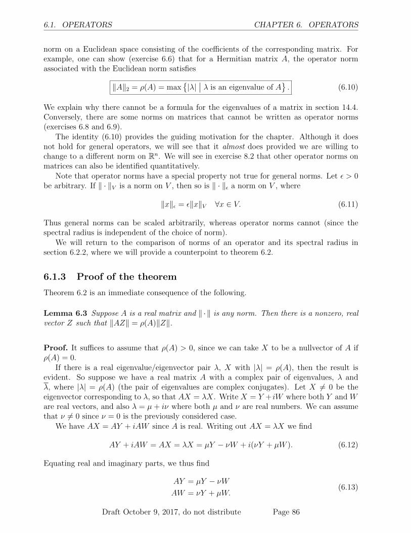
6.1. OPERATORS CHAPTER 6. OPERATORS
norm on a Euclidean space consisting of the coefficients of the corresponding matrix. Forexample, one can show (exercise 6.6) that for a Hermitian matrix A, the operator normassociated with the Euclidean norm satisfies
‖A‖2 = ρ(A) = max|λ|∣∣ λ is an eigenvalue of A
. (6.10)
We explain why there cannot be a formula for the eigenvalues of a matrix in section 14.4.Conversely, there are some norms on matrices that cannot be written as operator norms(exercises 6.8 and 6.9).
The identity (6.10) provides the guiding motivation for the chapter. Although it doesnot hold for general operators, we will see that it almost does provided we are willing tochange to a different norm on Rn. We will see in exercise 8.2 that other operator norms onmatrices can also be identified quantitatively.
Note that operator norms have a special property not true for general norms. Let ε > 0be arbitrary. If ‖ · ‖V is a norm on V , then so is ‖ · ‖ε a norm on V , where
‖x‖ε = ε‖x‖V ∀x ∈ V. (6.11)
Thus general norms can be scaled arbitrarily, whereas operator norms cannot (since thespectral radius is independent of the choice of norm).
We will return to the comparison of norms of an operator and its spectral radius insection 6.2.2, where we will provide a counterpoint to theorem 6.2.
6.1.3 Proof of the theorem
Theorem 6.2 is an immediate consequence of the following.
Lemma 6.3 Suppose A is a real matrix and ‖ · ‖ is any norm. Then there is a nonzero, realvector Z such that ‖AZ‖ = ρ(A)‖Z‖.
Proof. It suffices to assume that ρ(A) > 0, since we can take X to be a nullvector of A ifρ(A) = 0.
If there is a real eigenvalue/eigenvector pair λ, X with |λ| = ρ(A), then the result isevident. So suppose we have a real matrix A with a complex pair of eigenvalues, λ andλ, where |λ| = ρ(A) (the pair of eigenvalues are complex conjugates). Let X 6= 0 be theeigenvector corresponding to λ, so that AX = λX. Write X = Y + iW where both Y and Ware real vectors, and also λ = µ+ iν where both µ and ν are real numbers. We can assumethat ν 6= 0 since ν = 0 is the previously considered case.
We have AX = AY + iAW since A is real. Writing out AX = λX we find
AY + iAW = AX = λX = µY − νW + i(νY + µW ). (6.12)
Equating real and imaginary parts, we thus find
AY = µY − νWAW = νY + µW.
(6.13)
Draft October 9, 2017, do not distribute Page 86

CHAPTER 6. OPERATORS 6.1. OPERATORS
This says that A maps the space spanned by Y and W into itself. Call this space V . We willsee that V has to be two-dimensional, which is essential for the proof. We will find Z ∈ Vsuch that ‖AZ‖ = |λ|‖Z‖.
If Y and W were collinear, that is, W = αY , with α real, then we would have
(1 + iα)AY = A(Y + iαY ) = λ(Y + iαY ) = (1 + iα)λY, (6.14)
so that (dividing by 1 + iα) AY = λY . But this is not possible because both A and Y arereal. Thus V must be two dimensional.
Any vector in V can be written as c1Y + c2W , and we easily compute from (6.13) that
A(c1Y + c2W ) = d1Y + d2W (6.15)
where (µ ν−ν µ
)c = d, c =
(c1
c2
), d =
(d1
d2
). (6.16)
Since |λ|2 = µ2 + ν2, the vector |λ|−1(µ, ν) lies on the unit circle. Thus |λ|−1(µ, ν) =(cos θ, sin θ) for some 0 ≤ θ < 2π, that is, µ+ iν = λ = |λ|eiθ = |λ|(cos θ+ i sin θ). Then thematrix in (6.16) is a rotation and scaling:(
µ ν−ν µ
)=
(|λ| cos θ |λ| sin θ−|λ| sin θ |λ| cos θ
)= |λ|R(−θ), (6.17)
where R(θ) denotes the matrix that rotates a vector by an angle θ.Define Z(φ) = cos(φ)Y + sin(φ)W . Using (6.17) we have (exercise 6.28)
AZ(φ) = |λ|Z(φ− θ). (6.18)
Defineg(φ) = ‖Z(φ)‖. (6.19)
Then g is 2π-periodic and continuous (exercise 6.29). Define
φ∗ = argminφ∈[0,2π]g(φ) and φ∗ = argmaxφ∈[0,2π]g(φ). (6.20)
Then for any ϑ ∈ [0, 2π] we have
g(φ∗) ≤ g(φ∗ − ϑ) and g(φ∗ − ϑ) ≤ g(φ∗), (6.21)
so that for any ϑ ∈ [0, 2π] we have
g(φ∗ − ϑ)
g(φ∗)≤ 1 ≤ g(φ∗ − ϑ)
g(φ∗). (6.22)
Note that g never vanishes (exercise 6.29). By the intermediate value theorem, for anyϑ ∈ [0, 2π] there is a φ = φ(ϑ) such that g(φ(ϑ)− ϑ)) = g(φ(ϑ)). Thus (6.18) implies
‖AZ(φ(θ))‖ = |λ| ‖Z(φ(θ)− θ)‖ = |λ|g(φ(θ)− θ)) = |λ|g(φ(θ)) = |λ| ‖Z(φ(θ))‖. (6.23)
Therefore X = Z(φ(θ)) is the desired vector. QED
Draft October 9, 2017, do not distribute Page 87

6.2. SCHUR DECOMPOSITION CHAPTER 6. OPERATORS
6.2 Schur decomposition
To understand norms of operators better, we need to develop some technology. Fortunately,this technology is interesting in its own right as it provides insight into fundamental proper-ties of linear operators. The first result that we need is the Schur decomposition, which saysthat any matrix is unitarily equivalent to a triangular matrix.
Definition 6.4 A matrix U is unitary if U?U = I.
A unitary matrix corresponds to an operator that does not stretch coordinates in anydirection.
Theorem 6.5 For any square matrix A, there is a unitary matrix U such that T = U−1AU =U?AU is upper-triangular.
There are several applications of the Schur decomposition, but one of them involves eigen-values. In view of corollary 3.3, the diagonal entries of a triangular matrix are its eigenvalues.Since a similarity transformation does not change the eigenvalues (exercise 6.10), the eigen-values of A are the diagonal entries of the triangular factor T in the Schur decomposition.For the special case of a Hermitian matrix A, we obtain the following well-known result.
Corollary 6.6 For any Hermitian matrix A, there is a unitary matrix U such that D =U−1AU = U?AU is diagonal.
The proof of this corollary is a simple application of the Schur decomposition and con-jugation: T ? = (U?AU)? = U?A?U = U?AU = T . A Hermitian triangular matrix must bediagonal. Similarly, we can prove the following.
Corollary 6.7 For any matrix A, there is a unitary matrix U such that D = U−1AU =U?AU is diagonal if and only if A is normal, i.e., A?A = AA?.
The “only if” is clear. The “if” is an interesting result itself: a triangular matrix T isnormal (T ?T = TT ?) iff it is diagonal (exercise 6.12).
It might appear then that the Schur decomposition provides a means to compute eigen-values. We will see that the converse is true: we use the existence of eigenvectors to establishthe Schur decomposition. We postpone the proof of theorem 6.5 until section 6.2.3.
It is tempting to compare the QR factorization (5.54) with the Schur decomposition (the-orem 6.5). There is a superficial similarity in that both involve unitary and triangular factors.But there are significant differences. First, the QR factorization applies more generally inthat A need not be square. But more significantly, the Schur decomposition is a similaritytransformation, whereas the QR factorization is unbalanced. However, most significant isthe fact that we have a constructive algorithm that computes the QR factorization in a finitenumber of steps. We will see in section 14.4 why this is not possible in general for the Schurdecomposition.
Draft October 9, 2017, do not distribute Page 88

CHAPTER 6. OPERATORS 6.2. SCHUR DECOMPOSITION
6.2.1 Nearly diagonal matrices
As a step toward the proof of our main theorem on the relationship between the spectralradius and operator norms, there is an interesting intermediate result, namely, that with asuitable similarity transformation, any matrix can be transformed so that it is essentiallydiagonal.
Theorem 6.8 Suppose A is any square matrix and let ε > 0 be arbitrary. Then there is aninvertible matrix P such that
P−1AP = Λ + C, (6.24)
where Λ is a diagonal matrix (having the eigenvalues of A on the diagonal) and C is a strictlyupper-triangular matrix that satisfies |Cij| ≤ ε for all i, j (and Cij = 0 for i ≥ j).
This theorem says that we can make any matrix look as nearly diagonal as we want (butwe will see that this comes at the expense of making P very large in general). What thismeans is that general similarity transformations can be somewhat misleading, unlike theunitary transformations in the Schur decomposition.
Proof. We begin with the Schur decomposition U?AU = T , where T = Λ +B is an upper-triangular matrix and B is strictly upper-triangular (that is, B has zero diagonal entries andΛ is diagonal). Define
µ = max|bkl|
∣∣ k, l = 1, . . . , n.
If µ = 0, then we pick P = U and C = 0 for all ε > 0. So suppose that µ > 0, letζ = min1, ε/µ, and define D to be the diagonal matrix with Dii = ζ i−1 for i = 1, . . . , n.Then D−1TD = Λ + C, where C = D−1BD. Then C is also strictly upper-triangular, and(see exercise 6.13)
cij = ζ1−ibijζj−1 = ζj−ibij . (6.25)
But since B is strictly upper-triangular, bij 6= 0 only if j ≥ i+1, so cij 6= 0 only for j− i ≥ 1.By definition, ζk ≤ ζ for all integers k ≥ 1. Thus we have |cij| ≤ ζµ ≤ ε for all i and j.Define P = UD. Then P−1AP = D−1U?AUD = D−1TD = Λ + C. QED
6.2.2 The spectral radius is nearly a norm
We now consider one of the main results in the chapter, the gist of which is the title of thissection.
Theorem 6.9 Suppose A is any n × n matrix and let δ > 0 be arbitrary. Then there is anorm N on Cn such that the corresponding operator norm ‖ · ‖N satisfies
ρ(A) ≤ ‖A‖N ≤ ρ(A) + δ, (6.26)
where ρ(A) is the spectral radius.
We emphasize here that that the operator norm is defined by
‖A‖N = supx∈Cn, x 6=0
N(Ax)
N(x)(6.27)
Draft October 9, 2017, do not distribute Page 89

6.2. SCHUR DECOMPOSITION CHAPTER 6. OPERATORS
and depends on δ through the dependence of N on δ. In view of theorem 6.9, we are free tothink of the spectral radius ρ(A) as (essentially) a norm (recall the reverse inequality (6.7)which holds for all norms).
Proof. The first inequality in (6.26) is theorem 6.2, so we need to prove only the second.Let ε = δ/n and choose P according to theorem 6.8. Note that
ρ(A) = max|Λii|
∣∣ i = 1, . . . , n. (6.28)
Define N(x) = ‖P−1x‖∞ (see exercise 6.14). Then (making the substitution x = Py)
‖A‖N = supx∈Cn, x 6=0
‖P−1Ax‖∞‖P−1x‖∞
= supy∈Cn, y 6=0
‖P−1APy‖∞‖y‖∞
= supy∈Cn, y 6=0
‖(Λ + C)y‖∞‖y‖∞
≤ supy∈Cn, y 6=0
‖Λy‖∞‖y‖∞
+ supy∈Cn, y 6=0
‖Cy‖∞‖y‖∞
≤ supy∈Cn, y 6=0
‖Λy‖∞‖y‖∞
+ nε = ρ(A) + δ,
(6.29)
where we used exercise 6.15 in the penultimate step and exercise 6.16 in the last. QED
6.2.3 Derivation of the Schur decomposition
The proof of the Schur decomposition is by induction on the matrix dimension. For n = 1,the theorem is trivial, but this may not be as instructive as the case n = 2, as follows. Wepick an eigenpair for A: Ax = λx, normalized so that x?x = 1. This is the only nontrivialfact that we use in the proof. The property that every matrix has at least one eigenvector isworth reviewing; it stems from the fundamental theorem of algebra [36], which says that apolynomial always has a root (cf. exercise 5.24). In this case, the polynomial in question isthe characteristic polynomial pn(λ) = det(A−λI). The second ingredient in this fact is thatif the determinant of a matrix is zero, then the matrix (A− λI in our case) has a nontrivialnull vector.
Now we let b be the unique vector satisfying b?b = 1 and b?x = 0. More precisely, wehave
(b1, b2) = (x2?,−x1
?) = (x2,−x1),
where z denotes the complex conjugate of z. Thus U = [x b] is unitary via ordinary matrixmultiplication:
U?U =
(x?x x?bb?x b?b
)=
(1 00 1
). (6.30)
Similarly,
U?AU =
(x?Ax x?Abb?Ax b?Ab
)=
(x?(λx) x?Abb?(λx) b?Ab
)=
(λ ζ0 w
)= T, (6.31)
where ζ = x?Ab and w = b?Ab are (possibly complex) numbers, and T is obviously upper-triangular.
Draft October 9, 2017, do not distribute Page 90

CHAPTER 6. OPERATORS 6.2. SCHUR DECOMPOSITION
Note that w is an eigenvalue of A as well, since it a diagonal entry of T . But thatdoes not mean that b is the corresponding eigenvector. We can write Ab = εx + wb, but εneed not be zero. In fact, a short calculation shows that Ay = wy for y = αx + βb whereα/β = ε/(w − λ). If w = λ, then β = 0.
Now we consider the general case. So suppose the Schur decomposition is true for n− 1,and let us show that it holds for n. To begin with, we again pick an eigenpair for A: Ax = λx,normalized so that x?x = 1. Given the eigenvector x, we construct
U = [x B] (6.32)
by taking x to be the first column of U and filling in with the n×(n−1) matrix B as needed.We can see that U is unitary if we are willing to change coordinates so that x = [1 0 · · · 0];in this case, U = I. If we want to see this more concretely, we can study what it means forU = [x B] to be unitary:
U?U =
(x?x x?BB?x B?B
)=
(1 x?BB?x B?B
), (6.33)
where we have used a block-matrix multiplication formula (exercise 6.17) similar to (3.43).Let b1, . . . , bn−1 be an orthonormal basis for the (n− 1)-dimensional space
Y =y ∈ Cn
∣∣ x?y = 0. (6.34)
Such a basis could be generated by the Gram-Schmidt process as described in section 5.4.1.Then B = [b1, . . . , bn−1] has the required properties.
Now let us see what U does to A. By another block-matrix multiplication formula(exercise 6.18), we find
U?AU =
(x?Ax x?ABB?Ax B?AB
)=
(λ x?AB0 B?AB
)=
(λ z?
0 A(n−1)
), (6.35)
where z = B?A?x is some (column) vector of length n − 1 and A(n−1) = B?AB is an (n −1)×(n−1) matrix. We now invoke the induction hypothesis and let V be an (n−1)×(n−1)
unitary matrix such that V ?A(n−1)V = T (n−1) is upper-triangular. Define
V =
(1 0
0 V
). (6.36)
Then the block-matrix multiplication formula (3.43) implies
V ?U?AUV =V ?
(λ z?
0 A(n−1)
)V =
(λ z?
0 V ?A(n−1)
)V
=
(λ z?V
0 V ?A(n−1)V
)=
(λ z?V0 T (n−1)
).
(6.37)
Thus UV is the required unitary matrix. QED
The Schur decomposition is not an algorithm for determining eigenvalues. Unfortunately,its derivation is not constructive, in that it requires the provision of an eigenvector by someunspecified mechanism. Instead, we should think of the Schur decomposition as a way tocatalog the eigenvectors (and eigenvalues) in a useful way.
Draft October 9, 2017, do not distribute Page 91

6.2. SCHUR DECOMPOSITION CHAPTER 6. OPERATORS
6.2.4 Schur decomposition and flags
A flag is a nested sequence of subspaces V k of a vector space V [9]. More precisely, a flaghas the property that
0 = V 0 ⊂ V 1 ⊂ V 2 ⊂ · · · ⊂ V k = V, (6.38)
where the dimensions di = dimV i satisfy di > di−1 for all i ≥ 1. A complete flag is one inwhich di = i for all i.
An operator O : V → V supports a flag if O(V j) ⊂ V j for all j = 1, . . . , k. For example,
V i =
(x1, . . . , xn) ∈ Rn∣∣ xj = 0 ∀j > i
(6.39)
is a complete flag, and any upper-triangular matrix T supports the flag (6.39) (exercise 6.19).
The Schur decomposition has an abstract representation in terms of flags and operatorsas follows.
Theorem 6.10 Any operator on a finite-dimensional vector space V supports a completeflag.
In other words, for any operator O there exists some complete flag (6.38) that it supports.Thus the Schur decomposition of an operator has a natural expression independent of anybasis chosen to represent it as a matrix. Other matrix decompositions, such as the LUfactorization (section 3.2), do not enjoy this property.
The proof of theorem 6.10 is left as exercise 6.20.
6.2.5 Example of Schur decomposition
Consider the Schur decomposition of the matrix A = A(x) given by
A =
(0 x1 0
), (6.40)
for x ≥ 0. Define an orthogonal matrix U = U(x) by
U =
√ xx+1
√1
x+1√1
x+1−√
xx+1
. (6.41)
Note that U is symmetric and U2 = I. Then
UAU =
(√x 1− x
0 −√x
). (6.42)
Observe that both the eigenvalues λ(x) of A(x) and the orthononal matrix U(x) are notdifferentiable at x = 0. When x = 1, A is symmetric, consistent with the fact that UAU isdiagonal.
We leave as exercise 6.27 to work out the Schur decomposition of A(x) for x < 0.
Draft October 9, 2017, do not distribute Page 92

CHAPTER 6. OPERATORS 6.3. CONVERGENT MATRICES
6.3 Convergent matrices
There are many situations in which the result of an algorithm can be written as multiplicationof a vector X by a fixed matrix A. Thus repeating the algorithm n times is equivalent (byinduction) to applying the matrix Ak. Frequently, this represents the error in some iterativeprocess. Thus we are interested in precise conditions when A is a convergent matrix, that is,Ak → 0 as k →∞. We start with the following simple criterion.
Lemma 6.11 If ‖A‖ < 1 for some operator norm, then ‖Ak‖ → 0 as k →∞.
Proof. By induction, (6.3) implies that ‖Ak‖ ≤ ‖A‖k → 0 as k →∞. QED
Combining lemma 6.11 with theorem 6.9, we get the following precise characterization.
Theorem 6.12 For any matrix A, Ak → 0 as k →∞ if and only if ρ(A) < 1.
Proof. If ρ(A) < 1, choose a norm so that ‖A‖ < 1 by theorem 6.9 and apply lemma 6.11.Conversely, suppose there is an eigenvalue λ of A such that |λ| ≥ 1. There must be a
vector x 6= 0 such that Ax = λx. Thus Akx = Ak−1Ax = λAk−1x, so by induction we musthave Akx = λkx. But if Ak → 0, we conclude that λkx→ 0. Since |λk| = |λ|k ≥ 1, we havea contradiction. QED
theorem 6.12 provides the basis for the convergence theory for stationary iterative meth-ods (section 8.1), for the stability theory of time-stepping schemes for approximating thesolutions to differential equations that will be discussed in section 17.2), as well as for manyother applications.
6.4 Powers of matrices
Theorem 6.12 provides some information about powers of matrices. Here we develop thetheme in a bit more detail. Our objective is to prove the following result.
Theorem 6.13 For any n × n (real or complex) matrix A and any norm ‖ · ‖ (on Rn orCn, respectively),
limk→∞‖Ak‖1/k = ρ(A), (6.43)
where ρ(A) is the spectral radius of A and ‖Ak‖ denotes the corresponding operator norm.
This again shows the close connection between the spectral radius and the operator norm.To begin with, an analog of (6.9) is that
ρ(A) ≤ ‖Ar‖1/r (6.44)
for any norm and any positive integer r. For a complex norm, this is proved in the same way:ρ(A) = |λ| for some eigenvalue λ, with eigenvector X such that AX = λX. Multiplyingby A, we have A2X = A(λX) = λAX = λ2X. By induction, we have ArX = λrX for anyr. Thus ρ(A)r = |λ|r = ‖ArX‖/‖X‖ ≤ ‖Ar‖, proving (6.44). For a real norm, we need toutilize the techniques in the proof of lemma 6.3. With Z(φ) as defined there, we see that
Draft October 9, 2017, do not distribute Page 93

6.4. POWERS OF MATRICES CHAPTER 6. OPERATORS
ArZ(φ) = |λ|rZ(φ − rθ), and choosing φ = φ(rθ) completes the proof. We now use this toprove theorem 6.13.
It seems remarkable at first that this would hold for any operator norm, but the fact isthat it is sufficient to prove (6.43) for just one norm. For example, suppose that we knowthat
limk→∞‖Ak‖1/k
∞ = ρ(A). (6.45)
Then by the equivalence of norms (lemma 5.1 or theorem 5.3), we have
limk→∞‖Ak‖1/k ≤ lim
k→∞
(K‖Ak‖∞
)1/k= lim
k→∞K1/kρ(A) = ρ(A). (6.46)
Thus the limiting process quashes any constant factor. In view of (6.44), the theorem follows.Now let us verify (6.45).
The Schur decomposition shows that powers of a matrix tend to a very simple form.Suppose that T = U?AU is the Schur decomposition, where U is unitary and T is triangular.We can turn the decomposition around and write A = UTU?. Then A2 = U?TUU?TU =U?T 2U . By induction,
Ak = U?T kU (6.47)
for any k. WriteT = D +N, (6.48)
where D = diag(T ) is the diagonal matrix whose diagonal is the same as that of T . ThusN = T −D. Since the entries of D are the eigenvalues of T (and hence of A),
‖D‖∞ = ρ(T ) = ρ(A) (6.49)
(see exercise 6.16). We need to calculate the norm of T k, and since this is a somewhatlengthy step, we separate it as the following lemma.
Lemma 6.14 Suppose that T is an upper-triangular n × n matrix and N = T −D, whereD = diag(T ). Then for any matrix norm ‖ · ‖ satisfying the multiplicative property (6.3), wehave
‖T k‖ = ‖(D +N)k‖ ≤ kn‖D‖k−n (‖N‖+ ‖D‖)n . (6.50)
Proof. Note that N is nilpotent, that is, Nn = 0. More precisely, observe that N is strictlyupper-triangular, that is, it is 0 on and below the main diagonal. Not all nilpotent matricesare strictly upper-triangular, but all strictly upper-triangular matrices are nilpotent. Towork with such matrices, let us introduce some notation. We say that an upper-triangularmatrix M has shift index µ if Mij = 0 for i > j − µ. A diagonal matrix has shift index 0,and the matrix N = T −D has shift index 1.
The product MN of two upper-triangular matrices M and N , with shift indices µ andν, respectively, has shift index µ + ν (see exercise 6.23). In particular, since N = T − Dhas shift index 1, (Nk)ij = 0 for i > j − k (see exercise 6.24). Thus Nn ≡ 0. If D is adiagonal matrix, then the shift index of DN and ND is no less than the shift index of N(see exercise 6.25).
We now want to expand the expression T k = (D+N)k. SinceN andD need not commute,such an expression can be quite complicated. In particular, (D+N)2 = D2+DN+ND+N2.
Draft October 9, 2017, do not distribute Page 94

CHAPTER 6. OPERATORS 6.4. POWERS OF MATRICES
For (D +N)k, there are 2k such expressions. Fortunately, there is a one-to-one relationshipbetween each such expressions and the binary representation of some integer j ∈ [0, 2k − 1].Define
P (j) =k∏i=1
DbiN1−bi , (6.51)
where bkbk−1 · · · b1 denotes the binary expansion of j, that is,
j =k∑i=1
bi2i−1. (6.52)
Note that DbiN1−bi is D if bi = 1, and N if bi = 0. Then
(D +N)k =2k−1∑j=0
P (j). (6.53)
We can compute the shift index of P (j): it is at least ν(j), the number of N ’s in P (j) andof zeros in the binary expansion of j. Thus when ν(j) ≥ n, P (j) = 0 (exercise 6.26). Thus
(D +N)k =∑
0≤j<2k,ν(j)≤n
P (j). (6.54)
Note that‖P (j)‖ ≤ ‖D‖k−ν(j)‖N‖ν(j). (6.55)
From (6.55), we conclude
‖(D +N)k‖ ≤∑
0≤j<2k,ν(j)≤n
‖D‖k−ν(j)‖N‖ν(j)
=n∑`=0
∑0≤j<2k,ν(j)=`
‖D‖k−`‖N‖`
=n∑`=0
(k`
)‖D‖k−`‖N‖`
(6.56)
because the number of j ∈ [0, 2k − 1] such that ν(j) = ` is
(k`
). We use the elementary
estimate (k`
)=
(n`
)k!(n− `)!n!(k − `)!
=
(n`
)(k − `+ 1) · · · k(n− `+ 1) · · ·n
≤(n`
)k`. (6.57)
Therefore,
‖(D +N)k‖ ≤ kn‖D‖k−nn∑`=0
(n`
)‖D‖n−`‖N‖`
= kn‖D‖k−n (‖D‖+ ‖N‖)n ,(6.58)
which completes the proof of the lemma. QED
Draft October 9, 2017, do not distribute Page 95

6.5. DEFECTIVE MATRIX POWERS CHAPTER 6. OPERATORS
From (6.47), we have
‖Ak‖∞ = ‖U?T kU‖∞ ≤ ‖U?‖∞‖T k‖∞‖U‖∞ ≤ C‖T k‖∞, (6.59)
where C = ‖U?‖∞‖U‖∞. Therefore, (6.49) and lemma 6.14 imply
‖Ak‖∞ ≤ Ccnknρ(A)k−n, (6.60)
where cn = (‖D‖∞ + ‖N‖∞)n. But since both C and cn are positive constants,
limk→∞
(Ccnkn)1/k = 1. (6.61)
Therefore, (6.60) yields
limk→∞‖Ak‖1/k
∞ ≤ limk→∞
(Ccnkn)1/k ρ(A)1−n/k = ρ(A). (6.62)
Combined with (6.44), this proves (6.45) and completes the theorem.
6.5 Defective matrix powers
Although we have seen that the behavior of powers of a matrix M is ultimately determinedby the spectral radius ρ(M), it can take a long time for the asymptotic behavior to takeeffect. When M is defective, the behavior is more complex. If
M =
(λ 10 λ
), (6.63)
then induction shows that
Mk =
(λ 10 λ
)k= λk
(1 k/λ0 1
)= ρ(M)k
(1 k/λ0 1
), (6.64)
for any positive integer k. In particular, if
X0 =
(01
), (6.65)
we find the sequence of vectors Xk = MkX0 to be
Xk = λk(k/λ
1
)= kλk
(1/λ1/k
)= φ(k)
(1/λ1/k
), (6.66)
where φ(x) = xλx = xe(log λ)x. The function φ initially increases rapidly, decaying onlyfor large x. It reaches a maximum at x = 1/(log(1/λ); if λ = 1 − δ, then log(1/λ) ≈ δand x ≈ 1/δ. Thus the initial iterations appear to be going in the wrong direction. Insection 15.1.6, we consider more general examples of this form.
The algebraic defectiveness of M in (6.63) is not the unique cause of delayed convergence.In figure 6.2, we compare powers of M with λ = 0.99 with powers of the matrix B given by
B =
(0.98 1
0 0.99
), (6.67)
Draft October 9, 2017, do not distribute Page 96
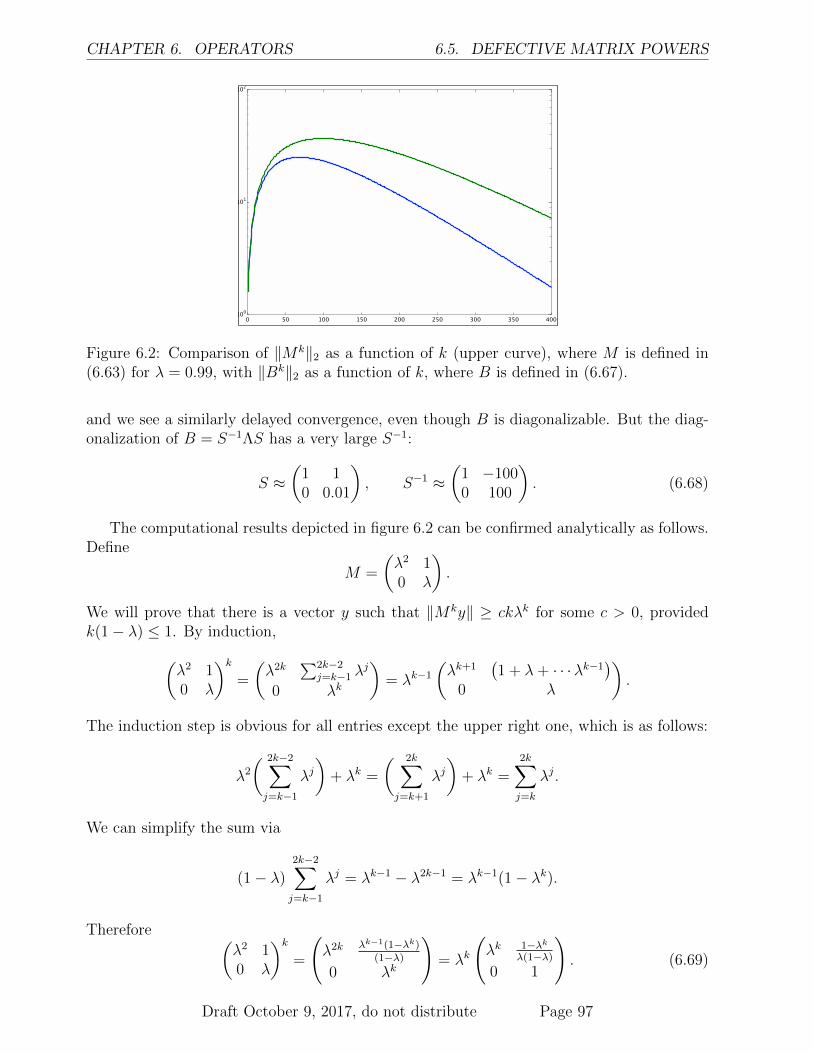
CHAPTER 6. OPERATORS 6.5. DEFECTIVE MATRIX POWERS
Figure 6.2: Comparison of ‖Mk‖2 as a function of k (upper curve), where M is defined in(6.63) for λ = 0.99, with ‖Bk‖2 as a function of k, where B is defined in (6.67).
and we see a similarly delayed convergence, even though B is diagonalizable. But the diag-onalization of B = S−1ΛS has a very large S−1:
S ≈(
1 10 0.01
), S−1 ≈
(1 −1000 100
). (6.68)
The computational results depicted in figure 6.2 can be confirmed analytically as follows.Define
M =
(λ2 10 λ
).
We will prove that there is a vector y such that ‖Mky‖ ≥ ckλk for some c > 0, providedk(1− λ) ≤ 1. By induction,(
λ2 10 λ
)k=
(λ2k
∑2k−2j=k−1 λ
j
0 λk
)= λk−1
(λk+1
(1 + λ+ · · ·λk−1
)0 λ
).
The induction step is obvious for all entries except the upper right one, which is as follows:
λ2
( 2k−2∑j=k−1
λj)
+ λk =
( 2k∑j=k+1
λj)
+ λk =2k∑j=k
λj.
We can simplify the sum via
(1− λ)2k−2∑j=k−1
λj = λk−1 − λ2k−1 = λk−1(1− λk).
Therefore (λ2 10 λ
)k=
(λ2k λk−1(1−λk)
(1−λ)
0 λk
)= λk
(λk 1−λk
λ(1−λ)
0 1
). (6.69)
Draft October 9, 2017, do not distribute Page 97

6.6. EXERCISES CHAPTER 6. OPERATORS
If λ = 1− δ, we can further simplify this as follows. We have
λk = (1− δ)k = ek log(1−δ).
But log(1− δ) ≤ −δ, soλk = (1− δ)k ≤ e−kδ.
Since e−x ≤ 1− x+ 12x2 for x ≥ 0
1− λk ≥ 1− e−kδ = kδ − 12(kδ)2 = kδ(1− 1
2kδ)
for all k. Thus1− λk
λ(1− λ)≥k(1− 1
2kδ)
λ≥ k
2λ
for k ≤ 1/δ. In particular, define
yk =
(λ2 10 λ
)k (01
)= λk
(λk 1−λk
λ(1−λ)
0 1
)(01
).
Thenyk1 ≥ 1
2kλk−1 = ckλk,
where c = λ/2, provided k ≤ 1/(1− λ) = 1/δ.
6.6 Exercises
Exercise 6.1 Show that the set Pn of polynomials of degree n in one variable can be viewedas a vector space of dimension n + 1. (Hint: define (f + g)(x) = f(x) + g(x) for all x anddefine (αf)(x) = αf(x) for all x. Use the monomials as a basis to determine the dimension.)
Exercise 6.2 Show that the derivative operator is a well-defined mapping from the set Pnof polynomials of degree n in one variable to itself (see exercise 6.1). Compute its matrixrepresentation in the basis given by the monomials.
Exercise 6.3 Prove that the operator norm defined by (6.1) is a norm on the linear spaceof operators from V to W .
Exercise 6.4 Prove the product expression (6.3). (Hint: consider (AB)u = A(Bu) andapply (6.2) twice.)
Exercise 6.5 Prove that ‖U‖2 = 1 for any unitary matrix. (Hint: just compute ‖Ux‖22 =
(Ux)?Ux = x?U?Ux = x?x.)
Exercise 6.6 Prove that‖A‖2 =
√ρ(A?A) (6.70)
for any matrix A. Use this to verify (6.10) for a Hermitian operator. (Hint: apply corol-lary 6.6 and compute
‖Ax‖22 = (Ax)?Ax = x?A?Ax = x?U?DUx. (6.71)
Apply exercise 6.5, or at least its hint.)
Draft October 9, 2017, do not distribute Page 98

CHAPTER 6. OPERATORS 6.6. EXERCISES
Exercise 6.7 Suppose that A is a Hermitian, positive definite matrix. Show that for theoperator norm associated with the Euclidean norm
‖A−1‖−12 = min
|λ|∣∣ λ is an eigenvalue of A
. (6.72)
(Hint: if λ is an eigenvalue of A, then λ−1 is an eigenvalue of A−1.)
Exercise 6.8 Show by example that the norm
‖A‖max := max|Aij|
∣∣ i, j = 1, . . . , n
(6.73)
does not satisfy the inequality (6.3).
Exercise 6.9 Prove that the Frobenius norm (6.5) satisfies the property (6.3) regarding thenorm of the product of matrices, even though it is not an operator norm in the sense of(6.1) for the case where V = W (demonstrate that by example). What happens if we allowV 6= W? (Hint: use Cauchy (5.33) for the product formula. To prove it is not an operatornorm for V = W , evaluate the Frobenius norm of the identity matrix. For the general case,see [34, 52].)
Exercise 6.10 Recall that a similarity transformation is of the form B = S−1AS, where Sis assumed to be invertible. Show that A and B have the same eigenvalues.
Exercise 6.11 Suppose that A and B are n × n matrices, and that A is invertible. Provethat AB and BA are similar matrices. (Hint: we seek an invertible matrix S such thatAB = S−1BAS. What if we choose S = A−1?)
Exercise 6.12 Prove that if an upper-triangular matrix T commutes with its conjugatetranspose (T ?T = TT ?), then it must be diagonal. (Hint: use the block-matrix multiplicationformula (3.43), where
T =
(α b?
0 S
)(6.74)
and S is also upper-triangular.)
Exercise 6.13 Suppose that D is a diagonal matrix with diagonal entries d1, . . . , dn. Showthat the matrices MD and DM are just M scaled by the diagonal entries of D via (MD)ij =Mijdj and (DM)ij = diMij.
Exercise 6.14 Let P be an invertible matrix. Show that N(x) := ‖Px‖ is a norm for anyvector norm ‖ · ‖.
Exercise 6.15 Prove that
‖Cy‖∞ ≤ n‖y‖∞max|Cij|
∣∣ i, j = 1, . . . , n
(6.75)
for any n× n matrix C and y ∈ Rn.
Exercise 6.16 Suppose that D is a diagonal n× n matrix. Prove that
‖D‖∞ = max|Dii|
∣∣ i = 1, . . . , n.
Draft October 9, 2017, do not distribute Page 99

6.6. EXERCISES CHAPTER 6. OPERATORS
Exercise 6.17 Verify the block-matrix multiplication formula expressed by the first equalityin (6.33). (Compare exercise 3.7.)
Exercise 6.18 Verify the block-matrix multiplication formula expressed by the first equalityin (6.35). (Compare exercise 3.7.)
Exercise 6.19 Show that (6.39) is a complete flag that supports any upper-triangular ma-trix.
Exercise 6.20 Prove theorem 6.10. (Hint: first represent the operator as a matrix using abasis of V and use the Schur decomposition to decompose this matrix. Show that the operatorcan be represented as a triangular matrix in some basis, and apply exercise 6.19.)
Exercise 6.21 Suppose that 1/p + 1/q = 1 (q = ∞ if p = 1, and p = ∞ if q = 1). Provethat for any x ∈ Fn,
‖x‖p = sup‖y‖q=1
|y?x|, (6.76)
where the supremum is over y ∈ Fn and F is either R or C. (Hint: first use Holder’sinequality (5.12). Then for p <∞ and x real, choose
yi = sign(xi)|xi|p−1‖x‖−pp . (6.77)
For p = ∞, note that ‖x‖∞ = |xi| for some i; choose y accordingly. In the complex case,modify (6.77) appropriately.)
Exercise 6.22 Suppose that 1/p + 1/q = 1 (q = ∞ if p = 1, and p = ∞ if q = 1). Provethat ‖A‖p = ‖A?‖q. (Hint: use exercise 6.21.)
Exercise 6.23 Suppose that M and N are n×n upper-triangular matrices with shift indicesµ and ν, respectively. Prove that MN has shift index µ+ ν. (Hint: observe that
(MN)ij =
j−ν∑k=i+µ
NikMkj (6.78)
for all i, j.)
Exercise 6.24 Suppose that N is an n × n matrix such that Nij = 0 for i > j − 1. Provethat Nk
ij = 0 for i > j − k. (Hint: use induction and exercise 6.23.)
Exercise 6.25 Suppose that N is an n× n matrix such that Nij = 0 for i > j − ν, that is,the shift index of N is µ. Suppose that D is an n× n diagonal matrix. Prove that DN andND have a shift index of at least ν. (Hint: see the hint for exercise 6.23.)
Exercise 6.26 Suppose that the binary expansion of j has at least n zeros, that is, ν(j) ≥ n.Thus there are at least n factors N in P (j) defined in (6.51). Prove that P (j) = 0. (Hint:use exercise 6.25 to prove that the shift index of P (j) is at least n.)
Exercise 6.27 Derive the Schur decomposition for the matrix in (6.40) for x < 0.
Exercise 6.28 Use (6.17) to prove (6.18).
Exercise 6.29 Prove that the function g defined in (6.19) is continuous and never vanishes.
Draft October 9, 2017, do not distribute Page 100

CHAPTER 6. OPERATORS 6.7. SOLUTIONS
6.7 Solutions
Solution of Exercise 6.10. First, note that by multiplying B = S−1AS on the left by S,we get SB = AS. Multiplying this on the right by S−1, we find SBS−1 = A. Thus thesimilarity relationship is symmetric. Suppose that AX = λX. Then
λX = AX = SBS−1X.
Multiplying this by S−1 on the left shows that
λS−1X = BS−1X.
Thus S−1X is an eigenvector of B with eigenvalue λ. Therefore, we have proved that all theeigenvalues of A are eigenvalues of B. Since the similarity relationship is symmetric, all theeigenvalues of B are thus eigenvalues of A, and so they are the same. QED
Solution of Exercise 6.12. Using the block-matrix multiplication formula (3.43), we findthat
TT ? =
(α b?
0 S
)(α 0b S?
)=
(|α|2 + b?b b?S?
Sb SS?
)(6.79)
and
T ?T =
(α 0b S?
)(α b?
0 S
)=
(|α|2 αb?
αb S?S
). (6.80)
Thus we see that TT ? = T ?T implies b = 0 (compare the upper-left entries) and SS? = S?S.Thus the result is easily completed via induction on the size of the matrix T .
Let us assume that T is n× n. If n = 2, then S is just a scalar, and thus b = 0 impliesT is diagonal. Now suppose that the result is known for matrices of size (n− 1)× (n− 1),for some n ≥ 3. Then the equality of (6.79) and (6.80) implies that SS? = S?S. Since S isan upper-triangular matrix of size (n− 1)× (n− 1), we conclude that S must be diagonal.Together with the fact that b = 0 implies that T is diagonal.
Solution of Exercise 6.13. Just compute:
(MD)ij =n∑k=1
MikDkj = Mijdj
and
(DM)ij =n∑k=1
DikMkj = diMij.
QED
Solution of Exercise 6.14. It is clear that N(sx) = |s|N(x) for any scalar s since P (sx) =sPx. The triangle inequality is equally easy: P (x+ y) = Px+ Py, so
N(x+ y) = ‖Px+ Py‖ ≤ ‖Px‖+ ‖Py‖ = N(x) +N(y).
Now suppose that N(x) = 0. Then Px = 0, and since P is invertible, we have x = 0. QED
Draft October 9, 2017, do not distribute Page 101

6.7. SOLUTIONS CHAPTER 6. OPERATORS
Draft October 9, 2017, do not distribute Page 102

Chapter 7
Nonlinear Systems
In 1740, Thomas Simpson published “Essays on several curious and use-ful subjects in speculative and mix’d mathematicks, illustrated by avariety of examples,” in which he presents Newton’s method essentiallyin the form (2.30), together with a generalization to systems of two equa-tions, and shows that Newton’s method can solve optimization problemsby setting the gradient to zero [183].
We now turn to finding solutions of nonlinear systems of equations. There are manyways in which nonlinear systems of equations arise. One common one is in the minimizationof a smooth, scalar-valued function φ, as anticipated already by Simpson [183]. Minima arecharacterized by the equation ∇φ(x) = 0, so this suggests applying the techniques of thischapter to the function f(x) = ∇φ(x).
We will take as an example a simple form of a problem in geodesy, the science of de-termining locations in space from distance data. This has occupied many mathematicians,including Gauss [20, 96]; it is pursued on a very large scale [101] and is the basis for lo-cation by global positioning systems (GPS) [160]. In figure 7.1, we depict the problem ofdetermining the position of a boat near a shoreline based on the distance from the boat totwo markers on shore. The distance might be determined by measuring the time it takesfor sound to travel to the boat. A flash of light could indicate when the sound was emitted.The mathematical problem can be described in two equations for the distances:
b =√x2 + y2 c =
√(x− a)2 + y2. (7.1)
c
(0, 0) (a, 0)
b
(x, y)
Figure 7.1: Determining position offshore. The unknown point (x, y) is to be determinedfrom the known distances b and c to points on the shore.
103

7.1. FUNCTIONAL ITERATION FOR SYSTEMSCHAPTER 7. NONLINEAR SYSTEMS
We can turn this into a problem similar to what we studied in chapter 2 by defining thefunction
f(x1, x2) =
(x2
1 + x22
(x1 − a)2 + x22
). (7.2)
Our problem is thus reduced to finding a solution to f(x1, x2) = (b2, c2). Now we considersuch problems in general.
Thus we suppose that we have a function f : Rn → Rn and we want to find points x ∈ Rn
where f(x) = y for some y ∈ Rn. Without loss of generality, we usually assume that y = 0by simply subtracting y from f to create a new function. Correspondingly, we may alsocast this as a fixed-point problem: g(x) = x. As we have seen in the one-dimensional case(chapter 2), there may be several different g’s whose fixed points correspond to the solutionsof f(x) = 0. However, the setting of fixed-point iteration is still, as in the one-dimensionalcase, the place to start.
7.1 Functional iteration for systems
We just need to interpret the notation: g now maps Rn to itself, and fixed-point iterationseeks to find a fixed point
ξ = g(ξ), (7.3)
where now ξ ∈ Rn. Fixed-point iteration
xν = g(xν−1) (7.4)
still has the property that, if it converges, it converges to a fixed point (7.3), assuming onlythat g is continuous (exercise 7.1).
We emphasize now that g represents n functions g1, . . . , gn that each map Rn to R (wewill limit our discussions to real-valued functions for simplicity). The basic behavior is thesame as in the one-dimensional case, provided we use norms to measure vectors where weused absolute values before. If g is Lipschitz-continuous with constant λ < 1, that is,
‖g(x)− g(y)‖ ≤ λ‖x− y‖ (7.5)
for some norm ‖ · ‖ on Rn, then convergence will happen for all starting points. Moreprecisely, if we define eν = xν − ξ, then by induction
‖eν+1‖ = ‖g(xν)− g(ξ)‖ ≤ λ‖eν‖ ≤ λν‖e0‖. (7.6)
In fact, we have used (7.5) with only one x, namely, x = ξ.The rest of the story is similar to the one-dimensional case, except that we need some
higher-dimensional calculus to figure out when and how fast it will converge. We can discoverthe local behavior by using a Taylor expansion:
g(y) = g(x) + Jg(x)(y − x) +Rg(x, y), (7.7)
where the remainder Rg(x, y) satisfies
‖Rg(x, y)‖ ≤ C‖x− y‖2 (7.8)
Draft October 9, 2017, do not distribute Page 104

CHAPTER 7. NONLINEAR SYSTEMS7.1. FUNCTIONAL ITERATION FOR SYSTEMS
and Jg denotes the Jacobian of g, that is, the matrix with entries
(Jg(x))ij =∂gi∂xj
(x). (7.9)
We can present this visually as
Jg(x) =
∂g1∂x1
(x) ∂g1∂x2
(x) · · · ∂g1∂xn
(x)
∂g2∂x1
(x) ∂g2∂x2
(x) · · · ∂g2∂xn
(x)...
......
...∂gn∂x1
(x) ∂gn∂x2
(x) · · · ∂gn∂xn
(x)
. (7.10)
For example, for f defined in (7.2), then
Jf (x) =
(2x1 2x2
2(x1 − a) 2x2
). (7.11)
We recall that Jg may be thought of as a matrix-valued function, that is, a map Rn → Rn2.
The expression Jg(x)(x − y) in (7.7) is just a matrix-vector multiplication. Reviewing theexpression (7.6), we have
‖eν+1‖ = ‖g(xν)− g(ξ)‖= ‖Jg(ξ)eν +Rg(ξ, x
ν)‖≤‖Jg(ξ)eν‖+ ‖Rg(ξ, x
ν)‖≤‖Jg(ξ)‖ ‖eν‖+ C‖eν‖2,
(7.12)
where ‖Jg(ξ)‖ is the operator norm of Jg(ξ). Thus we see that the limiting behavior offixed-point iteration will be determined by the value of ‖Jg(ξ)‖.
There are several “theorems” that one could present based on the analysis above, butthe following local result is the most important.
Theorem 7.1 Suppose that the spectral radius ρ(Jg(ξ)) < 1 at a fixed point ξ = g(ξ) andthat the Taylor expansion (7.7) holds with the constant C in (7.8) (in some norm) fixed forall y in a neighborhood of x = ξ. Then fixed-point iteration (7.3) converges provided that x0
is close enough to ξ.
The main point of this result is that there is no reference to any particular norm in theestimation of the size of Jg(ξ). We leave the proof of this result as exercise 7.2. The trick isto pick a norm sufficiently close to the spectral radius for the matrix Jg(ξ) using theorem 6.9.Note that if the Taylor expansion (7.7) holds with the constant C in (7.8) fixed for all yin a neighborhood of x = ξ, then it holds for any norm by the equivalence of norms on Rn
(section 5.3.2).
We need to justify the Taylor expansion (7.7) with the remainder term in (7.8). But todo so, we need to develop some notation, which we will do in section 7.1.2.
Draft October 9, 2017, do not distribute Page 105

7.1. FUNCTIONAL ITERATION FOR SYSTEMSCHAPTER 7. NONLINEAR SYSTEMS
7.1.1 Limiting behavior of fixed-point iteration
Fixed-point iteration in higher dimensions can have a more complicated set of behaviorsthan in the one-dimensional case. Using the Taylor expansion (7.7), we can write
eν+1 =xν+1 − ξ = g(xν)− g(ξ)
= Jg(ξ)(xν − ξ) +Rg(ξ, x
ν)
≈ Jg(ξ)eν +O(‖eν‖2
)≈ Jg(ξ)eν .
(7.13)
Thus the errors evolve iteratively by multiplying the Jacobian matrix Jg(ξ). These vectors arevery similar to those generated by the power method for solving eigenproblems in section 15.1.Thus we will see that the generic behavior is that eν will tend to an eigenvector of Jg(ξ)corresponding to an eigenvalue λ, where |λ| = ρ(Jg(ξ)), exactly in line with the statementof theorem 7.1. However, a simple example shows that other behaviors are possible. Define
g(x) = Ax+ ξ ‖x‖22, (7.14)
where A is a matrix such that Aξ = 0. The fixed point of interest is x = 0, and it is easy tosee that Jg(0) = A. Suppose that we take x0 = εξ. Then by induction,
xν = ε2ν
ξ. (7.15)
Thus we find quadratic convergence in this special case, even though Jg 6= 0.
7.1.2 Multi-index notation
For the time being, we will focus on scalar-valued (real- or complex-valued) functions. Wewill apply these ideas later to vector-valued functions. A multi-index, α, is an n-tuple ofnonnegative integers, αi. The length of α is given by
|α| :=n∑i=1
αi. (7.16)
For a smooth function φ : Rn → R, the notations
Dαφ,
(∂
∂x
)αφ, φ(α), ∂αxφ, and φ,α1α2···αn (7.17)
are used interchangeably to denote the partial derivative(∂
∂x1
)α1
· · ·(∂
∂xn
)αnφ. (7.18)
Given a vector x = (x1, . . . , xn) ∈ Rn, we define
xα := xα11 · xα2
2 · · ·xαnn . (7.19)
Note that if x is replaced formally by the symbol ∂∂x
:=(∂∂x1, . . . , ∂
∂xn
), then this definition
of xα is consistent with the previous definition of(∂∂x
)α. The order of this derivative is given
by |α|.
Draft October 9, 2017, do not distribute Page 106

CHAPTER 7. NONLINEAR SYSTEMS7.1. FUNCTIONAL ITERATION FOR SYSTEMS
For the moment, let us focus on scalar-valued functions, e.g., u : Rn → R. The Taylorpolynomial of order m expanded at y is given by
Tmy u(x) =∑|α|<m
1
α!Dαu(y)(x− y)α, (7.20)
where
α! =n∏i=1
αi!. (7.21)
For ϕ ∈ Cm([0, 1]
), we have (exercise 7.4)
ϕ(1) =m−1∑k=0
1
k!ϕ(k)(0) +
∫ 1
0
1
(m− 1)!sm−1ϕ(m)(1− s) ds. (7.22)
Let u be a Cm function on Rn. For x ∈ Rn and y ∈ Rn, define
ϕ(s) = u(y + s(x− y)
). (7.23)
Then, by using the chain rule, we obtain
1
k!ϕ(k)(s) =
∑|α|=k
1
α!Dαu
(y + s(x− y)
)(x− y)α. (7.24)
We will prove (7.24) shortly. Combining (7.22) and (7.24), we obtain
u(x) =∑|α|<m
1
α!Dαu(y)(x− y)α
+∑|α|=m
(x− y)α∫ 1
0
m
α!sm−1Dαu
(x+ s(y − x)
)ds
= Tmy u(x) +m∑|α|=m
(x− y)α∫ 1
0
1
α!sm−1Dαu
(x+ s(y − x)
)ds.
(7.25)
Applying (7.25) to each component of a function g : Rn → Rn for m = 2, we obtain thefollowing expression for the ith component of the error term Rg(x, y) in (7.7):
Rg(x, y)i = 2∑|α|=2
(x− y)α∫ 1
0
1
α!sDαgi
(x+ s(y − x)
)ds. (7.26)
To prove (7.24), we start with the chain rule:
ϕ′(s) = (x− y) · ∇u(y + s(x− y)
)=
n∑i=1
(xi − yi)u,i(y + s(x− y)
)=∑|α|=1
(x− y)αDαu(y + s(x− y)).
(7.27)
Draft October 9, 2017, do not distribute Page 107

7.1. FUNCTIONAL ITERATION FOR SYSTEMSCHAPTER 7. NONLINEAR SYSTEMS
This covers the case k = 1. We apply the chain rule again to (7.27) to find
ϕ′′(s) =n∑i=1
(xi − yi)(x− y) · ∇u,i(y + s(x− y)
)=
n∑i,j=1
(xi − yi)(xj − yj)u,ij(y + s(x− y)
)= (x− y)THu (y + s(x− y)) (x− y),
(7.28)
where the matrix Hu is called the Hessian1 of u. This allows a useful representation of theTaylor approximation of order 2:
u(x) ≈ u(y) +∇u(y) · (x− y) + 12(x− y)THu(y)(x− y). (7.29)
To establish the relationship with (7.24), we just count the terms in (7.28):
ϕ′′(s) =n∑
i,j=1
(xi − yi)(xj − yj)u,ij(y + s(x− y)
)=
n∑i=1
(xi − yi)2u,ii(y + s(x− y)
)+ 2
n∑i>j=1
(xi − yi)(xj − yj)u,ij(y + s(x− y)
)=∑|α|=2
2
α!(x− y)αDαu(y + s(x− y)).
(7.30)
This covers the case k = 2; since this is all we need to derive (7.26), we leave the generalcase to exercise 7.5.
7.1.3 Higher-order convergence
Suppose that Jg(ξ) = 0 at a fixed point ξ = g(ξ). By analogy with the one-dimensional case,we expect higher-order convergence in this case. Let us examine this now formally. We haveby (7.7),
g(y)− g(ξ) = Rg(ξ, y), (7.31)
where the remainder Rg(ξ, y) satisfies
‖Rg(ξ, y)‖ ≤ C‖ξ − y‖2 (7.32)
in view of (7.8), as can be verified by using (7.26). Therefore
‖eν+1‖ = ‖g(ξ)− g(xν)‖= ‖Rg(ξ, x
ν)‖≤C‖eν‖2,
(7.33)
and the convergence is second-order.
1Ludwig Otto Hesse (1811–1874) was a student of Jacobi (page 126) and was the advisor of Lipschitz(page 19).
Draft October 9, 2017, do not distribute Page 108

CHAPTER 7. NONLINEAR SYSTEMS 7.2. NEWTON’S METHOD
7.1.4 Particular methods
Not all of the one-dimensional methods generalize to n dimensions. The chord methodbecomes
xν+1 = xν − Af(xν), (7.34)
where A is a matrix. Thus g(x) = x− Af(x) and
Jg(x) = I − AJf (x) (7.35)
(see exercise 7.7). Thus we have Jg(ξ) small if A is close to Jf (ξ)−1. Therefore, adaptive
methods will attempt to approximate A ≈ Jf (ξ)−1.
7.2 Newton’s method
Newton’s method takes A = Jf (xν)−1 in the chord method (7.35); that is, we solve the linear
system
Jf (xν)(xν+1 − xν) = −f(xν) . (7.36)
We can write this as a fixed-point iteration with
g(x) = x− Jf (x)−1f(x). (7.37)
To compute Jg in this case will require some work.To begin with, let us rewrite the expression (7.37) as
Jf (x)g(x) = Jf (x)x− f(x). (7.38)
Thus we need to differentiate the product h(x) = Jf (x)g(x) for two different functions g, solet us consider this separately. Formally, we can expect this to be of the form
Jh(x) = Jf (x)Jg(x) +Hf (x)g(x), (7.39)
where Hf (x) (the Hessian of the vector function f) involves second-order derivatives of f .The reasoning is just that the derivative of a product satisfies the rule (uv)′ = uv′ + u′v.Note the similarity to (7.35). What is a bit unusual about the expression (7.39) is that, asan equation for matrices, the “type” of Hf (x) is new. It is an algebraic object that maps avector to a matrix.
7.2.1 Tensors
Let us consider a function of the form
u(x) = Jf (x)ξ, (7.40)
where ξ ∈ Rn is a fixed (constant) vector. Thus
uj(x) =n∑k=1
∂fj∂xk
(x)ξk. (7.41)
Draft October 9, 2017, do not distribute Page 109

7.2. NEWTON’S METHOD CHAPTER 7. NONLINEAR SYSTEMS
Differentiating, we find∂uj∂x`
(x) =n∑k=1
∂2fj∂xkx`
(x)ξk. (7.42)
Let us define Hf (x) as a map of Rn → Rn2via
(Hf (x)ξ)j,` =n∑k=1
∂2fj∂xkx`
(x)ξk ∀ξ ∈ Rn. (7.43)
Thus (7.42) can be written asJu(x) = Hf (x)ξ. (7.44)
This allows us to justify (7.39) (see exercise 7.8).The object Hf is called a tensor. We will not explore the algebraic properties of tensors in
detail, but suffice it to say they are things with indices. The number of indices is sometimescalled the “order” of the tensor, but we prefer to call the number of indices the arity of thetensor. The arity of Hf is 3. Tensors of arity 2 are matrices, and tensors of arity 1 arevectors (tensors of arity 0 are scalars).
The operation of multiplication of one tensor by another is often called contraction, andit reduces the arity correspondingly. A contraction of a tensor of arity k by one of arity `produces a tensor of arity k− `, as we saw in (7.44). Derivatives of tensor functions producetensors of higher arity, as we have seen.
The Hessian of a vector-valued function can be used to provide a Taylor approximationanalogous to (7.29):
u(x) ≈ u(y) + Ju(y)(x− y) + 12(x− y)THu(y)(x− y), (7.45)
which we leave as exercise 7.11.
7.2.2 Quadratic convergence of Newton’s method
Convergence of Newton’s method is again quadratic, as we now show. Returning to theexpression (7.38), we differentiate it to get
Hf (x)g(x) + Jf (x)Jg(x) = Hf (x)x+ Jf (x)− Jf (x) = Hf (x)x. (7.46)
Thus we can solve for Jg(x) to get
Jg(x) = Jf (x)−1 (Hf (x)x−Hf (x)g(x))
= Jf (x)−1 (Hf (x)(x− g(x)))
= Jf (x)−1(Hf (x)(Jf (x)−1f(x))
).
(7.47)
In the second step, we used the fact that tensors are linear operators (exercise 7.13), and thelast step is just the definition (7.37) of g. Thus we have proved the following.
Theorem 7.2 Suppose that g is the iteration function for Newton’s method defined in (7.37).Then at a point x where f(x) = 0, we have Jg(x) = 0 provided that Jf (x) is invertible. Inthis case, Newton’s method is quadratically convergent.
Draft October 9, 2017, do not distribute Page 110

CHAPTER 7. NONLINEAR SYSTEMS 7.2. NEWTON’S METHOD
Most convergence results for Newton’s method are essentially local in nature. In general,one expects chaotic behavior from Newton’s method globally [94]. The following result isjust one example of the type of local result that can be proved. See exercise 7.12 for a moresophisticated result of this type in which the Jacobian of f is allowed to be singular at theroot f(x) = 0.
Theorem 7.3 Suppose that y ∈ Rn is a root f(y) = 0. Suppose that R > 0 is chosen sothat for the set
Ω =x ∈ Rn
∣∣ |x− y| ≤ R, (7.48)
the following conditions hold for some constants α, β:
supx∈Ω‖J−1
f (x)f(x)‖ ≤α,
supx∈Ω‖J−1
f (x)Hf (x)z‖ ≤ β‖z‖ ∀z ∈ Rn such that ‖z‖ ≤ α(7.49)
for some norm ‖ · ‖ on Rn. Then if λ = αβ < 1, Newton’s method converges in Ω. That is,for all starting points x0 ∈ Ω, all subsequent iterates remain in Ω, and
‖xk − y‖∞ ≤ λkR. (7.50)
The gist of the theorem is that we can make α as small as we want by choosing R smallenough (exercise 7.17), provided the Jacobian Jf of f is not too badly behaved (cf. exer-cise 7.12). Concrete bounds on β can be made provided, e.g., we also assume that
supx∈Ω
maxj,k,`=1,...,n
∣∣∣∣ ∂2fj∂xkx`
(x)
∣∣∣∣ ≤ c, (7.51)
together with the assumption that Jf (x)−1 is bounded for x ∈ Ω. Note that we have writtenthe assumptions (7.49) in an invariant way. Newton’s method is invariant with respect tomultiplication on the left by a nonsingular matrix A. That is, the iterates are the samefor solving f(x) = 0 and Af(x) = 0 for fixed A. Thus assumptions regarding convergenceshould likewise be invariant [48].
The proof is just an application of (7.47): for x ∈ Ω, we have
‖Jg(x)‖ ≤‖Jf (x)−1Hf (x)(Jf (x)−1f(x))‖≤ β‖Jf (x)−1f(x)‖≤ βα = λ < 1.
(7.52)
Observe that the norm of the expression Jf (x)−1Hf (x)z is the operator norm associated with‖ · ‖. Applying (7.6) proves (7.50), which in turn guarantees that all iterates remain in Ω.
Note that if Jf (xν) is nearly singular at any point, then the change xν+1−xν can be huge.
This occurs even in one dimension: consider f(x) = cosx and start Newton’s method nearx = 0. However, the behavior of Newton’s method in multiple dimensions with a singularJacobian is much more complex than in the one-dimensional case (exercise 2.5). We give anexample in section 7.2.4.
Draft October 9, 2017, do not distribute Page 111

7.2. NEWTON’S METHOD CHAPTER 7. NONLINEAR SYSTEMS
7.2.3 No other methods
Unfortunately, the other methods we studied in the one-dimensional case do not generalizeto multidimensions. For example, Steffensen’s method fails for two reasons. At the simplestlevel, it is not clear how to “divide” by the difference quotient in the vector case. But morefundamentally, the difference approximation f(x + f(x)) − f(x) would provide differentialinformation in only one direction.
7.2.4 Eigen problems
The eigenvalue problem for an n×n matrix is really a system of nonlinear equations in n+1variables, which we can write as
Ax =λx
‖x‖2 = 1.(7.53)
This is a good example to study as it is almost linear, being nonlinear only in the lastequation and in the simple product λx. Since we are talking about eigenvalues, we alloweverything to be complex. We have seen that Newton’s method is generally effective atsolving nonlinear problems, so it is reasonable to ask how it would apply to this problem.The extension to complex variables does not make a substantial change.
Let us write (7.53) formally as solving F (x, λ) = 0, where we can take F to be definedby
F (x, λ) =
(Ax− λx
12
(1− ‖x‖22)
)=
(Ax− λx
12
(1− x?x)
). (7.54)
The Jacobian of F is given by
JF (x, λ) =
(A− λI −x−x? 0
). (7.55)
Note that if A is Hermitian, so is JF for λ ∈ R.Newton’s method for F is then
JF (xk, λk)
(xk+1 − xkλk+1 − λk
)= −F (xk, λk), (7.56)
which translates componentwise to
(A− λkI)(xk+1 − xk)− (λk+1 − λk)xk = − (A− λkI)xk
−(xk)?(xk+1 − xk) = − 12(1− ‖xk‖2
2).(7.57)
Simplifying, we find
(A− λkI)xk+1 = (λk+1 − λk)xk
−(xk)?xk+1 = − 12− 1
2‖xk‖2
2.(7.58)
We can unravel this system by observing that xk+1 = (λk+1 − λk)yk, where yk solves
(A− λkI)yk = xk. (7.59)
Draft October 9, 2017, do not distribute Page 112

CHAPTER 7. NONLINEAR SYSTEMS7.3. LIMITING BEHAVIOR OF NEWTON’S METHOD
Using the second equation in (7.58), we find that
λk+1 = λk +12
+ 12‖xk‖2
2
(xk)?yk. (7.60)
We will see that Newton’s method for the eigenvalue problem is essentially a version of whatis known as inverse iteration (section 15.2).
Suppose that x, λ is an eigenpair for A. Then JF (x, λ) is singular if and only if there isa nontrivial solution to
0 = JF (x, λ)
(yµ
)=
(Ay − λy − µx−x?y
). (7.61)
There are two types of solutions. We could have µ = 0, in which case y must be anothereigenvector corresponding to λ, orthogonal to x in view of the last component of (7.61). Orwe could have µ 6= 0, in which case (A − λI)2y = 0 and y is a generalized eigenvector of Acorresponding to λ [11]. In either case, this implies that λ is not a simple eigenvalue. Thusfor simple eigenvalues, JF (x, λ) is nonsingular.
It is somewhat surprising that for simple eigenvalues, the system (7.59) and (7.60), whichis equivalent to (7.56), is not singular. We return to this question at more length in sec-tion 15.2.
7.2.5 An example
The range of behaviors of Newton’s method for a singular Jacobian can best be seen by anexample [46]. Define
A =
(0 10 0
), (7.62)
for which λ = 0 is an eigenvalue of multiplicity 2. There is one eigenvector (1, 0)T. Then theJacobian (7.55) satisfies
Jf (ν, µ, λ) =
−λ 1 −ν0 −λ −µ−ν −µ 0
. (7.63)
If we start Newton’s method with x0 = (r, 0, λ)T, then the Newton step can be computedexplicitly to show that x1 = (r, 0, λ)T, where
r = 1 +(r − 1)2
2rand λ = λ
r2 − 1
2r2. (7.64)
Thus Newton’s method is essentially a two-dimensional iteration in this case, with the second(middle) coordinate of the iterates always remaining zero. Moreover, the iteration (r, λ) →(r, λ) converges to (1, 0) quadratically, whereas for general starting values, x0 = (ν, µ, λ)with µ 6= 0, the convergence is only linear (exercise 7.20).
7.3 Limiting behavior of Newton’s method
We are primarily interested in the rapid convergence of Newton’s method and perhaps do notcare how it gets there. But it is an interesting question in multiple dimensions as to whether
Draft October 9, 2017, do not distribute Page 113

7.3. LIMITING BEHAVIOR OF NEWTON’S METHODCHAPTER 7. NONLINEAR SYSTEMS
the iterates wander around as they approach the limit or perhaps instead approach thelimit in a systematic way. We can already get guidance from (2.36) in the one-dimensionalcase. The sign of f ′′(α)/f ′(α) at a root f(α) = 0 determines the sign of the error. Thus theiterates approach systematically from one side or the other at the end of the iteration process.Moreover, there is a precise asymptotic relationship between the errors that expresses thequadratic convergence. But in multiple dimensions, a wider range of behaviors might bepossible, so we consider this here.
To simplify the notation, let us assume that the root of interest for the function f : Rn →Rn is at the origin: f(0) = 0. Thus the errors ek = xk. Denote the Newton iterates by
xk+1 = xk − Jf (xk)−1f(xk). (7.65)
We do not want to assume that the Jacobian Jf is always invertible, so we interpret thenotation in (7.65) to mean that there is a solution yk ∈ Rn to the equation
Jf (xk)yk = f(xk), (7.66)
in which case xk+1 = xk − yk. If f(xk) is not in the range of the linear operator Jf (xk),
then no such solution is possible, and Newton’s method fails. But we will simply ignore thissituation.
Using the Taylor approximation (7.45), we have
f(xk+1) ≈ f(xk) + Jf (xk)(xk+1 − xk)
+ 12(xk+1 − xk)THf (x
k)(xk+1 − xk)= 1
2(xk+1 − xk)THf (x
k)(xk+1 − xk),(7.67)
where we have used the definition of the Newton step to cancel terms. On the other hand,we can Taylor-expand around zero to find
f(xk+1) ≈ f(0) + Jf (0)xk+1 = Jf (0)xk+1. (7.68)
Combining (7.67) and (7.68) we find
Jf (0)xk+1 ≈ 12(xk+1 − xk)THf (x
k)(xk+1 − xk)≈ 1
2(xk)THf (0)xk
(7.69)
since xk+1 = O((xk)2
), cf. (2.36).
Suppose we are interested in tracking the direction of the approach to the solution; sincewe have assumed that 0 = f(0), we can do this by defining
ξk = ‖xk‖−12 xk. (7.70)
Similarly, let
tk = ‖xk‖2. (7.71)
What we seek to understand is: do the vectors ξk on the unit sphere in Rn tend to a limit,cycle systematically, or wander chaotically?
Draft October 9, 2017, do not distribute Page 114

CHAPTER 7. NONLINEAR SYSTEMS 7.4. MIXING SOLVERS
Let us write (7.69) in terms of ξ’s and t’s:
tk+1Jf (0)ξk+1 = Jf (0)xk+1 ≈ 12(xk)THf (0)xk
= 12t2k(ξ
k)THf (0)ξk.(7.72)
Suppose there is a solution to the equation
λJf (0)ξ = ξTHf (0)ξ (7.73)
and that the vectors ξk → ξ as k →∞. Then tk+1 ≈ (1/2λ)t2k and Newton’s method behavesasymptotically like a one-dimensional iteration in the direction ξ. The problem (7.73) is atensor eigenproblem, and the iteration implicit in (7.72) is similar to the power method(section 15.1) [138, 137] for ordinary eigenproblems.
Let us consider a simple example in two dimensions where f(x) = x+Q(x) and
Q(x) =
(xTAxxTBx
), (7.74)
where A and B are 2 × 2 matrices. The limiting behavior of Newton’s method is governedby the behavior of the iteration
x← ‖Q(x)‖−12 Q(x). (7.75)
Let us consider the following examples. First, define
A =
(1 00 1
), B =
(0 11 0
). (7.76)
Then there are four eigenpairs given by
Q
(±10
)= ±1
(±10
)and Q
(±11
)= ±2
(±11
). (7.77)
Moreover, starting vectors x in (7.74) for which ±x1x2 > 0 tend rapidly to the eigenvectorwith eigenvalue ±2. The four cases where the initial vector x satisfies x1x2 = 0 go imme-diately to one of the eigenvectors with eigenvalue ±1 (see exercise 7.21). However, if weinstead define Q in (7.74) using
A =
(1 00 −1
), B =
(0 11 0
), (7.78)
then the iterations (7.74) are chaotic (see exercise 7.22). Thus we see that there can bequite complex ways in which Newton’s method can converge in terms of the directions ofapproach, even though the rate of convergence is quadratic. For more information, see [57].
7.4 Mixing solvers
So far, we have viewed the problem of solving a nonlinear system f(x) = 0 as a two-levelprocess. At the first level, we define a sequence of linear problems to be solved, e.g., (7.36)for Newton’s method. The second level is the solution of each of these linear systems, e.g.,by one of the methods studied earlier. But can we relax the separation barrier between thesetwo phases and potentially achieve the same result (f(x) ≈ 0) more efficiently? Given thegenerality of this question, there can be many answers. Here we will focus on only two tomake it clear what some of the possibilities are.
Draft October 9, 2017, do not distribute Page 115

7.5. MORE READING CHAPTER 7. NONLINEAR SYSTEMS
y0x x
x1
Figure 7.2: One step of Newton’s method goes from a starting point x0 to the next iteratex1 as part of the process of converging to x. Instead of finding x1 exactly, it may be usefulto settle for the approximation y to x1.
7.4.1 Approximate linear solves
Since the steps in the nonlinear process are themselves only approximate, it is not necessaryto solve the linear systems exactly. As long as the approximate solution is closer to the exactsolution for the next nonlinear iteration than the old one, we have made progress. We depictin figure 7.2 how this might work.
As we progress toward the solution, it may be necessary to solve the intermediate linearsystems more and more accurately, and there may be other restrictions along the way. Butthis suggests that we should be interested in techniques that can approximate the solutionof linear equations using less work than the methods studied earlier. This will be the majorsubject of chapters 8 and 9.
7.4.2 Approximate Jacobian
In section 2.2.4, we saw that the secant method can be more efficient than Newton’s methoddepending on the relative cost of evaluating the function f and its derivative f ′. In multi-dimensions, the dichotomy is even more compelling. In the case of Newton’s method, thelinear system to be solved at each step involves the Jacobian. Evaluating all the entriesin the Jacobian matrix Jf (x) requires O (n2) work, whereas evaluating f(x) requires onlyO (n) work. A more subtle approximation is thus to evaluate the Jacobian operator onlyapproximately, even if the resulting approximate linear system is solved exactly. The class ofquasi-Newton methods are of this form [125]. The mathematics surrounding these methodsis very interesting, but lack of time and space forces us to leave this for section 7.5.
We will see that many iterative methods require access only to the operator action cor-responding to the matrix in the linear system and not to the matrix itself. In the case ofNewton’s method, the operator in question is the Jacobian. There are iterative methodsthat utilize this fact and are called matrix free methods. By Taylor’s theorem,
f(x0 + εx)− f(x0) ≈ Jf (x0)εx+O
(ε2‖x‖2
). (7.79)
Thus we can use the approximation
Jf (x0)x ≈ ε−1
(f(x0 + εx)− f(x0)
)(7.80)
with a suitably chosen ε. Thus the action of the Jacobian operator Jf can be approximatedusing only function evaluations of f [100].
7.5 More reading
The field of optimization is large and diverse, but the book [125] provides a good place tostart. Also see [97, 98]. Optimization on manifolds is the subject of [1]. For more on howNewton’s method behaves for a singular Jacobian, see [46].
Draft October 9, 2017, do not distribute Page 116

CHAPTER 7. NONLINEAR SYSTEMS 7.6. EXERCISES
7.6 Exercises
Exercise 7.1 Suppose that g is a continuous function. Prove that, if fixed-point iteration(7.4) converges to some ξ, then ξ is a fixed point, i.e., it satisfies (7.3).
Exercise 7.2 Prove theorem 7.1. (Hint: pick a norm ‖·‖ on Rn such that the correspondingoperator norm satisfies ‖Jg(ξ)‖ < 1. Now apply Taylor’s theorem in this norm.)
Exercise 7.3 Suppose that g(x) = x + f(x)− y, where y ∈ Rn is fixed. Show that Jg(x) =I + Jf (x), where I denotes the n× n identity matrix.
Exercise 7.4 Prove Taylor’s theorem with an integral remainder in one dimension:
f(x)−m−1∑k=0
f (k)(y)
k!(x− y)k
=(x− y)m
(m− 1)!
∫ 1
0
(1− s)m−1f (m)(y + s(x− y)) ds
=1
(m− 1)!
∫ x
y
(x− t)m−1f (m)(t) dt .
(7.81)
(Hint: integrate by parts successively in the expression on the right-hand side of (7.81) andkeep track of the terms that appear. Show that they are the same as on the left-hand side.)
Exercise 7.5 Prove (7.24) for k ≥ 3. (Hint: use induction. Apply the chain rule to thecase k − 1 as in (7.28).)
Exercise 7.6 The Hessian Hφ of a scalar function φ is the matrix of second derivatives
(Hφ(x))ij :=∂2φ
∂xixj(x). (7.82)
Prove that the Hessian of a scalar function is the Jacobian of its gradient.
Exercise 7.7 Verify (7.35). (Hint: write it out coordinatewise. That is, consider eachgj(x) = xj −
∑nk=1 ajkfk(x) and just differentiate.)
Exercise 7.8 Verify (7.39). (Hint: use (7.44), or at least follow its derivation.)
Exercise 7.9 Apply Newton’s method to solve f(x) = (b2, c2), where f is defined in (7.2).
Exercise 7.10 Determine the set of points x at which the Jacobian Jf (x) is singular, wheref is defined in (7.2).
Exercise 7.11 Prove (7.45). (Hint: apply (7.29) for each coordinate ui and interpret thecorresponding terms.)
Draft October 9, 2017, do not distribute Page 117

7.6. EXERCISES CHAPTER 7. NONLINEAR SYSTEMS
Exercise 7.12 Weaken the α-condition in theorem 7.3 by the assumption that
‖Jf (x0)−1f(x0)‖∞ = ‖x1 − x0‖∞ ≤ a, (7.83)
where x1 is the Newton iterate obtained starting with x0, and weaken the β-condition intheorem 7.3 by the assumption that only ‖J−1
f (x0)‖∞ ≤ b. Note that this allows Jf (y) to
be singular. Let c be the constant in (7.51). Assuming that abc ≤ 12, prove that Newton’s
method converges. (Hint: see Theorem 3 in Chapter 3, Section 3.2 of [89]. Show that theJacobians ‖J−1
f (xk)‖∞ ≤Mk for some M <∞ as k →∞. Also see exercise 8.16.)
Exercise 7.13 Consider the operator ξ → Hf (x)ξ defined in (7.43) which maps Rn to Rn2.
Show that this is a linear operator. That is, show that
Hf (x)(ξ1 + sξ2) = (Hf (x)ξ1) + s(Hf (x)ξ2) (7.84)
for all ξ1, ξ2 ∈ Rn and all s ∈ R. (Hint: just apply the definition and use associativity.)
Exercise 7.14 Let A be an n× n matrix. Prove that
‖A‖∞ ≤ n maxi,j=1,...,n
|aij|. (7.85)
Exercise 7.15 Consider the Hessian operator defined in (7.43). Show that
maxj,`=1,...,n
|(Hf (x)ξ)j,`| ≤ maxj,k,`=1,...,n
∣∣∣∣ ∂2fj∂xkx`
(x)
∣∣∣∣ ‖ξ‖1. (7.86)
Exercise 7.16 Consider the Hessian operator defined in (7.43). Show that
‖Hf (x)ξ‖∞ ≤ n2 maxj,k,`=1,...,n
∣∣∣∣ ∂2fj∂xkx`
(x)
∣∣∣∣ ‖ξ‖∞. (7.87)
(Hint: apply exercises 7.14 and 7.15 and use (5.9).)
Exercise 7.17 Consider the set Ω defined in (7.48). Prove that the constant α in (7.49)may be bounded by
α ≤ R supx∈Ω‖Jf (x)−1‖2‖Jf (x)‖2. (7.88)
(Hint: apply (7.25) for m = 1.)
Exercise 7.18 Suppose that n ≥ 2. Construct g : Rn → Rn such that α = g(α), 0 <ρ(Jg(α)) < 1, and
limk→∞
‖xk − α‖ρ(Jg(α))k
=∞, (7.89)
for initial guesses x0 ∈ Rn arbitrarily close to α. (Hint: contrast the one-dimensional casein exercise 2.4. Pick g(x) = Mx for a suitable matrix M ; see (6.63).)
Draft October 9, 2017, do not distribute Page 118

CHAPTER 7. NONLINEAR SYSTEMS 7.7. SOLUTIONS
Exercise 7.19 Construct a smooth g : Rn → Rn with a fixed point α = g(α) and with theproperty that ρ(Jg(α)) > 0 but such that
limn→∞
‖xn − α‖ρ(Jg(α))n
= 0 (7.90)
for a suitable initial guess x0 ∈ Rn. (Hint: compare exercises 7.18 and 2.4. Pick the startingguess so that all iterates lie in a lower-dimensional subspace orthogonal to the eigenvectorcorresponding to the largest eigenvalue of Jg(α).)
Exercise 7.20 Prove that the iteration (r, λ) → (r, λ) defined in (7.64) converges quadrat-ically for r near 1 and λ near zero. Verify computationally that for general starting valuesthe convergence is only linear.
Exercise 7.21 Verify the tensor eigenrelations stated in (7.77) for Q defined by (7.74) usingthe matrices (7.76). Verify computationally the subsequent statements regarding the limitingbehavior of the iteration (7.75) for various starting vectors.
Exercise 7.22 Consider the iteration (7.75) with Q defined by (7.74) using the matrices(7.78). Show that the iterates appear to be chaotic for typical starting vectors.
7.7 Solutions
Solution of Exercise 7.4. Suppose that m = 1. Then the statement is
f(x)− f(y) = (x− y)
∫ 1
0
f (1)(y + s(x− y)) ds. (7.91)
If we let t = y + s(x− y), then dt = (x− y)ds. Then we see that
(x− y)
∫ 1
0
f (1)(y + s(x− y)) ds =
∫ x
y
f (1)(t) dt = f(x)− f(y). (7.92)
Note that s = (t− y)/(x− y) and 1− s = (x− t)/(x− y). This shows that the two forms ofthe remainder are the same after a change of variables.
We will think of s = s(t) as a function of t. Observe that s(x) = 1 and s(y) = 0. Usingthe same approach as in (7.92) for general m, we find by integrating by parts that
(x− y)m
(m− 1)!
∫ 1
0
(1− s)m−1f (m)(y + s(x− y)) ds
=(x− y)m−1
(m− 1)!
∫ x
y
(1− s(t))m−1f (m)(t) dt
=(x− y)m−1
(m− 1)!
∫ x
y
(m− 1)(1− s(t))m−2s′(t)f (m−1)(t) dt
− (x− y)m−1
(m− 1)!f (m−1)(y)
=(x− y)m−1
(m− 2)!
∫ 1
0
(1− s)m−2f (m−1)(y + s(x− y)) ds
− (x− y)m−1
(m− 1)!f (m−1)(y).
(7.93)
Draft October 9, 2017, do not distribute Page 119

7.7. SOLUTIONS CHAPTER 7. NONLINEAR SYSTEMS
That is, if we define
Rm−1 =(x− y)m
(m− 1)!
∫ 1
0
(1− s)(m−1)f (m)(y + s(x− y)) ds, (7.94)
then we have proved that
Rm−1 = Rm−2 −(x− y)m−1
(m− 1)!f (m−1)(y). (7.95)
Moreover, we also showed that R0 = f(x)− f(y). Thus iterating (7.95) completes the proof.
Solution of Exercise 7.10. We have from (7.11) that
det Jf (x) = 4 (x1x2 − (x1 − a)x2) = 4ax2. (7.96)
Thus Jf is singular only along the line joining the two stations along the shore.
Solution of Exercise 7.17. In order to get the best error estimates in exercise 7.17, ithelps to be able to work with integrals of operators. Suppose that M(s) is a continuousfunction of s ∈ R with values in Rn × Rn. Then
M =
∫ 1
0
M(s) ds
defines a matrix M . More precisely, for each i, j = 1, . . . , n, we define
Mij =
∫ 1
0
M(s)ij ds. (7.97)
Moreover, we can view this as defining an operator on Rn via
Mv =
∫ 1
0
M(s)v ds
for all v ∈ Rn. More precisely, for each j = 1, . . . , n, we define
(Mv)j =
∫ 1
0
(M(s)v)j ds. (7.98)
It is easy to see that the two definitions of Mv given using (7.97) and (7.98) agree.If we have a sequence of operators M =
∑iMi, we have
‖M‖ = ‖∑i
Mi‖ ≤∑i
‖Mi‖ (7.99)
via the triangle inequality. This follows by induction for finite sums, and by taking appro-priate limits for infinite sums, assuming convergence of the right-hand side in (7.99). UsingRiemann sums and appropriate limits, we can similarly show that
‖∫ 1
0
M(s) ds‖ ≤∫ 1
0
‖M(s)‖ ds (7.100)
Draft October 9, 2017, do not distribute Page 120

CHAPTER 7. NONLINEAR SYSTEMS 7.7. SOLUTIONS
Familiar inequalities follow, such as
‖(∫ 1
0
M(s) ds
)v‖ ≤ ‖
∫ 1
0
M(s) ds‖‖v‖. (7.101)
We have ‖J−1f (x)f(x)‖2 ≤ ‖J−1
f (x)‖2‖f(x)‖2 by (6.2). Using the hint and (7.25) withm = 1, we have (recall f(y) = 0)
fj(x) = fj(y) +∑|ν|=1
(x− y)ν∫ 1
0
Dνfj(x+ s(y − x)) ds
=
∫ 1
0
n∑k=1
(x− y)jfj,k(x+ s(y − x)) ds
=
∫ 1
0
((x− y)TJf (x+ s(y − x)))j ds
for each j = 1, . . . , n. Therefore f(x) = (x− y)TM(x) where
M(x) =
∫ 1
0
Jf (x+ s(y − x)) ds
is well defined using Riemann sums and appropriate limits. Using (6.2) again, we have
supx∈Ω‖f(x)‖2 ≤ R sup
x∈Ω‖M(x)‖2.
For each x ∈ Ω, we have
‖M(x)‖2 = sup06=v
‖M(x)v‖2
‖v‖2
and
M(x)v =
(∫ 1
0
Jf (x+ s(y − x)) ds
)v =
∫ 1
0
Jf (x+ s(y − x))v ds
by using Riemann sums and appropriate limits. Therefore
‖M(x)v‖2 ≤∫ 1
0
‖Jf (x+ s(y − x))v‖2 ds
≤∫ 1
0
‖Jf (x+ s(y − x))‖2 ds‖v‖2
≤ supw∈Ω‖Jf (w)‖2‖v‖2
Thereforesupx∈Ω‖M(x)‖2 ≤ sup
x∈Ω‖Jf (x)‖2,
and we conclude that
supx∈Ω‖J−1
f (x)f(x)‖2 ≤ supx∈Ω‖J−1
f (x)‖2 supx∈Ω‖Jf (x)‖2,
as required.
Draft October 9, 2017, do not distribute Page 121

7.7. SOLUTIONS CHAPTER 7. NONLINEAR SYSTEMS
Draft October 9, 2017, do not distribute Page 122

Chapter 8
Iterative Methods
Niels Henrik Abel (1802–1829) achieved much in his short life and ismemorialized by the Abel prize, sometimes referred to as the Nobelprize of mathematics. His name is used to denote commutativity in al-gebra, and he made seminal contributions to the question of formulas forroots of polynomials, which have implications for algorithms for findingeigenvalues (section 14.4).
This chapter considers approximate solution techniques with potentially fewer operationsthan the direct methods of chapters 3 and 4. Those methods have the property of producingthe exact answer (in exact arithmetic) in a predictable (finite) number of operations. How-ever, the number of operations can approach astronomical proportions, and there is onlylimited benefit with direct methods for sparse matrices (cf. section 4.3). Consider the familyof (2n− 1)× (2n− 1) matrices A which have
Aii = 2, Ai,i+1 = −1, Ai+n−1,i = −1 ∀i = 1, . . . , 2n− 1, (8.1)
with all other entries zero. Note that the bandwidth (section 4.3) of A is n− 1. In the casen = 5, we have
A =
2 −1 0 0 0 0 0 0 00 2 −1 0 0 0 0 0 00 0 2 −1 0 0 0 0 00 0 0 2 −1 0 0 0 0−1 0 0 0 2 −1 0 0 00 −1 0 0 0 2 −1 0 00 0 −1 0 0 0 2 −1 00 0 0 −1 0 0 0 2 −10 0 0 0 −1 0 0 0 2
. (8.2)
Since the bandwidth grows with n, even the banded direct methods in section 4.3 wouldrequire O(n3) operations. We will see that iterative methods can produce acceptable resultsin far fewer steps.
In many cases, we may be interested only in an approximate solution, say, with a specifiednumber of digits of accuracy. Moreover we saw in section 4.2, and will see in section 18.2,that floating-point errors render direct methods to be only approximate in practice. Thus itis reasonable to ask if there might be other methods that would provide approximate answers
123

8.1. STATIONARY ITERATIVE METHODS CHAPTER 8. ITERATIVE METHODS
in potentially fewer operations. Iterative methods may be of interest because they allow oneto stop when sufficient accuracy is reached, and they are self-correcting in that round-offerrors tend only to defer convergence not to deter it. In some cases, one might be interestedin a much lower level of accuracy from an approximation, so iterative methods similar tothose used to solve nonlinear equations might be of interest if there is the possibility ofmonitoring the progress of the approximation. In particular, if the linear equation solutionis the inner loop in an algorithm for solving a nonlinear system, a perfect solution in theintervening linear problems may not be useful.
8.1 Stationary iterative methods
We begin with a simple example, although it is one that captures the essence of stationarymethods. Suppose M is a given matrix. If we multiply the matrix I −M times the sumI +M +M2 +M3 + · · · , we get a telescoping series:
(I −M)n∑k=0
Mk =n∑k=0
Mk −n+1∑k=1
Mk = I −Mn+1. (8.3)
If we are allowed to let n→∞, then this provides a formula for the inverse of I −M :
(I −M)−1 =∞∑k=0
Mk, (8.4)
known as the Neumann1 series. Fortunately, we have a criterion for the validity of (8.4) asfollows.
Lemma 8.1 Suppose that the spectral radius ρ(M) < 1. Then I−M is an invertible matrixand the series in (8.4) converges to (I −M)−1.
Proof. The invertibility of I −M follows directly from ρ(M) < 1; if I −M is singular, then0 is an eigenvalue, and thus 1 is an eigenvalue of M . We know by theorem 6.12 that Mn → 0as n → ∞ if and only if ρ(M) < 1. Using (8.3) allows us to say that the partial sums ofmatrices B(n) =
∑nk=0M
k satisfy
B(n) = (I −M)−1(I −Mn+1). (8.5)
Therefore, the partial sums B(n) of the series in (8.4) tend to (I −M)−1 as n→∞. QED
1Carl Gottfried Neumann (1832—1925) was the son of Franz Ernst Neumann (1798–1895) who wasa teacher of Kirchhoff. Carl (a.k.a. Karl) is also known for a type of boundary condition for differentialequations, and he was the thesis advisor of William Edward Story who at Clark University was the thesisadvisor of Solomon Lefschetz.
Draft October 9, 2017, do not distribute Page 124

CHAPTER 8. ITERATIVE METHODS 8.1. STATIONARY ITERATIVE METHODS
8.1.1 An algorithm
We can use the formula (8.4) as the basis for an iterative algorithm to solve (I −M)x = f .We can write x = (I−M)−1f and approximate the result by truncating the series (8.4). Wewill see that it is possible to compute efficiently the result for n = 1, 2, . . . iteratively, andwe can stop the process once the approximation is sufficiently accurate. Thus suppose thatwe want to compute successively, for increasing n,
xn =
(n∑k=0
Mk
)f =
n∑k=0
Mkf. (8.6)
To start with, we have x0 = f , and
xn+1 =n+1∑k=0
Mkf = f +n+1∑k=1
Mkf
= f +M
(n∑k=0
Mkf
)= f +Mxn.
(8.7)
Thus the sequence xn defined in (8.6) can be computed by the simple iteration
x← f +Mx, (8.8)
starting with x← f . We leave the proof of the following as exercise 8.1.
Lemma 8.2 Suppose that the spectral radius ρ(M) < 1. Then the iteration (8.8) convergesto the solution of (I −M)x = f .
Note that (8.8) is fixed-point iteration for solving the equation
x = f +Mx, (8.9)
i.e., (I −M)x = f . The error en = x− xn satisfies
en = Mne0, (8.10)
so the convergence again follows from ρ(M) < 1.
8.1.2 General matrices
The algorithm (8.8) provides a way to solve a very special system, namely, (I −M)x = f .But what if we have a general matrix problem of the form Ax = f to solve? Simply defineM = I −A. Then A = I −M , and we are in a position to apply the previous results. Thatis, if ρ(I − A) < 1, then A is invertible, and the iteration
x← f + (I − A)x (8.11)
converges to a solution of Ax = f . We now consider more general algorithms of this type.
Draft October 9, 2017, do not distribute Page 125

8.2. GENERAL SPLITTINGS CHAPTER 8. ITERATIVE METHODS
8.2 General splittings
The idea is to use a general splitting of the matrix A into A = N−P , where N is an invertiblematrix for which we are “willing” to solve systems directly. The splitting in section 8.1.2corresponds to the splitting A = I − M = I − (I − A), so N = I. For example, Ncould be a diagonal matrix or a triangular matrix, as systems with such matrices are easilysolved directly. The Jacobi2 method has N diagonal, and the Gauss-Seidel3 method has Na triangular matrix.
Using the splitting, we convert the equation Ax = f to Nx = Px + f . Mathematically,the sequence that is generated using this splitting is defined by solving
Nxn+1 = f + Pxn. (8.12)
We can cast this as a fixed-point problem (by formally inverting N) as x = N−1Px + g,where Ng = f . Thus (8.12) takes the same form as (8.9), where M = N−1P (and f = g).The convergence theory for such methods is simple iff M = N−1P = I−N−1A is convergent.
Theorem 8.3 Suppose that A = N − P with N invertible and that the spectral radiusρ(N−1P ) = ρ(I−N−1A) < 1. Then the iteration (8.12) converges to the solution of Ax = f .
8.2.1 Jacobi method
The Jacobi method [65] has N diagonal: N = diag(A), where diag(A) denotes the diagonalmatrix whose diagonal is the same as the diagonal of A. Therefore, the iteration takes thespecial form
x← diag(A)−1f + (I − diag(A)−1A)x. (8.13)
The matrix MJ = (I − diag(A)−1A) for the Jacobi method is zero on the diagonal andelsewhere involves just a simple scaling of A. We will see that MJ also plays a role in theGauss-Seidel method (section 8.2.2).
We show in figure 8.1 the spectral radius of the Jacobi iteration matrices for the thefamily of matrices (8.1). Thus we see that in this example, the Jacobi interaction can bevery effective. We can show in certain cases that the diagonal scaling used to produce MJ
is a good idea, namely, when A is diagonally dominant.
Definition 8.4 An n× n matrix A is said to be diagonally dominant if
|aii| >∑j 6=i
|aij| (8.14)
for all i = 1, . . . , n.
2Carl Gustav Jacob Jacobi (1804–1851) (a.k.a. Jacques Simon) was applauded by Legendre as being “inthe ranks of the best analysts of our era” together with Abel (page 123).
3Philipp Ludwig von Seidel (1821–1896) was closely associated with Jacobi and worked on analysis aswell as in areas outside mathematics, including astronomy. He is credited with establishing, concurrentlywith Stokes, the notion of uniform convergence (cf. [106, pp. 131–141] and also exercise 16.2).
Draft October 9, 2017, do not distribute Page 126
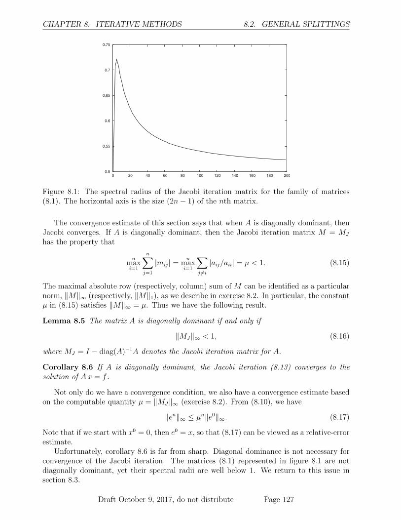
CHAPTER 8. ITERATIVE METHODS 8.2. GENERAL SPLITTINGS
0.5
0.55
0.6
0.65
0.7
0.75
0 20 40 60 80 100 120 140 160 180 200
Figure 8.1: The spectral radius of the Jacobi iteration matrix for the family of matrices(8.1). The horizontal axis is the size (2n− 1) of the nth matrix.
The convergence estimate of this section says that when A is diagonally dominant, thenJacobi converges. If A is diagonally dominant, then the Jacobi iteration matrix M = MJ
has the property that
nmaxi=1
n∑j=1
|mij| =n
maxi=1
∑j 6=i
|aij/aii| = µ < 1. (8.15)
The maximal absolute row (respectively, column) sum of M can be identified as a particularnorm, ‖M‖∞ (respectively, ‖M‖1), as we describe in exercise 8.2. In particular, the constantµ in (8.15) satisfies ‖M‖∞ = µ. Thus we have the following result.
Lemma 8.5 The matrix A is diagonally dominant if and only if
‖MJ‖∞ < 1, (8.16)
where MJ = I − diag(A)−1A denotes the Jacobi iteration matrix for A.
Corollary 8.6 If A is diagonally dominant, the Jacobi iteration (8.13) converges to thesolution of Ax = f .
Not only do we have a convergence condition, we also have a convergence estimate basedon the computable quantity µ = ‖MJ‖∞ (exercise 8.2). From (8.10), we have
‖en‖∞ ≤ µn‖e0‖∞. (8.17)
Note that if we start with x0 = 0, then e0 = x, so that (8.17) can be viewed as a relative-errorestimate.
Unfortunately, corollary 8.6 is far from sharp. Diagonal dominance is not necessary forconvergence of the Jacobi iteration. The matrices (8.1) represented in figure 8.1 are notdiagonally dominant, yet their spectral radii are well below 1. We return to this issue insection 8.3.
Draft October 9, 2017, do not distribute Page 127

8.2. GENERAL SPLITTINGS CHAPTER 8. ITERATIVE METHODS
8.2.2 Gauss-Seidel method
The easiest way to motivate the Gauss-Seidel algorithm4 is by considering the Jacobi algo-rithm at the element-by-element level:
xn+1i =
1
aii
(fi −
∑j 6=i
aijxnj
)(8.18)
for i = 1, . . . , n. Note that precomputations could be done to avoid the repeated divisions,but for n large, these do not add appreciably to the overall work.
If we write this using the assignment notation, it reads
yi ←1
aii
(fi −
∑j 6=i
aijxj
)∀i = 1, . . . , n, (8.19)
and once y has been computed, we update x: x← y. Consider the modified Jacobi algorithmdefined by
xi ←1
aii
(fi −
∑j 6=i
aijxj
)∀i = 1, . . . , n. (8.20)
For one thing, (8.20) avoids the need to keep a separate temporary vector y as needed in(8.19). Moreover, it has the heuristic benefit of using the most recent values of xj as soonas they are available. But to understand how it performs, we need to write it in differentnotation as
xn+1i =
1
aii
(fi −
i−1∑j=1
aijxn+1j −
n∑j=i+1
aijxnj
)(8.21)
for i = 1, . . . , n. We can write this as a system of equations for xn+1 as
i∑j=1
aijxn+1j = fi −
n∑j=i+1
aijxnj (8.22)
for i = 1, . . . , n. Now we can explain the algorithm (8.20) in terms of splitting. The system(8.22) corresponds to solving Nxn+1 = f + Pxn, where N is the lower-triangular part of Aand −P is the strictly upper-triangular part of A:
N =
a11 0 · · · 0a21 a22 · · · 0· · ·an1 an2 · · · ann
and − P =
0 a12 · · · a1n
0 0 · · · a2n
· · ·0 0 · · · 0
. (8.23)
The performance of Gauss-Seidel for the family of matrices in (8.1) is very similar tothat of Jacobi (exercise 8.6). On the other hand, for the family of matrices indicated in(4.20), the spectral radii of Jacobi and of Gauss-Seidel differ more substantially. In thiscase, ρ(MJ) ≈ 1 − cJn−2 and ρ(MGS) ≈ 1 − cGSn−2, where CGS = 2CJ and CJ ≈ 1.234.
4The relationship between the method described here and those considered by Gauss and Seidel is tenuous[65], but Gauss definitely advocated iterative methods of this type in a letter to a colleague in which he saidthe “procedure can be done while half asleep, or while thinking about other things” [64].
Draft October 9, 2017, do not distribute Page 128

CHAPTER 8. ITERATIVE METHODS 8.2. GENERAL SPLITTINGS
Since the error behaves like ρk after k iterations, as indicated in (8.17), we can estimate theperformance by considering the asymptotic behavior of
(1− ε)k = ek log(1−ε) ≈ e−εk. (8.24)
Thus we see that the error reduction with Jacobi for these matrices is about e−cJk/n2, and
for Gauss-Seidel it is about e−2cJk/n2
= (e−cJk/n2)2. This means that it takes twice as many
iterations for Jacobi to reduce the error as much as Gauss-Seidel does. Thus Gauss-Seidelshows a substantial performance improvement over Jacobi in this case, but both methodsrequire k = O(n2) to have substantial error reduction. In this case, the banded directmethods are vastly superior.
A result analogous to corollary 8.6 can be proved (exercise 8.7). But we now examinethe convergence properties of general splittings.
8.2.3 Convergence of general splittings
There are simple calculations that give a general criterion for the convergence of generalsplitting methods. This is useful in particular for establishing the convergence of Gauss-Seidel and of Jacobi for an important class of matrices. Although we are generally interestedin only real matrices, we will consider complex matrices for the moment to get a completecharacterization.
To begin with, we establish a simple estimate that reveals a key matrix that governs thesuccess of general splittings.
Lemma 8.7 Suppose the matrix A is Hermitian and that the splitting matrix N in (8.12)is nonsingular. Define the matrix
Q = N +N? − A. (8.25)
Then the subsequent iterations y = Mx = x−N−1Ax satisfy
y?Ay = x?Ax− (y − x)?Q(y − x). (8.26)
The expression√v?Bv forms a norm on v ∈ Cn under suitable conditions (exercise 8.8).
The interpretation of (8.26) is then that the norm of y is less than the norm of x (unlessy = x, in which case a fixed point has been reached).
Proof (of Lemma 8.7). We have Ny = Nx − Ax, so that N(y − x) = −Ax. Definee = y − x. Then e?Ne = −e?Ax, and by conjugating this expression, we also have
e?N?e = e?Ne = −e?Ax = −x?Ae.
Therefore,
(y − x)?Q(y − x) = e?(N +N? − A)e = −e?Ax− x?Ae− e?Ae= − e?Ax− (x+ e)?Ae = −e?Ax− y?Ae= − y?Ax+ x?Ax− y?Ay + y?Ax
=x?Ax− y?Ay. QED
(8.27)
Draft October 9, 2017, do not distribute Page 129

8.2. GENERAL SPLITTINGS CHAPTER 8. ITERATIVE METHODS
Lemma 8.8 Suppose that A is a Hermitian matrix and that the splitting matrix N in (8.12)is nonsingular. Suppose that the matrix Q defined in (8.25) is positive definite. Then thematrix M = I −N−1A satisfies ρ(M) < 1 if and only if A is positive definite.
Before proving the result, let us see why it is useful. For Gauss-Seidel, Q = diag(A),where diag(A) denotes the diagonal matrix whose diagonal is the same as the diagonal of A.When A is positive definite, diag(A) is always positive. Thus we have the following [142].
Corollary 8.9 Suppose that A is Hermitian with a positive diagonal. Then Gauss-Seidel isconvergent if and only if A is positive definite.
One simple corollary of this result is the following.
Theorem 8.10 Suppose that A is Hermitian and positive definite. Then Gauss-Seidel con-verges.
It appears that Gauss-Seidel provides a test for positive definiteness for a certain class ofmatrices (Hermitian with a positive diagonal). This is not surprising since iterations of thistype are closely linked to the power method for determining eigenvalues (section 15.1).
Proof (of Lemma 8.8). Suppose that Mx = λx. Then λx = x − N−1Ax, and so(1− λ)Nx = Ax. Thus
(1− λ)x?Nx = x?Ax. (8.28)
We are mainly interested in the “if” part of the theorem, so we start with that. Sosuppose that A is positive definite. Then x?Ax > 0 since x 6= 0. In particular, this showsthat x?Nx 6= 0 and λ 6= 1. Moreover,
1
1− λ=x?Nx
x?Ax. (8.29)
The complex conjugate of (8.29) is
1
1− λ=x?N?x
x?Ax. (8.30)
Adding (8.29) and (8.30), we find
2Re 1
1− λ=x?(N +N?)x
x?Ax=x?(A+Q)x
x?Ax= 1 +
x?Qx
x?Ax, (8.31)
where Re z is the real part of z. Because we have assumed Q is positive definite, the lastterm in (8.31) is positive, so (8.31) implies that
2Re 1
1− λ> 1. (8.32)
Using the relation 1/z = z/|z|2 for any complex z, we reduce (8.32) to
2Re (1− λ) > |1− λ|2. (8.33)
Draft October 9, 2017, do not distribute Page 130

CHAPTER 8. ITERATIVE METHODS8.3. NECESSARY CONDITIONS FOR CONVERGENCE
Writing λ = µ+ iν, (8.33) expands to give
2(1− µ) > |1− µ|2 + ν2 = 1− 2µ+ µ2 + ν2. (8.34)
But (8.34) is precisely the condition 1 > µ2 + ν2, i.e., |λ| < 1.For the “only if” case, we refer the reader to exercises 8.9 and 8.10. QED
For the Jacobi iteration, Q = 2 diag(A)−A, where diag(A) denotes the diagonal matrixwhose diagonal is the same as the diagonal of A. Suppose that A = I+B for some symmetricmatrix B. Then Q = I−B. Let the eigenvalues of B be denoted by λBi . Then the eigenvaluesof A are 1 + λBi , and those of Q are 1− λBi . Thus the condition for Jacobi to be convergentis that
minλBi > −1 (A > 0) and maxλBi < 1 (Q > 0). (8.35)
The Q-condition is clearly quite restrictive and indicates that diagonal dominance is quiteimportant for the success of the Jacobi method.
To give a concrete example, consider the matrix
A =
6 −4 1−4 6 −41 −4 6
, (8.36)
which has positive eigenvalues (and is thus positive definite). The eigenvalues of the corre-sponding Jacobi iteration matrix
MJ =1
6
0 4 −14 0 4−1 4 0
(8.37)
are 1/6 and (−1±√
129)/12. The eigenvalue (−1−√
129)/12 ≈ −1.03, and thus the Jacobiiteration is not convergent for the matrix A defined in (8.36).
8.3 Necessary conditions for convergence
In section 8.2.3, we proved some theorems establishing necessary and sufficient conditionsfor convergence of general splitting methods for a limited class of matrices. For more generalmatrices, only limited results are available. However, it is possible to establish a result thatprovides a converse to corollary 8.6. Moreover, it exposes some important structural featuresof the Jacobi iteration.
The main weakness in using the concept of diagonal dominance to characterize the Jacobiiteration is that it is not independent of scaling. Moreover, the Jacobi iteration itself isinvariant with respect to certain types of scaling. We can write the iteration matrix for theJacobi iteration for A as
MJ(A) = I − diag(A)−1A, (8.38)
where diag(A) denotes the diagonal matrix that agrees with A on the diagonal. Supposethat B is a diagonal matrix. Then Ax = f iff BAx = Bf , and
MJ(BA) = I − diag(BA)−1BA = I − diag(A)−1B−1BA = MJ(A) (8.39)
Draft October 9, 2017, do not distribute Page 131

8.3. NECESSARY CONDITIONS FOR CONVERGENCECHAPTER 8. ITERATIVE METHODS
since diag(BA) = B diag(A) (cf. exercise 8.12). Thus scaling by multiplication on the leftby a diagonal matrix does not change the convergence properties of Jacobi, and indeed thetwo methods generate the same sequence of iterates (exercise 8.14). And by lemma 8.5, Ais diagonally dominant iff BA is diagonally dominant. However, diagonal scaling by right-multiplication changes the concept of diagonal dominance substantially.
8.3.1 Generalized diagonal dominance
The notion of generalized diagonal dominance [92] captures the effect of scaling by right-multiplication. For any v ∈ Rn, define diag(v) to be the diagonal matrix such that diag(v)ii =vi. Note that
(A diag(v))ij = aijvj (8.40)
for all i, j. Let Rn+ denote the subset of Rn consisting of vectors with positive entries.
Definition 8.11 An n × n matrix A is said to satisfy generalized diagonal dominance (by
rows) if, for some positive scaling vector v ∈ Rn+, A = A diag(v) is diagonally dominant, that
is,
vi|aii| >∑j 6=i
vj|aij| (8.41)
for all i = 1, . . . , n.
Analogous to lemma 8.5, we have the following result.
Lemma 8.12 The matrix A satisfies generalized diagonal dominance iff for some positivescaling vector v ∈ Rn
+
‖I − diag(A)−1A‖∞ < 1, (8.42)
where A = A diag(v).
We saw that diagonal scaling of A on the left did not change the Jacobi iteration matrix.Scaling on the right changes it via a similarity transformation.
Lemma 8.13 Suppose that v ∈ Rn+ and A is any n×n matrix. Define A = A diag(v). Then
MJ(A) = diag(v)−1MJ(A)diag(v). (8.43)
Thus the Jacobi iteration (8.13) converges to the solution of Ax = f iff the Jacobi iteration
converges to the solution of Ay = g.
The proof of the latter statement could proceed by relating the iterates of the Jacobimethod for A and A. We leave this approach as exercise 8.15. Instead, we argue moreabstractly by exploiting the relationship (8.43) between their respective Jacobi iterationsmatrices.
Proof. By (8.40), we see that
diag(A diag(v)) = diag(A)diag(v). (8.44)
Draft October 9, 2017, do not distribute Page 132

CHAPTER 8. ITERATIVE METHODS8.3. NECESSARY CONDITIONS FOR CONVERGENCE
Therefore,
MJ(A diag(v)) = I − diag(A diag(v))−1A diag(v)
= I − diag(v)−1diag(A)−1A diag(v)
= diag(v)−1(I − diag(A)−1A
)diag(v)
= diag(v)−1MJ(A)diag(v).
(8.45)
Since (8.45) represents a similarity transformation,
ρ(MJ(A diag(v))) = ρ(MJ(A)) (8.46)
(exercise 6.10). Thus the Jacobi iteration for A converges iff the Jacobi iteration for Aconverges. QED
Analogous to corollary 8.6, we have the following result.
Corollary 8.14 If A satisfies generalized diagonal dominance, the Jacobi iteration (8.13)converges to the solution of Ax = f .
Proof. By lemma 8.13, theorem 6.2, and lemma 8.12,
ρ(MJ(A)) = ρ(MJ(A diag(v))) ≤ ‖MJ(A diag(v))‖∞ < 1. (8.47)
QED
Under certain conditions [92], generalized diagonal dominance provides a necessary con-dition for the convergence of Jacobi (and Gauss-Seidel). Rather than deriving conditions onA that are necessary for convergence, we take the point of view that the issue is to estimatethe spectral radius of the Jacobi iteration matrix more effectively. However, we will see thatthis leads to the same results.
8.3.2 Estimating the spectral radius
We know that the convergence of Jacobi depends precisely on the size of the spectral radiusρ(MJ). Thus what is needed is a better way to estimate ρ(MJ). We will do this in the casewhere MJ is nonnegative, as is the case with the families of matrices (4.20) and (8.1). Butfirst we establish an identity for a general matrix A.
For v ∈ Rn+, define a new norm on Rn by
‖x‖v = ‖diag(v)x‖∞ (8.48)
(cf. exercise 6.14). Note that (exercise 6.13)(diag(v)A diag(v)−1
)ij
=vivjaij (8.49)
Draft October 9, 2017, do not distribute Page 133

8.3. NECESSARY CONDITIONS FOR CONVERGENCECHAPTER 8. ITERATIVE METHODS
for any matrix A (exercise 8.17). Then the associated operator norm satisfies
‖A‖v = maxx 6=0
‖diag(v)Ax‖∞‖diag(v)x‖∞
= maxy 6=0
‖diag(v)A diag(v)−1y‖∞‖y‖∞
[y = diag(v)x]
= ‖diag(v)A diag(v)−1‖∞
= maxi=1,...,n
n∑j=1
vivj|aij|. [by (8.49) and exercise 8.2]
(8.50)
Note that by theorem 6.2,
ρ(A) ≤ infv∈Rn+‖A‖v. (8.51)
The following result says that we can effectively approximate the spectral radius using the∞-norm with the appropriate weight.
Lemma 8.15 Suppose that M is a nonnegative n×n matrix with a positive eigenpair λ > 0and x > 0, i.e., Mx = λx and x = (x1, . . . , xn) with xi > 0 for all i = 1, . . . , n. Then
ρ(M) = minv∈Rn+‖M‖v = ‖M‖w, (8.52)
where wi = 1/xi for all i = 1, . . . , n.
Proof. In view of (8.51), we just need to verify that ρ(M) = ‖M‖w. But by (8.50),
ρ(M) ≤ ‖M‖w = maxi=1,...,n
n∑j=1
xjxi|mij| = max
i=1,...,n
1
xi
n∑j=1
xjmij
= maxi=1,...,n
1
xiλxi = λ ≤ ρ(M).
(8.53)
QED
For the matrix in (8.1) for n = 50, figure 8.2 depicts the eigenvector corresponding to theeigenvalue λ = ρ(M) for the associated Jacobi iteration matrix. This depicts the weightingvector w in lemma 8.15 for this matrix.
The proof of lemma 8.15, and more precisely (8.53), leads to the following result, whichsays that the only positive eigenvalue associated with a positive eigenvector for a nonnegativematrix M is λ = ρ(M).
Corollary 8.16 Suppose that M is a nonnegative n × n matrix with a positive eigenpairλ > 0 and x > 0. Then λ = ρ(M).
Draft October 9, 2017, do not distribute Page 134

CHAPTER 8. ITERATIVE METHODS8.3. NECESSARY CONDITIONS FOR CONVERGENCE
0
0.05
0.1
0.15
0.2
0.25
0 10 20 30 40 50 60 70 80 90 100
Figure 8.2: The eigenvector of the Jacobi iteration matrix for the family of matrices (8.1)for n = 50. The horizontal axis is the index of the eigenvector.
8.3.3 Convergence conditions
If A is a matrix with positive diagonal and negative off-diagonal entries, then the Jacobiiteration matrix MJ(A) = I − diag(A)−1A is nonnegative. Thus if MJ(A) has a positiveeigenpair λ > 0 and x > 0, we conclude from lemma 8.15 that Jacobi converges only if‖MJ(A)‖w < 1, where wi = 1/xi for i = 1, . . . , n. We now show that this implies that Asatisfies generalized diagonal dominance. By (8.50), for all i = 1, . . . , n,
aiixi > aiixi
n∑j=1
xjximij = aiixi
n∑i 6=j=1
xjxi
|aij|aii
=n∑
i 6=j=1
xj|aij|. (8.54)
Thus we have proved the following result.
Theorem 8.17 Suppose A is a matrix with positive diagonal and negative off-diagonal en-tries and that the Jacobi iteration matrix
MJ(A) = I − diag(A)−1A
has a positive eigenpair λ > 0 and x > 0. If the Jacobi method for A is convergent, then Asatisfies generalized diagonal dominance (8.41) with v = x.
Fortunately, simple additional conditions are known that guarantee the existence of pos-itive eigenpairs for positive matrices, as we describe in the section 8.3.4. Thus theorem 8.17provides a broadly applicable converse to corollary 8.14.
8.3.4 Perron-Frobenius theorem
The Perron5-Frobenius6 theorem provides a sufficient condition to guarantee the existenceof the positive eigenpair appearing in lemma 8.15. The result holds for a nonnegative matrix
5Oskar Perron (1880–1975) was, like David Hilbert, Hermann Minkowski, Arnold J. W. Sommerfeld, andMartin Kutta (see page 294), a student of Lindemann, who was in turn a student of Felix Klein.
6See page 85.
Draft October 9, 2017, do not distribute Page 135

8.4. MORE READING CHAPTER 8. ITERATIVE METHODS
provided that it cannot be decomposed in a particular way.
Definition 8.18 An n× n matrix A is said to be reducible if the indices can be partitionedinto two sets
1, 2, . . . , n = i1, . . . , ik ∪ j1, . . . , jl, (8.55)
where n = k + l, with aiκ,jν = 0 for all κ = 1, . . . , k and ν = 1, . . . l. If no such partitionexists, A is said to be irreducible.
Theorem 8.19 Suppose that M is a nonnegative n × n irreducible matrix. Then it has apositive eigenpair λ > 0 and x > 0, i.e., Mx = λx and x = (x1, . . . , xn) with xi > 0 for alli = 1, . . . , n. Moreover, λ = ρ(M).
This theorem can be proved by considering the power method for computing eigenpairs,so we postpone it until chapter 14.
Note that the concept of reducibility relates only to off-diagonal elements of a matrix.Since indices of the nonzero off-diagonals of A and the Jacobi iteration matrix Mj(A) arethe same, we conclude that A is reducible iff MJ(A) is reducible. Thus we have the followingtheorem.
Theorem 8.20 Suppose that A is an n×n irreducible matrix that is positive on the diagonaland negative off-diagonal. Then the Jacobi iteration converges iff A satisfies generalizeddiagonal dominance.
8.4 More reading
For further information, see [13, 75, 177]. There are many variants and generalizationsof Jacobi and Gauss-Seidel iterations. In particular, parallel computation introduces newconstraints and leads to novel algorithms [151]. Algorithms have been proposed [109] todetermine whether a given matrix satisfies general diagonal dominance.
8.5 Exercises
Exercise 8.1 Prove lemma 8.2. (Hint: see the proof of lemma 8.1; note that xn = B(n)f .)
Exercise 8.2 Let B be an n× n matrix. Prove that the maximum absolute row sum can beidentified as
nmaxi=1
n∑j=1
|Bij| = ‖B‖∞ (8.56)
and that the maximum absolute column sum can be identified as
nmaxj=1
n∑i=1
|Bij| = ‖B‖1. (8.57)
Exercise 8.3 Consider the iteration matrix for the general splitting method M = I−N−1A,where N is any invertible matrix. Show that if λ = 1 is an eigenvalue of M , then A cannotbe invertible. (Hint: see the derivation of (8.28).)
Draft October 9, 2017, do not distribute Page 136

CHAPTER 8. ITERATIVE METHODS 8.5. EXERCISES
Exercise 8.4 Consider the iteration matrix for the general splitting method M = I−N−1A,where N is any invertible matrix. Show that if M is invertible and ρ(M) < 1, then successiveiterations y1 = My0 + b must satisfy y1 6= y0 unless y0 = x where x is the fixed pointx = Mx+ b. (Hint: consider successive errors ei = yi − x.)
Exercise 8.5 Consider the iteration matrix for the general splitting method M = I−N−1A,where N is any invertible matrix. Show that if M is invertible and ρ(M) < 1, then fixedpoint iteration cannot converge in a finite number of steps, unless we start with the exactfixed point as initial iterate. (Hint: consider successive errors ei = yi − x.)
Exercise 8.6 Compare the Jacobi iteration with the Gauss-Seidel iteration for the family ofmatrices in (8.1). Take for the right-hand side a vector F with all entries equal to 1, andtake for starting vector X0 = 0 in both cases. Compare the error for the two methods as afunction of the number of iterations. How does this change with the size of the matrices in(8.1) (that is, for different n)?
Exercise 8.7 Suppose that the Jacobi iteration matrix MJ = I−D−1A, where D = diag(A)is the diagonal matrix that agrees with A on the diagonal, satisfies ‖MJ‖∞ < 1. Prove thatGauss-Seidel converges, in particular, that ‖MGS‖∞ < 1. (Hint: at each iteration, wherey = MGSx, proceed by induction on i to show that |yi| ≤ ‖MJ‖∞‖x‖∞.)
Exercise 8.8 Prove that the expression ‖v‖B :=√v?Bv defines a norm on Cn provided that
B is Hermitian and positive definite. Compare this with exercise 6.14 and explain how thetwo results relate to each other.
Exercise 8.9 Suppose A, M , and Q are as in lemma 8.8 and that ρ(M) < 1. Show thatx?Ax ≥ 0 for all eigenvectors of M . (Hint: reverse the proof of the “if” case in lemma 8.8.)
Exercise 8.10 Suppose A, M , and Q are as in lemma 8.8 and that ρ(M) < 1. Prove thatA has to be positive definite. (Hint: Show that x?Ax ≤ 0 implies that y?Ay < 0, wherey = Mx, by using exercise 8.4. Show that all subsequent iterates w = Mnx for n > 1 satisfyw?Aw < y?Ay and hence that the w’s cannot tend to zero, yielding a contradiction.)
Exercise 8.11 Show that the matrix in (8.36) is positive definite. Compute the correspond-ing Jacobi iteration matrix and determine its eigenvalues. Show that one of them exceeds 1 inabsolute magnitude. Verify that the corresponding matrix Q, in the condition in lemma 8.8,is not positive definite.
Exercise 8.12 Suppose B is an n× n diagonal matrix. Show that for any n× n matrix A,
diag(BA) = B diag(A). (8.58)
Exercise 8.13 Suppose that A = I −M , where M is nonnegative and irreducible and sat-isfies diag(M) = 0. Prove that if the Jacobi iteration for solving Ax = f converges forany f and initial guess, then A has to satisfy generalized diagonal dominance. (Hint: usetheorem 8.19 to guarantee a positive eigenpair and see lemma 8.15 to define an appropriateweight as needed in definition 8.11.)
Draft October 9, 2017, do not distribute Page 137

8.5. EXERCISES CHAPTER 8. ITERATIVE METHODS
Exercise 8.14 Suppose B is an n× n diagonal matrix. Show that the Jacobi iterations forsolving Ax = f and BAx = Bf generate the same sequence of iterates xn.
Exercise 8.15 Suppose A is an n× n matrix and v ∈ Rn+. Show that the Jacobi iterations
for solving Ax = f and A diag(v)y = f generate sequences of iterates xn and yn related bydiag(A)yn = xn.
Exercise 8.16 Suppose that ‖M‖ < 1 for some norm. Prove that I −M is invertible and
‖(I −M)−1‖ ≤ 1
1− ‖M‖. (8.59)
(Hint: compare lemma 8.1.)
Exercise 8.17 Prove (8.49). (Hint: see exercise 6.13.)
Exercise 8.18 Show that the mapping z → 1/(1−z) maps the unit circle (minus one point)z = cos θ + i sin θ
∣∣ 0 < θ < 2π
to the linez = 1
2+ it
∣∣ t ∈ R. (8.60)
Exercise 8.19 Suppose that A is an n × n Hermitian matrix (A? = A) such that diag(A)has all positive entries. Show that if A is diagonally dominant, then A is positive definite.(Hint: apply exercise 8.7 and corollary 8.9.)
Exercise 8.20 Prove a converse to lemma 8.2. That is, suppose that the iteration (8.8)converges for any f and any starting vector. Prove that the spectral radius ρ(M) < 1.
Exercise 8.21 Consider an n × n matrix M with ρ(M) < 1, and suppose that M is notinvertible. Consider successive iterations y1 = My0 + b and the corresponding errors ei =yi−x with respect to the fixed point x = Mx+ b. Show that it is possible to have e1 = 0 withe0 6= 0, meaning that the iteration can terminate in a finite number of steps. What startingvector y0 is required in this case?
Exercise 8.22 Consider an n×n matrix M with ρ(M) < 1 and successive iterations xk+1 =Mxk + f , with x0 = 0 and f 6= 0. If we found xk ∈ kerM for some k > 1, then the sequencewould cycle: xlk+j = xj = f + · · · + M j−1f for all j = 1, . . . , k. Explain why this cannothappen unless xk = f for all k, i.e., f ∈ kerM . (Hint: prove that Mf = 0.)
Exercise 8.23 Consider an n×n matrix M that is nilpotent (see the proof of lemma 6.14).Consider successive iterations xk+1 = Mxk + b, with x0 = 0. Prove that the sequenceconverges in a finite number of steps.
Draft October 9, 2017, do not distribute Page 138

CHAPTER 8. ITERATIVE METHODS 8.6. SOLUTIONS
8.6 Solutions
Solution of Exercise 8.2. Define
µ =n
maxi=1
n∑j=1
|Bij|. (8.61)
Then for any x ∈ Rn and any i = 1, . . . , n,
|(Bx)i| =∣∣∣ n∑j=1
Bijxj
∣∣∣≤
n∑j=1
|Bij| |xj|
≤µ‖x‖∞.
(8.62)
Therefore, ‖Bx‖∞ ≤ µ‖x‖∞. Since x ∈ Rn was arbitrary, ‖B‖∞ ≤ µ.Pick i so that the ith absolute row sum equals µ, which we can assume is positive (if
µ = 0, the previous estimate shows that ‖B‖∞ = 0). Define xj = sign(Bij) for j = 1, . . . , n,where sign(t) is +1 if t > 0, −1 if t < 0, and 0 for t = 0. Then
(Bx)i =n∑j=1
Bijxj =n∑j=1
|Bij| = µ. (8.63)
Therefore, ‖Bx‖∞ ≥ µ, which incidentally shows that x 6= 0. Since ‖x‖∞ = 1, we have‖B‖∞ ≥ µ, as claimed.
Now define µ to be the maximum absolute column sum:
µ =n
maxj=1
n∑i=1
|Bij|. (8.64)
Then for any x ∈ Rn,
‖Bx‖1 =n∑i=1
|(Bx)i| =n∑i=1
∣∣∣ n∑j=1
Bijxj
∣∣∣≤
n∑i,j=1
|Bij| |xj| ≤ µ‖x‖1.
(8.65)
Since x ∈ Rn was arbitrary, ‖B‖1 ≤ µ.Pick j so that the jth absolute column sum equals µ, which we can assume is positive (if
µ = 0, the previous estimate shows that ‖B‖1 = 0). Define xi = δij for i = 1, . . . , n, whereδ is the Kronecker symbol. Then
(Bx)i =n∑k=1
Bikxk = Bij. (8.66)
Draft October 9, 2017, do not distribute Page 139

8.6. SOLUTIONS CHAPTER 8. ITERATIVE METHODS
Therefore, ‖Bx‖1 = µ. Since ‖x‖1 = 1, we have ‖B‖1 ≥ µ. Therefore, ‖B‖1 = µ, as claimed.
Solution of Exercise 8.9. Much of the “if” case argument is reversible. In particular, weshowed that |λ| < 1 if and only if 2Re (1−λ)−1 > 1. Moreover, as long as x?Ax is not zero,(8.31) is still valid, and so |λ| < 1 implies that
x?Qx
x?Ax= 2Re 1
1− λ− 1 > 0. (8.67)
This implies that x?Ax > 0.
Solution of Exercise 8.15. The sequence of iterates for the Jacobi method for solvingAx = f is
xn+1 = (I − diag(A)−1A)xn + g, (8.68)
where g = diag(A)−1f . The sequence of iterates for the Jacobi method for solving Ay = f is
yn+1 = (I − diag(A)−1A)yn + g, (8.69)
where g = diag(A)−1f . Then by (8.44),
diag(A)−1 = diag(v)−1 diag(A)−1,
so that
diag(v)yn+1 =(diag(v)− diag(A)−1A diag(v)
)yn + diag(v)g
=(I − diag(A)−1A
)diag(v)yn + g,
(8.70)
which agrees with (8.68) with xn = diag(v)yn.
Draft October 9, 2017, do not distribute Page 140

Chapter 9
Conjugate Gradients
In a letter to a colleague in 1824, Abel (see page 123) wrote “in analysisone is largely concerned with functions that can be represented by power-series. As soon as other functions enter—and this happens rarely—then[induction] does not work any more and an infinite number of incorrecttheorems arise from false conclusions” [106].
The conjugate gradient (CG) method was perceived for some time as a direct methodfor solving systems of linear equations. In exact arithmetic, the method produces the exactsolution in a finite number of steps. More precisely, for an n × n matrix, CG “converges”in at most n steps. The advantages of conjugate gradients as an iterative method were notwidely appreciated until much later. Not only does CG provide good approximate solutionswith fewer iterations than what is required to produce an exact result, it can also be seento be a more adaptive procedure than the stationary iterative methods studied previouslyin section 8.1.
We will develop the method in a sequence of steps to put it in context. It can be appliedto symmetric, positive definite matrices, so we will limit our discussion to linear systemswith such matrices.
9.1 Minimization methods
If A is an n × n symmetric, positive definite matrix, then there is a naturally associatedinner product
(u, v)A = uTAv (9.1)
defined for u, v ∈ Rn. As with any inner product, there is an associated norm (cf. exercise 8.8)
‖u‖A =√
(u, u)A . (9.2)
We will see that minimization algorithms can be viewed as an interplay between the innerproduct (u, v)A and the natural Euclidean inner product, which in this notation can bewritten
(u, v)I = uTv (9.3)
for u, v ∈ Rn. First, there is the obvious relationship (exercise 9.2)
(u, v)A = (Au, v)I = (u,Av)I . (9.4)
141

9.1. MINIMIZATION METHODS CHAPTER 9. CONJUGATE GRADIENTS
There is also a naturally associated quadratic function of v ∈ Rn defined by
QA(v)A = 12(v, v)A − (f, v)I (9.5)
defined for any f ∈ Rn. The relationship between these inner products is expressed in thefollowing lemma.
Lemma 9.1 The minimum of QA occurs at u ∈ Rn, which is the solution of the equation
Au = f. (9.6)
Proof. The proof for n = 1 is elementary (exercise 9.3). In general, we can reduce it to aone-dimensional problem by expanding, for u, v ∈ Rn and t ∈ R,
QA(u+ tv)A =QA(u) + t(u, v)A + 12t2(v, v)A − t(f, v)I
=QA(u) + t(uTA− fT)v + 12t2(v, v)A
=QA(u) + t(Au− f, v)I + 12t2(v, v)A,
(9.7)
where we used the symmetry of A in the last equality. Thus QA(u+tv)A = α+βt+γt2, whereβ = (Au− f)Tv = (Au− f, v)I . A quadratic q(t) = α+ βt+ γt2 with γ > 0 has a minimumat t = 0 iff β = 0 (exercise 9.5). Therefore, the minimum u of QA(u) is characterized by
(Au− f)Tv = 0 ∀v ∈ Rn. (9.8)
Setting v = Au − f , we conclude that (9.6) must hold if (9.8) holds, and the converse isobvious. QED
Thus a natural strategy to approximate the solution of Au = f is to minimize QA.
9.1.1 Descent methods
The geometry of the function (9.1) to be minimized is quite simple. When f = 0, the graphof QA is a simple elliptical bowl. When f 6= 0, the picture is tilted slightly. Thus a naturalapproach is to pick a search direction s 6= 0 in which QA is decreasing and proceed in thatdirection until you start to go up again. Suppose that u0 is our starting point. We searchfor the optimum along a line including the point u0 that is parallel to s; this part of thealgorithm is called a line search. This corresponds to minimizing the problem
QA(u0 + ts)A =QA(u0) + t(Au0 − f, s)I + 12t2(s, s)A (9.9)
in view of (9.7), where t is a scalar that measures the distance we have gone.
Definition 9.2 If u0 is the current approximation of the solution u of the equation Au− f ,then the residual r is defined by
r = Au0 − f. (9.10)
Draft October 9, 2017, do not distribute Page 142

CHAPTER 9. CONJUGATE GRADIENTS 9.1. MINIMIZATION METHODS
e + t s
e
s
0
Figure 9.1: The ellipse indicates points in the plane determined by s and e that have thesame norm. The solid line indicates the set of points ts for t ∈ R, and the dashed lineindicates the set of points e+ ts for t ∈ R.
The residual provides a way to monitor the approximation process. For example, if r = 0then Au0 = f , i.e., u0 = u. In general, we can define the error by
e = u0 − u, (9.11)
and we find that the error satisfies an equation with the residual as the right-hand side:
Ae = r. (9.12)
Thus e = A−1r is small if r is small (and A−1 is not too large).The minimum in (9.9) occurs where the derivative with respect to t is zero:
tmin = −(Au0 − f, s)I(s, s)A
= − (r, s)I(s, s)A
= −(Ae, s)I(s, s)A
= −(e, s)A(s, s)A
(9.13)
(cf. exercise 9.6 for the last step). Then the next position in our descent process will beu0 + tmins.
It is important to realize that line search really does search the entire line (in bothdirections), so that the search direction does not matter. That is, using s and −s give thesame result: the resulting product tmins, where tmin is defined in (9.13), is the same. If youchange the sign of s, you change the sign of tmin.
There is a geometric interpretation of the value of t in (9.13) (see figure 9.1). The valueof t is the length (in the norm ‖ · ‖A) of e in the direction s, with the sign of t indicatingwhether e correlates with plus or minus s. Note that we do not know u, and thus we do notknow e. Nevertheless, we can compute t (via the first or second equality) and find out thesize of e in the direction s. Consider minimizing
‖e+ ts‖2A = ‖e‖2
A + 2t(e, s)A + t2‖s‖2A (9.14)
over all t. Differentiating with respect to t and setting the result to zero, we find that t isgiven again by (9.13). Therefore, we have proved the following.
Lemma 9.3 Minimizing (9.9) is equivalent to minimizing (9.14). The minimum occurs atthe value of t given in (9.13).
Draft October 9, 2017, do not distribute Page 143

9.1. MINIMIZATION METHODS CHAPTER 9. CONJUGATE GRADIENTS
This can be visualized in figure 9.1. Remarkably, we are able to cause the maximumdecrease in the error (in the norm ‖ · ‖A) in the descent direction s by minimizing (9.9),even though we do not know e. An alternative interpretation is found in exercise 9.7, whichshows that
2QA(v) = (u− v, u− v)A − (u, u)A (9.15)
for all v ∈ Rn. That is, QA(v) differs from 12‖u− v‖2
A by a constant (12‖u‖2
A), so minimizingQA is equivalent to minimizing the error u− v in the A-norm.
At the minimum value given by (9.13), we find that (9.14) reduces to
‖e+ tmins‖2A = ‖e‖2
A −(e, s)2
A
‖s‖2A
= ‖e‖2A − t2min‖s‖2
A. (9.16)
Thus unless rTs = (r, s)I = (e, s)A = 0, the error is decreased at each step. In fact, (9.13)implies that the largest step, and thus the largest decrease in error, will occur if s = αr forsome scalar α.
9.1.2 Descent directions
Now we turn to the question of finding good descent directions. The best possible descentdirection would be the error e, but we do not know how to evaluate this. Instead, we canminimize QA; to do so, we compute the gradient ∇QA(u0) of the expression (9.5). Thisvector points in the direction of the maximum increase of QA(u0), so
s = −∇QA(u0) (9.17)
points in the direction of the greatest decrease.Computing the gradient of the quadratic QA is possible by calculus, but we can also infer
it from Taylor’s theorem:
QA(u0 + v) = QA(u0) +∇QA(u0) · v +O(v2). (9.18)
Comparing with the expansion (9.7), we find
∇QA(u0) = Au0 − f = r. (9.19)
Thus we see that (minus) the residual provides the direction of maximum descent, in concertwith the observation at the end of section 9.1.1 that s = αr provides the greatest errorreduction.
9.1.3 The gradient descent method
Suppose we decide to descend in the direction of the gradient at each step (so s = −r) andto proceed as far as the minimum at each step (so t = tmin). Since the notation gets denserat this point, we switch to denoting the scalar tmin by α. This corresponds to taking
rk =Auk − f
αk =(rk, rk)I(rk, rk)A
uk+1 =uk − αkrk.
(9.20)
Draft October 9, 2017, do not distribute Page 144

CHAPTER 9. CONJUGATE GRADIENTS 9.1. MINIMIZATION METHODS
−r0
ek
k
Figure 9.2: The ellipse indicates points in the plane determined by rk and uk that have thesame norm.
The error ek = uk − u at each step satisfies
ek+1 = uk+1 − u = uk − αkrk − u = ek − αkrk = (I − αkA)ek. (9.21)
The error ek = uk − u at each step is reduced, in view of (9.16), by
‖ek+1‖2A = ‖ek‖2
A −(rk, rk)
2I
‖rk‖2A
= ‖ek‖2A −
(rk, ek)2A
‖rk‖2A
. (9.22)
Although the gradient descent method makes the maximal reduction in QA, it is not thedirection that minimizes the error ek; that direction would be −ek. This sort of greedyalgorithm can be improved by an algorithm with a more global view. The difficulty canbe seen in figure 9.2. When the norm ‖ · ‖A is not very isotropic, the direction of greatestdescent for QA may not be the best global strategy for reducing the error.
9.1.4 Gradient-descent asymptotics
It is easy to see from (9.22) that, if the initial error e0 = u0−u = cv where c is any constantand v is as eigenvector of A, then gradient-descent converges in one step (exercise 9.24). Formore general initial errors, we can reason as follows. Expanding ek in terms of eigenvectorsvi of A, viz. ek =
∑ni=1 c
ki vi, we can write (Avi = λivi)
ek+1 =n∑i=1
cki (1− αkλi)vi, rk = Aek =n∑i=1
λicki vi, αk =
∑ni=1 λ
2i (c
ki )
2∑ni=1 λ
3i (c
ki )
2.
We can simplify the expression for αk as follows. Define
ωki = λ2i (c
ki )
2/
Ωk for all i = 1, . . . , n, where Ωk =n∑j=1
λ2j(c
kj )
2 = ‖Aek‖2.
Thus∑n
i=1 ωki = 1. Define λ
k=∑n
i=1 ωki λi. Then
αk =1∑n
i=1 ωki λi
=1
λk.
Thus we find
ck+1i = cki
(1− λi
λk
),
and we can derive a formula for the evolution of the ω’s:
ωk+1i =
(ck+1i λi
)2/Ωk+1 where Ωk+1 =
∑i
(ck+1i λi
)2.
Draft October 9, 2017, do not distribute Page 145

9.2. CONJUGATE GRADIENT ITERATIONCHAPTER 9. CONJUGATE GRADIENTS
Therefore
ωk+1i =
(cki
(1− λi
λk
)λi)2/Ωk+1 = ωki
(1− λi
λk
)2
(Ωk/Ωk+1).
As an example, let n = 2 and define ω01 = 1 − a, ω0
2 = a, where 0 < a < 1. Then
λ0
= (1− a)λ1 + aλ2 and for some constant C
ω1i = Cω0
i
(1− λi
(1− a)λ1 + aλ2
)2
= Cω0i
((1− a)λ1 + aλ2 − λi(1− a)λ1 + aλ2
)2
,
for i = 1, 2. Thus
ω11 = a2Cω0
1
( λ2 − λ1
(1− a)λ1 + aλ2
)2
= a2(1− a)C( λ2 − λ1
(1− a)λ1 + aλ2
)2
,
ω12 = (1− a)2Cω0
2
( λ2 − λ1
(1− a)λ1 + aλ2
)2
= a(1− a)2C( λ2 − λ1
(1− a)λ1 + aλ2
)2
=1− aa
ω11.
Recalling the constraint on the ω’s, we have
1 = ω11 + ω1
2 = ω11 +
1− aa
ω11 =
1
aω1
1.
Thus ω11 = a = ω0
2 and ω12 = 1 − a = ω0
1. By repeating the argument with a and 1 − areversed, we see that ωk+1
2 = ωk1 and ωk+11 = ωk2 for all k ≥ 1. In particular, ωk+2
i = ωki forall i = 1, 2, for all k ≥ 1. Therefore
c2k+1i = c1
i
( a2(1− a)2(λ2 − λ1)2
(aλ1 + (1− a)λ2)((1− a)λ1 + aλ2)
)k, i = 1, 2, (9.23)
for all k ≥ 1. Thus the convergence of gradient-descent is very similar to that of thestationery iterative methods, in that the error decreases geometrically. However, the rate isdata dependent: the initial error determines the value of a. Note that as a → 0 or a → 1,the rate of convergence goes to zero, consistent with the fact that for a = 0 or a = 1 weobtain convergence in one step (exercise 9.24). We leave as exercises 9.8, 9.9, and 9.10 todevelop further the convergence theory for gradient descent.
9.2 Conjugate Gradient iteration
The conjugate gradient method uses a more sophisticated choice for the search directionssk. Instead of just using the current residual (sk = −rk), the direction is chosen to beorthogonal (conjugate) to previous residuals. This avoids repeating previous mistakes, orrather it avoids repeating directions already traversed.
9.2.1 The basic iteration
We switch notation temporarily and consider solving Cy = g, where C is an n× n positivedefinite matrix. We define sequences yk, rk, sk ⊂ Rn × Rn × Rn and αk, βk ⊂ R× R asfollows. We assume that an initial approximation y0 is given, and we define
s0 = r0 = Cy0 − g. (9.24)
Draft October 9, 2017, do not distribute Page 146

CHAPTER 9. CONJUGATE GRADIENTS9.2. CONJUGATE GRADIENT ITERATION
k+1
k
k+1
s
r
s
Figure 9.3: Search directions and residuals in Conjugate Gradients. The choice of αk in(9.25) insures that rk+1 ⊥I sk, and the choice of βk in (9.29) insures that sk+1 ⊥C sk.
The main iteration steps proceed for k = 0, 1, 2, . . . by defining
αk = − (rk, sk)I(sk, sk)C
= −(rk, sk)I(sk, zk)I
(9.25)
yk+1 = yk + αksk, (9.26)
zk = Csk, (9.27)
rk+1 = Cyk+1 − g = rk + αkCsk = rk + αkzk, (9.28)
βk = −(rk+1, sk)C(sk, sk)C
= −(rk+1, zk)I(sk, zk)I
(9.29)
sk+1 = rk+1 + βksk. (9.30)
We can interpret these definitions as follows.
Equations (9.25) and (9.26) represent the descent method with direction sk.
Equation (9.27) can be viewed as just a definition, but it is also the only time in theiteration where the matrix C is applied to a vector. Thus it is the most computationallyintense step.
The first equation in (9.28) defines the residual in the usual way, and the second equationfollows because (9.26) implies that
rk+1 = Cyk+1 − g = C(yk + αksk)− g = rk + αkCsk. (9.31)
The third equation in (9.28) follows from (9.27).
Equations (9.29) and (9.30) define the new descent direction. The second equation in(9.29) follows from (9.27) and (9.4). Thus the conjugate gradient method is just a descentmethod in which the descent direction is derived from, but not equal to, the residual.
The choice of αk in (9.25) insures that rk+1 ⊥I sk. The choice of βk in (9.29) insuresthat sk+1 ⊥C sk. These orthogonalities are depicted only schematically in figure 9.3 sincethe geometry is different for the two orthogonalities. Here, a ⊥M b means (a, b)M = 0.
We have presented various forms for the coefficients αk and βk to indicate more efficientways to evaluate them. Note that only one matrix multiplication is required in (9.25)-(9.30),the evaluation of zk in (9.27). The different forms also simplify subsequent derivations. Wewill also derive other forms for these coefficients that can be used in alternate algorithms.
We will see that the convergence theory for the conjugate gradient method is quitesophisticated, but the derivation of these results takes some work. We begin with some basicorthogonality relations that are critical to the success of the CG method.
Draft October 9, 2017, do not distribute Page 147

9.2. CONJUGATE GRADIENT ITERATIONCHAPTER 9. CONJUGATE GRADIENTS
9.2.2 Orthogonality relations
There are three immediate orthogonality relations among the residuals and search directionsfor subsequent steps. Each of these has an important resulting equality and/or inequality.We develop all these in this section. We will ultimately see that other orthogonalities hold,but we will require a more complex induction to establish them.
Equations (9.29) and (9.30) say that the new search direction is based on the residual,modified so that it is orthogonal (with respect to the C-inner product) to the previous searchdirection:
(sk+1, sk)C = (rk+1 + βksk, sk)C = (rk+1, sk)C + βk(sk, sk)C = 0. (9.32)
Note that (9.30) and (9.32) imply that
‖sk+1‖2C = (sk+1, sk+1)C = (rk+1 + βksk, sk+1)C
= (rk+1, sk+1)C + βk(sk, sk+1)C
= (rk+1, sk+1)C ≤ ‖rk+1‖C‖sk+1‖C ,(9.33)
so that dividing by ‖sk+1‖C yields
‖sk+1‖C ≤ ‖rk+1‖C (9.34)
(if ‖sk+1‖C = 0, (9.34) holds trivially). We will see that a reverse inequality holds in adifferent norm.
The definition of αk ensures that the current residual is orthogonal in the Euclidean innerproduct to the previous search direction:
(rk+1, sk)I = (rk + αkCsk, sk)I [by (9.28)]
= (rk, sk)I + αk(sk, sk)C = 0 [by (9.4) and (9.25)].(9.35)
There is an immediate consequence of this orthogonality:
(rk, sk)I = ‖rk‖2I + (rk, sk − rk)I
= ‖rk‖2I + (rk, βk−1sk−1)I [by (9.30)]
= ‖rk‖2I [by (9.35)].
(9.36)
We should note that when k = 0, (9.36) holds trivially since r0 = s0 by definition. Therefore,we get a reverse inequality to (9.34) (see its proof for details):
‖sk‖I ≥ ‖rk‖I . (9.37)
The inequality (9.37) ensures that conjugate gradients can continue as long as rk 6= 0 sincethis implies that sk 6= 0. Once we have rk = 0, we are done.
Using the definitions of αk, rk, sk, and yk, find that (for k ≥ 1)
(rk+1, rk)I = (rk + αkCsk, rk)I [by (9.28)]
= ‖rk‖2I + αk(sk, rk)C [by (9.4)]
= ‖rk‖2I + αk(sk, sk − βk−1sk−1)C [by (9.30)]
= ‖rk‖2I + αk(sk, sk)C [by (9.32)]
= ‖rk‖2I − (rk, sk)I [by (9.25)]
= ‖rk‖2I − (rk, rk + βk−1sk−1)I [by (9.30)]
= βk−1(rk, sk−1)I = 0 [by (9.35)].
(9.38)
Draft October 9, 2017, do not distribute Page 148

CHAPTER 9. CONJUGATE GRADIENTS9.2. CONJUGATE GRADIENT ITERATION
From (9.35), we have 0 = (r1, s0)I = (r1, r0)I . Therefore,
(rk+1, rk)I = 0 ∀k ≥ 0. (9.39)
9.2.3 Further orthogonalities
Based on the three orthogonalities (9.32), (9.35), and (9.39) derived for subsequent iterations,we now derive some further orthogonalities among all iterates by induction.
Lemma 9.4 The conjugate gradient process (9.24)-(9.30) terminates at the kth step only ifrk = 0; i.e., if rk 6= 0, then sk 6= 0. Further, if rl 6= 0 for l = 0, . . . , k, then
0 = (rk+1, sq)I = (rk+1, rq)I = (sk+1, sq)C (9.40)
for 0 ≤ q ≤ k. The conjugate gradient process will terminate in at most n steps for an n×nmatrix C.
Proof. As we have noted, (9.37) ensures that the process will continue while rk 6= 0. Thefact that it will terminate after n steps is due to the orthogonality relations (9.40), whichcan hold for at most n nonzero vectors in Rn.
We have already verified the first three orthogonalities for k = 0. So we assume that thelemma holds for some value of k ≥ 0 and prove by induction that it also holds for k + 1.
We have already verified the three orthogonalities for q = k, so we may assume thatq < k. By (9.28),
(rk+1, sq)I = (rk, sq)I + αk(Csk, sq)I = 0, (9.41)
in view of (9.4) and the induction hypothesis. Also, by (9.28), (9.30), and the inductionhypothesis,
(rk+1, rq)I = (rk, rq)I + αk(Csk, rq)I
= (rk, rq)I + αk(Csk, sq
omit if q = 0︷ ︸︸ ︷−βq−1sq−1 )I
= 0 + αk(0− 0) = 0.
(9.42)
Similarly, by (9.30), (9.26), and (9.28),
(sk+1, Csq)I = (rk+1, Csq)I + βk
= 0︷ ︸︸ ︷(sk, Csq)I
= (rk+1,1
αq(yq+1 − yq))I
= (rk+1,1
αq(rq+1 − rq))I
= 0.
(9.43)
QED
Draft October 9, 2017, do not distribute Page 149

9.3. OPTIMAL APPROXIMATION OF CG CHAPTER 9. CONJUGATE GRADIENTS
Corollary 9.5 The search directions and residuals for conjugate gradients satisfy
0 = (sk+1, rq)C (9.44)
for 0 ≤ q ≤ k.
Proof. Again, by definition we have s0 = r0, so that
(s1, r0)C = (s1, s0)C = 0 (9.45)
since s0 = r0 by definition. So we assume that the lemma holds for some value of k ≥ 0 andprove by induction that it also holds for k + 1. For 0 ≤ q ≤ k, (9.30) implies that
(sk+1, rq)C = (sk+1, sq
omit if q = 0︷ ︸︸ ︷−βq−1sq−1 )C
= 0,
(9.46)
by (9.40). QED
9.2.4 New formulas for α and β
It is of interest to have different forms for the coefficients in CG as they tend to have differentbehaviors in floating-point computations because cancellations related to the orthogonalitiesin CG are avoided. Equation (9.36) implies that we can write αk as
αk = − ‖rk‖2I
‖sk‖2C
= − ‖rk‖2I
(sk, zk)I. (9.47)
Using the orthogonality (9.39), we can derive a new formula for βk:
βk = − (rk+1, sk)C(sk, sk)C
= −(rk+1, zk)I(sk, sk)C
[by (9.25)]
= − (rk+1, α−1k (rk+1 − rk))I(sk, sk)C
[by (9.28)]
= − (rk+1, rk+1)Iαk(sk, sk)C
[by (9.39)]
=(rk+1, rk+1)I
(rk, sk)I[by (9.25)]
=‖rk+1‖2
I
‖rk‖2I
[by (9.36)].
(9.48)
9.3 Optimal approximation of CG
Originally, we motivated conjugate gradients as an iterative method based on minimizing aquadratic form. We have seen that CG can also be viewed as a direct method, in that itis guaranteed to reduce the residual to zero in at most n steps for an n × n system. Nowwe change our point of view back to our original presentation of CG: as an approximationalgorithm. To do so, we need to develop some technology.
Draft October 9, 2017, do not distribute Page 150

CHAPTER 9. CONJUGATE GRADIENTS 9.3. OPTIMAL APPROXIMATION OF CG
9.3.1 Operator calculus
We have seen (exercise 6.1) that the set Pk of polynomials of degree k in one variable canbe viewed as a vector space of dimension k + 1. We will now see that there is a way to mapthis space to the linear space O(Rn,Rn) of operators on Rn (cf. section 6.1). Suppose wehave an n× n matrix C and consider the mapping v → Cv for all v ∈ Rn. Then this definessuch an operator in O(Rn,Rn), which we can also denote by C. Similarly, we can defineC2 by v → C(Cv) for all v ∈ Rn. In fact, for any integer k, Ck is defined inductively byv → C(Ck−1v). Thus for any polynomial P ∈ Pk, we can define P (C) by
P (C) =k∑i=0
aiCi, where P (x) =
k∑i=0
aixi. (9.49)
By convention, we define C0 = I, where I denotes the identity operator on Rn, associatedwith the n × n identity matrix. Thus (exercise 9.11) (9.49) defines a linear operator LC :Pk → O(Rn,Rn). Note that if P (x) ≡ 1 is the constant polynomial, then P (C) = I for anyC.
9.3.2 CG error representation
Recall that the residual rk = Cyk − g and the error ek = yk − y are related by rk = Cek.The next lemma relates the errors and search directions in CG to the initial error.
Lemma 9.6 For k ≥ 0, ek = Pk(C)e0 and sk = CQk(C)e0, where Pk and Qk are polynomi-als of degree at most k and Pk(0) = 1.
Proof. The proof is by induction. It is clear that P0 ≡ 1 and Q0 ≡ 1 work for k = 0 sinces0 = r0 = Ce0 by (9.12). For k ≥ 0 we have
ek+1 = ek + yk+1 − yk= ek + αksk [by (9.26)]
= (Pk(C) + αkCQk(C)) e0
=Pk+1(C)e0,
(9.50)
that is, Pk+1(x) := Pk(x) + αkxQk(x) (cf. exercise 9.12). Note that Pk+1(0) = Pk(0); hencePk+1(0) = 1. Similarly,
sk+1 =Cek+1 + βksk [by (9.30) and (9.12)]
= (CPk+1(C) + βkCQk(C)) e0
=CQk+1(C)e0,
(9.51)
that is, Qk+1(x) := Pk+1(x) + βkQk(x). QED
Lemma 9.7 Assuming that rk 6= 0, the set s0, . . . , sk of vectors defined in (9.30) spansthe Krylov1 subspace
Sk =v ∈ Rn
∣∣ v = CT (C)e0, T ∈ Pk. (9.52)
1Alexei Nikolaevich Krylov (1863–1945) first used this subspace in 1931 to transform characteristic poly-nomials [60]. He was very active in the theory and practice of shipbuilding and is commemorated by theKrylov Shipbuilding Research Institute.
Draft October 9, 2017, do not distribute Page 151

9.3. OPTIMAL APPROXIMATION OF CG CHAPTER 9. CONJUGATE GRADIENTS
Proof. First, we need to show that Sk is a vector space and that its dimension is k + 1. Bydefinition, Sk is a subset of Rn. If T1, T2 ∈ Pk, then set vi = CTi(C)e0, i = 1, 2. Expanding,we find
v1 + v2 =CT1(C)e0 + CT2(C)e0 = C(T1(C) + T2(C))e0
=C(T1 + T2)(C)e0 ∈ Sk,(9.53)
and similarly scalar multiples of v ∈ Sk are also in Sk. Thus Sk is a linear subspace of Rn
(cf. exercises 9.13 and 9.14).We can view Sk as the image of Pk in Rn via the mapping B defined by BT = CT (C)e0.
We have just shown that this mapping is linear. The image of a (k + 1)-dimensional spacecan be no more than k + 1, so we have shown that dimSk ≤ k + 1.
By lemma 9.6, each sl is in Sk for l = 0, . . . , k, and by (9.32) they are orthogonal (in theC-inner product). Hence they are a basis. QED
Lemma 9.8 DefineP0k =
P ∈ Pk
∣∣ P (0) = 1. (9.54)
The error ek is optimal in the sense that
‖ek‖C = min‖P (C)e0‖C
∣∣ P ∈ P0k
. (9.55)
Proof. Let Pk be the polynomial guaranteed by lemma 9.6. Since Pk ∈ P0k , we have
‖ek‖C ≥ inf‖P (C)e0‖C
∣∣ P ∈ P0k
because lemma 9.6 tells us that ek = Pk(C)e0. Now let
us prove the reverse inequality.Let P ∈ P0
k and define v = P (C)e0. Then
v = ek + (P − Pk)(C)e0. (9.56)
But since (P − Pk)(0) = 0, (P − Pk)(x) = xTk−1(x), where Tk−1 is a polynomial of degree≤ k − 1 (exercise 5.22). Hence
v = ek + δk, (9.57)
δk ∈ Sk−1. Now (ek, δk)C = (rk, δk)I = 0 since (rk, sq)I = 0 for all q < k. Thus
‖v‖2C = ‖ek‖2
C + 2(ek, δk)C + ‖δk‖2C
= ‖ek‖2C + ‖δk‖2
C ≥ ‖ek‖2C ,
(9.58)
which proves that ‖ek‖C ≤ inf‖P (C)e0‖C
∣∣ P ∈ P0k
and confirms the equality (9.55).
QED
9.3.3 Spectral theory
We now introduce a bit more technology from operator theory. Since we are working witha symmetric matrix C, we can expand in terms of its eigenvectors Xj, where CXj = λjXj.That is, for any v ∈ Rn, we can write
v =n∑j=1
ajXj. (9.59)
Draft October 9, 2017, do not distribute Page 152

CHAPTER 9. CONJUGATE GRADIENTS 9.3. OPTIMAL APPROXIMATION OF CG
Then Ckv =∑n
j=1 ajλkjXj, and indeed (exercise 9.15)
P (C)v =n∑j=1
ajP (λj)Xj (9.60)
for all P ∈ Pk. Note that we can choose the eigenvectors to be orthonormal:
(Xj, Xk)I = δjk, (9.61)
where δjk is the Kronecker δ. This means they are also orthogonal in the C-inner product:
(Xj, Xk)C = (CXj, Xk)I = (λjXj, Xk)I = λjδjk. (9.62)
Also, it follows for v of the form (9.59) that (exercise 9.16)
‖v‖2I =
n∑j=1
a2j and ‖v‖2
C =n∑j=1
λja2j . (9.63)
Therefore, by (9.60),
‖P (C)v‖2I =
n∑j=1
P (λj)2a2j and ‖P (C)v‖2
C =n∑j=1
P (λj)2λja
2j . (9.64)
Let us introduce the notation
‖P (λ(·))‖∞ = max|P (λj)|
∣∣ j = 1, . . . , n. (9.65)
Then from (9.63), we see that
‖P (C)v‖2C ≤ ‖P (λ(·))‖2
∞
n∑j=1
λja2j = ‖P (λ(·))‖2
∞‖v‖2C . (9.66)
The following result shows that error estimates for CG can be reduced to a polynomialapproximation result on the spectrum of C.
Theorem 9.9 Suppose that λ1, . . . , λn are the eigenvalues of C. Then
‖ek‖C ≤ inf‖P (λ(·))‖∞
∣∣ P ∈ P0k
‖e0‖C , (9.67)
where ‖P (λ(·))‖∞ is defined in (9.65) and P0k was defined in (9.54).
Proof. Apply (9.66) to lemma 9.8. QED
Draft October 9, 2017, do not distribute Page 153

9.3. OPTIMAL APPROXIMATION OF CG CHAPTER 9. CONJUGATE GRADIENTS
9.3.4 CG error estimates
There are many results that can be derived from theorem 9.9. Here we are able to give onlya sample.
Corollary 9.10 Suppose that there are only k distinct eigenvalues for C. Then the CGiteration terminates (in the absence of rounding error) in k steps.
Proof. The proof is an application of Lagrange interpolation (chapter 10). That is, we takeP to be a polynomial of degree k that is 1 at 0 and 0 at all eigenvalues:
P (0) = 1, P (λj) = 0, j = 1, . . . , k. (9.68)
The existence of P will be proved in section 10.2.1. (For example, if k = 1, we take P (x) =1− x/λ1.) Then P ∈ P0
k , and we conclude from theorem 9.9 that ek = 0. QED
Let us see what theorem 9.9 implies in a concrete case. Suppose there are only twoeigenvalues, λ1 < λ2. Let P (x) = 1−x/λ, where we will pick λ subsequently. Then P ∈ P0
1 ,and theorem 9.9 implies that
‖e1‖C ≤ max|1− λ1/λ|, |1− λ2/λ|‖e0‖C (9.69)
for all λ. Presumably, the minimum occurs when λ1 < λ < λ2, and
1− λ1/λ = −(1− λ2/λ), (9.70)
which implies that λ = 12(λ1 + λ2). Thus (cf. exercise 9.17)
‖e1‖C ≤(
1− 2λ1
λ1 + λ2
)‖e0‖C =
(λ2 − λ1
λ1 + λ2
)‖e0‖C . (9.71)
In general, we will prove the following result.
Lemma 9.11 Suppose that 0 < λ1 < λ2. Then there is a polynomial qk of degree k suchthat qk(0) = 1 and
‖qk‖∞,[λ1,λ2] ≤(
Λ +√
Λ2 − 1)−k
, (9.72)
where Λ = (λ1 + λ2)/(λ2 − λ1).
We postpone the proof of the lemma until section 11.1.2. We can write Λ = (κ+1)/(κ−1),where κ = λ2/λ1. By exercise 9.18, we then have
Λ +√
Λ2 − 1 =
√κ+ 1√κ− 1
. (9.73)
Thus we have the following result.
Corollary 9.12 Suppose that the eigenvalues of C lie in an interval [λ1, λ2], where 0 < λ1 <λ2. Define κ = λ2/λ1. Then
‖ek‖C ≤(√
κ− 1√κ+ 1
)k‖e0‖C =
(1− 2√
κ+ 1
)k‖e0‖C
≤ e−2k/(√κ+1)‖e0‖C .
(9.74)
Draft October 9, 2017, do not distribute Page 154

CHAPTER 9. CONJUGATE GRADIENTS 9.3. OPTIMAL APPROXIMATION OF CG
In the last inequality in (9.74), we used the fact that 1−x ≤ e−x for x ≥ 0 (exercise 9.19).If we set
λ1,2 = min,max|λ|∣∣ λ is an eigenvalue of A
,
then (6.10) and exercise 6.7 imply that (for A symmetric and positive definite)
κ = λ2/λ1 = ‖A‖2‖A−1‖2. (9.75)
The quantity κ is called the condition number of A with respect to the Euclidean norm.
9.3.5 Preconditioned Conjugate Gradient iteration
Suppose that we want to solveAx = b (9.76)
and that M−1 is an approximate inverse for A, that is, M is a symmetric positive definitematrix such that M−1A is close to the identity in some sense. Suppose there is a symmetricpositive definite matrix B such that B2 = M−1 (see exercise 9.20). We write B as M−1/2.Suppose that we apply CG to
C = M−1/2AM−1/2
(at least in our heads). ThenCy = g, (9.77)
where y = M1/2x and g = M−1/2b.Let x0 be given and take y0 = M1/2x0. Let the sequences yk, rk, αk, and βk be
defined by CG, as in (9.24)-(9.30). Let
xk =M−1/2yk,
σk =M−1/2sk,
ρk =M1/2rk.
(9.78)
Then the iteration can be cast in terms of these variables:
αk = − (M−1ρk, ρk)/(Aσk, σk),
xk+1 =xk + αkσk,
ρk+1 = ρk + αkAσk,
βk = (M−1ρk+1, ρk+1)/(M−1ρk, ρk),
σk+1 =M−1ρk+1 + βkσk.
(9.79)
The verification of these formulas involves not only (9.24)-(9.30) but also lemma 9.4.Note that the only additional work caused by the preconditioning is one application of
M−1 per iteration.If ek = yk − C−1g and εk = xk − A−1b, then
ek = M1/2xk −M1/2A−1M1/2b = M1/2εk
and
(Cek, ek) = ‖ek‖2C
= (M−1/2AM−1/2M1/2εk,M1/2εk)
= ‖εk‖2A.
This observation and the previous results on CG give the following theorem.
Draft October 9, 2017, do not distribute Page 155

9.4. COMPARING ITERATIVE SOLVERS CHAPTER 9. CONJUGATE GRADIENTS
Theorem 9.13 Suppose that
µ1,2 = min,max|λ|∣∣ λ is an eigenvalue of M−1A
and define κ = µ2/µ1. Then the error for the algorithm (9.78) and (9.79) satisfies
‖εk‖A ≤(√
κ− 1√κ+ 1
)k=
(1− 2√
κ+ 1
)k≤ e−2k/(
√κ+1).
9.4 Comparing iterative solvers
It is possible to compare the behavior of stationary iterative methods with that of conjugategradients. To simplify the analysis, let us assume that A is an n × n matrix with 1’s onthe the diagonal: diag(A) = I. Let us compare CG and Jacobi for A. First, note that theassumption diag(A) = I is not an essential restriction. Jacobi is invariant with respect toscaling (on the left) by a diagonal matrix, and we can then compare with the diagonallyscaled (preconditioned) CG.
We assume as well that A is symmetric and positive definite, so this means we can expandin eigenvectors as in (9.59). Let us write the initial error as
e0 =n∑i=1
aiXi. (9.80)
Combining (9.55) and (9.64), we see that the resulting CG error ekCG after k steps satisfies
‖ekCG‖2A ≤
n∑i=1
a2iPk(λi)
2λi. (9.81)
On the other hand, the error in Jacobi satisfies ekJ = MJ(A)ke0, where MJ(A) = I−A is theJacobi iteration matrix for A. The eigenvalues µi of MJ(A) are related to the eigenvaluesλi of A by µi = (1 − λi). Moreover, the eigenvectors of MJ(A) and A are the same. Inparticular, we have
ekJ =n∑i=1
(1− λi)kaiXi. (9.82)
Thus (9.63) implies that
‖ekJ‖2A =
n∑i=1
a2i (1− λi)2kλi. (9.83)
This corresponds to the choice P (λ) = (1− λ)k in (9.81). Thus we see that CG adapts thechoice of polynomial to the data, whereas for Jacobi it is fixed. Thus we see why the word“stationary” is appropriate for such iterative methods.
Draft October 9, 2017, do not distribute Page 156

CHAPTER 9. CONJUGATE GRADIENTS 9.5. MORE READING
9.5 More reading
The conjugate gradient method is attributed primarily to Hestenes2 and Stiefel3 althoughthere were additional influences [70], including Lanczos (see page 252) who was at UCLA atthe time [164]. There are several monographs on conjugate gradients and related methods[73, 123, 174]. The theory of convergence rates for CG has an intriguing relation to potentialtheory [55]. The CG algorithm applies as well to infinite-dimensional operators, and in somecases CG for such operators can have surprising convergence rates [182]. The role of CG andgradient descent in optimization is emphasized in [116].
9.6 Exercises
Exercise 9.1 Suppose that A is an n×n symmetric, positive definite matrix. Prove that theexpression (9.1) defines an inner product on Rn. In particular, verify that (u, v)A = (v, u)A.
Exercise 9.2 Suppose that A is an n× n symmetric, positive definite matrix. Prove (9.4).(Hint: use the symmetry of A.)
Exercise 9.3 Use calculus to verify that the minimum of the expression (9.5) occurs at thesolution of Au = f in the case n = 1. (Hint: just write out QA(u) and differentiate withrespect to u and find where the derivative is zero.)
Exercise 9.4 Verify all the steps in the derivation of the expression (9.7). (Hint: expandthe quadratic terms and use the symmetry of the inner product; cf. exercise 9.1 or 9.6).
Exercise 9.5 Suppose q(t) = α + βt + γt2. Prove that q(t) has a minimum at t = 0 iffβ = 0.
Exercise 9.6 Suppose that A is an n × n symmetric, positive definite matrix. Prove that(u, v)A = (Au)Tv for all u, v ∈ Rn. (Hint: use the symmetry of A.)
Exercise 9.7 Suppose that Au = f and that v ∈ Rn. Let r = Av− f and e = v−u (so thatAe = r). Prove that 2QA(v) = (e, e)A − (u, u)A.
Exercise 9.8 Suppose that A is a symmetric, positive definite matrix and that Au = f , anddefine E(v) = 1
2(v−u)
TA(v−u). Let the sequence of vectors uk be generated by the gradient
descent method (9.20). Prove that
E(uk+1) =
(1− (rk, rk)
2I
(rk, rk)A (rk, rk)A−1
)E(uk).
(Hint: see [116, Lemma 2, page 234].)
2Magnus Rudolph Hestenes (1906–1991) obtained a Ph.D. at the University of Chicago with Gilbert Blissin 1932. Bliss was an early graduate of Chicago, receiving a B.Sc. in 1897 and a Ph.D. in 1900 under thedirection of Oskar Bolza, who had studied with Felix Klein in Gottingen. Hestenes was a professor at UCLAfrom 1947 to 1973.
3Eduard L. Stiefel (1909–1978) was a student of Heinz Hopf, who was in turn a student of Erhard Schmidt.Stiefel was the advisor of Peter Henrici (page 305) as well as 63 other students over a period of 37 years.He is known for his work on the Stiefel-Whitney characteristic classes, and he was also an early user anddeveloper of computers [161].
Draft October 9, 2017, do not distribute Page 157

9.6. EXERCISES CHAPTER 9. CONJUGATE GRADIENTS
Exercise 9.9 Suppose that A is an n × n symmetric, positive definite matrix. Prove thatfor any vector x ∈ Rn
(x, x)2I
(x, x)A (x, x)A−1
≥ 4ab
(a+ b)2,
where a (resp., b) is the smallest (resp., largest) eigenvalue of A. (Hint: this is known asthe Kantorovich inequality.)
Exercise 9.10 Suppose that A is a symmetric, positive definite matrix and that Au = f ,and define E(v) = 1
2(v − u)
TA(v − u). Let the sequence of vectors uk be generated by the
gradient descent method (9.20). Prove that
E(uk+1) ≤(b− ab+ a
)2
E(uk) =
(1− a/b1 + a/b
)2
E(uk),
where a (resp., b) is the smallest (resp., largest) eigenvalue of A. Compare this with (9.23).(Hint: use exercises 9.8 and 9.9; see [116, Theorem 2, page 235].)
Exercise 9.11 Prove that the operator LC : Pk → O(Rn,Rn) defined by (9.49) is linear.That is, if P (x) =
∑ki=0 aix
i, Q(x) =∑k
i=0 bixi, and α ∈ R, then
LCP + αLCQ = LCR, (9.84)
where R is the polynomial given by R(x) =∑k
i=0 α(ai + bi)xi.
Exercise 9.12 Suppose that P is a polynomial given by P (x) =∑k
i=0 aixi and that C is an
n× n matrix. Prove that CP (C) = Q(C), where Q(x) =∑k
i=0 aixi+1.
Exercise 9.13 Suppose that M ⊂ O(Rn,Rn) is a linear subspace. Show that the setAv∣∣ A ∈M
is a linear subspace of Rn for any v ∈ Rn.
Exercise 9.14 Suppose that M ⊂ O(Rn,Rn) is a linear subspace and that B ∈ O(Rn,Rn).Prove that the set
BA
∣∣ A ∈M is a linear subspace of O(Rn,Rn).
Exercise 9.15 Verify (9.60). (Hint: Expand.)
Exercise 9.16 Verify (9.63). (Hint: Expand.)
Exercise 9.17 Suppose that λ1 > 0 and λ2 > 0. Prove that
argmin
max|1− λ1/λ|, |1− λ2/λ|∣∣ λ > 0
= 1
2(λ1 + λ2). (9.85)
(Hint: show that max|a|, |b| = 12|a+ b|+ 1
2|a− b| for a, b ∈ R.)
Exercise 9.18 Prove that (9.73) holds. (Hint: just expand and note that (√κ+1)(
√κ−1) =
κ− 1.)
Exercise 9.19 Prove that 1−x ≤ e−x for x ≥ 0. (Hint: expand e−x as an alternating seriesand note that 1− x represents the first two terms.)
Draft October 9, 2017, do not distribute Page 158

CHAPTER 9. CONJUGATE GRADIENTS 9.7. SOLUTIONS
Exercise 9.20 Prove that for any symmetric, positive definite matrix A, there is a sym-metric, positive definite matrix B such that B2 = A. (Hint: write A = UTDU , where U isorthogonal and D is diagonal with positive entries; cf. corollary 6.6 and set B = UT
√DU .)
Exercise 9.21 Prove theorem 9.13.
Exercise 9.22 Prove (9.37).
Exercise 9.23 Prove that a polynomial of degree n can have at most n roots, countingmultiplicity, unless it is identically zero. (Hint: use exercise 5.22 to represent the polynomialin terms of linear factors.)
Exercise 9.24 Suppose that the initial guess u0 in the gradient-descent method (9.20) hasthe property that u0 = u+cv where v is an eigenvector of A and c is any constant. Show thatu1 = u, that is, the gradient-descent method converges in one step. (Hint: we have Av = λv.First show that e0 = −cv and α0 = 1/λ. Then use (9.21).)
9.7 Solutions
Solution of Exercise 9.7. Recall that Au = f and e = v− u. We expand and use the factthat AT = A:
(e, e)A = (v − u, v − u)A = (v − u)TA(v − u)
= vTAv + uTAu− uTAv − vTAu
= vTAv + uTAu− uTAv − vTf
= vTAv + uTAu− (ATu)Tv − fTv
= vTAv + uTAu− (Au)Tv − fTv
= vTAv + uTAu− 2fTv
= 2QA(v) + uTAu.
(9.86)
Thus 2QA(v) = (e, e)A − uTAu.
Solution of Exercise 9.17. First, we show that
max|a|, |b| = 12|a+ b|+ 1
2|a− b| (9.87)
for a, b ∈ R. We can assume that |a| ≥ |b| without loss of generality since we can just renamethe variables if it is the other way around.
If a ≥ 0, then max|a|, |b| = a and a+ b ≥ 0 (since |b| ≤ a). Then
max|a|, |b| − 12|a+ b| = a− 1
2(a+ b) = 1
2(a− b) = 1
2|a− b|. (9.88)
The last equality also follows from the fact that |b| ≤ a.If a ≤ 0, then max|a|, |b| = −a and a+ b ≤ 0 and a− b ≤ 0 (since |b| ≤ −a). Then
max|a|, |b| − 12|a+ b| = −a+ 1
2(a+ b) = −1
2(a− b) = 1
2|a− b| (9.89)
as well. Thus we have completed the proof of (9.87).
Draft October 9, 2017, do not distribute Page 159

9.7. SOLUTIONS CHAPTER 9. CONJUGATE GRADIENTS
Now suppose that λ1 > 0 and λ2 > 0. Then
max|1− λ1/λ|, |1− λ2/λ| = |1− 12(λ1 + λ2)/λ|+ |1
2(λ1 − λ2)/λ|. (9.90)
Let us write r = 12(λ1 + λ2)/λ, so that λ = 1
2(λ1 + λ2)/r and
max|1− λ1/λ|, |1− λ2/λ| = |1− r|+ r|λ1 − λ2|λ1 + λ2
. (9.91)
Furthermore, our objective is now to show that
argmin
|1− r|+ r|λ1 − λ2|
λ1 + λ2
∣∣ r > 0
= 1. (9.92)
Define a function φ by
φ(r) = |1− r|+ r|λ1 − λ2|λ1 + λ2
. (9.93)
For r ≥ 1, φ(r) = r − 1 + r |λ1−λ2|λ1+λ2
is strictly increasing. For r ≤ 1, φ(r) = 1− r + r |λ1−λ2|λ1+λ2
isstrictly decreasing since
|λ1 − λ2| = maxλ1, λ2 −minλ1, λ2< maxλ1, λ2 ≤ λ1 + λ2
(9.94)
since both λi are positive. Thusargminφ(r) = 1. (9.95)
Draft October 9, 2017, do not distribute Page 160

Chapter 10
Polynomial Interpolation
The web site http://www.blackphoto.com/glossary/i.asp describes in-terpolation as “a technique used by digital cameras, scanners and print-ers to increase the size of an image in pixels by averaging the colour andbrightness values of surrounding pixels.”
The approximation of general functions by simple classes of functions has many applica-tions as well as theoretical implications. The uniform approximation of a general continuousfunction on an interval by polynomials (a theorem of Weierstrass1) is a fundamental resultthat casts light on the nature of both polynomials and continuous functions. In the era ofmodern computers, approximation via interpolation has emerged as a general paradigm forcomputing elementary functions as part of typical system software on current computers[110]. Probably one of the earliest applications of interpolation was simply to link scat-tered data to provide some sense of what a continuum representation might look like. Thephrase “connecting the dots” has become a common metaphor for problem solving, but thisis precisely what polynomial interpolation does.
One feature of the subject is that it introduces infinite-dimensional vector spaces in anatural way. Dealing with such spaces in a complete (pun intended) way is beyond the scopeof this book, but we hope that the ideas stimulate interest in further study of functionalanalysis. We start by considering approximation by polynomials in one dimension. Someof the technology we develop applies to other classes of approximating spaces, as well asmultivariate approximation.
10.1 Local approximation: Taylor’s theorem
Taylor’s theorem2 in calculus provides a polynomial approximation to a sufficiently smoothfunction:
Pn(x) =n∑k=0
f (k)(x0)
k!(x− x0)k. (10.1)
1Karl Theodor Wilhelm Weierstrass (1815–1897) was the only student of Christoph Gudermann, whowas, along with Friedrich Bessel, J. W. Richard Dedekind, Sophie Germain, and Georg Riemann, a studentof Gauss.
2This theorem appears to have been first discovered by Gregorie (see page 228) [171].
161

10.2. DISTRIBUTED APPROXIMATION: INTERPOLATIONCHAPTER 10. POLYNOMIAL INTERPOLATION
For x near x0, this yields an accurate approximation to the function f provided we have therequired data. Moreover, we have (exercise 7.4) a representation of the error:
f(x)− Pn(x) =(x− x0)n+1
n!
∫ 1
0
(1− s)nf (n+1)(x0 + s(x− x0)) ds . (10.2)
Thus we can say that f − Pn = O((x − x0)n+1) for x near x0, provided that f is smoothenough.
This is a very powerful, but local, result. Moreover, it requires knowing the values of high-order derivatives of f to construct Pn. We now consider a more distributed approximationand one that does not require derivatives, only the values of f .
10.2 Distributed approximation: interpolation
Suppose that we gather data fi associated with parameters xi and that we want to depictthese data as a function f(x) with the property that f(xi) = fi. This is clearly not awell-defined problem since there are many functions with this property. (To simplify thediscussion, we assume here that the xi’s are distinct, but also see exercise 12.12.) On theother hand, if we are restricted to the appropriate finite-dimensional space of functions, wecan potentially make the process well-posed. One simple approach is to interpolate the data,e.g., with polynomials.
The name of Lagrange3 is associated with the fact that a polynomial of degree n canbe determined uniquely to match arbitrary values fi at n + 1 distinct points xi, e.g., withi = 0, . . . , n. At the risk of further inflaming French-English relations, we point out thatNewton (see page 17) had solved this problem earlier in an adaptive way (section 10.2.3).
We begin by considering arbitrary (but distinct) interpolation points xi. In many data-fitting problems, there is little control on the spacing of the points, and in the application(9.68) the points are unknown. We will later consider specifying the points in a systematicway, but we will see that equally spaced points can be a bad choice. In chapter 11, weconsider a better choice.
10.2.1 Existence of interpolant
The existence of the Lagrange interpolant can be proved by constructing polynomials φi suchthat
φi(xj) = δij. (10.3)
Then the Lagrange interpolant is defined by
Lnf(x) =n∑i=0
fiφi. (10.4)
3Joseph-Louis Lagrange (1736–1813), born in Turin and baptized Giuseppe Lodovico Lagrangia, be-came a dominant figure in his adopted country France. Best known for his work in mechanics, essentiallyestablishing the variational calculus [104], his students included Poisson and Fourier. He is interred in thePantheon in Paris.
Draft October 9, 2017, do not distribute Page 162

CHAPTER 10. POLYNOMIAL INTERPOLATION10.2. DISTRIBUTED APPROXIMATION: INTERPOLATION
The magic perhaps is in the fact that one can write a formula for each φi:
φi(x) =
∏j 6=i(x− xj)∏j 6=i(xi − xj)
=
∏j 6=i(xj − x)∏j 6=i(xj − xi)
. (10.5)
Here the indices j in the products range over the set 0, 1, . . . , n. Each φi is a polynomialof degree n since it is presented as a product of n monomials. Also φi(xk) = 0 for k 6= isince one of the factors is (x − xk). Finally, φi(xi) = 1 because of the normalization. Thiscompletes the verification of (10.3).
The operator Ln defined in (10.4) maps the linear space Rn+1 to the space Pn of polyno-mials of degree n. The operator Ln is clearly linear, by construction. That is, if f ∈ Rn+1
and g ∈ Rn+1 are two sets of data, then Ln(f+g) = Lnf+Lng, and similarly Ln(sf) = sLnffor any scalar s.
The Lagrange interpolant can be extended to any continuous function f by
Lnf(x) =n∑i=0
f(xi)φi. (10.6)
The operator Ln is a projection, i.e.,
Lnq = q for all q ∈ Pn. (10.7)
To prove this, consider p = Lnq − q, which is also a polynomial of degree n such thatp(xi) = 0 for n + 1 points. By the fundamental theorem of algebra, a polynomial of degreen that vanishes at n + 1 distinct points must be identically zero (exercise 9.23). Therefore,Lnq = q. In fact, this approach can be used to show (exercise 12.19) the existence of theφi’s.
10.2.2 Error expression
The error in Lagrange interpolation vanishes at all the interpolation points, so we can assertthat the error is divisible by the function ωk defined by
ωk(x) =k−1∏i=0
(x− xi). (10.8)
It is possible to prove (exercise 10.1) that
f(x)− Lnf(x) =ωn+1(x)
(n+ 1)!f (n+1)(ξ(x)), (10.9)
where ξ(x) is just like the magic point in the pointwise remainder expression for Taylor’stheorem. This expression has limitations as a way to understand the error in Lagrangeinterpolation in general, but it is useful theoretically and motivates certain things we willderive independently.
It is easy to see in one important case that (10.9) is valid, namely, when p(x) = xn+1.Note that by expanding the expression (10.8), we find
ωn+1(x) = xn+1 + q(x) = p(x) + q(x), (10.10)
Draft October 9, 2017, do not distribute Page 163

10.2. DISTRIBUTED APPROXIMATION: INTERPOLATIONCHAPTER 10. POLYNOMIAL INTERPOLATION
where the degree of q is at most n. Thus p = ωn+1 − q. Because p− Lnp is a polynomial ofdegree n+ 1 that vanishes at the roots of ωn+1, we have p−Lnp = αωn+1 for some constantα. Thus
αωn+1 = p− Lnp = ωn+1 − q − Lnp, (10.11)
so that (1 − α)ωn+1 = q + Lnp is a polynomial of degree n. This can happen only if α = 1(and q = −Lnp). Thus we conclude that
p− Lnp = ωn+1, (10.12)
consistent with (10.9).
10.2.3 Newton’s divided differences
There is another approach to defining an interpolant that is associated with Newton (seepage 17) and thus predates Lagrange (see page 162). It proceeds inductively based on thenumber of interpolation points, and it could be viewed as an adaptive procedure in whichthe interpolant with n + 1 points is derived from the one with n points. This allows one toderive (and use) the nth-order interpolation and assess whether further points need to beadded.
Let f be fixed for the moment and let pn = Lnf . If n = 0, there is only one pointx0 and p0 is the constant function equal to f(x0). Now add another point x1 6= x0. Thenp1 = p0 + q1, where q1 is a linear polynomial. For p1 to interpolate f at x0, we must haveq1(x0) = 0, and thus q1(x) = a1(x− x0). For p1 to interpolate f at x1, we must have
f(x1) = f(x0) + a1(x1 − x0), (10.13)
so that the coefficient a1 must be
a1 =f(x1)− f(x0)
x1 − x0
=f(x0)− f(x1)
x0 − x1
. (10.14)
The coefficient a1 is what is known as a divided difference, i.e., a difference quotient ap-proximating the derivative of f near x0, x1. The standard notation for divided differencesis
f [x0, x1] =f(x1)− f(x0)
x1 − x0
. (10.15)
With this notation, we have p1 = p0+f [x0, x1](x−x0). If we define ω0 ≡ 1 and f [x0] = f(x0),then we can write
p1 = f [x0]ω0 + f [x0, x1]ω1(x), (10.16)
where ωk for k ≥ 0 is defined in (10.8).Lagrange interpolation was defined by exhibiting particular basis functions for polyno-
mials. The Newton approach can be viewed as one in which a different basis is chosen. It isnot hard to see that the error polynomials ωk defined in (10.8) form a basis for polynomials.The key observation is that they are linearly independent (exercise 10.4). Thus we can writeany polynomial p ∈ Pn as
p(x) =n∑i=0
aiωi(x), (10.17)
Draft October 9, 2017, do not distribute Page 164

CHAPTER 10. POLYNOMIAL INTERPOLATION10.2. DISTRIBUTED APPROXIMATION: INTERPOLATION
for suitable coefficients ai. Thus for any continuous function f , we define coefficients afi by
Lnf(x) =n∑i=0
afi ωi(x). (10.18)
Motivated by (10.16), we define
f [x0, x1, . . . , xi] = afi (10.19)
for i ≥ 0. Thus by definition we have the Newton divided difference form of (Lagrange)interpolation:
Lnf(x) =n∑k=0
f [x0, x1, . . . , xk]ωk(x). (10.20)
Divided differences are defined for any set of points x0, . . . , xn, and they obey rules similarto those of calculus. First, it is evident from (10.15) that f [x0, x1] = f [x1, x0]. But from thedefinition (10.19), we see that the order of the xi’s does not matter in general, that is,
f [x0, x1, . . . , xn] = f [xσ(0), xσ(1), . . . , xσ(n)] (10.21)
for any permutation σ of 0, 1, . . . , n, as we get the same interpolant independently of whatorder we use to introduce the points xi into the interpolation process.
It is useful to derive explicitly the expression of p2 in terms of second divided differences,but we leave this as exercise 10.5 and proceed to the general properties.
Theorem 10.1 For distinct points x0, . . . , xn, the nth coefficient of the Newton interpolation(10.20) defined by (10.19) satisfies
f [x0, x1, . . . , xn] =n∑k=0
f(xk)∏i 6=k(xk − xi)
, (10.22)
where f [x0] = f(x0) in the case of n = 0.
Note that (10.15) and (10.22) are consistent when n = 1.
Proof. We have two representations of the interpolant: (10.20) and (10.4). If we differentiatethese n times, we find
f [x0, x1, . . . , xn]ω(n)n (x) =
n∑i=0
f(xi)φ(n)i (x) (10.23)
since all the other terms in (10.20) vanish because ωk is a polynomial of degree k. Byinspection, we see that
φ(n)i (x) =
n!∏j 6=i(xi − xj)
(10.24)
because the leading-order term in the numerator in (10.5) is xn. Similarly, the leading-order
term in ωn(x) is also xn, so that ω(n)n ≡ n!. Plugging these values for the derivatives into
(10.23) completes the proof of the theorem. QED
Draft October 9, 2017, do not distribute Page 165

10.3. BEHAVIOR OF LAGRANGE INTERPOLATIONCHAPTER 10. POLYNOMIAL INTERPOLATION
Lemma 10.2 For distinct points x, x0, . . . , xn in an interval I,
f(x)− Lnf(x) = f [x0, x1, . . . , xn, x]ωn+1(x). (10.25)
Notice the similarity to Taylor’s theorem with a remainder. Both approximations arewritten in terms of a sequence of basis functions ((x − x0)k versus ωk(x)), and the errorterms are written in terms of the next basis functions in the sequence.
Proof. We think of x as an additional interpolation point and use (10.20) to write
Ln+1f(y) = Lnf(y) + f [x0, x1, . . . , xn, x]ωn+1(y). (10.26)
But since x is an interpolation point, we have Ln+1f(x) = f(x), so applying (10.26) withy = x completes the proof. QED
Corollary 10.3 For distinct points x0, . . . , xn in an interval I, there is a point ξ ∈ I satis-fying
f [x0, x1, . . . , xn] =f (n)(ξ)
n!, (10.27)
provided that f ∈ C(n)(I).
Proof. Apply (10.9) and lemma 10.2. QED
Further manipulation (exercise 10.7) of the indices in (10.22) shows that the nth divideddifference is a divided difference of divided differences of order n − 1, as described in thefollowing result.
Corollary 10.4 For distinct points x0, . . . , xn, the nth divided difference satisfies
f [x0, x1, . . . , xn] =f [xi]− f [xj]
j − i(10.28)
for any indices i 6= j, where xi = (x0, . . . , xi−1, xi+1, . . . , xn).
10.3 Behavior of Lagrange interpolation
We need to formalize a statement made about the definition of the Lagrange interpolationoperator. This requires some technology that extends what we have been doing with finite-dimensional vector spaces.
10.3.1 Norms in infinite-dimensional spaces
Initially, in (10.4) Lagrange interpolation was defined for f ∈ Rn+1, but then it was extendedin (10.6) to be defined for f ∈ C0, the space of continuous functions. This space is also avector space. Addition in C0 is defined by saying that
(f + g)(x) = f(x) + g(x) for all x, (10.29)
Draft October 9, 2017, do not distribute Page 166

CHAPTER 10. POLYNOMIAL INTERPOLATION10.3. BEHAVIOR OF LAGRANGE INTERPOLATION
and scalar multiplication is defined by
(sf)(x) = sf(x) for all x, (10.30)
for any scalar s. But C0 is an infinite-dimensional vector space. However, there is a naturalnorm defined on it, the maximum norm. To be more precise, for any closed interval I, wecan define
‖f‖∞ = supx∈I|f(x)|. (10.31)
We leave as exercise 10.8 the verification that this is indeed a norm.We can state a corollary to (10.9) using this notation as follows.
Theorem 10.5 For distinct points x0, . . . , xn in an interval I, the Newton-Lagrange inter-polation operator Ln using these points satisfies
‖f − Lnf‖∞ ≤1
(n+ 1)!‖f (n+1)‖∞‖ωn+1‖∞, (10.32)
where ωn+1(x) = (x− x0)(x− x1) · · · (x− xn).
10.3.2 Instability of Lagrange interpolation
Lagrange interpolation is more robust than Taylor approximation, but it has properties thatmake it sensitive to use in practice. In particular, the placement of the interpolation pointsis extremely influential regarding its performance. The main difficulty stems from a lack ofstability of the interpolation operator in the maximum norm for many choices of interpolationpoints.
For the moment, let us think of Lagrange interpolation as defining an operator Ln :C0(I) → Pn. If we take ‖ · ‖∞ as the norm for both of these spaces, we can define anoperator norm in the same way as we did in (6.1) in the finite-dimensional case:
‖Ln‖∞ = supf∈C0(I)
‖Lnf‖∞‖f‖∞
. (10.33)
In view of (6.2), we can think of ‖Ln‖∞ as the smallest constant C such that ‖Lnf‖∞ ≤C‖f‖∞. (See exercise 10.9 for a finite-dimensional interpretation of the norm defined in(10.33).)
We will see that ‖Ln‖∞ can be very large for typical choices of interpolation points.Suppose in this case that some small errors are made in the specification of the interpolationdata f . That is, suppose we apply interpolation to f + δ, where δ is small but somewhatarbitrary (e.g., due to round-off error). Since Ln is linear, the result is
Ln(f + δ) = Lnf + Lnδ. (10.34)
We can then assert that the error, which is equal to Lnδ, must be no larger than ‖Ln‖∞‖δ‖∞.But since we may have little control over δ, it could possibly be as large as ‖Ln‖∞‖δ‖∞.Thus ‖Ln‖∞ represents the error amplification factor.
Draft October 9, 2017, do not distribute Page 167

10.3. BEHAVIOR OF LAGRANGE INTERPOLATIONCHAPTER 10. POLYNOMIAL INTERPOLATION
–7
–6
–5
–4
–3
–2
–1
0
1
2
–1 –0.5 0 0.5 1
Figure 10.1: The Lagrange basis function φ5 for 11 equally spaced interpolation points onthe interval [−1, 1]. The circles indicate the interpolation data.
Let us estimate the size of ‖Ln‖∞. Since we can choose f in (10.33) arbitrarily, we canpick f to be 1 at the ith interpolation point and 0 at the others. In this case, Lnf = φi, thecorresponding basis function. Thus we conclude that
‖Ln‖∞ ≥ maxi=0,...,n
‖φi‖∞ . (10.35)
On the other hand, it is not hard (exercise 10.11) to show that
‖Ln‖∞ ≤n∑i=0
‖φi‖∞ . (10.36)
Thus we need to look carefully at the size of the Lagrange basis functions.Since the Lagrange basis functions are chosen to be 1 at one point and 0 at the others,
one might hope that the maximum of the basis functions will not be too big. In particular,it might be the case that the maximum occurs at the interpolation point where it is specifiedto be 1. But in general, this does not happen. A typical Lagrange basis function for equallyspaced interpolation points
xi = −1 + (i− 1)/k, i = 1, . . . , 2k + 1, (10.37)
is depicted in figure 10.1. For n = 2k + 1 equally spaced interpolation points on [−1, 1]as defined in (10.37), the largest norm appears to occur for φk (which is associated withthe interpolation point xk = −1/k), and its maximum appears to occur in the first interval[x1, x2] (see exercise 10.16). Computing the Lagrange basis functions for various values ofk and the maximum value φk in this interval yields lower bounds via (10.35), which growexponentially (see exercise 10.17). In particular, for k = 31, ‖L2k+1‖∞ exceeds 1016 (weexplain in section 11.3 how this operator norm can be computed with some confidence).This means that round-off errors in the data f could lead to order one errors in computingLnf for large n no matter how well-behaved f may be.
Draft October 9, 2017, do not distribute Page 168

CHAPTER 10. POLYNOMIAL INTERPOLATION10.3. BEHAVIOR OF LAGRANGE INTERPOLATION
0
0.1
0.2
0.3
0.4
0.5
0.6
0.7
0.8
0.9
1
–1 –0.5 0 0.5 1
Figure 10.2: The Runge function r3 (dashed line) and its Lagrange interpolant for 11 equallyspaced interpolation points on the interval [−1, 1]. The “+” signs indicate the interpolationdata.
10.3.3 Data-dependence of Lagrange interpolation
In addition to the inherent instability of Lagrange interpolation for large n, there are alsoclasses of functions that are not suitable for approximation by certain types of interpolation.There is a celebrated example of Runge4 [89] based on interpolating the function 1/(1 + x2)on various intervals. For simplicity, here we instead look at interpolating the function
rγ(x) = 1/(1 + (γx)2) (10.38)
on the fixed interval [−1, 1].The special feature of the Runge function rγ is that it has a singularity in the complex
plane at z = ±i/γ despite the fact that it is infinitely differentiable on the real line (wherethe interpolation is being done). As γ gets large, the singularity encroaches upon the domain[−1, 1] of approximation. For γ = 2, the maximum error
‖rγ − Lnrγ‖∞ (10.39)
slowly decreases as a function of n for uniformly spaced points (see table 10.1). However,for γ = 3, the error (10.39) increases; figure 10.2 depicts the error with n = 11. We againsee that the maximum error occurs in the first and last segments.
10.3.4 Runge versus Gauss
The behavior of Lagrange interpolation is mysterious. It is very sensitive to the distributionof higher derivatives of the function being interpolated as well as the distribution of the
4Carl David Tolme Runge (1856–1927) was a student of Weierstrass and Kummer, and he married theniece of Paul Du Bois-Reymond (see page 70). He was a close friend of, and student with, Max Planck, andhe was a teacher and mentor of Max Born.
Draft October 9, 2017, do not distribute Page 169

10.3. BEHAVIOR OF LAGRANGE INTERPOLATIONCHAPTER 10. POLYNOMIAL INTERPOLATION
γ n = 5 7 9 11 13 15 17 19 21√2 0.07 0.04 0.02 0.01 0.007 0.004 0.003 0.002 0.001
2 0.16 0.12 0.10 0.09 0.080 0.075 0.072 0.070 0.0683 0.30 0.32 0.38 0.50 0.67 0.94 1.3 1.9 2.7
Table 10.1: Errors ‖rγ − Lnrγ‖∞ in Lagrange interpolation Ln of the Runge function forvarious values of γ and polynomial order n.
function interpolated n = 15 17 19 21Runge 1/(1 + (3x)2) 0.937 1.32 1.89 2.73
Gaussian e−(3x)2 0.074 0.037 0.017 0.007
Table 10.2: Errors ‖f − Lnf‖∞ for Lagrange interpolation Ln of a function f , where f iseither the Runge function with γ = 3 or a Gaussian, as a function of the number n of equallyspaced interpolation points.
interpolation points. More precisely, we see from (10.25) and (10.27) that the quantitiesto focus on are f (k)/k! and the size of ωk. This is most evident for Lagrange interpolationon uniformly spaced points. In figure 10.3, we see the interpolant of the Runge function[10.37] together with the interpolant of a Gaussian. Superficially, the Runge function is thesmoother of the two: they have the same value and curvature at the origin, but the Gaussiandives toward zero much more rapidly. Nevertheless, the interpolation error is significantlysmaller for the Gaussian than for the Runge function once the number of interpolation pointsgets high enough.
The discrepancy has to do with the fact that the higher derivatives of the Gaussian growmore slowly than those of the Runge function. Indeed, Lagrange interpolation at a smallernumber of (uniformly spaced) points, as shown in figure 10.4 for 7 interpolation points, has alarger maximum error for the Gaussian (=0.381) than for the Runge function (=0.315). Forlarger numbers of points, Lagrange interpolation becomes sensitive to the higher derivativeswhich are not so easily visualized in a graph.
As shown in table 10.2, the interpolation increases for the Runge function but decreasesfor the Gaussian as the number of intepolation points is increased.
We can easily verify the relationship between the growth rates of the derivatives for theRunge function and a Gaussian. Let f(x) = r1(x) = 1/(1 + x2). Then the series
∞∑k=0
f (k)(0)
k!
diverges since f has a singularity in the complex plane at ±i. On the other hand, g(x) = e−x2
is an entire function, so∞∑k=0
g(k)(0)rk
k!<∞
for any finite value of r.
Draft October 9, 2017, do not distribute Page 170

CHAPTER 10. POLYNOMIAL INTERPOLATION10.3. BEHAVIOR OF LAGRANGE INTERPOLATION
Figure 10.3: Interpolation of the Runge function and a Gaussian at 15 uniformly spacedpoints. The maximum interpolation error is approximately 0.937 for the Runge function and0.0742 for the Gaussian.
Figure 10.4: Interpolation of the Runge function and a Gaussian at 7 uniformly spacedpoints. The maximum interpolation error is approximately 0.315 for the Runge function and0.381 for the Gaussian.
Draft October 9, 2017, do not distribute Page 171

10.4. MORE READING CHAPTER 10. POLYNOMIAL INTERPOLATION
10.4 More reading
Polynomial interpolation has been motivated by a variety of factors. With the advent ofmodern computing machines, the need to provide accurate approximations of various sorts[81, 117] includes interpolation [110] as a major technique.
The approach to the Newton form of interpolation was guided by [44], which should beconsulted for information about other types of interpolation as well.
We have shown that Lagrange interpolation requires some thought if we want to computestable approximations. See [86] regarding the influence of floating-point and stable ways ofcomputing Lagrange interpolants.
10.5 Exercises
Exercise 10.1 Prove (10.9). (Hint: explain why
f(x)− Lnf(x) = Cxωn+1(x), (10.40)
where Cx depends on x but will be held fixed for the calculations. Use Rolle’s theorem repeat-edly to show that the function
χ(y) = f(y)− Lnf(y)− Cxωn+1(y) (10.41)
has the property that χ(k) vanishes at n + 2− k distinct points in an interval containing allthe points x0, . . . , xn and x. Let ξ be the point where χ(n+1) vanishes.)
Exercise 10.2 Show that the Lagrange interpolation problem may be reduced to a linearsystem of equations with a Vandermonde matrix
1 x0 x20 · · · xn0
1 x1 x21 · · · xn1· · ·
1 xn x2n · · · xnn
. (10.42)
Prove that a Vandermonde matrix is invertible if and only if the xi’s are distinct. (Hint:represent polynomials in terms of the standard monomial basis functions xi.)
Exercise 10.3 Consider the determinant of a Vandermonde matrix
Vn(x0, . . . , xn) = det
1 x0 x2
0 · · · xn01 x1 x2
1 · · · xn1· · ·
1 xn x2n · · · xnn
. (10.43)
Show that V is a polynomial of degree 12n(n + 1) and that, for all 0 ≤ i < j ≤ n, xi − xj
divides Vn, that is, Vn(x0, . . . , xn) = (xi − xj)p(x0, . . . , xn) for some polynomial p. Use thisto show that
Vn(x0, . . . , xn) = C∏
0≤i<j≤n
(xi − xj)
for some constant C. (Hint: use exercise 10.2.)
Draft October 9, 2017, do not distribute Page 172

CHAPTER 10. POLYNOMIAL INTERPOLATION 10.5. EXERCISES
Exercise 10.4 Prove that the error polynomials ωn defined in (10.8) are linearly indepen-dent. (Hint: use induction. Note that you cannot have ωn =
∑n−1i=0 aiωi(x) because the
right-hand side is a polynomial only of degree n.)
Exercise 10.5 Derive the expression
p2(x) = f [x0] + f [x0, x1](x− x0) + f [x0, x1, x2](x− x0)(x− x1) (10.44)
following the approach used to construct the representation for p1.
Exercise 10.6 Suppose that f [x0, x1, x2] is defined as a divided difference of two first-orderdivided differences, e.g.,
f [x0, x1, x2] =f [x0, x2]− f [x0, x1]
x2 − x1
. (10.45)
Show thatf [x0, x1, x2] = f [xσ(0), xσ(1), xσ(2)] (10.46)
for any permutation σ of 0, 1, 2.
Exercise 10.7 Prove corollary 10.4. (Hint: use theorem 10.1 to show that
f [x0, x1, . . . , xn] =f [x1, . . . , xn]− f [x0, . . . , xn−1]
xn − x0
(10.47)
and then apply (10.21).)
Exercise 10.8 Show that ‖ ·‖∞ defined in (10.31) is a norm, that is, satisfies the properties(5.1)-(5.3).
Exercise 10.9 Show that the definition (10.33) yields the same number ‖Ln‖∞ if we replaceC0(I) by Rn+1 as the domain of Ln:
‖Ln‖∞ = supf∈Rn+1
‖Lnf‖∞‖f‖∞
, (10.48)
where we use the alternative interpretation Ln : Rn+1 → Pn defined in (10.4).
Exercise 10.10 Give an example of a function f such that Lnf = φi and has the requiredproperties that allow us to conclude the estimate (10.35).
Exercise 10.11 Prove (10.36).
Exercise 10.12 Prove that the determinant of a Vandermonde matrix as described in (10.42)satisfies
det
1 x0 x2
0 · · · xn01 x1 x2
1 · · · xn1· · ·
1 xn x2n · · · xnn
=∏
0≤i<j≤n
(xj − xi) (10.49)
and is thus invertible when all xi’s are distinct. (Hint: reduce this to a problem involvingLagrange interpolation by expanding the determinant along the last column.)
Draft October 9, 2017, do not distribute Page 173

10.5. EXERCISES CHAPTER 10. POLYNOMIAL INTERPOLATION
Exercise 10.13 Consider Lagrange interpolation Ln based on distinct interpolation pointsxi. Prove that, for any continuous function f ,
(Ln(xf)− xLnf) (x) = (−1)n+1f [x0, x1, . . . , xn]ωn(x). (10.50)
Here the commutator Ln(xf)−xLnf is defined as follows. We let g(x) = xf(x) and gn(x) =x(Lnf(x)). Then (Ln(xf)− xLnf) (x) = Lng(x)− gn.
Exercise 10.14 Determine a bound for the derivatives of the Runge function rγ defined in(10.38) as a function of n and γ. Use this in (10.9) to give an estimate for the error inLagrange interpolation.
Exercise 10.15 Suppose that f is a polynomial of degree n+ 1. Prove that
f [x0, x1, . . . , xn] =f (n+1)
(n+ 1)!, (10.51)
where we note that f (n+1) is a constant. (Hint: see corollary 10.3.)
Exercise 10.16 Let φi denote the ith basis function for Lagrange interpolation for n = 2k+1equally spaced interpolation points xi = −1 + (i− 1)/k on [−1, 1], i = 1, . . . , 2k + 1. Verifycomputationally that the largest norm occurs for φk associated with the interpolation pointxk = −1/k and that its maximum occurs in the first interval [x1, x2].
Exercise 10.17 Let φi denote the ith basis function for Lagrange interpolation for n = 2k+1equally spaced interpolation points xi = −1 + (i− 1)/k on [−1, 1], i = 1, . . . , 2k + 1. Verifycomputationally that
Mk = maxi=1,...,2k+1
‖φi‖∞ (10.52)
grows exponentially with k. In particular, verify that M63 > 1016. (Hint: plot (logMk)/k.)
Exercise 10.18 Verify table 10.1 computationally.
Exercise 10.19 Consider equally spaced points xi = i/n (i = 0, . . . , n) on [0, 1] and considerωn+1(x) =
∏ni=0(x − xi). Verify computationally that, for n odd, |ωn+1(1/2n)| ≈ e−an and
|ωn+1(1/2)| ≈ e−bn, where a ≈ 1.0 and b ≈ 1.7.
Exercise 10.20 Consider any distinct points x0, x1, . . . xn. Show that each Lagrange basisfunctions φi defined in (10.5) can be written as
φi(x) =ciωn+1(x)
x− xi(10.53)
for some constant ci, where ωn+1(x) = (x− x0)(x− x1) · · · (x− xn). What is ci?
Draft October 9, 2017, do not distribute Page 174

CHAPTER 10. POLYNOMIAL INTERPOLATION 10.6. SOLUTIONS
10.6 Solutions
Solution of Exercise 10.5.Suppose we add now x2 and try to determine p2 from p1 in the way that we determined
p1 from p0 and q1. Then we have p2 = p1 + q2, where q2 is quadratic and must vanish atx0, x1 (to avoid spoiling the interpolation at those points). Thus
q2(x) = a2(x− x0)(x− x1) = a2ω2, (10.54)
and the value of a2 will be determined by the requirement p2(x2) = f(x2):
f(x2) = f(x0) + f [x0, x1](x2 − x0) + a2(x2 − x0)(x2 − x1). (10.55)
Rearranging terms in (10.55), we find
f(x2)− f(x0) = (x2 − x0)(f [x0, x1] + a2(x2 − x1)), (10.56)
which says thatf [x2, x0] = f [x0, x1] + a2(x2 − x1). (10.57)
Thus we have found that
a2 =f [x2, x0]− f [x0, x1]
x2 − x1
. (10.58)
The result then follows from theorem 10.1.
Solution of Exercise 10.8. In the derivation of the properties of the norm, we have tocalculate the supremum of the set
|f(x)|
∣∣ x ∈ I for various functions f . By definition,‖f‖∞ ≥ 0 since it is the supremum of nonnegative numbers.
If ‖f‖∞ = 0, then f must be identically zero, since in this case we must have|f(x)|
∣∣ x ∈ I = 0. (10.59)
Now let f ∈ C0(I) be arbitrary, let s be any scalar, and let r = |s|. Note that
|f(x)| ≤ ‖f‖∞ ∀x ∈ I. (10.60)
Then|sf(x)| = r|f(x)| ≤ r‖f‖∞ (10.61)
for all x ∈ I. So r‖f‖∞ is an upper bound for|sf(x)|
∣∣ x ∈ I. Thus
‖sf‖∞ = sup|sf(x)|
∣∣ x ∈ I ≤ r‖f‖∞. (10.62)
If r = 0, then (10.62) implies that
‖sf‖∞ = 0 = |s| ‖f‖∞. (10.63)
So now suppose r > 0. If b is an upper bound for|sf(x)|
∣∣ x ∈ I, then
r|f(x)| = |sf(x)| ≤ b (10.64)
Draft October 9, 2017, do not distribute Page 175

10.6. SOLUTIONS CHAPTER 10. POLYNOMIAL INTERPOLATION
for all x ∈ I. Then |f(x)| ≤ b/r for all x ∈ I. Hence
‖f‖∞ = sup|f(x)|
∣∣ x ∈ I ≤ b/r. (10.65)
Since this holds for all b, we find
r‖f‖∞ ≤ sup|sf(x)|
∣∣ x ∈ I = ‖sf‖∞. (10.66)
Combining (10.66) and (10.62), we conclude that |s| ‖f‖∞ = ‖sf‖∞.Now let us address the triangle inequality. By (10.60), we have
|(f + g)(x)| = |f(x) + g(x)|≤ |f(x)|+ |g(x)| ≤ ‖f‖∞ + ‖g‖∞ ∀x ∈ I.
(10.67)
That is, ‖f‖∞ + ‖g‖∞ is an upper bound for|(f + g)(x)|
∣∣ x ∈ I. Thus
‖f + g‖∞ = sup|(f + g)(x)|
∣∣ x ∈ I ≤ ‖f‖∞ + ‖g‖∞. (10.68)
Solution of Exercise 10.12. For n = 1, we have
det
(1 x0
1 x1
)= x1 − x0 =
∏0≤i<j≤1
(xj − xi), (10.69)
so we may proceed by induction. For x ∈ Rn+1, define dn(x) via
dn(x0, x1, . . . , xn) =∏
0≤i<j≤n
(xj − xi). (10.70)
Expanding the Vandermonde determinant around the last column, we have by inductionthat
(−1)n det
1 x0 x2
0 · · · xn01 x1 x2
1 · · · xn1...
......
......
1 xn x2n · · · xnn
=
xn0dn−1(x1, x2, . . . , xn)−xn1dn−1(x0, x2, . . . , xn) +
...(−1)nxnndn−1(x0, x1, . . . , xn−1)
=n∑k=0
(−1)kxnkdn−1(x(k)),
(10.71)
where x(k) denotes the point in Rn obtained by deleting the kth coordinate of x ∈ Rn+1.Expanding the expression (10.70), we find
dn(x0, x1, . . . , xn) = dn−1(x(k))∏
0≤j<k
(xk − xj)∏
k<j≤n
(xj − xk). (10.72)
Therefore,
dn−1(x(k)) =dn(x0, x1, . . . , xn)
(−1)k∏
0≤j≤n, j 6=k(xj − xk). (10.73)
Draft October 9, 2017, do not distribute Page 176

CHAPTER 10. POLYNOMIAL INTERPOLATION 10.6. SOLUTIONS
Thus (10.71) becomes
(−1)n det
1 x0 x2
0 · · · xn01 x1 x2
1 · · · xn1· · ·
1 xn x2n · · · xnn
= dn(x0, x1, . . . , xn)
n∑k=0
xnk∏0≤j≤n, j 6=k(xj − xk)
.
(10.74)
Thus we have reduced the problem to prove the (unlikely looking) expression
(−1)n =n∑k=0
xnk∏0≤j≤n, j 6=k(xj − xk)
. (10.75)
The denominator of this expression is the same as in the Lagrange interpolation basis func-tions, so we can write
n∑k=0
xnk∏0≤j≤n, j 6=k(xj − xk)
=n∑k=0
xnkφk(x)∏0≤j≤n, j 6=k(xj − x)
= (−1)nn∑k=0
xnkφk(x)∏0≤j≤n, j 6=k(x− xj)
= (−1)nn∑k=0
xnkφk(x)(x− xk)∏0≤j≤n(x− xj)
= (−1)nωn+1(x)−1
n∑k=0
xnkφk(x)(x− xk)
(10.76)
for any x 6= xj for all j = 0, . . . , n, by (10.8). Let p(x) = xn+1 and q(x) = xn. Then
n∑k=0
xnkφk(x)(x− xk) =x
(n∑k=0
xnkφk(x)
)−
(n∑k=0
xn+1k φk(x)
)=xLnq(x)− Lnp(x) = xq(x)− Lnp(x)
= p(x)− Lnp(x) = ωn+1(x),
(10.77)
as required. Note that (10.75) implies that
(−1)n =n∑k=0
xnk∏0≤j≤n, j 6=k(xj − xk)
=n∑k=0
1∏0≤j≤n, j 6=k
(xjxk− 1)
=n∑k=0
∏0≤j≤n, j 6=k
(xjxk− 1
)−1
.
(10.78)
Solution of Exercise 10.13. Using the definition of the Lagrange interpolation basis
Draft October 9, 2017, do not distribute Page 177

10.6. SOLUTIONS CHAPTER 10. POLYNOMIAL INTERPOLATION
functions,
f [x0, x1, . . . , xn] =n∑k=0
f(xk)∏j 6=k(xj − xk)
=n∑k=0
f(xk)φk(x)(xk − x)∏nj=0(xj − x)
= (−1)n+1ωn+1(x)−1
n∑k=0
f(xk)φk(x)(xk − x)
= (−1)n+1ωn+1(x)−1 (Ln(xf)− xLnf) (x)
(10.79)
for any x 6= xj for all j. This proves the result for x 6= xj; for x = xj, the result is truebecause
xjLnf(xj) = xjf(xj) = Ln(xf)(xj). (10.80)
Draft October 9, 2017, do not distribute Page 178

Chapter 11
Chebyshev and Hermite Interpolation
“This is a mathematical textbook rather than a compendium of com-putational rules. It is hoped that the material included will provide auseful background for those seeking to devise and evaluate routines fornumerical computation.” (Alston S. Householder in [87])
For equally spaced points, two examples have suggested that bad things happen at theends of the interpolation interval: the basis functions are large there, and the approximationof the Runge function (10.38) can be as well. Also, the size of the error function ωk definedin (10.8) is relatively larger (exercises 10.19 and 11.1) at the ends of the interval. TheChebyshev1 points are a special set of Lagrange interpolation points that cluster at the endsof the interval:
xj = xj,n = − cos
(π(2j + 1)
2(n+ 1)
)= cos
(π(2(n− j) + 1)
2(n+ 1)
)(11.1)
for j = 0, 1, . . . , n (for interpolation on [−1, 1]). We include the extra subscript xj,n to beprecise, as we will compare error terms for different values of n. The key feature is thatthese points are clustered around the ends of the interval: x1− x0 = O(n−2), whereas in themiddle of the interval, the spacing is O(n−1).
We will also consider more general forms of interpolation involving derivative and otherinformation in addition to function values.
1Pafnuty Lvovich Chebyshev (1821–1894) “was probably the first mathematician to recognize the generalconcept of orthogonal polynomials” [146]. His students included Andrei Andreyevich Markov and AleksandrMikhailovich Lyapunov.
function interpolated n = 7 11 15Runge 1/(1 + (3x)2) 0.096 0.027 0.0074
Gaussian e−(3x)2 0.110 0.014 0.0010
Table 11.1: Errors ‖f − Lnf‖∞ for Lagrange interpolation Ln of a function f , where f iseither the Runge function for γ = 3 or a Gaussian, as a function of number n of Chebyshebinterpolation points.
179

11.1. CHEBYSHEV INTERPOLATIONCHAPTER 11. CHEBYSHEV AND HERMITE INTERPOLATION
Figure 11.1: Interpolation of the Runge function and a Gaussian at 7 Chebyshev points.The maximum interpolation error is reduced at the expense of a larger error in the middleof the interval; compare figure 10.4.
11.1 Chebyshev interpolation
By Chebyshev interpolation, we simply mean Lagrange interpolation at the Chebyshev points(11.1). We can compare Lagrange interpolation for the Runge function and a Gaussian atChebyshev points, as shown in figure 11.1. For a modest number of interpolation points, thepicture is not much different from what we saw with equally spaced points in figure 10.4.The maximum interpolation error is reduced, but at the expense of a larger error in themiddle of the interval. However, for larger numbers of points, the maximum error decreasesfor both functions, as indicated in table 11.1. For example, figure 11.2 shows very smallerror for 15 points.
11.1.1 Error term ω
There is a simple interpretation of the Chebyshev points in terms of the error function ωn+1
defined in (10.8), as follows.
Theorem 11.1 With the Chebyshev interpolation points (11.1), the error function ωn+1
defined in (10.8) for Lagrange interpolation satisfies
ωn+1(x) =
2−n cos((n+ 1) cos−1 x) ∀x ∈ [−1, 1]
2−n−1((x+√x2 − 1
)n+1+(x−√x2 − 1
)n+1)∀x ∈ R.
(11.2)
Moreover, the following three-term recursion relation holds:
ωn+1(x) = xωn(x)− 14ωn−1(x), (11.3)
where ωn+1−i(x) =∏n−i
j=0(x− xj,n−i) for i = 0, 1, 2 and xj,n is defined in (11.1).
Draft October 9, 2017, do not distribute Page 180

CHAPTER 11. CHEBYSHEV AND HERMITE INTERPOLATION11.1. CHEBYSHEV INTERPOLATION
Figure 11.2: Interpolation of the Runge function and a Gaussian at 15 Chebyshev points.The maximum interpolation error is very small in the eye-ball norm for both functions;compare figure 10.3.
Proof. The function cos((n+ 1) cos−1 x) has the right roots:
cos((n+ 1) cos−1 xj) = cos((π/2)(2(n− j) + 1)) = 0 (11.4)
since 2(n− j) + 1 = 1, 3, 5, . . . . It is somewhat remarkable that
cos((n+ 1) cos−1 x)
is a polynomial in x, of degree n + 1, but let us suppose for the moment that it is true(cf. exercise 11.2). Since cos((n + 1) cos−1 x) and ωn+1(x) have the same roots, they are aconstant multiple of each other.
It is also surprising that square-roots appear in (11.2) in a representation of a polyno-mial. But for n = 0, the two square-root terms cancel, giving ω1(x) = x, as required. Alsodisconcerting is the fact that, for |x| < 1, the square-roots are complex numbers. How-ever, expanding the terms in the second representation in (11.2) via the binomial theorem(exercise 11.3) shows that all the square-root terms cancel, leaving only polynomial terms:(
x+√x2 − 1
)k+(x−√x2 − 1
)k= 2
∑0≤j≤k/2
(k2j
)(x2 − 1)jxk−2j. (11.5)
Thus if we can identify the two expressions in (11.2), then we have shown that the cosineexpression is a polynomial in x.
We use some facts about complex variables, namely, that
(cos θ + i sin θ)k =(eiθ)k
= eikθ = cos kθ + i sin kθ, (11.6)
where i =√−1. The equality of the leftmost and rightmost terms in (11.6) is known as
a theorem of De Moivre, which was used by Euler2 to prove the equalities involving the
2Leonhard Euler (1707–1783) lived in the same period as Benjamin Franklin (1706–1790) [130] and wassaid by Laplace to be “the master of us all” [56].
Draft October 9, 2017, do not distribute Page 181

11.1. CHEBYSHEV INTERPOLATIONCHAPTER 11. CHEBYSHEV AND HERMITE INTERPOLATION
complex exponential and trigonometric functions [56]. For |x| ≤ 1, write x = cos t. Then
x±√x2 − 1 = cos t± i
√1− x2 = cos t± i sin t = e±it. (11.7)
Combining (11.7) with (11.6), we find(x+√x2 − 1
)k+(x−√x2 − 1
)k= eikt + e−ikt = 2 cos kt, (11.8)
which confirms that the two expressions in (11.2) are the same for |x| ≤ 1.The expression (11.2) shows that the leading term of cos((n + 1)t) is 2nxn+1, and since
the leading term of ωn+1(x) is xn+1, we must have cos((n+ 1)t) = 2nωn+1(x).We leave the recursion relation (11.3) as exercise 11.4. QED
11.1.2 Chebyshev asymptotics
The formula (11.2) provides a complete description of the error polynomial ωn+1(x) forall x. Between −1 and 1, the first representation shows that it just oscillates between±2−n (cf. exercise 10.19). For x outside this interval, ωn+1(x) increases in size dramatically.Fortunately, it is easy to describe its behavior precisely for large n based on the secondrepresentation in (11.2). Although the square-root terms cancel algebraically, they can beused to obtain a precise estimate of the growth.
To simplify notation, we switch subscripts and consider
ωn(x) = (x− x0,n−1)(x− x1,n−1) · · · (x− xn−1,n−1) (11.9)
in the remainder of the section, where the Chebyshev points are given in (11.1).
Theorem 11.2 Suppose that ωn is as in (11.9). For ±x > 1,
limn→∞
|ωn(x)|1/n = 12
(±x+
√x2 − 1
). (11.10)
Moreover,
|ωn(x)| >(
12
(±x+
√x2 − 1
))n. (11.11)
We leave the proof as exercise 11.6. Figure 11.3 depicts the ratio
ωn(x)(12
(x+√x2 − 1
))n (11.12)
for n = 10, 20, 40, 80 on the interval [1, 1.001].
11.1.3 Application to CG
One way to describe the error term ωn is to say that it is the polynomial of degree n thatdeviates least from zero on the interval [−1, 1] among all polynomials that are asymptoticto xn at infinity. We can make this precise by turning (11.11) around. Suppose we want a
Draft October 9, 2017, do not distribute Page 182

CHAPTER 11. CHEBYSHEV AND HERMITE INTERPOLATION11.2. CHEBYSHEV BASIS FUNCTIONS
1
1.1
1.2
1.3
1.4
1.5
1.6
1.7
1.8
1.9
2
2.1
1 1.0001 1.0002 1.0003 1.0004 1.0005 1.0006 1.0007 1.0008 1.0009 1.001
Figure 11.3: Plot of the ratio (11.12) for x ∈ [1, 1.001] and n = 10, 20, 40, 80 (top to bottom).
polynomial pn of degree n such that pn(Λ) = 1, for some fixed Λ > 1, and pn is small on[−1, 1]. Define
pn(x) = ωn(x)/ωn(Λ). (11.13)
Then
‖pn‖∞,[−1,1] = 2−n/ωn(Λ) <(
Λ +√
Λ2 − 1)−n
. (11.14)
Thus we see that even though pn(Λ) = 1, pn is exponentially small on the interval [−1, 1].We now use this to prove lemma 9.11.
Recall that 0 < λ1 < λ2 and define b = 12(λ2 − λ1) and
Λ =λ1 + λ2
λ2 − λ1
=λ1 + λ2
2b. (11.15)
Then we haveλ1 = (Λ− 1)b and λ2 = (Λ + 1)b. (11.16)
Define qn(x) = pn(Λ− x/b). Then qn(0) = 1, and
‖qn‖∞,[λ1,λ2] = ‖qn‖∞,[(Λ−1)b,(Λ+1)b] = ‖pn‖∞,[−1,1]. (11.17)
Thus (11.14) implies
‖qn‖∞,[λ1,λ2] ≤(
Λ +√
Λ2 − 1)−n
, where Λ =λ1 + λ2
λ2 − λ1
. (11.18)
This completes the proof of lemma 9.11.
11.2 Chebyshev basis functions
We can identify the jth basis function for the Chebyshev interpolation points (see exer-cise 10.20) as
φj(x) = φj(cos t) = c′jωn+1(x)
(x− xj)=cj cos((n+ 1)t)
cos t− cos tj, (11.19)
Draft October 9, 2017, do not distribute Page 183

11.3. LEBESGUE FUNCTIONCHAPTER 11. CHEBYSHEV AND HERMITE INTERPOLATION
where tj = π(2(n−j)+1)2(n+1)
and cj = c′j2n is defined such that φj(xj) = 1. By l’Hopital’s Rule, we
have
cj = limt→tj
cos t− cos tjcos((n+ 1)t)
=sin tj
(n+ 1) sin((n+ 1)tj)=
(−1)n−j sin tj(n+ 1)
(11.20)
because (n+ 1)tj = 12π(2(n− j) + 1) = (n+ 1
2)π, (n− 1
2)π, . . . , 1
2π.
Now let us develop some bounds for how big the Chebyshev basis functions can get. For| cos t − cos tj| ≥ |cj|, we have |φj(t)| ≤ 1. Thus we need to estimate |φj(t)| for t only neartj. For the numerator of |φj(t)|, we see
| cos((n+ 1)t)| = | cos((n+ 1)t)− cos((n+ 1)tj)|
=∣∣∣∫ (n+1)t
(n+1)tj
sinx dx∣∣∣ ≤ (n+ 1)|tj − t|
(11.21)
for any t. Similarly, if tj < t ≤ 12π, then the denominator of |φj(t)| can be estimated by
| cos(t)− cos(tj)| =∫ t
tj
sinx dx ≥ |tj − t| sin tj. (11.22)
Combining (11.22) and (11.21), we see that |φi(x)| ≤ 1 for xj < x ≤ 0 by (11.20).Unfortunately, the maximum of φj does not occur at xj, so we have |φi(x)| > 1 for
x < xj. Thus the norm of the Chebyshev interpolation operator is greater than 1. Ratherthan trying to estimate the basis functions in more detail, we approach the problem moregenerally.
11.3 Lebesgue function
We have seen by examples that the norm of the Lagrange interpolation operator can bechallenging to compute and that its size is strongly dependent on the choice of interpolationpoints. We now consider the issue in more depth. The norm of the Lagrange interpolationoperator is a double supremum, and it is useful to take the suprema one at a time. TheLebesgue function is defined to be
λn(x) = sup|(Lnf)(x)|
∣∣ ‖f‖∞ = 1. (11.23)
In figure 11.4, a typical case with Chebyshev points is presented (cf. exercise 11.9). Notethat the maximum value occurs at the ends of the interval [154].
The Lebesgue constant is the name for the norm of the Lagrange interpolation operator,and we see (exercise 11.8) that
‖Ln‖∞ = ‖λn‖∞. (11.24)
Fortunately, the Lebesgue function is easy to compute:
Theorem 11.3 For any set of interpolation points x0, . . . , xn and corresponding Lagrangebasis functions φj, the Lebesgue function (11.23) satisfies
λn(x) =n∑j=0
|φj(x)| (11.25)
for all x.
Draft October 9, 2017, do not distribute Page 184

CHAPTER 11. CHEBYSHEV AND HERMITE INTERPOLATION11.3. LEBESGUE FUNCTION
1
1.2
1.4
1.6
1.8
2
2.2
–1 –0.5 0 0.5 1
Figure 11.4: The Lebesgue function for Chebyshev interpolation points on the interval[−1, 1]. The circles indicate the interpolation points where the Lebesgue function has thevalue 1.
As a result of (11.25), we see that λn(xj) = 1 for all interpolation points xj; cf. figure 11.4.
Proof. For any x ∈ I, there is an f ∈ C0(I) such that
|Lnf(x)| =∣∣∣ n∑j=0
f(xj)φj(x)∣∣∣
=n∑j=0
|φj(x)| ,(11.26)
by taking f(xj) = sign(φj(x)). For example, we can take f to be the piecewise linear functionwith these values at the interpolation points, and we thus have ‖f‖∞ = 1. This proves thatλ(x) ≥
∑nj=0 |φj(x)|. The reverse inequality follows because
|Lnf(x)| =∣∣∣ n∑j=0
f(xj)φj(x)∣∣∣
≤‖f‖∞n∑j=0
|φj(x)|(11.27)
for any f ∈ C0(I). QED
It is beyond our scope to compute analytical expressions for the Lebesgue constants, butfor completeness we report on what is known. For equally spaced points, the behavior isexponential:
‖Ln‖∞ ≈2n
en log n, (11.28)
and for the Chebyshev points,‖Ln‖∞ ≈ 1
2π log n (11.29)
Draft October 9, 2017, do not distribute Page 185

11.4. GENERALIZED INTERPOLATIONCHAPTER 11. CHEBYSHEV AND HERMITE INTERPOLATION
(see [154] for references). We might think that the logarithmic growth in the Lebesgueconstant for Chebyshev points could be improved by a better choice of interpolation points(cf. exercise 11.13). In fact, it was proved by Erdos3 [59] that for all choices of n interpolationpoints on [−1, 1],
‖Ln‖∞ ≥ (12π log n)− E ∀n (11.30)
for some constant E (see exercise 11.14).
11.4 Generalized interpolation
Suppose that we have data associated not just with function values but also with otherquantities, such as derivatives, that we want to use in an interpolation scheme. An exampleof this is the Hermite4 interpolation scheme which involves the value and derivative at eachend of an interval [a, b]. These four parameters determine uniquely a cubic polynomial, butit is less simple to write down the basis functions than it was for Lagrange interpolation.Moreover, we might be interested in other interpolation data, such as the integral over theinterval. We will show that quadratics are determined uniquely to interpolate a function ata and b and to match the integral over [a, b].
Rather than approaching each of these interpolation problems in an ad hoc manner, wedevelop a systematic approach. The key concept that we use is that of a linear functional(or linear form) defined on a vector space V . Suppose that V is a vector space over thescalar field F. Then a linear functional L is a function L : V → F such that
L(v + αw) = L(v) + αL(w) (11.31)
for all v, w ∈ V and α ∈ F. For example, if V = C0(I), we can define Lx(v) = v(x) for agiven x ∈ I. Note that we can write the conditions for the Lagrange interpolant P of a givenfunction f as LxiP = Lxif for all interpolation points xi.
We assume in general that there are n linear functionals Lj for which we want to enforceinterpolation, that is, Ljp = Ljf to determine a polynomial p of degree n− 1. For Lagrangeinterpolation, Ljf = f(xj) for all j, but with Hermite Ljf = f ′(xj) for some j. And similarlywe can define
Lf =
∫ b
a
f(x) dx (11.32)
as well as an infinite variety of other functionals.
11.4.1 Existence of interpolant
The existence of the generalized interpolant can be proved by constructing polynomialsφi ∈ Pn such that
Ljφi = δij. (11.33)
3Paul Erdos (1913–1996) was one of the most prolific mathematicians of all time and a proponent of theimportance of beauty in proofs. He was a student of Leopold Fejer (see page 237).
4Charles Hermite (1822–1901) was, among many distinguished appointments, Maıtre de Conference atEcole Polytechnique, despite having had a low score on the entrance exam as a student and ultimatelyleaving before graduating. His name is also commemorated in the name “Hermitian matrix.”
Draft October 9, 2017, do not distribute Page 186

CHAPTER 11. CHEBYSHEV AND HERMITE INTERPOLATION11.4. GENERALIZED INTERPOLATION
Then the generalized interpolant is defined by
Gnf(x) =n∑i=0
(Lif)φi. (11.34)
We can again also think of Gn being defined on data f ∈ Rn by
Gnf(x) =n∑i=0
fiφi. (11.35)
As in the case of the Lagrange interpolant, Gn is a projection, and error estimates can bedetermined once a bound for the operator norm ‖Gn‖ is determined.
The key issue is to have a simple condition that is equivalent to (11.33).
Definition 11.4 A set of linear functionals L0,L1, . . . ,Ln uniquely determines Pn ifLjp = 0 for all j = 0, . . . , n implies p ≡ 0 for any p ∈ Pn.
We recall that the kernel of a linear function is the set where it vanishes:
kerL =p ∈ Pn
∣∣ Lp = 0
(11.36)
in our case. Then we can say that L0, . . . ,Ln uniquely determines Pn iff
∩ni=0 kerLj = 0. (11.37)
Another term often used is unisolvent; we say L0, . . . ,Ln is unisolvent on Pn iff (11.37)holds.
Lemma 11.5 There is a basis of Pn satisfying (11.33) if and only if the set of linear func-tionals L0,L1, . . . ,Ln uniquely determines Pn.
Proof. Define a matrix A by aij = Li(xj). Then if p(x) =∑n
i=0 cjxj, we have (AC)i = Lip.
Thus Ljp = 0 for all j = 0, . . . , n if and only if AC = 0. Therefore, L0, . . . ,Ln uniquelydetermines Pn if and only if AC = 0 implies C = 0, which in turn is equivalent to A beinginvertible. The condition (11.33) means that we need, for each i, a vector C of coefficientssuch that AC = D, where Dj = δij. But this is just another condition equivalent to theinvertibility of A. Thus we have shown that both conditions are equivalent to the invertibilityof A and hence are equivalent to each other. QED
We note that lemma 11.5 provides the basis for constructing multidimensional approxi-mations of a very general type [21]. The space Pn can be essentially any space of functionsof dimension n+ 1 for which the linear functionals Lj are defined.
Draft October 9, 2017, do not distribute Page 187

11.4. GENERALIZED INTERPOLATIONCHAPTER 11. CHEBYSHEV AND HERMITE INTERPOLATION
11.4.2 Applications
We now see how the (easy half of the) fundamental theorem of algebra guarantees theexistence of the Lagrange basis functions. In view of lemma 11.5, all we need to show is thatany polynomial of degree n that vanishes at n+ 1 distinct points is identically zero, and thisis part of what the fundamental theorem of algebra states (cf. exercise 9.23).
But now we can use the same idea with more complicated forms of interpolation. Inparticular, we can again use the fundamental theorem of algebra to guarantee the existence ofthe Hermite basis functions simply by observing that we count zeros with multiplicity. Thatis, a cubic function that vanishes to second-order at two distinct points must be identicallyzero. In view of lemma 11.5, there are cubic polynomials φi such that φ
(k)ij (`) = δikδj`. This
notation is suitable for the Hermite cubic basis on [0, 1], but the approach is the same forany interval.
Finally, consider quadratic polynomials p that vanish at a, b and have∫ b
a
p(x) dx = 0. (11.38)
We must havep(x) = c(a− x)(b− x) (11.39)
because p vanishes at a and b. But since∫ 1
0x(1 − x) dx 6= 0, we must have c = 0 (cf. exer-
cise 11.16). Thus we have an interpolation scheme for quadratics based on the values at theendpoints and the integral over the interval.
Lemma 11.5 does not always produce a positive result. It can also be used to show that aparticular interpolation scheme will not work. For example, it is easy to see that we cannotuse both the integral over an interval and the value at the midpoint to determine a linearinterpolant. Both of these linear functionals vanish on the linear function that is zero at themidpoint.
To demonstrate the power of the abstract approach, we consider an interpolation problemrelated to the Euler-Maclaurin formula (see section 13.3.4). This is also a good example ofthe general Birkhoff 5 interpolation problem [15, 115].
Lemma 11.6 Let k be a positive integer. Suppose that p is a polynomial of degree 2k + 1that vanishes at −1 and +1, together with its odd-order derivatives up through order 2k− 1.That is, p(±1) = 0 and
p(2i−1)(±1) = 0 (11.40)
for i = 1, . . . , k. Then p ≡ 0.
Proof. For k = 1, this is just Hermite interpolation. But for larger k we are missingeven-order derivative information, so we cannot apply the fundamental theorem of algebra.However, a simple application of Rolle’s theorem provides the missing information. Sincep(±1) = 0 as well, there is a point −1 < ξ1 < 1 such that p(1)(ξ1) = 0. Since p(1)(±1) = 0,there must be two points −1 < µ−1 < µ+
1 < 1 such that p(2)(µ±1 ) = 0 (in particular,µ−1 < ξ1 < µ+
1 ). Thus there is a point −1 < ξ2 < 1 such that p(3)(ξ2) = 0. Since p(3)(±1) = 0,
5George David Birkhoff (1884–1944) was born in Overisel Township, Michigan, and was a graduatestudent at the University of Chicago where he worked with E. H. Moore.
Draft October 9, 2017, do not distribute Page 188

CHAPTER 11. CHEBYSHEV AND HERMITE INTERPOLATION11.4. GENERALIZED INTERPOLATION
we conclude that there must be two points −1 < µ−2 < µ+2 < 1 such that p(4)(µ±2 ) = 0.
Continuing in this way, we find ultimately that there is a point −1 < ξk < 1 such thatp(2k−1)(ξk) = 0. Also since p(2k−1)(±1) = 0 and since p(2k−1) is a polynomial of degree atmost 2, p(2k−1) ≡ 0. It is sometimes useful to give a particular type of argument a name sothat we can refer to it without repeating all the steps as we do, e.g., with a proof involving a“telescoping series.” Thus we suggest that the previous argument is one in which we “Rolleup” the roots of derivatives of the polynomial p.
Now let us argue by induction. We have already demonstrated the case k = 1 sincethis is just Hermite interpolation. Thus suppose that we have demonstrated the lemma forj = k − 1 ≥ 1 and that we now want to verify it for k. So consider a polynomial p ofdegree 2k+ 1 satisfying the conditions of the lemma. Our argument in which we “Rolle up”the roots of derivatives of p allows us to assert that the degree of p is at most 2k − 2 sincep(2k−1) ≡ 0. But the data for the lemma for k include the data for j = k − 1, and since thedegree of p is ≤ 2k − 2 < 2j + 1, then p ≡ 0 by the induction hypothesis. QED
11.4.3 Numerical differentiation
Suppose we are given data and we want to compute the derivative of a function that the datarepresent. We can use interpolation as a general paradigm to compute any linear operatordefined on functions. Suppose that D is a linear functional defined on Ck(I), that is, a linearmapping D : Ck(I)→ R (cf. (11.31)). Suppose as well that we have a favorite interpolationscheme (Lagrange, Hermite, etc.) Ln that takes data f ∈ Rn and produces a polynomialp = Lnf that represents the data f in some way. Then for data f ∈ Rn, we define
Dnf = D(Lnf). (11.41)
Suppose now, by abuse of notation, we write Lnf for a function f ∈ Ck(I), where we meanthat the data f ∈ Rn used to define Ln are taken from the function f in (11.34). Then wecan compare the resulting approximation Dnf with the exact Df :
Df −Dnf = Df −D(Lnf) = D(f − Lnf). (11.42)
Thus the error D −Dn is just D applied to the error in interpolation. So far, we have notconsidered the error in derivatives for interpolation, but this can be done in a fashion similarto what we did for the function values for interpolation error.
For Df = f (k)(x) for some x ∈ I, Dnf provides an approximation to f (k)(x). Let usconsider some examples. Suppose that k = 1 and I = [0, 1]. Suppose that Ln representslinear (Lagrange) interpolation at the points x0 = 0 and x1 = 1. Then p = Lnf satisfies(cf. section 10.2.3)
p′ = f(x1)− f(x0) = f [x0, x1], (11.43)
and we note that p′ is constant. Thus if Df = f ′(x), we have Dnf = f(x1)−f(x0) = f [x0, x1]no matter which x ∈ I we choose. On the other hand, if we take Ln to represent quadraticinterpolation at x0 = 0, x1/2 = 1
2, and x1 = 1, then p = Lnf is quadratic and p′ is a linear
function. We can use the Newton divided difference representation (10.28) to determine theform of p′:
p′ = f [x0, x1]ω′1 + f [x0, x1, x1/2]ω′2, (11.44)
Draft October 9, 2017, do not distribute Page 189

11.5. MORE READINGCHAPTER 11. CHEBYSHEV AND HERMITE INTERPOLATION
where ω1(x) = (x − x0) = x and ω2(x) = (x − x0)(x − x1) = x(x − 1). Thus if we defineDf = f ′(1
2), then
f ′(12) ≈ Dnf = f [x0, x1] = f(x1)− f(x0) (11.45)
since ω′2(12) = 0. Thus we get the same approximation for f ′(1
2) using both linear and
quadratic interpolants.On the other hand, if we define Df = f ′(0), then we get a more complex expression for
Dnf :
f ′(0) ≈ Dnf
= f [x0, x1]ω′1(0) + f [x0, x1, x1/2]ω′2(0) = f [x0, x1]− f [x0, x1, x1/2]
= f [x0, x1]− (f [x0, x1]− f [x0, x1/2])/(x1 − x1/2) [by (10.28)]
= f [x0, x1]− 2(f [x0, x1]− f [x0, x1/2]) = −f [x0, x1] + 2f [x0, x1/2]
= − (f(x1)− f(x0)) + 2(f(x1/2)− f(x0))
= − 3f(x0) + 4f(x1/2)− f(x1).
(11.46)
Correspondingly, we see (e.g., by antisymmetry) that
f ′(1) ≈ f(x0)− 4f(x1/2) + 3f(x1). (11.47)
11.5 More reading
For more on approximation theory in general and Chebyshev approximation in particular,see [167]. Applications of Chebyshev polynomials to solving differential equations is the topicof [18]. For information on the history and current research on Chebyshev polynomials, see[141]. For more detailed information about Lebesgue constants, see [154]. The Newtonapproach to interpolation can be applied to Hermite and other types of interpolation [44].
11.6 Exercises
Exercise 11.1 Plot the error function ωn defined in (10.8) for points that are equally spaced(10.37) and for Chebyshev points.
Exercise 11.2 Prove the trigonometric identities
cos((n+ 1)t) = 2(cos t)(cosnt)− cos((n− 1)t). (11.48)
(Hint: use (11.6) to express cos kt = 12(eikt + e−ikt) and then use this to expand the product
(cos t)(cosnt).)
Exercise 11.3 Use the binomial theorem to expand
(a+ b)k + (a− b)k =(x+√x2 − 1
)k+(x−√x2 − 1
)kand show that the square-roots disappear; then verify (11.5). (Hint: odd powers of the square-root terms cancel.)
Draft October 9, 2017, do not distribute Page 190

CHAPTER 11. CHEBYSHEV AND HERMITE INTERPOLATION 11.6. EXERCISES
Exercise 11.4 Prove that the recursion relation (11.3) holds. (Hint: use (11.48). Note thatx = cos t and interpret the other expressions in terms of the ω’s as functions of x.)
Exercise 11.5 The functions Tk(x) = 2k−1ωk(x) are called Chebyshev (often spelled Tcheby-shev) polynomials when ωk is the error function corresponding to the Chebyshev points.Prove that these functions satisfy the following three-term recursion relation: Tk+1(x) =2xTk(x)− Tk−1(x).
Exercise 11.6 Prove theorem 11.2. (Hint: use the second relation in (11.2) and observethat ±(x±
√x2 − 1) > 1 and 1 > ±(x∓
√x2 − 1) > 0 for ±x > 1.)
Exercise 11.7 Prove that the functions ωk(x) (and Tk(x), cf. exercise 11.5) are orthogonalin the sense that ∫ 1
−1
ωj(x)ωk(x)(1− x2)−1/2 dx = 0 (11.49)
if j 6= k. (Hint: introduce the change of variables x = cos t.)
Exercise 11.8 Prove (11.24). (Hint: observe that
‖Ln‖∞ = sup|(Lnf)(x)|
∣∣ x ∈ I, ‖f‖∞ = 1, (11.50)
where I is the interval of interpolation.)
Exercise 11.9 Verify figure 11.4 computationally.
Exercise 11.10 Let x1, . . . , xn be the Chebyshev points for [−1, 1]. Consider the stretchedset of points defined by
xj =
(λ+
1− λ|x1|
)xj,
where λ ∈ [0, 1]. When λ = 1, these are the regular Chebyshev points, and when λ = 0, wehave x1 = −1 and xn = 1 [154]. Plot the Lebesgue function for various values of n and λ.Does λ = 1
2minimize the maximum norm of the Lebesgue function?
Exercise 11.11 Suppose that f ∈ C0(I). Prove that there is an x ∈ I such that |f(x)| =‖f‖∞,I .
Exercise 11.12 Consider mesh points where x1 = −1 + h2 and xi − xi−1 = h2(1 + h)i fori = 2, . . . n − 1, where n ≈ log(1 + 1/h)/ log(1 + h). Reflect this set of points around theorigin and add the origin as well. Compare polynomial interpolation on this set of pointswith the Chebyshev points.
Exercise 11.13 The Chebyshev points are not the optimal points for reducing the size ofthe Lebesgue function. The optimal points have the property that the Lebesgue function equi-oscillates in each subinterval [28, 45, 99], that is, between each pair of interpolation pointsxi and xi+1, there is a point ξi where λ(ξi) = ‖λ‖∞ (at the ends, λ(±1) = ‖λ‖∞ as well).Analytical solutions for optimal points are known only for small values of polynomial degreen [140]. Determine computationally [120, section 1.4.7] the set of points xi which minimize‖λ‖∞ for a given value of n.
Draft October 9, 2017, do not distribute Page 191

11.6. EXERCISES CHAPTER 11. CHEBYSHEV AND HERMITE INTERPOLATION
Exercise 11.14 The estimate (11.30) implies that there is a constant E such that
E ≥ (12π log n)− ‖Ln‖∞ ∀n (11.51)
so that we can define
E0 = sup
(12π log n)− ‖Ln‖∞
∣∣ n ≥ 1. (11.52)
Investigate the value of E0. (By analogy with (18.6), we could call E0 the Erdos number.)
Exercise 11.15 The error polynomial ωn+1 for Chebyshev interpolation oscillates between±1, and in particular |ωn+1(±1)| = 1. What is the derivative of ωn+1 at ±1?
Exercise 11.16 Explain why (11.38) implies that c = 0 for the polynomial (11.39).
Exercise 11.17 Define Df = f ′′(0) for f ∈ C2([−1, 1]). Let L2 denote Lagrange inter-polation by quadratics at −1, 0, 1. Determine the corresponding formula for D2f = DL2f .(Hint: see section 11.4.3.)
Exercise 11.18 Consider the error in Chebyshev approximation on a general interval [a, b].Let xi denote the Chebyshev points for [−1, 1] defined in (11.1) and define points xi in [a, b]by xi = a+ 1
2(b− a)(1 + xi). Prove that
‖f − Lnf‖∞,[a,b] ≤2
(n+ 1)!
(b− a
4
)n+1
‖f (n+1)‖∞,[a,b], (11.53)
where Ln denotes Lagrange interpolation at the points xi. (Hint: set h = 12(b−a) and define
f(x) = f(a + h(1 + x)). Compare Lagrange interpolation on [−1, 1] with points xi, and on[a, b] with points xi. Observe that f (k)(x) = hkf (k)(a+ h(1 + x)).)
Exercise 11.19 The Chebyshev polynomials Tn as defined in exercise 11.5 satisfy
Tn(x) = 12
((x+√x2 − 1
)n+(x−√x2 − 1
)n), (11.54)
in view of theorem 11.1. The Chebyshev polynomials of the second kind are denoted by Un(x)and can be defined by
Un(x) =1
2√x2 − 1
((x+√x2 − 1
)n+1
−(x−√x2 − 1
)n+1). (11.55)
Prove that U0(x) = 1 and U1(x) = 2x and in general that
Un(x) =∑
0≤j≤n/2
(n+ 12j + 1
)(x2 − 1)jxn−2j (11.56)
for all n ≥ 0.
Exercise 11.20 The Chebyshev polynomials of the second kind are defined in exercise 11.19.Prove the recursion relation
Uk+1(x) = 2xUk(x)− Uk−1(x), k ≥ 1. (11.57)
Exercise 11.21 The Chebyshev polynomials of the second kind are defined in exercise 11.19.Prove that T ′n = nUn−1 for all n ≥ 1, where Tn denotes the Chebyshev polynomial of the firstkind defined in exercise 11.5.
Draft October 9, 2017, do not distribute Page 192

CHAPTER 11. CHEBYSHEV AND HERMITE INTERPOLATION 11.7. SOLUTIONS
11.7 Solutions
Solution of Exercise 11.2. For n = 0, we have (note that x0 = 0 in this case)
cos((n+ 1) cos−1 x) = cos(cos−1 x) = x = x− x0 = ω1(x). (11.58)
Let t = cos−1 x. Then by a trigonometric identity,
cos 2t = (2 cos2 t)− 1 = 2x2 − 1. (11.59)
Thus we know that cos 2t = cos(2 cos−1 x) and ω2(x) are both polynomials of degree 2 withthe same roots. Matching the terms of order x2, we find that cos 2t = 2ω2(x). This coversthe case n = 1.
We can prove (11.48) by complex analysis; cf. (11.6):
cos((n± 1)t) =Re e(n±1)ti = Re (entie±ti)
= (cosnt) cos t∓ (sinnt) sin t,(11.60)
where i =√−1 and Re z denotes the real part of z. Then (11.48) follows by adding the plus
and minus versions of (11.60). Similarly,
sin((n± 1)t) = Ime(n±1)ti = Im (entie±ti)
= (sinnt) cos t± (cosnt) sin t,(11.61)
where Imz denotes the imaginary part of z.Using the induction hypothesis (11.48) translates to
cos((n+ 1)t) = 2nxωn(x)− 2n−2ωn−1(x). (11.62)
This proves that cos((n+ 1)t) = cos((n+ 1) cos−1 x) is a polynomial in x of degree n+ 1.
Solution of Exercise 11.11. By definition, there is a sequence of points xi ∈ I such that|f(xi)| > ‖f‖∞,I − 1/i. Since I is closed, there is an accumulation point for the points xi;that is, there is a subsequence xi` such that xi` → x as ` → ∞. Since f is continuous, wehave f(xi`)→ f(x). Of course, we must have |f(x)| ≤ ‖f‖∞,I . Thus
0 ≤ ‖f‖∞,I − |f(x)| < |f(xi`)| − |f(x)|+ 1/i`. (11.63)
Letting `→∞ completes the proof since the right-hand side of (11.63) goes to zero.
Solution of Exercise 11.15. We can differentiate the expression (11.2) to get
d
dxωn+1(x) = 2−n
d
dxcos((n+ 1) cos−1 x)
= − 2−n(n+ 1)
(d
dxcos−1 x
)sin((n+ 1) cos−1 x)
= 2−n(n+ 1)sin((n+ 1) cos−1 x)
sin(cos−1 x).
(11.64)
Draft October 9, 2017, do not distribute Page 193

11.7. SOLUTIONS CHAPTER 11. CHEBYSHEV AND HERMITE INTERPOLATION
Writing x = cos t, we have
ω′n+1(cos t) = 2−n(n+ 1)sin((n+ 1)t)
sin(t). (11.65)
Therefore, l’Hopital’s rule implies that
ω′n+1(1) = 2−n(n+ 1) limt→0
sin((n+ 1)t)
sin(t)
= 2−n(n+ 1) limt→0
(n+ 1) cos((n+ 1)t)
cos(t)
= 2−n(n+ 1)2.
(11.66)
By symmetry, ω′n+1(−1) = (−1)n2−n(n+ 1)2.
Solution of Exercise 11.19. By definition, we have
Un(x) =1
2w(x)
((x+ w(x))n+1 − (x− w(x))n+1) , (11.67)
where we have substituted w(x) =√x2 − 1 for simplicity. Using the binomial expansion, we
have
Un(x) =1
2w
( n+1∑j=0
(n+ 1j
)xn+1−jwj
−n+1∑j=0
(n+ 1j
)xn+1−j(−w)j
)
=1
2w
n+1∑j=0
(n+ 1j
)xn+1−jwj
(1− (−1)j
)=
1
w
( ∑0≤`≤n/2
(n+ 12`+ 1
)xn−2`w2`+1
),
(11.68)
where we used the fact that (1− (−1)j) is 0 for even j (and 2 for odd j) and made thesubstitution j = 2`+ 1 for odd j. The limits on the summation are verified as follows: 0 ≤ jfor j odd implies that j ≥ 1, and so ` ≥ 0; for the upper limit, j ≤ n + 1 iff 2` + 1 ≤ n + 1iff ` ≤ n/2. Thus
Un(x) =∑
0≤`≤n/2
(n+ 12`+ 1
)xn−2`w2`
=∑
0≤`≤n/2
(n+ 12`+ 1
)xn−2`(x2 − 1)`,
(11.69)
as claimed.
Draft October 9, 2017, do not distribute Page 194

Chapter 12
Approximation Theory
“The teaching of numerical analysis in a mathematics department posesa peculiar problem. At a time when the prime objectives in the instruc-tion of most mathematical disciplines are rigor and logical coherence,many otherwise excellent textbooks in numerical analysis still conveythe impression that computation is an art rather than a science, andthat every numerical problem requires its own trick for its successfulsolution. It is thus understandable that many analysts are reluctant totake much interest in the teaching of numerical mathematics.” (PeterHenrici in [83])
We now collect some important additional results about approximation theory. Not onlyare these results interesting in their own right, but the techniques of proof utilize novelconcepts. We begin by considering the problem of finding the best approximation in themaximum norm. This is the problem that we addressed in section 1.3.2. We will see thatthe best approximation may be viewed as an adaptive interpolation process. Moreover, themapping from a function to its best approximation is not linear, so we are forced outside thecomfortable realm of linear operators.
We also present Bernstein’s proof of Weierstrass’ approximation theorem. The proofintroduces a linear approximation operator, but unlike the Lagrange interpolant, this oper-ator is not a projection. We contrast this type of approximation with least squares, whichgenerates orthogonal polynomials. Finally, we compare all these with piecewise polynomialapproximation which forms the basis of the finite element method [21, 113].
12.1 Best approximation by polynomials
We have seen that polynomial interpolation (especially using Chebyshev interpolation points)can be used to get good approximations of general functions, but we have yet to characterizewhat the very best approximation might be. It turns out that it is possible to do so,and it provides valuable insight into the approximation process. We will see that bestapproximation is necessarily adaptive in nature and that it is necessarily a nonlinear process(see exercise 12.1).
First, let us define what we mean by best approximation. For any f ∈ C0(I), define dn(f)
195

12.1. BEST APPROXIMATION BY POLYNOMIALSCHAPTER 12. APPROXIMATION THEORY
bydn(f) = inf
‖f − P‖∞,I
∣∣ P ∈ Pn , (12.1)
where Pn denotes polynomials of degree n.
Definition 12.1 Let f ∈ C0(I). Then P ∈ Pn is a best approximation to f provided that
‖f − P‖∞,I = dn(f). (12.2)
As always, when the interval I is clear, we drop this from the subscripts on the norm.The existence of a best approximation is a simple matter of compactness. We always havedn(f) ≤ ‖f‖∞ by taking P in (12.1) to be the polynomial that is identically zero. If P is abest approximation, then it must satisfy
‖P‖∞ ≤ ‖P − f‖∞ + ‖f‖∞ = dn(f) + ‖f‖∞ ≤ 2‖f‖∞. (12.3)
Therefore, it suffices to look for best approximation polynomials among the set of polynomialsthat satisfy ‖P‖∞ ≤ 2‖f‖∞. Since this set is closed and bounded, the continuous functionφ(P ) := ‖P − f‖∞ takes on its minimum on this set (see exercises 12.2 and 12.3).
What is somewhat surprising is that the best polynomial approximation is unique. Forcertain types of norms, this uniqueness is guaranteed, as we will see when we switch to anintegral-based norm in section 12.3. But for the maximum norm, the uniqueness follows froma special alternation property that holds because we are working in one space dimension.We will prove the following result.
Theorem 12.2 Let f ∈ C0(I). Then any best approximation P ∈ Pn to f satisfying (12.2)must also satisfy the alternation condition
±(f − P )(ξj) = (−1)jdn(f) ∀j = 0, . . . , n+ 1, (12.4)
where the points ξ0 < ξ1 < · · · < ξn+1 lie in the interval I. Moreover, only one suchpolynomial can exist.
The expression ±(f − P )(ξj) = (−1)jdn(f) means that either
(f − P )(ξj) = (−1)jdn(f)
for all j, or(P − f)(ξj) = (−1)jdn(f)
for all j. That is,|f(ξj)− P (ξj)| = dn(f) (12.5)
for all j, and the signs of (f −P )(ξj) alternate as j goes from 0 to 1 to 2, and so forth. Thenumber of points ξj can be more than n+ 1. For example, the best constant approximation(n = 0) to sin πkx on [−1, 1] is zero (see exercise 12.4), and there are O(k) such points fork large. The set of such points can even include open intervals.
The best polynomial approximation is quite different from the Lagrange interpolant fora fixed set of interpolation points, in that the norm of the best-approximation operatoris uniformly bounded in the degree n of polynomials, whereas the norm of the Lagrange
Draft October 9, 2017, do not distribute Page 196

CHAPTER 12. APPROXIMATION THEORY12.1. BEST APPROXIMATION BY POLYNOMIALS
Q
ξj ts jj−1 j+1j+1sξ j ξt j−1 xj−1 xj
f
P
Figure 12.1: Notation for the alternation proof.
interpolant cannot be bounded, cf. (11.30). The inequality in (12.3) implies that the normof the best-approximation operator is not greater than 2.
On the other hand, the best approximation does interpolate. One corollary of theo-rem 12.2 is that there exist points x0 < x1 < · · · < xn in the interval I at which f(xj) = P (xj)(see exercise 12.5). In particular, we have
ξj < xj < ξj+1 (12.6)
for all j = 0, . . . , n. That is, the best approximation P ∈ Pn to an arbitrary functionf ∈ C0(I) interpolates f at n + 1 distinct points in the interval I. However, we have noinformation about the set of points. In this sense, the best approximation is an adaptiveLagrange interpolant. The specific interpolation points are adapted to the function beinginterpolated. It is easy to see as well that the mapping f → P cannot be a linear mapping(exercise 12.1).
Proof. To prove the property (12.4), we suppose that P ∈ Pn is any polynomial that satisfies(12.2). Define ξ0 as
ξ0 = infx ∈ I
∣∣ |f − P |(x) = dn(f). (12.7)
The set on the right-hand side of (12.7) is not empty in view of exercise 11.11. Since bothf and P are continuous, |f − P |(ξ0) = dn(f). Define
σ0 = (f − P )(ξ0)/dn(f) (= ±1). (12.8)
Now suppose that we have defined ξ0, . . . , ξk and σ0, . . . , σk for k ≥ 0. Then we define
ξk+1 = infx ∈ I
∣∣ x > ξk and (f − P )(x) = −σkdn(f), (12.9)
provided that the set on the right-hand side is not empty. In such a case, we define σk+1 =−σk. Thus
(f − P )(ξk+1) = −σkdn(f) = σk+1dn(f). (12.10)
With this choice of σ’s, we have
σj(f − P )(ξj) = dn(f) (12.11)
for all j.If the set on the right-hand side of (12.9) is empty, we stop the process. If we reach
k = n+ 1 as required by theorem 12.2, we also stop. Now we must show that if the processstops with k < n+ 1, we must have a contradiction.
Draft October 9, 2017, do not distribute Page 197

12.1. BEST APPROXIMATION BY POLYNOMIALSCHAPTER 12. APPROXIMATION THEORY
Note that (12.11) implies that
σj(f − P )(x) > dn(f)− ε
for x near ξj.
Lemma 12.3 There are points sj and tj satisfying
ξj−1 < sj < ξj < tj < ξj+1 (12.12)
such thatσj(f − P )(x) ≥ −dn(f) + εj for x ∈ [sj, tj] (12.13)
where εj > 0 for each j (see figure 12.1 and figure 12.2). Moreover, we have tj ≤ sj+1
because f − P switches signs. In between, we can be assured that
sup|(f − P )(x)|
∣∣ tj ≤ x ≤ sj+1
≤ 1
2dn(f). (12.14)
Proof. Since
σj−1(f − P )(ξj−1) = dn(f) = σj(f − P )(ξj) = −σj−1(f − P )(ξj),
we can choose tj−1 and sj such that
ξj−1 < tj−1 < sj < ξj (12.15)
and
(f − P )(tj−1) = 12σj−1dn(f)
(f − P )(sj) = 12σjdn(f) = −1
2σj−1dn(f).
(12.16)
More precisely, we assume that tj−1 is the largest, and sj > tj−1 is the smallest, value suchthat (12.16) holds. That is,
tj−1 = supx ∈ I
∣∣ ξj−1 < x < ξj and σj−1(f − P )(x) = 12dn(f)
sj = inf
x ∈ I
∣∣ tj−1 < x < ξj and σj−1(f − P )(x) = −12dn(f)
.
(12.17)
The definition of tj−1 implies that
σj−1(f − P )(x) ≤ 12dn(f) for tj−1 ≤ x ≤ ξj. (12.18)
Similarly, the definition of sj implies that
σj−1(f − P )(x) ≥ −12dn(f) for tj−1 ≤ x ≤ sj. (12.19)
Therefore|(f − P )(x)| ≤ 1
2dn(f) for tj−1 ≤ x ≤ sj. (12.20)
Thus (12.14) follows.Multiplying (12.18) by −1 yields
σj(f − P )(x) ≥ −12dn(f) for tj−1 ≤ x ≤ ξj. (12.21)
Draft October 9, 2017, do not distribute Page 198

CHAPTER 12. APPROXIMATION THEORY12.1. BEST APPROXIMATION BY POLYNOMIALS
jξj−1 tj−1 j
d/2
d
−d/2
−d
s ξ
Figure 12.2: Depiction of the error σj−1(f − P ) in a typical interval [ξj−1, ξj]. Note that theerror can be arbitrarily close to −d in the interval, but it cannot reach −d until the end ξj.
On the other hand,
σj−1(f − P )(x) ≥ −dn(f) + εj−1 for ξj−1 ≤ x ≤ tj−1 (12.22)
for some εj−1 > 0 because of the definition of ξj. Thus (12.13) is proved. QED
It should be noted that for x ≤ ξ0 (if there are any such points),
σ0(f − P )(x) > ε0 − dn(f) for some ε0 > 0.
Similarly, for the largest value of k for which ξk is defined, we have
σk(f − P )(x) > εk − dn(f) for some εk > 0
for all x ≥ ξk (if there are any such points). Thus (12.13) remains valid if we define s0 = aand tk = b where the interval in question is I = [a, b]. Let εmin = minj=0,...,k εj.
Definexj = 1
2(tj + sj+1) (12.23)
and define a polynomial Q ∈ Pk by
Q(x) = σ0(−1)k(x− x0)(x− x1) · · · (x− xk−1). (12.24)
For x < x0, all the monomials are negative, so σ0Q(x) is positive. Then σ0Q(x) alternatesin sign as x increases past each xj. In particular, for xj−1 < x < xj, σ0Q(x)(−1)j ispositive. But σ0(−1)j = σj for j = 1, 2, . . . , k. Thus σjQ(x) is positive for xj−1 < x < xj,j = 1, . . . , k − 1. Therefore there is a q > 0 such that for all j
σjQ(x) ≥ q (12.25)
for sj < x < tj (see figure 12.1).We claim that (12.25) holds also for x ≤ ξ0 and x ≥ ξk, with a possibly smaller but
still positive value of q. Since σ0Q(x) is positive for x < x0, (12.25) holds for x ≤ ξ0. Forx > xk−1, σk−1Q(x) is negative, so σkQ(x) is positive. Thus again (12.25) holds for x ≥ ξk.
Define β = ‖Q‖∞ and let ε > 0. Then (12.13) and (12.25) imply
−dn(f) + εmin − εβ ≤σj(f − P )(x)− εβ ≤ σj(f − P − εQ)(x)
≤σj(f − P )(x)− εq ≤ dn(f)− εq(12.26)
Draft October 9, 2017, do not distribute Page 199

12.1. BEST APPROXIMATION BY POLYNOMIALSCHAPTER 12. APPROXIMATION THEORY
for sj < x < tj, for j = 0, . . . , k. Therefore, for j = 0, . . . , k,
‖f − P − εQ‖∞,[sj ,tj ] ≤ dn(f)− εq, (12.27)
provided that 0 < ε ≤ εmin/(β + q).From (12.14), we have
‖f − P − εQ‖∞,[tj−1,sj ] ≤ 12dn(f) + εβ. (12.28)
Reducing ε > 0 if necessary, we conclude that from (12.27) and (12.28) that
‖f − P − εQ‖∞,[a,b] ≤ dn(f)− εq, (12.29)
implying that P + εQ is a better approximation to f than P . If k = n + 1, there is nocontradiction since the degree of P + εQ is n + 1 in this case. But if k < n + 1, thenP + εQ ∈ Pn, and we have a contradiction to the optimality of P . QED
Theorem 12.4 Let f ∈ C0(I). Then the best approximation P ∈ Pn to f satisfying (12.2)is unique.
Proof. To prove uniqueness of the best approximation, we suppose that there are twopolynomials P,Q ∈ Pn satisfying (12.2). Then so does the polynomial R = 1
2(P + Q)
because, by the triangle inequality,
‖f −R‖∞,I = ‖f − 12(P +Q)‖∞,I = ‖1
2(f − P ) + 1
2(f −Q)‖∞,I
≤ 12‖f − P‖∞,I + 1
2‖f −Q‖∞,I = dn(f).
(12.30)
By the alternating condition (12.4), we conclude that there exist alternating σj = ±1 suchthat
σj(f −R)(ξj) = dn(f) ∀j = 0, . . . , n+ 1, (12.31)
where the points ξ0 < ξ1 < · · · < ξn+1 lie in the interval I. Therefore, for each j = 0, . . . , n+1,
12σj(f − P )(ξj) + 1
2σj(f −Q)(ξj) = dn(f). (12.32)
We claim then (cf. exercise 12.6) that both
σj(f − P )(ξj) = dn(f) and σj(f −Q)(ξj) = dn(f). (12.33)
Otherwise, if, say, σj(f − P )(ξj) < dn(f), then we would have to have
σj(f −Q)(ξj) > dn(f), (12.34)
contradicting the optimality of Q. But then
σj(f − P )(ξj) = σj(f −Q)(ξj), (12.35)
which implies that P (ξj) = Q(ξj) for each j = 0, . . . , n + 1. Since P,Q ∈ Pn, their equalityat n+ 2 points implies they must be equal. QED
One application of the uniqueness of best approximation allows us to identify the bestapproximation of xn+1 by polynomials of degree at most n. If we let Pn be the Lagrangeinterpolant of xn+1 at the Chebyshev points, then by (10.9) and (11.2) we know that
xn+1 − Pn(x) = ωn+1(x) = 2−n cos((n+ 1) cos−1 x). (12.36)
Thus we see explicitly that xn+1−Pn(x) has the claimed oscillation property (12.4), and bytheorem 12.4, the Chebyshev-point Lagrange interpolant of xn+1 must be its best approxi-mation.
Draft October 9, 2017, do not distribute Page 200

CHAPTER 12. APPROXIMATION THEORY12.2. WEIERSTRASS AND BERNSTEIN
12.2 Weierstrass and Bernstein
The theorem of Weierstrass (see page 161) on the approximability of continuous functionsby polynomials is often considered one of the main waypoints of basic analysis. Bernstein1
developed an approximation scheme that can be used to prove Weierstrass’ theorem con-structively. Moreover, the Bernstein approximation introduces techniques of independentinterest.
12.2.1 Bernstein polynomials
The Bernstein polynomial Bnf is defined by
Bnf(x) =n∑i=0
f(i/n)βi,n(x), (12.37)
where the Bernstein basis functions are defined by
βi,n(x) =
(ni
)xi(1− x)n−i. (12.38)
Note that the basis functions βi,n are always nonnegative, so the Bernstein approximationBn is monotone in the sense that Bnf ≥ 0 whenever f ≥ 0.
Bn is not an interpolation operator, but it does have certain special properties. Forexample, Bn1 = 1; in other words,
n∑i=0
βi,n(x) = 1 ∀x ∈ [0, 1]. (12.39)
The verification of (12.39) is just the binomial expansion:
(X + Y )n =n∑i=0
(ni
)X iY n−i, (12.40)
applied with X = x and Y = 1− x. One consequence of (12.39) is a bound for operator Bn:
Lemma 12.5 The Bernstein operator satisfies ‖Bn‖∞ = 1.
Proof. Since the basis functions are nonnegative,
|Bnf(x)| ≤n∑i=0
|f(i/n)|βi,n(x)
≤‖f‖∞n∑i=0
βi,n(x) = ‖f‖∞(12.41)
1Sergei Natanovich Bernstein (1880–1968), see page 67, was a student in both Paris and Gottingen andworked with both Picard (see page 277) and David Hilbert. Subsequently, he returned to Russia where hewas required to complete additional graduate work in order to become qualified to be a professor “due tothe conditions of life in tsarist Russia” [6].
Draft October 9, 2017, do not distribute Page 201

12.2. WEIERSTRASS AND BERNSTEINCHAPTER 12. APPROXIMATION THEORY
for any x ∈ [0, 1]. Therefore ‖Bn‖∞ ≤ 1. But since Bn1 = 1, we must have equality. QED
It is also the case that Bnx = x, i.e.,
n∑i=0
i
nβi,n(x) = x ∀x ∈ [0, 1] (12.42)
(see exercise 12.7). However, Bn is not a projection in general. The Bernstein approximationto x2 is x2 + x(1− x)/n, that is,
n∑i=0
i2
n2βi,n(x) = x2 +
x(1− x)
n∀x ∈ [0, 1] (12.43)
(see exercise 12.7).Although the Bernstein basis functions do not separate points in a way that allows Bn
to be an interpolant, they are nevertheless quite local. The maximum of βi,n occurs ati/n (exercise 12.8), and the integral of βi,n is (n + 1)−1 for all i. Thus the Bernstein basisfunctions play the role of scaled approximate Dirac δ-functions. That is,∫ 1
0
f(x)βi,n(x) dx ≈ 1
n+ 1f(i/n). (12.44)
12.2.2 Modulus of continuity
We need a way to measure the smoothness of a function that is subtle enough to be usefulfor any continuous function. The modulus of continuity ω(f ; δ) is such a measure.
Definition 12.6 Let f ∈ C0(I) for some interval I. Then for all δ > 0,
ωI(f ; δ) = sup|f(x)− f(y)|
∣∣ x, y ∈ I and |x− y| ≤ δ. (12.45)
If the interval I is understood, we will drop the reference to it in the notation for themodulus of continuity and write ωI(f ; δ) as ω(f ; δ). We can relate the modulus of continuityto other smoothness measures. For example, if f ∈ C1(I), then
ωI(f ; δ) ≤ δ‖f ′‖∞,I (12.46)
for any δ > 0 (exercise 12.13). But the modulus of continuity is a more sensitive measure,as the following result shows.
Lemma 12.7 Suppose that I is a closed, bounded interval. Then
limδ→0
ωI(f ; δ) = 0 (12.47)
for any f ∈ C0(I).
Proof. Any continuous function on a closed, bounded interval is uniformly continuous onthat interval [147]. QED
The order of approximation for Bn is not optimal, but we do get convergence for anycontinuous function.
Draft October 9, 2017, do not distribute Page 202

CHAPTER 12. APPROXIMATION THEORY12.2. WEIERSTRASS AND BERNSTEIN
Theorem 12.8 For any continuous function,
‖f −Bnf‖∞ ≤ Cω(f ; 1/√n). (12.48)
Proof. By (12.39), we have for any x ∈ [0, 1],
|f(x)−Bnf(x)| =∣∣∣ n∑i=0
(f(x)− f(i/n))βi,n(x)∣∣∣
≤n∑i=0
|f(x)− f(i/n)|βi,n(x)
(12.49)
since the Bernstein basis functions are nonnegative. We now break up the sum into twoparts: one over points near x, and the other over points that are not close. Let δ > 0 anddefine Jx =
j∣∣ |x− j/n| ≤ δ
. By the definition of modulus of continuity and (12.39),∑
i∈Jx
|f(x)− f(i/n)|βi,n(x) ≤ω(f ; δ)∑i∈Jx
βi,n(x)
≤ω(f ; δ)n∑i=0
βi,n(x) = ω(f ; δ).
(12.50)
Now suppose that i is not in Jx, so that |x− i/n| > δ. For concreteness, let us suppose thatx > i/n. Let i/n = ξ0 < ξ1 < · · · < ξk = x be a set of points such that ξi − ξi−1 ≤ δ and kis as small as possible. This means that k is the smallest integer not less than |x − i/n|/δ,and thus k < 1 + |x− i/n|/δ. In this case,
|f(x)− f(i/n)| =∣∣∣ k∑j=1
f(ξi)− f(ξi−1)∣∣∣ ≤ k∑
j=1
|f(ξi)− f(ξi−1)|
≤ kω(f ; δ) ≤ (1 + |x− i/n|/δ)ω(f ; δ).
(12.51)
If instead x < i/n, let x = ξ0 < · · · < ξk = i/n and repeat the previous argument, so that(12.51) still holds. Therefore,∑
i/∈Jx
|f(x)− f(i/n)|βi,n(x) ≤ω(f ; δ)∑i/∈Jx
(1 + |x− i/n|/δ)βi,n(x)
≤ω(f ; δ)(
1 +∑i/∈Jx
(|x− i/n|/δ)βi,n(x)) (12.52)
by (12.39). To estimate the last term, we note that for i /∈ Jx, 1 < |x − i/n|/δ, so that|x− i/n|/δ < (|x− i/n|/δ)2. Therefore,∑
i/∈Jx
(|x− i/n|/δ)βi,n(x) ≤∑i/∈Jx
(|x− i/n|/δ)2βi,n(x)
≤n∑i=1
(|x− i/n|/δ)2βi,n(x).
= δ−2
n∑i=1
(x− i/n)2βi,n(x).
(12.53)
Draft October 9, 2017, do not distribute Page 203

12.3. LEAST SQUARES CHAPTER 12. APPROXIMATION THEORY
Using (12.39), (12.42), and (12.43), we can evaluate
n∑i=1
(x− i/n)2βi,n(x) =x2 − 2xn∑i=1
(i/n)βi,n(x) +n∑i=1
(i/n)2βi,n(x)
=x2 − 2x2 + x2 +x(1− x)
n=x(1− x)
n.
(12.54)
Thus we have proved that
|f(x)−Bnf(x)| ≤ ω(f ; δ)
(2 +
x(1− x)
nδ2
). (12.55)
Choosing δ = 1/√n completes the proof, with C = 9/4. QED
12.3 Least squares
Another way to define polynomial approximations is by least squares. This process is equiv-alent to expansion in orthogonal polynomials. The definition of such polynomials utilizesan inner-product structure on the linear space of square-integrable functions on an intervalI = [a, b]. The work has already been done in section 5.4, so we just need to translate it intoa new context. For simplicity, we continue to consider real-valued polynomials.
12.3.1 Polynomials as inner-product spaces
Define an inner product
(f, g) =
∫ b
a
f(x)g(x)w(x)dx, (12.56)
where w > 0 is some weight function. Then the associated norm is
‖f‖2 =√
(f, f) =
(∫ b
a
f(x)2w(x)dx
)1/2
. (12.57)
The condition ∫ b
a
f(x)2w(x)dx = 0
implies f = 0 under suitable integrability conditions on f , but we avoid full consideration ofthese issues. It is not hard to show that this holds (exercise 12.14) if f ∈ V = C0([a, b]), butissues such as this provide motivation for studying the Lebesgue integral [148] in order tomake these concepts rigorous for more general f . We have already seen the need to considerweights that vanish at the ends of the interval of integration in exercise 11.7, which showsthat the Chebyshev polynomials ωn are orthogonal with respect to the inner product (12.56)on the interval [−1, 1] with the weight w(x) = 1/
√1− x2.
Draft October 9, 2017, do not distribute Page 204

CHAPTER 12. APPROXIMATION THEORY 12.3. LEAST SQUARES
12.3.2 Orthogonal polynomials
We will construct polynomials that are orthonormal:
(Pi, Pj) =
∫ b
a
Pi(x)Pj(x)w(x)dx = δij, (12.58)
where Pi is a polynomial of degree i of the form
Pi(x) = aixi + qi(x), (12.59)
where ai 6= 0 and the degree of qi(x) is i − 1. Notice that these conditions imply (exer-cise 12.15) that the Pi’s are linearly independent. Thus the set P0, . . . , Pn forms a basisfor the space Pn of polynomials of degree n. For i = 0, it is trivial: P0 = 1/
√b− a.
The construction of the orthogonal polynomials is immediate from the results in sec-tion 5.4, where we take the starting vectors to be vk = vk(x) = xk−1. Renumbering asnecessary (starting at 0 instead of 1), the least-squares projection
LSnf =n∑i=0
(f, Pi)Pi (12.60)
is defined for any f ∈ V . Combining theorem 5.4 and lemma 5.4, we obtain
Theorem 12.9 Given any f ∈ V ,
(f − LSnf, q) = 0 (12.61)
for all polynomials q of degree n, and
‖f − LSnf‖2 = minq∈Pn‖f − q‖2. (12.62)
It is not hard to see that LSnf in (12.60) is defined for any integrable function f and thattheorem 12.9 holds for any square-integrable function f . However, we will stay with themore limited space V = C0(I) for the discussion here.
As before, there are some immediate corollaries. Suppose that q ∈ Pn. Then q = LSnq(LSn is a projection) because we must have ‖q − LSnq‖ = 0. Moreover,
‖f − LSnf‖2 = 0 (12.63)
if and only if f ∈ Pn.Using the results above, the orthogonal polynomials can be defined by
Pn+1 =1
‖xn+1 − LSnxn+1‖2
(xn+1 − LSnxn+1
). (12.64)
The coefficientan+1 = 1/‖xn+1 − LSnxn+1‖2 (12.65)
is well-defined (and nonzero) because we must have
xn+1 − LSnxn+1 6= 0
since xn+1 /∈ Pn. The scaling ensures that (Pn+1, Pn+1) = 1, and the orthogonality (Pn+1, Pj) =0 is a consequence of (12.62).
Draft October 9, 2017, do not distribute Page 205

12.4. PIECEWISE POLYNOMIAL APPROXIMATIONCHAPTER 12. APPROXIMATION THEORY
12.3.3 Roots of orthogonal polynomials
First, we claim that the real roots of Pn are all simple. Suppose that
Pn(x) = (x− x1)2r(x), (12.66)
where r ∈ Pn−2. Then Pn(x)r(x) = (x− x1)2r(x)2, and the orthogonality of Pn implies that
0 = (Pn, r) =
∫ b
a
(x− x1)2r(x)2w(x) dx. (12.67)
But this cannot happen unless r ≡ 0, which is impossible, as this would imply that Pn ≡ 0.Second, all the real roots of Pn are within the interior of the interval [a, b]. To see this,
enumerate all such roots in the interior of [a, b] as a < x0 < x1 < · · · < xm < b and define
q(x) = ±(x− x0)(x− x1) · · · (x− xm). (12.68)
These must all be simple, as they are real roots. Then r = Pnq is of one sign in [a, b]. Tosee this, start the sign of q at the beginning (just to the left of x0) with the same sign asPn by adjusting the sign of q as necessary. At the next root, they both change sign, as bothhave simple roots there. So they stay of the same sign. This continues for all the roots, byinduction. Thus (Pn, q) > 0. Since Pn is orthogonal to Pn−1, we must have m = n.
Thus we have proved the following result.
Theorem 12.10 The orthogonal polynomial Pn of degree n, defined equivalently by (12.64)and (12.65) or by (12.58), has n simple roots in the interior of the interval [a, b].
Recall that the Chebyshev polynomials are orthogonal with respect to the weight√
1− x2
on [−1, 1]. Thus it is natural to consider the roots of orthogonal polynomials as potentialinterpolation points, cf. exercise 12.16.
12.4 Piecewise polynomial approximation
The concept of piecewise approximation is simple. Suppose we have a subdivision of aninterval
a = x0 < x1 < · · · < xn = b. (12.69)
We can view each subinterval [xj−1, xj] as independent and construct a particular approx-imation on it. In principle, these approximations could all be independent, but a commonchoice is to take them to be the same for each interval. For example, we might take linearLagrange interpolation at the endpoints.
Once the local approximation is chosen, it may or may not be feasible (or of interest)to link them together. If we don’t link them, we get a discontinuous piecewise approxima-tion. For example, if we consider piecewise constant approximation, it necessarily must bediscontinuous to be interesting. We can define Π0
nf as a projection onto piecewise constantsvia
Π0nf =
n−1∑j=0
f(xj)φj, (12.70)
Draft October 9, 2017, do not distribute Page 206

CHAPTER 12. APPROXIMATION THEORY12.4. PIECEWISE POLYNOMIAL APPROXIMATION
j+1x xx
j−1 j
Figure 12.3: A picture of a typical basis function φj for continuous, piecewise linear inter-polation; φj is zero outside the interval [xj−1, xj+1].
where φj is the characteristic function of the interval ]xj−1, xj]. Then it follows from thedefinition of the modulus of continuity (12.45) that
‖f − Π0nf‖∞,I ≤ ωI(f ; δ), (12.71)
where δ is defined by
δ = maxxj − xj−1
∣∣ j = 1, . . . , n. (12.72)
From (12.46), we also conclude that
‖f − Π0nf‖∞,I ≤ δ‖f ′‖∞,I , (12.73)
provided that f ∈ C1(I).It is also possible to define continuous piecewise linear approximation. Define basis
functions φj for i = 0, . . . , n by the requirements that (see figure 12.3)
• φj ∈ C0([a, b]),
• φj is linear in each segment [xk−1, xk] for k = 1, . . . , n, and
• φj(xk) = δjk (Kronecker δ) for k = 1, . . . , n.
By definition, a continuous, piecewise linear function is any function satisfying the first twoconditions. We leave it as an exercise to see that any such function can be written as a linearcombination of the φj’s. Moreover, the φj’s are linearly independent in view of the thirdcondition.
The corresponding continuous, piecewise linear interpolant is defined by
Π1nf =
n∑j=0
f(xj)φj (12.74)
for any f ∈ C0([a, b]).The interpolant Π1
n is a composite of Lagrange interpolants, so Π1n is a projection since
the Lagrange interpolant is a projection on each segment [xj−1, xj] for j = 1, . . . , n. Like theBernstein approximation operator,
‖Π1n‖C0→C0 = 1 (12.75)
Draft October 9, 2017, do not distribute Page 207

12.5. ADAPTIVE APPROXIMATION CHAPTER 12. APPROXIMATION THEORY
because the basis functions are positive and
n∑j=0
φj(x) = 1 ∀x0 ≤ x ≤ xn (12.76)
(see exercise 12.17).Error estimates may be developed by considering the error on each segment separately.
For example, it is elementary to show that for k = 0, 1, 2,
‖f − Π1nf‖∞ ≤ ckδ
k‖f (k)‖∞, (12.77)
where δ is defined by (12.72) (the case k = 0 is (12.75), with c0 = 1; see exercise 12.19 fork = 1 and exercise 12.20 for k = 2).
12.5 Adaptive approximation
We have seen that best approximation by polynomials can be viewed as adaptive Lagrangeinterpolation. That is, the best approximant interpolates at points that depend on thefunction being approximated. This raises the question of whether adaptivity can be used toadvantage with other types of approximations. The answer is decidedly yes, but the generalsubject is so large that we can give only a simple example based on piecewise constantapproximation.
Observe that in all the examples considered in section 12.4, the measure of smoothnessused for the function being approximated was always global. For example, (12.77) is themaximum norm of a derivative of f . But the modulus of continuity is also a global measure.Many functions of interest may have a localized behavior that is different from the generalbehavior. For example, consider f(x) =
√x on the interval I = [0, 1]. The derivative of
f is not bounded, and its modulus of continuity is limited by its singularity at zero. Forthese reasons, we will consider instead a measure of smoothness that allows some localizedsingularities:
‖f‖1 =
∫ 1
0
|f ′(x)| dx. (12.78)
The subscript 1 denotes both that there is only one derivative and that only its first power(cf. (12.57)) is being integrated.
The expression in (12.78) is only a seminorm (see section 5.1.3). More seriously, it isnot simple to express the right class of functions for which (12.78) is well-defined [21]. Tobypass these issues, we make the simplifying assumption that f is differentiable on the openinterval ]0, 1[ with (12.78) finite. This allows functions of the form f(x) = xr for any r > 0.We can clearly generalize this concept to arbitrary finite intervals.
We propose to prove the following theorem [21].
Theorem 12.11 Suppose that f is continuous on [0, 1], that f is differentiable on the openinterval ]0, 1[, and that ‖f‖1 < ∞. Then there is a subdivision 0 = x0 < x1 < · · · < xn = 1such that
‖f − Π0nf‖∞ ≤
1
n‖f‖1, (12.79)
where Π0n denotes the piecewise constant interpolation defined in (12.70).
Draft October 9, 2017, do not distribute Page 208

CHAPTER 12. APPROXIMATION THEORY 12.6. MORE READING
Proof. If ‖f‖1 = 0, then f is constant and Π0nf = f for any n ≥ 1. So we assume that
‖f‖1 > 0. We introduce the auxiliary (continuous) function
φ(t) =1
‖f‖1
∫ t
0
|f ′(x)| dx. (12.80)
Then φ vanishes at x = 0 and is nondecreasing; moreover, φ(1) = 1. Thus there are pointsxj where φ(xj) = j/n, by the intermediate value theorem. If by chance xn < 1, so thatφ(t) ≡ 1 for t ∈ [xn, 1], we simply redefine xn = 1. By construction,
1
‖f‖1
∫ xj
xj−1
|f ′(x)| dx = φ(xj)− φ(xj−1) =1
n. (12.81)
Thus it suffices to prove that for all j,
‖f − Π0nf‖∞,[xj−1,xj ] ≤
∫ xj
xj−1
|f ′(x)| dx. (12.82)
But for x ∈ [xj−1, xj[,
f(x)− Π0nf(x) = f(x)− f(xj−1) =
∫ x
xj−1
f ′(x) dx, (12.83)
so (12.82) follows (note that f(x)− Π0nf(x) = 0 for all x = xj). QED
Similar results hold for arbitrary finite intervals and for higher-order approximation, e.g.,for Π1
n instead of Π0n [21].
12.6 More reading
We have now seen five distinct types of approximations involving polynomials. The mainfeatures of these schemes are summarized in table 12.1. The significant observation is thatthere is no linear projection onto polynomials that has a norm uniformly bounded for allpolynomial degrees n. This property is satisfied by piecewise linear approximation, but itcan be shown [135] that indeed there can be no linear projection onto polynomials that hasa norm uniformly bounded for all polynomial degrees n.
Approximation theory has been stimulated by a variety of influences. Polynomials arethe most basic example of a function, so it is understandable that people wanted to knowwhether such simple functions could approximate general functions, as well as answers toother fundamental questions [35, 114, 143]. In addition to approximation problems fromlinear spaces, it is also possible to explore nonlinear spaces of functions [144].
12.7 Exercises
Exercise 12.1 Let f± ∈ C0([−1, 1]) be defined by f±(x) = 12− |x± 1
2| for ±x ≤ 0 and zero
for ±x ≥ 0. Show that the best constant approximations to f+, f−, and f+ + f− are all thesame, and hence that the best approximations are not additive. (Hint: use exercise 12.4.)
Draft October 9, 2017, do not distribute Page 209

12.7. EXERCISES CHAPTER 12. APPROXIMATION THEORY
Approximation type Operator norm Linear operator Projection
Lagrange/Chebyshev ≥ (12π log n)− E Yes Yes
Best approximation ≤ 2 No YesBernstein 1 Yes No
Piecewise linear 1 Yes YesLeast squares 1 Yes Yes
Table 12.1: Comparison of principal features of different approximation schemes. The topfour are compared in the maximum norm; the top three involve polynomial approximation,whereas the fourth is piecewise polynomial. The fifth relates to approximation in the L2-norm.
Exercise 12.2 Prove that we can write
dn(f) = inf‖f − P‖∞
∣∣ P ∈ Pn, ‖P‖∞ ≤ 2‖f‖∞, (12.84)
where dn is defined in (12.1). (Hint: use (12.3).)
Exercise 12.3 Fill in the remaining details of the existence proof for best-approximationpolynomials. This will include answers to questions such as the following. Why can we viewthe set
P ∈ Pn∣∣ ‖P‖∞ ≤ 2‖f‖∞
(12.85)
as a closed and bounded subset of Rn+1? Why is φ(P ) = ‖f − P‖∞ continuous when viewedas a function on Rn+1? If you use a representation of P ∈ Pn in terms of some vector ofcoefficients a ∈ Rn+1 (e.g., the coefficients of the representation of P as a sum of monomials),how do you relate the fact that there is an a = minφ(a) to having a polynomial P withthe desired properties? That is, how do you make sure that the representation P ↔ a isinvertible?
Exercise 12.4 Show that the best approximation of f ∈ C0(I) by a constant c is
c = 12
(inff(x)
∣∣ x ∈ I+ supf(x)
∣∣ x ∈ I) . (12.86)
Exercise 12.5 Show that the best approximation P ∈ Pn to f ∈ C0(I) satisfies f(xj) =P (xj), where the points xj satisfy
ξ0 < x0 < ξ1 < x1 < · · · < xn < ξn+1. (12.87)
(Hint: apply the mean value theorem.)
Exercise 12.6 Suppose that x0 and x1 are two real numbers such that |xi| ≤ 12
for i = 0, 1and such that x0 + x1 = 1. Prove that x0 = x1 = 1
2.
Exercise 12.7 Prove (12.42) and (12.43). (Hint: differentiate (12.40) once for (12.42) andtwice for (12.43) and rearrange terms.)
Draft October 9, 2017, do not distribute Page 210

CHAPTER 12. APPROXIMATION THEORY 12.7. EXERCISES
Exercise 12.8 Prove that the maximum of the functions βi,n(x) defined in (12.38) occursat x = i/n and determine its maximum value. (Hint: use the following formula due toStirling 2:
enn!/nn ≈√
2πn (12.88)
for large n.)
Exercise 12.9 Prove that the integral of βi,n defined in (12.38) is 1/(n+ 1) for all i.
Exercise 12.10 For a Lipschitz function, show that the Bernstein approximation error(12.48) is no bigger than
√2λn−1/2, where λ is the Lipschitz constant on [0, 1].
Exercise 12.11 Consider piecewise constant approximation on a uniform mesh of pointsi/n on [0, 1]. For a Lipschitz function, what is the best error estimate that you can give?Contrast this with exercise 12.10.
Exercise 12.12 (Discrete least squares.) Suppose that we gather data fn associated withparameters xn and that we want to depict these data as a function f(x) with the propertythat f(xn) ≈ fn. But now suppose that some of the xn’s are the same (xn = xk for n 6= k)but the fn’s are not the same! We can still construct a function that attempts to representthe data in a reasonable way. Define a polynomial P that minimizes∑
n
(P (xn)− fn)2. (12.89)
Show that this minimization problem has a unique solution.
Exercise 12.13 Suppose that f ∈ C1(I) for some interval I. Prove (12.46).
Exercise 12.14 Prove that if f ∈ C0(I) and f ≥ 0 on I, then∫If(x) dx = 0 implies f ≡ 0.
(Hint: if f(x) > 0 for some, then f(y) ≥ ε > 0 for y ∈ [x− δ, x+ δ].)
Exercise 12.15 Show that the orthogonal polynomials (cf. (12.58)) are linearly independent.
Exercise 12.16 The Gauss points are the zeroes of orthogonal polynomials for the weightw ≡ 1 (see section 12.3.3). Investigate the size of the Lebesgue function (section 11.3) forthe Gauss points for various values of n.
Exercise 12.17 Prove (12.76). (Hint: consider interpolating a constant and see what hap-pens.)
Exercise 12.18 Prove (12.75). (Hint: compare (12.41) and then use exercise 12.17.)
Exercise 12.19 Suppose that f ∈ C0(I) and that δ is defined in (12.72). Prove that
‖f − Π1nf‖∞,I ≤ cωI(f ; δ) (12.90)
for some constant c. Use this to prove (12.77) for k = 1. (Hint: see the piecewise constantcase (12.71); use exercise 12.13.)
2James Stirling (1692–1770) was born in Scotland, near the town of Stirling, and entered Balliol CollegeOxford in 1711. He was proposed for membership of the Royal Society of London by Newton, to which hewas elected in 1726.
Draft October 9, 2017, do not distribute Page 211

12.8. SOLUTIONS CHAPTER 12. APPROXIMATION THEORY
Exercise 12.20 Prove (12.77) for k = 2. (Hint: in each interval [xj−1, xj], the error e = f−Π1nf vanishes at the endpoints. Note that e(2) = f (2). There must be some point ξ ∈ [xj−1, xj]
where e′(ξ) = 0 at which |e| takes on its maximum value. Do a Taylor expansion around ξ.)
Exercise 12.21 For any set of vectors v1, . . . , vn in an inner-product space, the matrix withentries (vi, vj) is known as the Gram matrix (cf. the Gram-Schmidt process in section 5.4.3).Consider the inner-product space consisting of polynomials with inner product (12.56) on theinterval [0, 1]. Prove that the Gram matrix in this case is the Hilbert matrix (4.14).
Exercise 12.22 Suppose that f is symmetric around 0: f(−x) = f(x). Prove that the bestapproximation P to f on a symmetric interval I = [−a, a] is also symmetric around 0. Showthat this implies that P (x) =
∑kj=1 cjx
2j.
Exercise 12.23 It is known [167] that the best approximation to |x| on [−1, 1] by polynomi-als of degree n is O (n−1). Show that the best approximation to
√t on [0, 1] is also O (n−1).
12.8 Solutions
Solution of Exercise 12.7. The derivative of (12.40) with respect to X is
n(X + Y )n−1 =n∑i=1
(ni
)iX i−1Y n−i. (12.91)
Multiply by X and divide by n to get
X(X + Y )n−1 =n∑i=1
(ni
)i
nX iY n−i =
n∑i=0
(ni
)i
nX iY n−i. (12.92)
Now set X = x and Y = 1− x to obtain (12.42). Now differentiate (12.91) to get
n(n− 1)(X + Y )n−2 =n∑i=2
(ni
)i(i− 1)X i−2Y n−i. (12.93)
Multiply by X2 and divide by n2 to get
n− 1
nX2(X + Y )n−2 =
n∑i=2
(ni
)i(i− 1)
n2X iY n−i
=n∑i=0
(ni
)i(i− 1)
n2X iY n−i.
(12.94)
Setting X = x and Y = 1− x and using (12.42), we have
n− 1
nx2 =
n∑i=0
(ni
)i2
n2xi(1− x)n−i − x
n. (12.95)
Draft October 9, 2017, do not distribute Page 212

CHAPTER 12. APPROXIMATION THEORY 12.8. SOLUTIONS
Therefore,n∑i=0
(ni
)i2
n2xi(1− x)n−i =
n− 1
nx2 +
x
n= x2 +
x− x2
n, (12.96)
which verifies (12.43).
Solution of Exercise 12.8. We have βi,n(x) = cxi(1− x)n−i, so
β′i,n(x) = c(ixi−1(1− x)n−i − (n− 1)xi(1− x)n−i−1
)= cxi−1(1− x)n−i−1 (i(1− x)− (n− i)x)
= cxi−1(1− x)n−i−1 (i− nx) .
(12.97)
The maximum value is thus
βi,n(i/n) =n!
i!(n− i)!ii(n− i)n−i
nn
=n!
nnii
i!
(n− i)n−i
(n− i)!=
φ(n)
φ(i)φ(n− i),
(12.98)
where φ(n) := enn!/nn. By Stirling’s formula (12.88), φ(n) ≈√
2πn for large n. Thus if0 < ε ≤ i/n ≤ 1− ε, then
βi,n(i/n) ≈√
2πn√2πi√
2π(n− i)=
1√2πn(i/n)(1− i/n)
. (12.99)
Note that β0,n(0) = βn,n(1) = 1, and it appears that these are the largest values basedon numerical computation (see figure 12.4).
Define bn to be the piecewise linear function with values βi,n(i/n) at the mesh pointsi/n for i = 0, . . . , n. This is the function plotted in figure 12.4 for three values of n =10, 100, 1000. It is easy to see from figure 12.4 and the computations above that
limn→∞
√nbn(x) = 1/
√2πx(1− x)
for any 0 < x < 1. This can be expressed in terms of a limit
limn→∞
√nβin,n(in/n) = 1/
√2πx(1− x),
where xn = in/n satisfies limn→∞ xn = x with 0 < x < 1.
Solution of Exercise 12.9. The integral of the Bernstein polynomials can be computedas follows. Suppose that 0 ≤ i < n. Then∫ 1
0
βi,n(x) dx =n!
i!(n− i)!
∫ 1
0
xi(1− x)n−i dx
=n!
(i+ 1)!(n− i)!
∫ 1
0
(d
dxxi+1
)(1− x)n−i dx
= − n!
(i+ 1)!(n− i)!
∫ 1
0
xi+1d
dx(1− x)n−i dx
=n!
(i+ 1)!(n− i− 1)!
∫ 1
0
xi+1(1− x)n−i−1 dx
=
∫ 1
0
βi+1,n(x) dx.
(12.100)
Draft October 9, 2017, do not distribute Page 213

12.8. SOLUTIONS CHAPTER 12. APPROXIMATION THEORY
0.01
0.1
1
0 0.1 0.2 0.3 0.4 0.5 0.6 0.7 0.8 0.9 1
Figure 12.4: Values of βi,n as a function i for n = 10, 100, 1000. The horizontal axis is thescaled variable i/n.
Since for i = n we have ∫ 1
0
βn,n(x) dx =
∫ 1
0
xn dx =1
n+ 1, (12.101)
all the integrals must have this value as well.
Solution of Exercise 12.19. In each interval [xj−1, xj], f − Π1nf may be written as
f(x)− Π1nf(x) = f(x)− (f(xj−1)ϕ0(x) + f(xj)ϕ1(x)) , (12.102)
where ϕi, i = 0, 1 denote the local basis functions. But since
ϕ0(x) + ϕ1(x) ≡ 1
for all x ∈ [xj−1, xj], we have
f(x)− Π1nf(x) = f(x) (ϕ0(x) + ϕ1(x))
− (f(xj−1)ϕ0(x) + f(xj)ϕ1(x))
=ϕ0(x)(f(x)− f(xj−1)) + ϕ1(x)(f(x)− f(xj)).
(12.103)
Since each ϕi has values only between 0 and 1,
|f(x)− Π1nf(x)| ≤ϕ0(x)|f(x)− f(xj−1)|+ ϕ1(x)|f(x)− f(xj)|
≤ (ϕ0(x) + ϕ1(x))ωI(f ; δ)
=ωI(f ; δ).
(12.104)
Since this holds for any x ∈ [xj−1, xj] and for any j,
‖f − Π1nf‖∞,I ≤ ωI(f ; δ). (12.105)
Applying exercise 12.13 completes the proof, with c = c1 = 1.
Draft October 9, 2017, do not distribute Page 214

CHAPTER 12. APPROXIMATION THEORY 12.8. SOLUTIONS
Solution of Exercise 12.21. Define polynomials vi(x) = xi−1. Then
(vi, vj) =
∫ 1
0
xi+j−2 dx =1
i+ j − 1, (12.106)
in accord with (4.15).
Draft October 9, 2017, do not distribute Page 215

12.8. SOLUTIONS CHAPTER 12. APPROXIMATION THEORY
Draft October 9, 2017, do not distribute Page 216

Chapter 13
Numerical Quadrature
“We now recognize these schemes as examples of fixed-point (or func-tional) iteration. Similar schemes were previously proposed by JamesGregory and communicated in letters to John Collins to solve the equa-tions bnc+xn+1 = bnx (8 November 1672) and bnc+xn+1 = bn−1(b+ c)x(2 April 1674)” [183].
The word quadrature is used in numerical analysis to denote approximate integration.We will see that some of the ideas predate the formal notions of the calculus. The mostcommonly used approaches involve polynomial interpolation as the basis.
Numerical quadrature may appear superficially as one of the simplest subjects coveredso far. But we will also see that it introduces some of the deepest notions in analysis.
13.1 Interpolatory quadrature
The idea behind interpolatory quadrature is to define the approximate integral as the integralof an interpolant (or other approximant):
Qf =
∫ b
a
Lf(x) dx =n∑i=0
f(xi)
∫ b
a
φi(x) dx =n∑i=0
αif(xi), (13.1)
where the quadrature coefficients αi are defined by
αi :=
∫ b
a
φi(x) dx. (13.2)
Here L denotes one of the operators we have constructed:
• Lagrange or Hermite interpolation (with the points chosen according to various objec-tives),
• piecewise polynomial interpolant (this is called a composite rule), or
• Bernstein (this is an unusual choice, but we will explore its properties briefly).
217

13.1. INTERPOLATORY QUADRATURECHAPTER 13. NUMERICAL QUADRATURE
The basis functions φi are the basis functions for the Lagrange interpolation given in (11.33).Least-squares approximation does not lead to such a quadrature rule directly because it isdefined in terms of an integral, but we will see that there is an intimate connection withGaussian quadrature (section 13.1.3).
The quadrature error is easy to estimate for interpolatory quadrature:
Qf −∫ b
a
f(x) dx =
∫ b
a
Lf(x)− f(x) dx. (13.3)
Thus we have, for example,
|Qf −∫ b
a
f(x) dx| ≤ (b− a)‖Lf − f‖∞,[a,b], (13.4)
so that we can apply estimates previously derived. For example, if L refers to Lagrangeinterpolation, then (10.9) implies that
|Qf −∫ b
a
f(x) dx| ≤ (b− a)
(n+ 1)!‖f (n+1)‖∞,[a,b]‖ωn+1‖∞,[a,b], (13.5)
where ωk is defined in (10.8).
13.1.1 Newton-Cotes formulas
A Newton-Cotes1 formula is based on choosing Lagrange interpolation with equally spacedpoints. There are two types of Newton-Cotes quadrature rules: open and closed. Withthe closed rules, the endpoints of the interval of integration are included as quadrature(interpolation) points. For example, the closed rule with two points is called the trapezoidalrule, ∫ b
a
f(x) dx ≈ b− a2
(f(a) + f(b)) =: QTRf, (13.6)
and the one with three points is called Simpson’s rule2∫ b
a
f(x) dx ≈ b− a6
(f(a) + 4f(12(b+ a)) + f(b)) =: QSRf. (13.7)
The Newton-Cotes open rule with one point is known as the midpoint rule:∫ b
a
f(x) dx ≈ (b− a)f(12(b+ a)) =: QMRf. (13.8)
Error estimates can be derived directly from (13.5). For example, with the trapezoidalrule, n = 1 and ω2(x) = (x−a)(x− b) has its maximum at x = 1
2(a+ b), so that ‖ω2‖∞,[a,b] =
14(b− a)2. Therefore,
|QTRf −∫ b
a
f(x) dx| ≤ (b− a)3
8‖f (2)‖∞,[a,b]. (13.9)
1Roger Cotes (1682–1716) was nearly 40 years younger than Newton but became a close colleague and“is best known for his meticulous and creative editing of the second edition of Newton’s Principia,” donejointly with Newton [71].
2See pages 22 and 103 for information on Simpson.
Draft October 9, 2017, do not distribute Page 218

CHAPTER 13. NUMERICAL QUADRATURE13.1. INTERPOLATORY QUADRATURE
Applying the same technique to Simpson’s rule would imply an error of order (b − a)4.However, for Simpson’s rule, a better estimate can be obtained (exercise 13.1). Similarly,the midpoint rule has a higher-order of accuracy (the same as the trapezoidal rule) thanwould be implied by (13.5) (exercise 13.2). In section 13.1.2, we show how these rules, andothers, can be treated in a uniform way. The key point is that a given quadrature rule canbe derived from different approximation schemes, and we are free to pick the approximationscheme that produces the best error estimate. Not surprisingly, we will then see that theerror in a quadrature rule is related to the problem of best approximation (section 12.1).
For all the Newton-Cotes rules, the quadrature coefficients (13.2) are proportional to theinterval length b− a and independent of the base point a (exercise 13.3). It is of interest toknow whether the coefficients (13.2) are positive or not. For the open Newton-Cotes rules,they are not all positive, for example, for the rules with three, five, and six points. When thecoefficients are negative, they are not suitable for certain applications. For example, it maybe a requirement that the approximate integral of a nonnegative function be nonnegative.
13.1.2 Order of exactness
In general, one is interested in quadrature rules for weighted integrals of the sort we consid-ered in section 12.3.2:
Qf =
∫ b
a
Lf(x)w(x) dx =n∑i=0
f(xi)
∫ b
a
φi(x)w(x) dx =n∑i=0
αif(xi). (13.10)
The determining factor for error estimates for quadrature rules is not estimates for theinterpolant as in (13.5) but rather is determined by their order of exactness together with astability estimate.
Definition 13.1 We say that a quadrature is exact for polynomials of degree k if
Qp =
∫ b
a
p(x)w(x) dx (13.11)
for all p ∈ Pk.
Thus we see that (for w ≡ 1) Simpson’s rule is exact for cubic polynomials (exercise 13.1),and the midpoint rule is exact for linear functions (exercise 13.2), as is trapezoidal rule.
Any quadrature rule may be viewed as a linear functional (cf. (11.31)), meaning a linearmap from a vector space to the set of scalars, more specifically (exercise 13.4),
Q(f + cg) = Qf + cQg (13.12)
for any continuous functions f and g and any scalar c. If a quadrature rule (13.10) is exactfor polynomials of degree k, then for any p ∈ Pk,∣∣∣Qf−∫ b
a
f(x)w(x) dx∣∣∣ =
∣∣∣Q(f − p)−∫ b
a
(f(x)− p(x))w(x) dx∣∣∣
≤ |Q(f − p)|+∣∣∣∫ b
a
(f(x)− p(x))w(x) dx∣∣∣
≤( n∑i=1
|αi|)‖f − p‖∞ +
∫ b
a
w(x) dx ‖f − p‖∞ = C‖f − p‖∞.
(13.13)
Draft October 9, 2017, do not distribute Page 219

13.1. INTERPOLATORY QUADRATURECHAPTER 13. NUMERICAL QUADRATURE
Note that if all αi > 0, then
n∑i=1
|αi| =n∑i=1
αi =
∫ b
a
w(x) dx, (13.14)
assuming that the quadrature rule is exact at least for constants. Thus we have provedthe following result, which reduces error estimates for quadrature to the previously studiedproblem of best approximation.
Theorem 13.2 Suppose that w is a nonnegative, integrable weight function and that thequadrature rule (13.10) is exact for polynomials of degree k. Then there is a constant C suchthat for all f ∈ C0([a, b]),
∣∣∣Qf − ∫ b
a
f(x)w(x) dx∣∣∣ ≤ C min
p∈Pk‖f − p‖∞,[a,b]. (13.15)
If all quadrature weights αi are positive, then we may take
C = 2
∫ b
a
w(x) dx. (13.16)
13.1.3 Gaussian quadrature
In the Newton-Cotes formulas, the points are fixed at specified points. The correspondingorder of accuracy is approximately equal to the number of points, with the proviso that theaccuracy (cf. (13.9)) can increase by 1 because of symmetry, as occurs with Simpson’s rule.One can pose the quadrature problem as finding xi’s and αi’s so that∫ b
a
p(x)w(x) dx =n∑i=1
αip(xi) ∀p ∈ Pk (13.17)
for k as large as possible. With the xi’s fixed, the system (13.17) is linear, and the αi’s arejust the integrals of the corresponding interpolation basis functions. But if we allow the xi’sto be variables, we have the possibility of getting exactness in (13.17) for a larger k, but atthe expense of having a nonlinear system to solve for the xi’s.
Gaussian quadrature may be defined by taking the points xi such that we get a formulaexact for as high a degree as possible. Stated as a system of equations, it is highly nonlinear.With n values of xi’s and n values of αi’s, we might expect to integrate a polynomial ofdegree 2n− 1 exactly since the dimension of P2n−1 is 2n.
By symmetry, the midpoint rule gives the optimal solution for n = 1 when w ≡ 1. Wepropose in exercise 13.5 to solve this problem for n = 2. However, proceeding in this wayfor higher degrees would be tedious. Fortunately, if we take the xi’s to be the roots ofthe orthogonal polynomial Pn, all is well. First, we know the roots are in the interval inquestion and that they are distinct (see section 12.3.3). We will refer to these roots as theGauss points and let LG
n be Lagrange interpolation at these points. We denote by QGn the
corresponding interpolatory quadrature rule.
Draft October 9, 2017, do not distribute Page 220

CHAPTER 13. NUMERICAL QUADRATURE13.1. INTERPOLATORY QUADRATURE
Suppose that f ∈ P2n−1. Then f − LGnf vanishes at the roots of Pn, so we can write
f − LGnf = Pnq, where q ∈ Pn−1. Therefore,
QG
nf −∫ b
a
f(x) dx =
∫ b
a
LG
nf(x)− f(x) dx =
∫ b
a
Pn(x)q(x) dx = 0 (13.18)
because Pn is orthogonal to Pn−1.Fortuitously, the coefficients αi are positive. Let f(x) = Pn(x)2/(x − xi)2. By (13.18),
since the degree of f is 2n− 2,
αif(xi) = QG
nf =
∫ b
a
f(x) dx > 0 (13.19)
since f is positive except at the xj’s, where it vanishes for all j 6= i. We also have f(xi) 6= 0since Pn has only a simple zero there. But we also know that f(x) > 0 for x near xi (f isthe square of a function that is not zero near xi), so we must have f(xi) > 0 as well. Sinceαi is the quotient of positive terms, it must be positive.
Thus we have proved the following result.
Theorem 13.3 Let xi be the roots of the orthogonal polynomial Pn (the Gauss points) and letthe quadrature coefficients be defined by (13.2) for the corresponding Lagrange interpolationbasis functions. Then the resulting Gaussian quadrature (13.10) is exact for polynomials ofmaximum degree 2n− 1.
13.1.4 Hermite quadrature
Any approximation scheme can be used to create a quadrature rule via the recipe
Qgenf =
∫ b
a
Gnf(x)w(x) dx (13.20)
for a general approximation operator Gn of the form (11.34). Hermite interpolation (sec-tion 11.4.2) is one example that introduces a new ingredient. In this case we have
QHf =b− a
2(f(a) + f(b)) +
(b− a)2
12(f ′(a)− f ′(b)), (13.21)
where the coefficients can be verified by various means. One approach of course is to evaluatethe integrals of the basis functions in (13.2). For a = 0 and b = 1, the basis functions areφ0(x) = 1 − 3x2 + 2x3 and φ1(x) = x(1 − x)2 for the value and derivative nodes at x = 0.The corresponding basis functions at x = 1 are φ0(1 − x) and −φ1(1 − x). Note the QH isagain a linear functional, but now it is defined only on C1-functions.
Consider the interpolation scheme implied in lemma 11.6. This suggests that there is aquadrature rule of the form
QEM
k f =b− a
2(f(a) + f(b)) +
k∑i=1
ci(b− a)2i(f (2i−1)(a)− f (2i−1)(b)) (13.22)
that is exact for polynomials of degree 2k+1 and defined for f ∈ C2k−1([a, b]). Here c1 = 112
,in keeping with the case k = 1 in which (13.22) is just the Hermite quadrature. This is basis
Draft October 9, 2017, do not distribute Page 221

13.1. INTERPOLATORY QUADRATURECHAPTER 13. NUMERICAL QUADRATURE
of the Euler-Maclaurin3 formula (13.25); we will see that the coefficients ci can be identifiedin general (section 13.3).
13.1.5 Composite rules
There are two ways to think of deriving composite rules. First, we start with a subdivisionof the interval a = ξ0 < ξ1 < · · · < ξn = b. We then apply one of the previously discussedmethods to each interval [ξi−1, ξi] for i = 1, . . . , n. For example, if we apply the trapezoidalrule to each interval, we obtain the rule
12h1f(a) +
n−1∑i=1
12(hi + hi+1)f(ξi) + 1
2hnf(b), (13.23)
where hi = ξi − ξi−1 for i = 1, . . . , n. The same quadrature rule arises from (13.1) if wedefine L to be continuous piecewise linear interpolation (section 12.4) using the points ξi.
It is interesting to consider the composite trapezoidal rule on a regular subdivision:ξj = a+ jh, where h = (b− a)/n. The quadrature rule then is
h
(12f(a) +
n−1∑i=1
f(ξi) + 12f(b)
). (13.24)
Except for the endpoints, this is a very simple rule, and yet it is very powerful, as we willsee shortly.
Suppose we consider the composite version of (13.22). The odd-order derivative termsall cancel in the intermediate intervals, and we obtain the quadrature rule
h
(12f(a) +
n−1∑i=1
f(ξi) + 12f(b)
)
+k∑i=1
cih2i(f (2i−1)(a)− f (2i−1)(b))
(13.25)
that is exact for polynomials of degree 2k + 1. It is again defined only on C2k−1 functions.We can think of this as the trapezoidal rule with end-point corrections. This formula isattributed to Euler and Maclaurin. We will provide an alternate derivation that identifiesthe coefficients ci (cf. section 13.3).
We can make the composite trapezoidal rule even simpler for periodic functions. Forsimplicity, let us assume that a = 0 and b = 1 and that f is 1-periodic. Then f(0) = f(1),and all the derivative corrections cancel, so (13.25) simplifies further to
1
n
n∑i=1
f(i/n). (13.26)
3Colin Maclaurin (1698–1746) entered the University of Glasgow in 1709 at the age of 11 and was awardedan M.A. at age 14. By 1717 he was a professor. He was significant for his clarification of the ideas of Newton,who supported the appointment of Maclaurin to the University of Edinburgh in 1725 [172].
Draft October 9, 2017, do not distribute Page 222

CHAPTER 13. NUMERICAL QUADRATURE 13.2. PEANO KERNEL THEOREM
n Integral Error3 1.15384615384615 8.5× 10⁻⁴
5 1.15469613259669 4.4× 10⁻⁶
7 1.15470051566839 2.3× 10⁻⁸
9 1.15470053826218 1.2× 10⁻¹⁰
11 1.15470053837865 6.0× 10⁻¹³
Table 13.1: Errors in computing the integral (13.28) via the trapezoidal rule with n points.The exact answer is 1.15470053837925, which is obtained with n = 13 and does not changefor larger n. The bold face digits are the first incorrect digits for each n.
Theorem 13.4 Suppose that f is a 1-periodic function. Then the trapezoidal rule (13.26)is exact to any order; that is, if f ∈ C2k+2([0, 1]), then
∣∣∣∫ 1
0
f(x) dx− 1
n
n∑i=1
f(i/n)∣∣∣ ≤ Ckn
−2k−2‖f (2k+2)‖∞ (13.27)
for any value of n ≥ 1, where Ck is a constant that depends only on k.
We postpone the proof of this theorem, as it is a simple corollary of the Peano kerneltheorem; cf. section 13.2. As an example of the use of the trapezoidal rule for a periodicfunction, we consider the integral [43]∫ 1
0
dt
1 + 12
sin(2πt). (13.28)
Computational results are shown for various values of n in table 13.1.
13.2 Peano kernel theorem
There is a general abstract result due to Peano4 that gives a representation of the error fora wide class of numerical approximations. The error in quadrature is a typical example.Consider the setup in theorem 13.2 and define
Ef = Qf −∫ b
a
f(x)w(x) dx. (13.29)
Note that EP = 0 for all polynomials of degree k, where k is the order of exactness of Q,and that E is linear,
E(f + cg) = Ef + cEg, (13.30)
as long as the same is true of Q, since this holds for the integral. In particular, Ef = E(f−P )for any polynomial P of degree k.
4Giuseppe Peano (1858–1932) is best known for his contributions to the foundations of mathematics. Buthe also did research on numerical analysis [132].
Draft October 9, 2017, do not distribute Page 223

13.2. PEANO KERNEL THEOREM CHAPTER 13. NUMERICAL QUADRATURE
Recall Taylor’s theorem with integral remainder (7.81):
f(x)− Pk(x) =1
k!
∫ x
a
(x− t)kf (k+1)(t) dt , (13.31)
where Pk is the Taylor polynomial
Pk(x) =k∑j=0
f (j)(a)
j!(x− a)j. (13.32)
Let us use the notation (X)+ to mean X if X ≥ 0 and 0 if X ≤ 0. Then we can rewrite(13.31) as
f(x)− Pk(x) =1
k!
∫ b
a
(x− t)k+f (k+1)(t) dt . (13.33)
Since E is linear, we have
Ef =E(f − P ) =1
k!E
[∫ b
a
(x− t)k+f (k+1)(t) dt
]=
1
k!
∫ b
a
E[(x− t)k+
]f (k+1)(t) dt.
(13.34)
The last equality may seem like a leap of faith, and in any case the notation needs to bemade more precise. Define
φ(x) =
∫ b
a
(x− t)k+f (k+1)(t) dt (13.35)
for x ∈ [a, b]. Then (13.33) says that f − Pk = (k!)−1φ, so Ef = (k!)−1Eφ. Similarly, definea one-parameter family of functions ψkt (x) = (x− t)k+ for x ∈ [a, b] and let
K(t) = Eψkt . (13.36)
Then we claim that
Ef =
∫ b
a
K(t)f (k+1)(t) dt. (13.37)
13.2.1 Continuity of Peano kernels
To make sense of the integral in (13.37), we need to know some regularity properties of K.Let us assume that Qf is defined for any f ∈ Cm([a, b]) for some m ≥ 0. More precisely, weassume that there is a positive constant CQ <∞ such that
|Qf | ≤ CQ‖f‖Cm([a,b]) (13.38)
for all f ∈ Cm([a, b]), where
‖f‖Cm([a,b]) = max0≤i≤m
‖f (i)‖∞,[a,b]. (13.39)
Draft October 9, 2017, do not distribute Page 224

CHAPTER 13. NUMERICAL QUADRATURE 13.2. PEANO KERNEL THEOREM
In particular, we can take m = 0 for trapezoidal rule, m = 1 for the Hermite rule, andm = 2k − 1 for the Euler-Maclaurin quadrature rule using k end corrections (k = 1 is theHermite case). Note that (13.38) implies that
|Ef | ≤ (CQ + (b− a))‖f‖Cm([a,b]). (13.40)
Then
|K(t+ h)−K(t)| = |Eψkt+h − Eψkt | = |E(ψkt+h − ψkt )|≤ (CQ + (b− a))‖ψkt+h − ψkt ‖Cm([a,b]) → 0
(13.41)
as h→ 0, provided m < k. In fact, it is sufficient to show that
‖ψkt+h − ψkt ‖C0([a,b]) → 0 as h→ 0, (13.42)
for k > 0, since (ψkt )′ = kψk−1t for k > 1. We leave the proof of (13.42) as exercise 13.22.
This shows that K is continuous.The proof of (13.37) relies on the linearity of E and the linearity of the integration
process. For example, this can be verified by approximating the integral by Riemann sums(exercise 13.6). Thus we have proved the following.
Theorem 13.5 Suppose that the quadrature Q is linear, exact of order k, and satisfies thebound (13.38) for m < k. Then the error E defined by (13.29) satisfies
Ef =1
k!
∫ b
a
K(t)f (k+1)(t) dt, (13.43)
where K is defined by (13.36).
The function K is called the Peano kernel for this error relation. We can provide an errorestimate using the Peano kernel:
|Ef | ≤ 1
k!
∫ b
a
|K(t)| dt ‖f (k+1)‖∞,[a,b], (13.44)
which can be compared with (13.5) (see exercise 13.7).For t ≤ x, ψkt ≡ 0, and so the kth derivative of ψkt is discontinuous at x = t. However, it
is easy to see that ψkt ∈ Ck−1(R) and
K ′(t) = limh→0
h−1 (K(t+ h)−K(t)) = limh→0
h−1(Eψkt+h − Eψkt
)= lim
h→0E(h−1
(ψkt+h − ψkt
)).
(13.45)
Similar to (13.42), we can show (exercise 13.23) that
‖h−1(ψkt+h − ψkt )− kψk−1t ‖Cm([a,b]) → 0 as h→ 0, (13.46)
for k ≥ m+ 2. Therefore by (13.40)
K ′(t) = limh→0
E(h−1
(ψkt+h − ψkt
))= E
(limh→0
h−1(ψkt+h − ψkt
) )= kE
(ψk−1t
),
(13.47)
Draft October 9, 2017, do not distribute Page 225

13.2. PEANO KERNEL THEOREM CHAPTER 13. NUMERICAL QUADRATURE
provided that Q satisfies (13.38). By definition, ψ0t (x) is the Heaviside function that is 0 for
x < t and 1 for x > t.When t = a, ψka(x) = xk on [a, b], so we have K(a) = 0 because Q is exact of order k.
Similarly, when t = b, ψkb ≡ 0 on [a, b], so again K(b) = 0. Therefore, (13.45) implies that
K(i)(a) = K(i)(b) = 0 (13.48)
for i = 0, 1, . . . , k − 1 −m, provided that Qf is well-defined for f ∈ Cm([a, b]). In the caseof the Hermite quadrature rule (13.21), we have m = 1.
13.2.2 Examples of Peano kernels
Now let us see if we can figure out what K might look like in examples. Let us start withQ = midpoint rule on [0, 1], which is exact for polynomials of degree k = 1. In this case, thestatement is
Ef = f(12)−
∫ 1
0
f(t) dt =
∫ 1
0
KMR(t)f (2)(t) dt. (13.49)
The quadrature rule Qf = f(12) is well-defined for f ∈ C0, so we conclude from (13.45) that
KMR ∈ C0 and that K ′MR is defined for x 6= 12
and bounded. Thus we can integrate by partsto find
Ef = f(12)−
∫ 1
0
f(t) dt = −∫ 1
0
K(1)MR(t)f (1)(t) dt. (13.50)
We can integrate by parts again, but we have to be careful since KMR is not C1. However,the only point where KMR fails to be smooth is x = 1
2, and so we can break the integral into
two parts and integrate by parts again. To make a long story short, we find that
KMR(t) = −
12t2 t ≤ 1
212(t− 1)2 t ≥ 1
2.
(13.51)
We leave as exercise 13.9 verification that this KMR satisfies (13.49) for all f ∈ C2. Similarly,it is not hard to see (exercise 13.7) that the kernel for the trapezoidal rule is
KTR(t) = 12t(1− t) (13.52)
and the kernel for Hermite quadrature (13.21) is
KH(x) = cHx2(1− x)2 (13.53)
for some constant cH (exercise 13.8). We will consider the form of the general kernels KEMk
for the Euler-Maclaurin quadrature subsequently.
13.2.3 Uniqueness of Peano kernels
Suppose that there were two kernels K and K in C0[a, b] such that (13.43) holds. Then we
claim that we must have K = K. To prove this, we use (13.43) twice to see that∫ b
a
(K(t)− K(t))f (k+1)(t) dt = 0 (13.54)
Draft October 9, 2017, do not distribute Page 226

CHAPTER 13. NUMERICAL QUADRATURE 13.2. PEANO KERNEL THEOREM
for all f ∈ Ck+1([a, b]). For any g ∈ C0[a, b], we can write
f(x) =
∫ x
a
∫ t
a
· · ·∫ s
a
g(s) ds, (13.55)
where there are k + 1 integrals. Then we conclude that g(x) = f (k+1)(x) for all x ∈ [a, b].Thus (13.54) implies ∫ b
a
(K(t)− K(t))g(t) dt = 0 (13.56)
for any g ∈ C0[a, b]. Define e(t) = K(t) − K(t) for t ∈ [a, b]. Suppose that there is somet0 ∈ [a, b] such that e(t0) 6= 0. Without loss of generality, we can assume that a < t0 < b,because if e(a) 6= 0 then by continuity of e we must have e(t) 6= 0 for some t > a, and theanalog would hold if e(b) 6= 0. Then there are some ε > 0 and δ > 0 such that e(t0)e(t) ≥ δfor all t ∈ [t0 − ε, t0 + ε] ⊂ [a, b]. Define g ∈ C0[a, b] by
g(t) =
e(t0)(ε2 − (t− t0)2) |t− t0| ≤ ε
0 |t− t0| ≥ ε. (13.57)
Then ∫ b
a
(K(t)− K(t))g(t) dt =
∫ t0+ε
t0−εe(t) g(t) dt
≥ δ
∫ t0+ε
t0−ε(ε2 − (t− t0)2) dt > 0,
(13.58)
contradicting (13.56). Thus we must have K(t) = K(t) for all t ∈ [a, b].
13.2.4 Composite Peano kernels
If we make a simple change of variables in the integration, the Peano kernel changes in apredictable way. Suppose that K denotes the Peano kernel for the interval [0, 1]. Then thekernel for the interval [a, a+ h] is
K(a+ ht) = hkK(t), (13.59)
where k is the order of exactness.To see why this is so, we need to perform the corresponding transformations for both the
integral and the quadrature rule. Define g(x) = a+ hx. Then for f : [a, a+ h]→ R∫ 1
0
f g(x) dx = h
∫ a+h
a
f(t) dt (13.60)
Suppose thatQ[0,1](f g(x)) = hQ[a,a+h](f). (13.61)
Then
hk+1
k!
∫ 1
0
K(t)(f (k+1) g)(t) dt =1
k!
∫ 1
0
K(t)(f g)(k+1)(t) dt
= E[0,1](f g(x)) = hE[a,a+h](f)
=h
k!
∫ a+h
a
K(t)f (k+1)(t) dt,
(13.62)
Draft October 9, 2017, do not distribute Page 227

13.3. GREGORIE-EULER-MACLAURIN FORMULASCHAPTER 13. NUMERICAL QUADRATURE
for any f ∈ Ck+1([a, a+ h], proving (13.59).For the Euler-Maclaurin formula (13.25), we have
h
(12f(a) +
n−1∑i=1
f(ξi) + 12f(b)
)+
k∑i=1
cih2i(f (2i−1)(a)− f (2i−1)(b))
=
∫ b
a
f(x) dx+h2k+3
(2k + 1)!
n−1∑i=0
∫ 1
0
KEM
k (x)f (2k+2)(a+ h(i+ x)) dx.
(13.63)
This completes the proof of theorem 13.4. The kernels KEMk are related to the Bernoulli
polynomials [43, 103].
13.3 Gregorie-Euler-Maclaurin formulas
Gregorie5 developed a formula for numerical integration that predated, or at least was con-temporary with, the work of Newton on calculus. This formula is also related to the formula(13.25) attributed later to Euler and Maclaurin. The Gregorie formula has been utilized incodes for solving partial differential equations [16]. The following derivation of these formulasprovides an application of operator calculus.
13.3.1 More operator calculus
In order to compute the coefficients arising in the Euler-Maclaurin formula (13.25), we makea small detour to develop further the technology regarding operators on function spaces thatwe began in section 9.3.1. We have seen many such operators so far, but we now treat themas abstractions in which we will view them much like a point in the complex plane. Wemake a formal analogy between functions of a complex variable and corresponding functionsof operators. We begin with an example.
Let h > 0 be fixed. We define the difference operator ∆ by
∆f(x) = f(x+ h)− f(x). (13.64)
This operator makes sense for any f ∈ C0(R), but we will often restrict the operators inthis discussion to the set of polynomials (a dense subset of C0 at least on finite intervals;cf. section 12.2). We have also used the notation D for the derivative operator (7.17), i.e.,
Df(x) = f ′(x) (13.65)
in the one-dimensional case. This operator is no longer defined on all of C0, so we restrict italways to polynomials. More precisely, we define the vector space (exercise 13.12) P∞ by
P∞ = ∪∞k=0Pk. (13.66)
Then both ∆ and D map P∞ → P∞. Note that although P∞ is infinite-dimensional, eachP ∈ P∞ has a finite degree.
5James Gregorie (1638–1675), a.k.a. James Gregory, a Scottish mathematician and astronomer, wassuccessively professor at the University of St. Andrews and the University of Edinburgh. He had “a reputationamong his peers second only to that of Newton” [171].
Draft October 9, 2017, do not distribute Page 228

CHAPTER 13. NUMERICAL QUADRATURE13.3. GREGORIE-EULER-MACLAURIN FORMULAS
It is not surprising that we could find a formal relationship between D and ∆. The Taylorexpansion (see exercise 7.4)
f(x+ h) =∞∑k=0
hkf (k)(x)
k!=∞∑k=0
(hD)kf(x)
k!(13.67)
(valid for any polynomial f) leads to the relationship
∆f(x) =∞∑k=1
(hD)kf(x)
k!=∞∑k=1
(hD)k
k!f(x) ∀f ∈ P∞. (13.68)
For any polynomial f , the sum in (13.68) is finite, so there are no convergence issues. Thefunction represented by the series in (13.68) is familiar since we can write
ζ(z) =∞∑k=1
zk
k!= ez − 1. (13.69)
Replacing z by hD formally, we obtain
∆f(x) = ζ(hD)f(x). (13.70)
We now explain how to make this rigorous.We now generalize the operator calculus derived in section 9.3.1 for matrices, especially
(9.49), to operators on polynomials. Of course, this is not exactly a generalization since anyoperator on a finite-dimensional vector space can be written as a matrix. But we want to usethe calculus for operators on P∞ which is infinite-dimensional, so it makes sense to approachthe theory more abstractly.
We know that for any linear operator T , it makes sense to talk about powers of T , e.g.,T 2f = T (Tf), and T kf = T (T k−1f) is defined by induction. We again define T 0 = I, whereI denotes the identity operator If = f for all f . Thus any polynomial p(z) =
∑nk=1 ciz
i
can be applied to T to get p(T ) by summing all the monomials T k with appropriate scalarcoefficients:
p(T )f =n∑k=1
ciTif. (13.71)
It also makes sense to talk about the infinite sum ζ(D)f for any polynomial f since it involvesonly finitely many terms in the sum in (13.69). Thus we have proved the following result.
Lemma 13.6 For any polynomial f ∈ P∞, we have
∆f(x) = ζ(hD)f(x) = ehDf(x)− f(x) ∀x ∈ R, (13.72)
where ζ(z) = ez − 1.
lemma 13.6 provides an explicit relationship between ∆ and D:
∆ = ehD − I, (13.73)
Draft October 9, 2017, do not distribute Page 229

13.3. GREGORIE-EULER-MACLAURIN FORMULASCHAPTER 13. NUMERICAL QUADRATURE
where I is the identity operator (and h is the parameter in the definition of ∆). This usesthe following fact that we leave as exercise 13.13:
∞∑k=0
(ck + bk)Tkf =
∞∑k=0
ckTkf +
∞∑k=0
bkTkf ∀f ∈ P∞. (13.74)
To make this a bit more formal, we need to say what operators T are allowed and show atleast that T = hD is one of them. Note that both T = D and T = ∆ have the propertythat the degree of Tf is 1 less than the degree of f for any polynomial f . Thus both D and∆ are in the following set of operators:
T =T : P∞ → P∞
∣∣ ∀f ∈ P∞ ∃k <∞ such that T kf ≡ 0. (13.75)
Note that if T kf ≡ 0, then T kf ≡ 0 for all k > k as well. Thus the set T comprises theoperators for which infinite expressions like (13.74) always reduce to finite expressions forany given f ∈ P∞. Restricting to this set greatly simplifies convergence arguments.
13.3.2 Product formula
The summation rule (13.74) for functions of operators is elementary, but the correspondingrule for products is more subtle. Suppose that µ(z) =
∑∞k=0 ckz
k and ν(z) =∑∞
k=0 bkzk are
power series that converge for |z| < ε for some ε > 0. Define υ(z) = µ(z)ν(z), which has thepower series υ(z) =
∑∞k=0 akz
k, where
ak =k∑i=0
cibk−i (13.76)
(see exercise 13.14).
Lemma 13.7 Let T ∈ T . If µ and ν are power series as above and υ(z) = µ(z)ν(z), thenυ(T )f = µ(T )(ν(T )f) for any polynomial f .
Proof. Let g = ν(T )f =∑k
k=0 bkTkf , where k is chosen depending on f ∈ P∞ according to
the defining property of (13.75). In particular, we conclude that g ∈ P∞, and we can thenwrite
µ(T )g =k∑k=0
ckTkg, (13.77)
where we have increased the value of k using (13.75) as necessary. Multiplying the twoexpressions gives the desired result. QED
Draft October 9, 2017, do not distribute Page 230

CHAPTER 13. NUMERICAL QUADRATURE13.3. GREGORIE-EULER-MACLAURIN FORMULAS
13.3.3 Inverse operators
Now we consider finding inverses in the operator calculus. There is a new ingredient in thatin addition to power series, we need to add the symbol 1/z to the set of functions that wecan apply to an operator T ∈ T . Since 1 is the symbol for the identity operator and zis the symbol for the operator itself, then 1/z should be the symbol for the inverse sincez(1/z) = 1, which is consistent with our calculus for products of power series. We alreadysaw this when we applied the expression
(1− z)−1 =∞∑k=0
zk (13.78)
to write the inverse of the matrix I −M as
(I −M)−1 =∞∑k=0
Mk (13.79)
for a convergent matrix M (section 8.1). We now apply this idea to compute an expansionfor η(z) = 1/ζ(z), where ζ was defined in (13.69).
First, note that (see exercise 13.15)
η(z) = 1/ζ(z) = 12(−1 + coth 1
2z) (13.80)
and recall that the hyperbolic cotangent has the expansion
12
coth 12z =
∞∑k=0
B2k
(2k)!z2k−1
= (1/z) + 112z − 1
720z3 + · · · ,
(13.81)
where Bn is the nth Bernoulli6 number (cf. exercises 3.12 and 13.17). We will show thatη(hD) is the inverse of ζ(hD), in the sense that for any polynomial f , we have f =ζ(hD)η(hD)f .
Lemma 13.8 Suppose that ζ(z) =∑∞
k=1 ckzk and that
ζ(z)−1 = 1/z +∞∑k=0
bkzk,
in the sense that both series converge for |z| < ε and
ζ(z)(
1/z +∞∑k=0
bkzk)
= 1 (13.82)
for all z in 0 < |z| < ε. Suppose that T ∈ T has a right inverse R: TRf = f for all f ∈ P∞.Then the operator U defined by U = R+
∑∞k=0 bkT
k satisfies ζ(T )Uf = f for any polynomialf .
6See page 50.
Draft October 9, 2017, do not distribute Page 231

13.3. GREGORIE-EULER-MACLAURIN FORMULASCHAPTER 13. NUMERICAL QUADRATURE
Note that we require that the operator R : P∞ → P∞, but we do not require that R ∈ T .
Proof. The expression ζ(z)(1/z +
∑∞k=0 bkz
k)
= 1 means that
ζ(z)ν(z) = 1− µ(z), (13.83)
where µ(z) =∑∞
k=1 ckzk−1 and ν(z) =
∑∞k=0 bkz
k. In particular, Uf = Rf + ν(T )f .We have ζ(z) = µ(z)z, so that
ζ(T )(Uf) = µ(T )(TUf) = µ(T )(f + Tν(T )f) (13.84)
for any f ∈ P∞. But rewriting (13.83) gives 1 − µ(z) = ζ(z)ν(z) = µ(z)zν(z), so that1 = µ(z)(1 + zν(z)), as required. QED
Combining lemmas 13.6 and 13.8 shows that the following holds.
Corollary 13.9 For any polynomial f ∈ P∞, we have
f(x) = ∆η(hD)f(x), (13.85)
where η(z) = 1/ζ(z) = (ez − 1)−1 = 12(−1 + coth 1
2z).
13.3.4 The Euler-Maclaurin formula
To understand corollary 13.9, we need to interpret the meaning of the term 1/z when D issubstituted for z. The inverse of differentiation is integration:
D−1f(x) =
∫ x
f(s) ds, (13.86)
but the inverse is not uniquely defined. That is, define
Icf(x) =
∫ x
c
f(s) ds (13.87)
for any constant c, and then we have DIcf = f for any polynomial f . What this meansis that Ic is a right inverse for D for any c, and thus we can write I = ζ(D)η(D), but theinterpretation of η(D)ζ(D) is problematic. The formal interpretation of η(hD) is then
η(hD) = h−1Ic − 12I + 1
12hD − 1
720(hD)3 + · · · . (13.88)
Fortunately,
∆Icf(x) =
∫ x+h
x
f(s) ds, (13.89)
which is independent of the value of c, so we have
f(x) = h−1
∫ x+h
x
f(s) ds− 12∆f(x) + 1
12h∆Df(x)− 1
720h3∆D3f(x) + · · · . (13.90)
Reorganizing (13.90), we find∫ x+h
x
f(s) ds = 12h(f(x+ h) + f(x))− 1
12h2∆Df(x) + 1
720h4∆D3f(x) + · · · . (13.91)
Draft October 9, 2017, do not distribute Page 232

CHAPTER 13. NUMERICAL QUADRATURE13.3. GREGORIE-EULER-MACLAURIN FORMULAS
m k = 0 k = 2 k = 410 0.576383160974208 0.577215660974208 0.57721566490079520 0.577007383589691 0.577215664839691 0.577215664901532100 0.577207331651528 0.577215664901528 0.5772156649015321000 0.577215581568205 0.577215664901530 0.577215664901530
Table 13.2: Computation of the Euler constant γ using (13.100) for various values of k andm. The first incorrect digit is shown in boldface. The cases k = 4 and m = 20, 100 agreewith the exact value to the digits shown.
Summing this as we do for a composite quadrature rule, we find∫ b
a
f(s) ds =h
n−1∑i=1
f(a+ ih) + 12h(f(a) + f(b))
− 112h2 (f ′(b)− f ′(a)) + 1
720h4(f (3)(b)− f (3)(a)
)+ · · · .
(13.92)
where b = a + nh. Note the appearance of the trapezoidal rule (cf. (13.27)) in the middleof (13.92), which is the Euler-Maclaurin formula (13.25). The coefficients ci in (13.25) arethose in the power series expansion of zη(z) = z/(ez − 1), i.e.,
z
ez − 1=z
2(−1 + coth 1
2z) = 1− 1
2z −
∞∑i=1
ciz2i. (13.93)
The numbers B2i = (2i)!ci are known as the Bernoulli numbers (cf. (13.81)): c1 = 1/12,c2 = −1/720, c3 = 1/30240, c4 = −1/1209600, and so forth.
13.3.5 Euler’s constant γ
Let us derive the result that
An =n∑i=1
1
i≈ γ + log n, (13.94)
where γ = 0.57721 · · · is Euler’s constant. We see that An is very close to the trapezoidalrule for the integral
log n =
∫ n
1
dx
x≈ 1
2+
1
2n+
n−1∑i=2
1
i. (13.95)
Set f(x) = 1/x. Then (by induction) f (k)(x) = (−1)kk!x−k−1. In particular, f (2i−1)(x) =−(2i− 1)!x−2i. Therefore, the Euler-Maclaurin formula gives
log(n/m) =
∫ n
m
dx
x≈
n∑i=m
1
i− 1
2m− 1
2n
−k∑i=1
B2i
2i(m−2i − n−2i) +O
(m−2k−2
),
(13.96)
Draft October 9, 2017, do not distribute Page 233

13.3. GREGORIE-EULER-MACLAURIN FORMULASCHAPTER 13. NUMERICAL QUADRATURE
n 3 5 7 9 11en 1.5× 10−01 1.9× 10−03 2.6× 10−06 4.0× 10⁻¹⁰ 6.9× 10⁻¹⁵
Table 13.3: Trapezoidal rule applied to the integral (13.101), truncated as in (13.102) to theinterval [0, 6]. Listed are the errors en as a function of the number n of composite intervals(the number of quadrature points is n+ 1).
where the numbers B2i are the Bernoulli numbers (exercises 3.12 and 13.17). More precisely,we have
log(n/m) =n∑
i=m
1
i− 1
2m− 1
2n−
k∑i=1
B2i
2i(m−2i − n−2i)
− (2k + 2)
∫ n
m
KEM
k (t)t−2k−3 dt,
(13.97)
where we have extended the Peano kernel KEMk to be 1-periodic. The error term at the end
of (13.97) can be estimated by∣∣∣∣(2k + 2)
∫ n
m
KEM
k (t)t−2k−3 dt
∣∣∣∣ ≤ ‖KEM
k ‖∞(2k + 2)
∫ n
m
t−2k−3
= ‖KEM
k ‖∞(m−2k−2 − n−2k−2
).
(13.98)
Thus we can write
n∑i=1
1
i=
m−1∑i=1
1
i+
n∑i=m
1
i=
m−1∑i=1
1
i+ log(n/m)
+1
2m+
1
2n+
k∑i=1
B2i
2i(m−2i − n−2i) +O
(m−2k−2
).
(13.99)
Thus we find (e.g., by letting n→∞) that
γ =m−1∑i=1
1
i− logm+
1
2m+
k∑i=1
B2i
2im−2i +O
(m−2k−2
). (13.100)
In table 13.2, we give the results of applying this algorithm for various values of k and mcomputed using floating-point arithmetic. Note the effect of round-off error for m = 1000and k = 4 (see section 18.1.1).
13.3.6 Integrating a Gaussian
It is well known that ∫ ∞0
e−x2
dx =
√π
2. (13.101)
We can apply the Euler-Maclaurin formula to this integral and use the known value to testits accuracy.
Draft October 9, 2017, do not distribute Page 234

CHAPTER 13. NUMERICAL QUADRATURE13.3. GREGORIE-EULER-MACLAURIN FORMULAS
Due to the symmetry properties of the Gaussian function g(x) = e−x2, all the odd order
derivative terms vanish at x = 0. On the other hand, terms at the other end are exponentiallysmall. More precisely, we make the approximation
√π
2≈∫ r
0
e−x2
dx. (13.102)
The error satisfies ∫ ∞r
e−x2
dx ≤ 1
2re−r
2
, (13.103)
for the following reason: ∫ ∞r
e−x2
r dx ≤∫ ∞r
e−x2
x dx =1
2e−r
2
. (13.104)
For example, if we take r = 6, the error (13.103) is less than round-off error in doubleprecision. Taking trapezoidal rule with 12 intervals (h = 1
2) to approximate the integral in
(13.102), we get a numerical error on the order of round-off error. In table 13.3, we list theerrors for various numbers of composite quadrature intervals.
The derivative correction terms at x = r in the Euler-Maclaurin expansion are alsoexponentially small, so we are not surprised at the accuracy of trapezoidal rule in this case.However, we might have thought that the interior points in trapezoidal rule might also notmatter. That is, the derivative correction terms at x = r in the Euler-Maclaurin expansionare the same except for scaling by the mesh size h. But clearly they do matter: trapezoidalrule for r = 6 with two points gives the answer 3 (to within rounding error). The firstEuler-Maclaurin correction term has magnitude
h
12|g′(r)| = hr
6e−r
2
. (13.105)
With only one interval, h = 6 for r = 6, but 6e−62 ≈ 1.3917 × 10⁻¹⁵, so having just onecorrection term would not change the answer very much. The next few terms would besomewhat larger, but not enough to account for the discrepancy. It would appear that theEuler-Maclaurin interpolation scheme described in lemma 11.6 is not very effective at leastfor modest values of k, if it converges at all as k →∞.
By constrast, decreasing h by a factor of 12 makes the error decrease by a factor of morethan 1016. The exponential decrease of the error seen in table 13.3 is well understood [169],but it requires complex analysis to explain.
13.3.7 Gregorie’s quadrature
The quadrature rule of Gregorie can now be realized as a simple application of the Euler-Maclaurin formula [178]. The derivatives at the ends of the intervals are replaced by suitabledifference quotients that approximate the derivatives [68]; cf. section 11.4.3. Because the firstfew Bernoulli numbers are quite small, and the trapezoidal rule is very efficient to compute(since the coefficients are all the same), the Gregorie rules can be quite useful in applications[16].
Draft October 9, 2017, do not distribute Page 235

13.4. OTHER QUADRATURE RULES CHAPTER 13. NUMERICAL QUADRATURE
1e-16
1e-14
1e-12
1e-10
1e-08
1e-06
0.0001
0.01
1 10 100 1000 10000
Figure 13.1: Errors (vertical axis) in computing the integral of x4 on [0, 1] via the Gregorierule (13.106) with n points (horizontal axis).
For example, if we take the approximation (11.46) (which we have to scale by a factor of2 to account for the interval size), for the derivative in (13.22) for k = 1, we get∫ b
a
p(s) ds ≈ QGEM =hn−1∑i=1
p(a+ ih) + 12h(p(a) + p(b))
+ 112h(−3
2p(a) + 2p(a+ h)− 1
2p(a+ 2h)
−(
32p(b)− 2p(b− h) + 1
2p(b− 2h)
)).
(13.106)
For n = 1, we obtain Simpson’s rule. Thus the quadrature rule is exact for cubics in thiscase. For larger n, it is clear that the quadrature rule is exact for quadratics because thedifference approximation (11.46) is exact for quadratics. The symmetry of the quadraturerule around the midpoint m = 1
2(a+ b) implies that QGEM(x−m)3 = 0, the exact result for
the integral. Thus QGEM is exact for cubics for all n.In figure 13.1, the use of (13.106) to approximate the integral of x4 on [0, 1] is depicted.
The slope of the error curve confirms that the approximation error is proportional to n−4,as would be expected from the Peano kernel theorem, cf. the error expression for the Euler-Maclaurin formula (13.63). For the periodic function in (13.28), the errors for QGEM aresimilar and therefore much larger than would be obtained using the trapezoidal rule QTR
given in (13.36) without any endpoint corrections, as is reflected in table 13.1. Thus forperiodic functions, the simple trapezoidal rule QTR given in (13.36) is more accurate thanthe formally more accurate rule QGEM defined in (13.106).
13.4 Other quadrature rules
Any type of approximation naturally leads to a quadrature rule. Here we briefly discuss twothat are related to approximation techniques studied earlier.
Draft October 9, 2017, do not distribute Page 236
CHAPTER 13. NUMERICAL QUADRATURE 13.5. MORE READING
13.4.1 Chebyshev quadrature
A natural quadrature rule can be associated with interpolation at the Chebyshev points(11.1). This quadrature is called the “first rule” of Fejer7 whereas Fejer’s “second rule” usesinstead the interior extrema of the Chebyshev polynomials,
xj = cos(jπ/n), 0 < j < n. (13.107)
The closely related rule, which includes the points in (13.107) for j = 0 and j = n (thatis, x = ±1), is known as the Clenshaw-Curtis rule. The latter rule is popular for severalreasons, including the fact that it is often as accurate as Gaussian quadrature with the samenumber of points as well as the availability of an algorithm that, in effect, computes thequadrature weights very efficiently [166].
13.4.2 Bernstein quadrature
We have seen that any linear approximation scheme can generate an interesting quadraturerule. The same holds for the Bernstein approximation. However, this does not yield anew quadrature rule but rather an interpretation of a variant of the trapezoidal rule. Inparticular, the Bernstein quadrature is of the form
QB
nf :=n∑j=0
(∫ 1
0
Bj,n(x) dx
)f(j/n) =
1
n+ 1
n∑j=0
f(j/n). (13.108)
What is striking is that theorem 12.8 implies that
limn→∞
QB
nf =
∫ 1
0
f(x) dx, (13.109)
for any f ∈ C0([0, 1]). It is easy to compare the quadrature rule (13.108) with the trapezoidalrule: the coefficients at the end differ by O (n−1) and the coefficients in the middle differby O (n−2), but the quadrature points are the same. In particular, this allows us to showthat the (composite) trapezoidal rule also converges to the integral, as in (13.109) for anyf ∈ C0([0, 1]) (see exercise 13.20).
13.5 More reading
The book [43] provides a comprehensive introduction to numerical quadrature. See [103] aswell for information on the Bernoulli polynomials which play the role of Peano kernels in theEuler-Maclaurin formula, as well as other applications. See [169] for a study of conditionsthat determine the exponential convergence of trapezoidal rule.
7Leopold (Lipot) Fejer (1880–1959) was a student of Schwarz (see page 74) and had a remarkable list ofadvisees including Paul Erdos, George Polya, Marcel Riesz, Gabor Szego, and John von Neumann.
Draft October 9, 2017, do not distribute Page 237

13.6. EXERCISES CHAPTER 13. NUMERICAL QUADRATURE
13.6 Exercises
Exercise 13.1 Prove that Simpson’s rule is exact for cubics (hint: use symmetry). Ex-plain how to modify (13.3) to reflect the extra accuracy of Simpson’s rule. (Hint: consider aHermite-type interpolation involving the derivative at the midpoint and show that the corre-sponding basis function has integral zero, so that there is no corresponding α.)
Exercise 13.2 Prove that the midpoint rule is exact for linear polynomials (hint: use sym-metry). Explain how to modify (13.3) to reflect the extra accuracy of the midpoint rule. (Hint:consider a Hermite-type interpolation involving the derivative at the midpoint and show thatthe corresponding basis function has integral zero, so that there is no corresponding α.)
Exercise 13.3 Show that the coefficients αi in (13.2) for the Newton-Cotes quadrature arelinearly proportional to the interval length b− a:
αi = (b− a)α1i , (13.110)
where the the coefficients α1i correspond to the integration rules with a = 0 and b = 1. (Hint:
show that the corresponding Lagrange basis functions satisfy a similar type of scaling whenyou map [a, b]→ [0, 1].)
Exercise 13.4 Prove that any quadrature rule Qf of the form (13.10), i.e., Qf =∑n
i=0 αif(xi),is a linear functional on continuous functions.
Exercise 13.5 Suppose that a = −1 and b = 1. Consider the problem (13.17) for n = 2.Determine the optimal points xi = ±ξ by solving the 4 × 4 system of equations. (Hint: usesymmetry, the representation (13.2), and the observation in exercise 13.1 to eliminate asmany variables as possible.)
Exercise 13.6 Give conditions on K such that (13.37) is valid. (Hint: write the integralas a limit of finite sums, e.g., (13.109), and show how E applied to the sum is the sum of Eapplied to the individual terms.)
Exercise 13.7 Prove that the error for the trapezoidal rule on [−1, 1] satisfies∫ 1
−1
f(t) dt− 12
(f(−1) + f(1)) =
∫ 1
0
12(t2 − 1)f (2)(t) dt. (13.111)
Use this to determine if the error estimate (13.9) is sharp.
Exercise 13.8 Prove that the kernel for Hermite quadrature (13.21) is of the form given in(13.53) for some constant cH (evaluate the constant).
Exercise 13.9 Verify that the K defined in (13.51) satisfies (13.49) for all f ∈ C2.
Exercise 13.10 Verify that the rule (13.23) arises as an example of interpolatory quadrature(13.1) if we define L to be continuous piecewise linear interpolation (section 12.4) using thepoints ξi.
Draft October 9, 2017, do not distribute Page 238

CHAPTER 13. NUMERICAL QUADRATURE 13.6. EXERCISES
Exercise 13.11 Derive the composite midpoint rule by summing the midpoint rule for eachinterval and show that it corresponds to interpolatory quadrature (13.1) if we define L to bepiecewise constant interpolation (section 12.4) at the midpoints of each interval [ξi−1, ξi] fori = 1, . . . , n.
Exercise 13.12 Show that P∞ defined in (13.66) is a vector space. Show that it also has aring structure defined by pointwise multiplication.
Exercise 13.13 Prove that (13.74) is valid for any T ∈ T (see (13.75)). Apply (13.74) tojustify the expression (13.73) by showing that the additive decomposition rule is valid:
ζ(hD) = ehD − hD. (13.112)
Verify that the operator ehD is well-defined on P∞. (Hint: use Taylor’s theorem; cf. exer-cise 7.4.)
Exercise 13.14 Prove that (13.76) defines a power series υ that is convergent for |z| < εprovided this holds for µ and ν.
Exercise 13.15 Prove (13.80). (Hint: write the definition of the hyperbolic cotangent andsimplify.)
Exercise 13.16 Prove that the power series in (13.93) converges for |z| < 2π. (Hint:ignoring the removable singularity z = 0, the smallest zeros of the denominator ez − 1 arez = ±2πi.)
Exercise 13.17 The generating function for the Bernoulli numbers is the function
χ(z) = z/(ez − 1), (13.113)
in the sense that
χ(z) =∞∑k=0
Bk
k!zk. (13.114)
Show that the power series (13.114) has no odd-order terms of degree 3 and higher. (Hint:consider the function
φ(z) = (z/(ez − 1))− 1 + 12z (13.115)
and show that φ(−z) = φ(z) for all z.)
Exercise 13.18 Prove the following analog of the Euler-Maclaurin formula in which thetrapezoidal rule is replaced by the midpoint rule: for any polynomial p,∫ b
a
p(s) ds =h
n−1∑i=0
p(a+ (i+ 12)h)
+∞∑i=1
cih2i(p(2i−1)(b)− p(2i−1)(a)
),
(13.116)
where h = (b− a)/n and the coefficients ci are also related to the Bernoulli numbers [172].
Draft October 9, 2017, do not distribute Page 239

13.7. SOLUTIONS CHAPTER 13. NUMERICAL QUADRATURE
Exercise 13.19 Determine the Peano kernel K2 for the Euler-Maclaurin quadrature for-mula for k = 2 on the interval [−1, 1]. (Hint: write
K2(x) = (6!)−1(1 + x)3(1− x)3 + α(1 + x)2(1− x)2
and determine the value of α that ensures that K(3)2 (±1) = 0. Integrate by parts to verify the
required formula.)
Exercise 13.20 Prove that the trapezoidal rule
1
n
(12f(0) + 1
2f(1) +
n−1∑j=1
f(j/n)
)(13.117)
converges to∫ 1
0f(x) dx as n→∞ for any f ∈ C0([0, 1]). Determine the rate of convergence
in terms of the modulus of continuity of f . (Hint: compare exercise 12.19).
Exercise 13.21 Define
γn =n∑i=1
1
i− log n.
Prove that γn+1 < γn for all n ≥ 1 and that γn ≥ 0 for all n. Explain why this proves thatthere is a limit γ = limn→∞ γn.
Exercise 13.22 Prove that (13.42) holds for k > 0.
Exercise 13.23 Prove that (13.46) holds for k ≥ m+ 2. (Hint: start with m = 0 and thenapply this result to successive derivatives.)
Exercise 13.24 Examine the behavior of the sequence
an = log(n)− 1
n
n∑i=1
(2n
i−⌈ni
⌉). (13.118)
Can you show that an → 0 as n→∞? Can you show that
|an|n→∞ (13.119)
as n→∞?
13.7 Solutions
Solution of Exercise 13.1. In view of exercise 13.3, it suffices to take a = 0 and b = 1.By symmetry,
φ0(x) = φ2(1− x) = 2(x− 12)(x− 1) = 2x2 − 3x+ 1, (13.120)
and thus
α2 = α0 =
∫ 1
0
2(x− 12)(x− 1) dx = 2
3− 3
2+ 1 = 1
6. (13.121)
Draft October 9, 2017, do not distribute Page 240

CHAPTER 13. NUMERICAL QUADRATURE 13.7. SOLUTIONS
Similarly, φ1(x) = 4x(1− x) = −4x2 + 4x, and
α1 =
∫ 1
0
−4x2 + 4x dx = −43
+ 2 = 23. (13.122)
To see that this rule is exact for cubics, observe that the cubic
φ3(x) = x(x− 12)(x− 1) (13.123)
is antisymmetric around x = 12, and thus
∫ 1
0φ3(x) dx = 0.
Since any cubic may be written as βφ3 +q, where q is quadratic, Simpson’s rule computesits integral exactly. If we define a Hermite-type interpolation involving Lagrange interpola-tion at 0, 1
2, 1 and derivative interpolation at 1
2, then the corresponding basis functions will
just involve simple additions of φ3 and not change the quadrature coefficients α. However,the interpolation error (13.3) will involve an interpolant that is exact for cubics.
Solution of Exercise 13.17. Consider the difference
φ(−z)− φ(z) =−z
e−z − 1− 1− 1
2z − z
ez − 1+ 1− 1
2z
=−z
e−z − 1− z
ez − 1− z
= − z(
1
e−z − 1+
1
ez − 1+ 1
).
(13.124)
But a common denominator yields (cf. exercise 2.12)
1
e−z − 1+
1
ez − 1=ez − 1 + e−z − 1
(e−z − 1)(ez − 1)
=ez + e−z − 2
1− e−z − ez + 1= −1.
(13.125)
Therefore, φ(−z)− φ(z) = 0 for all z.
Draft October 9, 2017, do not distribute Page 241

13.7. SOLUTIONS CHAPTER 13. NUMERICAL QUADRATURE
Draft October 9, 2017, do not distribute Page 242

Chapter 14
Eigenvalue Problems
“For his work on acceleration of the PageRank algorithm Gene [Golub]received Google stock; he donated most of these funds to found thePaul and Cindy Saylor Chair at the University of Illinois”–from GeneH. Golub Biography by Chen Greif. Gene Howard Golub (1932–2007)passed away shortly before his 19th (leap year) birthday, 29 February2008, which was celebrated as the Gene Golub Around the World Day.
Eigenvalues and eigenvectors arise in many situations. We have seen the fundamentalrole of the spectral radius (6.8) in determining the convergence rate of iterative methods(chapter 8). Similarly, the convergence properties of the conjugate gradient method (cf. the-orem 9.9) are encoded in the eigenvalues. These give only two hints of the crucial role ofeigenvalues and why it is natural to seek efficient algorithms to compute the eigenvalues ofmatrices.
We begin by giving some further examples of eigenproblems for motivation. Then wepresent results that allow estimation of the location of eigenvalues by simple computations.We then explain fundamental limitations of the eigenvalue problem which show that, ingeneral, only approximate algorithms are feasible, unlike the problem of solution of linearsystems for which “exact” algorithms like Gaussian elimination and conjugate gradients areavailable. Finally, we discuss the Hessenberg factorization, which simplifies the eigenproblemsubstantially.
14.1 Eigenvalue examples
We have seen several examples of families of matrices, e.g., (4.20) and (8.2), for which theeigenvalues may be of interest. We explain in one case why this is so. We also give otherexamples to provide some additional motivation.
14.1.1 Mechanical resonance
Many physical models are described by differential equations. For a two-point boundaryvalue problem, a finite difference approximation produces a linear system of the form (4.20).The model (4.20) is a reasonable approximation to the deflection of a string under modestloading. Thus the frequency of sounds can be determined as the eigenvalues of mechanicalsystems [128].
243

14.1. EIGENVALUE EXAMPLES CHAPTER 14. EIGENVALUE PROBLEMS
But far more complex physical systems, approximated by either finite difference or finiteelement methods, are modeled by matrices with structures very similar to (4.20), with thematrix size n limited only by the size of computer memory. Finding the deflection x of abridge subject to a force f would require solving Ax = f for such a system. But finding thefrequencies of vibration [14] require the eigenvalues of A.
14.1.2 Quality rankings
Suppose you want to quantify connectivity of related objects based on the quality of the re-lationships among the objects. For example, we might want to measure personal connectionsso that we can target advertising to people who influence influential people. To see how thismight be done, suppose we had access to all cell phone data. We can rank people based onwhether their numbers are kept in another person’s cell phones for “one-touch” dialing.
It is reasonable to say that you are more connected if the people who keep your numberare also highly connected. One way to implement this is to define your connectivity ratingto be a fixed multiple of the sum of all the ratings of the people who list you. Since thisdefinition is circular, we have to write an equation.
Let µ > 0 denote a parameter to be picked later. Let A = (aij) denote the matrix withthe property that aij = 1 if and only if the jth person keeps the ith person’s phone number,and zero otherwise. Then the connectivity ratings xi of the ith person can be determinedfrom other connectivity ratings (xj) by the relationship
xi = µ∑
j|aij 6=0
xj. (14.1)
This just says that the ith rating is proportional to the sum of the ratings of the people thatconnect to the ith person, with a constant of proportionality given by µ. By the definitionof the matrix A = (aij), we find for all i that
λxi =∑
j|aij 6=0
xj =∑j
aijxj = (AX)i , (14.2)
where λ = 1/µ. This says that x and λ form an eigenpair: Ax = λx.If A is irreducible (section 8.3.4), then there is a nonnegative eigenpair (theorem 8.19), so
that the ratings are all of the same sign. In many cases, only relative, not absolute, ratingsare of interest. In this case ratings, like eigenvectors, can be subjected to arbitrary scalingsby a constant factor.
The above example is similar to the problem of determining link relevance for searchengines for the World Wide Web. Instead of phone numbers, links between web pagesgenerate A, and a similar model can be derived. Current web search engines1 compute thecorresponding eigenvalue problem for the entire web periodically, with several billions ofweb pages ranked currently. For such a matrix size, it is significant that the matrices arequite sparse. A typical web page might link to only a few dozen other web pages. However,the location of the nonzero entries is quite arbitrary in this case, not leading to an obviousbanded structure.
1The PageRank algorithm of Google is similar but more involved, cf. [25, 93, 122].
Draft October 9, 2017, do not distribute Page 244

CHAPTER 14. EIGENVALUE PROBLEMS 14.2. GERSHGORIN’S THEOREM
14.1.3 Not so sparse eigenvalue problems
So far, all the examples given have sparse matrices. To avoid the impression that this is themain application area, we note that iterative eigenvalue methods are often employed withsuccess on nonsparse matrices as well. For example, the Lanczos algorithm has been used tosolve the eigenvalue problem associated with electronic structure prediction for large atoms[51].
14.2 Gershgorin’s theorem
Although computing eigenvalues of a matrix is quite difficult, getting useful bounds ontheir location is sometimes quite easy. As we have seen (corollary 3.3), the eigenvalues ofa triangular matrix are displayed on the diagonal. A theorem of Gershgorin2 extends thisobservation using a type of perturbation argument known as a homotopy method.
To start the discussion, let us imagine describing where eigenvalues are not to be found.The set of λ that are not eigenvalues of a matrix A are those for which A− λI is invertible.We know that a matrix that is diagonally dominant is invertible, by corollary 8.9. Thus if
|aii − λ| >n∑
i 6=j=1
|aij| (14.3)
for all j = 1, . . . , n, then λ is not an eigenvalue of A. In other words, each eigenvalue λ of Amust satisfy
|aii − λ| ≤n∑
i 6=j=1
|aij| (14.4)
for some j ∈ 1, . . . , n. This says that each eigenvalue must be in a disk of radius
ri =n∑
i 6=j=1
|aij| (14.5)
in the complex plane that is centered at the diagonal entry aii. We can call such a diskD(aii, ri). Therefore, all the eigenvalues are in ∪ni=1D(aii, ri). This is the main gist ofGershgorin’s theorem, but if the disks do not all overlap, we can say something more.
Theorem 14.1 Suppose that ∪ni=1D(aii, ri) consists of k distinct connected components Cj,where Cj ∩ Cj′ = ∅ if j 6= j′ and
∪ni=1D(aii, ri) = C1 ∪ · · · ∪ Ck, (14.6)
where each Cj is the union of lj disks. Then there are exactly lj eigenvalues (countingmultiplicity) in each connected component Cj.
2Semyon Aranovich Gershgorin (1901–1933) is credited with being the first to state the theorem in print,but it is said that the result, and its connection to diagonal dominance, was known earlier: “It seems thatthe circles theorem was known to Schur” [149] (see page 83 for more on Schur).
Draft October 9, 2017, do not distribute Page 245

14.2. GERSHGORIN’S THEOREM CHAPTER 14. EIGENVALUE PROBLEMS
Proof. We just need to establish the number of eigenvalues in each component. Define aone-parameter family of matrices
As = (1− s) diag(A) + sA, (14.7)
where s ∈ [0, 1] and diag(A) denotes the diagonal matrix with diagonal entries matchingthose of A. When s = 0, As = diag(A) and the eigenvalues are aii; when s = 1, As = A.Note that diag(As) = diag(A) for all s. By the first part of the theorem, the eigenvalues ofAs lie in the disks
∪ni=1D(aii, sri) = Cs1 ∪ · · · ∪ Cs
ks . (14.8)
When s = 0, the number of components k0 is the number of distinct coefficients aii, andeach C0
i = ajj for some j since the centers of the disks do not change with s. The numberof distinct components can decrease as disks merge, but it cannot increase.
The matrix coefficients of As are continuous in s, and this means that the eigenvalues λsidepend continuously on s, because of the following lemma.
Lemma 14.2 The eigenvalues of a matrix depend continuously on the coefficients.
We will prove this result in section 14.2.2.There is a set of discrete points 0 = s0 < s1 < · · · < sr ≤ 1 with the property that
the number ks of components in (14.8) does not vary in the intervals si−1 ≤ s < si fori = 1, . . . , r. That is, the values si denote the merge points of the monotonically growingcomponents. Fix i for the moment. Suppose that for some s < si, an eigenvalue that startedin one of the components C
si−1
j reaches the exterior of the component. Reducing the value ofs if necessary, we can ensure that the eigenvalue is in the complement of all the componentssince they are separated by a finite distance, in contradiction to the first part of Gershgorin’stheorem. So if there are mj eigenvalues in C
si−1
j , then there must be mj eigenvalues in Csj
for all s < si. If two components merge at si, all we can say is that the eigenvalues in eachseparate component for s < si are in the union at s = si, again by continuity. QED
Since we use the notion of diagonal dominance to define the Gershgorin disks, we couldalso use the notion of generalized diagonal dominance (section 8.3.1) and obtain more generalresults [176]. Instead, we leave such ideas to exercise 14.1, and we consider more complexgeometric estimates.
14.2.1 Ovals of Cassini
It is possible to locate eigenvalues even more precisely than by using the Gershgorin disks.Define the Cassini ovals
Cij =λ ∈ C
∣∣ |λ− aii||λ− ajj| ≤ rirj
(14.9)
for i, j = 1, . . . , n, where the ri’s are defined by (14.5). The following is a theorem ofA. Brauer.3
Theorem 14.3 The eigenvalues of A are contained in ∪ni,j=1Cij.3Alfred Theodor Brauer (1894–1985) was a student of Issai Schur and Erhard Schmidt, as was his younger
brother Richard Dagobert Brauer (1901–1977).
Draft October 9, 2017, do not distribute Page 246

CHAPTER 14. EIGENVALUE PROBLEMS 14.2. GERSHGORIN’S THEOREM
Proof. Consider an eigenpair Ax = λx with x 6= 0. For any index j, we find
(λ− ajj)xj =∑l 6=j
ajlxl. (14.10)
Let i be an index such that|xi| = ‖x‖∞, (14.11)
so that applying (14.10) for any j we have
|λ− ajj||xj| =∣∣∑l 6=j
ajlxl∣∣ ≤∑
l 6=j
|ajl||xi| = rj|xi|, (14.12)
by using (14.11). Then (14.12) yields for all j,
|λ− ajj| ≤ rj|xi|/|xj|. (14.13)
Now let j 6= i be an index such that
|xj| ≥ |xk| for all k 6= i. (14.14)
There are two cases to consider. It might be that xj = 0, which means that xk = 0 for allk 6= i. Computing, we find for k 6= i that
0 = λxk = (Ax)k =n∑l=1
aklxl = akixi. (14.15)
Thus aki = 0 for all k 6= i, so a repeat of the calculation (14.15) with k = i says that λ = aii.This trivially implies that λ ∈ Cik for all k.
Now suppose that xj 6= 0. Estimating (14.10) using (14.14), we find
|λ− aii||xi| ≤∑l 6=i
|ail||xj| = ri|xj|, (14.16)
yielding the inequality|λ− aii| ≤ ri|xj|/|xi|. (14.17)
Multiplying (14.13) and (14.17), we conclude that λ ∈ Cij. QED
The location of eigenvalues via Cassini ovals is at least as precise as using the Gershgorindisks, that is,
∪ni,j=1Cij ⊂ ∪ni=1D(aii, ri). (14.18)
To prove this, suppose that λ 6∈ D(aii, ri) ∪D(ajj, rj). Then
|λ− aii| > ri and |λ− ajj| > rj, (14.19)
so that |λ − aii| |λ − ajj| > rirj and λ 6∈ Cij. Thus if λ 6∈ ∪ni=1D(aii, ri), then λ 6∈ ∪ni,j=1Cij,which is just the set-theoretic complement of (14.18).
To compare the two predictions of Cassini and Gershgorin, consider the family of matrices(1 −tt −1
)(14.20)
Draft October 9, 2017, do not distribute Page 247

14.2. GERSHGORIN’S THEOREM CHAPTER 14. EIGENVALUE PROBLEMS
whose eigenvalues are λ± = ±√
1− t2 ≈ ±(1− 12t2). The Gershgorin estimate would predict
only that |λ± ∓ 1| ≤ t, whereas the Cassini estimate is more accurate:
|1∓ λ±| ≤ t2/|1± λ±|, (14.21)
which can be used to show that the Cassini ovals have a diameter that isO(t2) (exercise 14.2).The Cassini ovals are known to be optimal in the sense that for a given set of numbers aii
and ri, there is a matrix A with these diagonals and off-diagonal absolute row sums havingan eigenvalue λ for any λ ∈ ∪ni,j=1Cij [176, 177].
Locating eigenvalues is related to proving invertibility, in the sense that the latter isequivalent to λ = 0 not being an eigenvalue. Thus the following corollary holds.
Corollary 14.4 An n× n matrix A is invertible if
|aiiajj| > rirj (14.22)
for all i, j = 1, . . . , n, where the ri’s are defined by (14.5).
14.2.2 Eigenvalue continuity
The continuity of the eigenvalues of a matrix, as a function of the entries, can be provedby brute force. First, we can write the characteristic polynomial in terms of the coefficients(exercise 14.3), and this polynomial is clearly continuous with respect to the coefficients.Then we can show that the zeros of a polynomial are continuous functions of the coefficientsof the polynomial. This is the content of appendices A, B, and K in [127]. However, thisdependence is not very smooth. Consider the roots of p(x) = xn + a. One of them is thereal root x = n
√a (for a > 0), which is only Holder-continuous of order 1/n at a = 0; see
exercise 14.5 and appendix K in [127].Instead of reproducing the proof in [127], we take a completely different approach advo-
cated recently [121]. It relies on the Schur decomposition and the fact that unitary matricesform a compact set. This is easy to see since ‖U‖2 = 1 for any unitary matrix (exercise 6.5).Thus, in whatever norm you like (theorem 5.3), the unitary matrices form a bounded setin Cn2
. The limit of unitary matrices is also unitary (exercise 14.6), so that the unitarymatrices form a compact set in Cn2
.When we identify the eigenvalues of a matrix with the diagonal entries of the triangular
factor in the Schur decomposition, there is a great deal of possible ambiguity due to simplepermutations of indices since a permutation is itself a unitary matrix (exercise 14.7). Weneed a way to talk about eigenvalues that reflects their basic properties. The diagonal ofa matrix is naturally a vector, but since the order of the eigenvalues does not matter, theconcept of vector is not right. On the other hand, a discrete set correctly eliminates theambiguity of permutations of indices, but it eliminates too much, namely, the multiplicity ofthe eigenvalues. So we introduce a new space Ln to encapsulate the right properties. First,we define a relation R on Cn as follows:
xRy iff x = Πy for some permutation Π. (14.23)
Define Ln to be the set of equivalence classes (exercise 14.8) of R in Cn.We also need a way to measure closeness for sets of eigenvalues to deal with this ambiguity.
Draft October 9, 2017, do not distribute Page 248

CHAPTER 14. EIGENVALUE PROBLEMS 14.2. GERSHGORIN’S THEOREM
Definition 14.5 Define a nonnegative function D(x, y) on Cn × Cn by
D(x, y) = min‖x− Πy‖∞
∣∣ Π is a permutation matrix. (14.24)
Note that, for any n, there is a finite set of permutations, so we can assert that theminimum is attained in (14.24); that is, there is a permutation matrix Π such that D(x, y) =‖x−Πy‖∞. The function d is symmetric (D(x, y) = D(y, x)) and satisfies a triangle inequality
D(x, y) ≤ D(x,w) +D(w, y) (14.25)
for all w, x, y ∈ Cn (exercise 14.9). But for [x] ∈ Ln, D(x, y) = 0 for all y ∈ [x]. In fact, xRyiff D(x, y) = 0.
There is a natural extension of the function D to the space Ln:
D([x], [y]) = D(x, y) (14.26)
(but you have to check that this is well-defined, exercise 14.10). Thus (Ln,D) forms a metricspace [147]. The following result makes lemma 14.2 precise.
Lemma 14.6 Suppose that Ak → A as k → ∞. Apply the Schur decomposition to eachmatrix:
(Uk)?AkUk = T k and U?AU = T, (14.27)
where T and each T k are upper-triangular. Then
D(diag(T k), diag(T ))→ 0 as k →∞,
where diag(M) denotes the vector corresponding to the diagonal of M .
Proof. Since the unitary matrices are compact, we can pick a subset of the indices k suchthat (after renaming this subsequence k again) Uk → U as k → ∞, where U is unitary.With this subsequence, we have
T k = (Uk)?AkUk → U?AU. (14.28)
The limit of upper-triangular matrices is necessarily upper-triangular; thus we can write
T k → T = U?AU, (14.29)
where T is upper-triangular. Since the eigenvalues of Ak are the diagonal entries of T k,(14.29) implies that the eigenvalues of Ak converge to the diagonal entries of T . But sinceT = U?AU , these are eigenvalues of A (with some ordering). That is, D(diag(T ), diag(T )) =0.
This would be the end of the proof of continuity, except for the fact that we have estab-lished this only for a subsequence of the original sequence. However, we can also establishthis more generally. If we take any subsequence of the original sequence Ak, we can pick asubsequence of this subsequence for which convergence of eigenvalues occurs. In each case,the ordering of the eigenvalues on the diagonal of the limiting triangular matrix may bedifferent, but the set of values must be the same: the eigenvalues of A. As a result, we haveproved convergence of the original sequence (exercise 14.11).
QED
Draft October 9, 2017, do not distribute Page 249

14.3. SOLVING SEPARATELY CHAPTER 14. EIGENVALUE PROBLEMS
14.3 Solving separately
We have viewed the eigenproblem as a nonlinear system (section 7.2.4) in the variables (x, λ).But it is a special one, in that the expression Ax − λx is bilinear. Thus, if we know theeigenvalue λ, we just have to solve the linear system (A− λI)x = 0 for some nonzero x. Weshowed in section 3.4.4 that this can be carried out with LU factorization using appropriatepivoting, at least when the kernel of A−λI is one-dimensional. (The case when the dimensionis higher can be handled similarly; cf. section 3.4.3.)
On the other hand, if by chance we have an eigenvector x, we can also determine theeigenvalue easily. There are several ways to do this, but a convenient one is based on theRayleigh4 quotient
λR(x) =x?Ax
x?x, (14.30)
defined for any 0 6= x ∈ Cn. Thus if Ax = λx, then
λR(x) =x?Ax
x?x=x?λx
x?x= λ. (14.31)
We will look at the Rayleigh quotient in more detail in section 15.1.1.
14.4 How not to eigen
The eigenproblem sounds simple, at least for small matrix sizes: just find the roots of thecharacteristic equation. For the 2× 2 case, we have
p2(λ) = det (A− λI)
= det
(a11 − λ a12
a21 a22 − λ
)= (a11 − λ)(a22 − λ)− a12a21
=λ2 − λ(a11 + a22) + a11a22 − a12a21.
(14.32)
The roots of a quadratic are also easy to determine:
λ = 12
(a11 + a22 ±
√(a11 + a22)2 − 4(a11a22 − a12a21)
)= 1
2
(a11 + a22 ±
√a2
11 + a222 − 2a11a22 + 4a12a21
)= 1
2
(a11 + a22 ±
√(a11 − a22)2 + 4a12a21
).
(14.33)
It is a bit more cumbersome to write down the characteristic polynomial of a 3 × 3 matrixand then the equation for the roots of a cubic. Similarly, we can still imagine writing thecharacteristic polynomial of a 4× 4 matrix and then the equations for the roots of a quartic,but only in a smaller font.
But there the process stops, not just because the formulas get too messy or unstable.For some polynomials of degree 5 and higher, there is no general formula for their roots in
4John William Strutt, 3rd Baron Rayleigh (1842–1919) received the Nobel prize in physics in 1904 forhis study of gases and the discovery of argon. He was a student of Stokes (page 126).
Draft October 9, 2017, do not distribute Page 250

CHAPTER 14. EIGENVALUE PROBLEMS14.5. REDUCTION TO HESSENBERG FORM
terms of a finite sequence of steps involving radicals and ordinary algebraic operations. Thisresult, due originally to Abel,5 can be seen [156] by considering the equation
λ5 − aλ+ b = 0. (14.34)
Some polynomial roots can be written in terms of such formulas (e.g., if they can be fac-tored into lower-order polynomials whose roots would be determined by simple formulas),but Galois6 characterized the polynomials whose roots cannot be written in terms of suchformulas.
On the other hand, one has to temper this discussion by what it means to compute a“radical” since this is still a complicated computational issue. We saw in (1.2) an effectiveway to compute square roots, but it requires some attention. Similarly, a solution to
λ5 − λ+ b = 0 (14.35)
is called a Bring radical 7 (or ultraradical ), and one could easily develop algorithms to solvefor λ = λ(b) (exercise 2.17). If the ultraradical is allowed as a basic step, then there is aformula for quintic roots in general [2]. We leave as exercise 14.12 verification in the casethat the quintic takes the form (14.34).
However, in addition to the difficulty of finding a formula for the roots of a polynomial,there is also the complexity of determining the coefficients of pn(λ) = det(A − λI), whichcan be factorial in n if we choose the wrong approach (exercise 14.3). So we cannot simplyform the characteristic polynomial in a naıve way and then find its roots, at least for largen.
One solution to this problem is to first reduce the matrix via algebraic operations similarto Gaussian elimination to a form where the determinant can be evaluated efficiently. Sucha form is the Hessenberg8 form (section 14.5).
14.5 Reduction to Hessenberg form
We know from the work of Abel and Galois (section 14.4) that we cannot expect to find analgorithm that can, by a finite sequence of operations, reduce a matrix to triangular formvia similarity transformations. Likewise, we know that every matrix cannot be diagonalized.If we take the Jordan canonical form as guide, we might guess that it would be possibleto achieve a relaxed goal, to reduce a matrix to nearly triangular form, with, say, just oneextra subdiagonal. Such a form is called the Hessenberg form. More precisely, consider thefollowing definition analogous to definition 3.1.
5See the beginning of chapter 8.6The short life of Evariste Galois (1811–1832) “stands as a symbol of precocious mathematical genius,
misunderstood, disturbed, an object of persecution by the authorities of the time and particularly by theprincipal French mathematicians, who did not appreciate the depth and value of his work” [162]. The workleading to what we now call Galois theory was repeatedly rejected for publication in his lifetime.
7Erland Samuel Bring (1736–1798) was a Swedish mathematician who discovered a way to reduce ageneral quintic to the form (14.34).
8Karl Hessenberg (1904–1959) demonstrated the decomposition in his thesis [129] and worked for most ofhis career as an engineer for A.E.G., the German “general electric” company. He applied for a U.S. patenton “electric valve circuits” on 1 July 1939 (just two months before the invasion of Poland), which was issued(#2,356,589) on 22 August 1944 during the liberation of Paris.
Draft October 9, 2017, do not distribute Page 251

14.5. REDUCTION TO HESSENBERG FORMCHAPTER 14. EIGENVALUE PROBLEMS
Definition 14.7 A matrix B = (bij) is called upper-Hessenberg (respectively, lower-Hessenberg)if bij = 0 for all j > i+ 1 (respectively, i > j + 1).
We have seen before how to perform matrix decompositions to produce zeros in requiredplaces. Both the Schur decomposition and the triangular factorization produced by Gaussianelimination are of this type. In this case, we will see that an algorithm can be applied thatis very similar to the Gram-Schmidt process (5.45). The original algorithm was proposedby Lanczos9 for Hermitian matrices and then generalized by Arnoldi10 to arbitrary matrices.Since the general algorithm applies as well to the special case and gives the same result,we prefer to refer to the two cases as the Lanczos-Arnoldi algorithm. Note, however, thata Hermitian Hessenberg matrix is tridiagonal, so there can be a substantial computationalsimplification in the Hermitian case.
14.5.1 Lanczos-Arnoldi algorithm
The full Hessenberg decomposition takes the form
Q?AQ = H, (14.36)
where Q is unitary and H is upper-Hessenberg. We derive the Hessenberg form iterativelyas follows:
AQk = Qk+1Hk, (14.37)
where Qi is an n× i matrix and Hk is a k + 1× k matrix. Let us write
Qk =(q1 · · · qk
). (14.38)
For Q to be unitary, we need the q’s to be orthonormal:
‖qi‖2 = 1 for all i and (qi)?qj = 0 for i 6= j. (14.39)
The kth column of (14.37) can be written
Aqk =k+1∑j=1
hjkqj. (14.40)
The Lanczos-Arnoldi algorithm allows an arbitrary (normalized) initial vector q1 satisfying‖q1‖2 = 1. We will see later how this choice affects the quality of the decomposition. Fork = 1, we need to construct q2 and scalars h11 and h21 such that
Aq1 = h11q1 + h21q
2. (14.41)
9Cornelius Lanczos (1893–1974) studied with Fejer (page 237) in Budapest but then wrote a thesis inmathematical physics and later was Einstein’s assistant in Berlin. Lanczos moved to Purdue University in1932, and in the United States his interests turned computational. Prompted by McCarthy’s investigationsof political sympathies, Lanczos moved to Ireland in 1954 [123].
10Walter Edwin Arnoldi (1917–1995) was employed throughout his career at United Aircraft Corporation(later United Technologies) where he obtained several patents including U.S. Patent #3,144,317 for a freezingprocess to remove carbon dioxide from the air.
Draft October 9, 2017, do not distribute Page 252

CHAPTER 14. EIGENVALUE PROBLEMS14.5. REDUCTION TO HESSENBERG FORM
To create a unitary matrix, we need (q1)?q2 = 0, and if we multiply (14.42) by (q1)?, we seethat this means h11 = (q1)?Aq1. If by chance q1 is an eigenvector (the choice in the Schurdecomposition; cf. section 6.2.3), then h11 is the eigenvalue and we set h12 = 0 and chooseq2 arbitrarily such that ‖q2‖2 = 1. In this case, the algorithm essentially starts over.
If Aq1 and q1 are not collinear, we define h21 = ‖Aq1 − h11q1‖2 (necessarily, h21 > 0,
cf. exercise 14.15) and
q2 = h−121 (Aq1 − h11q
1), (14.42)
which satisfies ‖q2‖2 = 1.
In general, (14.40) provides an algorithm to generate the q’s and h’s inductively. Supposewe have defined orthonormal vectors q1, . . . , qk. Define
hjk = (qj)?Aqk, j = 1, . . . , k. (14.43)
Rewrite (14.40) as
rk = Aqk −k∑j=1
hjkqj = hk+1,kq
k+1. (14.44)
In view of (14.43), (qi)?rk = 0 for i = 1, . . . , k. With rk defined in this way, we define
hk+1,k = ‖rk‖2 and qk+1 = h−1k+1,kr
k. (14.45)
If by chance rk = 0, then we have AQk = HkQk, where Hk is the k × k matrix where weomit the last row of Hk. In this case, we can restart the process by choosing qk+1 to be anarbitrary vector of norm 1 that is orthogonal to q1, . . . , qk. Of course, when we reach k = n,we must have rk = 0 because the q’s form an orthonormal basis.
14.5.2 Optimality of Lanczos-Arnoldi
The quality of the Hessenberg matrix H in (14.36) depends on how small the off-diagonalterms hk+1,k are. We show that the Lanczos-Arnoldi algorithm minimizes these values amongcertain choices.
Suppose (as is the generic case) that q1 is not an eigenvector of A and that the residualr in (14.44) does not vanish. Then by (14.42) and (14.44) (and induction), qk+1 is a linearcombination of the first k + 1 Krylov vectors (see exercise 14.16)
q1, Aq1, . . . Akq1. (14.46)
That is, we can write qk+1 = Pk(A)q1 for some polynomial Pk of degree k. More precisely,provided that hk+1,k 6= 0, we can write
hk+1,kqk+1 = Pk(A)q1 = Akq1 + Pk−1(A)q1, (14.47)
where Pk−1 is a polynomial of degree k − 1 or less. Thus Pk is a monic polynomial (i.e., thecoefficient of the term of order k is 1). Define PMk to be the set of monic polynomials ofdegree k.
Draft October 9, 2017, do not distribute Page 253

14.5. REDUCTION TO HESSENBERG FORMCHAPTER 14. EIGENVALUE PROBLEMS
Lemma 14.8 Suppose that q1 is not an eigenvector of A and that the residuals r1, . . . , rk
in (14.44) do not vanish. Let Pk be the monic polynomial (14.47) generated by the Lanczos-Arnoldi process. Then
(Pk(A)q1, Q(A)q1)I = 0 (14.48)
for all polynomials Q of degree k − 1. Thus
hk+1,k = ‖Pk(A)q1‖2 = min‖Q(A)q1‖2
∣∣ Q ∈ PMk (14.49)
for k = 1, . . . , n.
Proof. From (14.47), we see that
qk+1 =k∑i=0
ciAiq1 ∈ [q1, Aq1, . . . , Akq1],
where the square bracket notation means the subspace spanned by the indicated vectors.Thus by induction we have
[q1, q2, . . . , qk+1] ⊂ [q1, Aq1, . . . , Akq1].
But since q1, . . . , qk+1 are orthonormal, these two sets must be equal. That is, the k + 1Krylov vectors (14.46) have to span a (k + 1)-dimensional space, that is, the one spannedby q1, . . . , qk+1 (exercise 14.17). Therefore, we conclude that (Ajq1)?Pk(A)q1 = 0 for all j =1, . . . , k. This proves (14.48). To prove (14.49), expand the expression ‖ (Pk(A) + tQ(A)) q1‖2
2
for any scalar t and polynomial Q of degree k− 1; cf. section 12.3 and in particular (12.62).QED
Suppose that A has a complete set of eigenvectors X1, . . . , Xn. Write q1 =∑n
j=1 ajXj,
where X1, . . . , Xn. Then by (9.64), the orthogonality (14.48) becomes
0 = (Pn(A)q1, Q(A)q1)I =n∑j=1
Pn(λj)Q(λj)a2j (14.50)
for any polynomial Q of degree less than n. Choosing Qi such that Qi(λj) = δij for i, j =1, . . . , n, we see that Pn(λj) = 0 for all j provided that none of the coefficients aj vanish.Thus Pn is a constant multiple of the characteristic polynomial of A. Since Pn is monic, theymust be equal.
Similarly, (9.64) implies that
h2k+1,k =
n∑j=1
P (λj)2a2j = ‖Pk(A)q1‖2
2
= min‖Q(A)q1‖2
2
∣∣ Q ∈ PMk = min
n∑j=1
Q(λj)2a2j
∣∣ Q ∈ PMk .(14.51)
In the case where A is Hermitian, the eigenvalues lie in an interval
I = [λmin, λmin + 2Λ]
Draft October 9, 2017, do not distribute Page 254

CHAPTER 14. EIGENVALUE PROBLEMS 14.6. MORE READING
for some Λ > 0. Thus (14.51) implies
h2k+1,k ≤ ‖Q‖2
∞,I
n∑j=1
a2j = ‖Q‖2
∞,I‖q1‖22 (14.52)
for any Q ∈ PMk . For example, we can take Q(x) = xn − Ln−1(xn), and Ln−1 denotesChebyshev interpolation on I. Thus (exercise 11.18) we have
hk+1,k ≤ 2
(Λ
2
)n. (14.53)
We leave as exercise 14.18 formulation and proof of a version of lemma 14.8 that coversthe case where the residual r in (14.44) vanishes and the algorithm is restarted.
14.6 More reading
The classic text [127] was referenced in section 14.2.2 but is also of general interest, as isthe monograph [181]. There are several more recent texts as well, cf. [123]. See [40] for adifferent approach to proving the continuity of roots of a polynomial as a function of thepolynomial coefficients.
14.7 Exercises
Exercise 14.1 Use the notion of generalized diagonal dominance (see section 8.3.1) to de-fine generalized Gershgorin disks of the form [176, page 7] D(aii, r
xi ), where rxi is the weighted
sum
rxi =n∑
i 6=j=1
|aij|xj/xi (14.54)
for any vector x with positive entries. Show that any eigenvalue of A must be in one of thedisks D(aii, r
xi ) for some i.
Exercise 14.2 Prove that the Cassini ovals have a diameter that is O(t2) for the matrices(14.20). (Hint: first use Gershgorin’s theorem to get the bound |λ± ∓ 1| ≤ t and use this tobound the denominator in (14.21) from below via the triangle inequality.)
Exercise 14.3 Write a code to determine the values of the characteristic polynomial ofa general n × n matrix A for a given value of λ using induction on n. That is, definep(A, n, λ) = A11 − λ for n = 1 and for n ≥ 2,
p(A, n, λ) =n∑i=1
(Aii − λ)p(e(A, i), n− 1, λ), (14.55)
where the matrix function e(A, i) eliminates the ith row and column of A. Test this code forvarious matrices A for which the characteristic polynomial is known and study its perfor-mance as a function of n.
Draft October 9, 2017, do not distribute Page 255

14.7. EXERCISES CHAPTER 14. EIGENVALUE PROBLEMS
Exercise 14.4 Write a code to determine the coefficients of the characteristic polynomialof a general n × n matrix as a polynomial in the variable λ using induction on n. That is,define c(a, n, λ) = [a,−1] for n = 1, corresponding to the representation of p1(λ) = a − λ.Determine the data structures needed to form the required iteration. Test this code for variousmatrices a for which the characteristic polynomial is known and study its performance as afunction of n.
Exercise 14.5 The notion of Holder continuity of order α > 0 generalizes Lipschitz conti-nuity (2.9):
|g(x)− g(y)| ≤ λ|x− y|α. (14.56)
In particular, Holder continuity of order α = 1 is the same as Lipschitz continuity. Provethat the zeros of a polynomial of degree n are Holder-continuous of order α = 1/n [26].
Exercise 14.6 Prove that the limit of unitary matrices is also unitary. (Hint: just provethat U?U = lim(Uk)?Uk if U = limUk.)
Exercise 14.7 A permutation matrix Π is a matrix such that Πi,σ(j) = δi,j (Kronecker δ) fora permutation σ of 1, . . . , n. Prove that a permutation matrix Π is unitary (orthogonal)and that ‖Π‖∞ = 1.
Exercise 14.8 Show that the relation R in (14.23) is reflexive, symmetric, and transitive.(Hint: use the facts that a product of permutations is a permutation and that the inverse ofa permutation is a permutation; cf. exercise 14.7).
Exercise 14.9 Prove that the function D defined in (14.24) is symmetric (D(x, y) = D(y, x))and satisfies the triangle inequality (14.25) for all w, x, y ∈ Cn.
Exercise 14.10 Consider the equivalence relation R in (14.23), with the correspondingequivalence classes denoted by [x]. Suppose that x1, x2 ∈ [x]. Prove that D(x1, y) = D(x2, y)for any y ∈ Cn. (Hint: write x2 = Πx1 and explain and exploit the expression D(x2, y) ≤‖x2 − ΠPy‖∞ for any permutation P to show that D(x2, y) ≤ D(x1, y).)
Exercise 14.11 Suppose that there is a real number x and a sequence of real numbers xn withthe property that for any subsequence xnj , there is a further subsequence xnjk that convergesto x. Prove that the full sequence must converge to x. (Hint: lack of convergence of the fullsequence would imply that there is a subsequence that avoids an open ball around x. But ifthis subsequence has a subsequence converging to x, we have a contradiction.)
Exercise 14.12 Suppose that λ = β(b) denotes a solution to (14.35). Show that the rootsof equation (14.34) can be written in the form
λ = a1/4β(a−5/4b
). (14.57)
For simplicity, assume that a > 0.
Draft October 9, 2017, do not distribute Page 256

CHAPTER 14. EIGENVALUE PROBLEMS 14.7. EXERCISES
Exercise 14.13 Write a code to determine the values of the characteristic polynomial ofan n × n Hessenberg matrix A for a given value of λ using induction on n. That is, definep(A, n, λ) = A11 − λ for n = 1 and for n ≥ 2,
p(A, n, λ) =n∑i=1
(Aii − λ)p(e(A, i), n− 1, λ), (14.58)
where the matrix function e(A, i) eliminates the ith row and column of A. Test this code forvarious matrices A for which the characteristic polynomial is known and study its perfor-mance as a function of n.
Exercise 14.14 Write a code to determine the coefficients of the characteristic polynomialof an n× n Hessenberg matrix as a polynomial in the variable λ using induction on n. Thatis, define c(a, n, λ) = [a,−1] for n = 1, corresponding to the representation of p1(λ) = a−λ.Determine the data structures needed to form the required iteration. Test this code for variousmatrices a for which the characteristic polynomial is known and study its performance as afunction of n.
Exercise 14.15 Suppose that x is a nonzero vector that is not an eigenvector of A. Showthat ‖Ax− tx‖2 6= 0 for any scalar t.
Exercise 14.16 Prove by induction on k that qk+1 can be written in terms of the vectors in(14.46).
Exercise 14.17 Suppose that n vectors x1, . . . , xn are orthonormal and are spanned by then vectors y1, . . . , yn. Prove that the vectors y1, . . . , yn have to be linearly independent.
Exercise 14.18 Formulate and prove a version of lemma 14.8 that covers the case wherethe residual r in (14.44) vanishes and the algorithm is restarted. (Hint: write H in blockform and show that lemma 14.8 holds for each block.)
Exercise 14.19 Prove that the roots of a monic polynomial are continuous functions of theircoefficents by using the continuity of eigenvalues as functions of the matrix entries. (Hint:consider the n× n companion matrix C(p) defined by
C(p) =
0 1 0 · · · 00 0 1 · · · 0...
...... · · · ...
0 0 0 · · · 1−c0 −c1 −c2 · · · −cn−1
(14.59)
for the polynomial p(t) = c0 + c1t + · · · + cn−1tn−1 + tn. Show that the roots of p are the
eigenvalues of C(p).)
Exercise 14.20 Prove that the set Cij defined in (14.9) is connected provided that |aii−ajj| ≤2√rirj. (Hint: consider what is required for the point m = 1
2(aii − ajj) to be in Cij.)
Draft October 9, 2017, do not distribute Page 257

14.8. SOLUTIONS CHAPTER 14. EIGENVALUE PROBLEMS
Exercise 14.21 Suppose that λ ∈ Cij, where Cij is the Cassini oval defined in (14.9), withcenters aii and ajj and radii ri, rj given in (14.5). Suppose that λ is not in the Gershgorindisk D(aii, ri). Prove that λ ∈ D(ajj, rj). Show that this means that Cij ⊂ D(aii, ri) ∪D(ajj, rj).
Exercise 14.22 Suppose that we choose the first vector q1 in the Lanczos-Arnoldi processto be of the form q1 = x + εy where x 6= 0 is an eigenvector with eigenvalue λ (Ax = λx).Show that h21 = O (ε).
Exercise 14.23 Assume that x1, . . . , xk are eigenvectors of an n×n matrix A having distincteigenvalues. Suppose that we choose the first vector q1 in the Lanczos-Arnoldi process to beof the form q1 =
∑ki=1 cix
i for coefficients ci ∈ C. Show that rk in (14.44) must be zero.(Hint: show that all of the qi’s stay in the space spanned by x1, . . . , xk.)
Exercise 14.24 Assume that x1, . . . , xk are orthogonal eigenvectors of an n × n matrix Aassociated with an eigenvalue of A of multiplicity k. Suppose that we choose the first vectorq1 in the Lanczos-Arnoldi process to be of the form q1 =
∑ki=1 cix
i for coefficients ci ∈ C.Show that rk in (14.44) must be zero. (Hint: show that all of the qi’s stay in the spacespanned by x1, . . . , xk.)
14.8 Solutions
Solution of Exercise 14.9. To prove symmetry, write D(y, x) = ‖y − Πx‖∞ and de-fine a new permutation P = Π−1, which is well-defined because permutations are unitary(exercise 14.7). Then by the definition (14.24),
D(x, y) ≤ ‖x− Py‖∞ = ‖P (Πx− y)‖∞ ≤ ‖Πx− y‖∞ = D(y, x) (14.60)
since the norm of a permutation matrix is 1 (exercise 14.7). Reversing the roles of x and yyields the reverse inequality, so they must be equal.
To prove (14.25), write D(x,w) = ‖x−Πw‖∞ and D(w, y) = ‖w −Qy‖∞. Define a newpermutation P = ΠQ. By definition,
D(x, y) ≤‖x− Py‖∞ ≤ ‖x− Πw‖∞ + ‖Πw − Py‖∞=D(x,w) + ‖Π(w −Qy)‖∞≤D(x,w) + ‖w −Qy‖∞ = D(x,w) +D(w, y)
(14.61)
since the norm of a permutation matrix is 1 (exercise 14.7).
Solution of Exercise 14.12. Let B = a−5/4b. If λ is defined by (14.57), we have λ =a1/4β (B), and thus
λ5 − aλ+ b = a5/4β (B)5 − aa1/4β (B) + b
= a5/4(β(B)5 − β (B)
)+ b
= a5/4 (−B) + b = 0
(14.62)
because (14.35) implies that β(B)5 − β(B) = −B.
Draft October 9, 2017, do not distribute Page 258

Chapter 15
Eigenvalue Algorithms
“Perhaps situations exist where highly sensitive eigenvalues of nonnor-mal operators are of genuine physical significance, but they are outnum-bered by situations where eigenvalues are mistakenly investigated whena deeper analysis is properly called for.” [168]
The number of different algorithms for computing eigenvalues and eigenvectors is exten-sive [84]. Here we will focus on one technique that is at once simple and fundamental, thepower method. We will see that the power method is primarily a method for approximatingeigenvectors, with various ways of generating associated eigenvalue approximations. Oneof these, using the Rayleigh quotient, has special properties. We also consider an impor-tant variant of the power method, called inverse iteration. Combining inverse iteration withthe Rayleigh quotient for computing the eigenvalue approximation gives an algorithm calledRayleigh quotient iteration. This has a surprising (third-order) rate of convergence.
We also consider the singular value decomposition in this chapter, and we compare itwith other factorizations we have seen before.
15.1 Power method
The power method approximates a single eigenpair by an iterative technique similar to fixed-point iteration. The basic idea is already encoded in theorem 6.12, which states that An → 0iff the eigenvalues of A are less than 1 in modulus. Thus we already have a way to test thesize of the eigenvalues. Suppose that Ax = λx and that we scale A by a fixed factor:B = αA. Then
Bx = αAx = αλx, (15.1)
so that αλ is an eigenvalue of the scaled matrix. So if Bn → 0, then |αλ| < 1. By scaling inthe right way, we could obtain an algorithm for determining the size of the largest eigenvalueof A; cf. exercise 15.1. Note that an additive shift B = A + αI also has a simple effect onthe eigenvalues (exercise 15.2).
What is not obvious from theorem 6.12 is that the basic iterations in chapter 8 also provideinformation on an eigenvector as well as an eigenvalue. We modify (8.8) by dropping f , andwe consider an iterative process of the form
x(k+1) = Ax(k), (15.2)
259

15.1. POWER METHOD CHAPTER 15. EIGENVALUE ALGORITHMS
where we will discuss later the effect of the choice of the starting vector x(0). We know thatx(k) may blow up if ρ(A) > 1, and it will tend to zero if ρ(A) < 1.
More generally, we can predict the expected behavior of the iteration (15.2) by startingwith x(0) = x, where x 6= 0 is an eigenvector with eigenvalue λ = reiθ. Then (by induction)
x(k) = λkx = rkeikθx. (15.3)
Thus the iterates grow (or decay) like rk, and they change direction because of the multipli-cation by eikθ. Thus there are two types of scaling we need to do. One of them is to moderatethe growth (or decay) of the vector sizes, but in addition, we need to be attentive to thedirectional change. For example, if θ = π and r = 1, then the vectors satisfy x(k) = (−1)kx.Only if θ = 0 can we ignore the direction.
Fortunately, we will see that we need to worry only about the “size” scaling as an integralpart of the algorithm. The directional scaling can be added later. Thus we modify (15.2) byintroducing a scaling:
y(k) =Ax(k),
x(k+1) =1
‖y(k)‖2
y(k).(15.4)
The choice of the norm in the definition of xk+1 is somewhat arbitrary, but we have made aconvenient choice that both simplifies the discussion and is computationally beneficial. Themain point is that the normalization ensures that ‖x(k+1)‖2 = 1. Note that since we havenot included any directional information about the vectors, we do not expect the vectors x(k)
themselves to converge in general. However, we can use the vectors x(k) and y(k) to generateconvergent eigenvalues. There are different ways to do this, but a convenient one is basedon the Rayleigh quotient (14.30):
λk = λR(x(k)). (15.5)
15.1.1 Rayleigh quotient
To begin with, let us investigate some properties of the Rayleigh quotient (14.30), namely,
λR(x) =x?Ax
x?x, (15.6)
defined for any 0 6= x ∈ Cn.
First, (14.31) says that the Rayleigh quotient is a fixed-point operator, in the sense thatif Ax = αx for x 6= 0, then λR(x) = α. Second, the Rayleigh quotient is independent ofscaling,
λR(αx) =(αx)?A(αx)
(αx)?(αx)=|α|2x?Ax|α|2x?x
= λR(x), (15.7)
for any complex number α 6= 0. Third, the Rayleigh quotient is bounded. If we defineα = max
|aij|
∣∣ i, j = 1, . . . , n
, then we see that |λR(x)| ≤ α. Therefore, all the iteratesλk defined in (15.5) are also bounded: |λk| ≤ α. Thus at least a subsequence of the λ’s willconverge. Finally, let us establish the continuity of the Rayleigh quotient.
Draft October 9, 2017, do not distribute Page 260

CHAPTER 15. EIGENVALUE ALGORITHMS 15.1. POWER METHOD
Lemma 15.1 Suppose that x and ε are two vectors in Cn such that ‖x‖2 > ‖ε‖2. Then
|λR(x+ ε)− λR(x)| ≤ 6‖A‖2‖x‖2‖ε‖2
(‖x‖2 − ‖ε‖2)2 . (15.8)
In particular, λR is Lipschitz-continuous onx ∈ Cn
∣∣ ‖x‖2 > 0
.
Proof. We write
λR(x+ ε)− λR(x) =1
‖x+ ε‖22
((x+ ε)?A(x+ ε)− ‖x+ ε‖2
2
‖x‖22
x?Ax
)=
1
‖x+ ε‖22
(ε?Ax+ x?Aε+ ε?Aε+
(1− ‖x+ ε‖2
2
‖x‖22
)x?Ax
)=
1
‖x+ ε‖22
(ε?Ax+ x?Aε+ ε?Aε−
(x?ε+ ε?x+ ε?ε
‖x‖22
)x?Ax
).
(15.9)
Observe that for all y, w ∈ Cn,
|y?Aw| ≤ ‖y‖2‖Aw‖2 ≤ ‖y‖2‖w‖2‖A‖2, (15.10)
by (5.12) and (6.2). Therefore,
|λR(x+ ε)− λR(x)| ≤ ‖A‖2 (4‖x‖2‖ε‖2 + 2‖ε‖22)
‖x+ ε‖22
≤ 6‖A‖2‖x‖2‖ε‖2
‖x+ ε‖22
(15.11)
since ‖ε‖2 < ‖x‖2. But by exercise 5.16, we have
1
‖x+ ε‖2
≤ 1
‖x‖2 − ‖ε‖2
. (15.12)
Combining (15.12) with (15.11) completes the proof. QED
15.1.2 Back to the power method
In the power method, we defined xk and yk by (15.4) and λk by (15.5). Thus
λk = λR(xk) =(xk)?Axk
(xk)?xk=
(xk)?yk
(xk)?xk= (xk)?yk, (15.13)
where λR(x) denotes the Rayleigh quotient (15.6). Here we have dropped the parenthesesaround the iteration indices (superscripts) on the x’s and y’s to simplify the notation. Notethat we have allowed for the possibility that the vectors xk may be complex, and we mustcheck that xk 6= 0, or rather that yk−1 6= 0. Of course, this algorithm continues only ifyk−1 6= 0. If by chance we find yk−1 = 0 at some point, we have found a null vector (xk−1)for A and thus an eigenpair with λ = 0. On the other hand, it may happen that λk = 0at some stage, i.e., that (xk)?Axk = 0. If A is symmetric and positive definite, this cannothappen at all (exercise 15.3), and if xk is close to an eigenvector x whose eigenvalue λ is notzero, it also will not happen since λR(xk) ≈ λR(x) = λ, as we will see.
Draft October 9, 2017, do not distribute Page 261

15.1. POWER METHOD CHAPTER 15. EIGENVALUE ALGORITHMS
15.1.3 Eigenvector convergence
Regarding convergence of the xk’s, we return to (15.3). We can see that at best we wouldexpect convergence of the sequence (λ/|λ|)kxk. Let us state a basic convergence resultanalogous to exercise 2.1.
Lemma 15.2 Suppose that the power method iteration (15.4) proceeds, with Axk 6= 0 andλk 6= 0, and converges, that is,
λk → λ 6= 0, (λ/|λ|)kxk → x, (15.14)
as k →∞. Then Ax = λx.
Proof. First, we see by using (15.7) that
λ = limk→∞
λk = limk→∞
λR(xk) = limk→∞
λR((λ/|λ|)kxk) = λR(x) (15.15)
because the Rayleigh quotient (15.6) is continuous (lemma 15.1) on the unit spherey ∈ Cn
∣∣ ‖y‖2 = 1. (15.16)
Since ‖xk‖2 = 1 for each k, ‖x‖2 = 1 (cf. exercise 15.5). It suffices to show that Ax = αxfor some complex α because (14.31) then implies that λ = λR(x) = α.
Note that the scaled convergence of xk implies scaled convergence of yk:
limk→∞
(λ/|λ|)kyk = limk→∞
(λ/|λ|)kAxk = A limk→∞
(λ/|λ|)kxk = Ax. (15.17)
In particular, we find that (cf. exercise 15.5)
limk→∞‖yk‖2 = lim
k→∞‖(λ/|λ|)kyk‖2 = ‖Ax‖2. (15.18)
But now recalling the definition of xk+1 in terms of yk, we find
Ax = limk→∞
(λ/|λ|)kyk = limk→∞
(λ/|λ|)k‖yk‖2xk+1
= limk→∞‖yk‖2
(|λ|/λ
) (λ/|λ|
)k+1xk+1
= ‖Ax‖2
(|λ|/λ
)x = ‖Ax‖2 (λ/|λ|)x = αx,
(15.19)
where we used exercise 15.5 regarding the limit of products. QED
This result says that it is always a reasonable idea to apply the power method becauseif it converges, it converges to an eigenpair. This also leads us to a special case of thePerron-Frobenius theorem (section 8.3.4).
Theorem 15.3 Suppose that M is a nonnegative matrix and that the power method con-verges to an eigenpair (x, λ) satisfying Mx = λx, starting with a nonnegative initial vectorx0. Then λ ≥ 0 and x ≥ 0.
The result is obvious because all the iterates xk are nonnegative. Since x is nonnega-tive, so is Mx, and thus λ must be also. We address convergence of the power method insection 15.1.4, and those results combined with theorem 15.3 give a proof of theorem 8.19under certain conditions. We leave the proof of the general form of theorem 8.19 to furtherreading [13, 177].
Draft October 9, 2017, do not distribute Page 262

CHAPTER 15. EIGENVALUE ALGORITHMS 15.1. POWER METHOD
15.1.4 Power method convergence
We now turn to the question of when we can anticipate that the power method will converge.Suppose that A is diagonalizable, that is, A = B−1MB, where M is diagonal with diagonalentries µ1, . . . , µn. Suppose, moreover, that there is an eigenvalue that is largest in modulusand renumber the indices so that it is µn:
|µn| > |µi| ∀i 6= n. (15.20)
Define
x = B−1En, (15.21)
where En is the unit vector with zeros in each entry except the nth. Note that MEn = µnEnand
Ax = (B−1MB)(B−1En) = B−1MEn
=B−1µnEn = µnB−1En = µnx.
(15.22)
To see how the power method converges, we return to the original concept (15.2) anddefine
Xk = AXk−1 ∀k ≥ 1, (15.23)
where we take X0 = x0. Then by induction we have
Xk = Akx0 ∀k ≥ 0. (15.24)
We claim that we can write
xk = ‖Xk‖−12 Xk (15.25)
for all k, where xk is generated by the algorithm (15.4). It is true for k = 0, so we proceedby induction:
xk+1 = ‖Axk‖−12 Axk [by (15.4)]
= ‖A(‖Xk‖−12 Xk)‖−1
2 A(‖Xk‖−12 Xk) [by (15.25) for k]
= ‖Xk‖2‖A(Xk)‖−12 ‖Xk‖−1
2 A(Xk)
= ‖AXk‖−12 AXk = ‖Xk+1‖−1
2 Xk+1,
(15.26)
which verifies (15.25) for k + 1. Therefore, by (15.7), we conclude that
λk = λR(xk) = λR(Xk). (15.27)
Now we consider the asymptotics of the sequence Xk. First, we note the fact that
Ak = B−1MkB, (15.28)
which can be proved by induction, see (6.47) and exercise 15.6. Because of our assumption
Draft October 9, 2017, do not distribute Page 263

15.1. POWER METHOD CHAPTER 15. EIGENVALUE ALGORITHMS
(15.20) about the eigenvalues of A (which are the diagonal entries of M) we see that
limk→∞
(µn)−kMk = limk→∞
(µ1/µn)k 0 · · · 0 0
...0 0 · · · (µn−1/µn)k 00 0 · · · 0 1
=
0 0 · · · 0 0
...0 0 · · · 0 00 0 · · · 0 1
= EnEn?.
(15.29)
But (15.24), (15.28), and (15.21) imply that
(µn)−kXk = (µn)−kAkx0 = B−1(µn)−kMkBx0
→ B−1EnEn?Bx0 = (En
?Bx0)x = ((Bx)?Bx0)x = αx(15.30)
as k →∞, where α = (Bx)?Bx0 = x?B?Bx0 = (x, x0)B?B.In addition to convergence, we can also establish a rate. Define
ρ = max|µi|/|µn|
∣∣ i 6= n< 1. (15.31)
Then‖(µn)−kMk − EnEn?‖∞ ≤ ρk, (15.32)
where ‖D‖∞ denotes the operator norm associated with the maximum norm, which happensto be the same as the maximum absolute entry for a diagonal matrix D (see exercise 8.2).Therefore,
‖(µn)−kXk − αx‖∞ ≤ ‖B−1‖∞‖B‖∞‖x0‖∞ρk. (15.33)
The product κ∞(B) := ‖B−1‖∞‖B‖∞ is often called the condition number of the matrix B(with respect to the maximum norm); cf. (9.75).
Suppose that α = x?B?Bx0 = (x, x0)B?B. By (15.6), (15.7), and (15.27), we know that
λk = λR(µ−kn Xk)→ λR(αx) = λR(x) = µn. (15.34)
Applying (15.33) and (15.8), we find that
|λk − µn| ≤ Cρk, (15.35)
provided that k is sufficiently large. More precisely, there are constants k0 and C such that(15.35) holds for all k ≥ k0. First, pick k0 large enough that
‖B−1‖∞‖B‖∞‖x0‖∞ρk0 ≤ 12‖αx‖∞. (15.36)
This allows us to erase the denominator on the right-hand side of (15.8), replacing the factor6 in the numerator by 24. Determining the remaining ingredients in C is left as an exercise.
Write µn = Reiθ with R > 0. Then
limk→∞
R−k‖Xk‖2 = limk→∞‖µ−kn Xk‖2 = ‖αx‖2. (15.37)
Draft October 9, 2017, do not distribute Page 264

CHAPTER 15. EIGENVALUE ALGORITHMS 15.1. POWER METHOD
Therefore, by (15.25),
e−ikθxk = e−ikθ‖Xk‖−12 Xk
=µ−kn (Rk/‖Xk‖2)Xk → ‖αx‖−12 αx.
(15.38)
Therefore, we have proved the following result.
Theorem 15.4 Suppose that A = B−1MB is a diagonalizable n×n matrix whose eigenval-ues µi satisfy (15.20). Suppose that the starting vector x0 satisfies
α = x?B?Bx0 = (x, x0)B?B 6= 0, (15.39)
where x is the eigenvector (15.21) of A corresponding to µn. Then (15.35) holds for theeigenvalue convergence, where ρ is defined in (15.31), and∥∥(|µn|/µn)kxk − ‖αx‖−1
2 αx∥∥ ≤ Cρk (15.40)
for k sufficiently large, where x is the eigenvector of A corresponding to µn.
15.1.5 Power method limitations
Unfortunately, the power method does not work universally. If the eigenvalues largest incomplex modulus occur as a conjugate pair, which happens frequently for a real matrix,then the power method will oscillate, as seen by considering the matrix
A =
(0 1−1 0
), (15.41)
which has the property that A4n+j = Aj for j = 1, 2, 3, 4 and n any positive integer. Inparticular, A2 = −I, A3 = −A, A4 = I, A5 = A, etc. If we define X(n) = AkX(0), we haveX(4n+2) = −X(0) for all n, whereas X(4n) = X(0). Note that if X(0) is normalized, then soare all the subsequent vectors. Thus convergence does not occur. We leave as exercise 15.7characterization of what happens when we apply the Rayleigh quotient to the vectors X(n).
15.1.6 Defective matrices
When A is defective, the behavior is more complex, but the power method still convergeswhen there is a single largest eigenvalue. We recall the matrix M defined in (6.63), whichsatisfies
Mk =
(λ 10 λ
)k= λk−1
(λ k0 λ
)(15.42)
for any positive integer k. Thus if we apply the power method starting with the vector
X(0) =
(01
), (15.43)
we get the sequence of vectors
X(k) = λk−1
(kλ
)= kλk−1
(1λk
). (15.44)
Draft October 9, 2017, do not distribute Page 265

15.1. POWER METHOD CHAPTER 15. EIGENVALUE ALGORITHMS
Thus we get convergence of the normalized xk to the eigenvector
(10
)at a rate of λ/k. On
the other hand (λ 10 λ
)k (10
)= λk
(10
)(15.45)
for all k. Thus it is easy to see that the power method converges to the correct eigenvector forany starting vector (exercise 15.8), but the convergence is no longer exponential in general.
The matrix M defined in (6.63), which appears in (15.42), is an example of what we mightcall a Jordan matrix A which is equal to λ on the diagonal, equal to 1 on the superdiagonal(ai,i+1 = 1), and 0 elsewhere:
λ 1 0 · · · 0 0 00 λ 1 · · · 0 0 0· · · · · · · · ·0 0 0 · · · 0 λ 10 0 0 · · · 0 0 λ
. (15.46)
The general form of the powers of a Jordan matrix A of order n has the form
(Ak)i,i+j = λk−j(kj
)(15.47)
for all i = 1, . . . , n and j = 0, . . . ,minn− i, k (exercise 15.11). Thus Akx can be computedas follows. Let m be the smallest index such that xj = 0 for all j > m. If xn 6= 0, then setm = n.
If m = 1, then x is an eigenvector of A (exercise 15.21), so Akx = λkx for all k. Sosuppose that m ≥ 2. Then for k > 2n,
(Akx)1 =m−1∑j=0
λk−j(kj
)xj+1
=λk−m+1
(k
m− 1
)(xm +
m−2∑j=0
ε(k)j xj+1
),
(15.48)
where the error terms ε(k)j are given by
ε(k)j =λm−j−1
(kj
)/(k
m− 1
)= λm−j−1 (m− 1)!(k −m+ 1)!
j!(k − j)!
=λm−j−1 (m− 1) · · · (j + 1)
(k − j) · · · (k −m+ 2)=
m−j−1∏i=1
λj + i
k + 1− j − i.
(15.49)
Estimating the terms in the fractions, we find
|ε(k)j | ≤
(λ(m− 1)
k −m+ 2
)m−1−j
→ 0 (15.50)
as k →∞ since m− 1− j ≥ 1. Therefore,
λm−j−1
(k
m− 1
)−1
(Akx)1 → xm as k →∞. (15.51)
Draft October 9, 2017, do not distribute Page 266

CHAPTER 15. EIGENVALUE ALGORITHMS 15.2. INVERSE ITERATION
Similarly, for i ≥ 2,
(Akx)i =m−i∑j=0
λk−j(kj
)xj+i
=λ−k+m−1
(k
m− 1
)(m−i∑j=0
ε(k)j xj+1
).
(15.52)
Therefore, for i ≥ 2,
λ−k+m−1
(k
m− 1
)−1
(Akx)i → 0 as k →∞. (15.53)
Lemma 15.5 Suppose that A is the n × n Jordan matrix shown in (15.46) and let x 6= 0be an arbitrary initial vector. Let m be the smallest index such that xj = 0 for all j > m.If xn 6= 0, then set m = n. If m = 1, then Akx = λkx for all k. If m ≥ 2, the powermethod starting with the initial vector x converges to the eigenvector E = (1, 0, . . . , 0)T, andthe error satisfies∣∣∣∣∣λ−k+m−1
(k
m− 1
)−1
Akx− xmE
∣∣∣∣∣ ≤ ‖x‖∞m−2∑j=0
(|λ|(m− 1)
k −m+ 2
)m−1−j
(15.54)
for k > 2n. If also k > (1 + |λ|)n, then∣∣∣∣∣λ−k+m−1
(k
m− 1
)−1
Akx− xmE
∣∣∣∣∣ ≤ ‖x‖∞Ck−1, (15.55)
where C is a constant that depends only on n and λ.
A general matrix resulting from the Jordan decomposition has several Jordan blocks, butthe analysis is similar. As long as there is a single µr with largest complex modulus, that is,the eigenvalues satisfy the following analog of (15.20),
|µr| > |µi| ∀i 6= r, (15.56)
then the power method converges provided there is a suitable starting vector (exercise 15.14).The convergence behavior is determined by the Jordan block having the eigenvalue largestin magnitude.
15.2 Inverse iteration
The power method is effective in determining the largest eigenvalue of a matrix, but with aslight variation it can be used to find any eigenvalue. If we want to find an eigenvalue closeto some value µ ∈ C, we can apply the power method to B = (A− µI)−1. If Bx = λx, then(A−µI)x = λ−1x, so that µ+λ−1 is an eigenvalue of A (see exercise 15.2). If λ is the largesteigenvalue of (A − µI)−1, then µ + λ−1 is the eigenvalue of A closest to µ. In particular,if µ = 0 then λ will be the eigenvalue with the smallest modulus. Of course, applying the
Draft October 9, 2017, do not distribute Page 267

15.2. INVERSE ITERATION CHAPTER 15. EIGENVALUE ALGORITHMS
power method to B requires solving systems (A − µI)x = y successively. For this reason,the algorithm is called inverse iteration, and is defined as follows:
(A− µI)yk =xk,
xk+1 =1
‖yk‖2
yk, and
λk+1 =λR(xk+1).
(15.57)
We can imagine applying inverse iteration at any stage in the process of approximatingeigenvalues. Even if we seek the largest eigenvalue of A, if we have found a good guess µ = λk,then we can apply inverse iteration, that is, the power method for B = (A−λkI)−1, to refineour estimate. We will pursue this idea in detail in section 15.2.2. But what is disconcertingabout this process is that, as λk becomes a better approximation to an eigenvalue, A− λkIbecomes more nearly singular.
We have seen that the eigenvalue problem for an n×n matrix can be viewed as a systemof nonlinear equations in n + 1 variables (7.53). In that case, we saw that the system wasequivalent to (7.59) and (7.60), with a different scaling relating xk and yk. These equationsare very similar to those in inverse iteration (15.57), and we saw that the linear system wasnonsingular provided the eigenvalue was simple. But we can look at inverse iteration moredirectly, as follows.
15.2.1 The nearly singular system
Suppose for simplicity that the eigenvalue of interest is λ = 0, so that the eigenvector x is anull vector of A. Inverse iteration involves solving an equation of the form
(A+ εI)xε = f, (15.58)
where we take f ≈ x and hope that xε is an even better approximation to x. It may seema strange choice to take f ≈ x to look for a null vector, but in fact xε = ε−1x is an exactsolution to
(A+ εI)xε = x (15.59)
since Ax = 0. Thus inverse iteration tends to amplify the null vector. It would be reasonableto expect that for f = x+ e, where x?e = 0, the solution to (15.58) would satisfy
xε = ε−1x+ w +O (ε) (15.60)
for some w. We can prove (15.60) in the case where A = A? as follows.Let V =
y ∈ Cn
∣∣ x?y = 0
. Then A maps V → V and is invertible when restricted toV . The reason that the range of A is again V corresponds to the fact that A?x = Ax = 0(see section 3.4.4). Note that A+ εI also maps V → V invertibly for ε small. Define
wε = (A+ εI)−1e. (15.61)
Then set xε = ε−1x+ wε and compute
(A+ εI)xε = x+ (A+ εI)wε = x+ e. (15.62)
Thus (15.60) holds, with w ∈ V determined uniquely by Aw = e.
Draft October 9, 2017, do not distribute Page 268
CHAPTER 15. EIGENVALUE ALGORITHMS 15.2. INVERSE ITERATION
15.2.2 Rayleigh quotient iteration
Rayleigh quotient iteration (RQI) is simply inverse iteration together with an adaptive up-date of the parameter µ in (15.57), that is, µ = λk. Thus
(A− λkI)yk = xk
xk+1 = ‖yk‖−12 yk
λk+1 = λR(xk+1).
(15.63)
This is very similar to Newton’s method applied to the eigensystem as described in sec-tion 7.2.4, except for the use of the Rayleigh quotient instead of (7.60). We know thatNewton’s method is quadratically convergent, so we might wonder why we would use (15.63)instead. It turns out that Rayleigh quotient iteration is even faster: it converges cubicly (atleast for normal matrices [128]).
We will not attempt to prove the cubic convergence in full detail but instead give asimple example that demonstrates this. Suppose that x and y are normalized eigenvectorsof A with eigenvalues λ and µ, respectively, with x?y = 0. By normalized, we mean thatx?x = y?y = 1. Suppose that for some k, the iterate in (15.63) satisfies
xk = αkx+ βky, (15.64)
with |αk|2 + |βk|2 = 1, so that xk?xk = 1. We also assume that
λk =λR(xk) = xk?Axk = (αkx+ βky)?A(αkx+ βky)
= (αkx+ βky)?(αkλx+ βkµy) = |αk|2λ+ |βk|2µ.(15.65)
Note that
λ− λk = (1− |αk|2)λ− |βk|2µ = |βk|2(λ− µ) (15.66)
and
µ− λk = −|αk|2λ+ (1− |βk|2)µ = |αk|2(µ− λ). (15.67)
If 0 < |αk| < 1 and λ 6= µ, as we now assume, then λk 6= λ and λk 6= µ. Then yk is definedby solving
(A− λkI)yk = xk = αkx+ βky. (15.68)
But the solution satisfies yk = αkx+ βky, where
(λ− λk)αk = αk and (µ− λk)βk = βk. (15.69)
In particular, yk 6= 0. Therefore,
αk =αk
λ− λk=
αk|βk|2(λ− µ)
and
βk =βk
µ− λk=
βk|αk|2(µ− λ)
.(15.70)
Draft October 9, 2017, do not distribute Page 269

15.3. SINGULAR VALUE DECOMPOSITIONCHAPTER 15. EIGENVALUE ALGORITHMS
Finally, xk+1 = syk, where s = 1/‖yk‖2 > 0. Thus (αk+1, βk+1) = s(αk, βk). The value of scan be determined via
s−2 = ‖yk‖22 = |αk|2 + |βk|2 =
1
|λ− µ|2
(|αk|2
|βk|4+|βk|2
|αk|4
)=
|αk|6 + |βk|6
|λ− µ|2|αk|4|βk|4=
(1− |βk|2)3 + |βk|6
|λ− µ|2|αk|4|βk|4
=1− 3|βk|2 + 3|βk|4
|λ− µ|2|αk|4|βk|4=
1− 3|βk|2 + 3|βk|4
|λ− µ|2(1− |βk|2)2|βk|4.
(15.71)
Now let us think about the component of the eigenvector y as the error. Thus we assumethat βk is small, and we can approximate (15.71) to give
s =|λ− µ|(1− |βk|2)|βk|2√
1− 3|βk|2 + 3|βk|4≈ |λ− µ||βk|2. (15.72)
Thus we find that
|βk+1| = s|βk| =s|βk|
|αk|2|λ− µ|≈ |βk|3. (15.73)
Thus the error is decreasing cubicly.Note the symmetry between α and β in (15.70). Thus if we start closer to y than to x,
RQI converges to (µ, y) instead of (λ, x). Moreover, if we start exactly in the middle, thatis, α0 = β0 = 1/
√2, then xk = x0 and λk = 1
2(λ+ µ) (and s = 1
2|λ− µ|) for all k.
15.3 Singular value decomposition
The singular value decomposition of a matrix A is closely related to the eigenvalue decom-position of B = A?A. Since B is Hermitian and positive semidefinite, we have B = U?ΛU ,where U is unitary and Λ is a diagonal matrix with nonnegative entries. Thus we can define
Σ =√
Λ, (15.74)
that is, Σ is the diagonal matrix with diagonal entries given by the (nonnegative) squareroots of the diagonal entries of Λ. Note that this holds even if A is not square. The diagonalentries of Σ are called the singular values of A.
The singular value decomposition is the representation
A = V ΣU?, (15.75)
where V is also unitary. Suppose that A is an m × n matrix. Then B = A?A is n × n andthus so are U and Σ, as we have defined them above. However, in (15.75) the matrix Σ ism × n, and V is m ×m. Thus we need a new way to see what Σ is since (15.74) does notsuffice in the case where m 6= n. Since we do not need this case for further developments,we will leave the details to further reading [168].
So we now suppose that m = n, and then assume that all the singular values are positive.Then Σ is unambiguously defined by (15.74) and is invertible, and the representation (15.75)is equivalent to
V = AUΣ−1. (15.76)
Draft October 9, 2017, do not distribute Page 270

CHAPTER 15. EIGENVALUE ALGORITHMS15.4. COMPARING FACTORIZATIONS
Let us take (15.76) as the definition of V . We just need to check that it is unitary:
V ?V = (Σ−1U?A?)AUΣ−1 = Σ−1U?A?AUΣ−1
= Σ−1U?BUΣ−1 = Σ−1ΛΣ−1 = I.(15.77)
Let us ask the question of how the singular values relate to eigenvalues of A in the casewhere A is diagonalizable. Suppose that A = W−1DW , where D is a diagonal matrix (whosediagonal elements are thus the eigenvalues of A). Then
B =A?A = (W−1DW )?W−1DW = (W ?D(W−1)?)W ?DW
=W ?DDW = W ?|D|2W,(15.78)
where |D| is the diagonal matrix whose entries are the complex modulus of the entries of D.Therefore, the eigenvalues of B are the same as the entries of |D|2 (up to some ordering),and hence the singular values of A are just the complex modulus of the eigenvalues of A.Thus the singular values provide a natural generalization of eigenvalues, provided we areinterested only in magnitude and not in phase. But they are also well-defined in the casewhere A is not diagonalizable and even when A is not square [168].
15.4 Comparing factorizations
We have seen three factorizations involving unitary matrix factors, and it may be usefulto see how they are related. The factorization A = QR (5.54) gives the Cholesky factor ofA?A = R?R, as noted in (5.55). Similarly, we have seen that the singular value decomposition(15.75) of A can be related to the eigen decomposition of A?A. On the other hand, wecontrasted the Schur decomposition with QR in section 6.2. Of course, for Hermitian A, theSchur decomposition is the eigen decomposition.
15.5 More reading
We have left the full proof of the general form of the Perron-Frobenius theorem 8.19 to furtherreading [13, 177]. The text [168] was mentioned in section 15.3 and should be consulted moregenerally. The classic monograph [181] is still of primary interest. For the interpretation ofinverse iteration as Newton’s method, see [133]. The QR decomposition is commonly usedto solve eigenproblems [159]. See [128] for more on Rayleigh quotient iteration.
15.6 Exercises
Exercise 15.1 Use (6.43) to compute ρ(A) via
ρ(A) = limk→∞‖Ak‖1/k
∞ . (15.79)
Prove that this works for diagonal A.
Exercise 15.2 Suppose that Ax = λx and B = A+ αI. Show that Bx = (λ+ α)x.
Draft October 9, 2017, do not distribute Page 271

15.6. EXERCISES CHAPTER 15. EIGENVALUE ALGORITHMS
Exercise 15.3 Prove that the Rayleigh quotient (15.6) cannot vanish for x 6= 0 for a sym-metric, positive definite matrix A. (Hint: if xTAx = 0, then (Ux)TΛ(Ux) = 0, whereA = UTΛU and U is orthogonal.)
Exercise 15.4 Prove that the Rayleigh quotient (15.6) is continuous on the unit spherey ∈ Cn
∣∣ ‖y‖ = 1
for any norm.
Exercise 15.5 Suppose that xk is a sequence of vectors in Cn such that limk→∞ xk = x and
that αk is a sequence of scalars such that limk→∞ αk = α. Prove that limk→∞ αkxk = αx.
Prove also that limk→∞ ‖xk‖ = ‖x‖. If yk is another sequence of vectors in Cn such thatlimk→∞ y
k = y, prove that limk→∞(xk)?yk = x?y.
Exercise 15.6 Suppose that A = B−1CB. Prove that for any integer k ≥ 1, Ak = B−1CkB.What are the minimal assumptions required of the matrix C for this to be true? (Hint: useinduction on k.)
Exercise 15.7 Consider the matrix A defined in (15.41) and the vectors X(n) generated bythe power method. Characterize what happens when the Rayleigh quotient is applied to thevectors X(n).
Exercise 15.8 Prove that the power method for the matrix
(1 10 1
)will converge for any
starting vector to the eigenvector
(10
)for any starting vector. (Hint: compute(
1 10 1
)n(ab
)=
(a+ nbb
)= n
(an
+ bbn
)(15.80)
and let n→∞.)
Exercise 15.9 Suppose that A is Hermitian (A? = A). Show that the Rayleigh quotient(15.6) is a real number. Define
λ = sup06=x∈Cn
λR(x) = sup06=x∈Cn
x?Ax
x?x. (15.81)
Prove that λ is an eigenvalue of A. Do the same for sup replaced by inf.
Exercise 15.10 Prove (15.42).
Exercise 15.11 Prove (15.47). (Hint: write A = λI + J and use the binomial theorem toexpand Ak. Here J is the matrix with 1’s on the superdiagonal and 0’s elsewhere.)
Exercise 15.12 Consider the matrix
A =
0 1 0 0−1 0 0 00 0 1 10 0 0 1
. (15.82)
Show that this matrix has three eigenvalues which all have complex modulus equal to 1.Describe how the power method for this matrix behaves for different starting vectors. (Hint:consider what happens with starting vectors x, where (1) x1 = x2 = 0, (2) x3 = x4 = 0, and(3) x1 = x2 = x3 = 0. What is the special role of having x4 nonzero?)
Draft October 9, 2017, do not distribute Page 272

CHAPTER 15. EIGENVALUE ALGORITHMS 15.6. EXERCISES
Exercise 15.13 An alternate version of the power method is given by
(1) yk = Axk, (2) λk = λR(xk), (3) xk+1 = (‖yk‖2λk/|λk|)−1yk. (15.83)
Note that λk can be computed via λk = λR(xk) = (xk)?yk/(xk)?xk. Prove that if xk → x,then x is an eigenvector with eigenvalue λ = λR(x). Compare this algorithm with (15.4) forthe matrix
A =
(−3 12 1
). (15.84)
Exercise 15.14 Suppose that A is any matrix whose eigenvalues satisfy (15.20). Prove thatthe power method will converge to the largest eigenvalue for a suitable starting vector. Givea characterization of the conditions required for the starting vector to guarantee convergence.(Hint: use the Jordan decomposition for A and apply lemma 15.5.)
Exercise 15.15 Let A be a real, symmetric matrix and number its eigenvalues λ1 ≤ λ2 ≤· · · ≤ λn. Let G denote the set of all subspaces of Rn. For S ∈ G, we say x ⊥ S if xTy = 0for all y ∈ S. Prove that
λi = supS∈G,dimS=i−1
(inf
06=x⊥SλR(x)
)= inf
S∈G,dimS=n−i
(sup
0 6=x⊥SλR(x)
), (15.85)
where λR(x) denotes the Rayleigh quotient (15.6). This is known as the Courant-Fischertheorem. (Hint: see exercise 15.9.)
Exercise 15.16 Show that RQI (15.63) can be written as fixed-point iteration yk+1 = g(yk),where
g(y) =1
‖y‖2
(A− λR(y)I
)−1y. (15.86)
Would you expect this to converge to a fixed-point y = g(y). Why or why not?
Exercise 15.17 Let A be an arbitrary complex matrix and define B = 12(A + A?), the
Hermitian part of A. Prove that the Rayleigh quotient for B is the real part of the Rayleighquotient for A. (Hint: show that x?Bx = Re (x?Ax).)
Exercise 15.18 Prove that any matrix A can be written as the limit of diagonalizable matri-ces, i.e., that the set of diagonalizable matrices is dense. (Hint: write A = U?TU using theSchur decomposition and perturb the diagonal entries of T to make the eigenvalues unique.)
Exercise 15.19 Prove a sharper form of lemma 15.2. Assume that t ∈ C has modulus 1:|t| = 1 (i.e., t = eiθ) and that the sequence xk generated by the power method (15.4) satisfiestkxk → x as k →∞. Prove that x is an eigenvector of A (i.e., Ax = µx for some µ). Makeno assumption about computing λk’s or their convergence.
Exercise 15.20 Let Km denote the n× n matrix with ones on the m-th superdiagonal andzeros elsewhere, and define Km = 0 for m ≥ n + 1. Thus (Km)ij = δ(i+m),j where δ is theusual Kronecker symbol. Note that Km has shift index m; see the proof of lemma 6.14. Provethat K`Km = K`+m for all `,m ≥ 0.
Draft October 9, 2017, do not distribute Page 273

15.7. SOLUTIONS CHAPTER 15. EIGENVALUE ALGORITHMS
Exercise 15.21 Let J denote the n× n Jordan matrix with λ on the diagonal and ones onthe first superdiagonal as shown in (15.46). Prove that x = (1, 0, . . . , 0)T is an eigenvectorof J with eigenvalue λ (Jx = λx).
Exercise 15.22 Suppose that A is an n × n matrix with λn as the largest eigenvalue butthat λn has multiplicity k > 1 but with k distinct eigenvectors. That is, suppose that |λ1| ≤· · · ≤ |λn−k| < |λn|, and the Jordan decomposition of A has k copies of λn on the diagonalwith no 1’s above them. Investigate how the power method performs in this case.
Exercise 15.23 Suppose that g : Rn → Rn is a C2 function such that α = g(α) and withthe property that ρ(Jg(α)) < 1. Give conditions on Jg(α) such that fixed-point iteration (2.5)converges asymptotically according to
lim supn→∞
|xn − α|ρ(Jg(α))n
<∞, (15.87)
at least for an initial guess x0 ∈ Rn sufficiently close to α (compare exercise 2.4). (Hint:consult the theory for the power method.)
15.7 Solutions
Solution of Exercise 15.11. We have
Ak = (λI + J)k =k∑j=0
(kj
)λk−jJ j. (15.88)
But J j is 1 on the jth superdiagonal (indices kl such that l = k + j) and 0 elsewhere.
Solution of Exercise 15.13. First, if xk → x, then yk = Axk → Ax := y. Sinceyk = ‖yk‖2x
k+1, we have
Ax = y = limk→∞
yk = limk→∞‖yk‖2x
k+1 = ‖y‖2x (15.89)
(see exercise 15.5 for the last step).
Draft October 9, 2017, do not distribute Page 274

Chapter 16
Ordinary Differential Equations
Bode’s Law of planetary distances says that the distance dn of the nthplanet from its star behaves like dn = a + bcn for n = 1, 2, . . . . For oursolar system, a = 0.4, b = 0.3, and c = 2, and the model is remarkablyaccurate for all the major planets except Neptune and with the additionof the asteroid Ceres [134].
Ordinary differential equations (ODEs) can be used to model a remarkable range of nat-ural phenomena [94]. For example, they can be used to predict the movement of celestialbodies [175]. They are used to model the evolution of our planetary system [72] and poten-tially could shed light on the validity of Bode’s Law (see the introductory comment above).However, there are significant mathematical challenges to performing simulations of suchsystems on the required time scales. We provide a brief introduction to these issues in thisand the following chapter.
An indefinite integral is the simplest form of ordinary differential equation. If u(x) =∫ xaf(y) dy, then u′(x) = f(x) for all x where the integral makes sense. Differential equations
become more complex when f is allowed to depend on u as well as x (cf. (16.3)). In thiscase, a simple integral no longer suffices, but it is not surprising that techniques developedfor numerical quadrature play a role in numerical methods for solving differential equations.
We develop the basic theory of ordinary differential equations here for two reasons. Forone, it keeps the book self-contained. But the more important reason is that the techniquesused are constructive and similar to ones we have used for numerical algorithms.
16.1 Basic theory of ODEs
The simplest differential equation to solve is an ordinary differential equation
du
dt= f(u, t) (16.1)
with initial valueu(0) = u0, (16.2)
where we are interested in solving on some interval [0, T ]. Equations (16.1) and (16.2) canbe cast as a single integral equation
u(x) = u0 +
∫ x
0
f(u(t), t) dt. (16.3)
275

16.1. BASIC THEORY OF ODESCHAPTER 16. ORDINARY DIFFERENTIAL EQUATIONS
–1
–0.8
–0.6
–0.4
–0.2
0
0.2
0.4
0.6
0.8
1
0 1 2 3 4 5 6 7 8 9
Figure 16.1: Two solutions to (16.5) for different initial values.
Most of what we develop will be insensitive to the “type” of u, so we could think of thisas having vector values in general, i.e., u : [0, T ] → Rn, in which case f : Rn+1 → Rn. Wecould let | · | be a fixed norm on Rn, so that |u| and |f(u, t)| indicate norms of the quantitiesu ∈ Rn and f(u, t) ∈ Rn. However, nothing of what we pursue here changes in this case, andit requires some additional care in the notation (e.g., in integrating vector functions and thedefinitions of function spaces), so we prefer to stick with the case n = 1.
The theory for the existence and uniqueness of solutions for systems (16.1) is still a subjectof research, but the basic results are classical. Suppose that the function f ∈ C0(R× [0, T ])satisfies a Lipschitz condition
|f(u, t)− f(v, t)| ≤ L|u− v| for all u, v ∈ R and t ∈ [0, T ]. (16.4)
Then (16.1) has a unique solution u whose first derivative is continuous. We will derive thisresult as theorem 16.2 for completeness.
Let us consider a simple example that provides some insight into the range of behaviorsto expect. Let f(u, t) = −u2, so that f is independent of t. Then by differentiation, we canverify that the corresponding solution to (16.1) is
u(t) =1
u−10 + t
=u0
1 + tu0
(16.5)
since u′(t) = −(u−10 + t)−2 = −u2. There are two distinct regimes of behavior. If u0 > 0,
then u decreases algebraically to zero as t→∞, but if u0 < 0, then u blows up in finite time,at t = −1/u0. These two different behaviors are depicted in figure 16.1. Thus in general,solutions to (nonlinear) ordinary differential equations may not exist for all time.
Draft October 9, 2017, do not distribute Page 276

CHAPTER 16. ORDINARY DIFFERENTIAL EQUATIONS16.2. EXISTENCE AND UNIQUENESS OF SOLUTIONS
16.2 Existence and uniqueness of solutions
There are several ways to prove the existence of smooth solutions to (16.1). We will presentthe Picard1 method, which uses (16.3) as the basis for a fixed-point iteration to define asequence of functions that converge to a solution u. The function for which the fixed-pointis being sought is a mapping Φ from the function space C0([0, T ]) to itself, defined by
Φ(v)(x) = u0 +
∫ x
0
f(v(t), t) dt. (16.6)
Thus u is a solution to (16.3), and, equivalently, to (16.1) if and only if u = Φ(u).
Lemma 16.1 Suppose that f ∈ C0(R × [0, T ]) satisfies the Lipschitz condition (16.4) withLipschitz constant L. Then the expression (16.6) defines a Lipschitz mapping Φ from thefunction space C0([0, T ]) to itself where
‖Φ(v)− Φ(w)‖∞,[0,T ] ≤ LT‖v − w‖∞,[0,T ]. (16.7)
An immediate corollary of lemma 16.1 is the uniqueness of solutions of (16.3) and (equiv-alently) (16.1). If there were two solutions u = Φ(u) and v = Φ(v), then we concludethat
‖u− v‖∞,[0,T ] = ‖Φ(u)− Φ(v)‖∞,[0,T ] ≤ LT‖u− v‖∞,[0,T ] (16.8)
for any T . But (16.8) implies that ‖u − v‖∞,[0,T ] = 0 if LT < 1. Of course, this showsuniqueness only on the interval [0, 1/L], but we can iterate this process to obtain uniquenesson the intervals [kL, (k + 1)L] for any k ≥ 0 by induction. That is, we can view u and v assolutions of a new problem starting at t = kL with initial values u(kL) = v(kL). This isoften called the semigroup property of (16.1). Thus uniqueness holds on any interval [0, T ].
Proof. A result slightly stronger than (16.7) is true, as follows. For all x ∈ [0, T ],
|Φ(v)(x)− Φ(w)(x)| =∣∣∣∣∫ x
0
f(v(t), t)− f(w(t), t) dt
∣∣∣∣≤∫ x
0
|f(v(t), t)− f(w(t), t)| dt
≤L∫ x
0
|v(t)− w(t)| dt.
(16.9)
This says that Φ is a Lipschitz mapping from L1 to C0. Bounding the last integrand in(16.9), we find
|Φ(v)(x)− Φ(w)(x)| ≤ Lx‖v − w‖∞,[0,x] ≤ Lx‖v − w‖∞,[0,T ] (16.10)
for all x ∈ [0, T ]. Taking the supremum of (16.10) over x ∈ [0, T ] completes the proof. QED
The inequality (16.8) shows that Φ is a contraction for T < 1/L. This property can beused to establish the existence of solutions (exercise 16.1) as well. However, we use a slightlydifferent approach to establish existence.
1Charles Emile Picard (1856–1941) was a mentor of Bernstein (see page 201), as well as JacquesHadamard, Paul Painleve (who, like Lagrange, is interred in the Pantheon), and Andre Weil, among others.
Draft October 9, 2017, do not distribute Page 277

16.2. EXISTENCE AND UNIQUENESS OF SOLUTIONSCHAPTER 16. ORDINARY DIFFERENTIAL EQUATIONS
Suppose that we have an initial function u0, e.g., u0(t) = u0 for all t ≥ 0. Given un,define un+1 = Φ(un), that is,
un+1(x) = u0 +
∫ x
0
f(un(t), t) dt. (16.11)
For n = 0, (16.11) implies that
|u1(x)− u0(x)| =∣∣∣∣∫ x
0
f(u0, t) dt
∣∣∣∣ ≤Mx ∀x ∈ [0, T ], (16.12)
where the constant M is defined by
M = sup|f(u0, t)|
∣∣ t ∈ [0, T ]. (16.13)
Applying (16.9), we find
|un+1(x)− un(x)| ≤L∫ x
0
∣∣un(t)− un−1(t)∣∣ dt (16.14)
for n ≥ 1. Using (16.12) and (16.14), we conclude that
|u2(x)− u1(x)| ≤∫ x
0
LMt dt = 12LMx2 ∀x ∈ [0, T ]. (16.15)
Proceeding by induction, (16.14) implies that
|un(x)− un−1(x)| ≤ MLn−1xn
n!∀x ∈ [0, T ] (16.16)
for all n ≥ 1. Using a telescoping sum, we can write
|un(x)− u0| =
∣∣∣∣∣n∑i=1
ui(x)− ui−1(x)
∣∣∣∣∣≤
n∑i=1
MLi−1xi
i!≤ M
L
(eLx − 1
).
(16.17)
Thus the infinite series
u(x) = u0 +∞∑i=1
ui(x)− ui−1(x) (16.18)
converges absolutely for all x ∈ [0, T ] and satisfies
|u(x)− u0| ≤M
L
(eLx − 1
). (16.19)
Each ui is a C1-function by definition (16.11) (and by induction). The uniform conver-gence of (16.18) implies that u is continuous (exercise 16.2). The differentiability of u ismore complex to establish. We could establish bounds on the derivatives of the ui’s andshow that they converge. Or we could simply show that u solves (16.3), which we need todo in any case.
Draft October 9, 2017, do not distribute Page 278

CHAPTER 16. ORDINARY DIFFERENTIAL EQUATIONS16.3. BASIC DISCRETIZATION METHODS
We can use (16.16) to establish a rate of convergence:
|u(x)− un(x)| =
∣∣∣∣∣∞∑
i=n+1
ui(x)− ui−1(x)
∣∣∣∣∣ ≤ M
L
∞∑i=n+1
(Lx)i
i!
≤ML
(Lx)n+1
(n+ 1)!
∞∑i=0
(Lx)i
i!≤ M
Lεn+1e
Lx
(16.20)
for any x ∈ [0, T ], where
εn =(LT )n
n!. (16.21)
For any γ > 0, there is a Cγ <∞ such that
εn ≤ Cγγn (16.22)
(see exercise 16.3). Therefore, by the Lipschitz condition (16.4),∣∣∣∣u(x)− u0−∫ x
0
f(u(t), t) dt
∣∣∣∣= ∣∣∣∣u(x)− un+1(x)
+
∫ x
0
f(un(t), t) dt−∫ x
0
f(u(t), t) dt
∣∣∣∣≤∣∣u(x)− un+1(x)
∣∣+ L
∫ x
0
∣∣un(t)− u(t)∣∣ dt
≤Cγ(M/L)eLx(γn+2 + LTγn+1
)(16.23)
for all x ∈ [0, T ]. Choosing γ < 1 and letting n → ∞ proves that u solves (16.3). Thus wehave proved the following.
Theorem 16.2 Suppose that f ∈ C0([0, T ] × R) satisfies the Lipschitz condition (16.4).Then there is a unique solution u ∈ C1([0, T ]) to (16.1) (and equivalently to (16.3)) thatsatisfies the bound
|u(x)− u0| ≤M
L
(eLx − 1
)∀x ∈ [0, T ], (16.24)
where M is defined by (16.13): M = sup|f(u0, t)|
∣∣ t ∈ [0, T ]
.
Theorem 16.2 is the best possible in a sense, in that non-Lipschitz functions f yieldpathological situations. For example, the equation u′ =
√u has two solutions with the
initial data u(0) = 0, namely, u ≡ 0 and u(x) = 14x2. Moreover, we know from the example
u′ = −u2 that solutions need not remain bounded for all T , as indicated in (16.5); heref(u) = −u2 is only locally Lipschitz (cf. exercise 16.4).
16.3 Basic discretization methods
The definition of the derivative as a limit of difference quotients suggests a method of dis-cretization:
du
dt(t) ≈ u(t+ ∆t)− u(t)
∆t, (16.25)
Draft October 9, 2017, do not distribute Page 279

16.3. BASIC DISCRETIZATION METHODSCHAPTER 16. ORDINARY DIFFERENTIAL EQUATIONS
0.001
0.01
0.1
1
10
0.001 0.01 0.1 1
Figure 16.2: Relative errors in computing eπ by the explicit Euler method (16.26) (×’s) andthe implicit Euler method (16.27) (+’s). The horizontal axis is ∆t, and the vertical axis isthe relative error at T = 1.
where ∆t is a small, positive parameter. This suggests algorithms for generating a sequenceof values un ≈ u(n∆t) given by (for example)
un = un−1 + ∆tf(un−1, tn−1) (16.26)
or by
un = un−1 + ∆tf(un, tn), (16.27)
where tn = n∆t.The algorithm (16.26) is called the explicit Euler method, and the algorithm (16.27) is
called the implicit Euler method. It can be shown (see section 16.4) that both generate asequence with the property that
|u(tn)− un| ≤ Cf,T∆t ∀tn ≤ T (16.28)
(at least provided that we solve the implicit equation (16.27) for un exactly). This is illus-trated in figure 16.2, which plots the relative errors as a function of ∆t for the simple casef(u, x) = πu and T = 1 for both schemes. The errors for the explicit Euler scheme (16.26)are represented by ×’s.
Although both methods (16.26) and (16.27) appear to be equally successful for our simpletest problem, they are not so accurate. In chapter 17, we consider methods that producemuch more accuracy with a comparable amount of work. However, we will see that it is noteasy to find such methods.
The issue of solving the nonlinear equation in the implicit Euler method (16.27) at eachstep is important but not a show stopper; one uses the methods we have studied in chapter 2(or chapter 7 in higher dimensions) for solving nonlinear equations. Moreover, we are in asituation where we have a very accurate approximation to the solution, e.g., one given by the
Draft October 9, 2017, do not distribute Page 280

CHAPTER 16. ORDINARY DIFFERENTIAL EQUATIONS16.3. BASIC DISCRETIZATION METHODS
explicit Euler method (16.26). More precisely, (16.27) is written in the form of a fixed-pointiteration, so as long as ∆t|f,u| remains small, fixed-point iteration will converge.
On the other hand, we might want to use a method that converges more rapidly thanfixed-point iteration, or we might want to take a larger time step than the size of |f,u| wouldallow. Thus we consider an example to see what issues may arise.
16.3.1 Nonuniqueness of the time step
If we consider the implicit Euler approximation (16.27) for (16.1) with f = −κu2, we haveto solve the quadratic equation
un + τu2n = un−1 (16.29)
at each time step, where
τ = κ∆t (16.30)
and ∆t is the size of the time step. Thus we find (cf. (2.77))
u±n =−1±
√1 + 4τun−1
2τ
≈−1±
(1 + 2τun−1 − 2(τun−1)2 +O ((τun−1)3)
)2τ
=
un−1(1− τun−1) +O
(τ 2u3
n−1
)(+)
un−1 (−1− τun−1 + (τun−1)2) /(τun−1) +O(τ 2u3
n−1
)(−)
≈
un−1(1− ξ) (+)
un−1(−ξ−1 − 1 + ξ) (−),
(16.31)
where ξ = τun−1 = κ∆tun−1.
If ξ is small, it is not hard to identify the appropriate solution
u+n ≈ un−1(1− ξ) = un−1 − κ∆tu2
n−1. (16.32)
This solution is much closer to un−1 than the other solution. In particular,
u+n (∆t)→ un−1 (16.33)
as ∆t→ 0, whereas u−n (∆t) diverges as ∆t→ 0. However, there is always a second solution,as depicted in figure 16.3, and as un gets small, the solution (16.5) does not change veryquickly. We may then become greedy and want to take τ larger. If by mistake we pick unnegative, there is the danger that subsequent steps will remain negative, and the computationwill blow up in finite time. In other problems, the unwanted behavior may be less spectacular[50] and thus more unlikely to be detected.
We might hope that a simple criterion would eliminate spurious solutions to (16.29). Wecan write (exercise 16.5)
un−1 − u±nun−1
= 1− −1±√
1 + 4ξ
2ξ→ 1 as ξ →∞. (16.34)
Draft October 9, 2017, do not distribute Page 281

16.3. BASIC DISCRETIZATION METHODSCHAPTER 16. ORDINARY DIFFERENTIAL EQUATIONS
–0.12
–0.1
–0.08
–0.06
–0.04
–0.02
0
0.02
0 100 200 300 400 500 600 700 800 900 1000
Figure 16.3: The two solutions to (16.29) as a function of τ , defined in (16.30), for un−1 =0.01. The horizontal axis is τ .
In figure 16.4, we depict the values of the expressions in (16.34) for various values of ξ. Anatural constraint on the solution process might be to require∣∣∣∣un − un−1
un−1
∣∣∣∣ ≤ K (16.35)
for some constant K. As indicated in figure 16.4, this is satisfied for both solutions u±n forreasonable values of K and ξ; cf. exercise 16.6.
16.3.2 Near uniqueness of the time step
The time-stepping equation for the implicit Euler method applied to the equation (16.1)takes the general form
g(u, τ) = u− τf(u, τ)− v = 0. (16.36)
We can think of this as defining a curve in R2 given by solving for un = u(τ) as a function ofτ , where v = un−1. In section 16.3.1, the solution u+
n corresponds to u(τ), in view of (16.33).The derivative of u with respect to τ gives a sense of where u lies with respect to v.
Differentiating (16.36) gives
0 = u′(τ)− f(u(τ), τ)− τ(u′(τ)f,u(u(τ), τ) + f,t(u(τ), τ)
). (16.37)
Rewriting, this becomes
(1− τf,u(u(τ), τ))u′(τ) = f(u(τ), τ)− τf,t(u(τ), τ). (16.38)
In particular,u′(0) = f(v, 0). (16.39)
On the other hand, Newton’s method for solving (16.36), starting with v as an initialguess, generates as the first step (here τ is fixed)
g,u(v, τ)(u− v) = −g(v, τ). (16.40)
Draft October 9, 2017, do not distribute Page 282

CHAPTER 16. ORDINARY DIFFERENTIAL EQUATIONS16.4. CONVERGENCE OF DISCRETIZATION METHODS
0
1
2
3
4
5
6
0 0.5 1 1.5 2 2.5 3 3.5 4 4.5 5
Figure 16.4: The expressions (16.34) as a function of ξ.
Rewriting, (16.40) becomes
(1− τf,u(v, τ)) (u− v) = τf(v, τ). (16.41)
For simplicity, suppose that f is independent of t. Then (16.38) simplifies to
(1− τf,u(u(τ)))u′(τ) = f(u(τ)), (16.42)
and (16.41) becomes
(1− τf,u(v)) (u− v) = τf(v). (16.43)
Define w = τ−1(u− v). Then
(1− τf,u(v))w = f(v). (16.44)
Thus we conclude that Newton’s method moves in the direction tangent to the solution curve(16.36). If the steps are taken small enough, then it is reasonable to hope that we will stayclose to this curve and not jump to another branch as described in section 16.3.1.
16.4 Convergence of discretization methods
We now prove the convergence result (16.28) for the explicit Euler discretization (16.26).We make a slight generalization to allow variable time steps in the spirit of the adaptiveapproximation in section 12.5:
un = un−1 + ∆tnf(un−1, tn−1), (16.45)
where now the nth time point is
tn =n∑i=1
∆ti. (16.46)
Draft October 9, 2017, do not distribute Page 283

16.4. CONVERGENCE OF DISCRETIZATION METHODSCHAPTER 16. ORDINARY DIFFERENTIAL EQUATIONS
Let us write g(t) = f(u(t), t) and set
Mn = ‖g′‖∞,[tn−1,tn]. (16.47)
We will see that the local error is bounded by
εn = ∆t2nMn (16.48)
for all n ≥ 1. We now show how this local error is related to global error.
16.4.1 Global error estimates
The main objective of the section will be to prove the following result.
Theorem 16.3 Suppose that the Lipschitz estimate (16.4) holds. Then
|u(tn)− un| ≤n∑j=1
εjeL(tn−tj) (16.49)
for all n ≥ 1, where εn is defined in (16.48) and Mn is defined in (16.47).
Proof. We can write
u(tn) =u(tn−1) +
∫ tn
tn−1
f(u(t), t) dt
=u(tn−1) + ∆tnf(u(tn−1), tn−1) + qn,
(16.50)
where qn is the quadrature error
qn =
∫ tn
tn−1
f(u(t), t) dt−∆tf(u(tn−1), tn−1). (16.51)
The techniques of chapter 13 can be applied to prove that
|qn| ≤ c∆t2nMn (16.52)
for some constant c < 1 (exercise 16.7). Define en = u(tn) − un. Subtracting (16.45) from(16.50), we have
en = en−1 + ∆tn (f(u(tn−1), tn−1)− f(un−1, tn−1)) + qn. (16.53)
Using the Lipschitz estimate (16.4), we find
|en| ≤ |en−1|(1 + ∆tnL) + εn. (16.54)
Note that u0 = u(0), so|e1| ≤ |q1| ≤ ∆t21M = ε1. (16.55)
We apply the elementary inequality
1 + µ ≤ eµ (16.56)
Draft October 9, 2017, do not distribute Page 284

CHAPTER 16. ORDINARY DIFFERENTIAL EQUATIONS16.4. CONVERGENCE OF DISCRETIZATION METHODS
(see exercise 16.10) to (16.54) to get
|en| ≤ |en−1|e∆tnL + εn (16.57)
for all n ≥ 1. By induction, we will show that this implies
|en| ≤n∑j=1
εjeL(tn−tj) (16.58)
for all n ≥ 1, which is the same as (16.49). Note that (16.55) implies (16.58) for n = 1. Soassume (16.58) holds for some n ≥ 1. Applying (16.57) to (16.58), we find
|en+1| ≤ |en|e∆tn+1L + εn+1
≤ e∆tn+1L
n∑j=1
εjeL(tn−tj) + εn+1
=n∑j=1
εjeL(tn+∆tn+1−tj) + εn+1
=n∑j=1
εjeL(tn+1−tj) + εn+1
=n+1∑j=1
εjeL(tn+1−tj),
(16.59)
which verifies the induction step, completing the proof of (16.58) and thus the theorem.QED
16.4.2 Interpretation of error estimates
We interpret the right-hand side of (16.49) as follows. It says that the error at time tnis influenced by all the discretization errors εj = ∆t2jMj. But the recent errors are lessimportant than the earlier errors. This is because the earlier errors can be amplified overtime. We can make this more precise as follows. Suppose we assume that
∆tnMn ≤ φ(tn) (16.60)
for all n for some function φ. Thus the error terms εn defined in (16.48) satisfy εn ≤ φ(tn)∆tn.Then we may view the right-hand side of (16.49) as bounded by a quadrature rule appliedto an integral:
n∑j=1
εjeL(tn−tj) ≤
n∑j=1
φ(tj)∆tjeL(tn−tj) ≈
∫ tn
0
φ(t)eL(tn−t) dt. (16.61)
In fact, if φ is nonincreasing, we can prove (exercise 16.11) that
n∑j=1
φ(tj)∆tjeL(tn−tj) ≤
n∑j=1
∫ tj
tj−1
φ(t)eL(tn−t) dt
= eLtn∫ tn
0
φ(t)e−Lt dt
(16.62)
Draft October 9, 2017, do not distribute Page 285

16.5. MORE READING CHAPTER 16. ORDINARY DIFFERENTIAL EQUATIONS
for all n ≥ 1. Thus we could define
φ(t) = sup
∆tnMn
∣∣ tn ≥ t. (16.63)
However, the case of interest is when φ is increasing. If φ is a smooth function, then theapproximation
|u(tn)− un| ≤n∑j=1
φ(tj)∆tjeL(tn−tj) ≈ eLtn
∫ tn
0
φ(t)e−Lt dt (16.64)
remains a good guide. We see that φ could be exponentially increasing without having anyserious impact. For example, suppose we take φ(t) = δeLt for some δ > 0. As long as
∆tnMn ≤ φ(tn) = δeLtn ,
(16.64) implies|u(tn)− un| ≤ δtne
Ltn . (16.65)
16.4.3 Discretization error example
Let us consider an example. Suppose f(u, t) = u, so the equation is u′ = u and u(t) = et
(we take u(0) = 1). Then the discrete solution is given by
un = un−1 + ∆tun−1 = (1 + ∆t)un−1 = (1 + ∆t)n (16.66)
for all n ≥ 0. Similarly, Mn ≈ et, so we take φ(t) = ∆tet (note that L = 1 here). Thus(16.65) predicts that
un − u(tn) ≈ tnetn∆t.
This is easily verified (exercise 16.14). Note that this says that the relative error in theapproximation
en =|u(tn)− un||u(tn)|
=|u(tn)− un|
etn(16.67)
is bounded by tn∆t and thus grows only linearly in time.
16.5 More reading
There are many books on the theory of ordinary differential equations, but two more recentones which cover modern ideas of dynamical systems are [10, 107].
16.6 Exercises
Exercise 16.1 The contraction mapping principle says that any Lipschitz function Φ withLipschitz constant less than 1 must have a fixed point. Verify this by using (16.8) to constructa fixed point for Φ defined by (16.6). (Hint: show that for any x, the sequence un(x) definedby fixed-point iteration (16.11) forms a Cauchy sequence.) Prove that the limit function uis in C0([0, t]) for t sufficiently small. As in the proof of existence, extend the solution toC0([0, T ]).
Draft October 9, 2017, do not distribute Page 286

CHAPTER 16. ORDINARY DIFFERENTIAL EQUATIONS 16.6. EXERCISES
Exercise 16.2 Suppose that the infinite sum
v(x) =∞∑i=1
vi(x)
converges uniformly for x ∈ [0, T ] and that each vi ∈ C0([0, T ]). Prove that v ∈ C0([0, T ]).(See the footnote on Seidel on page 126.)
Exercise 16.3 Show that εn as defined in (16.21) satisfies εn ≤ Cγγn for any γ > 0.
Exercise 16.4 Show that there is a unique solution to (16.1) for some T > 0 for a locallyLipschitz function f . Use this to prove existence and uniqueness for f(u) = u2 +sinu. (Hint:f is locally Lipschitz if it is Lipschitz on any bounded set of u’s.)
Exercise 16.5 Prove the equality in (16.34).
Exercise 16.6 Suppose that K > 2 and (K − 2)−1 ≤ ξ = τun−1, cf. (16.34). Prove that(16.35) holds for both solutions in (16.31).
Exercise 16.7 Consider the quadrature rule∫ b
a
f(x) dx ≈ Qf = (b− a)f(a). (16.68)
Prove that ∣∣∣∣∫ b
a
f(x) dx− (b− a)f(a)
∣∣∣∣ ≤ c(b− a)2‖f ′‖∞,[a,b] (16.69)
for some constant c < 1. (Hint: apply the Peano kernel theorem 13.5.)
Exercise 16.8 Prove that
n−1∑k=0
(1 + µ)k = ((1 + µ)n − 1)/µ
for any µ > 0 and any n. (Hint: this looks more familiar if you write r = 1 + µ.)
Exercise 16.9 Prove that the estimate (16.28) holds for the implicit Euler method. (Hint:repeat the argument in section 16.4 but with the quadrature rule∫ b
a
f(x) dx ≈ Qf = (b− a)f(b) (16.70)
instead of (16.68).)
Exercise 16.10 Prove that 1 + x ≤ ex for x ≥ 0. (Hint: see exercise 9.19.)
Draft October 9, 2017, do not distribute Page 287

16.6. EXERCISES CHAPTER 16. ORDINARY DIFFERENTIAL EQUATIONS
Exercise 16.11 Suppose that φ is an integrable, nonincreasing function, e.g., the step func-tion as defined in (16.63). Prove that
∆tjφ(tj)eL(tn−tj) ≤
∫ tj
tj−1
φ(t)eL(tn−t) dt (16.71)
for all j = 1, . . . , n.
Exercise 16.12 Consider the function
φ(x) =1
x2
(ex
1 + x− 1
). (16.72)
Prove that φ(0) = 12
and that φ is decreasing for x ∈ [0, 1]. (Hint: consider the Taylorexpansion of ex around zero.)
Exercise 16.13 Plot the function φ defined in (16.72) for x ∈ [0, 4]. For what interval is ittrue that φ ≤ 1
2?
Exercise 16.14 Suppose that 1 > ∆t > 0 and that n ≤ C∆t−1 for some constant C. Provethat
etn − (1 + ∆t)n ≈ tnetn∆t, (16.73)
where tn = n∆t. (Hint: note that (16.73) is equivalent to(1 + ∆t
e∆t
)n≈ 1− cn∆t2 (16.74)
for some constant c and that (1 + ∆t)/e∆t ≈ 1− 12∆t2. Use (16.72).)
Exercise 16.15 Experiment with graded meshes of the form
∆tn = δectn−1 ,
for a fixed parameter δ > 0, in solving u′ = u on [0, 1] with initial data u(0) = 1. Work withthe constant c as a small parameter and consider both positive and negative values. Whatis the best choice to make the relative error (16.67) smallest? Suppose that we define thecost-benefit factor to be nen; what strategy (choice of c) minimizes this factor?
Exercise 16.16 Experiment with graded meshes of the form ∆tn = δectn−1, for a fixed pa-rameter δ > 0, in solving u′ = u on [0, 1] with initial data u(0) = 1. Work with the constant cas a small parameter and consider both positive and negative values. What is the best choiceto make the absolute error en = |u(tn)−un| smallest? Suppose that we define the cost-benefitfactor to be nen; what strategy (choice of c) minimizes this factor?
Exercise 16.17 Consider using Newton’s method for solving (16.29), starting the iterationwith v0 = un−1. More precisely, define f(v) = v + τv2 − un−1 and apply Newton’s methodto solve f(v) = 0 (this determines un = v). Show that Newton’s method converges for allτ > 0 in this case and that the solution is v = u+
n , assuming that un−1 > 0. (Hint: applyexercise 2.20.)
Draft October 9, 2017, do not distribute Page 288

CHAPTER 16. ORDINARY DIFFERENTIAL EQUATIONS 16.7. SOLUTIONS
Exercise 16.18 Consider the function f(u) = u(log u)2 for u > 0. Show that it is notLipschitz near u = 0, but that it is Holder continuous (see exercise 14.5) of order α on [0, K]for any α < 1 and for any K satisfying 0 < K <∞.
Exercise 16.19 Consider the function f(u) = u(log u)2 for u > 0. Define u(t) = e−1/t fort > 0. With the obvious extension u(0) = 0, u becomes a C∞ function on [0,∞[. Note thatall derivatives of u at zero also vanish. With the obvious extension f(0) = 0, f ∈ C0[0,∞[,but it is not Lipschitz near u = 0 (see exercise 16.18) . Prove that there are two solutionsto v′ = f(v) on [0,∞[ satsifying v(0) = 0, namely, v = u and v ≡ 0.
16.7 Solutions
Solution of Exercise 16.3. Let K be the smallest integer such that K ≥ LT/γ. Bydefinition (16.21), we have
γ−nεn =(LT/γ)n
n!≤ Kn
n!. (16.75)
We will show that the function φK(n) = Kn/n! is increasing for n < K and decreasing forn > K and that φK(K − 1) = φK(K). Therefore,
γ−nεn ≤KK
K!= Cγ, (16.76)
where the last equality is our definition of Cγ.
To prove the asserted monotonicity properties of φK(n), observe that
φK(n)
φK(n− 1)=K
n
> 1 if n < K
= 1 if n = K
< 1 if n > K.
(16.77)
Solution of Exercise 16.12. We write
φ(x) =1
x2
(ex
1 + x− 1
)=ex − 1− xx2(1 + x)
. (16.78)
Write ψ(x) = ex − 1− x so that
φ(x) =ψ(x)
x2(1 + x). (16.79)
Differentiating, we find
φ′(x) =ψ′(x)x2(1 + x)− ψ(x)(2x+ 3x2)
x4(1 + x)2. (16.80)
Draft October 9, 2017, do not distribute Page 289

16.7. SOLUTIONS CHAPTER 16. ORDINARY DIFFERENTIAL EQUATIONS
Since ψ′(x) = ψ(x) + x, we can simplify to get
φ′(x) =(ψ(x) + x)x2(1 + x)− ψ(x)(2x+ 3x2)
x4(1 + x)2
=ψ(x)(x2(1 + x)− (2x+ 3x2)) + x3(1 + x)
x4(1 + x)2
=ψ(x)(−2− 2x+ x2) + x2(1 + x)
x3(1 + x)2
=(ψ(x)− 1
2x2)(−2− 2x+ x2) + 1
2x4
x3(1 + x)2
=(ψ(x)− 1
2x2 − 1
6x3)(−2− 2x+ x2)− 1
6x3(2− x− x2)
x3(1 + x)2.
(16.81)
Using the Taylor expansion of the exponential at zero, we find
ψ(x)− 12x2 − 1
6x3 = x4
∞∑k=0
xk
(k + 4)!. (16.82)
If we define η(x) =∑∞
k=0xk
(k+4)!, then (16.81) simplifies to
φ′(x) =xη(x)(−2− 2x+ x2)− 1
6(2− x− x2)
(1 + x)2, (16.83)
so we see that φ′(0) = −13. Moreover, since η(x) > 0 for x ≥ 0,
φ′(x) ≤−1
6(2− x− x2)
(1 + x)2< 0 (16.84)
for 0 ≤ x < 1. We can extend this to x = 1 since
φ′(1) = −3η(1)/4 < 0.
Thus φ is strictly decreasing on [0, 1].
Solution of Exercise 16.14. We know that
e∆t = 1 + ∆t+ 12∆t2 +O
(∆t3).
Using (16.72), let us writee∆t
1 + ∆t= 1 + φ(∆t)∆t2, (16.85)
where φ(0) = 12
and φ is decreasing as a function of ∆t. We need now to estimate the nthpower of the left-hand side of (16.85), and so we use the estimate
|(1 + ε)n − 1− nε| ≤ 12ε2n2e(n−2)ε, (16.86)
which we prove subsequently. We now take ε = φ(∆t)∆t2. Thus∣∣∣∣ en∆t
(1 + ∆t)n− 1− nφ(∆t)∆t2
∣∣∣∣ ≤ C2
8eC∆t/2∆t2 ≤ K∆t2, (16.87)
Draft October 9, 2017, do not distribute Page 290

CHAPTER 16. ORDINARY DIFFERENTIAL EQUATIONS 16.7. SOLUTIONS
since n∆t ≤ C and φ(∆t) ≤ 12, where we can take
K =C2
8eC/2.
Multiplying (16.89) by (1 + ∆t)n, we find
|etn − (1 + ∆t)n − φ(∆t)tn (1 + ∆t)n∆t| ≤ K∆t2 (1 + ∆t)n
≤K∆t2en∆t ≤ K∆t2eC ,(16.88)
where tn = n∆t, since e∆t > 1 + ∆t for ∆t > 0, cf. (16.56). In particular,
0 <etn − (1 + ∆t)n ≤ (1 + ∆t)n(
12tn∆t+K∆t2
)≤ etn
(12tn∆t+K∆t2
)≤ eC
(12tn∆t+K∆t2
).
(16.89)
Applying (16.89) in (16.88), we get
|etn − (1 + ∆t)n − φ(∆t)tnetn∆t| ≤ K∆t2, (16.90)
where K is a constant. Since φ(∆t) ≈ 12
+O (∆t), this completes the proof.The proof of (16.86) is as follows. Using the binomial expansion,
(1 + ε)n − 1− nε =n∑j=2
(nj
)εj = ε2
n∑j=2
(n− 2j − 2
)n(n− 1)
j(j − 1)εj−2
= ε2n−2∑k=0
(n− 2k
)n(n− 1)
(k + 2)(k + 1)εk
≤ 12n2ε2
n−2∑k=0
(n− 2k
)εk = 1
2n2ε2(1 + ε)n−2.
(16.91)
The proof of (16.86) is completed by using (16.56) (see exercise 16.10).
Draft October 9, 2017, do not distribute Page 291

16.7. SOLUTIONS CHAPTER 16. ORDINARY DIFFERENTIAL EQUATIONS
Draft October 9, 2017, do not distribute Page 292

Chapter 17
Higher-order ODE DiscretizationMethods
The internal title page of the book [12] reads (essentially) as follows:
An Attemptto Test
The Theories of Capillary Actionby comparing
the theoretical and measured formsof drops of fluid
by Francis Bashforth, B.D.with an explanation of the method of integration
employed in constructing the tables which give the theoreticalforms of such drops
by J. C. Adams, M.A., F.R.S.
In section 16.3, we considered two simple, low-accuracy methods and proved in sec-tion 16.4 (and exercise 16.9) that they converge to the solutions of the corresponding or-dinary differential equations (ODEs). There are many reasons for wanting higher accuracymethods. The most obvious ones are that we want a more accurate solution or a methodthat requires less work or both. In some cases, it is essential to have a higher-order methodto obtain an acceptable answer. We discuss one aspect of this in section 18.1.4.
Major advances in the understanding of numerical techniques for solving ordinary dif-ferential equations occurred at the end of the 19th century and in the beginning years of
293

17.1. HIGHER-ORDER DISCRETIZATIONCHAPTER 17. HIGHER-ORDER ODE DISCRETIZATION METHODS
1e-06
1e-05
0.0001
0.001
0.01
0.1
1
10
0.0001 0.001 0.01 0.1 1
Figure 17.1: Absolute error in computing eπ ≈ 23.141 by the explicit Euler method (16.26)(×’s) and by the centered scheme (17.1) (+’s). The horizontal axis is ∆t, and the verticalaxis is the absolute error at T = 1.
the 20th century. The Adams-Bashforth1 [12] and Runge-Heun-Kutta2 [31] methods wereestablished at a time when desktop computing devices3 were becoming common, allowingmuch more extensive computations than had been possible previously.
17.1 Higher-order discretization
The main way to achieve more accuracy is to choose a more accurate approximation tothe derivative (or quadrature rule, if we think of this as solving an integral equation). Thesimplest higher-order method is the centered difference
un+1 = un−1 + 2∆tf(un, tn). (17.1)
It requires extra work to get started because we need u−1, but let us ignore this difficultyfor the moment. The application of (17.1) to the case where f(x, u) = πu is illustrated infigure 17.1 by the +’s, which indicate the error as a function of ∆t, for T = 1. The situationis much improved over the first-order scheme (16.26) illustrated by the ×’s. For example, it
1John Couch Adams (1819–1892) was best known for his mathematical study of planetary motion. In1843, Adams won the Cambridge mathematical Tripos and was thus named Senior Wrangler; Second Wran-gler that year was Francis Bashforth. Other top Wranglers include Stokes (page 126) in 1841 and Rayleigh(page 250) in 1865.
2Martin Wilhelm Kutta (1867–1944) is known both for his difference method and for his work in aerody-namics. Karl L. W. M. Heun (1859–1929) is known as well for his equation related to the hypergeometricequation [118]. For information about Runge, see page 169.
3In 1886, the American Arithmometer Company was founded to manufacture and sell an “adding” ma-chine invented by William Seward Burroughs. The company was later named the Burroughs Adding MachineCompany in 1905, and it shipped its one-millionth adding machine in 1928. Burroughs and Sperry Corpo-ration merged in 1986 to form Unisys. Sperry was descended from the Sperry Gyroscope Company, whichproduced optical products connected to the secret NOSMO device at the end of World War II.
Draft October 9, 2017, do not distribute Page 294

CHAPTER 17. HIGHER-ORDER ODE DISCRETIZATION METHODS17.1. HIGHER-ORDER DISCRETIZATION
0
0.2
0.4
0.6
0.8
1
0 1 2 3 4 5
Figure 17.2: Comparison of values un computed via the centered scheme (17.1) (×’s) withthose computed via the explicit Euler scheme (16.26) (+’s) for solving u′ = −u2. The dottedline is the exact solution (16.5).
takes ∆t ≈ 10−6 to get an error of 10−4 for explicit Euler (16.26), whereas with the centeredscheme (17.1) we get an error of 10−6 with ∆t ≈ 10−4.
Let us apply a cost-benefit analysis (cf. exercise 16.15) where the cost is the numberof time steps, the benefit is the size of the error, and the product of the two is the cost-benefit factor of interest. Then the centered scheme is 104 times more effective than theexplicit Euler scheme. Of course, this number is not universal; it depends on the intervalof interest and the absolute level of accuracy required, and it will be different for differentproblems (different f). But this shows that the benefit of using a high-order scheme can beastronomical.
Although the centered scheme is much more accurate for a fixed T , it has some disturbingqualities as T increases for fixed ∆t. In figure 17.2, the centered scheme (17.1) is comparedto the explicit Euler scheme (16.26) for the problem
u′ = −u2.
Initially, the centered scheme is more accurate, as indicated in figure 17.3, but at later times,the error begins to increase (and “bounce”). The data in figure 17.3 are the relative absoluteerrors en defined by
en =|un − u(tn)||u(tn)|
, (17.2)
which are worse for tn ≥ 3 for the scheme (17.1). Note that for tn ≥ 3, the absolute valuemasks the bounce in the error (alternation between positive and negative signs) seen infigure 17.2.
As we integrate longer (see figure 17.4), the centered scheme becomes much less accurate,and eventually the approximate solution becomes negative, at which point the character ofthe equation changes dramatically The discretization scheme locks onto a solution that blowsup in finite time.
Draft October 9, 2017, do not distribute Page 295

17.1. HIGHER-ORDER DISCRETIZATIONCHAPTER 17. HIGHER-ORDER ODE DISCRETIZATION METHODS
1e-05
0.0001
0.001
0.01
0.1
1
0 1 2 3 4 5
Figure 17.3: Comparison of relative absolute errors (17.2) for the centered scheme (17.1)(×’s) and the explicit Euler scheme (16.26) (+’s) for solving u′ = −u2.
The success of a discretization method for a nonlinear problem depends on ∆t beingsmall enough. For our model problem u′ = −u2 and the explicit Euler scheme, we see thatu1 = u0 − ∆t(u0)2 < 0 if ∆t > 1/u0. Thus in one step we cross from a region where thesolution tends to zero into one where it blows up in finite time (see section 16.3.1).
17.1.1 An unstable scheme
We have seen that the centered scheme provides a more accurate method as ∆t is decreasedfor fixed T , but at a cost. Our first reaction may be to seek a more accurate scheme, but wewill see that things can actually get worse.
The book [89, chapter 8, section 1.4] derives what might be called a forward differentiationformula
du
dt(tn−1) ≈ P ′(tn−1) =
1
∆t
k∑i=0
aki un−i, (17.3)
where P is a polynomial interpolating the values uj at tj = j∆t and the coefficients aki arejust the derivatives of the Lagrange basis functions for this interpolation process, scaled by∆t. (The aki thus correspond to the derivatives at −1 of the Lagrange basis functions for thepoints
−k, 1− k, . . . ,−1, 0;
cf. exercise 17.2). This leads to the scheme
ak0un = −k∑i=1
aki un−i + ∆tf(un−1, tn−1). (17.4)
We could choose a different interpolation scheme involving k + 1 points, but if we choose Pto be of degree k, we provide maximum accuracy ∆tk. For low values of k, we do not get
Draft October 9, 2017, do not distribute Page 296

CHAPTER 17. HIGHER-ORDER ODE DISCRETIZATION METHODS17.1. HIGHER-ORDER DISCRETIZATION
–1.2
–1
–0.8
–0.6
–0.4
–0.2
0
0.2
5 10 15 20 25 30 35
Figure 17.4: Comparison of values un computed via the centered scheme (17.1) (×’s) withthose computed via the explicit Euler scheme (16.26) (+’s) for solving u′ = −u2, integrateduntil T = 32.
anything new. For k = 1, this is the explicit Euler scheme, and for k = 2, this is the centereddifference scheme (17.1) (exercise 17.3). However, for k = 3, the scheme is new and takesthe form
13un = −1
2un−1 + un−2 − 1
6un−3 + ∆tf(un−1, tn−1). (17.5)
Unfortunately, we will see that this scheme is unconditionally unstable. In figure 17.5, wesee what happens when (17.5) is applied to the solve the equation u′ = u on [0, 1]. Shownare the results of two time steps, ∆t = 0.1 and ∆t = 0.05. Unfortunately, the results areworse for the smaller value of ∆t, at least near t = 1. One might suspect that round-offerror is the cause of the problem, but the same behavior is found if rational arithmetic isused (exercise 17.5).
17.1.2 Improved Euler
So far we have seen some obstacles in deriving high-order schemes. We now consider ascheme that is second-order accurate and does not exhibit the oscillation problem of thecentered scheme:
un =un−1 + ∆tf(un−1, tn−1)
un =un−1 + 12∆t (f(un−1, tn−1) + f(un, tn)) .
(17.6)
The algorithm (17.6) is often called the improved Euler scheme. We see that the explicitEuler scheme is embedded in it, in the sense that the formula for un comes directly fromthat method. But this value is then used in what appears to be the trapezoidal rule appliedto (16.3), except that un is used in the evaluation to make the computation explicit.
In figure 17.6, we compare the improved Euler scheme to the explicit Euler scheme. Wesee that the former is much more accurate, and it does not suffer the error degradation intime that the centered scheme does.
Draft October 9, 2017, do not distribute Page 297

17.2. CONVERGENCE CONDITIONSCHAPTER 17. HIGHER-ORDER ODE DISCRETIZATION METHODS
–2
0
2
4
6
8
10
12
0 0.2 0.4 0.6 0.8 1
Figure 17.5: Result of using (17.5) to solve u′ = u on [0, 1] with two different values for thetime step ∆t = 0.1 (×’s) and ∆t = 0.05 (+’s). The horizontal axis is t, and the vertical axisis the value of u.
It is not immediately obvious why (17.6) should be second-order accurate since it isbased on using a first-order scheme to define the important ingredient un. Thus a carefulexamination is required to establish the order of accuracy rigorously.
The improved Euler scheme (17.6) may be viewed as an elementary example of variousclasses of schemes. We can view it as a simple type of predictor-corrector scheme; thefirst equation in (17.6) computes the (lower-order, in general) predictor un, and the second,corrector equation in (17.6) uses the predictor to compute the final value un. On the otherhand, the improved Euler scheme (17.6) was one of the original schemes analyzed by Runge[31] and forms a basic example of the Runge-Kutta schemes.
17.2 Convergence conditions
We have seen several different schemes for solving ODEs with different behaviors. We nowtry to understand how to predict these behaviors based on abstract properties of the scheme.We will see that two conditions that arise naturally are required for a convergent differenceapproximation: stability and consistency. We derive these by considering a very simplesituation.
17.2.1 Constant solutions
If we have an ODE of the form (16.1) with f(u, t) = 0, then we find u is constant. Thiscould happen at any time; u(t) could enter a regime where f(u, t) = 0, and it would staythere forever. Although we might not expect the numerical approximation to be constant insuch a situation, we might be interested in knowing whether or not the approximate solutionis growing or not.
Having f = 0 simplifies analysis of the numerical schemes. In this case they all take the
Draft October 9, 2017, do not distribute Page 298

CHAPTER 17. HIGHER-ORDER ODE DISCRETIZATION METHODS17.2. CONVERGENCE CONDITIONS
1e-07
1e-06
1e-05
0.0001
0.001
0.01
0.01 0.1 1 10 100
Figure 17.6: Relative absolute errors (17.2) for the explicit Euler scheme (16.26) (uppercurve) and the improved Euler scheme (17.6) (lower curve) for solving u′ = −u2, using∆t = 0.01. The horizontal axis is time.
Scheme a0 a1 a2 a3
Euler 1 −1Centered 1 0 −1Unstable 1
312−1 1
6
Table 17.1: Coefficients ai for various discretization schemes. The coefficients are the samefor all three (explicit, implicit, improved) Euler schemes.
formk∑i=0
aiun−i = 0, (17.7)
where a0 6= 0 and ak 6= 0. For the explicit Euler scheme (16.26), k = 1; for the schemes(17.1) and (17.5), k = 2 and 3, respectively. The improved Euler scheme (17.6) is a bit morecomplex in appearance, but when f = 0, it reduces to the explicit Euler scheme (16.26).When f = 0, the implicit Euler scheme (16.27) also matches the explicit Euler scheme(16.26). We collect these values of ai for the various schemes in table 17.1.
For the explicit Euler scheme, we find that un = un−1 when f = 0, so we have a constantapproximate solution which matches perfectly the behavior of the exact solution. But forthe higher-order schemes, we need a more subtle analysis to see what is going on. There areseveral ways to do this, but the most direct is to observe that there are solutions to (17.7)of the form un = ξn if and only if
0 =k∑i=0
aiξn−i = ξn−k
k∑i=0
aiξk−i = ξn−kp(ξ), (17.8)
Draft October 9, 2017, do not distribute Page 299

17.2. CONVERGENCE CONDITIONSCHAPTER 17. HIGHER-ORDER ODE DISCRETIZATION METHODS
where the characteristic polynomial p for the difference stencil (17.8) is defined by
p(ξ) =k∑i=0
aiξk−i. (17.9)
Since we assume that ak 6= 0, then ξ = 0 is not a root. Thus we have proved the followingresult.
Lemma 17.1 There is a solution to the equation (17.7) of the form un = ξn if and only ifp(ξ) = 0, where p is the characteristic polynomial p as defined by (17.9).
If all roots satisfy |ξ| < 1, then all solutions un = ξn will decay exponentially to zero.But this is too strong a design criterion; it turns out that at least one root must not lead todecaying solutions.
17.2.2 Consistency
To be convergent, it is natural to assume that the difference approximation applied to aconstant approximation gets the right answer, namely, zero. That is, since u′ = 0 forconstant u, we may expect this as well for the discrete approximation. Thus we expect thatall schemes must have p(1) = 0, i.e.,
k∑i=0
ai = 0 (17.10)
(cf. exercise 17.7). Thus we are forced to consider schemes whose characteristic polynomialshave a root ξ for which ξ = 1.
For the explicit Euler scheme this is the only root. With the centered scheme (17.1),p(ξ) = ξ2 − 1 and the roots are ξ = ±1. The root ξ = −1 is the cause of the oscillations wesee in figures 17.2, 17.3, and 17.4.
17.2.3 Unbounded discrete solutions
It is clear that if there is a solution of p(ξ) = 0 with |ξ| > 1, then an explosion can resulteven with no driving force (i.e., f = 0). We find a solution to p(ξ) = 0 for (17.5) where
−ξ =5 +√
29
4≈ 2.5963 . (17.11)
This explains the extreme blowup shown in figure 17.5.There is a more subtle way in which schemes can be unbounded when they should be
constant. Suppose that there is a root ξ of p in (17.9) such that |ξ| = 1. Suppose furtherthat this is a double root of p, so that also p′(ξ) = 0. Then
0 = p′(ξ) =k∑i=0
ai(k − 1)ξk−i−1. (17.12)
Thus a sequence of the form un = nξn is also a solution to (17.7), and unfortunately it isnot bounded. Thus we are led to define a root condition as follows.
Draft October 9, 2017, do not distribute Page 300

CHAPTER 17. HIGHER-ORDER ODE DISCRETIZATION METHODS17.2. CONVERGENCE CONDITIONS
Definition 17.2 We say that a difference stencil of the form (17.7) satisfies the root con-dition if
• none of the roots p(ξ) = 0 satisfy |ξ| > 1
• all the roots p(ξ) = 0 satisfying |ξ| = 1 are simple.
We have shown that whenever the root condition is violated, there are unbounded solu-tions of (17.7).
17.2.4 Zero stability
The first stability concept we will consider is zero stability, or 0-stability. Informally, thiscondition states that there are no unbounded solutions of (17.7). Thus it is natural to definezero stability just in terms of definition 17.2. But to know that this is a sufficient conditionfor boundedness, we must prove the following.
Theorem 17.3 The difference method (17.7) has bounded solutions if and only if the rootcondition definition 17.2 is satisfied.
Proof. We have already seen that a root p(ξ) = 0 with |ξ| > 1 leads to unbounded solutions,as well as to multiple roots for which |ξ| = 1.
Now we need to show that if the root condition (definition 17.2) is satisfied, thenthe solutions must remain bounded. Let us start by noting that un depends linearly onun−1, . . . , un−k. Think of v(n) ∈ Rk as the vector v = (un, . . . , un−k+1). Then v(n) = Av(n−1) =Anv(0), where the matrix A is defined by
A =
−a1/a0 −a2/a0 · · · −ak−1/a0 −ak/a0
1 0 · · · 0 00 1 · · · 0 0...
......
......
0 0 · · · 1 0
. (17.13)
By exercise 17.8, we have
(−1)k−1det(A− λI) = (−a1/a0 − λ)λk−1 +k∑i=2
(−ai/a0)λk−i
= − λk −k∑i=1
(ai/a0)λk−i
= − p(λ)/a0 .
(17.14)
Therefore, the roots of p are the eigenvalues of A. Thus we see that the term “characteristicpolynomial” for the difference stencil is consistent with the usual notion of the characteristicpolynomial of the matrix A.
Let λ1, . . . , λk be the eigenvalues of A that satisfy |λj| = 1. By assumption, these aresimple eigenvalues, so there are eigenvectors xj such that Axj = λjx
j, j = 1, . . . , k.
Draft October 9, 2017, do not distribute Page 301

17.2. CONVERGENCE CONDITIONSCHAPTER 17. HIGHER-ORDER ODE DISCRETIZATION METHODS
Let λ1, . . . , λk denote the eigenvalues of A such that |λj| = 1. Using the Jordan decom-position, we can write
A = S−1
(D 00 T
)S, (17.15)
where S is nonsingular, D is the diagonal matrix with entries λj, and T is upper-triangular,with the remaining eigenvalues of A on the diagonal of T . Thus the diagonal entries of Tare all less than 1 in complex modulus. Therefore (exercise 17.12),
v(n) = Anv(0) = S−1
(Dn 00 T n
)Sv(0). (17.16)
By lemma 6.14, we find that ‖T n‖∞ → 0 as n→∞ (see exercise 17.13).QED
17.2.5 Absolute stability regions
For reasons we will explain subsequently, we now consider complex-valued solutions to ODEs.Solutions to the model problem
u′ = λu (17.17)
are bounded for all complex λ with nonpositive real part, that is, Re λ ≤ 0. It is thus ofinterest to ask for what λ a particular scheme generates bounded solutions. This is similar tothe question we asked for λ = 0 in section 17.2.4, so we might call this λ-stability. Since wehave a linear f in our test problem (f(u, t) = λu), we can easily work with implicit schemesas well as explicit ones.
Definition 17.4 The region of absolute stability (or λ-stability) is the set of values of λ and∆t for which a numerical scheme for solving (17.17) has the property that un can be boundedin terms of un−1, un−2, . . . , un−k for some fixed k.
Although in general the absolute stability regions could describe complicated relationsbetween ∆t and λ, in all the cases we will consider, the regions take the form of a set S inthe complex plane such that the product λ∆t resides in S.
We should explain why complex values of λ might be of interest. Consider a system ofequations such as (
u1
u2
)′= B
(u1
u2
), where B =
(0 1−1 0
), (17.18)
which corresponds to the second-order equation u′′1 = −u1. We can diagonalize the systemusing a similarity transformation that converts the matrix B to diagonal form. If we call vjthe transformed variables, then the equations become v′j = (−1)jivj since the eigenvalues ofB are ±i (where i is the imaginary unit). In many cases, the behavior of a linear systemreduces to that of a diagonal system with the (complex, in general) eigenvalues on thediagonal. Thus even if we are interested only in systems with real coefficients, we need toconsider the behavior of schemes for (17.17) for complex λ for essentially the same reasonwe are forced to consider complex eigenproblems for real matrices.
For the explicit Euler scheme (16.26), the sequence of approximates satisfies un = un−1 +λ∆tun−1 = (1 + λ∆t)un−1. Thus |un| ≤ |un−1| iff |1 + λ∆t| ≤ 1. The set of values of the
Draft October 9, 2017, do not distribute Page 302

CHAPTER 17. HIGHER-ORDER ODE DISCRETIZATION METHODS17.2. CONVERGENCE CONDITIONS
(a)
(b)
(c)
Figure 17.7: Absolute stability regions for the (a) explicit Euler scheme (16.26), (b) implicitEuler scheme (16.27), and (c) centered scheme (17.1). The region for the implicit Eulerscheme is the complement of the hashed disk.
product λ∆t satisfying this condition is the unit disk in the complex plane centered at −1,as shown in figure 17.7(a).
The region of absolute stability for the implicit Euler scheme (16.27) is similar. Theapproximates are defined by un = un−1+λ∆tun, so that absolute stability (i.e., |un| ≤ |un−1|)holds iff |1 − λ∆t|−1 ≤ 1. Thus the region of absolute stability is the set of λ∆t in thecomplement of the unit disk in the complex plane centered at +1, as depicted in figure 17.7(b)(it is the complement of the hashed region). Note that this includes values of λ for whichsolutions to the model problem u′ = λu would not be bounded.
The centered scheme (17.1) applied to the model problem (17.17) yields un = un−2 +2λ∆tun−1. Now we cannot express un simply in terms of un−1 but rather must form a matrixequation similar to (17.13). We can thus write(
unun−1
)= A
(un−1
un−2
), where A =
(2λ∆t 1
1 0
). (17.19)
The eigenvalues µ of A satisfy
0 = det(A− µI) = −µ(2λ∆t− µ)− 1 = µ2 − (2λ∆t)µ− 1, (17.20)
so thatµ± = z ±
√z2 + 1, (17.21)
where z = λ∆t. We are interested in the set of z such that both
|µ+(z)| ≤ 1 and |µ−(z)| ≤ 1. (17.22)
Let us start by observing that for purely imaginary z = it, we find
|µ±(it)| =∣∣∣it±√−t2 + 1
∣∣∣ = 1 as long as |t| ≤ 1, (17.23)
since√−t2 + 1 is real in this case. In general, we have
µ+µ− = −1, (17.24)
either by multiplying out the expressions in (17.21) or by observing that the determinant ofA in (17.19), which is −1, must be the same as the product of its eigenvalues. But then
|µ+| = 1/|µ−|, (17.25)
Draft October 9, 2017, do not distribute Page 303

17.3. BACKWARD DIFFERENTIATION FORMULASCHAPTER 17. HIGHER-ORDER ODE DISCRETIZATION METHODS
k a0 a1 2a2 3a3 4a4 5a5 6a6 ρ′
1 1 −1 NA2 3/2 −2 1 0.333333 11/6 −3 3 −1 0.426404 25/12 −4 6 −4 1 0.560865 137/60 −5 10 −10 5 −1 0.708716 147/60 −6 15 −20 15 −6 1 0.86338
Table 17.2: Coefficients of the 0-stable BDF schemes of degree k. The number ρ′ is thelargest modulus of the roots of the characteristic polynomial (17.9) (and equivalently, theeigenvalues of the matrix (17.13)) excluding the common root (eigenvalue) ξ = 1.
and the only way to satisfy max|µ+|, |µ−| ≤ 1 is to have both |µ+| = 1 and |µ−| = 1,as we found for z = it and t ∈ [−1, 1] in (17.23). But the equations |µ+| = |µ−| = 1 andµ+µ− = −1 imply we can write (exercise 17.14)
µ± = ± cos θ + i sin θ. (17.26)
Adding the plus and minus terms in (17.21), we have
2z = µ+ + µ− = 2i sin θ. (17.27)
That is, we find that max|µ+|, |µ−| ≤ 1 implies that z = it for t ∈ [−1, 1], as we found in(17.23). Thus the absolute stability region contains only an interval on the imaginary axis:the set
it∣∣ |t| ≤ 1
, depicted in figure 17.7(c) as the dark interval on the vertical axis.
17.3 Backward differentiation formulas
Another way to increase the accuracy in (16.28) is to use a backward differentiation formula(BDF)
du
dt(tn) ≈ P ′(tn) =
1
∆t
k∑i=0
anun−i = f(un, tn), (17.28)
where the coefficientsai∣∣ i = 0, . . . k
are chosen so that (17.28) is exact for polynomials
of degree k. The BDF for k = 1 is the same as the implicit Euler scheme. BDF methodsarise by inverting the relation (13.73) to get
hD = log(I + ∆) (17.29)
and then expanding via the Taylor series log(1 + x) = −∑∞
j=1(−x)j/j:
hD =∞∑j=1
(−1)j+1
j∆j, (17.30)
which is valid as an expression for operators on polynomials (exercise 17.15). By truncatingthe infinite series (17.30) at a finite point, we get BDF formulas:
k∑i=0
aiun−i =k∑j=1
(−1)j
j∆jun, (17.31)
Draft October 9, 2017, do not distribute Page 304

CHAPTER 17. HIGHER-ORDER ODE DISCRETIZATION METHODS17.4. MORE READING
where we define ∆un to be the sequence whose nth entry is un − un−1. The higher powersare defined by induction: ∆j+1un = ∆(∆jun). (There is multiple notation abuse here: ∆unreally means the nth element of the sequence ∆u ·, where u · denotes the full sequence.)For example, ∆2un = un− 2un−1 +un−2, and in general ∆j has coefficients given by Pascal’striangle. We thus see that a0 6= 0 for all k ≥ 1.
In table 17.2 we give the coefficients for the first few instances of the BDF formulas. Wesee that a0 =
∑ki=1 1/i, a1 = −k, and for j ≥ 2, jaj is an integer conforming to Pascal’s
triangle.
Given this simple definition of the general case of a BDF, it is hard to imagine whatcould go wrong regarding stability. Unfortunately, the condition that |ξ| ≤ 1 for roots ofpk(ξ) = 0 restricts k to be 6 or less for the BDF formulas. Presumably, the same feature thatmakes the forward difference formula fail at k = 3 is at work. We simply cannot computesuch accurate approximations to the derivative by looking so exclusively in one direction ina stable way.
One can compute the roots of pk(ξ) = 0 by forming the matrix (17.13) and computingits eigenvalues. We find they are all simple up to order k = 7 (and higher), but there is acomplex pair with |ξ| ≈ 1.0222 for k = 7. For smaller values of k, all the eigenvalues otherthan the required ξ = 1 satisfy |ξ| < 1.
17.4 More reading
The careful reader will notice that we have not proved that a stable, consistent numericalmethod converges to the solution of an ordinary differential equation when the mesh isrefined. This is our stopping point; we leave to further study the general formulation ofsuch results for different classes of difference methods. There are many basic books on thenumerical solution of ordinary differential equations, such as the classic by Henrici4 [82] andthe more recent [30, 78], as well as advanced books such as [32, 77, 79].
17.5 Exercises
Exercise 17.1 Consider the ODE u′(t) = f(t) with u(0) = 0. Then u(T ) =∫ T
0f(t) dt.
Consider the explicit Euler scheme (16.26) for solving the ODE. Interpret this as a quadraturerule for computing the integral. What rule is it?
Exercise 17.2 Show that the coefficients aki in (17.3) are the derivatives of the basis func-tions for Lagrange interpolation for the points
−k∆t, (1− k)∆t, . . . ,−∆t, 0.
Show that the scaling with respect to ∆t is correct. (Hint: first you need to show that thecoefficients are independent of n. Then just do a scaling of the t variable by ∆t.)
4Peter Henrici (1923–1987) was a student of Eduard Stiefel and spent most of his career at ETH inSwitzerland, but he was at UCLA for several years where he was a colleague of Hestenes and the thesisadvisor of Gilbert Strang, his first student and recipient of the first Henrici prize in 2007.
Draft October 9, 2017, do not distribute Page 305

17.5. EXERCISESCHAPTER 17. HIGHER-ORDER ODE DISCRETIZATION METHODS
Exercise 17.3 Show that the coefficients aki in (17.3) for k = 1 correspond to the explicitEuler scheme, and for k = 2 to the centered scheme (17.1).
Exercise 17.4 Show that the coefficient ak0 in (17.3) is never zero. (Hint: show that thebasis function φ0 has a nonzero derivative at −1. Observe that φ0(−1) = 0 is a simple zero.)
Exercise 17.5 Show that round-off error is not the cause of the instability observed for(17.5). (Hint: try writing the equations in terms of rational numbers.)
Exercise 17.6 Examine the behavior of the improved Euler scheme (17.6) on the test prob-lem u′ = −u2 and compare its accuracy with that of the explicit Euler scheme (16.26). (Hint:the values un are not the same as in (16.26) because they restart at each step with the resultof (17.6) at the previous time step.)
Exercise 17.7 Show that any scheme of the form (17.4) must satisfy
k∑i=0
ai = 0 (17.32)
in order that un → u(n∆t) as ∆t → 0 uniformly for n∆t ≤ T , where u is the solution to(16.1). (Hint: show that we must have lim∆t→0
∑ki=0 aiun−i = u′(n∆t). Apply this to the
special case in which u is constant.)
Exercise 17.8 Prove that
det
α1 α2 · · · αk−1 αk1 −λ · · · 0 0· · · · · · ·0 0 · · · 1 −λ
= (−1)k−1
k∑i=1
αiλk−i. (17.33)
(Hint: by induction.)
Exercise 17.9 Verify the values claimed for the BDF coefficients, namely, that a0 =∑k
i=1 1/i,a1 = −k, and for j ≥ 2, jaj is an integer conforming to Pascal’s triangle.
Exercise 17.10 Verify directly that the roots µ± in (17.21) satisfy
|µ±(it)| > 1
for one of the choices of roots provided that |t| > 1. Also show that for r real, then ±µ±(r) >1.
Exercise 17.11 Suppose that λ1 6= λ2 are two eigenvalues of a symmetric matrix A withcorresponding eigenvectors xj, j = 1, 2. Prove that (x1)?x2 = 0. (Hint: suppose that λ1 6= 0and write (x1)?x2 = (1/λ1)(Ax1)?x2.)
Draft October 9, 2017, do not distribute Page 306

CHAPTER 17. HIGHER-ORDER ODE DISCRETIZATION METHODS17.5. EXERCISES
Exercise 17.12 Suppose that an m×m matrix A can be written in the block form
A =
(V 00 W
), (17.34)
where V is a k × k matrix and W is an (m− k)× (m− k) matrix. Prove that
An =
(V n 00 W n
)(17.35)
for any integer n ≥ 1.
Exercise 17.13 Suppose that an m×m matrix A can be written in the block form
A =
(V 00 W
), (17.36)
where V is a k × k matrix and W is an (m− k)× (m− k) matrix. Prove that
‖A‖∞ ≤ max‖V ‖∞, ‖W‖∞. (17.37)
(Hint: write m-vectors x in block form: x = (y, z)T, where y is a k-vector.)
Exercise 17.14 Suppose that µ± are complex numbers such that |µ+| = |µ−| = 1 andµ+µ− = −1. Prove that µ± = ± cos θ + i sin θ for some value of θ ∈ R. (Hint: start bywriting µ± = cos θ± + i sin θ±.)
Exercise 17.15 Verify that (17.30) is valid as an expression for operators on polynomials,i.e., for any polynomial P and any x,
hP ′(x) =∞∑j=1
(−1)j+1
j∆jP (x) =
k∑j=1
(−1)j+1
j∆jP (x),
where k is the degree of P . (Hint: show that ∆jP ≡ 0 for j > k.)
Exercise 17.16 Prove that there are eigenvectors of the form
(ξk−1, ξk−2, . . . , ξ, 1) (17.38)
for the matrix (17.13) when ξ is a root of (17.9).
Exercise 17.17 Suppose that the polynomial (17.9) has multiple roots ξ satisfying |ξ| =ρ(A), the spectral radius of the matrix (17.13). Prove that A is defective (not diagonalizable).(Hint: if A were diagonalizable, could there be solutions like (17.12) that grow faster thanρ(A)n?)
Exercise 17.18 Consider the polynomial p(ξ) = (ξ − 1)2. Determine the matrix B corre-sponding to (17.13) for this polynomial. Show that the only eigenvalue of B is ξ = 1 andthat B has only one eigenvector. Prove that
Bk =
(k + 2 −(k + 1)k + 1 −k
)=
(1 00 1
)+ k
(1 −11 −1
)(17.39)
for all integers k ≥ 1.
Draft October 9, 2017, do not distribute Page 307

17.6. SOLUTIONSCHAPTER 17. HIGHER-ORDER ODE DISCRETIZATION METHODS
17.6 Solutions
Solution of Exercise 17.5. If we multiply (17.5) by 24 and write it expressly for the casef(u, t) = u, we find
8un = (−12 + 24∆t)un−1 + 24un−2 − 4un−3. (17.40)
Thus for ∆t = 1/12 or 1/24 we have an expression with integer coefficients. Take, e.g.,∆t = 1/24. Then (17.40) becomes
8un = −11un−1 + 24un−2 − 4un−3 . (17.41)
Writing un = pn/qn, we find
pi = − 11pi−1qi−2qi−3 + 24qi−1pi−2qi−3 − 4qi−1qi−2pi−3
qi = 8qi−1qi−2qi−3 .(17.42)
To begin the algorithm, we can use the approximation ex ≈ 1 + x + x2/2 + x3/6 withx = ∆t, 2∆t to provide rational starting data for u1 and u2. To reduce the growth incoefficients, we can divide both pn and qn by their greatest common divisor (GCD). Usingoctave with this code produces integer results for pn and qn (use “format bank” to verifythis), and by plotting pn/qn we see the same results (to graphical accuracy) as for thecorresponding algorithm (17.5) performed in floating-point. The main loop in the octave
code to verify this looks like
pp=-11*p(i-1)*q(i-2)*q(i-3)
+24*q(i-1)*p(i-2)*q(i-3)
-4*q(i-1)*q(i-2)*p(i-3);
qq=8*q(i-1)*q(i-2)*q(i-3);
g=gcd(pp,qq);
p(i)=pp/g;
q(i)=qq/g;
u(i)=-(3/2)*u(i-1)+3*u(i-2)-0.5*u(i-3)+3*dt*u(i-1);
where dt = ∆t.
Draft October 9, 2017, do not distribute Page 308

CHAPTER 17. HIGHER-ORDER ODE DISCRETIZATION METHODS17.6. SOLUTIONS
Solution of Exercise 17.8. For k = 2, this is evident. For general k, we expand along thefirst column and use induction:
det
α1 α2 α3 · · · αk−1 αk1 −λ 0 · · · 0 00 1 −λ · · · 0 0...
......
......
...0 0 0 · · · 1 −λ
= α1 det
−λ 0 · · · 0 01 −λ · · · 0 0...
......
......
0 0 · · · 1 −λ
− det
α2 α3 · · · αk−1 αk1 −λ · · · 0 0...
......
......
0 0 · · · 1 −λ
= α1(−λ)k−1 − (−1)k−2
k−1∑i=1
αi+1λk−1−i
= α1(−λ)k−1 − (−1)k−2
k∑j=2
αjλk−j = (−1)k−1
k∑j=1
αjλk−j.
(17.43)
Solution of Exercise 17.10. For |t| > 1,
µ±(it) = i(t±√t2 − 1
), (17.44)
and thus |µ±(it)| > 1 for one of the choices of roots (e.g.,
µ− = t−√t2 − 1 (17.45)
if t < −1). On the other hand, if z = r is purely real, then
µ±(r) = r ±√r2 + 1 (17.46)
is also real. For r > 0, then
µ2+ =
(r +√r2 + 1
)2
> 1 + r > 1; (17.47)
if r < 0, then
µ2− =
(r −√r2 + 1
)2
< −1 + r < −1. (17.48)
Draft October 9, 2017, do not distribute Page 309

17.6. SOLUTIONSCHAPTER 17. HIGHER-ORDER ODE DISCRETIZATION METHODS
Draft October 9, 2017, do not distribute Page 310

Chapter 18
Floating Point
“To summarize, although there are practically occurring matrices forwhich partial pivoting yields a moderately large, or even exponentiallylarge, growth factor, the growth factor is almost invariably found to besmall. Explaining this fact remains one of the major unsolved problemsin numerical analysis.” N. Higham in [85].
It is beyond the scope of this book to consider the effect of floating-point in detail. Wehave noted its effect in certain areas where some rigorous estimates can be given. In thischapter we look at some central topics and point out areas where further research is needed.
One recurring concern in numerical computation has been the accumulation of floating-point errors when a very large number of steps are involved. One of the simplest computationsof this type is the summation of n numbers with n large. We will analyze this computation ingreat detail and show that the floating-point error can be bounded rigorously by a reasonableupper bound. However, we will also see that in typical computations, these upper boundsare too pessimistic and fall short of predicting the observed floating-point error.
Another topic is perturbation theory for systems of linear equations. We derive thestandard theory and show how it can motivate the iterative improvement algorithm. But wealso point out limitations of the standard theory in predicting actual errors in solving systemsof linear equations, which are again very pessimistic compared to observed computationalerrors.
18.1 Floating-point arithmetic
In section 1.5, we introduced a simple model of floating-point arithmetic. This provides away to analyze algorithms which are executed in floating-point arithmetic on a digital com-puter. The algorithms we have considered involve real numbers at an abstract level, but weare forced to work with a finite approximation of them in actual computations. Includingan analysis of the effect of floating-point allows us to prove theorems about the actual com-putations, not just about their theoretical counterparts executed using real numbers. Thelatter is of interest but not sufficient to guarantee success of the approximated computationsdone using floating-point arithmetic.
Cancellation is a major source of error. Note that f`(a − b) = (a − b)(1 + δ) does notmean that f`(f`(a + e) − b) is at all close to a + e − b. Floating-point arithmetic is not
311

18.1. FLOATING-POINT ARITHMETIC CHAPTER 18. FLOATING POINT
associative. Cancellation amplifies errors that have already occurred. It can easily be thatf`(a+ e) = a, and if b = a, we get zero for the result instead of e. However, we will see thatin other cases, the effect of floating-point arithmetic is much more subtle.
Floating-point arithmetic is quite complicated and does not lend itself to a simple repre-sentation. A floating-point hardware standard has been adopted by the Institute of Electricaland Electronics Engineers (IEEE), and most hardware follows this at the moment. How-ever, these specifications simply provide bounds on the behavior of floating-point. But it ispossible to use such a model to guarantee the success of computations using this standard[85].
We should note that there is no absolute guarantee that on every occasion a computerwill not make a mistake, say, because of some external force. Indeed, it used to be commonthat parity errors occurred in computers, that is, a piece of memory would be corrupted bya 1-bit error. Current technology typically can correct such errors and detect 2-bit errors(which are far more unlikely). We ignore such unlikely errors; they would be even moreunlikely to recur.
The model of floating-point arithmetic used in this book is a standard way of representingan upper bound of the inaccuracies of floating-point. We emphasize that it is just a modeland that other more accurate models are possible. One flaw of this model is that, even ifsome error bound is shown to be the worst case for the model, it may not be the worst casefor floating-point arithmetic for any set of data. And even if there is the possibility of aworst-case scenario, it is in many cases extremely unlikely to occur.
18.1.1 Summation
A common subproblem in many algorithms is the computation of a sum of n numbers forlarge n. This appears in the computation of inner products in the conjugate gradientsalgorithm (chapter 9), and in all the iterative methods the computation of a matrix-vectorproduct is of this type. Even in Gaussian elimination (chapter 3) or in a direct methodsuch as the Cholesky method, computation of inner products is a central issue. Considercomputing the sum
An =n∑i=1
ai. (18.1)
Let An denote the result obtained by floating-point arithmetic. The equation (1.39) impliesthat we can write
Ak = (1 + δk)(Ak−1 + ak), (18.2)
where |δk| ≤ ε (see section 1.5) and where we define A1 = A1 = a1. Define ek = Ak − Ak.Subtracting Ak from (18.2), we have
ek = Ak − Ak = Ak−1 − Ak−1 + δk(Ak−1 + ak)
= (1 + δk)(Ak−1 − Ak−1) + δkAk = (1 + δk)ek−1 + δkAk.(18.3)
Subtracting ek−1 from both sides of (18.3) gives
ek − ek−1 = δkek−1 + δkAk. (18.4)
Draft October 9, 2017, do not distribute Page 312

CHAPTER 18. FLOATING POINT 18.1. FLOATING-POINT ARITHMETIC
n (An − A>n )/An (An − A<n )/An103 +2.4× 10⁻¹⁶ +5.9× 10⁻¹⁶
104 +3.4× 10⁻¹⁵ −3.6× 10⁻¹⁵
105 +7.6× 10⁻¹⁵ +1.6× 10⁻¹⁵
106 +5.1× 10⁻¹⁴ −3.3× 10⁻¹⁵
107 +1.5× 10⁻¹³ −6.8× 10⁻¹⁵
108 +7.1× 10⁻¹⁴ +2.4× 10⁻¹⁴
109 −2.8× 10⁻¹⁴ +8.4× 10⁻¹⁴
Table 18.1: Normalized errors for two methods for summing the series (18.6), largest-first(A>n ) versus smallest-first (A<n ), are shown for various values of n.
Then by summing (18.4), we have (since e1 = 0)
An − An = en =n∑i=2
Aiδi +n∑i=2
ei−1δi =n∑i=2
Aiδi +O(ε2) (18.5)
for n ≥ 2. We postpone for a moment making this a rigorous estimate for |An − An|. Itprovides a useful guide in practice, but even if we ignore the O(ε2) term, it can still be hardto interpret. The individual errors δi are likely to be distributed around zero, not biased inpredictable ways, so if the partial sums Ai are slowly varying in i, there can be substantialcancellation.
One prediction that (18.5) makes is that the error will be smaller if we add the numbersstarting with the smallest a’s first and moving to the larger a’s at the end since this makesthe partial sums Ai smaller. Let us consider an example, the slowly diverging series
An =n∑i=1
1
i≈ γ + log n, (18.6)
where γ = 0.57721 · · · is Euler’s constant; cf. (13.94). A thought experiment explains why theorder of summation might matter. If we start with the largest numbers, then we eventually(for n large enough) get to the point where 1/i is below the level of round-off error for thesum Ai accumulated so far, i.e., i−1 < εAi. Thus the result of the summation process Anwill quit changing for some finite n and give the false impression that this is a convergentseries. On the other hand, if we start with the smallest terms, the results do not stabilize(exercise 18.1) for any n, although they might eventually overflow.
The errors for these two orders of summation are shown in table 18.1. We see that theerrors are often smaller if we sum the smallest terms first, but both errors are smaller than(18.5) predicts, as we explore in section 18.5. Moreover, the errors are not uniformly smallerfor the “smallest first” approach. The error difference for the two methods as a function ofn is depicted in figure 18.1, and we see that it looks somewhat like a random process. Inthese computations, ε ≈ 2.2 × 10⁻¹⁶ (exercise 18.2). We explain in section 18.1.3 how wewere able to compute the errors for these sums.
In exercise 18.3, a more complicated behavior is examined with the slowly convergingseries
π
4≈ An =
n∑i=1
(−1)i+1
2i− 1. (18.7)
Draft October 9, 2017, do not distribute Page 313

18.1. FLOATING-POINT ARITHMETIC CHAPTER 18. FLOATING POINT
Now we see a new behavior that is order-dependent. If we add the odd and even termsseparately, we get two diverging sums whose difference is the quantity of interest. Eventu-ally, the answer will be smaller than ε times these two diverging sums, and it will have nosignificant digits. Thus we can see that the order of computation could provide a variety ofresults for a single problem. On the other hand, the estimate (18.5) says that as long as thepartial sums Ai/An remain of reasonable relative size, the computation of a sum of numberswill not produce a very large error.
Lemma 18.1 The error in the expression (18.5) satisfies∣∣∣An − An − n∑i=2
Aiδi
∣∣∣ ≤ 2nε2n∑i=1
(n+ 1− i)|Ai|, (18.8)
provided that n ≤ 1/2ε.
Proof. Define σk =∑k
i=2Aiδi for k ≥ 2 and set σ1 = 0 and βk = ek − σk. Note that e1 = 0.Then (18.5) says that
en = σn +n∑i=2
ei−1δi, (18.9)
and thus
βk =k∑i=2
(βi−1 + σi−1)δi. (18.10)
Define S =∑n
i=2 |σi|. Then we claim that for all k,
|βk| ≤ ((1 + ε)k − 1)S. (18.11)
The proof is by induction using (18.10) (see exercise 18.6),
|βk+1| ≤ ε(S +
k+1∑i=2
|βi−1|)
≤ εS(
1 +k+1∑i=2
((1 + ε)i−1 − 1))
= εS + S((1 + ε)k+1 − 1− ε
)− kS
≤S((1 + ε)k+1 − 1
).
(18.12)
Applying exercise 18.7 shows that|βk| ≤ 2kεS. (18.13)
From the definition of S and the σi’s, we see that
S =n∑i=2
|σi| ≤n∑i=2
i∑k=2
ε|Ak| = ε
n∑k=2
(n+ 1− k)|Ak|, (18.14)
where we have used an elementary form of Fubini’s theorem to reverse the order of thesummations. QED
Draft October 9, 2017, do not distribute Page 314

CHAPTER 18. FLOATING POINT 18.1. FLOATING-POINT ARITHMETIC
–4e-15
–2e-15
0
2e-15
4e-15
6e-15
8e-15
1e-14
0 200 400 600 800 1000 1200 1400 1600
Figure 18.1: The vertical axis is the difference A>n − A<n between two methods (largest-firstminus smallest-first) for summing the series (18.6) for various values of n. The horizontalaxis is n.
18.1.2 Summation application
The most general application of the estimates in lemma 18.1 is to say that∣∣An − An∣∣ ≈ εn∑i=2
|Ai| (18.15)
since we do not know anything a priori about the distribution of the δi’s. Here we areimplicitly assuming that the term that is quadratic in ε is much smaller than the right-handside of (18.15). Let us apply this idea to some examples.
We can apply the estimates in lemma 18.1 to the summation problem (18.6). Let A<kdenote the partial sums progressing from the smallest to the largest terms. Then usingestimate in (18.6), we have
A<k =n∑
i=n+1−k
1
i≈ log
n
n− k. (18.16)
Since all the partial sums are positive, we thus find
n∑k=1
|A<k | =n∑k=1
A<k ≈n∑k=1
logn
n− k= log
(n∏k=1
n
n− k
)
= log
(nn
n!
)≈ log
en√2πn
= n− 12
log(2πn) ≈ n,
(18.17)
by Stirling’s formula (see page 211). Similarly, if we let A>k denote the partial sums pro-gressing from the largest to the smallest terms, we find (exercise 18.8) that
n∑k=1
|A>k | =n∑k=1
A>k ≈n∑k=1
γ + log k = γn+ log(n!)
≈ γn+ 12
log(2πn) + n logn
e≈ n log n.
(18.18)
Draft October 9, 2017, do not distribute Page 315

18.1. FLOATING-POINT ARITHMETIC CHAPTER 18. FLOATING POINT
Thus we see that the partial sums for the smallest-to-largest algorithm for computing (18.6)are smaller than those for the largest-to-smallest algorithm, but only by a factor of log n.We compare the results of the two algorithms computed using octave in table 18.1 andfigure 18.1. The errors are smaller for A<n , but neither grows like n as (18.17) and (18.18)would predict.
Now let us consider a more rapidly converging sum where there is a more distinct differ-ence in the way that the sums are done:
n∑k=1
1
k2≈ π2
6= 1.644934 · · · . (18.19)
Now the partial sums are quite order-dependent. First,
A<k =n∑
i=n+1−k
1
i2≤∫ n
n−k
dx
x2=
1
n− k− 1
n=
k
n(n− k). (18.20)
For k < n, this estimate is quite tight since we also have
A<k ≥∫ n+1
n+1−k
dx
x2=
1
n+ 1− k− 1
n+ 1=
k
(n+ 1)(n+ 1− k). (18.21)
However, for k = n, the estimate (18.20) fails, and we need to substitute
A<n = An ≤π2
6.
Summing (18.20), we find
n∑k=1
|A<k | =n∑k=1
A<k ≤π2
6+
n−1∑k=1
k
n(n− k)=π2
6+
1
n
n−1∑k=1
k
n− k
=π2
6+
1
n
n−1∑i=1
n− ii
=π2
6+
n−1∑i=1
1
i− n− 1
n≤ 2 + log n
(18.22)
(see exercise 18.10). From lemma 18.1,
|An − A<n | ≤ (2 + log n)ε+O(ε2). (18.23)
On the other hand, A>k ≥ 1 for all k, so that
n∑k=1
A>k ≥ n. (18.24)
Thus the errors for the two methods could be quite different. In particular, (18.23) says thatwe can take A<n as an estimate for An in evaluating the errors in A>n computationally. Intable 18.2 we give the differences in the results of the two algorithms, together with a moreprecise estimate of the individual errors. To estimate these errors, we need a formula for An,which we do not have explicitly. However, it is easy to see that
An =n∑k=1
1
k2=π2
6−
∞∑k=n+1
1
k2. (18.25)
Draft October 9, 2017, do not distribute Page 316

CHAPTER 18. FLOATING POINT 18.1. FLOATING-POINT ARITHMETIC
n A>n − A<n (18.28) for A>n (18.28) for A<n103 +1.7764× 10⁻¹⁵ +1.5543× 10⁻¹⁵ −2.2204× 10⁻¹⁶
104 +5.5511× 10⁻¹⁵ +5.5511× 10⁻¹⁵ 0.0105 +1.5987× 10⁻¹⁴ +1.6209× 10⁻¹⁴ +2.2204× 10⁻¹⁶
106 +4.3743× 10⁻¹⁴ +4.3521× 10⁻¹⁴ −2.2204× 10⁻¹⁶
107 −9.7189× 10⁻¹³ −9.7189× 10⁻¹³ 0.0108 +9.8635× 10⁻¹⁰ +9.8635× 10⁻¹⁰ 0.0109 −8.0137× 10⁻⁹ −8.0137× 10⁻⁹ 0.0
Table 18.2: The difference between two methods for summing the series (18.19), largest-first(A>n ) minus smallest-first (A<n ), for various values of n.
With a small correction, we can recognize the latter sum as the trapezoidal rule approximat-ing the integral
∞∑k=n+1
1
k2+
1
2n2≈∫ ∞n
dx
x2=
1
n. (18.26)
But we can also invoke the Euler-Maclaurin formula (13.92) to get an even more accurateapproximation:
∞∑k=n+1
1
k2≈ 1
n− 1
2n2+
1
6n3. (18.27)
The next term in the Euler-Maclaurin expansion (13.92) would contribute a term of ordern−5. For simplicity, in table 18.2 we have just listed the estimates
An −π2
6+
1
n− 1
2n2+
1
6n3, (18.28)
where by An we mean one of the methods computed in floating-point. We refer to these asA>n and A<n in table 18.2.
We see that the algorithm starting with the smallest summands appears to have at mosta 1-bit error for the values of n listed, whereas the algorithm starting with the largest entrieshas an error that grows with n. However, the error does not grow linearly with n as mighthave been expected from (18.24). The unpredictable nature of the distribution of the δi’sleads to a slower growth rate due to cancellations in the floating-point error. Unfortunately,we do not have a more precise model to predict this behavior in more detail.
We have seen that it is possible to derive rigorous error expressions for the summationproblem but that these still fall short of predicting the error behavior in several cases.Moreover, the error behavior is quite data-dependent. Doing the same level of analysis formore complex algorithms remains a topic of research.
18.1.3 Better summation algorithms
There are also simple techniques [85] to reduce the errors in large sums. Probably the simplestis called double precision accumulation which simply stores the current accumulated value asa double-precision variable, essentially reducing the value of ε substantially. However, there
Draft October 9, 2017, do not distribute Page 317

18.1. FLOATING-POINT ARITHMETIC CHAPTER 18. FLOATING POINT
is a much more sophisticated technique due to Kahan,1 which can be viewed as a type ofresidual correction algorithm (cf. section 18.2.2).
The gist of the Kahan summation algorithm is to keep an error estimate ek in addition tothe running sum sk. Then the error estimate is added to the next summand before addingit to the running sum:
yk = ak + ek−1
sk = sk−1 + yk
dk = sk−1 − skek = dk + yk.
(18.29)
The terms dk and yk are temporaries and do not need to be stored from one iteration tothe next, and only one storage location for the e’s is needed as well. But there need to betwo locations for the s’s, the old and the new values. Moreover, the computations of dkand ek can be collapsed into one line, eliminating dk completely. But it is critical that thedifference, sk−1 − sk, be computed (in floating-point) before adding yk.
It is possible to show that the errors using (18.29) satisfy
An − An =n∑i=1
δiai, (18.30)
where |δi| ≤ 2ε+O (nε2) [85]. The algorithm (18.29) was used to estimate the exact sum intable 18.1. The algorithm was applied with both orders, and the results were identical in allcases reported.
18.1.4 Solving ODEs
Algorithms for solving ordinary differential equations compute quantities very closely relatedto the simple sums (18.1). The requirement of using finite-precision arithmetic means thatthe best error behavior we could expect for the algorithm (16.26) is
|u(tn)− un| ≤ Cf,T∆t+ nε ∀tn ≤ T, (18.31)
where ε measures the precision error that occurs at each step in (16.27).Let us suppose that tn = T . It is useful to rewrite (18.31) using the fact that n = T/∆t
as
|u(T )− un| ≤ Cf,T∆t+Tε
∆t, (18.32)
which shows that the error reaches a minimum and cannot be reduced by reducing ∆t. Thisoccurs when Cf,T∆t = Tε/∆t, that is, ∆t =
√Tε/Cf,T , and the best accuracy is
√Cf,TTε.
We can turn this around to say that it occurs at the time T = Cf,T∆t2/ε.Choosing a more accurate difference method helps avoid the onset of round-off error since
we can use a larger ∆t to get the desired accuracy. The centered difference method (17.1)instead satisfies an error estimate of the form
|u(tn)− un| ≤ Cf,T∆t2 + nε = Cf,T∆t2 +tnε
∆t(18.33)
1William Morton (a.k.a. Velvel) Kahan (1933-) was a primary architect of the IEEE floating-point stan-dard and won the Turing award in 1989.
Draft October 9, 2017, do not distribute Page 318

CHAPTER 18. FLOATING POINT 18.2. ERRORS IN SOLVING SYSTEMS
for all tn ≤ T . Of course, the constant Cf,T may be different, but it is typically not different by
an order of magnitude. The critical value for ∆t occurs at the much smaller level 3
√tnε/Cf,T .
However, there is still a limitation in theory. In practice, very high-order schemes are used[72, 112, 175] primarily to achieve sufficient accuracy for longtime integration, but this alsohas the side effect of diminishing round-off error.
18.2 Errors in solving systems
Iterative methods for solving linear and nonlinear systems are inherently self-correcting withregard to floating-point error. However, direct methods for solving linear systems do nothave such a self-correction aspect, and it was an early concern whether it would be possibleto accurately compute with such methods. We address some of these questions here.
There are various issues to analyze for direct methods. The central point is that wecompute only approximate factorizations. It would be of interest to understand in detail howfloating-point errors affect the resulting factors, but this issue is not yet well understood. Itappears that the triangular factors are far better behaved than current analytical techniqueswould predict [168].
18.2.1 Condition number
The condition number of a matrix A has appeared in different contexts previously (cf. sec-tions 9.3.4 and 15.1.4). For a given norm, it is defined by
κ(A) = ‖A‖‖A−1‖. (18.34)
It is defined only for invertible matrices A. We show here how it quantifies the stability ofsolving a system of equations. Note that κ(I) = 1 for the identity matrix I, and indeedκ(A) ≥ 1 for any matrix A (exercise 18.11). Moreover, κ(A) is invariant under a simplescaling A→ tA for any scalar t (exercise 18.12).
One characterization of a matrix factorization in floating-point is that it produces theexact factors of a perturbed system A = LU , where L and U are the computed factorsincluding round-off. We will examine how this might affect the resulting solution of a per-turbed system. However, the best-known rigorous bounds are quite pessimistic, and a moreinvolved analysis like (18.5) for summation might be more revealing. However, such resultsare lacking.
Suppose we write X(t) for the solution of
A(t)X(t) = F (t), (18.35)
where we think of t as a perturbation parameter as might arise from floating-point or othererrors. Here we imagine that there can be independent errors in A and F , and we want tosee how this causes changes in X. We are interested in what happens for small t, so wedifferentiate (18.35) to find
A(t)X ′(t) + A′(t)X(t) = F ′(t), (18.36)
or equivalently,X ′(t) = A−1(t)F ′(t)− A−1(t)A′(t)X(t). (18.37)
Draft October 9, 2017, do not distribute Page 319

18.2. ERRORS IN SOLVING SYSTEMS CHAPTER 18. FLOATING POINT
This equation says that the change in X has two parts. The first part says somethingobvious: if you make an error in F , it will cause an error in X, and the relationship involvesthe operator A in the obvious way. The second part is more complicated; it depends on theinteraction between the perturbation in A and the solution vector X, all multiplied by theinverse of A. We begin by giving a standard estimate for both terms and then return topoint out why this may be pessimistic for the second term.
We take norms in (18.37) to find
‖X ′(t)‖ ≤ ‖A−1F ′‖+ ‖A−1A′X(t)‖, (18.38)
which we simplify to get
‖X ′(t)‖‖X(t)‖
≤ ‖A−1F ′‖‖X(t)‖
+‖A−1A′X(t)‖‖X(t)‖
≤ ‖A−1F ′‖‖X(t)‖
+ ‖A−1A′‖
≤‖A−1‖(‖F ′‖‖X(t)‖
+ ‖A′‖)
= κ(A)
(‖F ′‖
‖A‖‖X(t)‖+‖A′‖‖A‖
)≤κ(A)
(‖F ′‖‖F (t)‖
+‖A′‖‖A‖
),
(18.39)
where we used the estimate ‖F (t)‖ = ‖A(t)X(t)‖ ≤ ‖A(t)‖‖X(t)‖ in the last step. Theestimate (18.39) has a simple interpretation: the relative error in X is bounded by the sumof the relative errors in A and F , multiplied by the condition number of A.
Although this does provide a rigorous upper bound (see exercise 18.14), it shows thatthe interaction between perturbations in A and X is complicated. It could well be that forcertain solutions X, the term A−1(A′)X would be quite a bit smaller than in others. Forexample, if X is slowly varying (nearly constant) and if A−1 tends to smooth things out(cf. the matrix M in (4.22) which is the inverse of the matrix A in (4.20)), then both A−1F ′
and A−1(A′)X could be much smaller than in other situations. Using norms to bound thingsgives a worst-case estimate (see exercise 18.16).
On the other hand, solving equations HX = F with the Hilbert matrix (4.15) canbe quite different. The inverse of the Hilbert matrix (4.15) grows exponentially with n(exercise 18.17), and since the errors A′ and F ′ in (18.37) are not naturally correlated, weexpect the error X ′ to be quite large, as experiments show (exercise 18.18). In this case, theestimate (18.39) is unfortunately not overly pessimistic.
18.2.2 A posteriori estimates and corrections
The residual error R = F −AX left after applying some algorithm to “solve” AX = F can(1) give an estimate of the error and (2) be used to correct it. More precisely, let the functionf denote the solution process, so that Y = f(A,F ) is the result of such an algorithm, forwhich we know (e.g., from (18.39)) that, for some parameter µ,
‖f(A,Aw)− w‖ ≤ µ‖w‖ (18.40)
for any vector w. In particular, this implies that
‖Y −X‖ ≤ µ‖X‖. (18.41)
Draft October 9, 2017, do not distribute Page 320

CHAPTER 18. FLOATING POINT 18.2. ERRORS IN SOLVING SYSTEMS
Define the residual R = F −AY . (There is a small point in that there will be some floating-point error in computing R by this formula, but we are interested in the case where this ismuch smaller than the overall error parameter µ; thus we ignore this error here.) Then we“solve” AE = R, or more precisely, define E = f(A,R). Then, by (18.40),
‖E − E‖ = ‖f(A,R)− E‖ ≤ µ‖E‖. (18.42)
We expect that Y + E is a better approximation to X since
Y + E = X. (18.43)
(To prove (18.43), multiply by A: AY + AE = F −R +R = F = AX.) Therefore,
Y + E = Y + E − (E − E) = X − (E − E). (18.44)
To quantify this, we just estimate:
‖(Y + E)−X‖ = ‖E − E‖ [by (18.44)]
≤µ‖E‖ [by (18.42)]
=µ‖X − Y ‖ [by (18.43)]
≤µ2‖X‖ [by (18.41)].
(18.45)
If µ < 1, (18.45) implies that Y + E is a more accurate approximation to X than Y is.This algorithm is known as iterative improvement. If the level of accuracy in (18.45) is notenough, the process can be repeated by making the assignment Y ← Y + E and repeatingthe calculations (R = F −AY and E = f(A,R)) and estimates. After k applications of thesolution algorithm f(A, ·), the error satisfies
‖Y −X‖ ≤ µk‖X‖. (18.46)
This implies that the error would eventually go to zero, which does not necessarily happen infloating-point. This is true for all the iterative methods considered so far. Once the changein the iteration is the size of round-off error, it can bounce around unpredictably.
18.2.3 Pivoting
The intent of pivoting in Gaussian elimination is to reduce the error in the resulting A = LU .One cause of error is simply the size of the factors. Pivoting can reduce the size of the factorssubstantially. However, there is a well-known example that shows that partial pivoting isnot sufficient to control the growth of factors [85]. Consider the n× n matrix A given by
A =
1 0 0 · · · 0 0 1−1 1 0 · · · 0 0 1−1 −1 1 · · · 0 0 1...
......
......
...−1 −1 −1 · · · −1 1 1−1 −1 −1 · · · −1 −1 1
. (18.47)
Draft October 9, 2017, do not distribute Page 321

18.3. MORE READING CHAPTER 18. FLOATING POINT
That is, A has entries equal to−1 below the diagonal, 1’s on the diagonal and in the rightmostcolumn, and 0 elsewhere. For this matrix, the standard partial pivoting algorithm will dono pivoting, as the diagonal term in the standard order is at each step at least as large asthe entries below it. However, the entries in the right-hand column grow exponentially, sothat if A = LU , then ‖U‖∞ = 2n−1. In particular, it is easy to see that L and A agree onand below the diagonal and that U has 1’s on the diagonal except for the nth entry, the lastcolumn is uin = 2i−1, and there are 0’s elsewhere. If for example (see page 35), n = 105,then ‖U‖∞ ≈ 103010, even though there are entries in U of order unity. On the other hand,experience shows that such catastrophic growth is very uncommon [85, 168].
18.3 More reading
The book by Trefethen and Bao [168] reports interesting experiments regarding the effect(or lack thereof) of floating-point computation on matrix factorization. The comprehensivetext by Higham [85] should be consulted for a more detailed understanding of the effects offloating-point arithmetic. There is a recent handbook on floating-point arithmetic [124].
18.4 Exercises
Exercise 18.1 Write a code to compute the slowly diverging series
An =n∑i=1
1
i
and compare with (18.5), which estimates the error in terms of the partial sums. What isthe worst order? The best order? See if the results “converge” for one order and diverge forthe other. (Hint: you may need to work in a programming system that allows you to specify“single” precision, such as “float” in C.)
Exercise 18.2 You can estimate the size of ε in our floating-point model by ε = infx > 0
∣∣ f`(f`(1 + x)− 1) > 0
.On a computer with binary-based arithmetic, you can estimate ε by replacing x in the setabove by xk = 2−k. For the first k such that f`(f`(1 + xk)− 1) = 0, ε ≈ xk−1.
Exercise 18.3 Write a code to compute the slowly converging series
π
4≈
n∑i=1
(−1)i+1
2i− 1
and compare with the estimate (18.5), which estimates the error in terms of the partialsums. What is the worst order? The best order? What if you sum the odd and even termsseparately?
Exercise 18.4 Analyze the algorithms in section 1.5 for computing solutions to (1.40) forvarious values of b. Establish conditions on b that guarantee the success of each of the fouralgorithms.
Draft October 9, 2017, do not distribute Page 322

CHAPTER 18. FLOATING POINT 18.4. EXERCISES
Exercise 18.5 Perform some computational experiments with the numerical methods dis-cussed in chapter 17 to see whether the effects of round-off error can be easily discerned.
Exercise 18.6 Prove that
ε
k∑i=1
(1 + ε)i = (1 + ε)k+1 − 1− ε. (18.48)
(Hint: multiply the sum by ((1 + ε)− 1) and see how it telescopes.)
Exercise 18.7 Prove that
(1 + ε)n − 1 ≤ 2nε, (18.49)
provided that n ≤ 1/2ε. (Hint: expand the left-hand side in a binomial series and bound theterms, or use the fact that log(1 + ε) ≤ ε for ε > 0.)
Exercise 18.8 Justify all the steps in (18.18).
Exercise 18.9 Backward error analysis expresses
An =n∑i=1
ai(1 + γi). (18.50)
This represents the computed sum as the exact sum with modified summands. Develop ananalysis of the size of the γi’s in terms of the δi’s in (18.2).
Exercise 18.10 Prove that
π2
6+
n−1∑i=1
1
i− n− 1
n≤ 2 + log n. (18.51)
(Hint: see (13.96) for an estimate of the sum when n > 3. For n = 1, 2 make a directevaluation.)
Exercise 18.11 Prove that κ(A) ≥ 1 for any matrix A, where κ(A) = ‖A‖‖A−1‖ is thecondition number of A. Show that this holds for any choice of norm. (Hint: note that1 = ‖AA−1‖ and apply (6.3).)
Exercise 18.12 Prove that κ(tA) = κ(A) for any matrix A and scalar t, where κ(A) =‖A‖‖A−1‖ is the condition number of A. Show that this holds for any choice of norm. HeretA is the matrix with entries taij if A = (aij). (Hint: note that 1 = ‖AA−1‖ and apply(6.3).)
Exercise 18.13 Estimate the term of order ε2 in (18.23) and determine how it affects thesubsequent statements regarding using A<k as an “exact” sum.
Draft October 9, 2017, do not distribute Page 323

18.5. SOLUTIONS CHAPTER 18. FLOATING POINT
Exercise 18.14 The following is a more conventional version of (18.39). Suppose thatAX = F and AX = F . Prove that
‖X − X‖‖X‖
≤ κ(A)
(1− κ(A)
‖A− A‖‖A‖
)−1(‖F − F‖‖F‖
+‖A− A‖‖A‖
), (18.52)
where κ(A) = ‖A‖‖A−1‖ is the condition number of A.
Exercise 18.15 Experiment with different ways of computing Stirling’s formula (12.88).Find a way to control the size of the numerator and denominator. (Hint: write each as aproduct of n terms and write the quotient of the product as the product of the quotients.)
Exercise 18.16 Experiment computationally with solving Ax = f , where A is the n × nmatrix (4.20). Start with a given x and compute f = Ax by matrix-vector multiplication.Then use a standard routine (e.g., y=A\f in octave) to “solve” Ay = f and compare xto y (e.g., monitor the value of ‖x − y‖/‖x‖) for different x and different values of n).Also compute the size of the condition number κ(A) = ‖A‖‖A−1‖ and monitor the value of‖x− y‖/κ(A)‖x‖. Compare the choices where x is all 1’s (xi = 1 for all i = 1, . . . , n) and xis random (e.g., x=rand(n,1) in octave).
Exercise 18.17 Show that the inverse of the n × n Hilbert matrix H in (4.14) and (4.15)has entries of order one and exponentially large. In particular, show that
(H−1)11 =n∑i=1
1
j2≈ π√
6
(H−1)nn =u−2nn > 22n (for n > 2),
(18.53)
where H = U?U is the Cholesky factorization of H given by (4.16). (Hint: to estimate thesize of unn, see exercise 4.5.)
Exercise 18.18 Experiment computationally with solving Hx = f , where H is the n × nHilbert matrix in (4.14) and (4.15). Start with a given x and compute f = Hx by matrixmultiplication. Then use a standard routine (e.g., y=H\f in octave) to “solve” Hy = f andcompare x to y (e.g., monitor the value of ‖x−y‖/‖x‖) for different x and different values ofn). Also compute the size of the condition number κ(H) = ‖H‖‖H−1‖ and monitor the valueof ‖x− y‖/κ(H)‖x‖. Compare the choices where x is all 1’s (xi = 1 for all i = 1, . . . , n) andx is random (e.g., x=rand(n,1) in octave).
18.5 Solutions
Solution of Exercise 18.7. Let r = nε. Recall that r ≤ 12. Write
(1 + ε)n − 1 =n∑i=1
(ni
)εi =
n∑i=1
n!
(n− i)!i!εi
=n∑i=1
i−1∏k=0
n− ki− k
ε ≤n∑i=1
(nε)k
=n∑i=1
rk =r − rn+1
1− r≤ r
1− r≤ 2r.
(18.54)
Draft October 9, 2017, do not distribute Page 324

CHAPTER 18. FLOATING POINT 18.5. SOLUTIONS
Alternatively, since log(1 + ε) ≤ ε for ε > 0,
(1 + ε)n = en log(1+ε) ≤ enε.
For x ≤ 1, ex ≤ 1 + 2x since e1 = e = 2.718 · · · < 3 and the exponential function is strictlyincreasing. Therefore, (1 + ε)n ≤ 1 + 2εn, provided εn ≤ 1.
Solution of Exercise 18.14. Subtract AX = F and AX = F to get
A(X − X) = F − AX = F − F + (A− A)X. (18.55)
Multiplying by A−1 and taking norms gives
‖X − X‖ ≤ ‖A−1‖(‖F − F‖+ ‖A− A‖‖X‖
). (18.56)
We have ‖F‖ ≤ ‖A‖‖X‖, so that ‖X‖−1 ≤ ‖A‖/‖F‖. Therefore
‖X − X‖‖X‖
≤κ(A)
(‖F − F‖‖F‖
+‖A− A‖‖A‖
‖X‖‖X‖
)
≤κ(A)
(‖F − F‖‖F‖
+‖A− A‖‖A‖
(1 +‖X − X‖‖X‖
)).
(18.57)
Therefore,
‖X − X‖‖X‖
(1− κ(A)
‖A− A‖‖A‖
)≤κ(A)
(‖F − F‖‖F‖
+‖A− A‖‖A‖
). (18.58)
Draft October 9, 2017, do not distribute Page 325

18.5. SOLUTIONS CHAPTER 18. FLOATING POINT
Draft October 9, 2017, do not distribute Page 326

Chapter 19
Notation
“During the years 1831-80 the strange figure of Benjamin Peirce (A.B.1829) completely dominated the situation. His great natural mathemat-ical talent and originality of thought, combined with a total inability toput anything clearly, produced upon his contemporaries a feeling of awethat amounted almost to dread.” [38]
We follow standard notation in general, but we use some notation that is different fromwhat is sometimes used.
We will use the notation ]a, b[ to denote the open interval a < x < b. Similarly, ]a, b](a < x ≤ b) and [a, b[ (a ≤ x < b) denote the corresponding half-open intervals.
We use a tall vertical line as the separator in our notation for a set. Thus ]a, b] =x∣∣ a < x ≤ b
.
When the infimum of a set is known to be attained, we will often write min· · · forinf· · · , and similarly for max and sup.
We use the notation “argmin” to denote the point at which a minimum takes place. Thusargminφ(r) is the value of r0 (if it exists), where φ(r0) = min φ(r), where the minimum istaken over some set S. We can similarly define argmin
φ(r)
∣∣ r ∈ S in the same way.
We use the notation f := g to mean “f is defined to be g.” Sometimes the definitioncomes first, so we write g =: f in that case.
We use the notation x← y in an algorithm to mean that (the value of) y is assigned to(the value of) x. This notation is used instead of an equal sign (=), which is used in manyprogramming languages.
We generally use capital letters for matrices but frequently denote their entries by low-ercase. Thus the entries in A are denoted by aij, and those of B by bij. We use the notationB = A? for the conjugate transpose: bij = aji, where z denotes the complex conjugate ofz. The same notation applies to vectors as well: v? performs the complex conjugate andswitches from a column vector to a row vector (or conversely).
We write the transpose as AT or vT for a matrix or vector, respectively. In particular,we often write a (column) vector as v = (a, b, c, d, e, f, g)T to save space. Of course, for realmatrices, AT = A?, and similarly for real vectors.
327

CHAPTER 19. NOTATION
An expression of the form g(x) = O (f(x)) means that |g(x)| ≤ C|f(x)| for some constantC <∞.
For a function f , we use the expression f ≡ 0 to mean that f is “identically zero.” Thatis, we mean that f(x) = 0 for all x in the domain of f .
We use R to denote the field of real numbers, and C to denote the field of complexnumbers. For a complex number z = r + it, we write r = Re z and t = Imz. The notation`p is introduced in section 5.1.1 to denote Fn endowed with the p-norm, where Fn denoteseither Rn or Cn.
We define sign(t) to be 1 when t ≥ 0 and −1 when t < 0.
We use the notation “log x” for the natural logarithm (elog x = x).
We use the notation Pn to denote the space of polynomials of degree n in one variable;P∞ denotes the space of all such polynomials, cf. (13.66).
We use the notation ρ(A) for the spectral radius of A, the modulus of the largest eigen-value of A, cf. (6.8).
We use the notation κ(A) for the condition number of A, cf. (9.75), section 15.1.4 andexercise 18.11. The condition number depends on the particular norm being used.
Draft October 9, 2017, do not distribute Page 328

Bibliography
[1] P.-A. Absil, R. Mahony, and R. Sepulchre. Optimization Algorithms on Matrix Mani-folds. Princeton University Press, 2007.
[2] Victor S. Adamchik and David J. Jeffrey. Polynomial transformations of Tschirnhaus,Bring and Jerrard. SIGSAM Bulletin, 37(3):90–94, 2003.
[3] A. C. Aitken. Studies in practical mathematics. I. the evaluation, with application,of a certain triple product matrix. Proceedings of the Royal Society of Edinburgh,57:172–181, 1937.
[4] A. C. Aitken. Gallipoli to the Somme: Recollections of a New Zealand Infantryman.Oxford, 1963.
[5] Adrian Albert. Modern Higher Algebra. University of Chicago Press, 1937.
[6] P. S. Aleksandrov, N. I. Akhiezer, B. V. Gnedenko, and A. N. Kolmogorov. SergeiNatanovich Bernstein (obituary). Russian Mathematical Surveys, 24(3):169–176, 1969.
[7] Steven C. Althoen and Renate McLaughlin. Gauss-Jordan reduction: A brief history.American Mathematical Monthly, 94(2):130–142, 1987.
[8] Ned Anderson and Ake Bjorck. A new high order method of regula falsi type forcomputing a root of an equation. BIT Numerical Mathematics, 13:253–264, Sept.1973. 10.1007/BF01951936.
[9] V. I. Arnold. Remarks on eigenvalues and eigenvectors of Hermitian matrices, Berryphase, adiabatic connections and quantum Hall effect. Selecta Mathematica, NewSeries, 1(1):1–19, 1995.
[10] Vladimir I. Arnold. Ordinary Differential Equations. Springer Verlag, 2006.
[11] Sheldon J. Axler. Linear Algebra Done Right. Springer Verlag, 1997.
[12] Francis Bashforth and John Couch Adams. An Attempt to Test the Theories of Cap-illary Action. Cambridge University Press, 1883.
[13] A. Berman and R. J. Plemmons. Nonnegative Matrices in the Mathematical Sciences.Society for Industrial and Applied Mathematics, Philadelphia, PA, 1994.
[14] K. Yusuf Billah and Robert H. Scanlan. Resonance, Tacoma Narrows Bridge failure,and undergraduate physics textbooks. American Journal of Physics, 59(2):118–124,1991.
329

BIBLIOGRAPHY BIBLIOGRAPHY
[15] George David Birkhoff. General mean value and remainder theorems with applicationsto mechanical differentiation and quadrature. Transactions of the American Mathe-matical Society, 7(1):107–136, 1906.
[16] J. L. Bona, W. G. Pritchard, and L. R. Scott. Solitary-wave interaction. Physics ofFluids, 23:438–441, 1980.
[17] Jonathan Borwein and Adrian S. Lewis. Convex Analysis and Nonlinear Optimization:Theory and Examples. Springer, 2nd edition, 2005.
[18] John Boyd. Chebyshev and Fourier Spectral Methods. Dover, 2nd edition, 2001.
[19] Stephen P. Boyd. Convex Optimization. Cambridge University Press, 2004.
[20] Ernst Breitenberger. Gauss’s geodesy and the axiom of parallels. Archive for Historyof Exact Sciences, 31:273–289, Sept. 1984. 10.1007/BF00327704.
[21] S. C. Brenner and L. R. Scott. The Mathematical Theory of Finite Element Methods.Springer-Verlag, 3rd edition, 2008.
[22] Richard Brent. Algorithms for Minimization Without Derivatives. Dover Publications,2002.
[23] C. Brezinski. The life and work of Andre Cholesky. Numerical Algorithms, 43:279–288,Nov. 2006. 10.1007/s11075-006-9059-x.
[24] C. Brezinski and M. Gross-Cholesky. La vie et les travaux d’Andre Cholesky. Bulletinde la Societe des Amis de la Bibliotheque de l’Ec. Polytechnique, 39:7–32, 2005.
[25] Sergey Brin and Lawrence Page. The anatomy of a large-scale hypertextual web searchengine. Computer Networks and ISDN Systems, 30(1-7):107–117, 1998.
[26] David Brink. Holder continuity of roots of complex and p-adic polynomials. Commu-nications in Algebra, 38(5):1658–1662, 2010.
[27] Ezra Brown. Square roots from 1; 24, 51, 10 to Dan Shanks. College MathematicsJournal, 30(2):82–95, Mar. 1999.
[28] L. Brutman. On the Lebesgue function for polynomial interpolation. SIAM Journalon Numerical Analysis, 15(4):694–704, 1978.
[29] Richard L. Burden and J. Douglas Faires. Elementary Numerical Analysis.Brooks/Cole, 8th edition, 2005.
[30] J. C. Butcher. The Numerical Analysis of Ordinary Differential Equations: Runge-Kutta and General Linear Methods. John Wiley & Sons, 1987.
[31] J. C. Butcher. A history of Runge-Kutta methods. Applied Numerical Mathematics,20:247–260, March 1996.
[32] J. C. Butcher. Numerical Methods for Ordinary Differential Equations. John Wiley &Sons, 2nd edition, 2008.
Draft October 9, 2017, do not distribute Page 330

BIBLIOGRAPHY BIBLIOGRAPHY
[33] Florian Cajori. Historical note on the Newton-Raphson method of approximation.American Mathematical Monthly, 18(2):29–32, 1911.
[34] V. Chellaboina and W. M. Haddad. Is the Frobenius matrix norm induced? IEEETransactions on Automatic Control, 40(12):2137–2139, 1995.
[35] E. W. Cheney. Introduction to Approximation Theory. American Mathematical Society,Providence, RI, 2nd edition, 2000.
[36] Lindsay N. Childs. A Concrete Introduction to Higher Algebra. Springer Verlag, 3rdedition, 2009.
[37] William James Cody, Jr. and William Waite. Software Manual for the ElementaryFunctions. Prentice-Hall, 1980.
[38] Julian Coolidge. Mathematics 1870–1928. In Samuel Eliot Morison, editor, The Ter-centennial History of Harvard College and University 1636–1936, pages 248–257. Har-vard University Press, 1930.
[39] P. D. Crout. A short method for evaluating determinants and solving systems of linearequations with real or complex coefficients. Transactions of the American Institute ofElectrical Engineers, 60:1235–1240, 1941.
[40] Felipe Cucker and Antonio Gonzalez Corbalan. An alternate proof of the continuity ofthe roots of a polynomial. The American Mathematical Monthly, 96(4):342–345, 1989.
[41] Germund Dahlquist and Ake Bjorck. Numerical Methods. Dover, 2003.
[42] Harold Davenport. Dirichlet. Mathematical Gazette, 43(346):268–269, 1959.
[43] Philip J. Davis and Philip Rabinowitz. Methods of Numerical Integration. AcademicPress, 2nd edition, 1984.
[44] Carl de Boor. Divided differences. Surveys in Approximation Theory, 1:46–69, 2005.
[45] Carl de Boor and Allan Pinkus. Proof of the conjectures of Bernstein and Erdosconcerning the optimal nodes for polynomial interpolation. Journal of ApproximationTheory, 24:289–303, Dec. 1978.
[46] D. W. Decker, H. B. Keller, and C. T. Kelley. Convergence rates for Newton’s methodat singular points. SIAM Journal on Numerical Analysis, 20(2):296–314, 1983.
[47] James W. Demmel. Applied Numerical Linear Algebra. Society for Industrial andApplied Mathematics, Philadelphia, PA, 1997.
[48] P. Deuflhard and G. Heindl. Affine invariant convergence theorems for Newton’smethod and extensions to related methods. SIAM Journal on Numerical Analysis,16(1):1–10, 1979.
[49] Peter Deuflhard and Andreas Hohmann. Numerical Analysis: A First Course in Sci-entific Computation. Walter de Gruyter & Co., Hawthorne, NJ, USA, 1995.
Draft October 9, 2017, do not distribute Page 331

BIBLIOGRAPHY BIBLIOGRAPHY
[50] Luca Dieci and Donald Estep. Some stability aspects of schemes for the adaptiveintegration of stiff initial value problems. SIAM Journal on Scientific and StatisticalComputing, 12:1284–1303, 1991.
[51] E. Dikmen, A. Novoselsky, and M. Vallieres. Shell model calculations of 108Sb in thesdgh shell. Physical Review C, 66(5):057302, Nov 2002.
[52] S. M. Djouadi. Comments on “Is the Frobenius Matrix Norm Induced?”. IEEE Trans-actions on Automatic Control, 48(3):518–518, 2003.
[53] M. H. Doolittle. Method employed in the solution of normal equations and the ad-justment of a triangulation. U.S. Coast and Geodetic Survey Report, pages 115–120,1878.
[54] M. Dowell and P. Jarratt. A modified regula falsi method for computing the root of anequation. BIT Numerical Mathematics, 11:168–174, June 1971. 10.1007/BF01934364.
[55] Tobin A. Driscoll, Kim-Chuan Toh, and Lloyd N. Trefethen. From potential theory tomatrix iterations in six steps. SIAM Review, 40(3):547–578, 1998.
[56] William Dunham. Euler: The Master of Us All. Mathematics Association of America,Washington, D.C., 1999.
[57] Todd F. Dupont and L. Ridgway Scott. The end-game for Newton iteration. ResearchReport UC/CS TR-2010-10, University of Chicago, Department of Computer Science,2010.
[58] Alan Edelman. Large dense numerical linear algebra in 1993: the parallel comput-ing influence. International Journal of High Performance Computing Applications,7(2):113–128, 1993.
[59] Paul Erdos. Problems and results on the theory of interpolation. II. Journal ActaMathematica Hungarica, 12(1-2):235–244, 1961.
[60] D. K. Fadeev and V. N. Fadeeva. Computational Methods of Linear Algebra. W. H.Freeman, 1963.
[61] Richard William Farebrother. A memoir of the life of M. H. Doolittle. Bulletin of theInstitute of Mathematics and Its Application, 23(6/7):102, 1987.
[62] P. C. Fenton. A. C. Aitken (1895–1967). Gazette of the Australian MathematicalSociety, Mar. 1995.
[63] C. T. Fike. Computer evaluation of mathematical functions. Prentice-Hall, 1968.
[64] George Forsythe. Notes, 128. Mathematical Tables and Other Aids to Computation,5(36):255–258, 1951.
[65] George E. Forsythe. Solving linear algebraic equations can be interesting. Bulletin ofthe American Mathematical Society, 59:299–329, 1953.
Draft October 9, 2017, do not distribute Page 332

BIBLIOGRAPHY BIBLIOGRAPHY
[66] David Fowler and Eleanor Robson. Square root approximations in old Babylonianmathematics: YBC 7289 in context. Historia Mathematica, 25:366–378, Nov. 1998.
[67] L. Fox, H. D. Huskey, and J. H. Wilkinson. Notes on the solution of algebraic lin-ear simultaneous equations. Quarterly Journal Mechanics and Applied Mathematics,1(1):149–173, 1948.
[68] Herman H. Goldstine. A History of Numerical Analysis from the 16th through the 19thcentury. Springer, 1977.
[69] Gene H. Golub and Charles F. Van Loan. Matrix Computations. Dover, 3rd edition,1996.
[70] Gene H. Golub and Dianne P. O’Leary. Some history of the conjugate gradient andLanczos algorithms: 1948–1976. SIAM Review, 31(1):50–102, 1989.
[71] Ronald Gowing. Roger Cotes–Natural Philosopher. Cambridge University Press, 1983.
[72] K. R. Grazier, W. I. Newman, W. M. Kaula, and J. M. Hyman. Dynamical evolutionof planetesimals in the outer solar system. Icarus, 140:341–352, 1999.
[73] Anne Greenbaum. Iterative methods for solving linear systems. Society for Industrialand Applied Mathematics, Philadelphia, PA, 1997.
[74] David Alan Grier. When Computers Were Human. Princeton University Press, 2005.
[75] Wolfgang Hackbusch. Iterative Solution of Large Sparse Systems of Equations.Springer, 1993.
[76] Wolfgang Hackbusch. The Concept of Stability in Numerical Mathematics. Springer,2014.
[77] E. Hairer, Christian Lubich, and G. Wanner. Geometric Numerical Integration:Structure-Preserving Algorithms for Ordinary Differential Equations. Springer, 2ndedition, 2006.
[78] E. Hairer, Syvert P. Nørsett, and G. Wanner. Solving Ordinary Differential EquationsI: Nonstiff Problems. Springer, 2002.
[79] E. Hairer and G. Wanner. Solving Ordinary Differential Equations II: Stiff andDifferential-Algebraic Problems. Springer, 2004.
[80] Anders Hald. A History of Mathematical Statistics. John Wiley & Sons, 1998.
[81] John Fraser Hart et al. Computer Approximations. Krieger, 1978.
[82] Peter Henrici. Discrete Variable Methods in Ordinary Differential Equations. JohnWiley & Sons, 1962.
[83] Peter Henrici. Elements of Numerical Analysis. John Wiley & Sons, 1964.
Draft October 9, 2017, do not distribute Page 333

BIBLIOGRAPHY BIBLIOGRAPHY
[84] V. Hernandez, J. E. Roman, A. Tomas, and V. Vidal. A survey of software for sparseeigenvalue problems. Technical Report SLEPc Technical Report STR-6, UniversidadPolitecnica de Valencia, http://www.grycap.upv.es/slepc, 2005.
[85] Nicholas J. Higham. Accuracy and Stability of Numerical Algorithms. Society forIndustrial and Applied Mathematics, Philadelphia, PA, 2nd edition, 2002.
[86] Nicholas J. Higham. The numerical stability of barycentric Lagrange interpolation.IMA Journal of Numerical Analysis, 24(4):547–556, 2004.
[87] Alston S. Householder. Principles of Numerical Analysis. McGraw-Hill, 1953.
[88] I. M. L. Hunter. An exceptional talent for calculative thinking. British Journal ofPsychology, 53(3):243–258, 1962.
[89] E. Isaacson and H. B. Keller. Analysis of Numerical Methods. Dover, 1994.
[90] Nathan Jacobson. Lectures in Abstract Algebra II. Linear algebra. Springer Verlag,1953.
[91] Ioan James. Remarkable Mathematicians: From Euler to von Neumann. CambridgeUniversity Press, 2003.
[92] K. R. James and W. Riha. Convergence criteria for successive overrelaxation. SIAMJournal on Numerical Analysis, 12(2):137–143, 1975.
[93] Glen Jeh and Jennifer Widom. Scaling personalized web search. In WWW ’03: Pro-ceedings of the 12th international conference on World Wide Web, pages 271–279, NewYork, NY, USA, 2003. Association for Computing Machinery, New York, NY.
[94] D. Kalman. Uncommon Mathematical Excursions: Polynomia and Related Realms.Mathematical Association of America, 2008.
[95] Shen Kangshen, John N. Crossley, and Anthony W.-C. Lun. The Nine Chapters of theMathematical Art. Oxford, 1999.
[96] Daniel Kehlmann. Measuring the World. Vintage, 2007.
[97] C. T. Kelley. Iterative Methods for Linear and Nonlinear Equations. Society forIndustrial and Applied Mathematics, Philadelphia, PA, 1995.
[98] C. T. Kelley. Iterative Methods for Optimization. Society for Industrial and AppliedMathematics, Philadelphia, PA, 1995.
[99] Theodore A. Kilgore. A characterization of the Lagrange interpolating projection withminimal Tchebycheff norm. Journal of Approximation Theory, 24:273–288, Dec. 1978.
[100] D. A. Knoll and D. E. Keyes. Jacobian-free Newton-Krylov methods: A survey ofapproaches and applications. Journal of Computational Physics, 193(2):357–397, 2004.
[101] Gina Bari Kolata. Geodesy: Dealing with an enormous computer task. Science,200(4340):421–466, 1978.
Draft October 9, 2017, do not distribute Page 334

BIBLIOGRAPHY BIBLIOGRAPHY
[102] Nick Kollerstrom. Thomas Simpson and “Newton’s method of approximation:” anenduring myth. British Journal for the History of Science, 25(3):347–354, 1992.
[103] Vladimir Ivanovich Krylov. Approximate Calculation of Integrals. Macmillan Press,1962.
[104] J. L. Lagrange. Analytical Mechanics. Springer, 2001.
[105] F. M. Larkin. Root-finding by fitting rational functions. Mathematics of Computation,35(151):803–816, 1980.
[106] Imre Latakos. Proofs and Refutations. Cambridge University Press, 1976.
[107] Norman Lebovitz. Ordinary Differential Equations. Brooks/Cole, 2002.
[108] W. Ledermann. Issai Schur and his school in Berlin. Bulletin of the London Mathe-matical Society, 15(2):97–106, 1983.
[109] Hou-Biao Li and Ting-Zhu Huang. On a new criterion for the H-matrix property.Applied Mathematics Letters, 19:1134–1142, 2006.
[110] Ren-Cang Li. Near optimality of Chebyshev interpolation for elementary functioncomputations. IEEE Transactions on Computers, 53(6):678–687, 2004.
[111] Elliott H. Lieb and Michael Loss. Analysis. American Mathematical Society, Provi-dence, RI, 2nd edition, 2001.
[112] A. Logg. Multi-adaptive Galerkin methods for ODEs I. SIAM Journal on ScientificComputing, 24(6):1879–1902, 2003.
[113] A. Logg. Automating the finite element method. Archives of Computational Methodsin Engineering, 14(2):93–138, 2007.
[114] G. G. Lorentz. Approximation of Functions. Chelsea, New York, 2nd edition, 1986.
[115] G. G. Lorentz and K. L. Zeller. Birkhoff interpolation. SIAM Journal on NumericalAnalysis, 8(1):43–48, 1971.
[116] David G. Luenberger and Yinyu Ye. Linear and nonlinear programming. Springer, 4thedition, 1984.
[117] L. A. Lyusternik, O. A. Chervonenkis, and A. R. Yanpol’skii. Handbook for ComputingElementary Functions. Pergamon Press, 1965.
[118] Robert S. Maier. On reducing the Heun equation to the hypergeometric equation.Journal of Differential Equations, 213:171–203, 2005.
[119] L. Maligranda. Why Holder’s inequality should be called Rogers’ inequality. Mathe-matical Inequalities and Applications, 1(1):69–83, 1998.
[120] Giuseppe Mastroianni and Gradimir V Milovanovic. Interpolation processes: Basictheory and applications. Springer, 2008.
Draft October 9, 2017, do not distribute Page 335

BIBLIOGRAPHY BIBLIOGRAPHY
[121] Roy Mathias. Proof of two matrix theorems via triangular factorizations. Technicalreport, University of Birmingham.
[122] Frank McSherry. A uniform approach to accelerated PageRank computation. In WWW’05: Proceedings of the 14th International Conference on the World Wide Web, pages575–582, New York, NY, USA, 2005. Association for Computing Machinery, New York,NY.
[123] Gerard Meurant. The Lanczos and Conjugate Gradient Algorithms. Society for Indus-trial and Applied Mathematics, Philadelphia, PA, Philadelphia, PA, 2006.
[124] Jean-Michel Muller, Nicolas Brisebarre, Florent de Dinechin, Claude-Pierre Jeannerod,Vincent Lefevre, Guillaume Melquiond, Nathalie Revol, Damien Stehle, and SergeTorres. Handbook of Floating-Point Arithmetic. Birkhauser Boston, 2010. ACM G.1.0;G.1.2; G.4; B.2.0; B.2.4; F.2.1., ISBN 978-0-8176-4704-9.
[125] Jorge Nocedal and Stephen Wright. Numerical Optimization. Springer, 2nd edition,2006.
[126] J. Tinsley Oden and Leszek F. Demkowicz. Applied Functional Analysis. CRC Press,1996.
[127] A. M. Ostrowski. Solution of Equations and Systems of Equations. Academic Press,1966.
[128] B. N. Parlett. The Rayleigh quotient iteration and some generalizations for nonnormalmatrices. Mathematics of Computation, 28(127):679–693, 1974.
[129] Beresford Parlett. Very early days of matrix computations. SIAM News, 36(9), 2003.
[130] Paul C. Pasles. Benjamin Franklin’s Numbers: An Unsung Mathematical Odyssey.Princeton University Press, 2008.
[131] David A. Patterson and John L. Hennessy. Computer Organization and Design: TheHardware/Software Interface. Morgan Kaufmann, 3rd edition, 2007.
[132] Giuseppe Peano. Resto nelle formule di quadratura, espresso con un integrale definito.ATTI della Reale Accademia Dei Lincei-Rendiconti, 22:562–569, 1913.
[133] G. Peters and J. H. Wilkinson. Inverse iteration, ill-conditioned equations and New-ton’s method. SIAM Review, 21(3):339–360, 1979.
[134] Clifford A. Pickover. Archimedes to Hawking. Oxford, 2008.
[135] M. J. D. Powell. Approximation Theory and Methods. Cambridge University Press,1981.
[136] William H. Press, Saul A. Teukolsky, William T. Vetterling, and Brian P. Flannery.Numerical Recipes. Cambridge University Press, 3rd edition, 2007.
[137] Liqun Qi. Eigenvalues and invariants of tensors. Journal of Mathematical Analysisand Applications, 325(2):1363 – 1377, 2007.
Draft October 9, 2017, do not distribute Page 336

BIBLIOGRAPHY BIBLIOGRAPHY
[138] Liqun Qi, W. Sun, and Y. Wang. Numerical multilinear algebra and its applications.Frontiers of Mathematics in China, 2(4):501–526, 2007.
[139] Alfio Quarteroni, Riccardo Sacco, and Fausto Saleri. Numerical Mathematics. Springer,2nd edition, 2007.
[140] Heinz-Joachim Rack. An example of optimal nodes for interpolation revisited. InAdvances in Applied Mathematics and Approximation Theory, pages 117–120. Springer,2013.
[141] Th. M. Rassias, H. M. Srivastava, and A. Yanushauskas. Topics in Polynomials of Oneand Several Variables and Their Applications. River Edge, 1993.
[142] Edgar Reich. On the convergence of the classical iterative method of solving linearsimultaneous equations. Annals of Mathematical Statistics, 20(3):448–451, 1949.
[143] J. R. Rice. The Approximation of Functions, volume 1. Addison-Wesley, 1969.
[144] J. R. Rice. The Approximation of Functions, volume 2. Addison-Wesley, 1969.
[145] Ralph Tyrell Rockafellar. Convex Analysis. Princeton University Press, 1996.
[146] R. Roy. The work of Chebyshev on orthogonal polynomials. In Th. M. Rassias, H. M.Srivastava, and A. Yanushauskas, editors, Topics in Polynomials of One and SeveralVariables and Their Applications, pages 495–512. River Edge, 1993.
[147] Walter Rudin. Principles of Mathematical Analysis. McGraw-Hill, 3rd edition, 1976.
[148] Walter Rudin. Real and Complex Analysis. McGraw-Hill, 3rd edition, 1986.
[149] Hans Schneider. Olga Taussky-Todd’s influence on matrix theory and matrix theorists.Linear & Multilinear Alg., 5:197–224, 1977.
[150] L. R. Scott, T. W. Clark, and B. Bagheri. Scientific Parlallel Computing. PrincetonUniversity Press, 2005.
[151] L. R. Scott and Xie Dexuan. Parallel linear stationary iterative methods. In PetterBjørstad and Mitchell Luskin, editors, Parallel solution of partial differential equations,pages 31–55. Springer–Verlag, 2000.
[152] A. Seth and W.S. Gan. Fixed-point square roots using Lb truncation [DSP tips andtricks]. Signal Processing Magazine, IEEE, 28(6):149–153, 2011.
[153] J. R. Silvester. Determinants of block matrices. Mathematical Gazette, 84(501):460–467, 2000.
[154] Simon J. Smith. Lebesgue constants in polynomial interpolation. Annales Mathemat-icae et Informaticae, 33:109–123, 2006.
[155] Arnold Sommerfeld. Mechanics. Academic Press, 1952.
Draft October 9, 2017, do not distribute Page 337

BIBLIOGRAPHY BIBLIOGRAPHY
[156] Blair K. Spearman and Kenneth S. Williams. Characterization of solvable quinticsx5 + ax+ b. American Mathematical Monthly, 101(10):986–992, 1994.
[157] Neal Stephenson. The Baroque Cycle, Volume 1: Quicksilver. Harper Perennial, 2004.
[158] G. W. Stewart. Matrix Algorithms, Volume I: Basic Decompositions. Philadelphia :Society for Industrial and Applied Mathematics, 1998.
[159] G. W. Stewart. Matrix Algorithms, Volume II: Eigenvalue Problems. Philadelphia :Society for Industrial and Applied Mathematics, 2001.
[160] G. Strang and K. Borre. Linear Algebra, Geodesy, and GPS. Wellesley CambridgePress, 1997.
[161] V. Szebehely, D. Saari, J. Waldvogel, and U. Kirchgraber. Eduard L. Stiefel(1909–1978). Celestial Mechanics and Dynamical Astronomy, 21:2–4, Jan. 1980.10.1007/BF01230237.
[162] Rene Taton. Evariste Galois and his contemporaries. Bulletin of the London Mathe-matical Society, 15(2):107–118, 1983.
[163] David J. Thomas and Judith M. Smith. Joseph Raphson, F.R.S. Notes and Recordsof the Royal Society of London, 44(2):151–167, 1990.
[164] John Todd. Numerical analysis at the National Bureau of Standards. SIAM Review,17(2):361–370, 1975.
[165] H. R. Tolley and Mordecai Ezekiel. The Doolittle method for solving multiple correla-tion equations versus the Kelley-Salisbury “iteration” method. Journal of the AmericanStatistical Association, 22(160):497–500, 1927.
[166] Lloyd N. Trefethen. Is Gauss quadrature better than Clenshaw-Curtis? SIAM Review,50(1):67–87, 2008.
[167] Lloyd N. Trefethen. Approximatin theory and approximation practice. Society forIndustrial and Applied Mathematics, Philadelphia, PA, 2013.
[168] Lloyd N. Trefethen and David Bau, III. Numerical Linear Algebra. Society for Indus-trial and Applied Mathematics, Philadelphia, PA, 1997.
[169] Lloyd N Trefethen and JAC Weideman. The exponentially convergent trapezoidal rule.SIAM Review, 56(3):385–458, 2014.
[170] A. M. Turing. Rounding-off errors in matrix processes. Quarterly Journal of Mechanicsand Applied Mathematics, 1(1):287–308, 1948.
[171] Herbert Westren Turnbull. University of St. Andrews James Gregory Tercentenary.St. Andrews: The University, 1939.
[172] Ian Tweddle. The prickly genius–Colin Maclaurin (1698–1746). Mathematical Gazette,82(495):373–378, 1998.
Draft October 9, 2017, do not distribute Page 338

BIBLIOGRAPHY BIBLIOGRAPHY
[173] Robert A. van de Geijn and Enrique S. Quintana-Ortı. The Science of ProgrammingMatrix Computations. www.lulu.com, 2008.
[174] Henk A. van der Vorst. Iterative Krylov Methods for Large Linear Systems. CambridgeUniversity Press, 2003.
[175] F. Varadi, B. Runnegar, and M. Ghil. Successive refinements in long-term integrationsof planetary orbits. Astrophysical Journal, 592:620–630, 2003.
[176] Richard S. Varga. Gershgorin and His Circles. Springer, 2000.
[177] Richard S. Varga. Matrix Iterative Analysis. Springer, 2nd edition, 2000.
[178] John H. Welsch. Algorithm 280: Abscissas and weights for Gregory quadrature. Com-munincations of the ACM, 9(4):271, 1966.
[179] E. T. Whittaker and G. Robinson. The Calculus of Observations: A Treatise onNumerical Mathematics. Blackie, 1942.
[180] E. T. Whittaker and G. Robinson. The Calculus of Observations: An Introduction toNumerical Analysis. Dover, 4th edition, 1967.
[181] J. H. Wilkinson. The Algebraic Eigenvalue Problem. Oxford, 1965.
[182] Ragnar Winther. Some superlinear convergence results for the conjugate gradientmethod. SIAM Journal on Numerical Analysis, 17(1):14–17, 1980.
[183] Tjalling J. Ypma. Historical development of the Newton-Raphson method. SIAMReview, 37(4):531–551, 1995.
Draft October 9, 2017, do not distribute Page 339

INDEX INDEX
Draft October 9, 2017, do not distribute Page 340

Index
0-stability, 297
accuracy, 1adaptivity, 2Aitken, Alexander Craig, 28argmax, 87argmin, 87arity, 110Arnoldi, Walter Edwin, 248assignment, 2
backsubstitution, 37backward differentiation formula, 300band structure, 59banded matrix, 59bandwidth, 59BDF, 300Bernoulli number, 50Bernoulli, Jakob, 50Bernstein, Sergei Natanovich, 199best approximation, 193Birkhoff, George David, 186Bring radical, 247
cache, 55cache hit, 55cache miss, 55Cauchy, Augustin Louis, 74central processing unit, 55CG: conjugate gradients, 141characteristic polynomial, 296Chebyshev, Pafnuty Lvovich, 178Cholesky factorization, 57Cholesky, Andre-Louis, 57chord method, 22compact factorization, 53complete flag, 92complexity, 2
composite rules, 218condition number, 153, 260conjugate gradient method, 141consistency, 1contraction, 273contraction mapping principle, 283convergent matrix, 93CPU, 55Crout, Prescott Durand, 62
diagonally dominant, 126Dickson, L. E., xivDirichlet, Gustav Peter Lejeune, 63divided difference, 162Doolittle, Myrick Hascall, 55double precision accumulation, 313
efficiency, 2Erdos, Paul, 184Euler, Leonhard, 179Euler-Maclaurin formula, 228explicit Euler, 276
fangcheng, 35fixed point, 2fixed-point iteration, 2flag, 92forward substitution, 37Frobenius, Ferdinand Georg, 85full pivoting, 43functional iteration, 18
Gauss points, 216Gauss, Johann Carl Friedrich, 35generalized diagonal dominance, 131generating function, 235global convergence, 5Golub, Gene Howard, 239
341

INDEX INDEX
Gram, Jørgen Pedersen, 77Gram-Schmidt, 76greedy algorithm, 145Gregorie/Gregory, James, 224
Henrici, Peter, 301Hermite, Charles Hermite, 184Hessenberg form, 247Hessenberg matrix, 248Hestenes, Magnus Rudolph, 155Hilbert matrix, 58Hilbert, David, 58homotopy method, 241Holder, Otto Ludwig, 70
implicit Euler, 276improved Euler, 293inner-product spaces, 68interpolate, 160inverse iteration, 263irreducible, 135iterative improvement, 317
Jordan matrix, 261
Kahan, W. M. (a.k.a. Velvel), 314kernel, 70Klein, Felix, 135Krylov, Alexei Nikolaevich, 150Kummer, Ernst, 70
Lagrange, Joseph-Louis, 160Lanczos, Cornelius, 248Lebesgue constant, 182Lebesgue function, 182line search, 142linear form, 184linear functional, 184link relevance, 240Lipschitz, Rudolf Otto Sigismund, 18lower-Hessenberg matrix, 248lower-triangular matrix, 37LU factorization, 38
matrix free methods, 116matrix splitting, 125maximum norm, 165memory references, 53
midpoint rule, 214Minkowski, Hermann, 71modulus of continuity, 200Moore, E. H., xivMoore, R. L., xiiimultipliers, 36
Newton, Isaac, 17nilpotent, 94norm, 67normal equations, 78
octave, 2ODE: ordinary differential equation, 271operation estimates, 40order of exactness, 215orthogonality condition, 75
partial pivoting, 43Peano kernel, 221Peano, Giuseppe, 219Peirce, Benjamin, 323petaflop, 35Picard, Charles Emile, 273pivoting, 43predictor-corrector, 293projection, 161
QR factorization/decomposition, 78quadrature, 213quadrature coefficients, 213
Raphson, Joseph, 22Rayleigh a.k.a. John William Strutt, 246reducible, 135residual, 142root condition, 297Runge, Carl David Tolme, 167
Schmidt, Erhard, 77Schur decomposition, 88Schur, Issai, 83Schwarz, Karl Hermann Amandus, 74search direction, 142secant method, 25Seidel, Philipp Ludwig, 125semigroup property, 273Sherman-Morrison formula, 63
Draft October 9, 2017, do not distribute Page 342

INDEX INDEX
shift index, 94Simpson’s rule, 214Simpson, Thomas, 22singular value decomposition, 266singular values, 266sparse, 59sparsity, 53spectral radius, 85splitting, 125stability, 1stable, 9Stiefel, Eduard, 155Stirling, James, 208Stokes, George, 125Strang, Gilbert, 301supports a flag, 92
Taylor polynomial, 106tensor, 110
tensor eigenproblem, 114trapezoidal rule, 214triangular matrix, 37Turing, Alan, 57
ultraradical, 247uniquely determines, 185unisolvent, 185unit ball, 69upper-Hessenberg matrix, 248upper-triangular matrix, 37
Weierstrass, Karl Theodor Wilhelm, 159Wilkinson, James Hardy, 57work estimates, 40
Young, William Henry Young, 71
zero stability, 297
Draft October 9, 2017, do not distribute Page 343