Chapter / - Utah Math Department
86
Chapter / LINE INTEGRALS AND GREEN'S THEOREM The basic idea of analysis is the suitable approximation of complicated functions by simpler ones, such as linear functions. Thus a differentiable function will be one that is, near every point in its domain of definition, approximable by a linear function. It is our purpose to discover what knowledge about the function is deducible from knowledge of this approxi mation, called its differential. Two hundred years ago it might have been said that the differential expresses the infinitesimal, or instantaneous behavior of the function and the total behavior is the sum of its infinitesimal parts. Nowadays, it is generally conceded that such an assertion is nonsense; nevertheless it serves to describe the mood of the analyst as he begins his investigations. Up until now we have been mainly concerned with one-dimensional calculus; although some of the applications have led us into the plane and space, our techniques have been mainly one dimensional. In the present chapter we turn to two dimensions, and in the next chapter we shall deal with the calculus of three dimensions. Each dimension has its own flavor. In one dimension, the order of the real numbers plays an important role; in two, we have the influence of complex numbers; and in three, we discover the vector product. However, there is also much that is the same in all these dimensions, and for these common concepts there is much to be gained from a unified treatment. Thus we begin the present chapter with a study of differentiable #m-valued functions of n variables. We will be interested in mappings from Rl to R2, R3 to R2, and so on, but the concept of differenti- 525
-
Upload
khangminh22 -
Category
Documents
-
view
0 -
download
0
Transcript of Chapter / - Utah Math Department
Chapter /
LINE INTEGRALS AND
GREEN'S THEOREM
The basic idea of analysis is the suitable approximation of complicatedfunctions by simpler ones, such as linear functions. Thus a differentiable
function will be one that is, near every point in its domain of definition,
approximable by a linear function. It is our purpose to discover what
knowledge about the function is deducible from knowledge of this approxi
mation, called its differential. Two hundred years ago it might have been
said that the differential expresses the infinitesimal, or instantaneous behavior
of the function and the total behavior is the sum of its infinitesimal parts.
Nowadays, it is generally conceded that such an assertion is nonsense;
nevertheless it serves to describe the mood of the analyst as he begins his
investigations.
Up until now we have been mainly concerned with one-dimensional
calculus; although some of the applications have led us into the plane and
space, our techniques have been mainly one dimensional. In the present
chapter we turn to two dimensions, and in the next chapter we shall deal with
the calculus of three dimensions. Each dimension has its own flavor. In
one dimension, the order of the real numbers plays an important role; in two,
we have the influence of complex numbers; and in three, we discover the
vector product. However, there is also much that is the same in all these
dimensions, and for these common concepts there is much to be gained from
a unified treatment. Thus we begin the present chapter with a study of
differentiable #m-valued functions of n variables. We will be interested in
mappings from Rl to R2, R3 to R2, and so on, but the concept of differenti-
525
526 7 Line Integrals and Green's Theorem
ability is the same in all cases and it is important for us to take cognizanceof that fact. An .Revalued function f defined in a neighborhood of a point
p in R" will be said to be differentiable at p if it can be suitably approximatednear p by a linear transformation of R" to Rm. This definition will make
precise our usage up to now of the word differentiable. The transformation,
whose existence is required, is called the differential of f and is denoted
df(p). We shall see that a differentiable i^-valued function is an w-tupleof differentiable real-valued functions. We have already studied such
functions in R2, where we showed that if a function / has continuous first
partial derivatives near p, then it is differentiable there, and the differential
is given by
d/(F) = ^(P)^'(P)=i dx'
where x1, . . .
,x" are the rectangular coordinate functions of R".
We have studied, in Chapter 1,some examples of coordinate systems for
R2 and R3. We shall want, in the subsequent chapters, to consider more
general kinds of coordinates. A coordinate system near a point p in R"
arises in this way: if F is a continuously differentiable i?"-valued function
defined near p, and the differential JF(p) is a nonsingular linear transforma
tion, then the functions
y1=Fi(x),...,y" = F"(x)
are coordinates in a neighborhood of p. That is, the values of y1, ..., y"serve to identify all points near p. This fact, that the nonsingularity of the
differential implies that of the mapping, is called the inverse mapping theorem.
It asserts that the mapping F has an inverse near p when its differential at
p does.
Suppose that /is a differentiable real-valued function defined in a domain
D. Then its differential associates to each point in D a linear function on R".
Any rule which does this is called a differential form. An important questionwhich we shall study in thi%: just when is a differentialform the differential ofa
function! In one variable, this question is easily answered. For if /is a
differentiable function of a real variable, its differential is given by
f'(x) dx
Any continuous differential form in one variable is of the form g(x) dx. We
know from the fundamental theorem of calculus that if G is an indefinite
7.1 The Differential 527
integral of g :
G(x) = f git) dt
then G is differentiable and dG =
g dx. Thus the answer to our questionin one variable is always. The situation in several variables is not so easy.
But the extension of the idea of integration to differential forms provides
us with a tool for answering this question, and a several variable analog of
the fundamental theorem (Green's theorem in R2).Green's theorem provides us with a tool to extensively study complex
differentiable functions. This is the Cauchy integral formula which gives a
means for determining such a function at interior points of a domain by its
boundary values. It follows easily from this formula (a generalization of the
formula given in Section 6.7) that a complex differentiable function must be
analytic : expressible as a convergent power series. In fact, the entire behavior
of such functions can be read off from the integral formula; this is the basis
of the Cauchy theory of complex variables. We shall only begin this study.
7.1 The Differential
In Chapter 2 we studied differentiation of real-valued functions of many
variables, differentiating with respect to one variable at a time. This gave
us the concept of partial derivatives which generalized to the direction
derivatives df(\>, v) of a function /at a point p and in a direction v. Accord
ing to Proposition 20 of Chapter 2 if the partial derivatives are continuous in a
neighborhood of p, then the directional derivative rf/(p, v) varies linearlyin v.
This linear function we called the differential of /at p. Now we shall give
a more precise definition of this notion, in a style more like the definition of
the derivative of an Revalued function of a real variable (see Proposition 5
of Chapter 3).
Definition 1. Let p e R", and suppose f is an Revalued function defined
on a neighborhood of p. We say that f is differentiable at p if there is a
linear transformation T: R" -> Rm and a nonnegative real-valued function e
of a real variable such that lim (0 = 0 and
(->0
||f(p + v)-f(p)-T(v)||<(||v||)||v|| (7.1)
when ||v|| is sufficiently small.

528 7 Line Integrals and Green's Theorem
If such a linear transformation exists it is called the differential of f at p
and is denoted by c/f(p).
Notice that there can be at most one linear transformation T satisfyingthese requirements. For suppose also S: R" -* Rm satisfies (7.1). Then
||S(h)-T(h)||<2e(||h||)[|h||
for sufficiently small h. Let h = t\ and take the limit as t -+ 0,
||S(rv) - T(rv)|| = \t\ || S(v)- T(v)|| < 2e(0|r| ||v||
thus ||S(v)- T(v)|| <2e(t)||v|| for all small t. Letting f->0, we obtain
S(v) = T(v). Thus S = T.
Examples
1 . /(x, y) = xy2 is differentiable in the plane. Let (x0 , y0) e R2
and let (h, k) be any vector. Then
f(x0 + h,y0 + k)= (x0 + h)(y0 + k)2 = x0 y02 + y02h + 2y0 hk
+ 2x0 y0 k
=
x0 y02 + y02h + 2x0 y0 k + 2y0 hk + x0 k2 + hk2
Thus
f(x0 + h,y0 + k)- f(x0 , y0) - (y02h + 2x0 y0 k) =
2y0hk + x0k2 + hk2
This in norm is dominated by
2\y0\\hk\ + \x0\\k\2+\h\\k\2
< 2\y0\(h2 + k2) + \x0\(h2 + k2) + \h\(h2 + ^2)
< ||(A,A:)||[||(A,A:)||(|j;0| + |x0|)+ ||(A,A:)||]
since \\(h, k)\\ =(h2 + k2)i/2.
Thus xy2 is differentiable and has the differential at (x0 , y0) :
(h, k) -> y02/! + 2x0 y0 k

7.1 The Differential 529
This means that for small values of (h, k), the difference
(x0 + h)(y0 + k)2-x0y02
is effectively approximable by
y02h + 2x0 y0 k
The meaning of"
effective"
is that the error in this approximation is
of the order of e\\(h, k)\\, where e can be made as small as we please, by
choosing the neighborhood of (x0 , y0) small enough.
2. More generally, Proposition 20 of Chapter 2 suggests that
a real-valued function with continuous partial derivatives near
p0 is differentiable there. This means that for small values of v,
/(Po + v) /(Po) is effectively approximable by <V/(p0), v> =
(2 3//3x'(p0)yi). Let us complete Proposition 20 of Chapter 2 to
a verification of this fact (at least in R2). By the mean value theorem
we may write, for p = (x0 , y0), v = (h, k) :
/(P + fv)- /(p) = d- (0 , y0)h +^ (x0 + th, n0)k
where |0- x0| < h, \n0-y0\ ^k. Then
fif + ty)-fiv)-8-ip)h + fyiv)k< i-'<*> h +
dy ox
(7.2)
where pt , p2 are at least as close to p as p + v. By Schwarz's in-
quality (7.2) is dominated by
and the first term is dominated by
s(l|v||) =max{|(g(Pl)-g(p)7|(P2)-|(p))all p^ p2 in the ball fi(p, ||v||)
which tends to zero ||v|| -> 0.

530 7 Line Integrals and Green's Theorem
3. Error analysis. The differential of a function gives us approxi
mately the difference between two values of a function in terms of the
difference between the variables:
fix) -/(x0) = <V/(x0), x - x0> + error (7.3)
where the error is negligible if the difference is small. Considered this
way, the differential may be used to compute tolerance levels for
errors in measurement. For example, we can compute the maximal
error in the volume of a rectangular box, given certain tolerances in
the measurements of the sides. Suppose the sides can be measured
within an error of 2%. The function we are concerned with is
f(x, y, z) = xyz and V/ = (yz, xz, xy). The error in the measure
ment of a volume will be, according to (7.3), approximately equal to
{(yz, xz, xy), 0.02(x, y, z)> = 3[0.02(xyz)]
Thus, the percentage error is
100/(x)-/(x0) = 1000^6(xyz) = 6%f(x0) xyz
Thus an error is magnified threefold.
4. Let f(x, y, z) = x(cos y)ex+z. Given error tolerances of 2%,1 %> 5 % in the measurements of x, y, z, respectively, what error is
possible in the computation of/?Here
V/= ((cos y)ex+z(l + x), -x(sin y)ex+z, x(cos y)ex+z)
The ratio of the increment in / to the computed value of / is
approximately
V/(x, y, z), (0.02x, 0.02j>, 0.02z)
fix, y, z)
= (1 + x)(0.02) + y(tan y)(0.01) + (0.05)z
Here we see that the error in the computed value of/ depends onthe magnitude of the variables. If y is close to n/2, the error is very
bad. The maximum percent error for values of x, y, z in these
7.1 The Differential 531
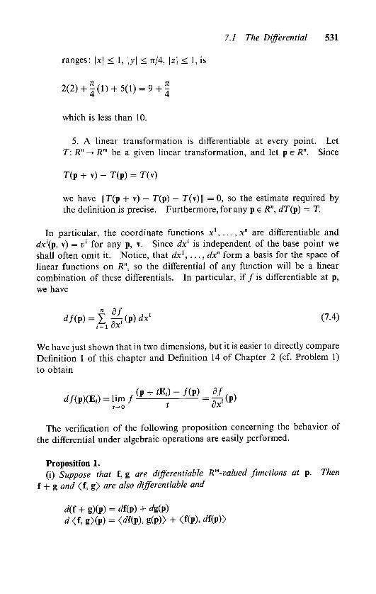
ranges: |x| < 1, |)>| < n/4, \z\ < 1, is
2(2) + J(l) + 5(1) = 9+|
which is less than 10.
5. A linear transformation is differentiable at every point. Let
T: R" -> Rm be a given linear transformation, and let p e R". Since
T(p + v)-
T(p) = T(v)
we have || T(p + v) T(p) T(v) || = 0, so the estimate required by
the definition is precise. Furthermore, for any p e R", dT(j>) = T.
In particular, the coordinate functions x1, ...,x" are differentiable and
dx'(p, v) = v' for any p, v. Since dx' is independent of the base point we
shall often omit it. Notice, that dx1, ..., dx" form a basis for the space of
linear functions on R", so the differential of any function will be a linear
combination of these differentials. In particular, if / is differentiable at p,
we have
dfiv)=t^-iiv)dxi (7.4)i=l OX
We have just shown that in two dimensions, but it is easier to directly compare
Definition 1 of this chapter and Definition 14 of Chapter 2 (cf. Problem 1)
to obtain
JffW,.. ,(p + *e,)-/(P) df
d/(p)(E;) = hm / =
^(p)
The verification of the following proposition concerning the behavior of
the differential under algebraic operations are easily performed.
Proposition 1.
(i) Suppose that f, g are differentiable Revalued functions at p. Then
f + g and <f, g> are also differentiable and
d(f + g)(p) = df(p) + dg(p)
d <f, g>(p) = <diij>), g(p)> + <f(p), <tf(P)>
532 7 Line Integrals and Green's Theorem
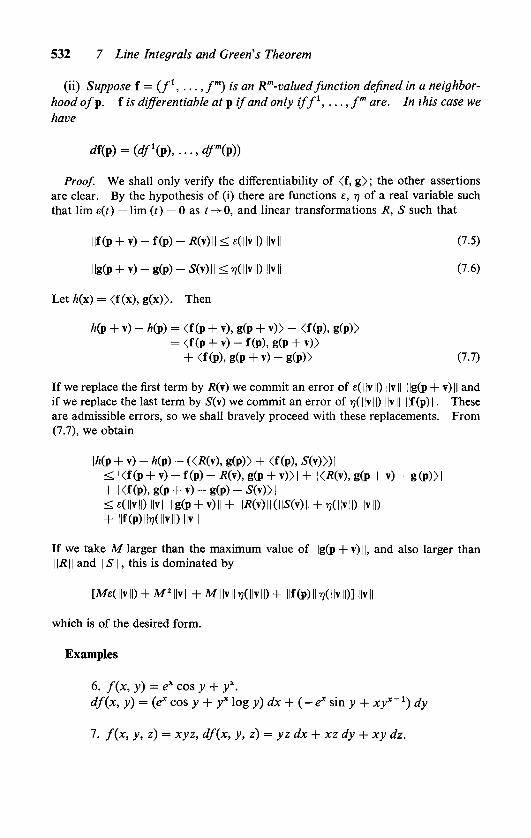
(ii) Suppose f = (f1, ..., fm) is an R"'-valuedfunction defined in a neighborhood off. f is differentiable at p ifand only iff1, ...,fm are. In this case we
have
d{(V) = (dfi(V),...,dr(p))
Proof. We shall only verify the differentiability of <f, g> ; the other assertions
are clear. By the hypothesis of (i) there are functions e, 77 of a real variable such
that lim e(t) = lim (t) = 0 as t ->-0, and linear transformations R, S such that
llf(p + v) - tip) - R(y)\\ < (||v||) ||v|| (7.5)
llg(p + v) - g(p)- 50)11 < tXHvII) llvll (7.6)
Let h(x) = <f (x), g(x)>. Then
hip + v)-
h(p) = <f (p + v), g(p + v)>- <f (p), g(p)>
= <f(p + v)-f(p),g(p + v)>
+ <f(p),g(p + v)-g(p)> (7.7)
If we replace the first term by R(\) we commit an error of e(||v||) ||v|| ||g(p + v)|| and
if we replace the last term by S(v) we commit an error of r?( | |v 1 1) ||v|| |[f(p)||. These
are admissible errors, so we shall bravely proceed with these replacements. From
(7.7), we obtain
\h(p + v)-
h(p)-
R(v), g(p)> + <f(p), 5(v)|< I <f (P + v)
- f (p)-
R(y), g(p + v)> I + I </?(v), g(p + v) - g (p)> |
+ l<f(p),g(p + v)-g(p)-5(v)>|
<(l|v||) ||v|| ||g(p + v)||+ ||iJ(v)||(||S(v)|| + r,(\\y\\) ||v||)
+ llf(p)IWIIvll) l|v||
If we take M larger than the maximum value of ||g(p + v)||, and also larger than
||.R[| and \\S ||, this is dominated by
[Me( ||v ||) + M2 ||v || +M ||v|| r,(\\y\\) + ||f(p)||ij(||v||)] ||v||
which is of the desired form.
Examples
6. f(x, y) = ex cos y + yx.
df(x, y) = (ex cos y + yx log y) dx + (-ex sin y + xyx_1) dy
1. f(x, y, z) = xyz, df(x, y, z) = yz dx + xz dy + xy dz.
7.1 The Differential 533
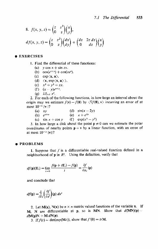
**>'>-(oz;)(;).
<**H X)+( 2z^)(;)
EXERCISES
1 . Find the differential of these functions :
(a) y cos x + sin zx.
(b) cos(e*+)l) + cos(xe>).
(c) exp<x, a>.
(d) <x, exp<x, a> >.
(e) x2 + y2 + zx.
(f ) (x - v)e'+)'.
(g) n?=1x'.
2. For each of the following functions, in how large an interval about the
origin may we estimate /(v) /(0) by <V/(0), v> incurring an error of at
most 10-3||v||?
(a) xy (d) sin(x + 2y)
(b) ex+y (e) x + e2"
(c) sin x + cos y (f ) exp(x2 + y2)
3. In how large a disk about the point p # 0 can we estimate the polar
coordinates of nearby points p + v by a linear function, with an error of
at most 10-3||v||?
PROBLEMS
1. Suppose that / is a differentiable real-valued function denned in a
neighborhood of p in R". Using the definition, verify that
mw^ v/(P + <E,)-/(P) /
df(p)(EL) = hm =-r- (p)
r->0 t OXi
and conclude that
mdfip) = 2\i:-t\ip)dx
2. Let M(x), N(x) be n x n matrix valued functions of the variable x. If
M, N are differentiable at p, so is MN. Show that rf(MN)(p) =
rfM(p)N +M dN(p).
3. If /(f) = det(exp(MO), show that/'(0) = trM.

534 7 Line Integrals and Green's Theorem
4. A quantity Q varies with x, v, z according to
e'
Q =-
yz
Suppose that x, y, z can be measured to within an error of 1 %, 1/2%, 3 %,
respectively. What will be the corresponding maximal error in Q at
corresponding values ? At (a) x = 0, y = 2, z = 5 ; (b) x = 2, y = 1,z = 3, in
particular ?
7.2 Coordinate Changes
In Chapter 1 we introduced some systems of coordinates in R", and we saw
that for certain problems a change of coordinates made the problem under
standable and solvable. Later on we saw, in the study of systems of linear
differential equations, that it was convenient, where possible, to switch to
coordinates relative to a basis of eigenvectors. In the geometric study of
surfaces, and in many physical problems it is advantageous to admit very
general coordinate changes. We now introduce a general notion of
coordinates.
Definition 2. Let U be a domain in Rn. A system of coordinates is an
n-tuple of continuously differentiable functions y= (y1, . . .
, y") defined on
U such that
(i) if P # q, then y(p) # y(q),
(ii) dy'-fat), .
.., dy"(p) are independent at all pet/.
The first condition states that any point is uniquely determined by the
value of y at that point. In this sense y1, . . ., y" are coordinates. We can
name points in U by means of the functions y1, ..., y". Further, if /is a
function defined on U, we can describe it as a function of the coordinates
y1, ..., y". The second condition asserts that the differentials dy1, ..., dy"
span the space of linear functions. Thus we can express the differential of a
function as a linear combination of these differentials; it should be no
surprise that (7.4) is valid in any coordinate system.
Proposition 2. Suppose that y1, . .., y" are coordinates in a neighborhood
ofp. Iff is a differentiable function defined in a neighborhood o/p, then
dfiv) = t f^(pW(p)i=i oy

7.2 Coordinate Changes 535
Proof. Let x\ . . .
,x" be the coordinates of R" relative to the standard basis. We
know that
df<P)=$ J-Mdx'1 = 1 dx
Now we can express the standard coordinates as differentiable functions of the new
coordinates y\ ..
., y": x' = x'(y\ ..., y"), i = 1, ...,n, and /can be expressed as a
function of v1, . . .
, y" by composition:
/(p)=/(x1(y(p)),...,x"(y(p))
Let us assume that p is the origin relative to both x and y coordinates. Now
df/dy' is the derivative of /with respect to y', holding the other variables yJ,j=i
constant. In other words, df/dy'(p) is the derivative of / at p along the curve
yJ = 0,j^ i. We can parametrize this curve by
xl = gl(t) = x\0, ...,0, t,0, ...,0)
x" = g"(t) = x"(0, . . ., 0, t, 0, . . .
, 0)
for t near 0. Now by Proposition 3 of Chapter 3, we have
df d 4. 8f dg"
^(p)=
^/(^),...,^))I.=o=2^(0)-(0)
But dgkldt(0) = dxkldy<(0). Thus
*.$**,*. (,8)dy' t=i dx" dy'
As the x' are differentiable functions of y; dx' =^(dx'ldyJ)dyJ and we conclude
that
8f df dx'^, df
dm^Mdx^l^M^dy^l^dy'
Examples
9. Polar coordinates: the change of coordinates
x = r cos 9 y= r sin 9
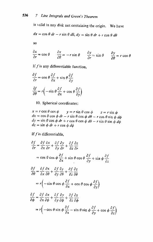
536 7 Line Integrals and Green's Theorem
is valid in any disk not containing the origin. We have
dx = cos 9 dr-r sin 9 d9, dy = sin 9 dr + r cos 9 d9
so
Sx dx. dy dv
-
= cos9Te=-rstn9
= sin e _Z= rcos
If/is any differentiable function,
df df df-f = cos 9^- + sin 9^-dr dx dy
= A-sm9-f + cos9 )d9 \ dx dy)
10. Spherical coordinates :
x = r cos 9 cos eb y= rsin9coseb z = r sin eb
dx = cos 9 cos eb dr-r sin 9 cos eb d9 - r cos 0 sin 0 deb
dy = sin 9 cos eb dr + r cos 9 cos eb d9 -
r sin 0 sin 0 -i</>c?z = sin eb dr + /- cos eb deb
If/is differentiable,
dj_ = df_dx dfdy dfdz
dr dx dr dy dr+ dz~dr
= cos 9 cos eb + sin 0 cos 0 + sin <box dj>
r
<3z
dj_= dj_d_x dfidy dj_d_z_
d9 dx d9+ dy d9+Tzd~9
= A -sin 0 cos </> + cos 9 cos </> )\ dx
v
dy)
d=
dfdx d_f_dy_ dj_dz_deb dx deb
+
dydep+ dz deb
= rl -cos 9 sin eb sin 9 sin eb + cos <A |\ ^x 5y dz/

7.2 Coordinate Changes 537
11. Let f(x, y, z) = exyz. Find df/dr, df/dO :
r\ f
= (cos 9 cos eb)exyz + (sin 9 cos eb)exz + (sin eb)exydr
= r exp(r cos 9 cos <)(r sin 9 cos 0 cos2 < sin eb
+ 2 sin 9 cos 0 sin <)
= r[( sin 9 cos eb)exyz + (cos 9 cos eb)exz~\d9
= r2 exp(r cos 0 cos eb)[_ r sin2 0 cos2 ebsineb + cos 0 cos < sin eb~\
12. Find 3//3x iff(r, 9, eb) = eb2 in spherical coordinates. In order
to solve this we have to write /explicitly as a function of the rectangularcoordinates. Since <b = arc sin(z/r),
^r= 2<P t- = 2 arc sin 7^ 2 2TT72
dx <3x (x2 + y2 + z2)1/2
x arc sin
dx \
The Jacobian
In general, if
/ = /V,-- ,x")
y" =/"(x1. ,*")
is a change of coordinates, we shall write this as y = F(x). The differential
dF(x0) is a nonsingular linear transformation on R". The matrix relative
to x coordinates representing this transformation is referred to as the Jacobian
of the mapping and denoted (when it is of value to make the coordinates
explicit) by
djy\...,yn) (dy'
3(x1,...,x") \dxJJi,j = 1, ..., n
According to Proposition 2
d/_"
d/ebS
dyJ~
ii dx" dyJ

538 7 Line Integrals and Green's Theorem
which is just the entry by entry form of the equation
d(y\...,f)d(x1,...,x")1 =
d(x1,...,x")d(y1,...,f)
Thus the matrices are inverse to each other as are the correspondingdifferentials :
dF-1iy0) = ldFixo)r1 ify0 = F(x0)
Example
13. Let
u = x + ey
v = x cos y
be a coordinate change in a domain in R2. Then
diu, v)
d(
Six, y) -
d(u, v) ey cos y
If/(, v) = u2 + v2, then
x, y) \cos y x sin y/
^1 / xsiny e"\
+ xsin y \ -cos y 1 /
df df du df dv= + = 2u + 2vcosy = 2(x + ey + x cos y)
ox ow ox Of ox
If g(x, y) = x2 + y2, then
dg dg dx dg dy x2 sin y + ye*
du dx du dy du ey cos y + x sin y
These observations form special cases of the multivariable chain rule. We
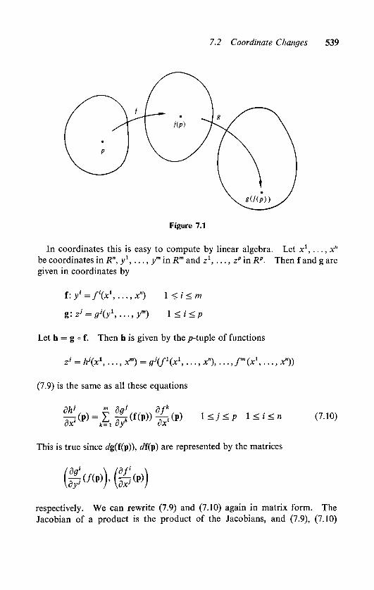
have already seen (Propositions 3.2, 3.3) other special cases. The generalsituation is this: the differential of a composed function (see Figure 7.1) is the
composition of the differentials:
dig o f)(p) = Jg(f(p)) odf (7.9)
7.2 Coordinate Changes 539
In coordinates this is easy to compute by linear algebra. Let x1, ..., x"
be coordinates in R", y1, . . ., ym in Rm and z1, . . .
,z" in Rp- Then f and g are
given in coordinates by
f:yi=f(x1,...,x") \<i<m
g:zJ = gj(y\...,ym) \<i<p
Let h = g o f. Then h is given by the /7-tuple of functions
z> = hj(x\ . . ., xm) = gJif'ix1, . . .
, x"), . . ., fm (x1, . . .
, x"))
(7.9) is the same as all these equations
dhj m daJ dfk
^(P)=
^(f(p))t^ l*>** ^^- ^
This is true since fi?g(f(p)), df(\>) are represented by the matrices
respectively. We can rewrite (7.9) and (7.10) again in matrix form. The
Jacobian of a product is the product of the Jacobians, and (7.9), (7.10)
540 7 Line Integrals and Green's Theorem
become
djz\...,z*) d(z\...,ZP) oXy1,...^")
d(x1,...,x")(P) =
d(y1,...,y"')m)
d(x1,...,x")(p)
Here is the proof of the chain rule.
Theorem 7.1. (The Chain Rule) Let p be apoint in R". Suppose f is a
differentiable Rm-valued function defined in a neighborhood of p, and g is a
differentiable Revalued function defined in a neighborhood of f(p). Then
h = g f is differentiable at p and dh(p) = dg(f(p)) ^(p)-
Proof. Let T= dg(f(p)), and S = df (p). We must show that
||h(p + v)- h(p) - T o S(y)\\ < e(v) ||v|| (7.11)
where lim s(v) = 0. LetIMI-.0
<t(v) = f (P + v)- f (p)
- S(y) (7.12)
+(w) = g(f (p + w))-
g(f (p))-
T(yy) (7.13)
Then, since f, g are differentiable,
ll*(v)||<S(v)||v|| ||<Kw)||^irtw)||w||
where 8(v) -0 as ||v|| ->0 and r;(v) ->0 as ||w|| ^0. Now, we verify (7.11) by com
putation :
h(p + v)-
h(p) = g(f(p + v))-
g(f (p))
= g(f (p)) + T(i (p + v)- f (p)) + <Kf(P + v)
- f (p))-
g(f (p))
(by taking w = f (p + v) f (p) in (7.13)). Now using (7.12) we can continue:
= T(S(y)) + o>(v)) + <\>(S(y) + <p(v))
= T o S(v) + r(<f>(v)) + +(S(v) + <J.(v))
since T is linear. Thus
lir(<KT II +II+CSW + ?(?)) II||h(p + v)-h(p)-ro5(v)||
7.2 Coordinate Changes 541
Now we must show that
, ,H7X<Kv))ll
,llK5(v) + ?(?)) II
<-v' = n~7i 1 ;rv;* 0
llvll l|v||
as ||v|| -*0. As for the first term
^^JE^m^rm)
which tends to zero as v -> 0, so that is alright. The second term is
llKS(v) + o>(v))ll <v(S(y) + <p(v)) ||S(v) + o>(v)||
llvll
<:T?(S(v) + <p(T)XII5'|| + 8(y))
As v -> 0, so does S(y) + o>(v) -* 0, and also r)(S(y) + o>(v)) -> 0. The final paren
thesis is bounded so the whole term tends to zero. We are through.
Finally, we wish to give a sufficient condition that an n-tuple of functions
y1 =/1(x), . . ., y" = f(x) gives a coordinate system in a domain D in R".
If y1, ..., y" are coordinates, then we can invert these equations, that is,
since the y's suffice to determine points in D, we can compute the x coordin
ates in terms of y1, . . .
, y". Thus there are functions x1 = g1(y), ...,x" =
g"(y) such that
x = g(y) if and only if y= g(x)
in the domain D. Now the second condition defining a coordinate system
is that the differentials df1, ..., df" are independent. The inverse mapping
theorem asserts that if this second condition is valid at a point, then the first
must hold in a neighborhood of that point. Thus the independence of the
vectors df1^), .
.., df"(p) are enough to guarantee that y1, ...,y" are
coordinates near p.
Theorem 7.2. (Inverse Function Theorem) Let F be a continuously different
iable Revaluedfunction defined in a neighborhood o/p0 in R". Let q0= F(p0).
If the differential dF(p0) " nonsingular, then there is a neighborhood Uofq
and a continuously differentiable mapping G defined on U such that G(q0) = p0
andfor each q in U
F(P) = q ifand only ifp = G(q)
542 7 Line Integrals and Green's Theorem
Proof. Let us, for simplicity of notation, assume that p0 = q0= 0. We have to
show that if q is small enough the equation
F(p)-
q= 0
has a unique solution p in a neighborhood of 0. This suggests Newton's method
for finding roots. The linear approximation to the mapping p^F(p) q at a
point pi is given in terms of the differential :
p -> F(p0-
q + rfF(pO(p-
pi) (7.14)
If pi is near enough to 0, rfF(pi) is nonsingular, so we can find a root of (7.14),
namely,
p=p1-aT(p1)-1[F(p1)-q] (7.15)
Now we consider the transformation Tq defined in a neighborhood of 0 by
Tip) = P-
</F(0)" '
[F(p)-
q] (7.1 6)
[For simplicity we have replaced dF(pi) in (7.15) by dF(0).] It is shown below, in
Lemma 3 that for q sufficiently small, T, is a contraction in a neighborhood of 0.
Thus, for each q near 0, T, has a unique fixed point, which we denote G(q). Clearly,
F(p) = q if and only if p is the fixed point of T, ,that is, if and only if p = G(q). It
remains only to verify that G is differentiable.
Let q0 be a point near 0, and p0= G(q0). Let T= dF(p0). Then, by definition
F(p)-
F(p0) = Tip-
p0) + <Kp-
Po) (7.17)
where ||<p(p p0)ll <e(P Po) lip Poll and e(t)->0 as /->0. Let p= G(q).
Then (7.17) becomes
q-
q0= T(G(q)
-
G(q)) + (G(q)-
G(q0))
Since T is invertible this can be rewritten as
G(q)-
G(q0) = J-'fo -
q0) + 7-'KG(q)-
G(q0)) (7.18)
If we can successfully study the behavior of the last term we will have verified the
differentiability of G at q0 ,with
^G(q0) = r-1=a'F(po)-1
7.2 Coordinate Changes 543
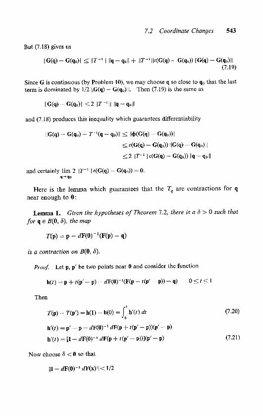
But (7.18) gives us
||G(q)-G(qo)||<||r-1|| ||q- q0|| + \\T~l\\t(G(q)- G(q0)) l|G(q)
- G(q0)ll
(7.19)
Since G is continuous (by Problem 10), we may choose q so close to q0 that the last
term is dominated by 1/2 ||G(q)-
G(q0)ll. Then (7.19) is the same as
|lG(q)-G(q0)||<2||r-1|lllq-qoll
and (7.18) produces this inequality which guarantees differentiability
||G(q)- G(q0)
- T~liq - q0) II < H4>(G(q)- G(q0)) ||
< e(G(q)-
G(q0)) IIG(q)- G(q0)||
<2||r-Mk(G(q)-G(qo))l|q-qoll
and certainly lim 2 \\T~l || s(G(q)-
G(q0)) = 0.
q-qo
Here is the lemma which guarantees that the Tq are contractions for q
near enough to 0 :
Lemma 1. Given the hypotheses of Theorem 7.2, there is a S > 0 such that
for q e B(0, S), the map
r(p) = p-JF(0)-I(F(p)-q)
is a contraction on B(0, 8).
Proof. Let p, p' be two points near 0 and consider the function
h(f ) = p + r(p'- p)
- dF(0)~i(F(p + t(p'- p))
-
q) 0 < t < 1
Then
T(p)- T(p') = h(l)
- h(0) = f h'(/) dt (7.20)Jo
h'(t) = p'-
p- ^F(O)"1 dF(p + r(p'
-
p))(p'- p)
h'(0 = [I- ^F(0)-' dF(p + t(p'
- p))](p'- p) (7.21)
Now choose 8 < 0 so that
||I-rfF(0)-1^F(x)||<l/2
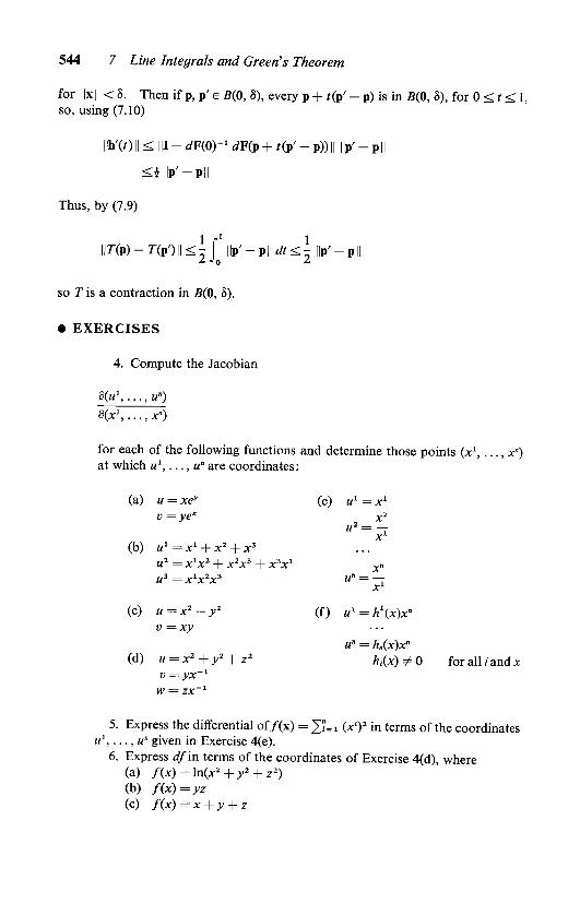
544 7 Line Integrals and Green's Theorem
for ||x|| < 8. Then if p, p' e B(0, 8), every p + t(p' - p) is in B(0, 8), for 0 < t < 1,so, using (7.10)
l|h'(OII 5= III - ^F(O)-1 dF(p + tip' - p))|| ||p'-
p||
<illp'-pll
Thus, by (7.9)
1 r1 1
nnp)-np')ii<-j iip'-pii^<-iip'-Pii
so T is a contraction in B(0, 8).
EXERCISES
4. Compute the Jacobian
8(u\ ...,u")
d(x\ . . .
, x")
for each of the following functions and determine those points (x1, . . .
, x")at which u1, ...,u" are coordinates:
(a) u = xes (e) u1 =x1
v = ye'2
X2
(b) u1 = X1 + X2 + X3
X1
H2 = X'x2 + X2X3 + X3Xl X"
u3 = X1X2X3 " = -
X1
(c) u = x2 y2
v =xy
(f ) tt1 = h\x)x"
u" = h(x)x"
(d) u = x2 + y2 + z2
v = yx'1
w = zx'1
h<(x) ^ 0 for all/ and x
5. Express the differential of/(x) = 2?=i (x1)2 in terms of the coordinatesu1, ..., u" given in Exercise 4(e).
6. Express <i/in terms of the coordinates of Exercise 4(d), where
(a) /(X) = ln(x2 + y2 + z2)
(b) /(x)=yz
(c) f(x)=x + y + z
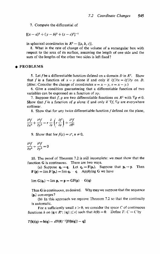
7.2 Coordinate Changes 545
7. Compute the differential of
[(x-a)2 + (y-b)2 + (z-c)2]-1
in spherical coordinates in R3 {(a, b, c)}.
8. What is the rate of change of the volume of a rectangular box with
respect to the area of its surface, assuming the length of one side and the
sum of the lengths of the other two sides is left fixed ?
PROBLEMS
5. Let/be a differentiable function defined on a domain D in R2. Show
that f is a function of x + y alone if and only if dfjdx = dfjdy on D.
(Hint: Consider the change of coordinates u = x + y, v = x y.)
6. Give a condition guaranteeing that a differentiable function of two
variables can be expressed as a function of xy.
1. Suppose that /, g are two differentiable functions on R2 with V# ^ o.
Show that / is a function of g alone if and only if V/ Vg are everywhere
collinear.
8. Show that for any twice differentiable function /defined on the plane,
02/ a2/ d i df\ d2f
'dX2+
'dy1=
r'd'r\'d7)+'dd2
9. Show that for f(z) = z",n= 0,
d2f a2/
dx1+~dy~2=
10. The proof of Theorem 7.2 is still incomplete: we must show that the
function G is continuous. There are two ways.
(a) Suppose q^q. Let q= F(p). Suppose that p-^-p. Then
F (p) = lim F (p) = lim q=
q. Applying G we have
lim G(q) = lim p=
p= GF(p) = G(q)
Thus G is continuous, as desired. Whymaywe suppose that the sequence
{p} converges ?
(b) In this approach we reprove Theorem 7.2 so that the continuity
is automatic.
For a sufficiently small e > 0, we consider the space C of continuous
functions h on {q e R": ||q|| < e} such that h(0) = 0. Define T: C -> C by
r(h)(q) = h(q)- rfF(0)-'[F(h(q))
-
q]
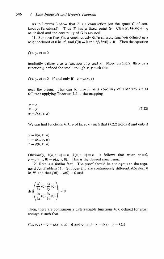
546 7 Line Integrals and Green's Theorem
As in Lemma 3 show that T is a contraction (on the space C of con
tinuous functions !). Thus T has a fixed point G. Clearly, F(G(q)) = q
as desired and the continuity of G is assured.
1 1 . Suppose that / is a continuously differentiable function defined in a
neighborhood of 0 in R3, and/(0) = 0 and 3//3z(0) = 0. Then the equation
/(x,y,z)=0
implicitly defines z as a function of x and y. More precisely, there is a
function g defined for small enough x, y such that
f(x, y, z) = 0 if and only if z = g(x, y)
near the origin. This can be proven as a corollary of Theorem 7.2 as
follows : applying Theorem 7.2 to the mapping
u x
v=y (7.22)
w=f(x,y,z)
We can find functions h, k, g of (u, v, w) such that (7.22) holds if and only if
x = h(u, v, w)
y= k(u, v, w)
z = g(u, v, w)
Obviously, h(u, v, w) = u, k(u, v, w) = v. It follows that when w = 0,
z = g(u, v, 0) =gix, y, 0). This is the desired conclusion.
12. Here is a similar fact. The proof should be analogous to the argu
ment for Problem 1 1 . Suppose /, g are continuously differentiable near 0
in R3 and that/(0) =#(0) = 0 and
'j- (0) ^(0)
f (0) f (0)Kdx dy
Then, there are continuously differentiable functions h, k defined for small
enough z such that
f(x, y, z) = 0 = g(x, y, z) if and only if x = h(z) y= k(z)
7.3 Differential Forms 547
7.3 Differential Forms
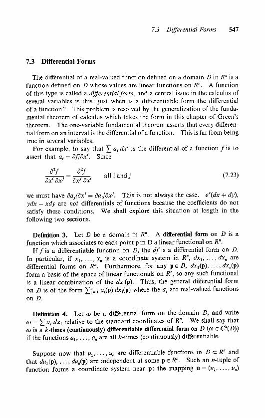
The differential of a real-valued function defined on a domain D in R" is a
function defined on D whose values are linear functions on R". A function
of this type is called a differentialform, and a central issue in the calculus of
several variables is this: just when is a differentiable form the differential
of a function ? This problem is resolved by the generalization of the funda
mental theorem of calculus which takes the form in this chapter of Green's
theorem. The one-variable fundamental theorem asserts that every differen
tial form on an interval is the differential of a function. This is far from being
true in several variables.
For example, to say that 2 ai dx' is the differential of a function / is to
assert that at= df/dx'. Since
all ( and; ('-23)dx' dxJ dx1 dx'
we must have daj/dx' = dajdx*. This is not always the case. ex(dx + dy),
ydx xdy are not differentials of functions because the coefficients do not
satisfy these conditions. We shall explore this situation at length in the
following two sections.
Definition 3. Let D be a domain in R". A differential form on D is a
function which associates to each point p in D a linear functional on R".
If / is a differentiable function on D, the df is a differential form on D.
In particular, if xu . . ., x is a coordinate system in R", dxu ...,dx are
differential forms on R". Furthermore, for any p e D, dxt(p), ..., dx(p)
form a basis of the space of linear functionals on R", so any such functional
is a linear combination of the <ix,(p). Thus, the general differential form
on D is of the form 2"=i g;(p) ^.(P) where the at are real-valued functions
on D.
Definition 4. Let ea be a differential form on the domain D, and write
co = 2 at dXi relative to the standard coordinates of R". We shall say that
co is a A:-times (continuously) differentiable differential form on D (co e C\D))
if the functions au . . .
, an are all fc-times (continuously) differentiable.
Suppose now that uu...,u are differentiable functions in D <= R" and
that du^p), ..., dun(p) are independent at some p e R". Such an n-tuple of
function forms a coordinate system near p: the mapping u = (wl5 ..., un)

548 7 Line Integrals and Green's Theorem
maps a neighborhood D of p onto a domain D' in one-to-one fashion.
Furthermore, du^p), ..., du(p) forms a basis for (/?")*, so any differential
form can be written as at dut . We can compute the relation between the
a, and the a} by the chain rule: since du' = du'/dxJ dx', we have
A du'
;=
.-^ (7.24)
Thus differential forms transform under a coordinate change as the differ
ential of a function (compare Equations (7.4) and (7.23)). Now the equalityofmixed partials of a twice differentiable function gives a necessary conditionfor a differential form to be the differential of a function.
Proposition 3. Let eobe a continuously differentiable differential form in a
domain D. Suppose ul,...,u" is any coordinate system for D. If eo =
at du' is the differential of a function we must have
da, da.
Proof. If w = df, then a,= df/du'. Then
du'~
du'\du')~
~du' \~du~')=
Jo]
Closed and Exact Forms
We shall say that a differential form is exact in a domain D if it is the
differential of a function, and closed if Equations (7.25) hold. It is easilyverified that if these equations hold in any coordinate system, then they holdin all coordinate systems (see Problem 13); so it is not too difficult to verifythat a form is closed.
In the plane a form has the expression eo = p dx + q dy with respect to
the rectangle coordinates. In this case there is only one nontrivial equation in
(7.25), namely,
d<7 dp
Tx-Ty=
<7-26)
We shall refer to this function as deo; that is, if
j j dq dpeo = p dx + q dy dco =
ox dy
7.3 Differential Forms 549
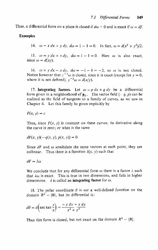
Thus, a differential form on a plane is closed if deo = 0 and is exact if eo = df.
Examples
14. eo = x dx + y dy, deo = 1 - 1 = 0. In fact, eo = d(x2 + y2)/2.
15. eo = y dx + x dy, deo = 1 1 = 0. Here eo is also exact,
since eo = d(xy).
16. eo = y dx x dy, deo = 1 1 = 2, so eo is not closed.
Notice however that y~2eo is closed, since it is exact (except for y = 0,
where it is not defined), y~2eo = d(x/y).
17. Integrating factors. Let eo = p dx + g dy be a differential
form given in a neighborhood of p0. The vector field ( q,p) can be
realized as the field of tangents to a family of curves, as we saw in
Chapter 4. Let this family be given implicitly by
Fix, y) = c
Thus, since F(x, y) is constant on these curves, its derivative along
the curve is zero; or what is the same
dFix, y)i-qix, y), p(x, y)) = 0
Since dF and eo annihilate the same vectors at each point, they are
collinear. Thus there is a function X(x, y) such that
dF = Xco
We conclude that for any differential form eo there is a factor X such
that Xeo is exact. This is true in two dimensions, and fails in higher
dimensions. X is called an integrating factor for eo.
18. The polar coordinate 9 is not a well-defined function on the
domain R2 - {0}, but its differential is:
/ y\ ydx + xdyd9 = d\ arc tan
- =
5 2
\ x) x2 + y2
Thus this form is closed, but not exact on the domain R2 - {0}.

550 7 Line Integrals and Green's Theorem
We shall now verify that every closed form on R2 {0} is equal to an
exact form plus a constant multiple of d9. Thus the space of closed forms
on R2 {0} is larger than the space of exact forms by one dimension.
Suppose that eo is a closed form in R2 {0}. In polar coordinates
eo(re'e) a(re'e)dr + bire'e)d9 and since eo is closed we have db/dr = da/d9.It follows that
F(r) = f nb(reie) d9Jo
is a constant. For
dF r2n db r2n da
1T= \ JTd(>= ^d9 = a(re2')-a(re0) = a(r)-a(r) = 0
dr J0 dr J0 d9
Let c(eo) be that constant. Notice that c(d9) = 2n. Further, if eo = df,then c(eo) = 0. For
c(eo) = Fb d9 = F%d0 = f(reM) - f(re) = 0Jn Jn OoJ0
Conversely, if c(eo) = 0, then eo is the differential of a function defined on
R2 - {0}. Let
fir, 9) = (ait) dt + f b(re) deb (7.27)jj j0
Since c(eo) = 0, f(r, 9 + 2n) =f(r, 9) for all r, 9, so we can define a function
FonR2 - {0} by Fireie) =f(r, 9). Differentiating (7.26), we have
d9 89K '
Thus, rfF = eo.
Finally, if eo is any closed form on R2 {0}, let 0 = eo c(eo)d9/2n.Then
c(0) = c(co) - ^ 277 = 0271
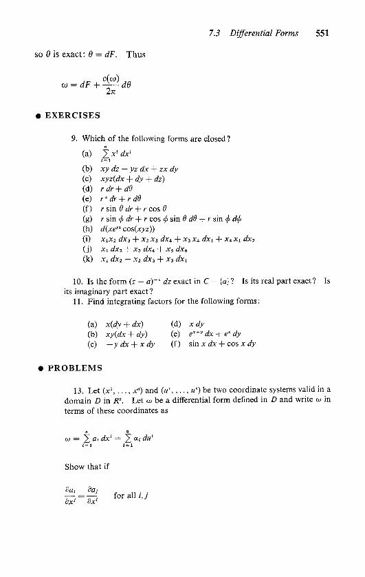
7.3 Differential Forms 551
so 9 is exact: 9 = dF. Thus
eo = dF + CPd92n
EXERCISES
9. Which of the following forms are closed ?
(a) 2 x' dx'1 = 1
(b) xy dz + yz dx + zx dy
(c) xyz(rfx + dy + rfz)
(d) rdr + dd
(e) r'dr + rdd
(f ) r sin 0 /> + / cos 6
(g) r sin <j> dr + r cos </>sind dd + r sin (/> <*/>(h) d(xez cos(xyz))
(i) XiX2 dx3 + x2 x3 dx* + x3 X4 rfxi + x4 Xi dx2
(j) Xi dx2 + x3 rfx4 + x5 dx6
(k) Xi <s?x2 + x2 dx3 + x3 rfxi
10. Is the form (z a)'1 dz exact in C {a}? Is its real part exact ? Is
its imaginary part exact ?
1 1 . Find integrating factors for the following forms :
(a) x(dy + dx) (d) x dy
(b) xy(dx + dy) (e) ex+ydx + e'dy
(c) ydx + x dy (f ) sin x dx + cos x rfy
PROBLEMS
13. Let (x1, . . . , x") and (u\ . . ., u") be two coordinate systems valid in a
domain D in R". Let w be a differential form defined in Z) and write to in
terms of these coordinates as
w = ^at dx' = 2 ai ^"'1=1 (=1
Show that if
8at daj=
,for all 1, j
dx' dx'
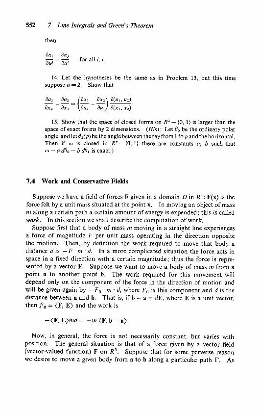
7 Line Integrals and Green's Theorem
then
dat daj
-=- for all l,j
14. Let the hypotheses be the same as in Problem 13, but this time
suppose n= 2. Show that
dai da2 ldat da2\ d(ui, u2)
dxi dxi \du2 dui) d(xi,x2)
15. Show that the space of closed forms on R2 {0, 1} is larger than the
space of exact forms by 2 dimensions. (Hint: Let 80 be the ordinary polar
angle, and let Qx (p) be the angle between the ray from 1 to p and the horizontal.
Then if to is closed in R2 {0, 1} there are constants a, b such that
w a dd0 b ddi is exact.)
7.4 Work and Conservative Fields
Suppose we have a field of forces F given in a domain D in R" : F(x) is the
force felt by a unit mass situated at the point x. In moving an object ofmass
m along a certain path a certain amount of energy is expended; this is called
work. In this section we shall describe the computation of work.
Suppose first that a body of mass m moving in a straight line experiencesa force of magnitude F per unit mass operating in the direction oppositethe motion. Then, by definition the work required to move that body a
distance d is F m d. In a more complicated situation the force acts in
space in a fixed direction with a certain magnitude ; thus the force is repre
sented by a vector F. Suppose we want to move a body of mass m from a
point a to another point b. The work required for this movement will
depend only on the component of the force in the direction of motion and
will be given again by -F0- m- d, where F0 is this component and d is the
distance between a and b. That is, if b -
a = dF, where E is a unit vector,
then F0 = <F, E> and the work is
-<F, E)md= -m<F, b -
a>
Now, in general, the force is not necessarily constant, but varies with
position. The general situation is that of a force given by a vector field
(vector-valued function) F on R3. Suppose that for some perverse reason
we desire to move a given body from a to b along a particular path Y. As

7.4 Work and Conservative Fields 553
is customary we try to adapt the above formula to this revised situation by
assuming that the force field varies little over small intervals (that is, F is
continuous) and that the path is very close to being a sequence of straight line
segments. Then, we get a reasonable approximation to the total work
involved by adding up the work required over each line segment assumingthe force is constant there. More precisely, then, we select a very largenumber of points a = p0 , p1( . . .
, ps= b numbered sequentially along the
path (see Figure 7.2). The work we seek is then approximated by
-m<F(p,),p,-p/_1> (7.28)i=i
We define the work as the limit of all such sums as the maximum of the
distance between successive points tends to zero, and we expect that, as
usual, the calculus will make that computable.And it does. Suppose given, for example, a field of force F given in a
domain Din R3; thenF =(/1(x),/2(x),/3(x))is an Revalued function defined
on D. Suppose r is an oriented curve in D, given by the parametrizationx = g(r) = (g^t), g2(t), g3(t)), a < t < b. We shall now compute the work
done in moving a particle of mass m from g(a) to g(b). Let g(a) = p0 ,. . .
,
ps= g(b) be a very large number of points situated along Y. Referring to
the parametrization we can write p0= g(f0), Pi = g(?i), ; . .
, ps= g(fs), with
a = t0 < tx < < ts = b. Then the approximate work done is given by
Figure 7.2
554 7 Line Integrals and Green's Theorem
(7.28):
-m<F(g(tJ)),g(r/)-g(rJ_1)> (7.29); = i
= -mtmtd)L9M ~
9iiti-i)l + f2(sitd)L92iti) ~
QiiU-J]i=l
+ /3(g('j))[03(f)-03(f|-l)]
By the mean value theorem, there are $i,
,- , 02, i $3, ;sucn that
0/'i)~
0j(*i- 1) = 9'jiOj, dih~
U- 1) r,_ i < 0,, ; < r,
Thus the approximating sum (7.29) becomes
-m
3
fMttWM.t) Oi-^-i) (7.30)
which is a typical Riemann sum approximating
-m ( imit))9'jit)dtJa j=l
= -m\ <[F(t),g'(t)ydt (7.31)
In fact, as the"
very large number of points"
on Y becomes infinite, the
sums (7.30) do tend to the integral (7.31), so we are justified in referring to
this as the work required to move the mass along Y. We are thus led to this
definition of work :
Definition 5. Let D be a domain in R" and F a force field defined in D;that is, F is an ^"-valued function on D. Let Y be an oriented curve defined
in D. The work required to move a unit mass along Y is
W(Y, F) = - f<F(0, g'(0> dtJa
where g : [a, b~] -> Y is a parametrization of Y.
Notice that since W(Y, F) is the limit of a collection of sums defined
independently of any particular parametrization that W(Y, F) is also inde
pendent of the parametrization.

7.4 Work and Conservative Fields 555
Sometimes paths of motion have a break in direction (see Figure 7.3).Such a curve is called a piecewise continuously differentiable curve, or a path
for short. More precisely, we make the following definition.
Definition 6. An oriented path is the image of an interval [a, U] under a
continuous function f such that
(i) f is continuously differentiable with nonzero derivative at all but
finitely many points tu ... , ts.
(ii) lim f '(0 and lim i'(t) exist (but are not necessarily equal) and are
nonzero.
If f(a) = f(b) the path is said to be closed. If Y is an oriented path we can
write r = r\ + + rs+1, where the Yt are the oriented curves between
the points ti _ t and tt . We define the work W(Y, F) by
W(Y,F) = zZW(Yi,F)
Examples
19. Let F(x, y) = (-y, x2) be a force field in R2. The work done
by moving a unit mass around the unit circle is found this way. First,
we parametrize the circle:
r:x = (cosr, sin f) 0 < t < 2n
Figure 7.3

556 7 Line Integrals and Green's Theorem
Then
-27t
W(Y, F) = -
<( - sin t, cos2 t), ( - sin t, cos r)> dtJo
.2k
= - (-sin2 t + cos3 t)dt = n
Jo
20. For the same force field, find the work done around the bound
ary of T of the rectangle [(0, 0), (1, 1)], traversed counterclockwise.
Here Y = Yx + Y2 + Y3 + T4 ,where
r\ : x = (f , 0) 0 < t < 1
r2:x = (l, 0 0<t<l
r3:x = (l-M) 0<t<l
T4:x = (0,1-t) 0<t<l
Then
W(T' F) = {/o<(' ^ (1' 0)> dt + /o<('' 1}' (' 1}> rf/
+ f <(-l,(l-02),(-l,0)>dr
+ j\l- t)2, 0),(0,-l)} dt\
= - f (0 + 1 + 1 + 0) dt = 2
21. Let F(x, y, z) = (yz, xz, xy) and compute the work done alongone full loop of the helix
T: x = (cos t, sin t, t) 0 < t < 2n
.2*
W(Y, F) = -
<(( sin t, t cos t, sin t cos t), (-sin t, cos t, 1)> dtJo
.271
= -
(-t sin2 t + i cos2 t + sin t cos t) dt = 0'o
22. Compute the work done in the presence of the same force field
along the curve x = 1, y= 0, 0 < z < 2n. Here Y is given para-

7.4 Work and Conservative Fields 557
metrically by
T:x = (1,0,0 0<i<27t
Thus
W(Y, F) = - F <(0, t, 0), (0, 0, 1)> dt = 0Jo
Conservation ofEnergy
Now let us suppose we are given a field of forces on a domain D. Let Y
be a closed path in D. Under optimal conditions we would hope for no
loss of energy in moving a mass around Y. We shall call a field conservative
if this situation is the case; that is, the field F is conservative if W(Y, F) = 0
for every closed path Y. Not every field is conservative, as Examples 19 and
20 show. In case F is a conservative field, then the work required to move
a unit mass from one point p0 to another pt will be the same no matter what
path from p0 to p, is followed. For suppose we take two such oriented paths
T, T'. Then the path from p0 to p0 obtained by first traversing r and then
T' (T' oriented from pt to p0) is a closed path. Thus W(Y Y', F) = 0
since F is conservative. But W(Y Y', F) = W(Y', F), so
W(Y, F) = W(Y', F)
Definition 7. Let F be a conservative field defined in the domain D. A
potential function for F is a real-valued function FI defined on D such that,
for any path Y from p to p' we have
W(Y, F) + n(p') - n(p) (7.32)
is a constant.
n is sometimes called the potential energy of the force field F and the
constancy of (7.32) is just the assertion that a conservative force field obeys
the law of conservation of energy. We can relate the potential function of a
conservative field with the field, by its differential. We obtain this important
result :
Theorem 7.3. Suppose that D is a domain such that any two points can be
joined by a path (we say D ispathwise connected).
(i) Every conservative field on D has a potential function.
(ii) Two potentials of the given field differ by a constant.

558 7 Line Integrals and Green's Theorem
(iii) If the field F = (f, ...,/) has the potential function Yl, then
dU=fldx1 + ---+fndx"
Proof, (i) Suppose that F = (f, . . . ,/) is a conservative field defined on D.
Then if T and I" are two oriented curves with the same end points, W(T, F) =
W(T', F) since F is conservative. Fix p0 e D. Since D is arcwise connected, if p
is any point of D there is a curve r from p0 to p. Define IT(p) = W(Y, F). n(p)
is a well-defined function of p since the work required does not depend on the
choice of r. Now let p and p' be two points in D, and let r be a path from p to p'.
If r0 is a curve from p0 to p, then r + T0 is a curve from p0 to p', so
- w(v0 , F) = nip),- w(v + r0, f) = n(p')
But W(V + T0 , F) = W(T, F) + W(T0 , F) = W(Y, F)-
n(p). Thus -Il(p') =
W(T, F)-
IT(p), or W(T, F) + II(p') - n(p) = 0, so (i) is proven.
(ii) If IT is another potential and r0 is a curve joining p0 to p then by the above
definition
U'(p)- n'(p0) + W(T0 , F)
is a constant, say C. But W(T0 , F) = II(p), by definition, thus
n'(p)-n(p) = C+H'(p0)
another constant. Thus two potentials for the field F indeed differ by a constant.
(iii) Finally, we prove that dTl = 2/ dx{ . Let pe D. Fix /, and let e be so
small that the ball B(p, e) <= D. Let Te be the curve with this parametrization
g(r) = p + rE, 0<t<e
Since IT is a potential for F,
II(p + eE,)- n(p) =
-
W(TC ,)=[' (Visit)), g'(/)> dtJo
Now g'(0 = E, and
<F(g(0), g'(0> = 2 fAP + 'E,) <E, , E,> =/,(p + IE.)j
Thus
IT(p + eE,)- IT(p) = \'f,(p + tE,) dt

7.4 Work and Conservative Fields 559
Thus
en
dxi(p) = lim - ff,(p + tE,) dt =/,(p)
e-0 Jo
and so the proof of the theorem is concluded.
EXERCISES
12. Find the work required to move a unit mass around the given pathT in the presence of the given force field:
(a) F(x, y)=(y, x) T: unit circle
(b) F(x,y) = (y2,y x1) Y: boundary of the triangle with
vertices at (0, 0), (0, 2), (0, 1)
(c) F(x,y)=(l,x) r:z(?)=exp(l + 0rfrom t = Q to t = l
(d) F(x, y, z) = (y, x, z) T : x = (cos t, sin t, t)
(e) F(x, y) = (x, xy) T : the portion of the parabola y= kx2
from (0, 0) to (a, ka2)
(f) F(x, v, z) = (z, x2, y) T: closed polygon with successive
vertices (0, 0, 0), (2, 0, 0), (2, 3, 0), (0, 0, 1), (0, 0, 0)
13. Which of these fields are conservative?
(a) F(x, y) = (cos x, cos v, sin x sin v)
(b) F(x, y) = (cos x cos y, sin x sin y)
(c) F(x,y)=(x,y)
(d) F(x,y,z)=(y,z,x)
(e) F(x, y, z) = i-y, x, 1)
(f) -(x2+y2)-"2(x,y)
(g) (x2 + y2)"1/2(- v, x)
PROBLEMS
16. Let F(x, y) = (A(x), B(y)). Show that W(T, F) = 0 for any closed
path T.
17. Find potential functions for these fields:
(a) F(x,y, z) = -(0, 0, 1)
(b) F(x, v, z) = -(x2 + v2 + z2)-1J2(x, y, z)
(c) F(x, y, z) = (y, x, 1)
(d) F(x, v, z) = xy dz + yz dx + zx rfy
18. Let F be a force field in the domain D and T an oriented path in D
from p0 to p. Show that the work W(T, F) can be written as
||F||cos0<fr'po
where 5 is arc length along Tt and 8 is the angle between F and the tangent
toT.
560 7 Line Integrals and Green's Theorem
19. Suppose the field F has the potential function IT. The surfaces
n = constant are called equipotential surfaces for the field F.
(a) What are the equipotential surfaces for a central force field ?
(b) What are the equipotentials for the fields of Exercise 1 3 which are
conservative ?
20. Show that if F is a conservative force field in R2 the lines of force for
F are orthogonal to the equipotential curves for F.
21. If F is a vector field in a domain D in the plane, we define *F as the
field perpendicular and clockwise to F of the same magnitude. Verify this
relation between F and *F if
F(p) = iAtip), A2(p)), *F = (-A2(p), At(p))
22. Suppose both F and *F are conservative fields with potentials II,
II*, respectively.
(a) IT is harmonic.
(b) II + ill* satisfies the Cauchy-Riemann equations.
23. If /= u + iv is a complex analytic function, u is the potential for a
field F such that *F is also conservative (and has potential function v).
24. A vector field F is called radial if it is central and its magnitude is a
function of the radius. Show that if F is a nonzero radial vector field it is
conservative, but *F is not.
7.5 Integration of Differential Forms
The study of work has led us to differentials of function via the obvious
relation between vector fields and differential forms. If F = (f, . ..,/)is a vector field defined on a domain in R", the differential form 2?= i f dx'
will be denoted <F, dx} (for obvious reasons). According to the results
of Section 7.4, the field F is conservative if and only if the form <F, dx}is exact. In this case <F, dx} = d(YL), where n is a potential function
for the field F.
On the other hand, if eo is a form we can write eo = <F, dx} for some vector
field F (if co = 2 ; dx', F = (aY, . . ., an)). We can thus rely on the notion of
work to define the integral of co over a path Y:
jco = j(F,dx}=-W(Y, F) (7.33)
Thus, if cu = 2 a; dx' and Y is parametrized explicitly by x' = x'(0 for
a < t <b, then
r cb ^ dx'
W.?*** (7"34)

7.5 Integration of Differential Forms 561
The idea of defining the integral of a form in terms of work presents us
with a subtle inconsistency which we would like to avoid. The notion of a
differential form on R" involves the geometry of R" only insofar as it is a
vector space. In the conception of differential form, the inner product of
R" is irrelevant and no particular coordinatization of R" is selected over any
other. But the notion of work is deliberately expressed in terms of the
Euclidean structure of R"; it essentially involves lengths and angles. As
a result, with the definition (7.33) of integration, we can only compute the
integral by means of (7.34) in terms of rectangular coordinates for R".
Since the concept of differential form is free of a particular basis, we want
accessory concepts (such as integration) also to be free; in fact, we would
hope to compute jr eo by means of (7.34) with respect to any coordinate
system as well as any parametrization of Y. This turns out to be the case,
and therein we begin to see the importance of the notion of invariance with
respect to coordinate choices.
Proposition 4. Let eo be a differential form defined on a domain D in R"
and suppose eo = /f dx' = eb; du' with respect to two different coordinate
systems (x1, . . .
, x"), (u1, . . ., u"). Let Y be a path in D parametrized in two
different ways by
x' = x'(t) a<t <b
u' = u'(t) a < x < /?
Then
rb dx1 r$ du'
\a /.WO)Ttdt=
\jL: 0(W)Tx
dx (7-35)
Proof. We can write the x's as functions of the it's and / as a function of t.
x' =x'(u\ ..., u") in D
t = t(r) <x<t<P
Now, according to (7.24)
^(u)=2//x)|^(u) (7.36)
when x, u are coordinates for the same point.
Now, let us compute the integral on the left of (7.35) by the change of coordinates
t ->- t, according to the calculus of one dimension.
r" dx' r dx' dt r"_
, , , ,dx'
J. ? fMt)) -d7dt= L lfM'(T)) -d~t^
= J. ?'' '(T)) T, dT
(7.37)
562 7 Line Integrals and Green's Theorem
But we can compute dx'jdr by the chain rule; x is a function of u which is a func
tion of t :
dx' _ dx' du'
~dr~~
T lu' Hh
(7.37) becomes
f'Vr/M 3xJ du' r",
du'
IfiWfir)) dr= j,i(u)(T)) dTJa Li du' dr J dr
by (7.36). The proof is concluded.
On the basis of that proposition we may now define the path integralof a form.
Definition 8. (The Path Integral) Let Y be an oriented path in a domain
in which the form eo is defined. If Y = 2f=i Tt, where the T, are parametrized by x = g;(0, a; < t < b^ we define
fo> = 2 fV&tt.feltt)^*+ i=l Jo,
Notice, that if Y is parametrized with respect to arc length, then g' is the
tangent and the integral may be written as
j eo = J co(T) ds
Examples
23. Find j/ r2 d9, where T is the boundary of the rectangle-1<x<1, -l<y<l. Now, in rectangular coordinates r2 d9 =
ydx + xdy. Thus
[r2d9Jr
= j-(-l)dx + j il) dy-f -(l)dx-f (-l)dy = 8
24. Find Jr (x2 + y2 + z2)(dx + xy dy + dz) around the curve

7.5 Integration of Differential Forms 563
x2 + y2 = a2, x2 + y2 + z2 = b2. This can be parametrized by
x = acos0 y= asin0 z = (b2 a2)1'2
and thus has two branches. Thus
f (x2 + y2 + z2)(dx + xydy + dz)Jr
.271
= 2 (-a sin 9 d9 + a2 cos2 9 sin 8d0) = 0Jn
In case the curve T is a closed path (a continuous image of a circle) it is
customary to write <j>r to indicate that the integration is around a loop. We
now summarize what we know so far about the integration of differential
forms.
Theorem 7.4. Let eo = 2 a ,- dx' be a differentiable differential form defined
on a domain D in R".
(i) eo is the differential of a function if and only ifreo = 0 for all closed
curves Y.
(ii) eo is the differential of a function if and only if the field (au .
.., a)
is conservative.
(iii) If eo = df then
Pti) = Piv) alii, j allpGD (7.38)dXj OX;
When is a Closed Form Exact?
For certain domains, Equations (7.38) are sufficient to guarantee that the
form eo is the differential of a function; but this is not always true. For
example, let
-ydx + xdy-mR2_mQ)}
x2 + y2
Certainly, eo satisfies the required conditions (recall Example 5) :
564 7 Line Integrals and Green's Theorem
If cu were the differential of a function, then we would have |r eo = 0 for
every closed curve Y. However since eo = d9 (as remarked in Example 5),
|r eo = In if T is a circle centered at the origin. Notice that in some sense
co is the differential of a function, albeit not single valued. If we exclude
the line x = 0 (or the line y= 0), in the remaining domain we can take a
principal value of 9 = tan_1 y/x; but we cannot find a continuous single-
valued function on all of R1 - {0, 0} whose differential is co.
Of course, in the above example in any small enough neighborhood of any
point in R2 - {(0, 0)} we can write to = df fox some function /. This is in
fact true for any differential form satisfying the compatability equations
(7.38). That is, suppose co = L\jai dxt is a differentiable differential form
defined in a neighborhood U of p0 in R" and the equations (7.38) are satisfied.
Then if B is a ball centered at p0 and contained in U, there is a differentiable
function / defined in B such that df= co in B. This is really easy to prove :
if p is any point in B, let Lp be the oriented line from p0 to p and define
/(P) = h <*> Then, we can differentiate/with respect to x' by differentiating
under the integral sign:
Now the integrand will have one term of the form ; dajdx' dx1, which is
by Equations (7.38) the same as ,- dajdx' dx1 = efaj . This is the essential
term: by the fundamental theorem of calculus we can conclude from dfjdx3 =
J dttj that df/dxJ = aj as desired. Here is the precise proof.
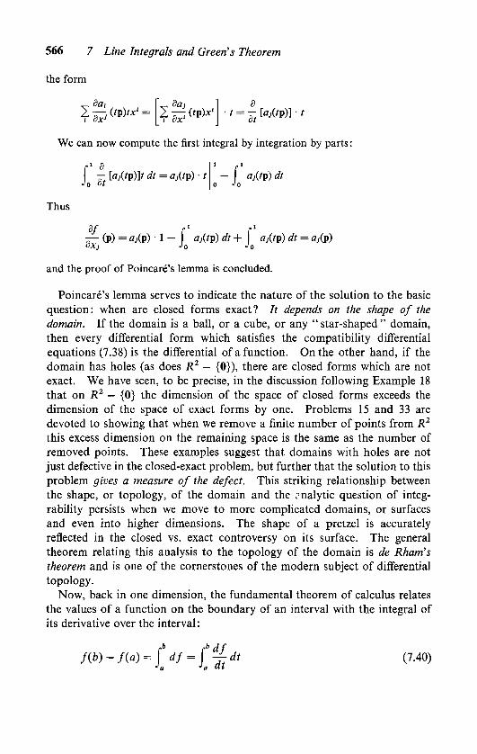
Theorem 7.5. (Poincar^'s Lemma) Suppose that D is a domain with this
property: there is a p0 e D such that for every p e D the line joining p to p0 is
also in D. (D is star shaped (see Figures 7.4 and 7.5).) Then in D every
closed form is exact.
Proof. We may suppose p0 is the origin. For pe D, let Lp be the oriented line
segment joining 0 to p. We may parametrize Lp by
Z,:x=x(r) = fp OsSf^l (7.39)
If co is a closed form, define /(p) = lLp co. We shall show that df=ext. In
coordinates, p = (x1, . . .
, x"), co = 2 d dx', and by (7.39)
r dx* r1 "
/(x1,...,x")= yZai dt=\ JlOt(tx)x'dt
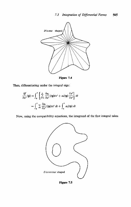
7.5 Integration ofDifferential Forms 565
Figure 7.4
Then, differentiating under the integral sign :
df r1 T dat 8x'"l
=
J J,j(tp)tx'dt+j aj(tp)dt
Now, using the compatibility equations, the integrand of the first integral takes
Figure 7.5
566 7 Line Integrals and Green's Theorem
the form
_ dax |" da.
t =-
[aj(tp)] t
We can now compute the first integral by integration by parts :
r1 8'
r1tt. [aj(tp)]t dt = aj(tp) -t
-
aj(tp) dt
Thus
8f r1 r1t~ (P) = a/P) 1 -
aj('P) * + a/'P) ^ = j(p)dxj J0 Jo
and the proof of Poincare's lemma is concluded.
Poincare's lemma serves to indicate the nature of the solution to the basic
question: when are closed forms exact? It depends on the shape of the
domain. If the domain is a ball, or a cube, or any"
star-shaped"
domain,
then every differential form which satisfies the compatibility differential
equations (7.38) is the differential of a function. On the other hand, if the
domain has holes (as does R2 {0}), there are closed forms which are not
exact. We have seen, to be precise, in the discussion following Example 18
that on R2 {0} the dimension of the space of closed forms exceeds the
dimension of the space of exact forms by one. Problems 15 and 33 are
devoted to showing that when we remove a finite number of points from R2
this excess dimension on the remaining space is the same as the number of
removed points. These examples suggest that domains with holes are not
just defective in the closed-exact problem, but further that the solution to this
problem gives a measure of the defect. This striking relationship between
the shape, or topology, of the domain and the r-nalytic question of integ-
rability persists when we move to more complicated domains, or surfaces
and even into higher dimensions. The shape of a pretzel is accuratelyreflected in the closed vs. exact controversy on its surface. The generaltheorem relating this analysis to the topology of the domain is de Rham's
theorem and is one of the cornerstones of the modern subject of differential
topology.
Now, back in one dimension, the fundamental theorem of calculus relates
the values of a function on the boundary of an interval with the integral of
its derivative over the interval:
f(b)-f(a) = fdf = f^dt (7.40)

7.5 Integration of Differential Forms 567
The analog of this theorem for differential forms in R2 is Green's theorem;there are many analogs in higher dimensions and we shall study some of
these in the next chapter. For the remainder of the present chapter we shallstudy only the two-variable case.
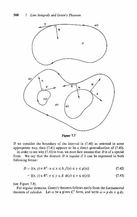
Suppose D is a domain in R2, and the boundary of D is made up of a finite
collection of curves (see Figure 7.6). We make the boundary into an
oriented path by choosing the direction of motion so that the domain D is
always on the left. If T -v N is the (right-handed) tangent-normal frame onthe domain, then the normal N always points into the domain (see Figure7.7). We shall refer to the boundary of D when so oriented as dD. Now
Green's theorem simply says this: if co is a C1 differential form defined on a
neighborhood of D, then
Figure 7.6
568 7 Line Integrals and Green's Theorem
Figure 7.7
If we consider the boundary of the interval in (7.40) as oriented in some
appropriate way, then (7.41) appears to be a direct generalization of (7.40).In order to see why (7.41) is true, we must first assume that D is of a special
form. We say that the domain D is regular if it can be expressed in both
following forms :
D = {(x, y) e R2 : a < x < b, f(x) <y< g(x)} (7.42)
= {(x, y)eR":a<y<P, eb(y) <x< <A(y)} (7.43)
(see Figure 7.8).For regular domains, Green's theorem follows easily from the fundamental
theorem of calculus. Let co be a given C1 form, and write co = p dx + qdy.

7.5 Integration of Differential Forms 569
/ .
/ .
a regular domain
an irregular domain
Figure 7.8

570 7 Line Integrals and Green's Theorem
Then
deo = \ (qx py) dx dy = qx dx dy py dy dxJD JD JD JD
We perform these integrations, by iteration.: use x first for the first integral,
y first for the second.
r ^\cHy)dq 1 j-" r"
\ qx dx dy = dxdy=\ q(\ji(y), y) dy - q(eb(y), y) dyjd Jx LJ<H>>) OX J Jx Ja
(7.44)
Now, we can parametrize dD in two parts as :
dD = rt + T2
Tt : x(0 = OKO, 0 < ' < 0-
Y2 : x(0 = (c6(0> 0 a < r < j8
Thus
f q dy = f q dy - f q dy = f ^(^(0- 0 d* - f (*(0, 0 dtj$d Jrt J-r2 Jx J
a
(7.45)
Comparing (7.44) and (7.45) we deduce that
f qx dx dy = f q dy (7.46)'d Jeo
We leave it to the reader to verify by the same kind of argument that
\ py dx dy=
p dx (7.47)Jd JdD
(Problem 25). Equations (7.46) and (7.47) together give Green's theorem.
Now, not every domain can be represented in both the required ways;
in fact, in general neither is possible. However, for most domains D it is
true that D can be covered by finitely many disks A1; . . .
, As so that D n A; =
Dt is regular for every /. Clearly, if D is bounded by finitely many polygonalcurves this is true. All but the most pathological domains that we have seen
have this property. The above argument generalizes easily to these types of
domains. We shall now call any such domain regular.
7.5 Integration of Differential Forms 571
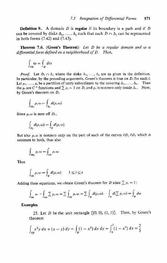
Definition 9. A domain D is regular if its boundary is a path and if D
can be covered by disks At, . . .
, As such that each D n A,- can be represented
in both forms (7.42) and (7.43).
Theorem 7.6. (Green's Theorem) Let D be a regular domain and eo a
differentialform defined on a neighborhood ofD. Then,
JdD JD
deo
Proof. Let Di n A, where the disks Ai, . . ., A are as given in the definition.
In particular, by the preceding arguments, Green's theorem is true on Z>, for each /.
Let pi, . . ., ps be a partition of unity subordinate to the covering Au . . . , As . Then
the pt areC functions and 2 p<= 1 on D, and pi is nonzero only inside A, . Now,
by Green's theorem on Dt
p,cj= d(piw)
JdDi JDi
Since p( co is zero off Di ,
d(piw)= d(p,co)Jd, Jd
But also pi co is nonzero only on the part of each of the curves dD, 8Di which is
common to both, thus also
>eDi
Thus
p,co= p,(JBD, J SD
p,co= d(piw) l<i<s
JdD J D
Adding these equations, we obtain Green's theorem for D since 2 P<= 1 :
f co = f 2P'aj=2l P'OJ=z\\ diP< <) = diz\ Piu)=\ du
JiD JdD JdD JD JD J D
Examples
25. Let D be the unit rectangle [(0, 0), (1, 1)]. Then, by Green's
theorem
f x2y dx + (x- y) dy = f (1 - x2) dx dy = f (1 - x2) dx = =
JdD JD J0 J

572 7 Line Integrals and Green's Theorem
26. The integral of co = cos xy dx + y cos x dy over the boundaryof the domain
> = {(x, y):0<x2 <y < 1}
is
co=[ ysinx + x cos xy] dx dyJdD Jd
= [( y sin x) + x cos xy] dy dx
Green's theorem is also convenient for transforming double integralsinto line integrals. Noticing that dx dy arises as d( y dx) or d(x dy)in Green's theorem, we may compute areas ofdomains by line integrals.
27. Find the area bounded by the curves y = 1 x4 and y = 1 x6
in the upper half plane :
area = dx dyjd
= - f y dx =- f (1 - x4) dx + f (1 - x6) dx =
JdD J-l J-l
4_35
28. Find the area inside the ellipse
x2 v2
E---2 + h=lcr b*
We can parametrize E by the polar angle :
x = a cos 9 y= b sin 9
Thus
fJE J0
EXERCISES
c c2narea = \ x dy = ab \ cos2 9 d9 = nab
J F Jn
14. Compute the line integrals of differential forms arising out of the
work problems in Exercise 12(a), (b) using Green's theorem.
15. Compute JY co for given co and T (using Green's theorem if con
venient).
7.5 Integration of Differential Forms 573
(a) co = z dx + x dy + y dz T: closed oriented polygon with
successive vertices (0, 0, 0), (0, 1, 1), (1, 0, 0), (-1, -1, -1).
(b) co = x2y dx + y2x dy T : the ellipse a2x2 + b2y2 = 1 .
(c) co = (x + y) dx + (x2 + y2) dy V : the triangle with successive
vertices (0, 0), (4, 0), (2, 3).
(d) co = x2 dy + 2xy dx T: z = e<1 + ' from t = 0 to t = 2.
(e) co = (x + y) dx + (y + z) dy + (z + x) c/x
T: the circle x2 + z2 = 1, y = 3.
16. Compute, using Green's theorem the area of the domain D:
(a) D = {(x,y): 0 <sinx<y <tanx< 1}
(b) D is the domain in the upper half plane bounded by the ellipsex2 + 2y2 = 1 and the parabola x = 2y2.
(c) D is the quadrilateral with vertices at (0, 0), (1, 0), (7, 3), (2, 5).
(d) Inside the curve x = cos" t, y= sin" t n > 0.
PROBLEMS
25. Verify Equation (7.47) in the text and conclude the proof of Green's
theorem.
26. Using Green's theorem prove that if co is a closed differential form in
all of R2, then co is exact.
27. A differential form is called radial, if it is of the form <F, dx} where
F is a radial vector field (see Problem 24). Show that if co is radial, it is of
the form f(r)dr.
28. Show that if co is a compactly supported (that is, it is identically zero
outside some large disk) form on the plane that
(a) fJi
dtx>=aR
(b) f co = f rfcoJx axis ^y>0
29. Show that if co is a compactly supported closed form in R2, it is the
differential of a compactly supported function.
30. If co is a differential form, define *co as follows: if
eo = <F, dx> *co = <*F, rfx>
(a) Show that if co =p dx + q dy, *co = q dx + p dy.
(b) Show that (in a disk) *df is also exact if and only if/is harmonic.
(c) Show, using complex notation
*co(T) = co(/T)

574 7 Line Integrals and Green's Theorem
(d) If/is harmonic, let/* be such that df* = *df. Show that/+ if*
satisfies the Cauchy-Riemann equations.
31. Let T be an oriented curve in R", with tangent T and normal N. If
/"is a differentiable function we define these derivatives of /along V:
^ = a/(T) = <V/,T> ^ = rf/(N) = <V/,N>
Show that
32. Suppose that D is a regular domain and / g are twice differentiable
functions defined on a neighborhood of D. Verify these formulas (using
Green's theorem) :
f 3/(a) ^ds=0Jsd ST
(b) I/^*=(I|-|I)^*
(d) L^*=J]>**
(e) J cyi & = JJ [*A/+ <Vc7, V/>] ax dy
7.6 Applications of Green's Theorem
Several of the exercises at the end of the previous section have indicated
the uses of Green's theorem. The rest of this chapter is devoted to the
application of this theorem to some of the topics we have been developing.
We shall leave aside until the next section its more profound uses in the study
of complex differentiable functions.

7.6 Applications ofGreen's Theorem 575
The Shape of the Domain
The most immediate implication of Green's theorem is the suggestion of
the relationship of the shape of a domain to the question of the exactness of
closed forms. If every closed curve in the domain D is the boundary of a
subdomain in D, then every closed form is exact. For, suppose co is a closed
form. By Theorem 7.4 (i), to show that eo is exact, we need only verify that
its integral over any closed curve is zero. If Y is such a curve, then by
hypothesis it is the boundary of the subdomain E. Then, by Green's theorem
\eo=\deo = 0
JT JE
since deo = 0.
We can say that a domain D"
has no holes"
if every closed curve in D
is the boundary of a subdomain of D. This is intuitively clear : we can draw
a loop around any hole which will bound the hole and this is not a subdomain
in D. The further study and precision of these notions is a rather difficult
branch of mathematics and falls within the domain of topology. It turns
out that there is a precise relation between this vague geometric study and
the question of exactness. The number of "holes" in the domain is the
same as the number of independent closed but nonexact forms. We already
saw that (in Section 7.2) for R2 - {0} and in Problem 15 for R2 - {0, 1}.
That argument easily generalizes to the case of the complement of finitely
many points, pu...,ps. Let 9((z) = arg(z - />,-) Although 9t is not a
well-defined function on R2 - {pu .. .,ps}, d9t is a well-defined form.
Clearly, d0u ..., d9s are independent, so there are at least s independent
closed nonexact forms on R2 = {pu...,ps}. Now, let eo be any closed
form and define
1 r
Ciico) =\ co
2ni Jct
where C; is a small circle centered at pt . Then
1 s
eo' = eo- 2 ciim) d9t2n i=i
is exact. This can be proven by verifying condition (i) of Theorem 7.4 by
Green's theorem (see Problem 33). Thus if eo is any closed form it is, but
for an exact form, a linear combination of the dQt .
576 7 Line Integrals and Green's Theorem
Area Computation
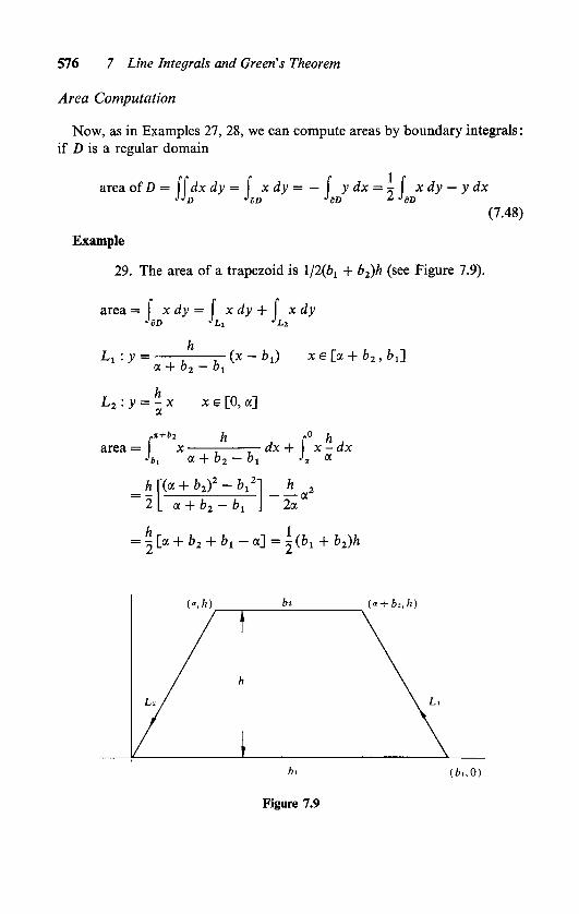
Now, as in Examples 27, 28, we can compute areas by boundary integrals :
if D is a regular domain
area ofD = \\dx dy = x dy = y dx = x x dy y dxJJd ^dD JdD ^ JdD
(7.48)
Example
29. The area of a trapezoid is 1/2(6! + b2)h (see Figure 7.9).
area = x dy = x ciy + x dy^D 'Li ,t2
Ll:y =
JdD JLi
h
a. + b2 bt
h
(x -b^ x e [a + b2 , frj
L2: y =- x x e [0, a]
area = x dx + x- dx
Jbl ex + bi-bi Jx a
+ Z>2)2 - Vl ft=H(:2|_ a + b2 - *>i 2a
=
2l> + ft2 + &i - a] =
2(fti + z)h
(" + bi.h)
(6.,0)
Figure 7.9

7.6 Applications ofGreen's Theorem 577
Integration after a Change of Variable
A line integral of a differential form is the same, no matter what coordinates
are used to compute it (recall Proposition 4). Using this knowledge and
the preceding computational techniques we can find a formula for computingdouble integrals by a coordinate change.
Suppose that F is a nonsingular differentiable transformation of the domain
D onto the domain E (that is, F maps D one-to-one onto E and dF is every
where nonsingular). Let us write F in terms of coordinates :
u = u(x, y) ,.
,. _, x = x(u, v) ,. ._
...,
F : ; -V (x, y) e D F1
: ) ( (w v) e E (7.49)v = v(x,y)
"'
y= y(u,v)
v
If T is a path in D, then F(Y) is a path in E. If co = p dx + q dy is a
differential form defined on D, we may associate it to a form on E: eo = a du
+ )S df , where the cooefficients are given (see (7.24)) by the coordinate
change (x, y) - (, v). Then Jr co = JF(r)d>, since they represent the same
integration relative to two different coordinate sets. Now, if Y bounds a
domain A, F(r) bounds F(A) and if we apply Green's theorem to both sides
we will obtain a relation between the double integrals. However, to applyGreen's theorem we must be sure that both Y and F(T) are oriented as the
boundary of the domains A, F(A), respectively. That is not necessarilythe case.
Example
30. The transformation
v = x
amounts to reflection in the line x = y. If Y is a circle centered on
that line, Y and F(T) are the same curve, but oriented in opposite
directions (see Figure 7.10).
This difficulty may be overcome by restricting attention exclusively to
transformations that preserve the sense of orientation around a curve. This
will be guaranteed if the sense of"
counterclockwise"
rotation about cor
responding points is the same. Thus, if we rotate the xy plane about the
point p in the clockwise sense, the induced motion under the transformation
T must also be clockwise. This will be the case if it is so for the linear

578 7 Line Integrals and Green's Theorem
Figure 7.10
approximation dT(p), and that is guaranteed by
Sjx, y)
3(u, v)(p) = det
{dxdu
(P)
\du
dx
~d~v(P)
8y< ^
Tviv)
>0 (7.50)
/
These remarks are not completely obvious, but we shall not pause to
verify them. It is intuitively clear that the sense of rotation at a point is the
same for the transformation and its differential. What is not so clear, and
more difficult to obtain is that this local criterion assures that the sense of
orientation of any boundary is the same in the two coordinate systems. All
these geometric considerations can be avoided, by replacing them with
appropriate algebraic considerations. We shall see further illustrations of
the difficulty in a purely geometric, rather than algebraic, approach in the
next chapter.In any event, if (7.49) defines a change of variables satisfying condition
(7.50), then for any subdomain A of D, dA and 3F_1(A) define the same
orientation on the boundary of co. Thus, if co is any differential form
/- = /Jr)A JdF-i
CO
SF-^A)
7.6 Applications ofGreen's Theorem 579
In particular,
dy dyr r r oy oyarea (A) = \ x dy = \ x dy = x du + x
Jd\ JdF'^A) JdF-L(A-) dU dVdv
= f \JL(x8-l)_(x?lX\dudv'f-i(A)l5w\ dv) dv\ du) \
= J/r- 1
Six, y)du dv
F-i(A) d(u,v)
A more important formula is that allowing us to compute double integrals
with respect to the new coordinates (u, v).
Theorem 7.7. Let D be a domain in the plane, and suppose
x = x(u, v)
y= y(u, v)
is an orientation-preserving change of coordinates (that is, d(x, y)/d(u, v) > 0).
Let E be. the domain in (u, v) variables corresponding to D. Iff is a function
defined on a rectangle containing D, then \Df can be computed in terms of the
(u, v) coordinates:
\ f=[ fixiu, v), y(u, t>))det^4 ("> 0 du dv (7'51)JD JE 0(U, V)
Proof. Let R = [(a, b), (a, B)] and define
F(x, y) = f fit, y) dt for (x, y) e RJa
Thus Fix, y) is a C1 differentiable function on R such that dF/dx =/. Now, by
Green's theorem
f fdxdy= f FdyJd Jsd
We can compute the integral over dD in the (, v) coordinates:
dy dy
lFdy=LFdy=LFidu+F *dv
dv
580 7 Line Integrals and Green's Theorem
By Green's theorem (in the (u, v) variables), the last integral is
JE [du \ dv) dv \
( fdFdxdy dFdy
JE \_dx du dv dy du
du dv
dy
dv
d2y dFdxdy dFdydy d2y
dudv
~
dx dv du dy dv du dv du
r &ix y)=
J f(x(u, v), y(u, v)) det-^ du dv
du dv
Thus (7.51) is proven.
Examples
31.
r dr d9 AV A*r dxdy
_
/ r ar at)_
r r,
J^+),3sl(x2 + y2)1/2_ V+,,^1 r Jq[j0dr = 2n
32.
f exp[-(x2 + y2)]cfxdy= f exp(-r2)r dr d9JRl JR2
= 2n exp(-r2)r drJo
= 7t[-exp(-r2)]? = 7r
Notice that
a00 \2 .00 <
e\p(-t2)dt\ =J exp(-t2)dt-J exp(-t2)dt
= exp(-x2)cfx- exp(-y2)<iy = exp[-(x2 + y2)] dx dyJ0 J0 JR2
Thus
-co ._
exp(-t2)dt = yjnJo
a computation that would have been impossible without the change
of variable to polar coordinates.
7.6 Applications ofGreen's Theorem 581
The Divergence Theorem
The general form of Green's theorem first came up in the study of fluid
flows and the theory of potentials. In this study it arises in the form of the
divergence theorem, which we shall now discuss in two variables.
Let v = (v, w) be a vector field defined in some open set in the plane and
let x = x(x0, 0 be the equations of the associated flow (that flow with velocityfield v). Let D be a domain on which the flow takes place. The fluid which
at time t = 0 occupies D has moved after a time t, to a domain D, given by
Dt= {x:x = x(xo,0 x0eZ>}
The area of Dt is
area (Dt) = f dx dy = f f(*t,y,) dx0 dy0JDt jd o(x0 , y0)
where we have rewritten the equations of flow as
x = x(x0, 0 = ixixo , y0), ytix0 , J>o))
The rate of change of the area of Dt is
^area(A)=f |[|^4'dt JD dt ld(x0 , y0).dxQ dy0 (7-52)
Now let us evaluate this at time t = 0. Remembering that x(x0 , 0) = x0 ,
we have
d_dt
dx, dy, dx, dy, S2x, m d2yix0,yo 0) + .
. (x0 , y0 , 0),=o dt dx0 dtdy,_dx0 dy0 8y0 dx0
Now
d2x_
d (dx\ __
dv d2y_
dw
dt dx0 dx0 \dt ) 8x0 dt dy0 dy0
Thus the instantaneous rate of change of the area of D (Equation (7.52))is given by
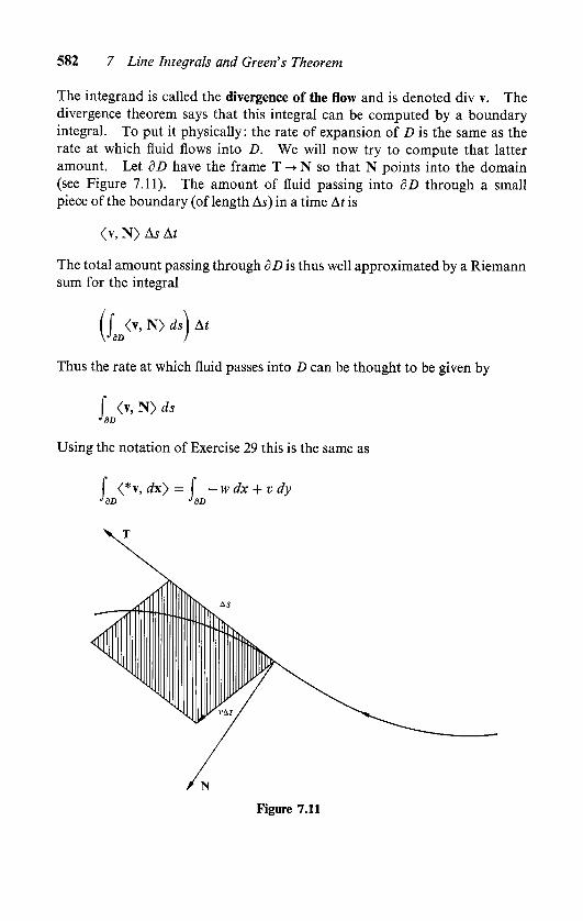
582 7 Line Integrals and Green's Theorem
The integrand is called the divergence of the flow and is denoted div v. The
divergence theorem says that this integral can be computed by a boundary
integral. To put it physically : the rate of expansion of D is the same as the
rate at which fluid flows into D. We will now try to compute that latter
amount. Let dD have the frame T -> N so that N points into the domain
(see Figure 7.11). The amount of fluid passing into dD through a small
piece of the boundary (of length As) in a time At is
<v, N> As At
The total amount passing through dD is thus well approximated by a Riemann
sum for the integral
(j <v, N>ds]AtThus the rate at which fluid passes into D can be thought to be given by
f <V,N>d5JdD
Using the notation of Exercise 29 this is the same as
| <*v, dx} = f wdx + vdydD JdD

7.6 Applications of Green's Theorem 583
By Green's theorem this is the same as (7.53). Thus the divergence theorem
is verified :
f <v, N> ds = f div v (7.54)JdD Jd
If v is a conservative field it has a potential function / and <v, dx} = df.
Then <*v, dx} = *df and (7.54) becomes
f *df = f d* df = f A/JdD JD JD
Thus, if/ is the potential function for a conservative and incompressible
(divergence free) flow, /must be a harmonic function. Dirichlet's problem
(to find a harmonic function with given boundary values) may be restated as :
find the conservative incompressible flow with given boundary potential
levels.
The Cauchy Theorem
This last remark leads directly to the study of complex analysis. Suppose
that /is a complex-valued complex differentiable C1 function defined on a
domain in the plane. Then
r/(z + h) - fjz)
hm;
= / (z)
exists for all z and (what is the same assertion) the Cauchy-Riemann equations
hold:
dl=-id-ldx dy
It follows that the form/(z) dz is a closed complex-valued form:
f dz = / dx + if dy
d(f dz) ='dcn
df'
d-x(lf)-Ty.= if
~
fy = 0
Theorem 7.8. (Cauchy's Theorem) // / is a C1 complex differentiable
function defined in the regular domain D, then
\ fdz = 0
JdD
584 7 Line Integrals and Green's Theorem
Proof. By Green's theorem
\ f dz=\ d(f dz) = 0JdD ^D
EXERCISES
17. Compute the area of these domains:
(a) x* + y4 < a*
(b) x2y<l,0<x<a
(c) r < 1 + 2 cos 8 (each section)
(d) r < e", 0 < 8 < 2tt
(e) The domain {u2 + v2 < 1/2}, where
u = x(l + x cos v)
v = y(l + y cos x)
(f ) The domain {0 < h < 1 , 0 < y < 1}, where u
18. Compute div v for these flows:
1 -1
-1(a) x(x0 ,t)= exp D< Xo
(b) x=x0(l + 0,y = vo(l-/2)
(c) v(x, y) = (x2 -y,y2 -
x)
(d) v(x, y) = (x + y, x-
v)
PROBLEMS
33. Let D = R2 {pi, ..., p,}, where pi, . .
., ps are s distinct points in the
plane. Show that there is an ^-dimensional space L of closed, but not exact
forms defined on D such that every closed form can be written df+oi, with
coei.
34. Let co be a closed form in R2 {(0, 0)}. Show that if co is exact in
some annulus {a < \z\ <b), then it is exact.
35. Let / be a complex-valued differentiable function defined in the
domain E. Show that /is complex analytic if and only ifUdf dz = 0 for all
subdomains D of E. (Hint: d(fdz)=0 is the same as the Cauchy-
Riemann equations.)
7.7 The Cauchy Integral Formula
In Chapter 5 we introduced the power series development of functions in
order to effectively compute solutions to certain differential equations.Those functions which admit an expansion into a power series are called
analytic. We saw that this is the most computable class of functions. We
7.7 The Cauchy Integral Formula 585
saw that such functions are differentiable in the complex sense, and that the
differential equations can be interpreted in the sense of complex variables.
In Chapter 6 we found that if a function is the sum of a convergent powerseries in the closed unit disk, it can be computed by means of an integralaround the circle :
if
/(0 = InCfor|CI<lii= 0
then
2* f(J*\J
2jt Jn e
fwde2n J0 e' - C
for | C| < 1 . The integral may be rewritten as a line integral :
m'
J M*zm J\z\ = i z 4
The Cauchy integral formula is a great generalization of this. It weakens
the hypothesis to that of complex differentiability and strengthens the con
clusion by replacing the unit circle by the boundary of any regular domain.
Theorem 7.9. (Cauchy Integral Formula) Suppose that f is a C1 complex-valued complex differentiable function defined in a neighborhood of the regulardomain D. Then, for e D,
/(C) = -Lj 1^1 (7.55)27tl JdD z L,
Proof. Let A = {z: \z l\<n~1}. If n is large enough, A is contained in
D (see Figure 7.12) and f(z)(z )_1 is a complex differentiable in D A . This is
because the product of complex differentiable functions is complex differentiable.
Thus f(z)(z )-1 dz is closed, so that
r f(z) dz
Jd(D-&) Z L,
Thus
r f(z)dz r f(z)dz ,r2" f(UWe")
_,. .f2" ^ , . M
T= F= / -Tli n1ewd8 = i\ /({ + n^e'^dd
J id z-t, JeAn zC Jo n V J0
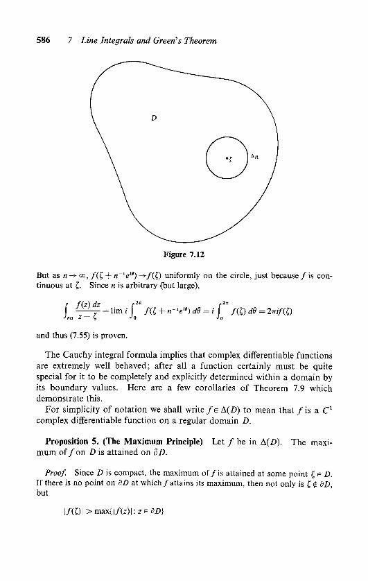
586 7 Line Integrals and Green's Theorem
Figure 7.12
But as n -* co, /( + n le") -?/() uniformly on the circle, just because / is con
tinuous at . Since n is arbitrary (but large),
r f(z)dz r2" c2n
J-^j- = lim i /( + -V) /0 = i /() dd = 2mf(QJdD Z C, Jo ^0
and thus (7.55) is proven.
The Cauchy integral formula implies that complex differentiable functions
are extremely well behaved; after all a function certainly must be quite
special for it to be completely and explicitly determined within a domain byits boundary values. Here are a few corollaries of Theorem 7.9 which
demonstrate this.
For simplicity of notation we shall write fe A(D) to mean that / is a C1
complex differentiable function on a regular domain D.
Proposition 5. (The Maximum Principle) Let / be in A(D). The maxi
mum off on D is attained on dD.
Proof. Since D is compact, the maximum of /is attained at some point e D.
If there is no point on dD at which /attains its maximum, then not only is $ dD,but
1/(01 >max{|/(z)|:*e 82)}

7.7 The Cauchy Integral Formula 587
We shall show that this assumption leads to a contradiction. Define
/(*)Qiz)-
7(0
Then geb.(D) also, #(0 = 1 and |lc7lU<l. Then gn 0 uniformly on dD as
n -> oo . Thus
g"(z) dz
z-i*0
as - co. But, by the Cauchy integral formula, that integral is 2-irig"(Q = 2m'
which does not tend to zero.
Proposition 6. Suppose f , f are all in A(D) and lim/ = / uniformly on
dD. Then lim/ = f uniformly in D.
Proof. By assumption, ||/ /||8D->0 as -><x>. But since ffeA(D), by
the maximum principle,
ll/n /I'd= II/, AI'sd so |'/ /|'d->0 as -> co also
Proposition 7. (Liouville's Theorem) /// is bounded and complex differentiable on the entire plane, f is constant.
Proof. Let Mbe an upper bound for \f(z)\. Let 0, 0 be any two points on the
plane.
1/(0) -/(0) I -f277/ J I-
<;
<-
277/ J|Z|=R
2rr
MR
1 1
z-Oj/(z) <fe
/-'(xl=c/z
(*-.)0 -0)
d8
<-
2
M
'2^
Jl ^'-l (to" - CMRe" - 0)
z r2~
r^-^LJo \e" r.iR-1\\e"-r.2R-'\
As /?->- oo, the integrand converges to 1. Thus the entire expression on the right
becomes arbitrarily small as i?-oo. On the other hand, the left-hand side is
independent of R, hence must be zero. Thus, /(0) =/(0) for any 0.0-
588 7 Line Integrals and Green's Theorem
The most important property of complex differentiable functions is that
they are analytic, that is, they can be expressed as the sum of a convergent
power series about any point. The following theorem brings together all
the notions of analyticity and summarizes the basic properties of analyticfunctions.
Theorem 7.10. Letfbe a C1 complex-valuedfunction defined in a neighborhood of the regular domain D. The following assertions are equivalent :
(i) For any e D, and R such that the disk A(, R) is contained in D, fis the sum in A(, R) ofa convergentpower series:
/(z) = f an(z - )" (7.56)71= 0
(ii) / is complex differentiable.
(iii) f satisfies the Cauchy-Riemann equations:
8-l=-i8-ldx dy
(iv) fdz is closed.
(v) for any e D,
2ni JdD z
In case f has these properties the coefficients an of (7.56) are given by
/<">() 1 r f(z) dz
a"==2^Li^irT (7-57)
Proof. The implications (i)=;(ii), (ii)=>(iii) were observed in Chapter 5,
(iii) => (iv) in the preceding section and (iv) => (v) is the Cauchy integral formula
(Theorem 7.10). That leaves only the implication (v) => (i) and the first part of the
theorem will be proven. Suppose then, that (v) holds, and A(, R) <= D. We have
to show that / can be expanded in a power series centered at . By hypothesis,
min{|z-
| : z e dD} ^ R. Thus for w e A(, R),
7.7 The Cauchy Integral Formula 589
for all z e dD. Thus
1 1 1 / w-A-1 (w-ty
M-^1Mz-w 2_ _/>_) z-i\ z-i) t-o(z-)+1
uniformly for z 6 dD. We can thus substitute this sum for the term (z-w)-1 in
the Cauchy integral:
/(W) "fcrfL T^w~
=
2^L /(Z) .? (T=1P*Z
=l[^l(z-^rT-0Thus /is represented by a power series whose coefficients are given by the integralsin (7.57). That the coefficients also are given by the successive derivatives as in
(7.57) was already observed as part of Taylor's formula. Thus, the theorem is
completely proven.
Examples
33. If / is analytic in the disk A(, R), then the power series re
presenting / near actually converges to / in the entire disk A(, R).For, by Theorem 7.10, /is, in this whole disk, the sum of a power
series centered at , but such a power series is uniquely determined by
/, so must be the given one. In particular, if/is analytic in the entire
plane it can be expanded in a power series converging everywhere.
34. Suppose that /is analytic near . Then
fi*)-fiO(7.58)
is also analytic near . For, we can easily factor the Taylor expansionof f(z) - /(). If f(z) = ,- 0 an(z -
)", then
fiz) -fit) = t alz - )" = (z - ) g an+1(z-
)"71=1 71 = 0
so (7.58) is given by "=0 an+iiz 0"- In particular, z-1 sin z is
analytic on the whole plane, and has the Taylor expansion
z-1sinz = f (-1)"-^-1 = 0 \Z )'
590 7 Line Integrals and Green's Theorem
35. fJ|z| = l
tan z dz tan z
-5= 27H = 2ni
z= 0
36- f -#T=fJ|z-(1 = 1 Z + 1 -'|z-i|=l
rfz 1= 2ni = 7t
i| = i(z + 0(z- 0 2i
37. f - -dz = 27ii(sinz)(''-1)|I=oJ\z\ = 2 z
' 0 n odd
(-1)"/227TJ
I in -1)1n even
r e" (ez)(n_1)38. f- dz = 2niy
J iz -iz - )" (n-1)!
2niel-
:=;
=
(n-l)!
r2*39- J. i-
d0
2c7 cos 0 + a
Ia|<l
This integral can be computed by means of Cauchy's theorem by
interpreting it as an integral over the unit circle. Since
cos 9 =ew + e~w
-H-Ddz = ieie d9 = iz d9
on the unit circle, we may rewrite the integral as
Jl*| = i\ \ 2 / ] xz iJ|z| = iz-
1 / dz~
~ia J|z| = i z2 - (a + (l/a))z + 1
dz
az2 a + a2z
ia Ji2i = i (z a
dz
M = i(z-a)(z-a )(7.59)
Since |a| < 1, the function (z a x) Ms analytic on the unit disk
and the integral (7.59) can be computed by the Cauchy integral

7.7 The Cauchy Integral Formula 591
formula
JUI = i
dz
iz-a-^iz-a)= 2ni -
a a
Thus
27t d9
J0 I -2a cos 9 + a2
Theory ofResidues
-In I 1 \_
2tt
a \a a-1/ I a2
There are many definite integrals which may be computed in similar
fashion. The integral formulas of complex analysis provide a powerful
technique for computing such definite integrals called the residue calculus.
We shall give a brief introduction to these methods. First, a few more
illustrations
40.r2" n C /z + z~1\bdz
cos6 9 d9=J0 J|*l = i\ 2 J iz
1 r (z2 + l)6 ,n
r, , ,N,
2!Jiz| = i z' 6!2d'1*1 =
TT 5 3 1
2s 6 4 2
41.+ COS2 0 J|2|
4 c z dz
r2* d9_
r |\ /+_L^\Jo l+cos20~J|2| = i [
+
\ 2 /
lJ|z| = l
tfz
iz
z4 + 6z2 + 1(7.60)
We are now not in a very good position, for we cannot recognize the
integrand as a Cauchy integrand. To do so we should be able to write it in
the form f(z)iz )"" for some function / analytic on the unit disk, and
in the disk. But it is not of that form. The integrand is
(z2 + 3 + 2^2)(z2 + 3 - 2^2)
z2+(3 + 2^2) z + (-3 + 2V2)1/2 z-(-3+2x/2)1/2
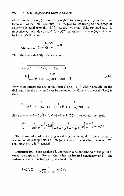
592 7 Line Integrals and Green's Theorem
which has the form f(z)(z - a)~1(z - /J)-1 for two points a, /? in the disk.
However, we can still compute this integral by returning to the proof of
Cauchy's integral formula. If Al5 A2 are two small disks centered at a, /?,
respectively, then f(z)(z - a)'1 (z /?)_1 is analytic in A (Ax u A2), so
by Cauchy's theorem
f(z)dz= 0
JarA-fA,. u a2)] (z- a)(z ~ P)
Thus, the integral (7.60) is the same as
r z dz
JsAi(z2 + 3 + 2^2)(z-P)(z-a)
z dz+ I.5A2(z2 + 3 + 2N/2)(z-a)(z-(5)
(7.61)
Now these integrands are of the form f(z)(z )_1 with / analytic on the
disk and in the disk, and can be evaluated by Cauchy's integral. (7.61) is
thus
2ni +P
.(a2 + 3 + 27'2)(a - p) (P2 + 3 + 2^2)(P - a)J
Since a = -(-3 + 2^2 )1/2, /? =(-3 + 2^2 )1/2, we obtain the result
Jo 1 +
d9
cos 9 i
4,- 2ni
L-3 +2^/2 + 3 + 2^2.
a-/?
a-jS= nJ2
The above idea of suitably generalizing the integral formula so as to
accommodate a larger class of integrals is called the residue theorem. We
shall now prove it in general.
Definition 10. Suppose that /is analytic in a neighborhood of the point ,
except perhaps at . We say that / has an isolated singularity at . The
residue of such a function /at is defined to be
Res(/,) = lim-i,f f(z)dz-.0 zm j|2-(| = e
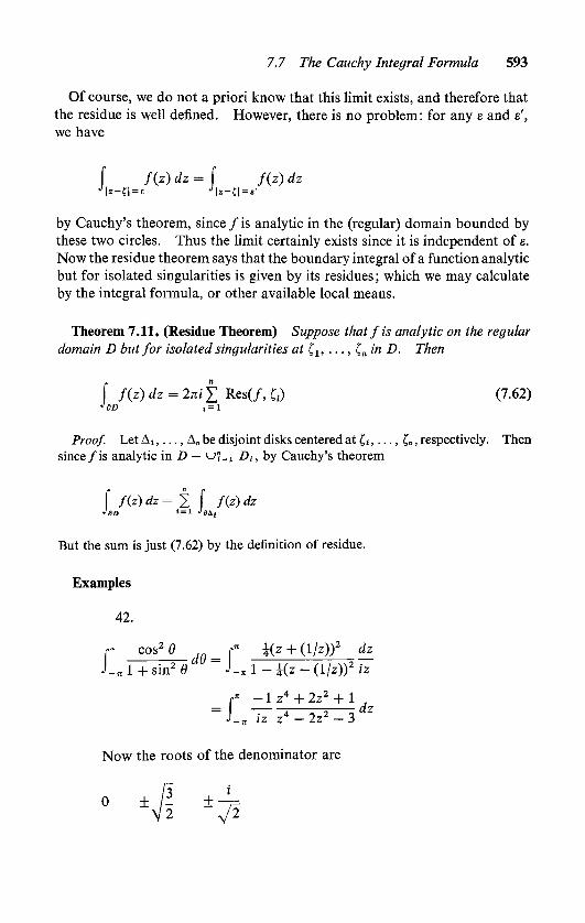
7.7 The Cauchy Integral Formula 593
Of course, we do not a priori know that this limit exists, and therefore that
the residue is well defined. However, there is no problem: for any e and e',
we have
f /(z) dz = f f(z) dzJ\*-a=e J|z-CI=*'
by Cauchy's theorem, since /is analytic in the (regular) domain bounded bythese two circles. Thus the limit certainly exists since it is independent of e.
Now the residue theorem says that the boundary integral of a function analyticbut for isolated singularities is given by its residues ; which we may calculate
by the integral formula, or other available local means.
Theorem 7.11. (Residue Theorem) Suppose that f is analytic on the regulardomain D but for isolated singularities at 1; . . .
, in D. Then
f f(z)dz = 2ni Res(/,;) (7.62)JdD ,= 1
Proof. Let At, . . .
, A be disjoint disks centered at 0, . . ., , respectively. Then
since /is analytic in D u;=1 D, , by Cauchy's theorem
f f(z)dz= J f f(z)dzJdD i = 1 Je&,
But the sum is just (7.62) by the definition of residue.
Examples
42.
C" cos2 9
J-Bl +sin2(-dO---L
i(z + (l/z))2
l-i(z-(l/z))2
dz
iz
-L- 1 z4 + 2z2 + 1
iz z4 - 2z2 - 3dz
Now the roots of the denominator are
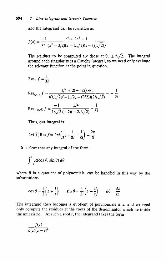
594 7 Line Integrals and Green's Theorem
and the integrand can be rewritten as
1 z4 + 2z2 + l
/CO =-
iz (z2-3/2)(z + i/V2)(z-(i/N/2))
The residues to be computed are those at 0, i/sJ2. The integralaround each singularity is a Cauchy integral, so we need only evaluate
the relevant function at the point in question.
ReS * =Ti
p, 1/4 + 2(- 1/2) + 1 1
Resi/V2 J = = 1==
TT
i(7>/2)(-(l/2)-(3/2)X2i/>/2) 8,
-1 1/4 1
ReS-i/'/l/ =l/N/2(-2)(-2i/V2)~8I-
Thus, our integral is
2-ZRes/=2,i(i-i + i)=fIt is clear that any integral of the form
f R(cos 9, sin 9) d9J-n
where R is a quotient of polynomials, can be handled in this way by the
substitutions
cos0 = i(z + i) sin0 = i(z-i) d9 =eh
iz
The integrand then becomes a quotient of polynomials is z, and we need
only compute the residues at the roots of the denominator which lie inside
the unit circle. At such a root r, the integrand takes the form
fiz)
g(z)(z- rf
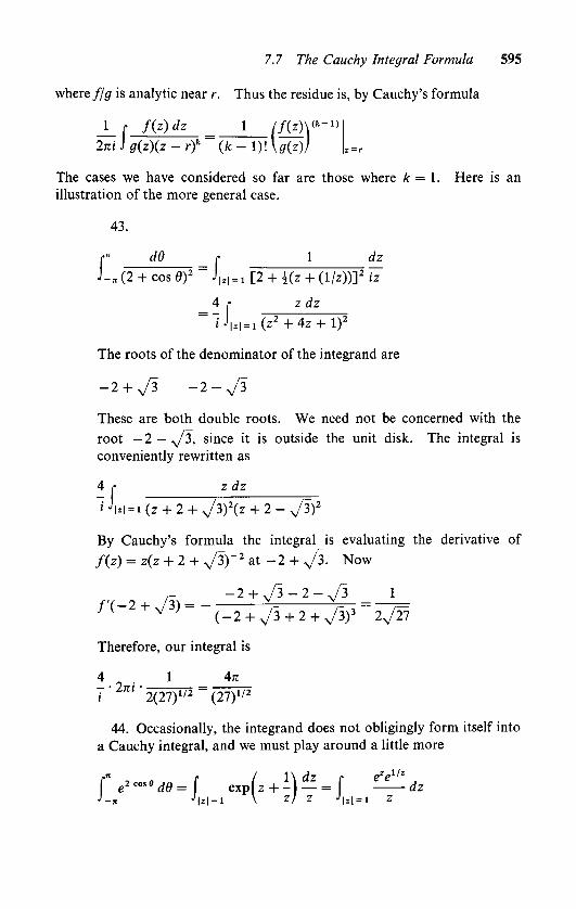
7.7 The Cauchy Integral Formula 595
where fg is analytic near r. Thus the residue is, by Cauchy's formula
1f f(z)dz i //coy*-1'_t_r f(z)dz
_
1 //(Z)\(
271/ J c7(z)(z - r)fc (fc-l)!\c7(z)j
The cases we have considered so far are those where k = 1. Here is an
illustration of the more general case.
43.
dO r I dzr" ao r
J-It(2 + cos0)2=
J|2, = 1(2 + cos 9)2 JM = 1 [2 + i(z + (I/O)]2 <z
4 r z dz
i 'm = ii|2| = !(z2+4z + l)2
The roots of the denominator of the integrand are
-2 + 73 -2-y/l
These are both double roots. We need not be concerned with the
root 2 ^/3, since it is outside the unit disk. The integral is
conveniently rewritten as
JUI = i
z dz
l = i(z + 2 + N/3)2(z + 2-V3)2
By Cauchy's formula the integral is evaluating the derivative of
/(z)= z(z + 2 + N/3)-2 at -2 + ^3. Now
_
-2 + 73-2-^3 1
f'(-2 + ^3) --
(_2 + y-3 + 2 + ^3~
2v/27
Therefore, our integral is
4 1 4- 2/71i 2(27)1/2 (27)1/2
44. Occasionally, the integrand does not obligingly form itself into
a Cauchy integral, and we must play around a little more
\\2d9=\ exP(z + i^=f ^ dz
J-K J\z\ = l \ Z] Z J|Z| = 1 Z

596 7 Line Integrals and Green's Theorem
The only singularity is at 0, but we cannot rearrange this in the form
/(z) z" 1. Thus we must compute the integral directly by some other
means. Since
ez=L^ ellz=2Z-T= o n ! = 0 n !
and
e'-e^= til i^z-n= oo i-j
=n ''J- I
\ J>0 /
Thus
f e2d9= t }Z -i-f z-^zJ-lt 11= -CO i-j=77 I'-;! J\l\ = l
i20
J>0
But that last integral is zero unless n = 0, in which case it is 2?r. We
conclude that
f e2d9 = 2n2Z^- = 2n>Z ,-UJ-* frj'!;! n=0(n!)2i^O
Integrals from oo to + oo
The techniques of residue calculus also apply to suitable integrals of theform
Hx) dx (7.63)'-no
If, say, F(z) is analytic but for isolated singularities at z1; ..., zt in the
upper half plane, then
f F(z)dz = 2ni\\ Res2i(F)JdD ;=i
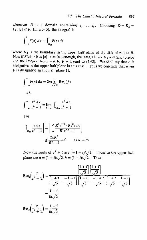
7.7 The Cauchy Integral Formula 597
whenever D is a domain containing zu...,zk. Choosing D=DR =
{z: \z\ < R, Im z> 0}, the integral is
f F(x) dx + f F(z) dzJ-R JHR
where HR is the boundary in the upper half plane of the disk of radius R.
Now if F(z) -> 0 as | z\ - oo fast enough, the integral over HR will tend to zero
and the integral from -R to R will tend to (7.63). We shall say that F is
dissipative in the upper half plane in this case. Thus we conclude that when
F is dissipative in the half plane II,
f F(x)dx = 2niYj Res,(/)'-oo zeII
45.
00 x2 dx,.
r
V* 4. 1
= llm J-oo X +1 K-.OD J^D
z2 dz
Rz4 + 1
For
fzdz
- cR2e2i" ' Rei6i dd
JRz4+l~
J0 R4eRie+l
2nR3
R*- 1as R-*- oo
Now the roots of z4 + 1 are (+ 1 + i)/y/2. Those in the upper half
plane are a = (1 + i)/y/l, b = (1 - 0A/2- Thus
Res,
i + ii ri + nn
/ z
\_ LV2JLV2J'\z4 + i/ ri + i -l-nri + i -i + nri + i 1
[ i] [1 +i_
-1 + i] [1^2 ^2 J L ^2 ^2 JL^/2 V2
1 + i
81^/2
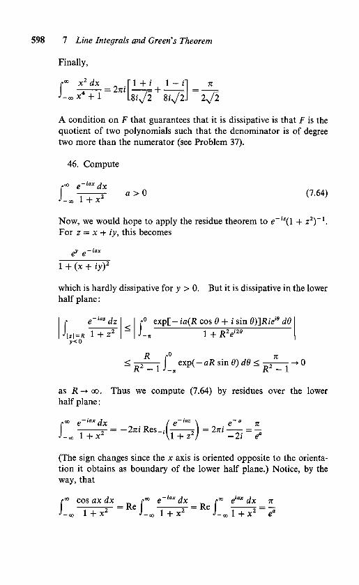
7 Line Integrals and Green's Theorem
Finally,
x2 dx/" x ax
J-x* + l= 27ri
1+i 1 - i
;= +
.8^/2 81V2J 2^2
A condition on F that guarantees that it is dissipative is that F is the
quotient of two polynomials such that the denominator is of degreetwo more than the numerator (see Problem 37).
46. Compute
/<*> e~iaxdx
J-00 1 +x2(7.64)
Now, we would hope to apply the residue theorem to e ,z(l + z2) l.
For z = x + iy, this becomes
e> e
1 + (x + iy)2
which is hardly dissipative for y > 0. But it is dissipative in the lower
half plane :
f ~
J\z\=R 1
e-'"dz
z\=R 1 + Z*
)><0
I.0exp[- ia(R cos 9 + i sin 0)]2?ie''fl d0
1 + KV2.i29
<j exp(-aR sin 0) dQ <
R \ J- R2-l
as R -* 00. Thus we compute (7.64) by residues over the lower
half plane :
5-= -2jtiRes_, j \=2m = -
J-00 1 +x2 '\1 + z2/ -2i e"
(The sign changes since the x axis is oriented opposite to the orienta
tion it obtains as boundary of the lower half plane.) Notice, by the
way, that
r00 cos ax dx e-,axdx r00 eiax dx nr cos ax ax c e ax r e ax n
=- = Re 5-= Re = =
-
J-00 1+x2 J-ool+x2 J-ool+x2 e"

7.7 The Cauchy Integral Formula 599
Since
r00 sin ax dxr~ sin
J-ooT+ x2= 0
(the integrand is an odd function), we obtain
r< eiax dx / e~iax n
J-o0ir^=
J-o0rT^dx=? a>0
EXERCISES
19. Perform the indicated integrations by residues:
(a) fdd
J-cos20 + 2sin20
(h) rde
V ;
J_(cos20 + 2sin20)2
(c) \ T nJ|,|=2 z(z-l)4
e"
dz
ezzdz
(d) J|2i = i(4z2 + 1)
r2' <#(e) J r= 4 cos 0
2* <#r"
a
(f) I nr-Jo 1 + a^o i + a sinj, a<l
r cosxrfx
(g) J-M(x2 + a2)(x2 + Z>2)
x2 dx
x6 + l
f*
J-GO (X
sin x
dx
D
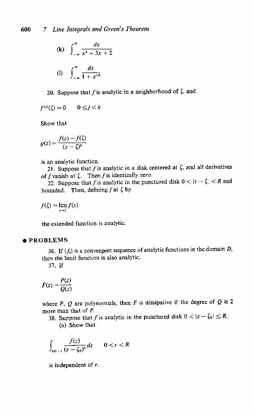
600 7 Line Integrals and Green's Theorem
rM dx
(k) J_x2 + 3x + 2
t" dx
(1) Li+*s
20. Suppose that /is analytic in a neighborhood of , and
f"\l) = 0 0<j<k
Show that
/(*)-/()<?(z) =
:
(z-)k
is an analytic function.
21. Suppose that /is analytic in a disk centered at , and all derivatives
of /vanish at . Then /is identically zero.
22. Suppose that /is analytic in the punctured disk 0 < \z- | < R and
bounded. Then, defining /at $ by
/() = lim/(z)
the extended function is analytic.
PROBLEMS
36. If {/} is a convergent sequence of analytic functions in the domain D,
then the limit function is also analytic.
37. If
P(z)
where P, Q are polynomials, then F is dissipative if the degree of Q is 2
more than that of P.
38. Suppose that /is analytic in the punctured disk 0 < \z 0| <R-
(a) Show that
f -
J[z\=r (rfz 0 < r < A
W"
is independent of r.
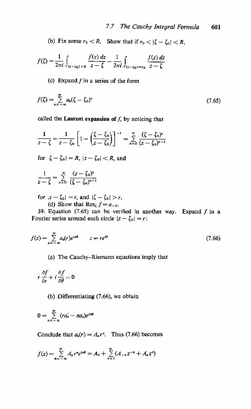
7.7 The Cauchy Integral Formula 601
(b) Fix some r0 < R. Show that if r0 < | - Co I < R,
l Jic-c0i=ji z L, 2m J|{-{oi=r0 z 4
(c) Expand /in a series of the form
/()= I fttf-W (7.65)n= oo
called the Laurent expansion of/, by noticing that
i_ir /g-goVT |- (->)"
z-
z- o L \z- o/J .tb (z - 0)"+l
for |C-0|=JI, |z-0|<*, and
1
|(z-W
z-g .^-W+1
for |z 0| =/-, and | 0| >r.
(d) Show that Res{ /= a_i.
39. Equation (7.65) can be verified in another way. Expand / in a
Fourier series around each circle \z go I = r:
/(*)= 2 aJrW z = re' (7.66)
(a) The Cauchy-Riemann equations imply that
df 8f
(b) Differentiating (7.66), we obtain
0= f (ran-nan)e'">n= oo
Conclude that a(r) = An r". Thus (7.66) becomes
/(z) = | A rV"* = A, + | C4 -. '- + A, z")

602 7 Line Integrals and Green's Theorem
40. Suppose that /is one-to-one in the domain D. Then by the residue
theorem
J-f2m JBt
z dz0
2m hD wf(z)
if w is not a value of /in D. Suppose /(o) = w. Then
z dz
a='-=hLhDV/f{z)
Conclude that the inverse of a one-to-one analytic function is again analytic.
7.8 Summary
Let p e R" and suppose f is an Revalued function defined in a neighbor
hood of p. / is differentiable at p if there is a linear transformation
T: R" -+ Rm such that
l|f(p + v)-f(p)-r(v)iLoas^0IMI
Tis called the differential off at p and is denoted df(p).
The differential is linear in the function f and also satisfies
/<f,g> = <tf,g> + <*,<*>
Let U be a domain in R". A system of coordinates on U is an w-tuple of
C1 functions y such that
(i) ifp#q, y(p)#y(q)
(ii) dy(p) is nonsingular at all p e U
The matrix
8(y\ ...,/) fly'
5(x1,...,x") 5xJ'
is called the Jacobian of the coordinate change.
7.8 Summary 603
the chain rule. The differentials of composed mappings compose as
linear transformations :
d(s f)(p) = 45(f(p)) df(p)
inverse mapping theorem. Suppose F is a C1 K"-valued function defined
in a neighborhood of p0 such that rfF(p0) is nonsingular. Then there are
neighborhoods N of p0 and U of F(p0) and a C1 mapping G: U-* N such that
G = F-1.
Let D be a domain in R". A differential form on D is a function which
associates to each point p in D a linear function co(p) on R". A differential
form has the form
n
co(v) = X a;(p) dx'(p)i=l
a> is said to be Ck on D if all the functions au ...,an are C*. If co is the
differential of a function we must have
pj =^ l<UJ<n (7.67)ox' ox
A differential form is exact if it is the differential of a function, and closed
if (7.67) holds.
Suppose that F is a force field defined in a domain Z) in R", and T is an
oriented path defined in D. The work required to move a unit mass along T is
W{T, F) =- J*<F((), g'(0> dt
where g furnishes a parametrization of T.
A field is conservative if W(r, F) = 0 over all closed paths T. A potential
function for a field F is a real-valued function II such that
w(r, F) + n(p')- n(p)
is the same for every oriented path T from p to p'.
Suppose D is a domain such that any two points can be joined by a path
in D. Then
(i) every field, conservative in D, has a potential function
(ii) two potentials of a given field differ by a constant
(iii) If F = (Ji, . . . ,/) has the potential IT, dU = /; </x'
604 7 Line Integrals and Green's Theorem
line integral of a differential form. Let r be an oriented path in a
domain on which the form co is defined. If T = Yj=i T{ ,define
"'r i=l Jat
If T is the tangent to T,
\ co = co(T) ds
Let co = Yj ai dx' be a C1 differential form defined on D. co = <// for
some function /
(i) if and only if the field (au ..., a) is conservative
(ii) if and only ifr co = 0 for all closed curves
(iii) only if
dat dajc7x1
=
~dxi
throughout D.
for all i, j
poincare's lemma. Suppose that D is a domain such that for some fixed
point p0 in D and every p e D, the line segment joining p0 to p is contained
in D. Then every closed form is exact in D.
In two dimensions a differential form has the form co = p dx + q dy.If co is C1 we shall denote the function
dq dp
dx dy
by dco. A regular domain in R2 is bounded by a piecewise C1 curve. We
orient this curve so that its principal normal points into D (it winds counter
clockwise around D). When so oriented we shall denote the bounding
path by dD.
green's theorem. If co is a C1 differential form defined on the regulardomain D,
Ud to = \Ddco

7.8 Summary 605
Integration under a coordinate change. Suppose
x = x(u, v)
y= y(u, v)
is a coordinate change on the domain D in R2. Let E be the domain in the
uv plane corresponding to D. If F is continuous on D, then
\ f =\ /(*("> u)> .K", v))JD JE
Let v = (v, w) be a C1 vector field. The divergence of v is
div v = +dx dy
divergence theorem. If v is a C1 vector field defined on the regulardomain D,
\ao <v, N> ds = \D div v
A C2 function / is the potential of a conservative divergence-free flow if
and only if it is harmonic.
cauchy's theorem. If / is a C1 complex differentiable function defined
on the regular domain D, then
\Dfdz = 0
cauchy integral formula. Under the same hypotheses on /, if e D,
2ni Jd z 4
maximum principle. If/is analytic on D, it attains its maximum on dD.
Theorem. Let /be a C1 complex-valued function defined on the regular
domain D. The following assertions are equivalent
(i) for any e D, and some R such that A(, R) <= Df is the sum in A(, R)
detojx, y)
d(u, v)du dv
606 7 Line Integrals and Green's Theorem
of a convergent power series
/(z) = an{z- )" (7.68)
n = 0
(ii) replace the word some in (i) by any
(iii) /is complex differentiable
(iv) / satisfies the Cauchy-Riemann equations
8l=-idldx dy
(v) fdz is closed
(vi) for any e D
27t( Jao z -
In case / has these properties (/ is analytic), the coefficients an of (7.68) are
given by
/<"({) 1 f /(z)dzJV1U i f
n! 2ni-'afl(z-)"+1
If/is analytic in {0 < | z z0 1 < R}, we say that /has an isolated singularityat z0 . In this case the integrals
^~.\ f(z)dz'\z-z0\=r
are all the same for 0 < r < R. Their common value is the residue of / at
z0 ,denoted Res (/, z0).
residue theorem. If /is an analytic function on the regular domain D,
except for isolated singularities at zlt . . ., z in D, then
f f(z)dz = 2ni Res(/,z()JdD i=l
7.8 Summary 607
FURTHER READING
The general theorems on differentiation in R" are fully discussed in:
H. K. Nickerson, N. Steenrod, D. C. Spencer, Advanced Calculus, D. Van
Nostrand Company, Inc., Princeton, N. J., 1957.
M. E. Munroe, Modern Multidimensional Calculus, Addison-Wesley,
Reading, Mass., 1963.
L. Loomis and S. Sternberg, Advanced Calculus, Addison-Wesley, Reading,Mass., 1968.
For further information on complex analytic functions see
Z. Nehari, Introduction to Complex Analysis, Allyn and Bacon, Inc., Boston,1961.
H. Cartan, Elementary Theory of Analytic Functions of One or Several
Complex Variables, Addison-Wesley, Reading, Mass., 1963.
E. Hille, Analytic Function Theory, Ginn and Company, Boston, 1959.
L. Ahlfors, Complex Analysis, McGraw-Hill, New York, 1953.
MISCELLANEOUS PROBLEMS
41 . Prove the assertion concerning integration under a coordinate change
as given in the summary (where no reference to the orientation is made).
42. Show that if u> is a differential form of compact support in R2, that
f dw=0
43. Recall the definition of connectedness given in Problem 78 of
Chapter 2. Show that a domain in R2 is connected if and only if it is path-
wise connected.
44. If co =p dx + q dy is a C1 form, define
*tu = qdx+pdy
(a) Show that for any regular domain D,
f o(N) ds = f dJdD J D
*,
D
where N is the interior normal to D.
(b) Show that the function u is harmonic if and only if d*du = 0.
(c) co is (locally) the differential of a harmonic function if and only
if d<a = 0, d*w = 0.
45. If is a harmonic function in the domain D and if *du is exact in D,
then u is the real part of an analytic function in D.
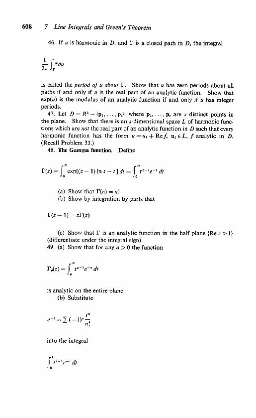
7 Line Integrals and Green's Theorem
46. If u is harmonic in D, and T is a closed path in D, the integral
hS;du
is called the period of u about T. Show that u has zero periods about all
paths if and only if u is the real part of an analytic function. Show that
exp(K) is the modulus of an analytic function if and only if has integer
periods.47. Let D = R2 {plt ..., ps), where pi, . . .
, ps are j distinct points in
the plane. Show that there is an ^-dimensional space L of harmonic func
tions which are not the real part of an analytic function in D such that every
harmonic function has the form = Hi + Re/ UieZ,, /analytic in D.
(Recall Problem 33.)
48. The Gamma function. Define
r(z)= exp[(z-l) In t-t]dt=\ t'-'e- dtJa Jo
(a) Show that T{n) = n\
(b) Show by integration by parts that
r(z+l)=zl\z)
(c) Show that Y is an analytic function in the half plane {Re z > 1}
(differentiate under the integral sign).49. (a) Show that for any a > 0 the function
r.(z)= t'-'e-'dt
is analytic on the entire plane.
(b) Substitute
e-'=Z(-v"-,n\
into the integral
\ t'-'e-dtJo
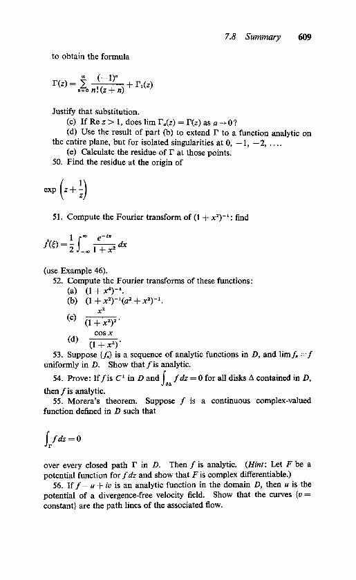
7.8 Summary 609
to obtain the formula
n = 0 !(Z+fl)
Justify that substitution.
(c) If Re z > 1, does lim r(z) = T{z) as a -> 0 ?
(d) Use the result of part (b) to extend T to a function analytic on
the entire plane, but for isolated singularities at 0, 1, 2
(e) Calculate the residue of T at those points.50. Find the residue at the origin of
expR51. Compute the Fourier transform of (1 + x2)"1: find
1 r" e~"
(use Example 46).
52. Compute the Fourier transforms of these functions :
(a) (1+x4)"1.
(b) (l+x2)-'(a2 + x2)-1.x2
(c)
(d)
(1 + x2)2
cosx
(1+x2)'53. Suppose {/,} is a sequence of analytic functions in D, and lim/, =/
uniformly in D. Show that /is analytic.
54. Prove: If/is C1 in D and fdz = 0 for all disks A contained in D,
then /is analytic.
55. Morera's theorem. Suppose / is a continuous complex-valued
function denned in D such that
j fdz=0
over every closed path T in D. Then / is analytic. {Hint: Let F be a
potential function for fdz and show that Fis complex differentiable.)
56. If /= u + iv is an analytic function in the domain D, then u is the
potential of a divergence-free velocity field. Show that the curves {v =
constant} are the path lines of the associated flow.
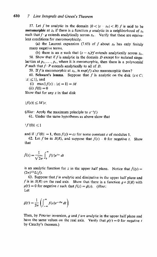
7 Line Integrals and Green's Theorem
57. Let / be analytic in the domain {0 < \z z0 1 < R} f is said to be
meromorphic at z0 if there is a function g analytic in a neighborhood of z0
such that/- g extends analytically across z0 . Verify that these are equivalent conditions for meromorphicity.
(a) the Laurent expansion (7.65) of / about z0 has only finitelymany negative terms.
(b) there is an n such that (z z0)"/ extends analytically across z0 .
58. Show that if /is analytic in the domain D except for isolated singularities atpi,...,p,, where it is meromorphic, then there is a polynomialP such that/ P extends analytically to all of D.
59. If /is meromorphic at z0, is exp(/) also meromorphic there?
60. Schwarz's lemma. Suppose that / is analytic on the disk {z e C:
\z\ < 1}, and
(i) max{|/(z)|:|z|=l} =M
(ii)/(0)=0Show that for any z in that disk
l/(z)|<M|z|
{Hint: Apply the maximum principle to z"1/.)61. Under the same hypotheses as above show that
i/'(o)i<n
and if |/'(0)| = 1, then/(z) = cz for some constant c of modulus 1.
62. Let / be in S{R), and suppose that /(/) = 0 for negative t. Show
that
/(z) = -r= f f{t)e'"dt
is an analytic function for z in the upper half plane. Notice that /(; =
(277)1'2L(/).63. Suppose that /is analytic and dissipative in the upper half plane and
f is in S{R) on the real axis. Show that there is a function g e S{R) with
g{t) = 0 for negative t such that /(z) = g{z). {Hint:Let
Then, by Fourier inversion, g and /are analytic in the upper half plane andhave the same values on the real axis. Verify that #(0=0 for negative /
by Cauchy's theorem.)