NLMAP - Localização e Navegação de Robôs Cooperativos para Inspeção
Upload
khangminh22Category
view
0download
0
PAGANINI BARCELLOS DE OLIVEIRA
NOVAS ABORDAGENS PARA O PROBLEMA
DE LOCALIZAÇÃO DE FACILIDADES EM DOIS
NÍVEIS: MODELOS E ALGORITMOS
Belo Horizonte27 de fevereiro de 2020
Universidade Federal de Minas GeraisEscola de Engenharia
Pós-Graduação em Engenharia de Produção
NOVAS ABORDAGENS PARA O PROBLEMA
DE LOCALIZAÇÃO DE FACILIDADES EM DOIS
NÍVEIS: MODELOS E ALGORITMOS
Tese apresentada ao Curso de Pós-Graduaçãoem Engenharia de Produção da UniversidadeFederal de Minas Gerais como requisito parcialpara a obtenção do grau de Doutor em Engen-haria de Produção.
Área de concentração: Pesquisa Opera-cional e Intervenção em Sistemas Sociotécnicos.
Linha de pesquisa: Otimização de SistemasLogísticos e de Grande Porte.
Orientador: Ricardo Saraiva de Camargo.
PAGANINI BARCELLOS DE OLIVEIRA
Belo Horizonte27 de fevereiro de 2020

Universidade Federal de Minas GeraisSchool of Engineering
Postgraduate Program in Production Engineering
NEW APPROACHES FOR THE TWO-LEVEL
FACILITY LOCATION PROBLEM: MODELS
AND ALGORITHMS
Thesis presented to the Graduate Program inProduction Engineering of the UniversidadeFederal de Minas Gerais in partial fulfillmentof the requirements for the degree of Doctor inProduction Engineering.
Concentration area: Operational Researchand Intervention in Sociotechnical Systems.
Line of research: Optimization of Logis-tics and Large-Scale Systems.
Advisor: Ricardo Saraiva de Camargo.
PAGANINI BARCELLOS DE OLIVEIRA
Belo HorizonteFebruary 27, 2020

Oliveira, Paganini Barcellos de. O48n Novas abordagens para o problema de localização de facilidades em
dois níveis [recurso eletrônico]: modelos e algoritmos / Paganini Barcellos de Oliveira. - 2020.
1 recurso online (xiv, 201 f. : il., color.) : pdf.
Orientador: Ricardo Saraiva de Camargo.
Tese (doutorado) - Universidade Federal de Minas Gerais, Escola de Engenharia. Apêndices: f. 131-182. Bibliografia: f. 123-130. Exigências do sistema: Adobe Acrobat Reader.
1. Engenharia de Produção - Teses. 2. Método de decomposição-Teses. 3. Algoritmos – Teses. 4. Logística empresarial – Teses. I. Camargo, Ricardo Saraiva de. II. Universidade Federal de Minas Gerais. Escola de Engenharia. III. Título.
CDU: 658 (043)
Ficha catalográfica: Biblioteca Profº Mário Werneck, Escola de Engenharia da UFMG


Resumo
Esta tese investiga a aplicação de algoritmos exatos e heurísticos para a resolução dediferentes variantes do problema de localização de facilidades em dois níveis, versõesestas poucos estudadas pela literatura. Trata-se de um tema de grande importân-cia dentro da área de Otimização de Sistemas de Grande Porte, tendo ainda amplaaplicação em diversos sistemas logísticos existentes. De forma geral, o problema con-siste em selecionar de um conjunto de locais candidatos um subconjunto de pontosque atuarão ou como suprimento ou como transbordo no atendimento, a custo mín-imo de instalação e transporte, de clientes espalhados geograficamente. Nas variantesestudadas, a rede de atendimento ou distribuição é hierarquizada, sendo formada porum primeiro nível composto por facilidades que suprem as demandas dos clientes viapontos de transbordo pertencentes ao segundo nível. As três variantes estudadas doproblema são: (i) a versão na qual facilidades e transbordos são não capacitados; (ii) ocaso no qual a demanda dos clientes varia num horizonte de planejamento discretizadoem períodos, resultando num problema de localização multi-período ou dinâmico; (iii)e a alternativa que considera custos adicionais oriundos dos efeitos de congestiona-mento em função do acúmulo de fluxo nas facilidades e pontos de transbordo. Emtodas as variantes investigadas consideram-se duas possibilidades de interligação entreo primeiro e segundo níveis. Na alocação simples, um ponto de transbordo só podeinteragir com uma única facilidade; enquanto, na atribuição múltipla, um ponto detransbordo pode estar conectado com um número qualquer de facilidades. Como ogrande desafio destes tipos de problemas é a natureza combinatória deles, para cadauma das variantes estudadas, modelos matemáticos e métodos especializados baseadosna decomposição de Benders e GRASP foram propostos e avaliados tanto em relaçãoao tempo computacional quanto à qualidade das soluções obtidas.
Palavra-chaves: Problemas de localização de facilidades em dois níveis; método dedecomposição de Benders; GRASP; otimização de sistemas logísticos de grande porte
i

Abstract
This thesis presents exact and heuristic algorithms to solve different variants of thetwo-level facility location problem; variants which were less studied in the literature uptill now. This is a topic of great relevance within the field of Large Scale System Opti-mization and with an ample presence in several logistics systems. Generally speaking,the problem consists of selecting a subset of points from a set of candidate sites toact either as a supply or as an transshipment point to serve customers geographicallyscattered at minimal installation and transportation costs. In the studied variants,the service or distribution network is hierarchical, being composed of a first level withfacilities that supply customer demands via a second tier having transshipment points.The three studied variants of the problem are: (i) the version in which the facilities andtransshipment points are assumed uncapacitated; (ii) the case in which customers’ de-mand varies over a discretized planning horizon, leading to a multi-period or dynamiclocation problem; (iii) and the alternative that considers additional costs arising fromthe effects of congestion derived from the delay of accumulated flow in the facilitiesand transfer points. All investigated variants consider two possible types of intercon-nection between the first and second levels. In the single allocation, a transshipmentpoint can interact with only one facility; while, in the multiple assignment, a transship-ment point can connect with many facilities. Finally, as one of the greatest challengesof these problems is their combinatorial nature, mathematical models and specializedmethods based on the Benders decomposition method and GRASP were proposed andassessed both in terms of computational running time and obtained solution qualityfor each of the studied variants.
Keywords: Two-level facility location problems; Benders decomposition method;GRASP; optimization of large-scale logistics systems
ii
For my mother Ana Lúcia, my father Verdi,my brothers Natasha, Giannini and Toscanini, my nephew Miguel, and my girlfriendMayara.
iii

“A daily effort of 1% on a project yields anaccumulated compound effort of 37.8 (≈ 1.01365) at the
end of an year.”
— Unknown author
iv

Acknowledgments
First and foremost, praises and thanks to God, for all the blessings bestowed upon methrough all these years of study and research. I would like to start by thanking myparents and my family and friends for their love, caring, sacrifices, and understanding.“-Guys, it was all worth it!”. I also wish to recognize the exceptional educationalinstitutions which have helped me to mold my academic career:
- E. M. Efigênio Mota;
- E. E. Antonio Papini;
- E. M. Vale do Sol;
- E. E. Luiz Prisco de Braga;
- C. F. P. Nansen Araújo – SENAI João Monlevade;
- Universidade Federal de Ouro Preto – UFOP;
- Universidade Federal de Minas Gerais – UFMG.
This thesis would not be possible without the financial support of Fapemig, CNPqand Capes, and the the aid of all the professors and administrative technicians ofUFOP and UFMG. I am specially indebted to the NTI technicians of UFOP, andto Professor Dr. Alexandre Xavier Martins, whose helpful suggestions and advisesencouraged me to push forward. I am also indebted to Professor Ph.D. Ivan Contrerasof the Concordia University, Canada, who generously assisted me on separating a newBenders optimality cut for the problem.
Last but not least, I would like to sincerely express my deepest gratitude to mymentors and major references in Operations Research, Professors Dr. Ricardo Saraivade Camargo, and Dr. Gilberto de Miranda Júnior. Their invaluable teachings wentbeyond of an thesis adviser. Their friendship and confidence in me and my work mademy quest for my master and doctorate degrees in Production Engineering a reality. Tothem, my wholehearted thank you!
v

Contents
1 Introduction 1
2 A comparison of separation routines for Benders optimality cuts fortwo-level uncapacitated facility location problems 72.1 Introduction . . . . . . . . . . . . . . . . . . . . . . . . . . . . . . . . . 72.2 The two-level uncapacitated facility location problem with multiple as-
signments . . . . . . . . . . . . . . . . . . . . . . . . . . . . . . . . . . 102.2.1 Benders reformulation for the TLUFLP-MA . . . . . . . . . . . 112.2.2 Separation routines for Benders optimality cuts . . . . . . . . . 132.2.3 Algorithm enhancements . . . . . . . . . . . . . . . . . . . . . . 20
2.3 The two-level uncapacitated facility location problem with single assign-ments . . . . . . . . . . . . . . . . . . . . . . . . . . . . . . . . . . . . 212.3.1 Benders reformulations for the TLUFLP-SA . . . . . . . . . . . 222.3.2 Separation routines for Benders optimality cuts . . . . . . . . . 23
2.4 Computational experiments . . . . . . . . . . . . . . . . . . . . . . . . 262.4.1 Results for the TLUFLP-MA . . . . . . . . . . . . . . . . . . . 272.4.2 Results for the TLUFLP-SA . . . . . . . . . . . . . . . . . . . . 33
2.5 Conclusion . . . . . . . . . . . . . . . . . . . . . . . . . . . . . . . . . . 41
3 A decomposition approach for the dynamic two-level uncapacitatedfacility location problem with single and multiple allocations 423.1 Introduction . . . . . . . . . . . . . . . . . . . . . . . . . . . . . . . . . 433.2 Notation, definitions and formulations . . . . . . . . . . . . . . . . . . 45
3.2.1 Formulations for the DTLUFLPM . . . . . . . . . . . . . . . . . 463.2.2 Formulations for the DTLUFLPS . . . . . . . . . . . . . . . . . 47
3.3 Decomposition approaches . . . . . . . . . . . . . . . . . . . . . . . . . 503.3.1 Benders decomposition for the DTLUFLPM . . . . . . . . . . . 513.3.2 Benders decomposition for the DTLUFLPS . . . . . . . . . . . 533.3.3 Separation routines for different BCs . . . . . . . . . . . . . . . 553.3.4 Algorithm enhancements . . . . . . . . . . . . . . . . . . . . . . 64
vi

3.4 GRASP algorithm . . . . . . . . . . . . . . . . . . . . . . . . . . . . . 653.5 Computational experiments . . . . . . . . . . . . . . . . . . . . . . . . 67
3.5.1 Benchmark Instances . . . . . . . . . . . . . . . . . . . . . . . . 673.5.2 Tuning the devised GRASP . . . . . . . . . . . . . . . . . . . . 683.5.3 Computational performance of the exact framework . . . . . . . 71
3.6 Conclusion . . . . . . . . . . . . . . . . . . . . . . . . . . . . . . . . . . 80
4 The hierarchical two-level facility location problem under the sup-ply and congestion costs effects 824.1 Introduction . . . . . . . . . . . . . . . . . . . . . . . . . . . . . . . . . 824.2 Notation, definitions and formulations . . . . . . . . . . . . . . . . . . 85
4.2.1 CTLUFLP formulations . . . . . . . . . . . . . . . . . . . . . . 874.2.2 Congestion functions . . . . . . . . . . . . . . . . . . . . . . . . 91
4.3 Decomposition approaches for CTLUFLPs . . . . . . . . . . . . . . . . 934.3.1 Outer-Approximation . . . . . . . . . . . . . . . . . . . . . . . . 954.3.2 Benders decomposition approaches . . . . . . . . . . . . . . . . 964.3.3 Acceleration methods . . . . . . . . . . . . . . . . . . . . . . . . 109
4.4 Computational experiments . . . . . . . . . . . . . . . . . . . . . . . . 1124.4.1 Comparing the methods . . . . . . . . . . . . . . . . . . . . . . 1134.4.2 Scalability experiments . . . . . . . . . . . . . . . . . . . . . . . 1164.4.3 Analysis of congestion function parameters . . . . . . . . . . . . 117
4.5 Conclusion . . . . . . . . . . . . . . . . . . . . . . . . . . . . . . . . . . 119
5 Conclusion 121
Bibliography 123
A Appendices of the Chapter 2 131
B Appendices of the Chapter 3 155
C Appendices of the Chapter 4 162
vii

List of Figures
1.1 Example of a two-level uncapacitated facility location problem . . . . . . . 21.2 Example of a two-level uncapacitated facility location problem with single
assignments . . . . . . . . . . . . . . . . . . . . . . . . . . . . . . . . . . . 31.3 An example of a dynamic two-level facility location problem . . . . . . . . 4
2.1 TLUFLP-MA Performance benchmark profiles for Gap instances. . . . . . 292.2 TLUFLP-MA Performance benchmark profiles for LGap instances. . . . . 292.3 TLUFLP-MA Performance benchmark profiles for Ro and Tcha instances. 322.4 MPz,y,π performance benchmark profiles for Gap instances. . . . . . . . . . 352.5 MPz,y,π performance benchmark profiles for LGap instances. . . . . . . . . 372.6 MPz,π performance benchmark profiles for Gap instances. . . . . . . . . . . 372.7 MPz,π performance benchmark profiles for LGap instances. . . . . . . . . . 382.8 TLUFLP-SA performance benchmark profiles for Ro and Tcha instances
using MPz,y,π formulation. . . . . . . . . . . . . . . . . . . . . . . . . . . . 392.9 TLUFLP-SA performance benchmark profiles for Ro and Tcha instances
using MPz,π formulation. . . . . . . . . . . . . . . . . . . . . . . . . . . . . 40
3.1 An example of a dynamic two-level facility location problem with singleassignments. . . . . . . . . . . . . . . . . . . . . . . . . . . . . . . . . . . . 45
3.2 The GRASP benchmarking profile concerning the percentage gaps of thebest-attained solutions (gapb) for when αmax is varied for all the instances. 69
3.3 The attained percentage gaps for the Ro and Tcha’s instance I-10-5-B, whenthe Imax is varied within the set 10, 50, 100, 150. . . . . . . . . . . . . . . 69
3.4 The benchmarking profile for formulations M and Myz solved by CPLEX,using the results of Table B.1 in Appendix B. . . . . . . . . . . . . . . . . 72
3.5 The benchmarking profile for formulations S, Sy, Syza and Syzb solved byCPLEX, using the results of Table B.3 in Appendix B. . . . . . . . . . . . 76
3.6 The SGM of the percentage of covered variables of the Benders cuts sepa-rated via MWf and P routines. . . . . . . . . . . . . . . . . . . . . . . . . 76
viii

3.7 The SGM of the percentage of covered variables of the Benders cuts sepa-rated via I, CF, MW, MWf and P routines. . . . . . . . . . . . . . . . . . 77
3.8 The benchmarking profile concerning the computational running time forseparation routines MWf and P based on formulation M comparing withCPX, and BD-CPX on solving larger instances (Table B.5 in Appendix B). 80
3.9 The benchmarking profile concerning the computational running time forall separation routines based on formulation S on solving larger instances(Table B.6 in Appendix B). CPX and BD-CPX curves omitted since theywere unable to solve all instances within the given time limit of 24h. . . . . 80
4.1 Example of single-and-single assignment problem . . . . . . . . . . . . . . 864.2 Examples of different supply patterns in a CTLUFLP . . . . . . . . . . . . 904.3 Attained percentage of total demand (Ω(%)
100 ) that each 1st level facility (Y-axis) and the respective number of customers linked to it (X-axis). . . . . . 91
4.4 Attained percentage of total demand (Ω(%)100 ) that each 2nd level facility (Y-
axis) and the respective number of customers linked to it (X-axis). . . . . . 924.5 Flow deviation algorithm convergence process via Golden Section search . 1084.6 The SGM of the computer running times for solving a set of Ro and Tcha
CTLUFLP instances under Power-Law congestion function costs via differ-ent formulations and methods. . . . . . . . . . . . . . . . . . . . . . . . . . 114
4.7 The SGM of the number of explored branch-and-bound nodes for solvinga set of Ro and Tcha CTLUFLP instances under Power-Law congestionfunction costs via different formulations and methods. . . . . . . . . . . . . 114
4.8 The SGM of the computer running times for solving a set of Ro and TchaCTLUFLP instances under Kleinrock congestion function costs via differentformulations and methods. . . . . . . . . . . . . . . . . . . . . . . . . . . . 115
4.9 The SGM of the number of explored branch-and-bound nodes for solving aset of Ro and Tcha CTLUFLP instances under Kleinrock congestion func-tion costs via different formulations and methods. . . . . . . . . . . . . . . 116
4.10 Bubble chart of the SGM of CPU running times for solving a 10×50×100CTLUFLP instance under Power-Law congestion function costs via OAalgorirthm, when % and % parameters are changed. . . . . . . . . . . . . . . 119
ix

List of Tables
2.1 Summary of computational experiments for TLUFLP-MA using Gap andLGap instances. . . . . . . . . . . . . . . . . . . . . . . . . . . . . . . . . . 30
2.2 Summary of TLUFLP-MA computational experiments combining Benderscuts. . . . . . . . . . . . . . . . . . . . . . . . . . . . . . . . . . . . . . . . 31
2.3 MA-MW variant’s computational experiments for when the number of cus-tomers is scaled up. . . . . . . . . . . . . . . . . . . . . . . . . . . . . . . . 32
2.4 MA-MW variant’s computational experiments for when the number of cus-tomers and fixed cost are scaled up. . . . . . . . . . . . . . . . . . . . . . . 33
2.5 Summary of computational experiments for TLUFLP-SA using MPz,y,π for-mulation. . . . . . . . . . . . . . . . . . . . . . . . . . . . . . . . . . . . . 35
2.6 Summary of computational experiments for TLUFLP-SA using MPz,π for-mulation. . . . . . . . . . . . . . . . . . . . . . . . . . . . . . . . . . . . . 36
2.7 Summary of TLUFLP-SA computational experiments using MPz,y,π formu-lation . . . . . . . . . . . . . . . . . . . . . . . . . . . . . . . . . . . . . . 38
2.8 Summary of TLUFLP-SA computational experiments using MPz,π formu-lation . . . . . . . . . . . . . . . . . . . . . . . . . . . . . . . . . . . . . . 39
2.9 SA-MW and MSA-MW variants’ computational experiments for when thenumber of customers are scaled up. . . . . . . . . . . . . . . . . . . . . . . 40
2.10 MSA-MW variant’s computational experiments for when the number ofcustomers and fixed cost are scaled up. . . . . . . . . . . . . . . . . . . . . 41
3.1 The SGM of the computer running times for formulations M and Myz solvedby CPLEX and the devised Benders algorithm with different types of BCs. 72
3.2 The SGM of the number of explored branch-and-bound nodes for formula-tions M and Myz solved by CPLEX and the devised Benders algorithm withdifferent types of BCs. . . . . . . . . . . . . . . . . . . . . . . . . . . . . . 73
3.3 The SGM of the computational running times for formulations S, Sy, Syzaand Syzb solved by CPLEX and the devised Benders algorithm with differenttypes of BCs. . . . . . . . . . . . . . . . . . . . . . . . . . . . . . . . . . . 74
x

3.4 The SGM of the number of explored branch-and-bound nodes for formu-lations S, Sy, Syza and Syzb solved by CPLEX and the Benders algorithmdifferent types of BCs. . . . . . . . . . . . . . . . . . . . . . . . . . . . . . 75
3.5 The SGM for the number of branch-and-bound nodes and computationalrunning times for routines MWf and P based on formulation M comparingwith the CPLEX and CPLEX’s built-in Benders. . . . . . . . . . . . . . . 77
3.6 The SGM for the number of branch-and-bound nodes and computationalrunning times for all routines based on formulation S comparing with theCPLEX and CPLEX’s built-in Benders. . . . . . . . . . . . . . . . . . . . 79
4.1 A comparison between different customers supply patterns . . . . . . . . . 904.2 Sets, parameters and variables of the decomposition approaches. . . . . . . 944.3 Summary of computational results when only total customers is expanded,
considering a Power-Law function with % = 1×10⁻⁵ and % = 1×10⁻⁴, whileKleinrock functions have ϑ = 1× 10⁵, ϑ = 1× 10⁴ and ρ = ρ = 0.99. . . . . 117
4.4 Summary of computational results when instance sizes are increased at alllevels, considering a Power-Law function with % = 1×10⁻⁵ and % = 1×10⁻⁴,while Kleinrock functions have ϑ = 1× 10⁵, ϑ = 1× 10⁴ and ρ = ρ = 0.99. 118
A.1 TLUFLP-MA computational experiments to GapA instances . . . . . . . . 132A.2 TLUFLP-MA computational experiments to GapB instances . . . . . . . . 133A.3 TLUFLP-MA computational experiments to GapC instances . . . . . . . . 134A.4 TLUFLP-MA computational experiments to LGapA instances . . . . . . . 135A.5 TLUFLP-MA computational experiments to LGapB instances . . . . . . . 136A.6 TLUFLP-MA computational experiments to LGapC instances . . . . . . . 137A.7 TLUFLP-MA computational experiments usingUserCutCallback and warm-
start iterations to Ro and Tcha instances . . . . . . . . . . . . . . . . . . . 138A.8 TLUFLP-MA computational experiments to Ro and Tcha instances . . . . 139A.9 TLUFLP-SA computational experiments to GapA instances . . . . . . . . 140A.10 TLUFLP-SA computational experiments to GapB instances . . . . . . . . 141A.11 TLUFLP-SA computational experiments to GapC instances . . . . . . . . 142A.12 TLUFLP-SA computational experiments to LGapA instances . . . . . . . 143A.13 TLUFLP-SA computational experiments to LGapB instances . . . . . . . 144A.14 TLUFLP-SA computational experiments to LGapC instances . . . . . . . 145A.15 TLUFLP-MSA computational experiments to GapA instances . . . . . . . 146A.16 TLUFLP-MSA computational experiments to GapB instances . . . . . . . 147A.17 TLUFLP-MSA computational experiments to GapC instances . . . . . . . 148A.18 TLUFLP-MSA computational experiments to LGapA instances . . . . . . 149
xi

A.19 TLUFLP-MSA computational experiments to LGapB instances . . . . . . 150A.20 TLUFLP-MSA computational experiments to LGapC instances . . . . . . 151A.21 TLUFLP-SA computational experiments using UserCutCallback and warm-
start iterations to Ro and Tcha instances . . . . . . . . . . . . . . . . . . . 152A.22 TLUFLP-SA computational experiments to Ro and Tcha instances . . . . 153A.23 TLUFLP-MSA computational experiments to Ro and Tcha instances . . . 154
B.1 Computational running times in seconds for the multiple assignment case . 156B.2 Number of explored branch-and-bound nodes for the multiple assignment
case. . . . . . . . . . . . . . . . . . . . . . . . . . . . . . . . . . . . . . . . 157B.3 Computational running times for the single assignment case. . . . . . . . . 158B.4 Number of explored branch-and-bound nodes for the single assignment case. 159B.5 Computational running times in seconds and number of branch-and-bound
nodes for the multiple case (larger instances). . . . . . . . . . . . . . . . . 160B.6 Computational running times in seconds and number of branch-and-bound
nodes for the single assignment case (larger instances). . . . . . . . . . . . 161
C.1 Computational experiments using OA algorithm to solve CTLUFLPs sub-jected to Power-Law functions with % = 1× 10⁻⁵ and % = 1× 10⁻⁴. . . . . 162
C.2 Computational experiments using OA-DB algorithm to solve CTLUFLPssubjected to Power-Law functions with % = 1× 10⁻⁵ and % = 1× 10⁻⁴. . . 163
C.3 Computational experiments using OA-BD algorithm with Papadakos BCsapproach to solve CTLUFLPs subjected to Power-Law functions with % =1× 10⁻⁵ and % = 1× 10⁻⁴. . . . . . . . . . . . . . . . . . . . . . . . . . . . 164
C.4 Computational experiments using GBD algorithm to solve CTLUFLPs sub-jected to Power-Law functions with % = 1× 10⁻⁵ and % = 1× 10⁻⁴. . . . . 165
C.5 Computational experiments using GBD algorithm with Papadakos BCs ap-proach to solve CTLUFLPs subjected to Power-Law functions with % =1× 10⁻⁵ and % = 1× 10⁻⁴. . . . . . . . . . . . . . . . . . . . . . . . . . . . 166
C.6 Computational experiments using OA algorithm to solve CTLUFLPs sub-jected to Kleinrock functions with ϑ = 1× 10⁴, ϑ = 1× 10⁴ and ρ = ρ = 0.99.167
C.7 Computational experiments using OA-BD algorithm to solve CTLUFLPssubjected to Kleinrock functions with ϑ = 1×10⁴, ϑ = 1×10⁴ and ρ = ρ =0.99. . . . . . . . . . . . . . . . . . . . . . . . . . . . . . . . . . . . . . . . 168
C.8 Computational experiments using OA-BD algorithm with Papadakos BCsapproach to solve CTLUFLPs subjected to Kleinrock functions with ϑ =1× 10⁴, ϑ = 1× 10⁴ and ρ = ρ = 0.99. . . . . . . . . . . . . . . . . . . . . 169
xii

C.9 Computational experiments using GBD algorithm to solve CTLUFLPs sub-jected to Kleinrock functions with ϑ = 1× 10⁴, ϑ = 1× 10⁴ and ρ = ρ = 0.99.170
C.10 Computational experiments using GBD algorithm with Papadakos BCs ap-proach to solve CTLUFLPs subjected to Kleinrock functions with ϑ =1× 10⁴, ϑ = 1× 10⁴ and ρ = ρ = 0.99. . . . . . . . . . . . . . . . . . . . . 171
C.11 Complete data of the computational experiments for OA algorithm whenonly total customers is expanded, considering a Power-Law function with% = 1× 10⁻⁵ and % = 1× 10⁻⁴. . . . . . . . . . . . . . . . . . . . . . . . . 172
C.12 Complete data of the computational experiments for CPLEX solver whenonly total customers is expanded, considering a Power-Law function with% = 1× 10⁻⁵ and % = 1× 10⁻⁴. . . . . . . . . . . . . . . . . . . . . . . . . 173
C.13 Complete data of the computational experiments for OA algorithm whenonly total customers is expanded, considering a Kleinrock function withϑ = 1× 10⁵, ϑ = 1× 10⁴ and ρ = ρ = 0.99. . . . . . . . . . . . . . . . . . . 174
C.14 Complete data of the computational experiments for OA algorithm whenthe instance size are increased, considering a Power-Law function with % =1× 10⁻⁵ and % = 1× 10⁻⁴. . . . . . . . . . . . . . . . . . . . . . . . . . . . 175
C.15 Complete data of the computational experiments for CPLEX solver whenthe instance size are increased, considering a Power-Law function with % =1× 10⁻⁵ and % = 1× 10⁻⁴. . . . . . . . . . . . . . . . . . . . . . . . . . . . 176
C.16 Complete data of the computational experiments for OA algorithm solverwhen the instance size are increased, considering a Kleinrock function withϑ = 1× 10⁵, ϑ = 1× 10⁴ and ρ = ρ = 0.99. . . . . . . . . . . . . . . . . . . 177
C.17 Computational results from the OA algorithm solving a Ro and Tcha in-stance of 10×50×100 size, when % and % parameters of the Power-Lawfunction are changed. . . . . . . . . . . . . . . . . . . . . . . . . . . . . . . 178
C.18 Computational results from the OA algorithm solving a Ro and Tcha in-stance of 10×50×100 size, when ϑ and ϑ parameters of the Kleinrock func-tion are changed, while ρ = ρ = 0.99. . . . . . . . . . . . . . . . . . . . . . 180
xiii

List of Algorithms
1 Solving dual subproblem by variable adjustment. . . . . . . . . . . . . 152 Solving the DSMit analytically . . . . . . . . . . . . . . . . . . . . . . . 573 Solving the DSSit analytically . . . . . . . . . . . . . . . . . . . . . . . . 574 Local search . . . . . . . . . . . . . . . . . . . . . . . . . . . . . . . . . 665 Flow Deviation algorithm for MM . . . . . . . . . . . . . . . . . . . . . 1076 Greedy heuristic . . . . . . . . . . . . . . . . . . . . . . . . . . . . . . . 110
xiv
Chapter 1
Introduction
Weber (1909) was the first author to introduce a facility location problem consisted ofstrategically located facilities in the Euclidean space to supply a set of demand pointssuch that the sum of all distances between demand points and the installed facilitiesis minimized. Over the years, Weber (1909)’s ideas have been incorporated with otherassumptions given rise to new models for different application problems (Klose andDrexl 2005).
These assumptions include, but are not limited to the installation of p facilities(Maranzana 1963, Hakimi 1965) or an unknown number of facilities (Efroymson andRay 1966, Kuehn and Hamburger 1963), the installation of a hierarchy of facilities(Kuehn and Hamburger 1963, Lawrence and Pengilly 1969), or installing facilities overmulti-periods of time (Roodman and Schwarz 1975, Wesolowsky and Truscott 1975),or the supply of multi-products (Geoffrion and Graves 1974); the reckoning of facil-ity capacities (Akinc and Khumawala 1977, Nauss 1978) or congestion effects (Groveand O’Kelly 1986); and the allowance of customer demands to be served by multiplefacilities or not, i.e. if customer nodes are multi or single assigned to facilities (Holm-berg et al. 1999). Nonetheless, two essential and fundamental features of all facilitylocation problems are the selection of facilities to be activated, and a product/servicedistribution logic to attend customer demands.
Though the facility location literature has grown vastly and maturely since Weber(1909)’s seminal work, there are still some research gaps to be explored or betterstudied, e.g. new modeling assumptions for real applications (Melo et al. 2009), theintegration with other decision problems like vehicle routing (Schneider and Drexl 2017,Drexl and Schneider 2015) and inventory management (Coelho et al. 2014) problems, orto propose new computational solution techniques. One of such research opportunitiesyet to be better understood and solved is a subclass of the multi-level facility locationproblems: the two-level hierarchical facility location problem and its variants.
1
1. Introduction 2
In a two-level facility location problem, the upper level usually supplies to inter-mediary transshipment facilities located in an immediately subsequent level of thehierarchy, which is then responsible to serve customers demands. Customers can beserved by a single or multiple intermediary facilities. This subclass of two-level prob-lems as the focus of our study was not arbitrarily defined. We have selected it becauseof its wide applicability in most real-world supply chain and logistics systems environ-ments (Klose and Drexl 2005). It’s easy to note that the production and distributionof products, data flow services, health care services and bank services are common realexamples of network supply systems, which has this two-level organization pattern.Moreover, another relevant motivation is that there are some variants that have beenpoorly investigated by the research community, being, therefore, the subject of thisthesis.
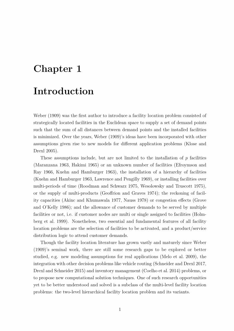
The first problem studied is the two-level uncapacitated facility location problemillustrated in Figure 1.1. Upper-level facilities (squares) supply the nearest lower-levelones (triangles) which then serve the nearest customer nodes (circles). An inadequatechoice of facility locations may impact installation and transportation costs, especiallyfor large-scale networks.
1st level facilities
2nd level facilities
clients
Figure 1.1: Example of a two-level uncapacitated facility location problem
Note that there are second-level facilities that are connected to more than one facil-
1. Introduction 3
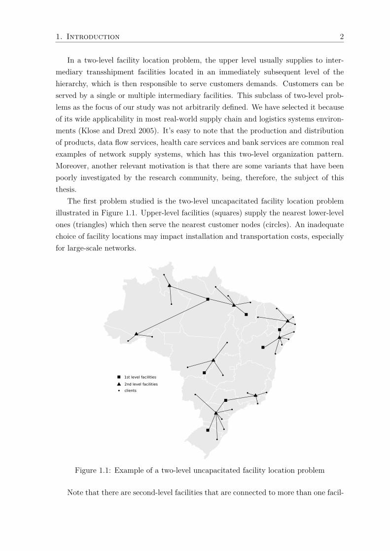
ity of the first level in the example of Figure 1.1. This occurs due to the transportationcost combination between first and second level facilities, and second-level facilities tocustomers. However, there are applications such as the design of some telecommuni-cation networks (Chardaire et al. 1999) that require second-level facilities to be singleassigned to first-level ones as exemplified in Figure 1.2. This gives rise to a more com-putational challenging problem than the multiple allocation variant. However, due tothe matrix structure of the adopted formulations, both problem variants are amenableto be solved by decomposition algorithms, the subject of Chapter 2.
1st level facilities
2nd level facilities
clients
Figure 1.2: Example of a two-level uncapacitated facility location problem with singleassignments
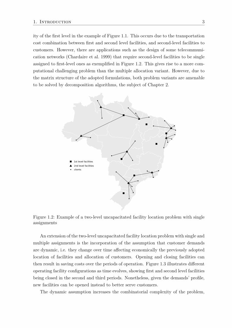
An extension of the two-level uncapacitated facility location problem with single andmultiple assignments is the incorporation of the assumption that customer demandsare dynamic, i.e. they change over time affecting economically the previously adoptedlocation of facilities and allocation of customers. Opening and closing facilities canthen result in saving costs over the periods of operation. Figure 1.3 illustrates differentoperating facility configurations as time evolves, showing first and second level facilitiesbeing closed in the second and third periods. Nonetheless, given the demands’ profile,new facilities can be opened instead to better serve customers.
The dynamic assumption increases the combinatorial complexity of the problem,
1. Introduction 4
1st level facilities
2nd level facilities
clients
1st period 2nd period 3rd period
Figure 1.3: An example of a dynamic two-level facility location problem
requiring thus different modeling considerations and computational approaches. Chap-ter 3 introduces new formulations which extend the models of Chapter 2 to cope withdemands over time and will have the solution algorithms as well.
Finally, as the use of the facilities intensifies and demands get closer to the installedsystem’s capacity, customers may start perceiving longer lead times between deliveries,or delays, or even worse, they might have their demands backlogged. Hence congestioneffects have to be dealt with during modeling and handled accordingly.
Instead of lessening these undesirable effects with capacity constraints, here theseseffects are modeled explicitly on the objective function as convex cost functions (e.gKleinrock (1964) average delay function or a power law) which increase costs exponen-tially as more flows go through the facilities. These convex cost functions capture theexponential nature of the congestion effects: the larger the flow demanded or passingthrough a facility, the increasingly greater the costs are.
Though they properly model the congestion effects, on the other hand, these convexcost functions introduce non-linearities to the problem that complicates the solutionprocess. Assumptions, and formulations, and strategies to handle these non-linearitiesare presented and discussed in Chapter 3.
In all the studied problems, whenever the first and second level facility location deci-sions are parameterized, a set of ease to solve transportation subproblems is obtained.This favors the use of exact decomposition methods such as the Benders algorithm(Benders 1962). Nonetheless, these decomposition methods are computationally en-hanced if combined with other solution techniques (e.g. specialized cut separationprocedures, the implication of sub-modular features (Mateus and Thizy 1999), heuris-tics and/or Lagrangian relaxation). Therefore this thesis combines different algorithmsto efficiently solve the aforementioned two-level location problem variants.
Instead of a traditional thesis text format, this work is the gathering of three self-

1. Introduction 5
contained articles, one for each problem variant. In each chapter or article, an intro-duction to the problem variant is studied, followed by a literature review, the adoptednotation and definitions, and the devised solution framework are presented. Further,the next chapters of this thesis are organized as follows: Chapter 2 the two-level un-capacitated facility location problem with single and multiple assignments is studied,whereas Chapters 3 and 4 introduce the dynamic problem and the problem whose con-gestion effects are being taken into account, respectively. Finally, Chapter 5 concludeswith our final remarks.
Main contributions of this thesis
The thesis’s contributions are presented below:Chapter 2: A comparison of separation routines for Benders optimality
cuts for two-level uncapacitated facility location problems
• To present accelerated Benders decomposition algorithms;
• To introduce closing facility Benders cut separation procedures;
• To separate near Pareto-optimal cuts through tailored methods adapted fromMagnanti and Wong (1981)’s work;
• To solve the Benders dual subproblems via two specialized algorithms withoutthe use of commercial solvers.
Chapter 3: A decomposition approach for the dynamic two-level unca-pacitated facility location problem with single and multiple allocations
• To introduce new dynamic formulations, based on adaptations in Barros andLabbé (1994a) and Gendron et al. (2016) formulations;
• To devise a fast GRASP (Feo and Resende 1989) based heuristic algorithm toattain near-optimal solutions to the problem, in a short computational time;
• To develop an exact decomposition approach to efficiently solve both single andmultiple assignment problems, considering different customer demand patterns.
Chapter 4: The hierarchical two-level facility location problem under thesupply and congestion costs effects
• To propose different formulations for the hierarchical two-level uncapacitatedfacility location problem, where congestion effects are taken into account, eitherfor single or multiple assignments between the levels;

1. Introduction 6
• To develop three different decomposition algorithms based on linearization pro-cedures and cut plane approaches to efficiently solve nonlinear problems.

Chapter 2
A comparison of separationroutines for Benders optimalitycuts for two-level uncapacitatedfacility location problems
This chapter studies two-level uncapacitated facility location problems, a class of dis-crete location problems that consider different hierarchies of facilities and their inter-actions. Benders reformulations for both single and multiple assignment variants andwhile several separation procedures for three classes of Benders cuts are presented:standard optimality cuts, lifted optimality cuts, and non-dominated optimality cuts.Extensive computational experiments are performed on difficult and large-scale bench-mark instances to assess the performance of the considered separation routines.
2.1 Introduction
Many large-scale transportation and telecommunication systems have a hierarchical,multi-echelon structure with two or more facility levels responsible for providing ser-vices or goods to customers scattered on a vast geographical area (Fortz 2015, Ortiz-Astorquiza et al. 2018). The role each level plays in the system distinguishes facilitiesamong different levels. First-level facilities are usually resource generators, whereassecond-level facilities act as intermediate transshipment points. They distribute theseresources to customers using the bottom echelon (Balinski 1964, Manne 1964, Meloet al. 2009).
Examples of hierarchical systems with at least two levels can be found in: (i) bankservices, in which bank branches (first-level) and service points with automated teller
7

2. A comparison of separation routines for Benders optimality cutsfor two-level uncapacitated facility location problems 8
machines (second-level) serve clients scattered over a country (Min and Melachrinoudis2001, Jayaraman et al. 2003, Genevois et al. 2015), (ii) health care services, in whichspecialty medical centers (first-level) together with regional hospitals (second-level)provide treatment to health care family offices (customers) in a province (Şahin andSüral 2007, Smith et al. 2009, Ahmadi-Javid et al. 2017), and (iii) in the productionand distribution of products (e.g. vehicles, food and clothing) in a supply chain, inwhich manufacturing facilities (first-level) supply to distribution centers (second-level)which will then pass these products to traders or dealerships (clients) located overa continental area (Vidal and Goetschalckx 1997, Klose and Drexl 2005, Pasandidehet al. 2015).
In this chapter we focus on a fundamental problem in discrete location known asthe warehouse and plant location problem introduced by Kaufman et al. (1977), alsodenoted as the two-level uncapacitated facility location problem (TLUFLP). Given aset of customers and set of potential facilities partitioned into two levels, TLUFLPsconsider the selection of a set of (uncapacitated) facilities to open at each level so thateach customer is assigned to a sequence of opened facilities, exactly one from eachlevel, while minimizing the total setup cost for installing the facilities at both levelsand the total transportation cost for routing customer demands through their allo-cated facilities. When we enforce that each second-level facility has to be connectedto at most one fist-level facility, we refer to this variant as the TLUFLP with singleassignments (TLUFLP-SA) (Gendron et al. 2016). Whenever such single assignmentconstraint is not considered, second-level facilities can be connected to more than onefirst-level facility and the problem is referred to as the TLUFLP with multiple assign-ments (TLUFLP-MA) (Barros and Labbé 1994b). A natural extension of TLUFLPs tomore than two levels correspond to multi-level uncapacitated facility location problemsintroduced by Aardal et al. (1999). For a survey and classification of multi-level facilitylocation problems, please refer to Ortiz-Astorquiza et al. (2018).
One class of problems that has attracted the most attention in multi-level facilitylocation is precisely the TLUFLP. Early works are those of Ro and Tcha (1984) andTcha and Lee (1984) who assumed that the well-known submodularity property of thesingle-level uncapacitated facility location problem extends directly to the case of twoand more levels. Barros and Labbé (1994b) analyzed the correctness of such assump-tion and showed that the standard combinatorial representation used for the single-levelcase (see, Nemhauser et al. 1978) did not satisfy submodularity when extended directlyto the multi-level case. However, Ortiz-Astorquiza et al. (2015) showed that anotherequivalent combinatorial optimization problem modeling the TLUFLP has an objectivefunction that actually satisfies submodularity. Ortiz-Astorquiza et al. (2017) employedthis alternative representation to derive MIP formulations and approximation algo-

2. A comparison of separation routines for Benders optimality cutsfor two-level uncapacitated facility location problems 9
rithms for a more general version of the TLUFLP, denoted as multi-level uncapacitatedp-location problems, in which cardinality constraints on the number of open facilitiesat each level are considered.
Barros and Labbé (1994a) studied a TLUFLP with multiple assignments includingsetup costs on the edges connecting facilities between levels and presented MIP formu-lations and a branch-and-bound algorithm based on a Lagrangean relaxation to solvethe problem. Chardaire et al. (1999) and Gendron et al. (2015) considered a TLU-FLP with single assignments in which setup costs on the edges are incorporated anddeveloped heuristic algorithms to solve this problem. Gendron et al. (2017) presentedseveral MIP formulations for the same problem, while assessing how they perform onCPLEX when solving standard test instances. Gendron et al. (2016) proposed an ex-act algorithm for the same problem in which a Lagrangean relaxation is used withina branch-and-bound algorithm to solve the problem. Ortiz-Astorquiza et al. (2019)studied a general class of multi-level uncapacitated p-location problems in which theselection of links between levels of facilities is part of the decision process. They pro-posed an exact branch-and-cut algorithm based on a Benders reformulation in whichBenders optimality cuts are separated by solving a series of network flow problems.
Themain contributions of this chapter are the following: Benders reformulationsfor both TLUFLP-MA and TLUFLP-SA variants are presented. These reformulationsare obtained by projecting out a large set of continuous variables from the arc-basedformulation introduced in Barros and Labbé (1994b) for the TLUFLP-MA and its ex-tension introduced in Gendron et al. (2016) for the TLUFLP-SA. Several separationroutines applicable to both problems for three classes of Benders cuts were developed:standard Benders optimality cuts, closing facility Benders cuts, and Pareto-optimalBenders optimality cuts. For the first class, we develop: i) a simple procedure thatexploits the optimal solution of the primal subproblem to generate an optimal solutionof dual subproblem using complementary slackness conditions, and ii) a more sophisti-cated procedure that relies on the solution of a bipartite matching problem to generatestronger cuts, not necessarily non-dominated. For the second class of cuts we use thecost structure to lift standard Benders optimality cuts in order to generate strongercuts. Finally, we present a fast procedure to approximately generate non-dominatedoptimality cuts. Extensive computational experiments are performed on difficult andlarge-scale benchmark instances to assess the performance of the considered separationroutines. Finally, we note that the ultimate goal of this work is not to present the mostefficient exact algorithm for two-level facility location problems but to analyze andcomputationally compare several separation procedures for Benders optimality cutsapplicable to this class of problems.
The reminder of the chapter is organized as follows. Sections 2.2 and Section 2.3

2. A comparison of separation routines for Benders optimality cutsfor two-level uncapacitated facility location problems 10
formally define the TLUFLP-MA and TLUFLP-SA, respectively, describe the Bendersreformulations and present the separation routines for the three classes of consideredBenders cuts. Section 2.4 presents the results of extensive computational experimentsperformed to compare the different separation procedures for Benders cuts. Conclu-sions follow in Section 2.5.
2.2 The two-level uncapacitated facility locationproblem with multiple assignments
Let K and J be the sets of candidate locations for the facilities of the first and secondlevel, respectively, and let I be the customer set. For each customer i ∈ I, a demand dimust be supplied by a facility selected within set K (first-level) through another facilitychosen among set J (second-level). Unitary transportation costs between nodes i ∈ Iand j ∈ J , and between nodes j ∈ J and k ∈ K are given as cij and cjk, respectively,whereas cijk = di(cij+cjk) represents the supply cost of facility k ∈ K serving customeri ∈ I via facility j ∈ J . For k ∈ K and j ∈ J , let fk and aj denote the fixed setup costfor the installation of first and second level facilities, respectively.
The TLUFLP-MA consists of locating first and second level facilities to serve allcustomers at minimal installation and transportation costs. While the TLUFLP-MAallows second-level installed facilities to interact with any number of first-level openedfacilities, the TLUFLP-SA restricts it to only one.
For each k ∈ K and j ∈ J , we define binary decision variables zk and yj to representlocational decisions in the first and second level, respectively. Let also the continuousvariables xijk ≥ 0 be equal to the percentage of demand of customer i ∈ I servedby first-level facility k ∈ K via second-level facility j ∈ J . To easy presentationand readability of the chapter, variables will have their indexes suppressed throughoutthe text without loss of comprehension of their meaning whenever their domains arepresented. Using these sets of variables, Barros and Labbé (1994b) propose an arc-based formulation (2.1)-(2.4) for the TLUFLP-MA.
Objective function (2.1) minimizes the total costs which is composed of transporta-tion, and first and second level installation costs. Constraints (2.2) ensure that allcustomer demands are satisfied, whereas constraints (2.3) and (2.4) are activation con-straints, i.e. customers can only be served by first and second level installed facilities,respectively.
2. A comparison of separation routines for Benders optimality cutsfor two-level uncapacitated facility location problems 11
minx≥0
y∈0,1|J|z∈0,1|K|
∑k∈K
fkzk +∑j∈J
ajyj +∑i∈I
∑j∈J
∑k∈K
cijkxijk (2.1)
s.t.:∑j∈J
∑k∈K
xijk = 1 ∀ i ∈ I (2.2)
yj −∑k∈K
xijk ≥ 0 ∀ i ∈ I, j ∈ J (2.3)
zk −∑j∈J
xijk ≥ 0 ∀ i ∈ I, k ∈ K. (2.4)
Formulation (2.1)-(2.4) has an interesting structure. When variables z and y areparameterized, the resulting system is a linear transportation problem that is easilysolved by inspection. This linear transportation problem has a block-diagonal structurewhich can be decomposed into smaller, easier to solve subsystems, one for each cus-tomer i ∈ I. This makes this formulation suitable to be used within a decompositionmethod. One of such approaches is the well-known Benders decomposition method(Benders 1962) which has been successfully and widely used in different applications.An excellent survey on the Benders decomposition method can be found in Rahmanianiet al. (2017).
2.2.1 Benders reformulation for the TLUFLP-MA
Benders decomposition relies on problem partitioning, variable projection and con-straint relaxation. It partitions the original problem into two smaller, easier to solveproblems: a master problem (MP), and a linear subproblem (SP). The MP is theoriginal problem with the continuous routing variables x of formulation (2.1)-(2.4) areprojected out and replaced by additional constraints known as Benders cuts (BCs).Although the number of BCs is exponential in size, most of them will not be bindingin an optimal solution. Hence they can be initially relaxed and added to the MP iter-atively on the fly by identifying which relaxed BCs are being violated by the currentMP solution.
Violated BCs are separated by the SP, which is the subproblem obtained after thez and y variables are temporarily fixed in the original formulation with the currentMP solution. The MP optimal solution values provide lower bounds (LB) on theoptimal solution value of the original problem, whereas an upper bound (UB) can beeasily obtained by combining the current MP and SP solutions. An optimal solutionis obtained when the difference between the LB nd UB is within a threshold value.
Let Y = B|J | × B|K| denote the set of binary vectors associated with the y and z

2. A comparison of separation routines for Benders optimality cutsfor two-level uncapacitated facility location problems 12
variables. When fixing the vector (y, z) ∈ Y in the original formulation (2.1)-(2.4), weobtain the Benders primal subproblem:
minx≥0
∑i∈I
∑j∈J
∑k∈K
cijkxijk (2.5)
s.t.:∑j∈J
∑k∈K
xijk = 1 ∀ i ∈ I (2.6)
−∑k∈K
xijk ≥ −yj ∀ i ∈ I, j ∈ J (2.7)
−∑j∈J
xijk ≥ −zk ∀ i ∈ I, k ∈ K. (2.8)
Note that different (y, z) ∈ Y binary vectors affect the primal feasible space (2.6)-(2.8). Dualizing the primal subproblem (2.5)-(2.8) by using the dual variables vi ∈ IR,i ∈ I, and wij ≥ 0, i ∈ I, j ∈ J , and uik ≥ 0, i ∈ I, k ∈ K associated with constraints(2.6)-(2.8), respectively, we obtain the following Benders dual subproblem:
maxv∈IRw,u≥0
∑i∈I
vi −∑i∈I
∑j∈J
yjwij −∑i∈I
∑k∈K
zkuik (2.9)
s.t.: vi − wij − uik ≤ cijk ∀ i ∈ I, j ∈ J, k ∈ K. (2.10)
From strong duality theory, we know that either the primal subproblem is feasibleand bounded, or it is infeasible. It is important to establish conditions under which(y, z) ∈ Y binary vectors render feasible, bounded primal solutions. Proposition 1presents such conditions.
Proposition 1. For any (y, z) ∈ Y such that ∑j∈J yj ≥ 1 and ∑k∈K zk ≥ 1, the primaland dual subproblems are feasible and bounded.
Proof. 1. For any vector (y, z) such that there exist at least one installed facility inboth decision levels or ∑j∈J yj ≥ 1 and ∑k∈K zk ≥ 1, and since there is no capacityconstraints, every client i ∈ I can be supplied by the first-level installed facility viathe second-level opened facility, i.e. there is at least one path for every client i ∈ I.Furthermore since cijk costs are finite and non-negative, and because of constraints(2.8), any primal subproblem’s feasible solution is bounded, leading thus to a feasible,bounded dual subproblem due to strong duality.
Note that, for different (y, z) ∈ Y binary vectors, the dual feasible space (2.10) isunaffected, and, by letting D denote the extreme points set of (2.10), that the dual

2. A comparison of separation routines for Benders optimality cutsfor two-level uncapacitated facility location problems 13
subproblem (2.9)-(2.10) can be restated as:
max(v,w,u)∈D
∑i∈I
vi −∑i∈I
∑j∈J
yjwij −∑i∈I
∑k∈K
zkuik.
Since the dual subproblem is decomposable by customers, it is possible to constructBenders optimality cuts for each i ∈ I. Using the auxiliary variables ηi ≥ 0, i ∈ I, weobtain the following (multi-cut) Benders reformulation:
minη≥0
y∈0,1|J|z∈0,1|K|
∑k∈K
fkzk +∑j∈J
ajyj +∑i∈I
ηi (2.11)
s.t.:ηi ≥ vi −∑j∈J
wijyj −∑k∈K
uikzk ∀ i ∈ I, (v, w, u) ∈ D (2.12)
∑j∈J
yj ≥ 1 (2.13)
∑k∈K
zk ≥ 1. (2.14)
Constraints (2.12) are the Benders optimality cuts. Observe that no Benders feasi-bility cuts are required because constraints (2.13) and (2.14) are enough to guaranteebounded and feasible primal and dual subproblems.
Note that the Benders reformulation has fewer variables, but many more constraintsas compared to the arc-based formulation (2.1)-(2.4). However, using a cutting planealgorithm the Benders cuts can be dynamically added as needed until an optimalsolution is obtained. A crucial ingredient in such cutting plane algorithm is an efficientseparation routine capable of finding violated and useful Benders optimality cuts whichare, in some sense, strong. In the next section, several separation routines for theBenders cuts are introduced.
2.2.2 Separation routines for Benders optimality cuts
Linear programs with a network flow structure, such as the SP, are usually degenerate,having multiple dual optimal solutions. When this is the case, the selections of dualoptimal values to construct Benders optimality cuts have to be judiciously done. Mag-nanti and Wong (1981) developed a procedure to generate strong Benders cuts whichare not dominated by any other cut and demonstrated their positive impact in improv-ing the convergence of the overall Benders decomposition algorithm. However, one hasto balance the computational effort on separating stronger cuts and on solving the MPwith the iterations saved to attain optimality. In this section, we propose differentseparation procedures for three classes of Benders cuts which seek an equilibrium on

2. A comparison of separation routines for Benders optimality cutsfor two-level uncapacitated facility location problems 14
cut strength versus computational effort.
2.2.2.1 Standard Benders optimality cuts
Solving the dual subproblem by specialized algorithms that do not rely on liner pro-gramming (LP) solvers is possible due to the structure of its associated primal subprob-lem (2.5)-(2.8). Two simple and fast separation procedures are presented to generatestandard Benders cuts which are not necessarily non-dominated.
Let Ohz = k ∈ K : zhk = 1 (Ch
z = k ∈ K : zhk = 0), and Ohy = j ∈ J :
yhj = 1 (Chy = j ∈ J : yhj = 0) be the installed (closed) facilities’ sets for the first
and second decision levels, respectively, for iteration h of the Benders decompositionalgorithm. The primal subproblem (2.5)-(2.8) solution consists of selecting which pairof first and second level installed facilities will serve each customer at minimal cost orφ(zh, yh) = ∑
i∈I φi(zh, yh) = ∑i∈I cij(i)k(i), where cij(i)k(i) = min(j,k)∈Ohy×Ohz cijk, and
k(i) and j(i) are the first and second level installed facilities closest to customer i ∈ I,respectively, at iteration h, and φ(zh, yh) is the primal subproblem’s optimal solutionvalue at (zh, yh).
Due to complementary slackness conditions, dual optimal values can be computedwithout relying on Simplex based solvers, giving the possibility of speeding up thesolution process. The complementary slackness conditions are:
wij(yj −∑k∈K
xijk) = 0 ∀ i ∈ I, j ∈ J
uik(zk −∑j∈J
xijk) = 0 ∀ i ∈ I, k ∈ K
xijk(cijk − vi + wij + uik) = 0 ∀ i ∈ I, j ∈ J, k ∈ K,
leading to the following natural dual solution, for each i ∈ I:
vhi = cij(i)k(i) (2.15)
uhik = 0 ∀ k ∈ Ohz (2.16)
whij = 0 ∀ j ∈ Ohy (2.17)
whij ≥ maxk∈Ohz
(vhi − cijk)+ ∀ j ∈ Chy (2.18)
uhik ≥ maxj∈Ohy
(vhi − cijk)+ ∀ k ∈ Chz , (2.19)
where (b)+ = max 0, b. Note that every feasible solution (v, w, u) ∈ D satisfying(2.15)-(2.19) is indeed an optimal solution of the dual subproblem.
It is possible to efficiently find an arbitrary optimal value for the variables (w, u)

2. A comparison of separation routines for Benders optimality cutsfor two-level uncapacitated facility location problems 15
associated with the first and second level closed facilities by adjusting their values onthe fly when checking the feasibility of constraints (2.10), row by row, while taking intoaccount the (w, u) lower bounds (2.18) and (2.19). Algorithm 1 shows, step by step,one of such dual variable adjustment techniques.
Algorithm 1 Solving dual subproblem by variable adjustment.1: function SolvingDualSubproblem(i ∈ I,Ohy ,Ohz ,Chy ,Chz )2: vhi ← min cijk : (j, k) ∈ Ohy ×Ohk3: uhik ← 0 ∀ k ∈ Ohz4: whij ← 0 ∀ j ∈ Ohy5: uhik ← maxj∈Ohy 0, v
hi − cijk ∀k ∈ Chz
6: whij ← maxk∈Ohz 0, vhi − cijk ∀j ∈ Chy
7: for (j, k) ∈ Chy × Chz do8: ∆← (vhi − cijk)− (uhik + whij)9: if ∆ > 0 then
10: if whij > uhik then uhik ← uhik + ∆ else whij ← whij + ∆11: end if12: end for13: return (v, w, u)hi14: end function
However dual optimal solutions (v, w, u) ∈ D with the smallest possible coeffi-cients associated with (y, z) variables are preferable as they lead to stronger opti-mality cuts (2.12) (not necessarily non-dominated). We are thus interested in de-termining the smallest possible values for (v, w, u) such that they satisfy conditions(2.15)-(2.19). We propose the following approach. By introducing new dual variablesu and w to transform inequalities (2.18) and (2.19) into equality equations or uhik =maxj∈Ohy max 0, vhi − cijk+ uhik, for all k ∈ Ch
z , and whij = maxk∈Ohz max 0, vhi −cijk + whij, for all j ∈ Ch
y we can optimize the values of uhik, for all k ∈ Chz , and whij,
for all j ∈ Chy by solving the following auxiliary problem:
minwh,uh≥0
∑j∈Chy
whij +∑k∈Chy
uhik
s.t.: whij + uhik ≥ cijk ∀j ∈ Chy , k ∈ Ch
z ,
where cijk = vhi − cijk −maxj∈Ohy(vhi − cijk)+ −maxk∈Ohz (v
hi − cijk)+.
The dual of the above problem is the well-known bipartite maximum weightedmatching problem (Wolsey 1998) which can be efficiently solved by the Hungarianmethod or the Jonker and Volgenant (1987) algorithm, known as JVC, for the linearassignment problem. Here the JVC method was chosen since it solves assignment

2. A comparison of separation routines for Benders optimality cutsfor two-level uncapacitated facility location problems 16
problems through their dual form. Further, a JVC C++ source code is freely availableat http://www.assignmentproblems.com/LAPJV.htm.
Our second separation routine, denoted as Algorithm 2, consists of replacing lines7-11 of Algorithm 1 by the solution of the above matching problem.
2.2.2.2 Closing facility Benders cuts
Magnanti and Wong (1990) introduced a different class of Benders cuts, denoted asclosing facility Benders cuts, for the well-known uncapacitated facility location prob-lem. In this class of cuts, transportation cost increments produced by closing facilitiesare incorporated into standard Benders cuts. Note that this additional informationis somehow complementary to the interpretation of the coefficients values of standardBenders cuts associated with the savings attributed to installing new facilities. Theaddition of this information can be seen as a simple lifting procedure for Benders cuts.Magnanti and Wong (1990) showed that optimality closing facility cuts either dominateor are equivalent to the standard Benders cuts for the uncapacitated facility locationproblem, and help to speed up the convergence of the Benders algorithm. We extendthe closing facility Benders cuts for the case of TLUFLPs.
To simplify notation, let ci = cij(i)k(i) represent the best serving cost for i. Let alsock(i) = mincijk : (j, k) ∈ J ×K ∧ k 6= k(i) and cj(i) = mincijk : (j, k) ∈ J ×K ∧ j 6=j(i) be the second best service costs for i ∈ I, if k(i) and j(i) are not present, i.e.excluding k = k(i) and j = j(i), respectively.
The idea is to assess how transportation cost increases if a first or second levelinstalled facility is considered to be closed. For instance, whenever (cj(i) − ci > 0),customer i ∈ I will have a cost increment of at least (cj(i) − ci) if the facility j(i)is closed. The same reasoning works for facility k(i). Hence, by summing theses costincrements, it is possible to estimate the overall cost augmentation if an installed facilityis closed or αhj = ∑
i∈I:j(i)=j(cj(i)− ci)+, for all j ∈ Ohy , and βhk = ∑
i∈I:k(i)=k(ck(i)− ci)+,for all k ∈ Oh
z .Which allows modifying the usual optimality Benders cuts into a closing facility
optimality Benders cuts or:
η ≥∑i∈I
vhi +∑j∈Ohy
(1− yj)αhj +∑k∈Ohz
(1− zk)βhk −∑i∈I
∑j∈Chy
yjwhij −
∑i∈I
∑k∈Chz
zkuhik, (2.20)
where (v, w, v)h are the optimal dual values for the dual subproblem associated withthe MP’s solution of iteration h, and coefficients α and β can be interpreted as penaltiesfor closing an opened facility. Further cuts (2.20) can also be disaggregated into one

2. A comparison of separation routines for Benders optimality cutsfor two-level uncapacitated facility location problems 17
for each client i ∈ I or:
ηi ≥ vhi + (1− yj(i))(cj(i) − ci)+ + (1− zk(i))(ck(i) − ci)+ −∑j∈Chy
yjwhij −
∑k∈Chz
zkuhik.
In order to separate closing facility Benders cuts, we first use either Algorithm 1 orAlgorithm 2 to obtain a Benders optimality cut and then lift the coefficients associatedwith the location variables that were open in the current solution h as described above.
2.2.2.3 Pareto-optimal cuts
Pareto-optimal cuts have been introduced by Magnanti and Wong (1981) which havedemonstrated that whenever the dual subproblems have multiple optimal solutions,non-dominated Benders cuts, i.e Pareto-optimal cuts, can be separated.
According to the Magnanti and Wong (1981)’s concept of cut dominance, a Ben-ders cut separated from the dual solution (v, w, u)a ∈ D dominates another cut gener-ated from the dual solution (v, w, u)b ∈ D if and only if ∑i∈I v
ai −
∑i∈I∑j∈J w
aijyj −∑
i∈I∑k∈K u
aikzk ≥
∑i∈I v
bi −
∑i∈I∑j∈J w
bijyj−
∑i∈I∑k∈K u
bikzk, for all (z, y) ∈ Y, with
strict inequality for at least one (z, y). A Benders cut is said to be Pareto-optimal if noother Benders cut dominates it. For a better understanding of Pareto-optimal Benderscuts, please refer to Magnanti and Wong (1981).
To separate Pareto-optimal cuts, an auxiliary Pareto-optimal subproblem has to besolved, one for each client i ∈ I, or:
maxv∈IRw,u≥0
vi −∑j∈J
y0jwij −
∑k∈K
z0kuik (2.21)
s.t. (2.10)
vi −∑j∈J
yjwij −∑k∈K
zkuik = cij(i)k(i), (2.22)
where (z, y)0 ∈ ri(Q) is a point belonging to the relative interior of polyhedron Qformed by constraints (2.13) and (2.14), and 0 ≤ zk ≤ 1, for all k ∈ K, and 0 ≤ yj ≤ 1,for all j ∈ J . Constraint (2.22) guarantees that the optimal solution to the Pareto-optimal subproblem (2.21)-(2.22) is selected from the optimal solution set of the dualsubproblem (2.9)-(2.10).
Pareto-optimal cuts greatly reduce the number of Benders iterations required toattain optimality (Magnanti and Wong 1981). However, the additional time requiredto solve |I| Pareto-optimal subproblems (2.21)-(2.22) by means of linear programmingsolvers may not compensate the reduction on the number of iterations. Moreover, thestrategies devised in Section 2.2.2.1 cannot be directly applied here due to the real

2. A comparison of separation routines for Benders optimality cutsfor two-level uncapacitated facility location problems 18
valued coefficients (z, y)0. A different approach is thus required to solve the Pareto-optimal subproblem.
Instead of explicitly solving subproblem (2.21)-(2.22), an approximate solution isobtained by means of a procedure, which extends Magnanti and Wong (1981)’s ideasto the present case, that produces stronger optimality cuts, but not necessarily Pareto-optimal.
After isolating vi on equation (2.22) to replace it on the objective function (2.21),problem (2.21)-(2.22) can be expressed as the maximization of a piecewise-linear con-cave function of vi when the dual variable vi is parameterized.
L(vi) = maxw,u≥0
cij(i)k(i) +∑j∈J
(yj − y0j )wij +
∑k∈K
(zk − z0k)uik (2.23)
s.t.: wij + uik ≥ vi − cijk ∀ j ∈ J, k ∈ K, (2.24)
which allows to restate the Pareto-optimal subproblem as
maxvi
F (vi) = vi − L(vi).
Proposition 2. F (vi) is a piecewise-linear, concave function of vi.
Proof. 2. By parameterizing dual variable vi, they can be transferred to the right handside of constraints (2.24) and interpreted as a perturbation on the right hand side of alinear program along an identity vector. From linear programming theory, parametricanalysis (Bazaraa et al. 2009) leads to a piecewise-linear, concave function or that L(vi)and therefore F (vi) are piecewise-linear concave functions of vi.
A parametric analysis on F (vi) determines linear segment ranges and break pointsat which optimal base changes take place in L(vi) concerning the vi, having each linearsegment slope given by its associated optimal basis’ information. Here, instead ofrelying on computationally expensive Simplex pivot iterations, an approximate strategyis used to approximately solve L(vi) to produce stronger cuts, not necessarily Pareto-optimal.
The procedure relies on the idea that for any k ∈ Oz and j ∈ Oy, zk = 1 andyj = 1, and the coefficients εzk = (zk − z0
k) and εyj = (yj − y0j ) are strictly positive,
while for any k ∈ Cz and j ∈ Cy, zk = 0 and yj = 0, and the coefficients εzk and εyj arestrictly negative. Hence the procedure seeks to increase as much as possible the dualvariables wij and uik associated with Oy and Oz, and maintain as low as possible theones associated with Cy and Cz.
To do so, the procedure estimates the function F (vi) by successively increasing viwithin the interval cij(i)k(i) ≤ vi ≤ mincj(i), ck(i) until F (vi) stops increasing or until

2. A comparison of separation routines for Benders optimality cutsfor two-level uncapacitated facility location problems 19
vi = mincj(i), ck(i), i.e. when it is more interesting to serve client i ∈ I through asecond best installed facility of any level.
To calculate the values of dual variables for client i ∈ I with value vi, it is importantto observe equation (2.22) and constraints (2.24). Equation (2.22) can be written as∑j∈Oy wij+
∑k∈Oz uik = vi−cij(i)k(i), but as constraints (2.24) state that wij(i) +uik(i) ≥
vi − cij(i)k(i), this implies that wij(i) + uik(i) = vi − cij(i)k(i) and wij = 0 and uik = 0, forall j ∈ Oy \ j(i) and k ∈ Oz \ k(i), respectively.
Further for constraints with wij(i) + uik ≥ vi − cij(i)k, for all k ∈ Oz \ k(i), andwij + uik(i) ≥ vi − cijk(i), for all j ∈ Oy \ j(i), upper bounds for wij(i) and uik(i)
can be derived, respectively, with the aid of wij(i) + uik(i) = vi − cij(i)k(i). Isolatingwij(i) first (wij(i) = vi − cij(i)k(i) − uik(i)), and replacing it into constraints wij(i) +uik ≥ vi − cij(i)k, for all k ∈ Oz \ k(i), it is possible to conclude that uik(i) ≤cij(i)k − cij(i)k(i), for all k ∈ Oz \ k(i), since uik ≥ 0, or to obtain an upper boundΥuik(i) = mincij(i)k − cij(i)k(i) : k ∈ K \ k(i). Likewise, the same reasoning leads
to the inequalities wij(i) ≤ cijk(i) − cij(i)k(i), for all j ∈ Oy \ j(i) or an upper boundΥwij(i) = mincijk(i)−cij(i)k(i) : j ∈ J\j(i). Note that to ensure feasibility on variables
wij(i) and uik(i) one can set them to wij(i) = Υwij(i)(vi − cij(i)k(i))/(Υw
ij(i) + Υuik(i)) and
uik(i) = Υuik(i)(vi − cij(i)k(i))/(Υw
ij(i) + Υuik(i)).
Given that wij and uik are non-negative, hence only constraints (2.24) which havecijk = vi − cijk > 0 are of interest to compute the remaining dual values, leading to areduced subproblem:
maxw,u≥0
∑j∈Cy
εyjwij +∑k∈Cz
εzkuik (2.25)
s.t.: wij + uik ≥ cijk ∀ j ∈ Cy, k ∈ Cz : cijk > 0 (2.26)
wij ≥ `wij ∀ j ∈ Cy (2.27)
uik ≥ `uik ∀ k ∈ Cz, (2.28)
where `wij = max0,maxcijk − uik : k ∈ Oz and `uik = max0,maxcijk − wij : j ∈Oy. Starting with the initial values wij = `wij and uik = `uik, the reduced subproblem(2.25)-(2.28) can be solved by adjusting the dual variable values for each constraint(2.26) akin lines 7-11 of Algorithm 1.
Lower and upper bounds for the interval of valid values for vi can be easily estab-lished. A lower bound can be derived from equality∑j∈Oy wij+
∑k∈Oz uik = vi−cij(i)k(i),
which can be read as vi = ∑j∈Oy wij +∑
k∈Oz uik + cij(i)k(i). But, as the dual variablesw and u assume non-negative values, this leads to the following relation vi ≥ cij(i)k(i).Moreover, an upper bound is also readily available by considering the second best in-

2. A comparison of separation routines for Benders optimality cutsfor two-level uncapacitated facility location problems 20
stalled facility of any level to serve client i ∈ I or vi ≤ mincj(i), ck(i). Having thisinterval of valid values for vi discretized into µ equal size, smaller intervals allows thesuccessive evaluation of F (vi) = vi− (cij(i)k(i) +∑
j∈Cy εyjwij +∑
k∈Cz εzkuik + εyj(i)wij(i) +
εzik(i)uik(i)) by the aforementioned scheme for each extreme point of these smaller inter-vals, thus efficiently and approximately solving the Pareto-optimal subproblem, hereinreferred to as Algorithm 3.
Another way to separate Pareto-optimal Benders cuts is by relying on Simplexbased solvers when following Papadakos (2008)’s guidelines. Given a (z, y)0 ∈ ri(Q),Papadakos’s Pareto-optimal subproblem consists of the objective function (2.21) andconstraints (2.10) only, and a linear convex combination scheme to update the relativeinterior points prior to solve Papadakos’s subproblem or z0
kh = λz0
kh−1 + (1 − λ)zkh,
for all k ∈ K, and y0jh = λy0
jh−1 + (1 − λ)yjh, for all j ∈ J , where 0 < λ < 1, being
usually set to 12 . Though computationally expensive, Papadakos’s guidelines frequently
provide good results in practice.
2.2.3 Algorithm enhancements
To speed up the Benders decomposition algorithm, McDaniel and Devine (1977) sug-gest performing some iterations with the MP variables’ integrality requirements re-laxed. In the first cycles, the MP has little or no information to attain the overalloptimality. Hence, instead of spending computationally expensive branch-and-boundsearches, Benders cuts are derived from linear solutions at a much cheaper computa-tional cost. Usually only a few iterations are enough to improve the first lower bounds,accelerating thus the convergence of the algorithm.
Another alternative to accelerate the Benders algorithm is to generate Benderscuts within the branch-and-bound by means of callback functions. Nowadays most op-timization solvers have callback functions which directly permit influencing the searchbehavior (Fortz and Poss 2009). Adding Benders cuts within the branch-and-boundnodes prevents re-exploring nodes already visited in previous cycles and allows theexploration of a single enumeration tree. In our algorithm, titer warm-start cycles areperformed before executing only one branch-and-bound search for the MP, enhancedwith Benders cuts separated via callback functions.
2. A comparison of separation routines for Benders optimality cutsfor two-level uncapacitated facility location problems 21
2.3 The two-level uncapacitated facility locationproblem with single assignments
The TLUFLP-SA imposes second-level facilities to interact with exactly one facility ofthe first-level. The TLUFLP-SA has been introduced by Gendron et al. (2016) whopropose a formulation based on the TLUFLP-MA model of Section 2.2, but havingadditional variables πjk = 0, 1 to determine which links between first and secondlevel facilities will be active in a solution. Using this set of variables together with the(x, z, y) variables form the previous model, we obtain the following formulation for theTLUFLP-SA:
minx,z≥0
y∈0,1|J|π∈0,1|J×K|
∑k∈K
fkzk +∑j∈J
ajyj +∑i∈I
∑j∈J
∑k∈K
cijkxijk (2.29)
s.t.:∑j∈J
∑k∈K
xijk = 1 ∀ i ∈ I (2.30)
zk −∑j∈J
xijk ≥ 0 ∀ i ∈ I, k ∈ K (2.31)
πjk − xijk ≥ 0 ∀ i ∈ I, j ∈ J, k ∈ K (2.32)∑k∈K
πjk − yj = 0 ∀ j ∈ J (2.33)
zk − πjk ≥ 0 ∀ j ∈ J, k ∈ K. (2.34)
Constraints (2.32) ensure that each client can only be served by active connectionslinking first to second level facilities, whereas constraints (2.33) guarantee that aninstalled second-level facility is single assigned to a first-level facility. Constraints(2.34) assure that active connections can only occur to installed first-level facilities.The remaining constraints have the same meaning as in Section 2.2. Note that whenthe πjk variables are forced to be binary, the integrality conditions of variables zk,k ∈ K, can now be relaxed due to constraints (2.34) and due the fact that the fixedcosts fk, k ∈ K, are strictly positive.
For fixed values for the variables z, y and π of formulation (2.29)-(2.34), the result-ing subproblem is a transportation problem like in the TLUFLP-MA model (2.1)-(2.4).Further, different strategies of variable partitioning between the Benders master prob-lem and the subproblem can be adopted. Variables y and π can be left in the MP,whereas variables x and z form the SP. Though this yields into a smaller MP, it pre-vents decomposing the SP into smaller subsystems, one for each client i ∈ I. Herevariables z, y and π are kept in the MP, while variables x are maintained in the SP.Moreover, one can replace variables y throughout the formulation by using constraints

2. A comparison of separation routines for Benders optimality cutsfor two-level uncapacitated facility location problems 22
(2.33) to obtain a more compact MP with fewer variables.
2.3.1 Benders reformulations for the TLUFLP-SA
Let L = R|K|×B|J |×B|J×K| be the set of real and binary vectors associated to variablesz and y and π. For any fixed vector (z, y, π) ∈ L in the formulation (2.29)-(2.34), thefollowing linear primal subproblem is obtained:
minx≥0
∑i∈I
∑j∈J
∑k∈K
cijkxijk (2.35)
s.t.:∑j∈J
∑k∈K
xijk = 1 ∀ i ∈ I (2.36)
− xijk ≥ −πjk ∀ i ∈ I, j ∈ J, k ∈ K (2.37)
−∑j∈J
xijk ≥ −zk ∀ i ∈ I, k ∈ K. (2.38)
Using dual variables vi ∈ IR, sijk ≥ 0, and uik ≥ 0 associated with constraints(2.36)-(2.38), respectively, we construct the following dual subproblem for each i ∈ I:
maxv∈IRu,s≥0
vi −∑j∈J
∑k∈K
πjksijk −∑k∈K
zkuik (2.39)
s.t.: vi − sijk − uik ≤ cijk ∀ j ∈ J, k ∈ K. (2.40)
Following the same reasoning as in Section 2.2, we obtain the following (multi-cut)Benders reformulation:
(MPz,y,π) minη,z≥0
y∈0,1|J|π∈0,1|J×K|
∑k∈K
fkzk +∑j∈J
ajyj +∑i∈I
ηi (2.41)
s.t.:(2.13),(2.14), (2.33) and (2.34)
ηi ≥ vi −∑j∈J
∑k∈K
πjksijk −∑k∈K
zkuik ∀ i ∈ I, (v, u, s) ∈ DSA,
(2.42)
where DSA denotes the set of extreme points of (2.40).An interesting feature about the MIP formulation (2.29)-(2.34) is that variables yj,
j ∈ J , can be removed from the formulation by using equations (2.33). This results in

2. A comparison of separation routines for Benders optimality cutsfor two-level uncapacitated facility location problems 23
a reduced Benders reformulation with fewer variables:
(MPz,π) minη,z≥0
π∈0,1|J×K|
∑k∈K
fkzk +∑j∈J
∑k∈K
ajπjk +∑i∈I
ηi (2.43)
s.t.:(2.14), (2.34) and (2.42)∑j∈J
πjk − zk ≥ 0 ∀ k ∈ K, (2.44)
where constraints (2.44) are added to ensure a minimal connectivity between first andsecond level facilities. In the computational experiments, we will compare these twoBenders reformulations for the TLUFLP-SA.
Proposition 3. For any (y, π, z) ∈ L such that ∑j∈J yj ≥ 1, and ∑k∈K zk ≥ 1 and∑j∈J πjk ≥ zk, for all k ∈ K, the primal and dual subproblems are feasible and bounded.
Proof. 3. For any vector (y, z, π) such that there exist one installed facility in bothdecision levels or ∑j∈J yj ≥ 1 and ∑k∈K zk ≥ 1, and such that there is at least oneactive connection linking both decision levels or ∑j∈J πjk ≥ zk, for all k ∈ K, and sincethere is no capacity constraints, every client i ∈ I can be supplied by the first-levelinstalled facility connected via a second-level opened facility by an active connectionπjk, i.e. there is at least one path for every client i ∈ I. Note that due to constraints(2.34), an installed second-level facility is single allocated to an opened first-level one.Furthermore since cijk costs are finite and non-negative, and because of constraints(2.40), any primal subproblem’s feasible solution is bounded, leading thus to a feasible,bounded dual subproblem due to strong duality.
2.3.2 Separation routines for Benders optimality cuts
Similar cut separation procedures described in Section 2.2 for the TLUFLP-MA canalso be developed for the TLUFLP-SA using similar arguments. We thus develop sim-ilar separation routines for each of the three classes of Benders cuts. Note that thereis no interaction between variables y and the dual subproblem (2.39)-(2.40). There-fore, the following separation procedures can be used for both Benders reformulationspresented above.
2.3.2.1 Standard Benders optimality cuts
Solving the dual subproblem (2.39)-(2.40) by specialized algorithms is also possible.Let Oh
π = (j, k) ∈ J × K : πjk = 1 and Chπ = (j, k) ∈ J × K : πjk = 0 be
sets indicating active and inactive connections between first and second level facilitiesfor iteration h of the Benders decomposition algorithm. Once again, complementary

2. A comparison of separation routines for Benders optimality cutsfor two-level uncapacitated facility location problems 24
slackness conditions are used to compute the dual optimal values without relying onLP solvers. The complementary slackness conditions are:
vi
∑j∈J
∑k∈K
xijk − 1 = 0 ∀ i ∈ I
uik
zk −∑j∈J
xijk
= 0 ∀ i ∈ I, k ∈ K
sijk(πjk − xijk) = 0 ∀ i ∈ I, j ∈ J, k ∈ K
xijk(cijk − vi + sijk + uik) = 0 ∀ i ∈ I, j ∈ J, k ∈ K.
The above conditions lead to the following natural solution of the dual subproblem,for each i ∈ I:
vhi = cij(i)k(i) = min(j,k)∈Ohπ
cijk (2.45)
uhik = 0 ∀ k ∈ Ohz (2.46)
shijk = (vhi − cijk)+ ∀ (j, k) ∈ J ×K (2.47)
shij(i)k(i) = 0 (2.48)
uhik =(
minj∈Jvhi − cijk − shijk
)+∀ k ∈ Ch
z . (2.49)
We note that in this case, contrary to the dual subproblem of the TLUFLP-MA, wenow have a unique solution to the system of equations (2.45)-(2.49). Therefore, thereis no need to develop a solution procedure to minimize the coefficients of the (z, π)variables in the Benders cuts.
2.3.2.2 Closing facility Benders cuts
Closing facility Benders cuts can also be separated for the TLUFLP-SA. The closingcost increase estimation βhk for a first-level opened facility k ∈ Oh
z at iteration h of theBenders decomposition algorithm is computed in the same manner as in Section 2.2.2.2.To assess how the cost is affected when an active link (j, k) ∈ Oh
π, connecting a firstand second level opened facilities is closed, let cj(i)k(i) = min(j,k)∈J×K\(j(i),k(i)cijkbe the second best serving cost for a client i ∈ I if connection (j(i), k(i)) is closed,and σi = (cj(i)k(i) − ci)+. The overall cost augmentation can then be written as γjk =

2. A comparison of separation routines for Benders optimality cutsfor two-level uncapacitated facility location problems 25∑i∈I:(j,k)=(j(i),k(i)) σi, for all (j, k) ∈ Oh
π, which leads to the following Benders cuts:
η ≥∑i∈I
vhi +∑
(j,k)∈Ohπ
(1− πjk)γhjk −∑i∈I
∑(j,k)∈Chπ
πjkshijk +
∑k∈Ohz
(1− zk)βhk −∑i∈I
∑k∈Chz
zkuhik,
or in its disaggregated form, one for each i ∈ I:
ηi ≥ vhi + (1− πj(i)k(i))σhi −∑
(j,k)∈Chπ
πjkshijk + (1− zk(i))(ck(i) − ci)+ −
∑k∈Chz
zkuhik.
To separate closing facility Benders cuts, we first use the natural solution (2.45)-(2.49) to generate a standard Benders cut and then, this cut is lifted with the locationvariables and activated links in the current solution h as described above.
2.3.2.3 Pareto-optimal cuts
Pareto-optimal cuts can be generated by analyzing the Pareto-optimal auxiliary sub-problem for each client i ∈ I:
maxv∈IRu,s≥0
vi −∑j∈J
∑k∈K
π0jksijk −
∑k∈K
z0kuik (2.50)
s.t.: (2.40)
vi −∑j∈J
∑k∈K
πjksijk −∑k∈K
zkuik = cij(i)k(i), (2.51)
where (z, π)0 ∈ ri(Q) is also a point belonging to the relative interior of polyhedron Qcomposed by constraints (2.14), (2.33) and (2.34), and 0 ≤ zk ≤ 1, for all k ∈ K, and0 ≤ πjk ≤ 1, for all j ∈ J and k ∈ K.
Following the same guidelines of Section 2.2.2.3, variable vi can be isolated andreplaced into the objective function (2.50) to attain a piecewise-linear concave functionto be maximized, when vi is parameterized.
Let L(vi) = maxu,s≥0 +∑j∈J
∑k∈K e
πjksijk + ∑
k∈K ezkuik, subject to sijk + uik ≥
vi − cijk, for all j ∈ J, k ∈ K, where ezk = (zk − z0k) and eπjk = (πjk − π0
jk). L(vi) allowsto restate the subproblem as maxvi F (vi) = vi − L(vi), which is a piecewise-linearconcave function of vi (see Proposition 2).
As before, coefficients ezk, k ∈ Oz, and eπjk, (j, k) ∈ Oπ, are strictly positive, whereasezk, k ∈ Cz, and eπjk, (j, k) ∈ Cπ, are strictly negative. Hence dual variables associatedwith opened facilities and connections are of interest to be increased as much as pos-sible. Conversely, the ones affiliated with closed facilities and links are to be kept as

2. A comparison of separation routines for Benders optimality cutsfor two-level uncapacitated facility location problems 26
low as possible. F (vi) can be estimated by successively increasing vi within the rangecij(i)k(i) ≤ vi ≤ cj(i)k(i) until F (vi) stops augmenting or until vi = cj(i)k(i).
Equation (2.51) can be restated as ∑(j,k)∈Oπ sijk +∑k∈Oz uik = vi− cij(i)k(i). But, as
sij(i)k(i) + uik(i) ≥ vi− cij(i)k(i), this leads to sij(i)k(i) + uik(i) = vi− cij(i)k(i), and sijk = 0,for all (j, k) ∈ Oπ \ (j(i), k(i)), and uik = 0, for all k ∈ Oz \ k(i). An upperbound Υs
ij(i)k(i) for the dual variable sij(i)k(i) is readily available if uik(i) is isolated insij(i)k(i) + uik(i) = vi − cij(i)k(i) and replaced into constraints sijk(i) + uik(i) ≥ vi − cijk(i),for all j ∈ Oy \ j(i), leading to sij(i)k(i) ≤ cijk(i) − cij(i)k(i), for all j ∈ Oy \ j(i) orΥsij(i)k(i) = mincijk(i) − cij(i)k(i) : j ∈ Oy \ j(i). An upper bound Υu
ik(i) for uik(i) isanalogously computed to §2.2.2.3. Variables sij(i)k(i) and uik(i) are then set to sij(i)k(i) =Υuij(i)k(i)(vi−cij(i)k(i))/(Υs
ij(i)k(i)+Υuik(i)) and uik(i) = Υu
ik(i)(vi−cij(i)k(i))/(Υsij(i)k(i)+Υu
ik(i))to ensure feasibility. The remaining dual values are calculated using equations (2.45)-(2.49). The aforementioned procedure is henceforth named Algorithm 4.
One valid core-point (z, π)0 ∈ ri(Q) can be obtained by setting π0jk = z0
k
|K| , forall j ∈ J and k ∈ K, where z0
k = 12 is a valid point of the relative interior of the
convex hull of Q for variables z. By using the aforementioned (z, π)0 as a starting core-point, Papadakos approach can also be used to generate Pareto-optimal cuts. One hasjust to solve the dual subproblem (2.39)-(2.40) with the coefficient parameters (z, π)replaced by (z, π)0 on the objective function (2.39), and to update (z, π)0 at everyiteration by a convex combination or z0
kh = λz0
kh−1 + (1 − λ)zkh, for all k ∈ K, and
π0jkh = λπ0
jkh−1 + (1− λ)πjkh, for all j ∈ J, k ∈ K, where λ is usually set to 1
2 .
2.4 Computational experiments
In this section we present the results of computational experiments carried out toassess the performance of the different separation routines presented for both TLUFLP-MA and TLUFLP-SA using three sets of benchmark instances. The first set wasgenerated following the guidelines suggested by Gendron et al. (2016), which are perse based on Landete and Marín (2009). In this set, 90 instances for the uncapacitatedfacility location problem (UFLP), which are available at http://www.math.nsc.ru/AP/benchmarks/UFLP/Engl/uflp_dg_eng.html and have 100 clients and 100 facilities,are transformed into 50× 50× 50 TLUFLP instances, with each level having 50 nodes.This transformation gives rise to three different problem classes: GapA, GapB andGapC. Similarly, the second set consists of another 90 slightly larger instance, knownas Large Gap (LGapA, LGapB and LGapC), of size 75 × 75 × 75. Some instanceswere discarded since they lead to infeasible solutions, as mentioned by Gendron et al.(2016).

2. A comparison of separation routines for Benders optimality cutsfor two-level uncapacitated facility location problems 27
The third test set was proposed by Ro and Tcha (1984) and has distances randomlyselected within a range of 100 to 5,000 units, but with different weight factors torepresent the relative economies of scale for connecting locations of different levels.Transportation costs between first and second level facilities and between second-levelfacilities and customers are equal to 0.0125 and 0.0250 per distance unit, respectively.Further, fixed costs were randomly chosen within a range of 15,000 to 20,000 units,for the second facility level, and within the interval of 50,000 to 60,000 units, for thefirst-level. Customer’s demands are also uniformly generated from the interval of 50to 2,000 units. These instances were named as |K| × |J | × |I| followed by a letter toindicate an instance with different values, but having the same size.
All algorithms were implemented in C++ using IBM Concert technology to haveaccess to the ILOG CPLEX 12.7.1 solver on a desktop computer equipped with an IntelXeon E5-2609 2.4GH processor and 98.0 GB RAM, running Ubuntu Linux operatingsystem. A stopping criterion of 86,400 seconds (24 hours) was imposed, being then theoptimality gap ((UB − LB)/UB) returned afterward. Only one thread was allowedto be executed, having the Benders cuts generated within the LazyConstraintCallbackand UserCutCallback of CPLEX, thus having a single search tree of branch-and-bound.We use a total of titer = 4 rounds of warm-start iterations, i.e. iterations that have theinteger master problem variables relaxed. All computational results of this chapter, inexpanded, format are available in the Appendix A, while the consolidated results arepresented below.
2.4.1 Results for the TLUFLP-MA
In the first set of computational experiments, we focus on a comparison among allproposed separation routines for the three classes of Benders optimality cuts introducedin Section 2.2 using the Gap and LGap instances. To provide a fair comparison forthese experiments, Benders cuts were generated only at integer nodes and no warm-start phase was performed.
The different Benders algorithm variants are also compared with CPLEX (MA-CPX) using the original path-based formulation and the built-in Benders algorithm ofCPLEX (MA-B-CPX). The six considered variants of the Benders algorithm differ inthe used separation routine:
i) Standard Benders cuts separated with Algorithm 1 (MA-I);
ii) Closing facility Benders cuts separated with Algorithm 1 (MA-CF);
iii) Pareto-optimal cuts approximately separated with Algorithm 3 (MA-MW);

2. A comparison of separation routines for Benders optimality cutsfor two-level uncapacitated facility location problems 28
iv) Pareto-optimal cuts separated with Papadakos approach (MA-P);
v) Standard Benders cuts separated with Algorithm 2 (MA-I-JVC);
vi) Closing facility Benders cuts separated with Algorithm 2 (MA-CF-JVC).
Table 2.1 provides summary of this comparison. In particular, it provides thegeometric average values for the linear programming optimality gaps (LR(%)), theCPU running times (CPU(s)), and the number of branch-and-bound nodes (Nodes)for all feasible Gap and LGap instances.
All devised algorithms were faster than MA-CPX for all instances. For the LGaptest problems, the MA-MW, MA-I-JVC, and MA-CF-JVC variants are the ones thathave a clear dominance of the MA-B-CPX algorithm. Though the MA-P variant sep-arates Pareto-optimal cuts, it requires the additional computational effort to solve theassociated subproblem via LP solvers. For larger instances, such as the LGap ones,this represents a significant burden when compared with the other variants. More-over, MA-I and MA-CF are the only outperformed by MA-B-CPX, particularly for theLGapA instance group which has the largest linear programming optimality gaps. It isimportant to remark that both variants rely on the complementary slackness conditionsto produce Benders cuts, but with a policy of all or nothing when computing the opti-mal values for the dual variables (lines 8-10 of Algorithm 1). This policy induces cutswith fewer master problem variables covered by non-null coefficients, differing from theJVC based variants, which most likely produce denser and stronger Benders cuts (MA-I-JVC and MA-CF-JVC). The MA-MW variant that separates near Pareto-Optimalcuts is very competitive for the all instances, though not clearly outperforming theother variants. Nevertheless, the MA-MW procedure has a better performance whencombined with other accelerating techniques as will be seen in the next experiment.
A performance benchmarking profile (Dolan and Moré 2002) is reported in Figures2.1 and 2.2 for the Gap and LGap instances, respectively. To evaluate the perfor-mance of different exact methods, Dolan and Moré created a methodology that usesthe following definitions: Let M and T be the sets of all methods and test problems,respectively, and let smt be the solution time for method m ∈M to solve test problemt ∈ T . A performance ratio rmt can be computed as rmt = smt/minh∈Msht and usedin a cumulative distribution function ψm(τ) = 1
|T | |t ∈ T : rmt ≤ τ|, m ∈ M , thatrepresents the percentage of instances that method m is capable of solving within agiven ratio τ of the best available method. Thus, the more to the left the benchmarkingprofile curve is drawn, the better its computational performance, since the method wasable to solve a larger percentage of instances in an interval of 1 to τ , when comparedto the others.

2. A comparison of separation routines for Benders optimality cutsfor two-level uncapacitated facility location problems 29
0
0.1
0.2
0.3
0.4
0.5
0.6
0.7
0.8
0.9
1
0 2 4 6 8 10 12 14
P(r
qs ≤
τ : 1
≤ s
≤ n
s)
τ
MA-MWMA-CF-JVC
MA-I-JVCMA-CF
MA-IMA-P
MA-B-CPX
Figure 2.1: TLUFLP-MA Performance benchmark profiles for Gap instances.
0
0.1
0.2
0.3
0.4
0.5
0.6
0.7
0.8
0.9
1
0 2 4 6 8 10 12 14
P(r
qs ≤
τ : 1
≤ s
≤ n
s)
τ
MA-CF-JVCMA-MW
MA-I-JVCMA-CF
MA-IMA-P
MA-B-CPX
Figure 2.2: TLUFLP-MA Performance benchmark profiles for LGap instances.
Algorithms MA-MW, MA-CF-JVC and MA-I-JVC are capable of solving all in-stances within ratios τ = 3.1 and τ = 4.3 for the Gap and LGap instance sets,respectively. The closer the plotted lines are to the vertical axis, the more efficientis the method. Therefore, as all Benders variants’ curves are to the left of the MA-B-CPX one, they can be considered more efficient. Figures 2.1 and 2.2 do not havethe MA-CPX algorithm because its computational performance was poorer than theothers.
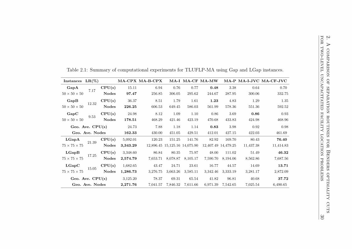
2.A
comparison
ofseparation
routinesfor
Benders
optimality
cutsfor
two-level
uncapacitatedfacility
locationproblem
s30
Table 2.1: Summary of computational experiments for TLUFLP-MA using Gap and LGap instances.
Instances LR(%) MA-CPX MA-B-CPX MA-I MA-CF MA-MW MA-P MA-I-JVC MA-CF-JVC
GapA7.17
CPU(s) 15.11 6.94 0.76 0.77 0.48 3.38 0.64 0.7050× 50× 50 Nodes 97.47 256.85 306.05 295.62 244.67 287.95 300.06 332.75
GapB12.32
CPU(s) 36.37 8.51 1.79 1.61 1.23 4.83 1.29 1.3550× 50× 50 Nodes 226.25 606.53 649.45 586.03 561.99 578.36 551.36 592.52
GapC9.53
CPU(s) 24.98 8.12 1.09 1.10 0.86 3.69 0.86 0.9350× 50× 50 Nodes 178.51 468.29 421.46 423.19 470.68 433.83 424.98 468.96
Geo. Ave. CPU(s) 24.73 7.88 1.18 1.14 0.83 3.98 0.92 0.98Geo. Ave. Nodes 162.33 430.00 451.05 429.51 412.01 427.15 422.03 461.69
LGapA21.39
CPU(s) 5,092.01 120.23 151.25 141.76 82.92 169.70 80.43 76.4075× 75× 75 Nodes 3,343.29 12,896.45 15,125.16 14,075.90 12,407.49 14,479.25 11,437.38 11,414.83
LGapB17.25
CPU(s) 3,348.60 86.84 80.35 75.97 48.00 111.02 51.49 46.3275× 75× 75 Nodes 2,574.79 7,653.71 8,078.87 8,105.17 7,590.70 8,194.06 8,562.86 7,687.56
LGapC15.05
CPU(s) 1,682.65 43.47 24.71 23.61 16.77 44.57 14.69 13.7175× 75× 75 Nodes 1,286.73 3,276.75 3,663.26 3,585.11 3,342.46 3,333.19 3,281.17 2,872.09
Geo. Ave. CPU(s) 3,125.20 78.37 69.31 65.54 41.82 96.81 40.68 37.72Geo. Ave. Nodes 2,271.76 7,041.57 7,846.32 7,611.66 6,971.39 7,542.65 7,025.54 6,490.65
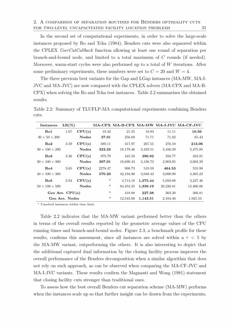
2. A comparison of separation routines for Benders optimality cutsfor two-level uncapacitated facility location problems 31
In the second set of computational experiments, in order to solve the large-scaleinstances proposed by Ro and Tcha (1984), Benders cuts were also separated withinthe CPLEX UserCutCallback function allowing at least one round of separation perbranch-and-bound node, and limited to a total maximum of C rounds (if needed).Moreover, warm-start cycles were also performed up to a total of W iterations. Aftersome preliminary experiments, these numbers were set to C = 20 and W = 4.
The three previous best variants for the Gap and LGap instances (MA-MW, MA-I-JVC and MA-JVC) are now compared with the CPLEX solvers (MA-CPX and MA-B-CPX) when solving the Ro and Tcha test instances. Table 2.2 summarizes the obtainedresults.
Table 2.2: Summary of TLUFLP-MA computational experiments combining Benderscuts.
Instances LR(%) MA-CPX MA-B-CPX MA-MW MA-I-JVC MA-CF-JVC
Ro1 1.67 CPU(s) 19.42 21.25 10.93 11.11 10.5630× 50× 200 Nodes 37.01 256.69 71.71 71.82 65.43
Ro2 3.59 CPU(s) 589.11 317.97 267.55 276.10 213.0630× 100× 200 Nodes 322.23 18,179.46 2,429.51 3,166.39 2,475.95
Ro3 3.36 CPU(s) 979.79 445.50 290.82 356.77 334.9130× 100× 300 Nodes 397.01 18,690.43 2,136.73 2,903.05 3,002.29
Ro4 3.65 CPU(s) 2278.47 908.73 519.59 464.53 555.9840× 100× 300 Nodes 570.20 42,194.90 3,948.42 3,090.90 4,365.23
Ro5 2.94 CPU(s) * 4,714.18 1,375.44 5,050.08 3,227.4650× 100× 500 Nodes * 84,453.35 1,330.19 20,226.81 12,466.86
Geo Ave. CPU(s) * 418.88 227.38 303.30 266.81Geo Ave. Nodes * 12,545.80 1,143.51 2,104.46 1,925.53
∗ Unsolved instances within time limit.
Table 2.2 indicates that the MA-MW variant performed better than the othersin terms of the overall results reported by the geometric average values of the CPUrunning times and branch-and-bound nodes. Figure 2.3, a benchmark profile for theseresults, confirms this assessment, since all instances are solved within a τ < 5 bythe MA-MW variant, outperforming the others. It is also interesting to depict thatthe additional captured dual information by the closing facility process improves theoverall performance of the Benders decomposition when a similar algorithm that doesnot rely on such approach, as can be observed when comparing the MA-CF-JVC andMA-I-JVC variants. These results confirm the Magnanti and Wong (1981) statementthat closing facility cuts stronger than traditional ones.
To assess how the best overall Benders cut separation scheme (MA-MW) performswhen the instances scale up so that further insight can be drawn from the experiments,

2. A comparison of separation routines for Benders optimality cutsfor two-level uncapacitated facility location problems 32
0
0.1
0.2
0.3
0.4
0.5
0.6
0.7
0.8
0.9
1
0 1 2 3 4 5 6
P(r
qs ≤
τ : 1
≤ s
≤ n
s)
τ
MA-MW-W4-C20MA-CF-JVC-W4-C20
MA-I-JVC-W4-C20MA-B-CPX
Figure 2.3: TLUFLP-MA Performance benchmark profiles for Ro and Tcha instances.
new instances having thousands of clients were created. The same guidelines andfeatures suggested by Ro and Tcha (1984) were adopted but having instance 50 ×100× 500 as a baseline. Transportation and installation costs patterns, as well as thenumber of candidate facilities to be installed in each level, were kept the same, butthe number of client nodes were varied within the set 1k, 2k, 3k, 4k, 5k, 10k, 20k, 30k,wherein k represents 103.
Table 2.3 reports the achieved results by presenting the name of the 8 instances,i.e. the instances’ respective sizes, in the first column (Instance), followed by columnswith the number of branch-and-bound nodes (Nodes), the computer running timespent in seconds (CPU(s)), the attained optimality gap after 24 hours (86,400 seconds)(Gap(%)), and the number of installed facilities in each level (1st and 2nd).
Table 2.3: MA-MW variant’s computational experiments for when the number of cus-tomers is scaled up.
Instance Nodes CPU(s) Gap(%) 1st 2nd
50× 100× 1k 636,666 86,400.00 1.47 14 5350× 100× 2k 951,760 86,400.00 0.24 18 6550× 100× 3k 90,029 8,715.79 25 7450× 100× 4k 27,230 1,130.64 24 8150× 100× 5k 1,500 402.03 28 8050× 100× 10k 818 351.44 33 9150× 100× 20k 1,940 505.48 40 9450× 100× 30k 625 684.38 39 99Blank results refer to a zero value.
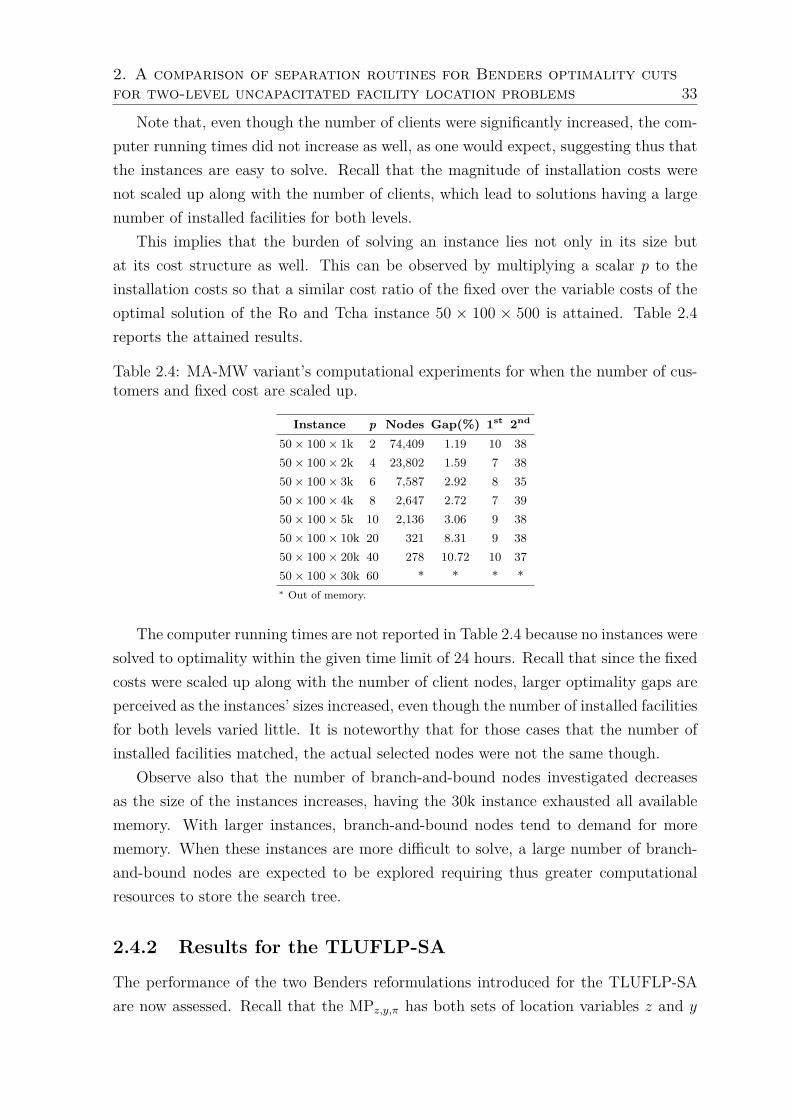
2. A comparison of separation routines for Benders optimality cutsfor two-level uncapacitated facility location problems 33
Note that, even though the number of clients were significantly increased, the com-puter running times did not increase as well, as one would expect, suggesting thus thatthe instances are easy to solve. Recall that the magnitude of installation costs werenot scaled up along with the number of clients, which lead to solutions having a largenumber of installed facilities for both levels.
This implies that the burden of solving an instance lies not only in its size butat its cost structure as well. This can be observed by multiplying a scalar p to theinstallation costs so that a similar cost ratio of the fixed over the variable costs of theoptimal solution of the Ro and Tcha instance 50 × 100 × 500 is attained. Table 2.4reports the attained results.
Table 2.4: MA-MW variant’s computational experiments for when the number of cus-tomers and fixed cost are scaled up.
Instance p Nodes Gap(%) 1st 2nd
50× 100× 1k 2 74,409 1.19 10 3850× 100× 2k 4 23,802 1.59 7 3850× 100× 3k 6 7,587 2.92 8 3550× 100× 4k 8 2,647 2.72 7 3950× 100× 5k 10 2,136 3.06 9 3850× 100× 10k 20 321 8.31 9 3850× 100× 20k 40 278 10.72 10 3750× 100× 30k 60 * * * *∗ Out of memory.
The computer running times are not reported in Table 2.4 because no instances weresolved to optimality within the given time limit of 24 hours. Recall that since the fixedcosts were scaled up along with the number of client nodes, larger optimality gaps areperceived as the instances’ sizes increased, even though the number of installed facilitiesfor both levels varied little. It is noteworthy that for those cases that the number ofinstalled facilities matched, the actual selected nodes were not the same though.
Observe also that the number of branch-and-bound nodes investigated decreasesas the size of the instances increases, having the 30k instance exhausted all availablememory. With larger instances, branch-and-bound nodes tend to demand for morememory. When these instances are more difficult to solve, a large number of branch-and-bound nodes are expected to be explored requiring thus greater computationalresources to store the search tree.
2.4.2 Results for the TLUFLP-SA
The performance of the two Benders reformulations introduced for the TLUFLP-SAare now assessed. Recall that the MPz,y,π has both sets of location variables z and y

2. A comparison of separation routines for Benders optimality cutsfor two-level uncapacitated facility location problems 34
and the link activation variables π, whereas MPz,π is a reduced formulation in whichthe location variables y are removed.
Similar to the previous section, we first focus on a comparison among all proposedseparation routines for the three classes of Benders cuts introduced in Section 2.3 usingthe Gap and LGap instances. Benders cuts were generated only at integer nodes andno warm-start phase was performed. For both MPz,y,π and MPz,π, we consider fourvariants of the Benders algorithm, which differ concerning the used separation routine:
i) Standard Benders cuts separated by using the natural dual solution (SA-I);
ii) Closing facility Benders cuts separated by using the natural dual solution (SA-CF);
iii) Pareto-optimal cuts approximately separated with Algorithm 4 (SA-MW);
iv) Pareto-optimal cuts separated with Papadakos approach (SA-P).
These variants were also compared with CPLEX (SA-CPX) using the original path-based formulation and the built-in Benders algorithm of CPLEX (SA-B-CPX).
Tables 2.5 and 2.6 give a summary of this comparison for the MPz,y,π and MPz,πformulations, respectively. The content of these tables follow the same structure as theprevious ones. Figures 2.4 to 2.7 present the performance benchmark profiles of thealgorithms for Gap and LGap instance set.
As shown in Figures 2.4-2.5 and Table 2.5, for the small instances (Gap and LGap)Benders algorithms SA-I, SA-CF and SA-MW have a very similar performance whenusing MPz,y,π formulation. Once again, as for the case with multiple assignments, theperformance of SA-P algorithm and CPLEX have a slower convergence when comparedto the others. On the other hand, when using MPz,π formulation, the results given inTable 2.6 show that only the MSA-MW algorithm performed slightly better than theothers. Note that the elimination of the variables y from the Benders reformulationresulted in a significant increase in both the CPU time and the number of branch-and-bound nodes, when considering the Gap and LGap instances.
The second set of computational experiments present the results of the differentBenders algorithms for the large-scale instances of Ro and Tcha. Similar to the case ofTLUFLP-MA, Benders cuts were also separated within the CPLEX UserCutCallbackfunction at the nodes of the enumeration tree. After some preliminary experiments,the number of rounds to generate cuts at each node was set to C = 10 and the numberof warm-start cycles was set to W = 4. Tables 2.7 and 2.8, complemented by Figures2.8 and 2.9, provide the summarized results when solving all Ro and Tcha instancesusing MPz,y,π and MPz,π formulations, respectively.

2. A comparison of separation routines for Benders optimality cutsfor two-level uncapacitated facility location problems 35Table 2.5: Summary of computational experiments for TLUFLP-SA using MPz,y,πformulation.
Instances LR(%) SA-CPX SA-B-CPX SA-I SA-CF SA-MW SA-P
GapA6.95
CPU(s) 9.76 1.74 0.71 0.70 0.73 3.4250× 50× 50 Nodes 108.82 134.87 85.45 78.69 85.45 230.02
GapB11.68
CPU(s) 36.91 3.24 1.08 1.13 1.11 4.2250× 50× 50 Nodes 414.80 440.07 178.09 187.77 178.09 310.34
GapC9.25
CPU(s) 21.00 2.35 0.92 0.97 0.94 3.9150× 50× 50 Nodes 264.23 287.19 129.15 136.89 129.15 289.87
Geo. Ave. CPU(s) 20.61 2.43 0.90 0.93 0.93 3.86Geo. Ave. Nodes 239.20 268.20 128.70 130.37 128.70 277.14
LgapA19.56
CPU(s) 3,010.38 98.85 26.38 25.93 26.57 44.6275× 75× 75 Nodes 3,078.19 5,503.80 4,695.30 4,512.21 4,695.30 4,298.90
LgapB16.32
CPU(s) 2,651.68 53.27 19.07 17.77 19.25 41.7675× 75× 75 Nodes 2,971.02 3,773.50 3,391.44 3,070.25 3,391.44 3,498.13
LgapC14.26
CPU(s) 1,811.86 48.40 9.32 9.34 9.44 28.6175× 75× 75 Nodes 1,793.60 2,313.72 1,264.46 1,234.36 1,264.46 1,541.00
Geo. Ave. CPU(s) 2,461.45 63.99 17.07 16.58 17.25 37.99Geo. Ave. Nodes 2,571.53 3,692.67 2,793.35 2,642.54 2,793.35 2,912.14
0
0.1
0.2
0.3
0.4
0.5
0.6
0.7
0.8
0.9
1
0 2 4 6 8 10
P(r
qs ≤
τ : 1
≤ s
≤ n
s)
τ
SA-ISA-MWSA-CF
SA-B-CPXSA-P
Figure 2.4: MPz,y,π performance benchmark profiles for Gap instances.
Two different behaviors can be noticed due to the additional computational com-plexity of ensuring single assignments. For the Ro and Tcha test set, with their largersizes, but smaller linear programming relaxation gaps, there is no clear distinctionon which Benders variants, whether the MSA-MW or the MSA-CF, performed bet-ter. Nonetheless it is easily noticeable that all MPz,y,π variants were slower for these

2. A comparison of separation routines for Benders optimality cutsfor two-level uncapacitated facility location problems 36Table 2.6: Summary of computational experiments for TLUFLP-SA using MPz,π for-mulation.
Instances LR(%) MSA-CPX MSA-B-CPX MSA-I MSA-CF MSA-MW MSA-P
GapA6.95
CPU(s) 10.93 1.59 3.51 3.31 0.92 4.4550× 50× 50 Nodes 135.20 173.56 251.21 238.08 251.21 898.28
GapB11.68
CPU(s) 41.79 3.29 5.22 5.09 2.20 6.3750× 50× 50 Nodes 494.67 565.67 931.33 920.10 931.33 2,070.03
GapC9.25
CPU(s) 23.90 2.25 4.81 4.77 1.57 5.5050× 50× 50 Nodes 327.92 379.19 642.20 579.19 642.20 2,081.34
Geo. Ave. CPU(s) 23.29 2.34 4.51 4.37 1.52 5.45Geo. Ave. Nodes 292.44 347.72 555.05 526.42 555.05 1,603.78
LgapA19.56
CPU(s) * 531.93 414.24 460.37 372.65 453.0075× 75× 75 Nodes * 44,694.33 97,045.91 105,575.59 97,045.91 97,496.19
LgapB16.32
CPU(s) * 251.76 294.51 314.72 241.64 297.3275× 75× 75 Nodes * 25,067.05 64,165.82 68,639.46 64,165.82 62,896.26
LgapC14.26
CPU(s) 6,958.25 167.91 172.43 174.25 126.13 191.9375× 75× 75 Nodes 11,380.72 13,881.54 31,058.43 32,371.93 31,058.43 34,197.14
Geo. Ave. CPU(s) * 287.35 280.57 298.68 229.31 300.12Geo. Ave. Nodes * 25,471.33 59,083.06 63,060.13 59,083.06 60,553.47
∗ Unsolved instances within time limit.
instances, as can be seen in Tables 2.7 and 2.8. However, for the Gap and LGap in-stances, with their smaller sizes, but larger linear programming relaxation gaps, theBenders algorithms based on MPz,y,π had a better performance than the other versions,i.e. the coupling between variables y and π on constraints (2.33) shortened the num-bers of nodes. Once again, capturing the dual information from Magnanti and Wong(1981)’s Pareto-optimality helped strengthen the cuts yielding a better performancethan the traditional and closing facility Benders cuts.
The same scalability experiment done for the TLUFLP-MA was carried out toassess the two overall Benders cut separation routines for the TLUFLP-SA, namelythe SA-MW and the MSA-MW. The same instance 50 × 100 × 500 was used as abaseline. Once again, client nodes were scaled up first, keeping the fixed installationcosts unchanged. Table 2.9 reports the achieved results.
As the size grows, the MSA-MW cut separation scheme derived from the formula-tion with fewer variables performs better than the SA-MW cut scheme. The MSA-MWwas almost 2 times faster than the SA-MW, on average. This implies that, for largerinstances, strong Benders cuts derived from leaner, lighter and stronger formulationsplay an important role. Like in the multiple case, scaling only the number of clients ledto solutions with a large number of facilities being installed for both levels, suggestingonce again that the instances got easier when the sizes were increased.

2. A comparison of separation routines for Benders optimality cutsfor two-level uncapacitated facility location problems 37
0
0.1
0.2
0.3
0.4
0.5
0.6
0.7
0.8
0.9
1
0 2 4 6 8 10
P(r
qs ≤
τ : 1
≤ s
≤ n
s)
τ
SA-CFSA-I
SA-MWSA-P
SA-B-CPX
Figure 2.5: MPz,y,π performance benchmark profiles for LGap instances.
0
0.1
0.2
0.3
0.4
0.5
0.6
0.7
0.8
0.9
1
0 2 4 6 8 10
P(r
qs ≤
τ : 1
≤ s
≤ n
s)
τ
MSA-MWMSA-B-CPX
MSA-CFMSA-I
MSA-P
Figure 2.6: MPz,π performance benchmark profiles for Gap instances.
To further assess the MSA-MW variant’s performance, both the number of clientsand the magnitude of the fixed costs were scaled up. The results are reported in Table2.10. Note that once again, as in the multiple case, none of the instances were solvedwithin the given time limit of 24 hours. The MSA-MW variant exhausted all of theavailable memory when solving the instance with 30k node clients as well.
Finally, it is worth noting that the attained optimality gaps for the single case(Table 2.10) were smaller than ones got for the multiple case (Table 2.4). Observe thatthe MSA-MW variant for the single case investigated more branch-and-bound nodes

2. A comparison of separation routines for Benders optimality cutsfor two-level uncapacitated facility location problems 38
0
0.1
0.2
0.3
0.4
0.5
0.6
0.7
0.8
0.9
1
0 2 4 6 8 10
P(r
qs ≤
τ : 1
≤ s
≤ n
s)
τ
MSA-MWMSA-I
MSA-B-CPXMSA-CF
MSA-P
Figure 2.7: MPz,π performance benchmark profiles for LGap instances.
Table 2.7: Summary of TLUFLP-SA computational experiments using MPz,y,π formu-lation
Instances LR(%) SA-CPX SA-B-CPX SA-I SA-CF SA-MW
Ro1 1.48 CPU(s) 127.70 48.13 15.71 15.55 15.7430× 50× 200 Nodes 40.03 122.02 47.38 47.57 48.51
Ro2 3.43 CPU(s) 9,425.52 248.91 132.60 119.61 128.0130× 100× 200 Nodes 532.30 2,671.34 1,826.60 1,704.03 1,716.10
Ro3 3.24 CPU(s) * 383.84 216.80 220.83 215.7730× 100× 300 Nodes * 4,368.84 3,022.15 2,732.42 3,056.27
Ro4 3.65 CPU(s) * 564.96 364.14 325.97 376.3440× 100× 300 Nodes * 4,830.83 3,711.77 3,220.47 3,520.52
Ro5 3.19 CPU(s) * 2,145.57 2,869.21 2,967.02 2,938.9550× 100× 500 Nodes * 12,041.40 17,791.63 20,177.49 19,117.54
Geo Ave. CPU(s) * 354.19 216.16 208.84 216.98Geo Ave. Nodes * 2,419.05 1,767.97 1,704.63 1,764.91
∗ Unsolved instances within time limit.
than the MA-MW version for the multiple case within the 24 hours. Most likely, theBenders cuts separated by the MSA-MW were better exploited by the cutting planestrategy of the CPLEX solver than the ones obtained by the MA-MW, impacting thusmore positively on the branch-and-bound search.

2. A comparison of separation routines for Benders optimality cutsfor two-level uncapacitated facility location problems 39Table 2.8: Summary of TLUFLP-SA computational experiments using MPz,π formu-lation
Instances LR(%) MSA-CPX MSA-B-CPX MSA-I MSA-CF MSA-MW
Ro1 1.48 CPU(s) 150.67 49.22 17.35 17.22 14.7030× 50× 200 Nodes 55.40 121.86 44.00 38.68 42.95
Ro2 3.43 CPU(s) 9,062.12 246.73 119.87 98.74 98.1730× 100× 200 Nodes 508.91 2,349.59 1,151.19 806.51 1,086.59
Ro3 3.24 CPU(s) * 501.26 171.49 170.15 150.0330× 100× 300 Nodes * 4,381.43 1,341.89 1,384.85 1,394.39
Ro4 3.65 CPU(s) * 618.87 296.09 304.38 269.6240× 100× 300 Nodes * 4,362.52 2,227.80 1,912.83 2,235.28
Ro5 3.19 CPU(s) * 2,062.85 1,935.43 1,246.50 1,628.3050× 100× 500 Nodes * 16,318.25 9,111.93 4,336.31 8,016.41
Geo Ave. CPU(s) * 378.53 182.85 161.48 156.89Geo Ave. Nodes * 2,455.70 1,066.48 814.46 1,031.18
∗ Unsolved instances within time limit.
0
0.1
0.2
0.3
0.4
0.5
0.6
0.7
0.8
0.9
1
0 1 2 3 4 5 6
P(r
qs ≤
τ : 1
≤ s
≤ n
s)
τ
SA-CF-W4-C10SA-MW-W4-C10
SA-I-W4-C10SA-B-CPX
Figure 2.8: TLUFLP-SA performance benchmark profiles for Ro and Tcha instancesusing MPz,y,π formulation.

2. A comparison of separation routines for Benders optimality cutsfor two-level uncapacitated facility location problems 40
0
0.1
0.2
0.3
0.4
0.5
0.6
0.7
0.8
0.9
1
0 1 2 3 4 5 6
P(r
qs ≤
τ : 1
≤ s
≤ n
s)
τ
MSA-MW-W4-C10MSA-I-W4-C10
MSA-CF-W4-C10MSA-B-CPX
Figure 2.9: TLUFLP-SA performance benchmark profiles for Ro and Tcha instancesusing MPz,π formulation.
Table 2.9: SA-MW and MSA-MW variants’ computational experiments for when thenumber of customers are scaled up.
SA-MW MSA-MW
Instance Nodes CPU(s) Nodes CPU(s) 1st 2nd
50× 100× 1k 184,521 23,505.00 109,675 12,485.78 14 5250× 100× 2k 6,843 1,483.48 9,673 2,846.79 19 6550× 100× 3k 616 1,010.37 3,181 1,800.90 24 7550× 100× 4k 338 1,001.50 883 415.50 24 8150× 100× 5k 435 1,546.25 370 357.98 28 8050× 100× 10k 303 3,234.49 118 348.89 33 9150× 100× 20k 227 2,528.57 102 702.49 40 9450× 100× 30k 21 735.01 36 747.20 39 99Geo. Ave. 843.62 2,066.85 956.02 1,077.74

2. A comparison of separation routines for Benders optimality cutsfor two-level uncapacitated facility location problems 41Table 2.10: MSA-MW variant’s computational experiments for when the number ofcustomers and fixed cost are scaled up.
Instance p Nodes Gap(%) 1st 2nd
50× 100× 1k 2 182,550 0.33 9 3650× 100× 2k 4 27,925 0.91 8 3950× 100× 3k 6 4,131 2.92 8 3850× 100× 4k 8 3,858 2.64 8 4050× 100× 5k 10 4,528 2.62 8 4050× 100× 10k 20 731 7.06 10 3950× 100× 20k 40 342 7.18 9 3550× 100× 30k 60 * * * *∗ Out of memory.
2.5 Conclusion
Different Benders cut separation schemes were investigate for the two-level uncapaci-tated facility location problem with single and multiple assignments, a class of discretelocation problems that considers different hierarchies of facilities and their interactions.Exact algorithms based on Benders decomposition reformulations for both studied vari-ants were devised considering several separation procedures for three classes of Benderscuts: standard optimality cuts, lifted optimality cuts, and non-dominated optimalitycuts. The extensive computational experiment results confirmed the efficiency of allour Benders approaches, both in speed and in explored branch-and-bound nodes, whensolving three different standard literature instance sets, specially when addressing thelarge-scale Ro and Tcha’s instances. In particular, for both single and multiple as-signment reformulations, using non-dominated optimality cuts was the most efficientoverall cut separation routine. Finally, note that our Benders algorithms can be furtherimproved by incorporating tailored heuristics or variable fixing and elimination proce-dures. Further, they can be also extended to address more elaborate problems such asconsidering capacities for the facilities or congestion effects by integrating Ramos andSáez (2005) ideas for the single-source capacitated facility location problem, or de Ca-margo and Miranda (2012) for the single-allocation hub location problem, respectively.

Chapter 3
A decomposition approach for thedynamic two-level uncapacitatedfacility location problem with singleand multiple allocations
Two variants of a dynamic or multi-period two-level uncapacitated facility locationproblem are here addressed. In this problem, first-level plants serve different demandpatterns of scattered clients over a planning horizon via second-level facilities. In thefirst variant, second-level facilities can be supplied by only one of the plants (singleassignment); whereas, in the second, they can be attended by any number of first-level plants (multiple allocations). As the client’s demands vary over time, differentconfigurations of operating plants and facilities, and client assignments need to besought in each period to serve demands at minimal installation and transportationcosts. Since both problem variants arise naturally within logistic and distributionsystems, it is of interest to practitioners and researchers to have solution techniquesat hand. To provide such a tool, an efficient decomposition approach was developedto solve the two problem variants. It relies on Benders decomposition reformulationswhile combined with a greedy randomized adaptive search procedure and differentBenders cut separation procedures. Results indicate that the devised decompositionoutperforms CPLEX general solver and its Benders built-in algorithm on solving twodifferent large-scale instance sets.
42

3. A decomposition approach for the dynamic two-level uncapacitatedfacility location problem with single and multiple allocations 43
3.1 Introduction
In many distribution systems, such as in electrical power and Internet distributions(Fortz 2015), banking and ATM branches (Min and Melachrinoudis 2001, Jayaramanet al. 2003, Genevois et al. 2015), and public safety and health care providers (Şahinand Süral 2007, Smith et al. 2009, Ahmadi-Javid et al. 2017), it is common to find ahierarchical network structure to serve clients (Ortiz-Astorquiza et al. 2018). In many ofthese, a two-level topology is present, in which first-level facilities serve geographicallyscattered customer nodes via intermediary second-level agents or transshipment points(Melo et al. 2009). Further, whenever these applications face demand variability overtime, the underlying service network needs to be adjusted or adapted to properly copewith these variations to continue serving customers at suitable costs (Arabani andFarahani 2012).
These adjustments may require the opening of new facilities closer to customers,or the closing of existing ones so that the overall business survivability is sustainedthroughout time (Jena et al. 2016). These decisions have to be properly taken in atimely manner over a planning horizon. Moreover, company managers and customersmay prefer to deal with a single or multiple suppliers to ease management on passingorders or to shorten lead times depending though on the service features (Gendronet al. 2016). Hence single or multiple assignments between levels may be an issue. Onesuitable way of designing the service network for such contexts is to model it as a multi-period variant of the warehouse and plant location problem introduced by Kaufmanet al. (1977), which is also known as the two-level uncapacitated facility location problem(TLUFLP) (Ortiz-Astorquiza et al. 2018). The problem consists of selecting a subsetof facilities within a set of candidates partitioned into two levels to operate or notin each period throughout a planning horizon such that the costs of opening, closing,and operating the facilities, and serving the scattered costumers are minimized. Theincorporation of dynamic decisions over a planning horizon gives rise to the dynamictwo-level uncapacitated facility location problem (DTLUFLP).
Only a few variants of this problem has been previously studied in the literature.Hinojosa et al. (2000) and Hinojosa et al. (2008) propose Lagrangean relaxation ap-proaches aided with constructive heuristics to solve a capacitated multi-product variantof the problem without and with inventory decisions, respectively. Instances with upto 75 (125) clients, 40 facility node candidates, 3 (12) products, and 4 (2) periodswere solved with optimality gaps of 5% (15.18%), on average, by Hinojosa et al. (2000)(Hinojosa et al. 2008). Brunaud et al. (2018) devise four formulations that take intoaccount: plant capacity, single assignment, discrete transportation costs, and safetystock considerations. Three small case studies with up to 15 customers, 36 periods, 14

3. A decomposition approach for the dynamic two-level uncapacitatedfacility location problem with single and multiple allocations 44
modes of transportation, and 14 and 18 second and first-level facility node candidates,respectively, were solved by GUROBI running on GAMS.
As far as the authors have investigated, there is no work in the literature addressingthe DTLUFLP per se up until now, nonetheless, its single-level counterpart has beenwell studied by the research community. Modeling dynamic decisions within facilitylocation problems have been carried out by Ballou (1968), Roodman and Schwarz(1975), Wesolowsky and Truscott (1975), and Roy and Erlenkotter (1982), which haveled to many variants and solution approaches for the single-level case such as Jena et al.(2014, 2015), Marufuzzaman et al. (2016), Jena et al. (2016, 2017), Correia and Melo(2017), Pearce and Forbes (2018), and Emirhüseyinoğlu and Ekici (2019) recently. Forthorough surveys on facility location theory and its wide range of problem variantsplease refer to Melo et al. (2009), Arabani and Farahani (2012) and Ortiz-Astorquizaet al. (2018).
The main contributions of this chapter are listed as follow: (i) Here two vari-ants of the DTLUFLP are investigated: One with single assignments or the DTLU-FLPS, in which each opened second-level facility can be served by at most one ofthe functioning first-level facilities in each period; and another with multiple assign-ments or the DTLUFLPM, in which the single assignment constraint is disregarded.Both multiple and single variants are modeled using the formulations of Barros andLabbé (1994b), and Gendron et al. (2016) as the underlying mathematical program,respectively. (ii) An exact solution framework based on a Benders and cut algorithmwhich projects out the continuous decision variables is devised to solve both variants.(iii) Different cut separation routines for different classes of Benders cuts (BC), notnecessarily non-dominated, are delved into via simple inspection techniques and spe-cialized network flow algorithms. (iv) Given the complexity of the problems (NP-hard,see Ortiz-Astorquiza et al. (2018)), an efficient and fast greedy randomized adaptivesearch procedure (GRASP) is also proposed to obtain near-optimal solutions to besupplied to the Benders and cut algorithm, and to used to separate Benders standardheuristic cuts as well as valid cut using the objective function information. (v) Finally,extensive computational experiments were carried out on large-scale instances to assessthe performance of the proposed exact solution framework.
This work is organized as followed: Section 3.2 introduces the adopted notation, def-initions and devised formulations; while section 3.3 presents the exact solution frame-work as well as the Benders cut separation procedures. The GRASP is shown in section3.4. Sections 3.5 and 3.6 concludes the chapter with the computational experimentsreport and analyses, and final remarks, respectively.

3. A decomposition approach for the dynamic two-level uncapacitatedfacility location problem with single and multiple allocations 45
3.2 Notation, definitions and formulations
The DTLUFLPM and DTLUFLPS use the following notation and definitions: Let Iand T be sets of customers scattered in a geographical area, and periods of a planninghorizon, respectively. Each client i ∈ I demands dit units of a commodity in periodt ∈ T which are supplied by first-level facilities via second-level ones acting as trans-shipment points that are selected within sets K and J of candidate nodes, respectively.Whenever a first (second) level facility k ∈ K (j ∈ J) is opened, closed, or kept oper-ating at a period t ∈ T fixed costs f okt (aojt), f ckt (acjt) and f
fkt (a
fjt), respectively, incur.
Wherever a customer i ∈ I is served by first-level facility k ∈ K through second-levelone j ∈ J , a serving cost cijkt = dit(cijt + cjkt) is accounted for, where c is the unittransportation cost between the involved nodes.
The underlying problem consists then in selecting which facilities will be opened,closed or operated at each level at each period of the planning horizon T so that cus-tomers are attended at the minimal total cost. For the DTLUFLPS, each operatingsecond-level facility can only be assigned to one of the functioning first-level facilities;whereas the DTLUFLPM disregards this assumption. Figure 3.1 illustrates the singleassignment case with an example having 3 periods, 2 first and 3 second-level facilitycandidates, and 4 customer nodes. As time evolves (t1,t2,t3), the example shows differ-ent operating facility configurations. It displays first and second level facilities beingopened, closed and operated over time. Note that each second-level facility is linkedto a single first-level facility; and that, from period t1 to t2, only one node candidateis opened and closed in the second and first levels, respectively, while the remainingfacilities, previously opened in period t1, still operate. Nonetheless, given the demandpattern throughout time, new facilities can be opened or closed to better serve clientsas depicted in period t3.
I
J
K
T t1 t2 t3
OpenOperatingClosed
Figure 3.1: An example of a dynamic two-level facility location problem with singleassignments.
The example of Figure 3.1 is also a feasible solution for the DTLUFLPM, but notnecessarily optimal. Note that savings stemmed from using multiple assignments canbe attained only in the first period (t1), since more than one first-level facility is active.
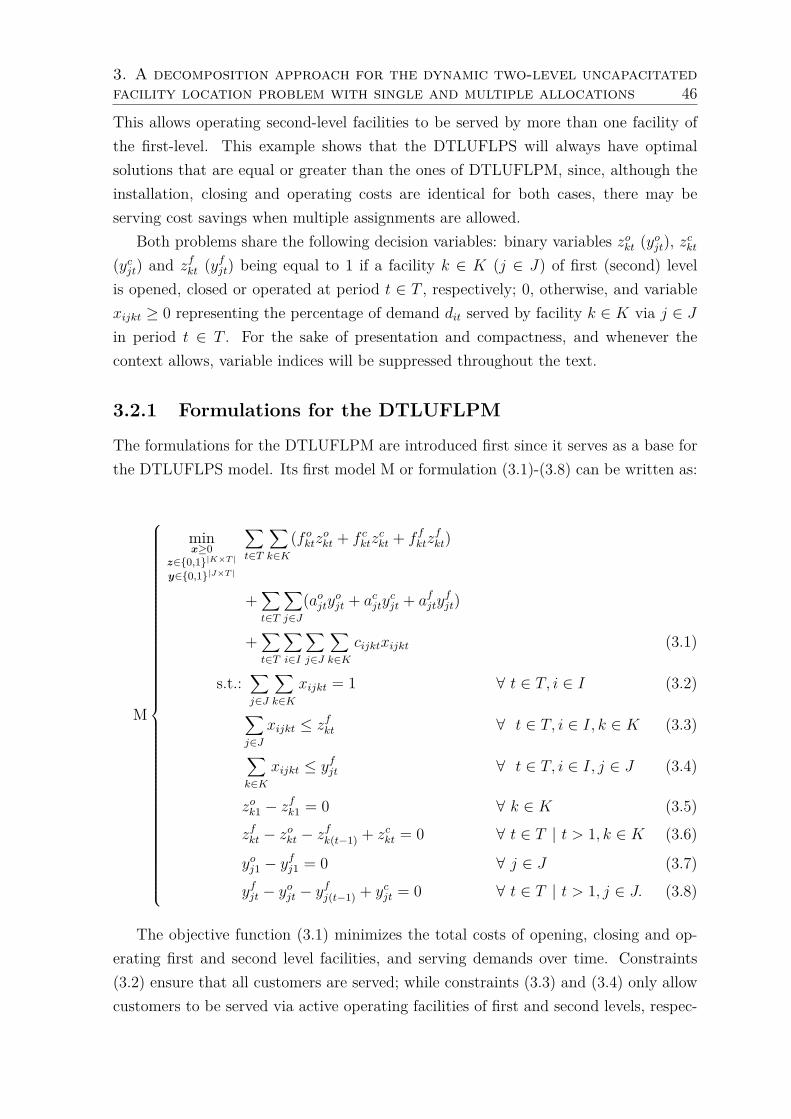
3. A decomposition approach for the dynamic two-level uncapacitatedfacility location problem with single and multiple allocations 46
This allows operating second-level facilities to be served by more than one facility ofthe first-level. This example shows that the DTLUFLPS will always have optimalsolutions that are equal or greater than the ones of DTLUFLPM, since, although theinstallation, closing and operating costs are identical for both cases, there may beserving cost savings when multiple assignments are allowed.
Both problems share the following decision variables: binary variables zokt (yojt), zckt(ycjt) and zfkt (y
fjt) being equal to 1 if a facility k ∈ K (j ∈ J) of first (second) level
is opened, closed or operated at period t ∈ T , respectively; 0, otherwise, and variablexijkt ≥ 0 representing the percentage of demand dit served by facility k ∈ K via j ∈ Jin period t ∈ T . For the sake of presentation and compactness, and whenever thecontext allows, variable indices will be suppressed throughout the text.
3.2.1 Formulations for the DTLUFLPM
The formulations for the DTLUFLPM are introduced first since it serves as a base forthe DTLUFLPS model. Its first model M or formulation (3.1)-(3.8) can be written as:
M
minx≥0
z∈0,1|K×T |y∈0,1|J×T |
∑t∈T
∑k∈K
(f oktzokt + f cktzckt + f fktz
fkt)
+∑t∈T
∑j∈J
(aojtyojt + acjtycjt + afjty
fjt)
+∑t∈T
∑i∈I
∑j∈J
∑k∈K
cijktxijkt
s.t.:∑j∈J
∑k∈K
xijkt = 1 ∀ t ∈ T, i ∈ I
∑j∈J
xijkt ≤ zfkt ∀ t ∈ T, i ∈ I, k ∈ K
∑k∈K
xijkt ≤ yfjt ∀ t ∈ T, i ∈ I, j ∈ J
zok1 − zfk1 = 0 ∀ k ∈ K
zfkt − zokt − zfk(t−1) + zckt = 0 ∀ t ∈ T | t > 1, k ∈ K
yoj1 − yfj1 = 0 ∀ j ∈ J
yfjt − yojt − yfj(t−1) + ycjt = 0 ∀ t ∈ T | t > 1, j ∈ J.
(3.1)
(3.2)
(3.3)
(3.4)
(3.5)
(3.6)
(3.7)
(3.8)
The objective function (3.1) minimizes the total costs of opening, closing and op-erating first and second level facilities, and serving demands over time. Constraints(3.2) ensure that all customers are served; while constraints (3.3) and (3.4) only allowcustomers to be served via active operating facilities of first and second levels, respec-

3. A decomposition approach for the dynamic two-level uncapacitatedfacility location problem with single and multiple allocations 47
tively, in each period. Finally, constraints (3.5)-(3.8) secure the proper opening, closingand operating balance of first and second level facilities between periods, respectively.
Formulation M can be simplified via constraints (3.5)-(3.8) in which variables zfktand yfjt can be eliminated after being isolated for each period, and replaced through-out the formulation. This leads to formulation Myz which has fewer variables andconstraints:
Myz
minx≥0
zo,zc∈0,1|K×T |yo,yc∈0,1|J×T |
∑t∈T
∑k∈K
(f oktzokt + f cktzckt)
+∑t∈T
∑k∈K
f fkt(t∑
r=1zokr −
t∑r=2
zckr)
+∑t∈T
∑j∈J
(aojtyojt + acjtycjt)
+∑t∈T
∑j∈J
afjt(t∑
r=1yojr −
t∑r=2
ycjr)
+∑t∈T
∑i∈I
∑j∈J
∑k∈K
cijktxijkt
s.t.: (3.2)∑j∈J
xijkt ≤t∑
r=1zokr −
t∑r=2
zckr ∀ t ∈ T, i ∈ I, k ∈ K
∑k∈K
xijkt ≤t∑
r=1yojr −
t∑r=2
ycjr ∀ t ∈ T, i ∈ I, j ∈ J.
(3.9)
(3.10)
(3.11)
3.2.2 Formulations for the DTLUFLPS
To model the DTLUFLPS, an additional set of binary variables πjkt is added to for-mulation M along with some new constraints to result in formulation S. Variable πjktis equal to 1 if the second-level facility j ∈ J is single assigned to the first-level facilityk ∈ K; 0, otherwise. Formulation S can be written as:

3. A decomposition approach for the dynamic two-level uncapacitatedfacility location problem with single and multiple allocations 48
S
minx≥0
z∈0,1|K×T |y∈0,1|J×T |
π∈0,1|J×K×T |
∑t∈T
∑k∈K
(f oktzokt + f cktzckt)
+∑t∈T
∑k∈K
(f fktzfkt)
+∑t∈T
∑j∈J
(aojtyojt + acjtycjt)
+∑t∈T
∑j∈J
(afjtyfjt)
+∑t∈T
∑i∈I
∑j∈J
∑k∈K
cijktxijkt
s.t.:(3.2)-(3.3) and (3.5)-(3.8)
πjkt − xijkt ≥ 0 ∀ t ∈ T, i ∈ I, j ∈ J, k ∈ K
zfkt − πjkt ≥ 0 ∀ t ∈ T, j ∈ J, k ∈ K∑k∈K
πjkt − yfjt = 0 ∀ t ∈ T, j ∈ J.
(3.12)
(3.13)
(3.14)
(3.15)
Constraints (3.13)-(3.15) replace constraints (3.4). Constraints (3.13) and (3.14)only allow flows by active assignments of operating first-level facilities, respectively.Constraints (3.15) guarantee that if a second-level facility is operating, then it mustbe connected to a first-level one.
By observing the equations and variables relations of formulation S, it is possibleto get different reformulations, being three of them here investigated. Replacing vari-ables yfjt by
∑k∈K πjkt throughout formulation S, while adjusting the constraints, yields
formulation Sy, which can be written as:

3. A decomposition approach for the dynamic two-level uncapacitatedfacility location problem with single and multiple allocations 49
Sy
minx≥0
z∈0,1|K×T |yo,yc∈0,1|J×T |π∈0,1|J×K×T |
∑t∈T
∑k∈K
(f oktzokt + f cktzckt + f fktz
fkt)
+∑t∈T
∑j∈J
(aojtyojt + acjtycjt)
+∑t∈T
∑j∈J
(afjt∑k∈K
πjkt)
+∑t∈T
∑i∈I
∑j∈J
∑k∈K
cijktxijkt
s.t.:(3.2)-(3.3), (3.5)-(3.6) and (3.13)-(3.14)
yoj1 −∑k∈K
πjk1 = 0 ∀ j ∈ J∑k∈K
πjkt − yojt −∑k∈K
πjk(t−1) + ycjt = 0 ∀ t ∈ T,
j ∈ J : t > 1.
(3.16)
(3.17)
(3.18)
The last two formulations S yza and S yzb are derived from replacing all variables yfjt andzfkt, at the same time. Formulation S yza is obtained by using zfkt = ∑t
r=1 zokr −
∑tr=2 z
ckr,
for all k ∈ K, t ∈ T , and yfjt = ∑tr=1 y
ojr −
∑tr=2 y
cjr, for all j ∈ J , t ∈ T ; whereas S
yzb is
generated via zfkt = ∑tr=1 z
okr −
∑tr=2 z
ckr, for all k ∈ K, t ∈ T , and yfjt = ∑
k∈K πjkt, forall j ∈ J , t ∈ T . Both formulations can be written as:
Syzb
minx≥0
zo,zc∈0,1|K×T |yo,yc∈0,1|J×T |π∈0,1|J×K×T |
∑t∈T
∑k∈K
f oktzokt + f cktz
ckt + f fkt(
t∑r=1
zokr −t∑
r=2zckr)
+∑t∈T
∑j∈J
(aojtyojt + acjtycjt + afjt
∑k∈K
πjkt)
+∑t∈T
∑i∈I
∑j∈J
∑k∈K
cijktxijkt
s.t.:(3.2), (3.10), (3.13), (3.17), (3.18) and (3.21).
(3.19)

3. A decomposition approach for the dynamic two-level uncapacitatedfacility location problem with single and multiple allocations 50
Syza
minx≥0
zo,zc∈0,1|K×T |yo,yc∈0,1|J×T |π∈0,1|J×K×T |
∑t∈T
∑k∈K
(f oktzokt + f cktzckt)
+∑t∈T
∑j∈J
(aojtyojt + acjtycjt)
+∑t∈T
∑k∈K
f fkt(t∑
r=1zokr −
t∑r=2
zckr)
+∑t∈T
∑j∈J
afjt(t∑
r=1yojr −
t∑r=2
ycjr)
+∑t∈T
∑i∈I
∑j∈J
∑k∈K
cijktxijkt
s.t.:(3.2), (3.10) and (3.13)t∑
r=1zokr −
t∑r=2
zckr − πjkt ≥ 0 ∀ t ∈ T, j ∈ J, k ∈ K
∑k∈K
πjkt − (t∑
r=1yojr −
t∑r=2
ycjr) = 0 ∀ t ∈ T, j ∈ J,
(3.20)
(3.21)
(3.22)
It is noteworthy that all proposed formulations with multiple and single assignmentsyield easy-to-solve linear transportation subproblems, one for each customer i ∈ I andperiod t ∈ T , whenever all integer variables are parameterized. This makes theseformulations suitable to be solved by a decomposition framework, the subject of thenext section.
3.3 Decomposition approaches
All the devised formulations have matrices with a staircase shape structure with thesteps coupled with the integer variables. When these integer variables are parameter-ized, these matrices decompose into subsystems or linear transportation subproblemswith only the x variables. This characteristic allows the x variables to be projectedout and replaced by constraints, probably exponential in size, to yield an equivalentproblem with fewer variables but many more constraints. This equivalent problem isknown as the master problem (MP). Many of these constraints but a few will not beactive in an optimal solution, suggesting thus an iterated procedure that relaxes all andthen adds them on demand. The procedure alternates between solving the relaxed MP(RMP) and separating violated cuts via the dual of the projected out subsystems ordual subproblem (DP) with the integer variables parameterized to the values attained

3. A decomposition approach for the dynamic two-level uncapacitatedfacility location problem with single and multiple allocations 51
by RMP. As the RMP is a relaxation of the MP, it produces a lower bound (LB) for theproblem, whereas an upper bound (UB) is readily available by composing the solutionsof the RMP and DP. This overall procedure iterates until the UB and LB converge toan optimal solution if one exists. The aforementioned strategy is known as the Bendersdecomposition method (Benders 1962).
Benders decomposition has been successfully applied to the TLUFLP (de Oliveiraet al. 2020) and the multi-level facility location problem (Ortiz-Astorquiza et al. 2019),as well to a wide range of other applications. For a thorough survey on the techniqueplease refer to Rahmaniani et al. (2017). Here the method is extended to the dynamicvariant of the TLUFLP, being the underlying Benders reformulation for all formulationspresented below.
3.3.1 Benders decomposition for the DTLUFLPM
Let A = B|J×T | × B|K×T | denote the set of binary vectors associated with the yf andzf variables. For any fixed vector (yf , zf ) ∈ A in the original M formulation, |I × T |linear transportation primal subproblems (PSMit ), one for each i ∈ I and t ∈ T , areobtained or:
minx≥0
∑j∈J
∑k∈K
cijktxijkt (3.23)
s.t.:∑j∈J
∑k∈K
xijkt = 1 (3.24)
−∑j∈J
xijkt ≥ −zfkt ∀ k ∈ K (3.25)
−∑k∈K
xijkt ≥ −yfjt ∀ j ∈ J. (3.26)
These |I × T | subproblems are known as the Benders primal subproblem (PSM).Note that the PSMit of formulations M and Myz are similar except that the current zfktand yfjt in M are replaced by ∑t
r=1 zokr −
∑tr=2 z
ckr and
∑tr=1 y
ojr −
∑tr=2 y
cjr, k ∈ K and
t ∈ T , respectively, in the Myz. Associating the dual variables vit ∈ IR, uikt ≥ 0 andwijt ≥ 0, i ∈ I, j ∈ J , k ∈ K and t ∈ T , to constraints (3.24)-(3.26), respectively,yields the following dual subproblem (DSMit ) of the PSMit :
maxv∈IRu,w≥0
vit −∑k∈K
zfktuikt −∑j∈J
yfjtwijt (3.27)
s.t.: vit − uikt − wijt ≤ cijkt ∀j ∈ J, k ∈ K. (3.28)

3. A decomposition approach for the dynamic two-level uncapacitatedfacility location problem with single and multiple allocations 52
The feasibility of the PSM and therefore of the DSM is ensured for any (yf , zf ) ∈ Abinary vector that respects Proposition 4.
Proposition 4. For any (yf , zf ) ∈ A, such that ∑j∈J yfjt ≥ 1 and ∑k∈K z
fkt ≥ 1, for
all t ∈ T , the PSM and DSM are always feasible and bounded.
Proof. 4. For any vector (yf , zf ) ∈ A with at least one operating facility in each levelfor every period t ∈ T or ∑j∈J y
fjt ≥ 1 and ∑k∈K z
fkt ≥ 1, every customer i ∈ I can
be served by one or more pairs of these operating first and second level facilities ateach period t ∈ T since there is no capacity constraints. Further, since cijkt costsare assumed to be finite and non-negative the PSM will always yield feasible boundedsolutions leading thus to feasible bounded dual solutions, i.e. the DSM is also alwaysbounded and feasible, due to strong duality.
Note that, for different (yf , zf ) ∈ A binary vectors, the dual feasible space (3.28)is unaffected, and, by letting DM denote the set of extreme points of (3.28), the DSMitcan be restated as:
max(v,u,w)∈DM
vit −∑k∈K
zfktuikt −∑j∈J
yfjtwijt.
Which, with the aid of an auxiliary variable ηit ≥ 0, i ∈ I and t ∈ T , responsiblefor sub-estimating the transportation costs, allows the Benders MP of formulation Mto be written as:
minη≥0
z∈0,1|K|y∈0,1|J|
∑t∈T
∑k∈K
(f oktzokt + f cktzckt + f fktz
fkt)
+∑t∈T
∑j∈J
(aojtyojt + acjtycjt + afjty
fjt) +
∑t∈T
∑i∈I
ηit (3.29)
s.t.:(3.5)-(3.8)
ηit ≥ vit −∑k∈K
zfktuikt −∑j∈J
yfjtwijt ∀ (v, u, w) ∈ DM (3.30)
∑k∈K
zfkt ≥ 1 ∀ t ∈ T (3.31)∑j∈J
yfjt ≥ 1 ∀ t ∈ T. (3.32)
Constraints (3.30) are known as the Benders optimality cuts. No further feasibil-ity is required, i.e. no Benders feasibility cuts, because constraints (3.31)-(3.32) are

3. A decomposition approach for the dynamic two-level uncapacitatedfacility location problem with single and multiple allocations 53
sufficient to guarantee bounded and feasible PSM and DSM . Note that the MP of theMyz formulation is similar to (3.29)-(3.32) but having no zfkt and y
fjt variables. Further,
constraints (3.33)-(3.34) are added to it to ensure proper coupling between all facilitieswhich are opened or closed in each level.
t−1∑r=1
(zokr − zckr)− zckt ≥ 0 ∀ t ∈ T, k ∈ K (3.33)
t−1∑r=1
(yojr − ycjr)− ycjt ≥ 0 ∀ t ∈ T, j ∈ J. (3.34)
3.3.2 Benders decomposition for the DTLUFLPS
The same rationality of the previous section can be extended to the formulations S, Sy,Syza , and Syzb of DTLUFLPS. Let Y = B|J×K×T | × B|J×T | × B|K×T | be the set of binaryvectors concerning the π, yf and zf variables. For any fixed vector (π, yf , zf ) ∈ Y inthe S formulation, the following |I×T | linear transportation PSSit, i ∈ I and t ∈ T , areattained:
minx≥0
∑j∈J
∑k∈K
cijktxijkt (3.35)
s.t.:∑j∈J
∑k∈K
xijkt = 1 (3.36)
−∑j∈J
xijkt ≥ −zfkt ∀ k ∈ K (3.37)
− xijkt ≥ −πjkt ∀ j ∈ J, k ∈ K. (3.38)
The PSSit (3.35)-(3.38) differs from its multiple assignment counterpart (3.23)-(3.26)by constraints (3.38) which replace constraints (3.26). This difference modifies theassociated dual problem. Let sijkt ≥ 0 be the dual variables associated to constraints(3.38), and by using the same dual variables and associations of the previous section,the following DSSit is attained, one for each pair i ∈ I and t ∈ T :
maxv∈IRu,s≥0
vit −∑k∈K
zfktuikt −∑j∈J
∑k∈K
πjktsijkt (3.39)
s.t.: vit − uikt − sijkt ≤ cijkt ∀j ∈ J, k ∈ K. (3.40)
Note that the parameterized binary vector yf plays no role in the in PSSit and DSSit.Again, the feasibility of PSS and DSS is guaranteed for any (π, yf , zf ) ∈ Y that respects

3. A decomposition approach for the dynamic two-level uncapacitatedfacility location problem with single and multiple allocations 54
Proposition 5.
Proposition 5. For any (π, yf , zf ) ∈ Y such that ∑j∈J yfjt ≥ 1 and ∑k∈K z
fkt ≥ 1,
t ∈ T , and ∑j∈J πjkt ≥ zfkt, k ∈ K, t ∈ T , the PSS and DSS are always feasible andbounded.
Proof. 5. The rationality is the same as Proposition 4. For any vector (π, yf , zf ) ∈ Ywith at least one operating facility in each level for every period t ∈ T or ∑j∈J y
fjt ≥ 1
and ∑k∈K zfkt ≥ 1 such that there is at least one active connection linking both decision
levels or ∑j∈J πjkt ≥ zfkt, k ∈ K, working together with constraints (3.15), for eachperiod t ∈ T , every customer i ∈ I can be supplied via only one of the active connectionsπjk in each period t ∈ T since there is no capacity constraints. Note that due toconstraints (3.15) an operating second-level facility is single allocated to an operatingfirst-level one in the single assignment formulations. Furthermore since cijkt costs arefinite and non-negative, the PSS will always be feasible and bounded which leads tobounded DSS due to strong duality.
Once again the dual feasible space (3.40) is unaffected by the values of (π, yf , zf ) ∈Y. By letting DS be the set of extreme points of (3.40), the DSSit can be rewritten as:
max(v,u,s)∈DS
vit −∑k∈K
zfktuikt −∑j∈J
∑k∈K
πjktsijkt.
This allows to reformulate formulation S for the DTLUFLPS as the following Ben-ders MP:
minη,z≥0
y∈0,1|J|π∈0,1|J×K|
∑t∈T
∑k∈K
(f oktzokt + f cktzckt + f fktz
fkt)
+∑t∈T
∑j∈J
(aojtyojt + acjtycjt + afjty
fjt) +
∑t∈T
∑i∈I
ηit (3.41)
s.t.:(3.5)-(3.8) and (3.31)-(3.32)
ηit ≥ vit −∑k∈K
zfktuikt −∑j∈J
∑k∈K
πjktsijkt ∀ (v, u, s) ∈ DS. (3.42)
As before, variables ηit ≥ 0 under-estimate the transportation costs. FormulationsSy, Syza and Syzb render MPs that have all of their respective constraints with no vari-

3. A decomposition approach for the dynamic two-level uncapacitatedfacility location problem with single and multiple allocations 55
ables xijkt, besides the Benders cuts (3.42). To ensure the feasibility of the PSS andboundness of the DSS, constraints (3.33)-(3.34) are added to their respective MPs.
Note that the Benders MPs have fewer variables but many more constraints than theoriginal formulations. Since only a few of these Benders cuts will be active on an optimalsolution, the cuts are relaxed to be dynamically generated via an iterative procedure,i.e. through a cutting plane algorithm, which alternates between the solution of theRMP and the dual subproblems until it converges to an optimal solution. The RMPprovides a lower bound for the original problem, whereas an upper bound is readilyavailable by composing the solutions of RMP and the dual subproblem of the currentiteration. At each iteration, the lower bound is improved as the result of the additionof the Benders cuts.
3.3.3 Separation routines for different BCs
Linear programs with a network flow structure, such as the primal subproblems (3.23)-(3.26) and (3.35)-(3.38), are usually degenerate, having thus multiple dual optimalsolutions (Hung et al. 1986, Sierksma 1996). As pointed out by Magnanti and Wong(1981), the strength of the Benders cuts depends on the selection of dual optimalvalues. Hence efficient separation routines capable of finding strong benders cuts playa crucial role in Benders decomposition algorithms. Nonetheless one has to balance thecomputational effort on separating stronger and/or denser cuts and the burden theyput on the MP with the number of iterations they save to attain optimality. With thisin mind, five procedures to separate Benders cuts are presented next.
3.3.3.1 Standard BCs
The structure of primal and dual subproblems of both single and multiple assignmentformulations allows the dual optimal values to be obtained by analytical procedureswithout relying on Simplex based solvers. These inspection techniques can separatestandard optimality Benders cuts very efficiently.
The analytical procedure uses the following definitions: Let Ohz = k ∈ K, t ∈ T :
zfhkt = 1 and Ohy = j ∈ J, t ∈ T : yfhjt = 1, and Ch
z = k ∈ K, t ∈ T : zfhkt = 0and Ch
y = j ∈ J, t ∈ T : yfhjt = 0 be the sets of installed and closed facilities for thefirst and second decision levels, respectively, for each period t ∈ T at an iteration h ofthe Benders decomposition algorithm. Further, let also Oh
π = (j, k, t) ∈ J ×K × T :πhjkt = 1 and Ch
π = (j, k, t) ∈ J × K × T : πhjkt = 0 be the sets of active andinactive connections, respectively, linking first and second level facilities for period t atan iteration h for the single assignment variant.

3. A decomposition approach for the dynamic two-level uncapacitatedfacility location problem with single and multiple allocations 56
The multiple allocation case
The optimal solution of the PSM consists in selecting which pair of the installed facilitiesin the first and second levels will serve each client i ∈ I at minimal cost at eachperiod t ∈ T or φ(zfh, yfh) = ∑
i∈I∑t∈T φit(zfh, yfh) = ∑
i∈I∑t∈T cit, where cit =
min(j,k)∈Ohy×Ohz cijkt, and φ(zfh, yfh) is the PSM ’s optimal solution value for (zfh, yfh).To find the optimal values for the variables of the DSM , the complementary slack-
ness conditions are used as shown in Algorithm 2. First, variables vit are set to theminimal transportation cost for each client i ∈ I considering only the installed facilitiesat each level (line 2). For these installed facilities, the values of dual variables uikt andwijt are set to zero (lines 3 and 4) due to the complementary slackness conditions.To ensure dual feasibility, i.e. to have the dual values respecting constraints (3.28),an initial value is first proposed (lines 5 and 6) for the remaining dual variables uiktand wijt referring to the closed facilities, and then adjusted accordingly to guaranteefeasibility for each constraint (lines 7-16). A formal proof that this procedure yieldsdual optimal solutions can be found in de Oliveira et al. (2020) for the static versionof the problem.
The single allocation case
Likewise, the optimal solution of the PSS can be computed for (zfh, πh) as φ(zfh, πh) =∑i∈I∑t∈T φit(zfh, πh) = ∑
i∈I∑t∈T min(j,k)∈Ohπcijkt, while Algorithm 3 shows how the
complementary slackness conditions can be used to compute dual optimal solutions forthe DSSit. Initially variables vit are set to the active pair (j, k) ∈ Oh
π which yieldsthe least transportation cost (line 2), followed by zeroing the variables uikt and sijkt
related to the operating first-level facilities k ∈ Ohz , and active pairs (j, k) ∈ Oh
π (lines3-4), respectively. As the matrix of the dual problem is underdetermined, differentstrategies to propose values to the remaining variables are possible. Here, it was chosento determine the s variables before u variables. For all inactive pairs (j, k) ∈ Ch
π ,variables sijkt are set to the greatest value between zero and the difference betweenthe vit and corresponding transportation cost cijkt (line 6). Finally, the u variables areadjusted accordingly to ensure dual feasibility (line 9).

3. A decomposition approach for the dynamic two-level uncapacitatedfacility location problem with single and multiple allocations 57
Algorithm 2 Solving the DSMit analytically1: function DSMul(i ∈ I,t ∈ T ,Ohy ,Ohz ,Chy ,Chz )2: vhit ← min cijkt : (j, k) ∈ Ohy ×Ohk3: uhikt ← 0 ∀ k ∈ Ohz4: whijt ← 0 ∀ j ∈ Ohy5: uhikt ← max
j∈Ohy0, vhit − cijkt ∀ k ∈ Chz
6: whijt ← maxk∈Ohz
0, vhit − cijkt ∀ j ∈ Chy
7: for (j, k) ∈ Chy × Chz do8: chijkt ← (vhi − cijk)− (uhik + whij)9: if chijkt > 0 then10: if whij > uhik then11: uhik ← uhik + chijkt12: else13: whij ← whij + chijkt14: end if15: end if16: end for17: return (v, u, w)hit18: end function
Algorithm 3 Solving the DSSit analytically1: function DSSin(i ∈ I,t ∈ T ,Ohπ,Ohz ,Chπ ,Chz )2: vhit ← min cijkt : (j, k) ∈ Ohπ3: uhikt ← 0 ∀ k ∈ Ohz4: shijkt ← 0 ∀ (j, k) ∈ Ohπ5: for (j, k) ∈ Chπ do6: shijkt ← max 0, vhit − cijkt7: end for8: for k ∈ Chz do9: uhikt ← max 0,min
j∈Jvhit − cijkt − shijkt
10: end for11: return (v, u, s)hit12: end function
3.3.3.2 Closing facility BCs
Magnanti and Wong (1981) have shown that instead of generating BCs from the sav-ings attained by installing new facilities, as the standard separation procedure does, itis possible to separate BCs derived from the cost increase produced by closing facilities(CF). These CF cuts are somehow complementary to the standard BCs, in which theirseparation can be seen as a simple lifting procedure (Magnanti and Wong 1990). Mag-nanti and Wong have demonstrated that the CF cuts either dominate or are equivalent

3. A decomposition approach for the dynamic two-level uncapacitatedfacility location problem with single and multiple allocations 58
to the standard BCs for the well-known uncapacitated facility location problem, help-ing thus in the convergence of the method. Here they are extended to the DTLUFLPfor both single and multiple variants.
The multiple allocation case
Let cit = chij(it)k(it)t be as defined in section 3.3.3.1 or the minimal cost of serving clienti ∈ I at period t ∈ T in iteration h, where j(it) and k(it) correspond to the indicesof the first and second level installed facilities that return this minimal cost; and letalso ck(it) = mincijkt : (j, k) ∈ J × K ∧ k 6= k(it) and cj(it) = mincijkt : (j, k) ∈J×K ∧ j 6= j(it) be the best service costs when k(it) and j(it) are not present withintheir respective candidate sets, respectively.
The idea is to assess how the service cost increases if a first or second-level installedfacility is considered closed instead. Whenever (cj(it) − cit) > 0, customer i ∈ I atperiod t ∈ T will face a cost increment of at least (cj(it) − cit) if the second-levelfacility j(it) is closed. Likewise, the same reasoning works for the first-level facilityk(it). It is then possible to calculate coefficients αj(it) = (cj(it) − cit)+, j ∈ Oh
y , andβk(it) = (ck(it) − cit)+, k ∈ Oh
z , to represent penalties for closing an operating facility,where operator ()+ returns the greatest value between the argument and zero.
To separate CF BCs, first a standard BC is separated from the solution (v, u, w)h ∈DM attained by Algorithm 2 in iteration h. Then this cut is lifted by computing thevalues of α and β as described above to get the following CF BC:
ηit ≥ vhit + (1− yfhj(it))αj(it) + (1− zfhk(it))βk(it) −∑j∈Chy
yfhjt whijt −
∑k∈Chz
zfhkt uhikt. (3.43)
The single allocation case
To separate CF BCs for the single assignment case, a similar approach to the multi-ple allocation version is carried out. For each client i ∈ I, a penalization coefficientγhj(it)k(it) = (cj(it)k(it) − cit)+ is computed for the active pair (j, k) ∈ Oh
π serving i inperiod t ∈ T at iteration h, where cj(it)k(it) = min(j,k)∈J×K\(j(it),k(it))cijkt is the bestserving cost for client i attained by a pair of first and second level facilities that isdifferent than the pair (j(it), k(it)). The idea here is the same or to calculate the costincrease if an active pair serving a client goes inactive. To separate such cut, first astandard BC is generated through the optimal solution (v, u, s)h ∈ DS obtained viaAlgorithm 3. Then, the penalization coefficient is determined as described before toproduce the following BC:

3. A decomposition approach for the dynamic two-level uncapacitatedfacility location problem with single and multiple allocations 59
ηit ≥ vhit + (1− πhj(it)k(it))γhj(it)k(it) + (1− zfhk(it))βhk(it) −
∑(j,k)∈Chπ
πhjktshijkt
−∑k∈Chz
zfhkt uhikt. (3.44)
3.3.3.3 Pareto-optimal BCs
Magnanti and Wong (1981) have demonstrated that whenever the dual subproblemsare degenerate, non-dominated BCs can be separated. For the DTLUFLPM, a BC sep-arated from a dual solution (v, u, w)a ∈ DM is said to dominate another cut generatedfrom the dual solution (v, u, w)b ∈ DM , if and only if, vait −
∑k∈K u
aiktz
fkt − waijty
fjt ≥
vbit −∑k∈K u
biktz
fkt − wbijty
fjt, for all (yf , zf ) ∈ A, with strict inequality for at least one
(yf , zf ). Likewise, the same definition can be extended to DTLUFLPS. These non-dominated BCs are known as Pareto-optimal BCs. For a formal definition of Pareto-optimal cuts, please refer to Magnanti and Wong (1981). To separate these cuts, threedifferent schemes are proposed. The first, here labeled as MW, follows the guidelinessuggested by Magnanti and Wong (1981) for the uncapacitated facility location prob-lem. The second, named MWf, uses an equivalent network flow algorithm adapted fromMagnanti et al. (1986) to solve the dual subproblem (MWf). The last one, designatedas P, uses the Papadakos (2008) dual subproblem.
- The MW scheme for the multiple allocation case
To separate BCs via the MW scheme an auxiliary Pareto-optimal subproblem needsto be solved for each customer i ∈ I and period t ∈ T in an iteration h:
maxv∈IRu,w≥0
vit −∑j∈J
yfjtwijt −∑k∈K
zfktuikt (3.45)
s.t.:(3.28)
vit −∑j∈J
yfjtwijt −∑k∈K
zfktuikt = cit, (3.46)
where (zf , yf ) ∈ ri(Q) is a point belonging to the relative interior of polyhedron Qformed by constraints (3.31) and (3.32), and 0 ≤ yfjt ≤ 1, j ∈ J , and 0 ≤ zfkt ≤ 1,k ∈ K, and t ∈ T . For sake of compactness, the h index was omitted from formulation(3.45)-(3.46). Constraint (3.46) ensures that the optimal values of the dual variablesof subproblem (3.45)-(3.46) will yield the same optimal solution of the DSMit (3.27)-(3.28). Instead of explicitly solving this auxiliary subproblem via a Simplex solver, an

3. A decomposition approach for the dynamic two-level uncapacitatedfacility location problem with single and multiple allocations 60
approximate alternative solution approach is chosen to produce stronger, not necessar-ily Pareto-optimal, BCs but much faster.
After isolating vit on constraint (3.46) and replacing it on the objective function(3.45), the problem can then be expressed as a maximization of a piecewise-linearconcave function of vit, i ∈ I and t ∈ T , or:
L(vit) = maxu,w≥0
cit +∑k∈K
(zfkt − zfkt)uikt +
∑j∈J
(yfjt − yfjt)wijt (3.47)
s.t.: uikt + wijt ≥ vit − cijkt ∀ j ∈ J, k ∈ K. (3.48)
Note that vit is now parameterized, allowing to restate the Pareto-optimal subprob-lem as maxvit F (vit) = vit − L(vit).
Proposition 6. F (vit) is a piecewise-linear, concave function of vit.
Proof. 6. Once the dual variable vit is parameterized, it can be transferred to the right-hand side of constraints (3.48) and interpreted as a perturbation on the right-hand sideof a linear program. From linear programming theory, parametric analysis (Bazaraaet al. 2009) leads to a piecewise-linear, concave function, i.e. L(vit) and therefore F (vit)are piecewise-linear concave functions of vit.
A parametric analysis on F (vit) determines linear segment ranges and break pointsat which optimal base changes take place in L(vit) concerning the vit, with each linearsegment slope given by its associated optimal basis’ information (Bazaraa et al. 2009).To perform this analysis, observe that, for any operating facility k ∈ Oz and j ∈ Oy,coefficients εzkt = (zfkt − z
fkt) and εyjt = (yfjt − y
fjt) are strictly positive; whereas, for any
closed ones k ∈ Cz and j ∈ Cy, coefficients εzkt and εyjt are strictly negative, at period
t ∈ T . Hence dual variables associated with all operating facilities in Oz and Oy areof interest to be increased as much as possible; whereas, conversely, the ones affiliatedwith closed facilities in Cz and Cy are to be kept as low as possible.
To accomplish that, the function F (vit) is estimated by augmenting vit successivelywithin the range cit ≤ vit ≤ mincj(it), ck(it) until F (vit) stops increasing or untilvit = mincj(it), ck(it). The idea is to seek a point in which it is more interestingto serve client i ∈ I through a second-best installed facility of any level at periodt ∈ T . When vit is increased, the dual variables uikt and wijt are adjusted accordingly.By restating constraint (3.46) as ∑j∈Oy wijt + ∑
k∈Oz uikt = vit − cit, and noting thatconstraints (3.48) lead to wij(it)t + uik(it)t ≥ vit − cit or wij(it)t + uik(it)t = vit − cit, it iseasy to see that wijt = 0 and uikt = 0, for all j ∈ Oy \ j(it) and k ∈ Oz \ k(it).

3. A decomposition approach for the dynamic two-level uncapacitatedfacility location problem with single and multiple allocations 61
Further, for constraints wij(it)t + uikt ≥ vit − cij(it)kt, k ∈ Oz \ k(it), and wijt +uik(it)t ≥ vit − cijk(it)t, j ∈ Oy \ j(it), upper bounds for uik(it)t and wij(it)t can bederived, respectively, with the aid of wij(it)t + uik(it)t = vit − cit. Isolating wij(it)t first(wij(it)t = vit− cit−uik(it)t), and replacing it into constraints wij(it)t+uikt ≥ vit−cij(it)kt,k ∈ Oz \ k(it), it is possible to conclude that uik(it)t ≤ cij(it)kt − cit, k ∈ Oz \ k(it),which leads to a proper upper bound Υu
k(it) = mincij(it)kt − cit : k ∈ K \ k(it)for variable ui(k(it)t. Repeating the same reasoning yields the upper bound Υw
j(it) =mincijk(it)t− cit : j ∈ J \j(it) for variable wij(it)t. To ensure feasibility on variablesuik(it)t and wij(it)t, one can set them to uik(it)t = Υu
k(it)(vit − cit)/(Υuk(it) + Υw
j(it)) andwij(it)t = Υw
j(it)(vit − cit)/(Υwj(it) + Υu
k(it)).As variables uiktj and wijt are non-negative, then only constraints (3.48) which
have cijkt = vit− cijkt > 0 are of interest to compute the remaining dual values via thefollowing reduced subproblem:
maxw,u≥0
∑j∈Cy
εyjtwijt +∑k∈Cz
εzktuikt (3.49)
s.t.: wijt + uikt ≥ cijkt ∀ j ∈ Cy, k ∈ Cz : cijkt > 0 (3.50)
wijt ≥ `wijt ∀ j ∈ Cy (3.51)
uikt ≥ `uikt ∀ k ∈ Cz, (3.52)
where `wijt = max0,maxcijkt − uikt : k ∈ Oz and `uikt = max0,maxcijkt − wijt :j ∈ Oy. Instead of relying on a Simplex solver, the reduced subproblem (3.49)-(3.52) can be solved by adjusting the remaining dual variable values for each constraint(3.50) akin the lines 7-16 of Algorithm 2, with the initial values set to wijt = `wijt anduikt = `uikt. Finally, by discretizing the interval cit ≤ vit ≤ mincj(it), ck(it) into µ equalsize intervals, it is possible to evaluate F (vit) = vit−(cit+
∑j∈Cy ε
yjtwijt+
∑k∈Cz ε
zktuikt+
εyj(it)twij(it)t + εzik(it)tuik(it)t) for each extreme point of these smaller intervals by theaforementioned scheme, thus efficiently and approximately solving the Pareto-optimalsubproblem, herein referred to MW.
The MW scheme for the single allocation case
A similar auxiliary subproblem to (3.45)-(3.46) can be generated for the single alloca-tion case, but using the specific information of the DSSit. Let (zf , π) ∈ ri(Q) be realvalued coefficients belonging to the relative interior of polyhedron Q. As done beforefor the multiple case, after isolating and eliminating the variable vit, the followingmaximization piecewise-linear concave function concerning the vit, i ∈ I and t ∈ T , is

3. A decomposition approach for the dynamic two-level uncapacitatedfacility location problem with single and multiple allocations 62
obtained:
L(vit) = maxu,s≥0
cit +∑k∈K
(zfkt − zfkt)uikt
+∑j∈J
∑k∈K
(πjkt − πjkt)sijkt (3.53)
s.t.: uikt + sijkt ≥ vit − cijkt ∀ j ∈ J, k ∈ K. (3.54)
Again, as vit is parameterized, the Pareto-optimal subproblem can be restated asmaxvit F (vit) = vit−L(vit) in which Proposition 6 is still valid. Therefore dual variablesassociated with coefficients εzkt = (zfkt − z
fkt) and επjkt = (πjkt − πjkt), when k ∈ Oz and
(j, k) ∈ Oπ, are of interested to be increased; whereas those variables associated withcoefficients related to k ∈ Cz and (j, k) ∈ Cπ are to be kept as small as possible.
Like before, F (vit) can be estimated by discretizing the interval cit ≤ vit ≤ cj(it)k(it)
into µ equal size intervals, and evaluating F (vit) = vit − (cit + ∑(j,k)∈Cπ ε
πjktsijkt +∑
k∈Cz εzktuikt + επj(it)k(it)tsij(it)k(it)t + εzik(it)tuik(it)t) in each of these intervals until F (vit)
stops increasing or until vit reaches cj(it)k(it). Upper bounds for the dual variablesuik(it)t and sij(it)k(it)t can be derived similarly to the multiple allocation case or Υu
k(it) =mincij(it)kt − cit : k ∈ K \ k(it) and Υs
j(it)k(it) = mincijk(it)t − cit : j ∈ J \ j(it),which allow to set the dual variables uik(it)t = Υu
k(it)(vit − cit)/(Υuk(it) + Υs
j(it)k(it)) andsij(it)k(it)t = Υs
j(it)k(it)(vit − cit)/(Υsj(it)k(it) + Υu
k(it)) to ensure feasibility. To computethe remaining dual variables an equivalent reduced subproblem akin (3.49)-(3.52) con-taining those constraints (3.54) with cijkt = vit − cijkt > 0 can be assembled and beefficiently solved by means of lines 5-10 of Algorithm 3, instead of a Simplex solver.As, in the multiple case, the aforementioned solves the Pareto-optimal subproblemefficiently, but approximately.
- The MWf scheme for the multiple case
The second way to separate Pareto-optimal BCs comes from the structural character-istics of the subproblems PSMit and DSMit . Magnanti et al. (1986) have shown that it ispossible to use minimum cost flow algorithms to solve the Pareto-optimal subproblemfor the uncapacitated facility location problem. Here their strategy is extended to theDTLUFLP.
To separate Pareto-Optimal Benders cuts with the MWf scheme, constraint (3.46)of the auxiliary subproblem (3.45)-(3.46) is first replaced by vit −
∑k∈K z
fktuikt −∑
j∈J yfjtwijt ≥ cit. The resulting problem is then dualized to obtain the following
linear program for each client i ∈ I and period t ∈ T :

3. A decomposition approach for the dynamic two-level uncapacitatedfacility location problem with single and multiple allocations 63
minx,δ0≥0
∑j∈J
∑k∈K
cijktxijkt − citδ0 (3.55)
s.t.:∑j∈J
∑k∈K
xijkt = 1 + δ0 (3.56)
∑j∈J
xijkt ≤ zfkt + δ0zfkt ∀ k ∈ K (3.57)
∑k∈K
xijkt ≤ yfjt + δ0yfjt ∀ j ∈ J. (3.58)
Note that δ0 ≥ 0 is the dual variable associated with the replacement of constraint(3.46).
The new auxiliary subproblem (3.55)-(3.58) can be seen as a parametric minimumcost flow problem concerning a scalar parameter represented by δ0, which affects theright-hand-side of the constraints. To solve (3.55)-(3.58) with δ0 parameterized, anauxiliary graph Git(N,A) is constructed. One fictitious node representing an artificialsource for the demand 1 + δ0 of client i is created and connected via arcs with cost andcapacity set to zero and 1 + δ0, respectively, to each first-level facility. Each facility isthen split into an arc with zero cost and with capacity equal to zfkt + δ0z
fkt or y
fjt + δ0y
fjt
depending of its level. The idea is thus to route the demand through the networkunderlined by the graph at minimal flow cost.
The demand flowing through the arcs depends on the their capacities. Arcs as-sociated to operating facilities have at most zfkt + δ0, k ∈ Oz, or yfjt + δ0, j ∈ Oy,units of demand passing through them; whereas those derived from closed facilitiesallows at most zfkt, k ∈ Cz, or yfjt, j ∈ Cy, units of flow. Once the original unitarydemand of 1 + δ0 is served, there may be an incentive to increase the value of δ0 untilno improvement on the objective function (3.55) is perceived. Note that for the closedfacilities the total available capacity is ΓC = ∑
j∈Cy yfjt +
∑k∈Cz z
fkt, t ∈ T , which means
that at most ΓC units of the demand 1 + δ0 will be flowing through these arcs. Theremaining flow of 1 + δ0 will have to go through arcs associated to operating facilities,which have the spare capacity of only zfkt, k ∈ Oz, or yfjt, j ∈ Oy units, leading thusto a total available capacity of ΓO = ∑
j∈Oy yfjt +∑
k∈Oz zfkt for them. Hence any value
for δ0 that ensure δ0 ≥ ΓC + ΓO must be an optimal for (3.55)-(3.58). As the auxiliaryproblem is solved as a minimum cost flow problem, whose optimal dual variables willdetermine the coefficients for the Pareto-optimal Benders cuts. For more informationon the reasoning of the scheme, please refer to Magnanti et al. (1986).

3. A decomposition approach for the dynamic two-level uncapacitatedfacility location problem with single and multiple allocations 64
- The MWf scheme for the single case
For the single case, constraint (3.46) is replaced by vit−∑k∈K z
fktuikt−
∑j∈J π
fjktsijkt ≥
cit instead. The graph construction is the same as before, but now only the first-levelfacilities are split, while the inter-level connections (j, k) ∈ J × K have capacitiesequal to πjkt + δ0πjkt. Further, the same logic of before leads to δ0 being at leastδ0 ≥
∑k∈K z
fkt + ∑
j∈J∑k∈K πjkt to yield an optimal solution for the new auxiliary
subproblem, which is once again solved as a minimum cost flow problem, whose optimaldual variables will determine the coefficients for the Pareto-optimal Benders cuts.
- The P scheme for the multiple and single cases
The last proposed scheme to separate Pareto-optimal BCs is by relying on the Simplexmethod to solve the Papadakos (2008)’ dual subproblem. This subproblem have thesame objective function (3.45) but it is only subject to constraints (3.28). At eachnew iteration, a linear convex combination is used to update the relative interior point(zf , yf ) ∈ ri(Q) prior of solving the Papadakos’ subproblem or zfhkt = λz
f(h−1)kt + (1 −
λ)zfhkt , k ∈ K, and yfhjt = λyf(h−1)jt + (1 − λ)yfhjt , j ∈ J and t ∈ T , where 0 < λ < 1,
being usually set to 12 . For the single case, the Papadakos’ subproblem is assembled
accordingly but using the following linear convex combination zfhkt = λzf(h−1)kt + (1 −
λ)zfhkt , and πhjkt = λπ(h−1)jkt +(1−λ)πhjkt, k ∈ K, j ∈ J , and t ∈ T , to update the relative
interior point (zf , π) ∈ ri(Q).Finally, all Pareto-optimal Benders cut separation schemes described above require
an initial valid relative interior point, which was here set to yjt = 12 , zkt = 1
2 andπjkt = zf
kt
|K| , j ∈ J , k ∈ K and t ∈ T , depending of the variant being addressed.
3.3.4 Algorithm enhancements
One manner to accelerate a Benders decomposition algorithm further is to properly andexplicitly select the branching priority order for the MP’s variables, rather than lettingthe choice to the optimization solver. Some preliminary tests were carried out for bothsingle and multiple variants of DTLUFLP. The chosen priority was set to branch onthe first-level variables zokt, z
fkt and zckt, k ∈ K, followed by the second-level variables
yojt, yfjt and ycjt, j ∈ J , and t ∈ T , in this order. This rule saved the computational
solution time of the MPs for all formulations.Another way to speed up a Benders algorithm is to perform some initial iterations
(warm-start cycles) with the MP’s variables integrality requirements relaxed (McDanieland Devine 1977). In the beginning, the MP has little or no information to attain theoverall optimality in the first cycles. Hence warm-start cycles attenuate the use of

3. A decomposition approach for the dynamic two-level uncapacitatedfacility location problem with single and multiple allocations 65
computationally expensive branch-and-bound searches and allow BCs to be generatedfrom linear solutions at a much cheaper computational cost. Although it is possibleto include BCs until the linear relaxation solution of the original problem is attained,a few iterations are enough to improve the first lower bounds, accelerating thus theconvergence of the algorithm.
Finally, a modern approach of implementing a Benders algorithm is to embed theseparation of BCs within the branch-and-bound search tree using callback functions(Fortz and Poss 2009), available in most optimization solvers. Separating BCs at thebranch-and-bound nodes prevents re-exploring nodes already visited in the previousiterations, which allows the exploration of a single enumeration tree. In this work, apredefined number of warm-start cycles is performed before calling just one branch-and-bound search tree for the MP, enhanced with different types of BCs separated viathe callback functions.
3.4 GRASP algorithm
To aid the proposed Benders decomposition algorithms to attain better and fasterupper bounds, a Greedy Randomized Adaptive Search Procedure (GRASP) (Feo andResende 1989) was embedded into the solution framework. The devised GRASP it-erates between the generation of partially greedy initial solutions followed by a localsearch refining process, consisted of different neighborhoods, to achieve better solu-tions. The procedure iterates until two stop criteria are met: The maximum runningtime or the maximum number of rounds is reached.
The algorithm has four input parameters: τmax and Imax are the maximum runningtime and maximum number of iterations of the algorithm, respectively; αmax is a stan-dard variability parameter of the classic GRASP algorithm to indicate the maximumallowed tolerance percentage for solutions to be considered, as a candidate improvingsolution within the local search phase; and γ is a threshold to characterize demandpattern trend between two consecutive periods, specific for local searches. If the totalperiod’s demand is less than the previous one by at least γ percent, i.e. if there is a de-creasing demand trend, then closing neighborhoods are prioritized; otherwise, openingones are favored.
The devised GRASP constructs an initial solution for each iteration by randomlyselecting a solution from a restricted candidate list (RCL) L. The RCL L is build fromset S of solutions having only one first and one second level installed facilities, fixed forall periods, or L = s ∈ S : φ(s) ≤ φmin + α(φmax − φmin), where φmin = mins∈S φ(s)and φmax = maxs∈S φ(s), and φ(s) is the objective function value of solution S, while

3. A decomposition approach for the dynamic two-level uncapacitatedfacility location problem with single and multiple allocations 66
α is randomly selected within [0, αmax] to control the size of L.A solution s consists of two sets and two assigning vectors that represent which
facilities are opened and which nodes are served at each level, respectively. Oncean initial solution is randomly selected from L, it is then refined by a local searchprocedure, shown in Algorithm 4.
Algorithm 4 Local search1: function LocalSearch(γ, s)2: for t ∈ T do3: if (t > 1) ∧ (∑i∈I di(t−1) > γ
∑i∈I dit) then h← D else h← I
4: for n ∈ Ph do s← N n(γ, s) end5: end for6: return s7: end function
The local search consists of six neighborhoods N n(γ, s), n ∈ o1, o2, o12, c1, c2, c12,organized in a variable neighborhood descent search (Mladenović and Hansen 1997).Neighborhoods represented by o have strategies to open facilities, whereas the onesdepicted by c have schemes to close them. Superscripts 1, 2, and 12 refer to solutionmodifications being done at first, and second, and both levels (pairwise) simultaneously,respectively. Depending of the adopted γ parameter used to characterize the demandtrend between two consecutive periods, the neighborhoods are organized in sorted setsas PI = o2, o1, o12, c2, c1, c12, if an augmenting demand trend is perceived, or asPD = c2, c1, c12, o2, o1, o12, otherwise.
Note that, for both sorted sets, we start in the second-level (2) first, since theyconnect first-level facilities to clients and have a greater impact on the overall cost of asolution. Further, whenever a facility or a pair of first-second-level facilities is opened orclosed, installed second-level facilities and clients are re-assigned to the nearest openedfirst and second level facilities, respectively. A restoration procedure, executed aftereach movement, fixes solutions with isolated facilities. The incumbent current solutionis updated in a traditional greedy way whenever the local search in each neighborhoodis completed. Here the best movement policy, instead of the first improving move one,was implemented. It searches for a better solution within a neighborhood as long as itis possible to update the incumbent solution before proceeding to the next local search.
Three different strategies to start the devised Benders decomposition algorithmswith the attained GRASP upper bounds were investigated: (i) The incumbent solutionof the branch-and-bound search tree of the MP was started with the GRASP solution.(ii) Inspection BCs via Algorithms 2 or 3, depending of the problem variant being

3. A decomposition approach for the dynamic two-level uncapacitatedfacility location problem with single and multiple allocations 67
addressed, were added to the MP. (iii) An upper bound for the MP’s objective functionwas established using the valid constraint (3.59).
∑t∈T
∑k∈K
(f oktzokt + f cktzckt + f fktz
fkt) +
∑j∈J
(aojtyojt + acjtycjt + afjty
fjt) +
∑i∈I
ηit
≤ UB. (3.59)
3.5 Computational experiments
Computational experiments were designed to assess the devised GRASP and Bendersdecomposition algorithms as well as the proposed formulations. All algorithms werecoded in C++ using IBM Concert technology to have access to the ILOG CPLEX12.8.1 solver. CPLEX was run on only one thread with its default configurations set.All tests were carried out on an Intel Core i7-8700 3.2GHz processor with 16.0GB RAMrunning a 64 bits Linux environment.
All Benders algorithms separated BCs from integer and fractional MP’s solutionsvia the LazyConstraintCallback and UserCutCallback functions of CPLEX, respectively.A stopping criterion of 86,400 seconds (24 hours) was imposed at which point the opti-mality gap UB−LB
UB was informed. After a preliminary computational test, three roundsof warm-start BCs, where BCs are created from a MP having its integer variables re-laxed, were performed before running the one tree Benders algorithms. Appendix Breports the full detailed computational results, while the next subsections bring themabridged but commented.
3.5.1 Benchmark Instances
Two different sets of Benchmark instances were adapted for the DTLUFLP. The firstone was derived from the two-level uncapacitated facility location problem proposedby Ro and Tcha (1984). This set has facilities’ and customers’ distances randomlyselected within a range of 100 to 5,000 units, but with different weight factors torepresent the relative economies of scale for connecting locations of different levels.The weight transportation costs for links connecting first and second level facilitiesand second-level facilities and customers are equal to 0.0125 and 0.0250 per unit ofdistance, respectively. For all periods, the same fixed installation costs were randomlychosen within the ranges 15,000 to 20,000, and 50,000 to 60,000 units, for the secondand first levels, respectively. Operating and closing costs were set to be 30% and 10%of the installation costs, respectively.
Instances having three different patterns for the customers’ demands were created:Random (R), Increasing (I) and Decreasing (D). The R pattern has demands generated
3. A decomposition approach for the dynamic two-level uncapacitatedfacility location problem with single and multiple allocations 68
uniformly from the interval of 50 to 2,000 units; while the I and D patterns uniformlyselect the demand for client i ∈ I and period t ∈ T using the following rule dit =U(50, τ 2,000
|T | ), where τ = t or τ = |T |+(1−t) depending of the pattern being produced,respectively. A total of 48 instances were created and named after R,I or D followedby |K| × |T | and a letter (“a” to “d”) to indicate an instance with different values,but having the same size. Note that the numbers of second-level facilities |J |, and ofcustomers |I| were fixed to 100 and 200, respectively, for all instances.
The second set was adapted from the instances of the dynamic capacitated facilitylocation problem proposed by Torres-Soto and Üster (2011). Coordinates [ai, bi] areuniformly selected for each customer i ∈ I within ranges ai ∈ U [0, 150] and bi ∈U [0, 100]. Each client’s coordinate is also candidate places to operating a first andsecond level facilities over time. Depending of its a-coordinate, each customer i ∈ I isassigned to a region A, B, or C delimited within values [0, 50], (50, 100], and (100, 150],respectively.
Fixed installation facility costs were randomly chosen within ranges from 100,000to 150,000, and from 25,000 to 37,500, for the first and second levels. As in Ro andTcha (1984), operating and closing costs were set to 30% and 10% of the opening costs.Again, three different demand patterns were used, but now changing the random labelR to S, for steady. The procedure to generate the customer’s demand values was thesame as Torres-Soto and Üster (2011), which takes into account the region (A, B or C),period and demand pattern of the instances. For further information, please refer tohttp://ise.tamu.edu/LNS/dcflp-data.html. For each type of pattern S, I and D,16 instances were created, summing 48 in total. These instances were named similarlyas before, but having the values for |J | and |I| fixed to 50 and 100 instead.
3.5.2 Tuning the devised GRASP
The devised GRASP requires tuning its parameters to achieve better performance.Preliminary computational experiments were carried out to understand the behaviorof the GRASP when subjected to changes in the αmax and Imax parameters. First,the parameter αmax was varied from 20 to 30%, in increments of five percent, whileImax and γ were set to 10 and 0.15, respectively, to evaluate the impact on the devisedGRASP. Each instance was solved 30 times after which the shifted geometric mean(SGM) of the computer running times and optimality percentage gaps were reported.The SGM with the shifted parameter set to 10 and 0.01 when referring to computa-tional times and gaps, respectively, was adopted to avoid interference of outliers in thecomparisons (Achterberg 2007). For the GRASP, percentage gaps for the best (gapb),worst (gapw), and SGM (gapg) of the achieved solutions concerning the optimal ones

3. A decomposition approach for the dynamic two-level uncapacitatedfacility location problem with single and multiple allocations 69
were also reported.
0
0.1
0.2
0.3
0.4
0.5
0.6
0.7
0.8
0.9
1
1 1.5 2 2.5 3 3.5 4 4.5 5
P(g m
q≤
τ:1
≤q
≤n q
)
τ
αmax = 30%αmax = 25%αmax = 20%
Figure 3.2: The GRASP benchmarking profile concerning the percentage gaps of thebest-attained solutions (gapb) for when αmax is varied for all the instances.
0
0.5
1
1.5
2
10 50 100 150 10 50 100 150 10 50 100 150
GRASP
gapg(%)gapw(%)gapb(%)
Figure 3.3: The attained percentage gaps for the Ro and Tcha’s instance I-10-5-B,when the Imax is varied within the set 10, 50, 100, 150.
Figure 3.2 shows the benchmarking profile (Dolan and Moré 2002) of the percentagegap of the best-attained solutions (gapb) by the GRASP for different values of αmax.To plot Figure 3.2, the following definitions were used: Let M and Q be the sets ofall possible configurations for the GRASP with different αmax values, and instances,respectively. Let also gmq be the attained percentage best gap (gapb) for algorithmm ∈ M when solving test problem q ∈ Q. A performance ratio rmq can then becomputed as rmq = gmq/minh∈Mghq, to be used in a cumulative distribution functionψm(τ) = 1
|Q| |q ∈ Q : rmq ≤ τ|, m ∈ M , that represents the percentage of instances
3. A decomposition approach for the dynamic two-level uncapacitatedfacility location problem with single and multiple allocations 70
that algorithm M is capable to approximate to the optimal solution within a givenratio τ of the best available GRASP configuration.
Figure 3.2 reveals that the proposed GRASP tends to find solutions closer to theoptimal ones when αmax is increased from 20 to 30%. Note that the closer the method’scurve is to the y-axis the better it is its computational performance, i.e. the GRASPwith αmax set to 30% performed better than others. On the other hand, for largervalues of αmax, poor average gaps were attained, since a higher degree of perturbationled to a more random behavior during the exploration of each neighborhood, degradingthus the efficiency of the local search.
Figure 3.3 reports the impact in the devised GRASP when the number of maximumiterations (Imax) is varied to values in the set 10, 50, 100, 150. To illustrate thiseffect, the randomly selected instance I-10-5-B was solved 30 times with γ and αmax
parameters set to 0.15 and 0.2, respectively. It is noteworthy that as Imax increases,from 10 to 150, the variability of the attained gaps reduces. For greater Imax values, thebars for the gapw and gapg get smaller. Nonetheless, despite the number of iterations(Imax), the devised GRASP is unable to escape non-promising neighborhoods as can beseen in the gapb bars. This indicates the need for additional neighborhoods to furtherand better explore the search space, and therefore a future research path to be taken.On the other hand, even with fewer iterations, the proposed GRASP still manages toachieve high-quality solutions that are within 0.5% of an optimal one, see the gapb
bars, though consuming much less computational time. Given the aforementionedresults and that the GRASP’s goal is to supply an initial upper bound to the Bendersalgorithms, a time limit of one second was set as a stopping criterion provided that atleast one complete iteration takes place and that Imax is equal to 10.
Moreover, the iRace package (López-Ibáñez et al. 2016) was used to efficientlyand automatically assess the most appropriate values for αmax and γ of the devisedGRASPs. The iRace package was coupled to the statistical software R version 3.3.3with the following configuration: The budget of experiments for the tuning (maxEx-periments) was set to 10,000; while the chosen statistical test type was the F-test, witha confidence level equal to 0.95 for the elimination test. Eight parallel calls to thescript (targetRunner) were allowed for each GRASP’s configuration. The number ofinstances that needs to be solved before the first elimination (firstTest) and betweenelimination tests (eachTest) was set to ten and one, respectively. Moreover, values forαmax and γ were pre-set as categorical types to be selected within 0.15, 0.20, . . . , 0.35,i.e. values between 15 to 35%, and 0.10, 0.15, . . . , 0.30, i.e. values between 10 to 30%,respectively. The iRace automatic calibration procedure returned the three best com-binations for the GRASP parameters (αmax, γ) or (0.2, 0.15), (0.25, 0.2), and (0.3,0.25) ranked by performance, i.e. αmax = 0.2 and γ = 0.15 were adopted for the next

3. A decomposition approach for the dynamic two-level uncapacitatedfacility location problem with single and multiple allocations 71
set of computational experiments.
3.5.3 Computational performance of the exact framework
The final computational experiments consist of two parts. The first compares thecomputational performance of the formulations for the multiple and single assignmentvariants, and the devised Benders cut separation routines of section 3.3.3. The secondone assesses how the best overall algorithms of the previous experiment perform whenthe instances scale. For this intent, the largest instances of Ro and Tcha (1984) andTorres-Soto and Üster (2011) were chosen as a test set. Further, the same randomseed was adopted for all tests so as not to distort the results of the CPLEX solver andproposed Benders algorithms, i.e. all assessed methods share the same initial solutionor upper bound obtained by the devised GRASP when solving a given instance.
Henceforth, the acronym CPX will represent the performance of the original for-mulations solved via CPLEX; while label I will identify separation routines using Al-gorithms 2 or 3, when addressing the multiple or single case, respectively. CF willname the closing facility BC scheme. Moreover, MW, MWf and P will refer to thethree different strategies to separate Pareto-optimal BCs or the Magnanti and Wong’sapproximate inspection alternative, the dual subproblem solved via the network flowalgorithm of the LEMON library (http://lemon.cs.elte.hu/), and the Papadakos’sapproach, respectively.
Tables 3.1 and 3.2 summarize the results of the first part of the experiments. Theyreport the shifted geometric mean values for the computer running times (CPU(s)) andnumber of branch-and-bound nodes (Nodes), respectively, for all 48 tested instances:24 based on Ro and Tcha, and 24 extracted from Torres-Soto and Üster. Further,Tables 3.1 and 3.2 consider only the multiple assignment formulations M and Myz;whereas Tables 3.3 and 3.4 bring the results for the single case or formulations S, Sy,Syza , and Syzb . For the unabridged results, please refer to Tables B.1-B.4 in AppendixB.
The results of Tables 3.1 and 3.2 show that formulation M outperforms, on average,the Myz one for all the investigated solution strategies, for both computers runningtimes and number of explored branch-and-bound nodes. Though formulation Myz hasfewer decision variables and constraints, being thus considered a lighter formulation,the M one has a better coupling of the variables and constraints (3.5)-(3.8) yielding,therefore, better linear relaxations. This better coupling greatly aids in the convergenceof the investigated methods. For the single problem case, please refer to Tables 3.3 and3.4, formulation S also outperforms the other formulations for the same reasons.
A benchmarking profile, shown in Figures 3.4 and 3.5, was carried out concerning

3. A decomposition approach for the dynamic two-level uncapacitatedfacility location problem with single and multiple allocations 72Table 3.1: The SGM of the computer running times for formulations M and Myz solvedby CPLEX and the devised Benders algorithm with different types of BCs.
Formulation M Formulation Myz
CPX I CF MW MWf P CPX I CF MW MWf P
Roan
dTc
ha
R-10-5 15.36 11.48 12.61 23.99 16.31 12.71 16.76 11.08 18.85 16.28 14.90 13.26R-10-10 34.36 91.73 84.51 76.61 96.72 61.07 29.67 99.07 95.03 85.68 107.66 67.14I-10-5 35.03 19.63 18.08 17.64 18.47 13.38 32.32 23.08 28.99 27.45 43.83 20.54I-10-10 633.88 186.44 182.70 205.72 198.78 126.86 761.02 556.37 460.05 508.21 371.81 302.03D-10-5 14.19 16.42 14.29 19.34 15.63 11.31 12.89 15.94 18.95 16.83 19.63 11.46D-10-10 219.69 158.79 154.76 177.74 158.61 105.27 807.67 306.77 290.64 365.56 375.29 234.14SGM 65.22 51.99 49.92 57.75 54.52 38.30 83.02 74.11 78.59 78.84 83.94 56.89
Torres
andÜster S-50-5 3.28 5.15 5.24 6.84 2.72 6.18 2.43 4.66 5.00 5.14 3.12 5.80
S-50-10 9.08 12.69 13.83 12.19 8.92 13.52 8.91 13.89 14.27 16.10 7.86 11.60I-50-5 3.88 4.08 4.17 5.40 3.66 5.53 2.97 4.86 4.49 4.60 2.76 5.32I-50-10 12.06 16.00 18.95 21.00 10.86 15.75 10.73 23.60 25.30 26.46 16.63 19.37D-50-5 3.42 3.83 3.50 4.80 2.62 6.39 3.28 4.18 4.04 5.61 3.17 5.58D-50-10 8.80 12.36 13.47 15.51 8.25 15.39 10.32 26.10 27.74 37.53 12.00 15.79SGM 6.42 8.41 9.01 10.17 5.84 9.97 6.04 11.15 11.50 13.20 6.87 9.88
GSGM 25.14 23.78 23.75 26.97 21.97 21.05 28.63 32.18 33.64 35.40 29.81 26.47
the computational running times to better illustrate the dominance of formulations Mand S over the other ones. Formulations M and S display the overall best performanceswhen solved by CPLEX since their curve is closer to the y-axis. Further, these plotsalso show that formulations M and S would take at most τ = 1.85 of the time of thebest method to solve an instance. The test problems that took longer to be solved byformulations M and S were instances D-10-5-c (Ro and Tcha) and R-10-5-a (Torres-Sotoand Üster), respectively.
0
0.1
0.2
0.3
0.4
0.5
0.6
0.7
0.8
0.9
1
1 1.5 2 2.5 3 3.5 4
P(g m
q≤
τ: 1
≤q
≤n q
)
τ
CPX-MCPX-My~
Figure 3.4: The benchmarking profile for formulations M and Myz solved by CPLEX,using the results of Table B.1 in Appendix B.

3. A decomposition approach for the dynamic two-level uncapacitatedfacility location problem with single and multiple allocations 73Table 3.2: The SGM of the number of explored branch-and-bound nodes for formula-tions M and Myz solved by CPLEX and the devised Benders algorithm with differenttypes of BCs.
Formulation M Formulation Myz
CPX I CF MW MWf P CPX I CF MW MWf P
Roan
dTc
ha
R-10-5 10.60 29.42 43.35 51.13 32.08 34.56 12.05 33.36 49.43 37.38 37.18 41.50R-10-10 13.44 32.71 35.92 46.14 57.79 31.71 10.73 49.04 50.87 95.72 60.19 62.28I-10-5 20.75 72.95 64.25 78.79 64.47 48.01 32.86 108.81 118.04 140.62 105.06 97.71I-10-10 514.36 414.94 454.64 462.51 327.30 340.89 319.40 847.55 900.31 983.43 493.08 1163.46D-10-5 8.12 43.15 53.15 69.32 49.41 36.47 6.30 41.58 44.75 58.83 36.90 32.33D-10-10 164.05 261.98 297.56 284.26 202.68 245.45 700.18 808.14 762.38 895.16 566.42 1048.21SGM 72.74 107.26 118.25 129.08 101.15 94.73 97.20 182.26 191.52 221.68 149.95 209.06
Torres
andÜster S-50-5 0.00 67.39 72.24 145.75 32.65 34.72 0.00 85.66 104.71 103.82 44.54 34.14
S-50-10 4.66 56.86 71.22 57.82 54.20 38.58 1.47 95.72 117.58 72.80 47.19 37.24I-50-5 0.00 64.28 68.64 98.30 49.26 36.22 0.00 134.85 108.70 132.37 54.45 32.79I-50-10 0.00 83.17 129.80 131.40 58.41 45.23 0.00 184.64 231.11 263.56 102.31 52.03D-50-5 0.00 53.84 48.69 80.07 37.13 38.38 0.00 72.29 70.85 130.18 51.49 35.93D-50-10 0.00 72.38 81.82 85.58 46.44 35.27 0.00 138.36 159.48 292.49 60.89 31.10SGM 0.76 66.04 77.14 97.57 46.07 38.02 0.24 115.36 126.90 154.04 59.07 37.04
GSGM 31.93 85.51 96.62 112.74 71.41 63.94 40.60 146.55 157.19 185.87 99.40 105.80
Tables 3.1 and 3.2 also show that the Benders cut separation routines MWf andP were more efficient on average than the others, when using formulation M, for bothcomputational running time and number of branch-and-bound nodes. Further, thoughscheme P performed better that MWf on the number of branch-and-bounds nodes,MWf is much faster than P for the Torres-Soto and Üster’s instances. To understandthis behavior better, the density of the cuts or the number of covered variables onthe Benders cuts separated by the MWf and P routines is investigated. The averagepercentage of the variables with non-zero coefficients on the cuts were recorded duringthe solution of the instances.
Figure 3.6 shows that the P scheme produces denser Benders cuts for the Ro andTcha’s instances, whereas the MWf routine yields much denser cuts than the P strat-egy for the Torres-Soto and Üster’s test problems. Denser cuts tend to yield betterlinear bounds and to shorten the branch-and-bound tree size, but at the possibility ofdemanding a greater computational effort to solve each branch-and-bound node. Herethey helped speed up the convergence of the Benders algorithms. Note that instanceswith demand patterns I and D had a higher percentage of the variables covered, onaverage, than the instances R and S. The separation routines P and MWf produceBenders cuts that captured the trend of the demand patterns I and D, facilitating thesolution of these instances when compared with those that were randomly created.
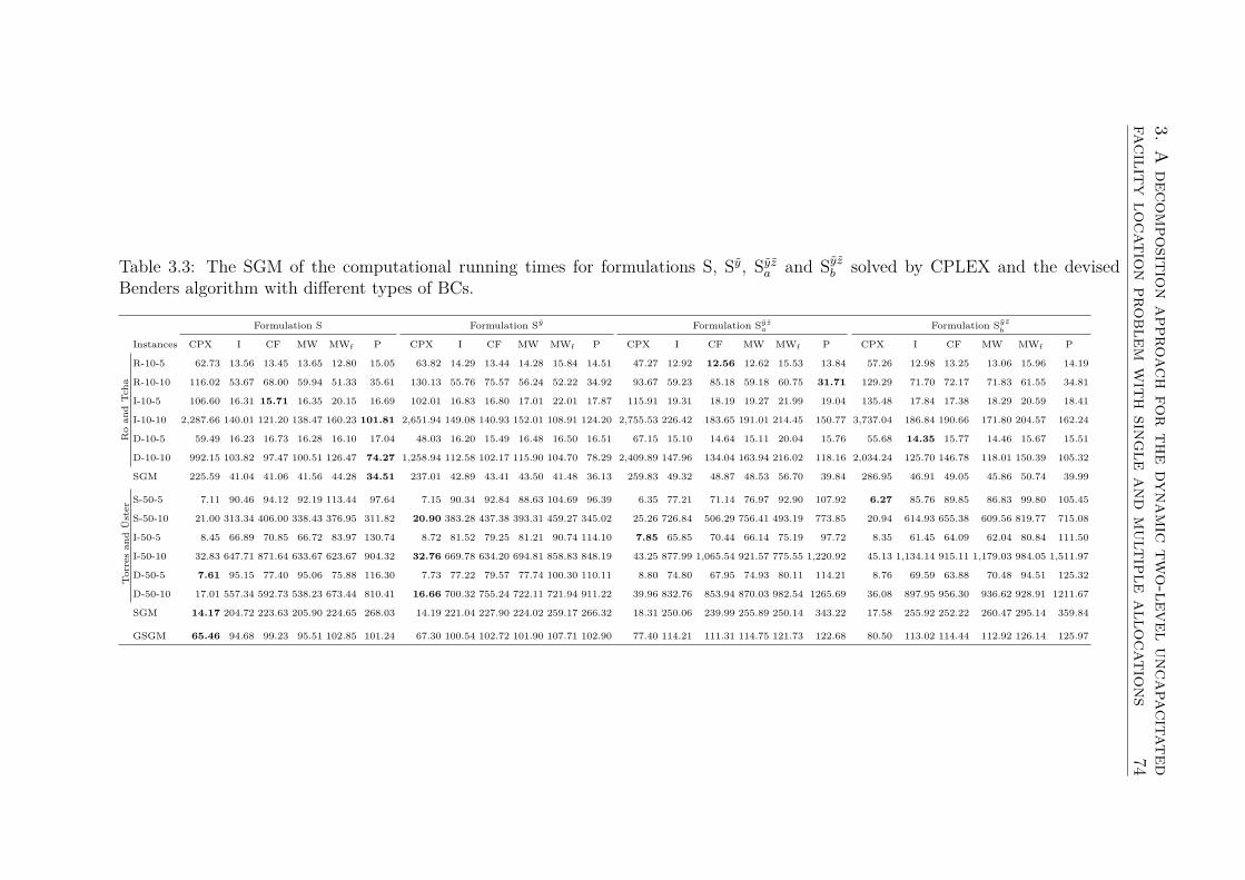
3.A
decomposition
approachfor
thedynam
ictw
o-leveluncapacitated
facilitylocation
problemw
ithsingle
andm
ultipleallocations
74
Table 3.3: The SGM of the computational running times for formulations S, Sy, Syza and Syzb solved by CPLEX and the devisedBenders algorithm with different types of BCs.
Formulation S Formulation Sy Formulation Syza Formulation Syz
b
Instances CPX I CF MW MWf P CPX I CF MW MWf P CPX I CF MW MWf P CPX I CF MW MWf P
Ro
and
Tch
a
R-10-5 62.73 13.56 13.45 13.65 12.80 15.05 63.82 14.29 13.44 14.28 15.84 14.51 47.27 12.92 12.56 12.62 15.53 13.84 57.26 12.98 13.25 13.06 15.96 14.19
R-10-10 116.02 53.67 68.00 59.94 51.33 35.61 130.13 55.76 75.57 56.24 52.22 34.92 93.67 59.23 85.18 59.18 60.75 31.71 129.29 71.70 72.17 71.83 61.55 34.81
I-10-5 106.60 16.31 15.71 16.35 20.15 16.69 102.01 16.83 16.80 17.01 22.01 17.87 115.91 19.31 18.19 19.27 21.99 19.04 135.48 17.84 17.38 18.29 20.59 18.41
I-10-10 2,287.66 140.01 121.20 138.47 160.23 101.81 2,651.94 149.08 140.93 152.01 108.91 124.20 2,755.53 226.42 183.65 191.01 214.45 150.77 3,737.04 186.84 190.66 171.80 204.57 162.24
D-10-5 59.49 16.23 16.73 16.28 16.10 17.04 48.03 16.20 15.49 16.48 16.50 16.51 67.15 15.10 14.64 15.11 20.04 15.76 55.68 14.35 15.77 14.46 15.67 15.51
D-10-10 992.15 103.82 97.47 100.51 126.47 74.27 1,258.94 112.58 102.17 115.90 104.70 78.29 2,409.89 147.96 134.04 163.94 216.02 118.16 2,034.24 125.70 146.78 118.01 150.39 105.32
SGM 225.59 41.04 41.06 41.56 44.28 34.51 237.01 42.89 43.41 43.50 41.48 36.13 259.83 49.32 48.87 48.53 56.70 39.84 286.95 46.91 49.05 45.86 50.74 39.99
Tor
res
and
Üst
er
S-50-5 7.11 90.46 94.12 92.19 113.44 97.64 7.15 90.34 92.84 88.63 104.69 96.39 6.35 77.21 71.14 76.97 92.90 107.92 6.27 85.76 89.85 86.83 99.80 105.45
S-50-10 21.00 313.34 406.00 338.43 376.95 311.82 20.90 383.28 437.38 393.31 459.27 345.02 25.26 726.84 506.29 756.41 493.19 773.85 20.94 614.93 655.38 609.56 819.77 715.08
I-50-5 8.45 66.89 70.85 66.72 83.97 130.74 8.72 81.52 79.25 81.21 90.74 114.10 7.85 65.85 70.44 66.14 75.19 97.72 8.35 61.45 64.09 62.04 80.84 111.50
I-50-10 32.83 647.71 871.64 633.67 623.67 904.32 32.76 669.78 634.20 694.81 858.83 848.19 43.25 877.99 1,065.54 921.57 775.55 1,220.92 45.13 1,134.14 915.11 1,179.03 984.05 1,511.97
D-50-5 7.61 95.15 77.40 95.06 75.88 116.30 7.73 77.22 79.57 77.74 100.30 110.11 8.80 74.80 67.95 74.93 80.11 114.21 8.76 69.59 63.88 70.48 94.51 125.32
D-50-10 17.01 557.34 592.73 538.23 673.44 810.41 16.66 700.32 755.24 722.11 721.94 911.22 39.96 832.76 853.94 870.03 982.54 1265.69 36.08 897.95 956.30 936.62 928.91 1211.67
SGM 14.17 204.72 223.63 205.90 224.65 268.03 14.19 221.04 227.90 224.02 259.17 266.32 18.31 250.06 239.99 255.89 250.14 343.22 17.58 255.92 252.22 260.47 295.14 359.84
GSGM 65.46 94.68 99.23 95.51 102.85 101.24 67.30 100.54 102.72 101.90 107.71 102.90 77.40 114.21 111.31 114.75 121.73 122.68 80.50 113.02 114.44 112.92 126.14 125.97

3.A
decomposition
approachfor
thedynam
ictw
o-leveluncapacitated
facilitylocation
problemw
ithsingle
andm
ultipleallocations
75
Table 3.4: The SGM of the number of explored branch-and-bound nodes for formulations S, Sy, Syza and Syzb solved by CPLEX andthe Benders algorithm different types of BCs.
Formulation S Formulation Sy Formulation Syza Formulation Syz
b
Instances CPX I CF MW MWf P CPX I CF MW MWf P CPX I CF MW MWf P CPX I CF MW MWf P
Ro
and
Tch
a
R-10-5 10.79 38.97 41.01 38.97 38.28 32.49 14.10 61.47 44.77 61.47 48.74 39.80 7.40 45.31 36.18 41.89 69.02 40.91 12.48 47.23 41.42 47.23 39.93 37.49
R-10-10 10.03 52.48 69.28 62.53 22.28 58.79 14.65 66.79 77.54 66.53 10.56 48.62 10.84 54.92 67.83 54.92 14.23 35.34 12.83 68.94 112.76 72.16 17.02 39.93
I-10-5 10.91 49.30 45.08 49.03 43.98 42.26 11.04 62.79 50.37 62.54 62.66 51.07 11.97 86.56 81.72 87.80 73.52 54.33 16.96 73.92 69.25 73.87 74.60 66.03
I-10-10 402.14 282.67 245.22 279.20 204.67 290.30 325.58 356.47 289.10 357.07 159.90 356.11 165.42 518.95 548.32 434.24 318.60 498.08 282.39 472.21 540.94 463.25 291.46 466.14
D-10-5 9.53 47.34 51.74 47.34 49.89 53.32 6.29 51.43 37.39 51.43 44.77 42.30 12.02 49.88 44.28 49.88 51.85 39.08 8.37 40.10 47.22 40.82 49.01 41.62
D-10-10 120.31 192.26 173.76 200.39 122.30 167.03 138.61 212.69 191.76 207.96 107.35 177.82 438.17 397.76 393.78 502.62 463.28 366.51 253.80 352.57 395.02 316.98 246.73 339.40
SGM 59.36 93.28 91.72 95.88 70.67 90.52 58.21 113.52 98.01 112.91 65.93 95.95 66.53 140.59 140.15 141.66 122.08 120.27 67.09 132.25 148.92 129.41 96.65 119.73
Tor
res
and
Üst
er
S-50-5 0.00 487.61 510.23 486.92 508.99 470.48 0.00 508.85 500.14 508.59 586.28 438.52 0.00 591.13 432.07 591.13 575.32 523.30 0.00 517.36 542.78 516.83 535.94 581.49
S-50-10 2.64 420.00 496.71 421.89 585.21 298.08 2.18 633.95 663.55 633.66 587.88 354.38 1.23 1,163.40 768.57 1,157.60 879.22 1,309.69 1.23 761.69 1,259.18 764.41 1,246.04 985.71
I-50-5 0.00 300.62 299.68 300.62 361.65 515.13 0.00 343.20 304.47 343.20 384.97 542.43 0.00 331.07 376.63 331.07 369.22 410.75 0.00 330.56 290.37 330.56 382.64 497.94
I-50-10 0.00 645.33 906.07 645.17 567.46 946.50 0.00 820.92 754.69 820.39 977.48 1,042.98 0.00 1,305.58 1,476.68 1,321.22 949.91 1,437.19 0.00 1,292.49 1,211.46 1,290.79 1,214.75 1,797.48
D-50-5 0.00 410.30 286.60 410.30 313.92 458.94 0.00 280.71 314.06 280.71 342.47 452.50 0.00 315.61 279.09 315.61 272.16 491.64 0.00 274.08 238.54 274.08 323.96 487.58
D-50-10 0.00 606.83 497.99 604.44 693.77 783.23 0.00 745.31 646.33 741.49 662.22 822.42 0.00 860.37 1,016.64 859.38 1,042.45 1,415.57 0.00 1,116.81 1,114.87 1,121.13 914.79 1,448.81
SGM 0.44 466.09 468.75 465.98 490.15 545.25 0.36 523.40 504.82 522.79 560.72 571.36 0.20 671.68 626.48 672.38 619.31 823.06 0.20 624.97 654.14 625.52 684.83 856.12
GSGM 26.51 230.78 230.22 232.97 217.37 250.62 26.01 264.84 246.07 264.14 231.11 262.70 29.18 330.88 317.69 332.04 299.68 350.91 29.40 310.33 333.26 307.97 292.85 358.35
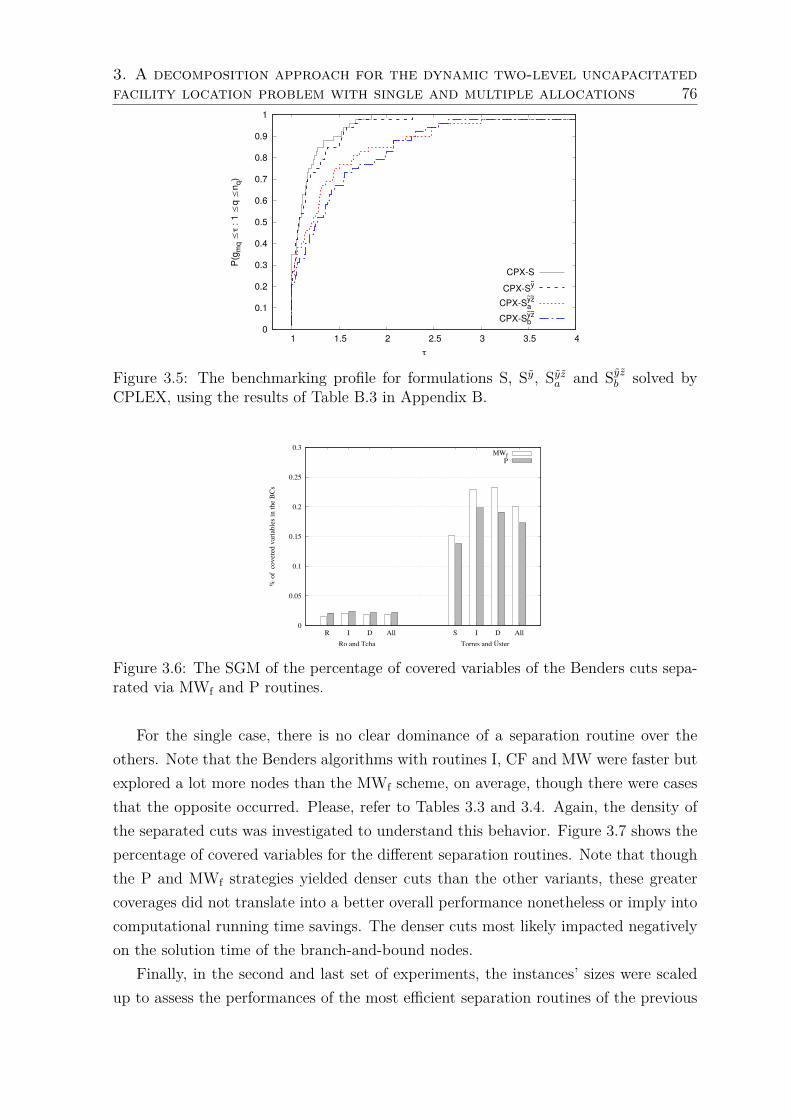
3. A decomposition approach for the dynamic two-level uncapacitatedfacility location problem with single and multiple allocations 76
0
0.1
0.2
0.3
0.4
0.5
0.6
0.7
0.8
0.9
1
1 1.5 2 2.5 3 3.5 4
P(g m
q≤
τ: 1
≤q
≤n q
)
τ
CPX-S
CPX-Sy~
CPX-Say~z~
CPX-Sby~z~
Figure 3.5: The benchmarking profile for formulations S, Sy, Syza and Syzb solved byCPLEX, using the results of Table B.3 in Appendix B.
0
0.05
0.1
0.15
0.2
0.25
0.3
R I D All S I D All
% o
f co
vere
d va
riabl
es in
the
BCs
MWfP
Torres and ÜsterRo and Tcha
Figure 3.6: The SGM of the percentage of covered variables of the Benders cuts sepa-rated via MWf and P routines.
For the single case, there is no clear dominance of a separation routine over theothers. Note that the Benders algorithms with routines I, CF and MW were faster butexplored a lot more nodes than the MWf scheme, on average, though there were casesthat the opposite occurred. Please, refer to Tables 3.3 and 3.4. Again, the density ofthe separated cuts was investigated to understand this behavior. Figure 3.7 shows thepercentage of covered variables for the different separation routines. Note that thoughthe P and MWf strategies yielded denser cuts than the other variants, these greatercoverages did not translate into a better overall performance nonetheless or imply intocomputational running time savings. The denser cuts most likely impacted negativelyon the solution time of the branch-and-bound nodes.
Finally, in the second and last set of experiments, the instances’ sizes were scaledup to assess the performances of the most efficient separation routines of the previous
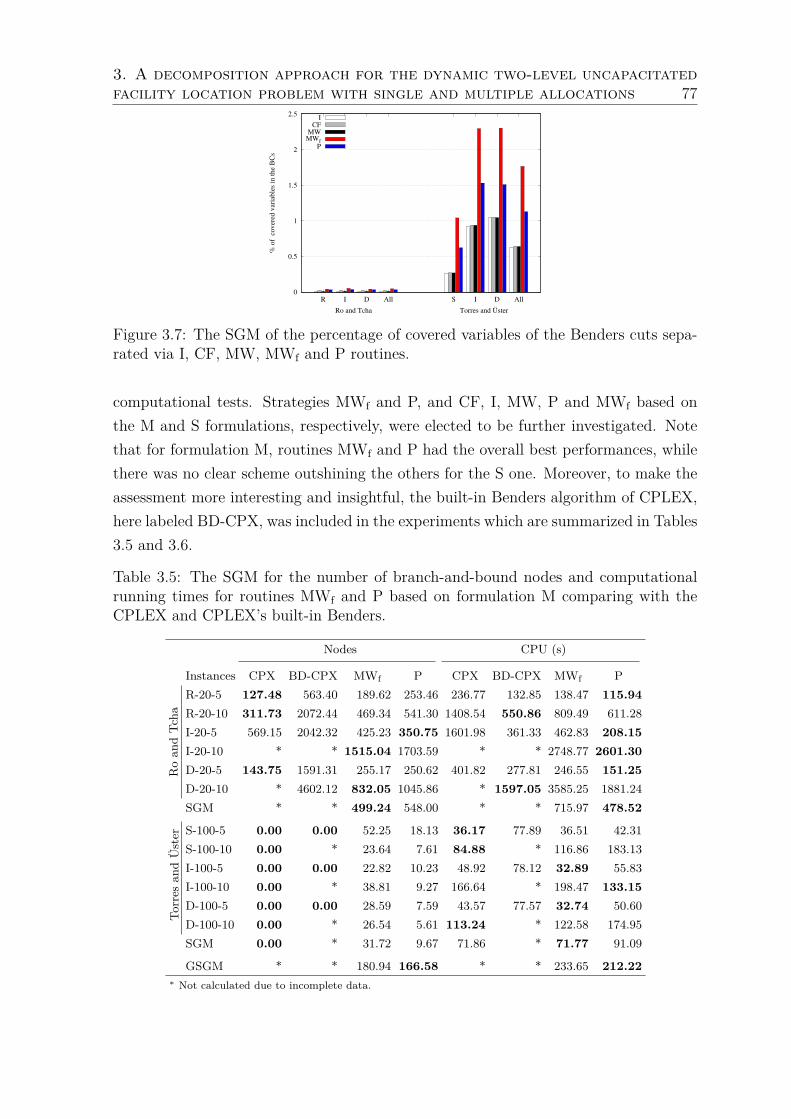
3. A decomposition approach for the dynamic two-level uncapacitatedfacility location problem with single and multiple allocations 77
0
0.5
1
1.5
2
2.5
R I D All S I D All
% o
f co
vere
d va
riabl
es in
the
BCs
ICF
MWMWf
P
Torres and ÜsterRo and Tcha
Figure 3.7: The SGM of the percentage of covered variables of the Benders cuts sepa-rated via I, CF, MW, MWf and P routines.
computational tests. Strategies MWf and P, and CF, I, MW, P and MWf based onthe M and S formulations, respectively, were elected to be further investigated. Notethat for formulation M, routines MWf and P had the overall best performances, whilethere was no clear scheme outshining the others for the S one. Moreover, to make theassessment more interesting and insightful, the built-in Benders algorithm of CPLEX,here labeled BD-CPX, was included in the experiments which are summarized in Tables3.5 and 3.6.
Table 3.5: The SGM for the number of branch-and-bound nodes and computationalrunning times for routines MWf and P based on formulation M comparing with theCPLEX and CPLEX’s built-in Benders.
Nodes CPU (s)
Instances CPX BD-CPX MWf P CPX BD-CPX MWf P
Roan
dTc
ha
R-20-5 127.48 563.40 189.62 253.46 236.77 132.85 138.47 115.94R-20-10 311.73 2072.44 469.34 541.30 1408.54 550.86 809.49 611.28I-20-5 569.15 2042.32 425.23 350.75 1601.98 361.33 462.83 208.15I-20-10 * * 1515.04 1703.59 * * 2748.77 2601.30D-20-5 143.75 1591.31 255.17 250.62 401.82 277.81 246.55 151.25D-20-10 * 4602.12 832.05 1045.86 * 1597.05 3585.25 1881.24SGM * * 499.24 548.00 * * 715.97 478.52
Torres
andÜster S-100-5 0.00 0.00 52.25 18.13 36.17 77.89 36.51 42.31
S-100-10 0.00 * 23.64 7.61 84.88 * 116.86 183.13I-100-5 0.00 0.00 22.82 10.23 48.92 78.12 32.89 55.83I-100-10 0.00 * 38.81 9.27 166.64 * 198.47 133.15D-100-5 0.00 0.00 28.59 7.59 43.57 77.57 32.74 50.60D-100-10 0.00 * 26.54 5.61 113.24 * 122.58 174.95SGM 0.00 * 31.72 9.67 71.86 * 71.77 91.09
GSGM * * 180.94 166.58 * * 233.65 212.22∗ Not calculated due to incomplete data.

3. A decomposition approach for the dynamic two-level uncapacitatedfacility location problem with single and multiple allocations 78
In both Tables 3.5 and 3.6, symbol ‘*’ represents that the studied group of in-stances has not been fully solved, either an out-of-memory error occurred or the re-ferred method did not convergence to an optimal solution on one or more instanceswithin the 24-hour time limit. For the detailed results, please see Tables B.5 and B.6in Appendix B. The Benders algorithms using the devised separation routines werecapable of solving all of the instances within the given time limit. With few instancegroup exceptions, the proposed methods outperformed both CPLEX and CPLEX’sbuilt-in Benders for both variants of the problem. Overall, routines P and CF basedon the M and S formulations, respectively, had a slightly better performance than theother examined methods. They were 10% and 14.5% faster on average than the otherroutines, respectively.
To better highlight the performance of the devised separation routines and the com-parison with the other methods, a benchmarking profile concerning the computationalrunning times was carried out and reported in Figures 3.8 and 3.9. For the multipleallocation problem variant, the CPX and BD-CPX methods were added to the compar-ison, while for the single version, they were omitted since they were unable to solve allinstances within the given time limit of 24h. Figure 3.8 confirms that, for the multipleassignment problem version, the P separation routine outperformed the others sinceit could solve all instances with the smallest τ < 2.7. For the single case, though theCF scheme induces less dense cuts when compared with the MW, MWf and P rou-tines, it was able to outperform these strategies by solving all instances with τ < 2.6.The additional dual information captured by the Benders cuts made the difference inclosing the optimality gaps faster. Finally, it is noteworthy that the GRASP attainedrelatively small optimality gaps given the short computational running time and smallnumber of iterations allowed for it to run.

3.A
decomposition
approachfor
thedynam
ictw
o-leveluncapacitated
facilitylocation
problemw
ithsingle
andm
ultipleallocations
79
Table 3.6: The SGM for the number of branch-and-bound nodes and computational running times for all routines based on formulationS comparing with the CPLEX and CPLEX’s built-in Benders.
Nodes CPU (s)
CPX BD-CPX I CF MW MWf P CPX BD-CPX I CF MW MWf P
Roan
dTc
ha
R-20-5 64.78 158.70 151.17 150.45 145.69 111.02 187.44 2288.14 337.36 90.00 90.06 89.95 85.50 109.39R-20-10 * * 529.95 446.44 532.00 464.50 445.13 * * 490.01 437.12 494.01 459.46 451.60I-20-5 * 1072.20 770.00 553.67 770.00 569.68 330.56 * 575.93 337.58 258.72 342.29 294.58 181.89I-20-10 * * 1444.29 1283.48 1644.37 1200.26 1000.68 * * 1646.48 1580.33 1986.20 2181.51 1266.48D-20-5 100.75 330.34 234.25 226.40 234.28 180.36 187.71 5425.16 415.63 133.07 139.96 132.96 153.37 134.59D-20-10 * * 696.39 620.17 698.91 648.35 669.99 * * 869.75 789.51 931.83 1629.29 912.74SGM * * 519.61 454.58 530.68 428.38 404.31 * * 381.91 353.12 400.28 437.35 338.81
Torres
andÜster S-100-5 0.00 * 1041.64 949.39 1041.83 880.55 850.28 87.35 * 1698.08 1515.14 1871.91 1572.95 1722.90
S-100-10 * * 764.49 792.16 763.43 1180.96 1259.47 * * 5464.13 6415.83 5558.32 9349.03 10789.55I-100-5 0.00 * 1394.31 1190.49 1387.18 1443.75 1345.48 147.21 * 2709.08 2352.62 2747.28 2995.01 3495.83I-100-10 * * 1286.31 1083.68 1254.11 1558.83 1556.88 * * 14562.93 13176.41 14074.58 18961.67 24111.79D-100-5 0.00 * 1085.36 1017.52 1071.76 1204.23 1018.95 115.02 * 2616.07 2772.61 2528.48 2796.96 2713.45D-100-10 * * 1630.62 1134.76 1499.00 1170.16 1465.10 * * 18220.32 12096.01 16744.50 12388.14 19981.44SGM * * 1169.91 1019.96 1144.77 1221.60 1225.30 * * 5096.80 4653.39 5076.00 5545.29 6635.95
GSGM * * 787.05 688.10 786.03 735.65 717.53 * * 1404.71 1291.29 1434.53 1566.44 1512.55∗ Not calculated due to incomplete data.

3. A decomposition approach for the dynamic two-level uncapacitatedfacility location problem with single and multiple allocations 80
0
0.1
0.2
0.3
0.4
0.5
0.6
0.7
0.8
0.9
1
1 1.5 2 2.5 3 3.5 4
P(g m
q≤
τ: 1
≤q
≤n q
)
τ
PMWf
BD-CPXCPX
Figure 3.8: The benchmarking profile concerning the computational running time forseparation routines MWf and P based on formulation M comparing with CPX, andBD-CPX on solving larger instances (Table B.5 in Appendix B).
0
0.1
0.2
0.3
0.4
0.5
0.6
0.7
0.8
0.9
1
1 1.5 2 2.5 3 3.5 4
P(g m
q≤
τ: 1
≤q
≤n q
)
τ
CFI
MWP
MWf
Figure 3.9: The benchmarking profile concerning the computational running time forall separation routines based on formulation S on solving larger instances (Table B.6in Appendix B). CPX and BD-CPX curves omitted since they were unable to solve allinstances within the given time limit of 24h.
3.6 Conclusion
In this work, a dynamic two-level uncapacitated facility location problem was studiedwhile considering two different forms of inter-level facility interconnections, i.e. if singleor multiple allocations between facilities of different levels are allowed. These prob-lems belong to a class of discrete multi-period facility location problem that considersdifferent hierarchies of facilities and their interactions. Mixed-integer formulations for

3. A decomposition approach for the dynamic two-level uncapacitatedfacility location problem with single and multiple allocations 81
the multiple and single cases were extended from the single-period arc-based formula-tion proposed by Barros and Labbé (1994b) and Gendron et al. (2016), respectively.Given their mathematical structure, the devised formulations were reformulated andsimplified to yield new ones with fewer variables and constraints. The matrix structureof the proposed formulations permitted the deployment of a Benders decompositionreformulation, which, combined with a fast GRASP and different Benders cut sepa-ration routines, was developed to solve standard test instances adapted from Ro andTcha (1984) and Torres-Soto and Üster (2011). At all, five Benders cuts separationstrategies were designed and investigated for each problem variant: standard and lifted(closing facility) optimality cuts obtained via analytical procedures and three differentclasses of Pareto-optimal (non-dominated) optimality cuts.
An extensive computational experiment showed the efficiency of the implementedBenders decomposition algorithm on solving the instances for both variants of theproblem when compared with the CPLEX solver and its Benders built-in. Further,the proposed GRASP was able to generate good and fast initial solutions to the devel-oped Benders algorithm. In particular, for the multiple allocation case, the separationroutine based on the Papadakos’s approach was the most efficient; while, for the sin-gle case, less dense Bender cuts attained by the strategy of gathering saving stemmedfrom the dual information of closing facilities performed better. Other enhancements,e.g. variable fixing procedures or different branching strategies, can be incorporatedinto the devised Benders algorithm to further improve its performance. Finally, as afuture research opportunity, the developed decomposition will be extended to handleuncertainty in the data via a robust optimization approach.

Chapter 4
The hierarchical two-level facilitylocation problem under the supplyand congestion costs effects
This chapter studies the hierarchical two-level facility location problem, in which facil-ities are subject to nonlinear congestion effects caused by the volume of customer re-quests from a large-scale supply network. This problem is assessed from three differentsupply chain patterns: multi-assignments, single-assignments or single-assignments-paths between facilities and customers. The first, we can bind each customer to oneor more facilities by level, while the second allows only one first-level facility to belinked to each second-level facility. The last one establishes a single pair of facilities,one by level, to serve each customer, i.e. there is a unique path between the customerand the first facility level. These approaches aim to minimize the total service costs,which include opening facilities, transport operations and also the congestion effects inthe facilities. Three different techniques for addressing congestion on facility locationproblems are developed: the Outer-Approximation method (OA); the OA coupled tothe Benders Decomposition method (OA-BD); and the Generalized Benders Decom-position method (GBD). Computational experiments indicate that OA outperformsthe CPLEX general solver and other methods on solving a set of Benchmark instanceswith different dimensions and subject to the classic nonlinear congestion functions ofthe literature.
4.1 Introduction
The productive resource management system brings together a series of decision-making that require sufficient organizational and operational intelligence to support
82
4. The hierarchical two-level facility location problem under thesupply and congestion costs effects 83
strategic decisions commonly embedded into an integrated supply chain (Melo et al.2009). This management decision process is closely related to the type of product orservice provided and it costs (Hajiaghayi et al. 2003). A supply network can haveseveral types of resource constraints, starting with the location of supply sources andtransport modes, followed by potential barriers caused by the high volume of orders orlimitations inherent in the physical distribution system (Garcia and You 2015).
These peculiarities aroused in the scientific community a significant interest inthe development of computational strategies able to represent and include geographi-cal, temporal and structural aspects of real logistic chains, either by deterministic orstochastic optimization models depending on the characteristics of the problems (El-hedhli 2006, Belotti et al. 2013, Ortiz-Astorquiza et al. 2018). One way of modelingthese problems that is widespread in the literature is the so-called Facility LocationProblems (FLP) introduced by Weber (1909).
Many logistics systems can be represented through hierarchical FLPs that enablethe physical transportation and distribution of products or services over an integratednetwork, provided strategic supply points are installed across a given geographic regionto serve all customer requests (Ortiz-Astorquiza et al. 2018). Nevertheless, and dueto difficulties of interpretation and knowledge of facilities capacity, as well as uncer-tainty aspects associated with the volume of customer requests, many cases are initiallytreated as problems without capacity constraints, or uncapacitated problems (Kauf-man et al. 1977). When we are dealing with the hierarchical problem of only two-levelfacilities we refer to the two-level uncapacitated facility location problem (TLUFLP)(Barros and Labbé 1994b). A computational advantage of uncapacitated problems intheir optimal configuration has its customers assigned to the nearest operating facilities(Boffey et al. 2007).
Conversely, even when facilities have an unlimited supply, delays or accumulation oforders can be generated. Therefore, a re-planning of logistics activities and operationsshould be performed to minimize costs and improve the quality of service (Elhedhli2006). These delays in logistics systems cause a ripple effect that establishes a queueof activity, also known as congestion (Desrochers et al. 1995). Examples of these con-gestion effects in facility location problems are noticeable in several environments: (i)health-care emergency service systems (fire, ambulance, police) Zhang et al. (2009),Berman and Krass (2015); (ii) postal delivery services and production and distribu-tion systems (Narula 1986, Daskin 2011, Farahani et al. 2014); and (iii) loading andunloading service in seaports (Meersman et al. 2012). In all cases, the same facility isresponsible to serve many customers at the same time, which makes the service lessqualified (Boffey et al. 2007). Moreover, congestion effects in location problems haveconvex cost functions, usually quadratic, which can lead to diseconomies of scale for

4. The hierarchical two-level facility location problem under thesupply and congestion costs effects 84
the installed facilities, as (nonlinear) congestion costs tend to grow faster than (linear)transport and installation costs (Desrochers et al. 1995).
These FLP problems under congestion can be conveniently modeled as a mixed-integer nonlinear programming (MINLP), i.e. it combines both the combinatorialpattern of discrete variable optimization and the particularities caused by nonlinearfunctions (Belotti et al. 2013). To solve convex MINLP many commercial solvers offerlimited alternatives for smooth problems, where the nonlinear functions are continu-ously differentiable (Kronqvist et al. 2019). On the other hand, according to Belottiet al. (2013) the use of congestion function linearization procedures and decompositiontechniques are also widespread alternatives in the literature, e.g. Outer-approximation(Duran and Grossmann 1986, Fletcher and Leyffer 1994) and Generalized Bendersdecomposition (Geoffrion 1972, Van Roy 1983).
The state-of-the-art on location and network flow problems under congestion hasbeen continuously expanded since Grove and O’Kelly (1986)’s work, in which the re-lationship between hub-and-spoke networks and congestion is analyzed in the airlineindustry. More specifically in facility location problems, Desrochers et al. (1995) arepioneers using a column generation method within a branch-and-bound algorithm tosolve a single-level capacitated problem. Boffey et al. (2007) presents a review of facil-ity location under congestion models with immobile servers, while heuristic approachesbased on a greedy algorithm on elastic demand problems and four different heuris-tic procedures used to solve the breast cancer screening center network problem inMontreal are proposed by Fang et al. (2009) and Zhang et al. (2009), respectively.
In recent studies, Şelfun (2011) propose different outer-approximation algorithmsfor the congested p-median problem, while Lu et al. (2014) have obtained good boundsfor a class of location problems, through a Lagrangian lower bound combining with aheuristic solution a heuristic coupled to a branch-and-price algorithm. Fischetti et al.(2016) propose a Benders decomposition approach incorporated into a branch-and-cut mixed-integer programming solver for a single-level linear and congested variants,which contains convex but non-separable quadratic terms. Ljubić and Moreno (2018)presents a branch-and-cut algorithm that combines two types of cutting planes: theouter-approximation and submodular cuts; for the maximum capture facility locationproblems with random utilities.
The main contributions of this chapter are the following: Three variants of theTLUFLP which the facilities are under congestion effects (CTLUFLP) are investigated:One with single assignments between levels or CTLUFLP-SS, in which each client canbe served by only one pair of opened first and second level facility; another with a singleallocation only between the facility levels or CTLUFLP-SM; and a multiple assignmentvariant or CTLUFLP-MM, in which the service flow can be fully splittable. All variants

4. The hierarchical two-level facility location problem under thesupply and congestion costs effects 85
are adaptations of the multiple and single mathematical programming models proposedby Barros and Labbé (1994b) and Gendron et al. (2016), respectively. Three differentdecomposition methods are developed to solve the problems: an Outer-Approximationmethod (OA) (Duran and Grossmann 1986, Fletcher and Leyffer 1994); a hybrid Outer-Approximation/Benders Decomposition algorithm (OA-BD) (de Camargo et al. 2011);and a Generalized Benders Decomposition method (GBD) (Geoffrion 1972, Van Roy1983). Computational experiments were carried out on large-scale instances to assessand highlight the behavior of the models, subject to different congestion functions whentheir parameters are changed.
This chapter is organized as follows: Section 4.2 describes the notation, definitions,and devised formulations, and provides the adopted congestion functions. Section 4.3introduces the decomposition approaches based on adding different cut-plane separa-tion schemes. Section 4.4 presents and discusses the results of computational experi-ments performed to compare all the proposed solution strategies. Finally, Section 4.5concludes and remarks on the chapter.
4.2 Notation, definitions and formulations
Let K and J be sets of candidate facilities to be opened in the first and second levels,respectively, and responsible for supplying a set of customers I scattered in a specificgeographical area. These three sets are organized into a hierarchical supply chain,where first-level facilities in K assumes the role of resource-generating agent and areconnected to one (single) or more (multiple) second-level facilities in J , which areresponsible for the transshipment of all the customer’s demand di, i ∈ I. This chainstructure implies direct operating and transportation costs, i.e. fixed cost componentsfk and aj generated from the facility location at levels K and J , respectively, andunitary transportation costs cijk obtained through the logistics service between thefacilities levels cjk, j ∈ J and k ∈ K, and the freight from the customers’ provisionfor the second-level facilities cij, i ∈ I and j ∈ J , or cijk = cij + cjk are characteristicparameters of the problem.
Now, considering that customer requests occur concurrently, a natural service back-log, at the same instant of time, cause delays in the customer supply process. One wayof modeling these problems is based on the idea of accounting for novel costs aris-ing from delays from first and second facility-level services. Let τk(hk) and τj(gj) bethe nonlinear cost functions to represent the congestion effects on the active facilities,where hk and gj indicate the cumulative volume orders supplied by the facilities k ∈ Kand j ∈ J , respectively. Thus, hk and gj must account for the sum of all products or

4. The hierarchical two-level facility location problem under thesupply and congestion costs effects 86
services that comes from a facility, while τk(hk) and τj(gj) must be able to representthe costs arising from the limitation in the immediate supply of all customers for afacility, although there is no type of explicit supply capacity constraint of the facilitiesin the proposed formulations. Let also zk ∈ 0, 1 and yj ∈ 0, 1 be binary decisionvariables to indicate if a facility k ∈ K and j ∈ J , respectively, is active (1) or not(0). Continuous variables xijk ≥ 0 can be incorporated into the problem to couplethe percentage of demand of customer i ∈ I served by first-level facility k ∈ K viasecond-level facility j ∈ J . Thus, the models consist of locating first (zk) and second(yj) level facilities, which are under congestion effect conditions, to serve all customersi ∈ I at minimal installation, transportation, and congestion costs.
Figure 4.1 illustrates an example of TLUFLP having single assignments betweenlevels through a set of nodes and edges that make up a graph. Figure 4.1a shows all setsand possibilities of connections between them, where the arrows indicate the directionof the service flow, i.e. it is a network with a rigid hierarchy. Note also that everyfacility node in operation and the percentage of total demand that flows through eachedge between levels are highlighted in Figures 4.1b and 4.1c, although this informationis used only to set up Figure 4.1c. When a facility supplies more than one customer ata time (k3), or the order volume of a single customer is relatively high (k1 and j1), thereis a network overhead, which may result in new facilities being opened, provided thecongestion costs exceed fixed installation costs, as shown in the proposed amendmentfrom Figure 4.1b to 4.1c.
k1 j1 i1
k2 j2 i2
k3 j3 i3
(a) initial sets
k1 j1 i1
k2 j2 i2
k3 j3 i3
41%
59%
41%
23%
36%
(b) TLUFLP
k1 j1 i1
k2 j2 i2
k3 j3 i3
41%
59%
41%
23%
36%
(c) CTLUFLP
Figure 4.1: Example of single-and-single assignment problem
Also, it is necessary to define the type of relationship between the hierarchical lev-els that one wishes to model. Three different variants of the supply chain patternsare studied: (i) multi-assignments (MM) adapted from the arc-based TLUFLP for-mulation (Barros and Labbé 1994b), whose supply flow can be splittable between thelevels; (ii) single-assignments (SM), introduced by Gendron et al. (2016), which limitseach second-level facility to be linked to only one first-level facility; and (iii) single-

4. The hierarchical two-level facility location problem under thesupply and congestion costs effects 87
assignments-paths (SS), in which there is only one path between the source (first-level)and the destination (client).
4.2.1 CTLUFLP formulations
The MM formulation may be formally presented by formulation (4.1)-(4.6).
MM
minx,h,g≥0y∈0,1|J|z∈0,1|K|
∑k∈K
[fkzk + τk(hk)] +∑j∈J
[ajyj + τj(gj)]
+∑i∈I
∑j∈J
∑k∈K
dicijkxijk
s.t.:∑j∈J
∑k∈K
xijk = 1 ∀ i ∈ I
∑j∈J
∑i∈I
dixijk ≤ hk ∀ k ∈ K
∑k∈K
∑i∈I
dixijk ≤ gj ∀ j ∈ J
zk −∑j∈J
xijk ≥ 0 ∀ i ∈ I, k ∈ K
yj −∑k∈K
xijk ≥ 0 ∀ i ∈ I, j ∈ J.
(4.1)
(4.2)
(4.3)
(4.4)
(4.5)
(4.6)
The objective (4.1) is to minimize all the supply chain costs, subject to the setof constraints (4.2)-(4.6). Constraints (4.2) guarantee that all customer demands aresatisfied, whereas constraints (4.3) and (4.4) are used to account for the outboundtraffic of the first and second level facilities, respectively. Constraints (4.5) and (4.6)ensure that customers can only be served by an active first and second level facility,respectively. By introducing the binary variables πjk = 0, 1, j ∈ J and k ∈ K, andreplacing constraints (4.6) to (4.8)-(4.10) of MM, we obtain a Gendron et al. problemvariant, which taking into account the congestion effects on the facilities, as shown bythe formulation SM.
Constraints (4.8) ensure that each client can only be served by active connectionslinking first to second level facilities, whereas constraints (4.9) and (4.10) assure thatactive connections between the facility levels can only occur to installing first-level fa-cilities, and a second-level facility is single assigned to a first-level facility, respectively.Note that the coupling caused by the constraints (4.10) can be perfectly satisfied with-out the use of the variables yj, j ∈ J , but adding constraints (4.12), and then renderinga SM variant with fewer variables, which we named SMy. Note that constraints (4.12)are used to ensure minimal connectivity between active first and second level facili-
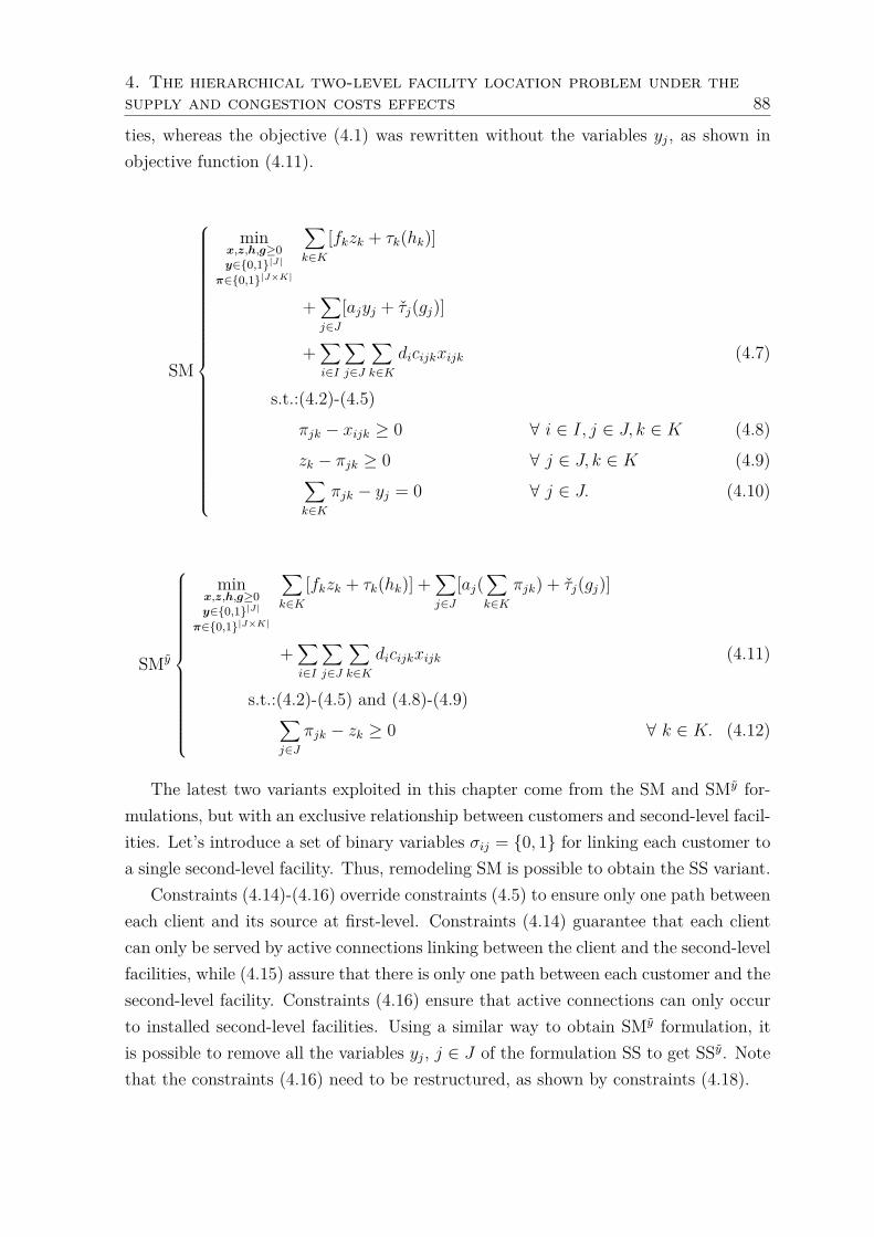
4. The hierarchical two-level facility location problem under thesupply and congestion costs effects 88
ties, whereas the objective (4.1) was rewritten without the variables yj, as shown inobjective function (4.11).
SM
minx,z,h,g≥0y∈0,1|J|
π∈0,1|J×K|
∑k∈K
[fkzk + τk(hk)]
+∑j∈J
[ajyj + τj(gj)]
+∑i∈I
∑j∈J
∑k∈K
dicijkxijk
s.t.:(4.2)-(4.5)
πjk − xijk ≥ 0 ∀ i ∈ I, j ∈ J, k ∈ K
zk − πjk ≥ 0 ∀ j ∈ J, k ∈ K∑k∈K
πjk − yj = 0 ∀ j ∈ J.
(4.7)
(4.8)
(4.9)
(4.10)
SMy
minx,z,h,g≥0y∈0,1|J|
π∈0,1|J×K|
∑k∈K
[fkzk + τk(hk)] +∑j∈J
[aj(∑k∈K
πjk) + τj(gj)]
+∑i∈I
∑j∈J
∑k∈K
dicijkxijk
s.t.:(4.2)-(4.5) and (4.8)-(4.9)∑j∈J
πjk − zk ≥ 0 ∀ k ∈ K.
(4.11)
(4.12)
The latest two variants exploited in this chapter come from the SM and SMy for-mulations, but with an exclusive relationship between customers and second-level facil-ities. Let’s introduce a set of binary variables σij = 0, 1 for linking each customer toa single second-level facility. Thus, remodeling SM is possible to obtain the SS variant.
Constraints (4.14)-(4.16) override constraints (4.5) to ensure only one path betweeneach client and its source at first-level. Constraints (4.14) guarantee that each clientcan only be served by active connections linking between the client and the second-levelfacilities, while (4.15) assure that there is only one path between each customer and thesecond-level facility. Constraints (4.16) ensure that active connections can only occurto installed second-level facilities. Using a similar way to obtain SMy formulation, itis possible to remove all the variables yj, j ∈ J of the formulation SS to get SSy. Notethat the constraints (4.16) need to be restructured, as shown by constraints (4.18).

4. The hierarchical two-level facility location problem under thesupply and congestion costs effects 89
SS
minx,z,h,g≥0y∈0,1|J|
π∈0,1|J×K|σ∈0,1|I×J|
∑k∈K
[fkzk + τk(hk)]
+∑j∈J
[ajyj + τj(gj)]
+∑i∈I
∑j∈J
∑k∈K
dicijkxijk
s.t.:(4.2)-(4.4) and (4.8)-(4.10)
σij − xijk ≥ 0 ∀ i ∈ I, j ∈ J, k ∈ K∑j∈J
σij = 1 ∀ i ∈ I
yj − σij ≥ 0 ∀ i ∈ I, j ∈ J.
(4.13)
(4.14)
(4.15)
(4.16)
SSy
minx,z,h,g≥0
π∈0,1|J×K|σ∈0,1|I×J|
∑k∈K
[fkzk + τk(hk)]
+∑j∈J
[aj(∑k∈K
πjk) + τj(gj)]
+∑i∈I
∑j∈J
∑k∈K
dicijkxijk
s.t.:(4.2)-(4.4), (4.8)-(4.9) and (4.14)-(4.15)∑k∈K
πjk − σij ≥ 0 ∀ i ∈ I, j ∈ J.
(4.17)
(4.18)
Figure 4.2 shows examples of feasible solutions to each problem. Note that Figure4.2a allows splitting the flow between levels. Figure 4.2b all second-level facility islinked to a single first-level facility, while more than one second-level facility can serveeach client. Finally, Figure 4.2c presents the situation when each client must be servicedto only a single active facility pair.
For better understanding of the impact of allowing single or multiple relationshipsbetween levels presented in Figure 4.2, Table 4.1 provides a comparison of objectivefunction (OF) values, the number of branch-and-bound nodes explored (Nodes) andthe computer running times (CPU(s)) of a standard TLUFLP literature instance(Ro and Tcha 1984) and its congestion variants subjected to the effect of a classiccongestion function (Elhedhli and Hu 2005). This instance has 50 clients, as well as5 and 15 candidate facilities to be opened at the first and second levels, respectively.

4. The hierarchical two-level facility location problem under thesupply and congestion costs effects 90
k1 j1 i1
k2 j2 i2
k3 j3 i3
33%
15%
52%
28%
5%
29%
38%
(a) MM problem
k1 j1 i1
k2 j2 i2
k3 j3 i3
46%
54%
28%
18%
16%
38%
(b) SM problem
k1 j1 i1
k2 j2 i2
k3 j3 i3
62%
38%
28%
34%38%
(c) SS problem
Figure 4.2: Examples of different supply patterns in a CTLUFLP
Note that the solution presented in SS can be seen as an upper bound for SM. Thesame statement is true for SM compared to MM.
Table 4.1: A comparison between different customers supply patterns
Formulation OF Nodes CPU(s) Open at 1st level Open at 2nd level
TLUFLP 1136714.05 0 0.01 1, 5 1, 4, 9, 11, 13, 15MM 1595457.37 25 0.61 1, 2, 3, 5 1, 2, 4, 5, 7, 9, 12, 13, 15SM 1595820.31 65 1.36 1, 2, 3, 5 1, 2, 4, 5, 7, 9, 12, 13, 15SS 1595915.62 74 2.61 1, 2, 3, 5 1, 2, 4, 5, 7, 9, 12, 13, 15
From Table 4.1 it is noticeable that there is a tendency to increase the complexity ofthe problem when models require single assignments. Although the open facilities areidentical in all optimal solutions, getting a single configuration it’s harder, as evidencedby CPUs and the number of nodes of this particular example. Note that no distinctionhas been made between single and multiple solutions in the non-congestion model(TLUFLP) since for this particular case the optimal solution of all is identical. Notealso that cases under congestion conditions have the same facilities opened at eachlevel. On the other hand, the number of clients served by each of them varies, i.e. therequirement for single connections modifies the percentage of total demand that eachfacility supplies, as shown by Figures 4.3 and 4.4 related to the first and second levelfacility, respectively.
A feature easily apparent from Figures 4.3 and 4.4 is that congestion costs implya more even distribution of supply because of opening a larger volume of facilities.By summing the number of customers that are served by all facilities, 54 (MM), 52(SM) and 50 (SS), it is clear that some of the customers are assigned to more thanone pair of facilities, i.e. non-integer x variables, resulting in savings for the objectivefunction. To better discuss other particularities of each of the problem variants and

4. The hierarchical two-level facility location problem under thesupply and congestion costs effects 91
0
0.1
0.2
0.3
0.4
0.5
0.6
0.7
0.8
36 15 14 14 0 13 13 13 0 9 9 8 0 0 0 0 14 17 16 15
Ω(%
)/100
1st
level facility
TLUFLPMMSMSS
z5z4z3z2z1
Figure 4.3: Attained percentage of total demand (Ω(%)100 ) that each 1st level facility
(Y-axis) and the respective number of customers linked to it (X-axis).
their formulations consistently, different types of congestion function will be studied,as presented in the following subsection.
4.2.2 Congestion functions
Two different nonlinear cost functions are here used to represent the congestion effectsin the facility levels, generated from the cumulative of customer requests: (i) a Power-law function (Elhedhli and Hu 2005); and (ii) a Kleinrock average delay function(Kleinrock 1964). The Elhedhli and Hu’s function can be represented by τk(hk) = %b
and τj(gj) = %b, first and second level facility, respectively. Power-law function can beincreased quickly on [0,+∞), as more customers are supplied by a facility, and it iscommonly characterized as proper convex and smooth, where parameters % and % arescalars that need to be set to greater than 0 and b ≥ 1. For real applications in delaycosts estimate examples, please refer Gillen and Levinson (1999).
Moreover, the Power-law function can be designed to consider congestion effects

4. The hierarchical two-level facility location problem under thesupply and congestion costs effects 92
0
0.05
0.1
0.15
0.2
0.25
0.3
8 5 5 5 0 4 4 4 0 0 0 0 7 6 6 6 0 4 4 4 0 0 0 0 0 4 4 4 0 0 0 0 12 8 8 8 0 0 0 0 6 0 0 0 0 5 5 5 11 9 7 6 0 0 0 0 6 9 9 8
Ω(%
)/100
2nd
level facility
TLUFLPMMSMSS
y15y14y13y12y11y10y9y8y7y6y5y4y3y2y1
Figure 4.4: Attained percentage of total demand (Ω(%)100 ) that each 2nd level facility
(Y-axis) and the respective number of customers linked to it (X-axis).
only when a given flow threshold γk and γj, both set to about 80% of the facility nominalcapacity has trespassed (de Camargo et al. 2011). Then γk and γj functions can betransformed into τk(hk) = %(max0, (hk − γk))b or τj(gj) = %(max0, (gj − γj))b,respectively, without loss of generality, whereas γk and γj can be modified to any valuethat hinders the natural flow in the supply chain.
The Kleinrock function or τk(hk) = ϑ hk(Γk−hk) works as a M/M/1 queue in steady-
state conditions for the first facility level k ∈ K, where hk < Γk and ϑ > 0 (Guldmannand Shen 1997, Elhedhli and Wu 2010). Note that this function can also be seenas proper convex and smooth, but requires some adjustments and considerations. Letτk(hk) = hk
(Γk−hk) , if hk ∈ [0, ρΓk]; θk(hk), if hk > Γk, whilst θk(hk) is a linear function.The τk and θk values are attained when their first derivative match at the point hk =ρΓk, whereas ρ can be set to 0.99 (de Camargo et al. 2011). Likewise, τj(gj) = ϑ gj
(Γj−gj),
ρΓj and θj(gj) can be extended to the second-level facility j ∈ J . Additional capacityconstraints (4.19)-(4.20) need to be incorporated into all formulations whenever wesolve problems with Kleinrock functions.

4. The hierarchical two-level facility location problem under thesupply and congestion costs effects 93
∑j∈J
∑i∈I
dixijk ≤ Γk − ε ∀ k ∈ K (4.19)
∑k∈K
∑i∈I
dixijk ≤ Γj − ε ∀ j ∈ J. (4.20)
The parameter ε set to small value prevents the facilities k ∈ K and j ∈ J reachingits nominal capacity Γk and Γj, respectively, both for (4.19)-(4.20), i.e. it ensures thatthe objective function does not reach extremely high values, close to infinity, wheneverthe facility capacity limit is reached in Kleinrock functions. Other particularities shouldalso be incorporated into the formulations depending on the solution method used,which will be set out in more detail in section 4.3.
4.3 Decomposition approaches for CTLUFLPs
According to Belotti et al. (2013), the most common solution strategies for solvingMINLPs are based on linearization procedures, approximations and relaxation of for-mulations of nonlinear functions via iterative methods, such as Outer-Approximationalgorithm – OA (Geoffrion 1972), generalized Benders decomposition method – GBD(Duran and Grossmann 1986) and the extended cutting-plane method (Westerlundand Pettersson 1995), which can be combined with specialized Branch-and-Boundsalgorithms.
These approaches are iterative procedures between a mixed-integer program (MIP),also known as the relaxed master problem (RMP), and its respective subproblems. Thefirst one provides lower-bounds for the optimal solution, and the second is responsiblefor generating and adding cuts violated to the RMP in each cycle until the optimalsolution is reached. Fischetti et al. (2016) and Ljubić and Moreno (2018), as well asde Camargo et al. (2011) and Camargo and Miranda Jr (2012) have demonstrated thatthese decomposition strategies are effective for solving different variants of facility andhub location problems, respectively, but for single-level problems. On the other hand,improper coupling of the method to the problem can result in a high computationaleffort depending on MINLP size its constraint matrix structure (Duran and Grossmann1986, de Camargo and Miranda 2012, Kronqvist et al. 2019).
A natural way to conduct the research comes from investigations into the structuralcharacteristics of the problems when subjected to different decomposition approaches,i.e. a strong match between the RMP and its subproblems. We selected three differentdecomposition approaches: (i) OA; (ii) GBD and (iii) a hybrid OA and Benders De-composition algorithm (OA-BD), to solve all the proposed formulations and compare

4. The hierarchical two-level facility location problem under thesupply and congestion costs effects 94
its computational performance. Also, to be clear, to assist the reader and to facilitatethe individual highlights of each formulation and method, Table 4.2 summarizes thesymbols used herein.
Table 4.2: Sets, parameters and variables of the decomposition approaches.Symbol DescriptionSetsK Set of first-level facility locationsJ Set of second-level facility locationsI Set of customersOz Set of opened first-level facility locations at the iteration lOy Set of opened second-level facility locations at the iteration lOπ Set of opened arcs between the first and second level facility locations at the iteration lOσ Set of opened arcs between the customers and second-level facility locations at the iteration lCz Set of closed first-level facility locations at the iteration lCy Set of closed second-level facility locations at the iteration lCπ Set of closed arcs between the first and second level facility locations at the iteration lCσ Set of closed arcs between the customers and second-level facility locations at the iteration l
Parameterscjk Transportation costs between each first (k) and the second (j) level facilitycij Transportation costs between the customers i and each second-level facility jcijk Transportation total costs when the customer i is supplied by a pair of first and second level facility (j, k), or cijk = cjk + cijdi Demand of each customer ib Number to represent the power of the Power-law function (Elhedhli and Hu 2005), in our case set to 2% Parameter of the Power-law function related to the first-level% Parameter of the Power-law function related to the second-levelϑ Parameter of the Kleinrock function related to the first-levelϑ Parameter of the Kleinrock function related to the second-levelΓk Capacity available for a first-level facility at location k, in the Kleinrock functionΓj Capacity available for a second-level facility at location j, in the Kleinrock functionγk The percentage flow threshold of the first-level facility nominal capacity at location k, in the Kleinrock functionγj The percentage flow threshold of the first second facility nominal capacity at location j, in the Kleinrock functionρ Fractional parameter between 0 and 1 in the Kleinrock function related to the first-levelρ Fractional parameter between 0 and 1 in the Kleinrock function related to the second-levell Current iteration of the decomposition approachΩ The sum of all customer demands, or
∑i∈I di
λ Defines the configuration of the convex combination between the MP† variables of an iteration l and its previous iteration (l − 1)ε Parameter set to 0.001 to prevent the facilities k ∈ K and j ∈ J reaching its nominal capacity Γk and Γj
Variables of the original problemsxijk Fraction of demand shipped from a pair of first and second level facility (j, k) to the customer i, in the interval [0, 1]zk Binary variable set to 1 if the first-level facility k is in operation and 0 otherwiseyj Binary variable set to 1 if the second-level facility j is in operation and 0 otherwiseπjk Binary variable set to 1 if the arc between the first and second level facility (j, k) is in operation and 0 otherwiseσij Binary variable set to 1 if the arc between the customers and second-level facility (i, j) is in operation and 0 otherwisehk Cumulative demand flow in each first-level facility kgj Cumulative demand flow in each second-level facility jτk(hk) Function that represents the various congestion patterns in the first-level facilityτj(gj) Function that represents the various congestion patterns in the second-level facility% Variable of the Power-law function (Elhedhli and Hu 2005) related to the first-level, that can be replaced by hk% Variable of the Power-law function (Elhedhli and Hu 2005) related to the second-level, that can be replaced by gjθk A linear function defined from τk when their first derivative coincide at the point hk = ρΓk, in the Kleinrock functionθj A linear function defined from τj when their first derivative coincide at the point gj = ρΓk, in the Kleinrock function
Variables used in decomposition approachesτ ′k(hk) First derivative of function τk(hk)τ ′j(gj) First derivative of function τj(gj)vi Dual variable of constraint 4.2 when the variables xijk are parameterizedαk Dual variable of constraint 4.3 when the variables xijk are parameterizedβj Dual variable of constraint 4.4 when the variables xijk are parameterizeduik Dual variable of constraint 4.5 when the variables xijk are parameterizedwij Dual variable of constraint 4.6 when the variables xijk are parameterizedsijk Dual variable of constraint 4.8 when the variables xijk are parameterizedrijk Dual variable of constraint 4.14 when the variables xijk are parameterizedιk Dual variable of constraint 4.19 when the variables xijk are parameterizedϕj Dual variable of constraint 4.20 when the variables xijk are parameterizedξk Variable that replaces τk(hk) when the Outer-Approximation technique is usedζj Variable that replaces τk(hk) when the Outer-Approximation technique is usedη Auxiliary variable introduced to generate the Benders optimality cuts$jk Additional variable of the Benders MP† when only the variables xijk are parameterized in all formulations except MMνij Additional variable of the Benders MP† when only the variables xijk are parameterized in SS and SSy and formulationszk Core points variables that override zk whenever the Papadakos’s dual subproblem in the Benders method is chosenyj Core points variables that override yj whenever the Papadakos’s dual subproblem in the Benders method is chosenπjk Core points variables that override πjk whenever the Papadakos’s dual subproblem in the Benders method is chosenσij Core points variables that override σij whenever the Papadakos’s dual subproblem in the Benders method is chosen
† Master problem of the Benders decomposition algorithms.

4. The hierarchical two-level facility location problem under thesupply and congestion costs effects 95
4.3.1 Outer-Approximation
The Outer-Approximation (OA) technique is a polyhedral cut-plane approach that,decomposes the original MINLP into a sequence of mixed-integer programming (MILP)and nonlinear programming (NLP) relaxations to reach the optimality. (Duran andGrossmann 1986, Fletcher and Leyffer 1994). This is an iterative method in which thepolyhedron of the MILP problem, also known as the relaxed master problem (RMP), ismodified by cuts from the linearization of NLPs subproblems to obtain lower bounds ofthe MINLP problem, while upper bounds are found by combining current informationfrom RMP and NLPs subproblems (Belotti et al. 2013). The iterative procedure endswhen the upper and lower bounds match. For more details, please refer to Grossmannand Kravanja (1995).
To better understand the development of the OA technique for CTLUFLPs, wepresent the following guidelines. Let’s first extract the nonlinear part of the objectivefunctions for all the original formulations presented in section 4.2.1 or ∑k∈K τk(hk) +∑j∈J τj(gj). This reformulation require to replace of τk(hk) and τj(gj) by ξk ≥ 0 and
ζj ≥ 0, for all k ∈ K and j ∈ J , respectively, both responsible for underestimatingcongestion costs. Now, by fixing the binary variable sets of the original formulationsfor some iteration l and linearizing the functions τk(hk) and τj(gj), it is possible toobtain an approximate solution of the NLP subproblems, which can be integrated intothe RMP via cutting planes. To illustrate this procedure, the equivalent RMP of MMformulation can be represented by formulation (4.21)-(4.23).
minx,h,g,ξ,ζ≥0y∈0,1|J|z∈0,1|K|
∑k∈K
[fkzk + ξk] +∑j∈J
[ajyj + ζj]
+∑i∈I
∑j∈J
∑k∈K
dicijkxijk (4.21)
s.t.:(4.2)-(4.6)
ξk ≥ τk(hlk) + τ ′k(hlk)[hk − hlk] ∀ k ∈ K, l = 1...L (4.22)
ζj ≥ τj(glj) + τ ′j(glj)[gj − glj] ∀ j ∈ J, l = 1...L. (4.23)
Constraints (4.22)-(4.23) are added to the problem until the method reaches conver-gence. Note that τ ′k(hlk) and τ ′j(glj) are used to symbolize the gradient of the functionsτk(hlk) and τj(glj), respectively. Note also that, when the congestion functions areproper convex for every RMP, then constraints (4.22)-(4.23) are necessary and suffi-cient to outer approximate the feasible region. Similar formulations are obtained whenthe above procedure is replicated for single assignment problems.

4. The hierarchical two-level facility location problem under thesupply and congestion costs effects 96
4.3.2 Benders decomposition approaches
Two decomposition approaches based on the original method proposed by Benders(1962) are explored here. Both have as their basic principle to parameterize a set ofvariables from the original problem, resulting in the partition of the problem into aMaster Problem (MP), which provides lower bounds for the original problem and aset of subproblems (SP), responsible for supplying the MP with the known Benderscuts until optimization. In other words, when the original problem is decomposed,non-parameterized components are extracted from the original problem, so whenevera prefixed configuration of the MP is obtained the SP underestimates (minimizationproblems) a portion of the problem information, which configures an interactive cycle(Benders 1962). Moreover, when addressing convex MINLPs the Benders methodshould be suitably refined (Geoffrion 1972).
We present two alternatives for projecting out the non-parameterized variables ofthe problem. The first one, called OA-BD, combines classic Benders method with OAtechnique, which only flow variables x are projected out the original formulations. Thesecond project out the variables that account for the service flow in the network, or hand g, for the first and second level facilities, respectively, plus the large-scale variablesx, denoted by GBD.
4.3.2.1 OA-BD algorithm
The aforementioned reformulations, section 4.3.2, can be too large to be efficientlysolved. Note that the large size of x variables set may represent a computational burdenthat may eventually overload the OA method when solving its RMP, so projecting outthese variables results in a lighter RMP. This procedure is the central idea of theBenders method (Benders 1962). The Benders algorithm is an attractive alternativewhen there is a balance between the computational effort for SPs resolution and howfast RMP reaches good bounds. The rapid growth of bounds depends on the qualityof the Benders cuts (BCs) generated from the SPs, which may be stronger or weakerdepending on the problem (Rahmaniani et al. 2017).
The OA congestion function linearization process coupled to the Benders method,also known in the literature as OA-BD algorithm, is based on parameterizing the vari-ables corresponding to the facility location (de Camargo and Miranda 2012). For singleassignment cases, the parameterization of the variables also includes the variables thatlink the levels, i.e. σ and/or π. Observing the constraints (4.3)-(4.4), it is noticeablethese constraints are naturally removed from the OA RMP when performing the xvariables projection procedure. Moreover, it is also discernible that whenever Klein-rock functions are solved, constraints (4.19)-(4.20) are eliminated from the OA RMP.

4. The hierarchical two-level facility location problem under thesupply and congestion costs effects 97
An outspread of the method, considering the particularities of the multiple and singleassignment cases studied here are presented below.
The multiple assignments case
Let A = B|J | × B|K| denote the set of binary vectors associated with the y and z
variables. For any fixed vector (yl, zl) ∈ A at some iteration l in the OA RMP, a lineartransportation primal SP is obtained as presented by formulation (4.24)-(4.29).
minx≥0
∑i∈I
∑j∈J
∑k∈K
dicijkxijk (4.24)
s.t.:∑j∈J
∑k∈K
xijk = 1 ∀ i ∈ I (4.25)
−∑j∈J
∑i∈I
dixijk ≥ −hlk ∀ k ∈ K (4.26)
−∑k∈K
∑i∈I
dixijk ≥ −glj ∀ j ∈ J (4.27)
−∑k∈K
xijk ≥ −ylj ∀ i ∈ I, j ∈ J (4.28)
−∑j∈J
xijk ≥ −zlk ∀ i ∈ I, k ∈ K. (4.29)
Note that there is an interdependence between the selection of x values caused byconstraints (4.26)-(4.27). This peculiarity precludes the primal SP be breaking downinto multiple SPs, one for each client, as in cases where the non-congestion problemvariants are solved (de Oliveira et al. 2020). Now, associating the dual variables vi ∈ IR,αk ≥ 0, βj ≥ 0, wij ≥ 0 and uik ≥ 0, i ∈ I, j ∈ J , k ∈ K to constraints (4.25)-(4.29),respectively, yields its corresponding Benders dual SP (4.30)-(4.31).
maxv∈IR
w,u,α,β≥0
∑i∈I
vi −∑j∈J
yljwij −∑k∈K
zlkuik
−∑j∈J
gljβj −∑k∈K
hlkαk (4.30)
s.t.: vi − wij − uik − di(αk + βj) ≤ dicijk ∀ i ∈ I, j ∈ J, k ∈ K. (4.31)
From dual SP (4.30)-(4.31) it is important to establish what conditions are necessaryto ensure that its primal SP under which (yl, zl) ∈ A binary vectors render feasible,bounded primal solutions, for any iteration l, considering the strong duality theory.Proposition 7 presents such conditions.

4. The hierarchical two-level facility location problem under thesupply and congestion costs effects 98
Proposition 7. For any iteration l whose (yl, zl) ∈ A such that∑j∈J ylj ≥ 1, ∑k∈K z
lk ≥
1, ∑j∈J glj = Ω and ∑k∈K h
lk = Ω, where Ω is total customer demand, the primal and
dual SPs, formulations (4.24)-(4.29) and (4.30)-(4.31), respectively, are always feasibleand bounded.
Proof. 7. For any iteration l whose (yl, zl) such that there exist at least one installedfacility in both decision levels or ∑j∈J y
lj ≥ 1 and ∑
k∈K zlk ≥ 1, and all customer
demand Ω can be supplied taking into account the impacts of congestion or∑j∈J glj = Ω
and ∑k∈K h
lk = Ω and since there is no capacity constraints, every client i ∈ I can
be supplied by the first-level installed facility via the second-level opened facility, i.e.there is at least one supply path for every client i ∈ I. Furthermore, since cijk areassumed to be finite and non-negative, and because of constraints (4.28) and (4.29),any primal SPs will always produce feasible and bounded solutions resulting to feasiblebounded dual SPs solutions due to strong duality.
A brief alternative for rewriting formulation (4.30)-(4.31) is to consider that differ-ent (yl, zl) ∈ A binary vectors does not affect the dual feasible space (4.31). So lettingDMM denote the set of extreme points of (4.31), the Benders dual SP can be restatedas:
max(v,u,w,α,β)∈DMM
∑i∈I
vi −∑j∈J
yljwij −∑k∈K
zlkuik
−∑j∈J
gljβj −∑k∈K
hlkαk. (4.32)
The new RMP design requires introducing an auxiliary variable η ≥ 0, responsibleunder-estimating the transportation costs, and adding other constraints that ensure afeasible solution in each iteration l of the OA-BD algorithm, as explicit by formulation(4.33)-(4.40).
Constraints (4.34) are the BCs, which are incorporated into the problem by theiterative process of the OA-BD algorithm. Constraints (4.35)-(4.40) are required toensure valid lower bounds (minimization) for OA RMP. Constraints (4.35)-(4.38) to-gether guarantee the distribution of all customer demand, Ω = ∑
i∈I di, among thefacilities in operation, while constraints (4.39) and (4.40) assure a minimum amountof operating facilities at first and second level, respectively.
When Kleinrock functions are being solved the primal and dual SPs are modified byadding capacity constraints (4.19)-(4.20) in the primal. Thus, a set of variables ιk ≥ 0and ϕj ≥ 0 must be binded to constraints (4.19) and (4.20), respectively, to obtain theBenders dual SP denoted by formulation (4.41)-(4.42).

4. The hierarchical two-level facility location problem under thesupply and congestion costs effects 99
minh,g,ξ,ζ,η≥0y∈0,1|J|z∈0,1|K|
∑k∈K
[fkzk + ξk]
+∑j∈J
[ajyj + ζj] + η (4.33)
s.t.:(4.22)-(4.23)
η ≥∑i∈I
vli −∑i∈I
∑j∈J
yjwlij
−∑i∈I
∑k∈K
zkulik −
∑j∈J
gjβlj
−∑k∈K
hkαlk ∀ (v, u, w, α, β) ∈ DMM, l = 1...L (4.34)
− hk ≥ −Ωzk ∀ k ∈ K (4.35)
− gj ≥ −Ωyj ∀ j ∈ J (4.36)∑k∈K
hk = Ω (4.37)∑j∈J
gj = Ω (4.38)
∑k∈K
zk ≥ 1 (4.39)∑j∈J
yj ≥ 1. (4.40)
maxv∈IR
w,u,α,β≥0ι,ϕ≥0
∑i∈I
vi −∑j∈J
yjwij −∑k∈K
zkuik
−∑j∈J
[gjβj + (Γj − ε)ϕj
]−∑k∈K
[hkαk + (Γk − ε)ιk
](4.41)
s.t.: vi − wij − uik − di(αk + βj + ιk + ϕj) ≤ dicijk ∀ i ∈ I, j ∈ J, k ∈ K. (4.42)
These capacity barriers modify the BCs (4.34) to (4.43).

4. The hierarchical two-level facility location problem under thesupply and congestion costs effects 100
η ≥∑i∈I
vli −∑j∈J
yjwlij −
∑k∈K
zkulik
−∑j∈J
[gjβlj + (Γj − ε)ϕj]
−∑k∈K
[hkαlk + (Γk − ε)ιk] ∀ (v, u, w, α, β, ι, ϕ) ∈ DMM, l = 1...L. (4.43)
The single assignments between facility levels case
The same arguments of the multiple assignment case can be extended for single assign-ment formulations SM and SMy of CTLUFLP. Let Y = B|J×K|×B|J |×B|K| be the setof binary vectors related to π, y and z variables, respectively. When fixing the vector(πl, yl, zl) ∈ Y at some iteration l in a single OA RMP of SM, we obtain formulation(4.44)-(4.49).
minx≥0
∑i∈I
∑j∈J
∑k∈K
dicijkxijk (4.44)
s.t.:∑j∈J
∑k∈K
xijk = 1 ∀ i ∈ I (4.45)
−∑j∈J
∑i∈I
dixijk ≥ −hlk ∀ k ∈ K (4.46)
−∑k∈K
∑i∈I
dixijk ≥ −glj ∀ j ∈ J (4.47)
−∑j∈J
xijk ≥ −zlk ∀ i ∈ I, k ∈ K (4.48)
− xijk ≥ −πljk ∀ i ∈ I, j ∈ J, k ∈ K. (4.49)
The previous SP is very similar to (4.24)-(4.29) but without the y variables. Now,let vi, αk, βj, uik and sijk be the set of dual variables associated to constraints (4.45) to(4.49), respectively. Then, dualizing from (4.44)-(4.49) yields a dual SP (4.50)-(4.51).
maxv∈IR
u,s,α,β≥0
∑i∈I
vi − ∑k∈K
zlkuik −∑j∈J
∑k∈K
πljksijk
−∑j∈J
gljβj −∑k∈K
hlkαk (4.50)
s.t.: vi − uik − sijk − di(αk + βj) ≤ dicijk ∀ i ∈ I, j ∈ J, k ∈ K. (4.51)
A contracted form (4.52) of formulation (4.50)-(4.51) can be obtained by estab-

4. The hierarchical two-level facility location problem under thesupply and congestion costs effects 101
lishing a set of extreme points of (4.51) or DSM resulting from the Benders interac-tive process, which defines the binary vectors (πl, yl, zl) ∈ Y whenever OA RMP issolved. Proposition 8 show under what conditions primal and dual SPs are feasibleand bounded.
max(v,u,s,α,β)∈DSM
∑i∈I
vi − ∑k∈K
zlkuik −∑j∈J
∑k∈K
πljksijk
−∑j∈J
gljβj −∑k∈K
hlkαk. (4.52)
Proposition 8. For any iteration l whose (πl, yl, zl) ∈ Y such that ∑j∈J ylj ≥ 1,∑
k∈K zlk ≥ 1, ∑j∈J π
ljk ≥ zk∀ k ∈ K, ∑j∈J g
lj = Ω and ∑
k∈K hlk = Ω, where
Ω = ∑i∈I di, the primal and dual SPs, formulations (4.44)-(4.49) and (4.50)-(4.51),
respectively, are always feasible and bounded.
Proof. For any iteration l whose vector (πl, yl, zl) ∈ Y with at least one opening facilityin each level or ∑j∈J y
lj ≥ 1 and ∑k∈K z
lk ≥ 1 such that there is at least one active
connection linking both decision levels or ∑j∈J πljk ≥ zlk, k ∈ K, and all customer
demand Ω can be supplied taking into account the congestion effects or ∑j∈J glj = Ω,
and ∑k∈K hlk = Ω, every customer i ∈ I can be supplied via a single active connection
πjk, since there is no capacity constraints and the constraints (4.10) are being respected.Furthermore, since cijk costs are finite and non-negative, and because of constraints(4.48) and (4.49), the primal SPs will always be feasible and bounded, which leads tobounded dual SPs due to strong duality.
Thus, structuring the OA-BD RPM requires the incorporation of a set of variables$jk, j ∈ J and k ∈ K, responsible for ensuring feasible solutions for the SM, aspresented by formulation (4.53)-(4.57).
Note that constraints (4.55)-(4.57) have been added to ensure that glj, j ∈ J , andhlk, k ∈ K, values have synergy with the supply paths πljk, j ∈ J , k ∈ K, in operationand also assure full distribution of service flow across the network. Similarly, a OA-BDRMP from SMy can be obtained, since the variables yl are not necessary. Constraints(4.59) are included to ensure congestion costs do not messed up single connectionsproperties. Both SM and SMy BCs are changed, constraints (4.54) to (4.60), whenKleinrock congestion functions are adopted, since constraints (4.19)-(4.20) are takeninto account.

4. The hierarchical two-level facility location problem under thesupply and congestion costs effects 102
min$,h,g,ξ,ζ,η≥0y∈0,1|J|z∈0,1|K|π∈0,1|J×K|
∑k∈K
[fkzk + ξk]
+∑j∈J
[ajyj + ζj] + η (4.53)
s.t.:(4.9)-(4.10), (4.22)-(4.23)
and (4.35)-(4.40)
η ≥∑i∈I
vli −∑i∈I
∑k∈K
zkulik
−∑i∈I
∑j∈J
∑k∈K
πjkslijk
−∑j∈J
gjβlj −
∑k∈K
hkαlk ∀ (v, u, s, α, β) ∈ DSM, l = 1...L (4.54)
∑j∈J
$jk = hk ∀ k ∈ K (4.55)
∑k∈K
$jk = gj ∀ j ∈ J (4.56)
−$jk ≥ −Ωπjk ∀ j ∈ J, k ∈ K. (4.57)
min$,h,g,ξ,ζ,η≥0z∈0,1|K|π∈0,1|J×K|
∑k∈K
[fkzk + ξk] +∑j∈J
[aj(∑k∈K
πjk) + ζj] + η (4.58)
s.t.:(4.9), (4.12), (4.22)-(4.23), (4.36)-(4.40)
and (4.54)-(4.57)∑k∈K
πjk ≤ 1 ∀ j ∈ J. (4.59)
η ≥∑i∈I
vli −∑i∈I
∑k∈K
zkulik
−∑i∈I
∑j∈J
∑k∈K
πjkslijk
−∑j∈J
[gjβlj + (Γj − ε)ιk]
−∑k∈K
[hkαlk + (Γk − ε)ϕj] ∀ (v, u, w, α, β, ι, ϕ) ∈ DSM, l = 1...L. (4.60)

4. The hierarchical two-level facility location problem under thesupply and congestion costs effects 103
The full single assignments case
An analogous process of the OA-BD method, but specifically directed to the SS andSSy formulations, can be obtained when the primal SP (4.61)-(4.66) and its respectivedual SP (4.67) are introduced.
minx≥0
∑i∈I
∑j∈J
∑k∈K
dicijkxijk (4.61)
s.t.:∑j∈J
∑k∈K
xijk = 1 ∀ i ∈ I (4.62)
−∑j∈J
∑i∈I
dixijk ≥ −hlk ∀ k ∈ K (4.63)
−∑k∈K
∑i∈I
dixijk ≥ −glj ∀ j ∈ J (4.64)
− xijk ≥ −πljk ∀ i ∈ I, j ∈ J, k ∈ K (4.65)
− xijk ≥ −σlij ∀ i ∈ I, j ∈ J, k ∈ K. (4.66)
max(v,s,r,α,β)∈DSS
∑i∈I
vi −∑j∈J
∑k∈K
(πljksijk + σlijrijk)−∑
j∈Jgljβj −
∑k∈K
hlkαk. (4.67)
Here, a fixed vector (πl, σl, yl, zl) ∈ E is generated for each iteration l, while vari-ables rijk are associated to constraints (4.66) and DSM symbolizes the set of extremepoints of the convex hull of the dual SP constraints. Proposition 9 highlights in whichsituations both primal and dual previously mentioned are feasible and bounded.
Proposition 9. For any iteration l whose (πl, σl, yl, zl) ∈ E such that ∑j∈J ylj ≥ 1,∑
k∈K zlk ≥ 1, ∑j∈J π
ljk ≥ zk∀ k ∈ K, yj − σij ≥ 0, i ∈ I, j ∈ J , ∑j∈J g
lj = Ω and∑
k∈K hlk = Ω, where Ω = ∑
i∈I di, the primal and dual SPs, formulations (4.61)-(4.66)and (4.67), respectively, are always feasible and bounded.
Proof. For any iteration l whose vector (πl, σl, yl, zl) ∈ E with at least one openingfacility in each level or ∑j∈J y
lj ≥ 1 and ∑
k∈K zlk ≥ 1 such that there is a single
supply path for each customer i ∈ I via a single connection between facility levels oryj − σij ≥ 0, i ∈ I, j ∈ J , ∑j∈J π
ljk ≥ zlk, k ∈ K, and all customer demand Ω can be
supplied taking into account the congestion effects or ∑j∈J glj = Ω, and ∑k∈K h
lk = Ω,
every customer i ∈ I can be fully supplied, since there is no capacity constraints andthe constraints (4.10) and (4.15) are being respected. Furthermore, since cijk costs are
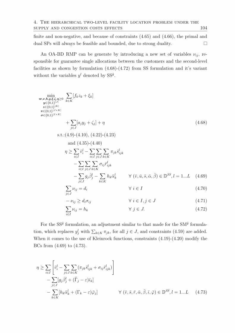
4. The hierarchical two-level facility location problem under thesupply and congestion costs effects 104
finite and non-negative, and because of constraints (4.65) and (4.66), the primal anddual SPs will always be feasible and bounded, due to strong duality.
An OA-BD RMP can be generate by introducing a new set of variables νij, re-sponsible for guarantee single allocations between the customers and the second-levelfacilities as shown by formulation (4.68)-(4.72) from SS formulation and it’s variantwithout the variables yl denoted by SSy.
min$,ν,h,g,ξ,ζ,η≥0y∈0,1|J|z∈0,1|K|π∈0,1|J×K|σ∈0,1|I×K|
∑k∈K
[fkzk + ξk]
+∑j∈J
[ajyj + ζj] + η (4.68)
s.t.:(4.9)-(4.10), (4.22)-(4.23)
and (4.35)-(4.40)
η ≥∑i∈I
vli −∑i∈I
∑j∈J
∑k∈K
πjkslijk
−∑i∈I
∑j∈J
∑k∈K
σij rlijk
−∑j∈J
gjβlj −
∑k∈K
hkαlk ∀ (v, u, s, α, β) ∈ DSS, l = 1...L (4.69)
∑j∈J
νij = di ∀ i ∈ I (4.70)
− νij ≥ diσij ∀ i ∈ I, j ∈ J (4.71)∑i∈I
νij = hk ∀ j ∈ J. (4.72)
For the SSy formulation, an adjustment similar to that made for the SMy formula-tion, which replaces ylj with
∑k∈K πjk, for all j ∈ J , and constraints (4.59) are added.
When it comes to the use of Kleinrock functions, constraints (4.19)-(4.20) modify theBCs from (4.69) to (4.73).
η ≥∑i∈I
vli −∑j∈J
∑k∈K
(πjkslijk + σij rlijk)
−∑j∈J
[gjβlj + (Γj − ε)ιk]
−∑k∈K
[hkαlk + (Γk − ε)ϕj] ∀ (v, s, r, α, β, ι, ϕ) ∈ DSS, l = 1...L (4.73)

4. The hierarchical two-level facility location problem under thesupply and congestion costs effects 105
4.3.2.2 Generalized Benders decomposition method
The GBD algorithm is based on the process of projected out all fractional variables, i.e.x, h and g of the original problem, while the integer variables z, y, π and σ dependingon the problem type, also known as complicating variables, are kept in RMP resultinginto an equivalent model with fewer variables, but many more constraints. Althoughthe number of constraints is much larger, the method does not require all constraintsto be bind to achieve optimization due to redundancy and/or overlapping rates whenconstructing the RMP convex hull.
In this sense, a formal description of the RMP and its SPs regarding the GBDapproach will now be exposed. Starting with the MM formulation, when the variablesx, h and g are projected out we get the primal SP (4.74)-(4.79).
minx,h,g≥0
∑i∈I
∑j∈J
∑k∈K
dicijkxijk +∑k∈K
τk(hk) +∑j∈J
τj(gj) (4.74)
s.t.:∑j∈J
∑k∈K
xijk = 1 ∀ i ∈ I (4.75)
hk −∑j∈J
∑i∈I
dixijk ≥ 0 ∀ k ∈ K (4.76)
gj −∑k∈K
∑i∈I
dixijk ≥ 0 ∀ j ∈ J (4.77)
−∑k∈K
xijk ≥ −ylj ∀ i ∈ I, j ∈ J (4.78)
−∑j∈J
xijk ≥ −zlk ∀ i ∈ I, k ∈ K. (4.79)
Now, by dualizing constraints (4.76) and (4.77) via αk and βj, respectively, theprimal SP (4.1)-(4.6) is reformulated to ΘMM(zl, yl, α, β).
ΘMM(zl, yl, α, β)
minx,h,g,α,β≥0
∑i∈I
∑j∈J
∑k∈K
(cijk + αk + βj)dixijk
+∑k∈K
[τk(hk)− hkαk] +∑j∈J
[τj(gj)− gjβj]
s.t.:(4.75) and (4.78)-(4.79).
(4.80)
Note that, the primal SP ΘMM(zl, yl, α, β) can be subdivided into two SP groups:non-linear SPs φMM
NL (zl, yl, α, β), having just the hk and gj variables; and a set of linearSPs φMM
L (zl, yl, α, β), having only the xijk variables and fixed α and β values. TheφMM
NL (zl, yl, α, β) is presented by Eq. (4.81).

4. The hierarchical two-level facility location problem under thesupply and congestion costs effects 106
φMMNL (zl, yl, α, β) = min
h,g,α,β≥0
∑k∈K
[τk(hk)− hkαk] +∑j∈J
[τj(gj)− gjβj]. (4.81)
As long as Eq. (4.81) be convex and differentiable, its Karush-Kuhn-Tucker con-ditions are being respected, and since the problem has no constraints, a simple wayto find αl and βl that guarantees the minimum objective function value is throughthe partial derivatives of φMM
NL (z, y, α, β), for each hl and gl variables at iteration l, asshown in Eq. (4.82)-(4.83).
αlk = τ ′k(hlk) ∀ k ∈ K (4.82)
βlj = τ ′j(glj) ∀ j ∈ J. (4.83)
Fixed values of αl and βl or αl and βl are necessary elements to properly solveφMM
L (z, y, α, β) or a set of |I| SPs, one for each customer i ∈ I, named φMML i(z, y, α, β),
corresponding to the cheapest supply path, but taking into account the congestioneffects in the network, see formulation (4.84)-(4.87).
φMML i(z, y, α, β)
minx≥0
∑j∈J
∑k∈K
(cijk + αk + βj)dixijk
s.t.:∑j∈J
∑k∈K
xijk = 1
−∑k∈K
xijk ≥ −ylj ∀ j ∈ J
−∑j∈J
xijk ≥ −zlk ∀ k ∈ K.
(4.84)
(4.85)
(4.86)
(4.87)
On the other hand, since the values of hlk and glj depend on the service flowthrough facility k ∈ K and j ∈ J , respectively, obtaining an optimal solution tothe ΘMM(zl, yl, α, β) by using φMM
NL (zl, yl, α, β) and φMML i(z, y, α, β) SPs can be con-
structed iteratively with the aid of a Flow Deviation Algorithm 5 adapted from thestate-of-the-art algorithm proposed by Kleinrock (1964).
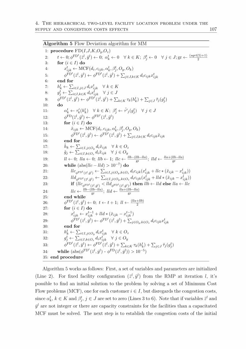
4. The hierarchical two-level facility location problem under thesupply and congestion costs effects 107
Algorithm 5 Flow Deviation algorithm for MM1: procedure FD(I,J ,K,Oy,Oz)2: t← 0;φFDt(zl, yl)← 0; αtk ← 0 ∀ k ∈ K; βtj ← 0 ∀ j ∈ J ; gr← (sqrt(5)+1)
23: for (i ∈ I) do4: xtijk ← MCF(di, cijk, αtk, βtj , Oy, Ok)5: φFDt(zl, yl)← φFDt(zl, yl) +
∑j∈J,k∈K dicijkx
tijk
6: end for7: htk ←
∑i∈I,j∈J dix
tijk ∀ k ∈ K
8: gtj ←∑i∈I,k∈K dix
tijk ∀ j ∈ J
9: φFDt(zl, yl)← φFDt(zl, yl) +∑k∈K τk(htk) +
∑j∈J τj(gtj)
10: do11: αtk ← τ ′k(htk) ∀ k ∈ K; βtj ← τ ′j(gtj) ∀ j ∈ J12: φFD(zl, yl)← φFDt(zl, yl)13: for (i ∈ I) do14: xijk ← MCF(di, cijk, αtk, βtj , Oy, Ok)15: φFDt(zl, yl)← φFDt(zl, yl) +
∑j∈J,k∈K dicijkxijk
16: end for17: hk ←
∑i∈I,j∈Oy dixijk ∀ k ∈ Oz
18: gj ←∑i∈I,k∈Oz dixijk ∀ j ∈ Oy
19: ll← 0; lla← 0; llb← 1; llc← llb−(llb−lla)gr ; lld← lla+(llb−lla)
gr20: while (abs(llc− lld) > 10−7) do21: llcφFDt (zl,yl) ←
∑i∈I,j∈Oy ,k∈Oz dicijk(x
tijk + llc ∗ (xijk − xtijk))
22: lldφFDt (zl,yl) ←∑i∈I,j∈Oy ,k∈Oz dicijk(x
tijk + lld ∗ (xijk − xtijk))
23: if (llcφFDt (zl,yl) < lldφFDt (zl,yl)) then llb← lld else lla← llc
24: llc← llb−(llb−lla)gr ; lld← lla+(llb−lla)
gr25: end while26: φFDt(zl, yl)← 0; t← t+ 1; ll← (lla+llb)
227: for (i ∈ I) do28: xtijk ← xt−1
ijk + lld ∗ (xijk − xt−1ijk )
29: φFDt(zl, yl)← φFDt(zl, yl) +∑j∈Oy ,k∈Oz dicijkx
tijk
30: end for31: htk ←
∑i∈I,j∈Oy dix
tijk ∀ k ∈ Oz
32: gtj ←∑i∈I,k∈Oz dix
tijk ∀ j ∈ Oy
33: φFDt(zl, yl)← φFDt(zl, yl) +∑k∈K τk(htk) +
∑j∈J τj(gtj)
34: while (abs(φFDt(zl, yl) - φFD(zl, yl)) > 10−5)35: end procedure
Algorithm 5 works as follows: First, a set of variables and parameters are initialized(Line 2). For fixed facility configuration (zl, yl) from the RMP at iteration l, it’spossible to find an initial solution to the problem by solving a set of Minimum CostFlow problems (MCF), one for each customer i ∈ I, but disregards the congestion costs,since αtk, k ∈ K and βtj, j ∈ J are set to zero (Lines 3 to 6). Note that if variables zl andyl are not integer or there are capacity constraints for the facilities than a capacitatedMCF must be solved. The next step is to establish the congestion costs of the initial

4. The hierarchical two-level facility location problem under thesupply and congestion costs effects 108
configuration, and hence get the value of the objective function φFD(zl, yl) (Lines 7to 9). Finally, an iterative procedure based on the Golden Section search strategy isperformed to obtain the minimum cost solution to the problem (Lines 10 to 34). Inother words, given initial αtk and βtj values (Line 11) it is possible to recalculate servicecosts to obtain a new current solution t to the problem or φFDt(zl, yl) (Lines 13 to 16).So, considering that xtijk, hk and gj have been defined individually for each customeri ∈ I, the next step is to perform a flow deviation procedure to minimize the aggregatetransport and congestion costs (Lines 19 to 33). Figure 4.5 illustrates this process offlow deviation which is possible to obtain an aggregate minimum cost solution for agiven αtk and βtj parameters configuration.
Parameters
OF
Initial
Optimal
(αtk, βtj)
Figure 4.5: Flow deviation algorithm convergence process via Golden Section search
Once Algorithm 5 provides the optimal primal solution, fixed αtk and βtj values,k ∈ K and j ∈ J , are used to solve the dual SP (4.88)-(4.89), where v, w and u arethe dual variable associated to constraints (4.85), (4.86) and (4.87), respectively.
maxv∈IRw,u≥0
∑i∈I
vi −∑j∈J
yljwij −∑k∈K
zlkuik
(4.88)
s.t.: vi − wij − uik ≤ di(cijk + αtk + βtj) ∀ i ∈ I, j ∈ J, k ∈ K (4.89)
The dual SP (4.88)-(4.89) can be easily solved by inspection-specific algorithms,as formal proof provided by de Oliveira et al. (2020). Once defined the optimalΘMM(zl, yl, α, β) and using the auxiliary variable η ≥ 0 we obtain the RMP associ-ated with the GBD technique or formulation (4.90)-(4.91).

4. The hierarchical two-level facility location problem under thesupply and congestion costs effects 109
minη≥0
y∈0,1|J|z∈0,1|K|
∑k∈K
fkzk +∑j∈J
ajyj + η (4.90)
s.t.:(4.39)-(4.40)
η ≥ φFD(zl, yl)−∑j∈J
W lj(yj − ylj)−
∑k∈K
U lk(zk − zlk) ∀ l = 1...L. (4.91)
Constraints (4.91) are the Benders optimality cuts, since W lj = ∑
i∈I wlij and U l
k =∑i∈I u
lik, j ∈ J and k ∈ K, respectively. In addition, when it comes to the Kleinrock
functions one must take into account constraints (4.19) and (4.20) and their respectivedual variables ιk and ϕj, k ∈ K and j ∈ J , respectively, to assemble the dual SP andits BCs (4.92).
η ≥ φFD(zl, yl)−∑j∈J
[W lj(yj − ylj) + (Γj − ε)ϕlj]
−∑k∈K
[U lk(zk − zlk) + (Γk − ε)ιlk] ∀ l = 1...L. (4.92)
A similar procedure, but considering its particularities can be extended to all for-mulations with single assignments. Algorithm 5, for example, can be adapted to SMvariants provided that the variables z, y and π are parameterized instead of only z andy in MM cases. The same goes for SS formulations, but using z, y, π and σ. There-fore, making variables slijk and its sum Sljk = ∑
i∈I slijk associated with constraints
(4.8) related to formulations SM, SMy, SS and SSy, and also variables rlijk and its sumRlij = ∑
k∈K rlijk linked to constraints (4.14) for SS and SSy will have the BCs (4.93) to
SM and SMy and (4.94) to SS and SSy.
η ≥ φFD(zl, πl)−∑k∈K
U lk(zk − zlk)−
∑j∈J
∑k∈K
Sljk(πjk − πljk) ∀ l = 1...L (4.93)
η ≥ φFD(πl, σl)−∑j∈J
∑k∈K
Sljk(πjk − πljk) +∑i∈I
∑j∈J
Rlij(σij − σlij)] ∀ l = 1...L. (4.94)
4.3.3 Acceleration methods
The literature shows that there are computational strategies that may eventually ac-celerate the convergence process of Benders decomposition algorithms. Among them,Pareto-Optimal cuts based on Papadakos’s ideas, heuristics, a warm start procedure,and additional features of the commercial solvers were used herein.

4. The hierarchical two-level facility location problem under thesupply and congestion costs effects 110
4.3.3.1 Pareto-optimal cuts
According to Magnanti and Wong (1981) whenever the dual SPs are degenerate, non-dominated or Pareto-optimal Benders optimality cuts can be separated, i.e. given afixed configuration of the RMP variables, (yl, zl) for the MM variant, for example, ifthe dual SP is degenerate, there is at least one stronger cut that can dominate all otherBCs, keeping the same optimal value for the objective function.
A widespread scheme to separate Pareto-optimal BCs brings with it the use of corepoint variables instead of the RMP parameterized variables to solve dual SP (Papadakos2008). The subproblem proposed by Papadakos is identical to Benders’ dual SP exceptthat the original (parameterized) variables are replaced by their respective core points,either for the OA-BD or GBD method. The core point variables used here are zl, yl,πl, σl, depending of the variant being addressed.
Furthermore, for each iteration l ∈ L, a linear convex combination is used to updatethe relative interior point prior to solving the Papadakos’ SP. To update the relativeinterior point (zl, yl) ∈ ri(Q) related to the MM variant, for example, we have zlk =λz
(l−1)k + (1− λ)zlk, k ∈ K, and ylj = λy
(l−1)j + (1− λ)ylj, j ∈ J , where 0 < λ < 1, being
usually set to 12 . Finally, it is still necessary to establish what are the initial valid core
points, which in our case are set to zlk = 12 , y
lj = 1
2 , πljk = zlk
|K| and σlij = 1, for all i ∈ I,
j ∈ J and k ∈ K.
4.3.3.2 Heuristic for CTLUFLP
To initialize the Benders algorithms with good and fast upper bounds a heuristic al-gorithm based on Greedy procedure coupled to a local search refining process wasdeveloped, as presented by Algorithm 6.
Algorithm 6 Greedy heuristic1: function Greedy(I, J,K,Oy, Oz)2: ofmin ← +∞3: for (j, k) | j ∈ J, k ∈ K do4: of ← minof | (zk, yj) = 15: if ofmin > of then ofmin ← of; kmin ← k; jmin ← j6: end for7: s← (zkmin , yjmin) = 18: for n ∈ P do s← N n(s) end9: s← FD(I,J ,K,Oy,Oz)
10: return s11: end function

4. The hierarchical two-level facility location problem under thesupply and congestion costs effects 111
A solution s in Algorithm 6 consists of two sets and two assigning vectors that rep-resent which facilities are opened and which nodes are served in each level, respectively.Algorithm 6 works as follows: First an initial solution is obtained from a minimum costsetting associated with a single facility pair in operation, where only one facility perlevel is active (Lines 2 to 7); A local search procedure built from six different neigh-borhood structures N n(s), n ∈ P = o2, o1, o12, c2, c1, c12, and organized in a variableneighborhood descent search (Mladenović and Hansen 1997), is performed aiming toachieve better solutions (Line 8). The neighborhoods denoted by o try to open newfacilities, whereas c aims to close them. The superscript numbers 1, 2, and 12 refer tosolution modifications being done at first, second or both facility levels, respectively;Finally, a flow deviation procedure (Algorithm 5) is performed to obtain a suitablesolution, where the congestion costs are taken into account, i.e a CTLUFLP solutions (Line 9).
When it comes to the local search procedure, it is also important to highlight otherparticularities. The best movement policy has been adopted during local searches,while the incumbent current solution is updated whenever the local search in eachneighborhood is completed. Further, whenever a facility is opened or closed a solu-tion restoration procedure must be performed to correct solutions with disconnectedfacilities. Note also that the local search procedure starts in the second-level, becausethey are cheaper and have a larger volume of open facilities than the first-level, eitherin real or fictitious problems. Moreover, for Kleinrock functions, either for the initialsolution or for local searches, capacity constraints are also checked to avoid infeasiblesolutions.
The choice of a simpler heuristic was due to the bounds offered in preliminary testsand the fact that it does not require parameter calibration. Thus, we assumed that afast solution with good upper bounds was sufficient to initialize the devised Bendersdecomposition algorithm. Both for OA-BD and GBD, three strategies for using theattained heuristic solution were adopted: (i) heuristic BCs were added to the RMP; (ii)An upper bound for the RMP’s objective function was established via a valid constraintor RMP objective function ≤ UB; and (iii) the incumbent solution s was the startingpoint of the branch-and-bound search tree of the RMP.
4.3.3.3 Other enhancements
To speed up a Benders algorithm other three different strategies were developed. Onemanner is to properly and explicitly select the branching priority order for the RMP’svariables, rather than letting the choice to the solver. For the CTLUFLPs the variablescorresponding to the first-level facilities were prioritized over those of the second-level

4. The hierarchical two-level facility location problem under thesupply and congestion costs effects 112
for all single and multiple variants. This rule was defined through some preliminarytests, where it was noticed average time savings to solve the RMPs.
Another common way, introduced by McDaniel and Devine (1977), is to performsome initial iterations of the Benders algorithm, but with the RMP’s variables withintegrality requirements relaxed, well known as warm-start cycles. At the beginning ofthe Benders algorithm, as RMP has little information, warm-start cycles allow us toinsert BCs from linear solutions at a much more attractive computational cost. Notethat, although it is possible to include BCs until the linear relaxation solution of theoriginal problem is attained, a few cycles is sufficient to achieve a significant gain inconvergence to the overall solution of the problem.
The third and last strategy is to generate BCs within the branch-and-bound viacallback functions (Fortz and Poss 2009), available in most commercial solvers. Theidea is to prevent re-exploring nodes already visited along with the branch-and-boundprocedure, i.e. a single enumeration tree is explored. All our Benders algorithms wereimplemented within structures that allow you to add BCs from integer and fractionalRMP’s solutions.
4.4 Computational experiments
All previously presented methods and algorithms have been coded in C++ using IBMConcert technology to have access to the ILOG CPLEX 12.8.1 solver. Computationalexperiments were designed to run on only one thread with its default CPLEX config-urations set, all of them were carried out on an Intel Core i7-8700 3.2GHz processorwith 16.0GB RAM running a 64 bits Linux environment. Further, all the algorithmswere developed in a one tree structure that allows you to insert cuts from the integer(LazyConstraintCallback) and fractional (UserCutCallback) RMP solutions, availableat CPLEX solver. Preliminary computational tests were performed to define the num-ber of warm-start cycles that would be performed, which was a total of 4 rounds. Astopping criterion of 24 hours (86,400 seconds) was imposed at which point the opti-mality gap UB−LB
UB was informed.A standard TLUFLP literature instance set proposed by Ro and Tcha (1984) was
selected to incorporate the congestion costs for both Power-Law (Elhedhli and Hu2005) and Kleinrock functions. The instances have the following characteristics: (i)distances between the facilities and customers randomly chosen within a range of 100to 5,000 units, but with different weight factors depending on the connecting locationsof different levels; (ii) transportation costs set to 0.0125 and 0.0250 per distance unit,for connections between first and second level facilities, and between second-level fa-
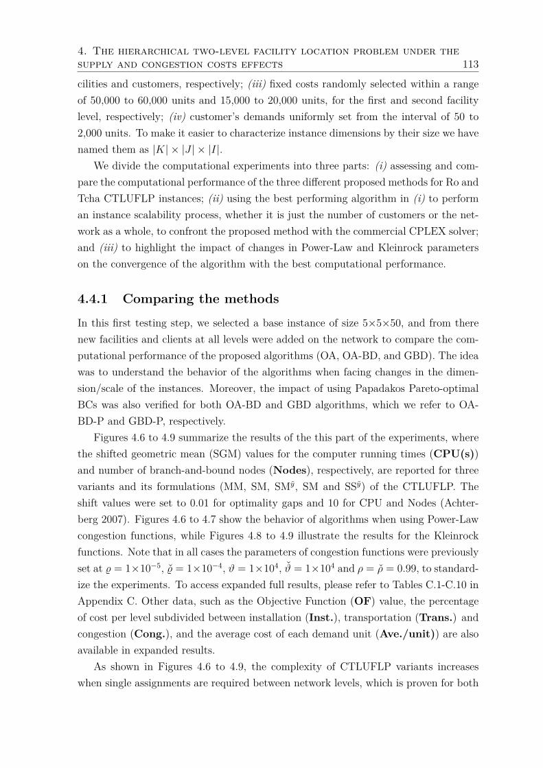
4. The hierarchical two-level facility location problem under thesupply and congestion costs effects 113
cilities and customers, respectively; (iii) fixed costs randomly selected within a rangeof 50,000 to 60,000 units and 15,000 to 20,000 units, for the first and second facilitylevel, respectively; (iv) customer’s demands uniformly set from the interval of 50 to2,000 units. To make it easier to characterize instance dimensions by their size we havenamed them as |K| × |J | × |I|.
We divide the computational experiments into three parts: (i) assessing and com-pare the computational performance of the three different proposed methods for Ro andTcha CTLUFLP instances; (ii) using the best performing algorithm in (i) to performan instance scalability process, whether it is just the number of customers or the net-work as a whole, to confront the proposed method with the commercial CPLEX solver;and (iii) to highlight the impact of changes in Power-Law and Kleinrock parameterson the convergence of the algorithm with the best computational performance.
4.4.1 Comparing the methods
In this first testing step, we selected a base instance of size 5×5×50, and from therenew facilities and clients at all levels were added on the network to compare the com-putational performance of the proposed algorithms (OA, OA-BD, and GBD). The ideawas to understand the behavior of the algorithms when facing changes in the dimen-sion/scale of the instances. Moreover, the impact of using Papadakos Pareto-optimalBCs was also verified for both OA-BD and GBD algorithms, which we refer to OA-BD-P and GBD-P, respectively.
Figures 4.6 to 4.9 summarize the results of the this part of the experiments, wherethe shifted geometric mean (SGM) values for the computer running times (CPU(s))and number of branch-and-bound nodes (Nodes), respectively, are reported for threevariants and its formulations (MM, SM, SMy, SM and SSy) of the CTLUFLP. Theshift values were set to 0.01 for optimality gaps and 10 for CPU and Nodes (Achter-berg 2007). Figures 4.6 to 4.7 show the behavior of algorithms when using Power-Lawcongestion functions, while Figures 4.8 to 4.9 illustrate the results for the Kleinrockfunctions. Note that in all cases the parameters of congestion functions were previouslyset at % = 1×10⁻⁵, % = 1×10⁻⁴, ϑ = 1×10⁴, ϑ = 1×10⁴ and ρ = ρ = 0.99, to standard-ize the experiments. To access expanded full results, please refer to Tables C.1-C.10 inAppendix C. Other data, such as the Objective Function (OF) value, the percentageof cost per level subdivided between installation (Inst.), transportation (Trans.) andcongestion (Cong.), and the average cost of each demand unit (Ave./unit)) are alsoavailable in expanded results.
As shown in Figures 4.6 to 4.9, the complexity of CTLUFLP variants increaseswhen single assignments are required between network levels, which is proven for both

4. The hierarchical two-level facility location problem under thesupply and congestion costs effects 114
0
2
4
6
8
10
12
MM SM SMy~ SS SSy~
Aver
age
CP
U r
unn
ing
tim
es (
seco
nd
s)
OAOA-BDOA-BD-PGBDGBD-P
Formulations
Figure 4.6: The SGM of the computer running times for solving a set of Ro andTcha CTLUFLP instances under Power-Law congestion function costs via differentformulations and methods.
0
100
200
300
400
500
600
MM SM SMy~ SS SSy~
Aver
age
bra
nch
-and
-bo
und n
od
es
OAOA-BDOA-BD-PGBDGBD-P
Formulations
Figure 4.7: The SGM of the number of explored branch-and-bound nodes for solvinga set of Ro and Tcha CTLUFLP instances under Power-Law congestion function costsvia different formulations and methods.

4. The hierarchical two-level facility location problem under thesupply and congestion costs effects 115
CPU times and branch-and-bound nodes, i.e. MM tend to be easier than SM andSMy, which in turn tend to be easier than SM and SSy except when it comes to theGBD method, related to the CPU running times. This particularity of GBD must bedirectly related to the fact that its linear subproblems are easier to solve, although theresulting BCs are weaker due to the σ variables parameterized by the RMP, which isconfirmed by the large number of branch-and-bound nodes explored.
Comparing the performance of the algorithms, there is a strong dominance of OAover OA-BD and GBD. Looking at performance as the problem grows, this dominanceprofile becomes even more accentuated (see Tables C.1-C.10 in Appendix C). Therefore,the idea of maintaining a lighter RMP, that is, with fewer variables and constraints, asin the case of the OA-BD and GD algorithms, was not effective for the acceleration ofconvergence of the algorithms.
When it comes to comparing the type of BC separation routines, Pareto-optimal ornot, it appears that Pareto-optimal BCs exploit fewer branch-and-bound nodes in thevast majority of cases, i.e. Pareto-optimal BCs are dense. On the other hand, Pareto-optimal BCs have not been able to provide CPU time savings for the GBD algorithm,although it is believed that further scaling up of the instances can save time.
0
2
4
6
8
10
12
MM SM SMy~ SS SSy~
Aver
age
CP
U r
unn
ing
tim
es (
seco
nd
s)
OAOA-BDOA-BD-PGBDGBD-P
Formulations
Figure 4.8: The SGM of the computer running times for solving a set of Ro and TchaCTLUFLP instances under Kleinrock congestion function costs via different formula-tions and methods.
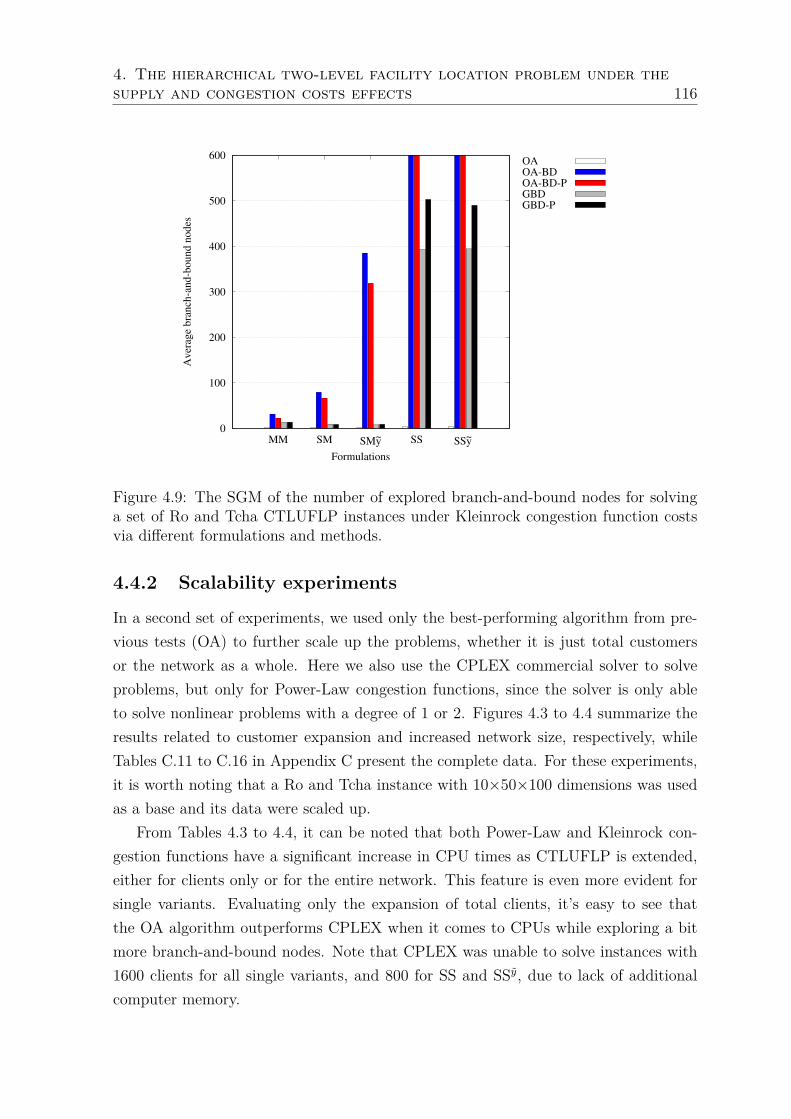
4. The hierarchical two-level facility location problem under thesupply and congestion costs effects 116
0
100
200
300
400
500
600
MM SM SMy~ SS SSy~
Aver
age
bra
nch
-an
d-b
oun
d n
od
es
OAOA-BDOA-BD-PGBDGBD-P
Formulations
Figure 4.9: The SGM of the number of explored branch-and-bound nodes for solvinga set of Ro and Tcha CTLUFLP instances under Kleinrock congestion function costsvia different formulations and methods.
4.4.2 Scalability experiments
In a second set of experiments, we used only the best-performing algorithm from pre-vious tests (OA) to further scale up the problems, whether it is just total customersor the network as a whole. Here we also use the CPLEX commercial solver to solveproblems, but only for Power-Law congestion functions, since the solver is only ableto solve nonlinear problems with a degree of 1 or 2. Figures 4.3 to 4.4 summarize theresults related to customer expansion and increased network size, respectively, whileTables C.11 to C.16 in Appendix C present the complete data. For these experiments,it is worth noting that a Ro and Tcha instance with 10×50×100 dimensions was usedas a base and its data were scaled up.
From Tables 4.3 to 4.4, it can be noted that both Power-Law and Kleinrock con-gestion functions have a significant increase in CPU times as CTLUFLP is extended,either for clients only or for the entire network. This feature is even more evident forsingle variants. Evaluating only the expansion of total clients, it’s easy to see thatthe OA algorithm outperforms CPLEX when it comes to CPUs while exploring a bitmore branch-and-bound nodes. Note that CPLEX was unable to solve instances with1600 clients for all single variants, and 800 for SS and SSy, due to lack of additionalcomputer memory.

4. The hierarchical two-level facility location problem under thesupply and congestion costs effects 117Table 4.3: Summary of computational results when only total customers is expanded,considering a Power-Law function with % = 1×10⁻⁵ and % = 1×10⁻⁴, while Kleinrockfunctions have ϑ = 1× 10⁵, ϑ = 1× 10⁴ and ρ = ρ = 0.99.
Power-Law KleinrockInstance CPLEX OA OA
Nodes CPU(s) Nodes CPU(s) Nodes CPU(s)MM
10×50×200 37 70.24 45 13.20 1 1.4010×50×400 15 30.72 37 20.81 1.9010×50×800 23 35.82 23 18.46 4.2010×50×1600 12 49.31 16 43.13 9.71
SGM 20.39 44.59 28.59 22.24 0.24 3.96
SM
10×50×200 44 189.38 78 54.14 4.2910×50×400 31 608.92 47 51.32 8.3710×50×800 20 4,115.51 68 91.42 20.0710×50×1600 † † 16 146.37 58.56
SGM 30.50∗ 788.48∗ 46.48 78.87 17.12
SMy
10×50×200 42 329.95 89 50.59 3.1010×50×400 33 848.63 74 72.67 4.8010×50×800 27 4,478.27 32 56.06 13.6210×50×1600 † † 14 115.73 42.63
SGM 33.57∗ 1,084.21∗ 43.81 70.31 12.16
SS
10×50×200 45 1,813.43 118 173.29 31 298.7810×50×400 42 7,431.51 34 122.45 1,349.2810×50×800 † † 212 229.49 5,834.5710×50×1600 † † 160 383.22 14,690.99
SGM 43.48∗ 3,673.62∗ 110.74 208.66 4.23 2,440.55
SSy
10×50×200 68 1,366.3 192 187.04 20 204.6610×50×400 46 8,221.39 171 234.58 934.8510×50×800 † † 249 281.43 3,252.7710×50×1600 † † 216 554.62 16,036.24
SGM 56.09∗ 3,355.84∗ 205.08 288.41 3.16 1,795.17∗ SGM for the fully solved instances.† Out-of-memory.Blank results refer to a zero value.
When the network was expanded, Table 4.4, both OA and CPLEX had difficultyin solving the CTLUFLPs. Again the commercial solver was limited by the memorycapacity of the computer. On the other hand, the OA algorithm just didn’t solve allinstances optimally, i.e. it presented only the optimality gap (Gap (%)) because theexperiments were interrupted after 24 hours of machine processing, both for Power-Lawand Kleinrock cases.
4.4.3 Analysis of congestion function parameters
The last set of experiments consisted of changing the parameter values of congestionfunctions to understand their dynamics and to show that it is not just the instancesize that directly influences the complexity of problems. Therefore, a single instancewith dimensions 10×50×100 and the OA algorithm was used in this step, as reportedby Tables C.17 to C.18 in the Appendix C. The Bubble Graph is shown in Figure 4.10summarizes the characteristic behavior of this set of experiments.

4. The hierarchical two-level facility location problem under thesupply and congestion costs effects 118Table 4.4: Summary of computational results when instance sizes are increased at alllevels, considering a Power-Law function with % = 1 × 10⁻⁵ and % = 1 × 10⁻⁴, whileKleinrock functions have ϑ = 1× 10⁵, ϑ = 1× 10⁴ and ρ = ρ = 0.99.
Power-Law KleinrockCPLEX OA OA
Instance Nodes CPU(s) Gap(%) Nodes CPU(s) Gap(%) Nodes CPU(s) Gap(%)
MM
15×75×150 271 558.60 197 81.51 88 49.8420×100×200 1535 39,261.74 779 2,480.44 66 192.8225×150×250 205 ? 8.51 2,396 ? 4.02 246 2,596.7130×200×300 2 ? 51.01 975 ? 11.28 2,42 70,319.21
SGM 172.94 N.C. 0.45 778.76 N.C. 0.25 250.90 1,211.33
SM
15×75×150 1011 6,038.68 2,791 21,165.13 270 186.2920×100×200 1,083 ? 2.63 1,786 ? 3.73 358 2,562.7925×150×250 124 ? 11.43 675 ? 9.80 1,296 ? 1.0730×200×300 † † † 243 ? 14.95 464 ? 4.83
SGM 520.78∗ N.C. 0.66∗ 956.29 N.C. 1.52 492.55 N.C. 0.14
SMy
15×75×150 986 5,782.97 1,383 6,204.89 177 129.5120×100×200 677 ? 5.03 2,500 ? 2.98 200 1,443.1325×150×250 143 ? 10.63 932 ? 8.61 1,8 ? 1.3830×200×300 † † † 368 ? 15.28 680 ? 4.76
SGM 461.31∗ N.C. 0.80∗ 1,046.31 N.C. 1.40 460.59 N.C. 0.15
SS
15×75×150 1,185 16,545.78 4,659 ? 2.18 2,716 4,790.2820×100×200 874 ? 5.24 909 ? 6.34 2,123 34,707.2825×150×250 † † † 926 ? 11.46 1,32 ? 3.6330×200×300 † † † 406 ? 16.46 57 ? 51.17
SGM 1,017.80∗ N.C. 0.22∗ 1,126.91 N.C. 7.15 838.42 N.C. 0.36
SSy
15×75×150 718 10,932.35 11,417 ? 1.10 2,571 2,656.1320×100×200 543 ? 4.78 4,751 ? 5.28 4,157 33,594.4125×150×250 † † † 1,374 ? 10.91 903 ? 4.0830×200×300 † † † 320 ? 16.61 30 ? 10.32
SGM 624.50∗ N.C. 0.21∗ 2,222.65 N.C. 5.70 781.65 N.C. 0.24∗ SGM for the fully solved instances.? Time limit of 86,400.00 secondsN.C. Not calculated due to incomplete data.† Out-of-memory.Blank results refer to a zero value.
Figure 4.10 was elaborated from the data from Table C.17, but with an adjustmentof proportionality according to the range of CPU times values by a variant of theproblem. Note that as % and % are enlarged, the time required for the convergenceof the OA algorithm grows exponentially. This same, but smoother, behavior canalso be observed for the Kleinrock congestion functions, provided that ϑ and ϑ bemodified (see Table C.18). However, it is believed that the significant difference in theresolution complexity of the single variants is due to the impossibility of distributingflow to supply customers, making the combinatorial problem even more difficult.

4. The hierarchical two-level facility location problem under thesupply and congestion costs effects 119
MM
SM
SS
Figure 4.10: Bubble chart of the SGM of CPU running times for solving a 10×50×100CTLUFLP instance under Power-Law congestion function costs via OA algorirthm,when % and % parameters are changed.
4.5 Conclusion
This chapter assessed three different supply chain patterns for the hierarchical two-level facility location problem, where the facilities are under nonlinear congestion func-tions: multi-assignments, single-assignments or single-assignments-paths between fa-cilities and customers. The first one allows that each customer can be linked to oneor more facilities by level. The second approach requires single connections betweenfacility levels, while the third demand that each customer is connected only by a singlefacility pair, i.e. only one per level.
We developed three different algorithms able to solve all the investigated variants:the Outer-Approximation method (OA); the OA coupled to the Benders Decomposi-tion method (OA-BD); and the Generalized Benders Decomposition method (GBD).The differences/particularities regarding the three variants of the problem were also ex-posed, considering each of the proposed methods. Moreover, Power-Law (Elhedhli andHu 2005) and Kleinrock functions were used to evaluate the efficiency of the proposedsolution strategies.
An extensive computational experiment showed the efficiency of the proposed de-composition methods on solving instances for the three variants analyzed, especiallythe OA algorithm that outperformed the others, including the CPLEX general solver.It has also been found that the degree of complexity of problems tends to increase

4. The hierarchical two-level facility location problem under thesupply and congestion costs effects 120
when single assignments are required. Further, it has been noted that in lighter singleformulations, i.e. having fewer variables and constraints, whether only between facil-ity levels or the network as a whole, there is a significant reduction in the numberof branch-and-bound nodes exploited, but with a higher computational running timethan the more robust formulations.
Finally, as goals for future work, other enhancements can be made, such as theimprovement of the proposed heuristic, aiming to obtain better starting points forthe decomposition algorithms or the incorporation of other uncertainty elements inthe problems, to be closer to reality. Besides, investigating other queuing policies oncongestion systems can also be a very interesting way to study.

Chapter 5
Conclusion
This thesis aimed at developing specialized decomposition algorithms to efficiently solvethree different variants of the hierarchical two-level facility location problem: (i) thesingle-period uncapacitated facility problem; (ii) the multi-period (dynamic) uncapaci-tated facility problem; and (iii) the single-period problem under the congestion effects.Multiple or single assignments between facilities and customers were investigated inall the studied problems. For all cases, extensive computational experiments were car-ried out to demonstrate the efficacy of the proposed formulations and their respectivealgorithms.
Chapter 1 presented a brief but consistent contextualization of the problems ad-dressed, highlighting the author’s main contributions to the literature, and also servedas the basis for opening discussion of the themes that would be addressed in subsequentchapters.
Chapter 2 were shown different Benders cut separation schemes for the two-level un-capacitated facility location problem, both for single and multiple assignments. Exactdecomposition Benders algorithms were devised, considering several separation proce-dures for three classes of Benders cuts: standard optimality cuts, lifted optimality cuts,and non-dominated optimality cuts. Three different standard literature instance setswere used to demonstrate that non-dominated optimality cuts were the most efficientoverall cut separation routine, for both single and multiple assignment problems.
Mixed-integer formulations for the multiple and single dynamic two-level uncapac-itated facility location problem were introduced in Chapter 3, as an extension of thesingle-period arc-based formulation proposed by Barros and Labbé (1994b) and Gen-dron et al. (2016), respectively. Benders decomposition reformulation combined witha fast greedy randomized adaptive search procedure (GRASP) were developed, includ-ing five Benders cut separation routines, to solve two benchmarking literature testinstances. The computational experiment demonstrated the efficiency of the proposed
121

5. Conclusion 122
algorithms when compared with the commercial CPLEX solver and its Benders built-in. For the multiple allocation case, it was checked that a non-dominated separationroutine based on the Papadakos approach was the most efficient; while, for the singlecase, Benders cuts attained by the strategy of gathering saving stemmed from the dualinformation of closing facilities performed better.
Chapter 4 studied the hierarchical two-level facility location problem, wherein thefacilities were under nonlinear congestion conditions caused by the volume of customerorders. Three different customer service supply chain patterns were evaluated, consid-ering multiple or single assignments. The Outer-Approximation (OA), the OA coupledto the Benders Decomposition method (OA-BD) and Generalized Benders Decompo-sition method (GBD) were implemented to all the problem variants. The OA methodoutperformed the others in all variants studied, whether for smaller or larger scale prob-lems, including the commercial solver. Also, it was found that the instance difficultydegree does not depend solely and exclusively on their size, but also the pre-definedparameters for the congestion functions.
Finally, as suggestions for future research, it is possible to extend this work toother problem variants, such as problems that incorporate economic aspects relatedto uncertainty, whether in terms of the degree of demand sensitivity to prices or thatconsiders the balance in the networks; or problems that carry reliability informationin the supply process, for example. Another interesting approach to study later iswhen single assignments between the second-level facilities and customers are required.Further, it is also possible to enlarge the range of solution methods for the problemsaddressed here by using other exact or heuristic approaches, as well as incorporatingother strategies for improving the proposed decomposition methods, such as carryingout variable fixing procedures or the improvement of the steps for obtaining non-dominated Benders optimality cuts.

Bibliography
Aardal, K., Chudak, F. A., and Shmoys, D. B. (1999). A 3-approximation algorithm for thek-level uncapacitated facility location problem. Information Processing Letters, 72:161–167.
Achterberg, T. (2007). Constraint Integer Programming. PhD thesis, Technische UniversitätBerlin.
Ahmadi-Javid, A., Seyedi, P., and Syam, S. S. (2017). A survey of healthcare facility location.Computers & Operations Research, 79:223–263.
Akinc, U. and Khumawala, B. M. (1977). An efficient branch and bound algorithm for thecapacitated warehouse location problem. Management Science, 23(6):585–594.
Arabani, A. B. and Farahani, R. Z. (2012). Facility location dynamics: An overview ofclassifications and applications. Computers & Industrial Engineering, 62(1):408–420.
Balinski, M. L. (1964). On finding integer solutions to linear programs. Technical report,IBM Data Processing Division.
Ballou, R. H. (1968). Dynamic warehouse location analysis. Journal of Marketing Research,5(3):271–276.
Barros, A. and Labbé, M. (1994a). A general model for uncapacitated facility and depotlocation problem. Location Science, 2(3):173–191.
Barros, A. and Labbé, M. (1994b). The multi-level uncapacitated facility location problemis not submodular. European Journal of Operational Research, 72(3):607–609.
Bazaraa, M. S., Jarvis, J. J., and Sherali, H. D. (2009). Linear programming and networkflows, Fourth Edition. Wiley-Interscience, 4th edition.
Belotti, P., Kirches, C., Leyffer, S., Linderoth, J., Luedtke, J., and Mahajan, A. (2013).Mixed-integer nonlinear optimization. Acta Numerica, 22:1–131.
Benders, J. F. (1962). Partitioning procedures for solving mixed-variables programmingproblems. Numerisch Mathematik, 4:238–252.
Berman, O. and Krass, D. (2015). Stochastic location models with congestion. In Laporte,G., Nickel, S., and Saldanha da Gama, F., editors, Location Science, pages 443–486.Springer International Publishing, Cham.
Boffey, B., ao, R. G., and Espejo, L. (2007). A review of congestion models in the location of
123

5. Conclusion 124
facilities with immobile servers. European Journal of Operational Research, 178(3):643–662.
Brunaud, B., Bassett, M. H., Agarwal, A., Wassick, J. M., and Grossmann, I. E. (2018). Ef-ficient formulations for dynamic warehouse location under discrete transportation costs.Computers & Chemical Engineering, 111:311–323.
Camargo, R. S. d. and Miranda Jr, G. d. (2012). Addressing congestion on single allocationhub-and-spoke networks. Pesquisa Operacional, 32:465–496.
Chardaire, P., Lutton, J.-L., and Sutter, A. (1999). Upper and lower bounds for the two-levelsimple plant location problem. Annals of Operations Research, 86:117–140.
Coelho, L. C., Cordeau, J.-F., and Laporte, G. (2014). Thirty years of inventory routing.Transportation Science, 48(1):1–19.
Correia, I. and Melo, T. (2017). A multi-period facility location problem with modular capac-ity adjustments and flexible demand fulfillment. Computers & Industrial Engineering,110:307–321.
Daskin, M. S. (2011). Network and discrete location: models, algorithms, and applications.John Wiley & Sons.
de Camargo, R. and Miranda, G. (2012). Single allocation hub location problem undercongestion. Expert Systems with Applications, 39(3):3385–3391.
de Camargo, R. S., de Miranda, G., and Ferreira, R. P. (2011). A hybrid outer-approximation/Benders decomposition algorithm for the single allocation hub locationproblem under congestion. Operations Research Letters, 39(5):329–337.
de Oliveira, P. B., Contreras, I., de Camargo, R. S., and de Miranda Júnior, G. (2020).A comparison of separation routines for Benders optimality cuts for two-level facilitylocation problems. Expert Systems with Applications, 141:112928.
Desrochers, M., Marcotte, P., and Stan, M. (1995). The congested facility location problem.Location Science, 3(1):9–23.
Dolan, E. D. and Moré, J. J. (2002). Benchmarking optimization software with performanceprofiles. Mathematical Programming, 91(2):201–213.
Drexl, M. and Schneider, M. (2015). A survey of variants and extensions of the location-routing problem. European Journal of Operational Research, 241(2):283–308.
Duran, M. A. and Grossmann, I. E. (1986). An outer-approximation algorithm for a class ofmixed-integer nonlinear programs. Mathematical Programming, 36(3):307–339.
Efroymson, M. and Ray, T. (1966). A branch and bound algorithm for plant location. Op-erations Research, 14:361–368.
Elhedhli, S. (2006). Service system design with immobile servers, stochastic demand, andcongestion. Manufacturing & Service Operations Management, 8(1):92–97.
Elhedhli, S. and Hu, F. X. (2005). Hub-and-spoke network design with congestion. Computers& Operations Research, 32(6):1615–1632.

5. Conclusion 125
Elhedhli, S. and Wu, H. (2010). A lagrangean heuristic for hub-and-spoke system design withcapacity selection and congestion. INFORMS Journal on Computing, 22(2):282–296.
Emirhüseyinoğlu, G. and Ekici, A. (2019). Dynamic facility location with supplier selectionunder quantity discount. Computers & Industrial Engineering, 134:64–74.
Fang, Y., Bian, Y., and Xuefeng, W. (2009). Solving service facilities location problem withelastic demand and congest effect. In 2009 6th International Conference on ServiceSystems and Service Management, pages 595–599.
Farahani, R. Z., Hekmatfar, M., Fahimnia, B., and Kazemzadeh, N. (2014). Hierarchical fa-cility location problem: Models, classifications, techniques, and applications. Computers& Industrial Engineering, 68:104–117.
Feo, T. A. and Resende, M. G. (1989). A probabilistic heuristic for a computationally difficultset covering problem. Operations Research Letters, 8(2):67–71.
Fischetti, M., Ljubić, I., and Sinnl, M. (2016). Benders decomposition without separability:A computational study for capacitated facility location problems. European Journal ofOperational Research, 253(3):557–569.
Fletcher, R. and Leyffer, S. (1994). Solving mixed integer nonlinear programs by outerapproximation. Mathematical Programming, 66(1):327–349.
Fortz, B. (2015). Location problems in telecommunications. In Laporte, G., Nickel, S., andSaldanha da Gama, F., editors, Location Science, pages 537–554. Springer InternationalPublishing, Cham.
Fortz, B. and Poss, M. (2009). An improved Benders decomposition applied to a multi-layernetwork design problem. Operations Research Letters, 37(5):359–364.
Garcia, D. J. and You, F. (2015). Supply chain design and optimization: Challenges andopportunities. Computers & Chemical Engineering, 81:153–170. Special Issue: Selectedpapers from the 8th International Symposium on the Foundations of Computer-AidedProcess Design (FOCAPD 2014), July 13-17, 2014, Cle Elum, Washington, USA.
Gendron, B., Khuong, P.-V., and Semet, F. (2015). Multilayer variable neighborhood searchfor two-level uncapacitated facility location problems with single assignment. Networks,66(3):214–234.
Gendron, B., Khuong, P.-V., and Semet, F. (2016). A lagrangian-based branch-and-bound al-gorithm for the two-level uncapacitated facility location problem with single-assignmentconstraints. Transportation Science, 50(4):1286–1299.
Gendron, B., Khuong, P.-V., and Semet, F. (2017). Comparison of Formulations for the Two-Level Uncapacitated Facility Location Problem with Single Assignment Constraints.Computers and Operations Research, 36(5):1335–1355.
Genevois, M. E., Celik, D., and Ulukan, H. (2015). Atm location problem and cash man-agement in automated teller machines. International Journal of Social, Behavioral,Educational, Economic, Business and Industrial Engineering, 9(7):2543–2548.

5. Conclusion 126
Geoffrion, A. M. (1972). Generalized Benders decomposition. Journal of Optimization Theoryand Applications, 10(4):237–260.
Geoffrion, A. M. and Graves, G. W. (1974). Multicommodity distribution system design byBenders decomposition. Management Science, 20(5):822–844.
Gillen, D. and Levinson, D. (1999). Full cost of air travel in the california corridor. Trans-portation Research Record: Journal of the Transportation Research Board, 1662:1–9.
Grossmann, I. E. and Kravanja, Z. (1995). Mixed-integer nonlinear programming techniquesfor process systems engineering. Computers & Chemical Engineering, 19:189–204.
Grove, P. G. and O’Kelly, M. E. (1986). Hub networks and simulated schedule delay. Papersin Regional Science, 59(1):103–119.
Guldmann, J.-M. and Shen, G. (1997). A general mixed integer nonlinear optimizationmodel for hub network design. In 44th North American meeting of the Regional ScienceAssociation International, pages 6–9, Buffalo, NY, USA.
Hajiaghayi, M. T., Mahdian, M., and Mirrokni, V. S. (2003). The facility location problemwith general cost functions. Networks, 42(1):42–47.
Hakimi, S. L. (1965). Optimum distribution of switching centers in a communication networkand some related graph theoretic problems. Operations Research, 13(3):462–475.
Hinojosa, Y., Kalcsics, J., Nickel, S., Puerto, J., and Velten, S. (2008). Dynamic supply chaindesign with inventory. Computers & Operations Research, 35(2):373–391. Part SpecialIssue: Location Modeling Dedicated to the memory of Charles S. ReVelle.
Hinojosa, Y., Puerto, J., and Fernández, F. (2000). A multiperiod two-echelon multicom-modity capacitated plant location problem. European Journal of Operational Research,123(2):271–291.
Holmberg, K., Rönnqvist, M., and Yuan, D. (1999). An exact algorithm for the capaci-tated facility location problems with single sourcing. European Journal of OperationalResearch, 113(3):544–559.
Hung, M., Rom, W., and Waren, A. (1986). Degeneracy in transportation problems. DiscreteApplied Mathematics, 13(2):223–237.
Jayaraman, V., Gupta, R., and Pirkul, H. (2003). Selecting hierarchical facilities in a service-operations environment. European Journal of Operational Research, 147(3):613–628.
Jena, S. D., Cordeau, J.-F., and Gendron, B. (2014). Solving a dynamic facility locationproblem with an application in forestry. Technical report, CIRRELT.
Jena, S. D., Cordeau, J.-F., and Gendron, B. (2015). Dynamic facility location with gener-alized modular capacities. Transportation Science, 49(3):484–499.
Jena, S. D., Cordeau, J.-F., and Gendron, B. (2016). Solving a dynamic facility locationproblem with partial closing and reopening. Computers & Operations Research, 67:143–154.

5. Conclusion 127
Jena, S. D., Cordeau, J.-F., and Gendron, B. (2017). Lagrangian heuristics for large-scaledynamic facility location with generalized modular capacities. INFORMS Journal onComputing, 29(3):388–404.
Jonker, R. and Volgenant, A. (1987). A shortest augmenting path algorithm for dense andsparse linear assignment problems. Computing, 38(4):325–340.
Kaufman, L., Eede, M. V., and Hansen, P. (1977). A plant and warehouse location problem.Operational Research Quarterly, 28(3):547–554.
Kleinrock, L. (1964). Communication Nets: Stochastic Message Flow and Delay. McGraw-Hill Book Company, New York. (Out of Print.) Reprinted by Dover Publications, 1972and in 2007. Published in Russian, 1971, Published in Japanese, 1975.
Klose, A. and Drexl, A. (2005). Facility location models for distribution system design.European Journal of Operational Research, 162(1):4–29.
Kronqvist, J., Bernal, D. E., Lundell, A., and Grossmann, I. E. (2019). A review andcomparison of solvers for convex MINLP. Optimization and Engineering, 20(2):397–455.
Kuehn, A. A. and Hamburger, M. J. (1963). A heuristic program for locating warehouses.Management Science, 9(4):643–666.
Landete, M. and Marín, A. (2009). New facets for the two-stage uncapacitated facility locationpolytope. Computational Optimization and Applications, 44(3):487–519.
Lawrence, R. M. and Pengilly, P. J. (1969). The number and location of depots required forhandling products for distribution to retail stores in south-east england. OR, 20(1):23–32.
Ljubić, I. and Moreno, E. (2018). Outer approximation and submodular cuts for maximumcapture facility location problems with random utilities. European Journal of Opera-tional Research, 266(1):46–56.
López-Ibáñez, M., Dubois-Lacoste, J., Cáceres, L. P., Birattari, M., and Stützle, T. (2016).The irace package: Iterated racing for automatic algorithm configuration. OperationsResearch Perspectives, 3:43–58.
Lu, D., Gzara, F., and Elhedhli, S. (2014). Facility location with economies and diseconomiesof scale: models and column generation heuristics. IIE Transactions, 46(6):585–600.
Magnanti, T. L., Mireault, P., and Wong, R. T. (1986). Tailoring Benders decompositionfor uncapacitated network design. In Gallo, G. and Sandi, C., editors, Netflow at Pisa,volume 26, pages 112–154. Springer, Berlin, Heidelberg.
Magnanti, T. L. and Wong, R. T. (1981). Accelerating Benders decomposition: Algorithmicenhancement and model selection criteria. Operations Research, 29(3):464–483.
Magnanti, T. L. and Wong, R. T. (1990). Decomposition methods for facility location prob-lems. In Mirchandani, P. B. and Francis, R. L., editors, Discrete location theory, pages209–262. Wiley, New York.

5. Conclusion 128
Manne, A. (1964). Plant location under economies of scale. Management Science, 11(2):213–235.
Maranzana, F. E. (1963). On the location of supply points to minimize transportation costs.IBM Systems Journal, 2(2):129–135.
Marufuzzaman, M., Gedik, R., and Roni, M. S. (2016). A Benders based rolling horizonalgorithm for a dynamic facility location problem. Computers & Industrial Engineering,98:462–469.
Mateus, G. and Thizy, J. (1999). Exact sequential choice of locations in a network. Annalsof Operations Research, 86(0):199–219.
McDaniel, D. and Devine, M. (1977). A modified Benders’ partitioning algorithm for mixedinteger programming. Management Science, 24(3):312–319.
Meersman, H., de Voorde, E. V., and Vanelslander, T. (2012). Port congestion and impli-cations to maritime logistics. In Song, D.-W. and Panayides, P. M., editors, MaritimeLogistics, pages 49–68. Emerald Group Publishing Limited.
Melo, M., Nickel, S., and da Gama, F. S. (2009). Facility location and supply chain manage-ment: A review. European Journal of Operational Research, 196(2):401–412.
Min, H. and Melachrinoudis, E. (2001). The three-hierarchical location-allocation of bankingfacilities with risk and uncertainty. International Transactions in Operational Research,8(4):381–401.
Mladenović, N. and Hansen, P. (1997). Variable neighborhood search. Computers & Opera-tions Research, 24(11):1097–1100.
Narula, S. C. (1986). Minisum hierarchical location-allocation problems on a network: Asurvey. Annals of Operations Research, 6(8):255–272.
Nauss, R. M. (1978). An improved algorithm for the capacitated facility location problem.Journal of the Operational Research Society, 29(12):1195–1201.
Nemhauser, G. L., Wolsey, L. A., and Fisher, M. L. (1978). An analysis of approximationsfor maximizing submodular set functions - I. Mathematical Programming, 14:265–294.
Ortiz-Astorquiza, C., Contreras, I., and Laporte, G. (2015). The multi-level facility loca-tion problem as the maximization of a submodular set function. European Journal ofOperational Research, 247:1013–1016.
Ortiz-Astorquiza, C., Contreras, I., and Laporte, G. (2017). Formulations and approxima-tion algorithms for multilevel uncapacitated facility location. INFORMS Journal onComputing, 29(4):767–779.
Ortiz-Astorquiza, C., Contreras, I., and Laporte, G. (2018). Multi-level facility locationproblems. European Journal of Operational Research, 267(3):791–805.
Ortiz-Astorquiza, C., Contreras, I. A., and Laporte, G. (2019). An exact algorithm formultilevel uncapacitated facility location. Transportation Science, 53:1085–1106.
5. Conclusion 129
Papadakos, N. (2008). Practical enhancements to the magnanti–wong method. OperationsResearch Letters, 36:444–449.
Pasandideh, S. H. R., Niaki, S. T. A., and Asadi, K. (2015). Optimizing a bi-objective multi-product multi-period three echelon supply chain network with warehouse reliability.Expert Systems with Applications, 42(5):2615–2623.
Pearce, R. H. and Forbes, M. (2018). Disaggregated Benders decomposition and branch-and-cut for solving the budget-constrained dynamic uncapacitated facility location andnetwork design problem. European Journal of Operational Research, 270(1):78–88.
Rahmaniani, R., Crainic, T. G., Gendreau, M., and Rei, W. (2017). The Benders decom-position algorithm: A literature review. European Journal of Operational Research,259(3):801–817.
Ramos, M. T. and Sáez, J. (2005). Solving capacitated facility location problems by fenchelcutting planes. Journal of the Operational Research Society, 56(3):297–306.
Ro, H. B. and Tcha, D.-W. (1984). A branch and bound algorithm for the two-level un-capacitated facility location problem with some side constraints. European Journal ofOperational Research, 18(3):349–358.
Roodman, G. M. and Schwarz, L. B. (1975). Optimal and heuristic facility phase-out strate-gies. AIIE Transactions, 7(2):177–184.
Roy, T. J. V. and Erlenkotter, D. (1982). A dual-based procedure for dynamic facility location.Management Science, 28(10):1091–1105.
Şahin, G. and Süral, H. (2007). A review of hierarchical facility location models. Computers& Operations Research, 34(8):2310–2331.
Schneider, M. and Drexl, M. (2017). A survey of the standard location-routing problem.Annals of Operations Research, 259(1):389–414.
Şelfun, S. (2011). Outer approximation algorithms for the congested p-median problem.Thesis for the degree of master of science, Bilkent University, Turkey.
Sierksma, G. (1996). Linear and Integer Programming: Theory and Practice. Marcel Dekker,New York, 2 edition.
Smith, H. K., Harper, P. R., Potts, C. N., and Thyle, A. (2009). Planning sustainablecommunity health schemes in rural areas of developing countries. European Journal ofOperational Research, 193(3):768–777.
Tcha, D. W. and Lee, B. (1984). A branch-and-bound algorithm for the multi-level uncapaci-tated facility location problem. European Journal of Operational Research, 18(1):35–43.
Torres-Soto, J. E. and Üster, H. (2011). Dynamic-demand capacitated facility locationproblems with and without relocation. International Journal of Production Research,49(13):3979–4005.
Van Roy, T. J. (1983). Cross decomposition for mixed integer programming. MathematicalProgramming, 25(1):46–63.

5. Conclusion 130
Vidal, C. J. and Goetschalckx, M. (1997). Strategic production-distribution models: A criticalreview with emphasis on global supply chain models. European Journal of OperationalResearch, 98(1):1–18.
Weber, A. (1909). Ueber den standort der industrien. 1. Teil: Reine Theorie des Standort.Verlag J.C.B. Mohr, Tubingen.
Wesolowsky, G. O. and Truscott, W. G. (1975). The multiperiod location-allocation problemwith relocation of facilities. Management Science, 22(1):57–65.
Westerlund, T. and Pettersson, F. (1995). An extended cutting plane method for solvingconvex minlp problems. Computers & Chemical Engineering, 19:131–136. EuropeanSymposium on Computer Aided Process Engineering 3-5.
Wolsey, L. A. (1998). Integer programming. Wiley-Interscience, New York, USA.
Zhang, Y., Berman, O., and Verter, V. (2009). Incorporating congestion in preventive health-care facility network design. European Journal of Operational Research, 198(3):922–935.

Appendix A
Appendices of the Chapter 2
The following tables are complete data from the computational experiments related tothe Chapter 2.
131

A.
Appendices
ofthe
Chapter
2132
Table A.1: TLUFLP-MA computational experiments to GapA instances
Instances OF Lin. OF LR MA-CPX MA-B-CPX MA-I MA-CF MA-MW MA-P MA-I-JVC MA-CF-JVC(%) CPU(s) Nodes CPU(s) Nodes CPU(s) Nodes CPU(s) Nodes CPU(s) Nodes CPU(s) Nodes CPU(s) Nodes CPU(s) Nodes
332-A 42189 38810.43 8.01 7.68 30 6.26 81 0.60 205 0.41 123 0.39 189 2.60 100 0.46 268 0.49 312432-A 54119 51572.56 4.71 7.90 35 5.91 127 0.53 192 0.67 220 0.25 74 2.85 113 0.35 122 0.34 108532-A 51183 46872.33 8.42 18.30 118 10.05 602 1.08 297 1.52 596 0.55 250 5.08 475 0.42 159 0.62 205632-A 54238 52050.71 4.03 13.96 95 7.15 194 0.72 264 0.54 191 0.53 141 3.15 343 0.45 201 0.75 310832-A 51144 47488.48 7.15 10.84 53 5.10 81 0.41 140 0.40 128 0.32 120 4.14 230 0.69 272 0.61 2361032-A 57120 51384.77 10.04 18.92 208 6.42 369 1.00 844 1.09 886 0.37 426 2.84 305 0.84 652 0.56 2911132-A 57133 51988.56 9.00 20.28 242 7.31 412 0.57 420 0.65 396 0.73 468 2.97 410 0.80 523 0.88 6451332-A 54176 52660.00 2.80 4.68 35 5.45 65 0.19 87 0.20 97 0.26 165 2.26 111 0.33 157 0.35 1581432-A 54149 50369.44 6.98 15.46 134 6.07 299 0.67 304 0.69 298 0.52 355 3.81 313 1.05 551 0.72 3421532-A 54142 48899.78 9.68 37.22 425 6.91 821 2.07 1145 2.49 1178 1.22 743 3.51 1066 1.73 1482 1.81 16471632-A 45150 43947.47 2.66 6.19 16 5.89 42 0.41 102 0.38 103 0.19 93 2.11 97 0.25 83 0.28 1241732-A 51191 47844.02 6.54 15.09 70 7.54 275 1.28 464 0.97 258 0.63 287 4.45 513 0.60 154 1.02 3751832-A 57131 52453.60 8.19 13.78 148 6.79 367 1.08 465 1.29 556 0.48 209 3.13 233 0.52 321 0.67 3881932-A 42121 38509.20 8.57 9.63 44 6.63 95 0.49 115 0.45 136 0.58 243 3.59 287 0.27 96 0.55 1962032-A 48112 43884.58 8.79 17.52 124 8.01 436 0.67 370 0.98 416 0.64 290 4.03 619 0.80 450 0.77 3732232-A 54133 50644.94 6.44 12.58 86 6.75 162 0.47 313 0.44 214 0.46 331 2.46 210 0.66 383 0.54 4162432-A 51153 47347.72 7.44 21.18 164 6.54 289 1.06 442 1.02 451 0.72 351 3.32 302 0.78 410 0.88 4032532-A 54182 50346.69 7.08 22.45 164 6.79 411 0.86 363 0.62 270 0.36 279 3.51 391 0.81 480 1.09 5212632-A 51175 45769.09 10.56 26.91 168 5.91 249 1.77 427 2.51 629 0.85 497 3.27 597 0.82 320 1.70 6912732-A 48136 40192.99 16.50 82.13 573 11.23 1366 3.68 1532 3.75 1368 2.26 1188 7.62 1066 2.55 980 2.21 9702932-A 51138 44314.00 13.34 57.41 438 9.67 2475 1.26 582 0.97 482 0.87 508 4.56 416 1.23 586 1.23 7163032-A 48191 44914.57 6.80 9.94 56 7.35 134 0.44 159 0.48 209 0.23 85 3.00 198 0.38 138 0.61 2643132-A 48148 45082.25 6.37 6.53 33 7.41 219 0.79 245 0.78 201 0.24 77 3.56 149 0.53 203 0.42 1453232-A 48161 45301.34 5.94 10.86 53 6.29 345 0.38 141 0.45 111 0.24 165 2.74 135 0.64 332 0.42 190Geo.Ave. 7.17 15.11 97.47 6.94 256.85 0.76 306.05 0.77 295.62 0.48 244.67 3.38 287.95 0.64 300.06 0.70 332.75

A.
Appendices
ofthe
Chapter
2133
Table A.2: TLUFLP-MA computational experiments to GapB instances
Instances OF Lin. OF LR MA-CPX MA-B-CPX MA-I MA-CF MA-MW MA-P MA-I-JVC MA-CF-JVC(%) CPU(s) Nodes CPU(s) Nodes CPU(s) Nodes CPU(s) Nodes CPU(s) Nodes CPU(s) Nodes CPU(s) Nodes CPU(s) Nodes
331-B 45157 41276.89 8.59 14.06 109 7.38 193 0.81 333 1.29 330 0.49 199 3.02 267 0.83 418 0.68 319431-B 45170 37725.81 16.48 38.80 228 9.23 1805 3.79 1077 1.99 588 1.70 809 5.67 750 1.93 727 2.05 688531-B 45170 39185.46 13.25 35.60 167 7.41 636 2.48 530 2.76 726 1.45 540 6.15 707 1.16 594 1.39 645631-B 45120 38015.38 15.75 38.00 318 9.50 764 2.76 1137 3.48 1008 1.72 811 4.25 932 2.68 1067 2.23 782731-B 48122 40282.08 16.29 75.08 510 8.56 706 2.50 1102 3.51 1511 1.54 940 5.30 1101 1.62 1278 1.51 794831-B 42150 37150.76 11.86 16.32 81 5.28 285 0.53 213 0.59 673 0.45 203 5.23 367 0.63 394 0.49 307931-B 48095 41424.79 13.87 39.91 370 9.03 886 1.36 700 1.24 801 0.99 591 4.39 1068 1.06 477 1.28 6241031-B 42177 34868.95 17.33 107.76 669 10.01 1066 3.33 1088 3.09 900 2.15 936 7.84 1482 3.12 1655 5.46 26081131-B 42191 37065.54 12.15 17.22 100 6.50 487 1.81 617 0.81 263 0.70 314 4.27 300 0.64 245 1.20 4781231-B 48123 41489.05 13.79 64.25 389 13.23 1796 4.08 1003 3.02 1037 2.72 1463 7.63 1123 1.98 895 1.40 7151331-B 42160 37804.91 10.33 45.32 236 8.95 594 1.93 600 1.91 600 1.39 646 4.73 371 1.14 266 1.01 3281431-B 45110 39991.19 11.35 32.33 179 7.75 251 0.67 226 0.76 259 1.05 535 3.57 324 1.20 444 0.94 4261531-B 48163 42700.35 11.34 36.51 289 7.68 1071 1.97 906 2.45 1854 0.91 424 6.99 1067 1.37 504 0.93 4331631-B 45198 42879.00 5.13 7.39 37 5.52 63 0.40 145 0.35 136 0.50 186 2.12 93 0.40 122 0.53 2021731-B 45183 40461.30 10.45 20.94 112 7.70 383 1.38 458 1.34 320 1.90 771 3.75 395 1.02 390 1.04 4971831-B 45200 40277.08 10.89 40.13 244 9.10 1029 1.88 611 0.85 275 1.67 654 4.46 460 1.20 378 2.19 9911931-B 39170 33353.45 14.85 26.22 110 9.41 427 2.11 625 0.98 260 0.76 268 4.91 258 0.98 297 0.88 2532031-B 45106 37736.43 16.34 108.01 813 10.31 1493 2.39 1928 2.84 1499 2.48 1372 7.57 1436 4.11 1820 6.02 25502131-B 48143 39987.39 16.94 89.41 681 9.59 974 4.32 1729 4.00 1445 2.40 1095 9.04 1233 3.34 1546 3.23 15282231-B 48163 42444.71 11.87 69.16 432 12.43 1598 2.72 774 1.67 486 2.63 1071 5.56 669 0.89 309 1.34 6092331-B 48138 39570.53 17.80 116.73 1012 14.10 3478 7.88 3494 6.11 1974 4.50 2072 8.01 2131 6.45 3408 5.70 25922431-B 45147 43544.78 3.55 6.88 24 6.17 88 0.52 118 0.69 162 0.30 101 1.96 26 0.17 47 0.18 582531-B 45131 38596.14 14.48 39.38 226 7.99 638 1.52 437 2.54 711 1.19 517 5.91 629 1.07 469 1.08 4322631-B 48154 44547.03 7.49 10.28 51 6.03 85 0.38 174 0.32 160 0.31 126 2.03 220 0.41 170 0.48 2312731-B 42124 37335.71 11.37 24.97 152 8.28 362 1.22 426 1.05 362 0.66 285 2.87 577 0.82 399 0.85 3562831-B 48139 43253.44 10.15 18.20 166 6.58 384 1.04 397 1.05 392 0.70 452 2.70 310 0.65 532 0.75 5802931-B 48139 39997.85 16.91 134.34 952 13.17 2328 5.83 2375 3.86 1724 4.34 2176 10.20 2331 6.36 2007 5.65 19923031-B 42123 34567.70 17.94 49.42 301 9.87 1084 2.66 1252 1.97 680 1.23 639 5.51 760 1.55 818 1.04 4693131-B 42163 35504.52 15.79 46.83 279 7.65 663 2.25 954 1.75 753 1.36 563 4.72 1122 1.98 922 2.25 10103231-B 48143 40583.49 15.70 58.00 451 8.79 716 2.57 823 2.52 893 2.00 1114 7.84 1431 1.87 919 1.92 957Geo.Ave. 12.32 36.37 226.25 8.51 606.53 1.79 649.45 1.61 586.03 1.23 561.99 4.83 578.36 1.29 551.36 1.35 592.52

A.
Appendices
ofthe
Chapter
2134
Table A.3: TLUFLP-MA computational experiments to GapC instances
Instances OF Lin. OF LR MA-CPX MA-B-CPX MA-I MA-CF MA-MW MA-P MA-I-JVC MA-CF-JVC(%) CPU(s) Nodes CPU(s) Nodes CPU(s) Nodes CPU(s) Nodes CPU(s) Nodes CPU(s) Nodes CPU(s) Nodes CPU(s) Nodes
333-C 54163 48808.50 9.89 24.42 201 7.91 477 0.83 338 1.10 375 0.57 359 3.51 505 0.81 605 0.77 547433-C 45140 40159.35 11.03 25.70 130 7.23 278 1.36 384 1.29 317 1.71 721 3.91 617 1.04 493 0.71 285533-C 51138 47514.97 7.08 10.40 82 6.50 212 0.88 397 0.63 266 0.55 423 2.28 199 0.52 295 0.54 419633-C 57134 52421.18 8.25 18.25 190 6.33 269 0.27 202 0.25 164 0.35 335 2.08 193 0.33 240 0.38 217733-C 51157 46620.00 8.87 17.90 122 6.40 175 0.68 219 0.71 319 0.94 551 4.22 429 0.41 214 0.62 342833-C 48127 38821.41 19.34 176.03 1416 17.66 4036 7.73 3060 5.97 2261 5.62 2607 13.17 3801 3.03 1984 3.72 2167933-C 54118 50773.88 6.18 9.36 63 6.49 161 0.45 160 0.63 171 0.49 294 2.23 260 0.39 188 0.38 2531033-C 54170 51154.76 5.57 16.19 141 8.90 541 0.77 222 0.38 92 0.77 342 2.60 413 0.35 108 0.64 2501133-C 51204 44350.03 13.39 99.37 674 16.39 2071 1.84 740 2.29 893 1.54 672 4.96 946 2.55 1204 3.53 17841233-C 54146 49226.07 9.09 18.89 159 8.15 497 0.83 352 0.64 311 0.86 603 4.21 393 1.03 452 0.95 3801333-C 51138 45836.86 10.37 44.32 289 9.70 417 1.20 445 1.33 598 1.21 575 5.26 648 0.91 444 1.16 6911433-C 48159 43315.04 10.06 45.83 242 10.46 810 2.27 696 1.38 505 0.70 382 4.55 392 1.31 511 1.45 5041533-C 54161 51155.00 5.55 14.72 121 8.08 228 1.01 421 0.70 219 0.43 197 2.40 363 0.50 244 0.58 2971633-C 57151 53178.67 6.95 6.25 69 5.62 218 0.36 271 0.56 418 0.57 621 2.15 144 0.55 392 0.78 8091833-C 48179 42918.83 10.92 27.91 194 7.09 633 1.55 377 2.66 1103 0.81 382 7.19 882 1.17 414 1.15 4092133-C 51166 46623.79 8.88 21.64 161 7.16 371 0.93 370 0.99 377 0.63 289 3.04 392 1.14 1003 1.08 6282233-C 51139 46038.10 9.97 36.71 292 7.17 808 1.11 610 1.38 526 1.16 684 4.88 660 1.08 632 1.10 6592333-C 45125 38220.26 15.30 60.57 352 9.96 1528 2.86 1002 4.01 1761 1.44 696 5.15 1228 2.94 1642 1.73 9832533-C 51141 43721.89 14.51 49.82 437 9.22 815 1.63 695 1.63 788 1.44 838 5.26 646 1.36 718 1.53 8332733-C 51130 45999.95 10.03 22.72 176 7.63 434 1.15 423 1.24 500 0.79 529 4.06 724 0.88 438 0.89 3742833-C 48159 44910.28 6.75 14.25 60 6.47 151 1.24 441 0.87 206 0.66 237 2.38 85 0.27 76 0.52 1832933-C 48149 43734.71 9.17 13.59 68 7.41 292 0.87 288 0.83 337 0.39 245 2.58 236 0.76 303 1.06 4853033-C 51164 45160.36 11.73 31.68 260 7.90 886 1.03 326 1.58 551 1.90 541 3.91 351 2.04 764 1.08 3343233-C 45132 40202.21 10.92 18.78 107 7.42 384 1.23 417 1.14 415 0.58 331 2.64 207 0.55 235 0.54 221Geo.Ave. 9.53 24.98 178.51 8.12 468.29 1.09 421.46 1.10 423.19 0.86 470.68 3.69 433.83 0.86 424.98 0.93 468.96

A.
Appendices
ofthe
Chapter
2135
Table A.4: TLUFLP-MA computational experiments to LGapA instances
Instances OF Lin. OF LR MA-CPX MA-B-CPX MA-I MA-CF MA-MW MA-P MA-I-JVC MA-CF-JVC(%) CPU(s) Nodes CPU(s) Nodes CPU(s) Nodes CPU(s) Nodes CPU(s) Nodes CPU(s) Nodes CPU(s) Nodes CPU(s) Nodes
GapA0 45248 37341.57 17.47 1437.06 919 85.87 8593 106.17 11708 58.26 5420 56.36 7920 111.00 8622 53.22 7715 27.59 4297GapA1 45202 34845.42 22.91 2766.01 1926 116.83 9303 94.34 9628 73.18 6168 43.88 6683 77.60 5486 33.42 4784 35.90 4127GapA2 45214 35090.72 22.39 6570.68 3253 155.88 17357 218.02 18214 114.41 10462 86.46 12015 237.49 14367 54.95 7498 47.31 6975GapA3 48225 37990.37 21.22 9949.88 6285 216.60 19181 300.07 22239 304.24 22013 223.34 36004 240.66 16980 185.53 17751 168.25 19400GapA4 45267 36519.43 19.32 1362.04 987 48.17 2907 57.65 5489 57.05 4914 22.46 3853 53.91 3668 54.51 6512 45.35 4986GapA5 45163 35774.76 20.79 2580.10 2078 65.04 9692 97.40 10402 99.27 9709 78.13 13235 83.20 6354 46.85 8332 52.51 8403GapA6 48164 37235.20 22.69 15524.09 11056 182.58 34286 765.17 63172 341.64 40640 308.84 40679 388.33 37891 194.92 29804 285.80 38631GapA7 42213 34120.66 19.17 4007.35 1487 95.85 7804 41.17 4880 117.57 11052 15.17 1878 67.75 5411 35.76 3937 13.43 2261GapA8 51151 38080.36 25.55 27833.01 24643 543.00 71639 1471.67 144987 1206.27 117964 446.05 77629 887.51 84902 287.82 56639 314.22 65241GapA9 42250 35390.20 16.24 955.69 491 29.59 1836 32.25 1903 26.86 2227 26.44 4123 97.73 4353 19.53 1588 23.33 2442GapA10 48190 38619.08 19.86 6763.92 4549 122.24 19566 107.25 14255 119.60 15031 89.74 13787 138.86 19953 121.30 18308 97.76 18512GapA11 48195 37301.61 22.60 11223.28 7646 226.02 31280 274.72 33172 280.93 31428 223.83 22638 628.01 40973 162.74 22419 165.62 22722GapA12 48184 37608.87 21.95 9641.82 6591 148.06 16593 255.28 29327 278.76 26135 166.95 20695 342.83 31730 141.07 16674 122.13 15659GapA13 48194 39055.88 18.96 1803.04 1214 52.26 6936 57.68 6225 58.68 8719 24.84 4599 56.72 4241 24.33 5485 27.14 7665GapA14 48219 38499.29 20.16 7178.58 4690 75.31 7657 107.94 10539 97.44 10429 51.87 8419 107.43 11481 56.59 9757 62.12 12428GapA15 48156 37010.10 23.15 7342.15 4838 144.48 16184 223.94 24422 137.70 15354 82.65 13558 218.33 17883 119.69 18153 92.00 16915GapA16 51195 39142.98 23.54 12216.26 8245 289.00 20059 236.69 25698 331.16 26819 254.28 31364 398.62 39109 128.32 16825 121.87 16419GapA17 45208 36836.64 18.52 1389.96 897 43.16 3170 25.41 2699 18.09 2311 29.66 3844 73.70 4183 15.22 2802 49.06 10259GapA18 48167 36215.54 24.81 15398.30 11839 259.38 41865 234.24 35484 359.75 33896 252.70 40360 328.30 48867 233.42 30263 205.92 29428GapA19 48237 37726.24 21.79 3124.19 2789 73.59 7835 134.52 14061 119.59 11898 45.10 9214 105.86 10908 61.02 6604 58.83 6198GapA0U 48160 34959.88 27.41 21542.17 17085 342.46 54532 580.07 64016 462.45 50817 436.05 68504 703.08 74952 325.13 70069 273.92 50902GapA1U 48163 36631.83 23.94 11676.15 8597 223.30 27239 345.59 34007 261.90 32494 143.48 23240 286.98 28480 212.11 28862 184.11 24565GapA2U 48206 38079.52 21.01 9577.58 6068 145.63 15606 167.44 11259 202.44 14622 222.03 26822 129.71 13620 110.33 17363 166.40 24955GapA3U 48163 36064.61 25.12 8365.06 5004 109.32 20354 262.80 31603 254.77 31258 82.64 18643 194.54 16115 87.84 17298 97.62 16911GapA4U 48222 37374.83 22.49 8649.18 5098 147.28 14197 155.08 23806 184.82 30197 100.24 14113 471.23 35640 91.07 14372 115.86 19797GapA5U 45213 35556.38 21.36 2457.22 1351 152.00 10403 92.47 8216 105.23 9424 40.96 5876 156.52 14403 94.33 11850 35.24 4852GapA6U 45175 34825.96 22.91 3087.85 2159 107.70 12054 126.21 9153 74.38 9400 69.68 10064 90.50 9076 53.61 5825 56.37 7232GapA7U 45277 36601.49 19.16 1793.42 1203 109.19 9672 166.07 13141 272.42 13360 45.43 6345 118.58 7835 81.49 9060 78.44 8413GapA8U 45171 34667.25 23.25 5759.23 3697 75.93 12338 140.69 14623 113.33 10436 77.53 11209 93.02 14040 63.43 10792 62.27 11397GapA9U 45279 37652.98 16.84 1372.23 791 62.46 4280 60.27 5415 60.67 5415 22.04 3152 101.28 6893 39.40 5414 28.76 3304Geo.Ave. 21.39 5092.01 3343.29 120.23 12896.45 151.25 15125.16 141.76 14075.90 82.92 12407.49 169.70 14479.25 80.43 11437.38 76.40 11414.83

A.
Appendices
ofthe
Chapter
2136
Table A.5: TLUFLP-MA computational experiments to LGapB instances
Instances OF Lin. OF LR MA-CPX MA-B-CPX MA-I MA-CF MA-MW MA-P MA-I-JVC MA-CF-JVC(%) CPU(s) Nodes CPU(s) Nodes CPU(s) Nodes CPU(s) Nodes CPU(s) Nodes CPU(s) Nodes CPU(s) Nodes CPU(s) Nodes
GapB0 54217 45801.93 15.52 2228.51 1808 79.82 8384 64.46 7012 57.94 7695 43.58 6584 82.02 5398 27.74 5017 29.42 4301GapB1 54203 43569.71 19.62 13204.75 10539 211.73 26024 490.64 40927 382.31 32142 177.67 24830 359.58 31285 187.83 30502 151.13 27043GapB2 51247 42799.73 16.48 1881.89 1973 47.34 4834 30.89 3111 27.96 3778 22.17 6178 76.37 5385 19.73 4117 14.37 2869GapB3 57208 49046.02 14.27 1885.67 2153 56.57 4773 25.54 4568 20.37 3437 11.52 2762 49.07 4138 10.40 2364 21.00 4833GapB4 54206 43288.98 20.14 2919.87 2705 82.55 9574 48.25 5382 83.47 9621 27.39 4874 64.85 7711 34.62 7347 34.58 7280GapB5 51226 44256.68 13.61 901.05 634 28.67 2388 20.68 1763 26.15 1937 11.02 1525 33.86 1026 18.28 2163 10.37 1285GapB6 51199 41818.97 18.32 6137.71 4175 86.82 7614 69.70 8479 70.37 8766 69.80 8019 142.24 12330 52.60 11657 34.97 5427GapB7 51201 38502.62 24.80 43710.63 33569 1043.53 108095 2298.08 146318 2286.71 167229 693.79 98582 1454.50 107037 959.79 114075 594.29 63759GapB8 51181 42615.60 16.74 1163.30 833 55.55 3367 21.21 2349 21.63 3335 15.33 2641 62.94 3338 38.26 5416 30.40 4306GapB9 51215 40074.93 21.75 11511.65 7213 295.97 25702 360.37 22195 302.03 30820 199.30 23267 591.55 34429 227.99 22971 207.77 28896GapB10 51232 43954.62 14.20 1453.51 988 48.07 3355 46.73 4488 20.58 2392 26.75 4091 56.06 4708 21.85 3245 26.32 4937GapB11 51185 43043.27 15.91 1241.23 1152 39.95 2685 14.60 1907 15.81 2472 8.79 2236 43.73 3038 15.29 2955 17.05 3483GapB12 48221 42621.27 11.61 296.27 184 26.73 1287 8.65 862 14.50 1844 2.96 426 23.18 635 7.74 1350 2.75 568GapB13 51235 43949.47 14.22 955.52 636 41.26 2016 25.45 2216 23.25 2008 14.82 2914 38.23 2676 13.52 2218 16.55 3169GapB14 57176 46351.23 18.93 20110.45 18406 379.34 43801 530.98 83270 436.84 55185 294.67 46894 573.16 51719 229.06 38717 262.77 50537GapB15 51294 42472.20 17.20 2812.88 1747 89.66 6840 72.74 5967 128.66 11055 112.61 17885 130.47 11897 307.66 40477 281.89 29140GapB16 57190 44953.54 21.40 25307.43 25487 395.32 69836 677.02 85345 695.61 82429 311.16 64019 433.41 50717 387.88 64231 390.60 68244GapB17 54204 44689.55 17.55 6035.25 4707 99.97 9081 113.55 12607 122.46 12053 73.95 11426 152.30 15390 80.04 13396 83.90 11201GapB18 51292 44169.35 13.89 1171.44 754 45.17 2327 30.47 2996 32.71 2858 36.53 3964 69.82 5769 19.06 3015 17.15 2385GapB19 54188 43870.46 19.04 9985.19 8146 108.64 12186 140.60 15806 150.29 15017 96.56 16115 155.32 18195 88.76 16779 100.36 19084GapB0U 51200 41258.09 19.42 2735.16 2211 91.01 9426 52.42 5744 67.82 6184 39.42 6366 71.96 7458 28.35 7264 26.63 4821GapB1U 51223 42253.50 17.51 2102.54 1719 65.79 4935 50.74 5143 43.19 4603 20.44 3915 76.50 5031 18.56 4426 30.38 6218GapB2U 48187 40026.32 16.94 1394.16 936 36.00 2334 54.37 5105 29.07 3379 23.95 2794 62.20 4095 13.91 2389 11.19 3566GapB3U 51233 42672.44 16.71 1548.00 1323 45.52 3497 38.78 4317 41.13 5209 21.45 3560 54.60 3585 15.74 3582 20.61 4254GapB4U 54172 44855.90 17.20 2444.32 1989 73.63 7157 57.93 5861 49.37 4927 42.71 5814 72.14 5541 62.65 10662 32.78 6953GapB5U 54216 43705.05 19.39 8418.29 6368 110.87 15131 235.52 21129 204.82 21919 293.25 33365 284.78 23274 124.72 18386 139.73 18586GapB6U 51214 44148.87 13.80 1431.61 1060 54.42 3450 72.42 6432 37.19 3211 23.46 3441 79.59 5939 37.71 6549 21.76 3999GapB7U 51203 40262.43 21.37 12092.88 7800 204.65 21760 208.94 19851 203.57 18800 109.04 18900 348.52 18690 160.99 23598 204.07 25564GapB8U 51185 41552.77 18.82 3948.31 3076 52.97 7457 112.04 9166 118.99 9524 35.47 5614 104.76 7095 67.24 7648 80.00 9613GapB9U 51252 41962.72 18.12 6263.21 3755 137.77 13814 186.73 16999 109.99 11464 236.84 32546 94.98 8209 158.69 19470 57.59 6298Geo.Ave. 17.25 3348.60 2574.79 86.84 7653.71 80.35 8078.87 75.97 8105.17 48.00 7590.70 111.02 8194.06 51.49 8562.86 46.32 7687.56

A.
Appendices
ofthe
Chapter
2137
Table A.6: TLUFLP-MA computational experiments to LGapC instances
Instances OF Lin. OF LR MA-CPX MA-B-CPX MA-I MA-CF MA-MW MA-P MA-I-JVC MA-CF-JVC(%) CPU(s) Nodes CPU(s) Nodes CPU(s) Nodes CPU(s) Nodes CPU(s) Nodes CPU(s) Nodes CPU(s) Nodes CPU(s) Nodes
GapC0 48243 42219.14 12.49 721.25 448 35.22 2519 6.41 811 10.80 1167 2.52 664 24.65 1561 6.52 2004 7.47 1711GapC1 51214 41486.38 18.99 2965.93 2428 59.56 6645 63.26 6352 64.61 6696 33.38 7238 99.03 9520 36.80 6969 29.84 5505GapC2 51193 42070.09 17.82 8638.47 5352 124.50 16139 151.97 20661 166.33 20707 98.94 16055 212.24 24657 115.44 20518 100.45 16542GapC4 48211 40031.55 16.97 2978.24 2615 59.00 5973 45.11 6452 49.19 6469 61.42 10331 61.51 6076 31.43 6292 30.35 5074GapC5 45356 39578.15 12.74 514.34 251 53.79 4202 38.17 3176 25.79 2847 9.16 1400 40.18 2146 12.90 1917 20.36 2739GapC6 51153 41791.03 18.30 5686.76 4539 57.78 8652 62.85 9251 74.92 16065 46.02 15469 68.55 10706 32.76 11497 31.15 9665GapC7 48243 41546.97 13.88 1269.76 773 43.07 3405 21.39 2484 21.34 2483 13.78 2584 37.02 2316 15.12 2285 26.38 2914GapC8 48180 38720.27 19.63 7720.20 6104 72.58 8538 81.82 13447 80.24 13195 81.29 12539 59.78 14930 51.14 9929 48.92 9832GapC9 45189 37868.94 16.20 1480.74 1270 38.01 3301 12.88 2580 12.96 2593 18.18 4418 47.21 2841 17.15 4729 12.77 2492GapC10 48229 40556.41 15.91 1225.02 914 30.97 2247 22.78 2510 22.60 2548 7.23 1419 29.67 2883 8.91 2185 9.23 2069GapC11 51188 43049.41 15.90 4913.64 4079 40.04 4957 34.31 8980 24.83 6411 40.05 8707 76.00 8322 39.96 9244 35.21 7756GapC12 48225 38465.59 20.24 3232.91 2506 58.91 4660 45.42 8175 39.90 7606 21.84 4097 74.10 4618 30.88 4505 25.89 4681GapC13 48250 41286.24 14.43 1611.75 1437 36.44 3440 21.80 3838 33.55 5708 16.35 3049 28.02 4315 7.25 2161 8.27 2209GapC14 45185 38744.29 14.25 838.76 679 23.77 1301 9.33 2196 13.64 2697 6.59 1456 16.80 1193 4.21 1189 3.55 1007GapC15 45195 37124.91 17.86 8427.27 4400 66.33 7788 121.87 12470 63.41 7534 56.31 6429 110.09 9227 75.86 14552 37.58 6014GapC16 51220 42761.80 16.51 2294.73 2600 55.31 4444 34.48 4051 38.00 5479 18.96 5508 49.87 4184 20.16 5841 17.32 3846GapC18 51267 44557.77 13.09 518.27 443 37.33 1938 19.78 3538 10.28 1452 10.28 2236 39.92 1736 5.22 1723 3.81 881GapC0U 45232 40480.55 10.50 343.57 258 25.31 876 6.29 916 4.68 640 1.93 536 15.75 512 1.91 472 2.47 516GapC1U 51175 43300.33 15.39 2073.59 2221 43.65 3975 40.10 4623 33.74 5116 31.69 4364 37.82 3498 20.26 4007 15.14 3254GapC2U 51228 43917.65 14.27 1036.76 888 28.84 1896 29.74 4337 16.50 2613 10.63 2735 29.12 1725 9.34 2046 7.32 1664GapC3U 51215 42167.48 17.67 9821.38 6317 154.54 15111 86.19 12827 84.32 12517 62.49 15006 234.96 19816 74.01 15396 81.24 18025GapC4U 48208 42002.94 12.87 583.54 497 27.07 1280 6.75 1091 6.20 1189 11.10 2000 18.02 1283 4.88 1686 4.92 1686GapC5U 48181 40374.09 16.20 5379.13 3315 46.61 4264 41.54 4197 53.64 7490 35.46 4642 59.30 5848 19.14 3178 20.44 4055GapC6U 48222 43234.30 10.34 313.80 285 26.14 679 5.46 1227 3.31 547 2.87 665 18.31 571 3.41 786 1.64 396GapC7U 45274 38397.92 15.19 1097.26 798 28.46 2190 14.70 2138 17.20 2369 12.35 2139 29.20 1823 11.92 2011 9.88 1799GapC8U 48240 41344.59 14.29 792.98 727 32.07 1652 7.09 1224 11.08 1919 13.00 1913 40.48 1862 6.62 1434 7.50 1810GapC9U 48214 42938.49 10.94 330.08 215 23.31 704 4.36 1003 4.13 847 4.76 1324 22.40 766 3.65 811 4.22 1041Geo.Ave. 15.05 1682.65 1286.73 43.47 3276.75 24.71 3663.26 23.61 3585.11 16.77 3342.46 44.57 3333.19 14.69 3281.17 13.71 2872.09

A.
Appendices
ofthe
Chapter
2138
Table A.7: TLUFLP-MA computational experiments using UserCutCallback and warm-start iterations to Ro and Tcha instances
Instances OF Lin. OF LR MA-I MA-I-C10 MA-I-C20 MA-I-W4-C10 MA-I-W4-C20 MA-I-WLR-C10 MA-I-WLR-C20(%) CPU(s) Nodes CPU(s) Nodes CPU(s) Nodes CPU(s) Nodes CPU(s) Nodes CPU(s) Nodes CPU(s) Nodes
30-50-200 2702434.06 2631564.39 2.62 27.87 2831 15.92 630 17.19 461 22.74 419 21.99 284 18.06 156 18.90 13630-50-200-A 2567372.43 2540152.61 1.06 15.31 1419 4.63 71 4.66 71 8.65 38 8.69 38 10.95 32 10.80 3230-50-200-B 2824350.58 2787357.51 1.31 18.60 2552 8.51 217 9.99 199 7.98 40 7.95 40 12.83 61 12.68 6130-50-200-C 2739287.77 2677162.99 2.27 30.61 3134 9.30 228 10.72 188 12.69 92 12.40 92 16.89 89 16.75 8930-50-200-D 2750655.84 2707905.01 1.55 13.73 1351 6.05 155 6.99 121 8.92 37 8.94 37 10.30 25 10.28 25Geo.Ave. 1.67 20.17 2125.75 8.12 202.80 9.03 171.46 11.22 73.66 11.10 68.14 13.46 58.37 13.48 56.7930-100-200 2779218.00 2667586.85 4.02 2809.11 123147 1856.27 50048 1206.92 23474 584.38 15906 523.51 6850 1547.12 18579 1558.85 1664630-100-200-A 2412877.98 2307840.23 4.35 752.52 21892 309.45 7977 189.24 2602 604.79 12009 416.93 6270 1141.96 19289 795.96 874030-100-200-B 2627461.14 2516863.23 2.91 1669.31 35431 615.41 9503 765.13 7312 203.70 3754 168.92 1792 280.84 3134 252.11 173230-100-200-C 2610127.69 2534284.63 3.42 685.67 23221 109.18 1862 80.73 774 86.68 972 89.54 701 83.16 421 80.67 28130-100-200-D 2579724.75 2491466.26 3.42 711.58 31033 233.40 5606 163.39 2717 96.69 1432 103.86 1032 170.84 1713 183.06 1382Geo.Ave. 3.59 1114.79 36945.32 389.88 8308.91 296.85 3931.45 227.05 3979.55 202.78 2234.29 371.22 3816.75 341.13 2501.0230-100-300 3420062.08 3279956.09 4.10 1983.05 37224 444.98 7902 403.16 4261 441.12 4746 455.41 3451 667.28 5818 727.47 669030-100-300-A 3456442.66 3342171.86 3.31 641.51 12620 160.69 2176 159.06 1626 132.96 929 119.96 559 171.57 936 174.35 77630-100-300-B 3409859.59 3289018.33 3.54 1246.93 21325 963.15 17064 865.51 11100 263.25 4012 229.38 2803 295.19 2141 269.29 152930-100-300-C 3647069.87 3509548.18 2.99 55255.97 1013549 6387.03 74715 4003.81 38010 2287.45 26976 2485.70 24228 7234.18 68407 3344.52 1916730-100-300-D 3367121.02 3266508.22 2.99 1904.35 96991 227.22 3449 267.84 2960 148.07 1796 133.55 1072 134.21 749 140.31 581Geo.Ave. 3.36 2782.92 62902.73 630.89 9456.18 568.76 6129.55 349.70 3860.09 334.05 2688.43 504.90 3591.28 437.50 2450.6740-100-300 3399890.22 3252221.54 4.34 23699.31 208193 5529.60 43034 3767.84 22044 2756.73 29865 1939.36 13018 7413.38 47336 8745.13 5194740-100-300-A 3292450.69 3193524.24 3.00 734.14 13541 380.09 3716 313.80 2177 183.22 673 214.28 666 241.68 839 235.88 54040-100-300-B 3381330.15 3257178.20 3.67 4173.79 106897 1024.68 16847 746.50 7042 354.36 2929 402.01 2226 631.10 3435 634.99 276340-100-300-C 3427186.43 3300776.28 3.69 2004.50 47345 594.86 10439 396.79 3804 272.15 2260 354.64 2473 346.65 2583 314.41 171740-100-300-D 3466509.83 3339807.77 3.66 10968.32 353978 831.66 14156 646.48 8190 359.40 3693 415.96 2414 2073.60 22602 1708.14 16663Geo.Ave. 3.65 4371.58 87230.14 1012.76 13182.62 742.98 6374.91 445.29 3453.64 476.81 2584.05 959.39 6028.79 932.07 4668.4450-100-500 4804176.09 4642949.19 3.36 * * 29553.94 154248 16597.90 82028 13861.38 108413 7838.12 40506 11465.35 55112 9560.05 4088250-100-500-A 4925340.42 4756778.21 3.42 * * 46188.37 369637 13280.21 71670 5049.13 28836 4446.50 20461 15747.30 63382 17459.53 6022750-100-500-B 4928096.69 4774447.53 3.12 * * 9018.30 42620 5341.29 19991 5743.16 26130 10843.65 44125 10412.63 41649 8725.17 2660850-100-500-C 4861224.99 4756953.04 2.14 54551.36 711322 439.16 2142 427.55 1234 456.32 612 485.46 461 548.28 547 636.61 68550-100-500-D 4907174.79 4766892.06 2.86 * * 35534.27 225695 14226.77 67055 4281.24 23665 2732.47 8932 7186.85 29006 5470.73 18921Geo.Ave. 2.94 * * 11394.85 65161.33 5902.00 24979.06 3793.17 16390.90 3467.55 10853.16 5942.09 18735.20 5508.55 15338.89Gl.Geo.Ave. 2.93 * * 470.46 6718.36 367.29 3661.31 272.57 2297.76 262.36 1629.24 428.10 2461.52 400.72 1902.51* Unsolved instances within time limit.

A.
Appendices
ofthe
Chapter
2139
Table A.8: TLUFLP-MA computational experiments to Ro and Tcha instances
Instances OF Lin. OF LR MA-CPX MA-B-CPX MA-MW-W4-C20 MA-I-JVC-W4-C20 MA-CF-JVC-W4-C20(%) CPU(s) Nodes CPU(s) Nodes CPU(s) Nodes CPU(s) Nodes CPU(s) Nodes
30-50-200 2702434.06 2631564.39 2.62 39.23 96 25.50 1121 14.27 135 14.74 136 16.52 14730-50-200-A 2567372.43 2540152.61 1.06 13.46 20 18.46 72 8.92 53 8.94 56 9.02 5130-50-200-B 2824350.58 2787357.51 1.31 11.86 18 19.03 132 9.85 62 10.08 62 8.90 4730-50-200-C 2739287.77 2677162.99 2.27 30.91 67 24.78 467 12.95 95 12.75 92 11.75 9230-50-200-D 2750655.84 2707905.01 1.55 14.26 30 19.52 224 9.61 45 9.98 44 8.43 37Geo.Ave. 1.67 19.42 37.01 21.25 256.69 10.93 71.71 11.11 71.82 10.56 65.4330-100-200 2779218.00 2667586.85 4.02 948.95 616 524.14 16171 1014.20 13875 1096.76 18786 568.24 1027130-100-200-A 2412877.98 2307840.23 4.35 763.88 396 514.16 52639 528.43 4751 284.38 2837 408.05 615230-100-200-B 2627461.14 2516863.23 2.91 1474.52 753 668.34 44988 324.90 3992 562.69 9688 211.08 214230-100-200-C 2610127.69 2534284.63 3.42 207.37 98 115.46 5099 67.44 361 76.27 602 77.04 53530-100-200-D 2579724.75 2491466.26 3.42 320.12 193 156.29 10169 116.74 891 119.86 1024 116.44 1285Geo.Ave. 3.59 589.11 322.23 317.97 18179.46 267.55 2429.51 276.10 3166.39 213.06 2475.9530-100-300 3420062.08 3279956.09 4.10 1447.36 622 596.97 28538 404.53 3471 627.74 8184 418.05 619330-100-300-A 3456442.66 3342171.86 3.31 507.44 176 205.59 8204 161.07 1122 182.55 1241 187.69 148930-100-300-B 3409859.59 3289018.33 3.54 895.77 317 374.34 16202 204.50 1576 236.34 1676 323.19 319130-100-300-C 3647069.87 3509548.18 2.99 3693.40 1662 2394.69 131170 1514.45 14427 1907.01 23029 1841.98 1834030-100-300-D 3367121.02 3266508.22 2.99 371.60 171 159.50 4584 103.09 503 111.91 526 90.20 452Geo.Ave. 3.36 979.79 397.01 445.50 18690.43 290.82 2136.73 356.77 2903.05 334.91 3002.2940-100-300 3399890.22 3252221.54 4.34 6634.15 1379 3414.44 155808 2672.48 29119 2090.65 16557 2393.35 1736840-100-300-A 3292450.69 3193524.24 3.00 1027.95 206 340.17 11500 238.60 1102 252.15 1211 219.04 99840-100-300-B 3381330.15 3257178.20 3.67 1665.14 504 625.19 25422 408.90 2928 352.92 1897 424.19 306240-100-300-C 3427186.43 3300776.28 3.69 1984.31 704 674.66 40329 228.10 1850 284.92 2342 451.62 590940-100-300-D 3466509.83 3339807.77 3.66 2725.23 598 1264.90 72809 636.77 5521 408.06 3167 528.97 5054Geo.Ave. 3.65 2278.47 570.20 908.73 42194.90 519.59 3948.42 464.53 3090.90 555.98 4365.2350-100-500 4804176.09 4642949.19 3.36 22516.84 2103 19109.64 548485 12934.12 64124 24005.14 133446 2976.58 1134450-100-500-A 4925340.42 4756778.21 3.42 * * 4219.52 45999 314.87 208 8685.82 54547 6184.84 3933650-100-500-B 4928096.69 4774447.53 3.12 20991.47 2526 6566.30 125266 254.58 12 10077.58 43559 8319.38 3657550-100-500-C 4861224.99 4756953.04 2.14 3440.37 344 522.67 7607 501.39 587 510.60 781 572.84 96850-100-500-D 4907174.79 4766892.06 2.86 16665.05 1037 8413.35 178700 9469.95 44326 3061.54 13672 3991.45 19062Geo.Ave. 2.94 * * 4714.18 84453.35 1375.44 1330.19 5050.08 20226.81 3227.42 12466.86Gl.Geo.Ave. 2.93 * * 418.88 12545.80 227.38 1143.51 303.30 2104.46 266.81 1925.53* Unsolved instances within time limit.

A.
Appendices
ofthe
Chapter
2140
Table A.9: TLUFLP-SA computational experiments to GapA instances
Instances OF Lin. OF LR SA-CPX SA-B-CPX SA-I SA-CF SA-MW SA-P MA-I-JVC MA-CF-JVC(%) CPU(s) Nodes CPU(s) Nodes CPU(s) Nodes CPU(s) Nodes CPU(s) Nodes CPU(s) Nodes CPU(s) Nodes CPU(s) Nodes
332-A 42189 39042.36 7.46 5.85 45 1.84 87 0.56 47 0.69 49 0.57 47 3.81 50 0.81 605 0.77 547432-A 54119 51624.88 4.61 4.74 34 1.34 56 0.52 37 0.57 39 0.53 37 3.50 187 1.04 493 0.71 285532-A 51183 46885.09 8.40 14.03 168 1.90 157 1.08 213 0.89 150 1.12 213 3.46 241 0.52 295 0.54 419632-A 54238 52216.39 3.73 5.81 43 1.46 108 0.57 43 0.58 43 0.58 43 2.71 151 0.33 240 0.38 217832-A 51144 47550.52 7.03 7.80 60 1.43 70 0.54 29 0.56 29 0.55 29 3.73 170 0.41 214 0.62 3421032-A 57120 51389.31 10.03 10.37 366 1.76 354 0.88 259 0.92 227 0.91 259 3.42 355 3.03 1984 3.72 21671132-A 57133 52000.09 8.98 15.74 503 1.80 585 0.78 206 0.90 213 0.81 206 3.55 1582 0.39 188 0.38 2531332-A 54176 52660.00 2.80 3.44 22 1.30 43 0.34 25 0.40 29 0.36 25 2.34 54 0.35 108 0.64 2501432-A 54149 50371.94 6.98 9.46 142 1.75 169 0.69 86 0.72 121 0.71 86 3.78 657 2.55 1204 3.53 17841532-A 54142 49039.50 9.42 21.07 571 1.81 442 1.13 465 0.93 316 1.16 465 3.57 854 1.03 452 0.95 3801632-A 45150 44079.43 2.37 3.44 25 1.11 32 0.34 21 0.35 21 0.35 21 2.46 32 0.91 444 1.16 6911732-A 51191 47887.70 6.45 13.80 160 1.60 97 0.85 102 0.95 136 0.87 102 2.39 103 1.31 511 1.45 5041832-A 57131 52455.63 8.18 7.31 177 1.72 243 0.74 189 0.62 139 0.76 189 4.15 582 0.50 244 0.58 2971932-A 42121 38595.72 8.37 7.22 50 1.86 90 0.59 40 0.74 48 0.63 40 3.16 98 0.55 392 0.78 8092032-A 48112 43894.87 8.77 10.13 100 1.82 101 0.87 91 0.68 77 0.90 91 2.94 160 1.17 414 1.15 4092232-A 54133 50846.63 6.07 5.62 62 1.73 147 0.66 83 0.72 57 0.69 83 3.23 402 1.14 1003 1.08 6282432-A 51153 47359.28 7.42 11.96 136 1.82 207 0.81 98 0.84 123 0.82 98 3.22 309 1.08 632 1.10 6592532-A 54182 50549.65 6.70 18.98 187 1.81 120 1.37 333 0.75 109 1.40 333 3.85 406 2.94 1642 1.73 9832632-A 51175 45981.44 10.15 22.00 185 1.96 239 0.91 110 0.94 119 0.93 110 4.16 274 1.36 718 1.53 8332732-A 48136 40224.05 16.44 59.61 766 4.07 852 1.52 384 1.40 298 1.54 384 6.62 705 0.88 438 0.89 3742932-A 51138 44451.85 13.07 56.68 829 3.35 587 1.14 192 1.19 184 1.17 192 4.68 527 0.27 76 0.52 1833032-A 48191 45065.79 6.49 4.98 34 1.62 52 0.60 34 0.61 34 0.63 34 3.46 174 0.76 303 1.06 4853132-A 48148 45087.06 6.36 3.55 29 1.33 43 0.34 18 0.35 18 0.36 18 3.80 141 2.04 764 1.08 3343232-A 48161 45695.52 5.12 6.69 54 1.45 51 0.52 47 0.45 37 0.54 47 2.31 129 0.55 235 0.54 221Geo.Ave. 6.95 9.76 108.82 1.74 134.87 0.71 85.45 0.70 78.69 0.73 85.45 3.42 230.02 0.86 424.98 0.93 468.96

A.
Appendices
ofthe
Chapter
2141
Table A.10: TLUFLP-SA computational experiments to GapB instances
Instances OF Lin. OF LR SA-CPX SA-B-CPX SA-I SA-CF SA-MW SA-P MA-I-JVC MA-CF-JVC(%) CPU(s) Nodes CPU(s) Nodes CPU(s) Nodes CPU(s) Nodes CPU(s) Nodes CPU(s) Nodes CPU(s) Nodes CPU(s) Nodes
331-B 45157 41278.82 8.59 8.46 143 1.72 154 0.57 49 0.59 62 0.59 49 3.98 277 0.83 418 0.68 319431-B 45170 38025.35 15.82 46.70 539 3.64 683 1.28 322 1.28 228 1.31 322 5.00 326 1.93 727 2.05 688531-B 45170 39693.12 12.13 45.58 507 2.82 416 1.36 307 1.39 301 1.39 307 4.83 284 1.16 594 1.39 645631-B 45120 38571.54 14.51 38.95 759 3.03 680 1.12 457 1.49 485 1.15 457 4.55 394 2.68 1067 2.23 782731-B 48122 40651.16 15.52 116.77 2240 7.45 2564 1.17 252 1.19 271 1.19 252 3.91 393 1.62 1278 1.51 794831-B 42150 37233.74 11.66 18.63 200 2.11 199 0.96 136 1.15 162 0.99 136 4.13 148 0.63 394 0.49 307931-B 48095 41660.39 13.38 23.40 484 2.60 597 0.93 209 0.97 215 0.99 209 4.15 493 1.06 477 1.28 6241031-B 42177 35472.92 15.90 234.93 2101 7.12 1327 2.13 642 3.21 1238 2.18 642 4.52 466 3.12 1655 5.46 26081131-B 42191 37261.20 11.68 28.99 342 2.30 188 0.98 129 1.12 165 1.00 129 3.48 172 0.64 245 1.20 4781231-B 48123 41672.14 13.40 68.57 710 4.42 899 1.73 437 1.72 380 1.75 437 4.41 520 1.98 895 1.40 7151331-B 42160 38354.91 9.03 42.81 408 2.25 138 0.86 63 1.04 127 0.88 63 4.44 237 1.14 266 1.01 3281431-B 45110 40027.83 11.27 28.17 307 3.01 453 1.11 181 1.17 204 1.15 181 4.32 234 1.20 444 0.94 4261531-B 48163 42811.97 11.11 20.01 246 2.60 289 1.12 165 1.15 158 1.21 165 4.54 387 1.37 504 0.93 4331631-B 45198 42905.82 5.07 4.38 29 1.13 45 0.31 12 0.32 12 0.32 12 2.70 51 0.40 122 0.53 2021731-B 45183 40646.42 10.04 15.49 137 2.37 257 1.32 211 1.01 122 1.36 211 4.15 336 1.02 390 1.04 4971831-B 45200 40385.35 10.65 17.58 167 2.81 253 1.22 134 1.20 108 1.26 134 4.59 167 1.20 378 2.19 9911931-B 39170 33960.13 13.30 26.97 202 2.19 254 0.96 118 0.86 108 0.99 118 3.51 106 0.98 297 0.88 2532031-B 45106 38128.65 15.47 114.35 1747 7.65 2061 1.97 640 1.87 597 2.01 640 5.42 1125 4.11 1820 6.02 25502131-B 48143 40236.96 16.42 89.35 1253 4.24 1162 1.70 613 1.89 620 1.74 613 6.14 822 3.34 1546 3.23 15282231-B 48163 42596.61 11.56 130.41 1374 6.72 1240 1.08 151 1.20 231 1.09 151 4.21 303 0.89 309 1.34 6092331-B 48138 40133.64 16.63 138.48 1587 7.13 1664 2.06 1026 2.17 1051 2.10 1026 5.40 1238 6.45 3408 5.70 25922431-B 45147 43720.23 3.16 5.88 26 1.64 47 0.43 18 0.36 12 0.45 18 2.87 75 0.17 47 0.18 582531-B 45131 38672.84 14.31 21.83 208 2.31 232 0.97 111 1.15 152 0.99 111 4.16 212 1.07 469 1.08 4322631-B 48154 45121.66 6.30 7.17 71 1.91 103 0.58 35 0.58 41 0.59 35 3.83 358 0.41 170 0.48 2312731-B 42124 37515.36 10.94 22.89 264 2.34 233 0.87 127 0.90 132 0.91 127 2.88 124 0.82 399 0.85 3562831-B 48139 43404.92 9.83 18.63 198 2.13 193 0.77 91 0.78 91 0.78 91 4.25 610 0.65 532 0.75 5802931-B 48139 40511.07 15.85 212.42 2683 7.03 2457 2.07 645 2.08 620 2.12 645 6.03 1014 6.36 2007 5.65 19923031-B 42123 35036.66 16.82 70.40 784 5.07 986 1.17 271 1.12 267 1.19 271 3.83 291 1.55 818 1.04 4693131-B 42163 35784.21 15.13 105.73 1195 4.82 1006 1.34 340 1.25 340 1.34 340 5.16 304 1.98 922 2.25 10103231-B 48143 40902.45 15.04 69.58 1051 4.70 1218 1.25 262 1.47 337 1.29 262 3.44 540 1.87 919 1.92 957Geo.Ave. 11.68 36.91 414.80 3.24 440.07 1.08 178.09 1.13 187.77 1.11 178.09 4.22 310.34 1.29 551.36 1.35 592.52

A.
Appendices
ofthe
Chapter
2142
Table A.11: TLUFLP-SA computational experiments to GapC instances
Instances OF Lin. OF LR SA-CPX SA-B-CPX SA-I SA-CF SA-MW SA-P MA-I-JVC MA-CF-JVC(%) CPU(s) Nodes CPU(s) Nodes CPU(s) Nodes CPU(s) Nodes CPU(s) Nodes CPU(s) Nodes CPU(s) Nodes CPU(s) Nodes
333-C 54163 49092.88 9.36 25.03 436 1.76 256 0.83 118 0.76 96 0.85 118 3.28 325 0.81 605 0.77 547433-C 45140 40427.38 10.44 56.67 672 2.35 263 1.06 132 1.05 123 1.08 132 4.59 184 1.04 493 0.71 285533-C 51138 47598.87 6.92 8.67 102 1.77 90 0.75 95 0.76 94 0.80 95 3.32 380 0.52 295 0.54 419633-C 57134 52431.91 8.23 7.84 104 1.38 97 0.59 75 0.57 68 0.60 75 3.78 208 0.33 240 0.38 217733-C 51157 46769.40 8.58 12.95 104 2.04 113 0.58 59 0.60 57 0.59 59 4.14 273 0.41 214 0.62 342833-C 48127 38915.39 19.14 203.36 1926 10.61 2597 2.35 666 2.45 596 2.41 666 6.51 1156 3.03 1984 3.72 2167933-C 54118 50787.13 6.15 8.72 137 1.37 97 0.56 56 0.60 52 0.58 56 3.04 90 0.39 188 0.38 2531033-C 54170 51298.50 5.30 12.58 158 1.88 153 0.83 79 1.00 118 0.86 79 2.58 77 0.35 108 0.64 2501133-C 51204 44444.24 13.20 67.34 1157 5.92 1279 1.54 402 1.86 575 1.56 402 3.89 391 2.55 1204 3.53 17841233-C 54146 49352.47 8.85 12.54 150 1.54 154 0.96 190 0.96 156 0.99 190 5.15 341 1.03 452 0.95 3801333-C 51138 45958.34 10.13 32.32 373 2.90 485 0.88 144 0.84 110 0.90 144 4.26 546 0.91 444 1.16 6911433-C 48159 43495.05 9.68 36.57 271 2.58 313 1.12 175 1.24 191 1.13 175 4.62 197 1.31 511 1.45 5041533-C 54161 51155.50 5.55 8.89 114 1.60 168 0.82 105 0.86 127 0.83 105 4.05 292 0.50 244 0.58 2971633-C 57151 53182.44 6.94 5.62 206 1.39 92 0.43 51 0.50 57 0.45 51 3.53 493 0.55 392 0.78 8091833-C 48179 43230.34 10.27 34.59 493 2.93 608 1.40 277 1.44 324 1.43 277 2.96 336 1.17 414 1.15 4092133-C 51166 46730.81 8.67 11.65 108 1.91 189 0.86 91 0.88 91 0.89 91 4.82 505 1.14 1003 1.08 6282233-C 51139 46044.13 9.96 19.75 322 2.70 449 0.94 195 0.94 208 0.95 195 4.19 536 1.08 632 1.10 6592333-C 45125 38314.35 15.09 134.06 1576 6.53 2019 1.71 285 1.90 356 1.80 285 5.66 313 2.94 1642 1.73 9832533-C 51141 44038.82 13.89 38.13 602 2.55 556 1.37 216 1.84 590 1.41 216 2.77 219 1.36 718 1.53 8332733-C 51130 46203.25 9.64 22.90 368 2.84 426 1.02 219 0.98 167 1.03 219 5.04 731 0.88 438 0.89 3742833-C 48159 44994.91 6.57 8.17 43 2.07 317 0.60 26 0.62 26 0.61 26 3.27 99 0.27 76 0.52 1832933-C 48149 43865.62 8.90 15.30 150 1.68 144 0.91 125 0.87 116 0.94 125 3.70 183 0.76 303 1.06 4853033-C 51164 45378.76 11.31 23.63 321 2.52 346 0.91 126 0.97 127 0.94 126 3.85 380 2.04 764 1.08 3343233-C 45132 40640.00 9.95 14.08 195 1.58 215 0.79 86 0.83 106 0.80 86 3.37 185 0.55 235 0.54 221Geo.Ave. 9.25 21.00 264.23 2.35 287.19 0.92 129.15 0.97 136.89 0.94 129.15 3.91 289.87 0.86 424.98 0.93 468.96

A.
Appendices
ofthe
Chapter
2143
Table A.12: TLUFLP-SA computational experiments to LGapA instances
Instances OF Lin. OF LR SA-CPX SA-B-CPX SA-I SA-CF SA-MW SA-P(%) CPU(s) Nodes CPU(s) Nodes CPU(s) Nodes CPU(s) Nodes CPU(s) Nodes CPU(s) Nodes
GapA0 45248 38172.79 15.64 2605.78 2343 102.68 6315 15.05 2405 11.76 1292 15.16 2405 29.31 1994GapA1 45202 35413.90 21.65 2144.56 1923 43.56 1937 9.40 1017 9.66 1051 9.45 1017 28.71 1568GapA2 45214 36237.63 19.85 2151.06 1775 158.71 9297 22.70 3993 29.05 5437 22.79 3993 35.11 2564GapA3 48225 39023.86 19.08 2639.79 2471 94.36 6494 33.88 6601 47.55 9585 33.86 6601 73.95 8153GapA4 45267 37262.02 17.68 1373.30 1186 52.98 2866 10.23 1304 9.92 1195 10.42 1304 24.59 1356GapA5 45163 36916.15 18.26 2450.11 2301 102.28 4994 14.90 2099 12.93 2042 15.09 2099 42.90 3993GapA6 48164 38119.05 20.86 5978.70 6768 141.54 8110 46.03 11568 61.07 12585 46.25 11568 56.90 8286GapA7 42213 35225.25 16.55 1155.24 740 66.60 1527 16.23 2216 9.31 1019 16.28 2216 15.20 563GapA8 51151 38970.25 23.81 9543.85 18113 585.35 37126 145.19 30839 110.80 22829 146.14 30839 157.95 27231GapA9 42250 36149.78 14.44 1845.38 1735 46.47 1787 6.94 643 8.15 873 7.10 643 23.00 966GapA10 48190 38988.61 19.09 4675.88 4962 108.46 8704 41.78 11517 34.44 6432 42.01 11517 54.60 8241GapA11 48195 38214.74 20.71 3903.56 4436 175.55 8522 49.08 10872 61.49 17055 49.19 10872 77.19 10088GapA12 48184 38411.05 20.28 3817.68 4106 120.11 8773 42.75 7904 37.19 7199 43.06 7904 71.35 7927GapA13 48194 40009.92 16.98 2011.27 1948 46.62 3239 9.98 1376 10.78 1393 10.03 1376 34.65 2833GapA14 48219 39205.21 18.69 2762.47 2551 78.13 5525 17.89 3230 16.36 2501 18.00 3230 32.19 3110GapA15 48156 37696.10 21.72 2889.96 2855 105.93 7820 51.77 9410 52.95 9934 52.31 9410 44.31 5616GapA16 51195 40008.00 21.85 4360.09 5060 150.27 11358 32.14 7082 36.41 7496 32.32 7082 68.18 9794GapA17 45208 37492.52 17.07 1664.00 2142 55.77 2653 8.89 1168 10.02 1459 9.04 1168 28.06 1615GapA18 48167 36982.10 23.22 8041.47 9574 245.28 16458 49.33 9945 54.45 12155 49.85 9945 105.66 15895GapA19 48237 38307.32 20.59 2661.00 3337 51.53 3692 15.15 2575 14.23 2242 15.34 2575 31.96 3808GapA0U 48160 36091.43 25.06 8612.74 11679 269.48 14810 297.24 88969 203.54 54286 297.25 88969 120.82 17609GapA1U 48163 37272.27 22.61 5146.00 8533 210.67 16467 51.93 10406 42.88 8752 52.15 10406 64.00 8062GapA2U 48206 38941.48 19.22 4254.47 4641 141.60 7320 39.45 8617 39.02 7669 39.64 8617 46.24 6808GapA3U 48163 36780.39 23.63 3060.39 3351 88.08 5545 22.90 5176 22.42 5230 22.99 5176 46.32 5167GapA4U 48222 38464.55 20.23 5614.87 5925 116.15 6351 46.92 8702 38.60 8331 46.91 8702 49.83 5744GapA5U 45213 36622.39 19.00 2382.73 1560 56.12 1669 23.75 3282 35.97 5268 23.97 3282 43.41 3098GapA6U 45175 35815.79 20.72 2451.40 2180 73.90 3668 16.79 2290 17.17 2730 16.95 2290 36.73 3467GapA7U 45277 37273.38 17.68 1682.02 1506 64.44 3854 23.58 5290 29.77 7116 23.68 5290 26.43 2427GapA8U 45171 35611.14 21.16 1878.24 1724 72.21 3870 20.59 5360 20.27 4721 20.87 5360 41.27 4475GapA9U 45279 38521.06 14.93 1693.00 1458 51.27 1996 15.87 2345 11.04 1553 15.96 2345 30.58 2208Geo.Ave. 19.56 3010.38 3078.19 98.85 5503.80 26.38 4695.30 25.93 4512.21 26.57 4695.30 44.62 4298.90

A.
Appendices
ofthe
Chapter
2144
Table A.13: TLUFLP-SA computational experiments to LGapB instances
Instances OF Lin. OF LR SA-CPX SA-B-CPX SA-I SA-CF SA-MW SA-P(%) CPU(s) Nodes CPU(s) Nodes CPU(s) Nodes CPU(s) Nodes CPU(s) Nodes CPU(s) Nodes
GapB0 54217 46194.42 14.80 2800.50 2915 39.80 3001 14.84 2751 10.65 1649 14.93 2751 27.70 2800GapB1 54203 44082.08 18.67 5025.01 7252 113.45 10304 64.83 17057 68.63 21518 65.31 17057 63.89 7817GapB2 51247 42960.75 16.17 953.02 1353 23.06 1813 7.69 1337 7.07 1379 7.76 1337 23.32 1304GapB3 57208 49421.72 13.61 1301.29 1928 25.61 2200 7.50 1010 7.02 966 7.67 1010 21.46 1576GapB4 54206 43551.43 19.66 2518.26 3291 41.01 3465 27.07 5544 24.49 4791 27.39 5544 29.99 2838GapB5 51226 44667.10 12.80 611.90 849 18.11 1272 6.51 1240 6.55 993 6.61 1240 18.23 909GapB6 51199 42480.98 17.03 4159.74 4622 91.37 7544 22.72 4589 33.33 7967 22.89 4589 71.52 10415GapB7 51201 39597.73 22.66 22672.66 24393 704.19 39684 274.75 48178 231.56 41720 274.86 48178 256.19 31507GapB8 51181 42899.53 16.18 1440.90 1394 28.06 1540 8.94 1417 7.65 1211 9.06 1417 26.03 1675GapB9 51215 40861.46 20.22 4931.56 4962 157.09 9406 31.55 5004 25.83 4645 31.61 5004 83.45 8621GapB10 51232 44207.28 13.71 1538.94 1489 26.04 1997 8.65 1250 9.08 1332 8.85 1250 34.41 3657GapB11 51185 43797.14 14.43 1317.41 2107 30.68 2255 8.97 1396 7.67 1097 9.23 1396 25.65 1329GapB12 48221 42995.83 10.84 433.08 445 14.66 918 3.92 266 3.57 198 4.00 266 14.30 292GapB13 51235 44512.57 13.12 1346.29 1111 34.28 2071 7.52 1324 7.78 1502 7.57 1324 28.34 1218GapB14 57176 46799.73 18.15 10142.62 17395 172.46 19450 84.10 24502 156.27 48366 84.28 24502 146.34 21904GapB15 51294 42856.37 16.45 1971.66 1771 42.93 2492 20.08 3368 11.97 1920 20.30 3368 64.54 7783GapB16 57190 45472.88 20.49 12579.71 17799 214.71 20163 94.42 23444 86.79 22281 94.98 23444 150.22 27933GapB17 54204 45158.57 16.69 2895.01 3508 52.84 3923 21.15 3180 15.33 2917 21.21 3180 42.98 3663GapB18 51292 44678.80 12.89 1915.58 1655 36.99 2228 18.84 4208 20.96 4151 18.94 4208 50.86 4620GapB19 54188 44548.44 17.79 6891.33 7323 111.19 7537 38.72 9598 27.97 6453 38.93 9598 49.44 7728GapB0U 51200 41692.19 18.57 1859.74 1813 50.79 3302 13.34 2252 14.61 2269 13.33 2252 40.98 3869GapB1U 51223 42666.11 16.71 2106.33 2309 33.77 2750 9.25 1224 10.35 1240 9.32 1224 22.35 1296GapB2U 48187 40654.86 15.63 1326.01 1041 44.81 2578 8.72 1474 8.84 1501 8.78 1474 24.34 1357GapB3U 51233 43263.55 15.56 2177.99 2512 31.69 1633 6.71 792 8.41 1042 6.84 792 27.47 1700GapB4U 54172 45152.62 16.65 2135.54 3089 41.36 3269 12.44 2564 11.80 2255 12.51 2564 32.91 3133GapB5U 54216 44321.25 18.25 5214.37 5178 74.53 6230 27.74 6586 34.86 7132 27.98 6586 59.02 6216GapB6U 51214 44334.73 13.43 1294.50 1168 34.26 2653 13.04 2263 12.33 1486 13.29 2263 35.29 2589GapB7U 51203 40837.24 20.24 6080.00 6065 136.62 8207 100.61 17225 55.99 8794 101.06 17225 62.29 8091GapB8U 51185 41928.91 18.08 3671.35 3464 48.26 3402 29.84 6489 14.87 3004 30.07 6489 32.90 1849GapB9U 51252 42608.76 16.86 6809.62 8243 47.03 2677 27.08 5691 25.85 5024 27.29 5691 46.03 4000Geo.Ave. 16.32 2651.68 2971.02 53.27 3773.50 19.07 3391.44 17.77 3070.25 19.25 3391.44 41.76 3498.13

A.
Appendices
ofthe
Chapter
2145
Table A.14: TLUFLP-SA computational experiments to LGapC instances
Instances OF Lin. OF LR SA-CPX SA-B-CPX SA-I SA-CF SA-MW SA-P(%) CPU(s) Nodes CPU(s) Nodes CPU(s) Nodes CPU(s) Nodes CPU(s) Nodes CPU(s) Nodes
GapC0 48243 42732.64 11.42 1591.70 1075 28.01 755 6.99 858 3.90 254 7.11 858 13.20 331GapC1 51214 41919.33 18.15 2887.40 2584 63.79 3641 16.50 2945 19.38 2677 16.66 2945 36.14 3434GapC2 51193 42457.84 17.06 6274.50 7683 141.34 7181 47.27 8641 41.30 8003 47.72 8641 79.00 8328GapC4 48211 40428.02 16.14 2126.81 1906 86.97 4806 20.89 4186 27.96 5758 21.12 4186 43.69 3363GapC5 45356 40199.41 11.37 1456.52 978 39.86 948 5.03 423 5.30 510 5.09 423 22.47 661GapC6 51153 42128.37 17.64 2938.63 3192 174.96 13146 19.75 4907 18.33 4380 19.68 4907 41.59 4627GapC7 48243 41972.63 13.00 1838.10 1178 51.39 1638 10.42 962 10.44 944 10.53 962 26.79 1243GapC8 48180 39042.18 18.97 3849.94 4453 78.32 5094 16.49 3736 18.79 4727 16.58 3736 48.56 5825GapC9 45189 38476.07 14.86 1511.37 1111 61.56 2556 12.75 1887 11.34 1667 12.97 1887 31.60 2177GapC10 48229 40934.82 15.12 1379.00 983 42.88 1814 7.42 772 7.55 775 7.58 772 21.97 877GapC11 51188 43332.23 15.35 2245.65 4699 72.14 6145 11.51 2537 11.50 2697 11.57 2537 44.54 6876GapC12 48225 38943.37 19.25 3098.35 2556 70.97 3366 12.31 1541 12.35 1541 12.37 1541 38.63 2025GapC13 48250 41568.60 13.85 1783.20 2747 39.27 2261 9.03 1618 8.85 1606 9.11 1618 27.52 1401GapC14 45185 38859.14 14.00 1436.63 1388 38.53 2090 5.10 685 6.23 688 5.19 685 20.60 819GapC15 45195 37623.27 16.75 3485.26 2182 68.09 2129 16.42 2306 16.82 2369 16.46 2306 36.60 2941GapC16 51220 43346.84 15.37 2415.82 2973 71.11 3457 10.26 1755 10.86 1770 10.37 1755 27.77 2803GapC18 51267 44791.69 12.63 989.53 1018 26.78 1399 6.00 760 6.04 760 6.08 760 25.73 803GapC0U 45232 40590.67 10.26 445.62 862 12.00 901 3.35 334 3.28 334 3.40 334 15.08 389GapC1U 51175 43486.38 15.02 1658.35 1458 39.73 2464 9.18 1175 8.12 1159 9.32 1175 28.57 1724GapC2U 51228 44575.98 12.99 1297.39 1162 44.55 2063 6.36 852 6.69 798 6.49 852 20.17 763GapC3U 51215 42496.20 17.02 5474.36 5537 133.44 7334 31.20 6111 31.65 5499 31.28 6111 61.51 6480GapC4U 48208 42434.75 11.98 929.79 2121 31.35 973 4.70 416 4.70 461 4.85 416 23.36 1144GapC5U 48181 40815.81 15.29 3092.80 1976 55.72 2581 11.00 1531 10.21 1502 11.09 1531 31.18 2220GapC6U 48222 43403.41 9.99 879.01 1072 15.03 890 3.32 225 3.75 259 3.45 225 19.35 404GapC7U 45274 38838.83 14.21 1461.86 906 37.94 1179 6.71 898 6.82 917 6.88 898 24.48 724GapC8U 48240 41793.75 13.36 1452.50 1490 41.36 2170 4.87 614 5.22 676 4.96 614 18.98 761GapC9U 48214 43232.60 10.33 575.33 657 16.18 776 3.55 264 3.58 264 3.64 264 17.04 441Geo.Ave. 14.26 1811.86 1793.60 48.40 2313.72 9.32 1264.46 9.34 1234.36 9.44 1264.46 28.61 1541.00

A.
Appendices
ofthe
Chapter
2146
Table A.15: TLUFLP-MSA computational experiments to GapA instances
Instances OF Lin. OF LR MSA-CPX MSA-B-CPX MSA-I MSA-CF MSA-MW MSA-P MA-I-JVC MA-CF-JVC(%) CPU(s) Nodes CPU(s) Nodes CPU(s) Nodes CPU(s) Nodes CPU(s) Nodes CPU(s) Nodes CPU(s) Nodes CPU(s) Nodes
332-A 42189 39042.36 7.46 7.69 63 1.13 62.00 2.16 127 2.17 128 0.59 127 3.73 1141 0.81 605 0.77 547432-A 54119 51624.88 4.61 5.29 37 1.24 75.00 2.23 48 1.42 66 0.48 48 2.63 188 1.04 493 0.71 285532-A 51183 46885.09 8.40 12.10 146 1.45 133.00 5.45 548 5.23 680 1.51 548 4.44 654 0.52 295 0.54 419632-A 54238 52216.39 3.73 8.56 58 1.61 108.00 3.21 277 3.24 268 0.86 277 4.91 653 0.33 240 0.38 217832-A 51144 47550.52 7.03 6.55 56 1.45 128.00 2.82 315 3.33 375 0.86 315 2.99 540 0.41 214 0.62 3421032-A 57120 51389.31 10.03 12.65 415 1.66 458.00 3.02 395 3.97 516 0.85 395 8.82 13281 3.03 1984 3.72 21671132-A 57133 52000.09 8.98 19.49 645 1.92 614.00 5.46 754 6.49 732 1.52 754 5.65 1056 0.39 188 0.38 2531332-A 54176 52660.00 2.80 3.63 44 1.09 51.00 2.73 41 3.56 26 0.38 41 3.90 181 0.35 108 0.64 2501432-A 54149 50371.94 6.98 11.46 211 1.61 234.00 4.14 345 2.09 278 0.99 345 5.24 1154 2.55 1204 3.53 17841532-A 54142 49039.50 9.42 30.74 873 2.06 977.00 6.21 1235 5.87 1422 2.04 1235 7.41 4348 1.03 452 0.95 3801632-A 45150 44079.43 2.37 2.83 16 1.07 44.00 3.37 36 3.38 36 0.42 36 2.62 78 0.91 444 1.16 6911732-A 51191 47887.70 6.45 13.45 150 1.38 102.00 3.36 279 2.49 266 1.02 279 2.89 254 1.31 511 1.45 5041832-A 57131 52455.63 8.18 8.40 224 1.77 329.00 2.60 156 2.61 147 0.63 156 4.41 1248 0.50 244 0.58 2971932-A 42121 38595.72 8.37 11.88 109 1.57 111.00 3.22 132 3.30 147 0.66 132 5.00 448 0.55 392 0.78 8092032-A 48112 43894.87 8.77 10.26 98 1.86 207.00 5.55 453 3.53 184 1.28 453 4.88 1242 1.17 414 1.15 4092232-A 54133 50846.63 6.07 6.05 73 1.48 149.00 3.92 203 2.93 135 0.79 203 3.68 1432 1.14 1003 1.08 6282432-A 51153 47359.28 7.42 20.29 347 1.99 357.00 4.10 336 3.85 337 1.10 336 4.96 1842 1.08 632 1.10 6592532-A 54182 50549.65 6.70 14.34 172 1.39 249.00 2.43 354 2.20 367 0.85 354 3.85 1452 2.94 1642 1.73 9832632-A 51175 45981.44 10.15 23.64 223 1.65 305.00 1.98 388 2.55 395 1.00 388 3.72 987 1.36 718 1.53 8332732-A 48136 40224.05 16.44 53.34 664 4.00 1101.00 11.36 3599 9.14 2668 6.34 3599 10.98 3896 0.88 438 0.89 3742932-A 51138 44451.85 13.07 45.62 732 2.64 722.00 5.25 1067 5.22 989 2.12 1067 7.56 3301 0.27 76 0.52 1833032-A 48191 45065.79 6.49 4.36 45 1.58 58.00 2.49 67 2.50 67 0.52 67 3.57 380 0.76 303 1.06 4853132-A 48148 45087.06 6.36 10.15 116 1.23 50.00 2.01 137 2.17 127 0.64 137 3.27 424 2.04 764 1.08 3343232-A 48161 45695.52 5.12 5.60 41 1.27 63.00 3.75 85 3.77 87 0.61 85 3.62 1122 0.55 235 0.54 221Geo.Ave. 6.95 10.93 135.20 1.59 173.56 3.51 251.21 3.31 238.08 0.92 251.21 4.45 898.28 0.86 424.98 0.93 468.96

A.
Appendices
ofthe
Chapter
2147
Table A.16: TLUFLP-MSA computational experiments to GapB instances
Instances OF Lin. OF LR MSA-CPX MSA-B-CPX MSA-I MSA-CF MSA-MW MSA-P MA-I-JVC MA-CF-JVC(%) CPU(s) Nodes CPU(s) Nodes CPU(s) Nodes CPU(s) Nodes CPU(s) Nodes CPU(s) Nodes CPU(s) Nodes CPU(s) Nodes
331-B 45157 41278.82 8.59 7.50 139 1.51 149.00 5.13 277 3.63 272 1.00 277 5.26 862 0.83 418 0.68 319431-B 45170 38025.35 15.82 59.02 768 3.38 698.00 5.10 1356 5.13 1252 2.73 1356 7.00 2053 1.93 727 2.05 688531-B 45170 39693.12 12.13 43.83 428 3.12 588.00 5.20 1433 6.09 1895 2.44 1433 6.86 2321 1.16 594 1.39 645631-B 45120 38571.54 14.51 44.22 682 3.34 1038.00 6.15 1796 6.04 1989 2.97 1796 8.00 7265 2.68 1067 2.23 782731-B 48122 40651.16 15.52 238.09 3503 11.65 3899.00 13.22 10184 9.73 6652 10.65 10184 12.71 10021 1.62 1278 1.51 794831-B 42150 37233.74 11.66 17.23 208 1.83 217.00 2.35 469 2.41 485 1.01 469 3.50 810 0.63 394 0.49 307931-B 48095 41660.39 13.38 28.45 641 2.47 737.00 6.38 1502 5.97 1448 2.27 1502 5.34 2538 1.06 477 1.28 6241031-B 42177 35472.92 15.90 101.94 1226 8.08 2194.00 4.37 2244 4.41 2308 3.60 2244 15.45 7597 3.12 1655 5.46 26081131-B 42191 37261.20 11.68 17.77 178 2.16 259.00 3.32 228 3.33 222 0.95 228 6.99 1670 0.64 245 1.20 4781231-B 48123 41672.14 13.40 294.50 2770 11.01 2676.00 9.07 3623 7.58 2917 5.91 3623 11.75 6933 1.98 895 1.40 7151331-B 42160 38354.91 9.03 21.75 161 2.25 119.00 4.30 410 4.29 409 1.31 410 3.61 587 1.14 266 1.01 3281431-B 45110 40027.83 11.27 40.07 442 2.67 615.00 5.41 1075 7.20 1194 2.29 1075 5.07 2401 1.20 444 0.94 4261531-B 48163 42811.97 11.11 22.07 280 2.47 407.00 8.03 1253 7.50 1216 2.58 1253 5.82 1335 1.37 504 0.93 4331631-B 45198 42905.82 5.07 6.37 57 1.22 56.00 1.89 16 1.93 16 0.31 16 3.56 304 0.40 122 0.53 2021731-B 45183 40646.42 10.04 14.86 135 1.67 184.00 5.16 641 4.05 529 1.43 641 4.16 760 1.02 390 1.04 4971831-B 45200 40385.35 10.65 19.38 198 2.00 213.00 6.38 610 5.12 668 1.79 610 4.59 944 1.20 378 2.19 9911931-B 39170 33960.13 13.30 41.86 339 2.66 362.00 2.76 409 2.78 411 1.20 409 5.88 1149 0.98 297 0.88 2532031-B 45106 38128.65 15.47 139.45 1844 13.25 3847.00 14.83 7421 12.68 6030 9.33 7421 13.89 10459 4.11 1820 6.02 25502131-B 48143 40236.96 16.42 102.71 1605 5.03 2014.00 7.68 3512 7.14 3342 4.98 3512 10.15 4101 3.34 1546 3.23 15282231-B 48163 42596.61 11.56 189.19 2297 3.24 748.00 4.38 1187 5.49 1306 2.32 1187 7.05 3113 0.89 309 1.34 6092331-B 48138 40133.64 16.63 340.90 5189 9.18 4017.00 10.29 6852 12.93 7421 8.22 6852 11.50 5639 6.45 3408 5.70 25922431-B 45147 43720.23 3.16 4.33 26 1.41 83.00 1.53 14 1.33 13 0.36 14 2.60 287 0.17 47 0.18 582531-B 45131 38672.84 14.31 25.54 245 2.09 234.00 3.11 391 2.84 387 1.15 391 3.64 856 1.07 469 1.08 4322631-B 48154 45121.66 6.30 8.36 79 1.58 140.00 2.32 135 2.32 135 0.74 135 2.65 408 0.41 170 0.48 2312731-B 42124 37515.36 10.94 27.01 333 2.09 298.00 3.51 587 3.55 582 1.16 587 4.41 1455 0.82 399 0.85 3562831-B 48139 43404.92 9.83 14.50 230 1.80 163.00 4.48 431 3.60 361 1.13 431 5.30 4081 0.65 532 0.75 5802931-B 48139 40511.07 15.85 181.90 2528 13.61 4166.00 16.89 7616 17.79 7421 11.26 7616 16.27 9076 6.36 2007 5.65 19923031-B 42123 35036.66 16.82 77.72 952 3.81 1046.00 4.69 2585 4.91 2951 3.52 2585 7.28 2197 1.55 818 1.04 4693131-B 42163 35784.21 15.13 103.17 1206 4.91 1495.00 7.19 2073 9.08 2724 3.47 2073 7.72 3043 1.98 922 2.25 10103231-B 48143 40902.45 15.04 111.37 1890 4.29 1323.00 9.39 4028 9.97 4000 5.11 4028 8.37 4349 1.87 919 1.92 957Geo.Ave. 11.68 41.79 494.67 3.29 565.67 5.22 931.33 5.09 920.10 2.20 931.33 6.37 2070.03 1.29 551.36 1.35 592.52

A.
Appendices
ofthe
Chapter
2148
Table A.17: TLUFLP-MSA computational experiments to GapC instances
Instances OF Lin. OF LR MSA-CPX MSA-B-CPX MSA-I MSA-CF MSA-MW MSA-P MA-I-JVC MA-CF-JVC(%) CPU(s) Nodes CPU(s) Nodes CPU(s) Nodes CPU(s) Nodes CPU(s) Nodes CPU(s) Nodes CPU(s) Nodes CPU(s) Nodes
333-C 54163 49092.88 9.36 21.66 469 1.72 309.00 2.99 1011 4.00 714 1.56 1011 5.49 1694 0.81 605 0.77 547433-C 45140 40427.38 10.44 83.29 1006 2.42 442.00 7.93 3019 4.43 734 4.46 3019 4.70 1032 1.04 493 0.71 285533-C 51138 47598.87 6.92 7.45 78 1.37 160.00 4.37 350 3.33 355 1.03 350 5.35 6870 0.52 295 0.54 419633-C 57134 52431.91 8.23 9.54 209 1.35 165.00 3.18 299 2.99 302 0.82 299 6.30 7326 0.33 240 0.38 217733-C 51157 46769.40 8.58 14.59 137 1.83 106.00 5.31 571 5.88 631 1.40 571 3.90 795 0.41 214 0.62 342833-C 48127 38915.39 19.14 440.27 5827 16.75 5935.00 17.02 10995 15.69 10162 13.55 10995 18.57 12472 3.03 1984 3.72 2167933-C 54118 50787.13 6.15 7.05 110 1.25 119.00 3.10 172 3.13 174 0.58 172 3.16 1702 0.39 188 0.38 2531033-C 54170 51298.50 5.30 9.03 91 1.70 324.00 2.28 74 2.29 74 0.51 74 3.53 441 0.35 108 0.64 2501133-C 51204 44444.24 13.20 80.06 1387 8.28 2316.00 9.75 2077 9.66 2529 3.58 2077 6.60 2703 2.55 1204 3.53 17841233-C 54146 49352.47 8.85 11.95 146 1.47 159.00 3.94 313 4.90 294 0.91 313 4.60 957 1.03 452 0.95 3801333-C 51138 45958.34 10.13 33.68 351 2.43 442.00 6.82 1567 6.74 1314 2.89 1567 7.14 2061 0.91 444 1.16 6911433-C 48159 43495.05 9.68 26.06 256 2.11 274.00 6.23 1201 5.86 884 2.54 1201 4.32 976 1.31 511 1.45 5041533-C 54161 51155.50 5.55 8.48 138 1.72 221.00 3.66 261 4.10 278 0.92 261 3.85 1198 0.50 244 0.58 2971633-C 57151 53182.44 6.94 7.45 191 1.50 284.00 3.75 225 3.20 258 0.59 225 3.88 1370 0.55 392 0.78 8091833-C 48179 43230.34 10.27 37.92 608 2.40 820.00 5.34 1116 5.34 1119 2.21 1116 5.56 1526 1.17 414 1.15 4092133-C 51166 46730.81 8.67 13.31 135 1.83 183.00 3.39 188 3.42 188 0.84 188 6.13 2115 1.14 1003 1.08 6282233-C 51139 46044.13 9.96 53.53 1116 2.59 965.00 4.89 1048 4.65 1002 1.79 1048 9.64 14342 1.08 632 1.10 6592333-C 45125 38314.35 15.09 194.91 2402 6.82 2180.00 10.71 4205 11.42 3685 6.78 4205 13.25 7776 2.94 1642 1.73 9832533-C 51141 44038.82 13.89 35.80 701 1.78 278.00 5.50 550 5.43 463 1.58 550 4.67 1890 1.36 718 1.53 8332733-C 51130 46203.25 9.64 35.14 742 2.60 675.00 5.60 1202 5.80 919 2.10 1202 6.60 2861 0.88 438 0.89 3742833-C 48159 44994.91 6.57 10.53 58 1.45 150.00 1.86 235 2.77 258 0.89 235 3.96 802 0.27 76 0.52 1832933-C 48149 43865.62 8.90 13.03 134 1.54 166.00 3.60 278 3.39 241 0.85 278 3.87 804 0.76 303 1.06 4853033-C 51164 45378.76 11.31 17.87 256 2.14 487.00 6.34 835 5.07 756 1.94 835 4.76 1677 2.04 764 1.08 3343233-C 45132 40640.00 9.95 26.58 356 2.03 444.00 4.10 396 4.63 455 1.15 396 6.00 3711 0.55 235 0.54 221Geo.Ave. 9.25 23.90 327.92 2.25 379.19 4.81 642.20 4.77 579.19 1.57 642.20 5.50 2081.34 0.86 424.98 0.93 468.96

A.
Appendices
ofthe
Chapter
2149
Table A.18: TLUFLP-MSA computational experiments to LGapA instances
Instances OF Lin. OF LR MSA-CPX MSA-B-CPX MSA-I MSA-CF MSA-MW MSA-P(%) CPU(s) Nodes CPU(s) Nodes CPU(s) Nodes CPU(s) Nodes CPU(s) Nodes CPU(s) Nodes
GapA0 45248 38172.79 15.64 5714.40 7597 110.74 9547 152.68 25287 336.27 71460 112.92 25287 206.74 42040GapA1 45202 35413.90 21.65 7650.50 10707 214.09 16197 205.79 37799 219.37 45402 168.66 37799 245.75 45660GapA2 45214 36237.63 19.85 14947.35 19181 436.36 33383 359.12 71771 759.08 166860 326.65 71771 572.12 119794GapA3 48225 39023.86 19.08 23558.76 40104 711.97 79868 1093.47 278110 1415.50 370509 1050.02 278110 579.11 127608GapA4 45267 37262.02 17.68 5232.59 8949 115.38 7589 132.37 22859 167.12 27964 103.10 22859 185.56 33062GapA5 45163 36916.15 18.26 8235.63 12036 176.57 15400 221.88 59090 222.51 59574 208.37 59090 279.03 72417GapA6 48164 38119.05 20.86 27496.55 57273 1029.45 95065 993.53 249958 1052.95 269190 954.49 249958 1104.81 275495GapA7 42213 35225.25 16.55 10426.67 15793 563.53 23048 89.91 20201 97.79 17222 77.96 20201 104.43 15373GapA8 51151 38970.25 23.81 * * 2960.52 347857 3759.15 1014808 3119.59 793492 3716.35 1014808 2691.63 642323GapA9 42250 36149.78 14.44 6226.36 9534 73.25 4762 67.30 11029 68.52 11237 47.87 11029 77.05 11131GapA10 48190 38988.61 19.09 31741.53 54746 879.52 74994 565.42 139858 553.62 139563 528.79 139858 490.10 116590GapA11 48195 38214.74 20.71 30520.13 59010 1337.83 106498 1156.68 265842 1100.44 264324 1129.34 265842 1286.30 311137GapA12 48184 38411.05 20.28 38749.26 69203 1418.49 141013 722.50 182851 758.78 173820 696.35 182851 958.42 255721GapA13 48194 40009.92 16.98 5913.09 8566 148.57 16186 205.42 42508 203.23 43360 171.27 42508 194.35 49557GapA14 48219 39205.21 18.69 9601.55 17781 306.38 32291 316.87 74090 371.44 77181 286.61 74090 319.31 64203GapA15 48156 37696.10 21.72 60782.44 104571 1314.38 157047 951.65 258091 970.48 267981 933.57 258091 1111.54 266256GapA16 51195 40008.00 21.85 55913.52 95953 1338.93 96436 1327.32 333664 1261.80 303964 1285.49 333664 1225.00 276060GapA17 45208 37492.52 17.07 4110.18 5472 73.24 4682 70.45 16948 64.04 15018 52.66 16948 72.98 14292GapA18 48167 36982.10 23.22 41220.70 122916 1729.88 134820 1046.12 253289 1024.77 234030 1014.18 253289 1046.65 266602GapA19 48237 38307.32 20.59 13566.45 23897 309.26 38755 185.94 49230 183.07 49038 167.12 49230 275.29 61657GapA0U 48160 36091.43 25.06 * * 4830.49 305202 2182.07 626140 2139.08 492429 2150.93 626140 3352.09 955748GapA1U 48163 37272.27 22.61 48046.90 134223 2212.66 147546 1008.72 296642 1146.82 324923 972.23 296642 1315.71 284528GapA2U 48206 38941.48 19.22 25587.88 35634 589.79 52543 354.32 82616 739.15 164950 336.12 82616 696.50 140535GapA3U 48163 36780.39 23.63 33623.17 65457 922.97 76212 1269.86 358034 1333.82 333997 1236.00 358034 651.72 143883GapA4U 48222 38464.55 20.23 76244.26 143794 1698.39 157291 789.54 218536 643.56 171433 754.72 218536 685.84 168216GapA5U 45213 36622.39 19.00 10710.06 14382 633.01 32227 450.70 100809 493.76 112365 429.20 100809 272.64 49058GapA6U 45175 35815.79 20.72 13199.92 19740 431.73 39310 365.50 94388 501.58 122198 343.72 94388 499.42 123368GapA7U 45277 37273.38 17.68 11507.96 19086 205.73 27114 163.03 48414 173.87 47276 144.86 48414 213.81 39728GapA8U 45171 35611.14 21.16 18497.29 32887 354.14 34549 427.71 112156 416.52 107968 402.75 112156 490.15 128077GapA9U 45279 38521.06 14.93 6134.70 9595 306.50 25066 84.10 11554 84.13 11554 60.08 11554 109.87 15132Geo.Ave. 19.56 * * 531.93 44694.33 414.24 97045.91 460.37 105575.59 372.65 97045.91 453.00 97496.19* Unsolved instances within time limit.

A.
Appendices
ofthe
Chapter
2150
Table A.19: TLUFLP-MSA computational experiments to LGapB instances
Instances OF Lin. OF LR MSA-CPX MSA-B-CPX MSA-I MSA-CF MSA-MW MSA-P(%) CPU(s) Nodes CPU(s) Nodes CPU(s) Nodes CPU(s) Nodes CPU(s) Nodes CPU(s) Nodes
GapB0 54217 46194.42 14.80 8027.50 14396 106.18 12837 174.65 35336 165.84 33550 144.47 35336 153.77 43216GapB1 54203 44082.08 18.67 48147.81 106518 996.34 102320 1027.67 242179 905.22 227623 986.07 242179 1168.66 251612GapB2 51247 42960.75 16.17 4431.43 8226 78.70 11800 107.43 19969 130.05 21220 75.03 19969 75.95 14032GapB3 57208 49421.72 13.61 8070.17 22927 92.45 12107 103.58 22773 118.52 24270 76.77 22773 126.62 31100GapB4 54206 43551.43 19.66 15735.21 39789 282.11 43956 649.04 168953 545.29 164470 597.59 168953 302.11 77492GapB5 51226 44667.10 12.80 949.55 1066 19.52 1510 50.71 6888 66.51 7356 30.05 6888 43.21 5560GapB6 51199 42480.98 17.03 13829.22 27765 407.92 48558 470.23 128671 471.19 126075 448.44 128671 418.87 94657GapB7 51201 39597.73 22.66 * * 24128.02 862450 7702.92 1892385 8142.46 2126929 7688.38 1892385 9602.07 2081194GapB8 51181 42899.53 16.18 6627.18 9809 74.53 7384 166.82 29238 206.81 54907 128.63 29238 139.47 31435GapB9 51215 40861.46 20.22 60532.99 101234 2111.62 121550 1345.45 324774 1649.30 370044 1321.68 324774 1639.29 344996GapB10 51232 44207.28 13.71 3279.31 4278 45.22 3742 82.09 12472 82.15 12472 51.03 12472 56.04 8610GapB11 51185 43797.14 14.43 2553.38 4733 52.26 5658 69.70 11926 73.21 10110 39.72 11926 77.82 16570GapB12 48221 42995.83 10.84 417.91 587 10.29 470 47.39 6824 47.49 6948 26.56 6824 26.41 2734GapB13 51235 44512.57 13.12 3452.14 4654 42.92 4324 88.58 18550 121.48 21743 64.72 18550 80.00 13059GapB14 57176 46799.73 18.15 * * 1884.69 269417 2290.67 558076 1973.29 514137 2249.94 558076 2190.04 678060GapB15 51294 42856.37 16.45 12935.97 22882 548.90 76011 282.48 68594 191.02 36737 251.45 68594 544.40 119531GapB16 57190 45472.88 20.49 * * 2633.45 373783 2894.53 740577 3346.90 729290 2854.64 740577 2665.27 630227GapB17 54204 45158.57 16.69 17832.15 36014 430.56 46589 376.64 109253 359.59 104597 353.94 109253 496.42 105076GapB18 51292 44678.80 12.89 5136.91 5882 227.97 21999 205.28 50526 266.17 54896 171.51 50526 354.19 80787GapB19 54188 44548.44 17.79 32012.75 60508 874.17 77039 991.79 234596 932.20 237336 950.12 234596 670.75 184802GapB0U 51200 41692.19 18.57 8448.30 26111 344.67 37462 352.09 110873 343.99 104092 330.08 110873 468.83 119916GapB1U 51223 42666.11 16.71 7188.44 11840 120.52 15554 171.50 27735 200.97 39282 123.77 27735 140.70 34382GapB2U 48187 40654.86 15.63 4898.88 6347 102.06 9355 134.15 28382 120.06 26674 102.78 28382 136.43 24596GapB3U 51233 43263.55 15.56 5661.11 11792 104.08 10767 113.27 23930 97.37 27191 92.15 23930 144.07 28380GapB4U 54172 45152.62 16.65 6105.30 14649 165.23 21192 171.89 43161 156.98 36840 142.28 43161 184.55 56012GapB5U 54216 44321.25 18.25 35991.53 59962 683.13 90726 488.14 138718 445.17 122008 467.72 138718 547.38 108701GapB6U 51214 44334.73 13.43 6853.73 12854 57.07 6235 101.88 14234 99.96 14536 63.28 14234 150.17 31868GapB7U 51203 40837.24 20.24 47950.30 78603 1274.74 70248 983.16 195266 1289.85 277714 947.99 195266 1085.30 201101GapB8U 51185 41928.91 18.08 13582.35 23812 333.00 25723 225.97 66284 223.52 63159 209.35 66284 246.50 52085GapB9U 51252 42608.76 16.86 25621.59 57118 553.73 60727 368.46 99322 1240.77 397024 344.71 99322 417.34 87207Geo.Ave. 16.32 * * 251.76 25067.05 294.51 64165.82 314.72 68639.46 241.64 64165.82 297.32 62896.26* Unsolved instances within time limit.

A.
Appendices
ofthe
Chapter
2151
Table A.20: TLUFLP-MSA computational experiments to LGapC instances
Instances OF Lin. OF LR MSA-CPX MSA-B-CPX MSA-I MSA-CF MSA-MW MSA-P(%) CPU(s) Nodes CPU(s) Nodes CPU(s) Nodes CPU(s) Nodes CPU(s) Nodes CPU(s) Nodes
GapC0 48243 42732.64 11.42 9890.00 12667 92.80 7374 90.71 17246 105.41 22999 60.57 17246 77.39 10657GapC1 51214 41919.33 18.15 34686.64 57376 903.72 70469 700.82 150165 701.82 150165 656.08 150165 611.67 133909GapC2 51193 42457.84 17.06 25376.58 82881 1230.94 76661 763.53 176826 825.62 179766 727.37 176826 902.09 180787GapC4 48211 40428.02 16.14 14667.38 22984 734.42 47745 379.55 85378 380.35 84978 350.95 85378 367.10 73774GapC5 45356 40199.41 11.37 2433.28 2118 202.68 13599 112.15 20561 111.94 20558 89.61 20561 314.42 71007GapC6 51153 42128.37 17.64 41214.14 105713 951.71 101670 660.27 231871 614.65 211668 638.41 231871 866.62 231608GapC7 48243 41972.63 13.00 6784.81 8133 161.59 10411 97.18 15555 95.70 15842 77.91 15555 130.18 18556GapC8 48180 39042.18 18.97 10824.46 33849 428.01 44531 466.06 133483 466.74 133483 433.08 133483 466.99 96650GapC9 45189 38476.07 14.86 8108.94 8931 136.33 8635 167.36 33935 158.81 33858 138.93 33935 163.12 21099GapC10 48229 40934.82 15.12 5538.14 7835 99.35 8414 103.28 16299 101.34 16299 73.31 16299 149.03 22346GapC11 51188 43332.23 15.35 12004.33 36647 264.12 42124 262.30 58363 261.88 58363 216.62 58363 326.65 62300GapC12 48225 38943.37 19.25 21217.82 32771 448.31 39034 303.32 60451 366.15 68581 270.63 60451 497.64 106510GapC13 48250 41568.60 13.85 6072.58 12114 172.73 19600 201.72 39458 178.55 35356 160.05 39458 172.93 28572GapC14 45185 38859.14 14.00 5479.91 10657 68.36 6693 87.37 8294 88.54 10348 39.83 8294 74.61 14205GapC15 45195 37623.27 16.75 19363.76 22630 512.52 29775 423.61 75635 361.54 68812 388.60 75635 513.85 80278GapC16 51220 43346.84 15.37 14269.39 27133 337.48 30064 343.43 89656 373.01 94010 306.81 89656 541.05 126577GapC18 51267 44791.69 12.63 2625.74 3277 30.41 2529 64.17 9629 67.19 13948 38.95 9629 69.49 10447GapC0U 45232 40590.67 10.26 356.35 683 12.22 972 25.52 2818 25.45 2818 10.58 2818 23.52 4365GapC1U 51175 43486.38 15.02 9032.35 20051 187.00 27421 278.22 68555 262.71 67429 247.41 68555 282.13 62794GapC2U 51228 44575.98 12.99 5093.55 6319 68.42 4824 84.08 16831 92.12 16843 64.84 16831 141.71 25955GapC3U 51215 42496.20 17.02 39354.94 67649 1312.28 107409 1085.05 217439 1098.74 224792 1046.04 217439 1383.22 263909GapC4U 48208 42434.75 11.98 3092.43 3979 64.70 4234 49.20 6588 51.12 6064 29.91 6588 60.96 6531GapC5U 48181 40815.81 15.29 14647.42 21818 345.72 25721 344.53 78517 350.33 77455 324.66 78517 265.55 49611GapC6U 48222 43403.41 9.99 521.05 1342 19.23 1777 52.93 2564 53.66 3722 12.79 2564 32.27 2043GapC7U 45274 38838.83 14.21 6994.53 7363 72.44 5810 63.21 13650 63.27 13650 48.44 13650 72.93 13105GapC8U 48240 41793.75 13.36 3666.93 6097 88.43 6529 108.96 27543 108.51 27543 84.78 27543 119.20 22414GapC9U 48214 43232.60 10.33 551.21 576 20.97 1599 43.69 3418 46.10 3555 16.84 3418 29.21 9472Geo.Ave. 14.26 6958.25 11380.72 167.91 13881.54 172.43 31058.43 174.25 32371.93 126.13 31058.43 191.93 34197.14

A.
Appendices
ofthe
Chapter
2152
Table A.21: TLUFLP-SA computational experiments using UserCutCallback and warm-start iterations to Ro and Tcha instances
Instances OF Lin. OF LR SA-I SA-I-C10 SA-I-C20 SA-I-W4-C10 SA-I-W4-C20 SA-I-WLR-C10 SA-I-WLR-C20(%) CPU(s) Nodes CPU(s) Nodes CPU(s) Nodes CPU(s) Nodes CPU(s) Nodes CPU(s) Nodes CPU(s) Nodes
30-50-200 2702434.06 2638565.42 2.36 22.30 750 17.46 170 18.58 170 20.53 162 21.57 153 22.45 159 24.49 15830-50-200-A 2567372.43 2542544.42 0.97 12.98 364 14.08 78 14.02 78 12.72 24 12.65 24 14.40 17 14.57 1730-50-200-B 2824350.58 2789893.81 1.22 14.26 490 11.79 51 11.99 51 13.62 25 13.56 25 15.95 26 16.03 2630-50-200-C 2739287.77 2690624.36 1.78 17.92 779 16.28 147 17.41 149 17.39 63 17.40 62 17.71 47 17.53 4730-50-200-D 2750655.84 2710917.34 1.44 15.75 762 11.54 57 11.55 57 15.44 39 15.36 39 18.07 36 18.09 36Geo.Ave. 1.48 16.34 602.52 14.03 89.26 14.44 89.50 15.70 47.38 15.81 46.69 17.52 41.21 17.85 41.1630-100-200 2779218.00 2675077.68 3.75 1378.62 28522 383.33 5082 309.52 3617 332.74 8918 321.19 8037 529.25 8221 517.18 789730-100-200-A 2412877.98 2319524.76 3.87 869.75 19345 252.04 2934 186.27 1748 136.29 2044 135.83 1622 173.77 1394 173.64 139630-100-200-B 2627461.14 2524437.03 3.92 701.35 14836 204.28 2632 258.97 2939 202.68 2613 200.28 2196 195.16 2358 213.89 240330-100-200-C 2610127.69 2541135.15 2.64 103.65 2239 57.32 253 63.54 242 56.80 344 62.17 316 77.87 443 81.98 40830-100-200-D 2579724.75 2498790.71 3.14 420.13 10714 103.27 1331 106.11 970 78.76 1241 86.48 1097 134.47 1335 157.63 1289Geo.Ave. 3.43 516.11 11444.96 163.50 1675.78 158.70 1342.57 132.68 1826.60 136.26 1582.47 179.81 1740.70 190.09 1693.5730-100-300 3420062.08 3290825.15 3.78 1377.78 34251 373.95 4757 309.58 3487 213.57 2833 207.10 2169 1053.70 13922 1053.95 1299430-100-300-A 3456442.66 3351515.42 3.04 361.65 5917 128.76 983 132.01 869 111.01 1188 117.69 1044 188.64 1201 194.70 119330-100-300-B 3409859.59 3298701.50 3.26 306.31 10016 153.68 2671 149.59 2117 217.68 3938 200.87 3107 201.63 1612 211.62 149830-100-300-C 3647069.87 3520070.19 3.48 1907.77 32002 883.50 10699 688.55 7965 851.98 12975 837.65 11923 1348.15 15241 1484.01 1677730-100-300-D 3367121.02 3275207.78 2.73 214.77 7730 88.99 761 109.57 1072 111.68 1466 111.48 1222 113.74 667 118.78 636Geo.Ave. 3.24 574.42 13809.09 225.40 2520.33 215.17 2226.97 217.88 3022.15 214.79 2524.36 361.17 3072.91 377.38 3011.7140-100-300 3453495.56 3259677.83 5.61 6747.57 74357 3117.12 28742 2384.64 16434 931.09 10778 1079.39 11544 2134.63 15712 2218.71 1487340-100-300-A 3292450.69 3199128.18 2.83 759.54 11337 239.53 1624 235.69 1357 132.59 857 149.41 812 327.80 2577 293.29 166740-100-300-B 3381330.15 3263940.59 3.47 1477.57 34681 331.23 3813 318.61 3517 327.71 3622 327.82 3036 940.36 9640 836.24 738540-100-300-C 3427186.43 3311882.24 3.36 1025.24 15869 435.04 4038 464.02 3917 290.44 3651 296.17 2862 483.55 4126 490.58 382240-100-300-D 3466509.83 3345275.24 3.50 1411.16 33069 523.34 6916 529.53 5392 546.34 5768 617.08 5561 2056.31 20092 2017.97 17490Geo.Ave. 3.65 1614.10 27363.80 562.49 5486.28 535.41 4403.92 364.34 3711.77 395.38 3397.87 918.65 7979.86 883.63 6569.8150-100-500 4806429.94 4652271.71 3.21 20554.12 123975 4649.59 21049 3874.67 16447 8894.46 72195 11022.65 77613 28077.26 119082 27964.79 10802450-100-500-A 4954525.68 4763192.67 3.86 17627.00 127215 4557.15 27400 3816.56 19545 3873.09 27158 5928.06 42139 14692.54 75772 10843.03 5180050-100-500-B 4988849.58 4778114.06 4.22 17543.59 126781 9985.41 50652 6389.09 31315 4467.98 29918 4181.47 25319 8234.58 40173 7891.26 3670350-100-500-C 4880400.38 4765411.88 2.36 1394.26 7494 594.81 1767 460.09 1111 334.83 1224 372.46 1200 851.38 2718 895.06 241150-100-500-D 4907174.79 4775233.55 2.69 19416.79 79883 4963.37 23030 4345.86 17109 3800.34 24829 4292.07 26451 6959.10 29686 5565.51 19602Geo.Ave. 3.19 11146.63 65406.20 3623.48 16406.72 2852.68 11385.78 2873.34 17791.63 3373.30 19228.16 7256.95 31132.79 6535.11 24969.50Gl.Geo.Ave. 2.86 613.85 11125.23 253.85 2023.61 237.35 1680.88 216.46 1767.97 228.09 1648.84 376.69 2226.93 374.80 2029.62

A.
Appendices
ofthe
Chapter
2153
Table A.22: TLUFLP-SA computational experiments to Ro and Tcha instances
Instances OF Lin. OF LR SA-CPX SA-B-CPX SA-I-W4-C10 SA-CF-W4-C10 SA-MW-W4-C10(%) CPU(s) Nodes CPU(s) Nodes CPU(s) Nodes CPU(s) Nodes CPU(s) Nodes
30-50-200 2702434.06 2638565.42 2.36 318.65 131 51.38 437 20.62 162 21.06 197 20.56 16230-50-200-A 2567372.43 2542544.42 0.97 65.49 14 46.42 89 12.79 24 12.68 22 13.02 2730-50-200-B 2824350.58 2789893.81 1.22 71.27 16 45.19 49 13.66 25 13.51 26 13.59 2530-50-200-C 2739287.77 2690624.36 1.78 216.96 73 52.42 83 17.27 63 16.25 47 17.31 6330-50-200-D 2750655.84 2710917.34 1.44 105.24 48 45.71 171 15.39 39 15.52 46 15.36 39Geo.Ave. 1.48 127.70 40.03 48.13 122.02 15.71 47.38 15.55 47.57 15.74 48.5130-100-200 2779218.00 2675077.68 3.75 24181.02 1640 409.79 10674 332.80 8918 223.76 5473 363.27 884730-100-200-A 2412877.98 2319524.76 3.87 12651.35 759 285.57 4922 135.04 2044 134.62 2224 135.38 204430-100-200-B 2627461.14 2524437.03 3.92 10201.47 422 345.64 5095 202.66 2613 116.56 1107 156.73 192830-100-200-C 2610127.69 2541135.15 2.64 4509.37 182 146.54 525 56.97 344 56.15 462 56.50 34430-100-200-D 2579724.75 2498790.71 3.14 5286.11 447 161.21 968 79.02 1241 124.17 2308 78.93 1241Geo.Ave. 3.43 9425.52 532.30 248.91 2671.34 132.60 1826.60 119.61 1704.03 128.01 1716.1030-100-300 3420062.08 3290825.15 3.78 41763.56 1881 547.44 10528 212.16 2833 434.92 7283 197.51 284730-100-300-A 3456442.66 3351515.42 3.04 10473.36 438 254.28 2152 110.24 1188 103.80 1119 111.58 117930-100-300-B 3409859.59 3298701.50 3.26 17373.79 715 346.18 4652 216.40 3938 166.75 1928 271.22 552330-100-300-C 3647069.87 3520070.19 3.48 * * 794.13 20297 851.65 12975 880.80 13968 768.71 1122030-100-300-D 3367121.02 3275207.78 2.73 6719.30 323 217.72 744 111.12 1466 79.20 694 101.79 1282Geo.Ave. 3.24 * * 383.84 4368.84 216.80 3022.15 220.83 2732.42 215.77 3056.2740-100-300 3453495.56 3259677.83 5.61 * * 1349.23 31035 932.57 10778 1050.54 14177 1035.47 1136440-100-300-A 3292450.69 3199128.18 2.83 15657.71 327 372.92 1511 132.35 857 164.10 1124 161.00 83340-100-300-B 3381330.15 3263940.59 3.47 22051.29 722 401.91 2701 326.51 3622 243.51 2220 273.78 278440-100-300-C 3427186.43 3311882.24 3.36 31406.02 896 399.89 2589 290.67 3651 284.11 3262 286.84 364140-100-300-D 3466509.83 3345275.24 3.50 59220.54 1103 711.75 8023 546.53 5768 308.58 3002 576.65 5636Geo.Ave. 3.65 * * 564.96 4830.83 364.14 3711.77 325.97 3220.47 376.34 3520.5250-100-500 4806429.94 4652271.71 3.21 * * 2834.17 16174 8847.89 72195 6819.99 60083 6856.66 4968950-100-500-A 4954525.68 4763192.67 3.86 * * 2779.04 26266 3874.18 27158 3808.36 26696 5062.41 3544850-100-500-B 4988849.58 4778114.06 4.22 * * 2612.13 13923 4436.40 29918 6207.63 49242 4503.82 3108450-100-500-C 4880400.38 4765411.88 2.36 * * 1132.77 2864 334.20 1224 442.22 2250 371.11 160550-100-500-D 4907174.79 4775233.55 2.69 * * 1950.98 14944 3826.10 24829 3224.91 18820 3779.26 29060Geo.Ave. 3.19 * * 2145.57 12041.40 2869.21 17791.63 2967.02 20177.49 2938.95 19117.54Gl.Geo.Ave. 2.86 * * 354.19 2419.05 216.16 1767.97 208.84 1704.63 216.98 1764.91* Unsolved instances within time limit.

A.
Appendices
ofthe
Chapter
2154
Table A.23: TLUFLP-MSA computational experiments to Ro and Tcha instances
Instances OF Lin. OF LR MSA-CPX MSA-B-CPX MSA-I-W4-C10 MSA-CF-W4-C10 MSA-MW-W4-C10(%) CPU(s) Nodes CPU(s) Nodes CPU(s) Nodes CPU(s) Nodes CPU(s) Nodes
30-50-200 2702434.06 2638565.42 2.36 325.75 122 60.06 442 22.86 167 21.77 98 19.44 14830-50-200-A 2567372.43 2542544.42 0.97 63.08 19 42.63 66 14.27 24 14.27 31 12.61 2430-50-200-B 2824350.58 2789893.81 1.22 146.39 38 47.97 40 14.58 25 15.69 18 12.79 2530-50-200-C 2739287.77 2690624.36 1.78 224.28 94 47.23 114 18.49 47 17.98 44 15.14 4730-50-200-D 2750655.84 2710917.34 1.44 115.10 63 49.82 202 17.89 35 17.29 36 14.45 35Geo.Ave. 1.48 150.67 55.40 49.22 121.86 17.35 44.00 17.22 38.68 14.70 42.9530-100-200 2779218.00 2675077.68 3.75 20619.00 1316 338.55 7202 275.48 4680 199.31 3259 224.75 427030-100-200-A 2412877.98 2319524.76 3.87 12961.68 606 335.89 3306 132.53 1732 114.23 1158 113.03 173230-100-200-B 2627461.14 2524437.03 3.92 15260.82 927 294.70 3962 184.12 2424 96.27 832 131.39 196730-100-200-C 2610127.69 2541135.15 2.64 3308.55 148 154.35 491 54.02 175 55.12 191 47.38 17530-100-200-D 2579724.75 2498790.71 3.14 4529.02 312 176.76 1546 68.15 588 77.70 569 57.66 595Geo.Ave. 3.43 9062.12 508.91 246.73 2349.59 119.87 1151.19 98.74 806.51 98.17 1086.5930-100-300 3420062.08 3290825.15 3.78 34129.81 1307 658.16 7375 227.37 2146 235.70 2784 213.10 263830-100-300-A 3456442.66 3351515.42 3.04 10699.46 445 315.79 2142 94.52 490 105.83 782 85.12 49030-100-300-B 3409859.59 3298701.50 3.26 19739.01 744 538.14 4890 123.10 859 131.49 815 100.15 84530-100-300-C 3647069.87 3520070.19 3.48 * * 1058.47 15883 498.75 9353 388.40 5054 481.42 935330-100-300-D 3367121.02 3275207.78 2.73 7476.46 368 267.32 1316 112.41 515 111.95 568 86.93 516Geo.Ave. 3.24 * * 501.26 4381.43 171.49 1341.89 170.15 1384.85 150.03 1394.3940-100-300 3453495.56 3259677.83 5.61 * * 959.16 11035 926.72 11416 772.60 8176 964.92 1210540-100-300-A 3292450.69 3199128.18 2.83 17334.65 330 382.92 827 131.19 377 148.44 438 106.85 37940-100-300-B 3381330.15 3263940.59 3.47 31147.33 757 598.34 5243 252.18 2777 262.77 1788 232.27 278540-100-300-C 3427186.43 3311882.24 3.36 44660.86 1057 565.30 4602 213.30 1781 216.60 1353 193.59 180740-100-300-D 3466509.83 3345275.24 3.50 66765.38 1279 730.74 7176 347.97 2578 400.27 2956 307.32 2417Geo.Ave. 3.65 * * 618.87 4362.52 296.09 2227.80 304.38 1912.83 269.62 2235.2850-100-500 4806429.94 4652271.71 3.21 * * 2525.89 33462 2997.47 18151 1694.61 8175 2237.91 1310250-100-500-A 4954525.68 4763192.67 3.86 * * 3748.77 62262 6715.71 47189 2838.90 15646 5946.21 4100050-100-500-B 4988849.58 4778114.06 4.22 * * 2281.72 21978 1842.28 9193 1404.29 5475 1600.20 771450-100-500-C 4880400.38 4765411.88 2.36 65603.60 456 945.49 1492 374.40 742 343.08 446 327.72 74250-100-500-D 4907174.79 4775233.55 2.69 * * 1828.57 16937 1955.93 10751 1298.35 4909 1640.26 10767Geo.Ave. 3.19 * * 2062.85 16318.25 1935.43 9111.93 1246.50 4336.31 1628.30 8016.41Gl.Geo.Ave. 2.86 * * 378.53 2455.70 182.85 1066.48 161.48 814.46 156.89 1031.18* Unsolved instances within time limit.

Appendix B
Appendices of the Chapter 3
The following tables are complete data from the computational experiments related tothe Chapter 3.
155

B.
Appendices
ofthe
Chapter
3156
Table B.1: Computational running times in seconds for the multiple assignment caseCPU (s) M CPU (s) Myz GRASP
Instance UB CPX I CF MW MWf P CPX I CF MW MWf P gaph(%)
Ro
and
Tch
a10
0×20
0
R-10-5-a 11,044,461.79 14.81 9.23 8.81 24.95 10.20 8.68 19.41 8.44 18.00 8.82 13.31 9.34 1.23R-10-5-b 11,090,359.93 22.37 14.87 9.93 27.09 15.08 18.27 19.69 14.46 24.78 24.41 10.01 17.40 0.64R-10-5-c 11,043,872.61 17.66 7.18 13.90 20.34 14.70 13.39 18.56 10.58 13.11 10.39 11.84 14.82 1.03R-10-5-d 11,081,448.06 8.61 15.93 19.15 23.94 28.29 11.53 10.55 11.28 20.78 26.12 27.72 12.26 0.50R-10-10-a 22,083,067.87 35.72 125.35 89.68 94.65 118.15 56.37 34.42 164.48 72.72 97.42 151.24 65.78 0.87R-10-10-b 21,149,324.01 34.04 78.15 66.60 50.82 103.18 40.58 34.49 91.05 101.27 65.59 91.38 47.02 2.21R-10-10-c 20,965,204.59 36.68 83.21 84.34 83.90 79.52 79.98 24.19 83.05 88.75 100.71 79.88 83.62 1.22R-10-10-d 21,064,035.66 31.20 86.29 100.77 84.13 89.92 74.46 26.64 76.25 123.89 83.22 120.45 77.52 1.45I-10-5-a 10,930,717.93 42.67 16.13 14.76 16.70 12.00 11.14 35.11 16.36 22.47 28.34 28.42 15.41 1.05I-10-5-b 10,690,447.41 36.74 24.39 22.01 16.42 15.78 14.78 30.92 26.35 34.67 23.43 34.00 21.25 0.93I-10-5-c 11,078,305.04 32.32 12.74 13.65 11.62 25.58 15.17 38.53 29.91 29.66 23.75 44.30 22.78 0.80I-10-5-d 11,075,044.96 29.45 27.71 23.18 28.28 22.55 12.68 25.79 21.30 30.16 35.47 81.44 23.43 0.91I-10-10-a 21,781,896.60 692.95 250.90 203.74 229.73 298.74 121.85 1285.04 602.33 460.61 893.27 492.57 253.81 2.14I-10-10-b 21,042,819.94 194.31 105.87 111.76 111.40 90.27 70.60 329.28 293.86 206.57 351.31 128.56 111.91 0.00I-10-10-c 20,890,629.12 366.62 138.14 156.62 157.65 159.74 118.22 364.53 267.15 334.80 258.25 197.20 205.70 0.47I-10-10-d 21,080,876.67 3167.58 322.54 307.97 433.79 351.58 247.46 2137.50 1985.35 1379.13 813.72 1462.87 1356.47 0.58D-10-5-a 10,933,566.69 27.85 14.11 12.76 30.58 13.20 8.50 32.45 14.96 13.06 19.29 19.10 8.38 2.27D-10-5-b 10,783,782.89 7.05 16.45 11.79 15.09 16.41 10.34 6.75 13.03 21.20 14.21 15.18 11.74 1.59D-10-5-c 11,085,731.24 21.69 13.57 11.82 12.44 14.27 14.58 11.76 12.43 18.28 12.09 18.08 14.50 1.21D-10-5-d 11,086,101.70 6.73 22.41 22.15 22.45 19.02 12.31 7.73 25.13 24.51 23.08 27.47 11.66 0.68D-10-10-a 21,828,372.18 200.66 168.35 174.51 189.90 168.63 98.99 508.68 275.30 280.57 306.14 450.66 167.46 2.17D-10-10-b 21,090,585.34 165.82 113.70 115.10 146.65 107.95 69.01 354.39 185.84 192.70 406.88 302.91 133.28 1.37D-10-10-c 20,967,669.47 95.74 153.00 142.33 139.02 111.99 107.40 255.55 248.71 227.25 278.98 184.39 138.75 1.15D-10-10-d 21,155,643.74 700.74 215.71 199.59 256.24 304.44 164.66 8896.24 686.52 574.63 512.37 776.48 929.27 0.78
Tor
res-
Soto
and
Üst
er50×
50
S-50-5-a 2,937,408.00 3.54 6.42 5.97 7.39 3.36 5.91 2.64 3.51 3.76 4.93 2.27 5.39 6.48S-50-5-b 2,896,559.00 3.07 5.70 5.95 6.48 2.66 6.28 2.44 5.03 4.69 5.76 4.15 5.47 4.10S-50-5-c 2,825,342.00 3.32 5.20 5.85 9.06 2.53 7.15 2.47 6.91 8.80 6.93 4.10 6.91 4.90S-50-5-d 2,724,222.50 3.19 3.44 3.35 4.71 2.37 5.44 2.16 3.46 3.32 3.18 2.10 5.48 2.21S-50-10-a 5,288,873.00 8.14 18.50 20.90 19.87 21.06 16.73 8.73 15.71 13.10 20.82 17.02 9.27 0.00S-50-10-b 4,937,556.00 16.84 14.92 16.96 13.56 10.14 11.80 14.70 15.58 23.88 18.27 8.70 15.29 0.00S-50-10-c 5,231,665.00 6.47 16.68 10.01 10.08 3.19 13.28 6.68 18.09 16.74 15.61 3.29 12.76 0.00S-50-10-d 4,868,281.00 6.54 3.99 9.36 7.15 5.52 12.56 6.58 7.62 6.57 10.80 5.14 9.62 2.56I-50-5-a 1,941,445.00 4.46 5.05 4.90 6.84 4.28 5.91 3.42 6.74 5.64 6.07 2.19 6.59 3.77I-50-5-b 1,980,111.50 4.13 3.87 4.98 5.59 4.17 6.21 3.16 3.83 4.23 4.55 3.31 5.22 0.00I-50-5-c 1,950,775.50 4.31 4.07 4.41 4.88 4.84 4.90 3.10 6.10 6.02 4.54 3.67 4.79 1.17I-50-5-d 1,949,023.00 2.68 3.40 2.52 4.39 1.60 5.14 2.25 3.09 2.36 3.37 1.97 4.76 1.73I-50-10-a 3,218,694.00 12.97 15.94 16.43 24.49 8.91 20.08 11.95 34.47 43.92 30.19 16.81 26.94 6.08I-50-10-b 2,745,488.00 12.56 15.86 20.78 21.77 9.91 18.49 12.53 30.11 36.06 24.70 13.85 20.57 4.13I-50-10-c 3,728,704.00 11.02 13.10 14.30 18.87 13.12 12.37 9.27 18.27 15.39 23.07 19.62 17.56 7.99I-50-10-d 3,350,786.00 11.74 19.49 25.52 19.18 11.77 12.95 9.37 15.28 14.62 28.32 16.55 13.91 8.74D-50-5-a 1,841,128.00 4.11 4.09 4.40 4.99 2.56 7.22 4.33 7.78 7.82 9.92 4.69 6.72 7.34D-50-5-b 1,995,085.50 3.44 4.81 4.07 4.95 4.03 6.51 3.30 4.19 4.25 4.78 3.40 5.11 3.29D-50-5-c 1,875,603.50 3.52 2.82 2.14 6.56 2.00 5.49 3.30 2.95 2.38 5.38 1.87 5.23 1.17D-50-5-d 1,856,735.00 2.66 3.67 3.51 2.94 2.01 6.38 2.27 2.36 2.36 3.12 2.88 5.31 5.72D-50-10-a 3,037,055.00 9.34 12.86 10.90 19.84 5.55 15.83 10.47 24.93 26.18 40.24 18.84 18.24 7.13D-50-10-b 2,760,789.00 8.22 10.44 14.97 12.41 6.71 13.62 10.61 28.74 31.75 31.65 7.94 15.76 3.35D-50-10-c 3,139,103.00 9.14 24.74 27.18 22.76 18.89 17.21 9.94 39.52 42.93 44.65 19.44 14.73 1.74D-50-10-d 3,167,577.00 8.53 5.39 5.63 9.33 4.78 15.03 10.25 15.35 15.38 34.63 5.37 14.60 5.62
h GRASP with time limit set to 1 second or 10 iterations.

B. Appendices of the Chapter 3 157
Table B.2: Number of explored branch-and-bound nodes for the multiple assignmentcase.
M Myz
Instance UB CPX I CF MW MWf P CPX I CF MW MWf P
Ro
and
Tch
a10
0×20
0
R-10-5-a 11,044,461.79 8 25 40 58 35 26 17 25 33 42 63 41R-10-5-b 11,090,359.93 18 35 32 50 23 50 9 33 48 28 21 40R-10-5-c 11,043,872.61 14 33 36 42 23 18 20 34 70 39 33 43R-10-5-d 11,081,448.06 3 25 68 55 49 47 3 42 49 41 35 42R-10-10-a 22,083,067.87 10 36 35 56 86 31 12 69 80 194 171 98R-10-10-b 21,149,324.01 10 46 40 47 103 31 10 42 40 62 39 57R-10-10-c 20,965,204.59 18 23 22 30 8 28 13 38 38 63 15 69R-10-10-d 21,064,035.66 16 27 48 53 52 37 8 49 49 89 52 32I-10-5-a 10,930,717.93 20 98 86 102 41 58 20 90 141 135 157 83I-10-5-b 10,690,447.41 22 79 42 72 82 61 12 95 105 104 49 66I-10-5-c 11,078,305.04 20 53 65 70 98 44 90 211 166 215 108 102I-10-5-d 11,075,044.96 21 65 67 73 44 31 22 65 72 122 122 149I-10-10-a 21,781,844.65 544 510 447 478 366 304 468 923 1035 2208 719 1022I-10-10-b 21,042,819.94 69 188 188 171 136 160 69 278 277 345 116 224I-10-10-c 20,890,360.66 317 273 376 370 209 215 144 369 528 433 225 950I-10-10-d 21,080,876.67 3039 973 1162 1260 881 1042 1221 4345 3626 2417 2052 6576D-10-5-a 10,933,566.69 12 42 72 77 41 34 12 42 60 84 35 18D-10-5-b 10,783,782.89 25 29 46 34 36 53 27 37 28 33D-10-5-c 11,085,731.24 22 82 61 86 68 35 14 36 45 65 32 48D-10-5-d 11,086,101.70 30 54 71 57 41 36 49 53 54 32D-10-10-a 21,828,372.18 86 257 291 264 165 212 344 532 534 679 465 550D-10-10-b 21,090,570.13 108 121 170 197 129 133 315 591 522 750 626 543D-10-10-c 20,967,615.88 48 220 249 197 159 208 227 330 343 604 203 442D-10-10-d 21,155,643.74 749 580 578 579 434 536 6704 3522 3066 2004 1487 7573
Tor
res-
Soto
and
Üst
er50×
50
S-50-5-a 2,937,408.00 70 82 118 40 31 37 43 71 27 26S-50-5-b 2,896,559.00 96 104 156 35 34 101 120 140 90 40S-50-5-c 2,825,342.00 52 51 204 27 39 182 219 188 36 33S-50-5-d 2,724,222.50 55 57 115 29 35 53 75 46 33 38S-50-10-a 5,288,873.00 55 83 61 109 64 113 63 72 124 30S-50-10-b 4,937,556.00 20 62 105 80 78 49 6 129 334 100 48 90S-50-10-c 5,231,665.00 96 58 54 16 29 118 140 80 17 33S-50-10-d 4,868,281.00 23 45 39 31 17 38 32 44 21 8I-50-5-a 1,941,445.00 84 84 129 58 58 221 123 165 17 36I-50-5-b 1,980,111.50 56 85 97 70 33 84 80 141 55 37I-50-5-c 1,950,775.50 75 76 109 65 28 226 213 126 151 49I-50-5-d 1,949,023.00 45 35 64 12 28 58 51 102 25 12I-50-10-a 3,218,694.00 127 74 189 43 66 225 360 327 98 55I-50-10-b 2,745,488.00 63 137 105 43 45 349 519 196 59 71I-50-10-c 3,728,704.00 69 96 118 78 54 89 101 196 151 39I-50-10-d 3,350,786.00 80 245 122 73 20 138 110 367 112 45D-50-5-a 1,841,128.00 44 46 77 21 37 199 194 251 104 38D-50-5-b 1,995,085.50 70 63 78 80 29 52 53 92 57 45D-50-5-c 1,875,603.50 30 30 135 23 25 31 28 154 15 21D-50-5-d 1,856,735.00 76 58 42 32 66 48 48 64 43 41D-50-10-a 3,037,055.00 57 69 120 33 35 90 97 339 105 41D-50-10-b 2,760,789.00 71 87 68 34 26 165 242 208 26 24D-50-10-c 3,139,103.00 153 166 126 97 55 241 278 312 118 42D-50-10-d 3,167,577.00 30 30 42 31 27 88 78 326 19 19
Blank results refer to a zero value.

B.
Appendices
ofthe
Chapter
3158
Table B.3: Computational running times for the single assignment case.S Sy Syz
aSyz
bGRASP
Instance UB CPX I CF MW MWf P CPX I CF MW MWf P CPX I CF MW MWf P CPX I CF MW MWf P gaph(%)
Ro
and
Tch
a10
0×20
0
R-10-5-a 11,044,461.79 144.54 15.99 16.31 16.11 16.85 16.30 133.56 16.23 14.84 16.35 20.28 20.01 78.52 13.04 16.16 13.14 16.00 15.46 121.66 17.28 18.15 17.41 14.56 15.13 1.23R-10-5-b 11,090,359.93 70.94 14.03 12.79 14.13 6.45 13.51 64.58 13.77 12.96 13.71 15.75 13.59 52.34 12.28 11.57 12.42 19.25 13.37 46.70 11.22 11.97 11.23 21.84 13.30 0.64R-10-5-c 11,043,872.61 44.03 11.92 12.32 12.01 15.34 17.30 60.11 10.90 11.00 11.08 15.50 13.09 38.01 14.31 11.64 12.85 13.43 13.85 64.49 12.14 11.94 12.18 14.74 14.30 1.03R-10-5-d 11,081,448.06 31.40 12.49 12.61 12.56 14.16 13.33 29.56 16.70 15.22 16.37 12.44 12.07 30.59 12.12 11.23 12.09 13.86 12.75 26.80 11.75 11.53 11.90 13.48 14.07 0.50R-10-10-a 22,083,067.87 162.02 37.75 50.30 37.69 50.45 35.93 144.34 42.41 54.31 43.60 43.49 37.26 116.21 32.15 30.47 32.26 46.00 31.58 112.19 33.81 40.37 33.64 41.24 38.23 2.14R-10-10-b 21,149,324.01 78.62 52.39 63.75 80.07 46.82 45.54 99.03 65.69 51.90 66.07 45.28 37.90 63.88 50.46 174.40 50.47 47.93 34.16 144.32 132.70 80.19 133.09 45.78 32.64 0.00R-10-10-c 20,965,204.59 71.65 43.78 52.26 43.65 59.61 31.89 122.10 53.23 45.16 53.93 74.38 32.55 53.71 51.59 42.17 51.30 128.08 28.64 76.20 43.79 36.98 44.29 152.33 36.77 0.47R-10-10-d 21,064,035.66 192.62 92.58 123.68 93.81 49.16 30.51 163.48 64.54 234.14 63.86 50.07 32.26 184.45 136.33 200.77 136.20 45.94 32.64 221.60 122.48 203.59 122.27 46.49 31.92 0.58I-10-5-a 10,930,717.93 165.42 18.20 18.34 18.14 21.53 16.68 252.23 21.81 21.98 22.39 29.77 20.24 270.39 24.95 20.65 24.77 28.01 24.37 331.66 21.55 19.88 21.84 27.19 22.52 0.87I-10-5-b 10,690,447.41 100.80 14.78 14.05 14.84 22.36 16.66 108.55 14.26 13.82 14.32 15.02 16.69 90.65 17.25 19.18 17.40 16.44 15.77 102.02 15.90 16.93 17.23 16.35 19.03 2.21I-10-5-c 11,078,305.04 127.62 15.92 17.00 16.08 27.22 17.76 79.28 17.06 16.85 17.30 25.67 19.62 135.61 18.95 19.53 19.04 32.61 21.79 163.88 17.86 18.26 17.94 25.52 18.21 1.22I-10-5-d 11,075,044.96 59.11 16.44 13.74 16.44 11.76 15.70 46.71 14.80 15.23 14.74 19.57 15.24 51.16 16.76 13.92 16.54 14.45 15.27 57.30 16.37 14.70 16.45 15.16 14.46 1.45I-10-10-a 21,781,844.65 2671.56 171.03 119.90 163.10 169.66 130.77 2660.45 145.45 118.39 143.66 102.63 126.76 3998.62 178.20 181.85 158.73 454.73 154.05 7089.30 197.43 183.16 197.92 175.47 123.30 2.27I-10-10-b 21,042,819.94 813.97 87.04 80.96 85.90 88.85 64.60 929.90 94.56 76.81 98.32 91.41 71.71 1472.43 230.32 127.08 142.04 73.19 82.77 1107.87 118.17 77.14 112.17 70.96 112.30 1.43I-10-10-c 20,890,360.66 1247.49 90.04 88.38 89.92 134.38 81.66 1401.66 111.82 115.94 116.79 55.74 102.21 1031.72 122.71 108.53 120.66 177.21 89.22 1691.26 117.40 122.77 87.63 440.73 107.45 1.21I-10-10-d 21,080,876.67 10020.83 278.13 244.92 282.92 317.50 152.37 14160.98 313.46 359.67 316.47 256.23 248.65 9439.16 510.51 441.17 477.08 340.65 432.40 14590.83 433.19 715.43 430.47 303.18 449.65 0.68D-10-5-a 10,933,566.69 129.58 16.97 16.62 16.96 18.08 19.02 118.32 17.44 17.62 17.65 18.03 16.75 145.12 15.18 13.95 15.19 16.38 14.60 112.98 12.79 16.87 12.80 14.13 13.78 1.05D-10-5-b 10,783,782.89 51.52 15.36 17.93 15.56 16.76 16.67 38.86 13.73 14.24 14.03 18.62 17.11 47.90 13.62 15.38 13.60 15.18 16.23 33.15 14.19 13.65 14.21 17.98 16.89 0.93D-10-5-c 11,085,731.24 73.15 17.80 18.52 17.89 17.08 18.00 43.88 21.54 17.54 21.99 16.66 16.19 90.88 16.65 15.61 16.78 27.98 17.88 81.96 18.21 17.69 18.23 18.47 17.03 0.80D-10-5-d 11,086,101.70 22.65 14.91 14.09 14.82 12.80 14.68 23.57 12.96 12.90 13.12 13.07 15.99 29.11 15.03 13.69 14.98 22.29 14.48 28.14 12.61 15.07 12.96 12.59 14.51 0.92D-10-10-a 21,828,372.18 873.83 93.85 93.31 94.07 113.26 69.60 1176.48 86.55 99.42 86.28 82.09 66.63 2617.52 119.03 95.58 136.51 153.84 100.60 2227.13 109.87 117.43 113.26 87.03 89.35 2.17D-10-10-b 21,090,570.13 804.08 94.39 82.77 96.08 86.52 59.60 833.04 121.22 82.29 126.38 79.31 64.24 826.74 124.03 174.30 130.42 212.14 104.78 1107.54 79.73 151.51 84.04 106.15 73.25 1.37D-10-10-c 20,967,615.88 564.71 91.13 74.54 64.18 138.13 66.97 635.24 80.95 77.95 87.38 119.12 68.60 821.56 76.08 79.12 72.21 169.00 69.40 611.75 62.11 81.01 59.19 117.60 77.72 1.15D-10-10-d 21,155,643.74 2429.24 143.06 154.63 172.09 186.84 108.26 4007.28 185.94 168.25 186.47 152.96 125.91 18746.38 408.24 238.20 531.25 390.56 257.62 11224.57 427.24 312.52 324.79 450.13 233.80 0.78
Tor
res-
Sot
oan
dÜ
ster
50×
50
S-50-5-a 2,937,408.00 7.11 87.10 108.31 83.74 101.30 80.59 7.49 91.37 100.36 87.80 89.43 97.22 6.47 76.80 75.80 77.23 99.31 108.46 6.50 79.74 80.13 82.10 91.36 100.43 6.48S-50-5-b 2,896,559.00 7.44 99.92 110.18 106.32 114.34 137.43 6.88 79.88 91.80 81.45 152.89 80.75 6.33 67.62 72.20 70.08 82.67 119.66 5.99 100.90 101.06 100.50 140.96 110.86 4.10S-50-5-c 2,825,342.00 7.57 91.29 79.84 97.10 98.67 73.44 7.85 73.93 78.97 72.04 73.37 79.25 7.07 77.46 68.16 76.80 90.25 84.18 6.89 84.13 87.14 81.93 73.14 82.71 4.90S-50-5-d 2,724,222.50 6.34 84.22 81.99 83.38 144.38 110.46 6.43 122.56 101.91 118.99 118.14 137.55 5.55 88.16 68.65 84.34 100.41 123.66 5.71 79.77 92.24 83.98 104.24 133.56 2.21S-50-10-a 5,288,873.00 17.43 487.24 657.13 524.34 496.71 437.77 18.05 583.54 620.55 625.25 476.26 635.84 23.74 1098.08 845.64 1167.70 760.46 819.20 19.97 784.36 932.38 866.35 660.83 672.45 6.08S-50-10-b 4,937,556.00 51.52 196.87 338.91 205.40 608.46 212.81 51.56 571.40 383.74 594.62 510.23 260.05 50.18 862.70 674.49 868.76 714.67 1027.82 40.84 407.14 530.74 391.42 1197.08 1027.92 4.13S-50-10-c 5,231,665.00 14.27 353.14 398.59 409.35 263.66 331.26 13.32 255.44 462.14 245.58 568.98 288.37 17.23 467.76 452.36 466.62 340.09 860.08 14.15 694.58 653.22 757.89 833.52 533.38 7.99S-50-10-d 4,868,281.00 12.54 282.62 304.90 295.35 251.43 305.05 12.64 251.17 331.76 259.53 321.09 295.28 17.96 628.05 252.38 689.47 318.00 494.18 14.91 643.29 569.97 535.47 684.04 708.15 8.74I-50-5-a 1,941,445.00 9.94 71.06 78.77 71.00 83.81 94.54 9.23 89.29 78.73 88.16 97.43 107.89 9.49 79.76 77.18 79.85 79.10 132.85 9.70 74.62 79.66 76.14 89.42 101.22 0.00I-50-5-b 1,980,111.50 9.08 94.49 96.72 93.28 126.73 170.47 10.74 95.18 96.52 94.83 119.88 141.26 8.25 77.45 73.91 77.63 88.73 147.37 9.46 73.56 88.75 74.20 102.87 133.77 0.00I-50-5-c 1,950,775.50 8.91 57.65 63.34 58.31 69.45 106.60 9.02 56.78 57.08 56.60 67.33 99.71 8.04 50.82 63.80 50.73 72.21 51.45 8.43 50.05 46.23 49.95 58.97 92.36 0.00I-50-5-d 1,949,023.00 6.12 50.99 51.50 50.62 66.52 168.34 6.18 90.59 90.06 90.97 85.46 111.23 5.83 59.35 67.55 60.29 62.82 87.48 6.06 51.39 50.53 51.95 77.97 123.15 2.56I-50-10-a 3,218,694.00 39.69 1040.53 1145.09 983.43 497.05 863.22 33.86 872.76 807.82 975.91 759.61 828.78 44.11 1175.31 1379.91 1283.57 969.86 1628.54 44.90 1589.12 1366.66 1611.45 970.76 2778.96 7.34I-50-10-b 2,745,488.00 33.08 618.33 610.74 635.03 663.46 870.69 33.66 564.54 477.16 570.22 784.31 791.31 54.47 746.32 969.27 721.79 1017.94 952.80 51.49 1032.70 956.98 1124.23 989.48 1339.52 3.29I-50-10-c 3,728,704.00 26.96 658.66 995.83 609.56 572.79 1067.36 28.68 680.34 669.50 692.86 803.04 697.50 33.68 730.11 976.71 831.53 443.69 1087.54 37.77 1066.90 689.32 1157.52 923.31 1026.15 1.17I-50-10-d 3,350,786.00 32.53 413.97 827.76 422.36 800.15 833.51 35.12 599.90 626.16 603.74 1136.47 1130.68 42.77 927.11 986.37 935.41 823.29 1315.90 47.30 944.33 776.79 920.89 1057.25 1365.88 5.72D-50-5-a 1,841,128.00 7.93 107.78 90.84 110.20 74.29 110.80 8.43 97.46 125.40 97.28 157.61 87.16 9.60 111.51 85.07 113.18 89.31 113.20 10.10 88.14 87.61 87.58 128.99 116.60 3.77D-50-5-b 1,995,085.50 7.88 97.72 100.93 97.21 115.88 156.31 8.40 88.56 90.64 88.44 106.41 170.46 9.41 69.63 65.18 68.59 102.06 118.73 9.83 79.04 76.34 78.19 97.52 142.12 0.00D-50-5-c 1,875,603.50 8.45 81.98 49.03 80.91 47.74 68.85 8.04 56.71 59.65 57.96 59.78 62.92 10.31 58.01 58.82 58.04 70.26 132.92 9.54 58.48 52.91 58.89 77.68 133.05 1.17D-50-5-d 1,856,735.00 6.25 94.76 78.37 93.99 78.77 150.63 6.14 71.91 57.81 72.57 98.72 152.78 6.17 68.59 65.04 69.00 63.80 95.00 5.90 57.07 46.19 60.75 81.06 111.70 1.73D-50-10-a 3,037,055.00 16.99 740.50 821.05 670.33 510.17 623.25 16.14 825.30 897.10 914.88 766.95 950.81 40.06 1265.72 1338.99 1383.67 1198.43 1669.80 33.44 1133.76 1156.67 1189.88 1401.58 1388.45 7.13D-50-10-b 2,760,789.00 17.12 535.86 323.40 491.66 651.75 806.35 17.62 629.18 529.97 630.46 757.18 827.69 43.64 618.68 588.50 644.11 595.38 978.53 39.54 1111.66 1141.61 1130.17 649.19 1144.43 3.35D-50-10-c 3,139,103.00 16.81 574.16 659.09 595.33 852.85 940.59 17.06 596.37 667.26 606.21 672.09 962.11 37.03 1138.32 1114.28 1181.54 1291.32 1066.56 33.45 650.39 727.81 721.71 1098.37 1354.87 1.74D-50-10-d 3,167,577.00 17.13 422.91 701.88 427.25 724.56 911.90 15.84 776.33 1023.74 777.05 695.94 910.48 39.32 537.74 603.74 542.16 1009.43 1471.46 38.20 792.14 869.52 792.15 743.53 1000.91 5.62
h GRASP with time limit set to 1 second or 10 iterations.

B.
Appendices
ofthe
Chapter
3159
Table B.4: Number of explored branch-and-bound nodes for the single assignment case.S Sy Syz
aSyz
b
Instance UB CPX I CF MW MWf P CPX I CF MW MWf P CPX I CF MW MWf P CPX I CF MW MWf PR
oan
dT
cha
100×
200
R-10-5-a 11,044,461.79 18 42 76 42 36 34 13 61 41 61 63 59 10 41 40 41 71 46 18 76 74 76 36 37R-10-5-b 11,090,359.93 14 37 32 37 34 30 25 38 34 38 45 40 12 43 29 43 63 42 14 28 32 28 37 37R-10-5-c 11,043,872.61 12 42 34 42 52 33 20 41 50 41 49 30 8 65 38 50 83 33 19 58 29 58 40 36R-10-5-d 11,081,448.06 35 27 35 32 33 117 55 117 39 32 34 38 34 60 43 32 35 32 47 40R-10-10-a 22,083,067.87 18 34 117 34 8 40 20 65 95 64 12 43 13 34 33 34 9 29 24 66 54 79 8 33R-10-10-b 21,149,324.01 48 46 90 69 69 51 69 59 38 91 38 42 92 187 92 41R-10-10-c 20,965,204.59 8 45 44 45 80 59 21 85 40 85 15 45 6 75 48 75 42 29 8 42 53 42 51 41R-10-10-d 21,064,035.66 15 88 80 89 15 69 19 50 141 50 16 48 26 78 111 78 10 42 21 80 203 80 15 45I-10-5-a 10,930,717.93 6 50 57 50 44 40 14 89 76 89 92 55 12 96 86 99 105 62 24 57 94 57 86 87I-10-5-b 10,690,447.41 17 39 46 38 37 41 17 47 34 47 66 54 16 75 89 77 69 33 17 61 65 60 63 74I-10-5-c 11,078,305.04 22 61 51 61 59 56 14 60 63 60 58 57 21 137 111 137 91 101 29 100 78 101 94 68I-10-5-d 11,075,044.96 48 28 48 37 33 58 33 57 39 39 49 47 49 37 31 81 44 81 58 39I-10-10-a 21,781,844.65 474 367 305 343 245 412 376 395 320 396 179 402 186 627 810 532 496 670 520 688 614 690 484 455I-10-10-b 21,042,819.94 35 131 93 131 50 133 32 159 115 157 37 128 70 245 187 120 27 175 30 192 136 202 28 159I-10-10-c 20,890,360.66 214 146 168 147 125 221 178 314 234 315 73 277 60 278 285 268 224 237 125 220 324 186 178 225I-10-10-d 21,080,876.67 2513 708 578 718 640 506 1778 718 660 725 590 903 538 1448 1657 1492 1152 1693 1079 1356 2262 1375 1030 2099D-10-5-a 10,933,566.69 17 39 48 39 59 83 15 44 39 44 37 52 24 40 34 40 47 37 14 32 51 32 40 34D-10-5-b 10,783,782.89 41 57 41 53 42 47 32 47 57 35 35 65 35 33 36 33 49 33 41 46D-10-5-c 11,085,731.24 23 67 69 67 56 53 11 84 46 84 48 48 27 58 39 58 85 51 21 59 44 60 85 49D-10-5-d 11,086,101.70 44 35 44 33 39 35 33 35 38 35 69 41 69 47 33 38 45 40 35 38D-10-10-a 21,828,372.18 85 172 209 172 102 157 112 183 176 164 95 117 339 206 308 350 209 233 262 217 180 211 162 226D-10-10-b 21,090,570.13 58 152 109 152 37 113 37 172 106 171 46 118 113 239 310 209 425 365 101 178 299 172 82 220D-10-10-c 20,967,615.88 33 119 92 128 150 126 39 144 140 147 101 157 172 218 212 192 280 159 64 121 260 114 101 191D-10-10-d 21,155,643.74 506 386 353 421 253 311 703 409 431 409 223 390 3198 1761 1039 3148 1533 1081 1213 2054 1393 1570 1408 1128
Tor
res-
Sot
oan
dÜ
ster
50×
50
S-50-5-a 2,937,408.00 531 514 531 420 355 495 530 495 458 471 547 491 547 576 451 578 529 578 518 472S-50-5-b 2,896,559.00 547 494 547 556 639 485 564 484 823 327 509 484 509 572 636 479 613 477 526 633S-50-5-c 2,825,342.00 539 431 536 404 250 358 469 358 463 288 711 440 711 484 391 538 601 538 488 437S-50-5-d 2,724,222.50 357 616 357 700 800 762 445 762 665 789 614 330 614 684 658 480 443 480 619 858S-50-10-a 5,288,873.00 974 947 974 972 526 821 779 821 463 953 1729 1110 1729 977 1363 1014 2011 1014 1352 679S-50-10-b 4,937,556.00 11 99 184 101 786 90 9 1173 738 1171 680 179 5 884 1025 869 856 1566 5 494 1020 494 1400 1119S-50-10-c 5,231,665.00 563 736 566 278 363 275 1020 275 804 229 979 715 979 841 1134 956 1153 956 917 888S-50-10-d 4,868,281.00 416 410 416 514 356 560 312 560 464 341 1212 413 1208 849 1213 689 1052 699 1382 1381I-50-5-a 1,941,445.00 305 342 305 432 404 396 310 396 495 480 397 521 397 382 750 429 307 429 419 346I-50-5-b 1,980,111.50 375 353 375 371 502 397 374 397 358 645 363 316 363 385 639 410 380 410 490 662I-50-5-c 1,950,775.50 273 255 273 280 472 233 193 233 278 491 266 341 266 421 144 237 204 237 253 476I-50-5-d 1,949,023.00 259 259 259 377 725 370 370 370 437 567 310 353 310 298 344 278 291 278 402 553I-50-10-a 3,218,694.00 1037 1089 1036 483 881 1204 854 1204 866 934 1509 2278 1539 1142 1674 1851 1453 1842 1094 1979I-50-10-b 2,745,488.00 531 631 531 549 823 602 721 602 749 1037 1160 1405 1174 1249 1316 1054 1084 1054 1421 2111I-50-10-c 3,728,704.00 934 1050 934 546 1152 819 737 819 1173 1087 978 1165 994 440 1373 1414 1116 1415 1262 1431I-50-10-d 3,350,786.00 316 925 316 712 958 755 714 753 1191 1123 1686 1265 1686 1243 1409 1003 1223 1002 1108 1742D-50-5-a 1,841,128.00 414 277 414 359 369 378 496 378 397 307 443 352 443 272 352 298 228 298 438 375D-50-5-b 1,995,085.50 499 428 499 562 704 280 368 280 388 717 374 295 374 327 563 317 310 317 312 685D-50-5-c 1,875,603.50 331 217 331 159 291 187 256 187 232 263 236 257 236 191 697 246 270 246 295 566D-50-5-d 1,856,735.00 411 254 411 273 562 303 196 303 376 672 245 224 245 315 413 241 164 241 269 380D-50-10-a 3,037,055.00 876 618 875 389 739 1005 948 1005 528 1030 1085 1467 1082 1255 1836 1295 1061 1292 1232 1890D-50-10-b 2,760,789.00 599 173 599 796 713 802 467 802 880 657 656 621 656 865 1197 1330 1676 1330 919 1189D-50-10-c 3,139,103.00 543 730 535 887 767 708 684 696 596 596 1156 1197 1154 1079 1197 812 978 827 963 1371D-50-10-d 3,167,577.00 469 686 469 818 929 534 566 532 688 1116 656 961 656 1005 1520 1105 880 1105 635 1425
Blank results refer to a zero value.

B.
Appendices
ofthe
Chapter
3160
Table B.5: Computational running times in seconds and number of branch-and-bound nodes for the multiple case (larger instances).LR-CPX CPX BD-CPX MWf P GRASP
Instance UB gaplr (%) CPU (s) gapc(%) Nodes CPU (s) Nodes CPU (s) Nodes CPU (s) Nodes CPU (s) gaph(%) CPU (s)
Ro
and
Tch
a10
0×20
0
R-20-5-a 10,590,175.22 0.79 17.89 24 87.52 50 67.91 53 50.61 75 57.34 3.56 1.43R-20-5-b 10,481,887.22 1.77 22.83 209 651.18 1122 140.11 287 204.86 342 173.16 1.81 1.38R-20-5-c 10,923,773.43 2.14 20.49 524 1210.58 7905 540.56 866 932.15 1554 484.91 1.74 1.49R-20-5-d 10,387,605.05 0.46 10.53 12 37.12 32 54.67 23 29.60 22 31.21 1.39 1.41R-20-10-a 20,615,632.65 1.46 87.40 946 5743.54 11164 1883.43 2970 5857.70 2712 2038.74 0.75 1.62R-20-10-b 19,511,892.27 0.48 41.87 45 236.85 191 186.56 30 309.38 35 282.55 1.84 1.47R-20-10-c 20,009,438.04 1.51 58.11 483 2162.83 8748 973.89 752 582.44 813 541.90 1.46 1.80R-20-10-d 20,647,763.14 0.63 72.29 225 1302.10 668 260.23 209 396.21 388 440.40 0.53 1.34I-20-5-a 10,238,315.28 0.89 35.10 122 480.34 446 112.82 144 179.07 188 111.62 4.14 1.39I-20-5-b 10,411,596.33 1.98 45.01 816 3629.64 10826 1219.86 1069 951.86 751 461.46 1.56 1.53I-20-5-c 10,901,065.11 2.21 42.67 7725 29135.53 13026 1420.03 1517 2819.08 1157 564.54 3.55 1.64I-20-5-d 10,427,267.63 0.60 23.57 26 119.81 169 78.02 65 87.15 34 58.75 2.02 1.43I-20-10-a 20,389,681.88 1.65 230.62 0.61 3943 86400.00 * * 14705 32402.91 12071 22379.00 2.01 1.79I-20-10-b 19,651,376.26 0.55 143.66 641 3647.71 5510 808.84 413 790.53 428 537.98 0.85 1.66I-20-10-c 19,745,108.18 1.45 181.75 4608 47582.30 85283 12284.90 1810 2528.73 2522 3270.86 2.01 1.97I-20-10-d 20,364,175.13 0.55 213.02 702 11856.25 4981 2674.22 369 869.32 528 1145.15 1.59 1.38D-20-5-a 10,218,221.55 0.76 21.69 25 152.91 106 76.49 53 69.19 57 66.04 3.79 1.52D-20-5-b 10,425,793.69 2.02 31.93 270 1282.36 9886 799.50 574 856.07 680 357.16 1.89 1.49D-20-5-c 10,960,055.47 2.27 26.34 558 2227.30 16004 1166.92 1043 986.91 763 405.77 2.11 1.56D-20-5-d 10,445,131.19 0.66 13.57 16 51.06 147 73.27 35 53.36 43 48.24 2.26 1.50D-20-10-a 20,414,334.84 1.68 136.13 0.16 5636 86400.00 25471 11989.75 9277 26832.87 9335 17960.42 1.95 1.55D-20-10-b 19,730,466.19 0.53 84.99 177 1130.30 814 330.06 162 535.62 110 405.50 0.75 1.68D-20-10-c 19,773,648.61 1.41 106.94 709 5559.54 18312 3353.52 737 4063.54 1825 1988.47 1.90 1.91D-20-10-d 20,440,933.21 0.64 141.77 162 2834.58 1036 475.96 267 2790.44 352 847.35 1.10 1.44
Tor
res-
Sot
oan
dÜ
ster
100×
100
S-100-5-a 4,422,960.50 11.70 34.76 77.81 37 30.11 16 46.25 6.69 8.97S-100-5-b 4,478,869.50 14.62 39.45 77.88 53 39.29 21 39.87 5.87 7.17S-100-5-c 4,383,907.00 13.69 34.48 77.63 44 34.93 25 45.58 6.50 7.70S-100-5-d 4,573,928.00 12.34 36.14 78.26 78 42.70 11 38.03 3.08 7.49S-100-10-a 8,225,841.00 26.87 76.86 * * 11 105.08 16 302.33 0.58 18.08S-100-10-b 8,157,227.00 30.92 82.70 * * 45 172.19 9 99.39 6.95 18.02S-100-10-c 8,239,255.00 40.48 100.93 * * 21 108.05 5 328.72 4.60 17.50S-100-10-d 8,326,957.00 0.01 29.21 80.72 * * 20 94.63 1 110.21 4.63 15.72I-100-5-a 2,891,966.50 17.29 46.04 77.54 9 18.32 10 48.89 7.38 9.24I-100-5-b 2,861,982.00 26.85 52.07 79.11 24 28.30 3 47.67 4.40 8.38I-100-5-c 2,904,623.50 18.37 45.42 76.46 22 37.88 1 61.78 6.14 11.23I-100-5-d 3,087,996.00 24.72 52.51 79.39 38 55.18 29 67.03 5.90 11.35I-100-10-a 4,675,005.00 83.22 147.44 * * 67 171.83 13 132.14 7.68 22.62I-100-10-b 4,641,771.00 70.12 143.09 * * 37 189.31 96.84 11.10 22.19I-100-10-c 4,954,900.00 181.48 252.15 * * 22 329.24 19 186.03 2.81 19.24I-100-10-d 5,231,316.00 83.44 144.08 * * 33 143.63 6 131.04 2.51 14.71D-100-5-a 2,940,466.50 13.32 38.39 77.44 38 26.10 24 44.69 7.53 9.25D-100-5-b 3,004,935.00 24.21 49.86 78.73 16 27.32 7 53.08 4.46 9.77D-100-5-c 2,937,341.50 19.21 42.72 76.87 40 41.95 1 59.26 5.27 11.26D-100-5-d 3,060,773.00 20.46 43.94 77.27 22 37.67 46.43 5.42 10.14D-100-10-a 4,546,091.00 57.14 121.98 * * 18 115.75 2 254.08 7.73 22.62D-100-10-b 4,730,662.00 42.34 83.67 * * 6 66.70 118.14 11.16 22.16D-100-10-c 4,784,380.00 103.57 144.29 * * 22 190.05 7 211.80 3.15 24.10D-100-10-d 5,154,930.00 60.94 110.92 * * 68 150.11 14 145.91 2.00 14.72
Blank results refer to a zero value. lr Linear Relaxation gap (%).∗ Out of memory. c CPLEX optimality gap (%).h GRASP with time limit set to 1 second or 10 iterations.

B.
Appendices
ofthe
Chapter
3161
Table B.6: Computational running times in seconds and number of branch-and-bound nodes for the single assignment case (largerinstances).
LR-CPX CPX BD-CPX I CF MW MWf P GRASPInstance UB gaplr (%) CPU (s) gapc(%) Nodes CPU (s) Nodes CPU (s) Nodes CPU (s) Nodes CPU (s) Nodes CPU (s) Nodes CPU (s) Nodes CPU (s) gaph(%) CPU (s)
Ro
and
Tch
a10
0×20
0
R-20-5-a 10,590,175.22 0.71 248.54 20 1374.57 49 354.49 35 50.61 36 52.91 35 53.29 29 53.52 37 56.72 3.56 1.49R-20-5-b 10,481,887.22 1.57 298.11 107 6256.95 180 326.28 169 115.03 194 115.59 165 112.11 137 103.86 274 148.55 1.81 1.43R-20-5-c 10,923,773.43 1.98 273.15 165 10989.00 752 449.28 791 247.29 741 242.60 728 246.99 445 202.18 1001 350.71 1.74 1.52R-20-5-d 10,387,605.05 0.36 101.06 12 282.27 26 248.63 23 41.28 17 40.23 23 40.24 19 44.21 21 43.25 1.39 1.41R-20-10-a 20,615,632.65 1.34 1299.74 0.33 523 86400.00 * * 2741 1980.90 2548 1758.86 2741 1971.38 2013 1629.32 2357 1587.00 0.75 1.68R-20-10-b 19,511,892.27 0.32 623.11 18 2683.35 * * 44 149.26 44 147.85 46 151.37 26 143.01 28 140.01 1.84 1.51R-20-10-c 20,009,438.04 1.46 706.11 * * * * * 1158 707.57 895 569.66 1157 720.47 868 597.37 772 544.34 1.46 1.86R-20-10-d 20,647,763.14 0.57 889.93 82 8597.01 * * 206 264.73 135 236.93 206 266.28 294 308.83 222 331.86 0.53 1.30I-20-5-a 10,238,315.28 0.79 413.22 70 5980.55 457 363.92 63 68.27 75 66.14 63 69.59 85 96.11 66 70.49 4.14 1.43I-20-5-b 10,411,596.33 1.79 556.43 672 61124.21 3918 960.46 5044 1694.23 2416 979.99 5044 1696.37 1894 759.85 910 402.14 1.56 1.53I-20-5-c 10,901,065.11 2.03 505.05 0.82 870 86400.00 4982 1018.56 5238 1869.49 3191 1122.10 5238 1881.20 4193 1644.76 1489 576.10 3.55 1.65I-20-5-d 10,427,267.63 0.45 231.18 16 865.45 66 305.78 28 48.22 26 51.10 28 49.97 27 53.67 29 59.74 2.02 1.48I-20-10-a 20,528,863.39 2.14 4207.56 1.90 198 86345.69 * * 10105 14073.30 14952 19090.29 12664 22405.69 10002 32210.17 7548 8822.70 2.01 1.74I-20-10-b 19,651,376.26 0.47 2270.40 471 45072.43 * * 422 383.59 346 423.26 458 416.06 405 549.42 318 405.68 0.85 1.64I-20-10-c 19,790,998.81 1.61 2645.53 1.10 262 86400.00 * * 1162 1384.08 998 1310.51 1144 1428.29 1197 1480.25 1208 1313.13 2.01 1.89I-20-10-d 20,364,175.13 0.50 2569.21 0.11 218 86400.00 * * 746 964.33 397 575.35 945 1145.96 332 848.72 251 536.51 1.59 1.38D-20-5-a 10,218,221.55 0.67 397.04 14 2210.22 57 329.14 40 56.62 45 63.00 30 53.00 28 57.84 29 64.75 3.79 1.53D-20-5-b 10,425,793.69 1.82 427.37 218 23216.33 694 467.38 280 154.24 250 169.23 306 162.44 370 300.78 294 175.60 1.89 1.53D-20-5-c 10,960,055.47 2.11 395.82 300 29816.88 1675 647.96 1691 627.77 1675 648.63 1706 648.05 678 461.32 996 461.50 2.11 1.57D-20-5-d 10,445,131.19 0.52 169.48 12 557.37 55 298.09 31 50.04 26 48.69 31 48.42 32 61.69 23 56.81 2.26 1.49D-20-10-a 20,481,513.41 1.86 2817.20 1.30 152 86400.00 * * 4128 5182.01 4229 4835.94 4137 5538.64 4023 19304.68 4496 4724.45 1.95 1.56D-20-10-b 19,730,466.19 0.46 1746.18 154 13953.70 * * 181 275.66 178 263.20 177 283.83 156 312.47 126 274.39 0.75 1.64D-20-10-c 19,773,648.61 1.35 1631.52 381 64017.49 * * 784 786.68 546 648.08 790 839.58 684 1403.97 856 922.40 1.90 1.89D-20-10-d 20,440,933.21 0.59 2269.21 86 43096.93 * * 283 496.96 246 458.99 290 558.06 279 809.99 254 567.46 1.10 1.53
Tor
res-
Sot
oan
dÜ
ster
100×
100
S-100-5-a 4,422,960.50 34.61 83.28 * * 704 1513.71 587 900.17 705 1425.96 820 1966.60 824 1354.83 6.69 9.04S-100-5-b 4,478,869.50 33.16 101.00 * * 849 1585.19 1371 2132.31 849 1683.60 1287 2004.35 908 1865.59 5.87 7.17S-100-5-c 4,383,907.00 22.29 72.69 * * 1559 2111.01 1387 2228.33 1558 2590.91 640 942.12 1587 3174.34 6.50 7.71S-100-5-d 4,573,928.00 33.10 94.90 * * 1242 1641.12 707 1229.68 1242 1972.99 879 1646.23 419 1096.27 3.08 7.55S-100-10-a 8,225,841.00 85.24 * * * * * 1005 10902.89 1209 6898.11 1005 10909.45 1309 21805.60 1606 16607.71 0.58 18.16S-100-10-b 8,157,227.00 105.00 * * * * * 445 3624.17 217 2522.28 445 3698.95 1176 5973.02 1657 13262.38 6.95 18.08S-100-10-c 8,239,255.00 198.74 * * * * * 1408 7285.91 1692 18441.28 1408 7465.99 1512 8985.24 721 8296.41 4.60 17.61S-100-10-d 8,326,957.00 0.01 81.15 * * * * * 515 3093.38 752 5272.26 512 3165.24 829 6524.65 1288 7414.89 4.63 15.88I-100-5-a 2,891,966.50 34.13 137.64 * * 958 1722.12 740 1516.40 952 1673.14 1521 2327.48 941 2736.15 7.38 9.23I-100-5-b 2,861,982.00 47.16 158.18 * * 1292 2573.25 1272 2899.71 1290 2945.94 1654 3594.19 1738 4104.34 4.40 8.39I-100-5-c 2,904,623.50 32.66 138.20 * * 1735 3580.05 1654 2868.58 1735 3075.24 1540 2489.76 1557 5163.99 6.14 11.44I-100-5-d 3,087,996.00 63.06 155.98 * * 1745 3392.87 1272 2427.12 1723 3755.49 1118 3861.93 1277 2574.12 5.90 11.28I-100-10-a 4,675,005.00 234.96 * * * * * 1700 18668.81 1157 19283.19 1581 16268.54 1617 18031.33 1437 15960.22 7.68 22.95I-100-10-b 4,641,771.00 221.83 * * * * * 1030 11950.45 1030 9540.51 1030 10239.97 1531 16138.87 1747 49347.31 11.10 22.30I-100-10-c 4,641,771.00 646.55 * * * * * 2153 30559.67 1903 32201.02 2096 31916.28 2019 43359.38 2116 41026.47 2.81 19.24I-100-10-d 5,231,316.00 309.80 * * * * * 706 6593.89 590 5084.15 706 7377.37 1176 10242.47 1098 10456.60 2.51 14.77D-100-5-a 2,940,466.50 27.40 93.79 * * 994 1655.57 1154 1802.33 994 1653.06 1182 2662.76 1167 2740.99 7.53 9.32D-100-5-b 3,004,935.00 40.84 167.91 * * 1009 2598.75 671 2373.57 1004 2966.04 997 3322.22 1287 2919.24 4.46 9.79D-100-5-c 2,937,341.50 46.92 118.09 * * 1349 4697.10 2017 6107.26 1310 3575.72 1923 4687.13 1360 3153.38 5.27 11.32D-100-5-d 3,060,773.00 44.56 93.30 * * 1023 2315.27 662 2258.74 1007 2329.78 917 1473.94 511 2148.15 5.42 10.12D-100-10-a 4,546,091.00 180.16 * * * * * 1382 14538.75 1341 10420.21 1382 14101.21 1473 11844.00 1182 17753.04 7.73 22.67D-100-10-b 4,730,662.00 83.91 * * * * * 2508 23493.62 894 17471.50 2506 25440.94 1332 12386.63 1684 29599.90 11.16 22.18D-100-10-c 4,784,380.00 333.10 * * * * * 1436 19924.23 1065 14742.03 1436 24758.95 629 7270.27 1815 26816.86 3.15 24.04D-100-10-d 5,154,930.00 135.23 * * * * * 1411 16193.80 1293 7975.11 1002 8848.30 1485 22075.66 1270 11310.15 2.00 14.83
Blank results refer to a zero value.∗ Out of memory.lr Linear Relaxation gap (%).c CPLEX optimality gap (%).h GRASP with time limit set to 1 second or 10 iterations.

Appendix C
Appendices of the Chapter 4
The following tables are complete data from the computational experiments related tothe Chapter 4.
Table C.1: Computational experiments using OA algorithm to solve CTLUFLPs sub-jected to Power-Law functions with % = 1× 10⁻⁵ and % = 1× 10⁻⁴.
CostsInstance Open facility OF Inst. Transp. Cong. Ave./unit CPU(s) Nodes
1(%)∗ 2(%)∗ 1(%)∗ 2(%)∗ (%)∗ 1(%)∗ 2(%)∗
MM
5×5×50 0.60 1.00 1,971,162.42 0.09 0.06 0.83 0.00 0.02 43.73 0.04 136×6×60 0.50 1.00 2,222,547.06 0.08 0.06 0.83 0.01 0.03 40.18 0.04 87×7×70 0.57 1.00 2,333,660.65 0.10 0.07 0.80 0.01 0.03 35.26 0.028×8×80 0.50 1.00 2,435,408.17 0.09 0.07 0.79 0.01 0.03 31.48 0.029×9×90 0.33 1.00 2,721,225.47 0.06 0.07 0.81 0.02 0.04 30.58 0.18 12
10×10×100 0.30 0.90 2,862,534.96 0.06 0.07 0.81 0.02 0.04 28.48 0.23 15SGM 0.09 6.84
SM
5×5×50 0.60 1.00 1,971,162.42 0.09 0.06 0.83 0.00 0.02 43.73 0.06 86×6×60 0.50 1.00 2,222,547.06 0.08 0.06 0.83 0.01 0.03 40.18 0.10 107×7×70 0.57 1.00 2,333,660.65 0.10 0.07 0.80 0.01 0.03 35.26 0.048×8×80 0.50 1.00 2,435,408.17 0.09 0.07 0.79 0.01 0.03 31.48 0.069×9×90 0.33 1.00 2,721,225.47 0.06 0.07 0.81 0.02 0.04 30.58 0.26 13
10×10×100 0.30 0.90 2,862,534.96 0.06 0.07 0.81 0.02 0.04 28.48 0.27 9SGM 0.13 5.83
SMy
5×5×50 0.60 1.00 1,971,162.42 0.09 0.06 0.83 0.00 0.02 43.73 0.06 86×6×60 0.50 1.00 2,222,547.06 0.08 0.06 0.83 0.01 0.03 40.18 0.08 137×7×70 0.57 1.00 2,333,660.65 0.10 0.07 0.80 0.01 0.03 35.26 0.038×8×80 0.50 1.00 2,435,408.17 0.09 0.07 0.79 0.01 0.03 31.48 0.069×9×90 0.33 1.00 2,721,225.47 0.06 0.07 0.81 0.02 0.04 30.58 0.27 13
10×10×100 0.30 0.90 2,862,534.96 0.06 0.07 0.81 0.02 0.04 28.48 0.29 9SGM 0.13 6.20
SS
5×5×50 0.60 1.00 1,971,162.42 0.09 0.06 0.83 0.00 0.02 43.73 0.11 116×6×60 0.50 1.00 2,222,557.81 0.08 0.06 0.83 0.01 0.03 40.18 0.17 167×7×70 0.57 1.00 2,333,725.79 0.10 0.07 0.80 0.01 0.03 35.26 0.08 18×8×80 0.50 1.00 2,435,426.31 0.09 0.07 0.79 0.01 0.03 31.48 0.07 19×9×90 0.33 1.00 2,721,225.47 0.06 0.07 0.81 0.02 0.04 30.58 0.38 18
10×10×100 0.30 0.90 2,862,539.86 0.06 0.07 0.81 0.02 0.04 28.48 0.52 14SGM 0.22 8.82
SSy
5×5×50 0.60 1.00 1,971,162.42 0.09 0.06 0.83 0.00 0.02 43.73 0.15 116×6×60 0.50 1.00 2,222,557.81 0.08 0.06 0.83 0.01 0.03 40.18 0.14 147×7×70 0.57 1.00 2,333,725.79 0.10 0.07 0.80 0.01 0.03 35.26 0.08 18×8×80 0.50 1.00 2,435,426.31 0.09 0.07 0.79 0.01 0.03 31.48 0.06 19×9×90 0.33 1.00 2,721,225.47 0.06 0.07 0.81 0.02 0.04 30.58 0.43 19
10×10×100 0.30 0.90 2,862,539.86 0.06 0.07 0.81 0.02 0.04 28.48 0.61 12SGM 0.24 8.41
∗ Amount divided by 100.
162
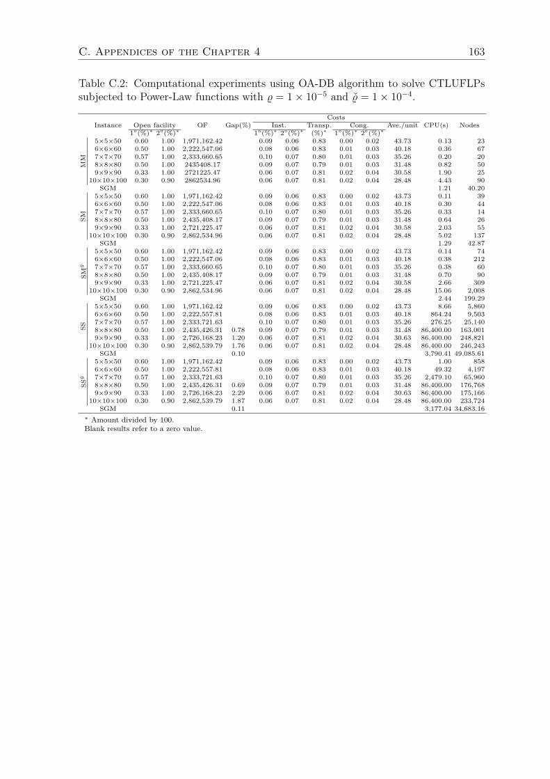
C. Appendices of the Chapter 4 163
Table C.2: Computational experiments using OA-DB algorithm to solve CTLUFLPssubjected to Power-Law functions with % = 1× 10⁻⁵ and % = 1× 10⁻⁴.
CostsInstance Open facility OF Gap(%) Inst. Transp. Cong. Ave./unit CPU(s) Nodes
1(%)∗ 2(%)∗ 1(%)∗ 2(%)∗ (%)∗ 1(%)∗ 2(%)∗
MM
5×5×50 0.60 1.00 1,971,162.42 0.09 0.06 0.83 0.00 0.02 43.73 0.13 236×6×60 0.50 1.00 2,222,547.06 0.08 0.06 0.83 0.01 0.03 40.18 0.36 677×7×70 0.57 1.00 2,333,660.65 0.10 0.07 0.80 0.01 0.03 35.26 0.20 208×8×80 0.50 1.00 2435408.17 0.09 0.07 0.79 0.01 0.03 31.48 0.82 509×9×90 0.33 1.00 2721225.47 0.06 0.07 0.81 0.02 0.04 30.58 1.90 25
10×10×100 0.30 0.90 2862534.96 0.06 0.07 0.81 0.02 0.04 28.48 4.43 90SGM 1.21 40.20
SM
5×5×50 0.60 1.00 1,971,162.42 0.09 0.06 0.83 0.00 0.02 43.73 0.11 396×6×60 0.50 1.00 2,222,547.06 0.08 0.06 0.83 0.01 0.03 40.18 0.30 447×7×70 0.57 1.00 2,333,660.65 0.10 0.07 0.80 0.01 0.03 35.26 0.33 148×8×80 0.50 1.00 2,435,408.17 0.09 0.07 0.79 0.01 0.03 31.48 0.64 269×9×90 0.33 1.00 2,721,225.47 0.06 0.07 0.81 0.02 0.04 30.58 2.03 55
10×10×100 0.30 0.90 2,862,534.96 0.06 0.07 0.81 0.02 0.04 28.48 5.02 137SGM 1.29 42.87
SMy
5×5×50 0.60 1.00 1,971,162.42 0.09 0.06 0.83 0.00 0.02 43.73 0.14 746×6×60 0.50 1.00 2,222,547.06 0.08 0.06 0.83 0.01 0.03 40.18 0.38 2127×7×70 0.57 1.00 2,333,660.65 0.10 0.07 0.80 0.01 0.03 35.26 0.38 608×8×80 0.50 1.00 2,435,408.17 0.09 0.07 0.79 0.01 0.03 31.48 0.70 909×9×90 0.33 1.00 2,721,225.47 0.06 0.07 0.81 0.02 0.04 30.58 2.66 309
10×10×100 0.30 0.90 2,862,534.96 0.06 0.07 0.81 0.02 0.04 28.48 15.06 2,008SGM 2.44 199.29
SS
5×5×50 0.60 1.00 1,971,162.42 0.09 0.06 0.83 0.00 0.02 43.73 8.66 5,8606×6×60 0.50 1.00 2,222,557.81 0.08 0.06 0.83 0.01 0.03 40.18 864.24 9,5037×7×70 0.57 1.00 2,333,721.63 0.10 0.07 0.80 0.01 0.03 35.26 276.25 25,1408×8×80 0.50 1.00 2,435,426.31 0.78 0.09 0.07 0.79 0.01 0.03 31.48 86,400.00 163,0019×9×90 0.33 1.00 2,726,168.23 1.20 0.06 0.07 0.81 0.02 0.04 30.63 86,400.00 248,821
10×10×100 0.30 0.90 2,862,539.79 1.76 0.06 0.07 0.81 0.02 0.04 28.48 86,400.00 246,243SGM 0.10 3,790.41 49,085.61
SSy
5×5×50 0.60 1.00 1,971,162.42 0.09 0.06 0.83 0.00 0.02 43.73 1.00 8586×6×60 0.50 1.00 2,222,557.81 0.08 0.06 0.83 0.01 0.03 40.18 49.32 4,1977×7×70 0.57 1.00 2,333,721.63 0.10 0.07 0.80 0.01 0.03 35.26 2,479.10 65,9608×8×80 0.50 1.00 2,435,426.31 0.69 0.09 0.07 0.79 0.01 0.03 31.48 86,400.00 176,7689×9×90 0.33 1.00 2,726,168.23 2.29 0.06 0.07 0.81 0.02 0.04 30.63 86,400.00 175,166
10×10×100 0.30 0.90 2,862,539.79 1.87 0.06 0.07 0.81 0.02 0.04 28.48 86,400.00 233,724SGM 0.11 3,177.04 34,683.16
∗ Amount divided by 100.Blank results refer to a zero value.

C. Appendices of the Chapter 4 164
Table C.3: Computational experiments using OA-BD algorithm with Papadakos BCsapproach to solve CTLUFLPs subjected to Power-Law functions with % = 1 × 10⁻⁵
and % = 1× 10⁻⁴.Costs
Instance Open facility OF Gap(%) Inst. Transp. Cong. Ave./unit CPU(s) Nodes1(%)∗ 2(%)∗ 1(%)∗ 2(%)∗ (%)∗ 1(%)∗ 2(%)∗
MM
5×5×50 0.60 1.00 1,971,162.42 0.09 0.06 0.83 0.00 0.02 43.73 0.06 216×6×60 0.50 1.00 2,222,547.06 0.08 0.06 0.83 0.01 0.03 40.18 0.26 547×7×70 0.57 1.00 2,333,660.65 0.10 0.07 0.80 0.01 0.03 35.26 0.16 168×8×80 0.50 1.00 2,435,408.17 0.09 0.07 0.79 0.01 0.03 31.48 0.62 379×9×90 0.33 1.00 2,721,225.47 0.06 0.07 0.81 0.02 0.04 30.58 1.05 36
10×10×100 0.30 0.90 2,862,534.96 0.06 0.07 0.81 0.02 0.04 28.48 2.64 90SGM 0.76 37.27
SM
5×5×50 0.60 1.00 1,971,162.42 0.09 0.06 0.83 0.00 0.02 43.73 0.06 216×6×60 0.50 1.00 2,222,547.06 0.08 0.06 0.83 0.01 0.03 40.18 0.47 1667×7×70 0.57 1.00 2,333,660.65 0.10 0.07 0.80 0.01 0.03 35.26 0.19 158×8×80 0.50 1.00 2,435,408.17 0.09 0.07 0.79 0.01 0.03 31.48 0.43 219×9×90 0.33 1.00 2,721,225.47 0.06 0.07 0.81 0.02 0.04 30.58 0.65 34
10×10×100 0.30 0.90 2,862,534.96 0.06 0.07 0.81 0.02 0.04 28.48 3.69 110SGM 0.85 43.06
SMy
5×5×50 0.60 1.00 1,971,162.42 0.09 0.06 0.83 0.00 0.02 43.73 0.07 436×6×60 0.50 1.00 2,222,547.06 0.08 0.06 0.83 0.01 0.03 40.18 0.54 3427×7×70 0.57 1.00 2,333,660.65 0.10 0.07 0.80 0.01 0.03 35.26 0.30 848×8×80 0.50 1.00 2,435,408.17 0.09 0.07 0.79 0.01 0.03 31.48 0.97 1079×9×90 0.33 1.00 2,721,225.47 0.06 0.07 0.81 0.02 0.04 30.58 1.98 299
10×10×100 0.30 0.90 2,862,534.96 0.06 0.07 0.81 0.02 0.04 28.48 8.43 1,214SGM 1.76 196.53
SS
5×5×50 0.60 1.00 1,971,162.42 0.09 0.06 0.83 0.00 0.02 43.73 12.74 7,6486×6×60 0.67 1.00 2,195,984.50 0.10 0.06 0.81 0.00 0.02 39.70 10.91 5,1687×7×70 0.57 1.00 2,333,721.63 0.10 0.07 0.80 0.01 0.03 35.26 158.03 18,1538×8×80 0.50 1.00 2,428,209.88 0.67 0.10 0.07 0.79 0.01 0.03 31.39 86,400.00 199,8479×9×90 0.33 1.00 2,726,168.23 1.88 0.06 0.07 0.81 0.02 0.04 30.63 86,400.00 110,539
10×10×100 0.20 0.80 2,862,539.79 1.73 0.04 0.06 0.83 0.02 0.05 28.41 86,400.00 326,428SGM 0.10 1,919.17 41,605.65
SSy
5×5×50 0.60 1.00 1,971,162.42 0.09 0.06 0.83 0.00 0.02 43.73 0.93 5546×6×60 0.50 1.00 2,222,557.81 0.08 0.06 0.83 0.01 0.03 40.18 374.65 9,5037×7×70 0.57 1.00 2,333,721.63 0.10 0.07 0.80 0.01 0.03 35.26 1,744.95 53,2258×8×80 0.50 1.00 2,435,426.31 0.09 0.07 0.79 0.01 0.03 31.48 6,2568.59 70,0129×9×90 0.33 1.00 2,726,168.23 1.92 0.06 0.07 0.81 0.02 0.04 30.63 86,400.00 140,019
10×10×100 0.30 0.90 2,862,539.79 1.57 0.06 0.07 0.81 0.02 0.04 28.48 86,400.00 218,064SGM 0.05 3,876.73 29,117.85
∗ Amount divided by 100.Blank results refer to a zero value.

C. Appendices of the Chapter 4 165
Table C.4: Computational experiments using GBD algorithm to solve CTLUFLPssubjected to Power-Law functions with % = 1× 10⁻⁵ and % = 1× 10⁻⁴.
CostsInstance Open facility OF Inst. Transp. Cong. Ave./unit CPU(s) Nodes
1(%)∗ 2(%)∗ 1(%)∗ 2(%)∗ (%)∗ 1(%)∗ 2(%)∗
MM
5×5×50 0.60 1.00 1,971,162.42 0.09 0.06 0.83 0.00 0.02 43.73 0.02 276×6×60 0.50 1.00 2,222,547.06 0.08 0.06 0.83 0.01 0.03 40.18 0.18 477×7×70 0.57 1.00 2,333,660.65 0.10 0.07 0.80 0.01 0.03 35.26 0.93 18×8×80 0.50 1.00 2,435,408.19 0.09 0.07 0.79 0.01 0.03 31.48 7.86 309×9×90 0.33 1.00 2,721,225.47 0.06 0.07 0.81 0.02 0.04 30.58 10.80 38
10×10×100 0.30 0.90 2,862,534.97 0.06 0.07 0.81 0.02 0.04 28.48 15.82 35SGM 4.84 25.51
SM
5×5×50 0.60 1.00 1,971,162.42 0.09 0.06 0.83 0.00 0.02 43.73 0.03 346×6×60 0.50 1.00 2,222,547.06 0.08 0.06 0.83 0.01 0.03 40.18 0.10 457×7×70 0.57 1.00 2,333,660.65 0.10 0.07 0.80 0.01 0.03 35.26 4.14 558×8×80 0.50 1.00 2,435,408.19 0.09 0.07 0.79 0.01 0.03 31.48 10.74 609×9×90 0.33 1.00 2,721,225.47 0.06 0.07 0.81 0.02 0.04 30.58 21.86 49
10×10×100 0.30 0.90 2,862,534.97 0.06 0.07 0.81 0.02 0.04 28.48 15.35 70SGM 6.98 51.09
SMy
5×5×50 0.60 1.00 1,971,162.42 0.09 0.06 0.83 0.00 0.02 43.73 0.04 296×6×60 0.50 1.00 2,222,547.06 0.08 0.06 0.83 0.01 0.03 40.18 1.04 397×7×70 0.57 1.00 2,333,660.65 0.10 0.07 0.80 0.01 0.03 35.26 1.37 478×8×80 0.50 1.00 2,435,408.19 0.09 0.07 0.79 0.01 0.03 31.48 8.10 479×9×90 0.33 1.00 2,721,225.47 0.06 0.07 0.81 0.02 0.04 30.58 18.69 106
10×10×100 0.30 0.90 2,862,534.97 0.06 0.07 0.81 0.02 0.04 28.48 14.49 82SGM 5.88 53.61
SS
5×5×50 0.60 1.00 1,971,162.42 0.09 0.06 0.83 0.00 0.02 43.73 0.22 2676×6×60 0.50 1.00 2,222,557.81 0.08 0.06 0.83 0.01 0.03 40.18 0.74 117×7×70 0.57 1.00 2,333,725.79 0.10 0.07 0.80 0.01 0.03 35.26 0.80 4308×8×80 0.50 1.00 2,435,426.31 0.09 0.07 0.79 0.01 0.03 31.48 1.67 8829×9×90 0.33 1.00 2,721,225.47 0.06 0.07 0.81 0.02 0.04 30.58 3.71 1,276
10×10×100 0.30 0.90 2,862,539.86 0.06 0.07 0.81 0.02 0.04 28.48 1.72 170SGM 1.42 274.34
SSy
5×5×50 0.60 1.00 1,971,162.42 0.09 0.06 0.83 0.00 0.02 43.73 0.36 3366×6×60 0.50 1.00 2,222,557.81 0.08 0.06 0.83 0.01 0.03 40.18 1.02 507×7×70 0.57 1.00 2,333,721.63 0.10 0.07 0.80 0.01 0.03 35.26 1.17 5998×8×80 0.50 1.00 2,435,426.31 0.09 0.07 0.79 0.01 0.03 31.48 2.79 1,1529×9×90 0.33 1.00 2,721,225.47 0.06 0.07 0.81 0.02 0.04 30.58 3.84 1,489
10×10×100 0.30 0.90 2,862,539.86 0.06 0.07 0.81 0.02 0.04 28.48 2.88 677SGM 1.95 487.32
∗ Amount divided by 100.

C. Appendices of the Chapter 4 166
Table C.5: Computational experiments using GBD algorithm with Papadakos BCsapproach to solve CTLUFLPs subjected to Power-Law functions with % = 1 × 10⁻⁵
and % = 1× 10⁻⁴.
CostsInstance Open facility OF Inst. Transp. Cong. Ave./unit CPU(s) Nodes
1(%)∗ 2(%)∗ 1(%)∗ 2(%)∗ (%)∗ 1(%)∗ 2(%)∗
MM
5×5×50 0.60 1.00 1,971,162.30 0.09 0.06 0.83 0.00 0.02 43.73 0.19 106×6×60 0.50 1.00 2,222,547.06 0.08 0.06 0.83 0.01 0.03 40.18 0.57 227×7×70 0.57 1.00 2,333,660.65 0.10 0.07 0.80 0.01 0.03 35.26 4.88 18×8×80 0.50 1.00 2,435,408.19 0.09 0.07 0.79 0.01 0.03 31.48 11.93 79×9×90 0.33 1.00 2,721,225.47 0.06 0.07 0.81 0.02 0.04 30.58 19.54 10
10×10×100 0.30 0.90 2,862,534.97 0.06 0.07 0.81 0.02 0.04 28.48 18.29 28SGM 7.57 11.21
SM
5×5×50 0.60 1.00 1,971,190.97 0.09 0.06 0.83 0.00 0.02 43.73 0.12 56×6×60 0.50 1.00 2,224,430.42 0.08 0.06 0.83 0.01 0.03 40.22 0.48 77×7×70 0.57 1.00 2,334,552.95 0.10 0.07 0.80 0.01 0.03 35.27 3.478×8×80 0.50 1.00 2,435,408.19 0.09 0.07 0.79 0.01 0.03 31.48 24.93 79×9×90 0.33 1.00 2,721,487.39 0.06 0.07 0.81 0.02 0.04 30.58 18.51 13
10×10×100 0.30 0.90 2,863,126.23 0.06 0.07 0.81 0.02 0.04 28.49 14.91 19SGM 8.12 7.52
SMy
5×5×50 0.60 1.00 1,971,190.97 0.09 0.06 0.83 0.00 0.02 43.73 0.12 76×6×60 0.50 1.00 2,224,430.42 0.08 0.06 0.83 0.01 0.03 40.22 0.51 77×7×70 0.57 1.00 2,334,226.15 0.10 0.07 0.80 0.01 0.03 35.26 3.87 18×8×80 0.50 1.00 2,437,215.52 0.09 0.07 0.79 0.01 0.03 31.50 21.06 99×9×90 0.33 1.00 2,721,225.46 0.06 0.07 0.81 0.02 0.04 30.58 40.55 7
10×10×100 0.30 0.90 2,862,590.76 0.06 0.07 0.81 0.02 0.04 28.48 29.19 22SGM 11.20 7.90
SS
5×5×50 0.60 1.00 1,971,162.29 0.09 0.06 0.83 0.00 0.02 43.73 0.42 1056×6×60 0.50 1.00 2,222,557.72 0.08 0.06 0.83 0.01 0.03 40.18 1.04 287×7×70 0.57 1.00 2,333,721.55 0.10 0.07 0.80 0.01 0.03 35.26 1.51 2248×8×80 0.50 1.00 2,435,426.25 0.09 0.07 0.79 0.01 0.03 31.48 2.54 2999×9×90 0.33 1.00 2,721,225.46 0.06 0.07 0.81 0.02 0.04 30.58 5.09 684
10×10×100 0.30 0.90 2,862,539.84 0.06 0.07 0.81 0.02 0.04 28.48 2.22 102SGM 2.05 160.49
SSy
5×5×50 0.60 1.00 1,971,162.33 0.09 0.06 0.83 0.00 0.02 43.73 0.45 1516×6×60 0.50 1.00 2,222,557.70 0.08 0.06 0.83 0.01 0.03 40.18 0.96 327×7×70 0.57 1.00 2,333,721.62 0.10 0.07 0.80 0.01 0.03 35.26 2.12 2898×8×80 0.50 1.00 2,435,426.20 0.09 0.07 0.79 0.01 0.03 31.48 2.91 1959×9×90 0.33 1.00 2,721,225.40 0.06 0.07 0.81 0.02 0.04 30.58 5.54 631
10×10×100 0.30 0.90 2,862,539.79 0.06 0.07 0.81 0.02 0.04 28.48 7.71 116SGM 3.05 169.52
∗ Amount divided by 100.

C. Appendices of the Chapter 4 167
Table C.6: Computational experiments using OA algorithm to solve CTLUFLPs sub-jected to Kleinrock functions with ϑ = 1× 10⁴, ϑ = 1× 10⁴ and ρ = ρ = 0.99.
CostsInstance Open facility OF Inst. Transp. Cong. Ave./unit CPU(s) Nodes
1(%)∗ 2(%)∗ 1(%)∗ 2(%)∗ (%)∗ 1(%)∗ 2(%)∗
MM
5×5×50 0.60 1.00 1,946,484.54 0.09 0.06 0.84 0.01 0.01 43.18 0.03 116×6×60 0.50 1.00 2,182,036.75 0.08 0.06 0.85 0.01 0.01 39.45 0.04 27×7×70 0.57 1.00 2,282,572.52 0.10 0.07 0.82 0.01 0.01 34.48 0.02 28×8×80 0.50 1.00 2,361,090.34 0.10 0.07 0.82 0.01 0.01 30.52 0.039×9×90 0.33 0.89 2,609,529.91 0.07 0.07 0.85 0.01 0.01 29.32 0.05
10×10×100 0.20 0.80 2,704,257.29 0.04 0.06 0.88 0.01 0.01 26.90 0.06SGM 0.04 2.03
SM
5×5×50 0.60 1.00 1,946,484.54 0.09 0.06 0.84 0.01 0.01 43.18 0.08 136×6×60 0.50 1.00 2,182,036.75 0.08 0.06 0.85 0.01 0.01 39.45 0.05 47×7×70 0.57 1.00 2,282,572.52 0.10 0.07 0.82 0.01 0.01 34.48 0.05 28×8×80 0.50 1.00 2,361,090.34 0.10 0.07 0.82 0.01 0.01 30.52 0.069×9×90 0.33 0.89 2,609,529.91 0.07 0.07 0.85 0.01 0.01 29.32 0.10
10×10×100 0.20 0.80 2,704,257.29 0.04 0.06 0.88 0.01 0.01 26.90 0.14SGM 0.08 2.53
SMy
5×5×50 0.60 1.00 1,946,484.54 0.09 0.06 0.84 0.01 0.01 43.18 0.08 156×6×60 0.50 1.00 2,182,036.75 0.08 0.06 0.85 0.01 0.01 39.45 0.05 47×7×70 0.57 1.00 2,282,572.52 0.10 0.07 0.82 0.01 0.01 34.48 0.05 28×8×80 0.50 1.00 2,361,090.34 0.10 0.07 0.82 0.01 0.01 30.52 0.079×9×90 0.33 0.89 2,609,529.91 0.07 0.07 0.85 0.01 0.01 29.32 0.09
10×10×100 0.20 0.80 2,704,257.29 0.04 0.06 0.88 0.01 0.01 26.90 0.13SGM 0.08 2.70
SS
5×5×50 0.60 1.00 1,946,537.86 0.09 0.06 0.84 0.01 0.01 43.18 0.16 126×6×60 0.50 1.00 2,182,095.23 0.08 0.06 0.85 0.01 0.01 39.45 0.18 87×7×70 0.57 1.00 2,282,572.52 0.10 0.07 0.82 0.01 0.01 34.48 0.38 28×8×80 0.50 1.00 2,361,090.34 0.10 0.07 0.82 0.01 0.01 30.52 0.699×9×90 0.33 0.89 2,609,533.57 0.07 0.07 0.85 0.01 0.01 29.32 1.10 1
10×10×100 0.20 0.80 2,704,257.29 0.04 0.06 0.88 0.01 0.01 26.90 1.89 4SGM 0.72 3.93
SSy
5×5×50 0.60 1.00 1,946,486.74 0.09 0.06 0.84 0.01 0.01 43.18 0.14 126×6×60 0.50 1.00 2,182,095.23 0.08 0.06 0.85 0.01 0.01 39.45 0.17 77×7×70 0.57 1.00 2,282,572.52 0.10 0.07 0.82 0.01 0.01 34.48 0.33 28×8×80 0.50 1.00 2,361,090.34 0.10 0.07 0.82 0.01 0.01 30.52 0.679×9×90 0.33 0.89 2,609,533.57 0.07 0.07 0.85 0.01 0.01 29.32 1.11 1
10×10×100 0.20 0.80 2,704,257.29 0.04 0.06 0.88 0.01 0.01 26.90 1.83 4SGM 0.69 3.80
∗ Amount divided by 100.

C. Appendices of the Chapter 4 168
Table C.7: Computational experiments using OA-BD algorithm to solve CTLUFLPssubjected to Kleinrock functions with ϑ = 1× 10⁴, ϑ = 1× 10⁴ and ρ = ρ = 0.99.
CostsInstance Open facility OF Gap(%) Inst. Transp. Cong. Ave./unit CPU(s) Nodes
1(%)∗ 2(%)∗ 1(%)∗ 2(%)∗ (%)∗ 1(%)∗ 2(%)∗
MM
5×5×50 0.60 1.00 1,946,484.54 0.09 0.06 0.84 0.01 0.01 43.18 0.43 306×6×60 0.50 1.00 2,182,036.75 0.08 0.06 0.85 0.01 0.01 39.45 0.90 497×7×70 0.57 1.00 2,282,572.52 0.10 0.07 0.82 0.01 0.01 34.48 0.56 138×8×80 0.50 1.00 2,361,090.34 0.10 0.07 0.82 0.01 0.01 30.52 4.35 399×9×90 0.33 0.89 2,609,529.91 0.07 0.07 0.85 0.01 0.01 29.32 5.53 28
10×10×100 0.20 0.80 2,704,257.29 0.04 0.06 0.88 0.01 0.00 26.90 15.15 39SGM 3.74 31.29
SM
5×5×50 0.60 1.00 1,946,484.54 0.09 0.06 0.84 0.01 0.01 43.18 0.44 826×6×60 0.50 1.00 2,182,036.75 0.08 0.06 0.85 0.01 0.01 39.45 2.51 2597×7×70 0.57 1.00 2,282,572.52 0.10 0.07 0.82 0.01 0.01 34.48 1.37 578×8×80 0.50 1.00 2,361,090.34 0.10 0.07 0.82 0.01 0.01 30.52 14.67 1519×9×90 0.33 0.89 2,609,529.91 0.07 0.07 0.85 0.01 0.01 29.32 5.79 23
10×10×100 0.20 0.80 2,704,257.29 0.04 0.06 0.88 0.01 0.00 26.90 19.29 48SGM 6.03 79.41
SMy
5×5×50 0.60 1.00 1,946,484.54 0.09 0.06 0.84 0.01 0.01 43.18 0.77 2476×6×60 0.50 1.00 2,182,036.75 0.08 0.06 0.85 0.01 0.01 39.45 3.81 8867×7×70 0.57 1.00 2,282,572.52 0.10 0.07 0.82 0.01 0.01 34.48 3.02 4028×8×80 0.50 1.00 2,361,090.34 0.10 0.07 0.82 0.01 0.01 30.52 8.19 4109×9×90 0.33 0.89 2,609,529.91 0.07 0.07 0.85 0.01 0.01 29.32 7.14 270
10×10×100 0.20 0.80 2,704,257.29 0.04 0.06 0.88 0.01 0.00 26.90 18.56 331SGM 6.07 385.11
SS
5×5×50 0.60 1.00 1,946,486.74 0.09 0.06 0.84 0.01 0.01 43.18 27.58 8,1486×6×60 0.50 1.00 2,182,048.32 0.08 0.06 0.85 0.01 0.01 39.45 2,421.23 61,7007×7×70 0.57 1.00 2,282,572.52 0.10 0.07 0.82 0.01 0.01 34.48 23,436.53 164,3468×8×80 0.38 1.00 2,369,367.38 1.50 0.07 0.07 0.84 0.01 0.01 30.63 86,400.00 226,0979×9×90 0.33 0.89 2,611,397.37 1.57 0.07 0.07 0.85 0.01 0.01 29.34 86,400.00 277,516
10×10×100 0.30 0.90 2,726,261.57 2.12 0.06 0.07 0.85 0.01 0.00 27.12 86,400.00 230,279SGM 0.12 10,544.21 103,013.42
SSy
5×5×50 0.60 1.00 1,946,486.74 0.09 0.06 0.84 0.01 0.01 43.18 12.16 3,2896×6×60 0.50 1.00 2,182,048.32 0.08 0.06 0.85 0.01 0.01 39.45 1,411.29 34,4087×7×70 0.57 1.00 2,282,572.52 0.10 0.07 0.82 0.01 0.01 34.48 4,339.24 73,6948×8×80 0.38 1.00 2,371,305.19 1.39 0.07 0.07 0.84 0.01 0.01 30.65 86,400.00 365,1149×9×90 0.33 0.89 2,609,533.57 0.15 0.07 0.07 0.85 0.01 0.01 29.32 86,400.00 341,636
10×10×100 0.20 0.80 2,704,801.15 1.03 0.04 0.06 0.88 0.01 0.00 26.91 86,400.00 346,168SGM 0.07 6,664.10 84,387.43
∗ Amount divided by 100.Blank results refer to a zero value.

C. Appendices of the Chapter 4 169
Table C.8: Computational experiments using OA-BD algorithm with Papadakos BCsapproach to solve CTLUFLPs subjected to Kleinrock functions with ϑ = 1 × 10⁴,ϑ = 1× 10⁴ and ρ = ρ = 0.99.
CostsInstance Open facility OF Gap(%) Inst. Transp. Cong. Ave./unit CPU(s) Nodes
1(%)∗ 2(%)∗ 1(%)∗ 2(%)∗ (%)∗ 1(%)∗ 2(%)∗
MM
5×5×50 0.60 1.00 1,946,484.54 0.09 0.06 0.84 0.01 0.01 43.18 0.17 236×6×60 0.50 1.00 2,182,036.75 0.08 0.06 0.85 0.01 0.01 39.45 0.31 227×7×70 0.57 1.00 2,282,572.52 0.10 0.07 0.82 0.01 0.01 34.48 0.22 148×8×80 0.50 1.00 2,361,090.34 0.10 0.07 0.82 0.01 0.01 30.52 0.77 279×9×90 0.33 0.89 2,609,529.91 0.07 0.07 0.85 0.01 0.01 29.32 3.33 24
10×10×100 0.20 0.80 2,704,257.29 0.04 0.06 0.88 0.01 0.00 26.90 5.01 28SGM 1.50 22.65
SM
5×5×50 0.60 1.00 1,946,484.54 0.09 0.06 0.84 0.01 0.01 43.18 0.23 526×6×60 0.50 1.00 2,182,036.75 0.08 0.06 0.85 0.01 0.01 39.45 1.18 1737×7×70 0.57 1.00 2,282,572.52 0.10 0.07 0.82 0.01 0.01 34.48 0.68 438×8×80 0.50 1.00 2,361,082.40 0.10 0.07 0.82 0.01 0.01 30.52 3.33 1339×9×90 0.33 0.89 2,609,529.91 0.07 0.07 0.85 0.01 0.01 29.32 1.46 24
10×10×100 0.20 0.80 2,704,257.29 0.04 0.06 0.88 0.01 0.00 26.90 6.52 59SGM 2.06 66.58
SMy
5×5×50 0.60 1.00 1,946,484.54 0.09 0.06 0.84 0.01 0.01 43.18 0.47 1516×6×60 0.50 1.00 2,182,036.75 0.08 0.06 0.85 0.01 0.01 39.45 1.72 6657×7×70 0.57 1.00 2,282,572.52 0.10 0.07 0.82 0.01 0.01 34.48 1.13 2078×8×80 0.50 1.00 2,361,090.34 0.10 0.07 0.82 0.01 0.01 30.52 5.91 4729×9×90 0.33 0.89 2,609,529.91 0.07 0.07 0.85 0.01 0.01 29.32 4.98 178
10×10×100 0.20 0.80 2,704,257.29 0.04 0.06 0.88 0.01 0.00 26.90 14.15 582SGM 4.10 318.87
SS
5×5×50 0.60 1.00 1,946,486.74 0.09 0.06 0.84 0.01 0.01 43.18 50.91 9,6956×6×60 0.50 1.00 2,182,048.32 0.08 0.06 0.85 0.01 0.01 39.45 2,858.71 58,9937×7×70 0.57 1.00 2,282,572.52 0.10 0.07 0.82 0.01 0.01 34.48 22,697.18 181,2548×8×80 0.38 1.00 2,368,759.89 1.30 0.07 0.07 0.84 0.01 0.01 30.62 86,400.00 327,0959×9×90 0.33 0.89 2,611,397.37 1.42 0.07 0.07 0.85 0.01 0.01 29.34 86,400.00 286,451
10×10×100 0.30 0.90 2,726,261.57 1.93 0.06 0.07 0.85 0.01 0.00 27.12 86,400.00 240,066SGM 0.11 11,686.03 115,170.89
SSy
5×5×50 0.60 1.00 1,946,486.74 0.09 0.06 0.84 0.01 0.01 43.18 26.31 6,726×6×60 0.50 1.00 2,182,048.32 0.08 0.06 0.85 0.01 0.01 39.45 204.04 19,5807×7×70 0.57 1.00 2,282,572.52 0.10 0.07 0.82 0.01 0.01 34.48 8,920.84 105,6398×8×80 0.38 1.00 2,367,217.45 1.55 0.07 0.07 0.84 0.01 0.01 30.60 86,400.00 282,3459×9×90 0.33 0.89 2,609,533.57 1.12 0.07 0.07 0.85 0.01 0.01 29.32 86,400.00 259,843
10×10×100 0.30 0.80 2,718,193.50 1.92 0.06 0.06 0.86 0.01 0.00 27.04 86,400.00 413,883SGM 0.11 5,949.15 86,630.52
∗ Amount divided by 100.Blank results refer to a zero value.

C. Appendices of the Chapter 4 170
Table C.9: Computational experiments using GBD algorithm to solve CTLUFLPssubjected to Kleinrock functions with ϑ = 1× 10⁴, ϑ = 1× 10⁴ and ρ = ρ = 0.99.
CostsInstance Open facility OF Inst. Transp. Cong. Ave./unit CPU(s) Nodes
1(%)∗ 2(%)∗ 1(%)∗ 2(%)∗ (%)∗ 1(%)∗ 2(%)∗
MM
5×5×50 0.60 1.00 1,946,484.54 0.09 0.06 0.84 0.01 0.01 43.18 0.02 336×6×60 0.50 1.00 2,182,036.75 0.08 0.06 0.85 0.01 0.01 39.45 0.04 287×7×70 0.57 1.00 2,282,572.52 0.10 0.07 0.82 0.01 0.01 34.48 0.04 98×8×80 0.50 1.00 2,361,090.34 0.10 0.07 0.82 0.01 0.01 30.52 0.06 59×9×90 0.33 0.89 2,609,529.91 0.07 0.07 0.85 0.01 0.01 29.32 2.72 26
10×10×100 0.20 0.80 2,704,257.29 0.04 0.06 0.88 0.01 0.00 26.90 0.10SGM 0.45 13.48
SM
5×5×50 0.60 1.00 1,946,484.54 0.09 0.06 0.84 0.01 0.01 43.18 0.02 146×6×60 0.50 1.00 2,182,036.75 0.08 0.06 0.85 0.01 0.01 39.45 0.03 137×7×70 0.57 1.00 2,282,572.52 0.10 0.07 0.82 0.01 0.01 34.48 0.06 68×8×80 0.50 1.00 2,361,090.34 0.10 0.07 0.82 0.01 0.01 30.52 0.08 39×9×90 0.33 0.89 2,609,529.91 0.07 0.07 0.85 0.01 0.01 29.32 0.13 1
10×10×100 0.20 0.80 2,704,257.29 0.04 0.06 0.88 0.01 0.00 26.90 0.22 31SGM 0.09 9.31
SMy
5×5×50 0.60 1.00 1,946,484.54 0.09 0.06 0.84 0.01 0.01 43.18 0.03 146×6×60 0.50 1.00 2,182,036.75 0.08 0.06 0.85 0.01 0.01 39.45 0.04 117×7×70 0.57 1.00 2,282,572.52 0.10 0.07 0.82 0.01 0.01 34.48 0.06 58×8×80 0.50 1.00 2,361,090.34 0.10 0.07 0.82 0.01 0.01 30.52 0.08 39×9×90 0.33 0.89 2,609,529.91 0.07 0.07 0.85 0.01 0.01 29.32 0.12 1
10×10×100 0.20 0.80 2,704,257.29 0.04 0.06 0.88 0.01 0.00 26.90 0.22 20SGM 0.09 7.86
SS
5×5×50 0.60 1.00 1,946,486.74 0.09 0.06 0.84 0.01 0.01 43.18 0.16 1536×6×60 0.50 1.00 2,182,048.32 0.08 0.06 0.85 0.01 0.01 39.45 0.26 1397×7×70 0.57 1.00 2,282,572.52 0.10 0.07 0.82 0.01 0.01 34.48 0.71 3848×8×80 0.50 1.00 2,361,090.34 0.10 0.07 0.82 0.01 0.01 30.52 0.89 3079×9×90 0.33 0.89 2,609,533.57 0.07 0.07 0.85 0.01 0.01 29.32 2.88 777
10×10×100 0.20 0.80 2,704,257.29 0.04 0.06 0.88 0.01 0.00 26.90 7.25 1796SGM 1.80 393.43
SSy
5×5×50 0.60 1.00 1,946,486.74 0.09 0.06 0.84 0.01 0.01 43.18 0.20 1856×6×60 0.50 1.00 2,182,095.23 0.08 0.06 0.85 0.01 0.01 39.45 0.40 2897×7×70 0.57 1.00 2,282,572.52 0.10 0.07 0.82 0.01 0.01 34.48 0.82 4418×8×80 0.50 1.00 2,361,090.34 0.10 0.07 0.82 0.01 0.01 30.52 1.04 3409×9×90 0.33 0.89 2,609,533.55 0.07 0.07 0.85 0.01 0.01 29.32 3.38 990
10×10×100 0.20 0.80 2,704,257.29 0.04 0.06 0.88 0.01 0.00 26.90 2.52 464SGM 1.34 394.22
∗ Amount divided by 100.

C. Appendices of the Chapter 4 171
Table C.10: Computational experiments using GBD algorithm with Papadakos BCsapproach to solve CTLUFLPs subjected to Kleinrock functions with ϑ = 1 × 10⁴,ϑ = 1× 10⁴ and ρ = ρ = 0.99.
CostsInstance Open facility OF Inst. Transp. Cong. Ave./unit CPU(s) Nodes
1(%)∗ 2(%)∗ 1(%)∗ 2(%)∗ (%)∗ 1(%)∗ 2(%)∗
MM
5×5×50 0.60 1.00 1,946,484.54 0.09 0.06 0.84 0.01 0.01 43.18 0.03 336×6×60 0.50 1.00 2,182,036.75 0.08 0.06 0.85 0.01 0.01 39.45 0.05 287×7×70 0.57 1.00 2,282,572.52 0.10 0.07 0.82 0.01 0.01 34.48 0.04 98×8×80 0.50 1.00 2,361,090.34 0.10 0.07 0.82 0.01 0.01 30.52 0.05 59×9×90 0.33 0.89 2,609,529.91 0.07 0.07 0.85 0.01 0.01 29.32 2.66 26
10×10×100 0.20 0.80 2,704,257.29 0.04 0.06 0.88 0.01 0.00 26.90 0.11SGM 0.45 13.48
SM
5×5×50 0.60 1.00 1,946,484.54 0.09 0.06 0.84 0.01 0.01 43.18 0.02 156×6×60 0.50 1.00 2,182,036.75 0.08 0.06 0.85 0.01 0.01 39.45 0.04 257×7×70 0.57 1.00 2,282,572.52 0.10 0.07 0.82 0.01 0.01 34.48 0.04 48×8×80 0.50 1.00 2,361,090.34 0.10 0.07 0.82 0.01 0.01 30.52 0.08 19×9×90 0.33 0.89 2,609,529.91 0.07 0.07 0.85 0.01 0.01 29.32 0.11 1
10×10×100 0.20 0.80 2,704,257.29 0.04 0.06 0.88 0.01 0.00 26.90 0.22 18SGM 0.08 8.61
SMy
5×5×50 0.60 1.00 1,946,484.54 0.09 0.06 0.84 0.01 0.01 43.18 0.02 156×6×60 0.50 1.00 2,182,036.75 0.08 0.06 0.85 0.01 0.01 39.45 0.05 237×7×70 0.57 1.00 2,282,572.52 0.10 0.07 0.82 0.01 0.01 34.48 0.04 68×8×80 0.50 1.00 2,361,090.34 0.10 0.07 0.82 0.01 0.01 30.52 0.07 19×9×90 0.33 0.89 2,609,529.91 0.07 0.07 0.85 0.01 0.01 29.32 0.11 1
10×10×100 0.20 0.80 2,704,257.29 0.04 0.06 0.88 0.01 0.00 26.90 0.18 17SGM 0.08 8.73
SS
5×5×50 0.60 1.00 1,946,486.58 0.09 0.06 0.84 0.01 0.01 43.18 0.16 1316×6×60 0.50 1.00 2,182,048.32 0.08 0.06 0.85 0.01 0.01 39.45 0.56 4147×7×70 0.57 1.00 2,282,572.52 0.10 0.07 0.82 0.01 0.01 34.48 0.63 3478×8×80 0.50 1.00 2,361,090.34 0.10 0.07 0.82 0.01 0.01 30.52 1.38 4769×9×90 0.33 0.89 2,609,533.57 0.07 0.07 0.85 0.01 0.01 29.32 5.34 1,424
10×10×100 0.20 0.80 2,704,257.29 0.04 0.06 0.88 0.01 0.00 26.90 5.04 1,214SGM 2.01 502.90
SSy
5×5×50 0.60 1.00 1,946,585.59 0.09 0.06 0.84 0.01 0.01 43.18 0.15 1216×6×60 0.50 1.00 2,182,048.32 0.08 0.06 0.85 0.01 0.01 39.45 0.40 2807×7×70 0.57 1.00 2,282,572.52 0.10 0.07 0.82 0.01 0.01 34.48 0.90 5908×8×80 0.50 1.00 2,361,090.34 0.10 0.07 0.82 0.01 0.01 30.52 1.48 5489×9×90 0.33 0.89 2,609,533.57 0.07 0.07 0.85 0.01 0.01 29.32 2.81 845
10×10×100 0.20 0.80 2,704,257.29 0.04 0.06 0.88 0.01 0.00 26.90 5.88 1,425SGM 1.79 489.90
∗ Amount divided by 100.

C. Appendices of the Chapter 4 172
Table C.11: Complete data of the computational experiments for OA algorithm whenonly total customers is expanded, considering a Power-Law function with % = 1× 10⁻⁵
and % = 1× 10⁻⁴.
Costs.Instance Open facility OF Inst. Transp. Cong. Ave./unit CPU(s) Nodes
1(%)∗ 2(%)∗ 1(%)∗ 2(%)∗ (%)∗ 1(%)∗ 2(%)∗
MM
10×50×200 0.50 0.42 3,092,380.77 0.09 0.15 0.67 0.03 0.07 15.75 13.20 4510×50×400 0.80 0.62 5,960,698.99 0.07 0.11 0.68 0.04 0.10 14.92 20.81 3710×50×800 1.00 0.76 12,235,526.10 0.04 0.07 0.68 0.06 0.15 15.21 18.46 2310×50×1600 1.00 0.94 28,134,140.50 0.02 0.04 0.62 0.10 0.23 17.42 43.13 16
SGM 22.24 28.59
SM
10×50×200 0.50 0.44 3,092,380.77 0.09 0.15 0.67 0.03 0.07 15.75 54.14 7810×50×400 0.80 0.62 5,960,698.99 0.07 0.11 0.68 0.04 0.10 14.92 51.32 4710×50×800 1.00 0.76 12,236,874.82 0.04 0.07 0.68 0.06 0.15 15.21 91.42 6810×50×1600 1.00 0.94 28,134,140.50 0.02 0.04 0.62 0.10 0.23 17.42 146.37 16
SGM 78.87 46.48
SMy
10×50×200 0.50 0.42 3,092,380.77 0.09 0.15 0.67 0.03 0.07 15.75 50.59 8910×50×400 0.80 0.62 5,960,698.99 0.07 0.11 0.68 0.04 0.10 14.92 72.67 7410×50×800 1.00 0.76 12,236,874.82 0.04 0.07 0.68 0.06 0.15 15.21 56.06 3210×50×1600 1.00 0.94 28,134,140.50 0.02 0.04 0.62 0.10 0.23 17.42 115.73 14
SGM 70.31 43.81
SS
10×50×200 0.50 0.42 3,092,537.16 0.09 0.15 0.67 0.03 0.07 15.75 173.29 11810×50×400 0.80 0.62 5,960,990.44 0.07 0.11 0.68 0.04 0.10 14.92 122.45 3410×50×800 1.00 0.76 12,237,516.63 0.04 0.07 0.68 0.06 0.15 15.21 229.49 21210×50×1600 1.00 0.94 28,135,568.90 0.02 0.04 0.62 0.10 0.23 17.42 383.22 160
SGM 208.66 110.74
SSy
10×50×200 0.50 0.42 3,092,537.16 0.09 0.15 0.67 0.03 0.07 15.75 187.04 19210×50×400 0.80 0.62 5,961,019.83 0.07 0.11 0.68 0.04 0.10 14.92 234.58 17110×50×800 1.00 0.76 12,237,661.04 0.04 0.07 0.68 0.06 0.15 15.21 281.43 24910×50×1600 1.00 0.94 28,135,333.77 0.02 0.04 0.62 0.10 0.23 17.42 554.62 216
SGM 288.41 205.08∗ Amount divided by 100.

C. Appendices of the Chapter 4 173
Table C.12: Complete data of the computational experiments for CPLEX solver whenonly total customers is expanded, considering a Power-Law function with % = 1× 10⁻⁵
and % = 1× 10⁻⁴.
Costs.Instance Open facility OF Inst. Transp. Cong. Ave./unit CPU(s) Nodes
1(%)∗ 2(%)∗ 1(%)∗ 2(%)∗ (%)∗ 1(%)∗ 2(%)∗
MM
10×50×200 0.50 0.42 3,092,380.77 0.09 0.15 0.67 0.03 0.07 15.75 70.24 3710×50×400 0.80 0.62 5,960,698.99 0.07 0.11 0.68 0.04 0.10 14.92 30.72 1510×50×800 1.00 0.76 12,235,526.10 0.04 0.07 0.68 0.06 0.15 15.21 35.82 2310×50×1600 1.00 0.94 28,134,140.50 0.02 0.04 0.62 0.10 0.23 17.42 49.31 12
SGM 44.59 20.39
SM
10×50×200 0.50 0.44 3,092,431.26 0.09 0.16 0.67 0.03 0.06 15.75 189.38 4410×50×400 0.80 0.62 5,960,698.99 0.07 0.11 0.68 0.04 0.10 14.92 608.92 3110×50×800 1.00 0.76 12,236,874.82 0.04 0.07 0.68 0.06 0.15 15.21 4,115.51 2010×50×1600 1.00 0.94 28,134,140.50 0.02 0.04 0.62 0.10 0.23 17.42 † †
SGM 788.48∗∗ 30.50∗∗
SMy
10×50×200 0.50 0.42 3,092,380.77 0.09 0.15 0.67 0.03 0.07 15.75 329.95 4210×50×400 0.80 0.62 5,960,698.99 0.07 0.11 0.68 0.04 0.10 14.92 848.63 3310×50×800 1.00 0.76 12,236,874.82 0.04 0.07 0.68 0.06 0.15 15.21 4,478.27 2710×50×1600 1.00 0.94 28,134,140.50 0.02 0.04 0.62 0.10 0.23 17.42 † †
SGM 1,084.21∗∗ 33.57∗∗
SS
10×50×200 0.50 0.42 3,092,537.16 0.09 0.15 0.67 0.03 0.07 15.75 1,813.43 4510×50×400 0.80 0.62 5,960,990.44 0.07 0.11 0.68 0.04 0.10 14.92 7,431.51 4210×50×800 1.00 0.76 12,237,516.63 0.04 0.07 0.68 0.06 0.15 15.21 † †10×50×1600 1.00 0.94 28,135,568.90 0.02 0.04 0.62 0.10 0.23 17.42 † †
SGM 3,673.62∗∗ 43.48∗∗
SSy
10×50×200 0.50 0.42 3,092,537.16 0.09 0.15 0.67 0.03 0.07 15.75 1,366.3 6810×50×400 0.80 0.62 5,961,019.83 0.07 0.11 0.68 0.04 0.10 14.92 8,221.39 4610×50×800 1.00 0.76 12,237,661.04 0.04 0.07 0.68 0.06 0.15 15.21 † †10×50×1600 1.00 0.94 28,135,333.77 0.02 0.04 0.62 0.10 0.23 17.42 † †
SGM 3,355.84∗∗ 56.09∗∗∗ Amount divided by 100.∗∗ SGM for the fully solved instances.† Out-of-memory.

C. Appendices of the Chapter 4 174
Table C.13: Complete data of the computational experiments for OA algorithm whenonly total customers is expanded, considering a Kleinrock function with ϑ = 1 × 10⁵,ϑ = 1× 10⁴ and ρ = ρ = 0.99.
CostsInstance Open facility OF Inst. Transp. Cong. Ave./unit CPU(s) Nodes
1(%)∗ 2(%)∗ 1(%)∗ 2(%)∗ (%)∗ 1(%)∗ 2(%)∗
MM
10×50×200 0.50 0.36 2,913,136.48 0.09 0.14 0.72 0.04 0.01 14.84 1.4 110×50×400 0.60 0.48 5,153,988.23 0.06 0.10 0.81 0.02 0.01 12.90 1.910×50×800 0.90 0.68 9,466,422.18 0.05 0.08 0.86 0.01 0.01 11.77 4.210×50×1600 0.90 0.72 17,785,513.90 0.03 0.04 0.92 0.01 0.01 11.01 9.71
SGM 3.96 0.24
SM
10×50×200 0.50 0.36 2,913,136.48 0.09 0.14 0.72 0.04 0.01 14.84 4.2910×50×400 0.60 0.48 5,153,988.23 0.06 0.10 0.81 0.02 0.01 12.90 8.3710×50×800 0.90 0.68 9,466,422.18 0.05 0.08 0.86 0.01 0.01 11.77 20.0710×50×1600 0.90 0.72 17,785,513.90 0.03 0.04 0.92 0.01 0.01 11.01 58.56
SGM 17.12
SMy
10×50×200 0.50 0.36 2,913,136.48 0.09 0.14 0.72 0.04 0.01 14.84 3.110×50×400 0.60 0.48 5,153,988.23 0.06 0.10 0.81 0.02 0.01 12.90 4.810×50×800 0.90 0.68 9,466,422.18 0.05 0.08 0.86 0.01 0.01 11.77 13.6210×50×1600 0.90 0.72 17,785,513.90 0.03 0.04 0.92 0.01 0.01 11.01 42.63
SGM 12.16
SS
10×50×200 0.50 0.36 2,913,136.48 0.09 0.14 0.72 0.04 0.01 14.84 298.78 3110×50×400 0.60 0.48 5,153,988.23 0.06 0.10 0.81 0.02 0.01 12.90 1,349.2810×50×800 0.90 0.68 9,466,422.18 0.05 0.08 0.86 0.01 0.01 11.77 5,834.5710×50×1600 0.90 0.72 17,785,513.90 0.03 0.04 0.92 0.01 0.01 11.01 14,690.99
SGM 2,440.55 4.23
SSy
10×50×200 0.50 0.36 2,913,136.48 0.09 0.14 0.72 0.04 0.01 14.84 204.66 2010×50×400 0.60 0.48 5,153,988.23 0.06 0.10 0.81 0.02 0.01 12.90 934.8510×50×800 0.90 0.68 9,466,422.18 0.05 0.08 0.86 0.01 0.01 11.77 3,252.7710×50×1600 0.90 0.72 17,785,513.90 0.03 0.04 0.92 0.01 0.01 11.01 16,036.24
SGM 1,795.17 3.16∗ Amount divided by 100.Blank results refer to a zero value.

C. Appendices of the Chapter 4 175
Table C.14: Complete data of the computational experiments for OA algorithm whenthe instance size are increased, considering a Power-Law function with % = 1 × 10⁻⁵
and % = 1× 10⁻⁴.
CostsInstance Open facility OF Gap(%) Inst. Transp. Cong. Ave./unit CPU(s) Nodes
1(%)∗ 2(%)∗ 1(%)∗ 2(%)∗ (%)∗ 1(%)∗ 2(%)∗
MM
15×75×150 0.33 0.27 2,224,457.80 0.13 0.20 0.61 0.02 0.05 15.64 81.51 19720×100×200 0.25 0.22 2,648,135.57 0.11 0.19 0.62 0.03 0.06 14.10 2,480.44 77925×150×250 0.24 0.18 3,064,394.90 4.02 0.11 0.20 0.59 0.03 0.08 12.67 86,400.00 239630×200×300 0.17 0.17 3,563,435.51 11.28 0.08 0.21 0.59 0.05 0.07 12.44 86,400.00 975
SGM 0.25 6,412.71 778.76
SM
15×75×150 0.33 0.27 2,224,457.80 0.13 0.20 0.61 0.02 0.05 15.64 21,165.13 279120×100×200 0.25 0.23 2,649,654.33 3.73 0.11 0.20 0.61 0.03 0.06 14.11 86,400.00 178625×150×250 0.24 0.21 3,100,140.56 9.80 0.11 0.22 0.57 0.03 0.07 12.82 86,400.00 67530×200×300 0.17 0.18 3,604,923.72 14.95 0.08 0.22 0.58 0.05 0.07 12.59 86,400.00 243
SGM 1.52 60,786.63 956.29
SMy
15×75×150 0.33 0.27 2,224,457.80 0.13 0.20 0.61 0.02 0.05 15.64 6,204.89 138320×100×200 0.25 0.22 2,648,135.57 2.98 0.11 0.19 0.62 0.03 0.06 14.10 86,400.00 250025×150×250 0.24 0.19 3,073,318.13 8.61 0.11 0.20 0.58 0.03 0.07 12.71 86,400.00 93230×200×300 0.17 0.18 3,604,923.72 15.28 0.08 0.22 0.58 0.05 0.07 12.59 86,400.00 368
SGM 1.40 44,738.80 1,046.31
SS
15×75×150 0.33 0.27 2,225,001.82 2.18 0.13 0.20 0.61 0.02 0.05 15.64 86,400.00 465920×100×200 0.25 0.23 2,656,004.65 6.34 0.11 0.19 0.61 0.03 0.06 14.14 86,400.00 90925×150×250 0.24 0.21 3,111,705.52 11.46 0.11 0.22 0.57 0.03 0.07 12.87 86,400.00 92630×200×300 0.17 0.18 3,614,233.86 16.46 0.08 0.22 0.58 0.05 0.07 12.62 86,400.00 406
SGM 7.15 86,400.00 1,126.91
SSy
15×75×150 0.33 0.27 2,225,011.93 1.10 0.13 0.20 0.61 0.02 0.05 15.64 86,400.00 1141720×100×200 0.25 0.23 2,656,004.65 5.28 0.11 0.19 0.61 0.03 0.06 14.14 86,400.00 475125×150×250 0.24 0.21 3,111,705.52 10.91 0.11 0.22 0.57 0.03 0.07 12.87 86,400.00 137430×200×300 0.17 0.18 3,613,805.69 16.61 0.08 0.22 0.58 0.05 0.07 12.62 86,400.00 320
SGM 5.70 86,400.00 2,222.65∗ Amount divided by 100.Blank results refer to a zero value.

C. Appendices of the Chapter 4 176
Table C.15: Complete data of the computational experiments for CPLEX solver whenthe instance size are increased, considering a Power-Law function with % = 1 × 10⁻⁵
and % = 1× 10⁻⁴.
CostsInstance Open facility OF Gap(%) Inst. Transp. Cong. Ave./unit CPU(s) Nodes
1(%)∗ 2(%)∗ 1(%)∗ 2(%)∗ (%)∗ 1(%)∗ 2(%)∗
MM
15×75×150 0.33 0.27 2,224,457.80 0.13 0.20 0.61 0.02 0.05 15.64 558.60 27120×100×200 0.25 0.22 2,648,135.57 0.11 0.19 0.62 0.03 0.06 14.10 39,261.74 153525×150×250 0.24 0.18 3,079,086.81 8.51 0.11 0.20 0.59 0.03 0.08 12.67 86,400.00 20530×200×300 0.17 0.17 6,204,299.12 51.01 0.08 0.21 0.59 0.05 0.07 12.44 86,400.00 2
SGM 0.45 20,197.09 172.94
SM
15×75×150 0.33 0.27 2,224,457.80 0.13 0.20 0.61 0.02 0.05 15.64 6,038.68 101120×100×200 0.25 0.23 2,648,135.57 2.63 0.11 0.20 0.61 0.03 0.06 14.11 86,400.00 108325×150×250 0.24 0.21 3,139,546.83 11.43 0.11 0.22 0.57 0.03 0.07 12.82 86,400.00 12430×200×300 † † † † † † † † † † † †
SGM 0.66∗∗ 35,601.99∗∗ 520.78∗∗
SMy
15×75×150 0.33 0.27 2,224,457.80 0.13 0.20 0.61 0.02 0.05 15.64 5,782.97 98620×100×200 0.25 0.22 2,685,591.91 5.03 0.11 0.19 0.62 0.03 0.06 14.10 86,400.00 67725×150×250 0.24 0.19 3,117,385.31 10.63 0.11 0.20 0.58 0.03 0.07 12.71 86,400.00 14330×200×300 † † † † † † † † † † † †
SGM 0.80∗∗ 35,092.91∗∗ 461.31∗∗
SS
15×75×150 0.25 0.23 2,224,511.01 0.11 0.19 0.61 0.03 0.06 14.14 16,545.78 118520×100×200 0.17 0.18 2,679,203.62 5.24 0.08 0.22 0.58 0.05 0.07 12.62 86,400.00 87425×150×250 † † † † † † † † † † † †30×200×300 † † † † † † † † † † † †
SGM 0.22∗∗ 37,813.07∗∗ 1,017.80∗∗
SSy
15×75×150 0.33 0.27 2,224,511.01 0.13 0.20 0.61 0.02 0.05 15.64 10,932.35 71820×100×200 0.17 0.18 2,666,699.23 4.78 0.08 0.22 0.58 0.05 0.07 12.62 86,400.00 54325×150×250 † † † † † † † † † † † †30×200×300 † † † † † † † † † † † †
SGM 0.21∗∗ 30,739.45∗∗ 624.50∗∗
∗ Amount divided by 100.∗∗ SGM for the fully solved instances.Blank results refer to a zero value.† Out-of-memory.

C. Appendices of the Chapter 4 177
Table C.16: Complete data of the computational experiments for OA algorithm solverwhen the instance size are increased, considering a Kleinrock function with ϑ = 1×10⁵,ϑ = 1× 10⁴ and ρ = ρ = 0.99.
CostsInstance Open facility OF Gap(%) Inst. Transp. Cong. Ave./unit CPU(s) Nodes
1(%)∗ 2(%)∗ 1(%)∗ 2(%)∗ (%)∗ 1(%)∗ 2(%)∗
MM
15×75×150 0.27 0.23 2,200,576.16 0.10 0.17 0.66 0.06 0.01 15.47 49.84 8820×100×200 0.25 0.22 2,538,215.43 0.11 0.20 0.64 0.05 0.00 13.52 192.82 6625×150×250 0.24 0.15 2,835,769.63 0.11 0.18 0.66 0.04 0.00 11.73 2,596.71 24630×200×300 0.17 0.13 3,165,526.28 0.09 0.18 0.69 0.04 0.00 11.05 70,319.21 2,42
SGM 1,211.33 250.90
SM
15×75×150 0.27 0.23 2,200,603.39 0.10 0.17 0.66 0.06 0.01 15.47 186.29 27020×100×200 0.25 0.22 2,538,215.43 0.11 0.20 0.64 0.05 0.00 13.52 2,562.79 35825×150×250 0.20 0.15 2,836,278.35 1.07 0.10 0.18 0.68 0.05 0.00 11.73 86,400.00 1,29630×200×300 0.17 0.14 3,198,201.05 4.83 0.09 0.19 0.68 0.04 0.00 11.17 86,400.00 464
SGM 0.14 7,826.24 492.55
SMy
15×75×150 0.27 0.23 2,200,603.39 0.10 0.17 0.66 0.06 0.01 15.47 129.51 17720×100×200 0.25 0.22 2,538,215.43 0.11 0.20 0.64 0.05 0.00 13.52 1,443.13 20025×150×250 0.24 0.15 2,835,769.63 1.38 0.11 0.18 0.66 0.04 0.00 11.73 86,400.00 1,830×200×300 0.17 0.14 3,215,154.93 4.76 0.09 0.20 0.67 0.04 0.00 11.23 86,400.00 680
SGM 0.15 6,227.48 460.59
SS
15×75×150 0.27 0.23 2,200,603.39 0.10 0.17 0.66 0.06 0.01 15.47 4,790.28 2,71620×100×200 0.25 0.22 2,538,215.71 0.11 0.20 0.64 0.05 0.00 13.52 34,707.28 2,12325×150×250 0.20 0.17 2,849,773.63 3.63 0.10 0.20 0.65 0.05 0.00 11.79 86,400.00 1,3230×200×300 0.70 0.20 6,087,590.49 51.17 0.19 0.14 0.65 0.02 0.00 21.25 86,400.00 57
SGM 0.36 33,389.12 838.42
SSy
15×75×150 0.27 0.23 2,200,603.39 0.10 0.17 0.66 0.06 0.01 15.47 2,656.13 2,57120×100×200 0.25 0.22 2,538,215.55 0.11 0.20 0.64 0.05 0.00 13.52 33,594.41 4,15725×150×250 0.20 0.17 2,849,773.63 4.08 0.10 0.20 0.65 0.05 0.00 11.79 86,400.00 90330×200×300 0.23 0.17 3,323,195.42 10.32 0.12 0.22 0.62 0.04 0.00 11.60 86,400.00 30
SGM 0.24 28,589.04 781.65∗ Amount divided by 100.Blank results refer to a zero value.

C. Appendices of the Chapter 4 178
Table C.17: Computational results from the OA algorithm solving a Ro and Tchainstance of 10×50×100 size, when % and % parameters of the Power-Law function arechanged.
Costs% % Open facility OF Gap(%) Inst. Transp. Cong. Ave./unit CPU(s) Nodes
1(%)∗ 2(%)∗ 1(%)∗ 2(%)∗ (%)∗ 1(%)∗ 2(%)∗
MM
1×10⁻⁵ 1×10⁻⁴ 0.40 0.26 1,703,685.14 0.13 0.17 0.64 0.02 0.05 17.65 4.38 302×10−5 1×10⁻⁴ 0.40 0.26 1,728,671.63 0.13 0.16 0.63 0.03 0.05 17.91 5.39 333×10−5 1×10⁻⁴ 0.40 0.26 1,753,488.53 0.13 0.16 0.62 0.04 0.05 18.16 6.06 344×10−5 1×10⁻⁴ 0.40 0.26 1,778,147.72 0.13 0.16 0.61 0.06 0.05 18.42 6.36 425×10−5 1×10⁻⁴ 0.40 0.26 1,802,712.61 0.12 0.16 0.61 0.07 0.05 18.67 7.70 53
1×10⁻⁵ 1×10⁻⁴ 0.40 0.26 1,703,685.14 0.13 0.17 0.64 0.02 0.05 17.65 4.38 301×10−5 2×10⁻⁴ 0.40 0.28 1,784,009.98 0.13 0.17 0.61 0.01 0.09 18.48 8.74 591×10−5 3×10⁻⁴ 0.40 0.28 1,859,732.88 0.12 0.16 0.58 0.01 0.12 19.27 10.32 701×10−5 4×10⁻⁴ 0.40 0.32 1,930,613.78 0.12 0.18 0.56 0.01 0.13 20.00 15.96 1021×10−5 5×10⁻⁴ 0.40 0.34 1,994,872.56 0.11 0.19 0.54 0.01 0.15 20.67 25.16 195
1×10⁻⁵ 1×10⁻⁴ 0.40 0.26 1,703,685.14 0.13 0.17 0.64 0.02 0.05 17.65 4.38 302×10−5 2×10⁻⁴ 0.40 0.28 1,808,441.33 0.12 0.17 0.60 0.03 0.08 18.73 8.41 523×10−5 3×10⁻⁴ 0.40 0.28 1,908,663.99 0.12 0.16 0.57 0.04 0.12 19.77 15.45 1104×10−5 4×10⁻⁴ 0.50 0.32 1,996,716.14 0.14 0.17 0.52 0.04 0.13 20.68 31.42 2325×10−5 5×10⁻⁴ 0.50 0.34 2,076,719.18 0.13 0.18 0.50 0.05 0.14 21.51 54.06 360
SM
1×10⁻⁵ 1×10⁻⁴ 0.40 0.26 1,703,685.14 0.13 0.17 0.64 0.02 0.05 17.65 8.94 362×10−5 1×10⁻⁴ 0.40 0.26 1,728,671.63 0.13 0.16 0.63 0.03 0.05 17.91 15.81 553×10−5 1×10⁻⁴ 0.40 0.26 1,753,488.53 0.13 0.16 0.62 0.04 0.05 18.16 26.66 744×10−5 1×10⁻⁴ 0.40 0.26 1,778,147.72 0.13 0.16 0.61 0.06 0.05 18.42 42.75 1115×10−5 1×10⁻⁴ 0.40 0.26 1,802,712.61 0.12 0.16 0.61 0.07 0.05 18.67 109.43 282
1×10⁻⁵ 1×10⁻⁴ 0.40 0.26 1,703,685.14 0.13 0.17 0.64 0.02 0.05 17.65 8.94 361×10−5 2×10⁻⁴ 0.40 0.28 1,784,009.98 0.13 0.17 0.61 0.01 0.09 18.48 32.97 941×10−5 3×10⁻⁴ 0.40 0.28 1,859,732.88 0.12 0.16 0.58 0.01 0.12 19.27 80.31 2181×10−5 4×10⁻⁴ 0.40 0.32 1,930,613.78 0.12 0.18 0.56 0.01 0.13 20.00 348.11 7521×10−5 5×10⁻⁴ 0.40 0.34 1,994,872.56 0.11 0.19 0.54 0.01 0.15 20.67 1,600.76 1,946
1×10⁻⁵ 1×10⁻⁴ 0.40 0.26 1,703,685.14 0.13 0.17 0.64 0.02 0.05 17.65 8.94 362×10−5 2×10⁻⁴ 0.40 0.28 1,808,441.33 0.12 0.17 0.60 0.03 0.08 18.73 49.01 1283×10−5 3×10⁻⁴ 0.40 0.28 1,908,663.99 0.12 0.16 0.57 0.04 0.12 19.77 336.03 7274×10−5 4×10⁻⁴ 0.50 0.32 1,996,716.14 0.14 0.17 0.52 0.04 0.13 20.68 11,639.72 6,5665×10⁻⁵ 5×10⁻⁴ 0.50 0.34 2,076,719.18 0.13 0.18 0.50 0.05 0.14 21.51 43,943.20 12,009
SMy
1×10⁻⁵ 1×10⁻⁴ 0.40 0.26 1,703,685.14 0.13 0.17 0.64 0.02 0.05 17.65 7.10 322×10−5 1×10⁻⁴ 0.40 0.26 1,728,671.63 0.13 0.16 0.63 0.03 0.05 17.91 12.53 513×10−5 1×10⁻⁴ 0.40 0.26 1,753,488.53 0.13 0.16 0.62 0.04 0.05 18.16 19.78 704×10−5 1×10⁻⁴ 0.40 0.26 1,778,147.72 0.13 0.16 0.61 0.06 0.05 18.42 27.75 1165×10−5 1×10⁻⁴ 0.40 0.26 1,802,712.61 0.12 0.16 0.61 0.07 0.05 18.67 56.74 251
1×10⁻⁵ 1×10⁻⁴ 0.40 0.26 1,703,685.14 0.13 0.17 0.64 0.02 0.05 17.65 7.10 321×10−5 2×10⁻⁴ 0.40 0.28 1,784,009.98 0.13 0.17 0.61 0.01 0.09 18.48 27.96 791×10−5 3×10⁻⁴ 0.40 0.28 1,859,732.88 0.12 0.16 0.58 0.01 0.12 19.27 90.77 3711×10−5 4×10⁻⁴ 0.40 0.32 1,930,613.78 0.12 0.18 0.56 0.01 0.13 20.00 310.03 1,1381×10⁻⁵ 5×10⁻⁴ 0.40 0.34 1,994,872.56 0.11 0.19 0.54 0.01 0.15 20.67 1,735.49 3,687
1×10⁻⁵ 1×10⁻⁴ 0.40 0.26 1,703,685.14 0.13 0.17 0.64 0.02 0.05 17.65 7.10 322×10−5 2×10⁻⁴ 0.40 0.28 1,808,441.33 0.12 0.17 0.60 0.03 0.08 18.73 48.23 1403×10−5 3×10⁻⁴ 0.40 0.28 1,908,663.99 0.12 0.16 0.57 0.04 0.12 19.77 298.90 9444×10−5 4×10⁻⁴ 0.50 0.32 1,996,716.14 0.14 0.17 0.52 0.04 0.13 20.68 6,814.91 5,6145×10⁻⁵ 5×10⁻⁴ 0.50 0.34 2,076,719.18 3.04 0.13 0.18 0.50 0.05 0.14 21.51 86,400.00 16,046
Continued on the next page

C. Appendices of the Chapter 4 179
Table C.17 – continued from previous page
Costs% % Open facility OF Gap(%) Inst. Transp. Cong. Ave./unit CPU(s) Nodes
1(%)∗ 2(%)∗ 1(%)∗ 2(%)∗ (%)∗ 1(%)∗ 2(%)∗
SS
1×10⁻⁵ 1×10⁻⁴ 0.40 0.26 1,703,685.14 0.13 0.17 0.64 0.02 0.05 17.65 47.91 392×10−5 1×10⁻⁴ 0.40 0.26 1,728,688.51 0.13 0.16 0.63 0.03 0.05 17.91 96.01 953×10−5 1×10⁻⁴ 0.40 0.26 1,7534,97.01 0.13 0.16 0.62 0.04 0.05 18.16 168.49 2234×10−5 1×10⁻⁴ 0.40 0.26 1,778,147.92 0.13 0.16 0.61 0.06 0.05 18.42 398.77 5125×10−5 1×10⁻⁴ 0.40 0.26 1,802,773.09 0.12 0.16 0.61 0.07 0.05 18.68 684.68 486
1×10⁻⁵ 1×10⁻⁴ 0.40 0.26 1,703,685.14 0.13 0.17 0.64 0.02 0.05 17.65 47.91 391×10−5 2×10⁻⁴ 0.40 0.28 1,784,124.94 0.13 0.17 0.60 0.01 0.09 18.48 364.51 4401×10−5 3×10⁻⁴ 0.40 0.28 1,859,890.01 0.12 0.16 0.58 0.01 0.12 19.27 3,159.94 8801×10−5 4×10⁻⁴ 0.40 0.32 1,930,733.58 0.12 0.18 0.56 0.01 0.13 20.00 5,192.31 3,1591×10⁻⁵ 5×10⁻⁴ 0.40 0.34 1,995,311.40 0.11 0.19 0.54 0.01 0.15 20.67 27,209.53 6,672
1×10⁻⁵ 1×10⁻⁴ 0.40 0.26 1,703,685.14 0.13 0.17 0.64 0.02 0.05 17.65 47.91 392×10−5 2×10⁻⁴ 0.40 0.28 1,808,548.41 0.12 0.17 0.60 0.03 0.09 18.74 1,542.73 1,2993×10⁻⁵ 3×10⁻⁴ 0.40 0.28 1,908,867.39 0.12 0.16 0.57 0.04 0.12 19.77 12,164.78 5,4754×10⁻⁵ 4×10⁻⁴ 0.50 0.32 1,997,346.67 0.85 0.14 0.17 0.52 0.04 0.13 20.69 86,400.00 12,2815×10⁻⁵ 5×10⁻⁴ 0.50 0.34 2,077,284.30 1.53 0.13 0.18 0.50 0.05 0.14 21.52 86,400.00 9,991
SSy
1×10⁻⁵ 1×10⁻⁴ 0.40 0.26 1,703,685.14 0.13 0.17 0.64 0.02 0.05 17.65 43.25 432×10−5 1×10⁻⁴ 0.40 0.26 1,728,688.51 0.13 0.16 0.63 0.03 0.05 17.91 101.69 1793×10−5 1×10⁻⁴ 0.40 0.26 1,753,497.01 0.13 0.16 0.62 0.04 0.05 18.16 138.72 2524×10−5 1×10⁻⁴ 0.40 0.26 1,778,147.92 0.13 0.16 0.61 0.06 0.05 18.42 176.77 2595×10−5 1×10⁻⁴ 0.40 0.26 1,802,773.09 0.12 0.16 0.61 0.07 0.05 18.68 311.04 293
1×10⁻⁵ 1×10⁻⁴ 0.40 0.26 1,703,685.14 0.13 0.17 0.64 0.02 0.05 17.65 43.25 431×10−5 2×10⁻⁴ 0.40 0.28 1,784,124.94 0.13 0.17 0.60 0.01 0.09 18.48 175.18 3011×10−5 3×10⁻⁴ 0.40 0.28 1,859,890.01 0.12 0.16 0.58 0.01 0.12 19.27 1,621.24 2,4601×10⁻⁵ 4×10⁻⁴ 0.40 0.32 1,930,733.58 0.12 0.18 0.56 0.01 0.13 20.00 16,886.05 10,6461×10⁻⁵ 5×10⁻⁴ 0.40 0.32 1,995,411.43 1.02 0.11 0.18 0.54 0.01 0.16 20.67 86,400.00 24,995
1×10⁻⁵ 1×10⁻⁴ 0.40 0.26 1,703,685.14 0.13 0.17 0.64 0.02 0.05 17.65 43.25 432×10−5 2×10⁻⁴ 0.40 0.28 1,808,548.41 0.12 0.17 0.60 0.03 0.09 18.74 413.35 8233×10−5 3×10⁻⁴ 0.40 0.28 1,908,867.39 0.12 0.16 0.57 0.04 0.12 19.77 9,662.17 4,7064×10⁻⁵ 4×10⁻⁴ 0.50 0.32 1,997,346.67 1.39 0.14 0.17 0.52 0.04 0.13 20.69 86,400.00 17,3475×10⁻⁵ 5×10⁻⁴ 0.50 0.34 2,077,284.30 1.62 0.13 0.18 0.50 0.05 0.14 21.52 86,400.00 10,656
∗ Amount divided by 100.Blank results refer to a zero value.

C. Appendices of the Chapter 4 180
Table C.18: Computational results from the OA algorithm solving a Ro and Tchainstance of 10×50×100 size, when ϑ and ϑ parameters of the Kleinrock function arechanged, while ρ = ρ = 0.99.
Costs% % Open facility OF Inst. Transp. Cong. Ave./unit CPU(s) Nodes
1(%)∗ 2(%)∗ 1(%)∗ 2(%)∗ (%)∗ 1(%)∗ 2(%)∗
MM
1×10⁴ 1×10⁴ 0.40 0.26 1,621,420.13 0.14 0.18 0.67 0.01 0.01 16.80 1.01 62×104 1×10⁴ 0.40 0.26 1,635,374.05 0.14 0.17 0.67 0.02 0.01 16.94 1.74 103×104 1×10⁴ 0.40 0.26 1,649,322.84 0.14 0.17 0.66 0.03 0.01 17.09 2.50 114×104 1×10⁴ 0.40 0.26 1,663,261.85 0.13 0.17 0.66 0.03 0.01 17.23 1.78 85×104 1×10⁴ 0.40 0.26 1,677,200.25 0.13 0.17 0.65 0.04 0.01 17.37 2.84 146×104 1×10⁴ 0.40 0.26 1,691,138.65 0.13 0.17 0.64 0.05 0.01 17.52 3.22 147×104 1×10⁴ 0.40 0.26 1,705,077.05 0.13 0.17 0.64 0.06 0.01 17.66 2.11 138×104 1×10⁴ 0.40 0.26 1,719,015.45 0.13 0.17 0.63 0.07 0.01 17.81 3.30 169×104 1×10⁴ 0.40 0.26 1,732,953.85 0.13 0.16 0.63 0.07 0.01 17.95 2.92 171×105 1×10⁴ 0.40 0.26 1,746,888.41 0.13 0.16 0.62 0.08 0.01 18.10 3.70 16
1×10⁴ 1×10⁴ 0.40 0.26 1,621,420.13 0.14 0.18 0.67 0.01 0.01 16.80 1.03 61×104 2×10⁴ 0.40 0.26 1,632,550.43 0.14 0.17 0.67 0.01 0.01 16.91 1.13 61×104 3×10⁴ 0.40 0.26 1,643,680.73 0.14 0.17 0.66 0.01 0.02 17.03 1.86 101×104 4×10⁴ 0.40 0.26 1,654,810.69 0.14 0.17 0.66 0.01 0.03 17.14 2.12 101×104 5×10⁴ 0.40 0.26 1,665,937.98 0.13 0.17 0.65 0.01 0.03 17.26 2.15 131×104 6×10⁴ 0.40 0.26 1,677,063.15 0.13 0.17 0.65 0.01 0.04 17.37 2.24 101×104 7×10⁴ 0.40 0.26 1,688,186.96 0.13 0.17 0.65 0.01 0.05 17.49 2.04 111×104 8×10⁴ 0.40 0.26 1,699,310.35 0.13 0.17 0.64 0.01 0.05 17.60 2.08 81×104 9×10⁴ 0.40 0.26 1,710,433.74 0.13 0.17 0.64 0.01 0.06 17.72 2.66 131×104 1×10⁵ 0.40 0.26 1,721,557.12 0.13 0.17 0.63 0.01 0.07 17.83 2.24 10
1×10⁴ 1×10⁴ 0.40 0.26 1,621,420.13 0.14 0.18 0.67 0.01 0.01 16.80 1.06 62×104 2×10⁴ 0.40 0.26 1,646,503.78 0.14 0.17 0.66 0.02 0.01 17.06 2.26 123×104 3×10⁴ 0.40 0.26 1,671,570.22 0.13 0.17 0.65 0.03 0.02 17.32 1.69 114×104 4×10⁴ 0.40 0.26 1,696,632.01 0.13 0.17 0.64 0.03 0.03 17.58 2.20 95×104 5×10⁴ 0.40 0.26 1,721,693.80 0.13 0.17 0.63 0.04 0.03 17.84 3.19 136×104 6×10⁴ 0.40 0.26 1,746,755.58 0.13 0.16 0.62 0.05 0.04 18.10 3.88 207×104 7×10⁴ 0.40 0.26 1,771,817.37 0.13 0.16 0.62 0.06 0.04 18.35 3.48 208×104 8×10⁴ 0.40 0.26 1,796,879.16 0.12 0.16 0.61 0.06 0.05 18.61 4.08 199×104 9×10⁴ 0.40 0.26 1,821,940.95 0.12 0.16 0.60 0.07 0.06 18.87 4.01 171×105 1×10⁵ 0.40 0.26 1,847,000.39 0.12 0.15 0.59 0.08 0.06 19.13 4.34 19
SM
1×10⁴ 1×10⁴ 0.40 0.26 1,621,420.13 0.14 0.18 0.67 0.01 0.01 16.80 1.99 42×104 1×10⁴ 0.40 0.26 1,635,374.05 0.14 0.17 0.67 0.02 0.01 16.94 4.07 163×104 1×10⁴ 0.40 0.26 1,649,322.84 0.14 0.17 0.66 0.03 0.01 17.09 4.01 124×104 1×10⁴ 0.40 0.26 1,663,261.85 0.13 0.17 0.66 0.03 0.01 17.23 5.02 115×104 1×10⁴ 0.40 0.26 1,677,200.25 0.13 0.17 0.65 0.04 0.01 17.37 5.20 116×104 1×10⁴ 0.40 0.26 1,691,138.65 0.13 0.17 0.64 0.05 0.01 17.52 5.57 117×104 1×10⁴ 0.40 0.26 1,705,077.05 0.13 0.17 0.64 0.06 0.01 17.66 4.72 138×104 1×10⁴ 0.40 0.26 1,719,015.45 0.13 0.17 0.63 0.07 0.01 17.81 5.88 199×104 1×10⁴ 0.40 0.26 1,732,953.85 0.13 0.16 0.63 0.07 0.01 17.95 7.71 121×105 1×10⁴ 0.40 0.26 1,746,888.41 0.13 0.16 0.62 0.08 0.01 18.10 9.04 21
1×10⁴ 1×10⁴ 0.40 0.26 1,621,420.13 0.14 0.18 0.67 0.01 0.01 16.80 2.12 41×104 2×10⁴ 0.40 0.26 1,632,550.43 0.14 0.17 0.67 0.01 0.01 16.91 2.06 51×104 3×10⁴ 0.40 0.26 1,643,680.73 0.14 0.17 0.66 0.01 0.02 17.03 2.07 51×104 4×10⁴ 0.40 0.26 1,654,810.69 0.14 0.17 0.66 0.01 0.03 17.14 3.11 141×104 5×10⁴ 0.40 0.26 1,665,937.98 0.13 0.17 0.65 0.01 0.03 17.26 3.83 161×104 6×10⁴ 0.40 0.26 1,677,063.15 0.13 0.17 0.65 0.01 0.04 17.37 3.54 141×104 7×10⁴ 0.40 0.26 1,688,186.96 0.13 0.17 0.65 0.01 0.05 17.49 3.82 131×104 8×10⁴ 0.40 0.26 1,699,310.35 0.13 0.17 0.64 0.01 0.05 17.60 4.20 141×104 9×10⁴ 0.40 0.26 1,710,433.74 0.13 0.17 0.64 0.01 0.06 17.72 4.12 111×104 1×10⁵ 0.40 0.26 1,721,557.12 0.13 0.17 0.63 0.01 0.07 17.83 4.56 13
Continued on the next page

C. Appendices of the Chapter 4 181
Table C.18 – continued from previous page
Costs% % Open facility OF Inst. Transp. Cong. Ave./unit CPU(s) Nodes
1(%)∗ 2(%)∗ 1(%)∗ 2(%)∗ (%)∗ 1(%)∗ 2(%)∗
SM
1×10⁴ 1×10⁴ 0.40 0.26 1,621,420.13 0.14 0.18 0.67 0.01 0.01 16.80 2.03 42×104 2×10⁴ 0.40 0.26 1,646,503.78 0.14 0.17 0.66 0.02 0.01 17.06 3.80 123×104 3×10⁴ 0.40 0.26 1,671,570.22 0.13 0.17 0.65 0.03 0.02 17.32 3.55 144×104 4×10⁴ 0.40 0.26 1,696,632.01 0.13 0.17 0.64 0.03 0.03 17.58 4.92 115×104 5×10⁴ 0.40 0.26 1,721,693.80 0.13 0.17 0.63 0.04 0.03 17.84 5.11 176×104 6×10⁴ 0.40 0.26 1,746,755.58 0.13 0.16 0.62 0.05 0.04 18.10 6.20 167×104 7×10⁴ 0.40 0.26 1,771,817.37 0.13 0.16 0.62 0.06 0.04 18.35 6.46 178×104 8×10⁴ 0.40 0.26 1,796,879.16 0.12 0.16 0.61 0.06 0.05 18.61 6.85 179×104 9×10⁴ 0.40 0.26 1,821,940.95 0.12 0.16 0.60 0.07 0.06 18.87 7.66 191×105 1×10⁵ 0.40 0.26 1,847,000.39 0.12 0.15 0.59 0.08 0.06 19.13 9.11 21
SMy
1×10⁴ 1×10⁴ 0.40 0.26 1,621,420.13 0.14 0.18 0.67 0.01 0.01 16.80 1.66 32×104 1×10⁴ 0.40 0.26 1,635,374.05 0.14 0.17 0.67 0.02 0.01 16.94 3.24 143×104 1×10⁴ 0.40 0.26 1,649,322.84 0.14 0.17 0.66 0.03 0.01 17.09 3.37 134×104 1×10⁴ 0.40 0.26 1,663,261.85 0.13 0.17 0.66 0.03 0.01 17.23 3.45 85×104 1×10⁴ 0.40 0.26 1,677,200.25 0.13 0.17 0.65 0.04 0.01 17.37 3.86 126×104 1×10⁴ 0.40 0.26 1,691,138.65 0.13 0.17 0.64 0.05 0.01 17.52 3.79 87×104 1×10⁴ 0.40 0.26 1,705,077.05 0.13 0.17 0.64 0.06 0.01 17.66 4.75 118×104 1×10⁴ 0.40 0.26 1,719,015.45 0.13 0.17 0.63 0.07 0.01 17.81 5.41 119×104 1×10⁴ 0.40 0.26 1,732,953.85 0.13 0.16 0.63 0.07 0.01 17.95 5.57 171×105 1×10⁴ 0.40 0.26 1,746,888.41 0.13 0.16 0.62 0.08 0.01 18.10 6.04 21
1×10⁴ 1×10⁴ 0.40 0.26 1,621,420.13 0.14 0.18 0.67 0.01 0.01 16.80 1.64 31×104 2×10⁴ 0.40 0.26 1,632,550.43 0.14 0.17 0.67 0.01 0.01 16.91 1.78 51×104 3×10⁴ 0.40 0.26 1,643,680.73 0.14 0.17 0.66 0.01 0.02 17.03 1.53 41×104 4×10⁴ 0.40 0.26 1,654,810.69 0.14 0.17 0.66 0.01 0.03 17.14 1.85 41×104 5×10⁴ 0.40 0.26 1,665,937.98 0.13 0.17 0.65 0.01 0.03 17.26 2.10 71×104 6×10⁴ 0.40 0.26 1,677,063.15 0.13 0.17 0.65 0.01 0.04 17.37 2.77 121×104 7×10⁴ 0.40 0.26 1,688,186.96 0.13 0.17 0.65 0.01 0.05 17.49 2.69 121×104 8×10⁴ 0.40 0.26 1,699,310.35 0.13 0.17 0.64 0.01 0.05 17.60 3.13 101×104 9×10⁴ 0.40 0.26 1,710,433.74 0.13 0.17 0.64 0.01 0.06 17.72 3.33 141×104 1×10⁵ 0.40 0.26 1,721,557.12 0.13 0.17 0.63 0.01 0.07 17.83 3.32 15
1×10⁴ 1×10⁴ 0.40 0.26 1,621,420.13 0.14 0.18 0.67 0.01 0.01 16.80 1.61 32×104 2×10⁴ 0.40 0.26 1,646,503.78 0.14 0.17 0.66 0.02 0.01 17.06 1.98 53×104 3×10⁴ 0.40 0.26 1,671,570.22 0.13 0.17 0.65 0.03 0.02 17.32 3.10 114×104 4×10⁴ 0.40 0.26 1,696,632.01 0.13 0.17 0.64 0.03 0.03 17.58 3.97 115×104 5×10⁴ 0.40 0.26 1,721,693.80 0.13 0.17 0.63 0.04 0.03 17.84 4.82 116×104 6×10⁴ 0.40 0.26 1,746,755.58 0.13 0.16 0.62 0.05 0.04 18.10 4.28 157×104 7×10⁴ 0.40 0.26 1,771,817.37 0.13 0.16 0.62 0.06 0.04 18.35 5.46 138×104 8×10⁴ 0.40 0.26 1,796,879.16 0.12 0.16 0.61 0.06 0.05 18.61 4.78 219×104 9×10⁴ 0.40 0.26 1,821,940.95 0.12 0.16 0.60 0.07 0.06 18.87 6.62 251×105 1×10⁵ 0.40 0.26 1,847,000.39 0.12 0.15 0.59 0.08 0.06 19.13 7.05 26
SS
1×10⁴ 1×10⁴ 0.40 0.26 1,621,420.13 0.14 0.18 0.67 0.01 0.01 16.80 83.64 392×104 1×10⁴ 0.40 0.26 1,635,374.05 0.14 0.17 0.67 0.02 0.01 16.94 127.22 343×104 1×10⁴ 0.40 0.26 1,649,323.44 0.14 0.17 0.66 0.03 0.01 17.09 132.72 474×104 1×10⁴ 0.40 0.26 1,663,261.85 0.13 0.17 0.66 0.03 0.01 17.23 134.46 405×104 1×10⁴ 0.40 0.26 1,677,200.25 0.13 0.17 0.65 0.04 0.01 17.37 139.31 636×104 1×10⁴ 0.40 0.26 1,691,138.65 0.13 0.17 0.64 0.05 0.01 17.52 137.83 477×104 1×10⁴ 0.40 0.26 1,705,077.05 0.13 0.17 0.64 0.06 0.01 17.66 134.13 468×104 1×10⁴ 0.40 0.26 1,719,015.45 0.13 0.17 0.63 0.07 0.01 17.81 134.22 569×104 1×10⁴ 0.40 0.26 1,732,953.85 0.13 0.16 0.63 0.07 0.01 17.95 134.34 471×105 1×10⁴ 0.40 0.26 1,746,888.52 0.13 0.16 0.62 0.08 0.01 18.10 138.50 61
1×10⁴ 1×10⁴ 0.40 0.26 1,621,420.13 0.14 0.18 0.67 0.01 0.01 16.80 84.61 391×104 2×10⁴ 0.40 0.26 1,632,550.43 0.14 0.17 0.67 0.01 0.01 16.91 88.47 341×104 3×10⁴ 0.40 0.26 1,643,680.73 0.14 0.17 0.66 0.01 0.02 17.03 125.57 41
Continued on the next page

C. Appendices of the Chapter 4 182
Table C.18 – continued from previous page
Costs% % Open facility OF Inst. Transp. Cong. Ave./unit CPU(s) Nodes
1(%)∗ 2(%)∗ 1(%)∗ 2(%)∗ (%)∗ 1(%)∗ 2(%)∗
SS
1×10⁴ 4×10⁴ 0.40 0.26 1,654,811.03 0.14 0.17 0.66 0.01 0.03 17.14 131.42 381×104 5×10⁴ 0.40 0.26 1,665,940.19 0.13 0.17 0.65 0.01 0.03 17.26 116.05 401×104 6×10⁴ 0.40 0.26 1,677,063.58 0.13 0.17 0.65 0.01 0.04 17.37 120.15 411×104 7×10⁴ 0.40 0.26 1,688,186.96 0.13 0.17 0.65 0.01 0.05 17.49 120.23 391×104 8×10⁴ 0.40 0.26 1,699,310.35 0.13 0.17 0.64 0.01 0.05 17.60 125.29 451×104 9×10⁴ 0.40 0.26 1,710,433.74 0.13 0.17 0.64 0.01 0.06 17.72 127.36 411×104 1×10⁵ 0.40 0.26 1,721,557.13 0.13 0.17 0.63 0.01 0.07 17.83 124.93 38
1×10⁴ 1×10⁴ 0.40 0.26 1,621,420.13 0.14 0.18 0.67 0.01 0.01 16.80 80.87 392×104 2×10⁴ 0.40 0.26 1,646,504.35 0.14 0.17 0.66 0.02 0.01 17.06 123.95 503×104 3×10⁴ 0.40 0.26 1,671,570.22 0.13 0.17 0.65 0.03 0.02 17.32 87.85 444×104 4×10⁴ 0.40 0.26 1,696,632.01 0.13 0.17 0.64 0.03 0.03 17.58 102.66 395×104 5×10⁴ 0.40 0.26 1,721,693.80 0.13 0.17 0.63 0.04 0.03 17.84 104.09 486×104 6×10⁴ 0.40 0.26 1,746,755.58 0.13 0.16 0.62 0.05 0.04 18.10 92.11 477×104 7×10⁴ 0.40 0.26 1,771,817.37 0.13 0.16 0.62 0.06 0.04 18.35 111.31 568×104 8×10⁴ 0.40 0.26 1,796,879.16 0.12 0.16 0.61 0.06 0.05 18.61 103.96 609×104 9×10⁴ 0.40 0.26 1,821,940.95 0.12 0.16 0.60 0.07 0.06 18.87 100.11 621×105 1×10⁵ 0.40 0.26 1,847,001.90 0.12 0.15 0.59 0.08 0.06 19.13 102.85 72
SSy
1×10⁴ 1×10⁴ 0.40 0.26 1,621,420.13 0.14 0.18 0.67 0.01 0.01 16.80 81.40 382×104 1×10⁴ 0.40 0.26 1,635,374.05 0.14 0.17 0.67 0.02 0.01 16.94 91.22 313×104 1×10⁴ 0.40 0.26 1,649,323.44 0.14 0.17 0.66 0.03 0.01 17.09 116.84 314×104 1×10⁴ 0.40 0.26 1,663,261.85 0.13 0.17 0.66 0.03 0.01 17.23 119.21 425×104 1×10⁴ 0.40 0.26 1,677,200.25 0.13 0.17 0.65 0.04 0.01 17.37 115.85 516×104 1×10⁴ 0.40 0.26 1,691,138.65 0.13 0.17 0.64 0.05 0.01 17.52 104.61 417×104 1×10⁴ 0.40 0.26 1,7050,77.05 0.13 0.17 0.64 0.06 0.01 17.66 107.54 388×104 1×10⁴ 0.40 0.26 1,719,015.45 0.13 0.17 0.63 0.07 0.01 17.81 110.31 469×104 1×10⁴ 0.40 0.26 1,732,953.85 0.13 0.16 0.63 0.07 0.01 17.95 117.73 461×105 1×10⁴ 0.40 0.26 1,746,888.52 0.13 0.16 0.62 0.08 0.01 18.10 113.82 44
1×10⁴ 1×10⁴ 0.40 0.26 1,621,420.13 0.14 0.18 0.67 0.01 0.01 16.80 75.73 381×104 2×10⁴ 0.40 0.26 1,632,550.43 0.14 0.17 0.67 0.01 0.01 16.91 76.94 291×104 3×10⁴ 0.40 0.26 1,643,680.73 0.14 0.17 0.66 0.01 0.02 17.03 110.22 311×104 4×10⁴ 0.40 0.26 1,654,811.03 0.14 0.17 0.66 0.01 0.03 17.14 106.80 311×104 5×10⁴ 0.40 0.26 1,665,940.19 0.13 0.17 0.65 0.01 0.03 17.26 107.88 371×104 6×10⁴ 0.40 0.26 1,677,063.58 0.13 0.17 0.65 0.01 0.04 17.37 106.22 291×104 7×10⁴ 0.40 0.26 1,688,186.96 0.13 0.17 0.65 0.01 0.05 17.49 111.96 351×104 8×10⁴ 0.40 0.26 1,699,310.35 0.13 0.17 0.64 0.01 0.05 17.60 110.65 361×104 9×10⁴ 0.40 0.26 1,710,433.74 0.13 0.17 0.64 0.01 0.06 17.72 109.90 331×104 1×10⁵ 0.40 0.26 1,721,557.13 0.13 0.17 0.63 0.01 0.07 17.83 108.29 46
1×10⁴ 1×10⁴ 0.40 0.26 1,621,420.13 0.14 0.18 0.67 0.01 0.01 16.80 76.48 382×104 2×10⁴ 0.40 0.26 1,646,504.35 0.14 0.17 0.66 0.02 0.01 17.06 95.43 263×104 3×10⁴ 0.40 0.26 1,671,570.22 0.13 0.17 0.65 0.03 0.02 17.32 91.48 394×104 4×10⁴ 0.40 0.26 1,696,632.01 0.13 0.17 0.64 0.03 0.03 17.58 94.47 315×104 5×10⁴ 0.40 0.26 1,721,693.80 0.13 0.17 0.63 0.04 0.03 17.84 85.00 416×104 6×10⁴ 0.40 0.26 1,746,755.58 0.13 0.16 0.62 0.05 0.04 18.10 81.76 437×104 7×10⁴ 0.40 0.26 1,771,817.37 0.13 0.16 0.62 0.06 0.04 18.35 99.55 598×104 8×10⁴ 0.40 0.26 1,796,879.16 0.12 0.16 0.61 0.06 0.05 18.61 108.95 429×104 9×10⁴ 0.40 0.26 1,821,940.95 0.12 0.16 0.60 0.07 0.06 18.87 113.21 521×105 1×10⁵ 0.40 0.26 1,847,001.90 0.12 0.15 0.59 0.08 0.06 19.13 95.47 50
∗ Amount divided by 100.Blank results refer to a zero value.
Copyright © 2022 FDOKUMEN


!['sou daltônico, não vejo cores': novas [velhas] estratégias de ...](https://static.fdokumen.com/doc/165x107/63147de0c72bc2f2dd0466bd/sou-daltonico-nao-vejo-cores-novas-velhas-estrategias-de-.jpg)