NONUNIFORMLY SPACED LINEAR ARRAY DESIGN FOR THE SPECIFIED BEAMWIDTH/SIDELOBE LEVEL OR SPECIFIED...

Progress In Electromagnetics Research M, Vol. 4, 185–209, 2008

NONUNIFORMLY SPACED LINEAR ARRAY DESIGNFOR THE SPECIFIED BEAMWIDTH/SIDELOBE LEVELOR SPECIFIED DIRECTIVITY/SIDELOBE LEVELWITH COUPLING CONSIDERATIONS

H. Oraizi and M. Fallahpour

Department of Electrical EngineeringIran University of Science and Technology (IUST)Narmak, Tehran, Iran

Abstract—In this paper, we investigate nonuniformly spaced lineararrays (NUSLA) rigorously. Several important problems in NUSLAdesign are solved with the combination of the Genetic Algorithmand Conjugate Gradient method (GA-CG). The pattern synthesisfor the specified beamwidth and minimum achievable sidelobe level(SLL) are performed and for the first time, the graphs which showthe relation between the beamwidth, sidelobe level and number ofelements for NUSLA are derived. Also, the NUSLA’s pattern forthe specified directivity and sidelobe level is synthesized. The graphsshowing the behavior of NUSLA relative to the increase of its lengthfor a fixed number of elements are derived. These graphs show therelations between the directivity and sidelobe level of NUSLA with itslength. As a practical design, an array of parallel dipoles is designedfor specified beamwidth/sidelobe level or specified directivity/sidelobelevel. Furthermore, a novel Neural Network based model for theNUSLA is presented for the rapid and accurate computation of S-parameters. The computed S-parameters are used for the computationof coupling among elements. Then the GA-CG method can adjustthese values in the synthesis process to achieve desired pattern andbearable coupling among elements.

1. INTRODUCTION

The analysis of nonuniformly spaced linear arrays originated withthe work of Unz [1], who developed a matrix formulation to obtainthe current distribution necessary to generate a prescribed radiationpattern for a NUSLA with specified geometry. Subsequent to the initial

186 Oraizi and Fallahpour

concept of Unz, NUSLA is divided into two categories: thinned arrays,which are derived by selectively zeroing some elements of an initialequally spaced linear array (ESLA), and arrays with randomly spacedelements.

In the first category, Skolnik [2] employed dynamic programmingfor zeroing elements. Mailloux and Cohen [3] utilized the statisticalthinning of arrays with quantized element weights to improve sidelobe level performance. The Genetic Algorithm [4–6] and SimulatedAnnealing (SA) [7] were used to thin an array. Razavi and Forooragi [8]used pattern search algorithm for array thinning.

In the second category that is of interest in this paper,Harrington [9] developed an iterative method to reduce the sidelobelevels of uniformly excited N -elements linear arrays by employingunequal spacing. His method can reduce the sidelobe level to about2/N times the field intensity of the mainlobe without increasing thebeamwidth of the mainbeam as obtained by ESLA. Andreasan [10]derived two important conclusions for NUSLA: 1) the 3-dB beamwidthof the mainlobe depends primarily on the length of the array and 2)the sidelobe level depends primarily on the number of elements in thearray and to a minimal extent on the average element spacing of thearray when the latter exceeds about two wavelengths. One of the firstanalytical methods in this category is Ishimaru’s classical analysis [11]of NUSLA. His work addressed the following points: 1) sidelobe levelreduction relative to a linear array with uniform excitation, 2) gratinglobe suppression of the linear array by the use of the Anger functionand 3) azimuthal frequency scanning by means of an unequally spacedcircular array. In recent years, other works such as [12, 13] proposedan analytical method for nonuniformly spaced array synthesis.

As mentioned in [14], since the element positions occur astrigonometric or exponential functions, element position synthesis isa nonlinear problem. Also, element spacing constraints has to beplaced on the solutions, for instance they must be real and positiveand greater than prescribed value to reduce the array element count.Reference [15] determined element excitations required to yield desiredfield pattern for an array with arbitrary geometry. In [16], the particleswarm optimization is applied to the optimization of nonuniformlyspaced antenna arrays and sidelobe level is reduced. In [17], withNeural Network (NN) and in [18] with least mean square, nonuniformlyspaced array are synthesized.

Most works consider the minimization of the sidelobe level at afixed main beamwidth and all of them consider the design problemas a single objective minimization problem. But there are no designcurves which show minimum achievable SLL for a specified beamwidth

Progress In Electromagnetics Research M, Vol. 4, 2008 187

for NUSLA with N elements. Also, no work has been reported forthe design of NUSLA with specified directivity and sidelobe level.Although, [19] provided directivity versus element spacing curvesfor ESLA with uniform excitation, there is no similar curves forNUSLA. Furthermore, the dependence of array directivity on its lengthand average element spacing for NUSLA is rarely addressed in theliterature.

On the other hand, the mutual coupling (MC) consideration forNUSLA is a cumbersome work. In a few recent works [20, 21], drivingpoint impedance matching has been derived with unequal spacingof elements. In [22], a NN-based model was developed to replacethe induced EMF formulation for approximating the mutual couplingamong array elements. This model has the notable advantage thatit is not element specific. Reference [23] extends the array designdevelopments reported in [20–22] to include the effects of frequencyvariation in the optimization process. The NN model in this workenabled rapid and accurate array element driving point impedanceestimation as a function of frequency, element position and scan angle.

In the aforementioned studies, the MC is included in the drivingpoint impedance. But according to [24], the coupling between twoelements can be measured by an appropriate criterion, which maybe defined for the transmitter and receiver individually. But thisparameter has not been included in the NUSLA design. The mainreason is the difficulty of its computation which requires S-parameters.

In this paper, we design NUSLA with N elements for the specifiedbeamwidth between first nulls (BW) and minimum possible SLL. Then,for the first time a family of curves showing the relations among SLL,number of elements and beamwidth as parameter are derived with anoptimization method. Also, NUSLA pattern synthesis for the specifieddirectivity (D) and minimum achievable SLL is performed and averageelement spacing is defined. A curve for the directivity and SLL versusaverage element spacing is derived. Furthermore, an optimum dipolearray for the specified D/SLL and specified BW/SLL with unequalspacing is designed. For the first time, we include coupling definitionin [24] for the NUSLA design. We design NUSLAs for minimum(bearable) coupling or specified coupling between its adjacent elements.For the coupling calculation, a NN-based model which is not elementspecific is introduced and used to estimate S-parameters.

The combination of GA and Conjugate Gradient (CG) is used asthe optimization method and the Neural Network is employed for thecoupling computations (GA-CG-NN).


2. BASIC RELATIONS FOR NONUNIFORMLY SPACEDLINEAR ARRAY DESIGN

The far field pattern of a NUSLA consisting of N elements placed atdn as shown in Fig. 1 with uniform excitation is:

0

d-1d-2 d1 d2d-M ......dM

x

z

Figure 1. Nonuniformly spaced elements geometry.

E(ϕ) =1N

n=M∑n=−M

ejkdn cosϕ ; N = 2M + 1 (1)

E(ϕ) =1N

n=M∑n=−M ,n �=0

ejkdn cosϕ ; N = 2M (2)

And for symmetrical geometry around origin:

E(ϕ) =1N

[1 +

n=M∑n=1

cos(kdn cosϕ)

]; N = 2M + 1 (3)

E(ϕ) =1N

n=M∑n=1

cos(kdn cosϕ) ; N = 2M (4)

where k is the wave number and ϕ and θ are the angle from the arrayaxis (x axis) and the z axis, respectively. Because of symmetry, onlyθ = 90 degree plane pattern is sufficient. Thus, ϕ is used as the anglefrom the array axis in the θ = 90 degree plane.

The sidelobe level is defined as:

SLL = max(|E(ϕ)|) |ϕ∈ϕsllϕsll = [0, ϕFNL] ∪ [ϕFNR, 180] (5)

where ϕFNL and ϕFNR are the left and right first nulls around thebroadside mainbeam. For the symmetrically specified beamwidth BW(null-to-null) case, these values are known to be:

ϕFNR = 90 +∣∣∣∣BW

2

∣∣∣∣ , ϕFNL = 90 −∣∣∣∣BW

2

∣∣∣∣ (6)

Also for a specified SLL, the values of these nulls can be approximatelyassumed to be equal to the nulls of ESLA with the same SLL. Then the


Taylor formula [25], gives these nulls. Also we may use a null findingprocedure to achieve the exact position of these nulls.

Another important parameter is directivity. A relation for thedirectivity of an array with isotropic elements is given in [19] as:

D =

M∑k=−M

Ik

2

M∑m=−M

M∑p=−M

ImIpej(αm−αp) sin(k(dm − dp)

k(dm − dp)

(7)

where In and αn are amplitude and phase of nth element’s excitation,respectively. In this paper, In =1 and αn = 0. When isotropic elementsare replaced with parallel dipoles an approximate relation for the wholearray directivity (Dw) is obtained as:

Dw ≈ De ·D (8)

where De is the element directivity and D is directivity of the arrayfactor (Eq. (7)). But this relation may not be sufficiently accurate andmay cause unbearable error. Reference [21] derived an approximateformula for the directivity of a parallel half wavelength dipoles array(shown in Fig. 2) as:

x

z

M-(M-2)-(M-1)

d -M

d -(M-1)

-M......

M-1

Figure 2. The position and orientation of dipoles in NUSLA.

Dw(ϕ) ∼=

M∑m=−M

M∑n=−M

ImInejk(dm−dn)(cosϕ−cosϕ0)

M∑m=−M

M∑n=−M

ImIne−jk(dm−dn)k cosϕ0S(k(dm − dn))

(9)

whereS(x) =

π

16

[3J0

(x

2

)− 4J2

1

(x

2

)+ J2

2

(x

2

)](10)


andS(0) ∼= 0.609412 (11)

and mainbeam of the array is directed along θ = 90◦ and ϕ = ϕ0. If weselect ϕ0 = 90◦ and In = 1, then the maximum value of D(ϕ) occursat ϕ = 90◦. Eqs. (5), (7) and (9) show that SLL and D are nonlinearfunctions of element spacing dn.

Also, for NUSLA, we define an average element spacing as:

dave =L

N − 1(12)

where L is the total length of the array, which for a uniform spacingd, is:

L = (N − 1)d (13)

This parameter also can be judged as an approximate criterion for thecoupling. Greater dave, may lead to the reduction of MC.

3. NUSLA DESIGN FOR SPECIFIED BEAMWIDTHAND MINIMUM SIDELOBE LEVEL (PENCIL BEAM)

In this section, with nonuniform spacing, for tightly specifiedbeamwidth between first nulls (BW), the minimum achievable sidelobelevel is derived. The NUSLA is designed to have minimum SLL forvery tightly specified symmetrical beamwidth. In this section, thearray geometry is assumed symmetric around the origin to reduce theunknown variables. Therefore, array pattern is symmetrical and rightor left sides of mainbeam is similar to each other. First null is selectedto be ϕFN = ϕFNR and is calculated by Eq. (6). To solve this nonlinearproblem, a fitness function (error function) is defined as:

errorBW−SLL = errorBW + errorSLL

errorBW =

{0 if |E(ϕFN )| ≤ 0.00110 else

errorSLL = max (|E(ϕ)|) |ϕ∈ϕsll

(14)

Tightly specified beamwidth means that the first null has to be locatedexactly at ϕFN . Thus beamwidth error (errorBW ) definition, shouldgive a high error value (for example 10) when the first null deviatesfrom this angle.

All variables to be calculated to minimize the fitness functionare the M element positions. These variables are derived with theoptimization algorithm.


In all of this paper we use a hybrid optimization algorithm. Thisalgorithm is the combination of the Genetic Algorithm and ConjugateGradient (GA-CG). Since GA as an evolutionary algorithm is supposedto be a global optimization method, it does not heavily depend onthe initial values of the variables. However, implementation of GA isvery computer time consuming. On the other hand, CG is largely alocal optimization method and its convergence to an extremum pointdepends on the initial values of variables. However, implementation ofCG is relatively fast, but it requires the computation of gradients offunctions. Consequently, combination of GA and CG may utilize theadvantages of each one, avoiding the shortcomings of both. Therefore,the combined algorithm starts by implementing GA with a set of initialvalues for variables which leads towards an extremum. At about thispoint, GA is stopped and CG is activated to speed up the convergencetowards a local extremum. Thereafter, the values of variables at thisextremum point are taken as the initial values for GA. This algorithm iscontinued until the global extremum is arrived at. In all optimizations,the element positions are assumed to be as dn = d

(0)n + δdn. Where

d(0)n is an appropriate value for the nth element position and δdn is

its variation, which is calculated by the hybrid algorithm to meet thedesired conditions. The complete flowchart of the GA-CG method isshown in Fig. 3.

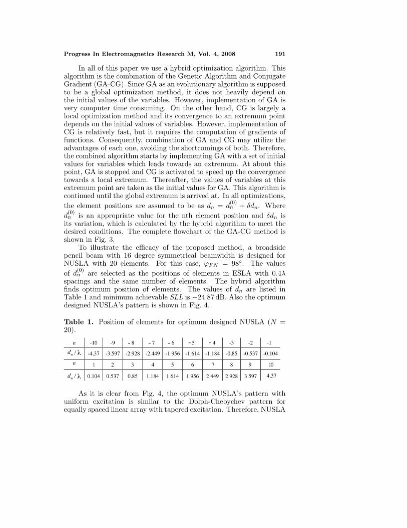
To illustrate the efficacy of the proposed method, a broadsidepencil beam with 16 degree symmetrical beamwidth is designed forNUSLA with 20 elements. For this case, ϕFN = 98◦. The valuesof d

(0)n are selected as the positions of elements in ESLA with 0.4λ

spacings and the same number of elements. The hybrid algorithmfinds optimum position of elements. The values of dn are listed inTable 1 and minimum achievable SLL is −24.87 dB. Also the optimumdesigned NUSLA’s pattern is shown in Fig. 4.

Table 1. Position of elements for optimum designed NUSLA (N =20).

n -10 -9 -3 -2 -1

/nd -4.37 -3.597 -2.928 -2.449 -1.956 -1.614 -1.184 -0.85 -0.537 -0.104

n

/nd 0.104 0.537 0.85 1.184 1.614 1.956 2.449 2.928 3.597 4.37

λ

λ

1 2 3 4 5 6 7 8 9 10

8 7 6 5 4- - - - -

As it is clear from Fig. 4, the optimum NUSLA’s pattern withuniform excitation is similar to the Dolph-Chebychev pattern forequally spaced linear array with tapered excitation. Therefore, NUSLA


Set appropriate values ( (0)nd ) and

initial population ( nd )

Set the GA parameters (such as population size and value, generation numbers, cross

over type, mutation rate, selection type and stopping criterions)

START

Optimization criteria obtained?

No

Cross over and mutation usage to produce new nd from initial population by GA

(a generation production)

Related Fitness Function (Error Function) calculation and best individuals (having the

lowest error value) selection

CG runs

Maximum iteration criterion is exceeded

Yes

END

No

NoSet obtained extremum point as initial population

Generation number is exceeded?

Optimization criteria obtained?

No

The obtained best individual is set as initial point

Yes

Yes

Yes

Figure 3. The complete flowchart of the GA-CG method.


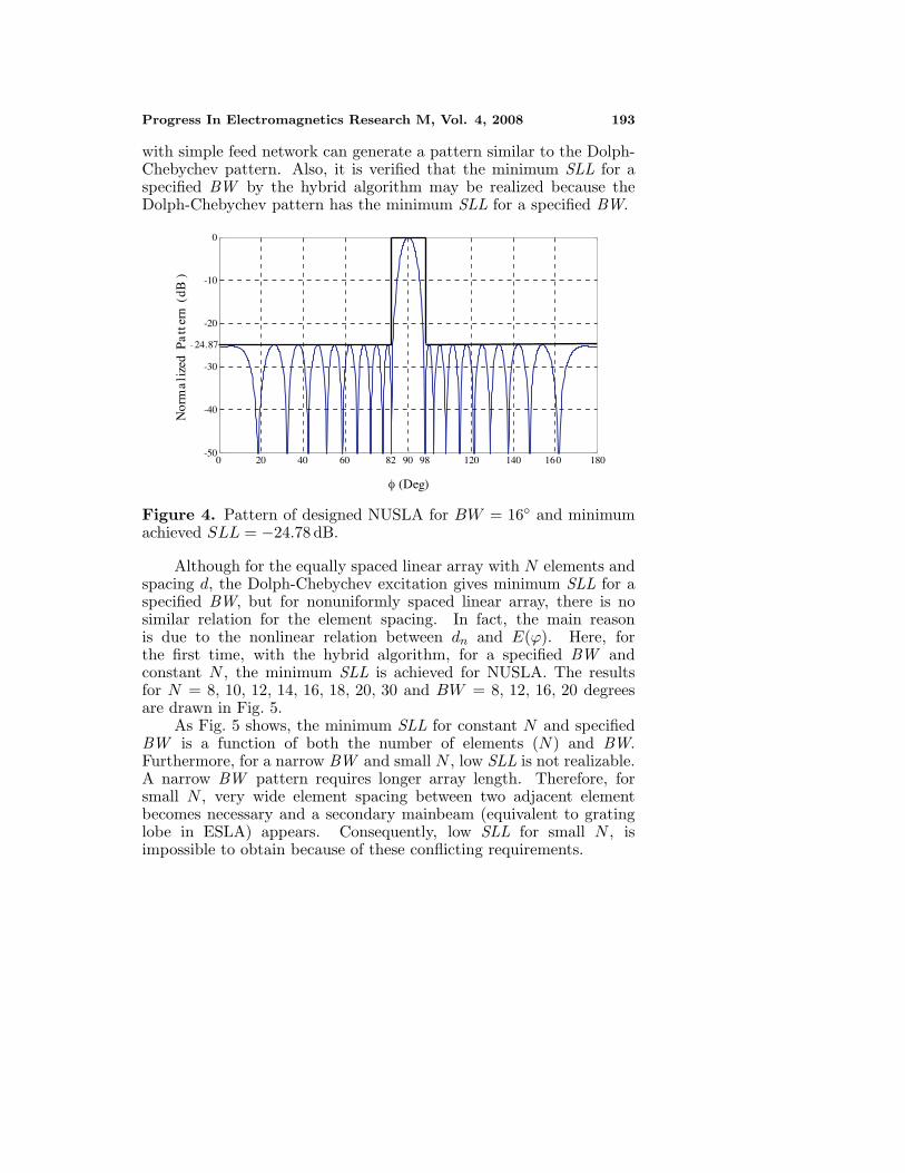
with simple feed network can generate a pattern similar to the Dolph-Chebychev pattern. Also, it is verified that the minimum SLL for aspecified BW by the hybrid algorithm may be realized because theDolph-Chebychev pattern has the minimum SLL for a specified BW.

0 20 40 60 120 140 160 1809882 90-50

-40

-30

-20

-10

0

- 24.87

(Deg)

Nor

ma

lize

d P

att

ern

(dB

)

φ

Figure 4. Pattern of designed NUSLA for BW = 16◦ and minimumachieved SLL = −24.78 dB.

Although for the equally spaced linear array with N elements andspacing d, the Dolph-Chebychev excitation gives minimum SLL for aspecified BW, but for nonuniformly spaced linear array, there is nosimilar relation for the element spacing. In fact, the main reasonis due to the nonlinear relation between dn and E(ϕ). Here, forthe first time, with the hybrid algorithm, for a specified BW andconstant N , the minimum SLL is achieved for NUSLA. The resultsfor N = 8, 10, 12, 14, 16, 18, 20, 30 and BW = 8, 12, 16, 20 degreesare drawn in Fig. 5.

As Fig. 5 shows, the minimum SLL for constant N and specifiedBW is a function of both the number of elements (N) and BW.Furthermore, for a narrow BW and small N , low SLL is not realizable.A narrow BW pattern requires longer array length. Therefore, forsmall N , very wide element spacing between two adjacent elementbecomes necessary and a secondary mainbeam (equivalent to gratinglobe in ESLA) appears. Consequently, low SLL for small N , isimpossible to obtain because of these conflicting requirements.


8 10 12 14 16 18 20 22 24 26 28 300

2.5

5

7.5

10

12. 5

15

17.5

20

22. 5

25

27.5

30

32. 5

35

N

|Min

imum

ach

ieva

ble

SLL

(dB

)|

BW = 8 Deg

BW = 12 Deg

BW = 16 Deg BW = 20 Deg

Figure 5. (Minimum achievable SLL)-N curves with BW asparameter for NUSLA.

4. NUSLA DESIGN FOR SPECIFIED DIRECTIVITYAND SIDELOBE LEVEL

In Section 3, we designed for the minimum SLL and tightly specifiedbeamwidth. However, sometimes designers may desire to designNUSLA for a specified directivity. The narrowest beamwidth may bejudged as maximum directivity, but it is not always the case. Whenthe array length of equally spaced linear array with mainbeam inϕ0 direction, increases (for constant N), beamwidth decreases anddirectivity increases until the element spacing (d) exceeds λ/(1 +| cosϕ0|) and grating lobe appears [19]. With the grating lobeappearance, the beamwidth still decreases but directivity falls sorapidly that the inverse relation between D and beamwidth is not truein this condition. For the broadside pattern (ϕ0 = 90◦), when d exceeds1λ, this situation happens. But what happens for the nonuniformlyspaced linear array in a similar condition? Before answering thisquestion, we would like to show that the NUSLA design for a constantspecified BW should not be interpreted as NUSLA design for constantD.

4.1. Directivity and Beamwidth Relationship

To show the relationship between directivity and BW for the designedNUSLA in Section 3 which its results is shown in Fig. 5, directivity is


8 10 12 14 16 18 20 22 24 26 28 307.5

10

12.5

15

17.5

20

22.5

25

27.5

30

32.5

35

N

Dir

ecti

vity

BW=12 Deg BW=20 DegBW=16 DegBW=8 Deg

Figure 6. Directivity-N curves with BW as parameter for thedesigned NUSLA in Section 3 for the minimum SLL and tightlyspecified BW .

calculated by Eq. (7) and plotted in Fig. 6. In this figure, D is drawnversus N and BW is a parameter. As we expect, the directivity for apattern with constant BW, is not constant and changes with N andspacing. Also, for instance, for BW = 8◦, when N is smaller than 16,the array directivity becomes smaller than the directivity of array withthe same number of elements but BW = 12◦. These results show thatin the case of array pattern design for a specified directivity, sometimesBW is not a good criterion.

Therefore, we propose the hybrid algorithm to design NUSLA withthe specified D and bearable SLL.

Fitness function (error function) for this problem defined as:

errorD−SLL=errorD+errorSLL

errorD=|D−Ddesired|2 (15)

errorSLL=

|SLL(dB)−SLLthreshold(dB)|2

if SLL(dB) > SLLthreshold(dB)0 else

where Ddesired is the desired directivity and SLLthreshold is the bearableSLL in dB.

For example we design NUSLA with N = 14, Ddesired = 22 forSLLthreshold = −15 dB. Also, a Minimum Allowable Distance (MAD)between two adjacent elements is included to reduce mutual coupling.


Then, the hybrid algorithm should solve the problem with the MADconstraint according to:

|dn − dn±1| > MAD (16)

Here, we set MAD = 0.5λ. The hybrid algorithm solved this problem.The resultant directivity is 22.1 and SLL is −15.5 dB. The values of dnare listed in Table 2. Because of symmetry, only positions of right sideelements are listed. Also, the optimally designed NUSLA’s pattern isshown in Fig. 7.

Table 2. Position of right side elements for optimum designed NUSLA(N = 14).

n

/nd λ

1 2 3 4 5 6 7

0.31 1.1 1.92 2.92 3.72 4.74 5.56

0 15 30 45 60 75 90 105 120 135 150 165 180-50

-40

-30

-20

-10

0

-15.46

(Deg)

Nor

mal

ized

Pat

tern

( dB

)

φ

Figure 7. Pattern of designed NUSLA (N = 14) with D = 22.1 andSLL = −15.46 dB.

In second example, we design a NUSLA with N = 20, Ddesired =20 and SLLthreshold = −21 dB. Here, MAD = 0.35λ is assumed. Thehybrid algorithm solved this problem. The resultant directivity is 20and SLL is −22.6 dB. The values of dn are listed in Table 3. Becauseof symmetry, only position of right side elements are listed. Also, theoptimally designed NUSLA’s pattern is shown in Fig. 8.


Table 3. Position of right side elements for optimum designed NUSLA(N = 20).

n

/nd λ

1 2 3 4 5 6 7 8 9 10

0.2 0.58 1.03 1.43 1.85 2.37 2.87 3.47 4.26 5.06

0 15 30 45 60 75 90 105 120 135 150 165 180-50

-40

-30

-2 0

-10

0

-22.6

(Deg)

Nor

mal

ized

Pat

tern

(d

B )

φ

Figure 8. Pattern of designed NUSLA (N = 20) with D = 20 andSLL = −22.6 dB.

It is necessary to mention that, there is a trade-off between D andSLL. Whenever the desired D is high, a low SLL is difficult to obtain.

We can enhance the value of directivity error or SLL error inEq. (15) by weighting functions as follow:

errorD−SLL = WDerrorD + WSLLerrorSLL (17)

where, WD and WSLL are the weights for directivity and SLL,respectively.

Therefore, with proper weighting, Eq. (17) may be used to designNUSLA for a desired D and bearable SLL or a desired SLL andthreshold D.

4.2. Directivity and Length Relationship for NUSLA

To answer the question about NUSLA’s directivity behavior when fora fixed number of elements, the array length increases, average elementspacing defined in Eq. (12), should be used. For the fixed number ofelements which is assumed 11, the array length slightly become longer,


and dave from Eq. (12) becomes wider. And then for each new length(or new dave), with the hybrid algorithm, the optimum NUSLA isdesigned to show a suitable directivity in comparison with ESLA withthe same length and same number of elements.

Here, with the hybrid algorithm, for some dave, NUSLA is designedto satisfy some constraints as follows:

1. The whole length of NUSLA should be exactly equal to thespecified value ((N − 1)dave) as:

|dM − d−M | = (N − 1)dave (18)

2. For dave/λ ≤ 0.5, MAD = dave and for dave/λ > 0.5,MAD = 0.5λ.

The desired directivity is specified to be as ESLA’s directivity(Duniform) for dave/λ ≤ 0.9 and bearable SLL equal to −13 dB.But for dave/λ > 0.9, that the grating lobe appears for ESLA anddirectivity falls rapidly, the NUSLA design purpose is reasonable SLLand maximum achievable directivity. Therefore, Eq. (17) with suitableWD and WSLL can be used as a fitness function. The elements ofNUSLA are not necessary to be symmetrically located. Therefore,Eqs. (1) or (2) for E(ϕ) may be used. The hybrid algorithm foundoptimum NUSLA for some dave and N = 11. Their D and SLL areplotted in Figs. 9 and 10, respectively. Also, in these figures, thedirectivity and SLL of ESLA for element spacing dave and N = 11 arealso shown. These results show that NUSLA for 1.4 > dave/λ > 0.9still results in good directivity and reasonable SLL.

0. 4 0.5 0.6 0.7 0.8 0.9 1 1.1 1.2 1.3 1.4 1.528

9

10

11

12

13

14

15

16

17

18

19

dave

/

Dir

ecti

vity

NUSLA

ESLA

λ

Figure 9. Comparison of D of ESLA and NUSLA having the sameaverage element spacing for N = 11.


0.4 0.5 0.6 0.7 0.8 0.9 1 1.1 1.2 1.3 1.4 1.52-15

-14

-13

-12

-11

-10

-9

-8

-7

-6

-5

dave

/

Sid

e L

obe

Lev

el (

dB

)

NUSLA

ESLAgrat ing lobe appear ance

in ESLA

λ

Figure 10. Comparison of SLL of ESLA and NUSLA having thesame average element spacing for N = 11.

The pattern of optimum NUSLA for dave = 1.2λ and that ofESLA with the spacing dave = 1.2λ between its elements is shown inFig. 11. The element positions for NUSLA and ESLA are also shownin Fig. 12. As we can see, the minimum distance between elements is0.68λ and maximum distance is 2.77λ to ensure the reduction of MCamong elements.

5. NONUNIFORMLY SPACED PARALLEL DIPOLEARRAY DESIGN

In this section, with the obtained results in Sections 3 and 4, theNUSLA with dipole elements will be designed.

5.1. Dipole Array Design for Specified BW and MinimumAchievable SLL

Consider an array of half wavelength dipoles with N = 16 as shownin Fig. 2. It is desired to have BW = 12◦ with MAD = 0.5λ. Withreference to Fig. 5, it is found that minimum achievable SLL is about−19.5 dB. The optimum position of elements for this case, which wascalculated by the hybrid algorithm, is listed in Table 4. Because ofsymmetry only the positions of right side elements are listed.


0 15 30 45 60 75 90 105 120 135 150 165 180-25

-20

-15

-10

-5

0

-11.6

(Deg)

No

rmal

ized

Pat

tern

( d

B )

NUSLAESLA

φ

Figure 11. Comparison of radiation pattern of ESLA and NUSLAfor dave = 1.2λ and N = 11.

-6 -4.8 -3.6 -2.4 -1.2 0 1.2 2.4 3.6 4.8 6

d n /

-5.19 -3.6 -0.83 -0.11 0.57 1.44 2.29 2.96 4.03

NUSLA

E SL A

-6 6

λ

Figure 12. Comparison of element positions in ESLA and NUSLAfor dave = 1.2λ and N = 11.

Table 4. Positions of right side elements for optimum designed paralleldipole array (N = 16).

n

/nd 0.252 0.793 1.436 1.992 2.616 3.44 4.272 5.134λ

1 2 3 4 5 6 7 8

The whole array pattern (Ew) is defined as:

Ew = E · Ee (19)

where E is the array factor (array with isotropic elements) defined inEqs. (1), (2), (3) and (4) and Ee is the element pattern of the half


wavelength dipole shown in Fig. 2, defined as:

Ee = cos(π

2cos θ

)/ sin θ (20)

The whole pattern of the designed parallel dipole array is drawn in thehorizontal plane (θ = 90◦) in Fig. 13. As we expected, the elementpattern does not change the first null position and SLL from those ofthe array factor.

0 15 30 45 60 75 90 105 120 135 150 165 1809684

0

(Deg)

Nor

mal

ized

Hor

izon

tal P

lane

Pat

tern

(dB

)

Figure 13. The horizontal plane pattern of the designed paralleldipole array (N = 16, BW = 12◦).

5.2. Dipole Array Design for Specified Directivity and SLL

Consider the dipole array in Section 5.1 with N = 12. It is desiredto have a pattern with Dw = 25 (13.98 dBi) and minimum achievableSLL with SLLthreshold = −17 dB for MAD = 0.55λ.

We use the result of Section 4 and Eq. (8) to design the arrayfactor with desired directivity. For half wavelength dipoles, De = 1.64.

Table 5. Position of right side elements for optimum designed paralleldipole array (N = 12).

n

/nd λ

1 2 3 4 5 6

0.28 0.84 1.41 2.09 2.88 3.69


The Eq. (8) gives D = Dw/De = 25/1.64 = 15.24, then withthis desired directivity and Eq. (15), the hybrid algorithm will find theoptimum dn for symmetrical geometry. Because of symmetry only theright side element positions are listed in Table 5. The achieved D is15.5 and SLL = −18.52 dB. The whole directivity is 25.42 (14.05 dBi).The whole directivity in the horizontal plane is drawn in Fig. 14.

0 15 30 45 60 75 90 105 120 135 150 165 180

0

5

10

14.0515.27

(Deg)

Hor

izon

tal P

lane

Dir

ecti

vity

(dB

i)

Directivity (Eq. (8))Directivity (Eq. (9))Simulation (Feko)

Figure 14. The directivity of the designed parallel dipole array,calculated by Eq. (8), Eq. (9) and simulation.

This array is simulated by fullwave software, FEKO program [26].For excitation, voltage sources with input impedances of 125 ohm areused. The directivity of simulated array in the horizontal plane isdrawn in Fig. 14. As we can see, for the peak directivity at ϕ = 90◦,there is 1.22 dBi difference between simulation and design values. Thisdifference is due to the fact that Eq. (8) is an approximate formula. Butit is acceptable. Also to show the accuracy of Eq. (9), in comparisonwith Eq. (8), the directivity of the designed array, is calculated byEq. (9) and plotted in Fig. 14. There is a good agreement betweenits results and simulation results. In Section 5.3, Eq. (9) will be usedfor the array design. It should be mentioned that MC causes the firstsidelobe in the simulation results to become greater than our designvalue.

5.3. Dipole Array Design for Bearable Coupling BetweenAdjacent Elements

In Section 5.2, the nonuniformly spaced dipole array was designed forthe specified D and SLL with some constraints on element positions.The average element spacing and MAD were introduced in this paper


as some criteria to limit coupling among elements. But these criteriaare not accurate enough. In [27–29], MC is defined. The couplingbetween two transmitter antennas is defined in [24] as:

C21 =P2

P1=

|S21|2

1 − |S11|2(21)

where P2 is the power received by antenna 2 and P1 is the powerdelivered by antenna 1. This parameter is a better criterion thanMAD or dave. However, for NUSLA, the S-parameters computationfor various distances among elements is a very cumbersome and timeconsuming problem. Since the array geometry is not kept fixed in theoptimization process, the S-parameters should be computed in eachrun of GA-CG. On the other hand, the S-parameters computation isvery difficult and their relations are scarce and imprecise. The arraysimulation by a fullwave simulator like IE3D is the best procedure,but by using the simulator for data generation for GA-CG, the CPUtime may increase abruptly. To overcome this problem, we proposea NN-based model for the S-parameters estimation. Although NN isused for solving some various antenna problems [30–33], NN using forthe calculation of S-parameters is proposed for the first time.

We propose a Radial Basis Function Neural Network (RBFNN)with three layers. For the training stage, we should generate the datawith a fullwave simulator like IE3D. As a good approximation, onlythe adjacent element effects are included in the simulation. Sincethe maximum coupling occurs between two neighboring elements,we consider an array of three half wavelength dipoles with variableelement spacing d1 and d2 as shown in Fig. 15 and simulateit by IE3D at 3 GHz. Computed S-parameters are used forRBFNN training. The values of d1 and d2 are selected from theset{10, 20, 30, 40, 50, 60, 70, 80, 90, 100, 110, 120, 130, 160, 200} allin mm. For instance, one possible case for (d1, d2) is (40 mm, 50 mm).About 15× 15 = 225 simulations are performed and S -parameters areobtained to train RBFNN. After the training and testing, RBFNNmay be used to estimate S -parameters between each two adjacentelements of NUSLA for element spacing from [10–200] all in millimeterwith 0.1 mm precision. In order to implement the proposed RBFNNmodel, the Neural Networks Toolbox of MATLAB, is used. Themain properties of the RBFNN of this toolbox are the utilizationof Gaussian distribution transfer functions in the hidden layer, purelinear transfer functions in the output layer, and the least meansquares algorithm for training in the output layer and optimization ofweights between neurons. For the hidden layer, the center of Gaussiandistribution transfer functions is calculated by k-means algorithm. The


trained RBFNN has 255 neurons in the hidden layer and 6 neurons inoutput layer (real and imaginary parts of S-parameters are separatelyproduced by RBFNN). This NN-based model is used by the hybridoptimization method. For instance, when the optimizer is to calculateC24 and C34, it gives (d24 = |d2−d4|, d34 = |d3−d4|) to RBFNN whichgenerates S44, S24 and S34 and then C24 and C34 by Eq. (21) can becomputed. Block diagram in Fig. 16 shows the proposed process.

d1 d2

Left adjacent Right adjacent

Figure 15. Three half wavelength dipoles with variable elementspacing d1 and d2.

R BFNNS-parameters : with two adjacent elements

Coupling with:

R ight adjacent,

L eft adjacent

d1

d2

Figure 16. S-parameters estimation by NN and computation ofcoupling with two adjacent elements.

Table 6. The optimum position of right side dipoles dn/λ obtainedby GA-CG-NN.

n

/nd λ

1 2 3 4 5 6 7 8

0.26 0.74 1.25 1.73 2.25 2.75 3.35 4.28

Now, we can design NUSLA for a specified Cij between twoadjacent elements. The fitness function (error function) is defined as:

errorD−SLL−C = WDerrorD + WSLLerrorSLL + WCerrorC (22)

The first two terms on the right side are the same as Eq. (17) anderrorC shows the deviation from the bearable coupling and may bedefined in various forms. WC is an enhancing coefficient, like WD andWSLL.


Here, for parallel half wavelength dipole array with N = 16, it isdesired to have SLL = −16 dB. Also, D is to be greater than 30 and|max(Cij)| > 29 dB.

With these conditions, the optimization with GA-CG-NN methodis performed. For the directivity computation, Eq. (9) which isaccurate sufficiently was used. The optimum position of right sideelements is listed in Table 6 and Cij are listed in Table 7. The achievedpeak directivity is 36.4 or 15.61 dBi and achieved SLL is −16.92 dB.Also, |max(Cij)| = 29.4 is achieved. The directivity in the θ = 90◦plane (horizontal plane) is shown in Fig. 17.

This array is simulated by FEKO for f = 3 GHz with unit voltagesources with 125 ohm impedances as excitations. The simulationdirectivity in the horizontal plane is shown in Fig. 17. The peakdirectivity is D = 15.61 dBi or D = 36.4. The values of Cij derivedfrom S-parameters by IE3D, are listed in Table 7 and compared withNN results. The value of SLL is −16.5 dB. As we expected, by keepingcoupling among elements below a specified bearable value, its effectdecreases. This is clearly seen by comparing Fig. 14 and Fig. 17especially in the first sidelobe and mainbeam. The data reportedin Table 7 verify the accuracy of the used RBFNN model for thecalculation of S-parameters and then Cij .

Table 7. Coupling in dB between each two adjacent elements of theoptimized dipole array which is computed by NN model and IE3D.

n Cn,n-1(dB) (NN) Cn,n-1(dB) (Simulation) Cn,n+1(dB)(NN) Cn,n+1(dB)(Simulation)

-7 -38.8156 -39.2257 -29.5123 -31.6374

-6 -31.3448 -31.9237 -29.4018 -31.7746

-5 -29.8641 -31.8301 -30.0084 -31.9677

-4 -29.7291 -31.9356 -29.5219 -32.0627

-3 -29.4741 -32.0658 -29.5617 -31.8354

-2 -29.5741 -31.8354 -29.4556 -32.1938

-1 -29.5386 -32.2047 -29.7186 -31.9496

1 -29.7291 -31.9496 -29.5219 -32.2047

2 -29.4741 -32.1938 -29.5617 -31.8354

3 -29.5741 -31.8354 -29.4556 -32.0658

4 -29.5386 -32.0627 -29.7186 -31.9356

5 -30.0176 -31.9677 -29.8533 -31.8301

6 -29.3907 -31.7746 -31.3384 -31.9237

7 -29.4981 -31.6374 -38.8571 -39.2257


0 15 30 45 60 75 90 105 120 135 150 165 180-40

-35

-30

-25

-20

-15

-10

-5

0

5

10

20

15.61

-1.6

(Deg)

Dir

ecti

vity

(d

Bi)

Directivity (Eq. (9))Directivity (Simulation)

φ

Figure 17. Directivity of optimized NUSLA in the horizontal plane(θ = 90◦) from Eq. (9) and simulation in FEKO.

6. CONCLUSION

In this paper, nonuniformly spaced linear array was investigatedrigoriously. By the combination of GA-CG as an optimizer, someimportant problems were solved for this type of arrays. For thefirst time the relation between SLL-BW and number of elements forNUSLA were derived and plotted in the design curves. The NUSLAwas designed for fixed N and BW to have minimum possible SLL.Also, for the first time, directivity was included in NUSLA designand NUSLA was optimally designed for specified directivity to havebearable (threshold) SLL. By using average element spacing, therelation between array length, directivity and SLL was derived forNUSLA and compared with ESLA with uniform excitation. As aresult, NUSLA for wider average element spacing (e.g., wider than 1λ),still had a good performance whereas ESLA’s performance degradebadly for such element spacing. As a practical design, parallel halfwavelength dipole array was designed for specified BW and minimumachievable SLL using the results of arrays of isotropic elements. Thenthis array was designed for specified directivity and SLL with someconstraint on the minimum distance among elements. For directivitycomputation, multiplication of array factor directivity and elementdirectivity was used with good accurate results. The dipole arraywas designed for specified directivity and SLL and a novel constraint,bearable coupling among elements. Here, Neural Network model wasused for the calculation of S-parameters and coupling among elements.


The obtained results show the efficacy of the hybrid algorithm.These results are general and may be used for nonuniformly spacedlinear array with arbitrary elements.

ACKNOWLEDGMENT

This work is supported in part by Iran Telecommunication ResearchCenter (ITRC).

REFERENCES

1. Unz, H., “Linear arrays with orbitrarily distributed elements,”IRE Trans. Antennas Propagat., Vol. 8, 222–223, Mar. 1960.

2. Skolnik, M. I., J. W. Sherman III, and G. Nemhauser, “Dynamicprogramming applied to unequally spaced arrays,” IEEE Trans.Antennas Propagat., Vol. 12, 35–43, Jan. 1964.

3. Mailloux, R. J. and E. Cohen, “Statistically thinned arrays withquantized element weights,” IEEE Trans. Antennas Propagat.,Vol. 39, 436–447, Apr. 1991.

4. Haupt, R. L., “Thinned arrays using genetic algorithms,” IEEETrans. Antennas Propagat., Vol. 42, No. 7, 993–999, July 1994.

5. Donelli, M., S. Caorsi, and F. DeNatale, M. Pastorino, andA. Massa, “Linear antenna synthesis with a hybrid geneticalgorithm,” Progress In Electromagnetics Research, PIER 49, 1–22, 2004.

6. Mahanti, G. K., N. Pathak, and P. Mahanti, “Synthesis ofthinned linear antenna arrays with fixed sidelobe level using realcoded genetic algorithm,” Progress In Electromagnetics Research,PIER 75, 319–328, 2007.

7. Meijer, C. A., “Simulated annealing in the design of thinnedarrays having low sidelobe levels,” Proc. South African Symp.Communication and Signal Processing, 361–366, 1998.

8. Razavi, C. A. and K. Forooraghi, “Thinned arrays using patternsearch algorithms,” Progress In Electromagnetics Research,PIER 78, 61–71, 2008.

9. Harrington, R. F., “Sidelobe reduction by nonuniform elementspacing,” IRE Trans. Antennas Propagat., Vol. 9, 187, Mar. 1961.

10. Andreasan, M. G., “Linear arrays with variable interelementspacings,” IEEE Trans. Antennas Propagat., Vol. 10, 137–143,Mar. 1962.


11. Ishimaru, A., “Theory of unequally-spaced arrays,” IRE Trans.Antennas Propagat., Vol. 10, 691–702, Nov. 1962.

12. Kumar, B. P. and G. R. Branner, “Design of unequally spacedarrays for performance improvement,” IEEE Trans. AntennasPropagat., Vol. 47, No. 3, 511–523, Mar. 1999.

13. Kumar, B. P. and G. R. Branner, “Generalized analyticaltechnique for the synthesis of unequally spaced arrays with linear,planar, cylendrical or spherical geometry,” IEEE Trans. AntennasPropagat., Vol. 53, No. 2, 621–634, Feb. 2005.

14. Chen, K., Z. He, and C. Han, “A modified real GA for the sparselineararray synthesis with multiple constraints,” IEEE Trans.Antennas Propagat., Vol. 54, No. 7, 2169–2173, July 2006.

15. Zhang, Y. F. and W. Cao, “Array pattern synthesis based onweighted biorthogonal modes,” J. of Electromagn. Waves andAppl., Vol. 20, No. 10, 1367–1376, 2006.

16. Lee, K.-C. and J.-Y. Jhang, “Application of particle swarmalgorithm to the optimization of unequally spaced antennaarrays,” J. of Electromagn. Waves and Appl., Vol. 20, No. 14,2001–2012, 2006.

17. Ayestaran, R. G., F. Las-Heras, and J. A. Martınez, “Nonuniform-antenna array synthesis using neural networks,” J. ofElectromagn. Waves and Appl., Vol. 21, No. 8, 1001–1011, 2007.

18. Kazemi, S. and H. R. Hassani, “Performance improvement inamplitude synthesis of unequally spaced array using least meansquare method,” Progress In Electromagnetics Research B, Vol. 1,135–145, 2008.

19. Stutzman, L. and G. A. Thiele, Antenna Theory and Design, 120–121, John Wiley & Sons, 1998.

20. Bray, M. G., D. H. Werner, D. W. Boeringer, and D. W. Machuga,“Optimization of thinned aperiodic linear phased arrays usinggenetic algorithms to reduce grating lobes during scanning,” IEEETrans. Antennas Propagat., Vol. 50, No. 12, 1732–1742, Dec. 2002.

21. Bray, M. G., D. H. Werner, D. W. Boeringer, and D. W. Machuga,“Thinned aperiodic, linear phased array optimizationfor reducedgrating lobes during scanning with input impedance bounds,”IEEE International Symposium on Antennas and PropagationDigest, Vol. 3, 688–691, Boston, MA, July 2001.

22. Bossard, J. A., D. H. Werner, and M. G. Bray, “Efficientimpedance interpolation and pattern approximation for linearmi-crostrip phased arrays using neural networks,” USNC/URSI Na-tional Radio Scicnce Meeting, 102, Columbus, OH, June 2003.


23. DeLuccia, C. S. and D. H. Werner, “Nature-based designof aperiodic linear arrays with broadband elements using acombination of rapid neural network estimation techniques andgenetic algorithms,” IEEE Antennas and Propagation Magazine,Vol. 49, No. 5, 13–23, Oct. 2007.

24. Daniel, J. P., “Mutual coupling between antennas for emission orreception-application to passive and active dipoles,” IEEE Trans.Antennas Propagat., Vol. 22, No. 2, 347–349, 1973.

25. Taylor, T. T., “Design of line-source antennas for narrow beamwidth and low side lobes,” IRE Trans. Antenna Propagat., Vol. 3,16–28, 1955.

26. FEKO 5.2, www.feko.info27. Zhu, Y.-Z., Y.-J. Xie, Z.-Y. Lei, and T. Dang, “Array a novel

method of mutual coupling matching for array antenna design,”J. of Electromagn. Waves and Appl., Vol. 21, No. 8, 1013–1024,2007.

28. Zhou, Q., Y. J. Xie, and Z. Chen, “Prediction of equipment-to-equipment coupling through antennas mounted on an aircraft,” J.of Electromagn. Waves and Appl., Vol. 21, No. 5, 653–663, 2007.

29. Ayestaran, R. G., F. Las-Heras, and L. F. Herran, “High-accuracyneural-network-based array synthesis including element coupling,”IEEE Antennas and Wireless Propagation Letters, Vol. 5, 45–48,2006.

30. Mohamed, M. D. A., E. A. Soliman, and M. A. El-Gamal, “Optimization and characterization of electromagneticallycoupled patch antennas using RBF neural networks,” J. ofElectromagn. Waves and Appl., Vol. 20, No. 8, 1101–1114, 2006.

31. Guney, K., C. Yildiz, S. Kaya, and M. Turkmen, “Artificialneural networks for calculating the characteristic impedance of air-suspended trapezoidal and rectangular-shaped microshield lines,”J. of Electromagn. Waves and Appl., Vol. 20, No. 9, 1161–1174,2006.

32. Ayestaran, R. G., J. Laviada, and F. Las-Heras, “Synthesis ofpassive-dipole arrays with a genetic-neural hybrid method,” J. ofElectromagn. Waves and Appl., Vol. 20, No. 15, 2123–2135, 2006.

33. He, Q.-Q., “Conformal array based on pattern reconfigurableantenna and its artificial neural model,” J. of Electromagn. Wavesand Appl., Vol. 22, No. 1, 99–110, 2008.

NONUNIFORMLY SPACED LINEAR ARRAY DESIGN FOR THE SPECIFIED BEAMWIDTH/SIDELOBE LEVEL OR SPECIFIED...

Documents

Transcript of NONUNIFORMLY SPACED LINEAR ARRAY DESIGN FOR THE SPECIFIED BEAMWIDTH/SIDELOBE LEVEL OR SPECIFIED...