Nontransitive Decomposable ConjointMeasurement 1

D. Bouyssou 2

CNRS – LAMSADEM. Pirlot 3

Faculte Polytechnique de Mons

Revised 16 January 2002 – Forthcoming in Journal ofMathematical Psychology

1We wish to thank M. Abdellaoui, J.-P. Doignon, Ch. Gonzales, Th. Marchant,P.P. Wakker and an anonymous referee for their very helpful suggestions and com-ments on earlier drafts of this text. The usual caveat applies. Denis Bouyssougratefully acknowledges the support of the Centre de Recherche de l’ESSEC andthe Brussels-Capital Region through a “Research in Brussels” action grant.

2LAMSADE, Universite Paris Dauphine, Place du Marechal de Lattre de Tas-signy, F-75775 Paris Cedex 16, France, tel: +33 1 44 05 48 98, fax: +33 1 44 0540 91, e-mail: bouyssou@lamsade.dauphine.fr.

3Faculte Polytechnique de Mons, 9, rue de Houdain, B-7000 Mons, Belgium,tel: +32 65 374682, fax: + 32 65 374689, e-mail: pirlot@mathro.fpms.ac.be.Corresponding author.

Abstract

Traditional models of conjoint measurement look for an additive representa-tion of transitive preferences. They have been generalized in two directions.Nontransitive additive conjoint measurement models allow for nontransitivepreferences while retaining the additivity feature of traditional models. De-composable conjoint measurement models are transitive but replace additiv-ity by a mere decomposability requirement. This paper presents general-izations of conjoint measurement models combining these two aspects. Thisallows us to propose a simple axiomatic treatment that shows the pure conse-quences of several cancellation conditions used in traditional models. Thesenontransitve decomposable conjoint measurement models encompass a largenumber of aggregation rules that have been introduced in the literature.

Keywords: Conjoint measurement, Cancellations conditions, Nontransitivepreferences, Decomposable models.

Suggested running title: Nontransitive Decomposable Conjoint Measurement

1 Introduction

Given a binary relation % on a set X = X1 ×X2 × · · · ×Xn, the theory ofconjoint measurement consists in finding conditions under which it is possibleto build a homomorphism between this relational structure and a relationalstructure on R. In traditional models of conjoint measurement % is supposedto be complete and transitive and the numerical representation is sought tobe additive; the desired measurement model is such that:

x % y ⇔n∑

i=1

ui(xi) ≥n∑

i=1

ui(yi) (1)

where ui are real-valued functions on the sets Xi and it is understood thatx = (x1, x2, . . . , xn) and y = (y1, y2, . . . , yn).

Many axiom systems have been proposed in order to obtain such a rep-resentation (Krantz, Luce, Suppes, & Tversky, 1971; Wakker, 1989). Twomain cases arise:

• When X is finite (but of arbitrary cardinality), it is well-known that thesystem of axioms necessarily involves a denumerable number of cancel-lation conditions guaranteeing the existence of solutions to a system of(finitely many) linear inequalities through the use of various versions ofthe theorem of the alternative (see Scott (1964) or Krantz et al. (1971,Chapter 9). For recent contributions, see Fishburn (1996, 1997)).

• When X is infinite the picture changes provided that conditions areimposed in order to guarantee that the structure of X is “close” to thestructure of R and that % behaves consistently in this continuum; thisis traditionally done using either an archimedean axiom together withsome solvability assumption (Krantz et al., 1971, Chapter 6) or impos-ing some topological structure on X and a continuity requirement on% (Debreu, 1960; Wakker, 1989). Under these conditions, it is well-known that model (1) obtains using a finite—and limited—number ofcancellation conditions (for recent contributions, see Gonzales (1996,2000) and Karni and Safra (1998); for an alternative approach, extend-ing the technique used in the finite case to the infinite one, see Jaffray(1974)). As opposed to the finite case, these structural assumptionsallow us to obtain nice uniqueness results for model (1): the functionsui define interval scales with a common unit.

1

In the finite case the axiom system is hardly interpretable and testable. Inthe infinite case, it is not always easy to separate the respective roles of the(unnecessary) structural assumptions from the (necessary) cancellation con-ditions as forcefully argued by Krantz et al. (1971, Chapter 9) and Furkhenand Richter (1991). One possible way out of this difficulty is to study moregeneral models replacing additivity by a mere decomposability requirement.Krantz et al. (1971, Chapter 7) introduced the following decomposable model:

x % y ⇔ F (u1(x1), u2(x2), . . . , un(xn)) ≥ F (u1(y1), u2(y2), . . . , un(yn)) (2)

where F is increasing in all its arguments.When X is denumerable (i.e. finite or countably infinite), necessary and

sufficient conditions for (2) consist in a transitivity and completeness require-ment together with a single cancellation condition requiring that the prefer-ence between objects differing on a single attribute is independent from theircommon level on the remaining n − 1 attributes. In the general case theseconditions turn out to have identical implication when supplemented withthe obviously necessary requirement that a numerical representation existsfor %. Though (2) may appear as exceedingly general when compared to (1),it allows us to deal with the finite and the infinite case in a unified way usinga simple axiom system while imposing nontrivial restrictions on %. The priceto pay is that uniqueness results for model (2) are much less powerful thanwhat they are for model (1), see Krantz et al. (1971, Chapter 7). It shouldbe finally observed that proofs for model (2) are considerably simpler thanthey are for model (1). A wide variety of models “in between” (1) and (2)are studied in Luce, Krantz, Suppes, and Tversky (1990).

Both (1) and (2) imply that % is complete and transitive. Among manyothers, May (1954) and Tversky (1969) (see however the interpretation ofTversky’s results in Iverson and Falmagne (1985)) have argued that the tran-sitivity hypothesis is unlikely to hold when subjects are asked to compareobjects evaluated on several attributes; more recently, Fishburn (1991a) hasforcefully shown the need for models encompassing intransitivities (it shouldbe noted that intransitive preferences have even attracted the attention ofsome economists, see e.g. Chipman (1971) or Kim and Richter (1986)). Tver-sky (1969) was one of the first to propose such a model generalizing (1),known as the additive difference model, in which:

x % y ⇔n∑

i=1

Φi(ui(xi)− ui(yi)) ≥ 0 (3)

2

where Φi are increasing and odd functions.It is clear that (3) allows for intransitive % but implies its completeness.

When attention is restricted to the comparison of objects that only differ onone attribute, (3), as well as (2) and (1), implies that the preference betweenthese objects is independent from their common level on the remaining n−1attributes. This allows us to unambiguously define a preference relation oneach attribute; it is clearly complete. Although model (3) can accommo-date intransitive %, a consequence of the increasingness of the Φi is that thepreference relations defined on each attribute are transitive. This, in partic-ular, excludes the possibility of any perception threshold on each attributewhich would lead to an intransitive indifference relation on each attribute(on preference models with thresholds, allowing for intransitive indifferencerelations, we refer to Fishburn (1985), Pirlot and Vincke (1997), or Suppes,Krantz, Luce, and Tversky (1989)). Imposing that Φi are nondecreasing in-stead of being increasing allows for such a possibility. This gives rise to whatBouyssou (1986) called the “weak additive difference model”.

As suggested by Bouyssou (1986), Fishburn (1990b, 1990a, 1991b) andVind (1991), the subtractivity requirement in (3) can be relaxed. This leadsto nontransitive additive conjoint measurement models in which:

x % y ⇔n∑

i=1

pi(xi, yi) ≥ 0 (4)

where the pi are real-valued functions on X2i and may have several additional

properties (e.g. pi(xi, xi) = 0, for all i ∈ {1, 2, . . . , n} and all xi ∈ Xi).This model is an obvious generalization of the (weak) additive difference

model. It allows for intransitive and incomplete preference relations % aswell as for intransitive and incomplete “partial preferences”. An interestingspecialization of (4) obtains when pi are required to be skew symmetric i.e.such that pi(xi, yi) = −pi(yi, xi). This skew symmetric nontransitive additiveconjoint measurement model implies the completeness of % and that thepreference between objects only differing on some attributes is independentfrom their common level on the remaining attributes.

Fishburn (1991a) gives an excellent overview of these nontransitive mod-els. Several axiom systems have been proposed to characterize them. Fish-burn (1990b, 1991b) gives axioms for the skew symmetric version of (4) bothin the finite and the infinite case. Necessary and sufficient conditions for anonstandard version of (4) are presented in Fishburn (1992b). Vind (1991)

3

gives axioms for (4) with pi(xi, xi) = 0 when n ≥ 4. Bouyssou (1986) givesnecessary and sufficient conditions for (4) with and without skew symmetryin the denumerable case when n = 2.

The additive difference model (3) was axiomatized in Fishburn (1992a)in the infinite case when n ≥ 3 and Bouyssou (1986) gives necessary andsufficient conditions for the weak additive difference model in the finite casewhen n = 2. Related studies of nontransitive models include Croon (1984),Fishburn (1980), Luce (1978) and Nakamura (1997). The implications ofthese models for decision-making under uncertainty were explored in Fish-burn (1990c) (for a different path to nontransitive models for decision makingunder risk and/or uncertainty see Fishburn (1982, 1988)).

It should be noticed that even the weakest form of these models, i.e.(4) without skew symmetry, involves an addition operation. Therefore it isunsurprising that the difficulties that we mentioned concerning the axiomaticanalysis of traditional models are still present here. Except in the specialcase in which n = 2, this case relating more to ordinal than to conjointmeasurement, the various axiom systems that have been proposed involveeither:

• a denumerable set of cancellation conditions in the finite case or

• a finite number of cancellation conditions together with unnecessarystructural assumptions in the general case (these structural assump-tions generally allow us to obtain nice uniqueness results for (4): thefunctions pi are unique up to the multiplication by a common positiveconstant).

The nontransitive decomposable models that we study in this paper may beseen both as a generalization of (2) dropping transitivity and completenessand as a generalization of (4) dropping additivity. In their most general formthey are of the type:

x % y ⇔ F (p1(x1, y1), p2(x2, y2), . . . , pn(xn, yn)) ≥ 0 (5)

where F and pi may have several additional properties, e.g. pi(xi, xi) = 0 orF nondecreasing or increasing in all its arguments.

This type of nontransitive decomposable conjoint models has been in-troduced by Goldstein (1991). They may be seen as exceedingly general.However we shall see that this model and its extensions:

4

• imply substantive requirements on %,

• may be axiomatized in a simple way avoiding the use of a denumerablenumber of conditions in the finite case and of unnecessary structuralassumptions in the general case,

• permit to study the pure consequences of cancellation conditions in theabsence of transitivity, completeness and structural requirements on X,

• are sufficiently general to include as particular cases many aggregationmodels that have been proposed in the literature.

Our project was to investigate how far it was possible to go in terms ofnumerical representations using a limited number of cancellation conditionswithout imposing any transitivity requirement on the preference relation andany structural assumptions on the set of objects. Rather surprisingly, as weshall see, such a poor framework allows us to go rather far.

It should be clear that, in models of type (5), numerical representationsare quite unlikely to possess any “nice” uniqueness properties. This is all themore true that we will refrain in this paper from using unnecessary structuralassumptions on the set of objects. Numerical representations are not studiedhere for their own sake; our results are not intended to provide clues on howto build them. We use them as a framework allowing us to understand theconsequences of a number of requirements on %.

The paper is organized as follows. We introduce our main definitions insection 2. We present the decomposable nontransitive conjoint measurementmodels to be studied in this paper and analyze some of their properties insection 3. We present our main results in section 4. A final section discussesour results and presents directions for future research.

2 Definitions and Notation

A binary relation S on a set A is a subset of A×A; we write aSb instead of(a, b) ∈ S. A binary relation S on A is said to be:

• reflexive if [aSa],

• irreflexive if [Not(aSa)],

• complete if [aSb or bSa],

5

• symmetric if [aSb]⇒ [bSa],

• asymmetric if [aSb]⇒ [Not(bSa)],

• transitive if [aSb and bSc]⇒ [aSc],

for all a, b, c ∈ A.A weak order (resp. an equivalence) is a complete and transitive (resp.

reflexive, symmetric and transitive) binary relation. If S is an equivalenceon A, A/S will denote the set of equivalence classes of S on A.

In this paper % will always denote a binary relation on a set X =∏n

i=1 Xi

with n ≥ 2. Elements of X will be interpreted as alternatives evaluated ona set N = {1, 2, . . . , n} of attributes and % as a “large preference relation”(x % y being read as “x is at least as good as y”) between these alternatives.We note � (resp. ∼) the asymmetric (resp. symmetric) part of %. A similarconvention holds when % is starred, superscripted and/or subscripted.

For any nonempty subset J of the set of attributes N , we denote byXJ (resp. X−J) the set

∏i∈J Xi (resp.

∏i/∈J Xi). With customary abuse of

notation, (xJ , y−J) will denote the element w ∈ X such that wi = xi if i ∈ Jand wi = yi otherwise. When J = {i} we shall simply write X−i and (xi, y−i).

Let J be a nonempty set of attributes. We define the following binaryrelations on XJ :

xJ %J yJ iff (xJ , z−J) % (yJ , z−J), for all z−J ∈ X−J ,

xJ %◦J yJ iff (xJ , z−J) % (yJ , z−J), for some z−J ∈ X−J ,

where xJ , yJ ∈ XJ . When J = {i} we write %i instead of %{i}.If, for all xJ , yJ ∈ XJ , xJ %◦

J yJ implies xJ %J yJ , we say that % isindependent for J . If % is independent for all nonempty subsets of attributeswe say that % is independent. It is not difficult to see that a binary relation isindependent if and only if it is independent for N \{i}, for all i ∈ N (Wakker,1989). A relation is said to be weakly independent if it is independent forall subsets containing a single attribute; while independence implies weakindependence, it is clear that the converse is not true (Wakker, 1989).

6

3 Nontransitive Decomposable Models

In view of the discussion in section 1, the most general model we envisagehere is such that:

x % y ⇔ F (p1(x1, y1), p2(x2, y2), . . . , pn(xn, yn)) ≥ 0 (M)

where pi are real-valued functions on X2i and F is a real-valued function on∏n

i=1 pi(X2i ), i.e. the Cartesian product of the codomains of the functions pi.

As already noted by Goldstein (1991) all binary relations satisfy model(M) when X is finite or countably infinite (see section 4). In particular, itshould be noticed that model (M) does not even imply the reflexivity of %which seems a hardly disputable property of any large preference relation.Requiring (M) together with reflexivity leads to a model that is not muchconstrained however.

In order to further specify model (M), it is useful to consider the additivenontransitive model (4). Like model (M), it does not imply the reflexiv-ity of % unless some additional constraints are imposed on the functionspi. A simple way to obtain the reflexivity of % in model (4) is to imposethat pi(xi, xi) = 0 (Vind, 1991). This also entails that % is independent.Mimicking this additional condition in model (M) leads to model (M0) inwhich:

x % y ⇔ F (p1(x1, y1), p2(x2, y2), . . . , pn(xn, yn)) ≥ 0 (M0)

with pi(xi, xi) = 0, for all xi ∈ Xi and all i ∈ N , and F (0) ≥ 0, abusingnotations in an obvious way.

Keeping in mind the additive nontransitive model (4), it is natural toadd to model (M0) the additional requirement that F is nondecreasing 1 orincreasing in all its arguments. This respectively leads to models (M1) and(M1 ′)

Except when xi = yi, models (M1) and (M1 ′) do not tie together thevalues of pi(xi, yi) and pi(yi, xi). Following what has often been done withmodel (4) (Fishburn, 1990b, 1991b), a simple way to establish such a link isto impose the skew symmetry of each function pi, i.e. pi(xi, yi) = −pi(yi, xi),for all xi, yi ∈ Xi. Adding this condition to (M1) and (M1 ′) leads to (M2)

1Let f be a real-valued function on K ⊆ Rk. We say that f is nondecreasing (resp.increasing) in its jth argument if, for all x ∈ K and all yj ∈ Xj such that (yj , x−j) ∈K, [yj > xj ] ⇒ [f(yj , x−j) ≥ f(x)] (resp. >). Furthermore, when K is such that x ∈ K⇒ −x ∈ K, we say that f is odd if, for all x ∈ K, f(x) = −f(−x).

7

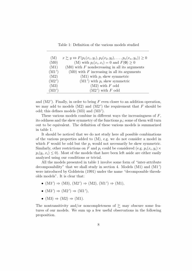
Table 1: Definition of the various models studied

(M) x % y ⇔ F (p1(x1, y1), p2(x2, y2), . . . , pn(xn, yn)) ≥ 0(M0) (M) with pi(xi, xi) = 0 and F (0) ≥ 0(M1) (M0) with F nondecreasing in all its arguments(M1 ′) (M0) with F increasing in all its arguments(M2) (M1) with pi skew symmetric(M2 ′) (M1 ′) with pi skew symmetric(M3) (M2) with F odd(M3 ′) (M2 ′) with F odd

and (M2 ′). Finally, in order to bring F even closer to an addition operation,we may add to models (M2) and (M2 ′) the requirement that F should beodd; this defines models (M3) and (M3 ′).

These various models combine in different ways the increasingness of F ,its oddness and the skew symmetry of the functions pi; some of them will turnout to be equivalent. The definition of these various models is summarizedin table 1.

It should be noticed that we do not study here all possible combinationsof the various properties added to (M), e.g. we do not consider a model inwhich F would be odd but the pi would not necessarily be skew symmetric.Similarly, other restrictions on F and pi could be considered (e.g. pi(xi, yi)×pi(yi, xi) ≤ 0). Most of the models that have been left aside are either easilyanalyzed using our conditions or trivial.

All the models presented in table 1 involve some form of “inter-attributedecomposability” that we shall study in section 4. Models (M1) and (M1 ′)were introduced by Goldstein (1991) under the name “decomposable thresh-olds models”. It is clear that:

• (M3 ′) ⇒ (M3), (M2 ′) ⇒ (M2), (M1 ′) ⇒ (M1),

• (M3 ′) ⇒ (M2 ′) ⇒ (M1 ′),

• (M3) ⇒ (M2) ⇒ (M1).

The nontransitivity and/or noncompleteness of % may obscure some fea-tures of our models. We sum up a few useful observations in the followingproposition.

8

Proposition 1 Let % be a binary relation on X =∏n

i=1 Xi and J ⊆ N .

1. If % satisfies model (M0) then it is reflexive and independent.

2. If % satisfies model (M1) or (M1 ′) then: [xi �i yi for all i ∈ J ⊆ N ]⇒Not[(yJ %J xJ)].

3. If % satisfies model (M2) or (M2 ′) then:

• %i is complete,

• [xi �i yi for all i ∈ J ⊆ N ]⇒ [xJ �J yJ ].

4. If % satisfies model (M3) then it is complete.

5. If % satisfies model (M3 ′) then:

• [xi %i yi for all i ∈ J ⊆ N ]⇒ [xJ %J yJ ],

• [xi %i yi for all i ∈ J ⊆ N, xj �j yj, for some j ∈ J ] ⇒ [xJ �J

yJ ].

Proof of Proposition 11) Obvious since pi(xi, xi) = 0 and F (0) ≥ 0.2) Using obvious notations, xi �i yi implies Not[yi %i xi] so that F (pi(yi,

xi), 0) < 0. Since F (0) ≥ 0 we know that pi(yi, xi) < 0 using the nondecreas-ingness of F . Suppose now that yJ %J xJ so that F ((pi(yi, xi)i∈J),0) ≥ 0.Since pi(yi, xi) < 0 for all i ∈ J and F is nondecreasing, this leads toF (pj(yj, xj),0) ≥ 0 for any j ∈ J , a contradiction.

3) Not[xi %i yi] and Not[yi %i xi] imply F (pi(xi, yi), 0) < 0 and F (pi(yi,xi), 0) < 0. Since F (0) ≥ 0 and F is nondecreasing, we have pi(xi, yi) < 0and pi(yi, xi) < 0, which contradicts the skew symmetry of pi. Hence %i iscomplete. Observe that xi �i yi is equivalent to F (pi(xi, yi), 0) ≥ 0 andF (pi(yi, xi), 0) < 0. Since F (0) ≥ 0 we know that pi(yi, xi) < 0 using thenondecreasingness of F . The skew symmetry of pi implies pi(xi, yi) > 0 >pi(yi, xi) and the desired property easily follows using the nondecreasingnessof F .

4) Obvious from the skew symmetry of pi and the oddness of F .5) Since F is increasing and odd, we have xi %i yi ⇔ pi(xi, yi) ≥ 0. The

desired properties easily follow from the increasingness of F and F (0) = 0.2

9

Except for (M3 ′), the monotonicity properties of our models linking %and %i may seem disappointing. Such properties should however be analyzedkeeping in mind that we are dealing with possibly nontransitive and/or non-complete preferences. In such a framework, some “obvious properties” maynot always be desirable. For example, when the relations ∼i are not transi-tive, it may not be reasonable to impose that:

[xi ∼i yi for all i ∈ J ]⇒ [xJ ∼J yJ ]

which would forbid any interaction between separately non-noticeable dif-ferences on each attribute (on this point see Gilboa and Lapson (1995) orPirlot and Vincke (1997)). Furthermore, as we shall see in section 4, nicemonotonicity properties obtain when “preference differences” are adequatelymodelled on each attribute (see lemma 3).

4 Results

4.1 Axioms

This section studies the variety of nontransitive decomposable models intro-duced in section 3. The intuition behind these models is that the functionspi “measure” preference differences between elements of Xi, these differencesbeing aggregated using F .

Wakker (1988, 1989) has powerfully shown how the consideration of in-duced relations comparing “preference differences” on each attribute mayilluminate the analysis of conjoint measurement models. We follow the samepath. Notice however that, although we use similar notation, our definitionsof relations comparing preference difference differ from his because of theabsence of structural assumptions on X.

Given a binary relation % on X, we define the binary relation %∗i on X2

i

letting, for all xi, yi, zi, wi ∈ Xi,

(xi, yi) %∗i (zi, wi) iff

[for all a−i, b−i ∈ X−i, (zi, a−i) % (wi, b−i)⇒ (xi, a−i) % (yi, b−i)].

Intuitively, if (xi, yi) %∗i (zi, wi), it seems reasonable to conclude that the

preference difference between xi and yi is not smaller that the preferencedifference between zi and wi. Notice that, by construction, %∗

i is transitive.

10

Contrary to our intuition concerning preference differences, the definitionof %∗

i does not imply that the two “opposite” differences (xi, yi) and (yi, xi)are linked. Henceforth we introduce the binary relation %∗∗

i on X2i letting,

for all xi, yi, zi, wi ∈ Xi,

(xi, yi) %∗∗i (zi, wi) iff [(xi, yi) %∗

i (zi, wi) and (wi, zi) %∗i (yi, xi)].

It is easy to see that %∗∗i is transitive and reversible, i.e. (xi, yi) %∗∗

i (zi, wi)⇔(wi, zi) %∗∗

i (yi, xi).The relations %∗

i and %∗∗i both appear to capture the idea of comparison

of preference differences between elements of Xi induced by the relation %.Hence, they are good candidates to serve as the basis of the definition of thefunctions pi. They will not serve well this purpose however unless they arecomplete. Hence, the introduction of the following two conditions.

Let % be a binary relation on a set X =∏n

i=1 Xi. For i ∈ N , this relationis said to satisfy:

RC1i if

(xi, a−i) % (yi, b−i)and

(zi, c−i) % (wi, d−i)

⇒

(xi, c−i) % (yi, d−i)or(zi, a−i) % (wi, b−i),

RC2i if

(xi, a−i) % (yi, b−i)and

(yi, c−i) % (xi, d−i)

⇒

(zi, a−i) % (wi, b−i)or(wi, c−i) % (zi, d−i),

for all xi, yi, zi, wi ∈ Xi and all a−i, b−i, c−i, d−i ∈ X−i. We say that % satisfiesRC1 (resp. RC2) if it satisfies RC1i (resp. RC2i) for all i ∈ N .

Condition RC1i implies that any two ordered pairs (xi, yi) and (zi, wi) ofelements of Xi are comparable in terms of the relation %∗

i . Indeed, it is easyto see that supposing Not[(xi, yi) %∗

i (zi, wi)] and Not[(zi, wi) %∗i (xi, yi)]

leads to a violation of RC1i. Similarly, RC2i implies that the two oppositedifferences (xi, yi) and (yi, xi) are linked. In terms of the relation %∗

i , it saysthat if the preference difference between xi and yi is not at least as largeas the preference difference between zi and wi then the preference differencebetween yi and xi should be at least as large as the preference differencebetween wi and zi.

We summarize these observations in the following lemma; we omit itsstraightforward proof.

11

Lemma 1 We have:

1. [%∗i is complete]⇔ RC1i,

2. RC2i ⇔[for all xi, yi, zi, wi ∈ Xi, Not[(xi, yi) %∗

i (zi, wi)]⇒ (yi, xi) %∗i (wi, zi)],

3. [%∗∗i is complete] ⇔ [RC1i and RC2i].

Condition RC1 was introduced in Bouyssou (1986) under the name “weakcancellation”. Technically RC1i amounts to defining a biorder, in the sense ofDucamp and Falmagne (1969) and Doignon, Ducamp, and Falmagne (1984),between the sets X2

i and X2−i. The extension of condition RC1 to subsets of

attributes is central to the analysis of (4) with pi(xi, xi) = 0 by Vind (1991)where this condition is called independence. Condition RC2 seems to benew.

We say that % satisfies:TCi if

(xi, a−i) % (yi, b−i)and

(zi, b−i) % (wi, a−i)and

(wi, c−i) % (zi, d−i)

⇒ (xi, c−i) % (yi, d−i),

for all xi, yi, zi, wi ∈ Xi and all a−i, b−i, c−i, d−i ∈ X−i. We say that % satisfiesTC if it satisfies TCi for all i ∈ N .

Condition TCi (Triple Cancellation) is a classical cancellation conditionthat has been often used in the analysis of model (1) (Krantz et al., 1971;Wakker, 1989). As shown below, it implies both RC1 and RC2 when % iscomplete. We refer to Wakker (1988, 1989) for a detailed analysis of TCincluding its interpretation in terms of difference of preference.

The following lemma (that omits the implications directly resulting fromthe links between our various models) shows that RC1, RC2 and TC areimplied by various versions of our nontransitive decomposable models andstates some links between these conditions.

Lemma 2 We have:

1. Model (M1) implies RC1,

2. Model (M2) implies RC2,

12

3. Model (M3 ′) implies TC,

4. If % is complete, TCi implies RC1i and RC2i,

5. If % satisfies RC2 then it is independent and either reflexive or irreflex-ive,

6. Reflexivity, independence and RC1 are independent conditions,

7. In the class of complete relations, RC1 and RC2 are independent con-ditions.

Proof of Lemma 21) Suppose that (xi, a−i) % (yi, b−i) and (zi, c−i) % (wi, d−i). Using model

(M1) we have:F (pi(xi, yi), (pj(aj, bj))j 6=i) ≥ 0

andF (pi(zi, wi), (pj(cj, dj))j 6=i) ≥ 0,

abusing notations in an obvious way.If pi(xi, yi) ≥ pi(zi, wi) then using the nondecreasingness of F , we have

F (pi(xi, yi), (pj(cj, dj))j 6=i) ≥ 0 so that (xi, c−i) % (yi, d−i). If pi(zi, wi) >pi(xi, yi) we have F (pi(zi, wi), (pj(aj, bj))j 6=i) ≥ 0 so that (zi, a−i) % (wi, b−i).

2) Suppose that (xi, a−i) % (yi, b−i) and (yi, c−i) % (xi, d−i). We thushave:

F (pi(xi, yi), (pj(aj, bj))j 6=i) ≥ 0

andF (pi(yi, xi), (pj(cj, dj))j 6=i) ≥ 0.

If pi(xi, yi) ≥ pi(zi, wi), the skew symmetry of pi implies pi(wi, zi) ≥ pi(yi, xi)so that (wi, c−i) % (zi, d−i) using the nondecreasingness of F . Similarly, ifpi(zi, wi) > pi(xi, yi) we have, using the nondecreasingness of F , (zi, a−i) %(wi, b−i).

3) Suppose that (xi, a−i) % (yi, b−i), (zi, b−i) % (wi, a−i), (wi, c−i) % (zi,d−i) and Not[(xi, c−i) % (yi, d−i)]. Using (M3 ′) we know that:

F (pi(xi, yi), (pj(aj, bj))j 6=i) ≥ 0

F (pi(zi, wi), (pj(bj, aj))j 6=i) ≥ 0

13

F (pi(wi, zi), (pj(cj, dj))j 6=i) ≥ 0

andF (pi(xi, yi), (pj(cj, dj))j 6=i) < 0.

Using the oddness of F , its increasingness and the skew symmetry of thepi’s, the first two inequalities imply pi(xi, yi) ≥ pi(wi, zi) whereas the lasttwo imply that pi(xi, yi) < pi(wi, zi), a contradiction.

4) In contradiction with RC1i suppose that (xi, a−i) % (yi, b−i), (zi, c−i) %(wi, d−i), Not[(zi, a−i) % (wi, b−i)] and Not[(xi, c−i) % (yi, d−i)]. Since % iscomplete, we have (wi, b−i) � (zi, a−i). Using TCi, (xi, a−i) % (yi, b−i),(wi, b−i) � (zi, a−i) and (zi, c−i) % (wi, d−i) imply (xi, c−i) % (yi, d−i), acontradiction.

Similarly suppose, in contradiction with RC2i that (xi, a−i) % (yi, b−i),(yi, c−i) % (xi, d−i), Not[(zi, a−i) % (wi, b−i)] and Not[(wi, c−i) % (zi, d−i)].Since % is complete, we know that (wi, b−i) � (zi, a−i). Using TCi, (wi, b−i)� (zi, a−i), (xi, a−i) % (yi, b−i) and (yi, c−i) % (xi, d−i) imply (wi, c−i) %(zi, d−i), a contradiction.

5) If (xi, a−i) % (xi, b−i), RC2i implies (yi, a−i) % (yi, b−i) for all yi ∈ Xi

so that % is independent. It is clear that an independent relation is eitherreflexive or irreflexive.

6) In order to show that these three properties are completely inde-pendent, we need 23 = 8 examples. It is easy to build a relation % thatdoes not satisfy RC1 and is neither reflexive nor independent (e.g. takeX = {a, b} × {z, w} and let % be an empty relation on X except that(a, z) % (b, z) and (b, w) % (a, w)). Any relation % satisfying the additiveutility model (1) satisfies the three properties. We provide here the six re-maining examples.

1. Let X = {a, b}×{z, w} and consider % on X defined by: for all (α, β),(γ, δ) ∈ X, (α, β) % (γ, δ) ⇔ f(α, γ)+ g(β, δ) ≥ 0, where f and g aresuch that: f(a, a) = −1, f(a, b) = 0.5, f(b, a) = −0.5, f(b, b) = 1,g(z, z) = g(w, w) = g(w, z) = 1, g(z, w) = 0

It is easy to see that % is reflexive. It satisfies RC1 by construction(see remark 5 in section 4.4). It is not independent since (b, z) % (b, w)and Not[(a, z) % (a, w)].

2. In example 1, taking f(a, a) = −2 leads to relation % that verifies RC1but is neither independent nor reflexive (since Not[(a, z) % (a, z)]).

14

3. Let X = {a, b} × {z, w} and consider % on X defined by: for all(α, β), (γ, δ) ∈ X, (α, β) % (γ, δ) ⇔ f(α, γ)+ g(β, δ) ≥ 0, where fand g are such that: f(a, a) = f(b, b) = f(b, a) = −1, f(a, b) = 1,g(z, z) = g(w, w) = 0, g(z, w) = 1, g(w, z) = −1

It is easy to see that % is not reflexive (it is in fact irreflexive). Itsatisfies RC1 by construction (see remark 5 in section 4.4). Sincef(a, a) = f(b, b) and g(z, z) = g(w, w), % is clearly independent.

4. Let X = {a, b, c} × {z, w} and consider % on X that is a clique (withall loops) except that Not[(a, z) % (c, w)] and Not[(a, w) % (b, z)].

It is clear that % is reflexive. It can easily be checked that % is inde-pendent. It does not satisfy RC1 since: (a, z) % (b, w), (a, w) % (c, z),Not[(a, z) % (c, w)] and Not[(a, w) % (b, z)].

5. Modifying example 4 in order to have % irreflexive gives an example ofrelation that is independent but violates RC1 and reflexivity.

6. Modifying example 4 in order to have Not[(b, z) % (b, w)] leads torelation % that is reflexive but violates independence and RC1.

7) Any relation % satisfying the additive utility model (1) is complete andsatisfies both RC1 and RC2. We provide here the three remaining examples.

1. Let X = {a, b, c}×{z, w, k} and consider % on X that is a clique (withall loops) except that Not[(a, z) % (c, w)], Not[(a, k) % (b, z)] andNot[(c, z) % (a, w)]. It is clear that % is complete. Since (a, z) % (b, w),(c, k) % (a, z), Not[(a, k) % (b, z)] and Not[(c, z) % (a, w)], % violatesRC1. Since (a, z) % (b, w), (b, z) % (a, w), Not[(a, z) % (c, w)] andNot[(c, z) % (a, w)], % violates RC2.

2. Modify example 1 adding the relation (a, z) % (c, w). It is clear that %is complete and violates RC1. Using lemma 1.(2), it is not difficult tosee that it satisfies RC2.

3. Let X = {a, b}×{z, w} and consider % on X defined by: for all (α, β),(γ, δ) ∈ X, (α, β) % (γ, δ) ⇔ f(α, γ)+ g(β, δ) ≥ 0, where f and gare such that: f(a, a) = −1, f(a, b) = f(b, a) = f(b, b) = 1, g(z, w) =0, g(z, z) = g(w,w) = g(w, z) = 1.

15

It is easy to see that % is complete. It satisfies RC1 by construction(see remark 5 in section 4.4). It is not independent since (b, z) % (b, w)and Not[(a, z) % (a, w)]. In view of part 5 of this lemma, this showsthat RC2 is violated. 2

For the sake of easy reference, we note a few useful connections between%∗

i , %∗∗i and % in the following lemma.

Lemma 3 For all x, y ∈ X and all zi, wi ∈ Xi,

1. [x % y and (zi, wi) %∗i (xi, yi)]⇒ (zi, x−i) % (wi, y−i),

2. [(zi, wi) ∼∗i (xi, yi) for all i ∈ N ]⇒ [x % y ⇔ z % w],

3. [x � y and (zi, wi) %∗∗i (xi, yi)]⇒ (zi, x−i) � (wi, y−i),

4. [(zi, wi) ∼∗∗i (xi, yi) for all i ∈ N ] ⇒ ([x % y ⇔ z % w] and [x � y ⇔

z � w]),

5. If TCi holds and % is complete, [x % y and (zi, wi) �∗∗i (xi, yi)] ⇒

(zi, x−i) � (wi, y−i).

Proof of Lemma 31) Obvious from the definition of %∗

i .By induction, 2) is immediate from 1).3) Given 1), we know that (zi, x−i) % (wi, y−i). Suppose that (wi, y−i)

% (zi, x−i). Since (zi, wi) %∗∗i (xi, yi) implies (yi, xi) %∗

i (wi, zi), 1) impliesy % x, a contradiction.

4) Immediate from 2) and 3).5) Notice that 1) implies (zi, x−i) % (wi, y−i). Suppose that (wi, y−i) %

(zi, x−i). From lemmas 2.(4) and 1.(3), we know that %∗∗i is complete. We

thus have (zi, wi) �∗∗i (xi, yi) ⇔ Not[(xi, yi) %∗∗

i (zi, wi)] ⇔ [Not[(xi, yi) %∗i

(zi, wi)] or Not[(wi, zi) %∗i (yi, xi)]]. In the first case we know that Not[(xi,

c−i) % (yi, d−i)] and (zi, c−i) % (wi, d−i) for some c−i, d−i ∈ X−i. UsingTCi we know that x % y, (wi, y−i) % (zi, x−i) and (zi, c−i) % (wi, d−i) imply(xi, c−i) % (yi, d−i), a contradiction. The other case is similar. 2

16

4.2 The denumerable case

Our first result says that for finite or countably infinite sets X conditionsRC1, RC2 and TC combined with reflexivity, independence and/or com-pleteness allow us to characterize our various models.

Theorem 1 Let % be a binary relation on a finite or countably infinite setX =

∏ni=1 Xi. Then:

1. % satisfies model (M),

2. % satisfies model (M0) iff it is reflexive and independent,

3. % satisfies model (M1 ′) iff it is reflexive, independent and satisfiesRC1,

4. % satisfies model (M2 ′) iff it is reflexive and satisfies RC1 and RC2,

5. % satisfies model (M3) iff it is complete and satisfies RC1 and RC2,

6. % satisfies model (M3 ′) iff it is complete and satisfies TC.

Proof of Theorem 11) Following Goldstein (1991), define on each X2

i a binary relation ∼∗i

letting, for all xi, yi, zi, wi ∈ Xi: (xi, yi) ∼∗i (zi, wi) iff [for all a−i, b−i ∈

X−i, (zi, a−i) % (wi, b−i) ⇔ (xi, a−i) % (yi, b−i)]. It is easily seen that ∼∗i is

an equivalence. Since X is finite or countably infinite, there is a real-valuedfunction pi on X2

i such that, for all xi, yi, zi, wi ∈ Xi: (xi, yi) ∼∗i (zi, wi) iff

pi(xi, yi) = pi(zi, wi). Define F on∏n

i=1 pi(X2i ) letting:

F (p1(x1, y1), p2(x2, y2), . . . , pn(xn, yn)) =

{1 if x % y,−1 otherwise.

Using the definition of ∼∗i , it is easy to show that F is well-defined.

Necessity of parts 2 to 6 results from proposition 1.(1) and 1.(4), lemma2.(1), 2.(2) and 2.(3) and the implications between the various models. Weestablish sufficiency below.

2) It is clear that: [% is independent] ⇔ [for all i ∈ N , % is independentfor N \ {i}] ⇔ [(xi, xi) ∼∗

i (yi, yi), for all i ∈ N and all xi, yi ∈ Xi].Since % is independent, we know that all the elements of the diagonal

of X2i belong to the same equivalence class of ∼∗

i . Define the functions

17

pi as in 1). They can always be chosen so that, for all i ∈ N and allxi ∈ Xi, pi(xi, xi) = 0. Using such functions, define F as in 1). The well-definedness of F results from the definition of ∼∗

i . Since % is reflexive, wehave F (0) = 1 ≥ 0, as required by model (M0).

3) Since RC1i holds, we know from lemma 1.(1) that %∗i is complete

and, thus, is a weak order. Since X is finite or countably infinite, there is areal-valued function pi on X2

i such that, for all xi, yi, zi, wi ∈ Xi, (xi, yi) %∗i

(zi, wi) ⇔ pi(xi, yi) ≥ pi(zi, wi). Since % is independent we proceed as in 2)and choose the functions pi so that pi(xi, xi) = 0. Given such a particularnumerical representation pi of %∗

i for i = 1, 2, . . . , n, we define F as follows:

F (p1(x1, y1), p2(x2, y2), . . . , pn(xn, yn)) ={f(g(p1(x1, y1), p2(x2, y2), . . . , pn(xn, yn))) if x % y,−f(−g(p1(x1, y1), p2(x2, y2), . . . , pn(xn, yn))) otherwise,

(6)

where g is any function from Rn to R increasing in all its arguments (e.g.Σ) and f is any increasing function from R into (0, +∞) (e.g. exp(·) orarctan(·) + π

2).

Let us show that F is well-defined and increasing in all its arguments.The well-definedness of F follows from lemma 3.(2) and the definition ofthe pi’s. To show that F is increasing, suppose that pi(zi, wi) > pi(xi, yi),i.e. that (zi, wi) �∗

i (xi, yi). If x % y, we know from lemma 3.(1) that(zi, x−i) % (wi, y−i) and the conclusion follows from the definition of F . IfNot[x % y] we have either Not[(zi, x−i) % (wi, y−i)] or (zi, x−i) % (wi, y−i).In either case, the conclusion follows from the definition of F . Since % isreflexive, we have F (0) ≥ 0, as required.

4) Since RC1i and RC2i hold, we know from lemma 1.(3) that %∗∗i is

complete so that it is a weak order. This implies that %∗i is a weak order

and, since X is finite or countably infinite, there is a real-valued function qi

on X2i such that, for all xi, yi, zi, wi ∈ Xi, (xi, yi) %∗

i (zi, wi) ⇔ qi(xi, yi) ≥qi(zi, wi). Given a particular numerical representation qi of %∗

i , let pi(xi, yi) =qi(xi, yi) − qi(yi, xi). It is obvious that pi is skew symmetric and represents%∗∗

i . Define F as in 3). Its well-definedness and increasingness is proved asin 3). Since % is reflexive, we have F (0) ≥ 0, as required.

5) Define pi as in 4) and F as:

F (p1(x1, y1), p2(x2, y2), . . . , pn(xn, yn)) =

18

f(g(p1(x1, y1), p2(x2, y2), . . . , pn(xn, yn))) if x � y,0 if x ∼ y,−f(−g(p1(x1, y1), p2(x2, y2), . . . , pn(xn, yn))) otherwise.

where g is any function from Rn to R, odd and increasing in all its argumentsand f is any increasing function from R into (0, +∞). That F is well definedfollows from lemma 3.(4). It is odd by construction. The nondecreasingnessof F follows from lemma 3.(1) and 3.(3).

6) Define pi and F as in 5). The increasingness of F follows from lemma3.(5).

2

4.3 The general case

In order to attain a generalization of theorem 1 to sets of arbitrary cardinalityit should be observed that:

• the weak orders %∗i may not have a numerical representation and

• a binary relation may have a representation in (M1) with functions pi

failing to satisfy:

(xi, yi) %∗i (zi, wi)⇔ pi(xi, yi) ≥ pi(zi, wi), (7)

i.e. pi is not necessarily a representation of the weak order %∗i .

The first point should be no surprise. In order to deal with the second point,suppose that the binary relation % satisfies model (M1). The nondecreas-ingness property of F clearly implies that:

(xi, yi) �∗i (zi, wi)⇒ pi(xi, yi) > pi(zi, wi).

Using this relation, it is not difficult to show that it is always possible tomodify a given numerical representation so that it satisfies (7) in (M1). If(7) is violated, pick a particular element from each equivalence class of ∼∗

i

and modify the function pi so that it is constant (and equal to the valueof pi for the element picked) on each equivalence class (this is the idea of“regularization” of a scale used in Roberts (1979)). This defines the func-tion qi on X2

i . Using (M1), it is easily proved that [(xi, yi) ∼∗i (zi, wi) and

pi(xi, yi) > pi(ki, `i) > pi(zi, wi)] imply (xi, yi) ∼∗i (ki, `i) so that the function

19

qi satisfies (7). The function G obtained by restricting the original func-tion F to

∏ni=1 qi(X

2i ) obviously inherits the nondecreasingness property of

F . Using G together with the functions qi leads to an alternative numericalrepresentation satisfying model (M1) together with (7). A similar reasoningis easily seen to be true for model (M1 ′).

A similar technique can be applied with model (M2). Indeed, if % hasa representation in (M2) it has a representation in (M1). Consider thisrepresentation in (M1) and modify it as above so that (7) is satisfied. Lettingri(xi, yi) = qi(xi, yi)− qi(yi, xi) we easily obtain that:

(xi, yi) %∗∗i (zi, wi)⇔ ri(xi, yi) ≥ ri(zi, wi) (8)

Using these functions ri, defining the function F as in the proof of theorem1.(5) leads to a representation in model (M2) in which (8) is satisfied. Asimilar technique can be applied with (M2 ′), (M3) and (M3 ′).

Similarly, there may exist representations in models (M) and (M0) inwhich the functions pi do not represent the equivalence relations ∼∗

i . It iseasy to see that it is always possible to modify a given representation inmodels (M) and (M0) so that this is the case.

The preceding observations prove the following lemma which defines whatcould be called regular representations of our models.

Lemma 4 We have:

1. If % satisfies model (M) (resp. (M0)), it has a representation in model(M) (resp. (M0)) such that (xi, yi) ∼∗

i (zi, wi)⇔ pi(xi, yi) = pi(zi, wi).

2. If % satisfies model (M1) (resp. (M1 ′)), it has a representation inmodel (M1) (resp. (M1 ′)) such that (xi, yi) %∗

i (zi, wi) ⇔ pi(xi, yi) ≥pi(zi, wi).

3. If % satisfies model (M2) (resp. (M2 ′), (M3), (M3 ′)), it has a represen-tation in model (M2) (resp. (M2 ′), (M3), (M3 ′)), such that (xi, yi) %∗∗

i

(zi, wi)⇔ pi(xi, yi) ≥ pi(zi, wi).

In view of the preceding lemma, the generalization of theorem 1 to setsof arbitrary cardinality for models (M) and (M0) (resp. models (M1 ′) and(M2 ′), (M3), (M3 ′)) is at hand if we impose conditions guaranteeing thatthe relations ∼∗

i (resp. %∗i and %∗∗

i ) have a numerical representation.

20

We first deal with models (M) and (M0). We say that % satisfies conditionC∗

i if there is a one-to-one correspondence between X2i / ∼∗

i and some subsetof R. Condition C∗ is said to hold when C∗

i holds for all i ∈ N . It is obviousthat C∗

i is a necessary and sufficient condition for the equivalence ∼∗i to have

a numerical representation. Thus, C∗ is a necessary condition for models(M) and (M0). In view of the proof of part 1 of theorem 1, it is clear thatC∗ (resp. C∗, reflexivity and independence) is also sufficient for model (M)(resp. (M0)). It is worth noting that C∗ is trivially satisfied when, for alli ∈ N , there exists a one-to-one mapping between Xi and some subset of R,which is hardly restrictive if, as is usual, Xi is interpreted as a set of levelson the ith attribute.

Let S be a binary relation on a set A and let B ⊆ A. Following e.g.Krantz et al. (1971, Chapter 2), we say that B is dense in A for S if, for alla, b ∈ A, [aSb and Not[bSa]]⇒ [aSc and cSb, for some c ∈ B]. The existenceof a finite or countably infinite set B dense in A for S is a necessary conditionfor the existence of a real-valued function f on A such that, for all a, b ∈ A,aSb⇔ f(a) ≥ f(b). Together with the fact that S is a weak order on A, it isalso sufficient for the existence of such a representation (see Fishburn (1970)or Krantz et al. (1971)).

We say that % satisfies OD∗i if there is a finite or countably infinite set

Ai ⊆ X2i that is dense in X2

i for %∗i . Condition OD∗ is said to hold if

condition OD∗i holds for all i ∈ N . This condition is trivially satisfied when

Xi is finite or countably infinite. In view of lemma 4, it is necessary for(M1 ′). Together with the fact that all relations %∗

i are weak orders, it is alsoclearly sufficient for (M1 ′). The following example shows that OD∗

i may notimply OD∗

j for j 6= i.

ExampleLet X = X1 ×X2 with X1 = R2 and X2 = R. Define % letting:

x % y ⇔ ((x1,1, x1,2), x2) % ((y1,1, y1,2), y2)⇔(x1,1 − y1,1) + (x2 − y2) > 0or

(x1,1 − y1,1) + (x2 − y2) = 0and

(x1,2 − y1,2) + (x2 − y2) ≥ 0.

It is easily shown that %∗1 is complete and such that:

21

((x1,1, x1,2), (y1,1, y1,2)) %∗1 ((z1,1, z1,2), (z1,1, z1,2)) ⇔

x1,1 − y1,1 > z1,1 − w1,1

orx1,1 − y1,1 = z1,1 − w1,1

andx1,2 − y1,2 ≥ z1,2 − w1,2,

so that OD∗1 is violated (see e.g. Fishburn (1970)) while we have (x2, y2) %∗

2

(z2, w2) ⇔ [x2 − y2 ≥ z2 − w2] so that OD∗2 clearly holds.

We now turn to the case of models (M2 ′), (M3) and (M3 ′). Suppose that%∗∗

i has a (skew symmetric) numerical representation so that there is a finiteor countably infinite set Ai ⊆ X2

i that is dense in X2i for %∗∗

i . Suppose that(xi, yi) �∗

i (zi, wi). Since %∗∗i is complete, we have (xi, yi) �∗∗

i (zi, wi). Thisimplies (xi, yi) %∗∗

i (ki, `i) and (ki, `i) %∗∗i (zi, wi) for some (ki, `i) ∈ Ai. This

in turn implies (xi, yi) %∗i (ki, `i) and (ki, `i) %∗

i (zi, wi) so that Ai is dense inX2

i for %∗i and OD∗

i holds. Hence, in view of lemma 4, OD∗ is a necessarycondition for models (M2 ′), (M3) and (M3 ′). It is not difficult to see that itis also sufficient when supplemented with the appropriate conditions used intheorem 1. Indeed, if the weak order %∗

i has a numerical representation pi,the function qi defined letting qi(xi, yi) = pi(xi, yi)− pi(yi, xi) is a numericalrepresentation of %∗∗

i .We omit the cumbersome and apparently uninformative reformulation

of C∗ and OD∗ in terms of %. Theorem 1, lemma 4 and the precedingobservations prove the central result in this paper:

Theorem 2 Let % be a binary relation on a set X =∏n

i=1 Xi. Then:

1. % satisfies model (M) iff it satisfies C∗,

2. % satisfies model (M0) iff it is reflexive, independent and satisfies C∗,

3. % satisfies model (M1 ′) iff it is reflexive, independent and satisfies RC1and OD∗,

4. % satisfies model (M2 ′) iff it is reflexive and satisfies RC1, RC2 andOD∗,

5. % satisfies model (M3) iff it is complete and satisfies RC1, RC2 andOD∗,

22

6. % satisfies model (M3 ′) iff it is complete and satisfies TC and OD∗.

In view of lemmas 2 and 4, we obtain the following:

Corollary 1 We have:

1. Models (M1) and (M1 ′) are equivalent,

2. Models (M2) and (M2 ′) are equivalent.

4.4 Remarks

The previous results prompt a number of remarks.

1. Parts 1, 2 and 3 of theorem 2 and the equivalence between (M1) and(M1 ′) were already noted by Goldstein (1991), under a slightly differentform. He also studies some variants of these models that are not dealtwith here.

2. Lemma 2 combined with theorem 2 shows that all the models char-acterized are indeed different. We provide examples of each type ofmodels in appendix.

3. It is not difficult to show that, when % is complete, [RC1, RC2 and(x ∼ y and (zi, wi) �∗∗

i (xi, yi) ⇒ (zi, x−i) � (wi, y−i))] ⇔ TC. Thisoffers an additional interpretation of TC and shows that the only dif-ference between (M3) and (M3 ′) is the possible failure in (M3) of“strict monotonicity” with respect to �∗∗

i for pairs such that x ∼ y(see lemma 2). Furthermore, it is worth noting that (M3 ′) is the onlyof our models for which there are close connections between partialpreference relations and relations comparing preference differences oneach attribute. Indeed, we have xi %i yi ⇔ pi(xi, yi) ≥ 0 so thatxi %i yi ⇔ (xi, yi) %∗∗

i (yi, yi). This explains why (M3 ′) was foundin proposition 1 to be the only of our models for which there are nicemonotonicity properties linking % and %i.

4. A word on the uniqueness of the numerical representations in theorem2 is in order. As should be expected, the uniqueness of our repre-sentations is very weak; it is even weaker than the uniqueness of therepresentations of the transitive decomposable model (2) (Krantz et al.,

23

1971, Chapter 7). Indeed, it should be obvious from the proof of the-orem 1 that there is much freedom in the choice of F and pi when arepresentation exists. We take the example of model (M1 ′). It is clearthat, in equation (6), the combination of:

• any representation pi of %∗i ,

• any function g from Rn to R increasing in all its arguments and

• any increasing function f from R into (0, +∞),

leads to an acceptable representation. The situation is even worseremembering that in (M1 ′) it is not necessarily true that:

pi(xi, yi) ≥ pi(zi, wi)⇔ (xi, yi) %∗i (zi, wi).

Therefore we will not try to explicitly formulate what would be the,obviously very awkward, conditions relating one representation to an-other in each of our models (thus, keeping in line with the idea thatthese numerical representations are not studied for their own sake andare only used in order to understand the pure consequences of our can-cellation conditions).

Uniqueness results may however be obtained if the ordered set on whichthe numerical representations are sought is restricted from R to a muchpoorer subset. Consider the particular case of model (M1). Let 〈F, pi〉be a representation of % in (M1). Let φ be a nondecreasing functionon R mapping (−∞, 0) to α < 0 and [0, +∞) to β ≥ 0. It is clear that〈φ ◦ F, pi〉 is another representation in (M1). We henceforth restrictour attention to representations in (M1) such that the codomain of Fis {α, β} for some α < 0 and β ≥ 0. We furthermore impose that theserepresentations are regular, i.e. such that each pi is a numerical repre-sentation of %∗

i . Given these additional restrictions, it is not difficultto devise a uniqueness result. Consider two representations 〈F, pi〉 and〈G, qi〉 of % in (M1) satisfying our additional assumptions. It is clearthat for all i ∈ N there is an increasing function ϕi on R such thatϕ(0) = 0 for which pi = ϕi(qi). Furthermore, F can be deduced fromG letting F (p1, p2, . . . , pn) = G(ϕ−1

1 (p1), ϕ−12 (p2) . . . , ϕ−1

n (pn)).

A similar analysis can easily be conducted with (M2) and (M3): in(M2), it suffices to consider %∗∗

i in lieu of %∗i and increasing odd func-

tions ϕi; in (M3), it suffices to consider representations in which the

24

codomain of F is {−β, 0, β} for some β 6= 0. The situation is morecomplex with (M3 ′).

5. It should be observed that RC1 and OD∗ are necessary and sufficientconditions to obtain a model in which:

x % y ⇔ F (p1(x1, y1), p2(x2, y2), . . . , pn(xn, yn)) ≥ 0 (9)

where F is increasing in all its arguments. This is easily shown observ-ing that, in the proof of part 3 of theorem 2, independence of % is onlyused to obtain that pi(xi, xi) = 0, reflexivity implying that F (0) ≥ 0.Since model (9) encompasses relations % that are neither reflexive norirreflexive, its interpretation is however subject to caution. This modelseems more interesting when applied to an asymmetric binary relationinterpreted as a strict preference relation. We do not explore this pointhere (see Bouyssou and Pirlot (2002)).

6. We already noticed that RC1i amounts to defining a biorder betweenthe sets X2

i and X2−i. Therefore RC1i on its own implies, when X is

finite or countably infinite, the existence of two real-valued functions pi

and P−i respectively on X2i and X2

−i such that, for all x, y ∈ X, x % y iffpi(xi, yi) + P−i(x−i, y−i) ≥ 0 (Ducamp & Falmagne, 1969, Proposition3). When supplemented with an appropriate density condition, RC1i

implies a similar result for sets of arbitrary cardinality (Doignon et al.,1984, Proposition 8). Therefore nontransitive additive conjoint modelsclosely relate to ordinal measurement when n = 2.

7. In a similar vein, Bouyssou (1986, Theorem 1) noted an interestingimplication of TCi on its own. When X is finite or countably infiniteTCi implies the existence of two real-valued skew symmetric functionspi and P−i respectively on X2

i and X2−i such that, for all x, y ∈ X,

x % y ⇔ pi(xi, yi) + P−i(x−i, y−i) ≥ 0. As in remark 6, this result caneasily be extended to sets of arbitrary cardinality. When n = 2 thisoffers an alternative to Fishburn (1991a, theorem B).

8. We already mentioned that the extension of RC1 to subsets of at-tributes is the main necessary condition used by Vind (1991) togetherwith topological assumptions on X to axiomatize model (4) with pi(xi,xi) = 0. This prompts two remarks. First observe that imposing the

25

generalization of RC1 to all subsets of attributes does not imply in-dependence. In Vind’s result independence obtains from a complexsynergy between the necessary conditions and his, unnecessary, struc-tural assumptions (and, in particular, his condition A). Secondly, itmay be interesting to observe the parallel between the axiomatizationof (1) and (2) on the one side and (4) with pi(xi, xi) = 0 and (9) on theother. Additivity obtains in (1) when independence is combined withtransitivity, completeness and structural assumptions. Decomposabil-ity in (2) results by keeping completeness and transitivity, droppingstructural assumptions and restricting independence to weak indepen-dence, i.e. a condition similar to independence but only applied oneattribute at a time. In the process of going from (1) to (2) the niceuniqueness result obtained with (1) was lost, whereas the proofs weremuch simpler. A surprisingly similar process is at work when goingfrom (4) to (9). In the first case RC1 is generalized to subsets of at-tributes together with structural assumptions; the resulting functionspi are unique up to the multiplication by a common positive constant.Dropping structural assumptions and using RC1 results in a decom-posable model without nice associated uniqueness result.

Similar remarks apply with skew symmetric and odd models when com-paring part 6 of theorem 2 with Fishburn (1991b, Theorem C) or Fish-burn (1990b, Theorem 1). The latter two results use a condition im-plying the generalization of TC to subsets of attributes and imposestructural assumptions on X. This leads to the skew symmetric ver-sion of (4) together with functions pi unique up to the multiplicationby a common positive constant. We use TC and drop all structuralassumptions to obtain model (M3 ′) for which there is no remarkableuniqueness property.

9. The various models studied in this paper allow us to draw the followingpicture of conjoint measurement models.

Additive Transitive ←→ Transitive DecomposableModel (1) Model (2)l l

Additive Nontransitive ←→ Decomposable NontransitiveModels (4) Models (Mx)

We analyze below how the various models in this diagram are related.

26

• The connections between models (1) and (2) are elucidated inKrantz et al. (1971, Chapters 6 and 7). When n ≥ 3, going frommodel (1) to model (2) amounts to replacing independence byweak independence and replacing the archimedean and solvabilityassumptions (or continuity and topological assumptions) by therequirement that the weak order % has a numerical representation.

• The connections between model (1) and the various models goingunder (4) (depending on the properties of the functions pi) havebeen well studied in Fishburn (1990b, 1991b, 1992a) and Vind(1991). We take here the example of the skew symmetric versionof (4) in which % is complete.

When n = 2 model (4) is significantly different from model (1)since it relates more to ordinal than to conjoint measurement.

When n ≥ 3, in the finite case, results for (1) and (4) are re-markably similar both using a denumerable set of necessary andsufficient conditions. The only, but essential, difference being thatonly cancellation conditions unrelated with transitivity are usedin the characterization of model (4) (compare e.g. Fishburn (1970,Theorem 4.1.C) with Fishburn (1991b, Theorem A)).

In the general case with n ≥ 3, the characterization of bothmodels appeals to unnecessary structural assumptions. Althoughthe structural assumptions needed for models of type (4) may beslightly different from the assumptions needed for model (1) (be-ing generally stronger), Fishburn (1990b, 1991b) show that addingtransitivity to the other conditions used in these results precipi-tates model (1). When proper structural assumptions are used,nice uniqueness results obtain in both models (with pi unique upto the multiplication by a common positive constant in (4) and ui

defining interval scales with a common unit in (1)).

• When investigating the links between model (2) and the modelsof type (M), it should be observed that (2) does not imply any ofRC1, RC2 and TC (examples are easily built using a polynomialrepresentation of the type (x+y)×z in (2)). It thus seems that theeasiest way to connect both types of models is to start with the,almost, trivial model (M) and add to it completeness, transitivityand weak independence.

• As mentioned in remark 8 above, the connections between models

27

of type (4) and models of type (M) are easily established. Forinstance going from (M3 ′) to the skew symmetric version of (4)mainly amounts to imposing a condition implying the generaliza-tion of TC to subsets of attributes and adding adequate structuralassumptions (compare Fishburn (1991b, Theorem C) with part 6of theorem 2). For clear reasons, in the n = 2 case both type ofmodels are equivalent. The same is true comparing model (M1 ′)with the version of (4) with pi(xi, yi) = 0 studied in Vind (1991),although in this last result the interactions between necessary con-ditions (the generalization of RC1 to subsets of attributes) andthe structural assumptions stated in topological terms seem verystrong (implying independence).

10. When n ≥ 3 most results on model (1) appeal to independence ratherthan TC (Debreu, 1960; Krantz et al., 1971). Although it is true thatindependence is a simpler condition that may be easier to test than TC,our results suggest to reconsider the role of independence as the “centralcondition” in conjoint measurement models. Indeed, theorem 2 showsthat some cancellation conditions has much more “power” on theirown (i.e. when analyzed without supposing any particular structureon X and any other property for %) than others (note that this isrelated to the comments of Furkhen and Richter (1991) concerning thedifficulty to separate, in classical theorems analyzing (1), the respectiveroles of necessary structural conditions and the unnecessary structuralassumptions). Although TC, in presence of reflexivity, is stronger thanindependence, its use leads:

• to avoid the asymmetry between the n = 2 and the n ≥ 3 casesin the analysis of model (1) (Wakker, 1989, Th.III.6.6.(iii)) and

• together with completeness, to the already rather well-structuredmodel (M3 ′) on sets having no particular structure.

11. A different line of specialization of (M) and its extensions involves“intra-attribute decomposability”, i.e. the specification of a particu-lar functional form for the functions pi. Let us notice that model (M)may equivalently, for finite or countably infinite X, be written as:

x % y ⇔ F (φ1(u1(x1), v1(y1)), . . . , φn(un(xn), vn(yn))) ≥ 0 (10)

28

where ui and vi are real-valued functions on Xi and φi is a real-valuedfunction on ui(Xi) × vi(Xi). To show how this is possible, define thebinary relations ER

i and ELi on Xi letting for all xi, yi ∈ Xi:

xiERi yi ⇔ (xi, zi) ∼∗

i (yi, zi), for all zi ∈ Xi,

xiELi yi ⇔ (zi, yi) ∼∗

i (zi, xi), for all zi ∈ Xi.

It is clear that ERi and EL

i are equivalence relations. Since X has beensupposed to be denumerable, there are real-valued functions ui and vi

on Xi so that, for all xi, yi ∈ Xi:

[xiERi yi ⇔ ui(xi) = ui(yi)] and

[xiELi yi ⇔ vi(xi) = vi(yi)].

Given a particular representation of % in model (M), define φi onui(Xi) × vi(Xi) letting, for all xi, yi ∈ Xi, φi(u(xi), v(yi)) = pi(xi, yi).The well-definedness of φi easily follows from the definitions of ∼∗

i , ERi

and ELi .

Imposing additional properties on the functions φi (e.g. requiring thatui ≡ vi or that φi is nondecreasing in its first argument and nonincreas-ing in its second argument) leads to nontrivial models that are studiedin Bouyssou and Pirlot (2001). These additional conditions may becombined with the variety of models studied in this paper. This largevariety of models will bring us closer to the additive difference model(3) while not invoking the full force “inter-attribute additivity” and“intra-attribute subtractivity”. This gives rise to models that are “inbetween” (2) and (M) much like the additive difference model (3) is“in between” models (1) and (4). The intuition behind these intra-decomposable models is that the “weight of the difference” betweenelements of Xi (i.e. pi(xi, yi)) may be understood via linear arrange-ments on these elements (through the functions ui and vi).

5 Discussion

We hope, in the preceding section, to have convinced the reader that theremay be a formal interest in studying “unconventional” representations ofnontransitive relations. Apart from this formal interest, let us mention that:

29

• The various cancellation conditions used in theorem 2 appear to beeasily subjected to empirical tests. In view of our results we are inclinedto consider that RC1, RC2 and TC qualify as central conditions forconjoint measurement models whether or not they are transitive orcomplete. This calls for empirical future research.

• The various models studied in this paper were shown in Greco, Ma-tarazzo, and S lowinski (1999a, 1999b) to have close connections withpreference models representable by “if . . . then . . . ” rules that fre-quently arise in Artificial Intelligence.

• As already discussed in Goldstein (1991), our models are flexible enoughto encompass many aggregation rules that have been proposed in theliterature, e.g. additive utility, additive differences, (weighted) major-ity or greatest attractiveness difference (Russo & Dosher, 1983; Huber,1979; Dahlstrand & Montgomery, 1984; Montgomery & Svenson, 1976;Svenson, 1979; Payne, Bettman, & Johnson, 1988; Ball, 1997; Aschen-brenner, 1981; Aschenbrenner, Albert, & Schalhofer, 1984).

• Our framework is sufficiently general to encompass “compensatory” aswell as “noncompensatory” preference relations, e.g. a preference basedon a weighted sum and a preference based on a lexicographic rule. Asshown in Bouyssou and Pirlot (2002), this leads to a characterizationof noncompensatory preferences avoiding the use of highly specific con-ditions as done in Fishburn (1976) and Bouyssou and Vansnick (1986)and gives clues on how to define the “degree of compensatoriness” of apreference relation.

Future research on the topics discussed in this paper will include:

• the study of various “intra-decomposable” versions of our models (Bou-yssou & Pirlot, 2001) exploring particular functional forms for the pi,

• the generalization of our results to aggregation methods leading to val-ued preference relations (Bouyssou & Pirlot, 1999; Bouyssou, Pirlot, &Vincke, 1997; Pirlot & Vincke, 1997),

• the specialization of our results to the case in which X is an homo-geneous Cartesian product (Xi = Xj,∀i, j ∈ N) which includes theimportant case of decision under uncertainty (Bouyssou, Perny, & Pir-lot, 2000),

30

• the study of additional conditions making possible to specify a precisefunctional form for F (e.g. min or max).

Appendix: Examples

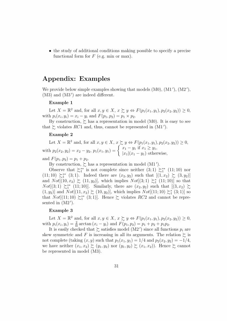
We provide below simple examples showing that models (M0), (M1 ′), (M2 ′),(M3) and (M3 ′) are indeed different.

Example 1

Let X = R2 and, for all x, y ∈ X, x % y ⇔ F (p1(x1, y1), p2(x2, y2)) ≥ 0,with pi(xi, yi) = xi − yi and F (p1, p2) = p1 × p2.

By construction, % has a representation in model (M0). It is easy to seethat % violates RC1 and, thus, cannot be represented in (M1 ′).

Example 2

Let X = R2 and, for all x, y ∈ X, x % y ⇔ F (p1(x1, y1), p2(x2, y2)) ≥ 0,

with p2(x2, y2) = x2 − y2, p1(x1, y1) =

{x1 − y1 if x1 ≥ y1,|x1|(x1 − y1) otherwise,

and F (p1, p2) = p1 + p2.By construction, % has a representation in model (M1 ′).Observe that %∗∗

1 is not complete since neither (3; 1) %∗∗1 (11; 10) nor

(11; 10) %∗∗1 (3; 1). Indeed there are (x2, y2) such that [(1, x2) % (3, y2)]

and Not[(10, x2) % (11, y2)], which implies Not[(3; 1) %∗1 (11; 10)] so that

Not[(3; 1) %∗∗1 (11; 10)]. Similarly, there are (x2, y2) such that [(3, x2) %

(1, y2)] and Not[(11, x2) % (10, y2)], which implies Not[(11; 10) %∗1 (3; 1)] so

that Not[(11; 10) %∗∗1 (3; 1)]. Hence % violates RC2 and cannot be repre-

sented in (M2 ′).

Example 3

Let X = R2 and, for all x, y ∈ X, x % y ⇔ F (p1(x1, y1), p2(x2, y2)) ≥ 0,with pi(xi, yi) = 2

Πarctan (xi − yi) and F (p1, p2) = p1 + p2 + p1p2.

It is easily checked that % satisfies model (M2 ′) since all functions pi areskew symmetric and F is increasing in all its arguments. The relation % isnot complete (taking (x, y) such that p1(x1, y1) = 1/4 and p2(x2, y2) = −1/4,we have neither (x1, x2) % (y1, y2) nor (y1, y2) % (x1, x2)). Hence % cannotbe represented in model (M3).

31

Example 4

Let X = R2 and, for all x, y ∈ X, x % y ⇔ F (p1(x1, y1), p2(x2, y2)) ≥ 0,

with pi(xi, yi) = xi − yi and F (p1, p2) =

{p1 + p2 if |p1 + p2| ≥ 1,0 otherwise.

By construction, % has a representation in (M3). Simple examples showthat % violates TC so that it cannot be represented in (M3 ′).

References

Aschenbrenner, K.M. (1981). Efficient sets, decision heuristics and single-peaked preferences. Journal of Mathematical Psychology, 23, 227–256.

Aschenbrenner, K.M., Albert, D., & Schalhofer, F. (1984). Stochastic choiceheuristics. Acta Psychologica, 56, 153–166.

Ball, C. (1997). A comparison of single-step and multiple-step transitionanalyses of multiattribute decision strategies. Organisational Behaviorand Human Decision Processes, 69, 195–204.

Bouyssou, D. (1986). Some remarks on the notion of compensation inMCDM. European Journal of Operational Research, 26, 150–160.

Bouyssou, D., Perny, P., & Pirlot, M. (2000). Nontransitive decomposableconjoint measurement as a general framework for MCDM and deci-sion under uncertainty. (Communication to EURO XVII, Budapest,Hungary, 16–19 July)

Bouyssou, D., & Pirlot, M. (1999). Conjoint measurement without additivityand transitivity. In N. Meskens & M. Roubens (Eds.), Advances indecision analysis (pp. 13–29). Dordrecht: Kluwer.

Bouyssou, D., & Pirlot, M. (2001). ‘Additive difference’ models withoutadditivity and subtractivity. (Working Paper)

Bouyssou, D., & Pirlot, M. (2002). A characterization of strict concordancerelations. In D. Bouyssou, E. Jacquet-Lagreze, P. Perny, R. S lowinski,D. Vanderpooten, & Ph. Vincke (Eds.), Aiding decisions with multiplecriteria: Essays in honour of Bernard Roy (pp. 121–145). Dordrecht:Kluwer.

32

Bouyssou, D., Pirlot, M., & Vincke, Ph. (1997). A general model of preferenceaggregation. In M.H. Karwan, J. Spronk, & J. Wallenius (Eds.), Essaysin decision making (pp. 120–134). Berlin: Springer Verlag.

Bouyssou, D., & Vansnick, J.-C. (1986). Noncompensatory and generalizednoncompensatory preference structures. Theory and Decision, 21, 251–266.

Chipman, J.S. (1971). Consumption theory without transitive indifference.In J.S. Chipman, L. Hurwicz, M.K. Richter, & H. Sonnenschein (Eds.),Studies in the mathematical foundations of utility and demand the-ory: A symposium at the University of Michigan, 1968 (pp. 224–253).Harcourt-Brace.

Croon, M.A. (1984). The axiomatization of additive difference models forpreference judgements. In E. Degreef & G. van Buggenhaut (Eds.),Trends in mathematical psychology (pp. 193–227). Amsterdam: North-Holland.

Dahlstrand, V., & Montgomery, H. (1984). Information search and evalua-tion processes in decision-making: A computer-based process trackingstudy. Acta Psychologica, 56, 113–123.

Debreu, G. (1960). Topological methods in cardinal utility theory. In S. K.K.J. Arrow & P. Suppes (Eds.), Mathematical methods in the socialsciences (pp. 16–26). Stanford: Stanford University Press.

Doignon, J.-P., Ducamp, A., & Falmagne, J.-C. (1984). On realizablebiorders and the biorder dimension of a relation. Journal of Mathe-matical Psychology, 28, 73–109.

Ducamp, A., & Falmagne, J.-C. (1969). Composite measurement. Journalof Mathematical Psychology, 6, 359–390.

Fishburn, P.C. (1970). Utility theory for decision-making. New-York: Wiley.

Fishburn, P.C. (1976). Noncompensatory preferences. Synthese, 33, 393–403.

Fishburn, P.C. (1980). Lexicographic additive differences. Journal of Math-ematical Psychology, 21, 191–218.

33

Fishburn, P.C. (1982). Nontransitive measurable utility. Journal of Mathe-matical Psychology, 26, 31–67.

Fishburn, P.C. (1985). Interval orders and intervals graphs. New-York:Wiley.

Fishburn, P.C. (1988). Nonlinear preference and utility theory. Baltimore:Johns Hopkins University Press.

Fishburn, P.C. (1990a). Additive non-transitive preferences. Economic Let-ters, 34, 317–321.

Fishburn, P.C. (1990b). Continuous nontransitive additive conjoint measure-ment. Mathematical Social Sciences, 20, 165–193.

Fishburn, P.C. (1990c). Skew symmetric additive utility with finite states.Mathematical Social Sciences, 19, 103–115.

Fishburn, P.C. (1991a). Nontransitive preferences in decision theory. Journalof Risk and Uncertainty, 4, 113–134.

Fishburn, P.C. (1991b). Nontransitive additive conjoint measurement. Jour-nal of Mathematical Psychology, 35, 1–40.

Fishburn, P.C. (1992a). Additive differences and simple preference compar-isons. Journal of Mathematical Psychology, 36, 21–31.

Fishburn, P.C. (1992b). On nonstandard nontransitive additive utility. Jour-nal of Economic Theory, 56, 426–433.

Fishburn, P.C. (1996). Finite linear qualitative probability. Journal ofMathematical Psychology, 40, 21–31.

Fishburn, P.C. (1997). Cancellation conditions for multiattribute preferenceson finite sets. In M.H. Karwan, J. Spronk, & J. Wallenius (Eds.), Essaysin decision making (pp. 157–167). Berlin: Springer Verlag.

Furkhen, G., & Richter, M.K. (1991). Additive utility. Economic Theory, 1,83–105.

Gilboa, I., & Lapson, R. (1995). Aggregation of semiorders: Intransitiveindifference makes a difference. Economic Theory, 5, 109–126.

34

Goldstein, W.M. (1991). Decomposable threshold models. Journal of Math-ematical Psychology, 35, 64–79.

Gonzales, Ch. (1996). Additive utilities when some components are solvableand others not. Journal of Mathematical Psychology, 40, 141–151.

Gonzales, Ch. (2000). Two factor additive conjoint measurement with onesolvable component. Journal of Mathematical Psychology, 44, 285–309.

Greco, S., Matarazzo, B., & S lowinski, R. (1999a). Rough approximationof a preference relation by dominance relations. European Journal ofOperational Research, 117, 63–83.

Greco, S., Matarazzo, B., & S lowinski, R. (1999b). The use of rough setsand fuzzy sets in MCDM. In T. Gal, T. Hanne, & T. Stewart (Eds.),Multicriteria decision making, Advances in mcdm models, algorithms,theory and applications (pp. 14.1–14.59). Kluwer.

Huber, O. (1979). Non transitive multidimensional preferences: Theoreticalanalysis of a model. Theory and Decision, 10, 147–165.

Iverson, G., & Falmagne, J.-C. (1985). Statistical issues in measurement.Mathematical Social Sciences, 10, 131–153.

Jaffray, J.-Y. (1974). On the extension of additive utilities to infinite sets.Journal of Mathematical Psychology, 11, 431–452.

Karni, E., & Safra, Z. (1998). The hexagon condition and additive rep-resentation for two dimensions: An algebraic approach. Journal ofMathematical Psychology, 42, 393–399.

Kim, T., & Richter, M.K. (1986). Nontransitive-nontotal consumer theory.Journal of Economic Theory, 38, 324–363.

Krantz, D.H., Luce, R.D., Suppes, P., & Tversky, A. (1971). Foundations ofmeasurement, vol. 1: Additive and polynomial representations. New-York: Academic Press.

Luce, R.D. (1978). Lexicographic tradeoff structures. Theory and Decision,9, 187–193.

35

Luce, R.D., Krantz, D.H., Suppes, P., & Tversky, A. (1990). Foundations ofmeasurement, vol. 3: Representation, axiomatisation and invariance.New-York: Academic Press.

May, K.O. (1954). Intransitivity, utility and the aggregation of preferencepatterns. Econometrica, 22, 1–13.

Montgomery, H., & Svenson, O. (1976). On decision rules and informa-tion processing strategies for choice among multiattribute alternatives.Scandinavian Journal of Psychology, 17, 283–291.

Nakamura, Y. (1997). Lexicographic additivity for multi-attribute prefer-ences on finite sets. Theory and Decision, 42, 1–19.

Payne, J.W., Bettman, J.R., & Johnson, E.J. (1988). Adaptative strat-egy selection in decision making. Journal of Experimental Psychology:Learning, Memory and Cognition, 14, 534–552.

Pirlot, M., & Vincke, Ph. (1997). Semiorders. Properties, representations,applications. Dordrecht: Kluwer.

Roberts, F.S. (1979). Measurement theory with applications to decisionmaking, utility and the social sciences. Reading: Addison-Wesley.

Russo, J.E., & Dosher, B.A. (1983). Strategies for multiattribute binarychoice. Journal of Experimental Psychology: Learning, Memory andCognition, 9, 676–696.

Scott, D. (1964). Measurement structures and linear inequalities. Journal ofMathematical Psychology, 1, 233–247.

Suppes, P., Krantz, D.H., Luce, R.D., & Tversky, A. (1989). Foundationsof measurement, vol. 2: Geometrical, threshold, and probabilistic rep-resentations. Academic Press, New York.

Svenson, O. (1979). Process description of decision making. OrganizationalBehavior and Human Performance, 23, 86–112.

Tversky, A. (1969). Intransitivity of preferences. Psychological Review, 76,31–48.

36

Vind, K. (1991). Independent preferences. Journal of Mathematical Eco-nomics, 20, 119–135.

Wakker, P.P. (1988). Derived strength of preference relations on coordinates.Economic Letters, 28, 301–306.

Wakker, P.P. (1989). Additive representations of preferences: A new foun-dation of decision analysis. Dordrecht: Kluwer.

37