
Nonlinear Control and Stability Analysis of Multi-Terminal ...
275
HAL Id: tel-01249585 https://tel.archives-ouvertes.fr/tel-01249585 Submitted on 4 Jan 2016 HAL is a multi-disciplinary open access archive for the deposit and dissemination of sci- entific research documents, whether they are pub- lished or not. The documents may come from teaching and research institutions in France or abroad, or from public or private research centers. L’archive ouverte pluridisciplinaire HAL, est destinée au dépôt et à la diffusion de documents scientifiques de niveau recherche, publiés ou non, émanant des établissements d’enseignement et de recherche français ou étrangers, des laboratoires publics ou privés. Nonlinear Control and Stability Analysis of Multi-Terminal High Voltage Direct Current Networks Yijing Chen To cite this version: Yijing Chen. Nonlinear Control and Stability Analysis of Multi-Terminal High Voltage Direct Current Networks. Automatic. Université Paris Sud - Paris XI, 2015. English. NNT: 2015PA112041. tel- 01249585
-
Upload
khangminh22 -
Category
Documents
-
view
0 -
download
0
Transcript of Nonlinear Control and Stability Analysis of Multi-Terminal ...
HAL Id: tel-01249585https://tel.archives-ouvertes.fr/tel-01249585
Submitted on 4 Jan 2016
HAL is a multi-disciplinary open accessarchive for the deposit and dissemination of sci-entific research documents, whether they are pub-lished or not. The documents may come fromteaching and research institutions in France orabroad, or from public or private research centers.
L’archive ouverte pluridisciplinaire HAL, estdestinée au dépôt et à la diffusion de documentsscientifiques de niveau recherche, publiés ou non,émanant des établissements d’enseignement et derecherche français ou étrangers, des laboratoirespublics ou privés.
Nonlinear Control and Stability Analysis ofMulti-Terminal High Voltage Direct Current Networks
Yijing Chen
To cite this version:Yijing Chen. Nonlinear Control and Stability Analysis of Multi-Terminal High Voltage Direct CurrentNetworks. Automatic. Université Paris Sud - Paris XI, 2015. English. NNT : 2015PA112041. tel-01249585
Université Paris-SudEcole Doctorale Sciences et Technologies del'Information, des Télécommunications et des
Systèmes (ED STITS)
Laboratoire des Signaux et Systèmes (L2S)
Discipline : Automatique
Thèse de doctoratSoutenue: le 8 Avril 2015 par
Yijing Chen
Commande Nonlinéaire et Analyse de
Stabilité de Réseaux Multi-Terminaux
Haute Tension à Courant Continu(Nonlinear Control and Stability Analysis of Multi-Terminal High
Voltage Direct Current Networks)
Composition du jury :
Directeur de thèse Dr. Françoise Directeur de Recherche, CNRS & L2S
LAMNABHI-LAGARRIGUE
Co-directeur de thèse : Dr. Gilney DAMM Maître de Conférences, HDR
Université d'Evry-Val-d'Essonn & L2S
Dr. Abdelkrim BENCHAIB Ingénieur de Recherche, HDR, Alstom
Rapporteurs : Dr. Anuradha ANNASWAMY Senior Research Scientist
Massachusetts Institute of Technology
Prof. Fouad GIRI Université de Caen Basse-Normandie
Examinateurs Prof. Alain GLUMINEAU Ecole Centrale de Nantes
Prof. Didier GEORGES ENSE3
Prof. Riccardo MARINO Università di Roma Tor Vergata

Acknowledgments
My deepest gratitude is to my three thesis supervisors, Dr. Françoise LAMNABHI-
LAGARRIGUE, Dr. Gilney DAMM and Dr. Abdelkrim BENCHAIB, for their
guidance, advices and assistance. It is my greatest pleasure to work with them.
Thanks a lot to Dr. Gilney DAMM for his unremittingly invaluable guidance and
comprehensive assistance. He is always ready to help me whenever I had scientic or
personal diculties. He usually shared his experience with me and gave me constant
advice in research and career orientation. He never put undue pressure on me. It was
really a great chance to work with him. Thanks a lot to Dr. Abdelkrim BENCHAIB
for oering invaluable advice from the point view of industry. After every discussion
with him, I acquired a greater depth of understanding of my thesis work. Thanks
a lot to Dr. Françoise LAMNABHI-LAGARRIGUE who admitted me as a Ph.D.
candidate in L2S. She helped me a lot to deal with all the administrative trivial
things. She always tried her best to build a convivial ambiance for work. With her
support and trust, my Ph.D. years have become a pleasant life journey.
I would like to thank the members of the jury, Dr. Anuradha ANNASWAMY,
Prof. Fouad GIRI, Prof. Alain GLUMINEAU, Prof. Riccardo MARINO and Prof.
Didier GEORGES, for their comments, questions and suggestions. Special thanks
to Dr. Anuradha ANNASWAMY and Prof. Fouad GIRI, who spent a lot of time
and eort to review my thesis and gave advice to improve my work. Thanks a lot to
Dr. Anuradha ANNASWAMY who warmly hosted me during my visit to the active
adaptive control laboratory (AACLAB) at Massachusetts Institute of Technology
(MIT). She introduced me to the domain of adaptive control which is a powerful
tool to solve the system uncertainties. Thanks to this visit, I have the opportunity
to meet researchers in the Department of Mechanical Engineering and discussed
with them to expand my knowledge.
I am indebted to the former and the current faculty, personnel, Ph.D. students
from L2S, who constantly helped me. Special thanks to Jing DAI who used to be a
post-doc in L2S. He helped me to correct many bad writing habits when I wrote my
rst paper. He also gave me lots of comments and suggestions on my dissertation and
other papers. I will always remember that even during the Christmas holiday, he still
corrected my dissertation and gave me feedbacks. Many thanks to Miguel Jiménez
Carrizosa for discussing with me. In fact, I did not take many courses in the eld
of electrical engineering during my undergraduate and master study. Miguel shared
his professional knowledge of electrical engineering. I also want to thank Fernando
DORADO NAVAS, Mawulikplimi Komlan Crédo PANIAH, Van Cuong NGUYEN,
Alessio Iovine, Alexandre Azevedo, Yujun HE · · · for their helpful discussions. I
would like to thank Mme. Maryvonne GIRON and Mme. Laurence ANTUNES for
helping me a lot to handle the visa paper work and renew of my "titre de séjour ".
I am grateful to my dear friends, Yuling ZHENG, Long CHEN, Chuan XU, Zheng
CHEN · · · . I shall evermore cherish the memory that we played badminton together.

ii
Last, my deepest gratitude is undoubtedly to my families who are always beside
me and support me. I want to thank my father, my oldest friend, who always
supported and encouraged me; my mother who always prayed for me and my sister
who always comforted me and straightened me out when I encountered unhappy
things. I'm so thankful that I have such wonderful families.
Abstract
Nowadays the world total electricity demand increases year by year while the exist-
ing alternating current (AC) transmission grids are operated close to their limits. As
it is dicult to upgrade the existing AC grids, high voltage direct current (HVDC)
is considered as an alternative solution to several related problems such as: the in-
crease of transmission capability; the interconnection of remote and scattered gen-
eration from renewable energy sources (in particular oshore); the interconnection
of dierent asynchronous zones. At present, over one hundred direct current (DC)
transmission projects exist in the world, the vast majority for two-terminal HVDC
transmission systems and only three for multi-terminal HVDC systems. The tra-
ditional two-terminal HVDC transmission system can only carry out point-to-point
power transfer. As the economic development and the construction of the power
grid require that the DC grid can achieve power exchanges among multiple power
suppliers and multiple power consumers, multi-terminal voltage-sourced converter
HVDC (MTDC) systems draw more and more attention. As a DC transmission net-
work connecting more than two converter stations, an MTDC transmission system
oers a larger transmission capacity than the AC network and also provides a more
exible and ecient transmission method. Most studies in the eld of MTDC sys-
tems have involved an empirical control approach, namely, vector control approach
consisting of several standard proportional-integral (PI) controllers. This control
concept is mainly based on the assertion that the system state variables exhibit the
performances with dierent dynamics. However, very rare relevant work has ever
presented a theoretically detailed explanation on the validity and the implications
of this assertion in the literature.
The research work in this dissertation was started with the intention of lling
some gaps between the theory and the practice, in particular: 1) to investigate var-
ious control approaches for the purpose of improving the performance of MTDC
systems; 2) to establish connections between existing empirical control design and
theoretical analysis; 3) to improve the understanding of the multi-time-scale behav-
ior of MTDC systems characterized by the presence of slow and fast transients in
response to external disturbances.
The main contributions of this thesis work can be put into three areas, namely
nonlinear control design of MTDC systems, analysis of MTDC system's dynamic
behaviors and application of MTDC systems for frequency control of AC systems.
In the area of nonlinear control design of MTDC systems, based on dierent
nonlinear control design techniques, new control schemes have been proposed with
corresponding theoretical analysis. Besides, the developed control algorithms have
been tested by numerical simulations, whose performances are evaluated in compar-
ison to the performance of the conventional vector control method.
The main motivation for the topic on analysis of MTDC system's dynamic behav-

iv
iors is the desire to provide a rigorous theoretical demonstration on the assertion
that part of system states' dynamics are much faster than the rest. As a conse-
quence, it is possible to simplify the control design procedure. The contribution
in this area consists of three parts: 1) control induced time-scale separation for a
class of nonlinear systems; 2) analysis of time-scale separation for an MTDC system
with master-slave control conguration; 3) analysis of time-scale separation for an
MTDC system with droop control conguration. Theoretical analysis, mainly based
on singular perturbation and Lyapunov theories, have been carried out for each of
the aforementioned aspects and conrmed by various simulation studies. The study
of the rst part has been mostly dedicated to propose a time-scale separation control
method which can drive a class of nonlinear systems to exhibit a multi-time-scale
performance. The theoretical results obtained from the rst part have been applied
to investigate the dynamic behaviors of MTDC systems where the two main control
congurations, i.e. master-slave and droop control congurations, are considered.
Empirical vector current control designs have been proposed for each control con-
guration. Theoretical explanations and fundamental analysis indicate that with
the proposed empirical control algorithms, the inductor currents indeed exhibit a
dynamic behavior with dierent dynamics. Furthermore, we have provided more
details on how and why these empirical vector current control designs work as well
as the rules of tuning the control parameters.
The nal contribution relates to the application of MTDC systems where fre-
quency support strategy using MTDC systems has been introduced and analyzed.
The principle of the frequency control is to regulate the AC frequency by modulating
each AC grid's scheduled (or prescribed) active power. A DC-voltage-based control
scheme for the AC frequency regulation is proposed, which achieves the objective of
sharing primary reserves between dierent AC areas interconnected via an MTDC
system without using remote information communication.
Contents
1 Introduction 1
1.1 History and background . . . . . . . . . . . . . . . . . . . . . . . . . 1
1.2 Overview of HVDC technology . . . . . . . . . . . . . . . . . . . . . 3
1.2.1 Line-commutated current source converters . . . . . . . . . . 4
1.2.2 Voltage-sourced converters . . . . . . . . . . . . . . . . . . . . 4
1.2.3 LCC vs VSC . . . . . . . . . . . . . . . . . . . . . . . . . . . 5
1.2.4 Advantages of HVDC over AC . . . . . . . . . . . . . . . . . 6
1.3 Literature review: related studies on control designs . . . . . . . . . 8
1.3.1 Control of a single VSC terminal . . . . . . . . . . . . . . . . 8
1.3.2 Control of MTDC systems . . . . . . . . . . . . . . . . . . . . 9
1.4 Motivations and contributions of the thesis . . . . . . . . . . . . . . 11
1.4.1 Motivations . . . . . . . . . . . . . . . . . . . . . . . . . . . . 11
1.4.2 Contributions . . . . . . . . . . . . . . . . . . . . . . . . . . . 12
1.5 Outline of the thesis . . . . . . . . . . . . . . . . . . . . . . . . . . . 14
1.6 Publications . . . . . . . . . . . . . . . . . . . . . . . . . . . . . . . . 14
2 VSC HVDC technology 17
2.1 Key components . . . . . . . . . . . . . . . . . . . . . . . . . . . . . 17
2.2 Operating principles of VSC . . . . . . . . . . . . . . . . . . . . . . . 19
2.3 Congurations of HVDC systems . . . . . . . . . . . . . . . . . . . . 19
2.4 AC network and control modes of VSC terminals . . . . . . . . . . . 23
2.4.1 AC network connected to VSC terminal . . . . . . . . . . . . 23
2.4.2 Control modes of VSC terminals . . . . . . . . . . . . . . . . 23
2.5 Chapter conclusions . . . . . . . . . . . . . . . . . . . . . . . . . . . 25
3 Dynamic model of multi-terminal VSC HVDC systems 27
3.1 Preliminary knowledge . . . . . . . . . . . . . . . . . . . . . . . . . . 27
3.2 Clarke's and Park's transformations . . . . . . . . . . . . . . . . . . 28
3.2.1 Clarke's transformation . . . . . . . . . . . . . . . . . . . . . 28
3.2.2 Park's transformation . . . . . . . . . . . . . . . . . . . . . . 30
3.3 Three-phase synchronous reference frame phase-locked loop . . . . . 31
3.4 Multi-terminal HVDC system model . . . . . . . . . . . . . . . . . . 32
3.4.1 Strong AC system side . . . . . . . . . . . . . . . . . . . . . . 32
3.4.2 Weak AC system side . . . . . . . . . . . . . . . . . . . . . . 34
3.4.3 DC network . . . . . . . . . . . . . . . . . . . . . . . . . . . . 36
3.4.4 Domain of interest . . . . . . . . . . . . . . . . . . . . . . . . 40
3.5 Conventional control methods . . . . . . . . . . . . . . . . . . . . . . 40
3.5.1 Direct control method . . . . . . . . . . . . . . . . . . . . . . 40
3.5.2 Vector control method . . . . . . . . . . . . . . . . . . . . . . 41
3.6 Chapter conclusions . . . . . . . . . . . . . . . . . . . . . . . . . . . 44

vi Contents
4 Control methods based on nonlinear control design tools 47
4.1 Feedback linearization control . . . . . . . . . . . . . . . . . . . . . . 48
4.1.1 Theoretical results . . . . . . . . . . . . . . . . . . . . . . . . 48
4.1.2 Application to a VSC HVDC link connected to a resistive load 51
4.1.3 Application to a VSC HVDC link consisting of a strong and
a weak AC system . . . . . . . . . . . . . . . . . . . . . . . . 61
4.1.4 Application to an MTDC system using master-slave control
conguration . . . . . . . . . . . . . . . . . . . . . . . . . . . 71
4.2 Feedback linearization with sliding mode control . . . . . . . . . . . 85
4.2.1 Control design . . . . . . . . . . . . . . . . . . . . . . . . . . 85
4.2.2 Simulation studies . . . . . . . . . . . . . . . . . . . . . . . . 88
4.3 Passivity-based control . . . . . . . . . . . . . . . . . . . . . . . . . . 92
4.3.1 Steady-state analysis . . . . . . . . . . . . . . . . . . . . . . . 93
4.3.2 Passive system . . . . . . . . . . . . . . . . . . . . . . . . . . 95
4.3.3 Control design . . . . . . . . . . . . . . . . . . . . . . . . . . 97
4.3.4 Control of zero dynamics . . . . . . . . . . . . . . . . . . . . 102
4.3.5 Simulation studies . . . . . . . . . . . . . . . . . . . . . . . . 116
4.4 Chapter conclusions . . . . . . . . . . . . . . . . . . . . . . . . . . . 125
5 Control induced time-scale separation 131
5.1 Control induced time-scale separation for a class of nonlinear systems 132
5.1.1 Introduction and motivation . . . . . . . . . . . . . . . . . . . 132
5.1.2 Problem formulation . . . . . . . . . . . . . . . . . . . . . . . 134
5.1.3 Control design . . . . . . . . . . . . . . . . . . . . . . . . . . 136
5.1.4 Theoretical study . . . . . . . . . . . . . . . . . . . . . . . . . 139
5.1.5 Study cases . . . . . . . . . . . . . . . . . . . . . . . . . . . . 145
5.2 Control induced time-scale separation for MTDC systems using
master-slave control conguration . . . . . . . . . . . . . . . . . . . . 152
5.2.1 Control design . . . . . . . . . . . . . . . . . . . . . . . . . . 153
5.2.2 Theoretical analysis . . . . . . . . . . . . . . . . . . . . . . . 156
5.2.3 Plug-and-play operations . . . . . . . . . . . . . . . . . . . . 164
5.2.4 Simulation studies . . . . . . . . . . . . . . . . . . . . . . . . 165
5.3 Control induced time-scale separation for MTDC systems using droop
control conguration . . . . . . . . . . . . . . . . . . . . . . . . . . . 174
5.3.1 VSC operation . . . . . . . . . . . . . . . . . . . . . . . . . . 174
5.3.2 Droop control structure . . . . . . . . . . . . . . . . . . . . . 175
5.3.3 Theoretical analysis . . . . . . . . . . . . . . . . . . . . . . . 178
5.3.4 Simulation studies . . . . . . . . . . . . . . . . . . . . . . . . 193
5.4 Conclusions . . . . . . . . . . . . . . . . . . . . . . . . . . . . . . . . 205
6 Frequency control using MTDC systems 209
6.1 Introduction and motivation . . . . . . . . . . . . . . . . . . . . . . . 209
6.2 Modeling . . . . . . . . . . . . . . . . . . . . . . . . . . . . . . . . . 210
6.2.1 DC grid . . . . . . . . . . . . . . . . . . . . . . . . . . . . . . 211
Contents vii
6.2.2 AC areas . . . . . . . . . . . . . . . . . . . . . . . . . . . . . 211
6.2.3 Reference operating point . . . . . . . . . . . . . . . . . . . . 212
6.3 Control strategy . . . . . . . . . . . . . . . . . . . . . . . . . . . . . 212
6.3.1 Control law . . . . . . . . . . . . . . . . . . . . . . . . . . . . 213
6.3.2 Choice of control gains . . . . . . . . . . . . . . . . . . . . . . 213
6.3.3 Algorithm for the denition and verication of control gains
and the associated region of attraction . . . . . . . . . . . . . 218
6.4 Simulation studies . . . . . . . . . . . . . . . . . . . . . . . . . . . . 219
6.5 Conclusions . . . . . . . . . . . . . . . . . . . . . . . . . . . . . . . . 224
7 Conclusions 225
7.1 Conclusions . . . . . . . . . . . . . . . . . . . . . . . . . . . . . . . . 225
7.2 Perspectives for future work . . . . . . . . . . . . . . . . . . . . . . . 228
7.2.1 Further research on the droop control conguration . . . . . . 228
7.2.2 Further research on the connection of other types of weak AC
systems . . . . . . . . . . . . . . . . . . . . . . . . . . . . . . 229
7.2.3 Further research on the operation of MTDC systems . . . . . 229
7.2.4 Further research on system modeling . . . . . . . . . . . . . . 229
7.2.5 Implementation on a real MTDC system . . . . . . . . . . . . 229
7.2.6 Control induced time-scale separation for the MMC . . . . . 229
A Appendix 231
A.1 Notations . . . . . . . . . . . . . . . . . . . . . . . . . . . . . . . . . 231
B Appendix 233
B.1 Proof of Lemma 4.1.6 . . . . . . . . . . . . . . . . . . . . . . . . . . 233
B.2 Proof of Lemma 4.1.9 . . . . . . . . . . . . . . . . . . . . . . . . . . 233
Bibliography 235


List of Abbreviations
AC Alternating current
CCC Capacitor-commutated converter
DC Direct current
DFIG Doubly fed induction generator
DPC Direct power control
GTO Gate turn-o thyristor
HVDC High voltage direct current
IGBT Insulated-gate bipolar transistor
IGCT Integrated gate-commutated thyristor
LCC Line-commutated current source converter
LMI Linear matrix inequality
MI Mineral-insulated
MMC Modular multilevel converter
MTDC Multi-terminal voltage-sourced converter high voltage direct current
PCC Point of common coupling
PI Proportional-integral
PLL Phase-locked loop
PWM Pulse-width modulation
RMS Root mean square
SAC Strong AC network
SCR Short circuit ratio
SRF-PLL Three-phase synchronous reference frame phase-locked loop
TSO Transmission system operator
VSC Voltage-sourced converter
WAC Weak AC network
XLPE Cross-linked polyethylene


Liste des Abréviations
AC Courant alternatif
CCC Convertisseur de condensateurs à commutation
DC Courant continu
DFIG Générateur d'induction à double alimentation
DPC Contrôle direct de la puissance
GTO Thyristor à extinction par la gâchette
HVDC Courant continu haute tension
IGBT Transistor bipolaire à grille isolée
LCC Convertisseurs commutés par les lignes
LMI Inégalité matricielle linéaire
MMC Convertisseurs multi-niveaux modulaire
MTDC Réseau multiterminal à courant continu
PCC Point de couplage commung
PI Proportionnel intégral
PLL Boucle à phase asservie
PWM Modulation de largeur d'impulsion
RMS Moyenne quadratique
SAC Réseau AC fort
SCR Rapport de court-circuit
TSO Gestionnaire de réseau de transport
VSC Convertisseurs en source de tension
WAC Réseau AC faible
XLPE Polyéthylène réticulé


List of Symbols
t Time
τ Time variable for fast dynamics
ε Small scalar to qualify the time scales
Lgi ith SAC connected VSC terminal's phase reactor inductance
Rgi ith SAC connected VSC terminal's phase reactor resistance
fgi Frequency of the ith SAC at the PCC
Vrms,gi AC voltage magnitude of the ith SAC at the PCC
vsgi,dq d− and q− axis AC voltage of the ith SAC at the PCC
vsgi,abc a−, b− and c− axis AC voltage of the ith SAC at the PCC
vcgi,dq d− and q− axis AC voltage of the ith SAC at the converter side
vcgi,abc a−, b− and c− axis AC voltage of the ith SAC at the converter side
igi,dq d− and q− axis phase reactor current of the ith SAC
igi,abc a−, b− and c− axis phase reactor current of the ith SAC
Pgi Active power of the ith SAC at the PCC
Qgi Reactive power of the ith SAC at the PCC
ωgi ith SAC system's pulsation
δgi Phase angle of the ith SAC connected VSC
mgi Modulation ratio of the ith SAC connected VSC
mgi,dq d− and q− axis modulation index of the ith SAC connected VSC
icgi DC current owing from the ith SAC connected VSC
Requi, gi Equivalent resistance representing the ith SAC connected VSC's loss
Lwj jth WAC connected VSC terminal's phase reactor inductance
Rwj jth WAC connected VSC terminal's phase reactor resistance
fwj Frequency of the jth WAC at the PCC
Cfwj jth WAC connected VSC terminal's lter capacitance
Vrms,wj AC voltage magnitude of the jth WAC at the PCC
vswj ,dq d− and q− axis AC voltage of the jth WAC at the PCC
vswj ,abc a−, b− and c− axis AC voltage of the jth WAC at the PCC
vcwj ,dq d− and q− axis AC voltage of the jth WAC at the converter side
vcwj ,abc a−, b− and c− axis AC voltage of the jth WAC at the PCC
Iwj ,dq d− and q− axis controlled current source of the jth WAC network
iwj ,dq d− and q− axis phase reactor current of the jth WAC
iwj ,abc a−, b− and c− axis phase reactor current of the jth WAC
Pwj Active power of the jth WAC at the PCC
Qwj Reactive power of the jth WAC at the PCC
ωwj jth WAC system's pulsation
δwj Phase angle of the jth WAC connected VSC
mwj Modulation ratio of the jth WAC connected VSC

xiv Contents
mwj ,dq d− and q− axis modulation index of the jth WAC connected VSC
icwj DC current owing from the jth WAC connected VSC
Requi, wj Equivalent resistance representing the jth WAC connected VSC's loss
Cgi ith SAC converter node's capacitance
Cwj jth WAC converter node's capacitance
Cth hth intermediate node's capacitance
ick kth transmission line's branch current
Rck kth transmission line's resistance
Lck kth transmission line's inductance
ic Transmission branch circuit current vector: ic = [ic1 · · · icL ]T
ucgi DC voltage of the ith SAC converter node
ucwj DC voltage of the jth WAC converter node
ucth DC voltage of the hth intermediate node
ucg DC voltage vector: ucg = [ucg1 · · · ucgN ]T
ucw DC voltage vector: ucw = [ucw1 · · · ucwM ]T
uct DC voltage vector: uct = [uct1 · · · uctP ]T
uc DC voltage vector: uc = [ucg ucw uct]T
z State variables of the DC grid: z = [uc ic]T
uc,min Acceptable minimum value of the DC voltage
uc,max Acceptable maximum value of the DC voltage
Srate Rated apparent power of the converter
urate Rated DC voltage of the transmission lines
H Incidence matrix of the weakly connected directed graph that maps to the
topology of the DC network
C Capacitance matrix: C = diag(Cg1 · · ·CgN CW1 · · ·CWMCt1 · · ·CtP )
L Inductance matrix: L = diag(Lc1 · · ·LcL)
R Inductance matrix: R = diag(Rc1 · · ·RcL)
N Number of SAC nodes
M Number of WAC nodes
P Number of intermediate nodes
L Number of branch circuits
N Set N = 1, · · · , NN−1 Set N−1 = 2, · · · , NM SetM = 1, · · · , MP Set P = 1, · · · , PL Set L = 1, · · · , LT Set T = 1, · · · , N +M + Pi Index i ∈ Nρ Index ρ ∈ N−1
j Index j ∈Mh Index h ∈ Pk Index k ∈ LVi ith AC area's DC voltage
P dci ith AC area's DC power injection

Contents xv
Rik Resistance of the transmission line between the ith and the kth AC areas
Pmi ith AC area's mechanical power input
Ji ith AC area's moment of inertia
Dgi ith AC area's damping factor of the aggregated generator
fi ith AC area's frequency
fnom,i ith AC area's nominal frequency
Pli ith AC area's load
Tsm,i ith AC area's time constant of the servomotor
P smi ith AC area's scheduled mechanical power input
Pnom,i ith AC area's nominal mechanical power input
σi ith AC area's generator droop

List of Figures
1.1 AC versus DC cost. . . . . . . . . . . . . . . . . . . . . . . . . . . . . 7
2.1 A simplied representation of a VSC HVDC converter station. Usu-
ally, the harmonic lters, the phase reactors, the converters and the
DC capacitors are located indoors while the transformers and the
cooling system are outdoors. . . . . . . . . . . . . . . . . . . . . . . . 18
2.2 Three phase bidirectional VSC. . . . . . . . . . . . . . . . . . . . . . 20
2.3 Monopolar HVDC link with earth, water or metallic return path. . . 20
2.4 Bipolar HVDC link with earth or metallic return path. . . . . . . . . 21
2.5 Back-to-back HVDC link. . . . . . . . . . . . . . . . . . . . . . . . . 22
2.6 Multi-terminal HVDC link with three terminals connected in parallel. 22
2.7 A single line representation of the AC side of a VSC. . . . . . . . . . 24
3.1 A three-phase PLL system. . . . . . . . . . . . . . . . . . . . . . . . 31
3.2 A multi-terminal VSC HVDC system with strong and weak AC systems. 32
3.3 A simplied schematic diagram of the ith VSC connected strong grid. 33
3.4 A VSC connected to wind farm. . . . . . . . . . . . . . . . . . . . . 34
3.5 A simplied schematic diagram of the jth VSC connected wind farm. 35
3.6 DC circuit. . . . . . . . . . . . . . . . . . . . . . . . . . . . . . . . . 37
3.7 An example of the DC grid. . . . . . . . . . . . . . . . . . . . . . . . 37
3.8 Block diagrams of direct control method. . . . . . . . . . . . . . . . . 41
3.9 Inner current loop. . . . . . . . . . . . . . . . . . . . . . . . . . . . . 42
3.10 Outer current loop. . . . . . . . . . . . . . . . . . . . . . . . . . . . . 43
4.1 A resistive load RL is connected to the ith SAC terminal. . . . . . . 51
4.2 Model of VSC HVDC link connected to a resistive load using Sim-
PowerSystems toolbox. . . . . . . . . . . . . . . . . . . . . . . . . . . 54
4.3 The response of DC voltage for the change of uocgi . (a) PI controller.
(b) Feedback nonlinear controller. . . . . . . . . . . . . . . . . . . . . 56
4.4 The response of igiq for the change of uocgi . (a) PI controller. (b)
Feedback nonlinear controller. . . . . . . . . . . . . . . . . . . . . . . 56
4.5 The response of iL for the change of uocgi . (a) PI controller. (b)
Feedback nonlinear controller. . . . . . . . . . . . . . . . . . . . . . . 57
4.6 The response of DC voltage for the changes of RL and iogiq. (a) PI
controller. (b) Feedback nonlinear controller. . . . . . . . . . . . . . 58
4.7 The response of igiq for the changes of RL and iogiq. (a) PI controller.
(b) Feedback nonlinear controller. . . . . . . . . . . . . . . . . . . . . 59
4.8 The response of igid for the changes of RL and iogiq. (a) PI controller.
(b) Feedback nonlinear controller. . . . . . . . . . . . . . . . . . . . . 59
xviii List of Figures
4.9 The response of iL for the changes of RL and iogiq. (a) PI controller.
(b) Feedback nonlinear controller. . . . . . . . . . . . . . . . . . . . . 60
4.10 The response of iL2 for the changes of RL and iogiq. (a) PI controller.
(b) Feedback nonlinear controller. . . . . . . . . . . . . . . . . . . . . 60
4.11 The response of iL3 for the changes of RL and iogiq. (a) PI controller.
(b) Feedback nonlinear controller. . . . . . . . . . . . . . . . . . . . . 61
4.12 A VSC HVDC link consists of one strong and one weak AC system. . 61
4.13 The response of vsw1d for the changes of vosw1dand vosw1q. (a) PI
controller. (b) Feedback nonlinear controller. . . . . . . . . . . . . . 67
4.14 The response of vsw1q for the changes of vosw1dand vosw1q. (a) PI
controller. (b) Feedback nonlinear controller. . . . . . . . . . . . . . 67
4.15 The response of vsw1,abc for the changes of vosw1d
and vosw1q using PI
controller. . . . . . . . . . . . . . . . . . . . . . . . . . . . . . . . . . 68
4.16 Zoom of the response of vsw1,abc for the changes of vosw1dand vosw1q
using PI controller. . . . . . . . . . . . . . . . . . . . . . . . . . . . . 69
4.17 The response of vsw1,abc for the changes of vosw1dand vosw1q using
feedback linearization controller. . . . . . . . . . . . . . . . . . . . . 69
4.18 Zoom of the response of vsw1,abc for the changes of vosw1dand vosw1q
using feedback linearization controller. . . . . . . . . . . . . . . . . . 70
4.19 fw1 = 50 Hz. . . . . . . . . . . . . . . . . . . . . . . . . . . . . . . . 70
4.20 The response of ucg1 for the changes of vosw1dand vosw1q. (a) PI con-
troller. (b) Feedback nonlinear controller. . . . . . . . . . . . . . . . 71
4.21 An MTDC system consists of two strong and two weak AC systems. 78
4.22 DC grid used to connect the four AC areas. . . . . . . . . . . . . . . 79
4.23 The response of ucg1 . (a) PI controller. (b) Feedback nonlinear con-
troller. . . . . . . . . . . . . . . . . . . . . . . . . . . . . . . . . . . . 80
4.24 The response of ig1q. (a) PI controller. (b) Feedback nonlinear con-
troller. . . . . . . . . . . . . . . . . . . . . . . . . . . . . . . . . . . . 81
4.25 The response of vsw1d. (a) PI controller. (b) Feedback nonlinear
controller. . . . . . . . . . . . . . . . . . . . . . . . . . . . . . . . . . 81
4.26 The response of vsw1q. (a) PI controller. (b) Feedback nonlinear
controller. . . . . . . . . . . . . . . . . . . . . . . . . . . . . . . . . . 82
4.27 The response of vsw1,abc using PI control technique. . . . . . . . . . . 82
4.28 The response of vsw1,abc using feedback linearization technique. . . . 83
4.29 The response of vsw2d. (a) PI controller. (b) Feedback nonlinear
controller. . . . . . . . . . . . . . . . . . . . . . . . . . . . . . . . . . 83
4.30 The response of vsw2q. (a) PI controller. (b) Feedback nonlinear
controller. . . . . . . . . . . . . . . . . . . . . . . . . . . . . . . . . . 84
4.31 The response of vsw2,abc using PI control technique. . . . . . . . . . . 84
4.32 The response of vsw2,abc using feedback linearization technique. . . . 85
4.33 Variations in the resistive load R. . . . . . . . . . . . . . . . . . . . . 89
4.34 Response of ucgi (curve (a)) and its reference uocgi (curve (b)). . . . . 89
4.35 Response of igid. . . . . . . . . . . . . . . . . . . . . . . . . . . . . . 90
4.36 Response of igiq. . . . . . . . . . . . . . . . . . . . . . . . . . . . . . 90
List of Figures xix
4.37 Response of mgid. . . . . . . . . . . . . . . . . . . . . . . . . . . . . . 91
4.38 Response of mgiq. . . . . . . . . . . . . . . . . . . . . . . . . . . . . . 91
4.39 The response of ucg1 (a) Feedback nonlinear controller. (b) Passivity-
based controller. . . . . . . . . . . . . . . . . . . . . . . . . . . . . . 117
4.40 The response of ig1q (a) Feedback nonlinear controller. (b) Passivity-
based controller. . . . . . . . . . . . . . . . . . . . . . . . . . . . . . 118
4.41 The response of ig2d (a) Feedback nonlinear controller. (b) Passivity-
based controller. . . . . . . . . . . . . . . . . . . . . . . . . . . . . . 118
4.42 The response of ig2q (a) Feedback nonlinear controller. (b) Passivity-
based controller. . . . . . . . . . . . . . . . . . . . . . . . . . . . . . 119
4.43 The response of vsw1,abc using feedback nonlinear controller. . . . . . 119
4.44 The response of vsw1,abc using passivity-based controller. . . . . . . . 120
4.45 The response of ucg1 (a) Feedback nonlinear controller. (b) Passivity-
based controller. . . . . . . . . . . . . . . . . . . . . . . . . . . . . . 121
4.46 The response of vsw1d (a) Feedback nonlinear controller. (b)
Passivity-based controller. . . . . . . . . . . . . . . . . . . . . . . . . 121
4.47 The response of vsw1q (a) Feedback nonlinear controller. (b)
Passivity-based controller. . . . . . . . . . . . . . . . . . . . . . . . . 122
4.48 The response of vsw2d (a) Feedback nonlinear controller. (b)
Passivity-based controller. . . . . . . . . . . . . . . . . . . . . . . . . 122
4.49 The response of vsw2q (a) Feedback nonlinear controller. (b)
Passivity-based controller. . . . . . . . . . . . . . . . . . . . . . . . . 123
4.50 Variations in Rfw1 . . . . . . . . . . . . . . . . . . . . . . . . . . . . . 124
4.51 Variations in Rfw2 . . . . . . . . . . . . . . . . . . . . . . . . . . . . . 124
4.52 The response of vsw1d (a) Nominal passivity-based controller (b)
Adaptive passivity-based controller (c) Reference values of vosw1d=
40.82 V. . . . . . . . . . . . . . . . . . . . . . . . . . . . . . . . . . . 125
4.53 The response of vsw1,abc under the nominal passivity-based controller. 126
4.54 The response of vsw1,abc under the adaptive passivity-based controller. 126
4.55 The response of vsw2d (a) Nominal passivity-based controller (b)
Adaptive passivity-based controller (c) Reference values of vosw2d=
40.82 V. . . . . . . . . . . . . . . . . . . . . . . . . . . . . . . . . . . 127
4.56 The response of vsw2,abc under the nominal passivity-based controller. 127
4.57 The response of vsw2,abc under the adaptive passivity-based controller. 128
4.58 Comparison between (a) the actual parameter value ψ31 =1
Rfw1
and
(b) the parameter estimation ψ31 =1
Rfw1
. . . . . . . . . . . . . . . . 128
4.59 Comparison between (a) the actual parameter value ψ32 =1
Rfw2
and
(b) the parameter estimation ψ32 =1
Rfw2
. . . . . . . . . . . . . . . . 129
5.1 A description of the proposed control scheme. . . . . . . . . . . . . . 133

xx List of Figures
5.2 Simulation results by using feedback linearization. . . . . . . . . . . . 146
5.3 Simulation results by using time-scale separation control: y = x2. . . 149
5.4 Simulation results by using time-scale separation control: y = x2. . . 150
5.5 An MTDC system with a WAC and two SAC terminals. . . . . . . . 165
5.6 Simulation results with constant Iw1,dq (1). . . . . . . . . . . . . . . . 167
5.7 Simulation results with constant Iw1,dq (2). . . . . . . . . . . . . . . . 168
5.8 Zooms of responses of iw1,dq and irew1,dq
during the initial interval. . . 169
5.9 Simulation results with variations in the wind power production (1). 170
5.10 Simulation results with variations in the wind power production (2). 171
5.11 Simulation results with unplugging and plugging the 2nd SAC con-
nected VSC terminal (1). . . . . . . . . . . . . . . . . . . . . . . . . 172
5.12 Simulation results with unplugging and plugging the 2nd SAC con-
nected VSC terminal (2). . . . . . . . . . . . . . . . . . . . . . . . . 173
5.13 An MTDC system with two WAC and two SAC terminals. . . . . . . 193
5.14 Simulation results with the control gains in Set 1 (1). . . . . . . . . . 196
5.15 Simulation results with the control gains in Set 1 (2). . . . . . . . . . 197
5.16 Simulation results with the variation in Iw1d. . . . . . . . . . . . . . 199
5.17 Simulation results with the variation in Iw1d. . . . . . . . . . . . . . 200
5.18 Simulation results with the variation in Iw2d. . . . . . . . . . . . . . 201
5.19 Simulation results with AC voltage regulation. . . . . . . . . . . . . . 202
5.20 Responses of active power during the interval [0, 8] s. . . . . . . . . 203
5.21 Comparison between Set 1 and Set 2. . . . . . . . . . . . . . . . . . . 204
5.22 Comparison between Set 1 and Set 3 (1). . . . . . . . . . . . . . . . . 206
5.23 Comparison between Set 1 and Set 3 (2). . . . . . . . . . . . . . . . . 207
6.1 Diagram of an MTDC system with N AC areas. . . . . . . . . . . . 211
6.2 Frequencies of 5 AC areas without any controller. . . . . . . . . . . . 220
6.3 Mechanical power inputs of 5 AC areas without any controller. . . . 220
6.4 Active power injections P dci of 5 AC areas without any controller. . . 221
6.5 DC voltage V dci of 5 AC areas without any controller. . . . . . . . . 221
6.6 Frequencies of 5 AC areas with controller. . . . . . . . . . . . . . . . 222
6.7 Mechanical power inputs of 5 AC areas with controller. . . . . . . . . 222
6.8 Active power injections P dci of 5 AC areas with controller. . . . . . . 223
6.9 DC voltage V dci of 5 AC areas with controller. . . . . . . . . . . . . . 223

List of Tables
4.1 Parameters of the VSC HVDC link. . . . . . . . . . . . . . . . . . . 55
4.2 Initial values of the system variables. . . . . . . . . . . . . . . . . . . 55
4.3 Sequence of events applied to the VSC HVDC link. . . . . . . . . . . 57
4.4 Parameters of the VSC HVDC link with two terminals. . . . . . . . . 66
4.5 Values of vosw1,dq. . . . . . . . . . . . . . . . . . . . . . . . . . . . . . 66
4.6 Two dierence control strategies by comparison. . . . . . . . . . . . . 66
4.7 Control conguration for the four-terminal VSC HVDC system. . . . 78
4.8 Initial values of the system state variables. . . . . . . . . . . . . . . . 79
4.9 Initial values of the system state variables. . . . . . . . . . . . . . . . 116
5.1 The parameter values. . . . . . . . . . . . . . . . . . . . . . . . . . . 146
5.2 The values of control gain (1). . . . . . . . . . . . . . . . . . . . . . . 148
5.3 The values of control gain (2). . . . . . . . . . . . . . . . . . . . . . . 148
5.4 The VSC terminal parameters. . . . . . . . . . . . . . . . . . . . . . 165
5.5 The transmission branch parameters. . . . . . . . . . . . . . . . . . . 165
5.6 Base quantities in the per-unit system. . . . . . . . . . . . . . . . . . 166
5.7 Parameters of the DC network. . . . . . . . . . . . . . . . . . . . . . 194
5.8 Parameters of the VSC terminal. . . . . . . . . . . . . . . . . . . . . 194
5.9 Base quantities used in the per-unit system. . . . . . . . . . . . . . . 194
5.10 Setpoints and initial values of the current source. . . . . . . . . . . . 195
5.11 Initial states of the MTDC system. . . . . . . . . . . . . . . . . . . . 195
5.12 Control gains applied to the MTDC system. . . . . . . . . . . . . . . 195
6.1 Parameter values of each AC area (`-'means dimensionless). . . . . . 219
6.2 Values of αi calculated by LMI. . . . . . . . . . . . . . . . . . . . . . 224

Chapter 1
Introduction
Contents
1.1 History and background . . . . . . . . . . . . . . . . . . . . . 1
1.2 Overview of HVDC technology . . . . . . . . . . . . . . . . . 3
1.2.1 Line-commutated current source converters . . . . . . . . . . 4
1.2.2 Voltage-sourced converters . . . . . . . . . . . . . . . . . . . . 4
1.2.3 LCC vs VSC . . . . . . . . . . . . . . . . . . . . . . . . . . . 5
1.2.4 Advantages of HVDC over AC . . . . . . . . . . . . . . . . . 6
1.3 Literature review: related studies on control designs . . . . 8
1.3.1 Control of a single VSC terminal . . . . . . . . . . . . . . . . 8
1.3.2 Control of MTDC systems . . . . . . . . . . . . . . . . . . . . 9
1.4 Motivations and contributions of the thesis . . . . . . . . . . 11
1.4.1 Motivations . . . . . . . . . . . . . . . . . . . . . . . . . . . . 11
1.4.2 Contributions . . . . . . . . . . . . . . . . . . . . . . . . . . . 12
1.5 Outline of the thesis . . . . . . . . . . . . . . . . . . . . . . . . 14
1.6 Publications . . . . . . . . . . . . . . . . . . . . . . . . . . . . . 14
This thesis was devoted to the study of Multi-Terminal High Voltage Direct
Current networks. The main contributions were in the eld of nonlinear automatic
control, applied to power systems, power electronics and renewable energy sources.
In the current chapter, we rst give a general introduction to HVDC technology
where its advantages and disadvantages are analyzed. Then, we present the related
research work on the control of HVDC. Finally, we elaborate the objectives and the
contributions of this dissertation.
1.1 History and background
Direct current (DC) technology was introduced at a very early stage in the eld of
power systems. The rst long-distance electrical energy transmission line was built
using DC technology between Miesbach and Munich in Germany in 1882. Since the
power losses in the transmission lines are proportional to the square of the current
owing through the conductors, electrical power is usually transmitted at a high
voltage level so as to reduce these power losses. In the early days, due to technical
limitations, it was dicult and uneconomic to convert the DC voltage between the
2 Chapter 1. Introduction
low voltage level for consumer's use and the high voltage level for transmission. In
alternating current (AC) system, thanks to the invention of AC transformer, it is
possible to convert the AC voltage between dierent levels in a simple and economic
way. In addition, a three-phase AC generator is superior to a DC generator in
many aspects. For example, the AC generator is more ecient, has a much simpler
structure with lower cost and requires easier maintenance. Because of these reasons,
AC technology has become dominant in the areas of power generation, transmission
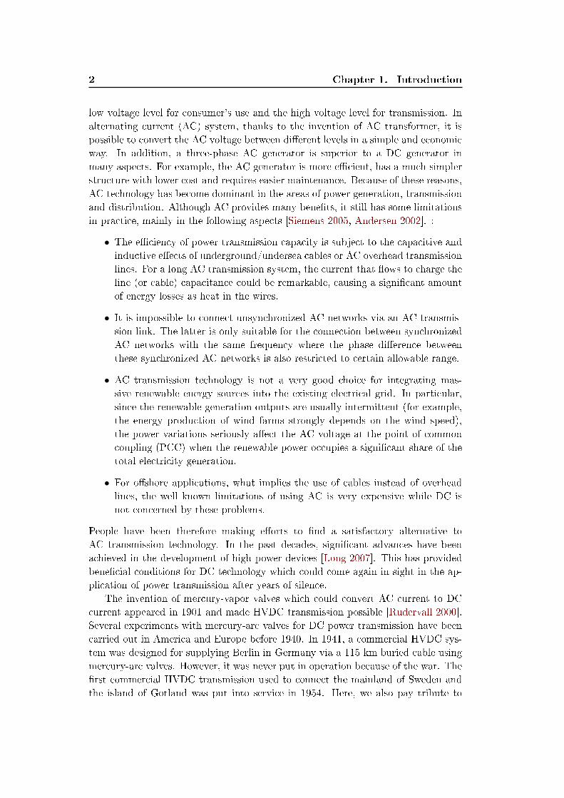
and distribution. Although AC provides many benets, it still has some limitations
in practice, mainly in the following aspects [Siemens 2005, Andersen 2002]. :
• The eciency of power transmission capacity is subject to the capacitive and
inductive eects of underground/undersea cables or AC overhead transmission
lines. For a long AC transmission system, the current that ows to charge the
line (or cable) capacitance could be remarkable, causing a signicant amount
of energy losses as heat in the wires.
• It is impossible to connect unsynchronized AC networks via an AC transmis-
sion link. The latter is only suitable for the connection between synchronized
AC networks with the same frequency where the phase dierence between
these synchronized AC networks is also restricted to certain allowable range.
• AC transmission technology is not a very good choice for integrating mas-
sive renewable energy sources into the existing electrical grid. In particular,
since the renewable generation outputs are usually intermittent (for example,
the energy production of wind farms strongly depends on the wind speed),
the power variations seriously aect the AC voltage at the point of common
coupling (PCC) when the renewable power occupies a signicant share of the
total electricity generation.
• For oshore applications, what implies the use of cables instead of overhead
lines, the well known limitations of using AC is very expensive while DC is
not concerned by these problems.
People have been therefore making eorts to nd a satisfactory alternative to
AC transmission technology. In the past decades, signicant advances have been
achieved in the development of high power devices [Long 2007]. This has provided
benecial conditions for DC technology which could come again in sight in the ap-
plication of power transmission after years of silence.
The invention of mercury-vapor valves which could convert AC current to DC
current appeared in 1901 and made HVDC transmission possible [Rudervall 2000].
Several experiments with mercury-arc valves for DC power transmission have been
carried out in America and Europe before 1940. In 1941, a commercial HVDC sys-
tem was designed for supplying Berlin in Germany via a 115 km buried cable using
mercury-arc valves. However, it was never put in operation because of the war. The
rst commercial HVDC transmission used to connect the mainland of Sweden and
the island of Gotland was put into service in 1954. Here, we also pay tribute to
1.2. Overview of HVDC technology 3
the father of HVDC, Uno Lamm, who made a signicant contribution towards the
application of HVDC in practice [Wollard 1988, Lamm 1966]. Since then, several
HVDC transmission systems have been built with mercury arc valves up to 1972, the
installation of the last mercury-arc HVDC system in Manitoba, Canada. The solid
state semiconductor valves (thyristor valves) rst appeared in 1970, and then soon
replaced the mercury-arc valves [Karady 1973]. Thyristor valves have many advan-
tages over mercury-arc valves. For example, it is easy to increase the voltage just by
connecting thyristors in series. The rst HVDC system using thyristor valves were
put into operation in 1972. Today, most of existing HVDC projects are still based on
thyristor valves [Asplund 2007, Varley 2004]. Since mercury-arc valves and thyris-
tors can not achieve the operation of turn-o by themselves, both of them need an
external AC circuit to force the current to zero and hence, the converters based on
these two valves are known as line-commutated converters (LCCs) [Daryabak 2014].
During the conversion process of LCCs, the converters need to consume the reactive
power which is usually supplied by the AC lters or series capacitors embedded
in the converter station [Bahrman 2007]. In the late 1990's, capacitor-commutated
converters (CCCs) were introduced where capacitors in series connected between the
thyristors and the transformers are used to provide the reactive power. The rst
CCC based HVDC system was built in 1998 used to connect Argentina and Brazil.
In fact, CCCs have not been widely applied in the construction of HVDC systems
because of the advent of new power electronics in the mid 1990's. The development
of high rated semiconductor devices such as integrated gate-commutated thyris-
tors (IGCTs), insulated-gate bipolar transistors (IGBTs), gate turn-o thyristors
(GTOs) etc. has marked the beginning of a new era in the area of HVDC sys-
tems [Andersen 2000, Poullain 2001, Flourentzou 2009, Andersen 2000]. The IGBT
diers from thyristor in that it has the ability to turn o by itself, which can be
used to make self-commutated converters. Converters built with IGBTs are known
as voltage-sourced converters (VSCs). The rst complete VSC HVDC system was
built in Gotland, Sweden, 1999 [Eriksson 2001]. Since then, many VSC HVDC sys-
tems have been put into operation [Asplund 2000, Johansson 2004, Stendius 2006,
Dodds 2010]. The recent rst three-terminal VSC HVDC system operated by China
Southern Power Grid has been put into service at the end of 2013, which is used
to feed wind power generated from Nanao island into the mainland of Guangdong
via a combination of underground cables, submarine cables and overheard lines
[Li 2014, Fu 2014].
1.2 Overview of HVDC technology
The most essential process in an HVDC system is the conversion of the energy
between AC and DC. The converter station located at the sending end is called
the rectier (to convert the current from AC to DC) while the one at the receiving
end is called the inverter (to convert the current from DC to AC). As mentioned in
Section 1.1, there are two basic converter technologies in today's HVDC transmission
4 Chapter 1. Introduction
systems, LCC and VSC.
1.2.1 Line-commutated current source converters
Conventional (or classical) HVDC systems are based on LCCs with thyristor valves
which are used to achieve the operation of converting the current between AC and
DC [Carlsson 2003, Carlsson 2002, Varley 2004, CIGRE 2014]. The essential com-
ponent of LCCs is the three-phase or six-pulse bridge composed of six controlled
switches or thyristor valves. In order to operate at the desired voltage rating, the
thyristors are usually connected in series to build up a suitable thyristor valve. The
drawback of the six-pulse bridge is that considerable AC current and DC voltage
harmonics are produced due to each phase change every 60. To deal with this
problem, two six-pulse bridges are connected in series to constitute a twelve-pulse
bridge. In this manner, with each of the two six-pulse bridges connected to one DC
rail, the 30 phase displacement can be achieved so that some harmonics can be
eliminated. In fact, the twelve-pulse bridge has become dominant in modern LCC
HVDC systems.
Since LCC can not be turned o by itself, an external relatively strong AC
voltage source is required to perform the commutation. As a result, it is impossible
to change the direction of the current. In an LCC HVDC system, in order to change
the power direction, it is necessary to change the polarity of the output voltage.
This leads to inherent diculty when a weak AC system or a passive network is
connected to an LCC converter station. As a controlled solid-state semiconductor
device, the thyristor can only be turned on by control action and hence, LCC has one
degree of freedom, i.e. the ring angle, which represents the phase lag of AC current
behind the voltage. The only way to regulate the DC voltage rating across a valve
is by means of controlling the ring angle. More details of the control of ring angle
are well documented in the literature [Arrillaga 1998, Kimbark 1971, CIGRE 2014].
1.2.2 Voltage-sourced converters
Voltage-sourced converter is built up with fully controlled semiconductor de-
vices such as IGBT and GTO with the ability of turn-o compared to LCC
[Flourentzou 2009, Dodds 2010, Wang 2011]. As a result, an external AC volt-
age is no longer required since the converter based on IGBTs (or GTOs) are self-
commutated. The additional controllability (the operation of turn-o) gives many
advantages to the VSC:
• Pulse-width modulation (PWM) can be applied to the operation of VSC,
which works at higher frequencies than the line frequency and gives rise to
high dynamic performance [Trzynadlowski 1996]. With PWM, the VSC can
generate any voltage with desired phase angle and amplitude. Less harmonics
are produced compared to LCC with PWM.
• Because the AC current always lags behind the voltage in the operation of
LCC, the converter needs to consume the reactive power to keep the amplitude

1.2. Overview of HVDC technology 5
of AC voltage within acceptable range, while the VSC itself has no reactive
power need. Therefore, it is exible to place the VSCs anywhere in the AC
system.
• Unlike LCC, a strong AC voltage source is not indispensable for the VSC
connected AC system and hence, there is no restriction on the inherent char-
acteristics of the connected AC networks.
• Since the VSC possesses two degrees of freedom, this converter has the ability
to control active and reactive power independently. This capability makes the
VSC act close to an ideal generator in a transmission network.
• The bidirectional power transmission can be achieved with the VSC by chang-
ing the current direct without changing the output voltage polarity.
More details of the operation of VSCs are presented in Section 2.
1.2.3 LCC vs VSC
Although the capability of turn-o produces many benets for the VSC, it does
not mean that VSC can replace LCC. Both of the two converters are applied in
modern HVDC systems and they have their respective merits that meet dierent
requirements [Marques 2011, Rudervall 2000]:
• In recent years, signicant advances and improvements in the thyristor tech-
nology have been achieved. In particular, the thyristor has a large capacity
that can withstand high voltage (up to 10 kV) and high current (4 kA) ratings.
Therefore, there is no special restriction on the power range of HVDC with
LCC since very high voltages can be achieved by connecting the thyristors in
series. Besides, the inductive and capacitive elements of the transmission lines
have no eect on the HVDC with LCC and hence, the power losses caused by
these elements do not limit the transmission distance. For these reasons, LCC
HVDC system is well established for long-distance bulk power transmission.
• VSC-HVDC technology is mainly used in medium-capacity power transmis-
sion based upon the considerations: 1) Unlike the thyristor, the IGBT has
a limit capacity with weak overload capability; 2) Due to the use of PWM
at high frequency, the switching losses of the VSC HVDC are higher than
the LCC HVDC. 3) A VSC HVDC system usually uses a special cross-linked
polyethylene (XLPE) cable which has a lower voltage capability compared to
the mineral-insulated (MI) cable used in LCC HVDC system.
• A VSC HVDC system can be used to supply the electrical power to passive or
weak AC networks with low short-circuit capacity. Since the semiconductor
devices used in the VSC are self-commutating, for the connected AC system,
a strong AC voltage source is not necessary.
6 Chapter 1. Introduction
• At present, the vast majority of existing HVDC links are composed of two
converter stations, only carrying out point-to-point power transfer. As the
economic development and the construction of the power grid require that
the DC grid can achieve power exchanges between multiple power suppliers
and multiple power consumers, multi-terminal HVDC system consisting of
more than two converter stations have drawn more and more attention. VSC
HVDC technology is more appropriate than LCC HVDC to build a multi-
terminal HVDC system because of the following reasons: 1) For the LCC
HVDC, the only way of reversing the power direction is to change the DC
voltage polarity. However, in a multi-terminal HVDC system, the reversal
of one terminal's DC voltage polarity gives remarkable disturbances to other
terminals and hence, it is essential to arrange the switching operation of each
terminals [Reeve 1980]. 2) For the VSC HVDC, the power direction can be
changed through the reversal of the current direction while keeping the DC
voltage polarity unchanged. Therefore, one terminal's power direction can be
changed without considering other terminal's power ow directions.
1.2.4 Advantages of HVDC over AC
As discussed in Section 1.1, the inherent drawbacks of AC encourage the develop-
ment of DC technology. The rationale for the choice of HVDC instead of AC is
often various and complex. The common applications in favor of HVDC are listed
as follows:
• Long-distance transmission:
For an AC transmission, the capacitive eect of long overhead lines not only
causes the additional power losses but also limits the transmission distance
while it has less impact on the HVDC transmission line. For these reasons,
HVDC technology provides bulk power transmission solution over very long
distances. From economic aspects, the costs of an HVDC transmission line are
less that an AC line for the same distance but the construction of a converter
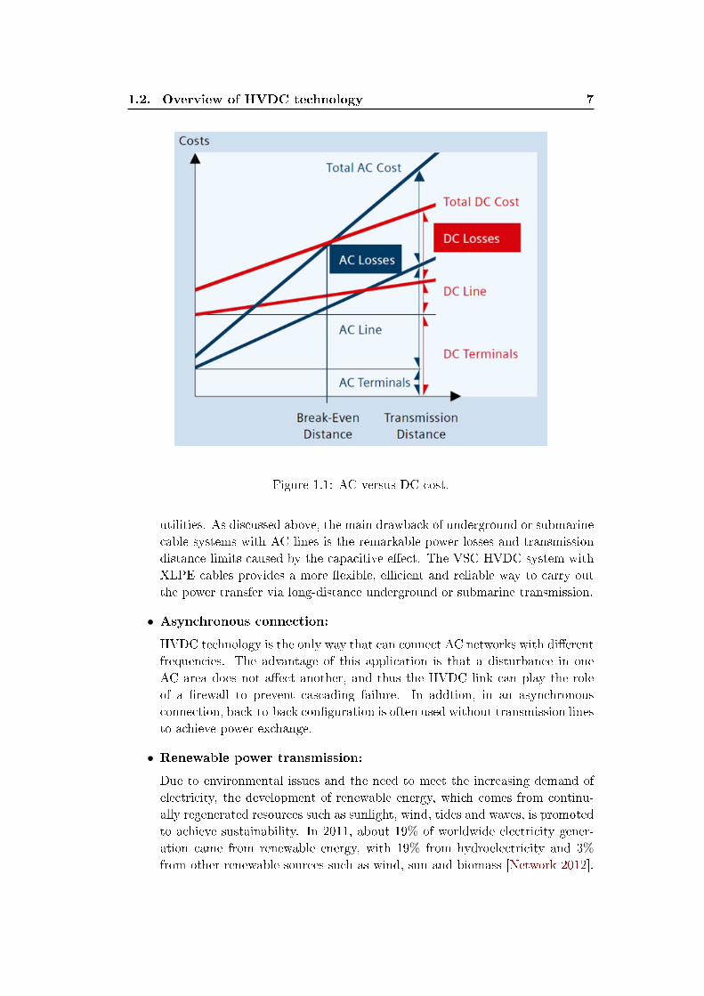
station is expensive. A famous diagram as illustrated in Fig. 1.1 shows a
typical cost analysis for AC and DC [SIEMENS 2014]. Above the break-even
distance, the HVDC transmission line becomes an attractive solution with less
costs in comparison to an AC transmission line with the same power capacity.
Moreover, DC overhead lines occupy much less space than AC transmission
lines with the same power capacity. This reduces the visual impact and the
usage of rights-of-way. Therefore, it is possible to realize the power delivery
from remote power resources such as oshore wind farms or hydro-power plants
using lower visual impact and fewer transmission lines with HVDC.
• Underground or submarine transmission:
From the environment aspects, it is hard to upgrade the electrical grid with
overhead AC lines which require large transmission line corridors. It is rec-
ommended to use underground cables that can share rights-of-way with other
1.2. Overview of HVDC technology 7
Figure 1.1: AC versus DC cost.
utilities. As discussed above, the main drawback of underground or submarine
cable systems with AC lines is the remarkable power losses and transmission
distance limits caused by the capacitive eect. The VSC HVDC system with
XLPE cables provides a more exible, ecient and reliable way to carry out
the power transfer via long-distance underground or submarine transmission.
• Asynchronous connection:
HVDC technology is the only way that can connect AC networks with dierent
frequencies. The advantage of this application is that a disturbance in one
AC area does not aect another, and thus the HVDC link can play the role
of a rewall to prevent cascading failure. In addtion, in an asynchronous
connection, back-to-back conguration is often used without transmission lines
to achieve power exchange.
• Renewable power transmission:
Due to environmental issues and the need to meet the increasing demand of
electricity, the development of renewable energy, which comes from continu-
ally regenerated resources such as sunlight, wind, tides and waves, is promoted
to achieve sustainability. In 2011, about 19% of worldwide electricity gener-
ation came from renewable energy, with 19% from hydroelectricity and 3%
from other renewable sources such as wind, sun and biomass [Network 2012].
8 Chapter 1. Introduction
Renewable power generators are spreading across many countries and espe-
cially, wind power already occupies a signicant share of electricity in Europe,
Asia and the United States. At the end of 2012, wind power grew at an
annual rate of 30% with a worldwide installed capacity of 282,482 MW. It
is expected that wind energy in 2020 should meet 15.7% of EU electricity
demand of 230 GW, and by 2030, 28.5% of 400 GW[Zervos 2009]. Large
wind farms consist of hundreds of individual turbines which are connected to
the electric power transmission network. In general, oshore wind is stead-
ier and stronger than onshore wind farms. However, on the one hand, o-
shore wind farms are usually located far away from the grid, and on the
other hand, wind power is consistent from year to year but has signicant
variation over short time scales. This inherent characteristic could aect the
stability of the interconnected power grid when wind power provides large
share of electricity. It is a big challenge to integrate these long-distance scat-
tered oshore wind farms through AC networks [Ayodele 2011]. Based upon
the above considerations, multi-terminal VSC HVDC (MTDC) transmission
systems consisting of more than two converter stations provide an ecient
solution [Chaudhary 2008, Livermore 2010, Kirby 2002].
1.3 Literature review: related studies on control designs
The control design is always one of the most popular research topics in the area of
VSC HVDC systems. A large number of studies have been devoted to the control
of VSC HVDC systems from dierent points of view.
1.3.1 Control of a single VSC terminal
For any VSC HVDC system, the converter is the most basic component, whose
operation has a great impact on the system's overall performance. Therefore, it is
particularly important to develop appropriate control structures for the VSC. There
are two most frequently discussed control methods, namely direct control method
and vector control method. The direct control approach is very straightforward
where the control inputs, the phase angle and the amplitude modulation ratio, are
directly derived from the measurements of the currents and the voltages at the
PCC [Ooi 1990, Ohnishi 1991, Noguchi 1998, Sood 2010]. The major advantage of
this control method is its simple structure easily implementable while the gravest
drawback is its incapability of limiting the current through the converter to protect
the semiconductor devices.
To overcome this shortcoming, the vector control method is widely used in the
context of the control of VSC [Lindberg 1994, Lindberg 1996, Blasko 1997, Li 2010,
Thomas 2001, Xu 2005, Beccuti 2010] where the VSC is modeled in a synchronous
reference dq frame. The main feature of this method is that it consists of two control
loops, namely the fast inner current loop and the slow outer loop, where the slow
outer loop provides the reference trajectories to the fast inner current one. Thanks

1.3. Literature review: related studies on control designs 9
to the fast inner current loop, this control structure has the ability to limit the
current through the converter.
Studies on comparing the direct control method and the vector control method
are carried out in [Sood 2010, Zakaria Moustafa 2008]. The conventional vector
control method is usually based on several standard PI controllers where a phase-
locked loop (PLL) is usually applied to provide a synchronous reference frame
[Lindberg 1994, Lindberg 1996, Blasko 1997]. However, several limitations of pure
PI control are presented in [Du 2005, Dannehl 2009, Durrant 2003], which show
that the maximum transferable power capability with the conventional vector con-
trol method is far less than the system's maximum achievable capacity and the
system overall performance is remarkably disturbed by the system uncertainties.
Thus, some modied vector control methods are developed. In [Zhao 2013],
adaptive backstepping control technique is applied to the DC voltage outer loop
and the inner current loop to ensure the global stability. In [Li 2010], an optimal
control strategy using a direct current vector control technology is proposed where
the current loop can be a combination of dierent technologies such as PID, adap-
tive control, etc. In [Beccuti 2010], a nonlinear model predictive control method is
applied to the inner current loop without the need of a PLL. Since the conventional
vector control does not fully use the potential of the VSC, in particular, in the case
of connecting to a weak AC system, several other control methods are developed.
In [Zhang 2010], power-synchronization control with a new synchronization method
as an alternative to PLL is established, whose control concept is derived from the
behaviors of synchronous generators. This method is eective when a very weak
AC system is connected to the DC grid via a VSC [Zhang 2011a, Zhang 2011b]. In
[Mariethoz 2014], a VSC HVDC decentralized model predictive control method is
proposed with the purpose of achieving fast control of active and reactive power,
improving power quality, etc. In [Xu 2007b], a new direct power control is pro-
posed where the converter voltage is directly derived from the dened power ux.
This method is applied to the control of doubly fed induction generators (DFIG)
with good performance [Zhi 2007]. Furthermore, an improved DPC is presented
in [Zhi 2009]. In [Durrant 2006], both linear matrix inequality (LMI) and heuris-
tic schemes like genetic algorithm are presented and a comparison is carried out
between them.
1.3.2 Control of MTDC systems
As mentioned in the previous section, AC transmission lines are not feasible for
carrying out power transfer from large oshore power plants due to the requirement
of transmission lines over long distances. In order to connect those large-scale,
oshore and scattered energy sources such as wind farms to the grid, MTDC systems
provide a exible, fast and reversible control of power ow. However, the operation
and the control of an MTDC system is still an open and challenging problem. For
example, since the semiconductor devices in VSC are very sensitive to overvoltage,
it is very important to restrict the DC voltage to an acceptable band.
10 Chapter 1. Introduction
Several research works have proposed dierent control structures to ensure the
normal operation of an MTDC system. Master-slave control strategy (or constant
DC voltage control strategy) are applied in [Ekanayake 2009, Zhang 2012, Lu 2003,
Lu 2005] where one terminal called master terminal is arranged to control the DC
voltage at a constant desired level while the remaining terminals control their respec-
tive active power or other variables. The main drawback of this control approach is
that N-1 secure operation can not be ensured in case of outage of the master termi-
nal. Besides, since only the master terminal is used to ensure the power balance of
the DC grid and keep the DC voltage constant, it is needed a master terminal with
large capacity.
To avoid the above problems, some other control strategies are introduced.
In [Tokiwa 1993, Haileselassie 2008, Nakajima 1999, Mier 2012], a control strategy
called voltage margin method is developed. With this approach, the operation of
each converter is characterized by specic active power-DC voltage (P−VDC) curve.With the voltage margin method, one VSC terminal, for instance, VSC 1, is initially
used to keep the DC voltage constant by adjusting its active power P1 to counteract
disturbances. When P1 reaches its upper or lower limit, VSC 1 starts to operate in
constant active power mode and the DC voltage will rise or decrease until it reaches
another VSC terminal's DC voltage reference setting, for instance, VSC 2's DC volt-
age reference setting. Then, VSC 2 is responsible for the regulation of DC voltage
according to its P − VDC characteristic. Furthermore, a modied two-stage volt-
age margin control is proposed in [Nakajima 1999] by considering each converter's
inherent physical features.
Another control scheme, namely, DC voltage droop control method, whose con-
trol philosophy is to use more than one converter to regulate the DC voltage, is
widely applied in the context of MTDC systems [Karlsson 2003, Prieto-Araujo 2011,
Wang 2014a, Chaudhuri 2013, Bianchi 2011, Chen 2014, Haileselassie 2012b,
Wang 2014b, Eriksson 2014, Johnson 1993, Liang 2009, Rogersten 2014]. With this
control approach, some or all converters are equipped with a droop controller which
is characterized by P − VDC or I − VDC (current vs DC voltage) curve with the
slope Kdroop called the droop gain. This control method has the advantage of 1)
sharing the duty of eliminating the power imbalance of the DC grid between several
terminals; 2) taking actions only based on local information without remote com-
munication. In [Pinto 2011], each of the aforementioned control strategies is tested
and moreover, a performance comparison between them is also carried out.
Concerning the power relations between converter terminals, three DC voltage
control and power dispatch modes are established in [Xu 2011]. In the rst mode,
one terminal, for instance, VSC 1, has priority over the other converters in car-
rying out the power transfer. When VSC achieves its active power's upper limit,
another converter takes over the duty of transmitting the energy. In the second
mode, two converters transmit the energy according to a power ratio which can
be varied in real time. The third mode is the combination of the two mentioned
modes. In [Pinto 2013], a novel distributed direct-voltage control strategy is in-
troduced. The main idea of this control approach is to provide a specic voltage
1.4. Motivations and contributions of the thesis 11
reference to each of the terminals which participate in the regulation of the DC
voltage. In [Rodrigues 2013], an optimal power ow control is proposed where the
convariance matrix adaptation (CMA) algorithm is applied to solve an optimal DC
load-ow problem and then provide the DC voltage references to the distributed
voltage control developed in [Pinto 2013].
The use of MTDC systems for connecting oshore wind farms have been
studied by a number of papers [Haileselassie 2012a, Li 2014, Karaagac 2014,
Haileselassie 2008, Chen 2011, Lie 2008, Prieto-Araujo 2011, Liang 2011,
Haileselassie 2009, Xu 2007a, Fu 2014] where the control structures are well
established and the simulation results are also carried out.
The above mentioned articles in this section are entirely dedicated to the control
design of VSC HVDC systems. There are also a large number of studies that focus on
the modeling of the VSC HVDC systems [Cole 2010, Beerten 2014], the protection
system [Kong 2014, Xiang 2015], the development of multilevel modular converters
(MMC) which generates less harmonics and reduces the losses of the semiconductor
devices [Shi 2015, Adam 2015, Ilves 2015], etc.
1.4 Motivations and contributions of the thesis
For years, people have been working on the development of a European supergrid
that allows the massive integration of renewable energy sources to meet the ever in-
creasing consumption of electricity. Due to some undesirable inherent characteristics
of the renewable energy sources, such as the variability of the generation output, the
conventional AC transmission lines are not quite suitable for the connection of large
shares of renewable energy sources while VSC HVDC systems provide an alternative
solution. Although numerous research studies on VSC HVDC systems have been
carried out, there are still many challenges and it is not yet totally feasible to build
such a supergrid.
1.4.1 Motivations
This dissertation is motivated by the challenges in the control design of MTDC
systems and analysis of MTDC system's dynamic behavior.
1.4.1.1 Control methods
As a system with complex dynamics, any operation of the VSC HVDC system may
give rise to both potential dangers of unexpected interaction and improvement of the
system performance. Therefore, developing control structures which are capable to
keep good performances like fast tracking or small overshoots, during disturbances
is always a challenge for the control of VSC HVDC systems.
As presented in Section 1.3.1, many control methods have been developed. How-
ever, most of them lack the corresponding theoretical support and usually need sig-
nicant eorts to adjust the controller. For example, though the traditional vector
12 Chapter 1. Introduction
control method based on standard PI controllers has a simple structure, we need to
tune the PI control gains by using other procedures [Bajracharya 2008]. Reference
[Zhang 2011c] gives a stability analysis for power synchronization control method.
Nevertheless, this analysis is carried out by linearizing the system around the operat-
ing point and hence, the nonlinear behavior of the system can not be well exhibited.
Reference [Dannehl 2009] also presents a study on the limitations of vector control
method, but, similar to the case of power synchronization control method, this re-
search work is done via linearization and it is only valid for the behavior within
a small neighborhood of the operating point. It is worth considering that, when
designing a control structure, we should not only focus on the actual results (or
performances) of the control strategy but also on the theoretical explanation of the
control operating principle.
1.4.1.2 Dynamic behaviors
As discussed in the section of literature review, vector control method, which is
composed of two control loops, is the most widely used control approach for VSC
HVDC systems due to its simple structure and its capability to limit the current
through the converter. The rationale of this method is based on the assertion that
the dynamics of the inductor currents are much faster than the dynamics of the
capacitor voltages. As a result, the independent control designs of the two control
loops are achievable. However, there exist very few relevant studies in the literature
that have ever presented a detailed theoretical explanation on the validity and the
implications of this assertion. It is not clear if the time-scale separation between the
dynamics of the current and the voltage is an inherent characteristics or it exists
only under certain conditions. For example, as demonstrated in [Kimball 2008],
for some DC-DC converters, the dynamic separation between the system variables
exists only when the stability requirement is satised. If the time-scale separation
exists in a high-order system, this feature has a great signicance to the analysis of
system's behavior. Based on the time-scale separation, two (or more) subsystems of
lower orders can usually be deduced from the original high-order system and then,
we can use the behaviors of the low-order subsystems to approximate the behaviors
of the high-order original system. This greatly reduces the complexity of analyzing
the system's dynamic performance. Therefore, the verication of the existence of
the time-scale separation is very desirable.
1.4.2 Contributions
The research work in this dissertation aims at lling some gaps between the theory
and the practice, i.e. 1) to investigate various control approaches for the purpose of
improving the performance of MTDC systems; 2) to establish connections between
existing empirical control designs and theoretical analysis; 3) to increase under-
standing of the multi-time-scale behavior of MTDC systems characterized by the
presence of slow and fast transients in response to external disturbances.
1.4. Motivations and contributions of the thesis 13
The main contributions of the research work reported in this thesis can be put
into three aspects, namely nonlinear control designs of MTDC systems, analysis of
MTDC system's dynamic behaviors and application of MTDC systems to provide
frequency support for AC networks.
1.4.2.1 Nonlinear control designs
In the area of nonlinear control design of MTDC systems, three nonlinear control
design tools, namely feedback linearization control, feedback linearization control
with sliding mode control and passivity-based state feedback control, are applied to
establish dierent control schemes with corresponding theoretical analysis. Besides,
the developed control algorithms have been tested by detailed and realistic numerical
simulations, whose performances are evaluated in comparison to the performance of
the conventional vector current algorithm.
1.4.2.2 Analysis of dynamic performances
The main motivation for the research work in the area of analysis of MTDC system's
dynamic behaviors is the desire to provide a rigorous theoretical demonstration to
verify a common assertion used in the control design of VSC HVDC systems, that
is, the dynamics of the inductor currents are much faster than the capacitor voltage.
The contribution in this area consists of three parts: 1) development of a general
control theory that we named "Control induced time-scale separation" for a class of
nonlinear systems; 2) analysis of control induced time-scale separation for an MTDC
system with master-slave control conguration; 3) analysis of control induced time-
scale separation for an MTDC system with droop control conguration. Theoretical
analysis, mainly based on singular perturbation and Lyapunov theories, have been
carried out for each of the aforementioned aspects and claried with various simu-
lation studies. The study of the rst part has been mainly performed to propose a
time-scale separation control method which can drive a class of nonlinear systems
to exhibit a multi-time-scale performance. The theoretical results obtained from
the rst part have been applied to investigate the dynamic behaviors of MTDC sys-
tems under the two main control congurations, i.e. master-slave and droop control.
Empirical vector current control designs have been proposed for each control cong-
uration. Theoretical explanations and fundamental analysis indicate that with the
currently used empirical control algorithms, the inductor currents indeed perform a
dynamic behavior with dierent dynamics. Furthermore, more details on how and
why these empirical vector current control designs work have been also provided.
1.4.2.3 Frequency support
The nal contribution relates to analysis of the application of MTDC systems for
frequency support strategy. A DC voltage based control scheme for the AC fre-
quency regulation is proposed, achieving the objective of sharing primary reserves
between dierent AC areas interconnected via MTDC system without using remote
14 Chapter 1. Introduction
information though telecommunication. The frequency control principle is to regu-
late the AC frequency by modulating each AC grid's scheduled (or prescribed) input
of active power.
1.5 Outline of the thesis
This dissertation is organized as follows: In Chapter 2 a brief introduction of VSC
HVDC technology is presented. In particular, the possible operation modes of the
VSC are discussed, which are essential for the design of a control system. In Chap-
ter 3 the dynamic model of a multi-terminal VSC HVDC system is established
based on a synchronous reference dq frame. This MTDC system consists of two
dierent AC networks connected via a generic DC grid. In Chapter 4 two most
used conventional control methods, namely direct control method and vector con-
trol method, are introduced. In addition, the merits and drawbacks of these two
methods are also discussed. In Chapter 5 three dierent nonlinear control structures
are proposed for VSC HVDC systems. With the help of numerical simulations, the
advantages claimed for each of the proposed controllers are veried in comparison
to the conventional vector current control method. In Chapter 6 the system dy-
namic behaviors are investigated. We rst demonstrate that there exists a control
structure that can drive a class of nonlinear systems to exhibit arbitrary multi-time-
scale dynamics that were not natural to the system. Then, we apply the obtained
theoretical results to the MTDC system under two control congurations, namely
master-slave control conguration and droop control conguration. The theoretical
analysis of the time-scale separation between the dynamics of the system states are
also carried out for each of the aforementioned control conguration. In Chapter
7 the potential of VSC HVDC technology for frequency regulation is investigated
where a DC-voltage-based control scheme is proposed to make the interconnected
AC networks share their primary reserves. In Chapter 8 conclusions are drawn and
future work is discussed.
1.6 Publications
Most of the materials in this thesis have been published in the following articles:
• "Nonlinear Control Design for a Multi-Terminal VSC-HVDC System", Yijing
Chen, Jing Dai, Gilney Damm, Françoise Lamnabhi-Lagarrigue, 2013 Euro-
pean Control Conference (ECC), July 17-19, 2013, Zürich, Switzerland.
• "A detailed study on a DC-voltage-based control scheme using a multi-
terminal HVDC system for frequency control", Yijing Chen, Jing Dai, Gilney
Damm, Françoise Lamnabhi-Lagarrigue, 2013 European Control Conference
(ECC), July 17-19, 2013, Zürich, Switzerland.
• "Control Induced Explicit Time-Scale Separation to Attain DC Voltage Stabil-
ity for a VSC-HVDC Terminal", Yijing Chen, Gilney Damm, Abdelkrim Ben-
1.6. Publications 15
chaib, Mariana Netto, Françoise Lamnabhi-Lagarrigue, 19th World Congress
of the International Federation of Automatic Control (IFAC), August 24-29,
2014, Cape Town, South Africa.
• "Feedback Linearization for the DC Voltage Control of a VSC-HVDC Termi-
nal", Yijing Chen, Gilney Damm, Abdelkrim Benchaib, Françoise Lamnabhi-
Lagarrigue, 2014 European Control Conference (ECC), June 24-27, 2014,
Strasbourg, France.
• "Multi-Time-Scale Stability Analysis and Design Conditions of a VSC Ter-
minal with DC Voltage Droop Control for HVDC Networks", Yijing Chen,
Gilney Damm, Abdelkrim Benchaib, Françoise Lamnabhi-Lagarrigue, 53rd
IEEE Conference on Decision and Control (CDC), December 15-17, 2014, Los
Angeles, CA, USA.
• "Multi-Terminal High Voltage Direct Current Networks for Renewable
Energy Sources", Miguel Jiménez Carrizosa, Yijing Chen, Gilney Damm,
Abdelkrim Benchaib and Françoise Lamnabhi-Lagarrigue, ERCIM News
No. 97 special theme: "Cyber-Physical Systems", Link: http://ercim-
news.ercim.eu/en97/special/multi-terminal-high-voltage-direct-current-
networks-for-renewable-energy-sources

Chapter 2
VSC HVDC technology
Contents
2.1 Key components . . . . . . . . . . . . . . . . . . . . . . . . . . 17
2.2 Operating principles of VSC . . . . . . . . . . . . . . . . . . . 19
2.3 Congurations of HVDC systems . . . . . . . . . . . . . . . . 19
2.4 AC network and control modes of VSC terminals . . . . . . 23
2.4.1 AC network connected to VSC terminal . . . . . . . . . . . . 23
2.4.2 Control modes of VSC terminals . . . . . . . . . . . . . . . . 23
2.5 Chapter conclusions . . . . . . . . . . . . . . . . . . . . . . . . 25
In order to get a good understanding of VSC HVDC technology, this chapter
rst introduces the main components of a VSC HVDC system in Section 2.1, each
performing a dierent function. Subsequently, the operating principles of VSC are
described in Section 2.2. Next, several congurations of HVDC systems are pre-
sented in Section 2.3. Finally, various control modes of VSC terminals are discussed
in Section 2.4.
2.1 Key components
A simplied representation of a VSC HVDC converter station is depicted in Fig.
2.1. The characteristics and purposes of the main components of a VSC HVDC
system are introduced in this section [Siemens 2005, Bahrman 2007, Dodds 2010,
Andersen 2002].
Transformer
A bank of transformers are installed to adapt the AC voltage level of the connected
AC grid to the rated DC voltage transmission level. Since harmonic lters are
located between the phase reactors and the transformers, harmonic currents have
little or no eects on the transformers. Therefore, ordinary transformers can be
used for VSC HVDC systems.
Harmonic lter
With VSCs, the generated harmonics are usually at high frequencies, which strongly
depend on the PWM method and converter topology. In a VSC HVDC system,
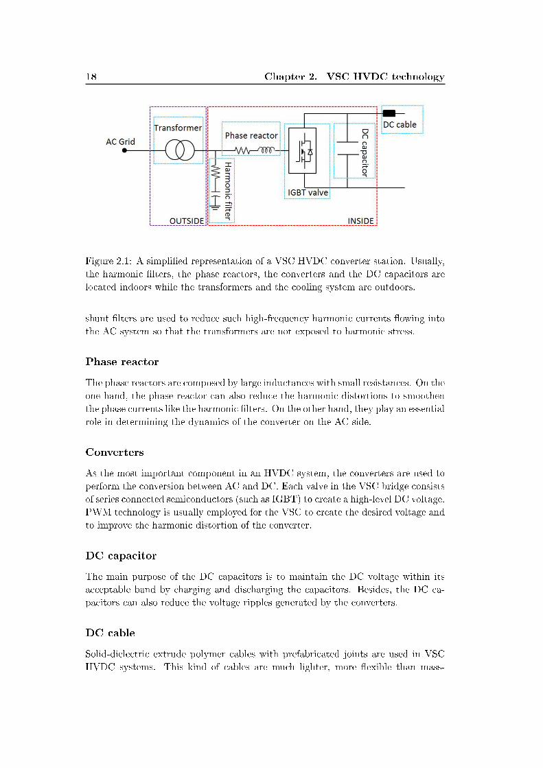
18 Chapter 2. VSC HVDC technology
Figure 2.1: A simplied representation of a VSC HVDC converter station. Usually,
the harmonic lters, the phase reactors, the converters and the DC capacitors are
located indoors while the transformers and the cooling system are outdoors.
shunt lters are used to reduce such high-frequency harmonic currents owing into
the AC system so that the transformers are not exposed to harmonic stress.
Phase reactor
The phase reactors are composed by large inductances with small resistances. On the
one hand, the phase reactor can also reduce the harmonic distortions to smoothen
the phase currents like the harmonic lters. On the other hand, they play an essential
role in determining the dynamics of the converter on the AC side.
Converters
As the most important component in an HVDC system, the converters are used to
perform the conversion between AC and DC. Each valve in the VSC bridge consists
of series connected semiconductors (such as IGBT) to create a high-level DC voltage.
PWM technology is usually employed for the VSC to create the desired voltage and
to improve the harmonic distortion of the converter.
DC capacitor
The main purpose of the DC capacitors is to maintain the DC voltage within its
acceptable band by charging and discharging the capacitors. Besides, the DC ca-
pacitors can also reduce the voltage ripples generated by the converters.
DC cable
Solid-dielectric extrude polymer cables with prefabricated joints are used in VSC
HVDC systems. This kind of cables are much lighter, more exible than mass-
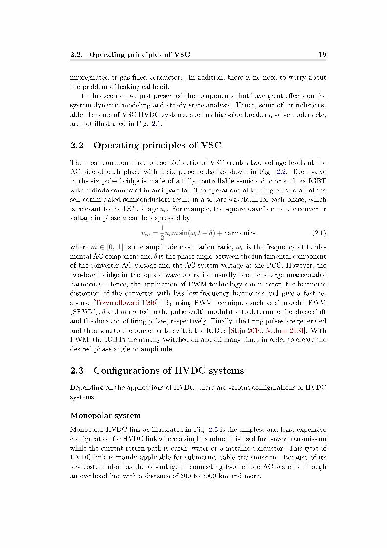
2.2. Operating principles of VSC 19
impregnated or gas-lled conductors. In addition, there is no need to worry about
the problem of leaking cable oil.
In this section, we just presented the components that have great eects on the
system dynamic modeling and steady-state analysis. Hence, some other indispens-
able elements of VSC HVDC systems, such as high-side breakers, valve coolers etc,
are not illustrated in Fig. 2.1.
2.2 Operating principles of VSC
The most common three-phase bidirectional VSC creates two voltage levels at the
AC side of each phase with a six pulse bridge as shown in Fig. 2.2. Each valve
in the six pulse bridge is made of a fully controllable semiconductor such as IGBT
with a diode connected in anti-parallel. The operations of turning on and o of the
self-commutated semiconductors result in a square waveform for each phase, which
is relevant to the DC voltage uc. For example, the square waveform of the converter
voltage in phase a can be expressed by
vca =1
2ucm sin(ωet+ δ) + harmonics (2.1)
where m ∈ [0, 1] is the amplitude modulation ratio, ωe is the frequency of funda-
mental AC component and δ is the phase angle between the fundamental component
of the converter AC voltage and the AC system voltage at the PCC. However, the
two-level bridge in the square wave operation usually produces large unacceptable
harmonics. Hence, the application of PWM technology can improve the harmonic
distortion of the converter with less low-frequency harmonics and give a fast re-
sponse [Trzynadlowski 1996]. By using PWM techniques such as sinusoidal PWM
(SPWM), δ andm are fed to the pulse width modulator to determine the phase shift
and the duration of ring pulses, respectively. Finally, the ring pulses are generated
and then sent to the converter to switch the IGBTs [Stijn 2010, Mohan 2003]. With
PWM, the IGBTs are usually switched on and o many times in order to create the
desired phase angle or amplitude.
2.3 Congurations of HVDC systems
Depending on the applications of HVDC, there are various congurations of HVDC
systems.
Monopolar system
Monopolar HVDC link as illustrated in Fig. 2.3 is the simplest and least expensive
conguration for HVDC link where a single conductor is used for power transmission
while the current return path is earth, water or a metallic conductor. This type of
HVDC link is mainly applicable for submarine cable transmission. Because of its
low cost, it also has the advantage in connecting two remote AC systems through
an overhead line with a distance of 300 to 3000 km and more.
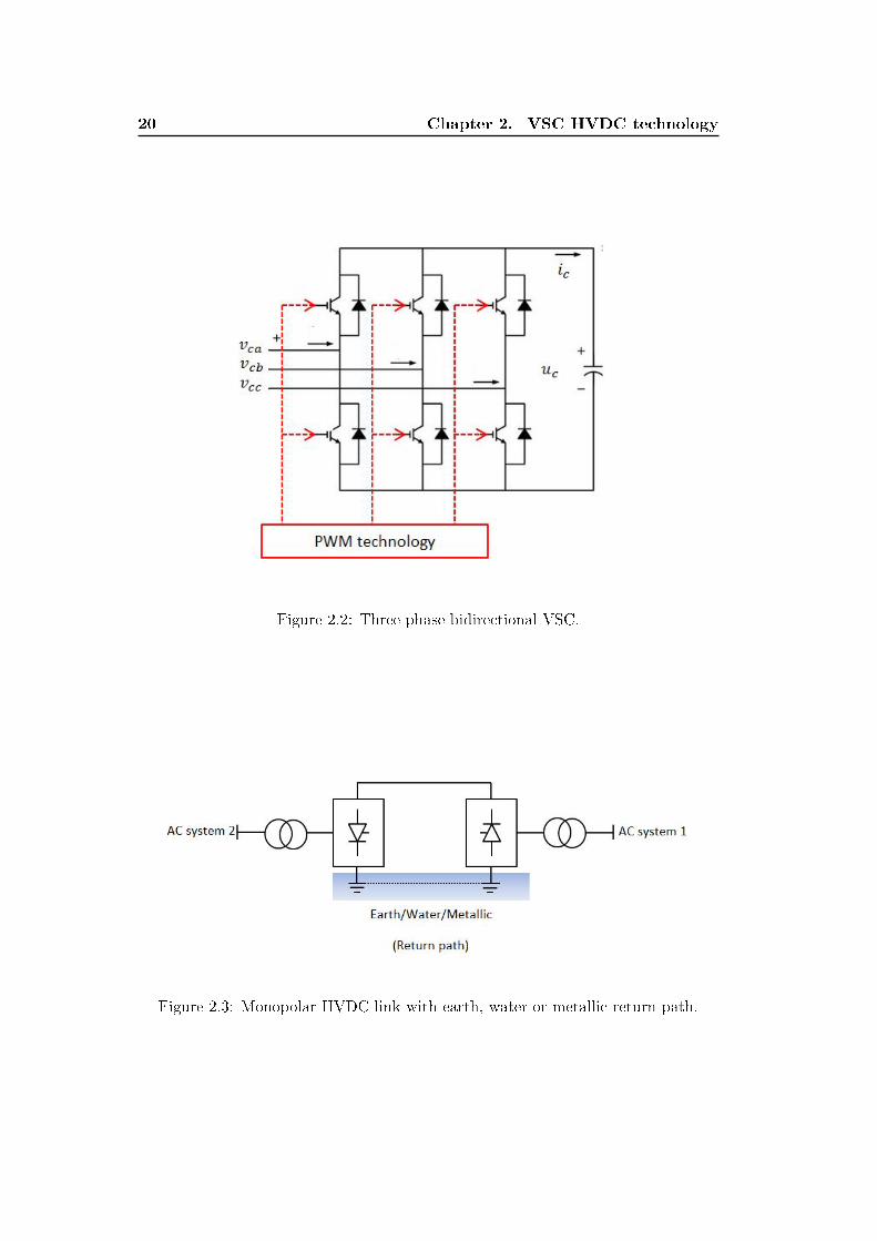
20 Chapter 2. VSC HVDC technology
Figure 2.2: Three phase bidirectional VSC.
Figure 2.3: Monopolar HVDC link with earth, water or metallic return path.
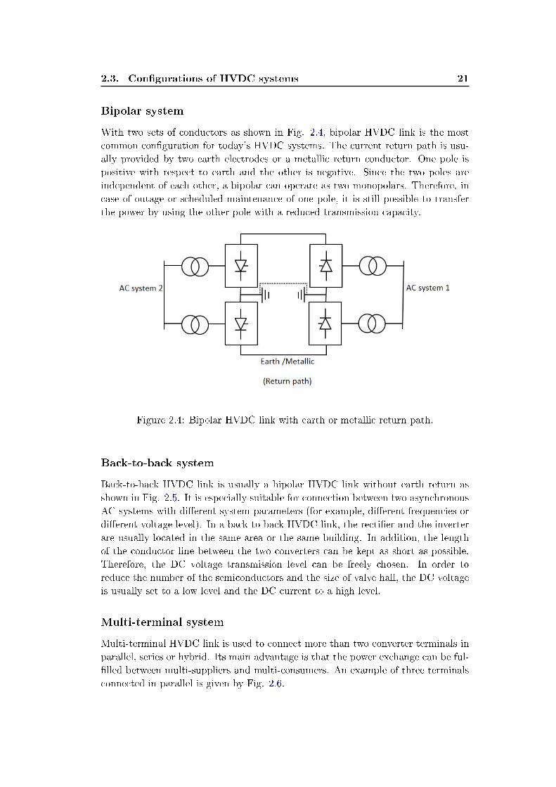
2.3. Congurations of HVDC systems 21
Bipolar system
With two sets of conductors as shown in Fig. 2.4, bipolar HVDC link is the most
common conguration for today's HVDC systems. The current return path is usu-
ally provided by two earth electrodes or a metallic return conductor. One pole is
positive with respect to earth and the other is negative. Since the two poles are
independent of each other, a bipolar can operate as two monopolars. Therefore, in
case of outage or scheduled maintenance of one pole, it is still possible to transfer
the power by using the other pole with a reduced transmission capacity.
Figure 2.4: Bipolar HVDC link with earth or metallic return path.
Back-to-back system
Back-to-back HVDC link is usually a bipolar HVDC link without earth return as
shown in Fig. 2.5. It is especially suitable for connection between two asynchronous
AC systems with dierent system parameters (for example, dierent frequencies or
dierent voltage level). In a back-to-back HVDC link, the rectier and the inverter
are usually located in the same area or the same building. In addition, the length
of the conductor line between the two converters can be kept as short as possible.
Therefore, the DC voltage transmission level can be freely chosen. In order to
reduce the number of the semiconductors and the size of valve hall, the DC voltage
is usually set to a low level and the DC current to a high level.
Multi-terminal system
Multi-terminal HVDC link is used to connect more than two converter terminals in
parallel, series or hybrid. Its main advantage is that the power exchange can be ful-
lled between multi-suppliers and multi-consumers. An example of three terminals
connected in parallel is given by Fig. 2.6.
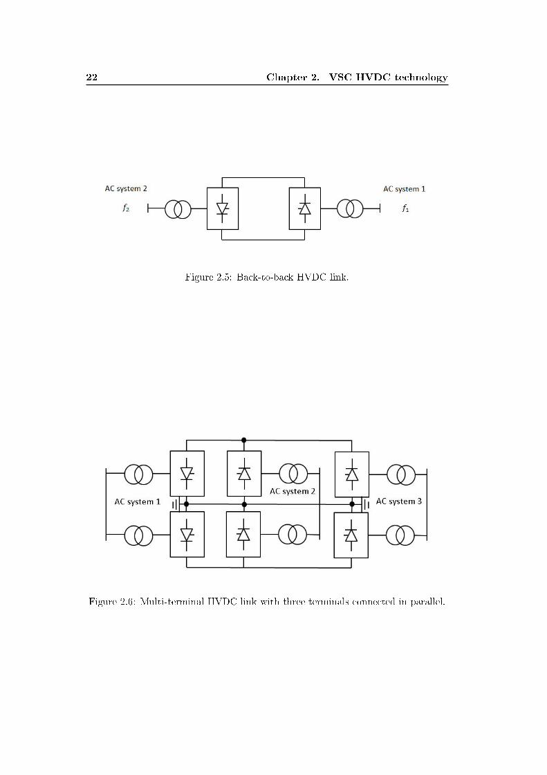
22 Chapter 2. VSC HVDC technology
Figure 2.5: Back-to-back HVDC link.
Figure 2.6: Multi-terminal HVDC link with three terminals connected in parallel.
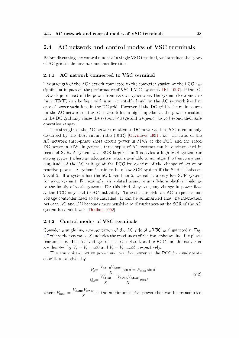
2.4. AC network and control modes of VSC terminals 23
2.4 AC network and control modes of VSC terminals
Before discussing the control modes of a single VSC terminal, we introduce the types
of AC grid in the inverter and rectier side.
2.4.1 AC network connected to VSC terminal
The strength of the AC network connected to the converter station at the PCC has
signicant impact on the performance of VSC HVDC systems [IEE 1997]. If the AC
network gets most of the power from its own generators, the system electromotive
force (EMF) can be kept within an acceptable band by the AC network itself in
case of power variations in the DC grid. However, if the DC grid is the main source
for the AC network or the AC network has a high impedance, the power variation
in the DC grid may cause the system voltage and frequency to go beyond their safe
operating ranges.
The strength of the AC network relative to DC power at the PCC is commonly
described by the short circuit ratio (SCR) [Gavrilovic 1991], i.e. the ratio of the
AC network three-phase short circuit power in MVA at the PCC and the rated
DC power in MW. In general, three types of AC systems can be distinguished in
terms of SCR. A system with SCR larger than 3 is called a high SCR system (or
strong system) where an adequate inertia is available to maintain the frequency and
amplitude of the AC voltage at the PCC irrespective of the change of active or
reactive power. A system is said to be a low SCR system if the SCR is between
2 and 3. If a system has the SCR less than 2, we call it a very low SCR system
(or weak system). For example, an isolated island or an oshore platform belongs
to the family of weak systems. For this kind of system, any change in power ow
at the PCC may lead to AC instability. To avoid this risk, an AC frequency and
voltage controller need to be installed. It can be summarized that the interaction
between AC and DC becomes more sensitive to disturbances as the SCR of the AC
system becomes lower [Thallam 1992].
2.4.2 Control modes of VSC terminals
Consider a single line representation of the AC side of a VSC as illustrated in Fig.
2.7 where the reactance X includes the reactances of the transmission line, the phase
reactors, etc. The AC voltages of the AC network at the PCC and the converter
are denoted by Vs = Vs,rms∠0 and Vc = Vc,rms∠δ, respectively.The transmitted active power and reactive power at the PCC in steady-state
condition are given by
Ps=Vs,rmsVc,rms
Xsin δ = Pmax sin δ
Qs=V 2s,rms
X− Vs,rmsVc,rms
Xcos δ
(2.2)
where Pmax =Vs,rmsVc,rms
Xis the maximum active power that can be transmitted
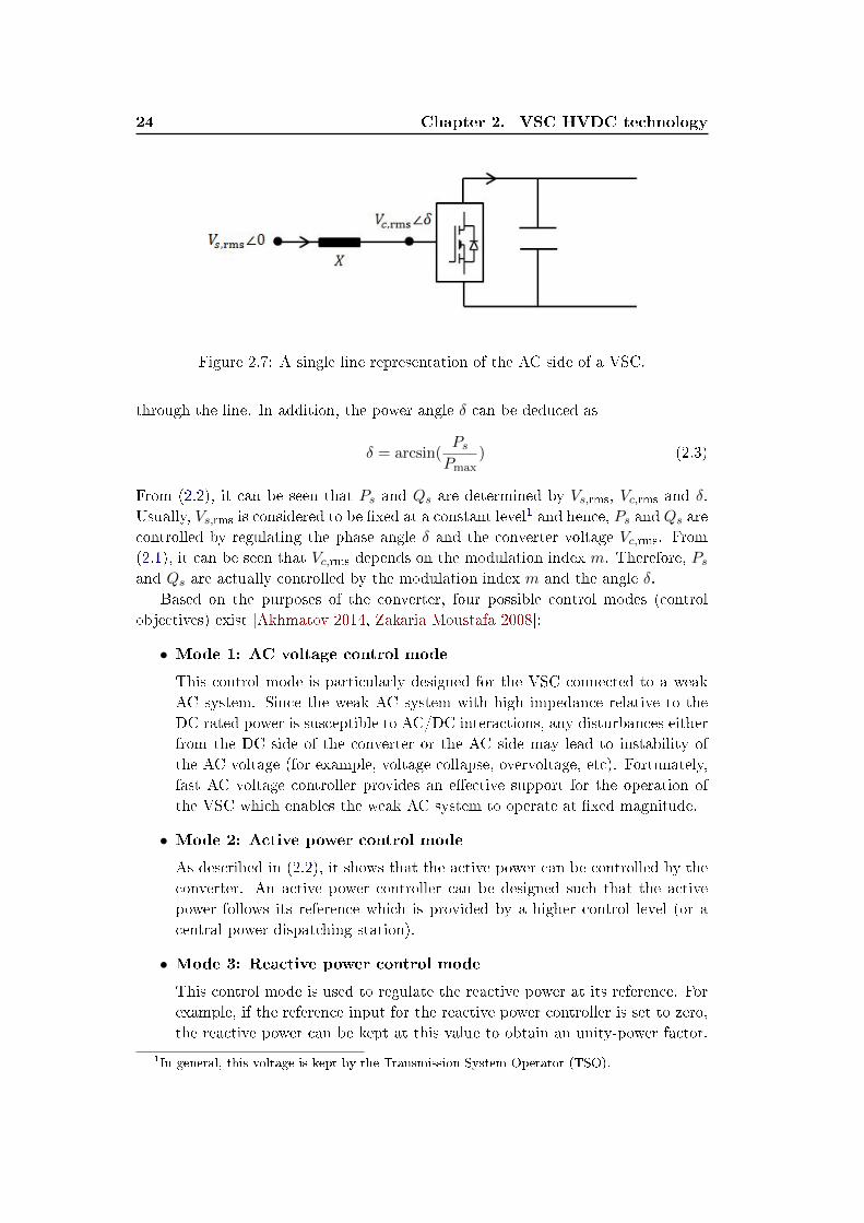
24 Chapter 2. VSC HVDC technology
Figure 2.7: A single line representation of the AC side of a VSC.
through the line. In addition, the power angle δ can be deduced as
δ = arcsin(PsPmax
) (2.3)
From (2.2), it can be seen that Ps and Qs are determined by Vs,rms, Vc,rms and δ.
Usually, Vs,rms is considered to be xed at a constant level1 and hence, Ps and Qs are
controlled by regulating the phase angle δ and the converter voltage Vc,rms. From
(2.1), it can be seen that Vc,rms depends on the modulation index m. Therefore, Psand Qs are actually controlled by the modulation index m and the angle δ.
Based on the purposes of the converter, four possible control modes (control
objectives) exist [Akhmatov 2014, Zakaria Moustafa 2008]:
• Mode 1: AC voltage control mode
This control mode is particularly designed for the VSC connected to a weak
AC system. Since the weak AC system with high impedance relative to the
DC rated power is susceptible to AC/DC interactions, any disturbances either
from the DC side of the converter or the AC side may lead to instability of
the AC voltage (for example, voltage collapse, overvoltage, etc). Fortunately,
fast AC voltage controller provides an eective support for the operation of
the VSC which enables the weak AC system to operate at xed magnitude.
• Mode 2: Active power control mode
As described in (2.2), it shows that the active power can be controlled by the
converter. An active power controller can be designed such that the active
power follows its reference which is provided by a higher control level (or a
central power dispatching station).
• Mode 3: Reactive power control mode
This control mode is used to regulate the reactive power at its reference. For
example, if the reference input for the reactive power controller is set to zero,
the reactive power can be kept at this value to obtain an unity-power factor.
1In general, this voltage is kept by the Transmission System Operator (TSO).
2.5. Chapter conclusions 25
This action is helpful in improving the power quality. Moreover, unlike LCC
HVDC systems, the VSC itself does not need reactive power support. Actually,
the VSC can work as a reactive power compensator to regulate the amplitude
of the AC system voltage by controlling the reactive power at the PCC.
Because of the ability to fully control the power ow, the VSC has become a
very important power ow controlling device [Van Hertem 2005]
• Mode 4: DC voltage control mode
It is very important to keep in mind that, the operation of VSC HVDC sys-
tem is always constrained by the DC voltage which is only acceptable in a
narrow operating band. As a result, for any VSC HVDC system with either
conventional two terminals or multi terminals, at least one terminal must be
equipped with DC voltage controller to ensure that the DC voltage always
remains in its acceptable range, what is obtained by the power ow balance
of the DC grid.
The dominant feature of VSC based on IGBTs is that both turn-on and turn-o
operations on the valves are available. Therefore, VSC possesses a second degree of
freedom compared to LCC. This additional controllability gives many advantages,
one of which is that the VSC has the possibility to control two output quantities.
According to the applications and the types of VSC connected AC systems, there
are possible combinations [Zakaria Moustafa 2008] for a single VSC operation:
• DC voltage and AC voltage control modes
• DC voltage and reactive power control modes
• Active and reactive power power control modes
• Active power and AC voltage control modes.
2.5 Chapter conclusions
In this chapter, we have introduced the key components of a VSC terminal, explained
the operating principles of the converter and classied AC systems into three types
in terms of SCR. According to various applications of VSC HVDC systems, four
dierent congurations have been presented. Furthermore, four possible control
modes for operating a VSC have been discussed. This chapter makes preparations
for the system modeling in the following chapter.

Chapter 3
Dynamic model of multi-terminal
VSC HVDC systems
Contents
3.1 Preliminary knowledge . . . . . . . . . . . . . . . . . . . . . . 27
3.2 Clarke's and Park's transformations . . . . . . . . . . . . . . 28
3.2.1 Clarke's transformation . . . . . . . . . . . . . . . . . . . . . 28
3.2.2 Park's transformation . . . . . . . . . . . . . . . . . . . . . . 30
3.3 Three-phase synchronous reference frame phase-locked loop 31
3.4 Multi-terminal HVDC system model . . . . . . . . . . . . . . 32
3.4.1 Strong AC system side . . . . . . . . . . . . . . . . . . . . . . 32
3.4.2 Weak AC system side . . . . . . . . . . . . . . . . . . . . . . 34
3.4.3 DC network . . . . . . . . . . . . . . . . . . . . . . . . . . . . 36
3.4.4 Domain of interest . . . . . . . . . . . . . . . . . . . . . . . . 40
3.5 Conventional control methods . . . . . . . . . . . . . . . . . . 40
3.5.1 Direct control method . . . . . . . . . . . . . . . . . . . . . . 40
3.5.2 Vector control method . . . . . . . . . . . . . . . . . . . . . . 41
3.6 Chapter conclusions . . . . . . . . . . . . . . . . . . . . . . . . 44
In this chapter, an average state-space model is developed for multi-terminal
VSC HVDC systems. In the modeling, a synchronously rotating dq frame is chosen
so that the three-phase quantities can be transformed into two-phase quantities.
Using basic physical laws, the dynamics of the converter's AC and DC sides are
modeled by dierential equations. A generic topology for the DC network is consid-
ered and the properties of the DC grid are discussed. Furthermore, two most widely
used control approaches are also presented.
3.1 Preliminary knowledge
There exist dierent approaches to modeling VSC HVDC systems. In the detailed
modeling approach, every semiconductor device should be treated as an individual
unit, where the type of modulation (sinusoidal PMW or optimized PMW), the con-
verter switching level (two-level or multi-level) and harmonics with high frequency
need to be analyzed. Such a method results in a very complex model which needs a

28 Chapter 3. Dynamic model of multi-terminal VSC HVDC systems
lot of memory and CPU times to run simulations. Compared to the detailed model-
ing approach, the time-averaged modeling approach [Middlebrook 1976] seems much
simpler and tractable while still enabling us to study the system behaviors related
to the fundamental frequency components of the voltage and the current. In the
time-averaged model, the VSC is viewed as a controllable AC voltage source from
AC side whereas it is considered as a controllable current source from DC side as
depicted in Fig. 2.2. By using the time-averaged modeling approach, there is no
need to consider the dynamics of each individual semiconductor device and more-
over, high frequency harmonics can also be neglected. This greatly simplies the
modeling process, save simulation memory and accelerates the simulation speed.
Based on the above considerations, the time-averaged modeling approach is applied
in this thesis work. As a result, according to (2.1), the converter voltage vc,abc and
the DC voltage uc in the time-averaged model satisfy
vc,abc =1
2ucmabc (3.1)
where ma, mb and mc ∈ [0, 1] are the modulation indices of the phase a, phase b
and phase c, respectively, determined by the amplitude modulation ratio m and the
phase angle δ, according to the following expressions
ma= m sin(ωet+ δ)
mb= m sin(ωet− 23π + δ)
mc= m sin(ωet+ 23π + δ)
(3.2)
In the remainder of this thesis, it is assumed that all VSC connected AC sys-
tems are under balanced network conditions. Thus, there is no negative sequence
component of the three-phase voltage or current, and the three phases have equal
voltage amplitudes with a phase angle of 120 between themselves.
3.2 Clarke's and Park's transformations
Clarke's and Park's transformations are widely used in many studies on synchronous
and asynchronous machines. Their basic principle is to transform a balanced three-
phase system into a two-phase system by simplifying the analysis of three-phase
circuit. The dierence between both transformations is that Clarke's transformation
is to project the three-phase quantities onto a stationary two-axis reference frame,
whereas Park's transformation onto a rotating two-axis reference frame.
3.2.1 Clarke's transformation
The stationary two axes of Clarke's transformation are denoted by α− and β−,which are orthogonal. In order to make the transformation invertible, the zero-
sequence component is usually added and then, Clarke's transformation matrix can

3.2. Clarke's and Park's transformations 29
be expressed by
xαβ0 = Tαβ0 xabc = kc
1 −12 −1
2
0√
32 −
√3
212
12
12
xabc (3.3)
where kc is a constant and x can represent the AC voltage, current, etc. The inverse
Clarke's transformation is given by
T−1αβ0 =
2
3k−1c
1 0 1
−12
√3
2 1
−12 −
√3
2 1
(3.4)
Let us take an example. Consider a balanced three-phase system whose voltages
and currents in a−, b−, and c−axis are given by
va=√
2Vrms cos(ωt+ δa)
vb=√
2Vrms cos(ωt− 23π + δa)
vc=√
2Vrms cos(ωt+ 23π + δa)
(3.5)
and
ia=√
2Irms cos(ωt+ δa + φ)
ib=√
2Irms cos(ωt− 23π + δa + φ)
ic=√
2Irms cos(ωt+ 23π + δa + φ)
(3.6)
where
• Vrms and Irms are the root mean square values of the AC voltage and current,
respectively.
• ω = 2πf is the angular frequency in rad/s and f is the frequency of the AC
system.
• δa is the phase of va and φ is the phase angle between the voltage and the
current.
Applying Clarke's transformation to vabc and iabc, we get
vα= 32kc√
2Vrms cos(ωt+ δa)
vβ= 32kc√
2Vrms sin(ωt+ δa)(3.7)
and
iα= 32kc√
2Irms cos(ωt+ δa + φ)
iβ= 32kc√
2Irms sin(ωt+ δa + φ)(3.8)
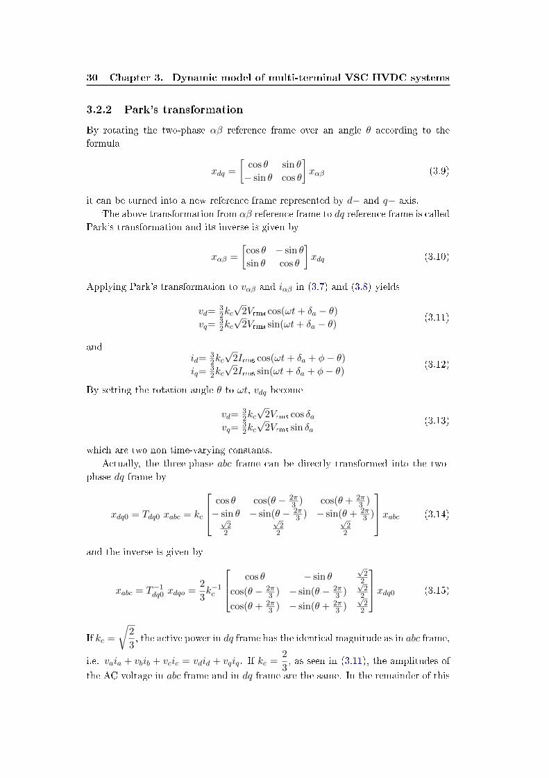
30 Chapter 3. Dynamic model of multi-terminal VSC HVDC systems
3.2.2 Park's transformation
By rotating the two-phase αβ reference frame over an angle θ according to the
formula
xdq =
[cos θ sin θ
− sin θ cos θ
]xαβ (3.9)
it can be turned into a new reference frame represented by d− and q− axis.
The above transformation from αβ reference frame to dq reference frame is called
Park's transformation and its inverse is given by
xαβ =
[cos θ − sin θ
sin θ cos θ
]xdq (3.10)
Applying Park's transformation to vαβ and iαβ in (3.7) and (3.8) yields
vd=32kc√
2Vrms cos(ωt+ δa − θ)vq=
32kc√
2Vrms sin(ωt+ δa − θ)(3.11)
andid=
32kc√
2Irms cos(ωt+ δa + φ− θ)iq=
32kc√
2Irms sin(ωt+ δa + φ− θ) (3.12)
By setting the rotation angle θ to ωt, vdq become
vd=32kc√
2Vrms cos δavq=
32kc√
2Vrms sin δa(3.13)
which are two non time-varying constants.
Actually, the three-phase abc frame can be directly transformed into the two-
phase dq frame by
xdq0 = Tdq0 xabc = kc
cos θ cos(θ − 2π3 ) cos(θ + 2π
3 )
− sin θ − sin(θ − 2π3 ) − sin(θ + 2π
3 )√2
2
√2
2
√2
2
xabc (3.14)
and the inverse is given by
xabc = T−1dq0 xdqo =
2
3k−1c
cos θ − sin θ√
22
cos(θ − 2π3 ) − sin(θ − 2π
3 )√
22
cos(θ + 2π3 ) − sin(θ + 2π
3 )√
22
xdq0 (3.15)
If kc =
√2
3, the active power in dq frame has the identical magnitude as in abc frame,
i.e. vaia + vbib + vcic = vdid + vqiq. If kc =2
3, as seen in (3.11), the amplitudes of
the AC voltage in abc frame and in dq frame are the same. In the remainder of this
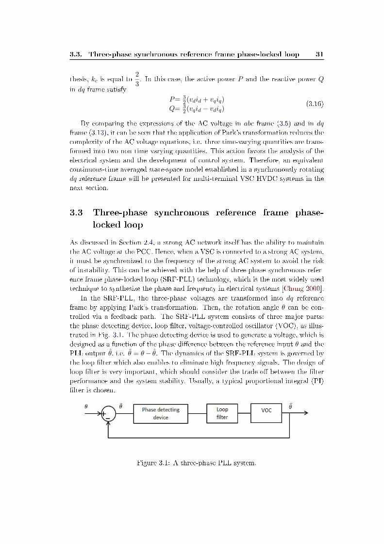
3.3. Three-phase synchronous reference frame phase-locked loop 31
thesis, kc is equal to2
3. In this case, the active power P and the reactive power Q
in dq frame satisfy
P= 32(vdid + vqiq)
Q= 32(vqid − vdiq)
(3.16)
By comparing the expressions of the AC voltage in abc frame (3.5) and in dq
frame (3.13), it can be seen that the application of Park's transformation reduces the
complexity of the AC voltage equations, i.e. three time-varying quantities are trans-
formed into two non time-varying quantities. This action favors the analysis of the
electrical system and the development of control system. Therefore, an equivalent
continuous-time averaged state-space model established in a synchronously rotating
dq reference frame will be presented for multi-terminal VSC HVDC systems in the
next section.
3.3 Three-phase synchronous reference frame phase-
locked loop
As discussed in Section 2.4, a strong AC network itself has the ability to maintain
the AC voltage at the PCC. Hence, when a VSC is connected to a strong AC system,
it must be synchronized to the frequency of the strong AC system to avoid the risk
of instability. This can be achieved with the help of three-phase synchronous refer-
ence frame phase-locked loop (SRF-PLL) technology, which is the most widely used
technique to synthesize the phase and frequency in electrical systems [Chung 2000].
In the SRF-PLL, the three-phase voltages are transformed into dq reference
frame by applying Park's transformation. Then, the rotation angle θ can be con-
trolled via a feedback path. The SRF-PLL system consists of three major parts:
the phase detecting device, loop lter, voltage-controlled oscillator (VOC), as illus-
trated in Fig. 3.1. The phase detecting device is used to generate a voltage, which is
designed as a function of the phase dierence between the reference input θ and the
PLL output θ, i.e. θ = θ− θ. The dynamics of the SRF-PLL system is governed by
the loop lter which also enables to eliminate high frequency signals. The design of
loop lter is very important, which should consider the trade-o between the lter
performance and the system stability. Usually, a typical proportional-integral (PI)
lter is chosen.
Figure 3.1: A three-phase PLL system.
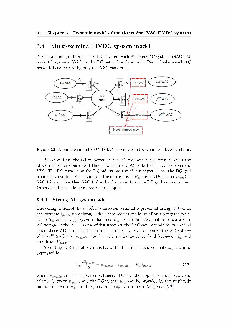
32 Chapter 3. Dynamic model of multi-terminal VSC HVDC systems
3.4 Multi-terminal HVDC system model
A general conguration of an MTDC system with N strong AC systems (SAC), M
weak AC systems (WAC) and a DC network is depicted in Fig. 3.2 where each AC
network is connected by only one VSC converter.
Figure 3.2: A multi-terminal VSC HVDC system with strong and weak AC systems.
By convention, the active power on the AC side and the current through the
phase reactor are positive if they ow from the AC side to the DC side via the
VSC. The DC current on the DC side is positive if it is injected into the DC grid
from the converter. For example, if the active power Pg1 (or the DC current icg1) of
SAC 1 is negative, then SAC 1 absorbs the power from the DC grid as a consumer.
Otherwise, it provides the power as a supplier.
3.4.1 Strong AC system side
The conguration of the ith SAC connection terminal is presented in Fig. 3.3 where
the currents igi,abc ow through the phase reactor made up of an aggregated resis-
tance Rgi and an aggregated inductance Lgi . Since the SAC enables to control its
AC voltage at the PCC in case of disturbances, the SAC can be modeled by an ideal
three-phase AC source with constant parameters. Consequently, the AC voltage
of the ith SAC, i.e. vsgi,abc, can be always maintained at xed frequency fgi and
amplitude Vgi,rms.
According to Kirchho's circuit laws, the dynamics of the currents igi,abc can be
expressed by
Lgidigi,abcdt
= vsgi,abc − vcgi,abc −Rgiigi,abc (3.17)
where vcgi,abc are the converter voltages. Due to the application of PWM, the
relation between vcgi,abc and the DC voltage ucgi can be provided by the amplitude
modulation ratio mgi and the phase angle δgi according to (3.1) and (3.2)
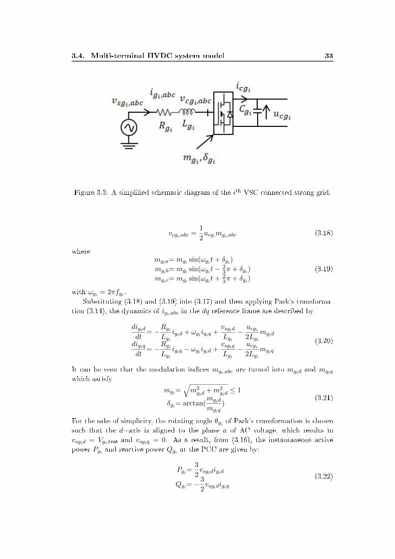
3.4. Multi-terminal HVDC system model 33
Figure 3.3: A simplied schematic diagram of the ith VSC connected strong grid.
vcgi,abc =1
2ucgimgi,abc (3.18)
wheremgia= mgi sin(ωgit+ δgi)
mgib= mgi sin(ωgit− 23π + δgi)
mgic= mgi sin(ωgit+ 23π + δgi)
(3.19)
with ωgi = 2πfgi .
Substituting (3.18) and (3.19) into (3.17) and then applying Park's transforma-
tion (3.14), the dynamics of igi,abc in the dq reference frame are described by
digiddt
= −RgiLgi
igid + ωgiigiq +vsgidLgi− ucgi
2Lgimgid
digiqdt
= −RgiLgi
igiq − ωgiigid +vsgiqLgi− ucgi
2Lgimgiq
(3.20)
It can be seen that the modulation indices mgi,abc are turned into mgid and mgiq
which satisfy
mgi=√m2gid
+m2gid≤ 1
δgi= arctan(mgid
mgiq)
(3.21)
For the sake of simplicity, the rotating angle θgi of Park's transformation is chosen
such that the d−axis is aligned to the phase a of AC voltage, which results in
vsgid = Vgi,rms and vsgiq = 0. As a result, from (3.16), the instantaneous active
power Pgi and reactive power Qgi at the PCC are given by:
Pgi=3
2vsgidigid
Qgi= −3
2vsgidigiq
(3.22)
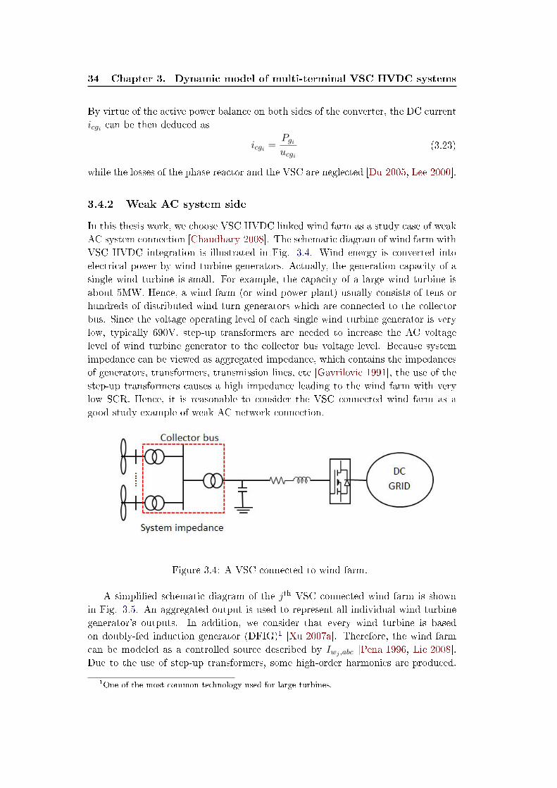
34 Chapter 3. Dynamic model of multi-terminal VSC HVDC systems
By virtue of the active power balance on both sides of the converter, the DC current
icgi can be then deduced as
icgi =Pgiucgi
(3.23)
while the losses of the phase reactor and the VSC are neglected [Du 2005, Lee 2000].
3.4.2 Weak AC system side
In this thesis work, we choose VSC HVDC linked wind farm as a study case of weak
AC system connection [Chaudhary 2008]. The schematic diagram of wind farm with
VSC HVDC integration is illustrated in Fig. 3.4. Wind energy is converted into
electrical power by wind turbine generators. Actually, the generation capacity of a
single wind turbine is small. For example, the capacity of a large wind turbine is
about 5MW. Hence, a wind farm (or wind power plant) usually consists of tens or
hundreds of distributed wind turn generators which are connected to the collector
bus. Since the voltage operating level of each single wind turbine generator is very
low, typically 690V, step-up transformers are needed to increase the AC voltage
level of wind turbine generator to the collector bus voltage level. Because system
impedance can be viewed as aggregated impedance, which contains the impedances
of generators, transformers, transmission lines, etc [Gavrilovic 1991], the use of the
step-up transformers causes a high impedance leading to the wind farm with very
low SCR. Hence, it is reasonable to consider the VSC connected wind farm as a
good study example of weak AC network connection.
Figure 3.4: A VSC connected to wind farm.
A simplied schematic diagram of the jth VSC connected wind farm is shown
in Fig. 3.5. An aggregated output is used to represent all individual wind turbine
generator's outputs. In addition, we consider that every wind turbine is based
on doubly-fed induction generator (DFIG)1 [Xu 2007a]. Therefore, the wind farm
can be modeled as a controlled source described by Iwj ,abc [Pena 1996, Lie 2008].
Due to the use of step-up transformers, some high-order harmonics are produced.
1One of the most common technology used for large turbines.
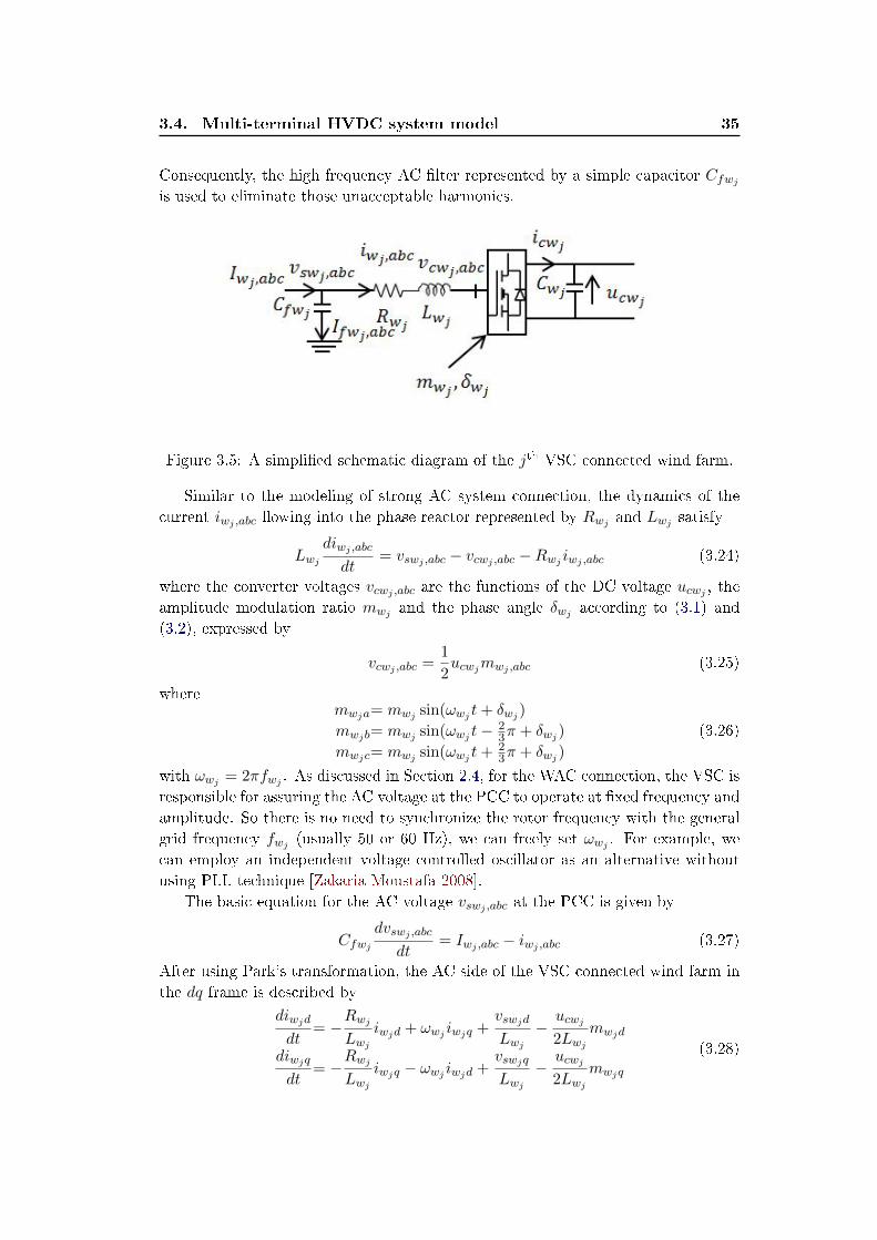
3.4. Multi-terminal HVDC system model 35
Consequently, the high frequency AC lter represented by a simple capacitor Cfwjis used to eliminate those unacceptable harmonics.
Figure 3.5: A simplied schematic diagram of the jth VSC connected wind farm.
Similar to the modeling of strong AC system connection, the dynamics of the
current iwj ,abc owing into the phase reactor represented by Rwj and Lwj satisfy
Lwjdiwj ,abc
dt= vswj ,abc − vcwj ,abc −Rwj iwj ,abc (3.24)
where the converter voltages vcwj ,abc are the functions of the DC voltage ucwj , the
amplitude modulation ratio mwj and the phase angle δwj according to (3.1) and
(3.2), expressed by
vcwj ,abc =1
2ucwjmwj ,abc (3.25)
wheremwja= mwj sin(ωwj t+ δwj )
mwjb= mwj sin(ωwj t− 23π + δwj )
mwjc= mwj sin(ωwj t+ 23π + δwj )
(3.26)
with ωwj = 2πfwj . As discussed in Section 2.4, for the WAC connection, the VSC is
responsible for assuring the AC voltage at the PCC to operate at xed frequency and
amplitude. So there is no need to synchronize the rotor frequency with the general
grid frequency fwj (usually 50 or 60 Hz), we can freely set ωwj . For example, we
can employ an independent voltage controlled oscillator as an alternative without
using PLL technique [Zakaria Moustafa 2008].
The basic equation for the AC voltage vswj ,abc at the PCC is given by
Cfwjdvswj ,abc
dt= Iwj ,abc − iwj ,abc (3.27)
After using Park's transformation, the AC side of the VSC connected wind farm in
the dq frame is described by
diwjd
dt= −
RwjLwj
iwjd + ωwj iwjq +vswjd
Lwj−ucwj2Lwj
mwjd
diwjq
dt= −
RwjLwj
iwjq − ωwj iwjd +vswjq
Lwj−ucwj2Lwj
mwjq
(3.28)
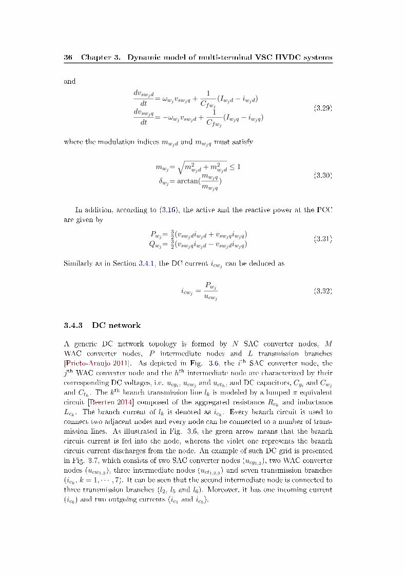
36 Chapter 3. Dynamic model of multi-terminal VSC HVDC systems
and
dvswjd
dt= ωwjvswjq +
1
Cfwj(Iwjd − iwjd)
dvswjq
dt= −ωwjvswjd +
1
Cfwj(Iwjq − iwjq)
(3.29)
where the modulation indices mwjd and mwjq must satisfy
mwj=√m2wjd
+m2wjd≤ 1
δwj= arctan(mwjq
mwjq)
(3.30)
In addition, according to (3.16), the active and the reactive power at the PCC
are given by
Pwj=32(vswjdiwjd + vswjqiwjq)
Qwj=32(vswjqiwjd − vswjdiwjq)
(3.31)
Similarly as in Section 3.4.1, the DC current icwj can be deduced as
icwj =Pwjucwj
(3.32)
3.4.3 DC network
A generic DC network topology is formed by N SAC converter nodes, M
WAC converter nodes, P intermediate nodes and L transmission branches
[Prieto-Araujo 2011]. As depicted in Fig. 3.6, the ith SAC converter node, the
jth WAC converter node and the hth intermediate node are characterized by their
corresponding DC voltages, i.e. ucgi , ucwj and ucth , and DC capacitors, Cgi and Cwjand Cth . The k
th branch transmission line lk is modeled by a lumped π-equivalent
circuit [Beerten 2014] composed of the aggregated resistance Rck and inductance
Lck . The branch current of lk is denoted as ick . Every branch circuit is used to
connect two adjacent nodes and every node can be connected to a number of trans-
mission lines. As illustrated in Fig. 3.6, the green arrow means that the branch
circuit current is fed into the node, whereas the violet one represents the branch
circuit current discharges from the node. An example of such DC grid is presented
in Fig. 3.7, which consists of two SAC converter nodes (ucg1,2), two WAC converter
nodes (ucw1,2), three intermediate nodes (uct1,2,3) and seven transmission branches
(ick , k = 1, · · · , 7). It can be seen that the second intermediate node is connected to
three transmission branches (l2, l5 and l6). Moreover, it has one incoming current
(ic6) and two outgoing currents (ic1 and ic5).
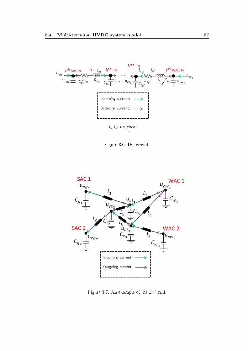
3.4. Multi-terminal HVDC system model 37
Figure 3.6: DC circuit.
Figure 3.7: An example of the DC grid.
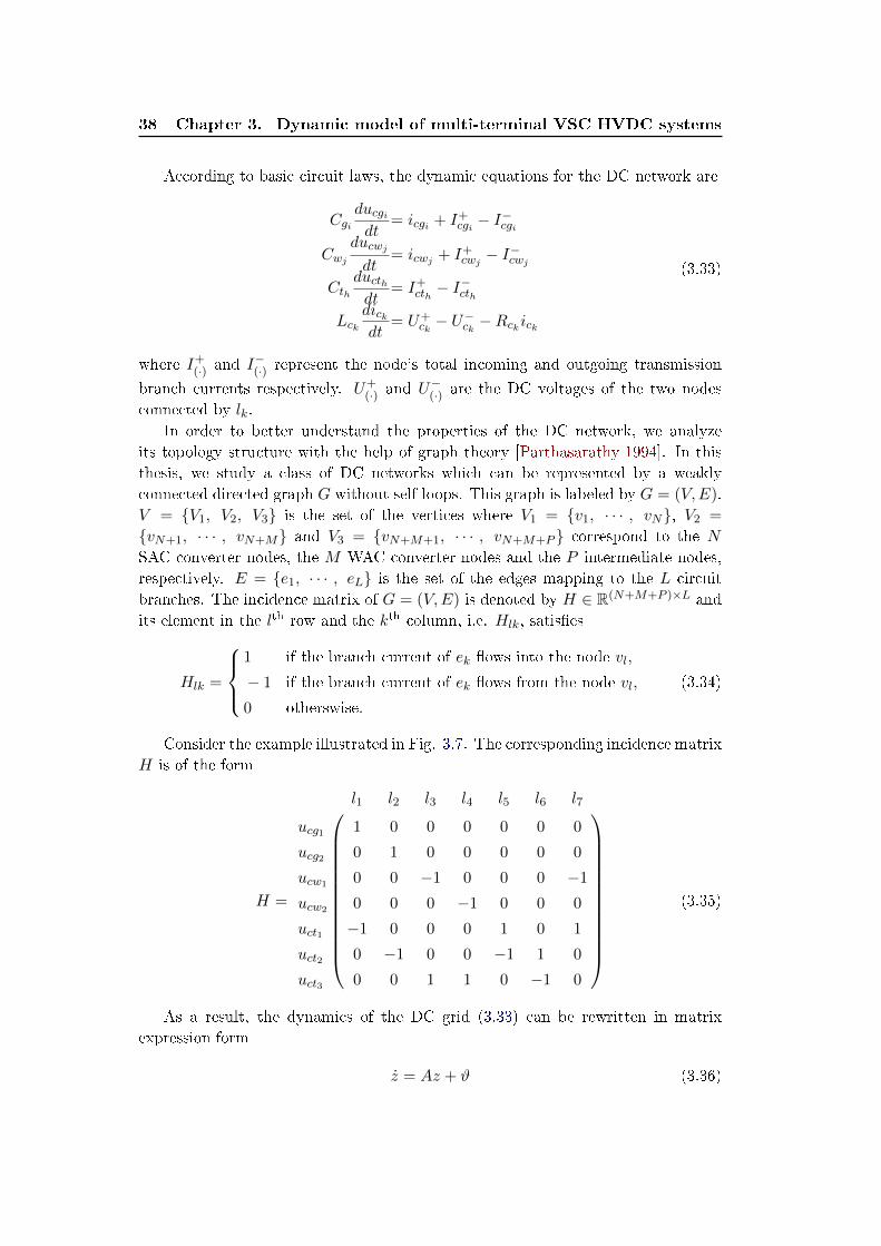
38 Chapter 3. Dynamic model of multi-terminal VSC HVDC systems
According to basic circuit laws, the dynamic equations for the DC network are
Cgiducgidt
= icgi + I+cgi − I
−cgi
Cwjducwjdt
= icwj + I+cwj − I
−cwj
Cthducthdt
= I+cth− I−cth
Lckdickdt
= U+ck− U−ck −Rckick
(3.33)
where I+(·) and I−(·) represent the node's total incoming and outgoing transmission
branch currents respectively. U+(·) and U−(·) are the DC voltages of the two nodes
connected by lk.
In order to better understand the properties of the DC network, we analyze
its topology structure with the help of graph theory [Parthasarathy 1994]. In this
thesis, we study a class of DC networks which can be represented by a weakly
connected directed graph G without self-loops. This graph is labeled by G = (V,E).
V = V1, V2, V3 is the set of the vertices where V1 = v1, · · · , vN, V2 =
vN+1, · · · , vN+M and V3 = vN+M+1, · · · , vN+M+P correspond to the N
SAC converter nodes, the M WAC converter nodes and the P intermediate nodes,
respectively. E = e1, · · · , eL is the set of the edges mapping to the L circuit
branches. The incidence matrix of G = (V,E) is denoted by H ∈ R(N+M+P )×L and
its element in the lth row and the kth column, i.e. Hlk, satises
Hlk =
1 if the branch current of ek ows into the node vl,
− 1 if the branch current of ek ows from the node vl,
0 otherswise.
(3.34)
Consider the example illustrated in Fig. 3.7. The corresponding incidence matrix
H is of the form
H =
l1 l2 l3 l4 l5 l6 l7
ucg1 1 0 0 0 0 0 0
ucg2 0 1 0 0 0 0 0
ucw1 0 0 −1 0 0 0 −1
ucw2 0 0 0 −1 0 0 0
uct1 −1 0 0 0 1 0 1
uct2 0 −1 0 0 −1 1 0
uct3 0 0 1 1 0 −1 0
(3.35)
As a result, the dynamics of the DC grid (3.33) can be rewritten in matrix
expression form
z = Az + ϑ (3.36)
3.4. Multi-terminal HVDC system model 39
with the following denitions
z,[uc ic
]T ∈ RN+M+P+L
uc,[ucg ucw uct
]Tucg,
[ucg1 · · · ucgN
]Tucw,
[ucw1 · · · ucwM
]Tuct,
[uct1 · · · uctP
]Tic,
[ic1 · · · icL
]Tϑ,
[icg1Cg1
· · · icgNCgN
icw1
Cw1
· · · icwMCwM
0(P+L)
]T(3.37)
The matrix A is of the form
A =
[0(N+M+P )×(N+M+P ) C−1H
−L−1HT −L−1R
](3.38)
where C ∈ R(N+M+P )×(N+M+P ) and L,R ∈ RL×L are the capacitor, inductance
and resistance matrices, respectively, which are given by
C = diag(Cg1 · · ·CgN Cw1 · · ·CwM Ct1 · · ·CtP )
L = diag(Lc1 · · ·LcL)
R = diag(Rc1 · · ·RcL)
In general, the incidence matrix H of the weakly connected directed graph G
without self-loops has the following features
• Since the directed graph G is weakly connected, the numbers of the vertices
and the edges must satisfy L ≥ (N +M + P )− 1.
• Every edge (transmission line) can only connect two vertices (nodes) and
hence, each column of H has only two non-zero elements, i.e. 1 and −1.
Based on these characteristics, we have the following results whose proofs are referred
in [Parthasarathy 1994, Bondy 1976].
Lemma 3.4.1. The vectors H(1, :), H(2, :), ..., H(N +M + P, :)2 are linearly de-
pendent. In addition, we have∑N+M+P
i=1 H(i, :) = 0TL. The rank of H, i.e. rank(H),
is equal to N +M + P − 1.
Lemma 3.4.2. If any one row is removed from H, for example, the lth row, i.e.
H(l, :), we obtain a reduced incidence matrix denoted by R(H)l whose rank is still
equal to N +M + P − 1. It means that any (N +M + P − 1) row vectors of H are
linearly independent.
2See the notations.
40 Chapter 3. Dynamic model of multi-terminal VSC HVDC systems
3.4.4 Domain of interest
It is worthwhile to keep in mind that taking into account physical considerations
[Mohan 2003], the feasible region of the state variables is not boundless [Stijn 2010,
Haileselassie 2012a]. Therefore, in this thesis work, we restrict the state variables to
some domains of interest. All DC voltage ucgi , ucwj and ucth are considered on the
domain Duc , [uc,min, uc,max] ∈ R where uc,min is positive. The current igi,dq and
iwj ,dq are dened on Digi,dq ∈ R and Diwj,dq ∈ R, respectively. All branch currents ickare on the domain Dic . Consequently, the domains D(·) are dened as the domains
of interest, which are bounded.
3.5 Conventional control methods
It is essential for any VSC HVDC system the ability to counteract disturbances
with fast response, good transient and steady-state performances. This ability is
strongly dependent on the employed control system and hence, a study of control
system design for MTDC systems is necessary. Many researches have been devoted
to the control design of VSC HVDC systems. In this section, we briey introduce
two conventional control methods, direct and vector control methods, which are
widely used and discussed.
3.5.1 Direct control method
Direct control strategy [Ohnishi 1991, Noguchi 1998] is realized by measuring and
comparing the controlled outputs to their references in such a way that the control
variables, i.e. the phase angle δ and the amplitude modulation ratio m, can be
directly obtained by means of PI control technique, and then sent to the pulse width
modulator. Figure 3.8 gives the block diagrams of direct control method applied
to the four control modes (as discussed in Section 2.4.2) of the ith VSC connected
strong grid [Sood 2010]. It can be seen that the errors denoted by (·) between the
measured values and the references denoted by (·)o are sent to PI controllers as
the inputs to generate the control variables of the converter. It is interesting to
remark that the choice of these PI controllers is completely arbitrary or empirical,
without vigorous mathematical proofs for their design. Nevertheless, the direct
control method has the following advantages:
• The design concept is quite simple and the controller is easy to be imple-
mented. The control variables are given by
δgi= Kgi,p1(P ogi − Pgi) +Kgi,i1
∫(P ogi − Pgi)
mgi= Kgi,p2(Qogi −Qgi) +Kgi,i2
∫(Qogi −Qgi)
δgi= Kgi,p3(uocgi − ucgi) +Kgi,i3
∫(uocgi − ucgi)
mgi= Kgi,p4(V ogi,rms − Vgi,rms) +Kgi,i4
∫(V ogi,rms − Vgi,rms)
(3.39)
where the control gains of the PI controllers, Kgi,p(·) and Kgi,i(·) , are positive.
It is shown that the formulas of δgi and mgi are indeed expressed in a fairly
simple way.
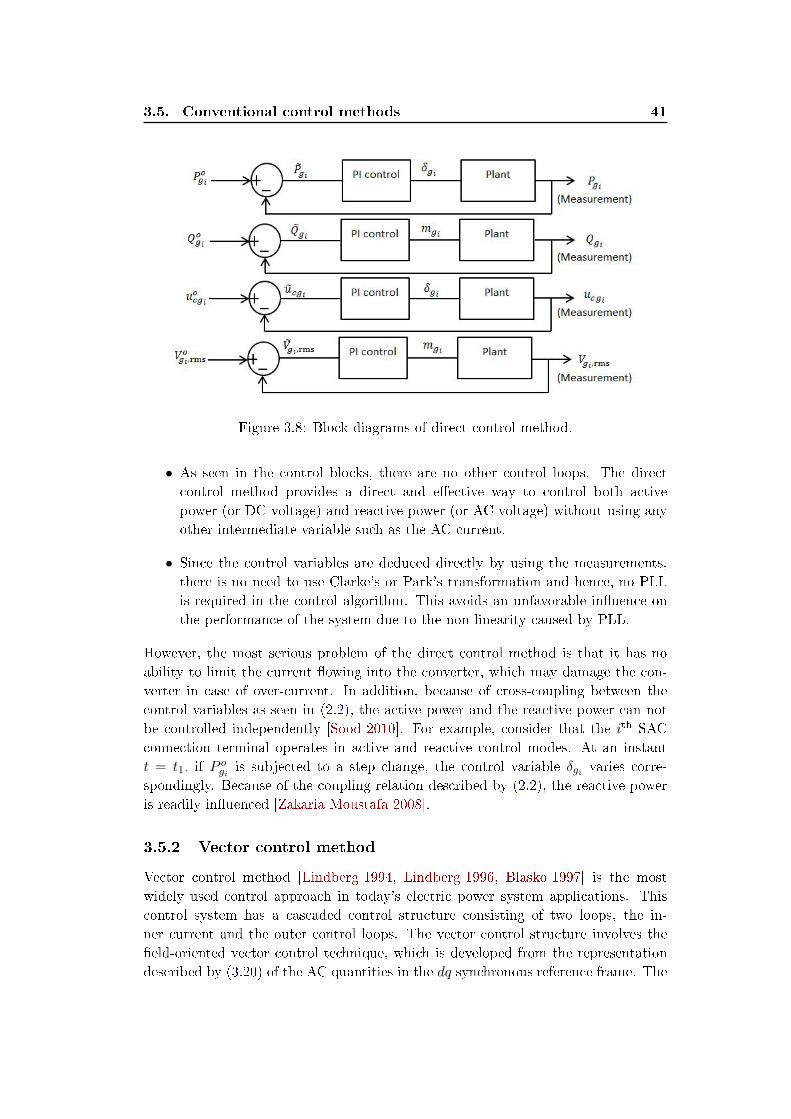
3.5. Conventional control methods 41
Figure 3.8: Block diagrams of direct control method.
• As seen in the control blocks, there are no other control loops. The direct
control method provides a direct and eective way to control both active
power (or DC voltage) and reactive power (or AC voltage) without using any
other intermediate variable such as the AC current.
• Since the control variables are deduced directly by using the measurements,
there is no need to use Clarke's or Park's transformation and hence, no PLL
is required in the control algorithm. This avoids an unfavorable inuence on
the performance of the system due to the non-linearity caused by PLL.
However, the most serious problem of the direct control method is that it has no
ability to limit the current owing into the converter, which may damage the con-
verter in case of over-current. In addition, because of cross-coupling between the
control variables as seen in (2.2), the active power and the reactive power can not
be controlled independently [Sood 2010]. For example, consider that the ith SAC
connection terminal operates in active and reactive control modes. At an instant
t = t1, if Pogi is subjected to a step change, the control variable δgi varies corre-
spondingly. Because of the coupling relation described by (2.2), the reactive power
is readily inuenced [Zakaria Moustafa 2008].
3.5.2 Vector control method
Vector control method [Lindberg 1994, Lindberg 1996, Blasko 1997] is the most
widely used control approach in today's electric power system applications. This
control system has a cascaded control structure consisting of two loops, the in-
ner current and the outer control loops. The vector control structure involves the
eld-oriented vector control technique, which is developed from the representation
described by (3.20) of the AC quantities in the dq synchronous reference frame. The
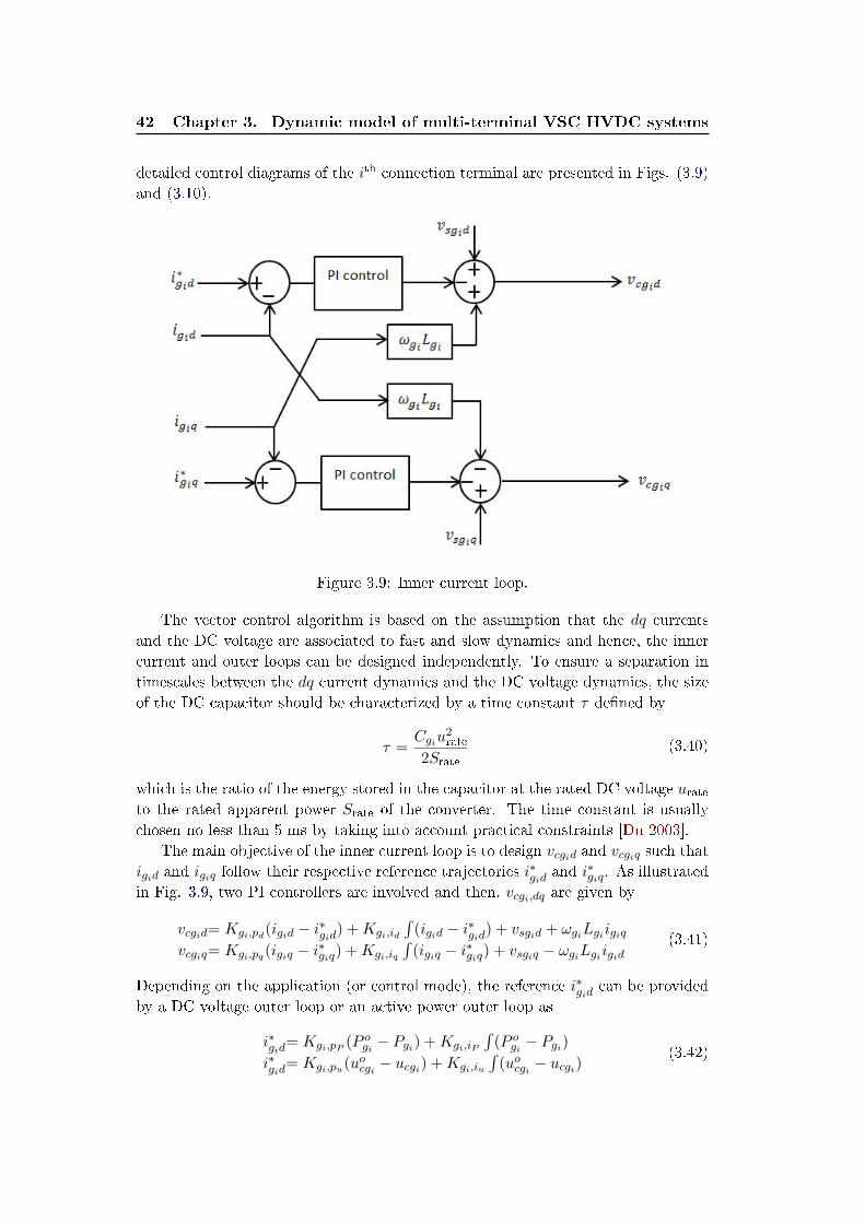
42 Chapter 3. Dynamic model of multi-terminal VSC HVDC systems
detailed control diagrams of the ith connection terminal are presented in Figs. (3.9)
and (3.10).
Figure 3.9: Inner current loop.
The vector control algorithm is based on the assumption that the dq currents
and the DC voltage are associated to fast and slow dynamics and hence, the inner
current and outer loops can be designed independently. To ensure a separation in
timescales between the dq current dynamics and the DC voltage dynamics, the size
of the DC capacitor should be characterized by a time constant τ dened by
τ =Cgiu
2rate
2Srate(3.40)
which is the ratio of the energy stored in the capacitor at the rated DC voltage urateto the rated apparent power Srate of the converter. The time constant is usually
chosen no less than 5 ms by taking into account practical constraints [Du 2003].
The main objective of the inner current loop is to design vcgid and vcgiq such that
igid and igiq follow their respective reference trajectories i∗gid and i∗giq. As illustrated
in Fig. 3.9, two PI controllers are involved and then, vcgi,dq are given by
vcgid= Kgi,pd(igid − i∗gid) +Kgi,id
∫(igid − i∗gid) + vsgid + ωgiLgiigiq
vcgiq= Kgi,pq(igiq − i∗giq) +Kgi,iq
∫(igiq − i∗giq) + vsgiq − ωgiLgiigid
(3.41)
Depending on the application (or control mode), the reference i∗gid can be provided
by a DC voltage outer loop or an active power outer loop as
i∗gid= Kgi,pP (P ogi − Pgi) +Kgi,iP
∫(P ogi − Pgi)
i∗gid= Kgi,pu(uocgi − ucgi) +Kgi,iu
∫(uocgi − ucgi)
(3.42)
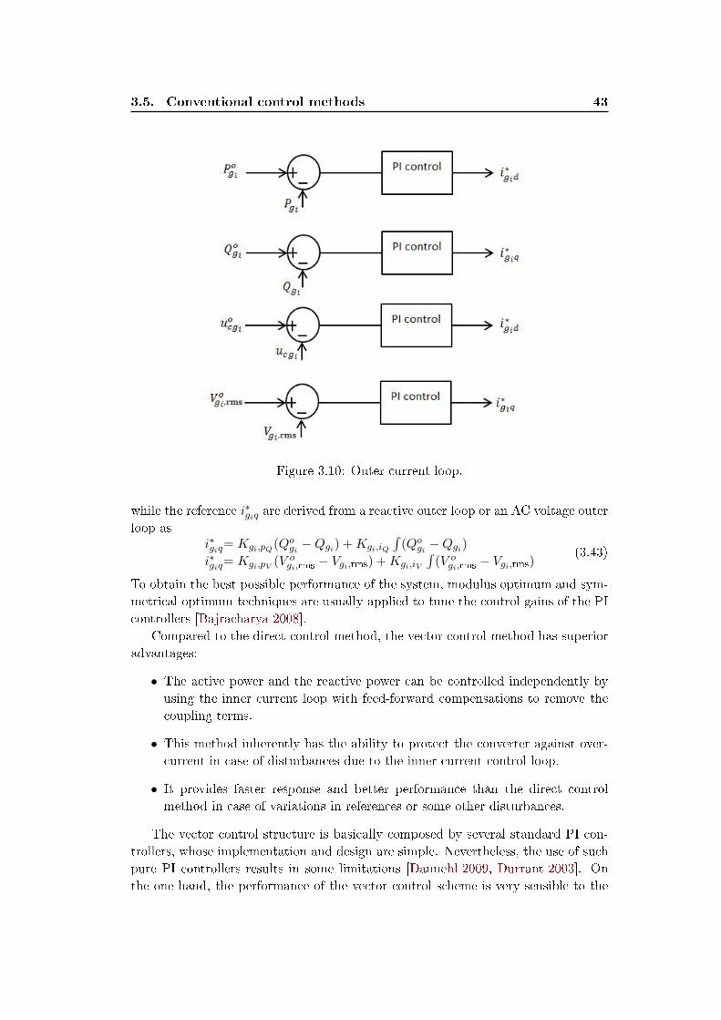
3.5. Conventional control methods 43
Figure 3.10: Outer current loop.
while the reference i∗giq are derived from a reactive outer loop or an AC voltage outer
loop asi∗giq= Kgi,pQ(Qogi −Qgi) +Kgi,iQ
∫(Qogi −Qgi)
i∗giq= Kgi,pV (V ogi,rms − Vgi,rms) +Kgi,iV
∫(V ogi,rms − Vgi,rms)
(3.43)
To obtain the best possible performance of the system, modulus optimum and sym-
metrical optimum techniques are usually applied to tune the control gains of the PI
controllers [Bajracharya 2008].
Compared to the direct control method, the vector control method has superior
advantages:
• The active power and the reactive power can be controlled independently by
using the inner current loop with feed-forward compensations to remove the
coupling terms.
• This method inherently has the ability to protect the converter against over-
current in case of disturbances due to the inner current control loop.
• It provides faster response and better performance than the direct control
method in case of variations in references or some other disturbances.
The vector control structure is basically composed by several standard PI con-
trollers, whose implementation and design are simple. Nevertheless, the use of such
pure PI controllers results in some limitations [Dannehl 2009, Durrant 2003]. On
the one hand, the performance of the vector control scheme is very sensible to the
44 Chapter 3. Dynamic model of multi-terminal VSC HVDC systems
system uncertainties. On the other hand, in order to apply Park's transformation,
a PLL is needed to provide a synchronous reference frame. The dynamics of the
PLL and AC lters increase the diculty in the VSC control when the SCR of the
connected AC system decreases.
3.6 Chapter conclusions
In this chapter, we choose the averaged modeling approach to develop the dynamical
model for a multi-terminal VSC HVDC system. The modeling work mainly focuses
on three parts, i.e. the VSC connected strong AC networks, the VSC connected
wind farms and the DC network. According to the features of the VSC connected
AC systems, we have dierent considerations:
• For the VSC connected strong AC networks, the SRF-PLL is usually required
to detect the phase and frequency of the electrical circuit such that the VSC
can be synchronized to its connected strong AC system whereas there is no
need for the VSC connected weak AC network.
• For a strong AC system, we consider that its AC voltage at the PCC can
be kept by TSO at xed frequency and amplitude. This is contrary to the
case of a weak AC system, which with high impedance is very sensible to any
disturbances (for example, the change of power ow), it is necessary in that
case to consider the dynamics of the weak AC system's AC voltage at the
PCC.
For the sake of convenience, Park's transformation is applied to transform the sys-
tem from the abc frame into the dq reference frame, which greatly simplies the
expression of the dynamic equations. For the DC network, we map it to a weakly
connected directed graph and then use a incidence matrix to describe its topology.
It is much easier to analyze the DC grid in matrix form since there exist quite a lot
of results on matrix and graph studies.
Finally, a detailed averaged state-space model for the multi-terminal VSC HVDC
system described by (3.20), (3.28), (3.29) and (3.36) is established. We summarize
this model as follows
• The dimension of the full scale system is 3N + 5M + P + L.
• The state variables are igi,dq, iwj ,dq, vswj ,dq, ucgi , ucwj , ucth and ick for i ∈ N ,
j ∈M, h ∈ P and k ∈ L3.
• The control inputs are the modulation indices, i.e. mgi,dq andmwj ,dq for i ∈ Nand j ∈M.
• The external parameters Iwj ,dq, for j ∈M, are considered constant.
3Unless otherwise stated, the subscripts i, j, t and k mean ∀i ∈ N = 1, · · · , N, ∀j ∈ M =
1, · · · ,M, ∀h ∈ P = 1, · · · , P and ∀k ∈ L = 1, · · · , L.

3.6. Chapter conclusions 45
• The values of all physical parameters, i.e. the resistances, the inductances and
the the capacitors, are positive.
Moreover, in this chapter, we have also presented two most investigated con-
ventional control strategies, direct and vector control strategies, and introduced
their control principles. In addition, we have also discussed their advantages and
disadvantages.

Chapter 4
Control methods based on
nonlinear control design tools
Contents
4.1 Feedback linearization control . . . . . . . . . . . . . . . . . . 48
4.1.1 Theoretical results . . . . . . . . . . . . . . . . . . . . . . . . 48
4.1.2 Application to a VSC HVDC link connected to a resistive load 51
4.1.3 Application to a VSC HVDC link consisting of a strong and a
weak AC system . . . . . . . . . . . . . . . . . . . . . . . . . 61
4.1.4 Application to an MTDC system using master-slave control
conguration . . . . . . . . . . . . . . . . . . . . . . . . . . . 71
4.2 Feedback linearization with sliding mode control . . . . . . 85
4.2.1 Control design . . . . . . . . . . . . . . . . . . . . . . . . . . 85
4.2.2 Simulation studies . . . . . . . . . . . . . . . . . . . . . . . . 88
4.3 Passivity-based control . . . . . . . . . . . . . . . . . . . . . . 92
4.3.1 Steady-state analysis . . . . . . . . . . . . . . . . . . . . . . . 93
4.3.2 Passive system . . . . . . . . . . . . . . . . . . . . . . . . . . 95
4.3.3 Control design . . . . . . . . . . . . . . . . . . . . . . . . . . 97
4.3.4 Control of zero dynamics . . . . . . . . . . . . . . . . . . . . 102
4.3.5 Simulation studies . . . . . . . . . . . . . . . . . . . . . . . . 116
4.4 Chapter conclusions . . . . . . . . . . . . . . . . . . . . . . . . 125
Although the vector control method occupies a predominant position in the
eld of control design for VSC HVDC systems, the limitations of this approach also
draw our attention [Dannehl 2009]. In particular, in [Dannehl 2009], it indicates
that the traditional vector current control is very sensitive to system uncertainties.
In [Durrant 2003], a detailed analysis of a VSC connected to a weak AC system
is carried out. It is shown that the dynamics of PLL and AC lter increase the
diculty in the VSC control when the SCR of the connected AC system decreases.
In order to improve the performance of VSC HVDC systems, developing new control
structures has been a very popular research topic.
In this chapter, we propose new control structures by means of dierent nonlinear
control design tools for VSC HVDC systems.
48 Chapter 4. Control methods based on nonlinear control design tools
4.1 Feedback linearization control
Feedback linearization is well-known in the eld of nonlinear control design. The
principle of this technique is to transform the nonlinear system fully or partly to a
linear one and thereafter, linear control, robust control or some other control tech-
niques can be applied. As presented in [Lee 2000, Kim 2010], feedback linearization
is applied to three-phase converters. However, only a single three-phase converter
station is considered in their study case. Reference [Moharana 2010] proposes a
nonlinear controller based on input-output feedback linearizaiton and sliding mode
control. However, in [Moharana 2010], the stability of the zero dynamics of the
system is not analyzed, which determines whether the feedback linearization is ap-
plicable for the control design.
In this section, according to the control objectives of HVDC systems, we develop
dierent nonlinear controllers by making full use of feedback linearization where the
corresponding zero dynamics are also analyzed.
Before designing the exact control structures to VSC HVDC systems, we give
a brief introduction to feedback linearizaiton for multi-input and multi-output
(MIMO) nonlinear systems [Khalil 1996, Isidori 1995, Slotine 1991, Hedrick 2005].
4.1.1 Theoretical results
Consider a class of MIMO systems
x= f(x) +∑j=m
j=1 gj(x)uj
y,[y1 · · · ym
]T=[h1(x) · · · hm(x)
]T (4.1)
where the control input vector u =[ui · · · um
]∈ Rm has the same dimension as
the output vector y. The functions f , gj and hj , i = 1, · · · , m, are suciently
smooth in an open set D ⊂ Rm. The mappings f : D→ Rn and gi : D→ R are the
vector elds on D. The derivative of the ith output yi is given by
yi = Lfhi(x) +∑j=m
j=1 Lgjhi(x)uj (4.2)
where
Lfhi(x),∂hi∂x
f(x)
Lgjhi(x),∂hi∂x
gj(x)(4.3)
are the Lie derivatives of hi(x) with respect to f and gi. If all Lgjhi(x) = 0, we
continue to dierentiate yi until some uj explicitly appears in the γthi derivative of
yi as follows
y(γi)i = Lγif hi(x) +
∑j=mj=1 Lgj (L
γi−1f hi)uj (4.4)
where Lgj (Lγi−1f hi) =
∂(Lγi−1f hi)
∂xgj 6= 0 for some j ∈ 1, , · · · , m. In this case, γi
is called the relative degree (see Denition 13.2 in [Khalil 1996]) of the ith output
4.1. Feedback linearization control 49
yi = hi(x). After performing the above procedure for each output, we obtain m
equations in a similar form as (4.4), which can be expressed in matrix form
yγ = lγ + Eu (4.5)
where the decoupling matrix E ∈ Rm×m and the vectors yγ , lγ and u are given by
E(x)=
Lg1(Lγ1−1f h1) · · · Lgm(Lγ1−1
f h1)
· · · · · · · · ·Lg1(Lγm−1
f hm) · · · Lgm(Lγm−1f hm)
yγ=
[y
(γ1)1 · · · y
(γm)m
]Tlγ=
[Lγ1f h1 · · · Lγmf hm
]Tu=
[u1 · · · um
]T(4.6)
If the decoupling matrix E is non-singular in D, then the control vector u can be
designed as
u = E−1(v − lγ) (4.7)
where v =[v1 · · · vm
]Tis the additional input vector. Substituting (4.7) into
(4.5) yields y(γ1)1
· · ·y
(γm)m
=
v1
· · ·vm
(4.8)
which results in a decoupled set of equations. The additional input v can be designed
using any linear method or other techniques. For example, if the control objective
is to make y follow the reference yd =[yd1 · · · ydm
]T, then v can be designed as v1
· · ·vm
=
−c1,0(y1 − yd1)− · · · − c1,γ1−1(y(γ1−1)1 − y(γ1−1)
d1 )
· · ·−cm,0(ym − ydm)− · · · − cm,γm−1(y
(γm−1)m − y(γm−1)
dm )
(4.9)
where the coecients c(·) are chosen such that for all j ∈ 1, · · · ,m
Cj =
0 1 0 · · · 0
0 0 1 · · · 0
· · · · · · · · · · · · · · ·0 0 0 · · · 1
−cj,0 −cj,1 −cj,2 · · · −cj,γj−1
∈ Rγj×γj (4.10)
are Hurwitz. In addition, with the integrated tracking error e ,[e1 · · · em
]T=
y − yd, v is then designed as v1
· · ·vm
=
−c1,0(y1 − yd1)− · · · − c1,γ1−1(y(γ1−1)1 − y(γ1−1)
d1 )− kI1eI1· · ·
−cm,0(ym − ydm)− · · · − cm,γm−1(y(γm−1)m − y(γm−1)
dm )− kImeIm
(4.11)

50 Chapter 4. Control methods based on nonlinear control design tools
where eIj satises
eIj = ej = yj − ydj (4.12)
Again, the control gains must be chosen such that for all j ∈ 1, · · · ,m
C′j =
0 1 0 · · · 0
0 0 1 · · · 0
· · · · · · · · · · · · · · ·0 0 0 · · · 1
−kIj −cj,0 −cj,1 · · · −cj,γj−1
∈ R(γj+1)×(γj+1) (4.13)
are Hurwitz. The term (−kIjeIj) is used to eliminate the tracking error so as to
improve the robustness of the system.
If the relative degree of the whole system (4.1)
γ =∑m
j=1 γj (4.14)
is smaller than n, there exist internal dynamics of order n−γ which are unobservable.We perform the change of variables
z = T (x) ,
η
− − −ξ
,
φ1(x)
· · ·φn−r(x)
− − −ξ
(4.15)
and ξ is taken as
ξ ,
ξ1
· · ·ξm
, ξj , yj· · ·
y(γj−1)j
(4.16)
where φk, k = 1, · · · , n − γ, are chosen to ensure that the transformation T is a
dieomorphism on D. In the new variable (η, ξ), the system (4.1) becomes
η= Ψ1(η, ξ) + Ψ2(η, ξ)u
ξj= Ajξj +Bjvj(4.17)
where
Aj =
0 1 0 · · · 0
0 0 1 · · · 0
· · · · · · · · · · · · · · ·0 0 0 · · · 1
0 0 0 · · · 0
∈ Rγj×γj , Bj =
0
0
· · ·0
1
∈ Rγj (4.18)
When the output y is identically equal to the reference yd, the system (4.17) is
degenerated into
η= Ψ1(η, ξ) + Ψ2(η, ξ)u (4.19)
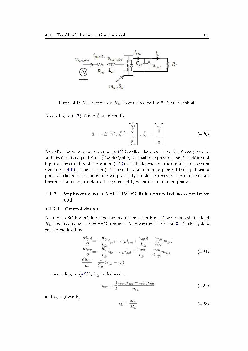
4.1. Feedback linearization control 51
Figure 4.1: A resistive load RL is connected to the ith SAC terminal.
According to (4.7), u and ξ are given by
u = −E−1lγ , ξ ,
ξ1
ξ2
· · ·ξm
, ξj =
ydj0
· · ·0
(4.20)
Actually, the autonomous system (4.19) is called the zero dynamics. Since ξ can be
stabilized at its equilibrium ξ by designing a suitable expression for the additional
input v, the stability of the system (4.17) totally depends on the stability of the zero
dynamics (4.19). The system (4.1) is said to be minimum phase if the equilibrium
point of the zero dynamics is asymptotically stable. Moreover, the input-output
linearization is applicable to the system (4.1) when it is minimum phase.
4.1.2 Application to a VSC HVDC link connected to a resistiveload
4.1.2.1 Control design
A simple VSC HVDC link is considered as shown in Fig. 4.1 where a resistive load
RL is connected to the ith SAC terminal. As presented in Section 3.4.1, the system
can be modeled by
digiddt
= −RgiLgi
igid + ωgiigiq +vsgidLgi− ucgi
2Lgimgid
digiqdt
= −RgiLgi
ilq − ωgiigid +vsgiqLgi− ucgi
2Lgimgiq
ducgidt
=1
Cgi(icgi − iL)
(4.21)
According to (3.23), icgi is deduced as
icgi =3
2
vsgidigid + vsgiqigiqucgi
(4.22)
and iL is given by
iL =ucgiRL
(4.23)
52 Chapter 4. Control methods based on nonlinear control design tools
Since there are two control inputs mgi,dq, it is possible to control two outputs. To
ensure the normal operation of the system, the DC voltage transmission level must
be always kept within its acceptable range. As a results, ucgi is chosen as one output,
which is required to track the reference uocgi . For the purpose of good power quality,
the reactive power Qgi should be well-behaved. From (3.22), it is clear that igid and
igiq regulate the active and reactive power, respectively. Consequently, igiq is chosen
as the other output, which is expected to follow the reference iogiq given by
iogiq = −2
3
Qogivsgid
(4.24)
where Qogi is the desired reactive power. For example, in order to get the unitary
power factor, Qogi is usually set to zero.
By dening[x1 x2 x3
],[igid igiq ucgi
], the system (4.21) can be rewritten
as
x = fx(x) + gdmgid + gqmgiq (4.25)
where f(x), gd and gq are given by
fx =
−RgiLgi
igid + ωgiigiq +vsgidLgi
−RgiLgi
ilq − ωgiigid +vsgiqLgi
1Cgi
(32
vsgidigid+vsgiqigiqucgi
− ucgiRL
)
(4.26)
and
gd =
−ucgi2Lgi0
0
, gq =
0
− ucgi2Lgi0
(4.27)
The two outputs in this case are dened as
y ,[y1 y2
]T=[igiq ucgi
]T(4.28)
which are needed to be regulated at yo ,[yo1 yo2
]T=[iogiq uocgi
]T.
It is evident that γ1 and γ2, the relative degrees of ucgi and igiq, are equal to 2
and 1, respectively. The relative degree of the whole system is 3 which is equal to the
dimension of the system (4.21). This means that the system is feedback linearizable
and there is no unobservable dynamics. The decoupling matrix E1 is given by
E1 =
[Lgd(igiq) Lgq(igiq)
LgdLfx(ucgi) LgqLfx(ucgi)
](4.29)
whereLgd(igiq)= 0
Lgq(igiq)= −ucgi2Lgi
LgdLfx(ucgi)= − 1Cgi
34
vsgidLgi
LgqLfx(ucgi)= − 1Cgi
34
vsgiqLgi
(4.30)
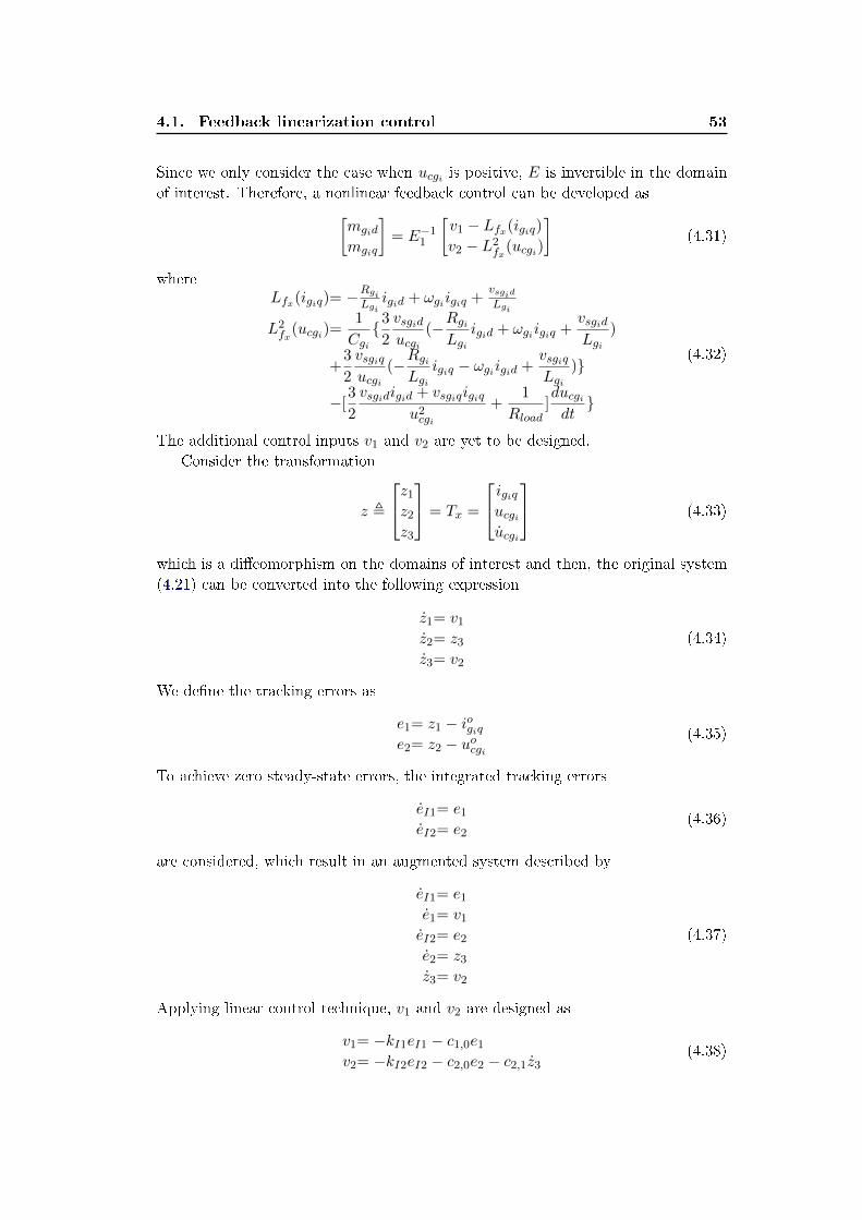
4.1. Feedback linearization control 53
Since we only consider the case when ucgi is positive, E is invertible in the domain
of interest. Therefore, a nonlinear feedback control can be developed as[mgid
mgiq
]= E−1
1
[v1 − Lfx(igiq)
v2 − L2fx
(ucgi)
](4.31)
whereLfx(igiq)= −
RgiLgi
igid + ωgiigiq +vsgidLgi
L2fx
(ucgi)=1
Cgi3
2
vsgiducgi
(−RgiLgi
igid + ωgiigiq +vsgidLgi
)
+3
2
vsgiqucgi
(−RgiLgi
igiq − ωgiigid +vsgiqLgi
)
−[3
2
vsgidigid + vsgiqigiqu2cgi
+1
Rload]ducgidt
(4.32)
The additional control inputs v1 and v2 are yet to be designed.
Consider the transformation
z ,
z1
z2
z3
= Tx =
igiqucgiucgi
(4.33)
which is a dieomorphism on the domains of interest and then, the original system
(4.21) can be converted into the following expression
z1= v1
z2= z3
z3= v2
(4.34)
We dene the tracking errors as
e1= z1 − iogiqe2= z2 − uocgi
(4.35)
To achieve zero steady-state errors, the integrated tracking errors
eI1= e1
eI2= e2(4.36)
are considered, which result in an augmented system described by
eI1= e1
e1= v1
eI2= e2
e2= z3
z3= v2
(4.37)
Applying linear control technique, v1 and v2 are designed as
v1= −kI1eI1 − c1,0e1
v2= −kI2eI2 − c2,0e2 − c2,1z3(4.38)
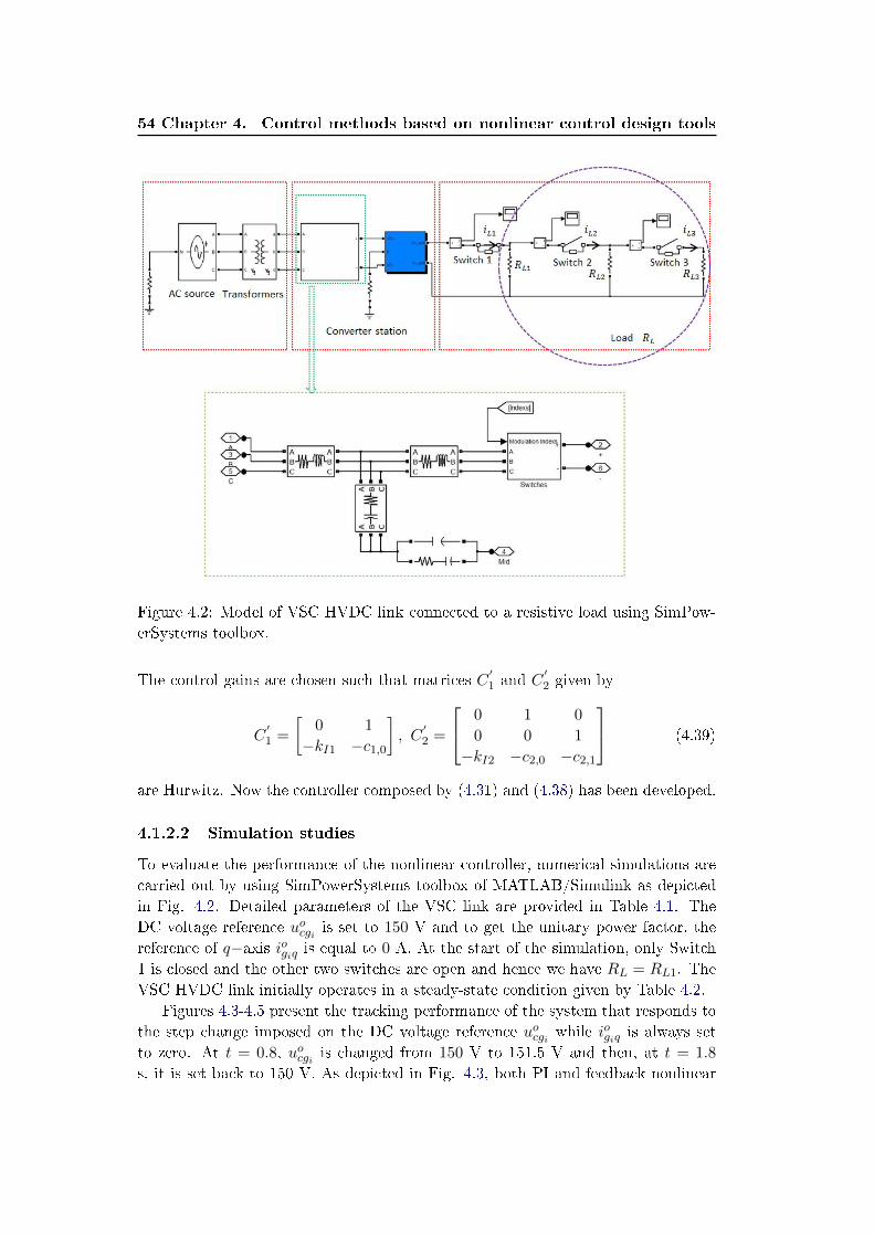
54 Chapter 4. Control methods based on nonlinear control design tools
Figure 4.2: Model of VSC HVDC link connected to a resistive load using SimPow-
erSystems toolbox.
The control gains are chosen such that matrices C′1 and C
′2 given by
C′1 =
[0 1
−kI1 −c1,0
], C
′2 =
0 1 0
0 0 1
−kI2 −c2,0 −c2,1
(4.39)
are Hurwitz. Now the controller composed by (4.31) and (4.38) has been developed.
4.1.2.2 Simulation studies
To evaluate the performance of the nonlinear controller, numerical simulations are
carried out by using SimPowerSystems toolbox of MATLAB/Simulink as depicted
in Fig. 4.2. Detailed parameters of the VSC link are provided in Table 4.1. The
DC voltage reference uocgi is set to 150 V and to get the unitary power factor, the
reference of q−axis iogiq is equal to 0 A. At the start of the simulation, only Switch
1 is closed and the other two switches are open and hence we have RL = RL1. The
VSC HVDC link initially operates in a steady-state condition given by Table 4.2.
Figures 4.3-4.5 present the tracking performance of the system that responds to
the step change imposed on the DC voltage reference uocgi while iogiq is always set
to zero. At t = 0.8, uocgi is changed from 150 V to 151.5 V and then, at t = 1.8
s, it is set back to 150 V. As depicted in Fig. 4.3, both PI and feedback nonlinear

4.1. Feedback linearization control 55
Table 4.1: Parameters of the VSC HVDC link.Parameters Value
Power System Rating 4 KVA
Source Voltage Amplitude (Vrms phase-to-phase) 127 V
Source Voltage Frequency 50 Hz
Switching Frequency for PWM 1500 Hz
Transformer Primary Voltage 127 V
Transformer Secondary Voltage 50 V
Inductance Lgi 2.1 mH
Resistance Rgi 0.142 Ω
RL1,2,3 150 Ω
Table 4.2: Initial values of the system variables.Variables Values
RL 150 Ω
ucgi 150 V
igiq 0 A
iL 1 A
igid 2.46 A
controllers have similar performance, i.e. they make ucgi track its reference uocgi with
fast response and good transient performance. In addition, igiq as displayed in Fig.
4.4 is always regulated at zero irrespective of the change in uocgi . As illustrated in Fig.
4.5, every time ucgi achieves a new steady state, iL1 also arrives at a corresponding
steady state since in steady-state condition, iL1 and ucgi satisfy ucgi = RLiL1.
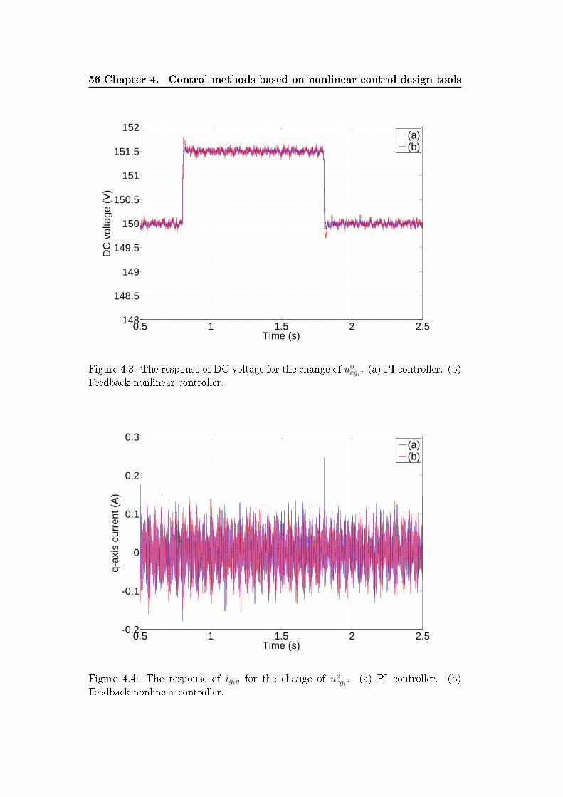
56 Chapter 4. Control methods based on nonlinear control design tools
0.5 1 1.5 2 2.5148
148.5
149
149.5
150
150.5
151
151.5
152
Time (s)
DC
vol
tage
(V
)
(a)(b)
Figure 4.3: The response of DC voltage for the change of uocgi . (a) PI controller. (b)
Feedback nonlinear controller.
0.5 1 1.5 2 2.5-0.2
-0.1
0
0.1
0.2
0.3
Time (s)
q-ax
is c
urre
nt (
A)
(a)(b)
Figure 4.4: The response of igiq for the change of uocgi . (a) PI controller. (b)
Feedback nonlinear controller.
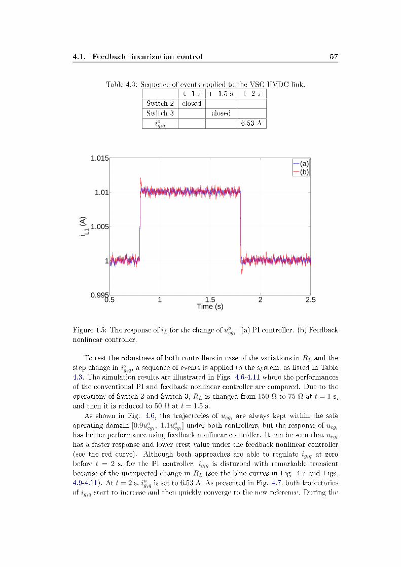
4.1. Feedback linearization control 57
Table 4.3: Sequence of events applied to the VSC HVDC link.t=1 s t=1.5 s t=2 s
Switch 2 closed
Switch 3 closed
iogiq 6.53 A
0.5 1 1.5 2 2.50.995
1
1.005
1.01
1.015
Time (s)
i L1 (
A)
(a)(b)
Figure 4.5: The response of iL for the change of uocgi . (a) PI controller. (b) Feedback
nonlinear controller.
To test the robustness of both controllers in case of the variations in RL and the
step change in iogiq, a sequence of events is applied to the system, as listed in Table
4.3. The simulation results are illustrated in Figs. 4.6-4.11 where the performances
of the conventional PI and feedback nonlinear controller are compared. Due to the
operations of Switch 2 and Switch 3, RL is changed from 150 Ω to 75 Ω at t = 1 s,
and then it is reduced to 50 Ω at t = 1.5 s.
As shown in Fig. 4.6, the trajectories of ucgi are always kept within the safe
operating domain [0.9uocgi , 1.1uocgi ] under both controllers, but the response of ucgihas better performance using feedback nonlinear controller. It can be seen that ucgihas a faster response and lower crest value under the feedback nonlinear controller
(see the red curve). Although both approaches are able to regulate igiq at zero
before t = 2 s, for the PI controller, igiq is disturbed with remarkable transient
because of the unexpected change in RL (see the blue curves in Fig. 4.7 and Figs.
4.9-4.11). At t = 2 s, iogiq is set to 6.53 A. As presented in Fig. 4.7, both trajectories
of igiq start to increase and then quickly converge to the new reference. During the
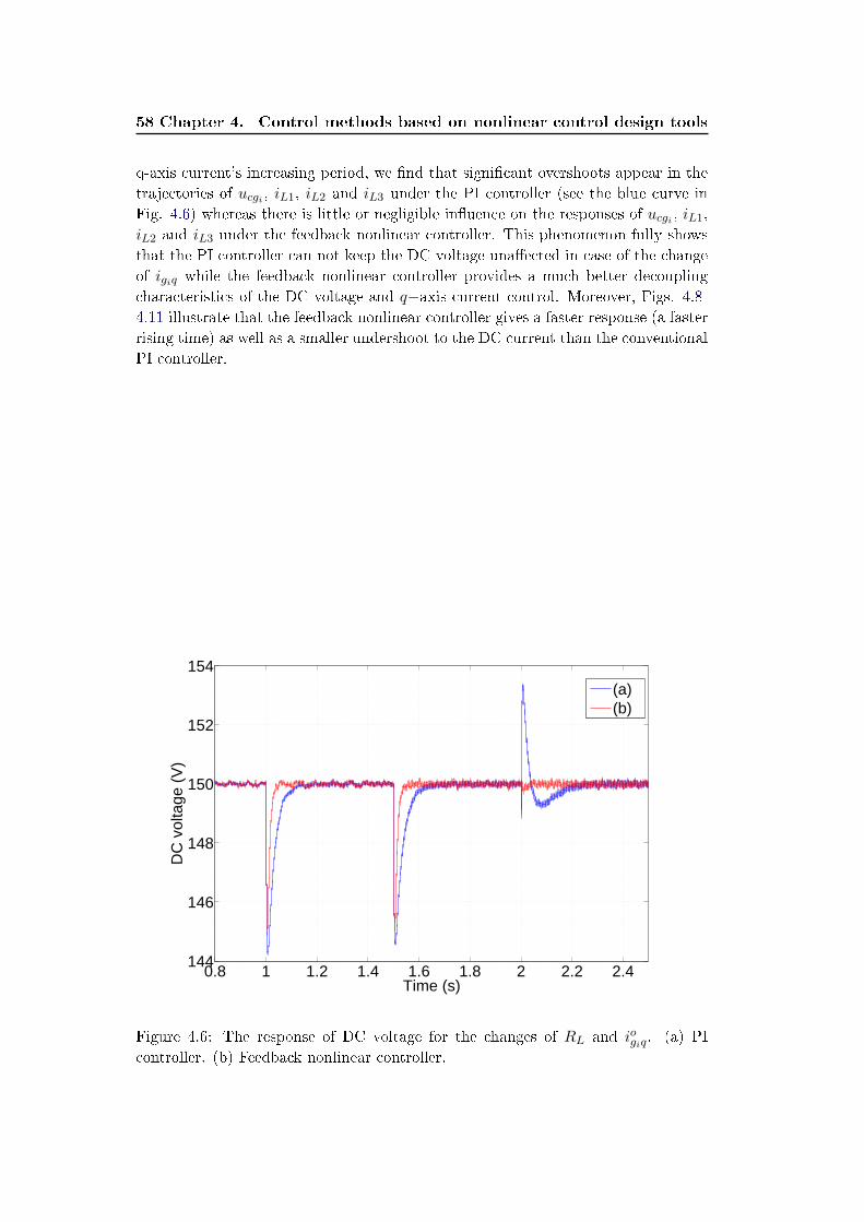
58 Chapter 4. Control methods based on nonlinear control design tools
q-axis current's increasing period, we nd that signicant overshoots appear in the
trajectories of ucgi , iL1, iL2 and iL3 under the PI controller (see the blue curve in
Fig. 4.6) whereas there is little or negligible inuence on the responses of ucgi , iL1,
iL2 and iL3 under the feedback nonlinear controller. This phenomenon fully shows
that the PI controller can not keep the DC voltage unaected in case of the change
of igiq while the feedback nonlinear controller provides a much better decoupling
characteristics of the DC voltage and q−axis current control. Moreover, Figs. 4.8-
4.11 illustrate that the feedback nonlinear controller gives a faster response (a faster
rising time) as well as a smaller undershoot to the DC current than the conventional
PI controller.
0.8 1 1.2 1.4 1.6 1.8 2 2.2 2.4144
146
148
150
152
154
Time (s)
DC
vol
tage
(V
)
(a)(b)
Figure 4.6: The response of DC voltage for the changes of RL and iogiq. (a) PI
controller. (b) Feedback nonlinear controller.
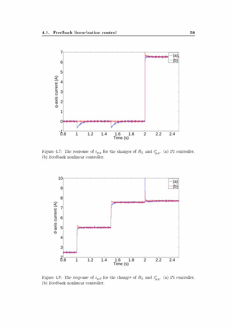
4.1. Feedback linearization control 59
0.8 1 1.2 1.4 1.6 1.8 2 2.2 2.4-1
0
1
2
3
4
5
6
7
Time (s)
q-ax
is c
urre
nt (
A)
(a)(b)
Figure 4.7: The response of igiq for the changes of RL and iogiq. (a) PI controller.
(b) Feedback nonlinear controller.
0.8 1 1.2 1.4 1.6 1.8 2 2.2 2.42
3
4
5
6
7
8
9
10
Time (s)
d-ax
is c
urre
nt (
A)
(a)(b)
Figure 4.8: The response of igid for the changes of RL and iogiq. (a) PI controller.
(b) Feedback nonlinear controller.
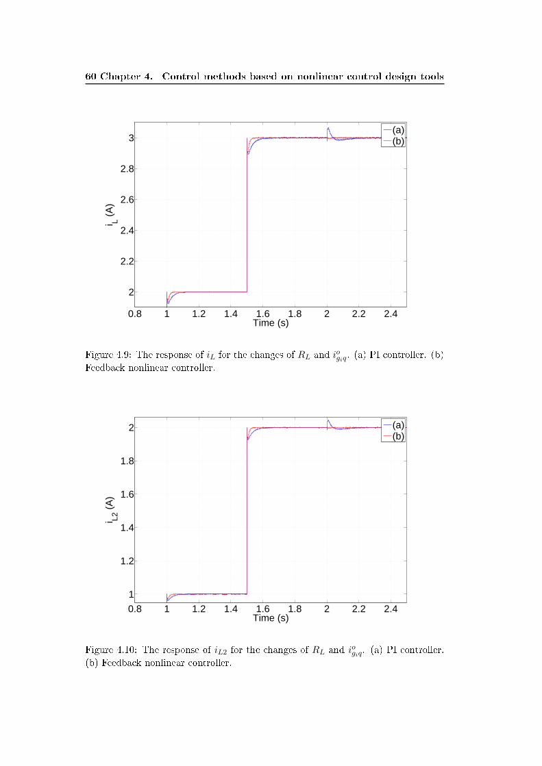
60 Chapter 4. Control methods based on nonlinear control design tools
0.8 1 1.2 1.4 1.6 1.8 2 2.2 2.4
2
2.2
2.4
2.6
2.8
3
Time (s)
i L (A
)
(a)(b)
Figure 4.9: The response of iL for the changes of RL and iogiq. (a) PI controller. (b)
Feedback nonlinear controller.
0.8 1 1.2 1.4 1.6 1.8 2 2.2 2.4
1
1.2
1.4
1.6
1.8
2
Time (s)
i L2 (
A)
(a)(b)
Figure 4.10: The response of iL2 for the changes of RL and iogiq. (a) PI controller.
(b) Feedback nonlinear controller.
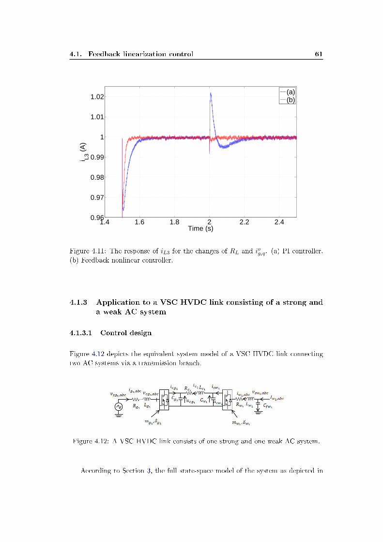
4.1. Feedback linearization control 61
1.4 1.6 1.8 2 2.2 2.40.96
0.97
0.98
0.99
1
1.01
1.02
Time (s)
i L3 (
A)
(a)(b)
Figure 4.11: The response of iL3 for the changes of RL and iogiq. (a) PI controller.
(b) Feedback nonlinear controller.
4.1.3 Application to a VSC HVDC link consisting of a strong anda weak AC system
4.1.3.1 Control design
Figure 4.12 depicts the equivalent system model of a VSC HVDC link connecting
two AC systems via a transmission branch.
Figure 4.12: A VSC HVDC link consists of one strong and one weak AC system.
According to Section 3, the full state-space model of the system as depicted in
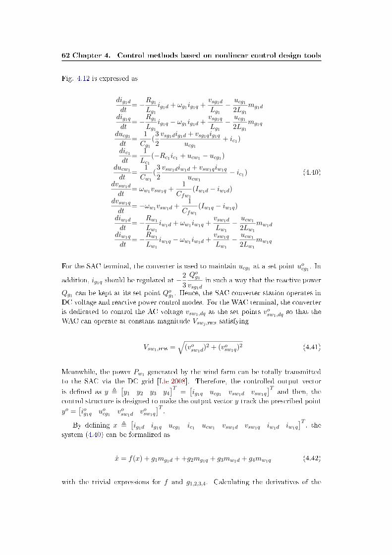
62 Chapter 4. Control methods based on nonlinear control design tools
Fig. 4.12 is expressed as
dig1ddt
= −Rg1Lg1
ig1d + ωg1ig1q +vsg1dLg1
− ucg12Lg1
mg1d
dig1qdt
= −Rg1Lg1
ig1q − ωg1ig1d +vsg1qLg1
− ucg12Lg1
mg1q
ducg1dt
=1
Cg1(3
2
vsg1dig1d + vsg1qig1qucg1
+ ic1)
dic1dt
=1
Lc1(−Rc1ic1 + ucw1 − ucg1)
ducw1
dt=
1
Cw1
(3
2
vsw1diw1d + vsw1qiw1q
ucw1
− ic1)
dvsw1d
dt= ωw1vsw1q +
1
Cfw1
(Iw1d − iw1d)
dvsw1q
dt= −ωw1vsw1d +
1
Cfw1
(Iw1q − iw1q)
diw1d
dt= −Rw1
Lw1
iw1d + ωw1iw1q +vsw1d
Lw1
− ucw1
2Lw1
mw1d
diw1q
dt= −Rw1
Lw1
iw1q − ωw1iw1d +vsw1q
Lw1
− ucw1
2Lw1
mw1q
(4.40)
For the SAC terminal, the converter is used to maintain ucg1 at a set point uocg1 . In
addition, ig1q should be regulated at −2
3
Qog1vsg1d
in such a way that the reactive power
Qg1 can be kept at its set point Qog1 . Hence, the SAC converter station operates in
DC voltage and reactive power control modes. For the WAC terminal, the converter
is dedicated to control the AC voltage vsw1,dq at the set points vosw1,dqso that the
WAC can operate at constant magnitude Vswj ,rms satisfying
Vsw1,rms =√
(vosw1d)2 + (vosw1q)
2 (4.41)
Meanwhile, the power Pw1 generated by the wind farm can be totally transmitted
to the SAC via the DC grid [Lie 2008]. Therefore, the controlled output vector
is dened as y ,[y1 y2 y3 y4
]T=[ig1q ucg1 vsw1d vsw1q
]Tand then, the
control structure is designed to make the output vector y track the prescribed point
yo =[iog1q uocg1 vosw1d
vosw1q
]T.
By dening x ,[ig1d ig1q ucg1 ic1 ucw1 vsw1d vsw1q iw1d iw1q
]T, the
system (4.40) can be formalized as
x = f(x) + g1mg1d + +g2mg1q + g3mw1d + g4mw1q (4.42)
with the trivial expressions for f and g1,2,3,4. Calculating the derivatives of the
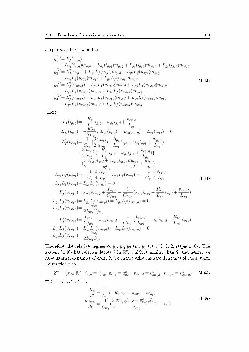
4.1. Feedback linearization control 63
output variables, we obtain
y(1)1 = Lf (ig1q)
+Lg1(ig1q)mg1d + Lg2(ig1q)mg1q + Lg3(ig1q)mw1d + Lg3(ig1q)mw1q
y(2)2 = L2
f (ucg1) + Lg1Lf (ucg1)mg1d + Lg2Lf (ucg1)mg1q
+Lg3Lf (ucg1)mw1d + Lg4Lf (ucg1)mw1q
y(2)3 = L2
f (vsw1d) + Lg1Lf (vsw1d)mg1d + Lg2Lf (vsw1d)mg1q
+Lg3Lf (vsw1d)mw1d + Lg4Lf (vsw1d)mw1q
y(2)4 = L2
f (vsw1q) + Lg1Lf (vsw1q)mg1d + Lg2Lf (vsw1q)mg1q
+Lg3Lf (vsw1q)mw1d + Lg4Lf (vsw1q)mw1q
(4.43)
where
Lf (ig1q)= −Rg1Lg1
ig1q − ωg1ig1d +vsg1qLg1
Lg2(ig1q)= −ucg12Lg1
, Lg1(ig1q) = Lg3(ig1q) = Lg4(ig1q) = 0
L2f (ucg1)=
1
Cg13
2
vsg1ducg1
(−Rg1Lg1
ig1d + ωg1ig1q +vsg1dLg1
)
+3
2
vsg1qucg1
(−Rg1Lg1
ig1q − ωg1ig1d +vsg1qLg1
)
−(3
2
vsg1dig1d + vsg1qig1qu2cg1
)ducg1dt
+dic1dt
Lg1Lf (ucg1)= − 1
Cg1
3
4
vsg1dLg1
, Lg2Lf (ucg1) = − 1
Cg1
3
4
vsg1qLg1
Lg3Lf (ucg1)= Lg4Lf (ucg1) = 0
L2f (vsw1d)= ωw1 vsw1q +
Iw1d
Cfw1
− 1
Cfw1
(ωw1iw1q −Rw1
Lw1
iw1d +vsw1d
Lw1
)
Lg1Lf (vsw1d)= Lg2Lf (vsw1d) = Lg4Lf (vsw1d) = 0
Lg3Lf (vsw1d)=ucw1
2Lw1Cfw1
L2f (vsw1q)=
Iw1q
Cfw1
− ωw1 vsw1d −1
Cfw1
(vsw1q
Lw1
− ωw1iw1d −Rw1
Lw1
iw1q)
Lg1Lf (vsw1d)= Lg2Lf (vsw1d) = Lg3Lf (vsw1d) = 0
Lg4Lf (vsw1d)=ucw1
2Lw1Cfw1
(4.44)
Therefore, the relative degrees of y1, y2, y3 and y4 are 1, 2, 2, 2, respectively. The
system (4.40) has relative degree 7 in R9, which is smaller than 9, and hence, we
have internal dynamics of order 2. To characterize the zero dynamics of the system,
we restrict x to
Z∗ = x ∈ R9 | ig1q ≡ iog1q, ucg1 ≡ uocg1 , vsw1d ≡ vosw1d
, vsw1q ≡ vosw1q (4.45)
This process leads to
dic1dt
=1
Lc1(−Rc1ic1 + ucw1 − uocg1)
ducw1
dt=
1
Cw1
(3
2
vosw1dIw1d + vosw1qIw1q
ucw1
− ic1)(4.46)
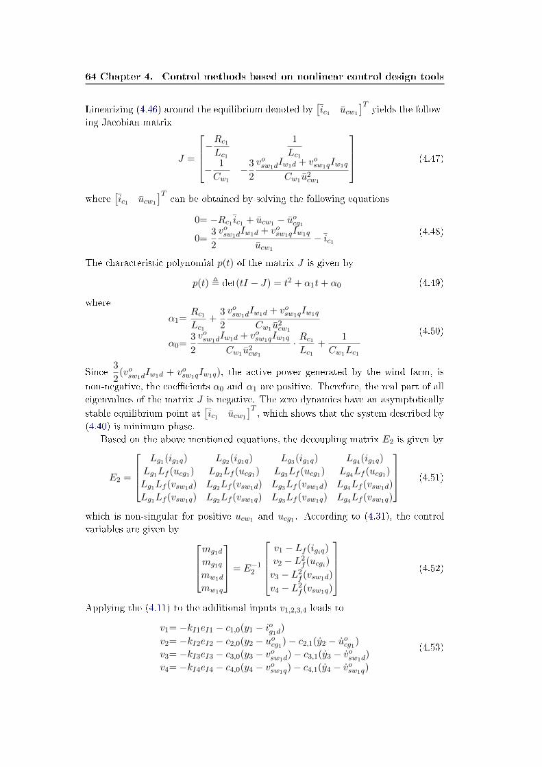
64 Chapter 4. Control methods based on nonlinear control design tools
Linearizing (4.46) around the equilibrium denoted by[ic1 ucw1
]Tyields the follow-
ing Jacobian matrix
J =
−Rc1Lc1
1
Lc1
− 1
Cw1
−3
2
vosw1dIw1d + vosw1qIw1q
Cw1 u2cw1
(4.47)
where[ic1 ucw1
]Tcan be obtained by solving the following equations
0= −Rc1 ic1 + ucw1 − uocg10=
3
2
vosw1dIw1d + vosw1qIw1q
ucw1
− ic1(4.48)
The characteristic polynomial p(t) of the matrix J is given by
p(t) , det(tI − J) = t2 + α1t+ α0 (4.49)
where
α1=Rc1Lc1
+3
2
vosw1dIw1d + vosw1qIw1q
Cw1 u2cw1
α0=3
2
vosw1dIw1d + vosw1qIw1q
Cw1 u2cw1
· Rc1Lc1
+1
Cw1Lc1
(4.50)
Since3
2(vosw1d
Iw1d + vosw1qIw1q), the active power generated by the wind farm, is
non-negative, the coecients α0 and α1 are positive. Therefore, the real part of all
eigenvalues of the matrix J is negative. The zero dynamics have an asymptotically
stable equilibrium point at[ic1 ucw1
]T, which shows that the system described by
(4.40) is minimum phase.
Based on the above mentioned equations, the decoupling matrix E2 is given by
E2 =
Lg1(ig1q) Lg2(ig1q) Lg3(ig1q) Lg4(ig1q)
Lg1Lf (ucg1) Lg2Lf (ucg1) Lg3Lf (ucg1) Lg4Lf (ucg1)
Lg1Lf (vsw1d) Lg2Lf (vsw1d) Lg3Lf (vsw1d) Lg4Lf (vsw1d)
Lg1Lf (vsw1q) Lg2Lf (vsw1q) Lg3Lf (vsw1q) Lg4Lf (vsw1q)
(4.51)
which is non-singular for positive ucw1 and ucg1 . According to (4.31), the control
variables are given by mg1d
mg1q
mw1d
mw1q
= E−12
v1 − Lf (igiq)
v2 − L2f (ucgi)
v3 − L2f (vsw1d)
v4 − L2f (vsw1q)
(4.52)
Applying the (4.11) to the additional inputs v1,2,3,4 leads to
v1= −kI1eI1 − c1,0(y1 − iog1d)v2= −kI2eI2 − c2,0(y2 − uocg1)− c2,1(y2 − uocg1)
v3= −kI3eI3 − c3,0(y3 − vosw1d)− c3,1(y3 − vosw1d
)
v4= −kI4eI4 − c4,0(y4 − vosw1q)− c4,1(y4 − vosw1q)
(4.53)
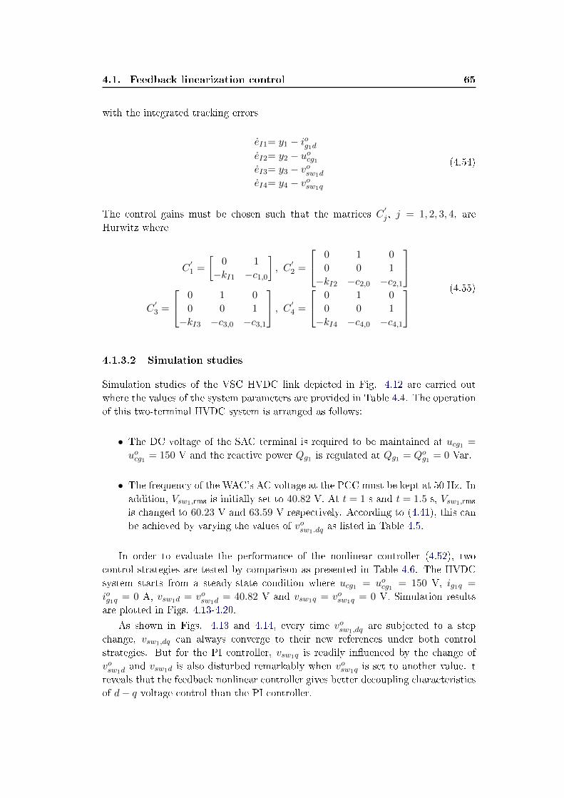
4.1. Feedback linearization control 65
with the integrated tracking errors
eI1= y1 − iog1deI2= y2 − uocg1eI3= y3 − vosw1d
eI4= y4 − vosw1q
(4.54)
The control gains must be chosen such that the matrices C′j , j = 1, 2, 3, 4, are
Hurwitz where
C′1 =
[0 1
−kI1 −c1,0
], C
′2 =
0 1 0
0 0 1
−kI2 −c2,0 −c2,1
C′3 =
0 1 0
0 0 1
−kI3 −c3,0 −c3,1
, C ′4 =
0 1 0
0 0 1
−kI4 −c4,0 −c4,1
(4.55)
4.1.3.2 Simulation studies
Simulation studies of the VSC HVDC link depicted in Fig. 4.12 are carried out
where the values of the system parameters are provided in Table 4.4. The operation
of this two-terminal HVDC system is arranged as follows:
• The DC voltage of the SAC terminal is required to be maintained at ucg1 =
uocg1 = 150 V and the reactive power Qg1 is regulated at Qg1 = Qog1 = 0 Var.
• The frequency of the WAC's AC voltage at the PCC must be kept at 50 Hz. In
addition, Vsw1,rms is initially set to 40.82 V. At t = 1 s and t = 1.5 s, Vsw1,rms
is changed to 60.23 V and 63.59 V respectively. According to (4.41), this can
be achieved by varying the values of vosw1.dqas listed in Table 4.5.
In order to evaluate the performance of the nonlinear controller (4.52), two
control strategies are tested by comparison as presented in Table 4.6. The HVDC
system starts from a steady-state condition where ucg1 = uocg1 = 150 V, ig1q =
iog1q = 0 A, vsw1d = vosw1d= 40.82 V and vsw1q = vosw1q = 0 V. Simulation results
are plotted in Figs. 4.13-4.20.
As shown in Figs. 4.13 and 4.14, every time vosw1,dqare subjected to a step
change, vsw1,dq can always converge to their new references under both control
strategies. But for the PI controller, vsw1q is readily inuenced by the change of
vosw1dand vsw1d is also disturbed remarkably when vosw1q is set to another value. t
reveals that the feedback nonlinear controller gives better decoupling characteristics
of d− q voltage control than the PI controller.
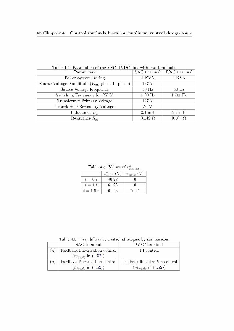
66 Chapter 4. Control methods based on nonlinear control design tools
Table 4.4: Parameters of the VSC HVDC link with two terminals.Parameters SAC terminal WAC terminal
Power System Rating 4 KVA 4 KVA
Source Voltage Amplitude (Vrms phase-to-phase) 127 V
Source Voltage Frequency 50 Hz 50 Hz
Switching Frequency for PWM 1500 Hz 1500 Hz
Transformer Primary Voltage 127 V
Transformer Secondary Voltage 50 V
Inductance Lgi 2.1 mH 3.3 mH
Resistance Rgi 0.142 Ω 0.165 Ω
Table 4.5: Values of vosw1,dq.
vosw1d(V) vosw1q (V)
t = 0 s 40.82 0
t = 1 s 61.23 0
t = 1.5 s 61.23 20.41
Table 4.6: Two dierence control strategies by comparison.SAC terminal WAC terminal
(a) Feedback linearization control PI control
(mg1,dq in (4.52))
(b) Feedback linearization control Feedback linearization control
(mg1,dq in (4.52)) (mw1,dq in (4.52))
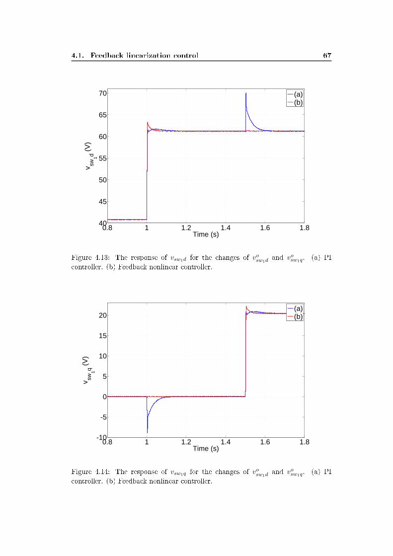
4.1. Feedback linearization control 67
0.8 1 1.2 1.4 1.6 1.840
45
50
55
60
65
70
Time (s)
v sw1d (
V)
(a)(b)
Figure 4.13: The response of vsw1d for the changes of vosw1dand vosw1q. (a) PI
controller. (b) Feedback nonlinear controller.
0.8 1 1.2 1.4 1.6 1.8-10
-5
0
5
10
15
20
Time (s)
v sw1q (
V)
(a)(b)
Figure 4.14: The response of vsw1q for the changes of vosw1dand vosw1q. (a) PI
controller. (b) Feedback nonlinear controller.
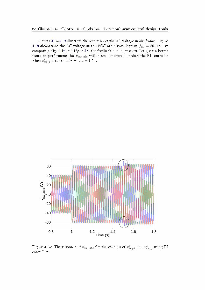
68 Chapter 4. Control methods based on nonlinear control design tools
Figures 4.15-4.19 illustrate the responses of the AC voltage in abc frame. Figure
4.19 shows that the AC voltage at the PCC are always kept at fw1 = 50 Hz. By
comparing Fig. 4.16 and Fig. 4.18, the feedback nonlinear controller gives a better
transient performance for vsw1,abc with a smaller overshoot than the PI controller
when vosw1q is set to 4.08 V at t = 1.5 s.
0.8 1 1.2 1.4 1.6 1.8
-60
-40
-20
0
20
40
60
Time (s)
v sw1,a
bc (
V)
Figure 4.15: The response of vsw1,abc for the changes of vosw1dand vosw1q using PI
controller.
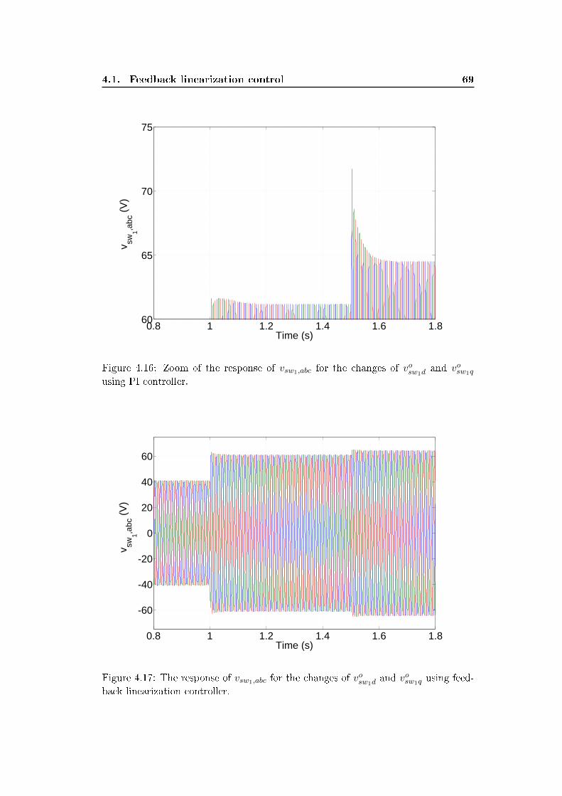
4.1. Feedback linearization control 69
0.8 1 1.2 1.4 1.6 1.860
65
70
75
Time (s)
v sw1,a
bc (
V)
Figure 4.16: Zoom of the response of vsw1,abc for the changes of vosw1dand vosw1q
using PI controller.
0.8 1 1.2 1.4 1.6 1.8
-60
-40
-20
0
20
40
60
Time (s)
v sw1,a
bc (
V)
Figure 4.17: The response of vsw1,abc for the changes of vosw1d
and vosw1q using feed-
back linearization controller.
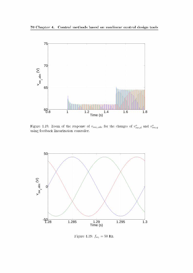
70 Chapter 4. Control methods based on nonlinear control design tools
0.8 1 1.2 1.4 1.6 1.860
65
70
75
Time (s)
v sw1,a
bc (
V)
Figure 4.18: Zoom of the response of vsw1,abc for the changes of vosw1dand vosw1q
using feedback linearization controller.
1.28 1.285 1.29 1.295 1.3-50
0
50
Time (s)
v sw1,a
bc (
V)
Figure 4.19: fw1 = 50 Hz.
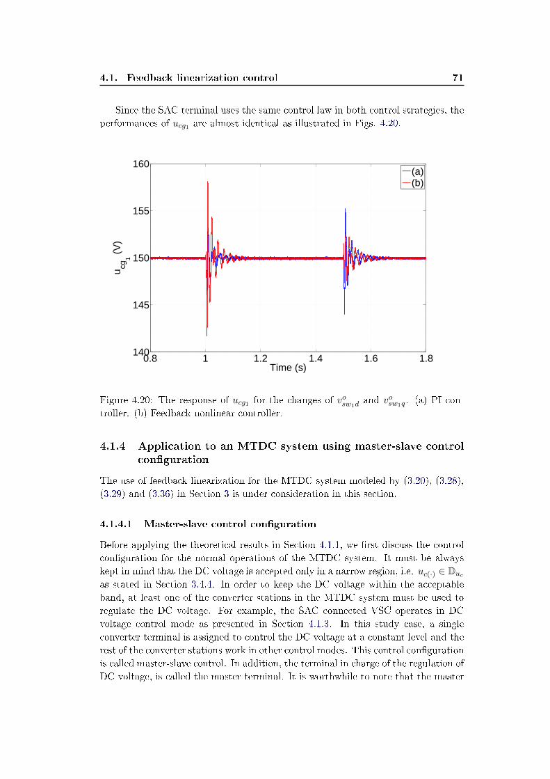
4.1. Feedback linearization control 71
Since the SAC terminal uses the same control law in both control strategies, the
performances of ucg1 are almost identical as illustrated in Figs. 4.20.
0.8 1 1.2 1.4 1.6 1.8140
145
150
155
160
Time (s)
u cg1 (
V)
(a)(b)
Figure 4.20: The response of ucg1 for the changes of vosw1dand vosw1q. (a) PI con-
troller. (b) Feedback nonlinear controller.
4.1.4 Application to an MTDC system using master-slave controlconguration
The use of feedback linearization for the MTDC system modeled by (3.20), (3.28),
(3.29) and (3.36) in Section 3 is under consideration in this section.
4.1.4.1 Master-slave control conguration
Before applying the theoretical results in Section 4.1.1, we rst discuss the control
conguration for the normal operations of the MTDC system. It must be always
kept in mind that the DC voltage is accepted only in a narrow region, i.e. uc(·) ∈ Ducas stated in Section 3.4.4. In order to keep the DC voltage within the acceptable
band, at least one of the converter stations in the MTDC system must be used to
regulate the DC voltage. For example, the SAC connected VSC operates in DC
voltage control mode as presented in Section 4.1.3. In this study case, a single
converter terminal is assigned to control the DC voltage at a constant level and the
rest of the converter stations work in other control modes. This control conguration
is called master-slave control. In addition, the terminal in charge of the regulation of
DC voltage, is called the master terminal. It is worthwhile to note that the master
72 Chapter 4. Control methods based on nonlinear control design tools
terminal takes responsibility for balancing the power ow of the DC network in case
of disturbances. Consequently, this terminal usually needs a large power capacity
to counteract all possible power imbalance.
The arrangement of VSC operation for the MTDC system is set as follows:
• The 1st SAC converter station chosen as the master terminal is used to main-
tain the DC voltage at the constant level uocg1 while the remaining SAC con-
verter stations operate in active control mode to control Pgρ at P ogρ1. Addi-
tionally, all reactive power Qgi should be kept at their respective references
Qogi .
• Each WAC converter station must ensure that the magnitude and the fre-
quency of the AC voltage at the PCC, Vsw,rms and fwj , are kept constant.
This can be fullled by regulating vswj ,dq at their references voswj ,dq
.
As mentioned in Section 4.1.3, Qgi can be kept at Qogi by regulating igiq at
iogiq = −2
3
Qogivswjd
. Likewise, we make igid track the reference iogid =2
3
P ogivswjd
for the
purpose of controlling Pgi at Pogi . According to the above arrangement, it is natural
to choose the output vector as
y ,[ig1q ucg1 igρd igρq vswjd vswjq
]T ∈ R2N+2M (4.56)
Obviously, the reference vector is set to
yo ,[iog1q uocg1 iogρd iogρq voswjd voswjq
]T∈ R2N+2M (4.57)
Through simple calculations, it is not dicult to get that the relative degrees of
ucg1 , ig1q, igρd, igρq, vswjd and vswjq are 2, 1, 1, 1, 2, 2, respectively, and hence, the
order of the internal dynamics is N − 1 +M + P + L.
Before designing the exact control algorithm, we need the following feasibility
assumption.
Assumption 4.1.1. Consider the MTDC system described by (3.20), (3.28), (3.29)
and (3.36). For the prescribed references uocg1, Qog1, P
ogρ , Q
ogρ , v
oswj ,dq
, there exist
1Unless otherwise stated, the subscript ρ mean ∀ρ ∈ N−1 = 2, · · · , N.
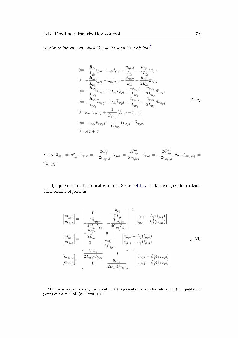
4.1. Feedback linearization control 73
constants for the state variables denoted by (·) such that2
0= −RgiLgi
igid + ωgi igiq +vsgidLgi− ucgi
2Lgimgid
0= −RgiLgi
igiq − ωgi igid +vsgiqLgi− ucgi
2Lgimgiq
0= −RwjLwj
iwjd + ωwj iwjq +vswjd
Lwj−ucwj2Lwj
mwjd
0= −RwjLwj
iwjq − ωwj iwjd +vswjq
Lwj−ucwj2Lwj
mwjq
0= ωwj vswjq +1
Cfwj(Iwjd − iwjd)
0= −ωwj vswjd +1
Cfwj(Iwjq − iwjq)
0= Az + ϑ
(4.58)
where ucg1 = uocg1, ig1q = −2Qog13vsg1d
, igρd =2P ogρ
3vsg1d, igρq = −
2Qogρ3vsg1d
and vswj ,dq =
voswj ,dq.
By applying the theoretical results in Section 4.1.1, the following nonlinear feed-
back control algorithm
[mg1d
mg1q
]=
0 − ucg12Lg1
−3vsg1d
4Cg1Lg1− 3vsg1q
4Cg1Lg1
−1 [
vg1q − Lf (ig1q)
vcg1 − L2f (ucg1)
][mgρd
mgρq
]=
−ucgρ2Lgρ
0
0 −ucgρ2Lgρ
−1 [
vgρd − Lf (igρd)
vgρq − Lf (igρq)
][mwjd
mwjq
]=
ucwj
2LwjCfwj0
0ucwj
2LwjCfwj
−1 [
vwjd − L2f (vswjd)
vwjq − L2f (vswjq)
](4.59)
2Unless otherwise stated, the notation (·) represents the steady-state value (or equilibrium
point) of the variable (or vector) (·).
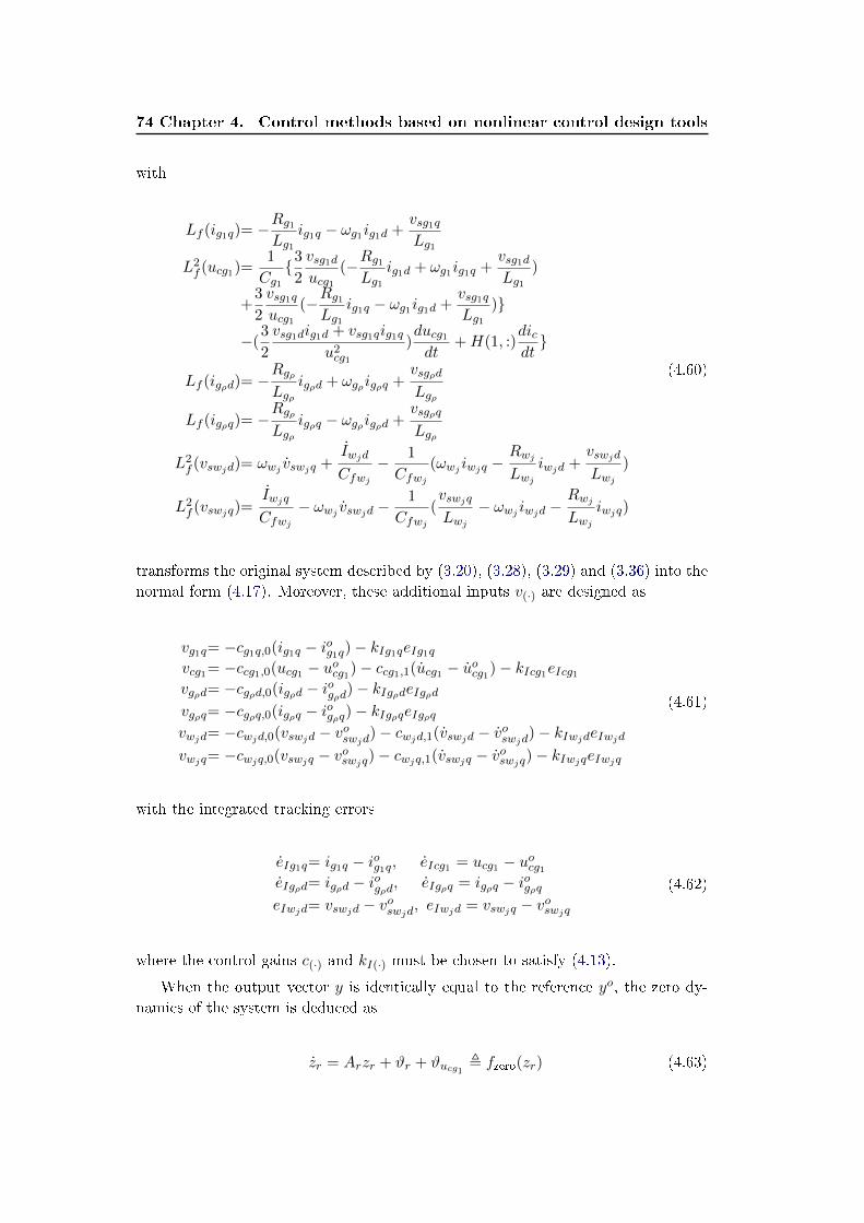
74 Chapter 4. Control methods based on nonlinear control design tools
with
Lf (ig1q)= −Rg1Lg1
ig1q − ωg1ig1d +vsg1qLg1
L2f (ucg1)=
1
Cg13
2
vsg1ducg1
(−Rg1Lg1
ig1d + ωg1ig1q +vsg1dLg1
)
+3
2
vsg1qucg1
(−Rg1Lg1
ig1q − ωg1ig1d +vsg1qLg1
)
−(3
2
vsg1dig1d + vsg1qig1qu2cg1
)ducg1dt
+H(1, :)dicdt
Lf (igρd)= −RgρLgρ
igρd + ωgρigρq +vsgρd
Lgρ
Lf (igρq)= −RgρLgρ
igρq − ωgρigρd +vsgρq
Lgρ
L2f (vswjd)= ωwj vswjq +
Iwjd
Cfwj− 1
Cfwj(ωwj iwjq −
RwjLwj
iwjd +vswjd
Lwj)
L2f (vswjq)=
Iwjq
Cfwj− ωwj vswjd −
1
Cfwj(vswjq
Lwj− ωwj iwjd −
RwjLwj
iwjq)
(4.60)
transforms the original system described by (3.20), (3.28), (3.29) and (3.36) into the
normal form (4.17). Moreover, these additional inputs v(·) are designed as
vg1q= −cg1q,0(ig1q − iog1q)− kIg1qeIg1qvcg1= −ccg1,0(ucg1 − uocg1)− ccg1,1(ucg1 − uocg1)− kIcg1eIcg1vgρd= −cgρd,0(igρd − iogρd)− kIgρdeIgρdvgρq= −cgρq,0(igρq − iogρq)− kIgρqeIgρqvwjd= −cwjd,0(vswjd − voswjd)− cwjd,1(vswjd − voswjd)− kIwjdeIwjdvwjq= −cwjq,0(vswjq − voswjq)− cwjq,1(vswjq − voswjq)− kIwjqeIwjq
(4.61)
with the integrated tracking errors
eIg1q= ig1q − iog1q, eIcg1 = ucg1 − uocg1eIgρd= igρd − iogρd, eIgρq = igρq − iogρqeIwjd= vswjd − voswjd, eIwjd = vswjq − voswjq
(4.62)
where the control gains c(·) and kI(·) must be chosen to satisfy (4.13).
When the output vector y is identically equal to the reference yo, the zero dy-
namics of the system is deduced as
zr = Arzr + ϑr + ϑucg1 , fzero(zr) (4.63)
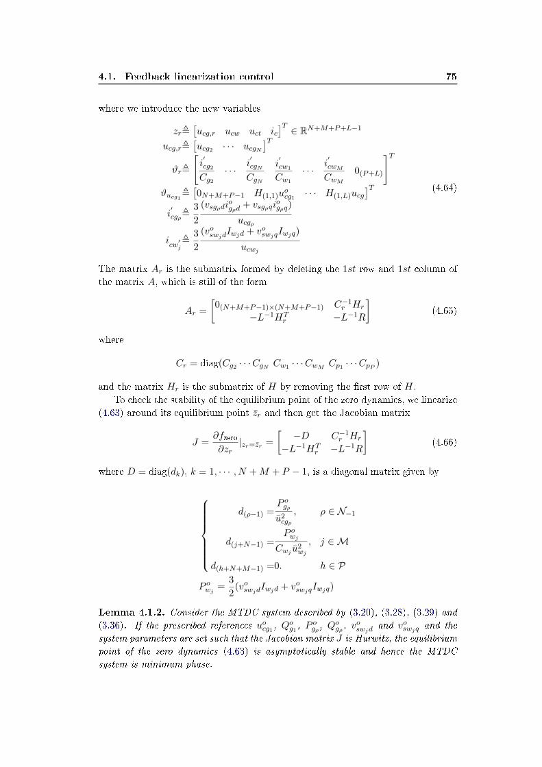
4.1. Feedback linearization control 75
where we introduce the new variables
zr,[ucg,r ucw uct ic
]T ∈ RN+M+P+L−1
ucg,r,[ucg2 · · · ucgN
]Tϑr,
[i′cg2
Cg2· · ·
i′cgN
CgN
i′cw1
Cw1
· · ·i′cwM
CwM0(P+L)
]Tϑucg1,
[0N+M+P−1 H(1,1)u
ocg1 · · · H(1,L)ucg
]Ti′cgρ,
3
2
(vsgρdiogρd
+ vsgρqiogρq)
ucgρ
icw′j,
3
2
(voswjdIwjd + voswjqIwjq)
ucwj
(4.64)
The matrix Ar is the submatrix formed by deleting the 1st row and 1st column of
the matrix A, which is still of the form
Ar =
[0(N+M+P−1)×(N+M+P−1) C−1
r Hr
−L−1HTr −L−1R
](4.65)
where
Cr = diag(Cg2 · · ·CgN Cw1 · · ·CwM Cp1 · · ·CpP )
and the matrix Hr is the submatrix of H by removing the rst row of H.
To check the stability of the equilibrium point of the zero dynamics, we linearize
(4.63) around its equilibrium point zr and then get the Jacobian matrix
J =∂fzero∂zr
|zr=zr =
[−D C−1
r Hr
−L−1HTr −L−1R
](4.66)
where D = diag(dk), k = 1, · · · , N +M + P − 1, is a diagonal matrix given by
d(ρ−1) =P ogρu2cgρ
, ρ ∈ N−1
d(j+N−1) =P owj
Cwj u2wj
, j ∈M
d(h+N+M−1) =0. h ∈ P
P owj =3
2(voswjdIwjd + voswjqIwjq)
Lemma 4.1.2. Consider the MTDC system described by (3.20), (3.28), (3.29) and
(3.36). If the prescribed references uocg1, Qog1, P
ogρ , Q
ogρ , v
oswjd
and voswjq and the
system parameters are set such that the Jacobian matrix J is Hurwitz, the equilibrium
point of the zero dynamics (4.63) is asymptotically stable and hence the MTDC
system is minimum phase.

76 Chapter 4. Control methods based on nonlinear control design tools
Lemma 4.1.3. Consider the MTDC system described by (3.20), (3.28), (3.29) and
(3.36). If P ogρ , ρ = 2, · · · , N and P owj , j = 1, · · · ,M are non-negative, the MTDC
system is minimum phase.
In order to prove Lemma 4.1.3, we need some properties of complex matrix as
referred in [Horn 1985]. We recall the following basic facts:
Denition 4.1.4. A matrix Ψ ∈ Cn×n is said to be semi-positive denite if
Re(xHΨx) is non-negative for every non-zero column vector x ∈ Cn×1. Moreover,
Ψ ∈ Cn×n is said to be positive denite if Re(xHΨx) is positive for every non-zero
column vector x ∈ Cn×1. The set of the positive denite matrix Ψ is denoted as P+C .
Lemma 4.1.5. For any complex matrix Ψ ∈ Cn×n, it can be expressed as Ψ =
H(Ψ) + S(Ψ) where H(Ψ) ,1
2(Ψ + ΨH) is a hermitian matrix and S(Ψ) ,
1
2(Ψ−
ΨH) is an anti-hermitian matrix.
Lemma 4.1.6. Matrix Ψ ∈ Cn×n is positive denite if and only if its hermitian
part H(Ψ) is positive denite.
Lemma 4.1.7. If matrix Γ is invertible and Ψ is positive denite, then ΓHΨΓ is
also positive denite.
Lemma 4.1.8. If Ψ1 is positive denite and Ψ2 is semi-positive denite, we have
Ψ1 + Ψ2 ∈ P+C .
Lemma 4.1.9. If Ψ ∈ P+C , then Ψ is invertible and Ψ−1 ∈ P+
C .
Based on the above statements, we can now demonstrate Lemma 4.1.3 as follows.
Proof. Let us assume that there exists a particular eigenvalue of J denoted by
λ = α+ jβ ∈ C, whose real part is non-negative, i.e. α ≥ 0. Then, λ satises
det(λI − J) = 0
Alternatively, it can be expressed as
det(
[λI +D −C−1
r Hr
L−1r HT
r λI + L−1R
]) = 0 (4.67)
We dene Φ1 , λI + L−1R = Λ1 + jΛ2 where Λ1,2 are expressed by
Λ1 = diag(α+Rc1Lc1
, · · · , α+RcLLcL
) ∈ RL×L
Λ2 = diag(β, · · · , β) ∈ RL×L
Since the Hermitian part of Φ1 is equal to H(Φ1) = Λ1, which is positive denite,
the complex matrix Φ1 is also positive denite (Lemma 4.1.6). Consequently, Φ1
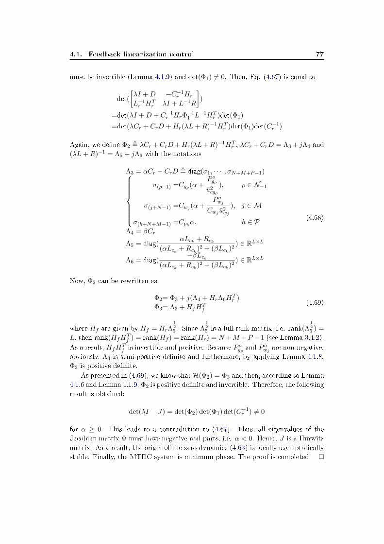
4.1. Feedback linearization control 77
must be invertible (Lemma 4.1.9) and det(Φ1) 6= 0. Then, Eq. (4.67) is equal to
det(
[λI +D −C−1
r Hr
L−1r HT
r λI + L−1R
])
=det(λI +D + C−1r HrΦ
−11 L−1HT
r )det(Φ1)
=det(λCr + CrD +Hr(λL+R)−1HTr )det(Φ1)det(C−1
r )
Again, we dene Φ2 , λCr +CrD+Hr(λL+R)−1HTr , λCr +CrD = Λ3 + jΛ4 and
(λL+R)−1 = Λ5 + jΛ6 with the notations
Λ3 = αCr − CrD , diag(σ1, · · · , σN+M+P−1)
σ(ρ−1) =Cgρ(α+P ogρu2cgρ
), ρ ∈ N−1
σ(j+N−1) =Cwj (α+P owj
Cwj u2wj
), j ∈M
σ(h+N+M−1) =Cphα. h ∈ PΛ4 = βCr
Λ5 = diag(αLck +Rck
(αLck +Rck)2 + (βLck)2) ∈ RL×L
Λ6 = diag(−βLck
(αLck +Rck)2 + (βLck)2) ∈ RL×L
(4.68)
Now, Φ2 can be rewritten as
Φ2= Φ3 + j(Λ4 +HrΛ6HTr )
Φ3= Λ3 +HfHTf
(4.69)
where Hf are given by Hf = HrΛ125 . Since Λ
125 is a full rank matrix, i.e. rank(Λ
125 ) =
L, then rank(HfHTf ) = rank(Hf ) = rank(Hr) = N +M +P −1 (see Lemma 3.4.2).
As a result, HfHTf is invertible and positive. Because P ogρ and P
owj are non-negative,
obviously, Λ3 is semi-positive denite and furthermore, by applying Lemma 4.1.8,
Φ3 is positive denite.
As presented in (4.69), we know that H(Φ2) = Φ3 and then, according to Lemma
4.1.6 and Lemma 4.1.9, Φ2 is positive denite and invertible. Therefore, the following
result is obtained:
det(λI − J) = det(Φ2) det(Φ1) det(C−1r ) 6= 0
for α ≥ 0. This leads to a contradiction to (4.67). Thus, all eigenvalues of the
Jacobian matrix Φ must have negative real parts, i.e. α < 0. Hence, J is a Hurwitz
matrix. As a result, the origin of the zero dynamics (4.63) is locally asymptotically
stable. Finally, the MTDC system is minimum phase. The proof is completed.
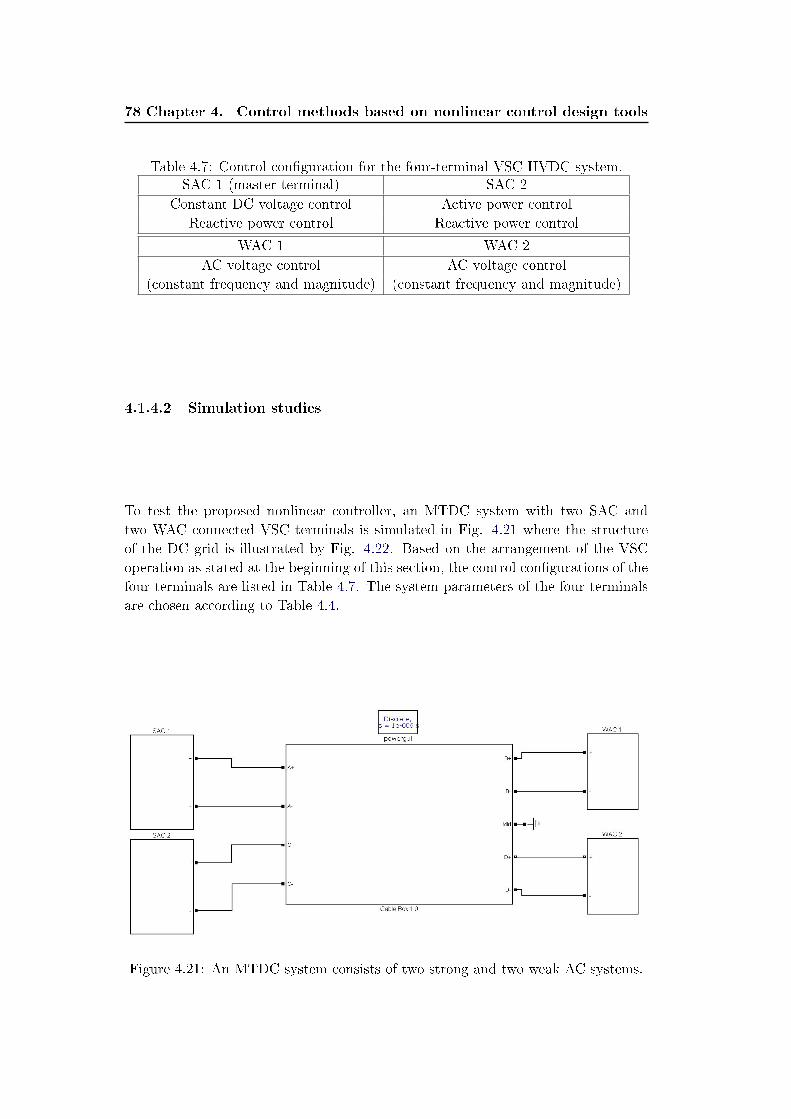
78 Chapter 4. Control methods based on nonlinear control design tools
Table 4.7: Control conguration for the four-terminal VSC HVDC system.SAC 1 (master terminal) SAC 2
Constant DC voltage control Active power control
Reactive power control Reactive power control
WAC 1 WAC 2
AC voltage control AC voltage control
(constant frequency and magnitude) (constant frequency and magnitude)
4.1.4.2 Simulation studies
To test the proposed nonlinear controller, an MTDC system with two SAC and
two WAC connected VSC terminals is simulated in Fig. 4.21 where the structure
of the DC grid is illustrated by Fig. 4.22. Based on the arrangement of the VSC
operation as stated at the beginning of this section, the control congurations of the
four terminals are listed in Table 4.7. The system parameters of the four terminals
are chosen according to Table 4.4.
Figure 4.21: An MTDC system consists of two strong and two weak AC systems.
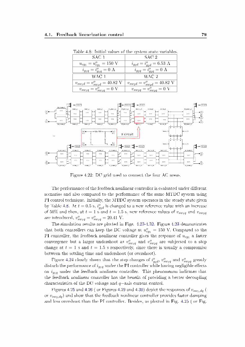
4.1. Feedback linearization control 79
Table 4.8: Initial values of the system state variables.SAC 1 SAC 2
ucg1 = uocg1 = 150 V ig2d = iog2d = 6.53 A
ig1q = iog1q = 0 A ig2q = iog2q = 0 A
WAC 1 WAC 2
vsw1d = vosw1d= 40.82 V vsw2d = vosw2d
= 40.82 V
vsw1q = vosw1q = 0 V vsw2q = vosw2q = 0 V
Figure 4.22: DC grid used to connect the four AC areas.
The performance of the feedback nonlinear controller is evaluated under dierent
scenarios and also compared to the performance of the same MTDC system using
PI control technique. Initially, the MTDC system operates in the steady state given
by Table 4.8. At t = 0.5 s, iog2d is changed to a new reference value with an increase
of 50% and then, at t = 1 s and t = 1.5 s, new reference values of vsw1q and vsw2q
are introduced, vosw1q = vosw1q = 20.41 V.
The simulation results are plotted in Figs. 4.23-4.32. Figure 4.23 demonstrates
that both controllers can keep the DC voltage at uocg1 = 150 V. Compared to the
PI controller, the feedback nonlinear controller gives the response of ucg1 a faster
convergence but a larger undershoot as vosw1q and vosw2q are subjected to a step
change at t = 1 s and t = 1.5 s respectively, since there is usually a compromise
between the settling time and undershoot (or overshoot).
Figure 4.24 clearly shows that the step changes of iog2d, vosw1q and v
osw2q greatly
disturb the performance of ig1q under the PI controller while having negligible eects
on ig1q under the feedback nonlinear controller. This phenomenon indicates that
the feedback nonlinear controller has the benet of providing a better decoupling
characteristics of the DC voltage and q−axis current control.Figures 4.25 and 4.26 ( or Figures 4.29 and 4.30) depict the responses of vsw1,dq (
or vsw2,dq) and show that the feedback nonlinear controller provides faster damping
and less overshoot than the PI controller. Besides, as plotted in Fig. 4.25 ( or Fig.
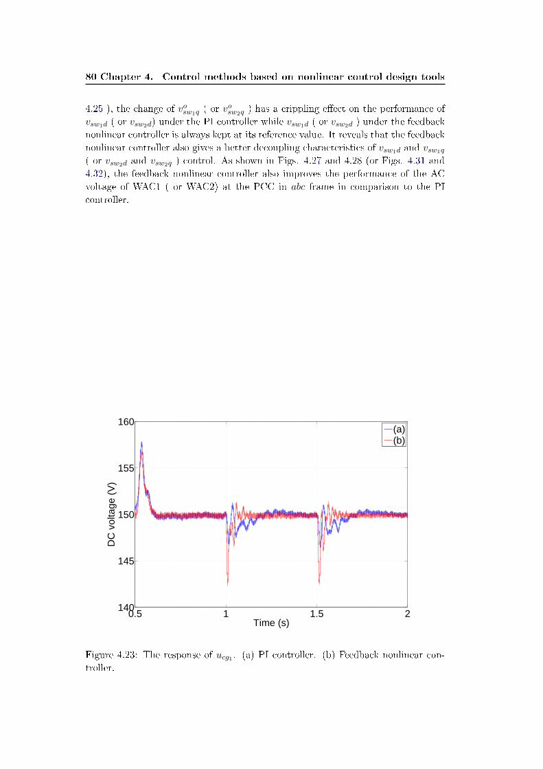
80 Chapter 4. Control methods based on nonlinear control design tools
4.25 ), the change of vosw1q ( or vosw2q ) has a crippling eect on the performance of
vsw1d ( or vsw2d) under the PI controller while vsw1d ( or vsw2d ) under the feedback
nonlinear controller is always kept at its reference value. It reveals that the feedback
nonlinear controller also gives a better decoupling characteristics of vsw1d and vsw1q
( or vsw2d and vsw2q ) control. As shown in Figs. 4.27 and 4.28 (or Figs. 4.31 and
4.32), the feedback nonlinear controller also improves the performance of the AC
voltage of WAC1 ( or WAC2) at the PCC in abc frame in comparison to the PI
controller.
0.5 1 1.5 2140
145
150
155
160
Time (s)
DC
vol
tage
(V
)
(a)(b)
Figure 4.23: The response of ucg1 . (a) PI controller. (b) Feedback nonlinear con-
troller.
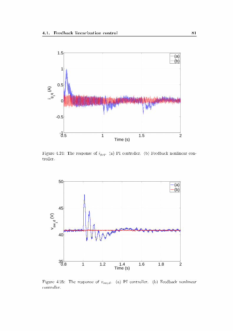
4.1. Feedback linearization control 81
0.5 1 1.5 2-1
-0.5
0
0.5
1
1.5
Time (s)
i g 1q (A
)
(a)(b)
Figure 4.24: The response of ig1q. (a) PI controller. (b) Feedback nonlinear con-
troller.
0.8 1 1.2 1.4 1.6 1.8 235
40
45
50
Time (s)
v sw1d (
V)
(a)(b)
Figure 4.25: The response of vsw1d. (a) PI controller. (b) Feedback nonlinear
controller.
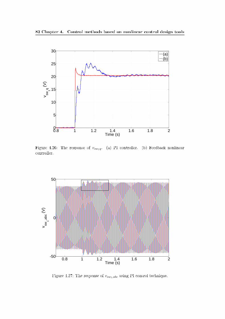
82 Chapter 4. Control methods based on nonlinear control design tools
0.8 1 1.2 1.4 1.6 1.8 20
5
10
15
20
25
30
Time (s)
v sw1q (
V)
(a)(b)
Figure 4.26: The response of vsw1q. (a) PI controller. (b) Feedback nonlinear
controller.
0.8 1 1.2 1.4 1.6 1.8 2-50
0
50
Time (s)
v sw1,a
bc (
V)
Figure 4.27: The response of vsw1,abc using PI control technique.
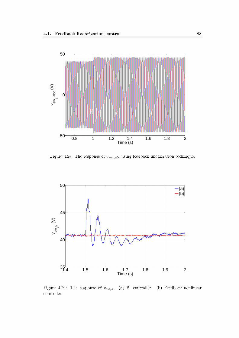
4.1. Feedback linearization control 83
0.8 1 1.2 1.4 1.6 1.8 2-50
0
50
Time (s)
v sw1,a
bc (
V)
Figure 4.28: The response of vsw1,abc using feedback linearization technique.
1.4 1.5 1.6 1.7 1.8 1.9 235
40
45
50
Time (s)
v sw2d (
V)
(a)(b)
Figure 4.29: The response of vsw2d. (a) PI controller. (b) Feedback nonlinear
controller.
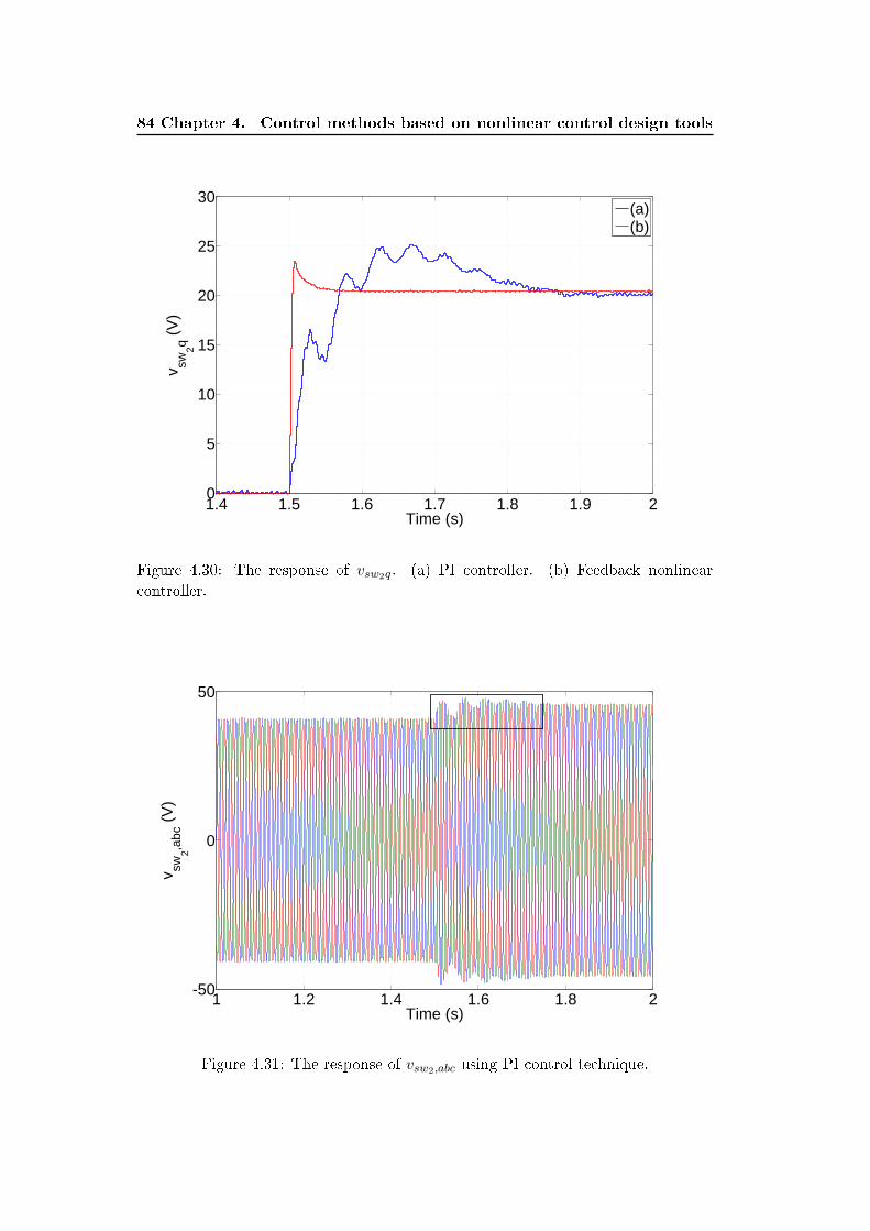
84 Chapter 4. Control methods based on nonlinear control design tools
1.4 1.5 1.6 1.7 1.8 1.9 20
5
10
15
20
25
30
Time (s)
v sw2q (
V)
(a)(b)
Figure 4.30: The response of vsw2q. (a) PI controller. (b) Feedback nonlinear
controller.
1 1.2 1.4 1.6 1.8 2-50
0
50
Time (s)
v sw2,a
bc (
V)
Figure 4.31: The response of vsw2,abc using PI control technique.
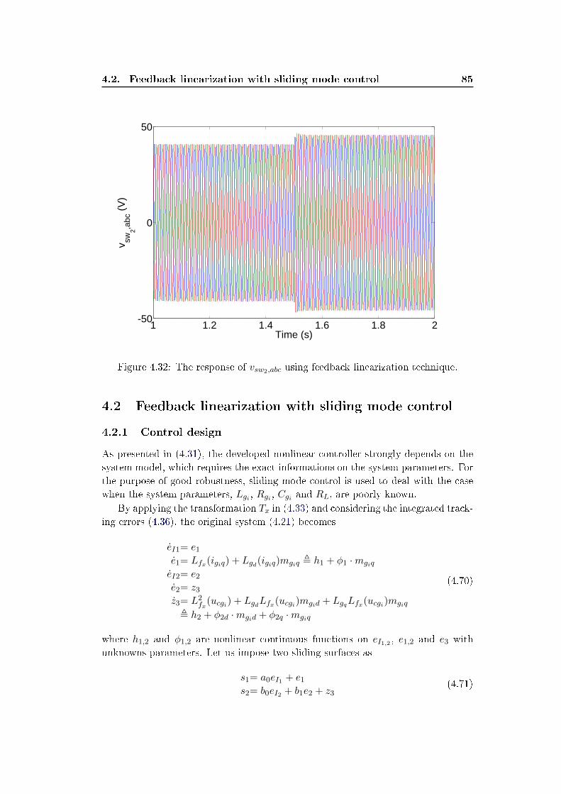
4.2. Feedback linearization with sliding mode control 85
1 1.2 1.4 1.6 1.8 2-50
0
50
Time (s)
v sw2,a
bc (
V)
Figure 4.32: The response of vsw2,abc using feedback linearization technique.
4.2 Feedback linearization with sliding mode control
4.2.1 Control design
As presented in (4.31), the developed nonlinear controller strongly depends on the
system model, which requires the exact informations on the system parameters. For
the purpose of good robustness, sliding mode control is used to deal with the case
when the system parameters, Lgi , Rgi , Cgi and RL, are poorly known.
By applying the transformation Tx in (4.33) and considering the integrated track-
ing errors (4.36), the original system (4.21) becomes
eI1= e1
e1= Lfx(igiq) + Lgd(igiq)mgiq , h1 + φ1 ·mgiq
eI2= e2
e2= z3
z3= L2fx
(ucgi) + LgdLfx(ucgi)mgid + LgqLfx(ucgi)mgiq
, h2 + φ2d ·mgid + φ2q ·mgiq
(4.70)
where h1,2 and φ1,2 are nonlinear continuous functions on eI1,2 , e1,2 and e3 with
unknowns parameters. Let us impose two sliding surfaces as
s1= a0eI1 + e1
s2= b0eI2 + b1e2 + z3(4.71)

86 Chapter 4. Control methods based on nonlinear control design tools
where a0 is positive and b0,1 are chosen such that the matrix
B0 =
[0 1
−b0 −b1
](4.72)
is Hurwitz. The derivatives of the sliding surfaces are given by
s1= a0e1 + h1 + φ1 ·mgiq
s2= b0e2 + b1z3 + h2 + φ2d ·mgid + φ2q ·mgiq(4.73)
Let us consider the Lyapunov function V1 = s21 + s2
2 and then, the derivative of V1
is deduced as
V1= W1 +W2
W1= s1(a0e1 + h1 + φ1 ·mgiq)
W2= s2(b0e2 + b1z3 + h2 + φ2d ·mgid + φ2q ·mgiq)
(4.74)
From (4.30), it is clear that φ1 and φ2d are always negative and moreover, φ1 and
φ2d are continuous and invertible for positive ucgi .
Assumption 4.2.1. In the domain of interest as described in Section 3.4.4, h1, h2,
φ1 and φ2,dq satisfy the inequalities
|h1| ≤ h1,max, 0 ≤ φ1,min ≤ |φ1| ≤ φ1,max
|h2| ≤ h2,max, 0 ≤ φ2d,min ≤ |φ2d| ≤ φ2d,max
0 ≤ φ2q,min ≤ |φ2q| ≤ φ2q,max
(4.75)
when the system parameters are bounded.
With Assumption 4.2.1, we can then dene the control law for mgiq as
mgiq = βq1
φ1,minsgn(s1) (4.76)
where βq are designed as
βq = a0|e1|+ h1,max + β0, β0 > 0 (4.77)
The control law for mgid is developed as
mgid = βd1
φ2d,minsgn(s2) (4.78)
where
βd = b0|e2|+ b1|z3|+ h2,max +φ2q,max
φ1,minβq + β1, β1 > 0 (4.79)
Applying (4.76) to W1, we obtain
W1 = s1(a0e1 + h1 + βqφ1
φ1,minsgn(s1)) (4.80)
The sign of W1 can be analyzed as follows:

4.2. Feedback linearization with sliding mode control 87
• If s1 > 0, then sgn(s1) = 1 and recalling that φ1 is negative and φ1,min is
positive, we have
φ1
φ1,min≤ −1
s1= a0e1 + h1 + (a0|e1|+ h1,max + β0)φ1
φ1,min< 0
• If s1 < 0, sgn(s1) = −1 leads to
s1 = a0e1 + h1 − (a0|e1|+ h1,max + β0)φ1
φ1,min> 0
As a result, W1 = s1s1 is negative for all s1 6= 0.
Substituting (4.76) and (4.78) into (4.74) yields
W2= s2(b0e2 + b1z3 + h2 + φ2d ·mgid + φ2q ·mgiq)
= s2(b0e2 + b1z3 + h2 + βqφ2q
φ1,minsgn(s1) + βd
φ2d
φ2d,minsgn(s2))
(4.81)
Recalling (4.75) and the design of βd in (4.79), we have the following results:
• If s2 > 0, sgn(s2) = 1 and then,
φ2d
φ2d,min≤ −1 (4.82)
s2 = b0e2 + b1z3 + h2 + βqφ2q
φ1,minsgn(s1) + βd
φ2d
φ2d,min< 0 (4.83)
• If s2 < 0, sgn(s2) = −1 and then, we have
s2 = b0e2 + b1z3 + h2 + βqφ2q
φ1,minsgn(s1)− βd
φ2d
φ2d,min> 0 (4.84)
Therefore, W2 = s2s2 is also negative for all s2 6= 0. From the above analysis, the
controller dened by (4.76) and (4.78) will lead to the manifolds s1 = 0 and s2 = 0.
On these two manifolds, the behavior of the system is totally governed by
eI1= e1
e1= −a0eI1eI2= e2
e2= −b0eI2 − b1e2
(4.85)
whose equilibrium point is asymptotically stable.
Since the use of sign function sgn(·) usually causes the chattering problem
[Khalil 1996], in order to deal with this issue, a high-slope saturation function sat(·)dened as
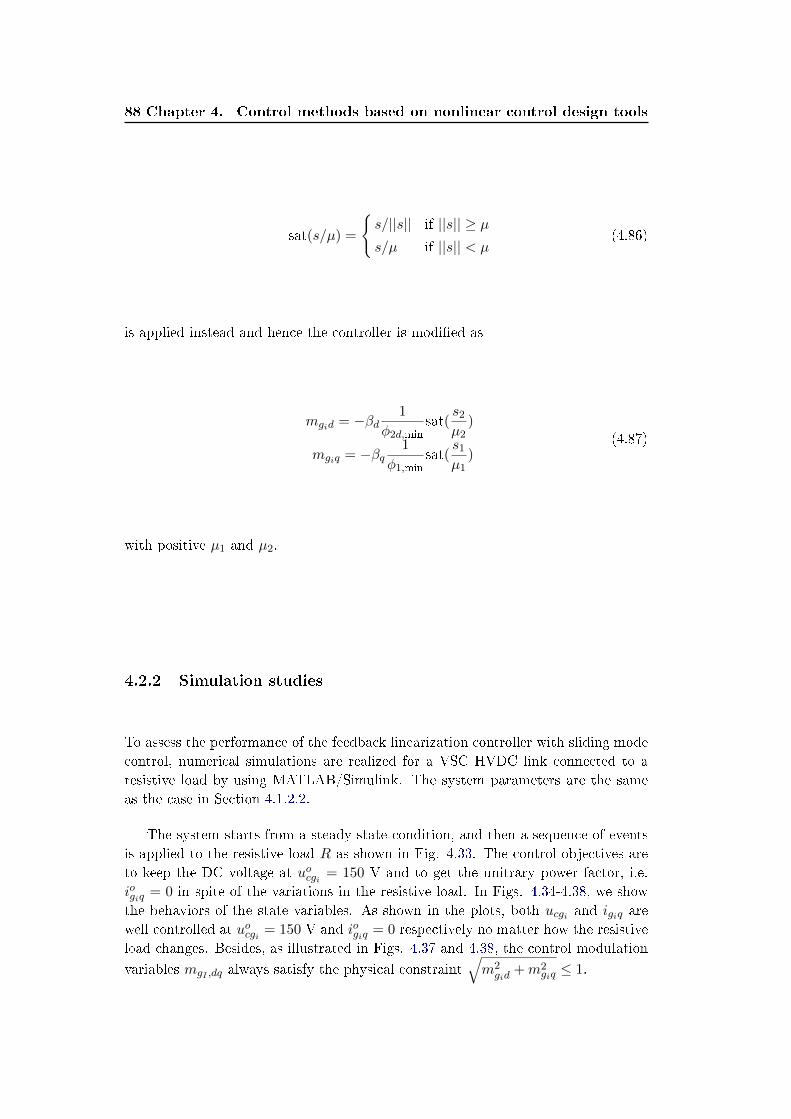
88 Chapter 4. Control methods based on nonlinear control design tools
sat(s/µ) =
s/||s|| if ||s|| ≥ µs/µ if ||s|| < µ
(4.86)
is applied instead and hence the controller is modied as
mgid = −βd1
φ2d,minsat(
s2
µ2)
mgiq = −βq1
φ1,minsat(
s1
µ1)
(4.87)
with positive µ1 and µ2.
4.2.2 Simulation studies
To assess the performance of the feedback linearization controller with sliding mode
control, numerical simulations are realized for a VSC HVDC link connected to a
resistive load by using MATLAB/Simulink. The system parameters are the same
as the case in Section 4.1.2.2.
The system starts from a steady-state condition, and then a sequence of events
is applied to the resistive load R as shown in Fig. 4.33. The control objectives are
to keep the DC voltage at uocgi = 150 V and to get the unitrary power factor, i.e.
iogiq = 0 in spite of the variations in the resistive load. In Figs. 4.34-4.38, we show
the behaviors of the state variables. As shown in the plots, both ucgi and igiq are
well controlled at uocgi = 150 V and iogiq = 0 respectively no matter how the resistive
load changes. Besides, as illustrated in Figs. 4.37 and 4.38, the control modulation
variables mgI ,dq always satisfy the physical constraint√m2gid
+m2giq ≤ 1.
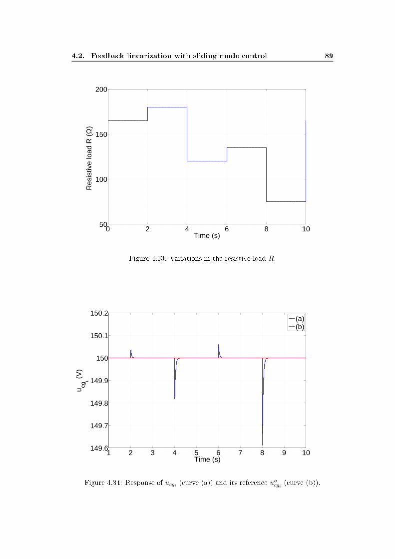
4.2. Feedback linearization with sliding mode control 89
0 2 4 6 8 1050
100
150
200
Time (s)
Res
istiv
e lo
ad R
(Ω
)
Figure 4.33: Variations in the resistive load R.
1 2 3 4 5 6 7 8 9 10149.6
149.7
149.8
149.9
150
150.1
150.2
Time (s)
u cgi (
V)
(a)(b)
Figure 4.34: Response of ucgi (curve (a)) and its reference uocgi (curve (b)).
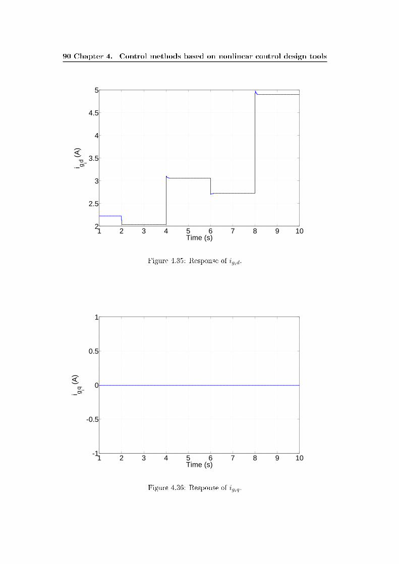
90 Chapter 4. Control methods based on nonlinear control design tools
1 2 3 4 5 6 7 8 9 102
2.5
3
3.5
4
4.5
5
Time (s)
i g id (A
)
Figure 4.35: Response of igid.
1 2 3 4 5 6 7 8 9 10-1
-0.5
0
0.5
1
Time (s)
i g iq (A
)
Figure 4.36: Response of igiq.
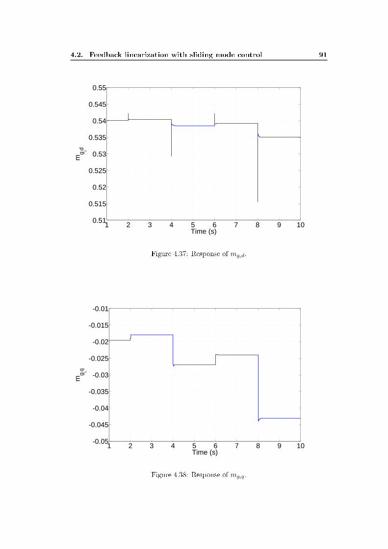
4.2. Feedback linearization with sliding mode control 91
1 2 3 4 5 6 7 8 9 100.51
0.515
0.52
0.525
0.53
0.535
0.54
0.545
0.55
Time (s)
mg id
Figure 4.37: Response of mgid.
1 2 3 4 5 6 7 8 9 10-0.05
-0.045
-0.04
-0.035
-0.03
-0.025
-0.02
-0.015
-0.01
Time (s)
mg iq
Figure 4.38: Response of mgiq.
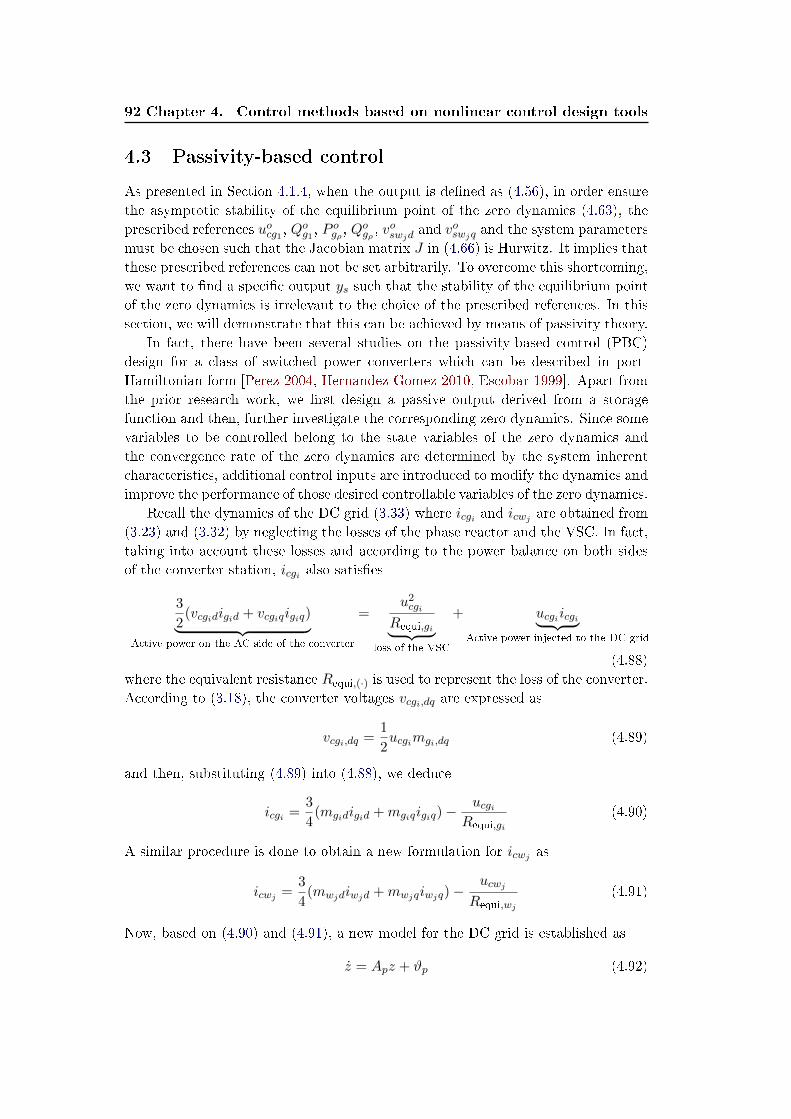
92 Chapter 4. Control methods based on nonlinear control design tools
4.3 Passivity-based control
As presented in Section 4.1.4, when the output is dened as (4.56), in order ensure
the asymptotic stability of the equilibrium point of the zero dynamics (4.63), the
prescribed references uocg1 , Qog1 , P
ogρ , Q
ogρ , v
oswjd
and voswjq and the system parameters
must be chosen such that the Jacobian matrix J in (4.66) is Hurwitz. It implies that
these prescribed references can not be set arbitrarily. To overcome this shortcoming,
we want to nd a specic output ys such that the stability of the equilibrium point
of the zero dynamics is irrelevant to the choice of the prescribed references. In this
section, we will demonstrate that this can be achieved by means of passivity theory.
In fact, there have been several studies on the passivity-based control (PBC)
design for a class of switched power converters which can be described in port-
Hamiltonian form [Perez 2004, Hernandez-Gomez 2010, Escobar 1999]. Apart from
the prior research work, we rst design a passive output derived from a storage
function and then, further investigate the corresponding zero dynamics. Since some
variables to be controlled belong to the state variables of the zero dynamics and
the convergence rate of the zero dynamics are determined by the system inherent
characteristics, additional control inputs are introduced to modify the dynamics and
improve the performance of those desired controllable variables of the zero dynamics.
Recall the dynamics of the DC grid (3.33) where icgi and icwj are obtained from
(3.23) and (3.32) by neglecting the losses of the phase reactor and the VSC. In fact,
taking into account these losses and according to the power balance on both sides
of the converter station, icgi also satises
3
2(vcgidigid + vcgiqigiq)︸ ︷︷ ︸
Active power on the AC side of the converter
=u2cgi
Requi,gi︸ ︷︷ ︸loss of the VSC
+ ucgiicgi︸ ︷︷ ︸Active power injected to the DC grid
(4.88)
where the equivalent resistance Requi,(·) is used to represent the loss of the converter.
According to (3.18), the converter voltages vcgi,dq are expressed as
vcgi,dq =1
2ucgimgi,dq (4.89)
and then, substituting (4.89) into (4.88), we deduce
icgi =3
4(mgidigid +mgiqigiq)−
ucgiRequi,gi
(4.90)
A similar procedure is done to obtain a new formulation for icwj as
icwj =3
4(mwjdiwjd +mwjqiwjq)−
ucwjRequi,wj
(4.91)
Now, based on (4.90) and (4.91), a new model for the DC grid is established as
z = Apz + ϑp (4.92)
4.3. Passivity-based control 93
where Ap and ϑp are given by
ϑp=
[· · ·
3(mgidigid +mgiqigiq)
4Cgi· · ·
3(mwjdiwjd +mwjqiwjq)
4Cwj· · · 0(P+L)
]TAp=
[−Dp C−1H
−L−1HT −L−1R
]Dp= C−1R−1
equi ∈ R(N+M+P )×(N+M+P )
Requi= diag(· · · , Requi,gi , · · ·Requi,wj , · · · , 0, · · · , 0)(4.93)
Let us consider the dynamics of vswj ,dq in (3.29). Similar to the modication of
the dynamics of the DC grid, here we use the equivalent resistance Rfwj to represent
the losses of the lter and hence, vswj ,dq are modeled by
dvswjd
dt= ωwjvswjq +
1
Cfwj(Iwjd − iwjd −
vswjd
Rfwj)
dvswjq
dt= −ωwjvswjd +
1
Cfwj(Iwjq − iwjq −
vswjq
Rfwj)
(4.94)
In this section, the passivity-based state feedback control design is developed
based on the above new DC grid and AC voltage model.
4.3.1 Steady-state analysis
The same master-slave control conguration is used in this section as in Section
4.1.4. In addition, in order to make all SAC systems operate with unity power
factor, we set
Qogi = 0 (4.95)
Similar to Assumption 4.1.1, to ensure the operating feasibility of the MTDC system,
we take the following assumption.
Assumption 4.3.1. Consider the MTDC system described by (3.20), (3.28), (4.94)
and (4.92). For the prescribed references uocg1 , Qog1, P
ogρ , Q
ogρ , v
oswj ,dq
, there exist
equilibrium values for the state variables such that
0= −RgiLgi
igid + ωgi igiq +vsgidLgi− ucgi
2Lgimgid
0= −RgiLgi
igiq − ωgi igid +vsgiqLgi− ucgi
2Lgimgiq
0= −RwjLwj
iwjd + ωwj iwjq +vswjd
Lwj−ucwj2Lwj
mwjd
0= −RwjLwj
iwjq − ωwj iwjd +vswjq
Lwj−ucwj2Lwj
mwjq
0= ωwj vswjq +1
Cfwj(Iwjd − iwjd −
vswjd
Rfwj)
0= −ωwj vswjd +1
Cfwj(Iwjq − iwjq −
vswjq
Rfwj)
0= Apz + ϑp
(4.96)
94 Chapter 4. Control methods based on nonlinear control design tools
where ucg1 = uocg1, ig1q = −2Qog13vsg1d
= 0, igρd =2P ogρ
3vsg1d, igρq = −
2Qogρ3vsg1d
= 0 and
vswj ,dq = voswj ,dq.
Under Assumption 4.3.1, the steady-state values of iwj ,dq and the control vari-
ables are deduced as
iwjd= Iwjd + Cfwjωwjvoswjq −
voswjd
Rfwj
iwjq= Iwjq − Cfwjωwjvoswjd −voswjq
Rfwj
(4.97)
and
mgid=2
ucgi(−Rgi igid + Lgiωgi igiq + vsgid)
mgiq=2
ucgi(−Rgi igiq − Lgiωgi igid + vsgiq)
mwjd=2
ucwj(−Rwj iwjd + Lwjωwj iwjq + voswjd)
mwjq=2
ucwj(−Rwj iwjq − Lwjωwj iwjd + voswjq)
(4.98)
Substituting (4.97) and (4.98) into (4.96), we nd that the DC grid in steady state
satises
(vsgidigid + vsgiq igiq)−Rgi (i2gid + i2giq) +2
3[H(i, :)icucgi −
u2cgi
Requi,gi
] = 0
(voswjdiwjd + voswjq iwjq)−Rwj (i2wjd
+ i2wjq) +2
3[H(N + j, :)icucwj −
u2cwj
Requi,wj
] = 0
H(N +M + h, :)ic = 0
H(:, k)T uc = 0(4.99)
Note that the above expression (4.99) contains several quadratic terms. It implies
that the MTDC system has more than one equilibrium point that corresponds to
the prescribed references [Lee 2003, Zonetti 2014]. But, not all of these equilibrium
points are achievable. As presented in [Lee 2003], there are two possible steady-state
values for the d−axis current. However, the larger one is physically impossible, mak-
ing the converter operate beyond its ability. The choice of the reasonable equilibrium
point is determined by the system physical characteristics, the feasibility of the mod-
ulation technique (see (3.21) and (3.30)), etc. But this issue is beyond the scope of
this thesis. Here, we make the following assumption on the equilibrium point.
Assumption 4.3.2. Consider the MTDC system described by (3.20), (3.28), (4.94)
and (4.92). For the prescribed references uocg1, Qog1, P
ogρ , Q
ogρ , v
oswj ,dq
, for every state
variable, only one steady-state value exists in their respective domain of interest
dened in Section 3.4.4.
4.3. Passivity-based control 95
4.3.2 Passive system
Let (·) = (·) − (·) denote the error between the variable (·) and its steady-state
value. By considering the steady-state condition (4.96), (·) satises the dierentialequations
˙igid= −RgiLgi
igid + ωgi igiq −1
2Lgi(mgiducgi + mgiducgi)
˙igiq= −RgiLgi
igiq − ωgi igid −1
2Lgi(mgiqucgi + mgiqucgi)
˙iwjd= −RwjLwj
iwjd + ωwj iwjq +vswjd
Lwj− 1
2Lwj(mwjducwj + mwjducwj )
˙iwjq= −RwjLwj
iwjq − ωwj iwjd +vswjq
Lwj− 1
2Lwj(mwjqucwj + mwjqucwj )
˙vswjd= ωwj vswjq −1
Cfwj(iwjd +
vswjd
Rfwj)
˙vswjq= −ωwj vswjd −1
Cfwj(iwjq +
vswjq
Rfwj)
˙z= Apz + ϑp
(4.100)
where ϑp is given by
ϑp(i) =3
4Cgi(mgidigid + mgidigid + mgiq igiq + mgiqigiq), i ∈ N
ϑp(N + j) =3
4Cwj(mwjdiwjd + mwjdiwjd + mwjq iwjq + mwjqiwjq), j ∈M
ϑp(N +M + h) = 0. h ∈ Pϑp(N +M + P + k) = 0. k ∈ L
In addition, setting mgi,dq = mwj ,dq = 0, we get the unforced system of (4.100) as
˙igid= −RgiLgi
igid + ωgi igiq −1
2Lgimgiducgi
˙igiq= −RgiLgi
igiq − ωgi igid −1
2Lgimgiqucgi
˙iwjd= −RwjLwj
iwjd + ωwj iwjq +vswjd
Lwj− 1
2Lwjmwjducwj
˙iwjq= −RwjLwj
iwjq − ωwj iwjd +vswjq
Lwj− 1
2Lwjmwjqucwj
˙vswjd= ωwj vswjq −1
Cfwj(iwjd +
vswjd
Rfwj)
˙vswjq= −ωwj vswjd −1
Cfwj(iwjq +
vswjq
Rfwj)
˙z= Apz + ϑ′p
(4.101)

96 Chapter 4. Control methods based on nonlinear control design tools
where ϑ′p is expressed as
ϑp(i) =
3
4Cgi(mgidigid + mgiq igiq), i ∈ N
ϑp(N + j) =3
4Cwj(mwjdiwjd + mwjq iwjq), j ∈M
ϑp(N +M + h) = ϑp(N +M + P + k) = 0. h ∈ P, k ∈ L
Take
V=1
2
∑Ni=1 Lgi [(igid)
2 + (igiq)2] +
1
2
∑Mj=1 Lwj [(iwjd)
2 + (iwjq)2]
+1
2
∑Mj=1Cfwj [(vswjd)
2 + (vswjq)2] +
1
2· 2
3zTΛz
(4.102)
as a storage function candidate with
Λ =
[C 0(N+M+P )×L
0L×(N+M+P ) L
]
The function V is positive denite and its derivative along the trajectories of (4.100)
satises
V= −∑N
i=1Rgi [(igid)2 + (igiq)
2]−∑M
j=1Rwj [(iwjd)2 + (iwjq)
2]
−2
3
∑Ni=1
(ucgi)2
Requi,gi
− 2
3
∑Mj=1
(ucwj )2
Requi,wj
−∑M
j=1[(vswjd)
2 + (vswjq)2
Rfwj]− 2
3
∑Lk=1Rck (ick)2
+1
2
∑Ni=1[mgid(ucgiigid − ucgi igid) + mgiq(ucgiigiq − ucgi igiq)]
+1
2
∑Mj=1[mwjd(ucwj iwjd − ucwj iwjd) + mwjq(ucwj iwjq − ucwj iwjq)]
(4.103)
Taking the output vector yp as
yp= [ypg ypw]T ∈ R2N+2M
ypg= [ypg1d ypg1q · · · ypgid ypgiq · · · ypgNd ypgN q]T ∈ R2N
ypw= [ypw1d ypw1q · · · ypwjd ypwjq · · · ypwMd ypwM q]T ∈ R2M
ypgid=1
2(ucgiigid − ucgi igid); ypgiq =
1
2(ucgiigiq − ucgi igiq)
ypwjd=1
2(ucwj iwjd − ucwj iwjd); ypwjq =
1
2(ucwj iwjq − ucwj iwjq)
(4.104)
V then satises
V= LfV + LgV u ≤ yTp u (4.105)

4.3. Passivity-based control 97
with
LgV= yTpLfV= −
∑Ni=1Rgi [(igid)
2 + (igiq)2]−
∑Mj=1Rwj [(iwjd)
2 + (iwjq)2]
−2
3
∑Ni=1
(ucgi)2
Requi,gi
− 2
3
∑Mj=1
(ucwj )2
Requi,wj
−∑M
j=1[(vswjd)
2 + (vswjq)2
Rfwj]− 2
3
∑Lk=1Rck (ick)2
u= [ug uw]T ∈ R2N+2M
ug= [mg1d mg1q · · · mgNd mgN q]T ∈ R2N
uw= [mw1d mw1q · · · mwMd mwM q]T ∈ R2M
(4.106)
It can be seen that the MTDC system has the Kalman-Yacubovitch-Popov (KYP)
property and it is passive with the passive output vector yp.
4.3.3 Control design
Since the steady-state values of all DC voltages are positive, uc(·) > 0, here we
change the output vector to
y= [yg yw]T ∈ R2N+2M
yg= [yg1d yg1q · · · ygid ygiq · · · ygNd ygN q]T ∈ R2N
yw= [yw1d yw1q · · · ywjd ywjq · · · ywMd ywM q]T ∈ R2M
ygid= αgiducgi − igid; ygiq = αgiqucgi − igiqywjd= αwjducwj − iwjd; ywjq = αwjqucwj − iwjq
αgi,dq=igi,dqucgi
; αwj ,dq =iwj ,dq
ucwj
(4.107)
Comparing yp in (4.104) and y in (4.107), it is easy to nd that
ygi,dq=2
ucgiypgi,dq; ywj ,dq =
2
ucwjypwj ,dq (4.108)
Accordingly, the reference of y is yo = 0(2N+2M)×1. Let us restrict y ≡ yo and then,
by performing the change of variables
igi,dq = αgi,dqucgi − ygi,dq; iwj ,dq = αwj ,dqucwj − ywj ,dq (4.109)
we obtain the following equations
0 = ygid= a1gimgid + a2gimgiq + fgid0 = ygiq= a3gimgid + a4gimgiq + fgiq
0 = ywjd= a1wjmwjd + a2wjmwjq + fwjd0 = ywjq= a3wjmwjd + a4wjmwjq + fwjq
(4.110)

98 Chapter 4. Control methods based on nonlinear control design tools
where
a1gi=3
4
αgidCgi
(αgiducgi − ygid) +ucgi2Lgi
a2gi=3
4
αgidCgi
(αgiqucgi − ygiq)
a3gi=3
4
αgiqCgi
(αgiducgi − ygid)
a4gi=3
4
αgiqCgi
(αgiqucgi − ygiq) +ucgi2Lgi
a1wj=3
4
αwjd
Cwj(αwjducwj − ywjd) +
ucwj2Lwj
a2wj=3
4
αwjd
Cwj(αwjqucwj − ywjq)
a3wj=3
4
αwjq
Cwj(αwjducwj − ywjd)
a4wj=3
4
αwjq
Cwj(αwjqucwj − ywjq) +
ucwj2Lwj
fgid=αgidCgi
[− ucgiRequi,gi
+H(i, :)ic] +RgiLgi
(αgiducgi − ygid)
−ωgi(αgiqucgi − ygiq)−vsgidLgi
fgiq=αgiqCgi
[− ucgiRequi,gi
+H(i, :)ic] +RgiLgi
(αgiqucgi − ygiq)
+ωgi(αgiducgi − ygid)−vsgiqLgi
fwjd=αwjd
Cwj[−
ucwjRequi,wj
+H(N + j, :)ic] +RwjLwj
(αwjducwj − ywjd)
−ωwj (αwjqucwj − ywjq)−vswjd
Lwj
fwjq=αwjq
Cwj[−
ucwjRequi,wj
+H(N + j, :)ic] +RwjLwj
(αwjqucwj − ywjq)
+ωwj (αwjducwj − ywjd)−vswjq
Lwj
(4.111)
Let us denote
Egi =
[a1gi a2gi
a3gi a4gi
]; Ewj =
[a1wj a2wj
a3wj a4wj
]; (4.112)
Lemma 4.3.3. The decoupling matrices Egi and Ewj are nonsingular at ygid =
ygiq = 0 and ywjd = ywjq = 0.
Proof. The determinants of Egi and Ewj are equal to
∆gi= det(Egi) =ucgi2Lgi
[ucgi2Lgi
+3
4
αgidCgi
(αgiducgi − ygid) +3
4
αgiqCgi
(αgiqucgi − ygiq)]
∆wj= det(Ewj ) =ucwj2Lwj
[ucwj2Lwj
+3
4
αwjd
Cwj(αwjducwj − ywjd)
+3
4
αwjq
Cwj(αwjqucwj − ywjq)]

4.3. Passivity-based control 99
Setting ygid = ygiq = 0 and ywjd = ywjq = 0 yields
∆gi0= ∆gi |ygid=ygiq=0
=ucgi2Lgi
[ucgi2Lgi
+3
4
(αgid)2
Cgiucgi +
3
4
(αgiq)2
Cgiucgi ]
∆wj0= ∆wj |ywjd=ywjq=0]
=ucwj2Lwj
[ucwj2Lwj
+3
4
(αwjd)2
Cwjucwj +
3
4
(αwjq)2
Cwjucwj ]
(4.113)
Because ucgi and ucwj are positive, ∆gi0 6= 0 and ∆wj0 6= 0 are always positive.
Since ∆gi (∆wj ) are continuously dierentiable for (αgid, αgiq, ygid, ygiq) ∈Bαgid×Bαgiq×Bygid×Bygiq ((αwjd, αwjq, ywjd, ywjq) ∈ Bαwjd×Bαwjq×Bywjd×Bywjq) where these B(·) ⊂ R are open connected sets, based on Lemma 4.3.3, we have the
following lemma.
Lemma 4.3.4. There exist a series of connected sets S(·) ⊂ B(·) such that the
decoupling matrices Egi and Ewj are nonsigular for (αgid, αgiq, ygid, ygiq) ∈ Sαgid×Sαgiq×Sygid×Sygiq and (αwjd, αwjq, ywjd, ywjq) ∈ Sαwjd×Sαwjq×Sywjd×Sywjq . Inaddition, Sygi,dq and Sywj,dq contain the origin. Sαgid , Sαgiq , Sαwjd and Sαwjq containigiducgi
,igiqucgi
,iwjd
ucwjand
iwjq
ucwj, respectively.
Since the solution of the state variables is restricted to (4.110) when the output
vector y is identically equal to yo, the control modulation indices must satisfy
mgid=1
∆gi
(a4gifgid − a2gifgiq)|ygid=ygiq=0
mgiq=1
∆gi
(a4gifgid − a2gifgiq)|ygid=ygiq=0
mwjd=1
∆wj
(a4wjfwjd − a2wjfwjq)|ywjd=ywjq=0
mwjq=1
∆wj
(a4wjfwjd − a2wjfwjq)|ywjd=ywjq=0
(4.114)
Substituting (4.114) into the MTDC system, the zero dynamics are characterized
100Chapter 4. Control methods based on nonlinear control design tools
by
dvswjd
dt= ωwjvswjq +
1
Cfwj(Iwjd − αwjducwj −
vswjd
Rfwj)
dvswjq
dt= −ωwjvswjd +
1
Cfwj(Iwjq − αwjqucwj −
vswjq
Rfwj)
Cgiducgidt
=1
∆gi0
1
2LgI[− ucgiRequi,gi
+H(i, :)ic]
− 1
∆gi0
3
4[RgiLgi
ucgi(α2gid
+ α2giq)−
1
Lgi(vsgidαgid + vsgiqαgiq)]
Cwjducwjdt
=1
∆wj0
1
2Lwj[−
ucwjRequi,wj
+H(N + j, :)ic]
− 1
∆wj0
3
4[RwjLwj
ucwj (α2wjd
+ α2wjq)−
1
Lwj(vswjdαwjd + vswjqαwjq)]
Cthducthdt
= H(N +M + h, :)ic
Lckdickdt
= −RckicK −H(:, k)Tuc
(4.115)
With
W=1
2
∑Mj=1Cfwj [(vswjd)
2 + (vswjq)2] +
1
2
∑Mj=1Cwjkwj (ucwj )
2
+1
2
∑Ph=1Cth
2
3(ucth)2 +
1
2
∑Lk=1
2
3Lck (ick)2 +
1
2
∑Ni=1Cgikgi(ucgi)
2(4.116)
as a Lyapunov function candidate for the zero dynamics (4.115) where
kwj= 1
2Lwj+
3
4[(αwjd)
2 + (αwjq)2]4
3Lwj
kgi= 1
2Lgi+
3
4[(αgid)
2 + (αgiq)2]4
3Lgi
(4.117)
The derivative of W along the trajectories of (4.115) is given by
W= −∑M
j=1[2
3Requi,wj
+Rwj (α2wjd
+ α2wjq)](uwj )
2
−∑N
i=1[2
3Requi,gi
+Rgi(α2gid
+ α2giq)](ugi)
2 − 2
3Rck (ick)2
−∑M
j=1[(vswjd)
2 + (vswjq)2
Rfwj] ≤ 0
(4.118)
which shows that the MTDC system with the output vector y in (4.107) is weakly
minimum phase. Furthermore, we have the following result.
Lemma 4.3.5. The equilibrium point of the zero dynamics (4.115) is asymptotically
stable.
Proof. This lemma can be proved using Barbalat's lemma. Since W is non-positive,
we then haveW (t) ≤W (t = 0), which means that all variables (·) inW are bounded.

4.3. Passivity-based control 101
Based on (4.118), W can be computed, which is composed only of bounded terms.
Hence, W is also bounded. As a consequence, W is uniformly continuous in time.
Applying Barbalat's lemma, we have W → 0 in (4.118) as t → ∞, which implies
that
ucwj→ 0; ucgi → 0; ick → 0; vswjd → 0; vswjq → 0 (4.119)
and˙ucwj→ 0; ˙ucgi → 0; ˙ick → 0; ˙vswjd → 0; ˙vswjq → 0 (4.120)
Combining (4.115), (4.119) and (4.120), we can obtain
HT uc → 0 (4.121)
with unknown ucth . Since Lemma 3.4.1 states that rank(H) = N +M +P − 1 ≥ P ,ucth → 0 is the only solution of (4.121). As a result, only the trivial solution exists
for W = 0 and then the lemma is proved.
Based on Lemma 4.3.5, we can also get that only the trivial solution of the
unforced system (4.101) can stay in the set y = yo = 0(2N+2M)×1 where y is
dened as (4.107). Finally, we can conclude that the error system (4.100) is zero-
state observable.
According to Theorem 3.2 in [Byrnes 1991], the control variables m(·) can be
developed as [mgid
mgiq
]= −
[φgid(ygid)
φgiq(ygiq)
];
[mwjd
mwjq
]= −
[φwjd(ywjd)
φwjd(ywjq)
](4.122)
where φ(·) are any smooth functions such that φ(·)(0) = 0 and
ygidφgid(ygid) > 0; ygiqφgiq(ygiq) > 0
ywjdφwjd(ywjd) > 0; ywjqφwjq(ywjq) > 0
for each nonzero y(·). Then, m(·) can be deduced as[mgid
mgiq
]=
[mgid
mgiq
]−[φgid(ygid)
φgiq(ygiq)
];
[mwjd
mwjq
]=
[mwjd
mwjq
]−[φwjd(ywjd)
φwjd(ywjq)
](4.123)
In fact, the choice of φ(·) is free. In this thesis, we choose the easiest way to design
the control variable as
mgid= −cgid,0 · ygid − kIgid · eIygidmgiq= −cgiq,0 · ygiq − kIgiq · eIygiqmwjd= −cwjd,0 · ywjd − kIwjd · eIywjdmwjq= −cwjq,0 · ywjq − kIwjq · eIywjq
(4.124)
with positive control gains c(·) and kI(·) and the integrated tracking errors
eIygid= ygid; eIygiq = ygiqeIywjd= ywjd; eIywjq = ywjq
102Chapter 4. Control methods based on nonlinear control design tools
4.3.4 Control of zero dynamics
Substituting (4.109) and the control algorithm (4.124) into (4.92) and (4.94), the
dynamics of the DC grid and the AC voltages vswj ,dq will be governed by the zero
dynamics (4.115) if ygi,dq and ywi,dq exactly converge to zero (or ifigi,dqucgi
andiwj ,dq
ucwjperfectly follow αgi,dq and αwj ,dq, respectively). Therefore, by controlling the output
variable at zero, we can indirectly drive ucg1 , igρd, igiq and the AC voltage vswj ,dqto the prescribed references (·)o given by (4.57). From Assumption 4.3.1, we get
igiq = 0 and hence αgiq =igiqucgi
= 0 can be directly obtained. However, there is
still a need to deduce αgid and αwj ,dq by solving (4.96). Due to the uncertainties
on the system parameters or unmodeled elements in the power system, it is usually
dicult to get the accurate values of αgid and αwj ,dq and then steady-state errors
may exist. Furthermore, the convergence rate of the uncontrolled zero dynamics
totally depends on the system inherent characteristics, which would be very slow.
Therefore, we expect to regulate the behaviors of the states of the zero dynamics
and to achieve good tracking performance, i.e. to make ucg1 , igρd, igiq and the AC
voltage vswj ,dq follow their respective prescribed values (·)o by designing αgid and
αwj ,dq. In the following part, we consider the case that igρd 6= 0. If P ogρd are set to
zero for some SAC terminals, then the corresponding αgρd =igiducgi
=2P ogρ
3ucgρvsgρd= 0
can be directly deduced without further design.
As mentioned in the previous section, the control goal is to make ucg1 , igρd,
igiq and vswj ,dq track their respective references. Thus, we substitute αgiq = 0,
the change of the variables igρd = αgρducgρ anddigρd
dt= αgρd
ducgρdt
into the zero
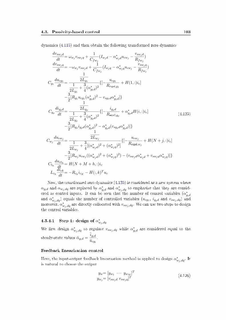
4.3. Passivity-based control 103
dynamics (4.115) and then obtain the following transformed zero dynamics
dvswjd
dt= ωwjvswjq +
1
Cfwj(Iwjd − α∗wjducwj −
vswjd
Rfwj)
dvswjq
dt= −ωwjvswjd +
1
Cfwj(Iwjq − α∗wjqucwj −
vswjq
Rfwj)
Cg1ducg1dt
=
1
2Lg11
2Lg1+
3
4(α∗g1d)
2
[− ucg1Requi,g1
+H(1, :)ic]
−3
2[Rg1ucg1(α∗g1d)
2 − vsg1dα∗g1d]
Cgρdigρd
dt=
1
2Lgρ1
2Lgρ+
3
4(α∗gρd)
2
[−igρd
Requi,gρ
+ α∗gρdH(i, :)ic]
−3
2[Rgρigρd(α
∗gρd
)2 − α∗gρd(vsgρdα∗gρd
)]
Cwjducwjdt
=
1
2Lwj1
2Lwj+
3
4[(α∗wjd)
2 + (α∗wjq)2][−
ucwjRequi,wj
+H(N + j, :)ic]
−3
2[Rwjucwj ((α
∗wjd
)2 + (α∗wjq)2)− (vswjdα
∗wjd
+ vswjqα∗wjq)]
Cthducthdt
= H(N +M + h, :)ic
Lckdickdt
= −RckicK −H(:, k)Tuc
(4.125)
Now, the transformed zero dynamics (4.125) is considered as a new system where
αgid and αwj ,dq are replaced by α∗gid and α∗wj ,dq
to emphasize that they are consid-
ered as control inputs. It can be seen that the number of control variables (α∗gidand α∗wj ,dq) equals the number of controlled variables (ucg1 , igρd and vswj ,dq) and
moreover, α∗wj ,dq are directly collocated with vswj ,dq. We can use two steps to design
the control variables.
4.3.4.1 Step 1: design of α∗wj ,dq
We rst design α∗wj ,dq to regulate vswj ,dq while α∗gid are considered equal to the
steady-state values αgid =igiducgi
.
Feedback linearization control
Here, the input-output feedback linearzation method is applied to design α∗wj ,dq. It
is natural to choose the output
yw= [yw1 · · · ywM ]T
ywj= [vswjd vswjq]T (4.126)

104Chapter 4. Control methods based on nonlinear control design tools
Then, following the input-output feedback linearization procedure, the control law
for α∗wj ,dq is deduced as
α∗wjd=1
ucwj[Iwjd −
vswjd
Rfwj+ Cfwjωwjvswjq − Cfwjvαwjd ]
α∗wjq=1
ucwj[Iwjq −
vswjq
Rfwj− Cfwjωwjvswjd − Cfwjvαwjq ]
(4.127)
whereeIαwjd= evswjd , vswjd − voswjdvαwjd= −cαwjd · evswjd − kIαwjd · eIαwjdeIαwjq= evswjq , vswjq − voswjqvαwjq= −cαwjq · evswjq − kIαwjq · eIαwjq
with positive control gains cαwj,dq and kIαwj,dq .
If the tracking errors eαwj,dq approach zero, we then take α∗wj ,dq = α∗wj ,dq where
α∗wjd=1
ucwj[Iwjd −
voswjd
Rfwj+ Cfwjωwjv
oswjq + kIαwjd eIαwjd ]
α∗wjq=1
ucwj[Iwjq −
voswjq
Rfwj− Cfwjωwjvoswjd + kIαwjq eIαwjq ]
(4.128)
which are calculated by restricting vswj ,dq = voswj ,dq and
0 = ωwjvoswjq +
1
Cfwj(Iwjd − α∗wjducwj −
voswjd
Rfwj)
0 = −ωwjvoswjd +1
Cfwj(Iwjq − α∗wjqucwj −
voswjq
Rfwj)
Recall that the steady-state values of α∗wj ,dq satisfy
αwjd =iwjd
ucwj=
1
ucwj[Iwjd −
vswjd
Rfwj+ Cfwjωwjv
oswjq + kIαwjd eIαwjd ]
αwjq =iwjq
ucwj=
1
ucwj[Iwjq −
vswjq
Rfwj− Cfwjωwjvoswjd + kIαwjq eIαwjq ]
and hence, α∗wj ,dq can be rewritten as
α∗wjd=1
ucwjiwjd
α∗wjq=1
ucwjiwjq
(4.129)
In addition, we can also obtain
∂α∗wjd
∂ucwj= − 1
(ucwj)2iwjd
∂α∗wjq
∂ucwj= − 1
(ucwj)2iwjq
(4.130)
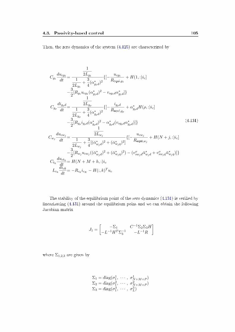
4.3. Passivity-based control 105
Then, the zero dynamics of the system (4.125) are characterized by
Cg1ducg1dt
=
1
2Lg11
2Lg1+
3
4(α∗g1d)
2
[− ucg1Requi,g1
+H(1, :)ic]
−3
2[Rg1ucg1(α∗g1d)
2 − vsg1dα∗g1d]
Cgρdigρd
dt=
1
2Lgρ1
2Lgρ+
3
4(α∗gρd)
2
[−igρd
Requi,gρ
+ α∗gρdH(ρ, :)ic]
−3
2[Rgρigρd(α
∗gρd
)2 − α∗gρd(vsgρdα∗gρd
)]
Cwjducwjdt
=
1
2Lwj1
2Lwj+
3
4[(α∗wjd)
2 + (α∗wjq)2][−
ucwjRequi,wj
+H(N + j, :)ic]
−3
2[Rwjucwj ((α
∗wjd
)2 + (α∗wjq)2)− (voswjdα
∗wjd
+ voswjqα∗wjq)]
Cthducthdt
= H(N +M + h, :)ic
Lckdickdt
= −RckicK −H(:, k)Tuc
(4.131)
The stability of the equilibrium point of the zero dynamics (4.131) is veried by
linearizating (4.131) around the equilibrium point and we can obtain the following
Jacobian matrix
J1 =
[−Σ1 C−1Σ2Σ3H
−L−1HTΣ−13 −L−1R
]
where Σ1,2,3 are given by
Σ1 = diag(σ11, · · · , σ1
N+M+P )
Σ2 = diag(σ21, · · · , σ2
N+M+P )
Σ3 = diag(σ31, · · · , σ3
L)
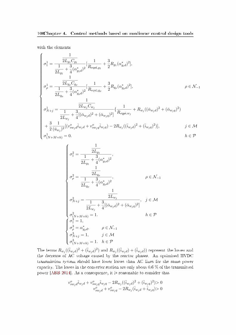
106Chapter 4. Control methods based on nonlinear control design tools
with the elements
σ11 =
1
2Lg1Cg11
2Lg1+
3
4(α∗g1d)
2
[1
Requi,g1
+3
2Rg1(α∗gid)
2],
σ1ρ =
1
2LgρCgρ1
2Lgρ+
3
4(α∗gρd)
2
[1
Requi,gρ
+3
2Rgρ(α
∗gρd)
2], ρ ∈ N−1
σ1N+j =
1
2LwjCwj1
2Lwj+
3
4[(αwjd)
2 + (αwjq)2] 1
Requi,wj
+Rwj ((αwjd)2 + (αwjq)
2)
+3
2
1
(uwj )2[(voswjdiwjd + voswjq iwjq)− 2Rwj ((iwjd)
2 + (iwjq)2)], j ∈M
σ1(N+M+h) = 0. h ∈ P
σ21 =
1
2Lg11
2Lg1+
3
4(α∗g1d)
2
,
σ2ρ =
1
2Lgρ1
2Lgρ+
3
4(α∗gρd)
2
, ρ ∈ N−1
σ2N+j =
1
2Lwj1
2Lwj+
3
4[(αwjd)
2 + (αwjq)2], j ∈M
σ2(N+M+h) = 1. h ∈ Pσ3
1 = 1,
σ3ρ = α∗gρd, ρ ∈ N−1
σ3N+j = 1, j ∈Mσ3
(N+M+h) = 1. h ∈ P
The terms Rwj ((iwjd)2 + (iwjd)
2) and Rwj ((iwjd) + (iwjd)) represent the losses and
the decrease of AC voltage caused by the reactor phases. An optimized HVDC
transmission system should have lower losses than AC lines for the same power
capacity. The losses in the converter station are only about 0.6 % of the transmitted
power [ABB 2014]. As a consequence, it is reasonable to consider that
voswjdiwjd + voswjq iwjq − 2Rwj ((iwjd)2 + (iwjq)
2)> 0
voswjd + voswjq − 2Rwj (iwjd + iwjq)> 0
4.3. Passivity-based control 107
Lemma 4.3.6. The system described by (4.125) with control variables α∗wj ,dq and
output yw in (4.126) is minimum phase .
Proof. To demonstrate this lemma, we only need to prove that the Jacobian matrix
J1 is Hurwitz. Similar to demonstrate Lemma 4.1.3, we also assume that there exists
an eigenvalue of J1 denoted by λ = α + β ∈ C whose real part is non-negative, i.e.
α ≥ 0. By denition of eigenvalues, we have
det(λI − J1) = det(
[λI + Σ1 −C−1Σ2Σ3H
L−1HTΣ−13 λI + L−1R
]) = 0 (4.132)
As described in the demonstration of Lemma 4.1.3 in Section 4.1.4.1, Φ1 , λI +
L−1R = Λ1 + jΛ2 are positive denite where Λ1,2 are given by
Λ1 = diag(α+Rc1Lc1
, · · · , α+RcLLcL
) ∈ RL×L
Λ2 = diag(β, · · · , β) ∈ RL×L
Therefore, det(λI − J1) is equivalent to
det(λI − J1)
=det(λI + Σ1 + C−1Σ2Σ3HΦ−11 L−1HTΣ−1
3 )det(Φ1)
=det(C−1Σ2Σ3Σ−13 )det(λΣ−1
3 Σ−12 CΣ3 + Σ−1
3 Σ−12 CΣ1Σ3 +HΦ−1
1 L−1HT )det(Φ1)
Since C and Σ1,2,3 are diagonal, the above expression can be rewritten as
det(λI − J1)
=det(C−1Σ2)det(λΣ−12 C + Σ−1
2 CΣ1 +HΦ−11 L−1HT )det(Φ1)
We introduce
Φ2 = λCΣ−12 + Σ1CΣ−1
2 +HΦ−11 L−1HT
λCΣ−12 + Σ1CΣ−1
2 = Λ3 + jΛ4
Φ−11 L−1 = (λI +R)−1 = Λ5 + jΛ6
Recalling the expressions of C, Σ1 and Σ2 (Σ1 and Σ2 are positive denite), it is
evident that Λ5 and Λ3 are semi-positive denite where Λ3 is given by
Λ3 = diag(σ1, · · · , σN+M+P )
and Λ5 is expressed in (4.68). Now, Φ2 can be rewritten as
Φ2= Φ3 + j(Λ4 + (Σ3H)Λ6(Σ3H)T )
Φ3= Λ13 + Λ1′
3 +HfHTf
(4.133)
108Chapter 4. Control methods based on nonlinear control design tools
where Λ13 is a diagonal matrix whose rst element on the main diagonal is σ1 > 0
and all other elements are zero. Λ1′3 and Hf are given by
Λ1′3 = Λ3 − Λ1
3
Hf = HΛ125
Let us dene
Φ4 = Λ13 +HfH
Tf
which is semi-positive denite. Then the determinant of Φ4 is calculated as
det(Φ4) = σ1det(R(Hf )1R(Hf )T1 ) + det(HfHTf )
Recall that R(Hf )1 is the matrix obtained by removing the rst row of Hf . Since
Λ125 is a full rank matrix, i.e. rank(Λ
125 ) = L, then rank(HfH
Tf ) = rank(Hf ) =
rank(H) = N +M + P − 1 and as a results, det(HfHTf ) = 0. According to Lemma
3.4.2, the rank of R(Hf )1 is N + M + P − 1. Consequently, R(Hf )1R(Hf )T1 is
invertible and positive denite. Because of the positive σ1, we then have
det(Φ4) = σ1det(R(Hf )1R(Hf )T1 ) + det(HfHTf )
= σ1det(R(Hf )1R(Hf )T1 ) > 0
and hence, the semi-denite matrix Φ4 must be positive denite. Recalling that
Φ3 = Φ4 + Λ1′3 as derived from (4.133), Φ3 is also positive denite (see Lemma
4.1.8). Since the hermitian part of Φ2, i.e. H(Φ2), is Φ3 which is positive denite,
we get the result that Φ2 is also positive denite (see Lemma 4.1.7). Therefore, we
deduce that
det(λI − J1)
=det(Φ2)det(Φ1)det(C−1Σ2) 6= 0
for α ≥ 0. This leads to a contradiction to (4.132). Thus, we must have that the
real part of all eigenvalues of J1 is negative, i.e. α < 0. Finally, we prove that J1 is
Hurwitz and as a result, the equilibrium point of the zero dynamics is asymptotically
stable. The proof is completed.
Adaptive control
Let us revisit the zero dynamics (4.125) which is a multiple-input and multiple-
output (MIMO) system with the control variables α∗wj ,dq. In the previous part,
by using the feedback linearization technique, α∗wj ,dq is designed as (4.127) which
strongly depend on the system parameters, Rfwj Cfwj , ωj and Iwj ,dq. However,
due to the ageing of the facilities, the system parameters are usually slowly varying.
4.3. Passivity-based control 109
In particular, Rfwj used to model the losses of the lter is very hard to obtain its
exact value. Several studies have been carried out to deal with the uncertainties
of the system parameters [Ruan 2007, Hernandez-Gomez 2010, Durrant 2004]. In
Section 4.2, the sliding mode control method is also applied to make the system more
robust. In this part, the adaptive control method is proposed to adjust the system
parameters for enhancing the dynamic performance of the system [Narendra 2012].
We recall the dynamics of vswj ,dq given by
dvswjd
dt= ωwjvswjq +
1
CfwjIwjd − α∗wjducwj
1
Cfwj−vswjd
Rfwj
1
Cfwjdvswjq
dt= −ωwjvswjd +
1
CfwjIwjq − α∗wjqucwj
1
Cfwj−vswjq
Rfwj
1
Cfwj
(4.134)
with the uncertain Cfwj , ωwj , Rfwj and Iwj ,dq. Our task here is to design α∗wj ,dqto make vswj ,dq track their respective references voswj ,dq. Then, the output tracking
errors are given by
evswjd= vswjd − voswjdevswjq= vswjq − voswjq
(4.135)
Augmenting (4.134) with the integrated output tracking errors
eIvswjd= evswjdeIvswjq= evswjq
(4.136)
results in the following extend open-loop system
eIvswjdvswjdeIvswjqvswjq
=
0 1 0 0
0 − 1
CfwjRfwj0 ωwj
0 0 0 1
0 −ωwj 0 − 1
CfwjRfwj
︸ ︷︷ ︸
APj
eIvswjdvswjdeIvswjqvswjq
+
0Iwjd
Cfwj0Iwjd
Cfwj
+
0 0
− 1
Cfwj0
0 0
0 − 1
Cfwj
︸ ︷︷ ︸
BPj
[ucwjα
∗wjd
ucwjα∗wjq
]+
−voswjd
0
−voswjq0
(4.137)

110Chapter 4. Control methods based on nonlinear control design tools
Let us consider the reference modeleIvswjd,mvswjd,meIvswjq,mvswjq,m
=
0 1 0 0
−kIαwjd −cαwjd 0 0
0 0 0 1
0 0 −kIαwjq −cαwjq
︸ ︷︷ ︸
Amj
eIvswjd,mvswjd,meIvswjq,mvswjq,m
+
0
cαwjdvoswd
0
cαwjqvoswq
+
−voswjd
0
−voswjq0
(4.138)
It is evident that Amj is Hurwitz. If all system parameters are known, αwj ,dq can
be developed as
α∗wjd=Cfwjucwj
[Iwjd
Cfwj−
vswjd
CfwjRfwj+ ωwjvswjq
+cαwjd · evswjd + kIαwjd · eIαwjd ]
α∗wjq=Cfwjucwj
[Iwjq
Cfwj−
vswjq
CfwjRfwj+cαwjd · evswjd + kIαwjd · eIαwjd ]
(4.139)
so that the closed-loop of the system (4.137) becomeseIvswjdvswjdeIvswjqvswjq
= Amj
eIvswjdvswjdeIvswjqvswjq
+
0
cαwjdvoswd
0
cαwjqvoswq
+
−voswjd
0
−voswjq0
(4.140)
which exhibits the same behavior as the reference model (4.138). However, in the
current study case, since the system parameters are unknown, the controller is
designed as
α∗wjd=1
ucwj[Iwjd −
vswjd
Rfwj+ Cfwj ωwjvswjq + Cfwj (cαwjd · evswjd + kIαwjd · eIαwjd)]
α∗wjq=1
ucwj[Iwjq −
vswjq
Rfwj− Cfwj ωwjvswjd + Cfwj (cαwjq · evswjq + kIαwjq · eIαwjq)]
(4.141)
which is based on the estimate of the parameter (·) denoted by (·). Due to the
nonlinear terms1
Rfwjand Cfwj ωwj , the parameter adjustment of the controller
(4.141) is a nonlinear parameterized adaptive control problem. For the sake of
simplicity, we perform the change of variables
ψ1j = Iwjd; ψ2j = Iwjq; ψ3j =1
Rfwj; ψ4j = Cfwjωwj ; (4.142)
4.3. Passivity-based control 111
and then, rewrite the controller (4.141) in these new variables as
α∗wjd=1
ucwj[ψ1j − ψ3jvswjd + ψ4jvswjq − Cfwjvαwjd ]
α∗wjq=1
ucwj[ψ2j − ψ3jvswjq − ψ4jvswjd − Cfwjvαwjq ]
(4.143)
Now, the parameter adjustment of the controller becomes a linear parameter adap-
tive control problem. Substituting (4.143) into the zero dynamics (4.125), we get
eIvswjdvswjdeIvswjqvswjq
=
1 0 0 0
0CfwjCfwj
0 0
0 0 1 0
0 0 0CfwjCfwj
Amj
eIvswjdvswjdeIvswjqvswjq
+
0
CfwjCfwj
cαwjdvoswd
0
CfwjCfwj
cαwjqvoswq
+
0 0 0 01
Cfwj0 − 1
Cfwjvswjd
1
Cfwjvswjq
0 0 0 0
01
Cfwj− 1
Cfwjvswjq −
1
Cfwjvswjd
ψ1j
ψ2j
ψ3j
ψ4j
+
−voswjd
0
−voswjq0
(4.144)
which can be rewritten as
eIvswjdevswjdeIvswjqevswjq
=
1 0 0 0
0CfwjCfwj
0 0
0 0 1 0
0 0 0CfwjCfwj
Amj
eIvswjdevswjdeIvswjqevswjq
+
0 0 0 01
Cfwj0 − 1
Cfwjvswjd
1
Cfwjvswjq
0 0 0 0
01
Cfwj− 1
Cfwjvswjq −
1
Cfwjvswjd
ψ1j
ψ2j
ψ3j
ψ4j
(4.145)
where ψ(·) = ψ(·) − ψ(·) denotes the error between the parameter's estimated value
and its actual value. Although the exact value of Cfwj is unknown, we can conrm
that Cfwj is positive. The classical adaptive law can be given by
Cfwj= sgn(Cfwj ) = 1˙ψ1j= −c1jevswjd˙ψ2j= −c2jevswjq˙ψ3j= c3j (evswjdvswjd + evswjqvswjq)˙ψ4j= c4j (evswjqvswjd − evswjdvswjq)
(4.146)
112Chapter 4. Control methods based on nonlinear control design tools
where the adaptive gains c1,2,3,4j are positive. We consider a quadratic positive
denite function as
V=1
2Cfwj (e
2vswjd
+ e2vswjd
) +1
2kIαwjde
2Ivswjd
+1
2kIαwjqe
2Ivswjq
+1
2c1j
ψ21j
+1
2c2j
ψ22j
+1
2c3j
ψ23j
+1
2c4j
ψ24j
(4.147)
whose derivative is deduced as
V =−cαwjde2vswjd
− cαwjqe2vswjq
≤ 0 (4.148)
Since V is non-positive, we have V (t) ≤ V (t = 0) and hence evswj,dq , eIvswj,dq
and ψ1,2,3,4j are bounded. Furthermore, V can be calculated, which contains only
bounded terms. Consequently, V is also bounded and then V is uniformly con-
tinuous. Based on Barbalat's lemma, we get V → 0 as t → ∞. It reveals that
evswj,dq → 0 as t → ∞. Finally, the adaptive controller is developed, which is
composed by (4.143) and (4.146).
4.3.4.2 Step 2: design of α∗gid
From the previous section, we get that, when vswj ,dq converge to voswjdq
, the system
behavior is governed by the zero dynamics (4.131) whose state variables, ucg1 , igρ ,
ucwj , ucth and ic, are uncontrolled. Again, we want to regulate these states via
α∗gid. In this part, the control algorithm for α∗gid is based on (4.131) where α∗gid are
considered as control variables and α∗wj ,dq are considered equal to their steady-state
values αwj ,dq =iwj ,dq
ucwj.
We rst consider using the following simple proportional controllers for α∗gid
α∗g1d= −kPucg1 ucg1 + αg1dα∗gρd= −kPigρd igρd + αgρd
(4.149)
with positive control gains kPucg1 and kPigρd . From (4.149), it can be seen that
when ucg1 and igρd converge to zero, α∗gid also converge to their steady-state values.
4.3. Passivity-based control 113
Substituting (4.149) into (4.131) results in the following closed-loop system
Cg1ducg1dt
=
1
2Lg11
2Lg1+
3
4(−kPucg1 ucg1 + αg1d)
2
[− ucg1Requi,g1
+H(1, :)ic]
−3
2[Rg1ucg1(−kPucg1 ucg1 + αg1d)
2 − vsg1d(−kPucg1 ucg1 + αg1d)]
Cgρdigρd
dt=
1
2Lgρ1
2Lgρ+
3
4(−kPigρd igρd + αgρd)
2
[−igρd
Requi,gρ
+(−kPigρd igρd + αgρd)H(ρ, :)ic]
+3
2[(vsρd −Rgρigρd)(−kPigρd igρd + αgρd)
2]
Cwjducwjdt
=
1
2Lwj1
2Lwj+
3
4[(α∗wjd)
2 + (α∗wjq)2][−
ucwjRequi,wj
+H(N + j, :)ic]
−3
2[Rwjucwj ((α
∗wjd
)2 + (α∗wjq)2)− (voswjdα
∗wjd
+ voswjqα∗wjq)]
Cthducthdt
= H(N +M + h, :)ic
Lckdickdt
= −RckicK −H(:, k)Tuc
(4.150)
To check the stability of the above closed-loop system, we linearize the system
(4.150) around the equilibrium point and then get the following Jacobian matrix
J2 =
[−Θ1 C−1Θ2Θ3H
−L−1HTΘ−13 Θ4 −L−1R
]
where Θ1,2,3,4 are given by
Θ1 = diag(θ11, · · · , θ1
N+M+P )
Θ2 = diag(σ21, · · · , σ2
N+M+P )
Θ3 = diag(σ31, · · · , σ3
L)
Θ4 = diag(σ41, · · · , σ4
L)
(4.151)
Keeping in mind that the steady-state value of igρd equals its prescribed setpoint
iogρd and the relation between αgid, ucgi and igid satisfy αgid =igiducgi
, then we can
114Chapter 4. Control methods based on nonlinear control design tools
deduced the elements of Θ1,2,3,4 as
θ11 =
1
2Lg1Cg11
2Lg1+
3
4(αg1d)
2
[1
Requi,g1
+3
2Rg1(αg1d)
2 +3
2(vsg1d − 2Rg1 ig1d)kPucg1 ],
θ1ρ =
1
2LgρCgρ1
2Lgρ+
3
4(αgρd)
2
[1
Requi,gρ
+3
2Rgρ(αgρd)
2
+ kPigρd [3
2· 2(vsgρd −Rgρ igρd)αgρd +H(ρ, :)ic], ρ ∈ N−1
θ1N+j =
1
2LwjCwj1
2Lwj+
3
4[(αwjd)
2 + (αwjq)2] 1
Requi,wj
+3
2Rwj ((α
∗wjd
)2 + (α∗wjq)2), j ∈M
θ1(N+M+h) = 0. h ∈ P
θ21 =
1
2Lg11
2Lg1+
3
4(αg1d)
2
,
θ2ρ =
1
2Lgρ1
2Lgρ+
3
4(αgρd)
2
, ρ ∈ N−1
θ2N+j =
1
2Lwj1
2Lwj+
3
4[(α∗wjd)
2 + (α∗wjq)2], j ∈M
θ2(N+M+h) = 1. h ∈ Pθ3
1 = 1,
θ3ρ = αgρd, ρ ∈ N−1
θ3N+j = 1, j ∈Mθ3
(N+M+h) = 1. h ∈ Pθ4
1 = 1,
θ4ρ = 1 + kPigρd ucgρ , ρ ∈ N−1
θ4N+j = 1, j ∈Mθ4
(N+M+h) = 1. h ∈ P(4.152)
When the system is in steady state, we have
−igρd
Requi,gρ
+ αgρdH(ρ, :)ic −3
2[Rgρigρd(αgρd)
2 − αgρd(vsgρdαgρd)] = 0
4.3. Passivity-based control 115
which leads to
H(ρ, :)ic =ucgρ
Requi,gρ
+3
2(Rgρigρd − vsgρd)αgρd (4.153)
Substituting (4.153) into θ1ρ in (4.152) yields
θ1ρ=
1
2LgρCgρ1
2Lgρ+
3
4(αgρd)
2
1
Requi,gρ
+3
2Rgρ(αgρd)
2
+kPigρd [3
2(vsgρd −Rgρ igρd)αgρd +
ucgρRequi,gρ
]
(4.154)
To ensure the stability of the closed-loop system (4.150), the control gains must
render the Jacobian matrix J2 Hurwitz.
Lemma 4.3.7. By choosing kPigρd such that
1 + kPigρd ucgρ> 01
Requi,gρ
+3
2Rgρ(αgρd)
2 + kPigρd [3
2(vsgρd −Rgρ igρd)αgρd +
ucgρRequi,gρ
]> 0(4.155)
J2 is Hurwitz.
Proof. When kPigρd satises (4.155), then Θ4 becomes positive dene. By the def-
inition of Θ1,2 (see (4.151)), both of them are diagonal and positive denite. By
following the similar procedure used in the proof of Lemma 4.3.6, we can prove that
J2 is Hurwitz.
The above description clearly shows that the simple proportional controller
(4.149) can stabilize the zero dynamics (4.131). To get good tracking performance,
we use the PI controllers to replace the proportional controllers as
eIucg1= ucg1α∗g1d= −kPucg1 ucg1 − kIucg1eIucg1eIigρd= igρdα∗gρd= −kPigρd igρd − kIigρdeIigρd
(4.156)
with the integrated errors and positive control gains kI(·).
Of course, there are dierent approaches to choosing the PI control gains. As
presented in [Lee 2003], the absolute tracking results for Lur'e plants is applied
to get a criterion for tuning the control gain. It can also be used to deduce the
constraints for kP (·) and kI(·) via linearization. In this thesis, we are not tangled
on this issue. Finally, the overall control structure are built, which is composed of
(4.122), (4.156) and the adaptive law (4.146).
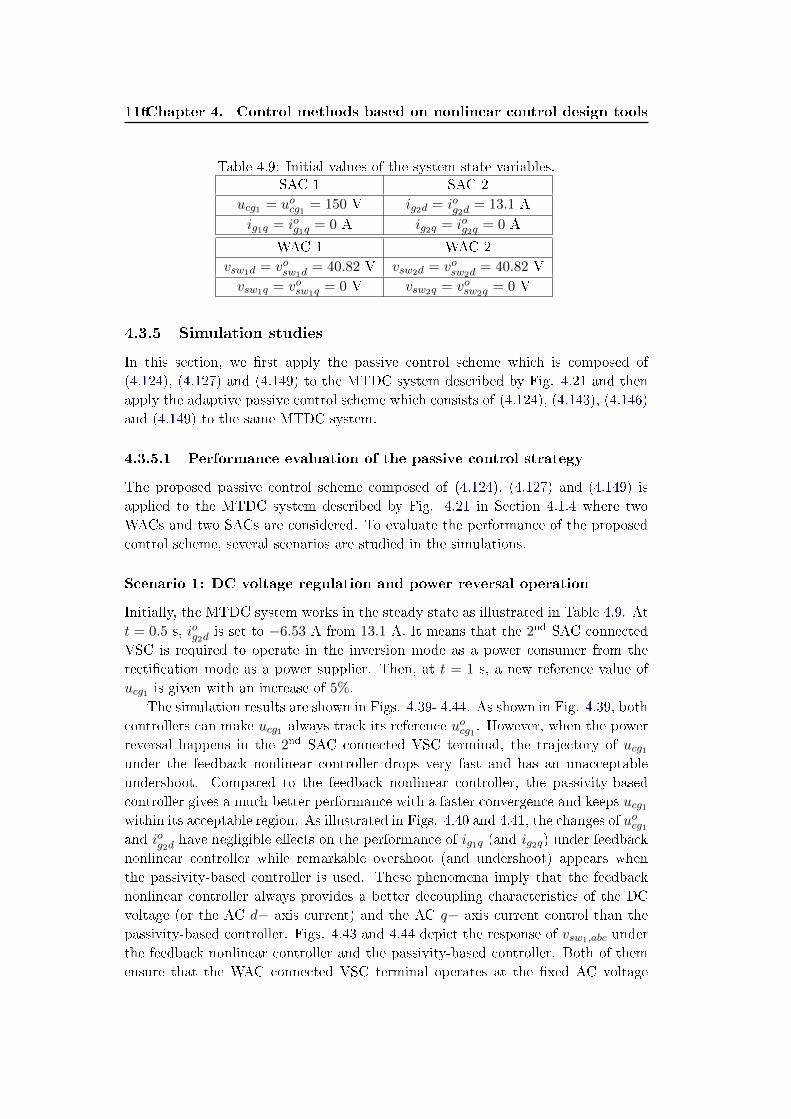
116Chapter 4. Control methods based on nonlinear control design tools
Table 4.9: Initial values of the system state variables.SAC 1 SAC 2
ucg1 = uocg1 = 150 V ig2d = iog2d = 13.1 A
ig1q = iog1q = 0 A ig2q = iog2q = 0 A
WAC 1 WAC 2
vsw1d = vosw1d= 40.82 V vsw2d = vosw2d
= 40.82 V
vsw1q = vosw1q = 0 V vsw2q = vosw2q = 0 V
4.3.5 Simulation studies
In this section, we rst apply the passive control scheme which is composed of
(4.124), (4.127) and (4.149) to the MTDC system described by Fig. 4.21 and then
apply the adaptive passive control scheme which consists of (4.124), (4.143), (4.146)
and (4.149) to the same MTDC system.
4.3.5.1 Performance evaluation of the passive control strategy
The proposed passive control scheme composed of (4.124), (4.127) and (4.149) is
applied to the MTDC system described by Fig. 4.21 in Section 4.1.4 where two
WACs and two SACs are considered. To evaluate the performance of the proposed
control scheme, several scenarios are studied in the simulations.
Scenario 1: DC voltage regulation and power reversal operation
Initially, the MTDC system works in the steady state as illustrated in Table 4.9. At
t = 0.5 s, iog2d is set to −6.53 A from 13.1 A. It means that the 2nd SAC connected
VSC is required to operate in the inversion mode as a power consumer from the
rectication mode as a power supplier. Then, at t = 1 s, a new reference value of
ucg1 is given with an increase of 5%.
The simulation results are shown in Figs. 4.39- 4.44. As shown in Fig. 4.39, both
controllers can make ucg1 always track its reference uocg1 . However, when the power
reversal happens in the 2nd SAC connected VSC terminal, the trajectory of ucg1under the feedback nonlinear controller drops very fast and has an unacceptable
undershoot. Compared to the feedback nonlinear controller, the passivity-based
controller gives a much better performance with a faster convergence and keeps ucg1within its acceptable region. As illustrated in Figs. 4.40 and 4.41, the changes of uocg1and iog2d have negligible eects on the performance of ig1q (and ig2q) under feedback
nonlinear controller while remarkable overshoot (and undershoot) appears when
the passivity-based controller is used. These phenomena imply that the feedback
nonlinear controller always provides a better decoupling characteristics of the DC
voltage (or the AC d− axis current) and the AC q− axis current control than the
passivity-based controller. Figs. 4.43 and 4.44 depict the response of vsw1,abc under
the feedback nonlinear controller and the passivity-based controller. Both of them
ensure that the WAC connected VSC terminal operates at the xed AC voltage
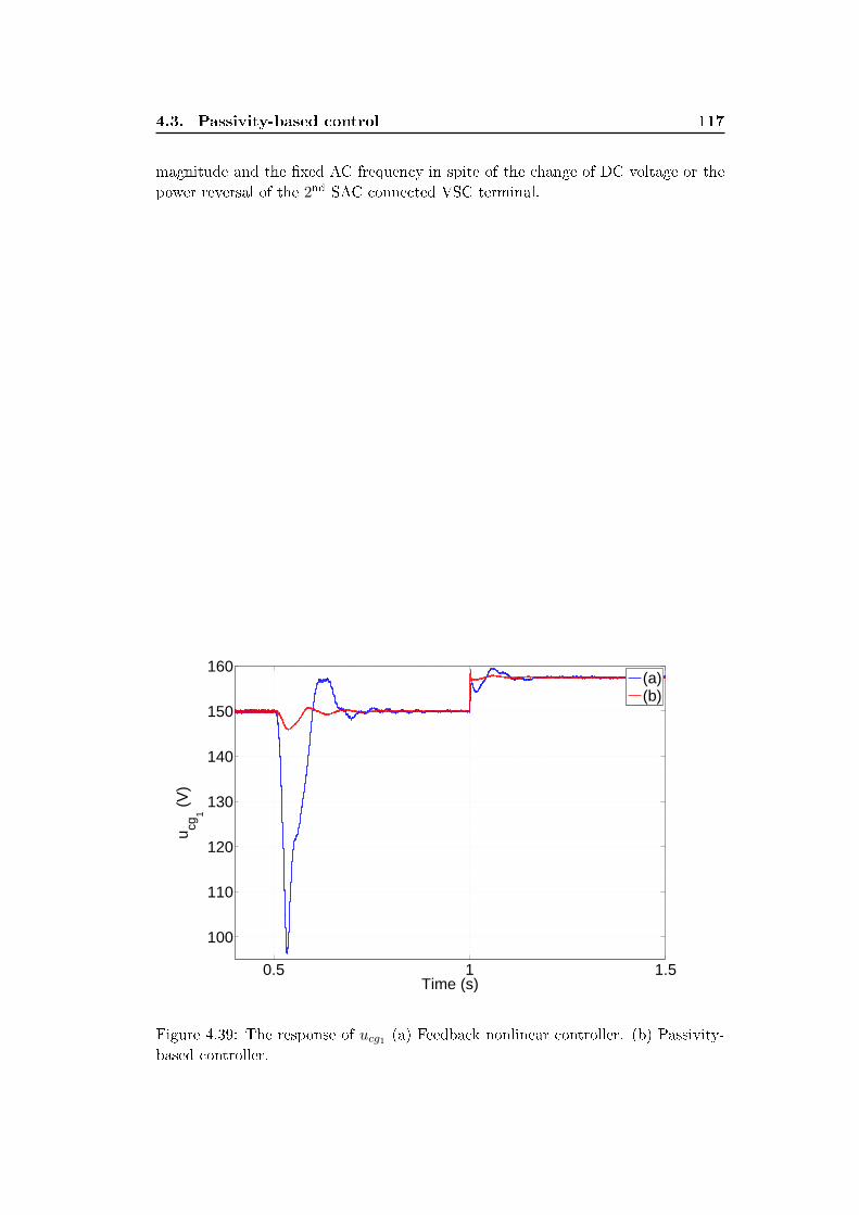
4.3. Passivity-based control 117
magnitude and the xed AC frequency in spite of the change of DC voltage or the
power reversal of the 2nd SAC connected VSC terminal.
0.5 1 1.5
100
110
120
130
140
150
160
Time (s)
u cg1 (
V)
(a)(b)
Figure 4.39: The response of ucg1 (a) Feedback nonlinear controller. (b) Passivity-
based controller.
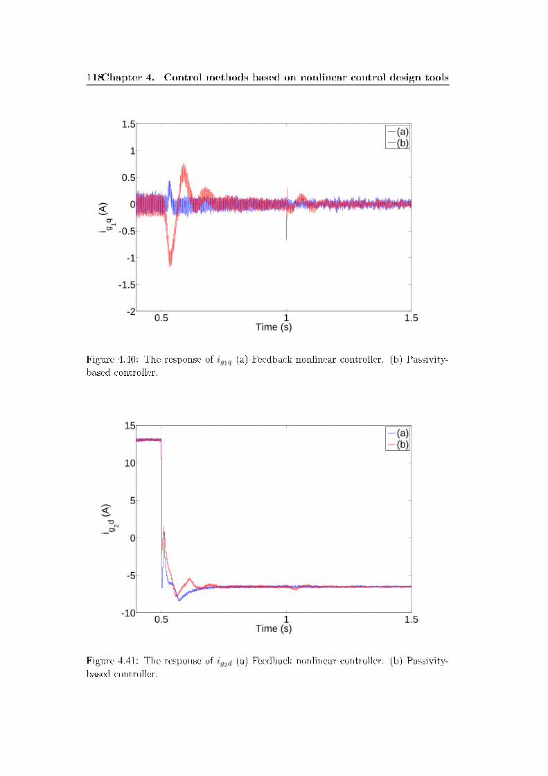
118Chapter 4. Control methods based on nonlinear control design tools
0.5 1 1.5-2
-1.5
-1
-0.5
0
0.5
1
1.5
Time (s)
i g 1q (A
)
(a)(b)
Figure 4.40: The response of ig1q (a) Feedback nonlinear controller. (b) Passivity-
based controller.
0.5 1 1.5-10
-5
0
5
10
15
Time (s)
i g 2d (A
)
(a)(b)
Figure 4.41: The response of ig2d (a) Feedback nonlinear controller. (b) Passivity-
based controller.
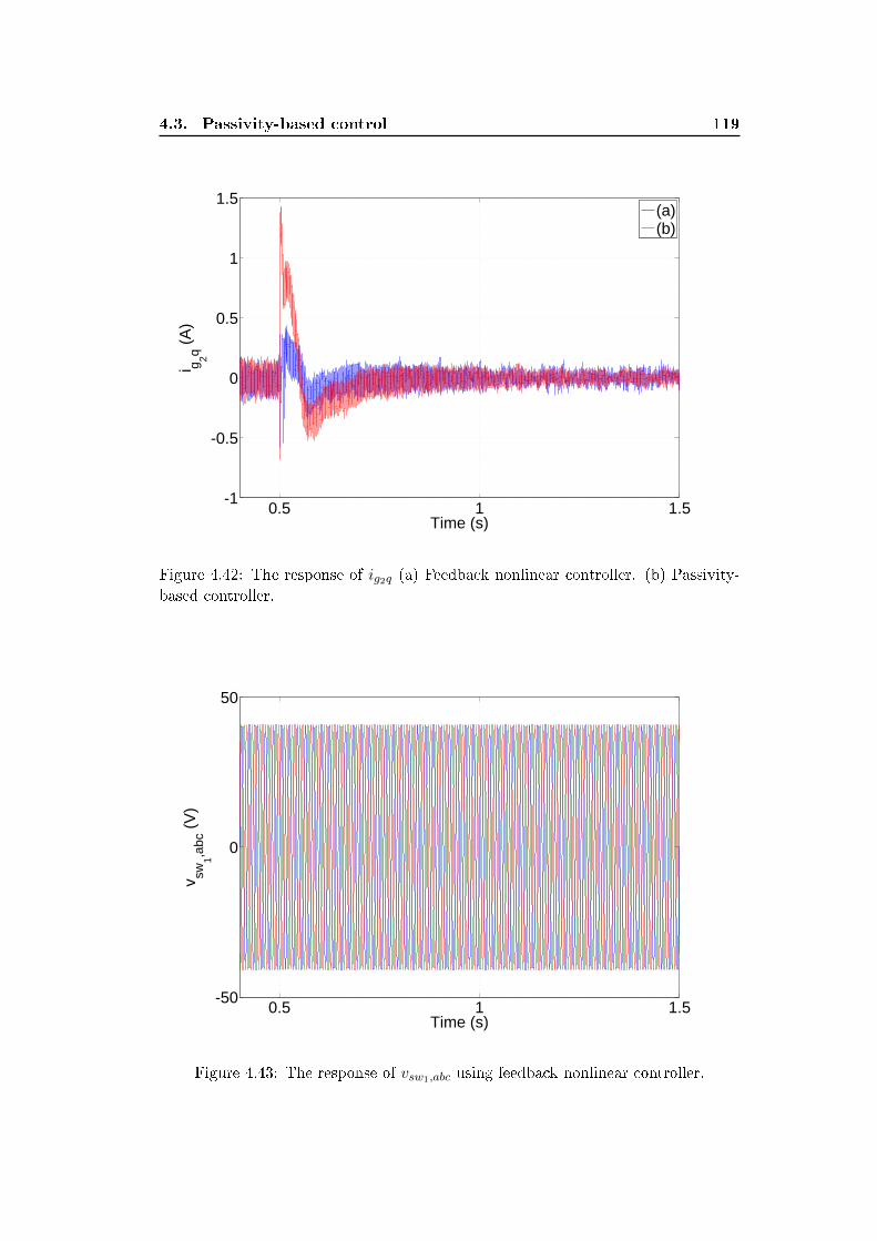
4.3. Passivity-based control 119
0.5 1 1.5-1
-0.5
0
0.5
1
1.5
Time (s)
i g 2q (A
)
(a)(b)
Figure 4.42: The response of ig2q (a) Feedback nonlinear controller. (b) Passivity-
based controller.
0.5 1 1.5-50
0
50
Time (s)
v sw1,a
bc (
V)
Figure 4.43: The response of vsw1,abc using feedback nonlinear controller.
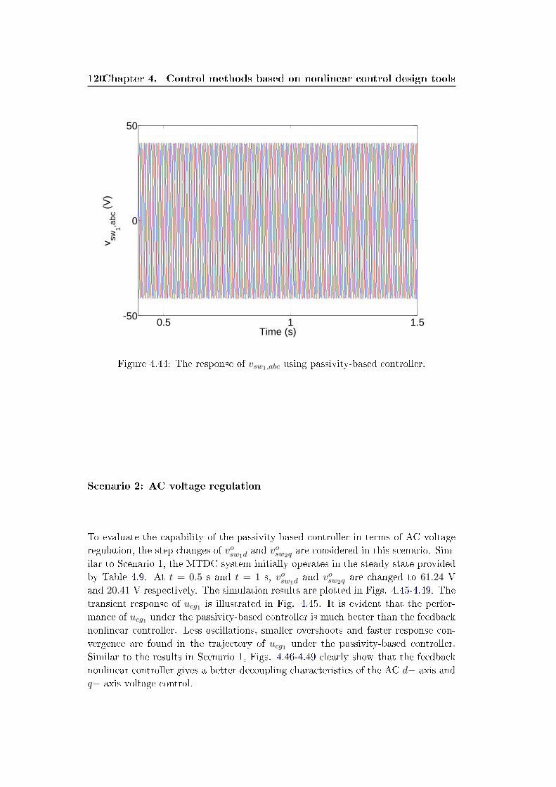
120Chapter 4. Control methods based on nonlinear control design tools
0.5 1 1.5-50
0
50
Time (s)
v sw1,a
bc (
V)
Figure 4.44: The response of vsw1,abc using passivity-based controller.
Scenario 2: AC voltage regulation
To evaluate the capability of the passivity-based controller in terms of AC voltage
regulation, the step changes of vosw1dand vosw2q are considered in this scenario. Sim-
ilar to Scenario 1, the MTDC system initially operates in the steady state provided
by Table 4.9. At t = 0.5 s and t = 1 s, vosw1dand vosw2q are changed to 61.24 V
and 20.41 V respectively. The simulation results are plotted in Figs. 4.45-4.49. The
transient response of ucg1 is illustrated in Fig. 4.45. It is evident that the perfor-
mance of ucg1 under the passivity-based controller is much better than the feedback
nonlinear controller. Less oscillations, smaller overshoots and faster response con-
vergence are found in the trajectory of ucg1 under the passivity-based controller.
Similar to the results in Scenario 1, Figs. 4.46-4.49 clearly show that the feedback
nonlinear controller gives a better decoupling characteristics of the AC d− axis and
q− axis voltage control.
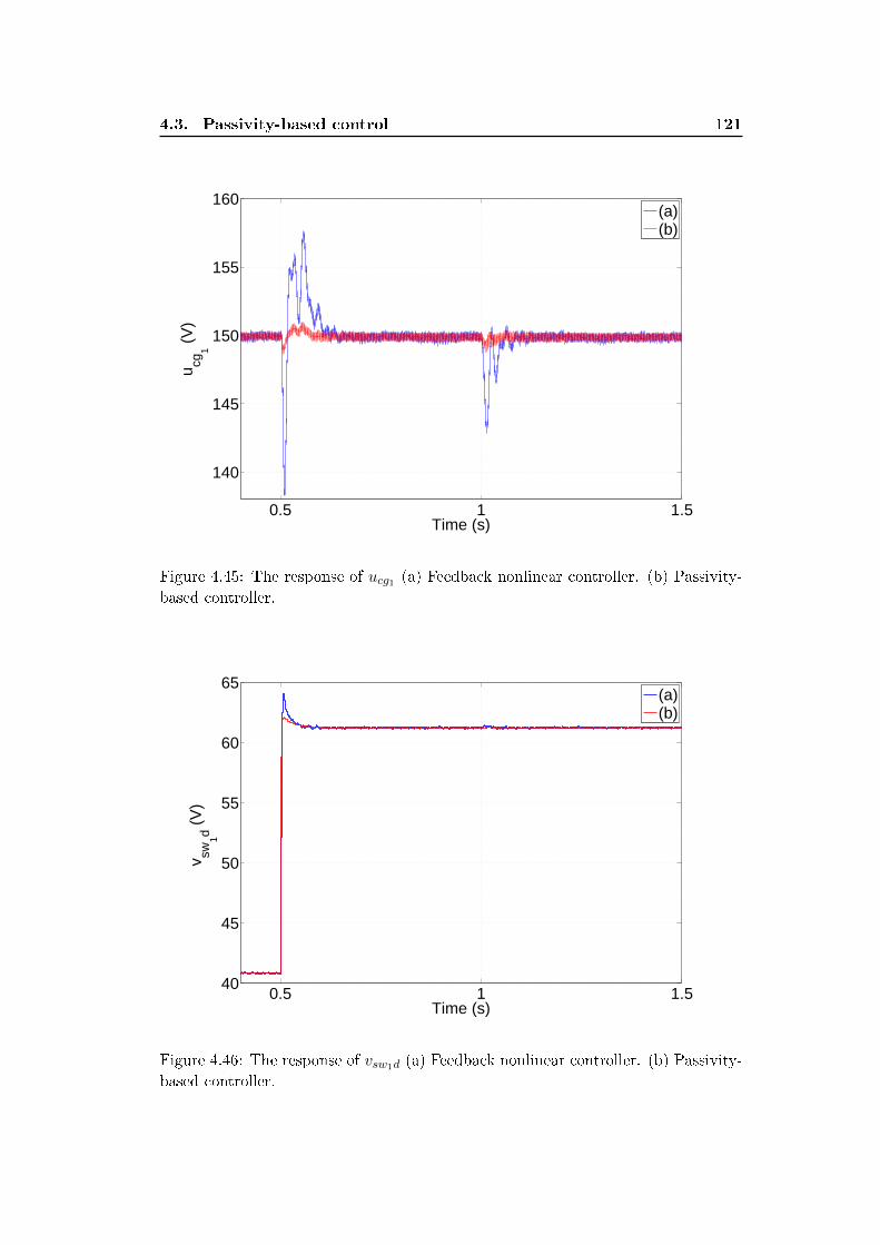
4.3. Passivity-based control 121
0.5 1 1.5
140
145
150
155
160
Time (s)
u cg1 (
V)
(a)(b)
Figure 4.45: The response of ucg1 (a) Feedback nonlinear controller. (b) Passivity-
based controller.
0.5 1 1.540
45
50
55
60
65
Time (s)
v sw1d (
V)
(a)(b)
Figure 4.46: The response of vsw1d (a) Feedback nonlinear controller. (b) Passivity-
based controller.
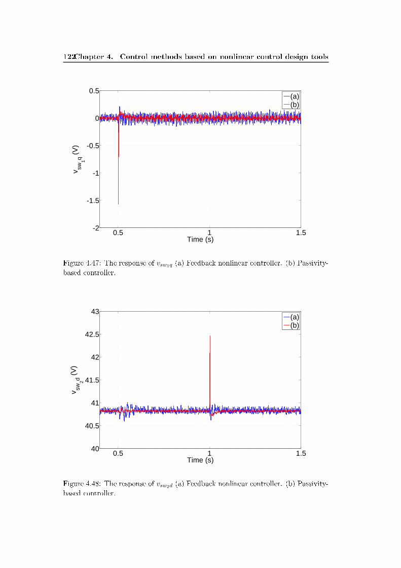
122Chapter 4. Control methods based on nonlinear control design tools
0.5 1 1.5-2
-1.5
-1
-0.5
0
0.5
Time (s)
v sw1q (
V)
(a)(b)
Figure 4.47: The response of vsw1q (a) Feedback nonlinear controller. (b) Passivity-
based controller.
0.5 1 1.540
40.5
41
41.5
42
42.5
43
Time (s)
v sw2d (
V)
(a)(b)
Figure 4.48: The response of vsw2d (a) Feedback nonlinear controller. (b) Passivity-
based controller.
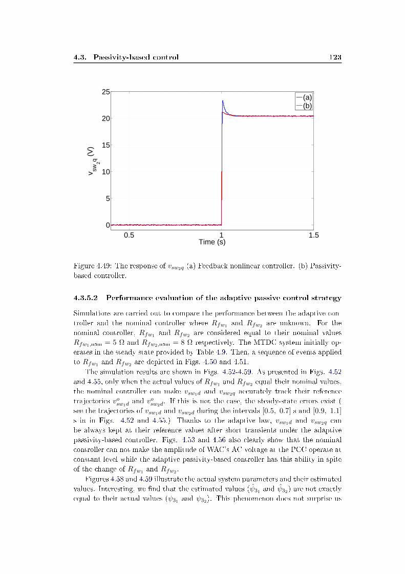
4.3. Passivity-based control 123
0.5 1 1.50
5
10
15
20
25
Time (s)
v sw2q (
V)
(a)(b)
Figure 4.49: The response of vsw2q (a) Feedback nonlinear controller. (b) Passivity-
based controller.
4.3.5.2 Performance evaluation of the adaptive passive control strategy
Simulations are carried out to compare the performance between the adaptive con-
troller and the nominal controller where Rfw1 and Rfw2 are unknown. For the
nominal controller, Rfw1 and Rfw2 are considered equal to their nominal values
Rfw1,nom = 5 Ω and Rfw2,nom = 8 Ω respectively. The MTDC system initially op-
erates in the steady state provided by Table 4.9. Then, a sequence of events applied
to Rfw1 and Rfw2 are depicted in Figs. 4.50 and 4.51.
The simulation results are shown in Figs. 4.52-4.59. As presented in Figs. 4.52
and 4.55, only when the actual values of Rfw1 and Rfw2 equal their nominal values,
the nominal controller can make vsw1d and vsw2q accurately track their reference
trajectories vosw1dand vosw2d
. If this is not the case, the steady-state errors exist (
see the trajectories of vsw1d and vsw2d during the intervals [0.5, 0.7] s and [0.9, 1.1]
s in in Figs. 4.52 and 4.55.) Thanks to the adaptive law, vsw1d and vsw2q can
be always kept at their reference values after short transients under the adaptive
passivity-based controller. Figs. 4.53 and 4.56 also clearly show that the nominal
controller can not make the amplitude of WAC's AC voltage at the PCC operate at
constant level while the adaptive passivity-based controller has this ability in spite
of the change of Rfw1 and Rfw2 .
Figures 4.58 and 4.59 illustrate the actual system parameters and their estimated
values. Interesting, we nd that the estimated values (ψ31 and ψ32) are not exactly
equal to their actual values (ψ31 and ψ32). This phenomenon does not surprise us
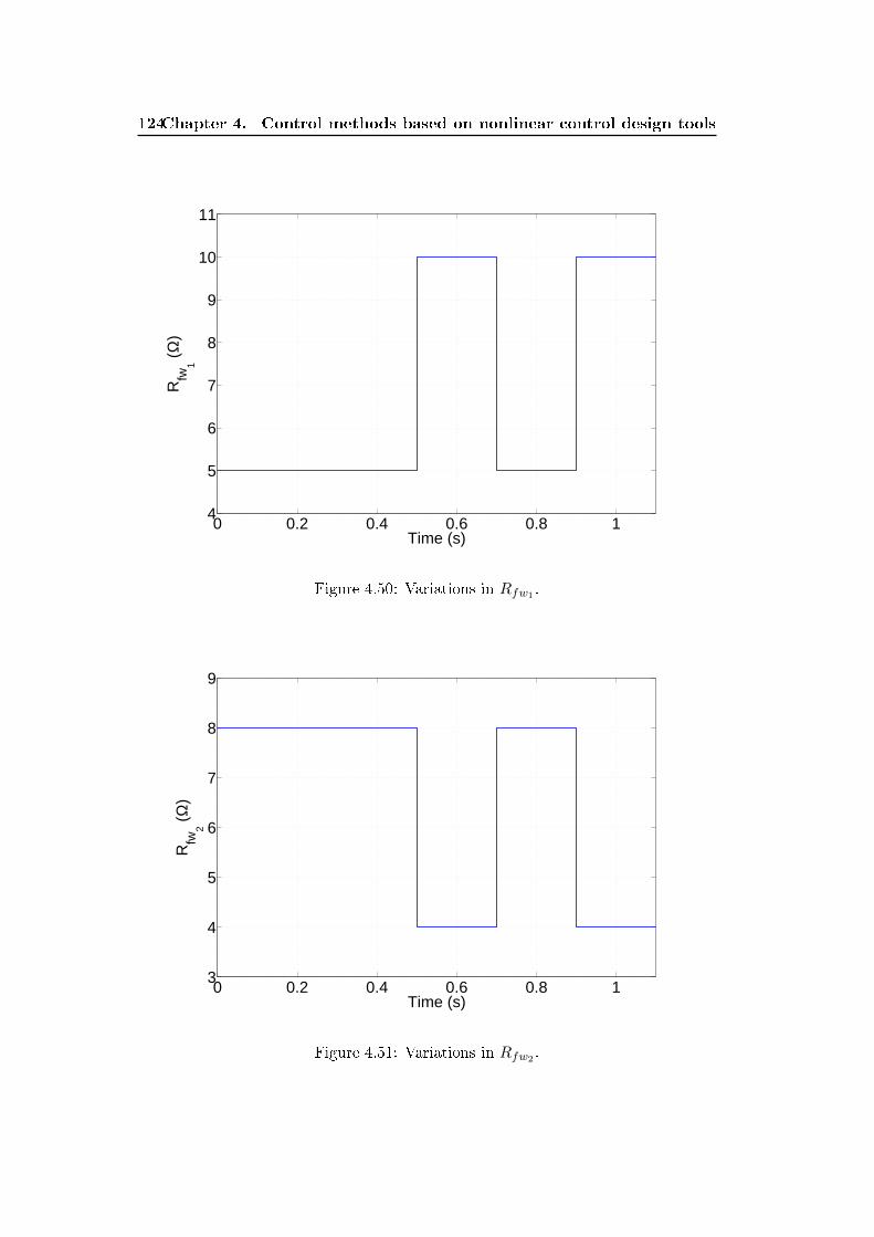
124Chapter 4. Control methods based on nonlinear control design tools
0 0.2 0.4 0.6 0.8 14
5
6
7
8
9
10
11
Time (s)
Rfw
1 (Ω
)
Figure 4.50: Variations in Rfw1 .
0 0.2 0.4 0.6 0.8 13
4
5
6
7
8
9
Time (s)
Rfw
2 (Ω
)
Figure 4.51: Variations in Rfw2 .
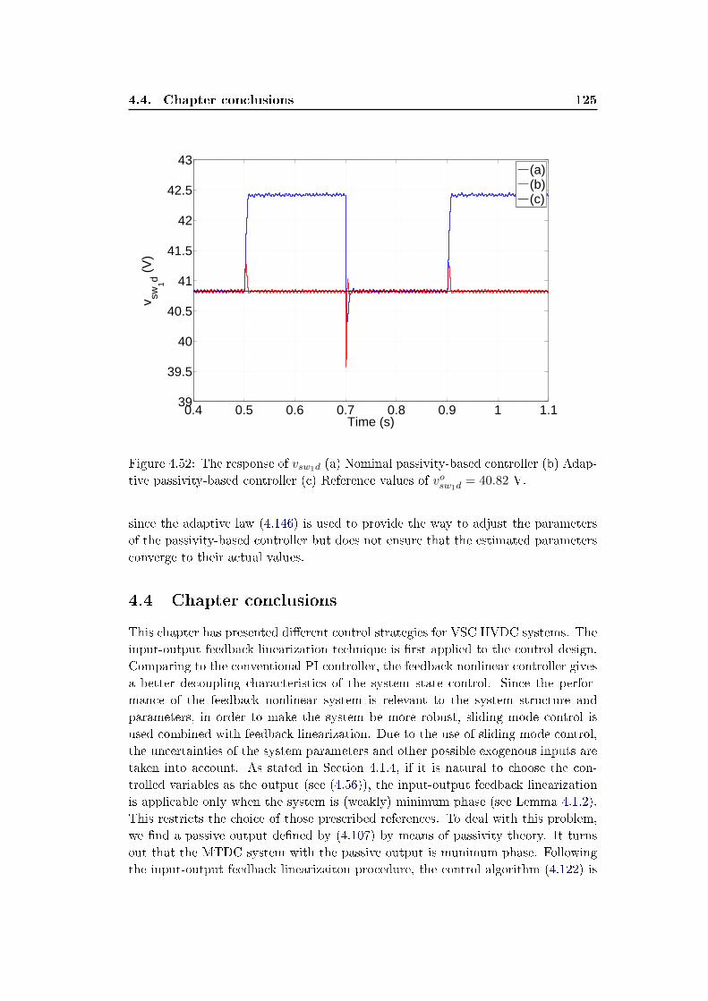
4.4. Chapter conclusions 125
0.4 0.5 0.6 0.7 0.8 0.9 1 1.139
39.5
40
40.5
41
41.5
42
42.5
43
Time (s)
v sw1d (
V)
(a)(b)(c)
Figure 4.52: The response of vsw1d (a) Nominal passivity-based controller (b) Adap-
tive passivity-based controller (c) Reference values of vosw1d= 40.82 V.
since the adaptive law (4.146) is used to provide the way to adjust the parameters
of the passivity-based controller but does not ensure that the estimated parameters
converge to their actual values.
4.4 Chapter conclusions
This chapter has presented dierent control strategies for VSC HVDC systems. The
input-output feedback linearization technique is rst applied to the control design.
Comparing to the conventional PI controller, the feedback nonlinear controller gives
a better decoupling characteristics of the system state control. Since the perfor-
mance of the feedback nonlinear system is relevant to the system structure and
parameters, in order to make the system be more robust, sliding mode control is
used combined with feedback linearization. Due to the use of sliding mode control,
the uncertainties of the system parameters and other possible exogenous inputs are
taken into account. As stated in Section 4.1.4, if it is natural to choose the con-
trolled variables as the output (see (4.56)), the input-output feedback linearization
is applicable only when the system is (weakly) minimum phase (see Lemma 4.1.2).
This restricts the choice of those prescribed references. To deal with this problem,
we nd a passive output dened by (4.107) by means of passivity theory. It turns
out that the MTDC system with the passive output is munimum phase. Following
the input-output feedback linearizaiton procedure, the control algorithm (4.122) is
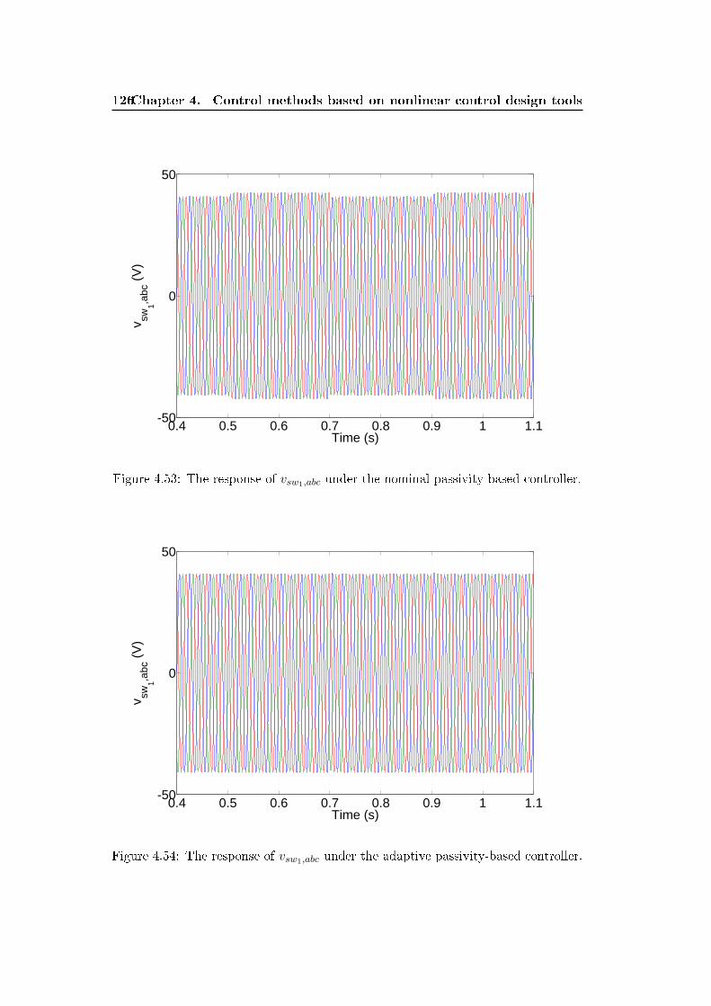
126Chapter 4. Control methods based on nonlinear control design tools
0.4 0.5 0.6 0.7 0.8 0.9 1 1.1-50
0
50
Time (s)
v sw1,a
bc (
V)
Figure 4.53: The response of vsw1,abc under the nominal passivity-based controller.
0.4 0.5 0.6 0.7 0.8 0.9 1 1.1-50
0
50
Time (s)
v sw1,a
bc (
V)
Figure 4.54: The response of vsw1,abc under the adaptive passivity-based controller.
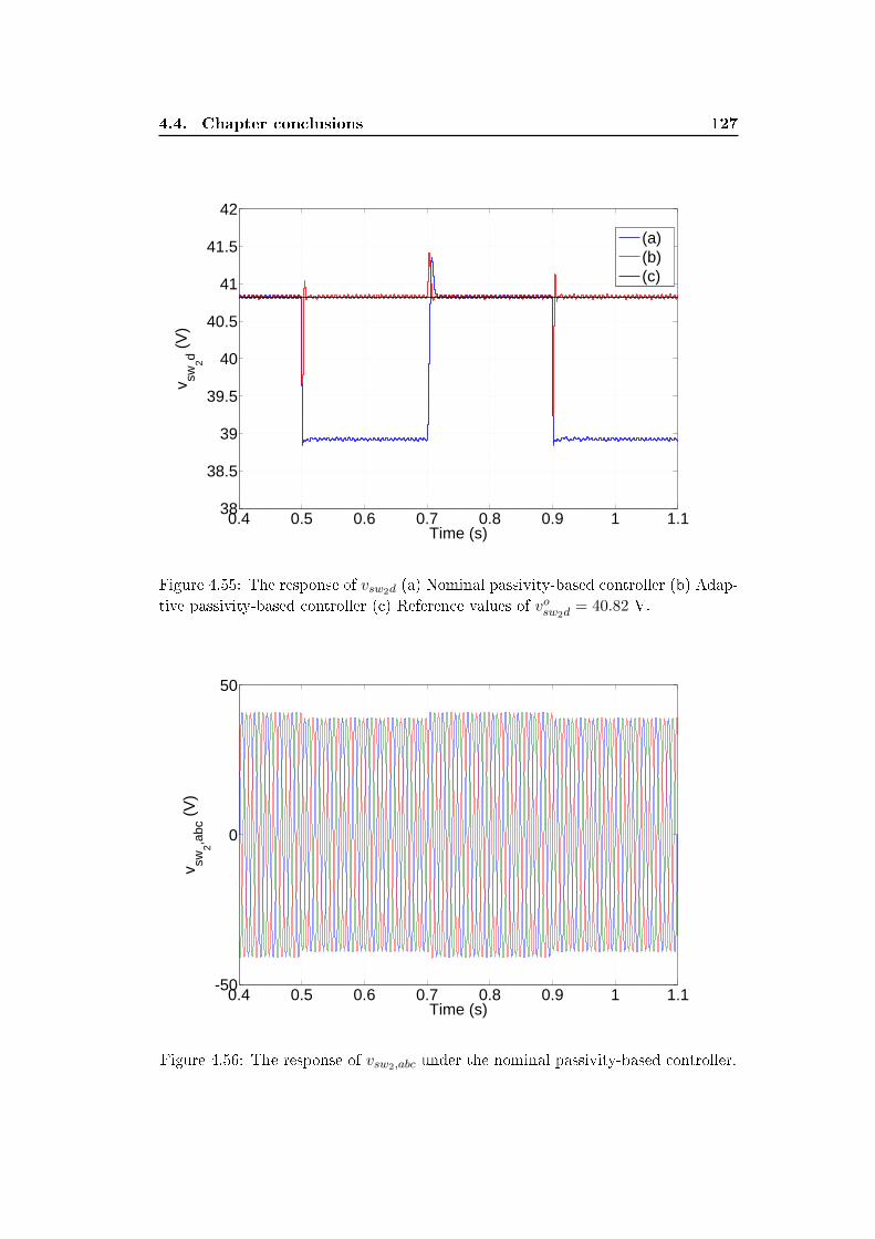
4.4. Chapter conclusions 127
0.4 0.5 0.6 0.7 0.8 0.9 1 1.138
38.5
39
39.5
40
40.5
41
41.5
42
Time (s)
v sw2d (
V)
(a)(b)(c)
Figure 4.55: The response of vsw2d (a) Nominal passivity-based controller (b) Adap-
tive passivity-based controller (c) Reference values of vosw2d= 40.82 V.
0.4 0.5 0.6 0.7 0.8 0.9 1 1.1-50
0
50
Time (s)
v sw2,a
bc (
V)
Figure 4.56: The response of vsw2,abc under the nominal passivity-based controller.
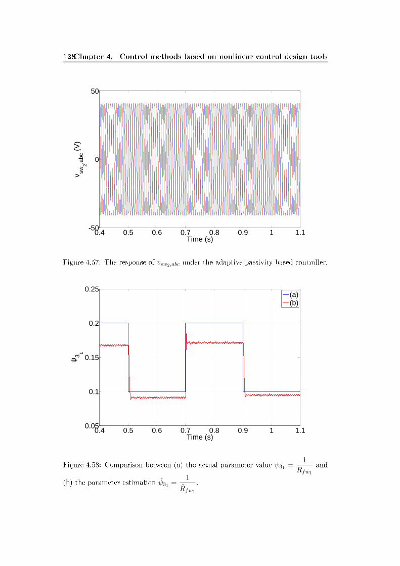
128Chapter 4. Control methods based on nonlinear control design tools
0.4 0.5 0.6 0.7 0.8 0.9 1 1.1-50
0
50
Time (s)
v sw2,a
bc (
V)
Figure 4.57: The response of vsw2,abc under the adaptive passivity-based controller.
0.4 0.5 0.6 0.7 0.8 0.9 1 1.10.05
0.1
0.15
0.2
0.25
Time (s)
ψ3 1
(a)(b)
Figure 4.58: Comparison between (a) the actual parameter value ψ31 =1
Rfw1
and
(b) the parameter estimation ψ31 =1
Rfw1
.
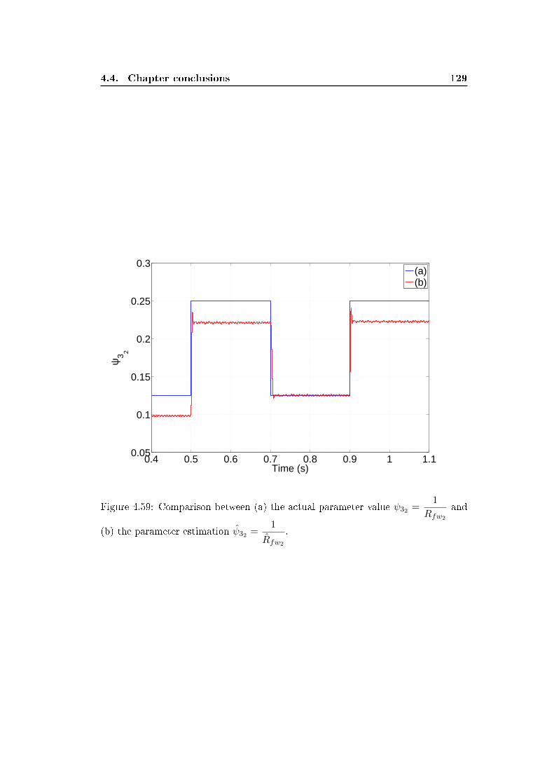
4.4. Chapter conclusions 129
0.4 0.5 0.6 0.7 0.8 0.9 1 1.10.05
0.1
0.15
0.2
0.25
0.3
Time (s)
ψ3 2
(a)(b)
Figure 4.59: Comparison between (a) the actual parameter value ψ32 =1
Rfw2
and
(b) the parameter estimation ψ32 =1
Rfw2
.

130Chapter 4. Control methods based on nonlinear control design tools
developed. When the output perfectly approaches to zero, the dynamics of ucg1 , igρd
and vswj ,dq are eventually governed by the zero dynamics (4.115). Regulatingigi,dqucgi
andigj ,dq
ucwjto the desired
igi,dqucgi
andigj ,dq
ucwj, obtained from the steady-state condition
(4.96), indirectly drives ucg1 , igρd and vswj ,dq to the prescribed values. However,
due to the uncertainties of the system, it is usually dicult to get the accurate
values ofigi,dqucgi
andigj ,dq
ucwj. Moreover, the convergence rate of the uncontrolled states
of the zero dynamics totally depends on the system parameters. Thus, to get a
better tracking performance and improve the dynamics of those uncontrolled state
variables, the control law (4.156) for α∗gi,dq and αwj ,dq is derived based on the zero
dynamics.
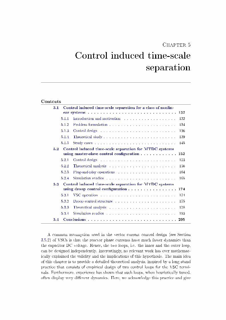
Chapter 5
Control induced time-scale
separation
Contents
5.1 Control induced time-scale separation for a class of nonlin-
ear systems . . . . . . . . . . . . . . . . . . . . . . . . . . . . . 132
5.1.1 Introduction and motivation . . . . . . . . . . . . . . . . . . 132
5.1.2 Problem formulation . . . . . . . . . . . . . . . . . . . . . . . 134
5.1.3 Control design . . . . . . . . . . . . . . . . . . . . . . . . . . 136
5.1.4 Theoretical study . . . . . . . . . . . . . . . . . . . . . . . . . 139
5.1.5 Study cases . . . . . . . . . . . . . . . . . . . . . . . . . . . . 145
5.2 Control induced time-scale separation for MTDC systems
using master-slave control conguration . . . . . . . . . . . . 152
5.2.1 Control design . . . . . . . . . . . . . . . . . . . . . . . . . . 153
5.2.2 Theoretical analysis . . . . . . . . . . . . . . . . . . . . . . . 156
5.2.3 Plug-and-play operations . . . . . . . . . . . . . . . . . . . . 164
5.2.4 Simulation studies . . . . . . . . . . . . . . . . . . . . . . . . 165
5.3 Control induced time-scale separation for MTDC systems
using droop control conguration . . . . . . . . . . . . . . . . 174
5.3.1 VSC operation . . . . . . . . . . . . . . . . . . . . . . . . . . 174
5.3.2 Droop control structure . . . . . . . . . . . . . . . . . . . . . 175
5.3.3 Theoretical analysis . . . . . . . . . . . . . . . . . . . . . . . 178
5.3.4 Simulation studies . . . . . . . . . . . . . . . . . . . . . . . . 193
5.4 Conclusions . . . . . . . . . . . . . . . . . . . . . . . . . . . . . 205
A common assumption used in the vector current control design (see Section
3.5.2) of VSCs is that the reactor phase currents have much faster dynamics than
the capacitor DC voltage. Hence, the two loops, i.e. the inner and the outer loop,
can be designed independently. Interestingly, no relevant work has ever mathemat-
ically explained the validity and the implications of this hypothesis. The main idea
of this chapter is to provide a detailed theoretical analysis, inspired by a long stand
practice that consists of empirical design of two control loops for the VSC termi-
nals. Furthermore, experience has shown that such loops, when heuristically tuned,
often display very dierent dynamics. Here, we acknowledge this practice and give
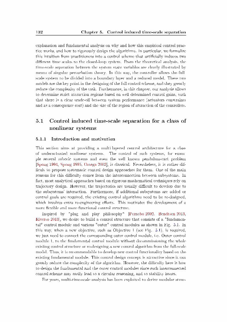
132 Chapter 5. Control induced time-scale separation
explanation and fundamental analysis on why and how this empirical control prac-
tice works, and how to rigorously design the algorithms. In particular, we formalize
this intuition from practitioners into a control scheme that articially induces two
dierent time scales to the closed-loop system. From the theoretical analysis, the
time-scale separation between the system state variables are clearly illustrated by
means of singular perturbation theory. In this way, the controller allows the full-
scale system to be divided into a boundary-layer and a reduced model. These two
models are the key point in the designing of the full control scheme, and they greatly
reduce the complexity of the task. Furthermore, in this chapter, our analysis allows
to determine strict attraction regions based on well determined control gains, such
that there is a clear trade-o between system performance (actuators constraints
and as a consequence cost) and the size of the region of attraction of the controllers.
5.1 Control induced time-scale separation for a class of
nonlinear systems
5.1.1 Introduction and motivation
This section aims at providing a multi-layered control architecture for a class
of underactuated nonlinear systems. The control of such systems, for exam-
ple several robotic systems and even the well known pendulum-cart problem
[Spong 1994, Spong 1995, Ortega 2002], is classical. Nevertheless, it is rather dif-
cult to propose systematic control design approaches for them. One of the main
reasons for this diculty comes from the interconnection between subsystems. In
fact, most analytical approaches based on rigorous mathematical techniques rely on
trajectory design. However, the trajectories are usually dicult to develop due to
the subsystems' interaction. Furthermore, if additional subsystems are added or
control goals are required, the existing control algorithms need to be re-designed,
which involves extra re-engineering eorts. This motivates the development of a
more exible and more functional control structure.
Inspired by "plug and play philosophy" [Pernebo 2002, Bendtsen 2013,
Riverso 2013], we desire to build a control structure that consists of a "fundamen-
tal" control module and various "outer" control modules as shown in Fig. 5.1. In
this way, when a new objective, such as Objective 1 (see Fig. 5.1), is required,
we just need to connect the corresponding outer control module, i.e. Outer control
module 1, to the fundamental control module without decommissioning the whole
existing control structure or re-designing a new control algorithm from the full-scale
model. Thus, it is recommendable to develop new control functionality based on the
existing fundamental module. This control design concept is attractive since it can
greatly reduce the complexity of the algorithm. However, the diculty here is how
to design the fundamental and the outer control modules since such interconnected
control scheme may easily lead to a circular reasoning, and to stability issues.
For years, multi-time-scale analysis has been exploited to derive modular struc-
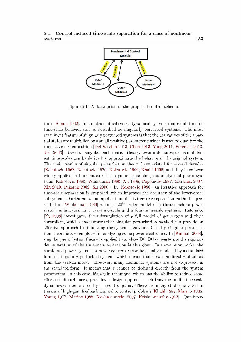
5.1. Control induced time-scale separation for a class of nonlinear
systems 133
Figure 5.1: A description of the proposed control scheme.
tures [Simon 1962]. In a mathematical sense, dynamical systems that exhibit multi-
time-scale behavior can be described as singularly perturbed systems. The most
prominent feature of singularly perturbed systems is that the derivatives of their par-
tial states are multiplied by a small positive parameter ε which is used to quantify the
time-scale decomposition [Del Vecchio 2013, Chen 2013, Yang 2011, Petersen 2013,
Teel 2003]. Based on singular perturbation theory, lower-order subsystems in dier-
ent time scales can be derived to approximate the behavior of the original system.
The main results of singular perturbation theory have existed for several decades
[Kokotovic 1968, Kokotovic 1976, Kokotovic 1999, Khalil 1996] and they have been
widely applied in the context of the dynamic modeling and analysis of power sys-
tems [Kokotovic 1980, Winkelman 1980, Xu 1998, Peponides 1982, Martinez 2007,
Xin 2010, Pekarek 2002, Xu 2000]. In [Kokotovic 1980], an iterative approach for
time-scale separation is proposed, which improves the accuracy of the lower-order
subsystems. Furthermore, an application of this iterative separation method is pre-
sented in [Winkelman 1980] where a 20th order model of a three-machine power
system is analyzed as a two-time-scale and a four-time-scale systems. Reference
[Xu 1998] investigates the reformulation of a full model of generators and their
controllers, which demonstrates that singular perturbation method can provide an
eective approach to simulating the system behavior. Recently, singular perturba-
tion theory is also employed in analyzing some power electronics. In [Kimball 2008],
singular perturbation theory is applied to analyze DC-DC converters and a rigorous
demonstration of the time-scale separation is also given. In those prior works, the
considered power systems or power converters can be usually modeled by a standard
form of singularly perturbed system, which means that ε can be directly obtained
from the system model. However, many nonlinear systems are not expressed in
the standard form. It means that ε cannot be deduced directly from the system
parameters. In this case, high-gain technique, which has the ability to reduce some
eects of disturbances, provides a design approach such that the multi-time-scale
dynamics can be created by the control gains. There are many studies devoted to
the use of high-gain feedback applied to control problems [Khalil 1987, Marino 1985,
Young 1977, Marino 1988, Krishnamurthy 2007, Krishnamurthy 2013]. Our inter-
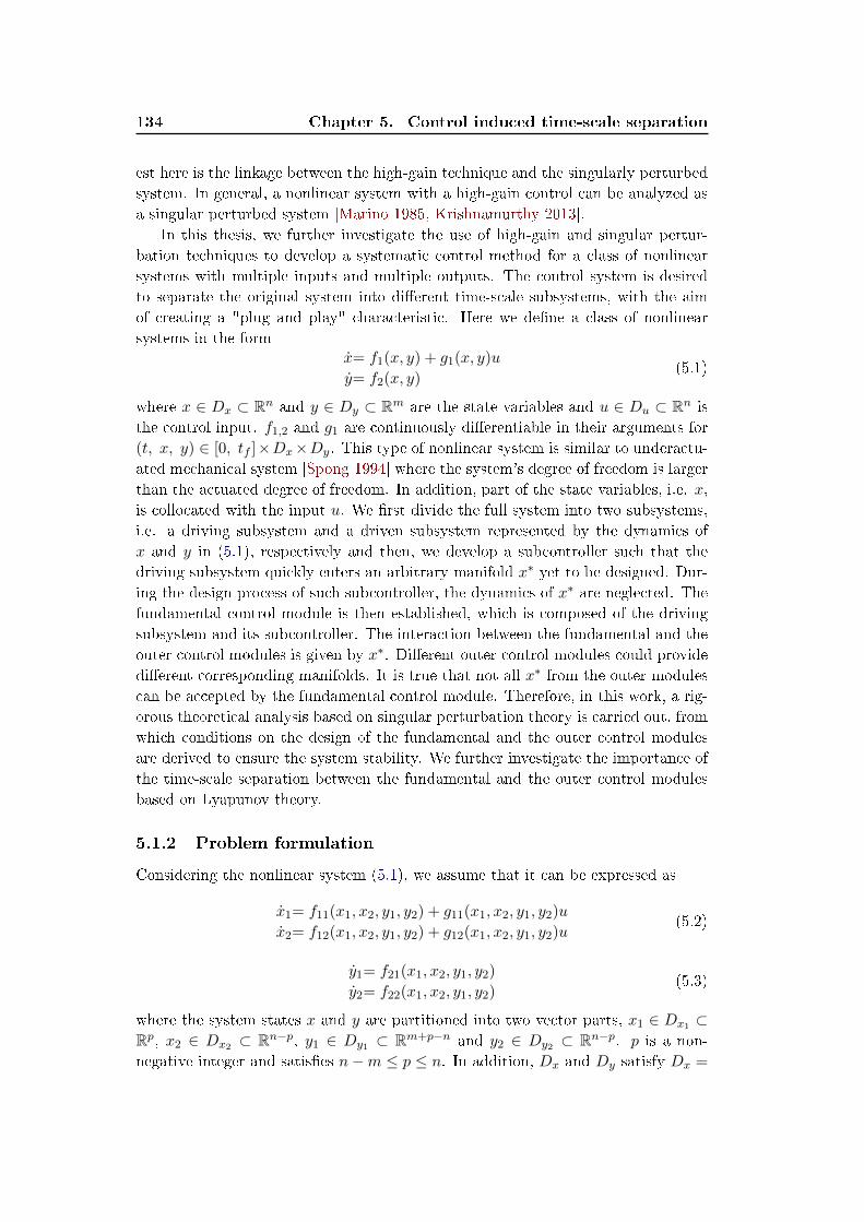
134 Chapter 5. Control induced time-scale separation
est here is the linkage between the high-gain technique and the singularly perturbed
system. In general, a nonlinear system with a high-gain control can be analyzed as
a singular perturbed system [Marino 1985, Krishnamurthy 2013].
In this thesis, we further investigate the use of high-gain and singular pertur-
bation techniques to develop a systematic control method for a class of nonlinear
systems with multiple inputs and multiple outputs. The control system is desired
to separate the original system into dierent time-scale subsystems, with the aim
of creating a "plug and play" characteristic. Here we dene a class of nonlinear
systems in the formx= f1(x, y) + g1(x, y)u
y= f2(x, y)(5.1)
where x ∈ Dx ⊂ Rn and y ∈ Dy ⊂ Rm are the state variables and u ∈ Du ⊂ Rn is
the control input. f1,2 and g1 are continuously dierentiable in their arguments for
(t, x, y) ∈ [0, tf ]×Dx×Dy. This type of nonlinear system is similar to underactu-
ated mechanical system [Spong 1994] where the system's degree of freedom is larger
than the actuated degree of freedom. In addition, part of the state variables, i.e. x,
is collocated with the input u. We rst divide the full system into two subsystems,
i.e. a driving subsystem and a driven subsystem represented by the dynamics of
x and y in (5.1), respectively and then, we develop a subcontroller such that the
driving subsystem quickly enters an arbitrary manifold x∗ yet to be designed. Dur-
ing the design process of such subcontroller, the dynamics of x∗ are neglected. The
fundamental control module is then established, which is composed of the driving
subsystem and its subcontroller. The interaction between the fundamental and the
outer control modules is given by x∗. Dierent outer control modules could provide
dierent corresponding manifolds. It is true that not all x∗ from the outer modules
can be accepted by the fundamental control module. Therefore, in this work, a rig-
orous theoretical analysis based on singular perturbation theory is carried out, from
which conditions on the design of the fundamental and the outer control modules
are derived to ensure the system stability. We further investigate the importance of
the time-scale separation between the fundamental and the outer control modules
based on Lyapunov theory.
5.1.2 Problem formulation
Considering the nonlinear system (5.1), we assume that it can be expressed as
x1= f11(x1, x2, y1, y2) + g11(x1, x2, y1, y2)u
x2= f12(x1, x2, y1, y2) + g12(x1, x2, y1, y2)u(5.2)
y1= f21(x1, x2, y1, y2)
y2= f22(x1, x2, y1, y2)(5.3)
where the system states x and y are partitioned into two vector parts, x1 ∈ Dx1 ⊂Rp, x2 ∈ Dx2 ⊂ Rn−p, y1 ∈ Dy1 ⊂ Rm+p−n and y2 ∈ Dy2 ⊂ Rn−p. p is a non-
negative integer and satises n−m ≤ p ≤ n. In addition, Dx and Dy satisfy Dx =
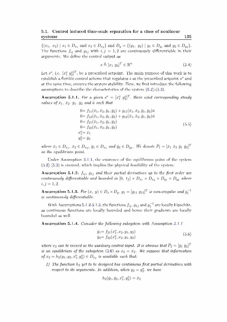
5.1. Control induced time-scale separation for a class of nonlinear
systems 135
(x1, x2) | x1 ∈ Dx1 and x2 ∈ Dx2 and Dy = (y1, y2) | y1 ∈ Dy1 and y2 ∈ Dy2.The functions fij and g1j with i, j = 1, 2 are continuously dierentiable in their
arguments. We dene the control output as
s , [x1 y2]T ∈ Rn (5.4)
Let so, i.e. [xo1 yo2]T , be a prescribed setpoint. The main purpose of this work is to
establish a exible control scheme that regulates s at the prescribed setpoint so and
at the same time, ensures the system stability. Here, we rst introduce the following
assumptions to describe the characteristics of the system (5.2)-(5.3).
Assumption 5.1.1. For a given so = [xo1 yo2]T , there exist corresponding steady
values of x1, x2, y1, y2 and u such that
0= f11(x1, x2, y1, y2) + g11(x1, x2, y1, y2)u
0= f12(x1, x2, y1, y2) + g12(x1, x2, y1, y2)u
0= f21(x1, x2, y1, y2)
0= f22(x1, x2, y1, y2)
xo1= x1
yo2= y2
(5.5)
where x1 ∈ Dx1 , x2 ∈ Dx2, y1 ∈ Dx1 and y2 ∈ Dy2. We denote P1 = [x1 x2 y1 y2]T
as the equilibrium point.
Under Assumption 5.1.1, the existence of the equilibrium point of the system
(5.2)-(5.3) is ensured, which implies the physical feasibility of the system.
Assumption 5.1.2. fij, g1j and their partial derivatives up to the rst order are
continuously dierentiable and bounded in [0, tf ] ×Dx1 ×Dx2 ×Dy1 ×Dy2 where
i, j = 1, 2.
Assumption 5.1.3. For (x, y) ∈ Dx×Dy, g1 = [g11 g12]T is non-singular and g−11
is continuously dierentiable.
With Assumptions 5.1.2-5.1.3, the functions fij , g1j and g−11 are locally Lipschitz,
as continuous functions are locally bounded and hence their gradients are locally
bounded as well.
Assumption 5.1.4. Consider the following subsystem with Assumption 5.1.1
y1= f21(xo1, x2, y1, y2)
y2= f22(xo1, x2, y1, y2)(5.6)
where x2 can be viewed as the auxiliary control input. It is obvious that P2 = [y1 y2]T
is an equilibrium of the subsystem (5.6) as x2 = x2. We suppose that information
of x2 = h2(y1, y2, xo1, y
o2) ∈ Dx2 is available such that:
1) The function h2 yet to be designed has continuous rst partial derivatives with
respect to its arguments. In addition, when y2 = yo2, we have
h2(y1, y2, xo1, y
o2) = x2
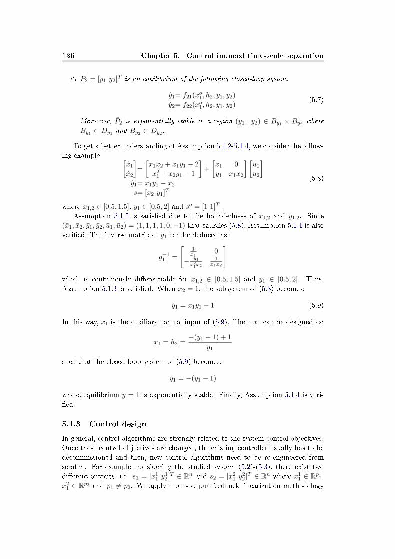
136 Chapter 5. Control induced time-scale separation
2) P2 = [y1 y2]T is an equilibrium of the following closed-loop system
y1= f21(xo1, h2, y1, y2)
y2= f22(xo1, h2, y1, y2)(5.7)
Moreover, P2 is exponentially stable in a region (y1, y2) ∈ By1 × By2 where
By1 ⊂ Dy1 and By2 ⊂ Dy2.
To get a better understanding of Assumption 5.1.2-5.1.4, we consider the follow-
ing example [x1
x2
]=
[x1x2 + x1y1 − 2
x21 + x2y1 − 1
]+
[x1 0
y1 x1x2
] [u1
u2
]y1= x1y1 − x2
s= [x2 y1]T
(5.8)
where x1,2 ∈ [0.5, 1.5], y1 ∈ [0.5, 2] and so = [1 1]T .
Assumption 5.1.2 is satised due to the boundedness of x1,2 and y1,2. Since
(x1, x2, y1, y2, u1, u2) = (1, 1, 1, 1, 0,−1) that satises (5.8), Assumption 5.1.1 is also
veried. The inverse matrix of g1 can be deduced as:
g−11 =
[1x1
0
− y1x21x2
1x1x2
]
which is continuously dierentiable for x1,2 ∈ [0.5, 1.5] and y1 ∈ [0.5, 2]. Thus,
Assumption 5.1.3 is satised. When x2 = 1, the subsystem of (5.8) becomes:
y1 = x1y1 − 1 (5.9)
In this way, x1 is the auxiliary control input of (5.9). Then, x1 can be designed as:
x1 = h2 =−(y1 − 1) + 1
y1
such that the closed-loop system of (5.9) becomes:
y1 = −(y1 − 1)
whose equilibrium y = 1 is exponentially stable. Finally, Assumption 5.1.4 is veri-
ed.
5.1.3 Control design
In general, control algorithms are strongly related to the system control objectives.
Once these control objectives are changed, the existing controller usually has to be
decommissioned and then, new control algorithms need to be re-engineered from
scratch. For example, considering the studied system (5.2)-(5.3), there exist two
dierent outputs, i.e. s1 = [x11 y
12]T ∈ Rn and s2 = [x2
1 y22]T ∈ Rn where x1
1 ∈ Rp1 ,x2
1 ∈ Rp2 and p1 6= p2. We apply input-output feedback linearization methodology
5.1. Control induced time-scale separation for a class of nonlinear
systems 137
to design the control scheme. When the system is required to track the reference
from s1 to s2, the entire control scheme must be redesigned since the corresponding
Lie derivatives are totally changed. Here, we aim at establishing a more exible
control scheme such that dierent control objectives can be achieved based on the
existing control structure.
The described system (5.2)-(5.3) has fewer control inputs (n) than state vari-
ables (n + m). In addition, u has an explicit eect on x and they have the same
degree of freedom. The above aspects prompt us to divide the full system into two
interconnected subsystems. The state variable x collocated with the control input u
is called the driving state. We denote the dynamics of x1,2 described by (5.2) as the
driving subsystem. As seen in (5.3), x1 and x2 can be viewed as the control inputs,
which implies that u indirectly inuences the behavior of y through x. Hence, y
and (5.3) is called the driven state and the driven subsystem. Such solution to the
division of the full system into two parts is inspired by underactuated mechanical
systems [Spong 1994].
We suppose that the proposed control scheme can make the system (5.2)-(5.3)
exhibit a multi-time-scale behavior where the driving subsystem has much faster
dynamics than the driven subsystem. Based on this assumption, the two subsystems
can be then designed independently.
5.1.3.1 Design of the driving subsystem
Step 5.1.5. For a given x0 ∈ Dx, let us impose the following autonomous system
x = −A1(x− x0) + r1(x, x0) (5.10)
where A1 = diag(a1i) ∈ Rn×n yet to be designed. We denote a1 = min(a11, · · · , a1n).
The system (5.10) is designed as
1. r1(x, x0) is a continuously dierentiable function and r1(x0, x0) = 0. As a
consequence, for a positive γ1, there exists b1 > 0 such that, when x ∈ Bx1 =
x ∈ Dx| ||x− x0|| < b1, we have
||r1(x, x0)|| < γ1||x− x0|| (5.11)
2. a1 is assigned to satisfy
γ1 + c1 ≤ a1
where c1 is a positive parameter.
Lemma 5.1.6. The equilibrium point x = x0 of (5.10) is exponentially stable in
Bx1 .
Proof. We choose the Lyapunov function as
V1(x− x0) =1
2(x− x0)T (x− x0)
138 Chapter 5. Control induced time-scale separation
The derivative of V1 along the trajectory of (5.10) is
V1≤ −||A1|| ||x− x0||2 + (x− x0)T r1(x, x0)
≤ −(a1 − γ1)||x− x0||2 = −c1||x− x0||2(5.12)
Hence, Lemma (5.1.6) is proved.
The values of γ1, a1 and b1 are strongly dependent on each other. For example,
considering the following system
x = −ax+ x3 − x
we then have x0 = 0, a1 = a and r1 = x3−x. If γ1 = 3, there exists b1 = 2 such that
(5.11) is satised. In this case, a1 should be chosen larger than 3 + c1. If a larger γ1
is given, i.e. γ1 = 8, a new b1 = 3 is then deduced. We obtain a new condition for
a1, i.e. a1 > 9 + c1. It is clear that a larger γ1 results in a smaller feasible region
for a1.
When γ1 is xed, the linear term −A1(x − x0) dominates the behavior of the
autonomous system (5.10) in Bx1. Consequently, the dynamics of (5.10) can be
regulated by A1.
Step 5.1.7. Supposing that there exists a reference x∗ ∈ Dx and with the acknowl-
edge of (5.10), we then develop a subcontroller u = h1(x, y, x∗) as
u = g−11 (x, y)[−A1(x− x∗) + r1(x, x∗)− f1(x, y)] (5.13)
such that the closed-loop system of the driving subsystem becomes
x = −A1(x− x∗) + r1(x, x∗)
The only information on x∗ is that it has a much slower dynamic than x. As
seen in (5.13), the derivative of x∗ is neglected in the subcontroller.
5.1.3.2 Design of the driven subsystem
Step 5.1.8. The main task in this step is to develop the unknown reference x∗ that
must be tracked by the driving subsystem. Since we suppose that x∗ has a very slow
dynamic, a large a1 can then be chosen such that the state variable of the driving
subsystem x quickly enters x∗. Then, the driven subsystem becomes
y1= f21(x∗1, x∗2, y1, y2)
y2= f22(x∗1, x∗2, y1, y2)
(5.14)
which is called the reduced model. Because x1 is required to track its reference tra-
jectory, x∗1 can be directly given by:
x∗1 = xo1 (5.15)
5.1. Control induced time-scale separation for a class of nonlinear
systems 139
Thus, the reduced model (5.14) becomes
y1= f21(xo1, x∗2, y1, y2)
y2= f22(xo1, x∗2, y1, y2)
(5.16)
According to Assumption 5.1.4, there exists
x∗2 = h2(y1, y2, xo1, y
o2) (5.17)
such that the reduced model (5.14) is exponentially stable.
Until now, the entire control algorithm is developed, consisting of two subcon-
trollers, i.e. u = h1(x, y, x∗) and x∗ = [xo1 h2(y1, y2, xo1, y
o2)]T , which are derived
from two lower order subsystems, i.e. the driving and the driven subsystems. As
mentioned in the previous section, the driving subsystem (5.2) with its subcon-
troller u = h1 composes the fundamental control module and the reduced model of
the driven subsystem (5.14) with its subcontroller x∗ constitutes the outer control
module. Furthermore, the proposed control structure has plug and play capabilities.
When a new objective is required, we only need to design a new corresponding outer
control module that provides a new x∗ to the fundamental control module without
abandoning the whole existing control structure. Dierent outer control modules
share the same fundamental control module. x∗ is thus considered as the tie that
binds the fundamental and the outer control modules together. In addition, the new
outer control module is designed based on the reduced model where the dynamics
of x are neglected. This greatly simplies the problem.
5.1.4 Theoretical study
During the design procedure in Section 5.1.3, we assume that the dynamics of the
driving and the driven subsystems can be divided into dierent time scales with
the aid of the proposed control methodology. In this section, we rst verify this
assumption by means of singular perturbation theory. Subsequently, we carry out
a theoretical stability analysis, from which sucient conditions for the construction
of the fundamental and the outer control modules are derived.
5.1.4.1 Multi-time-scale dynamics
In this section, we present how the system (5.2)-(5.3) exhibits a multi-time-scale
behavior under the proposed controller. Substituting the control algorithm (5.13),
(5.15) and (5.17) into the original system (5.1), we then obtain the following closed-
loop systemx= −A1(x− x∗) + r1(x, x∗)
y= f2(x, y)(5.18)
Let us introduce a new variable ε which satises
ε · a1 = 1
140 Chapter 5. Control induced time-scale separation
The system (5.18) can be rewritten as
εx= −A1ε(x− x∗) + εr1(x, x∗)
y= f2(x, y)(5.19)
where A1ε = diag(εa1i). Denoting a1iε = εa1i, we then have a1iε ≥ 11, for all i =
1, · · · , n. When ε is small enough, our problem (5.19) becomes a standard singular
perturbation problem. By setting ε = 0, the driving subsystem is degenerated into
the algebraic loop, i.e. A1ε(x − x∗) = 0, from which we can get the isolated root
x = x∗. We call x∗ the quasi-steady state of x. By recalling that x∗1 = xo1 in (5.15)
and x∗2 = h2 in (5.17), we substitute x = x∗ into the driven subsystem and then
obtain
y = f2(xo1, h2(y, xo1, yo2), y) (5.20)
Due to Assumption 5.1.4, the equilibrium point P2 of the reduced model (5.20) is
exponentially stable in By1 . In addition, we denote the solution of (5.20) as yre.
In order to analyze the closed-loop system (5.19) more conveniently, we introduce
the following new variables
x1 = x1 − x∗1; x2 = x2 − x∗2; x = [x1 x2]T
y1 = y1 − y1; y2 = y2 − y2; y = [y1 y2]T
In these new variables, the system (5.19) is rewritten as
ε ˙x= −A1εx+ εr1(x+ x∗, x∗)− εdx∗
dt˙y= f2(x+ x∗, y + y)
(5.21)
with x∗ = [xo1 h2(y+ y)]T . The origin is the equilibrium point of the system (5.21).
Moreover, there exist maps such that Dx → Dx and Dy → Dy. The (asymptotic)
stability of the origin of the error system (5.21) implies the (asymptotic) stability
of the equilibrium P1 of the system (5.18).
Let us introduce a new time scale τ which satises
εdx
dt=dx
dτ
In the τ time scale, the variables t, y and x∗ are considered slowly varying. We
rewrite the dynamics of x (in (5.21)) in the τ time scale
dx
dτ= −A1εx+ εr1(x+ x∗, x∗)− ε[0 ∂h2
∂yf2]T
When setting ε = 0 and freezing t, y and x∗ at their initial values, we get the
boundary-layer system
dx
dτ= −A1εx (5.22)
1See the denition of a1 in (5.10).
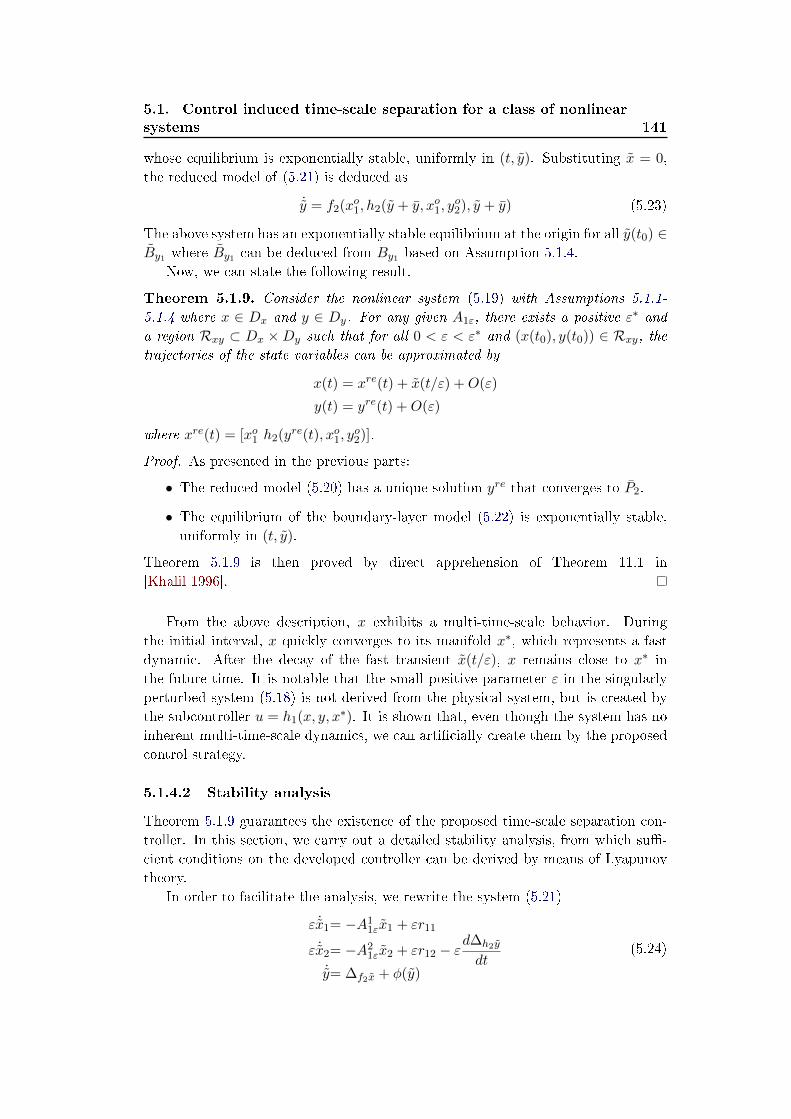
5.1. Control induced time-scale separation for a class of nonlinear
systems 141
whose equilibrium is exponentially stable, uniformly in (t, y). Substituting x = 0,
the reduced model of (5.21) is deduced as
˙y = f2(xo1, h2(y + y, xo1, yo2), y + y) (5.23)
The above system has an exponentially stable equilibrium at the origin for all y(t0) ∈By1 where By1 can be deduced from By1 based on Assumption 5.1.4.
Now, we can state the following result.
Theorem 5.1.9. Consider the nonlinear system (5.19) with Assumptions 5.1.1-
5.1.4 where x ∈ Dx and y ∈ Dy. For any given A1ε, there exists a positive ε∗ and
a region Rxy ⊂ Dx ×Dy such that for all 0 < ε < ε∗ and (x(t0), y(t0)) ∈ Rxy, thetrajectories of the state variables can be approximated by
x(t) = xre(t) + x(t/ε) +O(ε)
y(t) = yre(t) +O(ε)
where xre(t) = [xo1 h2(yre(t), xo1, yo2)].
Proof. As presented in the previous parts:
• The reduced model (5.20) has a unique solution yre that converges to P2.
• The equilibrium of the boundary-layer model (5.22) is exponentially stable,
uniformly in (t, y).
Theorem 5.1.9 is then proved by direct apprehension of Theorem 11.1 in
[Khalil 1996].
From the above description, x exhibits a multi-time-scale behavior. During
the initial interval, x quickly converges to its manifold x∗, which represents a fast
dynamic. After the decay of the fast transient x(t/ε), x remains close to x∗ in
the future time. It is notable that the small positive parameter ε in the singularly
perturbed system (5.18) is not derived from the physical system, but is created by
the subcontroller u = h1(x, y, x∗). It is shown that, even though the system has no
inherent multi-time-scale dynamics, we can articially create them by the proposed
control strategy.
5.1.4.2 Stability analysis
Theorem 5.1.9 guarantees the existence of the proposed time-scale separation con-
troller. In this section, we carry out a detailed stability analysis, from which su-
cient conditions on the developed controller can be derived by means of Lyapunov
theory.
In order to facilitate the analysis, we rewrite the system (5.21)
ε ˙x1= −A11εx1 + εr11
ε ˙x2= −A21εx2 + εr12 − ε
d∆h2y
dt˙y= ∆f2x + φ(y)
(5.24)
142 Chapter 5. Control induced time-scale separation
where [A1
1ε 0
0 A21ε
]= A1ε; [r11 r12]T = r1
φ(y) = f2(xo1, h2(y + y, xo1, yo2), y + y)
f2(x+ x∗, y + y) = f2(x+ x∗, y + y)−f2(x∗, y + y)︸ ︷︷ ︸∆f2x
+φ
h2(y + y, xo1, yo2) = h2(y + y, xo1, y
o2)−h2(y, xo1, y
o2)︸ ︷︷ ︸
∆h2y
+h2
h2 = h2(y, xo1, yo2)
It can be seen that the terms εd∆h2y
dtand ∆f2x in (5.24) reect the dynamic inter-
actions between the driving and the driven subsystems. Moreover, ∆f2x and ∆h2y
satisfy
||∆f2x|| → 0 when ||x|| → 0
||∆h2y|| → 0 when ||y|| → 0
Since h2(y + y, xo1, yo2) and f2(x + x∗, y + y) are continuously dierentiable, there
exist positive L1x and L1y such that
||∆f2x||≤ L1x||x||||∆h2y||≤ L1y||y||
(5.25)
for x ∈ Ω1x ⊂ Dx and y ∈ Ω1y ⊂ Dy.
Since the reduced model (5.23) is exponentially stable in By1 ⊂ Dy, there exists
a Lyapunov function V0 satisfying
c1||y||2 ≤ V2(y)≤ c2||y||2∂V2
∂yφ(y)≤ −c3||y||2
||∂V2
∂y||≤ c4||y||
(5.26)
for positive constants ci, i = 1, · · · , 4.According to Taylor's theorem, φ can be rewritten as
φ(y) = Aφy + gφ(y)y (5.27)
which is called the Peano form of the remainder where
Aφ =∂φ
∂y|y=0
limy→0
gφ(y) = 0 (5.28)

5.1. Control induced time-scale separation for a class of nonlinear
systems 143
Equation (5.28) means that, for any given L1φ > 0, there exists a positive b2 such
that
||gφ(y)|| ≤ L1φ (5.29)
for all y ∈ By2 = y ∈ Dy| ||y|| ≤ b2. It is worth noting that the values of L1x and
L1y depend on Ω1x and Ω1y. In general, a larger Ω1x(Ω1y) may result in a larger
L1x(L1y). The constants ci, i = 1, · · · , 4 are also strongly related to Ω2y.
We take
V = dV1(x) + (1− d)V2(y)
as a Lyapunov function candidate for the closed-loop system (5.24) where d ∈ (0, 1).
The rst part of V , V1(x), is derived from the boundary-layer model (5.22). Ac-
cording to Lemma 5.1.6, the origin of the system
˙x = −A1x+ r1(x)
is exponentially stable in Bx1 which corresponds to Bx1 . The second term V2 is
obtained from the reduced model. The composition of V (x, y) in this way provides
us a easier way to search the feasible region of ε.
The derivative of V along the trajectories (5.24) can be then deduced as
V =d[−xTA1x+ xT r1 − xT2∂∆h2y
∂y(∆f2x + φ)]
+ (1− d)∂V2
∂y(∆f2x + φ) (5.30)
Applying the inequalities (5.12) and (5.26) to (5.30), we have
V ≤− dc1||x||2 − (1− d)c3||y||2 + (1− d)∂V2
∂y∆f2x
− dxT2∂∆h2y
∂y(∆f2x +Aφy + gφy)
≤− dc1||x||2 − (1− d)c3||y||2 + (1− d)||∂V2
∂y|| ||∆f2x||
+ d||x2|| ||∂∆h2y
∂y|| [ ||∆f2x||
+ ( ||gφ||+ ||Aφ|| )||y|| ] (5.31)
When x ∈ Bx1 ∩Ω1x, y ∈ By2 ∩ By1 ∩Ω1y ∩Ω2y, and by using (5.25), (5.26), (5.29),
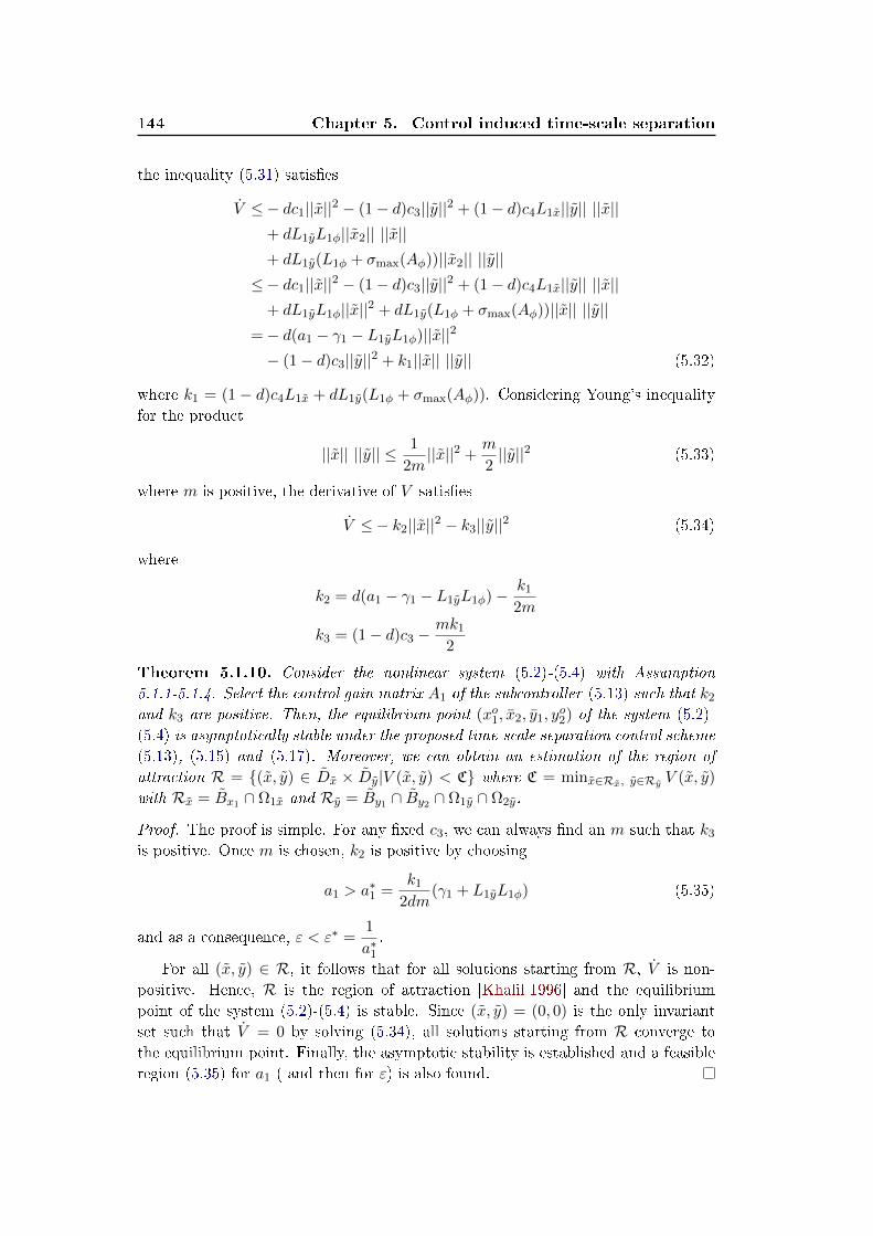
144 Chapter 5. Control induced time-scale separation
the inequality (5.31) satises
V ≤− dc1||x||2 − (1− d)c3||y||2 + (1− d)c4L1x||y|| ||x||+ dL1yL1φ||x2|| ||x||+ dL1y(L1φ + σmax(Aφ))||x2|| ||y||≤ − dc1||x||2 − (1− d)c3||y||2 + (1− d)c4L1x||y|| ||x||
+ dL1yL1φ||x||2 + dL1y(L1φ + σmax(Aφ))||x|| ||y||=− d(a1 − γ1 − L1yL1φ)||x||2
− (1− d)c3||y||2 + k1||x|| ||y|| (5.32)
where k1 = (1 − d)c4L1x + dL1y(L1φ + σmax(Aφ)). Considering Young's inequality
for the product
||x|| ||y|| ≤ 1
2m||x||2 +
m
2||y||2 (5.33)
where m is positive, the derivative of V satises
V ≤− k2||x||2 − k3||y||2 (5.34)
where
k2 = d(a1 − γ1 − L1yL1φ)− k1
2m
k3 = (1− d)c3 −mk1
2
Theorem 5.1.10. Consider the nonlinear system (5.2)-(5.4) with Assumption
5.1.1-5.1.4. Select the control gain matrix A1 of the subcontroller (5.13) such that k2
and k3 are positive. Then, the equilibrium point (xo1, x2, y1, yo2) of the system (5.2)-
(5.4) is asymptotically stable under the proposed time-scale separation control scheme
(5.13), (5.15) and (5.17). Moreover, we can obtain an estimation of the region of
attraction R = (x, y) ∈ Dx × Dy|V (x, y) < C where C = minx∈Rx, y∈Ry V (x, y)
with Rx = Bx1 ∩ Ω1x and Ry = By1 ∩ By2 ∩ Ω1y ∩ Ω2y.
Proof. The proof is simple. For any xed c3, we can always nd an m such that k3
is positive. Once m is chosen, k2 is positive by choosing
a1 > a∗1 =k1
2dm(γ1 + L1yL1φ) (5.35)
and as a consequence, ε < ε∗ =1
a∗1.
For all (x, y) ∈ R, it follows that for all solutions starting from R, V is non-
positive. Hence, R is the region of attraction [Khalil 1996] and the equilibrium
point of the system (5.2)-(5.4) is stable. Since (x, y) = (0, 0) is the only invariant
set such that V = 0 by solving (5.34), all solutions starting from R converge to
the equilibrium point. Finally, the asymptotic stability is established and a feasible
region (5.35) for a1 ( and then for ε) is also found.

5.1. Control induced time-scale separation for a class of nonlinear
systems 145
We note that the feasible region (5.35) of a1 strongly depends on the choice of
subcontroller x∗2 = h2(y, xo1, yo2). If we want to stabilize the reduced model (5.23)
in a larger region, we may need a larger L1φ, c3 and c4. Alternatively, if we want
to accelerate the speed of the convergence of the reduced model, it is necessary to
increase σmax(A1φ). Such scenarios may result in a larger a∗1. However, sometimes,
a very large a1 may cause a large peak value of the control input u, which is not
desired. Thus, it is very important to consider associated factors when we choose
a1.
5.1.5 Study cases
In order to get a better understanding of the proposed control algorithm, two ex-
amples are studied in this section.
5.1.5.1 Example 1
Consider the following nonlinear system
x1= x1x2 + x3u
x2= x1 + x3
x3= x2 + x3
(5.36)
Two control objectives exist:
Objective 1: making y = x3 track the reference xo3;
Objective 2: making y = x2 track the reference xo2.
We rst use the input-output feedback linearization method to design the control
structure and then apply the proposed time-scale separation control scheme.
Feedback linearization control: When x3 is the output, the system (5.36) is
feedback linearizable since the relative degree of y = x3 is three. Then, a controller
based on input-output feedback linearization method can be developed
u =1
LgL2f (y)
(−L3f (y) + v) (5.37)
where
v = −b0(x3 − xo3)− b1L1f (y)− b2L2
f (y)
L1f (y) = x2 + x3
L2f (y) = x1 + x2 + 2x3
L3f (y) = x1x2 + x1 + 2x2 + 3x3
LgL2f (y) = x3
The controller (5.37) is tested by numerical simulations as illustrated in Fig. 5.2.
The parameter values are listed in Table 5.1. The simulation results clearly show
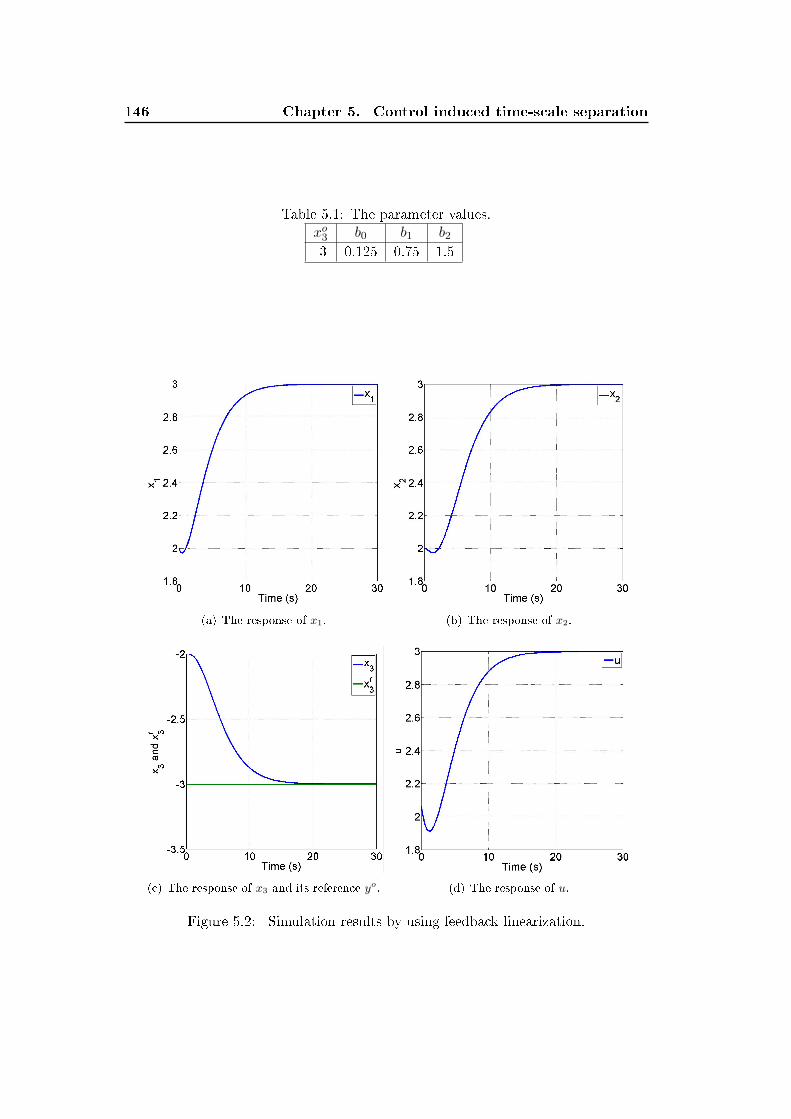
146 Chapter 5. Control induced time-scale separation
Table 5.1: The parameter values.xo3 b0 b1 b2-3 0.125 0.75 1.5
(a) The response of x1. (b) The response of x2.
(c) The response of x3 and its reference yo. (d) The response of u.
Figure 5.2: Simulation results by using feedback linearization.
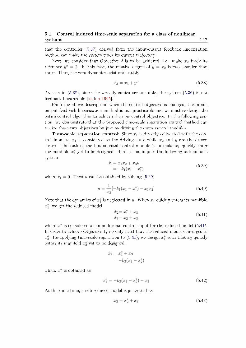
5.1. Control induced time-scale separation for a class of nonlinear
systems 147
that the controller (5.37) derived from the input-output feedback linearization
method can make the system track its output trajectory.
Next, we consider that Objective 2 is to be achieved, i.e. make x2 track its
reference yo = 2. In this case, the relative degree of y = x2 is two, smaller than
three. Thus, the zero dynamics exist and satisfy
x3 = x3 + yo (5.38)
As seen in (5.38), since the zero dynamics are unstable, the system (5.36) is not
feedback linearizable [Isidori 1995].
From the above description, when the control objective is changed, the input-
output feedback linearization method is not practicable and we must re-design the
entire control algorithm to achieve the new control objective. In the following sec-
tion, we demonstrate that the proposed time-scale separation control method can
realize these two objectives by just modifying the outer control modules.
Time-scale separation control: Since x1 is directly collocated with the con-
trol input u, x1 is considered as the driving state while x2 and y are the driven
states. The task of the fundamental control module is to make x1 quickly enter
the manifold x∗1 yet to be designed. Here, let us impose the following autonomous
systemx1= x1x2 + x3u
= −k1(x1 − x∗1)(5.39)
where r1 = 0. Then u can be obtained by solving (5.39)
u =1
x3[−k1(x1 − x∗1)− x1x2] (5.40)
Note that the dynamics of x∗1 is neglected in u. When x1 quickly enters its manifold
x∗1, we get the reduced model
x2= x∗1 + x3
x3= x2 + x3(5.41)
where x∗1 is considered as an additional control input for the reduced model (5.41).
In order to achieve Objective 1, we only need that the reduced model converges to
xo3. Re-applying time-scale separation to (5.41), we design x∗1 such that x2 quickly
enters its manifold x∗2 yet to be designed.
x2 = x∗1 + x3
= −k2(x2 − x∗2)
Then, x∗1 is obtained as
x∗1 = −k2(x2 − x∗2)− x3 (5.42)
At the same time, a sub-reduced model is generated as
x3 = x∗2 + x3 (5.43)
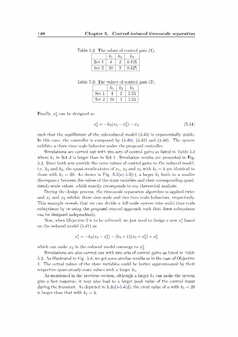
148 Chapter 5. Control induced time-scale separation
Table 5.2: The values of control gain (1).
k1 k2 k3
Set 1 4 2 0.125
Set 2 20 2 0.125
Table 5.3: The values of control gain (2).
k1 k2 k3
Set 1 4 2 2.25
Set 2 20 2 2.25
Finally, x∗2 can be designed as
x∗2 = −k3(x3 − xo3)− x3 (5.44)
such that the equilibrium of the sub-reduced model (5.43) is exponentially stable.
In this case, the controller is composed by (5.40), (5.42) and (5.44). The system
exhibits a three-time-scale behavior under the proposed controller.
Simulations are carried out with two sets of control gains as listed in Table 5.2
where k1 in Set 2 is larger than in Set 1. Simulation results are presented in Fig.
5.3. Since both sets provide the same values of control gains to the reduced model,
i.e. k2 and k3, the quasi-steady-states of x1, x2 and x3 with k1 = 4 are identical to
those with k1 = 20. As shown in Fig. 5.3(a)-5.3(c), a larger k1 leads to a smaller
discrepancy between the values of the state variables and their corresponding quasi-
steady-state values, which exactly corresponds to our theoretical analysis.
During the design process, the time-scale separation algorithm is applied twice
and x1 and x2 exhibit three-time-scale and two-time-scale behaviors, respectively.
This example reveals that we can divide a full-scale system into multi-time-scale
subsystems by re-using the proposed control approach such that these subsystems
can be designed independently.
Now, when Objective 2 is to be achieved, we just need to design a new x∗1 based
on the reduced model (5.41) as
x∗1 = −k2(x2 − xo2)− (k3 + 1)(x3 + xo2) + xo2
which can make x2 in the reduced model converge to xo2.
Simulations are also carried out with two sets of control gains as listed in Table
5.3. As illustrated in Fig. 5.4, we get some similar results as in the case of Objective
1. The actual values of the state variables could be better approximated by their
respective quasi-steady-state values with a larger k1.
As mentioned in the previous section, although a larger k1 can make the system
give a fast response, it may also lead to a larger peak value of the control input
during the transient. As depicted in 5.3(d)-5.4(d), the crest value of u with k1 = 20
is larger than that with k1 = 4.
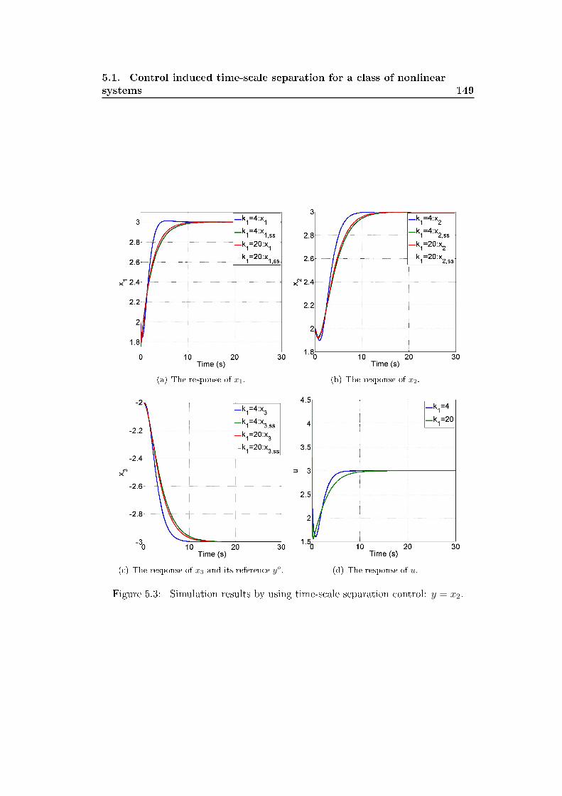
5.1. Control induced time-scale separation for a class of nonlinear
systems 149
(a) The response of x1. (b) The response of x2.
(c) The response of x3 and its reference yo. (d) The response of u.
Figure 5.3: Simulation results by using time-scale separation control: y = x2.
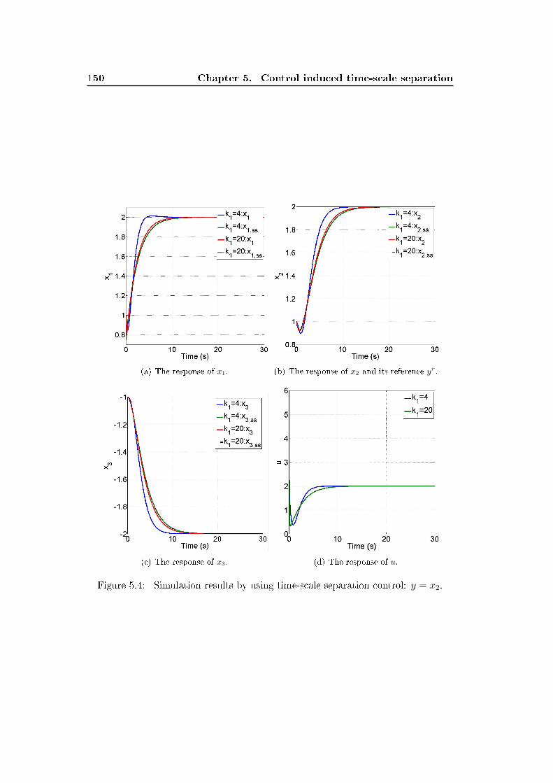
150 Chapter 5. Control induced time-scale separation
(a) The response of x1. (b) The response of x2 and its reference yr.
(c) The response of x3. (d) The response of u.
Figure 5.4: Simulation results by using time-scale separation control: y = x2.

5.1. Control induced time-scale separation for a class of nonlinear
systems 151
5.1.5.2 Example 2
The second example is expressed as
x1= x1x2 + x3u
x2= x1 + x3
x3= x2 − x3
(5.45)
which is required to achieve the same control objectives as in Example 1.
Feedback linearization control: When x3 is dened as the output in Ob-
jective 1, (5.45) is feedback linearizable and hence, a controller by means of in-
put/output feedback linearization is developed as
u =1
LgL2f (x3)
(−L3f (x3) + v) (5.46)
where
v = −b0(x3 − xo3)− b1L1f (x3)− b2L2
f (x3)
L1f (x3) = x2 − x3
L2f (x3) = x1x2 + 2x3
L3f (x3) = x1x2 − x1 + 2x2 − 3x3
LgL2f (x3) = x3
When Objective 2 is to be achieved, the relative degree of y = x2 is also 2 as in
Example 1. However, the zero dynamics here are expressed by
x3 = −x3 + xo2 (5.47)
whose equilibrium is exponentially stable. Hence, input/output feedback lineariza-
tion can be applied. The controller is developed as
u =1
LgLf (x2)(−L2
f (x2) + v) (5.48)
where
v = −b0(x2 − xo2)− b1L1f (x2)
L1f (x2) = x1 + x3
L2f (x2) = x1x2 + x2 − x3
LgLf (x2) = x3
It is clear that, when the new control objective (Objective 2) is to be achieved,
the existing control law (5.46) becomes invalid and should be rejected. The con-
trol design must be re-engineered to develop a new control algorithm (5.48). For a
system of very high order, it is very time-consuming to re-design the control struc-
ture. However, the time-scale separation control scheme proposed in this section
can eectively avoid a control re-design from scratch.
152 Chapter 5. Control induced time-scale separation
Time-scale separation control: First, we design the fundamental module as
in Example 1x1= x1x2 + x3u
= −k1(x1 − x∗1)(5.49)
and then u can be obtained by solving (5.49)
u =1
x3[−k1(x1 − x∗1)− x1x2]
When x1 quickly enters its manifold x∗1, the following reduced model is generated
x2 = x∗1 + x3
x3 = x2 − x3
In order to attain the control objective 1, the same procedure is used to design x∗1as in Example 1
x∗1 = −k2(x2 − x∗2)− x3
where x∗2 satises
x∗2 = −k3(x3 − xo3) + x3
If the control objective 2 is to be achieved, we just need to develop a new x∗1 as
x∗1 = −k2(x2 − xo2)
for the fundamental module without decommissioning the entire existing control
structure.
From this example, the advantage of the proposed control structure is explicitly
presented. In order to make the system achieve dierent control objectives, we only
need redesign the subcontroller of the reduced model and provide the new manifold
x∗ to the fundamental control module.
In the following sections, we will apply the obtained theoretical results to explain
why the vector control structure for VSC HVDC systems can consist of two control
loops with dierent dynamics and to demonstrate how the system exhibit a multi-
time-scale performance.
5.2 Control induced time-scale separation for MTDC
systems using master-slave control conguration
In the present section, based on the previous theoretical results, we give a detailed
description on how the MTDC system exhibits multiple time-scale dynamics using
master-slave control conguration. Furthermore, a theoretical stability study is
also performed where the stability limitations on this control conguration are also
analyzed.

5.2. Control induced time-scale separation for MTDC systems using
master-slave control conguration 153
5.2.1 Control design
We consider each VSC terminal as an individual unit, which is of the form
x1[i]= f1[i](x1[i]) + g1[i](x1[i], ucgi)u1[i]
x2[j]= f2[j](x2[j], y2[j]) + g2[j](x2[j], y2[j], ucwj )u2[j](5.50)
y2[j]= f3[j] + Iw[j](5.51)
where we use the following denitions
x1[i],[igid igiq
]T; x2[j] ,
[iwjd iwjq
]Tu1[i],
[mgid mgiq
]T; u2[j] ,
[mwjd mwjq
]Ty2[j],
[vswjd vswjq
]T; Iw[j]
,[Iwjd Iwjq
]T (5.52)
The expressions of f1[i], f2,3[j], g1[i] and g2[j] are obviously obtained from the MTDC
system described by (3.20), (3.28) and (3.29), which are continuous dierentiable
in their respective arguments for igi,dq ∈ Digi,dq , iwj ,dq ∈ Diwj,dq , vswj ,dq ∈ Dvswj,dq ,uc(·) ∈ Duc and mgi,dq, mwj ,idq ∈ [−1, 1].
For convenience, we also introduce
x , [x1[1] · · · x1[N ] x2[1] · · · x2[M ]]T = [x1[i] x2[j]]
T
u , [u1[1] · · · u1[N ] u2[1] · · · u2[M ]]T = [u1[i] u2[j]]
T
Therefore, the overall model of the MTDC system described in Chapter 3 can be
expressed by a general form (5.50), (5.51) and (3.36).
Now, we are ready to develop the control algorithm by following the procedure
presented in Section 5.1 as
• Step 1: We divide the full-scale system into two subsystems, i.e. the driving
subsystem (5.50) and the driven subsystem (5.51) and (3.36), where the driving
subsystem is directly collocated with the control inputs u1[i] and u2[j].
• Step 2: Assume that the proposed control algorithm is explicitly designed with
the purpose of making the driving subsystem have much faster dynamics than
the driven subsystem. Based on the dynamic separation, we then obtain a
boundary-layer and a reduced model where two subcontrollers are designed to
control both models, respectively.
• Step 3: Substituting the two subcontrollers into the original model, a standard
singularly perturbed system can be deduced. Applying singular perturbation
theory, we derive sucient conditions on the proposed control algorithm to
ensure the asymptotic stability of the MTDC system.
Note that, in Step 2, we assume that the state variables in the driving subsystem
have faster dynamics than those in the driven subsystem. In fact, this assumption is
only used to help us design the control system. In the section of theoretical analysis,
we will demonstrate that the controller based on this assumption indeed makes the
system exhibit a dynamic behavior characterized by the presence of fast and slow
transients.
154 Chapter 5. Control induced time-scale separation
5.2.1.1 Design of the driving subsystem
We assume that there exists a reference trajectory for the driving subsystem as
x∗ , [x∗1[1] · · · x∗1[N ] x
∗2[1] · · · x
∗2[M ]]
T
which is yet to be designed. The only information on x∗ is that it is a function of
the state variables of the driven subsystem with slow dynamic. We then design the
subcontrollers u1[i] = h1[i] and u2[j] = h2[j] such that the closed-loop of the driven
subsystem becomesx1[i]= v1[i]
x2[j]= v2[j](5.53)
where we introduce the auxiliary inputs v1[i] and v2[j]. Since g1[i] and g2[j] are
invertible, by combining (5.50) and (5.53), the subcontroller of the driving system
is designed ash1[i]= g−1
1[i][v1[i] − f1[i]]
h2[j]= g−12[j][v2[j] − f2[j]]
(5.54)
The design of v1[i], v2[j] ∈ R2 are free. We only need them so that the above au-
tonomous system (5.53) at least locally exponentially converges to x∗ when x∗ is
constant. To illustrate our control scheme more clearly, we design
eIx1[i]= x1[i] − x∗1[i]
v1[i]= −K1[i](x1[i] − x∗1[i])− Γ1[i]eIx1[i]eIx2[j]= x2[j] − x∗2[j]
v2[j]= −K2[j](x2[j] − x∗2[j])− Γ2[j]eIx2[j]
(5.55)
where the control gain matrices are of the form
K1[i]= diag(k11[i] , k
12[i] ); K2[j] = diag(k21
[j], k22[j])
Γ1[i]= diag(γ11[i] , γ
12[i] ); Γ2[j] = diag(γ21
[j] , γ22[j])
(5.56)
whose diagonal elements are positive.
5.2.1.2 Design of the driven system
With the aid of the subcontroller (5.54), we assume that x quickly enters the man-
ifold x∗ and then substitute x = x∗ into the driven subsystem (5.51) and (3.36),
leading to the following reduced model
y2[j]= f2[j](x∗2[j], y2[j])
z= Az + ϑ(x∗1[i], x∗2[j])
(5.57)
with (N + 3M + P + L)th order.
According to the master-slave control operation dened in Section 4.1.4 and the
design procedure presented in Section 5.1.3.2, we then set
i∗gρd = iogρd; i∗giq = iogiq (5.58)
5.2. Control induced time-scale separation for MTDC systems using
master-slave control conguration 155
As a consequence, some components of the vector x∗ are directly given by the
prescribed reference values. But we still need to design i∗g1d and i∗wj ,dq which are
considered as the control inputs of the reduced model (5.57). The control goal now
is to make ucg1 and vswj ,dq in (5.57) track the prescribed output reference, i.e.
so ,[uocg1 vosw1,dq
· · · voswN ,dq
](5.59)
via i∗g1d and i∗wj ,dq. Input-output feedback linearization is therefore applied for the
reduced model as2
ducg1dt
=1
Cg1(3
2
vsg1di∗g1d
+ vsg1qiog1q
ucg1−H(1, :)ic)
= vcg1dvswjd
dt= ωwjvswjq +
1
Cfwj(Iwjd − i
∗wjd
)
= vwjd
dvswjq
dt= −ωwjvswjd +
1
Cfwj(Iwjq − i∗wjq)
= vwjq
Taking into account the integrated tracking error, the additional inputs v(·) are
designed aseIcg1= ucg1 , ucg1 − uocg1vcg1= −kg1dug1 − kg2deIcg1eIwjd= vswjd , vswjd − voswjdvwjd= −kw1jdvswjd − kw2jdeIwjdeIwjq= vswjq , vswjq − voswjqvwjq= −kw1jqvswjq − kw2jqeIwjq
(5.60)
with positive control gains kg1d, kg2d, kw1j ,dq and kw2j ,dq. Then, by solving (5.60),
i∗g1d and i∗gj ,dq
are computed as
i∗g1d=2ucg13vsg1d
(Cg1vcg1 +H(1, :)ic)−vsg1qvsg1d
iog1q
i∗wjd= Cfwjωwjvswjq − Cfwjvwjd + Iwjd
i∗wjq= −Cfwjωwjvswjd − Cfwjvwjq + Iwjq
(5.61)
Finally, the full control scheme is established, composed by (5.54), (5.58) and (5.61).
For each VSC terminal, the controller u[k] just relies on local information without
the knowledge of other terminals. This can prevent the possible time delay of
information exchange from the collective model.
The manifold x∗ is deduced from the lower-order reduced model (5.57) instead
of the full-scale model (5.50), (5.51) and (3.36), and it greatly simplies the control
2Recall the denition of H in Section 3.4.3.
156 Chapter 5. Control induced time-scale separation
design. Clearly, x∗ is a function of the state variables of the driven system, i.e. y2[j]
and z. It is worthwhile to note that using a reduced model will introduce errors in
the system. Such errors may cause stability problems which will be studied in the
next section.
5.2.2 Theoretical analysis
Before stating the main results of this section, we recall that, to ensure the physical
feasibility of the MTDC system, Assumption 4.1.1 still holds and the equilibrium
point is denoted as
P1 = [· · · igid igiq · · · iwjd iwjq · · · vswjd vswjq · · · z]T (5.62)
In this section, we will demonstrate how the proposed controller divides the MTDC
system into dierent time scales and furthermore, the stability of the equilibrium
point P1 will be also studied.
5.2.2.1 Two-time-scale dynamics
The aim of this section is to show how the MTDC system exhibits a multi-time-scale
behavior. To establish this result, we substitute the control algorithm (5.54), (5.58)
and (5.61) into the original system consisting of (5.50), (5.51) and (3.36), resulting
in the following closed-loop system
eIx1[i]= x1[i] − x∗1[i]
x1[i]= −K1[i](x1[i] − x∗1[i])− Γ1[i]eIx1[i]eIx2[j]= x2[j] − x∗2[j]
x2[j]= −K2[j](x2[j] − x∗2[j])− Γ2[j]eIx2[j]eIwjd= vswjd − voswjdeIwjq= vswjq − voswjqeIcg1= ucg1y2[j]= f3[j] + Iw[j]
z= Az + ϑ
(5.63)
with (9M + 5N + P + L)th order. The equilibrium point of the above closed-loop
system is denoted as P2.
Let us introduce a small scalar parameter ε satisfying
ε · kmin = 1
where kmin = min(k11[i] , k
12[i] , k
21[j], k
22[j]). We then rewrite the dynamics of x1[i] and x2[j]
in (5.63) as
εx1[i]= −K1[i](x1[i] − x∗1[i])− εΓ1[i]eIx1[i]εx2[j]= −K2[j](x2[j] − x∗2[j])− εΓ2[j]eIx2[j]
(5.64)
5.2. Control induced time-scale separation for MTDC systems using
master-slave control conguration 157
where the new control gain matrices are dened as
K1[i] = diag(k11[i] , k
12[i] ) , diag(εk11
[i] , εk12[i] )
K2[j] = diag(k21[j], k
22[j]) , diag(εk21
[j], εk22[j])
k11[i] , k
12[i] , k
21[j], k
22[j] ≥ 1
Now, as an alternative expression, the closed-loop system (5.63) can be rewritten as
eIx1[i]= x1[i] − x∗1[i]
εx1[i]= −K1[i](x1[i] − x∗1[i])− εΓ1[i]eIx1[i]eIx2[j]= x2[j] − x∗2[j]
εx2[j]= −K2[j](x2[j] − x∗2[j])− εΓ2[j]eIx2[j]eIwjd= vswjd − voswjdeIwjq= vswjq − voswjqeIcg1= ucg1y2[j]= f3[j] + Iw[j]
z= Az + ϑ
(5.65)
which is of a standard singularly perturbed form when ε is small enough. We call
x∗ as the quasi-steady state of x. It is worth noticing that, the small parameter ε,
which is used to qualify the time-scale separation, is not derived from the physical
system parameters but is arbitrarily created by the designed subcontroller (5.54).
For convenience, we introduce the following new variables
x1[i] = x1[i] − x∗1[i]
x2[j] = x2[j] − x∗2[j]
that shift the quasi-steady state of x to the origin. In these new variables, the
driving subsystem (5.64) becomes
ε ˙x1[i]= −K1[i]x1[i] − εΓ1[i]eIx1[i] − εdx∗1[i]
dt
ε ˙x2[j]= −K2[j]x2[j] − εΓ2[j]eIx2[j] − εdx∗2[j]
dt
(5.66)
Now we dene t as the time-scale variable for slow dynamics and introduce a new
time variable τ for fast dynamics as
εdx
dt=dx
dτ, x = [x1[1] · · · x1[N ]x2[1] · · · x2[M ]]
T (5.67)
We then express (5.66) in the τ time scale as
dx1[i]
dτ= −K1[i]x1[i] − εΓ1[i]eIx1[i] − ε
dx∗1[i]
dtdx2[j]
dτ= −K2[j]x2[j] − εΓ2[j]eIx2[j] − ε
dx∗2[j]
dt
(5.68)
158 Chapter 5. Control induced time-scale separation
As ε→ 0,a boundary-layer system is deduced from (5.68), given by
dx1[i]
dτ= −K1[i]x1[i]
dx2[j]
dτ= −K2[j]x2[j]
(5.69)
whose equilibrium point is globally exponentially stable. Meanwhile, when x enters
its manifold x∗, the closed-loop system (5.65) is degenerated into a (5M +N +P +
L+ 1)th order reduced model expressed by
eIwjd= vswjd − voswjdeIwjq= vswjq − voswjqeIcg1= ucg1y2[j]= [vwjd vwjq]
T
z= Az + ϑ′
(5.70)
where ϑ′ is given by
ϑ′i =3
2
vsgidi∗gid
+ vsgiqi∗giq
Cgi(ucgi + ucgi), i ∈ N
ϑ′N+j =3
2
(vswjd + voswjd)i∗wjd
+ (vswjq + voswjq)i∗wjq
Cwj (ucwj + ucwj ), j ∈M
ϑ′N+M+h = 0, h ∈ Pϑ′N+M+P+k = 0, k ∈ L
(5.71)
Remember that i∗gi,dq and i∗wj ,dq
are given by (5.58) and (5.61). We denote the solu-
tion of the reduced model (5.70) as (yre2[j](t), zre(t)) and then, xre = x∗(yre2[j](t), z
re(t))
describes behavior of x∗ when (y2[j](t), z(t)) = (yre2[j](t), zre(t)). As a result, accord-
ing to Theorem 5.1.9 in Section 5.1.4.1, we are ready to state the following result:
Theorem 5.2.1. Consider the system (5.63). For xed control parameters K1[i],
K2[j], kg1,2d, kw1j ,dq and kw2j ,dq, there exists a region Rxyz and a positive constant
ε∗ (or k∗min) such that for all 0 < ε < ε∗ (or k∗min < kmin), if the system (5.63) starts
from Rxyz, we have
y2[j](t)= yre2[j](t) +O(ε)
z(t)= zre(t) +O(ε)
x(t)= xre(t) + x(τ) +O(ε)
(5.72)
where x(τ) is the solution of the boundary-layer model (5.69).
Theorem 5.2.1 clearly indicates that the state variables of the driving system, i.e.
all dq currents, exhibit a two-time-scale behavior. They start with a fast transient
x(τ) and then remain close to xre(t) which presents a slow transient. If we want a
remarkable time-scale separation, a smaller ε (or a lager kmin) should be chosen. In
the τ time scale, all y[j] and z seem slowly varying.

5.2. Control induced time-scale separation for MTDC systems using
master-slave control conguration 159
5.2.2.2 Stability analysis
The previous section shows that the exact solution of the original system (5.63) can
be approximated by the solutions of the boundary-layer and the reduced model. In
this section, we carry out a detailed stability analysis.
To simplify the analysis, we perform the change of variables
y2[j] = y2[j] − y2[j]
z = z − z
and then, rewrite the system (5.63) in these new variables as
eIx1[i]= x1[i]
˙x1[i]= −K1[i]x1[i] − Γ1[i]eIx1[i] −dx∗1[i]
dteIx2[j]= x2[j]
˙x2[j]= −K2[j]x2[j] − Γ2[j]eIx2[j] −dx∗2[j]
dteIwjd= vswjdeIwjq= vswjqeIcg1= ucg1˙y2[j]= vw[j] +B[j]x2[j]
˙z= Az + ϑ∗ +Az + ϑ
(5.73)
where
B[j]= −1
CfwjI2×2; vw[j] , [vwjd vwjq]
T
ϑ, [ϑ1 · · · ϑM+N 0P+L]T
ϑ∗, [ϑ∗1 · · · ϑ∗M+N 0P+L]T
(5.74)
with the elementsϑi =
3
2
vsgidigid + vgsiq igiqCgi(ucgi + ucgi)
, i ∈ N
ϑN+j =3
2
(vswjd + vswjd)iwjd + (vswjq + vswjq )iwjq
Ccwj (ucwj + ucwj ). j ∈M
ϑ∗i =3
2
vsgidi∗gid
+ vgsiqi∗giq
Cgi(ucgi + ucgi), i ∈ N
ϑ∗N+j =3
2
(vswjd + vswjd)i∗wjd
+ (vswjq + vswjq)i∗wjq
Cwj (ucwj + ucwj ). j ∈M
(5.75)
It is important to remark that since x∗ is the control signal of the slow subsystem,
its derivative would be very small compared to the derivative of x.
We rewrite the rst four equations of (5.73) in a novel matrix form
κ = Aκκ + θκ (5.76)
160 Chapter 5. Control induced time-scale separation
where
κ = [· · · eIx1[i] x1[i] · · · eIx2[j] x2[j] · · · ]T
θκ = [· · · 02×1
dx∗1[i]
dt· · · 02×1
dx∗2[j]
dt· · · ]T
Aκ = diag(· · · Ax1[i] · · · Ax2[j])
Ax1[i] =
[02×2 I2×2
−Γ1[i] −K1[i]
]; Ax2[j] =
[02×2 I2×2
−Γ2[j] −K2[j]
]The last ve equations of (5.73) can be expressed in the following form
ζ= Aζζ + ϑζ˙zr= Arzr + ϑ∗r +Arzr + ϑr + ϑic + ϑic
(5.77)
whereζ= [eIcg1 ucg1 · · · eIwjd vswjd · · · eIwjq vswjq · · · ]T
ϑζ= [0 ϑ1 · · · 0 − 1
Cfwjiwjd · · · 0 − 1
Cfwjiwjq · · · ]T
ϑic= [0N+M+P−1H(1, 1)
Lc1ucg1 · · ·
H(1, L)
LcLucg1 ]T
ϑic= [0N+M+P−1H(1, 1)
Lc1ucg1 · · ·
H(1, L)
LcLucg1 ]T
Aζ= diag(Ag1 Aw1d · · · AwMd Aw1q · · · AwM q)
Ag1=
[0 1
−kg1d −kg2d
]; Awj ,dq =
[0 1
−kw1j ,dq −kw2j ,dq
](5.78)
The vectors ϑr, ϑ∗r and zr are the sub-vectors formed by deleting the rst component
of ϑ, ϑ∗ and z (see (5.75)), respectively. The matrix Ar is given by (4.65) in Section
4.1.4 as
Ar =
[0(N+M+P−1)×(N+M+P−1) C−1
r Hr
−L−1HTr −L−1R
](5.79)
Now, the original closed-loop system (5.63) is transformed into the new form com-
posed of (5.76) and (5.77). Note that the above error system (5.76) and (5.77)
has an equilibrium at the origin, the asymptotic stability of which would imply the
asymptotic stability of P2 of the original system (5.63). If x1[i] and x2[j] quickly con-
verge to zero, the error system (5.76) and (5.77) is degenerated into the following
reduced modelζ= Aζζ˙zr= Arzr + ϑ∗r +Arzr + ϑic + ϑic
(5.80)
which consists the external and internal dynamics represented by ζ and zr, respec-
tively. As ζ converges to zero, the dynamics of the reduced model (5.80) is governed
by the internal dynamics
˙zr= Arzr + ϑ∗r |ζ=0 +Arzr + ϑic (5.81)
Similar to Lemma 4.1.2 in Section 4.1.4, we have the following result:
5.2. Control induced time-scale separation for MTDC systems using
master-slave control conguration 161
Lemma 5.2.2. Consider the system (5.73). If the prescribed references uocg1, Qog1,
P ogρ , Qogρ , v
oswjd
and voswjq and the system parameters are set such that the Jacobian
matrix of the internal dynamics (5.81) at the origin
J =
[−D C−1
r Hr
−L−1HTr −L−1R
](5.82)
is Hurwitz, where D = diag(dk), k = 1, · · · , N + M + P − 1, is a diagonal matrix
given by
d(ρ−1) =P ogρu2cgρ
, ρ ∈ N−1
d(j+N−1) =P owj
Cwj u2wj
, j ∈M
d(h+N+M) =0. h ∈ P
P owj =3
2(voswjdIwjd + voswjqIwjq)
then, there exist control matrices K1[i], K2[j], Γ1[i] and Γ2[j] such that the origin of
the system (5.73) is locally exponentially stable. As a consequence, the equilibrium
point P1 of the MTDC system (5.50), (5.51) and (3.36) is locally asymptotically
stable under the control algorithm (5.54), (5.58) and (5.61).
Proof. According to Taylor's theorem, the reduced model (5.77) can be expressed
in the Peano form of the remainder as[ζ˙zr
]=
[Aζ 0
A∗ J
] [ζ
zr
]+ φ1(ζ, zr)
[ζ
zr
]+
[0
ϑ∗ +Arzr + ϑic
], fp (5.83)
where ϑ∗ and φ(zr, ζ) satisfy
ϑ∗ =[ig2Cg2· · · igN
CgN
iw1
Cw1
· · · iwMCwM
0T(P+L)]T
ϑ∗+Arzr + ϑic = 0
lim||[ζ zr]T ||→0
||φ1(ζ, zr)|| = 0
For any positive Lφ1 , there exists a positive bφ1 such that:
||φ1|| ≤ Lφ1 , ∀ [ζ zr]T ∈ Bφ1
where
Bφ1 = [ζ zr]T | || [ζ zr]
T || < bφ1.
We denote H ,
[Aζ 0
A∗ J
]and hence, H is Hurwitz since Aζ and J are Hurwitz. For
any symmetric matrix Qr > 0, there exists Pr > 0 satisfying the Lyapunov equation
PrH +HTPr = −Qr. Let
Vr = [ζ zr]Pr[ζ zr]T
162 Chapter 5. Control induced time-scale separation
be a Lyapunov function candidate for the reduced model (5.83) and then, we have
dVrd[ζ zr]T
fp = −[ζ zr]Qr[ζ zr]T + [ζ zr](Prφ1 + φT1 Pr)[ζ zr]
T
≤ −(λmin(Qr)− 2Lφ1 ||Pr||)||[ζ zr]T ||2
for all ||[ζ zr]T || < bφ1 , where Lφ1 is chosen such that
β1 , (λmin(Qr)− 2Lφ1 ||Pr||) > 0
For the subsystem (5.76), we choose
Vb = κTPκκ
as a Lyapunov function candidate where
Pκ = diag(· · · Pκ1[i]· · · Pκ2[j]
· · · )
Pκ1[i]= diag(Γ1[i], I2×2) Pκ2[j]
= diag(Γ2[j], I2×2)
Then, the derivative of Vb is deduced as3
dVbdκ
κ = −2xTdiag(K1[i],K2[j])x+ 2xTdx∗
dt
≤ −2kmin||x||2 + 2||x|| ||dx∗
dt||
Now, we propose a Lyapunov function V based on Vr and Vb for (5.73)
V = (1− d)Vr + dVb, 0 < d < 1 (5.84)
where d is yet to be designed. The derivative of V along (5.76) and (5.77) becomes
V = (1− d)dVr
d[ζ zr]T(fp + [ϑζ ϑr]
T ) + ddVbdκ
κ
≤ −(1− d)β1||[ζ zr]T ||2 − 2dkmin||x||2 + 2d||x|| · ||dx∗
dt||
+ 2(1− d)[ζ zr]TPr[ϑζ ϑr]
T (5.85)
We have that [ϑζ ϑr]T vanishes at ||x|| = 0 and moreover, ϑζ and ϑr are continuously
dierentiable functions. Hence, there exists a Lipschitz parameter L2 such that:
||[ϑζ ϑr]T || < L2||x||, ∀ x ∈ Bx1 .
where
Bx1 = x| ||x|| < bx1
3Recall the denition of x in (5.67).
5.2. Control induced time-scale separation for MTDC systems using
master-slave control conguration 163
Since x∗ is a function of (ζ zr), we then have:
dx∗
dt=
∂x∗
∂[ζ zr]T[ζ zr]
T
=∂x∗
∂[ζ zr]T(H + φ)[ζ zr]
T
Concerning the term∂x∗
∂[ζ zr]T, there exists a positive bφ2 such that
|| ∂x∗
∂[ζ zr]T|| ≤ L3, ∀ || [ζ zr]
T || < bφ2
Taking the above mentioned inequalities into consideration, V in (5.85) becomes
V≤ −(1− d)β1||[ζ zr]T ||2 − 2dkmin||x||2+2dL3(||H||+ Lφ1)||x|| · ||[ζ zr]T ||+ 2(1− d)L2||Pr|| · ||x|| · ||[ζ zr]T ||
= −[ ||[ζ zr]T || ||x||][(1− d)β1 −β2
−β2 2dkmin
] [|| [ζ zr]
T ||||x||
] (5.86)
where β2 is a positive constant given by
β2 = dL3(||H||+ Lφ1) + (1− d)L2||Pr|| > 0
The quadratic expression (5.86) is negative denite as
kmin ≥ k∗min ,β2
2
2d(1− d)β1(5.87)
for all ||x|| < bx1 and ||[ζ zr]T || < min(bφ1 , bφ2). In addition, we can obtain an
estimation of the region of attraction
R = (κ, ζ, zr) ∈ Dκ ×Dζ ×Dzr |V < C (5.88)
where the sets D(·) ∈ R(·) are bounded and connected containing the origin and C
is given by
C = minx∈B2,[ζ zr]T∈Bφ1
V (κ, ζ, zr)
For all initial points starting from the attraction regionR, when the inequality (5.87)is satised, the solution of the problem (5.73) converges to the origin. Consequently,
when the control gains of the control algorithm (5.54), (5.58) and (5.61) are chosen
such that (5.87) is satised, the equilibrium point P1 of the MTDC system (5.50),
(5.51) and (3.36) is locally asymptotically stable.
Theorem 5.2.3. Consider the MTDC system (5.50), (5.51) and (3.36). If P ogρ ,
ρ = 2, · · · , N and P owj , j = 1, · · · ,M are non-negative, then, the control algorithm
(5.54), (5.58) and (5.61) exists such that the equilibrium point P1 of the MTDC
system (5.50), (5.51) and (3.36) is locally asymptotically stable, with a region of
attraction given by (5.88).
164 Chapter 5. Control induced time-scale separation
Proof. We have proved that, when P ogρ , ρ = 2, · · · , N and P owj , j = 1, · · · ,M are
non-negative, the Jacobian matrix J is Hurwitz (see the demonstration of Lemma
4.1.3 in Section 4.1.4)
5.2.3 Plug-and-play operations
Consider that the MTDC system (5.50), (5.51) and (3.36) with the proposed control
algorithm (5.54), (5.58) and (5.61) initially operates in a steady-state condition. If it
is required to add or remove a VSC terminal, we propose a plug-and-play operation.
5.2.3.1 Adding one terminal
we rst consider plugging in a WAC connected VSC terminal at t1, whose AC side is
characterized by x2[M+1], y2[M+1] and u2[M+1], i.e. iwM+1,dq, vswM+1,dq andmwM+1,dq.
On the DC side, a WAC converter node is associated to the plugged WAC connected
VSC terminal, characterized by ucwM+1 and CwM+1 . In particular, the (M + 1)th
WAC converter node is physically coupled to the DC network by a branch, which
is used to connect the plugged node to other existing nodes. The extra branch is
characterized by icL+1 , RcL+1 and LcL+1 . The new WAC connected VSC terminal
is equipped with local controller u2[M+1] with the control gain matrices K2[M+1],
Γ2[M+1], AwM+1,dq. Here we need to check whether this new terminal could be
added to the existing MTDC system without aecting the existing stability of the
system. The procedure is summarized as follows:
Step 1: Modify the DC network model (3.36) and then compute the new
equilibrium and the new Jacobian matrix J . If J is Hurwitz, go to the next
step. Otherwise, we stop here and declare that the new WAC connected VSC
terminal can not be added.
Step 2: When the new Jacobian matrix J is still Hurwitz, we dene a desired
region of attraction R′ for the new system with N +M +1 terminals and then
the feasible region for kmin could be estimated from Condition (5.87). There-
fore, it is possible to extend the MTDC system by adding the new terminal.
5.2.3.2 Removing one terminal
We consider removing a WAC connected VSC terminal. For example, the kth one
is expected to be disconnected at t2. Meanwhile, the branches used to connect this
terminal node to other nodes are removed as well. Then, a new modied MTDC
system is generated. We rst check if the corresponding Jacobian matrix J of the
new MTDC system is Hurwitz. If this is not the case, we can not remove the
kth terminal. When the new J is Hurwitz, we then estimate the new region of
attraction R′. If the state of the MTDC system at t1 is still in R′, the unplugging
of the terminal is allowable. Otherwise, the operation of removal may trigger the
instability of the system.
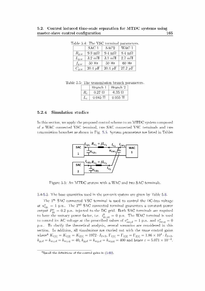
5.2. Control induced time-scale separation for MTDC systems using
master-slave control conguration 165
Table 5.4: The VSC terminal parameters.SAC 1 SAC2 WAC 1
Rg,w 9.9 mΩ 9.4 mΩ 8.4 mΩ
Lg,w 3.2 mH 3.1 mH 2.7 mH
fg,w 50 Hz 50 Hz 60 Hz
Cg,w 20.4 µF 20.4 µF 27.2 µF
Table 5.5: The transmission branch parameters.Branch 1 Branch 2
Rc 0.27 Ω 0.33 Ω
Lc 0.045 H 0.055 H
5.2.4 Simulation studies
In this section, we apply the proposed control scheme to an MTDC system composed
of a WAC connected VSC terminal, two SAC connected VSC terminals and two
transmission branches as shown in Fig. 5.5. System parameters are listed in Tables
Figure 5.5: An MTDC system with a WAC and two SAC terminals.
5.4-5.5. The base quantities used in the per-unit system are given by Table 5.6.
The 1st SAC connected VSC terminal is used to control the DC-bus voltage
at uocg1 = 1 p.u.. The 2nd SAC connected terminal guarantees a constant power
output P og2 = 0.2 p.u. injected to the DC grid. Both SAC terminals are required
to have the unitary power factor, i.e. i0g1,2q = 0 p.u. The WAC terminal is used
to control its AC voltage at the prescribed values of vosw1d= 1 p.u. and vosw1q = 0
p.u.. To clarify the theoretical analysis, several scenarios are considered in this
section. In addition, all simulations are carried out with the same control gains
where4 K1[1] = K1[2] = K2[1] = 1972 · I2×2, Γ1[1] = Γ1[2] = Γ2[1] = 1.86× 10⁴ · I2×2,
kg1d = kw11d = kw11q = 40, kg2d = kw21d = kw22q = 400 and hence ε = 5.071× 10⁻⁴.
4Recall the denitions of the control gains in (5.60).
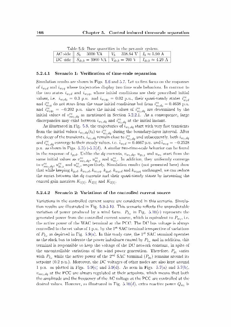
166 Chapter 5. Control induced time-scale separation
Table 5.6: Base quantities in the per-unit system.AC side Sb = 3000 VA Vb = 338.84 V Ib ≈ 5.90 A
DC side Sdc,b = 3000 VA Vdc,b = 700 V Idc,b ≈ 4.29 A
5.2.4.1 Scenario 1: Verication of time-scale separation
Simulation results are shown in Figs. 5.6 and 5.7. Let us rst focus on the responses
of iw1d and iw1q whose trajectories display two-time-scale behaviors. In contrast to
the two states iw1d and iw1q, whose initial conditions are their prescribed initial
values, i.e. iw1d0 = 0.3 p.u. and iw1q0 = 0.02 p.u., their quasi-steady states irew1d
and irew1q do not start from the same initial conditions but from irew1d0= 0.4638 p.u.
and irew1q0 = −0.202 p.u. since the initial values of irew1,dqare determined by the
initial values of vresw1,dqas mentioned in Section 5.2.2.1. As a consequence, large
discrepancies may exist between iw1,dq and irew1,dq
at the initial instant.
As illustrated in Fig. 5.8, the trajectories of iw1,dq start with very fast transients
from the initial values iw1,dq(t0) to irew1,dqduring the boundary-layer interval. After
the decay of the transients, iw1,dq remain close to irew1,dqand subsequently, both iw1,dq
and irew1,dqconverge to their steady values, i.e. iw1d = 0.4667 p.u. and iw1q = −0.2528
p.u. as shown in Figs. 5.7(c)-5.7(d). A similar two-time-scale behavior can be found
in the response of ig1d. Unlike the dq currents, vw1,dq, ug1,2 and uw1 start from the
same initial values as vresw1,dq, ureg1,2 and urew1
. In addition, they uniformly converge
to vresw1,dq, ureg1,2 and urew1
, respectively. Simulation results (not presented here) show
that while keeping kg1d, kw11d, kw11q, kg2d, kw21d and kw22q unchanged, we can reduce
the errors between the dq currents and their quasi-steady states by increasing the
control gain matrices K1[1], K2[1] and K2[1].
5.2.4.2 Scenario 2: Variations of the controlled current source
Variations in the controlled current source are considered in this scenario. Simula-
tion results are illustrated in Fig. 5.9-5.10. This scenario reects the unpredictable
variation of power produced by a wind farm. PIw in Fig. 5.10(c) represents the
generated power from the controlled current source, which is equivalent to Pw1 , i.e.
the active power of the WAC terminal at the PCC. The DC-bus voltage is always
controlled to the set value of 1 p.u. by the 1st SAC terminal irrespective of variations
of PIw as depicted in Fig. 5.9(a). In this study case, the 1st SAC terminal operates
as the slack bus to tolerate the power imbalance caused by PIw and in addition, this
terminal is responsible to keep the voltage of the DC network constant, in spite of
the uncontrollable variations of the wind power generation. Therefore, Pg1 varies
with PIw while the active power of the 2nd SAC terminal (Pg2) remains around its
setpoint (0.2 p.u.). Moreover, the DC voltages of other nodes are also kept around
1 p.u. as plotted in Figs. 5.9(c) and 5.9(d). As seen in Figs. 5.7(a) and 5.7(b),
vsw1,dq at the PCC are always regulated at their setpoints, which means that both
the amplitude and the frequency of the AC voltage at the PCC are controlled at the
desired values. However, as illustrated in Fig. 5.10(d), extra reactive power Qw1 is
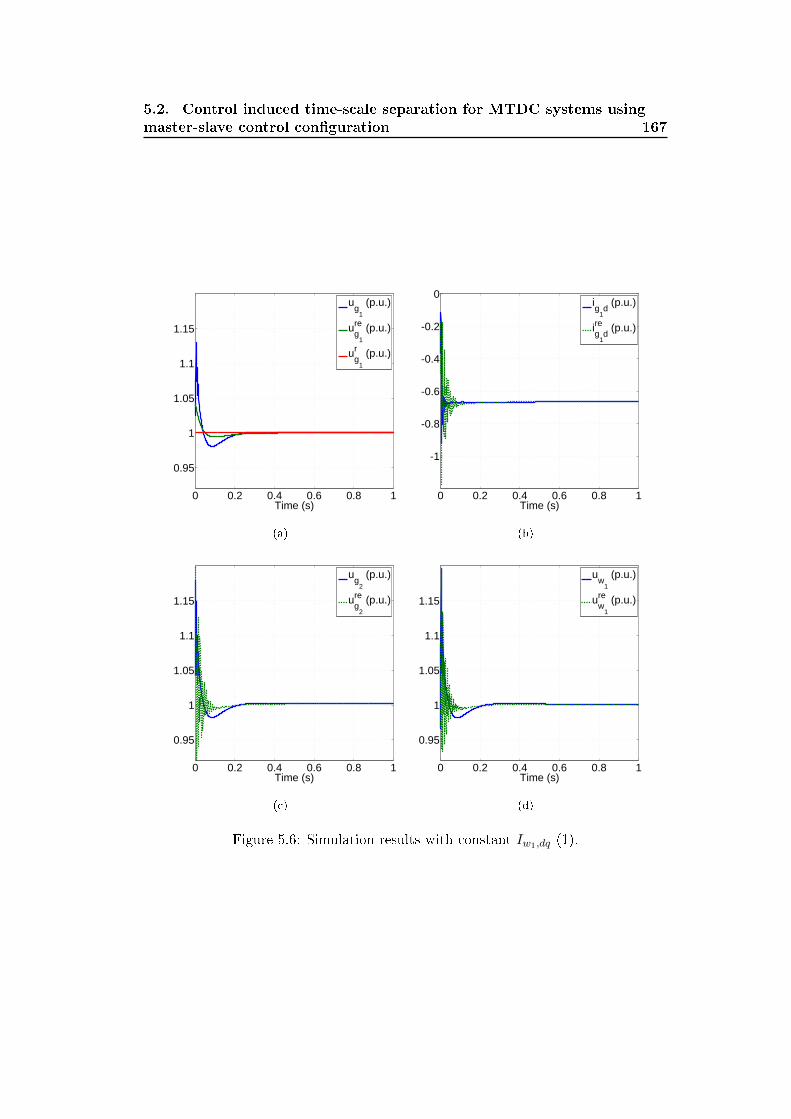
5.2. Control induced time-scale separation for MTDC systems using
master-slave control conguration 167
0 0.2 0.4 0.6 0.8 1
0.95
1
1.05
1.1
1.15
Time (s)
ug
1
(p.u.)
ug
1
re (p.u.)
ug
1
r (p.u.)
(a)
0 0.2 0.4 0.6 0.8 1
-1
-0.8
-0.6
-0.4
-0.2
0
Time (s)
ig
1d (p.u.)
ig
1d
re (p.u.)
(b)
0 0.2 0.4 0.6 0.8 1
0.95
1
1.05
1.1
1.15
Time (s)
ug
2
(p.u.)
ug
2
re (p.u.)
(c)
0 0.2 0.4 0.6 0.8 1
0.95
1
1.05
1.1
1.15
Time (s)
uw
1
(p.u.)
uw
1
re (p.u.)
(d)
Figure 5.6: Simulation results with constant Iw1,dq (1).
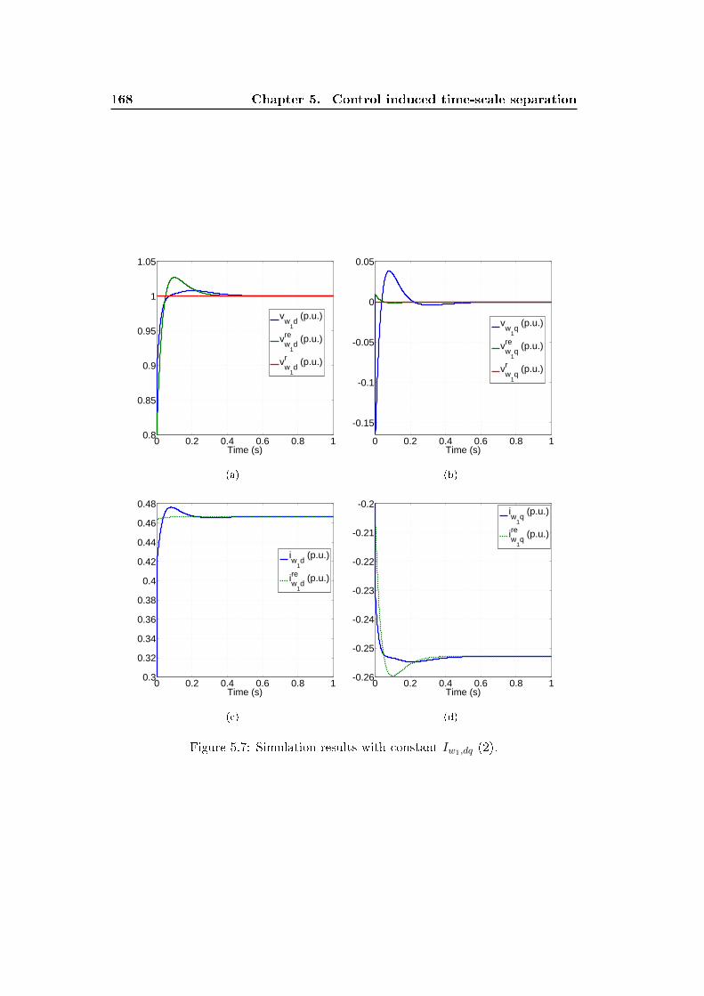
168 Chapter 5. Control induced time-scale separation
0 0.2 0.4 0.6 0.8 10.8
0.85
0.9
0.95
1
1.05
Time (s)
vw
1d (p.u.)
vw
1d
re (p.u.)
vw
1d
r (p.u.)
(a)
0 0.2 0.4 0.6 0.8 1
-0.15
-0.1
-0.05
0
0.05
Time (s)
vw
1q (p.u.)
vw
1q
re (p.u.)
vw
1q
r (p.u.)
(b)
0 0.2 0.4 0.6 0.8 10.3
0.32
0.34
0.36
0.38
0.4
0.42
0.44
0.46
0.48
Time (s)
iw
1d (p.u.)
iw
1d
re (p.u.)
(c)
0 0.2 0.4 0.6 0.8 1-0.26
-0.25
-0.24
-0.23
-0.22
-0.21
-0.2
Time (s)
iw
1q (p.u.)
iw
1q
re (p.u.)
(d)
Figure 5.7: Simulation results with constant Iw1,dq (2).
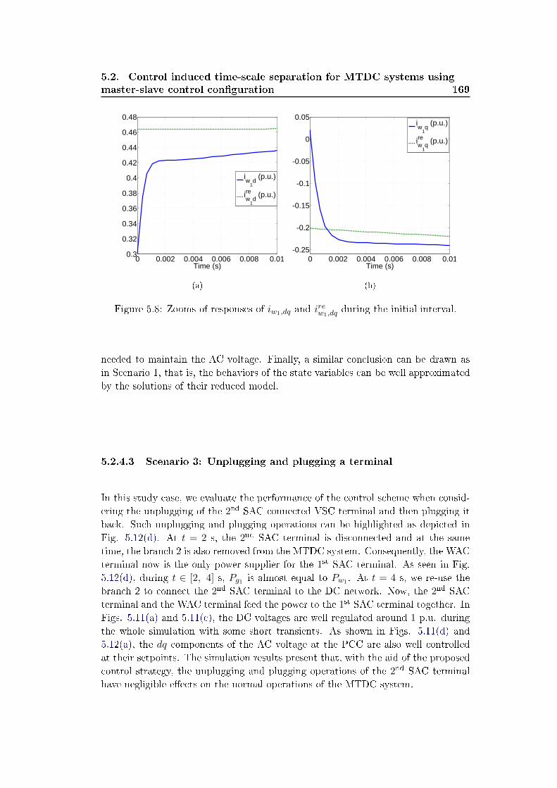
5.2. Control induced time-scale separation for MTDC systems using
master-slave control conguration 169
0 0.002 0.004 0.006 0.008 0.010.3
0.32
0.34
0.36
0.38
0.4
0.42
0.44
0.46
0.48
Time (s)
iw
1d (p.u.)
iw
1d
re (p.u.)
(a)
0 0.002 0.004 0.006 0.008 0.01-0.25
-0.2
-0.15
-0.1
-0.05
0
0.05
Time (s)
iw
1q (p.u.)
iw
1q
re (p.u.)
(b)
Figure 5.8: Zooms of responses of iw1,dq and irew1,dq
during the initial interval.
needed to maintain the AC voltage. Finally, a similar conclusion can be drawn as
in Scenario 1, that is, the behaviors of the state variables can be well approximated
by the solutions of their reduced model.
5.2.4.3 Scenario 3: Unplugging and plugging a terminal
In this study case, we evaluate the performance of the control scheme when consid-
ering the unplugging of the 2nd SAC connected VSC terminal and then plugging it
back. Such unplugging and plugging operations can be highlighted as depicted in
Fig. 5.12(d). At t = 2 s, the 2nd SAC terminal is disconnected and at the same
time, the branch 2 is also removed from the MTDC system. Consequently, the WAC
terminal now is the only power supplier for the 1st SAC terminal. As seen in Fig.
5.12(d), during t ∈ [2, 4] s, Pg1 is almost equal to Pw1 . At t = 4 s, we re-use the
branch 2 to connect the 2nd SAC terminal to the DC network. Now, the 2nd SAC
terminal and the WAC terminal feed the power to the 1st SAC terminal together. In
Figs. 5.11(a) and 5.11(c), the DC voltages are well regulated around 1 p.u. during
the whole simulation with some short transients. As shown in Figs. 5.11(d) and
5.12(a), the dq components of the AC voltage at the PCC are also well controlled
at their setpoints. The simulation results present that, with the aid of the proposed
control strategy, the unplugging and plugging operations of the 2nd SAC terminal
have negligible eects on the normal operations of the MTDC system.
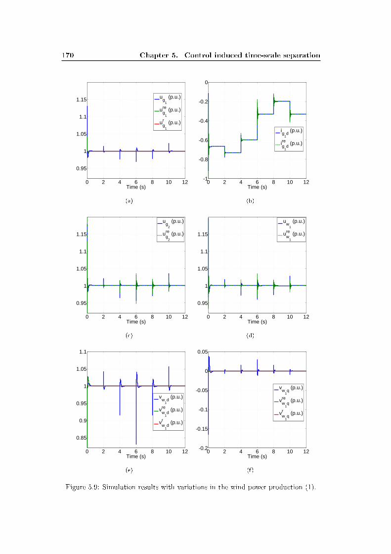
170 Chapter 5. Control induced time-scale separation
0 2 4 6 8 10 12
0.95
1
1.05
1.1
1.15
Time (s)
ug
1
(p.u.)
ug
1
re (p.u.)
ug
1
r (p.u.)
(a)
0 2 4 6 8 10 12-1
-0.8
-0.6
-0.4
-0.2
0
Time (s)
ig
1d (p.u.)
ig
1d
re (p.u.)
(b)
0 2 4 6 8 10 12
0.95
1
1.05
1.1
1.15
Time (s)
ug
2
(p.u.)
ug
2
re (p.u.)
(c)
0 2 4 6 8 10 12
0.95
1
1.05
1.1
1.15
Time (s)
uw
1
(p.u.)
uw
1
re (p.u.)
(d)
0 2 4 6 8 10 12
0.85
0.9
0.95
1
1.05
1.1
Time (s)
vw
1d (p.u.)
vw
1d
re (p.u.)
vw
1d
r (p.u.)
(e)
0 2 4 6 8 10 12-0.2
-0.15
-0.1
-0.05
0
0.05
Time (s)
vw
1q (p.u.)
vw
1q
re (p.u.)
vw
1q
r (p.u.)
(f)
Figure 5.9: Simulation results with variations in the wind power production (1).
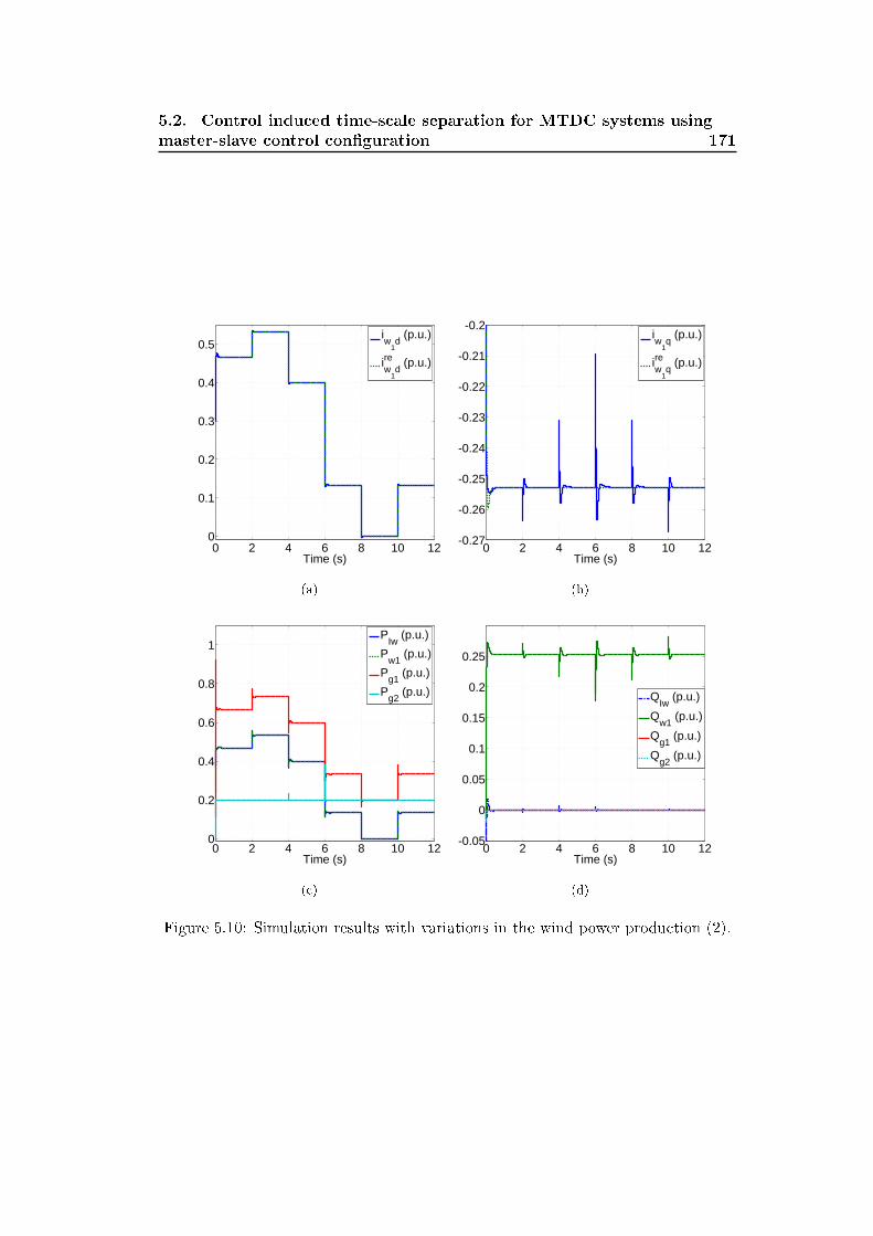
5.2. Control induced time-scale separation for MTDC systems using
master-slave control conguration 171
0 2 4 6 8 10 120
0.1
0.2
0.3
0.4
0.5
Time (s)
iw
1d (p.u.)
iw
1d
re (p.u.)
(a)
0 2 4 6 8 10 12-0.27
-0.26
-0.25
-0.24
-0.23
-0.22
-0.21
-0.2
Time (s)
iw
1q (p.u.)
iw
1q
re (p.u.)
(b)
0 2 4 6 8 10 120
0.2
0.4
0.6
0.8
1
Time (s)
PIw
(p.u.)
Pw1
(p.u.)
Pg1
(p.u.)
Pg2
(p.u.)
(c)
0 2 4 6 8 10 12-0.05
0
0.05
0.1
0.15
0.2
0.25
Time (s)
QIw
(p.u.)
Qw1
(p.u.)
Qg1
(p.u.)
Qg2
(p.u.)
(d)
Figure 5.10: Simulation results with variations in the wind power production (2).
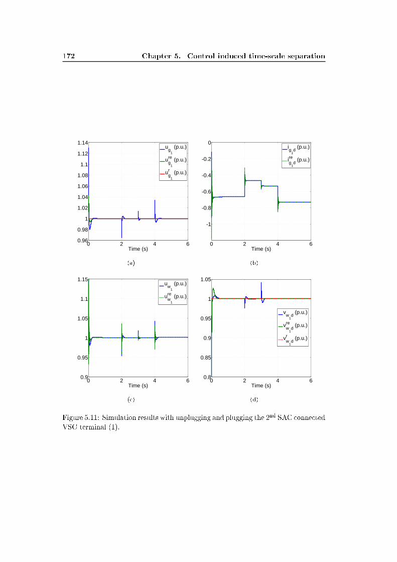
172 Chapter 5. Control induced time-scale separation
0 2 4 60.96
0.98
1
1.02
1.04
1.06
1.08
1.1
1.12
1.14
Time (s)
ug
1
(p.u.)
ug
1
re (p.u.)
ug
1
r (p.u.)
(a)
0 2 4 6
-1
-0.8
-0.6
-0.4
-0.2
0
Time (s)
ig
1d (p.u.)
ig
1d
re (p.u.)
(b)
0 2 4 60.9
0.95
1
1.05
1.1
1.15
Time (s)
uw
1
(p.u.)
uw
1
re (p.u.)
(c)
0 2 4 60.8
0.85
0.9
0.95
1
1.05
Time (s)
vw
1d (p.u.)
vw
1d
re (p.u.)
vw
1d
r (p.u.)
(d)
Figure 5.11: Simulation results with unplugging and plugging the 2nd SAC connected
VSC terminal (1).
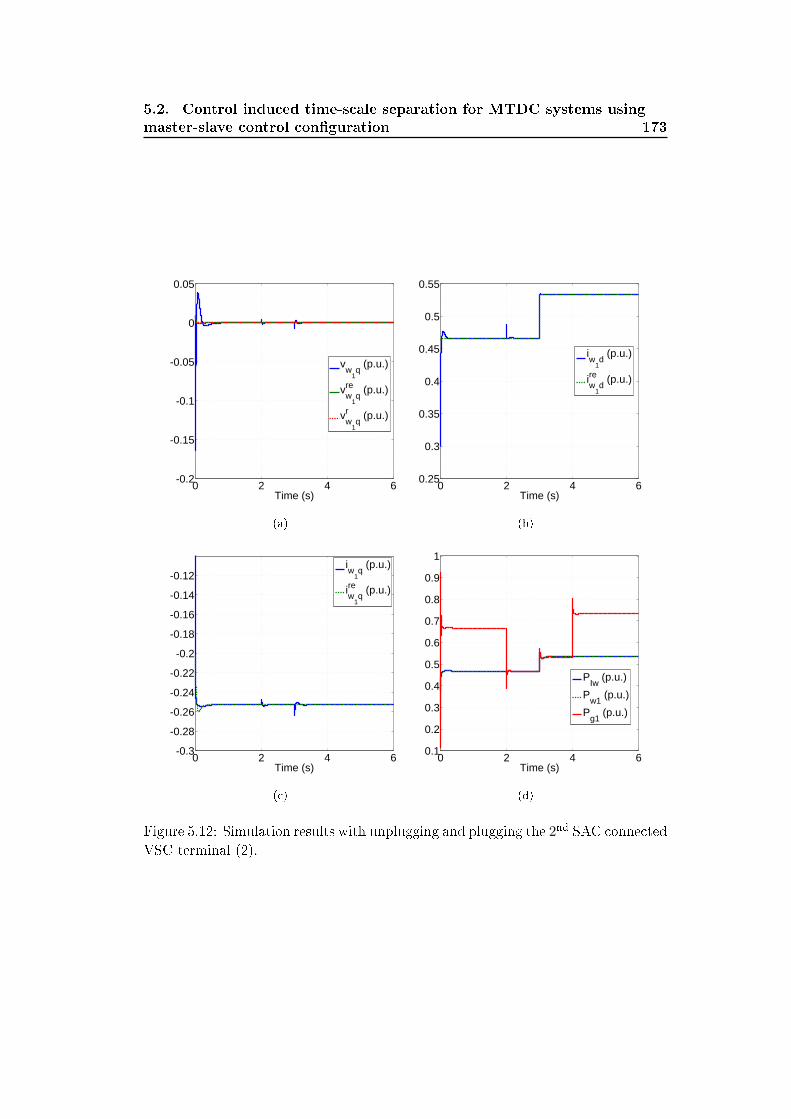
5.2. Control induced time-scale separation for MTDC systems using
master-slave control conguration 173
0 2 4 6-0.2
-0.15
-0.1
-0.05
0
0.05
Time (s)
vw
1q (p.u.)
vw
1q
re (p.u.)
vw
1q
r (p.u.)
(a)
0 2 4 60.25
0.3
0.35
0.4
0.45
0.5
0.55
Time (s)
iw
1d (p.u.)
iw
1d
re (p.u.)
(b)
0 2 4 6-0.3
-0.28
-0.26
-0.24
-0.22
-0.2
-0.18
-0.16
-0.14
-0.12
Time (s)
iw
1q (p.u.)
iw
1q
re (p.u.)
(c)
0 2 4 60.1
0.2
0.3
0.4
0.5
0.6
0.7
0.8
0.9
1
Time (s)
PIw
(p.u.)
Pw1
(p.u.)
Pg1
(p.u.)
(d)
Figure 5.12: Simulation results with unplugging and plugging the 2nd SAC connected
VSC terminal (2).
174 Chapter 5. Control induced time-scale separation
5.3 Control induced time-scale separation for MTDC
systems using droop control conguration
As described in the previous sections, for an MTDC system, the control of DC
voltage is indispensable. In Sections 4.1.4, 4.3 and 5.2, we have discussed the
master-slave conguration. In this control conguration, only one VSC terminal
(the master terminal) is used to regulate the DC voltage at a constant level while
the other terminals operate in other control mode. The responsibility for main-
taining power ow balance obviously falls on the master terminal. However, the
disconnection of the master terminal leads the DC voltage beyond the safe domain
of operation and thereby, damages the components of MTDC systems. In order
to overcome this drawback, DC voltage droop control conguration [Wang 2014a,
Prieto-Araujo 2011, Chaudhuri 2013, Bianchi 2011, Egea-Alvarez 2013, Chen 2014],
usually characterized by power vs DC voltage (P vs U) or current vs DC voltage (I
vs U) curves, becomes an alternative method, in particular for a large network.
In a DC voltage droop control scheme, more than one terminal is in charge of
regulating the DC voltage and hence, the burden caused by power imbalance could
be shared between several terminals. Additionally, this control method takes actions
only based on local information without relying on remote communication. In droop
control, the droop gains specify the system operation in steady-state condition and
also have a great eect on the system transient performance. Dierent methodologies
of choosing droop gains have been investigated. In [Prieto-Araujo 2011], a criterion
for tuning the droop gains based on the performance specications is proposed. In
[Bianchi 2011], the droop gains are obtained by solving a constraint convex opti-
mization problem. Reference [Chaudhuri 2013] develops an adaptive droop control
scheme according to each terminal's available spare capacity. However, prior studies
are usually under the unproven assertion that the dynamics of the inductor currents
are much faster than the dynamics of the DC network. Therefore, the currents
through the converters are assumed to equal their references and then, the dynamic
interaction between AC and DC sides of the converters can be neglected.
Similar to the study on master-slave control conguration in Section 5.2, in
this section, we acknowledge this assertion, then explore and explain the droop
control induced time-scale separation. To achieve this aim, we will carry out a full
theoretical analysis of the time-scale separation between the system state variables,
mainly based on the theoretical results in Section 5.1. Furthermore, we will also
demonstrate that the control gains have dierent eects on the system performance.
For example, the droop gains play a major role in regulating the DC grid dynamics.
Another objective of this section is to study the eects of the control gains, especially
the droop gains, on the system stability.
5.3.1 VSC operation
The greatest dierence between master-slave and droop control conguration is that
the latter involves more terminals in the regulation of the DC voltage. This dierence
5.3. Control induced time-scale separation for MTDC systems using
droop control conguration 175
leads to dierent VSC operation in droop control conguration, which is summarized
as follows:
• Same to master-slave control conguration, to ensure that the power gener-
ated by the wind farms can be totally delivered via the DC grid, all WAC
connected VSC terminals are still used to maintain their AC voltage magni-
tudes and frequencies constant at the PCCs, achieved by regulating vswj ,dq at
the prescribed values voswj ,dq.
• Every SAC terminal is equipped with the DC droop controller such that the
duty of eliminating the power imbalance of the DC grid is shared between the
SAC terminals. Moreover, the reactive powers of all the SAC terminals at the
PCCs, i.e. Qgi , are required to track the reference values Qogi .
5.3.2 Droop control structure
The control design of droop control conguration is similar to that of master-slave
control conguration in Section 5.2.1, which consists of two control loops, a fast
inner current and a slow outer control loop, where the dynamics of state variables
in the fast control loop are much faster than those in the slow control loop. But, in
droop control structure, a droop law is implemented in the slow outer control loop
of all SAC terminals, which generates the reference to the fast inner control loop.
5.3.2.1 Design of the fast control loop
As mentioned in Section 5.2.1.1, the control inputs m(·),dq are directly collocated
with the dq currents i(·),dq. Hence, a sub-controller can be developed such that
i(·),dq quickly converge to their reference trajectories i∗(·),dq yet to be designed.
We rst dene the dq current tracking errors by
eigi,dq = igi,dq − i∗gi,dq
eiwj,dq = iwj ,dq − i∗wj ,dq
With the introduction of the integrated tracking errors eIigi,dq and eIiwj,dq , an aug-
176 Chapter 5. Control induced time-scale separation
mented dq current subsystem is then generated by
deIigid
dt= eigid
deigid
dt= −Rgi
Lgiigid + ωgiigiq +
vsgidLgi−mgiducgi
2Lgi−di∗giddt
deIigiq
dt= eigiq
deigiq
dt= −Rgi
Lgiigiq − ωgiigid +
vsgiqLgi− mgiqucgi
2Lgi−di∗giqdt
deIiwid
dt= eiwid
deiwjd
dt= −
RwjLwj
iwjd + ωwj iwjq +vswjd
Lwj−mwjducwj
2Lwj−di∗wjd
dtdeIiwiq
dt= eiwiq
deiwjq
dt= −
RwjLwj
iwjq − ωwj iwjd +vswjq
Lwj−mwjqucwj
2Lwj−di∗wjq
dt
(5.89)
In practice, the dynamics of i∗gi,dq and i∗wj ,dq
are usually neglected and considered
as slow compared to igi,dq and iwj ,dq. As a result, the modulation indices can then
be designed as
mgid =2Lgiucgi
(−RgiLgi
igid + ωgiigiq +vsgidLgi
+ k1gideigid + k2gideIigid)
mgiq =2Lgiucgi
(−RgiLgi
igiq − ωgiigid +vsgiqLgi
+ k1giqeigiq + k2giqeIigiq)
mwjd =2Lwjucwj
(−RwjLwj
iwjd + ωwj iwjq +vswjd
Lwj+ k1wideiwid + k2wideIiwid)
mwjq =2Lwjucwj
(−RwjLwj
iwjq − ωwj iwjd +vswjq
Lwj+ k1wiqeiwiq + k2wiqeIiwiq)
(5.90)
with positive control gains k1gi,dq, k2gi,dq, k1wj ,dq and k2wj ,dq.
5.3.2.2 Design of the slow control loop
The main task of the slow control loop is to provide the slowly varying dq current
references to the fast control loop. Most importantly, the dq current references need
to be designed such that all control objectives are achieved. Since the operations of
SAC terminals and WAC terminals are dierent, the design principles of i∗gi,dq and
i∗wj ,dq are also dierent.
Design of i∗wj ,dq
We assume that iwj ,dq can quickly converge to their reference trajectories i∗wjdq
under
the sub-controller (5.90). From there on, the AC voltage dynamics (3.29) of the wind
5.3. Control induced time-scale separation for MTDC systems using
droop control conguration 177
farm at the PCC become
dvswjd
dt= ωwjvswjq +
1
Cfwj(Iwjd − i∗wjd)
dvswjq
dt= −ωwjvswjd +
1
Cfwj(Iwjq − i∗wjq)
(5.91)
where i∗wjdq can be viewed as the control inputs. We call (5.91) the reduced model
of (3.29) since the dynamics of iwj ,dq are neglected and iwj ,dq are replaced by i∗wj ,dq.
The control objective of WAC terminals is to keep vswj ,dq at their reference values
voswj ,dq in spite of variations in the power productions of the wind farms. We then
want to develop i∗wj ,dq in such a way that vswj ,dq in (5.91) can be controlled at voswj ,dq
.
Similar to the design procedure of the fast control loop, we dene the output tracking
errors of voltage at the PCC as
evswj,dq = vswj ,dq − voswj ,dq
(5.92)
We then augment (5.91) by taking the integrated tracking errors into account
deIvswjd
dt= evswjd
devswjd
dt=
1
Cfwj(Iwjd + Cfwjωwjvswjq − i∗wjd)−
dvoswjd
dtdeIvswjq
dt= evswjq
devswjdq
dt=
1
Cfwj(Iwjq − Cfwjωwjvswjd − i∗wjq)−
dvoswjq
dt
(5.93)
Since the prescribed values voswj ,dq are constant, we havedvoswj ,dq
dt= 0. Finally, i∗wj ,dq
can be designed as
i∗wjd= Iwjd + Cfwj (k1djevswjd + k2djeIvswjd + ωwjvswjq)
i∗wjq= Iwjq + Cfwj (k1qjevswjq + k2qjeIvswjq − ωwjvswjd)(5.94)
with positive k1,dqj and k2,dqj such that the equilibrium of the augmented model
(5.93) is exponentially stable.
Design of i∗gi,dq
As mentioned before, a droop law is implemented in the slow outer control loop of
all SAC terminal so that all SAC terminals participate in the regulation of the DC
voltage in case of power imbalance. The droop control is usually expressed by DC
voltage versus active power characteristic [Haileselassie 2012b].
Pgi = P ogi +Kdi(uocgi − ucgi) (5.95)
where uocgi and P ogi refer to the reference values of DC voltage and active power
respectively. The droop gain Kdi is the ratio of the change in DC voltage to the
178 Chapter 5. Control induced time-scale separation
change in active power. According to (5.95), the varying reference for igid can be
expressed by
i∗gid = iogid − kdi(ucgi − uocgi) (5.96)
where iogid is obtained from (3.22) and expressed as
iogid =2P ogi
3vsgid
In addition, the relation between Kdi and kdi is given by
kdi =2
3
1
vsgidKdi
The reference of igiq is directly provided by the prescribed reference value
i∗giq= iogiq
= −2
3
Qogivsgid
(5.97)
5.3.3 Theoretical analysis
As the master-slave control structure in Section 5.2.1, the developed droop control
design concept is also mainly based on the assumption that a dynamic separation in
time scales is imposed between the fast and slow control loops. As a consequence,
z and vswj ,dq can be considered as constant in the fast control loop, while the dq
currents can be replaced by their references in the slow control loop.
In this section, we give a detailed theoretical analysis to demonstrate the va-
lidity of the time-scale separation assumption in droop control conguration and
furthermore, to investigate the possible limitations on the droop gains.
5.3.3.1 Equilibrium analysis
Before going further, we give a brief analysis of the equilibruim point. Substituting
the controller composed by (5.90), (5.94) ,(5.96) and (5.97) into the plant model de-
scribed by (3.20), (3.28), (3.29) and (3.36) leads to the following augmented closed-
5.3. Control induced time-scale separation for MTDC systems using
droop control conguration 179
loop system
deIigid
dt= eigid
digiddt
= −k1gideigid − k2gideIigiddeIigiq
dt= eigiq
digiqdt
= −k1giqeigiq − k2giqeIigiqdeIiwjd
dt= eiwjd
diwjd
dt= −k1wjdeiwjd − k2wjdeIiwjd
deIiwjq
dt= eiwjq
diwjq
dt= −k1wjqeiwjq − k2wjqeIiwjq
deIvswjd
dt= evswjd
dvswjd
dt= −k1djevswjd − k2djeIvswjd −
eiwjd
CfwjdeIvswjq
dt= evswjq
dvswjq
dt= −k1qjevswjq − k2qjeIvswjq −
eiwjq
Cfwjz= Az + ϑ
(5.98)
It will be more convenient in the following analysis to divide ϑ into two parts as
ϑ = ϑg + ϑw
Recalling icgi in (3.23), icwi in (3.32), i∗wj ,dq in (5.94) and i∗gi,dq in (5.96) and (5.97),
the new variables ϑg and ϑw are given by
ϑg = ϑg1 + ϑg2 + ϑg3 , ϑw = ϑw1 + ϑw2 + ϑw3 + ϑw4
with
ϑg1(i)=
3
2Cgi
vsgidiogid
+ vsgiqiogiq
ucgi, i ∈ N
0. otherwise
ϑg2(i)=
−3
2Cgivsgidkdi
ucgi − uocgiucgi
, i ∈ N
0. otherwise
ϑg3(i)=
3
2Cgi
vsgideigid + vsgiqeigiq
ucgi, i ∈ N
0. otherwise
180 Chapter 5. Control induced time-scale separation
and
ϑw1(j +N)=
3
2Cwj
voswjdIwjd + voswjqIwjq
ucwj, j ∈M
0. otherwise
ϑw2(j +N)=
3
2Cwj
[voswjdCfwjωwjevswjq + evswjdIwjd
ucwj
+evswjqIwjq − v
oswjqCfwjωwjevswjd
ucwj
],
j ∈M0. otherwise
ϑw3(j +N)=
3
2Cwj
[vswjd(k1djevswjd + k2djeIvswjd)
ucwj
+vswjq(k1qjevswjq + k2qjeIvswjq)
ucwj
],
j ∈M0. otherwise
ϑw4(j +N)=
3
2Cwj
vswjdeiwjd + vswjqeiwjq
ucwj, j ∈M
0. otherwise
It is obvious that, if the dq currents quickly enter their respective manifolds, i.e.
eigi,dq → 0 and eiwj,dq → 0, ϑg3 and ϑw4 converge to zero. Moreover, ϑw2 and ϑw3
also go to zero as evswj,dq → 0. These results are helpful for the theoretical analysis
in the next part.
When the closed-loop system (5.98) is in the steady-state condition, the following
algebraic equations
Az + ϑg + ϑw = 0 (5.99)
must hold5. Since P ogi = 3/2(vsgidiogid
+ vsgiqiogiq), ϑg and ϑw can be then expressed
as
ϑg(i)=
P 0gi +
3
2kdivsgidu
ocgi
Cgi ugi−
3vsgid2Cgi
kdi , i ∈ N
0. otherwise
ϑw(j +N)=
P owj
Cwjucwj, j ∈M
0. otherwise
(5.100)
where we introduced the new variable
P owj = 3/2(voswjdIwjd + voswjqIwjq)
5Recall that the notation (·) denotes the steady-state value of the variable (·).
5.3. Control induced time-scale separation for MTDC systems using
droop control conguration 181
From the algebraic equation (5.99), it is shown that the prescribed values (·)o, theDC grid topology and the droop gains kdi determine the steady-state values of the
system variables and the distribution of power sharing together in case of power
imbalance. The control gains k1gi,dq, k2gi,dq, k1wj ,dq, k2wj ,dq, k1,dqj and k2,dqj have
no eect on the steady state of the system. However, as (4.58) in Section 4.1.4 and
(4.96) in Section 4.3.2, solving equation (5.99) to get the exact steady-state value is
not easy and is not considered in this section. More details about this issue can be
referred in [Wang 2014a, Haileselassie 2012b].
To ensure the operating feasibility of the MTDC system, we assume that igidq,
iwjdq, ucgi , ucwj , ucth and ick exist and belong to their respective safe operating
domains. The equilibrium of the closed-loop system is denoted by S.
In stead-state condition, From the droop law (5.95), we have
Pgi = P ogi +Kdi(uocgi − ucgi) (5.101)
Consider that the MTDC system initially (t = t0) operates in a steady-state con-
dition, if the production of the wind farms increases at the instant t1, this makes
the SAC terminals absorb more power from the DC grid. When the MTDC sys-
tem achieves a new steady state at t2, we have Pgi(t2) < Pgi(t0) (for example,
Pgi(t0) = −100 MW and Pgi(t2) = −200 MW). According to (5.101), we can de-
duce that the DC voltage also rises to a new level and that ugi(t2) > ugi(t0). It can
be summarized that ucgi will rise if more power is injected into the DC grid, and
vice versa. This statement will be illustrated by numerical simulations in Section
5.3.4.
5.3.3.2 Multi-time-scale dynamics
In this section, a theoretical analysis to describe the dynamic separation in time-
scales is carried out. We present that two dierent dynamics are created by the
designed control algorithm in Section 5.3.2. In particular, the two time-scales are
quantied by the fast control gains k1gi,dq, k2gi,dq, k1wj ,dq and k2wj ,dq.
In order to make the analysis convenient, we perform a change of variables.

182 Chapter 5. Control induced time-scale separation
Then, the rst eight equations of the closed-loop system (5.98) can be rewritten as
deIigid
dt= eigid
deigid
dt= −k1gideigid − k2gideIigid −
di∗giddt
deIigiq
dt= eigiq
deigiq
dt= −k1giqeigiq − k2giqeIigiq −
di∗giqdt
deIiwjd
dt= eiwjd
deiwjd
dt= −k1wjdeiwjd − k2wjdeIiwjd −
di∗wjd
dtdeIiwjq
dt= eiwjq
deiwjq
dt= −k1wjqeiwjq − k2wjqeIiwjq −
di∗wjq
dt
(5.102)
This shifts the quasi-steady states of the dq currents to the origin. Denote k1 =
min(k1gid, k2giq, k1wid, k2wiq) and then introduce a new variable ε satisfying εk1 = 1.
The subsystem (5.102) is given by
deIigid
dt= eigid
εdeigid
dt= −k1gideigid − εk2gideIigid − ε
di∗giddt
deIigiq
dt= eigiq
εdeigiq
dt= −k1giqeigiq − εk2giqeIigiq − ε
di∗giqdt
deIiwjd
dt= eiwjd
εdeiwjd
dt= −k1wjdeiwjd − εk2wjdeIiwjd − ε
di∗wjd
dtdeIiwjq
dt= eiwjq
εdeiwjq
dt= −k1wjqeiwjq − εk2wjqeIiwjq − ε
di∗wjq
dt
(5.103)
where
k1gid = εk1gid ≥ 1; k1giq = εk1giq ≥ 1
k1wjd = εk1wjd ≥ 1; k1wjq = εk1wjq ≥ 1
We dene a new time variable τ as
εdy
dt=dy
dτ(5.104)

5.3. Control induced time-scale separation for MTDC systems using
droop control conguration 183
Substituting (5.104) into (5.103) and then setting ε = 0, we obtain the following
autonomous systemdeigid
dτ= −k1gideigid
deigiq
dτ= −k1giqeigiq
deiwjd
dτ= −k1wjdeiwjd
deiwjq
dτ= −k1wjqeiwjq
(5.105)
which is called the boundary-layer model of the system (5.98). When ε → 0, it
seems that the time variable t and the slow state variables are frozen at their initial
values. By using Lyapunov analysis, the origin of the boundary system (5.105)
is exponentially stable. When the dq currents quickly converge to their reference
trajectories during the initial interval, the full-scale system (5.98) is degenerated
into the following reduced model
deIvswjd
dt= evswjd
dvswjd
dt= −k1djevswjd − k2djeIvswjd
deIvswjq
dt= evswjq
dvswjq
dt= −k1qjevswjq − k2qjeIvswjq
dz
dt= Az + ϑ′g + ϑ′w
(5.106)
where ϑ′g = ϑg1 + ϑg2 and ϑ′w = ϑw1 + ϑw2 + ϑw3 . In addition, the solution of the
reduced model (5.106) is denoted by (·)re. Now, we can state the rst result of this
section.
Theorem 5.3.1. Consider the system (5.98) where all state variables are restrict
to their respective safe operating domains for t ∈ [t0, t1]. There exists a positive
constant ε∗ such that for all 0 < ε = 1/k1 < ε∗, the system (5.98) has a unique
solution on [t0, t1], and the trajectories of the state variables can be approximated
by
igi,dq − i∗gi,dq(zre)− eigi,dq= O(ε)
iwj ,dq − i∗wj ,dq(zre, vreswj ,dq)− eiwj,dq= O(ε)
vswj ,dq − vreswj ,dq= O(ε)
z − zre= O(ε)
(5.107)
held uniformly for t ∈ [t0, t1] where eigi,dq and eiwj,dq are the solution of the
boundary-layer model (5.105)
eigi,dq= eigi,dq(t0) exp(−k1gi,dqτ)
eiwj,dq= eiwj,dq(t0) exp(−k1wj ,dqτ)(5.108)
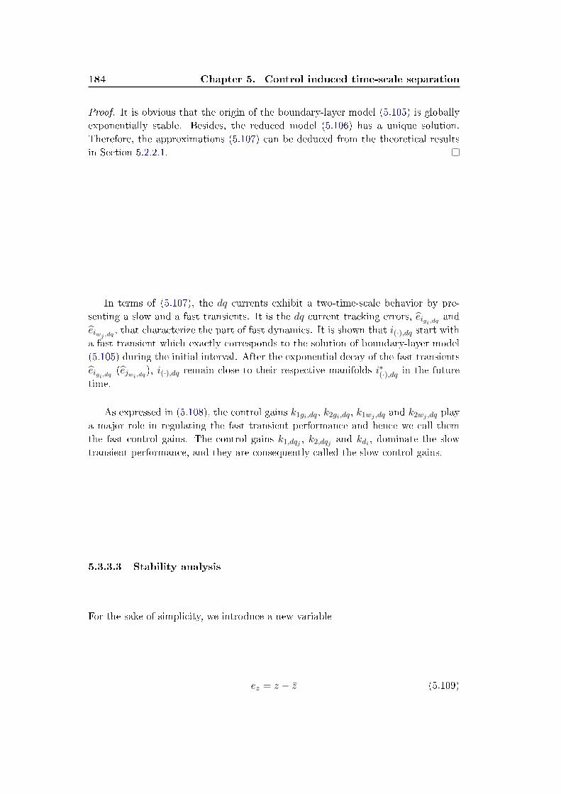
184 Chapter 5. Control induced time-scale separation
Proof. It is obvious that the origin of the boundary-layer model (5.105) is globally
exponentially stable. Besides, the reduced model (5.106) has a unique solution.
Therefore, the approximations (5.107) can be deduced from the theoretical results
in Section 5.2.2.1.
In terms of (5.107), the dq currents exhibit a two-time-scale behavior by pre-
senting a slow and a fast transients. It is the dq current tracking errors, eigi,dq and
eiwj,dq , that characterize the part of fast dynamics. It is shown that i(·),dq start with
a fast transient which exactly corresponds to the solution of boundary-layer model
(5.105) during the initial interval. After the exponential decay of the fast transients
eigi,dq (ejwi,dq), i(·),dq remain close to their respective manifolds i∗(·),dq in the future
time.
As expressed in (5.108), the control gains k1gi,dq, k2gi,dq, k1wj ,dq and k2wj ,dq play
a major role in regulating the fast transient performance and hence we call them
the fast control gains. The control gains k1,dqj , k2,dqj and kdi , dominate the slow
transient performance, and they are consequently called the slow control gains.
5.3.3.3 Stability analysis
For the sake of simplicity, we introduce a new variable
ez = z − z (5.109)
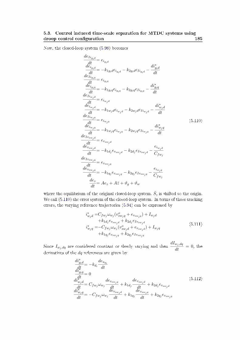
5.3. Control induced time-scale separation for MTDC systems using
droop control conguration 185
Now, the closed-loop system (5.98) becomes
deIigid
dt= eigid
deigid
dt= −k1gideigid − k2gideIigid −
di∗giddt
deIigiq
dt= eigiq
deigiq
dt= −k1giqeigiq − k2giqeIigiq −
di∗giqdt
deIiwjd
dt= eiwjd
deiwjd
dt= −k1wjdeiwjd − k2wjdeIiwjd −
di∗wjd
dtdeIiwjq
dt= eiwjq
deiwjq
dt= −k1wjqeiwjq − k2wjqeIiwjq −
di∗wjq
dtdeIvswjd
dt= evswjd
devswjd
dt= −k1djevswjd − k2djeIvswjd −
eiwjd
CfwjdeIvswjq
dt= evswjq
devswjq
dt= −k1qjevswjq − k2qjeIvswjq −
eiwjq
Cfwjdezdt
= Aez +Az + ϑg + ϑw
(5.110)
where the equilibrium of the original closed-loop system, S, is shifted to the origin.
We call (5.110) the error system of the closed-loop system. In terms of those tracking
errors, the varying reference trajectories (5.94) can be expressed by
i∗wjd =Cfwjωwj (voswjq + evswjq) + Iwjd
+k1djevswjd + k2djeIvswjdi∗wjq =−Cfwjωwj (voswjd + evswjd) + Iwjq
+k1qjevswjq + k2qjeIvswjq
(5.111)
Since Iwj ,dq are considered constant or slowly varying and thendIwj ,dq
dt= 0, the
derivatives of the dq references are given by
di∗giddt
= −kdideugidt
di∗giqdt
= 0
di∗wjd
dt= Cfwjωwj
devswjq
dt+ k1dj
devswjd
dt+ k2djevswjd
di∗wjq
dt= −Cfwjωwj
devswjd
dt+ k1qj
devswjq
dt+ k2qjevswjq
(5.112)
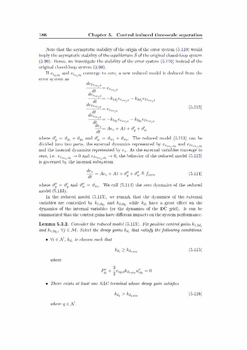
186 Chapter 5. Control induced time-scale separation
Note that the asymptotic stability of the origin of the error system (5.110) would
imply the asymptotic stability of the equilibrium S of the original closed-loop system
(5.98). Hence, we investigate the stability of the error system (5.110) instead of the
original closed-loop system (5.98).
If eigidq and eiwjdq converge to zero, a new reduced model is deduced from the
error system asdeIvswjd
dt= evswjd
devswjd
dt= −k1djevswjd − k2djeIvswjd
deIvswjq
dt= evswjq
devswjq
dt= −k1qjevswjq − k2qjeIvswjq
dezdt
= Aez +Az + ϑ′g + ϑ′w
(5.113)
where ϑ′g = ϑg1 + ϑg2 and ϑ′w = ϑw1 + ϑw2 . The reduced model (5.113) can be
divided into two parts, the external dynamics represented by evswj,dq and eIvswj,dqand the internal dynamics represented by ez. As the external variables converge to
zero, i.e. evswj,dq → 0 and eIvswj,dq → 0, the behavior of the reduced model (5.113)
is governed by the internal subsystem
dezdt
= Aez +Az + ϑ′′g + ϑ′′w , fzero (5.114)
where ϑ′′g = ϑ′g and ϑ′′w = ϑw1 . We call (5.114) the zero dynamics of the reduced
model (5.113).
In the reduced model (5.113), we remark that the dynamics of the external
variables are controlled by k1,dqj and k2,dqj while kdi have a great eect on the
dynamics of the internal variables (or the dynamics of the DC grid). It can be
summarized that the control gains have dierent impacts on the system performance.
Lemma 5.3.2. Consider the reduced model (5.113). Fix positive control gains k1,2dj
and k1,2qj , ∀j ∈M. Select the droop gains kdi that satisfy the following conditions:
• ∀i ∈ N , kdi is chosen such that
kdi ≥ kdimin(5.115)
where
P ogi +3
2vsgidkdimin
uocgi = 0
• There exists at least one SAC terminal whose droop gain satises
kdq > kdqmin(5.116)
where q ∈ N .
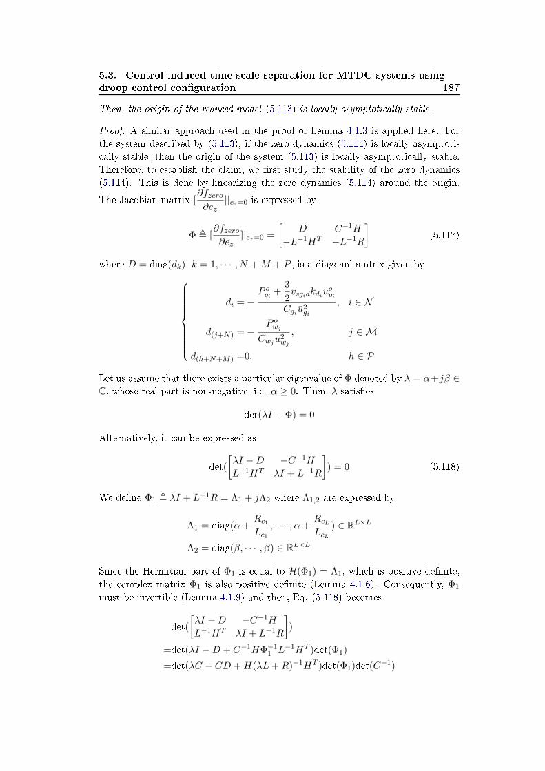
5.3. Control induced time-scale separation for MTDC systems using
droop control conguration 187
Then, the origin of the reduced model (5.113) is locally asymptotically stable.
Proof. A similar approach used in the proof of Lemma 4.1.3 is applied here. For
the system described by (5.113), if the zero dynamics (5.114) is locally asymptoti-
cally stable, then the origin of the system (5.113) is locally asymptotically stable.
Therefore, to establish the claim, we rst study the stability of the zero dynamics
(5.114). This is done by linearizing the zero dynamics (5.114) around the origin.
The Jacobian matrix [∂fzero∂ez
]|ez=0 is expressed by
Φ , [∂fzero∂ez
]|ez=0 =
[D C−1H
−L−1HT −L−1R
](5.117)
where D = diag(dk), k = 1, · · · , N +M + P , is a diagonal matrix given by
di =−P ogi +
3
2vsgidkdiu
ogi
Cgi u2gi
, i ∈ N
d(j+N) =−P owj
Cwj u2wj
, j ∈M
d(h+N+M) =0. h ∈ P
Let us assume that there exists a particular eigenvalue of Φ denoted by λ = α+jβ ∈C, whose real part is non-negative, i.e. α ≥ 0. Then, λ satises
det(λI − Φ) = 0
Alternatively, it can be expressed as
det(
[λI −D −C−1H
L−1HT λI + L−1R
]) = 0 (5.118)
We dene Φ1 , λI + L−1R = Λ1 + jΛ2 where Λ1,2 are expressed by
Λ1 = diag(α+Rc1Lc1
, · · · , α+RcLLcL
) ∈ RL×L
Λ2 = diag(β, · · · , β) ∈ RL×L
Since the Hermitian part of Φ1 is equal to H(Φ1) = Λ1, which is positive denite,
the complex matrix Φ1 is also positive denite (Lemma 4.1.6). Consequently, Φ1
must be invertible (Lemma 4.1.9) and then, Eq. (5.118) becomes
det(
[λI −D −C−1H
L−1HT λI + L−1R
])
=det(λI −D + C−1HΦ−11 L−1HT )det(Φ1)
=det(λC − CD +H(λL+R)−1HT )det(Φ1)det(C−1)
188 Chapter 5. Control induced time-scale separation
Again, we dene
Φ2= λC − CD +H(λL+R)−1HT
λC − CD= Λ3 + jΛ4
(λL+R)−1= Λ5 + jΛ6
(5.119)
with the notations
Λ3 = αC − CD , diag(σ1, · · · , σN+M+P )σi = Cgi(α+
P ogi +3
2vsgidkdiu
ogi
Cgi u2gi
), i ∈ N
σ(j+N) = Cwj (α+P owj
Cwj u2wj
), j ∈M
σ(h+N+M) = Cphα. h ∈ PΛ4 = βC
Λ5 = diag(αLck +Rck
(αLck +Rck)2 + (βLck)2) ∈ RL×L
Λ6 = diag(−βLck
(αLck +Rck)2 + (βLck)2) ∈ RL×L
(5.120)
Due to (5.116), we assume that kdq > kdq ,min, q ∈ N , where
P ogq +3
2vsgqdkdq .minu
ogq = 0 (5.121)
Now, Φ2 can be rewritten as
Φ2= Φ3 + j(Λ4 +HΛ6HT )
Φ3= Λq3 + Λq′
3 +HfHTf
(5.122)
where Λq3 is a diagonal matrix whose qth element on the main diagonal is σq and
other elements are zero. Λq′
3 and Hf are given by Λq′
3 = Λ3 − Λq3 and Hf = HΛ125 .
Let us dene Φ4 , Λq3 +HfHTf and then the determinant of Φ4 can be calculated
as
det(Φ4) = σq det(R(Hf )qR(Hf )Tq ) + det(HfHTf )
Since Λ125 is a full rank matrix, i.e. rank(Λ
125 ) = L, then rank(HfH
Tf ) = rank(Hf ) =
rank(H) = N + M + P − 1 and as a result, det(HfHTf ) = 0. Similar to Lemma
3.4.2, by removing any one row from Hf , such as Hf (j, :), j ∈ T , the rank of
the reduced matrix R(Hf )j is N + M + P − 1. Consequently, R(Hf )qR(Hf )Tq is
invertible and positive denite. Since kdq satises (5.121), we get σq > 0 and then,
det(Φ4) = σq det(R(Hf )qR(Hf )Tq ) > 0. On the other hand, Φ4 and Λq3 are semi-
positive denite because of (5.115) and (5.116) and hence, Φ4 is positive denite.
Recalling that Φ3 = Φ4 + Λq′
3 , it turns out that, Φ3 is also positive denite. As
presented in (5.122), we know that H(Φ2) = Φ3 and then, according to Lemma 4.1.6
5.3. Control induced time-scale separation for MTDC systems using
droop control conguration 189
and Lemma 4.1.9, Φ2 is positive denite and invertible. Therefore, the following
result is obtained:
det(λI − Φ) = det(Φ2) det(Φ1) det(C−1) 6= 0
for α ≥ 0. This leads to a contradiction to (5.118). Thus, all eigenvalues of the
Jacobian matrix Φ must have negative real part, i.e. α < 0. Hence, Φ is a Hurwitz
matrix. As a result, the origin of the zero dynamics (5.114) is locally asymptotically
stable. Thus, the reduced model (5.113) is also locally asymptotically stable. The
proof is completed.
Now, we can introduce another result of this section.
Theorem 5.3.3. Consider the MTDC system modeled by (3.20), (3.28), (3.29)
and (3.36) with the control strategy (5.90), (5.94), (5.96) and (5.97). Select the
droop gains that satisfy the conditions (5.115) and (5.116) in Lemma 5.3.2. Then,
there exist the control gains k1gid, k2giq, k1wid, k2wiq, k1,2dj and k1,2qj such that
the equilibrium S of the closed loop system (5.98) is locally asymptotically stable.
Thereby, the proposed control strategy can stabilize the MTDC system.
Proof. As previously mentioned, to study the stability of the origin of the error
system (5.110) is equivalent to investigating the stability of the equilibrium S of the
closed-loop system (5.98). So we still focus on the stability property of the error
system (5.110).
We rewrite the last equation in (5.110) in the following special form
dezdt
= fzero + ϑg3 + ϑw2 + ϑw3 + ϑw4 (5.123)
According to Taylor's theorem, fzero can be expressed by
fzero = Φ · ez + fzero · ez
where fzero satises
lim||ez ||→0
||fzero|| = 0
It means that, for any given α0, there exists a region Bez such that
||fzero|| ≤ α0 (5.124)
for all ez ∈ Bez . In addition, since Φ is a Hurwitz matrix, for any positive denite
matrix Gez , there exists a positive denite matrix Fez such that
FezΦ + ΦTFez = −Gez (5.125)
190 Chapter 5. Control induced time-scale separation
To simplify the notations, we introduce the following variables
eig,dq,[eig1,dq eIig1,dq · · · eigN ,dq eIigN ,dq
]Teiw,dq,
[eiw1,dq
eIiw1,dq· · · eiwM,dq
eIiwM,dq
]Tevw,dq,
[evsw1,dq
eIvsw1,dq· · · evswM,dq
eIvswM,dq
]TConsider a Lyapunov function W = dW1 + (1− d)W2 where d ∈ (0, 1). W1 and
W2 are designed as
W1 =1
2(eTigdFigdeigd + eTigqFigqeigq
+ eTiwdFiwdeiwd + eTiwqFiwqeiwq)
and
W2 =1
2(eTvwdFvwdevwd + eTvwqFvwqevwq + eTz Fezez)
where
Fig,dq= diag(F iig,dq); Fiig,dq
=
[1 0
0 k2gi,dq
]Fiw,dq= diag(F jiw,dq); F
jiw,dq
=
[1 0
0 k2wj ,dq
]Fvw,dq= diag(F jvw,dq)
F jvw,dq=
1 +1
k1,dqj
1
1 k1,dqj + k2,dqj +k2,dqj
k1,dqj
It is clear that Fig,dq , Fiw,dq and Fvw,dq are positive denite. Then, the derivative of
W along the trajectories (5.110) can be calculated bydW
dt= D1 +D2 where
D1 = Γ1 + Γ2
D2 = eTigdFigddηigddt
+ eTigqFigqdηigqdt
+ eTiwdFiwddηiwddt
+eTiwqFiwqdηiwqdt
+ eTvwqFvwqηvwq + eTvwdFvwdηvwd
+eTz Fez(fzero · ez + ϑg3 + ϑw2 + ϑw3 + ϑw4)
with
ηig,dq,[i∗g1,dq 0 · · · i∗gN ,dq 0
]Tηiw,dq,
[i∗w1,dq
0 · · · i∗wM ,dq 0]T
ηvw,dq,[ eiw1,dq
Cfw10 · · ·
eiwN ,dqCfwN
0]T
5.3. Control induced time-scale separation for MTDC systems using
droop control conguration 191
and the other expressions are given by
Γ1= −∑M
j=1(k1dje2vswjd
+ k2dje2Ivwjd
+ k1qje2vswjq
+k2qje2Ivwjq
)− eTz GezezΓ2= −
∑Ni=1(k1gide
2igid
+ k1giqe2igiq
)
−∑M
j=1(k1wjde2iwjd
+ k1wiqe2iwiq
)
Gig,dq= diag(Giig,dq), Giig,dq
=
[k1gi,dq 0
0 0
]Giw,dq= diag(Gjiw,dq), G
jiw,dq
=
[k1wj ,dq 0
0 0
]Gvw,dq= diag(Gjvw,dq), G
jvw,dq =
[k1,dqj 0
0 k2,dqj
]Since the dq current reference trajectories only depend on the state variables with
slow dynamics, we then have
dηigddt
=dηigddez
dezdt,dηigqdt
=dηigqdez
dezdt
dηiwddt
=dηiwddevwd
devwddt
+dηiwddevwq
devwqdt
+dηiwddez
dezdt
dηiwqdt
=dηiwqdevwd
devwddt
+dηiwqdevwq
devwqdt
+dηiwqdez
dezdt
(5.126)
From the aforementioned sections, we know that
||ϑg3 || → 0 as ||eigd || → 0 and ||eigq || → 0
||ϑw4 || → 0 as ||eiwd || → 0 and ||eiwq || → 0
||ϑw2 || → 0, ||ϑw3 || → 0 as ||evwd || → 0 and ||evwq || → 0
and then there exist positive βk, k = 1, · · · , 8 and convex regions Beig,dq , Beiw,dq ,Bevw,dq such that
||ϑg3 || ≤ β1||eigd ||+ β2||eigq ||||ϑw4 || ≤ β3||eiwd ||+ β4||eiwq ||||ϑw2 || ≤ β5||evwd ||+ β6||evwq ||||ϑw3 || ≤ β7||evwd ||+ β8||evwq ||
for all eig,dq ∈ Beig,dq , eiw,dq ∈ Beiw,dq and evw,dq ∈ Bevw,dq . Note that, in general, a
larger size of B(·) leads to larger values of βk.
Applying the above inequalities and (5.124) to (5.123), we then get that
||dezdt||≤ ||Φ|| · ||ez||+ α0||ez||+ β1||eigd ||+ β2||eigq ||+β3||eiwd ||+ β4||eiwq ||+ β5||evwd ||+ β6||evwq ||+β7||evwd ||+ β8||evwq ||
(5.127)

192 Chapter 5. Control induced time-scale separation
holds for all ez ∈ Bez , eig,dq ∈ Beig,dq , eiw,dq ∈ Beiw,dq and evw,dq ∈ Bevw,dq .Taking (5.112), (5.126) and (5.127) into account, it can be veried that there
exist positive parameters bik, for k = 1, · · · , L + 3, i ∈ N , and cjl , for l = 1, · · · , 8,j ∈M such that D2 satises the inequality
D2 ≤∑N
i=1
[|eigid |(b
i1|eigid |+ bi2|eigiq |+ bi3|eucgi |
+∑L
t=1 bit+3|eict |)
]+∑M
j=1
[(cj1|eiwjd |+ cj2|eiwjq |)
·(cj3|evswjd |+ cj4|eIvswjd |+ cj5|evswjq |+ cj6|eIvswjq |
+cj7|eiwjd |+ cj8|eiwjq |)
](5.128)
for all ez ∈ Bez ⊂ Bez , eig,dq ∈ Beig,dq ⊂ Beig,dq , eiw,dq ∈ Beiw,dq ⊂ Beiw,dq and
evw,dq ∈ Bevw,dq ⊂ Bevw,dq . These positive coecients (bik and cjl ) are determined by
the size of the domains B(·), the droop gains kdi , k1,2dj , k1,2qj , the system parameters
and the prescribed setpoints while they are independent of k1gi,dq, k2gi,dq, k1wj ,dq
and k2wj ,dq.
Using Young's inequality
||x|| · ||y|| ≤ 1
2µ||x||2 +
µ
2||y||2
for the cross terms in (5.128) where µ is a positive constant which can be chosen
arbitrarily, we obtain
D2 ≤ Γ3 + Γ4 (5.129)
with
Γ3=∑N
i=1
[bi12νi1|eigid |
2 +bi2
2νi2|eigiq |
2
]
+∑M
j=1
[dj12κj1|eiwjd |
2 +dj22κj2|eiwjq |
2
] (5.130)
and
Γ4=∑N
i=1
[bi3
2νi3|eucgi |
2 +∑L
t=1
bit+3
2νit+3
|eict |2
]
+∑M
j=1
[dj3
2κj3|evswjd |
2 +dj4
2κj4|eIvswjd |
2
+dj5
2κj5|evswjq |
2 +dj6
2κj6|eIvswjq |
2
] (5.131)
where ν(·) and κ(·) have the same role as µ, and can be chosen arbitrarily.
In order to make the derivative ofW negative except at the origin, we rst deter-
mine the values of droop gains kdi , k1,2dj , k1,2qj and the size of region of attraction
Ratt = Beig,dq × Beiw,dq × Bevw,dq × Bez
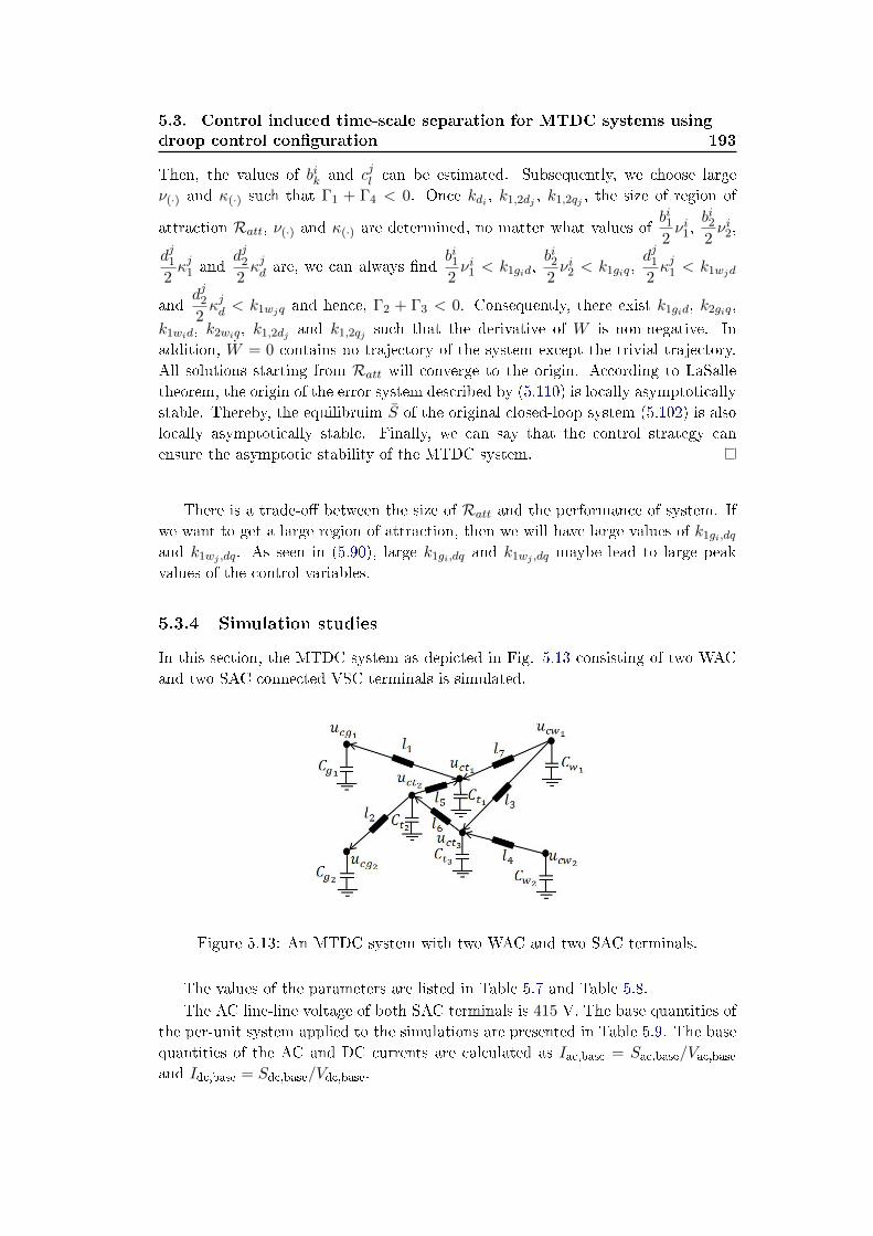
5.3. Control induced time-scale separation for MTDC systems using
droop control conguration 193
Then, the values of bik and cjl can be estimated. Subsequently, we choose large
ν(·) and κ(·) such that Γ1 + Γ4 < 0. Once kdi , k1,2dj , k1,2qj , the size of region of
attraction Ratt, ν(·) and κ(·) are determined, no matter what values ofbi12νi1,
bi22νi2,
dj12κj1 and
dj22κjd are, we can always nd
bi12νi1 < k1gid,
bi22νi2 < k1giq,
dj12κj1 < k1wjd
anddj22κjd < k1wjq and hence, Γ2 + Γ3 < 0. Consequently, there exist k1gid, k2giq,
k1wid, k2wiq, k1,2dj and k1,2qj such that the derivative of W is non-negative. In
addition, W = 0 contains no trajectory of the system except the trivial trajectory.
All solutions starting from Ratt will converge to the origin. According to LaSalle
theorem, the origin of the error system described by (5.110) is locally asymptotically
stable. Thereby, the equilibruim S of the original closed-loop system (5.102) is also
locally asymptotically stable. Finally, we can say that the control strategy can
ensure the asymptotic stability of the MTDC system.
There is a trade-o between the size of Ratt and the performance of system. If
we want to get a large region of attraction, then we will have large values of k1gi,dq
and k1wj ,dq. As seen in (5.90), large k1gi,dq and k1wj ,dq maybe lead to large peak
values of the control variables.
5.3.4 Simulation studies
In this section, the MTDC system as depicted in Fig. 5.13 consisting of two WAC
and two SAC connected VSC terminals is simulated.
Figure 5.13: An MTDC system with two WAC and two SAC terminals.
The values of the parameters are listed in Table 5.7 and Table 5.8.
The AC line-line voltage of both SAC terminals is 415 V. The base quantities of
the per-unit system applied to the simulations are presented in Table 5.9. The base
quantities of the AC and DC currents are calculated as Iac,base = Sac,base/Vac,baseand Idc,base = Sdc,base/Vdc,base.
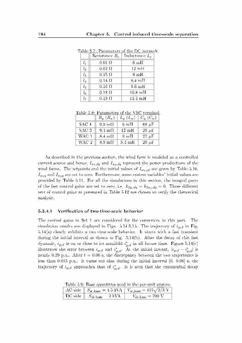
194 Chapter 5. Control induced time-scale separation
Table 5.7: Parameters of the DC network.Resistance Rc Inductance Lc
l1 0.01 Ω 6 mH
l2 0.02 Ω 12 mH
l3 0.15 Ω 9 mH
l4 0.14 Ω 8.4 mH
l5 0.16 Ω 9.6 mH
l6 0.18 Ω 10.8 mH
l7 0.19 Ω 11.4 mH
Table 5.8: Parameters of the VSC terminal.Rg (Rw) Lg (Lw) Cg (Cw)
SAC 1 9.9 mΩ 6 mH 68 µF
SAC 2 9.4 mΩ 12 mH 20 µF
WAC 1 8.4 mΩ 9 mH 27 µF
WAC 2 8.9 mΩ 8.4 mH 20 µF
As described in the previous section, the wind farm is modeled as a controlled
current source and hence, Iw1,dq and Iw2,dq represent the power productions of the
wind farms. The setpoints and the initial values of Iw1,2d are given by Table 5.10.
Iw1q and Iw2q are set to zero. Furthermore, some system variables' initial values are
provided by Table 5.11. For all the simulations in this section, the integral parts
of the fast control gains are set to zero, i.e. k2gi,dq = k2wj ,dq = 0. Three dierent
sets of control gains as presented in Table 5.12 are chosen to verify the theoretical
analysis.
5.3.4.1 Verication of two-time-scale behavior
The control gains in Set 1 are considered for the converters in this part. The
simulation results are displayed in Figs. 5.14-5.15. The trajectory of ig1d in Fig.
5.14(a) clearly exhibits a two-time-scale behavior. It starts with a fast transient
during the initial interval as shown in Fig. 5.14(b). After the decay of this fast
dynamic, ig1d is on or close to its manifold i∗g1d in all future time. Figure 5.14(c)
illustrates the error between ig1d and i∗g1d. At the initial instant, |ig1d − i∗g1d| isnearly 0.29 p.u.. After t = 0.06 s, the discrepancy between the two trajectories is
less than 0.015 p.u.. It turns out that during the initial interval [0, 0.06] s, the
trajectory of ig1d approaches that of i∗g1d. It is seen that the exponential decay
Table 5.9: Base quantities used in the per-unit system.
AC side Sac,base = 4.5 kVA Vac,base = 415√
2/3 V
DC side Sdc,base = 3 kVA Vdc,base = 700 V
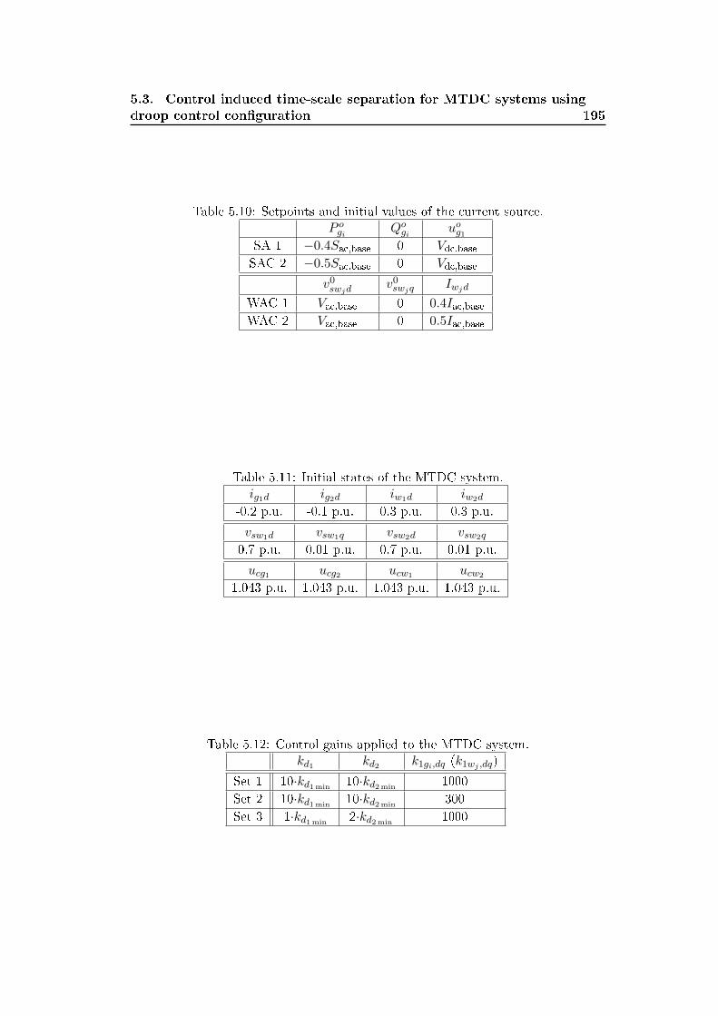
5.3. Control induced time-scale separation for MTDC systems using
droop control conguration 195
Table 5.10: Setpoints and initial values of the current source.P ogi Qogi uog1
SA 1 −0.4Sac,base 0 Vdc,baseSAC 2 −0.5Sac,base 0 Vdc,base
v0swjd
v0swjq Iwjd
WAC 1 Vac,base 0 0.4Iac,baseWAC 2 Vac,base 0 0.5Iac,base
Table 5.11: Initial states of the MTDC system.ig1d ig2d iw1d iw2d
-0.2 p.u. -0.1 p.u. 0.3 p.u. 0.3 p.u.
vsw1d vsw1q vsw2d vsw2q
0.7 p.u. 0.01 p.u. 0.7 p.u. 0.01 p.u.
ucg1 ucg2 ucw1 ucw2
1.043 p.u. 1.043 p.u. 1.043 p.u. 1.043 p.u.
Table 5.12: Control gains applied to the MTDC system.kd1 kd2 k1gi,dq (k1wj ,dq)
Set 1 10·kd1min10·kd2min
1000
Set 2 10·kd1min10·kd2min
300
Set 3 1·kd1min2·kd2min
1000
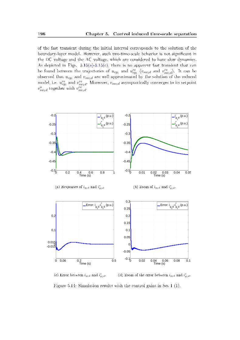
196 Chapter 5. Control induced time-scale separation
of the fast transient during the initial interval corresponds to the solution of the
boundary-layer model. However, such two-time-scale behavior is not signicant in
the DC voltage and the AC voltage, which are considered to have slow dynamics.
As depicted in Figs. 5.15(a)-5.15(c), there is no apparent fast transient that can
be found between the trajectories of ucg1 and urecg1 (vsw1d and vresw1d). It can be
observed that ucg1 and vsw1d are well approximated by the solution of the reduced
model, i.e. urecg1 and vresw1d
. Moreover, vsw1d asymptotically converges to its setpoint
vosw1dtogether with vresw1d
.
0 0.2 0.4 0.6 0.8 1-0.5
-0.45
-0.4
-0.35
-0.3
-0.25
-0.2
Time (s)
ig
1d (p.u.)
ig
1d
* (p.u.)
(a) Responses of ig1d and i∗g1d
.
0 0.01 0.02 0.03 0.04 0.05-0.5
-0.45
-0.4
-0.35
-0.3
-0.25
-0.2
Time (s)
ig
1d (p.u.)
ig
1d
* (p.u.)
(b) Zoom of ig1d and i∗g1d
.
0 0,06 0.2 0.5
-0.0150
0.015
0,1
0,2
Time (s)
Error: ig
1d-i
g1d
* (p.u.)
(c) Error between ig1d and i∗g1d
.
0 0.02 0.04 0.06 0.08 0.1-0.1
-0.05
0
0.05
0.1
0.15
0.2
0.25
0.3
Time (s)
Error: ig
1d-i
g1d
* (p.u.)
(d) Zoom of the error between ig1d and i∗g1d
.
Figure 5.14: Simulation results with the control gains in Set 1 (1).
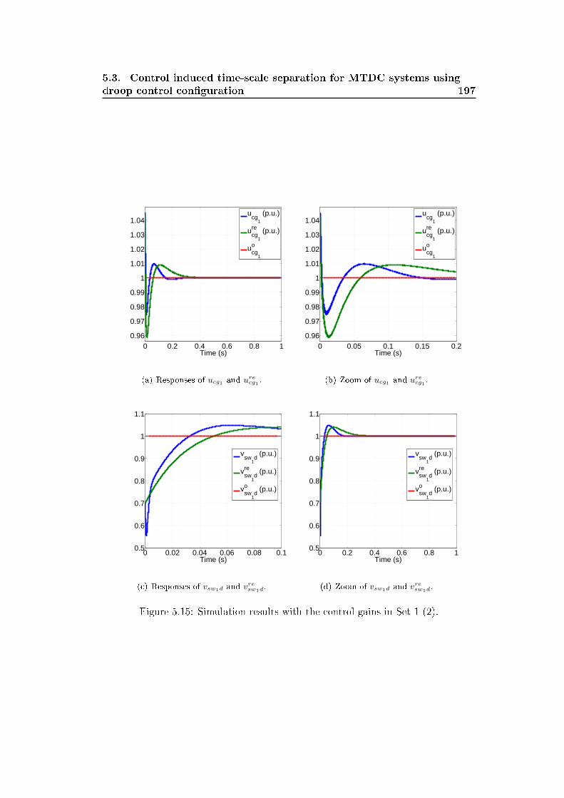
5.3. Control induced time-scale separation for MTDC systems using
droop control conguration 197
0 0.2 0.4 0.6 0.8 10.96
0.97
0.98
0.99
1
1.01
1.02
1.03
1.04
Time (s)
ucg
1
(p.u.)
ucg
1
re (p.u.)
ucg
1
o
(a) Responses of ucg1 and urecg1 .
0 0.05 0.1 0.15 0.20.96
0.97
0.98
0.99
1
1.01
1.02
1.03
1.04
Time (s)
ucg
1
(p.u.)
ucg
1
re (p.u.)
ucg
1
o
(b) Zoom of ucg1 and urecg1 .
0 0.02 0.04 0.06 0.08 0.10.5
0.6
0.7
0.8
0.9
1
1.1
Time (s)
vsw
1d (p.u.)
vsw
1d
re (p.u.)
vsw
1d
o (p.u.)
(c) Responses of vsw1d and vresw1d
.
0 0.2 0.4 0.6 0.8 10.5
0.6
0.7
0.8
0.9
1
1.1
Time (s)
vsw
1d (p.u.)
vsw
1d
re (p.u.)
vsw
1d
o (p.u.)
(d) Zoom of vsw1d and vresw1d
.
Figure 5.15: Simulation results with the control gains in Set 1 (2).
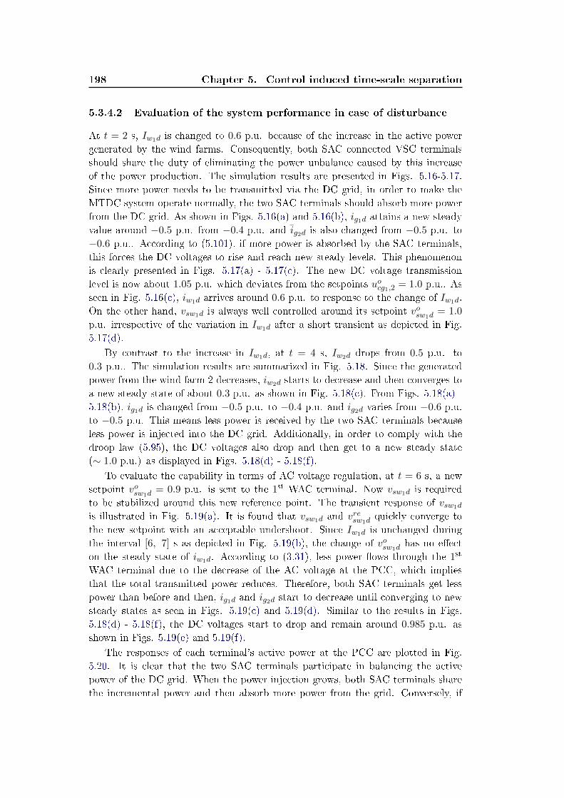
198 Chapter 5. Control induced time-scale separation
5.3.4.2 Evaluation of the system performance in case of disturbance
At t = 2 s, Iw1d is changed to 0.6 p.u. because of the increase in the active power
generated by the wind farms. Consequently, both SAC connected VSC terminals
should share the duty of eliminating the power unbalance caused by this increase
of the power production. The simulation results are presented in Figs. 5.16-5.17.
Since more power needs to be transmitted via the DC grid, in order to make the
MTDC system operate normally, the two SAC terminals should absorb more power
from the DC grid. As shown in Figs. 5.16(a) and 5.16(b), ig1d attains a new steady
value around −0.5 p.u. from −0.4 p.u. and ig2d is also changed from −0.5 p.u. to
−0.6 p.u.. According to (5.101), if more power is absorbed by the SAC terminals,
this forces the DC voltages to rise and reach new steady levels. This phenomenon
is clearly presented in Figs. 5.17(a) - 5.17(c). The new DC voltage transmission
level is now about 1.05 p.u. which deviates from the setpoints uocg1,2 = 1.0 p.u.. As
seen in Fig. 5.16(c), iw1d arrives around 0.6 p.u. to response to the change of Iw1d.
On the other hand, vsw1d is always well controlled around its setpoint vosw1d= 1.0
p.u. irrespective of the variation in Iw1d after a short transient as depicted in Fig.
5.17(d).
By contrast to the increase in Iw1d, at t = 4 s, Iw2d drops from 0.5 p.u. to
0.3 p.u.. The simulation results are summarized in Fig. 5.18. Since the generated
power from the wind farm 2 decreases, iw2d starts to decrease and then converges to
a new steady state of about 0.3 p.u. as shown in Fig. 5.18(c). From Figs. 5.18(a) -
5.18(b), ig1d is changed from −0.5 p.u. to −0.4 p.u. and ig2d varies from −0.6 p.u.
to −0.5 p.u. This means less power is received by the two SAC terminals because
less power is injected into the DC grid. Additionally, in order to comply with the
droop law (5.95), the DC voltages also drop and then get to a new steady state
(∼ 1.0 p.u.) as displayed in Figs. 5.18(d) - 5.18(f).
To evaluate the capability in terms of AC voltage regulation, at t = 6 s, a new
setpoint vosw1d= 0.9 p.u. is sent to the 1st WAC terminal. Now vsw1d is required
to be stabilized around this new reference point. The transient response of vsw1d
is illustrated in Fig. 5.19(a). It is found that vsw1d and vresw1dquickly converge to
the new setpoint with an acceptable undershoot. Since Iw1d is unchanged during
the interval [6, 7] s as depicted in Fig. 5.19(b), the change of vosw1dhas no eect
on the steady state of iw1d. According to (3.31), less power ows through the 1st
WAC terminal due to the decrease of the AC voltage at the PCC, which implies
that the total transmitted power reduces. Therefore, both SAC terminals get less
power than before and then, ig1d and ig2d start to decrease until converging to new
steady states as seen in Figs. 5.19(c) and 5.19(d). Similar to the results in Figs.
5.18(d) - 5.18(f), the DC voltages start to drop and remain around 0.985 p.u. as
shown in Figs. 5.19(e) and 5.19(f).
The responses of each terminal's active power at the PCC are plotted in Fig.
5.20. It is clear that the two SAC terminals participate in balancing the active
power of the DC grid. When the power injection grows, both SAC terminals share
the incremental power and then absorb more power from the grid. Conversely, if

5.3. Control induced time-scale separation for MTDC systems using
droop control conguration 199
2 2.1 2.2 2.3 2.4 2.5
-0.5
-0.48
-0.46
-0.44
-0.42
-0.4
Time (s)
ig
1d (p.u.)
ig
1d
* (p.u.)
(a) Responses of ig1d and i∗g1d
.
2 2.1 2.2 2.3 2.4 2.5
-0.6
-0.58
-0.56
-0.54
-0.52
-0.5
Time (s)
ig
2d (p.u.)
ig
2d
* (p.u.)
(b) Responses of ig2d and i∗g2d
.
2 2.1 2.2 2.3 2.4 2.5
0.4
0.45
0.5
0.55
0.6
Time (s)
iw
1d (p.u.)
iw
1d
* (p.u.)
(c) Responses of iw1d and i∗w1d
.
1.99 2 2.01 2.02
0.4
0.45
0.5
0.55
0.6
Time (s)
iw
1d (p.u.)
iw
1d
* (p.u.)
(d) Zoom of iw1d and i∗w1d
.
Figure 5.16: Simulation results with the variation in Iw1d.
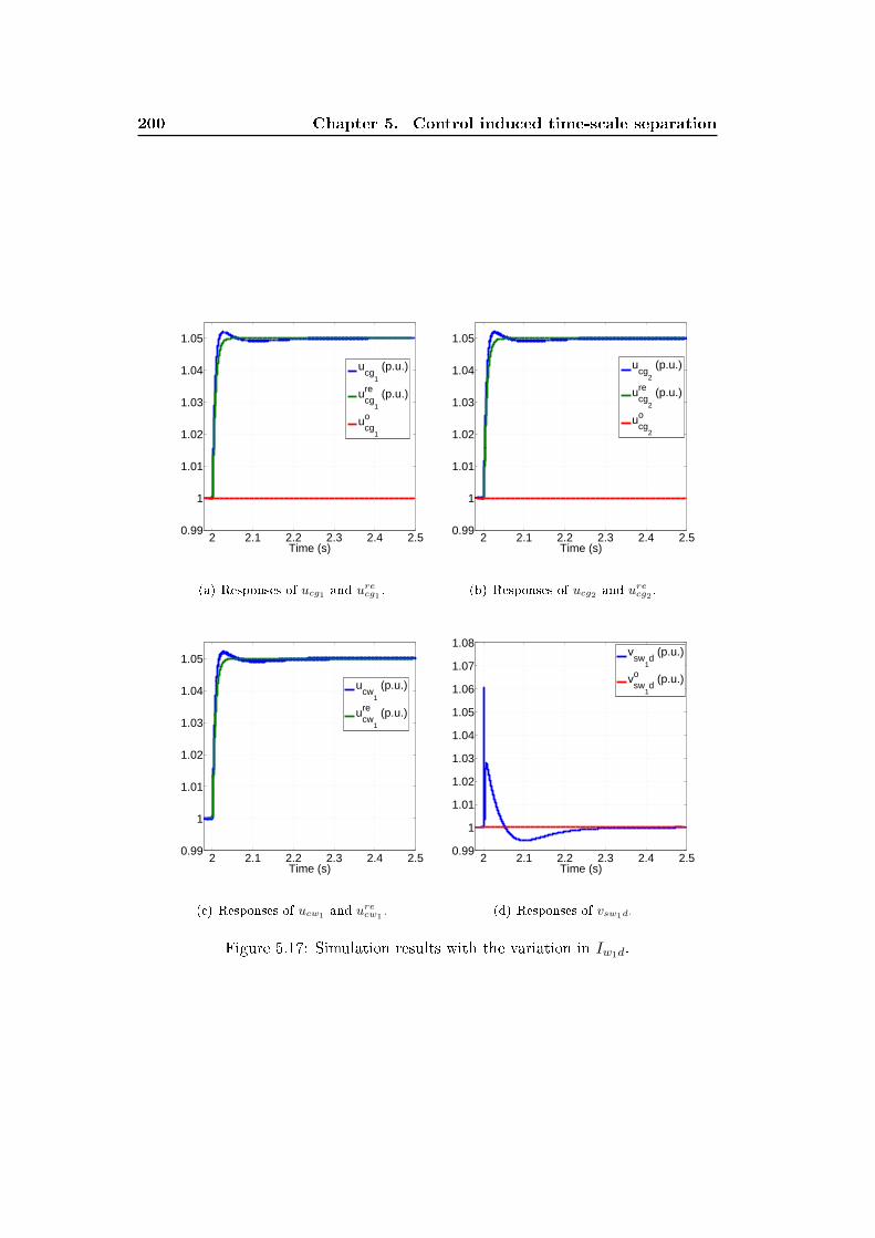
200 Chapter 5. Control induced time-scale separation
2 2.1 2.2 2.3 2.4 2.50.99
1
1.01
1.02
1.03
1.04
1.05
Time (s)
ucg
1
(p.u.)
ucg
1
re (p.u.)
ucg
1
o
(a) Responses of ucg1 and urecg1 .
2 2.1 2.2 2.3 2.4 2.50.99
1
1.01
1.02
1.03
1.04
1.05
Time (s)
ucg
2
(p.u.)
ucg
2
re (p.u.)
ucg
2
o
(b) Responses of ucg2 and urecg2 .
2 2.1 2.2 2.3 2.4 2.50.99
1
1.01
1.02
1.03
1.04
1.05
Time (s)
ucw
1
(p.u.)
ucw
1
re (p.u.)
(c) Responses of ucw1 and urecw1.
2 2.1 2.2 2.3 2.4 2.50.99
1
1.01
1.02
1.03
1.04
1.05
1.06
1.07
1.08
Time (s)
vsw
1d (p.u.)
vsw
1d
o (p.u.)
(d) Responses of vsw1d.
Figure 5.17: Simulation results with the variation in Iw1d.
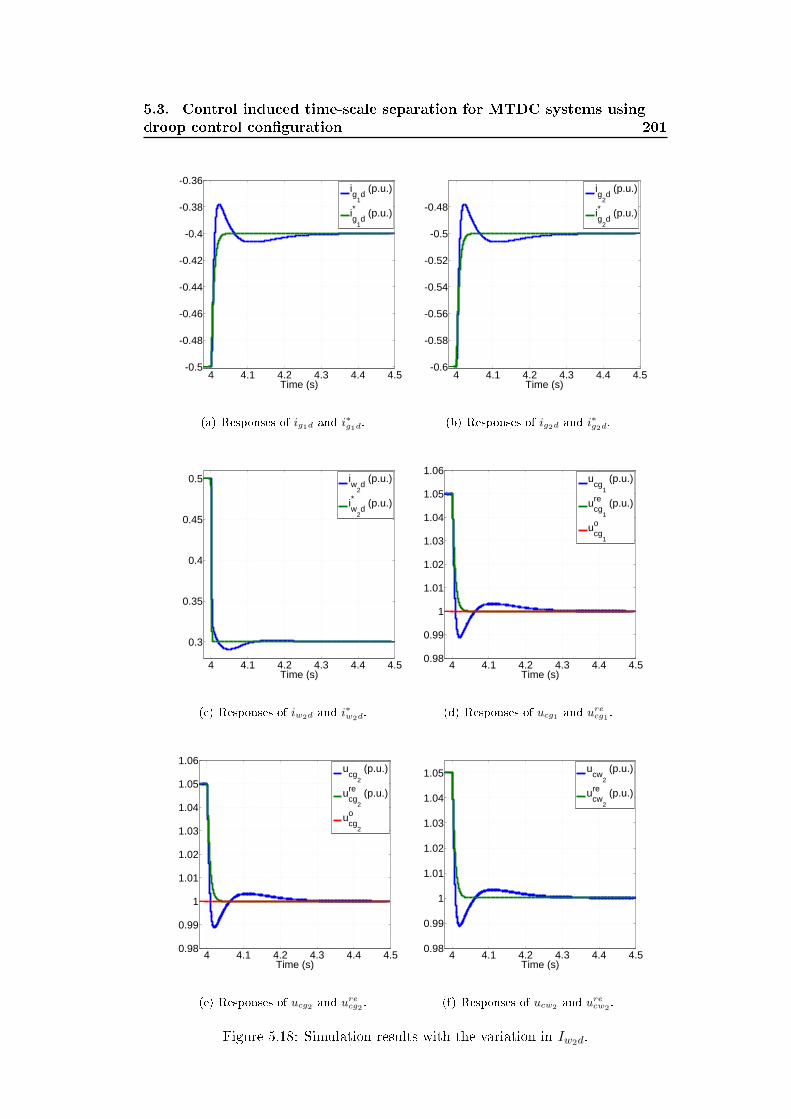
5.3. Control induced time-scale separation for MTDC systems using
droop control conguration 201
4 4.1 4.2 4.3 4.4 4.5-0.5
-0.48
-0.46
-0.44
-0.42
-0.4
-0.38
-0.36
Time (s)
ig
1d (p.u.)
ig
1d
* (p.u.)
(a) Responses of ig1d and i∗g1d
.
4 4.1 4.2 4.3 4.4 4.5-0.6
-0.58
-0.56
-0.54
-0.52
-0.5
-0.48
Time (s)
ig
2d (p.u.)
ig
2d
* (p.u.)
(b) Responses of ig2d and i∗g2d
.
4 4.1 4.2 4.3 4.4 4.5
0.3
0.35
0.4
0.45
0.5
Time (s)
iw
2d (p.u.)
iw
2d
* (p.u.)
(c) Responses of iw2d and i∗w2d
.
4 4.1 4.2 4.3 4.4 4.50.98
0.99
1
1.01
1.02
1.03
1.04
1.05
1.06
Time (s)
ucg
1
(p.u.)
ucg
1
re (p.u.)
ucg
1
o
(d) Responses of ucg1 and urecg1 .
4 4.1 4.2 4.3 4.4 4.50.98
0.99
1
1.01
1.02
1.03
1.04
1.05
1.06
Time (s)
ucg
2
(p.u.)
ucg
2
re (p.u.)
ucg
2
o
(e) Responses of ucg2 and urecg2 .
4 4.1 4.2 4.3 4.4 4.50.98
0.99
1
1.01
1.02
1.03
1.04
1.05
Time (s)
ucw
2
(p.u.)
ucw
2
re (p.u.)
(f) Responses of ucw2 and urecw2.
Figure 5.18: Simulation results with the variation in Iw2d.
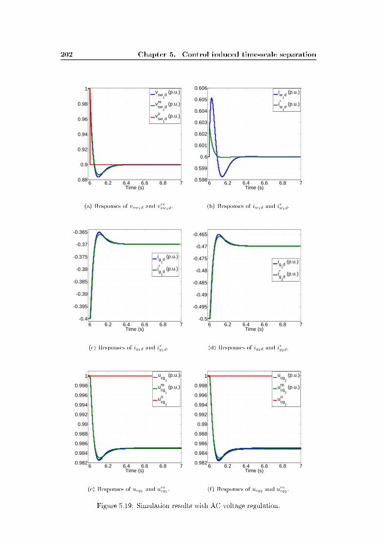
202 Chapter 5. Control induced time-scale separation
6 6.2 6.4 6.6 6.8 70.88
0.9
0.92
0.94
0.96
0.98
1
Time (s)
vsw
1d (p.u.)
vsw
1d
re (p.u.)
vsw
1d
o (p.u.)
(a) Responses of vsw1d and vresw1d
.
6 6.2 6.4 6.6 6.8 70.598
0.599
0.6
0.601
0.602
0.603
0.604
0.605
0.606
Time (s)
iw
1d (p.u.)
iw
1d
* (p.u.)
(b) Responses of iw1d and i∗w1d
.
6 6.2 6.4 6.6 6.8 7-0.4
-0.395
-0.39
-0.385
-0.38
-0.375
-0.37
-0.365
Time (s)
ig
1d (p.u.)
ig
1d
* (p.u.)
(c) Responses of ig1d and i∗g1d
.
6 6.2 6.4 6.6 6.8 7-0.5
-0.495
-0.49
-0.485
-0.48
-0.475
-0.47
-0.465
Time (s)
ig
2d (p.u.)
ig
2d
* (p.u.)
(d) Responses of ig2d and i∗g2d
.
6 6.2 6.4 6.6 6.8 70.982
0.984
0.986
0.988
0.99
0.992
0.994
0.996
0.998
1
Time (s)
ucg
1
(p.u.)
ucg
1
re (p.u.)
ucg
1
o
(e) Responses of ucg1 and urecg1 .
6 6.2 6.4 6.6 6.8 70.982
0.984
0.986
0.988
0.99
0.992
0.994
0.996
0.998
1
Time (s)
ucg
2
(p.u.)
ucg
2
re (p.u.)
ucg
2
o
(f) Responses of ucg2 and urecg2 .
Figure 5.19: Simulation results with AC voltage regulation.
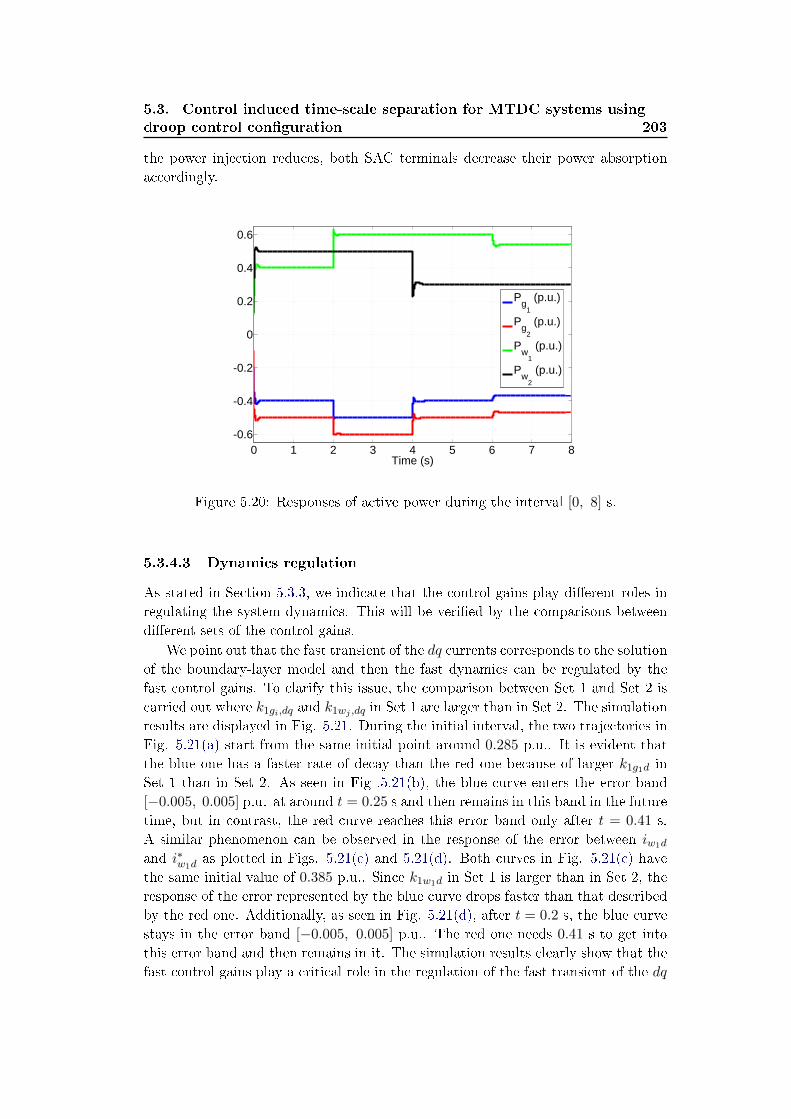
5.3. Control induced time-scale separation for MTDC systems using
droop control conguration 203
the power injection reduces, both SAC terminals decrease their power absorption
accordingly.
0 1 2 3 4 5 6 7 8-0.6
-0.4
-0.2
0
0.2
0.4
0.6
Time (s)
Pg
1
(p.u.)
Pg
2
(p.u.)
Pw
1
(p.u.)
Pw
2
(p.u.)
Figure 5.20: Responses of active power during the interval [0, 8] s.
5.3.4.3 Dynamics regulation
As stated in Section 5.3.3, we indicate that the control gains play dierent roles in
regulating the system dynamics. This will be veried by the comparisons between
dierent sets of the control gains.
We point out that the fast transient of the dq currents corresponds to the solution
of the boundary-layer model and then the fast dynamics can be regulated by the
fast control gains. To clarify this issue, the comparison between Set 1 and Set 2 is
carried out where k1gi,dq and k1wj ,dq in Set 1 are larger than in Set 2. The simulation
results are displayed in Fig. 5.21. During the initial interval, the two trajectories in
Fig. 5.21(a) start from the same initial point around 0.285 p.u.. It is evident that
the blue one has a faster rate of decay than the red one because of larger k1g1d in
Set 1 than in Set 2. As seen in Fig .5.21(b), the blue curve enters the error band
[−0.005, 0.005] p.u. at around t = 0.25 s and then remains in this band in the future
time, but in contrast, the red curve reaches this error band only after t = 0.41 s.
A similar phenomenon can be observed in the response of the error between iw1d
and i∗w1das plotted in Figs. 5.21(c) and 5.21(d). Both curves in Fig. 5.21(c) have
the same initial value of 0.385 p.u.. Since k1w1d in Set 1 is larger than in Set 2, the
response of the error represented by the blue curve drops faster than that described
by the red one. Additionally, as seen in Fig. 5.21(d), after t = 0.2 s, the blue curve
stays in the error band [−0.005, 0.005] p.u.. The red one needs 0.41 s to get into
this error band and then remains in it. The simulation results clearly show that the
fast control gains play a critical role in the regulation of the fast transient of the dq
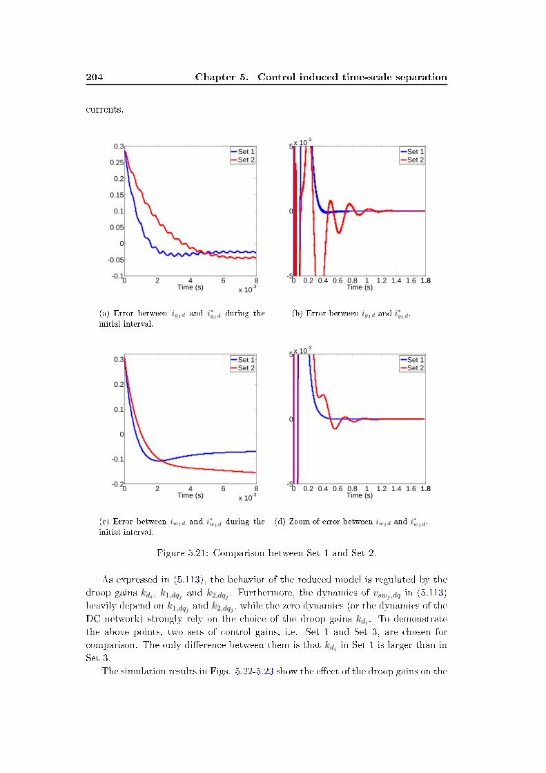
204 Chapter 5. Control induced time-scale separation
currents.
0 2 4 6 8x 10
-3
-0.1
-0.05
0
0.05
0.1
0.15
0.2
0.25
0.3
Time (s)
Set 1Set 2
(a) Error between ig1d and i∗g1d during the
initial interval.
0 0.2 0.4 0.6 0.8 1 1.2 1.4 1.6 1.81.8-5
0
5x 10⁻³
Time (s)
Set 1Set 2
(b) Error between ig1d and i∗g1d
.
0 2 4 6 8x 10
-3
-0.2
-0.1
0
0.1
0.2
0.3
Time (s)
Set 1Set 2
(c) Error between iw1d and i∗w1dduring the
initial interval.
0 0.2 0.4 0.6 0.8 1 1.2 1.4 1.6 1.81.8-5
0
5x 10⁻³
Time (s)
Set 1Set 2
(d) Zoom of error between iw1d and i∗w1d
.
Figure 5.21: Comparison between Set 1 and Set 2.
As expressed in (5.113), the behavior of the reduced model is regulated by the
droop gains kdi , k1,dqj and k2,dqj . Furthermore, the dynamics of vswj ,dq in (5.113)
heavily depend on k1,dqj and k2,dqj , while the zero dynamics (or the dynamics of the
DC network) strongly rely on the choice of the droop gains kdi . To demonstrate
the above points, two sets of control gains, i.e. Set 1 and Set 3, are chosen for
comparison. The only dierence between them is that kdi in Set 1 is larger than in
Set 3.
The simulation results in Figs. 5.22-5.23 show the eect of the droop gains on the
5.4. Conclusions 205
system performance. From Figs. 5.22(a) and 5.22(c), both ucg1 and ucw1 with Set 1
and Set 3 are asymptotically stabilized around 1.0 p.u.. However, it can be observed
that the blue trajectories remain in the domain [0.99, 1.01] p.u. after t = 0.05 s,
whereas the red ones need nearly 1.9 s to stay in the same region. Moreover, as seen
in Figs. 5.22(b) and 5.22(d), the response of ucg1 (ucw1) with Set 1 is much steeper
than that with Set 2 during the initial interval. The above description indicates that
the performance of the state variables related to the zero dynamics can be improved
by increasing the values of kdi appropriately.
Let us now focus on the responses of the AC voltage as depicted in Figs. 5.23(c)
- 5.23(f). Interestingly, as seen in Fig. 5.23(c), the response of vsw1d with Set 1 is
very close to that with Set 3. In particular, as seen in Fig. 5.23(d), the two curves,
the blue one and the red one, almost coincide with each other. A similar result can
also be obtained for vsw2d from Figs. 5.23(e) and 5.23(f). This implies that the
droop gains have little eect on controlling the AC voltage. It is k1,dqj and k2,dqj
that are predominant in the regulation of the AC voltage.
5.4 Conclusions
Vector current control has been widely applied in the context of VSC control, whose
principle is based on the assumption (or empirical practice) of time-scale separation
between the system state variables. However, this hypothesis (or experience) has
been rarely theoretically studied. This chapter has bridged the gap between the
theory and the practice.
First, in Section 5.1, a general control design problem was studied where a time-
scale separation based control structure consisting of two loops, the fast inner and
the slow outer loop, was established for a class of nonlinear systems. Further theo-
retical studies have been carried out, showing that the proposed control algorithm
can divide the dynamics of the system's state variables into dierent time scales and
the original closed-loop system can be divided into two models, the boundary-layer
and the reduced model. Interestingly, by analyzing the two models, we nd that
the control gains in both control loops have dierent eects on the system behavior.
The state variables with fast dynamics exhibit a signicant two time-scale dynami-
cal behavior by presenting a fast and a slow transient. Moreover, the fast transient
exactly corresponds to the solution of the boundary-layer model, whose dynamics
are dominated by the control gains of the fast inner loop.
Then, we have applied the theoretical results to the control of MTDC system
where two mostly used control congurations, master-slave and droop control cong-
uration, have been investigated in this chapter. According to the dierent VSC op-
erations of the two control congurations, two dierent time-scale separation based
controllers are presented. As stated in Lemma 5.2.2 of Section 5.2, we point out
that in master-slave control conguration, the developed controller can make the
system exhibit dierent time-scale dynamics when the system's physical structure
and the prescribed (or scheduled) references satisfy certain conditions. In addition,
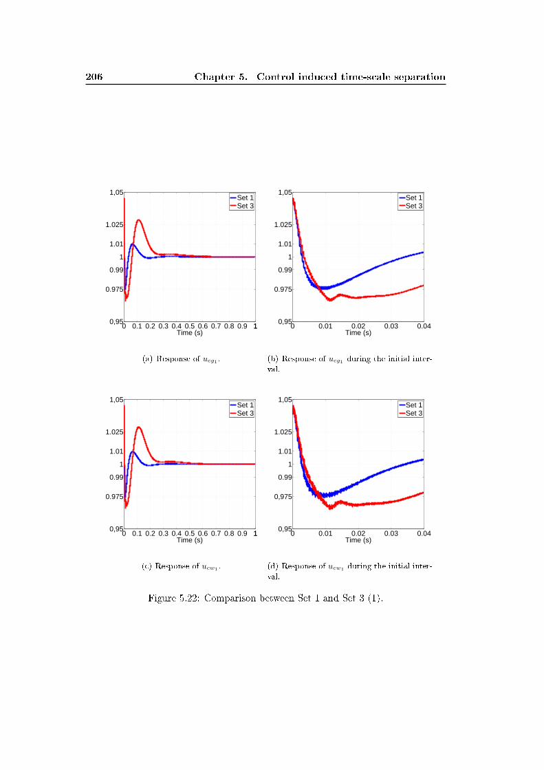
206 Chapter 5. Control induced time-scale separation
0 0.1 0.2 0.3 0.4 0.5 0.6 0.7 0.8 0.9 110,95
0.975
0.99
1
1.01
1.025
1,05
Time (s)
Set 1Set 3
(a) Response of ucg1 .
0 0.01 0.02 0.03 0.040,95
0.975
0.99
1
1.01
1.025
1,05
Time (s)
Set 1Set 3
(b) Response of ucg1 during the initial inter-
val.
0 0.1 0.2 0.3 0.4 0.5 0.6 0.7 0.8 0.9 110,95
0.975
0.99
1
1.01
1.025
1,05
Time (s)
Set 1Set 3
(c) Response of ucw1 .
0 0.01 0.02 0.03 0.040,95
0,975
0.99
1
1.01
1.025
1,05
Time (s)
Set 1Set 3
(d) Response of ucw1 during the initial inter-
val.
Figure 5.22: Comparison between Set 1 and Set 3 (1).
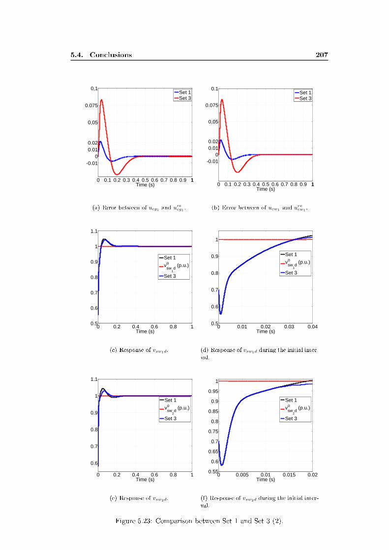
5.4. Conclusions 207
0 0.1 0.2 0.3 0.4 0.5 0.6 0.7 0.8 0.9 11
-0.010
0.010.02
0,05
0.075
0,1
Time (s)
Set 1Set 3
(a) Error between of ucg1 and urecg1 .
0 0.1 0.2 0.3 0.4 0.5 0.6 0.7 0.8 0.9 11
-0.010
0.010.02
0,05
0.075
0.1
Time (s)
Set 1Set 3
(b) Error between of ucw1 and urecw1.
0 0.2 0.4 0.6 0.8 10.5
0.6
0.7
0.8
0.9
1
1.1
Time (s)
Set 1
vsw
1d
o (p.u.)
Set 3
(c) Response of vsw1d.
0 0.01 0.02 0.03 0.040.5
0.6
0.7
0.8
0.9
1
Time (s)
Set 1
vsw
1d
o (p.u.)
Set 3
(d) Response of vsw1d during the initial inter-
val.
0 0.2 0.4 0.6 0.8 1
0.6
0.7
0.8
0.9
1
1.1
Time (s)
Set 1
vsw
2d
o (p.u.)
Set 3
(e) Response of vsw2d.
0 0.005 0.01 0.015 0.020.55
0.6
0.65
0.7
0.75
0.8
0.85
0.9
0.95
1
Time (s)
Set 1
vsw
2d
o (p.u.)
Set 3
(f) Response of vsw2d during the initial inter-
val.
Figure 5.23: Comparison between Set 1 and Set 3 (2).

208 Chapter 5. Control induced time-scale separation
we nd that in this control conguration, with the proposed controller, there exist
some uncontrolled internal dynamics (for example, the state variables of the DC
grid) whose behavior strongly depends on the system inherent characteristics.
Subsequently, we have applied the theoretical results of control induced time-
scale separation to droop control conguration. As stated in Lemma 5.3.3 of Section
5.3.3.3, the proposed time-scale separation controller has no specic requirements on
the system parameters, topology or those prescribed references. Unlike master-slave
control conguration, the dynamics of the DC grid are determined by the droop
gains and hence, there is no uncontrolled internal dynamics. The theoretical studies
carried out in this chapter have been veried with simulation results where various
simulated scenarios have been considered.
Chapter 6
Frequency control using MTDC
systems
Contents
6.1 Introduction and motivation . . . . . . . . . . . . . . . . . . . 209
6.2 Modeling . . . . . . . . . . . . . . . . . . . . . . . . . . . . . . 210
6.2.1 DC grid . . . . . . . . . . . . . . . . . . . . . . . . . . . . . . 211
6.2.2 AC areas . . . . . . . . . . . . . . . . . . . . . . . . . . . . . 211
6.2.3 Reference operating point . . . . . . . . . . . . . . . . . . . . 212
6.3 Control strategy . . . . . . . . . . . . . . . . . . . . . . . . . . 212
6.3.1 Control law . . . . . . . . . . . . . . . . . . . . . . . . . . . . 213
6.3.2 Choice of control gains . . . . . . . . . . . . . . . . . . . . . . 213
6.3.3 Algorithm for the denition and verication of control gains
and the associated region of attraction . . . . . . . . . . . . . 218
6.4 Simulation studies . . . . . . . . . . . . . . . . . . . . . . . . . 219
6.5 Conclusions . . . . . . . . . . . . . . . . . . . . . . . . . . . . . 224
As presented in the previous sections, the developed controllers are used to
guarantee the operation of the system states around their prescribed references which
are given by a higher control level. In this chapter, we will propose a possible method
based on frequency control for computing the active power references. The main
idea of this approach is to make the non-synchronous systems interconnected via
an MTDC system share their primary reserves by modifying their scheduled power
references. A DC-voltage-based control scheme, only needing local information, is
introduced to regulate the AC frequency, for which a sucient condition on tuning
the control gains are derived to ensure the system stability.
6.1 Introduction and motivation
In an AC system, the frequency, as an indication of power balance, is common ev-
erywhere on the time scale of a few milliseconds. With this common frequency, all
generating units within the system can sense a power imbalance and adjust their
power output to counter this disturbance. This mechanism of restoring power bal-
ance is commonly called primary frequency control, and the region of variation of
generators' output is referred to as primary reserve. With the current practice of
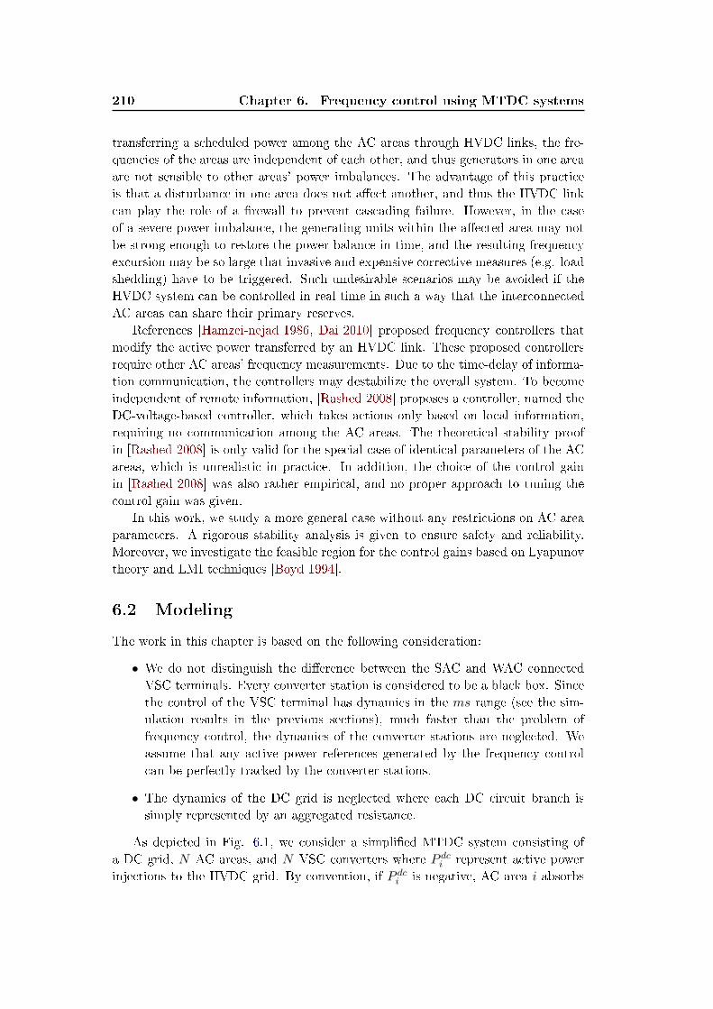
210 Chapter 6. Frequency control using MTDC systems
transferring a scheduled power among the AC areas through HVDC links, the fre-
quencies of the areas are independent of each other, and thus generators in one area
are not sensible to other areas' power imbalances. The advantage of this practice
is that a disturbance in one area does not aect another, and thus the HVDC link
can play the role of a rewall to prevent cascading failure. However, in the case
of a severe power imbalance, the generating units within the aected area may not
be strong enough to restore the power balance in time, and the resulting frequency
excursion may be so large that invasive and expensive corrective measures (e.g. load
shedding) have to be triggered. Such undesirable scenarios may be avoided if the
HVDC system can be controlled in real time in such a way that the interconnected
AC areas can share their primary reserves.
References [Hamzei-nejad 1986, Dai 2010] proposed frequency controllers that
modify the active power transferred by an HVDC link. These proposed controllers
require other AC areas' frequency measurements. Due to the time-delay of informa-
tion communication, the controllers may destabilize the overall system. To become
independent of remote information, [Rashed 2008] proposes a controller, named the
DC-voltage-based controller, which takes actions only based on local information,
requiring no communication among the AC areas. The theoretical stability proof
in [Rashed 2008] is only valid for the special case of identical parameters of the AC
areas, which is unrealistic in practice. In addition, the choice of the control gain
in [Rashed 2008] was also rather empirical, and no proper approach to tuning the
control gain was given.
In this work, we study a more general case without any restrictions on AC area
parameters. A rigorous stability analysis is given to ensure safety and reliability.
Moreover, we investigate the feasible region for the control gains based on Lyapunov
theory and LMI techniques [Boyd 1994].
6.2 Modeling
The work in this chapter is based on the following consideration:
• We do not distinguish the dierence between the SAC and WAC connected
VSC terminals. Every converter station is considered to be a black box. Since
the control of the VSC terminal has dynamics in the ms range (see the sim-
ulation results in the previous sections), much faster than the problem of
frequency control, the dynamics of the converter stations are neglected. We
assume that any active power references generated by the frequency control
can be perfectly tracked by the converter stations.
• The dynamics of the DC grid is neglected where each DC circuit branch is
simply represented by an aggregated resistance.
As depicted in Fig. 6.1, we consider a simplied MTDC system consisting of
a DC grid, N AC areas, and N VSC converters where P dci represent active power
injections to the HVDC grid. By convention, if P dci is negative, AC area i absorbs
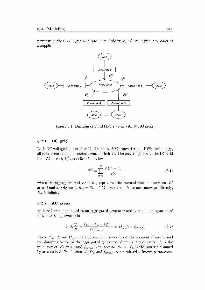
6.2. Modeling 211
power from the HVDC grid as a consumer. Otherwise, AC area i provides power as
a supplier.
Figure 6.1: Diagram of an MTDC system with N AC areas.
6.2.1 DC grid
Each DC voltage is denoted as Vi. Thanks to VSC converter and PWM technology,
all converters can independently control their Vi. The power injected to the DC grid
from AC area i, P dci , satises Ohm's law
P dci =N∑k=1
Vi(Vi − Vk)Rik
(6.1)
where the aggregated resistance Rik represents the transmission line between AC
areas i and k. Obviously Rik = Rki. If AC areas i and k are not connected directly,
Rik is innity.
6.2.2 AC areas
Each AC area is modeled as an aggregated generator and a load. The equation of
motion of the generator is
2πJidfidt
=Pmi − Pli − P dci
2πfnom,i− 2πDgi(fi − fnom,i) (6.2)
where Pmi , Ji and Dgi are the mechanical power input, the moment of inertia and
the damping factor of the aggregated generator of area i, respectively. fi is the
frequency of AC area i and fnom,i is its nominal value. Pli is the power consumed
by area i's load. In addition, Ji, Dgi and fnom,i are considered as known parameters.
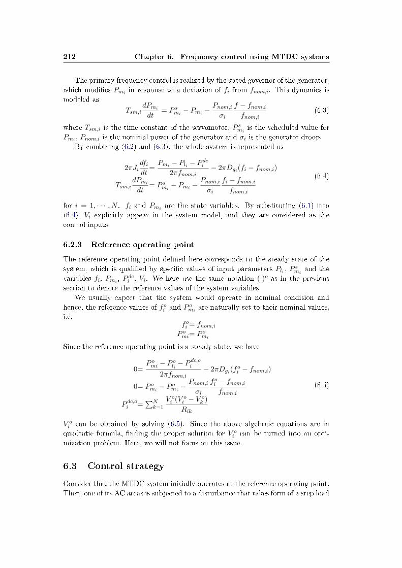
212 Chapter 6. Frequency control using MTDC systems
The primary frequency control is realized by the speed governor of the generator,
which modies Pmi in response to a deviation of fi from fnom,i. This dynamics is
modeled as
Tsm,idPmidt
= P smi − Pmi −Pnom,iσi
f − fnom,ifnom,i
(6.3)
where Tsm,i is the time constant of the servomotor, P smi is the scheduled value for
Pmi , Pnom,i is the nominal power of the generator and σi is the generator droop.
By combining (6.2) and (6.3), the whole system is represented as
2πJidfidt
=Pmi − Pli − P dci
2πfnom,i− 2πDgi(fi − fnom,i)
Tsm,idPmidt
= P smi − Pmi −Pnom,iσi
fi − fnom,ifnom,i
(6.4)
for i = 1, · · · , N . fi and Pmi are the state variables. By substituting (6.1) into
(6.4), Vi explicitly appear in the system model, and they are considered as the
control inputs.
6.2.3 Reference operating point
The reference operating point dened here corresponds to the steady state of the
system, which is qualied by specic values of input parameters Pli , Psmi and the
variables fi, Pmi , Pdci , Vi. We here use the same notation (·)o as in the previous
section to denote the reference values of the system variables.
We usually expect that the system would operate in nominal condition and
hence, the reference values of foi and P omi are naturally set to their nominal values,
i.e.foi = fnom,iP omi= P omi
Since the reference operating point is a steady state, we have
0=P omi − P oli − P
dc,oi
2πfnom,i− 2πDgi(f
oi − fnom,i)
0= P omi − Pomi −
Pnom,iσi
foi − fnom,ifnom,i
P dc,oi =∑N
k=1
V oi (V o
i − V ok )
Rik
(6.5)
V oi can be obtained by solving (6.5). Since the above algebraic equations are in
quadratic formula, nding the proper solution for V oi can be turned into an opti-
mization problem. Here, we will not focus on this issue.
6.3 Control strategy
Consider that the MTDC system initially operates at the reference operating point.
Then, one of its AC areas is subjected to a disturbance that takes form of a step load

6.3. Control strategy 213
change, i.e. Pli 6= P oli . It is true that this load change can be satised by the primary
frequency control of its own area (Pmi). However, in case of a large disturbance,
if we rely only on Pmi , the resulting frequency deviation may be so large that it
endangers the correct operation of the system. Thus, our objective is to improve
the transient frequency prole by calling for other area's primary reserves so that
the frequency excursions in area i are less pronounced.
6.3.1 Control law
The control objective is to regulate each converter's DC voltage Vi only based on
local measurements fi, i.e. Vi is a function of fi only. Therefore, a DC voltage based
controller is designed as
Vi = V oi + αi(fi − foi ) (6.6)
with positive gain αi > 0.
Under this controller, due to the physical coupling of the HVDC grid (6.1), the
resulting power injected to DC grid P dci can be regulated by controlling Vi. This
method leads our whole system to achieve the objective of sharing every area's
primary reserve. However, we are not sure whether fi and Pmi are ultimately
bounded around the reference operating point under the control law (6.6) with an
arbitrary positive control gain αi.
6.3.2 Choice of control gains
In this part, we give a detailed analysis for choosing the control gain αi to guarantee
ultimate boundedness of fi and Pmi under (6.6).
To simplify our problem, at rst, we shift the reference values to the origin by
introducing the following new variables
P dci = P dci − Pdc,oi
Pli= Pli − P oliPmi= Pmi − P omiVi= Vi − V o
i
(6.7)
Recalling (6.1), P dci can be expressed in these new variables as
P dci =N∑k 6=i
(V 2 + 2ViVoi − ViVk − ViV o
k − VkV oi )
Rik(6.8)
An error system of the original system (6.4) is generated in terms of the new variables
by applying (6.5) and (6.8)
˙fi =−a1ifi + a2iPmi − a2iPli − a2i·(∑N
k 6=i(V 2 + 2ViV
oi − ViVk − ViV o
k − VkV oi )
Rik
)˙Pmi =−a4ifi − a5iPmi
(6.9)
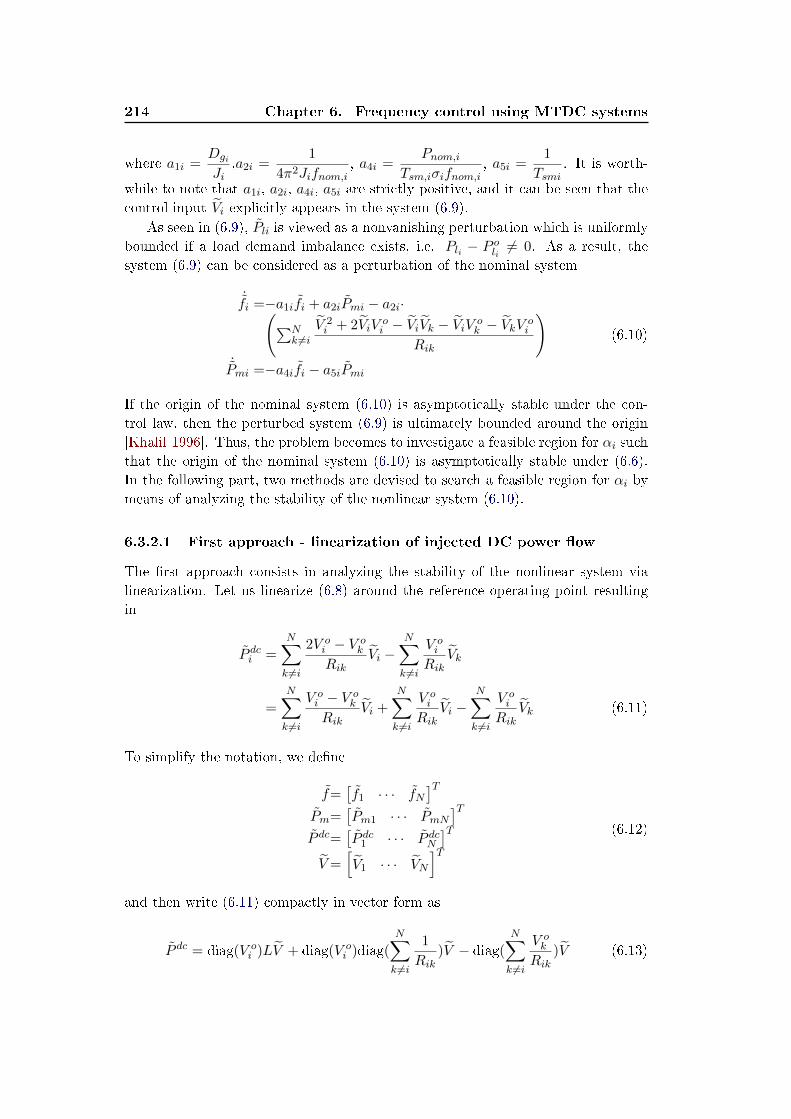
214 Chapter 6. Frequency control using MTDC systems
where a1i =Dgi
Ji,a2i =
1
4π2Jifnom,i, a4i =
Pnom,iTsm,iσifnom,i
, a5i =1
Tsmi. It is worth-
while to note that a1i, a2i, a4i, a5i are strictly positive, and it can be seen that the
control input Vi explicitly appears in the system (6.9).
As seen in (6.9), Pli is viewed as a nonvanishing perturbation which is uniformly
bounded if a load demand imbalance exists, i.e. Pli − P oli 6= 0. As a result, the
system (6.9) can be considered as a perturbation of the nominal system
˙fi =−a1ifi + a2iPmi − a2i·(∑N
k 6=iV 2i + 2ViV
oi − ViVk − ViV o
k − VkV oi
Rik
)˙Pmi =−a4ifi − a5iPmi
(6.10)
If the origin of the nominal system (6.10) is asymptotically stable under the con-
trol law, then the perturbed system (6.9) is ultimately bounded around the origin
[Khalil 1996]. Thus, the problem becomes to investigate a feasible region for αi such
that the origin of the nominal system (6.10) is asymptotically stable under (6.6).
In the following part, two methods are devised to search a feasible region for αi by
means of analyzing the stability of the nonlinear system (6.10).
6.3.2.1 First approach - linearization of injected DC power ow
The rst approach consists in analyzing the stability of the nonlinear system via
linearization. Let us linearize (6.8) around the reference operating point resulting
in
P dci =N∑k 6=i
2V oi − V o
k
RikVi −
N∑k 6=i
V oi
RikVk
=
N∑k 6=i
V oi − V o
k
RikVi +
N∑k 6=i
V oi
RikVi −
N∑k 6=i
V oi
RikVk (6.11)
To simplify the notation, we dene
f=[f1 · · · fN
]TPm=
[Pm1 · · · PmN
]TP dc=
[P dc1 · · · P dcN
]TV=
[V1 · · · VN
]T (6.12)
and then write (6.11) compactly in vector form as
P dc = diag(V oi )LV + diag(V o
i )diag(
N∑k 6=i
1
Rik)V − diag(
N∑k 6=i
V ok
Rik)V (6.13)
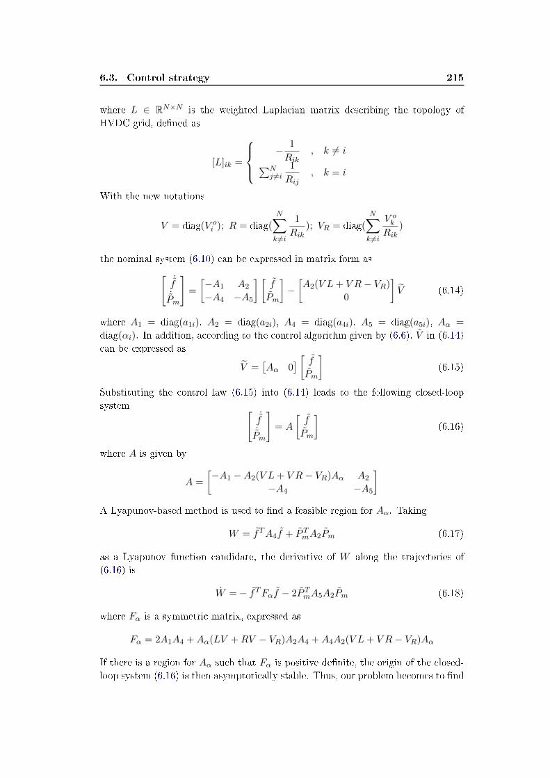
6.3. Control strategy 215
where L ∈ RN×N is the weighted Laplacian matrix describing the topology of
HVDC grid, dened as
[L]ik =
− 1
Rik, k 6= i∑N
j 6=i1
Rij, k = i
With the new notations
V = diag(V oi ); R = diag(
N∑k 6=i
1
Rik); VR = diag(
N∑k 6=i
V ok
Rik)
the nominal system (6.10) can be expressed in matrix form as[˙f˙Pm
]=
[−A1 A2
−A4 −A5
] [f
Pm
]−[A2(V L+ V R− VR)
0
]V (6.14)
where A1 = diag(a1i), A2 = diag(a2i), A4 = diag(a4i), A5 = diag(a5i), Aα =
diag(αi). In addition, according to the control algorithm given by (6.6), V in (6.14)
can be expressed as
V =[Aα 0
] [ fPm
](6.15)
Substituting the control law (6.15) into (6.14) leads to the following closed-loop
system [˙f˙Pm
]= A
[f
Pm
](6.16)
where A is given by
A =
[−A1 −A2(V L+ V R− VR)Aα A2
−A4 −A5
]A Lyapunov-based method is used to nd a feasible region for Aα. Taking
W = fTA4f + P TmA2Pm (6.17)
as a Lyapunov function candidate, the derivative of W along the trajectories of
(6.16) is
W =− fTFαf − 2P TmA5A2Pm (6.18)
where Fα is a symmetric matrix, expressed as
Fα = 2A1A4 +Aα(LV +RV − VR)A2A4 +A4A2(V L+ V R− VR)Aα
If there is a region for Aα such that Fα is positive denite, the origin of the closed-
loop system (6.16) is then asymptotically stable. Thus, our problem becomes to nd
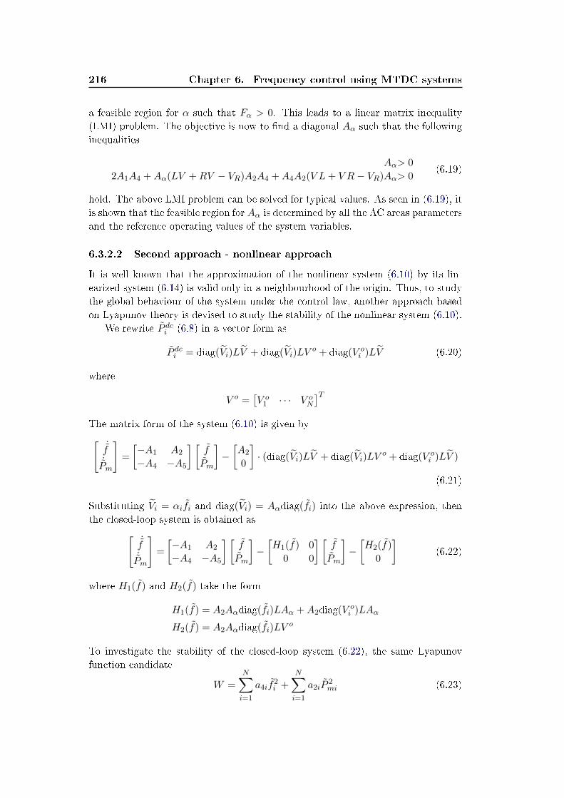
216 Chapter 6. Frequency control using MTDC systems
a feasible region for α such that Fα > 0. This leads to a linear matrix inequality
(LMI) problem. The objective is now to nd a diagonal Aα such that the following
inequalities
Aα> 0
2A1A4 +Aα(LV +RV − VR)A2A4 +A4A2(V L+ V R− VR)Aα> 0(6.19)
hold. The above LMI problem can be solved for typical values. As seen in (6.19), it
is shown that the feasible region for Aα is determined by all the AC areas parameters
and the reference operating values of the system variables.
6.3.2.2 Second approach - nonlinear approach
It is well known that the approximation of the nonlinear system (6.10) by its lin-
earized system (6.14) is valid only in a neighbourhood of the origin. Thus, to study
the global behaviour of the system under the control law, another approach based
on Lyapunov theory is devised to study the stability of the nonlinear system (6.10).
We rewrite P dci (6.8) in a vector form as
P dci = diag(Vi)LV + diag(Vi)LVo + diag(V o
i )LV (6.20)
where
V o =[V o
1 · · · V oN
]TThe matrix form of the system (6.10) is given by[
˙f˙Pm
]=
[−A1 A2
−A4 −A5
] [f
Pm
]−[A2
0
]· (diag(Vi)LV + diag(Vi)LV
o + diag(V oi )LV )
(6.21)
Substituting Vi = αifi and diag(Vi) = Aαdiag(fi) into the above expression, then
the closed-loop system is obtained as[˙f˙Pm
]=
[−A1 A2
−A4 −A5
] [f
Pm
]−[H1(f) 0
0 0
] [f
Pm
]−[H2(f)
0
](6.22)
where H1(f) and H2(f) take the form
H1(f) = A2Aαdiag(fi)LAα +A2diag(V oi )LAα
H2(f) = A2Aαdiag(fi)LVo
To investigate the stability of the closed-loop system (6.22), the same Lyapunov
function candidate
W =
N∑i=1
a4if2i +
N∑i=1
a2iP2mi (6.23)
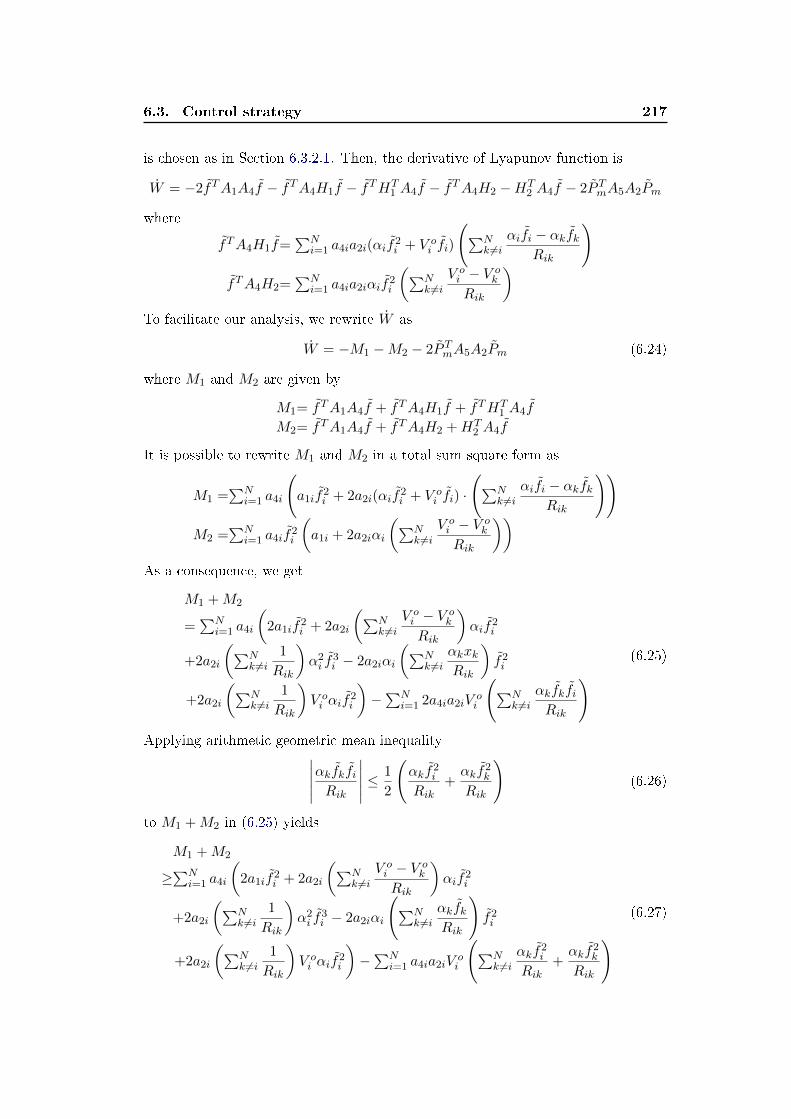
6.3. Control strategy 217
is chosen as in Section 6.3.2.1. Then, the derivative of Lyapunov function is
W = −2fTA1A4f − fTA4H1f − fTHT1 A4f − fTA4H2 −HT
2 A4f − 2P TmA5A2Pm
where
fTA4H1f=∑N
i=1 a4ia2i(αif2i + V o
i fi)
(∑Nk 6=i
αifi − αkfkRik
)fTA4H2=
∑Ni=1 a4ia2iαif
2i
(∑Nk 6=i
V oi − V o
k
Rik
)To facilitate our analysis, we rewrite W as
W = −M1 −M2 − 2P TmA5A2Pm (6.24)
where M1 and M2 are given by
M1= fTA1A4f + fTA4H1f + fTHT1 A4f
M2= fTA1A4f + fTA4H2 +HT2 A4f
It is possible to rewrite M1 and M2 in a total sum square form as
M1 =∑N
i=1 a4i
(a1if
2i + 2a2i(αif
2i + V o
i fi) ·
(∑Nk 6=i
αifi − αkfkRik
))M2 =
∑Ni=1 a4if
2i
(a1i + 2a2iαi
(∑Nk 6=i
V oi − V o
k
Rik
))As a consequence, we get
M1 +M2
=∑N
i=1 a4i
(2a1if
2i + 2a2i
(∑Nk 6=i
V oi − V o
k
Rik
)αif
2i
+2a2i
(∑Nk 6=i
1
Rik
)α2i f
3i − 2a2iαi
(∑Nk 6=i
αkxkRik
)f2i
+2a2i
(∑Nk 6=i
1
Rik
)V oi αif
2i
)−∑N
i=1 2a4ia2iVoi
(∑Nk 6=i
αkfkfiRik
) (6.25)
Applying arithmetic geometric mean inequality∣∣∣∣∣αkfkfiRik
∣∣∣∣∣ ≤ 1
2
(αkf
2i
Rik+αkf
2k
Rik
)(6.26)
to M1 +M2 in (6.25) yields
M1 +M2
≥∑N
i=1 a4i
(2a1if
2i + 2a2i
(∑Nk 6=i
V oi − V o
k
Rik
)αif
2i
+2a2i
(∑Nk 6=i
1
Rik
)α2i f
3i − 2a2iαi
(∑Nk 6=i
αkfkRik
)f2i
+2a2i
(∑Nk 6=i
1
Rik
)V oi αif
2i
)−∑N
i=1 a4ia2iVoi
(∑Nk 6=i
αkf2i
Rik+αkf
2k
Rik
) (6.27)
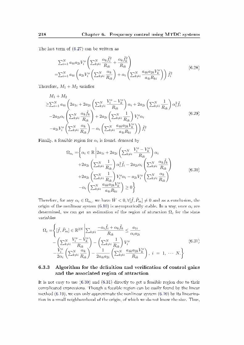
218 Chapter 6. Frequency control using MTDC systems
The last term of (6.27) can be written as
∑Ni=1 a4ia2iV
oi
(∑Nk 6=i
αkf2i
Rik+αkf
2k
Rik
)=∑N
i=1 a4i
(a2iV
oi
(∑Nk 6=i
αkRik
)+ αi
(∑Nk 6=i
a4ka2kVok
a4iRki
))f2i
(6.28)
Therefore, M1 +M2 satises
M1 +M2
≥∑N
i=1 a4i
(2a1i + 2a2i
(∑Nk 6=i
V oi − V o
k
Rik
)αi + 2a2i
(∑Nk 6=i
1
Rik
)α2i fi
−2a2iαi
(∑Nk 6=i
αkfkRik
)+ 2a2i
(∑Nk 6=i
1
Rik
)V oi αi
−a2iVoi
(∑Nk 6=i
αkRik
)− αi
(∑Nk 6=i
a4ka2kVok
a4iRki
))f2i
(6.29)
Finally, a feasible region for αi is found, denoted by
Ωαi =
αi ∈ R
∣∣∣∣2a1i + 2a2i
(∑Nk 6=i
V oi − V o
k
Rik
)αi
+2a2i
(∑Nk 6=i
1
Rik
)α2i fi − 2a2iαi
(∑Nk 6=i
αkfkRik
)+2a2i
(∑Nk 6=i
1
Rik
)V oi αi − a2iV
oi
(∑Nk 6=i
αkRik
)−αi
(∑Nk 6=i
a4ka2kVok
a4iRki
)≥ 0
(6.30)
Therefore, for any αi ∈ Ωαi , we have W < 0,∀[f , Pm] 6= 0 and as a conclusion, the
origin of the nonlinear system (6.10) is asymptotically stable. In a way, once αi are
determined, we can get an estimation of the region of attraction Ωc for the state
variables
Ωc =
[f , Pm] ∈ R2N
∣∣∣∣∣∑k 6=i−αifi + αkfk
Rik≤ a1i
αia2i
−(∑N
k 6=iV oi − V o
k
Rik
)−(∑N
k 6=i1
Rik
)V oi
− Voi
2αi
(∑Nk 6=i
αkRik
)− 1
2a4ia2i
(∑Nk 6=i
a4ka2kVok
Rik
), i = 1, · · · N.
(6.31)
6.3.3 Algorithm for the denition and verication of control gainsand the associated region of attraction
It is not easy to use (6.30) and (6.31) directly to get a feasible region due to their
complicated expressions. Though a feasible region can be easily found by the linear
method (6.19), we can only approximate the nonlinear system (6.10) by its lineariza-
tion in a small neighbourhood of the origin, of which we do not know the size. Thus,
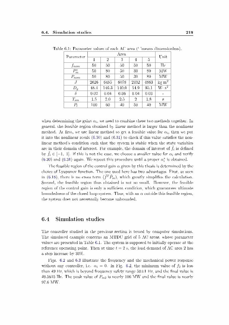
6.4. Simulation studies 219
Table 6.1: Parameter values of each AC area (`-'means dimensionless).
ParameterArea
Unit1 2 3 4 5
fnom 50 50 50 50 50 Hz
P sm 50 80 50 30 80 MW
Pnom 50 80 50 30 80 MW
J 2026 6485 6078 2432 4863 kg m2
Dg 48.4 146.3 140.0 54.9 95.1 W· s2δ 0.02 0.04 0.06 0.04 0.03 -
Tsm 1.5 2.0 2.5 2 1.8 s
Pl 100 60 40 50 40 MW
when determining the gains αi, we need to combine these two methods together. In
general, the feasible region obtained by linear method is larger than the nonlinear
method. At rst, we use linear method to get a feasible value for αi, then we put
it into the nonlinear result (6.30) and (6.31) to check if this value satises the non-
linear method's condition such that the system is stable when the state variables
are in their domain of interest. For example, the domain of interest of fi is dened
by fi ∈ [−1, 1]. If this is not the case, we choose a smaller value for αi and verify
(6.30) and (6.31) again. We repeat this procedure until a proper α∗i is obtained.
The feasible region of the control gain α given by this thesis is determined by the
choice of Lyapunov function. The one used here has two advantages. First, as seen
in (6.18), there is no cross term (fT Pm), which greatly simplies the calculation.
Second, the feasible region thus obtained is not so small. However, the feasible
region of the control gain is only a sucient condition, which guarantees ultimate
boundedness of the closed-loop system. Thus, with an α outside this feasible region,
the system does not necessarily become unbounded.
6.4 Simulation studies
The controller studied in the previous section is tested by computer simulations.
The simulated example concerns an MTDC grid of 5 AC areas, whose parameter
values are presented in Table 6.1. The system is supposed to initially operate at the
reference operating point. Then at time t = 2 s, the load demand of AC area 2 has
a step increase by 30%.
Figs. 6.2 and 6.3 illustrate the frequency and the mechanical power response
without any controller, i.e. αi = 0. In Fig. 6.2, the minimum value of f2 is less
than 49 Hz, which is beyond frequency safety range 50±1 Hz, and the nal value is
49.5615 Hz. The peak value of Pm2 is nearly 106 MW and the nal value is nearly
97.6 MW.
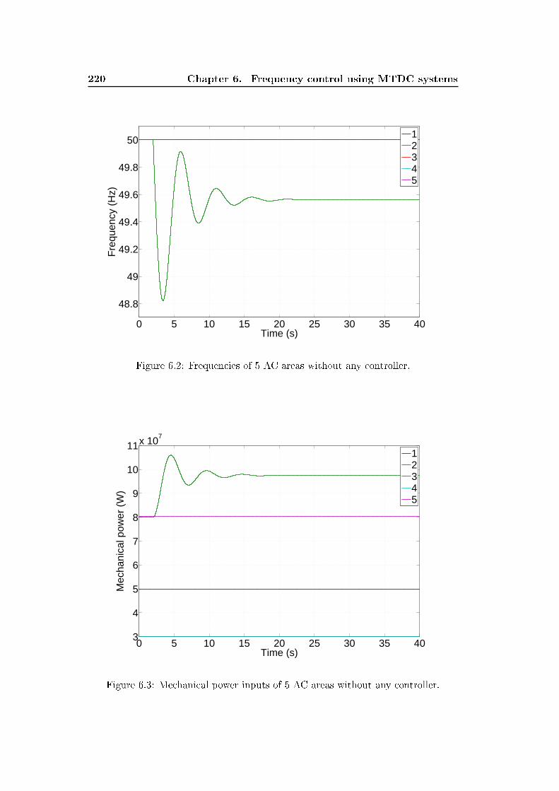
220 Chapter 6. Frequency control using MTDC systems
0 5 10 15 20 25 30 35 40
48.8
49
49.2
49.4
49.6
49.8
50
Time (s)
Fre
quen
cy (
Hz)
12345
Figure 6.2: Frequencies of 5 AC areas without any controller.
0 5 10 15 20 25 30 35 403
4
5
6
7
8
9
10
11x 107
Time (s)
Mec
hani
cal p
ower
(W
)
12345
Figure 6.3: Mechanical power inputs of 5 AC areas without any controller.
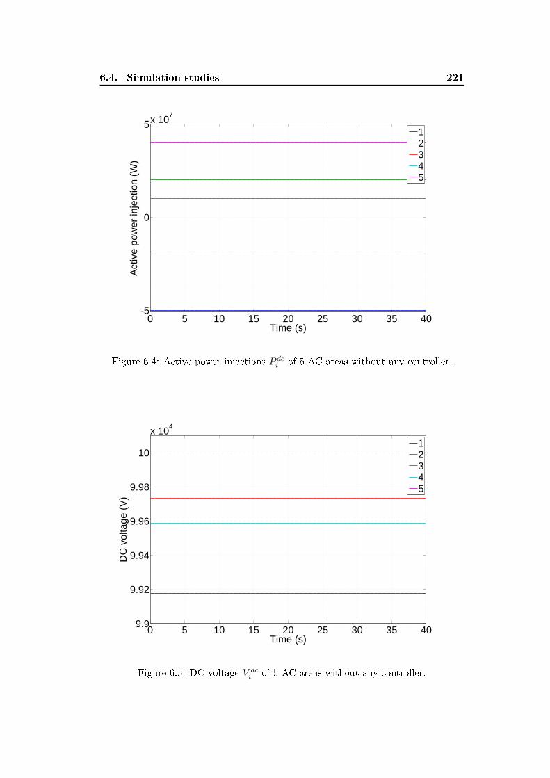
6.4. Simulation studies 221
0 5 10 15 20 25 30 35 40-5
0
5x 10⁷
Time (s)
Act
ive
pow
er in
ject
ion
(W)
12345
Figure 6.4: Active power injections P dci of 5 AC areas without any controller.
0 5 10 15 20 25 30 35 409.9
9.92
9.94
9.96
9.98
10
x 104
Time (s)
DC
vol
tage
(V
)
12345
Figure 6.5: DC voltage V dci of 5 AC areas without any controller.
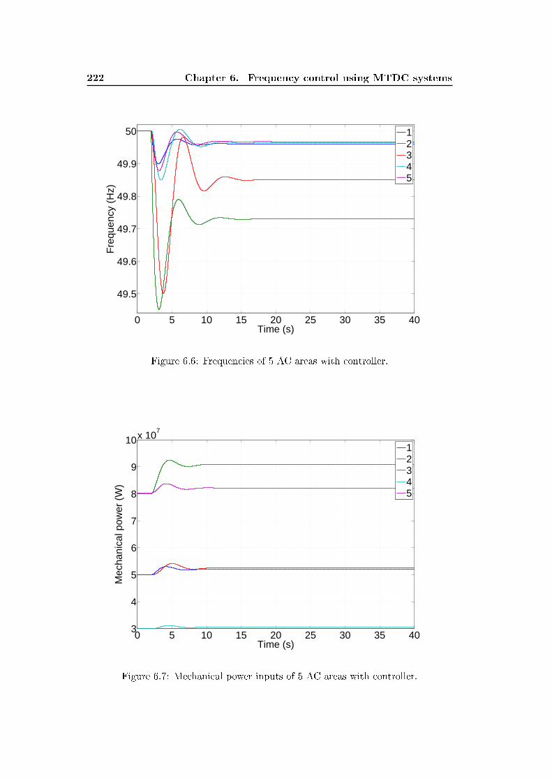
222 Chapter 6. Frequency control using MTDC systems
0 5 10 15 20 25 30 35 40
49.5
49.6
49.7
49.8
49.9
50
Time (s)
Fre
quen
cy (
Hz)
12345
Figure 6.6: Frequencies of 5 AC areas with controller.
0 5 10 15 20 25 30 35 403
4
5
6
7
8
9
10x 107
Time (s)
Mec
hani
cal p
ower
(W
)
12345
Figure 6.7: Mechanical power inputs of 5 AC areas with controller.
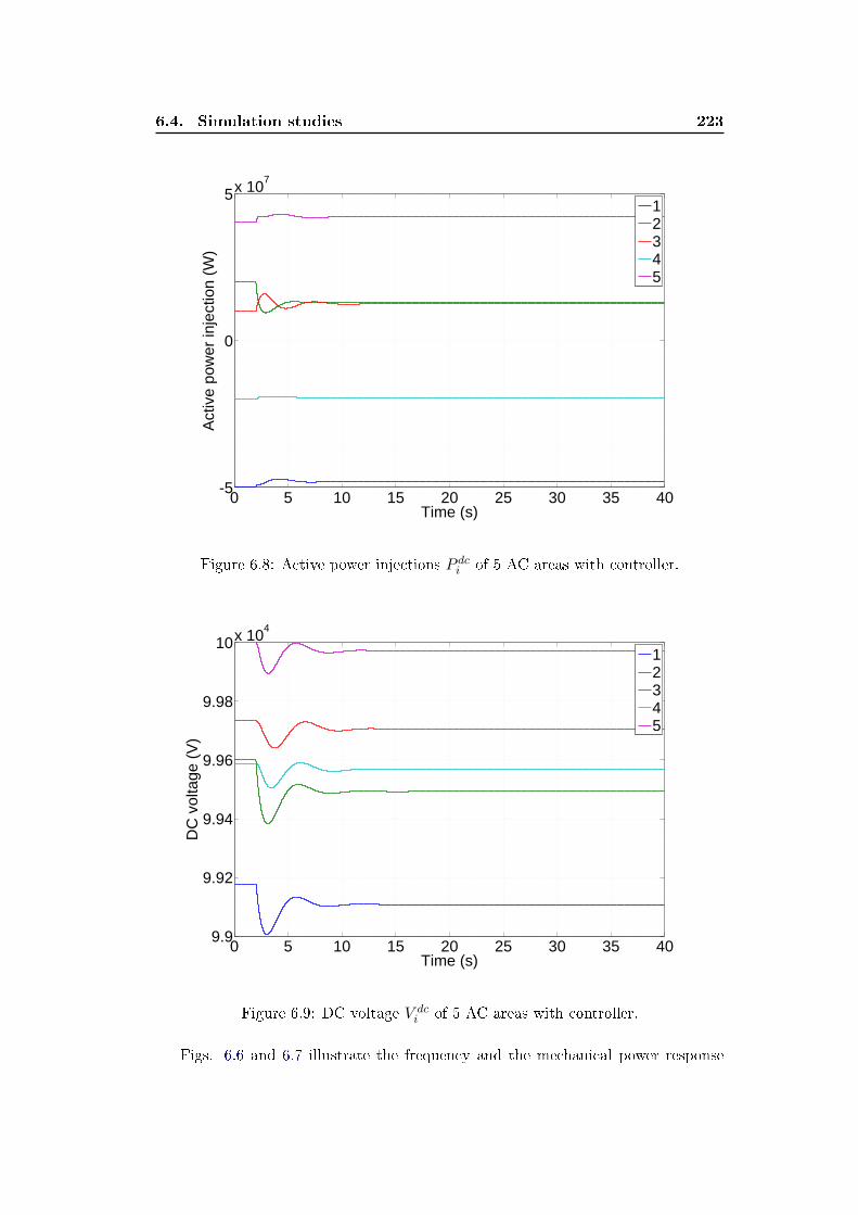
6.4. Simulation studies 223
0 5 10 15 20 25 30 35 40-5
0
5x 10⁷
Time (s)
Act
ive
pow
er in
ject
ion
(W)
12345
Figure 6.8: Active power injections P dci of 5 AC areas with controller.
0 5 10 15 20 25 30 35 409.9
9.92
9.94
9.96
9.98
10x 104
Time (s)
DC
vol
tage
(V
)
12345
Figure 6.9: DC voltage V dci of 5 AC areas with controller.
Figs. 6.6 and 6.7 illustrate the frequency and the mechanical power response
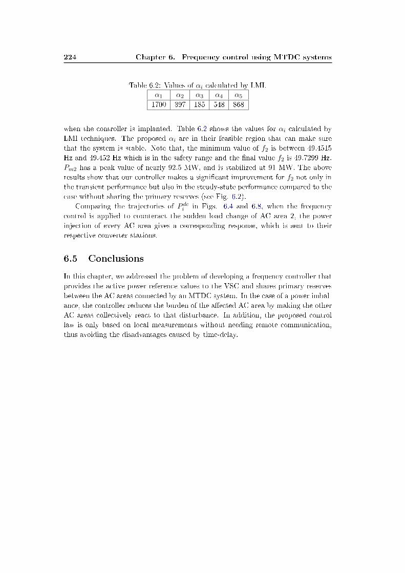
224 Chapter 6. Frequency control using MTDC systems
Table 6.2: Values of αi calculated by LMI.α1 α2 α3 α4 α5
1700 397 185 548 868
when the controller is implanted. Table 6.2 shows the values for αi calculated by
LMI techniques. The proposed αi are in their feasible region that can make sure
that the system is stable. Note that, the minimum value of f2 is between 49.4515
Hz and 49.452 Hz which is in the safety range and the nal value f2 is 49.7299 Hz.
Pm2 has a peak value of nearly 92.5 MW, and is stabilized at 91 MW. The above
results show that our controller makes a signicant improvement for f2 not only in
the transient performance but also in the steady-state performance compared to the
case without sharing the primary reserves (see Fig. 6.2).
Comparing the trajectories of P dci in Figs. 6.4 and 6.8, when the frequency
control is applied to counteract the sudden load change of AC area 2, the power
injection of every AC area gives a corresponding response, which is sent to their
respective converter stations.
6.5 Conclusions
In this chapter, we addressed the problem of developing a frequency controller that
provides the active power reference values to the VSC and shares primary reserves
between the AC areas connected by an MTDC system. In the case of a power imbal-
ance, the controller reduces the burden of the aected AC area by making the other
AC areas collectively react to that disturbance. In addition, the proposed control
law is only based on local measurements without needing remote communication,
thus avoiding the disadvantages caused by time-delay.
Chapter 7
Conclusions
Contents
7.1 Conclusions . . . . . . . . . . . . . . . . . . . . . . . . . . . . . 225
7.2 Perspectives for future work . . . . . . . . . . . . . . . . . . . 228
7.2.1 Further research on the droop control conguration . . . . . 228
7.2.2 Further research on the connection of other types of weak AC
systems . . . . . . . . . . . . . . . . . . . . . . . . . . . . . . 229
7.2.3 Further research on the operation of MTDC systems . . . . . 229
7.2.4 Further research on system modeling . . . . . . . . . . . . . . 229
7.2.5 Implementation on a real MTDC system . . . . . . . . . . . . 229
7.2.6 Control induced time-scale separation for the MMC . . . . . 229
7.1 Conclusions
In the last decades, the development of VSC HVDC systems becomes a very im-
portant topic in scientic researches. Due to their exibility, controllability and
eciency, VSC HVDC systems have been greatly promoted in today's electrical
networks. In particular, there is a growing need to integrate large-scale oshore
renewable energy sources via MTDC systems, whose generation outputs are usually
intermittent. Nevertheless, the MTDC technology is not yet mature enough for wide
commercial applications. There are still many issues that need to be solved. This
dissertation is dedicated to the challenges in the control of MTDC systems.
This thesis started by giving a brief introduction to HVDC technology where
the limits of the classical AC transmission technology are shown and the rationale
of HVDC systems is discussed. Besides, the comparisons between AC and DC
as well as LCC and VSC are also listed. Then, we introduced several existing
control structures of VSC HVDC systems according to their research groups in
the literature review. Interestingly, we found that most of the control methods
only focus on the operating results but neglect related theoretical analysis. As
a consequence, extra time-consuming processes are usually needed to accompany
these control approaches to achieve good performance. At the end of Chapter 1, we
dened the objectives of this thesis: 1) developing new control methods for MTDC
systems to improve the overall performance; 2) providing theoretical explanations
for the system dynamic behaviors to give new insights into how and why the existing
226 Chapter 7. Conclusions
conventional (or empirical) control structures work; 3) fully developing the potential
of MTDC systems for AC frequency regulation; 4) Developing a new control theory
named Control Induced Time-Scale Separation. This general control theory was
created aiming at the MTDC system, but indeed applies to a very broad class of
nonlinear systems, and allows plug-and-play capabilities. In addition, it ts well in
a Systems of Systems framework.
In Chapter 2, we rst gave an overview of the VSC technology to get a good
understanding of the classic operation of VSC HVDC systems. Then, we introduced
two dierent types of AC networks which are distinguished by their Short Circuit
Ratio. In line with the control objectives and the type of the connected AC network,
possible control modes of a single VSC terminal were discussed, which oer a basic
knowledge for the control design of MTDC systems.
In the modeling, the time-averaged modeling method which is the most generally
used modeling approach in the context of power systems was chosen and presented in
Chapter 3. This modeling approach is much simpler and tractable than the detailed
modeling one. In this thesis, the proposed MTDC system consists of N strong AC
networks,M weak AC networks and a DC grid. One of the main contributions of this
thesis is that a generic topology is considered for the structure of the DC grid, which
can be mapped to a weakly connected directed graph. Thus, our research is not only
suitable for the radial topology but also for the meshed topology. In addition, all
connected AC networks are considered in balanced three-phase condition and hence,
Park's transformation is applied to project all three-phase quantities onto a rotating
two-axis reference frame. The overall modeling work is divided into three parts: 1)
modeling of the strong AC network connected VSC terminals; 2) modeling of the
weak AC network connected VSC terminals; 3) modeling of the DC grid. At the end
of Chapter 3, an averaged state-space model of high order for the proposed MTDC
system was established.
In Chapter 4, two of the most widely used conventional control methods for VSC
HVDC systems, namely direct and vector control methods, were discussed. Both
advantages and disadvantages of the aforementioned control methods were analyzed.
Based on the existing problems of the two control approaches, new improved control
strategies were proposed in this dissertation.
In Chapter 5, new control structures by means of dierent nonlinear control
design tools for VSC HVDC systems were developed. We started by applying feed-
back linearization technique to the development of a nonlinear controller, which can
partly transform the nonlinear MTDC model to a linear one. A theoretical analysis
of the nonlinear feedback linearization controller was carried out, which indicates
that the stability of the equilibrium of the zero dynamics determines the stability of
the overall system. Furthermore, a sucient condition on the system parameters was
derived to ensure the stability of the zero dynamics. The performance comparisons
between this nonlinear controller and the conventional vector controller were given,
which show that the nonlinear control provides much better decoupling characteris-
tics of the DC voltage and the AC q−axis current control or the AC voltages vswjdand vswjq control than the PI controller. Besides, during the simulation process, we
7.1. Conclusions 227
found that when a new operating point of the MTDC systems is to be achieved, it is
usually needed to recalculate the proper PI control gains for the conventional vector
controller to obtain an optimal performance. However, this is time-consuming and
usually requires extra eorts. For the nonlinear feedback controller, we usually have
no need to deduce new control gains for dierent operating conditions. In order to
make the system more robust, a sliding mode control technique was applied to de-
velop a novel controller where the uncertainties of the system parameters and other
possible exogenous inputs were taken into account. During the design procedure of
the feedback linearization controller, we naturally chose the controlled variables as
the output. However, the theoretical analysis clearly shows that the MTDC sys-
tem is not always minimum phase. There exists a restriction on the choice of the
prescribed references and the system parameters (see Lemma 4.1.2). To overcome
this problem, a passive output was deduced by means of passivity theory so that
the MTDC system with the passive output is always minimum phase. Then, a new
control strategy based on the input-output feedback linearizaton and the passiv-
ity theory was devised. Simulation studies were also carried out to evaluate the
performance of the passivity-based state feedback controller.
In Chapter 6, the dynamic behaviors of the proposed MTDC system were ana-
lyzed. It is interesting to remark that these dynamics have never been extensively
rigorously studied in the literature. The research done on this issue is one of the
main contributions of this dissertation summarized as follow:
• Control induced time-scale separation design for a class of nonlinear
systems
A control induced time-scale separation method was developed for a class
of nonlinear systems, which enables the system to exhibit a multi-time-scale
behavior characterized by the presence of fast and slow transients. Based on
singular perturbation theory, a detailed theoretical analysis was performed,
which shows that the time-scale decomposition of the system dynamics is
qualied by the control gains of the driving subsystem. Besides, with the
help of the proposed controller, the original system can be divided into two
low-order subsystems and then, the behaviors of the system states can be
approximated by the solutions of the two simpler subsystems. Furthermore,
we gave an analytical expression to illustrate the trade-o between the system
performance and the region of attraction.
• Analysis of the conventional control structures and the dynamics of
the MTDC system
For an MTDC system, the concept of the conventional vector control method is
mainly based on the assertion that the dynamics of the system state variables
can be divided into dierent time scales and hence, the two control loops
can be designed independently. However, very few research has ever veried
and explained this assertion. In this dissertation, we applied the theoretical
results obtained from the study on the time-scale separation controller to
228 Chapter 7. Conclusions
bridge the gap between the practice and the theory where the master-slave and
the droop control congurations were studied. From the theoretical analysis
of the two control congurations, we identied several points: 1) how and
why the system exhibits a multi-time-scale behavior; 2) the rules of tuning
the control gains such that parts of those gains regulate the fast transient and
the remaining determines the behavior of the slow transient; 3) the existence
of uncontrollable state variables when the master-slave control conguration
is used. Moreover, we pointed out that the master-slave control conguration
based on vector control method is not always applicable for the MTDC system.
The stability of the MTDC system with the master-slave control conguration
can be ensured only when the system parameters and the scheduled references
satisfy certain conditions while for the droop control conguration, there is no
special limitation on them.
In Chapter 7, a potential application of MTDC systems was introduced where an
AC frequency support strategy via the MTDC system was proposed. This strategy
enables the asynchronous AC systems to share their primary reserves via an MTDC
system. The control method used in this application, namely the DC-voltage-based
controller, is based on local measurements without needing any remote communica-
tion, and avoids possible problems caused by time-delay. Simulation studies showed
that the proposed control strategy achieves the control objective with satisfactory
performances.
7.2 Perspectives for future work
This thesis have met some challenges in the area of MTDC systems. However, there
still exist many issues to be investigated.
7.2.1 Further research on the droop control conguration
In Section 5.3, we discussed the dynamic behavior of the MTDC system under the
droop control conguration. We found that the choice of the droop gains has great
impacts on: 1) the steady-state values of the system variables; 2) the distribution of
power sharing between the interconnected AC networks in case of power imbalance;
3) the dynamics of the DC grid. In this thesis, the droop gains are considered
constant. It would be interesting to consider the droop gains not as constants but as
variables, which could vary according to dierent operating conditions. For example,
each converter terminal has a dierent capability against the power imbalance. The
droop gain of each converter terminal could vary depending on its existing available
headroom of the capacity.

7.2. Perspectives for future work 229
7.2.2 Further research on the connection of other types of weakAC systems
One of the most important applications of VSC HVDC systems is to connect island
systems. It would be interesting to consider that the MTDC system has one or more
converter terminals connected to islands. Moreover, various components related to
the island, such as the synchronous generators, the passive loads, can be taken
into account. It is worthwhile to note that the passive loads are usually unknown
and hence, during the control design for the island connected converter terminal,
adaptive control technique could be applied to improve the system performance.
7.2.3 Further research on the operation of MTDC systems
In Section 4.1.4.1, we presented that the MTDC system has plug-and-play capabili-
ties. This ability is very important for the extension of the existing MTDC systems.
In this thesis, we provided a qualitative approach to determine whether an AC sys-
tem could be added or removed. One of possible further work is that a quantitative
approach need to be developed from a security point of view.
7.2.4 Further research on system modeling
In this thesis, the ideal three-phase AC source was used for every strong AC network
and the controlled three-phase current source was used for every weak AC network.
Therefore, we can take the dynamics of the generator and the wind turbine into
consideration when modeling an MTDC system. This would help us study the
system behaviors and the interactions between AC and DC.
7.2.5 Implementation on a real MTDC system
In this thesis, the developed nonlinear controllers were tested by using SimPowerSys-
tems toolbox of MATLAB/Simulink. From the simulation results, both advantages
and disadvantages of each control method are clearly presented. However, due to
the limit of the condition, these control methods are not yet implemented on a real
MTDC system. It will be interesting to test these proposed controllers on a real
MTDC system.
7.2.6 Control induced time-scale separation for the MMC
Compared to the VSC with PMW technology, multilevel modular converter (MMC)
has attracted a lot of attention due to its less generated harmonics and losses of
the semiconductor devices. Since the MMC has a more complicated structure than
the VSC with two (or three) voltage levels, in future work it is possible to apply
the obtained theoretical results on the control induced time-scale to analyze the
dynamic behavior of MMC in an easy way.

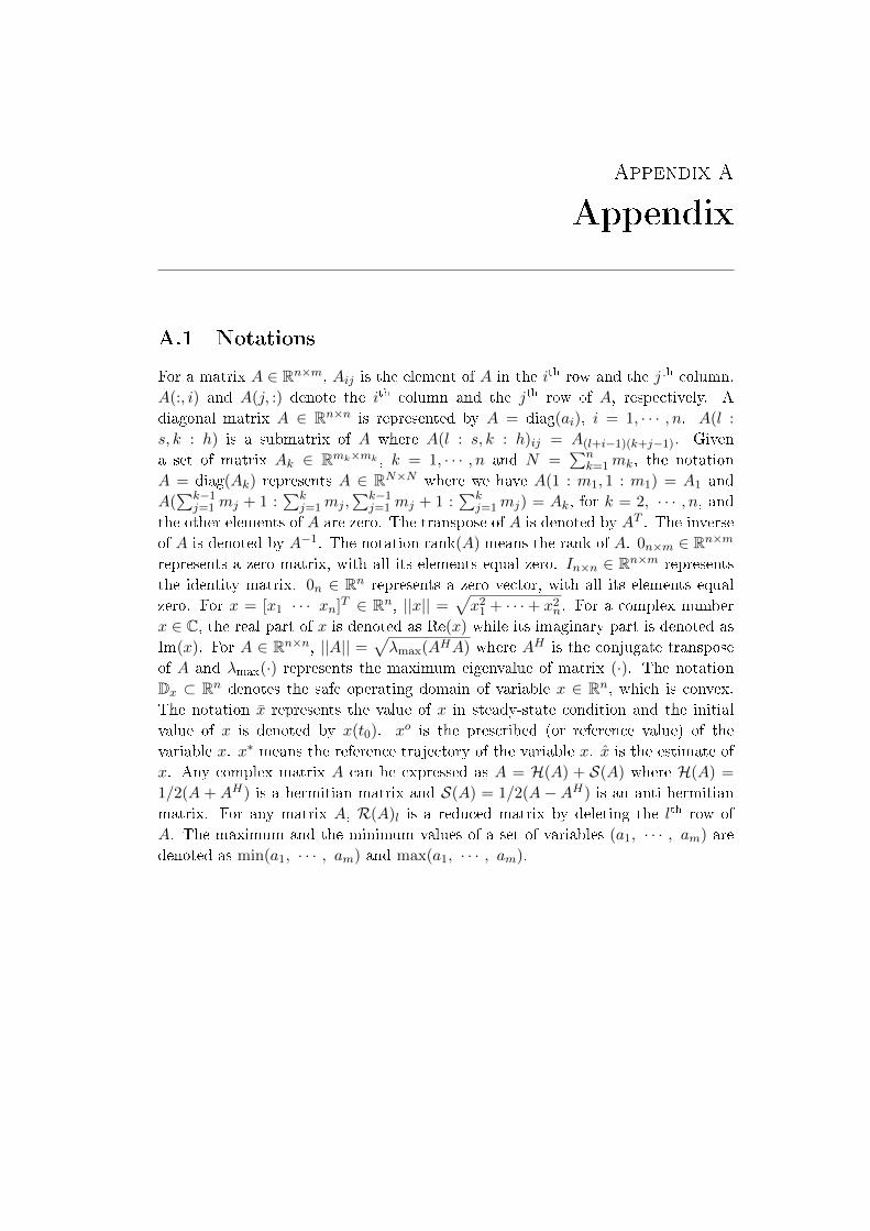
Appendix A
Appendix
A.1 Notations
For a matrix A ∈ Rn×m, Aij is the element of A in the ith row and the jth column.
A(:, i) and A(j, :) denote the ith column and the jth row of A, respectively. A
diagonal matrix A ∈ Rn×n is represented by A = diag(ai), i = 1, · · · , n. A(l :
s, k : h) is a submatrix of A where A(l : s, k : h)ij = A(l+i−1)(k+j−1). Given
a set of matrix Ak ∈ Rmk×mk , k = 1, · · · , n and N =∑n
k=1mk, the notation
A = diag(Ak) represents A ∈ RN×N where we have A(1 : m1, 1 : m1) = A1 and
A(∑k−1
j=1 mj + 1 :∑k
j=1mj ,∑k−1
j=1 mj + 1 :∑k
j=1mj) = Ak, for k = 2, · · · , n, andthe other elements of A are zero. The transpose of A is denoted by AT . The inverse
of A is denoted by A−1. The notation rank(A) means the rank of A. 0n×m ∈ Rn×mrepresents a zero matrix, with all its elements equal zero. In×n ∈ Rn×m represents
the identity matrix. 0n ∈ Rn represents a zero vector, with all its elements equal
zero. For x = [x1 · · · xn]T ∈ Rn, ||x|| =√x2
1 + · · ·+ x2n. For a complex number
x ∈ C, the real part of x is denoted as Re(x) while its imaginary part is denoted as
Im(x). For A ∈ Rn×n, ||A|| =√λmax(AHA) where AH is the conjugate transpose
of A and λmax(·) represents the maximum eigenvalue of matrix (·). The notation
Dx ⊂ Rn denotes the safe operating domain of variable x ∈ Rn, which is convex.
The notation x represents the value of x in steady-state condition and the initial
value of x is denoted by x(t0). xo is the prescribed (or reference value) of the
variable x. x∗ means the reference trajectory of the variable x. x is the estimate of
x. Any complex matrix A can be expressed as A = H(A) + S(A) where H(A) =
1/2(A + AH) is a hermitian matrix and S(A) = 1/2(A − AH) is an anti-hermitian
matrix. For any matrix A, R(A)l is a reduced matrix by deleting the lth row of
A. The maximum and the minimum values of a set of variables (a1, · · · , am) are
denoted as min(a1, · · · , am) and max(a1, · · · , am).


Appendix B
Appendix
B.1 Proof of Lemma 4.1.6
Proof. For any vector x ∈ Cn, x 6= 0n, we have
(xHH(Ψ)x)H = xHH(Ψ)Hx
= xHH(Ψ)x
Hence, xHH(Ψ)x is a real number. Similarly, we can obtain
(xHS(Ψ)x)H = xHS(Ψ)Hx
= −xHS(Ψ)x
Thus, xHS(Ψ)x is an imaginary number. So we get Re(xHΨx) = xHH(Ψ)x. As a
result, Re(xHΨx) is positive if and only if xHH(Ψ)x is positive.
B.2 Proof of Lemma 4.1.9
Proof. Since Ψ is positive denite, H(Ψ) is also positive denite and hence there
exists an invertible matrix Q such that
QHH(Ψ)Q = In×n
In addition, QHS(Ψ)Q is also an anti-hermitian matrix. Hence, there exists a
unitary matrix U such that
UHQHS(Ψ)QU = diag(jb1, jb2, ·, jbk, 0, · · · , 0)
where j =√−1, bi 6= 0 (i = 1, · · · , k) are real numbers and k = rank(S(Ψ)).
Moreover, we have
UHQHH(Ψ)QU = In×n
Let us denote P = QU and as a consequence, P is invertible. We then have
PHΨP = PHH(Ψ)P + PHS(Ψ)P
= diag(jb1 + 1, jb2 + 1, ·, jbk + 1, 1, · · · , 1) , T
Since matrices T and P are invertible and we also have
Ψ = (PH)−1TP−1
Ψ is invertible. Moreover, because H(T ) is positive denite, according to Lemma
4.1.6, T is also positive denite. Finally, we get the result that Ψ−1 is also positive
denite.

Bibliography
[ABB 2014] ABB. Lower losses. http://www.abb.com/industries/
db0003db004333/fd32594c4d4dea8cc1257481004a6140.aspx, 2014. (Cited
on page 106.)
[Adam 2015] G.P. Adam, I.A. Abdelsalam, K.H. Ahmed and B.W. Williams. Hybrid
Multilevel Converter With Cascaded H-bridge Cells for HVDC Applications:
Operating Principle and Scalability. IEEE Transactions on Power Electronic,
vol. 30, no. 1, pages 6577, Jan 2015. (Cited on page 11.)
[Akhmatov 2014] V. Akhmatov, M. Callavik, C.M. Franck, S.E. Rye, T. Ahndorf,
M.K. Bucher, H. Muller, F. Schettler and R. Wiget. Technical Guidelines
and Prestandardization Work for First HVDC Grids. IEEE Transactions on
Power Delivery, vol. 29, no. 1, pages 327335, Feb 2014. (Cited on page 24.)
[Andersen 2000] B. Andersen and C. Barker. A new era in HVDC? IEE Review,
vol. 46, no. 2, pages 3339, Mar 2000. (Cited on page 3.)
[Andersen 2002] B.R. Andersen, L. Xu, P.J. Horton and P Cartwright. Topologies
for VSC transmission. Power Engineering Journal, vol. 16, no. 3, pages
142150, Jun 2002. (Cited on pages 2 and 17.)
[Arrillaga 1998] Jos Arrillaga. High voltage direct current transmission. Nu-
meéro 29. Iet, 1998. (Cited on page 4.)
[Asplund 2000] G. Asplund. Application of HVDC Light to power system enhance-
ment. In IEEE Power Engineering Society Winter Meeting, volume 4, pages
24982503, 2000. (Cited on page 3.)
[Asplund 2007] Gunnar Asplund. Ultra high voltage transmission. ABB Review,
no. 2, pages 2227, 2007. (Cited on page 3.)
[Ayodele 2011] TR Ayodele, AA Jimoh, JL Munda and JT Agee. The inuence of
wind power on the small signal stability of a power system. In International
conference on renewable energy and power quality, pages 1315, Las Palmas
de Gra Canaria, Spain, April 2011. (Cited on page 8.)
[Bahrman 2007] Michael P Bahrman and Brian K Johnson. The ABCs of HVDC
transmission technologies. IEEE Power and Energy Magazine, vol. 5, no. 2,
pages 3244, 2007. (Cited on pages 3 and 17.)
[Bajracharya 2008] Chandra Bajracharya, Marta Molinas, Jon Are Suul, Tore M
Undelandet al. Understanding of tuning techniques of converter controllers
for VSC-HVDC. In Nordic Workshop on Power and Industrial Electronics,
Espoo, Finland, Jun 2008. Helsinki University of Technology. (Cited on
pages 12 and 43.)
236 Bibliography
[Beccuti 2010] G. Beccuti, G. Papafotiou and L. Harnefors. Multivariable predictive
control of voltage source converter HVDC transmission systems. In IEEE
International Symposium on Industrial Electronics (ISIE) pages 31453152,
Jul 2010. (Cited on pages 8 and 9.)
[Beerten 2014] J. Beerten, S. Cole and R. Belmans. Modeling of Multi-Terminal
VSC HVDC Systems With Distributed DC Voltage Control. IEEE Transac-
tions on Power Systems, vol. 29, no. 1, pages 3442, Jan 2014. (Cited on
pages 11 and 36.)
[Bendtsen 2013] Jan Bendtsen, Klaus Trangbaek and Jakob Stoustrup. Plug-and-
Play Control-Modifying Control Systems Online. IEEE Transactions on
Control Systems Technology, vol. 21, no. 1, pages 7993, 2013. (Cited on
page 132.)
[Bianchi 2011] F.D. Bianchi and O. Gomis-Bellmunt. Droop control design for
multi-terminal VSC-HVDC grids based on LMI optimization. In 2011 50th
IEEE Conference on Decision and Control and European Control Conference
(CDC-ECC), pages 48234828, Dec. 2011. (Cited on pages 10 and 174.)
[Blasko 1997] V. Blasko and V. Kaura. A new mathematical model and control of
a three-phase AC-DC voltage source converter. IEEE Transactions on Power
Electronics, vol. 12, no. 1, pages 116123, Jan 1997. (Cited on pages 8, 9
and 41.)
[Bondy 1976] John Adrian Bondy and Uppaluri Siva Ramachandra Murty. Graph
theory with applications, volume 6. Macmillan London, 1976. (Cited on
page 39.)
[Boyd 1994] S. Boyd, L. El Ghaoui, E. Feron and V. Balakrishnan. Linear ma-
trix inequalities in system and control theory. SIAM, Studies in Applied
Mathematics, 1994. (Cited on page 210.)
[Byrnes 1991] Christopher I Byrnes, Alberto Isidori and Jan C Willems. Passivity,
feedback equivalence, and the global stabilization of minimum phase nonlinear
systems. IEEE Transactions on Automatic Control, vol. 36, no. 11, pages
12281240, 1991. (Cited on page 101.)
[Carlsson 2002] Lennart Carlsson. " Classical" HVDC: still continuing to evolve.
Modern power systems, vol. 22, no. 6, pages 1922, 2002. (Cited on page 4.)
[Carlsson 2003] L Carlsson, G Flisberg and L Weimers. Recent Evolution in Clas-
sic HVDC. In The 4th International Conference on Power Transmission &
Distribution, 2003. (Cited on page 4.)
[Chaudhary 2008] S.K. Chaudhary, R. Teodorescu and P. Rodriguez. Wind Farm
Grid Integration Using VSC Based HVDC Transmission - An Overview. In
IEEE Energy 2030, pages 17, Nov 2008. (Cited on pages 8 and 34.)
Bibliography 237
[Chaudhuri 2013] N.R. Chaudhuri and B. Chaudhuri. Adaptive Droop Control for
Eective Power Sharing in Multi-Terminal DC (MTDC) Grids. IEEE Trans-
actions on Power Systems, vol. 28, no. 1, pages 2129, Feb. 2013. (Cited on
pages 10 and 174.)
[Chen 2011] Xia Chen, Haishun Sun, Jinyu Wen, Wei-Jen Lee, Xufeng Yuan, Naihu
Li and Liangzhong Yao. Integrating Wind Farm to the Grid Using Hybrid
Multiterminal HVDC Technology. IEEE Transactions on Industry Applica-
tions vol. 47, no. 2, pages 965972, Mar 2011. (Cited on page 11.)
[Chen 2013] Wu-Hua Chen, Guo Yuan and Wei Xing Zheng. Robust Stability of
Singularly Perturbed Impulsive Systems Under Nonlinear Perturbation. IEEE
Transactions on Automatic Control, vol. 58, no. 1, pages 168174, January
2013. (Cited on page 133.)
[Chen 2014] Yijing Chen, Gilney Damm, Abdelkrim Benchaib and Françoise
Lamnabhi-Lagarrigue. Multi-Time-Scale Stability Analysis and Design Con-
ditions of a VSC Terminal with DC Voltage Droop Control for HVDC Net-
works. In IEEE Conference on Decision and Control (CDC), Los Angeles,
CA, USA, Dec. 2014. IEEE. (Cited on pages 10 and 174.)
[Chung 2000] Se-Kyo Chung. A phase tracking system for three phase utility inter-
face inverters. IEEE Transactions on Power Electronics, vol. 15, no. 3, pages
431438, May 2000. (Cited on page 31.)
[CIGRE 2014] CIGRE. What is LCC HVDC ? http://b4.cigre.org/
Menu-links/What-is-SC-B4, 2014. (Cited on page 4.)
[Cole 2010] Stijn Cole. Steady-State and Dynamic Modelling of VSC HVDC Systems
for Power System Simulation. PhD thesis, PhD Dissertation, KU Leuven,
2010. (Cited on page 11.)
[Dai 2010] J. Dai, Y. Phulpin, A. Sarlette and D. Ernst. Impact of delays on a
consensus-based primary frequency control scheme for AC systems connected
by a multi-terminal HVDC grid. In Proceedings of the 2010 IREP Symposium
- Bulk Power Systems Dynamics and Control - VIII, Buzios, Rio de Janeiro,
Brazil, 1-6 August 2010. (Cited on page 210.)
[Dannehl 2009] J. Dannehl, C. Wessels and F.W. Fuchs. Limitations of Voltage-
Oriented PI Current Control of Grid-Connected PWM Rectiers With LCL
Filters. IEEE Transactions on Industrial Electronics, vol. 56, no. 2, pages
380388, Feb 2009. (Cited on pages 9, 12, 43 and 47.)
[Daryabak 2014] M. Daryabak, S. Filizadeh, J. Jatskevich, A. Davoudi, M. Saeedi-
fard, V.K. Sood, J.A. Martinez, D. Aliprantis, J. Cano and A. Mehrizi-Sani.
Modeling of LCC-HVDC Systems Using Dynamic Phasors. IEEE Transac-
tions on Power Delivery, vol. 29, no. 4, pages 19891998, Aug 2014. (Cited
on page 3.)
238 Bibliography
[Del Vecchio 2013] D. Del Vecchio and J.E. Slotine. A Contraction Theory Approach
to Singularly Perturbed Systems. IEEE Transactions on Automatic Control,
vol. 58, no. 3, pages 752757, March 2013. (Cited on page 133.)
[Dodds 2010] S Dodds, B Railing, K Akman, B Jacobson, T Worzyk and B Nilsson.
HVDC VSC (HVDC light) transmissionoperating experiences. Proc. CIGRE
Session, Paris, France, pages 19, 2010. (Cited on pages 3, 4 and 17.)
[Du 2003] Cuiqing Du. The control of VSC-HVDC and its use for large industrial
power systems. PhD thesis, Chalmers University of Technology, 2003. (Cited
on page 42.)
[Du 2005] Cuiqing Du, Ambra Sannino and Math HJ Bollen. Analysis of the control
algorithms of voltage-source converter HVDC. In IEEE Power Tech, pages
17, Russia, June 2005. (Cited on pages 9 and 34.)
[Durrant 2003] Martyn Durrant, H. Werner and Keith Abbott. Model of a VSC
HVDC terminal attached to a weak AC system. In IEEE Conference on
Control Applications, volume 1, pages 178182, Jun 2003. (Cited on pages 9,
43 and 47.)
[Durrant 2004] Martyn Durrant, H. Werner and Keith Abbott. Synthesis of multi-
objective controllers for a VSC HVDC terminal using LMIs. In IEEE Confer-
ence on Decision and Control, volume 4, pages 44734478, Dec 2004. (Cited
on page 109.)
[Durrant 2006] Martyn Durrant, H. Werner and Keith Abbott. A Comparison of
LMI and GA Based Robust Controller Designs for VSC HVDC. In 45th IEEE
Conference on Decision and Control, pages 39903995, Dec 2006. (Cited on
page 9.)
[Egea-Alvarez 2013] A. Egea-Alvarez, F. Bianchi, A. Junyent-Ferre, G. Gross and
O. Gomis-Bellmunt. Voltage Control of Multiterminal VSC-HVDC Trans-
mission Systems for Oshore Wind Power Plants: Design and Implemen-
tation in a Scaled Platform. IEEE Transactions on Industrial Electronics,
vol. 60, no. 6, pages 23812391, Jun. 2013. (Cited on page 174.)
[Ekanayake 2009] J.B. Ekanayake. Multi-terminal DC converters for connecting in-
duction generator based distribution generation. In International Conference
on Industrial and Information Systems (ICIIS), pages 466471, Dec 2009.
(Cited on page 10.)
[Eriksson 2001] Kjell Eriksson. Operational experience of HVDC LightTM. In Sev-
enth International Conference on AC-DC Power Transmission, pages 205
210, Nov 2001. (Cited on page 3.)
Bibliography 239
[Eriksson 2014] R. Eriksson, J. Beerten, M. Ghandhari and R. Belmans. Optimizing
DC Voltage Droop Settings for AC/DC System Interactions. IEEE Transac-
tions on Power DeliverY, vol. 29, no. 1, pages 362369, Feb 2014. (Cited on
page 10.)
[Escobar 1999] Gerardo Escobar, Arjan J Van Der Schaft and Romeo Ortega. A
Hamiltonian viewpoint in the modeling of switching power converters. Auto-
matica, vol. 35, no. 3, pages 445452, 1999. (Cited on page 92.)
[Flourentzou 2009] Nikolas Flourentzou, Vassilios G Agelidis and Georgios D Deme-
triades. VSC-based HVDC power transmission systems: an overview. Power
Electronics, IEEE Transactions on, vol. 24, no. 3, pages 592602, 2009. (Cited
on pages 3 and 4.)
[Fu 2014] Jiao Fu, Zhichang Yuan, Yizhen Wang, Shukai Xu, Wei Wei and Yu Luo.
Control strategy of system coordination in Nanao multi-terminal VSC-HVDC
project for wind integration. In IEEE PES General Meeting, pages 15, Jul
2014. (Cited on pages 3 and 11.)
[Gavrilovic 1991] A. Gavrilovic. AC/DC system strength as indicated by short circuit
ratios. In International Conference on AC and DC Power Transmission, pages
2732, Sep 1991. (Cited on pages 23 and 34.)
[Haileselassie 2008] Temesgen M Haileselassie, Marta Molinas, Tore Undelandet al.
Multi-terminal VSC-HVDC system for integration of oshore wind farms
and green electrication of platforms in the North Sea. In Nordic Workshop
on Power and Industrial Electronics. Helsinki University of Technology, Jun
2008. (Cited on pages 10 and 11.)
[Haileselassie 2009] T Haileselassie, Tore Undeland and Kjetil Uhlen. Multiterminal
HVDC for oshore wind farms-control strategy. In Wind Power to the Grid-
EPE Wind Energy Conferece, Stockholm, Sweden, 2009. (Cited on page 11.)
[Haileselassie 2012a] Temesgen Mulugeta Haileselassie. Control, Dynamics and Op-
eration of Multi-terminal VSC-HVDC Transmission Systems. PhD thesis,
Norwegian University of Science and Technology, 2012. (Cited on pages 11
and 40.)
[Haileselassie 2012b] T.M. Haileselassie and K. Uhlen. Impact of DC Line Voltage
Drops on Power Flow of MTDC Using Droop Control. IEEE Transactions
on Power Systems, vol. 27, no. 3, pages 14411449, Aug. 2012. (Cited on
pages 10, 177 and 181.)
[Hamzei-nejad 1986] A. Hamzei-nejad and C. M Ong. Coordinating the DC power
injections of a multiterminal HVDC system for dynamic control of AC line
ows. IEEE Transactions on Power Systems, vol. PWRS-1, no. 2, May 1986.
(Cited on page 210.)
240 Bibliography
[Hedrick 2005] JK Hedrick and A Girard. Control of nonlinear dynamic systems:
Theory and applications. Controllability and observability of Nonlinear Sys-
tems, 2005. (Cited on page 48.)
[Hernandez-Gomez 2010] M. Hernandez-Gomez, R. Ortega, F. Lamnabhi-
Lagarrigue and G. Escobar. Adaptive PI Stabilization of Switched Power
Converters. IEEE Transactions on Control Systems Technology, vol. 18,
no. 3, pages 688698, May 2010. (Cited on pages 92 and 109.)
[Horn 1985] Roger A Horn and Charles R Johnson. Matrix analysis. Cambridge
university press, 1985. (Cited on page 76.)
[IEE 1997] IEEE Guide for Planning DC Links Terminating at AC Locations Hav-
ing Low Short-Circuit Capacities. IEEE Std 1204-1997, 1997. (Cited on
page 23.)
[Ilves 2015] K. Ilves, L. Harnefors, S. Norrga and H.-P. Nee. Analysis and Operation
of Modular Multilevel Converters With Phase-Shifted Carrier PWM. IEEE
Transactions on Power Electronics, vol. 30, no. 1, pages 268283, Jan 2015.
(Cited on page 11.)
[Isidori 1995] A. Isidori. Nonlinear control systems, third edition. Springer, 1995.
(Cited on pages 48 and 147.)
[Johansson 2004] S.G. Johansson, L. Carlsson and G. Russberg. Explore the power
of HVDC light reg; - a web based system interaction tutorial. In IEEE PES
Power Systems Conference and Exposition, pages 839842 vol.2, Oct 2004.
(Cited on page 3.)
[Johnson 1993] B.K. Johnson, R.H. Lasseter, F.L. Alvarado and R. Adapa. Expand-
able multiterminal DC systems based on voltage droop. IEEE Transactions on
Power Delivery, vol. 8, no. 4, pages 19261932, Oct 1993. (Cited on page 10.)
[Karaagac 2014] U. Karaagac, S.O. Faried, J. Mahseredjian and A.-A. Edris. Coor-
dinated Control of Wind Energy Conversion Systems for Mitigating Subsyn-
chronous Interaction in DFIG-Based Wind Farms. IEEE Transactions on
Smart Grid vol. 5, no. 5, pages 24402449, Sep 2014. (Cited on page 11.)
[Karady 1973] G. Karady and T. Gilsig. The thyristor valve in HVDC transmission.
IEEE Spectrum, vol. 10, no. 12, pages 3643, Dec 1973. (Cited on page 3.)
[Karlsson 2003] P. Karlsson and J. Svensson. DC bus voltage control for a distributed
power system. IEEE Transactions on Power Electronics, vol. 18, no. 6, pages
14051412, Nov 2003. (Cited on page 10.)
[Khalil 1987] Hassan K Khalil and Ali Saberi. Adaptive stabilization of a class of
nonlinear systems using high-gain feedback. IEEE Transactions on Automatic
Control, vol. 32, no. 11, pages 10311035, 1987. (Cited on page 133.)
Bibliography 241
[Khalil 1996] H. Khalil. Nonlinear systems. Prentice Hall, New Jersey, 3rd édition,
1996. (Cited on pages 48, 87, 133, 141, 144 and 214.)
[Kim 2010] Dong-Eok Kim and Dong-Choon Lee. Feedback Linearization Control
of Three-Phase UPS Inverter Systems. IEEE Transactions on Industrial
Electronics, vol. 57, no. 3, pages 963968, Mar 2010. (Cited on page 48.)
[Kimball 2008] Jonathan W Kimball and Philip T Krein. Singular perturbation the-
ory for DCDC converters and application to PFC converters. IEEE Trans-
actions on Power Electronics, vol. 23, no. 6, pages 29702981, 2008. (Cited
on pages 12 and 133.)
[Kimbark 1971] Edward Wilson Kimbark. Direct current transmission, volume 1.
Wiley-Interscience New York, NY, 1971. (Cited on page 4.)
[Kirby 2002] N.M. Kirby, Lie Xu, M. Luckett and W. Siepmann. HVDC transmis-
sion for large oshore wind farms. Power Engineering Journal, vol. 16, no. 3,
pages 135141, Jun 2002. (Cited on page 8.)
[Kokotovic 1968] P.V. Kokotovic and P. Sannuti. Singular perturbation method for
reducing the model order in optimal control design. IEEE Transactions on
Automatic Control, vol. 13, no. 4, pages 377384, August 1968. (Cited on
page 133.)
[Kokotovic 1976] Petar V Kokotovicet al. Singular perturbations and order reduction
in control theory-an overview. Automatica, vol. 12, no. 2, pages 123132,
1976. (Cited on page 133.)
[Kokotovic 1980] Petar V Kokotovic, John J Allemong, James R Winkelman and
Joe H Chow. Singular perturbation and iterative separation of time scales.
Automatica, vol. 16, no. 1, pages 2333, 1980. (Cited on page 133.)
[Kokotovic 1999] Petar Kokotovic, Hassan K Khali and John O'reilly. Singular
perturbation methods in control: analysis and design, volume 25. Siam,
1999. (Cited on page 133.)
[Kong 2014] F. Kong, Z. Hao, S. Zhang and B. Zhang. Development of a Novel
Protection Device for Bipolar HVDC Transmission Lines. IEEE Transactions
on Power Delivery vol. 29, no. 5, pages 22702278, Oct 2014. (Cited on
page 11.)
[Krishnamurthy 2007] Prashanth Krishnamurthy and Farshad Khorrami. High-gain
output-feedback control for nonlinear systems based on multiple time scal-
ing. Systems & control letters, vol. 56, no. 1, pages 715, 2007. (Cited on
page 133.)
[Krishnamurthy 2013] Prashanth Krishnamurthy and Farshad Khorrami. A sin-
gular perturbation based global dynamic high gain scaling control design for
242 Bibliography
systems with nonlinear input uncertainties. IEEE Transactions on Auto-
matic Control, vol. 58, no. 10, pages 26862692, 2013. (Cited on pages 133
and 134.)
[Lamm 1966] A.Uno Lamm. The peculiarities of high-voltage dc power transmission.
IEEE Spectrum, vol. 3, no. 8, pages 7684, Aug 1966. (Cited on page 3.)
[Lee 2000] Dong-Choon Lee, G-Myoung Lee and Ki-Do Lee. DC-bus voltage control
of three-phase AC/DC PWM converters using feedback linearization. IEEE
Transactions on Industry Applications, vol. 36, no. 3, pages 826833, May
2000. (Cited on pages 34 and 48.)
[Lee 2003] Tzann-Shin Lee. Input-output linearization and zero-dynamics control of
three-phase AC/DC voltage-source converters. IEEE Transactions on Power
Electronics, vol. 18, no. 1, pages 1122, Jan 2003. (Cited on pages 94
and 115.)
[Li 2010] Shuhui Li, T.A. Haskew and Ling Xu. Control of HVDC Light System
Using Conventional and Direct Current Vector Control Approaches. IEEE
Transactions on Power Electronics, vol. 25, no. 12, pages 31063118, Dec
2010. (Cited on pages 8 and 9.)
[Li 2014] Xiaolin Li, Zhichang Yuan, Jiao Fu, Yizhen Wang, Tao Liu and Zhe Zhu.
Nanao multi-terminal VSC-HVDC project for integrating large-scale wind
generation. In IEEE PES General Meeting, pages 15, Jul 2014. (Cited on
pages 3 and 11.)
[Liang 2009] Jun Liang, O. Gomis-Bellmunt, J. Ekanayake and N. Jenkins. Control
of multi-terminal VSC-HVDC transmission for oshore wind power. In The
13th European Conference on Power Electronics and Applications, pages
110, Sep 2009. (Cited on page 10.)
[Liang 2011] Jun Liang, Tianjun Jing, Oriol Gomis-Bellmunt, Janaka Ekanayake
and Nicholas Jenkins. Operation and control of multiterminal HVDC trans-
mission for oshore wind farms. IEEE Transactions on Power Delivery,
vol. 26, no. 4, pages 25962604, 2011. (Cited on page 11.)
[Lie 2008] X Lie, B.W. Williams and Y Liangzhong. Multi-terminal DC transmis-
sion systems for connecting large oshore wind farms. In IEEE Power and
Energy Society General Meeting - Conversion and Delivery of Electrical En-
ergy in the 21st Century, pages 17, Jul 2008. (Cited on pages 11, 34 and 62.)
[Lindberg 1994] A. Lindberg and L. Lindberg. Inner current loop for large volt-
age low switching frequency. In Fifth International Conference on Power
Electronics and Variable-Speed Drives, pages 217222, Oct 1994. (Cited on
pages 8, 9 and 41.)
Bibliography 243
[Lindberg 1996] A. Lindberg and T. Larsson. PWM And Control Of Three Level
Voltage Source Converters In An Hvdc Back-to-back Station. In Sixth In-
ternational Conference on AC and DC Power Transmission, pages 297302,
Apr 1996. (Cited on pages 8, 9 and 41.)
[Livermore 2010] L. Livermore, Jun Liang and J. Ekanayake. MTDC VSC Technol-
ogy and its applications for wind power. In The 45th International Univer-
sities Power Engineering Conference (UPEC), pages 16, Aug 2010. (Cited
on page 8.)
[Long 2007] W. Long and S. Nilsson. HVDC transmission: yesterday and today.
IEEE Power and Energy Magazine, vol. 5, no. 2, pages 2231, Mar 2007.
(Cited on page 2.)
[Lu 2003] Weixing Lu and Boon-Teck Ooi. Optimal acquisition and aggregation of
oshore wind power by multiterminal voltage-source HVDC. IEEE Transac-
tions on Power Delivery vol. 18, no. 1, pages 201206, Jan 2003. (Cited on
page 10.)
[Lu 2005] Weixing Lu and Boon-Teck Ooi. Premium quality power park based on
multi-terminal HVDC. IEEE Transactions on Power Delivery vol. 20, no. 2,
pages 978983, Apr 2005. (Cited on page 10.)
[Mariethoz 2014] S. Mariethoz, A. Fuchs and M. Morari. A VSC-HVDC Decen-
tralized Model Predictive Control Scheme for Fast Power Tracking. IEEE
Transactions on Power Delivery vol. 29, no. 1, pages 462471, Feb 2014.
(Cited on page 9.)
[Marino 1985] Riccardo Marino. High-gain feedback in non-linear control systems.
International Journal of Control, vol. 42, no. 6, pages 13691385, 1985. (Cited
on pages 133 and 134.)
[Marino 1988] R Marino and Petar V Kokotovic. A geometric approach to nonlinear
singularly perturbed control systems. Automatica, vol. 24, no. 1, pages 3141,
1988. (Cited on page 133.)
[Marques 2011] M. Marques, R. Castro and M.E. Almeida. Connection of oshore
wind parks: HVAC and HVDC-LCC links with STATCOM. In The 11th In-
ternational Conference on Electrical Power Quality and Utilisation (EPQU),
pages 16, Oct 2011. (Cited on page 5.)
[Martinez 2007] I. Martinez, A.R. Messina and V. Vittal. Normal Form Analysis
of Complex System Models: A Structure-Preserving Approach. IEEE Trans-
actions on Power Systems, vol. 22, no. 4, pages 19081915, November 2007.
(Cited on page 133.)
244 Bibliography
[Middlebrook 1976] R. D. Middlebrook and S. Cuk. A general unied approach to
modeling switching-converter power stages. In Power Electronics Specialists
Conference, pages 7386, Cleveland, Ohio, 1976. (Cited on page 28.)
[Mier 2012] V Mier, PG Casielles, J Koto and Lorenzo Zeni. Voltage margin control
for oshore multi-use platform integration. In The International Conference
on Renewable Energies and Power Quality (ICREPQ'12), 2012. (Cited on
page 10.)
[Mohan 2003] N. Mohan and Tore M Undeland. Power electronics: Converters,
applications, and design. John Wiley & Sons Inc, 2003. (Cited on pages 19
and 40.)
[Moharana 2010] A. Moharana and P.K. Dash. Input-Output Linearization and Ro-
bust Sliding-Mode Controller for the VSC-HVDC Transmission Link. IEEE
Transactions on Power Delivery, vol. 25, no. 3, pages 19521961, Jul 2010.
(Cited on page 48.)
[Nakajima 1999] T. Nakajima and Shoichi Irokawa. A control system for HVDC
transmission by voltage sourced converters. In IEEE Power Engineering So-
ciety Summer Meeting, volume 2, pages 11131119, 1999. (Cited on page 10.)
[Narendra 2012] Kumpati S Narendra and Anuradha M Annaswamy. Stable adap-
tive systems. Courier Corporation, 2012. (Cited on page 109.)
[Network 2012] Renewable Energy Policy Network. (2011). Renewables 2011 Global
Status Report, 2012. (Cited on page 7.)
[Noguchi 1998] T. Noguchi, H. Tomiki, S. Kondo and I. Takahashi. Direct power
control of PWM converter without power-source voltage sensors. IEEE Trans-
actions on Industry Applications, vol. 34, no. 3, pages 473479, May 1998.
(Cited on pages 8 and 40.)
[Ohnishi 1991] T. Ohnishi. Three phase PWM converter/inverter by means of in-
stantaneous active and reactive power control. In International Conference on
Industrial Electronics, Control and Instrumentation, volume 1, pages 819
824, Oct 1991. (Cited on pages 8 and 40.)
[Ooi 1990] B. T Ooi and X. Wang. Voltage angle lock loop control of the boost
type PWM converter for HVDC application. IEEE Transactions on Power
Electronics vol. 5, no. 2, pages 229235, Apr 1990. (Cited on page 8.)
[Ortega 2002] R. Ortega, M.W. Spong, F. Gomez-Estern and G. Blankenstein. Sta-
bilization of a class of underactuated mechanical systems via interconnection
and damping assignment. IEEE Transactions on Automatic Control, vol. 47,
no. 8, pages 12181233, August 2002. (Cited on page 132.)
[Parthasarathy 1994] K. R. Parthasarathy. Basic graph theory. Tata McGraw-Hill,
1994. (Cited on pages 38 and 39.)
Bibliography 245
[Pekarek 2002] S.D. Pekarek, M.T. Lemanski and E.A. Walters. On the use of singu-
lar perturbations to neglect the dynamic saliency of synchronous machines.
IEEE Transactions on Energy Conversion, vol. 17, no. 3, pages 385391,
September 2002. (Cited on page 133.)
[Pena 1996] R. Pena, J.C. Clare and G.M. Asher. Doubly fed induction generator us-
ing back-to-back PWM converters and its application to variable-speed wind-
energy generation. IEE Proceedings - Electric Power Applications, vol. 143,
no. 3, pages 231241, May 1996. (Cited on page 34.)
[Peponides 1982] G. Peponides, P.V. Kokotovic and J. Chow. Singular perturbations
and time scales in nonlinear models of power systems. IEEE Transactions on
Circuits and Systems, vol. 29, no. 11, pages 758767, November 1982. (Cited
on page 133.)
[Perez 2004] M. Perez, R. Ortega and J.R. Espinoza. Passivity-based PI control of
switched power converters. IEEE Transactions on Control Systems Technol-
ogy, vol. 12, no. 6, pages 881890, Nov 2004. (Cited on page 92.)
[Pernebo 2002] Lars Pernebo and Bengt Hansson. Plug and play in control loop
design. Preprints Reglermöte, 2002. (Cited on page 132.)
[Petersen 2013] I.R. Petersen. Singular Perturbation Approximations for a Class of
Linear Quantum Systems. IEEE Transactions on Automatic Control, vol. 58,
no. 1, pages 193198, January 2013. (Cited on page 133.)
[Pinto 2011] R.T. Pinto, S.F. Rodrigues, P. Bauer and J. Pierik. Comparison of di-
rect voltage control methods of multi-terminal DC (MTDC) networks through
modular dynamic models. In Proceedings of the 14th European Conference
on Power Electronics and Applications, pages 110, Aug 2011. (Cited on
page 10.)
[Pinto 2013] R.T. Pinto, P. Bauer, S.F. Rodrigues, E.J. Wiggelinkhuizen, J. Pierik
and B. Ferreira. A Novel Distributed Direct-Voltage Control Strategy for
Grid Integration of Oshore Wind Energy Systems Through MTDC Network.
IEEE Transactions on Industrial Electronics, vol. 60, no. 6, pages 24292441,
Jun 2013. (Cited on pages 10 and 11.)
[Poullain 2001] S. Poullain, F. Heliodore, A. Henni, J.L. Thomas and E. Courbon.
Modelling of the dynamic characteristics of the DC line for VSC transmission
scheme. In Seventh International Conference on AC-DC Power Transmission,
pages 305310, Nov 2001. (Cited on page 3.)
[Prieto-Araujo 2011] E. Prieto-Araujo, F.D. Bianchi, A. Junyent-Ferre and
O. Gomis-Bellmunt. Methodology for Droop Control Dynamic Analysis of
Multiterminal VSC-HVDC Grids for Oshore Wind Farms. IEEE Transac-
tions on Power Delivery, vol. 26, no. 4, pages 24762485, Oct 2011. (Cited
on pages 10, 11, 36 and 174.)
246 Bibliography
[Rashed 2008] M. Rashed, S.M.A. El-Anwar and F.M.H. Youssef. Nonlinear control
scheme for VSC-HVDC transmission systems. In 12th International Middle-
East Power System Conference, MEPCON 2008, pages 486491, March 2008.
(Cited on page 210.)
[Reeve 1980] J. Reeve. Multiterminal HVDC Power Systems. Power Apparatus
and Systems, IEEE Transactions on, vol. PAS-99, no. 2, pages 729737, Mar
1980. (Cited on page 6.)
[Riverso 2013] S. Riverso, M. Farina and G. Ferrari-Trecate. Plug-and-Play Decen-
tralized Model Predictive Control for Linear Systems. IEEE Transactions on
Automatic Control, vol. 58, no. 10, pages 26082614, October 2013. (Cited
on page 132.)
[Rodrigues 2013] S. Rodrigues, R.T. Pinto, P. Bauer and J. Pierik. Optimal Power
Flow Control of VSC-Based Multiterminal DC Network for Oshore Wind
Integration in the North Sea. IEEE Journal of Emerging and Selected Topics
in Power Electronics, vol. 1, no. 4, pages 260268, Dec 2013. (Cited on
page 11.)
[Rogersten 2014] R. Rogersten, Lidong Zhang and P. Mitra. Applying power-
synchronization control in a multi-terminal DC system. In IEEE PES General
Meeting | Conference Exposition pages 15, Jul 2014. (Cited on page 10.)
[Ruan 2007] Si-Ye Ruan, Guo-Jie Li, Xiao-Hong Jiao, Yuan-Zhang Sun and TT Lie.
Adaptive control design for VSC-HVDC systems based on backstepping
method. Electric Power Systems Research, vol. 77, no. 5, pages 559565,
2007. (Cited on page 109.)
[Rudervall 2000] Roberto Rudervall, JP Charpentier and Raghuveer Sharma. High
voltage direct current (HVDC) transmission systems technology review paper.
Energy Week, vol. 2000, 2000. (Cited on pages 2 and 5.)
[Shi 2015] Xiaojie Shi, Zhiqiang Wang, Bo Liu, Yiqi Liu, L.M. Tolbert and F. Wang.
Characteristic Investigation and Control of a Modular Multilevel Converter-
Based HVDC System Under Single-Line-to-Ground Fault Conditions. IEEE
Transactions on Power Electronics vol. 30, no. 1, pages 408421, Jan 2015.
(Cited on page 11.)
[Siemens 2005] Siemens. High Voltage Direct Current-Proven Technology for Power
Exchange. Siemens publication, 2005. (Cited on pages 2 and 17.)
[SIEMENS 2014] SIEMENS. HVDC benets. http://www.energy.siemens.com/
br/en/power-transmission/hvdc/applications-benefits.htm, 2014.
(Cited on page 6.)
[Simon 1962] Herbert A Simon. The architecture of complexity. In the American
Philosophical Society, 1962. (Cited on page 133.)
Bibliography 247
[Slotine 1991] Jean-Jacques E Slotine and Weiping Li. Applied nonlinear control.
Prentice-Hall Englewood Clis, NJ, 1991. (Cited on page 48.)
[Sood 2010] V. Sood and H. Patel. Comparison between direct and vector control
strategy for VSC-HVDC system in EMTP-RV. In International Conference
on Power Electronics, Drives and Energy Systems (PEDES), pages 16, Dec
2010. (Cited on pages 8, 9, 40 and 41.)
[Spong 1994] Mark W Spong. The control of underactuated mechanical systems.
1st International Conference on Mechatronics, January 1994. (Cited on
pages 132, 134 and 137.)
[Spong 1995] M.W. Spong. The swing up control problem for the Acrobot. IEEE
Control Systems Magazine, vol. 15, no. 1, pages 4955, February 1995. (Cited
on page 132.)
[Stendius 2006] L. Stendius and P. Jones. The challenges of oshore power system
construction-bringing power successfully to Troll A, one of the worlds largest
oil and gas platform. In The 8th IEE International Conference on AC and
DC Power Transmission, pages 7578, Mar 2006. (Cited on page 3.)
[Stijn 2010] COLE Stijn. Steady-state and dynamic modelling of VSC HVDC sys-
tems for power system Simulation. PhD thesis, Katholieke University Leuven,
Belgium, 2010. (Cited on pages 19 and 40.)
[Teel 2003] A.R. Teel, L. Moreau and D. Nesic. A unied framework for input-
to-state stability in systems with two time scales. IEEE Transactions on
Automatic Control, vol. 48, no. 9, pages 15261544, September 2003. (Cited
on page 133.)
[Thallam 1992] R.S. Thallam. Review of the design and performance features of
HVDC systems connected to low short circuit ratio AC systems. IEEE Trans-
actions on Power Delivery vol. 7, no. 4, pages 20652073, Oct 1992. (Cited
on page 23.)
[Thomas 2001] J.L. Thomas, S. Poullain and A. Benchaib. Analysis of a robust
DC-bus voltage control system for a VSC transmission scheme. In Seventh
International Conference on AC-DC Power Transmission, pages 119124,
Nov 2001. (Cited on page 8.)
[Tokiwa 1993] Yukio Tokiwa, Fumitoshi Ichikawa, Kenichi Suzuki, Haruhisa
Inokuchi, Syunichi Hirose and Kazuaki Kimura. Novel control strategies for
HVDC system with self-contained converter. Electrical engineering in Japan,
vol. 113, no. 5, pages 113, 1993. (Cited on page 10.)
[Trzynadlowski 1996] A.M. Trzynadlowski. An overview of modern PWM techniques
for three-phase, voltage-controlled, voltage-source inverters. In Proceedings

248 Bibliography
of the IEEE International Symposium on Industrial Electronics, volume 1,
pages 2539, Jun 1996. (Cited on pages 4 and 19.)
[Van Hertem 2005] D. Van Hertem, J. Verboomen, R. Belmans and W.L. Kling.
Power ow controlling devices: an overview of their working principles and
their application range. In International Conference on Future Power Sys-
tems, Nov 2005. (Cited on page 25.)
[Varley 2004] James Varley. HVDC fty years on. Modern Power Systems, vol. 24,
pages 1820, Oct 2004. (Cited on pages 3 and 4.)
[Wang 2011] Feng Wang, Lina Bertling, Tuan Le, Anders Manniko and Anders
Bergman. An overview introduction of VSC-HVDC: State-of-art and poten-
tial applications in electric power systems. In Cigrè International Symposium,
Bologna, Italy, Sept. 2011., 2011. (Cited on page 4.)
[Wang 2014a] Wenyuan Wang and M. Barnes. Power Flow Algorithms for Multi-
Terminal VSC-HVDC With Droop Control. IEEE Transactions on Power
Systems, vol. 29, no. 4, pages 17211730, Jul 2014. (Cited on pages 10, 174
and 181.)
[Wang 2014b] Wenyuan Wang, A. Beddard, M. Barnes and O. Marjanovic. Analy-
sis of Active Power Control for VSC-HVDC. IEEE Transactions on Power
Delivery, vol. 29, no. 4, pages 19781988, Aug 2014. (Cited on page 10.)
[Winkelman 1980] James R Winkelman, Joe H Chow, John J Allemong and Petar V
Kokotovic. Multi-time-scale analysis of a power system. Automatica, vol. 16,
no. 1, pages 3543, 1980. (Cited on page 133.)
[Wollard 1988] K. Wollard. Uno Lamm: inventor and activist. Spectrum, IEEE,
vol. 25, no. 3, pages 4245, Mar 1988. (Cited on page 3.)
[Xiang 2015] B. Xiang, Z. Liu, Y. Geng and S. Yanabu. DC Circuit Breaker Us-
ing Superconductor for Current Limiting. IEEE Transactions on Applied
Superconductivity, vol. 25, no. 2, pages 17, Apr 2015. (Cited on page 11.)
[Xin 2010] H. Xin, D. Gan, M. Huang and K. Wang. Estimating the stability region
of singular perturbation power systems with saturation nonlinearities: an
linear matrix inequalitybased method. Control Theory Applications, IET,
vol. 4, no. 3, pages 351361, March 2010. (Cited on page 133.)
[Xu 1998] X Xu, RM Mathur, J Jiang, GJ Rogers and P Kundur. Modeling of gen-
erators and their controls in power system simulations using singular pertur-
bations. IEEE Transactions on Power Systems, vol. 13, no. 1, pages 109114,
1998. (Cited on page 133.)
[Xu 2000] X. Xu, R.M. Mathur, J. Jiang, G.J. Rogers and P. Kundur. Modeling
eects of system frequency variations in induction motor dynamics using
Bibliography 249
singular perturbations. IEEE Transactions on Power Systems, vol. 15, no. 2,
pages 764770, May 2000. (Cited on page 133.)
[Xu 2005] Lie Xu, B.R. Andersen and P. Cartwright. VSC transmission operating
under unbalanced AC conditions - analysis and control design. IEEE Trans-
actions on Power Delivery vol. 20, no. 1, pages 427434, Jan 2005. (Cited
on page 8.)
[Xu 2007a] Lie Xu, Liangzhong Yao and Christian Sasse. Grid Integration of Large
DFIG-Based Wind Farms Using VSC Transmission. IEEE Transactions on
Power Systems, vol. 22, no. 3, pages 976984, Aug 2007. (Cited on pages 11
and 34.)
[Xu 2007b] Lie Xu, Dawei Zhi and Liangzhong Yao. Direct Power Control of Grid
Connected Voltage Source Converters. In IEEE Power Engineering Society
General Meeting, pages 16, Jun 2007. (Cited on page 9.)
[Xu 2011] L. Xu and L. Yao. DC voltage control and power dispatch of a multi-
terminal HVDC system for integrating large oshore wind farms. IET Re-
newable Power Generation vol. 5, no. 3, pages 223233, May 2011. (Cited
on page 10.)
[Yang 2011] Chunyu Yang, Qingling Zhang, Jing Sun and Tianyou Chai. Lur'e
Lyapunov Function and Absolute Stability Criterion for Lur'e Singularly Per-
turbed Systems. IEEE Transactions on Automatic Control, vol. 56, no. 11,
pages 26662671, November 2011. (Cited on page 133.)
[Young 1977] Kar-Keung D Young, Petar V Kokotovic and Vadim I Utkin. A sin-
gular perturbation analysis of high gain feedback systems. In Joint Automatic
Control Conference, numéro 14, pages 12701277, 1977. (Cited on page 133.)
[Zakaria Moustafa 2008] M.M. Zakaria Moustafa and S. Filizadeh. Simulation of
a VSC transmission scheme supplying a passive load. In 34th Annual Con-
ference of IEEE Industrial Electronics, pages 942946, Nov 2008. (Cited on
pages 9, 24, 25, 35 and 41.)
[Zervos 2009] A Zervos, C Kjaer, S Azau, J Scola and J Quesada. Pure power
wind energy targets for 2020 and 2030. European Wind Energy Association,
vol. 250, 2009. (Cited on page 8.)
[Zhang 2010] Lidong Zhang, Lennart Harnefors and H.-P. Nee. Power-
Synchronization Control of Grid-Connected Voltage-Source Converters.
IEEE Transactions on Power Systems, vol. 25, no. 2, pages 809820, May
2010. (Cited on page 9.)
[Zhang 2011a] Lidong Zhang, Lennart Harnefors and H.-P. Nee. Interconnec-
tion of Two Very Weak AC Systems by VSC-HVDC Links Using Power-
Synchronization Control. IEEE Transactions on Power Systems vol. 26,
no. 1, pages 344355, Feb 2011. (Cited on page 9.)
250 Bibliography
[Zhang 2011b] Lidong Zhang, Lennart Harnefors and H.-P. Nee. Modeling and Con-
trol of VSC-HVDC Links Connected to Island Systems. Power Systems, IEEE
Transactions on, vol. 26, no. 2, pages 783793, May 2011. (Cited on page 9.)
[Zhang 2011c] Lidong Zhang, H.-P. Nee and Lennart Harnefors. Analysis of Stability
Limitations of a VSC-HVDC Link Using Power-Synchronization Control.
IEEE Transactions on Power Systems vol. 26, no. 3, pages 13261337, Aug
2011. (Cited on page 12.)
[Zhang 2012] Lirong Zhang, Yi Wang and Heming Li. Coordinated control of
MTDC-based microgrid with wind turbines. In The 7th International Power
Electronics and Motion Control Conference (IPEMC), volume 3, pages 2076
2080, Jun 2012. (Cited on page 10.)
[Zhao 2013] Xiaodong Zhao and Kang Li. Control of VSC-HVDC for wind farm
integration based on adaptive backstepping method. In IEEE International
Workshop on Intelligent Energy Systems (IWIES) pages 6469, Nov 2013.
(Cited on page 9.)
[Zhi 2007] Dawei Zhi and Lie Xu. Direct Power Control of DFIG With Constant
Switching Frequency and Improved Transient Performance. IEEE Transac-
tions on Energy Conversion vol. 22, no. 1, pages 110118, Mar 2007. (Cited
on page 9.)
[Zhi 2009] Dawei Zhi, Lie Xu and B.W. Williams. Improved Direct Power Con-
trol of Grid-Connected DC/AC Converters. IEEE Transactions on Power
Electronics vol. 24, no. 5, pages 12801292, May 2009. (Cited on page 9.)
[Zonetti 2014] Daniele Zonetti, Romeo Ortega and Abdelkrim Benchaib. Modeling
and Control of High-Voltage Direct-Current Transmission Systems: From
Theory to Practice and Back. Automatica, 2014. (Cited on page 94.)